Ray Tracing Jian Huang, CS 594, Fall, 2002 This set of slides are used at Ohio State by Prof. Roger Crawfis.

Ray Tracing

Jian Huang, CS 594, Fall, 2002

This set of slides are used at Ohio State by Prof. Roger Crawfis.

Ray Tracing

Y

X

Z

eye

screen

incident ray

worldcoordinates

scenemodel

nearestintersected

surface

refractedray

reflectedray

shadow“feeler”

ray

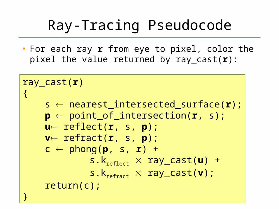
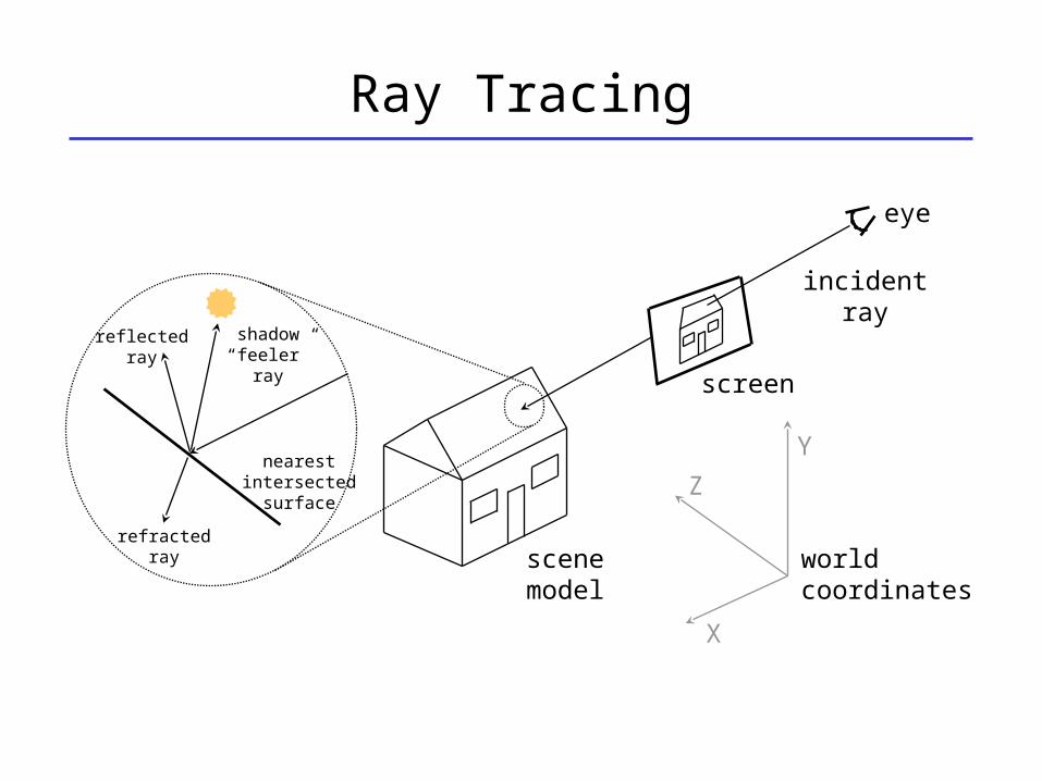
Ray-Tracing Pseudocode

• For each ray r from eye to pixel, color the pixel the value returned by ray_cast(r):

ray_cast(r){ s nearest_intersected_surface(r); p point_of_intersection(r, s); u reflect(r, s, p); v refract(r, s, p); c phong(p, s, r) + s.kreflect ray_cast(u) + s.krefract ray_cast(v); return(c);}

Pseudocode Explained

• s nearest_intersected_surface(r);– Use geometric searching to find the nearest

surface s intersected by the ray r

• p point_of_intersection(r, s);– Compute p, the point of intersection of ray r

with surface s

• u reflect(r, s, p); v refract(r, s, p);– Compute the reflected ray u and the

refracted ray v using Snell’s Laws

Reflected and Refracted Rays

• Reflected and refracted rays are computed using Snell’s Law

surface1

N

v

u rreflected

rayincident

ray

surfacenormal

refractedray

1

2

1

2

2

1

2

1

sin

sin

Pseudocode Explained

• phong(p, s, r)– Evaluate the Phong reflection model for the

ray r at point p on surface s, taking shadowing into account (see next slide)

• s.kreflect ray_cast(u)

– Multiply the contribution from the reflected ray u by the specular-reflection coefficient kreflect for surface s

• s.krefract ray_cast(v)

– Multiply the contribution from the refracted ray v by the specular-refraction coefficient krefract for surface s

The Phong Reflection Model

akkki R dc

sdl coscos

Set to 0 if shadow “feeler” ray to light source intersects any scene geometry

bisector ofeye and light

vectors

eye

lightsource

surface

N

LH

V

surfacenormal

About Those Calls to ray_cast()...

• The function ray_cast() calls itself recursively

• There is a potential for infinite recursion– Consider a “hall of mirrors”

• Solution: limit the depth of recursion– A typical limit is five calls deep– Note that the deeper the recursion, the less

the ray’s contribution to the image, so limiting the depth of recursion does not affect the final image much

Pros and Cons of Ray Tracing

• Advantages of ray tracing– All the advantages of the Phong model– Also handles shadows, reflection, and

refraction

• Disadvantages of ray tracing– Computational expense– No diffuse inter-reflection between surfaces– Not physically accurate

• Other techniques exist to handle these shortcomings, at even greater expense!

An Aside on Antialiasing

• Our simple ray tracer produces images with noticeable “jaggies”

• Jaggies and other unwanted artifacts can be eliminated by antialiasing:– Cast multiple rays through each image pixel– Color the pixel the average ray contribution– An easy solution, but it increases the number

of rays, and hence computation time, by an order of magnitude or more

Reflections

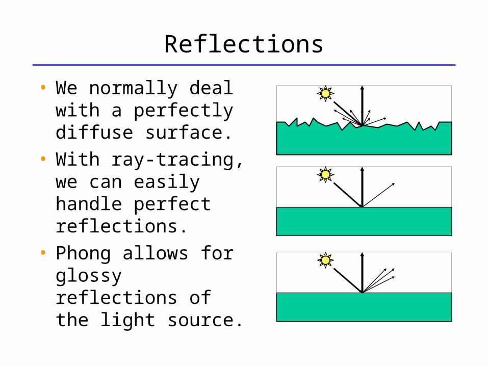
• We normally deal with a perfectly diffuse surface.

• With ray-tracing, we can easily handle perfect reflections.

• Phong allows for glossy reflections of the light source.

Reflections

• If we are reflecting the scene or other objects, rather than the light source, then ray-tracing will only handle perfect mirrors.

Jason Bryan, cis782, Ohio State, 2000

Reflections

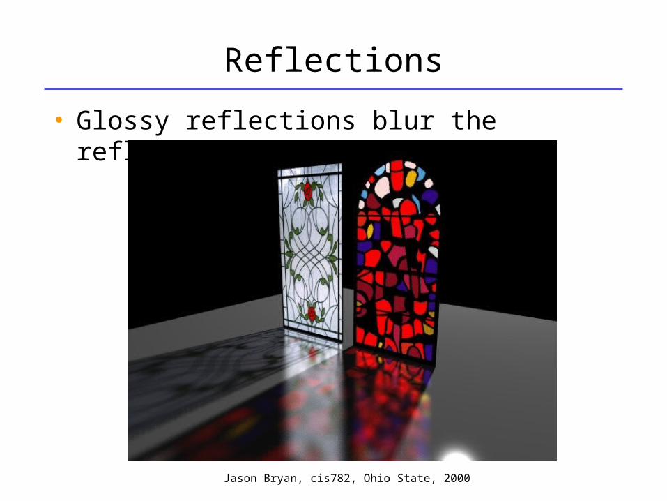
• Glossy reflections blur the reflection.

Jason Bryan, cis782, Ohio State, 2000

Reflections

• Mathematically, what does this mean?

What is thereflected

color?

Glossy Reflections

• We need to integrate the color over the reflected cone.

• Weighted by the reflection coefficient in that direction.

Translucency

• Likewise, for blurred refractions, we need to integrate around the refracted angle.

Translucency

Translucency

Translucency

Calculating the integrals

• How do we calculate these integrals?– Two-dimensional of the angles and ray-depth

of the cone.– Unknown function -> the rendered scene.

• Use Monte-Carlo integration

Shadows

• Ray tracing casts shadow feelers to a point light source.

• Many light sources are illuminated over a finite area.

• The shadows between these are substantially different.

• Area light sources cast soft shadows– Penumbra– Umbra

Soft Shadows

Soft Shadows

Umbra

Penumbra

Soft Shadows

• Umbra – No part of the light source is visible.

• Penumbra – Part of the light source is occluded and part is visible (to a varying degree).

• Which part? How much? What is the Light Intensity reaching the surface?

Camera Models

• Up to now, we have used a pinhole camera model.

• These has everything in focus throughout the scene.

• The eye and most cameras have a larger lens or aperature.

Depth-of-Field

Depth of Field

Depth-of-Field

• Details

Motion Blur

• Integrate (or sample) over the frame time.

Rendering the Scene

• So, we ask again, what is the color returned for each pixel?

What is thereflected

color?

Rendering a Scene

• For each frame– Generate samples in time and average (t):

• For each Pixel (nxn)– Sample the Camera lens (lxl)

• Sample the area light source for illumination (sxs)• Recursively sample the reflected direction cone (rxr).• Recursively sample the refracted direction cone (axa).

• Total complexity O(p*p*t*l*l*s*s*r*r*a*a)!!!!!• Where p is the number of rays cast in the

recursion – n2 primary rays, 3n2 secondary, …• If we super-sample on a fine sub-pixel grid, it

gets even worse!!!

Rendering a Scene

• If we only sample the 2D integrals with a mxm grid, and time with 10 samples, we have a complexity of O(m9p2).

Supersampling

• 1 sample per pixel

Supersampling

• 16 samples per pixel

Supersampling

• 256 samples per pixel

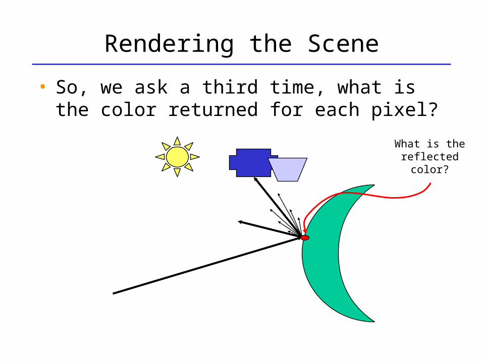
Rendering the Scene

• So, we ask a third time, what is the color returned for each pixel?

What is thereflected

color?

Rendering the Scene

• If we were to write this as an integral, each pixel would take the form:

• Someone try this in Matlab!!!

dtdudvdldrdldrdxdyddvutimelenslensryxrf yxyxrefractrefractlightlightreflrefl ),,,,,,,,,,(

Rendering the scene

• So, what does this tell us?• Rather than compute a bunch of 2D

integrals everywhere, use Monte-Carlo integration to compute this one integral.

Distributed Ray-Tracing

• Details of how Monte-Carlo integration is used in DRT.