Ceophys. J. Inf. (1992) 109, 294-322 Ray perturbation theory for traveltimes and ray paths in 3-D heterogeneous media Roe1 Snieder’ and Malcolm Sarnbridge2 ‘Department of Theoretical Geophysics, University of Utrecht, PO Box 80.021, 3508 TA Ufrecht, The Netherlands 21nstitute of Theoretical Geophysics, University of Cambridge. Cambridge CB2 3EQ. UK Accepted 1991 November 8. Received 1991 October 21; in original form 1991 July 26 SUMMARY Both paraxial ray tracing and two-point ray tracing are powerful tools for solving wave propagation problems. When a slowness model is mildly perturbed from a reference model, one can use perturbation theory for the determination of the ray positions and the traveltimes. An extension of Fermat’s theorem is presented, which states that the traveltime is stationary with respect to the perturbations in the ray position provided that the endpoints of the ray are perturbed along the wavefront of the unperturbed ray. It is shown that when the ray perturbation satisfies this condition the second-order traveltime perturbation can be computed from the first-order ray perturbation. A perturbation analysis of the equation of kinematic ray tracing leads to a simple second-order differential equation for the ray deflection expressed in ray coordinates. This constitutes a perturbation method based on a Lagrangian formulation, and leads to a first-order expression for the ray deflection and a second-order expression for the traveltime perturbation. This is of relevance to non-linear traveltime tomography because it leads to an efficient method for evaluating the lowest order ray deflection and the non-linear effect this has on the traveltimes. The theory is applicable both to two-point ray tracing and to the determination of paraxial rays. The derivations in this paper are completely self-contained. All expressions, including the transformation to ray coordinates, are derived from first principles. In this way one obtains insight in the approximations that are actually made. A scale analysis leads to dimensionless numbers that give an indication whether the theory is applicable to a specific problem. For the special case of a layered reference medium the final equations are particularly simple. Plane discontinuities in the reference model and the slowness perturbation are incorpor- ated in the theory. The final expressions for the ray deflection and the traveltime perturbation can be implemented numerically in a simple way. It is indicated how applications to very large-scale problems can be achieved. Several examples, including the propagation of waves through a quasi-random model of the earth’s mantle illustrate the theory. Key words: Fermat’s theorem, paraxial rays, perturbation theory, ray tracing, tomography. 1 INTRODUCTION Ray theory plays an important role both in exploration seismics and large-scale seismology. Green’s functions derived from ray theory form the basis of several algorithms for computing synthetic seismograms. Traveltime tomography is an important technique for the determination of seismic velocities on a variety of scales ranging from cross-borehole tomography to tomography of the earth’s mantle. There is a vast amount of literature on ray tracing methods. Traditionally one uses either shooting methods (e.g. Cerven? 1987) or bending methods (e.g. Julian & Gubbins 1077; Peyrera, Lee & Keller 1980). Recently, new algorithms have been developed which either solve the Eikonal equation with a finite difference method (Vidale 294

Welcome message from author
This document is posted to help you gain knowledge. Please leave a comment to let me know what you think about it! Share it to your friends and learn new things together.
Transcript
Ceophys. J . Inf. (1992) 109, 294-322
Ray perturbation theory for traveltimes and ray paths in 3-D heterogeneous media
Roe1 Snieder’ and Malcolm Sarnbridge2 ‘Department of Theoretical Geophysics, University of Utrecht, PO Box 80.021, 3508 TA Ufrecht, The Netherlands 21nstitute of Theoretical Geophysics, University of Cambridge. Cambridge CB2 3EQ. U K
Accepted 1991 November 8. Received 1991 October 21; in original form 1991 July 26
S U M M A R Y Both paraxial ray tracing and two-point ray tracing are powerful tools for solving wave propagation problems. When a slowness model is mildly perturbed from a reference model, one can use perturbation theory for the determination of the ray positions and the traveltimes. An extension of Fermat’s theorem is presented, which states that the traveltime is stationary with respect to the perturbations in the ray position provided that the endpoints of the ray are perturbed along the wavefront of the unperturbed ray. It is shown that when the ray perturbation satisfies this condition the second-order traveltime perturbation can be computed from the first-order ray perturbation. A perturbation analysis of the equation of kinematic ray tracing leads to a simple second-order differential equation for the ray deflection expressed in ray coordinates. This constitutes a perturbation method based on a Lagrangian formulation, and leads to a first-order expression for the ray deflection and a second-order expression for the traveltime perturbation. This is of relevance to non-linear traveltime tomography because it leads to an efficient method for evaluating the lowest order ray deflection and the non-linear effect this has on the traveltimes. The theory is applicable both to two-point ray tracing and to the determination of paraxial rays. The derivations in this paper are completely self-contained. All expressions, including the transformation to ray coordinates, are derived from first principles. In this way one obtains insight in the approximations that are actually made. A scale analysis leads to dimensionless numbers that give an indication whether the theory is applicable to a specific problem. For the special case of a layered reference medium the final equations are particularly simple. Plane discontinuities in the reference model and the slowness perturbation are incorpor- ated in the theory. The final expressions for the ray deflection and the traveltime perturbation can be implemented numerically in a simple way. It is indicated how applications to very large-scale problems can be achieved. Several examples, including the propagation of waves through a quasi-random model of the earth’s mantle illustrate the theory.
Key words: Fermat’s theorem, paraxial rays, perturbation theory, ray tracing, tomography.
1 INTRODUCTION
Ray theory plays an important role both in exploration seismics and large-scale seismology. Green’s functions derived from ray theory form the basis of several algorithms for computing synthetic seismograms. Traveltime tomography is an important technique for the determination of seismic velocities on a variety of scales ranging from cross-borehole tomography to tomography of the earth’s mantle. There is a vast amount of literature on ray tracing methods. Traditionally one uses either shooting methods (e.g. Cerven? 1987) or bending methods (e.g. Julian & Gubbins 1077; Peyrera, Lee & Keller 1980). Recently, new algorithms have been developed which either solve the Eikonal equation with a finite difference method (Vidale
294
Ray perturbation theory 295
1988) or search for the shortest path on a graph which approximates all possible ray paths emanating from a given source (Moser 1991). The bending method has recently been further developed by Moser, Nolet & Snieder (1992). In order t o use the full potential of the steadily increasing data sets it is important to have an efficient method for tracing rays in heterogeneous media.
This is especially important in traveltime tomography. When one linearizes the inverse problem for this case one can use Fermat’s theorem, which implies that one can use the rays of the reference medium and assume that the observed traveltimes are due to slowness perturbations along the unperturbed ray (e.g. Nolet 1987). In reality the inverse problem is non-linear, because the slowness perturbations perturb the rays themselves. The true rays are curves along which the traveltime is a minimum. This means that if one uses the rays in the reference medium for the inversion, rather than the true rays, that one overestimates the time needed for the propagation from the source to the receiver. In order to obtain a fit of the observed traveltimes one will obtain a velocity model that is too fast. This means that neglecting the non-linearity of the inverse problem leads to a bias in the reconstructed model.
The fact that a linearized approach has been relatively successful in traveltime tomography indicates that the effects of ray bending on the inversion may not be too dramatic. In fact, a radially stratified earth accounts for a large amount for the slowness variations within the earth. This suggests that perturbation theory could be used to account for the effect of the slowness perturbation on the ray positions and the traveltimes. It is shown by Snieder. (1990, 1991) how one can set up an inversion method based on a perturbation expansion of the forward problem. The theory presented here could be used for this.
The use of perturbation methods in ray theory is not new. The equations of dynamic ray tracing can be cast in a Hamiltonian form. Perturbation methods for Hamiltonian systems are well developed, and a number of authors have used this to develop a perturbation theory for ray tracing problems (Chapman 1985; Wunsch 1987; Farra & Madariaga 1987; Farra, Virieux & Madariaga 1989; Virieux 1991). As an alternative to Hamiltonian perturbation theory, one can also apply perturbation theory directly to the equation of kinematic ray tracing (Moore 1991). In the jargon of classical mechanics this corresponds to a Lagrangian formulation of the perturbation theory. It is a priori not evident that the different perturbation methods lead to the same result. Furthermore, i f one sets up a perturbation problem in two different coordinate systems that are related through a non-linear transformation, then perturbation theory in general leads to different physical results in the two formulations.
Another ambiguity in setting up a perturbation treatment is the choice of the independent parameter and the employed coordinate system. Wunsch (1987) uses the horizontal distance of a ray as independent parameter and solves for the depth of a ray. Farra & Madariaga (1987) use the distance along the unperturbed ray as independent parameter and employ ray coordinates. I n later studies Farra et al. (1989) and Virieux (1991) use Cartesian coordinates. Moore (1991) uses the distance along the perturbed ray as independent parameter. This last choice leads to conceptual problems since the independent parameter depends on the ray perturbation itself, which is a serious inconsistency in the theory. The approach of Moore (1991) also has the disadvantage that in two-point ray tracing the receiver is not a t a known position of the independent coordinate since the arc length of a perturbed ray joining a given source and receiver is not known a priori.
Treating ray perturbation theory with a Hamiltonian formalism has the advantage that the derivations are algebraically simple, and that one can change relatively easy from one coordinate system to another. However, the derivation of the perturbation equations from a Hamiltonian formalism gives little physical insight and it is often not trivial to derive the conditions of validity for Hamiltonian perturbation theory. In contrast to this, Lagrangian perturbation theory gives direct physical insight because the Lagrangian is the traveltime, and the Euler-Lagrange equation is the equation of kinematic ray tracing. The disadvantage of Lagrangian perturbation theory over Hamiltonian perturbation methods is that the algebra usually is more complicated, and that the algebra has to be redone whenever one changes to a new coordinate system.
The aim of this paper is to present a perturbation solution of the equation of kinematic ray tracing which is conceptually simple. In contrast to earlier perturbation methods, the theory leads to an explicit expression for the traveltime that is correct to second order in the slowness perturbation. The theory leads to equations that can be applied well to extremely large data sets, because the problem can be set up in such a way that the perturbations in the ray position and traveltimes can be reduced to vector operations. Two dimensionless numbers are derived that give an indication whether the method is applicable to a certain problem.
This paper has a tutorial flavour and is completely self-contained. Since the perturbation theory is applied directly to the equation of kinematic ray tracing, rather than to Hamilton’s equations, one can understand how the perturbation in the slowness affects the ray positions and the traveltimes. In Section 2 general expressions are derived for the perturbation of the traveltime, and it is established under which conditions one can obtain the second-order traveltime perturbation from the first-order ray deflection. The equation of kinematic ray tracing is perturbed in Section 3. A transformation to ray coordinates, as shown in Section 4, simplifies this expression considerably. All expressions needed to make the transformation to ray coordinates are derived. The relation with the Frenet equations is shown in Appendix A. In Section 5 , the second-order traveltime perturbation is related in three alternative ways to the ray perturbation derived in ray coordinates. Dimensionless numbers are derived in Section 6 which indicate whether the perturbation theory can be applied to a specific problem. In Section 7 the equations for the ray perturbation are simplified for the important case of a stratified reference medium. The
296 R. Snieder and M . Sambridge
theory is illustrated with several examples. In Section 8 the theory is applied to a model with a linear velocity gradient for which t h e exact solution is known in closed form. The theory is applied in Section 9 to rays propagating through a model of the earth’s mantle that is perturbed by quasi-random slowness fluctuations. The effect of slowness discontinuities is introduced in a heuristic way in Section 10 for the case of a two-layer model. In Section 11 it is shown in a more rigorous way how the theory can be adapted in order to handle plane discontinuities in the reference slowness and/or the slowness perturbation. Finally, the application to rays propagating through a mantle model where both the reference slowness and the slowness perturbation are discontinuous at the 670 discontinuity is shown in Section 12.
2 P E R T U R B A T I O N T H E O R Y FOR TRAVELTIMES
In geometrical optics, a ray is defined as a curve aloqg which the traveltime is stationary. The Euler-Lagrange equation corresponding to this variational problem is the equation of kinematic ray tracing
where the slowness is given by u(r), s is the arc length along the ray and r is the position vector. Suppose that the slowness can be written as a reference slowness uo(c) and a perturbation EuI(r)
u(r) = uo(c) + Eul(r). (2)
The reference slowness l~()(r) may for instance denote the slowness in a flat layered earth model, and the perturbation Eul(r) may denote lateral variations in the slowness. The parameter E is used for bookkeeping purposes and facilitates a systematic perturbation approach of the ray tracing problem. It is assumed momentarily that uo(r) and u,(r) are continuous functions of the space coordinates, but there are no further restrictions.
The case where the slowness is perturbed is relevant for two-point ray tracing problems. In paraxial ray tracing one perturbs the initial conditions of the ray, and one may or may not perturb the slowness too, depending on the application. For paraxial ray tracing problems with a fixed slowness one may simply set u , = 0 in ensuing expressions.
Let a ray in the reference medium uo(r) be denoted by rO(sl)), where so is the arc length along this reference ray. The ray in the perturbed medium is a non-linear function of the slowness perturbation. Except in the vicinity of caustics, the ray perturbation can b e expanded in a regular perturbation series
r(so) = r I M + Erl(So) + E ~ ~ ~ ( s ~ ~ ) + . . . . (3)
The ray perturbation i:i parametrized with the arc length along the reference ray. Perturbations in the ray position along the reference ray are irrelevant because these perturbations don’t change the position of the ray. Therefore without loss of generality the ray perturbations can be restricted t o the plane perpendicular to the direction of the reference ray
(ri * i(,) = 0 for i 2 1. (4)
‘I’ht: derivative along the reference ray is denoted with a dot:
In two-point ray tracing the perturbed ray joins the source and receiver of the reference ray; the ray perturbation therefore vanishes a t the endpoints of the ray
r,(O) = ri(&,) = 0 for i 2 1 (two-point ray tracing), 16)
where the source is a t location so = 0 and the unperturbed ray has total arc length So. Since sn measures the arc length along the reference ray rO(sO), the vector rO is of unit length:
The deflection of the ray due to the slowness perturbation has the effect that the perturbed ray has a different arc length than the unperturbed ray. By inserting (3) in the relation
and by using (4) and (7) one finds after some algebra that to second order
dS - = 1 + &(i0 * i l ) + E 2 [ $ ( i I * i l ) - ;(r,, * il)2 + (ill * i2)]. &,
Ray perturbation theory 297
and its reciprocal expression
- 1 - &(i" * i,) - E2[$(i1 * il) - &) * i,)2 + (i,) * i*)]. (9) 3s 0 - _ dS
Note that Moore (1991) ignores the distinction between the unperturbed and the perturbed arc length. In that case the O ( E ) and O(E') terms in (8) and (9) are ignored and the resulting perturbation scheme is not consistent.
Now consider the traveltime T
T = u[r(s)] ds. (10) J The perturbation in the slowness and the ray position has two effects. First, the perturbed ray samples different regions than the unperturbed ray. By inserting (3) into (2) and performing a Taylor expansion of uo and u I about r,,, une finds that to second order
u(r) = uo(r0) + E[ul(ro) + rl ~ u ~ , ( r ~ , ) I + ~ ~ [ r ~ - vul(rO) + tr lr l :VV~, l ( ro ) + rz * V ~ d r l l ) 1 . (11) In this expression the symbol ':' denotes a double contraction. Second, the perturbation of the ray path leads to a perturbed arc length. Using cts = ds/3s,, dso and (11) in (10) this leads with (8) to a perturbation expansion of the traveltime
T = T,, + E T ~ + E ~ T ~ + O ( E ~ ) , (12)
where it is understood that the slowness and its derivatives are to be evaluated on the reference ray rO(sO).
ray in the reference medium. Consider the following integral: The expressions for the first- and second-order traveltime perturbation can be simplified by using the fact that rO(so) is a
where 6(s,) is an arbitrary vector function along the reference ray which at the endpoints of the reference ray is perpendicular to the reference ray
(6 . i,m = (6 * io)(&) = 0.
VU,) = U$" + (1" . V U ( ) ) i ( ) .
(15)
It follows from (1) that the reference ray satisfies
(16)
In deriving this it is used that
- (i, * V F ) . dF -- ctso
Using integration by parts and the condition (15) one may derive the general result $1 .%I .%I
uo(5 -4J 4, = -J uo(k * 4)) 4, - (4, - VUo)(6 * 4)) dsw
By inserting (16) and (18) in (14) one finds
Using this expression in (13b, c), the first- and second-order traveltime perturbation have the simplified form
i7 = Ji[hu'(r")
298 R . Snieder and M . Sambridge
Equation (19) is nothing but Fermat's theorem. It has the consequence that the first-order traveltime perturbation is the integral of the slowness perturbation along the reference ray (see 20a). This expression forms the basis of linearized tomographic inversions. Another consequence of Fermat's theorem (19) is that the second-order traveltime perturbation does not depend on the second-order ray perturbation r2 (see 20b). This means that in order to obtain expressions of the traveltime perturbation which are correct to second order, it suffices to know the ray perturbation to first order. For this reason, only the first-order ray perturbation is derived in this paper.
Note that in the derivation it is not used that the ray perturbation vanishes at the endpoints of the ray, but that it is only required that (15) is satisfied. Since the wavefront is perpendicular to the ray, this expression states that Fermat's theorem is valid when the endpoint of the ray is perturbed along the wavefront of the reference ray. This means that (20b) is not only applicable to two-point ray tracing problems, but also to perturbed paraxial rays provided one works in a coordinate system where (15) is satisfied.
3 FIRST-ORDER PERTURBATION THEORY FOR THE RAY DEFLECTION
The first-order ray deflection can be derived by applying a perturbation analysis to the equation of kinematic ray tracing (1). With (17) this equation can be written as
d2r d r dr u ( r ) s + (z- vu) z= vu.
In evaluating the derivatives in this expression one should take into account that the derivative along the perturbed ray and the unperturbed ray are different:
d ds,, d ds - ds ds,,'
with 3s,,/& given by (9). For the gradient of the slowness one finds with (2), (3) and a Taylor expansion that
V4r) = v4)(ro) + 4VU, (ro ) + rl * ~ ~ ~ n ~ ~ o ~ ~ .
Inserting (ll), (22) and (23) in (21), and differentiating carefully, leads to a linear differential equation for r I :
~ $ 1 - ~ o ( i i 1 * in)i() - ~ ( ~ ( i i ~ ~ * i l ) i c ) - 2 ~ 4 4 , * il)?,) + (i1 V ~ o ) i o - 2(iO * il)(k(i * VU,))~,) + io(i(~1 : VVU,)) + ti(?() . V U ~ )
+ (rl Vuoyr, - r, - VVuo = Vu, - (in * V U , ) ~ , , - u,ro, (24)
where it is understood that the slowness and its derivatives are to be evaluated on the reference ray.
derivatives r,, can be eliminated by writing (16) in the form Equation (24) contains a large number of terms, but it is possible to simplify this expression considerably. The second
1
uo io=- [Vu,- (io * V ~ o ) i o ] .
Differentiating (4), using (25) to eliminate ro and invoking the orthogonality of rI and r,, gives
1 (il - in) = -- (cl - Vu,).
un
Inserting (25) and (26) in (24) leads after some algebra to
1
4) UOf, - u()(i() f l ) i ( ) + il(f() * vu(J) + - (rl * vu(l)[3vu() - 2(r[> ' vu())r<J] - ' vvuO) - ('($1 : vvU,))rl l l
= uov(;j - u,,[i,, * v(:)]i".
It follows that the slowness perturbation affects the first-order ray deflection only through the gradient of the relative slowness perturbation V(u,/u,,). Indeed, one finds from (1) that multiplying the slowness with a constant [u(r)-+ Cu(r)] leaves the rays unaffected. For such a perturbation ul(r) = (C - l)uo(r), hence V(u,/u,,) = 0 and the ray perturbation vanishes.
Because of the orthogonality condition (4), only the component of the ray deflection perpendicular to the reference ray is relevant. For an arbitrary vector 6 the component perpendicular to the reference ray may be denoted by
5, ZE g - ( r ( J g)iO> (28)
Ray perturbation theory 299
where it is used that io is of unit length (see 7). Using the definition (28) gives
3VU,) - 2(i0 * V U ( ) ) i ( ) = 3v, U() + (r() V U ( ) ) i ( ) ,
(rl * 5 ) = (rl * 5 1 ).
Since r l is perpendicular to the reference ray one has
From the definition (28), and the relations (26) and (30) it follows that
1 r, = i, , - - (rl * Vuo)ro,
4)
Using (29) and (31) in (27) gives with the definition (28):
ut;, + (iO * vuo)r1 I + - (rl - Vu,,)v I uo - (r, - V V ~ J = u(,v, (:). 3 4)
Note from this expression that we only need the perpendicular components of r l and 'i,.
4 THE TRANSFORMATION TO RAY COORDINATES
Expression (32) is considerably simpler than the original perturbation equation (24). Nevertheless, it is not the most convenient form to use in numerical computations. First, the simplicity of equation (32) is deceptive, because the relation between the perpendicular components of r, and its derivatives is in general not trivial. For example, in general one has (dr1/ds,,), # dr , L/dsO because the direction r,, of the unperturbed ray varies with so. Second, the first-order ray deflection r, is a 3-D vector. However, the constraint (4) reduces the number of independent components of r1 by one, SO that (32) should be solved under the constraint (4). These complications are both handled when a transformation to ray coordinates is made. An additional advantage of using ray coordinates is that the condition (15) for the validity of Fermat's theorem is automatically satisfied.
Consider two mutually orthogonal unit vectors G I and ij2 that are orthogonal to the reference ray. This implies that
(31 * 31) = ( 3 2 4*) = (io * 4,) = 1 . (34)
The direction i,, of the reference ray changes along the reference ray, so that the unit vectors 3, also change direction along the reference ray: lit = qz(so). Since the ray perturbation is perpendicular to the reference ray, it can be expanded as
r i = 41Ql+ 9 4 2 . (35)
It is the aim of this section to convert the differential equation (32) to a differential equation for the components q1 and q2.
expand as In order to do so one needs the derivatives of the unit vectors at. Since the basis ( Q l , ~ 2 , i o ) is orthonormal, one can
The vectors qi are normalized, it follows by differentiation of (34) that
($1 * 31) = ($2 * %) = 0. (37)
The quantity (6, Ci2) describes the rotation of the unit vectors tj, and Q2 along the reference ray. This quantity is completely arbitrary, since one is free in choosing the direction of the unit vector Q 1 in any direction within the plane perpendicular t o the reference ray. This choice may vary along the reference ray. Denote the rotation rate of the unit vectors Cjl and 42 along the reference ray by R(s,,):
($1 * 42) Q(sn). (38)
In order to find the term (6, * ro) in (36), differentiate the expression (qi io) = 0 with respect to so, and eliminate ro with (25); this gives
Note that (4, * Vu,,) is nothing but the derivative of uo in the normal direction ai. Inserting (37), (38) and (39) in (36) one finds
1
4) 4, = Q32 - - (ijl * V U ( ) ) i ( ) .
300 K. Snieder und M. Samhridge
A similar expression follows for q2. By differentiating the first term of (33) one finds that
(3, * i2) = - (q , * 3 2 , .
so that qz is given by
(40b) 1
% I q2 = -Qq, - - (ljz * vull)r(l .
I t is convenient to use the summation convention for summing over the two unit vectors 3, and G2 and their related components. Let F,, denote the second-order Levi-Cevita tensor:
F , , = &2* = o , E , Z = - E 2 , = 1. (42)
The expressions (40a) and (40b) can then be written as
1
4 1 q, = QE,/q/ - - (3; * vU(,)r(l. (43)
It is shown in Appendix A how equation (43) is rclated to the Frenet equations. The second derivative of 3, follows by differentiating (43) and eliminating rl) with (25) and q, with (43); this gives
where a, is used to represent the coefficient of the i,, terms and where we have expanded the vector VU,, using VUIJ = (VUO * G I ) % + (VUII * 32132 + (Vu,, * i l l ) 4 , .
In order to convert (32) to ray coordinates it is necessary to express the derivatives i, and r , in the components q, and their derivatives. It follows from the definition (28) that for any vector g
t , = (3, 5)iir Differentiate (35) with respect to y I l and use (43) to give
(45)
1
uo i, = (4; - QE,f?/ )3, - - 4;(3, * VU,Ih. (46)
Differentiate this expression once more with respect t o .v,~; with (45) one finds that
1
4 1 r,, = (ql - Q Z q , - 2Q&;jqj - &,/q/)q; - T(3, * Vu,,)($ * Vu,,)q,ij,. (47)
Insert (46) and (47) in (32) , and take the inner product o f the resulting expression with the unit vectors 3, and Cj2. Using the identities
2 1
UII vvu, , - - (Vu,,)(Vu,,) = -U:,VV -
and
one finds after some algebra that the components ql satisfy
This equation needs to be supplemented with two boundary conditions. For two-point ray tracing these are given by
q,(0) = q , (S , , ) = 0 (two-point ray tracing); (51)
for initial value ray tracing one prescribes q,(0) and q,(0). The system (50) for the ray perturbation constitutes a pair of coupled linear second-order differential equations and may
be solved efficiently using a variety of standard numerical techniques (see Press et al. 1986). After discretization, ( S O ) with the appropriate boundary conditions can be reduced to a linear system of equations, where only the main diagonal and four other bands of the involved matrix have non-zero elements. For the important application of layered reference media (see Section 7)
Ray perturbation theory 301
n n
(99 L ' l ' $ 0
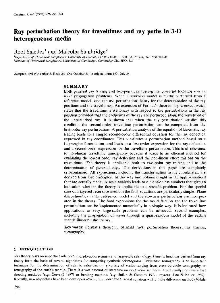
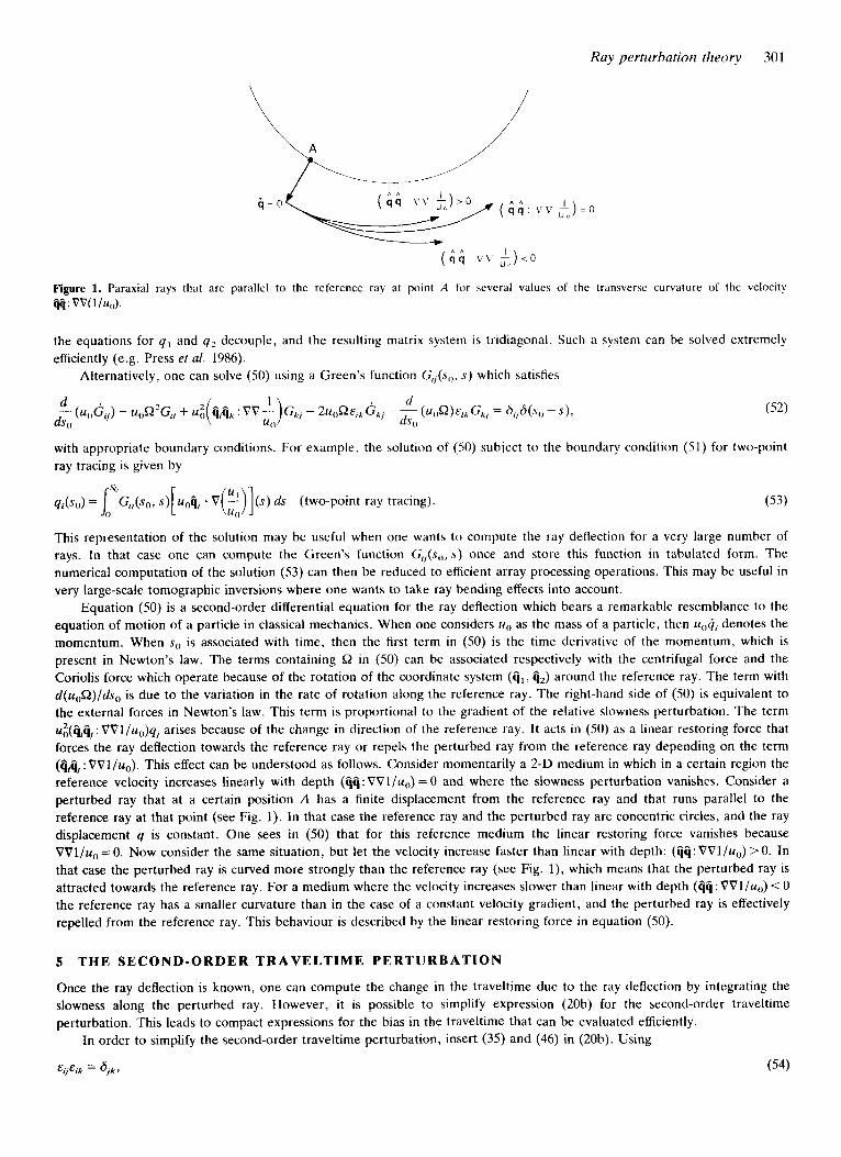
Figure 1. Paraxial rays that are parallel to the reference ray at point A for several values of the transverse curvature of the velocitv @:vv(l/u(,).
the equations for q , and q2 decouple, and the resulting matrix system is tridiagonal. Such a system can be solved extremely efficiently (e.g. Press et al. 1986).
Alternatively, one can solve (SO) using a Green's function G,,(s,,, s) which satisfies
with appropriate boundary conditions. For example, the solution of (SO) subject to the boundary condition ( 5 1) for two-point ray tracing is given by
This representation of the solution may be useful when one wants to compute the ray deflection for a very large number of rays. In that case one can compute the Green's function GJs,,, s) once and store this function in tabulated form. The numerical computation of the solution (53) can then be reduced to efficient array processing operations. This may be useful in very large-scale tomographic inversions where one wants to take ray bending effects into account.
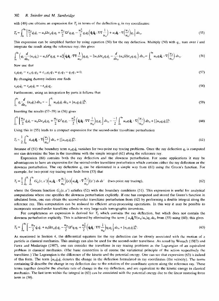
Equation (50) is a second-order differential equation for the ray deflection which bears a remarkable resemblance to the equation of motion of a particle in classical mechanics. When one considers ug as the mass of a particle, then uoq, denotes the momentum. When sg is associated with time, then the first term in (SO) is the time derivative of the momentum, which is present in Newton's law. The terms containing 9 in (50) can be associated respectively with the centrifugal force and the Coriolis force which operate because of the rotation of the coordinate system (q,, q2) around the reference ray. The term with d(u,Q)/ds,, is due to the variation in the rate of rotation along the reference ray. The right-hand side of (SO) is equivalent to the external forces in Newton's law. This term IS proportional to the gradient of the relative slowness perturbation. The term ui(gziil : VVl/u,,)q, arises because of the change in direction of the reference ray. It acts in (SO) as a linear restoring force that forces the ray deflection towards the reference ray or repels the perturbed ray from the reference ray depending on the term (Cjzij, : VVl/u,). This effect can be understood as follows. Consider momentarily a 2-D medium in which in a certain region the reference velocity increases linearly with depth (Qq: VV1 /uo ) = 0 and where the slowness perturbation vanishes. Consider a perturbed ray that at a certain position A has a finite displacement from the reference ray and that runs parallel to the reference ray at that point (see Fig. 1). In that case the reference ray and the perturbed ray are concentric circles, and the ray displacement q is constant. One sees in (SO) that for this reference medium the linear restoring force vanishes because VVl/u,, = 0. Now consider the same situation, but let the velocity increase faster than linear with depth: (39: VVl/u,,) > 0. In that case the perturbed ray is curved more strongly than the reference ray (see Fig. 1), which means that the perturbed ray is attracted towards the reference ray. For a medium where the velocity increases slower than linear with depth (qq : VVl/u,,) < 0 the reference ray has a smaller curvature than in the case of a constant velocity gradient, and the perturbed ray is effectively repelled from the reference ray. This behaviour is described by the linear restoring force in equation (SO).
5 THE SECOND-ORDER TRAVELTIME PERTURBATION
Once the ray deflection is known, one can compute the change in the traveltime due to the ray deflection by integrating the slowness along the perturbed ray. However, it is possible to simplify expression (20b) for the second-order traveltime perturbation. This leads to compact expressions for the bias in the traveltime that can be evaluated efficiently.
In order to simplify the second-order traveltime perturbation, insert (35) and (46) in (20b). Using
(54)
302
with (48) one obtains an expression for T2 in terms of the deflection q, in ray coordinates:
R . Snieder and M . Sambridge
This expression can be simplified further by using equation (50) for the ray deflection. Multiply (SO) with q, , sum over i and integrate the result along the reference ray; this gives
Now use that
E,/4*9, = E1241q2 + ~2lqzq l = q , q , - 9241 = 0
E,/q'q, = &/A/4, = -&&A/.
By changing dummy indices one finds
Furthermore, using an integration by parts it follows that
Inserting the results (57-59) in (56) gives
Using this in (55 ) leads to a compact expression for the second-order traveltime perturbation
Because of (51) the boundary term uoq,4i vanishes for two-point ray tracing problems. Once the ray deflection qi is computed one can determine the bias in the traveltime with the simple integral (61) along the reference ray.
Expression (61) contains both the ray deflection and the slowness perturbation. For some applications it may be advantageous t o have an expression for the second-order traveltime perturbation which contains either the ray deflection or the slowness perturbation. The ray deflection q1 can be eliminated in a simple way from (61) using the Green's function. For example, for two-point ray tracing one finds from (53) that
where the Greens function G,(s, s') satisfies (52) with the boundary conditions (51). This expression is useful for analytical computations where one specifies the slowness perturbation explicitly. If one has computed and stored the Green's function in tabulated form, one can obtain the second-order traveltime perturbation from (62) by performing a double integral along the reference ray. This computation can be reduced to efficient array-processing operations. In this way it may be possible t o incorporate second-order traveltime effects in very large-scale tomographic inversions.
For completeness a n expression is derived for T, which contains the ray deflection, but which does not contain the slowness perturbation explicitly. This is achieved by eliminating the term unqiV(u,/u,)q, ds,, from (55 ) using (60); this gives
As mentioned in Section 4, the differential equation for the ray deflection can be closely associated with the motion of a particle in classical mechanics. This analogy can also be used for the second-order traveltime. As noted by Wunsch (1987) and Farra and Madariaga (1987), one can consider the traveltime in ray tracing problems as the Lagrangian of an equivalent problem in classical mechanics. (The basic connection is of course the variational principle of the action respectively the traveltime.) The Lagrangian is the difference of the kinetic and the potential energy. One can see that expression (63) is indeed of this form. The term $u0qiqi denotes the change in the deflection formulated in ray coordinates (the velocity). The terms containing Q describe the change in ray deflection due to the rotation of the coordinate system along the reference ray. These terms together describe the absolute rate of change in the ray deflection, and are equivalent to the kinetic energy in classical mechanics. The last term within the integral in (63) can be associated with the potential energy due to the linear restoring force term in (50).
Ray perturbation theory 303
6 CONDITIONS FOR T H E APPLICABILITY O F FIRST-ORDER P E R T U R B A T I O N T H E O R Y
When the slowness perturbation i s large, the first-order perturbation method of this paper cannot be expected to give useful results. In this section estimates for the domain of the applicability of the first-order ray perturbation theory are derived. First, the change in the length of the ray induced by the perturbation may not be too severe, because the relations (8) and (9) are oniy useful when l ~ s / 3 . s , , - 11 << 1 . This condition is satisfied when
/ill << 1 . (64)
Furthermore a Taylor expansion of u I is used (up to order r l . V u , ) , and of u(, (up to order r lr l :VVuo) . Let uo vary on a length-scale L, , , and let u I vary on a length-scale L . The truncated Taylor expansions represent the true slowness variations with an acceptable accuracy only when
(rl( << Lo and ( r , ( << L. (65)
One can check the conditions (64) and (65) after one has computed the perturbed ray, and one can thus verify a posteriori whether it was justified to use first-order perturbation theory.
This is not very satisfactory from the practical point of view, where one would like to know a priori whether the first-order perturbation theory is sufficiently accurate. For this one needs to relate the slowness perturbation to the total ray deflection. As a simple model, consider a homogenous reference slowness ull , and let the slowness perturbation have a constant derivative perpendicular to the reference ray: tj - Vu, = u l / L . The solution of (50) for the ray deflection in the direction of the gradient of the slowness perturbation is given by
The condition (64) implies that for the first-order theory to be valid one must have (aq/&,,l<<l. The angle between the perturbed ray and the reference ray is largest for s,, = 0. Using this, the condition (64) implies that
The ray deflection of the solution (66) is largest when sll = S,,/2, so that the condition Ir, I << L is satisfied when
The simple model discussed here cannot be used to investigate the criterion Ir,I << Lo, because uO is constant. However, for most practical problems the slowness perturbation varies on a shorter length-scale than the reference slowness, so that the condition Ir, I << L usually ensures that Ir, 1 << Lo.
Note that the criteria (67) and (68) depend on two dimensionless numbers; a factor u I / u ( , (which is usually small), and a factor SJL (which may be large). The first-order perturbation theory is only valid when the weakness of the relative slowness perturbation ( u I / u o ) outweighs the factor SOIL. The criteria (67) and (68) depend critically on the length S, of the unperturbed ray. The reason for this is that for a given slowness perturbation, a longer ray is deflected more than a short ray, so that the condition that the deflection is small is more stringent for long rays than for short rays.
7 R A Y P E R T U R B A T I O N S IN A L A Y E R E D REFERENCE M E D I U M
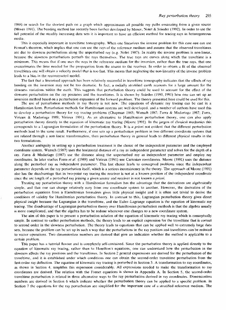
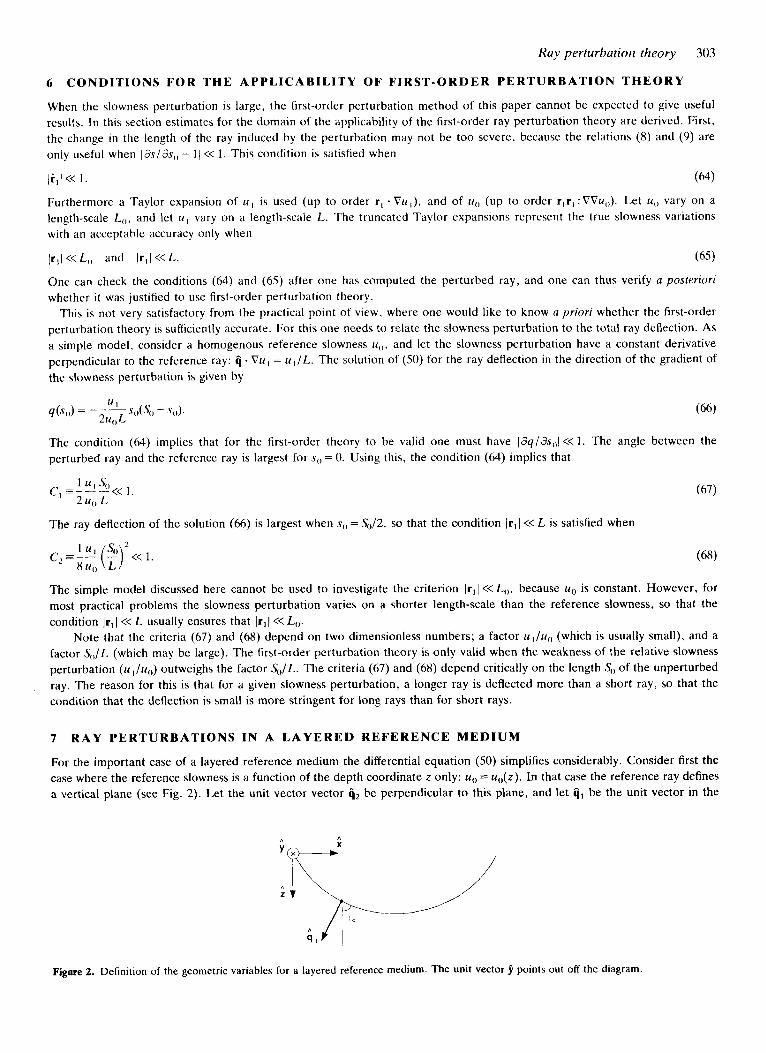
For the important case of a layered reference medium the differential equation (50) simplifies considerably. Consider first the case where the reference slowness is a function of the depth coordinate z only: ug = u,,(z). In that case the reference ray defines a vertical plane (see Fig. 2). Let the unit vector vector ljz be perpendicular to this plane, and let 4, be the unit vector in the
Figure 2. Definition of the geometric variables for a layered reference medium. The unit vector 9 points out off the diagram.
304
plane of the reference ray (Fig. 2). In that case, the unit vectors Cjl and Cj2 do not rotate around the reference ray, hence
R . Snieder and M . Sambridge
8 = 0 . (69)
Define a Cartesian coordinate system with the z-direction pointing downwards, and with the y-direction perpendicular to the vertical plane of the reference ray. In terms of the angle of incidence i,, of the reference ray, the unit vectors for defining the ray coordinates are given by
i,, = sin i,f + cos i& (704
ij, = -cos if$ + sin it#, (70b)
ij* = 9 . (7oc)
Since the reference slowness depends only on depth, one has
1 1
uo uo VV--2aedz,-,
and
The relations (69-72) can readily be inserted in equation (50) for the ray deflection; this gives
Since the coordinate system does not rotate around the reference ray (& = O), and since the cross terms (Cjiq,:VV(l/uo)) in (50) vanish (because u,, does not depend on the y-coordinate), the equations for q , are q2 decoupled. The trigonometric terms in (73a,b) can be eliminated by introducing the ray parameter p of the reference ray defined by
p = u ~ , sin ill. (74)
This parameter is constant along the reference ray (Aki & Richards 1980). Using this parameter, the equations (73a,b) can be written as
The equation for the transverse ray deflection q2 can be integrated in closed form. For example, for two-point ray tracing one finds with the boundary conditions (51) that
1 q2(sn) = - [F(s,)h(S,) - F(Sn)h(so)] (two-point ray tracing), (76)
h (&I)
where
and
Equation (75a) with the boundary conditions for q 1 reduces after discretization to a tridiagonal system of linear equations that can be solved efficiently. Alternatively, one can use a Green’s function solution analogous to (53) for the solution of (75a). Note that in the special case where the reference velocity varies linearly with depth [a,,(l/u,) = 01, one can integrate (75a)
Ray perturbation theory 305
analytically, and the solution for 4 , is of the form (76); the only difference is that the term d,,u, in (78) should be replaced by
For a reference model with a spherical geometry, a simple form of the differential equation for the ray deflection is obtained by choosing a system of spherical coordinates with the North Pole ( H = 0) at the source. Lct (r+ 8. 6) denote the unit vectors in the vertical, 0 and 4 directions respectively. As in the case of Cartesian coordinates, choose i j 2 perpendicular to the vertical plane of the reference ray. This means that the unit vectors do not rotate around the reference ray, condition (69). When i0 denotes the angle between the reference ray and the vertical, one has
,. Q 1 = -cos i,,8 - sin i,,i,
Q2 = 6. (79b)
(7%)
The spherical symmetry of the reference velocity implies that
1 1
UI) 4) vv - = ii d,, - .
Furthermore, one has
For a spherically symmetric slowness model the ray parameter defined by
p = rug sin in , (82)
is constant along the reference ray (Aki & Richards 1980). Inserting the expressions (79-81) in (50) and using (82) to eliminate i,, gives the following differential equations for the ray deflection
For two-point ray tracing the solution of (83b) is given by (76), where one should replace the derivative 3, by ( r sin 0)-' 3,.
8 EXAMPLE 1: T H E LINEAR VELOClTY G R A D I E N T
As an example of the ray perturbation theory, consider a homogeneous reference medium with velocity qI, where the velocity is perturbed with a linear gradient
c ( z ) = c g 1 + - . ( ;I The slowness perturbation ( l /c - l /cJ is given by
(84)
In this section the two-point ray tracing problem is considered. Since the relative slowness perturbation has a vanishing gradient in the horizontal direction, one needs only to consider the ray deflection q 1 of Fig. 2. Now consider the situation where the endpoints of the ray are located at z = 0, and the reference ray is horizontal. In this particular case equation (73a) reduces to
where u ~ , is the slowness of the reference medium, ug = 1 / q l . Equation (86), with the boundary condition (51), has the solution
The distance along the reference ray is just the Cartesian coordinate x, while the Q1 direction is the vertical. The ray deflection
306 R. Snieder and M . Sambridge
Cons tan t vel oci tv m a d ien t
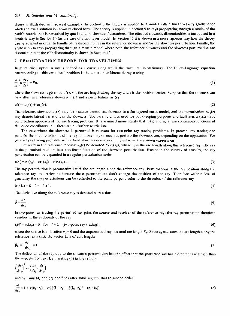
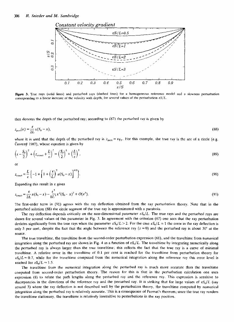
Figure 3. True rays (solid lines) and perturbed rays (dashed lines) for a homogeneous reference model and a slowness perturbation corresponding to a linear increase of the velocity with depth, f o r several values of the perturbation ES/L.
then denotes the depth of the perturbed ray; according to (87) the perturbed ray is given by
where it is used that the depth of the perturbed ray is zper, = E q , . For this example, the true ray is the arc of a circle (e.g. Cervenf 1987), whose equation is given by
or
z,,,,, = 4 8 [-1 + [I + ( ; )2x (s ( , -x ) ] ”2} .
Expanding this result in E gives
& E 3 ze,,,t=-x(sO-x) 2L --x2(s(,-x)2+ 8L3 O(&S). (91)
The first-order term in (91) agrees with the ray deflection obtained from the ray perturbation theory. Note that in the perturbed solution (88) the circle segment of the true ray is approximated with a parabola.
The ray deflection depends critically on the non-dimensional parameter &S0/L. The true rays and the perturbed rays are shown for several values of this parameter in Fig. 3 . In agreement with the criterion (67) one sees that the ray perturbation deviates significantly from the true rays when the parameter ES,)/L > 2. For the case &S0/L = 1 the error in the ray deflection is only 5 per cent, despite the fact that the angle between the reference ray ( z = 0) and the perturbed ray is about 30” at the source.
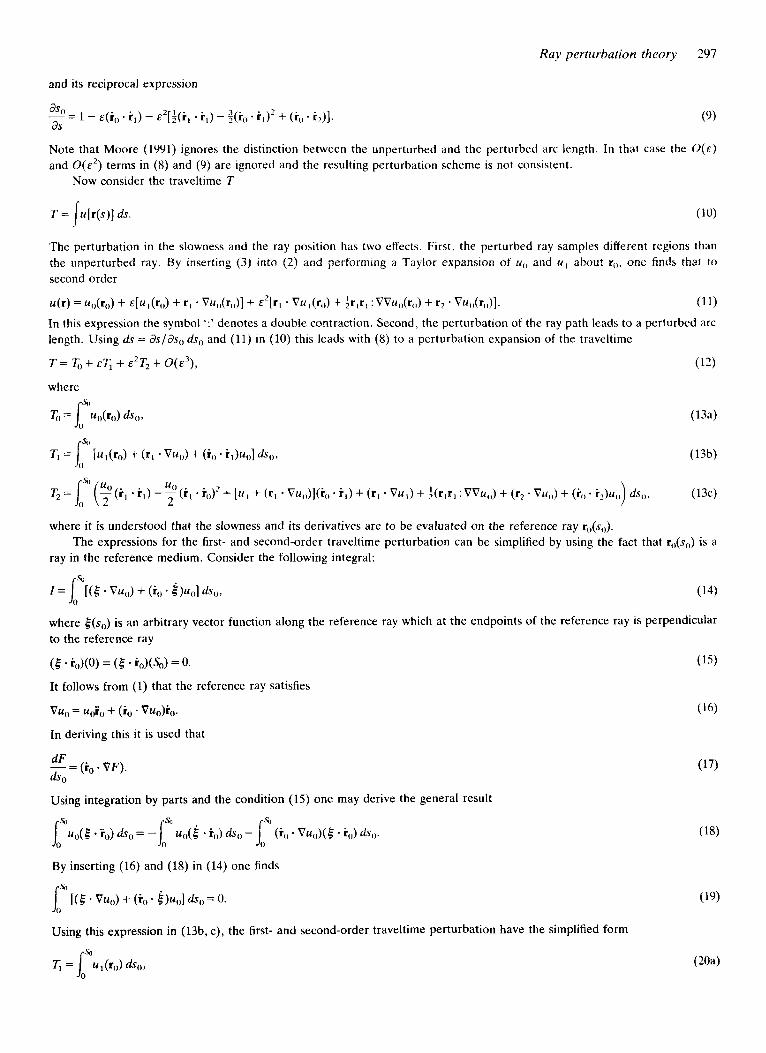
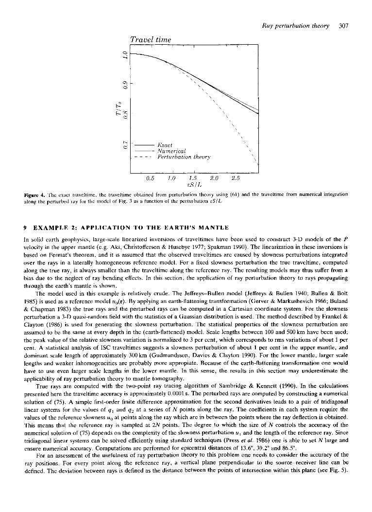
The true traveltime, the traveltime from the second-order perturbation expression (61), and the traveltime from numerical integration along the perturbed ray are shown in Fig. 4 as a function of ES,)/L. The traveltime by integrating numerically along the perturbed ray is always larger than the true traveltime; this reflects the fact that the true ray is a curve of minimal traveltime. A relative error in the traveltime of 0.1 per cent is reached for the traveltime from perturbation theory for &SO/L=O.7, while for the traveltime computed from the numerical integration along the reference ray this error level is reached for ES[,/L = 1.5.
The traveltime from the numerical integration along the perturbed ray is much more accurate than the traveltime computed from second-order perturbation theory. The reason for this is that in the perturbation calculation one uses expression (8) t o relate the path lengths along the perturbed ray and the reference ray. This expression is sensitive to discrepancies in the directions of the reference ray and the perturbed ray. It is striking that for large values of &SOIL (say around 3 ) where the ray deflection is not described well by the perturbation theory, the traveltime computed by numerical integration along the perturbed ray is relatively accurate. This is a consequence of Fermat’s theorem; since the true ray renders the traveltime stationary, the traveltime is relatively insensitive to perturbations in the ray position.
Ruy perturbation theory 307
Travel time I ' I ' I ' I ' I '
\ ,
Exact
Pertic rbnt ion t1ieor.y
\ \
- Numerical \ \ ~~-
\
1 , 1 / 1 ,
0.5 1.0 1.5 2.0 2.5 E S I I3
Figure 4. The exact traveltime, the traveltime obtained from perturbation theory using (61) and the traveltime from numerical integration along the perturbed ray for the model of Fig. 3 as a function of the perturbation E S / L .
9 EXAMPLE 2: APPLICATION TO THE EARTH'S MANTLE
In solid earth geophysics, large-scale linearized inversions of traveltimes have been used to construct 3-D models of the P velocity in the upper mantle (e.g. Aki, Christofferson & Husebye 1977; Spakman 1990). The linearization in these inversions is based on Fermat's theorem, and it is assumed that the observed traveltimes are caused by slowness perturbations integrated over the rays in a laterally homogeneous reference model. For a fixed slowness perturbation the true traveltime, computed along the true ray, is always smaller than the traveltime along the reference ray. The resulting models may thus suffer from a bias due to the neglect of ray bending effects. In this section, the application of ray perturbation theory to rays propagating through the earth's mantle is shown.
The model used in this example is relatively crude. The Jeffreys-Bullen model (Jeffreys & Bullen 1940; Bullen & Bolt 1985) is used as a reference model uo(r). By applying an earth-flattening transformation (Gerver & Markushevich 1966; Buland & Chapman 1983) the true rays and the perturbed rays can be computed in a Cartesian coordinate system. For the slowness perturbation a 3-D quasi-random field with the statistics of a Gaussian distribution is used. The method described by Frankel & Clayton (1986) is used for generating the slowness perturbation. The statistical properties of the slowness perturbation are assumed to be the same at every depth in the (earth-flattened) model. Scale lengths between 100 and 500 km have been used; the peak value of the relative slowness variation is normalized to 3 per cent, which corresponds to rms variations of about 1 per cent. A statistical analysis of ISC traveltimes suggests a slowness perturbation of about 1 per cent in the upper mantle, and dominant scale length of approximately 300 km (Gudmundsson, Davies & Clayton 1990). For the lower mantle, larger scale lengths and weaker inhomogeneities are probably more appropiate. Because of the earth-flattening transformation one would have to use even larger scale lengths in the lower mantle. In this sense, the results in this section may underestimate the applicability of ray perturbation theory to mantle tomography.
True rays are computed with the two-point ray tracing algorithm of Sambridge & Kennett (1990). In the calculations presented here the traveltime accuracy is approximately 0.0001 s. The perturbed rays are computed by constructing a numerical solution of (75). A simple first-order finite difference approximation for the second derivatives leads to a pair of tridiagonal linear systems for the values of q 1 and q2 at a series of N points along the ray. The coefficients in each system require the values of the reference slowness u ~ , at points along the ray which are in between the points where the ray deflection is obtained. This means that the reference ray is sampled at 2N points. The degree to which the size of N controls the accuracy of the numerical solution of (75) depends on the complexity of the slowness perturbation u 1 and the length of the reference ray. Since tridiagonal linear systems can be solved efficiently using standard techniques (Press et al. 1986) one is able to set N large and ensure numerical accuracy. Computations are performed for epicentral distances of 13.6", 39.2" and 86.5".
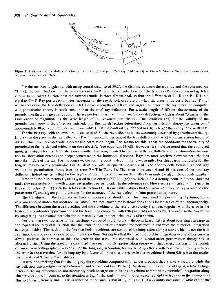
For an assessment of the usefulness of ray perturbation theory to this problem one needs to consider the accuracy of the ray positions. For every point along the reference ray, a vertical plane perpendicular to the source-receiver line can be defined. The deviation between rays is defined as the distance between the points of intersection within this plane (see Fig. 5).
308 R. Snieder and M . Sambridge
Source RANGE A-
P-T
Figure 5 , Definition of the distances between the true ray, the perturbed ray, and the ray in the reference medium. The distances are measured in the vertical plane.
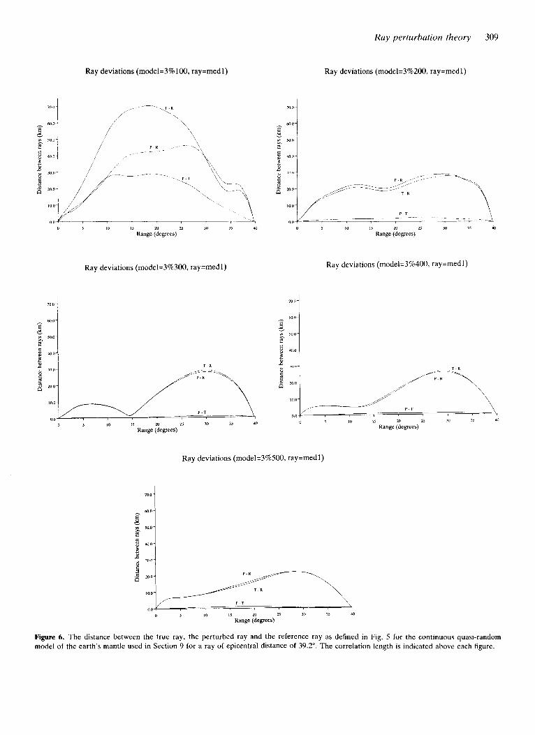
For the medium length ray, with an epicentral distance of 3 9 2 , the distance between the true ray and the reference ray (T - R), t h e perturbed ray and the reference ray (P - R) and the perturbed ray and the true ray (P-T) is shown in Fig. 6 for various scale lengths L. Note that the slowness model is three-dimensional, so that the difference of T - R and P - R is not equal to T - P. Ray perturbation theory accounts for the ray deflection accurately when the error in the perturbed ray (P - T) is much less than the true deflection ( T - R). For scale lengths of 200 km and larger, the error in the ray deflection computed with perturbation theory is much smaller than the total ray deflection. For a scale length of 100 km, the accuracy of the perturbation theory is greatly reduced. The reason for this is that in this case the ray deflection, which is about 70 km, is of the same order of magnitude as the scale length of the slowness perturbation. The condition (65) for the validity of the perturbation theory is therefore not satisfied, and the ray deflection determined from perturbation theory has an error of approximately 40 per cent. O n e can see from Table 1 that the constant Cz, defined in (68) is larger than unity for L = 100 km.
For the long ray, with an epicentral distance of 86.5", the ray deflection is less accurately described by perturbation theory. In this case the error in the ray deflection (P - T) is about 30 per cent of the true deflection ( T - R) for a correlation length of 400 km; this error increases with a decreasing correlation length. The reason for this is that the conditions for the validity of perturbation theory depend critically on the ratio S,,/L (see equations 67-68). However, it should be noted that the employed model is probably t o o rough for the lower mantle. This is aggravated by the use of the earth-flattening transformation because this transformation extends the deeper structures in the horizontal direction. Rays are most sensitive slowness perturbations near the middle of the ray. For the long ray, the turning point is deep in the lower mantle. For this reason the results for the long ray may be overly pessimistic. For the short ray, with an epicentral distance of 13.6", the ray deflection is described very well by the perturbation theory (see the error P - T in Table 1). This error is between 4 and 10 per cent of the total ray deflection. Indeed one finds that for this ray the constant C, and C, are much smaller than unity for all employed scale lengths.
Note that the parameters C, and C2 used in the criteria (67) and (68) are derived for a homogeneous reference slowness and a slowness perturbation with a constant gradient perpendicular to the reference ray. However, a comparison of the error in t h e ray deflection (P - T) with the total ray deflection (T - R) in Table 1 shows that for more complicated ray geometries the parameters C, and C, are good indicators for the accuracy of the ray deflection from perturbation theory.
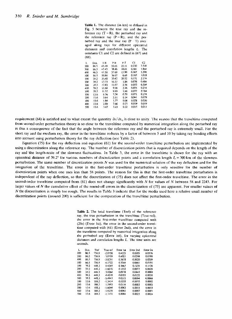
The traveltimes in the ISC data set have an accuracy of about 0.1 s. The theory used for performing the tomographic inversions should match this accuracy. In Table 2, the total traveltime is shown for various length-scales of the inhomogeneity. T h e difference between the true traveltime and the traveltime in the reference velocity is shown, together with the error in the first- and second-order approximations of the traveltime computed with (20a) and (61) respectively. The error in the traveltime by integrating the slowness perturbation numerically over the perturbed ray is also shown.
For the long ray, the error in the traveltime computed using Fermat's theorem (Error 1st) is about four times as large as t h e required accuracy of 0.1 s. Note that the error in the first-order traveltime perturbation and from the numerical integration is always positive. This is due t o the fact that both traveltimes are computed by integration along a curve which is not the true ray. Since the true ray is a curve of minimum traveltime this implies that the error induced by integrating over another curve is always positive. In contrast to this, the error in the traveltime computed with second-order perturbation theory has an alternating sign. Using the traveltime computed from second-order perturbation theory will thus reduce the bias in the models obtained from tomographic inversions. For the long ray, accounting for ray bending effects with perturbation theory reduces the error in the traveltime for the long ray by a factor of 10, so that the error in the traveltime is about 0.04 s (see the entries 'Error 2nd' and 'Error int' in Table 2).
It may be surprising that for the long ray the traveltime computed with ray perturbation theory is very accurate, while the ray deflection has a relative error between 10 and 50 per cent (see Table 1). As shown in the example of Fig. 4, relatively large errors in the ray deflection d o not necessarily produce large errors in the traveltime computed by numerical integration along the perturbed ray. In contrast t o the situation in Fig. 4, the angle between the reference ray and the true ray in the examples in this section is extremely small. This is reflected in the small value of C, in Table 1; this quantity measures to what extent the
Ray deviations (rnodel=3%100, ray=rnedl)
Huy perturbation theory 309
Ray deviations (model=3%200, ray=rnedl)
0 I 10 I S 20 zs 30 15 4n U 5 10 I 5 20 23 M 15 a Range (degrees) Range (degrees)
Ray deviations (rnodel=3%400, ray=medl) Ray deviations (model=3%300, ray=rnedl)
,,y ,, , I U u
P T
0 0 20 25 3u 35 do
U 5 10 1s m 2s 30 40 Range (degrees) 35 0 5 10 IS
Range (degrees)
Ray deviations (rnodel=3%500, ray=medl)
n 5 10 I5 20 l5 30 35 40
Range (degrees)
Figure 6. The distance between the true ray, the perturbed ray and the reference ray as defined in Fig. 5 for the continuous quasi-random model of the earth's mantle used in Section 9 for a ray of epicentral distance of 39.2". The correlation length is indicated above each figure.
310 R. Snieder and M . Sambridge
Table 1. The distance (in km) as defined in Fig. 5 between the true ray and the re- ference ray (T- R), the perturbed ray and the reference ray (P - R), and the per- turbed ray and the true ray (P -T) aver- aged along rays for different epicentral distances and correlation lengths L. The constants C1 and C2 are defined in (67) and (68). L Dist. T-R P-R P-T CI C2 ux) 86.5 45.49 33.05 22.11 0.230 3.548 300 86.5 43.43 38.46 16.01 0.181 1.864 400 86.5 47.50 37.69 15.90 0.167 1.290 500 86.5 50.84 3607 6.69 0.165 1.018 100 39.2 35.40 20.42 20.52 0.171 2.174 200 39.2 17.75 16.37 1.86 0.076 0.484 300 39.2 12.83 11.07 2.34 0.072 0.304 400 39.2 11.69 9.98 2.26 0.074 0.234 500 39.2 11.52 9.99 1.88 0.072 0.184 100 13.6 6.56 7.24 0.70 0.071 0.274 200 13.6 3.64 3.51 0.14 0.041 0.079 300 13.6 1.84 1.77 0.08 0.028 0.036 400 13.6 2.89 2.66 0.23 0.019 0.019 500 13.6 3.47 3.15 0.32 0.015 0.011
requirement (64) is satisfied and to what extent the quantity & / a s , , is close to unity. The reason that the traveltime computed from second-order perturbation theory is so close to the traveltime computed by numerical integration along the perturbed ray is thus a consequence of the fact that the angle between the reference ray and the perturbed ray is extremely small. For the short ray and the medium ray, the error in the traveltime reduces by a factor of between 5 and 10 by taking ray bending effects into account using perturbation theory for the ray deflection (see Table 2).
Equation (75) for the ray deflection and equation (61) for the second-order traveltime perturbation are implemented by using a discretization along the reference ray. The number of discretization points that is required depends on the length of the ray and 'the length-scale of the slowness fluctuations. In Table 3, the error in the traveltime is shown for the ray with an epicentral distance of 39.2" for various numbers of discretization points and a correlation length L = 300 km of the slowness perturbation. The same number of discretization points N was used for the numerical solution of the ray deflection and for the integration of the traveltime. The error in the first-order traveltime perturbation is only sensitive for the number of discretization points when one uses less than 58 points. The reason for this is that the first-order traveltime perturbation is independent of the ray deflection, so that the discretization of (75) does not affect the first-order traveltime. The error in the second-order traveltime computed from (61) does not change significantly with N for values of N between 58 and 2243. For larger values of N the cumulative effect of the round-off errors in the discretization of (75) are apparent. For smaller values of N the discretization is simply too rough. The results in Table 3 indicate that for the media used here a relative small number of discretization points (around 200) is sufficient for the computation of the traveltime perturbation.
Table 2. The total traveltime (Tref) of the reference ray, the true perturbation in the traveltime (True-ref), the error in the first-order traveltime computed with (20a) (Error lst), the error in the second-order travel- time computed with (61) (Error 2nd), and the error in the traveltime computed by numerical integration along the perturbed ray (Error int), for varying epicentral distances and correlation lengths L. The time units are seconds.
L 200 300 400 500 100 200 300 400 500 100 200 300 400 500
Dist. 86.5 86.5 86.5 86.5 39.2 39.2 39.2 39.2 39.2 13.6 13.6 13.6 13.6 13.6
Tref 756.9 756.9 756.9 756.9 448.3 448.3 448.3 448.3 448.3 188.2 188.2 188.2 188.2 188.2
True-ref E -2.0738 -3.0359 -3.8291 4.1722 -0.4365 - 1.6070 -3.0264 4.4218 -5.4943 -1.3414 -1.5993 -1.6044 - I ,6279 -1.7131
:nor IS1 0.4223 0.4021 0.3678 0.3344 0.3462 0.1332 0.0938 0.0703 0.0513 0.0355 0.0116 0.0063 0.0061 0.0084
Error 2nd 0.0305 -0.0398 -0.0020 0.0461 0.1235 0.0077 0.0143 0.01 22 0.0094 -0.0033 0.0003 0.0015 0.0007 0.0023
Error in1 0.0576 0.0399 0.0209 0.0191 0.1120 0.0026 0.0069 0.0030 0.0068 0.0002 0.0003 0.0015 0.0001 0.0024
Ray perturbation theory 31 1
Table 3. Accuracy of the traveltime computa- tions for the medium length ray, for the Jeffreys-Bullen reference model and the con- tinuous quasi-random slowness perturbation with a correlation length L = 300 km, as a function of the number of discretization points N . Thc errors arc dcfincd in Table 2.
N. Tref True-ref Error Is1 Enur2nd Error in1 22418 448.3 -3.026 0.0938 0.11143 0.0044 2243 448.3 -3.026 0.0938 11.0051 0.0023
114 48.3 -3 026 0.0937 o.oosn n.11155 sx 448.3 -3.026 0.0~37 n.wR 0.0526
226 448.3 -3.026 0.0938 0.0050 0.0056
22 448.3 -3.026 0.O967 0.0087 0.3784
The model used here for the slowness perturbation in the earth's mantle is rather crude. It does not take into account that the lower mantle may be smoother than the upper mantle. The length-scale o f the inhomogeneity is also not corrected for the effects of the earth-flattening transformation. Furthermore, a quasi-random slowness perturbation is not completely satisfactory for studying ray bending effects in mantle tomography, because the earth's mantle contains significant organized structures such as subduction zones. The validity of ray perturbation theory for mantle tomography is presently further investigated.
10 EXAMPLE 3: A DISCONTINUOUS SLOWNESS PERTURBATION
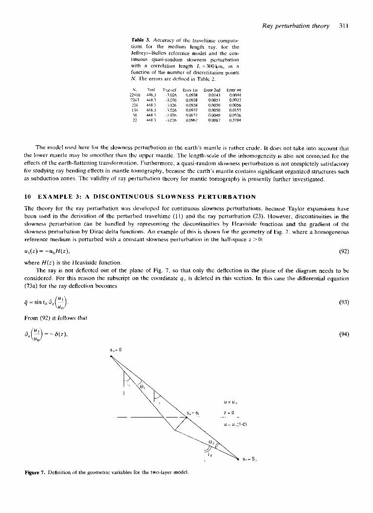
The theory for the ray perturbation was developed for continuous slowness perturbations, because Taylor expansions have been used in the derivation of the perturbed traveltime (11) and the ray perturbation (23). However, discontinuities in the slowness perturbation can be handled by representing the discontinuities by Heaviside functions and the gradient of the slowness perturbation by Dirac delta functions. An example of this is shown for the geometry of Fig. 7, where a homogeneous reference medium is perturbed with a constant slowness perturbation in the half-space z > 0:
u, (z ) = -uoH(z) , (92)
where H ( z ) is the Heaviside function. The ray is not deflected out of the plane of Fig. 7, so that only the deflection in the plane of the diagram needs to be
considered. For this reason the subscript on the coordinate q , is deleted in this section. In this case the differential equation (73a) for the ray deflection becomes
ij = sin i,, 8, (2). From (92) it follows that
so= 0
(93)
Figure 7. Definition of the geometric variables for the two-layer model.
312
where b ( z ) is the Dirac delta function. The derivatives in equation (93) are with respect t o the parameter sg. The delta function in the right-hand side of (94) needs to be expressed in s(,. This can be achieved using
R. Snieder and M . Sambridge
I dso/.,,,=,,
where s, denotes the distance between the source and the point of intersection of the straight reference ray with the slowness discontinuity.
Inserting (95) in (93) gives
q = -tan iO 6(s,, - s,).
Integrating this equation leads with the boundary conditions (51) to the solution
Note that this solution breaks down when i,, = n /2 . This is the case when the source and the receiver are on the same side of the slowness discontinuity. This situation is not consistent with the assumption that the straight reference ray intersects the slowness perturbation. It will be clear that the solution of (93) will not give an accurate description of rays that are refracted along interfaces.
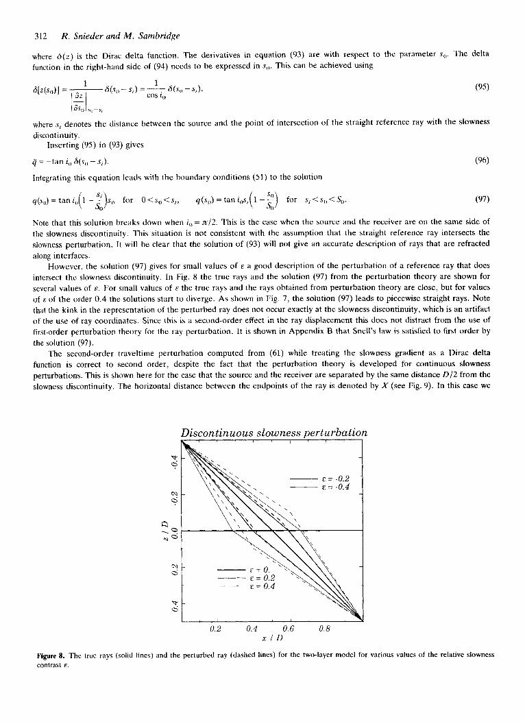
However, the solution (97) gives for small values of E a good description of the perturbation o f a reference ray that does intersect the slowness discontinuity. In Fig. 8 the true rays and the solution (97) from the perturbation theory are shown for several values of E. For small values of F the true rays and the rays obtained from perturbation theory are close, but for values of E of t h e order 0.4 the solutions start to diverge. As shown in Fig. 7, the solution (97) leads to piecewise straight rays. Note that the kink in the representation of the perturbed ray does not occur exactly a t the slowness discontinuity, which is an artifact of the use of ray coordinates. Since this is a second-order effect in the ray displacement this does not distract from the use of first-order perturbation theory for the ray perturbation. It is shown in Appendix B that Snell's law is satisfied to first order by the solution (97).
The second-order traveltime perturbation computed from (61) while treating the slowness gradient as a Dirac delta function is correct t o second order, despite the fact that the perturbation theory is developed for continuous slowness perturbations. This is shown here for the case that the source and the receiver are separated by the same distance D / 2 from the slowness discontinuity. The horizontal distance between the endpoints of the ray is denoted by X (see Fig. 9). In this case we
Discontinuous slowness perturbation
"I 0
h! 0
2
a: 0
I
& = -0.2 - E = -0.4
~
0.2 0.4 0.6 0.8 x l D
Figure 8. The true rays (solid lines) and the perturbed ray (dashed lines) for the two-layer model for various values of the relative slowness contrast E.
Ruy perturhution theory 3 13
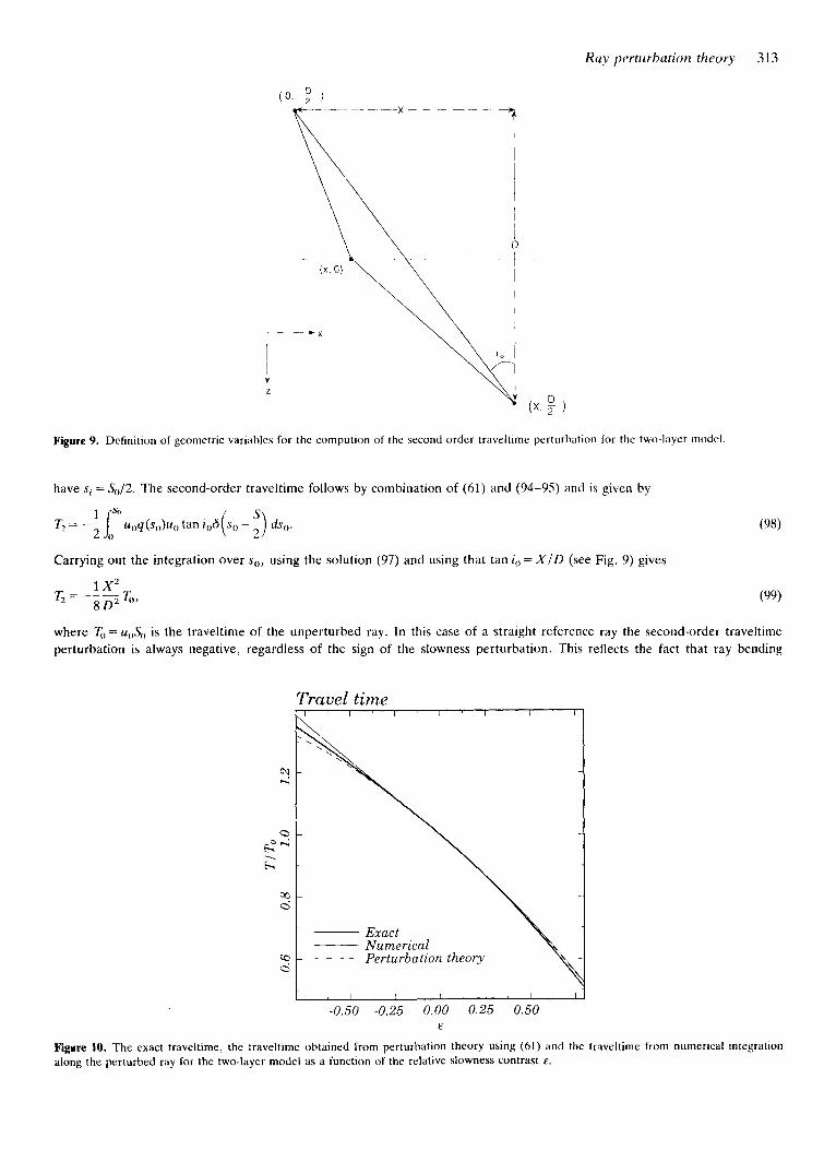
Figure 9. Definition o f geometric variables for the compution of the second-order traveltime perturbation f o r the two-layer model
have si = So/2. The second-order traveltime follows by combination of (61) and (94-95) and is given by
Carrying out the integration over s(,, using the solution (97) and using that tan iO = X / D (see Fig. 9) gives
where 7, = u,,S,, is the traveltime of the unperturbed ray. In this case of a straight reference ray the second-order traveltime perturbation is always negative, regardless of the sign of the slowness perturbation. This reflects the fact that ray bending
Trauel time
v, d
-0.50 -0.25 0.00 0.25 0.50 &
Figure 10. The exact traveltime, the traveltime obtained from perturbation theory using (61) and the traveltime from numerical integration along the perturbed ray for the two-layer model as a function of the relative slowness contrast E.
314 R. Snieder and M . Sambridge
effects reduce the traveltime. Note also that for x = 0 the second-order traveltime perturbation vanishes, which is due to the fact that a ray perpendicular to the slowness discontinuity is not affected by the slowness discontinuity. me second-order traveltime in (99) is based on perturbation theory for continuous slowness perturbations, where a discontinuity is treated as a Dirac delta function in the slowness gradient. AS shown in Appendix C the result (99) agrees with the second-order traveltime perturbation computed for a discontinuous slowness model.
The true traveltime, and the traveltime from the integration along the perturbed ray are shown in Fig. 10 as a function of E. As in Fig. 4, the traveltime along the perturbed ray is always larger than the true traveltime. Note that the traveltime perturbation is dominated by a linear trend, and that the second-order effects on the traveltime are rather small. Indeed, for values of the slowness perturbation as large as E = 0.2 the relative error in the traveltime is less than 0.1 per cent.
This example shows that one can use the ray perturbation theory of this paper for slowness perturbations with discontinuities, by describing the gradient of the slowness perturbation in terms of Dirac delta functions.
11 DISCONTINUITIES IN THE REFERENCE MODEL A N D THE SLOWNESS PERTURBATION
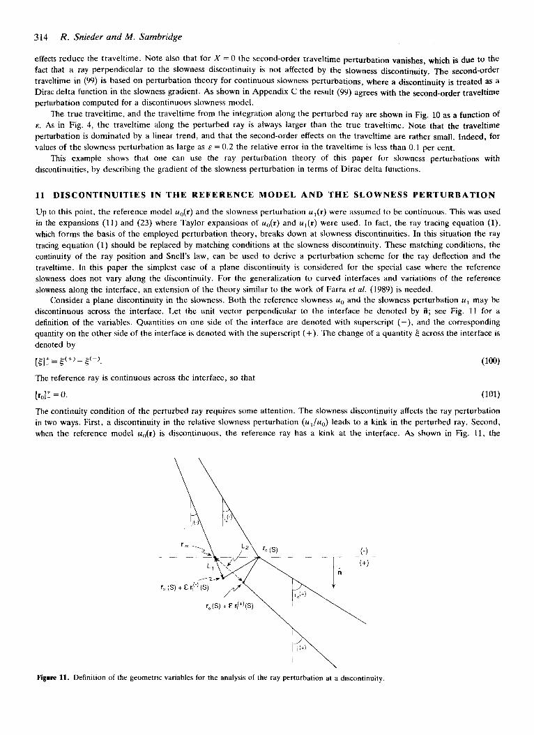
Up to this point, the reference model ug(r) and the slowness perturbation u I ( r ) were assumed to be continuous. This was used in the expansions (11) and (23) where Taylor expansions of u<,(r) and uI(r) were used. In fact, the ray tracing equation (l), which forms the basis of the employed perturbation theory, breaks down at slowness discontinuities. In this situation the ray tracing equation (1) should be replaced by matching conditions at the slowness discontinuity. These matching conditions, the continuity of the ray position and Snell’s law, can be used to derive a perturbation scheme for the ray deflection and the traveltime. In this paper the simplest case of a plane discontinuity is considered for the special case where the reference slowness does not vary along the discontinuity. For the generalization to curved interfaces and variations of the reference slowness along the interface, an extension of the theory similar to the work of Farra et al. (1989) is needed.
Consider a plane discontinuity in the slowness. Both the reference slowness u0 and the slowness perturbation u1 may be discontinuous across the interface. Let the unit vector perpendicular to the interface be denoted by 5; see Fig. 11 for a definition of the variables. Quantities on one side of the interface are denoted with superscript (-), and the corresponding quantity on the other side of the interface is denoted with the superscript (+). The change of a quantity 6 across the interface is denoted by
E ( + ) - t(-). (100)
[q,]: = 0. (101)
The reference ray is continuous across the interface, so that
The continuity condition of the perturbed ray requires some attention. The slowness discontinuity affects the ray perturbation in two ways. First, a discontinuity in the relative slowness perturbation ( u l / u o ) leads to a kink in the perturbed ray. Second, when the reference model uo(r) is discontinuous, the reference ray has a kink at the interface. As shown in Fig. 11, the
\ \
\ Figure 11. Definition of the geometric variables for the analysis of the ray perturbation at a discontinuity.
Ray perturbation theory 3 15
definition of the ray coordinates produces in this situation a discontinuity in the representation of the perturbed ray. This is an artifact of the use of ray coordinates that needs to be corrected. This can be achieved by determining the point of intersection of the perturbed rays (or their extensions) with the interface. By imposing an appropriate continuity condition on the ray deflection on the two sides of the interface, one can obtain a continuous perturbed ray by replacing the broken representation of the perturbed ray by a new representation which is continuous at the interface (see the dashed line in Fig. 11). The condition to be imposed on the perturbed rays is therefore that the perturbed rays (or their extensions) intersect the interface in the same position Tin,.
Consider for the moment a coordinate system with the z-axis perpendicular to the interface, and let the interface be located at z = zfJ. Let the interface be located at arc length S along the unperturbed ray. On either side of the interface the ray can in the vicinity of the interface be parametrized as
r(so) = a + bso, (102)
(103a)
(103b)
Let the point of intersection of the perturbed ray with the plane of the discontinuity occur for so = s,,[; this point is defined by the condition
to = (ii - r,,,) = (a - ii) + (b * s)~,,,~. (104)
Solving this expression for s,,,,, inserting the result in (102) and using the definitions (103a,b) gives to first order
In this expression and the ensuing matching conditions, all quantities should be evaluated at 3,) = S. Since the perturbed rays (or their extensions) must intersect the interface in the same position, the quantity derived in (105) must be continuous across the interace. Because of the continuity of r,) (see 101), this implies that
The second continuity condition comes from the requirement that the perturbed rays satisfy Snell's law, which states that (Aki & Richards 1980)
[ ii x u "1 +(S,,,) = 0. d s -
Note that this continuity condition holds a t the point of intersection rint of the perturbed ray with the interface, hence the argument sin[ rather than so = S. Expanding (107) around the point so = S gives
d [e x .d']'(S) + E(Sint - S) - [ii x u "]+(S) = 0. d s - 4 1 d s -
The factor E has been introduced because (sin, - S) is linear in the ray deflection. Consider the last term in (108). Since only the first-order ray deflection is desired one can replace all quantities in the term
by their zeroth-order approximations. Carrying out the differentiation with respect to so, using that the discontinuity is plane so that Fi is a constant, and using (17) for the differentiation of uo, one finds that to O(E)
With (16) this implies that
When u,] does not vary along the interface, Vu,, and ii are parallel, and the right-hand side of (110) vanishes. (This condition
316 R. Snieder and M. Sambridge
can in fact be slightly relaxed, since only the discontinuity in the gradient of ug along the interface needs to vanish.) Using this in (108) implies that
[P x u "1 + ( S ) = 0. l i p
From this point o n all quantities are evaluated for sg = S ; the variable S is therefore omitted. The unperturbed ray also satisfies Snell's law at the point s,, = S, so that
[ii x u(+l,]: = 0.
[ { u , - U 0 ( i l * r(J}fi x r,, + Uof i x ill: = 0.
(112)
Insert (2) and (22) in (111). with (112) this imp!ies that to first order
(113)
The condition (106) imposes a relation on [rl]T, while Snell's law (113) constrains the kink in the ray perturbation [ill:. The matching conditions (106) and (113) are expressed in terms of the ray perturbation r, . However, as in Section 4 it is
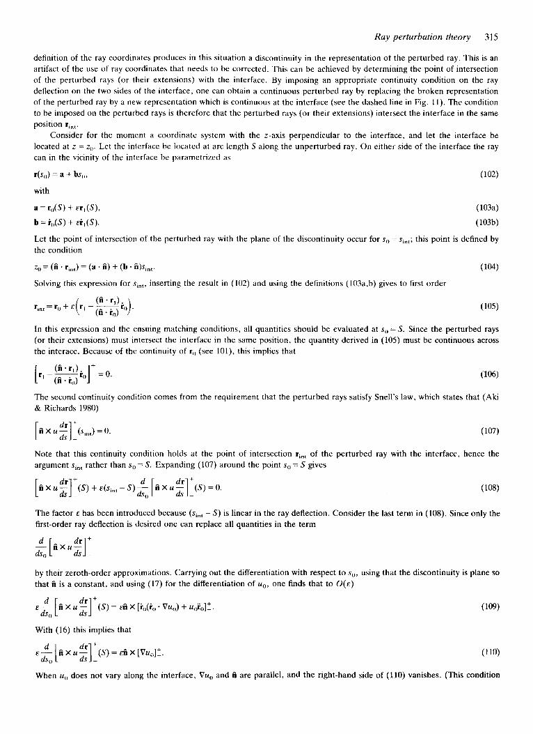
advantageous to re-express these conditions in ray coordinates. This results in matching conditions for q l , q2 and their derivatives. It is convenient to define two unit vectors CII and 6 , in the plane of the interface (see Fig. 12). The unit vector kIl lies along the intersection of the plane of the interface, with the plane spanned by the incoming and the outgoing rays. The unit vector is the unit vector in the interface perpendicular to CII. The orthogonality of CI, and @I implies that
el, (ci x ill) = 0. (114)
The conditions (106) and (113) can be recast as conditions for q , and q2 by using (35) and (46) and dotting the results with both CI I and 6 I . This gives using (114):
(1 15a)
(1 15b)
(115c)
(1 15d)
All unit vectors in these expressions are known, so they provide explicit matching conditions for q l , q2 , q I and q2. Note that the unit vectors 4, may be chosen completely differently on either side of the interface. In fact, if the reference
ray has a kink at least one of the 4; must be discontinuous across the interface. As long as one uses the 9; appropriate for the two sides of the interfaces in (115) this poses n o problems. Similarly, the rate of rotation Q of the unit vectors can be chosen independently on the two sides of the interface.
At the interface of the slowness discontinuity, the matching conditions ( 1 15) are to be used rather than the differential equation (50). In the regions between the slowness discontinuities one should of course use (50) for the computation of the ray perturbation. When one discretizes the ray perturbation, one can express the matching conditions as linear equations with a tridiagonal structure. The resulting h e a r equations thus have the same algebraic structure as the linear equations that result from the discretization of expression (50) for the regions between the slowness discontinuities. This means that incorporating discontinuities in the reference slowness does not alter the structure of the algorithm for the computation of the first-order ray deflection.
A s an example of the matching conditions, consider a layered reference medium with horizontal interfaces z = consfmi.
\
\ \
Figure l2. Definition of the unit vectors SII and 6, in the plane of the discontinuity.
Ray perturbation theory 317
For this situation it is convenient to assume that the 4 vectors d o not rotate around the reference ray. condition (69). and to use the expressions (70) for the q,. Referring to Fig. 2 we have in this case
(116a)
( 1 1hb)
( I Ihc)
Using these relations in (115) and using (74) to eliminate the sin i,, and cos i,, terms in favour of the ray parameter p one obtains the following matching conditions:
[Uoq,]' = 0.
(1 17b)
(1 17c)
( 1 17d)
As an example, for the slowness perturbation (92) of the two-layer model of Section 10, one finds from (1 17) and the definition (74) that [4,]" = -tan io. This result is equivalent to expression (96) obtained by replacing the gradient of (uI/uo) by a delta function when this quantity is discontinuous.
For the computation of the second-order traveltime perturbation one can either integrate numerically over the perturbed ray using the dashed interval L, in Fig. 11, or one can use the expressions of Section 5 for T,. T o see that these expressions can be used when slowness discontinuities are present one should realize that the derivations in the Sections 2 and 5 hold for any subsection of the ray between the discontinuities. There is no reason why the interval 0 < s,, < S,, in the Sections 2 and 5 should denote the whole ray, it may also denote a subsection of the ray between the interfaces. The generalized condition (15) for the validity of Fermat's theorem allows for this flexibility. Because o f the use o f ray coordinates, the boundary condition (15) is automatically satisfied at all points along the reference ray, hence also at the points where the reference ray intersects the interface. This implies that when one uses for example (61) for the computation of T,, that one should take the boundary term $u,qiqi in (61) into account at the interface because this quantity is not necessarily continuous across the interface. One can verify easily that the contribution of this boundary term in (61) from subsections of the ray at the opposite sides of the interface leads to a contribution [$uOqi4i]' to the second-order traveltime perturbation. Ignoring this contribution in the example of Section 12 for a mantle model with realistic discontinuities leads to a tenfold increase in the error in the second-order traveltime. For the special case of a layered reference medium with horizontal interfaces, as in expression (117), one can eliminate the q2 contribution to the interface term: [~uOqjqt] ' = [ ~ u o q l ~ , ] ~ .
12 EXAMPLE 4: DISCONTINUOUS SLOWNESS MODELS FOR THE EARTH'S MANTLE
As an illustration of the effect of discontinuities, it is shown in this section what the effect of discontinuities of the reference model and the slowness perturbation are for waves propagating through the earth's mantle. The PREM model (Dziewonski & Anderson 1981) is used as a reference model. This model has a pronounced discontinuity in the slowness at a depth of about 670 km. For the slowness perturbation, the quasi-random model used in Section 9 is used. The only difference is that the slowness perturbations are independent in the upper and lower mantle, so that the slowness perturbation is also discontinuous at a depth of 670 km.
The ray deviations for an epicentral distance of 39.2" are shown in Fig. 13 for various values of the correlation length L. The ray deviations, as defined in Fig. 5 , exhibit a kink at the location where the ray intersects the 670 km discontinuity. This is due to the fact that the ray deviations are measured in a vertical plane perpendicular to the source-receiver line. When the rays have a kink this implies that the ray deviation has a discontinuity.
A pronounced difference with the ray deviations of Fig. 6 for the continuous slowness model is that the ray deviation in Fig. 13 are largest a t the slowness discontinuity. A t these locations the ray has a kink; apparently this increases the sensitivity of the ray deflection to perturbations in the slowness. As in Fig. 6, the perturbed ray is not accurate for the shortest correlation length ( L = 100 km). For the continuous slowness model used for Fig. 6 the error in the perturbed ray steadily decreases when the correlation length L is increased and the model becomes smoother. In that case the error in the perturbed ray is negligible when L = 5 0 0 k m . This is not the case in Fig. 13 for the discontinuous slowness model. The reason for this is that for the discontinuous slowness model the ray deflection is caused both by the slowness variations with correlation length L in the upper and lower mantle, and by the discontinuity in the slowness perturbation [uI/u,,]+ at a depth of 670 km. When L increases, the effect of the quasi-random slowness perturbation on the ray deflection decreases, but the effect of the slowness discontinuity remains constant. One can conclude that the error in the ray deflection in Fig. 13 for L > 300 km is due to the
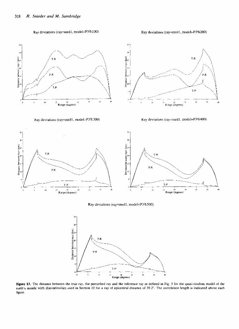
318 R. Snieder and M. Sarnbridge
Ray deviations (ray=medl, model=P3%100)
31 1
0 I 10 I S 20 15 10 40
Range (degrees)
Ray deviations (ray=rnedI, model=P3%300)
11
Ray deviations (ray=rnedl, rnodel=P3%200)
1, I0 l i Range (degrees) 20 7 3 0 15 40
Ray deviations (ray=rnedI, rnodel=P3%400)
n 5 10 I 5 i n 5 31) 17 do
Range (degrees) 0 5 in I 7 20 27 10 A 0
Range (degrees)
Ray deviations (ray=rnedl, rnodel=P3%500)
0 5 I0 I 7 zn 27 10 I, a Range (degrees)
Figure 13. The distance between the true ray, the perturbed ray and the reference ray as defined in Fig. 5 for the quasi-random model of the earth's mantle with discontinuities used in Section 12 for a ray of epicentral distance of 39.2". The correlation length is indicated above each figure.
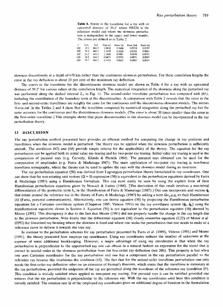
Ray perturbation theory 319
Table 4. Errors in the traveltime for a ray with an epicentral distance of 39.2” where PREM is the reference model and where the slowness perturba- tion is independent in the upper and lower mantle. The errors are defined as in Table 2.
L Dist. Trcf True-rcf Error 1st Emr2nd E m r in1 100 39.2 444.7 1.0616 0.1666 0.0514 0.0197 200 39.2 444.7 1.3109 0.1028 0.0165 0.0061 300 39.2 444.7 1.1690 0.0881 O.M)70 0.0031 400 39.2 444.7 0.6871 0.0765 0.0051 0.0042 500 39.2 444.7 0.1433 0.0635 0.0007 0.0014
slowness discontinuity at a depth of 670 km rather than the continuous slowness perturbation. For these correlation lengths the error in the ray deflection is about 20 per cent of the maximum ray deflection.
The errors in the traveltime for the discontinuous slowness model are shown in Table 4 for a ray with an epicentral distance of 39.2” for various values of the correlation length. The numerical integration of the slowness along the perturbed ray was performed along the dashed interval L, in Fig. 11. The second-order traveltime perturbation was computed with (61), including the contribution of the boundary term at the discontinuities. A comparison with Table 2 reveals that the error in the first- and second-order traveltimes are roughly the same for the continuous and the discontinuous slowness models. The entries ‘Error-int’ in the Tables 2 and 4 show that the traveltime computed by numerical integration along the perturbed ray has the same accuracy for the continuous and the discontinuous slowness models. (The error is about 20 times smaller than the error in the first-order traveltime.) This example shows that plane discontinuities in the slowness model can be incorporated in the ray perturbation theory.
13 DISCUSSION
The ray perturbation method presented here provides an efficient method for computing the change in ray positions and traveltimes when the slowness model is perturbed. The theory can be applied when the slowness perturbation is sufficiently smooth. The conditions (67) and (68) provide simple criteria for the applicability of the theory. The equation for the ray perturbation can be applied both to initial value ray tracing and for two-point ray tracing. Initial value ray tracing is used in the computation of paraxial rays (e.g. Cerveliy, Klimgs & PSenEik 1984). The paraxial rays obtained can be used for the computation of amplitudes (e.g. Farra & Madariaga 1987). The main application of two-point ray tracing is non-linear traveltime tomography, where the theory can be used to update the rays with the slowness model during an inversion.
The ray perturbation equation (50) was derived from Lagrangian perturbation theory formulated in ray coordinates. One can show that for non-rotating unit vectors (52 = 0) expression (50) is equivalent to the perturbation equations derived by Farra & Madariaga (1987) using a Hamiltonian formalism. This can most easily be seen by using the explicit form of their Hamiltonian perturbation equations given by Nowack & Lutter (1988). [The derivation of this result involves a non-trivial differentiation of the geometric term h , in the Hamiltonian of Farra & Madariaga (1987).] One can incorporate unit vectors qi that rotate around the reference ray in the theory of Farra & Madariaga (1987) by adding a term S2Ei,piq, to their Hamiltonian (4) (Farra, personal communication). Alternatively, one can derive equation (50) by projecting the Hamiltonian perturbation equations for a Cartesian coordinate system (Chapman 1985; Virieux 1991) on the ray coordinate system (a,, ij2) using the transformation equations shown in Section 4. Equation (50) is not equivalent to the perturbation equation (18) derived by Moore (1991). This discrepancy is due to the fact that Moore (1991) did not properly handle the change in the ray length due to the slowness perturbation. Note finally that the differential equation (50) closely resembles equation (C22) of Moser el af. (1992) for linearized ray bending where the slowness is fixed and where one seeks the perturbation that one needs to make to a reference curve to deform it towards the true ray.
In contrast to the perturbation schemes for ray perturbation presented by Farra et al. (1989), Virieux (1991) and Moore (1991), the theory presented here employs ray coordinates. Using ray coordinates reduces the number of unknowns at the expense of some additional bookkeeping. However, a major advantage of using ray coordinates is that when the ray perturbation is perpendicular to the unperturbed ray one can obtain in a natural fashion an expression for the travel that is correct to second order in the slowness perturbation from the first-order ray deflection (see 20b). This property is lost when one uses Cartesian coordinates for the ray perturbation and one has a component in the ray perturbation parallel to the reference ray because this invalidates the condition (15). The fact that for the second-order traveltime perturbation one only needs the first-order ray deflection relies on an extension of Fermat’s theorem, which states that the traveltime is stationary in the ray perturbation, provided the endpoints of the ray are perturbed along the wavefront of the reference ray (condition 15). This condition is trivially satisfied when applied to two-point ray tracing. For paraxial rays it can be satisfied provided one ensures that the ray perturbation is perpendicular to the reference ray. With the ray coordinates used here this condition is trivially satisfied. The rotation rate 52 of the employed ray coordinates gives an additional degree of freedom in the formulation
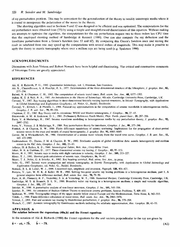
320
of ray perturbation problem. This may be convenient for the generalization of the theory to weakly anisotropic media where it is crucial t o incorporate the polarization of the waves in the theory.
The shooting algorithm used in Sections 9 and 12 was designed to b e efficient and was optimized. T h e computations for the ray perturbation were obtaiped from (75) by using a simple and straightforward discretization of this equation. Without making any attempts to optimize t h e algorithm, the computations for the ray perturbation require two t o three orders less CPU time than t h e employed shooting method of Sambridge & Kennett (1990). One can also compute the ray deflection and the traveltime perturbation from a Green's function (see 53 and 62). By computing this Green's function once and storing the result i n tabulated form o n e may speed up the computations with several orders of magnitude. This may make it possible to apply t h e theory t o mantle tomography where over a million rays are being used (e.g. Spakman 1990).
R . Snieder and M . Sambridge
ACKNOWLEDGMENTS
Discussions with J e a n Virieux and Robert Nowack have been helpful and illuminating. T h e critical and constructive comments of Veronique Farm are greatly appreciated.
REFERENCES
Aki, K. & Richards, P. G., 1980. Quantitative Seismology, vol. 1, Freeman, San Francisco. Aki, K. , Christofferson, A. & Husebye, E . S., 1977. Determination of the three-dimensional structure of the lithosphere, J . geophys. Res., 82,
Buland, R. & Chapman, C. H., 1983. The computation of seismic travel times, Bull. seism. SOC. A m . , 68, 1577-1593. Bullen, K. E. & Bolt, B. A, , 1985. A n Introduction to the Theory of Seismology, 4th edn, Cambridge University Press, Cambridge, UK. Cerveng, V., 1987. Ray tracing algorithms in three-dimensional laterally varying layered structures, in Seismic Tomography, with Applications
Cerveng, V., KlimeS, L. & PSenEik, I., 1984. Paraxial ray approximations in the computation of seismic wavefields in inhomogeneous media,
Chapman, C. H., 1985. Ray theory and its extensions: WKBJ and Maslov seismograms, J . Geophys., 58, 27-43. Dziewonski, A. M. & Anderson, D. L., 1981. Preliminary Reference Earth Model, Phys. Earth. planet Inter., 25, 297-356. Farra, V. & Madariaga, R., 1987. Seismic waveform modelling in heterogeneous media by ray perturbation theory, 1. geophys. Res., 92,
Farra, V., Virieux, J. & Madariaga, R., 1989. Ray perturbation theory for interfaces, Geophys. J. Int., 99, 377-390. Frankel, A. & Clayton, R. W . , 1986. Finite difference simulations of seismic scattering: Implications for the propagation of short-period
Gerver, M. & Markushevich, M., 1966. Determination of a seismic wave velocity from the travel time curve, Geophys. J. R. astr. Soc., 11,
Gudmundsson, O., Davies, J. H. & Clayton, R. W., 1990. Stochastic analysis of global traveltime data: mantle heterogeneity and random
Jeffreys, H. & Bullen, K. E., 1940. Seismological Tables, Brit. Ass., Grey-Milne Trust. Julian, B. R. & Gubbins, D., 1Y77. Three-dimensional seismic ray tracing, J . Ceophys., 43, 95-113. Moore, B. J . , 1991. Seismic rays in media with slight variation in velocity, Geophys. J . lnt., 105, 213-227. Moser, T. J. , 1991. Shortest path calculations of seismic rays. Geophysics, 56, 56-67. Moser, T . J . , Nolet, G. & Snieder, R., 1992. Ray bending revisited, Bull. seism. SOC. Am. , in press. Nolet, G., 1987. Seismic wave propagation and seismic tomography, in Seismic Tomography, with Applications in Global Seismology and
Nowack, R. L. & Lutter, W. J., 1988. Linearized rays, amplitude and inversion, Pageoph, 128, 401-421. Pereyra, V., Lee, W. H. K. & Keller, H. B., 1980. Solving two-point seismic ray tracing problems in a heterogeneous medium, part 1, A
Press, A. H., Flannery, B. P., Teukolsky, S. A. & Vetterling, W. T., 1986. Numerical Recipes, Cambridge University Press, Cambridge, UK. Sambridge, M. S. & Kennett, B. L. N. , 1990. Boundary value ray tracing in a heterogeneous medium; a simple and versatile algorithm,
Snieder, R., 1990. A perturbative analysis of non-linear inversion, Geophys. J. lnt., 101, 545-556. Snieder, R., 1991. An extension of Backus-Gilbert Theory to nonlinear inverse problems, Inverse Problems, 7 , 409-433. Spakman, W., 1990. Tomographic images of the upper mantle below central Europe and the Mediterranean, Terra Nova, 2 , 542-553. Vidale, J . , 1988. Finite-difference calculation of travel times, Bull. seism. SOC. Am. , 78, 2062-2076. Virieux, J . , 1991. Fast and accurate ray tracing by Hamiltonian perturbation, J . geophys. Rex , 96, 579-594. Wunsch, C., 1987. Acoustic tomography by Hamiltonian methods including ihc adiabatic approximation, Rev. Geophys. 25, 41-53.
277-296.
in Global Seismology and Exploration Geophysics, ed. Nolet, G . , Reidel, Dordrecht.
Geophys. J . R . astr. Soc., 79, 89-104.
2697-2712.
seismic waves in the crust and models of crustal heterogeneity, J. geophys. Res. 91, 6465-6489.
165-173 1990.
errors in the ISC data, Geophys. J . Int., 102, 25-43.
Exploration Geophysics, ed. Nolet, G . , Reidel, Dordrecht.
general adaptive finite difference method, Bull. seism. SOC. Am. , 70, 79-99.
Geophys. J . Int., 101, 157-168.
A P P E N D I X A The relation between the expressions (40a,b) and the Frenet equations
In the notation of Aki & Richards (1980) the Frenet equations for the unit vectors perpendicular to the ray are given by
$=-Ki"+6, &=-m.
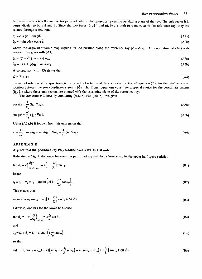
Ray perturbation theory 321
In this expression fi is the unit vector perpendicular to the reference ray in the osculating plane of the ray. The unit vector 6 is perpendicular to both ii and rO. Since the two bases (fit, tiz) and (ii, 6) are both perpendicular to the reference ray, they are related through a rotation:
8, = cos (~ii + sin ( ~ 6 , 4, = -sin $6 + cos $6, where the angle of rotation may depend on the position along the reference ray [(P=(P(s,J]. Differentiation of (A2) with respect to so gives with (Al)
A comparison with (43) shows that
Q = T + l j ; (A4)
the rate of rotation of the ti-vectors (Q) is the rate of rotation of the vectors in the Frenet equation ( T ) plus the relative rate of rotation between the two coordinate systems (6). The Frenet equations constitute a special choice for the coordinate system (ti,, ti2) where these unit vectors are aligned with the osculating plane of the reference ray.
The curvature K follows by comparing (A3a,b) with (40a,b), this gives
1
UO cos (PK =-(ti, * VU,,),
-1 sin (Pix = - (ti, - VU,).
Un
Using (A2a,b) it follows from this expression that
1 1
UO UO K = - [(cos $4, - sin @ti2) - Vu,] = - (6 * VuO).
APPENDIX B
A proof that the perturbed ray (97) satisfies Snell's law to first order
Referring to Fig. 7, the angle between the perturbed ray and the reference ray in the upper half-space satisfies
hence
i, = io - 0, = io- arctan [&(I -1) tan i,].
This means that
uo sin i, = u, sin i, - EU,
Likewise, one has for the lower half-space
and
i, = io + 6, = i, + arctan E 2 tan i , ( i o 0)
so that
uo(l - E ) sin i, = uo(l- E )
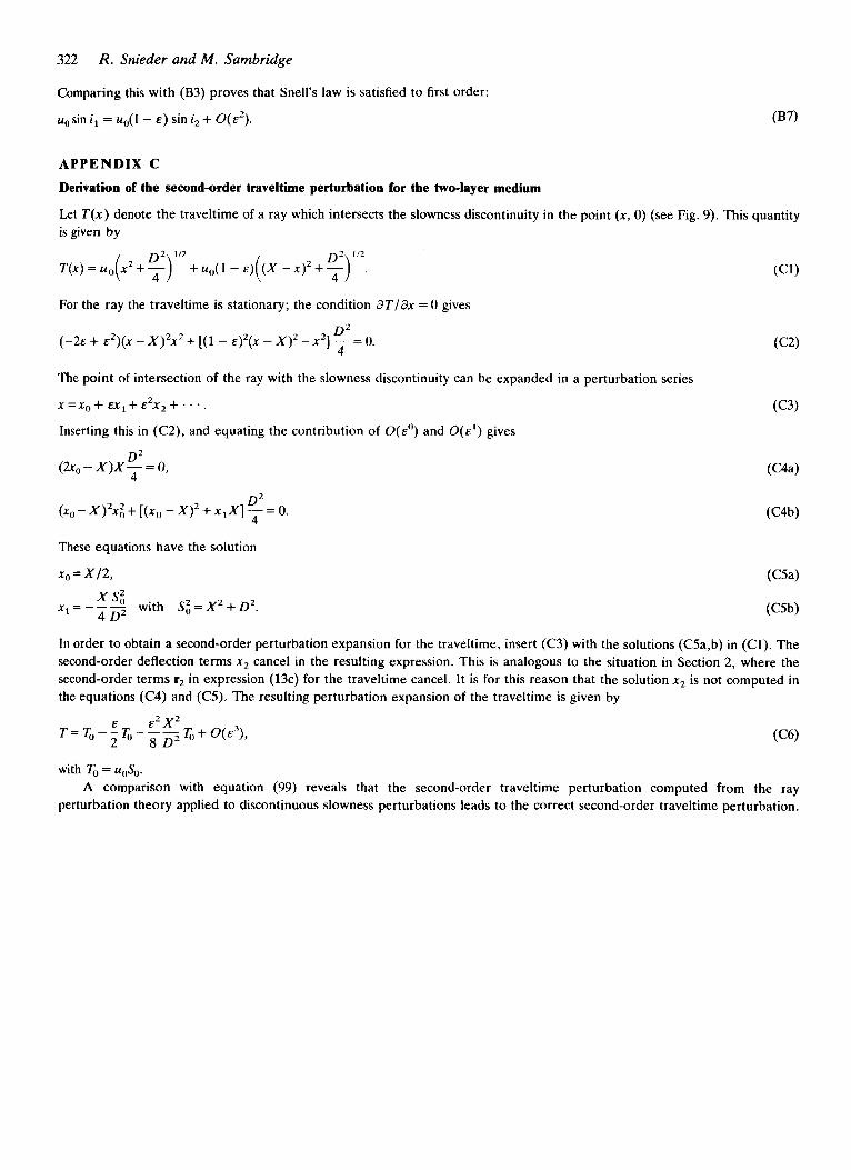
322 R. Snieder and M . Sambridge
Comparing this with (B3) proves that Snell’s law is satisfied to first order:
uo sin i , = u,Q- E ) sin i2 + o(E’).
APPENDIX C
Derivation of the second-order traveltime perturbation for the two-layer medium
Let T ( x ) denote the traveltime of a ray which intersects the slowness discontinuity in the point ( x , 0) (see Fig. 9). This quantity is given by
For the ray the traveltime is stationary; the condition d T / d x = 0 gives
D’ ( - 2 E + E2)(X - X ) ’ 2 + [(l - E)’(X - X)’ -x ’ ] - = 0.
4
The point of intersection of the ray with the slowness discontinuity can be expanded in a perturbation series
x = x , + E X 1 + & ~ x 2 + . . . . (C3)
Inserting this in (C2), and equating the contribution of O(E”) and O ( E ‘ ) gives
0’ (2ro - X ) X - = 0,
4 n 2 U
( X ( ) - X)’X:, + [ ( X ( ) - X)’ + x , X ] - = 0. 4
These equations have the solution
x , = X l 2 ,
x s:, x 1 = with S; = X 2 + 0’.
4 D2
In order to obtain a second-order perturbation expansion for the traveltime, insert (C3) with the solutions (CSa,b) in (Cl). The second-order deflection terms x2 cancel in the resulting expression. This is analogous to the situation in Section 2, where the second-order terms r2 in expression (13c) for the traveltime cancel. It is for this reason that the solution x2 is not computed in the equations (C4) and (C5). The resulting perturbation expansion of the traveltime is given by
& &’X’ T = T o - - &--- T + q E 3 ) ,
2 8 D2 ‘~ with To = u,So.
A comparison with equation (99) reveals that the second-order traveltime perturbation computed from the ray perturbation theory applied to discontinuous slowness perturbations leads to the correct second-order traveltime perturbation.
Related Documents