Rave in a Boxweb.mit.edu/6.111/volume2/www/f2018/projects/cherna...Figure 4: Chromagram of \The Bends" by Radiohead computed by our team. While an approach like this would certainly

$Page 1: Rave in a Boxweb.mit.edu/6.111/volume2/www/f2018/projects/cherna...Figure 4: Chromagram of \The Bends" by Radiohead computed by our team. While an approach like this would certainly$
Rave in a Box

Sammy Cherna, Josh Gruenstein & Matt Reeve

6.111 Project Report, Fall 2018

Abstract

This report describes the conception, design, and implementation ofRave in a Box, an FPGA-based audio-responsive laser projection system.The box takes in live music and performs Fourier-based signal processingmethods to identify peaks of structural novelty. It then uses a laser andset of galvanometers to project animated vector graphics onto a nearbysurface in time with transitions in the music, such as key changes, transi-tions from verse to chorus, and introduction of new instrumentals.

Contents

1 Overview 3

2 Project Logistics 3

3 Signal Processing 4

1

3.1 Algorithmic Approach . . . . . . . . . . . . . . . . . . . . . . . . 5

3.2 Modified Algorithm for Hardware . . . . . . . . . . . . . . . . . . 8

3.3 Module-level Implementation . . . . . . . . . . . . . . . . . . . . 9

4 Graphics 12

4.1 Path Generation . . . . . . . . . . . . . . . . . . . . . . . . . . . 12

4.2 Hardware Implementation . . . . . . . . . . . . . . . . . . . . . . 14

5 Hardware 14

6 Lessons Learned 15

A Project Verilog 16

B Project Python 51

2

1 Overview

FPGAs are uniquely powerful tools for live signal processing and real-timecontrol. Their tight timing capacity and reconfigurability allow these categoriesof computation and IO to occur with a far lower power budget than microcon-trollers or other embedded systems.

For our 6.111 final project, we sought to capitalize on these two uniquecapabilities by having an FPGA generate a live laser light show in response toa musical soundtrack. At the highest level, our design can be summarized viathe following block diagram:

FPGAmusic lasers

Figure 1: A macro view of the Rave in a Box.

Our box takes in audio via the Nexys4 DDR’s ADC, performs signal process-ing and graphics generation, and outputs analog galvonometer control signalsand delayed audio through a set of DACs. The galvanometers have mirrorsglued onto their axles which reflect a laser beam according to their angles. Wethen exploit persistence of vision to project shapes by cycling through a pathat high speeds.

The work necessary to achieve this can be broken down across signal process-ing, graphics generation, and IO, in that order of complexity. We will discussthe algorithms we utilized and developed for each of these domains, and specificdetails as to their implementation in hardware for the FPGA.

We began this project with only an abstract conception of our goals, and onlythrough iterative research and development arrived at a final working device.We hope to communicate that process of discovery propelled by a love of musicand bright shiny lights in this report.

2 Project Logistics

We divided up the responsibility for the project as follows: Sammy Chernawas responsible for the signal processing subsystem. Josh Gruenstein was re-sponsible for the graphics subsystem. Matt Reeve was responsible for all of thehardware and the hardware control subsystem. Despite these delineations, all

3

three of us collaborated heavily on all parts. The three of us live together, socollaborating together was natural.

Our original goals for the project were as follows. For our minimum projectgoals, we wanted to compute the spectrogram of incoming audio, and based ona feature of that spectrogram, display a certain static image (a frame) with thelaser galvonometers (controlled via DAC over SPI). Each frame would consistof instructions representing line segments to interpolate between. For our stan-dard project goals, we wanted to compute the spectrogram and chromagramof incoming audio, and based on a feature of that chromagram (for example,the most prominent pitch class), display a certain animation of images (a scenecomposed of frames) with the laser galvanometers. We had originally had manystretch goals, which can roughly be broken down as follows: more advancedgraphics generation (such as interpolating along Bezier curves instead of lines),more advanced signal processing (using Hanning window for better FFT, fur-ther processing on the chromagram to get more meaningful graphics selection),implementing tempo analysis and incorporating tempo into graphics, and moreadvanced hardware (potentially using 3 different colored lasers and combiningthem with optics).

While we did not have time to tackle tempo analysis or multiple coloredlasers, we accomplished all of our other stretch goals, aside from all of our stan-dard project goals, including one stretch goal that we did not even imagine: songsegmentation / structure analysis. We realized that merely selecting graphicsbased on the most prominent pitch class in the chromagram would only yieldpleasing results on very simple synthetic examples, and would not work wellon actual songs. Consequently, we decided to tackle the huge endeavor of songsegmentation by creating our own real-time adaptation of a song segmentationalgorithm, the first of its kind.

Aside from the song segmentation, we implemented our stretch goals of usinga Hanning window for better FFT results, interpolating along Bezier curves foradvanced graphics (as well as implementing a system to convert raster imagesto vector graphics for the laser galvos), and creating a sturdy yet stylish custombox for our system.

3 Signal Processing

Music Information Retrieval, or MIR, is the exciting interdisciplinary studyof extracting useful features from musical data. Part of our motivation to pur-sue a project in MIR stems from one of our members (Sammy Cherna) taking21M.387, Fundamentals of Music Processing. Many of the processes used in ourbox were adapted from material taught in that class.

In constructing an MIR system for our box, a major challenge we encoun-tered was adapting algorithms traditionally implemented in software and run

4

on stored audio samples to a live system implemented in hardware. Thus, inthis section we will discuss our signal processing in three steps: the fundamen-tal algorithms we used, the modifications and compromises we made to fit ourapplication, and our module-level implementation in hardware.

3.1 Algorithmic Approach

In the beginning, there were raw audio signals.

Our box takes incoming music as analog signals delivered via an aux cable,then transcribed into digital data and delivered to the FPGA via the Nexys4ADC. However, there is limited advanced processing that can be done on rawaudio data alone. Instead, nearly all approaches first run audio through a FastFourier Transform to produce a spectrogram.

This requirement stems from the fact that the fundamental building blockof audio signals are waves of different frequencies and amplitudes. In orderto determine useful information about a given signal, we must determine itscomposition across different frequencies. This representation is called a spec-trogram, which can be computed by running an FFT across a sequence of audiosignals.

Figure 2: Spectogram from Wikipedia of a violin recording. On the horizontalaxis is time, and on the vertical axis is increasing frequencies. Additional

bands of intensity are from harmonics.

The spectrogram tells us how much fundamental waves of different frequen-cies contribute to the signal at a given time. For example, if you were to playa middle C on a piano and generate a spectrogram from the recorded audio,you would expect to see high intensity at ∼262hz, in addition to slightly lowerintensity at overtones 524hz and 768hz, overtones and harmonics one and twooctaves away from middle C. Thus the spectrogram is far more informative thanraw audio, which is difficult to interpret without additional processing.

In addition to the spectrogram, we can also compute the chromagram of

5

audio by summing all of the harmonic frequencies of each of the 12 Westernpitch classes: C, C], D, D], E, F, F], G, G], A, A], and B. This allows us moreeasily to determine the note composition of audio (the piano example from abovewould clearly be far easier to classify).

Figure 3: Chromagram from Wikipedia of a C major scale played on a piano.

Our original plan was to continuously compute the chromagram on incomingaudio, and use the highest intensity pitch class to select a graphic to project.However, experimentation is software demonstrated that this approach on mostmusic would not yield scene transition timing that would make sense to a lis-tener. Chromagrams of popular music are often very noisy and fast-changingdue to the presence of many instruments and tracks.

Figure 4: Chromagram of “The Bends” by Radiohead computed by our team.

While an approach like this would certainly be of sufficient technical com-plexity, and work well for some recordings, research told us that raves rarelyplay pure sin tones or classical piano pieces. Thus, this methodology wouldprobably be insufficient for our goal of creating a true Rave in a Box.

What we needed was an algorithm for song segmentation. Unfortunately,song segmentation is still an open research problem, with a diverse array of pro-posed solutions but no definitive methodology. Additionally, nearly all methodsoperate on the entire song at once, and are extremely computationally intensive.

6

One common theme in recent song segmentation papers is the computation ofa two-dimensional self-similarity matrix, first utilized in [1]. In these approaches,a song chromagram matrix is multiplied by its transpose to produce an t × tmatrix, where t is the number of columns in the chromagram. As the dotproduct between two vectors is analogous to their covariance, each cell in theself-similarity matrix is proportional to the correlation between samples at timescorresponding to the row and column that cell is in.

Figure 5: Self-similarity matrix of Brahms’ Hungarian Dance computed by ourteam. We can see that square-shaped regions are regions of high homogeneity,while corners between them represent strong structural changes in the song.

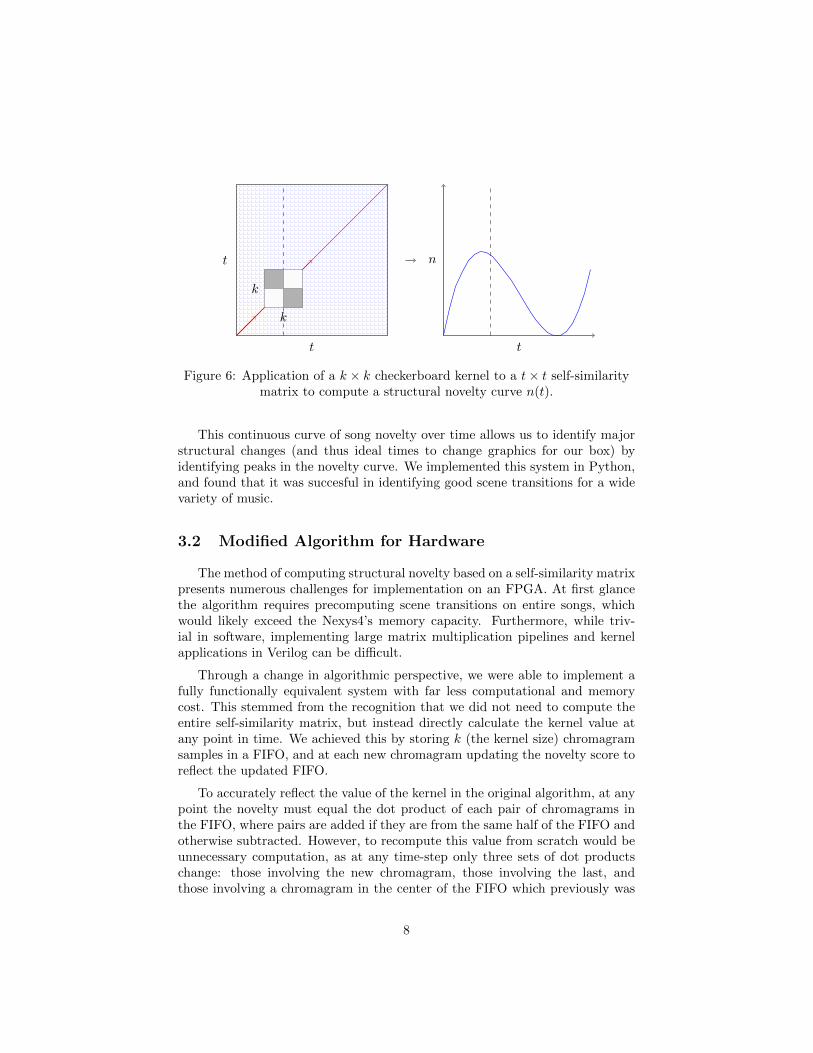
From the self-similarity matrix we can compute some score of structural nov-elty by applying a checkerboard kernel to its diagonal. If the kernel is centeredat sample t, it adds correlation values on the same side of t, and subtractsthose on different sides. Thus, the value is always greatest if the two halves ofthe music sampled by the kernel are similar to themselves but different fromeach-other, making it a successful measure of novelty.

7

t

t

t

k

k

n

Figure 6: Application of a k × k checkerboard kernel to a t× t self-similaritymatrix to compute a structural novelty curve n(t).

This continuous curve of song novelty over time allows us to identify majorstructural changes (and thus ideal times to change graphics for our box) byidentifying peaks in the novelty curve. We implemented this system in Python,and found that it was succesful in identifying good scene transitions for a widevariety of music.

3.2 Modified Algorithm for Hardware

The method of computing structural novelty based on a self-similarity matrixpresents numerous challenges for implementation on an FPGA. At first glancethe algorithm requires precomputing scene transitions on entire songs, whichwould likely exceed the Nexys4’s memory capacity. Furthermore, while triv-ial in software, implementing large matrix multiplication pipelines and kernelapplications in Verilog can be difficult.

Through a change in algorithmic perspective, we were able to implement afully functionally equivalent system with far less computational and memorycost. This stemmed from the recognition that we did not need to compute theentire self-similarity matrix, but instead directly calculate the kernel value atany point in time. We achieved this by storing k (the kernel size) chromagramsamples in a FIFO, and at each new chromagram updating the novelty score toreflect the updated FIFO.

To accurately reflect the value of the kernel in the original algorithm, at anypoint the novelty must equal the dot product of each pair of chromagrams inthe FIFO, where pairs are added if they are from the same half of the FIFO andotherwise subtracted. However, to recompute this value from scratch would beunnecessary computation, as at any time-step only three sets of dot productschange: those involving the new chromagram, those involving the last, andthose involving a chromagram in the center of the FIFO which previously was

8

on one half and just moved to another. By only computing these three sets ofdot products and applying them as deltas to the previous novelty score, we cando O(k) rather than O(k2) computation at every new chromagram.

While this method does entail storing k chromagrams and k/2 chromagramsworth of audio (to replay in synchrony with the computed novelty curve), thisis far less memory intensive than storing an entire song’s worth of both audioand chromagrams.

Interestingly, from a literature review we believe we are the first to create anysort of live song-segmentation algorithm, let alone implement one in hardware.

3.3 Module-level Implementation

XADC 64x Oversampler

4096 Sample Audio BRAMHanning

Audio FIFO DAC

FFT IP Core

Chroma CalculatorChroma Bins

Novelty Calculator

Σ Accum∆ Accum� EngineFIFO Control

Chroma Fifo

×

audioaudio

peak

9

Our Verilog for signal processing began with the sample FFT code providedfor the class by Mitchell Gu. This included creating a 104MHz clock, sam-pling the onboard ADC at 1MSPS, oversampling by 16x to get 14-bit samplesat 62.5KHz, storing 4096 of them in a circular BRAM, feeding them to theFFT Mag IP Core to get the magnitude (square root of real part squared plusimaginary part squared) of the FFT, storing the results in a BRAM, and finallydisplaying a histogram of this data (the spectrogram) on the VGA output. Inorder to get this code to work, we had to splice open an AUX cable and apply aDC bias to the signal (configurable via potentiometer) for it to be read properlyby the ADC. One issue we encountered was clipping from the ADC, despite thesignal staying in the acceptable 0-1V range, so we lowered the volume of theinput music until we did not have clipping. We decided to modify this code byoversampling by 64x instead of 16x, so that we could get 15-bit samples at arate of 15.625KHz. There were three reasons for this change: keeping a lowersampling rate would give us better frequency resolution (about 4Hz per bin inthe FFT), it would let us look at a larger window in time for each FFT (about0.26 seconds) which would help the novelty calculation be more robust, and theextra bit of precision could help for further calculations.

We also decided to pursue one of our stretch goals by incorporating a Han-ning window into the signal in order to get better FFT results. The standardprocess of taking 4096 samples at a time from a signal consists of multiplyingthe theoretically infinite signal by a rectangular window in time. This resultsin spectral leakage in the FFT output, which can make computation like notedetection less accurate, especially when accumulating many frequency bins intochromagram bins. In order to reduce spectral leakage, we can multiply the 4096samples by a different window shape, such as the Hanning window, derived froma sin wave. We computed 4096 16-bit samples of a single Hanning window, andstored them in a ROM. When a new ADC sample would be ready to store in thecircular BRAM, we would use its index out of 4096 to fetch the correct Hanningvalue from the ROM, multiply it by the Hanning value, and right-shift it by16 before storing the 16-bit result in the BRAM. The ROM had a latency of 2clock cycles, so we had to pipeline accordingly.

At this point we had working spectrogram computation. Our next step wasto turn this spectrogram into a chromagram. In order to create a chromagram,we needed to sum up many different frequency bins for each pitch class bin.Since every frequency bin contributes to at most 1 chromagram bin, we decidedto create a ROM which would take in a bin index and give us an integer 0-11representing the chromagram bin that it corresponds to, or 12 indicating thatit corresponds to no chromagram bin. This ROM was 4 bits wide (to representthe integers 0-12), and contained 1024 addresses, since we only cared aboutfrequencies in the first 1024 spectrogram bins. As new outputs came from theFFT module, we would check its index using the tuser output, look up thechroma bin, and add it to the correct chroma bin. Only after receiving all 4096outputs would we scale down each chroma bin and update the output from thechroma module.

10

Since our frequency resolution was only 4Hz, we did not want to consideroctaves with notes less than 4Hz apart. Additionally, while almost all softwareMIR tasks include normalization of each chroma vector for increased robustness,we could not perform meaningful normalization as division is very difficult inhardware. Accordingly, we wanted roughly the same number of spectrogrambins to contribute to each chromagram bin, so that each is roughly on the samescale. We decided to only consider notes C3 (130 Hz) through E7 (2637 Hz) forchromagram contribution. While we could not perform normalization, we foundthat this chromagram computation was sufficient for our needs. We modifiedthe spectrogram VGA module to display a histogram of chromagram intensitiesas well, so that we could observe our chromagram calculation in action.

Following the chromagram calculation for an entire window of samples, wepushed this new chromagram onto our 32-chromagram FIFO and computedthe new novelty score for this point in time. As described above, instead ofcomputing every possible dot product between pairs of the 32 chromagrams inthe FIFO, we would keep a running accumulator of the novelty score, and onlycompute the dot products necessary to calculate the delta from the previousnovelty score. This would require 3 sets of dot products, each one requiring afull pass through the FIFO. To simplify the process, we wrote a FIFO Controllermodule to interface with the FIFO, and a Dot Engine module to compute dotproducts. Unfortunately, both of these modules required significant debuggingin order to get correct operation. For the FIFO Controller module, we hadto ensure correct timing of the read and write lines in order to cycle properlythrough the FIFO. For the Dot Engine module, we had to properly pipelinein order to leave time for the 12 16-bit multiplications and subsequent 32-bitadditions.

Once we got the FIFO Controller and Dot Engine working, we created aDelta Accumulator to properly accumulate all of the dot products without over-flow or underflow. Each dot product result would either be added or subtractedfrom the accumulator, depending on the indices of the two chroma in the FIFO.The Novelty Calculator module then operated with the following state machine:push new chroma onto FIFO while storing the old chroma leaving FIFO, com-pute the dot product between the new chroma and all other chroma in the FIFO(by cycling through the FIFO), adding/subtracting from the Delta Accumula-tor accordingly, compute the dot product between the old chroma and all otherchroma in the FIFO, cycle through the FIFO to retrieve the middle chroma (inindex 16), compute the dot product between this middle chroma and all otherchroma in the FIFO, and finally take the accumulated delta and add it to ourrunning novelty score accumulator.

Amazingly, after an eternity of debugging, we were able to analyze the resultsof this novelty computation with Vivado’s Integrated Logic Analyzer and seeclear peaks in the novelty score at key transitions in song structure. In orderto detect these peaks properly, we first implemented a simple low-pass filter bycomputing an exponential moving average of the novelty score. The current

11

filtered novelty would be 0.5 times the new computed novelty plus 0.5 timesthe previous filtered novelty. This helped smooth out some of the bumps andextraneous peaks in the novelty curve. Then we store three novelty values: thenew one, the one from one timestep ago, and the one from two timesteps ago.We can then declare the one from one timestep ago a peak if it is greater thanboth the new one and the one from two timesteps ago. We also check that itis greater than a certain threshold before declaring it a peak. This resultedin quite accurate peak detection for certain songs, giving us pulses exactly attransitions from verse to chorus and vice versa. Unfortunately, due to our lackof normalization at various points in our computation, a good peak thresholdfor one song might not be good for a different song, and so our approach’srobustness was limited.

The output from the Novelty Calculator Module, indicating if there is apeak in novelty at the current timestep or not, is fed to the Graphics module,which would trigger a scene change on a peak. However, since we expect a peakin novelty when the chroma belonging to a structural transition in the song ishalfway through the 32-chroma FIFO, there is about a 4 second delay betweeninputting audio and outputting a peak. In order to remedy this, we also storea FIFO of audio samples corresponding to 4 seconds of audio (65536 15.625Khzsamples), before outputting the buffered audio to a DAC over SPI.

4 Graphics

The Rave in a Box generates graphics by following a path and turning alaser on and off along it. Thus, for the box to be able to project graphics andmaintain persistence of vision without obscene memory usage, it must be ableto interpolate along some compact representation of vector graphics that travelthe shortest possible path to across those graphics.

This challenge can be broken down across two domains: the generation insoftware of a shortest path of Bezier curves, and the interpolation in hardwareacross these curves.

4.1 Path Generation

Our team originally planned to generate line-based drawings by hand, whichwould likely have near-optimal path length due to human intuition. However, wequickly realized that even for 4 scenes, each with 16 frames, this would take aninordinate amount of time. Thus, we sought to find a method of automaticallygenerating scene paths from graphics found online, most of which being in rasterform.

We built the following software pipeline to intake animated GIFs and output.coe files containing Bezier curves and laser on/off instructions:

12

1. Split animated GIF into individual frames, and mask to black and white.

2. Trace a set of Bezier curves around each item in each frame.

3. Run a nearest-fragment greedy algorithm to find the ideal set of paths toconnect objects in frames, and refine with simulated annealing two-opt.

4. Split the largest Bezier curves in half until there is a power of 2 numberof curves in each frame.

5. Pack frames into a .coe file and output correct Verilog parameters.

Step 3 of this process is NP-Complete, as it is a close relative of the TravelingSalesman Problem which is also NP-Complete. Thus the generation of scene .coefiles can be somewhat time consuming. However, we found this was necessary tocreate short enough paths to allow persistence of vision with complex graphics.The details of this process can be found in the Python code in Appendix B.

P1 P4

P2

P3

Figure 7: Example cubic Bezier curve with four control points.

Practically, the ROM described by the COE file is addressed by dlog2(|S|)e+dlog2(max(|F |))e + dlog2(max(|I|))e bits, where |S| is the number of scenes,max(|F |) is the maximum number of frames per instruction, and max(|I|) is themaximum number of instructions per frame. Each line of the ROM correspondsto a cubic Bezier curve with four control points (and thus eight 12 bit numbers)and an additional bit to indicate whether the laser should be on or off.

13

4.2 Hardware Implementation

Interpolator

Bezier X

Bezier YBezier Y

Instruction ROM

scene

xy

laser

Figure 8: Block diagram of graphics generation subsystem.

The Interpolator module cycles through instructions in the provided sceneaddress, and outputs instruction coordinates to two combinational modules thatinterpolate along the Bezier curve. It then forwards those outputs out to theSPI module, which in turn exports them to the DAC. This design requires nohandshaking or clock-sharing with other modules.

5 Hardware

Our physical set-up consisted of a laser galvanometer set which includedtwo galvanometers with mirrors on an aluminum mount, motor driver boards, apower supply, and a 5mW red laser. The motor driver boards each took in analogvoltage inputs to control the galvanometers. Due to the fact that the Nexys canonly output digital signals, MCP4822 two channel digital-to-analog converterswere used over SPI to communicate with the motor driver boards. We also useda MCP4822 to output buffered audio, as PWMing audio out at our relativelylow 15.625hz sampling rate yielded noticeably poor audio quality. A bipolaramplifier circuit was built and used to increase the overall laser projection angle(and thus picture size) and allow configurable offsets and gains for the x and yaxes.

14

Figure 9: Rave in a Box 3D render from Autodesk Fusion 360.

Manufacturing of the project enclosure was an extensive process. First,the product was designed in computer aided design software to ensure fitmentand appearance. Thereafter DXF files were able to be made in order to waterjetand laser cut parts. Laser cut eighth inch acrylic sheets, separated by aluminumstandoffs were used as the frame of the box. A sixteenth inch Aluminum sheetwas waterjet and formed around the outside of the frame before finally beingbrushed with steel wool for a textured appearance. A plywood sheet was lasercut and acrylic letters were laid in the sheet for the top cover of the box. It wasthen stained for a darker aesthetic.

6 Lessons Learned

After many many hours of grueling debugging and toiling over small mis-takes, we have learned many lessons. We believe that the most significant lessonthat we can share is to never assume that a module is working, despite howsimple it may seem. Instead, it is crucial to validate the correct operation ofevery small module before moving on to other modules that use them. We usedVivado’s Integrated Logic Analyzer to help us validate and debug modules, par-ticularly ones sensitive to timing issues, and we highly recommend future 6.111students do the same. We also learned how useful it is to utilize the moduleabstraction and create small sub-modules for individual repeated tasks. Thisnot only allows for cleaner and more elegant code, but also helps with debuggingas it lets you validate small parts and declare them bug-free.

One big issue that we kept facing was timing. First we did not realize thatthe ROM had a 2 clock cycle latency, and so we were getting incorrect valuesfrom our ROMs. Another timing issue we faced was not properly enabling theread and write lines for the FIFO. In particular, if the FIFO is full, and bothread and write enables are raised high, one would expect that the FIFO wouldshift the new input in while shifting the old output out, remaining full. However,this is not the case. The old output will be shifted out, but the new input willnot be shifted in while the FIFO is full, even if it is read on the same clock cycle.Instead, one has to read from the FIFO first, and then write on the following

15

clock cycle, when the FIFO is not full. Lastly, we encountered a timing issuewith our Dot Engine module. We originally attempted to compute the dotproduct, consisting of 12 16-bit multiplies and 11 32-bit adds, combinationally.We did not realize that this was not possible. When inspecting the outputsfrom the Dot Engine module with the ILA, we realized that we were not gettingcorrect dot product results. Instead, we had to pipeline the module so that eachcombinational operation could fit in a single 104MHz clock cycle. We suggestthat future groups learn to use the timing report in Vivado in order to spotthese issues better than we did.

All in all, we are extremely proud of our end result and had a lot of fungetting there. We accomplished everything we wanted and more, yielding agreat-looking project that we can show off to friends. We learned an immenseamount about Verilog and how Vivado actually synthesizes and implementsVerilog, and we learned valuable skills in regards to project management. Wewould like to give a tremendous thank you to the 6.111 staff for teaching us,giving us invaluable guidance and debugging help, and giving us the opportunityto succeed.

References

[1] Jonathan Foote. Automatic Audio Segmentation Using A Measure of AudioNovelty. In Proc. ICME, volume 1, New York City, New York, USA, 2000.

A Project Verilog

1 parameter BEZIER_BITS = 10;

2 parameter FRAME_REPEAT_BITS = 1;

3

4 parameter SCENE_BITS = 2;

5 parameter FRAME_BITS = 4;

6 parameter INSTRUCTION_BITS = 8;

7

8 parameter COORD_BITS = 12;

9 parameter CHROMA_PRECISION = 16;

10 parameter CHROMA_WIDTH = (12* CHROMA_PRECISION )-1;

11

12 parameter MAX_DOT_BITS = 35 - 1;

13 parameter MAX_DELTA_BITS = 135 - 1;

14 parameter MAX_TOTAL_BITS = 200 - 1;

15

16 // Magic peak number. Translates to 10^8.

17 parameter PEAK_THRESHOLD = 200’ d1_0000_0000 +

18 200’ h8000_0000_0000_0000_0000_0000_0000_0000_0000_0000_0000_0000_00;

19

16

20 // Generate a spectrogram histogram reading from BRAM.

21 module spectro_histogram(

22 input wire clk ,

23 input wire [10:0] hcount ,

24 input wire [9:0] vcount ,

25 input wire blank ,

26 input wire [1:0] range ,

27 output wire [9:0] vaddr ,

28 input wire [15:0] vdata ,

29 output reg [2:0] pixel

30 );

31

32 // 1 bin per pixel , with the selected range

33 assign vaddr = hcount[9:0] >> range;

34

35 reg [9:0] hheight; // Height of histogram bar

36 reg [9:0] vheight; // The height of pixel above bottom of screen

37 reg blank1; // blank pipelined 1

38

39 always @(posedge clk) begin

40 // Pipeline stage 1

41 hheight <= vdata >> 7;

42 vheight <= 10’d767 - vcount;

43 blank1 <= blank;

44


46 pixel <= blank1 ? 3’b0 : (vheight < hheight) ? 3’b111 :

3’b0;

47 end

48

49 endmodule

50

51

52 // Generate a chromagram histogram from given chroma.

53 module chroma_histogram(

54 input wire clk ,

55 input wire [10:0] hcount ,

56 input wire [9:0] vcount ,

57 input wire blank ,

58 input wire [16*12 -1:0] chroma ,

59 output reg [2:0] pixel

60 );

61

62 // 1 bin per pixel , with the selected range

63 wire[3:0] bin_num = hcount[9:0] >> 6;

64

65 reg [9:0] hheight; // Height of histogram bar

66 reg [9:0] vheight; // The height of pixel above bottom of screen

67 reg blank1; // blank pipelined 1

68

17



71 if (bin_num < 12) hheight <= chroma[bin_num *16 +: 16] >> 6;

72 else hheight <= 0;

73

74 vheight <= 10’d767 - vcount;

75 blank1 <= blank;

76


78 pixel <= blank1 ? 3’b0 : (vheight < hheight) ? 3’b111 :

3’b0;

79 end

80

81 endmodule

82

83

84 // Module to bin spectrogram values from the BRAM into a chromagram.

85 // The BROM chroma_bins tells us for every bin in the spectrogram what

86 // bin it belongs to in the chromagram.

87 module chroma_calculator(

88 input wire clk ,

89 input wire valid_sample ,

90 input wire [11:0] new_sample_addr ,

91 input wire [CHROMA_PRECISION -1:0] new_sample_data ,

92 input wire last_sample ,

93 output reg [CHROMA_WIDTH:0] chroma ,

94 output reg done

95 );

96

97 // We are given a spectogram which represents the intensity

98 // of frequencies 0-1024hz. This spectogram is stored in a

99 // Block RAM indexed by spectogram_address. We seek to iterate through

100 // spectogram indices , and add each value to one of 12 bins.

101

102 parameter INNER_CHROMA_PRECISION = 18;

103 parameter INNER_CHROMA_WIDTH = (INNER_CHROMA_PRECISION *12) -1;

104 parameter BIT_DIFFERENCE = INNER_CHROMA_PRECISION - CHROMA_PRECISION;

105

106 reg[INNER_CHROMA_WIDTH:0] inner_chroma;

107 wire[3:0] chroma_bin;

108 integer i;

109

110 reg [11:0] prev_addr;

111 reg [11:0] prev_prev_addr;

112 reg [11:0] prev_prev_prev_addr;

113 reg [15:0] prev_data;

114 reg [15:0] prev_prev_data;

115 chroma_bins chroma_binz (

116 .clka(clk), // input wire clka

117 .ena(1), // input wire ena

18

118 .addra(new_sample_addr[10:0]), // input wire [10 : 0] addra

119 .douta(chroma_bin) // output wire [3 : 0] douta

120 );

121


123 prev_addr <= new_sample_addr;

124 prev_prev_addr <= prev_addr;

125 prev_prev_prev_addr <= prev_prev_addr;

126 prev_data <= new_sample_data;

127 prev_prev_data <= prev_data;

128

129 if (valid_sample && (prev_prev_prev_addr != prev_prev_addr )) begin

130 if (last_sample) begin

131 for (i=0; i<12; i=i+1) begin

132 chroma[i*CHROMA_PRECISION +: CHROMA_PRECISION]

133 <= inner_chroma[i*INNER_CHROMA_PRECISION +: INNER_CHROMA_PRECISION]

134 >> BIT_DIFFERENCE;

135 end

136

137 done <= 1;

138 inner_chroma <= 0;

139 end

140 else begin

141 done <= 0;

142

143 if (prev_prev_addr < 2048 && chroma_bin < 12) begin

144 inner_chroma[chroma_bin*INNER_CHROMA_PRECISION +: INNER_CHROMA_PRECISION]

145 <= inner_chroma[chroma_bin*INNER_CHROMA_PRECISION +: INNER_CHROMA_PRECISION] + prev_prev_data;

146 end

147 end

148 end else done <= 0;

149 end

150

151 endmodule

152

153

154 // Heavily pipelined module to perform dot products on two chromagrams.

155 // Has a 4 cycle delay.

156 module dot_engine(

157 input wire clk ,

158 input wire[CHROMA_WIDTH:0] dot_a ,

159 input wire[CHROMA_WIDTH:0] dot_b ,

160 output wire [MAX_DOT_BITS:0] out

161 );

162

163 reg [31:0] chroma_product_0 = 0;





19








175

176 reg [32:0] chroma_sum_0 = 0;

177 reg [32:0] chroma_sum_1 = 0;

178 reg [32:0] chroma_sum_2 = 0;

179 reg [32:0] chroma_sum_3 = 0;

180 reg [32:0] chroma_sum_4 = 0;

181 reg [32:0] chroma_sum_5 = 0;

182 reg [33:0] chroma_sum_01 = 0;

183 reg [33:0] chroma_sum_23 = 0;

184 reg [33:0] chroma_sum_45 = 0;

185 reg [33:0] ex_chroma_sum_45 = 0;

186 reg [34:0] chroma_sum_0123 = 0;

187

188

189 always @ (posedge clk) begin

190 chroma_product_0 <=

191 dot_a[1* CHROMA_PRECISION -1:0* CHROMA_PRECISION]

192 * dot_b[1* CHROMA_PRECISION -1:0* CHROMA_PRECISION];


























20









226

227 chroma_sum_0 <= chroma_product_0 + chroma_product_1;






233 chroma_sum_01 <= chroma_sum_0 + chroma_sum_1;



236 ex_chroma_sum_45 <= chroma_sum_45;


238 end

239

240 assign out = chroma_sum_0123 + ex_chroma_sum_45;

241

242 endmodule

243

244

245 // Module to accumulate deltas to structural novelty.

246 module delta_accumulator(


248 input wire rst ,

249 input wire new_addition ,

250 input wire [MAX_DOT_BITS:0] accumulate ,

251 input wire sign ,

252 output reg [MAX_DELTA_BITS:0] accumulated

253 );

254

255 reg state = 0;

256 parameter RESET = 0;

257 parameter COLLECT = 1;


259 case (state)

260 RESET: begin

261 accumulated <= 1 << MAX_DELTA_BITS;

262 state <= COLLECT;

263 end

264 COLLECT: begin

265 if (rst) state <= RESET;

266 else begin

267 if (new_addition) begin

21

268 if (sign) accumulated <=

269 accumulated - {92’b0, accumulate };

270 else accumulated <=

271 accumulated + {92’b0, accumulate };

272 end

273 end

274 end

275 default: state <= RESET;

276 endcase

277 end

278

279 endmodule

280

281

282 // Module to accumulate total structural novelty.

283 module total_accumulator(



286 input wire new_addition ,

287 input wire [MAX_DELTA_BITS:0] accumulate ,

288 input wire sign ,

289 output reg [MAX_TOTAL_BITS:0] accumulated

290 );

291

292 reg state = 0;

293 parameter RESET = 0;

294 parameter COLLECT = 1;


296 case (state)

297 RESET: begin

298 accumulated <= 1 << MAX_TOTAL_BITS;

299 state <= COLLECT;

300 end

301 COLLECT: begin

302 if (rst) state <= RESET;

303 else begin

304 if (new_addition) begin

305 if (sign) begin

306 if (accumulated > accumulate)

307 accumulated <= accumulated - {65’b0, accumulate };

308 else accumulated <= 0;

309 end

310 else begin

311 if (((1 << (MAX_TOTAL_BITS +1)) - {1’b0, accumulated })

312 > accumulate)

313 accumulated <= accumulated + {65’b0, accumulate };

314 else accumulated <=

315 (1 << (MAX_TOTAL_BITS + 1)) - 1;

316 end

317 end

22

318 end

319 end

320 default: state <= RESET;

321 endcase

322 end

323

324 endmodule

325

326

327 // Controller for the chromagram FIFO.

328 // Can load values , unload , cycle , and shift.

329 module fifo_controller(



332 input wire [2:0] mode ,

333 input wire [CHROMA_WIDTH:0] new_fifo_input ,

334 output wire [CHROMA_WIDTH:0] fifo_output ,

335 output wire [4:0] data_count ,

336 output wire fifo_full ,

337 output wire fifo_empty

338 );

339

340 reg fifo_read , fifo_write;

341 reg [CHROMA_WIDTH:0] fifo_in;

342 parameter FIFO_IDLE = 0;

343 parameter FIFO_LOAD = 1;

344 parameter FIFO_UNLOAD = 2;

345 parameter FIFO_CYCLE = 3;

346 parameter FIFO_SHIFT = 4;

347

348 always @ (*) begin

349 case (mode)

350 FIFO_IDLE: begin

351 fifo_read = 0;

352 fifo_write = 0;

353 end

354 FIFO_LOAD: begin

355 fifo_read = 0;

356 fifo_write = 1;

357 fifo_in = new_fifo_input;

358 end

359 FIFO_UNLOAD: begin

360 fifo_read = 1;

361 fifo_write = 0;

362 end

363 FIFO_CYCLE: begin

364 fifo_read = 1;

365 fifo_write = 1;

366 fifo_in = fifo_output;

367 end

23

368 FIFO_SHIFT: begin

369 fifo_read = 1;

370 fifo_write = 1;


372 end

373 endcase

374 end

375

376 chroma_fifo c (

377 .srst(rst),

378 .clk(clk),

379 .din(fifo_in),

380 .wr_en(fifo_write),

381 .rd_en(fifo_read),

382 .dout(fifo_output),

383 .full(fifo_full),

384 .empty(fifo_empty),

385 .data_count(data_count)

386 );

387

388

389 endmodule

390

391 // Controller for the audio buffer FIFO. Functions identically

392 // to the above.

393 module buffer_controller(



396 input wire [2:0] mode ,

397 input wire [11:0] new_fifo_input ,

398 output wire [11:0] fifo_output ,

399 output wire fifo_full ,

400 output wire fifo_empty

401 );

402

403 reg fifo_read , fifo_write;

404 reg [11:0] fifo_in;






410


412 case (mode)

413 FIFO_IDLE: begin

414 fifo_read = 0;

415 fifo_write = 0;

416 end

417 FIFO_LOAD: begin

24

418 fifo_read = 0;

419 fifo_write = 1;


421 end

422 FIFO_UNLOAD: begin

423 fifo_read = 1;

424 fifo_write = 0;

425 end

426 FIFO_CYCLE: begin

427 fifo_read = 1;

428 fifo_write = 1;

429 fifo_in = fifo_output;

430 end

431 FIFO_SHIFT: begin

432 fifo_read = 1;

433 fifo_write = 1;


435 end

436 endcase

437 end

438

439 buffer_fifo b (

440 .srst(rst),

441 .clk(clk),

442 .din(fifo_in),

443 .wr_en(fifo_write),

444 .rd_en(fifo_read),

445 .dout(fifo_output),

446 .full(fifo_full),

447 .empty(fifo_empty)

448 );

449

450

451 endmodule

452

453

454 // Module to compute structural novelty. The big boi.

455 module novelty_calc (



458 input wire [CHROMA_WIDTH:0] new_chroma ,

459 input wire chroma_done ,

460 output reg done ,

461 output reg peak ,

462 );

463





25


469

470 parameter NOVELTY_IDLE = 0;

471 parameter NOVELTY_LOAD = 1;

472 parameter NOVELTY_STORE_OLDEST_INT = 2;

473 parameter NOVELTY_STORE_OLDEST = 3;

474 parameter NOVELTY_DOT_NEWEST = 4;

475 parameter NOVELTY_DOT_OLDEST = 5;

476 parameter NOVELTY_COLLECT_MIDDLE = 6;

477 parameter NOVELTY_DOT_MIDDLE = 7;

478 parameter NOVELTY_DOT_MIDDLE_AGAIN = 8;

479 parameter NOVELTY_FINISH_DOTTING_MIDDLE = 9;

480 parameter NOVELTY_ADD_DELTA = 10;

481 parameter NOVELTY_MOVING_AVERAGE = 11;

482 parameter NOVELTY_PEAK = 12;

483

484 reg [3:0] state;

485 reg [2:0] fifo_mode;

486 reg [CHROMA_WIDTH:0] new_fifo_input;

487 wire [CHROMA_WIDTH:0] fifo_output;

488 wire [4:0] data_count;

489 wire fifo_full , fifo_empty;

490

491 reg [4:0] current_index;

492 reg [4:0] current_dot_index;

493

494 reg [CHROMA_WIDTH:0] dot_a , dot_b;

495 wire [MAX_DOT_BITS:0] dot_out;

496

497 reg add_to_total_novelty , add_to_delta_novelty;

498 reg add_to_total_novelty_sign , add_to_delta_novelty_sign;

499 wire [MAX_TOTAL_BITS:0] accumulated_total_novelty;

500 wire [MAX_DELTA_BITS:0] accumulated_delta_novelty;

501 reg [MAX_DELTA_BITS:0] total_novelty_addition;

502 reg delta_novelty_reset;

503

504 reg [CHROMA_WIDTH:0] oldest_chroma , newest_chroma , middle_chroma;

505

506 reg [MAX_TOTAL_BITS:0] old_total_novelty;

507 reg [MAX_TOTAL_BITS:0] mid_total_novelty;

508 reg [MAX_TOTAL_BITS:0] average_total_novelty;

509

510 reg [4:0] current_index_m1 = 0;




514

515 // Clocked block to define state transitions.


517 if (fifo_mode == FIFO_UNLOAD || fifo_mode == FIFO_CYCLE)

26

518 current_index <= current_index - 1;

519

520 current_index_m1 <= current_index;

521 current_index_m2 <= current_index_m1;



524 case (state)

525 NOVELTY_IDLE: begin

526

527 oldest_chroma <= 0;

528 middle_chroma <= 0;

529 current_index <= 0;

530 peak <= 0;

531 done <= 0;

532

533 if (chroma_done) begin

534 newest_chroma <= new_chroma;

535 if (fifo_full) begin

536 state <= NOVELTY_STORE_OLDEST_INT;

537

538 end

539 else begin

540 state <= NOVELTY_LOAD;

541 end

542 end

543 else newest_chroma <= 0;

544 end

545

546 NOVELTY_LOAD: begin

547 state <= NOVELTY_IDLE;

548 end

549

550 NOVELTY_STORE_OLDEST_INT: begin

551 state <= NOVELTY_STORE_OLDEST;

552 end

553

554 NOVELTY_STORE_OLDEST: begin

555 oldest_chroma <= fifo_output;

556 state <= NOVELTY_DOT_NEWEST;

557 end

558

559 NOVELTY_DOT_NEWEST: begin

560 if (current_index == 0)

561 state <= NOVELTY_DOT_OLDEST;

562 end

563

564 NOVELTY_DOT_OLDEST: begin


566 state <= NOVELTY_COLLECT_MIDDLE;

567 end

27

568

569 NOVELTY_COLLECT_MIDDLE: begin


571 middle_chroma <= fifo_output;

572 else if (current_index == 0)

573 state <= NOVELTY_DOT_MIDDLE;

574 end

575

576 NOVELTY_DOT_MIDDLE: begin


578 state <= NOVELTY_DOT_MIDDLE_AGAIN;

579 end

580

581 NOVELTY_DOT_MIDDLE_AGAIN: begin


583 state <= NOVELTY_FINISH_DOTTING_MIDDLE;

584 end

585

586 NOVELTY_FINISH_DOTTING_MIDDLE: begin

587 if (current_index_m4 == 1)

588 state <= NOVELTY_ADD_DELTA;

589 end

590

591 NOVELTY_ADD_DELTA: begin

592 state <= NOVELTY_MOVING_AVERAGE;

593 end

594

595 NOVELTY_MOVING_AVERAGE: begin

596 average_total_novelty <= (

597 {1’b0 , average_total_novelty}

598 + {1’b0, accumulated_total_novelty}

599 ) >> 1;

600

601 state <= NOVELTY_PEAK;

602 end

603

604 NOVELTY_PEAK: begin

605 done <= 1;

606 peak <= (mid_total_novelty > average_total_novelty)

607 && (mid_total_novelty > old_total_novelty)

608 && (mid_total_novelty > PEAK_THRESHOLD );

609

610 state <= NOVELTY_IDLE;

611 mid_total_novelty <= average_total_novelty;

612 old_total_novelty <= mid_total_novelty;

613 end

614

615 endcase

616

617 end

28

618

619 // Combinational assignment of control signals to fifo controller

620 // and accumulators based off the current state.


622 case (state)

623

624 NOVELTY_IDLE: begin

625 fifo_mode = FIFO_IDLE;

626 new_fifo_input = 0;

627 add_to_total_novelty = 0;

628 add_to_delta_novelty = 0;

629 add_to_total_novelty_sign = 0;

630 add_to_delta_novelty_sign = 0;

631 dot_a = 0;

632 dot_b = 0;

633 delta_novelty_reset = 0;

634 end

635

636 NOVELTY_LOAD: begin

637 fifo_mode = FIFO_LOAD;

638 new_fifo_input = newest_chroma;





643 dot_a = 0;

644 dot_b = 0;


646 end

647

648 NOVELTY_STORE_OLDEST_INT: begin

649 fifo_mode = FIFO_UNLOAD;






655 dot_a = 0;

656 dot_b = 0;


658 end

659

660 NOVELTY_STORE_OLDEST: begin

661 fifo_mode = FIFO_SHIFT;






667 dot_a = 0;

29

668 dot_b = 0;


670 end

671

672 NOVELTY_DOT_NEWEST: begin

673 fifo_mode = FIFO_CYCLE;



676 add_to_delta_novelty = current_index_m4 != 0;


678 add_to_delta_novelty_sign = current_index_m4 > 15;

679 dot_a = newest_chroma;

680 dot_b = fifo_output;


682 end

683

684 NOVELTY_DOT_OLDEST: begin




688 add_to_delta_novelty = current_index_m4 != 0;


690 add_to_delta_novelty_sign = current_index_m4 > 16;

691 dot_a = oldest_chroma;



694 end

695

696 NOVELTY_COLLECT_MIDDLE: begin




700 add_to_delta_novelty = (current_index_m4 < 4)

701 && (current_index_m4 != 0);



704 dot_a = 0;

705 dot_b = 0;


707 end

708

709 NOVELTY_DOT_MIDDLE: begin




713 add_to_delta_novelty = (current_index_m4 != 16)



716 add_to_delta_novelty_sign = current_index_m4 < 16;

717 dot_a = middle_chroma;

30



720 end

721

722 NOVELTY_DOT_MIDDLE_AGAIN: begin




726 add_to_delta_novelty = (current_index_m4 != 16)



729 add_to_delta_novelty_sign = current_index_m4 < 16;

730 dot_a = middle_chroma;



733 end

734

735 NOVELTY_FINISH_DOTTING_MIDDLE: begin

736 fifo_mode = (current_index_m4 == 4)

737 ? FIFO_LOAD : FIFO_IDLE;






743 dot_a = 0;

744 dot_b = 0;


746 end

747

748 NOVELTY_ADD_DELTA: begin





753 add_to_total_novelty_sign = accumulated_delta_novelty

754 < (1 << MAX_DELTA_BITS );


756 dot_a = 0;

757 dot_b = 0;


759 total_novelty_addition = (accumulated_delta_novelty

760 < (1 << MAX_DELTA_BITS ))

761 ? ((1 << MAX_DELTA_BITS) -

762 accumulated_delta_novelty)

763 : (accumulated_delta_novelty -

764 (1 << MAX_DELTA_BITS ));

765 end

766

767 NOVELTY_MOVING_AVERAGE: begin

31







774 dot_a = 0;

775 dot_b = 0;


777 total_novelty_addition = 0;

778 end

779

780 NOVELTY_PEAK: begin







787 dot_a = 0;

788 dot_b = 0;


790 total_novelty_addition = 0;

791 end

792 endcase

793 end

794

795 dot_engine dotter(

796 .clk(clk),

797 .dot_a(dot_a),

798 .dot_b(dot_b),

799 .out(dot_out)

800 );

801

802 fifo_controller fifo_control(

803 .clk(clk),

804 .rst(rst),

805 .mode(fifo_mode),

806 .new_fifo_input(new_fifo_input),

807 .fifo_output(fifo_output),

808 .data_count(data_count),

809 .fifo_full(fifo_full),

810 .fifo_empty(fifo_empty)

811 );

812

813 total_accumulator total_novelty(

814 .clk(clk),

815 .rst(rst),

816 .new_addition(add_to_total_novelty),

817 .accumulate(total_novelty_addition),

32

818 .sign(add_to_total_novelty_sign),

819 .accumulated(accumulated_total_novelty)

820 );

821

822 delta_accumulator delta_novelty(

823 .clk(clk),

824 .rst(delta_novelty_reset),

825 .new_addition(add_to_delta_novelty),

826 .accumulate(dot_out),

827 .sign(add_to_delta_novelty_sign),

828 .accumulated(accumulated_delta_novelty)

829 );

830

831 endmodule

832

833 // Nice helper function to flip the bits in a wire.

834 // Found on stackexchange , no idea how it works but it does.

835 function[11:0] bit_order (input[11:0] data);

836 integer i;

837 begin

838 for (i=0; i < 12; i=i+1) begin : reverse

839 bit_order[11-i] = data[i];

840 end

841 end

842 endfunction

843

844

845 // Combinational module to compute the current position

846 // on a Bezier curve.

847 module bezier_coordinate(

848 input wire[COORD_BITS -1:0] p0 ,




852 input wire[BEZIER_BITS -1:0] t,

853 output wire[COORD_BITS -1:0] out

854 );

855

856 // Full equation:

857 // (1-t)^3 * p0 + 3*t*(1-t)^2 * p1 + 3*t^2*(1-t)*p2 + t^3*p3

858

859 wire[50:0] t_com = (2** BEZIER_BITS -1) - t;

860 wire[50:0] t_com_2 = ({32’d0,t_com }*t_com) >> BEZIER_BITS;

861 wire[50:0] t_com_3 = ({32’d0,t_com }* t_com_2) >> BEZIER_BITS;

862 wire[50:0] t_2 = ({32’d0,t}*t) >> BEZIER_BITS;

863 wire[50:0] t_3 = ({32’d0,t}*t_2) >> BEZIER_BITS;

864

865 assign out = (t_com_3 * p0

866 + ((3 * t * t_com_2 * p1)>>>BEZIER_BITS)

867 + ((3 * t_2 * t_com * p2)>>>BEZIER_BITS)

33

868 + t_3 * p3) >>> BEZIER_BITS;

869 endmodule

870

871

872 // Interpolator module reads Instruction ROM , and interpolates

873 // between bezier curves in the given scene.

874 module interpolator(


876 input wire[SCENE_BITS -1:0] scene ,

877

878 output wire[COORD_BITS -1:0] x,

879 output wire[COORD_BITS -1:0] y,

880 output wire laser_on

881 );

882

883 reg[FRAME_BITS -1:0] frame;

884 reg[INSTRUCTION_BITS -1:0] instruction;

885

886 wire[SCENE_BITS+FRAME_BITS+INSTRUCTION_BITS -1:0] address = {

887 scene , frame , instruction

888 };

889

890 wire[8* COORD_BITS:0] instruction_out;

891

892 wire[COORD_BITS -1:0] p0x =

893 instruction_out[8* COORD_BITS:7* COORD_BITS +1];

894 wire[COORD_BITS -1:0] p0y =











905 instruction_out[2* COORD_BITS:COORD_BITS +1];


907 instruction_out[COORD_BITS:1];

908 assign laser_on = instruction_out[0];

909

910 reg[BEZIER_BITS -1:0] time_in_inst = 0;

911 reg[FRAME_REPEAT_BITS -1:0] time_in_frame = 0;

912 reg[SCENE_BITS -1:0] last_scene;

913

914 instruction_rom rom (

915 .clka(clk),

916 .ena(1),

917 .addra(address),

34

918 .douta(instruction_out)

919 );

920

921 bezier_coordinate bx (

922 .p0(p0x),

923 .p1(p1x),

924 .p2(p2x),

925 .p3(p3x),

926 .t(time_in_inst),

927 .out(x)

928 );

929

930 bezier_coordinate by (

931 .p0(p0y),

932 .p1(p1y),

933 .p2(p2y),

934 .p3(p3y),

935 .t(time_in_inst),

936 .out(y)

937 );

938


940 last_scene <= scene;

941

942 // When the scene changes , reset variables

943 if (last_scene != scene) begin

944 time_in_frame <= 0;

945 time_in_inst <= 0;

946 frame <= 0;

947 instruction <= 0;

948 end else begin

949 time_in_inst <= time_in_inst + 1;

950

951 // Increment the instruction before an overflow

952 if (& time_in_inst) begin

953 instruction <= instruction + 1;

954

955 // Increment the frame if not repeating

956 if (& instruction) begin

957 time_in_frame <= time_in_frame + 1;

958

959 // Increment the frame before overflow

960 if (& time_in_frame) frame <= frame + 1;

961 end

962 end

963 end

964 end

965

966 endmodule

967

35

968 // SPI module for MCP4822 DAC using both channels.

969 // Alternates between the X and Y channel , and thus

970 // updates each channel half as fast as audio_SPI.

971 module laser_SPI(

972 input wire clock ,

973 input wire [11:0] x,

974 input wire [11:0] y,

975 output reg cs ,

976 output wire s_out // mosi

977 );

978

979 reg[1:0] state;

980 reg[15:0] instruction;

981 reg[6:0] instruction_sent;

982 reg channel;

983

984 parameter IDLE = 0;

985 parameter SEND = 1;

986

987 assign s_out = instruction[0];

988

989 always @(posedge clock) begin

990 case (state)

991 IDLE: begin

992 instruction[0] <= channel;

993 instruction[3:1] <= 3’b100;

994 instruction[15:4] <= channel

995 ? bit_order(x) : bit_order(y);

996 instruction_sent <= 0;

997 state <= SEND;

998 cs <= 0;

999 end

1000

1001 SEND: begin

1002 instruction[14:0] <= instruction[15:1];

1003 instruction_sent <= instruction_sent + 1;

1004

1005 if (instruction_sent >= 16) begin

1006 cs <= 1;

1007 channel = ~channel;

1008 state <= IDLE;

1009 end

1010 end

1011 default: state <= IDLE;

1012 endcase

1013 end

1014

1015 endmodule

1016

1017

36

1018 // Similar to laser_SPI , but only outputs on one channel at twice

1019 // the frequency and half the gain.

1020 module audio_SPI(

1021 input wire clock ,

1022 input wire [11:0] audio ,

1023 output reg cs ,

1024 output wire s_out // mosi

1025 );

1026

1027 reg[1:0] state;

1028 reg[15:0] instruction;

1029 reg[6:0] instruction_sent;

1030

1031 parameter IDLE = 0;

1032 parameter SEND = 1;

1033

1034 assign s_out = instruction[0];

1035

1036 always @(posedge clock) begin

1037 case (state)

1038 IDLE: begin

1039 instruction[3:0] <= 4’b1100;

1040 instruction[15:4] <= bit_order(audio );

1041 instruction_sent <= 0;

1042 state <= SEND;

1043 cs <= 0;

1044 end

1045

1046 SEND: begin

1047 instruction[14:0] <= instruction[15:1];

1048 instruction_sent <= instruction_sent + 1;

1049

1050 if (instruction_sent >= 16) begin

1051 cs <= 1;

1052 state <= IDLE;

1053 end

1054 end

1055 default: state <= IDLE;

1056 endcase

1057 end

1058

1059 endmodule

1060

1061

1062 // Main module. Wires up all the major components.

1063 module main (

1064 input wire CLK100MHZ ,

1065 input wire [15:0] SW ,

1066 input wire BTNC , BTNU , BTNL , BTNR , BTND ,

1067 input wire AD3P , AD3N , // The top pair of ports on JXADC on Nexys 4

37

1068 output wire [3:0] VGA_R ,

1069 output wire [3:0] VGA_B ,

1070 output wire [3:0] VGA_G ,

1071 output wire VGA_HS ,

1072 output wire VGA_VS ,

1073 output wire AUD_PWM , AUD_SD ,

1074 output wire LED16_B , LED16_G , LED16_R ,

1075 output wire LED17_B , LED17_G , LED17_R ,

1076 output wire [15:0] LED , // LEDs above switches

1077 output wire [7:0] SEG , // segments A-G (0-6), DP (7)

1078 output wire [7:0] AN, // Display 0-7

1079 output wire [7:0] JB

1080 );

1081

1082 // SETUP CLOCKS

1083 // 104 Mhz clock for XADC and primary clock domain

1084 // It divides by 4 and runs the ADC clock at 26Mhz

1085 // And the ADC can do one conversion in 26 clock cycles

1086 // So the sample rate is 1Msps (not posssible w/ 100 Mhz)

1087 // 65Mhz for VGA Video

1088 // 208 mhz for ILA

1089 // 15mhz for DAC SPI

1090 // 6mhz for graphics generation

1091 wire clk_104mhz , clk_65mhz , clk_208mhz;

1092 clk_wiz_0 clockgen(

1093 .clk_in1(CLK100MHZ),

1094 .clk_out1(clk_104mhz),



1097 .clk_out4(JB[5]),

1098 .clk_out5(JB[1])

1099 );

1100

1101 // INSTANTIATE XVGA SIGNALS (1024 x768)

1102 wire [10:0] hcount;

1103 wire [9:0] vcount;

1104 wire hsync , vsync , blank;

1105 xvga xvga1(

1106 .vclock(clk_65mhz),

1107 .hcount(hcount),

1108 .vcount(vcount),

1109 .vsync(vsync),

1110 .hsync(hsync),

1111 .blank(blank ));

1112

1113

1114

1115 // Initiate 7seg display to show novelty value.

1116 wire[31:0] display_novelty;

1117 display_8hex display(

38

1118 .clk(clk_65mhz),

1119 .data(display_novelty),

1120 .seg(SEG[6:0]),

1121 .strobe(AN));

1122 assign SEG[7] = 1;

1123

1124 // Parametrized debounce module to do all 16 switches and 5 buttons

1125 wire BTNC_clean , BTNU_clean , BTND_clean , BTNL_clean , BTNR_clean;

1126 wire [15:0] SW_clean;

1127 debounce #(. COUNT (21)) db0 (


1129 .reset(1’b0),

1130 .noisy ({SW, BTNC , BTNU , BTND , BTNL , BTNR}),

1131 .clean ({SW_clean , BTNC_clean , BTNU_clean ,

1132 BTND_clean , BTNL_clean , BTNR_clean })

1133 );

1134

1135

1136 // Initiate XADC IP.

1137 wire [15:0] sample_reg;

1138 wire eoc , xadc_reset;

1139 xadc_demo xadc_demo (

1140 .dclk_in(clk_104mhz),

1141 .di_in (0),

1142 .daddr_in(6’h13), r

1143 .den_in (1),

1144 .dwe_in (0),

1145 .drdy_out(),

1146 .do_out(sample_reg),

1147 .reset_in(xadc_reset),

1148 .vp_in (0),

1149 .vn_in (0),

1150 .vauxp3(AD3P),

1151 .vauxn3(AD3N),

1152 .channel_out (),

1153 .eoc_out(eoc),

1154 .alarm_out(),

1155 .eos_out(),

1156 .busy_out ()

1157 );

1158 assign xadc_reset = BTNC_clean;

1159

1160 // INSTANTIATE 64x OVERSAMPLING

1161 // This outputs 15-bit samples at a 62.5/4 kHz sample rate

1162 // (3 more bits , 1/64 the sample rate)

1163 wire [14:0] osample64;

1164 reg [14:0] prev_osample64;

1165 reg [14:0] prev_prev_osample64;

1166 wire done_osample64;

1167 reg prev_done_osample64;

39

1168 reg prev_prev_done_osample64;

1169 oversample64 osamp64_1 (


1171 .sample(sample_reg[15:4]),

1172 .eoc(eoc),

1173 .oversample(osample64),

1174 .done(done_osample64 ));

1175

1176 always @ (posedge clk_104mhz) begin

1177 prev_osample64 <= osample64;

1178 prev_prev_osample64 <= prev_osample64;

1179 prev_done_osample64 <= done_osample64;

1180 prev_prev_done_osample64 <= prev_done_osample64;

1181 end

1182

1183

1184 // Audio buffer FIFO for ~4 second audio delay.






1190

1191 reg [3:0] buffer_mode;

1192 reg [11:0] new_buffer_input;

1193 wire [11:0] buffer_output;

1194 wire buffer_full , buffer_empty;

1195 buffer_controller buffer(


1197 .rst(0),

1198 .mode(buffer_mode),

1199 .new_fifo_input(new_buffer_input),

1200 .fifo_output(buffer_output),

1201 .fifo_full(buffer_full),

1202 .fifo_empty(buffer_empty)

1203 );

1204

1205 parameter BUFFER_IDLE = 0;

1206 parameter BUFFER_LOAD = 1;

1207 parameter BUFFER_UNLOAD = 2;

1208 reg [1:0] buffer_state = BUFFER_IDLE;


1210 case (buffer_state)

1211 BUFFER_IDLE: begin

1212 if (prev_prev_done_osample64) begin

1213 new_buffer_input <= prev_prev_osample64 >> 3;

1214 if (buffer_full) begin

1215 buffer_state <= BUFFER_UNLOAD;

1216 end

1217 else begin

40

1218 buffer_state <= BUFFER_LOAD;

1219 end

1220 end

1221 end

1222 BUFFER_LOAD: begin

1223 buffer_state <= BUFFER_IDLE;

1224 end

1225 BUFFER_UNLOAD: begin

1226 buffer_state <= BUFFER_LOAD;

1227 end

1228 endcase

1229 end

1230


1232 case (buffer_state)

1233 BUFFER_IDLE: begin

1234 buffer_mode = FIFO_IDLE;

1235 end

1236 BUFFER_LOAD: begin

1237 buffer_mode = FIFO_LOAD;

1238 end

1239 BUFFER_UNLOAD: begin

1240 buffer_mode = FIFO_UNLOAD;

1241 end

1242 endcase

1243 end

1244

1245 // Output audio FIFO output to DAC over SPI.

1246 audio_SPI s(

1247 .clock(JB[5]),

1248 .audio(buffer_output),

1249 .cs(JB[6]),

1250 .s_out(JB[4])

1251 );

1252

1253 // Instantiate audio sample block RAM , which stores

1254 // 4096 16 bit audio samples.

1255 wire fwe;

1256 reg [11:0] fhead = 0;

1257 reg [11:0] prev_fhead;

1258 reg [11:0] prev_prev_fhead;

1259 wire [15:0] fdata , fsample , fsample_regular , fsample_hanning;

1260 wire [11:0] faddr;

1261 bram_frame bram1 (

1262 .clka(clk_104mhz),

1263 .wea(fwe),

1264 .addra(prev_prev_fhead),

1265 .dina(fsample),

1266 .clkb(clk_104mhz),

1267 .addrb(faddr),

41

1268 .doutb(fdata)

1269 );

1270

1271 // Instatiate BROM for hanning window coefficients.

1272 wire [15:0] hanning_value;

1273 hanning hanning_values(


1275 .ena(1),

1276 .addra(fhead),

1277 .douta(hanning_value)

1278 );

1279

1280 // SAMPLE FRAME BRAM WRITE PORT SETUP

1281 always @(posedge clk_104mhz) begin

1282 // Move the pointer every oversample

1283 if (done_osample64) fhead <= fhead + 1;

1284 prev_fhead <= fhead;

1285 prev_prev_fhead <= prev_fhead;

1286 end

1287

1288 // Pad the oversample with zeros to pretend it’s 16 bits

1289 assign fsample_hanning = ({16’b0, prev_prev_osample64 , 1’b0}

1290 * {16’b0, hanning_value }) >> 16;

1291 assign fsample_regular = {prev_prev_osample64 , 1’b0};

1292 assign fsample = SW_clean[3] ? fsample_hanning : fsample_regular;

1293

1294 // Write only when we finish an oversample

1295 // (every 104*16 clock cycles)

1296 assign fwe = prev_prev_done_osample64;

1297

1298 // SAMPLE FRAME BRAM READ PORT SETUP

1299 wire vsync_104mhz , vsync_104mhz_pulse;

1300 synchronize vsync_synchronize(


1302 .in(vsync),

1303 .out(vsync_104mhz ));

1304

1305 level_to_pulse vsync_ltp(


1307 .level (~ vsync_104mhz),

1308 .pulse(vsync_104mhz_pulse ));

1309

1310 // INSTANTIATE BRAM TO FFT MODULE

1311 // This module handles the magic of reading sample frames

1312 // from the BRAM whenever start is asserted , and sending

1313 // it to the FFT block design over the AXI -stream interface.

1314 wire collected_frame;

1315 assign collected_frame = prev_prev_done_osample64

1316 && (& prev_prev_fhead );

1317

42

1318 // All these are control lines to the FFT block design

1319 wire last_missing;

1320 wire [31:0] frame_tdata;

1321 wire frame_tlast , frame_tready , frame_tvalid;

1322 bram_to_fft bram_to_fft_0(


1324 .head(prev_prev_fhead),

1325 .addr(faddr),

1326 .data(fdata),

1327 .start(collected_frame),

1328 .last_missing(last_missing),

1329 .frame_tdata(frame_tdata),

1330 .frame_tlast(frame_tlast),

1331 .frame_tready(frame_tready),

1332 .frame_tvalid(frame_tvalid)

1333 );

1334

1335 // FFT module , implemented as a block design with

1336 // a 4096pt, 16bit FFT that outputs in magnitude by

1337 // doing sqrt(Re^2 + Im^2) on the FFT result.

1338 //

1339 // It’s fully pipelined , so it streams 4096- wide frames

1340 // of frequency data as fast as you stream in 4096- wide

1341 // frames of time -domain samples.

1342

1343 // FFT magnitude for the current index

1344 wire [23:0] magnitude_tdata;

1345

1346 // Current index being output , from 0 to 4096

1347 wire [11:0] magnitude_tuser;

1348

1349 // Adjusts the scaling of the FFT

1350 wire [11:0] scale_factor;

1351 wire magnitude_tlast , magnitude_tvalid;

1352 fft_mag fft_mag_i(


1354 .event_tlast_missing(last_missing),

1355 .frame_tdata(frame_tdata),

1356 .frame_tlast(frame_tlast),

1357 .frame_tready(frame_tready),

1358 .frame_tvalid(frame_tvalid),

1359 .scaling(SW_clean[15:4]),

1360 .magnitude_tdata(magnitude_tdata),

1361 .magnitude_tlast(magnitude_tlast),

1362 .magnitude_tuser(magnitude_tuser),

1363 .magnitude_tvalid(magnitude_tvalid ));

1364

1365 // Only care about the range from index 0 to 1023,

1366 // which represents frequencies 0 to omega /2

1367 // where omega is the nyquist frequency (sample rate / 2)

43

1368 wire in_range = ~| magnitude_tuser[11:10];

1369

1370 // Instantiate 16x1024 bram for storing histogram data.

1371 wire [9:0] haddr; // The read port address

1372 wire [15:0] hdata; // The read port data

1373 bram_fft bram2 (


1375 // Only save if in range and valid

1376 .wea(in_range & magnitude_tvalid),

1377 .addra(magnitude_tuser[9:0]),

1378 .dina(magnitude_tdata[15:0]),

1379 .clkb(clk_65mhz),

1380 .addrb(haddr),

1381 .doutb(hdata)

1382 );

1383

1384

1385 // Histogram generation modules for chromagram and

1386 // spectrogram , switchable by switch 2.

1387 wire [2:0] hist_pixel;

1388 wire [2:0] chroma_pixel;

1389 wire [2:0] spec_pixel;

1390 wire [1:0] hist_range;

1391 wire[12*16 -1:0] chroma;

1392

1393 chroma_histogram chroma_histogram(




1397 .blank(blank),

1398 .chroma(chroma),

1399 .pixel(chroma_pixel)

1400 );

1401

1402 spectro_histogram histo(




1406 .blank(blank),

1407 .range(SW_clean[1:0]),

1408 .vaddr(haddr),

1409 .vdata(hdata),

1410 .pixel(spec_pixel)

1411 );

1412

1413 // Switch display to chroma or spectro.

1414 assign hist_pixel = SW_clean[2] ? chroma_pixel : spec_pixel;

1415

1416 // Chroma calculation hookup.

1417 wire chroma_done;

44

1418 chroma_calculator chroma_calc1(


1420 .valid_sample(magnitude_tvalid),

1421 .new_sample_addr(magnitude_tuser),

1422 .new_sample_data(magnitude_tdata[15:0]),

1423 .last_sample(magnitude_tlast),

1424 .chroma(chroma),

1425 .done(chroma_done)

1426 );

1427

1428 // Structual novelty calculator module hookup.

1429 wire peak_done , peak;

1430 novelty_calc nov(


1432 .rst(BTNC_clean),

1433 .new_chroma(chroma),

1434 .chroma_done(chroma_done),

1435 .done(peak_done),

1436 .peak(peak)

1437 );

1438

1439 // Flip LED and change scene on keak.

1440 reg led_reg = 0;

1441 reg [SCENE_BITS -1:0] scene;

1442


1444 if (peak && peak_done) begin

1445 led_reg <= ~ led_reg;

1446 scene <= scene + 1;

1447 end

1448 end assign LED16_B = led_reg;

1449

1450

1451 // Interpolator and galvo DAC output.

1452 wire [11:0] x, y;

1453 wire laser_on;

1454

1455 laser_SPI sc(. clock(JB[1]),

1456 .x(x),

1457 .y(y),

1458 .cs(JB[2]),

1459 .s_out(JB[0])

1460 );

1461

1462 interpolator i(

1463 .clk(JB[1]),

1464 .scene(scene),

1465 .x(x),

1466 .y(y),

1467 .laser_on(laser_on)

45

1468 );

1469

1470 assign JB[3] = !laser_on;

1471

1472

1473 // VGA OUTPUT

1474 // Histogram has two pipeline stages so we’ll

1475 // pipeline the hs and vs accordingly

1476 reg [1:0] hsync_delay;

1477 reg [1:0] vsync_delay;

1478 reg hsync_out , vsync_out;

1479 always @(posedge clk_65mhz) begin

1480 {hsync_out ,hsync_delay} <= {hsync_delay ,hsync};

1481 {vsync_out ,vsync_delay} <= {vsync_delay ,vsync};

1482 end

1483 assign VGA_R = {4{ hist_pixel[0]}};

1484 assign VGA_G = {4{ hist_pixel[1]}};

1485 assign VGA_B = {4{ hist_pixel[2]}};

1486 assign VGA_HS = hsync_out;

1487 assign VGA_VS = vsync_out;

1488

1489

1490 endmodule

1491

1492 // Below are helper modules written by 6.111

1493 // course staff or Mitchell Gu.

1494

1495 // BRAM to FFT interfacer , written by Mitchell Gu.

1496 module bram_to_fft(


1498 input wire [11:0] head ,

1499 output reg [11:0] addr ,

1500 input wire [15:0] data ,

1501 input wire start ,

1502 input wire last_missing ,

1503 output reg [31:0] frame_tdata ,

1504 output reg frame_tlast ,

1505 input wire frame_tready ,

1506 output reg frame_tvalid

1507 );

1508

1509 // Get a signed version of the sample by subtracting half the max

1510 wire signed [15:0] data_signed = {1’b0, data} - (1 << 15);

1511

1512 // SENDING LOGIC

1513 // Once our oversampling is done ,

1514 // Start at the frame bram head and send all 4096 buckets of bram.

1515 // Hopefully every time this happens , the FFT core is ready

1516 reg sending = 0;

1517 reg [11:0] send_count = 0;

46

1518


1520 frame_tvalid <= 0; // Normally do not send

1521 frame_tlast <= 0; // Normally not the end of a frame

1522 if (! sending) begin

1523 if (start) begin // When a new sample shifts in

1524 addr <= head; // Start reading at the new head

1525 send_count <= 0; // Reset send_count

1526 sending <= 1; // Advance to next state

1527 end

1528 end

1529 else begin

1530 if (last_missing) begin

1531 // If core thought the frame ended

1532 sending <= 0; // reset to state 0

1533 end

1534 else begin

1535 frame_tdata <= {16’b0, data_signed };

1536 frame_tvalid <= 1; // Signal to fft a sample is ready

1537 if (frame_tready) begin // If the fft module was ready

1538 addr <= addr + 1; // Switch to read next sample

1539 send_count <= send_count + 1; // increment send_count

1540 end

1541 if (& send_count) begin

1542 // We’re at last sample

1543 frame_tlast <= 1; // Tell the core

1544 if (frame_tready) sending <= 0; // Reset to state 0

1545 end

1546 end

1547 end

1548 end

1549 end

1550

1551 module debounce #( parameter DELAY =1000000 , parameter COUNT =1) (


1553 input wire reset ,

1554 input wire [COUNT -1:0] noisy ,

1555 output reg [COUNT -1:0] clean );

1556

1557 genvar i;

1558 generate

1559 for (i = 0; i < COUNT; i = i + 1) begin

1560 reg [19:0] count;

1561 reg new;

1562


1564 if (reset) begin

1565 count <= 0;

1566 new <= noisy[i];

1567 clean[i] <= noisy[i];

47

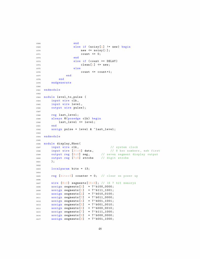
1568 end

1569 else if (noisy[i] != new) begin

1570 new <= noisy[i];

1571 count <= 0;

1572 end

1573 else if (count == DELAY)

1574 clean[i] <= new;

1575 else

1576 count <= count +1;

1577 end

1578 end

1579 endgenerate

1580

1581 endmodule

1582

1583 module level_to_pulse (


1585 input wire level ,

1586 output wire pulse );

1587

1588 reg last_level;


1590 last_level <= level;

1591 end

1592 assign pulse = level & ~last_level;

1593

1594 endmodule

1595

1596 module display_8hex(

1597 input wire clk , // system clock

1598 input wire [31:0] data , // 8 hex numbers , msb first

1599 output reg [6:0] seg , // seven segment display output

1600 output reg [7:0] strobe // digit strobe

1601 );

1602

1603 localparam bits = 13;

1604

1605 reg [bits:0] counter = 0; // clear on power up

1606

1607 wire [6:0] segments[15:0]; // 16 7 bit memorys

1608 assign segments[0] = 7’b100_0000;










48







1624


1626 counter <= counter + 1;

1627 case (counter[bits:bits -2])

1628 3’b000: begin

1629 seg <= segments[data[31:28]];

1630 strobe <= 8’b0111_1111 ;

1631 end

1632 3’b001: begin


1634 strobe <= 8’b1011_1111 ;

1635 end

1636 3’b010: begin


1638 strobe <= 8’b1101_1111 ;

1639 end

1640 3’b011: begin


1642 strobe <= 8’b1110_1111;

1643 end

1644 3’b100: begin


1646 strobe <= 8’b1111_0111;

1647 end

1648 3’b101: begin


1650 strobe <= 8’b1111_1011;

1651 end

1652 3’b110: begin


1654 strobe <= 8’b1111_1101;

1655 end

1656 3’b111: begin


1658 strobe <= 8’b1111_1110;

1659 end

1660 endcase

1661 end

1662 endmodule

1663

1664 module xvga(

1665 input wire vclock ,

1666 output reg [10:0] hcount , // pixel number on current line

1667 output reg [9:0] vcount , // line number

49

1668 output reg vsync , hsync , blank );

1669

1670 // horizontal: 1344 pixels total

1671 // display 1024 pixels per line

1672 reg hblank ,vblank;

1673 wire hsyncon ,hsyncoff ,hreset ,hblankon;

1674 assign hblankon = (hcount == 1023);

1675 assign hsyncon = (hcount == 1047);

1676 assign hsyncoff = (hcount == 1183);

1677 assign hreset = (hcount == 1343);

1678

1679 // vertical: 806 lines total

1680 // display 768 lines

1681 wire vsyncon ,vsyncoff ,vreset ,vblankon;

1682 assign vblankon = hreset & (vcount == 767);

1683 assign vsyncon = hreset & (vcount == 776);

1684 assign vsyncoff = hreset & (vcount == 782);

1685 assign vreset = hreset & (vcount == 805);

1686

1687 // sync and blanking

1688 wire next_hblank ,next_vblank;

1689 assign next_hblank = hreset ? 0 : hblankon ? 1 : hblank;

1690 assign next_vblank = vreset ? 0 : vblankon ? 1 : vblank;

1691 always @(posedge vclock) begin

1692 hcount <= hreset ? 0 : hcount + 1;

1693 hblank <= next_hblank;

1694 hsync <= hsyncon ? 0 : hsyncoff ? 1 : hsync; // active low

1695

1696 vcount <= hreset ? (vreset ? 0 : vcount + 1) : vcount;

1697 vblank <= next_vblank;

1698 vsync <= vsyncon ? 0 : vsyncoff ? 1 : vsync; // active low

1699

1700 blank <= next_vblank | (next_hblank & ~hreset );

1701 end

1702 endmodule

1703

1704 module oversample64(


1706 input wire [11:0] sample ,

1707 input wire eoc ,

1708 output reg [14:0] oversample ,

1709 output reg done

1710 );

1711

1712 reg [5:0] counter = 0;

1713 reg [17:0] accumulator = 0;

1714


1716 done <= 0;

1717 if (eoc) begin

50

1718 // Conversion has ended and we can read a new sample

1719 if (& counter) begin // If counter is full (64 accumulated)

1720 // Get final total , divide by 8 with (very limited) rounding.

1721 oversample <= (accumulator + sample + 3’b100) >> 3;

1722 done <= 1;

1723 // Reset accumulator

1724 accumulator <= 0;

1725 end

1726 else begin

1727 // Else add to accumulator as usual

1728 accumulator <= accumulator + sample;

1729 done <= 0;

1730 end

1731 counter <= counter + 1;

1732 end

1733 end

1734 endmodule

B Project Python

1 import random , math , scipy , potrace

2 import numpy as np

3 import matplotlib.pyplot as plt

4 import matplotlib.path as mpath

5 import matplotlib.patches as mpatches

6 from tqdm import tqdm

7 from PIL import Image

8 from potrace import Curve

9

10

11 # Convert an image to a black and white 2d array (or list for gifs).

12 def get_bw_file(filename , ratio =128):

13 img = Image.open(filename)

14

15 def handle_frame(frame):

16 new_data = np.array(frame.getdata(), dtype=np.uint8)

17 new_data = np.resize(new_data , (img.size[1], img.size[0]))

18

19 new_data[new_data <ratio] = 0

20 new_data[new_data >=ratio] = 1

21

22 return np.pad(

23 new_data ,

24 ((5, 5), (5, 5)),

25 ’constant ’,

26 constant_values =(1,)

27 )

28

29 if img.is_animated:

51

30 frames = []

31 for frame in range(0,img.n_frames):

32 img.seek(frame)

33 frames.append(handle_frame(img.convert(’L’)))

34

35 return frames

36 else:

37 return handle_frame(img.convert(’L’))

38

39

40 # Helper function to generate straight line bezier curves.

41 def straight_line_to_bezier(start , end):

42 c1 = tuple (0.666*s + 0.333*e for s,e in zip(start ,end))

43 c2 = tuple (0.333*s + 0.666*e for s,e in zip(start ,end))

44

45 return (start , c1, c2, end)

46

47

48 def greedy_path(lines , rand=False):

49 # Greedy pathing: start at an unconnected segment.

50 # It has a source and a sink. Choose the closest source or

51 # sink , and connect. Repeat.

52

53 # Distance between two points in 2d

54 def dist(a, b):

55 return math.sqrt((a[0]-b[0])**2 + (a[1]-b[1])**2)

56

57 # Calculate the min distance between two paths.

58 def calc_distance(a, b):

59 return min(

60 dist(a[0][0],b[0][0]),

61 dist(a[0][0],b[ -1][ -2]),

62 dist(a[ -1][ -2], b[ -1][ -2]),

63 dist(a[ -1][ -2],b[0][0])

64 )

65

66 # Connect two paths , with freedom to reverse them.

67 def connect(a, b):

68 d = calc_distance(a,b)

69

70 reverse = lambda x: [

71 tuple(reversed(k[:-1]))+(k[-1],)

72 for k in reversed(x)

73 ]

74

75 if d == dist(a[0][0],b[0][0]):

76 return reverse(a) + [straight_line_to_bezier(

77 a[0][0],

78 b[0][0]

79 )+(False ,)] + b

52

80

81 elif d == dist(a[0][0],b[ -1][ -2]):

82 return b + [straight_line_to_bezier(

83 b[-1][-2],

84 a[0][0]

85 )+(False ,)] + a

86

87 elif d == dist(a[ -1][ -2], b[0][0]):

88 return a + [straight_line_to_bezier(

89 a[-1][-2],

90 b[0][0]

91 )+(False ,)] + b

92

93 else:

94 return a + [straight_line_to_bezier(

95 a[-1][-2],

96 b[-1][-2]

97 )+(False ,)] + reverse(b)

98

99 lines = lines[:]

100 for _ in range(len(lines)-1):

101 min_d = 9999999999

102 min_path = None

103

104 focus = random.randrange(len(lines)) if rand else 0

105

106 for other_path in lines:

107 if other_path == lines[focus]:

108 continue

109

110 d = calc_distance(lines[focus], other_path)

111 if d < min_d:

112 min_d = d

113 min_path = other_path

114

115 lines[focus] = connect(lines[focus], min_path)

116 lines.remove(min_path)

117

118 if len(lines) > 0:

119 lines[0] = lines[0] + [straight_line_to_bezier(

120 lines[0][ -1][ -2],

121 lines[0][0][0]

122 )+(False ,)]

123

124 return lines[0]

125

126 return []

127

128

129 # Generate bezier curves and connect them from a BW image.

53

130 def generate_bezier_curves(image , scale=False , skip =0):

131 # Create a bitmap from the array

132 bmp = potrace.Bitmap(image)

133

134 # Trace the bitmap to a path

135 path = bmp.trace ()

136

137 objects = []

138

139 # Generate initial list for each objects

140 for i, curve in enumerate(path):

141 if i <= skip: continue

142

143 curves = []

144

145 p0 = curve.start_point

146 for seg in curve:

147 if not seg.is_corner:

148 # Is a bezier curve

149 curves.append ((p0, seg.c1, seg.c2, seg.end_point , True))

150 else:

151 # Is a corner , convert to two bezier curves (we hacky af)

152 curves.append(

153 straight_line_to_bezier(p0 , seg.c) + (True , )

154 )

155

156 curves.append(

157 straight_line_to_bezier(seg.c, seg.end_point) + (True ,)

158 )

159

160 p0 = seg.end_point

161

162 objects.append(curves)

163

164 path = greedy_path(objects , rand=True)

165

166 # Get the maximum coordinate , and scale everything

167 # such that it equals ~3300.

168 b = 3300.0/ max(

169 max(max(c) for c in curve[:-1])

170 for curve in path

171 )

172

173 scaled = [

174 tuple(

175 (b*x,b*y) for x,y in curve[:-1]

176 ) + (curve[-1],) for curve in path

177 ]

178

179 return scaled

54

180

181

182 # Plot a set of bezier curves with matplotlib.

183 def plot_bezier_curves(curves):

184 codes = [

185 mpath.Path.MOVETO ,

186 mpath.Path.CURVE4 ,

187 mpath.Path.CURVE4 ,

188 mpath.Path.CURVE4

189 ]

190

191 fig = plt.figure ()

192 ax = fig.add_subplot (111)

193 for v in curves:

194 if not v[-1]: continue

195

196 patch = mpatches.PathPatch(

197 mpath.Path(list(reversed(v[:-1])),codes),

198 facecolor=’none’,

199 lw=2, edgecolor=np.random.rand(3,)

200 )

201

202 ax.add_patch(patch)

203

204 ax.set_xlim(0, 4096)

205 ax.set_ylim(0, 4096)

206

207 plt.show()

208

209 # Convert a bezier curve to a .coe row.

210 def bezier_to_binary(curve):

211

212 flattened = (int(round(e)) for t in curve[:-1] for e in t)

213

214 return "".join(

215 "{0:{ fill }12b}".format(k, fill=’0’)

216 for k in flattened

217 ) + (’1’ if curve[-1] else ’0’)

218

219

220 # Output a set of bezier curves to a .coe file.

221 def bezier_to_coe(scenes , filename):

222 instruction_select_bits = int(math.ceil(math.log(

223 max(max(len(frame) for frame in s) for s in scenes)

224 )/math.log (2)))

225

226 frame_select_bits = int(math.ceil(math.log(

227 max(len(s) for s in scenes)

228 )/math.log (2)))

229

55

230 scene_select_bits = int(math.ceil(math.log(len(scenes ))/ math.log (2)))

231

232 total_size = instruction_select_bits+frame_select_bits+scene_select_bits

233

234 print "*************************************"

235 print "Scene select bits:", scene_select_bits

236 print "Frame select bits:", frame_select_bits

237 print "Inst select bits:", instruction_select_bits

238

239 buff = "memory_initialization_radix =2;\ nmemory_initialization_vector =\n"

240

241 print "Writing COE file now..."

242

243 # Iterate over every entry in our address space.

244 for i in tqdm(range (2** total_size )):

245 s = i >> (total_size - scene_select_bits)

246

247 f = (i >> (instruction_select_bits )) % 2**( frame_select_bits)

248

249 ins = i % 2**( instruction_select_bits)

250

251 scene = scenes[min(s, len(scenes )-1)]

252 frame = scene[f % len(scene)]

253

254 instruction = frame[ins % len(frame)]

255

256 buff += bezier_to_binary(instruction) \

257 + ("," if i != (2** total_size )-1 else ";") + "\n"

258

259 with open(filename , ’w’) as f:

260 f.write(buff)

261

262

263 # Slice a bezier curve into two at fraction t.

264 def slice_bezier(points , t):

265 x1, y1 = points[0]

266 x2, y2 = points[1]

267 x3, y3 = points[2]

268 x4 , y4 = points[3]

269

270 x12 = (x2 -x1)*t+x1

271 y12 = (y2 -y1)*t+y1

272

273 x23 = (x3 -x2)*t+x2

274 y23 = (y3 -y2)*t+y2

275

276 x34 = (x4 -x3)*t+x3

277 y34 = (y4 -y3)*t+y3

278

279 x123 = (x23 -x12)*t+x12

56

280 y123 = (y23 -y12)*t+y12

281

282 x234 = (x34 -x23)*t+x23

283 y234 = (y34 -y23)*t+y23

284

285 x1234 = (x234 -x123)*t+x123

286 y1234 = (y234 -y123)*t+y123

287

288 return (

289 ((x1 ,y1),(x12 ,y12),(x123 ,y123),(x1234 ,y1234), points[ -1]),

290 ((x1234 ,y1234),(x234 ,y234),(x34 ,y34),(x4,y4), points[ -1])

291 )

292

293

294 # Numerically compute the length of a bezier curve. Turns out doing this

295 # "prettier ways" is hard af.

296 def bezier_length(curve):

297 # Split curve into 1000 points , and find their sum distance

298

299 return sum(

300 sum(( first[k] - second[k])**2 for k in (0,1))

301 for first , second in (lambda x: zip(x,x[1:]))([

302 tuple(

303 (1-t)**3 * c[0] + 3*t*(1-t)**2 * c[1] +

304 3 * t**2 * (1-t) * c[2] + t**3 * c[3]

305 for c in zip(* curve[:-1])

306 ) for t in np.linspace (0 ,1 ,1000)

307 ])

308 )

309

310

311 # Expand a set of bezier curves such that they are a power of two

312 # by splitting the largest curves in half.

313 def expand_bezier(curves):

314 target = int (2** math.ceil(math.log(len(curves ))/ math.log (2)))

315

316 c = {curve: bezier_length(curve) for curve in curves}

317 for _ in range(target -len(curves )):

318 # Pick the biggest curve , and split it down the middle.

319

320 max_curve , max_len , max_index = None , -1, -1

321

322 for i, curve in enumerate(curves):

323 l = c[curve]

324

325

326 if l > max_len:

327 max_len = l

328 max_curve = curve

329 max_index = i

57

330

331 first , second = slice_bezier(max_curve , 0.5)

332 curves[max_index] = first

333 curves.insert(max_index +1, second)

334

335 c[first] = c[second] = l/2

336

337 return curves

338

339

340 # Apply the entire processing pipeline to a single gif.

341 def process_gif(filename ,

342 down_sample =1,

343 skip=0,

344 get_first=False ,

345 pad=0,

346 ratio =128):

347

348 print "Getting images from", filename

349 imgs = get_bw_file(filename , ratio=ratio)

350

351

352 imgs = [imgs[0]] if get_first else [

353 imgs[i] for i in range(0,len(imgs),down_sample)

354 ]

355

356 imgs = imgs[pad:0-pad -1] + ([imgs[ -1]] if pad == 0 else [])

357

358 print "Processing initial bezier curves ..."

359 frames = [generate_bezier_curves(x,scale=True ,skip=skip) for x in imgs]

360

361 print "Expanding bezier curves ..."

362 frames = [expand_bezier(x) for x in frames]

363

364 instruction_select_bits = int(math.ceil(math.log(

365 max(len(f) for f in frames)

366 )/math.log (2)))

367

368 frame_select_bits = int(math.ceil(math.log(len(frames ))/ math.log (2)))

369

370 return frames

371

372

373 # The final COE used during our checkoff + video.

374 saved = [

375 process_gif(’macaroni.gif’),

376 process_gif(’pear.gif’,skip=1),

377 process_gif(’square.gif’,down_sample =3),

378 process_gif(’dots.gif’,skip=1, down_sample =3)

379 ]

58

380

381 bezier_to_coe(saved , "rom.coe")

59

Rave in a Boxweb.mit.edu/6.111/volume2/www/f2018/projects/cherna...Figure 4: Chromagram of \The Bends" by Radiohead computed by our team. While an approach like this would certainly

Documents