Rauschreduktion versus Ortsaufl¨osung in digitalen Bildern Diplomarbeit im Fachbereich Medien- und Phototechnik an der Fachhochschule K¨oln Autor: Uwe Artmann Matr.Nr.: 11036802 Referent: Prof. Dr. Ing. Gregor Fischer Koreferent: Dipl.-Ing. Dietmar W¨ uller K¨ oln, im November 2007

Welcome message from author
This document is posted to help you gain knowledge. Please leave a comment to let me know what you think about it! Share it to your friends and learn new things together.
Transcript

Rauschreduktion versus Ortsauflosung in
digitalen Bildern
Diplomarbeit im Fachbereich
Medien- und Phototechnik
an der Fachhochschule Koln
Autor:
Uwe Artmann
Matr.Nr.: 11036802
Referent: Prof. Dr. Ing. Gregor Fischer
Koreferent: Dipl.-Ing. Dietmar Wuller
Koln, im November 2007
Noise-Reduction versus Spatial Resolution in
Digital Images
Thesis at the
Department of Media- and Phototechnology
University of Applied Sciences Cologne
Author:
Uwe Artmann
student ID.: 11036802
First Reviewer: Prof. Dr. Ing. Gregor Fischer
Second Reviewer: Dipl.-Ing Dietmar Wuller
Cologne, November 2007
Zusammenfassung
Titel: Rauschreduktion versus Ortsauflosung in digitalen Bildern
Autor: Uwe Artmann
Referenten: Prof. Dr. Gregor Fischer
Dipl.-Ing. Dietmar Wuller
Zusammenfassung: In modernen Digitalkameras werden immer komplexere
Algorithmen verwendet, die das Rauschen im Bild reduzieren sollen. In dieser
Arbeit wird untersucht, wie sich dies auf die Ortsauflosung auswirkt und ein
Verfahren entwickelt, diese mit verschiedenen Mitteln zu beschreiben.
Stichworter: Rauschreduktion, Digitalkamera, Ortsauflosung, SFR Edge, SFR Siemens
Sperrvermerk: Die vorgelegte Arbeit unterliegt keinem Sperrvermerk.
Datum: 20. November 2007
3
Abstract
Title: Noise-Reduction versus spatial resolution in digital images
Author: Uwe Artmann
Advisores: Prof. Dr. Gregor Fischer
Dipl.-Ing. Dietmar Wuller
Abstract: In the signal processing of digital still cameras more and more com-
plex algorithms take place to reduce the noise in the images. In this thesis
the influence of the noise reduction on spatial resolution is analyzed and a
measurement system is set up.
Keywords: Noisereduction, DSC, SFR Edge, SFR Siemens, Noise
Remark of closure: The thesis is not closed.
Date: 20. November 2007
4
Contents
Contents
1 Introduction 9
2 Basics 11
2.1 Noise in a digital still camera . . . . . . . . . . . . . . . . . . . . 11
2.1.1 Noise on the sensor level . . . . . . . . . . . . . . . . . . . 13
2.1.2 Noise on the processing level . . . . . . . . . . . . . . . . 16
2.1.3 Noise on the image level . . . . . . . . . . . . . . . . . . . 25
2.1.4 Problems of noise measurement . . . . . . . . . . . . . . . 30
2.2 Spatial Resolution in digital still cameras . . . . . . . . . . . . . . 31
2.2.1 ISO 12233:2000 . . . . . . . . . . . . . . . . . . . . . . . 32
2.2.2 SFR Edge . . . . . . . . . . . . . . . . . . . . . . . . . . 34
2.2.3 SFR Siemens . . . . . . . . . . . . . . . . . . . . . . . . . 35
2.2.4 Problems of resolution measurement . . . . . . . . . . . . 37
3 NoiseLab 39
5

Contents
3.1 User Interface . . . . . . . . . . . . . . . . . . . . . . . . . . . . 41
3.2 Degradation . . . . . . . . . . . . . . . . . . . . . . . . . . . . . 42
3.2.1 Low pass filtering . . . . . . . . . . . . . . . . . . . . . . 42
3.2.2 Adding noise . . . . . . . . . . . . . . . . . . . . . . . . . 43
3.3 Denoising . . . . . . . . . . . . . . . . . . . . . . . . . . . . . . . 44
3.3.1 Average . . . . . . . . . . . . . . . . . . . . . . . . . . . 44
3.3.2 Wiener . . . . . . . . . . . . . . . . . . . . . . . . . . . . 45
3.3.3 Median . . . . . . . . . . . . . . . . . . . . . . . . . . . . 45
3.3.4 Coring . . . . . . . . . . . . . . . . . . . . . . . . . . . . 46
3.3.5 Wavelet . . . . . . . . . . . . . . . . . . . . . . . . . . . 53
4 NoiseLab Chart 57
4.1 A -Siemens stars . . . . . . . . . . . . . . . . . . . . . . . . . . . 58
4.2 B - Edges . . . . . . . . . . . . . . . . . . . . . . . . . . . . . . 59
4.3 C - White Noise . . . . . . . . . . . . . . . . . . . . . . . . . . . 61
5 NoiseLab Analyzer 63
5.1 User Interface . . . . . . . . . . . . . . . . . . . . . . . . . . . . 65
5.2 SFR-Siemens . . . . . . . . . . . . . . . . . . . . . . . . . . . . . 66
5.3 SFR-Edge . . . . . . . . . . . . . . . . . . . . . . . . . . . . . . 71
5.4 Edge Profile - Intensity and Standard Deviation . . . . . . . . . . . 74
6

Contents
5.5 SFR-Noise . . . . . . . . . . . . . . . . . . . . . . . . . . . . . . 77
5.6 Line Profile . . . . . . . . . . . . . . . . . . . . . . . . . . . . . . 80
5.7 Histogram of Derivative . . . . . . . . . . . . . . . . . . . . . . . 82
5.8 Noise GLCM . . . . . . . . . . . . . . . . . . . . . . . . . . . . . 83
6 Results 86
6.1 Ideal Image . . . . . . . . . . . . . . . . . . . . . . . . . . . . . . 87
6.2 NoiseLab Images . . . . . . . . . . . . . . . . . . . . . . . . . . . 90
6.2.1 Summary NoiseLab Images . . . . . . . . . . . . . . . . . 93
6.3 Camera Images . . . . . . . . . . . . . . . . . . . . . . . . . . . . 94
6.3.1 Nikon D80 . . . . . . . . . . . . . . . . . . . . . . . . . . 94
6.3.2 Canon IXUS 950 IS . . . . . . . . . . . . . . . . . . . . . 97
6.3.3 FujiFilm FinePix S8000fd . . . . . . . . . . . . . . . . . . 101
6.4 Summary Camera Images . . . . . . . . . . . . . . . . . . . . . . 105
7 Conclusion 107
A Graphical and Numerical Results 108
B Additional Information 123
B.1 Noise Distribution . . . . . . . . . . . . . . . . . . . . . . . . . . 123
B.2 Linearization of image data in NoiseLab Analyzer . . . . . . . . . . 126
7

Contents
C Acknowledgement 128
D Remarks 129
Bibliography 132
8
Chapter 1. Introduction
Chapter 1
Introduction
The image quality of a digital still camera relies basically on low noise, high dy-
namic range, high spatial resolution and nice looking colors. Ten years ago, Image
Engineering Dietmar Wueller started testing these parameters by order of a german
photography magazine. Since then hundreds of cameras have been tested.
When the first digital cameras were on the market, major improvements in
image quality have been made with more pixels on the sensor to increase the spatial
resolution. In those days, more pixel lead to better images. This relationship is still
in mind of many customers, so the manufacturers increase the pixel count regularly,
by now (Fall 2007) we have reached 12 Million Pixel in compact cameras.
As the size of the sensors is a major matter of expense in camera production,
the cameras get more pixels on the same dimensions of the sensor and therefore
the size of the light sensitive area for each pixel decreases and the noise level
increases. Noise reduction algorithms are used to compensate and to keep the
noise on a considerable level but introduce artifacts. The images loose details in
fine structures and appear cartoon like.
A modern camera system is a highly non linear system, which makes it more and
more difficult to measure for image quality. Using the actual standard measurement
methods for image quality, it happens, that the imaging device gets good results
9

Chapter 1. Introduction
in noise and spatial resolution measurement, but the images lack of fine details
and appear degraded.
In this thesis I introduce a test system to get a more detailed description of the
spatial frequency response of a digital still camera and the introduced artifacts of
noise reduction, considering that the behavior of the camera is different on edges,
patterns and fine detailed structures.
10
Chapter 2. Basics
Chapter 2
Basics
2.1 Noise in a digital still camera
noise —noiz— technical - irregular fluctuations that accompany a transmitted
electrical signal but are not part of it and tend to obscure it. [1]
Noise is an unwanted part of the image signal, so it is part of the digital image,
but it does not represent a point in the scene that was captured. The optical
image that was projected by the lens onto the sensor is transfered into a digital
image file on the storage card within the camera. Noise from different sources is
added, modified or reduced in the image signal in different steps of the process.
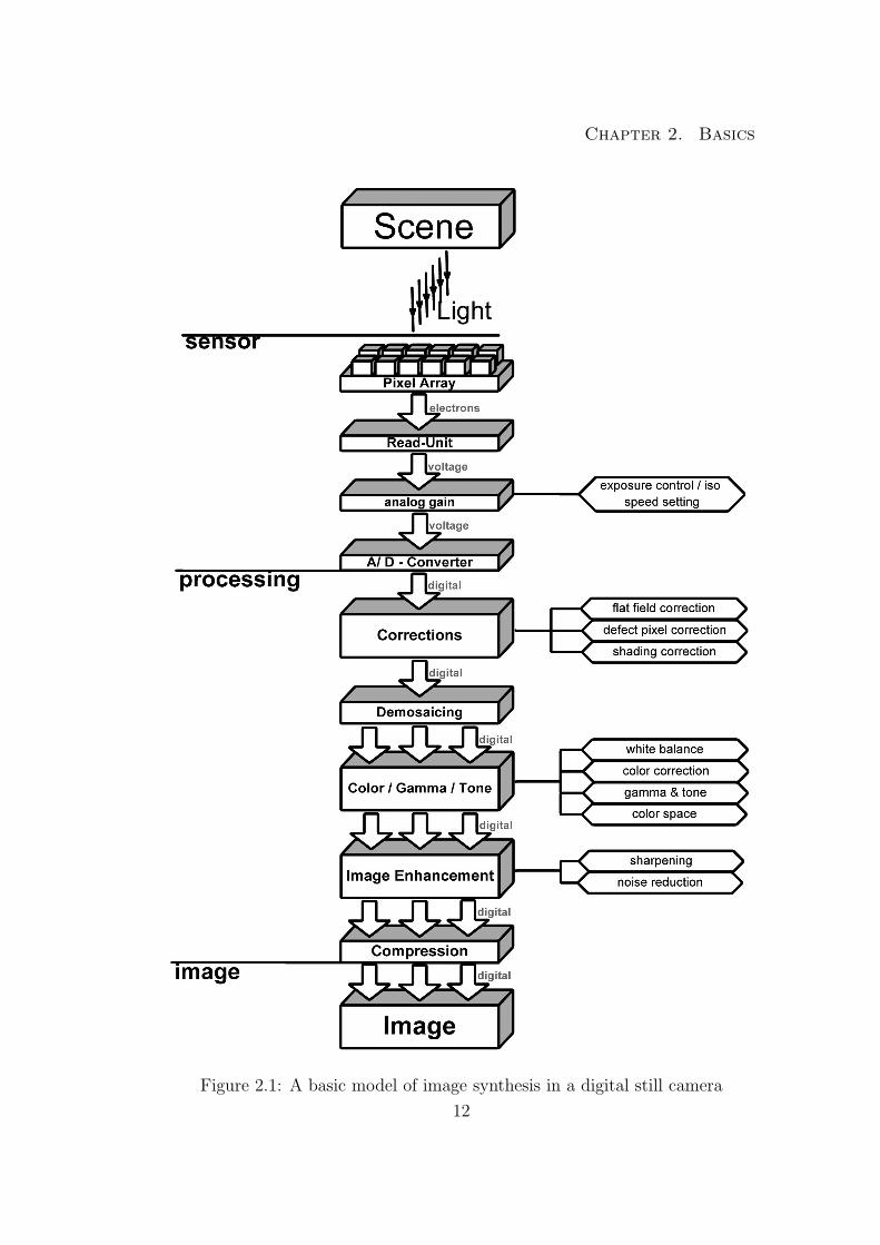
The next sections describe the different steps in the synthesis of a digital image
with a close look to noise. Figure 2.1 shows a basic model of the synthesis of a
digital image in a still camera. The actual order of the different items may vary in
different cameras, but the concept is basically the same.
11
Chapter 2. Basics
Figure 2.1: A basic model of image synthesis in a digital still camera
12
Chapter 2. Basics
2.1.1 Noise on the sensor level
Light can be considered as a flow of photons. While exposure time, a certain
amount of photons hits one pixel on the sensor. With a sensor depending probabil-
ity, free electrons are created in the pixel, correlated with the quantity of photons.
This is not a static process, the number of photons has a poisson distribution, so
it varies around its mean value even if the whole setup of light-source, lens and
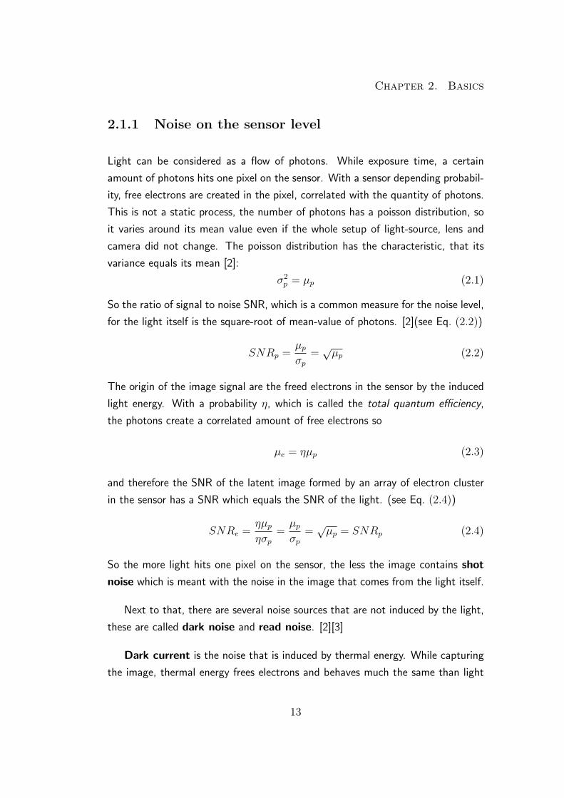
camera did not change. The poisson distribution has the characteristic, that its
variance equals its mean [2]:
σ2p = µp (2.1)
So the ratio of signal to noise SNR, which is a common measure for the noise level,
for the light itself is the square-root of mean-value of photons. [2](see Eq. (2.2))
SNRp =µpσp
=õp (2.2)
The origin of the image signal are the freed electrons in the sensor by the induced
light energy. With a probability η, which is called the total quantum efficiency,
the photons create a correlated amount of free electrons so
µe = ηµp (2.3)
and therefore the SNR of the latent image formed by an array of electron cluster
in the sensor has a SNR which equals the SNR of the light. (see Eq. (2.4))
SNRe =ηµpησp
=µpσp
=õp = SNRp (2.4)
So the more light hits one pixel on the sensor, the less the image contains shot
noise which is meant with the noise in the image that comes from the light itself.
Next to that, there are several noise sources that are not induced by the light,
these are called dark noise and read noise. [2][3]
Dark current is the noise that is induced by thermal energy. While capturing
the image, thermal energy frees electrons and behaves much the same than light
13
Chapter 2. Basics
energy in its distribution. So as shown in equation (2.1) the variance equals the
mean, which means that the dark current is not a homogeneously offset on all
pixels, it is a source of noise.
The capacitor used to transform the charge into a current has to be reset right
before the capturing process starts. This process does not work perfect all the time,
so some electrons are left and add themselves to the signal. This reset noise is also
called kTC noise because of the components to calculate its variance in voltage:
The Boltzman’s constant k, the temperature T in Kelvin and the capacitance C.
[2][3]
σkTC =
√kT
C(2.5)
The analog signal from each pixel is converted into a digital value using an A/D
converter. A quantization noise is introduced while matching the analogue signal
onto the digital values, but in digital cameras this is normally negligible, because
the quantisation steps used are small enough and the noise before quantization is
far more than the quantization noise.[4]
Signal
exposure control / isospeed setting
exposure time
factor K
photon shot noise
dark current noise+
X
+ read noise
X
ADC
+ quantization noise
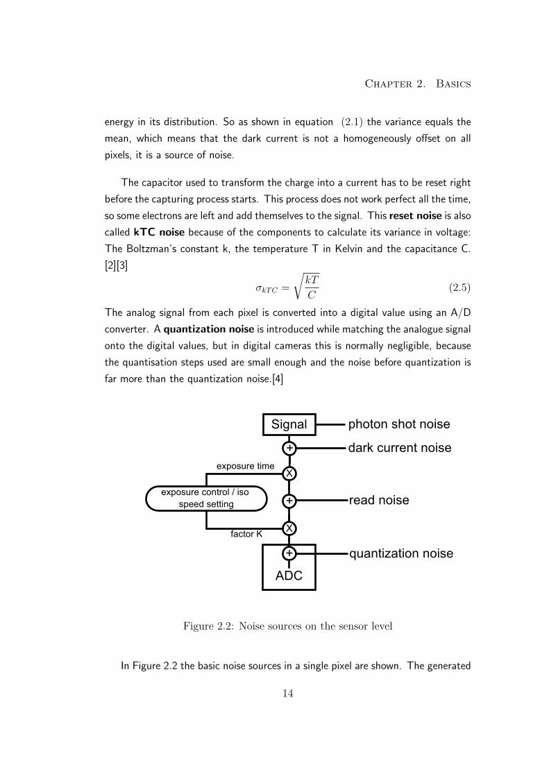
Figure 2.2: Noise sources on the sensor level
In Figure 2.2 the basic noise sources in a single pixel are shown. The generated
14
Chapter 2. Basics
signal at its beginning already contains photon shot noise. The signal gets more
noise the lower the light intensity is. So the smaller the pixel or the shorter the
exposure time is, the more shot noise we get. On the other side, the longer the
exposure time the greater the dark current. So the exposure time should be as
short as possible while catching as much photons as possible. One way to achieve
this is to enlarge the light sensitive area of each pixel. But depending on the sensor
design more or less space in one pixel is not light sensitive and is used for other
issues. A solution for this problem are micro-lenses that are placed on top of the
light sensitive area of each pixel. So the geometrical fill-factor, the ratio of pixel
size to the effective area, is kept on the same level, but the optical fill factor, the
ratio of light hitting the pixel and light hitting the area where light can be captured
is enlarged.
The analog gain that is used to enlarge the signal level prior the analog/digital
converter can not reduce the noise significantly. The standard deviations σ of the
different noise sources are added by their square, so one noise source can dominate
the others quickly. The gain can only reduce the quantization noise in the ADC so
the signal to noise ratio will increase with increasing gain and reach a maximum
quickly, which is limited by the shot noise and the dark noise as can be shown in
equation (2.6)[4]
SNR =Signal√
σ2shot&dark +
σ2quantification
K2
(2.6)
All noise sources described above can be seen as temporal noise or random
noise. This means that the digital output value of one pixel changes its output
under constant illumination and camera setup over the time, so each time an
image is taken. Another type of noise is known as spatial noise or pattern
noise., which describes the change of digital output of adjacent pixel under the
same, homogeneous illumination. [3]
An imaging sensor is based on doped silicon and is produced using lithographic
methods, so basically the projection of masks on the silicon wafer and then using
chemicals to develop the wafer. Due to this process it is obvious that not all pixel on
the sensor look exactly the same in their physical assembly. These differences in the
15
Chapter 2. Basics
pixel lithography and the structure of the silicon leads to a different total quantum
efficiency η (see Eq. (2.3)) of each pixel which is called PRNU (Photon Respone
Non Uniformity). In CMOS sensors much of the conversion from free electrons
to a digital value is done in each pixel rather than for each column or the whole
sensor like in CCD sensors. So the differences between the pixels in their response
to light includes differences in the analog gain or the analog/digital converter as
well, so normally the pattern noise is larger in CMOS than in CCD sensors. The
pattern noise can be differentiated in the PRNU which is light depending and a
static Fixed Pattern Noise (FPN) which is not depending on the light intensity.
Depending on the sensor design, a fixed difference can also be observed between
each pixel or for different columns of the sensor pixel array, which is the result of
variations in the dark current of each column (depending on the readout principle
of the sensor) or of column-wise gain variations.
2.1.2 Noise on the processing level
The digital signal that comes directly from the sensor is still ”raw”, which means
that it contains all necessary informations, but has to be processed to become a
displayable image. The model in Figure 2.1 shows the basic modules of image
processing. It may vary between different cameras what is done at which position
in the signal chain. The different steps in the image processing can increase or
decrease the noise and some modify or diffuse the noise.[4]
Corrections
Some corrections of the noise are already done in the sensor, with special circuits.
These circuits can reduce the read noise of the sensor but may also introduce more
pattern noise, as the setup of the noise reduction may change from pixel to pixel.
Flat field correction is a method to reduce the fixed pattern noise, pixel-wise
or column-wise. The basic concept is, that under a homogeneous illumination the
sensor is read out and with this values correction factors are calculated and then
16

Chapter 2. Basics
stored in a memory unit in the camera. If in normal use an image is taken, the
signal processing unit in the camera can reduce the fixed pattern noise using the
stored information.
As already mentioned in section 2.1.1, the sensor production always introduces
some deviance from the ideal result. Next to slight variations from pixel to pixel,
some pixel do not work at all, have a light independent output or always a maximum
output. These pixel are commonly called dead or hot pixel. The amount of pixel
defects in a sensor is a cost factor of it, so the less defects the sensor has to
show, the higher is the offal in the production and therefore the higher is the price.
The idea of the defect pixel correction is that the digital output value of the
known defect pixel are interpolated from its surrounding pixels. This will reduce
the spatial resolution in that area, but as long as the number of defect pixel is small
(< 0.1%) the loss is not visible. The difference between correction systems is the
way of detecting defect pixels. The cheapest and therefore commonly used for
mobile phone camera modules way is the on-the-fly-correction which means that
the processing unit has to detect which pixel seems to be defect and correct them
directly. The more accurate procedure is based on a calibration table containing
the known defect pixel of that sensor. The information received from a calibration
in the production of the camera is stored in the memory unit. This method is more
accurate and needs less time in the image processing but more time in production,
so it is more expensive.
The lens that projects the scene onto the sensor shows more or less vignetting,
a loss of light intensity from the image center to the corner. In digital cameras
normally the term shading is used to describe all factors that cause the same
effect than lens-vignetting. This could be a different response of the pixel and its
micro-lens or of the IR-filter on angular variations of the light-beam and can be
separated in intensity-shading and color-shading. The idea of shading correction
is to multiply the whole image with an inverse flat field image taken with the
camera and the lens. But as the shading depends on the aperture, the focus
and focal length position of the lens, it is not useful to create and to store a flat
field image for all possible situations. What could be done, is to store just some
parameter in the camera and to model the shading in the camera with the given
17
Chapter 2. Basics
parameter and settings of the camera. With this method a perfect correction is
not possible, but it reduces the shading in the image. The manufacturer has to
find a compromise between reducing shading and increasing the noise depending
on the position in the image due to increase amplification.[4]
Demosaicing
A single pixel of an image sensor is unable to detect color, as it is just a light-
intensity detector. To get a color image, the idea of a Kodak scientist named
Bayer is commonly used, the so called Bayer pattern. The pixel get color filter,
so each pixel is able to detect just one color. After taking the image, the image
processor has to interpolate the missing color information of all pixel to convert a
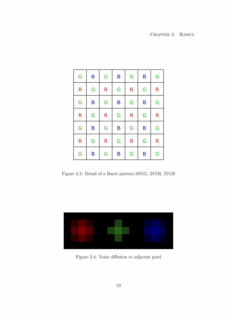
m× n image into a m× n× 3 image. One half of the pixel of a standard Bayer
pattern sensor have a green filter, one quarter a red and the last quarter a blue
one (see Fig. 2.3). The Bayer pattern uses more green pixel because green is the
most important color for the luminance information.
A challenge for the signal processor designer is to find an algorithm that can
interpolate the missing pixel information without introducing color artifact noise or
color aliasing and keeping the spatial resolution up. The demosaicing introduces a
spatial correlation of noise which is caused by the interpolation process where the
noise diffuses to adjacent pixel.(see Fig. 2.4)[4]
Color and Tone corrections
The human visual system has the ability to adjust to the dominant light color
temperature. So a white sheet of paper appears white in bright sunlight and in
candlelight. To simulate this in a digital camera the signal processor adjusts the
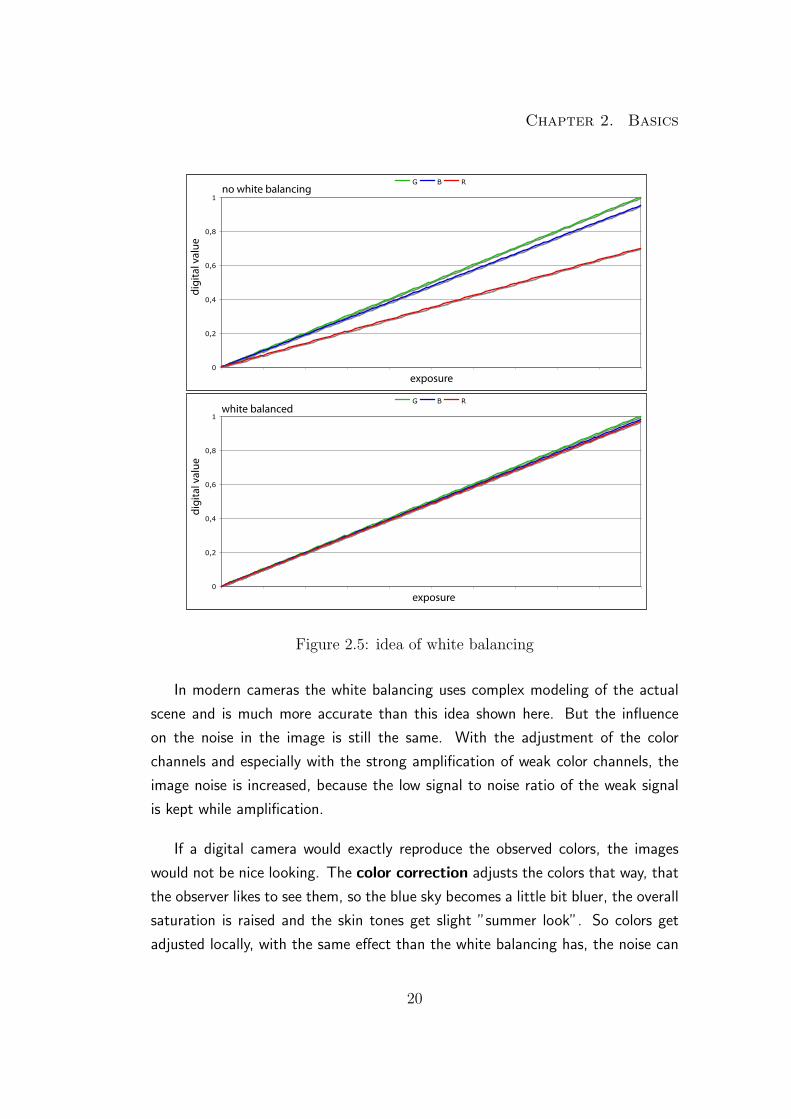
three color channels differently. In Figure 2.5 the basic concept is shown in a before
and after diagram. The white balancing has detected, that the red channel is
underexposed and adjusts the three channels that way, that they lie on top of each
other because the assumption is, that in average the whole image is gray.
18
Chapter 2. Basics
G B G B G B G
R G R G R G R
G B G B G B G
R G R G R G R
G B G B G B G
R G R G R G R
G B G B G B G
Figure 2.3: Detail of a Bayer pattern 50%G, 25%R, 25%B
Figure 2.4: Noise diffusion to adjacent pixel
19
Chapter 2. Basics
0
0,2
0,4
0,6
0,8
1
Digital Value [0...1]
G B R
0
0,2
0,4
0,6
0,8
1
Digital Value [0...1]
G B R
digi
tal v
alue
digi
tal v
alue
exposure
exposure
no white balancing
white balanced
Figure 2.5: idea of white balancing
In modern cameras the white balancing uses complex modeling of the actual
scene and is much more accurate than this idea shown here. But the influence
on the noise in the image is still the same. With the adjustment of the color
channels and especially with the strong amplification of weak color channels, the
image noise is increased, because the low signal to noise ratio of the weak signal
is kept while amplification.
If a digital camera would exactly reproduce the observed colors, the images
would not be nice looking. The color correction adjusts the colors that way, that
the observer likes to see them, so the blue sky becomes a little bit bluer, the overall
saturation is raised and the skin tones get slight ”summer look”. So colors get
adjusted locally, with the same effect than the white balancing has, the noise can
20
Chapter 2. Basics
be increased because of the amplification of weak signals.
In contrast to the human visual system, a digital imaging sensor has a linear
conversion function of light intensity to digital value. To compensate this, a
gamma function is applied and some other tone corrections are performed, for
example to enhance the scene related dynamic range by an amplification of the
dark regions of the image. Both steps lead to an amplification or reduction of
different signal levels and therefore increase or decrease the noise.
The spectral sensitivity of color sensors is slightly different from sensor to sensor
and all show more or less great difference to the human spectral sensitivity. So the
RGB values are not a direct representative of a certain color, these values represent
device depended colors and have to be converted to a defined color space. The
great majority of digital still cameras save their RGB values in sRGB, a standard
color space that can be mapped by most consumer image devices like cameras or
displays. The color space transformation camera-RGB to sRGB is performed
using a 3× 3 matrix M.RsRGB
GsRGB
BsRGB
=
m11 m12 m13
m21 m22 m23
m31 m32 m33
×Rcam
Gcam
Bcam
(2.7)
The larger the difference between RGBcam and the target color space (here:
RGBsRGB) the larger the off-diagonal matrix term and the larger the noise am-
plification because the noise of one color channel is added to another.
Image Enhancement
In digital image processing the image quality can be improved with suitable al-
gorithms. These image enhancements are processing steps, that try to make the
images appear sharper and to reduce the noise. These techniques can improve the
overall image quality to a certain level, but if it is overdone the image enhancement
can introduce artifacts and actually reduce the subjective image quality. [4]
21
Chapter 2. Basics
The possibilities of noise reduction in images will be explained in chapter 3
and different algorithms will be analyzed.
Sharpness is a subjective perception of the human visual system, so it is hard
to measure or to describe sharpness. In a MTF (Modulation Transfer Function)
the sharpness can be considered to be described with the modulation in the lower
frequencies, in contrast to the maximum resolution which can be seen in the highest
frequencies. (See chapter 2.2)
Both enhancements, noise reduction and sharpening, share the same prob-
lem: The image signal contains noise and the quality of the enhancement is based
on the possibility to differentiate between noise and image signal. The better this
can be done, the better the algorithms can sharp an image or reduce noise. The
quality of noise reduction and sharpening relies on the possibility to distinguish the
signal parts in the input image.
The idea of sharpening is to amplify the high spatial frequencies of the image,
because edges contain high spatial frequencies and therefore the amplification will
improve the contrast at the edges. This method works fine in the absence of
noise, but if the image contains noise, the high spatial frequencies of the noise
are amplified as well. This leads to a significant increase of the noise and the
DSP1 designer has to find a compromise between sharpening and noise level. The
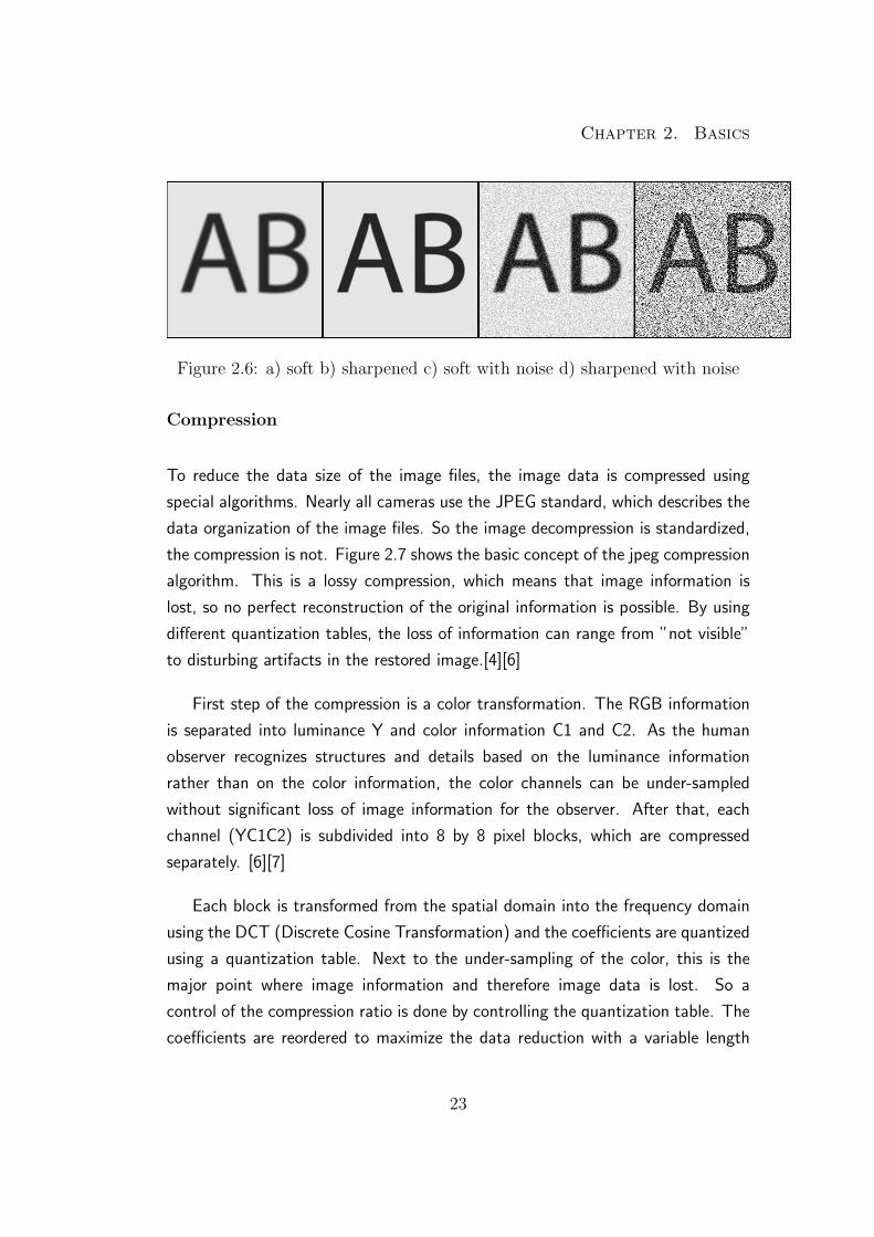
example in figure 2.6 shows the problem. Image a) was slightly low pass filtered
to get a unsharp image. Image b) is the same image after a simple sharpening
process, it appears sharper. Image c) is the same as image a), but noise was added.
Image d) is the sharpened version of image c), using the same sharpening process
than used to create image b). One can see, that the edges appear sharper, but as
a tradeoff the noise was increased as well.
So can be seen in the chapter ”Results”, digital still cameras do less sharpening
on images with high noise levels than on image with moderate noise level because
of the increase of noise with higher sharpening.
1DSP: Digital Signal Processing
22
Chapter 2. Basics
Figure 2.6: a) soft b) sharpened c) soft with noise d) sharpened with noise
Compression
To reduce the data size of the image files, the image data is compressed using
special algorithms. Nearly all cameras use the JPEG standard, which describes the
data organization of the image files. So the image decompression is standardized,
the compression is not. Figure 2.7 shows the basic concept of the jpeg compression
algorithm. This is a lossy compression, which means that image information is
lost, so no perfect reconstruction of the original information is possible. By using
different quantization tables, the loss of information can range from ”not visible”
to disturbing artifacts in the restored image.[4][6]
First step of the compression is a color transformation. The RGB information
is separated into luminance Y and color information C1 and C2. As the human
observer recognizes structures and details based on the luminance information
rather than on the color information, the color channels can be under-sampled
without significant loss of image information for the observer. After that, each
channel (YC1C2) is subdivided into 8 by 8 pixel blocks, which are compressed
separately. [6][7]
Each block is transformed from the spatial domain into the frequency domain
using the DCT (Discrete Cosine Transformation) and the coefficients are quantized
using a quantization table. Next to the under-sampling of the color, this is the
major point where image information and therefore image data is lost. So a
control of the compression ratio is done by controlling the quantization table. The
coefficients are reordered to maximize the data reduction with a variable length
23

Chapter 2. Basics
color transformation
R G B
undersampling
Y C1 C2
pixel blocks
each block
DCT
Quantization
reorder and variable lenghtcoding of coefficients
datareduction
informationloss
Figure 2.7: concept of lossy jpeg compression
coding. [6][7]
Lossy image compression is very similar to some noise reduction methods,
because the main structures of the image are kept and at first texture and small
details are lost. So image compression reduces noise on one side, but diffuses
the noise and introduces artifacts on the other side. So again the designer of the
digital image processor has to find a compromise to keep the image quality up.[7]
24
Chapter 2. Basics
2.1.3 Noise on the image level
In the previous sections the source of noise is shown and the influence of signal
processing to the noise. This section describes what in the end really matters to
the user of a digital camera, the noise in the processed and stored digital image
and how to measure it. It is difficult to differentiate between the different noise
sources in the digital image because in most cases the processed image is the
only information the user has got. Test methods have to treat the camera as a
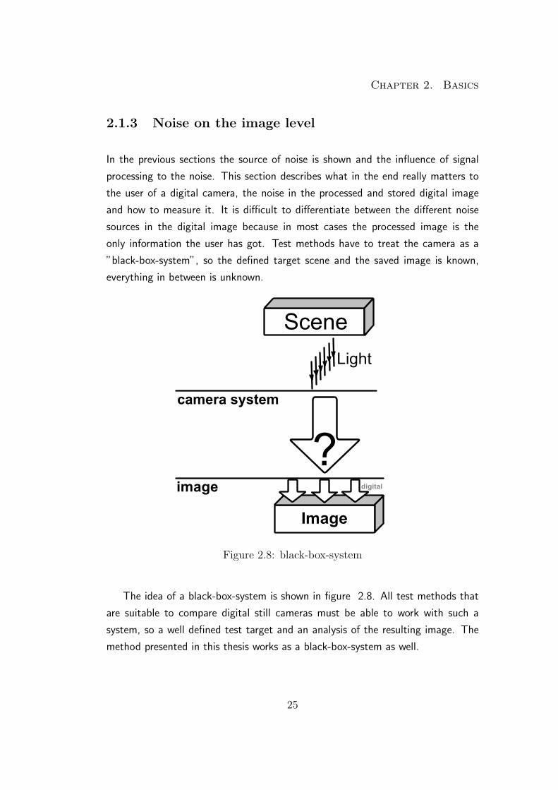
”black-box-system”, so the defined target scene and the saved image is known,
everything in between is unknown.
Light
Image
digitalimage
Scene
camera system
?
Figure 2.8: black-box-system
The idea of a black-box-system is shown in figure 2.8. All test methods that
are suitable to compare digital still cameras must be able to work with such a
system, so a well defined test target and an analysis of the resulting image. The
method presented in this thesis works as a black-box-system as well.
25
Chapter 2. Basics
Signal to Noise Ratio
As already mentioned in the section ”Noise on the sensor level”, the signal to
noise ratio (SNR) is a common measure of noise, not only of the image-noise but
signals in general. In case of an image with intensity Y, the SNR is the mean of Y
minus the dark current divided by the standard deviation of the signal. So
SNRY =µY − µYdark
σY(2.8)
The mean of the dark current is subtracted to get the light induced signal only, so
if the mean of the signal equals the mean of the dark current, Y contains no infor-
mation and the SNR becomes 0 (SNR = 0). The higher the SNR the less noise
the image contains, a noiseless image has a SNR towards infinity (SNR → ∞).
As a ratio the SNR has no unit. It is common practice to use decibel to express
the ratio, so the SNR becomes
SNRY [dB] = 20× log10(µY − µYdark
σY) (2.9)
Just providing the SNR is not a complete description of the camera in term of
noise. The signal and the noise are depending on the exposure level of the sensor,
which depends on the target and its illumination. To compare different cameras,
at least the luminance of the target needs to be reported as well. This would still
not include the difference in exposure, so if the camera underexposed the image
it will get a lower SNR than the same camera with an overexposed image. To
calculate the SNR as shown in Eq. (2.8), the data has to be linear, so without an
applied gamma function or other tone mapping functions. If the camera is treated
as a black-box and no details of the cameras are known, it is not possible to invert
the tone mapping to get linear data. [7]
ISO 15739
The international organization for standardization (ISO) describes a standardized
noise measurement method with the needed capabilities, so measurement of a black
26
Chapter 2. Basics
box system, fixed luminance values at measurement points and measurement of
the opto electronic conversion function (OECF) to invert the tone-mapping. [5]
The standard ISO 15739 describes the used target and the method to calculate
a signal to noise ratio based on a ”18% reference” signal level.
SNR =Lsat × 0.18× incremental gain
Average total noise(2.10)
Lsat maximum unclipped value of system ( 2bitdepth − 1 )
0.18 18% reflectance (target: D=0.9 and 140% maximum level)
incremental gain first differential of OECF (ISO14524)
Average total noise Average of the standard deviations of n samples, given by
σtotal =
√√√√ 1
n
n∑i=1
σ2total.i
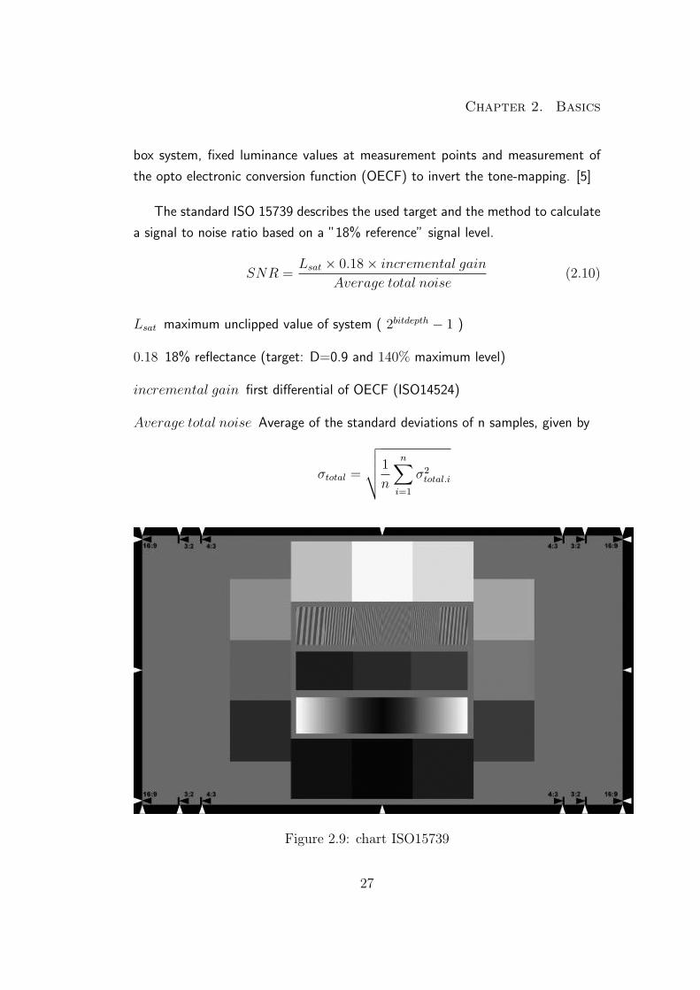
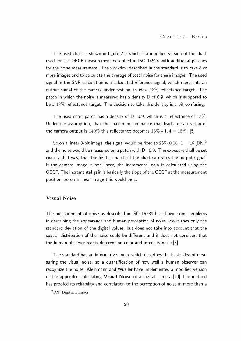
Figure 2.9: chart ISO15739
27
Chapter 2. Basics
The used chart is shown in figure 2.9 which is a modified version of the chart
used for the OECF measurement described in ISO 14524 with additional patches
for the noise measurement. The workflow described in the standard is to take 8 or
more images and to calculate the average of total noise for these images. The used
signal in the SNR calculation is a calculated reference signal, which represents an
output signal of the camera under test on an ideal 18% reflectance target. The
patch in which the noise is measured has a density D of 0.9, which is supposed to
be a 18% reflectance target. The decision to take this density is a bit confusing:
The used chart patch has a density of D=0.9, which is a reflectance of 13%.
Under the assumption, that the maximum luminance that leads to saturation of
the camera output is 140% this reflectance becomes 13% ∗ 1, 4 = 18%. [5]
So on a linear 8-bit image, the signal would be fixed to 255∗0.18∗1 = 46 [DN]2
and the noise would be measured on a patch with D=0.9. The exposure shall be set
exactly that way, that the lightest patch of the chart saturates the output signal.
If the camera image is non-linear, the incremental gain is calculated using the
OECF. The incremental gain is basically the slope of the OECF at the measurement
position, so on a linear image this would be 1.
Visual Noise
The measurement of noise as described in ISO 15739 has shown some problems
in describing the appearance and human perception of noise. So it uses only the
standard deviation of the digital values, but does not take into account that the
spatial distribution of the noise could be different and it does not consider, that
the human observer reacts different on color and intensity noise.[8]
The standard has an informative annex which describes the basic idea of mea-
suring the visual noise, so a quantification of how well a human observer can
recognize the noise. Kleinmann and Wueller have implemented a modified version
of the appendix, calculating Visual Noise of a digital camera.[10] The method
has proofed its reliability and correlation to the perception of noise in more than a
2DN: Digital number
28
Chapter 2. Basics
hundred camera tests. The concept takes into account, that it depends strongly
on the viewing conditions if noise is clearly visible or if it is not.
RGB
Opponentspace ACC
frequencydomain
weightedspectrum
color transformations
Fourier transformation
apply
spatial domain
CSF viewing condition
Fourier transformation(inverse)
Luv
color transformations
visual NoiseValue
weighted sum ofstandard deviations
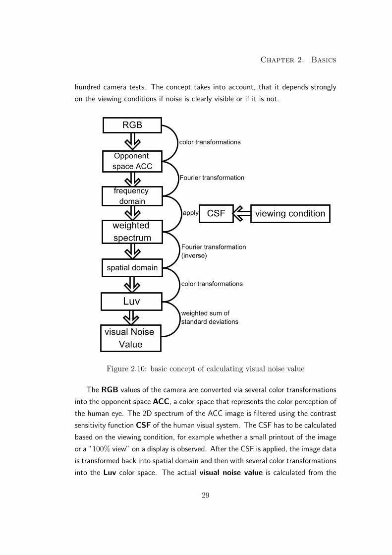
Figure 2.10: basic concept of calculating visual noise value
The RGB values of the camera are converted via several color transformations
into the opponent space ACC, a color space that represents the color perception of
the human eye. The 2D spectrum of the ACC image is filtered using the contrast
sensitivity function CSF of the human visual system. The CSF has to be calculated
based on the viewing condition, for example whether a small printout of the image
or a ”100% view” on a display is observed. After the CSF is applied, the image data
is transformed back into spatial domain and then with several color transformations
into the Luv color space. The actual visual noise value is calculated from the
29
Chapter 2. Basics
standard deviations of the three channels (L, u and v) of the image. Same as in
CIE-Lab, a geometrical distance of 1 in the color space is the minimum distance
a trained human observer can distinguish. So a visual noise value of less than one
represents an image with not visible noise. [8]
2.1.4 Problems of noise measurement
The approach of calculating a visual noise value rather than just a signal to noise
ratio improved the noise measurement very much. But both methods still have one
problem, the measurement is done on a homogeneously illuminated patch in the
image. This works well and is the only possibility if the test method should work
on black-box-systems, but more and more leads to problems because the digital
signal processing of the cameras become more complex and adaptive to the scene.
So the devices can suppress the noise in a patch and will get good results in noise
measurement, but still show much noise close to edges and on structures, where
the suppression can not be applied without loosing resolution and texture.
30

Chapter 2. Basics
2.2 Spatial Resolution in digital still cameras
Resolution as a criteria of image quality is often used controversy and with different
meanings. Often it is used as a synonym for sampling rate or number of pixels in a
sensor array, so one can read that a camera has ”a resolution of 8 Megapixel” or the
scanner has ”a resolution of 1200 pixel per inch”. This statements are commonly
used by the marketing departments of manufactures, because they represent the
ideal output of an imaging device. From a testing point of view the ideal resolution
is of minor interest, what drives the image quality is the real resolution as a
reproduction of fine detail.
In this thesis the term resolution is used to describe the scene related maximum
capability of an imaging device to transfer and resolve spatial frequencies. In other
words, resolution is not the spatial sampling rate of the system, it represents the
information content that is transfered. So one can increase the sampling rate easily
by adding additional interpolated pixels, but may not increase the spatial resolution
of the image that way, because no additional information is added.
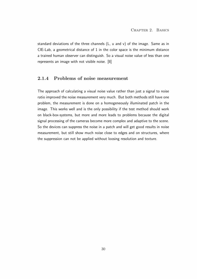
The limiting resolution is the highest frequency the imaging system can transfer
in its image signal. A spatial frequency is expressed as:
spatialfrequency =number of Linepairs
distance
The distance can have different units, common are millimeter, pixel height or pixel
[13].
The resolution can be expressed scene related or image related, the first is
the spatial frequency in the object that can be resolved, the second is the highest
spatial frequency in the image. In analog photography, it was common to report
the image related resolution of lenses or film, because the scene related resolution
could be calculated with the known reproduction scale and the image had the
physical size of the used filmformat.
A digital image has no physical expanse, only the representation on a display
or a print has one, so it is not useful to give an image related resolution. The
31
Chapter 2. Basics
distance [mm] or [pixel]
1 linepair =
number of linepairs
0 0,5 1min
Intensity
inte
nsity
max
distance
=
Figure 2.11: Visualization of spatial frequency
given resolution should refer to the maximum spatial frequency in the object that
is reproduced as digital copy. But on the other hand, the reproduction scale of a
black-box-system like a digital camera is unknown, so the object related resolution
can not be given with a physical distance basis like mm. Because of these problems
in defining the resolution in digital photography to a physical distance, the used
distance is expressed in pixels. Usual units are linepairs per pixel [LP/pix] or linepair
per picture-height [LP/PH]. [13]
In the following sections, resolution test methods are presented that are stan-
dardized or are under discussion to be part of the reviewed ISO 12233 standard
about resolution measurement.
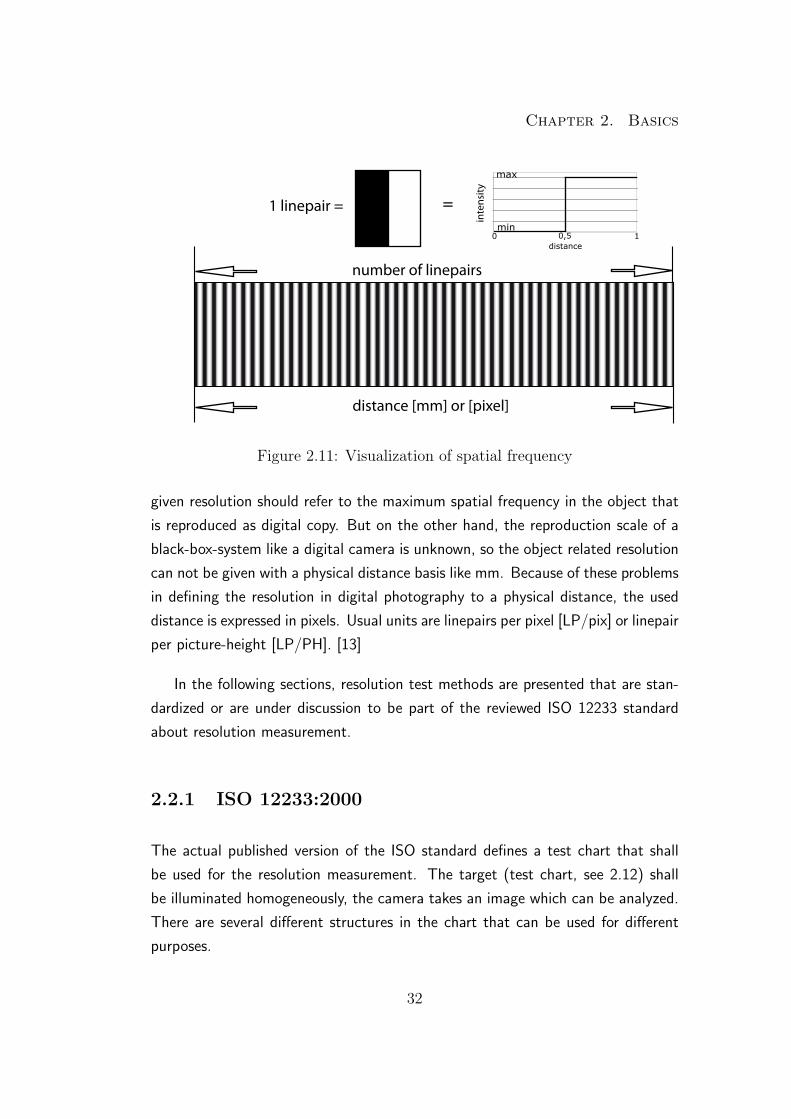
2.2.1 ISO 12233:2000
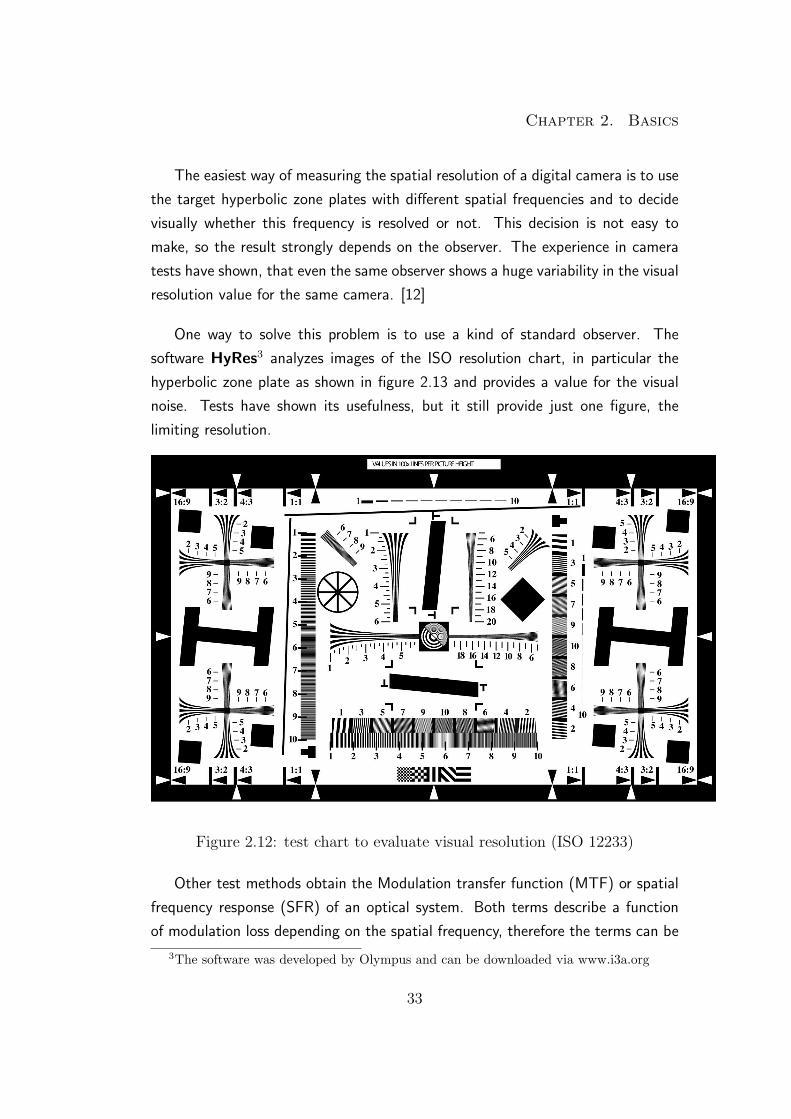
The actual published version of the ISO standard defines a test chart that shall
be used for the resolution measurement. The target (test chart, see 2.12) shall
be illuminated homogeneously, the camera takes an image which can be analyzed.
There are several different structures in the chart that can be used for different
purposes.
32
Chapter 2. Basics
The easiest way of measuring the spatial resolution of a digital camera is to use
the target hyperbolic zone plates with different spatial frequencies and to decide
visually whether this frequency is resolved or not. This decision is not easy to
make, so the result strongly depends on the observer. The experience in camera
tests have shown, that even the same observer shows a huge variability in the visual
resolution value for the same camera. [12]
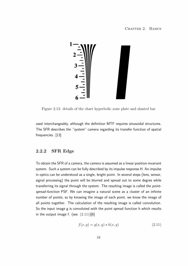
One way to solve this problem is to use a kind of standard observer. The
software HyRes3 analyzes images of the ISO resolution chart, in particular the
hyperbolic zone plate as shown in figure 2.13 and provides a value for the visual
noise. Tests have shown its usefulness, but it still provide just one figure, the
limiting resolution.
Figure 2.12: test chart to evaluate visual resolution (ISO 12233)
Other test methods obtain the Modulation transfer function (MTF) or spatial
frequency response (SFR) of an optical system. Both terms describe a function
of modulation loss depending on the spatial frequency, therefore the terms can be
3The software was developed by Olympus and can be downloaded via www.i3a.org
33
Chapter 2. Basics
Figure 2.13: details of the chart hyperbolic zone plate and slanted bar
used interchangeably, although the definition MTF requires sinusoidal structures.
The SFR describes the ”system” camera regarding its transfer function of spatial
frequencies. [13]
2.2.2 SFR Edge
To obtain the SFR of a camera, the camera is assumed as a linear position-invariant
system. Such a system can be fully described by its impulse response H. An impulse
in optics can be understood as a single, bright point. In several steps (lens, sensor,
signal processing) the point will be blurred and spread out to some degree while
transferring its signal through the system. The resulting image is called the point-
spread-function PSF. We can imagine a natural scene as a cluster of an infinite
number of points, so by knowing the image of each point, we know the image of
all points together. The calculation of the resulting image is called convolution.
So the input image g is convoluted with the point spread function h which results
in the output image f. (see. (2.11))[6]
f(x, y) = g(x, y) ? h(x, y) (2.11)
34

Chapter 2. Basics
Transferring the image from the spatial domain into the frequency domain with a
fourier transformation, the convolution becomes a multiplication, so:
F (x, y) = G(x, y)× F (x, y) (2.12)
So the impulse response H describes the ability of the camera to transfer spatial
frequencies. The limiting resolution is the highest frequency that can be transfered.
For the lower frequencies the amount of loss in modulation or contrast can be
described.
This signal theory point of view is the basic concept of the SFR-Edge method.
An impulse as needed for getting the impulse response as described above would
need to be infinite small and infinite strong, as the integral of the point intensity
distribution is defined to be 1. So even if it could be approximated there is still
the problem of the fixed pixel structure of a digital image sensor. So by trying
to obtain the point spread function directly, one would have to take care that the
impulse hits the sensor that way, that its center matches exactly the center of one
pixel. This is at least a very challenging task, if not impossible.
The SFR edge method does not rely on a single point as an impulse, it uses an
edge in the image. The derivative of the edge is the line spread function LSF and
its counterpart in the frequency domain is a one dimensional impulse response. So
it describes the SFR in one direction of the image. In the ISO chart a slated bar
is used to get two edges for the SFR edge calculation. [12]
This method is part of the software presented in chapter 5 and the algorithm
will be explained in detail.
2.2.3 SFR Siemens
The usage of the ISO test charts with the visual resolution and the SFR edge
did not give reliable results for a comparable digital still camera test. [9] The
test laboratory Image Engineering uses a different method for a couple of years.
This method was conceived by Bruno Klingen, a mathematics professor at the
35
Chapter 2. Basics
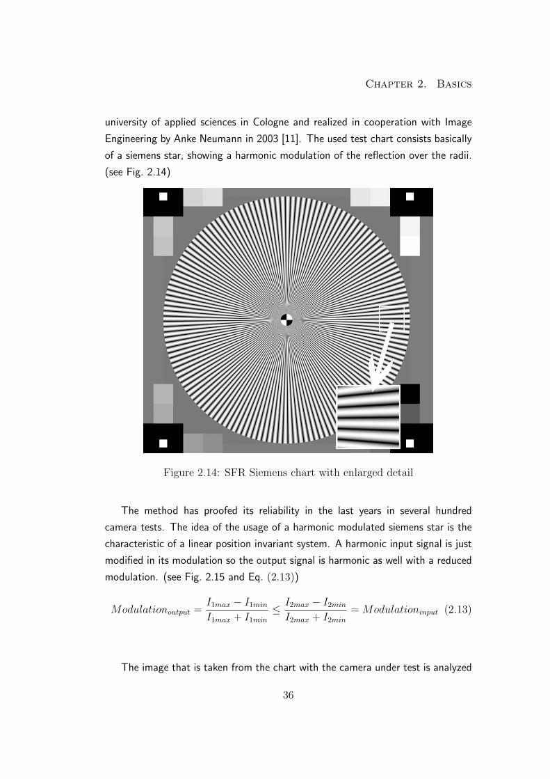
university of applied sciences in Cologne and realized in cooperation with Image
Engineering by Anke Neumann in 2003 [11]. The used test chart consists basically
of a siemens star, showing a harmonic modulation of the reflection over the radii.
(see Fig. 2.14)
Figure 2.14: SFR Siemens chart with enlarged detail
The method has proofed its reliability in the last years in several hundred
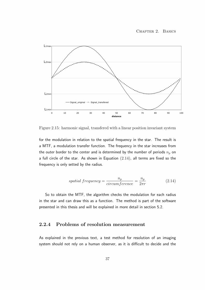
camera tests. The idea of the usage of a harmonic modulated siemens star is the
characteristic of a linear position invariant system. A harmonic input signal is just
modified in its modulation so the output signal is harmonic as well with a reduced
modulation. (see Fig. 2.15 and Eq. (2.13))
Modulationoutput =I1max − I1minI1max + I1min
≤ I2max − I2minI2max + I2min
= Modulationinput (2.13)
The image that is taken from the chart with the camera under test is analyzed
36
Chapter 2. Basics
L1min
L2min
L2max
L1max
0 10 20 30 40 50 60 70 80 90 100
distance
Signal_original Signal_transfered
Figure 2.15: harmonic signal, transfered with a linear position invariant system
for the modulation in relation to the spatial frequency in the star. The result is
a MTF, a modulation transfer function. The frequency in the star increases from
the outer border to the center and is determined by the number of periods np on
a full circle of the star. As shown in Equation (2.14), all terms are fixed so the
frequency is only setted by the radius.
spatial frequency =np
circumference=
np2πr
(2.14)
So to obtain the MTF, the algorithm checks the modulation for each radius
in the star and can draw this as a function. The method is part of the software
presented in this thesis and will be explained in more detail in section 5.2.
2.2.4 Problems of resolution measurement
As explained in the previous text, a test method for resolution of an imaging
system should not rely on a human observer, as it is difficult to decide and the
37
Chapter 2. Basics
result is hard to reproduce. Other methods like SFR Edge or SFR Siemens are
based on the assumption, that a digital camera can be described as a linear position
invariant system. This assumption is true as long as the SFR is only determined
by the optical system and the sensor. The digital image processing in the the
camera becomes more and more complex and especially the image enhancement
procedures for sharpening and noise reduction are non-linear. This means that the
response of the camera to, for example, an edge is different than to a pattern or
fine texture. The complete system becomes non-linear and to describe a non-linear
system completely is close to impossible. In this thesis I will use several methods
to check the SFR of a camera, using different structures to get a more complex
description of the camera system.
38
Chapter 3. NoiseLab
Chapter 3
NoiseLab
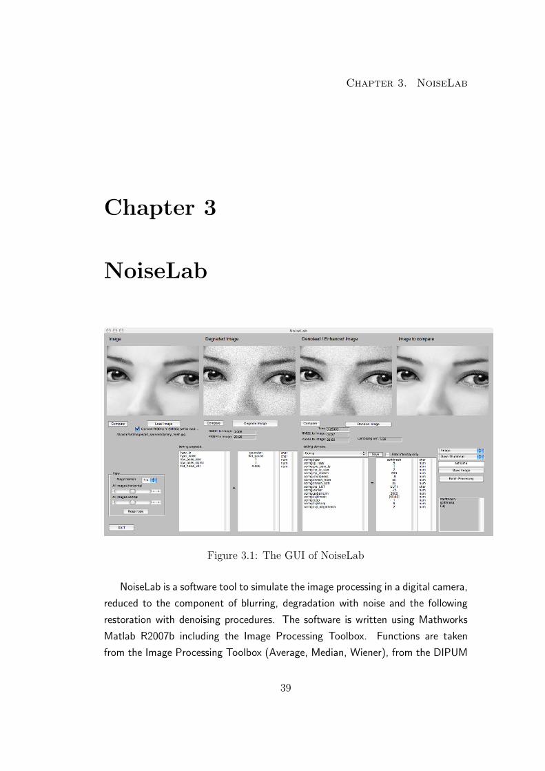
Figure 3.1: The GUI of NoiseLab
NoiseLab is a software tool to simulate the image processing in a digital camera,
reduced to the component of blurring, degradation with noise and the following
restoration with denoising procedures. The software is written using Mathworks
Matlab R2007b including the Image Processing Toolbox. Functions are taken
from the Image Processing Toolbox (Average, Median, Wiener), from the DIPUM
39

Chapter 3. NoiseLab
(Digital Image Processing Using Matlab [6]) Toolbox (Wavelet Transformation,
Adaptive Median) and own code (Coring, Thresholding).
The aim of this software tool is to simulate different methods of noise reduction
in digital still cameras. Denoising is proprietary knowledge of the camera manu-
factures, so it is hard to find out exactly what is done as image enhancement in
a DSC. NoiseLab simulated different concepts of noise reduction without claiming
to reproduce a camera signal processing. The procedure is reduced to the system
as shown in figure 3.2. An ideal image is degraded by additive noise and blurred
by a low pass filter. Both can be controlled by the parameters in the settings. The
degraded image is the source for an enhancement procedure, implemented in the
software. The user can choose between different types of denoising algorithms and
different implementations of these algorithms.
Enhancement/ DenoisingImage
DegradedImage
Low Pass / SFR
Noise
EnhancedImage
Figure 3.2: Image processing in NoiseLab
40
Chapter 3. NoiseLab
3.1 User Interface
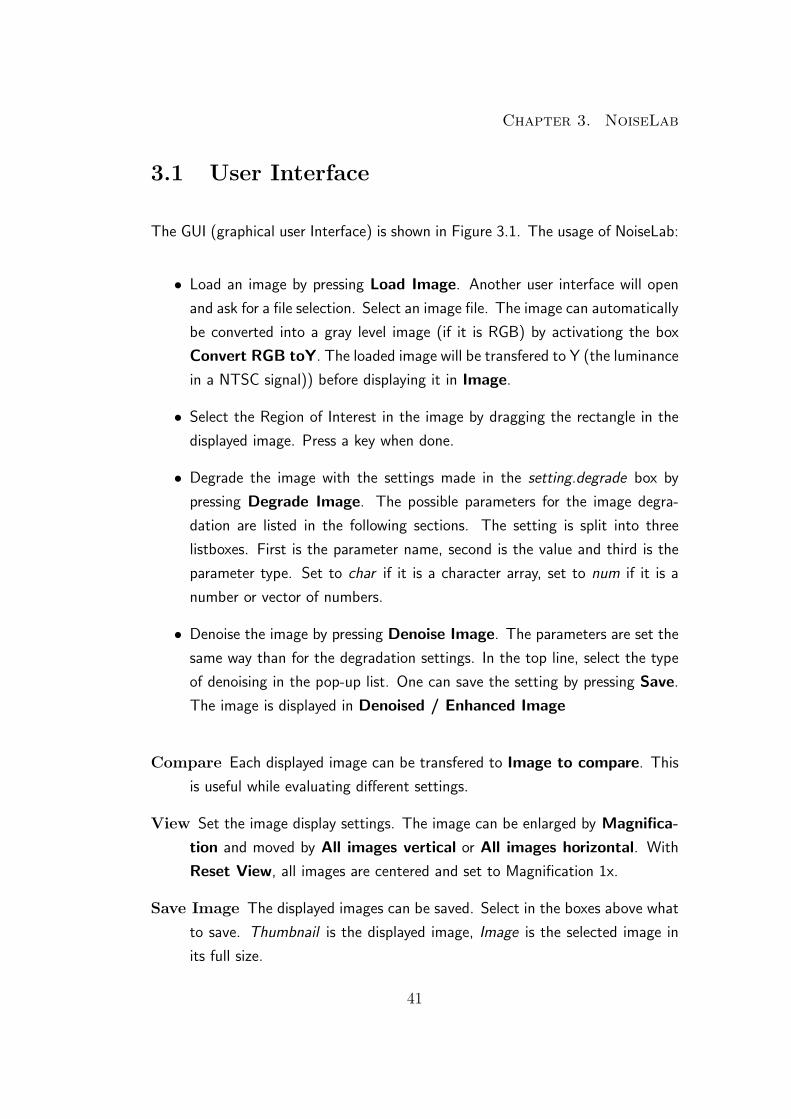
The GUI (graphical user Interface) is shown in Figure 3.1. The usage of NoiseLab:
• Load an image by pressing Load Image. Another user interface will open
and ask for a file selection. Select an image file. The image can automatically
be converted into a gray level image (if it is RGB) by activationg the box
Convert RGB toY. The loaded image will be transfered to Y (the luminance
in a NTSC signal)) before displaying it in Image.
• Select the Region of Interest in the image by dragging the rectangle in the
displayed image. Press a key when done.
• Degrade the image with the settings made in the setting.degrade box by
pressing Degrade Image. The possible parameters for the image degra-
dation are listed in the following sections. The setting is split into three
listboxes. First is the parameter name, second is the value and third is the
parameter type. Set to char if it is a character array, set to num if it is a
number or vector of numbers.
• Denoise the image by pressing Denoise Image. The parameters are set the
same way than for the degradation settings. In the top line, select the type
of denoising in the pop-up list. One can save the setting by pressing Save.
The image is displayed in Denoised / Enhanced Image
Compare Each displayed image can be transfered to Image to compare. This
is useful while evaluating different settings.
View Set the image display settings. The image can be enlarged by Magnifica-
tion and moved by All images vertical or All images horizontal. With
Reset View, all images are centered and set to Magnification 1x.
Save Image The displayed images can be saved. Select in the boxes above what
to save. Thumbnail is the displayed image, Image is the selected image in
its full size.
41
Chapter 3. NoiseLab
Batch Proocessing All images in a folder get degraded, denoised and saved in
a specified new folder.
Notepad Save settings via copy and paste into the notepad. The content will
be saved with the setting of the denoising type.
3.2 Degradation
Degradation summarizes all influences on a digital image that makes a difference to
the natural ideal scene. These steps include degradations like shading, distortion,
blurring, noise and all artifacts of sampling and digital signal processing. In the
NoiseLab simulation, the degradation is reduced to blurring and noise.
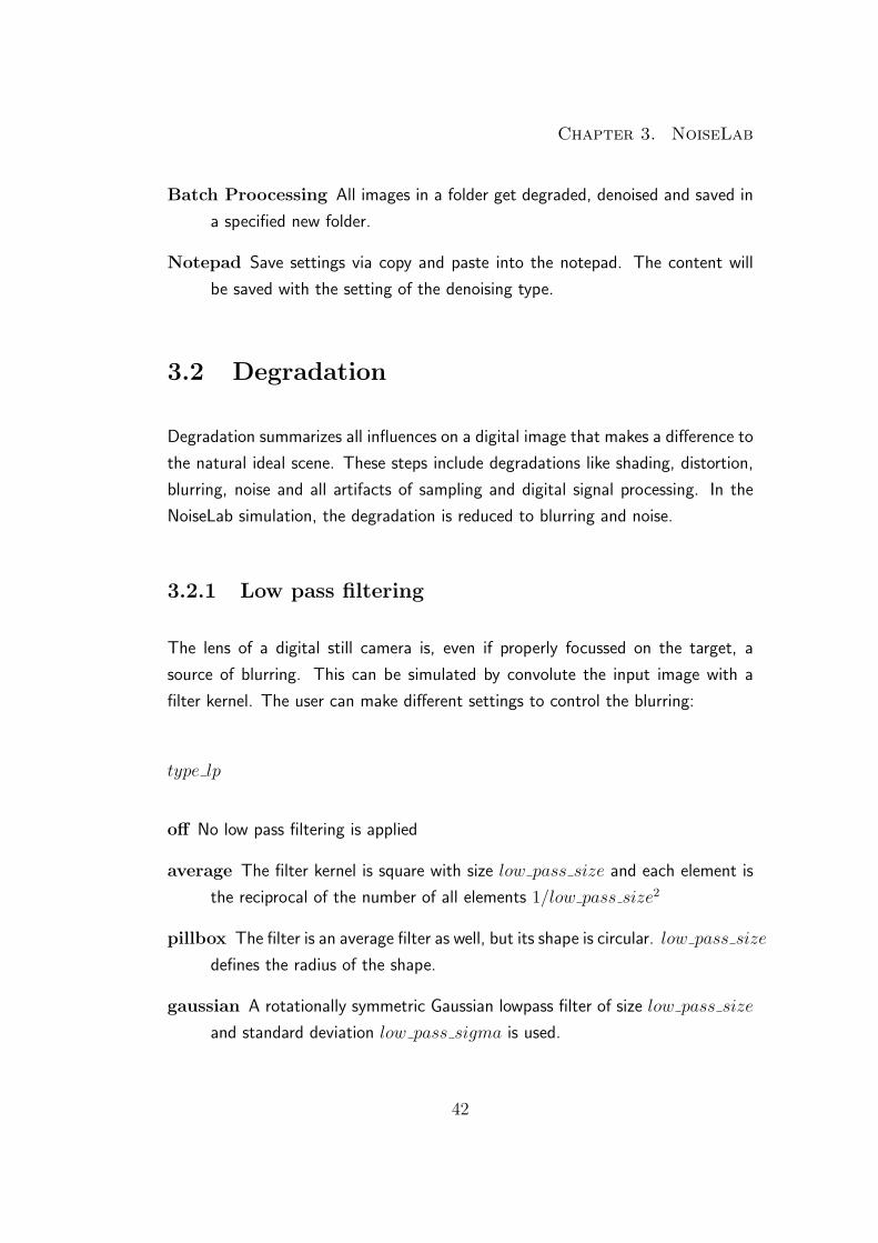
3.2.1 Low pass filtering
The lens of a digital still camera is, even if properly focussed on the target, a
source of blurring. This can be simulated by convolute the input image with a
filter kernel. The user can make different settings to control the blurring:
type lp
off No low pass filtering is applied
average The filter kernel is square with size low pass size and each element is
the reciprocal of the number of all elements 1/low pass size2
pillbox The filter is an average filter as well, but its shape is circular. low pass size
defines the radius of the shape.
gaussian A rotationally symmetric Gaussian lowpass filter of size low pass size
and standard deviation low pass sigma is used.
42
Chapter 3. NoiseLab
3.2.2 Adding noise
The software adds noise after applying the low pass filter to the image. This
is slightly different to the true noise of a digital still camera, but it could be
shown, that the noise distribution in a digital still camera can be assumed to be
white gaussian zero-mean noise (see Appendix B.1). Other noise distributions
are implemented as well, to have the possibility to see the influence of image
enhancement on different noise types.
type noise
off No noise is added to the image
speckle adds multiplicative noise to the image, calculated with the formula J =
I+n×I with I = SourceImage, J = DestinationImage and n as uniform
distributed random noise with zero-mean and the variance flat noise var.
poisson Using the image as input, poisson distributed noise is generated. So each
input pixel value is replaced with an output value in the poisson distribution
around this value.
flat gauss Adds gaussian white noise to the image with with zero-mean and the
variance flat noise var. The variance is independent from the intensity
value in Image.
cam gauss Adds gaussian white noise with zero-mean and a intensity depending
variance. The variance has an offset of cam gauss offset. The vari-
able part of the variance has a slope of one and a maximum value of
cam gauss delta. So the variance equals offset at digital value 0 and equals
offset+ delta at digital value 255 (for a 8-bit image)
43
Chapter 3. NoiseLab
3.3 Denoising
In the NoiseLab software, several different denoising algorithms have been imple-
mented. In the tool the main concepts can be chosen by the drop-down menu,
the selection of different implementations and their parameter can be set in the
setting window.
All denoising concepts have not been implemented to get best possible results.
The aim is more to learn about the artifacts introduced by these algorithms and
their influence on the spatial frequency response. Color images have been processed
as three independent images. So each color channel has been filtered separately.
As intensity noise is more disturbing than color noise [8] NoiseLab can filter the
intensity part of a color image only. If the box ”Filter intensity only” is active,
the RGB image is converted from RGB to HSV (Hue, Saturation, Value), the V
channel is denoised and the image is converted back to RGB, Saturation and Hue
unchanged.
The following section present the different denoising algorithms, the parameters
for NoiseLab are added to each section.
3.3.1 Average
The easiest noise reduction method is to average adjacent pixels. This is done by
a convolution with a mask of size m × n with all coefficients set to 1/(m × n).
So a single input pixel value is replaced with the mean value of the neighborhood
pixel values. low pass size defines the width of the square mask, so a value of 5
results in a 5×5 average filter.
average.low pass size Size of the N×N convolution mask. Should be odd inte-
ger value (e.g. 3,5,...)
44

Chapter 3. NoiseLab
3.3.2 Wiener
The filter used in this method are called ”minimum mean square error filter” or
”least square error filter”, but because it was proposed by N.Wiener, it is commonly
known as Wiener Filter. The idea is to minimize the mean square error σ2error
between an image f and its filtered counterpart f’ (see (3.1)).
σ2error = E{(f − f ′)2} (3.1)
In NoiseLab a pixelwise adaptive Wiener filtering is used. For the neighborhoods
NH with the size [NM ] (wiener.wienersize) the local mean µlocal and variance
σ2local are calculated.
µlocal =1
NM
∑x,y∈NH
f(x, y) (3.2)
σ2local =
1
NM
∑x,y∈NH
f(x, y)2 − µ2local (3.3)
The resulting image f’ is then calculated with these estimated parameters:
f ′(x, y) = µlocal +σ2local − σ2
noise
σ2local
(f(x, y)− µlocal) (3.4)
σ2noise is the noise variance. In NoiseLab this is assumed to be unknown, the
average of the local estimated variances is taken. [14] [6]
wiener.wienersize Size of the N×M neighborhood. Should be 2 value vector
with odd integer value (e.g. [3,3], [5,5],...)
3.3.3 Median
As order statistic filter, the filtering is based on ranking pixel values in the neigh-
borhood of the processed pixel. So the median filter replaces the value of a pixel
with the median of the pixel in the surrounding area, defined in median.size. A
value of [5 5] means, that the median of the 5×5 pixel area around the processed
45
Chapter 3. NoiseLab
pixel is taken. [15] An adaptive median filter has been implemented from the
DIPUM Toolbox [6], but as it is not intended for camera like noise distributions,
it was not further investigated. [6]
median.type median or adpmedian for a normal median filtering as explained or
the adaptive median filtering approach.
median.size median: Size of the N×M neighborhood. Should be 2 value vector
with odd integer value (e.g. [3,3], [5,5],...)
median.adp sizemax adaptive median: maximal allowable size of neighborhood.
Should be odd integer value ≥ 3.
3.3.4 Coring
In NoiseLab the term Coring is used to describe all kind of simple subband coding
for noise reduction. As these technique has a lot of different implementations with
dozens of parameters each, in this thesis I realized just some basic concepts. As
the technology implemented in the different cameras is confidential, it is hard to
find out what exactly is done in the image signal processing units.
The idea is to subdivide the frequency spectrum into two or more subbands and
to reduce the noise in these bands rather than in the whole image. The image is
filtered with a low-pass, so the high frequencies are eliminated. By subtracting the
low-pass image from the input image, one get a high pass image which contains
the high frequencies only. Adding the low-pass image LP to the high-pass image
HP would result in the input image, so the output would be equal to the input.
It is assumed that the important information about the shapes in the image is
represented in the high frequencies, so in the high values of the HP images. And
it is assumed, that disturbing noise is found in the lower frequencies. So to keep
the informations about the shapes and to reduce the noise in the image, the HP
image is modified, only high values higher than a certain threshold are kept, the
others are eliminated.
46

Chapter 3. NoiseLab
Input
LP
- ThresholdingHP
+ Output
Figure 3.3: The basic concept of coring
In the image one can imagine the technology as following: The image is low
pass filtered, therefore the noise is reduced and the edges and shapes are blurred.
To prevent the noise reduction from blurring the edges, the threshold decides where
in the images are edges which are worth to keep and where not. The edges are
not altered while the noise is reduced in flat regions. By amplifying the HP image,
the edges become more emphasized and the image appears sharper.
The challenge for the designer is the decision where to reduce noise and where
to keep or enhance the edges. The more the image contains noise, the more
difficult this task becomes.
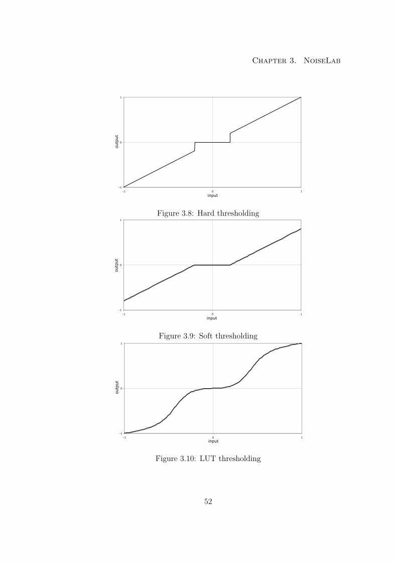
Three different thresholding concepts for the HP image altering have been im-
plemented in NoiseLab, hard threshold, soft threshold, the usage of a look up table
and two experimental versions, sobel mask and Fuji.
The possible values in the 8-bit HP image range from -127 to +128. Applying
a hard threshold forces all values DN to zero if their absolute value is smaller
than threshold t.(see Eq. (3.5) and Fig. 3.8)
DN = DN if |DN | ≤ t
DN = 0 otherwise(3.5)
Using a soft threshold means, that the digital values are forced towards zero.
(see Eq. (3.6) and Fig. 3.9) It is not defined if a following scaling is part of the
thresholding. In NoiseLab the soft thresholding does not include a scaling, but it
47

Chapter 3. NoiseLab
can be set.
DN = sgn(DN) max(0, |DN | − t) (3.6)
The third thresholding approach is to apply a function to the HP image.
The easiest way of implementing a function is a look up table. The tool
”LUT Creator” (Fig. 3.4) creates a LUT which can be used in NoiseLab. The
advantage of using a LUT is, that the thresholding can combined with the edge
emphasizing just by changing the LUT. In ”LUT Creator” only the positive part
of the LUT is shown, the complete LUT is a combination of this positive part and
the point symmetric negative counterpart to it.
Figure 3.4: Screenshot of LUT Creator
In NoiseLab the implementation of Coring has in comparison to the basic con-
cept some modifications and additional parameters (see Fig. 3.5). These changes
are based on experience while evaluating the concept and does not claim to be
realized in that way in any camera. But the artifacts that become visible after
denoising are comparable to the artifacts which can be observed in modern digital
still cameras or mobile phone cameras.
coring.type hardthresh, softthresh or LUTonHP for the different thresholding
methods described above
48

Chapter 3. NoiseLab
Input
LP_pre
LP
- ThresholdingHP
+ Output
X X
HP_stretch sharpness
Figure 3.5: Implementation of Coring in NoiseLab
coring.lp fsize size of the average filter used as LP, positive integer value
coring.pre core lp size of the average filter used as LP pre, positive integer value
coring.hp stretch factor applied to HP before thresholding, positive value
coring.sharpness factor applied to HP after thresholding, positive value
coring.thresh hard threshold for hard thresholding, positive value
coring.thresh soft threshold for soft thresholding, positive value
coring.hp LUT name of the .LUT file in the folder LUT
coring.outlier LUTonHP only: scaling the max value in HP before applying LUT,
range [0...1], if DN ≤ outlier ×max DN is clipped
coring.loop the complete coring can be performed several times, the output of
the first run is the input of the second and so on.
Additionally to the described thresholding methods, a masking methods has
been implemented. The concept is shown in Figure 3.6. Instead of altering the
HP based on its own values an additional mask is created. This mask is the result
of an edge detection and its values range from zero to one and therefore control
which parts of the HP image are kept and which are vanished. The edge detection
from another source than the high pass itself improves the distinction of signal and
noise.
49
Chapter 3. NoiseLab
Input
LP_pre
LP
- HP
+ Output
X X
HP_stretch sharpness
X
edgedetection
0...1
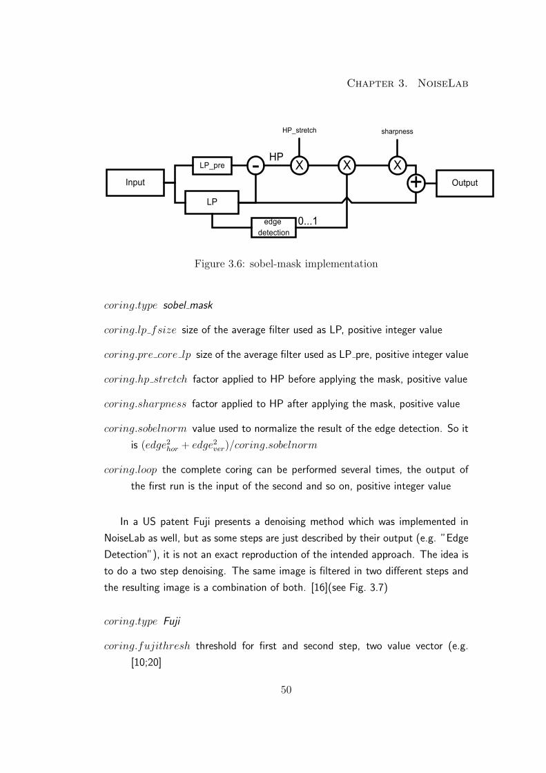
Figure 3.6: sobel-mask implementation
coring.type sobel mask
coring.lp fsize size of the average filter used as LP, positive integer value
coring.pre core lp size of the average filter used as LP pre, positive integer value
coring.hp stretch factor applied to HP before applying the mask, positive value
coring.sharpness factor applied to HP after applying the mask, positive value
coring.sobelnorm value used to normalize the result of the edge detection. So it
is (edge2hor + edge2ver)/coring.sobelnorm
coring.loop the complete coring can be performed several times, the output of
the first run is the input of the second and so on, positive integer value
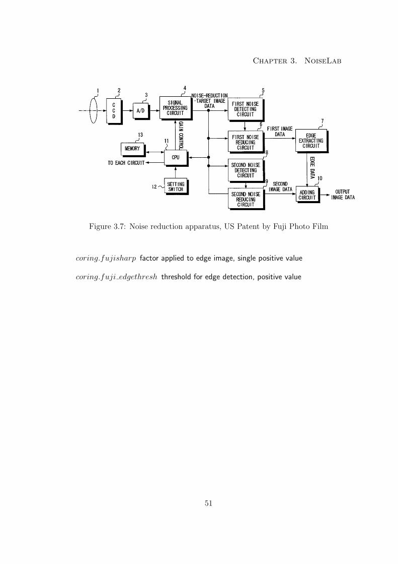
In a US patent Fuji presents a denoising method which was implemented in
NoiseLab as well, but as some steps are just described by their output (e.g. ”Edge
Detection”), it is not an exact reproduction of the intended approach. The idea is
to do a two step denoising. The same image is filtered in two different steps and
the resulting image is a combination of both. [16](see Fig. 3.7)
coring.type Fuji
coring.fujithresh threshold for first and second step, two value vector (e.g.
[10;20]
50
Chapter 3. NoiseLab
Figure 3.7: Noise reduction apparatus, US Patent by Fuji Photo Film
coring.fujisharp factor applied to edge image, single positive value
coring.fuji edgethresh threshold for edge detection, positive value
51
Chapter 3. NoiseLab
-1
0
1
-1 0 1
output
input
outp
ut
Figure 3.8: Hard thresholding
-1
0
1
-1 0 1
output
input
outp
ut
Figure 3.9: Soft thresholding
-1
0
1
-1 0 1
output
input
outp
ut
Figure 3.10: LUT thresholding
52
Chapter 3. NoiseLab
3.3.5 Wavelet
The wavelet transformation is a modern technique in image processing, providing
new possibilities in image compression and noise reduction. For example the pro-
posed image compression standard JPEG2000 is based on wavelet transformation.
”Unlike the Fourier transform, whose basis functions are sinusoids,
wavelet transforms are based on small waves, called wavelets, of vary-
ing frequency and limited duration. This allows them to provide the
equivalent of a musical score for an image, revealing not only what
notes (or frequencies) to play but also when to play them. Conven-
tional Fourier transforms, on the other hand, provide only the notes
or frequency information; tempral information is lost in transformation
process.” [6]
Wavelet transformation is a very complex topic and in this thesis only the multi-
resolution aspect of wavelet transformation in discrete data is presented. The aim
is to get a perfect signal decomposition in subbands and reconstruction of these
subbands. For denoising purposes, the coefficients in the subbands are altered
using thresholding as described in 3.3.4. The difference to the simple ”coring”
approach is the perfect or near perfect analysis and synthesis combination of the
subbands components and the down-sampling of the data in the transformation
representative, so the data rate is not increased.
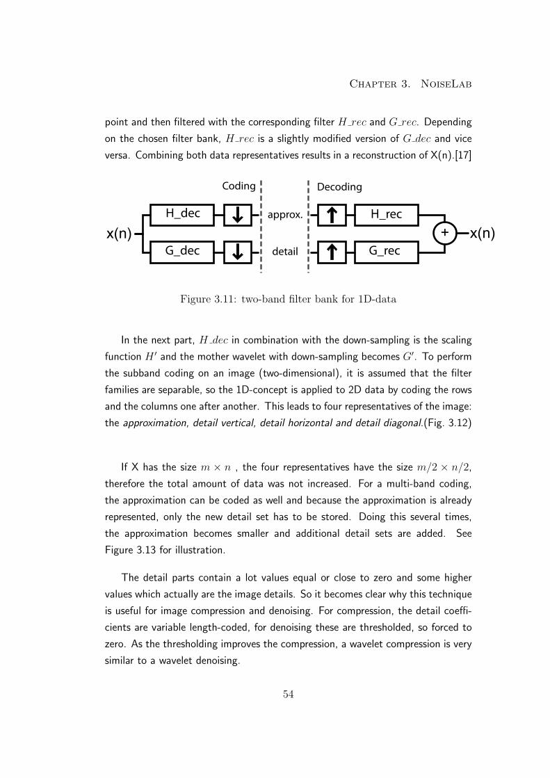
For this subband coding, the filter bank contains four filters: scaling and ana-
lyzing filter and both for decomposition and reconstruction. In literature one can
find a huge amount of different aspects about the filter design and characteris-
tics, only the basic construction is explained in this thesis. For decomposition, the
input data X(n) is filtered with a low-pass filter H dec and an analyzing filter
or mother-wavelet G dec. The filtering is a convolution with the specified ker-
nel. After filtering, the data is down-sampled by deleting every second data point.
Now we have two representatives of the input data, an approximation of X(n) after
low-pass filtering and the detail as the analyzing filter output. For reconstruction,
approximation and detail are up-sampled by setting a zero between each data-
53
Chapter 3. NoiseLab
point and then filtered with the corresponding filter H rec and G rec. Depending
on the chosen filter bank, H rec is a slightly modified version of G dec and vice
versa. Combining both data representatives results in a reconstruction of X(n).[17]
+x(n) x(n)
Coding Decoding
approx.
detail
H_recH_dec
G_dec G_rec
Figure 3.11: two-band filter bank for 1D-data
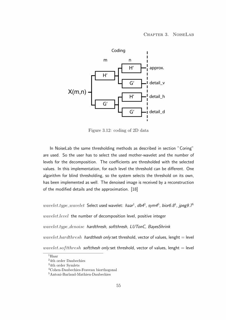
In the next part, H dec in combination with the down-sampling is the scaling
function H ′ and the mother wavelet with down-sampling becomes G′. To perform
the subband coding on an image (two-dimensional), it is assumed that the filter
families are separable, so the 1D-concept is applied to 2D data by coding the rows
and the columns one after another. This leads to four representatives of the image:
the approximation, detail vertical, detail horizontal and detail diagonal.(Fig. 3.12)
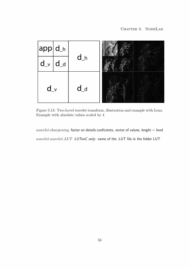
If X has the size m × n , the four representatives have the size m/2 × n/2,
therefore the total amount of data was not increased. For a multi-band coding,
the approximation can be coded as well and because the approximation is already
represented, only the new detail set has to be stored. Doing this several times,
the approximation becomes smaller and additional detail sets are added. See
Figure 3.13 for illustration.
The detail parts contain a lot values equal or close to zero and some higher
values which actually are the image details. So it becomes clear why this technique
is useful for image compression and denoising. For compression, the detail coeffi-
cients are variable length-coded, for denoising these are thresholded, so forced to
zero. As the thresholding improves the compression, a wavelet compression is very
similar to a wavelet denoising.
54
Chapter 3. NoiseLab
X(m,n)
Coding
approx.
detail_v
H‘
G‘
H‘
G‘
H‘
G‘
m n
detail_h
detail_d
Figure 3.12: coding of 2D data
In NoiseLab the same thresholding methods as described in section ”Coring”
are used. So the user has to select the used mother-wavelet and the number of
levels for the decomposition. The coefficients are thresholded with the selected
values. In this implementation, for each level the threshold can be different. One
algorithm for blind thresholding, so the system selects the threshold on its own,
has been implemented as well. The denoised image is received by a reconstruction
of the modified details and the approximation. [18]
wavelet.type wavelet Select used wavelet: haar1, db42, sym43, bior6.84, jpeg9.75
wavelet.level the number of decomposition level, positive integer
wavelet.type denoise hardthresh, softthresh, LUTonC, BayesShrink
wavelet.hardthresh hardthesh only:set threshold, vector of values, lenght = level
wavelet.softthresh softthesh only:set threshold, vector of values, lenght = level
1Haar24th order Daubechies34th order Symlets4Cohen-Daubechies-Feaveau biorthogonal5Antoni-Barlaud-Mathieu-Daubechies
55
Chapter 3. NoiseLab
Figure 3.13: Two-Level wavelet transform, illustration and example with Lena.Example with absolute values scaled by 4
wavelet.sharpening factor on details coeficients, vector of values, lenght = level
wavelet.wavelet LUT LUTonC only: name of the .LUT file in the folder LUT
56
Chapter 4. NoiseLab Chart
Chapter 4
NoiseLab Chart
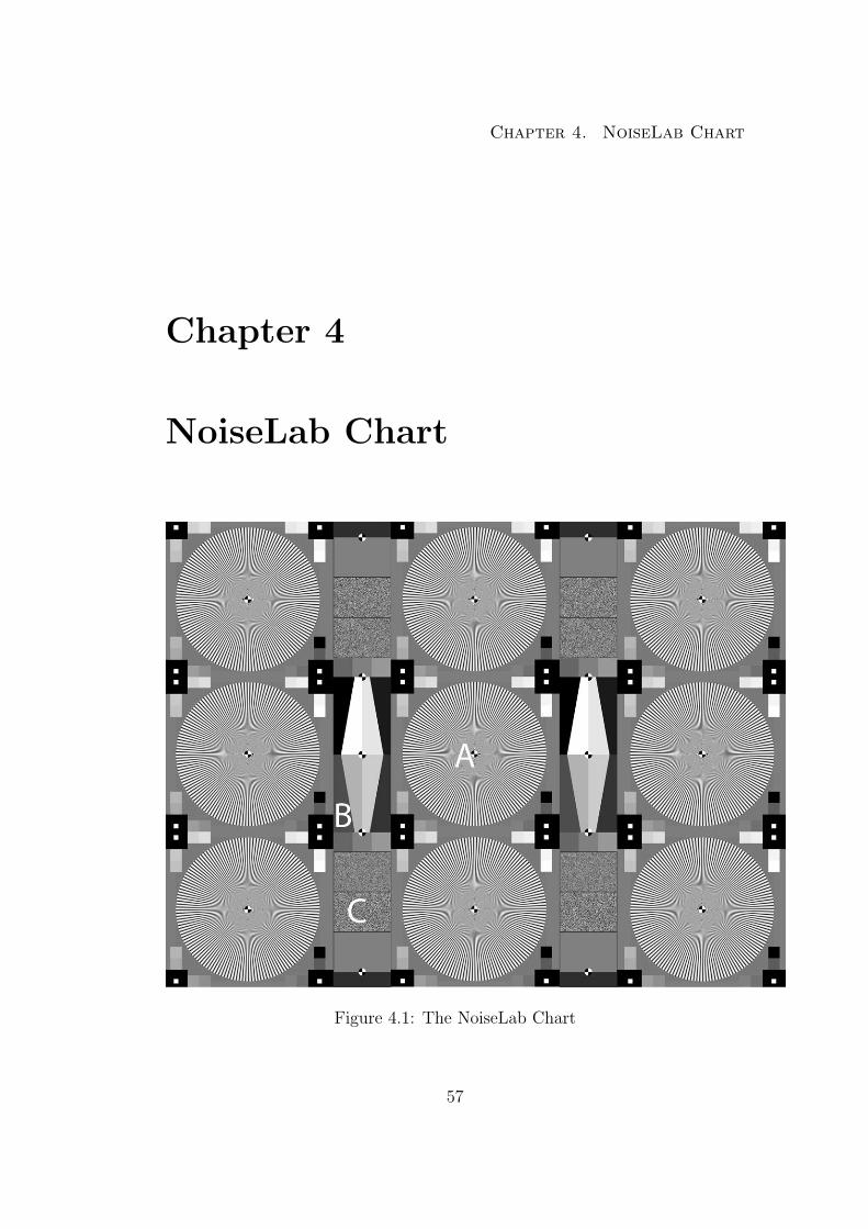
Figure 4.1: The NoiseLab Chart
57
Chapter 4. NoiseLab Chart
NoiseLab is a simulation of different denoising algorithms. To compare these
to real images taken with a digital still camera, the same input for camera and
simulation is needed. Instead of natural scenes, a file with different test patterns
has been created. The file is input for the software, a hardcopy of this file is the
test chart as ”input” for the camera. The chart shall be illuminated homogeneously
and the camera under test shall reproduce the chart completely. The structures
in the chart are chosen to measure different aspects of spatial frequency response
and / or noise appearance of the camera images. The images of the NoiseLab
Chart is the input for the NoiseLab Analyzer software which does the analysis
observer-independent.
The chart contains three main structures: (see Fig. 4.1)
A harmonic Siemens stars for SFR Siemens on 9 positions in the image, addi-
tional gray patches for linearization
B edges for SFR Edge, four different modulations, additional gray patches for
independent linearization
C gaussian white noise with different variances, a gray line between patches,
four flat patches without noise
Structure A is the already existing chart for the SFR Siemens method, so
structures B and C can be added to the existing chart.
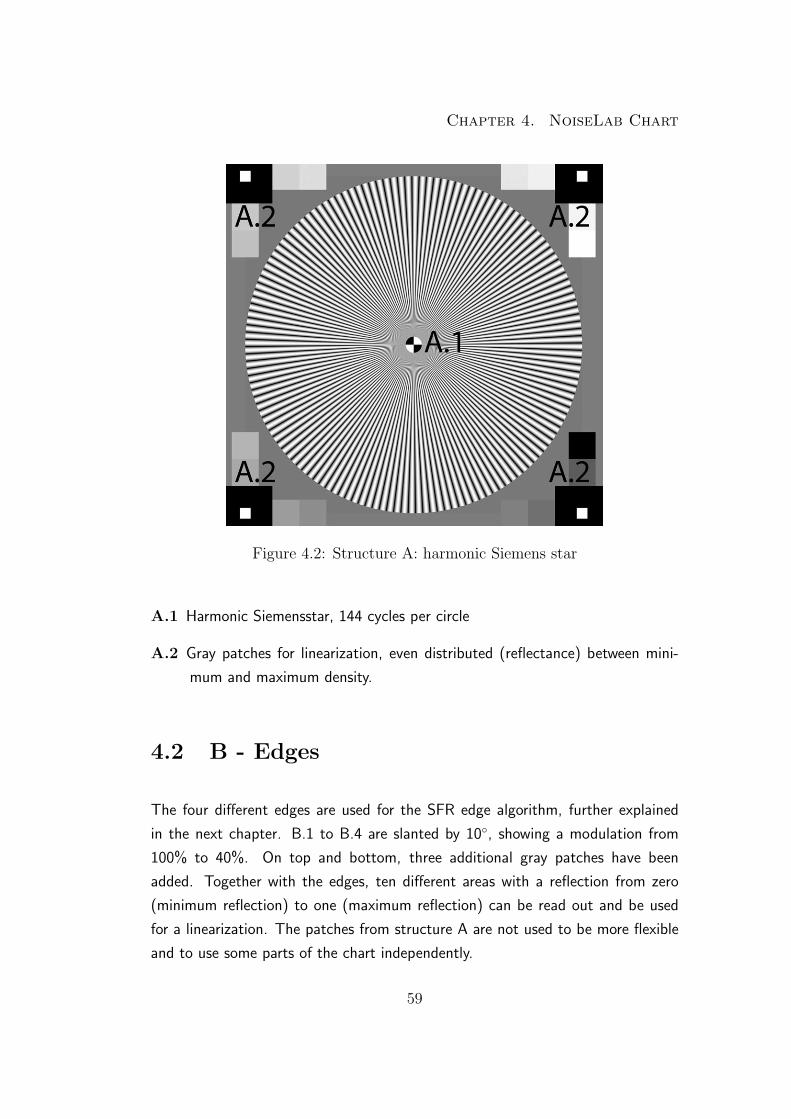
4.1 A -Siemens stars
The nine Siemens stars are arranged like shown in Figure 4.1, each star shows 144
periods per full circle. Defining the minimum reflection as 0 and the maximum
reflection as 1, the period is a sinus wave with a modulation of 1. (see Detail
in Fig. 2.14). In the center of each star a mark is placed, this is used for an
automatic center detection in the analyzing process. 16 gray patches around the
star are used for linearization of the input image. The reflection of the patches is
evenly distributed between the minimum and maximum reflection.
58
Chapter 4. NoiseLab Chart
Figure 4.2: Structure A: harmonic Siemens star
A.1 Harmonic Siemensstar, 144 cycles per circle
A.2 Gray patches for linearization, even distributed (reflectance) between mini-
mum and maximum density.
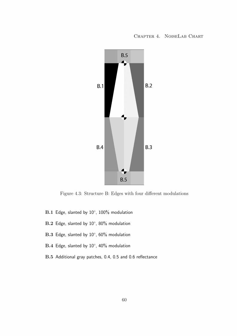
4.2 B - Edges
The four different edges are used for the SFR edge algorithm, further explained
in the next chapter. B.1 to B.4 are slanted by 10◦, showing a modulation from
100% to 40%. On top and bottom, three additional gray patches have been
added. Together with the edges, ten different areas with a reflection from zero
(minimum reflection) to one (maximum reflection) can be read out and be used
for a linearization. The patches from structure A are not used to be more flexible
and to use some parts of the chart independently.
59
Chapter 4. NoiseLab Chart
Figure 4.3: Structure B: Edges with four different modulations
B.1 Edge, slanted by 10◦, 100% modulation
B.2 Edge, slanted by 10◦, 80% modulation
B.3 Edge, slanted by 10◦, 60% modulation
B.4 Edge, slanted by 10◦, 40% modulation
B.5 Additional gray patches, 0.4, 0.5 and 0.6 reflectance
60
Chapter 4. NoiseLab Chart
4.3 C - White Noise
Structure C consists of five different patches that show a gaussian white noise. The
noise was created using Matlab and is realized that way, that the printer resolution
does not limit the frequency spectrum of the noise, but it is still high enough to
be able to measure cameras with up to idealized 14 Megapixel. Different variances
of the noise have been implemented as well as two patches without noise, which
have the same mean value as the noise patches. This is half of Dmax − Dmin.
Between the noise patches, a small line with no noise is implemented.
C.1 no noise, 0.5 of Dmax −Dmin
C.2 gaussian white noise, σ = 1/4, mean as C.1
C.3 gaussian white noise, σ = 1/8, mean as C.1
C.4 gaussian white noise, σ = 1/16, mean as C.1
C5 gaussian white noise, σ = 1/2, mean as C.1
C6 line between patches C.2 and C.3, mean as C.1
61

Chapter 4. NoiseLab Chart
Figure 4.4: Structure C: White noise
62
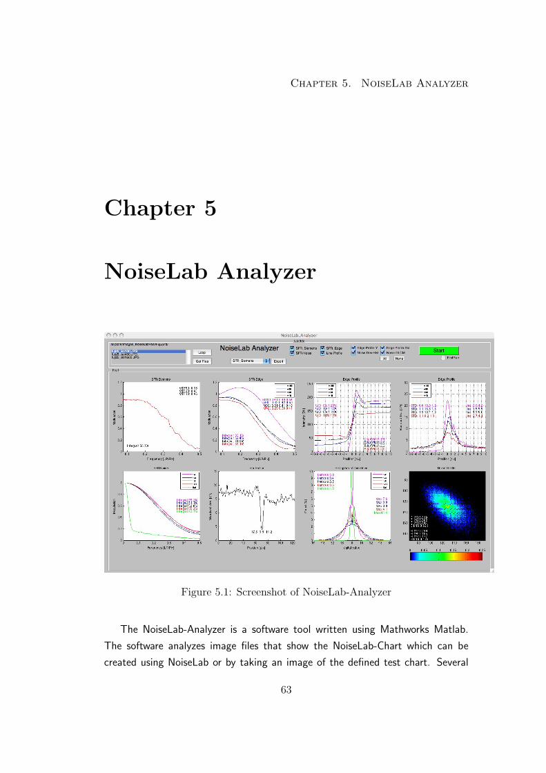
Chapter 5. NoiseLab Analyzer
Chapter 5
NoiseLab Analyzer
Figure 5.1: Screenshot of NoiseLab-Analyzer
The NoiseLab-Analyzer is a software tool written using Mathworks Matlab.
The software analyzes image files that show the NoiseLab-Chart which can be
created using NoiseLab or by taking an image of the defined test chart. Several
63
Chapter 5. NoiseLab Analyzer
measurements are done on the structures providing different informations about
the spatial frequency response of the camera and additional noise descriptions.
The measurements are:
• SFR-Siemens, providing a SFR measurement and a harmonic pattern
• SFR-Edge, SFR measurement on edges with four different modulations
• Edge Profile Y, showing the the intensity edge profile with informations about
over and undershoot and edge width
• Edge Profile Std, drawing the standard deviation parallel to the edge, giving
information about increasing noise near edges
• SFR-Noise, a experimental approach to describe the spatial frequency re-
sponse with the correlation of reproduced noise
• Line Profile, printing the standard deviation of a single line, embedded in the
noise structures
• Histogram of Derivative, the reproduction of the noise structure is analyzed
for the histogram of its derivative, revealing the noise distribution
• Noise GLCM, showing the gray level co-occurence matrix of the noise repro-
duction, giving texture information like correlation and homogeneity
64
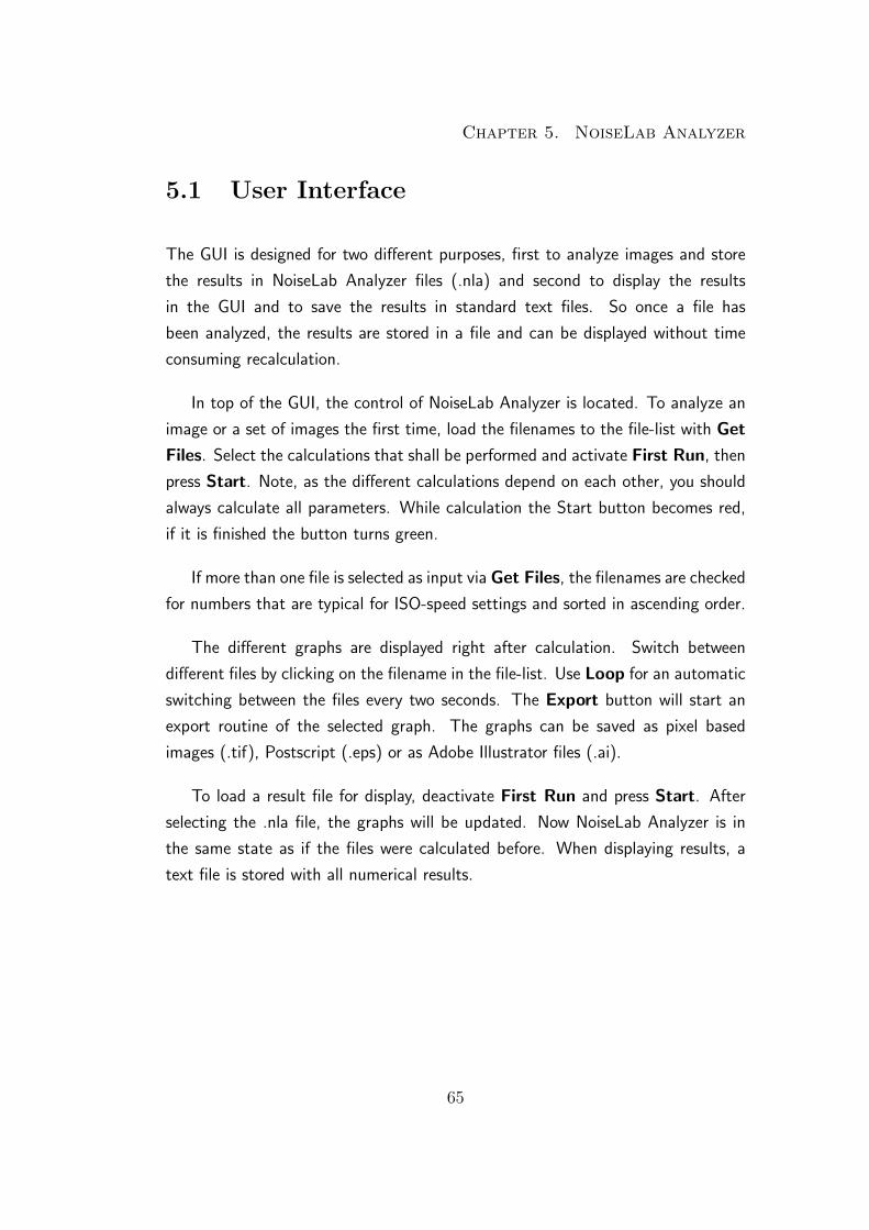
Chapter 5. NoiseLab Analyzer
5.1 User Interface
The GUI is designed for two different purposes, first to analyze images and store
the results in NoiseLab Analyzer files (.nla) and second to display the results
in the GUI and to save the results in standard text files. So once a file has
been analyzed, the results are stored in a file and can be displayed without time
consuming recalculation.
In top of the GUI, the control of NoiseLab Analyzer is located. To analyze an
image or a set of images the first time, load the filenames to the file-list with Get
Files. Select the calculations that shall be performed and activate First Run, then
press Start. Note, as the different calculations depend on each other, you should
always calculate all parameters. While calculation the Start button becomes red,
if it is finished the button turns green.
If more than one file is selected as input via Get Files, the filenames are checked
for numbers that are typical for ISO-speed settings and sorted in ascending order.
The different graphs are displayed right after calculation. Switch between
different files by clicking on the filename in the file-list. Use Loop for an automatic
switching between the files every two seconds. The Export button will start an
export routine of the selected graph. The graphs can be saved as pixel based
images (.tif), Postscript (.eps) or as Adobe Illustrator files (.ai).
To load a result file for display, deactivate First Run and press Start. After
selecting the .nla file, the graphs will be updated. Now NoiseLab Analyzer is in
the same state as if the files were calculated before. When displaying results, a
text file is stored with all numerical results.
65

Chapter 5. NoiseLab Analyzer
5.2 SFR-Siemens
The idea of SFR-Siemens has already been described in section 2.2.3. It uses a
siemens star with a harmonic function depending on the angle ϕ, taking the center
of the star as the base of the angle. The aim is to get a MTF, a Modulation
Transfer Function. The MTF describes the loss of modulation depending on the
spatial frequency fspatial(see Eq.(2.14),(5.1) and (5.2)).
MTF (fspatial) =Modulationimage(fspatial)
Modulationtarget(fspatial)(5.1)
Modulation =I1max − I1minI1max + I1min
=a+ b− (a− b)a+ b+ (a− b)
=2a
2b=a
b(5.2)
It is part of the chart production to take care that the Modulationtarget(fspatial)
is 1 for all frequencies used for the measurement. The intensity I in the ideal digital
image as a reproduction of the chart is
I(ϕ) = a+ b cos
(2π
g(ϕ− ϕ0)
)(5.3)
with angle ϕ (5.4), period lenght g see (5.5), mean value a, amplitude b and phase
ϕ0.
ϕ = arctan
(x
y
)x, y = projected coordinates in image
(5.4)
g =circumference [pixel]
number of periods=
2πr
np[pixel] (5.5)
The image that shows the siemens star is read in and linearized, using the
gray patches arranged around the star. The aim is to obtain the modulation
depending on the spatial frequency which is defined by the radius r. The image
coordinates are projected to the star coordinates, which sets the center of the star
to x=0 and y=0. The star is subdivided into 24 segments, so the Modulation is
66
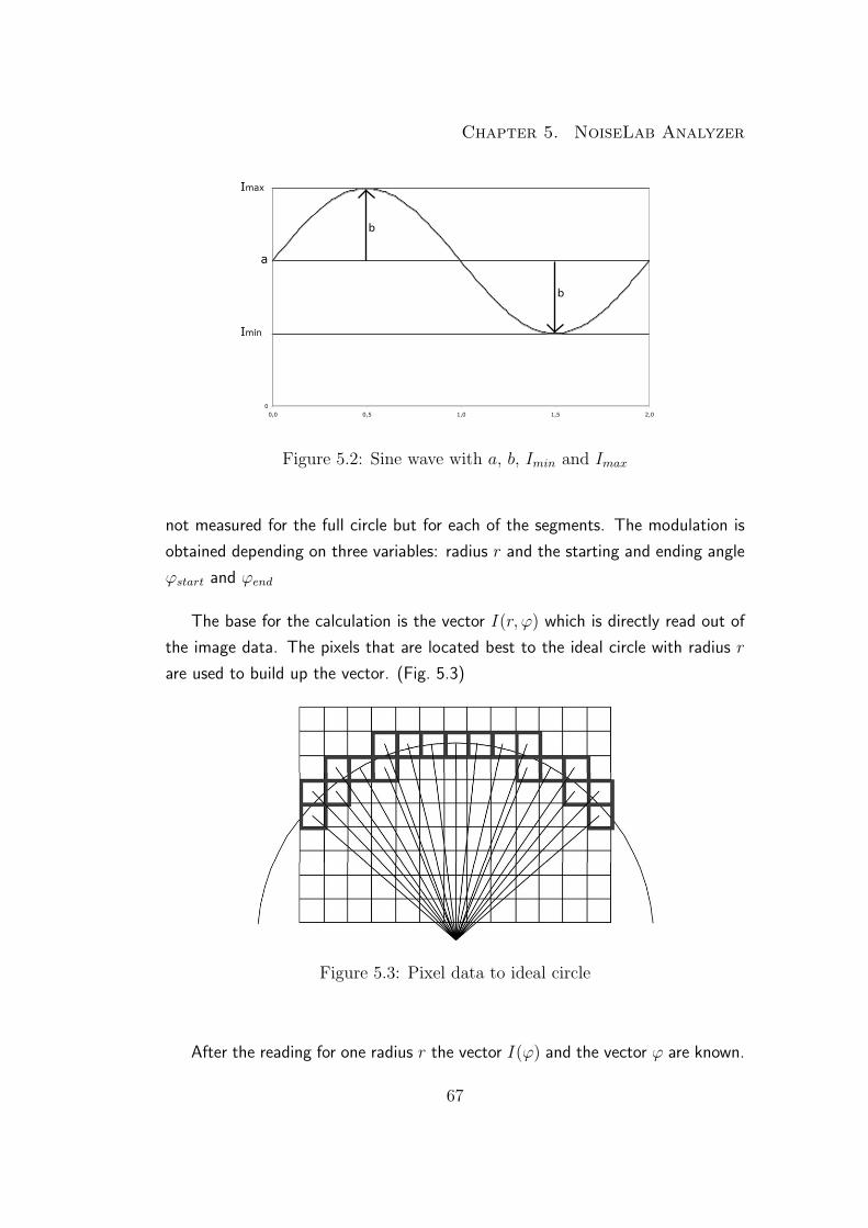
Chapter 5. NoiseLab Analyzer
0
Imin
a
Imax
0,0 0,5 1,0 1,5 2,0
b
b
Figure 5.2: Sine wave with a, b, Imin and Imax
not measured for the full circle but for each of the segments. The modulation is
obtained depending on three variables: radius r and the starting and ending angle
ϕstart and ϕend
The base for the calculation is the vector I(r, ϕ) which is directly read out of
the image data. The pixels that are located best to the ideal circle with radius r
are used to build up the vector. (Fig. 5.3)
Figure 5.3: Pixel data to ideal circle
After the reading for one radius r the vector I(ϕ) and the vector ϕ are known.
67

Chapter 5. NoiseLab Analyzer
Using (5.3) the unknown variables are the phase ϕ0 and a and b. To get the phase
out of the calculation the approximation (5.6) is used instead of (5.3).
I(ϕ) = a+ b1 sin
(2π
g(ϕ)
)+ b2 cos
(2π
g(ϕ)
)(5.6)
The mean a and the amplitude b1 and b2 are calculated using the least square error
fit method (left division in Mathworks Matlab) which fits an idealized harmonic
function to the obtained image intensity data. With the geometric mean of b1 and
b2 (see Eq. (5.7)) the modulation is calculated as mentioned in (5.2).
b =√b21 + b22 (5.7)
So the output of the calculation is a function Modulation(r, ϕstart, ϕend). The
radius r defines the spatial frequency and the angles are predefined for 24 segments.
The term MTF is commonly used for the the function Modulation(f), so by
analyzing a single star, we get 24 MTF sets and analyzing all nine stars we get
216 MTFs. This huge amount of data can be used to get informations about the
resolution depending on the position in the image or the orientation of patterns. In
NoiseLab Analyzer, to reduce the amount of data, only the center star is analyzed
and in this star the results of segment 3 and 7 are averaged.(see Fig. 5.4)
Figure 5.4: Segments of Siemens star
68
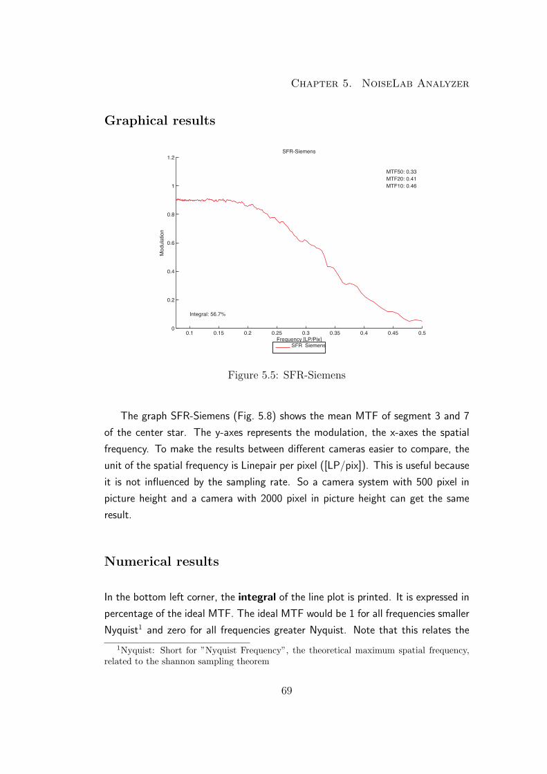
Chapter 5. NoiseLab Analyzer
Graphical results
0.1 0.15 0.2 0.25 0.3 0.35 0.4 0.45 0.50
0.2
0.4
0.6
0.8
1
1.2SFR-Siemens
Frequency [LP/Pix]
Mod
ulat
ion
Integral: 56.7%
MTF50: 0.33MTF20: 0.41MTF10: 0.46
SFR Siemens
Figure 5.5: SFR-Siemens
The graph SFR-Siemens (Fig. 5.8) shows the mean MTF of segment 3 and 7
of the center star. The y-axes represents the modulation, the x-axes the spatial
frequency. To make the results between different cameras easier to compare, the
unit of the spatial frequency is Linepair per pixel ([LP/pix]). This is useful because
it is not influenced by the sampling rate. So a camera system with 500 pixel in
picture height and a camera with 2000 pixel in picture height can get the same
result.
Numerical results
In the bottom left corner, the integral of the line plot is printed. It is expressed in
percentage of the ideal MTF. The ideal MTF would be 1 for all frequencies smaller
Nyquist1 and zero for all frequencies greater Nyquist. Note that this relates the
1Nyquist: Short for ”Nyquist Frequency”, the theoretical maximum spatial frequency,related to the shannon sampling theorem
69

Chapter 5. NoiseLab Analyzer
integral of the ideal to the real MTF, so a value of 100% can be achieved by em-
phasizing the lower frequencies (sharpening) as well. In this case, the modulation
can be greater than 1 for the real data.
In the top right, three different resolution values are printed, MTF50, MTF20
and MTF10. These values are the spatial frequency at modulation 0.5, 0.2 and
0.1. These steps are used to describe the MTF in one numerical result.
MTF10 is commonly called the limiting resolution, as a modulation of 10%
is the modulation where the raleigh criterion is met. The raleigh criterion says
that two adjacent points in an optical system can be declared as resolved, if in
their image the maximum of the first point hits the first minimum of the second
point. The combined intensity distribution has a minimum intensity of 0.81 at a
maximum of 1, which results in a Modulation of 0.105. Note that a point will get
a intensity distribution described by a Bessel function because of diffraction.(see
Fig. 5.6) [19]
Figure 5.6: Intensity distribution of two adjacent points that meet the raleighcriterion
70
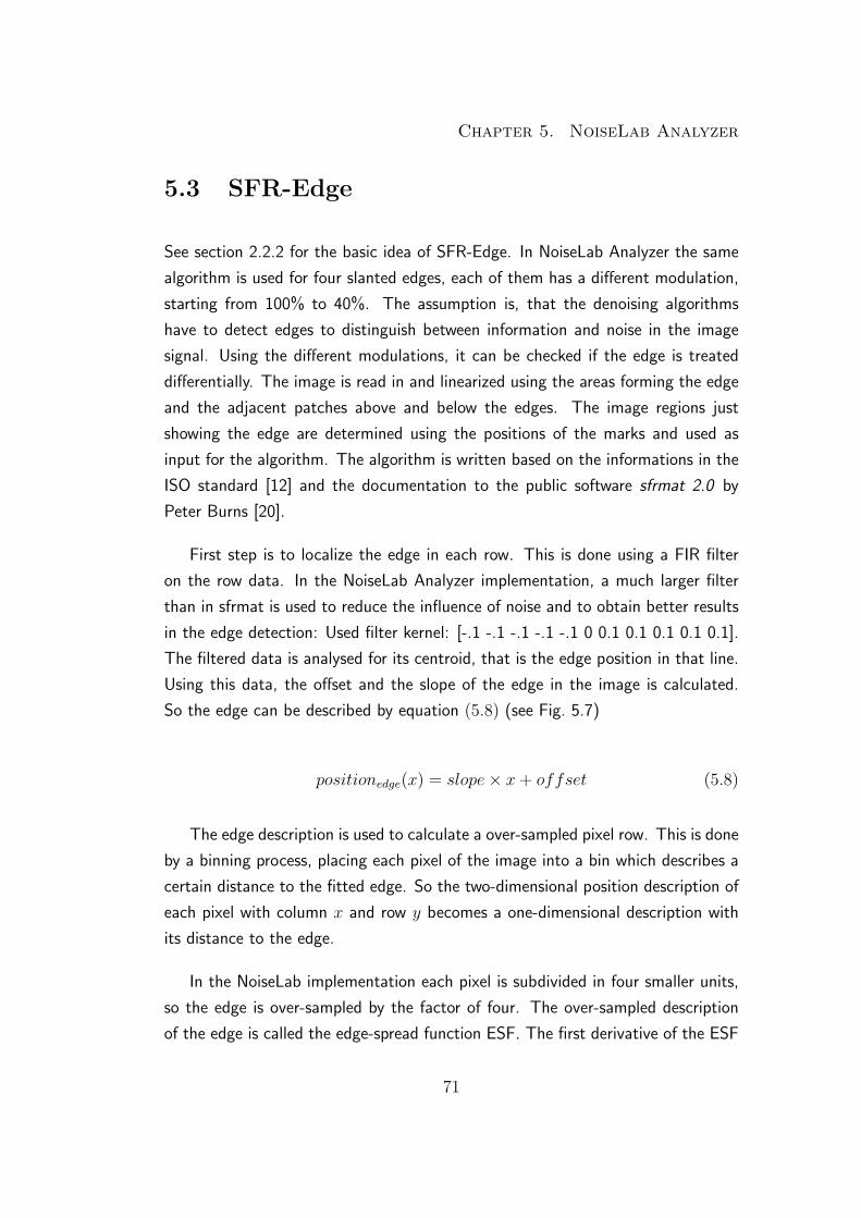
Chapter 5. NoiseLab Analyzer
5.3 SFR-Edge
See section 2.2.2 for the basic idea of SFR-Edge. In NoiseLab Analyzer the same
algorithm is used for four slanted edges, each of them has a different modulation,
starting from 100% to 40%. The assumption is, that the denoising algorithms
have to detect edges to distinguish between information and noise in the image
signal. Using the different modulations, it can be checked if the edge is treated
differentially. The image is read in and linearized using the areas forming the edge
and the adjacent patches above and below the edges. The image regions just
showing the edge are determined using the positions of the marks and used as
input for the algorithm. The algorithm is written based on the informations in the
ISO standard [12] and the documentation to the public software sfrmat 2.0 by
Peter Burns [20].
First step is to localize the edge in each row. This is done using a FIR filter
on the row data. In the NoiseLab Analyzer implementation, a much larger filter
than in sfrmat is used to reduce the influence of noise and to obtain better results
in the edge detection: Used filter kernel: [-.1 -.1 -.1 -.1 -.1 0 0.1 0.1 0.1 0.1 0.1].
The filtered data is analysed for its centroid, that is the edge position in that line.
Using this data, the offset and the slope of the edge in the image is calculated.
So the edge can be described by equation (5.8) (see Fig. 5.7)
positionedge(x) = slope× x+ offset (5.8)
The edge description is used to calculate a over-sampled pixel row. This is done
by a binning process, placing each pixel of the image into a bin which describes a
certain distance to the fitted edge. So the two-dimensional position description of
each pixel with column x and row y becomes a one-dimensional description with
its distance to the edge.
In the NoiseLab implementation each pixel is subdivided in four smaller units,
so the edge is over-sampled by the factor of four. The over-sampled description
of the edge is called the edge-spread function ESF. The first derivative of the ESF
71

Chapter 5. NoiseLab Analyzer
row
s y
columns x edge
o�set ∆x
∆yFigure 5.7: Slope and offset of edge in image (Illustration)
is the LSF, the line-spread function2. The SFR-Edge is the Fourier transform of
the line-spread function. Before the transformation, the data is windowed to avoid
leakage. The algorithm step by step:
1 read the image edge data
2 localize the edge in each row using a FIR filter
3 analyze the centroids in each line, calculate slope and offset for the edge
4 project the lines on a super sampled pixel row, using slope and offset, result-
ing in a over-sampled edge spread function ESF
5 calculate the derivative of the ESF to get the line spread function LSF
6 window the function (Hamming Window) to reduce leakage
7 calculate the Fourier transformation of the windowed LSF to obtain the SFR
8 normalize data so the absolute DC-value is 1
2The LSF can be imagined as a 1-D representative of the point-spread function PSF
72

Chapter 5. NoiseLab Analyzer
Graphical results
0.1 0.15 0.2 0.25 0.3 0.35 0.4 0.45 0.50
0.2
0.4
0.6
0.8
1
1.2SFR-Edge
Frequency [LP/Pix]
Mod
ulat
ion
Integral: 83.1%Integral: 62.4%Integral: 61.8%Integral: 55.1%
M100:0.41 0.49 0.54M80: 0.32 0.42 0.50M60: 0.31 0.41 0.49M40: 0.29 0.36 0.41
M100 M80 M60 M40
Figure 5.8: SFR-Edge in NoiseLab
The SFR-Edge graph plots the normalized SFR for all four edges. The normal-
ization relates to the lowest frequency obtained and sets this to modulation 1. As
all edges appears two times in the image, the average is taken of both.
The axes have the same dimension and meaning than in SFR-Siemens, so y-
axes is Modulation from zero to 1.2 and x-axes is the spatial frequency in linepairs
per pixel.
Numerical results
The numerical results are the same as for SFR-Siemens, but integral and MTF50,
MTF20 and MTF10 are calculated for all four plots. Note that especially in
SFR-Edge the modulation can go far over one, which means that this edge was
emphasized. The MTF results are calculated on the algorithm output, so the
numerical results could be greater Nyquist. As frequencies greater the theoretical
73

Chapter 5. NoiseLab Analyzer
maximum can be regarded as aliasing artifacts, the results are set to zero.
5.4 Edge Profile - Intensity and Standard De-
viation
The edge profile is obtained while calculation the SFR-Edge. The intensity edge
profile is the ESF as calculated in step 4. So the image pixels are bined by their
distance to the fitted edge description.
The edge profile based on the standard deviation is an additional step in the
SFR-Edge calculation. It represents the standard deviation of digital values in the
pixel columns, paralleled to the edge. This makes it possible to measure the noise
along an edge, which is interesting to measure, because most denoising algorithms
keep a certain distance to an edge to perform the denoising.
Graphical results
Figure 5.9 shows the Edge Profile Intensity plot of the four different edges, taking
the average of the two corresponding edges left and right. The y-axes is the
intensity in digital values, for a 8-bit image from 0 to 255. The x-axes represents
the position related to the edge. So value 0 is the position of the maximum of the
first derivative of the edge profile. For example a value of 4 means 4 pixels right
of the edge, therefore a value of -4 means 4 pixel left to the edge. Left always
represents the low intensity, right the high intensity side of the edge.
The Edge Profile Standard Deviation plot (Fig. 5.10) has the same x-axes, but
the y-axes is the standard deviation in digital values. So based on the bined data,
edge profile intensity is the mean value and edge profile standard deviation is the
standard deviation of the data.
74

Chapter 5. NoiseLab Analyzer
-10 -9 -8 -7 -6 -5 -4 -3 -2 -1 0 1 2 3 4 5 6 7 8 9 100
50
100
150
200
250Edge Profile
Position [pix]
Inte
nsity
[DV]
EdgeWidth:1.4EdgeWidth:2.8EdgeWidth:2.2EdgeWidth:2.0
U/O: 0% / 20%U/O: 1% / 17%U/O: 0% / 11%U/O: 10% / 0%
M100 M80 M60 M40
Figure 5.9: Edge Profile Intensity
-10 -9 -8 -7 -6 -5 -4 -3 -2 -1 0 1 2 3 4 5 6 7 8 9 100
5
10
15
20
25
30Edge Profile
Position [pix]
Stan
dard
Dev
.[DN
]
STD: 0.0 19.3 1.8STD: 1.1 15.5 1.5STD: 1.3 13.1 1.5STD: 1.1 8.2 1.3
Int: 2.9 4.9Int: 3.5 5.5Int: 3.3 5.0Int: 2.7 4.1
M100 M80 M60 M40
Figure 5.10: Edge Profile Standard Deviation
75
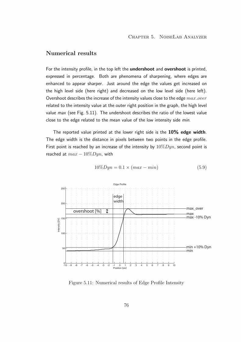
Chapter 5. NoiseLab Analyzer
Numerical results
For the intensity profile, in the top left the undershoot and overshoot is printed,
expressed in percentage. Both are phenomena of sharpening, where edges are
enhanced to appear sharper. Just around the edge the values get increased on
the high level side (here right) and decreased on the low level side (here left).
Overshoot describes the increase of the intensity values close to the edge max over
related to the intensity value at the outer right position in the graph, the high level
value max (see Fig. 5.11). The undershoot describes the ratio of the lowest value
close to the edge related to the mean value of the low intensity side min.
The reported value printed at the lower right side is the 10% edge width.
The edge width is the distance in pixels between two points in the edge profile.
First point is reached by an increase of the intensity by 10%Dyn, second point is
reached at max− 10%Dyn, with
10%Dyn = 0.1× (max−min) (5.9)
overshoot [%]
-10 -9 -8 -7 -6 -5 -4 -3 -2 -1 0 1 2 3 4 5 6 7 8 9 100
50
100
150
200
250Edge Profile
Position [pix]
Inte
nsity
[DV]
max
minmin +10% Dyn
max -10% Dyn
max_over
edgewidth
Figure 5.11: Numerical results of Edge Profile Intensity
76
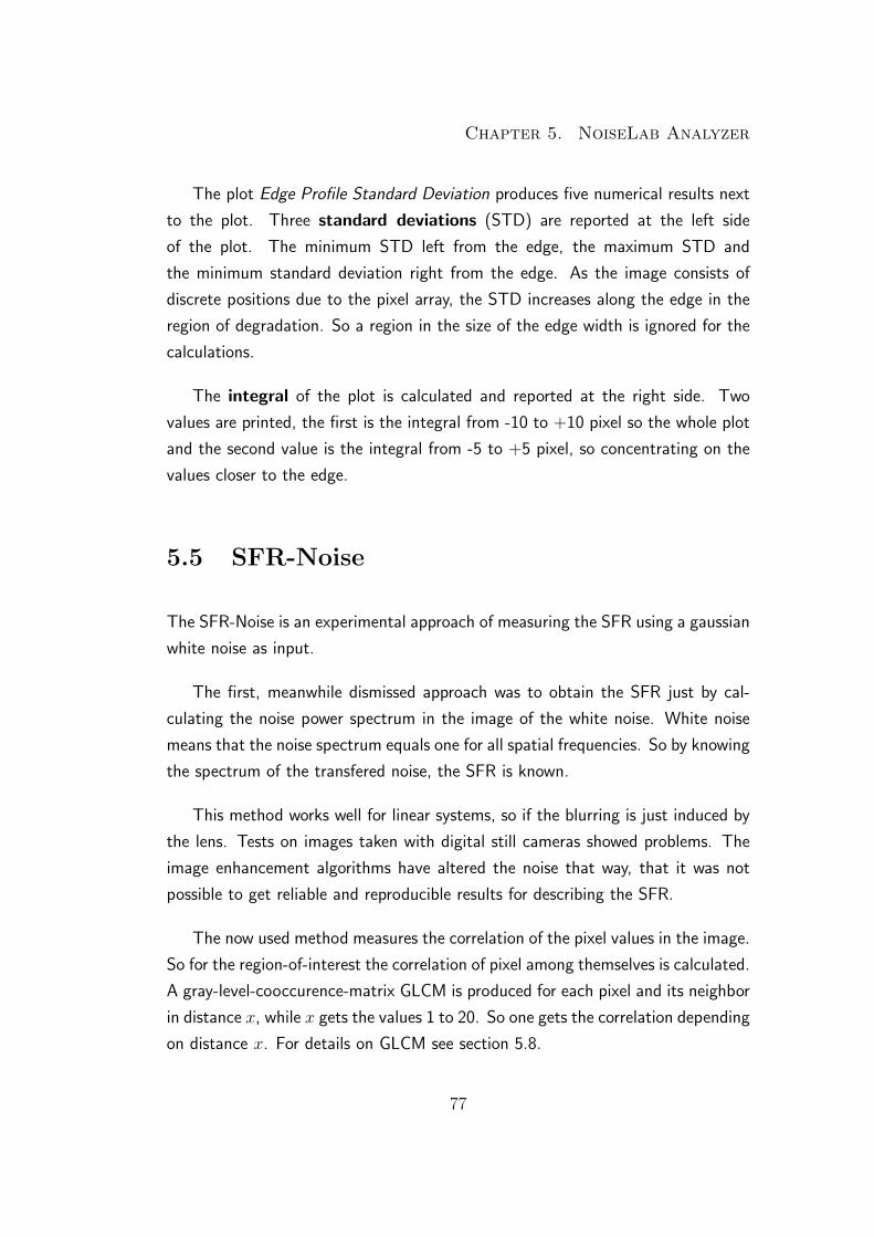
Chapter 5. NoiseLab Analyzer
The plot Edge Profile Standard Deviation produces five numerical results next
to the plot. Three standard deviations (STD) are reported at the left side
of the plot. The minimum STD left from the edge, the maximum STD and
the minimum standard deviation right from the edge. As the image consists of
discrete positions due to the pixel array, the STD increases along the edge in the
region of degradation. So a region in the size of the edge width is ignored for the
calculations.
The integral of the plot is calculated and reported at the right side. Two
values are printed, the first is the integral from -10 to +10 pixel so the whole plot
and the second value is the integral from -5 to +5 pixel, so concentrating on the
values closer to the edge.
5.5 SFR-Noise
The SFR-Noise is an experimental approach of measuring the SFR using a gaussian
white noise as input.
The first, meanwhile dismissed approach was to obtain the SFR just by cal-
culating the noise power spectrum in the image of the white noise. White noise
means that the noise spectrum equals one for all spatial frequencies. So by knowing
the spectrum of the transfered noise, the SFR is known.
This method works well for linear systems, so if the blurring is just induced by
the lens. Tests on images taken with digital still cameras showed problems. The
image enhancement algorithms have altered the noise that way, that it was not
possible to get reliable and reproducible results for describing the SFR.
The now used method measures the correlation of the pixel values in the image.
So for the region-of-interest the correlation of pixel among themselves is calculated.
A gray-level-cooccurence-matrix GLCM is produced for each pixel and its neighbor
in distance x, while x gets the values 1 to 20. So one gets the correlation depending
on distance x. For details on GLCM see section 5.8.
77
Chapter 5. NoiseLab Analyzer
The correlation can range from 1, perfectly positive correlated, to -1, per-
fectly negative correlated. I expect only values from 0, not correlated, to 1. The
correlation vector and a symmetric copy are placed in the correlation spread func-
tion CoSF. The fast fourier transformation of the CoSF is the SFR-Noise. (see
Fig. 5.13)
Image of white noise
GLCMx = 1
GLCMx = 2
GLCMx = 3
GLCMx = 4
GLCMx = 5
GLCMx = ...
corrx = 1
corrx = 3
corrx = 4
corrx = 5
corrx = ...
corrx = 2
... 1 ...corrx = 1
corrx = 2
corrx = 3
corrx = 4
corrx = 5
corrx = ...
corrx = 1
corrx = 2
corrx = 3
corrx = 4
corrx = 5
corrx = ...
0 0.05 0.1 0.15 0.2 0.25 0.3 0.35 0.4 0.45 0.50
0.2
0.4
0.6
0.8
1
1.2
Frequency [LP/Pix]
Mod
ulat
ion
1. Image
2. GLCM(x)
3. Correlation (x)
4. CoSF
5. SFR-Noise
Fourier Tranformation
Figure 5.12: Calculating SFR-Noise
The center is set to 1 as the center represents distance x = 0 which describes
the correlation of each pixel with itself, so 1. If the noise is not correlated at all,
the CSF becomes a single impulse with position zero set to 1 and all other values
equal 0. So the Fourier-Transform is a straight line with value 1. The more the
noise is correlated depending on the distance, the lower the SFR curve gets.
The SFR-Noise is measured for the gray patch as well. In that case, the pixel
values are supposed to be highly correlated, as they should have the same value.
The less the pixel values are correlated, the more noise contains the flat field.
78
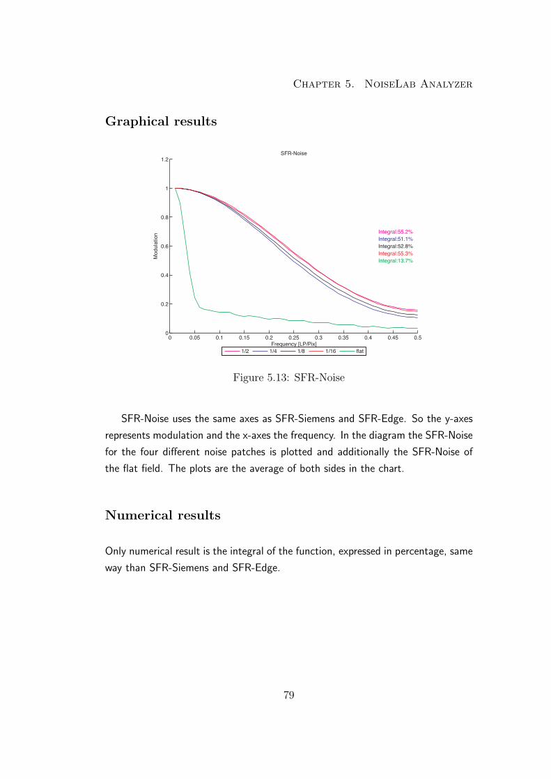
Chapter 5. NoiseLab Analyzer
Graphical results
0 0.05 0.1 0.15 0.2 0.25 0.3 0.35 0.4 0.45 0.50
0.2
0.4
0.6
0.8
1
1.2SFR-Noise
Frequency [LP/Pix]
Mod
ulat
ion
Integral:55.2%Integral:51.1%Integral:52.8%Integral:55.3%Integral:13.7%
1/2 1/4 1/8 1/16 flat
Figure 5.13: SFR-Noise
SFR-Noise uses the same axes as SFR-Siemens and SFR-Edge. So the y-axes
represents modulation and the x-axes the frequency. In the diagram the SFR-Noise
for the four different noise patches is plotted and additionally the SFR-Noise of
the flat field. The plots are the average of both sides in the chart.
Numerical results
Only numerical result is the integral of the function, expressed in percentage, same
way than SFR-Siemens and SFR-Edge.
79
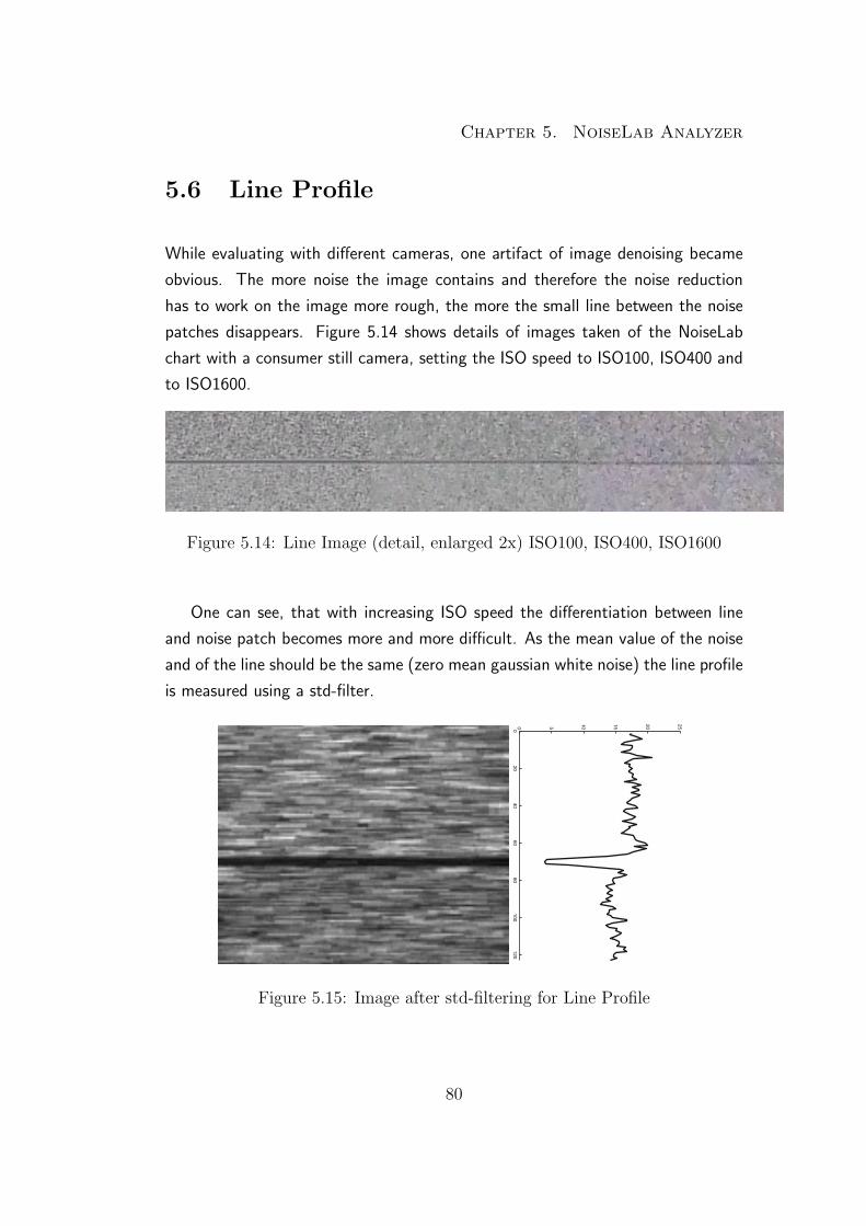
Chapter 5. NoiseLab Analyzer
5.6 Line Profile
While evaluating with different cameras, one artifact of image denoising became
obvious. The more noise the image contains and therefore the noise reduction
has to work on the image more rough, the more the small line between the noise
patches disappears. Figure 5.14 shows details of images taken of the NoiseLab
chart with a consumer still camera, setting the ISO speed to ISO100, ISO400 and
to ISO1600.
Figure 5.14: Line Image (detail, enlarged 2x) ISO100, ISO400, ISO1600
One can see, that with increasing ISO speed the differentiation between line
and noise patch becomes more and more difficult. As the mean value of the noise
and of the line should be the same (zero mean gaussian white noise) the line profile
is measured using a std-filter.
020
4060
80100
1200 5 10 15 20 25
Figure 5.15: Image after std-filtering for Line Profile
80

Chapter 5. NoiseLab Analyzer
The std-filter calculates the standard deviation in a neighborhood around each
pixel. In NoiseLab-Analyzer the neighborhood is a single horizontal line, 10% in
length of the full row. The neighborhood spans not the full row to minimize the
influence on the result if the image is slightly tilted.
Graphical results
0 20 40 60 80 100 1200
5
10
15
20
25Line Profile
Position [pix]
Stan
dard
Dev
. [D
N]
17.5 3.9 14.2
Line-Profile
Figure 5.16: Line Profile
The shown graph is the average of both used lines in the image. It plots the
mean value of the standard deviation per row against the position. Left site is
the noise patch with variance 1/4, right side is the noise patch with variance 1/8.
Around the center a minimum shows the standard deviation along the line.
Numerical results
Three values are printed into the plot. The global minimum and the mean value
left of the minimum and the mean value right of the minimum.
81
Chapter 5. NoiseLab Analyzer
5.7 Histogram of Derivative
The histogram of noise hold different informations about the noise characteristics.
But the histogram would change for different mean values of the noisy image signal,
so in NoiseLab, the histogram of the first derivative is used. This is calculated by
a convolution of the image with the kernel [-.5 .5]. The first derivative of a normal
distribution has also normal distribution and so on, so it is possible to check for
the distribution in the processed image.
The target is a gaussian white noise, so all digital values appear in the image
with a probability defined by the gaussian distribution around the mean value. In
the processed image, the mean value becomes zero, as the first derivative of a flat
image is zero. The more the image is low pass filtered, the more the histogram
gets a peak at its mean and the more the distributions become leptokurtic3 , so
the probability of values close to the mean is increased.
To describe the shape of the distribution, the excess kurtosis is calculated.
The value becomes 0 for a normal distribution and is increased for leptokurtic
distributions. The kurtosis is calculated as the fourth moment devided by the
square of the second moment of the distribution. The second moment is the
variance.
kurt =m4
m22
− 3 =m4
σ4− 3 =
(1
n
n∑i=1
(xi − µσ
)4)− 3 (5.10)
Graphical results
The histogram of the derivative of the four different noise patches and the neutral
gray-patches are displayed. The y-axes represents the relative count of the digital
values in the x-axes. The count of the values is expressed in percentage, so a count
of 10% means, that one tenth of all pixel have this value.
3”A frequency function with coefficient of kurtosis greater than zero is said to be lep-tokurtic. It is more peaked about the mode than the normal distribution”.[22]
82

Chapter 5. NoiseLab Analyzer
-64 -48 -32 -16 0 16 32 48 640
1
2
3
4
5
6
7
8
9
10Histogram of Derivative
digital value
Cou
nt [%
]
Kurtosis:0.9
Max:7.6
Kurtosis:0.4
Max:3.0
Kurtosis:0.5
Max:3.8
Kurtosis:0.6
Max:4.1
Kurtosis:1.8
Max:41.4
1/2 1/4 1/8 1/16 flat
Figure 5.17: Histogram of Derivative
Numerical results
The kurtosis as described in (5.10) is calculated for the four different noise patches
and for the flat patch. The reported value is the average of both identical structures
in the chart.
At the right side, the maximum value for each of the five plots is reported in
the unit of the y-axes, so relative count in percentage.
5.8 Noise GLCM
”A statistical method of examining texture that considers the spatial
relationship of pixels is the gray-level co-occurrence matrix (GLCM),
also known as the gray-level spatial dependence matrix.”[21]
The GLCM is a technique from texture analysis in images. The matrix has the
83
Chapter 5. NoiseLab Analyzer
size of n2 where n is the number of possible gray values in a digital image. So for a
8-bit image, the GLCM has the size 256× 256. The matrix is created by counting
how often a certain combination of two pixel values with distance x occurs in the
analyzed image. So for example the matrix entry GLCM(100, 120) = 250 with
distance 1 means, that 250 pixel have the value 100 and the pixel on the right
next to it has the value 120.
To make the results more comparable, the matrix values are normalized to
the total number of pixel in the image. A value of 0.25 in the NoiseLab-Analyzer
GLCM means that 0.25% of all pixels have the defined relationship to the neighbor
pixel.
The more pixel have the same value than their related neighbor pixel, the higher
the diagonal coefficients in the GLCM, the less correlated the noise is, the lower
are the single coefficients in the matrix and the lower are the diagonal entries.
Graphical results
The GLCM of the noise field C.4 is shown in NoiseLab-Analyzer. The colormap
is set that way, that values of 0 are represented by black. Values greater zero are
displayed as shown in the colorbar below the GLCM (Fig.: 5.18). The GLCM is
centered, so that different matrices are always displayed the same way regardless
of slight mean value variations. The GLCM is calculated using the linearized data,
in that process some value combinations get lost due to the tone-mapping. This
can be observed in the GLCM by some dark rows and/or columns.
Numerical results
For all noise patches the Correlation and Homogeneity is calculated based on the
GLCM.
Correlation is a measure for the interdependence of two variable quantities.[1]
In this case it measures the likeliness, that a pixel and its neighbor have the same
84
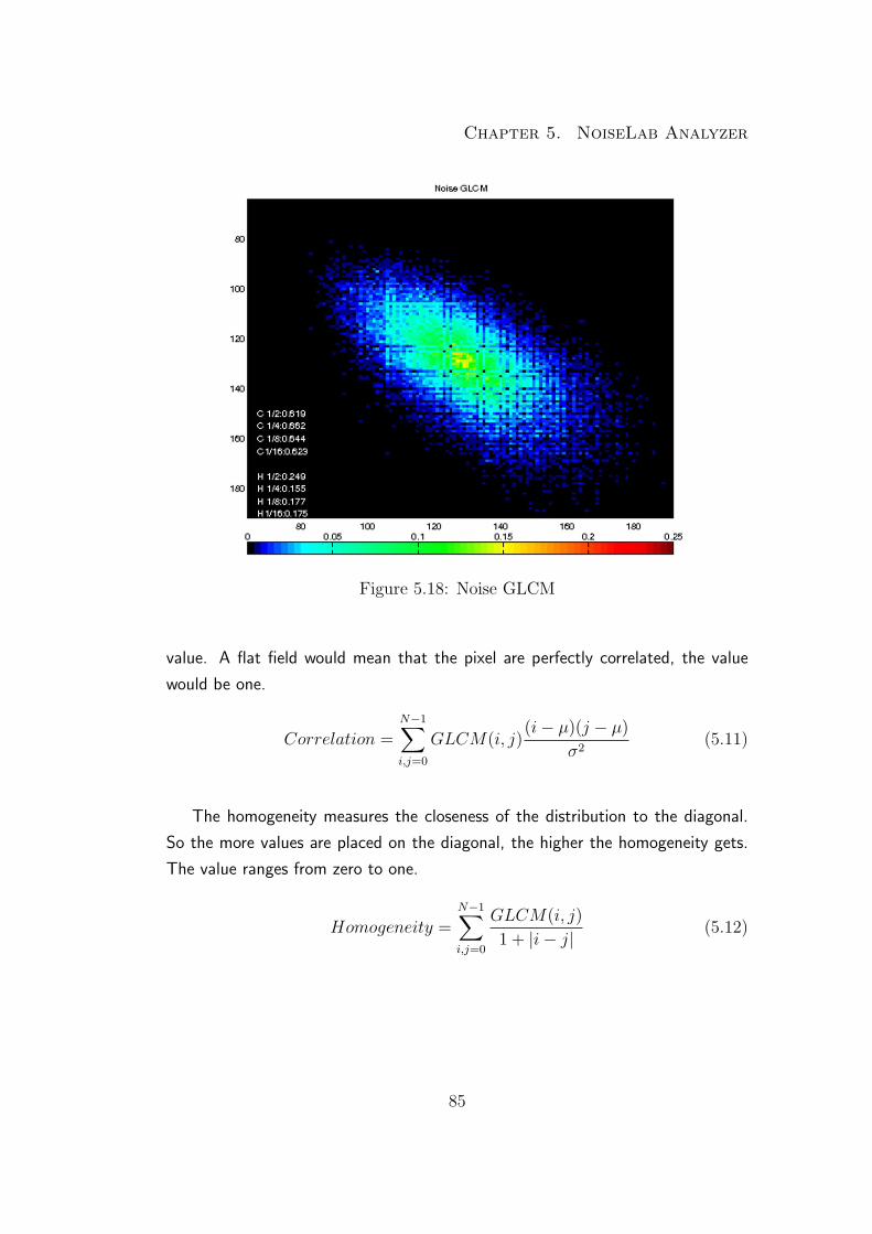
Chapter 5. NoiseLab Analyzer
Figure 5.18: Noise GLCM
value. A flat field would mean that the pixel are perfectly correlated, the value
would be one.
Correlation =N−1∑i,j=0
GLCM(i, j)(i− µ)(j − µ)
σ2(5.11)
The homogeneity measures the closeness of the distribution to the diagonal.
So the more values are placed on the diagonal, the higher the homogeneity gets.
The value ranges from zero to one.
Homogeneity =N−1∑i,j=0
GLCM(i, j)
1 + |i− j|(5.12)
85
Chapter 6. Results
Chapter 6
Results
Three different types of input data were analyzed by the NoiseLab-Analyzer: An
ideal copy of the NoiseLab chart, different images produced using NoiseLab and
real camera images, showing the NoiseLab chart.
All together more than 500 plots and even more numerical results have been
produced. This is more than it can be shown in the printed version of this thesis.
On the appended CD, all used NoiseLab result files (.nla) are stored for more
detailed investigations. In the following sections, only the most important results
are presented.
86
Chapter 6. Results
6.1 Ideal Image
The image used here as input for NoiseLab Analyzer is an ideal version of the
NoiseLab chart, it was not degraded by noise or blurring. The image file for the
chart production was reduced to six million pixel, which induced some artifacts.
Figure A.1 and Table A.1 to A.7 show the graphical and numerical results.
SFR-Siemens
Figure A.1 top row (left) Table A.1
In the ideal image, the modulation is one for all frequencies, therefore the integral
would be 100%. In the image used here, one can see an increasing of the modula-
tion at high frequencies close to the maximum (Nyquist). This is an interpolation
artifact that was induced while scaling the image to six ”megapixel”. But the
numerical result is 99%, so very close to the ideal. The values MTF50, MTF20
and MTF10 could not be calculated and are set to zero.
SFR-Edge
Figure A.1 top row (right) and Table A.2
Because of the pixel structure of an digital image, there is no real ideal image,
the edge width of a slanted edge will always stick to one pixel. In the SFR-Edge
algorithm the distance to an ideal line is used to project the pixels on the super
resolution profile. But expressed in pixels, the width of the ideal line is zero, the
width of a single pixel is one. Therefore the best possible SFR-Edge result is not a
line with modulation one for all frequencies, it loses modulation at high frequencies.
The graphical and the numerical results are nearly identical for the different edges.
The integral of the plot is close around 94% for the four different edges, the values
MTF50, MTF20 and MTF10 could not be calculated and are set to zero.
87
Chapter 6. Results
Edge Profile Intensity
Figure A.1 2nd row (left) and Table A.3
As mentioned in the SFR-Edge section, even in the ideal image the edge has a
certain width. The calculated edge width is 0.7 pixel for all four edges. Note that
this is the 10%-edge width as defined in Fig. 5.11, so the full edge would be 1
pixel.
Edge Profile STD
Figure A.1 2nd row (left) and Table A.3
No noise was added to the analyzed image, so all numerical results are 0. At the
edge position (Position 0) the standard deviation is very high, as the edge in the
digital image consists out of discrete positions. These high values are ignored for
the calculation of the integral and the maximum STD.
SFR-Noise
Figure A.1 3rd row (left) and Table A.4
The integral is 100% for all noise patches, the plot is a straight line at position 1
for all frequencies.
Line Profile
Figure A.1 3rd row (right) and Table A.5
The Line is not altered, so the STD is zero on the line and is set to a high value
around, which represents the noise patches adjacent to the line.
88
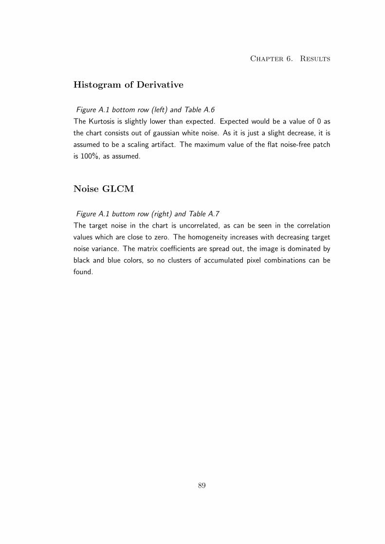
Chapter 6. Results
Histogram of Derivative
Figure A.1 bottom row (left) and Table A.6
The Kurtosis is slightly lower than expected. Expected would be a value of 0 as
the chart consists out of gaussian white noise. As it is just a slight decrease, it is
assumed to be a scaling artifact. The maximum value of the flat noise-free patch
is 100%, as assumed.
Noise GLCM
Figure A.1 buttom row (right) and Table A.7
The target noise in the chart is uncorrelated, as can be seen in the correlation
values which are close to zero. The homogeneity increases with decreasing target
noise variance. The matrix coefficients are spread out, the image is dominated by
black and blue colors, so no clusters of accumulated pixel combinations can be
found.
89
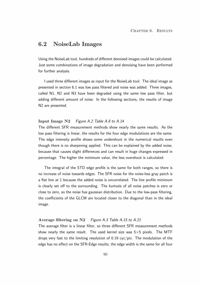
Chapter 6. Results
6.2 NoiseLab Images
Using the NoiseLab tool, hundreds of different denoised images could be calculated.
Just some combinations of image degradation and denoising have been performed
for further analysis.
I used three different images as input for the NoiseLab tool. The ideal image as
presented in section 6.1 was low pass filtered and noise was added. Three images,
called N1, N2 and N3 have been degraded using the same low pass filter, but
adding different amount of noise. In the following sections, the results of image
N2 are presented.
Input Image N2 Figure A.2 Table A.8 to A.14
The different SFR measurement methods show nearly the same results. As the
low pass filtering is linear, the results for the four edge modulations are the same.
The edge intensity profile shows some undershoot in the numerical results even
though there is no sharpening applied. This can be explained by the added noise,
because that causes slight differences and can result in huge changes expressed in
percentage. The higher the minimum value, the less overshoot is calculated.
The integral of the STD edge profile is the same for both ranges, so there is
no increase of noise towards edges. The SFR noise for the noise-less gray patch is
a flat line at 1 because the added noise is uncorrelated. The line profile minimum
is clearly set off to the surrounding. The kurtosis of all noise patches is zero or
close to zero, so the noise has gaussian distribution. Due to the low-pass filtering,
the coefficients of the GLCM are located closer to the diagonal than in the ideal
image.
Average filtering on N2 Figure A.3 Table A.15 to A.21
The average filter is a linear filter, so three different SFR measurement methods
show nearly the same result. The used kernel size was 5×5 pixels. The MTF
drops very fast to the limiting resolution of 0.19 cyc/pix. The modulation of the
edge has no effect on the SFR-Edge results, the edge width is the same for all four
90
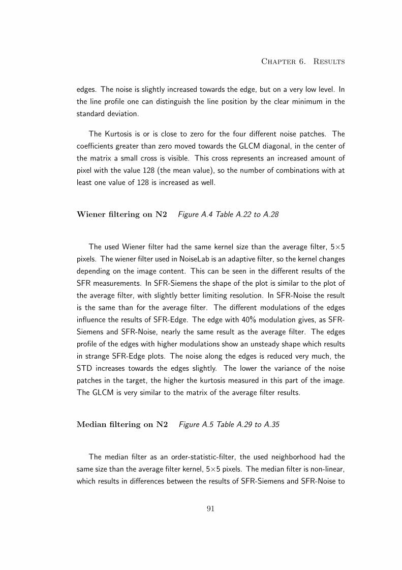
Chapter 6. Results
edges. The noise is slightly increased towards the edge, but on a very low level. In
the line profile one can distinguish the line position by the clear minimum in the
standard deviation.
The Kurtosis is or is close to zero for the four different noise patches. The
coefficients greater than zero moved towards the GLCM diagonal, in the center of
the matrix a small cross is visible. This cross represents an increased amount of
pixel with the value 128 (the mean value), so the number of combinations with at
least one value of 128 is increased as well.
Wiener filtering on N2 Figure A.4 Table A.22 to A.28
The used Wiener filter had the same kernel size than the average filter, 5×5
pixels. The wiener filter used in NoiseLab is an adaptive filter, so the kernel changes
depending on the image content. This can be seen in the different results of the
SFR measurements. In SFR-Siemens the shape of the plot is similar to the plot of
the average filter, with slightly better limiting resolution. In SFR-Noise the result
is the same than for the average filter. The different modulations of the edges
influence the results of SFR-Edge. The edge with 40% modulation gives, as SFR-
Siemens and SFR-Noise, nearly the same result as the average filter. The edges
profile of the edges with higher modulations show an unsteady shape which results
in strange SFR-Edge plots. The noise along the edges is reduced very much, the
STD increases towards the edges slightly. The lower the variance of the noise
patches in the target, the higher the kurtosis measured in this part of the image.
The GLCM is very similar to the matrix of the average filter results.
Median filtering on N2 Figure A.5 Table A.29 to A.35
The median filter as an order-statistic-filter, the used neighborhood had the
same size than the average filter kernel, 5×5 pixels. The median filter is non-linear,
which results in differences between the results of SFR-Siemens and SFR-Noise to
91
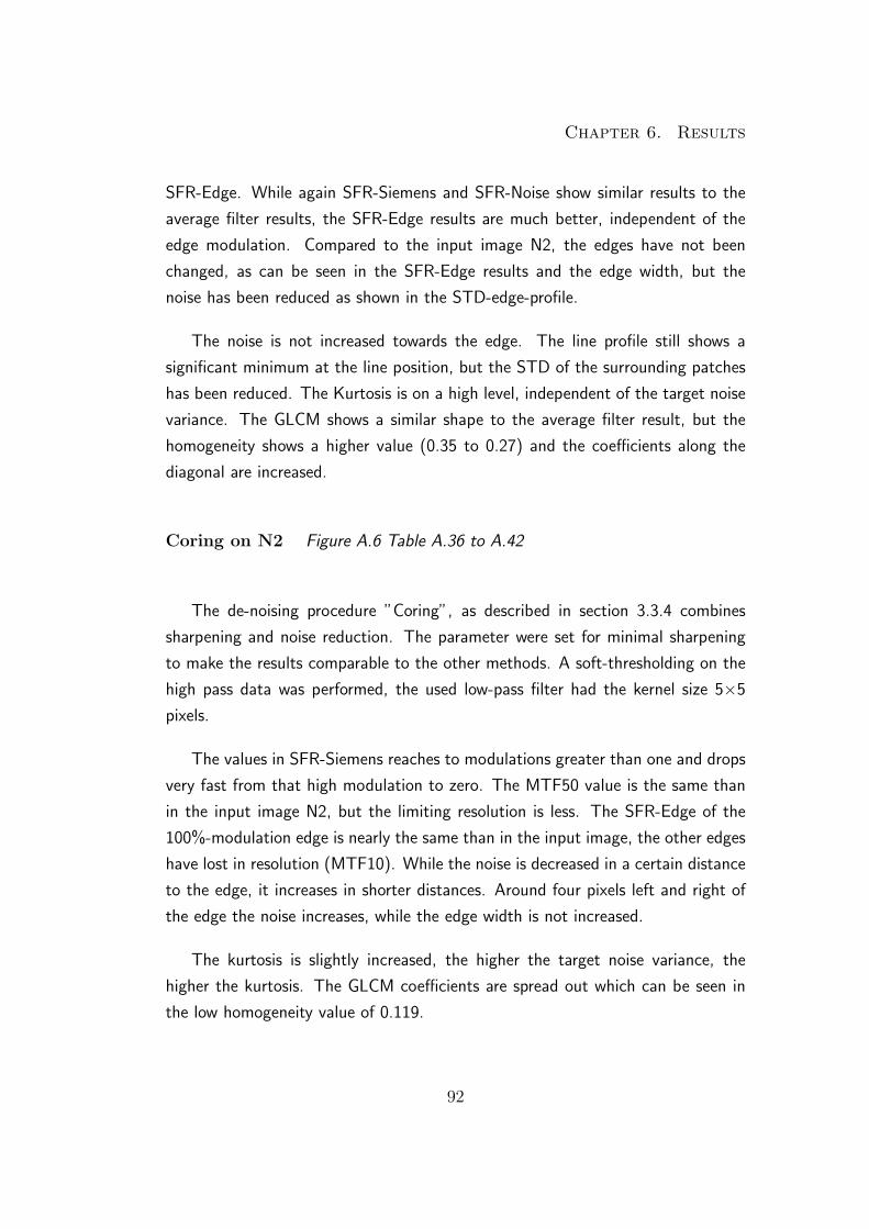
Chapter 6. Results
SFR-Edge. While again SFR-Siemens and SFR-Noise show similar results to the
average filter results, the SFR-Edge results are much better, independent of the
edge modulation. Compared to the input image N2, the edges have not been
changed, as can be seen in the SFR-Edge results and the edge width, but the
noise has been reduced as shown in the STD-edge-profile.
The noise is not increased towards the edge. The line profile still shows a
significant minimum at the line position, but the STD of the surrounding patches
has been reduced. The Kurtosis is on a high level, independent of the target noise
variance. The GLCM shows a similar shape to the average filter result, but the
homogeneity shows a higher value (0.35 to 0.27) and the coefficients along the
diagonal are increased.
Coring on N2 Figure A.6 Table A.36 to A.42
The de-noising procedure ”Coring”, as described in section 3.3.4 combines
sharpening and noise reduction. The parameter were set for minimal sharpening
to make the results comparable to the other methods. A soft-thresholding on the
high pass data was performed, the used low-pass filter had the kernel size 5×5
pixels.
The values in SFR-Siemens reaches to modulations greater than one and drops
very fast from that high modulation to zero. The MTF50 value is the same than
in the input image N2, but the limiting resolution is less. The SFR-Edge of the
100%-modulation edge is nearly the same than in the input image, the other edges
have lost in resolution (MTF10). While the noise is decreased in a certain distance
to the edge, it increases in shorter distances. Around four pixels left and right of
the edge the noise increases, while the edge width is not increased.
The kurtosis is slightly increased, the higher the target noise variance, the
higher the kurtosis. The GLCM coefficients are spread out which can be seen in
the low homogeneity value of 0.119.
92
Chapter 6. Results
Wavelet Denoising on N2 Figure A.7 Table A.43 to A.49
For this test the 4th order Daubechies wavelet (db4) with four subbands and
soft thresholding was used. With this technique some wavelet artifacts like ringing
at high contrast edge have been induced which could be reduced by a more carefully
setting of wavelet and threshold.
The resolution is reduced slightly in all three SFR measurements. The SFR-
Edge results depend on the edge-modulation, the lower the modulation the lower
the SFR plot, but the differences are not significant. The noise slightly increases
towards the edge which can be explained by the soft-threshold. The kurtosis is
increased on a similar level than in the coring results.
6.2.1 Summary NoiseLab Images
All techniques have an influence on the SFR. The average filter, as expected,
blurs the whole image independently of the image content, so the the different
SFR methods give similar results. For all non-linear or adaptive filter, the results
of SFR-Siemens and SFR-Edge are different, the SFR-Siemens results are more
comparable to the subjective visual impression of the resolution in the image.
All techniques reduce the standard deviation in a large distance to the edge
to more than a quarter of the input noise, except the wavelet denoising, which
would need more fine-tuning to get that results. The median filtering changes the
noise distribution very much, which can be seen in the highest kurtosis value of all
methods (around 2.2). The target noise is changed in its appearance, the image
noise consists of broader cluster of the same pixel value. The same, but less visible
effect can be seen in Coring denoising and Wiener filtering, which also results in an
increased kurtosis value. Wavelet denoising is the only technique that leaves the
SFR-Noise for the noise-free gray patch nearly unchanged. Average, Wiener and
Median filtering leads to the same results in SFR-Noise (Integral of 36%), Coring
has 45% and Wavelet denoising 90%.
93
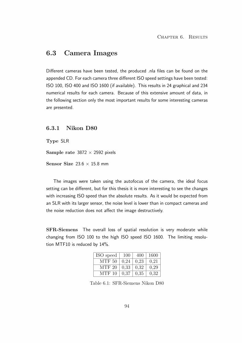
Chapter 6. Results
6.3 Camera Images
Different cameras have been tested, the produced .nla files can be found on the
appended CD. For each camera three different ISO speed settings have been tested:
ISO 100, ISO 400 and ISO 1600 (if available). This results in 24 graphical and 234
numerical results for each camera. Because of this extensive amount of data, in
the following section only the most important results for some interesting cameras
are presented.
6.3.1 Nikon D80
Type SLR
Sample rate 3872 × 2592 pixels
Sensor Size 23.6 × 15.8 mm
The images were taken using the autofocus of the camera, the ideal focus
setting can be different, but for this thesis it is more interesting to see the changes
with increasing ISO speed than the absolute results. As it would be expected from
an SLR with its larger sensor, the noise level is lower than in compact cameras and
the noise reduction does not affect the image destructively.
SFR-Siemens The overall loss of spatial resolution is very moderate while
changing from ISO 100 to the high ISO speed ISO 1600. The limiting resolu-
tion MTF10 is reduced by 14%.
ISO speed 100 400 1600MTF 50 0,24 0,23 0,21MTF 20 0,33 0,32 0,29MTF 10 0,37 0,35 0,32
Table 6.1: SFR-Siemens Nikon D80
94
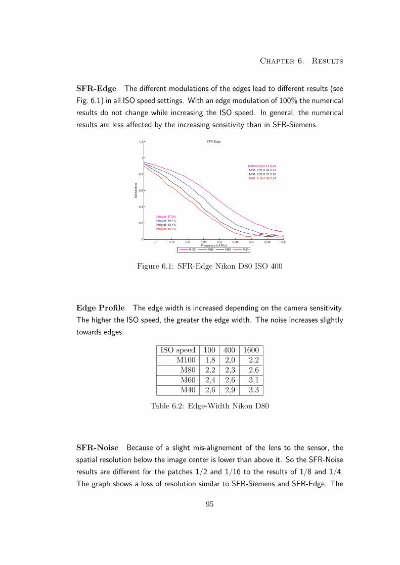
Chapter 6. Results
SFR-Edge The different modulations of the edges lead to different results (see
Fig. 6.1) in all ISO speed settings. With an edge modulation of 100% the numerical
results do not change while increasing the ISO speed. In general, the numerical
results are less affected by the increasing sensitivity than in SFR-Siemens.
0.1 0.15 0.2 0.25 0.3 0.35 0.4 0.45 0.50
0.2
0.4
0.6
0.8
1
1.2 SFR-Edge
Frequency [LP/Pix]
Mod
ulat
ion
Integral: 57.0%Integral: 49.1%Integral: 43.1%Integral: 39.7%
M100:0.29 0.41 0.49M80: 0.25 0.34 0.41M60: 0.22 0.31 0.36M40: 0.19 0.30 0.34
M100 M80 M60 M40
Figure 6.1: SFR-Edge Nikon D80 ISO 400
Edge Profile The edge width is increased depending on the camera sensitivity.
The higher the ISO speed, the greater the edge width. The noise increases slightly
towards edges.
ISO speed 100 400 1600M100 1,8 2,0 2,2M80 2,2 2,3 2,6M60 2,4 2,6 3,1M40 2,6 2,9 3,3
Table 6.2: Edge-Width Nikon D80
SFR-Noise Because of a slight mis-alignement of the lens to the sensor, the
spatial resolution below the image center is lower than above it. So the SFR-Noise
results are different for the patches 1/2 and 1/16 to the results of 1/8 and 1/4.
The graph shows a loss of resolution similar to SFR-Siemens and SFR-Edge. The
95
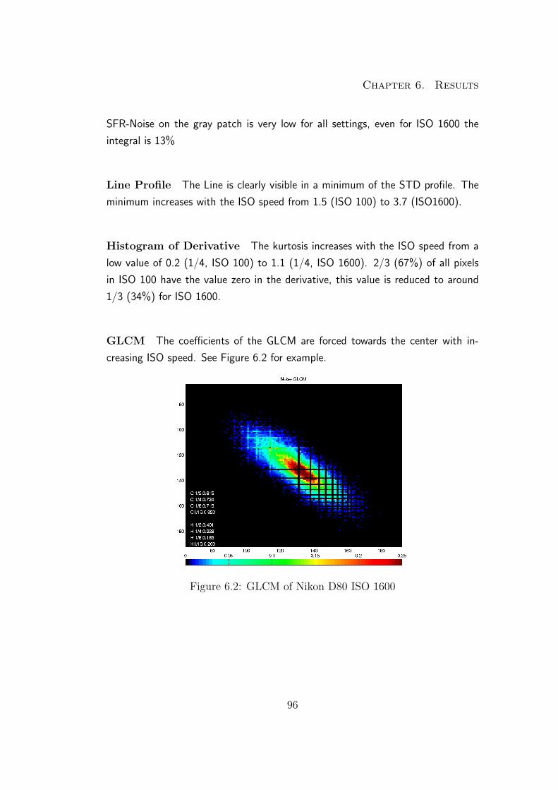
Chapter 6. Results
SFR-Noise on the gray patch is very low for all settings, even for ISO 1600 the
integral is 13%
Line Profile The Line is clearly visible in a minimum of the STD profile. The
minimum increases with the ISO speed from 1.5 (ISO 100) to 3.7 (ISO1600).
Histogram of Derivative The kurtosis increases with the ISO speed from a
low value of 0.2 (1/4, ISO 100) to 1.1 (1/4, ISO 1600). 2/3 (67%) of all pixels
in ISO 100 have the value zero in the derivative, this value is reduced to around
1/3 (34%) for ISO 1600.
GLCM The coefficients of the GLCM are forced towards the center with in-
creasing ISO speed. See Figure 6.2 for example.
Figure 6.2: GLCM of Nikon D80 ISO 1600
96
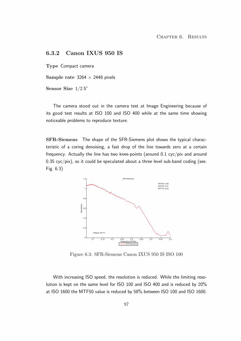
Chapter 6. Results
6.3.2 Canon IXUS 950 IS
Type Compact camera
Sample rate 3264 × 2448 pixels
Sensor Size 1/2.5”
The camera stood out in the camera test at Image Engineering because of
its good test results at ISO 100 and ISO 400 while at the same time showing
noticeable problems to reproduce texture.
SFR-Siemens The shape of the SFR-Siemens plot shows the typical charac-
teristic of a coring denoising, a fast drop of the line towards zero at a certain
frequency. Actually the line has two knee-points (around 0.1 cyc/pix and around
0.35 cyc/pix), so it could be speculated about a three level sub-band coding (see.
Fig. 6.3)
0.1 0.15 0.2 0.25 0.3 0.35 0.4 0.45 0.50
0.2
0.4
0.6
0.8
1
1.2 SFR-Siemens
Frequency [LP/Pix]
Mod
ulat
ion
Integral: 63.7%
MTF50: 0.36MTF20: 0.41MTF10: 0.42
SFR-Siemens
Figure 6.3: SFR-Siemens Canon IXUS 950 IS ISO 100
With increasing ISO speed, the resolution is reduced. While the limiting reso-
lution is kept on the same level for ISO 100 and ISO 400 and is reduced by 20%
at ISO 1600 the MTF50 value is reduced by 58% between ISO 100 and ISO 1600.
97
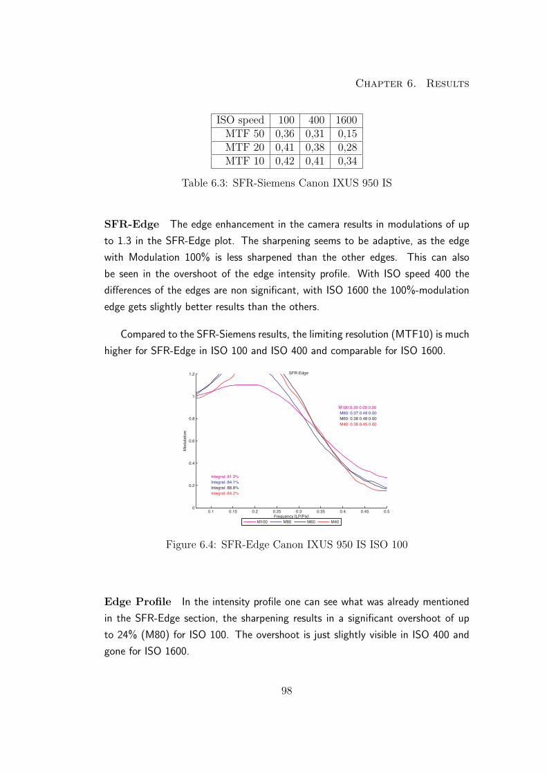
Chapter 6. Results
ISO speed 100 400 1600MTF 50 0,36 0,31 0,15MTF 20 0,41 0,38 0,28MTF 10 0,42 0,41 0,34
Table 6.3: SFR-Siemens Canon IXUS 950 IS
SFR-Edge The edge enhancement in the camera results in modulations of up
to 1.3 in the SFR-Edge plot. The sharpening seems to be adaptive, as the edge
with Modulation 100% is less sharpened than the other edges. This can also
be seen in the overshoot of the edge intensity profile. With ISO speed 400 the
differences of the edges are non significant, with ISO 1600 the 100%-modulation
edge gets slightly better results than the others.
Compared to the SFR-Siemens results, the limiting resolution (MTF10) is much
higher for SFR-Edge in ISO 100 and ISO 400 and comparable for ISO 1600.
0.1 0.15 0.2 0.25 0.3 0.35 0.4 0.45 0.50
0.2
0.4
0.6
0.8
1
1.2 SFR-Edge
Frequency [LP/Pix]
Mod
ulat
ion
Integral: 81.3%Integral: 84.1%Integral: 88.8%Integral: 84.2%
M100:0.39 0.00 0.00M80: 0.37 0.49 0.00M60: 0.38 0.48 0.00M40: 0.38 0.45 0.00
M100 M80 M60 M40
Figure 6.4: SFR-Edge Canon IXUS 950 IS ISO 100
Edge Profile In the intensity profile one can see what was already mentioned
in the SFR-Edge section, the sharpening results in a significant overshoot of up
to 24% (M80) for ISO 100. The overshoot is just slightly visible in ISO 400 and
gone for ISO 1600.
98
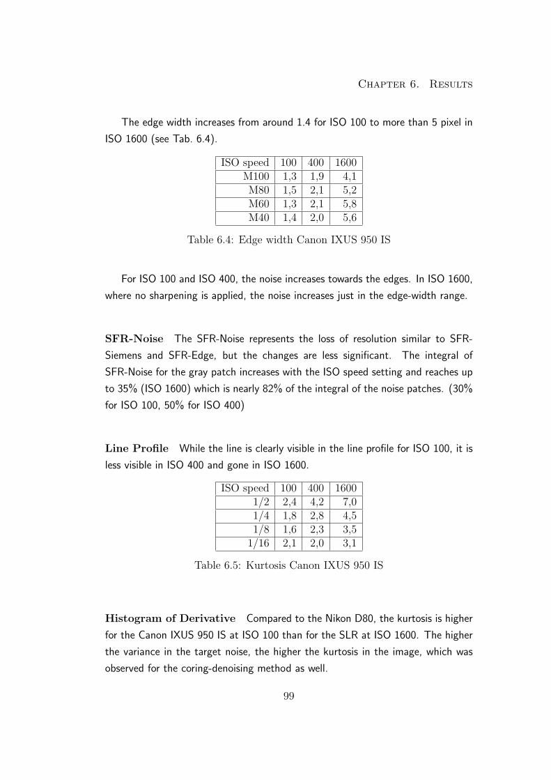
Chapter 6. Results
The edge width increases from around 1.4 for ISO 100 to more than 5 pixel in
ISO 1600 (see Tab. 6.4).
ISO speed 100 400 1600M100 1,3 1,9 4,1M80 1,5 2,1 5,2M60 1,3 2,1 5,8M40 1,4 2,0 5,6
Table 6.4: Edge width Canon IXUS 950 IS
For ISO 100 and ISO 400, the noise increases towards the edges. In ISO 1600,
where no sharpening is applied, the noise increases just in the edge-width range.
SFR-Noise The SFR-Noise represents the loss of resolution similar to SFR-
Siemens and SFR-Edge, but the changes are less significant. The integral of
SFR-Noise for the gray patch increases with the ISO speed setting and reaches up
to 35% (ISO 1600) which is nearly 82% of the integral of the noise patches. (30%
for ISO 100, 50% for ISO 400)
Line Profile While the line is clearly visible in the line profile for ISO 100, it is
less visible in ISO 400 and gone in ISO 1600.
ISO speed 100 400 16001/2 2,4 4,2 7,01/4 1,8 2,8 4,51/8 1,6 2,3 3,5
1/16 2,1 2,0 3,1
Table 6.5: Kurtosis Canon IXUS 950 IS
Histogram of Derivative Compared to the Nikon D80, the kurtosis is higher
for the Canon IXUS 950 IS at ISO 100 than for the SLR at ISO 1600. The higher
the variance in the target noise, the higher the kurtosis in the image, which was
observed for the coring-denoising method as well.
99
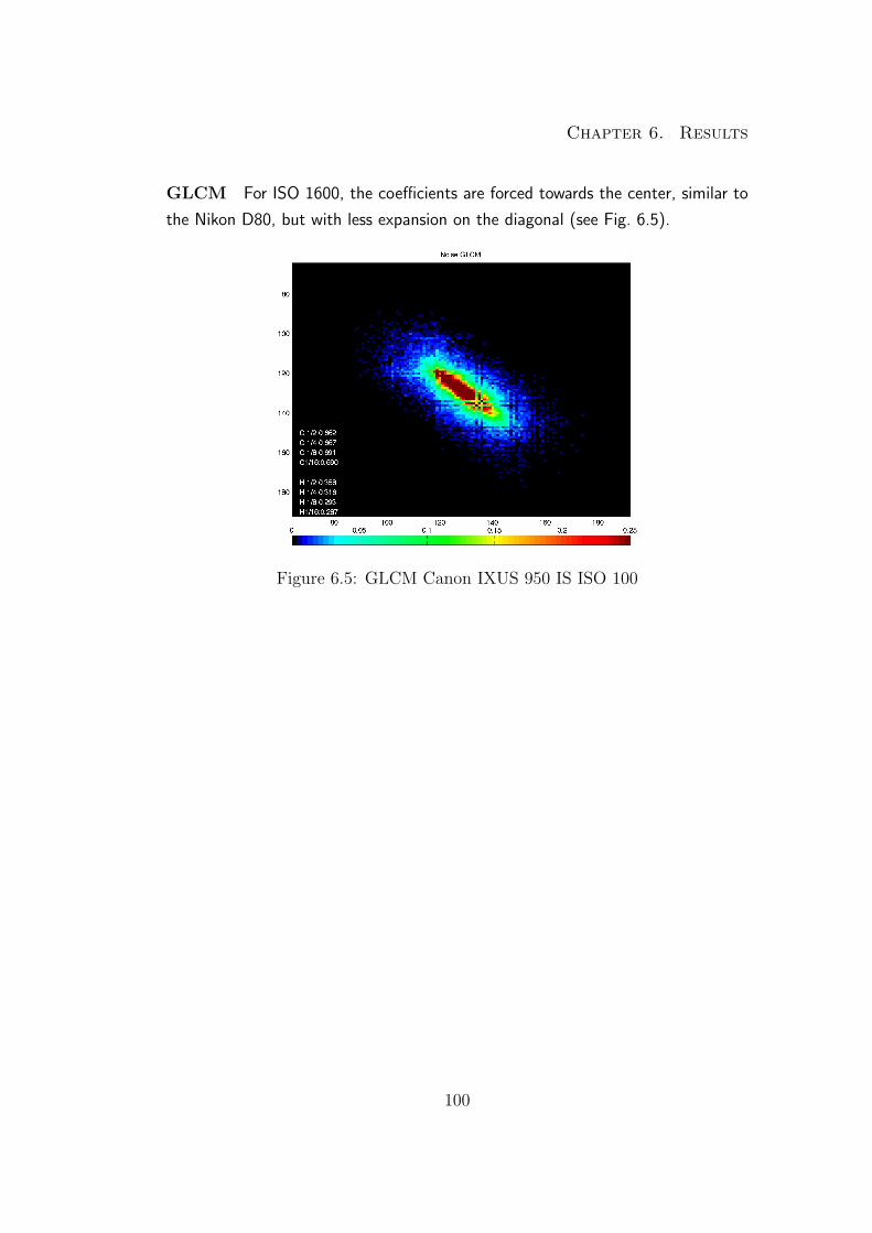
Chapter 6. Results
GLCM For ISO 1600, the coefficients are forced towards the center, similar to
the Nikon D80, but with less expansion on the diagonal (see Fig. 6.5).
Figure 6.5: GLCM Canon IXUS 950 IS ISO 100
100
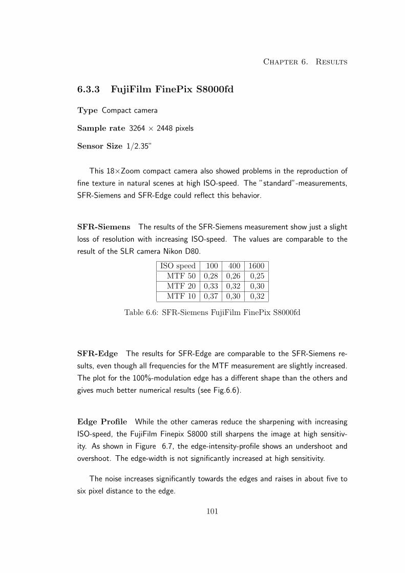
Chapter 6. Results
6.3.3 FujiFilm FinePix S8000fd
Type Compact camera
Sample rate 3264 × 2448 pixels
Sensor Size 1/2.35”
This 18×Zoom compact camera also showed problems in the reproduction of
fine texture in natural scenes at high ISO-speed. The ”standard”-measurements,
SFR-Siemens and SFR-Edge could reflect this behavior.
SFR-Siemens The results of the SFR-Siemens measurement show just a slight
loss of resolution with increasing ISO-speed. The values are comparable to the
result of the SLR camera Nikon D80.
ISO speed 100 400 1600MTF 50 0,28 0,26 0,25MTF 20 0,33 0,32 0,30MTF 10 0,37 0,30 0,32
Table 6.6: SFR-Siemens FujiFilm FinePix S8000fd
SFR-Edge The results for SFR-Edge are comparable to the SFR-Siemens re-
sults, even though all frequencies for the MTF measurement are slightly increased.
The plot for the 100%-modulation edge has a different shape than the others and
gives much better numerical results (see Fig.6.6).
Edge Profile While the other cameras reduce the sharpening with increasing
ISO-speed, the FujiFilm Finepix S8000 still sharpens the image at high sensitiv-
ity. As shown in Figure 6.7, the edge-intensity-profile shows an undershoot and
overshoot. The edge-width is not significantly increased at high sensitivity.
The noise increases significantly towards the edges and raises in about five to
six pixel distance to the edge.
101
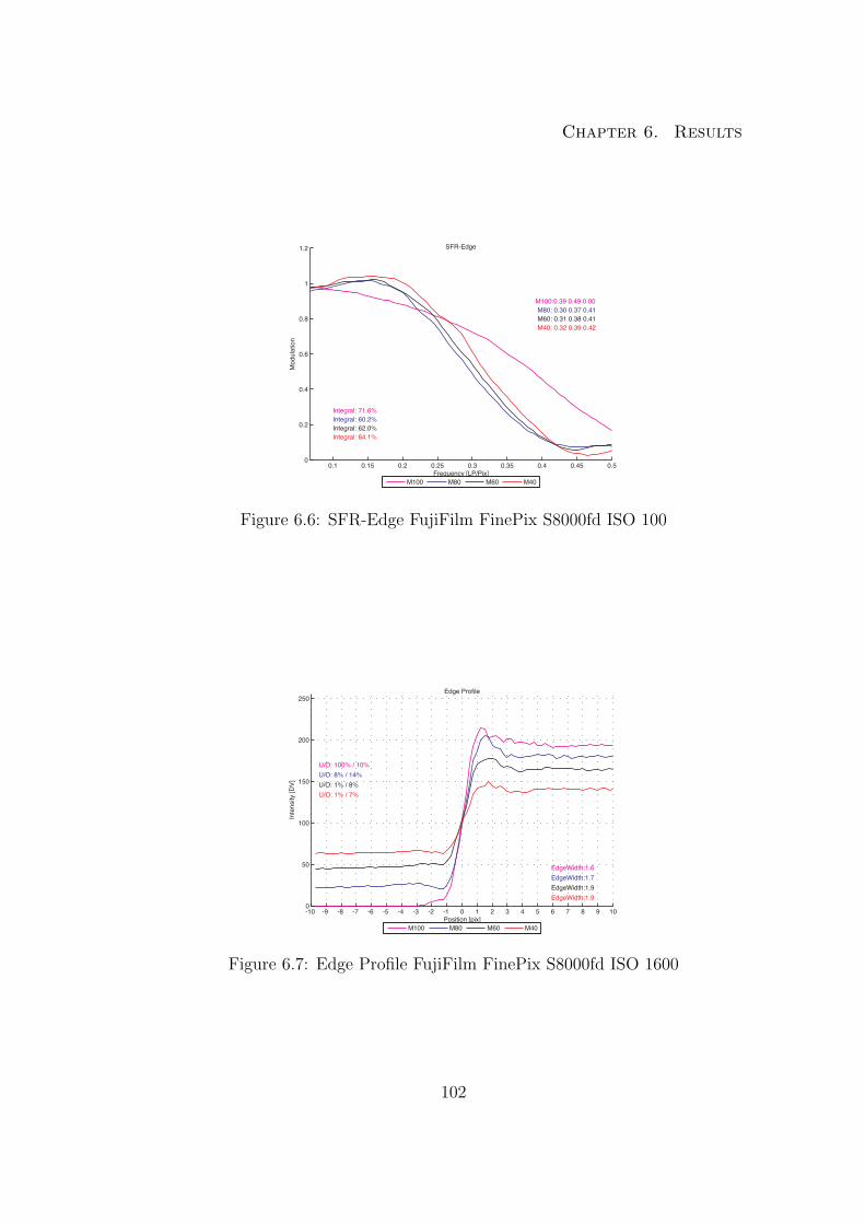
Chapter 6. Results
0.1 0.15 0.2 0.25 0.3 0.35 0.4 0.45 0.50
0.2
0.4
0.6
0.8
1
1.2 SFR-Edge
Frequency [LP/Pix]
Mod
ulat
ion
Integral: 71.6%Integral: 60.2%Integral: 62.0%Integral: 64.1%
M100:0.39 0.49 0.00M80: 0.30 0.37 0.41M60: 0.31 0.38 0.41M40: 0.32 0.39 0.42
M100 M80 M60 M40
Figure 6.6: SFR-Edge FujiFilm FinePix S8000fd ISO 100
-10 -9 -8 -7 -6 -5 -4 -3 -2 -1 0 1 2 3 4 5 6 7 8 9 100
50
100
150
200
250Edge Profile
Position [pix]
Inte
nsity
[DV]
EdgeWidth:1.6EdgeWidth:1.7EdgeWidth:1.9EdgeWidth:1.9
U/O: 100% / 10%U/O: 8% / 14%U/O: 1% / 8%U/O: 1% / 7%
M100 M80 M60 M40
Figure 6.7: Edge Profile FujiFilm FinePix S8000fd ISO 1600
102

Chapter 6. Results
SFR-Noise Against the expectation, the SFR-Noise plot increases at ISO 1600
to a level higher than ISO 100. The SFR-Noise plot for the gray patch has an
integral of 20% at ISO 100, which is 36% of the noise patch integral. With
increasing ISO speed the integral increases and reaches 90% of the noise patch
integral.
Line Profile While the line is clearly visible in the line profile for ISO 100, it is
less visible in ISO 400 and gone in ISO 1600.
Histogram of Derivative The kurtosis measured in the image on different
patches is on a low level for the ISO-speed settings 100 and 400, but is very high
for ISO 1600. This correlates with the visual impressions of the images. Setting
the camera to ISO 1600 results in images that show a significant loss of texture
and appear degraded by noise reduction.
ISO speed 100 400 16001/2 0,9 1,7 9,61/4 0,6 1,2 9,71/8 0,7 1,3 10,6
1/16 1,6 1,2 9,3
Table 6.7: Kurtosis FujiFilm FinePix S8000fd
GLCM For ISO 1600, the coefficients are forced towards the center. The expan-
sion on the diagonal is much lower than for the other cameras. This means, that
the values in the images are forced towards the mean value rather than building
up clusters with different digital values. (see Fig. 6.8).
103

Chapter 6. Results
Figure 6.8: GLCM FujiFilm FinePix S8000fd ISO 1600
104
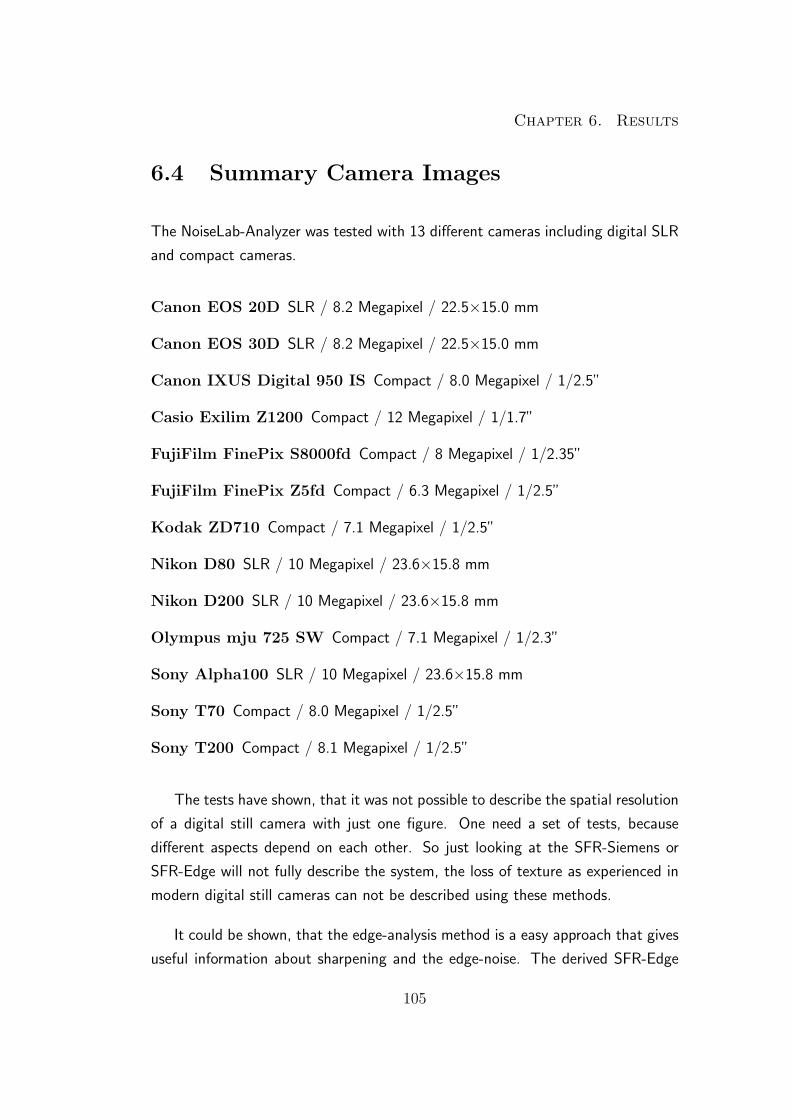
Chapter 6. Results
6.4 Summary Camera Images
The NoiseLab-Analyzer was tested with 13 different cameras including digital SLR
and compact cameras.
Canon EOS 20D SLR / 8.2 Megapixel / 22.5×15.0 mm
Canon EOS 30D SLR / 8.2 Megapixel / 22.5×15.0 mm
Canon IXUS Digital 950 IS Compact / 8.0 Megapixel / 1/2.5”
Casio Exilim Z1200 Compact / 12 Megapixel / 1/1.7”
FujiFilm FinePix S8000fd Compact / 8 Megapixel / 1/2.35”
FujiFilm FinePix Z5fd Compact / 6.3 Megapixel / 1/2.5”
Kodak ZD710 Compact / 7.1 Megapixel / 1/2.5”
Nikon D80 SLR / 10 Megapixel / 23.6×15.8 mm
Nikon D200 SLR / 10 Megapixel / 23.6×15.8 mm
Olympus mju 725 SW Compact / 7.1 Megapixel / 1/2.3”
Sony Alpha100 SLR / 10 Megapixel / 23.6×15.8 mm
Sony T70 Compact / 8.0 Megapixel / 1/2.5”
Sony T200 Compact / 8.1 Megapixel / 1/2.5”
The tests have shown, that it was not possible to describe the spatial resolution
of a digital still camera with just one figure. One need a set of tests, because
different aspects depend on each other. So just looking at the SFR-Siemens or
SFR-Edge will not fully describe the system, the loss of texture as experienced in
modern digital still cameras can not be described using these methods.
It could be shown, that the edge-analysis method is a easy approach that gives
useful information about sharpening and the edge-noise. The derived SFR-Edge
105
Chapter 6. Results
is strongly influenced by image enhancements and fails to determine the limiting
resolution. The approach to describe the noise depending on the distance to the
edge is useful and can extend the noise analysis in tests.
SFR-Siemens is a reliable method to test for spatial resolution. It is less influ-
enced by image enhancements and is useful to give the system SFR. But it fails
to describe the loss of texture in images, as well. As cameras have to be consid-
ered as non-linear systems, they behave different on the siemens-star pattern as
on texture.
The SFR-Noise approach could not proof its benefit in the camera tests, there
is no advantage against the SFR-Siemens method. The differences in SFR-Noise
of gray patches and of patches with target noise showed a coherence with the
visual impression of the images.
The degradation of lines in the image is one aspect of noise-reduction in digital
images. The line profile is a good tool to describe this phenomenon.
The kurtosis of the image-noise, where image-noise is a combination of target-
noise and camera-noise, seems to be a good measurement for describing the non-
linearity of a digital camera. It could be seen, that the higher the kurtosis, the
more the image appear degraded and lack of fine details.
The GLCM as a texture analysis tool is very useful in its visual representation,
but needs more numerical results. The calculated correlation and homogeneity
could not describe the appearance of the GLCM.
106

Chapter 7. Conclusion
Chapter 7
Conclusion
The aim of this thesis was to describe the influence of noise-reduction methods on
the spatial resolution in digital images.
Existing methods have been checked for their usefulness and new approaches
have been developed and tested. The tools NoiseLab and NoiseLab-Analyzer in
combination with the NoiseLab-Chart have been developed and tested.
It could be shown, that the established resolution measurement methods need
to be extended with a texture measurement to give more complex and reliable
information about a digital camera.
The new approaches to test for texture reproduction using gaussian white noise
as target seem to be promising, but needs further testing with a greater amount
of test samples.
107

Appendix A. Graphical and Numerical Results
Appendix A
Graphical and Numerical
Results
108
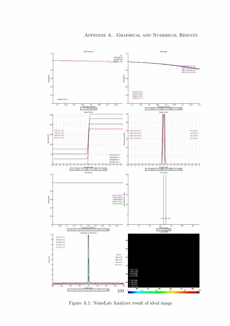
Appendix A. Graphical and Numerical Results
0.1 0.15 0.2 0.25 0.3 0.35 0.4 0.45 0.50
0.2
0.4
0.6
0.8
1
1.2SFR-Siemens
Frequency [LP/Pix]
Mod
ulat
ion
Integral: 99.1%
MTF50: 0.00MTF20: 0.00MTF10: 0.00
SFR-Siemens
0.1 0.15 0.2 0.25 0.3 0.35 0.4 0.45 0.50
0.2
0.4
0.6
0.8
1
1.2SFR-Edge
Frequency [LP/Pix]
Mod
ulat
ion
Integral: 94.3%Integral: 93.9%Integral: 93.5%Integral: 94.1%
M100:0.00 0.00 0.00M80: 0.00 0.00 0.00M60: 0.00 0.00 0.00M40: 0.00 0.00 0.00
M100 M80 M60 M40
-10 -9 -8 -7 -6 -5 -4 -3 -2 -1 0 1 2 3 4 5 6 7 8 9 100
50
100
150
200
250Edge Profile
Position [pix]
Inte
nsity
[DV]
EdgeWidth:0.7EdgeWidth:0.7EdgeWidth:0.7EdgeWidth:0.7
U/O: 0% / 0%U/O: 0% / 0%U/O: 0% / 0%U/O: 0% / 0%
M100 M80 M60 M40
-10 -9 -8 -7 -6 -5 -4 -3 -2 -1 0 1 2 3 4 5 6 7 8 9 100
5
10
15
20
25
30Edge Profile
Position [pix]
Stan
dard
Dev
.[DN
]
STD: 0.0 0.0 0.0STD: 0.0 0.0 0.0STD: 0.0 0.0 0.0STD: 0.0 0.0 0.0
Int: 0.0 0.0Int: 0.0 0.0Int: 0.0 0.0Int: 0.0 0.0
M100 M80 M60 M40
0 0.05 0.1 0.15 0.2 0.25 0.3 0.35 0.4 0.45 0.50
0.2
0.4
0.6
0.8
1
1.2SFR-Noise
Frequency [LP/Pix]
Mod
ulat
ion
Integral:100.0%Integral:99.9%Integral:99.9%
Integral:100.0%Integral:NaN%
1/2 1/4 1/8 1/16 flat
0 20 40 60 80 100 1200
5
10
15
20
25Line Profile
Position [pix]
Stan
dard
Dev
. [D
N]
91.9 0.0 72.7
Line-Profile
-64 -48 -32 -16 0 16 32 48 640
1
2
3
4
5
6
7
8
9
10Histogram of Derivative
digital value
Cou
nt [%
]
Kurtosis:-0.3
Max:8.1
Kurtosis:-0.7
Max:18.6
Kurtosis:-0.5
Max:13.8
Kurtosis:-0.8
Max:22.0
Kurtosis:-2.0
Max:100.0
1/2 1/4 1/8 1/16 flat
Figure A.1: NoiseLab Analyzer result of ideal image
109
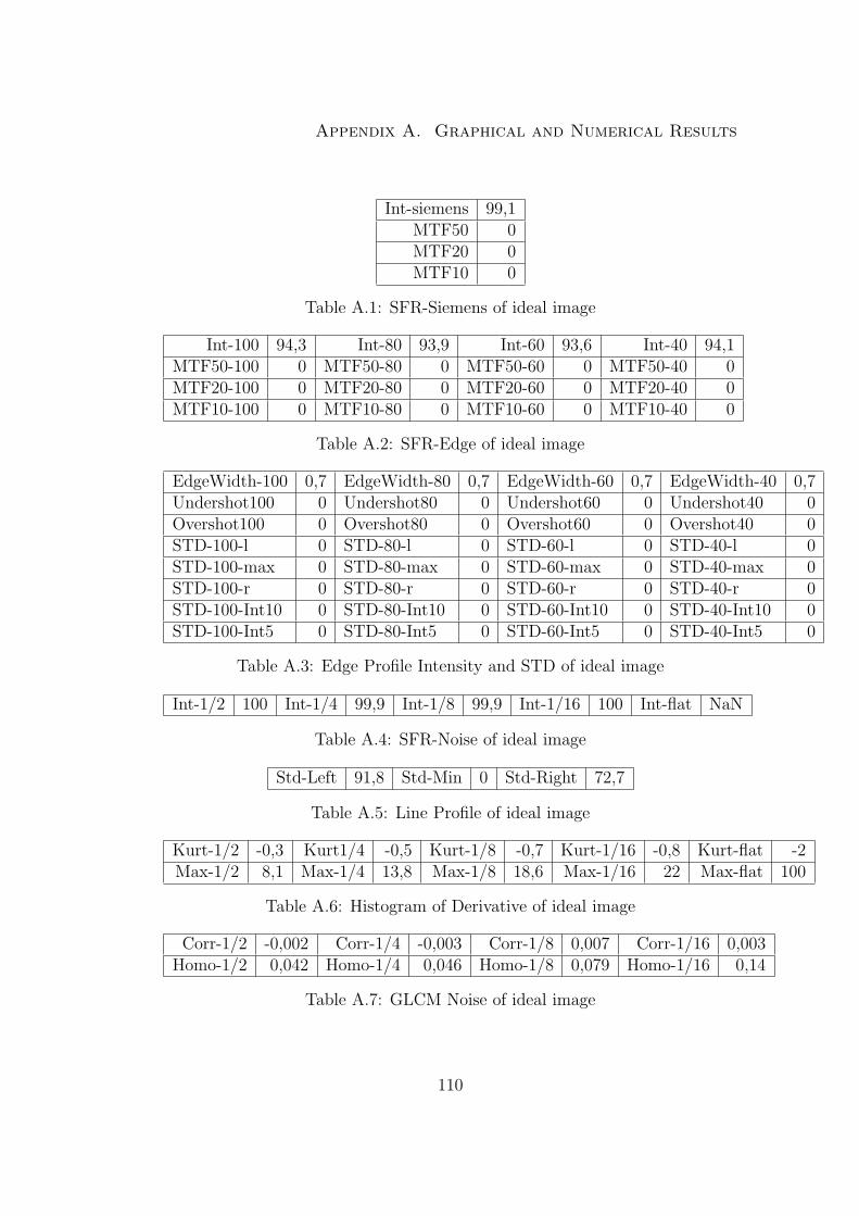
Appendix A. Graphical and Numerical Results
Int-siemens 99,1MTF50 0MTF20 0MTF10 0
Table A.1: SFR-Siemens of ideal image
Int-100 94,3 Int-80 93,9 Int-60 93,6 Int-40 94,1MTF50-100 0 MTF50-80 0 MTF50-60 0 MTF50-40 0MTF20-100 0 MTF20-80 0 MTF20-60 0 MTF20-40 0MTF10-100 0 MTF10-80 0 MTF10-60 0 MTF10-40 0
Table A.2: SFR-Edge of ideal image
EdgeWidth-100 0,7 EdgeWidth-80 0,7 EdgeWidth-60 0,7 EdgeWidth-40 0,7Undershot100 0 Undershot80 0 Undershot60 0 Undershot40 0Overshot100 0 Overshot80 0 Overshot60 0 Overshot40 0STD-100-l 0 STD-80-l 0 STD-60-l 0 STD-40-l 0STD-100-max 0 STD-80-max 0 STD-60-max 0 STD-40-max 0STD-100-r 0 STD-80-r 0 STD-60-r 0 STD-40-r 0STD-100-Int10 0 STD-80-Int10 0 STD-60-Int10 0 STD-40-Int10 0STD-100-Int5 0 STD-80-Int5 0 STD-60-Int5 0 STD-40-Int5 0
Table A.3: Edge Profile Intensity and STD of ideal image
Int-1/2 100 Int-1/4 99,9 Int-1/8 99,9 Int-1/16 100 Int-flat NaN
Table A.4: SFR-Noise of ideal image
Std-Left 91,8 Std-Min 0 Std-Right 72,7
Table A.5: Line Profile of ideal image
Kurt-1/2 -0,3 Kurt1/4 -0,5 Kurt-1/8 -0,7 Kurt-1/16 -0,8 Kurt-flat -2Max-1/2 8,1 Max-1/4 13,8 Max-1/8 18,6 Max-1/16 22 Max-flat 100
Table A.6: Histogram of Derivative of ideal image
Corr-1/2 -0,002 Corr-1/4 -0,003 Corr-1/8 0,007 Corr-1/16 0,003Homo-1/2 0,042 Homo-1/4 0,046 Homo-1/8 0,079 Homo-1/16 0,14
Table A.7: GLCM Noise of ideal image
110

Appendix A. Graphical and Numerical Results
0 20 40 60 80 100 1200
5
10
15
20
25Line Profile
Position [pix]
Stan
dard
Dev
. [D
N]
26.7 6.2 22.6
Line-Profile
-64 -48 -32 -16 0 16 32 48 640
1
2
3
4
5
6
7
8
9
10Histogram of Derivative
digital value
Cou
nt [%
]
Kurtosis:0.0
Max:2.5
Kurtosis:-0.1
Max:2.1
Kurtosis:-0.1
Max:1.9
Kurtosis:-0.1
Max:1.6
Kurtosis:0.1
Max:5.2
1/2 1/4 1/8 1/16 flat
0.1 0.15 0.2 0.25 0.3 0.35 0.4 0.45 0.50
0.2
0.4
0.6
0.8
1
1.2SFR-Siemens
Frequency [LP/Pix]
Mod
ulat
ion
Integral: 48.8%
MTF50: 0.25MTF20: 0.36MTF10: 0.43
SFR-Siemens
0.1 0.15 0.2 0.25 0.3 0.35 0.4 0.45 0.50
0.2
0.4
0.6
0.8
1
1.2SFR-Edge
Frequency [LP/Pix]
Mod
ulat
ion
Integral: 43.0%Integral: 42.1%Integral: 43.1%Integral: 44.1%
M100:0.22 0.31 0.37M80: 0.21 0.31 0.36M60: 0.21 0.31 0.38M40: 0.20 0.31 0.38
M100 M80 M60 M40
0 0.05 0.1 0.15 0.2 0.25 0.3 0.35 0.4 0.45 0.50
0.2
0.4
0.6
0.8
1
1.2SFR-Noise
Frequency [LP/Pix]
Mod
ulat
ion
Integral:49.4%Integral:47.1%Integral:47.2%Integral:47.0%Integral:99.9%
1/2 1/4 1/8 1/16 flat
-10 -9 -8 -7 -6 -5 -4 -3 -2 -1 0 1 2 3 4 5 6 7 8 9 100
50
100
150
200
250Edge Profile
Position [pix]
Inte
nsity
[DV]
EdgeWidth:2.5EdgeWidth:2.6EdgeWidth:2.6EdgeWidth:2.6
U/O: 41% / 0%U/O: 6% / 0%U/O: 3% / 0%U/O: 1% / 1%
M100 M80 M60 M40
-10 -9 -8 -7 -6 -5 -4 -3 -2 -1 0 1 2 3 4 5 6 7 8 9 100
5
10
15
20
25
30Edge Profile
Position [pix]
Stan
dard
Dev
.[DN
]
STD: 1.9 5.7 3.2STD: 5.7 7.2 5.8STD: 5.4 7.4 5.4STD: 5.5 7.1 5.6
Int: 3.5 3.6Int: 6.4 6.4Int: 6.3 6.3Int: 6.2 6.2
M100 M80 M60 M40
Figure A.2: NoiseLab Analyzer result of N2
111
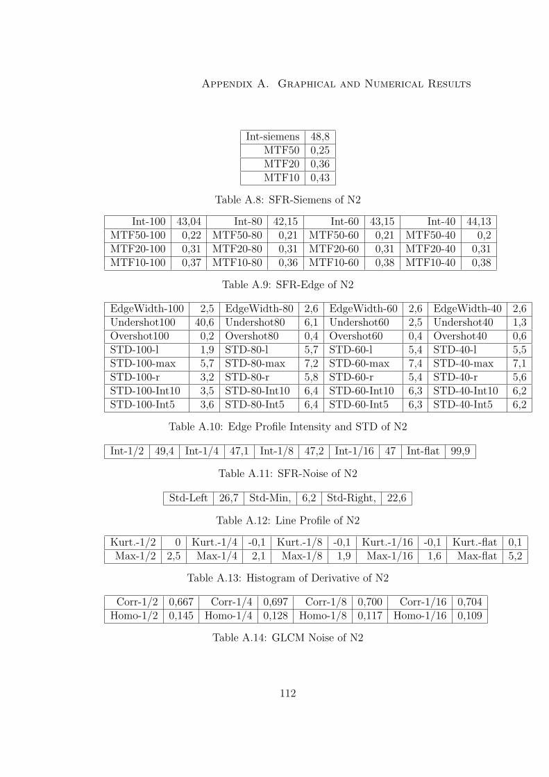
Appendix A. Graphical and Numerical Results
Int-siemens 48,8MTF50 0,25MTF20 0,36MTF10 0,43
Table A.8: SFR-Siemens of N2
Int-100 43,04 Int-80 42,15 Int-60 43,15 Int-40 44,13MTF50-100 0,22 MTF50-80 0,21 MTF50-60 0,21 MTF50-40 0,2MTF20-100 0,31 MTF20-80 0,31 MTF20-60 0,31 MTF20-40 0,31MTF10-100 0,37 MTF10-80 0,36 MTF10-60 0,38 MTF10-40 0,38
Table A.9: SFR-Edge of N2
EdgeWidth-100 2,5 EdgeWidth-80 2,6 EdgeWidth-60 2,6 EdgeWidth-40 2,6Undershot100 40,6 Undershot80 6,1 Undershot60 2,5 Undershot40 1,3Overshot100 0,2 Overshot80 0,4 Overshot60 0,4 Overshot40 0,6STD-100-l 1,9 STD-80-l 5,7 STD-60-l 5,4 STD-40-l 5,5STD-100-max 5,7 STD-80-max 7,2 STD-60-max 7,4 STD-40-max 7,1STD-100-r 3,2 STD-80-r 5,8 STD-60-r 5,4 STD-40-r 5,6STD-100-Int10 3,5 STD-80-Int10 6,4 STD-60-Int10 6,3 STD-40-Int10 6,2STD-100-Int5 3,6 STD-80-Int5 6,4 STD-60-Int5 6,3 STD-40-Int5 6,2
Table A.10: Edge Profile Intensity and STD of N2
Int-1/2 49,4 Int-1/4 47,1 Int-1/8 47,2 Int-1/16 47 Int-flat 99,9
Table A.11: SFR-Noise of N2
Std-Left 26,7 Std-Min, 6,2 Std-Right, 22,6
Table A.12: Line Profile of N2
Kurt.-1/2 0 Kurt.-1/4 -0,1 Kurt.-1/8 -0,1 Kurt.-1/16 -0,1 Kurt.-flat 0,1Max-1/2 2,5 Max-1/4 2,1 Max-1/8 1,9 Max-1/16 1,6 Max-flat 5,2
Table A.13: Histogram of Derivative of N2
Corr-1/2 0,667 Corr-1/4 0,697 Corr-1/8 0,700 Corr-1/16 0,704Homo-1/2 0,145 Homo-1/4 0,128 Homo-1/8 0,117 Homo-1/16 0,109
Table A.14: GLCM Noise of N2
112
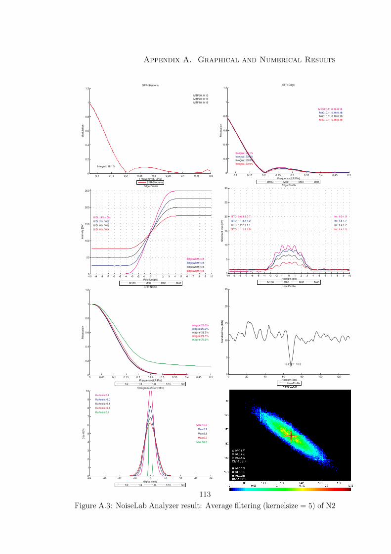
Appendix A. Graphical and Numerical Results
-64 -48 -32 -16 0 16 32 48 640
1
2
3
4
5
6
7
8
9
10Histogram of Derivative
digital value
Cou
nt [%
]
Kurtosis:0.1
Max:10.5
Kurtosis:-0.0
Max:8.2
Kurtosis:-0.1
Max:6.9
Kurtosis:-0.1
Max:6.2
Kurtosis:0.7
Max:59.0
1/2 1/4 1/8 1/16 flat
0 20 40 60 80 100 1200
5
10
15
20
25Line Profile
Position [pix]
Stan
dard
Dev
. [D
N]
12.2 2.1 10.2
Line-Profile
0 0.05 0.1 0.15 0.2 0.25 0.3 0.35 0.4 0.45 0.50
0.2
0.4
0.6
0.8
1
1.2SFR-Noise
Frequency [LP/Pix]
Mod
ulat
ion Integral:23.0%
Integral:23.0%Integral:23.2%Integral:24.1%Integral:35.5%
1/2 1/4 1/8 1/16 flat
-10 -9 -8 -7 -6 -5 -4 -3 -2 -1 0 1 2 3 4 5 6 7 8 9 100
5
10
15
20
25
30Edge Profile
Position [pix]
Stan
dard
Dev
.[DN
]
STD: 0.6 3.8 0.7STD: 1.1 3.4 1.2STD: 1.2 2.7 1.1STD: 1.1 1.9 1.0
Int: 1.0 1.5Int: 1.5 1.7Int: 1.4 1.7Int: 1.4 1.5
M100 M80 M60 M40
-10 -9 -8 -7 -6 -5 -4 -3 -2 -1 0 1 2 3 4 5 6 7 8 9 100
50
100
150
200
250Edge Profile
Position [pix]
Inte
nsity
[DV]
EdgeWidth:4.8EdgeWidth:4.8EdgeWidth:4.8EdgeWidth:4.8
U/O: 14% / 0%U/O: 2% / 0%U/O: 0% / 0%U/O: 0% / 0%
M100 M80 M60 M40
0.1 0.15 0.2 0.25 0.3 0.35 0.4 0.45 0.50
0.2
0.4
0.6
0.8
1
1.2SFR-Siemens
Frequency [LP/Pix]
Mod
ulat
ion
Integral: 18.1%
MTF50: 0.13MTF20: 0.17MTF10: 0.19
SFR-Siemens
0.1 0.15 0.2 0.25 0.3 0.35 0.4 0.45 0.50
0.2
0.4
0.6
0.8
1
1.2SFR-Edge
Frequency [LP/Pix]
Mod
ulat
ion
Integral: 23.1%Integral: 23.0%Integral: 23.0%Integral: 23.0%
M100:0.11 0.16 0.18M80: 0.11 0.16 0.18M60: 0.11 0.16 0.18M40: 0.11 0.16 0.18
M100 M80 M60 M40
Figure A.3: NoiseLab Analyzer result: Average filtering (kernelsize = 5) of N2
113
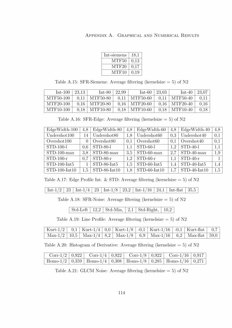
Appendix A. Graphical and Numerical Results
Int-siemens 18,1MTF50 0,13MTF20 0,17MTF10 0,19
Table A.15: SFR-Siemens: Average filtering (kernelsize = 5) of N2
Int-100 23,13 Int-80 22,99 Int-60 23,03 Int-40 23,07MTF50-100 0,11 MTF50-80 0,11 MTF50-60 0,11 MTF50-40 0,11MTF20-100 0,16 MTF20-80 0,16 MTF20-60 0,16 MTF20-40 0,16MTF10-100 0,18 MTF10-80 0,18 MTF10-60 0,18 MTF10-40 0,18
Table A.16: SFR-Edge: Average filtering (kernelsize = 5) of N2
EdgeWidth-100 4,8 EdgeWidth-80 4,8 EdgeWidth-60 4,8 EdgeWidth-40 4,8Undershot100 14 Undershot80 1,8 Undershot60 0,3 Undershot40 0,1Overshot100 0 Overshot80 0,1 Overshot60 0,1 Overshot40 0,1STD-100-l 0,6 STD-80-l 1,1 STD-60-l 1,2 STD-40-l 1,1STD-100-max 3,8 STD-80-max 3,5 STD-60-max 2,7 STD-40-max 1,9STD-100-r 0,7 STD-80-r 1,2 STD-60-r 1,1 STD-40-r 1STD-100-Int5 1 STD-80-Int5 1,5 STD-60-Int5 1,4 STD-40-Int5 1,4STD-100-Int10 1,5 STD-80-Int10 1,8 STD-60-Int10 1,7 STD-40-Int10 1,5
Table A.17: Edge Profile Int. & STD: Average filtering (kernelsize = 5) of N2
Int-1/2 23 Int-1/4 23 Int-1/8 23,2 Int-1/16 24,1 Int-flat 35,5
Table A.18: SFR-Noise: Average filtering (kernelsize = 5) of N2
Std-Left 12,2 Std-Min, 2,1 Std-Right, 10,2
Table A.19: Line Profile: Average filtering (kernelsize = 5) of N2
Kurt-1/2 0,1 Kurt-1/4 0,0 Kurt-1/8 -0,1 Kurt-1/16 -0,1 Kurt-flat 0,7Max-1/2 10,5 Max-1/4 8,2 Max-1/8 6,9 Max-1/16 6,2 Max-flat 59,0
Table A.20: Histogram of Derivative: Average filtering (kernelsize = 5) of N2
Corr-1/2 0,922 Corr-1/4 0,922 Corr-1/8 0,922 Corr-1/16 0,917Homo-1/2 0,359 Homo-1/4 0,308 Homo-1/8 0,285 Homo-1/16 0,271
Table A.21: GLCM Noise: Average filtering (kernelsize = 5) of N2
114

Appendix A. Graphical and Numerical Results
-64 -48 -32 -16 0 16 32 48 640
1
2
3
4
5
6
7
8
9
10Histogram of Derivative
digital value
Cou
nt [%
]
Kurtosis:0.1
Max:10.5
Kurtosis:0.3
Max:8.2
Kurtosis:0.6
Max:7.0
Kurtosis:2.2
Max:6.3
Kurtosis:0.7
Max:59.0
1/2 1/4 1/8 1/16 flat
0 20 40 60 80 100 1200
5
10
15
20
25Line Profile
Position [pix]
Stan
dard
Dev
. [D
N]
12.2 2.1 10.2
Line-Profile
0 0.05 0.1 0.15 0.2 0.25 0.3 0.35 0.4 0.45 0.50
0.2
0.4
0.6
0.8
1
1.2SFR-Noise
Frequency [LP/Pix]
Mod
ulat
ion
Integral:23.0%Integral:23.0%Integral:23.5%Integral:24.9%Integral:35.5%
1/2 1/4 1/8 1/16 flat
-10 -9 -8 -7 -6 -5 -4 -3 -2 -1 0 1 2 3 4 5 6 7 8 9 100
5
10
15
20
25
30Edge Profile
Position [pix]
Stan
dard
Dev
.[DN
]
STD: 0.6 4.2 0.7STD: 1.2 3.3 1.1STD: 1.2 2.4 1.1STD: 1.2 1.8 1.0
Int: 1.2 1.8Int: 1.5 1.8Int: 1.4 1.6Int: 1.3 1.4
M100 M80 M60 M40
-10 -9 -8 -7 -6 -5 -4 -3 -2 -1 0 1 2 3 4 5 6 7 8 9 100
50
100
150
200
250Edge Profile
Position [pix]
Inte
nsity
[DV]
EdgeWidth:2.8EdgeWidth:4.0EdgeWidth:4.8EdgeWidth:4.8
U/O: 15% / 0%U/O: 2% / 0%U/O: 0% / 0%U/O: 0% / 0%
M100 M80 M60 M40
0.1 0.15 0.2 0.25 0.3 0.35 0.4 0.45 0.50
0.2
0.4
0.6
0.8
1
1.2SFR-Siemens
Frequency [LP/Pix]
Mod
ulat
ion
Integral: 24.0%
MTF50: 0.17MTF20: 0.20MTF10: 0.21
SFR-Siemens
0.1 0.15 0.2 0.25 0.3 0.35 0.4 0.45 0.50
0.2
0.4
0.6
0.8
1
1.2SFR-Edge
Frequency [LP/Pix]
Mod
ulat
ion
Integral: 41.4%Integral: 38.4%Integral: 35.5%Integral: 23.9%
M100:0.16 0.36 0.40M80: 0.14 0.37 0.41M60: 0.13 0.27 0.48M40: 0.11 0.16 0.18
M100 M80 M60 M40
Figure A.4: NoiseLab Analyzer result: Wiener filtering (kernelsize = 5) of N2
115
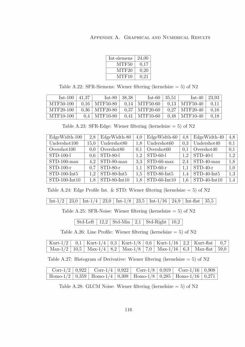
Appendix A. Graphical and Numerical Results
Int-siemens 24,00MTF50 0,17MTF20 0,20MTF10 0,21
Table A.22: SFR-Siemens: Wiener filtering (kernelsize = 5) of N2
Int-100 41,37 Int-80 38,38 Int-60 35,51 Int-40 23,93MTF50-100 0,16 MTF50-80 0,14 MTF50-60 0,13 MTF50-40 0,11MTF20-100 0,36 MTF20-80 0,37 MTF20-60 0,27 MTF20-40 0,16MTF10-100 0,4 MTF10-80 0,41 MTF10-60 0,48 MTF10-40 0,18
Table A.23: SFR-Edge: Wiener filtering (kernelsize = 5) of N2
EdgeWidth-100 2,8 EdgeWidth-80 4,0 EdgeWidth-60 4,8 EdgeWidth-40 4,8Undershot100 15,0 Undershot80 1,8 Undershot60 0,3 Undershot40 0,1Overshot100 0,0 Overshot80 0,1 Overshot60 0,1 Overshot40 0,1STD-100-l 0,6 STD-80-l 1,2 STD-60-l 1,2 STD-40-l 1,2STD-100-max 4,2 STD-80-max 3,3 STD-60-max 2,4 STD-40-max 1,8STD-100-r 0,7 STD-80-r 1,1 STD-60-r 1,1 STD-40-r 1,0STD-100-Int5 1,2 STD-80-Int5 1,5 STD-80-Int5 1,4 STD-40-Int5 1,3STD-100-Int10 1,8 STD-80-Int10 1,8 STD-60-Int10 1,6 STD-40-Int10 1,4
Table A.24: Edge Profile Int. & STD: Wiener filtering (kernelsize = 5) of N2
Int-1/2 23,0 Int-1/4 23,0 Int-1/8 23,5 Int-1/16 24,9 Int-flat 35,5
Table A.25: SFR-Noise: Wiener filtering (kernelsize = 5) of N2
Std-Left 12,2 Std-Min 2,1 Std-Right 10,2
Table A.26: Line Profile: Wiener filtering (kernelsize = 5) of N2
Kurt-1/2 0,1 Kurt-1/4 0,3 Kurt-1/8 0,6 Kurt-1/16 2,2 Kurt-flat 0,7Max-1/2 10,5 Max-1/4 8,2 Max-1/8 7,0 Max-1/16 6,3 Max-flat 59,0
Table A.27: Histogram of Derivative: Wiener filtering (kernelsize = 5) of N2
Corr-1/2 0,922 Corr-1/4 0,922 Corr-1/8 0,919 Corr-1/16 0,908Homo-1/2 0,359 Homo-1/4 0,308 Homo-1/8 0,285 Homo-1/16 0,271
Table A.28: GLCM Noise: Wiener filtering (kernelsize = 5) of N2
116
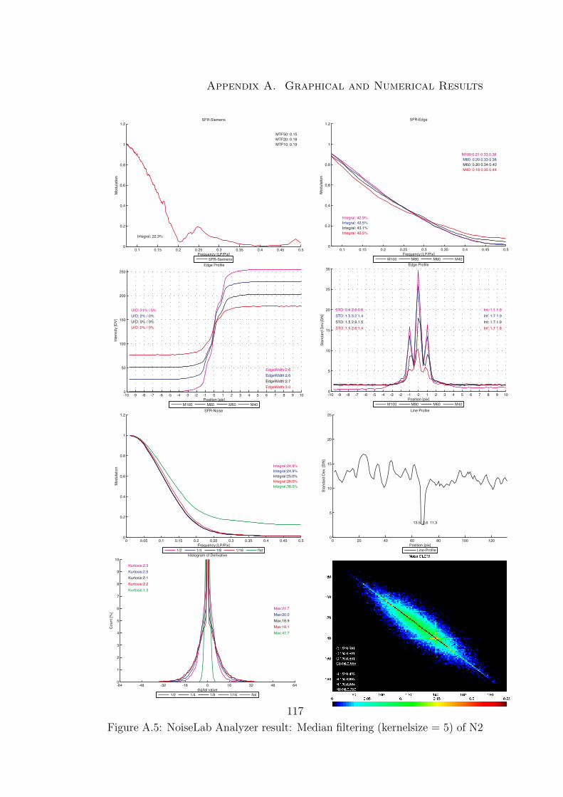
Appendix A. Graphical and Numerical Results
-64 -48 -32 -16 0 16 32 48 640
1
2
3
4
5
6
7
8
9
10Histogram of Derivative
digital value
Cou
nt [%
]
Kurtosis:2.3
Max:21.7
Kurtosis:2.5
Max:20.0
Kurtosis:2.1
Max:18.9
Kurtosis:2.2
Max:18.1
Kurtosis:1.3
Max:47.7
1/2 1/4 1/8 1/16 flat
0 20 40 60 80 100 1200
5
10
15
20
25Line Profile
Position [pix]
Stan
dard
Dev
. [D
N]
13.5 2.6 11.3
Line-Profile
0 0.05 0.1 0.15 0.2 0.25 0.3 0.35 0.4 0.45 0.50
0.2
0.4
0.6
0.8
1
1.2SFR-Noise
Frequency [LP/Pix]
Mod
ulat
ion
Integral:24.9%Integral:24.9%Integral:25.0%Integral:26.0%Integral:36.0%
1/2 1/4 1/8 1/16 flat
-10 -9 -8 -7 -6 -5 -4 -3 -2 -1 0 1 2 3 4 5 6 7 8 9 100
5
10
15
20
25
30Edge Profile
Position [pix]
Stan
dard
Dev
.[DN
]
STD: 0.4 2.6 0.8STD: 1.5 3.2 1.4STD: 1.5 2.9 1.5STD: 1.4 2.6 1.4
Int: 1.1 1.6Int: 1.7 1.9Int: 1.7 1.9Int: 1.7 1.8
M100 M80 M60 M40
-10 -9 -8 -7 -6 -5 -4 -3 -2 -1 0 1 2 3 4 5 6 7 8 9 100
50
100
150
200
250Edge Profile
Position [pix]
Inte
nsity
[DV]
EdgeWidth:2.6EdgeWidth:2.6EdgeWidth:2.7EdgeWidth:3.0
U/O: 31% / 0%U/O: 2% / 0%U/O: 0% / 0%U/O: 0% / 0%
M100 M80 M60 M40
0.1 0.15 0.2 0.25 0.3 0.35 0.4 0.45 0.50
0.2
0.4
0.6
0.8
1
1.2SFR-Siemens
Frequency [LP/Pix]
Mod
ulat
ion
Integral: 22.3%
MTF50: 0.15MTF20: 0.18MTF10: 0.19
SFR-Siemens
0.1 0.15 0.2 0.25 0.3 0.35 0.4 0.45 0.50
0.2
0.4
0.6
0.8
1
1.2SFR-Edge
Frequency [LP/Pix]
Mod
ulat
ion
Integral: 42.9%Integral: 42.5%Integral: 43.1%Integral: 42.5%
M100:0.21 0.33 0.38M80: 0.20 0.33 0.38M60: 0.20 0.34 0.40M40: 0.18 0.35 0.44
M100 M80 M60 M40
Figure A.5: NoiseLab Analyzer result: Median filtering (kernelsize = 5) of N2
117
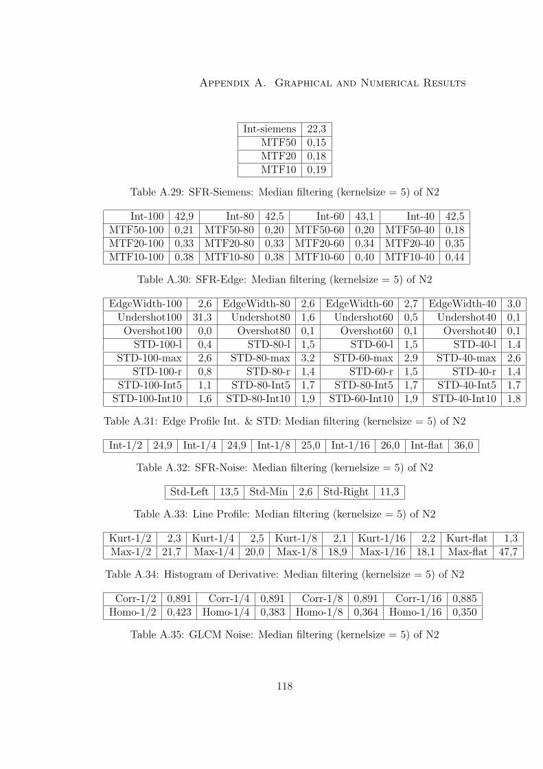
Appendix A. Graphical and Numerical Results
Int-siemens 22,3MTF50 0,15MTF20 0,18MTF10 0,19
Table A.29: SFR-Siemens: Median filtering (kernelsize = 5) of N2
Int-100 42,9 Int-80 42,5 Int-60 43,1 Int-40 42,5MTF50-100 0,21 MTF50-80 0,20 MTF50-60 0,20 MTF50-40 0,18MTF20-100 0,33 MTF20-80 0,33 MTF20-60 0,34 MTF20-40 0,35MTF10-100 0,38 MTF10-80 0,38 MTF10-60 0,40 MTF10-40 0,44
Table A.30: SFR-Edge: Median filtering (kernelsize = 5) of N2
EdgeWidth-100 2,6 EdgeWidth-80 2,6 EdgeWidth-60 2,7 EdgeWidth-40 3,0Undershot100 31,3 Undershot80 1,6 Undershot60 0,5 Undershot40 0,1
Overshot100 0,0 Overshot80 0,1 Overshot60 0,1 Overshot40 0,1STD-100-l 0,4 STD-80-l 1,5 STD-60-l 1,5 STD-40-l 1,4
STD-100-max 2,6 STD-80-max 3,2 STD-60-max 2,9 STD-40-max 2,6STD-100-r 0,8 STD-80-r 1,4 STD-60-r 1,5 STD-40-r 1,4
STD-100-Int5 1,1 STD-80-Int5 1,7 STD-80-Int5 1,7 STD-40-Int5 1,7STD-100-Int10 1,6 STD-80-Int10 1,9 STD-60-Int10 1,9 STD-40-Int10 1,8
Table A.31: Edge Profile Int. & STD: Median filtering (kernelsize = 5) of N2
Int-1/2 24,9 Int-1/4 24,9 Int-1/8 25,0 Int-1/16 26,0 Int-flat 36,0
Table A.32: SFR-Noise: Median filtering (kernelsize = 5) of N2
Std-Left 13,5 Std-Min 2,6 Std-Right 11,3
Table A.33: Line Profile: Median filtering (kernelsize = 5) of N2
Kurt-1/2 2,3 Kurt-1/4 2,5 Kurt-1/8 2,1 Kurt-1/16 2,2 Kurt-flat 1,3Max-1/2 21,7 Max-1/4 20,0 Max-1/8 18,9 Max-1/16 18,1 Max-flat 47,7
Table A.34: Histogram of Derivative: Median filtering (kernelsize = 5) of N2
Corr-1/2 0,891 Corr-1/4 0,891 Corr-1/8 0,891 Corr-1/16 0,885Homo-1/2 0,423 Homo-1/4 0,383 Homo-1/8 0,364 Homo-1/16 0,350
Table A.35: GLCM Noise: Median filtering (kernelsize = 5) of N2
118
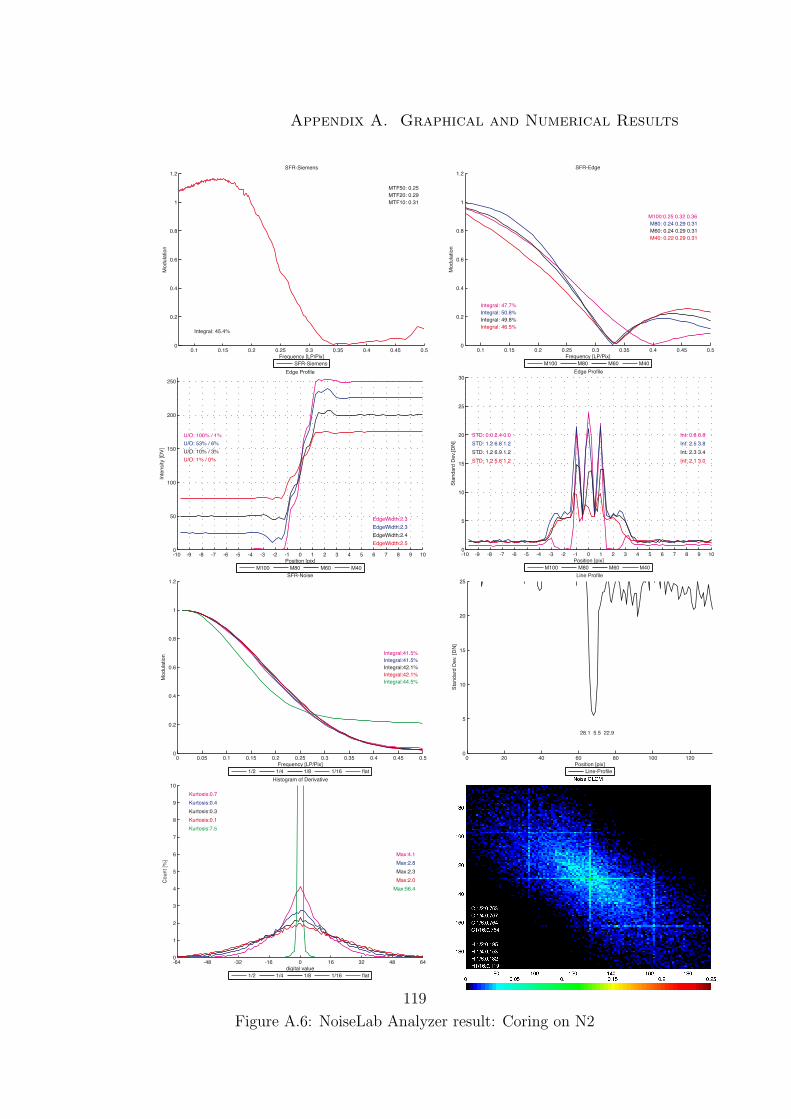
Appendix A. Graphical and Numerical Results
-64 -48 -32 -16 0 16 32 48 640
1
2
3
4
5
6
7
8
9
10Histogram of Derivative
digital value
Cou
nt [%
]
Kurtosis:0.7
Max:4.1
Kurtosis:0.4
Max:2.8
Kurtosis:0.3
Max:2.3
Kurtosis:0.1
Max:2.0
Kurtosis:7.5
Max:56.4
1/2 1/4 1/8 1/16 flat
0 20 40 60 80 100 1200
5
10
15
20
25Line Profile
Position [pix]
Stan
dard
Dev
. [D
N]
28.1 5.5 22.9
Line-Profile
0 0.05 0.1 0.15 0.2 0.25 0.3 0.35 0.4 0.45 0.50
0.2
0.4
0.6
0.8
1
1.2SFR-Noise
Frequency [LP/Pix]
Mod
ulat
ion
Integral:41.5%Integral:41.5%Integral:42.1%Integral:42.1%Integral:44.5%
1/2 1/4 1/8 1/16 flat
-10 -9 -8 -7 -6 -5 -4 -3 -2 -1 0 1 2 3 4 5 6 7 8 9 100
5
10
15
20
25
30Edge Profile
Position [pix]
Stan
dard
Dev
.[DN
]
STD: 0.0 2.4 0.0STD: 1.2 6.8 1.2STD: 1.2 6.9 1.2STD: 1.2 5.6 1.2
Int: 0.8 0.8Int: 2.5 3.8Int: 2.3 3.4Int: 2.1 3.0
M100 M80 M60 M40
-10 -9 -8 -7 -6 -5 -4 -3 -2 -1 0 1 2 3 4 5 6 7 8 9 100
50
100
150
200
250Edge Profile
Position [pix]
Inte
nsity
[DV]
EdgeWidth:2.3EdgeWidth:2.3EdgeWidth:2.4EdgeWidth:2.5
U/O: 100% / 1%U/O: 53% / 6%U/O: 10% / 3%U/O: 1% / 0%
M100 M80 M60 M40
0.1 0.15 0.2 0.25 0.3 0.35 0.4 0.45 0.50
0.2
0.4
0.6
0.8
1
1.2SFR-Siemens
Frequency [LP/Pix]
Mod
ulat
ion
Integral: 45.4%
MTF50: 0.25MTF20: 0.29MTF10: 0.31
SFR-Siemens
0.1 0.15 0.2 0.25 0.3 0.35 0.4 0.45 0.50
0.2
0.4
0.6
0.8
1
1.2SFR-Edge
Frequency [LP/Pix]
Mod
ulat
ion
Integral: 47.7%Integral: 50.8%Integral: 49.8%Integral: 46.5%
M100:0.25 0.32 0.36M80: 0.24 0.29 0.31M60: 0.24 0.29 0.31M40: 0.22 0.29 0.31
M100 M80 M60 M40
Figure A.6: NoiseLab Analyzer result: Coring on N2
119
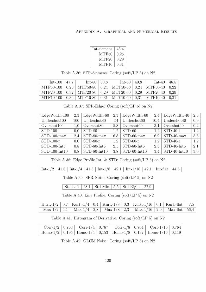
Appendix A. Graphical and Numerical Results
Int-siemens 45,4MTF50 0,25MTF20 0,29MTF10 0,31
Table A.36: SFR-Siemens: Coring (soft/LP 5) on N2
Int-100 47,7 Int-80 50,8 Int-60 49,8 Int-40 46,5MTF50-100 0,25 MTF50-80 0,24 MTF50-60 0,24 MTF50-40 0,22MTF20-100 0,32 MTF20-80 0,29 MTF20-60 0,29 MTF20-40 0,29MTF10-100 0,36 MTF10-80 0,31 MTF10-60 0,31 MTF10-40 0,31
Table A.37: SFR-Edge: Coring (soft/LP 5) on N2
EdgeWidth-100 2,3 EdgeWidth-80 2,3 EdgeWidth-60 2,4 EdgeWidth-40 2,5Undershot100 100 Undershot80 54 Undershot60 10,4 Undershot40 0,9Overshot100 1,0 Overshot80 5,8 Overshot60 3,1 Overshot40 0,2STD-100-l 0,0 STD-80-l 1,2 STD-60-l 1,2 STD-40-l 1,2STD-100-max 2,4 STD-80-max 6,8 STD-60-max 6,9 STD-40-max 5,6STD-100-r 0,0 STD-80-r 1,2 STD-60-r 1,2 STD-40-r 1,2STD-100-Int5 0,8 STD-80-Int5 2,5 STD-80-Int5 2,3 STD-40-Int5 2,1STD-100-Int10 0,8 STD-80-Int10 3,8 STD-60-Int10 3,4 STD-40-Int10 3,0
Table A.38: Edge Profile Int. & STD: Coring (soft/LP 5) on N2
Int-1/2 41,5 Int-1/4 41,5 Int-1/8 42,1 Int-1/16 42,1 Int-flat 44,5
Table A.39: SFR-Noise: Coring (soft/LP 5) on N2
Std-Left 28,1 Std-Min 5,5 Std-Right 22,9
Table A.40: Line Profile: Coring (soft/LP 5) on N2
Kurt,-1/2 0,7 Kurt,-1/4 0,4 Kurt,-1/8 0,3 Kurt,-1/16 0,1 Kurt,-flat 7,5Max-1/2 4,1 Max-1/4 2,8 Max-1/8 2,3 Max-1/16 2,0 Max-flat 56,4
Table A.41: Histogram of Derivative: Coring (soft/LP 5) on N2
Corr-1/2 0,763 Corr-1/4 0,767 Corr-1/8 0,764 Corr-1/16 0,764Homo-1/2 0,195 Homo-1/4 0,153 Homo-1/8 0,132 Homo-1/16 0,119
Table A.42: GLCM Noise: Coring (soft/LP 5) on N2
120

Appendix A. Graphical and Numerical Results
-64 -48 -32 -16 0 16 32 48 640
1
2
3
4
5
6
7
8
9
10Histogram of Derivative
digital value
Cou
nt [%
]
Kurtosis:0.8
Max:4.5
Kurtosis:0.5
Max:3.1
Kurtosis:0.4
Max:2.6
Kurtosis:0.3
Max:2.4
Kurtosis:10.1
Max:58.0
1/2 1/4 1/8 1/16 flat
0 20 40 60 80 100 1200
5
10
15
20
25Line Profile
Position [pix]
Stan
dard
Dev
. [D
N]
21.6 3.6 17.8
Line-Profile
0 0.05 0.1 0.15 0.2 0.25 0.3 0.35 0.4 0.45 0.50
0.2
0.4
0.6
0.8
1
1.2SFR-Noise
Frequency [LP/Pix]
Mod
ulat
ion
Integral:40.7%Integral:40.8%Integral:41.6%Integral:42.0%Integral:89.7%
1/2 1/4 1/8 1/16 flat
-10 -9 -8 -7 -6 -5 -4 -3 -2 -1 0 1 2 3 4 5 6 7 8 9 100
5
10
15
20
25
30Edge Profile
Position [pix]
Stan
dard
Dev
.[DN
]
STD: 0.7 5.9 1.8STD: 2.1 6.2 1.5STD: 2.1 5.3 1.4STD: 1.4 4.3 1.7
Int: 2.2 3.1Int: 2.9 3.7Int: 2.6 3.4Int: 2.4 2.9
M100 M80 M60 M40
-10 -9 -8 -7 -6 -5 -4 -3 -2 -1 0 1 2 3 4 5 6 7 8 9 100
50
100
150
200
250Edge Profile
Position [pix]
Inte
nsity
[DV]
EdgeWidth:2.8EdgeWidth:3.0EdgeWidth:3.1EdgeWidth:3.3
U/O: 11% / 1%U/O: 9% / 0%U/O: 3% / 0%U/O: 1% / 0%
M100 M80 M60 M40
0.1 0.15 0.2 0.25 0.3 0.35 0.4 0.45 0.50
0.2
0.4
0.6
0.8
1
1.2SFR-Siemens
Frequency [LP/Pix]
Mod
ulat
ion
Integral: 42.1%
MTF50: 0.24MTF20: 0.32MTF10: 0.36
SFR-Siemens
0.1 0.15 0.2 0.25 0.3 0.35 0.4 0.45 0.50
0.2
0.4
0.6
0.8
1
1.2SFR-Edge
Frequency [LP/Pix]
Mod
ulat
ion
Integral: 39.8%Integral: 38.3%Integral: 37.3%Integral: 35.4%
M100:0.19H.29H.36M80: 0.19H.27H.35M60: 0.18H.27H.34M40: 0.17H.25H.32
M100 M80 M60 M40
Figure A.7: NoiseLab Analyzer result: Wavelet Denoising on N2
121

Appendix A. Graphical and Numerical Results
Int-siemens 42,1MTF50 0,24MTF20 0,32MTF10 0,36
Table A.43: SFR-Siemens: Wavelet Denoising (soft) on N2
Int-100 39,8 Int-80 38,3 Int-60 37,4 Int-40 35,4MTF50-100 0,19 MTF50-80 0,19 MTF50-60 0,18 MTF50-40 0,17MTF20-100 0,29 MTF20-80 0,27 MTF20-60 0,27 MTF20-40 0,25MTF10-100 0,36 MTF10-80 0,35 MTF10-60 0,34 MTF10-40 0,32
Table A.44: SFR-Edge: Wavelet Denoising (soft) on N2
EdgeWidth-100 2,8 EdgeWidth-80 3,0 EdgeWidth-60 3,1 EdgeWidth-40 3,3Undershot100 10,8 Undershot80 8,6 Undershot60 2,7 Undershot40 0,5Overshot100 0,6 Overshot80 0,2 Overshot60 0,1 Overshot40 0,5STD-100-l 0,7 STD-80-l 2,1 STD-60-l 2,1 STD-40-l 1,4STD-100-max 5,9 STD-80-max 6,2 STD-60-max 5,3 STD-40-max 4,3STD-100-r 1,8 STD-80-r 1,5 STD-60-r 1,4 STD-40-r 1,7STD-100-Int5 2,2 STD-80-Int5 2,9 STD-80-Int5 2,6 STD-40-Int5 2,4STD-100-Int10 3,1 STD-80-Int10 3,7 STD-60-Int10 3,4 STD-40-Int10 2,9
Table A.45: Edge Profile Int. & STD: Wavelet Denoising (soft) on N2
Int-1/2 40,7 Int-1/4 40,8 Int-1/8 41,6 Int-1/16 42,0 Int-flat 89,7
Table A.46: SFR-Noise: Wavelet Denoising (soft) on N2
Std-Left 21,6 Std-Min 3,6 Std-Right 17,8
Table A.47: Line Profile: Wavelet Denoising (soft) on N2
Kurt-1/2 0,8 Kurt-1/4 0,5 Kurt-1/8 0,4 Kurt-1/16 0,3 Kurt-flat 10,1Max-1/2 4,5 Max-1/4 3,1 Max-1/8 2,6 Max-1/16 2,4 Max-flat 58
Table A.48: Histogram of Derivative: Wavelet Denoising (soft) on N2
Corr-1/2 0,763 Corr-1/4 0,766 Corr-1/8 0,759 Corr-1/16 0,758Homo-1/2 0,212 Homo-1/4 0,173 Homo-1/8 0,151 Homo-1/16 0,140
Table A.49: GLCM Noise: Wavelet Denoising (soft) on N2
122
Appendix B. Additional Information
Appendix B
Additional Information
B.1 Noise Distribution
In literature it is assumed, that a gaussian distribution of noise is a good description
of the camera noise. To proof this argument, I have made some tests on that
matter. Source were RAW images of a gretagmacbeth ColorChecker taken with
several digital still cameras, SLR and compact. The images have been processed
using the David Coffin’s software dcraw from RAW to Tif. The not demosaiced
images have been separated for their red, green and blue pixels. For each of the
six gray patches in the ColorChecker the mean value and the variance has been
calculated. Using these parameters, a gaussian distribution has been calculated
and was compared to the image data. See the example figures printed in here,
more can be found on the CD. The result is, that a gaussian distribution is a good
estimation of camera noise.
123
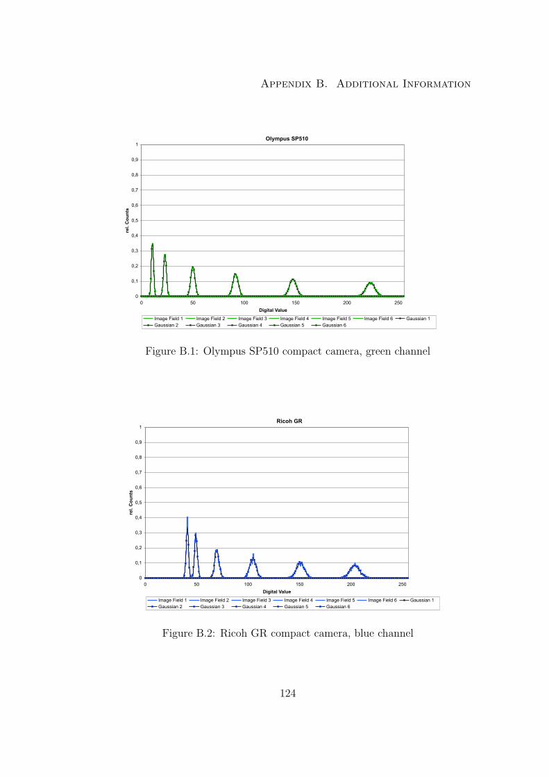
Appendix B. Additional Information
Olympus SP510
0
0,1
0,2
0,3
0,4
0,5
0,6
0,7
0,8
0,9
1
0 50 100 150 200 250
Digital Value
rel.
Co
un
ts
Image Field 1 Image Field 2 Image Field 3 Image Field 4 Image Field 5 Image Field 6 Gaussian 1Gaussian 2 Gaussian 3 Gaussian 4 Gaussian 5 Gaussian 6
Figure B.1: Olympus SP510 compact camera, green channel
Ricoh GR
0
0,1
0,2
0,3
0,4
0,5
0,6
0,7
0,8
0,9
1
0 50 100 150 200 250
Digital Value
rel.
Co
un
ts
Image Field 1 Image Field 2 Image Field 3 Image Field 4 Image Field 5 Image Field 6 Gaussian 1Gaussian 2 Gaussian 3 Gaussian 4 Gaussian 5 Gaussian 6
Figure B.2: Ricoh GR compact camera, blue channel
124
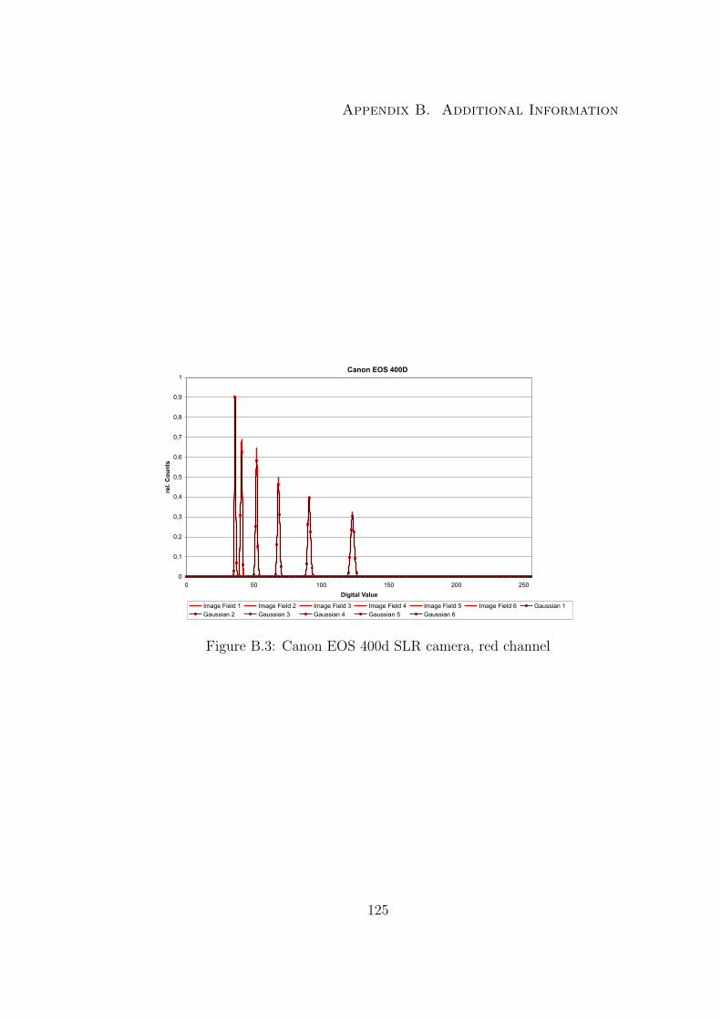
Appendix B. Additional Information
Canon EOS 400D
0
0,1
0,2
0,3
0,4
0,5
0,6
0,7
0,8
0,9
1
0 50 100 150 200 250
Digital Value
rel.
Co
un
ts
Image Field 1 Image Field 2 Image Field 3 Image Field 4 Image Field 5 Image Field 6 Gaussian 1Gaussian 2 Gaussian 3 Gaussian 4 Gaussian 5 Gaussian 6
Figure B.3: Canon EOS 400d SLR camera, red channel
125

Appendix B. Additional Information
B.2 Linearization of image data in NoiseLab
Analyzer
The image data used in NoiseLab Analyzer is linearized prior further analysis.
The input data is based on the patches described in the chart design. The
digital mean values of these patches are read in and build the base for a LUT
calibration.
All values in the image are forced towards zero by the minimum value. So the
minimum in the input image is set to zero in the linearized output image. The max-
imum in the input image is set to the maximum signal level, so maximuminput −minimuminput.
The LUT is calculated as the 4th order polynomial fit of the ideal linear response
and applied to the image. In Figure B.4 one can see an example on real image data.
”Image Data” is the result of the reading of the patch values. ”Lin.Image Data” is
the output image (linearized) and ”ideal Lin.Data” represents the idealized linear
response of the system.
126
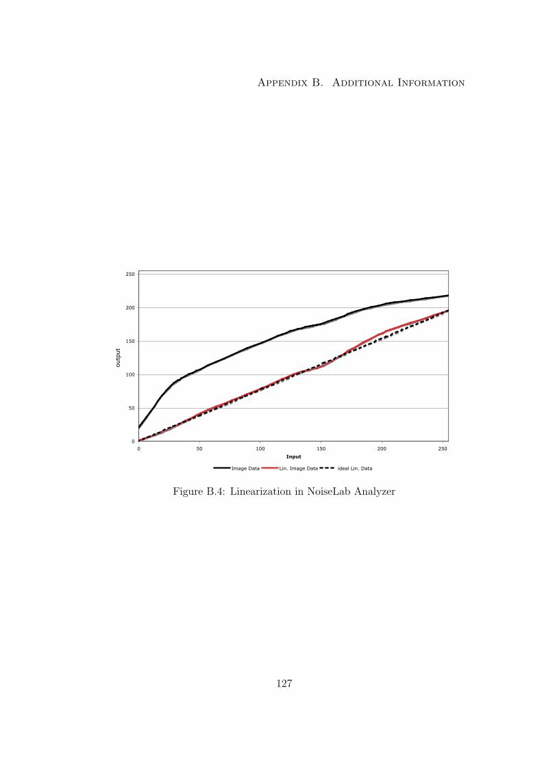
Appendix B. Additional Information
0
50
100
150
200
250
0 50 100 150 200 250
Input
Output
Image Data Lin. Image Data ideal Lin. Data
output
Figure B.4: Linearization in NoiseLab Analyzer
127

Appendix C. Acknowledgement
Appendix C
Acknowledgement
Ich sage Allen ein herzliches ”Danke Schon” die mich bei der Erstellung dieser Ar-
beit unterstutzt haben. Insbesondere mochte ich dem Team von Image Engineering
Dietmar Wuller danken.
I want to say ”‘Thank you”’ to everyone who made this thesis possible. Special
thanks go to the team of Image Engineering Dietmar Wuller.
128

Appendix D. Remarks
Appendix D
Remarks
129
Appendix D. Remarks
Affirmation / Eidesstattliche Erklarung
Ich versichere hiermit, die vorgelegte Arbeit in dem gemeldeten Zeitraum ohne
fremde Hilfe verfaßt und mich keiner anderen als der angegebenen Hilfsmittel und
Quellen bedient zu haben.
Koln, den 20.November 2007
Unterschrift
(Vorname, Nachname)
130

Appendix D. Remarks
Remark of closure / Sperrvermerk
This thesis is not closed.
Die vorgelegte Arbeit unterliegt keinem Sperrvermerk.
Declaration of publication / Weitergabeerklarung
I declare, that this thesis and / or a copy of it may be used for scientific purposes.
Ich erklare hiermit mein Einverstandnis, dass das vorliegende Exemplar meiner
Diplomarbeit oder eine Kopie hiervon fur wissenschaftliche Zwecke verwendet wer-
den darf.
Koln, den 20. November 2007
Unterschrift
(Vorname, Nachname)
131
Bibliography
Bibliography
[1] Apple Computer Inc. ”New Oxford American Dictionary, 2nd Edition”
[2] Dr. Friedrich Dierks, Basler AG ”Sensitivity and Image Quality of Digital
Cameras” Version 1.1, 2004
[3] R.I.Hornsey, University of Waterloo, ”Part III: Noise in Image Sensors”,1999
[4] Rick Baer, micron, ”Noise at the System Level”, ISSCC 2007 Forum: ”Noise
in Imaging Systems”
[5] International Organization of Standardization, ”ISO 15739: Noise measure-
ments”
[6] Gonzales, Woods, ”Digital Image Processing”, 2nd International Edition,
Prentice Hall, 2002
[7] Prof. Dr. Kunz, University of Applied Sciences Cologne, ”Digitale Bildverar-
beitung”, scripts to lectures
[8] Kleinmann, ”Quantification of noise based on two visual Models”, Diploma
thesis at University of applied Sciences Cologne, 2006.
[9] Loebich, Wueller, ”Three Years of Practical Experience in Using ISO Stan-
dards for Testing Digital Cameras”, IS&T/PICS Final Program and Pro-
ceedings,2001, pp. 257-261.
[10] Kleinmann, Wueller, ”Investigation of two Methods to quantify Noise in dig-
ital Images based on the Perception of the human Eye”, Electronic Imaging
Conference 2007
132

Bibliography
[11] Anke Neumann, ”Verfahren zur Aufloesungsmessung digitaler Kameras”,
Diploma thesis at University of applied Sciences Cologne, 2006.
[12] International Organization of Standardization,”ISO12233:2000 Resolution
measurements”
[13] Dr. Kevin J. Matherson, HP Digital Cameras ”An introduction to image-
quality testing”,2005
[14] Mathworks, Documentation Image Processing Toolbox, ”wiener2”, Version
6.0
[15] Mathworks, Documentation Image Processing Toolbox, ”medfilt2”, Version
6.0
[16] United States Patent, Fuji Photo Film, Co., Ltd.,Kanagawa, Japan, ”Patent:
US 6,781,625 B2 ”Noise Reduction Apparatus”, 2004
[17] Werner Bani, ”Wavelets - Eine Einfuhrung fur Ingenieure”, Oldenbourg,
2002
[18] Gonzales, Woods, ”Digital Image Processing using Matlab”, Prentice Hall,
2004
[19] Loebich,Wueller,Klingen,Jaeger, ”Digital Camera Resolution Measurement
Using Sinusoidal Siemens Stars”, Electronic Imaging Conference 2007
[20] Peter Burns, ”sfrmat 2.0 User’s Guide”, download via www.image-
engineering.de
[21] Mathworks, Documentation Image Processing Toolbox, ”Analyzing the Tex-
ture of an Image”, Version 6.0
[22] University of Cambridge ”http://thesaurus.maths.org/” Entry ”Leptokurtic”
17.11.2007
[23] Steven W. Smith, ”Digital Signal Processing, A Practical Guide for Engineers
and Scientists”, Newnes, 2003
[24] Bernd Jaehne, ”Digitale Bildverarbeitung”, Springer Verlag, 2005
133

Bibliography
[25] Bruno Klingen, ”Fouriertransformation fYr Ingenieur- und Naturwis-
senschaften”, Springer Verlag, 2001
[26] Vinay K.Ingle, John G. Proakis, ”Digital Signal Processing using MATLAB”.
Thomson, 2007
134
Related Documents


