The Annals of Statistics 2000, Vol. 28, No. 4, 1105–1127 RATES OF CONVERGENCE FOR THE GAUSSIAN MIXTURE SIEVE By Christopher R. Genovese 1 and Larry Wasserman 2 Carnegie Mellon University Gaussian mixtures provide a convenient method of density estimation that lies somewhere between parametric models and kernel density estima- tors. When the number of components of the mixture is allowed to increase as sample size increases, the model is called a mixture sieve. We establish a bound on the rate of convergence in Hellinger distance for density esti- mation using the Gaussian mixture sieve assuming that the true density is itself a mixture of Gaussians; the underlying mixing measure of the true density is not necessarily assumed to have finite support. Computing the rate involves some delicate calculations since the size of the sieve—as measured by bracketing entropy—and the saturation rate, cannot be found using standard methods. When the mixing measure has compact support, using k n ∼ n 2/3 /log n 1/3 components in the mixture yields a rate of order log n 1+η/6 /n 1/6 for every η> 0 The rates depend heavily on the tail behavior of the true density. The sensitivity to the tail behavior is dimin- ished by using a robust sieve which includes a long-tailed component in the mixture. In the compact case, we obtain an improved rate of log n/n 1/4 . In the noncompact case, a spectrum of interesting rates arise depending on the thickness of the tails of the mixing measure. 1. Introduction. Statistical inference using mixtures of Gaussians is used for many purposes including density estimation, clustering and robust estimation; see, for example, Lindsay (1995), McLachlan and Basford (1988), Banfield and Raftery (1993) and Robert (1996). When the number of compo- nents of the mixture is allowed to increase with sample size, the model is called a Gaussian mixture sieve [Grenander (1981), Wong and Shen (1995)]. These sieves have been studied by several authors including Geman and Hwang (1982), Roeder (1992), Priebe (1994) and Roeder and Wasserman (1997). Related work from a Bayesian point of view is discussed in Escobar and West (1995). Priebe argues that in many cases, a mixture sieve has many advantages as a density estimator over kernel density estimates. For exam- ple, Priebe showed that with n = 10000 observations, a log-normal density can be well approximated by a mixture of about 30 normals. In contrast, a kernel density estimator uses a mixture of 10,000 normals. Despite the ubiq- uity of mixture sieve models, little is known about their asymptotic properties. In particular, the rate of convergence of the density estimator of this sieve has not been established. In this paper, we bound the rate of convergence. Rates of Received November 1998; revised July 2000. 1 Supported by NSF Grant DMS-97-05034. 2 Supported by NIH Grant R01-CA54852-07 and NSF Grant DMS-98-03433. Key words and phrases. Density estimation, mixtures, rates of convergence, sieves. 1105

Welcome message from author
This document is posted to help you gain knowledge. Please leave a comment to let me know what you think about it! Share it to your friends and learn new things together.
Transcript

The Annals of Statistics2000, Vol. 28, No. 4, 1105–1127
RATES OF CONVERGENCE FOR THE GAUSSIANMIXTURE SIEVE
By Christopher R. Genovese1 and Larry Wasserman2
Carnegie Mellon University
Gaussian mixtures provide a convenient method of density estimationthat lies somewhere between parametric models and kernel density estima-tors. When the number of components of the mixture is allowed to increaseas sample size increases, the model is called a mixture sieve. We establisha bound on the rate of convergence in Hellinger distance for density esti-mation using the Gaussian mixture sieve assuming that the true densityis itself a mixture of Gaussians; the underlying mixing measure of thetrue density is not necessarily assumed to have finite support. Computingthe rate involves some delicate calculations since the size of the sieve—asmeasured by bracketing entropy—and the saturation rate, cannot be foundusing standard methods. When the mixing measure has compact support,using kn ∼ n2/3/�log n�1/3 components in the mixture yields a rate of order�log n��1+η�/6/n1/6 for every η > 0� The rates depend heavily on the tailbehavior of the true density. The sensitivity to the tail behavior is dimin-ished by using a robust sieve which includes a long-tailed component in themixture. In the compact case, we obtain an improved rate of �log n/n�1/4.In the noncompact case, a spectrum of interesting rates arise dependingon the thickness of the tails of the mixing measure.
1. Introduction. Statistical inference using mixtures of Gaussians isused for many purposes including density estimation, clustering and robustestimation; see, for example, Lindsay (1995), McLachlan and Basford (1988),Banfield and Raftery (1993) and Robert (1996). When the number of compo-nents of the mixture is allowed to increase with sample size, the model is calleda Gaussian mixture sieve [Grenander (1981), Wong and Shen (1995)]. Thesesieves have been studied by several authors including Geman and Hwang(1982), Roeder (1992), Priebe (1994) and Roeder and Wasserman (1997).Related work from a Bayesian point of view is discussed in Escobar andWest (1995). Priebe argues that in many cases, a mixture sieve has manyadvantages as a density estimator over kernel density estimates. For exam-ple, Priebe showed that with n = 10�000 observations, a log-normal densitycan be well approximated by a mixture of about 30 normals. In contrast, akernel density estimator uses a mixture of 10,000 normals. Despite the ubiq-uity of mixture sieve models, little is known about their asymptotic properties.In particular, the rate of convergence of the density estimator of this sieve hasnot been established. In this paper, we bound the rate of convergence. Rates of
Received November 1998; revised July 2000.1Supported by NSF Grant DMS-97-05034.2Supported by NIH Grant R01-CA54852-07 and NSF Grant DMS-98-03433.Key words and phrases. Density estimation, mixtures, rates of convergence, sieves.
1105
1106 C. R. GENOVESE AND L. WASSERMAN
convergence for the mixing distribution function have been studied in Chen(1995). Also, van der Geer (1996) obtains rates for a different mixture model.
Let φ�x�µ�σ� denote a Gaussian density with mean µ and variance σ2.A finite Gaussian mixture is a density of the form
fθ�x� =k∑j=1pjφ�x�µj� σj��(1)
where θ = �µ�σ�p�� µ = �µ1� � � � � µk�� σ = �σ1� � � � � σk�� p = �p1� � � � � pk�.Here, the µj’s are real, the σj’s are positive reals, pj ≥ 0 and
∑j pj = 1.
Let mk, sk and S be positive constants such that mk → ∞ and sk ↓ 0 ask→∞ and let
�k={f�·� =
k∑j=1pjφ�· �µj� σj�� �µj� ≤mk�
and sk ≤ σj ≤ S� j = 1� � � � � k}�
(2)
Let kn be a sequence of integers such that kn → ∞ as ∞. The sieve we areinterested in is �kn
. Our estimate of the true density is fn�·� = fθ�·� where θis the maximum likelihood estimate of θ in the model (2). We have chosen tofix S mainly for convenience. This parameter can also be allowed to increasewith k but the results do not change materially.
We will assume that the true density is a “general Gaussian mixture” ofthe form
f0�x� =∫ ∞0
∫ ∞−∞φ�x�µ�σ� dP�µ�σ�(3)
for some probability measure P on the Borel σ-algebra over � × �+� Let� denote all such densities. Of course, � contains all finite and countablemixtures as a special case. It is worth noting that the Dirichlet process mixtureprior used in nonparametric Bayesian inference [Escobar and West (1995)]uses a prior with support in � .
We measure the error in the estimate by Hellinger distance dH�f0� fn�where dH�f�g�2 =
∫ �√f−√g�2. We bound the rate at which dH�f0� fn� goesto 0, in two steps: (i) we bound the likelihood ratio outside Hellinger neighbor-hoods of the true density and (ii) we compute the rate at which finite mixturessaturate the set � . The first task is addressed in Section 2 by computing the“size” of �kn
in terms of its Hellinger bracketing entropy, and then appealingto recent results of Wong and Shen (1995). The second task is addressed inSection 3. Calculating the bracketing entropy and the saturation rate is usu-ally straightforward for finite-dimensional models. However, mixture modelsdo not behave as nicely as most finite-dimensional parametric families so thesecalculations require special attention. In particular, the square root of thedensity of a mixture model is not differentiable everywhere so that standardmethods for computing entropy are not available. Hence, we believe that the
CONVERGENCE RATES FOR GAUSSIAN MIXTURE SIEVE 1107
calculations in Sections 2 and 3 might be useful for other nonregular fami-lies as well. We put these pieces together and compute the rate in Section 4.Specifically we find tn such that P∗�dH�f0� fn� > tn� = o�1�. In section 5 wediscuss an improvement on the sieve. Section 6 contains closing remarks andunsolved problems.
The main conclusion of this paper is as follows. If the mixing measureP is compactly supported, then taking Kn ∼ n2/3�log n�2/3 yields the rate�log n��1+η�/6/n1/6 for every η > 0. If the mixing measure is not compactlysupported then we cannot compute the rate without the adjusted sieve inSection 5. In this case we get a rate of �log n�1/4/n1/4 for the compact caseand, in the noncompact case, we get a spectrum of rates depending on the tailbehavior of P. We should mention that independently of our work, Li (1999)and Li and Barron (1999) also obtained a rate of �log n�1/4/n1/4 for mixturemodels. More precisely, they obtained a rate in Kullback–Leibler distance,which corresponds to the above rate in Hellinger. Their proof is quite differentfrom ours. On the one hand, it is more general since it applies to other mixturesbesides Gaussian mixtures. On the other hand, their results do not directlyapply to our case since their rates contain a constant which can be infiniteand, furthermore, they assume the parameter space has been discretized. Theresults of Li and Barron are very interesting and they nicely complement theresults in this paper.
Remark. After a revision of this paper was submitted, Ghosal and vander Vaart (2000) obtained an improved rate of convergence for this prob-lem. Our results are driven by the approximation error infg∈�k
D�f0� g� =O�log k/k� where D�f�g� is Kullback–Leibler distance. This implies that oneneeds k�ε� ≈ 1/ε mixture components to approximate an arbitrary f0 towithin ε Kullback–Leibler distance. In bounding this approximation error wedid not make use of the smoothness of the Gaussian densities. Ghosal andvan der Vaart obtained an improved bound infg∈�k
D�f0� g� = O�log k/ek�.This implies that one needs only k�ε� ≈ log�1/ε� mixture components. As aconsequence, they obtain a near parametric rate of �log n�δ/√n for some δ > 0�in the case where the variances of the mixture components are bounded belowby a known constant. This result appears to depend strongly on the smooth-ness of the Gaussians. Ghosal and van der Vaart did not obtain rates in thecase where no such bound is known, though we believe that a n−1/2 rate is notpossible in this more general case. It appears that theO�log k/k� bound on theapproximation error holds quite generally (i.e., without smoothness conditionson the densities being mixed) and could thus be used to obtain a convergencerate of �log n/n�1/4 without strong assumptions on the mixands. Indeed, Liand Barron (1999) obtained a bound of O�1/k� with essentially no conditionson the mixands, though there are constants in their results which can be infi-nite in some cases. We suspect that these infinities can be eliminated at theexpense of increasing the O�1/k� term to O�log k/k�. Currently, no results areavailable for the case where mk, sk and k are chosen using the data.
1108 C. R. GENOVESE AND L. WASSERMAN
2. Bounding the likelihood ratio. In this section we bound the supre-mum of the likelihood outside a Hellinger neighborhood of the true density.Thoughout, we consider densities on the real line with respect to Lebesguemeasure. Let dH�f�g� be Hellinger distance, dTV�f�g� total variation dis-tance and D�f�g� be Kullback–Leibler divergence; that is,
d2H�f�g� =∫ (√
f�x� − √g�x�)2 dx = ∫f�x�dx
+∫g�x�dx− 2
∫ √f�x�g�x�dx�
dTV�f�g� = 12
∫�f�x� − g�x��dx�
D�f�g� =∫f�x� log f�x�/g�x�dx�
The following inequalities are well known and will be used in what follows.
Proposition. Consider nonnegative, integrable functions f and g, not nec-essarily probability density functions and suppose that g�x� ≤ f�x� for almost
all x with respect to Lebesgue measure. Then, dH�f�g� ≤√2dTV�f�g� and
dTV�f�g� ≤ dH�f�g�√∫f�x�dx�
2.1. The bracketing entropy of �k. In this subsection, we measure thesize of �k using bracketing entropy [van der Vaart and Wellner (1996), Sec-tion 2.7]. If � is a set of nonnegative, integrable functions and d is a metricon this set, then an ε-bracketing (with respect to d) is a set of pairs of inte-grable functions �l1� u1�� � � � � �lm� um� such that (1) for each f ∈ � there exists�lj� uj� such that lj ≤ f ≤ uj, a.e. with respect to Lebesgue measure and (2)d�lj� uj� ≤ ε� j = 1� � � � �m.
The smallest number of such brackets to cover � is called the bracketingnumber and is denoted by N���� � d�. The bracketing entropy is defined byH���� � d� = logN���� � d�.
Generally, if � is a parametric model of dimension j, then N���ε�� � d� ∼ε−j as can be proved using a Lipschitz argument; see, for example, van derVaart and Wellner [(1996), Section 2.7.4]. But such arguments require thatthe derivative of the square root of the density be bounded by an L2 function.This is not the case for mixtures. This is easy to see even in a simple mixturemodel like �1−p�φ�y�0�1�+pφ�y�0�1/2�; the derivative of the square root ofthis density at p = 0 behaves like ex
2/2. Instead, we must bound the entropyby other methods. The result is given in the following theorem.
Theorem 1. Consider the set �k defined by �2�. If ε ≤ 1, there exists posi-tive constants c1 and c2, not depending on k or ε, such that
N���ε��k� dH� ≤ c1ck2mkk(S
sk
)2k(1ε
)3k−1�
CONVERGENCE RATES FOR GAUSSIAN MIXTURE SIEVE 1109
To prove Theorem 1, we need some lemmas.
Lemma 1. Let s, m and S be positive constants and define
� = �φ�·�µ�σ�� �µ� ≤m�s ≤ σ ≤ S��Then, for S ≥ 1 and ε ∈ �0�1�,
N���ε�� � dH� ≤128�2m��S/s�2
ε2�
Proof. Let δ = ε/2 and τ2 = �1+ δ�S2. Let
r =⌈4 log
(S√1+ δ/s)
log(1+ δ
) ⌉
where �a� denotes the smallest integer greater than or equal to a. Define σ2j =
τ2�1+ δ�−j/2 for j = 2� � � � � r. Note that σ2r ≤ s2 ≤ S2 = σ2
2 . For j ∈ �2� � � � � r�let γj = δσj−2/2, let Ij = �m/γj� and let µij = iγj for i = −Ij� � � � �0� � � � � Ij.Note that �−m�m� ⊂ �−Ijγj� Ijγj�. For j ∈ �2� � � � � r� and −Ij ≤ i ≤ Ij let
Bij ={�µ�σ��µ ∈
[µij −
δσj
4� µij +
δσj
4
]� σ2 ∈
[σ2j+1� σ
2j
]}�(4)
The Bij cover the parameter space. [A similar construction is used in Tongand Viele (1998).]
Let
lij�y� = �1+ δ�−1φ(y�µij�
σ2j+1
�1+ δ�1/4)
and
uij�y� = �1+ δ�φ(y�µij� σ2
j�1+ δ�)�
We claim that �lij� uij� brackets Bij. This follows, after some algebra, from thefact that, whenever σ1 < σ2,
φ�y�µ1� σ1�φ(y�µ2� σ2
) ≤ σ2σ1
exp{ �µ1 − µ2�22(σ22 − σ2
1
)}�Next we bound dH�lij� uij�. In general, if f and g are probability density
functions then d2H��1+δ�f� �1+δ�−1g� = d2H�f�g�+δ2/�1+δ� ≤ d2H�f�g�+δ2.Also, if f�y� = φ�y�µ1� σ1� and g�y� = φ�y�µ2� σ2�, then
d2H�f�g� = 2
[1−
{2σ1σ2σ21 + σ2
2
}1/2exp
{− �µ1 − µ2�2
4(σ21 + σ2
2
)}]�
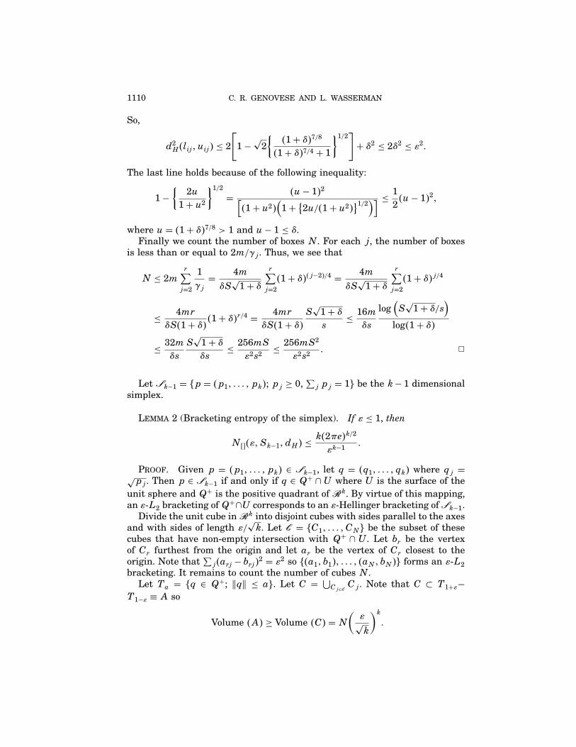
1110 C. R. GENOVESE AND L. WASSERMAN
So,
d2H�lij� uij� ≤ 2
[1−
√2{ �1+ δ�7/8�1+ δ�7/4 + 1
}1/2]+ δ2 ≤ 2δ2 ≤ ε2�
The last line holds because of the following inequality:
1−{
2u1+ u2
}1/2= �u− 1�2[
�1+ u2�(1+ {2u/�1+ u2�}1/2)] ≤ 1
2�u− 1�2�
where u = �1+ δ�7/8 > 1 and u− 1 ≤ δ.Finally we count the number of boxes N. For each j, the number of boxes
is less than or equal to 2m/γj. Thus, we see that
N ≤ 2mr∑j=2
1γj= 4m
δS√1+ δ
r∑j=2�1+ δ��j−2�/4 = 4m
δS√1+ δ
r∑j=2�1+ δ�j/4
≤ 4mrδS�1+ δ��1+ δ�
r/4 = 4mrδS�1+ δ�
S√1+ δs
≤ 16mδs
log(S√1+ δ/s
)log�1+ δ�
≤ 32mδs
S√1+ δδs
≤ 256mSε2s2
≤ 256mS2
ε2s2� ✷
Let �k−1 = �p = �p1� � � � � pk�; pj ≥ 0,∑j pj = 1� be the k− 1 dimensional
simplex.
Lemma 2 (Bracketing entropy of the simplex). If ε ≤ 1, then
N���ε�Sk−1� dH� ≤k�2πe�k/2εk−1
�
Proof. Given p = �p1� � � � � pk� ∈ �k−1, let q = �q1� � � � � qk� where qj =√pj. Then p ∈ �k−1 if and only if q ∈ Q+ ∩U where U is the surface of the
unit sphere and Q+ is the positive quadrant of �k. By virtue of this mapping,an ε-L2 bracketing ofQ+∩U corresponds to an ε-Hellinger bracketing of�k−1.
Divide the unit cube in�k into disjoint cubes with sides parallel to the axesand with sides of length ε/
√k. Let � = �C1� � � � � CN� be the subset of these
cubes that have non-empty intersection with Q+ ∩ U. Let br be the vertexof Cr furthest from the origin and let ar be the vertex of Cr closest to theorigin. Note that
∑j�arj − brj�2 = ε2 so ��a1� b1�� � � � � �aN� bN�� forms an ε-L2
bracketing. It remains to count the number of cubes N.Let Ta = �q ∈ Q+; �q� ≤ a�. Let C = ⋃
Cj∈� Cj. Note that C ⊂ T1+ε−T1−ε ≡ A so
Volume �A� ≥ Volume �C� =N(ε√k
)k�

CONVERGENCE RATES FOR GAUSSIAN MIXTURE SIEVE 1111
Let Vk�a� = akπk/2/6��k/2� + 1� denote the volume of a sphere of radius a.Then,
N ≤ Volume �A�(ε/√k)k = 1
2k�Vk�1+ ε� −Vk�1− ε��(
ε/√k)k
= 12k��1+ ε�k − �1− ε�k�(
ε/√k)k πk/2
�k/2�! ≤(πe
2
)k/2 ��1+ ε�k − �1− ε�k�εk
since x! ≥ xxe−x. Now, �1 + ε�k − �1 − ε�k = k ∫ �1+ε��1−ε� xk−1 dx ≤ 2εk�1 + ε�k−1.
The conclusion follows. ✷
Lemma 3. Let �l1� u1�� � � � � �lm� um� be any ε Hellinger bracketing. If ε ≤ 1then
7ε ≡ maxj
∫uj�x�dx ≤ 1+ 3ε�
Proof. Let u denote one of the upper brackets and let l denote the cor-responding lower bracket. Then,
∫u = �√u�22 ≤ ��√l�2 + �
√u − √l�2�2 ≤
�1+ ε�2 ≤ 1+ 3ε. ✷
Lemma 4. Let �l1� � � � � lk� and �u1� � � � � uk� be nonnegative, integrablefunctions and let �a1� � � � � ak� and �b1� � � � � bk� be vectors of nonnegative real
numbers. Let l =∑kj=1 ajlj and u =
∑kj=1 bjuj. Then,
d2H�l� u� ≤k∑j=1d2H�ajlj� bjuj��
Proof. Note that
d2H�l� u� =∑j
bj
∫uj +
∑j
aj
∫lj − 2
∫ √∑j
bjuj∑j
ajlj
and
k∑j=1d2H�ajlj� bjuj� =
∑j
bj
∫uj +
∑j
aj
∫lj − 2
∫ ∑j
√ajbjljuj�
Thus, it suffices to show that∫ √∑j
bjuj∑j
ajlj ≥∫ ∑
j
√ajbjljuj
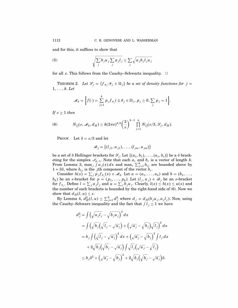
1112 C. R. GENOVESE AND L. WASSERMAN
and for this, it suffices to show that√∑j
bjuj∑j
ajlj ≥∑j
√ajbjljuj(5)
for all x. This follows from the Cauchy–Schwartz inequality. ✷
Theorem 2. Let �j = �fθj � θj ∈ 8j� be a set of density functions for j =1� � � � � k. Let
�k ={f�·� =
k∑j=1pjfθj�·�� θj ∈ 8j�pj ≥ 0�
∑j
pj = 1}�
If ε ≥ 1 then
N���ε��k� dH� ≤ k�2πe�k/2(3ε
)k−1 k∏j=1N���ε/3��j� dH��(6)
Proof. Let δ = ε/3 and let
�j ={�lj1� uj1�� � � � � (ljm� ujm)}
be a set of δ Hellinger brackets for �j. Let ��a1� b1�� � � � � �as� bs�� be a δ brack-eting for the simplex �k−1. Note that each ar and br is a vector of length k.From Lemma 3, maxj
∫uj�x�dx and maxr
∑kj=1 brj are bounded above by
1+ 3δ, where brj is the jth component of the vector br.Consider h�x� = ∑
j pjfθj�x� ∈ �k. Let a = �a1� � � � � ak� and b = �b1� � � � �bk� be an ε-bracket for p = �p1� � � � � pk�. Let �lj� uj� ∈ �j be an ε-bracketfor fθj . Define l =
∑j ajlj and u = ∑
j bjuj. Clearly, l�x� ≤ h�x� ≤ u�x� andthe number of such brackets is bounded by the right-hand side of (6). Now weshow that dH�l� u� ≤ ε.
By Lemma 4, d2H�l� u� ≤∑kj=1 d
2j where dj = dH�bjuj� ajlj�. Now, using
the Cauchy–Schwarz inequality and the fact that∫lj ≤ 1 we have
d2j =∫ (√
ajlj −√bjuj
)2dx
=∫ (√
bj
(√lj −
√uj
)+(√aj −
√bj
)√lj
)2dx
= bj∫ (√
lj −√uj
)2dx+
(√aj −
√bj
)2 ∫lj dx
+ 2√bj
(√bj −
√aj
) ∫ √lj
(√uj −
√lj
)≤ bjδ2 +
(√aj −
√bj
)2+ 2
√bj
(√bj −
√aj
)δ�
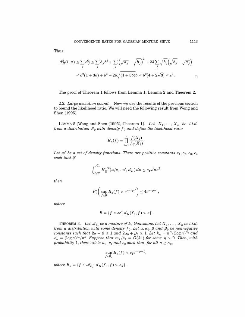
CONVERGENCE RATES FOR GAUSSIAN MIXTURE SIEVE 1113
Thus,
d2H�l� u� ≤∑j
d2j ≤∑j
bjδ2 +∑
j
(√aj −
√bj
)2+ 2δ
∑j
√bj
(√bj −
√aj
)≤ δ2�1+ 3δ� + δ2 + 2δ
√�1+ 3δ�δ ≤ δ2�4+ 2
√3� ≤ ε2� ✷
The proof of Theorem 1 follows from Lemma 1, Lemma 2 and Theorem 2.
2.2. Large deviation bound. Now we use the results of the previous sectionto bound the likelihood ratio. We will need the following result from Wong andShen (1995).
Lemma 5 [Wong and Shen (1995), Theorem 1]. Let X1� � � � �Xn be i.i.d.from a distribution P0 with density f0 and define the likelihood ratio
Rn�f� =n∏i=1
f�Xi�f0�Xi�
�
Let � be a set of density functions. There are positive constants c1� c2� c3� c4such that if
∫ √2εε2/28
H1/2�� �u/c3�� � dH�du ≤ c4
√nε2
then
P∗0
(supf∈BRn�f� > e−nc1ε
2)≤ 4e−c2nε
2�
where
B = �f ∈ � � dH�f0� f� > ε��
Theorem 3. Let�knbe a mixture of kn Gaussians. LetX1� � � � �Xn be i.i.d.
from a distribution with some density f0. Let α� α0� β and β0 be nonnegativeconstants such that 2α + β ≤ 1 and 2α0 + β0 ≥ 1. Let kn = nβ/�log n�β0 andεn = �log n�α0/nα. Suppose that mk/sk = O�kη� for some η > 0. Then, withprobability 1, there exists n0, c1 and c2 such that, for all n ≥ n0,
supf∈Bn
Rn�f� < c1e−c2nε2n�
where Bn = �f ∈�kn� dH�f0� f� > εn�.
1114 C. R. GENOVESE AND L. WASSERMAN
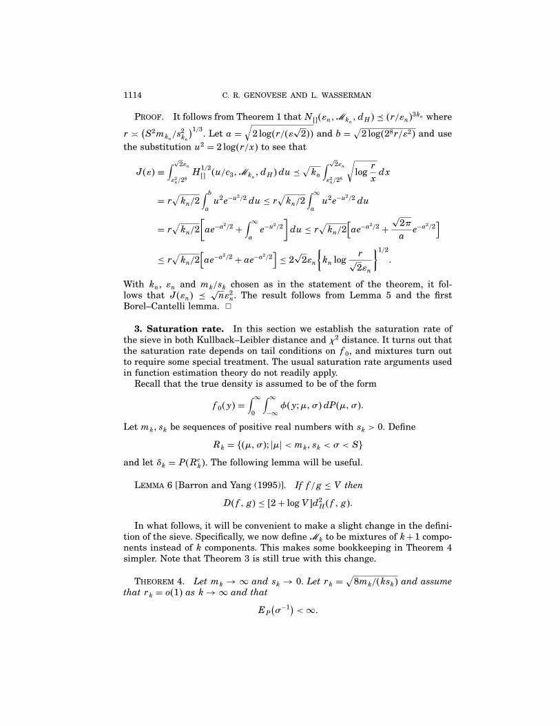
Proof. It follows from Theorem 1 thatN���εn��kn� dH� � �r/εn�3kn where
r (S2mkn/s
2kn
)1/3. Let a = √2 log�r/�ε√2�� and b = √
2 log�28r/ε2� and usethe substitution u2 = 2 log�r/x� to see that
J�ε� ≡∫ √2εnε2n/28
H1/2�� �u/c3��kn
� dH�du �√kn
∫ √2εnε2n/28
√logr
xdx
= r√kn/2
∫ bau2e−u
2/2 du ≤ r√kn/2
∫ ∞au2e−u
2/2 du
= r√kn/2
[ae−a
2/2 +∫ ∞ae−u
2/2]du ≤ r
√kn/2
[ae−a
2/2 +√2πae−a
2/2]
≤ r√kn/2
[ae−a
2/2 + ae−a2/2]≤ 2
√2εn
{kn log
r√2εn
}1/2�
With kn, εn and mk/sk chosen as in the statement of the theorem, it fol-lows that J�εn� �
√nε2n. The result follows from Lemma 5 and the first
Borel–Cantelli lemma. ✷
3. Saturation rate. In this section we establish the saturation rate ofthe sieve in both Kullback–Leibler distance and χ2 distance. It turns out thatthe saturation rate depends on tail conditions on f0, and mixtures turn outto require some special treatment. The usual saturation rate arguments usedin function estimation theory do not readily apply.
Recall that the true density is assumed to be of the form
f0�y� =∫ ∞0
∫ ∞−∞φ�y�µ�σ�dP�µ�σ��
Let mk� sk be sequences of positive real numbers with sk > 0. Define
Rk = ��µ�σ�� �µ� < mk� sk < σ < S�and let δk = P�Rck�. The following lemma will be useful.
Lemma 6 [Barron and Yang (1995)]. If f/g ≤ V then
D�f�g� ≤ �2+ logV�d2H�f�g��
In what follows, it will be convenient to make a slight change in the defini-tion of the sieve. Specifically, we now define �k to be mixtures of k+1 compo-nents instead of k components. This makes some bookkeeping in Theorem 4simpler. Note that Theorem 3 is still true with this change.
Theorem 4. Let mk → ∞ and sk → 0. Let rk =√8mk/�ksk� and assume
that rk = o�1� as k→∞ and that
EP(σ−1
)<∞�
CONVERGENCE RATES FOR GAUSSIAN MIXTURE SIEVE 1115
Let ak be the smallest real number such that
EP
(1σeµ
2/a2k
∣∣∣Rck) ≤ ak�(7)
where the expectation is taken to be the essential supremum over Rk ifP�Rck� = 0. Then, for rk < 2�5,
inff∈�k
D�f0� f�≤2δk[2+ log
(1+ ak
√S2 + a2k
)]+ log�1+ δk� + 2rk ≡ ωk
(8)
Proof. Let
fk�y� =∫ Ssk
∫ mk−mk
φ�y�µ�σ�dP�µ�σ� + δkφ0�y��
where φ0�y� is a normal density with mean 0 and variance S2 + a2k. Given aset of points ��µ1� σ1�� � � � � �µk� σk�� and a partition �A1� � � � �Ak� of Rk, to bechosen later, define
gk =k∑j=1pjφ�y�µj� σj� + δkφ0�
where pj =∫AjdP. Let hk = gk/�1 + δk�. Then hk ∈ �k, D�f0� hk� =
D�f0� gk� + log�1+ δk� and
D�f0� gk� = D�f0� fk� +∫f0 log
fkgk�(9)
To bound D�f0� fk�, it is helpful to first bound f0/fk. To this end, let
γ = µ/σ2
1/σ2 − 1/�S2 + a2k�and note that
f0fk=
∫RkφdP∫
RkφdP+ δkφ0
+∫RckφdP∫
RkφdP+ δkφ0
≤ 1+ 1δk
∫Rck
φ
φ0dP
≤ 1+√S2 + a2kδk
∫Rck
1σexp
{− 1
2
[�x− µ�2σ2
− x2
S2 + a2k
]}dP
≤ 1+√S2 + a2kδk
∫Rck
1σexp
{− 1
2
[1σ2− 1
S2 + a2k
]�x− γ�2
}
× exp
{µ2
σ2�S2 + a2k��1/σ2 − 1/�S2 + a2k��
}dP

1116 C. R. GENOVESE AND L. WASSERMAN
≤ 1+√S2 + a2kδk
∫Rck
1σexp
{µ2
S2 + a2k − σ2
}dP
≤ 1+√S2 + a2kδk
∫Rck
1σeµ
2/a2k dP ≤ 1+√S2 + a2k ak�
where the last inequality follows from (7). By Lemma 6, and the fact thatd2H�f0� fk� ≤ 2dTV�f0� fk� ≤ 2δk, we have
D�f0� fk� ≤ 2δk
[2+ log
(1+ ak
√S2 + a2k
)]�
Thus we have bounded the first term in (9). Next we bound the second term.Consider any Aj in the partition. Let φj�x� = φ�x�µj� σj� and define
v−2 = 1σ2− 1
σ2j
and γ = µ/σ2 − µj/σ2
j
1/σ2 − 1/σ2j
�
Then∫Aj
φdP = φj∫Aj
φ
φjdP = φj
∫Aj
σj
σexp
(− 1
2
[�x− µ�2σ2
− �x− µj�2
σ2j
])dP
= φj∫Aj
σj
σexp
(− 1
2v2�x− γ�2
)exp
(12
�µ− µj�2σ2j − σ2
)dP
≤ φj∫Aj
σj
σexp
(12
�µ− µj�2σ2j − σ2
)dP�
Below we will show that(σj
σ
)exp
(12
�µ− µj�2σ2j − σ2
)≤ �1+ rk�2�(10)
It then follows that ∫Aj
φdP ≤ �1+ rk�2pjφj�
Hence,
fkgk
=∑j
∫AjφdP+ rkφ0∑
j pjφj + rkφ0≤ �1+ rk�
2∑j pjφj + rkφ0∑
j pjφj + rkφ0≤ �1+ rk�2
and so ∫f0 log
fkgk
≤ 2 log�rk + 1� ≤ 2rk�
It remains to be shown that (10) holds and that gk ∈�k.
CONVERGENCE RATES FOR GAUSSIAN MIXTURE SIEVE 1117
Let
v1 < v2 < · · · < vJ ≡ S�where
vj = vj−1√1+ rk and σj = vj
√1+ rk�
Here, J is the largest integer such that sk ≤ v1. Also, for σ ∈ �vj−1� vj�, divide�−mk�mk� into intervals of length ξj where
ξj = vj√2rk log�1+ rk��(11)
Then, for σ ∈ �vj−1� vj�, σj/σ ≤ σj/vj−1 = �1+rk�. Also, for σ2j −σ2 ≥ rkv2j.
Hence,
exp{12
�µ− µj�2σ2j − σ2
}≤ exp
{12
ξ2j
rkv2j
}≤ �1+ rk�
using (11). Thus,
σj
σexp
{12
�µ− µj�2σ2j − σ2
}≤ �1+ rk�2
which confirms (10).To ensure that gk ∈ �k we have to make sure that the above scheme
partitions Rk into no more than k pieces. For fixed σj, the number of divisionsof µ is
total lengthξj
= 2mkvj√2rk log�1+ rk�
�
So, using the fact that rk < 2�5, the total number N of rectangles is
N = 2mk√2rk log�1+ rk�
[1v1+ · · · + 1
vJ
]
= 2mk√2rk log�1+ rk�
[1sk+ 1sk�1+ rk�1/2
+ 1sk�1+ rk�
+ · · · + 1sk�1+ rk�J/2
]
≤ 2mksk√2rk log�1+ rk�
∞∑j=0
(1
1+ rk
)j/2= 2mksk√2rk log�1+ rk�
√1+ rk√
1+ rk − 1
≤(mksk
)4√2√
rk log�1+ rk�1rk≤ 8mkskr
2k
≤ k� ✷
Corollary 1. Let hk be as defined in the proof of Theorem 3. Then∫f0�y�
(logf0�y�hk�y�
)2
dy ≤ ωk logVk�
1118 C. R. GENOVESE AND L. WASSERMAN
where
Vk =(1+ ak
√S2 + a2k
)�1+ rk�2�1+ δk��
As noted in Wong and Shen (1995), it is sometimes useful to have the sat-uration rate in a distance that is stronger than Kullback–Leibler. Corollary 2records the χ2 saturation rate. Recall that the χ2 distance is defined by
χ2�f�g� =∫ �f− g�2
g�
Lemma 7. If f/g < V then
χ2�f�g� ≤ 2�1+V1/2�2dTV�f�g��
Proof.
χ2�f�g� =∫ �f− g�2
g=∫�√f−√g�2
(1+
√f
g
)2
≤ �1+V1/2�2d2H�f�g� ≤ 2�1+V1/2�2dTV�f�g�� ✷
Corollary 2. Under the conditions of Theorem 3,
ρk ≡ inff∈�k
χ2�f0� f� ≤ 2�1+V1/2k �2
{2δk
[2+ log�1+ ak
√S2 + a2k�
]+ 2rk
}�
where
Vk =(1+ ak
√S2 + a2k
)�1+ rk�2
and ak is as defined in �7�.
Proof. Define fk and hk as in Theorem 4. Then from the proof ofTheorem 4 we see that
f0hk= f0fk
fkhk≤ Vk�
Then, from Lemma 7 and Theorem 4,
ρk ≤ χ2�f0� hk� ≤ 2�1+V1/2k �2dTV�f0� hk� ≤ 2�1+V1/2
k �2D�f0� hk�
≤ 2�1+V1/2k �2
{2δk
[2+ log�1+ ak
√S2 + a2k�
]+ 2rk
}� ✷
CONVERGENCE RATES FOR GAUSSIAN MIXTURE SIEVE 1119
4. Rate of convergence. Here we combine the results of the previoussections to compute the rate.
Theorem 5. Let α�β > 0 and α0� β0 ≥ 0 be such that 2α + β ≤ 1 and2α0 + β0 ≥ 1. Let kn = nβ/�log n�β0 . Define ωk as in �8� from Theorem 4and let
tn = max{�log n�α0
nα�
2
c1/21
ω1/2kn
}�(12)
Define rk as in Theorem 4. Then,
P∗�dH�f0� fn� > tn�
≤ 4e−c2nt2n +
4 log(�1+ akn√S2 + akn��1+ rkn�2�1+ δk�
)c1nt
2n
�
(13)
Proof. This proof parallels the argument in Theorem 3 of Wong and Shen(1995). Let hk ∈ �k be the density defined in the proof of Theorem 4. LetBn = �f ∈�kn
� dH�f0� f� > tn�. Then,
P∗�dH�f0� fn� > tn� ≤ P∗(supf∈Bcn
n∏i=1
f�Yi�hkn�Yi�
≥ e−c1nt2n/2)
≤ P∗(supf∈Bcn
n∏i=1
f�Yi�f0�Yi�
≥ e−c1nt2n)
+P( n∏i=1
f0�Yi�hkn�Yi�
≥ e−c1nt2n/2)= P1 +P2�
Now, P1 ≤ 4e−c2nt2n by Theorem 3. We bound P2 using Chebyshev’s inequal-
ity, Theorem 4 and Corollary 1. Specifically, let Dn = D�f0� hkn� and let
γn =∫f0�y�
(log
f0�y�hkn�y�
)2
dy�
Note that Dn ≤ ωkn ≤ �c1/4�t2n. Define Vk as in Corollary 1. Then,
P
( n∏i=1
f0�Yi�hkn�Yi�
≥ ec1nt2n/2)=P
( n∑i=1
logf0�Yi�hkn�Yi�
≥ c1nt2n/2)
=P( n∑i=1
(log
f0�Yi�hkn�Yi�
−Dn)≥ n�c1t2n/2−Dn�
)≤ nVar
(log�f0�Y�/hkn�Y��
)n2�c1t2n/2−Dn�2
≤ 16
c21n
γnt4
≤ 16
c21n
ωkn logVknt4n
≤ 4c1
logVknnt2n
� ✷
1120 C. R. GENOVESE AND L. WASSERMAN
Now we consider some special cases.
4.1. Compact support. An important special case studied in Roeder (1992)is when the mixing measure P has compact support. Thus, suppose thatP�R� = 1 where R = ��µ�σ�� s < σ < S� −m < µ < m� and s�S and mare positive constants. This class is still fully nonparametric but the condi-tions rule out infinite spikes and constrain the density f0 to have thin tails.
First suppose that we take mk→∞ and sk ↓ 0 in such a way that mk/sk =kη for some η ∈ �0�1�. By Theorem 4, δkn = 0 for large n so that ωkn ∼ rkn .Hence,
tn max{�log n�α0
nα� r
1/2kn
} max
{�log n�α0nα
��log n�β0�1−η�/4ηβ�1−η�/4
}�
The expression is minimized by taking β = 1− 2α, β0 = 1− 2α0 and α = α0 =�1/2��1− η�/�3− η� giving the rate
tn (log nn
)��1−η�/�3−η��/2which can be made arbitrarily close to �log n/n�1/6. We suspect that the log ncan be eliminated by replacing the bracketing entropy with local entropy; seethe comment after Theorem 1 of Wong and Shen (1995). In Section 5.1 weshow how this rate can be improved to �log n/n�1/4.
Now consider choosing mk and sk so that mk/sk = �log k�η for η > 0. Then,an analysis like that above yields the rate
tn max{�log n�α0
nα��log n�β0/4nβ/4
�β log n− β0 log log n�η/4}
(log nn
)1/6
�log n�η/6�
where the best rate is obtained by taking α = 1/6, β = 1− 2α, α0 = �1+ η�/6and β0 = 1 − 2α0. In summary, choosing kn ∼ n2/3/�log n�1/3 yields the rate�log n��1+η�/6/n1/6.
Now we consider data based choices of mk and sk. A reasonable restrictionon mkn is mn = max �Xi� and it is easy to show that eventually �−m�m� ⊂�−mn� mn�. From Roeder (1992), mn = O�
√log n� a.s. Next we estimate s. For
this, we let sn be the strongly consistent estimate from Theorem 4.2 of Roeder(1992), denoted by hn in her paper. Her model is slightly different from oursbut it can be shown her estimate of s is still consistent in our setting. It followsthat mn/sn = O�
√log n� almost surely for all large n. This corresponds to the
above analysis with η = 1/2 giving a rate �log n�1/4/n1/6.
CONVERGENCE RATES FOR GAUSSIAN MIXTURE SIEVE 1121
4.2. Noncompact support. To see how the tails ofP affect the rate, considerthe simplified case where s = S = 1, say, so that f0�x� =
∫φ�x�µ�1�dP�µ�.
Let P have density p with respect to Lebesgue measure. Suppose that p issuch that either (1) p�µ� ∝ e−λµ or (2) p�µ� ∝ �µ�−λ for λ > 0 and �µ� large.In both these cases, the ak defined in Theorem 4 is infinite, which precludesus from finding a rate. Indeed, we conjecture that the estimate might evenbe inconsistent. This is not too surprising. To our knowledge, all sieve-basedmaximum likelihood estimates assume either a compactly supported densityor a thin-tailed density. Similar, problems occur with kernel density estimatesunder Kullback–Leibler loss [Hall (1987)]. A remedy for this problem is dis-cussed in the next section.
5. Improving the rate. As we have seen, when the mixing P does nothave compact support, the rate of convergence is heavily affected by tail behav-ior of P. The sensitivity to the tails can be mitigated as follows. Let ψ0�x� bethe density of a t-distribution with 1 degree of freedom and scale parameterS = 4
√π/2.
Remark. In general, we can take ψ�x�λ�µ� σ� to be the density of at-distribution with 1/λ degrees of freedom centered on µ with scale, parame-ter σ . But this extra freedom does not appear to be needed.
Define a new sieve �knby
�k={f�·� = p0ψ0�x� +
k∑j=1pjφ�·�µj� σj��
�µj� ≤mk and sk ≤ σj ≤ S� j = 1� � � � � k}�
(14)
Theorem 6. Assume that the conditions of Theorem 4 hold except insteadof ak we define ak = E�µ2/σ � Rck�. Then,
inff∈�k
D�f0� f� ≤ 2δk �2+ log�1+ ak�� + 2rk ≡ ωk�(15)
Proof. For any µ and σ > 0,
φµ�σ�x�ψ0�x�
= S√π
21σexp
(− 1
2
(x− µσ
)2)�1+ �x− µ+ µ�2/S2��(16)
Note that e−au2�u + b�2 for a > 0 and any b attains a maximum that is less
than or equal to �b+ 1/√a�2. Hence,
φµ�σ�x�ψ0�x�
≤ 1σ2π[1+ �µ+ σ
√2�2/S2](17)
≤ µ2
σfor �µ� ≥ 4 and σ ≤ 1�(18)
1122 C. R. GENOVESE AND L. WASSERMAN
Now, if we replace φ0 by ψ0 everywhere it appears in the proof of Theorem 4,we have the following. First,
f0fk≤ 1+ 1
δk
∫Rck
φ
ψ0dP(19)
≤ 1+ 1δk
∫Rck
µ2
σdP(20)
= 1+ ak�(21)
By Lemma 6, it follows that D�f0� fk� ≤ 2δk�2+ log�1+ ak��. This bounds thefirst term in (9). The argument bounding the second term proceeds exactly asbefore with ψ0 in place of φ0. This proves the theorem. ✷
Note that changing φ0 to ψ0 in the sieve does not increase the bracketingentropy of the sieve, since ψ0 is a fixed function. In other words, �ψ0� is aset of functions with bracketing number 1 (for all ε) and hence contributes afactor of 1 to the product in (6). We have immediately the following analogueof Theorem 5.
Theorem 7. Let α� α0� β�β0 > 0 be such that 2α+β ≤ 1 and 2α0 +β0 ≥ 1.Let kn = nβ/�log n�β0 . Define ωk as in �15� from Theorem 4 and let
tn = max{�log n�α0
nα�
2
c1/21
ω1/2kn
}�(22)
Define rk as in Theorem 4. Then,
P∗�dH�f0� fn� > tn� ≤ 4e−c2nt2n + 4 log��1+ akn��1+ rkn�2�
c1nt2n
�(23)
Proof. Substitute Vk = �1+ ak��1+rk�2 for Vk in the proof of Theorem 5and use the gk as modified in Theorem 6. The calculation then proceeds exactlyas before. ✷
5.1. Compact support revisited. Now we show that, in the adjusted sieve,ifP has compact support, then the bound on inff∈�k
D�f0� f� can be improved.This leads to an improved rate of convergence.
Theorem 8. Suppose that there exists 0 < s < S < ∞ and 0 < m < ∞such that P���µ�σ��−m ≤ µ ≤m�s < σ < S�� = 1. Then
Dk ≡ inff∈�k
D�f0� f� = O(log kk
)�
Proof. Let f0�x� =∫φ�x�µ�σ�dP�µ�σ�. Define a probability measure Q
on the real line by
Q��−∞� t�� =∫ t−∞P(µ+
√σ2 − s2z ≤ t
)φ�z�dz�

CONVERGENCE RATES FOR GAUSSIAN MIXTURE SIEVE 1123
where φ�z� ≡ φ�z�0�1�. We claim that f0�x� =∫φ�x� t� s�dQ�t�. To see
this, let �µ�σ��Z1�Z2�Z3 be independent with �µ�σ� ∼ P and Z1�Z2�Z3 ∼N�0�1�. Then,
Xd=µ+ σZ1
d=µ+√σ2 − s2Z2 + sZ3
d=T+ sZ3�
where T ∼ Q.Set ck = m + 7k where 72k = 2b2�log k − log log k� and b2 = S2 − s2. Let
fk�x� =∫ ck−ck φ�x� t� s�dQ�t� + δkψ0�x�. Arguing as in Theorem 6,
D�f0� fk� ≤ 2δk�2+ log�1+ ak���
where δk = Q��T� > ck� and ak = s−1EQ�T2� �T� > ck�. Let Z denote a stan-dard normal random variable. Now,
Q�T > ck� = Pr�µ+√σ2 − s2Z > ck�
≤ Pr�µ+√σ2 − s2�Z� > ck�
≤ Pr�m+√S2 − s2�Z� > m+ 7k� = Pr
(�Z� > 7k
b
)
≤ 2b√2π7k
exp{− 1
272kb2
}�
Hence,
δk ≤4b√2π7k
exp{− 1
272kb2
}= 2√
π
1�log k− log log k�
log kk
≤ log kk
for large k.By a similar argument,
E�T2 � �T� > ck� ≤4b7k√2π
exp{− 1
272kb2
}≤ 4b2 log k√
πk�
So, for large k,
D�f0� fk� ≤ 2δk�2+ log�1+ ak�� ≤6 log kk
�
Let Bk = 2�m + 7k�/k and define A1 = �−ck�−ck + Bk�� A2 = �−ck +Bk�−ck + 2Bk�� � � � �An = �ck − Bk� ck�. Let tj be a point in Aj and definegk�x� =
∑j pjφ�x� tj� sk� + δkψ0�x� where pj =
∫AjdQ�t� and
s2k = s2(1+ log k
k
)�
1124 C. R. GENOVESE AND L. WASSERMAN
Let φj�x� ≡ φ�x� tj� s�. Then,∫Aj
φ�x� t� s�dQ�t� = φj∫Aj
φ�x� t� s�φj
dQ�t�
≤ φjsks
∫Aj
exp{12
�t− tj�2s2k − s2
}dQ�t�
≤ pjφjsksexp
{12B2k
s2k − s2}
= pjφj{1+ log k
k
}1/2exp
{124�m+ 7k�2kk2s2 log k
}
≤ pjφj{1+ log k
k
}1/2(1+ 4�m+ 7k�2k
k2s2 log k
)for large k since ex ≤ 1+ 2x for 0 < x < 2. For large k, we thus have that∫
Aj
φ�x� t� s�dQ�t� ≤ pjφj(1+ log k
k
)3/2
�
Hence,
fkgk
≤∑j
∫Ajφ�x� t� s�dQ�t�∑j pjφj
≤(1+ log k
k
)3/2
�
Thus,
D(f0� gk
) ≤ D�f0� fk� + supx
logfkgk
≤ 152log kk
for large k. Finally, we must check that gk ∈�k. For this to be true, it sufficesthat the number of elements N in the partition A1� � � � �AN is less than orequal to k. ButNBk = length�−ck� ck� = 2�m+7k�. So,N = 2�m+7k�/Bk = kfrom the definition of Bk. ✷
Combining this result with Theorem 5 leads to the following.
Corollary 3. Assume the conditions in Theorem 8 above. Then choosingkn
√n/ log n yields the rate of convergence εn ∼ �log n/n�1/4.
5.2. Noncompact support case revisited. The revisited sieve allows us tocompute a rate whenP has noncompact support. Consider again the simplifiedcase where s = S = 1, so that f0�x� =
∫φ�x�µ�1�dP�µ�. Let P have density
p with respect to Lebesgue measure such that p has regularly varying tails,that is, either (1) p�µ� ∝ e−λ�µ� or (2) p�µ� ∝ �µ�−λ, for λ > 0 and �µ� large.
In case (1),
δk ∝ e−λmk and ak ∝ �1+ �λmk + 1�2��(24)
CONVERGENCE RATES FOR GAUSSIAN MIXTURE SIEVE 1125
for any λ > 0. It follows that
ωk = ce−λmk{2+ log�1+ �1+ c′�λmk + 1�2��}+ rk(25)
∼ c′′e−λmk log�mk� + rk�(26)
for some constants c� c′� c′′ > 0 and where the second statement holds for largeenough mk. If mk = kη for 0 < η < 1, then
e−λmk log�mk�rk
∝ exp[12�1− η� lnk− λkη
]log�k� → 0(27)
as k → ∞. hence, ωk rk and we recover the rates from the compact case.On the other hand, ifmk = log�k�, then the size of λ determines the dominantterm. Specifically,
e−λmk log�mk�rk
∝ k1/2−λ log log k√log k
�(28)
If λ ≥ 1, rk again dominates and we recover the rate from the compact case.If on the other hand λ < 1, then ωk ∝ k−λ log log k. Hence,
ω1/2kn∝ n−βλ/2�log n�β0λ/2
√log�β log n− β0 log log n��(29)
Choosing exponents to calibrate equation (22) gives us that
tn (log nn
)�λ/�1+λ��/2√log log n�(30)
Similarly, in case (2),
δk ∝m1−λk and ak ∝m2
k�(31)
for λ > 3. If λ ≤ 3, then ak is infinite, and we cannot compute a rate. It followsthat when λ > 3,
ωk = cm−�λ−1�k
[2+ log
(1+ c′m2
k
)]+ rk(32)
∼ c′′m−�λ−1�k log�mk� + rk�(33)
for some constants c� c′� c′′ > 0.If mk = kη for 0 < η < 1, then rk dominates whenever λ > ��1+η�/η� and
we recover the rates in the compact case. This happens whenever η > 1/2because λ > 3. If λ ≤ ��1+ η�/η�, then
ωkn k−η�λ−1�n log kn(34)
= �log n�β0η�λ−1�n−βη�λ−1��β log n− β0 log log n��(35)
1126 C. R. GENOVESE AND L. WASSERMAN
Calibrating exponents as above, the best rate is obtained with β0 and β =1/�1+ η�λ− 1��. This yields
tn (log nn
)�η�λ−1�/�1+η�λ−1���/2log n�1/�1+η�λ−1���/2
=n−�η�λ−1�/�1+η�λ−1���/2√log n�
(36)
Since λ ≤ �1+ η�/η the exponent in the rate is no faster than 1/4.If mk = log k, then m−�λ−1�
kn= �β log n − β0 log log n�−�λ−1� log�β log n −
β0 log log n� while rkn ∝ �β log n − β0 log log n�1/2n−1/2, so the first term inωkn dominates for large enough kn. Taking β0 = 0, α0 = 1/2 and any α�β > 0satisfying the conditions of the theorem, we obtain
tn �log n�−�λ−1�/2√log log n�(37)
where the exponent is negative because λ > 3.
6. Concluding remarks. We have established an upper bound on therate of convergence for this mixture of Gaussian sieves. Our results suggestthere is value in including long-tailed components in the sieve. The resultsare also interesting because the entropy calculations and saturation rate arenonstandard. We hope that these calculations will be useful for others workingin the area of mixture asymptotics.
Finally, we mention three outstanding problems that form the subject ofour current work. First, there is the question of whether the rate we haveobtained is also a lower bound. (Authors’ note: see the remark at the endof the introduction for recent developments on this question.) Second thereis the problem of choosing the number of components kn from the data. Wefind the current methods for computing rates when the sieve index is chosenfrom the data—as in Barron and Yang (1995) for example—do not directlyapply to finite mixtures. Third, we believe that some log terms in the rates canbe eliminated by using local entropy instead of entropy. Again, for mixtures,calculating the local entropy appears to be nontrivial. We hope to report onthese issues in a future paper.
Acknowledgments. We thank Kert Viele for helpful discussions and tworeferees for helpful comments.
REFERENCES
Banfield, J. and Raftery, A. (1993). Model-based Gaussian and non-Gaussian clustering. Bio-metrics 49 803–821.
Barron, A. and Yang, Y. (1995). An asymptotic property of model selection criteria. Technicalreport, Dept. Statistics, Yale Univ.
Chen, J. (1995). Optimal rate of convergence for finite mixtures models. Ann. Statist. 23 221–233.Escobar, M. and West, M. (1995). Bayesian density estimation and inference using mixtures.
J. Amer. Statist. Assoc. 90 577–588.
CONVERGENCE RATES FOR GAUSSIAN MIXTURE SIEVE 1127
Gemen, S. and Hwang, C. (1982). Nonparametric maximum likelihood estimation by the methodof sieves. Ann. Statist. 10 401–414.
Ghosal, S. and van der Vaart, A. (2000). Rates of convergence for Bayes and maximum likelihoodestimation for mixtures of normal densities. Unpublished manuscript.
Grenander, U. (1981). Abstract Inference. Wiley, New York.Hall, P. (1987). On Kullback–Leibler loss and density estimation. Ann. Statist. 15 1491–1519.Li, J. (1999). Estimation of mixtures models. Ph.D. dissertation, Dept. Statistics. Yale Univ.Li, J. and Barron, A. (1999). Mixture density estimation. Preprint.Lindsay, B. (1995). Mixture Models: Theory, Geometry and Applications. IMS, Hayward, CA.McLachlan, G. and Basford, K. (1988).Mixture Models: Inference and Applications to Clustering.
Dekker, New York.Priebe, C. (1994). Adaptive mixtures. J. Amer. Statist. Assoc. 89 796–806.Robert, C. (1996). Mixtures of distributions: inference and estimation. In Markov Chain Monte
Carlo in Practice (W. Gilks, S. Richardson, D. Spiegelhalter, eds.) 441–464. Chapmanand Hall, London.
Roeder, K. and Wasserman, L. (1997). Practical Bayesian density estimation using mixtures ofnormals. J. Amer. Statist. Assoc. 92 894–902.
Roeder, K. (1992). Semiparametric estimation of normal mixture densities. Ann. Statist. 20929–943.
Tong, B., and Viele, K. (1998). Mixtures of normal linear regressions. Technical report, Univ.Kentucky.
van de Geer, S. (1996). Rates of convergence for the maximum likelihood estimator in mixturemodels. Nonparametric Statist. 6 293–310.
van der Vaart, A. and Wellner, J. (1996). Weak Convergence and Empirical Processes. Springer,New York.
Wong, W. and Shen, X. (1995). Probability inequalities for likelihood ratios and convergence ratesof sieve MLEs. Ann. Statist. 23 339–362.
Department of Statistics232 Baker HallCarnegie Mellon UniversityPittsburgh, Pennsylvania 15213E-mail: [email protected]
Related Documents