Ratchet Models of Molecular Motors Dissertation zur Erlangung des akademischen Grades Doktor der Naturwissenschaften (Dr. rer. nat.) in der Wissenschaftsdisziplin Theoretische Physik eingereicht an der Mathematisch-Naturwissenschaftlichen Fakult¨ at der Universit¨ at Potsdam angefertigt am Max-Planck-Institut f¨ ur Kolloid- und Grenzfl¨ achenforschung in Golm von Nicole Jaster geboren am 24. September 1974 in Hasel¨ unne Potsdam, im Juni 2003

Welcome message from author
This document is posted to help you gain knowledge. Please leave a comment to let me know what you think about it! Share it to your friends and learn new things together.
Transcript
Ratchet Models of Molecular Motors
Dissertation
zur Erlangung des akademischen GradesDoktor der Naturwissenschaften (Dr. rer. nat.)
in der Wissenschaftsdisziplin Theoretische Physik
eingereicht an derMathematisch-Naturwissenschaftlichen Fakultat der Universitat Potsdam
angefertigt amMax-Planck-Institut fur Kolloid- und Grenzflachenforschung in Golm
von
Nicole Jaster
geboren am 24. September 1974 in Haselunne
Potsdam, im Juni 2003
ii
Zusammenfassung
Transportvorgange in und von Zellen sind von herausragender Bedeutung fur das Uberleben desOrganismus. Muskeln mussen sich kontrahieren konnen, Chromosomen wahrend der Mitose anentgegengesetzte Enden der Zelle bewegt und Organellen, das sind von Membranen umschlosseneKompartimente, entlang molekularer Schienen transportiert werden.
Molekulare Motoren sind Proteine, deren Hauptaufgabe es ist, andere Molekule zu bewegen.Dazu wandeln sie die bei der ATP-Hydrolyse freiwerdende chemische Energie in mechanischeArbeit um. Die Motoren des Zellskeletts gehoren zu den drei Superfamilien Myosin, Kinesin undDynein. Ihre Schienen sind Filamente des Zellskeletts, Actin und die Microtubuli.
In dieser Arbeit werden stochastische Modelle untersucht, welche dazu dienen, die Fortbewe-gung dieser linearen molekularen Motoren zu beschreiben. Die Skala, auf der wir die Bewegungbetrachten, reicht von einzelnen Schritten eines Motorproteins bis in den Bereich der gerichtetenBewegung entlang eines Filaments. Ein Einzelschritt uberbruckt je nach Protein etwa 10 nm undwird in ungefahr 10ms zuruckgelegt. Unsere Modelle umfassen M Zustande oder Konformationen,die der Motor annehmen kann, wahrend er sich entlang einer eindimensionalen Schiene bewegt.An K Orten dieser Schiene sind Ubergange zwischen den Zustanden moglich. Die Geschwindigkeitdes Proteins lasst sich in Abhangigkeit von den vertikalen Ubergangsraten zwischen den einzelnenZustanden analytisch bestimmen. Wir berechnen diese Geschwindigkeit fur Systeme mit bis zu vierZustanden und Orten und konnen weiterhin eine Reihe von Regeln ableiten, die uns einschatzenhelfen, wie sich ein beliebiges vorgegebenes System verhalten wird.
Daruber hinaus betrachten wir entkoppelte Subsysteme, also einen oder mehrere Zustande, diekeine Verbindung zum ubrigen System haben. Mit einer bestimmten Wahrscheinlichkeit kann einMotor einen Zyklus von Konformationen durchlaufen, mit einer anderen Wahrscheinlichkeit einendavon unabhangigen anderen.
Aktive Elemente werden in realen Transportvorgangen durch Motorproteine nicht auf dieUbergange zwischen den Zustanden beschrankt sein. In verzerrten Netzwerken oder ausgehendvon der diskreten Mastergleichung des Systems konnen auch horizontale Raten spezifiziert wer-den und mussen weiterhin nicht mehr die Bedingungen der detaillierten Balance erfullen. Damitergeben sich eindeutige, komplette Pfade durch das jeweilige Netzwerk und Regeln fur die Ab-hangigkeit des Gesamtstroms von allen Raten des Systems. Außerdem betrachten wir die zeitlicheEntwicklung fur vorgegebene Anfangsverteilungen.
Bei Enzymreaktionen gibt es die Idee des Hauptpfades, dem diese bevorzugt folgen. Wirbestimmen optimale Pfade und den maximalen Fluss durch vorgegebene Netzwerke.
Um daruber hinaus die Geschwindigkeit des Motors in Abhangigkeit von seinem TreibstoffATP angeben zu konnen, betrachten wir mogliche Reaktionskinetiken, die den Zusammenhangzwi- schen den unbalancierten Ubergangsraten und der ATP-Konzentration bestimmen. Je nachTyp der Reaktionskinetik und Anzahl unbalancierter Raten ergeben sich qualitativ unterschiedlicheVerlaufe der Geschwindigkeitskurven in Abhangigkeit von der ATP-Konzentration.
Die molekularen Wechselwirkungspotentiale, die der Motor entlang seiner Schiene erfahrt, sindunbekannt. Wir vergleichen unterschiedliche einfache Potentiale und die Auswirkungen auf dieTransportkoeffizienten, die sich durch die Lokalisation der vertikalen Ubergange im Netzwerk-modell im Vergleich zu anderen Ansatzen ergeben.
iii
iv
Abstract
Transport processes in and of cells are of major importance for the survival of the organism.Muscles have to be able to contract, chromosomes have to be moved to opposing ends of thecell during mitosis, and organelles, which are compartments enclosed by membranes, have to betransported along molecular tracks.
Molecular motors are proteins whose main task is moving other molecules. For that purposethey transform the chemical energy released in the hydrolysis of ATP into mechanical work. Themotors of the cytoskeleton belong to the three super families myosin, kinesin and dynein. Theirtracks are filaments of the cytoskeleton, namely actin and the microtubuli.
Here, we examine stochastic models which are used for describing the movements of these linearmolecular motors. The scale of the movements comprises the regime of single steps of a motorprotein up to the directed walk along a filament. A single step bridges around 10 nm, dependingon the protein, and takes about 10ms, if there is enough ATP available. Our models comprise Mstates or conformations the motor can attain during its movement along a one-dimensional track.At K locations along the track transitions between the states are possible. The velocity of theprotein depending on the transition rates between the single states can be determined analytically.We calculate this velocity for systems of up to four states and locations and are able to derive anumber of rules which are helpful in estimating the behaviour of an arbitrary given system.
Beyond that we have a look at decoupled subsystems, i.e., one or a couple of states which haveno connection to the remaining system. With a certain probability a motor undergoes a cycle ofconformational changes, with another probability an independent other cycle.
Active elements in real transport processes by molecular motors will not be limited to thetransitions between the states. In distorted networks or starting from the discrete Master equationof the system, it is possible to specify horizontal rates, too, which furthermore no longer have tofulfill the conditions of detailed balance. Doing so, we obtain unique, complete paths through therespective network and rules for the dependence of the total current on all the rates of the system.Besides, we view the time evolutions for given initial distributions.
In enzymatic reactions there is the idea of a main pathway these reactions follow preferably.We determine optimal paths and the maximal flow for given networks.
In order to specify the dependence of the motor’s velocity on its fuel ATP, we have a look atpossible reaction kinetics determining the connection between unbalanced transitions rates andATP-concentration. Depending on the type of reaction kinetics and the number of unbalancedrates, we obtain qualitatively different curves connecting the velocity to the ATP-concentration.
The molecular interaction potentials the motor experiences on its way along its track areunknown. We compare different simple potentials and the effects the localization of the verticalrates in the network model has on the transport coefficients in comparison to other models.
Contents
1 Introduction 1
1.1 Introduction to molecular motors . . . . . . . . . . . . . . . . . . . . . . . . . . . . 1
1.1.1 Basic biological knowledge on molecular motors . . . . . . . . . . . . . . . . 1
1.1.2 Experimental results on the movement of molecular motors . . . . . . . . . 2
1.1.3 Regimes of motor movement and models . . . . . . . . . . . . . . . . . . . . 3
1.1.4 The mechanochemical cycle of motor proteins . . . . . . . . . . . . . . . . . 4
1.2 The idea of ratchets . . . . . . . . . . . . . . . . . . . . . . . . . . . . . . . . . . . 4
1.2.1 History of ratchets . . . . . . . . . . . . . . . . . . . . . . . . . . . . . . . . 4
1.2.2 Ratchet effect and molecular motors . . . . . . . . . . . . . . . . . . . . . . 5
2 Models for molecular motors 7
2.1 Stochastic models . . . . . . . . . . . . . . . . . . . . . . . . . . . . . . . . . . . . . 7
2.1.1 Motor cycles . . . . . . . . . . . . . . . . . . . . . . . . . . . . . . . . . . . 7
2.1.2 Basic ingredients . . . . . . . . . . . . . . . . . . . . . . . . . . . . . . . . . 7
2.1.3 Langevin and Smoluchowski equation . . . . . . . . . . . . . . . . . . . . . 8
2.1.4 Time evolution in the multi-state system . . . . . . . . . . . . . . . . . . . 10
2.2 General solution for stationary states . . . . . . . . . . . . . . . . . . . . . . . . . . 11
2.2.1 Stationary states . . . . . . . . . . . . . . . . . . . . . . . . . . . . . . . . . 11
2.2.2 Boundary conditions and normalization . . . . . . . . . . . . . . . . . . . . 11
2.2.3 Currents . . . . . . . . . . . . . . . . . . . . . . . . . . . . . . . . . . . . . . 11
2.2.4 Current-resistance relationships . . . . . . . . . . . . . . . . . . . . . . . . . 13
2.2.5 Recursion relation for currents and densities . . . . . . . . . . . . . . . . . . 14
2.2.6 Implementation of periodic boundary conditions . . . . . . . . . . . . . . . 16
2.2.7 Implementation of normalization condition . . . . . . . . . . . . . . . . . . 17
2.2.8 Calculation of the total current . . . . . . . . . . . . . . . . . . . . . . . . . 18
3 Results for various (M, K)-models and universal rules 21
3.1 Examples of (M, K)-models . . . . . . . . . . . . . . . . . . . . . . . . . . . . . . . 21
3.1.1 The special case of a single internal state . . . . . . . . . . . . . . . . . . . 21
3.1.2 Results for two internal levels . . . . . . . . . . . . . . . . . . . . . . . . . . 22
3.1.3 Model with three states . . . . . . . . . . . . . . . . . . . . . . . . . . . . . 26
3.1.4 Four internal states . . . . . . . . . . . . . . . . . . . . . . . . . . . . . . . 33
3.2 Generic rules for the matrices and polynomials . . . . . . . . . . . . . . . . . . . . 34
3.2.1 Matrix A(M,K) and vertical transition rates . . . . . . . . . . . . . . . . . . 34
3.2.2 Polynomials Pol(M,K)i and vertical transition rates . . . . . . . . . . . . . . 35
3.3 Enzymatic activity - unbalanced transitions . . . . . . . . . . . . . . . . . . . . . . 38
3.3.1 A single unbalanced vertical transition . . . . . . . . . . . . . . . . . . . . . 38
3.3.2 Two unbalanced vertical transitions . . . . . . . . . . . . . . . . . . . . . . 40
3.3.3 Four unbalanced vertical transitions . . . . . . . . . . . . . . . . . . . . . . 40
v
vi CONTENTS
4 Decoupled states, horizontal rates and networks 434.1 Decoupled states . . . . . . . . . . . . . . . . . . . . . . . . . . . . . . . . . . . . . 43
4.1.1 Decoupled states and continuous x-direction . . . . . . . . . . . . . . . . . . 444.1.2 Decoupled levels and localized transitions . . . . . . . . . . . . . . . . . . . 484.1.3 Numerical approach to decoupled levels . . . . . . . . . . . . . . . . . . . . 504.1.4 Coupling parameter and bifurcations . . . . . . . . . . . . . . . . . . . . . . 52
4.2 Distorted networks . . . . . . . . . . . . . . . . . . . . . . . . . . . . . . . . . . . . 534.2.1 Concepts of distortion and unbalanced transitions in x-direction . . . . . . 544.2.2 Application and rules . . . . . . . . . . . . . . . . . . . . . . . . . . . . . . 54
4.3 Master equation and horizontal rates . . . . . . . . . . . . . . . . . . . . . . . . . . 564.3.1 General outline . . . . . . . . . . . . . . . . . . . . . . . . . . . . . . . . . . 564.3.2 Complete s-cycles and horizontal rates . . . . . . . . . . . . . . . . . . . . . 584.3.3 Rules: dependence of the total current on vertical and horizontal rates . . . 62
4.4 Time evolution of initial probability distributions . . . . . . . . . . . . . . . . . . . 644.4.1 Integration of the Master equation . . . . . . . . . . . . . . . . . . . . . . . 644.4.2 Markov chains in continuous time . . . . . . . . . . . . . . . . . . . . . . . 75
4.5 Maximum flow and shortest paths . . . . . . . . . . . . . . . . . . . . . . . . . . . 804.5.1 The main pathway in unspecified networks . . . . . . . . . . . . . . . . . . 804.5.2 Maximum flow and cut-sets . . . . . . . . . . . . . . . . . . . . . . . . . . . 814.5.3 Flow carried along motor networks . . . . . . . . . . . . . . . . . . . . . . . 814.5.4 Search for paths . . . . . . . . . . . . . . . . . . . . . . . . . . . . . . . . . 814.5.5 Paths with minimal costs . . . . . . . . . . . . . . . . . . . . . . . . . . . . 84
5 ATP-concentration and transport properties 855.1 Reaction kinetics . . . . . . . . . . . . . . . . . . . . . . . . . . . . . . . . . . . . . 85
5.1.1 Michaelis-Menten equation . . . . . . . . . . . . . . . . . . . . . . . . . . . 855.1.2 Allosteric effects . . . . . . . . . . . . . . . . . . . . . . . . . . . . . . . . . 86
5.2 Potentials and transport coefficients . . . . . . . . . . . . . . . . . . . . . . . . . . 905.2.1 Fokker-Planck equation and integration . . . . . . . . . . . . . . . . . . . . 905.2.2 Localizing transitions . . . . . . . . . . . . . . . . . . . . . . . . . . . . . . 905.2.3 Molecular interaction potentials . . . . . . . . . . . . . . . . . . . . . . . . . 925.2.4 Free diffusion . . . . . . . . . . . . . . . . . . . . . . . . . . . . . . . . . . 94
6 Conclusions And Outlook 97
A Matrices A(M,K) IA.1 Matrix A(2,3) . . . . . . . . . . . . . . . . . . . . . . . . . . . . . . . . . . . . . . . IA.2 Matrix A(2,4) . . . . . . . . . . . . . . . . . . . . . . . . . . . . . . . . . . . . . . . IIA.3 Matrix A(3,2) . . . . . . . . . . . . . . . . . . . . . . . . . . . . . . . . . . . . . . . VIA.4 The elements of A(2,2) derived from a (3, 2)-matrix . . . . . . . . . . . . . . . . . VIIA.5 Decoupling of a (4, 2)-network into two (2, 2)-networks . . . . . . . . . . . . . . . . VIII
B Polynomials and vertices of every state XI
C Terminology and basics on graph theory XIII
D Stationary probabilities for general (2, 2)-networks XV
E Algorithms for path problems XVIIE.1 Maximum-flow problem . . . . . . . . . . . . . . . . . . . . . . . . . . . . . . . . . XVIIE.2 Shortest-path problem . . . . . . . . . . . . . . . . . . . . . . . . . . . . . . . . . . XVII
Chapter 1
Introduction
The topic of our work are the movements of molecular motors, which we describe by stochasticmodels based on the idea of ratchets. At the beginning, we provide the reader with an overviewexplaining the properties of molecular motors, their occurrences in living beings and the idea ofratchets and its foundations.
1.1 Introduction to molecular motors
Molecular motors are ubiquitous in the cells of living beings. The biological outcomes and theexperimental results obtained up to now are starting points for choosing models which describethe movements of these motors with respect to the underlying chemistry.
1.1.1 Basic biological knowledge on molecular motors
A eucaryotic cell, which, in contrast to the smaller and simpler procaryotic cells of bacteria, isfound in contemporary animals and plants, contains up to one billion of protein molecules. Ina single cell of a vertebrate, there are about ten thousand different types of proteins, most ofwhich are spatially oriented. The cytoskeleton, the protein scaffold of eucaryotic cells, createsand maintains a high level of organization, so that the living cell might be compared to a citywith services concentrated in different areas and cross-linked in various ways [1]. The cytoskeletonis formed by three different types of protein filaments, namely actin filaments, microtubuli andintermediate filaments, which, among other tasks as stabilizing the cell, serve as tracks for thetransport of organelles or of chromosomes to opposite ends of the cell during mitosis. Actinfilaments or so-called microfilaments are two-stranded helical polymers of the protein actin andhave a diameter between 5 and 9 nm. Microtubules are long, hollow cylinders which are made ofthe protein tubulin. Their outer diameter is 25 nm, and they are more rigid than actin filaments.Intermediate filaments have a diameter of around 10 nm and consist of intermediate filamentproteins. The actin and microtubule tracks are used by molecular motors, which themselves areproteins capable of converting chemical energy into mechanical work without going a roundaboutway over heat or electrical energy. This chemical energy, which is used in order to generate cellularmotility [2], is released in the hydrolysis of adenosine triphosphate (ATP), see 1.1.4.
Linear molecular motors bind to a cytoskeletal filament, transport cargoes as organelles alongit or control the movements of filaments, e.g. by causing them to slide against each other. Repeatedcycles of ATP hydrolysis provide the energy necessary for a steady movement.
The contributions of molecular motors to the going well of the human body become obviousif they fail to work properly. There are many diseases or defects in the course of which molecularmotors play a role [3]. People with Griscelli syndrome (GS) have a mutation in the molecular motormyosin V, which is involved in organelle transport along actin bundles. Melanosomes are badlytransferred from the melanocytic cytoplasm toward their neighbouring keratinocytes. Accordingly,
1
2 CHAPTER 1. INTRODUCTION
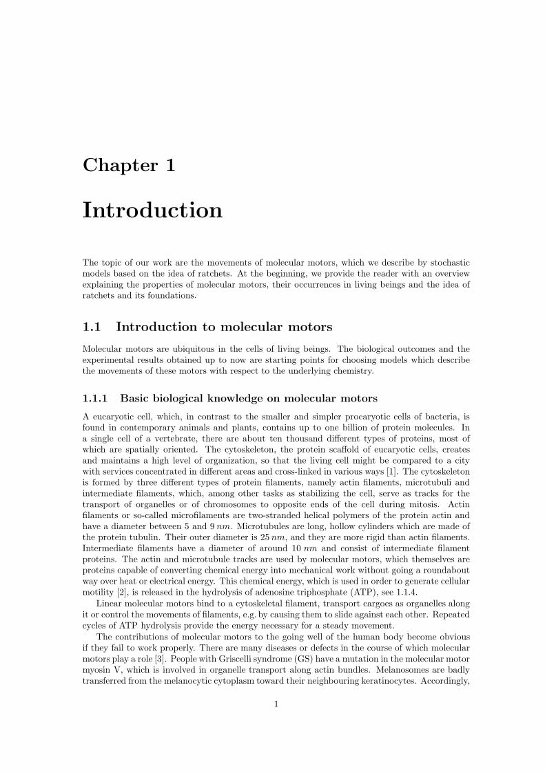
Figure 1.1: Silvery hair due to mutated myosin V [4].
a typical symptom in patients with GS is their silvery hair, see fig. 1.1. Usher’s syndrome, to namea second example, is caused by mutations of myosin VII. The typical symptoms of this syndromeare a loss of hearing, night blindness and a loss of peripheral vision.
There are dozens of different motor proteins in every eucaryotic cell. They differ in the typesof filaments they bind to, in the direction of movement along them, and in the cargo they carry.The cytoskeletal motor proteins associate with their filaments through a head region, the motordomain, which binds and hydrolyzes ATP. The proteins undergo a cycle of nucleotide hydrolysisand conformational change with states in which they are bound to their filamental tracks and statesin which they are unbound. Through a mechanochemical cycle of filament binding, conformationalchange, filament release, conformational relaxation, and filament rebinding, the motor protein andits cargo move one step at a time along the filament. The motor head determines the motor’s trackand the direction of movement along it, while the tail determines the cargo and the correspondingbiological function. Altogether, there are three groups of cytoskeletal motor proteins. All knownmotor proteins which move on actin filaments are members of the myosin superfamily, whereasthe motor proteins which move on microtubules are members either of the kinesin superfamily orthe dynein family [1]. The only structural element shared among all members of each superfamilyis the motor head domain. These heads can be attached to a wide variety of tails, which on theother hand attach to different types of cargo and enable the various family members to performdifferent functions in the cell.
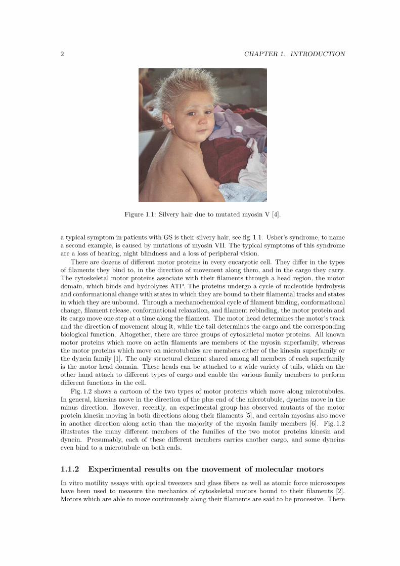
Fig. 1.2 shows a cartoon of the two types of motor proteins which move along microtubules.In general, kinesins move in the direction of the plus end of the microtubule, dyneins move in theminus direction. However, recently, an experimental group has observed mutants of the motorprotein kinesin moving in both directions along their filaments [5], and certain myosins also movein another direction along actin than the majority of the myosin family members [6]. Fig. 1.2illustrates the many different members of the families of the two motor proteins kinesin anddynein. Presumably, each of these different members carries another cargo, and some dyneinseven bind to a microtubule on both ends.
1.1.2 Experimental results on the movement of molecular motors
In vitro motility assays with optical tweezers and glass fibers as well as atomic force microscopeshave been used to measure the mechanics of cytoskeletal motors bound to their filaments [2].Motors which are able to move continuously along their filaments are said to be processive. There
1.1. INTRODUCTION TO MOLECULAR MOTORS 3
!!!!!!""""""######$$$$$$%%%%%%&&&&&&''''''(((((())))))******
++++++,,,,,,------......//////000000111111222222333333444444555555666666777777888888999999::::::;;;;;;<<<<<<======>>>>>>??????@@@@@@AAAAAABBBBBBCCCCCCDDDDDDEEEEEEFFFFFFGGGGGGHHHHHHIIIIIIJJJJJJKKKKKKLLLLLLMMMMMMNNNNNNOOOOOOPPPPPP
QQQQQQRRRRRRSSSSSSTTTTTTUUUUUUVVVVVVWWWWWWXXXXXXYYYYYYZZZZZZ[[[[[[\\\\\\]]]]]]^^^^^^______``````aaaaaabbbbbbccccccddddddeeeeeeffffffgggggghhhhhhiiiiiijjjjjjkkkkkkllllllmmmmmmnnnnnnooooooppppppqqqqqqrrrrrrssssssttttttuuuuuuvvvvvvwwwwwwxxxxxx
yyyyyyzzzzzz||||||~~~~~~
¡¡¡¡¡¡¢¢¢¢¢¢££££££¤¤¤¤¤¤¥¥¥¥¥¥¦¦¦¦¦¦
§§§§§§¨¨¨¨¨¨©©©©©©ªªªªªª««««««¬¬¬¬¬¬®®®®®®
¯¯¯¯¯¯°°°°°°
±±±±±±²²²²²²³³³³³³´´´´´´
µµµµµµ¶¶¶¶¶¶······¸¸¸¸¸¸¹¹¹¹¹¹ºººººº»»»»»»¼¼¼¼¼¼
½½½½½½¾¾¾¾¾¾¿¿¿¿¿¿ÀÀÀÀÀÀÁÁÁÁÁÁÂÂÂÂÂÂ
ÃÃÃÃÃÃÄÄÄÄÄÄ
ÅÅÅÅÅÅÆÆÆÆÆÆÇÇÇÇÇÇÈÈÈÈÈÈ
ÉÉÉÉÉÉÊÊÊÊÊÊ
ËËËËËËÌÌÌÌÌÌ
ÍÍÍÍÍÍÎÎÎÎÎÎÏÏÏÏÏÏÐÐÐÐÐÐÑÑÑÑÑÑÒÒÒÒÒÒÓÓÓÓÓÓÔÔÔÔÔÔÕÕÕÕÕÕÖÖÖÖÖÖ××××××ØØØØØØÙÙÙÙÙÙÚÚÚÚÚÚÛÛÛÛÛÛÜÜÜÜÜÜÝÝÝÝÝÝÞÞÞÞÞÞßßßßßßàààààà
ááááááââââââ
ããããããääääääååååååææææææ
ççççççèèèèèè
ééééééêêêêêêëëëëëëììììììííííííîîîîîî
ïïïïïïðððððð
ññññññññññññññññññññ
òòòòòòòòòòòòòòò
óóóóóóóóóóóóóóóóóóóó
ôôôôôôôôôôôôôôô
õõõõõõõõõõõõõõõõõõõõ
öööööööööööööööööööö
÷÷÷÷÷÷÷÷÷÷÷÷÷÷÷÷÷÷÷÷÷÷÷÷÷÷÷÷
øøøøøøøøøøøøøøøøøøøøøøøøøøøø
ùùùùùùùùùùùù
úúúúúúúúúúúú
ûûûûûûûûûûûû
üüüüüüüüüüüü
ýýýýýýþþþþþþ ÿÿÿ
ÿÿÿÿÿÿÿÿÿÿÿÿ
!!!!!!
""""""######$$$$$$%%%%%%
&&&&&&''''''
(())
***+++ ,,,---
..//
0011 2233444555
66778888889999
::::;;;;<<<<
<<======>>>>????
@@@@@@@@@@@@@@@@@@@@@@@@@@@@
AAAAAAAAAAAAAAAAAAAAAAAAAAAA BBBBBBCCCCCCDDDDDDDDDD
EEEEE
FFFGGG
HHHIIIJJJJJJJJJJ
KKKKKKKKKK
LLLLLLLLLLLLLLLLMMMMMMMMMMMMMMMM
NNNOOO
PPPPQQQQRRRSSSTTTTUUUU
VVVVVVVVVVVVVVVVWWWWWWWWWWWWWWWW
end
microtubule
cargo
tail
motor head
tail
cargo
motor head
minus plusend
dyneins
kinesins
Figure 1.2: The motor proteins of the families kinesin and dynein move along microtubules. Thisis only a rough cartoon, as naturally-occurring dyneins, e.g., have two or three heads.
have been experiments on two-headed kinesin [7, 8, 9, 10, 11, 12, 13, 14, 15], one-headed kinesin[16], myosin V [17, 18, 19, 20], and dynein [21, 22, 23]. Conventional kinesin, cytoplasmic dyneinand myosin V are examples of processive motors.
Several of the experiments on two-headed kinesin have shown that the average motor velocityv increases monotonically with the ATP concentration Γ and exhibits a saturation behaviour forlarge values of Γ. The hyperbolic form v (Γ) ' vmaxΓ/ (Γ∗ + Γ) has been used to fit the data forzero or small external load forces F [7, 9, 11]. Visscher et al. [15] have assumed force-dependentfit parameters vmax (F ) and Γ∗ (F ), and have found that the preceding fit is even possible overthe whole range of accessible forces, 0 ≤ |F | ≤ 5.6 pN , which leads to
v (Γ, F ) ' vmax (F ) Γ/ [Γ∗ (F ) + Γ] . (1.1)
Rief et al. as well as Mehta [18, 19] have proposed an analogous relation for the experimental dataon myosin V.
1.1.3 Regimes of motor movement and models
Before beginning to model molecular motors, one has to make sure what pieces of information onewants to obtain knowledge on. The starting point for modelling is the differentiation between thethree different scales of motor movement as described in the following.
Regime (i) is the regime of the molecular dynamics of a single step. Here, one considers theactual stepping process of the molecular motor in the context of single steps of about ∼ 10 nmwith corresponding stepping times of ∼ 10 ms, if there is enough ATP present.
Regime (ii) deals with the directed walk of a motor along a filament. The typical walkingdistances are in the range of µm and the walking times span seconds.
4 CHAPTER 1. INTRODUCTION
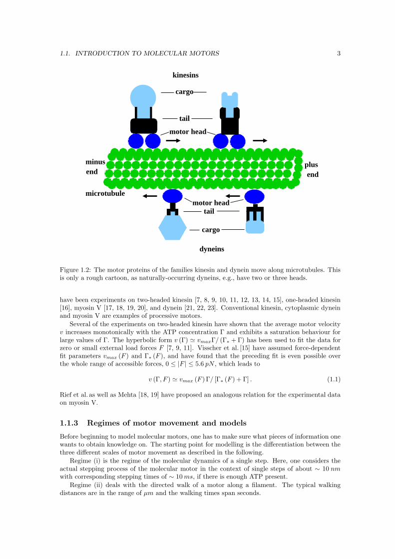
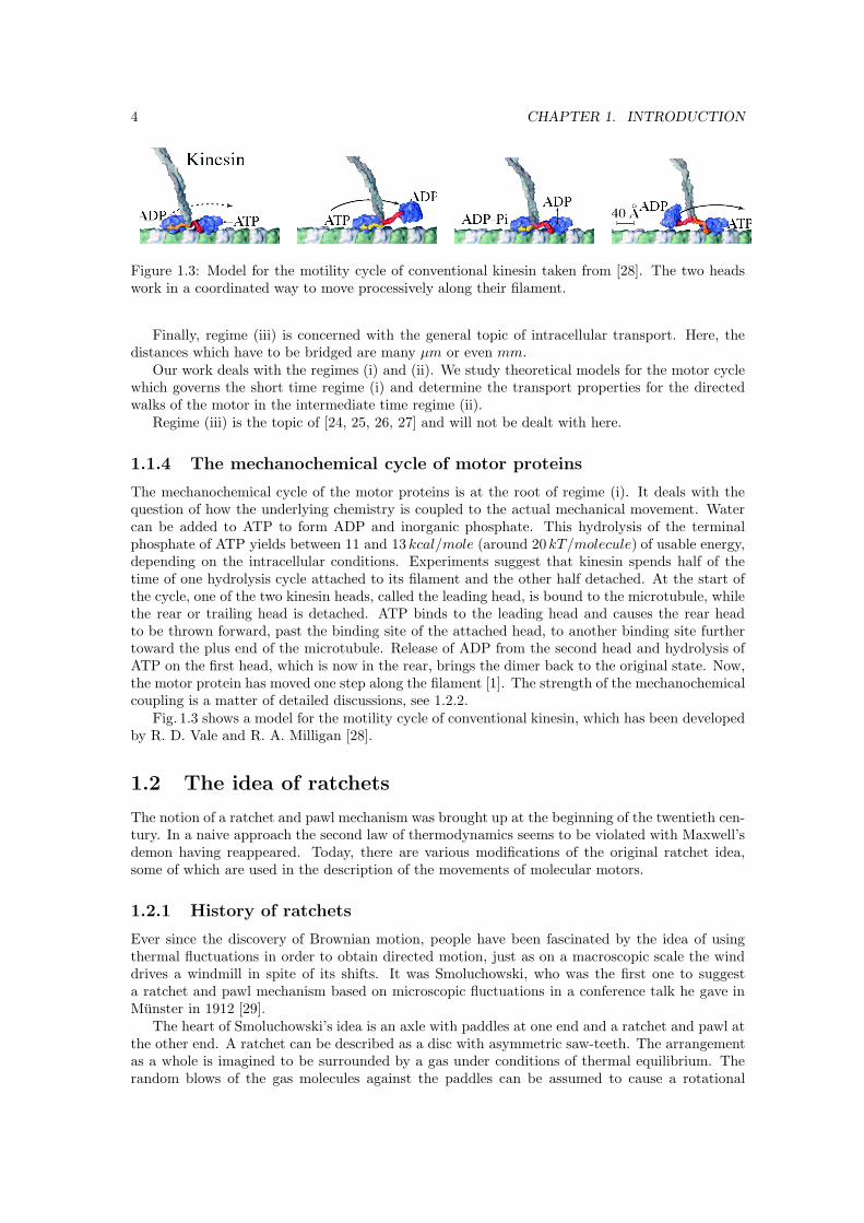
Figure 1.3: Model for the motility cycle of conventional kinesin taken from [28]. The two headswork in a coordinated way to move processively along their filament.
Finally, regime (iii) is concerned with the general topic of intracellular transport. Here, thedistances which have to be bridged are many µm or even mm.
Our work deals with the regimes (i) and (ii). We study theoretical models for the motor cyclewhich governs the short time regime (i) and determine the transport properties for the directedwalks of the motor in the intermediate time regime (ii).
Regime (iii) is the topic of [24, 25, 26, 27] and will not be dealt with here.
1.1.4 The mechanochemical cycle of motor proteins
The mechanochemical cycle of the motor proteins is at the root of regime (i). It deals with thequestion of how the underlying chemistry is coupled to the actual mechanical movement. Watercan be added to ATP to form ADP and inorganic phosphate. This hydrolysis of the terminalphosphate of ATP yields between 11 and 13 kcal/mole (around 20 kT/molecule) of usable energy,depending on the intracellular conditions. Experiments suggest that kinesin spends half of thetime of one hydrolysis cycle attached to its filament and the other half detached. At the start ofthe cycle, one of the two kinesin heads, called the leading head, is bound to the microtubule, whilethe rear or trailing head is detached. ATP binds to the leading head and causes the rear headto be thrown forward, past the binding site of the attached head, to another binding site furthertoward the plus end of the microtubule. Release of ADP from the second head and hydrolysis ofATP on the first head, which is now in the rear, brings the dimer back to the original state. Now,the motor protein has moved one step along the filament [1]. The strength of the mechanochemicalcoupling is a matter of detailed discussions, see 1.2.2.
Fig. 1.3 shows a model for the motility cycle of conventional kinesin, which has been developedby R. D. Vale and R. A. Milligan [28].
1.2 The idea of ratchets
The notion of a ratchet and pawl mechanism was brought up at the beginning of the twentieth cen-tury. In a naive approach the second law of thermodynamics seems to be violated with Maxwell’sdemon having reappeared. Today, there are various modifications of the original ratchet idea,some of which are used in the description of the movements of molecular motors.
1.2.1 History of ratchets
Ever since the discovery of Brownian motion, people have been fascinated by the idea of usingthermal fluctuations in order to obtain directed motion, just as on a macroscopic scale the winddrives a windmill in spite of its shifts. It was Smoluchowski, who was the first one to suggesta ratchet and pawl mechanism based on microscopic fluctuations in a conference talk he gave inMunster in 1912 [29].
The heart of Smoluchowski’s idea is an axle with paddles at one end and a ratchet and pawl atthe other end. A ratchet can be described as a disc with asymmetric saw-teeth. The arrangementas a whole is imagined to be surrounded by a gas under conditions of thermal equilibrium. Therandom blows of the gas molecules against the paddles can be assumed to cause a rotational
1.2. THE IDEA OF RATCHETS 5
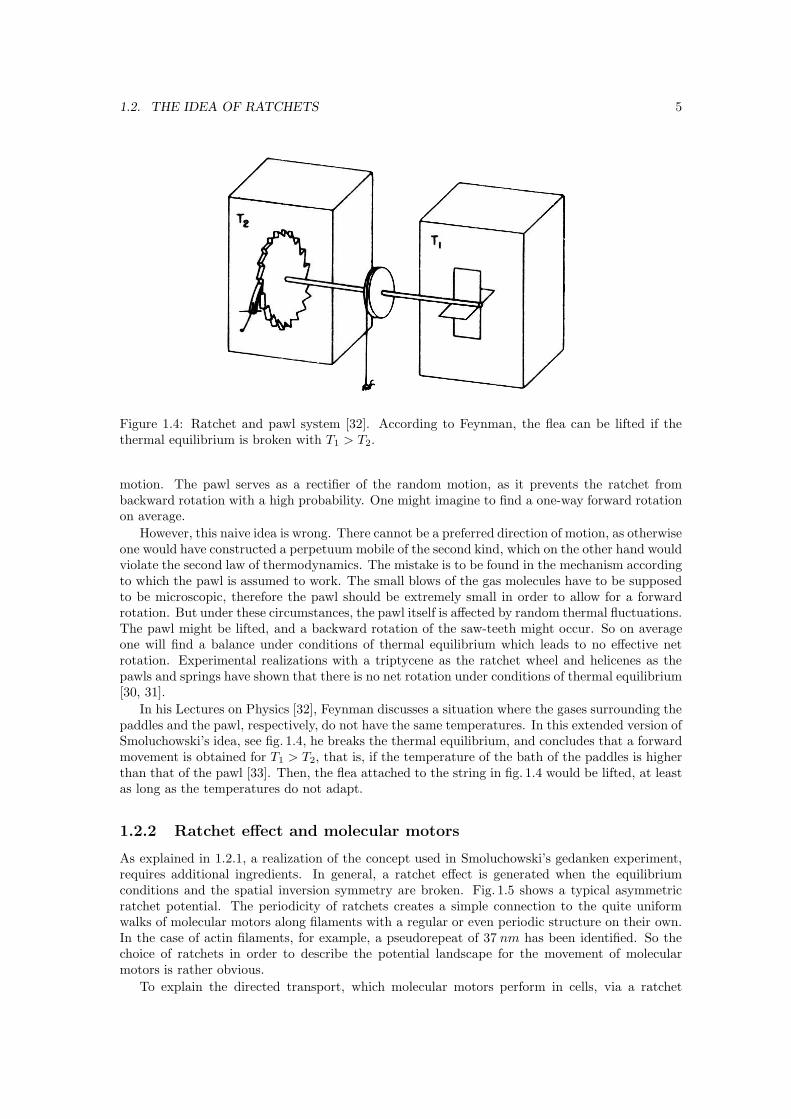
Figure 1.4: Ratchet and pawl system [32]. According to Feynman, the flea can be lifted if thethermal equilibrium is broken with T1 > T2.
motion. The pawl serves as a rectifier of the random motion, as it prevents the ratchet frombackward rotation with a high probability. One might imagine to find a one-way forward rotationon average.
However, this naive idea is wrong. There cannot be a preferred direction of motion, as otherwiseone would have constructed a perpetuum mobile of the second kind, which on the other hand wouldviolate the second law of thermodynamics. The mistake is to be found in the mechanism accordingto which the pawl is assumed to work. The small blows of the gas molecules have to be supposedto be microscopic, therefore the pawl should be extremely small in order to allow for a forwardrotation. But under these circumstances, the pawl itself is affected by random thermal fluctuations.The pawl might be lifted, and a backward rotation of the saw-teeth might occur. So on averageone will find a balance under conditions of thermal equilibrium which leads to no effective netrotation. Experimental realizations with a triptycene as the ratchet wheel and helicenes as thepawls and springs have shown that there is no net rotation under conditions of thermal equilibrium[30, 31].
In his Lectures on Physics [32], Feynman discusses a situation where the gases surrounding thepaddles and the pawl, respectively, do not have the same temperatures. In this extended version ofSmoluchowski’s idea, see fig. 1.4, he breaks the thermal equilibrium, and concludes that a forwardmovement is obtained for T1 > T2, that is, if the temperature of the bath of the paddles is higherthan that of the pawl [33]. Then, the flea attached to the string in fig. 1.4 would be lifted, at leastas long as the temperatures do not adapt.
1.2.2 Ratchet effect and molecular motors
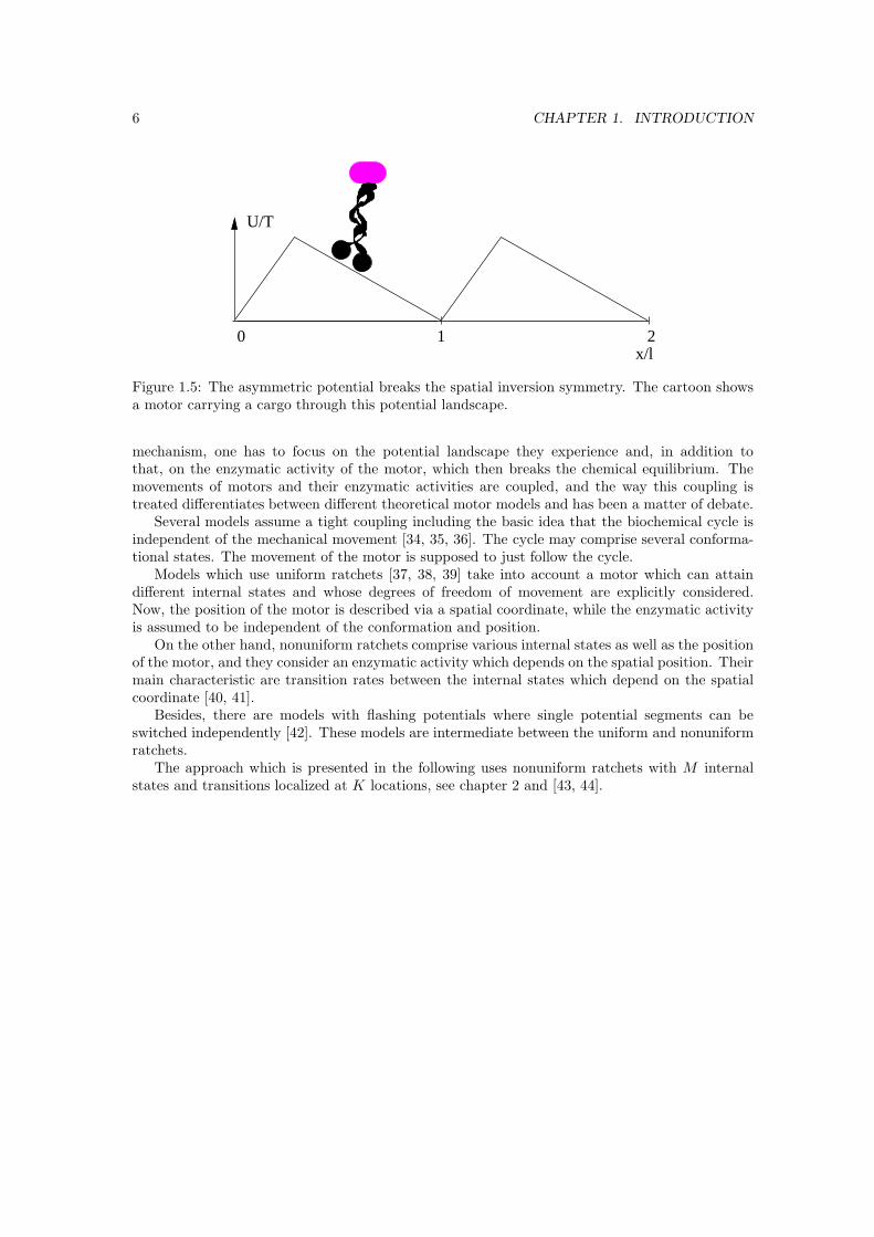
As explained in 1.2.1, a realization of the concept used in Smoluchowski’s gedanken experiment,requires additional ingredients. In general, a ratchet effect is generated when the equilibriumconditions and the spatial inversion symmetry are broken. Fig. 1.5 shows a typical asymmetricratchet potential. The periodicity of ratchets creates a simple connection to the quite uniformwalks of molecular motors along filaments with a regular or even periodic structure on their own.In the case of actin filaments, for example, a pseudorepeat of 37 nm has been identified. So thechoice of ratchets in order to describe the potential landscape for the movement of molecularmotors is rather obvious.
To explain the directed transport, which molecular motors perform in cells, via a ratchet
6 CHAPTER 1. INTRODUCTION
0 1 2x/l
U/T
Figure 1.5: The asymmetric potential breaks the spatial inversion symmetry. The cartoon showsa motor carrying a cargo through this potential landscape.
mechanism, one has to focus on the potential landscape they experience and, in addition tothat, on the enzymatic activity of the motor, which then breaks the chemical equilibrium. Themovements of motors and their enzymatic activities are coupled, and the way this coupling istreated differentiates between different theoretical motor models and has been a matter of debate.
Several models assume a tight coupling including the basic idea that the biochemical cycle isindependent of the mechanical movement [34, 35, 36]. The cycle may comprise several conforma-tional states. The movement of the motor is supposed to just follow the cycle.
Models which use uniform ratchets [37, 38, 39] take into account a motor which can attaindifferent internal states and whose degrees of freedom of movement are explicitly considered.Now, the position of the motor is described via a spatial coordinate, while the enzymatic activityis assumed to be independent of the conformation and position.
On the other hand, nonuniform ratchets comprise various internal states as well as the positionof the motor, and they consider an enzymatic activity which depends on the spatial position. Theirmain characteristic are transition rates between the internal states which depend on the spatialcoordinate [40, 41].
Besides, there are models with flashing potentials where single potential segments can beswitched independently [42]. These models are intermediate between the uniform and nonuniformratchets.
The approach which is presented in the following uses nonuniform ratchets with M internalstates and transitions localized at K locations, see chapter 2 and [43, 44].
Chapter 2
Models for molecular motors
As pointed out in chapter 1, our approach for modelling the directed walks of molecular motorsis based on nonuniform stochastic ratchets. These stochastic ratchets are equivalent to diffusion-reaction models or composite Markov processes [45] with space-dependent transition rates. Theycan be mapped onto stochastic networks of discrete states. Our models can be solved analytically.
2.1 Stochastic models
Our models for molecular motors are based on a Smoluchowski-equation approach. In this sectionwe focus on the basic ingredients of the model and take a look at the time evolution in themulti-state system.
2.1.1 Motor cycles
The cytoskeletal motor proteins associate with their filamental tracks through their head regionor motor domain, which binds and hydrolyzes ATP. Coordinated with their cycle of nucleotidehydrolysis and conformational change, the proteins cycle between states in which they are boundstrongly to their filament, states in which they are unbound and several intermediate states.
Usually, the mechanochemical cycles of molecular motors are discussed in terms of biochemicalreactions and enzyme kinetics, compare the overview in 1.1.4. One then has kinetic pathwayswhich are coupled to the conformational changes of the motor molecule. In our case a pathwaydenotes a cyclic sequence of molecular conformations which leads to a forward or backward stepof the molecular motor along the filament.
2.1.2 Basic ingredients
We use multi-state models with space-dependent transition rates. The basic ingredients are(i) a spatial coordinate x which describes the displacement of the centre-of-mass of the motor
molecule along the filament,(ii) M internal states which represent the various conformations the molecule can attain for a
fixed value of x,(iii) K spatial positions per motor cycle at which the motor molecule can undergo transitions
between these different internal states [43, 44].We visualize the meaning of these basic ingredients by taking a second look at fig. 1.3. On the
far left, each catalytic core is bound to a tubulin heterodimer along a microtubule. We can saythat the motor is in conformation m = 1 at location x1. It is possible that the motor unbindsor stretches further in both directions along the filament without a change in the centre-of-masscoordinate. In this case the motor would be in the internal state m = 2 or m = 3 at positionx1. So, the conformations or states of our models do not necessarily refer to different chemical
7
8 CHAPTER 2. MODELS FOR MOLECULAR MOTORS
conformations in a strict sense, but imply that the motor has somehow changed with respect toits environment.
In the next picture of fig. 1.3, the leading head is still bound, but the second head has movedin the forward direction for 16 nm and is now unbound. The conformation of the motor is againdifferent from the above mentioned, it can be m = 4. The centre-of-mass has moved forward toposition x2. Between this unbound situation and the rebinding in the third picture, the motorhead “searches” for the new binding site, so that we can distinguish a couple of subconformations,partly with centre-of-mass coordinates which are different from x2 or the new one x3, 8 nm awayfrom its starting position, in picture three. In the last picture we see that ADP dissociates andATP binds to the new leading head. If we make a distinction between the two heads, the motorhas attained a new conformation once again. After that, the cycle starts again. If there wassomething different in the second cycle, for example a defect of the filament, we have the choicebetween not starting at location x1 again, but introducing further locations, or otherwise startingat x1 with additional conformations. The second choice is sensible if the lengths of the “substeps”of the cycle are not changed. In general, the distances between the locations xk where transitionsbetween the states are possible are arbitrary. There are no constraints by a “lattice constant” ofany kind.
2.1.3 Langevin and Smoluchowski equation
One of the basic examples of a stochastic process is the Brownian motion of a particle. It isdescribed by the Langevin equation
v = −ζv + f (t) . (2.1)
In order to explain this equation we imagine a heavy particle whose mass is set to one and whichhas the velocity v. It moves in a liquid of light particles and receives pushes by the particles ofthe fluid at random. The pushes cause a slowing-down force −mζv with the friction coefficient ζand the stochastic force f (t).
As a next step, we introduce the probability density
P (ξ, t) = 〈δ (ξ − v (t))〉 (2.2)
that the Brownian particle has the velocity ξ at time t. The equation of motion for the probabilitydensities is then given by the Fokker-Planck-equation
∂
∂tP (v, t) = ζ
∂
∂vvP (v, t) + ζT
∂2
∂v2P (v, t) , (2.3)
which can also be written as a continuity equation,
∂
∂tP (v, t) = −ζ
∂
∂v
(−vP (v, t) − T
∂
∂vP (v, t)
). (2.4)
Here and in the following, we use energy units for the temperature. The current density, which isthe part in brackets, contains a drift part and a diffusional part. The equilibrium distribution ofthe Fokker-Planck equations is the Maxwell distribution with P (v, t) ∝ exp
(−v2/ (2T )
)
Now, we have a look at the Brownian motion in an effective external force field −∂V (x) /∂x.Note that V (x) is proportional to T−1.
The corresponding Langevin equation is
x = −ζx −∂V (x)
∂x+ f (t) . (2.5)
The case of a strong damping ζx x leads to the over-damped Langevin equation
x = −D
T
∂V
∂x+ r (t) (2.6)
2.1. STOCHASTIC MODELS 9
with the diffusion coefficient D and the fluctuating force r (t) as given by
D ≡T
ζ,
r (t) ≡1
ζf (t) . (2.7)
In the following we use the probability density
P (ξ, t) = 〈δ (ξ − x (t))〉 (2.8)
with P (ξ, t) dξ being the probability of finding the particle at time t at location ξ in the intervaldξ. The equation of motion is given by
∂
∂tP (ξ, t) = −
∂
∂ξ〈δ (ξ − x (t)) x (t)〉
= −∂
∂ξ
⟨δ (ξ − x (t))
(−
D
T
∂V (ξ)
∂ξ+ r (t)
)⟩
=∂
∂ξ
(D
TP (ξ, t)
∂V (ξ)
∂ξ
)−
∂
∂ξ〈δ (ξ − x (t)) r (t)〉
(2.9)
with
〈δ (ξ − x (t)) r (t)〉 = 2D
⟨δ
δr (t)δ (ξ − x (t))
⟩
= −2D∂
∂ξ
⟨δ (ξ − x (t))
δx (t)
δr (t)
⟩
= −D∂
∂ξP (ξ, t) . (2.10)
(2.9) and (2.10) yield the Smoluchowski equation
∂
∂tP (ξ, t) =
∂
∂ξ
(D
TP (ξ, t)
∂V (ξ)
∂ξ
)+ D
∂2
∂ξ2P (ξ, t) . (2.11)
The Smoluchowski equation on the other hand can be written as a continuity equation,
∂
∂tP (x, t) = −
∂
∂xJ (x, t) (2.12)
with the current
J (x, t) = −D
(∂V (x)
∂x+
∂
∂x
)P (x, t) , (2.13)
compare [46, 45, 47].A stationary solution of the Smoluchowski equation is
P (x, t) ∝ exp (−V (x)) , (2.14)
which leads to a vanishing current. This solution only holds in the case that there are no restrictionsof the x-coordinate. In the following, we will use periodic systems where P (x, t) has to fulfillperiodic boundary conditions. Nevertheless, the Smoluchowski equation as given by (2.12) can beused to describe the lateral movement for a one-state model of a motor protein, compare chapter4.1.1, where the periodicity is explicitly imposed.
10 CHAPTER 2. MODELS FOR MOLECULAR MOTORS
2.1.4 Time evolution in the multi-state system
In general, we need more than one state to describe the movement of a motor. Actually, it isoften necessary to consider more than two states, and accordingly, in contrast to the approachesdiscussed in [37, 38, 39, 48, 49], we examine multi-state systems. So in our systems, we have anumber of M states, and for each of these states we can write down a current equation (2.13), butwith level-dependent Jm, Dm, Vm and Pm. Then, we look at the time evolution of the probabilitydensities Pm (x, t) to find the particle or molecular motor at the centre-of-mass coordinate x andin its internal state or level m. The state variable m can attain the M values m = 1, ..., M .
The models include two ingredients by which a change of the probability density Pm (x) maytake place, namely
(i) lateral diffusion within state m, which leads to lateral currents Jm and(ii) transitions between the different internal states.Therefore, the probability densities Pm satisfy the equations
∂Pm (x, t) /∂t + ∂Jm (x, t) /∂x = Im (x, t) (2.15)
with the transition current densities Im and the lateral currents Jm. As we have already pointedout before, the lateral currents Jm have the form (2.13),
Jm (x, t) ≡ −Dm
(∂
∂xVm (x) +
∂
∂x
)Pm (x, t)
= −Dme−Vm(x) ∂
∂x
(eVm(x)Pm (x, t)
), (2.16)
with the small-scale diffusion coefficient Dm in level m. The friction coefficients are given byT/Dm.
The lateral currents Jm depend on the molecular interaction potentials Um (x) and on theexternal force F , which together define the effective force potentials
Vm (x) ≡ [Um (x) − Fx] /T, (2.17)
where T is the temperature in energy units. The external force F is an applied tangential force,which might be caused by a cargo. In experimental situations, people use artificial cargoes asbeads, which, for example, are held in an optical trap. It is natural to assume periodic andasymmetric molecular interaction potentials Um (x). The precise shape of the molecular interactionpotentials Um (x) is unknown, though, as these potentials are not accessible to experiments. So,as an example, we might imagine a simple asymmetric ratchet potential as drawn in fig. 1.5. Themolecular interaction potentials are assumed to be periodic with the characteristic length scale` representing the potential period, Um (x + `) = Um (x). In terms of experiments on motorproteins, F is the applied tangential force.
The transition current densities Im in (2.15) on their parts depend on the transition ratefunctions Ωmn from state m to state n via
Im (x, t) ≡∑
n,n6=m
[−Pm (x, t) Ωmn (x) + Pn (x, t) Ωnm (x)] . (2.18)
The transition rates are localized in space following recent considerations in the context of molec-ular motors [39, 40, 41], as we assume that the conformational changes of the motor depend onthe spatial position, compare 1.2.2, for example given by a localized binding site of the filamentaltrack. In the general case, the transitions can take place between any two states of the system.There is no fixed sequence of transitions.
The transition functions obey Ωmn (x) ≥ 0 and are given by
Ωmn (x) ≡∑
k
ωmn (xk) `Ωδ (x − xk) , (2.19)
so that they are localized at the discrete set of positions x = xk with k = 1, ..., K and xk withinthe interval 0 ≤ x1 < ... < xK < ` [40, 41, 43]. In (2.19), the ωmn (xk) ≥ 0 are transition rates,whereas `Ω ` represents a molecular localization length, and δ (z) is Dirac’s delta function.
2.2. GENERAL SOLUTION FOR STATIONARY STATES 11
2.2 General solution for stationary states
Now, the model systems which we have introduced in section 2.1 will be solved for stationarystates. Recursion relations for the currents and densities in the system are written down with theuse of a transfer matrix formalism. In the end, we obtain a result for the total lateral current,which is proportional to the velocity of the motor particle. A shorter version of this solutionprocedure is outlined in [43, 44].
2.2.1 Stationary states
Calculating the sum over all M states in (2.18), we find
∑
m
Im (x, t) = 0, (2.20)
which is obvious from the structure of (2.18), as each term occurs twice, but the second timewith a change in its sign. If the probability densities Pm are stationary with ∂Pm/∂t = 0, wehave ∂Ptot/∂t = 0 for the total probability Ptot =
∑m Pm. Then the total lateral current fulfills
Jtot =∑
m Jm = const, which is a result of (2.15). We consider such a stationary state, andintegrate the expression (2.16) for the lateral currents Jm in the region between x∗ and x, whichleads to
Pm (x) = Pm (x∗) em (x∗, x) −1
Dm
∫ x
x∗
dyJm (y) em (x∗, x) , (2.21)
where we introduce the exponential functions
em (y, z) ≡ exp (Vm (y) − Vm (z)) = 1/em (y, z) , (2.22)
which on the other hand depend on the effective force potentials Vm (x) = [Um (x) − Fx] /T asdefined in (2.17). In 2.2.4, equation (2.21) will be evaluated for several choices of the yet unspecifiedlimits x and x∗.
It is clear from their definitions that the exponential functions (2.22) obey the product rule
em (x1, x2) em (x2, x3) = e (x1, x3) . (2.23)
2.2.2 Boundary conditions and normalization
As indicated in fig. 1.5, it stands to reason to choose periodic molecular interaction potentials.The periodicity is an obvious assumption for the rather regular walks of molecular motors withsteps and substeps along filaments, which themselves show an inherent periodicity as in the case ofthe natural pseudorepeat distance of actin. The distances of the sites along the filament where abinding of the motor is most probable are fixed for “normal”filaments and motors. Accordingly, inorder to obtain a well-defined stationary state, we restrict ourselves to the finite interval 0 ≤ x < `and use periodic boundary conditions with the box normalization
∫ x1+`
x1
dxPtot (x) =
∫ x1+`
x1
dx∑
m
Pm (x) ≡ 1, (2.24)
which implies one particle per box. The size of the box can be identified with the potential periodof the periodic potentials Um (x) or with multiples thereof, so that we have Um (x + `) = Um (x).The particle velocity v is proportional to the total current with v = `Jtot.
2.2.3 Currents
In (2.19), we have introduced spatially localized transition rates, which are now shown to result inrather simple expressions for the local currents. First of all, we define the local transition current
Jmn (xk) ≡ Pm (xk) ωmn (xk) `Ω ≥ 0, (2.25)
12 CHAPTER 2. MODELS FOR MOLECULAR MOTORS
by which we describe the current from level m to level n at the spatial position xk.Then the localized transition rates (2.19) are inserted into the transition current densities Im
as given by (2.18). Integration of the equation ∂Jm/∂x = Im yields
Jm (x) = Jm +
K∑
k=1
∆Jm (xk) θ (x − xk) (2.26)
with spatially independent coefficients Jm and with the current discontinuities
∆Jm (xk) ≡∑
n,n6=m
[−Jmn (xk) + Jnm (xk)] . (2.27)
θ is Heaviside’s step function,
θ (x − xk) =
0 for x < xk
1 for x > xk. (2.28)
For the sum of the current discontinuities, we have∑
m ∆Jm (xk) = 0 for all xk, because thedouble sum over m and n again contains each term twice but with opposite sign. Therefore,summation of (2.26) over m leads to a total lateral current Jtot =
∑m Jm =
∑m Jm.
According to (2.26), the currents Jm (x) are piecewise constant functions of the spatial coor-dinate x. The local lateral current Jm (xk , xk+1) between position xk and position xk+1 in levelm is given by
Jm (xk, xk+1) = Jm +
k∑
q=1
∆Jm (xq)
= Jm +k∑
q=1
∑
n,n6=m
[−Jmn (xq) + Jnm (xq)] . (2.29)
This relationship is equivalent to
Jm (xk, xk+1) = Jm (xk−1, xk) +∑
n,n6=m
[−Jmn (xk) + Jnm (xk)] , (2.30)
which is an obvious consequence of (2.29) written down for Jm (xk−1, xk).In summary, we conclude that the systems we have introduced consist of a network of ver-
tices (m, xk). These vertices are ordered pairs whose first components are given by the respectiveinternal states m and whose second components are the corresponding spatial positions xk . Neigh-bouring vertices are connected via local currents as suggested by (2.29). At each vertex, the sumof all local currents vanishes, which defines a knot rule similar to Kirchhoff’s first rule in the caseof electric currents.
The networks and their representations as graphs are the topic of the chapters 3 and 4. Alisting of the terminology and the basic concepts of graph theory is provided in appendix C.Fig. 2.1 shows an overview of the vertices and their mutual connections via rates in a typicalnetwork. For fixed k, each pair of internal states, m and m′, can be connected by a pair ofvertical transition rates ωmn (xk) and ωnm (xk). This means that a motor whose centre-of-mass isat location xk in conformation m = 1 can change into conformation 2 with a certain probability,but also into conformation 3 or 4. This is an extension compared to other models with a fixedsequence of states [50, 51, 52]. Such fixed sequences of states correspond to a special path out ofthe total number of paths, which the motors can take along the networks in our models.
Now, we anticipate some expressions from the field of graph theory, compare appendix C,which will be used later on. A graph G is an ordered 2-tuple, (V (G) , E (G)), which consists of aset V (G) of vertices and a set E (G) of edges. The arrows in fig. 2.1, which connect two vertices,are called directed edges of the network. A walk or an edge train in the network of fig. 2.1 is an
2.2. GENERAL SOLUTION FOR STATIONARY STATES 13
k=1 k=2 k=K
m=2
m=1
m=M
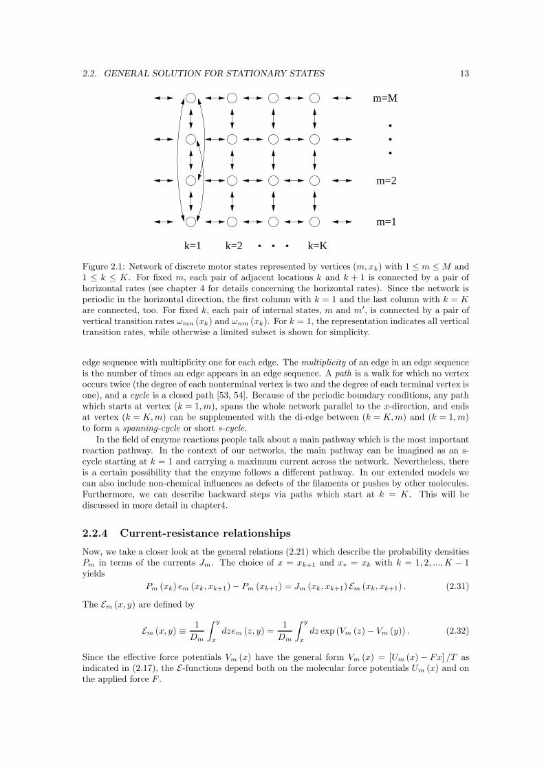
Figure 2.1: Network of discrete motor states represented by vertices (m, xk) with 1 ≤ m ≤ M and1 ≤ k ≤ K. For fixed m, each pair of adjacent locations k and k + 1 is connected by a pair ofhorizontal rates (see chapter 4 for details concerning the horizontal rates). Since the network isperiodic in the horizontal direction, the first column with k = 1 and the last column with k = Kare connected, too. For fixed k, each pair of internal states, m and m′, is connected by a pair ofvertical transition rates ωmn (xk) and ωnm (xk). For k = 1, the representation indicates all verticaltransition rates, while otherwise a limited subset is shown for simplicity.
edge sequence with multiplicity one for each edge. The multiplicity of an edge in an edge sequenceis the number of times an edge appears in an edge sequence. A path is a walk for which no vertexoccurs twice (the degree of each nonterminal vertex is two and the degree of each terminal vertex isone), and a cycle is a closed path [53, 54]. Because of the periodic boundary conditions, any pathwhich starts at vertex (k = 1, m), spans the whole network parallel to the x-direction, and endsat vertex (k = K, m) can be supplemented with the di-edge between (k = K, m) and (k = 1, m)to form a spanning-cycle or short s-cycle.
In the field of enzyme reactions people talk about a main pathway which is the most importantreaction pathway. In the context of our networks, the main pathway can be imagined as an s-cycle starting at k = 1 and carrying a maximum current across the network. Nevertheless, thereis a certain possibility that the enzyme follows a different pathway. In our extended models wecan also include non-chemical influences as defects of the filaments or pushes by other molecules.Furthermore, we can describe backward steps via paths which start at k = K. This will bediscussed in more detail in chapter4.
2.2.4 Current-resistance relationships
Now, we take a closer look at the general relations (2.21) which describe the probability densitiesPm in terms of the currents Jm. The choice of x = xk+1 and x∗ = xk with k = 1, 2, ..., K − 1yields
Pm (xk) em (xk, xk+1) − Pm (xk+1) = Jm (xk , xk+1) Em (xk, xk+1) . (2.31)
The Em (x, y) are defined by
Em (x, y) ≡1
Dm
∫ y
x
dzem (z, y) =1
Dm
∫ y
x
dz exp (Vm (z) − Vm (y)) . (2.32)
Since the effective force potentials Vm (x) have the general form Vm (x) = [Um (x) − Fx] /T asindicated in (2.17), the E-functions depend both on the molecular force potentials Um (x) and onthe applied force F .
14 CHAPTER 2. MODELS FOR MOLECULAR MOTORS
In 2.2.3 we have seen that the currents obey a knot rule. Now, we consider relation (2.31) andassume the difference Pm (xk) em (xk, xk+1) − Pm (xk+1) to be the local voltage and the functionEm (xk, xk+1) to be the local resistance of the networks. The equations (2.31) thus are current-resistance relationships which resemble Ohm’s law for electrical circuits. If a molecular interactionpotential Um (x) has a high potential barrier within a given interval xk < x < xk+1, we derivefrom (2.32) that in this case we will find a large resistance Em (xk , xk+1) and, correspondingly, asmall current Jm (xk, xk+1).
We consider a vertex (m, xk) at which all local transition currents Jmn (xk), i.e., the verticalcurrents given by (2.25), vanish. We have Jm (xk , xk+1) = Jm (xk−1, xk) ≡ Jk
m. Consideringa series combination of the corresponding two resistances Em (xk−1, xk) and Em (xk, xk+1), thecurrent-resistance relationships (2.31) with xk−1, xk and xk, xk+1, respectively, lead to the equa-tion
Pm (xk−1) em (xk−1, xk+1) − Pm (xk+1) = JkmEm (xk−1, xk+1) , (2.33)
which contains the combined series resistance Em (xk−1, xk+1) which is calculated from (2.32) as
Em (xk−1, xk+1) = Em (xk−1, xk) em (xk, xk+1) + Em (xk , xk+1) , (2.34)
or, if we introduce the modified resistances
E ′m (x, y) = Em (x, y) exp (Vm (y)) , (2.35)
asE ′
m (xk−1, xk+1) = E ′m (xk−1, xk) + E ′
m (xk, xk+1) . (2.36)
Thus, the series combination of two modified resistances is the sum of the two single resistancesas in the case of electric circuits.
2.2.5 Recursion relation for currents and densities
Now, our aim is to combine the vertex rules (2.30) for the local currents and the current-resistancerelationships (2.31) into recursion relations for the local currents and densities.
At first, we consider the vertex rules (2.30) for the local currents and express the local transitioncurrents Jmn (xk) in terms of the probability densities Pm (xk) as done in (2.25). This yields therecursion relation
Jm (xk, xk+1) = Jm (xk−1, xk)
+∑
n,n6=m
[−Pm (xk) ωmn (xk) + Pn (xk) ωnm (xk)] lΩ, (2.37)
which provides us with a possibility of calculating the outgoing lateral currents Jm (xk , xk+1) fromposition xk to xk+1 in terms of the incoming lateral currents Jm (xk−1, xk) and the probabilitydensities Pm (xk) at location xk.
We introduce the two transfer matrices TJJ with
T JJnm ≡ δnm (2.38)
and TPJ (xk) which is given by
T PJnm (xk) ≡ −δnm
∑
p6=m
ωmp (xk) `Ω + (1 − δnm) ωnm (xk) `Ω. (2.39)
In order to further simplify our writing, we define the row vectors J ≡ (J1, ..., JM ) and P ≡(P1, .., PM ). Using this short notation, the recursion relation for the currents (2.37) can be writtenin the compact form
J (xk, xk+1) = J (xk−1, xk)TJJ + P (xk)TPJ (xk) (2.40)
2.2. GENERAL SOLUTION FOR STATIONARY STATES 15
where the first transfer matrix TJJ is equal to the unit matrix according to (2.38).There is a second set of equations which can be obtained from the current-resistance relations
(2.31) and which is needed for the recursion relation for the probability densities. We rewrite(2.31) as
Pm (xk+1) = −Jm (xk, xk+1) Em (xk, xk+1) + Pm (xk) em (xk, xk+1) (2.41)
and obtain a way of calculating the densities Pm (xk+1) at location xk+1 in terms of the outgoingcurrents Jm (xk , xk+1) from xk to xk+1 and the densities Pm (xk) at the former location xk .
As we want to use the row vectors J and P for a comprehensive formulation of this second setof recursion relations again, we further set up two diagonal matrices DJP and DPP with matrixelements
DJPnm (xk, xk+1) ≡ −δnmEm (xk, xk+1) (2.42)
andDPP
nm (xk , xk+1) ≡ δnmem (xk, xk+1) . (2.43)
Besides, we define the additional transfer matrices
TJP ≡ TJJDJP (2.44)
andTPP ≡ TPJDJP + DPP . (2.45)
With the help of these matrices, the recursion relations (2.41) can be rewritten in the compactform
P (xk+1) = J (xk, xk+1)DJP (xk, xk+1) + P (xk)DPP (xk , xk+1)
= J (xk−1, xk)TJP (xk, xk+1) + P (xk)TPP (xk, xk+1) , (2.46)
where we have reused (2.40) to obtain the second equation. In this way, we arrive at recursionrelations which express the probability densities P (xk+1) at xk+1 in terms of the incoming currentsJ (xk−1, xk), which arrive at location xk from xk−1, and the probability densities P (xk) at locationxk.
Finally, the two recursion relations (2.40) and (2.46) for the outgoing currents and the newdensities may be united in a single recursion relation given by
(J (xk, xk+1) , P (xk+1)) = (J (xk−1, xk) , P (xk))T (xk, xk+1) , (2.47)
where we have defined the row vector (J, P ) with 2M components and the 2M × 2M transfermatrix T which contains the four M × M transfer matrices TJJ , TPJ , TJP and TPP .
The system as described so far comprises a set of 2MK variables, which is made up of MK lat-eral currents J (xk, xk+1) and MK probability densities P (xk). As a result we have characterizeda network consisting of MK discrete states.
Now, we focus on a further reduction of the number of variables. To do so, we use the recursionrelation (2.47) and express all lateral currents and probability densities in terms of the densitiesPm (x1) of location x1 and the lateral currents which enter the system from x < x1 (2.26).
Using the notation J ≡(J1, ..., JM
), iteration of (2.47) leads to
(J (xk−1, xk) , P (xk)) =(J, P (x1)
)T(k) (2.48)
with the combined transfer matrices
T(k) ≡
k−1∏
j=1
T (xj , xj+1) . (2.49)
The combined transfer matrices T(k) with k = 2, ..., K relate the local lateral currents Jm (xk−1, xk)arriving at x = xk and the densities Pm (xk) to the average currents Jm and the densities Pm (x1)at location x1. We supplement these matrices by the matrix T(1) which is equal to the unit matrix.
16 CHAPTER 2. MODELS FOR MOLECULAR MOTORS
Now, we take a closer look at the separate components of (2.48). The first M components ofthis equation determine the local lateral currents J (xk−1, xk) via
Jm (xk−1, xk) =M∑
i=1
J iT(k)i,m +
2M∑
i=M+1
Pi−M (x1) T(k)i,m (2.50)
where T(k)i,m denotes the matrix element of T(k) in the ith row and the mth column. Jm (xk−1, xk)
is calculated via the elements in column m of T(k).The remaining M components of the transfer matrix equation (2.48) determine the densities
Pm (xk) via
Pm (xk) =M∑
i=1
J iT(k)i,M+m +
2M∑
i=M+1
Pi−M (x1) T(k)i,M+m. (2.51)
We notice that the densities Pm (xk) on the other hand depend on the matrix elements in the(M + m)th column of T(k).
2.2.6 Implementation of periodic boundary conditions
In 2.2.5 we have come to conclude that in order to solve our problem, we need 2M equationswhich define the 2M unknowns Jm and Pm (x1). These equations are provided by the periodicboundary conditions together with the normalization condition. In this subsection we implementthe periodic boundary conditions. The normalization condition is treated in 2.2.7.
The system is taken to be periodic in the spatial coordinates x with 0 ≤ x < `, see 2.2.2.This implies that the currents and densities satisfy the periodic boundary conditions Jm (x + `) =Jm (x) and Pm (x + `) = Pm (x) with xK+1 ≡ x1 + ` per definition.
We start with the periodic boundary conditions for the lateral currents using Jm (x) = Jm +∑Kk=1 ∆Jm (xk) θ (x − xk) as in (2.26). If we now choose x > xK with Jm (x) = Jm, we obtain
K∑
k=1
∆Jm (xk) /`Ω =K∑
k=1
∑
n,n6=m
[−Pm (xk) ωmn (xk) + Pn (xk)ωnm (xk))] = 0 for m = 1, ..., M.
(2.52)
The above equation results from inserting (2.25).Since
∑m ∆Jm (xk) = 0 for any value of xk as explained in 2.2.3, only M − 1 of the M
equations given by (2.52) are linearly independent. In general, we can choose any subset whichcontains (M − 1) equations from this set of M equations. However, we can always relabel theinternal states so that the omitted equation corresponds to m = M . We will assume this to bedone and therefore keep the first (M − 1) equations from (2.52).
As announced, in these (M − 1) equations we replace all densities Pm (xk) with k ≥ 2 by theaverage currents Jm and the densities Pm (x1) by using the transfer matrix equations (2.51). Inthis way, we arrive at a new set of equations as given by
M∑
i=1
J iA(M,K)i,m +
2M∑
i=M+1
Pi−M (x1) A(M,K)i,m = 0 (2.53)
with 1 ≤ m ≤ M −1 which defines the first (M − 1) columns of a new matrix A(M,K) with matrixelements
A(M,K)i,m ≡
K∑
k=1
∑
n,n6=m
S (k, m, n) (2.54)
andS (k, m, n) ≡ −T
(k)i,M+mωmn (xk) + T
(k)i,M+nωnm (xk) . (2.55)
2.2. GENERAL SOLUTION FOR STATIONARY STATES 17
It is noteworthy that each term of the matrix elements A(M,K)i,m in (2.54) contains one explicit
factor ωmn (xk) or ωnm (xk), i.e., in the case of non-vanishing transfer matrix elements each termis proportional to one or more vertical transition rates. In fact, for K 6= 1 there is always at
least one non-vanishing transfer matrix element T(K)i,j since in a single row of T(K)there are no M
neighbouring columns which contain elements equal to zero.
Now, we take into account the periodic boundary conditions for the densities Pm (x). First,we use equation (2.41) for k = K which leads to
Pm (xK+1) = −Jm (xK , xK+1) Em (xK , xK+1) + Pm (xK) em (xK , xK+1) (2.56)
with xK+1 = x1+` as before. The periodic boundary conditions imply Pm (xK+1) = Pm (x1 + `) =Pm (x1) and Jm (xK , xK+1) = Jm. If this is inserted into (2.56), we obtain, after rearranging theequation,
Pm (xK) = JmEm (xK , xK+1)
em (xK , xK+1)+ Pm (x1)
1
em (xK , xK+1). (2.57)
On the other hand, it follows from (2.51) when inserting k = K that
Pm (xK) =
M∑
i=1
J iT(K)i,M+m +
2M∑
i=M+1
Pi−M (x1) T(K)i,M+m. (2.58)
Now, if we equate (2.57) and (2.58), we obtain another set of M equations given by
M∑
i=1
J iA(M,K)i,M+m−1 +
2M∑
i=M+1
Pi−M (x1) A(M,K)i,M+m−1 = 0 (2.59)
with m = 1, ..., M . The new elements of the matrix A(M,K) are given by
A(M,K)i,M+m−1 ≡ T
(K)i,M+m − δi,m
Em (xK , xK+1)
em (xK , xK+1)for 1 ≤ i ≤ M (2.60)
and by
A(M,K)i,M+m−1 ≡ T
(K)i,M+m −
δi−M,m
em (xK , xK+1)for M + 1 ≤ i ≤ 2M. (2.61)
According to (2.49), the combined transfer matrix T(K) is a product of transfer matricesT (xj , xj+1) with j ≤ K − 1. The latter transfer matrices depend on the local transition cur-rents Jmn (xk) with k ≤ K − 1 but are independent of the local transition currents Jmn (xK) ≡Pm (xK) ωmn (xK) `Ω. Therefore, the combined transfer matrix T(K) is independent of these latter
currents, too. This implies that the matrix elements A(M,K)i,M+m−1 in (2.60) and (2.61) do not depend
on the vertical transition rates ωmn (xK).
2.2.7 Implementation of normalization condition
As we have shown in 2.2.6, the periodic boundary conditions lead to 2M − 1 linearly independentequations which are provided by (2.53) and (2.59). In order to determine the 2M variables Jm andPm (x1) unambiguously, we need one additional equation which is supplied by the normalizationcondition.
When the explicit form of the densities and currents is inserted into the normalization condition(2.24), we obtain the expression
1 =∑
m
[Pm (x1) em − JmEm (x1) −
K∑
k=1
∆Jm (xk) Em (xk)
], (2.62)
18 CHAPTER 2. MODELS FOR MOLECULAR MOTORS
which depends on the integrals
em ≡
∫ x1+`
x1
dxem (x1, x) (2.63)
and
Em (xk) ≡
∫ x1+`
xk
dxEm (xk, x) . (2.64)
The normalization condition (2.62) contains the current discontinuities ∆Jm (xk) for all k. How-ever, it follows from the relation (2.52) that
∆Jm (xK) = −K−1∑
k=1
∆Jm (xk) . (2.65)
When this relation is inserted into (2.62), we obtain
∑
m
[−JmEm (x1) + Pm (x1) em −
K−1∑
k=1
∆Jm (xk)Dm (xk)
]= 1 (2.66)
withDm (xk) ≡ Em (xk) − Em (xK) . (2.67)
Since this equation no longer involves the current discontinuities ∆Jm (xK) at location xK , it doesnot depend on the transition rate constants ωmn (xK).
The current discontinuities ∆Jm (xk) with 1 ≤ k ≤ K − 1 can be expressed in terms of thedensities Pm (xk) via (2.27) and (2.25). These densities on the other hand can be expressed interms of the variables Jm and Pm (x1) using the transfer matrix relations (2.51).
In this way we get the equation
M∑
i=1
J iA(M,K)i,2M +
2M∑
i=M+1
Pi−M (x1) A(M,K)i,2M = 1, (2.68)
which defines the last or 2Mth column of the matrix A(M,K) with elements
A(M,K)i,2M ≡ −E i (x1) −
K−1∑
k=1
∑
m
∑
n,n6=m
S (k, m, n)Dm (xk) lΩ for 1 ≤ i ≤ M (2.69)
and
A(M,K)i,2M ≡ ei−M −
K−1∑
k=1
∑
m
∑
n,n6=m
S (k, m, n)Dm (xk) lΩ for M + 1 ≤ i ≤ 2M (2.70)
with S (k, n, m) as defined in (2.55).
2.2.8 Calculation of the total current
As all lateral currents and probability densities can be described in terms of the 2M densitiesPm (x1) and the lateral currents Jm which enter the system from x < x1, we have
[J, P (x1)
]= [0, ..., 0, 1]
(A(M,K)
)−1
= [0, ..., 0, 1]C
detA(M,K), (2.71)
where A(M,K) is a 2M×2M matrix as explained in the preceding sections. The matrix elements ofC are the cofactors Cij ≡ (−1)
i+jdetA(M,K)[j, i], where A(M,K) [j, i] is the (2M − 1)× (2M − 1)
2.2. GENERAL SOLUTION FOR STATIONARY STATES 19
matrix obtained from A(M,K) by erasing its jth row and ith column. Each of the first M − 1columns of A(M,K) corresponds to the periodic boundary condition for one lateral current Jm,each of the next M columns to the periodic boundary condition for one density Pm and the last
one to the normalization condition. The total current J(M,K)tot =
∑Mm=1 Jm which determines the
motor velocity v(M,K) via v(M,K) = `J(M,K)tot is
J(M,K)tot =
M∑
m=1
Jm =M∑
m=1
(−1)2M+m detA(M,K) [m, 2M ] /detA(M,K). (2.72)
As we use algebraic computer systems [55], which soon reach their limitations in complex
matrix calculations, computing the complete inverse matrix(A(M,K)
)−1is often impossible so
that we generally confine ourselves to the calculation of the elements contributing to J(M,K)tot as
explained above.It is convenient to write
J(M,K)tot =
Pol(M,K)1
(ω12 (x1) , ω12 (x2) , . . . , ω(M−1)M (xK)
)
Pol(M,K)2
(ω12 (x1) , ω12 (x2) , . . . , ω(M−1)M (xK)
) (2.73)
with two polynomials Pol(M,K)1 and Pol
(M,K)2 which depend on the vertical transition rates of the
respective model. In chapter 3 we will calculate and characterize the total current and the twopolynomials for various model systems.

20 CHAPTER 2. MODELS FOR MOLECULAR MOTORS
Chapter 3
Results for various (M,K)-models
and universal rules
In chapter 2 we have shown that our stochastic ratchets can be mapped onto stochastic networksof MK discrete states, which are represented by their respective vertices (m, xk), where m is thecoordinate of the state or level, and xk is the spatial coordinate.
Here, we present a detailed investigation of models with explicitly specified values of M andK [44]. The maximal number of states as well as the number of locations in these models variesbetween one and four. In this way we show that our general class of models has the advantageof comprising the possibility of describing the movements of a variety of different motor proteins.
At first, we calculate the resulting total current J(M,K)tot for each of these models, then we take
a closer look at the various terms which contribute to the current and their dependence on thevertical transition rates of the model. We also discuss conceivable implications of these modelsin terms of the mechanochemical cycles of molecular motors and their structures. Several rules
concerning the matrices A(M,K) and the total current J(M,K)tot , which is calculated with the help
of these matrices, can be derived. These rules impose constraints on the terms contributing to thecurrent, so that if we have a network with a specified number of states and locations, we can list
the combinations of vertical rates occurring in the terms of J(M,K)tot without actually calculating
the matrix A(M,K) for this special case. Furthermore, we examine ratchets with several explicitlyunbalanced transitions, which can arise from the enzymatic activity of the motor. With the helpof the rules for the current we can predict possible simplifications in the dependence of the motorvelocity on these unbalanced rates, too.
3.1 Examples of (M, K)-models
Here, we investigate models with different values of M and K. The inspected models comprise oneto four states and one to four locations. We focus on the question of how the vertical transition
rates enter the total current, which is the quotient of the two polynomials Pol(M,K)1 and Pol
(M,K)2 .
Mainly, we centre on the terms of Pol(M,K)1 as they correspond to paths through the network,
whereas Pol(M,K)2 provides a standardization of the total current with respect to the set of vertical
rates which actually occur in the present model.
3.1.1 The special case of a single internal state
In the case of a single internal state , there are no vertical transition rates, i.e., the state isfixed. We have diffusion within this state, and there can be a periodic landscape described bythe state’s effective force potential, but no chemical reaction or conformational change. Withoutan external force the motor might find itself in a situation as the one depicted in fig. 1.5. The
21
22 CHAPTER 3. RESULTS FOR VARIOUS (M, K)-MODELS AND UNIVERSAL RULES
single-state situation applies to a motor which is for some reason cut off its supply of fuel andwhose conformation is fixed. The fixed conformation might be a consequence of the lack of fuel,but it can also result from a genetic defect.
The corresponding matrix A(1,K) is a 2 × 2 matrix whose elements depend on the effectiveforce potential V1 (x), the small-scale diffusion coefficient D1 and the spatial positions xk . In thecase of a single location, i.e., K = 1, A(1,1) reads
A(1,1) =
(−E1 (x1, x1 + `) /e1 (x1, x1 + `) −E1 (x1)
1 − 1/e1 (x1, x1 + `) e1
)(3.1)
with E1 (x1, x1 + `), e1 (x1, x1 + `), E1 (x1) and e1 as defined in chapter 2. The total current J(1,1)tot
is calculated as
J(1,1)tot =
1 − e1 (x1, x1 + `)
(e1 (x1, x1 + `) − 1) E1 (x1) − E1 (x1, x1 + `) e1
. (3.2)
This current vanishes in the absence of an external force for all single state models, no matter whatis the choice of K, as there cannot be a net current with a single fixed molecular interaction poten-tial. This is obvious in 3.2, since in this case we have e1 (x1, x1 + `) = exp (U1 (x1) − U1 (x1)) = 1.
If there is a finite external force, while the molecular interaction potential vanishes, the totalcurrent reads
J(1,1)tot (U1 = 0) =
FD1
`T, (3.3)
This relationship will be explained further in 4.1.1.
3.1.2 Results for two internal levels
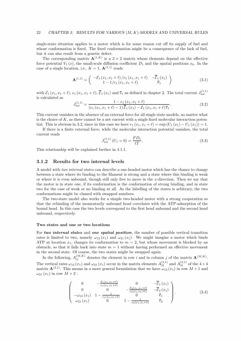
A model with two internal states can describe a one-headed motor which has the chance to changebetween a state where its binding to the filament is strong and a state where this binding is weakor where it is even unbound, though still only free to move in the x-direction. Then we say thatthe motor is in state one, if its conformation is the conformation of strong binding, and in statetwo for the case of weak or no binding at all. As the labelling of the states is arbitrary, the twoconformations might be classed with swapped numbers.
The two-state model also works for a simple two-headed motor with a strong cooperation sothat the rebinding of the momentarily unbound head correlates with the ATP-adsorption of thebound head. In this case the two levels correspond to the first head unbound and the second headunbound, respectively.
Two states and one or two locations
For two internal states and one spatial position , the number of possible vertical transitionrates is limited to two, namely ω12 (x1) and ω21 (x1). We might imagine a motor which bindsATP at location x1, changes its conformation to m = 2, but whose movement is blocked by anobstacle, so that it falls back into state m = 1 without having performed an effective movementin the second state. Of course, the two states might be swapped again.
In the following, A(M,K)ij denotes the element in row i and in column j of the matrix A(M,K).
The vertical rates ω12 (x1) and ω21 (x1) occur in the matrix elements A(2,1)31 and A
(2,1)41 of the 4× 4
matrix A(2,1). This means in a more general formulation that we have ω12 (x1) in row M + 1 andω21 (x1) in row M + 2 :
0 −E1(x1,x1+`)e1(x1,x1+`) 0 −E1 (x1)
0 0 −E2(x1,x1+`)e2(x1,x1+`) −E2 (x1)
−ω12 (x1) 1 − 1e1(x1,x1+`) 0 e1
ω21 (x1) 0 1 − 1e2(x1,x1+`) e2
. (3.4)
3.1. EXAMPLES OF (M, K)-MODELS 23
k=1 k=2
m=1
m=2
Figure 3.1: Network representation for (M, K) = (2, 2). In this general model, there are fourvertical transition rates connecting the two states.
If there is no external force, F = 0, the total current J(2,1)tot vanishes as expected from the idea
of the blocked motor above. There is no ratchet effect present, the switching back to the originalstate takes place at the same position.
For an external force F 6= 0, the polynomials Pol(2,1)1 and Pol
(2,1)2 which enter the total current
as explained in chapter 2, consist of terms containing a single vertical transition rate. Squares(or higher powers) or products of the two rates do not occur. Here, a net movement can occurbecause of the external force, which might even be effective against hindrances.
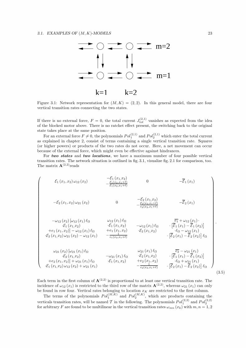
For two states and two locations , we have a maximum number of four possible verticaltransition rates. The network situation is outlined in fig. 3.1, visualize fig. 2.1 for comparison, too.The matrix A(2,2)reads
E1 (x1, x2) ω12 (x2)−E1 (x1,x2)
−E1(x2,x1+`)E1(x2,x1+`)
0 −E1 (x1)
−E2 (x1, x2) ω21 (x2) 0−E2 (x1,x2)
−E2(x2,x1+`)e2(x2,x1+`)
−E2 (x1)
−ω12 (x2) [ω12 (x1) `Ω
·E1 (x1,x2)+e1 (x1, x2)] − ω12 (x1) `Ω
·E2 (x1,x2) ω21 (x2) − ω12 (x1)
ω12 (x1) `Ω
·E1 (x1,x2)+e1 (x1, x2)− 1
e1(x2,x1+`)
−ω12 (x1) `Ω
·E2 (x1,x2)
e1 + ω12 (x1) ··[E1 (x1) − E1 (x2)
]
·`Ω − ω12 (x1)·[E2 (x1) − E2 (x2)
]`Ω
ω21 (x2) [ω21 (x1) `Ω
·E2 (x1,x2)+e2 (x1, x2)] + ω21 (x1) `Ω
·E1 (x1,x2) ω12 (x2) + ω21 (x1)
−ω21 (x1) `Ω
·E1 (x1,x2)
ω21 (x1) `Ω
·E2 (x1,x2)+e2 (x1, x2)− 1
e2(x2,x1+`)
e2 − ω21 (x1)·[E1 (x1) − E1 (x2)
]
·`Ω + ω21 (x1)
·[E2 (x1) − E2 (x2)
]`Ω
.
(3.5)
Each term in the first column of A(2,2) is proportional to at least one vertical transition rate. Theincidence of ω12 (x1) is restricted to the third row of the matrix A(2,2), whereas ω21 (x1) can onlybe found in row four. Vertical rates belonging to location xK are restricted to the first column.
The terms of the polynomials Pol(M,K)1 and Pol
(M,K)2 , which are products containing the
verticals transition rates, will be named T in the following. The polynomials Pol(2,2)1 and Pol
(2,2)2
for arbitrary F are found to be multilinear in the vertical transition rates ωmn (xk) with m, n = 1, 2
24 CHAPTER 3. RESULTS FOR VARIOUS (M, K)-MODELS AND UNIVERSAL RULES
m=1
m=2
k=1 k=2
m=1
m=2
k=1 k=2
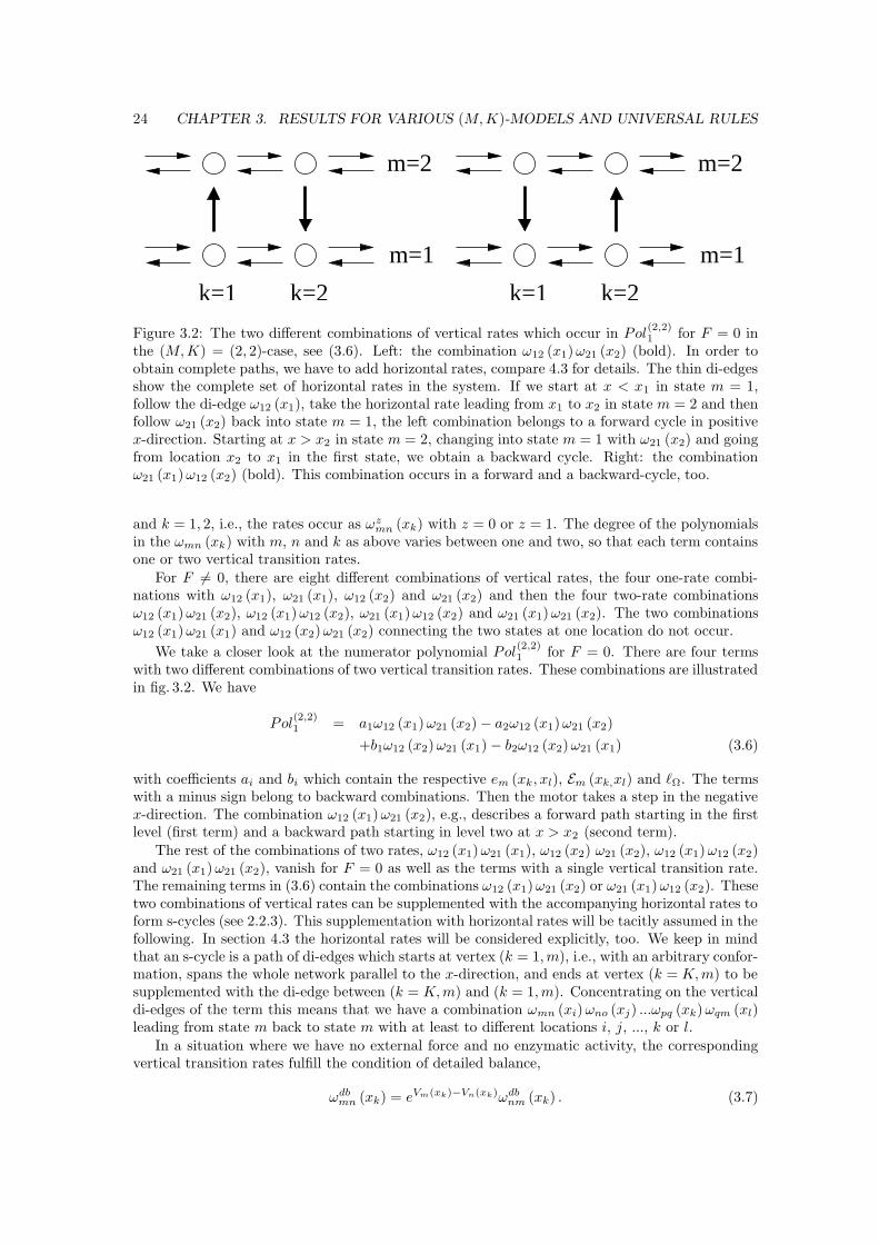
Figure 3.2: The two different combinations of vertical rates which occur in Pol(2,2)1 for F = 0 in
the (M, K) = (2, 2)-case, see (3.6). Left: the combination ω12 (x1) ω21 (x2) (bold). In order toobtain complete paths, we have to add horizontal rates, compare 4.3 for details. The thin di-edgesshow the complete set of horizontal rates in the system. If we start at x < x1 in state m = 1,follow the di-edge ω12 (x1), take the horizontal rate leading from x1 to x2 in state m = 2 and thenfollow ω21 (x2) back into state m = 1, the left combination belongs to a forward cycle in positivex-direction. Starting at x > x2 in state m = 2, changing into state m = 1 with ω21 (x2) and goingfrom location x2 to x1 in the first state, we obtain a backward cycle. Right: the combinationω21 (x1) ω12 (x2) (bold). This combination occurs in a forward and a backward-cycle, too.
and k = 1, 2, i.e., the rates occur as ωzmn (xk) with z = 0 or z = 1. The degree of the polynomials
in the ωmn (xk) with m, n and k as above varies between one and two, so that each term containsone or two vertical transition rates.
For F 6= 0, there are eight different combinations of vertical rates, the four one-rate combi-nations with ω12 (x1), ω21 (x1), ω12 (x2) and ω21 (x2) and then the four two-rate combinationsω12 (x1) ω21 (x2), ω12 (x1) ω12 (x2), ω21 (x1) ω12 (x2) and ω21 (x1) ω21 (x2). The two combinationsω12 (x1) ω21 (x1) and ω12 (x2) ω21 (x2) connecting the two states at one location do not occur.
We take a closer look at the numerator polynomial Pol(2,2)1 for F = 0. There are four terms
with two different combinations of two vertical transition rates. These combinations are illustratedin fig. 3.2. We have
Pol(2,2)1 = a1ω12 (x1) ω21 (x2) − a2ω12 (x1) ω21 (x2)
+b1ω12 (x2) ω21 (x1) − b2ω12 (x2) ω21 (x1) (3.6)
with coefficients ai and bi which contain the respective em (xk, xl), Em (xk,xl) and `Ω. The termswith a minus sign belong to backward combinations. Then the motor takes a step in the negativex-direction. The combination ω12 (x1) ω21 (x2), e.g., describes a forward path starting in the firstlevel (first term) and a backward path starting in level two at x > x2 (second term).
The rest of the combinations of two rates, ω12 (x1) ω21 (x1), ω12 (x2) ω21 (x2), ω12 (x1) ω12 (x2)and ω21 (x1) ω21 (x2), vanish for F = 0 as well as the terms with a single vertical transition rate.The remaining terms in (3.6) contain the combinations ω12 (x1) ω21 (x2) or ω21 (x1) ω12 (x2). Thesetwo combinations of vertical rates can be supplemented with the accompanying horizontal rates toform s-cycles (see 2.2.3). This supplementation with horizontal rates will be tacitly assumed in thefollowing. In section 4.3 the horizontal rates will be considered explicitly, too. We keep in mindthat an s-cycle is a path of di-edges which starts at vertex (k = 1, m), i.e., with an arbitrary confor-mation, spans the whole network parallel to the x-direction, and ends at vertex (k = K, m) to besupplemented with the di-edge between (k = K, m) and (k = 1, m). Concentrating on the verticaldi-edges of the term this means that we have a combination ωmn (xi) ωno (xj) ...ωpq (xk) ωqm (xl)leading from state m back to state m with at least to different locations i, j, ..., k or l.
In a situation where we have no external force and no enzymatic activity, the correspondingvertical transition rates fulfill the condition of detailed balance,
ωdbmn (xk) = eVm(xk)−Vn(xk)ωdb
nm (xk) . (3.7)
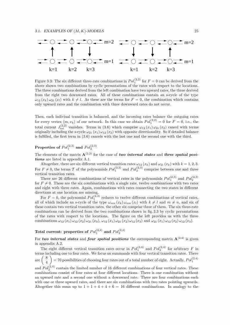
3.1. EXAMPLES OF (M, K)-MODELS 25
k=1 k=2
m=2
m=1
k=3 k=1 k=2
m=2
m=1
k=3
Figure 3.3: The six different three-rate combinations in Pol(2,3)1 for F = 0 can be derived from the
above shown two combinations by cyclic permutations of the rates with respect to the locations.The three combinations derived from the left combination have two upward rates, the three derivedfrom the right two downward rates. All of these combinations contain an s-cycle of the typeω12 (xk) ω21 (xl) with k 6= l. As these are the terms for F = 0, the combination which containsonly upward rates and the combination with three downward rates do not occur.
Then, each indiviual transition is balanced, and the incoming rates balance the outgoing rates
for every vertex (m, xk) of our network. In this case we obtain Pol(2,2)1 = 0 for F = 0, i.e., the
total current J(2,2)tot vanishes. Terms in (3.6) which comprise ω12 (x1) ω21 (x2) cancel with terms
originally including the s-cycle ω21 (x1) ω12 (x2) with opposite directionality. So if detailed balanceis fulfilled, the first term in (3.6) cancels with the last one and the second one with the third.
Properties of Pol(2,3)1 and Pol
(2,3)2
The elements of the matrix A(2,3) for the case of two internal states and three spatial posi-
tions are listed in appendix A.1.Altogether, there are six different vertical transition rates ω12 (xk) and ω21 (xk) with k = 1, 2, 3.
For F 6= 0, the terms T of the polynomials Pol(2,3)1 and Pol
(2,3)2 comprise between one and three
vertical transition rates.There are 26 different combinations of vertical rates in the polynomials Pol
(2,3)1 and Pol
(2,3)2
for F 6= 0. These are the six combinations with a single rate, twelve combinations with two ratesand eight with three rates. Again, combinations with rates connecting the two states in differentdirections at one location are missing.
For F = 0, the polynomial Pol(2,3)1 reduces to twelve different combinations of vertical rates,
all of which include an s-cycle of the type ωmn (xk) ωnm (xl) with k 6= l and m 6= n, and six ofthese contain two vertical transition rates, the other six comprise three of them. The six three-ratecombinations can be derived from the two combinations shown in fig. 3.3 by cyclic permutationsof the rates with respect to the locations. The figure on the left provides us with the threecombinations ω12 (x1) ω12 (x2) ω21 (x3), ω12 (x1) ω21 (x2) ω12 (x3) and ω21 (x1) ω12 (x2) ω12 (x3).
Total current: properties of Pol(2,4)1 and Pol
(2,4)2
For two internal states and four spatial positions the corresponding matrix A(2,4) is givenin appendix A.2.
The eight different vertical transition rates occur in Pol(2,4)1 and Pol
(2,4)2 for arbitrary F in
terms including one to four rates. We focus on summands with four vertical transition rates. There
are
(84
)= 70 possibilities of choosing four rates out of a total number of eight. Actually, Pol
(2,4)1
and Pol(2,4)2 contain the limited number of 16 different combinations of four vertical rates. These
combinations consist of four rates at four different locations. There is one combination withoutan upward rate and a second one without a downward rate. There are four combinations eachwith one or three upward rates, and there are six combinations with two rates pointing upwards.Altogether this sums up to 1 + 1 + 4 + 4 + 6 = 16 different combinations. In analogy to the
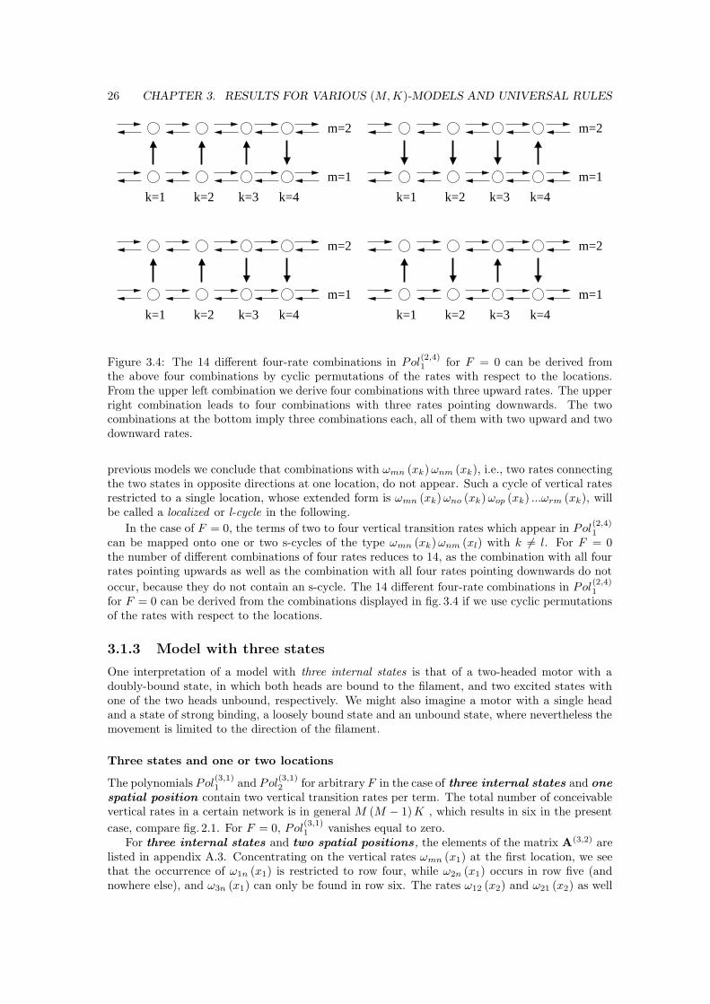
26 CHAPTER 3. RESULTS FOR VARIOUS (M, K)-MODELS AND UNIVERSAL RULES
k=1 k=2 k=3 k=4
m=2
m=1
k=1 k=2 k=3 k=4
m=2
m=1
k=1 k=2 k=3 k=4
m=2
m=1
k=1 k=2 k=3 k=4
m=2
m=1
Figure 3.4: The 14 different four-rate combinations in Pol(2,4)1 for F = 0 can be derived from
the above four combinations by cyclic permutations of the rates with respect to the locations.From the upper left combination we derive four combinations with three upward rates. The upperright combination leads to four combinations with three rates pointing downwards. The twocombinations at the bottom imply three combinations each, all of them with two upward and twodownward rates.
previous models we conclude that combinations with ωmn (xk) ωnm (xk), i.e., two rates connectingthe two states in opposite directions at one location, do not appear. Such a cycle of vertical ratesrestricted to a single location, whose extended form is ωmn (xk) ωno (xk) ωop (xk) ...ωrm (xk), willbe called a localized or l-cycle in the following.
In the case of F = 0, the terms of two to four vertical transition rates which appear in Pol(2,4)1
can be mapped onto one or two s-cycles of the type ωmn (xk) ωnm (xl) with k 6= l. For F = 0the number of different combinations of four rates reduces to 14, as the combination with all fourrates pointing upwards as well as the combination with all four rates pointing downwards do not
occur, because they do not contain an s-cycle. The 14 different four-rate combinations in Pol(2,4)1
for F = 0 can be derived from the combinations displayed in fig. 3.4 if we use cyclic permutationsof the rates with respect to the locations.
3.1.3 Model with three states
One interpretation of a model with three internal states is that of a two-headed motor with adoubly-bound state, in which both heads are bound to the filament, and two excited states withone of the two heads unbound, respectively. We might also imagine a motor with a single headand a state of strong binding, a loosely bound state and an unbound state, where nevertheless themovement is limited to the direction of the filament.
Three states and one or two locations
The polynomials Pol(3,1)1 and Pol
(3,1)2 for arbitrary F in the case of three internal states and one
spatial position contain two vertical transition rates per term. The total number of conceivablevertical rates in a certain network is in general M (M − 1)K , which results in six in the present
case, compare fig. 2.1. For F = 0, Pol(3,1)1 vanishes equal to zero.
For three internal states and two spatial positions, the elements of the matrix A(3,2) arelisted in appendix A.3. Concentrating on the vertical rates ωmn (x1) at the first location, we seethat the occurrence of ω1n (x1) is restricted to row four, while ω2n (x1) occurs in row five (andnowhere else), and ω3n (x1) can only be found in row six. The rates ω12 (x2) and ω21 (x2) as well
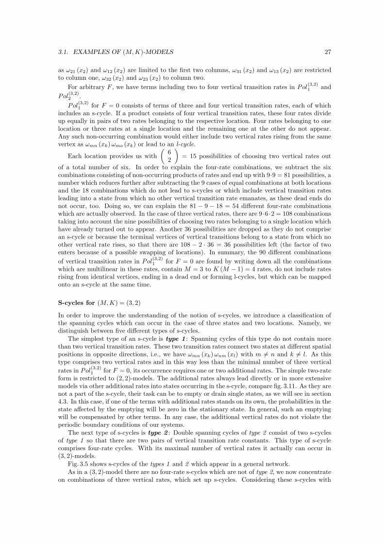
3.1. EXAMPLES OF (M, K)-MODELS 27
as ω21 (x2) and ω12 (x2) are limited to the first two columns, ω31 (x2) and ω13 (x2) are restrictedto column one, ω32 (x2) and ω23 (x2) to column two.
For arbitrary F , we have terms including two to four vertical transition rates in Pol(3,2)1 and
Pol(3,2)2 .
Pol(3,2)1 for F = 0 consists of terms of three and four vertical transition rates, each of which
includes an s-cycle. If a product consists of four vertical transition rates, these four rates divideup equally in pairs of two rates belonging to the respective location. Four rates belonging to onelocation or three rates at a single location and the remaining one at the other do not appear.Any such non-occurring combination would either include two vertical rates rising from the samevertex as ωmn (xk) ωmo (xk) or lead to an l-cycle.
Each location provides us with
(62
)= 15 possibilities of choosing two vertical rates out
of a total number of six. In order to explain the four-rate combinations, we subtract the sixcombinations consisting of non-occurring products of rates and end up with 9·9 = 81 possibilities, anumber which reduces further after subtracting the 9 cases of equal combinations at both locationsand the 18 combinations which do not lead to s-cycles or which include vertical transition ratesleading into a state from which no other vertical transition rate emanates, as these dead ends donot occur, too. Doing so, we can explain the 81 − 9 − 18 = 54 different four-rate combinationswhich are actually observed. In the case of three vertical rates, there are 9 ·6 ·2 = 108 combinationstaking into account the nine possibilities of choosing two rates belonging to a single location whichhave already turned out to appear. Another 36 possibilities are dropped as they do not comprisean s-cycle or because the terminal vertices of vertical transitions belong to a state from which noother vertical rate rises, so that there are 108 − 2 · 36 = 36 possibilities left (the factor of twoenters because of a possible swapping of locations). In summary, the 90 different combinations
of vertical transition rates in Pol(3,2)1 for F = 0 are found by writing down all the combinations
which are multilinear in these rates, contain M = 3 to K (M − 1) = 4 rates, do not include ratesrising from identical vertices, ending in a dead end or forming l-cycles, but which can be mappedonto an s-cycle at the same time.
S-cycles for (M, K) = (3, 2)
In order to improve the understanding of the notion of s-cycles, we introduce a classification ofthe spanning cycles which can occur in the case of three states and two locations. Namely, wedistinguish between five different types of s-cycles.
The simplest type of an s-cycle is type 1 : Spanning cycles of this type do not contain morethan two vertical transition rates. These two transition rates connect two states at different spatialpositions in opposite directions, i.e., we have ωmn (xk) ωnm (xl) with m 6= n and k 6= l. As thistype comprises two vertical rates and in this way less than the minimal number of three vertical
rates in Pol(3,2)1 for F = 0, its occurrence requires one or two additional rates. The simple two-rate
form is restricted to (2, 2)-models. The additional rates always lead directly or in more extensivemodels via other additional rates into states occurring in the s-cycle, compare fig. 3.11. As they arenot a part of the s-cycle, their task can be to empty or drain single states, as we will see in section4.3. In this case, if one of the terms with additional rates stands on its own, the probabilities in thestate affected by the emptying will be zero in the stationary state. In general, such an emptyingwill be compensated by other terms. In any case, the additional vertical rates do not violate theperiodic boundary conditions of our systems.
The next type of s-cycles is type 2 : Double spanning cycles of type 2 consist of two s-cyclesof type 1 so that there are two pairs of vertical transition rate constants. This type of s-cyclecomprises four-rate cycles. With its maximal number of vertical rates it actually can occur in(3, 2)-models.
Fig. 3.5 shows s-cycles of the types 1 and 2 which appear in a general network.As in a (3, 2)-model there are no four-rate s-cycles which are not of type 2, we now concentrate
on combinations of three vertical rates, which set up s-cycles. Considering these s-cycles with
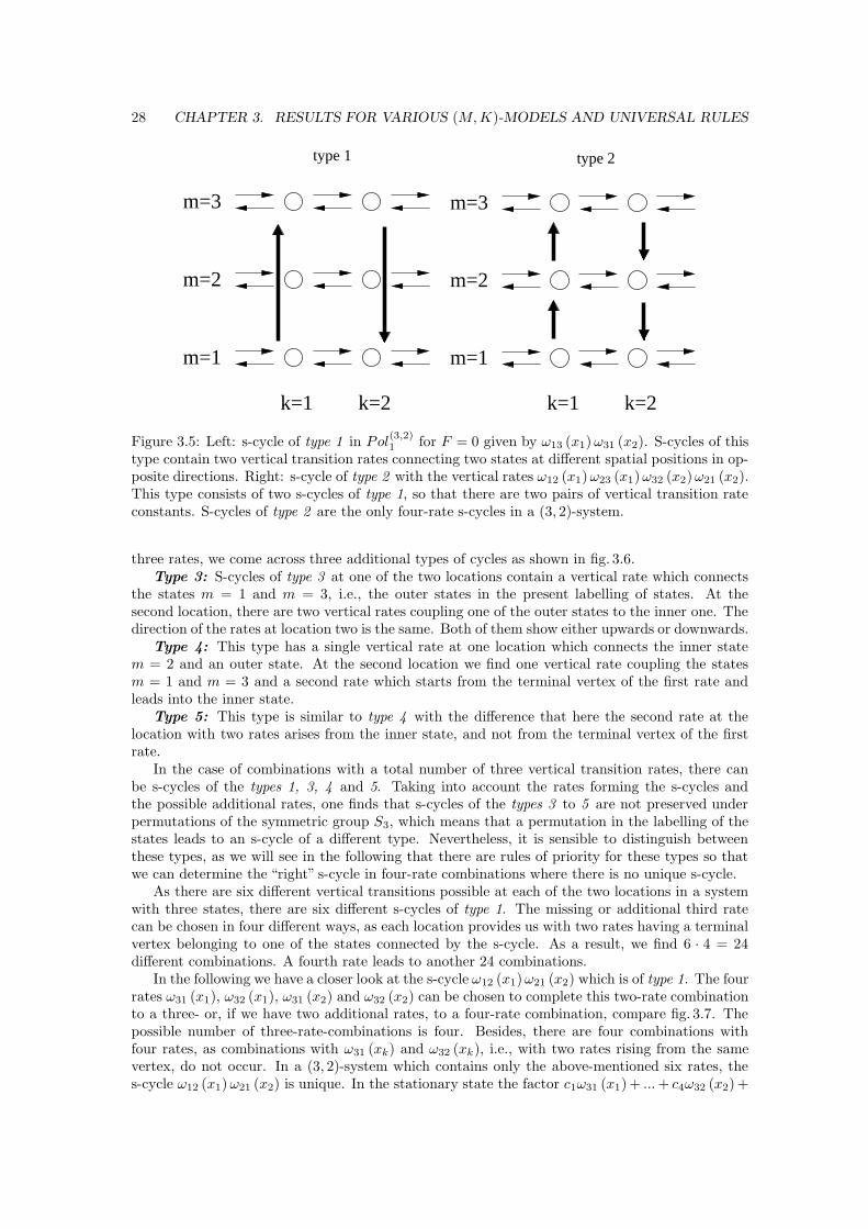
28 CHAPTER 3. RESULTS FOR VARIOUS (M, K)-MODELS AND UNIVERSAL RULES
k=1 k=2
m=2
m=1
m=3
type 1
k=1 k=2
m=2
m=1
m=3
type 2
Figure 3.5: Left: s-cycle of type 1 in Pol(3,2)1 for F = 0 given by ω13 (x1) ω31 (x2). S-cycles of this
type contain two vertical transition rates connecting two states at different spatial positions in op-posite directions. Right: s-cycle of type 2 with the vertical rates ω12 (x1) ω23 (x1) ω32 (x2) ω21 (x2).This type consists of two s-cycles of type 1, so that there are two pairs of vertical transition rateconstants. S-cycles of type 2 are the only four-rate s-cycles in a (3, 2)-system.
three rates, we come across three additional types of cycles as shown in fig. 3.6.Type 3: S-cycles of type 3 at one of the two locations contain a vertical rate which connects
the states m = 1 and m = 3, i.e., the outer states in the present labelling of states. At thesecond location, there are two vertical rates coupling one of the outer states to the inner one. Thedirection of the rates at location two is the same. Both of them show either upwards or downwards.
Type 4: This type has a single vertical rate at one location which connects the inner statem = 2 and an outer state. At the second location we find one vertical rate coupling the statesm = 1 and m = 3 and a second rate which starts from the terminal vertex of the first rate andleads into the inner state.
Type 5: This type is similar to type 4 with the difference that here the second rate at thelocation with two rates arises from the inner state, and not from the terminal vertex of the firstrate.
In the case of combinations with a total number of three vertical transition rates, there canbe s-cycles of the types 1, 3, 4 and 5. Taking into account the rates forming the s-cycles andthe possible additional rates, one finds that s-cycles of the types 3 to 5 are not preserved underpermutations of the symmetric group S3, which means that a permutation in the labelling of thestates leads to an s-cycle of a different type. Nevertheless, it is sensible to distinguish betweenthese types, as we will see in the following that there are rules of priority for these types so thatwe can determine the “right” s-cycle in four-rate combinations where there is no unique s-cycle.
As there are six different vertical transitions possible at each of the two locations in a systemwith three states, there are six different s-cycles of type 1. The missing or additional third ratecan be chosen in four different ways, as each location provides us with two rates having a terminalvertex belonging to one of the states connected by the s-cycle. As a result, we find 6 · 4 = 24different combinations. A fourth rate leads to another 24 combinations.
In the following we have a closer look at the s-cycle ω12 (x1) ω21 (x2) which is of type 1. The fourrates ω31 (x1), ω32 (x1), ω31 (x2) and ω32 (x2) can be chosen to complete this two-rate combinationto a three- or, if we have two additional rates, to a four-rate combination, compare fig. 3.7. Thepossible number of three-rate-combinations is four. Besides, there are four combinations withfour rates, as combinations with ω31 (xk) and ω32 (xk), i.e., with two rates rising from the samevertex, do not occur. In a (3, 2)-system which contains only the above-mentioned six rates, thes-cycle ω12 (x1) ω21 (x2) is unique. In the stationary state the factor c1ω31 (x1) + ... + c4ω32 (x2) +
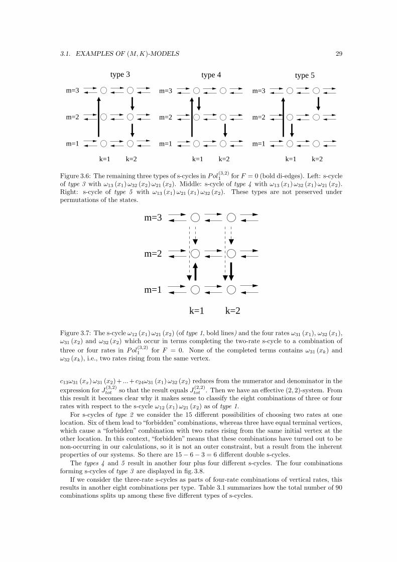
3.1. EXAMPLES OF (M, K)-MODELS 29
k=1 k=2
m=2
m=1
m=3
type 3
k=1 k=2
m=2
m=1
m=3
type 4
k=1 k=2
m=2
m=1
m=3
type 5
Figure 3.6: The remaining three types of s-cycles in Pol(3,2)1 for F = 0 (bold di-edges). Left: s-cycle
of type 3 with ω13 (x1) ω32 (x2) ω21 (x2). Middle: s-cycle of type 4 with ω13 (x1) ω32 (x1) ω21 (x2).Right: s-cycle of type 5 with ω13 (x1) ω21 (x1) ω32 (x2). These types are not preserved underpermutations of the states.
k=1 k=2
m=2
m=1
m=3
Figure 3.7: The s-cycle ω12 (x1) ω21 (x2) (of type 1, bold lines) and the four rates ω31 (x1), ω32 (x1),ω31 (x2) and ω32 (x2) which occur in terms completing the two-rate s-cycle to a combination of
three or four rates in Pol(3,2)1 for F = 0. None of the completed terms contains ω31 (xk) and
ω32 (xk), i.e., two rates rising from the same vertex.
c13ω31 (xx) ω31 (x2)+ ...+ c24ω31 (x1) ω32 (x2) reduces from the numerator and denominator in the
expression for J(3,2)tot so that the result equals J
(2,2)tot . Then we have an effective (2, 2)-system. From
this result it becomes clear why it makes sense to classify the eight combinations of three or fourrates with respect to the s-cycle ω12 (x1) ω21 (x2) as of type 1.
For s-cycles of type 2 we consider the 15 different possibilities of choosing two rates at onelocation. Six of them lead to“forbidden”combinations, whereas three have equal terminal vertices,which cause a “forbidden” combination with two rates rising from the same initial vertex at theother location. In this context, “forbidden” means that these combinations have turned out to benon-occurring in our calculations, so it is not an outer constraint, but a result from the inherentproperties of our systems. So there are 15 − 6 − 3 = 6 different double s-cycles.
The types 4 and 5 result in another four plus four different s-cycles. The four combinationsforming s-cycles of type 3 are displayed in fig. 3.8.
If we consider the three-rate s-cycles as parts of four-rate combinations of vertical rates, thisresults in another eight combinations per type. Table 3.1 summarizes how the total number of 90combinations splits up among these five different types of s-cycles.
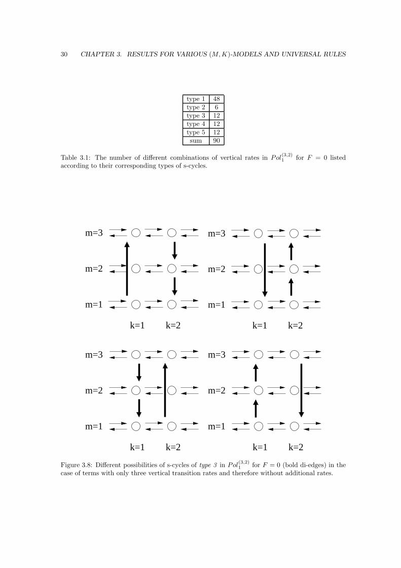
30 CHAPTER 3. RESULTS FOR VARIOUS (M, K)-MODELS AND UNIVERSAL RULES
type 1 48type 2 6type 3 12type 4 12type 5 12sum 90
Table 3.1: The number of different combinations of vertical rates in Pol(3,2)1 for F = 0 listed
according to their corresponding types of s-cycles.
k=1 k=2
m=2
m=1
m=3
k=1 k=2
m=2
m=1
m=3
k=1 k=2
m=2
m=1
m=3
k=1 k=2
m=2
m=1
m=3
Figure 3.8: Different possibilities of s-cycles of type 3 in Pol(3,2)1 for F = 0 (bold di-edges) in the
case of terms with only three vertical transition rates and therefore without additional rates.
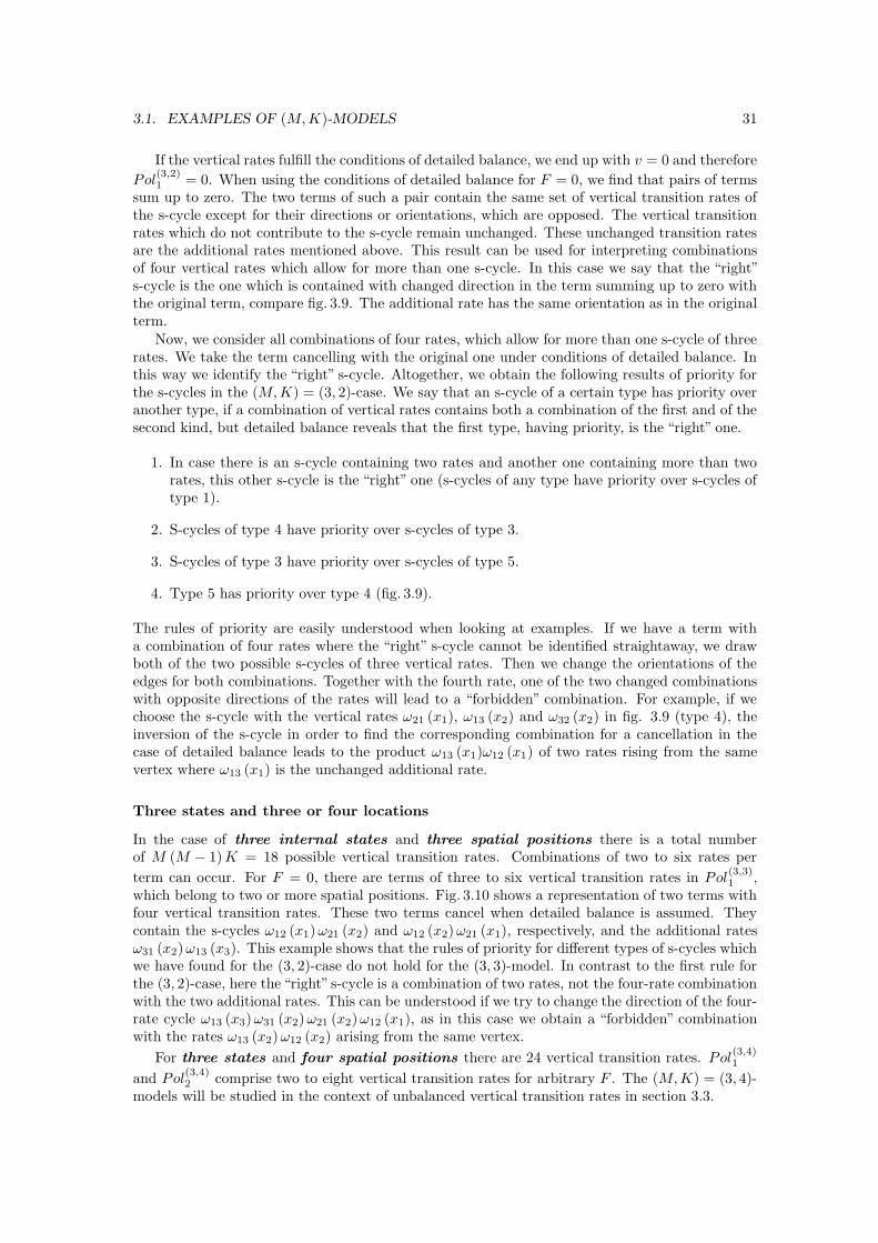
3.1. EXAMPLES OF (M, K)-MODELS 31
If the vertical rates fulfill the conditions of detailed balance, we end up with v = 0 and therefore
Pol(3,2)1 = 0. When using the conditions of detailed balance for F = 0, we find that pairs of terms
sum up to zero. The two terms of such a pair contain the same set of vertical transition rates ofthe s-cycle except for their directions or orientations, which are opposed. The vertical transitionrates which do not contribute to the s-cycle remain unchanged. These unchanged transition ratesare the additional rates mentioned above. This result can be used for interpreting combinationsof four vertical rates which allow for more than one s-cycle. In this case we say that the “right”s-cycle is the one which is contained with changed direction in the term summing up to zero withthe original term, compare fig. 3.9. The additional rate has the same orientation as in the originalterm.
Now, we consider all combinations of four rates, which allow for more than one s-cycle of threerates. We take the term cancelling with the original one under conditions of detailed balance. Inthis way we identify the “right” s-cycle. Altogether, we obtain the following results of priority forthe s-cycles in the (M, K) = (3, 2)-case. We say that an s-cycle of a certain type has priority overanother type, if a combination of vertical rates contains both a combination of the first and of thesecond kind, but detailed balance reveals that the first type, having priority, is the “right” one.
1. In case there is an s-cycle containing two rates and another one containing more than tworates, this other s-cycle is the “right” one (s-cycles of any type have priority over s-cycles oftype 1).
2. S-cycles of type 4 have priority over s-cycles of type 3.
3. S-cycles of type 3 have priority over s-cycles of type 5.
4. Type 5 has priority over type 4 (fig. 3.9).
The rules of priority are easily understood when looking at examples. If we have a term witha combination of four rates where the “right” s-cycle cannot be identified straightaway, we drawboth of the two possible s-cycles of three vertical rates. Then we change the orientations of theedges for both combinations. Together with the fourth rate, one of the two changed combinationswith opposite directions of the rates will lead to a “forbidden” combination. For example, if wechoose the s-cycle with the vertical rates ω21 (x1), ω13 (x2) and ω32 (x2) in fig. 3.9 (type 4), theinversion of the s-cycle in order to find the corresponding combination for a cancellation in thecase of detailed balance leads to the product ω13 (x1)ω12 (x1) of two rates rising from the samevertex where ω13 (x1) is the unchanged additional rate.
Three states and three or four locations
In the case of three internal states and three spatial positions there is a total numberof M (M − 1) K = 18 possible vertical transition rates. Combinations of two to six rates per
term can occur. For F = 0, there are terms of three to six vertical transition rates in Pol(3,3)1 ,
which belong to two or more spatial positions. Fig. 3.10 shows a representation of two terms withfour vertical transition rates. These two terms cancel when detailed balance is assumed. Theycontain the s-cycles ω12 (x1) ω21 (x2) and ω12 (x2) ω21 (x1), respectively, and the additional ratesω31 (x2) ω13 (x3). This example shows that the rules of priority for different types of s-cycles whichwe have found for the (3, 2)-case do not hold for the (3, 3)-model. In contrast to the first rule forthe (3, 2)-case, here the “right” s-cycle is a combination of two rates, not the four-rate combinationwith the two additional rates. This can be understood if we try to change the direction of the four-rate cycle ω13 (x3) ω31 (x2) ω21 (x2) ω12 (x1), as in this case we obtain a “forbidden” combinationwith the rates ω13 (x2) ω12 (x2) arising from the same vertex.
For three states and four spatial positions there are 24 vertical transition rates. Pol(3,4)1
and Pol(3,4)2 comprise two to eight vertical transition rates for arbitrary F . The (M, K) = (3, 4)-
models will be studied in the context of unbalanced vertical transition rates in section 3.3.
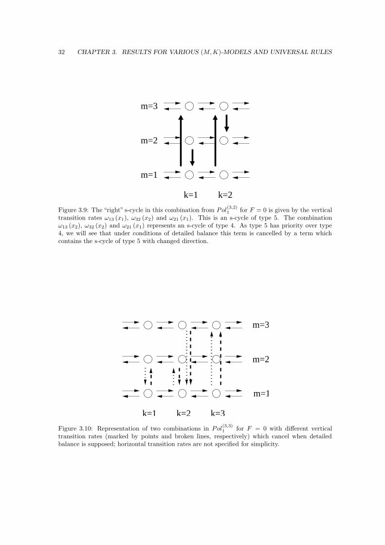
32 CHAPTER 3. RESULTS FOR VARIOUS (M, K)-MODELS AND UNIVERSAL RULES
k=1 k=2
m=2
m=1
m=3
Figure 3.9: The “right” s-cycle in this combination from Pol(3,2)1 for F = 0 is given by the vertical
transition rates ω13 (x1), ω32 (x2) and ω21 (x1). This is an s-cycle of type 5. The combinationω13 (x2), ω32 (x2) and ω21 (x1) represents an s-cycle of type 4. As type 5 has priority over type4, we will see that under conditions of detailed balance this term is cancelled by a term whichcontains the s-cycle of type 5 with changed direction.
k=1 k=2 k=3
m=1
m=3
m=2
Figure 3.10: Representation of two combinations in Pol(3,3)1 for F = 0 with different vertical
transition rates (marked by points and broken lines, respectively) which cancel when detailedbalance is supposed; horizontal transition rates are not specified for simplicity.
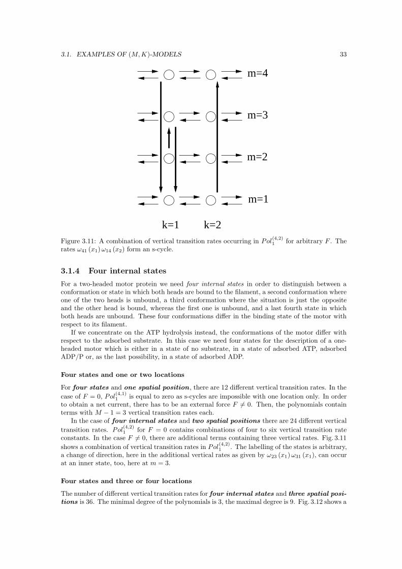
3.1. EXAMPLES OF (M, K)-MODELS 33
k=1 k=2
m=4
m=2
m=3
m=1
Figure 3.11: A combination of vertical transition rates occurring in Pol(4,2)1 for arbitrary F . The
rates ω41 (x1) ω14 (x2) form an s-cycle.
3.1.4 Four internal states
For a two-headed motor protein we need four internal states in order to distinguish between aconformation or state in which both heads are bound to the filament, a second conformation whereone of the two heads is unbound, a third conformation where the situation is just the oppositeand the other head is bound, whereas the first one is unbound, and a last fourth state in whichboth heads are unbound. These four conformations differ in the binding state of the motor withrespect to its filament.
If we concentrate on the ATP hydrolysis instead, the conformations of the motor differ withrespect to the adsorbed substrate. In this case we need four states for the description of a one-headed motor which is either in a state of no substrate, in a state of adsorbed ATP, adsorbedADP/P or, as the last possibility, in a state of adsorbed ADP.
Four states and one or two locations
For four states and one spatial position , there are 12 different vertical transition rates. In the
case of F = 0, Pol(4,1)1 is equal to zero as s-cycles are impossible with one location only. In order
to obtain a net current, there has to be an external force F 6= 0. Then, the polynomials containterms with M − 1 = 3 vertical transition rates each.
In the case of four internal states and two spatial positions there are 24 different vertical
transition rates. Pol(4,2)1 for F = 0 contains combinations of four to six vertical transition rate
constants. In the case F 6= 0, there are additional terms containing three vertical rates. Fig. 3.11
shows a combination of vertical transition rates in Pol(4,2)1 . The labelling of the states is arbitrary,
a change of direction, here in the additional vertical rates as given by ω23 (x1) ω31 (x1), can occurat an inner state, too, here at m = 3.
Four states and three or four locations
The number of different vertical transition rates for four internal states and three spatial posi-
tions is 36. The minimal degree of the polynomials is 3, the maximal degree is 9. Fig. 3.12 shows a
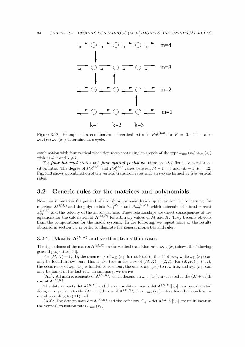
34 CHAPTER 3. RESULTS FOR VARIOUS (M, K)-MODELS AND UNIVERSAL RULES
k=1 k=2 k=3
m=4
m=3
m=2
m=1
Figure 3.12: Example of a combination of vertical rates in Pol(4,3)1 for F = 0. The rates
ω23 (x2) ω32 (x1) determine an s-cycle.
combination with four vertical transition rates containing an s-cycle of the type ωmn (xk) ωnm (xl)with m 6= n and k 6= l.
For four internal states and four spatial positions , there are 48 different vertical tran-
sition rates. The degree of Pol(4,4)1 and Pol
(4,4)2 varies between M − 1 = 3 and (M − 1) K = 12.
Fig. 3.13 shows a combination of ten vertical transition rates with an s-cycle formed by five verticalrates.
3.2 Generic rules for the matrices and polynomials
Now, we summarize the general relationships we have drawn up in section 3.1 concerning the
matrices A(M,K) and the polynomials Pol(M,K)1 and Pol
(M,K)2 , which determine the total current
J(M,K)tot and the velocity of the motor particle. These relationships are direct consequences of the
equations for the calculation of A(M,K) for arbitrary values of M and K. They become obviousfrom the computations for the model systems. In the following, we repeat some of the resultsobtained in section 3.1 in order to illustrate the general properties and rules.
3.2.1 Matrix A(M,K) and vertical transition rates
The dependence of the matrix A(M,K) on the vertical transition rates ωmn (xk) shows the followinggeneral properties [43]:
For (M, K) = (2, 1), the occurrence of ω12 (x1) is restricted to the third row, while ω21 (x1) canonly be found in row four. This is also true in the case of (M, K) = (2, 2). For (M, K) = (3, 2),the occurrence of ω1n (x1) is limited to row four, the one of ω2n (x1) to row five, and ω3n (x1) canonly be found in the last row. In summary, we derive
(A1): All matrix elements of A(M,K), which depend on ωmn (x1), are located in the (M + m)throw of A(M,K).
The determinants det A(M,K) and the minor determinants detA(M,K)[j, i] can be calculateddoing an expansion to the (M + m)th row of A(M,K), thus ωmn (x1) enters linearly in each sum-mand according to (A1) and
(A2): The determinant det A(M,K) and the cofactors Cij ∼ detA(M,K)[j, i] are multilinear inthe vertical transition rates ωmn (x1).
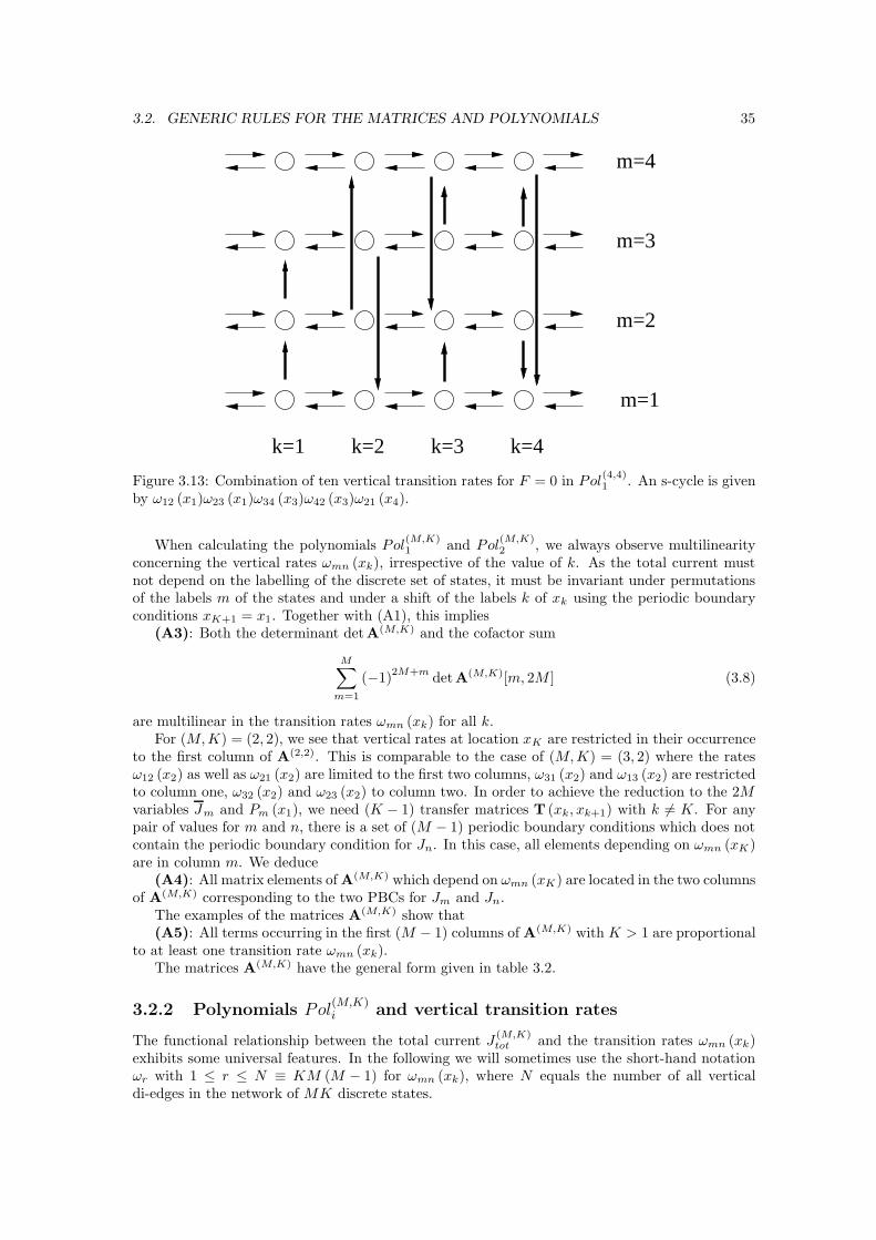
3.2. GENERIC RULES FOR THE MATRICES AND POLYNOMIALS 35
k=1 k=2
m=2
m=3
m=4
m=1
k=4k=3
Figure 3.13: Combination of ten vertical transition rates for F = 0 in Pol(4,4)1 . An s-cycle is given
by ω12 (x1)ω23 (x1)ω34 (x3)ω42 (x3)ω21 (x4).
When calculating the polynomials Pol(M,K)1 and Pol
(M,K)2 , we always observe multilinearity
concerning the vertical rates ωmn (xk), irrespective of the value of k. As the total current mustnot depend on the labelling of the discrete set of states, it must be invariant under permutationsof the labels m of the states and under a shift of the labels k of xk using the periodic boundaryconditions xK+1 = x1. Together with (A1), this implies
(A3): Both the determinant detA(M,K) and the cofactor sum
M∑
m=1
(−1)2M+m
detA(M,K)[m, 2M ] (3.8)
are multilinear in the transition rates ωmn (xk) for all k.For (M, K) = (2, 2), we see that vertical rates at location xK are restricted in their occurrence
to the first column of A(2,2). This is comparable to the case of (M, K) = (3, 2) where the ratesω12 (x2) as well as ω21 (x2) are limited to the first two columns, ω31 (x2) and ω13 (x2) are restrictedto column one, ω32 (x2) and ω23 (x2) to column two. In order to achieve the reduction to the 2Mvariables Jm and Pm (x1), we need (K − 1) transfer matrices T (xk, xk+1) with k 6= K. For anypair of values for m and n, there is a set of (M − 1) periodic boundary conditions which does notcontain the periodic boundary condition for Jn. In this case, all elements depending on ωmn (xK)are in column m. We deduce
(A4): All matrix elements of A(M,K) which depend on ωmn (xK) are located in the two columnsof A(M,K) corresponding to the two PBCs for Jm and Jn.
The examples of the matrices A(M,K) show that(A5): All terms occurring in the first (M − 1) columns of A(M,K) with K > 1 are proportional
to at least one transition rate ωmn (xk).The matrices A(M,K) have the general form given in table 3.2.
3.2.2 Polynomials Pol(M,K)i and vertical transition rates
The functional relationship between the total current J(M,K)tot and the transition rates ωmn (xk)
exhibits some universal features. In the following we will sometimes use the short-hand notationωr with 1 ≤ r ≤ N ≡ KM (M − 1) for ωmn (xk), where N equals the number of all verticaldi-edges in the network of MK discrete states.
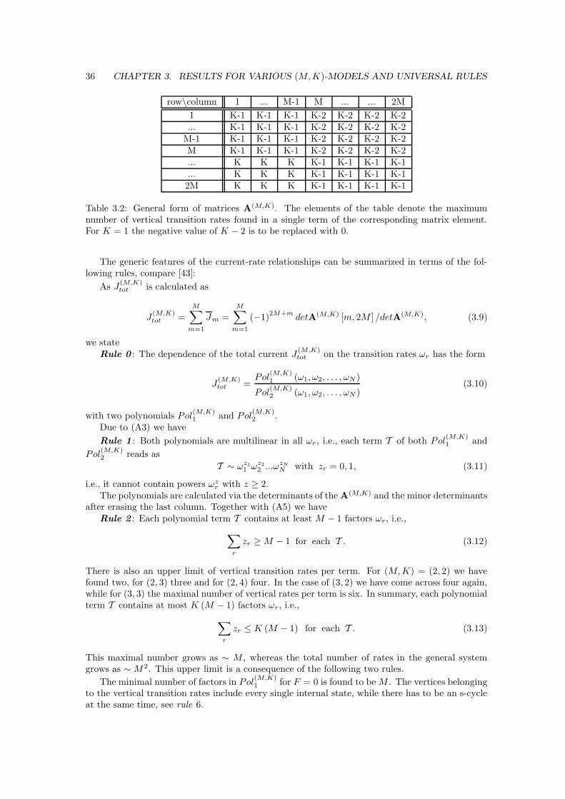
36 CHAPTER 3. RESULTS FOR VARIOUS (M, K)-MODELS AND UNIVERSAL RULES
row\column 1 ... M-1 M ... ... 2M
1 K-1 K-1 K-1 K-2 K-2 K-2 K-2... K-1 K-1 K-1 K-2 K-2 K-2 K-2
M-1 K-1 K-1 K-1 K-2 K-2 K-2 K-2M K-1 K-1 K-1 K-2 K-2 K-2 K-2... K K K K-1 K-1 K-1 K-1... K K K K-1 K-1 K-1 K-12M K K K K-1 K-1 K-1 K-1
Table 3.2: General form of matrices A(M,K). The elements of the table denote the maximumnumber of vertical transition rates found in a single term of the corresponding matrix element.For K = 1 the negative value of K − 2 is to be replaced with 0.
The generic features of the current-rate relationships can be summarized in terms of the fol-lowing rules, compare [43]:
As J(M,K)tot is calculated as
J(M,K)tot =
M∑
m=1
Jm =
M∑
m=1
(−1)2M+m
detA(M,K) [m, 2M ] /detA(M,K), (3.9)
we stateRule 0 : The dependence of the total current J
(M,K)tot on the transition rates ωr has the form
J(M,K)tot =
Pol(M,K)1 (ω1, ω2, . . . , ωN )
Pol(M,K)2 (ω1, ω2, . . . , ωN )
(3.10)
with two polynomials Pol(M,K)1 and Pol
(M,K)2 .
Due to (A3) we have
Rule 1 : Both polynomials are multilinear in all ωr, i.e., each term T of both Pol(M,K)1 and
Pol(M,K)2 reads as
T ∼ ωz1
1 ωz2
2 ...ωzN
N with zr = 0, 1, (3.11)
i.e., it cannot contain powers ωzr with z ≥ 2.
The polynomials are calculated via the determinants of the A(M,K) and the minor determinantsafter erasing the last column. Together with (A5) we have
Rule 2 : Each polynomial term T contains at least M − 1 factors ωr, i.e.,
∑
r
zr ≥ M − 1 for each T . (3.12)
There is also an upper limit of vertical transition rates per term. For (M, K) = (2, 2) we havefound two, for (2, 3) three and for (2, 4) four. In the case of (3, 2) we have come across four again,while for (3, 3) the maximal number of vertical rates per term is six. In summary, each polynomialterm T contains at most K (M − 1) factors ωr, i.e.,
∑
r
zr ≤ K (M − 1) for each T . (3.13)
This maximal number grows as ∼ M , whereas the total number of rates in the general systemgrows as ∼ M2. This upper limit is a consequence of the following two rules.
The minimal number of factors in Pol(M,K)1 for F = 0 is found to be M . The vertices belonging
to the vertical transition rates include every single internal state, while there has to be an s-cycleat the same time, see rule 6.
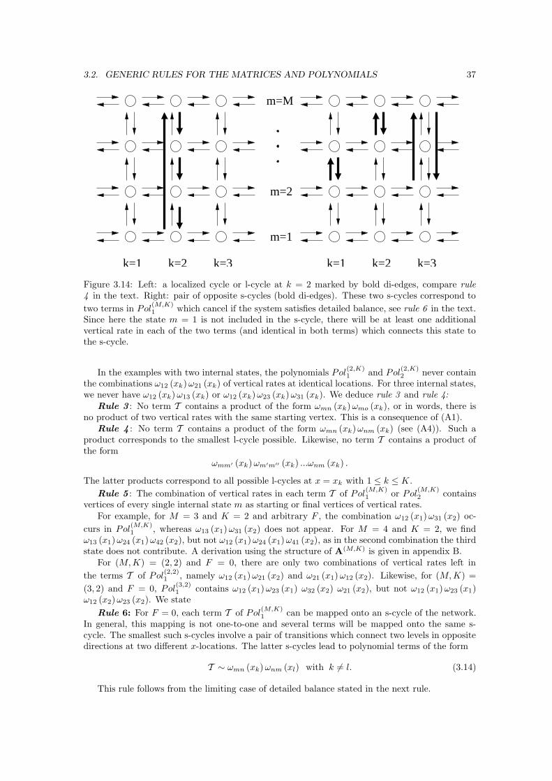
3.2. GENERIC RULES FOR THE MATRICES AND POLYNOMIALS 37
k=1 k=2 k=3 k=1 k=2 k=3
m=M
m=2
m=1
Figure 3.14: Left: a localized cycle or l-cycle at k = 2 marked by bold di-edges, compare rule4 in the text. Right: pair of opposite s-cycles (bold di-edges). These two s-cycles correspond to
two terms in Pol(M,K)1 which cancel if the system satisfies detailed balance, see rule 6 in the text.
Since here the state m = 1 is not included in the s-cycle, there will be at least one additionalvertical rate in each of the two terms (and identical in both terms) which connects this state tothe s-cycle.
In the examples with two internal states, the polynomials Pol(2,K)1 and Pol
(2,K)2 never contain
the combinations ω12 (xk) ω21 (xk) of vertical rates at identical locations. For three internal states,we never have ω12 (xk) ω13 (xk) or ω12 (xk) ω23 (xk) ω31 (xk). We deduce rule 3 and rule 4:
Rule 3 : No term T contains a product of the form ωmn (xk) ωmo (xk), or in words, there isno product of two vertical rates with the same starting vertex. This is a consequence of (A1).
Rule 4 : No term T contains a product of the form ωmn (xk) ωnm (xk) (see (A4)). Such aproduct corresponds to the smallest l-cycle possible. Likewise, no term T contains a product ofthe form
ωmm′ (xk) ωm′m′′ (xk) ...ωnm (xk) .
The latter products correspond to all possible l-cycles at x = xk with 1 ≤ k ≤ K.
Rule 5 : The combination of vertical rates in each term T of Pol(M,K)1 or Pol
(M,K)2 contains
vertices of every single internal state m as starting or final vertices of vertical rates.For example, for M = 3 and K = 2 and arbitrary F , the combination ω12 (x1) ω31 (x2) oc-
curs in Pol(M,K)1 , whereas ω13 (x1) ω31 (x2) does not appear. For M = 4 and K = 2, we find
ω13 (x1) ω24 (x1) ω42 (x2), but not ω12 (x1) ω24 (x1) ω41 (x2), as in the second combination the thirdstate does not contribute. A derivation using the structure of A(M,K) is given in appendix B.
For (M, K) = (2, 2) and F = 0, there are only two combinations of vertical rates left in
the terms T of Pol(2,2)1 , namely ω12 (x1) ω21 (x2) and ω21 (x1) ω12 (x2). Likewise, for (M, K) =
(3, 2) and F = 0, Pol(3,2)1 contains ω12 (x1) ω23 (x1) ω32 (x2) ω21 (x2), but not ω12 (x1) ω23 (x1)
ω12 (x2) ω23 (x2). We state
Rule 6: For F = 0, each term T of Pol(M,K)1 can be mapped onto an s-cycle of the network.
In general, this mapping is not one-to-one and several terms will be mapped onto the same s-cycle. The smallest such s-cycles involve a pair of transitions which connect two levels in oppositedirections at two different x-locations. The latter s-cycles lead to polynomial terms of the form
T ∼ ωmn (xk) ωnm (xl) with k 6= l. (3.14)
This rule follows from the limiting case of detailed balance stated in the next rule.
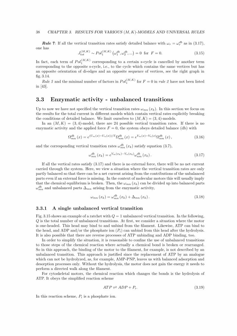
38 CHAPTER 3. RESULTS FOR VARIOUS (M, K)-MODELS AND UNIVERSAL RULES
Rule 7: If all the vertical transition rates satisfy detailed balance with ωr = ωdbr as in (3.17),
one has
J(M,K)tot ∼ Pol
(M,K)1
(ωdb
1 , ωdb2 , ...
)= 0 for F = 0. (3.15)
In fact, each term of Pol(M,K)1 corresponding to a certain s-cycle is cancelled by another term
corresponding to the opposite s-cycle, i.e., to the cycle which contains the same vertices but hasan opposite orientation of di-edges and an opposite sequence of vertices, see the right graph infig. 3.14.
Rule 5 and the minimal number of factors in Pol(M,K)1 for F = 0 in rule 2 have not been listed
in [43].
3.3 Enzymatic activity - unbalanced transitions
Up to now we have not specified the vertical transition rates ωmn (xk). In this section we focus onthe results for the total current in different models which contain vertical rates explicitly breakingthe conditions of detailed balance. We limit ourselves to (M, K) = (3, 4)-models.
In an (M, K) = (3, 4)-model, there are 24 possible vertical transition rates. If there is noenzymatic activity and the applied force F = 0, the system obeys detailed balance (db) with
Ωdbmn (x) = e(Um(x)−Un(x))/T Ωdb
nm (x) = eVm(x)−Vn(x)Ωdbnm (x) , (3.16)
and the corresponding vertical transition rates ωdbmn (xk) satisfy equation (3.7),
ωdbmn (xk) = eVm(xk)−Vn(xk)ωdb
nm (xk) . (3.17)
If all the vertical rates satisfy (3.17) and there is no external force, there will be no net currentcarried through the system. Here, we view a situation where the vertical transition rates are onlypartly balanced so that there can be a net current arising from the contributions of the unbalancedparts even if an external force is missing. In the context of molecular motors this will usually implythat the chemical equilibrium is broken. Then, the ωmn (xk) can be divided up into balanced partsωdb
mn and unbalanced parts ∆mn arising from the enzymatic activity,
ωmn (xk) = ωdbmn (xk) + ∆mn (xk) . (3.18)
3.3.1 A single unbalanced vertical transition
Fig. 3.15 shows an example of a ratchet with Q = 1 unbalanced vertical transition. In the following,Q is the total number of unbalanced transitions. At first, we consider a situation where the motoris one-headed. This head may bind to and unbind from the filament. Likewise, ATP can bind tothe head, and ADP and/or the phosphate ion (Pi) can unbind from this head after the hydrolysis.It is also possible that there are reverse processes of ATP unbinding and ADP binding, too.
In order to simplify the situation, it is reasonable to confine the use of unbalanced transitionsto those steps of the chemical reaction where actually a chemical bond is broken or rearranged.So in this approach, the binding of the motor to the filament, for example, is not described by anunbalanced transition. This approach is justified since the replacement of ATP by an analoguewhich can not be hydrolyzed, as, for example, AMP-PNP, leaves us with balanced adsorption anddesorption processes only. Without the hydrolysis, the motor does not gain the energy it needs toperform a directed walk along the filament.
For cytoskeletal motors, the chemical reaction which changes the bonds is the hydrolysis ofATP. It obeys the simplified reaction scheme
ATP ADP + Pi. (3.19)
In this reaction scheme, Pi is a phosphate ion.
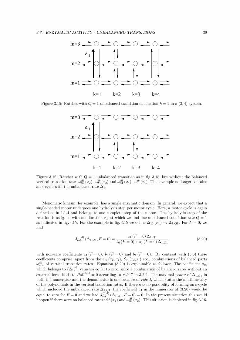
3.3. ENZYMATIC ACTIVITY - UNBALANCED TRANSITIONS 39
k=1 k=2
m=2
m=1
m=3
k=3 k=4
∆ 1
Figure 3.15: Ratchet with Q = 1 unbalanced transition at location k = 1 in a (3, 4)-system.
k=1 k=2
m=2
m=1
m=3
k=3 k=4
∆ 1
Figure 3.16: Ratchet with Q = 1 unbalanced transition as in fig. 3.15, but without the balancedvertical transition rates ωdb
32 (x2), ωdb23 (x2) and ωdb
31 (x4), ωdb13 (x4). This example no longer contains
an s-cycle with the unbalanced rate ∆1.
Monomeric kinesin, for example, has a single enzymatic domain. In general, we expect that asingle-headed motor undergoes one hydrolysis step per motor cycle. Here, a motor cycle is againdefined as in 1.1.4 and belongs to one complete step of the motor. The hydrolysis step of thereaction is assigned with one location xk at which we find one unbalanced transition rate Q = 1as indicated in fig. 3.15. For the example in fig. 3.15 we define ∆13 (x1) =: ∆1,Q1. For F = 0, wefind
J(3,4)tot (∆1,Q1, F = 0) =
a1 (F = 0)∆1,Q1
b0 (F = 0) + b1 (F = 0) ∆1,Q1(3.20)
with non-zero coefficients a1 (F = 0), b0 (F = 0) and b1 (F = 0). By contrast with (3.6) thesecoefficients comprise, apart from the em (xk , xl), Em (xk,xl) etc., combinations of balanced partsωdb
mn of vertical transition rates. Equation (3.20) is explainable as follows: The coefficient a0,
which belongs to (∆1)0, vanishes equal to zero, since a combination of balanced rates without an
external force leads to Pol(3,4)1 = 0 according to rule 7 in 3.2.2. The maximal power of ∆1,Q1 in
both the numerator and the denominator is one because of rule 1, which states the multilinearityof the polynomials in the vertical transition rates. If there was no possibility of forming an s-cyclewhich included the unbalanced rate ∆1,Q1, the coefficient a1 in the numerator of (3.20) would be
equal to zero for F = 0 and we had J(3,4)tot (∆1,Q1, F = 0) = 0. In the present situation this would
happen if there were no balanced rates ωdb31 (x4) and ωdb
32 (x2). This situation is depicted in fig. 3.16.
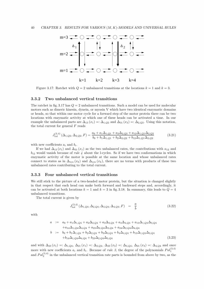
40 CHAPTER 3. RESULTS FOR VARIOUS (M, K)-MODELS AND UNIVERSAL RULES
k=1 k=2
m=2
m=1
m=3
k=3 k=4
∆ 1 ∆ 2
Figure 3.17: Ratchet with Q = 2 unbalanced transitions at the locations k = 1 and k = 3.
3.3.2 Two unbalanced vertical transitions
The ratchet in fig. 3.17 has Q = 2 unbalanced transitions. Such a model can be used for molecularmotors such as dimeric kinesin, dynein, or myosin V which have two identical enzymatic domainsor heads, so that within one motor cycle for a forward step of the motor protein there can be twolocations with enzymatic activity at which one of these heads can be activated a time. In ourexample the unbalanced parts are ∆13 (x1) =: ∆1,Q2 and ∆31 (x3) =: ∆2,Q2. Using this notation,the total current for general F reads
J(3,4)tot (∆1,Q2, ∆2,Q2, F ) =
a0 + a1∆1,Q1 + a2∆2,Q2 + a12∆1,Q1∆2,Q2
b0 + b1∆1,Q1 + b2∆2,Q2 + b12∆1,Q1∆2,Q2(3.21)
with new coefficients ai and bi.If we had ∆13 (x1) and ∆31 (x1) as the two unbalanced rates, the contributions with a12 and
b12 would vanish because of rule 4 about the l-cycles. So if we have two conformations in whichenzymatic activity of the motor is possible at the same location and whose unbalanced ratesconnect to states as in ∆mn (xk) and ∆nm (xk), there are no terms with products of these twounbalanced rates contributing to the total current.
3.3.3 Four unbalanced vertical transitions
We still stick to the picture of a two-headed motor protein, but the situation is changed slightlyin that respect that each head can make both forward and backward steps and, accordingly, itcan be activated at both locations k = 1 and k = 3 in fig. 3.18. In summary, this leads to Q = 4unbalanced transitions.
The total current is given by
J(3,4)tot (∆1,Q4, ∆2,Q4, ∆3,Q4, ∆4,Q4, F ) =
a
b(3.22)
with
a := a0 + a1∆1,Q4 + a2∆2,Q4 + a3∆3,Q4 + a4∆4,Q4 + a13∆1,Q4∆3,Q4
+a14∆1,Q4∆4,Q4 + a23∆2,Q4∆3,Q4 + a24∆2,Q4∆4,Q4
b := b0 + b1∆1,Q4 + b2∆2,Q4 + b3∆3,Q4 + b4∆4,Q4 + b13∆1,Q4∆3,Q4
+b14∆1,Q4∆4,Q4 + b23∆2,Q4∆3,Q4 (3.23)
and with ∆23 (x1) =: ∆1,Q4, ∆21 (x1) =: ∆2,Q4, ∆23 (x3) =: ∆3,Q4, ∆21 (x3) =: ∆4,Q4 and once
more with new coefficients ai and bi. Because of rule 3, the degree of the polynomials Pol(3,4)1
and Pol(3,4)2 in the unbalanced vertical transition rate parts is bounded from above by two, as the
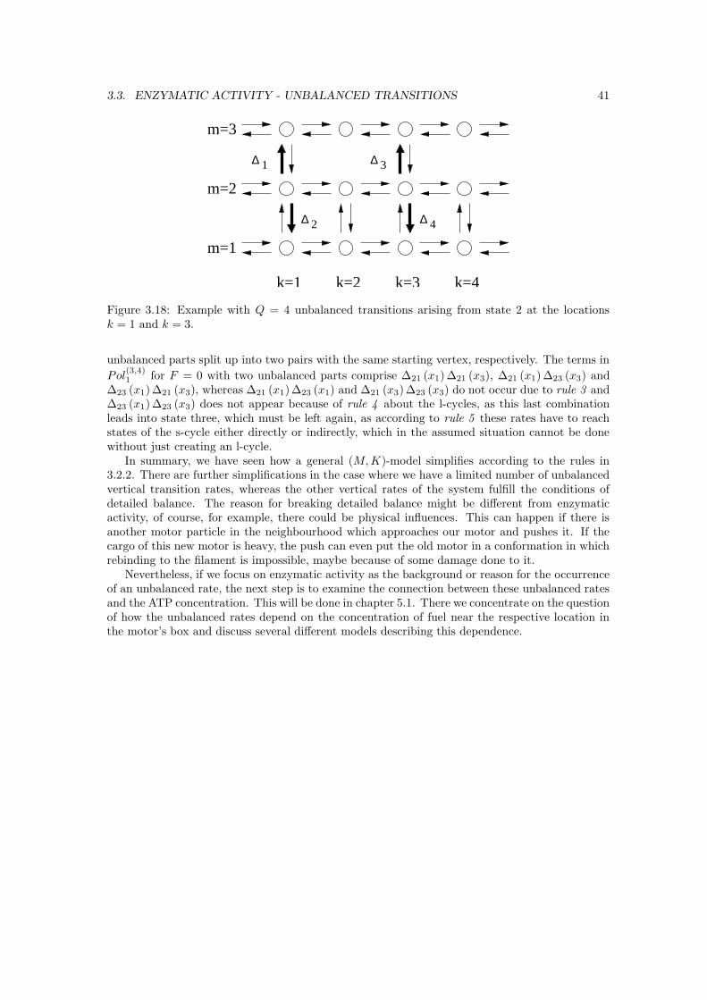
3.3. ENZYMATIC ACTIVITY - UNBALANCED TRANSITIONS 41
k=1 k=2
m=2
m=1
m=3
k=3 k=4
∆ 1 ∆ 3
∆ 2 ∆ 4
Figure 3.18: Example with Q = 4 unbalanced transitions arising from state 2 at the locationsk = 1 and k = 3.
unbalanced parts split up into two pairs with the same starting vertex, respectively. The terms in
Pol(3,4)1 for F = 0 with two unbalanced parts comprise ∆21 (x1) ∆21 (x3), ∆21 (x1) ∆23 (x3) and
∆23 (x1) ∆21 (x3), whereas ∆21 (x1) ∆23 (x1) and ∆21 (x3) ∆23 (x3) do not occur due to rule 3 and∆23 (x1) ∆23 (x3) does not appear because of rule 4 about the l-cycles, as this last combinationleads into state three, which must be left again, as according to rule 5 these rates have to reachstates of the s-cycle either directly or indirectly, which in the assumed situation cannot be donewithout just creating an l-cycle.
In summary, we have seen how a general (M, K)-model simplifies according to the rules in3.2.2. There are further simplifications in the case where we have a limited number of unbalancedvertical transition rates, whereas the other vertical rates of the system fulfill the conditions ofdetailed balance. The reason for breaking detailed balance might be different from enzymaticactivity, of course, for example, there could be physical influences. This can happen if there isanother motor particle in the neighbourhood which approaches our motor and pushes it. If thecargo of this new motor is heavy, the push can even put the old motor in a conformation in whichrebinding to the filament is impossible, maybe because of some damage done to it.
Nevertheless, if we focus on enzymatic activity as the background or reason for the occurrenceof an unbalanced rate, the next step is to examine the connection between these unbalanced ratesand the ATP concentration. This will be done in chapter 5.1. There we concentrate on the questionof how the unbalanced rates depend on the concentration of fuel near the respective location inthe motor’s box and discuss several different models describing this dependence.

42 CHAPTER 3. RESULTS FOR VARIOUS (M, K)-MODELS AND UNIVERSAL RULES
Chapter 4
Decoupled states, horizontal rates
and networks
The models of the (M, K)-systems as examined in chapter 3 still have various restrictions orinconveniences. Here we show how to overcome them and introduce several new concepts, too.
We take a look at decoupled states or subsystems without a mutual coupling via verticaltransition rates. The motor has a certain probability of being in these decoupled subsystems, butit cannot change between them. The reasons may be outer influences on the motor as a shortageof fuel or inner reasons as mutations of the motor protein. We explain why decoupled subsystemshave not occurred in our previous calculations in chapter 3.
Furthermore, the horizontal rates in our systems are specified now, and active, unbalancedtransitions in x-direction are introduced. From a discrete Master-equation approach we derivenew rules for the total current, which now include the dependence on horizontal rates, too. Thenwe examine the time evolution for given initial probabilities on the way to a stationary state.
In the context of the idea of a main pathway and several other minor pathways in chemicalreactions, we eventually focus on the different importance of single paths or pathways through anetwork of vertices.
Most of the concepts which we establish here are based on the network representation indicatedin fig. 2.1. For a listing of the terminology and concepts of graph theory which are used in thischapter see appendix C.
4.1 Decoupled states
A decoupled state is a state which has no connection to any other state. There are no verticalrates starting from or ending in this state. Likewise, there can be subsystems of states which haveno connections to states of the remaining system. With certain initial probabilities the motor canbe in these decoupled states in the beginning, but it cannot leave them or their subsystem. Thiscan be the case if, with a certain probability, we are dealing with a mutation of a motor which isunable to take part in the enzymatic reaction or if the binding sites of the motor’s filament areblocked so that the motor still diffuses or even is driven by an external force, but its conformationis frozen.
The stationary state in such a decoupled system depends on the initial probability distribution,as the contribution of each of the decoupled subsystems to the total current depends on its partof the initial probability. For identical subsystems with a small or no coupling there can be bifur-cations, so that the same “macroscopic”stationary total current belongs to different “microscopic”situations. Here, we at first consider a continuous x-direction. Then we return to network-basedsystems with localized vertical transitions.
43
44 CHAPTER 4. DECOUPLED STATES, HORIZONTAL RATES AND NETWORKS
4.1.1 Decoupled states and continuous x-direction
Here, the centre of interest is on analytic calculations of the total current for simple cases ofdecoupled states. Initially, we abstain from the idea of networks as presented in the chapters 2and 3, but focus on the case of decoupled states with continuous coordinates in x-direction. Atfirst, there is no molecular interaction potential, but a constant external force. Then we introduce alocalized coupling between the states and consider situations with molecular interaction potentials,too.
In the restricted cases presented here the results for the currents and the probability distribu-tions can be written down with their explicit coefficients. A straight decoupling of states has beenimpossible in the formalism of chapter 3 because of rule 5 in 3.2.2 stating that vertices of every
state have to occur in the combination of vertical rates of every term of the polynomials Pol(M,K)i .
Decoupled states, no potentials and constant force
We calculate the total current for a number of decoupled states under the conditions that theexternal force is an arbitrary constant, but there are no molecular interaction potentials. In thiscase the effective force potentials in (2.17) reduce to
Vm (x) ≡ −Fx/T. (4.1)
Initially, we look at a single internal state. Without a molecular interaction potential Um, theSmoluchowski equation (2.11) for this single state m reads
∂Pm (x, t)
∂t≡ Dm
∂
∂x
[∂
∂x(−Fx) /T +
∂
∂x
]Pm (x, t) = −
∂Jm (x, t)
∂x. (4.2)
In the stationary state, the probability current Jm (x, t) is constant with
Jm/Dm = (F/T )Pm − ∂Pm/∂x. (4.3)
The solution of (4.2) for the probability density of the stationary state is given by
Pm (x) = exp (Fx/T )
[C − Jm/Dm
∫ x
0
exp (−Fx′/T ) dx′
](4.4)
with the integration constant C [47]. Although we have no molecular interaction potential, westill stick to the period `. It is reasonable to assume that Pm (x) is bounded for x large enough.We calculate the integral
∫ `n+x
0
exp (−Fx′/T ) dx′ =
∫ `
0
exp (−Fx′/T ) dx′ + ...
+
∫ `n+x
n`
exp (−Fx′/T ) dx′. (4.5)
Because of −F/T · (x + `n) = −Fx/T − `nF/T we obtain∫ `n+x
0
exp (−Fx′/T )dx′ =
∫ `
0
exp (−Fx/T )dx1 − exp (−`nF/T )
1 − exp (−`F/T )=
+ exp (−`nF/T )
∫ x
0
exp (−Fx′/T ) dx′. (4.6)
This leads to
Pm (x + `n) = exp (Fx/T )
[C − Jm
I
Dm (1 − exp (−`F/T ))
]· exp (`nF/T )
+ exp (Fx/T )
[−Jm
I
Dm (1 − exp (−`F/T ))+
Jm
Dm
∫ x
0
exp (−Fx′/T ) dx
].
(4.7)
4.1. DECOUPLED STATES 45
In order to obtain a bounded expression in the limits F > 0, n → +∞ and F < 0, n → −∞respectively, the first bracket has to vanish,
JmI/Dm = C (1 − exp (−`F/T )) , (4.8)
so that Pm (x) is periodic in x with period `, Pm (x + `) = Pm (x). The distribution of theprobability density is normalized in the interval from 0 to `,
∫ `
0
Pm (x) dx = C
∫ `
0
exp (Fx/T ) dx
−Jm/Dm
∫ `
0
exp (Fx/T )
(∫ x
0
exp (−Fx′/T )dx′
)dx
= 1. (4.9)
We solve (4.8) with respect to C and obtain
C =JmT
DmF. (4.10)
This expression can then be inserted into (4.9) and supplies us with
Jm =FDm
`T. (4.11)
This is the same result obtained for Jm in equation (3.3).Insertion of the preceding results into (4.4) yields Pm (x) = 1/`. This stationary solution is
different from (2.14) to the effect that the above given Pm does not violate the periodic boundaryconditions. Here, the current Jm is non-zero for F 6= 0, and the probability distribution is constant,as is to be expected in a periodic system without a molecular interaction potential.
The next step is to assume a situation where we look at a set of an arbitrary number M internalstates, each without any molecular interaction potential. The external force stays constant. TheM states are considered to be completely decoupled.
In this case we have to solve M Smoluchowski equations (4.2). The normalization of thedistribution is then given by
∫ `
0
(P multi
1 (x) + P multi2 (x) + ... + P multi
M (x))dx = 1, (4.12)
where the index “multi” refers to the multi-state system we consider now. If we assume equidistri-bution of the probability densities in the initial configuration, we have to choose a normalizationwhich is weighted by 1/M for each single state. The current in state m of the multi-state systemis then accordingly given by
Jmultim =
FDm
M`T, (4.13)
while the total current reads
Jmultitot =
FD1
M`T+
FD2
M`T+ ... +
FDM
M`T. (4.14)
By choosing different small-scale diffusion coefficients Dm, a specific hindrance or promotionagainst or in favour of moving in the horizontal direction, which might be inherent to a certainconformation of the protein, can easily be modelled.
It is also possible that the initial weights of the internal states vary. This is the case if theconformations refer to defects or mutations of the motor protein which in general occur withdifferent probabilities. Then we have
1
M1+
1
M2+ ... +
1
MM= 1 (4.15)
46 CHAPTER 4. DECOUPLED STATES, HORIZONTAL RATES AND NETWORKS
and, accordingly,
Jmultitot =
FD1
M1`T+
FD2
M2`T+ ... +
FDM
MM`T. (4.16)
In this situation of decoupled levels the resulting lateral currents Jmultim depend on the initial
probability distribution of our system. In the special case that the motor can be localized in acertain state at time t = 0, the weights of the other states are zero.
Connection to coupling between states
Now, we reintroduce a coupling between the states. This coupling is attained by vertical transitionrates ωmn, which enter the transition current densities Im as explained in chapter 2. If all thesetransition rates are chosen to be equal to ω, ωmn (xk) =: ω, for any values of m, n and k, theyfulfill the conditions of detailed balance, as up to now we still do not have any potentials, butUm (x) =: 0 for all m, and therefore exp (Vm (xk) − Vn (xk)) = 1, irrespective of the choices of m,n or k.
The vertical rates drop out from the total current Jmultitot and we obtain equipartition with 1/M
as in (4.14). If the small-scale diffusion coefficients fulfill D1 + D2 + ... + DM = MD1, this meansthat the same value of the total current might result either from a single-state system or from theabove-mentioned M -state system. The number of locations where vertical transitions can occuris arbitrary, as a different choice does not change the result.
In a next step, we consider a situation with two states and two locations where vertical tran-sitions can take place. The vertical transition rates are completely unbalanced,
ωmn (xk) = ∆mn (xk) , (4.17)
compare equation (3.18). The upward rates are chosen to be ω12 (x1) = ω12 (x2) =: ∆1, thedownward rates are ω21 (x1) = ω21 (x2) =: ∆2. For ∆1 := ∆2 and ∆2 := ∆, the total lateralcurrent reads
Jmultitot =
F∆ (D1 + D2)
2`T∆=
F (D1 + D2)
2`T. (4.18)
If we have ∆1 6= ∆2, the symmetry between the states is broken. In this general case, Jmultitot is
calculated as
Jmultitot =
FD1∆2
`T (∆1 + ∆2)+
FD2∆1
`T (∆1 + ∆2), (4.19)
where the first summand belongs to the lateral current in the first state, the second one accordinglyto the current in state two. The contribution of one single state to the total current Jmulti
tot growswith the share the rates leading into this state have of the sum of all rates.
If D1 = D2 and D2 =: D, Jmultitot yields for arbitrary values of ∆1 and ∆2
Jmultitot =
FD
`T. (4.20)
As ∆1 and ∆2 can take arbitrary values, the contributions of the respective states to the totallateral current might be considerably distinct, whereas the total lateral current Jmulti
tot itself remainsunchanged.
Result with potential
Here, we consider a situation where we have non-zero molecular interaction potentials. The oneor more states are uncoupled or either coupled by balanced vertical transition rates again.
At first, m is the only state the motor can attain. The Smoluchowski equation with an effectiveforce potential V (x) = [U (x) − Fx] /T is given by
∂Pm (x, t)
∂t≡ Dm
∂
∂x
[∂
∂xVm (x) +
∂
∂x
]Pm (x, t) = −
∂Jm (x, t)
∂x. (4.21)
4.1. DECOUPLED STATES 47
Here, the solution for the probability density reads
Pm (x) = exp (Vm (x))
[C ′ − Jm/Dm
∫ x
0
exp (−Vm (x′)) dx′
](4.22)
with the new integration constant C ′. Because of Vm (x + `n) = Vm (x) − `nF we obtain
∫ `n+x
0
exp (Vm (x′)) dx′ =
∫ `
0
exp (Vm (x)) dx1 − exp (−`nF/T )
1 − exp (−`F/T )
+ exp (−`nF/T )
∫ x
0
exp (Vm (x′)) dx′. (4.23)
Again, we impose the normalization condition and the condition that we must get a boundedexpression for Pm (x + `n) in the limits F > 0, n → +∞ and F < 0, n → −∞. This yields
C ′ =Jm
Dm
∫ `
0
exp (V (x)) dx/ (1 − exp (−F`/T )) (4.24)
for the integration constant. The current results as
Jm = Dm
[∫ `
0
exp (Vm (x)) dx
∫ `
0
exp (−Vm (x)) dx/ (1 − exp (−F`/T ))
−
∫ `
0
exp (−Vm (x))
(∫ x
0
exp (Vm (x′)) dx′
)dx
]−1
, (4.25)
which is in general a non-zero expression. In terms of a (M, K) = (1, 1)-model as in 3.1.1, we haveJ1 = Jtot. Then (4.25) is equal to
Jtot =1 − e1 (0, `)
(e1 (0, `) − 1)E1 (0) − E1 (0, `) e1
, (4.26)
which follows from (3.2) for x1 = 0.The distribution Pm (x) reads
Pm (x) = Jm/Dm (exp (−V (x)))
[∫ `
0
exp (V (x)) dx/ (1 − exp (−F`/T ))
−
∫ x
0
exp (V (x′)) dx′
]. (4.27)
As we have used the same considerations as in the context of (4.7), we have Pm (x + `n) = Pm (x)for all n. The probability distribution shows the same periodicity as the underlying molecularinteraction potentials.
If the external force F is zero, we have
Pm (x + `n) = exp (−U (x) /T )
[C ′′ −
Jm
Dm
∫ x+`n
0
exp (U (x′) /T ) dx′
]
= exp (−U (x) /T )
[C ′′ − n
Jm
Dm
∫ `
0
exp (U (x′) /T ) dx′+
Jm
Dm
∫ x
0
exp (U (x′) /T )dx′
]. (4.28)
In order to receive a bounded expression for Pm (x + `n) in the limits n → +∞ and n → −∞, thecondition
nJm
Dm
∫ `
0
exp (U (x′) /T )dx′ = 0 (4.29)
48 CHAPTER 4. DECOUPLED STATES, HORIZONTAL RATES AND NETWORKS
has to be fulfilled. Therefore we can conclude that in a one-state system in the case of an arbitraryexponentially integrable molecular interaction potential, but no external force we have Jm = 0 asin 3.1.1.
In a multi-state system with M states and arbitrary constant force F we impose the normal-ization (4.12). For a balanced coupling between the states this leads to the total current
Jmultitot = Jmulti
1 + Jmulti2 + ... + Jmulti
M (4.30)
with the single-state currents Jmultim = Jm/M and Jm as in (4.25). The same is true for the
probability densities P multim ,
P multitot = P multi
1 + P multi2 + ... + P multi
M (4.31)
with P multim = Pm/M and Pm as in (4.27). In this way we have shown that in a multi-state system
with an external force in which all transitions fulfill the conditions of detailed balance the currentsJmulti
m are in general finite with Jm 6= 0 due to F , and the probability densities P multim reflect the
periodicity of the molecular interaction potentials. The conditions of detailed balance are fulfilledin a model without active processes as enzymatic activity.
In this subsection we have treated the decoupling of states for special simple systems. For morecomplex systems, we return to the network-based approach, compare 4.1.2.
4.1.2 Decoupled levels and localized transitions
The calculation of the total current with the use of linear algebra as in (3.9) fails in the presenceof decoupled levels, as in this case we have detA(M,K) = 0. Here we show how the network-based approach used in chapter 3 has to be modified so that more comprehensive systems withdecoupling of states or subsystems can be dealt with, too. We remember that a decoupled state isdefined as a level without any non-zero vertical rates connecting it to another state. The matricesA(M,K) as calculated in chapter 2 and their submatrices are singular. The corresponding graph isdisconnected, which means that there are vertices which are not connected by a path. No vertexbelonging to the states one and two in fig. 4.1 can be reached by a path from a vertex of state threeor the other way round. In the following, the decoupled level is taken to be M . As the labelling ofthe states is arbitrary, we can choose any level to be the decoupled one without a loss of generality.In contrast to chapter 4.1.1, here decoupled levels are treated in the discrete network approach.
Decoupled states: algebraic approach
Single decoupled state
In the following, A(M,K),1,2,...,M−1,M denotes the 2M × 2M -matrix, which is obtained fromA(M,K) by neglecting the vertical rates between state M and other states, i.e., we set ωMm (xk) = 0and ωmM (xk) = 0 for arbitrary m and k. The first braces in the exponent refer to the subsystemwith the states 1, 2, ..., M − 1, the second braces to the subsystem with the single state M .
We consider an example with (M, K) = (3, 2), where we decouple the third state M = 3 as infig. 4.1.
The resulting matrix A(3,2),1,2,3 is given in appendix A.4. The general matrix A(2,2) asin (3.5) is regained from A(3,2),1,2,3 if we cross out the second and the fifth column and thethird and sixth row. Similarly, the A(1,1) matrix is obtained from the matrix A(2,1),1,2 byeliminating the first and third column as well as the second and fourth row, and the A(3,1) matrixcan be obtained from the A(4,1),1,2,3,4-matrix by cancelling the columns three and seven andthe rows four and eight. A(2,3) results from A(3,3),1,2,3 when we cross out the columns twoand five as well as the rows three and six.
In summary, we obtain the matrix A(M−1,K) from A(M,K),1,2,...,M−1,M by erasing the(M − 1) th and the (2M − 1) th column as well as the Mth and 2Mth row. The elements of the(2M − 1) th column and the Mth and 2Mth row of A(M,K),1,2,...,M−1,M are equal to zero or
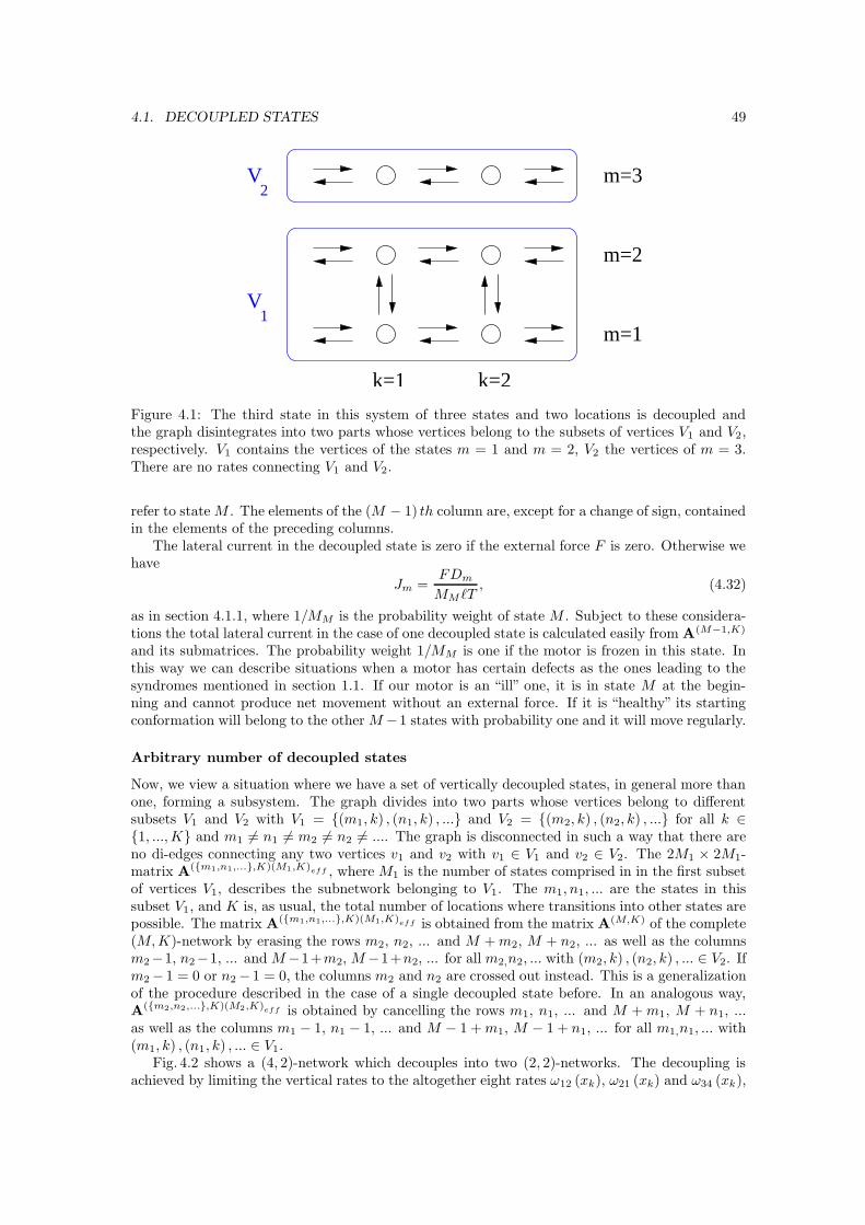
4.1. DECOUPLED STATES 49
k=1
m=3
m=2
m=1
2
1
k=2
V
V
Figure 4.1: The third state in this system of three states and two locations is decoupled andthe graph disintegrates into two parts whose vertices belong to the subsets of vertices V1 and V2,respectively. V1 contains the vertices of the states m = 1 and m = 2, V2 the vertices of m = 3.There are no rates connecting V1 and V2.
refer to state M . The elements of the (M − 1) th column are, except for a change of sign, containedin the elements of the preceding columns.
The lateral current in the decoupled state is zero if the external force F is zero. Otherwise wehave
Jm =FDm
MM `T, (4.32)
as in section 4.1.1, where 1/MM is the probability weight of state M . Subject to these considera-tions the total lateral current in the case of one decoupled state is calculated easily from A(M−1,K)
and its submatrices. The probability weight 1/MM is one if the motor is frozen in this state. Inthis way we can describe situations when a motor has certain defects as the ones leading to thesyndromes mentioned in section 1.1. If our motor is an “ill” one, it is in state M at the begin-ning and cannot produce net movement without an external force. If it is “healthy” its startingconformation will belong to the other M −1 states with probability one and it will move regularly.
Arbitrary number of decoupled states
Now, we view a situation where we have a set of vertically decoupled states, in general more thanone, forming a subsystem. The graph divides into two parts whose vertices belong to differentsubsets V1 and V2 with V1 = (m1, k) , (n1, k) , ... and V2 = (m2, k) , (n2, k) , ... for all k ∈1, ..., K and m1 6= n1 6= m2 6= n2 6= .... The graph is disconnected in such a way that there areno di-edges connecting any two vertices v1 and v2 with v1 ∈ V1 and v2 ∈ V2. The 2M1 × 2M1-matrix A(m1,n1,...,K)(M1,K)eff , where M1 is the number of states comprised in in the first subsetof vertices V1, describes the subnetwork belonging to V1. The m1, n1, ... are the states in thissubset V1, and K is, as usual, the total number of locations where transitions into other states arepossible. The matrix A(m1,n1,...,K)(M1,K)eff is obtained from the matrix A(M,K) of the complete(M, K)-network by erasing the rows m2, n2, ... and M + m2, M + n2, ... as well as the columnsm2−1, n2−1, ... and M −1+m2, M −1+n2, ... for all m2,n2, ... with (m2, k) , (n2, k) , ... ∈ V2. Ifm2 − 1 = 0 or n2 − 1 = 0, the columns m2 and n2 are crossed out instead. This is a generalizationof the procedure described in the case of a single decoupled state before. In an analogous way,A(m2,n2,...,K)(M2,K)eff is obtained by cancelling the rows m1, n1, ... and M + m1, M + n1, ...as well as the columns m1 − 1, n1 − 1, ... and M − 1 + m1, M − 1 + n1, ... for all m1,n1, ... with(m1, k) , (n1, k) , ... ∈ V1.
Fig. 4.2 shows a (4, 2)-network which decouples into two (2, 2)-networks. The decoupling isachieved by limiting the vertical rates to the altogether eight rates ω12 (xk), ω21 (xk) and ω34 (xk),
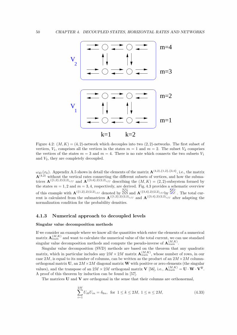
50 CHAPTER 4. DECOUPLED STATES, HORIZONTAL RATES AND NETWORKS
k=1 k=2
m=4
m=3
m=2
m=1
1
2V
V
Figure 4.2: (M, K) = (4, 2)-network which decouples into two (2, 2)-networks. The first subset ofvertices, V1, comprises all the vertices in the states m = 1 and m = 2. The subset V2 comprisesthe vertices of the states m = 3 and m = 4. There is no rate which connects the two subsets V1
and V2, they are completely decoupled.
ω43 (xk). Appendix A.5 shows in detail the elements of the matrix A(4,2),1,2,3,4, i.e., the matrixA(4,2) without the vertical rates connecting the different subsets of vertices, and how the subma-trices A(1,2,2)(2,2)eff and A(3,4,2)(2,2)eff describing the (M, K) = (2, 2)-subsystem formed bythe states m = 1, 2 and m = 3, 4, respectively, are derived. Fig. 4.3 provides a schematic overview
of this example with A(1,2,2)(2,2)eff denoted byand A(3,4,2)(2,2)eff by
. The total cur-rent is calculated from the submatrices A(1,2,2)(2,2)eff and A(3,4,2)(2,2)eff after adapting thenormalization condition for the probability densities.
4.1.3 Numerical approach to decoupled levels
Singular value decomposition methods
If we consider an example where we know all the quantities which enter the elements of a numerical
matrix A(M,K)num and want to calculate the numerical value of the total current, we can use standard
singular value decomposition methods and compute the pseudo-inverse of A(M,K)num .
Singular value decomposition (SVD) methods are based on the theorem that any quadratic
matrix, which in particular includes any 2M × 2M matrix A(M,K)num , whose number of rows, in our
case 2M , is equal to its number of columns, can be written as the product of an 2M×2M column-orthogonal matrix U, an 2M×2M diagonal matrix W with positive or zero elements (the singular
values), and the transpose of an 2M × 2M orthogonal matrix V [56], i.e., A(M,K)num = U ·W ·VT.
A proof of this theorem by induction can be found in [57].
The matrices U and V are orthogonal in the sense that their columns are orthonormal,
2M∑
i=1
UikUin = δkn, for 1 ≤ k ≤ 2M, 1 ≤ n ≤ 2M, (4.33)
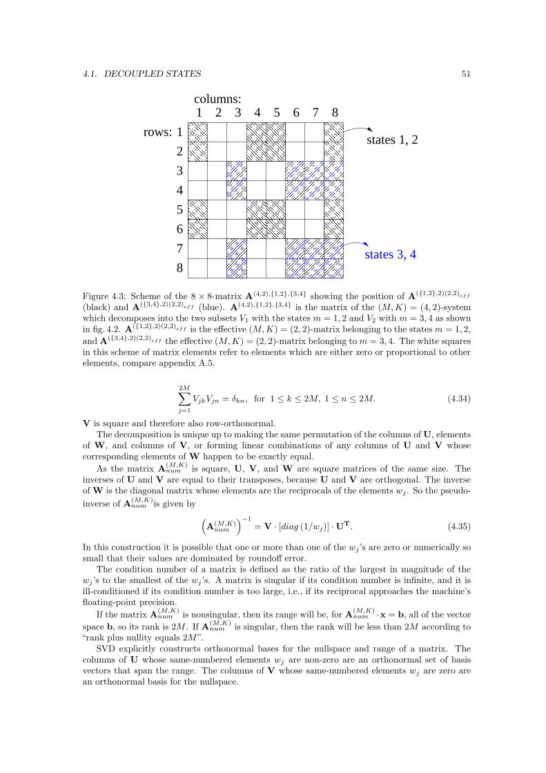
4.1. DECOUPLED STATES 51
!!!!!!""""""######$$$$$$ %%%%&&
&& ''''(((())))))****++++,,,, ----....//////0000
111111222222333333444444 555566
66 77778888999999::::;;;;<<<< ====>>>>??????@@@@
1 2 3 4 5 6 7 8
1
2
3
4
5
6
7
8
rows:
columns:
states 1, 2
states 3, 4
Figure 4.3: Scheme of the 8 × 8-matrix A(4,2),1,2,3,4 showing the position of A(1,2,2)(2,2)eff
(black) and A(3,4,2)(2,2)eff (blue). A(4,2),1,2,3,4 is the matrix of the (M, K) = (4, 2)-systemwhich decomposes into the two subsets V1 with the states m = 1, 2 and V2 with m = 3, 4 as shownin fig. 4.2. A(1,2,2)(2,2)eff is the effective (M, K) = (2, 2)-matrix belonging to the states m = 1, 2,
and A(3,4,2)(2,2)eff the effective (M, K) = (2, 2)-matrix belonging to m = 3, 4. The white squaresin this scheme of matrix elements refer to elements which are either zero or proportional to otherelements, compare appendix A.5.
2M∑
j=1
VjkVjn = δkn, for 1 ≤ k ≤ 2M, 1 ≤ n ≤ 2M. (4.34)
V is square and therefore also row-orthonormal.The decomposition is unique up to making the same permutation of the columns of U, elements
of W, and columns of V, or forming linear combinations of any columns of U and V whosecorresponding elements of W happen to be exactly equal.
As the matrix A(M,K)num is square, U, V, and W are square matrices of the same size. The
inverses of U and V are equal to their transposes, because U and V are orthogonal. The inverseof W is the diagonal matrix whose elements are the reciprocals of the elements wj . So the pseudo-
inverse of A(M,K)num is given by
(A(M,K)
num
)−1
= V · [diag (1/wj)] ·UT. (4.35)
In this construction it is possible that one or more than one of the wj ’s are zero or numerically sosmall that their values are dominated by roundoff error.
The condition number of a matrix is defined as the ratio of the largest in magnitude of thewj ’s to the smallest of the wj ’s. A matrix is singular if its condition number is infinite, and it isill-conditioned if its condition number is too large, i.e., if its reciprocal approaches the machine’sfloating-point precision.
If the matrix A(M,K)num is nonsingular, then its range will be, for A
(M,K)num ·x = b, all of the vector
space b, so its rank is 2M . If A(M,K)num is singular, then the rank will be less than 2M according to
“rank plus nullity equals 2M”.SVD explicitly constructs orthonormal bases for the nullspace and range of a matrix. The
columns of U whose same-numbered elements wj are non-zero are an orthonormal set of basisvectors that span the range. The columns of V whose same-numbered elements wj are zero arean orthonormal basis for the nullspace.
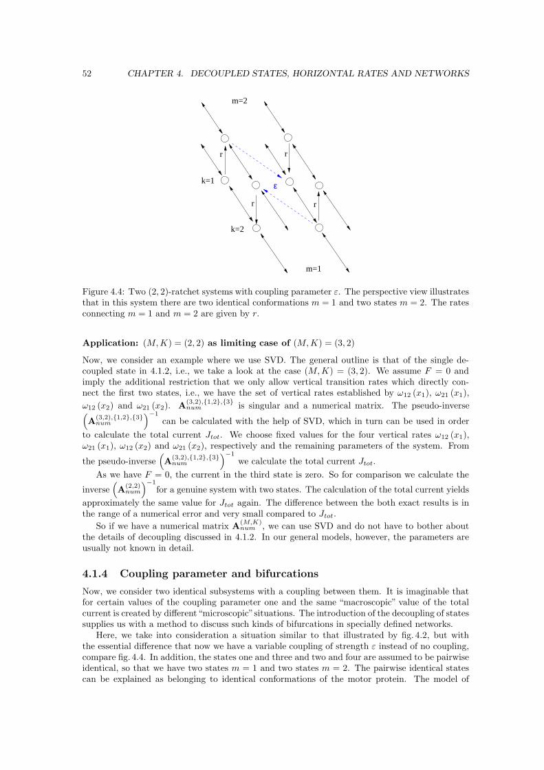
52 CHAPTER 4. DECOUPLED STATES, HORIZONTAL RATES AND NETWORKS
k=1
k=2
m=1
m=2
rr
r r
ε
Figure 4.4: Two (2, 2)-ratchet systems with coupling parameter ε. The perspective view illustratesthat in this system there are two identical conformations m = 1 and two states m = 2. The ratesconnecting m = 1 and m = 2 are given by r.
Application: (M, K) = (2, 2) as limiting case of (M, K) = (3, 2)
Now, we consider an example where we use SVD. The general outline is that of the single de-coupled state in 4.1.2, i.e., we take a look at the case (M, K) = (3, 2). We assume F = 0 andimply the additional restriction that we only allow vertical transition rates which directly con-nect the first two states, i.e., we have the set of vertical rates established by ω12 (x1), ω21 (x1),
ω12 (x2) and ω21 (x2). A(3,2),1,2,3num is singular and a numerical matrix. The pseudo-inverse(
A(3,2),1,2,3num
)−1
can be calculated with the help of SVD, which in turn can be used in order
to calculate the total current Jtot. We choose fixed values for the four vertical rates ω12 (x1),ω21 (x1), ω12 (x2) and ω21 (x2), respectively and the remaining parameters of the system. From
the pseudo-inverse(A
(3,2),1,2,3num
)−1
we calculate the total current Jtot.
As we have F = 0, the current in the third state is zero. So for comparison we calculate the
inverse(A
(2,2)num
)−1
for a genuine system with two states. The calculation of the total current yields
approximately the same value for Jtot again. The difference between the both exact results is inthe range of a numerical error and very small compared to Jtot.
So if we have a numerical matrix A(M,K)num , we can use SVD and do not have to bother about
the details of decoupling discussed in 4.1.2. In our general models, however, the parameters areusually not known in detail.
4.1.4 Coupling parameter and bifurcations
Now, we consider two identical subsystems with a coupling between them. It is imaginable thatfor certain values of the coupling parameter one and the same “macroscopic” value of the totalcurrent is created by different“microscopic”situations. The introduction of the decoupling of statessupplies us with a method to discuss such kinds of bifurcations in specially defined networks.
Here, we take into consideration a situation similar to that illustrated by fig. 4.2, but withthe essential difference that now we have a variable coupling of strength ε instead of no coupling,compare fig. 4.4. In addition, the states one and three and two and four are assumed to be pairwiseidentical, so that we have two states m = 1 and two states m = 2. The pairwise identical statescan be explained as belonging to identical conformations of the motor protein. The model of
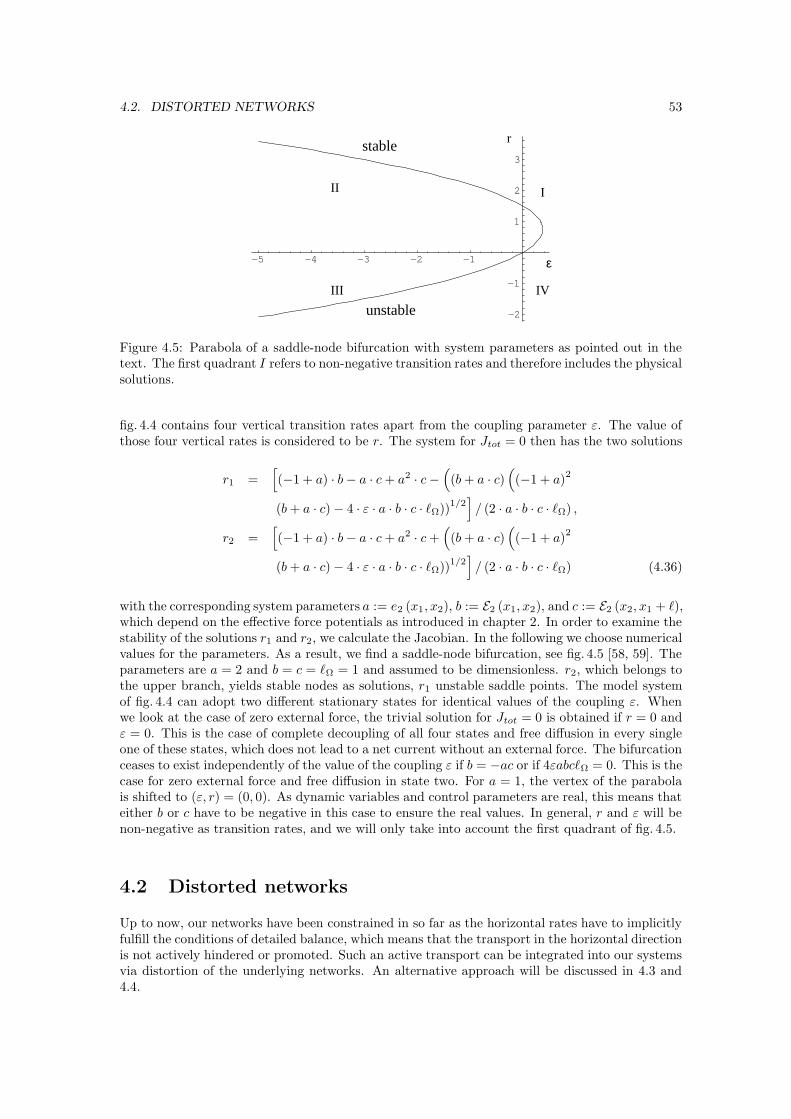
4.2. DISTORTED NETWORKS 53
−5 −4 −3 −2 −1
−2
−1
1
2
3
ε
rstable
unstable
III
III IV
Figure 4.5: Parabola of a saddle-node bifurcation with system parameters as pointed out in thetext. The first quadrant I refers to non-negative transition rates and therefore includes the physicalsolutions.
fig. 4.4 contains four vertical transition rates apart from the coupling parameter ε. The value ofthose four vertical rates is considered to be r. The system for Jtot = 0 then has the two solutions
r1 =[(−1 + a) · b − a · c + a2 · c −
((b + a · c)
((−1 + a)2
(b + a · c) − 4 · ε · a · b · c · `Ω))1/2]/ (2 · a · b · c · `Ω) ,
r2 =[(−1 + a) · b − a · c + a2 · c +
((b + a · c)
((−1 + a)
2
(b + a · c) − 4 · ε · a · b · c · `Ω))1/2]/ (2 · a · b · c · `Ω) (4.36)
with the corresponding system parameters a := e2 (x1, x2), b := E2 (x1, x2), and c := E2 (x2, x1 + `),which depend on the effective force potentials as introduced in chapter 2. In order to examine thestability of the solutions r1 and r2, we calculate the Jacobian. In the following we choose numericalvalues for the parameters. As a result, we find a saddle-node bifurcation, see fig. 4.5 [58, 59]. Theparameters are a = 2 and b = c = `Ω = 1 and assumed to be dimensionless. r2, which belongs tothe upper branch, yields stable nodes as solutions, r1 unstable saddle points. The model systemof fig. 4.4 can adopt two different stationary states for identical values of the coupling ε. Whenwe look at the case of zero external force, the trivial solution for Jtot = 0 is obtained if r = 0 andε = 0. This is the case of complete decoupling of all four states and free diffusion in every singleone of these states, which does not lead to a net current without an external force. The bifurcationceases to exist independently of the value of the coupling ε if b = −ac or if 4εabc`Ω = 0. This is thecase for zero external force and free diffusion in state two. For a = 1, the vertex of the parabolais shifted to (ε, r) = (0, 0). As dynamic variables and control parameters are real, this means thateither b or c have to be negative in this case to ensure the real values. In general, r and ε will benon-negative as transition rates, and we will only take into account the first quadrant of fig. 4.5.
4.2 Distorted networks
Up to now, our networks have been constrained in so far as the horizontal rates have to implicitlyfulfill the conditions of detailed balance, which means that the transport in the horizontal directionis not actively hindered or promoted. Such an active transport can be integrated into our systemsvia distortion of the underlying networks. An alternative approach will be discussed in 4.3 and4.4.
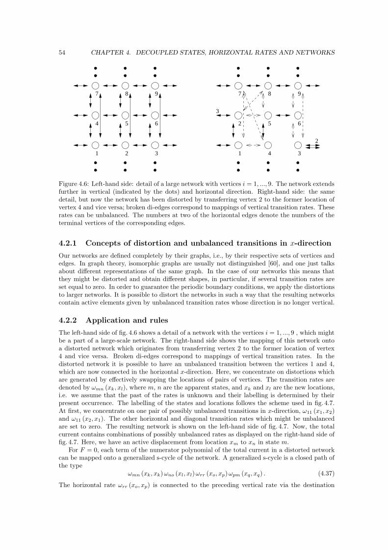
54 CHAPTER 4. DECOUPLED STATES, HORIZONTAL RATES AND NETWORKS
1 2 3
4 5 6
7 8 9
1 3
5 6
7 8 9
2
4
3
2
Figure 4.6: Left-hand side: detail of a large network with vertices i = 1, ..., 9. The network extendsfurther in vertical (indicated by the dots) and horizontal direction. Right-hand side: the samedetail, but now the network has been distorted by transferring vertex 2 to the former location ofvertex 4 and vice versa; broken di-edges correspond to mappings of vertical transition rates. Theserates can be unbalanced. The numbers at two of the horizontal edges denote the numbers of theterminal vertices of the corresponding edges.
4.2.1 Concepts of distortion and unbalanced transitions in x-direction
Our networks are defined completely by their graphs, i.e., by their respective sets of vertices andedges. In graph theory, isomorphic graphs are usually not distinguished [60], and one just talksabout different representations of the same graph. In the case of our networks this means thatthey might be distorted and obtain different shapes, in particular, if several transition rates areset equal to zero. In order to guarantee the periodic boundary conditions, we apply the distortionsto larger networks. It is possible to distort the networks in such a way that the resulting networkscontain active elements given by unbalanced transition rates whose direction is no longer vertical.
4.2.2 Application and rules
The left-hand side of fig. 4.6 shows a detail of a network with the vertices i = 1, ..., 9 , which mightbe a part of a large-scale network. The right-hand side shows the mapping of this network ontoa distorted network which originates from transferring vertex 2 to the former location of vertex4 and vice versa. Broken di-edges correspond to mappings of vertical transition rates. In thedistorted network it is possible to have an unbalanced transition between the vertices 1 and 4,which are now connected in the horizontal x-direction. Here, we concentrate on distortions whichare generated by effectively swapping the locations of pairs of vertices. The transition rates aredenoted by ωmn (xk , xl), where m, n are the apparent states, and xk and xl are the new locations,i.e. we assume that the past of the rates is unknown and their labelling is determined by theirpresent occurrence. The labelling of the states and locations follows the scheme used in fig. 4.7.At first, we concentrate on one pair of possibly unbalanced transitions in x-direction, ω11 (x1, x2)and ω11 (x2, x1). The other horizontal and diagonal transition rates which might be unbalancedare set to zero. The resulting network is shown on the left-hand side of fig. 4.7. Now, the totalcurrent contains combinations of possibly unbalanced rates as displayed on the right-hand side offig. 4.7. Here, we have an active displacement from location xm to xn in state m.
For F = 0, each term of the numerator polynomial of the total current in a distorted networkcan be mapped onto a generalized s-cycle of the network. A generalized s-cycle is a closed path ofthe type
ωmn (xk , xk) ωno (xl, xl) ωrr (xo, xp) ωpm (xq , xq) . (4.37)
The horizontal rate ωrr (xo, xp) is connected to the preceding vertical rate via the destination
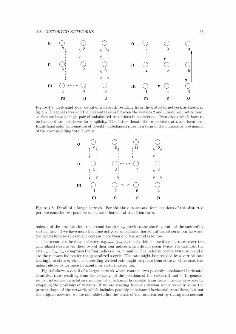
4.2. DISTORTED NETWORKS 55
1 3
5 6
7 8 9
2
4
n
o
m
n om1 3
5 6
7 8 9
2
4
n
o
m
n om
Figure 4.7: Left-hand side: detail of a network resulting from the distorted network as shown infig. 4.6. Diagonal rates and the horizontal rates between the vertices 2 and 5 have been set to zero,so that we have a single pair of unbalanced transitions in x-direction. Transitions which have tobe balanced are not shown for simplicity. The letters denote the respective states and locations.Right-hand side: combination of possibly unbalanced rates in a term of the numerator polynomialof the corresponding total current.
1 6 4
5 3 7 8
9 10 11 12
2
o
m
n
pm n o
Figure 4.8: Detail of a larger network. For the three states and four locations of this distortedpart we consider two possibly unbalanced horizontal transition rates.
index o of the first location, the second location xp provides the starting state of the succeedingvertical rate. If we have more than one active or unbalanced horizontal transition in our network,the generalized s-cycles might contain more than one horizontal rate, too.
There can also be diagonal rates, e.g.ωom (xm, xn) in fig. 4.6. These diagonal rates enter thegeneralized s-cycles via these two of their four indices which do not occur twice. For example, therate ωom (xm, xn) comprises the four indices o, m, m and n. The index m occurs twice, so o and nare the relevant indices for the generalized s-cycle. The rate might be preceded by a vertical rateleading into state o, while a succeeding vertical rate might originate from state n. Of course, thisindex rule holds for mere horizontal or vertical rates, too.
Fig. 4.8 shows a detail of a larger network which contains two possibly unbalanced horizontaltransition rates resulting from the exchange of the positions of the vertices 3 and 6. In general,we can introduce an arbitrary number of unbalanced horizontal transitions into our networks byswapping the positions of vertices. If we are starting from a situation where we only know thepresent shape of the network, which includes possibly unbalanced horizontal transitions, but notthe original network, we are still able to list the terms of the total current by taking into account
56 CHAPTER 4. DECOUPLED STATES, HORIZONTAL RATES AND NETWORKS
generalized s-cycles.
4.3 Master equation and horizontal rates
In this section we introduce a discrete Master-equation approach to our system. This approachexplicitly comprises the horizontal forward and backward rates. With the help of these horizontalrates we are able to determine uniquely complete s-cycles, which contribute to the total current inour network, rather than only contributions by vertical rates. In this way it becomes clear whethera combination of rates belongs to the motor taking a forward or a backward step. Furthermore,with this additional piece of information we can determine for sure which conformation can beassociated with the motor entering the network from the left, or, in the case of a backward step,with the motor entering it from the right. In the Master-equation approach it is possible to abstainfrom the original definition of the horizontal rates, so that we can break the conditions of detailedbalance for these rates, too, and have active horizontal elements. Besides, we derive extensionsto the rules in 3.2.2, since now the polynomials depend on the vertical and also on the horizontalrates. The Master equation has been introduced in [43], but this is the first time that this approachis used to perform calculations for general model systems.
4.3.1 General outline
At first, we introduce several changes in our notation as compared to chapter 2.Now, the probabilities of finding the motor in the discrete states (m, k) are denoted by
P (m, k) ≡ Pm (xk) `Ω (4.38)
We introduce the forward transition rate
W (m, k |m, k + 1) ≡em (xk, xk+1)
Em (xk, xk+1) `Ω, (4.39)
which belongs to the motor moving from location xk in state m to location xk+1 in the same state.The rate for a backward move in level m from position xk+1 to xk is accordingly denoted as
W (m, k + 1 |m, k ) ≡1
Em (xk, xk+1) `Ω. (4.40)
Here, the horizontal rates show a pairwise dependence,
W (m, k |m, k + 1) =em (xk, xk+1)
Em (xk, xk+1) `Ω
= em (xk , xk+1) W (m, k + 1 |m, k ) , (4.41)
and accordingly fulfill the conditions of detailed balance. As em (xk, xk+1) 6= 0 for every choice ofm and k, a horizontal forward rate can never vanish equal to zero. The same is true for backwardrates, W (m, k + 1 |m, k ) ≡ 1/Em (xk, xk+1) `Ω, as their numerators are constant and equal to one.Nevertheless, the horizontal rates might attain small values and approach zero, if the correspondingEm (xk, xk+1) are large. The interlevel current Jmn (xk) as given by (2.25) is rewritten in the form
Jmn (xk) ≡ P (m, k)W (m, k |n, k ) , (4.42)
where we have adapted the notation for the vertical transition rates to
W (m, k |n, k ) ≡ ωmn (xk) . (4.43)
Now, equation (2.41) reads
P (m, k + 1) = −J (m, k |m, k + 1)1
W (m, k + 1 |m, k )+ P (m, k)
W (m, k |m, k + 1)
W (m, k + 1 |m, k )(4.44)
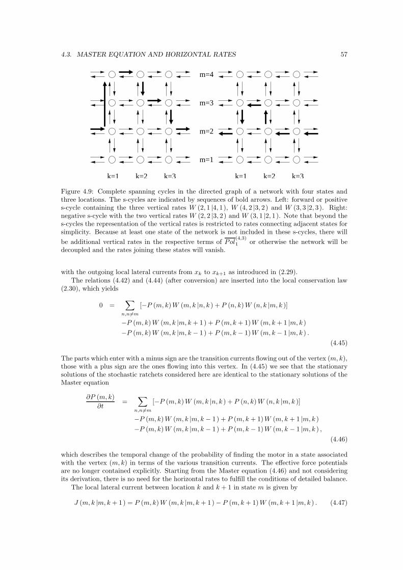
4.3. MASTER EQUATION AND HORIZONTAL RATES 57
k=1 k=2 k=3 k=1 k=2 k=3
m=2
m=1
m=3
m=4
Figure 4.9: Complete spanning cycles in the directed graph of a network with four states andthree locations. The s-cycles are indicated by sequences of bold arrows. Left: forward or positives-cycle containing the three vertical rates W (2, 1 |4, 1), W (4, 2 |3, 2) and W (3, 3 |2, 3). Right:negative s-cycle with the two vertical rates W (2, 2 |3, 2) and W (3, 1 |2, 1). Note that beyond thes-cycles the representation of the vertical rates is restricted to rates connecting adjacent states forsimplicity. Because at least one state of the network is not included in these s-cycles, there will
be additional vertical rates in the respective terms of Pol(4,3)
1 or otherwise the network will bedecoupled and the rates joining these states will vanish.
with the outgoing local lateral currents from xk to xk+1 as introduced in (2.29).The relations (4.42) and (4.44) (after conversion) are inserted into the local conservation law
(2.30), which yields
0 =∑
n,n6=m
[−P (m, k)W (m, k |n, k ) + P (n, k) W (n, k |m, k )]
−P (m, k) W (m, k |m, k + 1) + P (m, k + 1)W (m, k + 1 |m, k )
−P (m, k) W (m, k |m, k − 1) + P (m, k − 1)W (m, k − 1 |m, k ) .
(4.45)
The parts which enter with a minus sign are the transition currents flowing out of the vertex (m, k),those with a plus sign are the ones flowing into this vertex. In (4.45) we see that the stationarysolutions of the stochastic ratchets considered here are identical to the stationary solutions of theMaster equation
∂P (m, k)
∂t=
∑
n,n6=m
[−P (m, k)W (m, k |n, k ) + P (n, k) W (n, k |m, k )]
−P (m, k) W (m, k |m, k − 1) + P (m, k + 1)W (m, k + 1 |m, k )
−P (m, k) W (m, k |m, k − 1) + P (m, k − 1)W (m, k − 1 |m, k ) ,
(4.46)
which describes the temporal change of the probability of finding the motor in a state associatedwith the vertex (m, k) in terms of the various transition currents. The effective force potentialsare no longer contained explicitly. Starting from the Master equation (4.46) and not consideringits derivation, there is no need for the horizontal rates to fulfill the conditions of detailed balance.
The local lateral current between location k and k + 1 in state m is given by
J (m, k |m, k + 1) = P (m, k) W (m, k |m, k + 1) − P (m, k + 1) W (m, k + 1 |m, k ) . (4.47)
58 CHAPTER 4. DECOUPLED STATES, HORIZONTAL RATES AND NETWORKS
By transforming (4.47), we obtain the probability at location k + 1,
P (m, k + 1) = −J (m, k |m, k + 1)1
W (m, k + 1 |m, k )+ P (m, k)
W (m, k |m, k + 1)
W (m, k + 1 |m, k ). (4.48)
We introduce the diagonal matrices DJP
and DPP
with matrix elements
DJP
nm (k, k + 1) ≡ −δnm1
W (m, k + 1 |m, k )(4.49)
and
DPP
nm (k, k + 1) ≡ δnmW (m, k |m, k + 1)
W (m, k + 1 |m, k ). (4.50)
The bar above the symbols refers to the Master-equation approach which is used here in contrastto chapter 2. Besides, we define the additional transfer matrices
TJP
≡ TJJ
DJP
(4.51)
andT
PP≡ T
PJD
JP+ D
PP(4.52)
where TJJ
is equal to the unit matrix and TPJ
(k) is given by
TPJ
nm (k) ≡ −δnm
∑
p6=m
W (m, k |p, k ) + (1 − δnm) W (n, k |m, k ) . (4.53)
With the help of these additional matrices we obtain
P (m, k + 1) = J (k, k + 1)DJP
(k, k + 1) + P (k)DPP
(k, k + 1)
= J (k − 1, k)TJP
(k, k + 1) + P (k)TPP
(k, k + 1) . (4.54)
This relation and (4.47) can be combined into the recursion relation
(J (k, k + 1) , P (k + 1)) = (J (k − 1, k) , P (k))T (k, k + 1) . (4.55)
We proceed by analogy to the procedure described in section 2.2 and take into account that thenormalization for the discrete probability distribution is now given by
∑
k
∑
m
P (m, k) ≡ 1. (4.56)
Doing so, we obtain new matrices A(M,K)
which explicitly contain all the horizontal and verticalrates of the system.
4.3.2 Complete s-cycles and horizontal rates
Spanning cycles or s-cycles have already been introduced in 2.2.3 and examined later in chapter3. We remember that an s-cycle starts at vertex (k = 1, m), spans the whole network parallel tothe x-direction, and then ends at vertex (k = K, m), i.e., in the same state m it started in. Ans-cycle has to contain vertical rates. In the preceding chapters, we have identified these s-cyclesvia their vertical rates. Because of the Master-equation approach, we now have the possibility ofdetermining complete paths of vertical and horizontal rates. Note, that here we do not refer to thegeneralized s-cycles of 4.2.2 for distorted networks, but to complete s-cycles explicitly containingall their horizontal and vertical rates. Furthermore, we extend the original definition providedin 2.2.3 in such a way that we distinguish between positive spanning-cycles or positive s-cycles,which traverse the network in positive x-direction, in fig. 4.9 to the right, and negative s-cyclestraversing it in negative x-direction. Accordingly, positive spanning-cycles are associated with aforward stepping of the motor, negative ones with a backward stepping. Usually, there is a maindirection of movement for a certain motor protein. Conventional kinesin, for example, most of thetime steps in the direction of the plus end of its microtubule. We define this main direction to bethe positive x-direction with respect to a special motor protein.
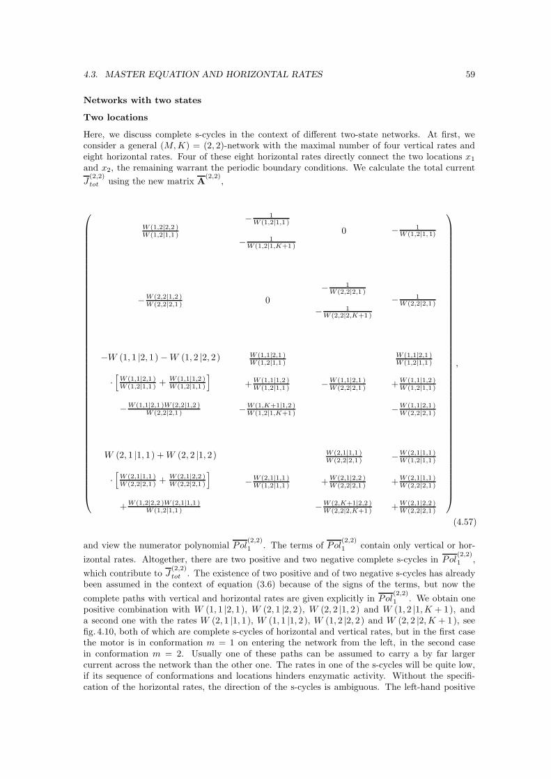
4.3. MASTER EQUATION AND HORIZONTAL RATES 59
Networks with two states
Two locations
Here, we discuss complete s-cycles in the context of different two-state networks. At first, weconsider a general (M, K) = (2, 2)-network with the maximal number of four vertical rates andeight horizontal rates. Four of these eight horizontal rates directly connect the two locations x1
and x2, the remaining warrant the periodic boundary conditions. We calculate the total current
J(2,2)
tot using the new matrix A(2,2)
,
W (1,2|2,2 )W (1,2|1,1 )
− 1W (1,2|1,1 )
− 1W (1,2|1,K+1)
0 − 1W (1,2|1,1)
−W (2,2|1,2 )W (2,2|2,1 ) 0
− 1W (2,2|2,1 )
− 1W (2,2|2,K+1)
− 1W (2,2|2,1 )
−W (1, 1 |2, 1) − W (1, 2 |2, 2)
·[
W (1,1|2,1 )W (1,2|1,1 ) + W (1,1|1,2 )
W (1,2|1,1 )
]
−W (1,1|2,1 )W (2,2|1,2 )W (2,2|2,1 )
W (1,1|2,1 )W (1,2|1,1 )
+W (1,1|1,2 )W (1,2|1,1 )
−W (1,K+1|1,2 )W (1,2|1,K+1)
−W (1,1|2,1 )W (2,2|2,1 )
W (1,1|2,1 )W (1,2|1,1 )
+W (1,1|1,2 )W (1,2|1,1 )
−W (1,1|2,1 )W (2,2|2,1 )
W (2, 1 |1, 1) + W (2, 2 |1, 2)
·[
W (2,1|1,1 )W (2,2|2,1 ) + W (2,1|2,2 )
W (2,2|2,1 )
]
+W (1,2|2,2 )W (2,1|1,1 )W (1,2|1,1 )
−W (2,1|1,1 )W (1,2|1,1 )
W (2,1|1,1 )W (2,2|2,1 )
+W (2,1|2,2 )W (2,2|2,1 )
−W (2,K+1|2,2 )W (2,2|2,K+1)
−W (2,1|1,1 )W (1,2|1,1 )
+W (2,1|1,1 )W (2,2|2,1 )
+W (2,1|2,2 )W (2,2|2,1 )
,
(4.57)
and view the numerator polynomial Pol(2,2)
1 . The terms of Pol(2,2)
1 contain only vertical or hor-
izontal rates. Altogether, there are two positive and two negative complete s-cycles in Pol(2,2)
1 ,
which contribute to J(2,2)
tot . The existence of two positive and of two negative s-cycles has alreadybeen assumed in the context of equation (3.6) because of the signs of the terms, but now the
complete paths with vertical and horizontal rates are given explicitly in Pol(2,2)
1 . We obtain onepositive combination with W (1, 1 |2, 1), W (2, 1 |2, 2), W (2, 2 |1, 2) and W (1, 2 |1, K + 1), anda second one with the rates W (2, 1 |1, 1), W (1, 1 |1, 2), W (1, 2 |2, 2) and W (2, 2 |2, K + 1), seefig. 4.10, both of which are complete s-cycles of horizontal and vertical rates, but in the first casethe motor is in conformation m = 1 on entering the network from the left, in the second casein conformation m = 2. Usually one of these paths can be assumed to carry a by far largercurrent across the network than the other one. The rates in one of the s-cycles will be quite low,if its sequence of conformations and locations hinders enzymatic activity. Without the specifi-cation of the horizontal rates, the direction of the s-cycles is ambiguous. The left-hand positive
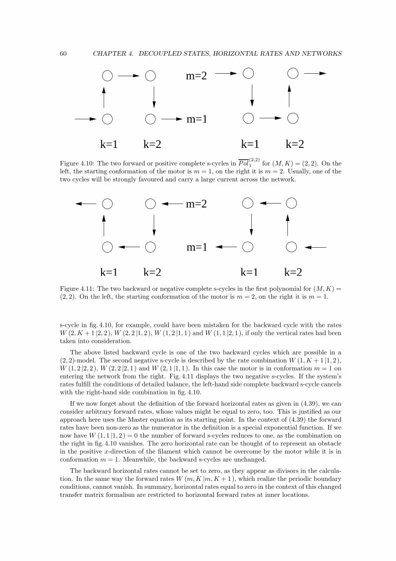
60 CHAPTER 4. DECOUPLED STATES, HORIZONTAL RATES AND NETWORKS
k=1 k=2
m=1
m=2
k=1 k=2
Figure 4.10: The two forward or positive complete s-cycles in Pol(2,2)
1 for (M, K) = (2, 2). On theleft, the starting conformation of the motor is m = 1, on the right it is m = 2. Usually, one of thetwo cycles will be strongly favoured and carry a large current across the network.
k=1 k=2
m=1
m=2
k=1 k=2Figure 4.11: The two backward or negative complete s-cycles in the first polynomial for (M, K) =(2, 2). On the left, the starting conformation of the motor is m = 2, on the right it is m = 1.
s-cycle in fig. 4.10, for example, could have been mistaken for the backward cycle with the ratesW (2, K + 1 |2, 2), W (2, 2 |1, 2), W (1, 2 |1, 1) and W (1, 1 |2, 1), if only the vertical rates had beentaken into consideration.
The above listed backward cycle is one of the two backward cycles which are possible in a(2, 2)-model. The second negative s-cycle is described by the rate combination W (1, K + 1 |1, 2),W (1, 2 |2, 2), W (2, 2 |2, 1) and W (2, 1 |1, 1). In this case the motor is in conformation m = 1 onentering the network from the right. Fig. 4.11 displays the two negative s-cycles. If the system’srates fulfill the conditions of detailed balance, the left-hand side complete backward s-cycle cancelswith the right-hand side combination in fig. 4.10.
If we now forget about the definition of the forward horizontal rates as given in (4.39), we canconsider arbitrary forward rates, whose values might be equal to zero, too. This is justified as ourapproach here uses the Master equation as its starting point. In the context of (4.39) the forwardrates have been non-zero as the numerator in the definition is a special exponential function. If wenow have W (1, 1 |1, 2) = 0 the number of forward s-cycles reduces to one, as the combination onthe right in fig. 4.10 vanishes. The zero horizontal rate can be thought of to represent an obstaclein the positive x-direction of the filament which cannot be overcome by the motor while it is inconformation m = 1. Meanwhile, the backward s-cycles are unchanged.
The backward horizontal rates cannot be set to zero, as they appear as divisors in the calcula-tion. In the same way the forward rates W (m, K |m, K + 1), which realize the periodic boundaryconditions, cannot vanish. In summary, horizontal rates equal to zero in the context of this changedtransfer matrix formalism are restricted to horizontal forward rates at inner locations.
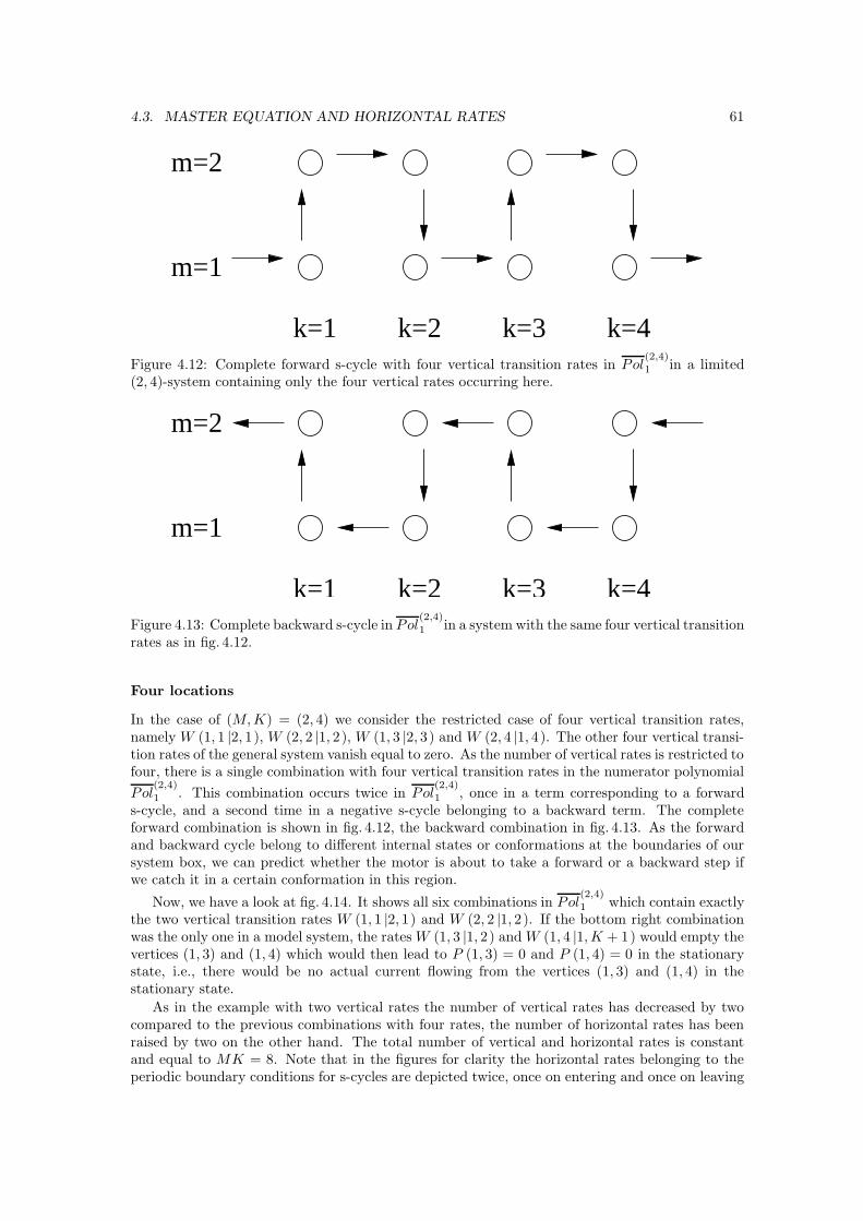
4.3. MASTER EQUATION AND HORIZONTAL RATES 61
k=1 k=2
m=2
m=1
k=3 k=4Figure 4.12: Complete forward s-cycle with four vertical transition rates in Pol
(2,4)
1 in a limited(2, 4)-system containing only the four vertical rates occurring here.
k=1 k=2
m=2
m=1
k=3 k=4Figure 4.13: Complete backward s-cycle in Pol
(2,4)
1 in a system with the same four vertical transitionrates as in fig. 4.12.
Four locations
In the case of (M, K) = (2, 4) we consider the restricted case of four vertical transition rates,namely W (1, 1 |2, 1), W (2, 2 |1, 2), W (1, 3 |2, 3) and W (2, 4 |1, 4). The other four vertical transi-tion rates of the general system vanish equal to zero. As the number of vertical rates is restricted tofour, there is a single combination with four vertical transition rates in the numerator polynomial
Pol(2,4)
1 . This combination occurs twice in Pol(2,4)
1 , once in a term corresponding to a forwards-cycle, and a second time in a negative s-cycle belonging to a backward term. The completeforward combination is shown in fig. 4.12, the backward combination in fig. 4.13. As the forwardand backward cycle belong to different internal states or conformations at the boundaries of oursystem box, we can predict whether the motor is about to take a forward or a backward step ifwe catch it in a certain conformation in this region.
Now, we have a look at fig. 4.14. It shows all six combinations in Pol(2,4)
1 which contain exactlythe two vertical transition rates W (1, 1 |2, 1) and W (2, 2 |1, 2). If the bottom right combinationwas the only one in a model system, the rates W (1, 3 |1, 2) and W (1, 4 |1, K + 1) would empty thevertices (1, 3) and (1, 4) which would then lead to P (1, 3) = 0 and P (1, 4) = 0 in the stationarystate, i.e., there would be no actual current flowing from the vertices (1, 3) and (1, 4) in thestationary state.
As in the example with two vertical rates the number of vertical rates has decreased by twocompared to the previous combinations with four rates, the number of horizontal rates has beenraised by two on the other hand. The total number of vertical and horizontal rates is constantand equal to MK = 8. Note that in the figures for clarity the horizontal rates belonging to theperiodic boundary conditions for s-cycles are depicted twice, once on entering and once on leaving
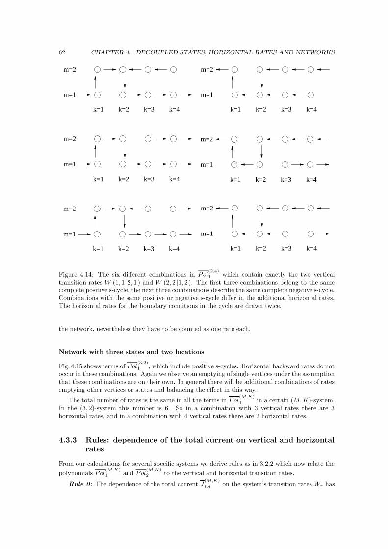
62 CHAPTER 4. DECOUPLED STATES, HORIZONTAL RATES AND NETWORKS
k=1 k=2
m=2
m=1
k=3 k=4 k=1 k=2
m=2
m=1
k=3 k=4
k=1 k=2
m=2
m=1
k=3 k=4 k=1 k=2
m=2
m=1
k=3 k=4
k=1 k=2
m=2
m=1
k=3 k=4 k=1 k=2
m=2
m=1
k=3 k=4
Figure 4.14: The six different combinations in Pol(2,4)
1 which contain exactly the two verticaltransition rates W (1, 1 |2, 1) and W (2, 2 |1, 2). The first three combinations belong to the samecomplete positive s-cycle, the next three combinations describe the same complete negative s-cycle.Combinations with the same positive or negative s-cycle differ in the additional horizontal rates.The horizontal rates for the boundary conditions in the cycle are drawn twice.
the network, nevertheless they have to be counted as one rate each.
Network with three states and two locations
Fig. 4.15 shows terms of Pol(3,2)
1 , which include positive s-cycles. Horizontal backward rates do notoccur in these combinations. Again we observe an emptying of single vertices under the assumptionthat these combinations are on their own. In general there will be additional combinations of ratesemptying other vertices or states and balancing the effect in this way.
The total number of rates is the same in all the terms in Pol(M,K)
1 in a certain (M, K)-system.In the (3, 2)-system this number is 6. So in a combination with 3 vertical rates there are 3horizontal rates, and in a combination with 4 vertical rates there are 2 horizontal rates.
4.3.3 Rules: dependence of the total current on vertical and horizontal
rates
From our calculations for several specific systems we derive rules as in 3.2.2 which now relate the
polynomials Pol(M,K)
1 and Pol(M,K)
2 to the vertical and horizontal transition rates.
Rule 0 : The dependence of the total current J(M,K)
tot on the system’s transition rates Wr has
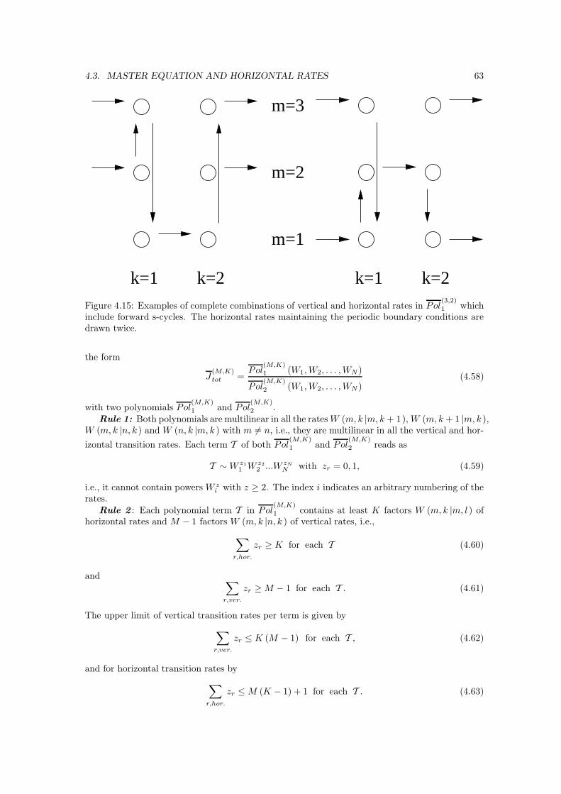
4.3. MASTER EQUATION AND HORIZONTAL RATES 63
k=1 k=2 k=1 k=2
m=2
m=1
m=3
Figure 4.15: Examples of complete combinations of vertical and horizontal rates in Pol(3,2)
1 whichinclude forward s-cycles. The horizontal rates maintaining the periodic boundary conditions aredrawn twice.
the form
J(M,K)
tot =Pol
(M,K)
1 (W1, W2, . . . , WN )
Pol(M,K)
2 (W1, W2, . . . , WN )(4.58)
with two polynomials Pol(M,K)
1 and Pol(M,K)
2 .Rule 1: Both polynomials are multilinear in all the rates W (m, k |m, k + 1), W (m, k + 1 |m, k ),
W (m, k |n, k ) and W (n, k |m, k ) with m 6= n, i.e., they are multilinear in all the vertical and hor-
izontal transition rates. Each term T of both Pol(M,K)
1 and Pol(M,K)
2 reads as
T ∼ W z1
1 W z2
2 ...W zN
N with zr = 0, 1, (4.59)
i.e., it cannot contain powers W zi with z ≥ 2. The index i indicates an arbitrary numbering of the
rates.Rule 2 : Each polynomial term T in Pol
(M,K)
1 contains at least K factors W (m, k |m, l ) ofhorizontal rates and M − 1 factors W (m, k |n, k ) of vertical rates, i.e.,
∑
r,hor.
zr ≥ K for each T (4.60)
and ∑
r,ver.
zr ≥ M − 1 for each T . (4.61)
The upper limit of vertical transition rates per term is given by
∑
r,ver.
zr ≤ K (M − 1) for each T , (4.62)
and for horizontal transition rates by
∑
r,hor.
zr ≤ M (K − 1) + 1 for each T . (4.63)
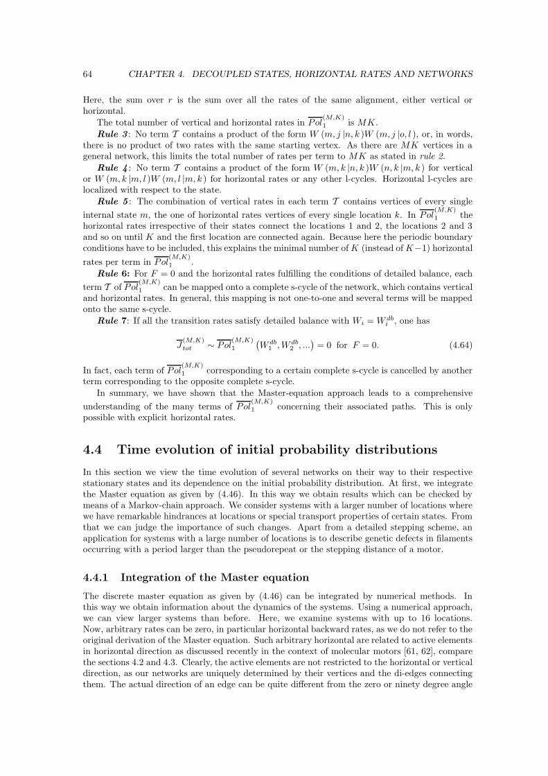
64 CHAPTER 4. DECOUPLED STATES, HORIZONTAL RATES AND NETWORKS
Here, the sum over r is the sum over all the rates of the same alignment, either vertical orhorizontal.
The total number of vertical and horizontal rates in Pol(M,K)
1 is MK.
Rule 3 : No term T contains a product of the form W (m, j |n, k )W (m, j |o, l ), or, in words,there is no product of two rates with the same starting vertex. As there are MK vertices in ageneral network, this limits the total number of rates per term to MK as stated in rule 2.
Rule 4 : No term T contains a product of the form W (m, k |n, k )W (n, k |m, k ) for verticalor W (m, k |m, l )W (m, l |m, k ) for horizontal rates or any other l-cycles. Horizontal l-cycles arelocalized with respect to the state.
Rule 5 : The combination of vertical rates in each term T contains vertices of every single
internal state m, the one of horizontal rates vertices of every single location k. In Pol(M,K)
1 thehorizontal rates irrespective of their states connect the locations 1 and 2, the locations 2 and 3and so on until K and the first location are connected again. Because here the periodic boundaryconditions have to be included, this explains the minimal number of K (instead of K−1) horizontal
rates per term in Pol(M,K)
1 .
Rule 6: For F = 0 and the horizontal rates fulfilling the conditions of detailed balance, each
term T of Pol(M,K)
1 can be mapped onto a complete s-cycle of the network, which contains verticaland horizontal rates. In general, this mapping is not one-to-one and several terms will be mappedonto the same s-cycle.
Rule 7: If all the transition rates satisfy detailed balance with Wi = W dbi , one has
J(M,K)
tot ∼ Pol(M,K)
1
(W db
1 , W db2 , ...
)= 0 for F = 0. (4.64)
In fact, each term of Pol(M,K)
1 corresponding to a certain complete s-cycle is cancelled by anotherterm corresponding to the opposite complete s-cycle.
In summary, we have shown that the Master-equation approach leads to a comprehensive
understanding of the many terms of Pol(M,K)
1 concerning their associated paths. This is onlypossible with explicit horizontal rates.
4.4 Time evolution of initial probability distributions
In this section we view the time evolution of several networks on their way to their respectivestationary states and its dependence on the initial probability distribution. At first, we integratethe Master equation as given by (4.46). In this way we obtain results which can be checked bymeans of a Markov-chain approach. We consider systems with a larger number of locations wherewe have remarkable hindrances at locations or special transport properties of certain states. Fromthat we can judge the importance of such changes. Apart from a detailed stepping scheme, anapplication for systems with a large number of locations is to describe genetic defects in filamentsoccurring with a period larger than the pseudorepeat or the stepping distance of a motor.
4.4.1 Integration of the Master equation
The discrete master equation as given by (4.46) can be integrated by numerical methods. Inthis way we obtain information about the dynamics of the systems. Using a numerical approach,we can view larger systems than before. Here, we examine systems with up to 16 locations.Now, arbitrary rates can be zero, in particular horizontal backward rates, as we do not refer to theoriginal derivation of the Master equation. Such arbitrary horizontal are related to active elementsin horizontal direction as discussed recently in the context of molecular motors [61, 62], comparethe sections 4.2 and 4.3. Clearly, the active elements are not restricted to the horizontal or verticaldirection, as our networks are uniquely determined by their vertices and the di-edges connectingthem. The actual direction of an edge can be quite different from the zero or ninety degree angle
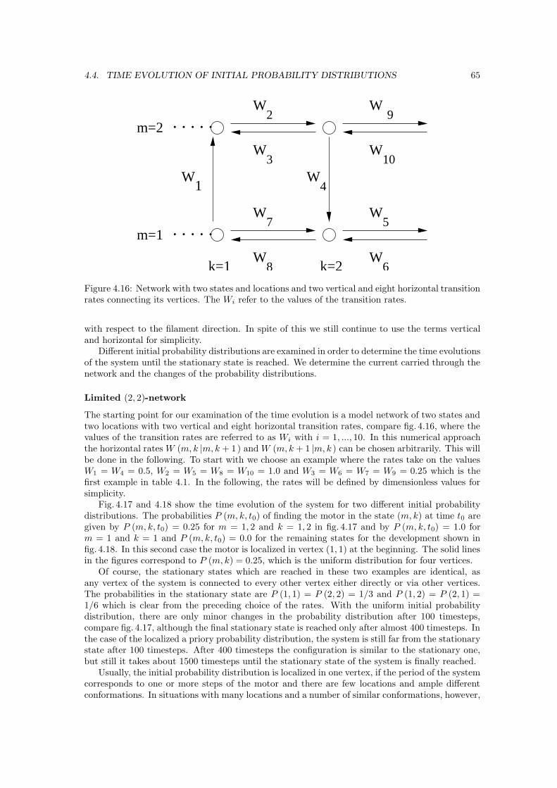
4.4. TIME EVOLUTION OF INITIAL PROBABILITY DISTRIBUTIONS 65
m=1 . . . . .
m=2 . . . . .
k=1 k=2
W
W1
2
W
W
W
W
W
W
W
W3
4
5
6
7
8
9
10
Figure 4.16: Network with two states and locations and two vertical and eight horizontal transitionrates connecting its vertices. The Wi refer to the values of the transition rates.
with respect to the filament direction. In spite of this we still continue to use the terms verticaland horizontal for simplicity.
Different initial probability distributions are examined in order to determine the time evolutionsof the system until the stationary state is reached. We determine the current carried through thenetwork and the changes of the probability distributions.
Limited (2, 2)-network
The starting point for our examination of the time evolution is a model network of two states andtwo locations with two vertical and eight horizontal transition rates, compare fig. 4.16, where thevalues of the transition rates are referred to as Wi with i = 1, ..., 10. In this numerical approachthe horizontal rates W (m, k |m, k + 1) and W (m, k + 1 |m, k ) can be chosen arbitrarily. This willbe done in the following. To start with we choose an example where the rates take on the valuesW1 = W4 = 0.5, W2 = W5 = W8 = W10 = 1.0 and W3 = W6 = W7 = W9 = 0.25 which is thefirst example in table 4.1. In the following, the rates will be defined by dimensionless values forsimplicity.
Fig. 4.17 and 4.18 show the time evolution of the system for two different initial probabilitydistributions. The probabilities P (m, k, t0) of finding the motor in the state (m, k) at time t0 aregiven by P (m, k, t0) = 0.25 for m = 1, 2 and k = 1, 2 in fig. 4.17 and by P (m, k, t0) = 1.0 form = 1 and k = 1 and P (m, k, t0) = 0.0 for the remaining states for the development shown infig. 4.18. In this second case the motor is localized in vertex (1, 1) at the beginning. The solid linesin the figures correspond to P (m, k) = 0.25, which is the uniform distribution for four vertices.
Of course, the stationary states which are reached in these two examples are identical, asany vertex of the system is connected to every other vertex either directly or via other vertices.The probabilities in the stationary state are P (1, 1) = P (2, 2) = 1/3 and P (1, 2) = P (2, 1) =1/6 which is clear from the preceding choice of the rates. With the uniform initial probabilitydistribution, there are only minor changes in the probability distribution after 100 timesteps,compare fig. 4.17, although the final stationary state is reached only after almost 400 timesteps. Inthe case of the localized a priory probability distribution, the system is still far from the stationarystate after 100 timesteps. After 400 timesteps the configuration is similar to the stationary one,but still it takes about 1500 timesteps until the stationary state of the system is finally reached.
Usually, the initial probability distribution is localized in one vertex, if the period of the systemcorresponds to one or more steps of the motor and there are few locations and ample differentconformations. In situations with many locations and a number of similar conformations, however,
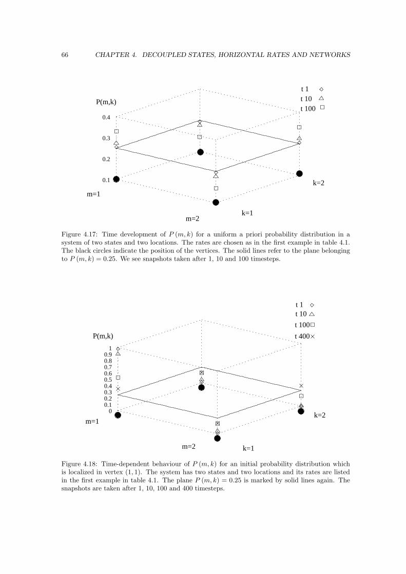
66 CHAPTER 4. DECOUPLED STATES, HORIZONTAL RATES AND NETWORKS
m=1
m=2k=1
k=2
P(m,k)t 100t 10t 1
0.1
0.2
0.3
0.4
Figure 4.17: Time development of P (m, k) for a uniform a priori probability distribution in asystem of two states and two locations. The rates are chosen as in the first example in table 4.1.The black circles indicate the position of the vertices. The solid lines refer to the plane belongingto P (m, k) = 0.25. We see snapshots taken after 1, 10 and 100 timesteps.
m=1
k=1
k=2
m=2
P(m,k)
t 1t 10
t 400
t 100
0.10.20.30.40.50.60.70.80.9
1
0
Figure 4.18: Time-dependent behaviour of P (m, k) for an initial probability distribution whichis localized in vertex (1, 1). The system has two states and two locations and its rates are listedin the first example in table 4.1. The plane P (m, k) = 0.25 is marked by solid lines again. Thesnapshots are taken after 1, 10, 100 and 400 timesteps.
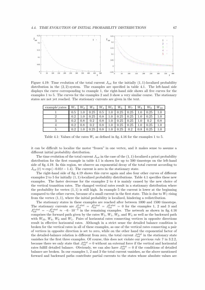
4.4. TIME EVOLUTION OF INITIAL PROBABILITY DISTRIBUTIONS 67
Jtot
t
1
0
0.05
0.1
0.15
0.2
0.25
0 50 100 150 200 250 300 350 400 450 500
J tot
t−0.05
0
0.05
0.1
0.15
0.2
0.25
0 50 100 150 200 250 300 350 400
4
3
2
1
5
Figure 4.19: Time evolution of the total current Jtot for the initially (1, 1)-localized probabilitydistribution in the (2, 2)-system. The examples are specified in table 4.1. The left-hand sidedisplays the curve corresponding to example 1, the right-hand side shows all five curves for theexamples 1 to 5. The curves for the examples 2 and 3 show a very similar course. The stationarystates are not yet reached. The stationary currents are given in the text.
example\rates W1 W2 W3 W4 W5 W6 W7 W8 W9 W10
1 0.5 1.0 0.25 0.5 1.0 0.25 0.25 1.0 0.25 1.02 0.2 1.0 0.25 0.8 1.0 0.25 0.25 1.0 0.25 1.03 0.2 0.8 0.2 0.8 1.0 0.25 0.25 1.0 0.2 0.84 0.2 0.8 0.2 0.8 1.0 0.25 0.25 1.0 0.25 1.05 0.2 1.0 0.25 0.8 1.0 0.25 0.2 0.8 0.25 1.0
Table 4.1: Values of the rates Wi as defined in fig. 4.16 for the examples 1 to 5.
it can be difficult to localize the motor “frozen” in one vertex, and it makes sense to assume adifferent initial probability distribution.
The time evolution of the total current Jtot in the case of the (1, 1)-localized a priori probabilitydistribution for the first example in table 4.1 is shown for up to 500 timesteps on the left-handside of fig. 4.19. In this region, we observe an exponential decay of the total current according toJtot (t) ≈ exp (−0.01t− 1.4). The current is zero in the stationary state.
The right-hand side of fig. 4.19 shows this curve again and also four other curves of differentexamples 2 to 5 for initially (1, 1)-localized probability distributions. Table 4.1 specifies these newexamples. The faster decrease for the examples 2 to 4 is mainly caused by the new choice ofthe vertical transition rates. The changed vertical rates result in a stationary distribution wherethe probability for vertex (1, 1) is still high. In example 5 the current is lower at the beginningcompared to the other curves, because of a small current in the first state. This is due to W7 risingfrom the vertex (1, 1), where the initial probability is localized, hindering a redistribution.
The stationary states in these examples are reached after between 1000 and 1500 timesteps.The stationary currents are J1 stat
tot = J2 stattot = J3 stat
tot = 0 for the examples 1, 2 and 3 andJ4 stat
tot = −J5 stattot ≈ −6 · 10−3 in the remaining examples. The network as shown in fig. 4.16
comprises the forward path given by the rates W5, W1, W2, and W4 as well as the backward pathwith W10, W4, W8 and W1. Pairs of horizontal rates connecting vertices in opposite directionsresult in effective horizontal rates. Although in a strict sense the detailed balance condition isbroken for the vertical rates in all of these examples, as one of the vertical rates connecting a pairof vertices in opposite direction is set to zero, while on the other hand the exponential factor ofthe detailed-balance relation is different from zero, the total current J stat
tot in the stationary statevanishes for the first three examples. Of course, this does not violate our previous rule 7 in 3.2.2,because there we only state that Jstat
tot = 0 without an external force if the vertical and horizontalrates fulfill detailed balance. Obviously, we can also have J stat
tot = 0 if the conditions of detailedbalance are broken. In our examples 1, 2 and 3 the total current vanishes, as the above mentionedforward and backward paths contribute partial currents to the states whose absolute values are
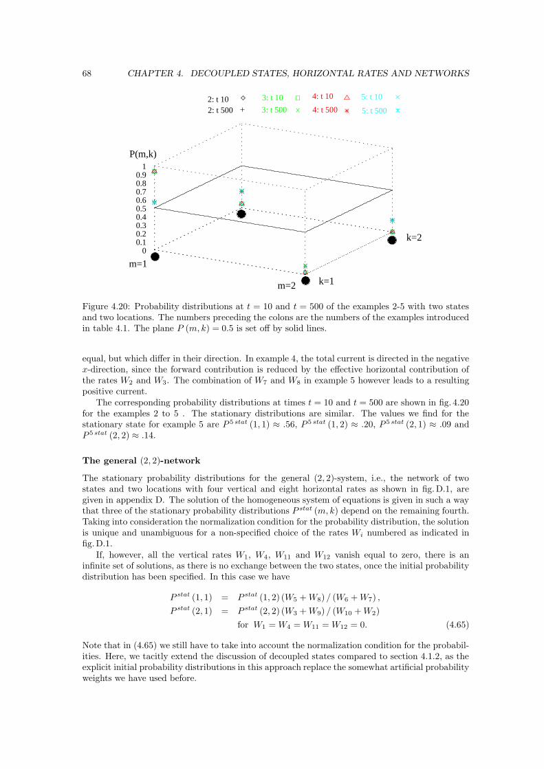
68 CHAPTER 4. DECOUPLED STATES, HORIZONTAL RATES AND NETWORKS
m=1
P(m,k)
k=1
k=2
m=2
00.10.20.30.40.50.60.70.80.9
1
4: t 10
2: t 500
5: t 10
4: t 500
3: t 10
3: t 500 5: t 5002: t 10
Figure 4.20: Probability distributions at t = 10 and t = 500 of the examples 2-5 with two statesand two locations. The numbers preceding the colons are the numbers of the examples introducedin table 4.1. The plane P (m, k) = 0.5 is set off by solid lines.
equal, but which differ in their direction. In example 4, the total current is directed in the negativex-direction, since the forward contribution is reduced by the effective horizontal contribution ofthe rates W2 and W3. The combination of W7 and W8 in example 5 however leads to a resultingpositive current.
The corresponding probability distributions at times t = 10 and t = 500 are shown in fig. 4.20for the examples 2 to 5 . The stationary distributions are similar. The values we find for thestationary state for example 5 are P 5 stat (1, 1) ≈ .56, P 5 stat (1, 2) ≈ .20, P 5 stat (2, 1) ≈ .09 andP 5 stat (2, 2) ≈ .14.
The general (2, 2)-network
The stationary probability distributions for the general (2, 2)-system, i.e., the network of twostates and two locations with four vertical and eight horizontal rates as shown in fig.D.1, aregiven in appendix D. The solution of the homogeneous system of equations is given in such a waythat three of the stationary probability distributions P stat (m, k) depend on the remaining fourth.Taking into consideration the normalization condition for the probability distribution, the solutionis unique and unambiguous for a non-specified choice of the rates Wi numbered as indicated infig.D.1.
If, however, all the vertical rates W1, W4, W11 and W12 vanish equal to zero, there is aninfinite set of solutions, as there is no exchange between the two states, once the initial probabilitydistribution has been specified. In this case we have
P stat (1, 1) = P stat (1, 2) (W5 + W8) / (W6 + W7) ,
P stat (2, 1) = P stat (2, 2) (W3 + W9) / (W10 + W2)
for W1 = W4 = W11 = W12 = 0. (4.65)
Note that in (4.65) we still have to take into account the normalization condition for the probabil-ities. Here, we tacitly extend the discussion of decoupled states compared to section 4.1.2, as theexplicit initial probability distributions in this approach replace the somewhat artificial probabilityweights we have used before.
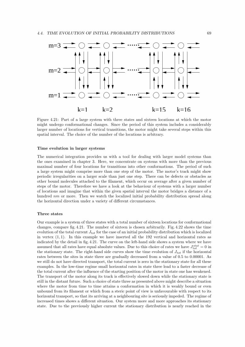
4.4. TIME EVOLUTION OF INITIAL PROBABILITY DISTRIBUTIONS 69
k=1 k=2
m=2
m=1
m=3 ......
......
......
k=15 k=16Figure 4.21: Part of a large system with three states and sixteen locations at which the motormight undergo conformational changes. Since the period of this system includes a considerablylarger number of locations for vertical transitions, the motor might take several steps within thisspatial interval. The choice of the number of the locations is arbitrary.
Time evolution in larger systems
The numerical integration provides us with a tool for dealing with larger model systems thanthe ones examined in chapter 3. Here, we concentrate on systems with more than the previousmaximal number of four locations for transitions into other conformations. The period of sucha large system might comprise more than one step of the motor. The motor’s track might showperiodic irregularities on a larger scale than just one step. There can be defects or obstacles asother bound molecules attached to the filament, which occur on average after a given number ofsteps of the motor. Therefore we have a look at the behaviour of systems with a larger numberof locations and imagine that within the given spatial interval the motor bridges a distance of ahundred nm or more. Then we watch the localized initial probability distribution spread alongthe horizontal direction under a variety of different circumstances.
Three states
Our example is a system of three states with a total number of sixteen locations for conformationalchanges, compare fig. 4.21. The number of sixteen is chosen arbitrarily. Fig. 4.22 shows the timeevolution of the total current Jtot for the case of an initial probability distribution which is localizedin vertex (1, 1). In this example we have inserted all the 192 vertical and horizontal rates asindicated by the detail in fig. 4.21. The curve on the left-hand side shows a system where we haveassumed that all rates have equal absolute values. Due to this choice of rates we have J stat
tot = 0 inthe stationary state. The right-hand side curves show the time evolution of Jtot if the horizontalrates between the sites in state three are gradually decreased from a value of 0.5 to 0.00001. Aswe still do not have directed transport, the total current is zero in the stationary state for all theseexamples. In the low-time regime small horizontal rates in state three lead to a faster decrease ofthe total current after the influence of the starting position of the motor in state one has weakened.The transport of the motor along its track is effectively slowed down while the stationary state isstill in the distant future. Such a choice of state three as presented above might describe a situationwhere the motor from time to time attains a conformation in which it is weakly bound or evenunbound from its filament or which from a steric point of view is unfavourable with respect to itshorizontal transport, so that its arriving at a neighbouring site is seriously impeded. The regime ofincreased times shows a different situation. Our system more and more approaches its stationarystate. Due to the previously higher current the stationary distribution is nearly reached in the
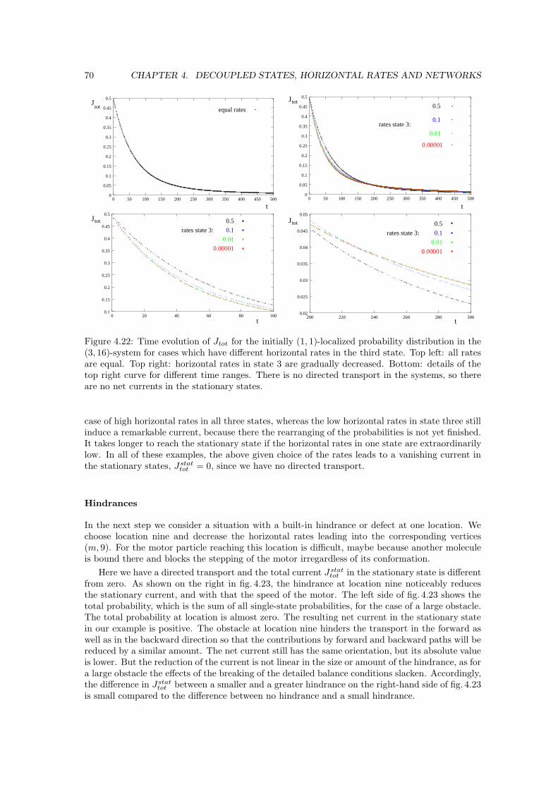
70 CHAPTER 4. DECOUPLED STATES, HORIZONTAL RATES AND NETWORKS
J
t
tot equal rates
0
0.05
0.1
0.15
0.2
0.25
0.3
0.35
0.4
0.45
0.5
0 50 100 150 200 250 300 350 400 450 500
tot
t
J
rates state 3:
0
0.05
0.1
0.15
0.2
0.25
0.3
0.35
0.4
0.45
0.5
0 50 100 150 200 250 300 350 400 450 500
0.00001
0.01
0.1
0.5
totJ
t
rates state 3:
0.1
0.15
0.2
0.25
0.3
0.35
0.4
0.45
0.5
0 20 40 60 80 100
0.5
0.1
0.01
0.00001
totJ
t
rates state 3:
0.5
0.1
0.01
0.00001
0.02
0.025
0.03
0.035
0.04
0.045
0.05
200 220 240 260 280 300
Figure 4.22: Time evolution of Jtot for the initially (1, 1)-localized probability distribution in the(3, 16)-system for cases which have different horizontal rates in the third state. Top left: all ratesare equal. Top right: horizontal rates in state 3 are gradually decreased. Bottom: details of thetop right curve for different time ranges. There is no directed transport in the systems, so thereare no net currents in the stationary states.
case of high horizontal rates in all three states, whereas the low horizontal rates in state three stillinduce a remarkable current, because there the rearranging of the probabilities is not yet finished.It takes longer to reach the stationary state if the horizontal rates in one state are extraordinarilylow. In all of these examples, the above given choice of the rates leads to a vanishing current inthe stationary states, Jstat
tot = 0, since we have no directed transport.
Hindrances
In the next step we consider a situation with a built-in hindrance or defect at one location. Wechoose location nine and decrease the horizontal rates leading into the corresponding vertices(m, 9). For the motor particle reaching this location is difficult, maybe because another moleculeis bound there and blocks the stepping of the motor irregardless of its conformation.
Here we have a directed transport and the total current J stattot in the stationary state is different
from zero. As shown on the right in fig. 4.23, the hindrance at location nine noticeably reducesthe stationary current, and with that the speed of the motor. The left side of fig. 4.23 shows thetotal probability, which is the sum of all single-state probabilities, for the case of a large obstacle.The total probability at location is almost zero. The resulting net current in the stationary statein our example is positive. The obstacle at location nine hinders the transport in the forward aswell as in the backward direction so that the contributions by forward and backward paths will bereduced by a similar amount. The net current still has the same orientation, but its absolute valueis lower. But the reduction of the current is not linear in the size or amount of the hindrance, as fora large obstacle the effects of the breaking of the detailed balance conditions slacken. Accordingly,the difference in Jstat
tot between a smaller and a greater hindrance on the right-hand side of fig. 4.23is small compared to the difference between no hindrance and a small hindrance.

4.4. TIME EVOLUTION OF INITIAL PROBABILITY DISTRIBUTIONS 71
k
Ptot
t = 2000
0
0.01
0.02
0.03
0.04
0.05
0.06
0.07
0.08
0.09
0.1
2 4 6 8 10 12 14 16
totJno hindrance
great hindrance
t
small hindrance
0
0.0002
0.0004
0.0006
0.0008
0.001
16900 16920 16940 16960 16980 17000
Figure 4.23: Left: the total probability Ptot at time t = 2000 for a (3, 16)-system with directedtransport and a hindrance at location nine. Right: the stationary current J stat
tot of the system fordifferent degrees of the built-in hindrance at location nine.
k
1P t = 300
t = 5000
t = 2000
0
0.1
0.2
0.3
0.4
0.5
0.6
2 4 6 8 10 12 14 16
Figure 4.24: Probability distribution P1 for state 1 in a system of two states and sixteen locationsat different times from t = 300 to t = 5000. Transport in the positive x-direction is favoured.
Two states again
Now, we reduce the system by one state, but keep the number of sixteen locations. Fig. 4.24shows the time evolution of the probability P1 in state 1 at the sixteen different locations k for acase where transport in the positive horizontal direction is favoured. Because the horizontal ratesdo not have to fulfill the conditions of detailed balance any longer, there can be active processesdriving the horizontal transport.
The horizontal rates are chosen in such a way that small and large rates alternate for one state,and this sequence is shifted in the second state, so that a switching between the conformationsis favoured. The choice of the locations is arbitrary, in particular it is not necessary to chooseequidistant k. If the horizontal rate W (m, k |m, k + 1) between location k and k + 1 is large, itcorresponds to a favoured movement of the motor. Difficult transitions against hindrances on theother hand correspond to low rates.
In the beginning, the probability distribution is localized in vertex (1, 1). The value of P1 atlocation 1 is still larger than 0.5 after 300 timesteps. With ongoing time the probability distributionwanders to the right and flattens more and more as can be seen in fig. 4.24. The zigzag form withlocal maxima and minima of the curves occurs due to the underlying sequence of small and largerates in one state.
The left-hand side of fig. 4.25 displays a comparison of P1 and P2 at the same time t = 5000.The local minima of the probability distributions correspond to locations with large effective rates
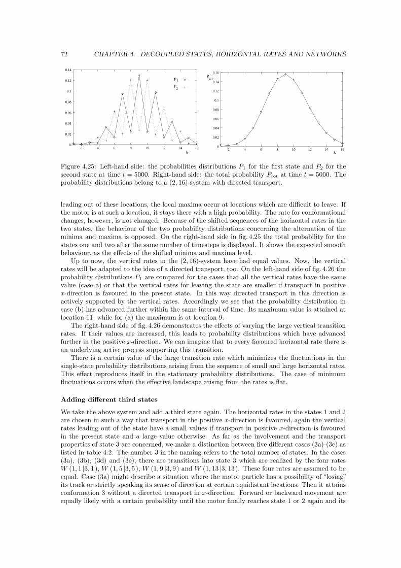
72 CHAPTER 4. DECOUPLED STATES, HORIZONTAL RATES AND NETWORKS
k
P
P
1
2
0
0.02
0.04
0.06
0.08
0.1
0.12
0.14
2 4 6 8 10 12 14 16
P
k
tot
0
0.02
0.04
0.06
0.08
0.1
0.12
0.14
0.16
2 4 6 8 10 12 14 16
Figure 4.25: Left-hand side: the probabilities distributions P1 for the first state and P2 for thesecond state at time t = 5000. Right-hand side: the total probability Ptot at time t = 5000. Theprobability distributions belong to a (2, 16)-system with directed transport.
leading out of these locations, the local maxima occur at locations which are difficult to leave. Ifthe motor is at such a location, it stays there with a high probability. The rate for conformationalchanges, however, is not changed. Because of the shifted sequences of the horizontal rates in thetwo states, the behaviour of the two probability distributions concerning the alternation of theminima and maxima is opposed. On the right-hand side in fig. 4.25 the total probability for thestates one and two after the same number of timesteps is displayed. It shows the expected smoothbehaviour, as the effects of the shifted minima and maxima level.
Up to now, the vertical rates in the (2, 16)-system have had equal values. Now, the verticalrates will be adapted to the idea of a directed transport, too. On the left-hand side of fig. 4.26 theprobability distributions P1 are compared for the cases that all the vertical rates have the samevalue (case a) or that the vertical rates for leaving the state are smaller if transport in positivex-direction is favoured in the present state. In this way directed transport in this direction isactively supported by the vertical rates. Accordingly we see that the probability distribution incase (b) has advanced further within the same interval of time. Its maximum value is attained atlocation 11, while for (a) the maximum is at location 9.
The right-hand side of fig. 4.26 demonstrates the effects of varying the large vertical transitionrates. If their values are increased, this leads to probability distributions which have advancedfurther in the positive x-direction. We can imagine that to every favoured horizontal rate there isan underlying active process supporting this transition.
There is a certain value of the large transition rate which minimizes the fluctuations in thesingle-state probability distributions arising from the sequence of small and large horizontal rates.This effect reproduces itself in the stationary probability distributions. The case of minimumfluctuations occurs when the effective landscape arising from the rates is flat.
Adding different third states
We take the above system and add a third state again. The horizontal rates in the states 1 and 2are chosen in such a way that transport in the positive x-direction is favoured, again the verticalrates leading out of the state have a small values if transport in positive x-direction is favouredin the present state and a large value otherwise. As far as the involvement and the transportproperties of state 3 are concerned, we make a distinction between five different cases (3a)-(3e) aslisted in table 4.2. The number 3 in the naming refers to the total number of states. In the cases(3a), (3b), (3d) and (3e), there are transitions into state 3 which are realized by the four ratesW (1, 1 |3, 1), W (1, 5 |3, 5), W (1, 9 |3, 9) and W (1, 13 |3, 13). These four rates are assumed to beequal. Case (3a) might describe a situation where the motor particle has a possibility of “losing”its track or strictly speaking its sense of direction at certain equidistant locations. Then it attainsconformation 3 without a directed transport in x-direction. Forward or backward movement areequally likely with a certain probability until the motor finally reaches state 1 or 2 again and its
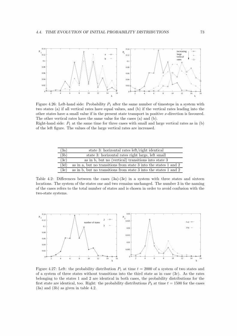
4.4. TIME EVOLUTION OF INITIAL PROBABILITY DISTRIBUTIONS 73
b
aP
1
k
0
0.02
0.04
0.06
0.08
0.1
0.12
0.14
2 4 6 8 10 12 14 16
k
1P increasing
rates
largevertical
0
0.02
0.04
0.06
0.08
0.1
0.12
0.14
2 4 6 8 10 12 14 16
Figure 4.26: Left-hand side: Probability P1 after the same number of timesteps in a system withtwo states (a) if all vertical rates have equal values, and (b) if the vertical rates leading into theother states have a small value if in the present state transport in positive x-direction is favoured.The other vertical rates have the same value for the cases (a) and (b).Right-hand side: P1 at the same time for three cases with small and large vertical rates as in (b)of the left figure. The values of the large vertical rates are increased.
(3a) state 3: horizontal rates left/right identical(3b) state 3: horizontal rates right large, left small(3c) as in b, but no (vertical) transitions into state 3(3d) as in a, but no transitions from state 3 into the states 1 and 2(3e) as in b, but no transitions from state 3 into the states 1 and 2
Table 4.2: Differences between the cases (3a)-(3e) in a system with three states and sixteenlocations. The system of the states one and two remains unchanged. The number 3 in the namingof the cases refers to the total number of states and is chosen in order to avoid confusion with thetwo-state systems.
k
1P
number of states2
3
0
0.02
0.04
0.06
0.08
0.1
0.12
0.14
2 4 6 8 10 12 14 16k
P3
3 a)
3 b)
0
0.005
0.01
0.015
0.02
0.025
0.03
2 4 6 8 10 12 14 16
Figure 4.27: Left: the probability distribution P1 at time t = 2000 of a system of two states andof a system of three states without transitions into the third state as in case (3c). As the ratesbelonging to the states 1 and 2 are identical in both cases, the probability distributions for thefirst state are identical, too. Right: the probability distributions P3 at time t = 1500 for the cases(3a) and (3b) as given in table 4.2.
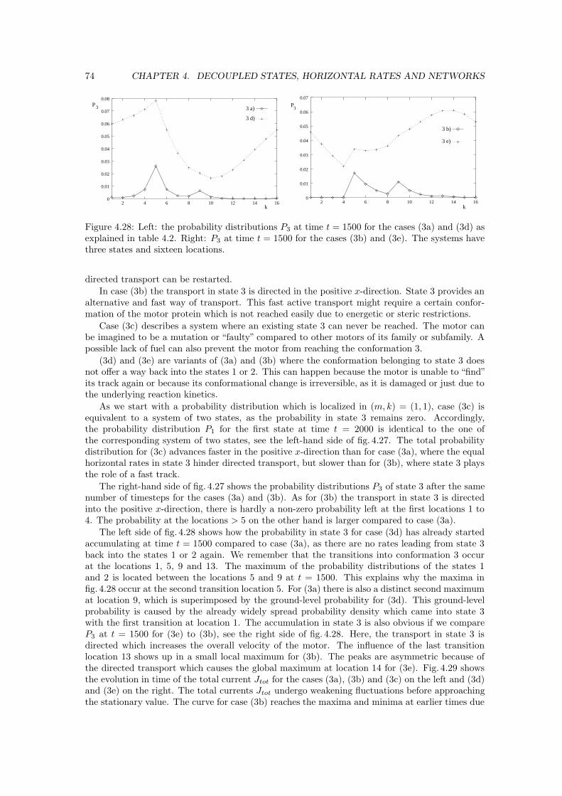
74 CHAPTER 4. DECOUPLED STATES, HORIZONTAL RATES AND NETWORKS
k
3P3 a)
3 d)
0
0.01
0.02
0.03
0.04
0.05
0.06
0.07
0.08
2 4 6 8 10 12 14 16k
P3
3 b)
3 e)
0
0.01
0.02
0.03
0.04
0.05
0.06
0.07
2 4 6 8 10 12 14 16
Figure 4.28: Left: the probability distributions P3 at time t = 1500 for the cases (3a) and (3d) asexplained in table 4.2. Right: P3 at time t = 1500 for the cases (3b) and (3e). The systems havethree states and sixteen locations.
directed transport can be restarted.
In case (3b) the transport in state 3 is directed in the positive x-direction. State 3 provides analternative and fast way of transport. This fast active transport might require a certain confor-mation of the motor protein which is not reached easily due to energetic or steric restrictions.
Case (3c) describes a system where an existing state 3 can never be reached. The motor canbe imagined to be a mutation or “faulty” compared to other motors of its family or subfamily. Apossible lack of fuel can also prevent the motor from reaching the conformation 3.
(3d) and (3e) are variants of (3a) and (3b) where the conformation belonging to state 3 doesnot offer a way back into the states 1 or 2. This can happen because the motor is unable to “find”its track again or because its conformational change is irreversible, as it is damaged or just due tothe underlying reaction kinetics.
As we start with a probability distribution which is localized in (m, k) = (1, 1), case (3c) isequivalent to a system of two states, as the probability in state 3 remains zero. Accordingly,the probability distribution P1 for the first state at time t = 2000 is identical to the one ofthe corresponding system of two states, see the left-hand side of fig. 4.27. The total probabilitydistribution for (3c) advances faster in the positive x-direction than for case (3a), where the equalhorizontal rates in state 3 hinder directed transport, but slower than for (3b), where state 3 playsthe role of a fast track.
The right-hand side of fig. 4.27 shows the probability distributions P3 of state 3 after the samenumber of timesteps for the cases (3a) and (3b). As for (3b) the transport in state 3 is directedinto the positive x-direction, there is hardly a non-zero probability left at the first locations 1 to4. The probability at the locations > 5 on the other hand is larger compared to case (3a).
The left side of fig. 4.28 shows how the probability in state 3 for case (3d) has already startedaccumulating at time t = 1500 compared to case (3a), as there are no rates leading from state 3back into the states 1 or 2 again. We remember that the transitions into conformation 3 occurat the locations 1, 5, 9 and 13. The maximum of the probability distributions of the states 1and 2 is located between the locations 5 and 9 at t = 1500. This explains why the maxima infig. 4.28 occur at the second transition location 5. For (3a) there is also a distinct second maximumat location 9, which is superimposed by the ground-level probability for (3d). This ground-levelprobability is caused by the already widely spread probability density which came into state 3with the first transition at location 1. The accumulation in state 3 is also obvious if we compareP3 at t = 1500 for (3e) to (3b), see the right side of fig. 4.28. Here, the transport in state 3 isdirected which increases the overall velocity of the motor. The influence of the last transitionlocation 13 shows up in a small local maximum for (3b). The peaks are asymmetric because ofthe directed transport which causes the global maximum at location 14 for (3e). Fig. 4.29 showsthe evolution in time of the total current Jtot for the cases (3a), (3b) and (3c) on the left and (3d)and (3e) on the right. The total currents Jtot undergo weakening fluctuations before approachingthe stationary value. The curve for case (3b) reaches the maxima and minima at earlier times due
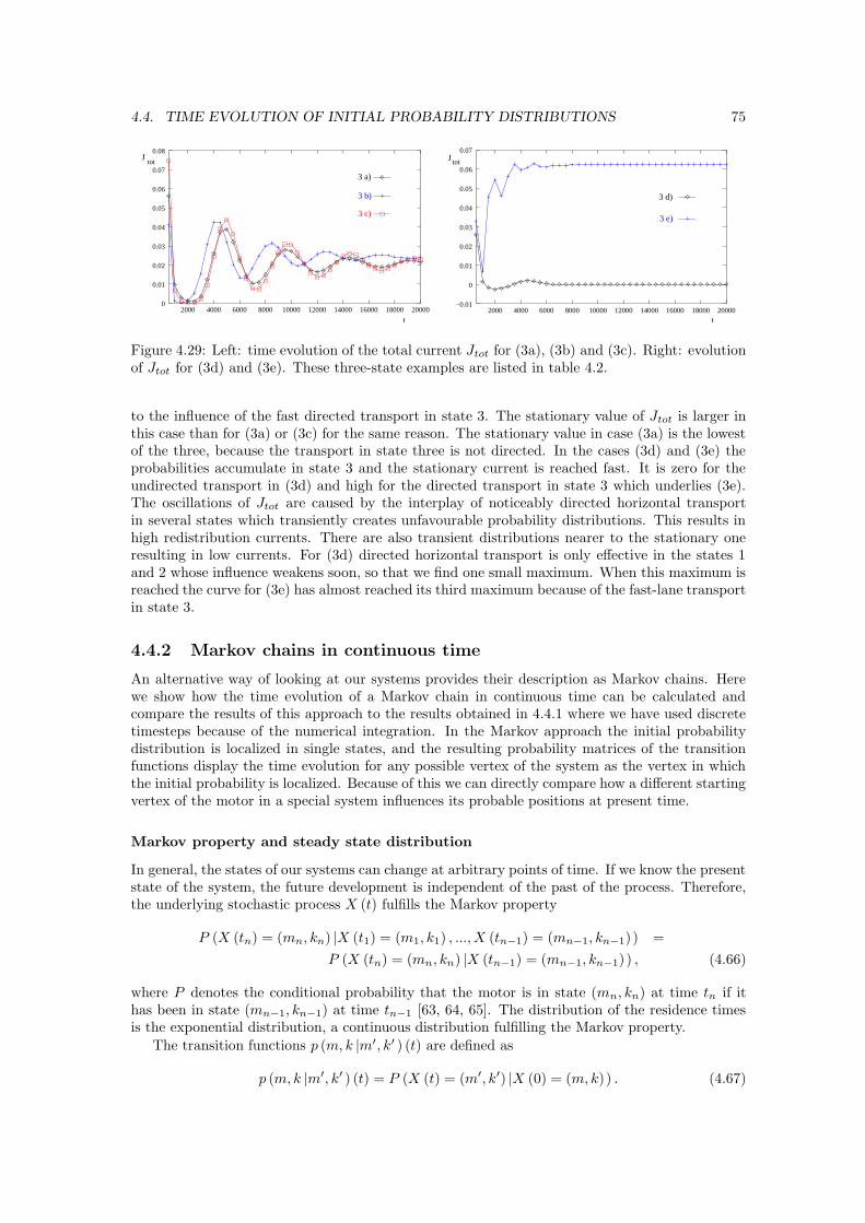
4.4. TIME EVOLUTION OF INITIAL PROBABILITY DISTRIBUTIONS 75
t
tot
3 a)
3 b)
3 c)
J
0
0.01
0.02
0.03
0.04
0.05
0.06
0.07
0.08
2000 4000 6000 8000 10000 12000 14000 16000 18000 20000
t
J tot
3 d)
3 e)
−0.01
0
0.01
0.02
0.03
0.04
0.05
0.06
0.07
2000 4000 6000 8000 10000 12000 14000 16000 18000 20000
Figure 4.29: Left: time evolution of the total current Jtot for (3a), (3b) and (3c). Right: evolutionof Jtot for (3d) and (3e). These three-state examples are listed in table 4.2.
to the influence of the fast directed transport in state 3. The stationary value of Jtot is larger inthis case than for (3a) or (3c) for the same reason. The stationary value in case (3a) is the lowestof the three, because the transport in state three is not directed. In the cases (3d) and (3e) theprobabilities accumulate in state 3 and the stationary current is reached fast. It is zero for theundirected transport in (3d) and high for the directed transport in state 3 which underlies (3e).The oscillations of Jtot are caused by the interplay of noticeably directed horizontal transportin several states which transiently creates unfavourable probability distributions. This results inhigh redistribution currents. There are also transient distributions nearer to the stationary oneresulting in low currents. For (3d) directed horizontal transport is only effective in the states 1and 2 whose influence weakens soon, so that we find one small maximum. When this maximum isreached the curve for (3e) has almost reached its third maximum because of the fast-lane transportin state 3.
4.4.2 Markov chains in continuous time
An alternative way of looking at our systems provides their description as Markov chains. Herewe show how the time evolution of a Markov chain in continuous time can be calculated andcompare the results of this approach to the results obtained in 4.4.1 where we have used discretetimesteps because of the numerical integration. In the Markov approach the initial probabilitydistribution is localized in single states, and the resulting probability matrices of the transitionfunctions display the time evolution for any possible vertex of the system as the vertex in whichthe initial probability is localized. Because of this we can directly compare how a different startingvertex of the motor in a special system influences its probable positions at present time.
Markov property and steady state distribution
In general, the states of our systems can change at arbitrary points of time. If we know the presentstate of the system, the future development is independent of the past of the process. Therefore,the underlying stochastic process X (t) fulfills the Markov property
P (X (tn) = (mn, kn) |X (t1) = (m1, k1) , ..., X (tn−1) = (mn−1, kn−1) ) =
P (X (tn) = (mn, kn) |X (tn−1) = (mn−1, kn−1) ) , (4.66)
where P denotes the conditional probability that the motor is in state (mn, kn) at time tn if ithas been in state (mn−1, kn−1) at time tn−1 [63, 64, 65]. The distribution of the residence timesis the exponential distribution, a continuous distribution fulfilling the Markov property.
The transition functions p (m, k |m′, k′ ) (t) are defined as
p (m, k |m′, k′ ) (t) = P (X (t) = (m′, k′) |X (0) = (m, k)) . (4.67)
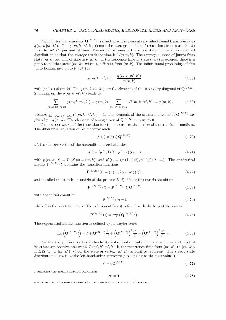
76 CHAPTER 4. DECOUPLED STATES, HORIZONTAL RATES AND NETWORKS
The infinitesimal generator Q(M,K) is a matrix whose elements are infinitesimal transition ratesq (m, k |m′, k′ ). The q (m, k |m′, k′ ) denote the average number of transitions from state (m, k)to state (m′, k′) per unit of time. The residence times of the single states follow an exponentialdistribution so that the average residence time is 1/q (m, k). The average number of jumps fromstate (m, k) per unit of time is q (m, k). If the residence time in state (m, k) is expired, there is ajump to another state (m′, k′) which is different from (m, k). The infinitesimal probability of thisjump leading into state (m′, k′) is
p (m, k |m′, k′ ) =q (m, k |m′, k′ )
q (m, k)(4.68)
with (m′, k′) 6= (m, k). The q (m, k |m′, k′ ) are the elements of the secondary diagonal of Q(M,K).Summing up the q (m, k |m′, k′ ) leads to
∑
(m′,k′)6=(m,k)
q (m, k |m′, k′ ) = q (m, k)∑
(m′,k′)6=(m,k)
P (m, k |m′, k′ ) = q (m, k) , (4.69)
because∑
(m′,k′)6=(m,k) P (m, k |m′, k′ ) = 1. The elements of the primary diagonal of Q(M,K) are
given by −q (m, k). The elements of a single row of Q(M,K) sum up to 0.The first derivative of the transition functions measures the change of the transition functions.
The differential equation of Kolmogorov reads
p′ (t) = p (t)Q(M,K). (4.70)
p (t) is the row vector of the unconditional probabilities,
p (t) = (p (1, 1) (t) , p (1, 2) (t) , ...) , (4.71)
with p (m, k) (t) = P (X (t) = (m, k)) and p′ (t) = (p′ (1, 1) (t) , p′ (1, 2) (t) , ...). The quadraticalmatrix P(M,K) (t) contains the transition functions,
P(M,K) (t) = (p (m, k |m′, k′ ) (t)) , (4.72)
and is called the transition matrix of the process X (t). Using this matrix we obtain
P′ (M,K) (t) = P(M,K) (t)Q(M,K) (4.73)
with the initial conditionP(M,K) (0) = I (4.74)
where I is the identity matrix. The solution of (4.73) is found with the help of the ansatz
P(M,K) (t) = exp(Q(M,K)t
). (4.75)
The exponential matrix function is defined by its Taylor series
exp(Q(M,K)t
)= I + Q(M,K) t
1!+(Q(M,K)
)2 t2
2!+(Q(M,K)
)3 t3
3!+ ... (4.76)
The Markov process Xt has a steady state distribution only if it is irreducible and if all ofits states are positive recurrent. T (m′, k′ |m′, k′ ) is the recurrence time from (m′, k′) to (m′, k′).If E (T (m′, k′ |m′, k′ )) < ∞, the state or vertex (m′, k′) is positive recurrent. The steady statedistribution is given by the left-hand-side eigenvector p belonging to the eigenvalue 0,
0 = pQ(M,K). (4.77)
p satisfies the normalization conditionpe = 1. (4.78)
e is a vector with one column all of whose elements are equal to one.
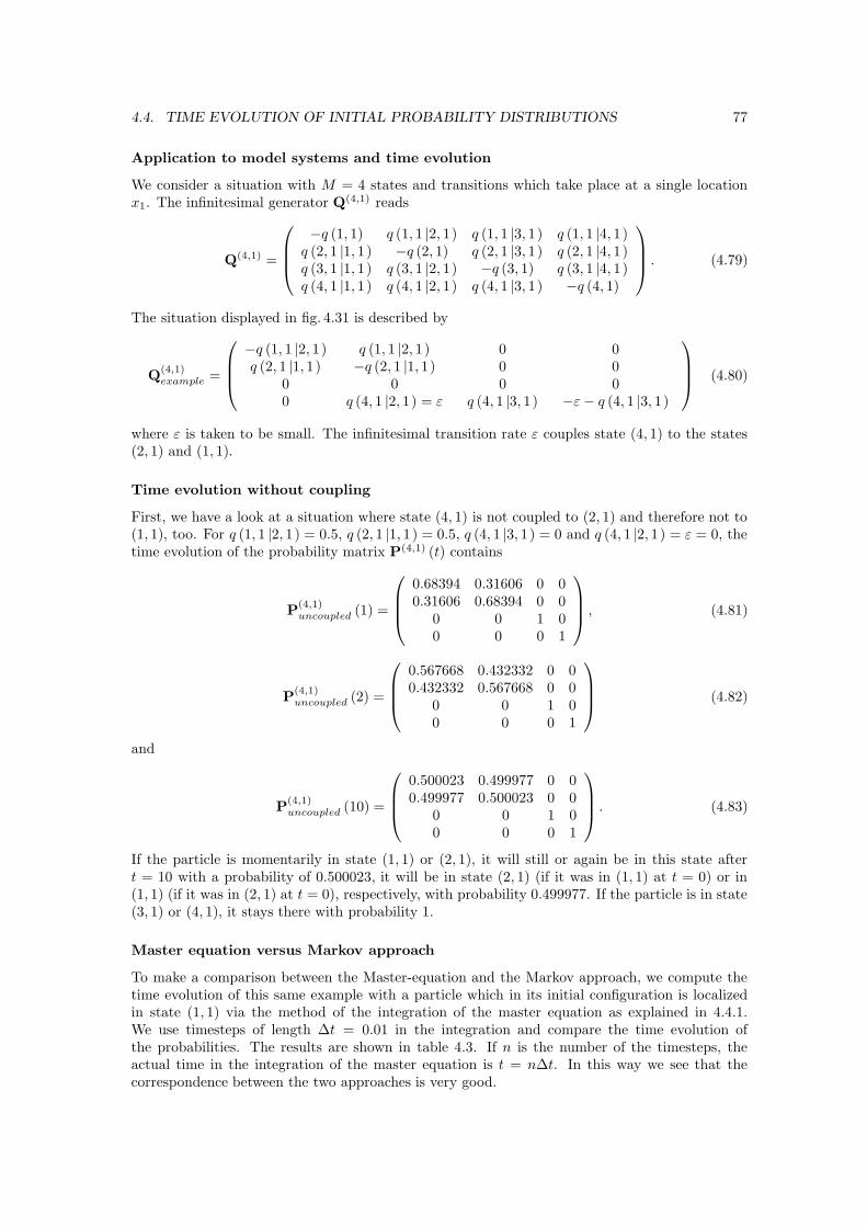
4.4. TIME EVOLUTION OF INITIAL PROBABILITY DISTRIBUTIONS 77
Application to model systems and time evolution
We consider a situation with M = 4 states and transitions which take place at a single locationx1. The infinitesimal generator Q(4,1) reads
Q(4,1) =
−q (1, 1) q (1, 1 |2, 1) q (1, 1 |3, 1) q (1, 1 |4, 1)q (2, 1 |1, 1) −q (2, 1) q (2, 1 |3, 1) q (2, 1 |4, 1)q (3, 1 |1, 1) q (3, 1 |2, 1) −q (3, 1) q (3, 1 |4, 1)q (4, 1 |1, 1) q (4, 1 |2, 1) q (4, 1 |3, 1) −q (4, 1)
. (4.79)
The situation displayed in fig. 4.31 is described by
Q(4,1)example =
−q (1, 1 |2, 1) q (1, 1 |2, 1) 0 0q (2, 1 |1, 1) −q (2, 1 |1, 1) 0 0
0 0 0 00 q (4, 1 |2, 1) = ε q (4, 1 |3, 1) −ε − q (4, 1 |3, 1)
(4.80)
where ε is taken to be small. The infinitesimal transition rate ε couples state (4, 1) to the states(2, 1) and (1, 1).
Time evolution without coupling
First, we have a look at a situation where state (4, 1) is not coupled to (2, 1) and therefore not to(1, 1), too. For q (1, 1 |2, 1) = 0.5, q (2, 1 |1, 1) = 0.5, q (4, 1 |3, 1) = 0 and q (4, 1 |2, 1) = ε = 0, thetime evolution of the probability matrix P(4,1) (t) contains
P(4,1)uncoupled (1) =
0.68394 0.31606 0 00.31606 0.68394 0 0
0 0 1 00 0 0 1
, (4.81)
P(4,1)uncoupled (2) =
0.567668 0.432332 0 00.432332 0.567668 0 0
0 0 1 00 0 0 1
(4.82)
and
P(4,1)uncoupled (10) =
0.500023 0.499977 0 00.499977 0.500023 0 0
0 0 1 00 0 0 1
. (4.83)
If the particle is momentarily in state (1, 1) or (2, 1), it will still or again be in this state aftert = 10 with a probability of 0.500023, it will be in state (2, 1) (if it was in (1, 1) at t = 0) or in(1, 1) (if it was in (2, 1) at t = 0), respectively, with probability 0.499977. If the particle is in state(3, 1) or (4, 1), it stays there with probability 1.
Master equation versus Markov approach
To make a comparison between the Master-equation and the Markov approach, we compute thetime evolution of this same example with a particle which in its initial configuration is localizedin state (1, 1) via the method of the integration of the master equation as explained in 4.4.1.We use timesteps of length ∆t = 0.01 in the integration and compare the time evolution ofthe probabilities. The results are shown in table 4.3. If n is the number of the timesteps, theactual time in the integration of the master equation is t = n∆t. In this way we see that thecorrespondence between the two approaches is very good.
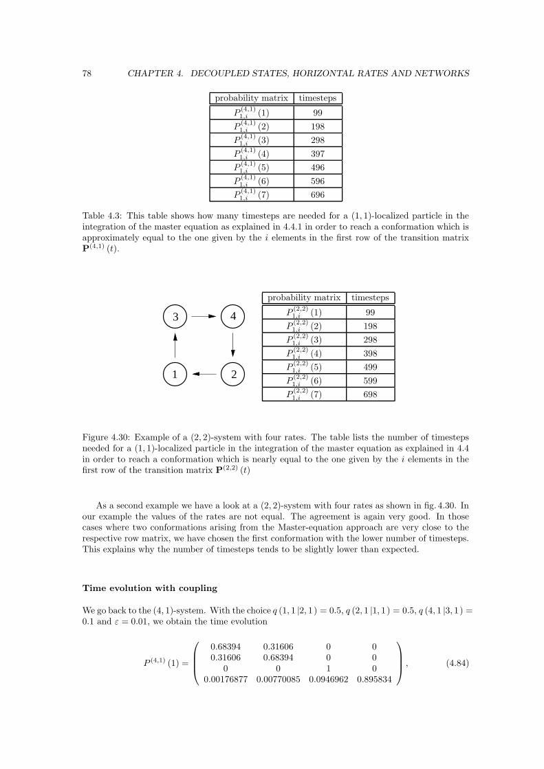
78 CHAPTER 4. DECOUPLED STATES, HORIZONTAL RATES AND NETWORKS
probability matrix timesteps
P(4,1)1,i (1) 99
P(4,1)1,i (2) 198
P(4,1)1,i (3) 298
P(4,1)1,i (4) 397
P(4,1)1,i (5) 496
P(4,1)1,i (6) 596
P(4,1)1,i (7) 696
Table 4.3: This table shows how many timesteps are needed for a (1, 1)-localized particle in theintegration of the master equation as explained in 4.4.1 in order to reach a conformation which isapproximately equal to the one given by the i elements in the first row of the transition matrixP(4,1) (t).
3
1 2
4
probability matrix timesteps
P(2,2)1,i (1) 99
P(2,2)1,i (2) 198
P(2,2)1,i (3) 298
P(2,2)1,i (4) 398
P(2,2)1,i (5) 499
P(2,2)1,i (6) 599
P(2,2)1,i (7) 698
Figure 4.30: Example of a (2, 2)-system with four rates. The table lists the number of timestepsneeded for a (1, 1)-localized particle in the integration of the master equation as explained in 4.4in order to reach a conformation which is nearly equal to the one given by the i elements in thefirst row of the transition matrix P(2,2) (t)
As a second example we have a look at a (2, 2)-system with four rates as shown in fig. 4.30. Inour example the values of the rates are not equal. The agreement is again very good. In thosecases where two conformations arising from the Master-equation approach are very close to therespective row matrix, we have chosen the first conformation with the lower number of timesteps.This explains why the number of timesteps tends to be slightly lower than expected.
Time evolution with coupling
We go back to the (4, 1)-system. With the choice q (1, 1 |2, 1) = 0.5, q (2, 1 |1, 1) = 0.5, q (4, 1 |3, 1) =0.1 and ε = 0.01, we obtain the time evolution
P (4,1) (1) =
0.68394 0.31606 0 00.31606 0.68394 0 0
0 0 1 00.00176877 0.00770085 0.0946962 0.895834
, (4.84)
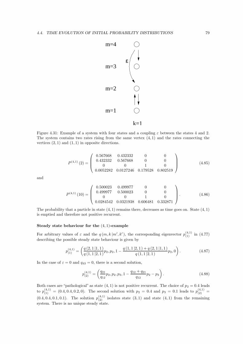
4.4. TIME EVOLUTION OF INITIAL PROBABILITY DISTRIBUTIONS 79
k=1
m=2
m=1
m=3
m=4
ε
Figure 4.31: Example of a system with four states and a coupling ε between the states 4 and 2.The system contains two rates rising from the same vertex (4, 1) and the rates connecting thevertices (2, 1) and (1, 1) in opposite directions.
P (4,1) (2) =
0.567668 0.432332 0 00.432332 0.567668 0 0
0 0 1 00.0052282 0.0127246 0.179528 0.802519
(4.85)
and
P (4,1) (10) =
0.500023 0.499977 0 00.499977 0.500023 0 0
0 0 1 00.0284542 0.0321938 0.606481 0.332871
. (4.86)
The probability that a particle in state (4, 1) remains there, decreases as time goes on. State (4, 1)is emptied and therefore not positive recurrent.
Steady state behaviour for the (4, 1)-example
For arbitrary values of ε and the q (m, k |m′, k′ ), the corresponding eigenvector p(4,1)(1) in (4.77)
describing the possible steady state behaviour is given by
p(4,1)(1) =
(q (2, 1 |1, 1)
q (1, 1 |2, 1)p2, p2, 1 −
q (1, 1 |2, 1) + q (2, 1 |1, 1)
q (1, 1 |2, 1)p2, 0
). (4.87)
In the case of ε = 0 and q43 = 0, there is a second solution,
p(4,1)(2) =
(q21
q12p2, p2, p3, 1−
q12 + q21
q12p2 − p3
). (4.88)
Both cases are “pathological” as state (4, 1) is not positive recurrent. The choice of p2 = 0.4 leads
to p(4,1)(1) = (0.4, 0.4, 0.2, 0). The second solution with p2 = 0.4 and p3 = 0.1 leads to p
(4,1)(2) =
(0.4, 0.4, 0.1, 0.1). The solution p(4,1)(2) isolates state (3, 1) and state (4, 1) from the remaining
system. There is no unique steady state.
80 CHAPTER 4. DECOUPLED STATES, HORIZONTAL RATES AND NETWORKS
In the context of the systems of chapter 3 the calculation of(A(M,K)
)−1for this example after
adding the periodic boundary conditions would have been impossible as in the (4, 1)-case therethe minimal number of vertical rates in the polynomials is 3, which here is impossible due to theproblem of creating l-cycles or having to vertices rising from the same vertex.
The Markov approach is helpful for estimating the influences of differently localized initialprobability distributions. The time evolution is obtained for the initial probability localized in anyof the system’s vertices. The results here confirm the results obtained in 4.4.1. For larger systemsthe calculations for Markov chains are resource- and time-consuming, though.
4.5 Maximum flow and shortest paths
In general, there are many paths across a certain network. Molecular motors are enzymes, and inthe field of enzyme kinetics, one usually distinguishes one special cycle of chemical reactions whichis then called the main pathway of the enzyme. In the context of our networks, the main pathwaycan be imagined to be a positive s-cycle carrying a maximum current across the network. Here,we use the concept of a main pathway and search for paths with s-cycles in flow networks whichcarry large flows. We focus on the question of what is the maximum flow which can be gainedfrom a set of possible pathways. This is the question of an optimal utilization of a given networkwith limited capacities. It is sensible to assume upper boundaries for the capacities, as in cellsthere are chemical and physical limitations to transport processes, e.g. given by the concentrationof ATP. If the flow is fixed in our networks, we look for the path with the lowest costs or fees.Here, costs can refer to energetic considerations, for example.
4.5.1 The main pathway in unspecified networks
As stated in rule 1 in 3.2.2, the total current along a model network is the quotient of two polyno-mials Poli (ω1, ω2, . . . , ωN ) which depend on the vertical transition rates ωi. The contribution acertain path along the network gives to the total current is judged by its occurrence in Pol1. Theassignment of a path to a term with a combination of vertical rates can be achieved for completepaths of vertical and horizontal rates as outlined in section 4.3. The different paths, which con-tribute to the total current in our systems, actually do have a right to exist. Recent simulationshave shown that chemical reactions do not necessarily follow the minimum energy pathway, ifvibrational and kinetic energy effects of finite temperature are taken into account [66]. In otherwords, the stochasticity in our models is not artificial, but on the contrary a characteristic ofchemical reactions.
In a first step we assume a very simple criterion in judging the value of the contribution ofa path. The small-scale diffusion coefficients Dm are taken to be the small parameters of thesystem as we are in an over-damped regime. Then the directed walk of the motor is “diffusion-limited” according to the basic idea of diffusion-based transport in the horizontal direction, whichis of course not a necessary prerequisite as we have pointed out before. The Em (xk , xk+1) areproportional to D−1
m . A term T containing n vertical transition rates implies the factor D−nm .
According to this reasoning the path carrying the maximum flow across the network will containK (M − 1) vertical rates. If the external force F is negligibly small, the contribution of certainpaths with s-cycles will be more important as they in general contain horizontal forward ratesbelonging to different states and with shifted locations. This can result in a number of considerablefactors if the interplay of state and location fits the respective shift of the molecular interactionpotentials. For example, we have a look at fig. 4.10 again, where the two forward s-cycles ina general (2, 2)-network are depicted. In a situation where the molecular interaction potentialin state 1 impedes the motor particle reaching vertex (m, k) = (1, 2) if it presently is in vertex(1, 1), whereas the potential of state 2 favours a transition from (2, 1) to (2, 2), the left-handforward s-cycle is the main pathway. But of course this can only be true if the effect is supportedby the corresponding vertical rates W (1, 1 |2, 1) and W (2, 2 |1, 2), since if we, for example, hadW (1, 1 |2, 1) = 0, the path would not contribute to the current at all.
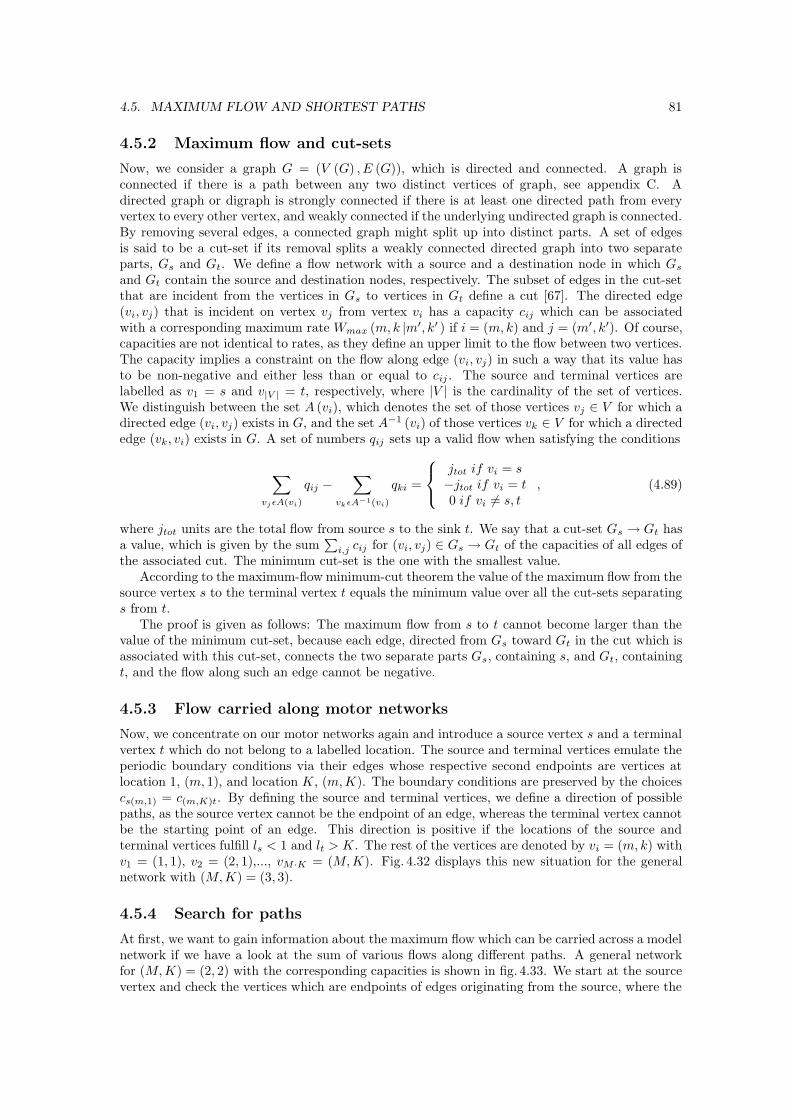
4.5. MAXIMUM FLOW AND SHORTEST PATHS 81
4.5.2 Maximum flow and cut-sets
Now, we consider a graph G = (V (G) , E (G)), which is directed and connected. A graph isconnected if there is a path between any two distinct vertices of graph, see appendix C. Adirected graph or digraph is strongly connected if there is at least one directed path from everyvertex to every other vertex, and weakly connected if the underlying undirected graph is connected.By removing several edges, a connected graph might split up into distinct parts. A set of edgesis said to be a cut-set if its removal splits a weakly connected directed graph into two separateparts, Gs and Gt. We define a flow network with a source and a destination node in which Gs
and Gt contain the source and destination nodes, respectively. The subset of edges in the cut-setthat are incident from the vertices in Gs to vertices in Gt define a cut [67]. The directed edge(vi, vj) that is incident on vertex vj from vertex vi has a capacity cij which can be associatedwith a corresponding maximum rate Wmax (m, k |m′, k′ ) if i = (m, k) and j = (m′, k′). Of course,capacities are not identical to rates, as they define an upper limit to the flow between two vertices.The capacity implies a constraint on the flow along edge (vi, vj) in such a way that its value hasto be non-negative and either less than or equal to cij . The source and terminal vertices arelabelled as v1 = s and v|V | = t, respectively, where |V | is the cardinality of the set of vertices.We distinguish between the set A (vi), which denotes the set of those vertices vj ∈ V for which adirected edge (vi, vj) exists in G, and the set A−1 (vi) of those vertices vk ∈ V for which a directededge (vk, vi) exists in G. A set of numbers qij sets up a valid flow when satisfying the conditions
∑
vjεA(vi)
qij −∑
vkεA−1(vi)
qki =
jtot if vi = s−jtot if vi = t0 if vi 6= s, t
, (4.89)
where jtot units are the total flow from source s to the sink t. We say that a cut-set Gs → Gt hasa value, which is given by the sum
∑i,j cij for (vi, vj) ∈ Gs → Gt of the capacities of all edges of
the associated cut. The minimum cut-set is the one with the smallest value.According to the maximum-flow minimum-cut theorem the value of the maximum flow from the
source vertex s to the terminal vertex t equals the minimum value over all the cut-sets separatings from t.
The proof is given as follows: The maximum flow from s to t cannot become larger than thevalue of the minimum cut-set, because each edge, directed from Gs toward Gt in the cut which isassociated with this cut-set, connects the two separate parts Gs, containing s, and Gt, containingt, and the flow along such an edge cannot be negative.
4.5.3 Flow carried along motor networks
Now, we concentrate on our motor networks again and introduce a source vertex s and a terminalvertex t which do not belong to a labelled location. The source and terminal vertices emulate theperiodic boundary conditions via their edges whose respective second endpoints are vertices atlocation 1, (m, 1), and location K, (m, K). The boundary conditions are preserved by the choicescs(m,1) = c(m,K)t. By defining the source and terminal vertices, we define a direction of possiblepaths, as the source vertex cannot be the endpoint of an edge, whereas the terminal vertex cannotbe the starting point of an edge. This direction is positive if the locations of the source andterminal vertices fulfill ls < 1 and lt > K. The rest of the vertices are denoted by vi = (m, k) withv1 = (1, 1), v2 = (2, 1),..., vM ·K = (M, K). Fig. 4.32 displays this new situation for the generalnetwork with (M, K) = (3, 3).
4.5.4 Search for paths
At first, we want to gain information about the maximum flow which can be carried across a modelnetwork if we have a look at the sum of various flows along different paths. A general networkfor (M, K) = (2, 2) with the corresponding capacities is shown in fig. 4.33. We start at the sourcevertex and check the vertices which are endpoints of edges originating from the source, where the
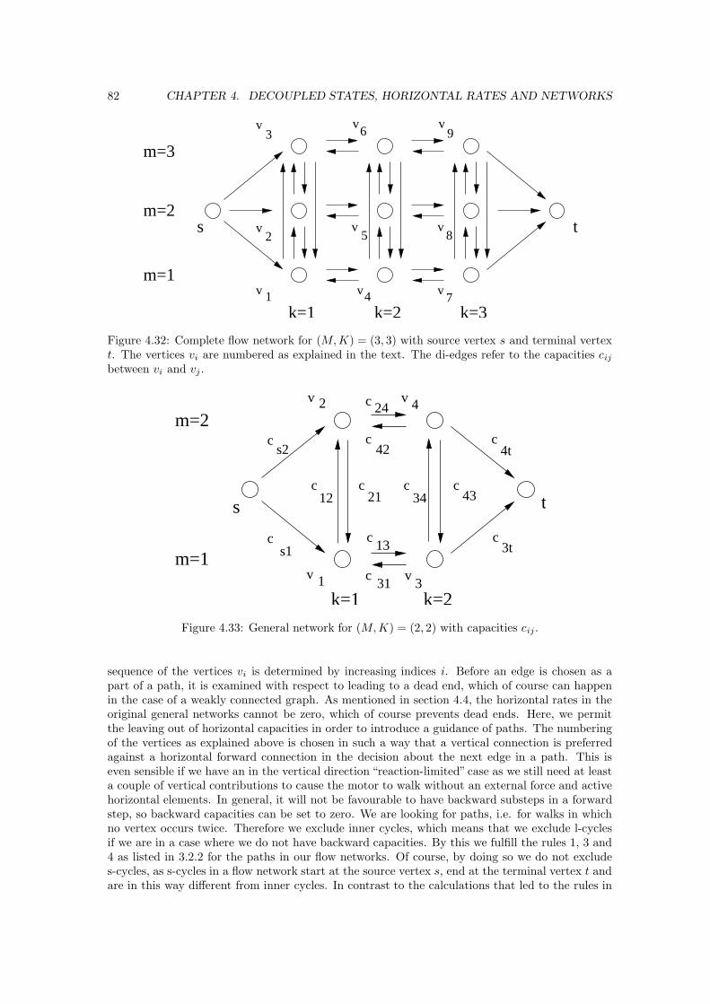
82 CHAPTER 4. DECOUPLED STATES, HORIZONTAL RATES AND NETWORKS
k=2k=1 k=3
m=2
m=3
m=1
s tv2
v
v
vv v
v
vv 4
5
1
3 6
7
8
9
Figure 4.32: Complete flow network for (M, K) = (3, 3) with source vertex s and terminal vertext. The vertices vi are numbered as explained in the text. The di-edges refer to the capacities cij
between vi and vj .
k=2k=1
m=1
s
v
t
v 4
31v
2v
m=2c
c
c
c
c c c
c
c
c
c
s2
s1
34 43
24
42 4t
13
12
31
3t
21c
Figure 4.33: General network for (M, K) = (2, 2) with capacities cij .
sequence of the vertices vi is determined by increasing indices i. Before an edge is chosen as apart of a path, it is examined with respect to leading to a dead end, which of course can happenin the case of a weakly connected graph. As mentioned in section 4.4, the horizontal rates in theoriginal general networks cannot be zero, which of course prevents dead ends. Here, we permitthe leaving out of horizontal capacities in order to introduce a guidance of paths. The numberingof the vertices as explained above is chosen in such a way that a vertical connection is preferredagainst a horizontal forward connection in the decision about the next edge in a path. This iseven sensible if we have an in the vertical direction “reaction-limited” case as we still need at leasta couple of vertical contributions to cause the motor to walk without an external force and activehorizontal elements. In general, it will not be favourable to have backward substeps in a forwardstep, so backward capacities can be set to zero. We are looking for paths, i.e. for walks in whichno vertex occurs twice. Therefore we exclude inner cycles, which means that we exclude l-cyclesif we are in a case where we do not have backward capacities. By this we fulfill the rules 1, 3 and4 as listed in 3.2.2 for the paths in our flow networks. Of course, by doing so we do not excludes-cycles, as s-cycles in a flow network start at the source vertex s, end at the terminal vertex t andare in this way different from inner cycles. In contrast to the calculations that led to the rules in
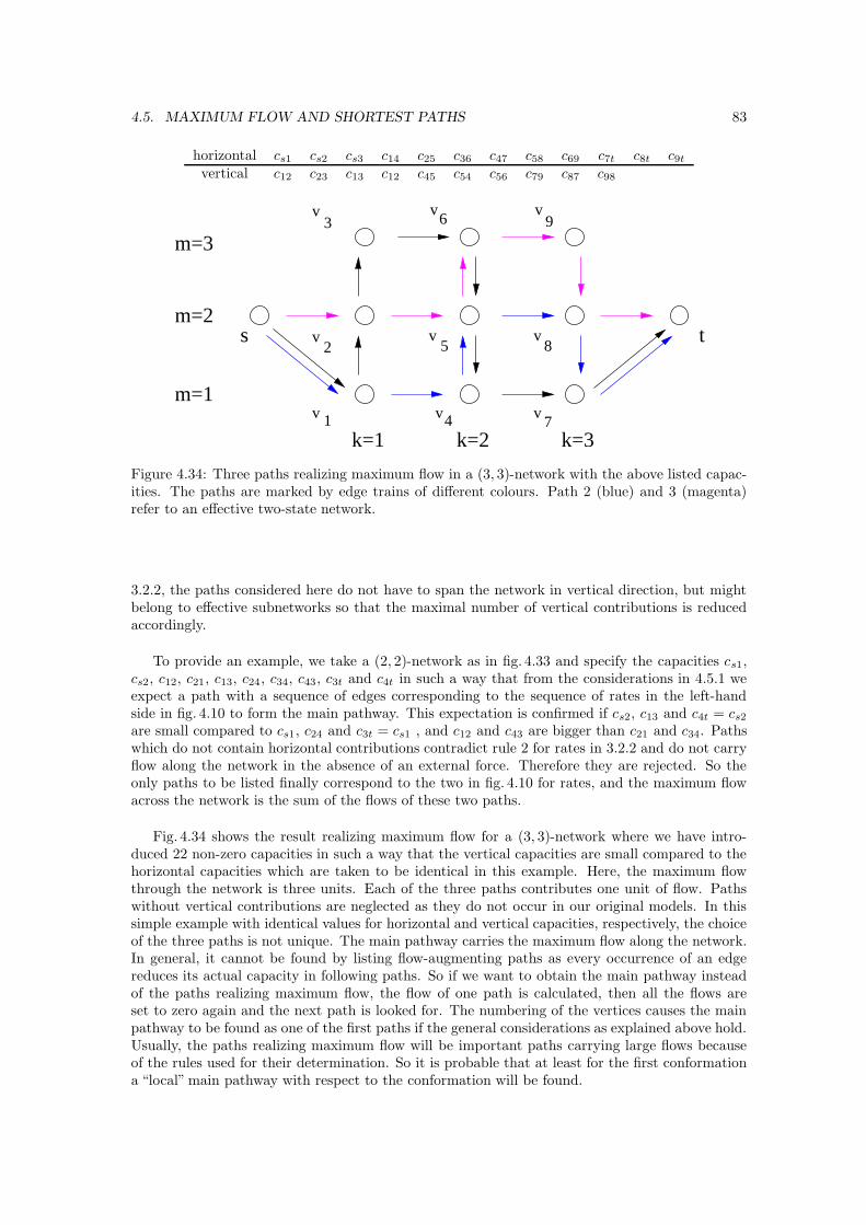
4.5. MAXIMUM FLOW AND SHORTEST PATHS 83
horizontal cs1 cs2 cs3 c14 c25 c36 c47 c58 c69 c7t c8t c9t
vertical c12 c23 c13 c12 c45 c54 c56 c79 c87 c98
k=2k=1 k=3
m=2
m=3
m=1
s tv2
v
v
vv v
v
vv 4
5
1
3 6
7
8
9
Figure 4.34: Three paths realizing maximum flow in a (3, 3)-network with the above listed capac-ities. The paths are marked by edge trains of different colours. Path 2 (blue) and 3 (magenta)refer to an effective two-state network.
3.2.2, the paths considered here do not have to span the network in vertical direction, but mightbelong to effective subnetworks so that the maximal number of vertical contributions is reducedaccordingly.
To provide an example, we take a (2, 2)-network as in fig. 4.33 and specify the capacities cs1,cs2, c12, c21, c13, c24, c34, c43, c3t and c4t in such a way that from the considerations in 4.5.1 weexpect a path with a sequence of edges corresponding to the sequence of rates in the left-handside in fig. 4.10 to form the main pathway. This expectation is confirmed if cs2, c13 and c4t = cs2
are small compared to cs1, c24 and c3t = cs1 , and c12 and c43 are bigger than c21 and c34. Pathswhich do not contain horizontal contributions contradict rule 2 for rates in 3.2.2 and do not carryflow along the network in the absence of an external force. Therefore they are rejected. So theonly paths to be listed finally correspond to the two in fig. 4.10 for rates, and the maximum flowacross the network is the sum of the flows of these two paths.
Fig. 4.34 shows the result realizing maximum flow for a (3, 3)-network where we have intro-duced 22 non-zero capacities in such a way that the vertical capacities are small compared to thehorizontal capacities which are taken to be identical in this example. Here, the maximum flowthrough the network is three units. Each of the three paths contributes one unit of flow. Pathswithout vertical contributions are neglected as they do not occur in our original models. In thissimple example with identical values for horizontal and vertical capacities, respectively, the choiceof the three paths is not unique. The main pathway carries the maximum flow along the network.In general, it cannot be found by listing flow-augmenting paths as every occurrence of an edgereduces its actual capacity in following paths. So if we want to obtain the main pathway insteadof the paths realizing maximum flow, the flow of one path is calculated, then all the flows areset to zero again and the next path is looked for. The numbering of the vertices causes the mainpathway to be found as one of the first paths if the general considerations as explained above hold.Usually, the paths realizing maximum flow will be important paths carrying large flows becauseof the rules used for their determination. So it is probable that at least for the first conformationa “local” main pathway with respect to the conformation will be found.
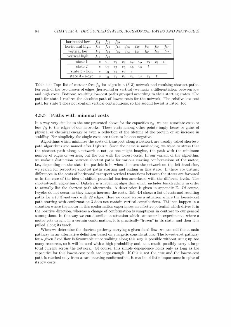
84 CHAPTER 4. DECOUPLED STATES, HORIZONTAL RATES AND NETWORKS
horizontal low fs1 f25 f69
horizontal high fs2 fs3 f14 f36 f47 f58 f8t f9t
vertical low f12 f23 f45 f54 f56 f65 f98 f87
vertical high f13 f79
state 1 s v1 v2 v5 v6 v9 v8 v7 tstate 2 s v2 v5 v6 v9 v8 t
state 3 - hor. s v3 v6 v9 tstate 3 - s-cyc. s v3 v6 v5 v4 v7 v9 t
Table 4.4: Top: list of costs or fees fij for edges in a (3, 3)-network and resulting shortest paths.For each of the two classes of edges (horizontal or vertical) we make a differentiation between lowand high costs. Bottom: resulting low-cost paths grouped according to their starting states. Thepath for state 1 realizes the absolute path of lowest costs for the network. The relative low-costpath for state 3 does not contain vertical contributions, so the second lowest is listed, too.
4.5.5 Paths with minimal costs
In a way very similar to the one presented above for the capacities cij , we can associate costs orfees fij to the edges of our networks. These costs among other points imply losses or gains ofphysical or chemical energy or even a reduction of the lifetime of the protein or an increase instability. For simplicity the single costs are taken to be non-negative.
Algorithms which minimize the costs of transport along a network are usually called shortest-path algorithms and named after Dijkstra. Since the name is misleading, we want to stress thatthe shortest path along a network is not, as one might imagine, the path with the minimumnumber of edges or vertices, but the one with the lowest costs. In our variant of the algorithm,we make a distinction between shortest paths for various starting conformations of the motor,i.e., depending on the state the particle is in when it enters the network on the left-hand side,we search for respective shortest paths starting and ending in this state. If there are distinctdifferences in the costs of horizontal transport vertical transitions between the states are favouredas in the case of the idea of shifted potential barriers associated with the different levels. Theshortest-path algorithm of Dijkstra is a labelling algorithm which includes backtracking in orderto actually list the shortest path afterwards. A description is given in appendix E. Of course,l-cycles do not occur, as they always increase the costs. Tab. 4.4 shows a list of costs and resultingpaths for a (3, 3)-network with 22 edges. Here we come across a situation where the lowest-costpath starting with conformation 3 does not contain vertical contributions. This can happen in asituation where the motor in this conformation experiences an effective potential which drives it inthe positive direction, whereas a change of conformation is sumptuous in contrast to our generalassumptions. In this way we can describe an situation which can occur in experiments, where amotor gets caught in a certain conformation, it is practically “frozen” in its state, and then it ispulled along its track.
When we determine the shortest pathway carrying a given fixed flow, we can call this a mainpathway in an alternative definition based on energetic considerations. The lowest-cost pathwayfor a given fixed flow is favourable since walking along this way is possible without using up toomany resources, so it will be used with a high probability and, as a result, possibly carry a largetotal current across the network. Of course, this simple dependence holds only as long as thecapacities for this lowest-cost path are large enough. If this is not the case and the lowest-costpath is reached only from a rare starting conformation, it can be of little importance in spite ofits low costs.
Chapter 5
ATP-concentration and transport
properties
In this chapter we at first examine the dependence of the motor’s velocity on the ATP concentra-tion. The energy for the movement of the molecular motor is released in the hydrolysis of ATP,which is an enzymatic reaction. When the motor shows enzymatic activity, we have unbalancedrates in our system describing the deviation from equilibrium and detailed balance. In order to re-late the unbalanced rates to the concentration of ATP, we discuss the underlying reaction kinetics,compare section 5.1. The dependence of the velocity of the motor on the ATP-concentration varieswith the number of centres of enzymatic activity and the type of the assumed reaction kinetics.
In section 5.2 we have a look at an alternative stochastic two-state model. This model has acontinuous x-direction and uses finite vertical transition widths, which we change gradually. Wedetermine transport coefficients and consider different explicit molecular interaction potentials.The numerical solution provides us with a time evolution of the probabilities. This last section isbased on [73].
5.1 Reaction kinetics
In section 3.3 we have shown that the enzymatic activity of the motor proteins enters our (M, K)-systems via breaking the conditions of detailed balance. If there is enzymatic activity for the motortaking on a certain conformation at a specified location, the corresponding transition rate has anunbalanced part. Without a loss of generality, we assume that the unbalanced rates are verticalrates leading to conformational changes. Nevertheless, it is not clear yet how the unbalanced ratesare connected to the chemical reaction, the hydrolysis of ATP. This connection is established byincluding the underlying reaction kinetics into our systems, which determine the dependence ofthe unbalanced transition rates on the fuel or ATP concentration.
5.1.1 Michaelis-Menten equation
Just as many other intra- and extracellular proteins, molecular motors are enzymes [68]. Theyare biological catalysts, which raise the speed of chemical reactions by influencing the energy ofactivation. Enzymes have active sites which are crucial for their catalytic activity and their specificreaction. Besides, they need specific binding bags in which they bind their substrates.
The enzyme reaction in the case of linear molecular motors is the hydrolysis of ATP, so ATPis the motors’ substrate. The chemical equilibrium in the simplified reaction scheme
ATP ADP + Pi. (5.1)
would be reached ifκ1ΓATP = κ2ΓADP ΓP (5.2)
85
86 CHAPTER 5. ATP-CONCENTRATION AND TRANSPORT PROPERTIES
with the reaction rate constants κ1 and κ2 and the respective concentrations Γ of ATP, ADP andphosphate P [43].
In actual experiments where the motor runs processively along its filament and produces anet movement, the chemical equilibrium is broken, as will be explained later. In the following, weconsider the motor’s deviation from the equilibrium state, which here is described by the deviationof the vertical transition rates from the conditions of detailed balance.
If the motor is in state (o, k) before, and in state (p, k) after the hydrolysis, the correspondingunbalanced transition rates connecting the two vertices are
∆op (xk) = exp (Vo (xk)) κ1 (F ) ΓATP ≡ κ1 (F ) ΓATP (5.3)
and∆po (xk) = exp (Vp (xk)) κ2 (F ) ΓADP ΓP ≡ κ2 (F ) ΓADP ΓP . (5.4)
Because in experimental situations the concentration of ATP will usually be high in the beginning,and the concentration of ADP very low at the same time, the state of the system is far fromchemical equilibrium for small concentrations of motors within the time scale of the experiment.There is almost no ADP, ΓADP is low so that ∆po (xk) ≈ 0. In this case we need a single unbalancedvertical rate to describe the movement of a motor with one hydrolysis step in its motor cycle.
Strictly speaking, the hydrolysis of motor proteins as kinesin (K), which we have summarizedin (5.1), comprises several substeps. Kinesin binds to a microtubule (M), until ATP arrives andbinds to the kinesin molecule. Then the actual hydrolysis follows, in the course of which K/ADPunbinds and phosphate is released,
M/K + ATP → M/K/ATP → M/K/ADP/Pi → M + K/ADP + Pi. (5.5)
The common way of describing the reaction kinetics in this sequence is to assume the simplestcase of an enzymatic catalyzed reaction, namely a reaction using a single molecule of the substrateat a time. The unbalanced transition rate ∆op (xk) is then given by the Michaelis-Menten equation
∆op (xk) =κ2 (F ) ΓATP
κ2 (F ) /κ1 (F ) + ΓATP, (5.6)
with reaction rate constants κ1 and κ2 [69].
5.1.2 Allosteric effects
The Michaelis-Menten equation as stated in 5.1.1 is valid for simple systems. In the case ofmolecular motors however, there might be allosteric centres which bind regulatory molecules sothat the dependence of the unbalanced rates ∆op (xk) on the ATP-concentration ΓATP is changed.This discussion is new compared to [43].
Concept
If an effector, a ligand which influences the binding characteristics, binds to a regulatory bindingdomain, which is in this case not identical with that of the substrate, there will be a conformationalchange of the enzyme influencing the enzymatic activity. In such a situation the unbalanced partsof the transition rates can show a sigmoidal dependence on ΓATP . In the simplest case the ∆op
obey
∆sigm.op (xk) =
µ2 (F ) nΓnATP
µ2 (F ) /µ1 (F ) + ΓnATP
(5.7)
with constants µ1 (F ), µ2 (F ) and a number n, which denotes the number of identical units ofthe allosteric enzyme. The number n will be called the Hill coefficient in the following. Theabbreviation “sigm.” refers to “sigmoidal”.
Equation (5.7) is derived from the Hill equation which describes the binding of n moleculesof the substrate to the enzyme. Schnitzer and Block have suggested a Hill coefficient of one for
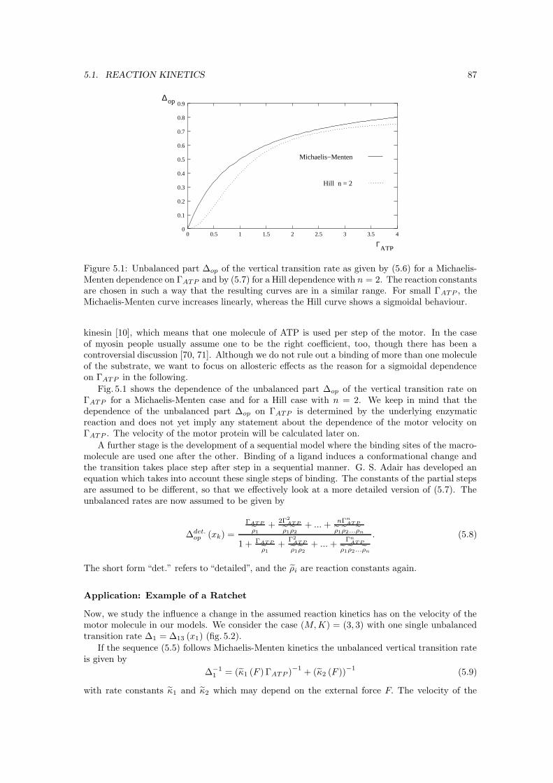
5.1. REACTION KINETICS 87
ΓATP
∆op
Hill n = 2
0
0.1
0.2
0.3
0.4
0.5
0.6
0.7
0.8
0.9
0 0.5 1 1.5 2 2.5 3 3.5 4
Michaelis−Menten
Figure 5.1: Unbalanced part ∆op of the vertical transition rate as given by (5.6) for a Michaelis-Menten dependence on ΓATP and by (5.7) for a Hill dependence with n = 2. The reaction constantsare chosen in such a way that the resulting curves are in a similar range. For small ΓATP , theMichaelis-Menten curve increases linearly, whereas the Hill curve shows a sigmoidal behaviour.
kinesin [10], which means that one molecule of ATP is used per step of the motor. In the caseof myosin people usually assume one to be the right coefficient, too, though there has been acontroversial discussion [70, 71]. Although we do not rule out a binding of more than one moleculeof the substrate, we want to focus on allosteric effects as the reason for a sigmoidal dependenceon ΓATP in the following.
Fig. 5.1 shows the dependence of the unbalanced part ∆op of the vertical transition rate onΓATP for a Michaelis-Menten case and for a Hill case with n = 2. We keep in mind that thedependence of the unbalanced part ∆op on ΓATP is determined by the underlying enzymaticreaction and does not yet imply any statement about the dependence of the motor velocity onΓATP . The velocity of the motor protein will be calculated later on.
A further stage is the development of a sequential model where the binding sites of the macro-molecule are used one after the other. Binding of a ligand induces a conformational change andthe transition takes place step after step in a sequential manner. G. S. Adair has developed anequation which takes into account these single steps of binding. The constants of the partial stepsare assumed to be different, so that we effectively look at a more detailed version of (5.7). Theunbalanced rates are now assumed to be given by
∆det.op (xk) =
ΓAT P
ρ1
+2Γ2
AT P
ρ1ρ2
+ ... +nΓn
AT P
ρ1ρ2...ρn
1 + ΓAT P
ρ1
+Γ2
AT P
ρ1ρ2
+ ... +Γn
AT P
ρ1ρ2...ρn
. (5.8)
The short form “det.” refers to “detailed”, and the ρi are reaction constants again.
Application: Example of a Ratchet
Now, we study the influence a change in the assumed reaction kinetics has on the velocity of themotor molecule in our models. We consider the case (M, K) = (3, 3) with one single unbalancedtransition rate ∆1 = ∆13 (x1) (fig. 5.2).
If the sequence (5.5) follows Michaelis-Menten kinetics the unbalanced vertical transition rateis given by
∆−11 = (κ1 (F ) ΓATP )
−1+ (κ2 (F ))
−1(5.9)
with rate constants κ1 and κ2 which may depend on the external force F. The velocity of the
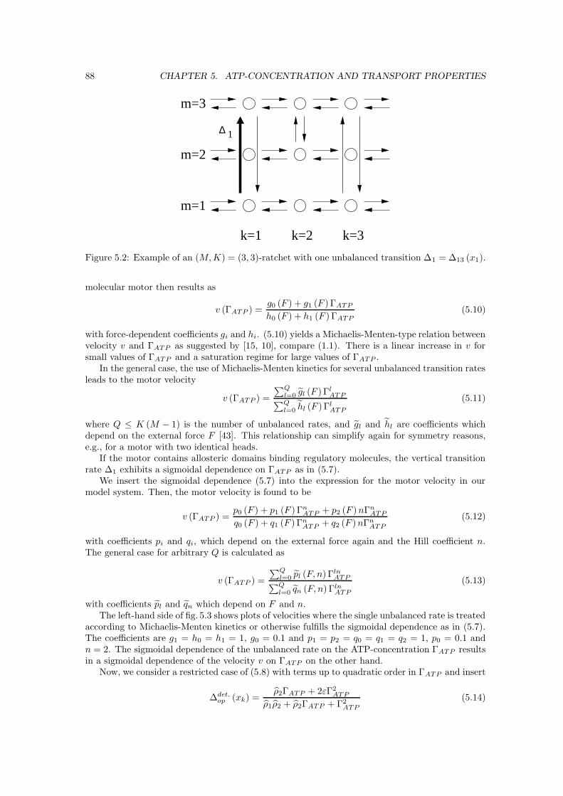
88 CHAPTER 5. ATP-CONCENTRATION AND TRANSPORT PROPERTIES
k=1 k=2
m=2
m=1
m=3
k=3
∆ 1
Figure 5.2: Example of an (M, K) = (3, 3)-ratchet with one unbalanced transition ∆1 = ∆13 (x1).
molecular motor then results as
v (ΓATP ) =g0 (F ) + g1 (F ) ΓATP
h0 (F ) + h1 (F ) ΓATP(5.10)
with force-dependent coefficients gi and hi. (5.10) yields a Michaelis-Menten-type relation betweenvelocity v and ΓATP as suggested by [15, 10], compare (1.1). There is a linear increase in v forsmall values of ΓATP and a saturation regime for large values of ΓATP .
In the general case, the use of Michaelis-Menten kinetics for several unbalanced transition ratesleads to the motor velocity
v (ΓATP ) =
∑Ql=0 gl (F ) Γl
ATP∑Ql=0 hl (F ) Γl
ATP
(5.11)
where Q ≤ K (M − 1) is the number of unbalanced rates, and gl and hl are coefficients whichdepend on the external force F [43]. This relationship can simplify again for symmetry reasons,e.g., for a motor with two identical heads.
If the motor contains allosteric domains binding regulatory molecules, the vertical transitionrate ∆1 exhibits a sigmoidal dependence on ΓATP as in (5.7).
We insert the sigmoidal dependence (5.7) into the expression for the motor velocity in ourmodel system. Then, the motor velocity is found to be
v (ΓATP ) =p0 (F ) + p1 (F ) Γn
ATP + p2 (F ) nΓnATP
q0 (F ) + q1 (F ) ΓnATP + q2 (F ) nΓn
ATP
(5.12)
with coefficients pi and qi, which depend on the external force again and the Hill coefficient n.The general case for arbitrary Q is calculated as
v (ΓATP ) =
∑Ql=0 pl (F, n) Γln
ATP∑Ql=0 qn (F, n) Γln
ATP
(5.13)
with coefficients pl and qn which depend on F and n.The left-hand side of fig. 5.3 shows plots of velocities where the single unbalanced rate is treated
according to Michaelis-Menten kinetics or otherwise fulfills the sigmoidal dependence as in (5.7).The coefficients are g1 = h0 = h1 = 1, g0 = 0.1 and p1 = p2 = q0 = q1 = q2 = 1, p0 = 0.1 andn = 2. The sigmoidal dependence of the unbalanced rate on the ATP-concentration ΓATP resultsin a sigmoidal dependence of the velocity v on ΓATP on the other hand.
Now, we consider a restricted case of (5.8) with terms up to quadratic order in ΓATP and insert
∆det.op (xk) =
ρ2ΓATP + 2εΓ2ATP
ρ1ρ2 + ρ2ΓATP + Γ2ATP
(5.14)
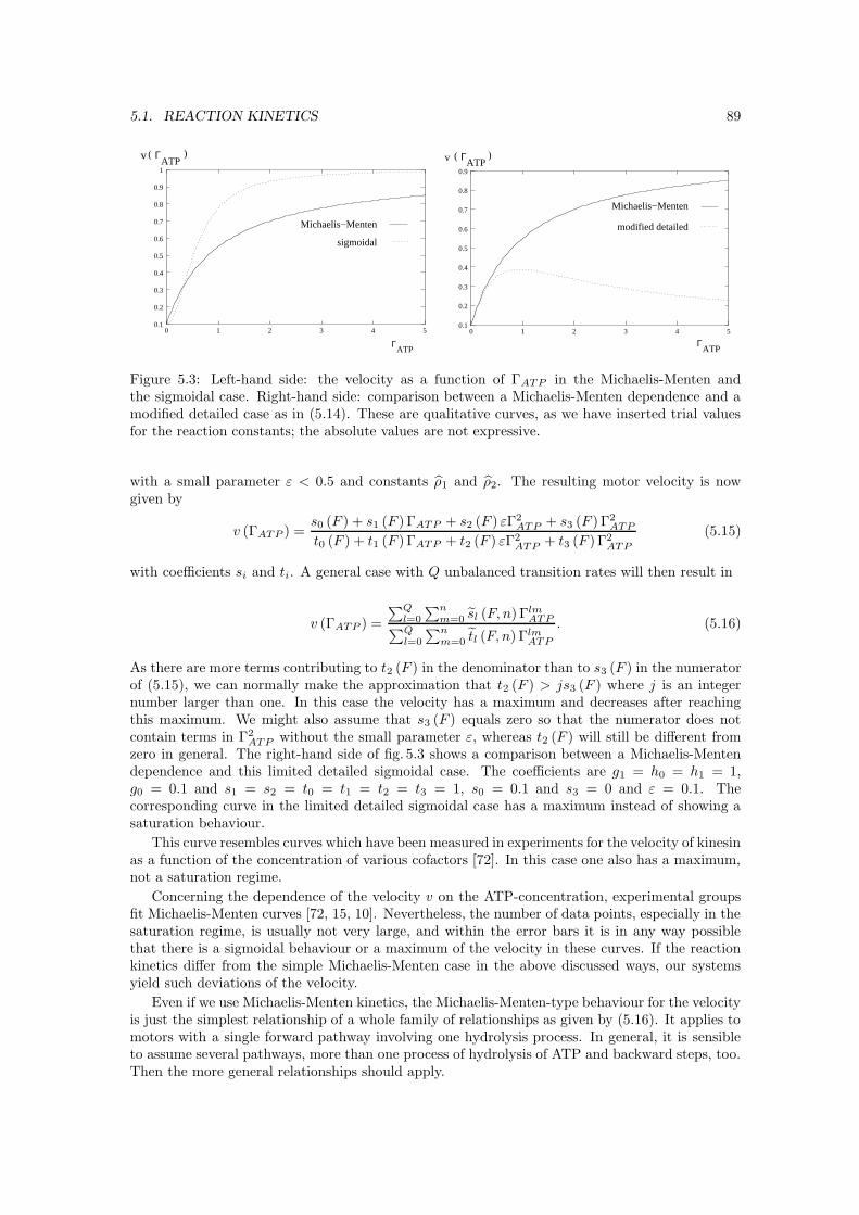
5.1. REACTION KINETICS 89
ΓATP
( )
ΓATP
v
0.1
0.2
0.3
0.4
0.5
0.6
0.7
0.8
0.9
1
0 1 2 3 4 5
Michaelis−Menten
sigmoidal
ΓATP
ΓATP
( )v
0.1
0.2
0.3
0.4
0.5
0.6
0.7
0.8
0.9
0 1 2 3 4 5
modified detailed
Michaelis−Menten
Figure 5.3: Left-hand side: the velocity as a function of ΓATP in the Michaelis-Menten andthe sigmoidal case. Right-hand side: comparison between a Michaelis-Menten dependence and amodified detailed case as in (5.14). These are qualitative curves, as we have inserted trial valuesfor the reaction constants; the absolute values are not expressive.
with a small parameter ε < 0.5 and constants ρ1 and ρ2. The resulting motor velocity is nowgiven by
v (ΓATP ) =s0 (F ) + s1 (F ) ΓATP + s2 (F ) εΓ2
ATP + s3 (F ) Γ2ATP
t0 (F ) + t1 (F ) ΓATP + t2 (F ) εΓ2ATP + t3 (F ) Γ2
ATP
(5.15)
with coefficients si and ti. A general case with Q unbalanced transition rates will then result in
v (ΓATP ) =
∑Ql=0
∑nm=0 sl (F, n) Γlm
ATP∑Ql=0
∑nm=0 tl (F, n) Γlm
ATP
. (5.16)
As there are more terms contributing to t2 (F ) in the denominator than to s3 (F ) in the numeratorof (5.15), we can normally make the approximation that t2 (F ) > js3 (F ) where j is an integernumber larger than one. In this case the velocity has a maximum and decreases after reachingthis maximum. We might also assume that s3 (F ) equals zero so that the numerator does notcontain terms in Γ2
ATP without the small parameter ε, whereas t2 (F ) will still be different fromzero in general. The right-hand side of fig. 5.3 shows a comparison between a Michaelis-Mentendependence and this limited detailed sigmoidal case. The coefficients are g1 = h0 = h1 = 1,g0 = 0.1 and s1 = s2 = t0 = t1 = t2 = t3 = 1, s0 = 0.1 and s3 = 0 and ε = 0.1. Thecorresponding curve in the limited detailed sigmoidal case has a maximum instead of showing asaturation behaviour.
This curve resembles curves which have been measured in experiments for the velocity of kinesinas a function of the concentration of various cofactors [72]. In this case one also has a maximum,not a saturation regime.
Concerning the dependence of the velocity v on the ATP-concentration, experimental groupsfit Michaelis-Menten curves [72, 15, 10]. Nevertheless, the number of data points, especially in thesaturation regime, is usually not very large, and within the error bars it is in any way possiblethat there is a sigmoidal behaviour or a maximum of the velocity in these curves. If the reactionkinetics differ from the simple Michaelis-Menten case in the above discussed ways, our systemsyield such deviations of the velocity.
Even if we use Michaelis-Menten kinetics, the Michaelis-Menten-type behaviour for the velocityis just the simplest relationship of a whole family of relationships as given by (5.16). It applies tomotors with a single forward pathway involving one hydrolysis process. In general, it is sensibleto assume several pathways, more than one process of hydrolysis of ATP and backward steps, too.Then the more general relationships should apply.
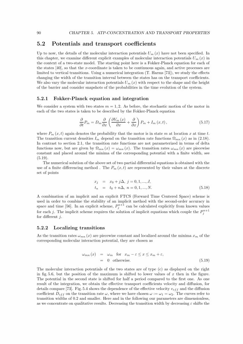
90 CHAPTER 5. ATP-CONCENTRATION AND TRANSPORT PROPERTIES
5.2 Potentials and transport coefficients
Up to now, the details of the molecular interaction potentials Um (x) have not been specified. Inthis chapter, we examine different explicit examples of molecular interaction potentials Um (x) inthe context of a two-state model. The starting point here is a Fokker-Planck equation for each ofthe states [40], so that the x-coordinate is taken to be continuous again, and active processes arelimited to vertical transitions. Using a numerical integration (T. Harms [73]), we study the effectschanging the width of the transition interval between the states has on the transport coefficients.We also vary the molecular interaction potentials Um (x) with respect to the shape and the heightof the barrier and consider snapshots of the probabilities in the time evolution of the system.
5.2.1 Fokker-Planck equation and integration
We consider a system with two states m = 1, 2. As before, the stochastic motion of the motor ineach of the two states is taken to be described by the Fokker-Planck equation
∂
∂tPm = Dm
∂
∂x
(∂Vm (x)
∂x+
∂
∂x
)Pm + Im (x, t) , (5.17)
where Pm (x, t) again denotes the probability that the motor is in state m at location x at time t.The transition current densities Im depend on the transition rate functions Ωmn (x) as in (2.18).In contrast to section 2.1, the transition rate functions are not parameterized in terms of deltafunctions now, but are given by Ωmn (x) = ωmn (x). The transition rates ωmn (x) are piecewiseconstant and placed around the minima of the corresponding potential with a finite width, see(5.19).
The numerical solution of the above set of two partial differential equations is obtained with theuse of a finite differencing method . The Pm (x, t) are represented by their values at the discreteset of points
xj = x0 + j∆, j = 0, 1, ..., J,
tn = t0 + n∆, n = 0, 1, ..., N. (5.18)
A combination of an implicit and an explicit FTCS (Forward Time Centered Space) scheme isused in order to combine the stability of an implicit method with the second-order accuracy inspace and time [56]. In an explicit scheme, P n+1
j can be calculated explicitly from known values
for each j. The implicit scheme requires the solution of implicit equations which couple the P n+1j
for different j.
5.2.2 Localizing transitions
As the transition rates ωmn (x) are piecewise constant and localized around the minima xm of thecorresponding molecular interaction potential, they are chosen as
ωmn (x) = ωm for xm − ε ≤ x ≤ xm + ε,
= 0 otherwise. (5.19)
The molecular interaction potentials of the two states are of type (c) as displayed on the rightin fig. 5.6, but the position of the maximum is shifted to lower values of x then in the figure.The potential in the second state is shifted for half a period compared to the first one. As oneresult of the integration, we obtain the effective transport coefficients velocity and diffusion, fordetails compare [73]. Fig. 5.4 shows the dependence of the effective velocity veff and the diffusioncoefficient Deff on the transition rate ω, where we have chosen ω := ω1 = ω2. The curves refer totransition widths of 0.2 and smaller. Here and in the following our parameters are dimensionless,as we concentrate on qualitative results. Decreasing the transition width by decreasing ε shifts the
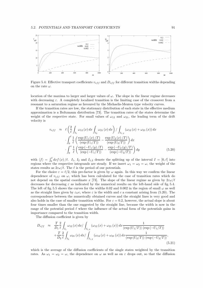
5.2. POTENTIALS AND TRANSPORT COEFFICIENTS 91
ω
veff
width
5
10
15
20
25
0 200 400 600 800 1000
0.20.02
0.002
ω
effD width
0
1
2
3
4
5
0 200 400 600 800 1000
0.020.2
0.002
Figure 5.4: Effective transport coefficients veff and Deff for different transition widths dependingon the rate ω.
location of the maxima to larger and larger values of ω. The slope in the linear regime decreaseswith decreasing ε. A completely localized transition is the limiting case of the crossover from aresonant to a saturation regime as favoured by the Michaelis-Menten type velocity curves.
If the transition rates are low, the stationary distribution of each state in the effective mediumapproximation is a Boltzmann distribution [73]. The transition rates of the states determine theweight of the respective state. For small values of ω12 and ω21, the leading term of the driftvelocity is
veff ≈ `
(2
`
∫
I1
ω12 (x) dx
∫
I2
ω21 (x) dx
)/
∫
I1,2
(ω12 (x) + ω21 (x)) dx
·
∫ `
0
1
`
(exp (U1 (x) /T )
〈exp (U1/T )〉−
exp (U2 (x) /T )
〈exp (U2/T )〉
)dx
·
∫ x
0
1
`
(exp (−U1 (y) /T )
〈exp (−U1/T )〉−
exp (−U2 (y) /T )
〈exp (−U2/T )〉
)dy (5.20)
with 〈f〉 =∫ `
0dxf (x) /`. I1, I2 and I1,2 denote the splitting up of the interval I = [0, `] into
regions where the respective integrands are steady. If we insert ω1 = ω2 = ω, the weight of thestates results as 2εω/`. The ` is the period of our potentials.
For the choice ε = `/2, this pre-factor is given by ω again. In this way we confirm the lineardependence of veff on ω, which has been calculated for the case of transition rates which donot depend on the spatial coordinate x [73]. The slope of the linear regime as given by 2εω/`decreases for decreasing ε as indicated by the numerical results on the left-hand side of fig. 5.4.The left of fig. 5.5 shows the curves for the widths 0.02 and 0.002 in the region of small ω as wellas the straight lines given by εωc, where ε is the width and c a constant arising from (5.20). Thecorrespondence between the numerically obtained curves and the straight lines is very good andalso holds in the case of smaller transition widths. For ε = 0.2, however, the actual slope is aboutfour times smaller than the one suggested by the straight line, because the width is now in therange of the potential period ` where the influence of the actual form of the potentials gains inimportance compared to the transition width.
The diffusion coefficient is given by
Deff ≈T
D1
2
`
∫
I1
ω12 (x) dx/
∫
I1,2
(ω12 (x) + ω21 (x)) dx1
〈exp (U1/T )〉 〈exp (−U1/T )〉
+T
D2
2
`
∫
I2
ω21 (x) dx/
∫
I1,2
(ω12 (x) + ω21 (x)) dx1
〈exp (U2/T )〉 〈exp (−U2/T )〉,
(5.21)
which is the average of the diffusion coefficients of the single states weighted by the transitionrates. As ω1 = ω2 = ω, the dependence on ω as well as on ε drops out, so that the diffusion
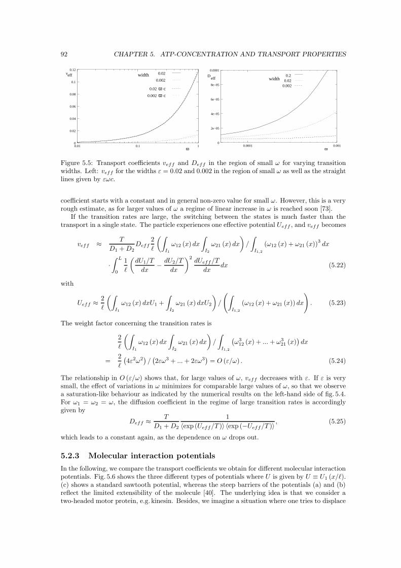
92 CHAPTER 5. ATP-CONCENTRATION AND TRANSPORT PROPERTIES
ω
veff
cωω c
width
0
0.02
0.04
0.06
0.08
0.1
0.12
0.01 0.1 1
0.002
0.02
0.002
0.02eff
D
ω
width
0.0020.020.2
0
2e−05
4e−05
6e−05
8e−05
0.0001
0.0001 0.001
Figure 5.5: Transport coefficients veff and Deff in the region of small ω for varying transitionwidths. Left: veff for the widths ε = 0.02 and 0.002 in the region of small ω as well as the straightlines given by εωc.
coefficient starts with a constant and in general non-zero value for small ω. However, this is a veryrough estimate, as for larger values of ω a regime of linear increase in ω is reached soon [73].
If the transition rates are large, the switching between the states is much faster than thetransport in a single state. The particle experiences one effective potential Ueff , and veff becomes
veff ≈T
D1 + D2Deff
2
`
(∫
I1
ω12 (x) dx
∫
I2
ω21 (x) dx
)/
∫
I1,2
(ω12 (x) + ω21 (x))3dx
·
∫ L
0
1
`
(dU1/T
dx−
dU2/T
dx
)2dUeff/T
dxdx (5.22)
with
Ueff ≈2
`
(∫
I1
ω12 (x) dxU1 +
∫
I2
ω21 (x) dxU2
)/
(∫
I1,2
(ω12 (x) + ω21 (x)) dx
). (5.23)
The weight factor concerning the transition rates is
2
`
(∫
I1
ω12 (x) dx
∫
I2
ω21 (x) dx
)/
∫
I1,2
(ω3
12 (x) + ... + ω321 (x)
)dx
=2
`
(4ε2ω2
)/(2εω3 + ... + 2εω3
)= O (ε/ω) . (5.24)
The relationship in O (ε/ω) shows that, for large values of ω, veff decreases with ε. If ε is verysmall, the effect of variations in ω minimizes for comparable large values of ω, so that we observea saturation-like behaviour as indicated by the numerical results on the left-hand side of fig. 5.4.For ω1 = ω2 = ω, the diffusion coefficient in the regime of large transition rates is accordinglygiven by
Deff ≈T
D1 + D2
1
〈exp (Ueff/T )〉 〈exp (−Ueff/T )〉, (5.25)
which leads to a constant again, as the dependence on ω drops out.
5.2.3 Molecular interaction potentials
In the following, we compare the transport coefficients we obtain for different molecular interactionpotentials. Fig. 5.6 shows the three different types of potentials where U is given by U ≡ U1 (x/`).(c) shows a standard sawtooth potential, whereas the steep barriers of the potentials (a) and (b)reflect the limited extensibility of the molecule [40]. The underlying idea is that we consider atwo-headed motor protein, e.g. kinesin. Besides, we imagine a situation where one tries to displace
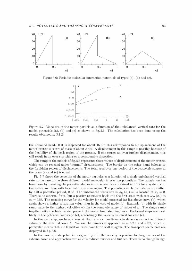
5.2. POTENTIALS AND TRANSPORT COEFFICIENTS 93
0 1
U/T
x/l
(a)40
30
20
10
00.5
00 1
U/T
x/l
(b)40
30
20
10
0.50
0 1
U/T
x/l
(c)40
30
20
10
0.5
Figure 5.6: Periodic molecular interaction potentials of types (a), (b) and (c).
0.001 0.01 0.1 1 10 100
0.00001
0.0001
0.001
0.01
0.1
1 a
b
c
v
ω
Figure 5.7: Velocities of the motor particle as a function of the unbalanced vertical rate for themodel potentials (a), (b) and (c) as shown in fig. 5.6. The calculation has been done using theresults obtained in 3.1.2.
the unbound head. If it is displaced for about 16 nm this corresponds to a displacement of themotor protein’s centre of mass of about 8 nm. A displacement in this range is possible because ofthe flexibility of the neck region of the protein. If one causes an even further displacement, thiswill result in an over-stretching or a considerable distortion.
The ramp in the models of fig. 5.6 represents those values of displacements of the motor proteinwhich can be reached under “normal” circumstances. The barrier on the other hand belongs tothe forbidden region of displacements. The total area over one period of the geometric shapes inthe cases (a) and (c) is equal.
Fig. 5.7 shows the velocities of the motor particles as a function of a single unbalanced verticalrate in the case of the three different model molecular interaction potentials. The calculation hasbeen done by inserting the potential shapes into the results as obtained in 3.1.2 for a system withtwo states and here with localized transitions again. The potentials in the two states are shiftedby half a potential period, 0.5`. The unbalanced transition is ω12 (x1) =: ω located at x1 = 0.There is no external force, but a passive relaxation back into the first state with rate ω21 (x2) atx2 = 0.5`. The resulting curve for the velocity for model potential (a) lies above curve (b), whichagain shows a higher saturation value than in the case of model (c). Example (a) with its singleramp leads to the highest velocities within the complete range of values of ω. The single ramptogether with the high barrier prevent the motor from stepping back. Backward steps are mostlikely in the potential landscape (c), accordingly the velocity is lowest for case (c).
In the next step, we have a look at the transport coefficients in dependence on the differentvalues of the external force F . We use the numerical approach as in 5.2.1 and 5.2.2, which inparticular means that the transition rates have finite widths again. The transport coefficients aredisplayed in fig. 5.8.
In the case of a steep barrier as given by (b), the velocity is positive for large values of theexternal force and approaches zero as F is reduced further and further. There is no change in sign
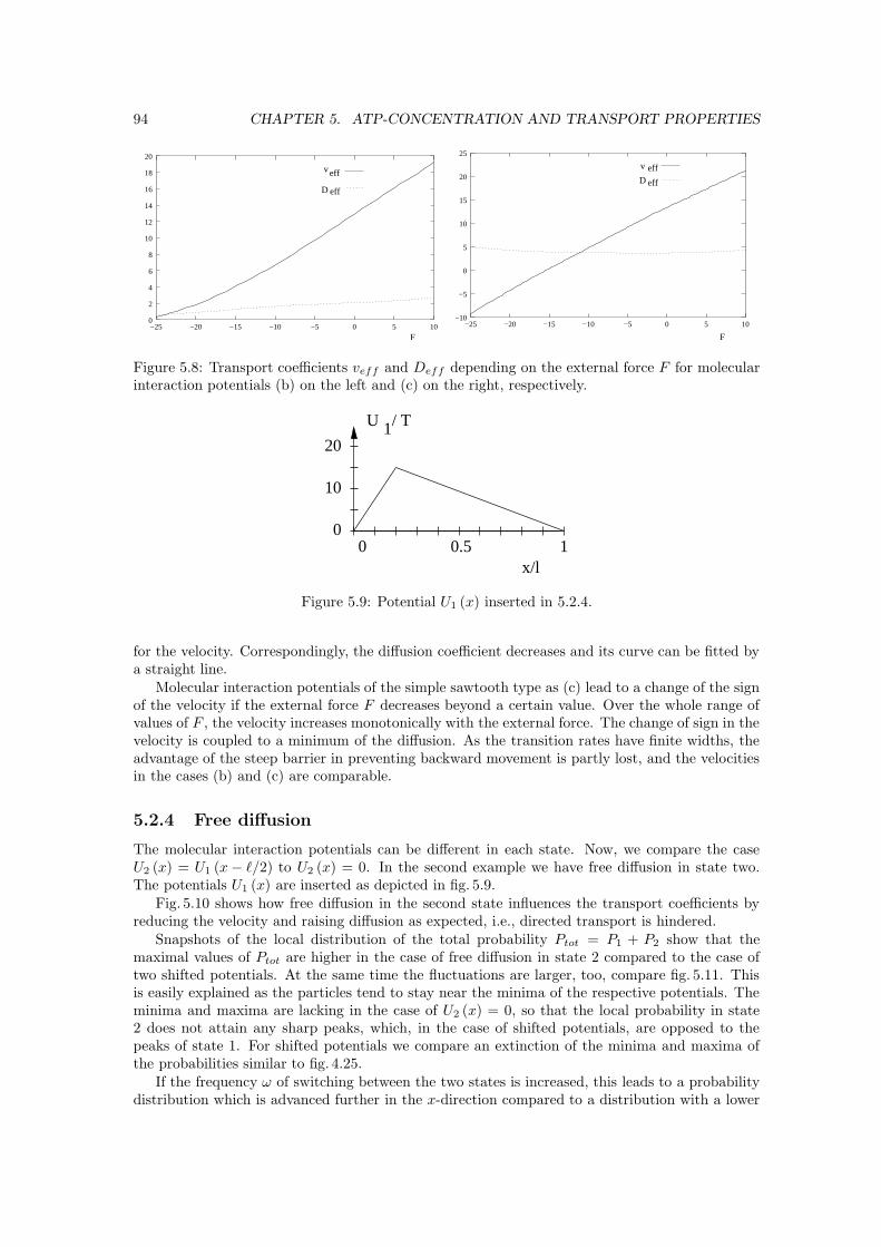
94 CHAPTER 5. ATP-CONCENTRATION AND TRANSPORT PROPERTIES
F
eff
eff
v
D
0
2
4
6
8
10
12
14
16
18
20
−25 −20 −15 −10 −5 0 5 10F
eff
effD
v
−10
−5
0
5
10
15
20
25
−25 −20 −15 −10 −5 0 5 10
Figure 5.8: Transport coefficients veff and Deff depending on the external force F for molecularinteraction potentials (b) on the left and (c) on the right, respectively.
0 1x/l
0.5
10
0
20
U 1/ T
Figure 5.9: Potential U1 (x) inserted in 5.2.4.
for the velocity. Correspondingly, the diffusion coefficient decreases and its curve can be fitted bya straight line.
Molecular interaction potentials of the simple sawtooth type as (c) lead to a change of the signof the velocity if the external force F decreases beyond a certain value. Over the whole range ofvalues of F , the velocity increases monotonically with the external force. The change of sign in thevelocity is coupled to a minimum of the diffusion. As the transition rates have finite widths, theadvantage of the steep barrier in preventing backward movement is partly lost, and the velocitiesin the cases (b) and (c) are comparable.
5.2.4 Free diffusion
The molecular interaction potentials can be different in each state. Now, we compare the caseU2 (x) = U1 (x − `/2) to U2 (x) = 0. In the second example we have free diffusion in state two.The potentials U1 (x) are inserted as depicted in fig. 5.9.
Fig. 5.10 shows how free diffusion in the second state influences the transport coefficients byreducing the velocity and raising diffusion as expected, i.e., directed transport is hindered.
Snapshots of the local distribution of the total probability Ptot = P1 + P2 show that themaximal values of Ptot are higher in the case of free diffusion in state 2 compared to the case oftwo shifted potentials. At the same time the fluctuations are larger, too, compare fig. 5.11. Thisis easily explained as the particles tend to stay near the minima of the respective potentials. Theminima and maxima are lacking in the case of U2 (x) = 0, so that the local probability in state2 does not attain any sharp peaks, which, in the case of shifted potentials, are opposed to thepeaks of state 1. For shifted potentials we compare an extinction of the minima and maxima ofthe probabilities similar to fig. 4.25.
If the frequency ω of switching between the two states is increased, this leads to a probabilitydistribution which is advanced further in the x-direction compared to a distribution with a lower
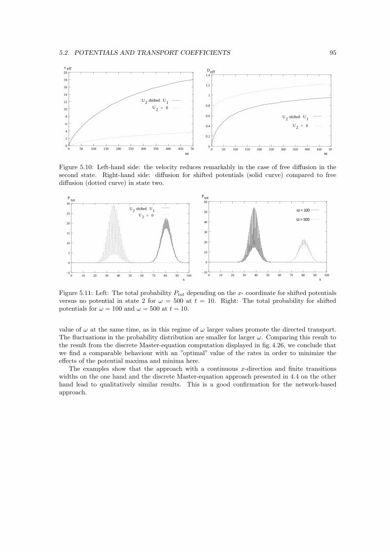
5.2. POTENTIALS AND TRANSPORT COEFFICIENTS 95
v
ω
shifted U1U2
2U = 0
eff
0
2
4
6
8
10
12
14
16
18
20
0 50 100 150 200 250 300 350 400 450 500
D
ω
eff
shifted
U
2U
1U2
= 0
0
0.2
0.4
0.6
0.8
1
1.2
1.4
0 50 100 150 200 250 300 350 400 450 500
Figure 5.10: Left-hand side: the velocity reduces remarkably in the case of free diffusion in thesecond state. Right-hand side: diffusion for shifted potentials (solid curve) compared to freediffusion (dotted curve) in state two.
shifted U1U2
2U = 0
Ptot
x
−5
0
5
10
15
20
25
30
0 10 20 30 40 50 60 70 80 90 100
Ptot
x
ω = 100
ω = 500
−10
0
10
20
30
40
50
60
0 10 20 30 40 50 60 70 80 90 100
Figure 5.11: Left: The total probability Ptot depending on the x- coordinate for shifted potentialsversus no potential in state 2 for ω = 500 at t = 10. Right: The total probability for shiftedpotentials for ω = 100 and ω = 500 at t = 10.
value of ω at the same time, as in this regime of ω larger values promote the directed transport.The fluctuations in the probability distribution are smaller for larger ω. Comparing this result tothe result from the discrete Master-equation computation displayed in fig. 4.26, we conclude thatwe find a comparable behaviour with an ”optimal” value of the rates in order to minimize theeffects of the potential maxima and minima here.
The examples show that the approach with a continuous x-direction and finite transitionswidths on the one hand and the discrete Master-equation approach presented in 4.4 on the otherhand lead to qualitatively similar results. This is a good confirmation for the network-basedapproach.
96 CHAPTER 5. ATP-CONCENTRATION AND TRANSPORT PROPERTIES
Chapter 6
Conclusions And Outlook
Linear molecular motors use the energy released in the hydrolysis of ATP to move other molecules,their cargoes, along filamental tracks. Coupled to the hydrolysis of ATP is a cycle of conformationalchanges of the motor protein. Such a motor cycle leads to a single step along the filament.
Here, we have examined stochastic models for these motor cycles, which determine the trans-port properties for the directed walks of the motor along its filament. In the short time regime ofconformational changes and motor cycles, the motor performs single steps in the range of about10 nm, and the corresponding stepping times are of the order of 10 ms, if there is a sufficientamount of ATP around. This short time regime determines the regime of directed walks wherethe motor takes up to several hundred steps along its track.
The main ingredients of our stochastic models as introduced in chapter 2 are a spatial co-ordinate x describing the displacement of the motor along the filament, a set of M states orconformations the motor particle can attain as well as a set of K locations at which transitionsbetween these different states take place.
The ratchet models can be solved analytically using a transfer matrix formalism as describedin chapter 2. Besides, we have shown that they can be mapped onto stochastic networks withMK discrete states or vertices. Finally, we obtain a general solution scheme by which the totalcurrent can be calculated.
In chapter 3 we have calculated explicit solutions for stochastic systems with up to four statesor conformations and with one to four locations for transitions between the states. The totalcurrent which is carried along such a network is the quotient of two polynomials which depend onthe transitions between the states via the corresponding vertical transition rates. The current isproportional to the motor’ s velocity. From the explicit solutions and from the general propertiesof the matrices used for the computations, we derive a number of universal rules which imposerestrictions on the dependence of the velocity on the vertical transition rates connecting the states.The terms in the numerator polynomial of the total current are shown to be connected to pathsthrough the networks if corresponding implicit horizontal rates are added. If we do not apply anexternal force, every such term of the first polynomial can be mapped onto an s-cycle spanningthe network in horizontal direction.
If a given motor follows a stepping scheme with a known number of different conformationsand locations, the above-mentioned rules enable us to derive combinations of vertical rates whichcontribute to its velocity via certain paths entering the numerator polynomial. Furthermore, weare able to exclude those combinations which do not contribute, even if we have not explicitlycalculated the solution of this special model.
In principle, our models are not limited as far as the number of their states or locations isconcerned. In this way, quite a variety of different stepping mechanisms for different motors canbe described and new findings about how a specific motor walks can be integrated. As more andmore experiments are performed, people frequently identify new substeps in the stepping schemesof motors. These substeps can easily be modelled in our approach.
In the first section of chapter 4 we have shown how decoupled states or subsystems can be
97
98 CHAPTER 6. CONCLUSIONS AND OUTLOOK
handled. Although for decoupled states a straightforward calculation as used for the model systemsin the preceding chapter fails due to the singularity of the underlying matrices, the subsystemsare inherent in these matrices. States or subsystems without a direct or indirect connection to theremaining system play a role if the motor can, with a certain probability, attain conformationswhich exclude transitions into certain other conformations, which might be the case if there is,for example, no possibility of the motor binding ATP. Likewise, in a system with decouplingwe can include additional states which are needed for the description of certain mutants of themotor or faulty motor proteins. In addition to the “normal” or “healthy” stepping, we then havealternative paths if such a special situation occurs. The introduction of a control parametercoupling two identical subsystems reveals bifurcations with different branches for the internal ratesof the subsystems, while the total current in the stationary state is fixed, so that the“macroscopic”appearance corresponds to different “microscopic” configurations.
In the sections 4.2 and 4.3 we introduce active elements or unbalanced rates in other than thevertical and, in particular, in the horizontal direction. One way of achieving this is by distortionof the networks as done in 4.2. The new approach in 4.3 is based on a discrete Master equation.This no longer requires horizontal transition rates fulfilling the conditions of detailed balance,but allows us to view arbitrary horizontal rates, if we start from the Master equation withoutconsidering its former derivation. The unbalanced rates drive the transport in horizontal directionor any other direction obtained by distorting the underlying networks.
Now, the total current obtained from the Master-equation calculations explicitly depends onthe vertical and also on the horizontal rates of the systems. Its numerator polynomial containsterms with complete paths of vertical and horizontal rates along the network. From calculations inmodel systems we derive universal rules for the dependence of the total current on all the transitionrates of the system. The results of the model systems relate one and the same combination ofvertical rates to several forward and backward paths with possible additional horizontal ratesfulfilling rules analogous to the ones derived before for vertical rates.
By integrating the discrete Master equation numerically, it is possible to take into accountlarger systems where the spatial periodicity comprises a number of steps as shown in section 4.4.Beginning with a certain probability distribution, we look at how the stationary state is reachedwith ongoing time. Doing so, we examine the hindrance of the transport by a defect or obstacleon its track reducing the total current. The dependence of the motor’s transport on a singleconformation, which is attained in the course of a multi-state stepping process, can be significant,if this conformation allows for fast directed transport or otherwise for no directed transport at alland if there are few possibilities of leaving this conformation again. Several results concerning thetime evolution of the systems are confirmed in a Markov-chain approach.
In the field of enzyme kinetics, one usually distinguishes one special cycle of chemical processeswhich is then called the main pathway of the enzyme. In our system this is the positive s-cyclecarrying the largest current along the network.
In section 4.5 we have discussed how possible “candidates” for this main pathway can be iden-tified in a special system. If we have maximum rates given in a system, these rates correspondto an upper limit of transport. The systems are then associated with flow networks with certaincapacities for the edges. A number of paths realizing maximum flow along the network is deter-mined. If the flow is fixed, a preferred pathway will be one with low costs. From our modelswe suggest that the main pathway irregardless of its importance is not the only pathway throughthe network. Furthermore, there are other pathways whose contributions might be smaller, butstill existent. This view is already accepted for a number of chemical reactions, and it can beinteresting to examine such alternative pathways for molecular motors, too.
The network-oriented approach to the movements of molecular motors has turned out to offer asimple picture for the motor cycles which nevertheless comprises many details of motor transport.This can be an impulse to further models.
The underlying reaction kinetics of the hydrolysis of ATP or other chemical processes entersour models via the dependence of the unbalanced rates on the respective concentrations, here theconcentration of ATP. We have shown in section 5.1 that if we assume different reaction kineticsfor the dependence on the concentration of ATP, this leads to velocities whose dependence on the
99
ATP-concentration can differ from the usually assumed Michaelis-Menten type behaviour. Apartfrom the Michaelis-Menten curves for the simple case of Michaelis-Menten kinetics and a singleunbalanced rate, we obtain curves with sigmoidal courses or maxima. These differences can occurdue to allosteric effects when the motor binds regulatory molecules. The tolerances and the lownumber of data points in the present experimental results still offer possibilities for such deviatingdependences which might be determined in future experiments.
In section 5.2 we have looked at the influences different choices of the molecular interactionpotentials have on the transport properties in systems without active horizontal transport. Besides,we have examined the effects of localized vertical transitions as used in our networks comparedto other models with finite transition widths, where the horizontal direction is continuous again.If the widths are small, the maxima of the transport coefficients are shifted to large rates and weapproach the crossover to a saturation regime. Some of the qualitative results obtained from ournetwork models as, for example, for the time evolution of the probabilities, are comparable to theresults of these alternative models. In this way we have been able to elucidate the characteristicsof our models as well as the results when inserting experimental data.
Our stochastic models can be mapped onto networks, which simplifies the calculations and offerspossibilities for approaches from the field of graph theory. The models are meant to qualitativelydescribe a variety of different features of motor transport rather than to fit data for the steppingprocess of a certain motor construct. In the context of our models we can handle backward stepsand substeps, transient conformations, faulty motors and mutants, periodic defects of the filament,active elements in vertical, horizontal or any distorted direction as well as the idea of a main anda couple of minor pathways. The future challenge will be the building in of newly discoveredproperties and characteristics of the motors and their tracks.

100 CHAPTER 6. CONCLUSIONS AND OUTLOOK
Appendix A
Matrices A(M,K)
In the following sections A.1-A.3 we list the matrix elements A(M,K)ij , where i indicates the corre-
sponding row and j the column, for the general model systems (M, K) = (2, 3), (M, K) = (2, 4)and (M, K) = (3, 2).
The sections A.4 and A.5 show the derivation of matrices describing subsystems of an (M, K) =(3, 2) and an (M, K) = (2, 4)-system, respectively.
A.1 Matrix A(2,3)
Here, we list the matrix elements of A(2,3). The notation is as given in chapter 2.
A(2,3)11 = E1 (x1, x2) ω12 (x2) − (−E1 (x2, x3) − E1 (x1, x2) (e1 (x2, x3) + E1 (x2, x3)
`Ωω12 (x2))) ω12 (x3) + E1 (x1, x2) E2 (x2, x3) `Ωω12 (x2) ω21 (x3)
A(2,3)12 = −E1 (x2, x3) − E1 (x3, x1 + `) /e1 (x3, x1 + `) − E1 (x1, x2)
(e1 (x2, x3) + E1 (x2, x3)) `Ωω12 (x2)
A(2,3)13 = E1 (x1, x2) E2 (x2, x3) `Ωω12 (x2)
A(2,3)14 = −E1 (x1) − E1 (x1, x2)
(E1 (x2) − E1 (x3)
)`Ωω12 (x2)
+E1 (x1, x2)(E2 (x2) − E2 (x3)
)`Ωω21 (x2)
A(2,3)21 = − (E2 (x1, x2) ω21 (x2)) − E1 (x2, x3) E2 (x1, x2) `Ωω12 (x3) ω21 (x2)
+ (−E2 (x2, x3) E2 (x1, x2) (e2 (x2, x3) + E2 (x2, x3) `Ωω21 (x2))) ω21 (x3)
A(2,3)22 = E1 (x2, x3) E2 (x1, x2) `Ωω21 (x2)
A(2,3)23 = −E2 (x2, x3) − E2 (x3, x1 + `) /e2 (x3, x1 + `) − E2 (x1, x2)
(e2 (x2, x3) + E2 (x2, x3) `Ωω21 (x2))
A(2,3)24 = −E2 (x1) + E2 (x1, x2)
(E1 (x2) − E1 (x3)
)`Ωω21 (x2)
−E2 (x1, x2)(E2 (x2) − E2 (x3)
)`Ωω21 (x2)
A(2,3)31 = −ω12 (x1) − (e1 (x1, x2) + E1 (x1, x2) `Ωω12 (x1)) ω12 (x2)
−E2 (x1, x2) `Ωω12 (x1) ω21 (x2) − ω12 (x3) (E1 (x2, x3) `Ωω12 (x1)
+ (e1 (x1, x2) + E1 (x1, x2) `Ωω12 (x1)) (e1 (x2, x3) + E1 (x2, x3) `Ωω12 (x2))
+E1 (x2, x3) E2 (x1, x2) `2Ωω12 (x1) ω21 (x2)
)+ (− (E2 (x2, x3) `Ωω12 (x1))
−E2 (x2, x3) `Ω (e1 (x1, x2) + E1 (x1, x2) `Ωω12 (x1)) ω12 (x2)
−E2 (x1, x2) `Ωω12 (x1) (e2 (x2, x3) + E2 (x2, x3) `Ωω21 (x2))) ω21 (x3)
A(2,3)32 = −1/e1 (x3, x4) + E1 (x2, x3) `Ωω12 (x1)
I
II APPENDIX A. MATRICES A(M,K)
+ (e1 (x1, x2) + E1 (x1, x2) `Ωω12 (x1)) (e1 (x2, x3) + E1 (x2, x3) `Ωω12 (x2))
+E1 (x2, x3) E2 (x1, x2) `2Ωω12 (x1) ω21 (x2)
A(2,3)33 = − (E2 (x2, x3) `Ωω12 (x1)) − E2 (x2, x3) `Ω (e1 (x1, x2) + E1 (x1, x2) `Ωω12 (x1))
ω12 (x2) − E2 (x1, x2) `Ωω12 (x1) (e2 (x2, x3) + E2 (x2, x3) `Ωω21 (x2))
A(2,3)34 = e1 +
(E1 (x1) − E1 (x3)
)`Ωω12 (x1) −
(E2 (x1) − E2 (x3)
)`Ωω12 (x1)
−(E1 (x2) − E1 (x3)
)`Ω (− ((e1 (x1, x2) + E1 (x1, x2) `Ωω12 (x1)) ω12 (x2))
−E2 (x1, x2) `Ωω12 (x1) ω21 (x2)) −(E2 (x2) − E2 (x3)
)`Ω
((e1 (x1, x2) + E1 (x1, x2) `Ωω12 (x2)) ω12 (x1) + E2 (x1, x2) `Ωω12 (x1) ω21 (x2))
A(2,3)41 = ω21 (x1) + E1 (x1, x2) `Ωω12 (x2) ω21 (x1) + (e2 (x1, x2) + E2 (x1, x2) `Ωω21 (x1))
ω21 (x2) − ω12 (x3) (− (E1 (x2, x3) `Ωω21 (x1)) − E1 (x1, x2) `Ω
(e1 (x2, x3) + E1 (x2, x3) `Ωω12 (x2)) ω21 (x1) − E1 (x2, x3) `Ω
(e2 (x1, x2) + E2 (x1, x2) `Ωω21 (x1)) ω21 (x2)) +(E2 (x2, x3) `Ωω21 (x1) + E1 (x1, x2) E2 (x2, x3) `2
Ωω12 (x2) ω21 (x1)
+ (e2 (x1, x2) + E2 (x1, x2) `Ωω21 (x1)) + (e2 (x2, x3) + E2 (x2, x3) `Ωω21 (x2)))
ω21 (x3)
A(2,3)42 = −E1 (x2, x3) `Ωω21 (x1) − E1 (x1, x2) `Ω (e1 (x2, x3) + E1 (x2, x3) `Ωω12 (x2))
ω21 (x1) − E1 (x2, x3) `Ω (e2 (x1, x2) + E2 (x1, x2) `Ωω21 (x1)) ω21 (x2)
A(2,3)43 = −1/e2 (x3, x4) + E2 (x2, x3) `Ωω21 (x1)
+E1 (x1, x2) E2 (x2, x3) `2Ωω12 (x2) ω21 (x1) + (e2 (x1, x2) + E2 (x1, x2) `Ωω21 (x1))
(e2 (x2, x3) + E2 (x2, x3) `Ωω21 (x2))
A(2,3)44 = e2 −
(E1 (x1) − E1 (x3)
)`Ωω21 (x1) +
(E2 (x1) − E2 (x3)
)`Ωω21 (x1)
−(E2 (x2) − E2 (x3)
)`Ω (− (E1 (x1, x2) `Ωω12 (x2) ω21 (x1))
− (e2 (x1, x2) + E2 (x1, x2) `Ωω21 (x1)) ω21 (x2))
−(E1 (x2) − E1 (x3)
)`Ω (E1 (x1, x2) `Ωω12 (x2) ω21 (x1)
+ (e2 (x1, x2) + E2 (x1, x2) `Ωω21 (x1)) ω21 (x2) (A.1)
A.2 Matrix A(2,4)
In the following the elements of the 4× 4-matrix A(2,4) as used for calculations in 3.1.2 are listed.
A(2,4)11 = E1 (x1, x2) ω12 (x2) − (−E1 (x2, x3) − E1 (x1, x2) (e1 (x2, x3)
+E1 (x2, x3) `Ωω12 (x2))) ω12 (x3) + E1 (x1, x2) E2 (x2, x3) `Ω
ω12 (x2) ω21 (x3) − ω12 (x4) (− (E1 (x3, x4) (1 + E1 (x1, x2) `Ωω12 (x2)))
+ (−E1 (x2, x3) − E1 (x1, x2) (e1 (x2, x3) + E1 (x2, x3) `Ωω12 (x2)))
(e1 (x3, x4) + E1 (x3, x4)Ω ω12 (x3)) − E1 (x1, x2) E1 (x3, x4) E2 (x2, x3)
`2Ωω12 (x2) ω21 (x3)
)+ (E1 (x1, x2) E2 (x3, x4) `Ωω12 (x2) − E2 (x3, x4) `Ω
(−E1 (x2, x3) − E1 (x1, x2) (e1 (x2, x3) + E1 (x2, x3) `Ωω12 (x2)))
ω12 (x3) + E1 (x1, x2) E2 (x2, x3) `Ωω12 (x2) (e2 (x3, x4)
+E2 (x1, x3) `Ωω21 (x3))) ω21 (x4)
A(2,4)12 = −E1 (x4, x1 + `) /e1 (x4, x1 + `) − E1 (x3, x4) (1 + E1 (x1, x2) `Ωω12 (x2))
+ (−E1 (x2, x3) − E1 (x1, x2) (e1 (x2, x3) + E1 (x2, x3) `Ωω12 (x2)))
(e1 (x3, x4) + E1 (x3, x4) `Ωω12 (x3)) − E1 (x1, x2) E1 (x3, x4) E2 (x2, x3)
A.2. MATRIX A(2,4) III
`2Ωω12 (x2) ω21 (x3)
A(2,4)13 = E1 (x1, x2) E2 (x3, x4) `Ωω12 (x2) − E2 (x3, x4) `Ω (−E1 (x2, x3) − E1 (x1, x2)
(e1 (x2, x3) + E1 (x2, x3) `Ωω12 (x2))) ω12 (x3) + E1 (x1, x2) E2 (x2, x3)
`Ωω12 (x2) (e2 (x3, x4) + E2 (x3, x4) `Ωω21 (x3))
A(2,4)14 = −E1 (x1) − E1 (x1, x2)
(E1 (x2) − E1 (x4)
)`Ωω12 (x2) + E1 (x1, x2)(
E2 (x2) − E2 (x4))`Ωω12 (x2) −
(E2 (x3) − E2 (x4)
)`Ω
((−E1 (x2, x3) − E1 (x1, x2) (e1 (x2, x3) + E1 (x2, x3) `Ωω12 (x2))) ω12 (x3)
−E1 (x1, x2) E2 (x2, x3) `Ωω12 (x2) ω21 (x3)) −(E1 (x3) − E1 (x4)
)`Ω
(− ((−E1 (x2, x3) − E1 (x1, x2) (e1 (x2, x3) + E1 (x2, x3) `Ωω12 (x2))) ω12 (x3))
E1 (x1, x2) E2 (x2, x3) `Ωω12 (x2) ω21 (x3))
A(2,4)21 = −E2 (x1, x2) ω21 (x2) − E1 (x2, x3) E2 (x1, x2) `Ωω12 (x3) ω21 (x2)
+ (−E2 (x2, x3) − E2 (x1, x2) (e2 (x2, x3) + E2 (x2, x3) `Ωω21 (x2))) ω21 (x3)
−ω12 (x4) (E1 (x3, x4) E2 (x1, x2) `Ωω21 (x2) + E1 (x2, x3) E2 (x1, x2) `Ω
(e1 (x3, x4) + E1 (x3, x4) `Ωω12 (x3)) ω21 (x2) − E1 (x3, x4) `Ω (−E2 (x2, x3)
−E2 (x1, x2) (e2 (x2, x3) + E2 (x2, x3) `Ωω21 (x2))) ω21 (x3))
+((−E1 (x2, x3) E2 (x1, x2) E2 (x3, x4) `2
Ωω12 (x3) ω21 (x2))− E2 (x3, x4)
(1 + E2 (x1, x2) `Ωω21 (x2)) + (−E2 (x2, x3) − E2 (x1, x2)
(e2 (x2, x3) + E2 (x2, x3) `Ωω21 (x2))) (e2 (x3, x4) + E2 (x3, x4) `Ωω21 (x3)))
ω21 (x4)
A(2,4)22 = E1 (x3, x4) E2 (x1, x2) `Ωω21 (x2) + E1 (x2, x3) E2 (x1, x2) `Ω (e1 (x3, x4)
+E1 (x3, x4) `Ωω12 (x3)) ω21 (x2) − E1 (x3, x4) `Ω (−E2 (x2, x3) − E2 (x1, x2)
(e2 (x2, x3) + E2 (x2, x3) `Ωω21 (x2))) ω21 (x3)
A(2,4)23 = −E2 (x4, x1 + `) /e2 (x4, x1 + `) − E1 (x2, x3) E2 (x1, x2) E2 (x3, x4) `2
Ωω12 (x3)
ω21 (x2) − E2 (x3, x4) (1 + E2 (x1, x2) `Ωω21 (x2)) + (−E2 (x2, x3) − E2 (x1, x2)
(e2 (x2, x3) + E2 (x2, x3) `Ωω21 (x2))) (e2 (x3, x4) + E2 (x3, x4) `Ωω21 (x3))
A(2,4)24 = −E2 (x1) + E2 (x1, x2)
(E1 (x2) − E1 (x4)
)`Ωω21 (x2) − E2 (x1, x2)(
E2 (x2) − E2 (x4))`Ωω21 (x2) −
(E2 (x3) − E2 (x4)
)`Ω
(E1 (x2, x3) E2 (x1, x2) `Ωω12 (x3) ω21 (x2) − (E2 (x2, x3) − E2 (x1, x2) (e2 (x2, x3)
+E2 (x2, x3) `Ωω21 (x2))) ω21 (x3)) −(E1 (x3) − E1 (x4)
)`Ω
(− (E1 (x2, x3) E2 (x1, x2) `Ωω12 (x3) ω21 (x2)) + (−E2 (x2, x3) − E2 (x1, x2)
(e2 (x2, x3) + E2 (x2, x3) `Ωω21 (x2))) ω21 (x3))
A(2,4)31 = −ω12 (x1) − (e1 (x1, x2) + E1 (x1, x2) `Ωω12 (x1)) ω12 (x2) − E2 (x1, x2) `Ωω12 (x1)
ω21 (x2) − ω12 (x3) (E1 (x2, x3) `Ωω12 (x1) + (e1 (x1, x2) + E1 (x1, x2) `Ωω12 (x1))
(e1 (x2, x3) + E1 (x2, x3) `Ωω12 (x2)) + E1 (x2, x3) E2 (x1, x2) `2Ωω12 (x1) ω21 (x2)
)
+ (− (E2 (x2, x3) `Ωω12 (x1)) − E2 (x2, x3) `Ω (e1 (x1, x2) + E1 (x1, x2) `Ωω12 (x1))
ω12 (x2) − E2 (x1, x2) `Ωω12 (x1) (E2 (x2, x3) + E2 (x2, x3) `Ωω21 (x2))) ω21 (x3)
−ω12 (x4) (− (E1 (x3, x4) (− (`Ωω12 (x1)) − `Ω (e1 (x1, x2) + E1 (x1, x2) `Ω)
ω12 (x2) − E2 (x1, x2) `2Ωω12 (x1) ω21 (x2)
))+ (e1 (x3, x4) + E1 (x3, x4) `Ωω12 (x3))
(E1 (x2, x3) `Ωω12 (x1) + (e1 (x1, x2) + E1 (x1, x2) `Ωω12 (x1)) (e1 (x2, x3)
+E1 (x2, x3) `Ωω12 (x2)) + E1 (x2, x3) E2 (x1, x2) `2Ω ω12 (x1) ω21 (x2)) − E1 (x3, x4)
`Ω (− (E2 (x2, x3) `Ωω12 (x1)) − E2 (x2, x3) `Ω (e1 (x1, x2) + E1 (x1, x2) `Ωω12 (x1))
ω12 (x2) − E2 (x1, x2) `Ωω12 (x1) (e2 (x2, x3) + E2 (x2, x3) `Ωω21 (x2))) ω21 (x3))
IV APPENDIX A. MATRICES A(M,K)
+ (− (E2 (x3, x4) (`Ωω12 (x1) + `Ω (e1 (x1, x2) + E1 (x1, x2) `Ωω12 (x1)) ω12 (x2)
+E2 (x1, x2) `2Ωω12 (x1) ω21 (x2)
))− E2 (x3, x4) `Ωω12 (x3) (E1 (x2, x3) `Ωω12 (x1)
+ (e1 (x1, x2) + E1 (x1, x2) `Ωω12 (x1)) (e1 (x2, x3) + E1 (x2, x3) `Ωω12 (x2))
+E1 (x2, x3) E2 (x1, x2) `2Ωω12 (x1) ω21 (x2)
)+ (− (E2 (x2, x3) `Ωω12 (x1))
−E2 (x2, x3) `Ω (e1 (x1, x2) + E1 (x1, x2) `Ωω12 (x1)) ω12 (x2) − E2 (x1, x2)
`Ωω12 (x1) (e2 (x2, x3) + E2 (x2, x3) `Ωω21 (x2))) (e2 (x3, x4)
+E2 (x3, x4) `Ωω21 (x3))) ω21 (x4)
A(2,4)32 = −1/e1 (x4, x1 + `) − E1 (x3, x4) (− (`Ωω12 (x1)) − `Ω (e1 (x1, x2)
+E1 (x1, x2) `Ωω12 (x1)) ω12 (x2) − E2 (x1, x2) `2Ωω12 (x1) ω21 (x2)
)
+ (e1 (x3, x4) + E1 (x3, x4) `Ωω12 (x3)) (E1 (x2, x3) `Ωω12 (x1) + (e1 (x1, x2)
+E1 (x1, x2) `Ωω12 (x1)) (e1 (x2, x3) + E1 (x2, x3) `Ωω12 (x2)) + E1 (x2, x3)
E2 (x1, x2) `2Ωω12 (x1) ω21 (x2)
)− E1 (x3, x4) `Ω (− (E2 (x2, x3) `Ωω12 (x1))
−E2 (x2, x3) `Ω (e1 (x1, x2) + E1 (x1, x2) `Ωω12 (x1)) ω12 (x2) − E2 (x1, x2)
`Ωω12 (x1) (e2 (x2, x3) + E2 (x2, x3) `Ωω21 (x2))) ω21 (x3)
A(2,4)33 = − (E2 (x3, x4) (`Ωω12 (x1) + `Ω (e1 (x1, x2) + E1 (x1, x2) `Ωω12 (x1)) ω12 (x2)
+E2 (x1, x2) `2Ωω12 (x1) ω21 (x2)
))− E2 (x3, x4) `Ωω12 (x3) (E1 (x2, x3) `Ω
ω12 (x1) + (e1 (x1, x2) + E1 (x1, x2) `Ωω12 (x1)) (e1 (x2, x3) + E1 (x2, x3) `Ωω12 (x2))
+E1 (x2, x3) E2 (x1, x2) `2Ωω12 (x1) ω21 (x2)
)+ (− (E2 (x2, x3) `Ωω12 (x1))
−E2 (x2, x3) `Ω (e1 (x1, x2) + E1 (x1, x2) `Ωω12 (x1)) ω12 (x2) − E2 (x1, x2) `Ω
ω12 (x1) (e2 (x2, x3) + E2 (x2, x3) `Ωω21 (x2))) (e2 (x3, x4) + E2 (x3, x4) `Ωω21 (x3))
A(2,4)34 = e1 +
(E1 (x1) − E1 (x4)
)`Ωω12 (x1) −
(E2 (x1) − E2 (x4)
)`Ωω12 (x1)
−(E1 (x2) − E1 (x4)
)`Ω (− ((e1 (x1, x2) + E1 (x1, x2) `Ωω12 (x1)) ω12 (x2))
−E2 (x1, x2) `Ωω12 (x1) ω21 (x2)) −(E2 (x2) − E2 (x4)
)`Ω ((e1 (x1, x2)
+E1 (x1, x2) `Ωω12 (x1)) ω12 (x2) + E2 (x1, x2) `Ωω12 (x1) ω21 (x2))
−(E2 (x3) − E2 (x4)
)`Ω (ω12 (x3) (E1 (x2, x3) `Ωω12 (x1)
+ (e1 (x1, x2) + E1 (x1, x2) `Ωω12 (x1)) (e1 (x2, x3) + E1 (x2, x3) `Ωω12 (x2))
+E1 (x2, x3) E2 (x1, x2) `2Ωω12 (x1) ω21 (x2)
)− (− (E2 (x2, x3) `Ωω12 (x1))
−E2 (x2, x3) `Ω (e1 (x1, x2) + E1 (x1, x2) `Ωω12 (x1)) ω12 (x2) − E2 (x1, x2) `Ω
ω12 (x1) (e2 (x2, x3) + E2 (x2, x3) `Ωω21 (x2))) ω21 (x3))
−(E1 (x3) − E1 (x4)
)`Ω (− (ω12 (x3) (E1 (x2, x3) `Ωω12 (x1) + (e1 (x1, x2)
+E1 (x1, x2) `Ωω12 (x1)) (e1 (x2, x3) + E1 (x2, x3) `Ωω12 (x2))
+E1 (x2, x3) E2 (x1, x2) `2Ωω12 (x1) ω21 (x2)
))+ (− (E2 (x2, x3) `Ωω12 (x1))
−E2 (x2, x3) `Ω (e1 (x1, x2) + E1 (x1, x2) `Ωω12 (x1)) ω12 (x2) − E2 (x1, x2)
`Ωω12 (x1) (e2 (x2, x3) + E2 (x2, x3) `Ωω21 (x2)) ω21 (x3))
A(2,4)41 = ω21 (x1) + E1 (x1, x2) `Ωω12 (x2) ω21 (x1) + (e2 (x1, x2) + E2 (x1, x2) `Ωω21 (x1))
ω21 (x2) − ω12 (x3) (− (E1 (x2, x3) `Ωω21 (x1)) − E1 (x1, x2) `Ω (e1 (x2, x3)
+E1 (x2, x3) `Ωω12 (x2)) ω21 (x1) − E1 (x2, x3) `Ω (e2 (x1, x2) + E2 (x1, x2)
`Ωω21 (x1)) ω21 (x2)) + (E2 (x2, x3) `Ωω21 (x1) + E1 (x1, x2) E2 (x2, x3)
`2Ωω12 (x2) ω21 (x1) + (e2 (x1, x2) + E2 (x1, x2) `Ωω21 (x1)) (e2 (x2, x3)
)
+E2 (x2, x3) `Ωω21 (x2)) ω21 (x3) − ω12 (x4) (− (E1 (x3, x4) (`Ωω21 (x1)
+E1 (x1, x2) `2Ωω12 (x2) ω21 (x1) + `Ω (e2 (x1, x2) + E2 (x1, x2) `Ωω21 (x1))
ω21 (x2))) + (e1 (x3, x4) + E1 (x3, x4) `Ωω12 (x3)) (− (E1 (x2, x3) `Ωω21 (x1))
A.2. MATRIX A(2,4) V
−E1 (x1, x2) `Ω (e1 (x2, x3) + E1 (x2, x3) `Ωω12 (x2)) ω21 (x1) − E1 (x2, x3)
`Ω (e2 (x1, x2) + E2 (x1, x2) `Ωω21 (x1)) ω21 (x2)) − E1 (x3, x4) `Ω
(E2 (x2, x3) `Ωω21 (x1) + E1 (x1, x2) E2 (x2, x3) `2Ωω12 (x2) ω21 (x1)
+ (e2 (x1, x2) + E2 (x1, x2) `Ωω21 (x1)) (e2 (x2, x3) + E2 (x2, x3) `Ωω21 (x2)) ω21 (x3))
+(−(E2 (x3, x4)
(−`Ωω21 (x1) − E1 (x1, x2) `2
Ωω12 (x2) ω21 (x1)
−`Ω (e2 (x1, x2) + E2 (x1, x2) `Ωω21 (x1)) ω21 (x2)))
−E2 (x3, x4) `Ωω12 (x3) (−E1 (x2, x3) `Ωω21 (x1) − E1 (x1, x2) `Ω
(e1 (x2, x3) + E1 (x2, x3) `Ωω12 (x2)) ω21 (x1) − E1 (x2, x3) `Ω (e2 (x1, x2)
+E2 (x1, x2) `Ωω21 (x1)) ω21 (x2)) + (E2 (x2, x3) `Ωω21 (x1) + E1 (x1, x2)
E2 (x2, x3) `2Ωω12 (x2) ω21 (x1) + (e2 (x1, x2) + E2 (x1, x2) `Ωω21 (x1))
(e2 (x2, x3) + E2 (x2, x3) `Ωω21 (x2))) (e2 (x3, x4) + E2 (x3, x4) `Ωω21 (x3))) ω21 (x4)
A(2,4)42 = −
(E1 (x3, x4)
(`Ωω21 (x1) + E1 (x1, x2) `2
Ωω12 (x2) ω21 (x1) + `Ω (e2 (x1, x2)
+E2 (x1, x2) `Ωω21 (x1)) ω21 (x2))) + (e1 (x3, x4) + E1 (x3, x4) `Ωω12 (x3))
(−E1 (x2, x3) `Ωω21 (x1)) − E1 (x1, x2) `Ω (e1 (x2, x3) + E1 (x2, x3) `Ωω12 (x2))
ω21 (x1) − E1 (x2, x3) `Ω (e2 (x1, x2) + E2 (x1, x2) `Ωω21 (x1)) ω21 (x2))
−E1 (x3, x4) `Ω
(E2 (x2, x3) `Ωω21 (x1) + E1 (x1, x2) E2 (x2, x3) `2
Ωω12 (x2) ω21 (x1)
+ (e2 (x1, x2) + E2 (x1, x2) `Ωω21 (x1)) (e2 (x2, x3) + E2 (x2, x3) `Ωω21 (x2))) ω21 (x3)
A(2,4)43 = −1/e2 (x4, x1 + `) − E2 (x3, x4)
(−`Ωω21 (x1) − E1 (x1, x2) `2
Ωω12 (x2) ω21 (x1)
−`Ω (e2 (x1, x2) + E2 (x1, x2) `Ωω21 (x1)) ω21 (x2)) − E2 (x3, x4) `Ωω12 (x3)
(− (E1 (x2, x3) `Ωω21 (x1)) − E1 (x1, x2) `Ω (e1 (x2, x3) + E1 (x2, x3) `Ωω12 (x2))
ω21 (x1) − E1 (x2, x3) `Ω (e2 (x1, x2) + E2 (x1, x2) `Ωω21 (x1)) ω21 (x2))
+(E2 (x2, x3) `Ωω21 (x1) + E1 (x1, x2) E2 (x2, x3) `2
Ωω12 (x2) ω21 (x1)
+ (e2 (x1, x2) + E2 (x1, x2) `Ωω21 (x1)) (e2 (x2, x3) + E2 (x2, x3) `Ωω21 (x2)))
(e2 (x3, x4) + E2 (x3, x4) `Ωω21 (x3))
A(2,4)44 = e2 −
(E1 (x1) − E1 (x4)
)`Ωω21 (x1) +
(E2 (x1) − E2 (x4)
)`Ωω21 (x1)
−(E2 (x2) − E2 (x4)
)`Ω (− (E1 (x1, x2) `Ωω12 (x2) ω21 (x1)) − (e2 (x1, x2)
+E2 (x1, x2) `Ωω21 (x1)) ω21 (x2)) −(E1 (x2) − E1 (x4)
)`Ω
(E1 (x1, x2) `Ωω12 (x2) ω21 (x1) + (e2 (x1, x2) + E2 (x1, x2) `Ωω21 (x1)) ω21 (x2))
−(E2 (x3) − E2 (x4)
)`Ω (ω12 (x3) (− (E1 (x2, x3) `Ωω21 (x1)) − E1 (x1, x2) `Ω
(e1 (x2, x3) + E1 (x2, x3) `Ωω12 (x2)) ω21 (x1) − E1 (x2, x3) `Ω
(e2 (x1, x2) + E2 (x1, x2) `Ωω21 (x1)) ω21 (x2)) − (E2 (x2, x3) `Ωω21 (x1) + E1 (x1, x2)
E2 (x2, x3) `2Ωω12 (x2) ω21 (x1) + (e2 (x1, x2) + E2 (x1, x2) `Ωω21 (x1))
(e2 (x2, x3) + E2 (x2, x3) `Ωω21 (x2))) ω21 (x3) −(E1 (x3) − E1 (x4)
)
`Ω (− (ω12 (x3) (−E1 (x2, x3) `Ωω21 (x1) − E1 (x1, x2) `Ω
(e1 (x2, x3) + E1 (x2, x3) `Ωω12 (x2)) ω21 (x1) − E1 (x2, x3) `Ω
(e2 (x1, x2) + E2 (x1, x2) `Ωω21 (x1)) ω21 (x2))) + (E2 (x2, x3) `Ωω21 (x1)
+E1 (x1, x2) E2 (x2, x3) `2Ωω12 (x2) ω21 (x1) + (e2 (x1, x2) + E2 (x1, x2) `Ωω21 (x1))
(e2 (x2, x3) + E2 (x2, x3) `Ωω21 (x2))) ω21 (x3)) (A.2)
VI APPENDIX A. MATRICES A(M,K)
A.3 Matrix A(3,2)
The matrix A(3,2) as used for computations in 3.1.3 is a 6 × 6-matrix.
A(3,2)11 = E1 (x1, x2) ω12 (x2) + E1 (x1, x2) ω13 (x2) ,
A(3,2)12 = −E1 (x1, x2) ω12 (x2) ,
A(3,2)13 = −E1 (x1, x2) − E1 (x2, x1 + `) /e1 (x2, x1 + `) ,
A(3,2)14 = 0,
A(3,2)15 = 0,
A(3,2)16 = −E1 (x1) ,
A(3,2)21 = −E2 (x1, x2) ω21 (x2) ,
A(3,2)22 = E2 (x1, x2) ω21 (x2) + E2 (x1, x2) ω23 (x2) ,
A(3,2)23 = 0,
A(3,2)24 = −E2 (x1, x2) − E2 (x2, x1 + `) /e2 (x2, x1 + `) ,
A(3,2)25 = 0,
A(3,2)26 = −E2 (x1) ,
A(3,2)31 = −E3 (x1, x2) ω31 (x2) ,
A(3,2)32 = −E3 (x1, x2) ω32 (x2) ,
A(3,2)33 = 0,
A(3,2)34 = 0,
A(3,2)35 = −E3 (x1, x2) − E3 (x2, x1 + `) /e3 (x2, x1 + `) ,
A(3,2)36 = −E3 (x1) ,
A(3,2)41 = −ω12 (x1) − ω13 (x1) − ω12 (x1) ω12 (x2) `ΩE1 (x1, x2) − ω13 (x1) ω12 (x2) `ΩE1 (x1, x2)
−ω12 (x2) e1 (x1, x2) − ω12 (x1) ω21 (x2) `ΩE2 (x1, x2) − ω12 (x1) ω13 (x2) `ΩE1 (x1, x2)
−ω13 (x1) ω13 (x2) `ΩE1 (x1, x2) − ω13 (x2) e1 (x1, x2) − ω13 (x1) ω31 (x2) `ΩE3 (x1, x2) ,
A(3,2)42 = ω12 (x1) + ω12 (x1) ω21 (x2) `ΩE2 (x1, x2) + ω12 (x1) ω12 (x2) `ΩE1 (x1, x2)
+ω13 (x1) ω12 (x2) `ΩE1 (x1, x2) + ω12 (x2) e1 (x1, x2) + ω12 (x1) ω23 (x2) `ΩE2 (x1, x2)
−ω13 (x1) ω32 (x2) `ΩE3 (x1, x2) ,
A(3,2)43 = ω12 (x1) `ΩE1 (x1, x2) + ω13 (x1) `ΩE1 (x1, x2) + e1 (x1, x2) − 1/e1 (x2, x1 + `) ,
A(3,2)44 = −ω12 (x1) `ΩE2 (x1, x2) ,
A(3,2)45 = −ω13 (x1) `ΩE3 (x1, x2) ,
A(3,2)46 = e1 + ω12 (x1)
(E1 (x1) − E1 (x2)
)`Ω + ω13 (x1)
(E1 (x1) − E1 (x2)
)`Ω
−ω12 (x1)(E2 (x1) − E2 (x2)
)`Ω − ω13 (x1)
(E3 (x1) − E3 (x2)
)`Ω,
A(3,2)51 = ω21 (x1) + ω21 (x1) ω12 (x2) `ΩE1 (x1, x2) + ω21 (x1) ω21 (x2) `ΩE2 (x1, x2)
+ω23 (x1) ω21 (x2) `ΩE2 (x1, x2) + ω21 (x2) e2 (x1, x2) + ω21 (x1) ω13 (x2) `ΩE1 (x1, x2)
−ω23 (x1) ω31 (x2) `ΩE3 (x1, x2) ,
A(3,2)52 = −ω21 (x1) − ω23 (x1) − ω21 (x1) ω21 (x2) `ΩE2 (x1, x2) − ω23 (x1) ω21 (x2) `ΩE2 (x1, x2)
−ω21 (x2) e2 (x1, x2) − ω21 (x1) ω12 (x2) `ΩE1 (x1, x2) − ω21 (x1) ω23 (x2) `ΩE2 (x1, x2)
−ω23 (x1) ω23 (x2) `ΩE2 (x1, x2) − ω23 (x2) e2 (x1, x2) − ω23 (x1) ω32 (x2) `ΩE3 (x1, x2) ,
A(3,2)53 = −ω21 (x1) `ΩE1 (x1, x2) ,
A.4. THE ELEMENTS OF ENGLISHA(2,2) DERIVED FROM A (3, 2)-MATRIX VII
A(3,2)54 = ω21 (x1) `ΩE2 (x1, x2) + ω23 (x1) `ΩE2 (x1, x2) + e2 (x1, x2) − 1/e2 (x2, x1 + `) ,
A(3,2)55 = −ω23 (x1) `ΩE3 (x1, x2) ,
A(3,2)56 = e2 − ω21 (x1)
(E1 (x1) − E1 (x2)
)`Ω + ω21 (x1)
(E2 (x1) − E2 (x2)
)`Ω
+ω23 (x1)(E2 (x1) − E2 (x2)
)`Ω − ω23 (x1)
(E3 (x1) − E3 (x2)
)`Ω,
A(3,2)61 = ω31 (x1) + ω31 (x1) ω12 (x2) `ΩE1 (x1, x2) − ω32 (x1) ω21 (x2) `ΩE2 (x1, x2)
+ω31 (x1) ω13 (x2) `ΩE1 (x1, x2) + ω31 (x1) ω31 (x2) `ΩE3 (x1, x2)
+ω32 (x1) ω31 (x2) `ΩE3 (x1, x2) + ω31 (x2) e3 (x1, x2) ,
A(3,2)62 = ω32 (x1) + ω32 (x1) ω21 (x2) `ΩE2 (x1, x2) − ω31 (x1) ω12 (x2) `ΩE1 (x1, x2)
+ω32 (x1) ω23 (x2) `ΩE2 (x1, x2) + ω31 (x1) ω32 (x2) `ΩE3 (x1, x2)
+ω32 (x1) ω32 (x2) `ΩE3 (x1, x2) + ω32 (x2) e3 (x1, x2) ,
A(3,2)63 = −ω31 (x1) `ΩE1 (x1, x2) ,
A(3,2)64 = −ω32 (x1) `ΩE2 (x1, x2) ,
A(3,2)65 = ω31 (x1) `ΩE3 (x1, x2) + ω32 (x1) `ΩE3 (x1, x2) + e3 (x1, x2)
−1/e3 (x2, x1 + `) ,
A(3,2)66 = e3 − ω31 (x1)
(E1 (x1) − E1 (x2)
)`Ω − ω32 (x1)
(E2 (x1) − E2 (x2)
)`Ω
+ω31 (x1)(E3 (x1) − E3 (x2)
)`Ω + ω32 (x1)
(E3 (x1) − E3 (x2)
)`Ω. (A.3)
A.4 The elements of A(2,2) derived from a (3, 2)-matrix
A(3,2),1,2,3 denotes the matrix, which is obtained from A(3,2) by neglecting the vertical ratesbetween state M and other states. Its elements are compared to the elements of A(2,2).
A(3,2),1,2,311 = E1 (x1, x2) ω12 (x2) = A
(2,2)11 ,
A(3,2),1,2,312 = −E1 (x1, x2) ω12 (x2) ,
A(3,2),1,2,313 = −E1 (x1, x2) − E1 (x2, x1 + `) /e1 (x2, x1 + `) = A
(2,2)12 ,
A(3,2),1,2,314 = 0 = A
(2,2)13 ,
A(3,2),1,2,315 = 0,
A(3,2),1,2,316 = −E1 (x1) = A
(2,2)14 ,
A(3,2),1,2,321 = −E2 (x1, x2) ω21 (x2) = A
(2,2)21 ,
A(3,2),1,2,322 = E2 (x1, x2) ω21 (x2) ,
A(3,2),1,2,323 = 0 = A
(2,2)22 ,
A(3,2),1,2,324 = −E2 (x1, x2) − E2 (x2, x1 + `) /e2 (x2, x1 + `) = A
(2,2)23 ,
A(3,2),1,2,325 = 0,
A(3,2),1,2,326 = −E2 (x1) = A
(2,2)24 ,
A(3,2),1,2,331 = 0,
A(3,2),1,2,332 = 0,
A(3,2),1,2,333 = 0,
A(3,2),1,2,334 = 0,
A(3,2),1,2,335 = −E3 (x1, x2) − E3 (x2, x1 + `) /e3 (x2, x1 + `) ,
A(3,2),1,2,336 = −E3 (x1) ,
VIII APPENDIX A. MATRICES A(M,K)
A(3,2),1,2,341 = −ω12 (x1) − ω12 (x1) ω12 (x2) `ΩE1 (x1, x2)
−ω12 (x2) e1 (x1, x2) − ω12 (x1) ω21 (x2) `ΩE2 (x1, x2) = A(2,2)31 ,
A(3,2),1,2,342 = ω12 (x1) + ω12 (x1) ω21 (x2) `ΩE2 (x1, x2) + ω12 (x1) ω12 (x2)
`ΩE1 (x1, x2) + ω12 (x2) e1 (x1, x2) ,
A(3,2),1,2,343 = ω12 (x1) `ΩE1 (x1, x2) + e1 (x1, x2) − 1/e1 (x2, x1 + `) = A
(2,2)32 ,
A(3,2),1,2,344 = −ω12 (x1) `ΩE2 (x1, x2) = A
(2,2)33 ,
A(3,2),1,2,345 = 0,
A(3,2),1,2,346 = e1 + ω12 (x1)
(E1 (x1) − E1 (x2)
)`Ω
−ω12 (x1)(E2 (x1) − E2 (x2)
)`Ω = A
(2,2)34 ,
A(3,2),1,2,351 = ω21 (x1) + ω21 (x1) ω12 (x2) `ΩE1 (x1, x2) + ω21 (x1) ω21 (x2)
`ΩE2 (x1, x2) + ω21 (x2) e2 (x1, x2) = A(2,2)41 ,
A(3,2),1,2,352 = −ω21 (x1) − ω21 (x1) ω21 (x2) `ΩE2 (x1, x2)
−ω21 (x2) e2 (x1, x2) − ω21 (x1) ω12 (x2) `ΩE1 (x1, x2) ,
A(3,2),1,2,353 = −ω21 (x1) `ΩE1 (x1, x2) = A
(2,2)42 ,
A(3,2),1,2,354 = ω21 (x1) `ΩE2 (x1, x2) + e2 (x1, x2) − 1/e2 (x2, x1 + `) = A
(2,2)43 ,
A(3,2),1,2,355 = 0,
A(3,2),1,2,356 = e2 − ω21 (x1)
(E1 (x1) − E1 (x2)
)`Ω + ω21 (x1)
(E2 (x1) − E2 (x2)
)`Ω = A
(2,2)44 ,
A(3,2),1,2,361 = 0,
A(3,2),1,2,362 = 0,
A(3,2),1,2,363 = 0,
A(3,2),1,2,364 = 0,
A(3,2),1,2,365 = e3 (x1, x2) − 1/e3 (x2, x1 + `) ,
A(3,2),1,2,366 = e3. (A.4)
A.5 Decoupling of a (4, 2)-network into two (2, 2)-networks
As explained in 4.1.2, the (M, K)-networks can be decoupled into subnetworks by limiting thenumber of vertical rates so that the corresponding graph is disconnected. Here, we show how theA(2,2)-matrices A(1,2,2)(2,2)eff and A(3,4,2)(2,2)eff , which describe the subnetworks with thestates m = 1, 2 and m = 3, 4, respectively, are obtained from the matrix A(4,2),1,2,3,4, i.e., thematrix A(4,2) without the vertical rates connecting the two subsets of vertices.
A(4,2),1,2,3,411 = E1 (x1, x2) ω12 (x2) = A
(1,2,2)(2,2)eff
11 ,
A(4,2),1,2,3,412 = −E1 (x1, x2) ω12 (x2) ,
A(4,2),1,2,3,413 = 0,
A(4,2),1,2,3,414 = −E1 (x1, x2) − E1 (x2, x1 + `) /e1 (x2, x1 + `) = A
(1,2,2)(2,2)eff
12 ,
A(4,2),1,2,3,415 = 0 = A
(1,2,2)(2,2)eff
13 ,
A(4,2),1,2,3,416 = 0,
A(4,2),1,2,3,417 = 0,
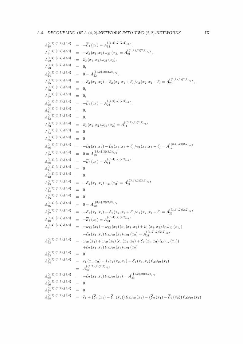
A.5. DECOUPLING OF A (4, 2)-NETWORK INTO TWO (2, 2)-NETWORKS IX
A(4,2),1,2,3,418 = −E1 (x1) = A
(1,2,2)(2,2)eff
14 ,
A(4,2),1,2,3,421 = −E2 (x1, x2) ω21 (x2) = A
(1,2,2)(2,2)eff
21 ,
A(4,2),1,2,3,422 = E2 (x1, x2) ω21 (x2) ,
A(4,2),1,2,3,423 = 0,
A(4,2),1,2,3,424 = 0 = A
(1,2,2)(2,2)eff
22 ,
A(4,2),1,2,3,425 = −E2 (x1, x2) − E2 (x2, x1 + `) /e2 (x2, x1 + `) = A
(1,2,2)(2,2)eff
23 ,
A(4,2),1,2,3,426 = 0,
A(4,2),1,2,3,427 = 0,
A(4,2),1,2,3,428 = −E2 (x1) = A
(1,2,2)(2,2)eff
24 ,
A(4,2),1,2,3,431 = 0,
A(4,2),1,2,3,432 = 0,
A(4,2),1,2,3,433 = E3 (x1, x2) ω34 (x2) = A
(3,4,2)(2,2)eff
11
A(4,2),1,2,3,434 = 0
A(4,2),1,2,3,435 = 0
A(4,2),1,2,3,436 = −E3 (x1, x2) − E3 (x2, x1 + `) /e3 (x2, x1 + `) = A
(3,4,2)(2,2)eff
12
A(4,2),1,2,3,437 = 0 = A
(3,4,2)(2,2)eff
13
A(4,2),1,2,3,438 = −E3 (x1) = A
(3,4,2)(2,2)eff
14
A(4,2),1,2,3,441 = 0
A(4,2),1,2,3,442 = 0
A(4,2),1,2,3,443 = −E4 (x1, x2) ω43 (x2) = A
(3,4,2)(2,2)eff
21
A(4,2),1,2,3,444 = 0
A(4,2),1,2,3,445 = 0
A(4,2),1,2,3,446 = 0 = A
(3,4,2)(2,2)eff
22
A(4,2),1,2,3,447 = −E4 (x1, x2) − E4 (x2, x1 + `) /e4 (x2, x1 + `) = A
(3,4,2)(2,2)eff
23
A(4,2),1,2,3,448 = −E4 (x1) = A
(3,4,2)(2,2)eff
24
A(4,2),1,2,3,451 = −ω12 (x1) − ω12 (x2) (e1 (x1, x2) + E1 (x1, x2) `Ωω12 (x1))
−E2 (x1, x2) `Ωω12 (x1) ω21 (x2) = A(1,2,2)(2,2)eff
31
A(4,2),1,2,3,452 = ω12 (x1) + ω12 (x2) (e1 (x1, x2) + E1 (x1, x2) `Ωω12 (x1))
+E2 (x1, x2) `Ωω12 (x1) ω21 (x2)
A(4,2),1,2,3,453 = 0
A(4,2),1,2,3,454 = e1 (x1, x2) − 1/e1 (x2, x3) + E1 (x1, x2) `Ωω12 (x1)
= A(1,2,2)(2,2)eff
32
A(4,2),1,2,3,455 = −E2 (x1, x2) `Ωω12 (x1) = A
(1,2,2)(2,2)eff
33
A(4,2),1,2,3,456 = 0
A(4,2),1,2,3,457 = 0
A(4,2),1,2,3,458 = e1 +
(E1 (x1) − E1 (x2)
)`Ωω12 (x1) −
(E2 (x1) − E2 (x2)
)`Ωω12 (x1)
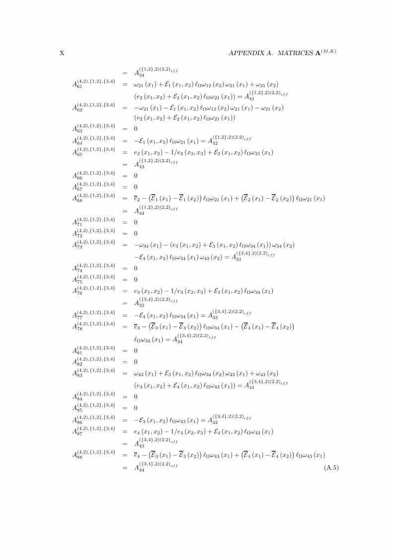
X APPENDIX A. MATRICES A(M,K)
= A(1,2,2)(2,2)eff
34
A(4,2),1,2,3,461 = ω21 (x1) + E1 (x1, x2) `Ωω12 (x2) ω21 (x1) + ω21 (x2)
(e2 (x1, x2) + E2 (x1, x2) `Ωω21 (x1)) = A(1,2,2)(2,2)eff
41
A(4,2),1,2,3,462 = −ω21 (x1) − E1 (x1, x2) `Ωω12 (x2) ω21 (x1) − ω21 (x2)
(e2 (x1, x2) + E2 (x1, x2) `Ωω21 (x1))
A(4,2),1,2,3,463 = 0
A(4,2),1,2,3,464 = −E1 (x1, x2) `Ωω21 (x1) = A
(1,2,2)(2,2)eff
42
A(4,2),1,2,3,465 = e2 (x1, x2) − 1/e2 (x2, x3) + E2 (x1, x2) `Ωω21 (x1)
= A(1,2,2)(2,2)eff
43
A(4,2),1,2,3,466 = 0
A(4,2),1,2,3,467 = 0
A(4,2),1,2,3,468 = e2 −
(E1 (x1) − E1 (x2)
)`Ωω21 (x1) +
(E2 (x1) − E2 (x2)
)`Ωω21 (x1)
= A(1,2,2)(2,2)eff
44
A(4,2),1,2,3,471 = 0
A(4,2),1,2,3,472 = 0
A(4,2),1,2,3,473 = −ω34 (x1) − (e3 (x1, x2) + E3 (x1, x2) `Ωω34 (x1)) ω34 (x2)
−E4 (x1, x2) `Ωω34 (x1) ω43 (x2) = A(3,4,2)(2,2)eff
31
A(4,2),1,2,3,474 = 0
A(4,2),1,2,3,475 = 0
A(4,2),1,2,3,476 = e3 (x1, x2) − 1/e3 (x2, x3) + E3 (x1, x2) `Ωω34 (x1)
= A(3,4,2)(2,2)eff
32
A(4,2),1,2,3,477 = −E4 (x1, x2) `Ωω34 (x1) = A
(3,4,2)(2,2)eff
33
A(4,2),1,2,3,478 = e3 −
(E3 (x1) − E3 (x2)
)`Ωω34 (x1) −
(E4 (x1) − E4 (x2)
)
`Ωω34 (x1) = A(3,4,2)(2,2)eff
34
A(4,2),1,2,3,481 = 0
A(4,2),1,2,3,482 = 0
A(4,2),1,2,3,483 = ω43 (x1) + E3 (x1, x2) `Ωω34 (x2) ω43 (x1) + ω43 (x2)
(e4 (x1, x2) + E4 (x1, x2) `Ωω43 (x1)) = A(3,4,2)(2,2)eff
41
A(4,2),1,2,3,484 = 0
A(4,2),1,2,3,485 = 0
A(4,2),1,2,3,486 = −E3 (x1, x2) `Ωω43 (x1) = A
(3,4,2)(2,2)eff
42
A(4,2),1,2,3,487 = e4 (x1, x2) − 1/e4 (x2, x3) + E4 (x1, x2) `Ωω43 (x1)
= A(3,4,2)(2,2)eff
43
A(4,2),1,2,3,488 = e4 −
(E3 (x1) − E3 (x2)
)`Ωω43 (x1) +
(E4 (x1) − E4 (x2)
)`Ωω43 (x1)
= A(3,4,2)(2,2)eff
44 (A.5)
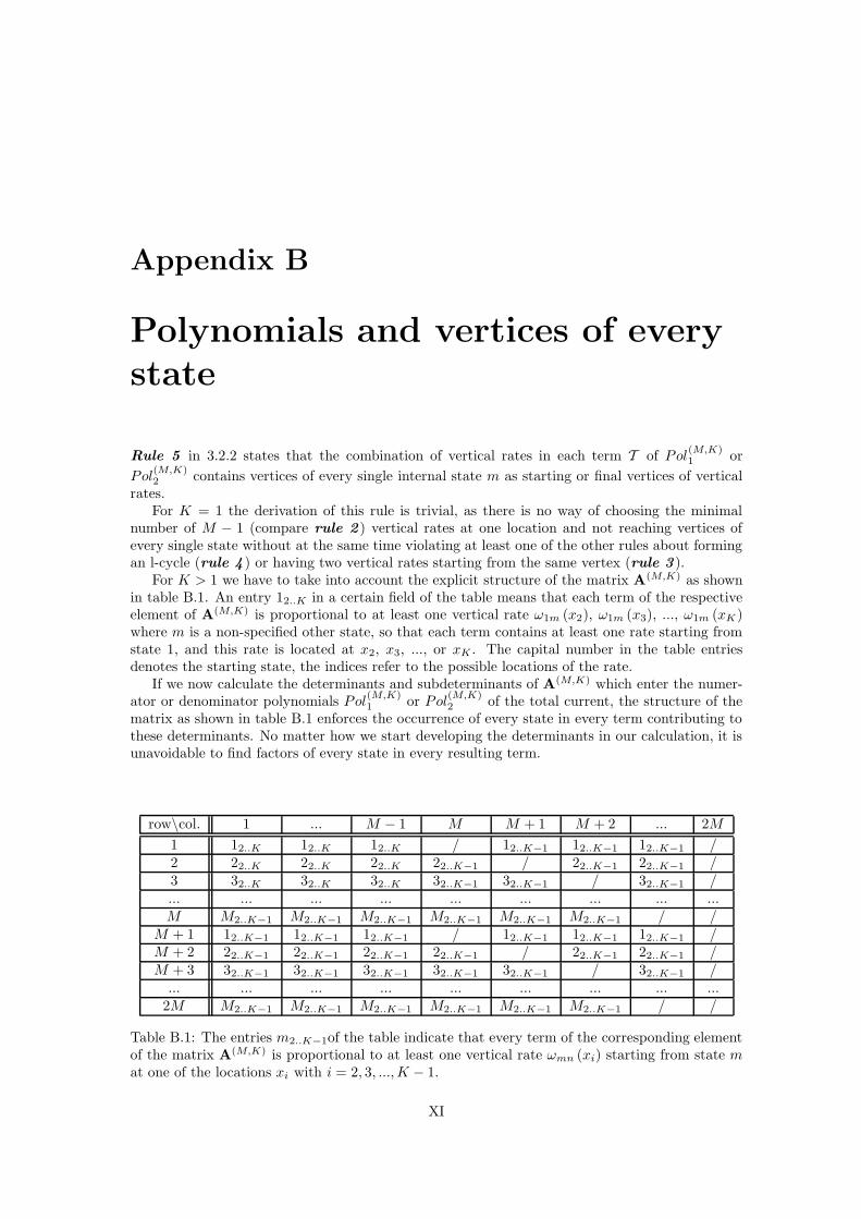
Appendix B
Polynomials and vertices of every
state
Rule 5 in 3.2.2 states that the combination of vertical rates in each term T of Pol(M,K)1 or
Pol(M,K)2 contains vertices of every single internal state m as starting or final vertices of vertical
rates.For K = 1 the derivation of this rule is trivial, as there is no way of choosing the minimal
number of M − 1 (compare rule 2 ) vertical rates at one location and not reaching vertices ofevery single state without at the same time violating at least one of the other rules about formingan l-cycle (rule 4 ) or having two vertical rates starting from the same vertex (rule 3 ).
For K > 1 we have to take into account the explicit structure of the matrix A(M,K) as shownin table B.1. An entry 12..K in a certain field of the table means that each term of the respectiveelement of A(M,K) is proportional to at least one vertical rate ω1m (x2), ω1m (x3), ..., ω1m (xK)where m is a non-specified other state, so that each term contains at least one rate starting fromstate 1, and this rate is located at x2, x3, ..., or xK . The capital number in the table entriesdenotes the starting state, the indices refer to the possible locations of the rate.
If we now calculate the determinants and subdeterminants of A(M,K) which enter the numer-ator or denominator polynomials Pol
(M,K)1 or Pol
(M,K)2 of the total current, the structure of the
matrix as shown in table B.1 enforces the occurrence of every state in every term contributing tothese determinants. No matter how we start developing the determinants in our calculation, it isunavoidable to find factors of every state in every resulting term.
row\col. 1 ... M − 1 M M + 1 M + 2 ... 2M
1 12..K 12..K 12..K / 12..K−1 12..K−1 12..K−1 /2 22..K 22..K 22..K 22..K−1 / 22..K−1 22..K−1 /3 32..K 32..K 32..K 32..K−1 32..K−1 / 32..K−1 /... ... ... ... ... ... ... ... ...M M2..K−1 M2..K−1 M2..K−1 M2..K−1 M2..K−1 M2..K−1 / /
M + 1 12..K−1 12..K−1 12..K−1 / 12..K−1 12..K−1 12..K−1 /M + 2 22..K−1 22..K−1 22..K−1 22..K−1 / 22..K−1 22..K−1 /M + 3 32..K−1 32..K−1 32..K−1 32..K−1 32..K−1 / 32..K−1 /
... ... ... ... ... ... ... ... ...2M M2..K−1 M2..K−1 M2..K−1 M2..K−1 M2..K−1 M2..K−1 / /
Table B.1: The entries m2..K−1of the table indicate that every term of the corresponding elementof the matrix A(M,K) is proportional to at least one vertical rate ωmn (xi) starting from state mat one of the locations xi with i = 2, 3, ..., K − 1.
XI

XII APPENDIX B. POLYNOMIALS AND VERTICES OF EVERY STATE
Appendix C
Terminology and basics on graph
theory
In this appendix we summarize important terms and relationships from the field of graph theory.For a detailed overview see [53, 67].
A graph G is an ordered 2-tuple, (V (G) , E (G)), which consists of a set V (G) of vertices anda set E (G) of edges.
A vertex can be imagined as a point, node or 0-simplex.An edge can be referred to as a line, an arc or a 1-simplex.A directed graph is a graph whose edges have an orientation.If V (G) and E (G) are finite sets, the graph is said to be finite.The degree of a vertex is given by the number of edges having that vertex for one of their
endpoints.A graph in which every vertex is of even degree belongs to the class of Euler graphs.An edge sequence is a graph or subgraph whose edges can be ordered in such a way that each
edge with the exclusion of the initial edge and the final edge has a vertex in common with thepreceding edge in the ordered sequence and the other vertex in common with the succeeding edge.
The multiplicity of an edge in an edge sequence is the number of times an edge appears in anedge sequence.
If the multiplicity of each edge in an edge sequence is one, the edge sequence is called an edgetrain or walk.
The terminal vertices of the edge sequence are the initial and final vertices.In the case of coinciding terminal vertices the edge train is a closed edge train.An edge train is a path if the degree of each nonterminal vertex is two and the degree of each
terminal vertex is one.In a connected graph there is a path between any two distinct vertices of the graph.A digraph is strongly connected if there is at least one directed path from every vertex to every
other vertex.A digraph is weakly connected if the underlying undirected graph is connected.A graph without self-loops and parallel edges is a simple graph.Self-loops are edges with identical endpoints.A cut set is a set of edges whose removal splits a weakly connected directed graph into two
separate parts.An edge train that contains more than one edge, is closed and only has vertices of degree two
is a loop, circuit or cycle.A spanning-cycle or short s-cycle starts at vertex (m, k = 1), spans the whole network parallel
to the x-direction, ends at vertex (m, k = K) and can be supplemented with the di-edge between(m, k = K) and (m, k = 1) to form a cycle, see fig. 2.1. If the horizontal di-edges are not knownexplicitly the s-cycle shows as an edge train of vertical rates starting and ending in state m where
XIII
XIV APPENDIX C. TERMINOLOGY AND BASICS ON GRAPH THEORY
each edge with the exclusion of the initial edge and the final edge has a state in common with thepreceding edge and the other state in common with the succeeding edge.
A localized or l-cycle is a cycle of vertical di-edges at a single location.A self-loop is a closed edge train with only one edge.A subgraph H of a graph G consists of subsets of vertices and edges of G such that the endpoints
of every edge in H are in H , too.A spanning tree is any connected subgraph of a graph over the same set of nodes which does
not comprise loops.
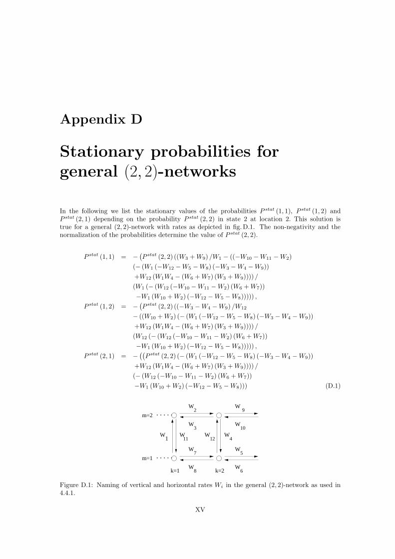
Appendix D
Stationary probabilities for
general (2, 2)-networks
In the following we list the stationary values of the probabilities P stat (1, 1), P stat (1, 2) andP stat (2, 1) depending on the probability P stat (2, 2) in state 2 at location 2. This solution istrue for a general (2, 2)-network with rates as depicted in fig.D.1. The non-negativity and thenormalization of the probabilities determine the value of P stat (2, 2).
P stat (1, 1) = −(P stat (2, 2) ((W3 + W9) /W1 − ((−W10 − W11 − W2)
(− (W1 (−W12 − W5 − W8) (−W3 − W4 − W9))
+W12 (W1W4 − (W6 + W7) (W3 + W9)))) /
(W1 (− (W12 (−W10 − W11 − W2) (W6 + W7))
−W1 (W10 + W2) (−W12 − W5 − W8))))) ,
P stat (1, 2) = −(P stat (2, 2) ((−W3 − W4 − W9) /W12
− ((W10 + W2) (− (W1 (−W12 − W5 − W8) (−W3 − W4 − W9))
+W12 (W1W4 − (W6 + W7) (W3 + W9)))) /
(W12 (− (W12 (−W10 − W11 − W2) (W6 + W7))
−W1 (W10 + W2) (−W12 − W5 − W8))))) ,
P stat (2, 1) = −((
P stat (2, 2) (− (W1 (−W12 − W5 − W8) (−W3 − W4 − W9))
+W12 (W1W4 − (W6 + W7) (W3 + W9)))) /
(− (W12 (−W10 − W11 − W2) (W6 + W7))
−W1 (W10 + W2) (−W12 − W5 − W8))) (D.1)
m=1 . . . . .
m=2 . . . . .
k=1 k=2
W
W1
2
W
W
W
W
W
W
W
3
5
6
7
8
9
10
4WW
11W
12
Figure D.1: Naming of vertical and horizontal rates Wi in the general (2, 2)-network as used in4.4.1.
XV
XVI APPENDIX D. STATIONARY PROBABILITIES FOR GENERAL (2, 2)-NETWORKS
Appendix E
Algorithms for path problems
E.1 Maximum-flow problem
Every edge connecting a pair of vertices vi and vj has a certain capacity cij . Before starting anew cycle of the algorithm with the starting vertex vs = s, the actual flow qij for each edge isupdated. In the beginning, all the edge flows are zero. Then a label is attached to a vertex in apossible flow-augmenting path which is the minimum of the label of the preceding vertex and thedifference between edge capacity and momentary flow. This process of labelling is continued untileither no additional labels can be placed and the algorithm stops or the terminal vertex becomesthe new starting vertex and the path is completed. Backtracking is necessary in order to updatethe actual flows, before the next flow-augmenting path is looked for.
E.2 Shortest-path problem
Every edge between a pair of vertices vi and vj has a certain cost or fee fij associated with it.We start in state 1. The source vertex receives the label 0 which is set permanent. The other
vertices are labelled with ∞ or, in an actual implementation with a number which is very largecompared to the system costs. The temporary labels lab (vj) of the vertices which are terminalvertices of edges originating from the starting vertex vs are updated according to lab (vj) =min (lab (vj) , lab (vs) + fsj). The minimum label of the vertices with temporary labels is thenmarked as permanent. The choice is not necessarily unambiguous. The vertex with the newpermanent label is the new starting vertex vs. The updating is repeated until the terminal vertexis set the starting vertex. Its label gives the costs for the shortest path. The corresponding pathis found by backtracking from the terminal vertices as the difference of the labels between thecurrent vertex and the preceding vertex of the path equals the cost of the respective edge. If theshortest path does not include horizontal edges, we search for an alternative path whose costs arehigher, but which forms a proper s-cycle.
Then the operation is continued with the search for the shortest path of the next state. Theprocedure is repeated until the shortest path for the last level M is found.
XVII

XVIII APPENDIX E. ALGORITHMS FOR PATH PROBLEMS
List of symbols
• A(M,K) is a 2M × 2M matrix describing a system of M states and K locations
• A(M,K),m1,n1,...,m2,n2,... is the matrix of the (M, K)-system which decomposes into thetwo subsets V1 with the states m1, n1,... and V2 with m2, n2,...
• A(m1,n1,...,K)(M1,K)eff the effective (M1, K) matrix where M1 is the number of states com-prised in the first subset of vertices V1 belonging to the states m1, n1,...; describes thesubnetwork belonging to V1
• cij capacity of directed edge (vi, vj)
• Dm diffusion coefficient in lateral currents Jm
• ∆mn (xk) unbalanced parts of transition rates
• em (y, z) exponential functions given by exp (Vm (y) − Vm (z))
• ε coupling parameter, in 5.2 transition width
• Em (x, y) integral defined by 1Dm
∫ y
x dzem (z, y)
• fij costs or fees for edges
• F applied (tangential) force; a load force corresponds to F < 0
• G = (V (G) , E (G)) directed connected graph with corresponding set of vertices V (G) andset of edges E (G)
• Γ concentration of fuel molecules such as ATP
• Γ∗ characteristic intermediate concentration
• Im transition current density for internal state m
• Jm lateral current for internal state m
• Jm average currents
• J(M,K)tot total lateral current in an (M, K)-system
• J(M,K)
tot total current in the Master-equation approach
• ∆Jm current discontinuities
• K number of locations for transitions between internal states
• ` period of molecular force potentials
• `Ω molecular “localization” length for transition rates
XIX
XX LIST OF SYMBOLS
• M total number of internal motor states
• M−1i probability weight of state i
• Ωmn spatially dependent transition rate from state m to state n
• ωmn transition rate from state m to state n
• ωdbmn part of transition rate fulfilling detailed balance
• p (m, k |m′, k′ ) (t) time-dependent transition functions
• Pm probability density for internal state m
• Pol(M,K)i polynomial in the numerator (i = 1) or denominator (i = 2) of the expression for
J(M,K)tot
• Pol(M,K)
i polynomials in the Master-equation approach
• Ptot total probability density
• P(M,K) (t) quadratical matrix of the transition functions
• q (m, k |m′, k′ ) infinitesimal transition rates
• Q number of unbalanced transition rates
• Q(M,K) infinitesimal generator
• s source vertex
• t time, in 4.5 terminal vertex
• T temperature in energy units
• T term of polynomial Pol(M,K)i
• Um molecular interaction potential for internal state m
• Vi subsets of vertices
• Vm effective force potential
• v motor velocity
• vi with vi = (m, k) vertex of the network in state m at location k
• W (m, k |m′, k′ ) transition rate from state (m, k) into state (m′, k′)
• x spatial coordinate for motor position
• xk position at which motor undergoes localized transition
• X (t) stochastic process
Bibliography
[1] B.Alberts, A. Johnson, J Lewis, M.Raff, K.Roberts, and P. Walter, Molekularbiologie derZelle, 3. Auflage (VCH, 1995), and Molecular Biology of the Cell, 4th edition (Garland, 2002).
[2] J.Howard, Mechanics of Motor Proteins and the Cytoskeleton, 1 ed. (Sinauer, New York,2001).
[3] M. Schliwa and G. Woehlke, Nature (London) 422, 759 (2003).
[4] http://home19.inet.tele.dk/griscellisyndrome.
[5] S.A. Endow, H. Higuchi, Nature (London) 406, 913 (2000).
[6] K.Homma, M. Yoshimura, J. Salto, R. Ikebe and M. Ikebe, Nature (London) 412, 831 (2001).
[7] J.Howard, A. J.Hudspeth, and R. D. Vale, Nature (London) 342, 154 (1989).
[8] K. Svoboda, C. Schmidt, B. Schnapp, and S. Block, Nature (London) 365, 721 (1993).
[9] K. Svoboda and S.Block, Cell 77, 773 (1994).
[10] M. J. Schnitzer and S. M. Block, Nature (London) 388, 386 (1997).
[11] W. Hua, E.C. Young, M. L. Fleming, and J.Gelles, Nature (London) 388, 390 (1997).
[12] W. O.Hancock and J.Howard, J.Cell Biol. 140, 1395 (1998).
[13] M.Thormahlen, A. Marx, S. A. Mueller, Y.-H. Song, E.-M.Mandelkow, U. Aebi, andE.Mandelkow, J.Mol. Biol. 275, 795 (1998).
[14] S.Gilbert, M. Moyer, and K. Johnson, Biochemistry 37, 792 (1998).
[15] K.Visscher, M. J. Schnitzer, and S. M.Block, Nature (London) 400, 184 (1999).
[16] Y. Okada and N. Hirokawa, Science 283, 1152 (1999).
[17] A. D. Mehta, R. S. Rock, M. Rief, J. A. Spudich, M. S. Mooseker, and R. E.Cheney, Nature(London) 400, 590 (1999).
[18] M.Rief, R. S. Rock, A. D. Mehta, M. S. Mooseker, R. E. Cheney, and J. A. Spudich,Proc. Nat. Acad. Sci. USA 97, 9482 (2000).
[19] A. Mehta, J. Cell Sci. 114, 1981 (2001).
[20] C.Veigel, F. Wang, M. L. Bartoo, J. R. Sellers and J.E. Molloy, Nature Cell Biol. 4, 59 (2002).
[21] Z.Wang and M.P. Sheetz, Biophys. J. 78, 1955 (2000).
[22] S.King, Biochimica Acta - Mol. Cell Res. 1496, 60 (2000).
[23] E.Hirakawa, H. Higuchi, and Y. Y. Toyoshima, Proc.Nat. Acad. Sci. USA 97, 2533 (2000).
XXI
XXII BIBLIOGRAPHY
[24] R. Lipowsky, S. Klumpp, and Th. M. Nieuwenhuizen, Phys. Rev. Lett.87, 108101.1 (2001).
[25] Th.M. Nieuwenhuizen, S. Klumpp, and R. Lipowsky, Europhys. Lett.58, 468 (2002).
[26] Th.M. Nieuwenhuizen, S. Klumpp, and R. Lipowsky, in preparation.
[27] S.Klumpp, Movements of Molecular Motors: Diffusion and Directed Walks (Dissertation,Potsdam, 2003).
[28] R.D. Vale and R. A. Milligan, Science 288, 88 (2000).
[29] P.Reimann, Brownian motors: noisy transport far from equilibrium, Phys. Rep. 361, 57(2001).
[30] T.R. Kelly, I. Tellitu, and J.P. Sestelo, Angew.Chem. Int. Ed. Engl. 36, 1866 (1997).
[31] K.L. Sebastian, Phys. Rev. E 61, 937 (2000).
[32] R.Feynman,The Feynman lectures on physics (Addison-Wesley, Reading, Massachusetts,1963).
[33] Several people have pointed out that Feynman’s arrangement contains a misconception con-cerning reversibility, see e.g. Parrondo, Espanol, Am. J. Phys. 64 (9), September 1996 andMagnasco, Stolovitzky, J. Stat. Phys. 93, Nos. 3/4, 1998.
[34] A. F. Huxley, Prog. Biophys. Mol. Biol. 7, 255 (1957).
[35] J.Howard, A. J.Hudspeth, and R. D. Vale, Nature 342, 154 (1989).
[36] S. Leibler and D. A. Huse, J.Cell Biol. 121, 1357 (1993).
[37] J.Prost, J.-F.Chauwin, L. Peliti, and A. Ajdari, Phys. Rev. Lett.72, 2652 (1994).
[38] T.Harms and R. Lipowsky, Phys. Rev. Lett.79, 2895 (1997).
[39] F. Julicher, A. Ajdari, and J. Prost, Rev.Mod. Phys. 69, 1269 (1997).
[40] R. Lipowsky and T. Harms, Eur. Biophys. J.29, 542 (2000).
[41] R. Lipowsky, Phys. Rev. Lett.85, 4401 (2000).
[42] L. Schimansky-Geier, M. Kschischo, and T. Fricke, Phys. Rev. Lett.79, 3335 (1997).
[43] R. Lipowsky and N. Jaster, J. of Stat. Phys. 110, 1141 (2003).
[44] N. Jaster and R. Lipowsky, in preparation.
[45] N. van Kampen, Stochastic processes in physics and chemistry (Elsevier, Amsterdam, 1992).
[46] F. Schwabl, Statistische Mechanik (Springer, Berlin, 2000)
[47] H. Risken, The Fokker-Planck equation: methods of solution and applications (Springer Ver-lag, Berlin, 1989).
[48] R.Astumian and M. Bier, Phys. Rev. Lett.72, 1766 (1194).
[49] A. Parmeggiani, F. Julicher, A. Ajdari, and J. Prost, Phys. Rev. E 60, 2127 (1999).
[50] A. Kolomeisky and B. Widom, J. of Stat. Phys. 93, 633 (1998).
[51] M.E. Fisher and A. B. Kolomeisky, Proc. Nat. Acad. Sci. USA 98, 7748 (2001).
[52] G.Lattanzi and A. Maritan, Biophys. J.82, 2348 (2002).
BIBLIOGRAPHY XXIII
[53] W. D. Wallis, A beginner’s guide to graph theory (Birkhauser, Boston, 2000).
[54] R.G. Busacker and T. L. Saaty, Finite graphs and networks, an introduction with applications(McGraw-Hill, 1965).
[55] Mathematica and Maple.
[56] W. H. Press and S. A. Teukolsky, Numerical recipes in C: the art of scientific computing, 2ndedition (Cambridge Univ. Press, 1992).
[57] J. Stoer, R. Bulirsch, Introduction to Numerical Analysis, Second Edition (Springer-VerlagNew York, Inc., 1993).
[58] K.Meyberg and P. Vachenauer, Hohere Mathematik, 2. Auflage (Springer-Verlag Berlin, 1997).
[59] A. J. Lichtenberg and M. A. Lieberman, Regular and Chaotic Dynamics, Second Edition(Springer-Verlag New York, Inc., 1992).
[60] R.Diestel, Graph Theory, Second Edition (Springer-Verlag New York, Inc., 2000).
[61] K.Kruse and F. Julicher, Phys. Rev. Lett.85, 1778 (2000).
[62] K.Kruse, S. Camalet and F. Julicher, Phys. Rev. Lett.87, 138101 (2001).
[63] A. T.Bharucha-Reid, Elements of the Theory of Markov Processes and their Applications(McGraw-Hill, 1960).
[64] J.G. Kemeny and J. L. Snall, Finite Markov Chains (Springer-Verlag New. York, Inc., 1976).
[65] http://mathstat.wu-wien.ac.at.
[66] S.C. Ammal, H. Yamataka, M. Aida, M. Dupuis, Science 299, 1555 (2003).
[67] N. K.Bose and P. Liang, Neural network fundamentals with graphs, algorithms, and applica-tions (McGraw-Hill, 1996).
[68] J. Falbe, M.Regnitz, Rompp Lexikon Chemie, 9. Auflage (Thieme Verlag Stuttgart 1989).
[69] H. Bisswanger, Enzymkinetik, Theorie und Methoden, 2. Auflage (VCH VerlagsgesellschaftmbH Weinheim, 1994).
[70] K.Burton, J.Muscle Res. Cell Motil. 13, 590 (1992).
[71] T.Yanagida, Y. Harada and A. Ishijima, Trends Biochem. Sci. 18, 319 (1993).
[72] K. J.Bohm, R. Stracke and E.Unger, Cell Biol. Int.24, No. 6, 335 (2000).
[73] T. J. Harms, Transporteigenschaften geordneter und ungeordneter Ratschen (Dissertation,Potsdam, 1998).
Related Documents