Rare Events in Stochastic Systems: Modeling, Simulation Design and Algorithm Analysis Yixi Shi Submitted in partial fulfillment of the requirements for the degree of Doctor of Philosophy in the Graduate School of Arts and Sciences Columbia University 2013

Welcome message from author
This document is posted to help you gain knowledge. Please leave a comment to let me know what you think about it! Share it to your friends and learn new things together.
Transcript

Rare Events in Stochastic Systems:Modeling, Simulation Design and Algorithm Analysis
Yixi Shi
Submitted in partial fulfillment of therequirements for the degree of
Doctor of Philosophyin the Graduate School of Arts and Sciences
Columbia University
2013

c©2013 – Yixi ShiAll rights reserved.

Abstract
Rare Events in Stochastic Systems: Modeling,
Simulation Design and Algorithm Analysis
Yixi Shi
This dissertation explores a few topics in the study of rare events in stochastic systems,
with a particular emphasis on the simulation aspect. This line of research has been
receiving a substantial amount of interest in recent years, mainly motivated by scientific
and industrial applications in which system performance is frequently measured in terms
of events with very small probabilities.
The topics mainly break down into the following themes:
- Algorithm Analysis: Chapters 2, 3, 4 and 5.
- Simulation Design: Chapters 3, 4 and 5.
- Modeling: Chapter 5.

Contents
Table of Contents iv
List of Tables vi
List of Figures vii
Acknowledgement viii
1 Introduction 1
1.1 Overview . . . . . . . . . . . . . . . . . . . . . . . . . . . . . . . . . . . . . 1
1.2 Rare Event Simulation: Preliminaries . . . . . . . . . . . . . . . . . . . . . 6
1.2.1 Asymptotic Notations . . . . . . . . . . . . . . . . . . . . . . . . . 6
1.2.2 Heavy-tailed Distributions . . . . . . . . . . . . . . . . . . . . . . . 7
1.2.3 Importance Sampling and Multilevel Splitting . . . . . . . . . . . . 10
1.2.4 Notions of Efficiency . . . . . . . . . . . . . . . . . . . . . . . . . . 12
1.2.5 Constructing Efficient Simulation Estimators in Light-tailed Sys-
tems: The Subsolution Approach . . . . . . . . . . . . . . . . . . . 15
1.2.6 State-dependent Importance Sampling for Heavy-tailed Systems . . 20
i

1.2.7 Variance Control via Lyapunov Functions . . . . . . . . . . . . . . 22
2 Analysis of a Splitting Estimator 26
2.1 Introduction . . . . . . . . . . . . . . . . . . . . . . . . . . . . . . . . . . . 27
2.2 Benchmark to the Splitting Algorithm . . . . . . . . . . . . . . . . . . . . 31
2.3 Jackson Networks: Notation and Properties . . . . . . . . . . . . . . . . . 33
2.4 The Splitting Algorithm . . . . . . . . . . . . . . . . . . . . . . . . . . . . 43
2.5 Analysis of Splitting Estimators . . . . . . . . . . . . . . . . . . . . . . . . 47
3 Splitting for Heavy-tailed Systems 69
3.1 Introduction . . . . . . . . . . . . . . . . . . . . . . . . . . . . . . . . . . . 69
3.2 Problem Setting and Assumptions . . . . . . . . . . . . . . . . . . . . . . . 74
3.3 Hazard Rate Splitting . . . . . . . . . . . . . . . . . . . . . . . . . . . . . 75
3.3.1 Splitting Mechanism and “Tree” Construction . . . . . . . . . . . . 75
3.3.2 Fully Branching Representation of Π . . . . . . . . . . . . . . . . . 79
3.4 A Splitting-Resampling Algorithm . . . . . . . . . . . . . . . . . . . . . . . 80
3.5 Analysis of the Splitting-Resampling Algorithm . . . . . . . . . . . . . . . 84
3.5.1 Number of Particles . . . . . . . . . . . . . . . . . . . . . . . . . . 84
3.5.2 Logarithmic Efficiency and Optimal Choice of θ . . . . . . . . . . . 87
3.6 An Improved Hazard Function Splitting Algorithm . . . . . . . . . . . . . 94
3.6.1 The “Mega” Splitting Algorithm . . . . . . . . . . . . . . . . . . . 95
3.6.2 Analysis of the Mega-Splitting Algorithm . . . . . . . . . . . . . . . 98
3.7 Numerical Examples . . . . . . . . . . . . . . . . . . . . . . . . . . . . . . 105
4 Rare Event Simulation via Cross Entropy 108
4.1 Introduction . . . . . . . . . . . . . . . . . . . . . . . . . . . . . . . . . . . 109
4.2 Heavy-tailed Increment Distributions . . . . . . . . . . . . . . . . . . . . . 112
ii

4.3 Parametric Family of IS Distributions . . . . . . . . . . . . . . . . . . . . . 113
4.4 Strong Efficiency of the Family under Consideration . . . . . . . . . . . . . 118
4.5 Cross Entropy Method and the Iterative Equations for the Mixture Family 123
4.5.1 Review of Cross-Entropy Method . . . . . . . . . . . . . . . . . . . 123
4.5.2 Iterative Equations for the Mixture IS Family . . . . . . . . . . . . 125
4.6 Numerical Examples . . . . . . . . . . . . . . . . . . . . . . . . . . . . . . 130
4.6.1 Example 1: Regularly Varying Increments . . . . . . . . . . . . . . 130
4.6.2 Example 2: Weibull Increments . . . . . . . . . . . . . . . . . . . . 134
5 Stochastic Insurance-Reinsurance Networks 135
5.1 Motivations and Goals . . . . . . . . . . . . . . . . . . . . . . . . . . . . . 136
5.2 The Network Model and Its Properties . . . . . . . . . . . . . . . . . . . . 140
5.2.1 Contractual Specifications and Network Topology . . . . . . . . . . 141
5.2.2 Settlement Mechanism and Network Equilibrium . . . . . . . . . . 147
5.2.3 Connections to the Eisenberg-Noe ([40]) Formulation . . . . . . . . 153
5.2.4 Effective Claims and Reserve Processes . . . . . . . . . . . . . . . . 159
5.2.5 Conditional Spillover Loss at System Dislocation . . . . . . . . . . 161
5.3 Asymptotic Description of the Network System . . . . . . . . . . . . . . . 162
5.3.1 Large Deviations Description via An Integer Program . . . . . . . . 163
5.3.2 Characterizing Asymptotic Behavior of A Special Network . . . . . 168
5.4 Design of Efficient Simulation Algorithms for Ne . . . . . . . . . . . . . . . 178
5.4.1 Guidelines for Simulation Design . . . . . . . . . . . . . . . . . . . 179
5.4.2 A Mixture-based SDIS . . . . . . . . . . . . . . . . . . . . . . . . . 180
5.4.3 The Algorithm . . . . . . . . . . . . . . . . . . . . . . . . . . . . . 186
5.4.4 Proof of Theorem 5.5 and 5.7. . . . . . . . . . . . . . . . . . . . . . 190
5.5 Numerical Examples . . . . . . . . . . . . . . . . . . . . . . . . . . . . . . 195
iii

5.6 Proofs of Technical Results . . . . . . . . . . . . . . . . . . . . . . . . . . . 199
Bibliography 214
iv

List of Tables
3.1 Numerical results for p1, i.e., sums of Pareto with α = 1.5. . . . . . . . . . 106
3.2 Numerical results for p2, i.e., sums of Weibull with β = 0.2. . . . . . . . . . 106
3.3 Numerical results for p2, i.e., sums of Weibull with β = 0.75. . . . . . . . . 107
4.1 Performance of the SDIS-CE estimator compared to the SDIS algorithm
without CE procedure where the input mixing probabilities are set to be
pk = 0.9/(m− k) for k = 1, 2, ...,m− 1. . . . . . . . . . . . . . . . . . . . . 131
4.2 Performance of the SDIS-CE estimator compared to the SDIS without CE
procedure where the input mixing probabilities are set to be the optimal
choice obtained in Dupuis, Leder and Wang (2006). . . . . . . . . . . . . . 132
4.3 Comparison of performance between 1) SDIS using CE optimal mixing
probabilities and 2) Analytical optimal mixing probabilities from Dupuis,
Leder and Wang (2006), m = 2. . . . . . . . . . . . . . . . . . . . . . . . . 133
4.4 Average optimal CE .mixing probabilities, m = 4, b = 106. . . . . . . . . . 133
v

4.5 Performance of the SDIS-CE estimator compared to SDIS without CE
procedurein the case of Weibull-type of increments, m = 4. We used
pk,j = 1/(K + 2)(m− k), for j = 0, 1, ...K and k = 1, 2, ...,m − 1 as the
“standard” choice of the mixing probabilities. . . . . . . . . . . . . . . . . 134
5.1 Values of model parameters in numerical examples. . . . . . . . . . . . . . 196
5.2 Numerical results with scenarios 1-3 with A = 3. . . . . . . . . . . . . . 197
5.3 Numerical results with scenarios 1-3 with A = 2, 3. . . . . . . . . . . . . 198
5.4 Comparison of results in Scenario 2, A = 3, without/with IS for Zn
switched off. . . . . . . . . . . . . . . . . . . . . . . . . . . . . . . . . . . . 199
vi

List of Figures
3.1 Example of a constructed tree. In this example, b = 1012, α = 0.2. The
subgraph on the left illustrates a constructed tree in the hazard function
of the increment X. The subgraph on the right shows the sampled values
(in the original space) of those black-colored leafs in the tree on the left. . 78
5.1 Network Ne1 . Each insurer enters into excess-of-loss reinsurance contracts
with multiple reinsurers. A “reinsurance-spiral” among the reinsurance
companies exists and is indicated by the “cycle” consisting of the curved
lines. . . . . . . . . . . . . . . . . . . . . . . . . . . . . . . . . . . . . . . 147
5.2 (a): For each reinsurer the initial reserve levels are stated in the parenthe-
ses. For each insurer, the initial reserve as well as the reinsurance deductible
are given in the parentheses next to the company. Transfer ratios are given
next to the arrow representing the flow of contracts. (b): State of the net-
work after all claims have been collected, before the write-offs. Bracketed
numbers are the sizes of the claims. Numbers in parentheses are effective
claims to the companies. And the rest is the transferred amount. . . . . . . 149
5.3 An example of a “star-shaped” network. . . . . . . . . . . . . . . . . . . . 169
vii

Acknowledgments
As the ancient Romans put it: Every new beginning comes from other beginning’s
end, while this dissertation unlatches my journeys ahead, it also marks, sadly, the
end of my PhD life here at the IEOR department of Columbia University. I would like to
dearly thank everyone that brought strength and joy to me during this otherwise arduous
experience.
I am indebted to Professor Jose Blanchet, my advisor, teacher, mentor and friend.
Jose took me as his first PhD student in Columbia when he came to IEOR from Harvard
Statistics, and during the course of the past four and half years, he has been ungrudgingly
sharing with me his sophisticated understanding of the field of rare event simulation. I
enjoyed every bit of our discussion, whether it was in Mudd 340, in the pizza place on
Amsterdam Ave., or over Skype (and believe it or not, we almost pulled off an academic
meeting in Metropolitan Museum of Art). I am in awe of his abysmal knowledge, his
astute intuition, his passionate and meticulous attitude towards research, and his humble
and affable personality. Without his patience and support, I can hardly imagine getting
this far.
viii

I am wholeheartedly thankful to my dissertation committee, Professors Ward Whitt,
Karl Sigman, Jingchen Liu and Henry Lam, for taking time to be the readers of my dis-
sertation, and providing useful feedbacks on my work. I am also grateful to Professor
Martin Haugh, who had been a reader of Chapter 5 of the dissertation and returned can-
did comments and constructive suggestions on the insurance network model therein; and
Professor Kevin Leder (from Industrial and Systems Engineering Department of Univer-
sity of Minnesota) whom I collaborated with along with Jose in the work of Chapter 2. I
also benefited lifelong from the remarkable teachings of Professors Ward Whitt, Donald
Goldfarb, Daniel Bienstock, David Yao, Steve Kou, Jose Blanchet, Rama Cont, Mariana
Olvera-Cravioto, Cliff Stein, Jingchen Liu (Statistics) Julien Dubedat (Maths), Duong
Hong Phong (Maths), Assaf Zeevi (CBS), Michael Johannes (CBS) and Mark Broadie
(CBS). I would like to also extend my gratitude to all the staff from IEOR department,
who has being doing an awesome job creating a pleasant and homey atmosphere in the
department, including the high-frequency supply of free food of course.
Research life in a windowless cubicle (Mudd 313) could have been depressing and
monotonous. But thanks to my unique office mates, those days in the office have been
my most cherished memories in the past few years. After all, how many PhD offices have
their own t-shirts? I would certainly miss all of you, Cecilia Zenteno, Rodrigo Carrasco,
Tulia Humphries, Jinbeom Kim, Xingbo Xu, Haowen Zhong, Tony Qin, Arseniy Kukanov,
Andrew Ang, and those who have already graduated: Serhat Aybat, Rishi Talreja, Nur
Ayvaz, Ohad Perry, Zongjian Liu and Rouba Ibrahim. Indeed, all of my friends and
colleagues in Columbia added colors to my PhD life.
I would like to reserve my last gratitudes to my family. In particular, I would like
ix

to dedicate this dissertation to my parents, Bingcheng Shi and Huanya Jiang, who have
given me unconditional support and love in every dimension imaginable. And special
thanks to my beloved wife Jingjing Song, for keeping me smiling, giving me confidence
and putting up with my random schedules along the way.
x

To my parents Huanya and Bingcheng.
xi

Organize, don’t agonize.
Nancy Pelosi
1Introduction
1.1 Overview
This dissertation explores a few topics in the study of rare events in stochastic systems,
with a particular emphasis on the simulation aspect. This line of research has been
receiving a substantial amount of interest in recent years, mainly motivated by scientific
and industrial applications in which system performance is frequently measured in terms
of events with very small probabilities.
The topics mainly break down into the following themes:
1

CHAPTER 1. INTRODUCTION 2
- Algorithm Analysis: Chapters 2, 3, 4 and 5.
- Simulation Design: Chapters 3, 4 and 5.
- Modeling: Chapter 5.
After this overview we shall briefly review some standard definitions and results that are
used throughout the development in this dissertation. In order to have a better overview
of the topics covered in the ensuing chapters, I lay out the organizations of the main
chapters as follows.
1) Chapter 2 is devoted to the study of splitting methodology in rare event simulation.
The study is inspired by the recent work of [31], in which a splitting estimator is pro-
posed and shown to possess asymptotic optimality (see the definition in Subsection
1.2.4) for estimating small probabilities in a light-tailed setting that can be properly
approximated using large deviations techniques. Our curiosity is fueled by the fact
that in many circumstances the large deviation scaling seems not sufficient to make
a precise statement on the performance advantage of splitting over system-specific
benchmark algorithms. In addition, it is also helpful to better understand the con-
nection and therefore make guidance implications between splitting and importance
sampling strategies. We therefore attempt a sharper analysis on the splitting esti-
mator developed in [31] (a variant of the class of splitting based strategies proposed
by [58]), for the particular problem of estimating overflow probabilities in an open
Jackson network. Recognizing that crude Monte Carlo is not the correct bench-
mark to use in this problem setup, we directly compare the complexity of splitting
algorithm to that of solving a system of linear equations. While we find out that
splitting does outperform the benchmark solution algorithm, it does hold its bells
and whistles against competing importance sampling strategies. The analysis serves

CHAPTER 1. INTRODUCTION 3
as a natural supplement to the series of papers by Paul Dupuis, Hui Wang and their
students (e.g., [37], [35], [36], [39] and [31]) on the use of rigorous control theory to
construct provably efficient rare event simulation algorithms.
2) The endeavor in Chapter 2 raises a natural question to the applicability of splitting-
based strategies that goes beyond the light-tailed setting. The construction of impor-
tance sampling and splitting algorithms are shown to share a similar root, (see e.g.,
[37] and [31] and the discussion in Subsection 3.1). In fact, splitting based estima-
tors are in some sense more convenient to come up with. Do we have a similar story
in heavy-tailed systems? These are the questions we attempt to address in Chapter
3. We try to open the door this line of research by exploring two related splitting-
based algorithms designed for a suitable class of heavy-tailed stochastic systems.
Both algorithms circumvent the original state space of the underlying stochastic
process, and take advantage of some desirable properties of the hazard functions of
the increment distributions. More precisely, we embed a splitting procedure in the
hazard function space, for which we refer to as the hazard function splitting (HFS)
strategy. The algorithms are shown to enjoy a uniform setup across the class of in-
put structure of the system. However, on the flip side, although these algorithms are
both proved to satisfy the designated asymptotic optimality property, they are not
as efficient as some importance sampling based strategies that exploit the distinct
large deviation characterizations of heavy-tailed systems.
3) In Chapter 4, we switch gear to study a parametric class of state-dependent impor-
tance sampling (SDIS) estimators that is more consistent with how rare events tend
to occur in heavy-tailed systems. Quite different from their light-tailed counterparts,
in which large deviations occur in a more “cooperative” fashion among the system
inputs, the occurrence of rare events for heavy-tailed systems complies with the so

CHAPTER 1. INTRODUCTION 4
called “principle of large jumps” (see the brief introduction in Subsections 1.2.2 and
1.2.6). In earlier works, for example [22], this mixture based SDIS is shown to be
closely tracking the most likely paths of heavy-tailed systems. As a result, with very
mild conditions on the parameters, this class of estimators is guaranteed to possess
strong efficiency. This desirable “closedness” property enables us to leverage the
tool of cross entropy to achieve a better performance within the class of strongly
efficient mixture-based importance sampling estimators. Closed form recursive for-
mulas to update the mixing probability parameters are provided in this chapter,
and a few interesting observations are discussed following the numerical examples
illustrated at the end of the chapter.
4) The last chapter, Chapter 5, takes on a holistic approach to study rare events in a
specific heavy-tailed financial network system, which is carried out in three major
steps, namely a) system modeling, b) asymptotic analysis and c) simulation design
and analysis. After carefully specifying the model in step a), the analysis in step
b) provides a qualitative but enlightening description on how the system tends to
go wrong (in terms of the failure of a specific set of companies). And the goal is to
develop efficient Monte Carlo strategies in Step c) to obtain a more quantitative and
precise gauge of the degree of systemic risk embedded in this highly inter-correlated
risk network system. The measure of the systemic risk comes in the form of the
conditional default impact given the failure of a subset of the entire network. The
high degree of inter-correlation in the network system is a result of both contractual
links and network connectedness. While we are aware of the proliferate amount
of research in the area of financial network modeling, the task of finding a unified
approach to blend modeling, analysis and risk evaluation remains a very challenging
one. Our contribution is the proposition of such an integrated modeling framework

CHAPTER 1. INTRODUCTION 5
in light of an insurance application.
We carry out our plan in the following way:
Step a) A factor-based discrete time dynamic risk model is built from top down
to accommodate typical features in the insurance-reinsurance market, among
which the stop-loss contracts written by the insurers, the proportional rein-
surance contracts between insurers and reinsurers, and retrocessions among
the reinsurance companies, to name a few. Moreover, payment and default
settlements at the end of each period are distributed according to the system
equilibrium associated with the unique optimal solution to a linear optimiza-
tion program, properly set up for each period.
Step b) The linear program sheds light on how rare event tends to occur in the
system. The large deviations characterization of the system is subsequently
shown to be equivalent to solving an integer programming problem, which is
identified as a multidimensional Knapsack type of problem.
Step c) Last but not least, aided by the asymptotic description of the system
thanks to Step b), we deploy a state-dependent importance sampling strategy,
similar in spirit to the one investigated in Chapter 4, to make a more precise
quantitative statement on the degree of systemic risk in the network. The
associated estimator is shown to be strongly efficient.

CHAPTER 1. INTRODUCTION 6
1.2 Rare Event Simulation: Preliminaries
1.2.1 Asymptotic Notations
We first list a few notation conventions which will be heavily used in the asymptotic
analysis throughout this dissertation.
Definition 1.1 (Big O,Θ,Ω, little o, and aymptotically equivalent ∼). Given two non-
negative functions f(·) and g(·), we say
1) f (n) = O[g (n)
]if there exists c, n0 such that f (n) ≤ cg (n) for all n ≥ n0;
2) f(n) = Ω[g(n)
]if there exists c, n0 such that f(n) ≥ cg(n) for all n ≥ n0;
3) f(n) = Θ[g(n)
]if f(n) = Ω
[g(n)
]and f (n) = O
[g (n)
];
4) f(n) = o[g(n)
]if for any ε > 0, there exists n1, such that f(n) ≤ εg(n) for all
n ≥ n1;
5) f ∼ g if f(n) =(1 + o(1)
)g(n), or equivalently, f(n)/g(n)→ 1, as n∞.
In Chapter 5 we also use the following probabilistic analogues to the big O, Ω and Θ
notations.
Definition 1.2 (Big O, Ω and Θ in Probability). Let Xn and an be a set of random
variables and a set of constants, respectively. We denote by
1. Xn = Op (an) if there exists M1(ω), non-negative and finite almost surely, such that
P(
limn→∞
|Xn/an| ≤M1(ω))
= 1.
2. Xn = Ωp (an) if there exists M2(ω), non-negative and finite almost surely, such that
P(
limn→∞
|Xn/an| ≥M2(ω))
= 1.

CHAPTER 1. INTRODUCTION 7
3. Xn = Θp (an) if Xn = Op (an) and Xn = Ωp (an).
1.2.2 Heavy-tailed Distributions
In this subsection we review some standard definitions and properties of heavy-tailed
distributions that are subsequently used in the dissertation.
Conventionally, heavy-tailed distributions refer to all those distributions that fail to
have moment generating functions. Formally, let Xjj≥1 be a series of independent
random variables on (0,∞), with common distribution function F (x) = P (X > x). And
let F (x) = 1− F (x) be its tail distribution function. We have the following definition.
Definition 1.3 (Heavy-tailedness). A distribution function F is said to be heavy-tailed
if for all ε > 0,
E(eεX)
=
∫ ∞0
eεXF (dx) =∞,
or equivalently, eεXF (x)→∞, as x∞.
One useful subclass of heavy-tailed distributions that has been extensively used in
the area of queueing theory and insurance risk modeling is the class of subexponential
distributions. We use the following weakened characterization of subexponentiality given
in [41].
Definition 1.4 (Subexponentiality). A distribution function F is subexponential, F ∈ S,
if
F ∗n(x)
F (x)=
P (X1 + · · ·+Xn > x)
P (X > x)−→ n, (1.1)
as x∞.
An equally useful characterization of the class S is given as follows.

CHAPTER 1. INTRODUCTION 8
Definition 1.5. F ∈ S if for some n ≥ 2,
P (X1 + · · ·+Xn > x) ∼ P(
max1≤j≤n
Xj > x
).
The preceding two characterizations of S sheds light on how large deviations tend to
occur in systems with subexponential inputs. In particular, large exceedance of sums is
most likely caused by the occurrence of one extremal component. This so-called catas-
trophe principle is very much different in nature from the large deviations principle in a
light-tailed systems (see, e.g., [67] and [32]), in which rare events tend to occur because of
a more “concerted” effort among all the components. As mentioned in the Introduction,
this well-known discrepancy in large deviations characterization has been the key that
drives dichotomous developments in the design of rare event simulation algorithms for
light-tailed and heavy-tailed systems.
In addition to the previous characterizations of subexponentiality, the following result
from [61] allows one to identify subexponentiality from the hazard rate function of the
distribution function F , defined as
λ(x) = dΛ(x)/dx = −d logF (x)/dx,
where Λ(·) is called the hazard function of F .
Lemma 1.1 (Pitman’s Condition). Let λ(x) be the hazard rate function of F . Suppose
λ(x) is eventually decreasing to 0. Then F ∈ S if and only if
∫ t
0
λ(x)exλ(t)−Λ(x)dx −→ 1,
as t∞.

CHAPTER 1. INTRODUCTION 9
In Chapters 3 and 4 we shall both work on large classes of the subexponential family,
which are specified based on conditions on the hazard rate function λ(x) and the hazard
function Λ(x).
A very important example of the subexponential family is the regularly varying dis-
tribution.
Definition 1.6 (Slowly Varying Function). A function f is said to be slowly varying if
for all t > 0,
f(tx)
f(x)−→ 1,
as x∞.
Definition 1.7 (Regularly Varying Distribution). A non-negative random variable X is
called regularly varying of index −α, X ∈ RV−α if
F (x) = L(x)x−α,
for α ≥ 0, where L(·) is some slowly varying function.
The following properties of regularly varying distributions are particularly useful in
the analysis in Chapter 5.
Lemma 1.2. Let X ∈ RV−α.
1) (Breiman’s Theorem [27]). If Y is a non-negative random variable, independent of
X that satisfies E [Y α+ε] <∞ for some ε > 0, then XY ∈ RV−α. Moreover,
P (XY > x) ∼ E (Y α)P (X > x) .

CHAPTER 1. INTRODUCTION 10
2) (Pareto Conditional Overshoot). We have
P (X − bx > by|X > bx) −→ 1
(1 + y/x)α,
as b∞.
1.2.3 Importance Sampling and Multilevel Splitting
One powerful tool to achieve variance reduction in estimating rare event probabilities is
importance sampling, which involves obtaining samples of the system from an alternative
probability measure under which the target event is no longer rare. Specifically, let P(·)
be this alternative, or “importance sampling” measure. If the likelihood ratio or Radon-
Nikodym derivative between the original probability measure P (·) and P(·) is well defined
on the event of interest, En, then the importance sampling estimator for pn = P (En) is
simply set as
pn∆=dPdP
(ω)I (w ∈ En) ,
where ω denotes the random outcome or sample path of the underlying system simulated
under the probability measure P. Unbiasedness of the estimator pn is guaranteed because
Epn =
∫En
dPdP
(ω)dP (ω) = P (En) = pn.
It turns out that a judiciously picked importance sampling measure oftentimes leads to
estimators that enjoy desirable efficiency characteristics, for example strong efficiency as
described by Definition 1.9 later. An interesting case from a theoretical standpoint is
obtained by setting
P (·) = P∗n (·) ∆= P (·|En) ,

CHAPTER 1. INTRODUCTION 11
which yields the corresponding estimator
p∗n =dPdP∗n
(ω)I (ω ∈ En) = P (En) , (1.2)
which is non-random and is therefore called the zero variance change of measure (ZVCM)
(see for example, [8]). The ZVCM cannot be implemented since the quantity of interest is
unfortunately involved. The characterization of the ZVCM as the conditional distribution
of the system given the rare event of interest left us with a handy guidance behind the
construction of many efficient importance sampling estimators. Obtaining descriptions of
P∗n(·) as n ∞ using asymptotic theories acts as a very useful first step in the design
of efficient importance sampling estimators. Many existing provably efficient algorithms
benefit from tailoring their importance sampling distributions to tracking the conditional
behavior of the system according to the descriptions of P∗n(·), see for example [23], [20],
[36] and [2].
Multilevel splitting (in what follows we shall simply refer to it as splitting) is a pop-
ular alternative machinery to importance sampling in rare event simulation, particularly
in light tailed setting as we have mentioned in the previous introductory section. The
prototype of a splitting based algorithm proceeds as follows. The target rare event is
decomposed into a series of nested “milestone” events or levels, with the last event coin-
ciding with the target event. Particles representing the underlying stochastic processes are
then propagated and split (or replaced by “offspring” particles) whenever such milestone
events are hit along the propagation. A weight is endowed to each particle during this
process, with the initial particle given a unit weight. Whenever a particle splits, its off-
spring carries a weight equal to the weight of its parent, divided by the number of offspring
particles generated at that split. The final estimate is given by the weighted average of

CHAPTER 1. INTRODUCTION 12
the particles that make it to the last milestone level. The root of the splitting idea can
trace back as early as [53]. Some early developments on splitting are documented in [45].
In the early nineties the conference papers of [58] and [70] introduced the algorithm of
RESTART (REstart Simulation Trials After Reaching Thresholds), which blends the idea
of splitting into the research of rare event simulation. Since then a few implementation
variations of RESTART have been studied (see the conference paper of [43]).
The rationale behind splitting in achieving variance reduction is that, particles or
paths that survive longer or manage to enter “later” milestone levels are emphasized and
given more importance in terms of the degree of “presence”. The design of the splitting
algorithm benefits a great deal from the analyses such as in [45], [44] and [43]. We mention
in particular [45], which is among the first works that guide the design of splitting based
algorithms by a formal notion of efficiency, (work-normalized) asymptotic optimality (see
the definition in given in the next subsection) in particular, which turns out to be the
common efficiency characteristics for splitting based estimators in general (see Chapters
2 and 3).
The development in Chapter 2 is inspired by the Splitting Algorithm (SA) proposed by
the recent work of [31]. The techniques used therein in analyzing the splitting algorithm
(for example, decomposing the final particles by their last common ancestors) are also
valuable for a similar class of estimators, and are key techniques used in the analysis in
Chapters 2 and 3.
1.2.4 Notions of Efficiency
We shall review concepts of efficiency and complexity in rare event simulation. Let us
consider, in a general setting, a sequence of events indexed by a rarity parameter n,
En, n = 1, 2, ... such that pn = P (En) → 0 as n ∞. The design of efficient rare

CHAPTER 1. INTRODUCTION 13
event simulation algorithms involves the construction of an unbiased estimator pn such
that Epn = pn. A probability estimate is then formed by averaging a number, say m of
i.i.d. replications p(1)n , ..., p
(m)n , i.e.,
pn(m) =1
m
m∑j=1
p(j)n .
The goal of algorithm design for rare event probabilities is, generally speaking, to achieve
variance reduction over some benchmark algorithms, often naturally taken to be crude
Monte Carlo. More precisely, define the coefficient of variation of pn as
CV (pn)∆=
[V ar (pn)
p2n
]1/2
.
Given ε > 0, we have, by virtue of Chebychev’s inequality,
P(|pn − pn|
pn> ε
)≤ CV (pn)2
mε2.
This implies that the number of replications needed to control the relative error (in a
probabilistic sense) is proportional to the squared coefficient of variation:
m∗ = dε−2δ−1CV (pn)2e.
That is, if m ≥ m∗, the probability that the relative error |pn − pn|/pn exceeds ε is at most
1 − δ. With this guidance in mind, the notorious inefficiency (in an asymptotic sense)
for crude Monte Carlo stems from the fact that the coefficient of variation grows as fast
as 1/p1/2b . As a result, the number of replications necessary to control the relative error
grows exponentially, i.e., Ω(
1/p1/2n
). In order to control the relative error significantly
over that of crude Monte Carlo, the estimator must be constructed with a coefficient of

CHAPTER 1. INTRODUCTION 14
variation growing subexponentially, or even remaining bounded in the rarity parameter
n, which lead to the following two notions of efficiency, respectively.
Definition 1.8 (Asymptotic Optimality). An estimator pn is said to be weakly efficient,
or asymptotically optimal, logarithmically efficient if logCV (pn) = o (1/ log pn), as n
∞. Or equivalently, if for any ε > 0 we have
Ep2n = O
(p2−εn
),
as n∞.
Definition 1.9 (Strong Efficiency). An estimator pn is said to have bounded relative
error, or strong efficiency, if CV (pn) = O(1), as n∞. Or equivalently,
Ep2n = O
(p2n
),
as n∞.
The discussion up to now leaves aside the issue of the cost of generating a single
replication. It is important to recognize that for any splitting based algorithm the com-
putational effort varies drastically with the degree of splitting performed. Splitting, simply
put, involves progressively multiplying sample paths of the underlying system. In gen-
eral, holding the number of replications constant, the faster the propagation rate, the
smaller relative error one is able to achieve. However, the increase of the corresponding
computation time effectively increases the number of replications. In other words, if the
cost of replication grows exponentially, an estimator which is logarithmically efficient is
no better than its benchmark crude Monte Carlo counterpart. We shall therefore consider
efficiency in a work-normalized sense. LetWn be the cost per replication of pn. (We mea-
sure such cost in terms of the number of elementary function evaluations which we take

CHAPTER 1. INTRODUCTION 15
to be simple addition, multiplication, comparison and the generation of a single uniform
random variable. Depending on the particular setup of the splitting algorithm, we may
also need to include operations such as taking logarithms and computing exponentials.)
We shall base our analysis on the following definition of the work-normalized version of
logarithmic efficiency.
Definition 1.10 (Work-normalized Asymptotic Efficiency). A splitting estimator pn is
said to be logarithmically efficient if, for each ε > 0 we have that
E(p2n
)Wn = O
(p2−εn
), (1.3)
as n∞.
The criterion (1.3) is equivalent to requiring the total number of function evaluations
necessary to obtain one single estimate has to grow at least at the same rate as the work-
normalized squared coefficient of variation CV (pn)2Wn. One has to keep in mind that,
when considering splitting based estimator, this notion of efficiency is by far the most
common, although not the strongest.
1.2.5 Constructing Efficient Simulation Estimators in Light-tailed
Systems: The Subsolution Approach
A meaningful takeaway from the work of [31] is that in the light-tailed setting (which
we shall make precise shortly in the next paragraph), the design of provably efficient
splitting-based rare-event simulation algorithms can be put in the same design framework
of their importance sampling counterparts. Moreover, splitting estimators constructed in
this way are in some sense easier to construct. The aforementioned design framework, sys-
temically developed in a series of papers following [37], uses a control theoretical approach

CHAPTER 1. INTRODUCTION 16
and the use of subsolutions of the associated PDE system underlying the large deviations
rate function for the target probability to construct asymptotically optimal (see previ-
ous Subsection for definition) importance sampling and splitting-based estimators. In
order to better appreciate the design framework just mentioned, in this subsection we
shall briefly review this methodology in the setting of multi-dimensional state-dependent
random walks.
Formally, let the family of systems Y (∆) = Ytt∈0,∆,2∆,... , indexed by the scaling
parameter ∆ > 0, taking values in a subset D of Rd, and having dynamics defined via
Yt+∆ = Yt + ∆Vt+∆ (Yt) .
Here the increment Vt(y)’s are assumed to be i.i.d. random variables, dependent upon
the current position y. Define the log-moment generating function
ψ(θ, y) = logE[exp
(θTVt(y)
)]. (1.4)
We only consider the light-tailed setting, in the sense that ψ(θ, y) < ∞ for each y ∈ D,
for all θ ∈ Rd. It is well-known (see e.g., [67]) that the large deviation behavior of the
system as ∆ 0 is governed by the rate function of the system, determined by
J(w) =
∫ τ
0
I (w(s), w(s)) ds,
where
I (w(s), w(s)) = maxθ
(θw(s)− ψ (θ, w(s))
),
and 0 < τ <∞ is some deterministic time.

CHAPTER 1. INTRODUCTION 17
Consider the problem of computing the following probability
α∆(y) = P(∆)y (TA < TB, TA∪B <∞)
= P (TA(∆) < TB(∆), TA∪B(∆) <∞|Y0 = y) ,
where, for any set C, TC = inft ≥ 0 : Yt ∈ C; moreover, A and B are assumed to be
disjoint sets. Furthermore, we assume the following large deviations requirement holds,
(see e.g., [32]),
−∆ logα∆(y) −→ IA,B(y),
where
IA,B(y) = infw(·)∈C
J(w),
where the infimum is taken over the set C of absolutely continuous functions satisfying
w(0) = y, w(t) ∈ A for some t < ∞ and w(s) 6∈ A ∪ B for any s < t. Consider the
following natural choice of parametric family of exponential changes of measure (see e.g.,
[9]),
Pθ(y) (Vt+∆(y) ∈ v + dv) = exp(θ(y)Tv − ψ (θ(y), y)
)P (Vt+∆(y) ∈ v + dv) , (1.5)
where ψ (·, ·) is the log-moment generating function defined in (1.4). The following result,
which is modified from Theorem 8.1 of [38], summarizes the subsolution approach in the
particular setting we are considering.
Lemma 1.3 (Subsolution Approach to Construct IS Estimators). Let G(·) be a smooth

CHAPTER 1. INTRODUCTION 18
differentiable function satisfying
ψ (θ∗(y), y) + ψ (−∇G∆(y)− θ∗(y), y)
= minθ
[ψ (θ(y), y) + ψ (−∇G∆(y)− θ(y), y)
]≤ 0, y 6∈ A ∪B. (1.6)
And G∆(y) ≤ 0, y ∈ A. Suppose further that G∆(y) ≥ 2IA,B(y). Then the estimator,
Z∆(θ∗) corresponding to sampling the k-th increment of the system using the change of
measure given by
Pθ∗(Y(k−1)∆)(Vk∆
(Y(k−1)∆
)∈ v + dv
)(1.7)
= exp(θ∗(Y(k−1)∆
)Tv − ψ
(θ∗(Y(k−1)∆
), Vt+∆
(Y(k−1)∆
)))· P(Vt+∆
(Y(k−1)∆
)∈ v + dv
)has second moment satisfying
lim inf∆→0
(−∆ logE
[Z∆(θ∗)2
])≥ G(0).
Note that (1.6) can be easily expressed, by virtue of first order optimality conditions,
as
ψ (−∇G∆(y)/2, y) ≤ 0, y 6∈ A ∪B.
In other words, G∆(y)/2 is a subsolution to the associated system ψ (−∇U(y), y) = 0,
with U(y) =∞ for y ∈ B and U(y) = 0 for y ∈ A, which is called the Isaacs equation (see
[38]). The essence of this approach is that, finding a subsolution to the Isaacs equation
is in some sense equivalent to obtaining a tight upper bound, say W∆(y), for the second
moment of parametric family of estimators, Z∆ (θ). The latter is in turn sufficiently

CHAPTER 1. INTRODUCTION 19
achieved by requiring that (see Lemma 1, [17])
W∆(y) ≥ minθ
E[
exp(− θ(y)TV (y) + ψ (θ(y), y)
)W∆ (y + V (y))
],
for y 6∈ A ∪ B, and the boundary condition that W∆(y) ≥ 1 for y ∈ B. We shall
illustrate this idea using a heuristic argument, following closely the developments given
in Subsections 4.1 and 4.2 of [17].
Large deviations scaling suggests writing W∆(y) = exp (−∆−1G∆(y)). We shall pos-
tulate that G∆(y) → G(y) as ∆ 0 for some function G(y). Proceeding using this
expected limit, we obtain
−∆−1G(y)
>≈ min
θlogE
[exp
(−θ(y)TV (y) + ψ (θ(y), y)−∆−1G (y + ∆V (y))
) ]= min
θlogE
[exp
(−θ(y)TV (y) + ψ (θ(y), y)−∆−1G (y) +∇G(y)TV (y)
)+ o(1)
]≈ min
θ
[log exp
(ψ (θ(y), y)−∆−1G (y) + ψ (−∇G(y)− θ(y)) , y
)],
where we have used first order Taylor approximation to reach the second equation. This
yields, approximately,
minθ
[ψ (θ(y), y) + ψ (−∇G(y)− θ(y), y)
]≤ 0,
precisely (1.6).
We need to emphasize that the smoothness condition of the subsolution used in the
construction of IS estimator is sufficient, which makes the application of this approach
more subtle to random walks with constrained behavior on the boundaries, such as Jackson
network (see Chapter 2). Construction of efficient importance sampling estimators using

CHAPTER 1. INTRODUCTION 20
subsolutions in such cases can be performed using a mollification technique (see [39] and
also [17]) to slightly modify the candidate subsolution function on the boundaries.
Interestingly, efficient splitting based estimators can be constructed based on a very
similar subsolution approach. The authors in [31] suggest that if level placement is de-
signed according to some viscosity subsolution to the associated Isaacs equation, then the
resulting splitting estimator is guaranteed to be asymptotically optimal. The difference,
also viewed as an advantage of splitting-based strategies over their importance sampling
alternatives, lies in the fact that these subsolutions need not be smooth. A similar heuris-
tic development as we did following Lemma 1.3 above is carried out in Chapter 2.
1.2.6 State-dependent Importance Sampling for Heavy-tailed
Systems
In Subsection 1.2.2 we mentioned that large deviations in heavy-tailed systems occur out
of the so-called principle of large jumps. The event Sm > b, in particular, belongs to
the “single jump domain”. The following result from [17] is based on this large deviation
characterization in the context of tail probabilities of sums, and has useful implication on
the construction of efficient simulation algorithms for heavy-tailed systems. In Chapter
5, in particular, we shall leverage knowledge of this result to develop a similar result on a
specific heavy-tailed system with more complex structures.
Lemma 1.4. Let Xj, j ≤ m be i.i.d. random variables having common distribution
F ∈ S, then
P(
max1≤j≤m
Xj > n|X1 + · · ·+Xm > n
)−→ 1,

CHAPTER 1. INTRODUCTION 21
as n∞. Moreover, for each Borel set A ⊂ Rm, define Pn(·) via
Pn ((X1, . . . , Xm) ∈ A) =m∑j=1
P ((X1, . . . , Xm) ∈ A|Xj > n) /m.
Then,
supA|P ((X1, . . . , Xm) ∈ A|X1 + · · ·+Xm > n)− Pn ((X1, . . . , Xm) ∈ A) | −→ 0,
as n∞.
In this dissertation (in Chapters 4 and 5 in particular), we shall consider a parametric
class of state-dependent importance samplers (SDIS) that are compatible with the way
in which rare event occurs in heavy-tailed systems. In simple words, SDIS is designed
to sample the increments of the system from a distribution that is dependent on the
current status of the system being simulated. The family of estimators we consider is
in the form of a mixture. Let us denote by pj
= (pj,0, ..., pj,K) the vector of mixture
probabilities applied to the j-th increment, j = 1, 2, . . . , where K + 2 is the number of
mixture determined by the heaviness of the tail (the lighter the tail is, the larger K is).
Assume that the increments Xj’s have densities, which is denoted by f(·). We consider
the following general form of the mixture-based sampling density for the k-th increment
of the system,
hk
(x; p
k
∣∣Sk−1 = s)
=
(K∑j=0
pk,jI (Aj (s))wj (s, x) +
(1−
K∑j=0
pk,j
)I (A†(s))w† (s, x)
)f(x), (1.8)
whereA†(s) =⋃Kj=0Aj(s), and wj (s, x) , w† (s, x) > 0 satisfy E (wj (s,X)) = E (w† (s,X)) =
1. Here the event A†(s) specifies the region in which the increment is determined to be a

CHAPTER 1. INTRODUCTION 22
large shock. One can think of the mixture as a mechanism to control the magnitude of
the increments based on evaluations of the current status of the system, and therefore it’s
a natural choice in order to induce the “principle of big jump” in the sampled paths.
1.2.7 Variance Control via Lyapunov Functions
A useful tool developed for systemically controlling the relative errors of SDIS estimators
for heavy-tailed systems is the construction of Lyaponov inequalities. This approach has
been successfully applied to the design and analysis of the mixture family introduced in
the previous subsection for the heavy-tailed setting, see for example [15], [16], [23], and has
been shown to be in close relation to the subsolution approach introduced in subsection
1.2.5, see [18]. It turns out that judiciously constructed Lyapunov function, v(·), as we
shall introduce momentarily, almost effortless guarantees controlled second moment of the
associated SDIS estimators.
Let us again put ourselves in the setting of estimating the probability of the sum of
the tails, Sm > b. Denote by ζ(Sk−1, Xk
)the local likelihood for the k-th sampling
step, k = 1, . . . ,m, between the original measure and the measure induced by the state-
dependent change of measure, where the notation S =(Sk : k ≥ 0
)is used to emphasize
that the process follows the law induced by the change of measure. For the mixture
sampler in (1.8), in particular,
[ζ(Sk−1, Xk
)]−1
=K∑j=0
pk,jI (Aj (s))wj (s, x) +
(1−
K∑j=0
pk,j
)I (A†(s))w† (s, x).
Define τb = infk ≥ 1 : Sk > b, and τ = τb∧m. The associated estimator therefore takes
the form
Rm(b) =τ−1∏k=0
ζ(Sk, Xk+1
)I(Sτ > b
).

CHAPTER 1. INTRODUCTION 23
Note that the applicability of this approach extends beyond this problem setting, the
version we illustrate here is simply tailored for the class of problems studied in the ensuing
chapters of this dissertation (in particular, Chapter 4).
Lemma 1.5 (Lyapunov Inequality). Suppose that there exists a non-negative function
v(·), a constant ρ > 0 and δ ≥ 0 such that
v(s) exp(δ) ≥ Es[ζ (s,X) v(s+X)
],
for s ≤ b, and v(Sτ
)≥ ρI
(Sτ > b
). Then we have,
v(0)
ρ≥ E
[exp(−δτ)
τ−1∏k=0
ζ(Sk, Xk+1
)2
I(Sτ > b
)]. (1.9)
Proof. We follow directly the proof given in [15]. Note first that
Mk = v (Sτ∧k)τ∧k−1∏j=0
(exp(−δ)ζ (Sj, Xj+1)
),
defines a non-negative super-martingale, adapted to the filtration Fk = σ (Sj, j ≤ k). In
particular,
E (Mk+1|Fk) I (τ > k)
=k−1∏j=0
(exp(−δ)ζ (Sj, Xj+1)
)E[v (Sk+1) exp(−δ)ζ (Sk, Xk+1) |Fk
]I (τ > k)
≤ v (Sk)k−1∏j=0
(exp(−δ)ζ (Sj, Xj+1)
)I (τ > k) = MkI (τ > k) .

CHAPTER 1. INTRODUCTION 24
As a result,
E (Mk+1|Fk) = E (Mk+1|Fk) I (τ ≤ k) + E (Mk+1|Fk) I (τ > k)
≤ MkI (τ ≤ k) +MkI (τ > k) = Mk.
Therefore
v(0) = M0 ≥ E (Mm) ≥ E
[v(Sτ )
τ−1∏j=0
(exp(−δ)ζ (Sj, Xj+1)
)]
≥ ρE
[I (Sτ > b) exp (−δτ)
τ−1∏j=0
ζ (Sj, Xj+1)
]
≥ ρE
[exp(−δτ)
τ−1∏j=0
ζ(Sj, Xj+1
)2
I(Sτ > b
)].
Immediately from the previous result we can obtain the following upper bound for the
second moment of the estimator Rm(b). In particular,
E[Rm(b)2
]= E
[τ−1∏j=0
ζ(Sj, Xj+1
)2
I(Sτ > b
)]≤ ρ−1 exp(δm)v(0). (1.10)
The previous equation suggests a strategy for selecting the Lyapunov function in order
to enforce strong efficiency (see the definition in Subsection 1.2.4) of the estimator: if the
Lyapunov function at step k is chosen to be O[P (Sm > b|Sk−1 = s)2], (1.10) provides
a “certificate” for the strong efficiency of the SDIS estimator. We shall explore this
choice in detail in Chapter 4. In general, the choice of Lyapunov functions is usually
guided by large deviations approximations and heuristics available for the square of the
target probabilities. For example, [23] successfully utilizes the so-called fluid heuristics to

CHAPTER 1. INTRODUCTION 25
construct Lyapunov functions in the setting of estimating large deviations probabilities
for heavy-tailed random walks, Snn=1,2,..., such as u(b) = P (Sn > b) as b ∞, where
b = an1/2+ε. See also [15], [22], [16] and the survey paper [17] for more discussions.

The journey is the reward.
Chinese Proverb
2Analysis of a Splitting Estimator for Rare
Event Probabilities in Jackson Networks
We consider a standard splitting algorithm for the rare-event simulation of overflow
probabilities in any subset of stations in a Jackson network at level n, starting
at a fixed initial position. It was shown in [31] that a subsolution to the Isaacs equation
guarantees that a subexponential number of function evaluations (in n) suffices to estimate
such overflow probabilities within a given relative accuracy (see Definition 1.8). Our
analysis here shows that in fact O(n2βV +1
)function evaluations suffice to achieve a given
26

CHAPTER 2. ANALYSIS OF A SPLITTING ESTIMATOR 27
relative precision, where βV is the number of bottleneck stations in the subset of stations
under consideration in the network. This is the first rigorous analysis that favorably
compares splitting against directly computing the overflow probability of interest, which
can be evaluated by solving a linear system of equations with O(nd) variables.
2.1 Introduction
The development of rare-event simulation algorithms for overflow probabilities in stable
open Jackson networks has been the subject of a substantial amount of papers in the
literature during the last decades (see Section 2 for the specification of an open Jackson
network). A couple of early references on the subject are [60] and [4]. Subsequent work
which has also been very influential in the development of efficient algorithms for overflows
of Jackson networks include [70, 45, 46, 55, 50, 35, 59, 39] and [31]. The survey papers of
[52] and [24] provide additional references on this topic.
The two most popular approaches that are applied to the construction of efficient rare-
event simulation algorithms are importance sampling and splitting (see [8]). Importance
sampling involves simulating the system under consideration (in our case the Jackson net-
work) according to a different set of probabilities in order to induce the occurrence of the
rare event. Then, one attaches a weight to each simulation corresponding to the likelihood
ratio of the observed outcome relative to the nominal/original distribution. In splitting,
on the other hand, there is no attempt to bias the behavior of the system. Instead, the
rare event of interest (in our case overflow in a Jackson network) is decomposed into a
sequence of nested “milestone” events whose subsequent occurrence is not rare. The rare
event occurs when the last of the milestone events occurs. The idea is to keep splitting
the particles as they reach subsequent milestones. Of course, each particle is associated
with a weight corresponding to the total number of times it has split, so that the overall

CHAPTER 2. ANALYSIS OF A SPLITTING ESTIMATOR 28
estimation (which is the sum of the weights corresponding to the particles that make it
to the last milestone) provides an unbiased estimator of the probability of interest.
The most popular performance measure for efficiency analysis of rare-event simulation
algorithms for Jackson networks corresponds to that of “asymptotic optimality” or “weak
efficiency”(see the definitions in Subsection 1.2.4). In order to both explain the computa-
tional complexity implied by this notion and to put in perspective our contributions let
us discuss the class of problems we are interested in: Starting from any fixed state, we
consider the problem of computing the probability that the total number of customers in
any fixed set of stations in the network reaches level n prior to reaching the origin. In
other words, we consider the probability that the sum of the queue lengths in any given
subset of stations reaches level n within a busy period. The number of stations in the
whole network is assumed to be d and the number of bottleneck stations (i.e. stations
with the maximum traffic intensity in equilibrium) is β.
Weak efficiency guarantees that a subexponential number of replications (as a function
of the overflow level, say n) suffices for computing the underlying overflow probability of
interest within a given relative accuracy. In contrast, as we shall explain in Section 2.2,
overflow probabilities in the setting of Jackson networks can be computed by solving a lin-
ear system of equations with O(nd) unknowns. It is well known that Gaussian elimination
then requires O(n3d) operations (additions and multiplications) to find the exact solution.
Moreover, since in our case the associated linear system has some sparsity properties the
linear equations can be solved in at most O(n3d−2) operations (see the discussion in Sec-
tion 2.2). Our analysis for the solution of the associated linear system of equations is not
intended to be exhaustive. Our objective is simply to make the point that naive Monte
Carlo (which indeed takes an exponential number of replications in n to achieve a given
relative accuracy) is not the natural benchmark that one should be using in order to test

CHAPTER 2. ANALYSIS OF A SPLITTING ESTIMATOR 29
the performance of an efficient simulation estimator for overflows in Jackson networks.
Rather, a more natural benchmark is the application of a straightforward method for
solving the associated system of linear equations. It would be interesting to provide a
detailed study of various methods for solving linear systems of equations (such as multi-
grid procedures) that are suitable for our environment and can even be combined with
the ideas behind efficient simulation procedures. This, however, would be the subject of
an entire paper and therefore is left as a topic for future research.
Our goal here is to analyze a class of splitting algorithms similar to those introduced
in [70] for the evaluation of overflow probabilities at level n. Further analysis was given
in [31], where the authors provide necessary and sufficient conditions for the design of the
“milestone events” in order to achieve subexponential complexity in n.
Our contribution is to show that if the milestone events are properly placed as sug-
gested by [31], the splitting algorithm requires O(n2β+1) function evaluations (basically
simple operations, see page 5 for a definition and discussion) to achieve a fixed relative
error. Since clearly the number of bottleneck stations β is at most d, the complexity of
splitting is O(n2d+1), which is substantially smaller than that of the direct solution of the
associated linear system. Our analysis therefore provides theoretical justification for the
superior performance observed when applying splitting algorithms compared to directly
solving the associated linear system. The precise statement of our main results is given
in Theorem 2.1, at the end of Section 2.5.
We believe that our results shed light into the type of performance that can be expected
when applying particle algorithms beyond the setting of Jackson networks. This feature
should be emphasized, specially given the fact that a linear time algorithm for computing
overflows in Jackson networks has been developed very recently (see [13]). Contrary
to particle methods, which are versatile and that can in principle be applied in great

CHAPTER 2. ANALYSIS OF A SPLITTING ESTIMATOR 30
generality, the algorithm in [13] takes advantage of certain properties of Jackson networks
which are not shared by all classes of systems.
In addition, our results also provide interesting connections to recent performance
analyses studied in the context of state-dependent importance sampling algorithms for a
class of Jackson networks. These connections might eventually help guide the users of rare
event simulation algorithms to decide when to apply importance sampling or splitting.
For instance, consider the overflow at level n of the total population of a tandem network
with d stations. The work of [35] proposes an importance sampling estimator based on the
subsolution of an associated Isaacs equation. In particular, [35] shows that if exponential
tiltings are applied using the gradient of the associated subsolution as the tilting parameter
(depending on the current state), the corresponding algorithm is weakly efficient. It turns
out that many subsolutions can be constructed by varying certain so-called “mollification
parameters”. A recent analysis based on Lyapunov inequalities given in [18] shows that a
natural selection of mollification parameters guarantees O(n2(d−β)+1) function evaluations
to achieve a given relative error. Our analysis here therefore guarantees that one can
achieve a running time of order O(nd+1) if one chooses importance sampling when there
are more than d/2 bottleneck stations in the network and splitting if there are less than
d/2 bottleneck stations. Although our analysis is still not sharp we believe that our results
provide a significant step forward in understanding the connections between splitting and
importance sampling.
The rest of the chapter is organized as follows. A brief discussion on complexity and
efficiency considerations is given in Section 2.2. Then we discuss the necessary large
deviations asymptotics for Jackson networks required for our analysis in Section 2.3. The
introduction of the splitting algorithm as well as connections to the theory developed in
[31] is given in Section 2.4. Our complexity analysis is finally given in Section 2.5.
CHAPTER 2. ANALYSIS OF A SPLITTING ESTIMATOR 31
2.2 Benchmark to the Splitting Algorithm
In the setting of Jackson networks, it is important to recognize that overflow probabilities
can be obtained by solving a system of linear equations. Therefore, a reasonable bench-
mark procedure for testing “efficiency” in any simulation based algorithm is to compare
costs with those associated with directly solving the linear system. Jackson networks
are basically multidimensional simple random walks with constrained behavior on the
boundaries. In particular, they are Markov chains living on a countable state-space. The
overflow probabilities can be conveniently expressed as first passage time probabilities,
which in turn can be characterized as the solution to certain linear system of equations
thanks to its countable state-space Markov chain structure. We shall quickly review how
to obtain such linear system for a generic Markov chain Q = Qk : k ≥ 0 living on a
countable state-space S with transition matrix K (x, y) : x, y ∈ S. Let A, B be two
disjoint subsets of S, define σA , infk ≥ 0 : X ∈ A, σB , infk ≥ 0 : X ∈ B and put
p (x) = Px (σA ≤ σB). A simple conditioning argument on the first transition leads to
p (x) =∑y∈S
K (x, y) p (y) (2.1)
subject to the boundary conditions
p (x) = 1 for x ∈ A, p (x) = 0 for x ∈ B.
In fact, p (·) is the minimum non-negative solution to the above system (see [15]).
Now, if Q describes the state of the embedded discrete time Markov chain corre-
sponding to a Jackson network with d stations then S = Zd+. The transition dynamics
of a Jackson network are specified as follows (see [64] p. 92). Inter-arrival times and
service times are all independent and exponentially distributed random variables. The

CHAPTER 2. ANALYSIS OF A SPLITTING ESTIMATOR 32
arrival rates are given by the vector λ = (λ1, . . . , λd)T and service rates are given by
µ = (µ1, . . . , µd)T . (By convention all of the vectors in this dissertation are taken to be
column vectors and T denotes transposition.) A job that leaves station i joins station j
with probability Pi,j and it leaves the system with probability
Pi,0 , 1−d∑j=1
Pi,j.
The matrix P = Pi,j : 1 ≤ i, j ≤ d is called the routing matrix. We shall consider open
Jackson networks, which satisfy the following conditions:
i) ∀i, either λi > 0 or λj1Pj1j2 . . . Pjki > 0 for some j1, . . . , jk.
ii) ∀i, either Pi0 > 0 or Pij1Pj1j2 . . . Pjk0 > 0 for some j1, . . . , jk.
iii) The network is stable (i.e. a stationary distribution exists).
These conditions simply require that each station will receive jobs either directly from
the outside or routed from other stations, and each job will leave the system eventually.
Our main interest lies in the evaluation of pn (x) assuming that B = 0 and An = y :
vTy = n where v is a binary vector which encodes a particular subset of the network
(i.e., the i-th position of the vector v is 1 if station i falls in the subset of interest, and 0
otherwise). We shall denote by V (x) = xTv the mapping recording the total population
in the stations corresponding to the vector v. The case in which v = 1 = (1, 1, . . . , 1)T
corresponds to the total population of the system. So, pn (x), or more precisely pVn (x),
corresponds to the overflow probability in the subset encoded by v within a busy period
starting from x. In this setting, it follows (as we shall review in the next section) that
pVn (x) −→ 0 exponentially fast in n as n ∞ and the system of equations (2.1) has
O(nd) unknowns. Gaussian elimination requires O(n3d) function evaluations to find the

CHAPTER 2. ANALYSIS OF A SPLITTING ESTIMATOR 33
solution of such system. But since each state of the Markov chain in this case has possible
interactions with only a small fraction of the entire state-space, it is therefore possible
to permute the states (say in lexicographic order) so that the system is banded (i.e. the
associated matrix is sparse in the sense that its non-zero entries fall to a diagonal band.)
One can show that the bandwidth is O(nd−1), and therefore solving such a banded linear
system requires O(nd · (nd−1)2) = O(n3d−2) operations (see, e.g., [5]).
Estimators that possess weak efficiency (in a work-normalized sense) are guaranteed
to run at subexponential complexity, see Subsection 1.2.4. When comparing to the above
polynomial algorithms of solving systems of linear equations, the efficiency analysis of such
estimators appears to be insufficient. We will show in later analysis that the multilevel
splitting algorithm suggested by Dean and Dupuis [31], applied to estimate the overflow
probabilities in Jackson networks, requires fewer function evaluations than directly solving
the associated system of linear equations.
2.3 Jackson Networks: Notation and Properties
As we mentioned in the previous section, a Jackson network is encoded by two vectors
of arrival and service rates, λ = (λ1, . . . , λd)T and µ = (µ1, . . . , µd)
T , together with a
routing matrix P = Pi,j : 1 ≤ i, j ≤ d. Without loss of generality, we assume that∑di=1 (λi + µi) = 1. The network is assumed to be open and stable so conditions i), ii),
and iii) described in the previous section are in place.
Given the stability assumption, the system of equations given by
φi = λi +d∑j=1
φjPji, ∀i = 1, 2, . . . , d (2.2)
admits a unique solution φT = λT (I − P )−1 (see [8]). The traffic intensity at station i in

CHAPTER 2. ANALYSIS OF A SPLITTING ESTIMATOR 34
the system in equilibrium is given by ρi which is defined by
ρi =φiµi
=[λT (I − P )−1]i
µi, (2.3)
and satisfies ρi ∈ (0, 1) for all i = 1, 2, . . . , d. Define ρ∗ = max1≤i≤d ρi and let β be the
cardinality of the set i : ρi = ρ∗.
We shall study the queueing network by means of the embedded discrete time Markov
chain Q = Q(k) : k ≥ 0, where Q(k) = (Q1(k), . . . , Qd(k)). For each k, Qi(k) represents
the number of customers in station i immediately after the k-th transition epoch of the
system. As mentioned before, the process Q lives in the space S = Zd+.
Let V (x) = xTv be the total population in the stations corresponding to the binary
vector v. We are interested in the overflow probability in any given subset of the Jackson
network. More precisely, we wish to estimate
pVn = P total population in stations encoded by v reaches
n before returning to 0, starting from 0. (2.4)
In turn, pVn can be expressed in terms of the following stopping times,
Tx , infk ≥ 1 : Q (k) = x,
T Vn , infk ≥ 1 : V (Q (k)) ≥ n.
Indeed, if we use the notation Px(·) , P(·|Q(0) = x) then we can rewrite pVn as
pVn = P0(T Vn ≤ T0). (2.5)

CHAPTER 2. ANALYSIS OF A SPLITTING ESTIMATOR 35
Similarly,
pVn (x) = Px(T Vn ≤ T0). (2.6)
The asymptotic analysis of pVn (x) can be studied by means of large deviations theory.
We shall indicate how this theory can be applied to specify an efficient splitting algorithm
in the next section. In the mean time, let us provide a representation for the dynamics
of the queue length process that will be convenient in order to motivate the elements of
the efficient splitting algorithm that we shall analyze.
As mentioned earlier, Jackson networks are basically constrained random walks. The
constraints arise because the number of customers in each station must be non-negative.
Thinking about Jackson networks as constrained random walks facilitates the introduc-
tion and motivation of the necessary large deviations elements behind the description of
the splitting algorithm. In order to specify the dynamics of the embedded discrete time
Markov chain in terms of a random walk type representation we need to introduce no-
tations which will be useful to specify the transitions at the boundaries induced by the
non-negativity constraints.
The state-space Zd+ can be partitioned into 2d different regions which are indexed by
all the subsets E ⊆ 1, . . . , d. The region encoded by a given subset E is defined as
∂E = z ∈ Zd+ : zi = 0, i ∈ E, zi > 0, i /∈ E.
The interior of the domain is given by ∂∅ and the origin is represented by ∂1,2,...,d. Subsets
other than the empty set represent the “boundaries” of the state-space and correspond to
system configurations in which at least one station is empty. The collection of all possible
values that the increments of the process Q can take depends on the current region at

CHAPTER 2. ANALYSIS OF A SPLITTING ESTIMATOR 36
which Q is positioned. However, in any case, such collection is a subset of
V , ei,−ei + ej,−ej : i, j = 1, 2, . . . , d,
where ei is the vector whose i-th component is one and the rest are zero. An element of
the form ei represents an arrival at station i, an element of the form −ei + ej represents a
departure from station i that flows to station j and an element of the form −ej represents
a departure from station j out of the system. The set of all possible departures from
station i is a subset of
V−i , w : w = −ei or w = −ei + ej for some j = 1, . . . , d.
Because of the non-negativity constraints on the boundaries of the system we have to
be careful when specifying the transition dynamics. First we define a sequence of i.i.d.
random variables Y (k) : k ≥ 1 so that for each w ∈ V
P (Y (k) = w) =
λi if w = ei,
µiPij if w = −ei + ej,
µiPi0 if w = −ei.
The dynamics of the queue-length process admit the random walk type representation
given by
Q(k + 1) = Q(k) + ζ (Q(k), Y (k + 1)) , (2.7)

CHAPTER 2. ANALYSIS OF A SPLITTING ESTIMATOR 37
where ζ (·) is the constrained mapping and it is defined for x ∈ ∂E via
ζ (x,w) ,
0 if w ∈ ∪i∈EV−i ,
w otherwise.
The large deviations theory associated with Jackson networks is somewhat similar (at
least in form) to that of random walks, technical results can be found in [33, 49] and [57].
One has to recognize, of course, that the non-smoothness of the constrained mapping as
a function of the state of the system creates substantial technical complications, but we
will leave aside this issue in our discussion because our objective is simply to describe the
form of the necessary large deviations results for our purposes. An extremely important
role behind the development of large deviations theory for light-tailed random walks is
played by the log-moment generating function of the increment distribution. So, given
the similarities suggested by the dynamics of (2.7) and those of a simple random walk it
is not surprising that the log-moment generating function of the increments, namely,
ψ (x, θ) , logE[exp
(θT ζ (x, Y (k))
)](2.8)
also plays a crucial role in the large deviations behavior of pVn (x) as n∞.
In order to understand the large deviations behavior of pVn it is useful to scale space
by 1/n, thereby introducing a scaled queue length process Qn (k) : k ≥ 0 which evolves
according to
Qn(k + 1) = Qn(k) +1
nζ (Qn(k), Y (k + 1)) .
Suppose that Qn (0) = y = x/n and note that T0 and T Vn can also be written as
T0 = infk ≥ 1 : Qn (k) = 0, T Vn = infk ≥ 1 : V (Qn (k)) ≥ 1.

CHAPTER 2. ANALYSIS OF A SPLITTING ESTIMATOR 38
Note that using the scaled queue length process one can write
pVn (y) = E[pVn (y +
1
nζ (y, Y (1)))
]. (2.9)
Here with a slight abuse of notation we use pVn (y) to mean
P(T Vn ≤ T0|Qn(0) = y
).
Large deviations theory dictates that
pVn (y) = exp (−nWV (y) + o (n)) (2.10)
as n∞ for some non-negative function WV (·). In order to characterize WV (·) we can
combine the previous expression together with (2.9) and a formal Taylor expansion to
obtain
1 =1
pVn (y)E[pVn (y +
1
nζ (y, Y (1)))
]≈ E exp−nWV [y +
1
nζ (y, Y (1))] + nWV (y)
= E exp−∂WV (y)T ζ (y, Y (1)) + o (1)
= exp (ψ (y,−∂WV (y)) + o (1)) .
Sending n∞ we formally arrive at the equation
ψ (y,−∂WV (y)) = 0 (2.11)
together with the boundary condition WV (y) = 0 if V (y) ≥ 1. The previous equation is

CHAPTER 2. ANALYSIS OF A SPLITTING ESTIMATOR 39
the so-called Isaacs equation which characterizes the large deviations behavior of pVn (·)
and it was introduced together with a game theoretic interpretation by Dupuis and Wang
in [37]. The solution to (2.11) is understood in a weak sense (as viscosity solution) because
the function WV (·) is typically not differentiable everywhere. Nevertheless, it coincides
with a certain calculus of variations representation which can be obtained out of the local
large deviations rate function for Jackson networks (see [57]).
An asymptotic lower bound for WV (y) can be obtained by finding an appropriate
subsolution to the Isaacs equation, in which the equality signs in (2.11) are appropriately
replaced by inequalities thereby obtaining a so-called subsolution to the Isaacs equation.
In particular, W V (·) is said to be a subsolution to the Isaacs equation if
ψ(y,−∂W V (y)) ≤ 0 (2.12)
subject to W V (y) ≤ 0 if V (y) ≥ 1. The subsolution property guarantees W V (y) ≤
WV (y), which translates to an asymptotic logarithmic upper bound of pVn (y). The sub-
solution is said to be maximal at zero if W V (0) = WV (0). Not surprisingly, subsolutions
are easier to construct than solutions and, as we shall discuss in the next section, beyond
their use in the development of asymptotic upper bounds they can be applied to the de-
sign of efficient simulation procedures. The use of subsolutions to the Isaacs equation for
the design of efficient simulation algorithms was introduced in [37]. A derivation of the
subsolution equation (2.12) following the same spirit leading to (2.11) using Lyapunov
inequalities is given in [18].
As we mentioned in Section 2.2, the efficiency analysis of a rare-event simulation esti-
mator depends on the growth rate of its coefficient of variation. We are interested in an
asymptotic analysis that goes beyond the error term exp(o (n)) given by the large devia-
tions approximation (2.10). So, we must enhance the large deviations approximations in
CHAPTER 2. ANALYSIS OF A SPLITTING ESTIMATOR 40
order to provide a more precise estimate for pVn . Developing such an estimate is the aim
of the following proposition which follows as a consequence of Proposition 2.3 in Section
2.5 of this chapter (see also Proposition 1 and the analysis in Section 5 in [13]).
Proposition 2.1. There exists K > 0 (independent of x and n) such that
pVn (x) ≤ KPV (Q (∞)) = n/PQ (∞) = x,
where Q∞ is the steady state queue length. Moreover, if ‖x‖ ≤ c for some c ∈ (0,∞) then
pVn (x) = Ω[PV (Q (∞)) = n/PQ (∞) = x] (2.13)
as n∞.
Remark 2.1. It is important to keep in mind that we shall mostly work with the process
Q (·) directly, as opposed to the scaled version Qn (·) which is used in the analysis of [31].
The previous proposition provides the necessary means to estimate pVn up to a constant;
we just need to recall that the distribution of Q (∞) is computable in closed form (see
[64] p. 95). In particular, we have that
π (m1, . . . ,md) =d∏j=1
P (Qj (∞) = mj)
=d∏j=1
(1− ρj) ρmjj , j = 1, . . . , d, and mj ≥ 0.
We shall use π (·) to denote the stationary measure of Q. In simple words, the previous
equation says that the steady state queue length process has independent components
which are geometrically distributed. In particular, P (Qj (∞) = m) = ρmj (1 − ρj) for
m ≥ 0. The next proposition follows directly from standard properties of the geometric

CHAPTER 2. ANALYSIS OF A SPLITTING ESTIMATOR 41
distribution (see Proposition 3 in [13]). Before we proceed, it’s useful to look at V (Q(∞))
in the following way. Without loss of generality, we assume
V (Q(∞)) = vTQ(∞) = Qj1(∞) + · · ·+Qjs(∞),
i.e., j1, j2, . . . , js are the stations encoded by the vector v. Further suppose that we can
group these s stations into k groups by their traffic intensities. In other words, stations
in i11 , . . . , i1m1 have traffic intensity equal to ρt1 , . . . , stations in ik1 , . . . , i
kmk have
traffic intensity equal to ρtk ; and we have m1 + · · ·+mk = s. Now if we define
Mi = Qji1
(∞) + · · ·+Qjimi
(∞),
then it’s clear that the Mi’s are negative binomially distributed with parameters mi and
pi = 1− ρti . Therefore,
V (Q(∞)) = M1 + · · ·+Mk,
is the sum of negative binomial random variables.
Proposition 2.2. P [V (Q (∞)) = n] = Θ(e−nγV nβV −1), where γV = − log ρV∗ , in which
ρV∗ = maxρi : vi = 1; and βV =∑
i Iρi = ρV∗ , vi = 1 is the number of bottleneck
stations in the target subset corresponding to v.
Proof. We have just showed that V (Q (∞)) is the sum of negative binomial random
variables, so it suffices to show that if M1, . . . ,Mk are independent random variables so
that Mi is negative binomial with parameters (mi, pi) and p1 < · · · < pk, then
P (M1 + · · ·+Mk = n) = Θ (P (M1 = n)) (2.14)
as n ∞; that is, the tail of the probability mass function of the sum of independent

CHAPTER 2. ANALYSIS OF A SPLITTING ESTIMATOR 42
negative binomials has the same behavior as the tail of the heaviest terms in the sum
(in this case M1 has the heaviest tail among the Mj’s). In turn, it is easy to verify that
P (M1 = n) = Θ((1−p1)nnm1−1), so to show the proposition we just need to verify (2.14).
We proceed by induction in k. First, let us treat the case k = 2. Assume that p1 < p2
and note that
P (M1 +M2 = n)
=n∑j=0
P (M1 = n− j)P (M2 = j)
=n∑j=0
(1− p1)n−jpm11
(m1 + n− j − 1
m1 − 1
)(1− p2)jpm2
2
(m2 + j − 1
m2 − 1
)
=n∑j=0
(1− p1)n−j(1− p2)jΘ((n− j)m1−1 jm2−1)
= (1− p1)nnm1−1
n∑j=0
(1− p2
1− p1
)jΘ(jm2−1).
Since (1− p2)/(1− p1) ∈ (0, 1) it follows that the previous sum converges as n∞ and
therefore we conclude that (2.14) for k = 2. Now we assume that the claim is valid for
some value k > 2, we need to verify the claim for k+1. Assume without loss of generality
that p1 < · · · < pk < pk+1 (otherwise re-label the random variables so that the order of
the probabilities is as stated). Note that, by induction hypothesis,
P (M1 + · · ·+Mk+1 = n) =n∑j=0
P (M1 + · · ·+Mk = n− j)P (Mk+1 = j)
= Θ
(n∑j=0
P (M1 = n− j)
)P (Mk+1 = j) .
The rest of the analysis then proceeds just as in the case of k = 2 analyzed earlier,
therefore we conclude the proof of the proposition.

CHAPTER 2. ANALYSIS OF A SPLITTING ESTIMATOR 43
2.4 The Splitting Algorithm
The previous section discussed some large deviations properties required to guide the
construction of an efficient splitting scheme using the theory developed in the work of
Dean and Dupuis [31]. In order to explain the construction suggested by Dean and
Dupuis let us first discuss the general idea behind the splitting algorithm that we shall
analyze; a variation of which was first applied to Jackson networks by Villen-Altamirano
and Villen-Altamirano [58].
The strategy is to divide the state-space into a collection of regions Cnj : 0 ≤ j ≤
ln (x) which are nested and that help define “milestone” events that interpolate between
the initial position of the process and the target set, which corresponds to the region Cn0 .
That is, in our setting we put Cn0 , x ∈ S : V (x) ≥ n and the remaining Cn
j ’s are
placed so that Cn0 ⊆ Cn
1 ⊆ · · · ⊆ CnMn
. How to construct the level sets Cnj in order to
induce efficiency will be discussed below. An observation that is intuitive at this point,
however, is that one should have Mn = Θ (n) so that the next milestone event becomes
accessible given the current level. For the moment, let us assume that the Cnj ’s have been
placed. The splitting algorithm proceeds as follows.
Algorithm SA
1.– Initiate the simulation procedure with a single particle starting from position x ∈ Cnk
for a given k ≥ 1. Let w1 = 1 be the initial weight associated with such particle.
2.– Evolve the initial particle until either it hits 0 or it hits level Cnk−1. If the particle
hits 0, then the particle is said to die. If the particle reaches level Cnk−1 then it is
replaced by r identical particles (for a given integer r > 1). The replacing particles
are called the immediate descendants or children of the initial particle, which in turn
is said to be their parent. The children are positioned precisely at the place where the

CHAPTER 2. ANALYSIS OF A SPLITTING ESTIMATOR 44
parent particle reached level Cnk−1. The weight wj associated with the j-th children
(enumerate the children arbitrarily) has a value equal to the weight of the parent
particle multiplied by 1/r.
3.– The procedure starting from step 1 is replicated for each of the offspring particles in
place; carrying over the value of each of the weights at each level for the surviving
particles (the weights of the particles that die can be disregarded).
4.– Steps 1 to 3 are repeated until all the particles either die or reach level Cn0 .
Dean and Dupuis in [31] show how to apply large deviations theory to select the Cnj ’s in
order to obtain a weakly efficient splitting algorithm. One needs to balance the number of
the Cnj ’s so that it is not unlikely for a given particle to reach the next level while keeping
the total number of particles controlled. We now provide a formal motivation for the use
of large deviations for constructing the Cnj ’s in a balanced way.
It is convenient, as we did in our formal large deviations discussion in the previous
section, to consider the scaled process Qn (·). Let us assume that the splitting mechanism
indicated in Algorithm SA is in place and that our initial position is set at level Q (0) = x,
so that Qn (0) = y = x/n. The Cnj ’s are typically constructed in terms of the level sets
of a so-called importance function which we shall denote by U (·). In particular, put
Dn , y ∈ n−1S : V (y) < 1 and set Cnj = nLzn(j), where
Lz , y ∈ Dn : U (y) ≤ z, (2.15)
and the zn (j)’s are appropriately chosen momentarily. Then, define
ln (x) = minj ≥ 0 : x ∈ Cnj = minj ≥ 0 : y ∈ Lzn(j). (2.16)

CHAPTER 2. ANALYSIS OF A SPLITTING ESTIMATOR 45
The total weight corresponding to a particle that reaches level Cn0 given that it started
at level ln (x) is r−ln(x). In order to have at least a weakly efficient algorithm we wish to
achieve two constraints. The first one imposes the aggregate weight of a particle reaching
level Cn0 to be pVn (x) exp (−o (n)); this would guarantee that the second moment of the
resulting estimator achieves asymptotic optimality. The second constraint dictates that
the expected number of particles that make it to Cn0 , which is roughly rln(x)pVn (x) exhibits
subexponential growth (i.e. exp(o(n))); this would guarantee a cost per replication that
is subexponential. Note that both constraints lead to the requirement of rln(x)pVn (x) =
exp (o (n)). So, given a subsolution W V (·) to the corresponding Isaacs equation, which
implies that
pVn (x) ≤ exp(−nW V (x/n) + o (n)
),
it suffices to ensure that
ln (x) log (r)− nW V (x/n) = o (n) . (2.17)
The behavior of ln (x) as n ∞ only relates to the properties of the function U (·)
and it is really independent of the large deviations behavior of the system. In particular,
picking zn (j) = ∆j/n,∆ > 0 yields ln (x) = dnU (x/n) /∆e and therefore, equation (2.17)
suggests that one should select U (y) = ∆W V (y) / log (r) with W V (0) = WV (0) in order
to obtain a weakly efficient estimator for pVn . This is precisely the conclusion obtained
in the work of [31] who present a rigorous analysis that justifies the previous heuristic
discussion. Our development in the next section will sharpen the efficiency properties of
the sampler proposed in [31] when applied to Jackson networks. So, we content ourselves
with the previous heuristic motivation for the splitting method that we will analyze in

CHAPTER 2. ANALYSIS OF A SPLITTING ESTIMATOR 46
the next section and which in turn is based on the viscosity subsolution given by
W V (y) = %Ty − log ρV∗ , (2.18)
where %i = log ρi for i = 1, . . . , d, see e.g., [39] and [31].
We close this section with a precise definition of the estimator that we will analyze.
First, given a constant ∆ > 0 (the level size) define W V (·) as indicated in (2.18) for each
y = x/n with x ∈ S. Then, select an integer r > 1 and define U (y) = ∆W V (y) / log (r).
Given the initial position x define the sets Cnj : 1 ≤ j ≤ ln (x) as indicated above (see
equation (2.16)). Run Algorithm SA and let Nn be the number of particles that survive
up to Cn0 ; their corresponding final weight is 1/rln(x). Our estimator for pVn (x) is simply
Rn (x) = Nn (x) /rln(x). (2.19)
Now, for the sake of analytical convenience, when analyzing the second moment of
Rn (x) we will adopt the so-called fully branching representation of the previous estimator
(see [31]). Such fully branching representation is obtained by splitting death particles at
level zero. In particular, we modify Algorithm SA to obtain the following algorithm:
Algorithm SFB
1.– Initiate the simulation procedure with a single particle starting from position x ∈ Cnk
for a given k ≥ 1. Let w1 = 1 be the initial weight associated with such particle.
2.– Evolve the initial particle until it either hits 0 (and die) or hits level Cnk−1 (remain
active or alive), in either case the particle becomes the parent and is replaced by r
descendants, positioned where the parent is located (either 0 or the location where
it enters level Cnk−1). The weight of the j-th particle is set to equal the weight of its
parent multiplied by 1/r.

CHAPTER 2. ANALYSIS OF A SPLITTING ESTIMATOR 47
3.– For each living offspring particle, the procedure starting from step 1 is replicated.
For each dead offspring particle, replace it by r descendants, set the weight of each
child to be that of the parent multiplied by 1/r.
4.– Steps 1 to 3 are repeated until all the particles either die or reach level Cn0 .
In other words, after ln (x) iterations we have rln(x) total particles labeled 1, 2, . . . , rln(x),
each with weight 1/rln(x). We define Ij as the indicator function of the event that the
j-th particle is in Cn0 so that Nn (x) =
∑rln(x)
j=1 Ij. The fully branching representation of
Rn (x) is simply
Rn (x) = r−ln(x)
rln(x)∑j=1
Ij. (2.20)
2.5 Analysis of Splitting Estimators
We are now in a good position to perform a refined efficiency analysis for the estimator
Rn (x). We shall break our analysis into two parts. The first part corresponds to the
expected number of particles generated per run and the second part deals with the second
moment of Rn (x). We establish upper bounds on both quantities that enable us to reach
the conclusion that this multilevel splitting algorithm substantially outperforms the direct
polynomial time algorithm for solving the associated system of linear equations.
Our analysis takes advantage of the time reversed process associated with the under-
lying Jackson network which we shall now define. Given the transition matrix K (x, y) :
x, y ∈ S of the process Q, we define the reversed Markov chain Q = Q (k) : k ≥ 0 via
the transition matrix K (·):
K (y, x) = K (x, y)π (x) /π (y) ,

CHAPTER 2. ANALYSIS OF A SPLITTING ESTIMATOR 48
for x, y ∈ S. It turns out that Q also describes the queue length process of an open stable
Jackson network with stationary distribution equal to π (·), (see [64] p. 95). We will
use Px (·) to denote the probability measure in path space associated with Q given that
Q (0) = x.
The following result is similar to that of Proposition 1 in [13]. However, our represen-
tation in (2.21) is slightly more useful for our purposes.
Proposition 2.3.
pVn (x) =Pπ(Q (0) ∈ Cn
0 , Tx ≤ T0, Tx < T Vn)
π(x)Px(Tx ≥ T Vn ∧ T0)(2.21)
=Pπ(Q (0) ∈ Cn
0 , σx < T0 < T Vn)
π(0)P0
(σx < T Vn ∧ T0
) (2.22)
where T Vn = infk ≥ 1 : V (Q(k)) ≥ n = infk ≥ 1 : Q(k) ∈ Cn0 , Tx = infk ≥ 1 :
Q(k) = x, σx , infk ≥ 0 : Q(k) = x and σx , infk ≥ 0 : Q(k) = x. Moreover,
there exists δ > 0 (independent of x 6= 0 and n) such that
Px(Tx ≥ T Vn ∧ T0) ≥ δ. (2.23)
Proof. We assume that x 6= 0. The case x = 0 is included in the analysis of (2.22). First,
we observe that
pVn (x) =Px(T Vn <T0, Tx<T
Vn ∧T0
)+Px
(T Vn <T0, Tx≥T Vn ∧T0
)= pVn (x)Px
(Tx<T
Vn ∧ T0
)+ Px
(T Vn < T0, Tx ≥ T Vn ∧ T0
).
Therefore,
pVn (x) =Px(T Vn < T0, Tx ≥ T Vn ∧ T0
)Px(Tx ≥ T Vn ∧ T0
) .
CHAPTER 2. ANALYSIS OF A SPLITTING ESTIMATOR 49
Following the same technique as in Proposition 1 in [13] we have that
π (x)Px(T Vn < T0, Tx ≥ T Vn ∧ T0
)(2.24)
=∞∑k=0
π (x)Px(T Vn < T0, Tx ≥ T Vn ∧ T0, T Vn = k
)=∞∑k=1
π (x)∑
y0=x,y1,..,yk−1∈S\(0,x∪Cn0 ),yk∈Cn0
K (y0, y1)× · · · ×K (yk−1, yk)
=∞∑k=1
∑y0=x,y1,..,yk−1∈S\(0,x∪Cn0 ),yk∈Cn0
K (y1, y0)× · · · × K (yk, yk−1) π (yk) .
Letting yi = yk−i for i = 1, . . . k we see that the summation in each of the terms above
ranges over paths y0, . . . , yk satisfying that y0 ∈ Cn0 , Tx = k (so in particular yk = x)
and also that T0 ≥ k, T Vn > k. So, we can interpret the previous sum as
Pπ(Q (0) ∈ Cn
0 , Tx ≤ T0, Tx < T Vn
).
This yields part (2.21). Part (2.22) corresponds to Proposition 1 of [13]; it follows using
the same trick as in the analysis of display (2.24), after multiplying and dividing by π (0)
when computing the probability of going from zero to the target set via the point x. The
most interesting part is the bound (2.23), which is essentially the argument in Proposition
7 of [13], but we discuss it here to make our exposition self contained. We need to show
that there exists δ > 0, such that Px(Tx ≥ T Vn ∧ T0) ≥ δ uniformly over x 6= 0. The
strategy follows the following steps: 1) Argue first that the probability is positive if x 6= 0
and, therefore, bounded away from zero over compact sets in x, 2) Now consider the case
in which x is outside a suitably defined compact set, then argue that by intersecting with
an event involving finitely many service times and routing events inside the network, we
can reach a system configuration with m1 fewer customers in the system than the total

CHAPTER 2. ANALYSIS OF A SPLITTING ESTIMATOR 50
number initially present in configuration x, 3) Finally, once we have m1 fewer customers,
argue, using the stability of the Jackson network, that with high probability, the system
will eventually empty before coming back to any configuration with as many customers
as the initial configuration x. Thus, effectively our plan is to show that
infx:x 6=0
Px(Tx ≥ T Vn ∧ T0) ≥ δ.
We now proceed to carry over the previous program. First, if x 6= 0, we must clearly
have that Px(Tx ≥ T0) > 0 (i.e. for each x 6= 0, the event Tx > T0 is a possible
event). To see this, we argue as follows. Note that we have an open Jackson network, so
each customer in the system must eventually leave the system if no arrivals are allowed
to enter the network. So, if we intersect with the event that the next inter-arrival time
into the system is sufficiently large (which clearly is an event with positive probability),
we can work only with the current customers inside the network, which are distributed
in each of the stations according to the state of the system x. Let us use ||x|| to denote
the L1 norm of x (since the components of x are non-negative, ||x|| is just the sum of the
components of x). If ||x|| ≤ m0 for some constant m0, we can always construct an event
with the property that, given the initial configuration of the system x, everybody leaves
the network prior to an arrival and before we find the network once again in the initial
configuration x. Observe that if we are forced to cycle back to the initial configuration x
with probability one assuming that no arrivals are allowed into the system, then it would
not be true that each customer must eventually leave the system and this violates the
condition that the network is open. Therefore, since the set of configurations x such that
||x|| ≤ m0 is finite we can find δ0 > 0 (possibly depending on m0) such that
infx:x 6=0,||x||≤m0
Px(Tx ≥ T0) ≥ δ0. (2.25)

CHAPTER 2. ANALYSIS OF A SPLITTING ESTIMATOR 51
Now, we proceed with part 2) of the program. Let us assume that ||x|| > m0 for m0 > 0
chosen momentarily. Following the same type of reasoning described earlier we have that
if m1 < m0, then we can find δ1 > 0 (possibly depending on m1) such that
inf||x||≥m0
Px(Tx ≥ T||x||−m1) > δ1,
where T||x||−m1 = infk ≥ 1 : ||Q (k)|| = ||x|| − m1. In simple words, we can make
sure that m1 customers leave the system prior to an arrival and prior to cycling back to
configuration x, regardless of the initial configuration x; this is done by intersecting with
an event that depends on the order in which finitely many services are completed and
jobs are routed through the network. Therefore, we have that
Px(Tx ≥ T0) ≥ Px(Tx ≥ T0, Tx ≥ T||x||−m1)
≥ δ1 infξ:||ξ||=||x||−m1
Pξ(T||x|| ≥ T0).
Finally, we proceed with step 3) of the program, namely, arguing that if m1 is chosen
sufficiently large, then one can actually find ε > 0 such that
supξ:||ξ||=||x||−m1
Pξ(T||x|| < T0) < 1− ε. (2.26)
Let N = ||x|| and assume that ξ is such that ||ξ|| = N −m1. We observe that if δ2 > 0 is
chosen small enough, then
Pξ(T||x||<T0) = Pξ(T||x||<T0,T||x||≤ Nδ2) + Pξ(T||x||<T0,T||x||>Nδ2). (2.27)

CHAPTER 2. ANALYSIS OF A SPLITTING ESTIMATOR 52
Now, note that
Pξ(T||x|| < T0,T||x|| > Nδ2) = Eξ[I(T||x|| > Nδ2)PQ(Nδ2)(T||x|| < T0)]. (2.28)
Given the initial configuration ξ, large deviation results for Jackson networks (see [49])
guarantee that for any ε0 > 0,
Pξ(||Q(Nδ2)− Nq (δ2) || > Nε0
)= exp
(−NI (ε0) + o(N)
),
as N ∞ for some I (ε0) > 0 and some q (δ2) (which corresponds to the fluid limit
evaluated at δ2). In the language of large deviations, the fluid limit corresponds to the
zero-cost trajectory. And trajectories outside of the band that centers on the fluid limit
have probabilities that decay exponentially fast. Moreover, since the network is stable
and open, we have that ||q (δ2) || < 1−δ3 for some δ3 > 0. Therefore, once again appealing
to the large deviations results of [49], we obtain that if ε0 < δ3, then
supq:||q−q(δ2)||<ε0
PNq(T||x|| < T0
)≤ sup
q:||q||≤1−δ3+ε0<1PNq
(TN < T0
)= O
(e−δN
),
for some δ > 0. Consequently,
Eξ(I(T||x|| > Nδ2
)PQ(Nδ2)
(T||x|| < T0
))≤ P
(||Q(Nδ2
)− Nq (δ2) || > ε0N
)+ supq:||q||≤1−δ3+ε0<1
PNq(T||x|| < T0
)= O
(e−δN
),
for some δ > 0. Therefore the right hand side of (2.28) decreases exponentially fast in N .

CHAPTER 2. ANALYSIS OF A SPLITTING ESTIMATOR 53
It suffices then to study the first term in (2.27). Note that
Pξ(T||x|| < T0,T||x|| ≤ Nδ2) ≤ Pξ(∪k≤Nδ2||Q (k) || ≥ N)(2.29)
≤∑k≤Nδ2
Pξ(||Q (k) || ≥ N).
We will apply a Chernoff-bound argument to bound the right hand side of the previous
display. Fix an integer m3 > 0 and write k = m3s + l for some integer s ≥ 0 and
l ∈ 0, 1, . . . ,m3 − 1. Let Q (0) = ξ and note that
||Q (k) || − ||ξ|| = ||Q (m3s+ l) || − ||Q (m3s) ||
+s−1∑j=0
[||Q (m3(j + 1)) || − ||Q (m3j) ||].
Because the network is stable it follows that one can choose m3 > 0 (depending only on
the characteristics of the network) so that if ||z|| ≥ N(1− 2δ2) > m3, then
Ez[||Q (m3) || − ||z||] ≤ −ε1.
In simple words, if the initial population is very large, on average we shall expect more
customers to leave than those who arrive. Clearly, one also has that ||Q (m3) ||−||z|| ≤ m3
(at most m3 people leave or arrive in m3 transitions of the network), so we have that one
can compute a constant m4 > 0, uniform in z as long as ||z|| ≥ N(1 − 2δ2) > m3 such
that
logEz exp(θ[||Q (m3) || − ||z||]) ≤ −ε1θ +m4θ2.

CHAPTER 2. ANALYSIS OF A SPLITTING ESTIMATOR 54
So, selecting θ∗ > 0 sufficiently small we obtain that
logEz exp(θ∗[||Q (m3) || − ||z||]) ≤ −ε1θ∗/2. (2.30)
Now we are in good shape to apply the Chernoff-bound argument. Note that
Pξ(||Q (k) || ≥ N) ≤ Pξ(||Q (k) || − ||ξ|| ≥ m1)
≤ exp (−θ∗m1) exp(θ∗m3)
· Eξ
(θ∗ exp
(s−1∑j=0
[||Q (m3(j + 1)) || − ||Q (m3j) ||]
)).
Note that we can apply (2.30) repeatedly to estimate the exponential of the the expecta-
tion in the previous display given that ||ξ|| = N−m1 and that k ≤ Nδ2, which in particular
(because Jackson networks increase or decrease by at most one unit in each transition,
and recall that N is large, so that m1 < Nδ2), implies that ||Q (k)|| ≥ N(1 − 2δ2) if
k ≤ Nδ2. Therefore, we obtain that
Pξ(||Q (k) || ≥ N) ≤ exp (−θ∗m1) exp(θ∗m3) exp(−sε1θ∗/2)
= exp (−θ∗(m1 −m3)) exp(−[k/m3]ε1θ∗/2).
Adding over k and choosing m1 sufficiently large we conclude that the right hand side
of (2.29) can be made arbitrarily small. (Note that having selected m1, we then choose
m0 > m1 in the discussion following (2.25)). This combined with our analysis for (2.28)
allows us to conclude (2.26) and therefore we conclude our result.
Proposition 2.1 and 2.2 from Section 2.3 follow as a consequence of this result, the rest
of the details are given in Section 5 of [13]. Nevertheless, in the interest of making this
chapter as self-contained as possible, without compromising its length, we mention that

CHAPTER 2. ANALYSIS OF A SPLITTING ESTIMATOR 55
the most difficult part remaining in Proposition 2.1 involves the lower bound in equation
(2.13). For this part, one can use identity (2.22) combined with a similar analysis behind
(2.23) to show that there exists δ > 0 such that for all n large enough
Pπ(σx < T0 < T Vn |Q (0) ∈ Cn
0
)≥ δ.
The rest of the argument behind Proposition 2.1 and 2.2 from Section 2.3 then follows
from elementary properties of the steady-state distribution π (·).
Given the subsolution we proposed in Section 2.4, the importance function can be
written as
U (x/n) = W V (x/n)∆
log r=
(1
n%Tx− log ρV∗
)∆
log r
(2.31)
= C
(∆− 1
nαTx∆
),
where C = − log ρV∗ / log r, and α = % / log ρV∗ . The level index function also simplifies to
ln (x) =
⌈nU (x/n)
∆
⌉=
⌈nC
(1− 1
nαTx
)⌉= dC(n− αTx)e. (2.32)
We shall first look at the expected number of surviving particles of the splitting algorithm
which characterizes the stability of the algorithm. One shall keep in mind that when
the complexity of the splitting algorithm is concerned, what actually matters is the total
function evaluation involved in each run. An upper bound is obtained for this quantity, as
measured by the sum of all particles generated at interim levels weighted by the maximum
remaining function evaluations associated with each of them. We first have the following
result.

CHAPTER 2. ANALYSIS OF A SPLITTING ESTIMATOR 56
Proposition 2.4. The expected terminal number of particles for the splitting algorithm
specified by (∆, U) above satisfies
E [Nn (x)] = Θ(nβV −1
)(2.33)
where βV , introduced in Proposition 2.2, denotes the number of bottleneck stations corre-
sponding to the vector v.
Proof. It can be seen from the fully-branching algorithm that
E [Nn (x)] = rln(x) pVn (x) .
From Proposition 2.2 we know that pVn (x) = Θ(π−1(x)e−γV nnβV −1). Since e−γV = elog ρV∗ =
e−C log r = r−C , we can write pVn (x) = Θ(π−1(x)r−nCnβV −1). Hence, plug in ln(x) =
dC(n− αTx)e, and note that π−1(x) = crCαT x for some positive constant c, we have
E [Nn (x)] = Θ(rCα
T xr−nCnβV −1rdC(n−αT x)e)
= Θ(nβV −1
).
As pointed out earlier, the number of terminal surviving particles, although a rea-
sonable proxy to measure the stability of the algorithm, is not suitable for quantifying
the complexity. We also need to take into account the number of function evaluations
required to generate Rn (x). The next result addresses precisely this issue.
Proposition 2.5. The expected computational effort per run required to generate a single
replication of Rn (x) is O(nβV +1).
To prove this, we need the following result, which upper bounds the probability that
a particle makes it to the level Cnln(x)−m. We first state the result and postpone the proof

CHAPTER 2. ANALYSIS OF A SPLITTING ESTIMATOR 57
until after the proof of Proposition 2.5.
Proposition 2.6. For a given generation m, denote by Qm,j the position of the j-th
particle, then
Px(Qm,1 ∈ Cn
ln(x)−m)
= O
((m− 1
C
)βV −1 (ρV∗)m−1
C
). (2.34)
Given this result, we now proceed to prove Proposition 2.5.
Proof of Proposition 2.5. Let Nnm, m = 0, . . . . , ln (x), be the number of particles that
survive to level Cnln(x)−m. Again fully-branching algorithm allows us to write
E[Nnm] = rmPx
(Qm,1 ∈ Cn
ln(x)−m).
Thanks to Proposition 2.6, along with(ρV∗)−1/C
= r, we have
E[Nnm] = O
(rm(m− 1
C
)βV −1 (ρV∗)m−1
C
)= O
(r
(m− 1
C
)βV −1). (2.35)
Also let ηm,j be the remaining computational effort of the j-th particle at the start of
the m-th level until it either reaches the next level or it dies out. Put ηm,j (xj) to be the
expectation of ηm,j given that the position of the j-th particle at the start of level m is
xj. Note that the norm of the position of xj is less than c ·m for a given constant c that
depends on the traffic intensities of the system but not on the position of the particle
per-se. Therefore, it is easy to see that
sup1≤j≤Nn
m
ηm,j (xj) ≤ c ·m, (2.36)
for some c ∈ (0,∞). Intuitively, each particle at level m either advances to the next level,

CHAPTER 2. ANALYSIS OF A SPLITTING ESTIMATOR 58
or it dies out by hitting the zero level before moving to the next one, since it takes Θ (1)
work to cross one single layer, ηm,j is dominated by the work required to die out, and
hence its mean is bounded from above by c ×m for some constant c. Using (2.35) and
(2.36), we can bound the expected total work per run as follows
E
ln(x)−1∑m=0
Nnm∑
j=1
ηm,j
=
ln(x)−1∑m=0
E
[Nnm∑
j=1
ηm,j (xj)
]
≤ln(x)−1∑m=0
E [Nnm] · c ·m
≤ c′ ·ln(x)−1∑m=0
(m− 1
C
)βV −1
m
= O(nβV +1
),
for some positive constant c and c′ where in the last step we use the definition of ln(x)
given in (2.32).
It remains to prove Proposition 2.6.
Proof of Proposition 2.6. We begin the proof with an important property implied by the
splitting algorithm:
V (Qm,1) > 0⇔ Qm,1 ∈ Cnln(x)−m = nL(ln(x)−m)∆/n
⇔ Qm,1 ∈ z ∈ nDn : U (z/n) ≤ (ln (x)−m) ∆/n
⇔ Qm,1 ∈z ∈ nDn : C
(1− 1
nαT z
)≤ 1
n
(C(n− αTx
)−m+ 1
)⇔ Qm,1 ∈ z ∈ nDn : αT z ≥ αTx+
m− 1
C
⇔ Qm,1 ∈ z ∈ nDn : %T z ≤ %Tx− (m− 1) log r (2.37)
where we used the representations of U (·) and ln (x) in (2.31) and (2.32) and the definition

CHAPTER 2. ANALYSIS OF A SPLITTING ESTIMATOR 59
of Lz in (2.15). In other words, if a particle survivesm generations then its current position
is beyond the m-th level, which implies that the weighted sum of system population, with
weight given by the vector %, is bounded from above by that of the initial position adjusted
by a linear function in m. If we define the stopping time TmC
, infk ≥ 1 : αTQ (k) ≥
αTx+ m−1C = infk ≥ 1 : %TQ (k) ≤ %Tx−(m− 1) log r, the above property also implies
that Qm,1 ∈ Cnln(x)−m ⇔ Tm
C< T0. Following an argument similar to the proof of (2.21)
in Proposition 2.3 (in fact easier because here we are interested in an upper bound only),
it follows that there exists constant c > 0, independent of x and m, such that
Px(Qm,1 ∈ Cn
ln(x)−m)
= Px(TmC< T0
)≤ c
π (x)P[%TQ (∞) ≤ %Tx− (m− 1) log r
]=
c
π (x)P[αTQ (∞) ≥ αTx+
(m− 1)
C
].
To finish the proof we need the following Lemma.
Lemma 2.1.
P[αTQ (∞) ≥ αTx+
(m− 1)
C
]= Θ
[P(Z(βV , 1− ρV∗
)≥ αTx+
m− 1
C
)]= Θ
[(m− 1
C
)βV −1 (ρV∗)m−1
C
]
where Z (n, p) denotes a NBin (n, p) (negative binomial) random variable.

CHAPTER 2. ANALYSIS OF A SPLITTING ESTIMATOR 60
Proof of Lemma. Note that
αTQ (∞) = Q (∞)T%
log ρV∗
=d∑i=1
Qi (∞) I(ρi = ρV∗
)+
d∑i=1
Qi (∞) I(ρi 6= ρV∗
) log ρilog ρV∗
= Z(βV , 1− ρV∗
)+W.
One direction is elementary, since αTQ (∞) ≥ Z(βV , 1− ρV∗
), we clearly have
P[αTQ (∞) ≥ αTx+
(m− 1)
C
]≥ P
[Z(βV , 1− ρV∗
)≥ αTx+
(m− 1)
C
]. (2.38)
For the other direction, note that there exists constants c4 > 0, and ρ < ρV∗ such that
W =d∑i=1
Qi (∞) I(ρi 6= ρV∗
) log ρilog ρV∗
≤ c4
d∑i=1
Qi (∞) I(ρi 6= ρV∗
)≤st c4Z (d− βV , 1− ρ) ,
where “ ≤st” denotes that the left hand side is stochastically dominated by the right hand
side. As a result,
αTQ (∞) ≤st Z(βV , 1− ρV∗
)+ c4Z (d− βV , 1− ρ) .
But since 1 − ρV∗ < 1 − ρ, a similar argument as given in the proof of Proposition 2.2

CHAPTER 2. ANALYSIS OF A SPLITTING ESTIMATOR 61
allows us to obtain
P[αTQ (∞) ≥ αTx+
(m− 1)
C
]≤ c0P
[Z(βV , 1− ρV∗
)≥ αTx+
(m− 1)
C
], (2.39)
for some finite constant c0 that is independent of m. Combining (2.38) and (2.39), we
have
P[αTQ (∞) ≥ αTx+
(m− 1)
C
](2.40)
= Θ
[P(Z(βV , 1− ρV∗
)≥ αTx+
(m− 1)
C
)].
Using again Proposition 3 of [13], we reach the conclusion that
P[αTQ (∞) ≥ αTx+
(m− 1)
C
]= Θ
[(m− 1
C
)βV −1 (ρV∗)m−1
C
]
The result of Proposition 2.6 directly follows.
To facilitate the analysis of the second moment of Rn (x) we add the following no-
tations. We follow the analysis in [31] to make our exposition here self-contained. For
a given generation m, denote by Qm,j the position of the j-th particle; recall that the
accumulated weight up to the m-th stage of such a particle is rm. Let χm,j be the disjoint
grouping of particles in the next generation (i.e., m + 1) according to their “parents” in
generation m. For k ∈ χm,j, denote by dk the offsprings of this particle at the final stage

CHAPTER 2. ANALYSIS OF A SPLITTING ESTIMATOR 62
ln (x). We then have the following expansion of the second moment of Rn (x):
Ex
rln(x)∑j=1
Ij r−ln(x)
2 (2.41)
=
ln(x)−1∑m=0
Ex
rm∑j=1
∑k,l∈χm,j ,k 6=l
( ∑mk∈dk
Imkr−ln(x)
)(∑ml∈dl
Imlr−ln(x)
)+Ex
rln(x)∑j=1
Ij r−2ln(x)
,where we define Imk to be the indicator function of the event that particle mk is in the set
Cn0 . The second term above is essentially the diagonal terms of the second moment (2.41),
and for the off-diagonal terms, for each generation, we categorize particles according to
their common ancestors, a technique used by [31]. For the first term, we have
ln(x)−1∑m=0
Ex
rm∑j=1
∑k,l∈χm,j ,k 6=l
( ∑mk∈dk
Imkr−ln(x)
)(∑ml∈dl
Imlr−ln(x)
)=
ln(x)−1∑m=0
Ex
[rm∑j=1
I (V (Qm,j) > 0)(r−m
)2
·∑
k,l∈χm,j ,k 6=l
(1
r
∑mk∈dk
Imkr−(ln(x)−m−1)
)(1
r
∑ml∈dl
Imlr−(ln(x)−m−1)
) .Conditioning on the whole genealogy up to step m, we obtain
Ex
[rm∑j=1
I (V (Qm,j) > 0)(r−m
)2
·∑
k,l∈χm,j ,k 6=l
(1
r
∑mk∈dk
Imkr−(ln(x)−m−1)
)(1
r
∑ml∈dl
Imlr−(ln(x)−m−1)
)
CHAPTER 2. ANALYSIS OF A SPLITTING ESTIMATOR 63
= Ex
rm∑j=1
I (V (Qm,j) > 0)(r−m
)2 Ex
∑k,l∈χm,j ,k 6=l(
1
r
∑mk∈dk
Imkr−(ln(x)−m−1)
)(1
r
∑ml∈dl
Imlr−(ln(x)−m−1)
)∣∣∣Qm,j
)]
= Ex
rm∑j=1
I (V (Qm,j) > 0) r−2m∑
k,l∈χm,j ,k 6=l(1
rEQm,j
( ∑mk∈dk
Imkr−(ln(x)−m−1)
)1
rEQm,j
(∑ml∈dl
Imlr−(ln(x)−m−1)
))].
Note that
EQm,j [∑mk∈dk
Imkr−(ln(x)−m−1)] = pVn (Qm,j) ,
and W =∑
k,l∈χm,j ;k 6=l r−2 = (r − 1)/r. Summing over m we obtain
Ex
rln(x)∑j=1
Ij r−ln(x)
2− Ex
rln(x)∑j=1
Ijr−2ln(x)
= W
ln(x)−1∑m=0
Ex
[rm∑j=1
I (V (Qm,j) > 0) r−2mpVn (Qm,j)2
]
= Wln(x)−1∑m=0
r−mEx[I (V (Qm,1) > 0) pVn (Qm,1)2] .
Combining this with the diagonal term in (2.41), which can be readily expressed as
r−ln(x)pVn (x), we arrive at the following expansion for the second moment of Rn (x):
Ex[Rn (x)2] = W
ln(x)−1∑m=0
r−mEx[I (V (Qm,1) > 0) pVn (Qm,1)2]
(2.42)
+ r−ln(x)pVn (x) .
The next result takes advantage of expression (2.42) to obtain an upper bound for

CHAPTER 2. ANALYSIS OF A SPLITTING ESTIMATOR 64
Ex[Rn (x)2].
Proposition 2.7. The second moment of Rn (x) satisfies
E [Rn (x)]2 = pVn (x)2 O(nβV). (2.43)
where βV is the number of bottleneck stations in the subset corresponding to V .
In order to prove the previous result, we will show that the second moment of Rn (x)
is dominated by the first item on the right hand side of the equality in (2.42). In turn,
the asymptotic behavior of such term hinges on the conditional distribution of the exact
position of the particle in generation m, Qm,1 in Cnln(x)−m.
Proof. Using the equivalence observed in (2.37), the expectation term in the sum of (2.42)
can be expressed as
Ex[I (V (Qm,1) > 0) pVn (Qm,1)2]
= Ex[I(%TQm,1 ≤ %Tx− (m− 1) log r
)pVn (Qm,1)2] (2.44)
= Ex[pVn (Qm,1)2 |%TQm,1 ≤ %Tx− (m− 1) log r
]Px(TmC< T0
)
where we used the property derived in (2.37). Before we proceed, let us define the inverse
mapping V −1 : Z+ → Zd+ by
V −1(n) = x ∈ Zd+ : V (x) = n,
i.e., the configuration of the network such that the total population in stations encoded
by v is n. For the first item in (2.44), we have
Ex[pVn (Qm,1)2 |%TQm,1 ≤ %Tx− (m− 1) log r
]

CHAPTER 2. ANALYSIS OF A SPLITTING ESTIMATOR 65
≤ KE[π2 (V −1(n))
π2 (Qm,1)|%TQm,1 ≤ %Tx− (m− 1) log r
](2.45)
= Kπ2(V −1(n)
)c1Eπ
[e−2%TQm,1|%TQm,1 ≤ %Tx− (m− 1) log r
]
where c1, K are some constants independent of n. Here for the inequality we used Propo-
sition 1. To reach the equality we used the fact that π−1 (Qm,1) = c1e−%TQm.1 for some
positive constant c1. As for the expectation term in (2.45), since the process Q (·) has for
each dimension an increment at most of unit size, we can write
Eπ[e−2%TQm,1|%TQm,1 ≤ %Tx− (m− 1) log r
](2.46)
= Eπ[e−2%TQm,1|%Tx− (m− 1) log r − δ ≤ %TQm,1 ≤ %Tx− (m− 1) log r
]≤ c2 exp
(−2%Tx+ 2 (m− 1) log r
)= c3 exp
(−2
m− 1
Clog ρV∗
)= c3
(ρV∗)−2m−1
C ,
where c2, c3 and δ are some positive constants. Combining this with
Px(TmC< T0
)= O
((m− 1
C
)βV −1 (ρV∗)m−1
C
)
according to Proposition 2.6, we obtain the following upper bound for the expectation
term in the sum of expression (2.42):
Ex[I (V (Qm,1) > 0) pVn (Qm,1)2]
= Kπ2(V −1(n)
)π−2(x)
(ρV∗)−2m−1
C O
((m− 1
C
)βV −1 (ρV∗)m−1
C
)
= O
(pVn (x)2 rm−1
(m− 1
C
)βV −1)
(2.47)
where for the second equality we used again Proposition 2.1 and the fact that ρV∗ = r−C .

CHAPTER 2. ANALYSIS OF A SPLITTING ESTIMATOR 66
Putting the bound in (2.47) back to the sum in the first item of (2.42), we have
ln(x)−1∑m=0
r−mEx[I (V (Qm,1) > 0) pVn (Qm,1)2]
= r−1
ln(x)−1∑m=0
O
(pVn (x)2
(m− 1
C
)βV −1)
(2.48)
= pVn (x)2 O(nβV).
Finally, note that the second item of (2.42) is dominated by (2.48), and it follows
immediately that
E [Rn (x)]2 = pVn (x)2O(nβV).
Equipped with these results, we are ready to summarize our discussions in the state-
ment of the following Theorem, which is the main result of this chapter.
Theorem 2.1. To estimate the overflow probability pVn (x) using Rn (x), the number of
function evaluations needed for a given level of relative error is O(n2βV +1).
Proof. Recall from Section 2.2 that the number of function evaluations sufficient to achieve
a pre-determined level of relative accuracy for the splitting estimator is proportional to
the work-normalized squared coefficient of variation. This is therefore immediate by
combining the upper bound analysis of the computational effort per run in Proposition
2.5 along with the upper bound of the second moment of Rn (x) available in Proposition
2.7.
A direct comparison to the O(n3d−2) complexity of solving a system of linear equations
(see Section 2.2) yields the immediate conclusion that the splitting algorithm is “efficient”
in the sense that it is an improvement over the “benchmark” polynomial algorithm. Even

CHAPTER 2. ANALYSIS OF A SPLITTING ESTIMATOR 67
in the worst case scenario, when we look at the total population of the network and the
network is totally symmetric, i.e., all stations are bottlenecks (βV = d > 3), the number of
function evaluations needed is a substantial reduction of nd−3. In the case where βV = 1,
the algorithm only requires a number of function evaluations that at most grows cubically
in the level of overflow n. Furthermore, if the number of bottlenecks is less than half of
the total number of stations, i.e. βV < d/2, the splitting algorithm enjoys a running time
of order smaller than O(nd), which is not worse than storing the vector that encodes the
solution to the associated linear system. If, on the other hand, more than half of the
stations are bottlenecks, faster importance sampling based algorithms do exist at least
for the case of tandem networks; see the analysis in [18], which implies that O(n2(d−β)+1)
function evaluations suffice to obtain an estimator with a given relative precision. Overall,
the analysis thus provides some sort of guidance on the choice of simulation algorithms.
It is meaningful to point out that the previous comparison is not based on the sharpest
analysis. In fact we only resort to a rather crude upper bound in the analysis of the second
moment of Rn (x) in (2.45). A sharper result is possible by bounding the expectation term
in (2.44) with more care. But as pointed out in the Introduction, even though there is
still room for a more refined analysis, we believe our work provides substantial insights
leading to a better understanding of the relations between these two classes of algorithms.
Remark 2.2. Numerical experiments have been performed for this class of algorithms in
[31]. We replicated some of their experiments and from the numerical evidence we could
see that there is still room for a sharper bound. In particular, when studying overflow
for the total population of the network, our experiments suggest a computational cost
roughly similar to O(nβV ) (as opposed to O(n2βV +1)) for a fixed level of relative error.
We have chosen not to present the numerical details in this chapter since we think a
sharper analysis is needed for a better interpretation of the results. The rough O(nβV +1)

CHAPTER 2. ANALYSIS OF A SPLITTING ESTIMATOR 68
additional effort in our estimate, we believe, comes from the application of (2.34) in the
proofs of both Proposition 2.5 and Proposition 2.7. Note that the bound becomes too loose
when the position of the survival particle at level m satisfying V (Qm,1) > 0 is no longer
O(1). Instead, conditional on a particle surviving at level m = Θ(n), the particle is with
high probability in the most likely fluid trajectory to overflow. However, to account for its
exact position, we would need a conditional local central limit theorem correction. This
accounts for a factor of nβV /2 in both 1) expected computational effort per run for a single
replication of the estimator and 2) the second moment of the estimator. Combining these
two terms seems to explain most of the gap between our bound and what appears to be the
actual empirical performance.

Do not fear going forward slowly; fear only to
stand still.
Chinese Proverb
3Splitting for Heavy-tailed Systems:
An Exploration with Two Algorithms
3.1 Introduction
The design of simulation algorithms to estimate rare event probabilities in heavy-
tailed systems has been dominated by importance sampling based strategies, for
example [16], [34], [15], [23] and [20] , to name a few. In light-tailed systems where
the inputs have exponentially decaying tails, in contrast, both importance sampling and
69

CHAPTER 3. SPLITTING FOR HEAVY-TAILED SYSTEMS 70
splitting are popular approaches applied in the construction of efficient rare event simu-
lation algorithms (see [8]). In simple words, importance sampling involves simulating the
system under consideration according to a different set of probabilities under which the
occurrence of the rare event is less unlikely. A weight is then attached to each simula-
tion corresponding to the likelihood ratio of the observed outcome relative to the original
distribution. Whereas, in splitting, the effort of biasing the behavior of the system is
replaced by laying out a sequence of “milestone” events (with the last milestone event
corresponding to the target event) whose sequential occurrence is no longer rare. Particles
are then evolved according to the system’s dynamics and kept splitting whenever a new
milestone is reached. Attached with each particle is a weight defined by the total number
of times it has split so that the final estimator is unbiased. We refer readers to [45] for a
review of earlier developments in the splitting method and the references therein.
In fact, recent research suggests that, in the light tailed setting, splitting and impor-
tance sampling based algorithms are very much related. When rare event probabilities
can be approximated using conventional large deviations techniques, the exponential rate
of decay is characterized by means of a variational problem (see [32]). The work of [35]
and [36] shows that asymptotically optimal importance sampling strategies can be con-
structed out of smooth subsolutions of the HJB equations associated with the variational
problem for the rate of decay of the target probability. Later [31] shows how to de-
sign splitting based algorithms for the same class of problems that enjoy a comparable
asymptotic optimality properties. But the design, instead of requiring the construction of
smooth subsolutions of the associated HJB equations, relies on subsolutions of a weaker
sense, which are often easier to construct.
In contrast, we are not aware of any provably efficient splitting algorithms studied in
the literature that are tailored for the heavy-tailed systems. Why is the landscape so much

CHAPTER 3. SPLITTING FOR HEAVY-TAILED SYSTEMS 71
different in the heavy-tailed realm? The difficulty stems from the fundamentally different
large deviations descriptions of the heavy-tailed system from its light-tailed counterparts.
In light-tailed systems, the story behind the applicability of efficient splitting technique
lies in the “collaborative” effect among all the system inputs. Under the guidance of this
principle, the “optimal” trajectory is predictable given the current position of the random
walk. In contrast, it’s not possible, in the heavy-tailed setting, to steer the system along
the “most likely” path. This is because only one or very few jumps contribute to the
occurrence of large deviations in systems with heavy-tailed inputs, which we refer to as
the “single jump domain” and the “multiple jump domain”, respectively. (For rigorous
accounts we refer readers to [48], [42] and [71].) Such an “individual” effect among the
increments, which differs considerably from the large deviations theory in the light-tailed
setting, implies that any sample path can stand out to be an “optimal” one. Consider the
classical problem of estimating P (X1 + · · ·+Xn > b), where the Xi’s are i.i.d. suitably
heavy-tailed random variables. The observation that no large increments have occurred up
to the (n− k)-th increment, 1 ≤ k < n, doesn’t lead to the conclusion that the trajectory
followed by the current path is not “important”. Consequently, we expect that any level
placement strategies would result in a splitting algorithm that performs no better than
crude Monte Carlo.
In this chapter we take the step to explore rare event simulation via splitting based
simulation algorithms for heavy-tailed stochastic systems. A very natural class of prob-
lems to start with is the tail probability of sums of random variables,
q(b) = P (Sn > b) , (3.1)
where Sn = X1 + X2 + ... + Xn. Here the Xi’s are i.i.d. random variables, with a
suitable heavy-tailed structure. This class of problem has been a classical problem in the

CHAPTER 3. SPLITTING FOR HEAVY-TAILED SYSTEMS 72
operations research field, which is motivated by estimating the steady state large delay
probabilities in a M/G/1 queue (see e.g, [6]) that has been served as a vehicle to initialize
the studies of importance sampling algorithms for rare event simulations.
We have to point out, however, that there are indeed a few very efficient important
sampling based algorithms, the development of which was enlightened by the distinct
characteristics of the large deviations theory for heavy-tailed random walks. To name a
few, the work of [34] develops a state-dependent two-point mixture importance sampling
algorithm to estimate the probability P (SN > b) where SN is a random walk with regularly
varying inputs and N can be either deterministic or random that satisfies E(zN)< ∞
for some z > 1. The authors of [22] propose using a multiple mixture as the importance
sampling distribution for random walk that admits a large class of subexponential inputs
(see the definition in Section 3.2 for the definition of subexponential distributions.). In
[20], a state-dependent importance sampling estimator is constructed for estimating the
tail distribution of compound sums of i.i.d. subexponential random variables. These three
algorithms have been shown (albeit using different methods) to admit strong efficiency,
which implies that the number of replications needed to achieve a pre-determined level
of relative accuracy is bounded as the probability of interest decreases. Strong efficiency
is a more powerful notion of efficiency than logarithmic efficiency (see again Section 3.2
for a brief review). (See also [17] for an in-depth survey on the recent advances of state-
dependent importance sampling for rare-event simulation.) Therefore, the goal of this
chapter is not trying to develop an algorithm that is superior in efficiency to some of the
existing algorithms; but rather we contribute by giving a first attempt to explore the idea
of splitting in rare event simulation for heavy-tailed systems, and we hope the work will
lay the ground for future work in this direction. Our motivation is to see if, as in the
light-tailed case, splitting algorithms might have a hope of being easier to set up while

CHAPTER 3. SPLITTING FOR HEAVY-TAILED SYSTEMS 73
still maintaining provable efficiency, in the form of logarithmic efficiency (also known as
asymptotic optimality, see [17]). As we shall see, we conclude that, in some sense, there
seems to be some evidence that this may well be the case.
The different nature of how large deviations occur in a heavy-tailed system forces us
to abandon the idea of splitting in the original state space. Our idea is hazard function
splitting for the system input Xj’s. Instead of splitting in the original state space, we
embed a splitting procedure in the hazard function space, and then transform back to
the original space to obtain the sampled increments. We propose two related algorithms
based on this idea. In the sense that we sample the increments via their hazard function,
our algorithms are closest in spirit to the importance sampling based hazard rate twisting
algorithm in [51]. We show that if properly set up, both splitting algorithms guarantee
logarithmic efficiency. While it is in some sense not surprising that such a splitting based
strategy is less efficient than importance sampling strategies, the design of these splitting
algorithms is uniform in the class of system inputs. In contrast to importance sampling,
which requires different types of distributions depending on tail properties (see [22]). In
that regard, the splitting based algorithms benefit from an easier set-up, in a similar spirit
to the light-tailed case.
The rest of the chapter is organized as follows. Section 3.2 formally defines the problem
we work on, and lists the assumptions of the hazard function in which splitting occurs.
A brief review on the notion of efficiency is also provided. We describe the first hazard
function splitting idea in detail in Section 3.3. Based on this idea, we propose two related
splitting-based algorithms. The first one, based on a resampling step on top of the splitting
procedure, is introduced in Section 3.4, the analyses of which are carried out in Section
3.5. In Section 3.6, an improved algorithm is constructed and analyzed, in parallel to
the development ins Section 3.4 and 3.5. We end the discussion with some numerical

CHAPTER 3. SPLITTING FOR HEAVY-TAILED SYSTEMS 74
examples in Section 3.7.
3.2 Problem Setting and Assumptions
Consider a probability space (Ω,F ,P). Let Xj, j ≤ n be a series of independent, con-
tinuous random variables with distribution function given by F (·), with support (0,∞).
The spectrum of distributions we are considering is specified in the following assumption
on the hazard function Λ(x).
Assumption 3.1. We assume the following conditions on the hazard functions, Λ(x) =
− logF (x), to hold:
1) Λ(X) is strictly increasing in x.
2) The hazard rate function, λ(x) = Λ′(x), is eventually everywhere differentiable.
3) Λ(x) ∼ xβL(x), for some 0 ≤ β < 1 and L (·) is some slowly varying function, i.e.,
limx→∞ L(tx)/L(x) = 1 for any t > 0.
It’s not hard to verify that the distributions covered by the previous assumption fall
into the subexponential family (see Definition 1.4) by directly checking Pitman’s condition
(see Lemma 1.1). Note that the strictly increasing restriction implies that Λ is bijective
and therefore allows a unique solution to x = Λ−1(y) for y > 0, which is critical to the
applicability of our splitting algorithm.
These mild assumptions on the hazard function enable us to operate on a practical
subset of the subexponential family:
i) β = 0. Regularly varying distributions (see Definition 1.7) belong to this realm.
It’s easy to see that Λ(x) = − log(F (x)
)= −α log x + o (log x) which is slowly

CHAPTER 3. SPLITTING FOR HEAVY-TAILED SYSTEMS 75
varying. To a less obvious extent are lognormal distributions. Consider a lognormal
distributed random variable X with parameters µ and σ, it’s easy to verify that
F (x) = P (X > x) = Φ
(lnx− µ
σ
)∼ c
log xexp
(−(log x− µ)2
2σ2
)
for some positive constant c. It therefore implies that the hazard function satisfies
Λ(x) = − (log x)2 / (2σ2) + o(log2 x
), again slowly varying.
ii) 0 < β < 1. Weibull distributions with decreasing failure rate (i.e., F (x) = exp (−λx−η),
for η ∈ (0, 1)) fall into this category.
3.3 Hazard Rate Splitting
Our splitting algorithms builds upon the following well-known observation:
P (Λ(X) > x) = P(X > Λ−1(x)
)= exp(−x), (3.2)
where Λ(·) is the hazard function of X. It is convenient to take advantage of the memory-
less property of the exponential distribution to implement a particle splitting procedure
in terms of Λ (X). In this section we introduce a splitting procedure with fixed step size in
the space of the hazard function Λ (X). In particular, particles that reach a high level are
favored and split. Moreover, higher levels in the space of Λ(X) correspond to subsequent
larger jumps in the space of X.
3.3.1 Splitting Mechanism and “Tree” Construction
Sampling of a random variable X is conducted in two phases: in the first phase we
use a splitting based procedure to sample the lifetime of Λ(X), which is exponentially

CHAPTER 3. SPLITTING FOR HEAVY-TAILED SYSTEMS 76
distributed with unit rate according to (3.2), and in the second phase, we transform it
back to the original space with the inverse function Λ−1(·). Given the state independent
nature of the idea, it suffices to focus our attention momentarily on the generation of a
single component.
The splitting based procedure is perhaps best described in terms of a “tree” construc-
tion procedure. To fix ideas, let us denote by Π the tree to be constructed in the space of
X’s hazard function Λ(·). Let ∆ be a pre-determined positive number. We first section
the hazard function, Λ(·), into a series of milestone levels. Define m(b), the total number
of ∆-sized levels via
m = m(b) = mink ≤ 1 : k∆ ≥ Λ(b) = dΛ(b)/∆e.
Moreover, let us define the mapping τ(k), k = 0, . . . ,m by τ (k) = [k∆, (k + 1)∆), if
0 ≤ k ≤ m−1, and τ (m) = [m∆,∞). In other words, τ(k) is the k-th level in the hazard
function space.
Now, we start with a single “active” particle, endowed with unit weight. A tree is
constructed by propagating and splitting the particle in the space of the hazard func-
tion. During the tree construction procedure to be introduced shortly, the particles are
grouped as active or inactive in a dynamic way. An active particle may keep splitting
and propagating, until it becomes inactive, since then it remains at the position where it
turns inactive. Each particle will evolve through at most m generations. Let us denote
by Z(k) and D(k) the number of active and inactive particles at level k, or generation
k, 0 ≤ k ≤ m. The formal definitions will be provided later in (3.5) and (3.6). We shall
refer to the set of all the inactive particles after m generations as the set of leafs in the

CHAPTER 3. SPLITTING FOR HEAVY-TAILED SYSTEMS 77
final tree, defined as
L (Π) =m∑k=0
D(k). (3.3)
The final tree, Π, is characterized by the heights of those leafs. For now let us denote by
V (s) the height of leaf s, s ∈ L (Π). The tree is constructed in the following “process-like”
manner:
Tree Construction via Particle Propagation and Splitting
1) At the beginning of generation k, 1 ≤ k ≤ m, each “active” particle 1 ≤ s ≤ Z(k−1)
is given an exponential lifetime, Ak(s). Set Z(k) = D(k) = 0. For k ≤ m− 1,
• if Ak(s) > ∆, the particle is “split” and replaced by r ∈ N “descendant”
particles s1, . . . , sr, each carrying a weight equal to 1/r times the weight of
their “parent”, and remains active at level k + 1. Set Z(k) = Z(k) + r.
• if, however, Ak(s) < ∆, the particle is said to be “dead” or “inactive”, and
will stay in τ(k) until the end of the procedure. Set D(k) = D(k) + 1, and
V (s) = k∆ + Ak(s).
2) For each s ∈ Z(m), set V (s) = m∆ + Am(s).
The final tree is therefore encoded by the vector V (s)s∈L(Π). Note that if V (s) ∈ τ(k),
it carries a weight equal to r−k, k = 1, 2, . . . ,m. Furthermore, define the random variable
L = L(s) to be the level attained by leaf s. And define
W (L) = W (L(s)) = AI (L(s) = m) + AI (A ≤ ∆) I (L(s) < m) . (3.4)
Then we obtain
V = V (s) = L(s)∆ +W (L(s)) .

CHAPTER 3. SPLITTING FOR HEAVY-TAILED SYSTEMS 78
An illustration of a constructed tree is shown in Figure 3.1.
Figure 3.1: Example of a constructed tree. In this example, b = 1012, α = 0.2. Thesubgraph on the left illustrates a constructed tree in the hazard function of the incrementX. The subgraph on the right shows the sampled values (in the original space) of thoseblack-colored leafs in the tree on the left.
It’s well-known that splitting procedures that take place in the original state space
of the stochastic processes (see, e.g., [45] and [31]) require careful treatment of level
placements in order to achieve logarithmic efficiency (see the analysis in, e.g., [44] and
[19]). If one adopts a fixed number of descendants per split, one general guideline is (see
Section VI.9 of [8]) to distribute the milestone levels such that the conditional probability
of the process reaching the (k+1)-st level given it gets to the k-th level is roughly identical.
However for many cases it’s not easy to analytically find such an alignment of the levels.
This becomes less of a concern in our tree construction procedure described above. In

CHAPTER 3. SPLITTING FOR HEAVY-TAILED SYSTEMS 79
particular, let qk be the conditional probability of a particle reaching level k given it has
reached level k − 1, for k = 1, . . . ,m, then the memoryless property ensures that
p = pk = exp (−∆) .
This particular feature brings up extra convenience in the performance analysis of the
algorithm. The fixed level crossing probability p enables us to easily apply elementary
properties of branching processes to analyze the performance of the splitting algorithm. In
fact, it’s not hard to realize that the active and inactive sets of the particles, Z(k)1≤k≤m,
D(k)1≤k≤m can be defined underlying a standard Galton Watson branching process. In
particular,
Z(k + 1) =
Z(k)∑j=1
rI (j, k + 1) , (3.5)
where I (j, k + 1) equals to one if the jth particle at level k makes it to the next level and
zero otherwise. We have that E (I(j, k + 1)) = q = exp (−∆). Define
D(k) =
Z(k)∑j=1
I (j, k + 1) = Z(k)− Z(k + 1)
r, k = 0, . . . ,m− 1,
D(m) = Z(m),
where I = 1− I.
3.3.2 Fully Branching Representation of Π
Before we proceed, we shall introduce a fully branching representation of the tree, Π, con-
structed using the procedure described in the previous subsection. A similar description
can be found in [31]. The representation is particularly convenient in the second moment
analysis (see Subsection 3.5.2) of the splitting estimator to be introduced in the next

CHAPTER 3. SPLITTING FOR HEAVY-TAILED SYSTEMS 80
section.
Let us denote the fully branching tree by Π′. In a nutshell, Π′ can simply be constructed
from Π by replacing each s ∈ L (Π) with a “cluster” of rm−L(s) identical leafs. Note that
becausem∑k=0
D(k)rm−k = rm, (3.6)
the fully branching tree, Π′ has exactly rm leafs at the top, each carrying weight equal to
r−m.
Recall that the tree Π is constructed via particle propagation and splitting through
m generation in the hazard function space. We therefore have the following equivalent
description in terms of the splitting procedure. In particular, Π′ is obtained by forcing
each inactive particle to split until the end of the m-th generation. More precisely, consider
a single particle, instead of “killing” it at level k, we “pretend” that it keeps splitting for
another m− k times. When being inactive, each time it splits, it is replaced by r inactive
descendent particles, inheriting the same position as their parent particle, and carrying
a weight equal to 1/r times the weight of their parent. The particles and weights of Π
therefore has a one-to-one correspondence with the leafs and weights of Π. In what follows
we shall refer to a fully branching tree, Π′ as a full tree (recall that we refer to Π simply
as tree).
3.4 A Splitting-Resampling Algorithm
We are now in a good position to propose our first splitting based algorithm. Suppose
that a tree Π has been constructed using the procedure introduced in the previous section.
The idea of the algorithm is to judiciously resample a leaf s from L (Π). Once the leaf, say
s0, has been chosen, the corresponding sampled value for random variable X is realized

CHAPTER 3. SPLITTING FOR HEAVY-TAILED SYSTEMS 81
the following transformation
X = Λ−1 (L(s0)∆ +W (L(s0))) .
The resampling distribution should, intuitively, place more probabilities to those leafs at
higher levels, which correspond to larger values of X in the original space, due to the
increasing function Λ−1.
It’s not hard to see that sampling from the leafs is equivalent to sampling from the
associated level set L(s)s∈L(Π). Conditioning on the realization of the tree, Π, define
P0 (L = l) =D(l)rm−l∑mk=0 D(k)rm−k
= D(l)r−l, l = 0, . . . ,m, (3.7)
where we have used (3.6). Simply put, under P0, the probability of the levels are propor-
tional to the number of leafs at level l in Π′. From now on we shall refer to the probability
measure given by P0 as the full-tree measure. Clearly, sampling the levels L from the full-
tree measure is equivalent to uniformly sampling from the rm leafs from the full tree,
Π′. To this end we have left the choice of the integer r unspecified. With ∆ fixed, the
behavior of D(k) is directly controlled by r; the larger the choice of r, the larger D(k)
turns out to be on average. We shall see momentarily that D(k) grows approximately at
a rate equal to r exp (−∆). It is meaningful at this point to reiterate the general principle
of the splitting method: whether applied to the original state space, or in this case to the
hazard function space, splitting aims to induce the occurrence of rare events by inflating
the number of subpaths as they enter rarer intermediate levels. Translating this to the
sampling of L means that we shall place Θ(1) probabilities to higher levels of the tree.
Based on our discussions just now, sampling L from the full-tree measure amounts to,

CHAPTER 3. SPLITTING FOR HEAVY-TAILED SYSTEMS 82
approximately, sampling from
P (L = l) = D(l)r−l ≈ e−∆l,
i.e., a geometric distribution with parameter p = exp (−∆), which is no different from
the full-tree measure with r = 1. In other words, it seems almost futile from a variance
reduction point of view to apply splitting to construct Π (Π′), and then sample the level
L (and hence the leaf) using the full-tree measure. Indeed, the probabilities of the levels
under P0 deflates too much the importance of those leafs at higher levels of the tree (due
to the term r−l). Therefore, we shall search for some alternative level sampling measure
that balances out the following two criteria:
1. Places higher, Θ(1) probabilities to higher levels in the tree.
2. Produces a likelihood ratio (with respect to the tree measure) that does not grow
too fast.
Sampling measures that satisfy these conditions will likely lead to an algorithm that en-
joys logarithmical efficiency.
Consider the following parametric sampling distribution for L:
Pθ (L = l) =θ−lD(l)∑mk=0 θ
−kD(k), (3.8)
where θ is some parameter satisfying 1 ≤ θ ≤ r to be chosen in the sequel. Clearly Pr is
identical to P0. And θ = 1 corresponds to sampling L = l with probability proportional
to the number of “clusters” present at level l in Π′ (or equivalently, proportional to the
number of leafs at level l in Π). We shall show in Section 3.5 that any Pθ with θ ≤ 1

CHAPTER 3. SPLITTING FOR HEAVY-TAILED SYSTEMS 83
won’t produce a logarithmically efficient algorithm because it violates Criterion 2 above,
i.e., the likelihood ratio grows too fast. In what follows we shall call the sampling measure
associated with Pθ the θ- sampling measure for the level L.
Going back to the classical problem of estimating q(b) = P (Sn > b). Before we pro-
ceed to describe our first splitting estimator for q(b), let’s put up with a few additional
notations. Denote by Πj the tree constructed for Xj, j ≤ n. Given ∆ > 0 and 1 ≤ θ ≤ r,
define
Zj(k)d= Z(k), Dj(k)
d= D(k), mj = dΛ(b)/∆e, Nj(θ) =
mj∑k=0
θ−kDj(k). (3.9)
for j = 1, . . . , n. Let Lj(sj) denote the sampled level for Πj, where sj is the associated leaf
in L (Πj). In what follows we shall simply write Lj to refer to Lj(sj) for notational conve-
nience. Finally, let Wj = Wj (Lj)d= W (L), where W (L) is defined in (3.4). The Hazard
Function Splitting-Resampling (HFSR) algorithm for q(b) is therefore described as follows.
The Hazard Function Splitting-Resampling (HFSR) Algorithm
For each j = 1, . . . , n:
1) Construct Πj.
2) Resample a leaf sj ∈ L (Πj) by resampling Lj from the θ-sampling measure Pθ(·).
3) Given Lj, sample Wj = W (Lj).
4) Estimate q(b) with the following HFSR estimator
Rθ(b) = Eθ
[I
(n∑j=1
Λ−1 (Lj∆ +Wj) > b
)n∏j=1
(e−Lj∆Nj (θ)
)], (3.10)

CHAPTER 3. SPLITTING FOR HEAVY-TAILED SYSTEMS 84
where the expectation Eθ is taken under the θ-sampling measure Pθ, and∏n
j=1
(e−Lj∆Nj (θ)
)is the likelihood ratio between the nominal tree measure P0 and the θ-sampling mea-
sure Pθ.
3.5 Analysis of the Splitting-Resampling Algorithm
To this point, the choices of the splitting parameters (∆, r) along with the level sampling
parameter θ have been left open. In this section, we fill these gaps while analyzing the
performance of the HFSR estimator Rθ(b). We found out that, in order to guarantee
logarithmic efficiency, one must properly
1. inflate the number of particles across the tree in the splitting phase;
2. resample the leaf according to a sampling measure which corresponds to resampling
the leafs uniformly from a critical tree.
The first goal is achieved by tuning the parameter r such that the Galton-Watson process
Z(k) is slightly supercritical. To achieve the second goal, we must pick the sampling
parameter θ in a savvy way. In fact, as we shall unveil soon, provided with a fixed pair
of (∆, r), only one choice of θ guarantees logarithmical efficiency.
3.5.1 Number of Particles
Recall from Subsection 1.2.4 that logarithmic efficiency requires the work normalized
coefficient of variation V ar (Rθ(b))W(b)/q(b)2 to grow at an o [1/q(b)] rate. This implies
that the work required for a single replication, given by W(b) can only grow at most at
the following rate
logW(b) = o[− log q (b)
],

CHAPTER 3. SPLITTING FOR HEAVY-TAILED SYSTEMS 85
as b ∞. Consider the tree constructed using the procedure introduced in Subsection
3.3.1, it’s reasonable to proxy W(b) by the expected total number of leafs generated
throughout the tree because the number of elementary function evaluations to generate
and maintain each particle is Θ(1). In particular, we shall write in our case
W(b) = O
[E
(n∑j=1
mj∑k=0
Dj(k)
)].
Therefore, the splitting parameter r has to be chosen such that the total number of
leafs generated in any of the n trees constructed satisfies logE(N) = o[− log q (b)
],
as b ∞, where N∆=∑m
k=0D1(k). We also need to keep in mind that, the level
sampling distribution becomes meaningless if the resulting number of the leafs, D(k)’s,
are insignificant. We therefore also need to appropriately choose r so that the tree is not
too sparse. In addition, the expected number of leafs at the top level of the tree shall be
expected to have the same order as the total number of leafs in the tree. It turns out that
if we properly choose the splitting parameter r, the cost per replication W(b) satisfies
the aforementioned requirements. Before proceeding to the result, we state the following
lemma, which will be used in the second moment analysis as well.
Lemma 3.1. Let γ = r exp(−∆). Recall that N (γ) =∑m
k=0 γ−kD(k), where m =
dΛ(b)/∆e = d− log q(b)/∆e. We have
E[N (γ)d
]= Θ
[md]
= Θ[(− log q(b))d
], d = 1, 2, (3.11)
as b∞.
Proof. From the elementary theory of branching processes ([47]),
EZ(k) = [φ′ (1)]k
=(re−∆
)k= γk,

CHAPTER 3. SPLITTING FOR HEAVY-TAILED SYSTEMS 86
where φ(s) = sr exp (−∆) + 1 − exp (−∆) is the probability generating function of the
number of progeny of the Galton Watson process Z. And therefore,
ED(k) = E [Z(k)− Z(k + 1)/r] = (1− exp(−∆)) γk,
for 0 ≤ k ≤ m− 1, and ED(i) = EZ(m) = γm. As a result,
EN (γ) =m∑k=0
γ−kED(k) = (1− exp(−∆))m+ 1 = Θ [− log q(b)] .
On the other hand,
EZ(k)2 = σ2γk−1(γk − 1
)γ − 1
+ γ2k = Θ[γ2k],
where σ2 = V ar (Z(1)) = re−∆(1− e−∆
)= γ
(1− e−∆
). Moreover, observe that D(k) ≤
Z(k), ∀k ≤ m. Therefore, on assuming, without loss of generality, k ≤ l (the case k ≥ l is
symmetric) we obtain the following by elementary algebra
E [D(k)D(l)] = Θ [E (Z(k)Z(l))] = Θ[E(Z(k)2γl−k
)]= Θ
[γk+l
].
Finally,
EN(γ)2 =m∑k=0
m∑l=0
γ−(k+l)E [D(k)D(l)] = Θ[m2]
= Θ[(− log q(b))2] .
As a direct consequence of Lemma 3.1, we have the following bound on the cost per
replication W(b).
Theorem 3.1. There exists ξ > 0, independent of b, such that if r = e∆(1+ξ), then, given

CHAPTER 3. SPLITTING FOR HEAVY-TAILED SYSTEMS 87
any ε > 0,
W(b) = Θ[ED(m)
]= o [1/q(b)ε] ,
as b∞.
Proof. For the first equality of the result, note that
E
[m∑k=0
D(k)
]=
m−1∑k=0
(EZ(k)− E [Z(k + 1)] /r
)+ EZ(m)
=(1− e−∆
)m−1∑k=0
exp (ξ∆k) + γm = Θ [ED(m)] .
For the second equality, just note from Lemma (3.1) that
E
[m∑k=0
D(k)
]≥ E
[m∑k=0
γ−kD(k)
]= E [N (γ)] = Θ [m] .
Remark 3.1. We recognize that the sampling of each Xj does involve one array sorting
and searching procedure. However, algorithms with modest complexity, for example, merge
sort and binary search, require at most O [m logm] = o [1/q(b)ε], for any ε > 0 as b∞.
It therefore suffices to consider the expected number of particles generated throughout the
trees.
3.5.2 Logarithmic Efficiency and Optimal Choice of θ
The next and more challenging question to tackle is, what is a reasonable choice of θ
to ensure a proper growth of CV 2 (R2θ(b)) in order to have logarithmic efficiency? The
question ultimately boils down to the design of the level sampling distribution Pθ. In
the previous section we have briefly touched upon the general principle of choosing such

CHAPTER 3. SPLITTING FOR HEAVY-TAILED SYSTEMS 88
a distribution. In what follows let us assume that ξ > 0 has been chosen by the user
and the trees have been constructed based on r = exp ((1 + ξ)∆). The first intuition
amounts to a choice of θ such that under Pθ, sampling levels that are close to level m
shall have a significantly higher probability than that under the full-tree measure. We
know that the tree is constructed such that both Z(k) and D(k) grows on average at the
rate γ = r exp(−∆) = exp (ξ∆). If θ = exp (ξ∆),
Pθ (L = l) ∝ exp (−ξ∆l)D (l) ≈ 1.
Therefore, θ = γ = exp (ξ∆) seems to be a good start. Note that this choice corresponds
to sampling the leafs from a critical tree. The following theorem justifies this selection.
Theorem 3.2. Given the notations in (3.9), if
θ = γ = exp (ξ∆) = r exp(−∆),
where ξ > 0 is some fixed small number, then the HFSR estimator
Rγ(b) = I
(n∑j=1
Λ−1 (Lj∆ +Wj) > b
)n∏j=1
(e−Lj∆Nj (γ)
), (3.12)
is a logarithmically efficient estimator for q(b) = P (Sn > b). Here the expectation Eγ is
taken under the γ-sampling measure defined as Pγ = Pθ|θ=γ, where Pθ is defined in (3.8).
In order to prove the result, we need the following result. It appeared as Lemma 3.1
in [51].
Lemma 3.2. With the hazard functions Λ(·) satisfying Assumption 3.1, we have, for

CHAPTER 3. SPLITTING FOR HEAVY-TAILED SYSTEMS 89
every ε > 0, there exists b(ε) > 0, such that
n∑j=1
Λ (xj) ≥ Λ
(n∑j=1
xj
)− ε,
for all (x1, . . . , xn) ≥ 0 with∑n
j=1 xj > b(ε).
Proof. See [51].
Proof of Theorem 3.2. For notational convenience let us suppress the subscript γ in Pγ
and Eγ throughout the proof.
1) Unbiasedness. It suffices to show that
E [Rγ(b)] = P0
(n∑j=1
Λ−1 (Lj∆ +Wj) > b
)= P
(n∑j=1
Xj > b
).
Let us again write Vj = Λ (Xj) = Lj∆ +Wj, j = 1, 2, . . . , n. Let τ(l) be defined as in
the beginning of Subsection 3.3.1. We then have
P0
(n∑j=1
Λ−1 (Lj∆ +Wj) > b
)
= E0
[E0
(I
(n∑j=1
Λ−1 (Vj) > b
)∣∣∣∣∣Vjnj=1
)]
= E0
n∑j=1
mj∑lj=0
Dj(lj)r−ljE0
(I
(n∑j=1
Λ−1 (Vj) > b
)∣∣∣∣∣Vj ∈ τ(lj)
) .Note that by virtue of the definition of the full-tree measure in (3.7), Dj(lj)r
−lj =
P0 (Lj = lj) = P0 (Vj ∈ τ(lj)). Therefore,
P0
(n∑j=1
Λ−1 (Lj∆ +Wj) > b
)

CHAPTER 3. SPLITTING FOR HEAVY-TAILED SYSTEMS 90
=n∑j=1
mj∑lj=0
E0
[P0
(Vj ∈ τ (lj)
)E0
(I
(n∑j=1
Λ−1 (Vj) > b
)∣∣∣∣∣Vj ∈ τ(lj)
)]
=n∑j=1
mj∑lj=0
P
(n∑j=1
Λ−1 (Vj) > b;Vj ∈ τ (lj) , j = 1, . . . , n
)
= P
(n∑j=1
Xj > b
).
Unbiasedness follows.
2) Efficiency.
Note that, given ε > 0,
n∑j=1
Λ−1 (Vj) > b
=⇒n∑j=1
Λ(Λ−1 (Vj)
)=
n∑j=1
Vj ≥ Λ
(n∑j=1
Λ−1 (Vj)
)− ε > Λ(b)− ε,
which is a direct consequence of Lemma 3.2. Therefore,
E[R2γ(b)
]= E
[I
(n∑j=1
Λ−1 (Vj) > b
)n∏j=1
(e−Lj∆Nj (γ)
)2
]
≤ E
[I
(n∑j=1
Vj > Λ(b)− ε
)n∏j=1
(e−Lj∆Nj (γ)
)2
]
≤ E
[I
(n∑j=1
Lj∆ > Λ(b)− n∆− ε
)n∏j=1
(e−Lj∆Nj (γ)
)2
]≤ exp
(− 2 (Λ(b)− n∆− ε)
)E [N1 (γ)]n
= K exp(− 2 (Λ(b)− ε)
)E [N1 (γ)]n ,
where we can change from E to E in the last inequality because the quantity Nj (γ) is
independent of the sampling of the level Lj’s. Combining this with Lemma 3.1, which

CHAPTER 3. SPLITTING FOR HEAVY-TAILED SYSTEMS 91
says that E[Nj (γ)2] = o
[log2 q(b)
], we obtain, for any ε′ > 0,
E[R2γ(b)
]= O
[e−(2−ε′)Λ(b)
]= O
[q(b)2−ε′
],
as b∞. Logarithmic efficiency follows.
Interestingly, θ = γ = exp (ξ∆) turns out to be the only choice of parameter that leads
to logarithmic efficiency in the parametric family of estimators Rθ(b)1≤θ≤r. (Recall that
ξ > 0 is pre-determined to enforce a super-critical tree constructed using the procedure
introduced in Subsection 3.3.1.) The intuition is that, when θ < γ, the likelihood ratio∏nj=1 exp (−Lj∆)Nj (γ) grows too fast. On the other hand, when θ > γ, the θ-sampling
measure Pθ doesn’t give sufficiently large weight to higher levels in the tree to substantially
improve over the full-tree sampling measure P0. We close this section with the following
theorem on the optimal choice of θ, which makes the preceding intuitions precise.
Theorem 3.3. The HFSR estimator Rθ(b) achieves logarithmic efficiency if and only if
θ = γ = exp (ξ∆).
Proof. Again let Eθ be the expectation taken under Pθ defined in (3.7), and let Vj =
Lj∆ + Wj, for j = 1, . . . , n. Note that the second moment of the estimator can be
expressed in the following way:
Eθ[R2θ(b)]
= Eγ
[I
(n∑j=1
Λ−1 (Vj) > b
)n∏j=1
(r
γ
)−2Lj
Nj (γ)2n∏j=1
(γθ
)−Lj Nj (θ)
Nj (γ)
]
= Eγ
[I
(n∑j=1
Λ−1 (Vj) > b
)n∏j=1
(r
γ
)−2Lj (γθ
)−LjNj (θ)Nj (γ)
].
Our strategy is to find η > 0 such that
lim infb→∞
Eθ(R2θ(b))/q(b)2−η =∞, (3.13)

CHAPTER 3. SPLITTING FOR HEAVY-TAILED SYSTEMS 92
when θ 6= exp (ξ∆). We separately treat the case θ < γ and θ > γ.
1) (1 ≤ θ < γ).
Note that L1 = m
⊆
n∑j=1
Λ−1 (Vj) > b
Therefore, starting from (3.13), and taking advantage of the independence among the
trees, we obtain
Eθ[R2θ(b)]
(3.14)
≥ Eγ
[I (L1 = m)
n∏j=1
(r
γ
)−2Lj (γθ
)−LjNj (θ)Nj (γ)
]
= Eγ
[I (L1 = m)
(r
γ
)−2m (γθ
)−mNj (θ)Nj (γ)
]
·Eγ
[(r
γ
)−2L (γθ
)−LN1 (θ)N1 (γ)
]n−1
.
The first expectation term in (3.14) can be further evaluated as
Eγ
[I (L1 = m)
(r
γ
)−2m (γθ
)−mNj (θ)Nj (γ)
]
= E
[m∑l=0
(r
γ
)−2m
N1 (θ) γ−mD(m)
]
= r−2mθmm∑l=0
m∑k=0
θ−kE[D(k)D(m)
]= r−2mθm
m∑l=0
m∑k=0
θ−kΘ(γk+l
).
The last equality in the previous display follows because E[D(k)D(l)
]= Θ
(E[Z(k)Z(l)
])=

CHAPTER 3. SPLITTING FOR HEAVY-TAILED SYSTEMS 93
Θ(γk+l
), as shown in the proof of Lemma 3.1. We can therefore conclude that
Eγ
[I (L1 = m)
(r
γ
)−2m (γθ
)−mNj (θ)Nj (γ)
]
= Ω
[(r
γ
)2m]
= Ω[
exp(− 2Λ(b)
)]. (3.15)
On the other hand, a lower bound for the second expectation term in (3.14) can be
obtained in a similar fashion:
Eγ
[(r
γ
)−2L1 (γθ
)−L1
N1 (θ)N1 (γ)
]
= E
[m∑l=0
γ−lD(l)
(r
γ
)−2l (γθ
)−lN1 (θ)
]
=m∑l=0
m∑k=0
r−2lθlθ−kΘ(γk+l
)= Θ
[m∑l=0
(γθ
r2
)l m∑k=0
(γθ
)k]= Ω
[(γθ
)m]. (3.16)
Combining (3.15) and (3.16), we have
Eθ[R2θ(b)]
= Ω[exp
(− 2Λ(b)
)(γ/θ)m(n−1)
]. (3.17)
Note that, by virtue of (1.1), we have q(b) = Θ (exp (−Λ(b))). Now, let us write θ =
exp ((ξ − ε)∆), where ε is some constant satisfying 0 < ε ≤ ξ. Consequently, if we choose
0 < η < ε(n − 1), equation (3.13) holds and therefore Rθ(b) fails to have logarithmic
efficiency when θ < γ.
2) (γ < θ ≤ r).
Observe that Nj (θ) ≥ 1, the expectations in (3.14) therefore bear the following lower

CHAPTER 3. SPLITTING FOR HEAVY-TAILED SYSTEMS 94
bounds:
Eγ
[I (L1 = m)
(r
γ
)−2m (γθ
)−mNj (θ)Nj (γ)
]
≥(r
γ
)−2m(θ
γ
)mE[I (L1 = m)N1(γ)
]= (m+ 1) exp
(− 2Λ(b)
)( θγ
)m. (3.18)
Here we used E [I (L1 = m)N1(γ)] =∑m
l=0 γ−mE
[D(m)
]= m + 1. Meanwhile, from the
derivation in (3.16),
Eγ
[(r
γ
)−2L1 (γθ
)−L1
N1 (θ)N1 (γ)
]= Ω
[m∑l=0
(γθ
r2
)l m∑k=0
(γθ
)k]= Ω(1). (3.19)
We therefore conclude, as a result of (3.18) and (3.19),
Eθ[H2θ (b)
]= Ω
[(m+ 1) exp
(− 2Λ(b)
)(θ/γ)m
].
The same procedure as in the case 1 ≤ θ < γ can now be performed and we are done.
3.6 An Improved Hazard Function Splitting Algo-
rithm
Although the Splitting-Resampling (HFSR) algorithm studied so far is proved to be log-
arithmically efficient, there is potential room for improvement. Note from the description
of the previous algorithm that, it takes some effort to construct a tree that is not too
sparse (in the sense that the probability of having at least one particle/leaf at the top
of the tree (see Figure 3.1) is bounded away from zero). However, for such trees, if the

CHAPTER 3. SPLITTING FOR HEAVY-TAILED SYSTEMS 95
leaf at the top is not sampled according to the “optimal” level sampling measure Pγ(·),
much of the effort in the tree construction phase is wasted. In this section we propose an
alternative splitting strategy in which we take the previous observation into account.
3.6.1 The “Mega” Splitting Algorithm
Recall that in the HFSR algorithm, we propagate and construct independent trees sepa-
rately for each random variable Xj. The basic idea behind this alternative algorithm is
to utilize every particle/leaf that has already been simulated. In order to do this, each
time we have completed the construction of a tree, instead of re-sampling from the tree,
we superimpose and grow a new tree at the position of each leaf of the preceding tree,
thereby creating a “mega tree” for the random sum Sn =∑n
j=1 Xj. Since every particle
is fully utilized in the construction of the mega tree, we can in fact broaden the choices
of r to include the case r = exp(∆), i.e., we allow the case when the resulting mega tree
is critical. As usual, we need to endow each particle with a weight and keep diluting the
weight when splitting occurs. In particular, starting from a weight equal to one, when-
ever a split occurs during the propagation phase, each offspring particle is endowed with
a weight equal to the weight of its parent, multiplied by 1/r.
To be more precise, our construction of the Mega-tree is sequential and it proceeds as
follows. First we construct Π1 = Π1, i.e., Π1 is identical to Π1 in the HFSR algorithm
described in previous sections. We call this the first growth step, and define L(
Π1
)the set
of leafs on top of Π1. Then, for each leaf s ∈ L(
Π1
), we construct a subtree Π(s)
d= Π1.
In other words, the subtree Π(s) is constructed in the same way as Π1, but instead of
rooted at zero, it is rooted at s. Let us call the constructions of the trees Π(s)s∈L(Π1)
the second growth step. Define the Mega-tree constructed at the end of the second growth

CHAPTER 3. SPLITTING FOR HEAVY-TAILED SYSTEMS 96
step to be Π2, and define the set of leafs on top of Π2 to be L(
Π2
). The j-th growth
step, along with Πj and L(
Πj
), for j = 3, . . . , n, are similarly defined as in the second
growth step. Therefore, at the end of the n-th growth step, the Mega-tree Πn is in place.
At the time of each split, each offspring particle generated inherits the same path along
the Mega-tree of its “parent” particle, up to the point of splitting, and evolve independently
thereafter. Note that, for each s ∈ Πj, 1 ≤ j ≤ n, we are able to extract the “stem
information” carried by s, defined via
Hj (s) =(w(s, 1), w(s, 2), . . . , w(s, j)
)T, s ∈ L
(Πj
), (3.20)
where w(s, j) = s, and w(s, i), is the root of the (i + 1)-st subtree, 1 ≤ i ≤ j − 1. In
other words, Hj(s) records all the roots of the j − 1 subtrees that s belongs to, as well
as s itself. Furthermore, let us define 0 ≤ L (w(s, i)) ≤ m, the level attained by w(s, i) in
the i-th subtree, Π (w(s, i)), 1 ≤ i ≤ j. Define
L (Hj(s)) = (L (w(s, 1)) , . . . , L (w(s, j))) . (3.21)
Note that each leaf s ∈ L(
Πj
)carries a cumulative weight equal to r−
∑ji=1 L(w(s,i)).
Finally, define the sampled random sum associated with leaf s in the final Mega-tree, Πn,
via
Sn(s) = ψ (Hn(s))∆=
n∑i=1
Λ−1(L (w(s, i)) ∆ +W
(L (w(s, i))
)), s ∈ L
(Πn
), (3.22)
where W (L) is defined in (3.9). The “Mega”-Splitting algorithm can therefore be per-
formed in the following steps:

CHAPTER 3. SPLITTING FOR HEAVY-TAILED SYSTEMS 97
The “Mega” Hazard Function Splitting (MHFS) Algorithm
1) j = 1. Construct Π1.
2) For 1 ≤ j ≤ n− 1, obtain Πj+1 by constructing Π(s), for each s ∈ L(
Πj
).
3) The final MHFS estimator for the tail probability q(b) = P (Sn > b) is therefore
Z(
Πn
)=
∑s∈L(Πn)
I (ψ (Hn(s)) > b) r−∑nj=1 L(w(s,j)). (3.23)
Similar to the HFSR estimator, we shall measure the cost per replication of the previous
MHFS estimator by the expected total number of leafs generated in a single Mega-tree,
which says
W(b)=O[E(∣∣∣L(Πn
)∣∣∣)] . (3.24)
A similar “fully branching” representation for the MHFS algorithm can be defined as
follows. In the first growth step construct a tree identical to Π1. Then, each s ∈ L(
Π1
)is
replaced by a cluster, K(s), of rm−L(s) of identical leafs, thereby obtaining a tree denoted
by Π′1. Note that the clusters form a partition of L(
Π′1
). The set L
(Π′1
)of leafs at the
top of Π′1 is of size rm and each leaf is attached a weight equal to r−m. This concludes
the first growth step of the fully branching Mega-tree. The second growth step proceeds
as follows. For each s ∈ L(
Π′1
)construct a subtree Π′1 (s) with distribution Π′1, rooted
at s instead of at zero. The leafs of Π′(s) are partitioned into clusters as indicated earlier
for Π′1. All of these subtrees are independent. We obtain a tree which we denote as Π′2,
which has r2m leafs at its top. And the clusters form a partition of L(N ′2
). Each leaf is
attached with a weight equal to r−2m. This concludes the second growth step of the fully
branching tree.
In this way, at the j-th growth step, j = 2, . . . , n, Π′j is obtained recursively by con-

CHAPTER 3. SPLITTING FOR HEAVY-TAILED SYSTEMS 98
structing, independently, subtrees Π′1 (s) for each s ∈ L(
Π′j−1
), partitioning L
(Π′1(s)
)into clusters as indicated earlier. The Mega-tree Π′j has rjm leafs at its top, and each leaf
is attached a weight equal to r−jm. The particles and weights of our fully Mega-splitting
procedure are in one-to-one correspondence with the leafs of the tree Π′n and their corre-
sponding weights. Consequently we arrive at the following MHFS estimator for the fully
branching representation:
Z(
Π′n
)=
rn×m∑s=1
I (ψ (Hn(s)) > b) r−n×md= Z
(Πn
), (3.25)
where ψ(·) is defined in (3.22). Note that it is obviously inefficient from an implementa-
tion perspective to construct subtrees and hence the Mega-tree using the fully branching
method, but the representation turns out to be particularly convenient in the analysis of
the second moment of the estimator Z(
Πn
). The benefit lies in the fact that, weight
assignment and trajectory propagation can be treated as independent procedures in a
fully branching tree. Since Z(
Π′n
)d= Z
(Πn
), we shall therefore consider Z
(Π′n
)in our
ensuing analysis of the algorithm.
3.6.2 Analysis of the Mega-Splitting Algorithm
Let us first simplify notation and define
1s(b) = I (ψ (Hn(s)) > b) ,
for 1 ≤ s ≤ L(
Π′n
). In words, 1s(b) is equal to one if the s-th particle ends up with a
position in the hazard function space that, when transformed back into the original space,
leads to a sum that is larger than b; and it is equal to zero otherwise. It’s not surprising
that the MHFS algorithm is at least as efficient as the HFSR algorithm. The following

CHAPTER 3. SPLITTING FOR HEAVY-TAILED SYSTEMS 99
result summarizes the performance of the Mega-Splitting Algorithm.
Theorem 3.4. Let r = exp(
(1 + ξ) ∆)
be the number of offspring particles per splitting,
where ξ > 0 is the criticality parameter, and ∆ is the level size in the hazard function
space, both pre-chosen by the user. Then the MHFS estimator,
Z (Π) =rn×m∑s=1
1s(b)r−n×m D
= Z (Π′) =∑
s∈L(Πn)
1s(b)r−∑nj=1 L(w(s,j)),
is logarithmically efficient for estimating q(b) = P (Sn > b).
To prove the result, we shall take advantage of a technique used in [31] that genealogi-
cally categorizes different particles according to their last common roots, which is formally
defined as follows.
Definition 3.1. Let Dn(s) ⊆ L(
Π′n
)denote the set of the offspring leafs of s at the
top of Π′n. Let dv ∈ Dn(vk+1), dw ∈ Dn(wk+1), where vk+1, wk+1 ∈ Π′(sk), for some
1 ≤ k ≤ n− 1. Then sk is called the last common root for dv and dw if
K(vk+1) 6= K(wk+1),
where K(s) is the cluster that leaf s belongs to.
Proof of Theorem 3.4. First it’s not hard to see that
W(b) = O[E(∣∣∣L(Πn
)∣∣∣)] = O
[E
(m∑k=0
D(k)
)n],
where D(k)’s are defined in (3.6). Therefore, applying Lemma 3.1, we have
W(b) = Θ [(− log q(b))n] = o [1/q(b)ε] , (3.26)

CHAPTER 3. SPLITTING FOR HEAVY-TAILED SYSTEMS 100
for any ε > 0.
Using the fully branching representation, the second moment of the estimator Z(
Πn
)can be written as
E
(rnm∑s=1
1sr−nm
)2
= E
∑s∈L(Π′n)
1sr−2nm
+ E
∑v,w∈L(Π′n),v 6=w
1v1wr−2nm
= E
[rnm∑s=1
1sr−2nm
]+
n∑j=1
E
∑l(j)∈Hj
∑s(j)∈L(Π′j)
r−2jmI(L(Hj(s
(j)))
= l(j))
(3.27)
·∑
vj+1,wj+1∈Π′(s(j))K(vj+1)6=K(wj+1)
∑dv∈Dn(vj+1)
1
rmr−(n−j−1)m
1dv
∑dw∈Dn(wj+1)
1
rmr−(n−j−1)m
1dw
.
Here the second equality holds because we have decomposed pairs of different leafs in
L(
Π′n
)into disjoint sets, according to their last common ancestor root in the final Mega-
tree, see Definition 3.1. In particular, s(j) is the last common root for the pair of leafs,
(dv, dw) ∈ L(
Π′n
).
Now let Fj = σ(
Π′1, . . . , Π′j
)denote the sigma algebra generated by the random
variables used to yield all the Mega-trees up to Π′j. For the expectation term in the
summand in (3.28), we can condition on Fj and obtain
E
∑l(j)∈Hj
∑s(j)∈L(Π′j)
r−2jmI(L(Hj(s
(j)))
= l(j))
(3.28)

CHAPTER 3. SPLITTING FOR HEAVY-TAILED SYSTEMS 101
·∑
vj+1,wj+1∈Π′(s(j))K(vj+1)6=K(wj+1)
∑dv∈Dn(vj+1)
1
rmr−(n−j−1)m
1dv
∑dw∈Dn(wj+1)
1
rmr−(n−j−1)m
1dw
= E
∑l(j)∈Hj
∑s(j)∈L(Π′j)
r−2jmI(L(Hj(s
(j)))
= l(j))
·∑
vj+1,wj+1∈Π′(s(j))K(vj+1)6=K(wj+1)
r−mE ∑t∈dkj+1
r−(n−j−1)m1t
∣∣∣Fj2
.
Define τ(l) as we did in Subsection 3.3.1. Using the property of the fully branching
presentation, which says that the weight and trajectory can be viewed as independent
objects, we have
qj,l(j)(b)∆= E
∑t∈dkj+1
r−(n−j−1)m1t
∣∣∣∣∣Fj = P
(n∑j=1
Xj > b
∣∣∣∣∣Fj)
= P
(n∑j=1
Xj > b
∣∣∣∣∣Λ (Xh) ∈ τ(lh),∀h ≤ j
).
Therefore, (3.28) can be expressed as
ME
∑l(j)∈Hj
∑s(j)∈L(Π′j)
r−2jmI(L(Hj(s
(j)))
= l(j)) [qj,l(j)(b)
]2 , (3.29)
where
M ∆=
∑vj+1,wj+1∈Π′(s(j)),K(vj+1)6=K(wj+1)
r−2m = 1− r−m.
Now, depending on the value of β, our strategy is to appropriately decompose the set
L(Hj(s
(j)))
= l(j). We separate the development into two cases.

CHAPTER 3. SPLITTING FOR HEAVY-TAILED SYSTEMS 102
1) β = 0.
Note that Λ(b)−Λ(b/n) ≤ ∆ when b is sufficiently large. And recall that m = dΛ(b)/∆e.
Therefore, we have, for b large enough, Λ−1 ((m− k)∆) < b/n, for all 2 ≤ k ≤ m.
And hence Xi ≤ b/n, for all 1 ≤ i ≤ j. As a result, for 1 ≤ j ≤ n − 1, we have
qj,l(j)(b) ≤ P(∑n
h=j+1Xh > (1− j/n)b)
, and qn,l(n)(b) = 0. Moreover, from the property
of regularly varying distributions, we know that
P
(n∑
h=j+1
Xh > (1− j/n)b
)= Θ [q(b)] .
We therefore conclude that
ME
[ ∑l(j)∈Hj
∑s(j)∈L(Π′j)
r−2jmI(L(Hj(s
(j)))
= l(j))
·I (L (w(s, i)) ≤ m− 2,∀i ≤ j)[qj,l(j)(b)
]2 ]=∑
l(j)∈Hj
∑s(j)∈L(Π′j)
r−2jmP(L(Hj(s
(j)))
= l(j);L (w(s, i)) ≤ m− 2,∀i ≤ j) [qj,l(j)(b)
]2≤ K1
j∏i=1
(m−2∑li=0
rm∑si=1
r−2me−li∆
)q(b)2
≤ K1
[r−m
1− exp(−∆)
]jq(b)2 = o
[q(b)2
], (3.30)
where K1 is a positive constant depending only n and ∆. Here we have used
P(L(Hj(s
(j)))
= l(j))
=
j∏i=1
P(L (w(s, i)) = li
)≤ e−
∑i≤j li∆.

CHAPTER 3. SPLITTING FOR HEAVY-TAILED SYSTEMS 103
On the other hand, for some positive constant K2 that depends only on ∆, we have
∑l(j)∈Hj
∑s(j)∈L(Π′j)
r−2jmP(L(Hj(s
(j)))
= l(j);
L (w(s, i)) > m− 2, for some i ≤ j)[qj,l(j)(b)
]2≤
j∑i=1
(m∑
li=m−1
rm∑si=1
r−2mr−li
)≤ K2r
−2m = O[q(b)2
], (3.31)
where we have replaced qj,l(j)(b) with one. The last equality holds because
r−m = exp (−(1 + ξ)m∆) = q(b)1+ξ ≥ q(b).
Consequently, recognizing that E[∑rmn
s=1 1sr−2nm
]= q(b)2, we conclude by combining
(3.30) and (3.31) with (3.28) that
E[Z(
Πn
)2]
= E[Z(
Π′n
)2]
= E
(rmn∑s=1
1sr−nm
)2 = O
[q(b)2
].
2) 0 < β < 1.
Given δ > 0 , let κδ(b) be defined via
κδ(b) = b(Λ (b)− δ
)/∆c.
Note that
E
[ ∑l(j)∈Hj
∑s(j)∈L(Π′j)
r−2jmI(L(Hj(s
(j)))
= l(j))
·I (L (w(s, i)) ≤ κδ(b),∀i ≤ j)[qj,l(j)(b)
]2 ]

CHAPTER 3. SPLITTING FOR HEAVY-TAILED SYSTEMS 104
≤∑
l(j)∈Hj
∑s(j)∈L(Π′j)
r−2jmP (∑n
i=1 Xi > b; Λ (Xh) ∈ τ (lh) ,Λ (Xh) ≤ κδ(b)∆,∀h ≤ j)2
P (Λ (Xh) ∈ τ (lh) ,Λ (Xh) ≤ κδ(b)∆,∀h ≤ j)
≤∑
l(j)∈Hj
∑s(j)∈L(Π′j)
r−2jmE[exp
(−ρ∑
h≤j Λ(Xh))I (∑n
i=1Xi > b)]2
exp (2jρκδ(b)∆)∏h≤j[
exp (−lh∆) ·min (1,∆ exp (−∆))]
≤ exp(2jρκδ(b)∆
)∏h≤j
κδ(b)∑lh=0
rm∑sh=1
r−2melh∆
q(b)2
= K3
[exp
((1 + 2ρ)κδ(b)∆
)r−m
]jq(b)2, (3.32)
where ρ > 0 to be chosen momentarily, K3 is some positive constant independent of b,
and the second inequality holds by virtue of Chebychev’s inequality and
P (Λ(Xh) ∈ τ(lh)) ≥ min(
exp (−lh∆) ,∆ exp (−(lh + 1)∆)).
Since r = exp((1 + ξ)∆
), it suffices to choose ρ so that
log[exp ((1 + 2ρ)κδ(b)∆) r−m
]= (1 + 2ρ)κδ(b)∆− (1 + ξ)Λ(b) ≤ 0.
Note that κδ(b)∆ ≤ Λ(b) − δ. We can therefore simply pick 0 < ρ ≤ ξ/2, so that the
expression in (3.32) is O [q(b)2].
On the other hand,
∑l(j)∈Hj
∑s(j)∈L(Π′j)
r−2jmP(L(Hj(s
(j)))
= l(j);
L (w(s, i)) > κδ(b), for some i ≤ j)[qj,l(j)(b)
]2≤
j∑i=1
m∑li=κδ(b)+1
rm∑si=1
r−2mr−li

CHAPTER 3. SPLITTING FOR HEAVY-TAILED SYSTEMS 105
≤ 2j exp(− (m+ κδ(b)) ∆
)= O [q(b)]2 . (3.33)
Combining (3.32) and (3.33), we have
E[Z(
Πn
)2]
= E[Z(
Π′n
)2]
= O[q(b)2
].
And the proof is complete.
3.7 Numerical Examples
In this section, we implement and test the two proposed splitting based algorithms on the
following examples, for various choices of b:
(i) p1 = P (X1 + · · ·+X4 > b), whereXj’s are Pareto with index α = 1.5, i.e., P (X > x) =
1/ (1 + x)α. Note that this corresponds to the case β = 0.
(ii) p2 = P (Y1 + · · ·+ Y4 > b), where Yj’s are Weibull, with parameter 1) γ = 0.2 and
2) γ = 0.75, i.e., P (Y > y) = exp (−yγ). This corresponds to the case 0 < β < 1.
Both algorithms are benchmarked against crude Monte Carlo. The results are demon-
strated in Tables 3.1 - 3.3 below. For each algorithm, we report the following quantities:
1) Estimate. Both the HFSR and MHFS algorithms are run N = 106 times. For crude
Monte Carlo, we produce N = 108 replications for each example.
2) Work-normalized relative error. For each algorithm, this is calculated as the equiv-
alent relative error of the estimate as if the algorithm is run for the same length of
time as the benchmark crude Monte Carlo. In particular, let T, Tc be the running
time for the splitting based algorithm and the crude Monte Carlo, respectively, then

CHAPTER 3. SPLITTING FOR HEAVY-TAILED SYSTEMS 106
the work-normalized relative error for this splitting algorithm is calculated as
REnormalized
=
(V ar (p)
Np
TcT
)1/2
,
where p is the associated estimator under consideration.
3) Variance reduction factor, which is calculated as REcrudeMC
/REnormalized
, where
REcrudeMC
is the relative error of the crude Monte Carlo estimator.
Table 3.1: Numerical results for p1, i.e., sums of Pareto with α = 1.5.
b = 5× 10⁴ Crude MC HFSR MHFSEstimate 3.80× 10⁻⁷ 3.47× 10⁻⁷ 3.51× 10⁻⁷
Work-normalized rel. err. 16.22% 3.07% 1.89%Var. reduction factor 1.00 5.29 8.60
b = 105 Crude MC HFSR MHFSEstimate 1.10× 10⁻⁷ 1.27× 10⁻⁷ 1.25× 10⁻⁷
Work-normalized rel. err. 30.15% 4.59% 1.25%Var. reduction factor 1.00 7.02 24.15
Table 3.2: Numerical results for p2, i.e., sums of Weibull with β = 0.2.
b = 106 Crude MC HFSR MHFSEstimate 7.10× 10⁻⁷ 6.23× 10⁻⁷ 6.38× 10⁻⁷
Work-normalized rel. err. 11.87% 4.09% 1.65%Var. reduction factor 1.00 2.90 7.18
b = 2× 10⁶ Crude MC HFSR MHFSEstimate 6.00× 10⁻⁸ 5.93× 10⁻⁸ 6.09× 10⁻⁸
Work-normalized rel. err. 40.82% 4.44% 2.56%Var. reduction factor 1.00 9.20 15.98
The performance of HFSR and MHFS algorithms illustrated in the tables is consistent
with the analysis provided in previous sections. Both algorithms, the MHFS algorithm in
particular, display controlled growth of relative error as b increases in all of the three input
structures. The less competitive performance of HFSR algorithm reflects our discussions
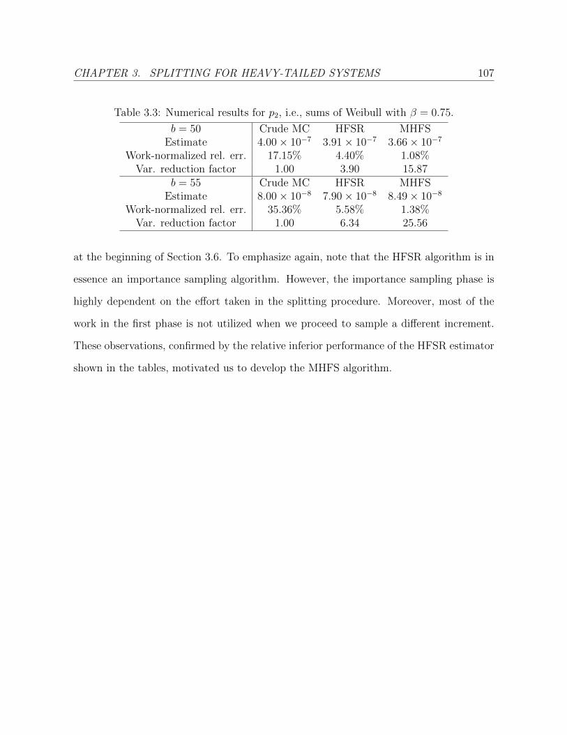
CHAPTER 3. SPLITTING FOR HEAVY-TAILED SYSTEMS 107
Table 3.3: Numerical results for p2, i.e., sums of Weibull with β = 0.75.
b = 50 Crude MC HFSR MHFSEstimate 4.00× 10⁻⁷ 3.91× 10⁻⁷ 3.66× 10⁻⁷
Work-normalized rel. err. 17.15% 4.40% 1.08%Var. reduction factor 1.00 3.90 15.87
b = 55 Crude MC HFSR MHFSEstimate 8.00× 10⁻⁸ 7.90× 10⁻⁸ 8.49× 10⁻⁸
Work-normalized rel. err. 35.36% 5.58% 1.38%Var. reduction factor 1.00 6.34 25.56
at the beginning of Section 3.6. To emphasize again, note that the HFSR algorithm is in
essence an importance sampling algorithm. However, the importance sampling phase is
highly dependent on the effort taken in the splitting procedure. Moreover, most of the
work in the first phase is not utilized when we proceed to sample a different increment.
These observations, confirmed by the relative inferior performance of the HFSR estimator
shown in the tables, motivated us to develop the MHFS algorithm.

A journey of a thousand miles begins with a single
step.
Lao-tzu
4State Dependent Importance Sampling with
Cross Entropy for Heavy-tailed Systems
The cross entropy method is a popular technique that has been used in the context of
rare event simulation in order to obtain a good selection (in the sense of variance
performance tested empirically) of an importance sampling distribution. This iterative
method requires the selection of a suitable parametric family to start with. The selection
of the parametric family is very important for the successful application of the method.
Two properties must be enforced in such a selection. First, subsequent updates of the
108

CHAPTER 4. RARE EVENT SIMULATION VIA CROSS ENTROPY 109
parameters in the iterations must be easily computable and, second, the parametric family
should be powerful enough to approximate, in some sense, the zero-variance importance
sampling distribution. In this chapter we obtain parametric families for which these two
properties are satisfied for a large class of heavy-tailed systems including Pareto and
Weibull tails. Our estimators are shown to be strongly efficient in these settings.
4.1 Introduction
Tail probabilities of sums of heavy-tailed increments are a fundamental problem in the
applied probability field. A large number of applications boils down to these building
blocks. In this chapter we focus our attention on the tail probabilities of a finite sum of
heavy-tailed random variables, and we propose a method to improve variance reduction
of an existing class of estimators with proved efficiency.
Let Sm = X1 + X2 + ... + Xm be a sum of independently and identically distributed
(i.i.d.) random variables, with S0 = 0 and that the Xn’s are suitably heavy-tailed. The
primary interest is the design of efficient estimators for the tail probability of the sum
u (b) = P (Sm > b) . (4.1)
The basic intuition behind the construction of efficient importance sampling estimators
is that one should mimic the behavior of the zero variance change of measure, which
coincides with the conditional distribution
P (S ∈ ·|Sm > b) (4.2)
(see for example, [8]). Therefore, the behavior of the heavy tailed random walk condi-

CHAPTER 4. RARE EVENT SIMULATION VIA CROSS ENTROPY 110
tional on the rare event becomes the target to be tracked by paths generated under the
importance sampling distribution. It is well known from the theory of heavy-tailed large
deviations that this “target” is characterized by the so-called “principle of big jump”,
which states that as b∞ the rare event occurs due to the contribution of a single large
increment of size Ω (b) (see Definition 1.1). On the other hand, paths with more than
one jumps of order Ω(b) shall not be neglected in the construction of importance sampler,
because of an observation pointed out by [12] that the second moment of the estimator
for heavy tailed large deviation probabilities is very much sensitive to the likelihood ratio
of these paths (see also Example 4.1 in Section 4.2).
Guided by these observations, it is natural to suggest a mixture based sampler for the
increments as the candidate importance sampler. Recently several state-dependent im-
portance sampling estimators based on such mixtures ([34] and [22]) have been developed
and shown to be strongly efficient (which means that the number of samples needed to
achieve a fixed relative precision is bounded as b ∞). In simple words, one samples
the next increment from different regions of its support with different probabilities. We
shall delay the specific form of the mixture to the next section.
Since the zero variance change of measure (4.2), optimal among all possible sampling
distribution, involves the unknown quantity of interest u(b) and is therefore infeasible,
the search of global optimal sampling distribution is a futile attempt. But if one restricts
optimization within a specific parametric family of sampler, there is hope that an improved
change of measure within that family can be obtained. One powerful tool that exactly
fits into this setting is Cross Entropy (CE) minimization (see for example, [66] and [56]).
Instead of directly minimizing the variance of the estimator, the CE method minimizes the
cross-entropy discrepancy between two densities. The main advantage of the CE method
is that, if the parametric family is well chosen, the optimization problem often admits

CHAPTER 4. RARE EVENT SIMULATION VIA CROSS ENTROPY 111
closed-form solutions, as opposed to the variance minimization (VM) method (we refer
readers to [28] for an in-depth comparison between these two methods).
The successful application of the CE method is closely tied to the quality of the se-
lected parametric family of densities to start with. Two properties must be enforced in
such a selection. First, the parametric family should be powerful enough to approximate,
in some sense, the zero-variance importance sampling distribution and, second, subse-
quent updates of the parameters in the iterations must be easily computable. We shall
focus on elaborating these properties on the mixture family of our choice in this chapter
and demonstrate empirically the performance of this approach applied to the mixture
family. We noticed that in existing works, the application of the CE method on esti-
mating tail probabilities of sums of heavy-tailed random variables has been restricted to
importance sampling densities that do not capture the “principle of big jump”; for exam-
ple [28] and [14] considered importance sampling densities by tilting the scale parameters
of the Weibull and log-normal increment distributions, respectively. As expected, the
corresponding estimators are asymptotically efficient in a weak sense, as opposed to the
strong efficiency criterion that our proposed family satisfies (see Theorem 4.1 below). The
contribution of this chapter is to justify the applicability of the CE method to a paramet-
ric family of densities that capture the large deviations behavior of the heavy-tailed sum,
and the resulting estimator is strongly efficient.
The rest of the chapter is organized as follows. In Section 4.2 we introduce the as-
sumptions for the heavy-tailed increments, and put forward the parametric family of
importance sampling densities to work on. Section 4.4 justifies the preservation of strong
efficiency when switching among the same parametric mixture family. In Section 4.5 the
CE method is reviewed and we discuss how it can be applied to the mixture family under
consideration, after which the iterative equations are derived in closed-form. Finally in

CHAPTER 4. RARE EVENT SIMULATION VIA CROSS ENTROPY 112
Section 4.6 we test the performance of our approach on two examples and give further
discussions.
4.2 Heavy-tailed Increment Distributions
We assume that the increments of the system satisfy the following two assumptions, which
encompass virtually all models used in practice, including regularly varying (see Definition
1.7), Weibull and log-normal.
Assumption 4.1. Xi ∈ RVα, for some α > 1. Recall from Definition 1.7 that Xi ∈
RV−α if F (x) = L(x)x−α where L(·) is a slowly varying function.
Assumption 4.2. There exists b0 such that for all x > b0 the following conditions hold.
2a limx→∞ xλ(x) =∞.
2b There exists β0 ∈ (0, 1) such that ∂logΛ(x) = λ(x)/Λ(x) ≤ β0x−1 for x ≥ b0.
2c Λ(·) is concave for all x ≥ b0; equivalently, λ(·) is assumed to be non-increasing for
x ≥ b0.
We remark that under Assumption 4.2, the increment distribution F is essentially
assumed to possess a tail at least as heavy as some Weibull distribution with shape
parameter β0 < 1. Note that under these Assumptions, adopted from [22], the increments
Xi’s are subexponential, i.e., F ∈ S (see Definition 1.4), which means that
P (Sm > b) ∼ mP (Xi > b) , (4.3)
as b∞ (see Lemma 6 of [22]).

CHAPTER 4. RARE EVENT SIMULATION VIA CROSS ENTROPY 113
4.3 Parametric Family of IS Distributions
State-dependent importance sampler (SDIS) is designed to sample the increments of the
system from a distribution that is dependent on the current status of the system being
simulated. We consider a mixture based SDIS. Let us denote by pj
= (pj,0, ..., pj,K) the
vector of mixture probabilities applied to the j-th increment, j = 1, 2, ...,m − 1, where
K + 2 is the number of mixture determined by the heaviness of the tail (the lighter the
tail is, the larger K is). We consider the following family of mixture based densities
parameterized by the mixing probabilities
p = p1, p
2, ..., p
m−1 = (p1,0, p1,1, ..., p1,K), ..., (pm,0, pm,1..., pm,K), (4.4)
where K ≥ 0, from which we sample the k-th increment of the heavy-tailed system:
hk
(x; p
k
∣∣Sk−1 = s)
= pk,0f0 (x|s) +K∑j=1
pjfj (x|s) +
(1−
K∑j=0
pj
)f† (x|s) , (4.5)
where f† and fj for j = 0, 1, ..., K are properly normalized density functions, which have
disjoint supports and depend on the current position of the system Sk−1 = s. The two
prevalent specifications are from [34] and [22]. The former works for random walks with
increments of regularly varying-type tails that satisfy Assumption 4.1, in which case a
mixture of two is used, i.e., K = 0. In particular,
hk (x|s) =
(I (x > a(b− s))F (a(b− s))
+I (x ≤ a(b− s))F (a(b− s))
)f(x), (4.6)
where a ∈ (0, 1) is necessary for analytical reasons and is typically set to be close to 1.
For increments that have distributions covered by Assumption 4.2, for example Weibull,
estimators based on two mixtures might fail to achieve bounded relative error. As dis-

CHAPTER 4. RARE EVENT SIMULATION VIA CROSS ENTROPY 114
cussed in the previous section, this is because the weight of the contribution of those
“rogue” paths (i.e., paths with multiple jumps of order Ω(b)) to the relative variance of
the estimator is growing increasingly pronounced. Consider the following example.
Example 4.1. Suppose we are interested in estimating P (X1 +X2 > b), where X1, X2
are i.i.d. Weibull with parameter β ∈ (0, 1), i.e., P (Xi > t) = F (t) = exp(−tβ
). Note
that P (X1 +X2 > b) ∼ P (X1 > b) + P (X2 > b) due to the properties of subexponential
distributions. A two-mixture sampler leads to the following importance sampling strategy:
sample the increments
(Y1, Y2) =
(X1, X2
∣∣ (X1; X2 > b−X1))
w.p.1/2(X1
∣∣ (X2; X1 > b−X2) , X2
)w.p.1/2.
The corresponding IS estimator is therefore
µb =fX1(y1)fX2(y2)
fX1,X2(y1, y2)=
2F (b− y1)F (b− y2)I (y1 + y2 > b)
F (b− y1) + F (b− y2).
It’s not hard to see that for some choice of β < 1, the relative error is unbounded as
b∞. In particular, consider the path (y1, y2) = (b/2, b/2), one has
E (µ2b)
P (X1 +X2 > b)2 =Ep (µb)
P (X1 +X2 > b)2
≥ 1
P (X1 +X2 > b)2
fX1(b/2)fX2(b/2)
fY1,Y2(b/2, b/2)fX1(b/2)fX2(b/2)
=F (b/2)2fX1(b/2)2
P (X1 +X2 > b)2 F (b/2)≈
exp(−3 (b/2)β + 2bβ
)4
,
which grows rapidly as b∞ if e.g., β = 2/3.
As the previous example illustrates, more mixtures are needed for the increments

CHAPTER 4. RARE EVENT SIMULATION VIA CROSS ENTROPY 115
covered by Assumption 4.2 to absorb the impact of such “rogue” paths on the second
moment of the estimator. Following this observation, [22] proposed a multi-point mixture
family, which is general enough to cover all the increment types that satisfy Assumption
4.1 and Assumption 4.2. The support of the mixture based densities is defined in terms
of the hazard function of the increments, and the number of mixtures used is dependent
on the tail heaviness of the increments which is expressed in terms of the concavity of
the hazard function of the increment distribution. More mixtures are needed when the
tails are not as heavy as regularly varying, for example Weibull. More precisely, let
Λ(x) = − logF (x) be the integrated hazard function of the increments, given a∗, a∗∗ > 0,
let
f0(x|s) = f(x)I (x ≤ b− s− Λ−1 (Λ(b− s)− a∗))P (x ≤ b− s− Λ−1 (Λ(b− s)− a∗))
, (4.7)
and
f†(x|s) = f(x)I (x > b− s− Λ−1 (Λ(b− s)− a∗∗))P (x > b− s− Λ−1 (Λ(b− s)− a∗∗))
. (4.8)
The densities fj’s are defined by a set of cut-off points cj = aj(b−s) for j = 1, 2, ..., K−1
where 0 < a1 < a2 < ... < aK−1 < 1 is a sequence satisfying, for given β0 ∈ (0, 1) and a
positive constant σ1,
aβj + (1− aj+1)β ≥ 1 + σ2,
and
aj+1 − aj ≤ σ1/2,
for each 1 ≤ j ≤ K − 2 for some σ2 > 0, and aK−1 ≥ 1 − σ1, a1 ≤ σ1. Set c0 =
b − s − Λ−1 (Λ(b− s)− a∗), cK = b − s − Λ−1 (Λ(b− s)− a∗∗) and write c−1 = −∞, we
define
fj(x) = (4.9)

CHAPTER 4. RARE EVENT SIMULATION VIA CROSS ENTROPY 116
f(x)I (x ∈ (cj−1, cj])/P (X ∈ (cj−1, cj]), 0 ≤ j ≤ K − 1
f(b− s− x)I (x ∈ (cK−1, cK ])/P (X ∈ (b− s− cK , b− s− cK−1]), j = K
f(x)I (x ∈ (cK ,∞)) /P (X ∈ (cK ,∞)) , j = †
for j = 1, 2, ..., K. Note that the two specifications of the mixtures (by [34] and [22]) have
the same spirits when the increments are regularly varying (see equation (14) in [22]).
[22] also showed that this mixture based distribution converges in total variation to the
zero-variance distribution in a certain random walk problem, as b∞. In what follows,
unless specified otherwise, we shall work on the general form of the mixture given in (1.8),
i.e.,
hk
(x; p
k
∣∣Sk−1 = s)
=
(K∑j=0
pk,jI (Aj (s))wj (s, x) +
(1−
K∑j=0
pk,j
)I (A†(s))w† (s, x)
)f(x),
where A†(s) =⋃Kj=0 Aj(s), and wj(s, x), w†(s, x) > 0 satisfy E(wj(s,X)) = E(w†(s,X)) =
1. Note that the mixture family specified by [34] corresponds to setting
w0 (s, x) =I (x ≤ a(b− s))F (a(b− s))
, w† (s, x) =I (x > a(b− s))F (a(b− s))
.
And the one proposed by [22] corresponds to setting
wj (s, x) =I (Aj(s))
P (Aj(s))=I (x ∈ (cj−1, cj])
P (x ∈ (cj−1, cj]),

CHAPTER 4. RARE EVENT SIMULATION VIA CROSS ENTROPY 117
for j = 0, 1, ..., K − 1 and again write c−1 = −∞. And
w† (s, x) =f(b− s− x)I (x ∈ (cK−1, cK ])
f(x)P (X ∈ (b− s− cK , b− s− cK−1]), w†(s, x) =
I (x ∈ (cK ,∞])
P (x ∈ (cK ,∞])
If we write the joint density of the increments under the original measure as
f (x) = f (x1) f (x2) ...f (xm) ,
where x = (x1, ..., xm), and we can express the joint importance sampling density for the
mixture based SDIS as
h (x; p)
=m−1∏k=1
[K∑j=0
pk,jI (Aj (sk−1))wj (s, xk) +
(1−
K∑j=0
pk,j
)I (A†(sk−1))w† (s, xk)
]· (I (Sm−1 < b)P (Xm > (b− Sm−1)) + I (Sm−1 ≥ b)) f (x) . (4.10)
And the associated SDIS estimator for u(b) is therefore defined as
Zm(b; p) =m−1∏k=1
K∑j=0
I (Aj(Sk−1))
pk,jwj(Sk−1, Xk)+
I (A†(Sk−1))
w†(Sk−1, Xk)(
1−∑K
j=0 pk,j
)
×(
I(Sm−1 > b)
P (Xm > b− Sm−1)+ I(Sm−1 > b)
), (4.11)
where p is the mixing probability vector defined in (4.4).

CHAPTER 4. RARE EVENT SIMULATION VIA CROSS ENTROPY 118
4.4 Strong Efficiency of the Family under Consider-
ation
The following theorem states the efficiency property of the mixture family. In particular,
the mixture family remains in the class of strongly efficient estimators, subject to mild
conditions on the mixing parameters. The proof of which boils down to the construction
of a valid Lyapunov function, as introduced in Subsection 1.2.7.
Theorem 4.1. Let Pp be the measure induced by the mixture family with mixing probability
vector p, and let Ep be the associated expectation operator. If there exists a ξ > 0 such
that p > ξ · 1, for all b > 0, where 1 is a vector of ones of dimension (m− 1)× (K + 2),
then one can explicitly compute K ∈ (0,∞), uniform in b, such that
Ep [Zm(b; p)2]
u(b)2< K,
as b ∞, where the estimator Zm(b; p) is defined in (4.11). In particular, Zm(b; p) is
strongly efficient for estimating u(b).
Since the estimator introduced in [22] covers both Assumptions 4.1 and 4.2, and the
mixture-based estimator proposed in [34] can be shown to be equivalent to the one given in
[22] under Assumption 4.1, it suffices to work on the mixture given in [22]. The discussions
at the end of Subsection 1.2.7 suggest that a natural candidate for the Lyapunov function,
v(s), at time k, is approximately P (Sm > b|Sk−1 = s)2. In fact it suffices to work on the
following straightforward choice,
v(s) = F (b− s)2. (4.12)

CHAPTER 4. RARE EVENT SIMULATION VIA CROSS ENTROPY 119
The associated Lyapunov inequality (see Lemma 1.5) can therefore be written as
E[v (s+X)
v(s)ζ (s,X)
]≤ c, (4.13)
for some constant c ∈ (0,∞) independent of b, where ζ (Sk−1, Xk) is the local likelihood
function between the original measure and the one induced by the mixture sampling
density at the k-th step. Let us write the left hand side of (4.13) according to the
following decomposition
E[v (s+X)
v(s)ζ (s,X)
]=
K∑j=0
Jjpk,j
+J†pk,†
,
where pk,† = 1−∑K
j=0 pk,j, and specifically,
J† = P(X > Λ−1
(Λ(b− s)− a∗∗
))E[v(s+X)
v(s);X > Λ−1
(Λ(b− s)− a∗∗
)](4.14)
J0 = P(X ≤ b− s− Λ−1
(Λ(b− s)− a∗
))×E
[v(s+X)
v(s);X ≤ b− s− Λ−1
(Λ(b− s)− a∗
)](4.15)
Jj = P (X ∈ (cj−1, cj])E[v(s+X)
v(s);X ∈ (cj−1, cj]
], for j = 1, . . . , K − 1 (4.16)
JK = P (b− s−X ∈ (ck−1, ck])E[v(s+X)f(X)
v(s)f(b− s−X);X ∈ (ck−1, ck]
]. (4.17)
Therefore the proof of the previous result boils down to carefully upper bounding each of
the previous term so thatK∑j=0
Jjpk,j
+J†pk,†≤ c.
The following lemma is useful for deriving an upper bound for Jj, 1 ≤ j ≤ K, which
corresponds to Lemma 4 in [22] and we therefore dispense ourselves with the proof.

CHAPTER 4. RARE EVENT SIMULATION VIA CROSS ENTROPY 120
Lemma 4.1. Under Assumption 4.2, the following holds,
Λ(x)
Λ(x+ y)≥(
x
x+ y
)β0
,
for all x ≥ b0 and y ≥ 0.
We now proceed to carry out our plan in details.
Proof. 1) The term J†.
By definition simply note that v(s) ≤ 1, therefore we have
J† ≤P(X > Λ−1
(Λ(b− s)− a∗∗
))2
v(s)
= exp (2a∗∗)F
2(b− s)v(s)
= exp (2a∗∗). (4.18)
2) The term J0.
We can bound J0 from above as follows,
J0 ≤ E[v(s+X)
v(s);X ≤ b− s− Λ−1
(Λ(b− s)− a∗
)]≤
F(Λ−1
(Λ(b− s)− a∗
))2
F (b− s)2= exp (2a∗) . (4.19)
3) The terms Jj, j = 2, . . . , K − 1.
By virtue of Lemma 4.1, we have
Λ(x) + Λ(y)− Λ(x+ y + z) ≥ Λ(x+ y + z)
((x
x+ y + z
)β0
+
(y
x+ y + z
)β0
− 1
),

CHAPTER 4. RARE EVENT SIMULATION VIA CROSS ENTROPY 121
for sufficiently large x, y, z. Therefore, as b− s∞,
Jj =P(X ∈ (cj−1, cj]
)F (b− s)2
∫ cj
cj−1
F (b− s− x)2 f(x)dx
≤ F (cj−1)2 F (b− s− cj)2
F (b− s)2
≤ exp(
2Λ(b− s)− 2Λ(cj−1)− 2Λ(b− s− cj))
≤ exp(−2Λ(b− s)
(aβ0
j−1 + (1− aj)β0 − 1))≤ 1. (4.20)
4) The term J1.
Once again from Lemma 4.1, for x ∈[b− s− Λ−1 (Λ(b− s)− a∗) , a1(b− s)
], we have
Λ(x) + Λ(b− s− x)− Λ(b− s) ≥ Λ(b− s)
((x
b− s
)β0
+
(b− s− xb− s
)β0
− 1
),
and
Λ(b− s)− Λ(b− s− x) ≤ Λ(b− s)
(1−
(1− 1
(b− s)
)β0).
Combining the preceding two inequalities, we obtain
2Λ(b− s)− 2Λ(b− s− x)− Λ(x) ≥ Λ(b− s)
(2− 2
(1− x
b− s
)β0
−(
x
b− s
)β0)≤ 0.
Hence, along with the fact that limx→∞ λ(x) = 0, we have, , as b− s∞,
J1 =P(X > b− s− Λ−1 (Λ(b− s)− a∗)
)F (b− s)2
∫ c1
b−s−Λ−1(Λ(b−s)−a∗)F (b− s− x)2 f(x)dx
≤∫ c1
b−s−Λ−1(Λ(b−s)−a∗)exp
(2Λ(b− s)− 2Λ(b− s− x)− Λ(x)
)dx ≤ δ1,
(4.21)
for some δ1 > 0 independent of b.

CHAPTER 4. RARE EVENT SIMULATION VIA CROSS ENTROPY 122
5) The term JK.
Note that by construction (see the paragraph before (4.9)),
cK−1 = aK−1(b− s) ≥ (1− σ1)(b− s),
for sufficiently small but positive σ1. Therefore, by resorting to Lemma 4.1 one last time,
we have
2Λ(b− s)− 2Λ(x)− Λ(b− s− x) ≤ 2− 2
(x
b− s
)β0
−(
1− x
b− s
)β0
≤ 0, (4.22)
which leads to
JK = P (b− s− cK , b− s− cK−1)
∫ cK
cK−1
F (b− s− x)2
F (b− s)2
f 2(x)
f(b− s− x)dx
≤∫ cK
cK−1
λ2(x)
λ(b− s− x)exp
(2Λ(b− s)− 2Λ(x)− Λ(b− s− x)
)dx
≤ δ2, (4.23)
for some δ2 > 0 independent of b, as b − s ∞. Here the last inequality arises due to
(4.22) and the fact that λ−1(x) grows at most linearly in x by Assumption 4.2-b).
In summary, by combining (4.18), (4.19), (4.20), (4.21) and (4.23), we arrive at
K∑j=0
Jjpk,j
+J†pk,†≤ ξδ = c, (4.24)
where ξ = min1≤k≤m,j∈†,0,...,K pk,j, and δ = (K + 2) maxexp(2a∗∗), exp(2a∗), 1, δ1, δ2.
Now by definition it is clear that v(0) = P (Sm > b)2, and it suffices to pick ρ = 1 in

CHAPTER 4. RARE EVENT SIMULATION VIA CROSS ENTROPY 123
Lemma 1.5. The result in Lemma 1.5 allows us to conclude that
Ep
[Zm(b; p)2
]≤ cmv(0) ≤ cmu2(b),
where c is defined in (4.24).
Remark 4.1. The result enables us to comfortably switch to different choices of mix-
ing probabilities within the same parametric family without violating the strong efficiency
property of the final estimator, which lays the ground for the applicability of the CE method
to be introduced shortly.
4.5 Cross Entropy Method and the Iterative Equa-
tions for the Mixture Family
4.5.1 Review of Cross-Entropy Method
If we restrict our search of importance sampler to this particular parametric class, the
optimal choice of the vector p can be obtained by minimizing the so-called Kullback-Leibler
divergence or the cross-entropy distance.
Definition 4.1. The Kullback-Leibler cross-entropy between two densities g and h is given
by
D (g, h) =
∫g(x) log
g(x)
h(x)dx
=
∫g(x) log g(x)dx−
∫g(x) log h(x)dx. (4.25)
If we fix g to be the optimal importance sampling density g∗ (x) ∝ ϕ (S (x; b)) f(x),
where ϕ (S (x; b)) is the performance measure of the system (for example, S(X) =∑m
j=1 Xj,

CHAPTER 4. RARE EVENT SIMULATION VIA CROSS ENTROPY 124
and ϕ (S (x; b)) = I (S (x) > b)), then our search of the optimal mixture is the output of
the following parametric optimization problem
minpD (g∗, h(·,p))⇐⇒ max
pD (p) = max
pEp?ϕ (S (X; b)) log h (X; p)
= maxp
Epϕ (S (X; b))h (X; p?)
h (X; p)log h (X; p)
= maxp
Epϕ (S (X; b))f (X)
h (X; p)log h (X; p) , (4.26)
where f (X)/h (X; p) is the likelihood ratio between the original measure and the measure
induced by the mixture based density with some fixed parameter p (Recall that X =
(X1, ..., Xm)). In particular,
f (X)
h (X; p)=
m−1∏k=1
K∑j=0
I (xk ∈ Aj (Sk−1))
pk,jwj (Sk−1, xk)+
I (xk ∈ A†(Sk−1))(1−
∑Kj=0 pk,j
)w† (Sk−1, xk)
· (I (Sm−1 < b)P (Xm > (b− Sm−1)) + I (Sm−1 ≥ b)) . (4.27)
In most cases the expectation in (4.26) is analytically inaccessible. [66] suggested a re-
cursive method based on the following stochastic counterpart of (4.26)
maxp
D (p) = maxp
1
N
N∑i=1
ϕ (S (X(i)) ; b)f (X(i))
h (X(i); p)log h (X(i),p) . (4.28)
Cross Entropy (CE) Algorithm [66]
1. Choose an initial vector of mixing probabilities p(0). Set T = 1.
2. Generate a random sample X1, ...,XN from the joint density h(·; p(T−1)
).

CHAPTER 4. RARE EVENT SIMULATION VIA CROSS ENTROPY 125
3. Solve the stochastic optimization program (4.28). Denote the solution by p(T ), i.e.,
p(T ) = arg minp
1
N
N∑i=1
ϕ (S (X(i)) ; b)f (X(i))
h (X(i); p(T−1))log h (X(i),p) .
4. Stop if convergence is reached; otherwise, set T = T + 1, go to Step 2.
It’s very convenient to embed the CE algorithm in the main SDIS algorithm to further
reduce variance. Let M be the total simulation budget, and τ be the number of recursions
in the CE algorithm until convergence of p. If τN < M , then the SDIS with CE algorithm
add-on corresponds to generating τ batches of independent samples from the mixture
based importance sampling density parameterized by p(T ), for T = 0, 1, ..., τ − 1, and one
batch of size M − τN of independent samples from the importance density with optimal
CE probability vector p∗. Depending on the size of M − τN , the final estimator can be
obtained by averaging either the last batch of M − τN samples, or the entire M samples
from different batches. In either case we are able to achieve variance reduction while
maintaining strong efficiency property. Even for the case where τN ≥ M , the improved
cross-entropy after each iteration typically will reduce the variance of the future samples
over those from previous iterations, since each iteration gives us a parameterized density
closer to the zero-variance importance density.
4.5.2 Iterative Equations for the Mixture IS Family
We now proceed to characterize the solution to (4.28). In the case where we are interested
in the tail probability of the sum P (Sm > b), ϕ (S (X) ; b) = I (Sm > b). Note that D is
concave and differentiable with respect to the components pk, therefore the solution to

CHAPTER 4. RARE EVENT SIMULATION VIA CROSS ENTROPY 126
(4.28) is directly given by the first order optimality condition:
N∑i=1
I (Sm(i) > b)f (X(i))
h (X(i); p)5p log h (X(i),p) = 0. (4.29)
The product structure of the likelihood function is particularly useful because the sensi-
tivity of the likelihood function to the mixing probabilities can be localized. Indeed, a
few lines of elementary algebra gives
d log h (X,p)
dpk,l
=(I (Xk ∈ Al (Sk−1))wl (Sk−1, Xk)− I (Xk ∈ A† (Sk−1))w† (Sk−1, Xk)
)/[
K∑j=0
pk,jI (Xk ∈ Aj (Sk−1))wj (Sk−1, Xk)
+
(1−
K∑j=0
pk,j
)I (Xk ∈ A†(Sk−1))w† (Sk−1, Xk)
]
=I (Xk ∈ Al (Sk−1))
pk,l− I (Xk ∈ A† (Sk−1))
1−∑K
j=0 pk,j. (4.30)
We denote
W (X−l(i); p?, p) =
m−1∏k=1,k 6=l
h(Xk(i); p
?k
)h(Xk(i); pk
) (I (Sm−1 < b)P (Xm(i) > (b− Sm−1(i))) + I (Sm−1(i) ≥ b)) ,
where p?k
= p?k,0, ...p?k,K, and pk
= pk,0, ...pk,K. And further let
Θl,j =
∑Ni=1W (X−l(i); p
?, p)(
1−∑K
j=0 pl,j
)w† (Sl−1, Xl(i))∑N
i=1W (X−l(i); p?, p) pl,jwl (Sl−1, Xl(i)).
The first order optimality condition (4.29) therefore yields the following solution p∗

CHAPTER 4. RARE EVENT SIMULATION VIA CROSS ENTROPY 127
to the stochastic optimization problem (4.28), we shall call this vector of optimal solution
optimal CE mixing probability vector :
p∗l,j =Θl,j
1 +∑K
k=0 Θk,j
, (4.31)
for j = 0, 1, ..., K and l = 1, 2, ...,m. It doesn’t take long to realize that the previous
expression has the following equivalent form
p?l,j =
∑Ni=1 I (Sm(i) > b)W (X(i); p?, p) I (Xl ∈ Aj (Sl−1))∑N
i=1 I (Sm(i) > b)W (X(i); p?, p), (4.32)
for j = 0, 1, ..., K and k = 1, 2, ...,m, where W (·; p?, p) = h (·; p?) /h (·; p) = f (·) /h (·; p)
is given by (4.27). It’s worth pointing out that (4.32) is computationally advantageous
over (4.31), because it avoids dividing by zero in computing Θl,j, especially when the
number of “pilot” run is small. (Note that the sampling of the mth increment ensures
Sm(i) > b.) Moreover, the expression (4.32) entails a nice interpretation: the optimal
mixing probability is the proportion of the contribution to the likelihood function from
the jth “band” of the kth increment.
For completeness we also include the explicit iteration equations for cases where the
increments satisfy Assumption 4.1 and 4.2, respectively. We write, for ease of exposition,
Wm(i) = (I (Sm−1(i) < b)P (Xm(i) > (b− Sm−1(i))) + I (Sm−1(i) > b)) .
For regularly varying increments, the solution for the T th iteration of the recursive algo-
rithm can be written as
p(T )k =
[N∑i=1
I (Sm(i) > b;Xk > a(b− sk−1))Wm(i)

CHAPTER 4. RARE EVENT SIMULATION VIA CROSS ENTROPY 128
·m−1∏k=1
P (Xk > a(b− sk−1))
p(T−1)k I (Xk > a(b− sk−1))
+P (Xk ≤ a(b− sk−1))(
1− p(T−1)k
)I (Xk ≤ a(b− sk−1))
/[
N∑i=1
I (Sm(i) > b)Wm(i)
·m−1∏k=1
P (Xk > a(b− sk−1))
p(T−1)k I (Xk > a(b− sk−1))
+P (Xk ≤ a(b− sk−1))(
1− p(T−1)k
)I (Xk ≤ a(b− sk−1))
(4.33)
For increment distributions that satisfy Assumption 4.2, W (·; p?,p(T−1)), the likelihood
function, becomes
W(X(T−1); p?,p(T−1)
)=
f(x(T−1)
)h (X(T−1),p(T−1))
=m−1∏k=1
Wm(i)
P(X
(T−1)k ≤ c0
)p
(T−1)k,0 I
(x
(T−1)k ≤ c0
)+
P(X
(T−1)k > cK
)(
1−∑K
j=0 p(T−1)k,j
)I(X
(T−1)k > cK
) +K−1∑j=1
P(X
(T−1)k ∈ (cj−1, cj]
)p
(T−1)k,j I
(x
(T−1)k ∈ (cj−1, cj]
)+f(b− s− x(T−1)
k )P(X
(T−1)k ∈ (b− s− cK−1, b− s− cK ]
)p
(T−1)k,K f(x
(T−1)k )I
(x
(T−1)k ∈ (cK−1, cK ]
) ,
where cj’s are the cutoff points of the “bands” and we have explicitly written out the iter-
ation count. Note that at the beginning of iteration T , the only part that is dependent on
the unknown parameters p in the stochastic program (4.28) is log h(X(i),p(T )
)and hence
5p lnh(X(i),p(T )
)in the optimality condition (4.29); W
(·; p?,p(T−1)
)is a function of
the probability vector passed from the (T −1)st iteration as well as the samples generated
from IS density specified by that probability vector. In that regard at the beginning of
the T th iteration, all the ingredients in the expression above are available. The iteration
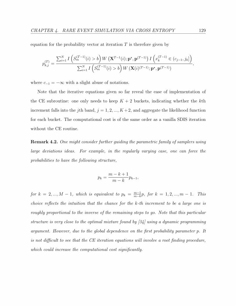
CHAPTER 4. RARE EVENT SIMULATION VIA CROSS ENTROPY 129
equation for the probability vector at iteration T is therefore given by
p(T )k,j =
∑Ni=1 I
(S
(T−1)m (i) > b
)W(XT−1(i); p?,p(T−1)
)I(x
(T−1)k ∈ (cj−1, jk]
)∑N
i=1 I(S
(T−1)m (i) > b
)W (X(i)(T−1); p?,p(T−1))
,
where c−1 = −∞ with a slight abuse of notations.
Note that the iterative equations given so far reveal the ease of implementation of
the CE subroutine: one only needs to keep K + 2 buckets, indicating whether the kth
increment falls into the jth band, j = 1, 2, ..., K+2, and aggregate the likelihood function
for each bucket. The computational cost is of the same order as a vanilla SDIS iteration
without the CE routine.
Remark 4.2. One might consider further guiding the parametric family of samplers using
large deviations ideas. For example, in the regularly varying case, one can force the
probabilities to have the following structure,
pk =m− k + 1
m− kpk−1,
for k = 2, ...,M − 1, which is equivalent to pk = m−1m−kp, for k = 1, 2, ...,m − 1. This
choice reflects the intuition that the chance for the k-th increment to be a large one is
roughly proportional to the inverse of the remaining steps to go. Note that this particular
structure is very close to the optimal mixture found by [34] using a dynamic programming
argument. However, due to the global dependence on the first probability parameter p. It
is not difficult to see that the CE iteration equations will involve a root finding procedure,
which could increase the computational cost significantly.

CHAPTER 4. RARE EVENT SIMULATION VIA CROSS ENTROPY 130
4.6 Numerical Examples
4.6.1 Example 1: Regularly Varying Increments
We illustrate the empirical performance of the SDIS with CE routine (SDIS-CE) by
considering two examples. In the first example, the increments are regularly varying with
index α = 1/2, in particular, Xn’s have tail distribution
P (Xi > b) = (1 + b)−1/2 .
Following [34], given the parameters of the model, a given number of increments m and
a tail parameter b, we estimate P (Sm > b) and the standard deviation of the estimator
as follows. We simulate 20000 replications of our estimator. The estimates are obtained
based on averages of the replications. This is the output of a single run. Then we produce
500 independent runs. The results displayed are the averages of the outputs of these runs.
We run the experiments with two different sets of input mixing probabilities. In the first
case, which we shall later refer to as the “standard choice”, we consider the heuristic
choice pk = θ/ (m− k) where θ = 0.9. And for the second set of input we use the optimal
choice of the probabilities obtained by [34], i.e.,
p∗k =a−α/2
(m− k)a−α/2 + 1, (4.34)
which we call the “DLW” selection. In both cases we select a = 0.9. The results of the
experiment are reported in the Table 4.1 and Table 4.2.
From the results of Table 4.1 we observe that even for a reasonable choice of mixing
probabilities based on large deviations intuition, the CE algorithm produces a smaller
relative error. On the other hand, it is outperformed by the optimal choice of the prob-

CHAPTER 4. RARE EVENT SIMULATION VIA CROSS ENTROPY 131
Table 4.1: Performance of the SDIS-CE estimator compared to the SDIS algorithm with-out CE procedure where the input mixing probabilities are set to be pk = 0.9/(m− k) fork = 1, 2, ...,m− 1.
m b Standard CE Method4 1e + 06 3.999E-03 4.000E-03 Average Estimate
3.148E-05 1.395E-05 Average Std. Error0.787% 0.349% Avg.SE/Avg.Est (%)
1e + 12 3.999E-06 4.000E-063.151E-08 1.403E-08
0.788% 0.351%1e + 18 4.000E-09 4.000E-09
3.153E-11 1.393E-110.788% 0.348%
25 1e + 06 2.503E-02 2.498E-021.525E-03 3.404E-04
6.094% 1.363%1e + 12 2.496E-05 2.499E-05
1.518E-06 3.458E-076.082% 1.384%
1e + 18 2.496E-08 2.502E-081.524E-09 3.409E-10
6.103% 1.363%

CHAPTER 4. RARE EVENT SIMULATION VIA CROSS ENTROPY 132
Table 4.2: Performance of the SDIS-CE estimator compared to the SDIS without CEprocedure where the input mixing probabilities are set to be the optimal choice obtainedin Dupuis, Leder and Wang (2006).
m b DLW CE Method4 1e + 06 4.000E-03 4.000E-03 Average Estimate
5.660E-06 1.374E-05 Average Std. Error0.141% 0.344% Avg.SE/Avg.Est (%)
1e + 12 4.000E-06 4.000E-065.683E-09 1.382E-08
0.142% 0.346%1e + 18 4.000E-09 4.001E-09
5.691E-12 1.373E-110.142% 0.343%
25 1e + 06 2.499E-02 2.500E-023.925E-05 1.555E-04
0.157% 0.622%1e + 12 2.500E-05 2.500E-05
4.032E-08 1.567E-070.161% 0.627%
1e + 18 2.500E-08 2.500E-084.027E-11 1.568E-10
0.161% 0.627%

CHAPTER 4. RARE EVENT SIMULATION VIA CROSS ENTROPY 133
abilities obtained in [34], as can be seen in Table 4.2, one shall keep in mind, however,
that in many applications, the structure of the problem doesn’t allow for such analytical
solutions easily. We also point out that the optimal solution from [34] hinges on the
assumption that b is sufficiently large for large deviations asymptotics to be valid. For
smaller exceedance level b, we might expect a better performance using the CE routine,
which is underpinned by the results shown in Table 4.3.
Table 4.3: Comparison of performance between 1) SDIS using CE optimal mixing prob-abilities and 2) Analytical optimal mixing probabilities from Dupuis, Leder and Wang(2006), m = 2.
b DLW CE Method5 6.999E-01 6.999E-01 Average Estimate
1.110E-03 5.742E-04 Average Std. Error0.159% 0.082% Avg.SE/Avg.Est (%)
20 4.166E-01 4.166E-014.727E-04 4.410E-04
0.113% 0.106%
We have mentioned in the previous section that since the recursive CE algorithm is
carried out on the pilot sample, it neglects the fact that the increments are simulated in
a sequential manner, but rather treats them in an independent way. We averaged the
output CE optimal probability vector over the experiments, the near identical mixing
probabilities in Table 4.4 is in line with the expected behavior of the method that each
increment has probability at roughly 1/4 of causing the rare event.
Table 4.4: Average optimal CE .mixing probabilities, m = 4, b = 106.
k 1 2 3pk 0.248 0.253 0.251

CHAPTER 4. RARE EVENT SIMULATION VIA CROSS ENTROPY 134
4.6.2 Example 2: Weibull Increments
We now proceed to the second example where the increments are assumed to have the
following Weibull-type of distribution,
P (X > b) = e−2√b+1,
for t ≥ −1. This corresponds to the case considered by [22], where the authors use a
5-point mixtures specified by the cut-off points c0 = 0.1√b− s, c1 = 0.1(b − s), c2 =
0.5(b− s), c3 = 0.9(b− s) and c4 = b− s− 0.1√b− s. Since the number of cut-off points
increases from the previous mixture sampler, we increase the pilot sample number to 5000;
all the other algorithmic parameters (number of runs and number of replications per run)
remain the same. The results of the experiments are summarized in Table 4.5.
Table 4.5: Performance of the SDIS-CE estimator compared to SDIS without CE proce-durein the case of Weibull-type of increments, m = 4. We used pk,j = 1/(K + 2)(m− k),for j = 0, 1, ...K and k = 1, 2, ...,m−1 as the “standard” choice of the mixing probabilities.
b Standard CE Method150 7.977E-11 7.966E-11 Avg. Est.
2.580E-12 7.642E-13 Avg. Std. Err.3.235% 0.959% Avg. SE/Avg. Est. (%)
450 1.371E-18 1.372E-184.835E-20 1.071E-20
3.526% 0.781%750 6.086E-24 6.069E-24
2.209E-25 3.185E-263.630% 0.525%

By failing to prepare, you are preparing to fail.
Benjamin Franklin
5Stochastic Insurance-Reinsurance Networks:
Modeling, Analysis and Efficient
Monte Carlo
The financial crisis has been plaguing the world since its outburst in 2007. Since then,
there has been extensive discussions on the significance of systemic risk within the
financial system. And a vast amount of research has been devoted to this field. In the
135

CHAPTER 5. STOCHASTIC INSURANCE NETWORKS 136
modeling stream along this line of research, it remains particularly challenging to develop
a dynamic model that encompasses stylized features on conventions such as contractual
structure, network connectivity, payment / default settlement and netting mechanism,
while still maintaining a comfortable level of analytical tractability. Simulation turns out
to be a natural choice. Nevertheless, as the level of complexity of the model increases, it
may not even be clear a posteriori how simulation techniques can be properly engineered
to analyze some particular performance measures to gauge the level of systemic risks in
the network under consideration. In this chapter we aim to provide a framework to blend
modeling and analysis (via simulation) of risk networks in the financial world. We base
our development particularly on an insurance / reinsurance application.
5.1 Motivations and Goals
We develop efficient simulation methodology for risk assessment in the context of multiple
insurance and / or financial entities with correlated exposures to each others risks and
to systematic market factors. We also introduce a modeling framework for insurance /
reinsurance networks that evolves according to equilibrium settlements at the time of
default of companies. These settlements are computed as the solution of an associated
linear program at each time period. Our types of models are closely related to and, in
fact, inspired by network models that have been analyzed in the literature in recent years,
for example [29], [30], [3], [40] and [65], to name a few.
Our interest lies in efficiently computing the conditional expected amount of the losses
in the entire system, given the failure of a selected set of market participants. We say
a market or system dislocation occurs when a specific group of participants fails. Using
our results and simulation procedures we aim at characterizing the features that dictate
a significant change in the nature of the system’s exposures given market dislocation. For

CHAPTER 5. STOCHASTIC INSURANCE NETWORKS 137
instance, if a specific set of market participants is not sufficiently capitalized to fulfill
their obligations, what is the most likely reason for such a situation, a systemic shock in
the market or a sequence of specific idiosyncratic events pertaining to the specific set of
participants?
Because of the various levels of dependence present in our model, and the structure
of rare-events of interest (involving several companies defaulting) it turns out that the
design of efficient simulation procedures for rare events in our setting typically involves
more than one jump, whereas most of the rare-event simulation literature dealing with
heavy tailed models involves single-jump events. The challenge in this situation lies in
the fact that we are conditioning on rare events (involving several market participants)
whose occurrence could most likely be caused by several large jumps. Also, as it will
become clear given the integer programming formulation that we provide in Theorem 5.5,
obtaining the large deviations behavior involves dealing with a combinatorial problem.
Our goal is to provide a simulation framework that can be rigorously shown to achieve
strong optimality properties (in terms of designing estimators with bounded coefficient of
variation uniformly as the event of interest becomes increasingly rare), and yet it is simple
to implement in practice. Our contributions can therefore be summarized as follows:
a) We propose a dynamic network model that allows to deal with counterparty default
risks with a particular aim of capturing cascading losses at the time of company
defaults by means of the solution of a linear programming problem that can be
interpreted in terms of an equilibrium. This formulation allows us to define the
evolution of reserve processes in the network throughout time, see Theorem 5.2 and
Theorem 5.4.
b) The linear programming formulation and therefore the associated equilibrium of
settlements at the time of default recognizes: 1) the correlations among the risk

CHAPTER 5. STOCHASTIC INSURANCE NETWORKS 138
factors, which are assumed to follow a linear factor model, 2) the contractual obli-
gations among the companies, which are assumed to follow popular contracts in the
insurance industry (such as stop-loss and proportional reinsurance retrocesion), and
3) the interconnectedness of the network. The equilibrium approach we adopted
(see (5.5)) turns out to be closely related to the market clearing framework estab-
lished in [40], see Subsection 5.2.3. Our approach, however, permits reinsurance
companies to net against each other’s losses in the wake of default.
c) Our model allows to obtain asymptotic results and a description of the asymptotic
most likely way in which the default of a specific group of participants can occur.
This description indicated is fleshed out explicitly, by means of an integer program-
ming problem (a Knapsack problem with multiple knapsacks). Such a description
emphasizes the impact of the interactions between the severity of the exogenous
claims, their dependence structure, and the interconnectedness of the companies on
the systemic risk landscape of the entire network under consideration, see Theorem
5.5 and Theorem 5.6 and Proposition 5.1.
d) We propose a class of strongly efficient estimators for computing the expected loss
of the network at the time of dislocation conditioning on the event that a specific set
of market participants fails to meet their obligations. In addition, these estimators
allow to compute associated conditional distributions of the network exposures given
the dislocation of a set of specific players. The estimation of these conditional
distributions is performed with a computational cost (as measured by the number of
simulation replications) that remains bounded even if the event of interest becomes
increasingly rare, see Theorem 5.7.
We are aware of only a limited amount of research that provides a risk analytical
framework in an integrated insurance-reinsurance market with heavy-tailed risks. The

CHAPTER 5. STOCHASTIC INSURANCE NETWORKS 139
work of [68] considers a simple two-node insurance-reinsurance network involving light-
tailed claims. Our work, however, puts into consideration a more complex and general
network that captures more stylized features of the insurance market in practice. This
is also the first work to the best of our knowledge that constructs provably efficient
estimators in the setting of heavy-tailed risk networks. We have formulated our results in
terms of regularly varying distributions for simplicity. Deriving logarithmic asymptotics
with basically the same qualitative conclusions under other types of tail distributions is
straightforward (see e.g., [21]). Our asymptotic results are obtained with the intention
of gaining qualitative insight in the form of approximations that are correct up to a
constant in the regularly varying setting. The role of the simulation algorithms, then, is
to endow these asymptotic approximations with a computational device that allows one
to efficiently obtain quantitatively accurate results. Thus, the entire approach we use,
namely analysis and efficient computation, must be thought as a coherent contribution.
Now, as the connections in the network increase, one must account for all possibilities
in which failure can occur. We have aimed at laying out a program to obtain estimators
that have uniform relative error, for a fixed network architecture, as the probability of
a failure event becomes more and more rare. At the same time, we have settled for
estimators that are relatively easy to implement with the indicated performance guarantee.
When the networks have more connections, the relative variance (even though uniformly
bounded as rare events of interest become more and more rare) could grow. The question
of designing rare-event simulation algorithms in which both uniformity in the size of the
network and the underlying large deviations parameter are ensured is certainly important
but too open-ended at this point. We plan to investigate this avenue in future research.
We envision that our model and our computational approach, based on efficient sim-
ulation, can serve as a prototype for the analysis of other types of risk networks. The

CHAPTER 5. STOCHASTIC INSURANCE NETWORKS 140
philosophy behind our work is that in the presence of network risk models, the settle-
ments and the evolution of the associated risk reserve processes should obey equilibrium
constraints that dictate the cascading effect when default occurs. These constraints can
effectively be modeled in terms of linear programs, which, coupled with a heavy-tailed
linear factor model, allow to describe qualitatively the most likely way in which simulta-
neous defaults occur. Efficient simulation, in the form of provably efficient Monte Carlo
estimators, should then be used to make more precise quantitative statements.
The rest of the chapter is organized as follows. In Section 5.2 we describe in detail our
network model and discuss the associated linear programming formulation for the evolu-
tion of contract settlements in the event of company failures. The asymptotic analysis of
the model is given in Section 5.3. In Section 5.4 we propose a dynamic simulation scheme
that balances practicality and efficiency, accompanied by a rigorous efficiency analysis at
the end of the section. Numerical experiments are given in Section 5.5 on a test network
under various configurations and target sets. We also include in Section 5.6 the proofs of
several useful results in our development.
5.2 The Network Model and Its Properties
In this section we provide a precise description of the model in light of the insurance
setting. Specifically, we consider an insurance market with two types of companies:
1. Insurance companies or Insurers whose core business involves underwriting insur-
ance policies and thereby providing protection to policy-holders. In turn, they
receive premiums upfront from policy holders as a source of funding.
2. Reinsurance companies or Reinsurers, acting as “insurers of insurers”, primarily
sell reinsurance contracts to insurance companies, in exchange for collections of

CHAPTER 5. STOCHASTIC INSURANCE NETWORKS 141
reinsurance premiums to get funded.
In order to cover typical features of an insurance market with these two sets of participants,
the model is set up to allow reasonable generalities regarding
1) contractual specifications, which include types of contracts traded among the par-
ticipants, correlation structure among the contracts, and specific dynamics of the
stochastic models governing the profit and loss from these contracts;
2) network topology / architecture, which specifies how the participants are connected
to each other, and rules of how such connections are changed in time;
3) settlement / clearing mechanisms, which stipulate how the participants make /
receive payments from their contracts, as well as how company defaults are settled.
We refer to the class of networks covered by our model as Ne. Specifications covering
feature 1) and 2) above will be introduced in Subsection 5.2.1 and Subsection 5.2.4; and
a detailed description of the settlement mechanisms is provided in Subsection 5.2.2.
5.2.1 Contractual Specifications and Network Topology
Let us denote by I = 1, 2, . . . , KI and R = 1, 2, . . . , KR, the set of vertices in Ne
representing the insurance and reinsurance companies in the market, respectively. The
letters I and R are adopted for obvious mnemonic convenience. We then endow the
following claim structure to this insurance network.
Claim arrival and heavy-tailed claim structure. We consider a slotted time model.
Claims arrive to each player Ii, i = 1, . . . , K exogenously at time n = 1, 2, . . . according

CHAPTER 5. STOCHASTIC INSURANCE NETWORKS 142
to the following dynamics
Ni(n) = B1(n) +B2(n) + · · ·+BNn(n), (5.1)
for i ∈ I, where Bj(n) is a Bernoulli random variable for the j-th claim at the n-th period
with success parameter qn > 0. Here Nn is a fixed positive number representing the max-
imum number of claims at period n. In other words, the number of total claims, Ni(n),
collected by Ii at time n follows a Binomial(Nn, qn
). We must ensure that EzNi(n) <∞
for some z > 1. The correlation structure among the Bj(n)’s can actually be made ar-
bitrary. We shall study the system during time periods n ∈ 1, 2, . . . ,M for M < ∞.
Note that the methodology and results developed here can be extended immediately to
finite-state Markov modulation.
We assume that claim sizes adopt a linear factor model with heavy-tailed structure.
Let Vi,j(n) be the size of the j-th claim that Ii receives during the n-th period, its structure
is specified as follows:
Vi,j(n) =d∑
h=1
γi,hZh(n) + βiYi,j(n), (5.2)
Here Zhh≤d is a series of common factors, introducing dependence among the claims.
In particular, Ii is exposed to Zh if the factor loading, γi,h, is positive. In other words,
we allow each claim that arrive exogenously to the insurance companies to be exposed
to multiple common risks, each of them possibly affecting different groups of insurers
in the network. The set of common factors Zh quantifies the “sectoral risk” that is
shared by a subset of insurance companies in the network. For example, geographic risk
in catastrophic insurance, demographic risk in life insurance, etc. On the other hand,
Yi,j(n) is the factor individual to the i-th insurance participant and is independent of all
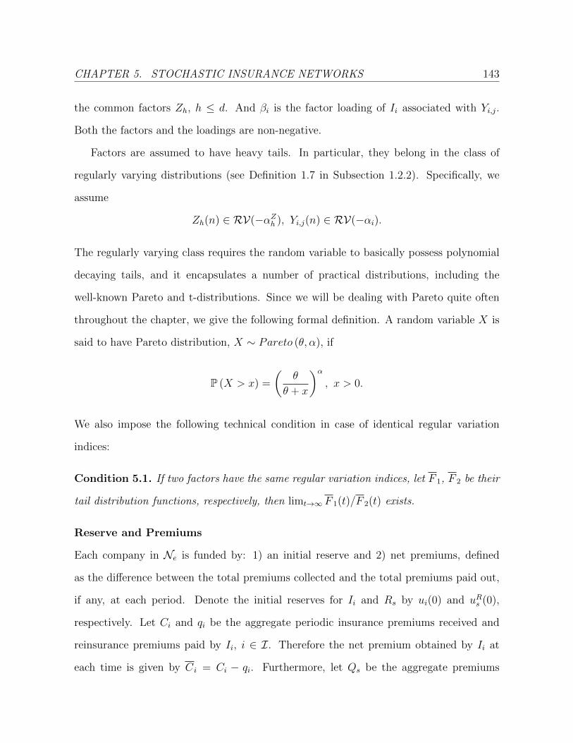
CHAPTER 5. STOCHASTIC INSURANCE NETWORKS 143
the common factors Zh, h ≤ d. And βi is the factor loading of Ii associated with Yi,j.
Both the factors and the loadings are non-negative.
Factors are assumed to have heavy tails. In particular, they belong in the class of
regularly varying distributions (see Definition 1.7 in Subsection 1.2.2). Specifically, we
assume
Zh(n) ∈ RV(−αZh ), Yi,j(n) ∈ RV(−αi).
The regularly varying class requires the random variable to basically possess polynomial
decaying tails, and it encapsulates a number of practical distributions, including the
well-known Pareto and t-distributions. Since we will be dealing with Pareto quite often
throughout the chapter, we give the following formal definition. A random variable X is
said to have Pareto distribution, X ∼ Pareto (θ, α), if
P (X > x) =
(θ
θ + x
)α, x > 0.
We also impose the following technical condition in case of identical regular variation
indices:
Condition 5.1. If two factors have the same regular variation indices, let F 1, F 2 be their
tail distribution functions, respectively, then limt→∞ F 1(t)/F 2(t) exists.
Reserve and Premiums
Each company in Ne is funded by: 1) an initial reserve and 2) net premiums, defined
as the difference between the total premiums collected and the total premiums paid out,
if any, at each period. Denote the initial reserves for Ii and Rs by ui(0) and uRs (0),
respectively. Let Ci and qi be the aggregate periodic insurance premiums received and
reinsurance premiums paid by Ii, i ∈ I. Therefore the net premium obtained by Ii at
each time is given by Ci = Ci − qi. Furthermore, let Qs be the aggregate premiums

CHAPTER 5. STOCHASTIC INSURANCE NETWORKS 144
collected from its reinsurance policy holders at each period, s ∈ R. ui(0) and uRs (0) along
with the premiums Ci and qi, constitute the capital base of the (re)insurance companies
to fulfill their obligations. Let us further denote by ui(n) and uRs (n) the level of reserve
for Ii, i ∈ I and Rs, s ∈ R, respectively, at the end of period n. If the reserves ui(n) or
uRs (n) is not sufficiently large to cover all the claims collected, then the company is forced
to fail. Precise definitions of ui(n)i∈I and uRs (n)s∈R will be given in (5.17) later in
Subsection 5.2.4.
Contractual Links and Network Topology
Naturally, the effective claims received by the companies are contingent on the survival of
its counterparty, which in turn is influenced by how the participants deal with each other
in the network. It is therefore crucial to first set the rules that govern the connectivity of
the network, which is summarized in the following assumption.
Assumption 5.1 (Contractual Links and Network Topology for Ne).
i) Insurer-Reinsurer: Each insurer Ii enters into “quater-share” reinsurance con-
tracts with more than one standing reinsurers. The proportion it reinsured with Rs,
and therefore the contractual link between Ii and Rs, is summarized by the nonneg-
ative vector ωi,si∈I,s∈R, with∑
s∈R ωi,s = 1, ∀i ∈ I. Each reinsurance contract
between Ii and Rs is assumed to be of a stop-loss type, with a reinsurance deductible
equal to vsi . If ωi,s > 0, there is a directed edge from Ii to Rs in the graph repre-
senting a contractual presence in the network, highlighting the business link between
these two companies.
ii) Reinsurance re-routing: If one or some of the multiple reinsurance counterpar-
ties of insurer Ii fails at some time n, the vector ωi,s is re-weighted proportionally
among the survival reinsurance counterparties of Ii after time n. And the edges are

CHAPTER 5. STOCHASTIC INSURANCE NETWORKS 145
re-directed reflecting the renewed contractual links. If, however, all of Ii’s reinsur-
ance companies have failed, then Ii will remain exposed to the claim risks until the
end of the time horizon M <∞.
iii) Reinsurer-Reinsurer: Each reinsurer Rs, s ∈ R, cannot reinsure the exposure
transferred from one reinsurer Rs1 , s1 6= s to some other reinsurer Rs2 , s2 6= s1, s
(i.e. there are only two ‘hoops’ in the reinsurance sequence). Moreover, Rs can only
enter into a proportional reinsurance contract (retrocession) with other reinsurers,
covering exposures that are directly transferred from the insurers. The proportions
of retrocession from reinsurer Rs1 to Rs2 is specified by the vector ωRs1,s2s1,s2∈R,
with ωRs,s = 1−∑
s′ 6=s ωRs,s′. If ωRs1,s2 > 0, there is an edge from Rs1 leading to Rs2 in
the network graph. And we further define
Pi,s1,s2 = ωi,s1ωRs1,s2
, (5.3)
the weight of the reinsurance connection between Ii and Rs2 via Rs1.
iv) Network Coverage: For each s ∈ R, define
inV (Rs)∆=i ∈ I : ωi,s > 0
∪s′ ∈ R : ωs′,s > 0
, (5.4)
i.e., the vertices that have an incoming edge or arc from node Rs. We assume that
⋃s∈R
inV (Rs) = I.
We need to point out that the results obtained in this chapter hold in greater generality
than in the networks with activities stipulated by Assumptions 5.1-i) and iii), which are
mainly made to facilitate the definitions of the proportions that are transferred back in

CHAPTER 5. STOCHASTIC INSURANCE NETWORKS 146
the event of failures of the participants; these quantities, to be defined momentarily, are
denoted by ρsi and ρss′ . The motivation of Assumption 5.1-ii) is that, each insurance
company has its own specialty and risk-profile, meanwhile each reinsurance company
specializes in different domains of reinsurance coverage. The assumption describes an
insurance market in which each insurer Ii has fixed preferences, as measured by the
vector ωi,ss∈R, over the reinsurance providers that underwrite reinsurance contracts on
the particular type of risks Ii wishes to hedge against. The reinsurers are willing and
are allowed to exchange risks among each other in the form of a proportional insurance
contracts that are tailored to their own risk preferences. Note also that Assumption 5.1-
iv) is a very mild one. We are only interested in a group of reinsurance companies along
with the group of insurance companies they cover.
An example of such a network is illustrated in Figure 5.1 below. Let Ne1 ∈ Ne be
the particular network given in the figure. Note that in Ne1 multiple reinsurers share
the reinsurance liabilities from the insurers, and successive reinsurance and retrocession
transactions among the reinsurance companies creates a so-called reinsurance-spiral in the
network, which could be a source of systemic risk hibernating therein (see [62] and [1]).
It is important to emphasize that the assumptions stated above, permits the formulation
of such a reinsurance spiral. However, the risk re-sharing activity is strictly regulated by
Assumption 5.1-iii). The rule basically forbids the reinsurer to cede reinsurance coverage
back to the reinsurance companies which initially seek protection on that particular cov-
erage. Again the stipulation of no more than two ‘hoops’ in the retrocession sequence is
imposed merely for the sake of expositional simplicity (and only affects the definitions of
ρsi and ρss′ to be introduced shortly). In fact, as long as the reinsurance contract ends
up with a party other than the one that buys protection at the first place, or equivalently
if the “hoops” do not create a “loop”, the framework introduced in this chapter works.

CHAPTER 5. STOCHASTIC INSURANCE NETWORKS 147
Figure 5.1: Network Ne1 . Each insurer enters into excess-of-loss reinsurance contractswith multiple reinsurers. A “reinsurance-spiral” among the reinsurance companies existsand is indicated by the “cycle” consisting of the curved lines.
5.2.2 Settlement Mechanism and Network Equilibrium
At the end of each period, each existing company in the network is faced with the settle-
ment of the claims collected during the period. Due to the sophisticated contractual links
among the companies, the state of the system at the end of period n is defined after a
sequence of events that might involve a cascade of write-offs and settlements throughout
the network at time n. In order to cope with these situations, we define the equilibrium
state of the network at each period as follows.
Definition 5.1. We say a network Ne ∈ Ne is in equilibrium state at time n, 1 ≤ n ≤M ,
if no companies in Ne are left unsettled from the failures, if any, of other companies in
Ne that occur at time n.
Note that, depending on the methods of settlements as well as the structure of the
contractual links among the companies, there may or may not exist an equilibrium state for
a given network. In the following assumption we make it clear how each counterparty of a
ruined company gets settled at the time of such failure. We shall argue momentarily that,
if companies in a network operating under Assumption 5.1 negotiate an arrangement under

CHAPTER 5. STOCHASTIC INSURANCE NETWORKS 148
which the spillover loss at counterparty default (i.e., who gets how much) is distributed
according to a reasonable mechanism (in the form of a linear program system), there exists
a unique equilibrium state for the network at all times. We first specify the following
assumption on the rules governing the allocation of spillover losses in the network system.
Assumption 5.2 (Rules for Spillover Loss Allocation). Upon the incident of Rs defaulting
during period n, n ≤M , Ii gets partially settled by an amount proportional to its unsettled
reinsurance exposure to Rs, if any, at period n; and Rs′ , s′ 6= s, gets settled by an amount
proportional to its unsettled retrocession exposure to Rs, if any, at time n.
In what follows, we shall denote by ρsi the proportion of spillover loss that Ii gets if
Rs fails, i ∈ I, s ∈ R, and similarly, denote by ρss′ the proportion that R′s takes on in
the event of the failure of Rs, s, s′ ∈ R, s 6= s′. Both ρsi and ρss′ depend on the claims
arriving to the network at the particular period when the failure of Rs occurs. We shall
give the formal definitions shortly in (5.16). For now, we contend ourselves with the fact
that both sets of proportions can be computed as soon as all the claims to the network
system within a given period have been collected.
Nevertheless, having Assumption 5.2 alone turns out to be inadequate to secure a
well-defined settlement mechanism in the event of a cascade of failures. Let us take a
closer look using the following example.
Example 1. Consider the simple network illustrated in Figure 5.2. Right after the claims
have been collected, reinsurer R1 does not have sufficient reserve base to buffer the size of
the claims arrived at that period. A write-off procedure is therefore triggered. According
to Assumption 5.2, R2 will get an amount of the spillover loss from R1 equal to (10 −
30)× (1/3) = −20/3. With this allocation of contagion loss, R2 is subsequently forced to
fail because 25 − 20 − 20/3 = −5/3 < 0. But we immediately ran into a dilemma if the
recurrent spillover loss from R2 is to be allocated to I1 and R1: should R1, a bankrupt

CHAPTER 5. STOCHASTIC INSURANCE NETWORKS 149
(a) Network Example: Initial Configurations (b) Network Example: Before Write-offs
Figure 5.2: (a): For each reinsurer the initial reserve levels are stated in the parentheses.For each insurer, the initial reserve as well as the reinsurance deductible are given in theparentheses next to the company. Transfer ratios are given next to the arrow representingthe flow of contracts. (b): State of the network after all claims have been collected, beforethe write-offs. Bracketed numbers are the sizes of the claims. Numbers in parenthesesare effective claims to the companies. And the rest is the transferred amount.
company, take on the spillover loss from R2? If we allow this process to iterate by arguing
that any failure/bankruptcy shall not be declared until all the subsequent cascading write-
offs are settled, then a more precise write-off mechanism is called for to ensure a unique
network state after all the contagion losses have been settled and received.
In order to address the afore-mentioned issue, we take an equilibrium approach. In
particular, we require that, in addition to the principle stipulated in Assumption 5.2, the
companies work out the spillover loss allocation at the end of each period according to
the following single-period linear optimization problem, which we proceed to formulate
now and interpret after we summarize that the equilibrium is well defined.
To streamline notations, let us suppress the time index and denote by ui and uRs the
levels of reserves at the beginning of the period for Ii, i ∈ I and Rs, s ∈ R, respectively.
Moreover, let Li be the effective claims, net the reinsured amount before any settlement,
retained by Ii. Similarly, let LRs be the effective reinsurance claims transferred to Rs

CHAPTER 5. STOCHASTIC INSURANCE NETWORKS 150
before any settlement. The mathematical definitions of Li and LRs are provided later in
(5.15). Note that both Li and LRs are obtained after all claims at that period have been
collected, but before any write-off/settlement has occurred. Define I+ = l ∈ I : ul > 0
and R+ = v ∈ R : uRv > 0, the set of survival insurers and reinsurers, respectively. An
equilibrium state for Ne corresponds to the state of the network after all companies mark
write-offs and make settlements according to the optimal solution vector of the following
linear optimization problem:
[P (κ)] : (5.5)
min∑i∈I+
π−i + ξ∑s∈R+
ψ−s
s.t. π+i − π−i = ui + Ci − Li −
∑s∈R+
ψ−s · ρsi, ∀i ∈ I+ (I)
ψ+s − ψ−s = uRs +Qs − LRs −
∑s′∈R+,s′ 6=s
(ψ−s′ · ρs′s − κψ
−s · ρss′
), ∀s ∈ R+ (II)
π+i , π
−i , ψ
+s , ψ
−s ≥ 0.
Here κ ∈ [0, 1] is a parameter controlling the degree of netting agreement between each
two reinsurance companies. When κ = 0, none of the contracts between two reinsurers
are netted. And κ = 1 corresponds to a fully netted scenario, for example, when all
the contracts between two reinsurers are fungible/exchangeable. Of course the netting
parameter κ can be made arc dependent, but for simplicity we consider the situation
where κ is identical throughout the network. We shall interpret the linear program shortly
after we state the following results, which indicate desirable “stability” properties of the
equilibrium state of the network underscored by the preceding linear program. We delay
the proofs until later in Section 5.6.
Theorem 5.2. The linear program [P (κ)], given in (5.5), has the following properties:
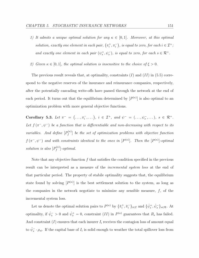
CHAPTER 5. STOCHASTIC INSURANCE NETWORKS 151
1) It admits a unique optimal solution for any κ ∈ [0, 1]. Moreover, at this optimal
solution, exactly one element in each pair,(π+i , π
−i
), is equal to zero, for each i ∈ I+;
and exactly one element in each pair (ψ+s , ψ
−s ), is equal to zero, for each s ∈ R+.
2) Given κ ∈ [0, 1], the optimal solution is insensitive to the choice of ξ > 0.
The previous result reveals that, at optimality, constraints (I) and (II) in (5.5) corre-
spond to the negative reserves of the insurance and reinsurance companies, respectively,
after the potentially cascading write-offs have passed through the network at the end of
each period. It turns out that the equilibrium determined by [P (κ)] is also optimal to an
optimization problem with more general objective functions.
Corollary 5.3. Let π− =(. . . , π−i , . . .
), i ∈ I+, and ψ− = (. . . , ψ−s , . . . ), s ∈ R+.
Let f (π−, ψ−) be a function that is differentiable and non-decreasing with respect to its
variables. And define [P(κ)f ] be the set of optimization problems with objective function
f (π−, ψ−) and with constraints identical to the ones in [P (κ)]. Then the [P (κ)]-optimal
solution is also [P(κ)f ]-optimal.
Note that any objective function f that satisfies the condition specified in the previous
result can be interpreted as a measure of the incremental system loss at the end of
that particular period. The property of stabile optimality suggests that, the equilibrium
state found by solving [P (κ)] is the best settlement solution to the system, as long as
the companies in the network negotiate to minimize any sensible measure, f , of the
incremental system loss.
Let us denote the optimal solution pairs to P (κ) by π+i , π
−i i∈I and ψ+
s , ψ−s s∈R. At
optimality, if ψ−s > 0 and ψ+s = 0, constraint (II) in P (κ) guarantees that Rs has failed.
And constraint (I) ensures that each insurer Ii receives the contagion loss of amount equal
to ψ−s · ρsi. If the capital base of Ii is solid enough to weather the total spillover loss from

CHAPTER 5. STOCHASTIC INSURANCE NETWORKS 152
the reinsurers (which is represented by the amount∑
s∈R ψ−s ), i.e., ui+Ci > Li+
∑s∈R ψ
−s ,
then Ii will remain solvent, in which case π+i > 0 = π−i . If otherwise, then Ii fails, in
which case π+i = 0 and π−i > 0. As a result, the vectors π−i i∈I and ψ−s s∈R represent
the loss at default for Ii and Rs, respectively, at the equilibrium state of the network.
Note that the preceding optimization problem would yield the same optimal solution if
we impose the additional constraint that π+i ×π−i = 0,∀i ∈ I+, and ψ+
s ×ψ−s = 0,∀s ∈ R+.
Therefore, we can interpret the equilibrium state associated with the optimal solution
vector to [P (κ)] as the equilibrium state of the network in which the weighted total loss of
the network is minimized at the optimal objective value, equal to∑
i∈I+ π−i +ξ
∑s∈R+ ψ−s .
Example 2 (Example 1 (Con’d)). Consider again the network given in Figure 5.2. Let
ξ = 1.
1) If we set κ = 0, i.e., no netting is allowed for the default losses, and each contract
has to be honored, the optimal solution to [P (κ=0)] becomes
ψ−1 = 30, ψ−2 = 15, π+1 = 10, π−2 = 5. (5.6)
Note that the associated equilibrium state corresponds to increasing the negative
reserve levels for R1 and R2 before the write-offs both by 10. Since no netting
agreement is in force, the write-off process continues until the levels of unsettled
claims for both companies have reached the equilibrium levels.
2) If, however, we set κ = 1, i.e., allow maximal netting, the optimal solution to
[P (κ=1)] is given by
ψ−1 = 55/3, ψ−2 = 20/3, π+1 = 115/9, π+
2 = 25/9.

CHAPTER 5. STOCHASTIC INSURANCE NETWORKS 153
Note that the equilibrium levels of unsettled claims for R1 and R2 are both lower
than their negative reserves after absorbing the “first-degree” spillover losses from
each other, i.e., 55/3 < 20+5×2/3, and 20/3 < 5+20×1/3. Eventually, under full
netting agreement, R1 only needs to transfer an amount equal to 5/3 = 20− 55/3 =
20/3− 5 of its losses to R2, and there is no need to take on any further losses back
from R2.
5.2.3 Connections to the Eisenberg-Noe ([40]) Formulation
Note that the optimal solution to [P (κ=0)] can be alternatively obtained using the approach
given in [40]. In this subsection we use the particular network studied in Example 1 to
discuss the connections between these two formulations.
The target output of the formulation in [40] is a so-called optimal payment or “clear-
ing” vector, p which summarizes the equilibrium amount paid out by the market partici-
pants. For the insurance-reinsurance network we study in this chapter, in particular, we
can write p =(. . . , pi, . . . , p
Rs . . .
), i ∈ I, s ∈ R. According to [40], this clearing payment
vector can be obtained as the optimal solution to a particular optimization problem.
In order to put our model into the framework of [40], we need to create an extra
“fictitious” vertex in our network, representing the “external” insureds who directly buy
protection from the insurers. Let us denote by this extra node vertex E . In the language of
[40], the insurance market (at any single period) is then fully characterized by specifying
(Π,p,u). In particular, u is the vector of initial endowments of the participants, p is the
vector of aggregate nominal exposures to the participants, and Π is a square liability matrix
specifying the amount (in proportions) of obligations between any two participants in the
system, in which the element Πij is the proportion of the total obligations to participant
i that is owed to participant j. The clearing payment vector p (for the period) is then

CHAPTER 5. STOCHASTIC INSURANCE NETWORKS 154
shown to be the solution to the following optimization problem:
[P (Π,p,u, f)] : max f(p) (5.7)
s.t. p ≤ ΠTp + u
0 ≤ p ≤ p.
where the objective function f(p) can be taken as any increasing function in p to guarantee
a unique optimal solution.
Now we illustrate how the equilibrium state for the network considered in Example 1
is derived using the program [P (Π,p,u, f)] above, for the particular period depicted in
Figure 5.2. We define the pairwise exposure matrices, E+ and E−. In particular, each
entry of E+, E+i,j, represents the nominal exposure from i to j, or the nominal amount
that i is supposed to pay j; and each entry of E−, E−i,j, identifies the amount that i is
expected to receive from j. For the network as presented in Figure 5.2, we have
E+ =
I1 I2 R1 R2 E
I1 0 0 0 0 50
I2 0 0 0 0 80
R1 0 40 0 10 0
R2 20 0 20 0 0
E 0 0 0 0 0
, (5.8)

CHAPTER 5. STOCHASTIC INSURANCE NETWORKS 155
and
E− =
I1 I2 R1 R2 E
I1 0 0 0 0 0
I2 0 0 0 0 0
R1 0 0 0 20 0
R2 0 0 10 0 0
E 0 0 0 0 0
. (5.9)
The aggregate exposure vector p is then obtained by aggregating the individual exposures
summarized in E+ and E−, via
p = eT(E+ − E−
)= (50, 80, 30, 30, 0)T . (5.10)
Note that in [40], the information of aggregate exposure p is sufficient to pin down the
equilibrium payment vector. However, as we shall reveal shortly, in order to transform
the equilibrium payment vector obtained from [P (Π,p,u, f)] to the equilibrium reserve
level identified by [P (κ=0)], one needs to explicitly construct E+ and E−.
Meanwhile, it is not hard to write down Π and u as follows,
Π =
I1 I2 R1 R2 E
I1 0 0 0 0 1
I2 0 0 0 0 1
R1 0 4/5 0 1/5 0
R2 1/2 0 1/2 0 0
E 0 0 0 0 0
, u =
45
55
10
25
0
.
Note that the vector u for the insurance market we study is just the initial reserve at the
beginning of a period. If we simply let f(p) = eTp, then the program, (5.7), yields the

CHAPTER 5. STOCHASTIC INSURANCE NETWORKS 156
unique optimal solution equal to
p =(p1, p2, p
R1 , p
R2 , 0)
= (50, 75, 25, 30, 0) .
We now demonstrate how the associated equilibrium end-of-period reserves can be
obtained from the preceding optimal payment vector, p, and how they can be shown to
match the unique optimal solution of the linear program [P (κ=0)] in (5.5). The first step is
to further break down the payment to the pairwise level. In order to do this, let us denote
by p−ij the specific equilibrium payment made from company i to company j, defined via
p−ij = piΠij.
Equivalently, the associated pairwise payment matrix, p−, can be obtained using the
following matrix operation,
p− =[p |p |p |p |p
] Π, (5.11)
where the notation denotes matrix component-wise multiplication (i.e., if A and B are
matrices of the same dimension, then (A B)i,j = Ai,j ×Bi,j). Moreover, define
p+ =(p−)T, (5.12)
i.e., p+ji denotes the amount of payment received by j from i, and p+
ji = p−ij. For the

CHAPTER 5. STOCHASTIC INSURANCE NETWORKS 157
particular network example we are studying the matrix p− is given by
p− =
I1 I2 R1 R2 E
I1 0 0 0 0 50
I2 0 0 0 0 75
R1 0 20 0 5 0
R2 15 0 15 0 0
E 0 0 0 0 0
,
or equivalently the non-zero elements of p− are
p−R2,I1= 15, p−R1,I2
= 20, p−R1,R2= 5, p−R2,R1
= 15,
p−I1,E = p1 = 50, p−I2,E = p2 = 75.
In order to obtain the resulting reserve levels from these payments it is necessary to
compare them with the individual nominal exposures given by the matrices E+ and E−.
Therefore, let us define
G = min(p+ − E+,0
)+ min
(p− − E−,0
),
where the minimum is performed component-wise (i.e., min(A,B) = C where Cij =
min(Aij, Bij)), and p+, p−, E+ and E− are given in (5.12), (5.11), (5.8) and (5.9). In
other words, G summaries the negative loss on each directional exposure between two
participants.
Consequently the relation between the optimal solutions to [P (Π,p,u, f)] and [P (κ=0)]

CHAPTER 5. STOCHASTIC INSURANCE NETWORKS 158
is established via
(π−1 , π
−2 , ψ
−1 , ψ
−2
)T= −
(eTG
)−E = (0, 5, 30, 15)T(
π+1 , π
+2 , ψ
+1 , ψ
+2
)T=
(u− (I− Π)T p
)−E
= (10, 0, 0, 0)T , (5.13)
where the subscript −E denotes the associated vector without the element corresponding
to the “fictitious” vertex E . In summary, 15 out of the 20 nominal reinsurance exposure
from I1 to R2 is honored by R2, but I1 is financially solid enough to weather this situation
and pays the insureds the 50 in full, and eventually it is only able to cover 75 out of the
80 claims it received. I2 is not so lucky because the 20 payment it receives from R1 is not
sufficient to prevent itself from failure. R1 and R2 settle with each other with payments
of amount equal to 15 and 5, respectively. Note that the reserve levels obtained from the
preceding operations coincide with the equilibrium reserve levels output from the linear
program [P (κ=0)], see (5.6).
We need to point out, however, that the advantage of using the LP formulation in
(5.5) is manifold.
a) It allows us to incorporate netting of default losses in a flexible way, which is not
captured in the approach developed in [40]. For example, the mutual payment
between R1 and R2 in the previous example can be reduced if certain level of netting
is enforced in the settlement of default losses. Scenario 2) in Example 2 illustrates
the benefit of allowing netting to the whole system: I1 no longer defaults in this
scenario, and all claims submitted from the insureds are honored.
b) Moreover, the output of the linear optimization problem [P (κ)] are the end-of-the-
period reserve levels, which turn out to be the direct inputs to our dynamic reserve
processes, see Theorem 5.4 below. In contrast, although the approach in [40] yields

CHAPTER 5. STOCHASTIC INSURANCE NETWORKS 159
an equivalent equilibrium state of the network at each stage (in the case when
κ = 0), a few extra steps of calculation is required to transform the payment vector
to the vector of reserve levels, as illustrated in the development leading to (5.13).
c) Recall that our ultimate goal is to efficiently evaluate the conditional spillover loss
at system dislocation using simulation. An additional benefit of our LP formulation
lies in the fact that some natural intuition on the large deviations description of
the system can be derived out of the setup of the optimization problem, which we
shall turn to shortly in the next section. Consequently, we believe the equilibrium
approach adopted here is better suited for this dynamic network system we proposed
in this insurance setting.
5.2.4 Effective Claims and Reserve Processes
Now we are in a good position to fill the gap and specify the rest of the model. Let
Xi,j(n), Wi,j(n) be the effective claim size of the j-th claim (1 ≤ j ≤ Ni(n)) arrived to Ii
which is reinsured by Rs at period n, and the amount reinsured for this particular claim,
respectively. The two quantities are defined via
Xi,j(n) =∑s∈R
ωi,s (min (Vi,j(n), vsi ) I (τRs > n− 1) + Vi,j(n)I (τRs ≤ n− 1)) ,
Wi,j(n) = Vi,j(n)−Xi,j(n) =∑s∈R
ωi,s max (0, Vi,j(n)− vsi ) I (τRs > n− 1)
=∑s∈R
ωi,sWsi,j(n), (5.14)
where W si,j(n)
∆= ωi,s max (0, Vi,j(n)− vsi ) I (τRs > n− 1), and vsi · ωi,s represents the rein-
surance deductibles between Ii and Rs, and τRs is the first time at which the reserve of
Rs are non-positive. Note that the cap vsi loses effect as soon as Rs fails. At the same

CHAPTER 5. STOCHASTIC INSURANCE NETWORKS 160
time, any claim with size exceeding the cap vsi ·ωi,s is covered by Rs. The effective claims
for insurer Ii and reinsurer Rs during period n are therefore
Li(n) =
Ni(n)∑j=1
Xi,j(n), i ∈ I,
LRs (n) =∑t∈R
∑v∈I
Nv(n)∑l=1
W tv,l(n)Pv,t,s, s ∈ R, (5.15)
where Pv,t,s is defined in (5.3).
Based on Assumption 5.2, the allocation ratios of spillover losses at time n, ρsi(n)
and ρss′(n) are defined via
ρsi(n)∆=
∑Ni(n)j=1 W s
i,j(n)Pi,s,sLRs (n)
=
∑Ni(n)j=1 W s
i,j(n)Pi,s,s∑t∈R∑
v∈I∑Nv(n)
l=1 W tv,l(n)Pv,t,s
, i ∈ I,
ρss′(n)∆=
∑v∈I∑Nv(n)
j=1 W s′v,j(n)Pv,s′,s
LRs (n)=
∑v∈I∑Nv(n)
j=1 W s′v,j(n)Pv,s′,s∑
t∈R∑
v∈I∑Nv(n)
l=1 W tv,l(n)Pv,t,s
, s′ ∈ R, s′ 6= s.
(5.16)
Let us index the single-period linear program [P (κ)], defined in (5.5), by n, i.e., [P (κ)(n)]
is set-up by replacing the constraints and objectives with their time-n counterparts. Then
at the end of each period, the system reaches the equilibrium state associated with the
unique optimal solution to [P (κ)(n)]. And the end-of-period reserves are determined by
the unique optimal solution vectors π+i (n), π−i (n)i∈I+(n) and ψ+
s (n), ψ−s (n)s∈R+(n), via
ui(n) = π+i (n) + π−i (n), i ∈ I+(n),
uRs (n) = ψ+s (n) + ψ−s (n), s ∈ R+(n). (5.17)
Note that ui(n) = uRs (n) = 0 if i 6∈ I+(n) and s 6∈ R+(n). The following result is a direct
CHAPTER 5. STOCHASTIC INSURANCE NETWORKS 161
implication of Theorem 5.2.
Theorem 5.4. The stochastic processes, ui(n)0≤n≤M , i ∈ I, and uRs (n)0≤n≤M , s ∈ R,
given in (5.17) are well-defined.
5.2.5 Conditional Spillover Loss at System Dislocation
Motivated by the insurance applications discussed in the previous section, we shall study
the performance measure Conditional Spillover Loss at System Dislocation which is in the
form of a conditional expectation. In simple words, it is the expected loss in the entire
system conditioning on the failure of a subset of the network constituents. Before giving
the formal definition we proceed to introduce a few more necessary notations.
Let AI and AR be subsets of I and R, respectively; and set A = AI ∪ AR. We define
the following failure times associated with Ne:
τi = infn > 0 : ui(n) ≤ 0, i ∈ I,
τRs = infn > 0 : uRs (n) ≤ 0, s ∈ R,
τAI = maxi∈AI
τi, τAR = maxs∈AR
τs,
τA = τAI ∨ τAR ,
i.e., τA is the first time when all names in A have failed. Finally, if we define
Di(A)∆= −minui(τA), 0,
the lost reserve at system dislocation at time τA for Ii, we can therefore introduce the
following formal definition of Conditional Spillover Loss at System Dislocation:

CHAPTER 5. STOCHASTIC INSURANCE NETWORKS 162
Definition 5.2. The Conditional Spillover Loss at System Dislocation for the subset
A = AI ∪ AR ⊆ I ∪ R in time horizon [0,M ] is defined as
CSD(A) = E
[∑i∈I
Di(A)∣∣∣τA ≤M
]. (5.18)
In words, the performance measure of the system, CSD(A), measures the contagion
(or spillover) impact of the collapse of the companies encoded by A to the entire system.
The idea of such a measure is motivated by the so-called Systemic Risk Index or Contagion
Index, following the terminology in [10], and studied in, for example [29] and [30]. The
authors in [29] used a Cauchy copula to evaluate the Systemic Risk Index, which is
also defined in terms a conditional expectation. Their simulation procedure does not
necessarily meet any provable optimality property, and it appears to be suited to the case
where conditioning event is the failure of a single player. Our work in this chapter aims
to provide a provably efficient procedure that can capture multiple-jumps.
5.3 Asymptotic Description of the Network System
Having fixed the architecture of the network, we now embark on providing a qualitative
characterization of the large deviations behavior of the system given τA ≤ M, i.e., the
event of system dislocation caused by the set A occurring before the fixed horizon M .
In the analysis that follows let us scale the initial reserves by b, and we later send b to
infinity. Let b > 0 and assume that ui(0) = rib is the initial reserve for Ii, i ∈ I, and let
uRs (0) = rsb, s ∈ R, where ri and rs are fixed positive constants. In what follows we will
also make explicit the dependence of various model quantities on b.
Our plan is to first pin down the asymptotic description of the general network system
portrayed in the previous section. As we shall reveal momentarily, this description can be

CHAPTER 5. STOCHASTIC INSURANCE NETWORKS 163
identified by solving another optimization problem. We then show that for some special
network structure, a more in-depth characterization can in fact be obtained with care.
5.3.1 Large Deviations Description via An Integer Program
We shall demonstrate that the large deviations description for the network has a “multiple-
regime” characterization. Depending on the tail structure of the claim size distributions,
the failure of the system arises from different numbers of extreme shocks in the claims.
This particular feature of the system inspires us to tailor a sequential algorithm for evalu-
ating CSD(A), for any given set A, which we shall describe in details in the next section.
It is interesting to realize that useful implications about the asymptotic behavior of
the system can be obtained from the linear program [P (κ)] given in (5.5). To see this,
recall that constraints (I) in (5.5) require, for each i ∈ I+ that,
π+i − π−i = ui + Ci − Li −
∑s∈R+
ψ−s · ρsi.
From the definitions in (5.15) and (5.14) as well as Assumption 5.1-ii), it’s not hard to
see that the effective claims Li are capped from above if and only if all the reinsurance
counterparties to Ii have not yet failed, and in that case ui +Ci − Li = Θp(b), where the
notation Θp(·) is defined in Definition 1.2 in Subsection 1.2.1. Therefore, the intuition is
that, P(π−i > 0) = Θ(1) if and only if there exists s ∈ R+, such that both of the following
are satisfied:
i) ψ−s = Θp(b),
ii) ρsi = Θp(1).
In other words, both the default loss for Rs and the contractual link between Ii and

CHAPTER 5. STOCHASTIC INSURANCE NETWORKS 164
Rs need to be sufficiently large in order for Ii with Θ(1) probability. This can occur due
to either of the following two possible cases:
a) Zh = Θ(b), for some 1 ≤ h ≤ d such that γi,h > 0,
b) Yi,j = Θ(b), for some 1 ≤ j ≤ Ni.
The intuitions above are certainly helpful, for now we are able to restrict the enumer-
ation of possible paths (leading to the event τA ≤ M) down to a much smaller subset.
In fact, as we shall see shortly, the combinatorial task of singling out the cheapest route
to the target event boils down to solving a Knapsack problem with multiple constraints.
Let us denote by Ξ the factor exposure matrix for the insurers in the network, which
is an |I| × (d+ |I|) matrix. Each column corresponds to a specific factor. We align the
factors in such a way that the first d factors are the common factors, and the remaining
|I| factors are the individual factors for the |I| insurers. Let Ξcj be the j-th column of Ξ.
In what follows we shall denote by Uj the factor, common or individual, corresponding
to Ξcj. On the other hand, the i-th row of Ξ, Ξr
i , represents the i-th insurance company.
Define νij to be the exposure of insurer Ii to factor Uj. In other words,
νij =
γij, if j ≤ d
βi, if j = i+ d, i ∈ I
0, otherwise.
The entries of the matrix Ξ is therefore defined via
Ξij = I (νij > 0) . (5.19)
Last but not least, define αj to be the regularly varying index of Uj, i.e., αj = αZj if j ≤ d,

CHAPTER 5. STOCHASTIC INSURANCE NETWORKS 165
and αj = αi if j = i + d, i ∈ I. The following result shows that, the large deviation
description of the system is simply obtained by solving an integer programming problem,
which is easily identified as a Knapsack type of problem with multiple knapsacks. We
shall delay the proof of the theorem to the end of Section 5.4. We mention that a one
dimensional Knakpsack formulation has also be used by [71] in the setting of heavy-tailed
large deviations.
Theorem 5.5. As b∞, we have
logP (τA(b) ≤M)
log b−→ −ζ, (5.20)
where ζ is the optimal cost to the following integer programming problem:
[IP ] : minm∑j=1
αjxj (5.21)
s.t.m∑j=1
xjΞi,j ≥ 1, ∀i ∈ A
xj ∈ 0, 1, 1 ≤ j ≤ m
Remark 5.1. For any [IP ]-optimal solution x∗ = (x∗1, . . . , x∗m)T , x∗j is interpreted as the
“indicator of activation” which dictates the occurrence of a large factor Uj. In particular,
if for fixed i ∈ I, x∗i+d = 1, then Yi = Θ(b) in the large deviations description of the
system; if x∗h = 1, for some h ≤ d, then Zh = Θ(b) in the large deviations description of
the system. For a survey of the algorithms to solve this Knapsack type of problems, we
refer the readers to e.g. [54].
There are several interesting features of this characterization.
1. The large deviations behavior of the network (conditioning on the event τA ≤M)

CHAPTER 5. STOCHASTIC INSURANCE NETWORKS 166
is dictated only by a set of tail indices. Depending on the choice of A, the description
of the most likely way leading to τA ≤M may change domains. For instance, the
event τA1 ≤M, where A1 = AIG, Prudential, could most likely result from the
occurrence of a few large common factors, while τA2 ≤ M, where A2 = Lincoln
Benefit, Northwestern Mutual, might occur most likely due to multiple phenomenal
idiosyncrasies, or a mixture of extremal idiosyncratic and common shocks.
2. Local to each insurer Ii, large deviations is characterized by the so-called “single
jump domain”; however on the network level, depending on the characteristics of
the claim size distributions, the large deviations of the system might fall into the
“multiple jump domain”, in which more than one shocks are necessary for the rare
event to occur.
An important albeit slightly counter-intuitive implication from Thereom 5.5 is that,
the existence of the reinsurance companies does not alter the asymptotic description of
the network system, in the sense that the most likely way leading to the failure of the
subset A is identical to that of a network consisting stand-alone insurance companies that
do not enter into any reinsurance contracts. We need to point out that this observation
does not suggest the roles of the reinsurance companies as risk buffers are vulnerable and
therefore flawed. Under market conditions in which moderately large claims arrive, the
reinsurance companies function well as a centralized risk mitigator, and might successfully
ward off the failure of some of its otherwise financially vulnerable insurance counterparties.
Furthermore, we find this observation to be consistent with various empirical studies,
which argue that reinsurance failure may not be a substantial source of systemic risk for
the insurance industry, see for example [62], [1] and [69].
We could, however, further strengthen the roles of the reinsurance companies by en-
forcing a more stringent capital requirement for the reinsurers. In order to see this, let us

CHAPTER 5. STOCHASTIC INSURANCE NETWORKS 167
assume that
uRs (0) = Θ (bρ) , ρ > 1,
for all s ∈ R, thereby demanding each reinsurer in the network to pledge more capital
than the insurance companies (recall that ui(0) = Θ(b) for i ∈ I). The following result
indicates that asymptotic description for the system with this modified assumption can
be identified by solving a different integer programming problem.
Theorem 5.6. Define
R (A) =⋃i∈A
s ∈ R :
∑r∈R
Pi,r,s > 0
,
for A ⊆ I, where Pi,r,s is defined in (5.3). In words, R (A) is the set of reinsurance
counterparties of companies in A. Then we have, as b∞,
logP (τA(b) ≤M)
log b−→ −ζ (ρ) (5.22)
where ζ (ρ) is the optimal cost to the following integer programming problem:
[IP(ρ)
] : minm∑j=1
ραjxj +m∑j=1
αjyj (5.23)
s.t.m∑j=1
Ξi,jxj ≥ 1, ∀i ∈ R(A)
m∑j=1
Ξl,j (xj + yj) ≥ 1, ∀l ∈ A
xj, yj ∈ 0, 1, 1 ≤ j ≤ m
We dispense ourselves with the formal proof of the result, which can be carried out in
a similar fashion as the proof of Theorem 5.5. The basic intuition is that, since uRs (0) =

CHAPTER 5. STOCHASTIC INSURANCE NETWORKS 168
Θ (bρ), the corresponding spillover losses from reinsurer Rs, is of the same order, i.e.,
ψ−s = Θ (bρ) as a result of Lemma 5.2 given in the next subsection. Now for i ∈ A, as long
as ρsi = o(b−(ρ−1)
), for all s ∈ R(i), P
(π−i > 0
)= o (1) and therefore Ii survives, with
overwhelming probability, after all its counterparties have been brought down (by some
other factors that Ii is not exposed to). From then on, it loses reinsurance protection and
requires a factor of order Θ(b) to get ruined. If, however, the exposure between Ii and
Rs, for some s ∈ R(i), is substantial enough such that ρsi = Ω(b−(ρ−1)
), then Ii fails with
overwhelming probability by the spillover loss passed on from the failure of Rs.
Remark 5.2. In any [IP(ρ)
]-optimal solution (x∗,y∗), x∗j and y∗j are interpreted as the
“strong” and “weak” activation indicators, respectively. If x∗j = 1, then the corresponding
factor Uj is among the factors that most likely lead to the failure of the counterparty set
R(A), i.e., Uj = Θ (bρ); if y∗j = 1, then Uj is among the factors that result in the failure
of some companies in A after they lost protections from their reinsurance counterparties,
and in that case, Uj = Θ (b).
5.3.2 Characterizing Asymptotic Behavior of A Special Net-
work
The development in the previous subsection suggests that, for a general network defined
in Section 5.2 one needs to explicitly solve the IP given by (5.21) to obtain an asymptotic
description of the system. We shall demonstrate in this subsection that for some special
network architecture, a more detailed characterization for the most likely way of the
network hitting the event τA(b) ≤M is readily accessible, without even resorting to the
optimization problem.
Consider an insurance-reinsurance network with a single reinsurance company, which
we refer to as R = R1. Let us write K = KI , the number of insurers in the system. An

CHAPTER 5. STOCHASTIC INSURANCE NETWORKS 169
example of such a network is shown in Figure 5.3. Because the shape of such a network
is in close resemblance of a star, in what follows we shall refer to it as the star-shaped
network. Endowed with such a special structure, Assumption 5.1 can be greatly simplified.
In particular, since there is only one reinsurer in business in the network, ωi,1 = 1 and
Pi,1,1 = 1, for all i ∈ I. And there is apparently no retrocession activity in the star-shaped
network. Furthermore, the reinsurance re-routing assumption becomes trivial: as soon
as R fails, the remaining insurers no longer receive any reinsurance protection, and are
subject to absorbing all potential claim risks from their policy holders.
Figure 5.3: An example of a “star-shaped” network.
In addition to the star-shape topological simplification, the number of claims arrived
to Ii at each time n is assumed to be Poisson with mean λi, i.e., Ni(n) ∼ Poisson (λi).
And we further simplify the correlation structure among the claims by fixing the total
number of common factors to be one, i.e., d = 1. Therefore under this specification, the
exogenous claim size, V , the effective insurance claim size, X, and the effective reinsurance
claim size, W , can be expressed in the following way:
Vi,j(n) = γiZ(n) + βiYi,j(n), 1 ≤ j ≤ Ni(n),
Xi,j(n) = min (Vi,j(n), vi) I (τR > n− 1) + Vi,j(n)I (τR ≤ n− 1) ,

CHAPTER 5. STOCHASTIC INSURANCE NETWORKS 170
Wi,j(n) = Vi,j(n)−Xi,j(n),
for each i ∈ I, n ≤ M < ∞ and 1 ≤ j ≤ Ni(n). Here τR is the failure time of R to be
defined shortly.
Note that for the star-shaped network, the equilibrium of the system and hence the
payment / settlement to each company at each time is easily solved from the linear
program in (5.5). In particular, let ψ−1 (n) be the optimal solution variable for ψ−1 (n) in
(5.5), associated with the star-shaped network. It’s not hard to convince ourselves that
ψ−1 (n) = −min(u(n), 0
). Therefore we can express “feedback” allocation of unsettled
claims from R to Ii at time n, denoted as Γi, defined via
Γi(n) = ψ−1 (n) · ρ1i = −min(u(n), 0
)×
∑Ni(n)j=1 Wi,j(n)∑K
l=1
∑Nl(n)j=1 Wl,j(n)
, (5.24)
for 1 ≤ n ≤ M . Let the initial reserve for R and Ii be u(0) = rb and ui(0) = rib,
respectively, where r, ri > 0 are some positive constants. We can therefore express the
reserve processes for R and Ii, i ∈ I, as
u(n) = u(n− 1) +QI (τR > n− 1)−K∑i=1
Ni(n)∑j=1
Wi,j(n), (5.25)
ui(n) = ui(n− 1) + Ci −Ni(n)∑j=1
Xi,j(n)− Γi(n), (5.26)
for 1 ≤ n ≤ M , where Q = Q1 is the periodic reinsurance premiums R receives. Here
the failure times τR and τi are formally defined as τR = infk > 0 : u(k) ≤ 0 and
τi = infk > 0 : ui(k) ≤ 0.
We now proceed to characterize the asymptotic behavior of the star-shaped network.
Note first that, given the Poisson nature of the claim arrival process, the probability

CHAPTER 5. STOCHASTIC INSURANCE NETWORKS 171
P (τA ≤M) is dominated by the probability of one or a few extremal claims. To see this,
Note that
P (τA(b) < M ∧ τR(b)) ≤ P (τA(b) < τR(b))
≤M∑n=1
P (ui(n) < 0,∀i ∈ A)
=M∑n=1
P
Cin− n∑k=1
Ni(k)∑j=1
Xi,j(k)
+ ui(0) < 0,∀i ∈ A
≤
M∑n=1
∏i∈A
P
(n∑k=1
Ni(k)vi > Cin+ ui(0)
)
≤M∑n=1
∏i∈A
P
(n∑k=1
Ni(k) > rb
), (5.27)
for some positive constant r that depends only on the set A. In fact, we can pick for b
large enough, r = mini∈Ari/ (2vi). Hence the term P (τA(b) < M ∧ τR(b)) decays at least
exponentially in b. We can therefore conclude, with the aid of the following proposition,
that
P (τA(b) ≤M) ∼ P (τR(b) ≤ τA(b) ≤M) (5.28)
as b∞.
Proposition 5.1. Let α and αi be the indices of regularly variation for the single common
factor and the i-th individual factor, respectively. Assume that the reserve levels are
sufficiently large (i.e., b is large).
(i) If
α <∑i∈A
αi, (5.29)
the event τA ≤M is caused with overwhelming probability (as b∞) by a large
common factor.

CHAPTER 5. STOCHASTIC INSURANCE NETWORKS 172
(ii) If α >∑
i∈A αi, the event τA ≤ M occurs with overwhelming probability (as
b∞) in the following way: the occurrence of a single large individual factor from
some insurer Ii in A first leads to the failure of R, after which insurers in A break
down because of the occurrence of a series of additional individual factors, one from
each of the insurers in A\i.
(iii) If, however, α =∑
i∈A αi, the event τA ≤ M can be caused, with probability
bounded away from zero, either by the occurrence of a large common factor as in
case (i), or by the sequence of events as described in case (ii) above.
In order to prove the proposition, we need the following results, the proofs of which
are given in the Section 5.6.
Lemma 5.1. Suppose Xii≥1 is a sequence of i.i.d. regularly varying random variables
with index α; Z is regularly varying with index α0 and is independent of the Xi’s. And
N ∼ Poisson(λ), independent of both Z and Xi’s. Moreover, Condition 1 is in force for
Xi and Z. Suppose further that ψ : N → R is a non-decreasing mapping which satisfies
E[ψ(N)α(1+δ)
]<∞, for some δ > 0. Then
P
(N∑i=1
Xi + ψ(N)Z > b
)∼ ENP (X1 > b) + P
(Z >
b
Eψ(N)
). (5.30)
Lemma 5.2. 1) Suppose Z is a nonnegative regularly varying random variable with index
α > 0, and Y is a nonnegative random variable satisfying E[Y α(1+2ε)
]< ∞ for some
ε > 0. Then
P (ZX > b+ x|ZX > b) −→(
1
1 + x/b
)α.
2) Suppose Xi is nonnegative and regularly varying with index αi > 0, i = 1, . . . , K.
Xi,j is the j-th independent copy of Xi. Ni is nonnegative random variable satisfying

CHAPTER 5. STOCHASTIC INSURANCE NETWORKS 173
E[Nαi(1+2ε′)i
]<∞ for some ε′ > 0. And Condition 1 holds for Xi and Xj, i 6= j. Then
P
(K∑i=1
Ni∑j=1
Xi,j > b+ x
∣∣∣∣∣K∑i=1
Ni∑j=1
Xi,j > b
)−→
(1
1 + x/b
)α∗,
where α∗ = minKi=i αi.
Proof of Proposition 5.1. We shall study the probability P (τR ≤ τA ≤M). Note that, if
τR ≤M , then there exist 1 ≤ n ≤M and 1 ≤ i ≤M such that
max
γiNi(n)Zn,
Ni(n)∑j=1
βiYi,j(n)
+n−1∑k=1
Ni(k)vi > rib.
On the other hand, if there exist 1 ≤ n ≤M and 1 ≤ i ≤M such that
max
γiNi(n)Zi,
Ni(n)∑j=1
βiYi,j(n)
> (ri + r) b,
we would guarantee that τR ≤ n ≤M . Let δ∆= (r,mini∈A ri) / (2KM), and define
BZ =
∃n ≤M :
(K∑i=1
γiNi(n)
)Zn > Kδb, τA ≥ τR = n
,
BY =
∃n ≤M, i ≤ K :
Ni(n)∑j=1
βiYi,j(n) > δb, τA ≥ τR = n
=⋃i≤K
∃ni ≤M :
Ni(ni)∑j=1
βiYi,j(ni) > δb, τA ≥ τR = ni
=⋃i≤K
BY,i,
where BY,i∆=∃n ≤ M :
∑Ni(n)j=1 βiYi,j(n) > δb, τA ≥ τR = n
, and the BY,i’s are disjoint

CHAPTER 5. STOCHASTIC INSURANCE NETWORKS 174
sets. Note that τR ≤ τA ≤M ⊆ BY ∪BZ . Further define the following probabilities:
pZ = P (τR ≤ τA ≤M ;BZ) and pY = P (τR ≤ τA ≤M ;BY ) .
Note that
pZ + pY − P (BZ ∩BY ) ≤ P (τR ≤ τA ≤M) ≤ pZ + pY .
And since P (BZ ∩BY ) = o (pZ ∨ pY ), it suffices to compare pZ and pY . The cases pY =
o (pZ), pZ = o (pY ) and pZ = Θ (pY ) correspond to case i), ii) and iii) in the proposition,
respectively.
1) Analysis of pZ .
From Lemma 5.2 we know
[(K∑i=1
γiNi(n)
)Zn
∣∣∣∣∣(
K∑i=1
γiNi(n)
)Zn > Kδb
]∼ (Kδ +KδW ) b, (5.31)
where W ∼ Pareto (1, α). Intuitively, the overshoot, and hence the amount that is unable
to be covered by the failed R, is asymptotically Pareto (≈ δWb). When R collapses,
Assumption 1 is in place, and each Ii has to absorb a fraction of this unsettled exposure
proportional to its current reserve level. Since in this case the shock is common to all the
claims, the allocation to each player in set A is expected to be roughly proportional to
γiNi(n), i ∈ A. To make this intuition precise, let A0 be a strict subset of A. Note that
P(τR < τA ≤M |BZ
)=
M−1∑n=1
P(τR = n < τA ≤M |BZ
)=∑A0⊂A
M−1∑n=1
P(ui(n) ≥ 0,∀i ∈ A0
∣∣BZ
)P(n = τR < τA ≤M |BZ , ui(n) ≥ 0,∀i ∈ A0
)

CHAPTER 5. STOCHASTIC INSURANCE NETWORKS 175
≤∑A0⊂A
M−1∑n=1
Θ[P(γiNi(n− 1)δWb ≤ ui(n− 1) + Ci,∀i ∈ A0
)]× P
(n = τR < τA ≤M |BZ , ui(n) ≥ 0,∀i ∈ A0
)=o (1) ,
where the third line follows by virtue of (5.31). The last equality holds because, for the
first probability in the summand,
P(γiNi(n− 1)δWb ≤ ui(n− 1) + Ci,∀i ∈ A0
)=Θ
[∏i∈A0
P
(W ≤ ri
γiδE(Ni(n− 1)
))] = Θ (1) ,
where we used Lemma 5.1. At the same time,
P(n = τR < τA ≤M |BZ , ui(n) ≥ 0,∀i ∈ A0
)= o(1)
since we need a few more large factors in the remaining players in A\A0 in order to bring
down those in set A. Therefore, let σi∆= ri/2, i ∈ A, we have
P(τR ≤ τA ≤M |BZ
)= Θ
(P(τR = τA ≤M |BZ
))= Θ
( M∑n=1
P(γiNi(n)δWb > σib,∀i ∈ A; τR = n
))= Θ(1), (5.32)

CHAPTER 5. STOCHASTIC INSURANCE NETWORKS 176
once again by virtue of (5.31) and Lemma 5.1. On the other hand, since
P
((K∑i=1
γiNi(1)
)Z1 ≥ δb; τA ≥ 1 = τR
)≤ P (BZ) ≤
M∑n=1
P
((K∑i=1
γiNi(n)
)Zn ≥ δb
),
(5.33)
along with (5.32) we conclude that
pZ = Θ(P (BZ)
)= Θ
(b−α). (5.34)
2) Analysis of pY .
The intuition is that, it is cheaper to bring down R by the occurrence of a large individual
factor from some company, say Ii, in the set A than from outside A. From Lemma 5.2 we
know that, for 1 ≤ i ≤ K,
Ni(n)∑j=1
βiYi,j(n)
∣∣∣∣∣Ni(n)∑j=1
βiYi,j(n) > δb
∼ (δ + δWi) b, (5.35)
where Wi ∼ Pareto(1, αi). Consider first the case if R is failed by some large individual
factor from, say Il, l 6∈ A, the same factor will create an overshoot of unsettled claims of
size Θ(b). And spelled by Assumption 1, Il will absorb Θ(1) proportion of the overshoot,
large enough to fail Il itself with Θ(1) probability. Whereas the remaining companies,
Il′ , l′ ∈ A, l′ 6= l will take on merely Θ(1/b) proportion of the unsettled claim, and hence
will fail by this large individual factor from Il with probability of size only Θ (b−αl′ ) , l′ ∈
A, l 6= l′. The probability of failing the remaining companies in A is of order Θ(b−
∑i∈A αi
),
leading to a total probability of Θ(b−αl−
∑i∈A αi
). If, however, it is some individual factor
from Ii, i ∈ A that fails R in the first place, the probability of τA ≤ M happening out
of this scenario amounts to Θ(b−
∑i∈A αi
).
We now proceed to make the previous argument more precise. First, we have, for any
CHAPTER 5. STOCHASTIC INSURANCE NETWORKS 177
i ≤ K,
P(τi = τR ≤M |BY,i
)= Θ
[P(δWib > min
i≤Krb)]
= Θ(1).
As soon as R fails, the remaining insurers no longer receive protection. Subsequently they
face complete exogenous claims that are heavy-tailed. The event EY,i, i ≤ K, defined via
EY,i∆= τA ≤ τR ≤M |BY,i, τi = τR ≤M
comes about out of the following two scenarios.
i) Arrival of a large common factor.
Similar to the analysis at the beginning of the proof, EY,i is induced by the occurrence of
a common factor if and only if there exists τR ≤ n ≤M , such that
∑l∈A\i
γlNl(n)
Zn ≥ minl∈A\i
rlb/2,
the probability of which, by virtue of Lemma 5.1, is again Θ (b−α).
ii) Individual factors.
For each l ∈ A \ i, we require that there exists τR ≤ nl ≤M , such that
Ni(nl)∑j=1
βlYl,j(nl) ≥ rlb/2
which, again due to Lemma 5.1, independently has probability of order Θ (b−αl). There-
fore,
P (EY,i) = Θ(b−
∑l∈A\i αl
).

CHAPTER 5. STOCHASTIC INSURANCE NETWORKS 178
It remains to calculate P (BY,i). Applying similar bounds as in (5.33), we have
P
Ni(1)∑j=1
βiYi,j(1) ≥ δb, τA ≥ 1 = τR
≤ P (BY,i) ≤M∑n=1
P
Ni(n)∑j=1
βiYi,j(n) ≥ δb
.
Lemma 5.1 allows us to conclude that P (BY ) = Θ (b−αi). Consequently,
pY =∑i≤K
P(EY,i
)P(τi = τR ≤M |BY,i
)= Θ
[∑i∈A
P(EY,i
)P(τi = τR ≤M |BY,i
)P (BY,i)
]
=
Θ[b−(α+mini≤K αi)
], Individual → Common
Θ[b−
∑i∈A αi
]. Individual → Individual
(5.36)
And therefore the criteria given by (5.29) distinguishes pZ from pY . Recall from the
discussion at the beginning of the section that the probability P (τA < M ∧ τR) decays
exponentially, it’s immediate from (5.34) and (5.36) that
P (τA < M ∧ τR) = o(P (τR ≤ τA ≤M)
).
The result follows.
5.4 Design of Efficient Simulation Algorithms for Ne
The asymptotic analysis in the preceding section is useful in obtaining a qualitative de-
scription of the systemic risk landscape of the entire network. However, in order to
achieve this one is required to fully solve a combinatorial problem. Moreover, the re-
sulting asymptotic description is rather coarse. In this section we aim to achieve a more

CHAPTER 5. STOCHASTIC INSURANCE NETWORKS 179
precise quantitative assessment and make sharper evaluations of the embedded systemic
risk throughout the network Ne. We resort to the tool of Monte Carlo methods, and
our goal is to propose an efficient simulation algorithm to evaluate the conditional system
dislocation (5.18). We do this by designing an algorithm for the probability
q(b) = P (τA(b) ≤M)
instead. Estimators for (5.18) is a natural consequence.
5.4.1 Guidelines for Simulation Design
As pointed out in Subsection 1.2.3, the design of provably efficient simulation algorithms
oftentimes relies on a careful asymptotic description of the system as a meaningful depart-
ing point. Therefore, constructing efficient estimators for the network system introduced
in Section 5.2 will hinge on the insight from the large deviations analysis presented in the
previous section.
Before we proceed, we require that our final estimator shall possess strong efficiency,
an efficiency characteristics given in Definition 1.9 in Subsection 1.2.4. Given this notion
of efficiency, our goal is to search for an estimator within the class of strongly efficient
estimators that is practically convenient. Ideally, we hope the algorithm shares a uniform
setup under various configurations of the system, and is easy to implement, without
sacrificing too much efficiency. This translates to the search of a probability measure
P (·) ∆= P
(·|En
)
for some conditioning event En carefully “maneuvered” so that
1) Path sampling under P is not complicated.

CHAPTER 5. STOCHASTIC INSURANCE NETWORKS 180
2) The behavior of the system under P, i.e., conditional on En, is reasonably close to
P∗n.
3) The associated estimator possesses the required notion of efficiency, in this setting
in particular, strong efficiency.
And on top of these criteria we demand that
4) The algorithm requires minimum and uniform setup under various system configu-
rations.
Considering the network model we study, it might be desirable to have the same
estimator no matter how the claim structure varies that leads to different large deviations
behavior (see Theorem 5.5 and Proposition 5.1). The bottom line is, within the class of
strongly efficient estimators, one might be willing to sacrifice efficiency in exchange for
convenience and flexibility.
5.4.2 A Mixture-based SDIS
Loosely speaking, large deviations behaviors of heavy-tailed systems are governed by
the so-called “principle of large jumps” or “catastrophe principle”, which declares that
large deviations are triggered by one or a few components with immoderate magnitudes
(see Subsection 1.2.2; also see [12] for an extended discussion). Recall from Section 5.2
that the reserve processes u(n) and ui(n) are essentially heavy-tailed random walks whose
increments are random sums of factors per se. The natural direction to pursue is therefore
biasing the sampling distribution of the factors to be “locally” compatible with the large
deviations rule of thumb stated above. The challenge is, however, how to judiciously pick
the change of measure so that paths generated under such a measure can be sufficiently
close to the most likely paths of the system that underscore both regimes (see Section

CHAPTER 5. STOCHASTIC INSURANCE NETWORKS 181
5.3). We need the following proposition in order to further connect the dots and achieve
this goal. The essence of the result is of the same flavor as Proposition 1 in [17].
Proposition 5.2. Given the network Ne defined in Section 5.2, define
δN∆= min
i∈A
ri
2MN i
(∑dh=1 γi,h + βi
) ,where N i = maxk≤M Ni(k), i ∈ I. Let X be the set of feasible solutions to the IP given
in (5.21). And define
AδN (b)∆=
⋃x∈X
⋂i∈A
⋃k≤M
⋃
1≤h≤dγi,hxh>0
Zh(k) ≥ δNb
⋃ ⋃
1≤l≤Ni(k)xi+d=1
Yi,l(k) ≥ δNb
Then we have
i) AδN (b) is a superset of τA(b) ≤M, i.e.,
AδN (b) ⊇ τA(b) ≤M. (5.37)
ii) Conditioning on Ni(k), i ∈ I, k ≤M , we have, as b∞,
logP(AδN (b)
)log b
−→ −ζ,
where ζ is the optimal cost to [IP ] in (5.21).
Proof. i) Suppose there exists i′ ∈ A, such that 1) Zh(k) < δNb for all h ≤ d such that
γi′,hxh > 0, and for all 1 ≤ k ≤ M , and 2) Yi′,l(k) < δNb for all 1 ≤ l ≤ Ni′(k) and

CHAPTER 5. STOCHASTIC INSURANCE NETWORKS 182
for all 1 ≤ k ≤M , then we have, for any n ≤M ,
ui′(n)
≥ rib−n∑k=1
d∑h=1
γi′,hZh(k)Ni′(k) +
Ni′ (k)∑l=1
βi′Yi′,l(k)
− n∑k=1
∑s∈R
ψ−s (k) · ρsi′(k)
≥ rib− δNb · nN i′
(d∑
h=1
γi′,h + βi′
)−
n∑k=1
∑s∈R
ψ−s (k) · ρsi′(k)
≥ rib/2−n∑k=1
∑s∈R
ψ−s (k) · ρsi′(k),
where ψ−s (k) is the optimal solution for ψ−s (k), s ∈ R for the linear program [P κ(k)].
Furthermore, the model setup ensures that at any point in time, each insurer cannot
receive an allocation of the spillover losses from all of its reinsurance counterparties
of an aggregate amount larger than the total amount it reinsures. In what follows,
we shall refer to this observation as limited spillover impact. Therefore, we have
n∑k=1
∑s∈R
ψ−s (k) · ρsi′(k) ≤n∑k=1
d∑h=1
γi′,hZh(k)Ni′(k) +
Ni′ (k)∑l=1
βi′Yi′,l(k)
≤ ri′b/2.
And consequently ui′(n) ≥ 0, for all n ≤ M , and this implies that τA(b) > M.
We have thus established (5.37).
ii) An equivalent expression for AδN (b) is given by
AδN (b) =⋃x∈X
⋃k≤M
⋂i∈A
⋃1≤j≤m,Ξijxj≥1
Uj(k) ≥ δNb
,
where Ξ is the factor exposure matrix defined in (5.19), and m = d + |I| is the
number of column of Ξ. Recall that Uj = Zh if 1 ≤ j ≤ d, and Uj = Yi if j = d+ i,

CHAPTER 5. STOCHASTIC INSURANCE NETWORKS 183
i ∈ I. Let us further define
S(x) = j = d+ i : i ∈ I, xj = 1 ∪ h ≤ d : xh = 1 , (5.38)
i.e., S(x) is the index set of active factors associated with [IP ]-feasible solution x.
For the lower bound, we note that
P (AδN (b)) ≥ P
⋂i∈A
⋃1≤j≤m,Ξijx∗j≥1
Uj(1) ≥ δNb
=
∏j∈S(x∗)
P(Uj(1) ≥ δNb
)≥ E [δN ]−α
T e b−αTx∗ ≥ κ1b
−αTx∗ ,
for some positive constant κ1, where x∗ is an [IP ]-optimal solution. Here the second
inequality arises from Lemma 5.1.
And for the other direction, we utilize a union bound instead. In particular,
P (AδN (b)) ≤∑x∈X
M∑n=1
P
⋂i∈A
⋃1≤j≤m,Ξijxj≥1
Uj(n) ≥ δNb
≤ κ2b−αTx∗ , (5.39)
for some positive constant κ2, where x∗ is again an optimal solution to [IP ]. The
result follows immediately after taking log for both the lower and upper bounds.
An immediate implication of the previous results is a sampling scheme that induces the
occurrence of adequately large (of size at least δN) common or individual factors at each
period might be sufficient to guarantee bounded relative error of the estimator. We in fact
implemented this state-independent algorithm, and realized that a dynamic version of the

CHAPTER 5. STOCHASTIC INSURANCE NETWORKS 184
change of measure seems to be as easy to implement as the state-independent counterpart,
but could further reduce the relative variance of the associated estimator. From the
simulation perspective, the order of occurrence of the factors during each period deems
irrelevant. Our strategy is therefore to view the factors as if they arrive sequentially. At
each period, we can consider the random sums of the factors, as random walks themselves,
thereby creating this “internal” layer of random walks. From this point on we can borrow
apparatus from established state-dependent rare event simulation algorithms to aid the
design of our importance sampling estimator. In particular, we shall exploit the idea
developed in [34] (see also the survey paper [17]).
The key ingredient is a mixture based importance sampling distribution for the in-
crements: with some probability p(n), the increment is sampled conditioning on it being
“large”, and with probability 1− p(n), it’s sampled as if it’s a “normal” shock. Let X be
the increment of the system, and without loss of generality suppose its density is given
by f(x), then the nth increment is drawn from the importance density gn(·), defined as
gn(x) =
p(n)I(x ∈ An(b)
)P(Xn ∈ An(b)
) + (1− p(n))I(x ∈ An(b)
)P(Xn ∈ An(b)
) f(x), (5.40)
where An(b) specifies the region in which the increment is qualified to be a large shock.
Note that the part in (5.40) corresponding to the “normal” jumps is necessary in order to
conciliate the sensitivities of large deviations probabilities to the likelihood ratio of those
paths that have more than one jumps of order Ω(b), a crucial observation pointed out by
[12] (see also Example 4.1 in Chapter 4).
In the one dimensional random walk case, An(b) is typically chosen to be proportional
to the “distance to go” for the current position of the random walk, i.e., An(b) = a(b −
sn−1), for some a ∈ (0, 1) and sn = x1 + · · · + xn. In more general cases, An(b) can be
CHAPTER 5. STOCHASTIC INSURANCE NETWORKS 185
derived from some “auxiliary” or “steering” processes other than the targeting process. A
convenient choice of such an auxiliary process in our setting is obtained by “eliminating”
the reinsurance participants R a priori and allocating the reserve process uRs (n), s ∈ R
proportionally to each ui(n), i ∈ I. Equivalently, we pretend that the Ii’s absorb full
sized claims without reaching out to R to hedge risks. In principle, to recoup this higher
risks taken by the insurers, the initial reserves ui(0)’s, i ∈ I shall also be adjusted up
accordingly, but we dispense ourselves with this adjustment in the auxiliary process. The
benefit of doing so will be discussed after we outline the algorithm in the next subsection.
Effectively the auxiliary process consists of KI random walks, dependent 1) explicitly
upon the common factor Zhh≤d and 2) implicitly on the presence of Rss∈R. At the
beginning of each period, we first sample the common factors for the current period in
order to strip off the first layer of dependence among the claims; and then sequentially
sample the remaining individual factors. The mixture sampling density (5.40) is used to
sample each factor that corresponds to the survival companies in A, with the “distance
to go” An(b) properly defined in a dynamic way. We shall detail this choice in the
next subsection. The resulting sampling scheme is easy to carry out, self-adjusting in
nature, and saves the user the trouble of setting up the algorithm differently according to
different network structures. Proposition 5.2 implies that the system simulated in this way
is guaranteed to be within a moderate “distance” from the large deviations description
of the system, which is sufficient to preserve strong efficiency of the associated estimator.
Formally we have the following efficiency result, the proof of which is postponed after we
have detailed the algorithm in the next subsection.
Theorem 5.7. The adaptive importance sampling estimator qZ,Y,N (to be defined in (5.44)
and (5.45) in the next subsection) is strongly efficient for estimating q(b) = P (τA(b) ≤M).

CHAPTER 5. STOCHASTIC INSURANCE NETWORKS 186
If, in addition, αi > 2, for all i ∈ I, and αZh > 2, for all 1 ≤ h ≤ d, then the estimator
hZ,Y,N∆=∑i∈I
qZ,Y,NDi(A)
is also strongly efficient for estimating CSD(A) =∑
i∈I E[Di(A)I (τA ≤M)
].
5.4.3 The Algorithm
We are now ready to carry out our plan and pinpoint the state-dependent importance
sampling idea in details. We start by defining the auxiliary process via
Si(n) =n∑k=1
Ni(k)∑j=1
Vi,j(k)− Cin,
S(0)i (n+ 1) = Si(n) + Ni(n+ 1)
d∑h=1
γi,hZh(n+ 1)− Ci,
S(l)i (n+ 1) = S
(l−1)i (n+ 1) + βiYi,l(n+ 1), 1 ≤ l ≤ Ni(n+ 1), (5.41)
for each i ∈ A, where Vi,j(k) is the claim size random variable defined in (5.2). We then
summarize the details of our general SDIS algorithm for Ne as follows.
Description of The SDIS Algorithm
1) Solve the integer program, [IP ], given in (5.21). Recall that X is the set of feasible
solutions to [IP ]. Define
S =⋃x∈X
S(x), S∗ =⋂x∈X
S(x), (5.42)
where S(x) is defined in (5.38). In other words, l ∈ S if the l-th factor is active in
some [IP ]-feasible solutions, and l ∈ S∗ if the l-th factor is active in all [IP ]-optimal

CHAPTER 5. STOCHASTIC INSURANCE NETWORKS 187
solutions.
2) Sample Ni(n) from Binomial(Nn, qn
), for each i ∈ I, n ≤M .
3) While n ≤M , at the beginning of period n, 1 ≤ n ≤M , let the survival companies in
A be denoted as A(n). For each 1 ≤ h ≤ d, let fZh(·) be the density for the common
factor Zh. For h ∈ S, given that SA(n− 1) = Si(n− 1)i∈A(n) = sA, sample Zh(n)
from the following mixture density
gh,n(z|sA) =[pZh(n)
I(z ≥ adn(b, sA)
)P(Zh(n) ≥ adn(b, sA)
) +(1− pZh(n)
) I(z < adn(b, sA)
)P(Zh(n) < adn(b, sA)
)] fZh(z),
for some positive choice the mixing probability pZh(n) ∈ (0, 1), where the “distance
to go” dn is defined as
dn (b, SA(n− 1)) = max
(0, min
i∈A(n),γi,h>0,h∈S
(rib− Si(n− 1)
dγi,hNi(n)
)).
For h 6∈ S, sample Zh(n) from its original density. It is understood that pZh(n) = 0
if dn (b, SA(n− 1)) ≤ 0, i.e., importance sampling is switched off when the auxiliary
process hits the corresponding initial reserve level.
4) For each i ∈ A(n), if τi ≤ n−1, sample Yi,l(n), for each 1 ≤ l ≤ Ni(n), from its original
distribution. Otherwise, if d + i ∈ S, given S(l−1)i (n − 1) = s, sample Yi,l(n) from
the mixture density given by
g(l)i,n(y|s) =[pi,j(n)
I(y > ad
(l)i,n(b, s)
)P(Yi(n) > ad
(l)i,n(b, s)
) +(1− pi,j(n)
) I(y ≤ ad
(l)i,n(b, s)
)P(Yi(n) ≤ ad
(l)i,n(b, s)
)] fYi(y),
CHAPTER 5. STOCHASTIC INSURANCE NETWORKS 188
for some positive mixing probability pi,j(n) ∈ (0, 1), with the “distance to go”
defined via
d(l)i,n(b, S
(l−1)i (n− 1)) = max
(0,rib− S(l−1)
i (n− 1)
βi
), ∀i : i ∈ A(n) and d+ i ∈ S.
And if d+ i 6∈ S, sample Y from its original density.
5) Given Zh(n), h ≤ d and Yi,l(n) sampled in Step 3) and 4), update S(l)i (n−1) by (5.41).
6) Set ρsi and ρs′s, s, s′ ∈ R, i ∈ I according to (5.16).
7) Let the survival insurers and reinsurers at the beginning of period n be denoted as I+(n)
and R+(n), respectively. Solve the single-period linear program [P κ] given in (5.5),
with I+ andR+ replaced by I+(n) andR+(n), respectively. Let(π+s (n), π−s (n), ψ+
s (n), ψ−s (n))
be the optimal solution vector. Update the true reserve processes according to
(5.17), i.e., ui(n) = π+s (n) + π−s (n) for each i ∈ I+(n), and uRs (n) = ψ+
s (n) + ψ−s (n),
for each s ∈ R+(n).
8) Set n = n+ 1, and go to Step 3).
Remark 5.3. In the algorithm above, we can further guide the choices of the mixing
probabilities pZh and pi,j by setting pZh(n) = θ/(M−n+1) if h ∈ S∗, and setting pi,j(n) =
θ′/∑M
k=nNi(k) if d + i ∈ S∗, where S∗ is defined in (5.42), and θ, θ′ are some positive
constants independent of b. The choices are consistent with the asymptotic behaviors of
the system in the sense that they
1) reflects the large deviations description of the system, as specified by Theorem 5.5
(i.e., we endow a large value to the mixing probability if the associated factor is
active in all [IP ]-feasible solutions, and hence must be active in all [IP ]-optimal
solutions).

CHAPTER 5. STOCHASTIC INSURANCE NETWORKS 189
2) reflects the large deviations heuristics local to each company i ∈ A (i.e., the choices
θ/(M−n+1) and θ′/∑M
k=nNi(k) are roughly proportional to the remaining chances
that Zh and Yi are large).
It is, however, necessary to assign a small (bounded away from zero) probability to the
mixing probability for which the associated factor is active in some but not all [IP ]-optimal
solutions. This is because paths in which these factors are large create a non-negligible
contribution to the variance of the estimator. Therefore, if h ∈ S\S∗, we set pZh(n) =
εZ θ/(M − n + 1); and if d + i ∈ S\S∗, we set pi,j(n) = εY θ′/∑M
k=nNi(k), where
both εZ and εY are small positive constants.
Remark 5.4. It is necessary to simulate all the claims within a period for Ii even if some
intermediate claim causes its reserve to go below zero. This is because claims are assumed
to be aggregated at the end of each period. However, the SDIS scheme should be switched
off as soon as that insurer fails, and one shall continue with Crude Monte Carlo towards
the end of that period.
Before we state the formal expression of the estimator for q(b), in light of the previous
remark, let us define, with a slight abuse of notation, ni,l the moment immediately after
the l-th individual factor for insurer Ii has been sampled at period n. And write
ui(ni,l)
= ui(n− 1)−l∑
j=1
Xi,j(n),
for 1 ≤ l ≤ Ni(n), i ∈ I. Further define
τi = infk≤M,l≤Ni(n)
ki,l : ui
(ki,l)≤ 0. (5.43)
The Estimator

CHAPTER 5. STOCHASTIC INSURANCE NETWORKS 190
Define the local likelihood ratio of the aggregate claims between the original and change
of measure as follows:
ξZ,Y,N(n)
=
(∏h∈S
fZh(Zh(n))
gh,n (Zh(n)|SA(n− 1))
)×
∏i∈A(n)∩S
Ni(n)∏j=1
I (τi > n− 1)fYi (Yi,j)
g(j)i,j
(Yi,j|S(j−1)
i
)
=∏h∈S
[P (Zh(n) > adn(b, SA(n− 1)))
pZh(n)I(Zh(n) > adn(b, SA(n− 1))
)+
P (Zh(n) ≤ adn(b, SA(n− 1)))
1− pZh(n)I(Zh(n) ≤ adn(b, SA(n− 1))
)]×
∏i:i∈A(n),d+i∈S
Ni(n)∏j=1
I(τi > ni,j−1
)P(Yi(n) > ad
(j)i,n
(b, S
(j−1)i (n)
))pi,j(n)
I(Yi(n) > ad
(j)i,n
(b, S
(j−1)i (n)
))
+P(Yi(n) ≤ ad
(j)i,n
(b, S
(j−1)i (n)
))1− pi,j(n)
I(Yi(n) ≤ ad
(j)i,n
(b, S
(j−1)i (n)
)) , (5.44)
for n ≤M . The estimator for the probability q(b) = P (τA(b) ≤M) is therefore given by
qZ,Y,N =M∏n=1
ξZ,Y,N(n)I (τA ≤M) =M∏n=1
ξZ,Y,N(n)I(A(M+1) = ∅
). (5.45)
5.4.4 Proof of Theorem 5.5 and 5.7.
We first prove Theorem 5.7, which concludes our efficiency analysis of the algorithm, and
then we finish the proof of Theorem 5.5 given in Section 5.3.
Proof of Theorem 5.7. Let P (·) be the probability measure induced by the proposed im-
portance sampling distribution, and E (·) the associated expectation operator. Note that
along a sample path generated under P that eventually leads to the ruin of the set A

CHAPTER 5. STOCHASTIC INSURANCE NETWORKS 191
before time M <∞, there exists (ki, j, k) where 1 ≤ ki, k ≤M , 1 ≤ j ≤ Ni(ki) such that
at least one of the following cases occurs:
1. Zh(k) > adk (SA(k − 1)) , for some d ≤ h,
2. Yi,j(ki) > ad(j)i,ki
(b, S
(j−1)i (ki)
), (5.46)
for all i ∈ A. Otherwise, we would obtain, for some i ∈ A,
S(l)i (n)− S(l−1)
i (n) ≤ βiYi,l(n) ≤ a(rib− S(l−1)
i (n)), for 1 ≤ l ≤ Ni(n),
and
S(0)i (n)− Si(n− 1) ≤ Ni(n)
d∑h=1
γi,hZh(n) ≤ a (rib− Si(n− 1)) ,
for all 1 ≤ n ≤M . We want to use a telescopic sum over l, we therefore define S(−1)i (n) =
Si(n − 1), so that the previous two inequalities can be put together. As a result, we
obtain,
S(j)i (n) ≤ arib+ a(1− a)rib+ · · ·+ a(1− a)j+
∑n−1k=1(Ni(k)+1)rib
≤ rib(
1− (1− a)j+1+∑n−1k=1(Ni(k)+1)
)< rib, (5.47)
for some i ∈ A for all 1 ≤ n ≤ M,−1 ≤ j ≤ Ni(n). This implies τi > M and hence
τA(b) > M . Now, for each i ∈ A, let n∗ ∈ 1, . . . ,M be the time at which a large factor
(i.e., either (1) or (2) in (5.46) occurs). Furthermore, let j∗i = 0 if such a large factor turns
out to be any of the common factors (corresponding to the occurrence of (1) in (5.46)).
Otherwise, we set j∗i ∈ 1, . . . , Ni(n∗i ), corresponding to the index of the claim at which

CHAPTER 5. STOCHASTIC INSURANCE NETWORKS 192
(2) in (5.46) first occurs. It’s not difficult to see from (5.47) that, if (n∗i , j∗i ) = (n, j),
S(j−1)i (n) ≤ rib
(1− (1− a)
∑Mk=1(Ni(k)+1)
), i ∈ A.
Hence if j = 0,
dn(b, SA(n− 1)) = max
(0, min
i∈A(n),γi,h>0,h∈S
rib− Si(n− 1)
dγi,hNi(n)
)
≥ mini∈A(n),γi,h>0,h∈S
(1− a)∑Mk=1(Ni(k)+1)rib
dγi,hNi(n). (5.48)
And if 1 ≤ j ≤ Ni(n), for each i ∈ S,
d(j)i,n
(b, S
(j−1)i
)≥ riβi
(1− a)∑Mk=1(Ni(k)+1)b. (5.49)
Now, let Ω (X ) be the subset of all the sample paths generated under P (·) that contains
large common factors or large individual factors (in the sense of (5.46)) matching the
active factors corresponding to any [IP ]-feasible solution in X . It follows from (5.48) and
(5.49) that those paths must be included on the event τA(b) ≤ M. Let the indicator
I(
(Z, Y,N) ∈ Ω (X ))
be equal to one if the sample path encoded by the vector (Z, Y,N)
belongs to Ω (X ), and zero otherwise. Further define
cN = mini∈A
[riν∗i
(1− a)M(N∗i +1)
], (5.50)
where N∗i = maxk≤M Ni(k), ν∗i = max (maxh∈S γi,hN∗i ,maxl:d+l∈S βl), and let the set
AcN ,x(b) be defined as
AcN ,x(b) =
⋃k≤M
⋂i∈A
⋃1≤j≤m,Ξijxj≥1
Uj(k) ≥ cNb
, (5.51)

CHAPTER 5. STOCHASTIC INSURANCE NETWORKS 193
for x ∈ X , where we have used the unified factor representation U introduced in Subsec-
tion 5.3.1 (see the paragraph before (5.19)). Let
φ(p)
=M∏k=1
∏h∈S
1
min(pZh(k), 1− pZh(k)
) ∏i:i∈A,d+i∈S
Ni(k)∏j=1
1
min(pYi(k), 1− pYi(k)
) .
Then, we have
qZ,Y,NI(
(Z, Y,N) ∈ Ω (X ))≤ max
x∈XP(AcN ,x(b)
)φ(p). (5.52)
Now, once again by virtue of Lemma 5.1, we obtain, for any x ∈ X ,
P(AcN ,x(b)
)≤
∑k≤M
P
⋂i∈A
⋃1≤j≤m,Ξijxj≥1
Uj(k) ≥ cNb
=
∑k≤M
∏i:i∈A,d+i∈S(x)
P (Yi ≥ cNb)∏
h∈S(x)
P (Zh ≥ cNb)
≤ ME (cN)−α
T e
∏i:i∈A,d+i∈S(x)
P (Yi ≥ b)∏
h∈S(x)
P (Zh ≥ b)
≤ K1
∏i:i∈A,d+i∈S(x)
P (Yi ≥ b)∏
h∈S(x)
P (Zh ≥ b) (5.53)
for some positive constant K1 independent of N and b, where α is defined in the paragraph
following (5.19), and S(x) is defined in (5.38).
Meanwhile, on defining
cN(x) =
[mini∈A
(min
l∈S(x),Ξilxl≥1riΞil
)]−1
,

CHAPTER 5. STOCHASTIC INSURANCE NETWORKS 194
we have the following lower bound for q(b) = P(τA(b) ≥M
),
P(τA(b) ≥M
)≥ max
x∈XP
⋂i∈A
⋃1≤j≤m,Ξijxj≥1
Uj(1) ≥ cN(x)b
≥ max
x∈X
E (cN)−αT e
∏i:i∈A,d+i∈S(x)
P (Yi ≥ b)∏
h∈S(x)
P (Zh ≥ b)
≥ max
x∈X
K2
∏i:i∈A,d+i∈S(x)
P (Yi ≥ b)∏
h∈S(x)
P (Zh ≥ b)
, (5.54)
for some positive constant K2 independent of N and b, thanks to Lemma 5.1.
Let us further define NA∆= maxi∈AN
∗i . The way we choose the mixing probabilities
(see Step 3) and Step 4) in the description of the algorithm in the previous subsection)
leads us to the following bound for φ(p),
0 < φ(p)≤ (1/p∗)
M(NA+1) , (5.55)
where
p∗∆= min
(mink≤M
(pZ(k), 1− pZ(k)
), mini∈A,j≤Ni(k)
(pYi(k), 1− pYi(k)
))> 0.
Now combining (5.53), (5.54) and (5.55) we conclude that the right hand side of (5.52)
can be bounded from above by
CN = K1 (1/p∗)M(NA+1) /K2. (5.56)
Consequently,
qZ,Y,NP (τA(b) ≤M)
≤ 2CN ,

CHAPTER 5. STOCHASTIC INSURANCE NETWORKS 195
with positive constant CN defined in (5.56). Recall that the number of claims N is
Binomial, therefore
E[q2Z,Y,N
]≤ 2E
(C2N
)q2(b) = O
[q2(b)
].
And the result follows.
Proof of Theorem 5.5. From the proof of Proposition 5.2 we know thatAδN (b) ⊇ τA(b) ≤
M. And from (5.39), we have
P (τA(b) ≤M) ≤ P(AδN (b)
)≤ κ2b
−αTx∗ ,
where κ2 is some positive constant independent of b, and x∗ is an optimal solution to [IP ]
given in (5.21). On the other hand, from the lower bound in (5.54), it’s immediate that
P (τA(b) ≤M) ≥ K2b−αTx∗ .
Consequently the result follows.
5.5 Numerical Examples
In this section we illustrate how to apply the simulation strategy described in the previ-
ous Section on a simple network consisting of three insurance companies along with one
reinsurer, i.e., an example of the star-shaped network considered in Subsection 5.3.2. We
assume the factors follow Pareto distributions. In particular,
P (Z > z) =
(θ
θ + z
)α, and P (Yi > y) =
(θi
θi + y
)αi, i = 1, 2, 3.
Model parameters are given in the following table:

CHAPTER 5. STOCHASTIC INSURANCE NETWORKS 196
Table 5.1: Values of model parameters in numerical examples.I1 I2 I3 R Z
λ 4.0 8.0 16.0γ 0.8 0.4 0.2β 1.0 1.0 1.0θ 100 100 100 100r 0.8 0.4 0.2 0.6× (0.8 + 0.4 + 0.2)
In addition, the premium C and q are set according to the mean aggregate claim
sizes EX and EW , respectively, properly loaded up by an adjustment coefficient equal
to 0.5. We take the horizon to be M = 12. In other words, claims are aggregated on
a monthly basis, and we are evaluating system dislocation in a one-year horizon. We
test our simulation strategy with two target sets, A1 = 3, and A2 = 2, 3. For each
of target set, we consider the following scenarios, which include all incidents of system
configurations discussed in Section 5.3:
1. α = 2.1, α1 = 4.9, α2 = 5.2, α3 = 6.3.
2. α = 6.1, α1 = 3.9, α2 = 2.2, α3 = 3.3.
3. α = 3.4, α1 = 2.1, α2 = 2.8, α3 = 2.3.
The simulation results are demonstrated in Table 5.2 and Table 5.3 below. Each
estimate is based on an average over 106 replications of the procedure described in the
previous section. We report the mean estimate of the probability q(b) = P (τA(b) ≤M),
standard error as a percentage of the probability estimate, as well as the estimate of the
Conditional Spillover Loss at System Dislocation of the set A, CSD(A). For moderate
values of b we compare our estimates against crude Monte Carlo in order to verify that
our implementations are correct. The cost per replication of our importance sampling
estimator and that of crude Monte Carlo are very comparable.
From the resulting tables we have a few noteworthy remarks. First of all, the relative
stable ratio between the standard error and the mean of the estimates is in line with the

CHAPTER 5. STOCHASTIC INSURANCE NETWORKS 197
Table 5.2: Numerical results with scenarios 1-3 with A = 3.Secnario # 1. b = 107 b = 108 b = 109
q(s.e./q(%)) 2.06× 10⁻⁸ (0.573%) 1.61× 10⁻¹⁰ (0.574%) 1.30× 10⁻¹² (0.588%)95% C.I. (2.04, 2.09)× 10−8 (1.60, 1.63)× 10−10 (1.29, 1.32)× 10−12
D(A)(s.e./D(A)(%)) 0.2043 (3.230%) 0.0161 (1.704%) 1.272× 10⁻³ (1.684%)95%C.I. (0.1913, 0.2172) (0.0155, 0.0166) (1.230, 1.314)× 10−3
CSD 9.902× 10⁶ 9.952× 10⁷ 9.771× 10⁸
Scenario # 2. b = 105 b = 106 b = 107
q(s.e./q(%)) 1.72× 10⁻⁸ (6.832%) 9.52× 10⁻¹² (3.704%) 4.91× 10⁻¹⁵ (3.492%)95% C.I. (1.50, 1.94)× 10−8 (0.88, 1.02)× 10−11 (4.58, 5.25)× 10−15
D(A)(s.e./D(A)(%)) 6.453× 10⁻⁴ (8.115%) 4.415× 10⁻⁶ (8.057%) 2.399× 10⁻⁸ (6.991%)95%C.I. (5.427, 7.480)× 10−4 (3.717, 5.112)× 10−6 (2.070, 2.728)× 10−8
CSD 3.752× 10⁴ 4.636× 10⁵ 4.884× 10⁶
Scenario # 3. b = 106 b = 107 b = 108
q(s.e./q(%)) 9.75× 10⁻⁸ (1.459%) 5.03× 10⁻¹⁰ (1.438%) 2.55× 10⁻¹² (1.428%)95% C.I. (0.95, 1.00)× 10−7 (4.89, 5.17)× 10−10 (2.48, 2.62)× 10−12
D(A)(s.e./D(A)(%)) 0.0787 (3.261%) 4.195× 10⁻³ (4.915%) 2.027× 10⁻⁴ (2.958%)95%C.I. (0.0736, 0.0837) (3.791, 4.599)× 10−3 (1.910, 2.145)× 10−4
CSD 8.068× 10⁵ 8.335× 10⁶ 7.951× 10⁷
strong efficiency of the algorithm. In other words, as b increases, it’s not necessary to
increase the number of replications in order to achieve the same relative accuracy. On
the other hand, there is some discernible performance differential across various system
configurations, for example, the relative error experiences a deterioration moving from
Scenario 1 to Scenario 2. This relates to Remark 5.3. Our explanation is as follows.
Recall from Section 5.4 that the dynamic importance sampling scheme is switched off
as soon as the auxiliary processes hit the initial reserve levels. Under a network setup
such as Scenario 2, we know from Section 5.3 that the individual factors of insurer I3 are
most likely the “trouble-makers”. However, since at each aggregation period, our uniform
algorithm set-up ensures that the common factor is sampled first, before all the individ-
ual factors, one or several large common factors thus sampled will very likely inflate the
auxiliary process rather quickly, which in turn handicaps the ensuing chances for impor-
tance sampling of individual factors; in particular those corresponding to I3. To put it a
different way, sample paths generated from our sampling scheme, although they deviate

CHAPTER 5. STOCHASTIC INSURANCE NETWORKS 198
Table 5.3: Numerical results with scenarios 1-3 with A = 2, 3.Secnario # 1. b = 107 b = 108 b = 109
q(s.e./q(%)) 1.03× 10⁻⁸ (2.961%) 8.01× 10⁻¹¹ (2.367%) 6.46× 10⁻¹³ (2.898%)95% C.I. (0.97, 1.09)× 10−8 (7.64, 8.38)× 10−11 (6.10, 6.83)× 10−13
D(A)(s.e./D(A)(%)) 0.1906 (5.063%) 0.0148 (3.900%) 1.164× 10⁻³ (3.509%)95%C.I. (0.1717, 0.2095) (0.0137, 0.0159) (1.084, 1.244)× 10−3
CSD 1.857× 10⁷ 1.847× 10⁸ 1.801× 10⁹
Scenario # 2. b = 105 b = 106 b = 107
q(s.e./q(%)) 9.78× 10⁻¹¹ (2.90%) 1.09× 10⁻¹⁶ (1.91%) 3.13× 10⁻²² (1.57%)95% C.I. (0.92, 1.03)× 10−10 (1.05, 1.13)× 10−16 (3.04, 3.23)× 10−22
D(A)(s.e./D(A)(%)) 1.069× 10⁻⁵ (4.287%) 1.231× 10⁻¹⁰ (4.151%) 3.664× 10⁻¹⁵ (4.196%)95%C.I. (0.9787, 1.158)× 10−5 (1.131, 1.331)× 10−10 (3.363, 3.966)× 10−15
CSD 1.092× 10⁵ 1.134× 10⁶ 1.169× 10⁷
Scenario # 3. b = 106 b = 107 b = 108
q(s.e./q(%)) 6.64× 10⁻¹¹ (5.272%) 2.80× 10⁻¹⁴ (4.249%) 1.03× 10⁻¹⁷ (4.539%)95% C.I. (5.96, 7.33)× 10−11 (2.57, 3.04)× 10−14 (0.94, 1.12)× 10−17
D(A)(s.e./D(A)(%)) 5.538× 10⁻⁵ (6.326%) 2.282× 10⁻⁷ (4.971%) 8.144× 10⁻¹⁰ (5.475%)95%C.I. (4.852, 6.225)× 10−5 (2.060, 2.505)× 10−7 (7.270, 9.018)× 10−10
CSD 8.337× 10⁵ 8.138× 10⁶ 7.923× 10⁷
from the large deviations description by an acceptable distance to still guarantee bounded
relative error, seem to stray a bit farther away from the most likely characterization than
those under other configurations. A similar argument explains the trailing performance in
Scenario 3 in Table 5.3. A quick and simple solution is to weight the factors correspond-
ing to the “trouble-makes” substantially more than the rest of the other factors. The
asymptotically optimal waiting requires explicitly computing the asymptotic conditional
distributions of each factor’s contribution to the rare event. Since, as we saw in our later
sections, this becomes difficult due to the dependence induced another approach could
be to use cross-entropy or another adaptive technique as illustrated in [25]. Table 5.2,
corresponding to Scenario 2, is produced by assigning a very small weight (equal to 1/100)
to the factors that should not contribute to the rare event. Similar improving results have
been obtained for Scenario 3 in Table 5.3.

CHAPTER 5. STOCHASTIC INSURANCE NETWORKS 199
Table 5.4: Comparison of results in Scenario 2, A = 3, without/with IS for Zn switchedoff.
Before b = 105 b = 106 b = 107
q(s.e./q(%)) 1.72× 10⁻⁸ (6.832%) 9.52× 10⁻¹² (3.704%) 4.91× 10⁻¹⁵ (3.492%)95% C.I. (1.50, 1.94)× 10−8 (0.88, 1.02)× 10−11 (4.58, 5.25)× 10−15
D(A)(s.e./D(A)(%)) 6.453× 10⁻⁴ (8.115%) 4.415× 10⁻⁶ (8.057%) 2.399× 10⁻⁸ (6.991%)95%C.I. (5.427, 7.480)× 10−4 (3.717, 5.112)× 10−6 (2.070, 2.728)× 10−8
CSD 3.752× 10⁴ 4.636× 10⁵ 4.884× 10⁶
After b = 105 b = 106 b = 107
q(s.e./q(%)) 1.76× 10⁻⁸ (3.153%) 1.08× 10⁻¹¹ (1.856%) 5.13× 10⁻¹⁵ (1.849%)95% C.I. (1.65, 1.87)× 10−8 (1.04, 1.12)× 10−11 (4.95, 5.32)× 10−15
D(A)(s.e./D(A)(%)) 8.109× 10⁻⁴ (7.695%) 5.076× 10⁻⁶ (3.435%) 2.261× 10⁻⁸ (3.236%)95%C.I. (6.886, 9.332)× 10−4 (4.734, 5.417)× 10−6 (2.118, 2.405)× 10−8
CSD 4.610× 10⁴ 4.690× 10⁵ 4.405× 10⁶
5.6 Proofs of Technical Results
Proof of Lemma 5.1. First of all,
P
(N∑i=1
Xi > b
)∼ ENP (X > b)
results from the well-known properties of subexponential family (see Chapter IX, Lemma
2.2 in [7]), and
P (ψ(N)Z > b) ∼ P (Z > b/Eψ(N)) (5.57)
due to Breiman’s Theorem (see for example [63]). It remains to show that, if Y1 ∈ RV(α1),
Y2 ∈ RV(α2) for α1, α2 > 0, and β, γ ≥ 0,
P(βY1 + γY2 > b
)∼ P (βY1 > b) + bP (γY2 > b) ,
as b∞.
The result is trivial if β, γ = 0. Without loss of generality, suppose β, γ > 0. One direction
is elementary. For the upper bound, first consider the case where the indices of regularly
variation are different, i.e., α1 6= α2. Without loss of generality, suppose α1 < α2. Fix

CHAPTER 5. STOCHASTIC INSURANCE NETWORKS 200
δ ∈ (0, 1/2), note that
P(βY1 + γY2 > b
)≤ P
(βY1 > (1− δ)b
)+ P
(γY2 > (1− δ)b
)+ P
(βY1 > δb
)P(γY2 > δb
),
Since α1 < α2, we have P (βY1 > (1− δ)b) /P (γY2 > b)→ 0, as b∞. Therefore
lim supb∞
P(βY1 + γY2 > b
)− P (βY1 > b)
P (γY2 > b)≤ lim sup
b∞
P (γY2 > (1− δ)b)P (γY2 > b)
= 1, (5.58)
as a result of the property of regular variation.
Now consider the case where α1 = α2 = α. Let L1(·), L2(·) be the slowly varying functions
associated with the tail distributions of Y1, Y2, respectively. That is, P (Y1 > t) = t−αL1(t)
and P (Y2 > t) = t−αL2(t). Condition 1 implies that the limit r = limt∞ L1(t)/L2(t)
exists. There are two cases:
i) r <∞. Note that
P (βY1 > (1− δ)b)− P (βY1 > b)
P (γY2 > b)≤ L1 (b/γ)
L2 (b/γ)
L1
((1− δ)b/β
)− L1 (b/β)
L1 (b/γ)→ 0,
as b∞. The upper bound (5.58) follows.
ii) r =∞. In this case consider instead the ratio
P(βY1 + γY2 > b
)− P (γY2 > b)
P (βY1 > b).
Proof of Lemma (5.2). Part 1) is a direct consequence of Breiman’s Theorem ([63]). For

CHAPTER 5. STOCHASTIC INSURANCE NETWORKS 201
part 2), define
L∗∆= 1 ≤ i ≤ K : αi = α∗.
Denote by Li the slowly varying function associated with the tail distribution function of
Xi. Note that by virtue of (5.57), for any ε > 0, there exists b0 > 0, such that for b > b0,
we have
P
(K∑i=1
Ni∑j=1
Xi,j > b+ x
∣∣∣∣∣K∑i=1
Ni∑j=1
Xi,j > b
)≤∑K
i=1 ENiP (Xi > b+ x)∑Ki=1 ENiP (Xi > b)
(1 + ε) . (5.59)
Now, dividing both the denominator and the nominator of the expression on the right
hand side by P (Xl∗ > b), l∗ ∈ L∗, the index of any component that has the minimum
index α∗, we obtain
∑Ki=1 ENi
(P (Xi > b+ x)/P (Xl∗ > b)
)∑K
i=1 ENi
(P (Xi > b)
)/P (Xl∗ > b)
) =
∑Ki=1 ENi (b+ x)−αi bα∗
(Li (b+ x) /Ll∗ (b)
)∑K
i=1 ENib−(αi−α∗)(Li (b) /Ll∗ (b)
) .
Recall that Condition 1 stipulates the existence of the limit ri = limb∞(Li(b)/Ll∗(b)
), i =
1, 2, . . . , K. Also, Li(b + x)/Li(b) → 1 as b ∞, i = 1, . . . , K, thanks to the properties
of slowly varying functions Li(·). As a result, the right hand side of (5.59) is of order
∑i∈L∗ riENiO
[(b/(b+ x)
)−α∗]∑i∈L∗ riENi
= O
[(1
1 + x/b
)α∗].
The other direction is obtained similarly.
Proof of Theorem 5.2. 1) Uniqueness of Optimality.
i) [Existence of [P ]-Optimality.] Throughout the proof we shall denote by e vector of ones,
0 vector of zeros, and ej a vector with all entries zero except for the j-th position, which

CHAPTER 5. STOCHASTIC INSURANCE NETWORKS 202
has entry one. The dimensions of the matrices and vectors are self-manifest depending
on the contexts they appear in. Let us introduce the following matrix notations. Let u
be an |I+| × 1 vector with the i-th entry given by ui + Ci, and uR an |R+| × 1 vector
with the s-th entry given by uRs + Qs. Define % to be an |I+| × |R+| matrix with the
(s, i)-th entry given by ρsi, and define % to be an |R+| × |R+| matrix, with zero diagonals
and the (s, s′)-th entry being ρs′s, s′ 6= s. Furthermore, denote by ϑR the diagonal matrix
with the s-th diagonal entry being∑
s′ 6=s ρss′ , s ∈ R. We can therefore express the linear
program [P (κ)] in the following matrix form:
[P ′(κ)] : min eTπ− + ξeTψ−
s.t. π+ − π− = u− L− %ψ− (ϕ)
ψ+ − (I + κϑR − %)ψ− = uR − LR (η)
π+, π− ≥ 0
ψ+, ψ− ≥ 0.
Here ϕ and ψ are the dual variables associated with the first two sets of constraints in
[P ′(κ)]. Therefore, the dual of [P ′(κ)] can be formulated as
[D′(κ)] : max ϕT (u− L) + ηT(uR − LR
)s.t. ϕ ≤ 0 (π+)
− ϕ ≤ e (π−)
η ≤ 0 (ψ+)
ϕT%− ηT (I + κϑR − %) ≤ ξe, (ψ−) (5.60)
Clearly we have −1 ≤ ϕ ≤ 0 and ϕi is bounded, for each i ∈ I+. Note that the matrices

CHAPTER 5. STOCHASTIC INSURANCE NETWORKS 203
% and % satisfy:
a) eT%+ eT % = e.
b) eT (κϑR − %) ≤ 0, for 0 ≤ κ ≤ 1.
Both properties are direct implications from Assumption 5.1-i) and Assumption 5.1-iii).
Property b) implies that the matrix % is sub-stochastic. Along with the fact that the
matrix I + κϑR has spectral radius smaller than one, we obtain the invertibility of the
matrix (I + κϑR − %). On the other hand, it is obvious by virtue of Property b) above
that eT (I + κϑR − %) > 0. Therefore, the vector ϕT%− ξe ≤ 0 preserves signs after left
multiplying the inverse of the matrix (I + κϑR − %). Consequently we obtain
(%Tϕ− ξeT
)×(I + κϑR − %T
)−1 ≤ η ≤ 0.
As a result the dual problem [D′(κ)] is bounded, and since apparently η = 0 and ϕ = 0 is
[D′(κ)]-feasible, the dual [D′(κ)] has finite optimal objective value and optimality of [P (κ)]
follows as a consequence of strong duality (see e.g., [11], Chapter 4). ii) [Uniqueness of
[P (κ)]-optimality.] Let us define
d = (dπ+ , dπ− , dψ+ , dπ−)T ,
i.e., d is the direction variable corresponding to the [P (κ)]-solution vector given by (π+, π−, ψ+, ψ−)T .
And write
A =
0T eT 0T ξeT
I −I 0 %
0 0 I − (I + κϑR − %)
.

CHAPTER 5. STOCHASTIC INSURANCE NETWORKS 204
It suffices to show that the auxiliary linear program indexed by j, 1 ≤ j ≤ 2 (|I|+ |R+|),
[P(κ)(j) ] : min 0Td
s.t. Ad = 0 (y)
d ≥ ej (δ)
is infeasible for all j. Equivalently, we show that the associated duals [D(κ)(j) ], given by
[D(κ)(j) ] : max δT ej
s.t. ATy + δ = 0 (d)
δ ≥ 0
is unbounded for any j, 1 ≤ j ≤ 2 (|I|+ |R+|). Indeed, note that if we set y =(−a,−e|I|,−e|R|
)T, and δ =
(e|I|, (a− 1) e|I|, e|R|, aξe|R| − κeTϑR
)T, the pair
(y, δ)
is
easily shown to be [D(κ)(j) ]-feasible , provided that
a > max(1, κ/ξ
),
using the property eT%+eT % = e. In the meantime, it yields a positive objective value no
matter where the index j is. Therefore, the pair(ky, kδ
), ∀k > 0, is also [D
(κ)(j) ]-feasible.
The unboundedness of [D(κ)(j) ] follows. Consequently we conclude that there exists no zero-
cost direction for any [P (κ)]-feasible solutions. We have therefore established that [P (κ)]
entails a unique optimal solution, and that this optimal solution is non-degenerate.
2) Insensitivity of Optimality to ξ.
Fix κ ∈ [0, 1], let(π+, π−, ψ+, ψ−
)and (ϕ, η) be the optimal solution pair to [P κ], when

CHAPTER 5. STOCHASTIC INSURANCE NETWORKS 205
ξ = ξ1 > 0. The strategy is to construct a feasible solution pair to the primal, [P′(κ)] and
the dual, [D′(κ)] that satisfies complementary slackness, from the solution pair associated
with ξ = ξ1, when ξ is changed to ξ2 > 0, ξ2 6= ξ1. In order to do so, we first set ϕ∗ = ϕ.
Then, define
t(ξ2) = ξ2e− (ϕ∗)T % ≥ ξ2e > 0,
and let ts(ξ2) be the s-th element of t(ξ2), s ∈ R+. Now, set η∗s = ηs/ts(ξ2). The
pair(π+, π−, ψ+, ψ−
)and (ϕ∗, η∗) is then [P
′κ]-feasible and [D′(κ)]-feasible, when ξ = ξ2.
Moreover, it’s not hard to convince ourselves that it satisfies complementary slackness.
Therefore(π+, π−, ψ+, ψ−
)is the unique optimal solution to [P
′(κ)] when ξ = ξ2 > 0 as
well. The result follows due to the arbitrariness of ξ1 and ξ2.
Proof of Corollary 5.3. Let ν =(π+, π−, ψ+, ψ−
)be the optimal solution to [P (κ)]. For
notational convenience let us define I = (I + κϑR − %). Note that the Lagrangian of
[P(κ)f ] evaluated at ν is given by
L (ν, µ) =f(π−, ψ−
)+ xT
[u− L−
(%ψ− − π+ + π−
)]+ yT
[uR − LR − ψ+ + Iψ−
]−(zTπ+ π+ + zTπ−π
− + zTψ+ψ+ + zTψ−ψ−) ,
where µ = (x,y, z). Here x,y and z = (zπ+ , zπ− , zψ+ , zψ−) are the Lagrange multipliers.
The plan is to search for a specific set of Lagrange multipliers, corresponding to each
choice of f , such that the resulting vector µf =(xf ,yf , zf
)is feasible to the Lagrange
dual problem, and the associated solution pair(ν, µf
)achieves zero duality gap, which
then leads to the [P(κ)f ]-optimality of ν, for any f .
We construct such a dual solution vector from the Karush-Kuhn-Tucker (KKT) con-
ditions. Note that if(ν, µf
)enforces a zero duality gap, the following conditions must

CHAPTER 5. STOCHASTIC INSURANCE NETWORKS 206
hold (see e.g., [26], Chapter 5):
f ′π+ − xf − zfπ+ = 0
f ′π− + xf − zfπ− = 0
f ′ψ+ − yf − zfψ+ = 0 (5.61)
f ′ψ− − %Txf + ITyf − zfψ− = 0 (5.62)
zπ+iπ+i = zπ−π
−i = zψ+ψ+
s = zψ−ψ−s = 0, i ∈ I+, s ∈ R+
π+ − π− = u− L− %ψ−
ψ+ − Iψ− = uR − LR.
zf ≥ 0
Guided by these conditions we can construct the multipliers in the following way.
i) For each i ∈ I+,
(a) if π+i = 0, π−i > 0, set
xfi = 0, zfπ+i
= 0, and zfπ−i
= f ′π−i≥ 0;
(b) if π−i = 0, π+i > 0, then set
xfi = −f ′π−i, zf
π−i= 0, and zf
π+i
= f ′π−i≥ 0.
ii) Define D = s ∈ R+, ψ−s > 0. For each s ∈ D, set zfψ−s
= 0, and for each
s ∈ D = R+\D, set zfψ+s
= 0.

CHAPTER 5. STOCHASTIC INSURANCE NETWORKS 207
iii) Note that (5.61) and (5.62) can be expressed as
yf = −zfψ− , ITzfψ+ + zfψ− = f ′ψ− − %Txf . (5.63)
Now, without loss of generality we can assume that the index s ∈ R+ are aligned
such that the first |D| are all those belonging to D, and the remaining ones belonging
to D. Let zfψ+D
be the vector consisting of the first |D| elements of zfψ+ , and zfψ−DR
be the vector containing the last |D| elements of zfψ− . Define zfψ =
[zfψ+D
; zfψ−D
], and
note that zfψ−D
= zfψ+D
= 0. Furthermore, we can write
zfψ+ = PD × zfψ, zfψ− = (I − PD) zfψ,
where PD is an |R+| × |R+| diagonal matrix, with the first |D| diagonal elements
equal to one, and the remaining components being zero. It’s not hard to recognize
that the matrix given by
ITPD + (I − PD) = I + κϑRPD − %TPD
is invertible, because I + κϑRPD has spectral radius smaller than one, and %TPD is
sub-stochastic. Therefore, from (5.63) we can set
zfψ =(ITPD + I − PD
)−1 (f ′ψ− − %Txf
).
Note that zfψ ≥ 0 because f is increasing in ψ−s , s ∈ R+, and the multiplier xf
constructed in i) is non-positive.
Consequently, the vector of multipliers µf =(xf ,yf , zf
)constructed from the procedures

CHAPTER 5. STOCHASTIC INSURANCE NETWORKS 208
above is a feasible solution to the Lagrange dual of [P κf ]. Moreover, it’s easy to see that
L(ν, µf
)= f
(π−, ψ−
), i.e., the primal-dual pair,
(ν, µf
), leads to a zero-duality gap.
Strong duality guarantees the [P κf ]-optimality of ν. The proof is complete.

Bibliography
[1] Systemic risk in insurance: An analysis of insurance and financial stability. SpecialReport of The Geneva Association Systemic Risk Working Group, 2010.
[2] R. Adler, J. Blanchet, and J.C. Liu. Efficient simulation of high excursions of gaussianrandom fields. Annals of Applied Probability, To Appear.
[3] H. Amini, R. Cont, and A. Minca. Stress testing the resilience of financial networks.International Journal of Theoretical and Applied Finance, 14, 2011.
[4] V. Anantharam, P. Heidelberger, and P. Tsoucas. Analysis of rare events in contin-uous time marked chains via time reversal and fluid approximation. IBM ResearchReport, REC 16280, 1990.
[5] P. Arbenz and W. Gander. A survey of direct parallel algorithms for banded linearsystems. Technical Report 221, Department Informatik,ETH Zurich, 1994.
[6] S. Asmussen. Applied Probability and Queues. Wiley, 1987.
[7] S. Asmussen. Ruin Probabilities. World Scientific, River Edge, NJ, 2000.
[8] S. Asmussen and P. Glynn. Stochastic Simulation: Algorithms and Analysis.Springer-Verlag, New York, NY, USA, 2008.
[9] S. Asmussen and R. Y. Rubinstein. Steady-state rare events simulation in queueingmodels and its complexity properties. pages 429 – 466, 1995.
[10] O. D. Bandt and P. Hartmann. Systemic risk: A survey. volume 35 of Working PaperSeries. European Central Bank, Frankfurt, Germany, 2000.
[11] D. Bertsimas and J. N. Tsitsiklis. Introduction to Linear Optimization. AthenaScientific, Nashua, U.S.A, 1997.
[12] S. Asmussen K. Binswanger and B. Hojgaard. Rare events simulation for heavy-taileddistributions. Bernoulli, 6:303–322, 1997.
[13] J. Blanchet. Optimal sampling of overflow paths in jackson networks. forthcoming,2009.
209

BIBLIOGRAPHY 210
[14] J. Blanchet, Joshua C.C. Chan, and D.P. Kroese. Asymptotics and fast simulationfor tail probabilities of the maximum and minimum of sums of lognormals. workingpaper, 2010.
[15] J. Blanchet and P. Glynn. Efficient rare-event simulation for the maximum of aheavy-tailed random walk. Annals of Applied Probability., 18:1351–1378, 2008.
[16] J. Blanchet, P. Glynn, and J. C. Liu. Fluid heuristics, lyapunov bounds and efficientimportance sampling for a heavy-tailed g/g/1 queue. QUESTA, 57:99–113, 2007.
[17] J. Blanchet and H. Lam. State-dependent importance sampling for rare-event sim-ulation: An overview and recent advances. Submitted to Surveys in OperationsResearch and Management Sciences, 2011.
[18] J. Blanchet, K. Leder, and P. Glynn. Lyapunov functions and subsolutions for rareevent simulation. Preprint, 2009.
[19] J. Blanchet, K. Leder, and Y. Shi. Analysis of a splitting estimator for rare eventprobabilities in jackson networks. Stochastic Systems, 1:306–339, 2011.
[20] J. Blanchet and C. Li. Efficient rare event simulation for heavy-tailed compoundsums. ACM TOMACS, 21(2):Article 9, 2011.
[21] J. Blanchet, J. Li, and M. Nakayama. A conditional monte carlo for estimatingthe failure probability of a network with random demands. In J. Himmelspach K.P. White S. Jain, R. R. Creasey and M. Fu, editors, Proceedings of the 2011 WinterSimulation Conference, 2011.
[22] J. Blanchet and J. Liu. Efficient simulation and conditional functional limit theoremsfor ruinous heavy-tailed random walks. Stochastic Processes and Their Applications,2011.
[23] J. Blanchet and J. C. Liu. State-dependent importance sampling for regularly varyingrandom walks. Advances in Applied Probability, 40:1104–1128, 2008.
[24] J. Blanchet and M. Mandjes. Rare event simulation for queues. In G. Rubino andB. Tuffin, editors, Rare Event Simulation Using Monte Carlo Methods, pages 87–124.Wiley, West Sussex, United Kingdom, 2009. Chapter 5.
[25] J. Blanchet and Y. Shi. Efficient rare event simulation for heavy-tailed systems viacross entropy. In S. Jain, R. R. Creasey, J. Himmelspach, K. P. White, and M. Fu,editors, Proceedings of the 2011 Winter Simulation Conference. IEEE Press, 2011.
[26] S. Boyd and L. Vandenberghe. Convex Optimization. Cambridge University Press,Cambridge, UK, 2004.

BIBLIOGRAPHY 211
[27] L. Breiman. On some limit theorems similar to the arc-sin law. Theory of Probabilityand its Applications., 10:323–331, 1965.
[28] J. C. C. Chan, P. W. Glynn, and D. P. Kroese. A comparison of cross-entropy andvariance minimization strategies. Journal of Applied Probability, 48, 2011.
[29] R. Cont and A. Moussa. Too interconnected to fail: contagion and systemic riskin financial networks. Financial Engineering Report 2009-04, Columbia University,2009.
[30] R. Cont, A. Moussa, and Edson Bastos e Santos. The brazilian financial system:network structure and systemic risk analysis. Working Paper, 2010.
[31] T. Dean and P. Dupuis. Splitting for rare event simulation: A large deviationapproach to design and analysis. Stochastic Processes and Their Applications,119(2):562–587, February 2009.
[32] A. Dembo and O. Zeitouni. Large deviations techniques and applications. Springer,New York, second edition, 1998.
[33] P. Dupuis and R. S. Ellis. The large deviation principle for a general class of queueingsystems I. Transactions of the American Mathematical Society, 347:2689 – 2751, 1995.
[34] P. Dupuis, K. Leder, and H. Wang. Importance sampling for sums of random variableswith regularly varying tails. ACM TOMACS, 17, 2006.
[35] P. Dupuis, A. Sezer, and H. Wang. Dynamic importance sampling for queueingnetworks. Ann. Appl. Probab., 17:1306–1346, 2007.
[36] P. Dupuis, A. Sezer, and H. Wang. Subsolutions of an isaacs equation and efficientschemes for importance sampling. Mathematics of Operations Research, 32:1–35,2007.
[37] P. Dupuis and H. Wang. Importance sampling, large deviations, and differentialgames. Stoch. and Stoch. Reports, 76:481–508, 2004.
[38] P. Dupuis and H. Wang. Subsolutions of an Isaacs equation and efficient schemes ofimportance sampling. Mathematics of Operations Research, 32:723–757, 2007.
[39] P. Dupuis and H. Wang. Importance sampling for jackson networks. QueueingSystems., 62(1-2):113–157, 2009.
[40] L. Eisenberg and T. Noe. Systemic risks in financial systems. Management Science,47:236–249, 2001.
[41] P. Embrechts and C. Goldie. On convolution tails. Stochastic Processes and theirApplications, 13:263–278, 1982.

BIBLIOGRAPHY 212
[42] S. Foss and D. Korshunov. Heavy tails in multi-server queue. Queueing Systems,52:31–48, 2006.
[43] M. J. J. Garvels and D. P. Kroese. A comparison of restart implementations. InProceedings of the Winter Simulation Conference, pages 601–609. IEEE Press, 1998.
[44] P. Glasserman, P. Heidelberger, P. Shahabuddin, and T. Zajic. A large deviationsperspective on the efficiency of multilevel splitting. IEEE Transactions on AutomaticControl, 43(12):1666–1679, 1998.
[45] P. Glasserman, P. Heidelberger, P. Shahabuddin, and T. Zajic. Multilevel splittingfor estimating rare event probabilities. Operations Research, 47:585 – 600, 1999.
[46] P. Glasserman and S. Kou. Analysis of an importance sampling estimator for tandemqueues. ACM TOMACS, 5:22–42, 1995.
[47] T. Harris. The Theory of Branching Processes. Springer-Verlag, New York, 1963.
[48] H. Hult, F. Lindskog, T. Mikosch, and G. Samordnitsky. Functional large devia-tions for multivariate regularly varying random walks. Annals of Applied Probability,15:2651–2680, 2005.
[49] I. Ignatiouk-Robert. Large deviations of Jackson networks. Annals of Applied Prob-ability, 10:962–1001, 2000.
[50] S. Juneja and V. Nicola. Efficient simulation of buffer overflow probabilities in jacksonnetworks with feedback. ACM Trans. Model. Comput. Simul., 15(4):281–315, 2005.
[51] S. Juneja and P. Shahabuddin. Simulating heavy-tailed processes using delayed haz-ard rate twisting. ACM TOMACS, 12:94–118, 2002.
[52] S. Juneja and P. Shahabuddin. Rare event simulation techniques: An introductionand recent advances. In S. G. Henderson and B. L. Nelson, editors, Simulation,Handbooks in Operations Research and Management Science, pages 291–350. Else-vier, Amsterdam, The Netherlands, 2006. Chapter 2.
[53] H. Kahn and T.E. Harris. Estimation of particle transmission by random sampling.National Bureau of Standard Applied Mathematics Series., 12:27–30, 1951.
[54] H. Kellerer, U. Pferschy, and D. Pisinger. Knapsack Problems. Springer-Verlag,Berlin-Heidelberg, 2004.
[55] D. Kroese and V. Nicola. Efficient simulation of a tandem jackson network. ACMTrans. Model. Comput. Simul., 12:119–141, 2002.

BIBLIOGRAPHY 213
[56] D. P. Kroese, R. Y. Rubinstein, and P. W. Glynn. The cross-entropy method for esti-mation. In V. Govindaraju and C. R. Rao, editors, Handbook of Statistics, volume 31.Elsevier, 2010.
[57] K. Majewski and K. Ramanan. How large queues build up in a Jackson network. ToAppear in Mathematics of Operations Research, 2008.
[58] M.Villen-Altamirano and J. Villen-Altamirano. Restart: A method for acceleratingrare even simulations. In J.W. Colhen and C.D. Pack, editors, Proceedings of the 13thInternational Teletraffic Congress. In Queueing, performance and control in ATM,pages 71–76. Elsevier Science Publishers, 1991.
[59] V. Nicola and T. Zaburnenko. Efficient importance sampling heuristics for the sim-ulation of population overflow in jackson networks. ACM Trans. Model. Comput.Simul., 17(2), 2007.
[60] S. Parekh and J. Walrand. Quick simulation of rare events in networks. IEEETransactions of Automatic Control, 34:54–66, 1989.
[61] E. J. G. Pitman. Subexponential distribution functions. J. Austral. Math. Soc. Ser.A., 29:337 – 347, 1980.
[62] Swiss Re. Reinsurance - a systemic risk? Sigma, 2003.
[63] S. I. Resnick. Heavy Tail Phenomena: Probabilistic and Statistical Modeling. NewYork, 2006.
[64] P. Robert. Stochastic Networks and Queues. Springer-Verlag, Berlin, 2003.
[65] L. C. G. Rogers and L. A. M. Veraat. Failure and rescue in an interbank network.Working Paper, 2011.
[66] R. Y. Rubinstein and D. P. Kroese. The Cross-Entropy Method. Springer, New York,NY, 2004.
[67] A. Schwartz and A. Weiss. Large Deviations for Performance Analysis. Chapmanand Hall, London, 1995.
[68] A. D. Sezer. Modeling of an insurance system and its large deviations analysis.Journal of Computational and Applied Mathematics, 235(3):535 – 546, 2010.
[69] I. van Lelyveld, F. Liedorp, and M. Kampman. An empirical assessment of reinsur-ance risk. Journal of Financial Stability, 7(4):191 – 203, 2011.
[70] M. Villen-Altamirano and J. Villen-Altamirano. Restart: a straightforward methodfor fast simulation of rare events. In Winter Simulation Conference, pages 282–289,1994.

BIBLIOGRAPHY 214
[71] B. Zwart, S. Borst, and M. Mandjes. Exact asymptotics for fluid queues fed bymultiple heavy-tailed on-off flows. The Annals of Applied Probability, 14:903 – 957,2004.
Related Documents