Rare Events and Long-Run Risks - aei.org€¦ · Rare Events and Long-Run Risks* ... the Russian Revolution and Civil War after World War I, ... particularly potential events akin

Rare Events and Long-Run Risks

Rare Events and Long-Run Risks*

Robert J. Barro and Tao Jin

Harvard University and Tsinghua University

Abstract

Rare events (RE) and long-run risks (LRR) are complementary approaches for characterizing

macroeconomic variables and for understanding asset pricing. We estimate a model with RE and LRR

using long-term consumption data for 42 economies. RE typically associates with major historical

episodes, such as world wars and depressions and analogous country-specific events. LRR reflects

gradual processes that influence long-run growth rates and volatility. A match between the model and

observed average rates of return requires a coefficient of relative risk aversion, γ, around 6. Most of the

explanation for the equity premium derives from RE, although LRR makes a moderate contribution.

JEL Classification: G12, G17, E21, E32, E44

Keywords: rare events, long-run risks, asset pricing, risk aversion

_________________________________

*Email addresses: [email protected] and [email protected]. We appreciate helpful comments

from John Campbell, Hui Chen, Ian Dew-Becker, Winston Dou, Herman van Dijk, Rustam Ibragimov,

David Laibson, Yulei Luo, Anna Mikusheva, Emi Nakamura, Neil Shephard, Jón Steinsson, Andrea

Stella, James Stock, José Ursúa, and Hao Zhou. Thanks also go to seminar participants at Harvard, MIT,

Tsinghua University, The University of Hong Kong, Peking University, City University of Hong Kong,

Renmin University of China, and Central University of Finance & Economics. Jin is supported by

Tsinghua University Initiative Scientific Research Program (Project No. 20151080450).

Rare macroeconomic events, denoted RE, provide one approach for modeling the long-

term evolution of macroeconomic variables such as GDP and consumption. Another approach,

called long-run risks or LRR, emphasizes variations in the long-run growth rate and the variance

of shocks to the growth rate (stochastic volatility). An extensive literature has studied RE and

LRR as distinct phenomena, but a joint approach does better at describing the macro data.

Moreover, although we prefer a model that incorporates both features, we can assess the relative

contributions of RE and LRR for explaining asset-pricing properties, such as the average equity

premium and the volatility of equity returns.

As in previous research, this study treats RE and LRR as unobserved latent variables.

Our specification views RE as comprising sporadic, drastic, and jumping outbursts, whereas

LRR exhibits persistent, moderate, and smooth fluctuations. Our formalization of this

distinction provides the basis for separately identifying the two forces using data on real per

capita consumption for 42 economies going back as far as 1851 and ending in 2012 (4814

country-year observations).

With respect to RE, our results include characterizations for when the world and

individual countries are in disaster states and by how much. We also isolate patterns of

economic recovery, related to the extent to which disaster shocks have permanent or temporary

impacts. At the world level, the periods labeled as RE (based on posterior probability

distributions) correspond to familiar historical events, such as the world wars, the Great

Depression, and possibly the Great Influenza Epidemic of 1918-20 (but not the recent Great

Recession). For individual or small groups of countries, examples of events associated with rare

disasters are the Asian Financial Crisis of 1997-98, the Russian Revolution and Civil War after

World War I, the 1973 Chilean coup and its aftermath, and the German hyperinflation

in 1921-24.

Similarly, for LRR, our results include ex-post characterizations of movements in the

long-run growth rate and volatility. In contrast to RE, LRR exhibits much smoother, low-

frequency evolution. For example, for the United States, the long-run growth component is

estimated to be well above normal for 1962-67, 1971, 1982-85, and 1997-98—recent periods

typically viewed as favorable for economic growth. At earlier times, the long-run growth rate is

unusually high in 1933-36 (recovery from the Great Depression), 1898, and 1875-79 (resumption

of the gold standard). On the down side, the estimated U.S. long-run growth rate is unusually

low in 2007-09 (Great Recession), 1990, 1979, 1910-13, 1907, 1882-93, 1859-65, and 1852-55.

As examples for other countries, the estimated long-run growth rate is high in Germany

for 1945-71; Japan for 1945-72; Chile for 1986-96, 2003-06, and 2009-11; Russia for 1999-

2011; and the United Kingdom for 1983-88 and 1995-2002. Weak periods for the long-run

growth rate include Russia in 1989-97 and the United Kingdom in 2007-11.

The estimated process for stochastic volatility is even smoother than that for the long-run

growth rate. The results for recent years exhibit the frequently mentioned pattern of

moderation—the estimated volatility was particularly low in the late 1990s for many countries,

including the United States, Germany, and Japan. In contrast, Russia experienced a sharp rise in

volatility from 1973 to 2007.

To assess asset pricing, we embed the estimated time-series process for consumption into

an endowment economy with a representative agent that has Epstein-Zin-Weil (EZW)

preferences (Epstein and Zin [1989] and Weil [1990]). This analysis generates predictions for

the average equity premium, the volatility of equity returns, and so on. Then we compare these

predictions with averages found in the long-term data for a group of countries.

The rest of the paper is organized as follows. Section I relates our study to the previous

literature on rare macroeconomic events and long-run risks. Section II lays out our formal

model, which includes rare events (partly temporary, partly permanent) and long-run risks

(including stochastic volatility). Section III discusses the long-term panel data on consumption,

describes our method of estimation, and presents empirical results related to the time evolution

of consumption in each country. The analysis includes a detailed description for six illustrative

countries of the evolution of posterior means of the key variables related to rare events and long-

run risks. Section IV presents the framework for asset pricing. We draw out the implications of

the estimated processes for consumption for various statistics, including the average equity

premium and the volatility of equity returns. Section V discusses the potential addition of time

variation in the disaster probability or the size distribution of disasters. Section VI has

conclusions.

I. Relation to the Literature

Rietz (1988) proposed rare macroeconomic disasters, particularly potential events akin to

the U.S. Great Depression, as a possible way to explain the “equity-premium puzzle” of Mehra

and Prescott (1985). The Rietz idea was reinvigorated by Barro (2006) and Barro and Ursúa

(2008), who modeled macroeconomic disasters as short-run cumulative declines in real per

capita GDP or consumption of magnitude greater than a threshold size, such as 10%. Using the

observed frequency and size distribution of these disasters for 36 countries, Barro and Ursúa

(2008) found that a coefficient of relative risk aversion, , around 3.5 was needed to match the

observed average equity premium of about 7% (on levered equity). Barro and Jin (2011)

modified the analysis to gauge the size distribution of disasters with a fitted power law, rather

than the observed histogram. This analysis estimated the required to be around 3, with a 95%

confidence interval of 2 to 4.

Nakamura, Steinsson, Barro, and Ursúa (2013), henceforth NSBU, modified the baseline

rare-disasters model in several respects: (1) the extended model incorporated the recoveries

(sustained periods of unusually high economic growth) that typically followed disasters;

(2) disasters were modeled as unfolding in a stochastic manner over multiple years, rather than

unrealistically occurring as a jump over a single “period;” and (3) the timing of disasters was

allowed to be correlated across countries, as is apparent for world wars and global depressions.

The empirical estimates indicated that, on average, a disaster reached its trough after six

years, with a peak-to-trough drop in consumption averaging about 30% and that, on average, half

of the decline was reversed in a gradual period of recovery. With an intertemporal elasticity of

substitution (IES) of two, NSBU found that a coefficient of relative risk aversion, γ, of about 6.4

was required to match the observed long-term average equity premium. Although the NSBU

model improved on the baseline rare-disasters models in various ways, the increase in the

required γ was a negative in the sense that a value of 6.4 may be unrealistically high. The main

reason for the change was the allowance for recoveries from disasters; that is, disasters had a

smaller impact on asset pricing than previously thought because they were not fully permanent.

In the present formulation, we improve in several respects on the NSBU specification of rare

events.

The notion of rare macroeconomic events has been employed by researchers to explain a

variety of phenomena in asset and foreign-exchange markets, as surveyed in Barro and

Ursúa (2012). Examples of this literature are Gabaix (2012), Gourio (2008, 2012), Farhi and

Gabaix (2016), Farhi et al. (2015), Wachter (2013), Seo and Wachter (2016), and Colacito and

Croce (2013).

Bansal and Yaron (2004), henceforth BY, introduced the idea of long-run risks. The

central notion is that small but persistent shocks to expected growth rates and to the volatility of

shocks to growth rates are important for explaining various asset-market phenomena, including

the high average equity premium and the high volatility of stock returns. The main results in BY

and in the updated study by Bansal, Kiku, and Yaron (2010) required a coefficient of relative risk

aversion, γ, around 10, even higher than the values needed in the rare-disasters literature. (BY

assumed an intertemporal elasticity of substitution of 1.5 and also assumed substantial leverage

in the relation between dividends and consumption.) In our study, we incorporate the long-run

risks framework of BY, along with an updated specification for rare macroeconomic events.

The idea of long-run risks has been applied to many aspects of asset and foreign-

exchange markets. This literature includes Bansal and Shaliastovich (2013); Bansal, Dittmar,

and Lundblad (2005); Hansen, Heaton, and Li (2008); Malloy, Moskowitz, and Vissing-

Jorgensen (2009); Croce, Lettau, and Ludvigson (2015); Chen (2010); Colacito and Croce

(2011); and Nakamura, Sergeyev, and Steinsson (2016). Beeler and Campbell (2012) provide a

critical empirical evaluation of the long-run-risks model.

There is a large literature investigating separately the implications of rare events, RE, and

long-run risks, LRR. However, our view is that—despite the order-of-magnitude increase in the

required numerical analysis—it is important to assess the two core ideas, RE and LRR, in a

simultaneous manner.1 This study reports the findings from this joint analysis.

II. Model of Rare Events and Long-Run Risks

The model allows for rare events, RE, and long-run risks, LRR. The RE part follows

Nakamura, Steinsson, Barro, and Ursúa (2013) (or NSBU) in allowing for macroeconomic

1Nakamura, Sergeyev, and Steinsson or NSS (2016, section 3) filter the consumption data for crudely estimated disaster effects

based on the results in Nakamura, Steinsson, Barro, and Ursúa (2013) or NSBU. Thus, NSS do not carry out a joint analysis of

rare events and long-run risks. This joint analysis was also not present in NSBU (which neglected long-run risks). In their

analysis of asset pricing, NSS consider only the role of long-run risks (applied to their disaster-filtered data), whereas NSBU

allowed only for effects from rare events. Thus, neither NSS nor NSBU carried out an analysis that allows for both rare events

and long-run risks.

disasters of stochastic size and duration, along with recoveries that are gradual and of stochastic

proportion. We modify the NSBU framework in various dimensions, including the specification

of probabilities for world and individual country transitions between normal and disaster states.

Most importantly, we expand on NSBU by incorporating long-run risks, along the lines of

Bansal and Yaron (2004). The LRR specification allows for fluctuations in long-run growth

rates and for stochastic volatility.

A. Components of consumption

As in NSBU, the log of consumption per capita for country i at time t, , is the sum of

three unobserved variables:

(1) ,

where is the “potential level” (or permanent part) of the log of per capita consumption and

is the “event gap,” which describes the deviation of from its potential level due to current and

past rare events. The potential level of consumption and the event gap depend on the disaster

process, as detailed below. The term is a temporary shock, where is an i.i.d. standard

normal variable. The standard deviation, σεi, of the shock varies by country. We also allow σεi to

take on two values for each country, one up to 1945 and another thereafter.2 This treatment

allows for post-WWII moderation in observed consumption volatility particularly because of

improved measurement in national accounts—see Romer (1986) and Balke and Gordon (1989).

B. Disaster probabilities

We follow NSBU, but with significant modifications, in assuming that rare

macroeconomic events involve disaster and normal states. Each state tends to persist over time,

2When the data for country i begin after 1936, takes on only one value.

but there are possibilities for transitioning from one state to the other. The various probabilities

have world and country-specific components.

For the world component, we have in mind the influence from major international

catastrophes such as the two world wars and the Great Depression of the early 1930s. Additional

possible examples are the Great Influenza Epidemic of 1918-20 and the current threat from

climate change.3 However, the recent global financial crisis of 2008-09 turns out not to be

sufficiently important to show up as a world disaster.

We characterize the world process with two probabilities—one, denoted p0, is the

probability of moving from normalcy to a global disaster state (such as the start of a world war or

global depression), and two, denoted p1, is the probability of staying in a world disaster state.

Thus, is the probability of moving from a world disaster state to normalcy (such as the

end of a world war or global depression). Formally, if is a dummy variable for the presence

of a world event, we assume:

(2)

We expect p1 > p0; that is, a world event at t is (much) more likely if the world was experiencing

an event at t 1.

For each country, we assume that the chance of experiencing a rare macroeconomic event

depends partly on the world situation and partly on individual conditions. We specify four

probabilities—reflecting the presence or absence of a contemporaneous world event and whether

the country experienced a rare event in the previous period. Formally, if Iit is a dummy variable

for the presence of an event in country i, we have

3See Barro (2015) for an application of the rare-events framework to environmental issues.

(3)

We expect q01 > q00 and q11 > q10; that is, the presence of a world event at time t makes it (much)

more likely that country i experiences an event at t. We also expect q10 > q00 and q11 > q01; that

is, an individual country event at t is (much) more likely if the country experienced an event

at t- 1. In the present specification, the various disaster probabilities—p0, p1, q00, q01, q10, and

q11—are constant over time. The q-parameters also do not vary across countries.

C. Potential consumption

The growth rate of potential consumption includes effects from rare events, RE, and

long-run risks, LRR. The specification for country i at time t is:

(4) ,

where , is the constant long-run average growth rate of potential

consumption, picks up the permanent effect of a disaster, is the evolving part of the

long-run growth rate, represents stochastic volatility, and is an i.i.d. standard normal

variable.

D. Rare events

The RE part of equation (4) appears in the term , which operates for country i at

time t when the country is in a disaster state (Iit = 1). The random shock ηit determines the long-

run effect of a current disaster on the level of country i’s potential consumption. If ηit < 0, a

disaster today lowers the long-run level of potential consumption; that is, the projected recovery

from a disaster is less than 100%. We assume that ηit is normally distributed with a mean and

variance that are constant over time and across countries. In practice, we find that the mean of

ηit is negative, but a particular realization may be positive. Thus, although the typical recovery is

less than complete, a disaster sometimes raises a country’s long-run level of consumption (so

that the projected recovery exceeds 100%).

E. Long-run risks

The LRR part of equation (4) appears in the terms and . These terms

capture, respectively, variations in the long-run growth rate and stochastic volatility. Our

analysis of these variables follows Bansal and Yaron (2004, p. 1487, equation [8]).4

We think of the sum of μi and as a country’s long-run growth rate for period t. The

term is the evolving part of the long-run growth rate and is governed by:

(5) ,

where is a first-order autoregressive coefficient, with 0 ≤ < 1. The shock includes the

standard normal variable eit, multiplied by the stochastic volatility, , and adjusted by the

positive constant, k. The parameter k is the ratio of the standard deviation of the shock to the

long-run growth rate, , to the standard deviation of the shock to the growth rate of potential

consumption, from equation (4). The constancy of k means that the volatility of these

two shocks moves in tandem over time within each country.

F. Stochastic volatility

Stochastic volatility, , enters in equations (4) and (5). We follow Bansal and Yaron

(2004, p. 1487) in modeling the evolution of volatility as an AR(1) process for the variance:

(6) ,

where is the average country-specific variance, and is a first-order autoregressive

coefficient, with 0 ≤ <1. The shock includes the standard normal variable multiplied by

the country-specific volatility of volatility, . In the estimation, we use a method similar to

4The main difference in specification is that Bansal and Yaron (2004) exclude rare-event components. Another difference,

important for asset pricing, is that they assume a levered relationship between dividends and consumption.

Bansal and Yaron (2004, p. 1495, n. 13) in constraining to be non-negative (see

Appendix A.3).

G. Dynamics of event gaps

Returning to equation (1), we now consider the event gap, , which describes the

deviation of from its potential level due to current and past rare events. We assume,

following NSBU, that follows a modified autoregressive process:

(7) ,

where is a first-order autoregressive coefficient, with 0 ≤ < 1. The term picks up the

immediate effect of a disaster on consumption, whereas the term captures the permanent

part of this effect. Thus, the term is the temporary part of the disaster shock. The

error term includes the standard normal variable multiplied by the country-specific constant

volatility .

The direct effect of a disaster during period t appears in equation (7) as the term .

We assume that is negative, and we model it as a truncated normal distribution (with mean

and variance for the non-truncated distribution that are constant over time and across countries).

Thus, in the short run, a disaster lowers in equation (1). However, as the event gap vanishes

in equation (7), part of this disaster effect on disappears. Specifically, for given , the

shock does not affect in the long run.

The long-run impact of a disaster involves the term in equation (7), which

operates in conjunction with the term in equation (4). The combination of these two

terms means that the short-run effect of on in equation (1) is nil. However, as the event

gap, , vanishes, the long-run impact on consumption approaches . Thus, if < 0 (the

typical case), the effect on the long-run consumption level is negative.

If , the long- and short-run effects of a disaster coincide; that is, disasters have

only permanent effects on . If , the long-run effect of a disaster is nil; that is, disasters

have only temporary effects on . We find empirically, as do NSBU, that recoveries tend to

occur but are typically only partial. This result corresponds to a mean for that is negative but

smaller in magnitude than that for .

H. Consumption growth

The estimation is based on the observable growth rate of per capita consumption, Δ .

To see how this variable relates to the underlying rare events and long-run risks, start by taking a

first-difference of equation (1). Then substitute for Δ from equation (4) and for and

from equation (7) to get:

(8)

+ .

Equation (8) shows that consumption growth can be decomposed into a rare-events (RE)

component, the long-run growth rate (which includes long-run risks or LRR), and an error term.

This error depends on (equation [4]) and the contemporaneous and lagged values of

(equation [1]) and (equation [7]).

To bring out the main properties for the RE term, assume first that in equation (8),

so that event gaps have zero persistence over time in equation (7). In an RE state ( =1), the

shock <0 gives the initial downward effect on consumption growth. For given , this effect

exactly reverses the next period—that is, the effect on the level of c is temporary, so that an

equal-size rise in consumption growth follows the initial fall. In contrast, if , the effect

on the level of c is permanent, and there is no impact on next period’s consumption growth rate.

The lagged term in equation (8) brings in more lags of rare-events shocks through the

dynamics of event gaps in equation (7). This lag structure applies when .

To assess LRR, consider the term for the long-run growth rate in equation (8). The first

part, , is assumed to be constant for country i. The LRR effect is given by , which is the

variable part of the long-run growth rate. This term evolves in accordance with equations (5)

and (6), which allow for stochastic volatility.

III. Data, Estimation Method, and Empirical Results

We use an expanded version of the data on annual consumption (real per capita personal

consumer expenditure) provided for 42 economies in Barro and Ursúa (2010). We extended on

this data set by including observations as far back as 1851 (rather than 1870) and going through

2012. There are 4814 country-year observations. Appendix A.1 provides details.

We follow NSBU in estimating the model with the Bayesian Markov-Chain Monte-Carlo

(MCMC) method. Our application features nearly flat prior distributions for the various

underlying parameters. See Appendix A.3 for details. We focus our discussion on the posterior

means of each parameter.

A. Estimated model

Table 1 contains the posterior means and standard deviations for the main parameters of

the model. These parameters apply across countries and over time.

1. Transition probabilities. The first group of parameters in Table 1 applies to

transition probabilities between normal and disaster states. With respect to a world event, we

find that p0, the estimated probability of moving from a normal to a disaster state, is 2.9% per

year. Once entering a disaster, there is a lot of persistence: the estimated conditional

probability, p1, of the world remaining in a disaster state the following year is 65.8%.

The probability of a disaster for an individual country depends heavily on the global

situation and also on whether the country was in a disaster state in the previous year. If there is

no contemporaneous world disaster, the estimated probability, q00, of a country moving from a

normal to a disaster state is only 0.66% per year. The estimated conditional probability, q10, of a

country remaining in a disaster state from one year to the next is 71.9% (if there is no

contemporaneous world disaster).

In the presence of a world disaster, the estimated probability, q01, of a country moving

from normalcy to disaster is 36.0% per year. Finally, if there is a world disaster, the estimated

conditional probability, q11, of a country staying in a disaster state from one year to the next is

85.7%.

The matrix of transition probabilities determines, in the long run, the fraction of time that

the world and individual countries spend in normal and disaster states. Specifically, the world is

estimated to be in a disaster state 7.8% of the time, and each country is estimated to be in a

disaster state 9.8% of the time. The average duration of a disaster state is 4.2 years for a country

(2.9 years for the world).

As a comparison, Barro and Ursúa (2008, Figure 1, p. 285) found a mean duration for

consumption disasters of 3.6 years. That study used a peak-to-trough methodology for

measuring disaster sizes and defined a disaster as a cumulative contraction by least 10%. If we

restrict our present analysis to condition on a disaster cumulating to a decline by at least 10%, we

get that a country is in a disaster state 8.6% of the time and that the duration of a disaster

averages 5.0 years.

We can also compute for each year the posterior mean of , the dummy variable for a

world disaster event. This value, plotted in Figure 1, exceeds 50% for 14 of the 162 sample

years (which covers 1851 to 2012): 1914-19, 1930, and 1939-45. In many of these years, the

posterior mean exceeds 90% (1914-15, 1930, 1939-40, 1943-45). These results accord with

Barro and Ursúa (2008), who noted that the main world macroeconomic disasters in the long-

term international data (in that study since 1870) applied to World War I, the Great Depression,

and World War II, with the possible addition of the Great Influenza Epidemic of 1918-20.

Aside from 1914-19, 1930, and 1939-45, the only other years where the posterior mean

of is at least 10% in Figure 1 are 1867, 1920, 1931, and 1946. In particular, the recent global

financial crisis of 2008-10 does not register in the figure (although it does show up for Greece

and Iceland). Specifically, the posterior world event probability peaks at only 0.001 in 2008.

We can similarly compute for each year the posterior mean of , the dummy variable for

a disaster event for each country. Not surprisingly, many countries are gauged to be in a disaster

state when the world is in a disaster. Outside of the main world disaster periods (1867, 1914-20,

1930-31, 1939-46), the cases in which individual countries have posterior means for of 25%

or more are shown in Table 2. These events include the 1973 Chilean coup, the collapse of the

Argentinean fixed-dollar regime in 2001-02, the German hyperinflation in 1921-24, the Great

Recession in Greece for 2009-12, Indian independence in 1947, the Asian Financial Crisis of

1997-98 for Malaysia and South Korea, the Mexican financial crisis of 1995, the violence and

economic collapse in Peru in 1985-89, the Portuguese Revolution of 1975, the Russian

Revolution and civil war for 1921-24, the Spanish Civil War in 1936-38, the Korean War for

South Korea for 1950-52, the Russo-Turkish War for Turkey in 1876-81, and the extended Great

Depression in the United States for 1932-33.

2. Size distribution of disasters. The next group of parameters in Table 1 relates to rare

events, corresponding to the RE term in equation (8) and the dynamics of event gaps in

equation (7). The parameter determines how rapidly a country recovers from a disaster. The

estimated value, 0.30 per year, implies that only 30% of a temporary disaster shock remains after

one year; that is, recoveries are rapid. Note, however, that recovery refers only to the undoing of

the effects from the temporary shock, in equation (7). The economy’s consumption

approaches, in the long run, a level that depends on the permanent part of the shock, . This

channel implies that there can be a great deal of long-run consequence from a disaster—

depending on the realizations of while the disaster state prevails.

The estimated mean of the disaster shock, , is 0.079; that is, consumption falls on

average by about 8% in the first year of a disaster. (Note that this mean applies to a truncated

normal distribution; that is, one that admits only negative values of the shock.) The estimated

standard deviation, , of this shock is 0.057. Hence, there is considerable dispersion in the

distribution of first-year disaster sizes. The dispersion in cumulative disaster sizes depends also

on the stochastic duration of disaster states, which depends on the transition probabilities given

in equations (2) and (3).

The estimated mean of the permanent part of the disaster shock, , is 0.028; that is,

consumption falls on average in the long run by about 3% for each year of a disaster. (In this

case, the mean applies to a normal distribution.) The estimated standard deviation, , is 0.148.

Hence, there is a great deal of dispersion in the long-run consequences of a disaster.

The final group of parameters in Table 1 concerns long-run risks (LRR), corresponding

in equation (8) to the term , which is the variable part of the long-run growth rate. The

estimated value of , the AR(1) coefficient for in equation (5), is 0.73, which indicates

substantial persistence from year to year. Recall that the shock to has a country-specific

standard deviation, , which evolves over time in accordance with the model of stochastic

volatility in equation (6). The estimated value of , the AR(1) coefficient for , is 0.96, which

indicates very high persistence from year to year.5 The baseline volatility, corresponding to the

mean across countries of the σi, is 0.024.

In key respects, our estimated parameters for the LRR part of the model accord with

those presented by Bansal and Yaron (2004) and in an updated version, Bansal, Kiku, and

Yaron (2010). Our estimated of 0.73 compares to their respective values of 0.78 and 0.74

(when their monthly values are expressed in annual terms). Our estimated of 0.96 compares

to their respective values of 0.86 and 0.99. Our estimated mean σi of 0.024 compares to their

respective values of 0.027 and 0.025.

From the perspective of equation (8), we can think of how the three components

contribute to explaining the observed variations in the growth rate of consumption. Table 3

summarizes these results. The overall mean of the annual growth rate of per capita consumption,

, is 0.0201, and the means of the three parts are -0.0025 for rare events (RE), 0.0223 for the

long-run growth rate (of which the variable part is the long-run risk or LRR), and 0.0003 for the

error term. When considering the relative contributions to the variance of , the RE part has

53%, LRR has 10%, and the error term has 36%. Therefore, the RE part is roughly five times as

important as LRR from the perspective of explaining variations in consumption growth rates.

The combination of the various parameters determines the size distribution of disasters

and recoveries. Simulations reveal that the mean negative cumulative effect of a disaster on a

country’s level of per capita consumption is 22%. This effect combines the first-year change

with those in subsequent years until the transition occurs from a disaster to a normal state. If we

condition on a disaster cumulating to at least 10%, the mean cumulative disaster size is 28%.6

5The estimated value of k is 0.71. This parameter determines the standard deviation of the shock in equation (5) compared to that

in equation (4). 6In Nakamura, et al. (2013, p. 47), the effect of a “typical disaster is approximately a 27 percent fall in consumption.” This

typical disaster corresponds roughly to our consideration of disasters that cumulate to contractions by at least 10%.

As a comparison, Barro and Ursúa (2008, Figure 1, p. 285) found a mean size of consumption

disaster of 22% when conditioning on disasters of 10% or more.

In our present analysis, the mean recovery turns out to cumulate to 44% of the prior

decline. That is, on average, 56% of the fall in consumption during a disaster is permanent.

Recoveries were not considered in Barro and Ursúa (2008). In Nakamura, et al. (2013, p. 47),

the typical recovery is estimated to be 48%.

Because the estimated standard deviation of the permanent part of the disaster shock, ,

is large, 0.15, there is considerable variation across disasters in the extent of recovery. In fact,

simulations of the estimated model reveal that 42 percent of disasters have recoveries that exceed

100%. That is, the estimated long-run effects of many disasters are positive for the level of per

capita consumption. One possible explanation is the long-term “cleansing” effects of some wars

and depressions on the quality of institutions, wealth distribution, and so on. However, the

estimated long-run level effect is negative in the majority of cases.

B. Six illustrative countries

Figures 2-7 describe the dynamics of the model by considering the time evolution of the

main variables for six illustrative countries: Chile, Germany, Japan, Russia, United Kingdom,

and United States. An online appendix contains comparable figures for the other countries in the

sample. The figures show the evolution of each country’s posterior mean of the disaster state,

, the disaster shock, , the permanent part of the disaster shock, , the variable part of

the long-run growth rate, , and the stochastic volatility, . This volatility is expressed as a

standard deviation and is multiplied by ten to be visible in the graphs. The other variables are

expressed as quantities per year.

A general finding is that variables related to rare disasters behave very differently from

those related to long-run risks. The disaster shocks, and , operate only on the rare

occasions when the posterior mean of the disaster dummy variable, , is high. For example, for

Germany (Figure 3), the posterior disaster probability is close to one during World War I and its

aftermath (including the hyperinflation) and during World War II and its aftermath. Similar

patterns hold for Russia (Figure 5) and in a milder form for the United Kingdom (Figure 6). For

Japan (Figure 4), World War II is the main event. For the United States (Figure 7), the

prominent times of disaster are the Great Depression of the early 1930s and the aftermath of

World War I (possibly reflecting the Great Influenza Epidemic). Chile (Figure 2) has a much

greater frequency of disaster, notably following the Pinochet coup of 1973.

Figures 2-7 show that the disaster periods feature sharply negative shocks, , that are

particularly large in the wartime periods for Germany, Japan, and Russia. For the United States,

the main disaster shocks are for the early 1930s and just after World War I.

The figures show that the permanent part of the disaster shocks, , are also often large

in magnitude during disaster periods. However, these shocks are much more diverse than the

temporary shocks and are often positive—for example, in Germany during much of the 1920s

and 1947, in Japan in 1945, and in Russia in the early 1920s and in 1943, 1945, and 1946. These

occurrences of favorable permanent shocks may reflect improvements in a country’s prospects

for the coming post-war or post-financial-crisis environment. An interesting extension would

relate these measured permanent disaster shocks to observable variables, such as military

outcomes or institutional/legal changes.

In our approach, the permanent parts of disaster shocks are classified as dimensions of

rare disasters, rather than long-run risks. We use this terminology because the permanent shocks

under consideration, , arise only during the unusual times when rare events are present.

Moreover, these episodes can usually be identified with clear historical events, such as the world

wars and the Great Depression. However, these permanent shocks surely have long-term

implications for the economy’s level of consumption and are, in that sense, a “long-run risk.”

More broadly, we view rare disasters and long-run risks as complementary ideas, and our

analysis reflects the combination of these forces.

In contrast to the disaster variables, the long-run-risk variables, and , exhibit much

smoother, low-frequency evolution, as shown in Figures 2-7. (In Table 3, the first-order

autocorrelation of the long-run growth rate term is 0.88.) The variable indicates the excess of

the projected growth rate of per capita consumption (over a persisting interval) from its long-run

mean, which averaged 0.020 per year across the countries in our sample. For the United States

(Figure 7), the estimated exceeds 0.010 for 1962-67, 1971, 1982-85, and 1997-98—recent

periods that are typically viewed as favorable for economic growth. At earlier times, this

variable exceeds 0.010 for 1933-36 (recovery from the Great Depression), 1898, and 1875-79

(resumption of the gold standard). On the down side, the estimated is negative and larger

than 0.010 in magnitude for 2007-09 (Great Recession), 1990, 1979, 1910-13, 1907, 1882-93,

1859-65, and 1852-55.

For the other illustrative countries, the estimated is particularly high in Chile for

1986-96, 2003-06, and 2009-11; in Germany for 1945-71; in Japan for 1945-72; in Russia for

1999-2011; and in the United Kingdom for 1983-88 and 1995-2002. Bad periods for include

Russia in 1989-97 and the United Kingdom in 2007-11.

The estimated stochastic volatility, gauged by the standard deviation, , is even

smoother than the estimated . In the figures, the United States, Germany, and Japan exhibit

the frequently mentioned pattern of moderation, whereby the estimated reaches low points of

0.0115 for the United States in 2000, 0.0106 for Germany in 1995, and 0.0117 for Japan in 1999.

In all three cases, ticks up going toward 2012. As a contrast, Russia experiences a sharp rise

in the estimated from 0.0142 in 1973 to 0.0343 in 2007.

IV. Asset Pricing

A. Framework

The asset-pricing implications of the estimated model are analyzed following Mehra and

Prescott (1985), Nakamura, et al. (2013) (NSBU), and other studies. To delink the coefficient of

relative risk aversion, CRRA, from the intertemporal elasticity of substitution, IES, we assume

that the representative agent has Epstein-Zin (1989)-Weil (1990) or EZW preferences. For these

preferences, Epstein and Zin (1989) show that the return on any asset satisfies the condition

, (10)

where subjective discount factor = β, CRRA = γ, IES = 1/θ, is the gross return on asset

from to , and is the corresponding gross return on overall wealth. Overall wealth

in our model equals the value of the equity claim on a country’s consumption (which

corresponds to GDP for a closed economy without capital or a government sector).

Since the model cannot be solved in closed form, we adopt a numerical method that

follows Nakamura, et al. (2013, p.56, n.26). Specifically, Equation (10) gives a recursive

formula for the price-dividend ratio (PDR) of the consumption claim, and the iteration procedure

finds the fixed point of the corresponding function. Then the pricing of other assets follows from

equation (10).

To analyze the asset-pricing implications of the model, we need the parameter estimates

from Table 1, along with values of CRRA (γ), IES (1/θ), and the subjective discount factor ( ).

The macroeconomics and finance literature has debated appropriate values for the IES. For

example, Hall (1998) estimates the IES to be close to zero, Campbell (2003) and Guvenen

(2009) claim that it should be less than 1, Seo and Wachter (2016) assume that the IES equals 1,

Bansal and Yaron (2004) use a value of 1.5, and Barro (2009) adopts Gruber’s (2013) empirical

analysis to infer an IES of 2. Nakamura, et al. (2013) show that low IES values, such as IES ≤ 1,

are inconsistent with the observed behavior of asset prices during consumption disasters.

Moreover, as stressed by Bansal and Yaron (2004), IES > 1 is needed to get the “reasonable”

sign (positive) for the effect of a change in the expected growth rate on the price-dividend ratio

for an unlevered equity claim on consumption. Similarly, Barro (2009) notes that IES > 1 is

required for greater uncertainty to lower this price-dividend ratio. For these reasons, our main

analysis follows Gruber (2013) and Barro (2009) to use IES = 2 (θ = 0.5).

We determine the values of and to fit observed long-term averages of real rates of

return on corporate equity and short-term government bills (our proxy for risk-free claims).

Specifically, for 17 countries with long-term data, we find from an updating of Barro and Ursúa

(2008, Table 5) that the average (arithmetic) real rate of return is 7.90% per year on levered

equity and 0.75% per year on government bills (see Table 4, column 1). Hence, the average

levered equity premium is 7.15% per year. Therefore, we calibrate the model to fit a risk-free

rate of 0.75% per year and a levered equity premium of 7.15% per year (when we assume a

corporate debt-equity ratio of 0.5). It turns out that, to fit these observations, our main analysis

requires γ = 5.9 and β = 0.973.

We follow Nakamura, et al. (2013) and Bansal and Yaron (2004) by making the

assumption for asset pricing that the representative agent is aware contemporaneously of the

values of the underlying shocks. These random variables include the indicators for a world and

country-specific disaster state, the temporary and permanent shocks during disasters, the current

value of the long-run growth rate, and the current level of volatility. We think that the

assumption of complete current information about these underlying shocks is unrealistic.

However, we also found that relaxation of this assumption had only a minor impact on the equity

premium delivered by the model. The effects on the model’s volatility of equity returns was

more noticeable.7

B. Empirical Evaluation

Table 4, column 1, shows target values of various asset-pricing statistics. These targets

are the mean and standard deviation of the risk-free rate, , the rate of return on levered equity,

, and the equity premium, ; the Sharpe ratio;8 and the mean and standard deviation of

the dividend yield. These target statistics are inferred from averages in the cross-country panel

data described in the notes to Table 4.

Table 4, column 2, refers to our baseline model, which combines rare events (RE) and

long-run risks (LRR). Given the parameter estimates from Table 1, along with IES = 1/θ = 2

(and a corporate debt-equity ratio of 0.5), the model turns out to require a coefficient of relative

risk aversion, γ, of 5.9 and a subjective discount factor, β, of 0.973 (in an annual context) to fit

the target values of = 0.75% per year and = 7.15% per year. Heuristically, we can

think of γ as chosen to attain the target equity premium, with β selected to get the right overall

level of rates of return.

As comparisons, Barro and Ursúa (2008) and Barro and Jin (2011) required a coefficient

of relative risk aversion, γ, of 3-4 to fit the target average equity premium. In these analyses, the

observed macroeconomic disasters were assumed to be fully permanent in terms of effects on the

level of per capita consumption. In Nakamura, et al. (2013), the required γ was higher—around

6.4—mostly because the incorporation of post-disaster recoveries meant that observed disasters

had smaller effects on the equilibrium equity premium. A required γ of 6.4 may be

7We analyzed incomplete current information about the extent to which a disaster shock was temporary or permanent. This

extension introduces effects involving the time resolution of uncertainty. This time resolution would not matter in the standard

case of time-additive utility, where the coefficient of relative risk aversion, γ, equals θ, the reciprocal of the intertemporal

elasticity of substitution. In our case, where γ>θ, people prefer early resolution of uncertainty, and incomplete current

information about the permanence of realized shocks affects the results. However, we found quantitatively that the impact on the

model’s equity premium was minor.

8This value is the ratio of the mean of to its standard deviation.

unrealistically high, and one motivation for the present analysis was that the incorporation of

long-run risks (LRR) into the rare-disaster framework would reduce the required γ. In fact, there

is a modest reduction—to 5.9—and, therefore, the required degree of risk aversion may still be

too high.

Table 4, column 2, shows that the baseline model substantially underestimates measures

of volatility. Specifically, the model’s predicted standard deviation of (0.096) is substantially

lower than that observed in the data (0.245 in column 1). We had thought that the incorporation

of long-run risks, especially stochastic volatility, would help to improve the model’s fit with

respect to the volatility of .9 However, even with the LRR component included, this volatility

is substantially underestimated. We think that a major remaining gap is the omission of time-

varying disaster probability, p (or time variation in the distribution of disaster sizes). We plan to

make this extension, but the required numerical analysis is an order-of-magnitude more

complicated than that in our present model.

The Sharpe ratio in the baseline model, 0.83 (column 2), is substantially higher than the

value 0.29 found in the data (column 1). However, this result is essentially a restatement of the

model’s understatement of the volatility of the return on equity (or of the equity premium). That

is, the values of γ and β are determined to match the average equity premium, which is the

numerator of the Sharpe ratio. Then the Sharpe ratio is too high because the model’s estimated

volatility of the equity premium (the denominator of the ratio) is too low (when evaluated using

the specified γ and β). This finding of an excessive Sharpe ratio applies also to the models

considered next.

The remaining columns of Table 4 divide up the baseline model—which incorporates the

rare events, RE, and long-run risks, LRR, pieces—into individual contributions to the

9The observed volatility of also involves the impact of realized inflation on the real return on a nominally denominated asset.

This consideration is not present in the underlying real model.

explanations of means and volatilities of returns. In all cases, we retain the parameter estimates

for the consumption process from Table 1, along with IES = 1/θ = 2 (and a debt-equity ratio

of 0.5). We then recalculate for each case the values of γ and β needed to match the observed

averages of 0.75% for and 7.15% for . Given these tailored parameter values, each

model matches the target averages of and .

Table 4, column 3 (RE only), shows results with the omission of the long-run risks, LRR,

parts of the model. In this case, the value of γ has to be 6.4, rather than 5.9, for the model to

generate the observed average equity premium of 0.072. From this perspective, the inclusion of

LRR in the baseline model (column 2) generates moderate improvements in the results; that is,

the lower required value of γ seems more realistic. Viewed alternatively, if we retain the

baseline parameter values of γ = 5.9 and β = 0.973, the model’s average equity premium would

fall from 0.072 (column 2) to 0.057 (column 3).

With regard to the standard deviation of , the model with rare events only (column 3)

has a value of 0.086, whereas the model that incorporates LRR has the higher value of 0.096

(column 2). In this sense, the incorporation of LRR improves the results on volatility of equity

returns. However, as already noted, the standard deviation of in the baseline model

(column 2) still understates the observed value of 0.245 (column 1).

Table 4, column 4 (LRR only), shows the results with the omission of the rare-events, RE,

parts; that is, with only the long-run-risk part, LRR, included. In this case, the value of γ

required to fit the target mean equity premium of 0.072 is 18, an astronomical degree of risk

aversion.10 Hence, the omission of the RE terms makes the model clearly unsatisfactory with

respect to explaining the average equity premium. Viewed alternatively, if we keep the baseline

10Bansal and Yaron (2004) argued that a value of γ = 10 was sufficient, although that value is still much too high to be realistic.

Our results differ mostly because Bansal and Yaron incorporate high leverage in the relation between dividends and

consumption.

parameter values of γ and β, the model’s average equity premium would fall from 0.072

(column 2) to 0.023 (column 4). With regard to the standard deviation of , the LRR only

model has a value of 0.074, below the values of 0.086 from the RE only model (column 3), 0.096

from the baseline model (column 2), and 0.245 in the data (column 1).

Table 4, column 5, shows the effects from the omission of only the stochastic volatility

part of the long-run risks, LRR, model. In this case, the value of γ required to match the

observed average equity premium is 6.0, not much higher than the value 5.9 in the baseline

specification (column 2). Alternatively, if we retain the baseline parameter values of γ and β, the

model’s average equity premium would fall only slightly from 0.072 (column 2) to 0.069

(column 5). Therefore, to the extent that the inclusion of LRR improves the fit with regard to the

equity premium, it is the evolution of the mean growth rate, not the fluctuation in the variance of

shocks to the growth rate, that matters. With regard to the standard deviation of , the value of

0.0963 in column 5 is very close to the value 0.0964 in the baseline model (column 2). In this

sense, the incorporation of stochastic volatility contributes negligibly to explaining the volatility

of equity returns.

Column 6 of Table 4 corresponds to using only the permanent-shock part of the rare-

events, RE, model. In this case, the value of γ required to match the observed average equity

premium is 6.9, not too much higher than the value 6.4 in column 3. This result shows that the

main explanatory power of the RE model for the equity premium comes from the permanent

parts of rare events. Recall in this context that earlier analyses, such as Barro and Ursúa (2008)

and Barro and Jin (2011), assumed that all of the rare-event shocks had fully permanent effects

on the level of per capita consumption. Alternatively, if we keep the baseline parameter values

of γ and β, the model’s average equity premium falls from 0.057 in the full RE model (column 3)

to 0.045 (column 6). Hence, the exclusion of the temporary parts of RE shocks has only a

moderate impact on the model’s average equity premium.

Table 5 shows how the results from the baseline model change with differences in the

coefficient of relative risk aversion, γ, or the intertemporal elasticity of substitution, 1/θ.

Column 1 has γ = 4, instead of the baseline value of 5.9. In other respects, the parameters are

unchanged from those in Table 4, column 2. The reduction in γ lowers the model’s average

equity premium from 0.072 (Table 4, column 2) to 0.031 (Table 5, column 1). Conversely,

Table 5, column 2, has γ = 10. This increase in γ raises the model’s average equity premium to

0.221. Therefore, the average equity premium is highly sensitive to the value of γ.

Table 5, column 3, has IES = 1/θ = 1.5, instead of the baseline value of 2.0. This change

lowers the model’s mean equity premium to 0.054. A further reduction in the IES to 1.1

(column 4) reduces the model’s average equity premium further, to 0.029. Therefore, changes in

the IES matter for the equity premium but, in a plausible range, not nearly as much as changes

in γ.11

V. Time-Varying Disaster Probability

A number of rare-disaster models argue that volatility of the disaster probability, p, or

parameters that describe the size distribution of disasters is important for understanding aspects

of asset pricing, notably for pricing of stock-index options. In this context, Gabaix (2012)

emphasizes time variation in the distribution of disaster sizes, whereas Seo and Wachter (2016),

Siriwardane (2015), and Barro and Liao (2016) stress changes in disaster probability. For most

11In a pure i.i.d. model, as in Barro (2009), the equity premium would not depend on the IES. The dependence on the IES arises

in our model because of the dynamics of disasters and recoveries. See Nakamura, et al. (2013) for discussion.

purposes, the time-varying disaster variable can be viewed as a composite of disaster probability

and disaster size density.12

We think that an allowance for stochastic variation in disaster probability (or size

distribution) may be an important extension of our present analysis. In the “normal” situation

(associated with θ<1, so that the intertemporal elasticity of substitution exceeds 1), a rise in

disaster probability or the typical size of a disaster lowers the price of equity. Through this

channel, variations in disaster probability and sizes would impact volatility of the rate of return

on equity. There may also be less direct effects on means, such as the average equity premium.

The extension to allow for stochastic disaster probability (or size distribution) is

challenging because it constitutes an order-of-magnitude increase in the complexity of our

numerical analysis. Since the estimation of the existing framework was already complicated, we

are unsure about the feasibility of this extension. However, we hope to carry out this extension

in future research.

VI. Concluding Observations

Rare events (RE) and long-run risks (LRR) are complementary approaches for

characterizing the long-term evolution of macroeconomic variables such as GDP and

consumption. These approaches are also complementary for understanding asset-pricing

patterns, including the averages of the risk-free rate and the equity premium and the volatility of

equity returns. We constructed a model with RE and LRR components and estimated this joint

model using long-term data on per capita consumption for 42 economies. This estimation allows

us to distinguish empirically the forces associated with RE from those associated with LRR.

12Time variation in the coefficient of relative risk aversion, γ, can similarly affect asset pricing.

Rare events (RE) typically associate with major historical episodes, such as the world

wars and the Great Depression and possibly the Great Influenza Epidemic (but not the recent

Great Recession). In addition to these global forces, the data reveal many disasters that affected

one or a few countries. The estimated model determines the frequency and size distribution of

macroeconomic disasters, including the extent and speed of eventual recovery. The distribution

of recoveries is highly dispersed; that is, disasters differ greatly in terms of the relative

importance of temporary and permanent components.

In contrast to RE, the long-run risks (LRR) parts of the model reflect gradual and

evolving processes that apply to changing long-run growth rates and volatility. Some of these

patterns relate to familiar notions about moderation and to times of persistently low or high

expected growth rates.

We applied the estimated time-series model of consumption to asset pricing. A match

between the model and observed average rates of return on equity and risk-free bonds requires a

coefficient of relative risk aversion, γ, of 5.9. Most of the explanation for the equity premium

derives from the RE components of the model, although the LRR parts make a moderate

contribution.

We had thought that the addition of LRR to the RE framework would help to match the

observed volatility of equity returns. However, the joint model still substantially understates the

volatility found in the data. We think that this aspect of the model will improve if we allow for

stochastic evolution of the probability or size distribution of disasters. We hope to undertake this

extension, but the required numerical analysis is challenging.

Table 1

Estimated Parameters—Model with Rare Events and Long-Run Risks

Parameter Definition Posterior

Mean

Posterior

s.d.

World disaster probability, conditional on:

p0 No prior-year world disaster 0.029 0.011

p1 Prior-year world disaster 0.658 0.139

Country disaster probability, conditional on:

q00 No prior-year disaster, no current world disaster 0.0066 0.0022

q10 Prior-year disaster, no current world disaster 0.719 0.050

q01 No prior-year disaster, current world disaster 0.360 0.052

q11 Prior-year disaster, current world disaster 0.857 0.037

ρz AR(1) coefficient for event gap (Eq. 7) 0.304 0.030

ϕ Temporary disaster shock (Eq. 7) 0.0790 0.0081

η Permanent disaster shock (Eq. 7) 0.0282 0.0081

s.d. of ϕ shock 0.0574 0.0063

s.d. of η shock 0.148 0.011

AR(1) coefficient for variable part of long-

run growth rate (Eq. 5) 0.730 0.034

AR(1) coefficient for stochastic volatility

(Eq. 6) 0.963 0.014

k Multiple on error term for variable part of

long-run growth rate (Eq. 5) 0.705 0.093

(mean over i) Long-run average growth rate (Eq. 4) 0.020

(mean over i) s.d. for shock to consumption (Eq. 1), pre-

1946 0.0231

(mean over i) s.d. for shock to consumption (Eq. 1), post-

1945 0.0061

(mean over i) Average variance for stochastic volatility

(Eq. 6) 0.000572

(mean over i) s.d. for shock to (Eq. 6) 0.0000840

(mean over i) s.d. for shock to event gap (Eq. 7) 0.00515

Notes to Table 1

The model corresponds to equations (1)-(8) in the text. The model is estimated with data

on real per capita consumer expenditure for 42 economies observed as far back as 1851 and

ending in 2012 (4814 country-year observations). The data and estimation procedure are

discussed in Appendix A. The table shows the posterior mean and standard deviation for each

parameter.

Table 2

Country-years with Posterior Disaster Probability of 25% or More

(Outside of global event years: 1867, 1914-20, 1930-31, 1939-46)

Country Years

Argentina 1891-1902, 2001-02

Australia 1932, 1947

Belgium 1947

Brazil 1975

Canada 1921-22, 1932

Chile 1921-22, 1932-33, 1955-57, 1972-85

Colombia 1932-33, 1947-50

Denmark 1921-24, 1947-48

Egypt 1921-23, 1947-59, 1973-79

Finland 1868, 1932

Germany 1921-27, 1947-49

Greece 1947, 2009-12

Iceland 2008

India 1947-50

Malaysia 1998

Mexico 1932, 1995

New Zealand 1894-97, 1921-22, 1947-52

Norway 1921-22

Peru 1932, 1985-89

Portugal 1975

Russia* 1921-24, 1947-48

Singapore 1950-53, 1958-59

South Korea 1947-52, 1997-98

Spain 1932-38, 1947-52, 1960

Sweden 1868-69, 1921, 1947-50

Switzerland 1853-57, 1947

Taiwan 1901-12, 1947-51

Turkey 1876-81, 1887-88, 1921, 1947-50

United States 1921, 1932-33

Venezuela 1932-33, 1947-58

*For Russia in the 1990s, the posterior disaster probability peaks at 0.14 in 1991. Using data on

GDP, rather than consumption, Russia clearly shows up as a macroeconomic disaster for much

of the 1990s.

Note: These results correspond to those reported in Table 1. Table 2 reports years in which the

posterior mean of the rare-event dummy variable, Iit for country i at time t, is at least 0.25. See

equation (3) in the text.

Table 3

Decomposition of Consumption Growth

Mean Share of variance

of

1st-order auto-

correlation

0.0201 -- 0.122

RE -0.0025 0.53 0.193

Long-run growth

rate (includes

LRR)

0.0223 0.10 0.876

Error term 0.0003 0.36 -0.308

Note: The entries refer to the decomposition of the annual growth rate of per capita

consumption, , into three parts in equation (8). RE is the rare-events term. The term for the

long-run growth rate incorporates long-run risks (LRR). The share refers to the variance in

associated with each term expressed as a ratio to the overall variance in associated with the

three terms.

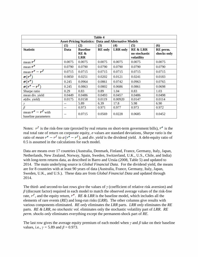
Table 4

Asset-Pricing Statistics: Data and Alternative Models

(1) (2) (3) (4) (5) (6)

Statistic Data Baseline

RE &

LRR

RE only LRR only RE & LRR

no stochastic

volatility

RE perm.

shocks only

mean 0.0075 0.0075 0.0075 0.0075 0.0075 0.0075

mean 0.0790 0.0790 0.0790 0.0790 0.0790 0.0790

mean 0.0715 0.0715 0.0715 0.0715 0.0715 0.0715

0.0850 0.0251 0.0202 0.0121 0.0241 0.0183

0.245 0.0964 0.0861 0.0742 0.0963 0.0765

0.245 0.0863 0.0802 0.0686 0.0861 0.0698

Sharpe ratio 0.29 0.83 0.89 1.04 0.83 1.03

mean div. yield 0.0449 0.0486 0.0493 0.0457 0.0486 0.0498

σ(div. yield) 0.0175 0.0158 0.0119 0.00920 0.0147 0.0114

γ -- 5.89 6.39 17.8 5.98 6.90

β -- 0.973 0.971 0.977 0.973 0.972

mean with

baseline parameters -- 0.0715 0.0569 0.0228 0.0685 0.0452

Notes: is the risk-free rate (proxied by real returns on short-term government bills), is the

real total rate of return on corporate equity, σ values are standard deviations, Sharpe ratio is the

ratio of mean to , and div. yield is the dividend yield. A debt-equity ratio of

0.5 is assumed in the calculations for each model.

Data are means over 17 countries (Australia, Denmark, Finland, France, Germany, Italy, Japan,

Netherlands, New Zealand, Norway, Spain, Sweden, Switzerland, U.K., U.S., Chile, and India)

with long-term returns data, as described in Barro and Ursúa (2008, Table 5) and updated to

2014. The main underlying source is Global Financial Data. For the dividend yield, the means

are for 8 countries with at least 90 years of data (Australia, France, Germany, Italy, Japan,

Sweden, U.K., and U.S.). These data are from Global Financial Data and updated through

2014.

The third- and second-to-last rows give the values of γ (coefficient of relative risk aversion) and

β (discount factor) required in each model to match the observed average values of the risk-free

rate, , and the equity return, . RE & LRR is the baseline model, which includes all the

elements of rare events (RE) and long-run risks (LRR). The other columns give results with

various components eliminated. RE only eliminates the LRR parts. LRR only eliminates the RE

parts. RE & LRR, no stochastic vol. eliminates only the stochastic volatility part of LRR. RE

perm. shocks only eliminates everything except the permanent-shock part of RE.

The last row gives the average equity premium of each model when γ and β take on their baseline

values, i.e., γ = 5.89 and β = 0.973.

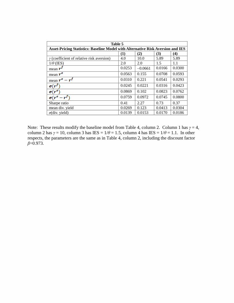
Table 5

Asset-Pricing Statistics: Baseline Model with Alternative Risk Aversion and IES

(1) (2) (3) (4)

γ (coefficient of relative risk aversion) 4.0 10.0 5.89 5.89

1/θ (IES) 2.0 2.0 1.5 1.1

mean 0.0253 0.0661 0.0166 0.0300

mean 0.0563 0.155 0.0708 0.0593

mean 0.0310 0.221 0.0541 0.0293

0.0245 0.0221 0.0316 0.0423

0.0869 0.102 0.0823 0.0762

0.0759 0.0972 0.0745 0.0800

Sharpe ratio 0.41 2.27 0.73 0.37

mean div. yield 0.0269 0.123 0.0413 0.0304

σ(div. yield) 0.0139 0.0153 0.0170 0.0186

Note: These results modify the baseline model from Table 4, column 2. Column 1 has γ = 4,

column 2 has γ = 10, column 3 has IES = 1/θ = 1.5, column 4 has IES = 1/θ = 1.1. In other

respects, the parameters are the same as in Table 4, column 2, including the discount factor

β=0.973.

Figure 1: World Rare-Event Probability

Note: This figure plots the posterior mean of the world rare-event dummy variable, , and,

therefore, corresponds to the estimated probability that a world rare event was in effect for each

year from 1851 to 2012. See equation (2) in the text.

Figure 2: Fitted Model for Chile

1890 1900 1910 1920 1930 1940 1950 1960 1970 1980 1990 2000 20100

0.1

0.2

0.3

0.4

0.5

0.6

0.7

0.8

0.9

1

i = 0.023

Pro

babili

ty

1890 1900 1910 1920 1930 1940 1950 1960 1970 1980 1990 2000 2010-0.5

-0.4

-0.3

-0.2

-0.1

0

0.1

0.2

0.3

0.4

0.5

I it

it, I it

it,

it, &

10

it

Chile

Year

Prob. of a Rare Event

Iit

it

Iit

it

it

10it

Figure 3: Fitted Model for Germany

1850 1860 1870 1880 1890 1900 1910 1920 1930 1940 1950 1960 1970 1980 1990 2000 20100

0.1

0.2

0.3

0.4

0.5

0.6

0.7

0.8

0.9

1

i = 0.019

Pro

babili

ty

1850 1860 1870 1880 1890 1900 1910 1920 1930 1940 1950 1960 1970 1980 1990 2000 2010-0.5

-0.4

-0.3

-0.2

-0.1

0

0.1

0.2

0.3

0.4

0.5

I it

it, I it

it,

it, &

10

it

Germany

Year

Prob. of a Rare Event

Iit

it

Iit

it

it

10it

Figure 4: Fitted Model for Japan

1870 1880 1890 1900 1910 1920 1930 1940 1950 1960 1970 1980 1990 2000 20100

0.1

0.2

0.3

0.4

0.5

0.6

0.7

0.8

0.9

1

i = 0.020

Pro

babili

ty

1870 1880 1890 1900 1910 1920 1930 1940 1950 1960 1970 1980 1990 2000 2010-0.5

-0.4

-0.3

-0.2

-0.1

0

0.1

0.2

0.3

0.4

0.5

I it

it, I it

it,

it, &

10

it

Japan

Year

Prob. of a Rare Event

Iit

it

Iit

it

it

10it

Figure 5: Fitted Model for Russia

1880 1890 1900 1910 1920 1930 1940 1950 1960 1970 1980 1990 2000 20100

0.1

0.2

0.3

0.4

0.5

0.6

0.7

0.8

0.9

1

i = 0.021

Pro

babili

ty

1880 1890 1900 1910 1920 1930 1940 1950 1960 1970 1980 1990 2000 2010-0.5

-0.4

-0.3

-0.2

-0.1

0

0.1

0.2

0.3

0.4

0.5

I it

it, I it

it,

it, &

10

it

Russia

Year

Prob. of a Rare Event

Iit

it

Iit

it

it

10it

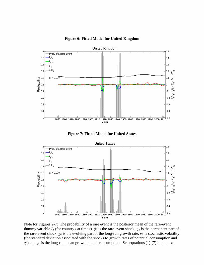
Figure 6: Fitted Model for United Kingdom

1850 1860 1870 1880 1890 1900 1910 1920 1930 1940 1950 1960 1970 1980 1990 2000 20100

0.1

0.2

0.3

0.4

0.5

0.6

0.7

0.8

0.9

1

i = 0.015

Pro

babili

ty

1850 1860 1870 1880 1890 1900 1910 1920 1930 1940 1950 1960 1970 1980 1990 2000 2010-0.5

-0.4

-0.3

-0.2

-0.1

0

0.1

0.2

0.3

0.4

0.5

I it

it, I it

it,

it, &

10

it

United Kingdom

Year

Prob. of a Rare Event

Iit

it

Iit

it

it

10it

Figure 7: Fitted Model for United States

1850 1860 1870 1880 1890 1900 1910 1920 1930 1940 1950 1960 1970 1980 1990 2000 20100

0.1

0.2

0.3

0.4

0.5

0.6

0.7

0.8

0.9

1

i = 0.019

Pro

babili

ty

1850 1860 1870 1880 1890 1900 1910 1920 1930 1940 1950 1960 1970 1980 1990 2000 2010-0.5

-0.4

-0.3

-0.2

-0.1

0

0.1

0.2

0.3

0.4

0.5

I it

it, I it

it,

it, &

10

it

United States

Year

Prob. of a Rare Event

Iit

it

Iit

it

it

10it

Note for Figures 2-7: The probability of a rare event is the posterior mean of the rare-event

dummy variable Iit (for country i at time t), ϕit is the rare-event shock, ηit is the permanent part of

the rare-event shock, χit is the evolving part of the long-run growth rate, σit is stochastic volatility

(the standard deviation associated with the shocks to growth rates of potential consumption and

χit), and μi is the long-run mean growth rate of consumption. See equations (1)-(7) in the text.

References

Balke, N. S. and R. J. Gordon (1989). “The Estimation of Prewar Gross National Product:

Methodology and New Evidence,” Journal of Political Economy, 97, 38–92.

Bansal, R., R. F. Dittmar, and C. T. Lundblad (2005). “Consumption, Dividends, and the Cross

Section of Equity Returns,” Journal of Finance, 60 (4), 1639–1672.

Bansal, R., D. Kiku, and A. Yaron (2010). “Long Run Risks, the Macroeconomy, and Asset

Prices,” American Economic Review: Papers & Proceedings, 100, 542–546.

Bansal, R. and I. Shaliastovich (2013). “A Long-Run Risks Explanation of Predictability Puzzles

in Bond and Currency Markets,” Review of Financial Studies, 26 (1), 133.

Bansal, R. and A. Yaron (2004). “Risks for the Long Run: A Potential Resolution of Asset

Pricing Puzzles,” Journal of Finance, 59, 1481–1509.

Barro, R.J. (2006). “Rare Disasters and Asset Markets in the Twentieth Century,” Quarterly

Journal of Economics, 121, 823–866.

Barro, R.J. (2009). “Rare Disasters, Asset Prices, and Welfare Costs,” American Economic

Review, 99, 243–264.

Barro, R.J. (2015). “Environmental Protection, Rare Disasters, and Discount Rates,” Economica,

82, 123.

Barro, R.J. and T. Jin (2011). “On the Size Distribution of Macroeconomic Disasters,”

Econometrica, 79, 1567–1589.

Barro, R.J. and J.F. Ursúa (2008). “Macroeconomic Crises since 1870,” Brookings Papers on

Economic Activity, 255–335.

Barro, R.J. and J.F. Ursúa (2010). “Barro-Ursúa Macroeconomic Data,” available at

economics.harvard.edu/faculty/barro/files/Barro_Ursúa_MacroDataSet_101111.xls, 2010.

Barro, R.J. and J.F. Ursúa (2012). “Rare Macroeconomic Disasters,” Annual Review of

Economics, 4, 83–109.

Beeler, J. and Campbell J. (2012). “The Long-Run Risks Model and Aggregate Asset Prices: An

Empirical Assessment,” Critical Finance Review, 1, 141–182.

Campbell, J. Y. (2003). “Consumption-Based Asset Pricing,” Handbook of the Economics of

Finance, ed. by G. Constantinides, M. Harris, and R. Stulz, Amsterdam, Elsevier, 804–887.

Chen, H. (2010). “Macroeconomic Conditions and the Puzzles of Credit Spreads and Capital

Structure,” The Journal of Finance, 65, 2171–2212.

Chib, S., F. Nardari, and N. Shephard (2002). “Markov Chain Monte Carlo Methods for

Stochastic Volatility Models,” The Journal of Econometrics, 108, 281–316.

Colacito, R. and M.M. Croce (2011). “Risks for the Long-Run and the Real Exchange Rate,”

Journal of Political Economy, 119, 153–181.

Colacito, R. and M.M. Croce (2013). “International Asset Pricing with Recursive Preferences,”

Journal of Finance, 68 (6), 26512686.

Croce, M.M., M. Lettau, and S.C. Ludvigson (2015). “Investor Information, Long-Run Risk, and

the Term Structure of Equity,” Review of Financial Studies, 8(3), 706-742.

Epstein, L.G. and S.E. Zin (1989). “Substitution, Risk Aversion, and the Temporal Behavior of

Consumption and Asset Returns: A Theoretical Framework,” Econometrica, 57, 937–969.

Farhi, E. and X. Gabaix (2016). “Rare Disasters and Exchange Rates,” Quarterly Journal of

Economics, 131, 1-52.

Farhi, E., S. P. Fraiberger, X. Gabaix, R. Ranciere, and A. Verdelhan (2015), “Crash Risk in

Currency Markets,” working paper, Harvard University.

Gabaix, X. (2012). “Variable Rare Disasters: An Exactly Solved Framework for Ten Puzzles in

Macro-Finance,” Quarterly Journal of Economics, 127, 645–700.

Gelman, A., J. B. Carlin, H. S. Stern, and D. Rubin (2004). Bayesian Data Analysis, 2nd Ed.,

Chapman & Hall/CRC.

Gourio, F. (2008). “Disasters and Recoveries,” American Economic Review, 98, 68–73.

Gourio, F. (2012). “Disaster Risk and Business Cycles,” American Economic Review, 102,

2734–2766.

Gruber, J. (2013). “A Tax-Based Estimate of the Elasticity of Intertemporal Substitution,”

Quarterly Journal of Finance, 3 (1).

Guvenen, F. (2009). “A Parsimonious Macroeconomic Model for Asset Pricing,” Econometrica,

77, 1711–1750.

Hall, R. E. (1988). “Intertemporal Substitution in Consumption,” Journal of Political Economy,

96, 339–357.

Hansen, L. P., J. C. Heaton, and N. Li (2008). “Consumption Strikes Back? Measuring Long-

Run Risk,” Journal of Political Economy, 116, 260–302.

Hodrick, R. J. and E. C. Prescott (1997). “Postwar U.S. Business Cycles: An Empirical

Investigation,” Journal of Money, Credit, and Banking, 29, 1–16.

Koop, G. and S. M. Potter (2007). “Estimation and Forecasting in Models with Multiple Breaks,”

Review of Economic Studies, 74, 763–789.

Lucas, R. E. (1978). “Asset Prices in an Exchange Economy,” Econometrica, 46, 1429–1445.

Malloy, C.J., T.J. Moskowitz, and A. Vissing-Jorgensen (2009). “Long-Run Stockholder

Consumption Risk and Asset Returns,” Journal of Finance, 64, 2427–2479.

Mehra, R. and E. C. Prescott (1985). “The Equity Premium: A Puzzle,” Journal of Monetary

Economics, 15, 145–161.

Nakamura, E., J. Steinsson, R.J. Barro, and J.F. Ursúa (2013). “Crises and Recoveries in an

Empirical Model of Consumption Disasters,” American Economic Journal:

Macroeconomics, 5, 35–74.

Nakamura, E., D. Sergeyev, and J. Steinsson (2016). “Growth-Rate and Uncertainty Shocks in

Consumption: Cross-Country Evidence,” American Economic Journal, Macroeconomics,

forthcoming.

Pesaran, M.H., D. Pettenuzzo, and A. Timmermann (2006). “Forecasting Time Series Subject to

Multiple Structural Breaks,” Review of Economic Studies, 73, 1057–1084.

Rietz, T.A. (1988). “The Equity Risk Premium: A Solution,” Journal of Monetary Economics,

22, 117–131.

Romer, C.D. (1986). “Is the Stabilization of the Postwar Economy a Figment of the Data,”

American Economic Review, 76, 314–334.

Seo, S. and J.A. Wachter (2016). “Option Prices in a Model with Stochastic Disaster Risk,”

working paper, University of Pennsylvania, June.

Wachter, J.A. (2013). “Can time-varying risk of rare disasters explain aggregate stock market

volatility?” Journal of Finance, 68, 987–1035.

Weil, P. (1990). “Nonexpected Utility in Macroeconomics,” Quarterly Journal of Economics,

105, 29–42.

Dept. of Economics, Harvard University, 1805 Cambridge Street, Cambridge MA 02138-

3001, U.S.A.; [email protected]

and

PBC School of Finance, Tsinghua University, 43 Chengfu Road, Haidian District, Beijing,

100083, China; [email protected], and Hang Lung Center for Real Estate, Tsinghua

University.

For Online Publication

Appendix

A.1 Data used in this study

This study uses an enlarged version of the Barro-Ursúa macroeconomic data set (2010). The

original data set contains annual consumption series for 42 economies up to 2009, and we

expand it to 2012. This data set covers the major economies in the world: Argentina, Australia,

Austria, Belgium, Brazil, Canada, Chile, China, Colombia, Denmark, Egypt, Finland, France,

Germany, Greece, Iceland, India, Indonesia, Italy, Japan, Korea, Mexico, Malaysia, Netherlands,

New Zealand, Norway, Peru, Philippines, Portugal, Russia, South Africa, Singapore, Spain, Sri

Lanka, Sweden, Switzerland, Taiwan, Turkey, United Kingdom, Uruguay, United States, and

Venezuela.

The availability of uninterrupted annual data varies across economies. To best utilize the rich

information contained in the data set, we adopt the longest possible uninterrupted series between

1851 and 2012 for each economy, yielding a total of 4814 country-year observations. We

choose 1851 as the starting date because it is the earliest year when uninterrupted data are

available for at least 10 countries. The reason for this criterion is that the model incorporates the

correlation in the timing of rare events across countries through a world event indicator, and it is

undesirable if this indicator is estimated from data for only a few countries. The ten countries

with uninterrupted data since 1851 are Denmark, France, Germany, Netherlands, Norway, Spain,

Sweden, Switzerland, the United Kingdom, and the United States. The data set used in this study

is much larger than those in previous studies. For example, the total number of country-year

observations explored in NSBU is 2685, and that number is almost doubled here.

A.2 Missing data at the beginning of series

When t = 1851, i.e., for the first year in the data, the value of is missing. In this case, we

use the proportion of world event years in all the years in the simulation to simulate the value of

and then simulate the value of based on the simulated and other information.

Let denote the earliest date when uninterrupted consumption data are available for country i.

When = , Formula (3) is not directly applicable, because is missing. Following the

idea of (3), we calculate the following prior conditional probability instead

=

+

(A.1)

.

For simplicity, we further assume

,

where the prior probability is estimated by , the fraction of event periods in all

the periods studied for country i. So

, (A.2)

and we impose the restriction that .

For other cases of missing data, we also specify reasonable prior distributions to improve the

estimation accuracy

A.3 Prior distributions of parameters and unknown quantities

Bayesian MCMC has two major advantages in estimating the model here: (1) necessary

information can be incorporated into prior beliefs, and (2) it is relatively easy to implement for a

model as complicated as the one proposed in this study. The prior distributions of parameters

and unknown quantities in the proposed model are listed in detail here.

In this study, a prior being “uninformative” means that the posterior distribution is proportional

to the likelihood. With an uninformative prior, the mode of the posterior distribution

corresponds to the maximum-likelihood estimate. A typical uninformative prior for a parameter

is the uniform distribution on an infinite interval (e.g., a half-line or the entire real line).

Extending that idea, we also say that the uniform distribution on a finite interval is uninformative

if the finite interval contains the parameter with probability 1. More generally, we say a prior

distribution is “almost uninformative” (or more rigorously, “not very informative”) if it is close

to a flat prior. In this study, the general guideline for the specification of priors is to make them

as uninformative as possible (in certain regions). Thus, many priors are taken to be uniform.

Prior distributions of parameters. In this study, is assumed to follow the normal

distribution , and is assumed to follow the truncated normal distribution

, where and denote the mean and variance, respectively, of the

underlying normal distribution (i.e., the normal distribution before truncation). The mean value

and standard deviation of are denoted by and , respectively. Another possible choice

for the prior distribution of and is the exponential distribution. Corresponding to Barro

and Jin (2011), if power law distribution with (upper-tail) exponent , where the

disaster size b is the fraction of contraction in C, then exponential distribution

with rate parameter . This relationship suggests exponential distributions for and .

The prior distribution of the long-term average growth rate of country i is assumed to follow

, where the prior mean and variance are set to the mean values of the long-

term average growth rates of per capita consumption and Gross Domestic Product (GDP) of the

42 economies in the enlarged Barro-Ursúa data set. (More specifically, the corresponding mean

value and standard deviation are 0.0189 and 3.16105, respectively.) As a summary, the prior

distributions of the parameters are listed in the following table.

Parameter Distribution Parameter Distribution

U(0, 0.05) U(0.3, 0.9)

U(0.3, 1) U(0, 0.03)

U(0.3, 0.9) U(0, 0.9)

N(0.025, 0.12) U(0.01, 0.25)

U(0.25, 0) U(0.01, 0.25)

U(0.001, 0.015) U(0, 0.9)

U(0, 0.98) U(0, 0.98)

U(0.1, 10) U(105, 103)

N(0.02, 0.30.012) U(0.001, 0.15)

Conditional prior distribution of event gaps. It is intuitive that event gaps will gradually

diminish if no events occur in a country. Based on this notion, we specify the conditional prior

distribution of as follows. When , i.e., country i is in a rare event at time t, the prior

distribution of is assumed to be . We take , which is very large, so the prior

is fairly uninformative on a region local to 0. If year t is the first uneventful year after a rare

event in country i, equation (7) becomes

,

which implies

i.e.,

,

where “SD” stands for “standard deviation.” When year t is the mth uneventful year after the

most recent rare event in country i, the upper bound of can be calculated

recursively, and we assume that the prior distribution of follows .13 Note that the

above specification of prior distributions of event gap is intuitive and is conditional on when

the last event before year t happens in country i.

Conditional prior distribution of potential consumption. Based on the prior distribution of

, we derive the conditional prior distribution of as follows. According to equation (1), the

upper bound of satisfies

,

when year t is the mth ( ) uneventful year after the most recent event in country i. We

define

and assume that the prior distribution of is . Figure A.1 shows the standard

deviation ( ) of the prior distribution of ( ) as a function of m. As m goes to ,

( ) is decreasing and converges to 0.15 (0.3), which is large (based on economic common

sense). Therefore, the prior distributions of and are fairly uninformative.

13Here, m = 0 indicates that country i is in a rare event. In the simulation, if no event happens in year for

country i, a simple simulation using probability qi is implemented to determine the number m. (See Appendix A.1

for the meaning of qi.)

0 50 100 150 2000

0.2

0.4

0.6

0.8

1

1.2

1.4

m

zm

or

xm

zm

xm

Figure A.1. and as Functions of m

Non-negativity of . The method for excluding negative values of is similar to that

employed by Bansal and Yaron (2004). Instead of “replacing negative realizations with a very

small number,” we assume that the prior distribution of follows the uniform distribution

.

Thus, the posterior distribution of follows a truncated normal distribution. This treatment is

natural from the Bayesian point of view, and it is similar to that in Bansal and Yaron (2004), as

both methods are using (variants of) truncated normal distributions to exclude possible negative

realizations of .

A.4 Estimation procedure

The model is estimated by the Bayesian MCMC method, which has been applied to many

problems in economics and finance, e.g., Chib, Nardari, and Shephard (2002); Pesaran,

Pettenuzzo, and Timmermann (2006); and Koop and Potter (2007). Specifically, we use the

algorithm of the Gibbs sampler for the random draws of parameters and unobserved quantities

(see Gelman, Carlin, Stern, and Rubin, 2004 for a discussion of the MCMC algorithms).

The convergence of the MCMC simulation is guaranteed under very general conditions. In order

to accurately estimate parameters and unknown quantities, we run four simulation chains, similar

to the procedure in NSBU (see Appendix A.5 for details of the specification of the four

simulation chains). Besides simulating multiple sequences with over-dispersed starting points

throughout the parameter space and visually evaluating the trace plots of parameters and

unknown quantities from the simulation, we also assess the convergence by comparing variation

“between” and “within” simulated sequences (see Chapter 11 of Gelman, Carlin, Stern, and

Rubin [2004] for a discussion of this method).

After a half million iterations, the simulation results from the four sets of far-apart initial values

stabilize and become very close to each other. So we iterate each chain 2 million times and use

the later 1 million iterations to analyze the posterior distributions of parameters and unknown

quantities of interest. The first million iterations are dropped as burn-in.

A.5 Specification of four simulation chains

In order to accurately estimate the model and assess convergence, we run four independent

simulation chains in a way similar to that of NSBU. We specify two extreme scenarios: one is

called the “no-event scenario,” the other the “all-event scenario.” For the no-event scenario, we

set , , , and for all i and t. For the all-event scenario, we set

and for all i and t and extract a smooth trend using the Hodrick-Prescott filter

(see Hodrick and Prescott [1997]). Let denote the trend component and the remainder,

i.e.,

.

We then let

and .

For each scenario, we specify two sets of initial values for parameters: one is called the “lower

values,” the other the “upper values.” For the set of “lower values,” the initial parameter values

are either close to their lower bounds or very low compared to their mean values. For the “upper

values,” we have the opposite situation. Thus, the four sets of initial values of parameters for the

four simulation chains are far apart from each other.