This file is part of the following reference: Rankine, Kelda S. (2007) Development of two and three-dimensional method of fragments to analyse drainage behaviour in hydraulic fill stopes. PhD thesis, James Cook University. Access to this file is available from: http://eprints.jcu.edu.au/2093

Welcome message from author
This document is posted to help you gain knowledge. Please leave a comment to let me know what you think about it! Share it to your friends and learn new things together.
Transcript

This file is part of the following reference:
Rankine, Kelda S. (2007) Development of two and three-dimensional method of fragments to analyse drainage behaviour in hydraulic fill
stopes. PhD thesis, James Cook University.
Access to this file is available from:
http://eprints.jcu.edu.au/2093

DEVELOPMENT OF TWO AND THREE-DIMENSIONAL METHOD OF FRAGMENTS TO
ANALYSE DRAINAGE BEHAVIOR IN HYDRAULIC FILL STOPES
Thesis submitted by
Kelda Shae RANKINE BEng(Hons)
in September 2007
for the degree of Doctor of Philosophy in the School of Engineering
James Cook University

ii
STATEMENT OF ACCESS
I, the undersigned, the author of this thesis, understand that James Cook University will make it available for use within the University Library and, by microfilm or other means, allow access to users in other approved libraries. All users consulting this thesis will have to sign the following statement:
In consulting this thesis, I agree not to copy or closely paraphrase it in whole or in part without the written consent of the author; and to make proper public written acknowledgement for any assistance which I have obtained from it.
Beyond this, I do not wish to place any restriction on access to this thesis. _________________________________ __________
Signature Date

iii
STATEMENT OF SOURCES
DECLARATION
I declare that this thesis is my own work and has not been submitted in any form for another degree or diploma at any university or other institution of tertiary education. Information derived from the published or unpublished work of others has been acknowledged in the text and a list of references is given.
_________________________________ __________
Signature Date
DECLARATION – ELECTRONIC COPY
I, the undersigned, the author of this work, declare that to the best of my knowledge, the electronic copy of this thesis submitted to the library at James Cook University is an accurate copy of the printed thesis submitted. _________________________________ __________
Signature Date

iv
Acknowledgements
The author wishes to thank,
My family – Dad, Mum, Tegan, Rudd, Shauna, Briony, Kirralee and Lachlan.
Thankyou for being there through the good times and the bad, for sharing my laughter,
tears, frustrations and achievements. I feel blessed to have the family that I have, and
want to thank each and every one of them for always being there.
Another person who I am very thankful to who constantly provided their support,
guidance, and encouragement is Assoc. Prof. Nagaratnam Sivakugan. Siva, you have
taught me so much and have not only been an excellent teacher and mentor throughout
my research, but you have also been a true friend for whom I will never forget and
with whom I hope to share a friendship with for the rest of my life. You have helped
me in so many ways, and for that I am forever grateful. Thankyou.
I would also like to thank Siva’s wife Rohini, for her friendship and for sharing Siva
and so much of his time with me.
Finally, I would like to thank the School of Engineering at James Cook University for
allowing me to undertake this dissertation.

v
This work is dedicated to my wonderful family – Dad,
Mum, Tegan, Rudd, Shauna, Briony, Kirralee and
Lachlan

vi
Abstract The extraction and processing of most mineral ores, result in the generation of large
volumes of finer residue or tailings. The safe disposal of such material is of prime
environmental, safety and economical concern to the management of mining
operations. In underground metaliferous mining operations, where backfilling of
mining voids is necessary, one option is to fill these voids with a tailings-based
engineered product. In cases where the fill is placed as a slurry and the fill contains
free water, permeable barricades are generally constructed to contain the fill within the
mining void whilst providing a suitable means for the drainage water to escape from
the fill. Recent barricade failures, resulting from poor drainage, have led to an
immediate need for an increased understanding of the pore pressure developments and
flow rates throughout the filling operation. This thesis presents simple analytical
solutions, based on the ‘method of fragments,’ for estimating discharge and maximum
pore pressure for two and three-dimensional hydraulically filled stopes. Shape factors
were developed to account for the inherent individuality associated with stope and
drain geometry. The influence of scaling on discharge and pore pressure
measurements is also investigated. The proposed solutions are verified against
solutions derived from a finite difference program and physical modelling of a scaled
mine stope and results showed excellent agreement. Using these analytical solutions
developed for flow through three-dimensional hydraulic fill stopes, a user-friendly
EXCEL model was developed to accurately and efficiently model the drainage
behaviour in three-dimensional stopes. The model simulates the complete filling and
draining of the stopes and was verified using the finite difference software FLAC3D.
The variation and sensitivity in drainage behaviour and pore water pressure
measurements with, the variation in geometry, fill properties and filling-cycles of a
three-dimensional hydraulic fill stope was also investigated.

vii
List of Publications Journals
Rankine, K.S. and Sivakugan N. (2007) “Application of Method of Fragments in
Three-Dimensional Hydraulic Fill Stopes.” Journal of the Geotechnical Division
ASCE, Under Review 3rd draft
Sivakugan, N. and Rankine, K.S. (2006). "A simple solution for drainage through
2-dimensional hydraulic fill stope," Geotechnical and Geological Engineering,
Springer, 24, 1229-1241.
Sivakugan, N., Rankine, K.J., and Rankine, K.S. (2006). "Study of drainage
through hydraulic fill stopes using method of fragments," Journal of Geotechnical
and Geological Engineering, Springer, 24, 79-89.
Sivakugan, N., Rankine, R.M., Rankine, K.J., and Rankine, K.S. (2006).
"Geotechnical considerations in mine backfilling in Australia," Journal of Cleaner
Production, Elsevier, 14(12-13), 1168-1175.
Refereed Conference Proceedings
Rankine K.S., Sivakugan N., Rankine K.J. (2007). Drainage behaviour of three-
dimensional hydraulic fill stopes: A sensitivity analysis, 10th Australian and New
Zealand Conference on Geomechanics – Common Ground, Paper accepted
Rankine, K.S. and Sivakugan, N. (2005). "A 2-D numerical study of the effects of
anisotropy, ancillary drains and geometry on flow through hydraulic fill mine
stopes," Proceedings of the 16th ISSMGE, Osaka, Vol.2, 955-958
Rankine, K.J., Sivakugan, N. and Rankine, K.S. (2004). Laboratory tests for mine
fills and barricade bricks, Proceedings of 9th ANZ Conference on Geomechanics,
Auckland, 1, pp. 218–224

viii
Rankine, K.J., Rankine, K.S., and Sivakugan, N. (2003). "Three-dimensional
drainage modelling of hydraulic fill mines," Proc. 12th Asian Regional Conf. on
Soil Mech. and Geotech. Engineering, Eds. CF Leung, KK Phoon, YK Chow, CI
Teh and KY Yong, 937-940.
Rankine, K.J., Rankine, K.S. and Sivakugan, N. (2003). “Quantitative Validation
of Scaled Modelling of Hydraulic Mine Drainage Using Numerical Modelling,”
Proc. of the International Congress on Modelling and Simulation, MODSIM 2003,

ix
Contents
Statement of Access ii
Statement of Sources iii
Acknowledgements iv
Dedication v
Abstract vi
List of Publications vii
Table of Contents ix
List of Figures xv
List of Tables xx
List of Symbols xxii 2. INTRODUCTION 1
2.1 General 1
2.2 Problem Statement 4
2.3 Objectives 4
2.4 Relevance of the Research 5
2.5 Thesis Overview 5
2. LITERATURE REVIEW 8
2.1 General 8
2.2 Mining with Minefills 9
2.3 Purpose of Minefill 10
2.4 Minefill Performance Requirements 12
2.4.1 Static Requirerments 12
2.4.2 Dynamic Requirements 12
2.4.3 Drainage Requirements 12
2.5 Minefill Types and Selection 14
2.6 Brief History of Minefill 16
2.7 Hydraulic Fill 18
2.8 Hydraulic Fill Properties 19
2.8.1 Grain Shape, Texture and Mineralogy 19

x
2.8.2 Grain Size Distribution 21
2.8.3 Specific Gravity 23
2.8.4 Dry Density, Relative Density and Porosity 24
2.8.5 Friction angle 27
2.8.6 Placement Property Test 28
2.8.7 Degree of Saturation 30
2.8.8 Chemical Reactivity 30
2.8.9 Permeability 30
2.8.9.1 Anisotropic Permeability 36
2.8.9.2 The effect of cement on permeability measurements 39
2.9 Empirical Relationships of Permeability 42
2.10 Consolidation 49
2.11 Placement and Drainage 48
2.12 Barricades 51
2.13 Physical Modelling of Hydraulic Fill Stopes 64
2.14 In situ Monitoring 65
2.15 Numerical Modelling of Hydraulic Fill Stopes 68
3. APPLICATION OF METHOD OF FRAGMENTS TO TWO- 72
DIMENSIONAL HYDRAULIC FILL STOPES
3.1 Overview 72
3.2 Introduction 72
3.3 Method of Fragments applied to a two-dimensional hydraulic-filled 77
Stope
3.3.1 Numerical Model 78
3.3.1.1 Numerical Package FLAC 78
3.3.1.2 Boundary Conditions and Assumptions 79
3.3.1.3 Grid Generation and Input Parameters 81
3.3.2 Form Factors, Maximum Pore Pressure and Flow rate 82
3.3.3 Fragment Comparison 88
3.3.4 Decant Water in Two-dimensional Hydraulic Fill Stopes 91
3.3.5 Entry and Exit Hydraulic Gradients 91

xi
3.3.6 Scaling Effect on Method of Fragments 96
3.3.7 Typical Stope Geometries 96
3.3.8 Validation of the Application of two-dimensional method of 97
fragments
3.3.9 Further analysis of the pore water pressure in two-dimensional 99
Stopes
3.4 Anisotropy 102
3.4.1 Laboratory Testing 102
3.4.1.1 Results 105
3.4.2 Pore Water Pressure 106
3.4.3 Flow rate 107
3.5 Ancillary Drainage in Two-dimensional Hydraulic Fill Stopes 109
3.5.1 Pore Water Pressure 110
3.5.2 Flow rate 111
3.6 Summary and Conclusions 113
4. APPLICATION OF METHOD OF FRAGMENTS TO THREE- 115
DIMENSIONAL HYDRAULIC FILL STOPES
4.1 Overview 115
4.2 Introduction 115
4.3 Method of Fragments for Three-dimensional Hydraulic Filled Stopes 116
4.3.1 Numerical Model 118
4.3.1.1 Numerical Package FLAC3D 118
4.3.1.2 Input Parameters, Boundary Conditions and Assumptions 119
4.3.1.3 Grid Generation 119
4.3.2 Developing Equations for Form Factors, Flow rate and 121
Maximum Pore Water Pressure
4.3.2.1 Drain Shape 126
4.3.2.2 Drain Location 128
4.3.2.3 Stope Shape 131
4.3.3 Scaling Effect on three-dimensional Method of Fragments 132
4.3.4 Summary of Equations 132

xii
4.4 Possible Drain Arrangements 134
4.5 Validation of MOF3D Analytical solutions of Varying Stope Geometries 135
4.6 Comparison of pseudo three-dimensional model with actual three- 136
dimensional numerical models
4.7 Physical Modelling of Flow through a Hydraulic Filled-stope 138
4.7.1 Similitude and Dimensional Analysis 139
4.7.2 Laboratory Setup 145
4.7.3 Sample material 147
4.7.4 Procedure 150
4.7.5 Numerical Modelling of Scaled Laboratory Stope 151
4.7.6 Interpretation of Results 151
4.8 Application of three-dimensional method of fragments 155
4.9 Summary and Conclusions 156
5. EXCEL MODEL 158
5.1 Overview 158
5.2 Verification Exercise 158
5.2.1 Problem Definition 158
5.2.2 Overview of Previous Drainage Models 159
5.2.3 Geometry and Boundary Conditions 159
5.2.4 Input parameters 161
5.2.5 Simulation of filling schedule within stope 162
5.2.6 Fill and water heights 162
5.3 Sequential Filling and Draining for Hydraulic Fill Stope Calculations 166
5.4 Sensitivity Analysis 172
5.4.1 Geometry 172
5.4.2 Geotechnical Properties 175
5.4.2.1 Permeability 176
5.4.2.2 Specific gravity and dry density 178
5.4.2.3 Solids Content 180
5.4.2.4 Residual water content 185
5.4.3 Filling Schedule 186

xiii
5.4.4 Filling Rate 187
5.5 Two-dimensional versus three-dimensional stopes 188
5.6 Summary and Conclusions 189
6. SUMMARY, CONCLUSIONS AND RECOMMENDATIONS 191
6.1 Summary 191
6.2 Conclusions 194
6.3 Recommendations for future research 198
REFERENCES 201
APPENDICES
APPENDIX A: Cemented hydraulic fill laboratory testing 213
A.1. Initial and Final parameters for Copper Tailings 214
A.2. Initial and Final parameters for Zinc Tailings 214
A.3. Grain Size Distribution Curves for Copper and Zinc Tailings 214
A.4. Summary of Copper Permeability Results 215
A.3. Summary of Zinc Permeability Results 216
APPENDIX B: FLAC / FLAC3D Codes 217
B.1. Source listing FISH and FLAC code for progam used to develop 218
the two-dimensional form factor
B.2. Source listing FISH and FLAC code for two-dimensional Anisotropic 220
Permeability analysis
B.3. Source listing FISH and FLAC3D code for program used to develop 222
Three-dimenensional form factor
APPENDIX C: Validation plots for additonal points on two-dimensional stope 226
C.1. Validation graphs for Point A and B on two dimensional stope 227
C.2. Validation graph for Point C on two-dimensional stope 228

xiv
C.3. Validation graph for Point D on two-dimensional stope 229
C.4. Validation graph for Point E and F on two-dimensional stop 230
APPENDIX D: Anisotropic Permeability Cell Testing 231
D.1. Permeability Cell Testing on Sample D3 232
D.2. Permeability Cell Testing on Sample D4 233
D.3. Permeability Cell Testing on Sample A1 234
APPENDIX E: Physical Modelling Results 235
E.1. Scaled Stope Analysis: Numerical / Laboratory / MOF3D results for 236
scaled stope

xv
List of Figures Figure Details Page
1.1 Schematic diagram of idealized hydraulic fill stope 3
2.1 Plan view of an ore body showing typical stope extraction
sequence in a nine-stope grid arrangement
9
2.2 Idealized hydraulic fill stope 10
2.3 Brief timeline of Australian mines from 1850 – 2004 17
2.4 Electron micrograph of hydraulic fill sample at James Cook
University
20
2.5 Grain Size Distribution of Hydraulic Fills tested at James Cook
University
22
2.6 Decrease in minefill permeability with increasing ultrafines
content (Lamos, 1993)
23
2.7 Dry density versus specific gravity (Rankine et al. 2006) 25
2.8 Placement property curve of an Australian hydraulic fill (Rankine
et al. 2006)
29
2.9 Three field permeameters (Herget and De Korompay, 1978) 32
2.10 Constant head permeability test (a) Schematic diagram, (b)
Permeameter set-up in the Laboratory
34
2.11 Falling head permeameter (a) Schematic diagram, (b) Actual
permeameter set-up
35
2.12 Sample prepared in the permeameter – prior to testing 40
2.13 Permeability Variation with Time for Copper CHF 41
2.14 Permeability Variation with Time for Zinc CHF 41
2.15 Various laboratory measured soil permeabilities versus void
ratios (Qiu and Sego, 2001)
47
2.16 Various laboratory measured soil permeabilities for various void
ratios (Lambe and Whitman, 1979)
48
2.17 (a) A brick used in the construction of barricades (b) A barricade
wall under construction
53

xvi
2.18 Forces acting on the fill in an access drive (Potvin et al. 2005 56
2.19 Test apparatus for observing piping mechanism 57
2.20 Piping development in hydraulic fill due to unfilled access drive 59
2.21 Piping development due to fill escaping through rock joints 60
2.22 (a) Erosion pipe seen during drainage trials (Grice, 1989) (b)
Failed planar masonry barricade (Grice, 1998)
61
2.23 Bulkhead pressure measurements (Mitchell et al. 1975) 67
3.1 Simplified schematic diagram of two-dimensional stope 77
3.2 Hydraulic fill stope with single drain (a) Flownet (b) Selected
equipotential lines (c) Flow region and three fragments
78
3.3 Two possible pore water pressure distribution assumptions for
fill-barricade interface
80
3.4 Two dimensional meshes investigated (a) 1 m x 1 m mesh; (b) 0.5
m x 0.5 m mesh; (c) 0.25 m x 0.25 m mesh (d) combination of
fine and coarse mesh (0.25 m x 0.25 m mesh in drain and 1 m x 1
m mesh in stope)
81
3.5 Form factor for fragment 2 for case 1: Hw/B ≥ 1 84
3.6 Form factor for fragment 2 for all cases of Hw 84
3.7 Head losses within fragments (a) Case 1: Hw > B (b) Case 2: Hw <
B
86
3.8 Coefficient α2D for fragment 2 87
3.9 Flow rate comparison using varying fragments including Griffiths
(1984) and Table 3.4 fragments against finite difference model
FLAC
90
3.10 Dependence of ientry for several cases of X/D, D/B and Hw/B 94
3.11 Hw/B against ientry for two-dimensional stopes 95
3.12 Scaling of two dimensional stope and flow nets 96
3.13 Maximum pore water pressure comparison 98
3.14 Flow rate comparison 98
3.15 Points for pore pressure analysis 99
3.16 Coefficient αC for fragment 2 for point C 101

xvii
3.17 Coefficient αD for fragment 2 for point D 101
3.18 (a) Permeability cell with filter paper (b) Placement of slurry in
permeability cell (c) Secured permeability cell (d) Permeability
cell connected to constant head apparatus
103
3.19 Design chart for pore water pressure measurements for
anisotropic fill material: D/B = 0.025; X/D = 1
106
3.20 Design chart for pore water pressure measurements for
anisotropic fill material: D/B = 0.05; X/D = 1
107
3.21 Design chart: effect of anisotropic permeability on flow rate
D/B=0.025; X/D=1
108
3.22 Geometry of stope with ancillary drainage 110
3.23 Effects of ancillary drain on pore water pressure measurements 111
3.24 Comparison between maximum pore water pressures obtained
from FLAC and those calculated using Eq. 3.20
112
3.25 Effect of ancillary drain on flow rate results 112
4.1 Three-dimensional hydraulic fill stope (a) Selected equipotential
surfaces (b) Flow region, dimensions and three fragments of 3D
stope
117
4.2 Mesh sensitivity (a) 2 m mesh spacing, (b) 1 m mesh spacing (c)
Combination of fine and coarse mesh (d) 0.5 mesh spacing
120
4.3 Form Factor for fragment 2 (Γ2) for a three-dimensional stope 124
4.4 Coefficient α3D for fragment 2 in a three-dimensional (Case 1) 126
4.5 Effect of drain shape on pore pressure measurements 127
4.6 Effect of drain shape on discharge measurements 127
4.7 Drain Location Analysis (a) Centre Square drain (b) Corner
square drain
128
4.8 Effect of drain location on maximum pore pressure measurement 129
4.9 Effect of drain location on discharge measurements 129
4.10 Scaled three-dimensional stope 132
4.11 Validation of pore pressure measurements for varying stope
geometries
135

xviii
4.12 Validation of discharge measurements for varying geometries 136
4.13 Investigated two and three dimensional models (a) Pseudo three-
dimensional stope (b) Three-dimensional stope with long, flat
drain (c) Three-dimensional stope with square drain of
equivalent cross-section as Model 1 and Model 2
137
4.14 General Form of the typical soil-fluid-flow problem (Butterfield,
2000)
141
4.15 Permeability versus vertical normal stress for various hydraulic
fills tested at James Cook University (Singh, 2007)
143
4.16 Schematic diagram of Experimental Apparatus 146
4.17 Barricade (Hall, 2006) 146
4.18 Three different drain lengths of 5 cm, 20 cm and 14 cm (Hall,
2006)
147
4.19 Grain size distribution of sand samples (Hall, 2006) 148
4.20 Laboratory model stope setup 151
4.21 Comparison between laboratory, numerical model and 3-D
method of fragment solution
152
5.1 Verification Geometry (a) two-dimensional stope (b) three-
dimensional stope
160
5.2 Pseudo three-dimensional stope used for comparison of models 161
5.3 Fill and water height comparison between Isaacs and Carter,
FLAC, FLAC3D, Rankine-file for the verification problem
163
5.4 Magnified fill and water heights for a 24 hour period 164
5.5 Discharge rate comparison for between Isaacs and Carter, FLAC,
FLAC3D and Rankine-file
164
5.6 Magnified discharge rate comparison for between Isaacs and
Carter, FLAC, FLAC3D and Rankine-file
165
5.7 Input dimensions of a three-dimensional stope modelled in
Rankine-file simulations
167
5.8 Water mass balance 170
5.9 Sensitivity analysis for varying geometries versus maximum pore 174

xix
water pressure
5.10 Sensitivity analysis for varying geometries versus discharge 174
5.11 Dimensions of sample stope used in the geotechnical property
sensitivity analysis
175
5.12 Permeability versus discharge 176
5.13 Permeability versus maximum pore pressure 177
5.14 Fill and water heights for varying specific gravity values 179
5.15 Maximum pore pressure versus specific gravity 180
5.16 Discharge versus specific gravity 181
5.17 Hydraulic fill Slurry density ranges (Potvin et al. 2005) 182
5.18 Fill and water heights for varying specific gravities 183
5.19 Magnified fill and water heights for varying specific gravities 183
5.20 Discharge versus specific gravity 184
5.21 Maximum pore water pressure versus specific gravity 184
5.22 Water and fill heights during filling and draining of three-
dimensional stope with varying residual moisture contents
186
5.23 Fill and water heights during filling for various filling schedules 188

xx
List of Tables Table Description Page
2.1 Ten largest Australian mines using minefill 15
2.2 Specific gravity values for a range of hydraulic fills 24
2.3 Published porosity values for hydraulic fills 26
2.4 Recorded relative density values of hydraulic fills 27
2.5 Published permeability values for a range of hydraulic fills 37
2.6 Hazen’s constant values reported by various authors 43
2.7 Mount Isa fill and pouring resting regimes (Cowling et al., 1988) 51
3.1 Summary of Harr’s Fragments (Harr, 1977) 75
3.2 Summary of Griffith’s form factors (Griffiths, 1984) 76
3.3 Outputs by different mesh arrangements 82
3.4 Summary of equations for two-dimensional analysis 89
3.5 Summary of pore water pressure equations and design charts for
various points
100
3.6 Permeability anisotropy values for hydraulic fills 105
4.1 Output for various three-dimensional meshes 120
4.2 The effect of drain location and drain shape on discharge
measurements
130
4.3 Equations for three-dimensional hydraulic fill stopes 133
4.4 Four common cases and corresponding equations for various
Drain Arrangements
134
4.5 Results of the investigated two and three-dimensional models 138
4.6 Classification summary of sand samples 148
4.7 Hall (2006) empirical relationships 149
4.8 Constant head permeability tests for various relative densities
(Hall, 2006)
149
4.9 Summarized percent differences between the numerical /
laboratory and MOF3D models for the various cases
154
5.1 Input parameter for Verification Stope 161

xxi
5.2 Input data for FLAC3D and EXCEL comparison 166
5.3 Results for various simulations described in Table 5.3 166
5.4 Suggested filling schedules (Cowling et al. 1988) 187

xxii
List of Symbols A = cross-sectional area
a = air content
B = stope width
C = Hazen’s constant
Cslurry = percent solids of slurry
Cu = coefficient of uniformity
Cv = viscosity coefficient
C0 = Terzaghi (1925) shape factor
C2 = Kozeny-Carman (1938) shape factor
C3 = Taylor (1948) shape factor
C4 = Samarasinghe (1982) constant
C5 = Amer and Awad (via Das, 2002) constant
c’ = effective cohesional stress
D = drain height
Dr = relative density
Ds = effective particle dimeter
D5 = the grain size for which 5% of the particles are finer
D10 = the grain size for which 10% of the particles are finer; effective grain size
D30 = the grain size for which 30% of the particles are finer
D50 = the grain size for which 50% of the particles are finer
D60, = the grain size for which 60% of the particles are finer
E1, E2 = material property constants, Carrier et al. (1983)
e = void ratio
emax = maximum void ratio
emin = minimum void ratio
F = drain width
Fr = Froude number
f = soil fabric
G = equivalent drain height
Gs = Specific gravity
g = acceleration due to gravity

xxiii
H = height
Hw = height of water
hi = head loss in ith fragment
hL = head loss
Δh = change in head between two points
i = hydraulic gradient
ientry = entry hydraulic gradient
iexit = exit hydraulic gradient
J = fill height increase per hour
K0 = horizontal pressure coefficient (assumed to be 0.5)
k = permeability
k0.85 = permeability at void ratio of 0.85
ke = effective permeability
kequiv = equivalent permeability for a layered system
kh = permeability in the horizontal direction
kv = permeability in the vertical direction
L = length
La = length of ancillary drain
m = soil compressibility
ms = mass of solids
mw = mass of water
Nd = number of equipotential drops
Nf = number of flow channels
n = porosity
neff = effective porosity
Pb = pressure exerted by the bulkhead on the fill
Q = discharge
q = discharge per unit length
Re = Reynold’s number
Rs = solids filling rate
S = saturation
Ss = specific surface area of grains

xxiv
Sv = grain surface per unit volume
s = shape factor
T = temperature
t = time
u = pore water pressure
umax = maximum pore water pressure
v = discharge velocity
Vdrained = volume of water that has drained
Vf = volume of fill
Vfree = total free water that is drainable
Vin = volume of water entering stope
Vout = volume of water draining from the stope
Vresidual = volume of residual water
Vs = volume of solids
Vto-drain = volume of water that is yet to drain
Vv = volume of voids
Vw =volume of water
W = stope thickness
w = water content
wres = residual water content
wsat = saturated water content
wslurry = water content of hydraulic fill slurry
X = drain length
α2D = fraction of the head loss within fragment 2 for a two-dimensional stope that
takes place in the horizontal segment of the largest stream line
α3D = fraction of the head loss within fragment 2 for a three-dimensional stope that
takes place in the horizontal segment of the largest stream line
Δh = change in head between two points
Φ = two-dimensional form factor for ith fragment
Γi = three-dimensional form factor for ith fragment
γt = total bulk unit weight of fill
γw = unit weight of water

xxv
η = dynamic viscosity
ϕ = effective frictional stress
κ = intrinsic permeability
μ = water viscosity
μT = water viscosity at T degrees Celsius
μ10 = water viscosity at 10 degrees Celsius
ρd = dry density
ρs = soil grain density
ρw = density of water
σh = horizontal/ barricade pressure
σh′ = effective horizontal pressure
σv′ = effective vertical pressure
τw = shear strength of rock-fill interface
ω = fluid surface tension

1
CHAPTER 1
INTRODUCTION
1.1. General
Minefill refers to any waste material that is placed into voids mined underground to
dispose of mining waste (tailings) or used to perform some engineering function. In
addition to this, minefill provides the following benefits:
• Effective means of tailings disposal,
• Increased local and regional rock stability,
• Improvement in ore recovery,
• Reduced environmental impacts of mining operations.
To accurately determine the support benefits that the minefill will provide, it is
important that the geotechnical characteristics are properly understood. This will
ensure that adequate provisions are made for the drainage, static and dynamic strength
considerations. The static and dynamic strength stability requirements are typically
imposed to ensure that the minefill has enough strength to prevent failure during the
exposure of a minefill surface wall in the mining sequence and during blasting within
the ore body. The dynamic and drainage requirements are linked inherently through
the in-situ pore pressure in the fill mass. The major cause of failure in underground
stopes is often attributed to the build-up of high pore water pressures behind the
barricade, resulting in liquefaction due to blasting or piping (Bloss & Chen 1998;
Grice 1998 a). Liquefaction occurs when the pore pressure increases dramatically, thus
reducing the effective stress in the fill mass, to the point where the shear resistance of
the soil is so low that the soil begins to “flow” like a liquid. If the fill mass liquefies,
implications arise for the loading on the barricade walls which retain the fill in the
stopes and prevent it from flowing into the mine. During liquefaction, all arching in the
fill mass is lost and the loadings on the barricades will increase, which is significantly

2
greater than current design strengths for which barricade walls are designed. A flow of
fill material would then follow, with potentially catastrophic consequences.
The open stoping mining method is a mining technique used as a means of obtaining
ore from underground metalliferous mines. This method involves dividing the ore
body into a series of prisms, approximately rectangular in geometry, called stopes.
Blasting techniques are used to break down the ore within an individual stope to a size
suitable for being removed via horizontal access at the bottom of the stope. Excavation
initiates from the bottom of the stope and progresses upwards, so the ore falls to the
base of the stope. Once the ore is extracted, it is processed, removing the valuable
minerals from the rock and producing a waste material known as tailings. When used
as minefill, these tailings are mixed with water and reticulated to an existing stope
void. Where the walls of the fill mass are exposed by adjacent stoping, cement must
be added to the minefill to provide sufficient strength to stabilize the fill over the
exposed area.
To complete the extraction of an ore body, many stopes are required. These stopes are
generally set out in a standard grid pattern, but specific details depend on the ore body
geometry, the host rock and specific mine conditions. At any given stage of an
underground mine operation, the excavation of several stopes will be under way at one
time, and similarly several stopes will be in the backfilling stage. These individual
stope operations are planned and sequenced to allow sufficient distance between
excavations to avoid stability problems.
This research will focus on the drainage characteristics and associated properties of a
particular type of minefill material known as hydraulic fill and issues related to using
this fill material in underground mining operations. Hydraulic filling is one of the more
popular backfilling methods used in Australia and worldwide and consists of deslimed
tailings (i.e. finer fraction is removed via cycloning) and is placed underground
hydraulically as a slurry. Hydraulic fills can be classified as sandy silts or silty sands
with no clay fraction and are generally placed with a solids density of 65% – 75%.

3
Due to the high water content and permeability of hydraulic fill, free water exists in the
placed fill and must be allowed to drain in order to minimize pore pressures
To contain the hydraulic fill, barricades are constructed at each of the entrances to the
stopes. A schematic diagram of an idealized hydraulic fill stope is shown in Fig. 1.1.
Barricade construction varies from mine to mine. In a number of cases, these
barricades are made of special porous bricks that have permeabilities 2 – 3 orders of
magnitude greater than those of the hydraulic fills (Rankine et al. 2004). These
barricades contain the wet hydraulic fill, whilst draining the water into the drives thus
reducing the build-up of pore water pressure behind the barricades. The remaining
water either pools on the surface as decant water, or is retained in the interstices of the
fill. Upon placement in the stope, the hydraulic fill rapidly develops sufficient shear
strength to prevent transmission of geostatic (earth) pressure to the barricades.
Therefore once dewatering is complete, pressures on the barricades are minimal.
After dewatering and resulting consolidation in stopes underground, the fill becomes
capable of accepting loads and the next stope is ready to be blasted.
Barricade
Decant Water
Hydraulic fill
Fill access
Hydraulic fillDrives
Fig. 1.1. Schematic diagram of idealized hydraulic fill stope

4
Recent barricade failures Grice, 1998 a; Torlach, 2000), resulting from poor drainage,
have emphasized a need for an increased understanding of the pore pressure
developments and flow rates throughout the filling operation. The primary objective of
this thesis is the improvement in the filling and drainage operations through a greater
understanding of the drainage behavior in hydraulic fill mines, as well as the means by
which the drainage of these mines is analyzed.
1.2 Problem Statement
Hydraulic fill is generally placed in the form of a slurry with high water content for the
ease of transportation and placement. The problem with high water content is that there
is a substantial amount of water entering the stope. During the filling process and in
the early stages of draining, several failures have occurred as a result of poor drainage
of excess water from the stope causing substantial financial and human loss to the
mines. As a result of these failures, there has been great importance placed on
developments in drainage analysis of hydraulically placed minefill. Therefore, it is
necessary to be able to predict the pore water pressure developments and flow rates
throughout the filling process, so that barricade performance can be predicted and
barricades can be engineered to prevent failure.
1.3 Objectives
The focus of this research is to study the fundamental aspects of the drainage behavior
in hydraulic fill stopes. More specifically, this thesis aims to achieve the following
objectives:
• To develop and verify simple analytical solutions, based on the ‘method of
fragments,’ for estimating discharge and maximum pore pressure for two-
dimensional hydraulically filled stopes.
• To extend method of fragments to three dimensional geometries and use this to
develop and verify analytical solutions to predict the discharge rates and pore
water pressures in three-dimensional hydraulic fill stopes.
• Develop a user-friendly EXCEL model to accurately and efficiently model the
filling and draining of a three-dimensional minefill stope.

5
• Undertake a sensitivity analysis into the drainage behavior and pore water
pressure measurements based on fill properties, geometries and filling
schedules of a three-dimensional hydraulic fill stope.
1.4 Relevance of Research
The frequent historical occurrence of fill barricade failures around Australia and
numerous underground mines worldwide has led to a need for an increased
understanding of the factors which lead to failure of the fill in underground mining
operations. Two major factors that have been identified are:
i) The flow of water through the hydraulic fill mass, and
ii) Poor drainage that leads to build-up of pore pressures, which results in
piping, liquefaction and other forms of failures.
By understanding the processes that lead to failure, an increased level of confidence in
design of hydraulic fills will be achieved. More efficient mining, safer minefilling
practices and increased cost savings may also result from the introduction of new
designs.
The drainage performance of hydraulic fill needs to be properly understood as it plays
an important roll in the safety of underground hydraulic fill mining operations.
Reliable knowledge of the drainage characteristics of underground hydraulic fill mines
will improve mine safety and productivity through confidence in design and
prediction.
1.5 Thesis Overview
Chapter 1 introduces the research problem, objectives and the relevance of the
research. An overview of the major issues associated with the drainage of hydraulic fill
mines and a brief description of the mining method have been presented. A broad
overview of the thesis chapters is also discussed.
Chapter 2 presents a more detailed introduction into hydraulic fill. Initially an
overview of minefill types and selections, the purpose of minefill and a brief historical
overview of hydraulic filling practices within Australia are given. Research carried

6
out on the characterization of hydraulic fills and barricade bricks is also presented. As
well as the current practices and recent developments with regard to underground
hydraulic fill mining and drainage analysis and prediction, including physical
modeling, in-situ monitoring and previous numerical modeling of the hydraulic fill
stopes
Chapter 3 deals with the application of the method of fragments in two-dimensional
stopes. Using method of fragments (Harr 1962, 1977) and the finite difference
software FLAC (Fast Lagraingian Analysis of Continua, Itasca 2002), drainage and
pore water pressure characteristics within a two-dimensional hydraulic fill stope were
investigated in this chapter. Analytical solutions were proposed for determining the
flow rate and the maximum pore water pressure within the stope. The proposed
solutions were verified against solutions derived from the finite difference software
package FLAC and were found to be in excellent agreement. The effects of ancillary
drains and anisotropic permeability were also investigated.
Chapter 4 deals with the development of method of fragments in three-dimensions.
This chapter provides simple analytical solutions and design charts for estimating the
maximum pore water pressure and discharge within three-dimensional hydraulic fill
stopes of varying geometries. Shape factors were developed to account for the inherent
individuality associated with stope and drain geometry and the influence of scaling on
discharge and pore pressure measurements were also investigated. Previously, method
of fragments has only been applied in two-dimensions; this chapter extends the
concepts into a three-dimensional analysis. The proposed solutions are verified against
solutions derived from the finite difference software package FLAC3D and results are
found to be satisfactory.
Using the analytical solutions developed for flow through three-dimensional hydraulic
fill stopes in chapter 4, an EXCEL model was developed to accurately and efficiently
model the drainage behaviour in three-dimensional stopes. This chapter discusses the
development, application and verification of the EXCEL model which simulates the
complete filling and draining of the stopes. Using this model, the sensitivity of

7
drainage behaviour and pore water pressure measurements with the fill properties,
geometries and filling schedules of a three-dimensional hydraulic fill stope was
investigated.
A summary of the findings from this research and recommendations for future research
are presented in Chapter 6.

8
CHAPTER 2
LITERATURE REVIEW
2.6 General
Australians enjoy one of the highest living standards in the world and part of the
reason for this is that we are a major trading nation. The minerals industry is one of
the biggest contributors to Australia’s export trade with estimated export earnings of
$58.3 billion in 2004-2005 (http://www.australianmineralsatlas.gov.au).
The extraction and processing of most mineral ore, result in the generation of large
volumes of finer residue or tailings. The safe disposal of such material is of prime
environmental, safety and economical concern to the management of mining
operations. For underground mines, the use of tailings in minefill not only reduces the
environmental impact of surface disposal of tailings but also provides the base of an
engineering material that can be used to improve both the ground conditions and
economics of mining. Recent failures in Australia and worldwide have emphasized the
need for proper understanding of underground filling practices, and in particular the
use of hydraulic filling. Minefill refers to any waste material that is placed into voids
mined underground for purposes of either disposal, or to perform some engineering
function. This thesis is concerned with one particular minefill material, called
hydraulic fill, which can be defined as deslimed mine tailings and a D10 value in excess
of 10 μm. Hydraulic filling is one of the most popular minefilling methods used in
Australia and worldwide.
The literature review is not only limited to this chapter which deals with the hydraulic
filling of mine stopes; problems associated with hydraulic filling; and research carried
out on the characterization of hydraulic fills and barricade bricks. A more extensive
coverage on method of fragments, anisotropy, ancillary drainage, scale, numerical and
physical modelling is given in latter chapters.
9
2.7 Mining with Minefills
There are two distinct types of mining methods: stable stope and caving, with a
complete spectrum of methods available between these two extremes. The three stable
stope methods which use minefill are the open stoping, room and pillar, and cut and
fill mining methods. Caving is an unstable form of mining where ore is allowed to
collapse under its own weight through prolific natural cracking and failures. In caving
the ore will fail where undermined and will continue to fail while there is a void to fill
and when there is sufficient cracking of the ore body. A comprehensive description of
each of the mining methods is given by Brady and Brown (1985); Franklin and
Dusseault (1991) and Reedman (1979). This research is based on the open stoping
mining method in conjunction with hydraulic fill.
In an open stoping mining operation, the ore body is divided into separate stopes for
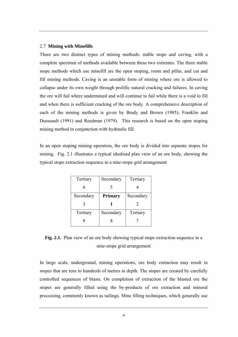
mining. Fig. 2.1 illustrates a typical idealised plan view of an ore body, showing the
typical stope extraction sequence in a nine-stope grid arrangement
Tertiary
6
Secondary
5
Tertiary
4
Secondary
3
Primary
1
Secondary
2
Tertiary
9
Secondary
8
Tertiary
7
Fig. 2.1. Plan view of an ore body showing typical stope extraction sequence in a
nine-stope grid arrangement
In large scale, underground, mining operations, ore body extraction may result in
stopes that are tens to hundreds of metres in depth. The stopes are created by carefully
controlled sequences of blasts. On completion of extraction of the blasted ore the
stopes are generally filled using the by-products of ore extraction and mineral
processing, commonly known as tailings. Mine filling techniques, which generally use

10
these by-products, provide ground support to permit removal of adjacent, remaining
ore, and are also effective means of disposal of waste materials. When hydraulic fill is
used, barricades are constructed at each of the entrances to the stopes to contain the
fill. These barricades can be made of special porous bricks that have permeabilities 2
– 3 orders of magnitudes greater than those of the hydraulic fills (Rankine et al. 2004).
These barricades contain the wet hydraulic fill, whilst draining the water into the
drives thus reducing the build-up of pore water pressure behind the barricades. The
remaining water either pools on the surface as decant water, or is tied up in the
interstices of the fill. After dewatering and resulting consolidation in stopes
underground, the fill becomes capable of accepting loads and the next stope is ready to
be blasted. It should be noted that for stoping sequences where adjacent stoping
exposes the minefill, cemented hydraulic fill may be used and must cure to achieve the
recommended design strength prior to adjacent stope extraction. A schematic diagram
of an idealized hydraulic fill stope is shown in Fig. 2.2.
Fig. 2.2. Idealized hydraulic fill stope
2.8 Purpose of Minefill
Minefill refers to any waste material that is placed into underground voids, created by
mining for the extraction of ore. Minefill is primarily used to maximise ore recovery
Barricade
Decant Water
Hydraulic fill
Fill access
Hydraulic fillDrives

11
with the objective of optimising the economics of the mining operation. Minefill may
be placed underground as a means of disposing it and to provide additional support for
the remaining mine infrastructure (mine pillars etc). In addition to this, minefill
provides the following benefits:
• Reduces the environmental impacts of the mining operations;
• Increases local and regional rock stability;
• Reduces risk of rockbursting;
• Provides an effective means of tailings disposal;
• Improves ore recovery;
• Reduces the need for large tailings dams; and
• Provides a working floor in minefill stoping methods.
To accurately determine the support benefits that the minefill will provide, it is
important that the geotechnical characteristics of the fill are properly understood. This
will enable adequate provisions to be made for the drainage, static and dynamic
stability considerations. The static and dynamic strength stability requirements are
typically imposed to ensure that the minefill has enough strength to prevent failure
during the exposure of a wall in the mining sequence and during adjacent blasting
within the ore body. The dynamic stability and drainage requirements are linked
inherently through the in situ pore pressure in the fill mass. A brief overview of these
requirements is given in section 2.4.
Nantel (1998) refers to the trend in Canada where future environmental legislations
require the maximum quantity of mine waste to be returned to the underground
workings. The obvious limit of this mining direction was reached when the Australian
Federal Government recommended approving an alternative for the proposed Jabiluka
Mine (JMA) whereby all mill wastes were required to be placed underground.
Superficially, this may seem like a reasonable requirement based on a desire to
preserve environmental integrity; however, such an approach may limit the financial
viability of a significant number of mines (Grice, 1998 b). Grice showed that for one
particular operation there was an excess mine volume of 46% which would have to be
created to store all mill waste in the form of pastefill.

12
2.9 Minefill Performance Requirements
Minefill is an engineered product and in order to satisfy performance criteria as part of
an economic mine plan, it must achieve defined static stability, dynamic stability and
drainage requirements (where the mine fill is placed as a slurry and contains free
water, as well as minimising environmental impact. Each of these requirements is
discussed briefly below.
2.9.1 Static Requirements
Grice (2001) summarises the key static stability requirements as:
• Stand open in vertical faces when exposed by adjacent pillar mining;
• Support the weight of loading equipment when used as a mucking (trafficked)
floor;
• Confine the rock mass surrounding the stope in order to maintain local and
regional stability within mining areas;
• Permit mining underneath fill by production blasting for undercut ore
extraction; and
• Permit mining through in development sized headings for the purposes of
access or ventilation.
2.9.2 Dynamic Requirements
The key dynamic stability requirements are:
• Withstand the effects of close proximity blasting from production or
development sized excavations; and
• Withstand the effects of regional seismic events
2.9.3 Drainage Requirements
Drainage is an important consideration in hydraulic backfilling where free drainage
water is present. The main requirements include:
• Permit drainage of excess water from minefilled stope to reduce liquefaction
potential

13
• Reduce potential excessive pore pressure being applied to stope access
barricades that may fail as a result of high loading.
Excess water in stopes may come from three main sources including:
• Water used in transporting the fill material;
• Groundwater seepage from the stope walls; and
• Service water (e.g. machine water from drilling).
Generally the majority of the water to be drained through the fill mass comes from the
water used to transport the fill to the site of deposition i.e. the water used to suspend
the particles, as a hydraulic fill. Once placed, the solid particles tend to consolidate,
leaving the water on top of the solidified material to percolate through the fill mass.
Research undertaken by Thomas (1969) was instrumental in establishing and
documenting the rule-of-thumb percolation rate for hydraulic fill as 100 mm/hr, which
has been standard across the industry since around the 1950’s (Nantel, 1998; Cowling,
1998; Keren and Kainian, 1983). With improved understanding into fill drainage and
placement practices this standard has come under debate and the published
permeability values of many hydraulic fills that are satisfactorily being used across
Australia and worldwide fall well below this value (Brady and Brown, 2001; Herget
and De Korompay, 1978; Pettibone and Kealy, 1971). It should also be noted that this
value was often used as a good rate for cut and fill mining, which required relatively
fast drainage to get back quickly on top of the fill with the mining equipment. In the
1980’s and 1990’s tailings became finer (due to finer grind) and this reduced
percolation rates in the fill. For most open stoping methods, this was not as much of a
problem because unlike cut and fill it was not necessary to be back on top of the fill
within hours of placement. Also, cut and fill started reducing in popularity.
Minefill barricades are also typically designed to allow for the drainage of water from
stopes. Sivakugan et al. (2006) conducted permeability testing on barricades which use
porous bricks and hydraulic fills and found the ratio of the permeability of the brick to
hydraulic fill to be in the range of 100 – 1500. Therefore it was assumed in this

14
dissertation that the fill-barricade interface is free draining and avoids any restriction to
the flow of water from the stope and subsequent pore pressure buildup.
2.10 Min
efill Types and Selection
There is a vast range of materials that can be used in minefill systems, including
quarried rock, natural sands and gravels, total mill tailings, deslimed mill tailings,
development mullock, open pit overburden, binders such as Portland cement, gypsum,
lime, MINECEM and pozzolans (e.g. Flyash or slags) and chemical additives. Water
is also required for the transport of hydraulic materials, hydration of binders and for
dust control in “dry” systems. These materials provide a wide range of minefills that
can be used in underground mines.
Dorricott and Grice (2002) discuss four major fill types used in Australia:
- Hydraulic fill: This may be produced directly from coarse sands and or mill
tailings, or by desliming tailings with hydrocyclones to meet a nominal
standard of <10% passing 10 μm and adequate drainage rates. Current
industry practice suggests that provided the hydraulic fill meets this
specification, drainage requirements will be met. Hydraulic fill slurries are
usually placed at a solids densities ranging from 65% - 75%, to minimize
the amount of excess transport water that must be drained and pumped to
the surface.
- Pastefill: Consists of total mill tailings that are dried using filters and
thickened to around 80% solids density. The size of tailings used in
pastefill depends on what product is produced by the mill. Cement and
water are added to the mix to achieve the required rheological and strength
characteristics.
- Rock fill: Waste rock, quarry rock or aggregate are used as bulking
materials. Depending on the engineering purpose of the fill, a hydraulic
component (cement slurry or cemented tailings) can be combined with the
bulking material to produce a cemented fill mass.

15
- Blended fill: Blended fills are created by adding rock or aggregate to sand,
hydraulic or pastefill.
For mines that use minefill, the economics can be significantly influenced by minefill
selection. The overall mine efficiency and viability is largely based on minefill
selection and therefore minefill type is of paramount importance to the plan for the
mining of an ore body.
For a more detailed description of fill types and production methods refer to
McKinstry (1989) and Neindorf (1983). Table 2.1 illustrates the ten largest minefilling
operations in Australia and the fill types used at each of these.
Table 2.1. Ten largest Australian mines using minefill (vide Dorricott and Grice,
2002)
* CHF = cemented hydraulic fill, HF = hydraulic fill, PF = pastefill, PAF = paste aggregate fill, CAF =
cemented aggregate fill, CRF = cemented rock fill, RF = rock fill
The type of fill used at a mine site is chiefly controlled by the on-site availability of the
particular waste materials, financial costs involved with that minefill (e.g. are binders
Company Mine Fill Types*
BHP Billiton (WMC) Olympic Dam CAF, RF
MIM Mt Isa Copper CAF, CHF, HF
MIM Enterprise PF, CHF
Delta Gold Kanowna Belle CAF, PF
Normandy Yandal Bronzewing CAF, CHF, HF
MIM George Fisher CAF
BHP Billiton Cannington PF
Normandy NFM Granites CAF
Placer Pacific Osborne HF, RF
Normandy Golden Grove HF, RF

16
required etc) performance characteristics and convenience of use. The selection of a
minefill system involves a cost/benefit analysis of those systems that meet the basic
technical and operational requirements. EDUMine Online – Professional
Development Underground Mine Backfill 1- Introduction (2003)
(www.civil.uwa.edu.au/teaching/MINE4162?f=130747) provides a design rationale for the
minefill in six simple steps and is outlined below:
1. Specify the mining environment and mining system.
2. Identify the minefill purposes according to the mining system specified
in step 1.
3. Define the target properties of minefill materials to serve the minefill
purposes, based on the minefill purposes and mining condition.
4. Define the operating system so that minefill materials match target
properties and the minefill operation itself. These include:
Minefill material preparation;
Minefill material transportation;
Minefill material placement; and
Minefill operation quality control and environment monitoring.
To modify the design parameters, information monitoring at this stage
will be fed back to earlier steps.
5. Do an economic evaluation of minefill system.
6. Document and implement minefill mining system.
This research deals with the placement, containment and drainage of hydraulic fill,
which can be considered as the traditional tailings based mine filling practice (Thomas
and Holtham, 1989). Therefore hydraulic fill and the drainage and containment of
hydraulic fill within underground stopes will be discussed further.
2.11 Brief History of Minefill
The concept of using recycled extracted material for backfills in mines dates back
hundreds of years. The original minefills in underground mines consisted mainly of
waste rock and filling may have occurred naturally through caving of overlying strata
or as part of a mining process to conveniently dispose of waste rock.

17
Over the past 150 years the Australian mining industry has developed into one of the
world’s leading mining nations. The gold rushes of the 1850’s that put the Australian
mining industry on the map have since expanded with the discovery of new minerals
and resources. At present the Australian minerals industry is the third largest minerals
sector by value of production of any country in the world
(http://www.minerals.org.au/corporate). Fig. 2.3 depicts a brief timeline of Australian
mines from the 1850’s to that of present day. The export earnings from the past 25
years (1980 – 2004) have expanded from 7.2 billion to 52.2 billion dollars.
Fig. 2.3. Brief timeline of Australian mines from 1850 – 2004
One of the earliest recordings of the systematic use of fill is that of the use of mullock
fill at Mount Lyell and North Lyell mines in Tasmania in 1915 (Murray, 1915).
Barkley (1927) reveals that although the use of fill was only documented in 1915, the
practice had been in progress since approximately the turn of the century.

18
The introduction of hydraulically transported fill in Australia was first reported by
Black (1941) at the South Mine of Broken Hill South Limited, Broken Hill, New South
Wales in 1939. By 1944, all underground transportation of fill within the South Mine
was hydraulic.
Hydraulic fill has been used for a long time in the mining industry and remains the
most commonly placed mine fill type (Potvin et al. 2005). The historical development
of hydraulic fill practice in Australia runs roughly parallel with that in other countries.
Hydraulic fill is now used extensively in underground mines throughout the world.
Therefore, a move towards an improved understanding of hydraulic fill performance is
needed.
The early days of fill in North America were not dissimilar to the Australian
experience. Minefilling in Canadian mines has been practiced for close to 100 years
and evidence suggests the application of minefill technology at an increasing rate
during this decade (Nantel 1998, Udd and Annor 1993). The evolution of minefill
technology is closely related to the establishment of new mining methods.
2.12 Hydraulic Fill
The most common source of material for hydraulic fill is the finely ground residues of
mineral processing activities, however, they can be produced from a number of
materials such as natural sand deposits and quarries. Hydraulic fills are simply silty
sands or sandy silts with no clay fraction, which classify as ML or SM under the
Unified Soil Classification System. The clay fraction is mostly removed through a
process known as desliming, where the entire fill material is processed through
hydrocyclones, and the fine fraction is sent to the tailings dam. The coarse fraction
(referred to as hydraulic fill) is reticulated in the form of slurry through pipelines to the
underground voids. Hydraulic fill is mostly commonly prepared using hydrocyclones,
however several other less conventional methods are available. These can include:
mechanical classifiers and thickeners, with sieve bend, filtration, and flocculation
systems also worthy of consideration perhaps in conjunction with other more
conventional processes (Thomas and Holtham, 1989). Differences in mineralogy,

19
particle shape and size distribution can affect transport, placement, drainage and
performance properties.
Over the past decade, there has been a steady increase in the solids content of the
hydraulic fill slurry placed in mines in an attempt to reduce the quantity of water that
has to be drained and to increase the solids proportion. The problem with high solid
content is that it becomes difficult to transport the slurry through the pipelines due to
rheological considerations. Currently, solids contents of the hydraulic fill typically
range between 65% - 75%. (Sivakugan et al. 2006). Even at 75% solid content,
assuming specific gravity of 3.00 for the solid grains, 50% of the slurry volume is
water. Therefore, there is a substantial amount of water that has to be drained from the
hydraulic fill stope.
To contain the fill, barricades or bulkheads generally block horizontal drives. The
horizontal access drives are large enough to let the machinery in during the mining
operation and are blocked by the barricades during filling. The drives are often located
at more than one level. The upper level drains let the decant water out and also would
serve as an additional drain when the fill slurry reaches this level (Refer to Fig. 2.2).
2.13 Hydraulic Fill Properties
Hydraulic fill is a tailings-based material that is sourced from a wide variety of rock
types and processing techniques. Many geotechnical properties of typical hydraulic
fills may be characterized or described within a range. The following section aims to
detail some of the properties of hydraulic fills, commonly found within the mining
industry.
2.13.1 Grain Shape, Texture and Mineralogy
Fig. 2.4 illustrates the typical grain shape of a hydraulic fill sample tested at James
Cook University. As shown in Fig. 2.4 and reported by Pettibone and Kealy (1971)
and Nicholson and Wayment (1964), hydraulic fills contain very angular grains, which
is a result of the crushing of waste rock from the milling process.

20
Fig. 2.4. Electron micrograph of hydraulic fill sample at James Cook University
Permeability of fill varies according to particle shape and texture of the soil. Generally,
rough-surfaced particles produce a greater frictional resistance to fluid flow, thus
reducing the permeability (Head, 1982). Irregular-shaped particles create longer, more
tortuous flow paths for the fluid to flow through, thus reducing the permeability.
Conversely, when particles are smooth and spherical, interlocking between particles is
less and the flow paths are less tortuous, thus increasing permeability.
In fine-grained soils different types of minerals hold on to different thicknesses of
adsorbed water and consequently the effective pore size varies. Thus, the mineral
composition affects the permeability of clays, but has little effect on granular soils.
The mineral composition of the fill also indirectly affects the frictional resistance of
the fill grains. Mineralogy controls important grain characteristics such as size, shape,
surface attributes, angularity, and strength of particles Angular grains interlock more
effectively than rounded ones, creating a larger friction angle and increasing the fill
strength. Fill consisting of hard particles with rough surfaces that oppose grain
movements off greater resistance to deformation and displacement.

21
2.13.2 Grain Size Distribution
Hydraulic fill is produced by passing the tailings from mineral processing in
metalliferous mines through hydrocyclones to dewater and remove the fine fraction of
the material. Research has suggested that the behavior of hydraulic fills depends
critically on their grain size distribution (Clarke, 1988; Hinde, 1993). In general the
smaller the grain, the smaller the voids between them and therefore the larger the
resistance to flow of water. It is widely accepted within the mining industry that the
effective grain size (D10 - which is defined as the grain size for which 10% of the
particles are finer than), most suitably defines the ability of a hydraulic fill to
percolate water and settle from a slurry (Nicholson and Wayment, 1964; Thomas and
Holtham, 1989). Current industry specification suggests that provided a hydraulic fill
has less than 10% of the grain size distribution smaller than 10 μm, drainage
requirements will be met (Grice and Fountain, 1991; Grice et al., 1993; Bloss and
Chen, 1998, Dorricott and Grice, 2002). Herget and De Korompay (1978), quote 35
μm as the typical D10 value, whilst other researches including Kuganathan (2002) and
Brady and Brown (2002) have quoted typical hydraulic fill D10 values in excess of 10
μm. The D10 range for fills tested by Rankine et al. (2006) fell between 12 μm and 43
μm. It should be noted that this criteria can vary, as long as the mining operation
understands how their minefill drains and what it means for their mining process.
Wen at al. (2002) presents the results of a comparative study of particle size analyses
by sieve-hydrometer and laser diffraction methods and suggests that laser diffraction
methods should be adopted as the standard in geotechnical and geoenvironmental
engineering. From the results, it was found that the sieve-hydrometer analysis
underestimates the coarse silt and fine sand fractions which are the sizing that
hydraulic fills fall within, and therefore this method may not be suitable or accurate.
Due to the importance placed on the accuracy of the grain size distribution, all analysis
is done through laser sizing in the mining industry.
More than 20 different hydraulic fills representing a wide range of mines in Australia
were studied at James Cook University, and the grain size distribution for all these fall

22
within a narrow band as shown in Fig. 2.5. Along with them, the grain size
distribution curve for a paste fill is shown. The addition of a very small percentage of
cement has a limited effect on the grain size distribution. However, paste fills
generally have a much larger fine fraction than hydraulic fills or cemented hydraulic
fills as they contain the full plant tailings, but have negligible colloidal fraction finer
than 2 μm.
0
10
20
30
40
50
60
70
80
90
100
1 10 100 1000 10000
Partical Size (μm)
Per
cent
Fin
er
Pastefill Sample
Hydraulic Fill Samples
Fig. 2.5. Grain Size Distribution of Hydraulic Fills tested at James Cook University
Lamos (1993), Uys (1993) and Thomas (1978) suggest that the portion of particles
finer then 10 μm in size (ultrafines) strongly influences the properties of minefills and
in particular its permeability. Fig. 2.6 illustrates the decrease in minefill permeability
with increased ultrafines content (Lamos, 1993).
The shear strength of a fill is also affected by the grain size distribution. As the
friction angle increases so does the shear strength of a fill. Since well-graded fills have
higher friction angles than poorly-graded fills, well graded fills tend to have a higher
shear strength in the fill. Well graded fills also exhibit a large range of fine and coarse

23
particle sizes; this tends to decrease void space between grains, in turn increasing the
frictional resistance of the fill particles.
Fig. 2.6 Decrease in minefill permeability with increasing ultrafines content (Lamos,
1993)
2.13.3 Specific Gravity
Typically, the specific gravity of natural soil grains, falls within a narrow range of 2.6
– 2.9. However, due to the presence of heavy metals in the hydraulic fill tailings, the
specific gravities vary significantly, ranging from approximately 2.8 – 4.4 for various
Australian hydraulic fills tested at James Cook University (Sivakugan et al. 2005).
These values agree well with the classified tailings tested by Pettibone and Kealy
(1971) who recorded specific gravities ranging from 2.80 – 3.35. Table 2.2 presents a
range of previously recorded specific gravities for a variety of minefills and in
particular hydraulic fills.
Irrespective of specific gravity value, all hydraulic fills are generally placed into the
stope at water contents of 30%-45%. At a certain solid content, the larger the specific
gravity, the larger is the volume of water in the slurry, therefore the greater the volume
of water that has to be drained from the stope.

24
Table 2.2. Specific gravity values for a range of hydraulic fills
1Tailings ranged from gold, copper, coal and consolidated tailings
2.13.4 Dry Density, Relative Density and Porosity
A common belief within the mining industry is that hydraulic fill settles to a dry
density of approximately half the specific gravity of the material (Cowling, 1998). By
simulating the hydraulic filling process in the mines, several laboratory sedimentation
experiments were undertaken by Rankine et al. (2006). When these hydraulic fills, in
the form of slurries at 65% - 75% solid content settled within the permeameter, they
settled to porosity values in the narrow range of 36 – 49% and therefore it may be
expected that the dry density is proportional to the specific gravity. Fig 2.7 illustrates
the variation of dry density of the settled fill against the specific gravity, for hydraulic
fills from several Australian and US mines as tested in the laboratory and in situ
(Rankine et al. 2006).
In situ measurements both from overseas hydraulic fill mines (Pettibone and Kealy,
1971) and several Australian mines, agree well with the laboratory values tested at
James Cook University (Rankine et al. 2004). From Fig. 2.7, Rankine et al. (2006)
showed that the dry density of the hydraulic fill is directly proportional to the specific
gravity and can be estimated by Eq. 2.1
Author Material Type Testing Specific Gravity
No. of Samples
Rankine et al. (2006) Hydraulic fill Laboratory 2.80 - 4.40 24
Kuganathan (2001) Hydraulic fill Assumed 2.70 - 3.60 NA
Pettibone and Kealy (1971) Hydraulic fill Laboratory 2.80 - 3.35 9
Nicholson and Wayment (1964) Hydraulic fill Laboratory 2.82 - 2.96 4
Cowling et al. (1988) Hydraulic fill Assumed 2.90 - 3.00 NA
Qiu and Sego (2001)1 Mine tailings Laboratory 1.94 - 3.17 4

25
Fig. 2.7. Dry density versus specific gravity (Rankine et al. 2006)
Laboratory dry density (g/cm3) = 0.56 x Specific gravity (g/cm3) (2.1)
The dry density (ρd) and void ratio (e) are related by:
eG ws
d +=
1.ρρ (2.2)
Brandon et al. (2001) conducted large and small scale testing on the fabrication of silty
sand specimens and concluded that the density of the specimens along a vertical
profile varied less than 6% from the average density. Sample sizes range from 3.1 by
7.6 cm in diameter to 1.5 by 1.5 m in diameter).
The porosity is given by:
0.0
0.5
1.0
1.5
2.0
2.5
0.0 0.5 1.0 1.5 2.0 2.5 3.0 3.5 4.0 4.5
Specific gravity of soil grains
Dry
den
sity
of f
ill (g
/cm
3 )
A1A2B1B2C1DIn situ - Pettibone & Kealy (1971)In situ - mine AIn situ - mine BIn situ - mine D
dry density (g/cm3) = 0.56 x specific gravity r2 = 0.81

26
een+
=1
(2.3)
Grice (1998 b) assumes the porosity of a free-draining hydraulic fill to be
approximately 50%, whilst published in situ values (Nicholson and Wayment, 1964;
Pettibone and Kealy, 1971; Potvin et al., 2005) have been in the range of 30 % - 50%.
A summary of several published porosity values for a number of hydraulic fills is
recorded in Table 2.3.
Table 2.3. Published porosity values for hydraulic fills
Relative density is a good measure of the density of the grain packing, and it depends
on the maximum and minimum possible void ratios for the soil, still maintaining
intergranular contact. The relative density can be defined as:
%100minmax
max ×−
−=
eeeeD current
r (2.4)
The maximum void ratio is generally achieved by saturating the tailings and vibrating
them to attain the densest possible packing whilst the minimum void ratio is generally
determined by pouring the dry tailings from a fixed height so that the grains are placed
at the loosest possible state. Using the two extreme void ratios and the current void
ratio, the relative density of the fill is calculated from Eq. 2.4. Laboratory
Author Material Type Testing Porosity (%)
No. of Samples
Potvin et al (2005) Hydraulic fill Assumed 29 - 50 NA
Nicholson and Wayment (1964) Hydraulic fill Laboratory 41 - 48 4
Grice (1998) Hydraulic fill Assumed 50 NA
In situ 45 - 48 2
Laboratory 37 1
Rankine et al. (2006) Hydraulic fill Laboratory 37 - 49 24
Hydraulic fillHerget and De Korompay (1978)

27
sedimentation exercises at James Cook University laboratories (Rankine et al. 2004),
showed that when the slurry settles under its self-weight, the relative density of the fill
is in the range of 40%-70%. These values suggest that the hydraulic fills settle to a
dense packing of grains. Extensive in situ testing at various hydraulic fill operations
around the world indicate hydraulic fills are typically placed at a medium-dense state,
with a relative density of approximately 55% (Nicholson and Wayment, 1964;
Pettibone and Kealy, 1971; Corson et al., 1981). Refer to Table 2.4 for a list of various
published relative densities of a number of hydraulic fills.
Table 2.4. Recorded relative density values of hydraulic fills
1Mine H data omitted (Relative density = 11%), as was an anomaly in results 2Mine H data omitted (Relative density = 23%) as produced highly variable results
The relative density of the fill also affects the shearing resistance. As the void ratio
decreases the amount of space between grains is reduced resulting in a denser fill. The
increase in density of the fill implies an increase in interparticle contact area, and thus,
in shearing resistance of the fill (Terzaghi et al., 1996). The closely packed grains of a
dense fill give a greater resistance to shear forces, as grains must be forced up and
around adjoining grains.
2.13.5 Friction Angle
Friction angle is an important parameter in the static and dynamic stability analysis of
hydraulic fill mine stopes. Due to the limited access and safety issues, it is often
difficult to carry out in situ tests within the stopes. Therefore laboratory tests such as
direct shear testing on reconstituted samples are the preferred alternative.
Author Material Type Testing Relative Density (%)
No. of Samples
Pettibone and Kealy (1971)1 Hydraulic fill Laboratory 44 - 66 4
Corson D.R. (1981) Hydraulic fill Assumed 55 NA
Nicholosn and Wayment (1964)2 Hydraulic fill Laboratory 51 - 65 3
Rankine et al. (2006) Hydraulic fill Laboratory 50 - 80 9

28
Several hydraulic fills have been reported with friction angles between 30º and 47º
Bloss (1992), and published triaxial test results on several hydraulic fill samples across
the world also fall within this range (Pettibone and Kealy, 1971; Nicholson and
Wayment, 1964). As the friction angle increases, so does the shear strength of the fill.
It should be noted that the hydraulic fill sample with a friction angle of 47˚ recorded by
Bloss (1992) was recorded for a high density sample.
Using reconstituted fills representing the in situ grain packing in the stope, a number of
direct shear tests were conducted at James Cook University (Rankine et al. 2006). The
tests reveal that the friction angles determined from direct shear tests are significantly
higher than those determined for common granular soils. This can be attributed to the
very angular grains that result from crushing the waste rock, which interlock more than
the common granular soils. From limited experimental data, Rankine et al (2006)
showed that a unique relationship exists between the friction angle of the hydraulic fill
and the relative density.
2.13.6 Placement Property Test
The initial water content of hydraulic fill has significant influence on the in situ void
ratio. A placement property test, proposed by Clarke (1988) is essentially a
compaction test, where the compactive effort is applied through 5 minutes of vibration
on a vibrating table. The main objective of the placement property test is to identify
the optimum water content for the hydraulic fill that gives the minimum porosity and
thus maximum dry density on placement in the stope. It is important to note that
although this test provides us with the optimum water content, the rheological
requirements required for ease of transportation through pipes generally results in
water contents much higher than the optimum water content.
Fig. 2.8 illustrates porosity versus the water content for a sample tested at JCU
(Rankine et al. 2006), where air contours are also shown. The shaded region, bounded
by the horizontal maximum porosity (loosest state) and minimum porosity (densest
state) lines at the top and bottom, and the saturation line on the right, is where the fill
can exist with intergranular contact. The intersection of the saturation line and the

29
minimum porosity line gives the theoretical optimum water content that can give the
lowest porosity on placement. However, the fill materials are transported by pipes, and
should have sufficient flow characteristics that require the hydraulic fill be transported
and placed in the form of slurry, with water content higher than the optimum water
content. The slurry follows the saturation line when settling under its self-weight and
the density increasing with some vibratory loading. The placement property test is
useful when assessing whether the fill will contract or dilate when subjected to
vibratory loading such as blasting.
20
25
30
35
40
45
50
55
60
65
70
0 10 20 30 40 50 60
Water Content (%)
Poro
sity
(%)
saturation line (a = 0%)
Minimum porosity (Densest)
Maximum porosity (Loosest)
No vibration (free settling) - most loose state
< 5 minute vibration - partially compacted
5 minute vibration - compacted
Sample D6
a=60%
a=50% a=40 a=30% a=20% a=5a=10%
Fig. 2.8. Placement property curve of an Australian hydraulic fill (Rankine et al.
2006)
When the initial water content is very high, in the order of 40% - 50%, the suspension
followed the saturation line and settled to a porosity value slightly less than the
maximum porosity as shown by the two “ ” symbols in Figure 2.8. The higher the
water content of the suspension, the closer the porosity is to the maximum porosity.
The points shown by the “ ” symbol were obtained from slurries mixed at water
contents ranging from 20% to 50%, but were vibrated for less than 5 minutes. They

30
follow the saturation line in the shaded zone, and will move towards the optimum
point with increased duration of vibration.
2.13.7 Degree of Saturation
Changes of the coefficient of permeability with less than 100% saturation are
significant. Wallace (1975) showed that the higher the saturation the higher the
percolation rate. Herget and De Korompay (1978) reported that a reduction in
saturation of approximately 10% could easily result in a percolation rate reduction of
50%. To develop a numerical relationship for this effect is not feasible, because of the
fabric differences in various granular materials. Head (1982) also states that if the
degree of saturation is less than about 85%, air is likely to be continuous, instead of
being isolated bubbles. If this arises the permeability becomes also becomes function
of saturation.
In this dissertation, it is assumed that the hydraulic fill beneath the water level is fully
saturated. Fourie et al. (2001) observed from physical and laboratory tests that tailings
could remain unsaturated below the phreatic surface.
2.13.8 Chemical Reactivity
Thomas (1969) states that in general, fill cannot be regarded as chemically inert, since
it does react chemically with the solutions percolating through it and the gases they
contain, as well as with atmospheric gases after dewatering. The rate of reactions is
generally low though in certain circumstances it may become appreciable (Patton,
1957).
2.13.9 Permeability
Permeability is the measure of the ability of a fluid to percolate through a porous
media. The permeability of hydraulic fill is the property of primary interest in
hydraulic fill because it is commonly used as the sole criteria in establishing the
suitability of a tailings product for placement as hydraulic fill (Corson et al., 1981;

31
Lamos, 1993; Thomas 1978). The coefficient of permeability is a measure of the
superficial velocity of water through the fill mass and is reported as meters per second
at a unit gradient. This is not the true velocity since the actual flow path is quite
tortuous.
Approaches to both laboratory and field measurement of permeability through the
hydraulic fill, are discussed by Herget and De Korompay (1978). Their results
highlight that in many cases there is little consistency between permeability values
observed in the laboratory and those existing in the field. Laboratory permeability
values are referred to as ‘absolute permeability’ (k) and can be defined as the flow
velocity for a fully saturated material at 20° Celsius under the influence of a hydraulic
gradient of 1 unit of water head at 20° Celsius divided by the apparent flow path
(Herget and De Korompay 1978). Refer Eq. 2.5 for absolute percolation rate
definition.
AHQLC
k v= (2.5)
Here,
k = absolute percolation rate (cm/hr);
Q = flow rate (cm3/hr);
L = length of sample (cm);
Cv = a dimensionless viscosity coefficient (the viscosity of water divided by the
viscosity at 20º Celsius);
A = cross sectional area of sample (cm2); and
H = height of water column (cm).
Effective permeability is the term used to describe permeability at a given saturation.
In situ effective percolation rate studies were undertaken in the field, using three
different permeameters as shown in Fig. 2.9. Permeameters used include the tube
permeameter, twin-rod permeameter and measuring electrode permeameter. Using the
tube permeameter, the effective permeability was calculated from Eq. 2.6.

32
tHke = (2.6)
Here,
ke = effective permeability,
H = height between the electrodes, and
t = the time taken for the water level to fall between the two electrodes.
Fig. 2.9. Three field permeameters (Herget and De Korompay, 1978)
Both the twin-rod and measuring electrode methods illustrated above employed similar
falling head analysis to calculate the effective permeability with more accurate
measurements. The results obtained from the three different permeameters compared
well, but these in situ permeability values varied considerably from the absolute
permeability values calculated in the laboratory. When factors for the parameters that
effect drainage were applied to the absolute values, they related well to the effective
values (Herget and De Korompay, 1978).
A series of laboratory permeability tests were undertaken in 1981 as part of a research
project by the United States Bureau of Mines, aimed at accurately defining the
physical properties of hydraulic fill materials (Corson et al., 1981). The dependence of
percolation rate on the void ratio of the material was identified, and as a consequence,
a modified test that correlated the permeability of hydraulic fill to a range of densities
was devised. This modified test is described in Wayment and Nicholson, (1964), and

33
the results may be used to estimate the flow of water through a fill material in a
particular underground state. As discussed in section 2.8.5, most hydraulic fills
commonly settle under self-weight in both laboratory tests and in situ conditions to
relative densities and void ratios within a reasonably small band.
Martys et al. (2000) used image-processing techniques to capture the porous
microstructure of a steady flow of water through soils. Images of soil microstructure
were captured from soil specimens with the aid of an optical microscope and an image
analysis system. Using image analysis of the soil samples, the average porosity and
directional autocorrelation function of soil specimens were used to simulate the
anisotropic three-dimensional microstructure of the soil specimens. The anisotropic
permeability of the soils was then determined by the image processing techniques and
numerical modelling of the pore structure. Several laboratory tests were carried out on
a number of soil specimens to provide a comparison to the image processing
techniques. For the test materials, the numerical values of permeability and the
permeability anisotropy ratio compare well with experimental data.
The permeability of soil is generally determined in the laboratory by constant head
permeability tests or falling head permeability tests. Constant head permeability tests
are suitable for coarse-grained soils and falling head tests are suitable for fine-grained
soils. Hydraulic fills, which contain a combination of sand-size and silt-size grains,
may be studied using either of the two tests. Both tests are based on the application
Darcy’s law and assume laminar flow.
Darcy first investigated the flow properties of water through sand in 1856. Darcy
developed the relationship relating the permeability, discharge velocity and hydraulic
gradient of a soil, through a porous granular medium, under steady conditions and
laminar flow as:
kiv = (2.7)
where:

34
v = discharge velocity (m/s),
k = coefficient of permeability (m/s)
i = hydraulic gradient (fall in hydraulic head per unit length)
Hansbo (1960) and Holtz and Broms (1972) found that there was a deviation from
Darcy’s Law for low permeability clays at a very low hydraulic gradient. This is in
contrast to Mitchell’s (1976) observations, who after reviewing a number of
investigations regarding the applicability of Darcy’s Law and stated that “with all else
held equal, Darcy’s Law is valid, even for fine grained soils at low hydraulic
gradients”. Mitchell (1976) cited the difficulties associated with obtaining accurate
results with material of very low permeability, using laboratory test methods as the
main source of deviation.
In a constant head test, water flows through the sample until discharge (Q) and the
hydraulic head loss (hL) has reached a steady state. The flow rate and head loss are
then measured and the coefficient of permeability calculated using Eq. 2.8. A
schematic diagram and an apparatus setup are shown in Fig. 2.10.
h L
L
(a) (b)
Fig. 2.10. Constant head permeability test (a) Schematic diagram, (b) Permeameter
set-up in the laboratory

35
AhQLk
L
= (2.8)
Here,
Q = the flow rate (cm3/s),
L = sample length (cm),
A = sample cross-sectional area (cm2),
h = the head loss (cm), and
k = coefficient of permeability (cm/s).
In a falling head permeability test, the water in the standpipe is allowed to fall during a
period of time t, where the head drops from h1 to h2. A schematic diagram and
experimental set-up is given in Fig. 2.11.
h
L
stand pipe
water column
(a) (b)
Fig 2.11. Falling head permeameter (a) Schematic diagram, (b) Actual permeameter
set-up
Applying Darcy’s law, it can be shown that the permeability is given by:

36
2
1tan lnhh
tALA
ksample
dpipes= (2.9)
where Astandpipe and Asample are the cross-sectional areas of the standpipe and the
sample, respectively, and t is the time taken for height of water column h to drop from
h1 to h2 in the standpipe. L is the length of the sample.
The constant head and falling head permeability tests carried out on hydraulic fill
samples (Rankine et al., 2004) gave permeability values in the range of 7 - 35
mm/hour. In spite of having permeability values much less than the 100 mm/hr
threshold suggested by Herget and De Korompay (1978) and Thomas (1979), all these
hydraulic fills have performed satisfactorily in the mines, with no serious drainage
problems reported. Anecdotal evidences and back calculations using the measured
flow in the mine stopes suggest that permeability of the hydraulic fill in the mine is
often larger than what is measured in the laboratory under controlled conditions. Table
2.5 details a list of permeability values recorded in literature for a range of hydraulic
fills.
2.13.9.1 Anisotropic Permeability
Hydraulic fill materials, produced by crushing the waste rocks, have very angular
grains as shown in the electron micrograph in Fig 2.4. When settling from the slurry
they sometimes produce an anisotropic fill due to the finer fractions of the material
settling with slower velocities than the coarser fractions. This stratification can lead to
anisotropic behaviour in the permeability of the fill material. Fourie (1988) conducted
Rowe cell testing to determine the variation in vertical and horizontal coefficients of
permeability. The testing consisted of slurry mixtures set up at water contents of
approximately 1.2 times the liquid limit. Fourie concluded that the ratio between
horizontal and vertical coefficients of permeability were about unity for poorly graded
coarse bauxite tailings, and increased to approximately ten for the well-graded fine-
grained coal tailings.

37
Table 2.5. Published permeability values for a range of hydraulic fills
1Permeability values measured at void ratio of 0.8; Mine H data omitted 2Field permeability values recorded for porosity of 0.47 and adjusted for water temperature at 20
degrees Celsius and 100% saturation; Laboratory data recorded at porosity of 0.37, therefore adjusted to
field porosity of 0.47 3Mine H data omitted as produced highly variable results * Laboratory permeability value for porosity of 0.37. When sample was adjusted for porosity of 0.47 (as
in the field case, permeability = 101mm/hr
Hatanaka (2001) conducted a series of permeability tests using a large-scale triaxial
cell on high-quality undisturbed gravel samples recovered by the in situ freezing
sampling method and also the reconstituted samples. Results suggest that:
• Although the data is limited, the permeability of gravel or sandy soils is not
affected by the soil fabric. Therefore it can be concluded that the in situ
Author Material Type Testing Permeability (mm/hr)
No. of Samples
Potvin et al. (2005) Hydraulic fill Assumed 1- 36 NA
Pettibone and Kealy (1971)1 Hydraulic fill Assumed 22 - 76 NA
Field 89 - 93 2
Laboraotry 37 1*
Nicholson and Wayment (1964)3 Hydraulic fill Laboraotry 51 - 102 3
Grice (2001) Hydraulic fill Assumed 30 - 100 NA
Kuganathan (2001) Hydraulic fill Assumed 30 - 45 NA
Doricott and Grice (2002) Hydraulic fill Assumed 60 - 100 NA
Grice (1989) Hydraulic fill Field 14 1
Potvin et al. (2005) Hydraulic fill Assumed 1 - 36 NA
Rankine et al. (2006) Hydraulic fill Laboraotry 1 - 38 24
Brady and Brown (2002) Hydraulic fill Laboraotry 30 - 50 2
Herget and De Korompay (1978)2 Hydraulic fill

38
permeabilities could be estimated with a degree of confidence from the samples
reconstituted in the laboratory.
• The coefficient of permeability in the horizontal direction is larger than that in
the vertical direction. However the difference is below 70% and considered
insignificant.
• The coefficient of permeability of gravely soils is almost the same as that of
sandy soils, even though the 50% diameter of gravely soils is about ten to a
hundred times that of sandy soils. This result implies that the large size
particles of gravely soils are not significant in the permeability characteristics
of gravely soils.
Using the image-processing techniques discussed by Martys et al. (2000) in section
2.8.10, the degree of anisotropy in the permeability was also determined for the
varying sand types with values ranging from 1.10 – 1.30. Most of the available
measurements of the permeability anisotropy ratio are for cohesive soils and rocks that
can be cut and tested in different directions (Chapius et al. 1989). Few reliable results
are available for cohesionless soils. Chapius et al (1989) presented laboratory results
on the effect of densification methods of a cohesionless soil. The permeability
anisotropy ratio was lower than 1 (≈ 0.87 – 1.00) for dynamically compacted samples,
whereas it was in the range of 1.33 – 1.83 for static compaction. Mansur and Dietrich
(1965) reported the ratio of horizontal to vertical permeability to vary in the range of
1.4 – 4.1 with an average of 2 for granular soils.
Witt and Brauns (1983) also conducted some experimental testing using a
permeameter with cube sample dimensions of 10 cm x 10 cm x 10 cm (similar to that
used at James Cook University) which allows sedimentation of the particles parallel
and perpendicular to the direction of flow. Results from his testing indicate an
anisotropic ratio of approximately 2.3. However, the testing undertaken by Witt and
Brauns used hydraulic oil as the fluid which has a much larger viscosity than that of
water.

39
Anisotropic permeability has also been estimated by various other authors including
Ouellet and Servant (1998) and Pettibone and Kealy (1971). Pettibone and Kealy
(1971) estimated an anisotropic ratio 0.5 whilst Ouellet and Servant (1998)
investigated kh/kv values of 10, 20 and 30 in their numerical model. Although these
authors provide an insight into the degree of anisotropy associated with similar soil
types, laboratory testing was undertaken on hydraulic fill samples at James Cook
University to analyse the degree of anisotropy associated with the particular minefill
investigated in this dissertation.
2.13.9.2 The effect of cement on permeability measurements
Previous experimental testing by Manoharen et al. (2002) and Pettibone and Kealy
(1971) suggest that the permeability of cemented soil changes with time. This
behaviour is expected, since the cement in the hydraulic fill material cures over time,
the permeability value reduces. Cowling et al (1988) discusses the application of a
finite difference seepage model to the prediction of pore water pressure and water
levels during filling of underground mining excavations. Cowling’s analysis utilises
the model to investigate the effect of various backfill materials on drainage behaviour,
in particular cemented hydraulic fill. However, the model uses a single permeability
value to model the cemented hydraulic filled stope. As a result, Cowling noted a
variation in the measured and computed heights of the fill and water levels within the
stope. Although this dissertation concentrates primarily on the use of hydraulic fill in
underground stopes, a preliminary investigation into the effect of cement on the
permeability measurements was undertaken.
Using two different hydraulic fills (copper and zinc tailings), permeability tests were
carried out to determine the effect of cement on permeability measurements. The
binder MINECEM used in the testing produces a higher bond between the tailings than
other binders such as Portland cement. For each of the samples tested, specific gravity,
porosity and bulk density values were determined using the Australian standard testing
procedures. The permeability testing for each of the samples (copper and zinc)
consisted of:
• 3 x permeability tests with 5 % Minecem binder and;

40
• 1 x permeability test with no binder (control).
The cemented hydraulic fill samples were tested continuously for 28 days with hourly
readings on the first day then readings at 3, 7, 14 and 28 days after the samples were
prepared. The initial slurry was mixed at 33% water content, representing 75% solids
by weight, which is similar to the consistency of the slurry placed in the mine. The
cemented hydraulic fill sample was prepared in the permeameter and is shown in Fig.
2.12. Once testing was completed, the samples were removed using a mechanical
extruder.
Fig. 2.12. Sample prepared in the permeameter – prior to testing
The variation in permeability of the cemented hydraulic fill (CHF) samples with time
is shown in Fig 2.13 and Fig. 2.14 for the copper and zinc tailings respectively. A
rapid decay of permeability, by an order of magnitude is evident in both fills, within 7
days. There is very little decay in permeability after 14 days, and it appears to reach
an asymptotic value at the end of 14 days. Therefore constant head permeability tests
was used for the initial permeability testing (i.e. hourly readings on the first day, 3 day,
7 day) and the falling head tests was adopted as a better alternative to the constant
head permeability test from this point onwards (i.e. 14 day and 28 day permeability
tests). Appendix A summarises the results for each of the samples tested including the
initial and final water contents, void ratio, specific gravity dry and bulk densities. A
summary of the permeability values recorded is also given in Appendix A.

41
0
1
2
3
4
5
6
7
8
9
0 5 10 15 20 25 30Time (days)
Perm
eabi
lity
(mm
/hr)
CHF 1CHF 2CHF 3Avg CHF
Fig. 2.13. Permeability Variation with Time for Copper CHF
0
2
4
6
8
10
12
14
0 5 10 15 20 25 30
Time (days)
Perm
eabi
lity
(mm
/hr)
CHF 1CHF 2CHF 3Avg CHF
Fig. 2.14. Permeability Variation with Time for Zinc CHF

42
Empirical Relationships of Permeability
In 1880, Seelheim (vide Chapius 2004) wrote that permeability should be related to the
squared value of some characteristic pore diameter. Since then, many equations have
been proposed to predict the saturated hydraulic conductivity, k of porous materials.
According to several publications (Scheidegger 1953, 1954, 1974; Bear 1972; Vukovic
and Soro 1992; Mbonimpa et al. 2002; Aubertin et al. 2003; Chapius and Aubertin
2003), k can be predicted using empirical relationships, capillary models, statistical
models and hydraulic radius theories.
The original Hazen equation developed in 1892 was defined as:
)03.070.0)(/()( 210 TLhCDDarcyv += (2.10)
Therefore, Hazen’s empirical relationship for the permeability can be calculated using:
)03.07.0(210 TCDk += (2.11)
where v (Darcy) is the Darcy (1856) velocity expressed in m/d, h is the hydraulic head
loss along the distance L (h and L have the same units), D is D10 in mm, T is the water
temperature in degrees Celsius, and C is a constant close to 1000 in this system of
units and k is the permeability in (m/d). Assuming T at 20 degrees Celsius and
rearranging units, for the maximum void ratio, Eq. 2.11 becomes:
21050.1 Dk = (2.12)
where k represents the permeability in cm/s and D10 is the effective grain size in mm.
Hazen formulated his empirical equation for permeability using clean filter sands in
loose state. The effective grain size D10, is an important value in regulating the flow
through granular soils, including hydraulic fills (Budhu, 2000). There are a number of
variations of Hazen’s equation, however, it is generally written as:
210CDk = (2.13)

43
Several authors have suggested a Hazen’s constant value of 1.0 (Lambe and Whitman,
1969; Freeze and Cherry 1979) However, several studies have been conducted and
many geotechnical papers and textbooks cite a range of different values for Hazen’s
constant. Table 2.6 summarizes a range of values for Hazen’s constant that have been
published in geotechnical papers and textbooks.
Table 2.6. Hazen’s constant values reported by various authors
Author / Textbook Suggested Hazen's constant
Coduto (1999) 0.80 - 1.20
Das (1997) 1.00 - 1.50
Terzaghi et al. (1996) 0.50 - 2.00
Holtz and Kovacs (1981) 0.40 - 1.20
Lambe and Whitman (1979) 0.01 - 0.42
Cedegren (1967) 0.90 - 1.20
Terzaghi and Peck (1964) 1.00 - 1.50
Leonards (1962) 1.00 - 1.50
Taylor (1948) 0.41 - 1.46
Kozeny’s (1927) formula and its modification by Carman (1938) use the relationship
of permeability, particle size, porosity, angularity of particles, specific surface and
viscosity of water. The equations are:
Kozeny (1927): 2
3
22 )1( n
nSCg
kw
w
−⋅=
ηρ (2.14)
Kozeny-Carman (1938): e
eSCg
kw
w
+⋅=1
3
22ηρ (2.15)
where:
k = coefficient of permeability (m/s);
ρw = density of water (1.00Mg/m3);

44
g = acceleration due to gravity;
n = porosity;
ηw = dynamic viscosity of water at 20 degrees Celsius;
Ss = Specific surface area of grains (mm2/mm3);
C2 = shape factor, varying depending on shape of particle, and ranges between 5 for
spherical grains and 7 for angular grains.
Terzaghi (1925) also developed an empirical equation for estimating the permeability
for sand.
210
2
310
0 113.0 Dn
nCkT
⎟⎟⎠
⎞⎜⎜⎝
⎛−
−=
μμ
(2.16)
where the constant C0 equals 8 for smooth, rounded grains and 4.6 for grains of
irregular shape (Terzaghi, 1925); and μ10 and μT are the water viscosities at 10 degrees
Celsius and T degrees Celsius, respectively. For laboratory conditions, the data are
usually given at T equals 20 degrees Celsius, for which the ratio of viscosities is 1.3.
Using Poiseuille’s law, and considering flow through bundled capillary tubes, Taylor
(1948) developed the following equation, which is in fact a simplification of Kozeny-
Carman equation.
3
32
1C
eeDk w
s +=
μγ
(2.17)
where:
k = coefficient of permeability;
Ds = effective particle diameter (m);
γ = unit weight of water (N/m3);
μ = viscosity of water (m2/Ns);
e = void ratio;
C3 = shape factor (dimensionless).

45
For any clay, Taylor (1948) showed that by plotting e in arithmetic scale versus k in
log scale, the trend could be approximated by a straight line. This was questioned by
Samarasinghe et al. (1982). They showed that permeability of sands and clays could be
related to void ratio by:
)1(
4
eCek
C
+= (2.18)
where the constant C4 depends on the soil, with values of 3.2 for crushed glass, 4 for
kaolinite, and 5.2 for Liskeard clay
The Naval Facilities Engineering Command (NAVFAC) design manual DM7
(NAVFAC, 1974) proposes a chart to estimate the saturated permeability of clean sand
and gravel as a function of e and D10. Analysing this chart, Chapius (2004) developed
an equation given by Eq. 2.20 which relates the permeability, void ratio and D10 which
is valid for parameters respecting the four conditions of NAVFAC (1974). These
include:
• 0.3 < e < 0.7,
• 0.10 < D10 < 2.0 mm,
• 2 < Cu < 12, and
• D10/D5 < 1.4.
where Cu is the coefficient of uniformity and is calculated by Eq. 2.19:
10
60
DD
Cu = (2.19)
Where D10 is the effective grain size through which 10% of the particles are finer; D5
is the grain size through which 5% of the particles are finer and D60 is the grain size
through which 60% of the particles are finer.

46
Their equation is:
5504.0294.010
106435.0291.110
+−=
e
Dk e (2.20)
Carrier et al. (1983) showed that for slurried fine grained mineral wastes, including
minefill and dredged materials, and remoulded clays, Eq. 2.21 provides a good
approximation of the permeability value of these types of materials. E1 and E2
represent the material property constants and range from 10-13 to 10-9 m/s and 4 – 11
respectively; e represents the void ratio of the soil and k is the permeability (m/s).
Carrier et al. (1983) details more in depth explanations for the constants given by
Carrier et al. equation of permeability (Eq. 2.21)
eeEk
E
+=
1
2
1 (2.21)
Casagrande (vide Das 1997) suggested that for fine or medium clean sands the
permeability relationship could be calculated using:
2
85.04.1 ekk = (2.22)
where k0.85 is the coefficient of permeability of a void ratio of 0.85.
Several other relationships for the coefficient of permeability and void ratio are given
in Eq. 2.23 – Eq. 2.25.
Lambe (1951): e
ek+
∝1
3 (2.23)
Karol (1960): 2ek ∝ (2.24)
Das (1985): e
ek+
∝1
2 (2.25)

47
Qiu and Sego (2001) performed permeability tests at varying void ratios for four
different types of tailings. Results agree well with those reported by Lambe and
Whitman (1979) and are illustrated in Fig. 2.15.
Fig. 2.15. Various laboratory measured soil permeabilities versus void ratios (Qiu and
Sego, 2001)
As shown in Fig. 2.16 for all soils, e versus log k is a straight line (Lambe and
Whitman, 1979). The permeability values documented by Lambe & Whitman (1979)
are given for a wide range of different soils and were measured in the laboratory. All
these developments suggest that k is proportional to en where n is a real number, and
plotting e in arithmetic scale and k in log scale is approximated by a straight line.
Amer and Awad (vide Das 2002) suggest that the permeability of a coarse grained soil
is related to the effective grain size, uniformity coefficient and void ratio and is given
by Eq. 2.26.
eeCDCk u +
=1
36.032.2
105 (2.26)
where:
D10 = effective grain size (mm);
Cu = uniformity coefficient;
e = void ratio
C4 = constant

48
Fig. 2.16. Various laboratory measured soil permeabilities for various void ratios
(Lambe and Whitman, 1979)
In laboratory tests conducted by Cedegren (1989) it was shown that permeability
values can vary by as much as one order of magnitude between the loosest and densest
states of a soil.
2.14 Consolidation
According to Nicholson and Wayment (1964), “consolidation” is a term used to
describe a volume change in saturated soil that is achieved under a constant load with
the passage of time. This is different from “compression,” which is used to describe a
volume change due to an increase in load.
Carrier et al. (1983) states that if the solid particles are essentially sand to silt sized
(e.g. hydraulic fill), the slurry material will sediment very rapidly to its final void ratio

49
and very little consolidation will occur as additional materials are deposited above.
Thomas et al. (1979) noted that the consolidation of hydraulic fill is complete within a
few seconds, whilst Clarke (1988) shows that consolidation of hydraulic fills results in
a small initial volume reduction but no further changes occur with subsequent
drainage.
Cohesionless materials, such as most hydraulic minefills, are not generally brought to
maximum density by dynamic or static loading. Vibrators, however, very quickly
bring this material to a high density provided the material is sufficiently free draining.
This dissertation does not deal with the use of vibrators on hydraulic fill before
placement. However the reader is directed towards Nicholson and Wayment (1964) for
further information.
2.15 Placement and Drainage
Hydraulic fill placed into stopes, must be allowed to drain to remove transport water
that exists as free draining water in the stope. The consequences of not meeting this
requirement could lead to barricade failure, allowing a rush of fluidised fill into the
mine workings with the possibility of tragic consequences.
In June 2000, a large brick barricade failed only three weeks after the start of the filling
operation, killing three workers at the Normandy Bronzewing Mine in Western
Australia. In the same year, two barricades failed at the Osborne Mine in Queensland.
In both locations, hydraulic back filling was stopped for an extended period of time
pending the outcomes of investigations. In the case of the Osborne Mine, fill activities
were terminated for the remainder of 2000 and all of 2001 resulting in significant
economic loss. Several other failures resulting in economic and human loss have been
recorded within Australia and worldwide emphasizing the need for careful design and
consideration of fill placement and drainage.
Potvin et al. (2005) discusses two important guiding principles and a number of
conditions that should be met when designing the fill placement and drainage. The
two guiding principles are:

50
• For a particular stope at any mine, there will be a rate of fill placement and
resting time for drainage which should not be exceeded.
• If a mine employee has concerns about the safety of hydraulic filling operations
that may result in an inrush situation developing, he/she should advise the
supervisor to suspend fill placement. The supervisor should then warn and
evacuate any personnel that may be exposed to an inrush of hydraulic fill.
The conditions detailed by Potvin et al. (2005) are as follows:
• Earth pressure and/or pore pressure loads applied to retaining barricades must
be lower than the design strength of these structures,
• The excess transport water with which the hydraulic fill is delivered must be
able to drain freely from the fill and the stope,
• The excess water should be minimised by:
- Maximising slurry placement density, and
- Reducing, diverting or eliminating flushing water delivered to the stope.
• The permeability of the fill and drainage system should be maximised by
meeting or exceeding the permeability specification.
There are several approaches to the design of the filling schedule. In particular, the
pour and rest times of the fill material. Drainage of excess transport water will
commence immediately upon the start of placing fill and will continue while there is
sufficient driving head to promote flow and the overall water content into the stope
exceeds the residual moisture content (Cowling et al., 1988).
A number of authors have attempted to model fill placement and drainage process and
most make some recommendation on pouring and resting regimes. Cowling et al.
(1988) proposed a guideline for stopes at Mount Isa that are characterised by tall
sublevel open stopes with multiple permeable masonry barricades located close to
draw points. The filling schedules suggested by Cowling (see Table 2.7) were based
on a fill rate of 300 t/hr at 72+2% solids content and a specific gravity of 2.90.

51
Table 2.7. Mount Isa fill and pouring resting regimes (Cowling et al., 1988)
Stope plan area Pouring time Resting time
m2 (hrs) (hrs)
< 400 8 16
<1000 12 12
< 1600 16 8
> 1600 Unrestricted N/A
Mitchell et al. (1975) describes a method of fill pouring based on monitoring the water
balance in a filling stope. The criteria of the water balance method described by
Mitchell et al. (1975) required that at any given time the total water content in a stope
should not exceed 60% of the total water placed in the slurry. By measuring and
subtracting the water drained out of the stope from the total water in the placed slurry,
a continuous drainage state could be monitored. If the water in the stope exceeded the
target figure, then filling must be suspended until that condition was satisfied.
Likewise, if the water content was less than the target, then filling could either start or
continue. The difficulties associated with the water balance method are accurately
measuring the total quantity of water draining from the stope. Even for an isolated
stope in good unfractured ground conditions, it is very difficult to capture all of the
water. In most filling operations, there are filled stopes alongside or below that can be
rewetted, or there are discrete water pathways in the rock that will result in missed
measurements. However, drainage monitoring does provide an upper bound method
that can highlight drainage problems. Since the unknown water losses cannot be
measured, it is not possible to reliably set a lower target to compensate.
2.16 Barricades
Porous brick barricades can be used in underground mine operations to retain the
hydraulic minefill that is used to fill the cavities created by mining. These barricades
are designed to facilitate free drainage from the minefill. The rate and volume of water
that drains is dependent on the initial density of the slurry and the residual water
content of the minefill (Grice, 1998 a).

52
Barricade failures in underground mines are known to occur throughout the world.
They are often catastrophic, generally resulting in substantial economic loss, and in
some cases loss of life (Grice, 1998 a; Torlach, 2000). Barricade failure can lead to
free flow of hydraulic fill slurry into the access tunnels, potentially trapping miners
and machinery underground. Several mechanisms from piping to liquefaction have
been suggested to explain barricade failures. Between 1980 and 1997, eleven barricade
failures were recorded at Mount Isa Mines in both hydraulic and cemented hydraulic
fill. Also, in 2000 a barricade failure in Normandy Bronzewing Mine in Western
Australia resulted in a triple fatality, and another two permeable brick failures were
reported later that same year, at Osborne Mine in Queensland.
As a result of several major bulkhead failures in the mid 1980’s Mount Isa Mines
instigated a research program aimed at developing an improved understanding of
drainage behaviour. The research involved monitoring water flows and pressures in
stopes, and testing the limiting strengths of barricade. The development of numerical
models to predict seepage behaviour of the hydraulic fills was concurrently being
undertaken, and the data gained from monitoring used to verify these models through
back analysis (Isaacs and Carter, 1983; Cowling et al., 1988; Traves, 1988; Grice,
1989; Cowling et al., 1989). The research concluded that provided the barricades were
free draining, insufficient pressure was built up behind the barricades to cause failure.
The major cause of failure is often attributed to the build-up of high pore water
pressures behind the barricade, resulting in liquefaction due to blasting or piping
(Bloss and Chen, 1998; Grice, 1998).
The specialized barricade bricks often used for the containment of hydraulic fill in
underground mines are generally constructed of a mortar composed of a gravel, sand,
cement and water mixed in the approximate ratio of 40:40:5:1 respectively (Sivakugan
et al. 2006). Fig 2.17 (a) shows a photograph of a barricade brick, and Fig. 2.17 (b)
shows an underground containment wall constructed from the bricks. Traditionally, the
walls were constructed in a vertical plane, but the recent industry trend has been to

53
increase wall strength by constructing them in a curved manner, with the convex side
toward the hydraulic fill as shown in Fig 2.17 (b).
(a) (b)
Fig. 2.17. (a) A brick used in the construction of barricades (b) A barricade wall under
construction
According to Duffield et al. (2003), the design and construction objectives for brick
barricades are:
• The barricade must have adequate strength to resist the pressure from the
minefill (including initial hydrostatic pressure),
• The barricade must have adequate drainage/permeability (more than the
minefill) to ensure minimal pore water pressure.
Rankine et al. (2004) conducted a series of laboratory tests on a number of typical
Australian permeable bricks used for the construction of underground hydraulic fill
barricades. The main objective of this testing was to study the drainage and strength
characteristics of the barricade bricks, and their performance under pressures as high as
350 kPa. Typical barricade bricks were tested and showed porosities between the
values of 18% and 24%, and a specific gravity range of 2.39 to 2.50 (Rankine et al.
2004).

54
Sivakugan et al. (2006) discusses permeability tests on barricade bricks that were
carried out using a special pressure chamber, to study the one dimensional flow
characteristics of barricades in the axial direction, under water pressures as high as 350
kPa. Three methods of determining the permeability of underground permeable
barricade bricks were undertaken and the results were reproducible and correlated very
well among all three methods.
From the results, it was shown that although there was substantial deviation in
permeability between bricks, the average permeability of the barricade bricks has been
quantified as two to three orders of magnitude larger than the values obtained for the
hydraulic fill. The sizeable difference indicates that provided the barricades are built
from the bricks in such a way that the construction or future migration of fines from
the fill does not impede the drainage performance, for modelling purposes it may be
assumed that the barricade does not contribute to the pore pressure development within
the fill, and hence the drainage of the system is not related to the permeability of these
bricks.
Rankine (2004) also conducted unconfined compressive strength tests on 9
longitudinally cored bricks, 95 lateral brick cores, 8 intact bricks and two specially cast
cylinders. The bricks were sourced from three separate mines and were obtained by
those mines from two different Australian manufacturers. The average unconfined
compressive strength for the samples regardless of exposure condition was
approximately 7.0 MPa, with a standard deviation of 2.8 MPa. Under in situ
conditions, the bricks are saturated; therefore the effect of wetting the bricks was
investigated by comparing dry and wet (7 days or 90 days wetted) samples (Rankine,
2004). Results indicated a distinct loss of strength in the order of approximately 25%,
which is notable considering bricks are generally exposed to a saturated condition
when placed underground, and manufacturer strength quotes are based on dry testing
only.
Cowling et al. (1988) detail the specification of the bulkheads to be of approximately
10 MPa compressive strength and to remain porous. They use the general purpose

55
stress program BEFE (computer program for the static two and three-dimensional
linear and nonlinear analysis of structures and solids using the Boundary Element
(BEM) and/or the Finite Element (FEM) methods) to model the bulkhead stability.
Based on the results of large-scale tests of bulkheads as reported by Grice (1989),
elastic and strength properties were derived. From the analysis it was concluded that
the standard bulkhead is more than adequate for all loading conditions likely to be
experienced during filling operations, provided that they are constructed according to
design.
Although it is known within the mining industry, that the porous bricks used in
underground barricade construction are prone to variability in strength properties
(Kuganathan, 2001), the manufacturers often guarantee a minimum value for uniaxial
compressive strength for the bricks in the order of 10 MPa (Duffield et al. 2003).
Kuganathan (2001) and Duffield et al. (2003) have reported uniaxial compressive
strength values from 5 MPa to over 26 MPa.
Bridges (2003) discusses the use of field investigations for each type of barricade-fill
combination. Experiments of controlled failures, like those conducted at Mt Isa mine
in 1986 are required for each type of barricade, reasonably replicating the conditions in
which barricades would be applied in the mine. Bridges (2003) suggests that a
selection of stope barricades should be monitored for imposed fill pressures,
displacements and flows of water during and after filling of stopes. Results from both
types of investigations would be back analysed with numerical models to determine
mechanisms of behaviour and design parameters that would be applied for future
design and construction.
Duffield et al. (2003) utilized an analytical approach developed by Park and Gamble
(2000), to model reinforced and un-reinforced concrete slab floors restrained on all
four sides with the supports capable of resisting arch thrust, to compare predicted
barricade strengths to those obtained experimentally by full-scale testing of an
underground brick barricade at Mount Isa Mines in collaboration with CSIRO (Beer,
1986 vide Duffield et al., 2003; and Grice, 1989). The model predicted a failure

56
pressure of 427 kPa, which was well below the experimental failure pressure of 750
kPa for a 4 m x 4 m x 0.46 m thick barricade subjected to uniform loading (Duffield et
al., 2003). This along with many other analytical methods of barricade performance
contains too many simplifications, which extensively limits the reality of the
predictions.
Potvin et al. (2005) analyses forces acting in the access drive including those exerted
by fill earth pressure, seepage forces, shearing resistance along the drive rock wall and
bulkhead pressure. These forces are illustrated in Fig. 2.18. The seepage force acting
on the fill is given by A.L.i.γw and is resisted by the lateral support given by the
bulkhead and the contact shear resistance provided at the rock-fill interface along the
access drive. If τw is the shear strength of the rock fill interface and Pb is the pressure
exerted by the bulkhead on the fill then the force balance equation in the access drive
is given by Eq. 2.27.
Fig. 2.18. Forces acting on the fill in an access drive (Potvin et al. 2005)
bwwh PALPiLAA ...... '. +=+ τγσ (2.27)
where:
L
Δh
Seepage forces Area (A) Bulkhead
pressure Fill earth pressure
Shearing resistance along the drive rock wall

57
A = area of access drive,
L = length of access drive at the bottom of a stope through which seepage occurs,
i = hydraulic gradient = Δh/L,
σ’h = effective lateral earth pressure from the fill at the stope boundary,
τw = shear strength of rock-fill interface,
Pb = pressure exerted by the bulkhead on the fill,
γw = unit weight of water.
If the applied hydraulic pressure exceeds the strength of the barricade, then failure
occurs. Bloss and Chen (1998) associate the failure behaviour depicted, with the piping
mechanism described in geotechnical engineering by Terzaghi and Peck (1964). Piping
is a condition where the pore pressures exceed the vertical effective stresses therefore
causing buoyancy of the soil particles (this is commonly referred to as liquefaction or
quick-condition) which propagates in the form of a pipe. Other descriptions and
explanations of piping are clearly provided in Holtz and Kovacs (1981), Reddi (2004)
and Harr (1962).
To improve the understanding of pipe formation and propagation, Bloss and Chen
(1998) conducted a series of laboratory test simulations of the piping process. A
constant head permeability apparatus was set-up with a standard uncemented minefill
sample of 300 mm height. A two meter constant head of water was applied to the fill
and a small hole was then created at the base of the column to provide a discharge
location for water and eroded fill as shown in Fig 2.19.
Fig 2.19. Test apparatus for observing the piping mechanism
Water
Hole in base 150 mm
2000
mm
300
mm
Minefill sample
Constant head tank

58
The research described by Bloss and Chen (1998) illustrates three key issues:
• The significance of the piping mechanism in drainage-related
bulkhead failures,
• The ease with which this piping can be initiated and propagate within
the hydraulic fill, and
• The relatively poor understanding that exists in the area of piping in
minefill.
The results confirm that to limit the occurrence of a pipe of this type developing in
hydraulic fill stopes the slurry density should be maximised, thereby reducing the free
water in the stope. The rate of fill and water heights in the stope should be monitored
to reduce the amount of free water in the stope and regular inspections of bulkheads be
undertaken to ensure minefill does not leak from them. Without a location for the
minefill to discharge, the pipe will not generate.
The experimental investigation undertaken into the development of an erosion tube in
hydraulic fill by Bloss and Chen (1998) described above, refers to a “piping” mode of
failure and correctly describes the processes as follows:
“Piping will commence at a fill boundary where there is a hole
sufficiently large to discharge the eroded fill (for example a hole in
a bulkhead or adjacent country rock). The pipe will propagate into
the fill given that the flow rate is sufficient to erode particles of fill
and the result pipe structure. Piping by itself cannot pressurise a
bulkhead; however if the pipe intersects a body of water such as
water ponding on top of the fill surface, then the energy contained
in the water will not be dissipated in the low permeability fill
medium. In this case, pressure will be transmitted along the pipe to
the surface where piping initiated.”

59
When leakage of fill is observed from a barricade, the failure would occur as detailed
by Bloss and Chen (1998) with the development of the erosion tube initiating from the
barricade. Several cases have been recorded whereby the erosion tube is the believed
method of failure, but a leakage point on the barricade was not identified. Several
reasons for this include.
• Piping into a void behind a bulkhead. When tight filling has not been
achieved behind the barricade, a tube may propagate as a result of fill discharge
into the void behind the barricade as shown in Fig 2.20 (Bloss and Chen, 1998).
Minimising the distance between the stope edge and the bulkhead improves
tight filling in the stope, therefore minimising the potential of piping. If an
erosion channel were to initiate from a void, the overlying fill would continually
erode into the gap, until it had been filled, in the form of ‘slip’. Pressurization
of the bulkhead can then occur without leakage of fill from the bulkhead.
Fig. 2.20. Piping development in hydraulic fill due to unfilled access drive
• Piping development in hydraulic fill due to fill escaping into fractures of the
country or host rock as shown in Fig. 2.21. The effect of arching can play a
significant role in this case. The degree of arching within a stope depends on
the geometry and location within the stope or drive (Rankine et al., 2004; Belem
et al. 2004). Given the degree of arching that can occur in areas such as the
stope drives, the vertical stresses in these areas can be very low. If an erosion
tube develops from a region experiencing high degrees of arching, it is possible
Piping developing into unfilled access drive

60
that the pore pressures imposed by the erosion tube reaching the free surface
would exceed the vertical stresses already reduced by arching. In this case
liquefaction would occur and if this region of liquefaction propagates to the
barricade, the full hydrostatic head of the free water would be applied to the
barricade.
Fig. 2.21. Piping development due to fill escaping through rock joints
• Development of a tube initiating from an unobserved leakage point (Grice,
1998 a). Although possible, this is an unlikely scenario, as significant emphasis
is placed on barricade safety and continual monitoring of barricades is generally
undertaken in mining operations. Also, the quantity of fill that must escape for
the tube to reach the surface is considerable; therefore it is unlikely that the
barricade leak would go undetected.
Fig. 2.22 illustrates several examples of barricade failures. Fig. 2.22 (a) illustrates an
example of a pipe which has reached the upper surface (Grice, 1989). Whilst Fig 2.22
(b) illustrates a failed barricade whereby 100 m3 of minefill ran into the drive and to an
adjacent sump (Grice, 1998). The barricade shown in Fig. 2.22 (b) had a circular
failure surface consistent with the application of a point load at the centre of the
surface. It was concluded by Grice, that a pipe had initiated at the site of the original
leak and grew to meet the upper backfill surface. When it connected with the ponded
water hydrostatic loads were applied, causing barricade failure. The ponded water and
Rock joints

61
the saturated backfill then rushed downwards through the pipe and into the access
drive.
(a)
(b)
Fig. 2.22. (a) Erosion pipe seen during drainage trials (Grice, 1989) (b) Failed planar
masonry barricade (Grice, 1998)
Kuganathan, (2001 a) used experimental and numerical modelling to identify the
general failure mechanism of hydraulic fill barricades. Two case studies of barricade
failure incidents in Australia were analysed to identify the key issues in barricade
design and analysis. He suggests that there are four areas of concern when dealing with
the drainage of a hydraulic fill system. They include:
• Preparation of fill mass within the stope,

62
• Fill in the access drive between the stope and the bulkhead,
• A properly designed drainage system, and
• Barricade design and installation.
Kuganathan suggests that for optimum safety in the hydraulic-filled stopes, careful
attention is required to the design and details of the access drives. In particular the
hydraulic gradient in the drive; size of the drive; offset distance between the stope and
barricade; barricade construction; additional drainage behind the barricade; and the
effective permeability of the hydraulic fill/brick system.
Kuganathan, (2001 b) designed an experiment to simulate the free draining bulkhead,
which consisted of a 200 mm diameter galvanized steel pipe that was used to represent
the drive in a real stope. The bottom end of pipe was closed and connected to a water
supply through a 30 mm hole. Inside the cylinder a wire mesh and filter fabric were
laid at the bottom and the cylinder was filled with hydraulic fill slurry until the fill
solids level reached the top end of the cylinder. At the top end, a flat sheet plate with a
100 mm diameter hole was clamped to the cylinder. Care was taken to ensure there
was no gap between the fill and steel plate. A 100 mm diameter perforated wooden
disk was used at the top end of the cylinder to represent the model bulkhead.
Geofabric filter cloth placed between fill and the model bulkhead prevented fill solids
from leaking through the perforations, while allowing the water to drain freely. The
model bulkhead was loaded to resist fill and water pressure during testing. First
different water heads were applied at the bottom and the rate of water seepage was
measured. Fill permeability was calculated from the seepage rates at various water
levels. Water pressure was gradually increased until the model bulkhead failed. When
the failure pressure was reached, the bulkhead was still draining freely. However,
when the hydraulic gradient in the fill reached 30, a plug of fully mobilized fill pushed
the bulkhead first and emerged through the failed bulkhead. Once the fill plug was
pushed out, water was ejected from the failed bulkhead through erosion pipes, which
developed after failure. The experiment was repeated with different sized model
bulkheads and the failure mechanism was the same in all cases.

63
The experiment demonstrated that high seepage gradient in the fill caused it to fail,
lose its strength and move like a heavy fluid to pressurize the bulkhead. The
bulkheads fail under high pressure exerted by mobilized fill, and piping develops after
the fill and bulkhead failure, due to the high pore water pressure that still exists in the
fill. From these experiments, Kuganathan concluded that for from the analysis of his
experiments, piping was not the cause of bulkhead failure; it is an after effect of
bulkhead failure.
Martin (2001) performed test work to investigate the effects of introducing engineered
drainage into a hydraulically minefilled stope. The tests were conducted in a laboratory
environment using a custom built vessel to represent the stope. The tests incorporated
the testing of drainage rates under two different conditions. The first test situation was
to measure the drainage rate of the water in the stope through the simulated barricade,
initially with no engineered drainage, and secondly, with engineered drainage.
The 450 mm (thickness) x 450 mm (depth) x 1100 mm (height) scaled stope was
constructed of 3 mm sheet metal. Two drainage outlets were drilled into the base of the
stope. Two fittings were also attached so that 5 mm copper tubing drainage pipes could
be attached to the scaled stope. An access drive constructed of 75 mm square hollow
tubing and measuring 45 mm in length, was welded to the sidewall of the tank. Holes
were drilled along the length of the drive so that pressure readings could be taken. The
internal drainage system was constructed out of 5 mm copper tubing. The copper
tubing had 1 mm holes drilled along its entire length so that water would be able to
percolate through the minefill and into the pipe. To prevent any fine particles from
entering the pipe work, a geotextile fabric was placed over the pipe work. The vertical
sections of the drainage pipe had 1 mm drainage holes drilled on both sides; whilst the
horizontal sections had 1 mm drainage holes drilled on the upper surface. By simply
removing the plugs that screwed into the bottom of the vessel drainage points, Martin
was able to test the effect of engineered drainage on the stope.
The minefill mass in the stope vessel was placed under a constant head of water so that
the pore water pressure in the access drive could be compared with and without

64
engineered drainage. Martin’s results identified that engineered drainage reduced the
flow of water through the barricade, and the pressure in the access drive behind the
barricade. His results also concluded that lower moisture content developed in the
stope with engineered drainage as opposed to the vessel with no engineered drainage.
Although Martin produced various trends that will aid in the design and construction
of drainage in minefills, there were a number of problems evident in his testing. These
include:
• Scaling of the apparatus. Engineered drainage (5 mm copper tubing with 1mm
holes drilled along its entire length) was not typical engineered drainage used
in mines.
• The constant head of water applied to the minefill is not realistic in an actual
operating drainage system.
2.17 Physical Modelling of Hydraulic Fill Stopes
The use of laboratory testing to study hydraulic fills is very attractive for the following
reasons:
• Generally more economical then in situ testing,
• More controlled manner than at field scale,
• Possible to perform a larger number of tests and study the effects of several
variables.
To the author’s knowledge there has been no reported scale modelling data published
on the drainage of hydraulic fill stopes. However, physical modelling of induced
stresses within the fill mass using centrifuge testing and simulation of in-situ soil
fabrics have been investigated and are briefly described below.
Previously, small, laboratory scale models of geotechnical structures, under gravity
loads, lacked the proper similitude to generate the induced stresses within a fill mass.
Using centrifuge testing, the modelling of such structures under an increased
gravitational force has overcome this problem. Centrifuge testing has been frequently
used as a modelling tool over the past 50 years. Studies on the static stability of
cemented fills as well as the effects of blast loading on minefill using centrifuge

65
modelling have been reported in literature (Butterfield, 2000; Mitchell, 1998; Belem et
al., 2004; Nnadi and Mitchell, 1991). More recently, laboratory modelling of
hydraulic conductivity in centrifuges has been undertaken by Singh and Gupta (2000).
Brandon et al. (2001) used laboratory testing to investigate the fabrication of silty sand
specimens for large and small-scale tests. The objective of their research was to
simulate the in situ soil fabric and to allow for creation of a range of densities. Four
alternate procedures were studied, including kneading, compaction, pluviation through
air, pluviation through vacuum, and consolidation from a slurry. From his research, it
was shown that slurry consolidation proved to be the best method to form silty sand
specimens. The method approximates the natural formation process and leads to a
specimen with a high degree of saturation. Densities can be varied over a wide range,
and specimen structure is similar to that of silty sand in situ. Using this technique,
Brandon conducts testing in the calibration chamber and concludes that the density of
the specimens along a vertical profile varied by no more than 6% from the average
density and their was little evidence of segregation of fines.
2.18 In situ Monitoring
In situ monitoring of hydraulic fill stopes provides several major advantages that are
critical to underground operations. The measurements included pore water pressures,
flow rates and fill/water heights. The advantages are:
1. Identifies abnormalities in the filling and draining process.
2. Provides data for the evaluation of numerical modelling techniques and
empirical developments as prediction tools.
The disadvantages associated with the monitoring of hydraulic fill and barricade
pressures and drainage include:
1. Very high expenses associated with the purchase of measuring and monitoring
equipment.
2. The measuring equipment is typically non-retrievable.

66
Although the financial costs associated with monitoring hydraulic fill stopes are very
high, the advantages well outweigh those disadvantages and many operations have
successfully monitored the discharge rates and pore pressures during the filling and
drainage of stopes (Grice, 1998 a; Ouellet and Servant, 1998; Brady and Brown,
2002). It is common practice these days to install monitoring equipment in stopes prior
to filling.
One of the largest in situ monitoring programs in the world has been at Mt Isa Mines,
with the results being successfully used to verify several numerical modelling drainage
tools and gain invaluable knowledge and understanding into the drainage behaviour of
stopes (Cowling et al. 1988). Some of the comprehensive measurements taken during
the filling of stopes at Mount Isa Mines, have included pore water pressures, earth
pressures, fill and water heights within the stope, water volumes discharged from the
stope and barricade loading and deformation.
All instruments in the stope drainage trials were linked to a data acquisition system and
results were recorded at 15 minute intervals throughout the 82 days of the project.
Back analysis of the field measurements undertaken by Grice (1989), confirmed the
application of a seepage model developed by Isaacs and Carter (1983).
Grice (1989) also conducted a series of tests to establish the performance of full sized
concrete brick bulkheads. Three full sized bulkheads were built and tested
underground and a modelling project with CSIRO Division of Geomechanics was
initiated. The bulkheads were sealed then loaded and monitored until failure and the
corresponding pressures and failure mechanisms recorded. The testing showed that
pressure build-up was only possible if the bulkheads were sealed because of high
permeability of the bulkheads. A sealed bulkhead is subjected to much higher pore
water pressure loadings than one which is permitted to drain freely. A more detailed
analysis of the in situ testing is provided by Grice (1989) and Cowling (1989).
Mitchell et al. (1975) present a case where the use of in situ monitoring was used to
study the barricade pressures due to cemented hydraulic fill. Instrumentation was

67
placed in several heavily reinforced concrete barricades in a stope at Fox Mine in
Northern Manitoba. The instrumentation included piezometers to measure the water
pressures and pressure gradients, total pressure measurement devices which were
incorporated in the barricade formwork, several ‘mousetrap’ drains and mid-level
pressure gauges to detect if any water pressure was conveyed to the inner face of the
barricade. The barricade stresses measured by Mitchell et al. (1975) were substantially
less than values predicted based on using overburden weight (Eq. 2.28).
th HK γσ 0= (2.28)
Here,
σh = barricade pressure,
K0 = horizontal pressure coefficient (assumed to be 0.5),
γt = total bulk unit weight of fill
H = the height of the minefill above the barricade.
Fig. 2.23 illustrates the results obtained from Mitchell et al. (1975) research and
compares their results to predicted values based on Eq. 2.28.
Eq. 2.28 assuming no load after 14 days
Fill Rate 0.6m per day
γT = 25 kN/m3 K0 = 0.5
Equation 2.28
Avg. pressure F.W. bulkhead
Avg. pres. H.W. bulkhead
Fig. 2.23. Bulkhead pressure measurements (Mitchell et al. 1975)

68
The footwall bulkhead showed continually increasing pressures up to 50 days while
the load of the hanging wall bulkhead decreased after approximately 30 days. From
Fig. 2.23, Mitchell suggested that the gradual decrease in pressure transfer to the
bulkheads was due to the strength gain in the cured minefill, and also due to the effects
of arching (Barrett et al., 1978). The water balance study showed that the drainage
characteristics of the hydraulic fill compared favourably to the predictions based on
laboratory control specimens.
2.19 Numerical Modelling of Hydraulic Fill Stopes
With the development of higher powered and more affordable computers, numerical
methods have been increasingly utilized in minefill design to identify areas of potential
instability. Computer models play an important role with respect to understanding
mechanisms of fill behavior and in designing economical strategies. Based on the
results of this numerical modeling, a number of initiatives are proceeding with the
objective of improving fill performance and economics.
Numerical simulation of hydraulic fill in mine stopes was initiated by a research
contract between Mount Isa Mines (MIM) and L. Isaacs and J. Carter, which resulted
in the development of a two-dimensional model, intended to provide a basic
understanding of the concepts of the drainage of hydraulic fills in underground stopes
(Isaacs and Carter, 1983). Through the use of this model, the developers were able to
predict the drainage behavior of hydraulic fill throughout the filling and drainage of an
underground stope. The model utilized limited parameter inputs, which were typical of
very fine sand, and was restricted in its adaptability due to its fundamental geometric
limitations. The barricades were assumed to be placed in flush with the stope, which is
not very realistic. For safety reasons, barricades are always constructed at some
distance from the stope. Work place health and safety requirements prohibit any access
beyond the stope wall, into the unsupported empty stope. Therefore, barricades are
always built at least a few meters away from the stope wall.
The model developed by Isaacs and Carter used an integrated finite difference solution
method to determine the drainage configuration at each specified time step. The model

69
assumed the porous hydraulic fill material was homogeneous and isotropic and that
Darcy’s law for laminar flow was applicable. The top of the fill and the phreatic
surface were assumed to be horizontal, and when the phreatic surface fell below the
full height of the tailings, the upper boundary used for the seepage analysis was the
phreatic surface. The position of the phreatic surface was calculated based on the
quantity of water in the stope. When new hydraulic fill and water was added, the fill
was added directly to the existing hydraulic fill and the water directly to the phreatic
surface. Therefore, the addition of each pour had an immediate effect on the flow from
the drains at the base of the stope. This introduced minor error in the times and
quantities for predicted drain flows.
The results from the numerical model developed by Isaacs and Carter indicate that
unless the pour rate was very low, the pore pressure developments within the stope
were not significantly affected by the permeability of the hydraulic fill or the pour rate.
They also concluded that the positioning of multiple drains had considerable impact on
the pore pressure development within the system.
Although the research conducted by Isaacs and Carter has probably made the most
significant contribution to date, to the understanding of the drainage behavior of
hydraulic fill stopes, further evidence suggests that both pour rate and the hydraulic
conductivity of the hydraulic fill do have a substantial effect on the pore pressure
development within the system if the fill is not saturated. Considerable pore pressures
may develop behind the wetting fronts in the hydraulic fill where the percolation rates
have dropped significantly as a result of unsaturated flow (Wallace, 1975). The
incorporation of saturated and unsaturated flow regimes would detect this effect. The
other major shortfall of the two-dimensional model occurs in relating the output of the
model to field measurements. The simplest method of in situ stope performance
measurement is through outflow drainage rates from each of the barricades. The two-
dimensional model developed by Isaacs and Carter only indicates the overall quantities
for individual levels (Cowling et al., 1988). Individual drain discharge approximation
may be made by dividing the total discharge for each level by the number of drains on
that level.

70
Work was conducted which extended the program through field experiments and
parameter studies including minefill type, pulp density, pour and rest time, stope
dimensions, blocked barricades and flushing time, to provide field data from which to
back analyze the model parameters and verify the value of Isaacs and Carter’s program
as a stope drainage prediction tool.
Isaacs and Carter (1983) provided valuable trends of drainage in stopes, the accuracy
of the model’s results was limited by the lack of laboratory and field measurements.
Cowling et al. (1988) confirmed the application of the seepage model derived by
Isaacs and Carter through the back analysis of field measurements. The work
concluded that the coefficient of permeability values derived from this back analysis
varied significantly from the laboratory values and that these values could only
realistically be derived through the back analysis procedure. Cowling et al. (1988)
determined that the influence the water content has on the effective porosity1 is
essential in the use of the model, and when accounted for provides close agreement
with regard to pore pressure distribution as well as water balance within the system.
The two-dimensional model developed by Isaacs and Carter was further extended by
Traves (1988). The model was advanced into a three-dimensional program, which
incorporated several features allowing it to be more applicable to field conditions. The
three-dimensional model was capable of simulating the filling and drainage of
irregular stope geometries, with heterogeneous hydraulic fill, and provided predictions
of pore pressures and flows at specific positions within the stope. Traves and Isaacs
(1991) extended this model to three dimensions, but the model remains yet to be
validated against field measurements.
Traves utilized a cells-based approach to model the geometry of the stope and the
moisture flow through the fill. Flow simulation encompasses both the saturated and
partially saturated regimes, allowing for the replication of the delays in time between
1 Effective porosity accounts for the fraction of the voids that are active in conducting the water in the process of draining. It discounts the voids occupied by the residual water, which does not drain in engineering time.

71
the placement of a hydraulic fill pour, and the time in which the wetting front reached
the phreatic surface. Traves’ model was also able to permit spatial variability in
hydraulic fill properties and provided output data, which was in an appropriate form
for analysis and comparison to both the existing two-dimensional model and field data.
Ouellet and Servant (1998) analysed the findings from a series of two-dimensional
finite element simulations for cemented hydraulic fill stopes. Ouellet and Servant
hypothesised that the geometry of the drain system of a stope had a significant impact
on the drainage of the stope and aimed their research on providing a better knowledge
of the role the drain system has on the dewatering process of the stope. A cemented
hydraulic fill stope was instrumented and daily records were taken during the entire
filling process. These field observations and instrumentation data obtained confirmed
findings previously reported by others. The 2-dimensional model developed by Ouellet
and Servant was done in the commercially available finite element program SEEP/W,
which was capable of modelling both saturated and unsaturated flow regimes. The
results from the application of the model varied considerably from seepage simulation
analysis reported from programs written by Traves and Isaacs and Carter, as well as
others including Barrett and Cowling (1980) and Grice (1989 a). The simulation
results could not be quantitatively verified against the field results as was done by the
other researchers and a qualitative rationale whereby the movement of water in the
vertical direction is less than the horizontal one due to layering effects was suggested
by Ouellet and Servant to justify their findings.
Finally Rankine et al. (2003) developed two and three-dimensional drainage models in
FLAC (Fast Lagrangian Analysis of Continua) and FLAC3D to predict fill and water
levels, discharge rates and pore pressures within two and three-dimensional hydraulic
fill stopes as they are being filled and drained and verified it against the predictions
from Isaacs and Carter (1983) model. These findings are discussed in further detail in
chapters 3 and 4.

72
CHAPTER 3
APPLICATION OF METHOD OF FRAGMENTS TO TWO-
DIMENSIONAL HYDRAULIC FILL STOPES
3.1 Overview
Using method of fragments (Harr 1962, 1977) and the finite difference software FLAC
(Fast Lagraingian Analysis of Continua, Itasca 2002), the drainage and pore water
pressure developments within a two-dimensional hydraulic fill stope were investigated
in this chapter. Analytical solutions were proposed for determining the flow rate and
the maximum pore water pressure within the stope. The proposed solutions were
verified against solutions derived from the finite difference software package FLAC
and were found to be in excellent agreement. Using these equations the effects of
ancillary drains and anisotropic permeability were also investigated.
3.2 Introduction
In recent years, there has been an increasing trend to use numerical modelling as a
prediction tool in studying the drainage of hydraulic fill stopes. Isaacs and Carter
(1983) developed the first two-dimensional model which provided a basic
understanding of the concepts of the drainage of hydraulic fills in underground stopes.
Cowling et al. (1988) confirmed the validity of the seepage model developed by Isaacs
and Carter through back analysis of the field measurements. Traves and Isaacs (1991)
extended this into a three dimensional model however this is yet to be validated against
field data. Rankine (2005) developed a two dimensional and more versatile three
dimensional numerical model using FLAC and FLAC3D respectively to study the pore
water pressure developments and drainage with due considerations to the filling rate,
slurry water content, tailing characteristics, etc. The model also allows for provision of
multiple drains of different lengths and at different sub-levels. Although these models
provide valuable information, they are often time-consuming and require specialist

73
knowledge of the numerical package used to model the stope. Using the parametric
study carried out using FLAC and the method of fragments (Harr, 1962, 1977), this
chapter presents an approximate solution for estimating the maximum pore water
pressure and discharge within a two-dimensional hydraulic fill stope.
Method of fragments refers to an approximate analytical method of solution directly
applicable to seepage problems where the flow rate, pore water pressures and the exit
hydraulic gradients can be computed. The method was originally developed by
Pavlovsky (1956) but was later bought to the attention of the western world by Harr
(1962, 1977). The key assumption in this method is that the equipotential lines at
some critical parts of the flow net can be approximated by straight vertical or
horizontal lines that divide the flow region into fragments. (It should be noted that if
the flow domain is tilted as a rigid body, these flow lines could be inclined.)
The flow region for the confined flow problem is divided into fragments by the vertical
and/or horizontal equipotential lines. A dimensionless quantity, known as form factor
(Φi) is then introduced for each fragment and is defined as:
( )f
idi N
N==Φ
channelsflow of No.fragment i in drops ialequipotent of No. th
(3.1)
The flow rate can be given by:
d
fL N
Nkhq = (3.2)
Therefore, substituting Eq. 3.1 into Eq. 3.2, the flow rate can be calculated as follows:
∑=
Φ=∴ n
ii
Lkhq
1
(3.3)
Since the flow rate is the same through all fragments,

74
∑Φ=
Φ==
Φ=
Φ= L
i
i khkhkhkhq ....2
2
1
1 (3.4)
where q, k, hi and hL are the flow rate per unit length, permeability, head loss in the ith
fragment and total head loss across the flow domain respectively. The method of
fragments, as described by Harr (1977), contained nine fragments (Type I, II … IX)
given in Table 3.1. The first six fragments represent confined flow scenarios, whilst
the remaining three consider unconfined flow cases.
Using method of fragments and numerical analysis, Griffiths (1984) condensed Harr’s
six confined flow fragments into two fragment types (Types A and B) and also
introduced an additional fragment (Type C) as shown in Table 3.2. Griffiths presented
a number of design charts for estimating the form factors (see Table 3.2) for varying
geometries in which anisotropic soil properties can be accounted for directly. These
form factors can then be used for estimating flow rates and exit gradients for various
confined flow scenarios. The validity of the assumptions was assessed using finite
elements and results indicate that the charts presented by Griffiths enable reliable
estimates of flow rates and exit gradients to be made for a wide range of confined flow
problems.
Sivakugan and Al-Aghbari (1993 a) carried out an optimization study on seepage
beneath a concrete dam using the method of fragments. Initially, Sivakugan and Al-
Aghbari also condensed Harr’s six confined flow fragments to two main types (Types
A and B) similar to Griffiths (1984). Then, using the charts and equations outlined in
their paper, the effectiveness of using an upstream blanket and sheetpile on the
quantity of flow rate, exit gradient and uplift was investigated. Sivakugan and Al-
Aghbari (1993 b) compared the solutions from flow net and method of fragments, for
seepage beneath concrete dams and sheet piles, and found excellent agreement
between them. More recently, Mishra and Singh (2005) used the method of fragments
to approximate the seepage through a levee with a toe drain resting on an impervious
base. Their research was based on the unconfined flow fragment (Type VII) given by
Harr (1977). Collectively these researchers have shown the method of fragments

75
Table 3.1. Summary of Harr’s Fragments (Harr, 1977)
Fragment Type Illustration Form Factor, Φ Fragment
type Illustration Form Factor, Φ
I
aL=Φ V
)1ln(2:2
2aL
sL+=Φ
≤
TsL
as
sL2
2 )1ln(2:2
−++=Φ≥
II
( )Qkh
21=Φ
III
( )Qkh
21=Φ
VI
( )( )[ ] TssL
as
as
ssL)"'(
""
'' 11ln
:"'+−+++=Φ
+≥
( )( )[ ]""
'' 11ln
:"'
ab
ab
ssL++=Φ
+≤
2)"'("
':
2)"'(
ssLb
bWhere
ssL
−−=
= −+
VII
Lhh
hhL
kQ 2
2
22
21
21
−
+
=
=Φ
VIII
hhhhhd
dkQ −−= lncot
1α IV
)1ln(:
ab
sb+=Φ
≤
Tsb
as
sb−++=Φ
≥)1ln(
:
IX ( )2
222 ln1cot ahaakQ ++= β

76
Table 3.2. Summary of Griffith’s form factors (Griffiths, 1984) Fragment A Fragment B Fragment C
02 ≥c 02 <c
12 lncc −=Φ ⎥ ⎦ ⎤
⎢⎣⎡ +=Φ
1
2 2
4) 2(ln c
c
( )( )T s Tsc ′′ −−= 11 '
1
TssLRc )(
2′′+′−=
h
vkkR =

77
is a simple and effective means of analyzing seepage for a wide variety of geotechnical
problems.
3.3 Method of Fragments applied to a two-dimensional hydraulic filled stope
Initially, a simplified two-dimensional stope with no decant water, drain length (X),
drain height (D), stope width (B), and height of water (Hw) was investigated and is
shown in Fig. 3.1. Using FLAC, the flow net was developed for this stope and is
shown in Fig. 3.2 (a). A few selected equipotential lines are shown in Fig. 3.2 (b).
From this figure it is quite clear that, within the stope, above the height of B the
equipotential lines are horizontal implying the flow is vertical. Similarly, beyond a
distance of 0.5D within the drain, the equipotential lines are vertical implying the flow
is horizontal. Based on these observations, the flow domain was divided into three
fragments given in Fig 3.2 (c) and the method of fragments was extended to quantify
the flow rate and the maximum pore water pressure within a two-dimensional
hydraulic fill stope. Form factors were then computed for each of the fragments given
in Fig 3.2 (c). Fragments 1 and 3 within the stope, with one-dimensional flow, are of
type I of Harr’s fragments (see Table 3.1). Fragment 2 cannot be approximated by any
of Harr’s six confined flow fragments; therefore it was necessary to develop a new
fragment and to compute its form factor. This was achieved through several numerical
models developed in FLAC.
HW
B
D
X
Hydraulic Fill
Barricade
DATUM
Fig. 3.1. Simplified schematic diagram of two-dimensional stope

78
Fig. 3.2. Hydraulic fill stope with single drain (a) Flownet (b) Selected equipotential
lines (c) Flow region and three fragments
3.3.1 Numerical Model
The finite difference package FLAC was used to model the two-dimensional stope
illustrated in Fig. 3.1. The inbuilt programming language FISH was also used to write
simple subroutines for functions that were not available in FLAC. The program written
for this stope simulated a flow-only uncoupled analysis for a specified stope geometry
and is given in Appendix B.
3.3.1.1 Numerical Package FLAC
FLAC is an acronym for Fast Lagrangian Analysis of Continua, and represents the
name for a two-dimensional explicit finite difference program, which was originally
developed by the Itasca Consulting Group to model soil and rock behaviour in
geotechnical applications. The materials are represented by zones in a grid which may
be moulded or adjusted to fit the geometry of the shape being modelled. The materials
may yield and undergo plastic flow based on specified constitutive model behaviour,
and in large-strain mode, the grid may deform and move with the material being
modelled. The simulations detailed in this chapter, use FLAC Version 4.00, released in
2000.
FLAC contains a very powerful in-built programming language called FISH, which
enables the user to implement special programming requirements by defining new
h L
B X
Hw - B
0.5D
D
B

79
variables, functions and even constitutive models. For example, FISH permits user-
prescribed property variations within the grid, custom-designed plotting and printing
of user-defined variables, implementation of special grid generators, and specification
of unusual boundary conditions, such as the changing boundary conditions required for
the filling of a stope. Looping and conditional if-statements available in most
programming languages (e.g., FORTRAN, BASIC) are also available through FISH.
The basic fluid-flow model capabilities in FLAC Version 4.00 are listed in the manual
as follows (ITASCA, 2002):
1. The fluid transport law corresponds to both isotropic and
anisotropic permeability.
2. Different zones may have different fluid-flow properties.
3. Fluid pressure, flux, and impermeable boundary conditions
may be prescribed.
4. Fluid sources (wells) may be inserted into the material as
either point sources (interior discharge) or volume sources
(interior well). These sources correspond to either a prescribed
inflow or outflow of fluid and vary with time.
5. Both explicit and implicit fluid-flow solution algorithms are
available.
6. Any of the mechanical models may be used with the fluid-flow
models. In coupled problems, the compressibility of a saturated
material is allowed.
3.3.1.2 Boundary Conditions and Assumptions
To develop the two-dimensional numerical model in FLAC, several assumptions were
made and are discussed below.
1. The simulation was a flow-only analysis for a completely saturated material.
The calculations applied Darcy’s law which is applicable to a homogeneous,
isotropic fill material with laminar flow. The limited velocity by the flow of
water through a fine grained soil such as hydraulic tailings justifies this
assumption.

80
2. Since the deslimed hydraulic fills are granular, they consolidate quickly and the
excess pore water pressure is assumed to dissipate immediately upon
placement. Therefore, the numerical model was solved as a flow-only problem,
where the soil mass acts as an incompressible skeleton.
3. Water enters at the top of the fill and exits through the drains. All other
boundaries (see Fig. 3.1) are assumed to be impervious. In reality, there may
be cracks on the surrounding walls, however, these are not considered in this
analysis.
4. Sivakugan et al. (2006) studied two possible assumptions for the pore water
pressure distribution along the fill-barricade interface (see Fig. 3.3).
Hydraulic fill
Barricade
D
z (m)
u (kPa)
2 1
Fill-barricade interface
Dγw
Fig. 3.3. Two possible pore water pressure distribution assumptions for fill-barricade
interface
5. The most common assumption is that pore water pressure is zero along the fill-
barricade interface (Isaacs and Carter, 1983; Traves and Isaacs, 1991; Rankine,
2005). Since the interconnected voids in the porous bricks are filled with
water, it is more realistic to assume that the pore water pressure increases
linearly with depth along the fill-barricade interface, with a value of zero at the

81
top and Dγw at the bottom, where D is the drain height and γw the unit weight of
water. Nevertheless, Sivakugan et al. (2006) showed that the differences
between the two assumptions was insignificant in the computed values of flow
rate and maximum pore water pressure due to the height of the stope being
much greater than that of the drain. Therefore the pore water pressure was
assumed as zero along the fill barricade interface for all analysis made in this
dissertation.
6. The fill and water levels were horizontal within the stope
7. The fill in the access drive was assumed to be tight filled.
8. Previous laboratory tests carried out at James Cook University on the porous
barricade bricks have shown the permeability of the barricades that are used to
contain the wet hydraulic fill, are 2 – 3 orders of magnitude larger than that of
the fill (Rankine et al. 2004). Therefore, the barricade was assumed to be free
draining.
3.3.1.3 Grid Generation and Input Parameters
The simulations were modelled with 1 m x 1 m grid spacing as this provided the right
balance between accuracy and solution time. Fig. 3.4 and Table 3.3 illustrates various
meshes investigated and the corresponding computational times taken to solve a
sample stope with dimensions Hw = 40 m; B = 40 m; D = 2 m; X = 2 m.
(a) (b) (c) (d)
Fig. 3.4. Two dimensional meshes investigated (a) 1 m x 1 m mesh; (b) 0.5 m x 0.5 m
mesh; (c) 0.25 m x 0.25 m mesh (d) combination of fine and coarse mesh (0.25 m x
0.25 m mesh in drain and 1 m x 1 m mesh in stope)

82
Table 3.3. Outputs by different mesh arrangements
Output Mesh
Type
Mesh spacing Actual running
time umax (kPa) Flow rate
(lit/min per m)
A 1m x 1m throughout 7 sec 248.6 1.847
B 0.5m x 0.5m throughout 4 min 25 sec 250.2 1.827
C 0.25m x 0.25m throughout 97 min 29 sec 250.8 1.818
D 1m x 1m in stope & 0.25m
x 0.25m in drain 1 min 14 sec 248.9 1.840
It can be assumed that increasing the mesh fineness, increases the accuracy of the
results. By comparing the overall difference in solution times between each of the
meshes there is a difference of over 1.5 hours. However, the overall difference
between the maximum pore water pressure and discharge is approximately 1% which
is considered negligible. Therefore, for all remaining simulations a mesh of 1 m x 1 m
was used.
The input parameters required in the model were determined from extensive laboratory
testing carried out on hydraulic fills at James Cook University (Rankine et al., 2004).
3.3.2 Form Factors, Maximum Pore Pressure and Flow rate
Fig. 3.2 shows the two-dimensional stope broken down into three fragments. Since
fragments 1 and 3 are of Type I of Harr’s fragments (see Table 3.1), the form factors
can be written as:
BBH w −
=Φ1 (3.5)
DDX 5.0
3−
=Φ (3.6)
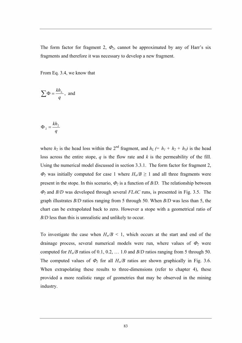
83
The form factor for fragment 2, Φ2, cannot be approximated by any of Harr’s six
fragments and therefore it was necessary to develop a new fragment.
From Eq. 3.4, we know that
∑ =Φq
khL , and
qkh2
2 =Φ
where h2 is the head loss within the 2nd fragment, and hL (= h1 + h2 + h3) is the head
loss across the entire stope, q is the flow rate and k is the permeability of the fill.
Using the numerical model discussed in section 3.3.1. The form factor for fragment 2,
Φ2 was initially computed for case 1 where Hw/B ≥ 1 and all three fragments were
present in the stope. In this scenario, Φ2 is a function of B/D. The relationship between
Φ2 and B/D was developed through several FLAC runs, is presented in Fig. 3.5. The
graph illustrates B/D ratios ranging from 5 through 50. When B/D was less than 5, the
chart can be extrapolated back to zero. However a stope with a geometrical ratio of
B/D less than this is unrealistic and unlikely to occur.
To investigate the case when Hw/B < 1, which occurs at the start and end of the
drainage process, several numerical models were run, where values of Φ2 were
computed for Hw/B ratios of 0.1, 0.2, … 1.0 and B/D ratios ranging from 5 through 50.
The computed values of Φ2 for all Hw/B ratios are shown graphically in Fig. 3.6.
When extrapolating these results to three-dimensions (refer to chapter 4), these
provided a more realistic range of geometries that may be observed in the mining
industry.
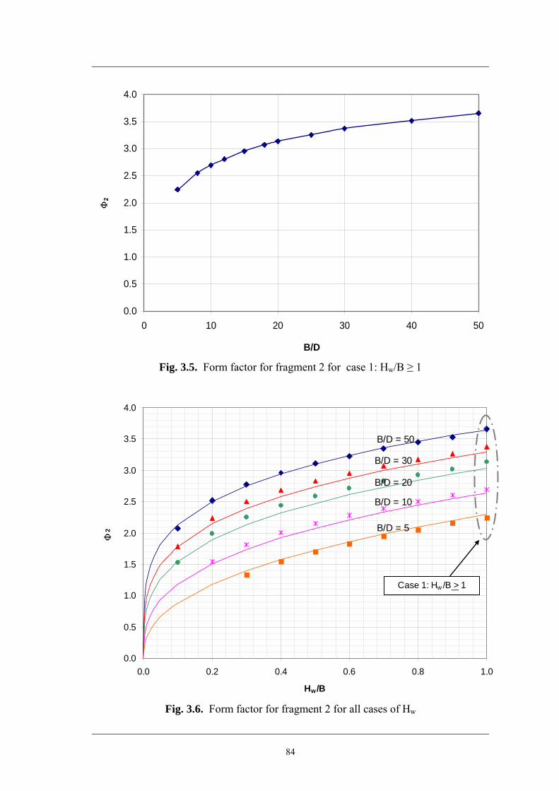
84
0.0
0.5
1.0
1.5
2.0
2.5
3.0
3.5
4.0
0 10 20 30 40 50
B/D
Φ2
Fig. 3.5. Form factor for fragment 2 for case 1: Hw/B ≥ 1
0.0
0.5
1.0
1.5
2.0
2.5
3.0
3.5
4.0
0.0 0.2 0.4 0.6 0.8 1.0
Hw/B
Φ2
B/D = 50
B/D = 30
B/D = 20
B/D = 10
B/D = 5
Case 1: Hw /B > 1
Fig. 3.6. Form factor for fragment 2 for all cases of Hw

85
Using these plots, equations of Φ2 for all cases of Hw/B can be obtained. For Hw ≥ B,
when the height of water of fragment 2 is greater than or equal to B:
5/1
2 35
⎟⎠⎞
⎜⎝⎛=Φ
DB (3.7)
For Hw < B, when the height of water is less than B, i.e. at the start and end of the
drainage process:
d
w
BH
DB
⎟⎟⎠
⎞⎜⎜⎝
⎛⎟⎠⎞
⎜⎝⎛=Φ
5/1
2 35 (3.8)
where d is given by:
4/1
62.0 ⎟⎠⎞
⎜⎝⎛=
BDd (3.9)
Values of Φ2, computed using FLAC and the above equations are shown in Fig. 3.6
and an excellent fit can be seen. The curves plotted on Fig. 3.6 represent a graphical
representation of Eq. 3.6 – Eq. 3.9 and actual FLAC results are given by the data
points.
Intuitively and from the numerical model runs, it was evident that the maximum pore
water pressure within the stope occurs at the bottom corner of the stope (point Q in
Fig. 3.7). OPQRS and PQRS are the longest stream lines for case 1 (Hw > B) and case
2 (Hw < B) respectively. Here α2D is the fraction of the head loss within fragment 2
that takes place in the horizontal segment of the largest stream line and ranges between
0 and 1. Denoting the head loss in fragment two as h2, the head losses from Q to R
and from P to Q can be defined as α2Dh2 and (1 - α2D)h2 respectively.
Assuming the top of drain as the datum, the total, elevation and pressure heads at the
corner of the stope for case 1 (point Q in Fig. 3.7 a) are given by:

86
Fig. 3.7. Head losses within fragments
LD
D hhh ⎟⎟⎠
⎞⎜⎜⎝
⎛Φ+Φ+Φ
Φ+Φ=+=
321
322322 head Total αα (3.10)
Elevation head = -D (3.11)
DhLD +⎟⎟
⎠
⎞⎜⎜⎝
⎛Φ+Φ+Φ
Φ+Φ=∴
321
322 head Pressure α (3.12)
Therefore the maximum pore water pressure that occurs at the corner of the stope is
given by:
wLD Dhu γ
α⎥⎦
⎤⎢⎣
⎡+⎟⎟
⎠
⎞⎜⎜⎝
⎛Φ+Φ+Φ
Φ+Φ=
321
322max (3.13)
(a) Case 1: Hw > B (b) Case 2: Hw < B
1
2
3 3
2
P
Q R
α2Dh2
(1-α2D)h2
h3
Q
h3α2Dh2
(1-α2D)h2
h1
O
S S R
P
Datum

87
For case 2, when the height of water (Hw) is less than the stope width (B) as shown in
Fig. 3.7 (b), fragment 1 does not exist and Φ1 equals zero.
Using FLAC, α2D was computed for different values of D/B and Hw/B to represent
typical stope geometries, these ranged from 0.02 to 0.20, and from 0.1 to 1.0
respectively. The variation of α2D against these aspect ratios is shown in Fig. 3.8. As
D/B is lowered, a larger head loss fraction occurs between Q and R, since more
resistance has to be overcome in flowing from Q to R than from P to Q. Also, the
greater the Hw/B ratio, the smaller the head loss fraction between Q and R.
0.70
0.75
0.80
0.85
0.90
0.95
1.00
0.00 0.05 0.10 0.15 0.20
D/B
α2D
Hw/B Values
>1.0 (Case 1)
0.8
0.6
0.4
Fig. 3.8. Coefficient α2D for fragment 2
It can be seen from Fig. 3.8 that the coefficient α2D varies linearly with D/B for a
specific Hw/B. Therefore can be expressed in the form:
cBDm += )/(α (3.14)
where m and c are the slope and intercept on the α2D-axis. Plotting the values of m and
c separately against Hw/B shows that,

88
2473.07788.0 +−=B
Hm w (3.15)
0689.12193.0 +−=B
Hc w (3.16)
Here, the coefficients of determination (r2) for Eq. 3.15 and Eq. 3.16 are 0.9741 and
0.9928 respectively, showing a very strong straight line fit between m and c against
Hw/B. Substituting Eq. 3.15 and Eq. 3.16 in Eq. 3.14, α2D can be written as:
0689.12193.02473.07788.02 +⎟⎠⎞
⎜⎝⎛−⎟
⎠⎞
⎜⎝⎛+⎟
⎠⎞
⎜⎝⎛
⎟⎠⎞
⎜⎝⎛−=
BH
BD
BD
BH ww
Dα (3.17)
For case 1 (Fig. 3.7 a), when Hw/B > 1, the value of Hw/B, when calculating Φ2 and
α2D is equal to 1. Here, the flow domain above the height of B becomes fragment 1.
Fig 3.8 also illustrates that when Hw/B < 0.3, the value of α2D can be approximated as
1.
Fig. 3.5, Fig. 3.6 and Fig 3.8 present design charts to calculate Φ2 and α2D for typical
stope geometries. Table 3.4 summarizes the equations used to calculate the maximum
pore pressure, form factors and flow rate for a two-dimensional hydraulic fill stope
with a single drain at the stope base and no decant water for all cases of Hw/B.
3.3.3 Fragment Comparison
It should be noted, that although none of Harr’s six fragments could be used to
estimate fragment 2 in the two-dimensional stope, Griffith’s Type B and Type C
fragments given in Table 3.2, can be used to approximate the form factors for the two-
dimensional stope. Therefore, an overview of the various models was conducted to
justify the need for the new fragments developed in Table 3.4.

89
Table 3.4. Summary of equations for two-dimensional analysis
Parameter Equation
Form Factor for fragment 1 Φ1
BBH w −
=Φ1
1≥B
Hw c=Φ 2
1<B
H w d
w
BH
c ⎟⎟⎠
⎞⎜⎜⎝
⎛=Φ 2 Form Factor for
fragment 2 (Fig. 3.5 – Fig 3.6) Φ2 where:
5/1
35
⎟⎠⎞
⎜⎝⎛=
DBc
4/1
62.0 ⎟⎠⎞
⎜⎝⎛=
BDd
Form Factor for fragment 3 Φ3
DDX 5.0
3−
=Φ
3.0<B
H w 12 ≈Dα Fraction of head lost in fragment 2 that takes place in the horizontal segment of the streamline (Fig. 3.8) α2D
3.0≥B
H w 07.122.025.078.02 +⎟⎠
⎞⎜⎝
⎛−⎟⎟
⎠
⎞⎜⎜⎝
⎛+⎟
⎠
⎞⎜⎝
⎛−=
BH
BD
BH ww
Dα
Maximum pore pressure umax
wLD Dhu γα
⎥⎦
⎤⎢⎣
⎡+⎟⎟
⎠
⎞⎜⎜⎝
⎛Φ+Φ+Φ
Φ+Φ=
321
322max
Flow Rate q ∑
=
Φ
=n
ii
Lkhq
1
To provide a comparison between the models, several randomly selected stope
geometries were analyzed and values of discharge were calculated using:
• The fragment types discussed in Table 3.4,

90
• Griffiths (1984) fragment types shown in Table 3.2, and
• Finite difference model
The results are illustrated in Fig. 3.9.
0
2
4
6
8
10
12
14
16
0 2 4 6 8 10 12 14 16
Flow from FLAC (lit/min per m)
Flow
from
MO
F (li
t/min
per
m)
Hw< B: Table 3.4
Hw < B: Griffiths (1984)
Hw > B: Table 3.4
Hw > B: Griffiths (1984)
Fig. 3.9. Flow rate comparison using varying fragments including Griffiths (1984)
and Table 3.4 fragments against finite difference model FLAC
As shown in Fig. 3.9, the fragments developed and tabulated in Table 3.4, provide a
much closer approximation than those suggested by Griffiths (1984). For the randomly
selected samples, Table 3.4 fragments contained a maximum percent error of 2%,
whilst Griffiths varied as much as 16%. This investigation illustrates that the
application of Griffith’s fragments to the two-dimensional stope contains significant
percent error as opposed to those calculated using Table 3.4 fragments. Therefore
when applying the method of fragments in two-dimensions, the fragments and
analytical solutions given in Table 3.4 were used.

91
3.3.4 Decant Water in Two-dimensional Hydraulic Fill Stopes
Thus far it has been assumed that there is no decant water and the height of water (Hw)
is equal to or less than the tailings height (Htailings). If decant water is present in the
hydraulic fill stope as (i.e. Hw > Htailings) then Htailings should be substituted for Hw in
the formulas outlined in Table 3.4. It is important to note that even when decant water
is present, the head loss (hL) remains the same (i.e. hL = Hw (with/without decant water) – D).
3.3.5 Entry and Exit Hydraulic Gradients
One of the main objectives in the design of a hydraulic fill system is to remove the
water from the stope as quickly as possible. This is often achieved by ensuring that the
hydraulic fill has adequate permeability. Soil mechanics combined with simple mass
balance can be used to define an upper bound value for the permeability of a specific
fill to ensure there is no build up of decant water on the surface of the fill.
Since all other boundaries are assumed impervious and the only water entering the
stope is via the slurry mixture, the volume of water entering the stope per hour (Vin)
can be calculated by:
w
slurrysin
wRV
ρ= (3.18)
where Rs is the solids filling rate (e.g. 250 t/hour), wslurry is the water content of the
hydraulic fill slurry and ρw is the density of water.
The volume of water draining from the stope every hour is:
AkiV entryout = (3.19)
where k is the permeability, ientry is the hydraulic gradient at the top of the water, and A
is the plan area of the stope.
92
At a certain stage in backfilling, to ensure there is no more increase in water height,
Vout must be greater than Vin. Therefore,
waterentry
slurrys
AiwR
kρ
≥ (3.20)
The above inequality is used to determine a threshold value for k, however, it often
gives very high and unrealistic values for permeability, particularly stopes with small
plan area. Here, ientry varies with the height of water during the filling operation and
subsequent draining.
A less conservative and more realistic approach is to allow the water to rise during the
fill placement, but to remain below the fill level. This will ensure that there is no
decant water at all times during filling. The derivation of the limiting value of
permeability to ensure that water height remains below the fill height is given below.
wρs
s
GRhourevery in solids of Volume = (3.21)
Where Gs refer to the specific gravity of the fill and ρw refers to the water density.
Anw )1(1
GR hourper height fill in Increases
s
−=∴
ρ (3.22)
Here n is the porosity of the settled hydraulic fill.
w
slurryswR hour per stope theentering water of Volume
ρ= (3.23)
A ik hourper stope theleaving water of Volume entry= (3.24)

93
A ik R
hour per stope theentering water of Net volume entrys −=∴
w
slurrywρ
(3.25)
nA
Aik R
hour per height water in Increaseentry
s −=∴ w
slurrywρ (3.26)
To ensure there is no decant water above the fill, the increase in fill height has to be
greater than the increase in water height every hour. Therefore,
nki
nAwR
AnGR entryslurry
w
s
ws
s −≥− ρρ )1(1 (3.27)
Rearranging Eq. 3.27, the permeability (k) can be determined by:
⎥⎦
⎤⎢⎣
⎡−
−≥s
slurryentryw
s
Gnnw
AiRk 1
)1(1
ρ (3.28)
In the absence of realistic values for ientry, a gravitational gradient of unity is often
assumed. Several runs in FLAC and FLAC3D, for two and three dimensional stopes,
show that the hydraulic gradients at the top of the water level can be significantly less
than unity. Using the method of fragments, a simple expression is developed below for
ientry for a two-dimensional stope.
DXh
DXh
i Li
ii
exit 5.05.0 3
1
33
−Φ
Φ=
−=
∑=
=
(3.29)
From Eq. 3.18 and Eq. 3.29,
DDH
i wi
ii
exit)(1
3
1
−
Φ=
∑=
=
(3.30)

94
Therefore, ientry can be written as:
BDH
i wi
ii
entry)(1
3
1
−
Φ=
∑=
=
(3.31)
It can be seen from Eq. 3.31 and in Fig. 3.10, that the hydraulic gradient at the top of
the water level (ientry) is a function of X/D, D/B and Hw/B.
0
1
2
3
4
5
6
0.0 0.1 0.2 0.3 0.4 0.5 0.6 0.7
ientry
Hw/B
X/D=1 & D/B=0.1X/D=1 & D/B=0.02X/D=5 & D/B=0.1X/D=5 & D/B=0.02
Fig. 3.10. Dependence of ientry for several cases of X/D, D/B and Hw/B
For randomly selected values of X, D, B and Hw the hydraulic gradients at the top of
the water level were computed using Eq. 3.31. In Fig. 3.11, Hw/B is plotted against
ientry without any considerations to the different values of X/D and D/B. From the
figure, it is evident that as the water level rises, the hydraulic gradient increases. The
hydraulic gradient at the top of the water level can be approximated as:
75.0
2.0 ⎟⎠⎞
⎜⎝⎛=
BH
i wentry (3.32)

95
0
1
2
3
4
5
6
0.0 0.1 0.2 0.3 0.4 0.5 0.6 0.7
ientry
Hw/B
Hw>BHw<B
Fig. 3.11. Hw/B against ientry for two-dimensional stopes
The curve in Fig. 3.11 illustrates the approximation of ientry given in Eq. 3.32. The
data points represent the theoretical values given by Eq. 3.31.
The use of Eq. 3.20, Eq. 3.28 and Eq. 3.32 is illustrated through a numerical example.
For a 30 m wide stope with water height of 60 m, from Eq. 3.32, ientry can be estimated
as 0.34. For a filling rate of 5 t/hour per m and slurry water content of 33%, the
permeability necessary to ensure no increase in water height can be estimated from Eq.
3.20 as 162 mm/hour. However, using a value of unity for ientry would have grossly
underestimated the required permeability as 55 mm/hr. From the permeability values
computed using Eq. 3.20 (162 mm/hr); it appears that the permeability of the hydraulic
fill has to be unrealistically large to ensure that there is no rise in water level. The
more relaxed criterion of ensuring the fill rise is faster than the water (i.e. no decant
water above the fill at any time) and assuming a porosity of 40% and specific gravity
of 2.80 for the settled hydraulic fill, calculates that the permeability only as to be
greater than 45 mm/hr (Eq 3.28.),

96
3.3.6 Scaling Effect on Method of Fragments
Method of fragments can also be used to explain the influence of scaling on pore water
pressure measurements and flow rate from the stope. If a two-dimensional stope is
scaled by a factor of x, as shown in Fig. 3.12, the entire geometry is scaled by a factor
of x. Therefore, the total head loss across the stope, the head loss between each of the
equipotential lines and the number of equipotential drops are also scaled by a factor of
x. Hence the form factors (Φi) remain the same, even when the stope has been scaled.
However, the permeability remains constant. Substituting the scaled geometries into
Eq. 3.3 and Eq. 3.13, the flow rate and the pore water pressures scale by a factor of x
for a two-dimensional stope.
Fig. 3.12. Scaling of two dimensional stope and flow nets
3.3.7 Typical Stope Geometries
Typical stope geometries vary significantly in underground mining operations. The
size of stope can depend on the ore body geometry, the geotechnical characteristics of
the host rock and particular mine conditions. Stope widths and depths can vary
between 20 m and 50 m and stope heights can be as high as 200 m. Drains are
generally between 3 m and 6 m in width, which makes the drain typically between 9
m2 - 36 m2 in cross-sectional area. Drain lengths have a considerable influence on the
pore pressure distribution as well as the discharge from the stope assuming that there is
consistent permeability along the drain and that the drive is tight-filled. Increasing the
drain length, often results in increased pore pressure and a reduction in drain
discharge. Intuitively, as a barricade gets further from the stope, the flow path
increases and the hydraulic gradient across the entire model decreases, resulting in
Stope scaled by a factor of x. h L
x.h L
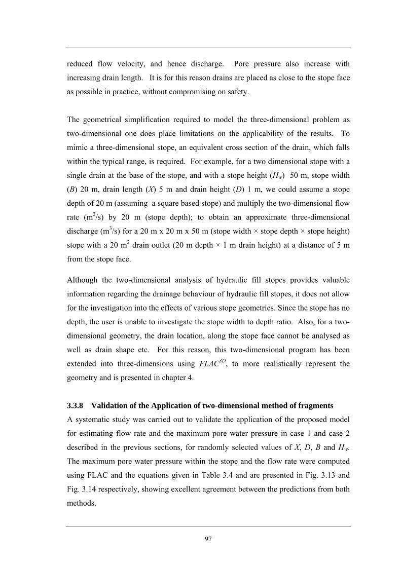
97
reduced flow velocity, and hence discharge. Pore pressure also increase with
increasing drain length. It is for this reason drains are placed as close to the stope face
as possible in practice, without compromising on safety.
The geometrical simplification required to model the three-dimensional problem as
two-dimensional one does place limitations on the applicability of the results. To
mimic a three-dimensional stope, an equivalent cross section of the drain, which falls
within the typical range, is required. For example, for a two dimensional stope with a
single drain at the base of the stope, and with a stope height (Hw) 50 m, stope width
(B) 20 m, drain length (X) 5 m and drain height (D) 1 m, we could assume a stope
depth of 20 m (assuming a square based stope) and multiply the two-dimensional flow
rate (m2/s) by 20 m (stope depth); to obtain an approximate three-dimensional
discharge (m3/s) for a 20 m x 20 m x 50 m (stope width × stope depth × stope height)
stope with a 20 m2 drain outlet (20 m depth × 1 m drain height) at a distance of 5 m
from the stope face.
Although the two-dimensional analysis of hydraulic fill stopes provides valuable
information regarding the drainage behaviour of hydraulic fill stopes, it does not allow
for the investigation into the effects of various stope geometries. Since the stope has no
depth, the user is unable to investigate the stope width to depth ratio. Also, for a two-
dimensional geometry, the drain location, along the stope face cannot be analysed as
well as drain shape etc. For this reason, this two-dimensional program has been
extended into three-dimensions using FLAC3D, to more realistically represent the
geometry and is presented in chapter 4.
3.3.8 Validation of the Application of two-dimensional method of fragments
A systematic study was carried out to validate the application of the proposed model
for estimating flow rate and the maximum pore water pressure in case 1 and case 2
described in the previous sections, for randomly selected values of X, D, B and Hw.
The maximum pore water pressure within the stope and the flow rate were computed
using FLAC and the equations given in Table 3.4 and are presented in Fig. 3.13 and
Fig. 3.14 respectively, showing excellent agreement between the predictions from both
methods.

98
0
100
200
300
400
500
600
700
800
900
1000
1100
0 100 200 300 400 500 600 700 800 900 1000 1100
Max. pore water pressure from FLAC (kPa)
Max
. por
e w
ater
pre
ssur
e fr
om M
OF
(kPa
)
Hw < BHw > B
Fig. 3.13. Maximum pore water pressure comparison
0
2
4
6
8
10
12
14
16
0 2 4 6 8 10 12 14 16
Flow rate from FLAC (lit/min per m)
Flow
rate
from
MO
F (li
t/min
per
m)
Hw < B
Hw > B
Fig. 3.14. Flow rate comparison

99
3.3.9 Further analysis of the pore water pressure in two-dimensional stopes
So far, the analysis of the two-dimensional hydraulic fill stope has only considered the
most critical values for understanding the drainage and pore pressure development
within a two-dimensional stope. These include the point of maximum pore pressure
(point Q in Fig. 3.15) and discharge values for varying geometries. Using FLAC
several other points were analysed and equations developed to determine the pore
pressure development throughout the stope. Fig 3.15 illustrates the locations of
several other points analysed.
αh2
A B
Q F
E
D
C
h3
(1-α)h2
0.5×B
Datum
h1
Fig. 3.15. Points for pore pressure analysis
Eq. 3.13 gives the maximum pore water pressure (point Q) for the two-dimensional
stope shown in Fig 3.15. The pore water pressure at several other points shown in Fig.
3.15, are calculated using the equations given in Table 3.5. The coefficient α is the
fraction of the head loss within fragment 2 and ranges between 0 and 1. This
coefficient varies for each of the points being analysed and also varies with varying
geometries, therefore design charts were developed for the points shown above and are
given in Fig. 3.8, Fig 3.16 and Fig 3.17. To verify the proposed equations given in
Table 3.5, several randomly selected geometries of the two-dimensional stope were
modelled and compared with the equations given in Table 3.5. The validation plots for
each of the points analysed are given in Appendix C and results show excellent
agreement.

100
Table 3.5. Summary of pore water pressure equations and design charts for various
points
Location Pore water pressure (ui) αi
Point A & B wLBA Dhuu γ⎥
⎦
⎤⎢⎣
⎡+⎟⎟
⎠
⎞⎜⎜⎝
⎛Φ+Φ+Φ
Φ+Φ==
321
32 NA
Point Q – Maximum Pore Pressure
D
C
A
Q F
αQh2
(1 - αQ)h2
B
E
wLQ
Q Dhuu γα
⎥⎦
⎤⎢⎣
⎡+⎟⎟
⎠
⎞⎜⎜⎝
⎛Φ+Φ+Φ
Φ+Φ==
321
32max
Refer to Fig. 3.8 or Eq. 3.14 – Eq. 3.16
Point C
(1-αC)h2
αCh2 Q
D C
A B
E
F
wLC
C DBhu γα
⎥⎦
⎤⎢⎣
⎡−−⎟⎟
⎠
⎞⎜⎜⎝
⎛Φ+Φ+Φ
Φ+Φ= )5.0(
321
32
Refer to Fig. 3.16
Point D
αDh2
Q
(1-αD)h2
D C
BA
E
F
wLD
D hu γα
⎥⎦
⎤⎢⎣
⎡⎟⎟⎠
⎞⎜⎜⎝
⎛Φ+Φ+Φ
Φ+Φ=
321
32 Refer to Fig. 3.17
Point E wLE hu γ
⎥⎥⎦
⎤
⎢⎢⎣
⎡⎟⎟⎠
⎞⎜⎜⎝
⎛Φ+Φ+Φ
Φ=
321
3 NA
Point F wLF Dhu γ⎥
⎦
⎤⎢⎣
⎡+⎟⎟
⎠
⎞⎜⎜⎝
⎛Φ+Φ+Φ
Φ=
321
3 NA

101
0.70
0.75
0.80
0.85
0.90
0.95
1.00
0.00 0.05 0.10 0.15 0.20
D/B
αC
0.6
0.8
1.0
Hw /B
Fig. 3.16. Coefficient αC for fragment 2 for point C
0.15
0.25
0.35
0.45
0.55
0.65
0.75
0.00 0.05 0.10 0.15 0.20
D/B
αD
0.7
0.2
0.3
0.9
0.5
Hw/B
1.0
Fig. 3.17. Coefficient αD for fragment 2 for point D

102
3.4 Anisotropy
Hydraulic fill materials, produced by crushing the waste rocks have very angular
grains as shown in the electron micrograph in Fig 2.4. When settling from the slurry
they sometimes produce an anisotropic fill due to the finer fractions of the material
settling with slower velocities than the coarser fractions. This stratification can lead to
anisotropic behaviour in the permeability of the fill material. Therefore, a preliminary
investigation into the effect of the directional variation in permeability was undertaken
using a combination of the finite difference program FLAC and method of fragments.
A simple apparatus and method were developed for measuring the permeability
variation within the hydraulic fill material. Using the apparatus, horizontal and
vertical permeability values were measured for a variety of hydraulic fill samples.
Although these results provide an indication into the degree of anisotropy, several
problems were encountered in the testing; therefore results from previous laboratory
testing and image processing techniques (Witt and Brauns, 1983; Martys et al., 2000;
Mansur and Dietrich, 1965) along with those determined at James Cook University,
were used.
3.4.1 Laboratory Testing
The permeability cell testing procedure is a modified version of the constant head
permeability test outlined in AS 1289.6.7.1 (2001) and the test procedure developed by
Witt and Brauns (1983). Using a 150 mm x 150 mm x 150 mm cubic permeability
cell, simple laboratory test procedures were developed to measure the vertical and
horizontal permeability for a reconstituted hydraulic fill sample as shown in Fig 3.18.
Hydraulic fills were mixed at water contents that matched the placement water
contents of the slurry at the respective mines.
The permeability cell was set up and saturated filter paper placed along all sides and
base of the cell. Steel clamps and sealant were used to seal the cell as shown in Fig
3.18 (a). The slurry sample was then prepared to the specified solids content and
placed evenly into the area of the mould in approximately 3 – 5 equal layers until the
cell was completely full as shown in Fig 3.18 (b). The sample was left to stand
untilthe build up of decant water was present on the surface. The decant water was

103
then removed and the filling continued until the entire cell was filled with the saturated
fill. The final piece of filter paper was then saturated and lowered onto the top of the
fill surface with careful attention to ensure no air voids were caught between the
sample and the filter paper. The end caps were then attached to the apparatus and the
end caps secured to the permeability cell using another clamp and sealant as shown in
Fig. 3.18 (c). The void within the top end-cap was then completely filled with
distilled water and the entire apparatus attached to the constant head assembly. A ring
fastener was used to ensure the permeability cell setup and constant head apparatus
were securely fastened. The overflow tank surrounding the permeability cell was filled
with water to the level of the overflow pipe. The apparatus was then left to stand to
ensure the flow had reached steady state. Standard constant head tests were then
carried out on the sample, using the setup shown in Fig. 3.18 (d) and the permeability
values were computed from the Eq. 3.33.
(a)
(b)
End Caps
Steel plates
(c)
(d)
Fig. 3.18. (a) Permeability cell with filter paper (b) Placement of slurry in
permeability cell (c) Secured permeability cell (d) Permeability cell connected to
constant head apparatus

104
hAQLk = (3.33)
where Q is the discharge per unit time, L is the length of the cell, h is the head, and A is
the cross sectional area of the permeability cell.
Once the vertical permeability measurements were recorded, the cube was removed
from the constant head apparatus setup and rotated 90 degrees to measure the
horizontal permeability. The two end caps were exchanged with two-opposite steel
plates surrounding the permeability cell and the apparatus set up as per the vertical
permeability testing. It is important to note than whenever steel plates and end caps
were secured using the clamps, sealant was applied to the connections and edges as an
additional safety measure to ensure no leakage occurred during testing.
Previous laboratory testing that measured the degree of permeability (ratio of
horizontal to vertical permeability) used two samples of soil. The first test would be
carried out with flow in the direction of maximum permeability and the second with
the flow at right angles to that in the first test. Difficulties with this approach could
arise if the two samples were not exactly the same in terms of permeability
characteristics. This testing procedure uses a single soil sample that is tested under
the same conditions for both vertical and horizontal permeability measurements.
However, during testing several problems were encountered with the permeability cell,
these included:
• The movement of the cell when rotating it by 90 degrees may dislodge some
particles and allow movement of soil grains within the sample, thus not
accurately obtaining the ‘true’ horizontal discharge.
• During testing, several leaks were observed and were sealed using a silicone
based sealant. However during the constant head permeability testing some of
the apparatus was submerged in water, Refer to Fig 3.18 (d), therefore some
leaks may have gone undetected which may have also influenced results.

105
• When measuring the horizontal permeability, it was necessary to switch the
two end caps with two steel plates on opposite sides of the cell (see Fig 3.18
(c)). Once switched, the cell was resealed using the sealant and the remainder
of the testing was undertaken. This part of the procedure is not practical and
very labor intensive, therefore it is recommended that future testing on the
degree of anisotropy is undertaken using an alternative testing procedure and
apparatus.
• It would be more beneficial if vertical and horizontal permeability readings
could be measured under confined pressures (as would be the case in the
mines). This cell could only take measurements under the self weigh of the fill.
3.4.1.1 Results
Table 3.6 summarizes the results obtained from the anisotropic permeability testing
using the permeability cell and also standard constant head permeability testing that
was conducted from the same batch of hydraulic fill in 2004. Appendix D provides the
full results. As was suspected, the degree of anisotropy in the three samples tested was
very low. The results of vertical permeability from both test methods (standard
constant head and the permeability cell) provided similar values for samples D3 and
D4, however A1 was significantly higher than previously tested in 2004. In general,
the overall degree of anisotropy for all three samples varied only slightly ranging from
1.28 – 1.34.
Table 3.6. Permeability anisotropy values for hydraulic fills
Degree of anisotropy
kV (2004) kV (2006) kH (2006) kH / kV
D4 3.50 24.41 23.45 31.52 1.34
D3 3.53 37.84 51.47 71.72 1.39
A1 2.79 9.07 94.77 121.77 1.28
SamplePermeability (mm/hr)Specific
Gravity
Using a combination of the finite difference program FLAC, EXCEL, method of
fragments and the anisotropic values obtained from both previous and present testing,

106
the effect of anisotropic permeability was investigated. To take account of the
anisotropic permeability, in-built functions in FLAC were applied to the model and the
codes given in Appendix B. As mentioned previously, the maximum pore water
pressure and flow rate are of interest mainly when the water height is quite significant,
therefore only case 1 (Hw>B) was considered. Based on previous literature and on the
testing conducted at James Cook University, a permeability ratio of 1 – 3 was
investigated in the numerical simulations.
3.4.2 Pore Water Pressure
When there is no directional variation in the permeability of hydraulic fill, the
maximum pore water pressure is independent of the magnitude of permeability and the
flow rate is proportional to permeability. However, if the hydraulic fill exhibits
anisotropy with respect to permeability, the degree of anisotropy (i.e. kh/kv) can have
significant influence on the maximum pore water pressure and flow rate. Fig. 3.19 and
Fig. 3.20 illustrate the results for two cases that are modelled with typical aspect ratios
encountered for a two-dimensional stope with varying degrees of anisotropy. Case 1
considered a stope with a D/B ratio of 0.025 and an X/D ratio of 1, whilst case 2
considered a D/B ratio of 0.05 and X/D ratio 1.
0
1
2
3
4
5
6
0.0 0.2 0.4 0.6 0.8 1.0
umax/γhL
Hw/B
D/B = 0.025X/D = 1
123
kh / kv
Fig. 3.19. Design chart for pore water pressure measurements for
anisotropic fill material: D/B = 0.025; X/D = 1

107
0
1
2
3
4
5
6
0.0 0.2 0.4 0.6 0.8 1.0umax/γhL
Hw/B
D/B = 0.05X/D = 1
123
kh / kv
Fig. 3.20. Design chart for pore water pressure measurements for
anisotropic fill material: D/B = 0.05; X/D = 1
These figures illustrate the effect of geometry and degree of anisotropy on the
maximum pore pressure measurements. It is interesting to note that whilst the absolute
magnitude of permeability has no influence on the pore water pressures within the
stope, the presence of anisotropy in permeability reduces the pore water pressures
quite significantly for a specific height of water.
3.4.3 Flow rate
The rate of drainage of water from the stope will be governed to some extent by the
hydraulic properties of the fill material. With permeability being proportional to flow
rate, it is obvious that materials of higher permeability will drain more quickly than
those of lower permeability. However, the effect of anisotropic permeability on flow
rate of hydraulic fill material has had little attention. Fig. 3.21 demonstrates the effect
of varying anisotropic ratios on a stope with an X/D ratio of 1 and D/B ratio of 0.025.

108
0
1
2
3
4
5
6
0.0 0.5 1.0 1.5 2.0 2.5 3.0
q/kequivhL
Hw/B
D/B = 0.025X/D = 1
123
kh / kv
Fig. 3.21. Design chart: effect of anisotropic permeability on flow rate D/B=0.025;
X/D=1
As shown in Fig. 3.21, as the anisotropic permeability and the Hw/B ratios increase
within the stope, the flow rate decreases. When analysing Eq. 3.34 that calculates flow,
the effect of the anisotropic permeability can be broken into two specific terms: kequiv =
(khkv)0.5 and Nf/Nd which equals the ratio of flow channels to equipotential drops. From
Eq. 3.34, ΣΦ = khL / q, which represents the x-axis in Fig. 3.21. Therefore, from the
above figure, it can be deduced that for a specific geometry, as the anisotropic ratio
increases, the equivalent permeability (kequiv) increases and Nf/Nd decreases
d
fLvh
d
fLequiv N
Nhkk
NN
hkQ ×== (3.34)
However, these terms are not proportional to each other, and care must be taken when
analyzing the effect of anisotropic permeability on flow rate as the flow rate trends
vary for differing geometries.

109
3.5 Ancillary Drainage in Two-Dimensional Hydraulic Fill Stopes
Upon discharge into a stope, hydraulic fill generally consists of a solids density of
approximately 65% - 75% solids by weight and, because of its liquid nature, possess
minimal shear strength. Before it can satisfactorily perform its function in the mining
operation as an engineered backfill, it must go through a process of dewatering.
Currently solids contents of 65 – 75% are used. Even at 75% solid content, assuming
specific gravity of 3.00 for solid grains, 50% of the slurry volume is water. Although
not all this water is required to drain i.e. some remains in the fill as residual moisture,
there is still a substantial amount of water that has to be drained from the hydraulic fill
stope. To expedite the drainage, there had been recent attempts to use prefabricated
drains in vertical, horizontal and inclined positions within the stope, thus reducing the
drainage paths (Kuganathan, 2001; Neindorf 1983).
Through the use of a two-dimensional model developed in FLAC, it can be shown that
the prefabricated drains are effective in accelerating the drainage process and reducing
the pore water pressures within the stope. Previously, prefabricated drains have been
successfully used in consolidation of clays. However, this is the first numerical
modeling study that looks at the effects of prefabricated drains on drainage through
hydraulically filled mine stopes, where the material is granular and the prefabricated
drains are used simply to shorten the drainage paths. Although, it would be premature
to regard the two-dimensional model developed here as a proven design tool, it will
provide a better understanding of the effect of using ancillary drainage in effectively
draining a hydraulically filled stope.
The effects of ancillary drains on the pore water pressures and discharge were studied
through a two dimensional numerical model developed in FLAC. Most of the runs
were made on a 50 m wide stope containing hydraulic fill with a water level at 80 m
height and with a 5 m long by 5 m high drain (Fig. 3.22). The ancillary drain is placed
horizontally at the bottom of the drain. The first few trials were run with the above
stope dimensions whilst varying the length of the ancillary drain. Later, a few more
runs were made for stopes with different dimensions and drain lengths, to verify the
findings.

110
X B
Ancillary Drain
Hw
D La
Fig. 3.22. Geometry of stope with ancillary drainage
3.5.1 Pore Water Pressure
As discussed in section 3.3.2, the maximum pore water pressure (umax) within a two-
dimensional hydraulic fill stope with no ancillary drain, occurs at the corner of the
stope and can be calculated using Eq. 3.13, shown below.
wD
L Dhu γα⎥⎦
⎤⎢⎣
⎡+⎟⎟
⎠
⎞⎜⎜⎝
⎛Φ+Φ+Φ
Φ+Φ=
321
322max
Using FLAC, it was shown that for all values of ancillary drain lengths, the pore water
pressures were still the maximum at the corner of the stope. For the 50 m wide stope
described in (Fig. 3.22), the maximum pore water pressure, which occurs at the corner
of the stope, decreases linearly with the drain length. This is shown in Fig. 3.23.
When the ancillary drain extends to the full width of the stope (i.e., La = X+B), the
maximum pore water pressure is zero. This assumes the drain has infinite permeability
i.e. no head loss along the drain. Therefore, for a given length of ancillary drain (La)
the maximum pore water pressure can be simply interpolated, and can be expressed as:
wLa DhXB
Lu γα⎥⎦
⎤⎢⎣
⎡+⎟⎟
⎠
⎞⎜⎜⎝
⎛Φ+Φ+Φ
Φ+Φ⎟⎠⎞
⎜⎝⎛
+−=
321
32max 1 (3.35)

111
0
50
100
150
200
250
300
350
400
0.0 0.2 0.4 0.6 0.8 1.0
La/(X+B)
u max
(kPa
)Hw = 80 mB = 20 mD = 2 mX = 2 m
Fig. 3.23. Effects of ancillary drain on pore water pressure measurements
Fig. 3.24 illustrates the comparison between the maximum pore pressures calculated
using Eq. 3.35 and those obtained from FLAC for varying geometries and ancillary
drain lengths. As shown in the figure, Eq. 3.35 slightly overestimates the value of umax
when compared with those from FLAC. In other words, the equation provides an
upper bound for the maximum pore pressure values. The actual values of umax are
almost certain to be less than those computed from Eq 3.35.
3.5.2 Flow rate
The values of flow rate (Q) were computed for a number of simulations with varying
ancillary drain lengths in FLAC. These results are illustrated in Fig. 3.25. From this
figure it is clear that as the ancillary drain length is increased, the flow rate also
increases thus reducing pore pressure build-up behind the barricades. However, the
cost and difficulty of installation is increased as the drain length increases, therefore it
is important to reach a compromise between the two.

112
0
50
100
150
200
250
300
350
400
450
500
0 100 200 300 400 500
FLAC3D : umax (kPa)
EQN
: um
ax (k
Pa)
Fig. 3.24. Comparison between maximum pore water pressures obtained from FLAC
and those calculated using Eq. 3.13
Q = -6.2(La/(X+B))2 + 10.4(La/(X+B)) + 7.8
0
2
4
6
8
10
12
14
0.0 0.2 0.4 0.6 0.8 1.0La/(X+B)
Q (l
it/m
in p
er m
)
Hw = 80 mB = 20 mD = 2 mX = 2 m
k = 36 mm/hr
Fig. 3.25. Effect of ancillary drain on flow rate results

113
3.6 Summary and Conclusions Using method of fragments (Harr 1962, 1977) and the finite difference software FLAC,
the drainage and pore water pressure developments within a two-dimensional
hydraulic fill stope were investigated in this chapter. It was shown that the flow region
can be divided into three fragments, for which the form factors can be determined from
the dimensions of the stope and the drain. The flow is vertical at heights above the
stope width (B), and is horizontal within the drain a short distance (0.5D) from the
stope face. At the bottom of the stope, up to a height of the stope width, flow is two-
dimensional. Since the bottom of the stope (fragment 2) does not conform to any of
the fragments suggested by Harr (1962), a new fragment was developed. The
dimensionless form factor of the new fragments was expressed as a function of the
dimensions of the stope and drain. Analytical solutions were proposed for
determining the entry hydraulic gradient at the top of the stope, flow rate and the
maximum pore water pressure that occurs at the bottom corner of the stope. The model
was verified through several numerical examples of hydraulic fill stopes with
randomly selected dimensions and was found to be in excellent agreement. Several
other points within the two-dimensional stope were also analysed and equations
developed to determine the pore pressure development throughout the stope. For all
analysis in chapter 3, tight filling was assumed in the access drive.
The effect of anisotropic permeability in hydraulic fill material was investigated using
FLAC, EXCEL and the method of fragments. From the results, it is evident that the
anisotropic permeability has a significant effect on pore pressure development and
discharge within the stope. As the anisotropy in permeability is increased there is a
substantial reduction in pore pressure. A number of design charts were created to
quantify the effect of varying anisotropic ratios and geometries on pore pressure and
discharge within the stope.
Through the use of a two-dimensional model developed in FLAC, it was demonstrated
that the use of ancillary drainage behind barricades is effective in accelerating the
drainage process within a hydraulically filled stope - consequently, reducing the build-
up of pore pressure behind the barricades, assuming tight filling of the drain. It was
shown that the horizontal ancillary drain provided at the bottom of the drain reduces

114
the pore water pressure at all points within the fill, with the reduction being
proportional to the length of the drain. A simple expression was developed to
determine the maximum pore water pressure for the given stope and ancillary drain
arrangement. The ancillary drain also increases the hydraulic gradient, thus the rate of
flow, resulting in quicker drainage of the two-dimensional stope.

115
CHAPTER 4
APPLICATION OF METHOD OF FRAGMENTS TO THREE-
DIMENSIONAL HYDRAULIC FILL STOPES
4.1 Overview
Underground stope arrangements are very much three-dimensional in geometry, and
although the two-dimensional solutions discussed in Chapter 3 provide a valuable tool
for drainage prediction, the inherent approximations required, substantially reduce the
value of the model when dealing with complex three-dimensional stopes. This chapter
provides simple analytical solutions and design charts for estimating the maximum
pore water pressure and discharge within three-dimensional hydraulic fill stopes of
varying geometries. Previously, complex numerical models were required to analyze
these three-dimensional hydraulic filled stopes. Shape factors were developed to
account for the inherent individuality associated with stope and drain geometry and the
influence of scaling on discharge and pore pressure measurements were also
investigated. The proposed solutions have been verified against solutions derived from
the finite difference software package FLAC3D and physical modeling of a scaled stope
and results are found to be satisfactory.
4.2 Introduction
As discussed in Chapter 3, several numerical models have been developed to simulate
the drainage and pore water pressure developments within two and three-dimensional
stopes. These included Isaacs and Carter (1983) two-dimensional model which
provided a basic understanding of the concepts of the drainage of hydraulic fills in
undergrounds stopes. Traves and Isaacs (1991) extended this model to three-
dimensions; however the model remains yet to be validated against field
measurements. More recently, Rankine (2005) developed several drainage models in
FLAC and FLAC3D with similar features and verified them against the predictions from

116
the Isaacs and Carter (1983) model. A major restriction with these models is that the
simulations are often time consuming and in most cases, specialist knowledge of the
corresponding software package is required. Therefore a quicker and less complicated
solution was desirable.
Chapter 3 presents closed form solutions, based on the method of fragments and FLAC
simulations that can be used to determine the discharge and maximum pore water
pressures within a two-dimensional stope with a single drain at the stope base.
However, many mine stope geometries are not two-dimensional, and a more adaptable
three-dimensional solution was required. Using FLAC3D and the method of fragments,
simple analytical solutions and design charts were formulated for estimating the
maximum pore water pressure and discharge within three-dimensional hydraulic fill
stopes of varying geometries. The three-dimensional solutions derived from FLAC3D
were then compared with pseudo three-dimensional solutions derived in Chapter 3
using the Rankine (2005) model, Isaacs and Carter’s verification problem and FLAC3D
simulations.
4.3 Method of Fragments for Three-dimensional Hydraulic Filled Stopes
The three-dimensional flow net is approached in much the same manner as the two-
dimensional net. However equipotential lines are viewed as equipotential surfaces,
and the flow channels incorporate the third dimension. The total head loss (hL) across
the entire system is divided into a number of equipotential drops (Nd), which are
defined by Nd +1 equipotential surfaces. The total head loss across the entire system
is:
hNh dL Δ= (4.1)
As shown in the three dimensional stope depicted in Fig 4.1 (a), the equipotential
surface within the stope, at the height of B above the bottom, is approximately
horizontal as in the case with two-dimensional flow. Similarly, the equipotential
surface within the drain, at a distance of 0.5D from the stope, is approximately vertical.
Several FLAC3D runs, using various dimensions for the stope and the drain, were made

117
to justify these assumptions. Fig 4.1 (a) illustrates a few selected equipotential
surfaces for a simplified three-dimensional stope. Only half the geometry is shown
here.
Typical drain dimensions are generally, 3 m to 6 m wide and 3 m to 6 m high, and the
barricades are located a short distance from the stope. As discussed by Rankine et al.
(2003) the position of the barricade has considerable influence on pore water pressure
and discharge measurements. As the position of the barricade progresses further from
the stope face, the rate of discharge decreases. The closer the barricade the more
efficient is the drainage. Intuitively, as the barricade gets further away from the
stope, the flow path increases and the hydraulic gradient decreases. This results in a
reduction in the velocity and flow discharge. For safety reasons, barricades cannot be
constructed in flush with the stope face. Thus, for all modelling, the drain has been
assumed to be located at a minimum distance of 0.5D away from the stope face. Also,
the equipotential surface only becomes vertical, a short distance (≈ 0.5D) from the
stope edge. These two equipotential surfaces divide the flow domain into three
fragments similar to those in two-dimensions (see Fig. 4.1 b). In fragments 1 and 3, the
flow is one-dimensional.
(a) (b)
Fig. 4.1. Three-dimensional hydraulic fill stope (a) Selected equipotential surfaces
(b) Flow region, dimensions and three fragments of 3D stope

118
4.3.1 Numerical Model
The three-dimensional finite difference package FLAC3D was used to model the three-
dimensional hydraulic fill stope illustrated in Fig. 4.1 b. The program written for the
simulations undertaken in this dissertation was originally developed by Rankine (2005)
for an uncoupled, flow-only analysis of a specified geometry. The inbuilt programming
language FISH was also used to write simple subroutines for functions that were not
available in FLAC3D.
4.3.1.1 Numerical Package FLAC3D
FLAC3D is an extension to the well established two-dimensional numerical modelling
program FLAC developed by the Itasca Consulting Group (used in Chapter 3). Like
FLAC, FLAC3D is an explicit finite difference program used in computational
geomechanics. The numerical methods used in FLAC3D are essentially the same as
FLAC but the simulations model the three-dimensional behaviour of structures built of
soil, rock or other materials that undergo plastic flow when their yield criteria are
reached. Both FLAC and FLAC3D allow the user to implement subroutines written in
FISH.
Like FLAC, the variables involved in the description of fluid-flow through a porous
media are the pore pressure (u), saturation (S), and the three components of the specific
discharge vector (qx, qy, qz). These variables are related through Darcy’s law (the fluid
transport law), the fluid mass-balance equation, the constitutive equation2 and an
equation of state for the unsaturated range which relates pore pressure to saturation.
Assuming the volumetric strain rates are known, by substitution of the mass-balance
equation into the constitutive relation, using Darcy’s law, a differential equation in
terms of pore pressure and saturation is formed. For a flow-only analysis such as the
programs developed in this research, where grains are assumed incompressible, the
volumetric strain rates are obviously not required. This differential equation may be
solved for various geometries, properties, boundary and initial conditions.
2 The constitutive equation specifies the fluid response to changes in pore pressure, saturation and volumetric strains

119
The discretization and finite difference methods follow the general scheme presented
in the “Theory and Background” of the Itasca FLAC3D manuals. Each brick-shaped
element is further discretized into tetrahedra. The equations that describe pressures and
saturation values are based on nodal or “gridpoints” calculations, and zone pressures
and saturations are derived by simply averaging surrounding nodal values.
Attention is directed to two specifics of the numerical formulation:
1. All equations for both fluid analysis and boundary conditions in FLAC and
FLAC3D are expressed in terms of pore water pressure rather than head,
which are more conventionally used in soil mechanics.
2. Permeability, described in FLAC and FLAC3D refers to the mobility
coefficient, the coefficient of the pore pressure term in Darcy’s law. It is
defined as the ratio of intrinsic permeability to fluid dynamic viscosity,
(see– FLAC 4.0 Manual – User’s Guide, 2.8 System of Units).
In traditional soil mechanics, dxdhkkiv == , however, in FLAC
computations dxdukv = . Therefore, it can be shown that if du has the units
of Pa, and v has the SI units m/s, the permeability (k) must have the units
m2/(Pa.s). The two permeabilities are related by:
w
FLACk
kγmechanics soil= (4.2)
4.3.1.2 Input Parameters, Boundary Conditions and Assumptions
All material input parameters were identical to those used for the two-dimensional
simulations performed in chapter 3, as were the boundary conditions and assumptions
detailed in section 3.3.1.2. However, the three-dimensional problem investigated in
this chapter does not need the geometrical simplification that was required in the two-
dimensional solution as actual three dimensional geometries were modeled.
4.3.1.3 Grid Generation
The initial geometry investigated was a square based stope, with one drain located
centrally along the base of one of the stope walls, as shown in Fig. 4.1 b. To ensure

120
the most accurate and efficient modelling, a sensitivity analysis of mesh spacing was
undertaken. The meshes investigated are shown in Fig. 4.2 and include: (a) 2 m mesh
spacing, (b) 1 m mesh spacing, (c) a combination of a fine and coarse mesh (0.5 m
mesh spacing within drain with 1 m mesh spacing for the remainder of the stope) and
(d) 0.5 m mesh spacing throughout the stope.
(a) (b) (c) (d) Fig. 4.2. Mesh sensitivity (a) 2 m mesh spacing, (b) 1 m mesh spacing (c)
Combination of fine and coarse mesh (d) 0.5 mesh spacing Table 4.2 presents a summary of the output data from the various meshes investigated.
The difference in maximum pore water pressure between these meshes was minimal
with a variation of only 2%, whilst the difference in discharge varied as much as 10%.
From Table 4.2, it is clear that as the mesh fineness increases, so too does the
computational time. A 1 m x 1 m mesh shown Fig. 4.2 (b), was selected for use with
the remaining simulations, as this provided an efficient balance between accuracy and
solution time.
Table 4.1. Output for various three-dimensional meshes
Output Mesh Type
Mesh Size No. of steps
Computational Time (min) umax
(kPa) Flow rate (m3/s)
a 2m x 2m mesh throughout
9096 0.8 327.3 0.464
b 1m x 1m mesh throughout
32988 22.3 329.3 0.450
c Combination of 1m x 1m mesh in stope with 0.5m x 0.5m mesh in drain
132539 86.5 333.8 0.448
d 0.5m x 0.5m mesh throughout
114939 430.1 330.1 0.447

121
4.3.2 Developing Equations for Form Factors, Flow rate and Maximum Pore
Water Pressure
In two-dimensional analysis, for the ith fragment,Qkh
NN
i
f
di
i ==Φ . This makes Φi a
function of the fragment geometry, independent of flow net, and dimensionless.
However, this will not be the case in three dimensions. Fig 4.1 (b) illustrates the three-
dimensional stope broken down into the three fragments and the various dimensions
used in analysis.
When defining the form factor (Γ) for a fragment in three-dimensions, it is necessary
to ensure the following conditions:
a) The form factor is dimensionless,
b) Γstope = Γ1 + Γ2 + Γ3,
c) Within the fragments, head losses (hi) and the form factors (Γi) are in the same
proportions. i.e., h1/Γ1 = h2/Γ2= h3/Γ3 = hL/(Γ1 + Γ2 + Γ3),
d) Form factor remains the same when the flow domain is scaled.
To satisfy the above conditions, Γi was defined as:
3 1,2,ifor ==ΓQ
hkh iLi (4.3)
where hi is the head loss within the ith fragment and hL (= h1 + h2 + h3) is the head loss
across the entire stope, Q is the flow rate and k is the permeability of the fill.
The flow rate (Q) is the same through all fragments, therefore, Eq. 4.3 can be written
as:
321
2
3
3
2
2
1
1
Γ+Γ+Γ=
Γ=
Γ=
Γ= LLLL khhkhhkhhkhQ (4.4)

122
Initially form factors were computed for the three fragments, on the basis that the stope
and the drain have square cross sections and that the drain was located centrally at the
base of the stope (see Fig. 4.1 b). Shape factors were later developed to account for
non-square stope and drain cross-sections.
Case 1 illustrated in Fig. 4.1 (b) considers a square-based stope with a single drain
placed in the centre at the base of one of the stope faces. The model also assumes no
decant water is present.
From Darcy’s law:
Lhkki
AQv Δ
=== (4.5)
where v is the velocity, i is the hydraulic gradient which is the ratio of the head loss
(Δh) over a distance l, A is the area, k is the coefficient of permeability and Q is the
rate of seepage. Therefore, through rearranging Eq. 4.5, the flow velocities within the
fragments 1 and 3 are given by:
21111 B
BHkhAvQw
×−
== (4.6)
23333 )5.0(
GGX
khAvQ ×−
== (4.7)
where G represents the equivalent drain height for a non-square drain outlet and is
given by:
FDG ×= (4.8)
where D and F represent the height of the drain and width of the drain respectively as
shown in Fig. 4.1 (b).

123
Rearranging Eq. 4.4 and substituting it into Eq. 4.6 and Eq. 4.7, the form factors for
fragments and 1 and 3 can be written as:
21
211
1)(
)/( BhBH
BHkhBhkh
Qhkh Lw
w
LL −=
−==Γ (4.9)
23
233
3)5.0(
)5.0/( GhGX
GXkhGhkh
Qhkh LLL −
=−
==Γ (4.10)
The form factor for fragment 2 (Γ2) cannot be derived in a straight forward manner
since the flow is not one-dimensional within this fragment. Numerous simulations
were undertaken for a wide range of stope dimensions using the three-dimensional
model combined with Eq. 4.9 and Eq. 4.10. For each of these models, values of Γ2,
maximum pore water pressure and discharge were computed. The form factor, Γ2, is a
function of Hw/B and D/B and the results are presented graphically in Fig. 4.3.
The form factor for fragment 2, Γ2 was initially calculated for the case where Hw/B ≥ 1
and all three fragments were present in the stope (i.e. as was the case for the two-
dimensional analysis). In this case, Γ2, illustrates a linear relationship for the varying
D/B ratios analysed and is given in Eq. 4.11. To investigate the case when Hw/B < 1,
which occurs at the start and end of the drainage process, several numerical models
were run, where values of Γ2 were computed for Hw/B ratios ranging from 0.1 to 1.0
and D/B ratios ranging from 0.125 to 0.300. Fig. 4.3 presents a design chart for Γ2 for
all cases of Hw/B. The curves illustrated in Fig. 4.3 represent a graphical
representation of Eq. 4.11 – Eq. 4.14, whilst the data points represent actual FLAC 3D
results.
For Hw > B
2 ⎟⎟⎠
⎞⎜⎜⎝
⎛=Γ
BH
a w (4.11)

124
For Hw < B
b
2 ⎟⎟⎠
⎞⎜⎜⎝
⎛=Γ
BH
a w (4.12)
where the values of a and b are given by:
1.1
82.0−
⎟⎠⎞
⎜⎝⎛=
BDa (4.13)
⎟⎠⎞
⎜⎝⎛
= BD
eb2.3
142.1 (4.14)
0
5
10
15
20
25
30
35
40
45
0.0 1.0 2.0 3.0 4.0 5.0Hw/B
Γ2
D/B Values
0.125
0.20
0.25
0.30
Hw/B < 1 Hw/B > 1
Fig. 4.3. Form Factor for fragment 2 (Γ2) for a three-dimensional stope
Most of the time during the filling and drainage of a hydraulic fill stope, Hw is greater
than B, and Γ2 is proportional to the height of water Hw. When this is the case, the
values computed using FLAC3D agree with Eq. 4.11 very well. When the height of

125
water is less than B, (i.e. at the beginning of filling and end of drainage) values of Γ2
computed using Eq. 4.12 are only approximate (see Fig. 4.3). Nevertheless, when
Hw<B, there is very little concern with the pore water pressure developments and
liquefaction within the fill and the subsequent breach of the barricades. Therefore, the
slight error in estimating Γ2 using Eq. 4.12 for Hw ≤ B is considered acceptable.
The maximum pore water pressure within a hydraulic fill stope with a single drain at
the bottom in the centre of the stope face, occurs at the two bottom corners furthest
from the drain. The magnitude of this maximum pore water pressure is given by Eq.
4.15 and takes the same form as the maximum pore pressure for a two-dimensional
stope.
wLD Ghu γ
α
⎥⎥⎦
⎤
⎢⎢⎣
⎡+⎟⎟
⎠
⎞⎜⎜⎝
⎛Γ+Γ+ΓΓ+Γ
=321
323max (4.15)
However, α3D represents the fraction of head loss in fragment 2, (h2) that is lost
between the point of maximum pore water pressure and the barricade at the exit.
FLAC3D was used to compute the values of α3D for various values of Hw/B and D/B.
These results are presented graphically in Fig. 4.4. When Hw > B, the coefficient α3D is
a function solely of B/D. When Hw < B, only two fragments are present and α3D
depends on Hw/B and D/B. In this situation (i.e. Hw < B), the pore water pressure is low
and does not pose a serious threat.
The coefficient α3D can be expressed mathematically as:
For Hw/B > 1
56.00.13 ⎟⎠⎞
⎜⎝⎛−=
BD
Dα (4.16)
For Hw/B < 1
124.0B
H8.0 w
3 +⎟⎠⎞
⎜⎝⎛
⎟⎟⎠
⎞⎜⎜⎝
⎛+⎟⎟
⎠
⎞⎜⎜⎝
⎛−=
BD
Dα (4.17)

126
0.80
0.85
0.90
0.95
1.00
0.00 0.05 0.10 0.15 0.20 0.25 0.30 0.35
D/B
α3D
Hw/B Values
1.0
0.75
0.5
Fig. 4.4. Coefficient α3D for fragment 2 in a three-dimensional stope
Realistically, it is unlikely that the stope dimensions have a square base and square
drain; therefore it was necessary to explore varying stope dimensions. Several FLAC3D
runs were made with non-square drains and stopes, and the maximum pore water
pressures and flow rates were compared with the results from stopes with square
sections having the same cross sectional areas.
4.3.2.1 Drain Shape
To determine the effect of drain shape on discharge and pore pressure measurements,
three types of drains with equivalent cross-sectional areas were investigated. They
include:
1) 4 m x 4 m drain (square cross-section as in case 1),
2) 2 m x 8 m drain, and
3) 8 m x 2 m drain.
Using these drain geometries, various ratios of Hw/B and D/B aspect ratios ranging
from 1 – 3 and from 0.1 – 0.4 respectively, were investigated. In all simulations a drain
length of 4 m was assumed. Fig. 4.5 and Fig. 4.6 illustrate dimensionless charts that

127
represent the effect of drain shape on pore water pressure and flow rates respectively.
It is important to re-iterate that when calculating headloss an equivalent drain height
(G) was used (See Eq. 4.8).
0.0
0.1
0.2
0.3
0.4
0.5
0.6
0.7
0.8
0.9
1.0
0 0.5 1 1.5 2 2.5 3 3.5
Hw/B
umax
/ γH
w
2 m x 8 m4 m x 4 m
8 m x 2 m
Fig. 4.5. Effect of drain shape on pore pressure measurements
0
5
10
15
20
25
30
35
0 0.5 1 1.5 2 2.5 3 3.5
Hw/B
kHw
2 /Q
2 m x 8 m4 m x 4 m8 m x 2 m
Fig. 4.6. Effect of drain shape on discharge measurements

128
From Fig 4.5, it is evident that for the geometries investigated, drain shape has
negligible effect on pore pressure measurements within the three dimensional stope.
Fig. 4.6 illustrates the effect of drain shape on discharge and shows that drain shape
also has minimal influence on discharge when placed at the centre of the stope.
However the drain shape has more effect on discharge when Hw/B < 1, then when Hw/B
>1 at this drain location.
4.3.2.2 Drain Location
Sivakugan et al. (2005) showed using FLAC (2002) that even in the presence of sub
level drains, most of the drainage occurs through the bottom drains; which is
commonly observed in the mines too. Therefore, the drainage through hydraulic fills
was studied by neglecting the flow through all upper drains. Only stopes with drains
located at the base of the stope are considered within this dissertation.
To investigate the effect of drain location on pore water pressure and discharge
measurements, two scenarios were considered and are illustrated in Fig 4.7. These
include:
1) Centre square drain, Fig 4.7 (a)
2) Corner square drain, Fig 4.7 (b)
(a) (b)
Fig 4.7. Drain Location Analysis (a) Centre Square drain (b) Corner square drain
Fig. 4.8 and Fig. 4.9 illustrate the effect of drain location on maximum pore water
pressure and discharge measurements. From Fig. 4.8, it can be concluded drain
location has negligible effect on the maximum pore pressure within a three-
dimensional hydraulic fill stope when it is placed at the bottom of the stope face, as
shown in Fig. 4.7. However, as shown in Fig. 4.9, drain location does have an
influence on discharge measurements.

129
0.0
0.2
0.4
0.6
0.8
1.0
1.2
1.4
1.6
1.8
0 0.5 1 1.5 2 2.5 3 3.5
Hw/B
u max
/ γh L
CornerCentre
Fig 4.8. Effect of drain location on maximum pore pressure measurements
0.0
0.1
0.2
0.3
0.4
0.5
0.6
0.7
0 0.5 1 1.5 2 2.5 3 3.5
Hw/B
Q (m
3 /hr)
Corner
Centre
Fig. 4.9. Effect of drain location on discharge measurements

130
For the square drain modeled in Fig. 4.9, the centre drain consistently produced
discharge approximately 10% greater than that of the corner drain. If we investigate
the drain shapes discussed in section 4.3.2.1, we notice that the drain shape has an
increased influence on discharge measurements when placed at the corner.
.
Table 4.2 summarizes the effect of varying drain locations and drain shapes on
discharge measurements.
Table 4.2. The effect of drain location and drain shape on discharge measurements
Hw B W X D Fumax
(kPa)Q
(m3/hr)umax
(kPa)Q
(m3/hr)umax Q
1 10 20 20 4 97.7 0.081 97.4 0.093 0.33 12.982 15 20 20 4 144.2 0.141 142.9 0.164 0.89 13.70
3 20 20 20 4 187.9 0.199 185.3 0.230 1.41 13.40
4 40 20 20 4 339.4 0.403 329.5 0.457 3.01 11.98
5 60 20 20 4 462.2 0.568 443.1 0.637 4.31 10.84
6 10 20 20 4 97.5 0.102 97.1 0.115 0.44 11.17
7 15 20 20 4 143.5 0.158 142.2 0.179 0.96 11.30
8 20 20 20 4 186.8 0.213 184.3 0.239 1.37 11.09
9 40 20 20 4 337.9 0.405 329.3 0.450 2.64 10.01
10 60 20 20 4 461.8 0.563 445.6 0.619 3.64 9.11
11 10 20 20 4 97.3 0.120 96.9 0.128 0.40 6.22
12 15 20 20 4 142.8 0.180 141.7 0.192 0.78 6.38
13 20 20 20 4 185.4 0.236 183.5 0.252 1.02 6.26
14 40 20 20 4 333.2 0.435 327.4 0.460 1.75 5.62
15 60 20 20 4 453.2 0.596 443.0 0.628 2.32 5.10
Case
% DifferenceCentre
8 2
Geometry (m) Corner
4 4
2 8
From Table 4.2, the following trends were present:
• As the Hw/B aspect ratio increases, the percent difference in discharge between
the centre and corner drains is decreased.
• As the D/F ratio decreases, i.e. the drain is ‘flattened’ along the stope face; the
difference in discharge between the centre and corner stopes is decreased.

131
• An increase in the percent difference of the maximum pore water pressure
measurements is observed between the centre and corner drains with
increasing Hw/B ratios
4.3.2.3 Stope Shape
To investigate the effect of stope shape on maximum pore water pressure and
discharge measurements numerous FLAC3D models, for a wide range of stope
dimensions were undertaken. The values of maximum pore pressure and discharge
were recorded for each of these cases and shape factors were developed to take
account of the varying W/B ratios. The shape factor coefficient given in Eq. 4.18, is
applied to non-square stopes (i.e. where W/B ≠ 1).
Therefore, to calculate the maximum pore water pressure and/or discharge for a non-
square stope, the following steps are performed:
• Initially the problem assumes a square based stope with plan area of B x B. The
flow rate and pore water pressure are calculated using Eq. 4.4 and Eq. 4.15
respectively.
• The shape factor is then multiplied to these equations to approximate the
discharge and pore water pressure for the non-square stope (refer to Eq. 4.19
and Eq. 4.20).
Simulations were undertaken for both corner and centre drain arrangements and based
on cases where W/B ≥ 0.5.
11.0
⎟⎠⎞
⎜⎝⎛=
BWs (4.18)
For non-square stopes the maximum pore pressure and discharge are calculated by Eq.
4.19 and Eq. 4.20.
sGhu wD
L ×⎟⎟⎠
⎞⎜⎜⎝
⎛⎥⎦
⎤⎢⎣
⎡+⎟⎟
⎠
⎞⎜⎜⎝
⎛Γ+Γ+ΓΓ+Γ
= γα
321
323max (4.19)

132
skhQ L ×⎟⎟⎠
⎞⎜⎜⎝
⎛Γ+Γ+Γ
=321
2
(4.20)
These analytical solutions have been validated later in the chapter in section 4.5.
4.3.3 Scaling Effect on three-dimensional Method of Fragments
When a stope is scaled by a factor of x as shown in Fig. 4.10, all length dimensions of
the stope are scaled by x (i.e. xB, xHw,, xW, xD, xF etc) and head losses are scaled by x
(xhL). Substituting these scaled values into Eq. 4.4 and Eq. 4.15, results in the flow
rate being scaled by x2 and the pore water pressure at any point in the flow domain
being scaled by x. When the scaled geometries are substituted into the three-
dimensional form factor equations, the form factors remain the same, as in the case of
two-dimensional fragments. For example, when a prototype hydraulic fill stope is
scaled down to a 1/50 laboratory model, the pore water pressures are scaled by 1/50
and the flow rate is scaled by 1/2500.
All dimensions scaled by x
Fig. 4.10. Scaled three-dimensional stope
4.3.4 Summary of Equations
The expressions for computing the form factors, maximum pore water pressure and
flow rate within a three-dimensional stope are summarized in Table 4.3.

133
Table 4.3. Equations for three-dimensional hydraulic fill stopes
Parameter Equation
Form Factor for fragment 1
Γ1
( )21
BhBH Lw −
=Γ
1≥B
H w ⎟⎠⎞
⎜⎝⎛=Γ
BHa w
2
1<B
H w b
w
BHa ⎟
⎠⎞
⎜⎝⎛=Γ2 Form Factor for
fragment 2 (Fig. 4.3)
Γ2 where:
1.1
82.0−
⎟⎠⎞
⎜⎝⎛=
BDa
⎟⎠⎞
⎜⎝⎛
= BD
eb2.3
142.1
Form Factor for fragment 3
Γ3
( )235.0
GhGX L−
=Γ
1≥B
H w ⎟⎠⎞
⎜⎝⎛−=
BD
D 56.013α Fraction of head lost in
fragment 2 (Fig. 4.4)
α3D 1<B
H w 124.08.03 +⎟⎠⎞
⎜⎝⎛
⎟⎟⎠
⎞⎜⎜⎝
⎛+⎟⎟
⎠
⎞⎜⎜⎝
⎛−=
BD
BH w
Dα
Maximum Pore Pressure
umax (kPa)
wD
L Ghu γα⎥⎦
⎤⎢⎣
⎡+⎟⎟
⎠
⎞⎜⎜⎝
⎛Γ+Γ+ΓΓ+Γ
=321
323max
Discharge Q
(m3/hr) 321
2
Γ+Γ+Γ= LkhQ
Shape Factor S
11.0
⎟⎠⎞
⎜⎝⎛=
BWs

134
4.4 Possible Drain Arrangements
In hydraulic fill stopes, there can be more than one drain at any level and they can be
placed at the centers or corners of the stope face. There are an infinite number of
possible stope and drain geometry and size combinations, and therefore only a few
typical arrangements and dimensions have been studied. Table 4.4 illustrates four
common drain arrangements and their corresponding shape factors. The lines of
symmetry used in the analysis, are shown as dashed lines and the point of maximum
pore pressure is shown by the red cross on each of the cases shown in Table 4.4.
These coefficients were obtained by considering the symmetry of the drain
arrangements and the shape factor coefficient given in Eq. 4.18.
Table 4.4. Four common cases and corresponding equations for various Drain
Arrangements**
Case Plan View of Case Shape Factor Maximum Pore Pressure Discharge
Case 1
1.00
umax = (umax) case 1
Q = Q case 1
Case 2
0.93
umax = 0.93(umax) case 1
Q = 1.85Q case 1
Case 3
1.08
umax = 1.08(umax) case 1
Q = 2.16Q case 1
Case 4*
1.00
umax = (umax) case 1
Q = 4Q case 1
* Use B/2 and W/2 for stope width and length as shown by shaded region, in computing flow rate and
maximum pore water pressure. ** Cross section of stope and drain are assumed to be square
It should be noted, that because of the symmetry between some geometric
configurations, these results may be used to provide discharge and pore pressure
predictions for other stope arrangements.

135
4.5 Validation of MOF3D Analytical Solutions of Varying Stope Geometries
To verify the numerical integrity of the predictions of flow rate (Eq. 4.4) and
maximum pore water pressure within the stope (Eq. 4.15), for square and non-square
sections, a series of drainage problems were simulated for a number of stope
geometries. Randomly selected values of Hw, B, W, X, D and F were used in this study
to ensure that regardless of the stope and drain geometries, the above equations
provide satisfactory solutions for the flow rate and maximum pore water pressure
within a three-dimensional stope.
The maximum pore water pressure within the stope and the flow rate were computed
using the equations and FLAC3D, and the values are compared in Fig. 4.11 and Fig.
4.12 respectively. Since the situations when Hw < B pose very little or no threat due to
low values of flow rates and pore water pressures, most of the cases considered above
were for Hw > B. From these two figures, it is evident that the proposed analytical
solutions predicts the maximum pore water pressure and flow rate within 10% of what
is given by FLAC3D.
0
100
200
300
400
500
0 100 200 300 400 500
Max. pore pressure from FLAC 3D (kPa)
Max
. por
e pr
essu
re fr
om M
OF
(kPa
)
Hw/B > 1; non-square stopes
Hw/B > 1; square stopes
Hw/B < 1; non-square stopes
Hw/B < 1; square stopes
Fig. 4.11. Validation of pore pressure measurements for varying stope geometries

136
0.0
0.2
0.4
0.6
0.8
1.0
0.0 0.2 0.4 0.6 0.8 1.0
Flow from FLAC 3D (m3/hr)
Flow
from
MO
F (m
3 /hr)
Hw/B > 1; non-square stopes
Hw/B > 1; square stopes
Hw/B < 1; non-square stopes
Hw/B < 1; square stopes
Fig. 4.12. Validation of discharge measurements for varying geometries
From Fig. 4.11 and Fig. 4.12, it is shown that when the height of water is greater than
the stope width (Hw/B > 1), the equations given in Table 4.3 provide excellent
agreement to those obtained from FLAC3D for both square and non-square stopes.
When the height of water is less than the stope width (Hw/B < 1), the equations provide
satisfactory agreement for square stopes. However, for non-square stopes with Hw/B <
1, the equations provide rough approximations.
4.6 Comparison of pseudo three-dimensional model with actual three-dimensional
models
Chapter 3 discussed the use of a two-dimensional hydraulic filled stope. To mimic the
three-dimensional problem in two-dimensions, an equivalent cross section of the drain,
which falls within the typical range, was used. Three cases shown in Fig. 4.13 were
investigated to determine the effect of simplifying the three-dimensional solution. It is
important to note that when modelling this problem, an equivalent cross-section of the
drain which falls within the typical range was used for all three models

137
(a) Model 1 (b) Model 2 (c) Model 3
Fig. 4.13. Investigated two and three-dimensional models (a) Pseudo three-
dimensional stope (b) Three-dimensional stope with long, flat drain (c) Three-
dimensional stope with square drain of equivalent cross-section as Model 1 and 2
Model 1 illustrates a pseudo three-dimensional stope. Using FLAC, a simplified two-
dimensional model is simulated. A stope depth equal to that of the stope width (B)
was assumed and the two-dimensional discharge multiplied by the stope depth to
obtain a pseudo three-dimensional discharge for the stope.
Model 2 was developed using FLAC3D and contains the actual geometry of the pseudo
three-dimensional model simulated in Fig 4.13 (a). That is, using FLAC3D a three-
dimensional stope with a drain of height and length equivalent to Model 1 and width
equal to Model 3 was developed.
Model 3 consists of a three-dimensional stope with a single drain in the centre of one
of the stope faces and contains an equivalent drain cross section to the models
developed in Fig 4.13 (a) and (b).

138
Table 4.5 presents the results for the three models for a sample stope with Hw = 40 m,
B = 20 m, X = 4 m and varying drain height depending on the model. (i.e. all drain
cross-sections have equivalent cross-sectional area).
Table 4.5. Results of the investigated two and three-dimensional models
Model Maximum Pore
Pressure umax
(kPa)
Discharge
(m3/hr)
1 290.5 0.436
2 290.9 0.435
3 297.7 0.409
The results shown for the sample problem indicate that a pseudo three-dimensional
problem simulated in two-dimensions provides a reasonably good approximation for
three-dimensional stopes with equivalent cross-sections. However, there are
numerous limitations for this pseudo three-dimensional solution including:
• Varying stope width to depth aspect ratios cannot be simulated,
• Varying drain locations,
• Varying drain arrangements,
• Varying drain geometries.
4.7 Physical Modelling of Flow through a Hydraulic Filled Stope
Physical modeling of flow through a hydraulic filled stope was undertaken using a
scaled model and compared with the three-dimensional analytical solutions presented
in Table 4.3 and also compared to numerical simulations undertaken in FLAC3D.
The basis of all physical modelling is the idea that the model behaves in a manner
similar to the prototype it is intended to emulate. Prototype usually refers to the real
object whereas model refers to a scaled form of the prototype. A properly validated
physical model can be used to predict the prototype under a specified set of
conditions. This important concept allows us to perform model studies to obtain
information that will aid in the design of the prototype and therefore avoid costly
mistakes.

139
Prior to physical modeling, a dimensional analysis of the two systems was undertaken
to ensure similitude between model and prototype.
4.7.1 Similitude and Dimensional Analysis
Similitude is a concept used in the testing of engineering models. A model is said to
have similitude with the real application if the two share:
• Geometric similarity – The model is of the same shape as the application
(usually scaled).
• Kinematic similarity – Fluid flow of both the model and prototype must
undergo similar time rates of change motions (fluid streamlines are similar).
• Dynamic similarity – Ratios of all forces acting on corresponding fluid
particles and boundary surfaces in the two systems are the same.
Using similitude, the flow through a scaled laboratory model of a three-dimensional
hydraulic fill stope was investigated.
Geometric similarity is a similarity of shape. For a model and prototype to be
geometrically similar they must have similarity of shape as well as similarity of solid
boundaries that control the flow of a fluid. Simply, to satisfy this condition, the ratios
of the respective lengths in the model and its prototype must be the same. The
geometry of the scaled laboratory model consisted of a square based stope with one
drain located centrally along the base of one of the stope walls with a scale ratio of
1/100. i.e. 1 cm in the laboratory model represented 100 cm in the prototype.
Kinematic similarity implies that, in addition to geometric similarity, the ratio of the
velocities at all corresponding points in the flows are the same. That is, the velocities
in the prototype (vp) are equal to those in the model (vm). Therefore, using Darcy’s law:
pm vv =

140
pm Lhk
Lhk ⎟
⎠⎞
⎜⎝⎛ Δ
=⎟⎠⎞
⎜⎝⎛ Δ
∴ (4.21)
Since the same soil is used for both model and prototype, the permeability (k) is the
same. Also, assuming the model is scaled to 1:x, the change in head (Δh) and length of
flow path (L) are scaled to 1/x, thus the hydraulic gradient remains the same at
corresponding points in the model. Therefore, the seepage velocity remains the same,
regardless of scaling.
For a model and prototype to be dynamically similar, they must have similarity of
forces acting on the model through the flow. Obviously, to satisfy this condition there
must also be geometric and kinematic similarities. There are many forces that affect
fluid flow but in most cases, all of them may not exist or may be insignificant. So, a
good understanding of the fluid phenomenon under study is necessary to determine the
irrelevant forces. With such knowledge, the number of variables affecting a flow
problem can be arranged into suitable dimensionless groups by dimensional analysis
and insignificant parameters can be dropped out. By keeping the most important
parameters the same for both model and prototype, we can simplify the analysis of the
problem.
Butterfield (2000) described the general form of a typical soil-fluid flow problem in
which flow occurs through a system of specific geometry, driven by a fluid head
differential Δh, under a gravitational acceleration g. The absolute size of the system is
fixed by a characteristic dimensional L as shown in Fig. 4.14.
For a general steady-state flow problem as described in Fig 4.14, Butterfield (2000)
produces a list V of 16 variables required to define such a system:
{ }',',,,,',,,,,,,,,, cmugvfDLhV wss ϕωσμκρρΔ= (4.22)
where Δh equals the fluid head differential; L is the length of system; D is the
characteristic particle dimension, which also characterizes a specific grading of

141
Ds
Δh
Fig. 4.14. General Form of the typical soil-fluid-flow problem (Butterfield, 2000)
particle sizes and shape; ρs is the soil grain density; ρ is the fluid density; κ is the
intrinsic permeability; f is the soil fabric, signifying all aspects of its structure; v is the
seepage velocity; μ is the kinematic fluid viscosity; g is the gravitational acceleration;
σ′ is the current effective stress regime, (in steady-state conditions this will not vary
with time); u represents the pore water pressure; m equals soil compressibility; ω is
fluid surface tension; ϕ is the effective stress frictional parameter; and c′ is the
effective stress cohesional parameter.
To simplify for dimensional analysis, Butterfield rearranged these 16 variables into 12
dimensionless groups. Using Buckingham pi theorem, Butterfield (2000) provided the
following dimensionless groups (DG):
⎭⎬⎫
⎩⎨⎧Δ
=dgd
vvdcmgH
fDL
LhDG
sw
s
s ',,,
',',',',',,,,
2
σω
μρκ
σϕσ
μσ
ρσ
ρρ (4.23)
For the model and prototype to be truly dynamically similar, all the dimensionless
groups listed in Eq. 4.24 should be identical. However, as discussed previously, in

142
many cases not all forces acting on the model through the flow are significant and
insignificant parameters can be dropped out. Butterfield (2000) provided an extensive
dimensional analysis for each of the dimensionless groups above. This chapter is only
concerned with the flow through a particular soil type (hydraulic fill); therefore, a new
dimensional analysis was undertaken.
Douglas et al. (2001) investigated the study of flow through granular media and
provides the following list of variables:
( )iegDf s ,,,,, μρν = (4.24)
where v is the seepage velocity based on the flow divided by the seepage area, D is the
assumed particles size, ρ is the fluid density, μ is the kinematic fluid viscosity, e is the
void ratio and i is the hydraulic head driving the flow.
The following assumptions were made when analyzing the two systems:
• The flow of water in soils is considered incompressible because density
changes can be neglected at ordinary stress levels for most geotechnical
engineering applications (Holtz and Kovacs, 1981).
• Hydraulic fill is generally classified as silty sand or sandy silt, with less than
10% passing 10 μm in sieve analysis. Therefore, it is assumed the hydraulic fill
behaves as a granular soil.
• Since the deslimed hydraulic fills are granular, the consolidation is almost
instantaneous and the excess pore water pressure is assumed to dissipate
immediately upon placement (Potvin et al. 2006, Clarke 1988, Isaacs and
Carter 1983).
• In the flow through porous or granular media it is usual to exclude the effect of
capillary action and concentrate upon gravity-driven flow (Douglas et al.
2001).
• Since the same material (soil) is being used in both model and prototype, it is
assumed they contain the same grain size distribution. Therefore, the
characteristic particle diameter Ds is the same for both model and prototype.

143
• The dimensional analysis assumes a fabric scale ratio of 1 (Butterfield 2000).
That is the soil fabric for both model and prototype is the same. This condition
is unlikely to be met due to the inherent individuality in soils; however the
effect of this on flow through hydraulic fill is considered insignificant.
• Preliminary testing of the effect of stress versus permeability for various
hydraulic fills (C4, D6, C3, D3, A2) was tested at James Cook University and
is shown in Fig. 4.15 (Singh, 2007). The results illustrate that although there is
slight change in permeability with increased stress, the overall permeability
remained relatively constant. Therefore a constant permeability was assumed
for the entire stope.
Fig. 4.15. Permeability versus vertical normal stress for various hydraulic fills tested
at James Cook University (Singh, 2007)
• Surface tension forces are considered insignificant and ignored in the analysis.
• Since the same soil is being used in both systems, the permeability and soil
particle density (ρs) for both model and prototype are considered equal.
• It is assumed that the water density remains the same for both systems. It
should be noted that water density varies with temperature; therefore it is
assumed both systems contain water at the same temperature.
0
5
10
15
20
25
0 200 400 600 800 1000
Vertical stress (kPa)
k (m
m/h
r)
C4 D6 C3 D3 A2

144
• The way in which hydraulic fill is placed effects the size and nature of voids
between particles thus affecting flow through a hydraulic filled stope. The
greater the void ratio, the greater the permeability and thus the flow. However,
research conducted by Carrier et al. (1983) states that if the solid particles are
essentially sand to silt sized (e.g. hydraulic fill), the slurry material will
sediment very rapidly to its final void ratio and very little consolidation will
occur as additional materials are deposited above. Therefore, it is assumed that
the void ratio will remain constant through the filling process even after
additional materials are deposited above In situ and laboratory testing of
hydraulic fill samples mimicking fill placement suggest void ratio values
between 0.6 – 0.8 (Sivakugan et al. 2005).
Applying these assumptions, a list of parameters affecting flow through the hydraulic
fill is given:
{ }SwigDv w ,,,,,, ηρ= (4.25)
where v is the seepage velocity (m/s); D is the characteristic dimension, which is the
effective diameter, D10, of the soil grains; η is the dynamic viscosity (N.s/m2); ρw is the
density of water (kg/m3); i is the hydraulic gradient, w is the moisture content; and S is
the saturation of the hydraulic fill. It is important to note that the dimensional analysis
and similitude carried out above, only applies to this case scenario i.e. flow through a
hydraulic filled stope, where drainage is of primary concern. Using dimensional
analysis and the Buckingham pi theorem, the following dimensionless groups were
listed:
{ }wSFrwSgDvvD
DG w ,,Re,,,,2
=⎪⎭
⎪⎬⎫
⎪⎩
⎪⎨⎧
=ηρ
(4.26)
where Re is the dimensionless number known as Reynolds number and Fr is the
dimensionless number referred to as Froude number. Therefore for specified moisture
content for both models and assuming saturation, the dynamic similarity is:

145
modelprototype⎟⎟⎠
⎞⎜⎜⎝
⎛=⎟⎟
⎠
⎞⎜⎜⎝
⎛ηρν
ηρν ww DD and, (4.27)
model
2
prototype
2
⎟⎟⎠
⎞⎜⎜⎝
⎛=⎟⎟
⎠
⎞⎜⎜⎝
⎛gDv
gDv (4.28)
As discussed in the assumptions the water used in both systems is assumed to be at
constant temperature and thus ρw and η are equal for both systems. Gravity remains
constant for both systems. Since the same fill is used in both, it can be assumed that
the average diameter of the soil and permeability of the hydraulic fill is also
equivalent. From kinematic similarity analysis, it is shown that the seepage velocity is
also equivalent. Therefore, Reynolds and Froude numbers are equal in both systems
and dynamic similarity is satisfied and similitude between the scaled laboratory model
and prototype exists for the two systems when analyzing the flow through the
hydraulic filled stopes.
4.7.2 Laboratory Setup
The laboratory model was designed and developed by the author and preliminary
testing of the scaled stope was performed. Further testing was then carried out by the
Hall (2006) and his more extensive results used in the analysis. The experimental
apparatus shown in Fig 4.16 was constructed out of Perspex in the scale of 1:100. The
model dimensions were 20 cm by 20 cm in plan area and 100 cm in height. A drive
with dimensions of 4 cm by 4 cm was located at the bottom of the stope and is
illustrated in Fig. 4.17. Several barricade attachments were constructed so as to enable
laboratory testing of varying drain lengths (see Fig. 4.18). Note, the dimensions
selected for the laboratory model were chosen, so as to represent a typical stope
geometry in the mining industry (20 m by 20 m plan area at 100 m in height with a 4 m
by 4 m drain).

146
Fig. 4.16. Schematic diagram of Experimental Apparatus
Fig. 4.17. Barricade (Hall, 2006)
20 cm
100 cm
20 cm
4 cm
4 cm
Variable drive length
Screw holes for fastening drive to stope
Filter paper Wire mesh
Rubber seals

147
Fig. 4.18. Three different drain lengths of 5 cm, 20 cm and 14 cm (Hall, 2006)
Three different sand samples were used to fill the laboratory model to investigate the
drainage in the three-dimensional stope. For each of the three samples investigated the
following geometries were analyzed:
• Varying heights of material in the stope (B, 3B, 5B etc), and
• The location of barricade along the drive (5 cm, 10 cm, 14 cm).
The results obtained from the laboratory testing were compared with the three-
dimensional closed form solutions given in Table 3.4 and numerical models developed
in FLAC3D.
4.7.3 Sample material
Three samples labeled, S1 (dune sand), S2 (washed silica sand) and S3 (graded sand)
were analyzed in the scaled laboratory model. Hall (2006) performed a number of
standard procedures to determine the geotechnical parameters of the three types of
sands. The tests and relevant Australian standards are:
• Grain Size Analysis (AS1289.3.6.1-1995),
• Particle Density Test (1289.3.5.1-1995),
• Maximum and minimum dry density tests (AS1289.5.5.1-1998),
• Moisture content test (AS1289.2.1.1-2005),

148
• Permeability Testing (Falling head AS1289.6.7.2-2001; Constant Head
AS1289.6.7.1-2001).
Table 4.6 and Fig 4.19 provide a summary of the classification tests and grain size
distribution for the three sand samples, showing the main parameters of interest. Hall
then conducted several laboratory tests to determine the effect of relative density on
permeability values and developed empirical relationships relating these parameters.
Table 4.6. Classification summary of sand samples
Sample Description D10 (mm) Cc Cu Gs emin emax
S1 Dune sand 0.15 1.00 1.60 2.59 0.638 0.891
S2 Washed silica sand 0.18 1.24 3.06 2.62 0.575 0.819
S3 Graded sand 0.07 1.62 5.57 2.59 0.535 0.824
Fig. 4.19. Grain size distribution of sand samples (Hall, 2006)
Table 4.7 presents several empirical relationships developed by Hall (2006) for
estimating the magnitude of permeability (cm/s) based on relative density for the three
sands investigated.

149
Table 4.7. Hall (2006) empirical relationships
Sample k - Dr Relationship
S1 ( ) 45.0032.0 −= rDk
S2 ( ) 45.0047.0 −= rDk
S3 ( ) 45.0042.0 −= rDk
As expected, when the relative density of a soil increases, the permeability decreases.
This is because as the relative density increases, the soil will become more compacted,
thus will have a smaller amount of voids for water to flow through. Both constant head
and falling head permeability tests were undertaken by Hall, however, the constant
head permeability test data was used to develop the relationships relating the relative
density and permeability of the various sand samples since this is the recommended
permeability testing for granular materials. Table 4.8 presents the constant head
permeability results for the various relative densities measured by Hall, 2006.
Table 4.8. Constant head permeability tests for various relative densities (Hall, 2006)
Measured Estimated (Table 4.7)
S1-20 20.0 7.53E-03 8.31E-03 10.38S1-40 40.2 6.58E-03 6.07E-03 7.74S1-60 62.6 4.81E-03 4.97E-03 3.41S1-80 84.4 4.65E-03 4.35E-03 6.49S2-20 28.6 1.07E-02 1.04E-02 2.51S2-40 40.3 8.73E-03 8.91E-03 2.02S2-60 60.1 7.64E-03 7.44E-03 2.61S2-80 80.2 6.40E-03 6.53E-03 2.10S3-20 26.2 9.95E-03 9.66E-03 2.91S3-40 45.7 7.38E-03 7.52E-03 1.91S3-60 63.0 6.64E-03 6.51E-03 1.97S3-80 76.4 5.38E-03 5.97E-03 10.94
Sample Dr (%)k (cm/s)
% Difference

150
As shown in Table 4.8, the variation of actual measured permeability values and those
estimated using the formulas given in Table 4.7 vary by up to 11%.
4.7.4 Procedure
For the scaled laboratory testing, the following procedure was undertaken by Hall.
Initially the vertical walls of the stope were marked at 20 cm intervals along the
stope’s height and the required drive length was attached to the stope using a
screwdriver. The stope was placed on its support in the container of water so that the
water surface was just at the top of the drain as shown in Fig. 4.20.
1. The stope was filled to a height of 20 cm with a known sample mass, so that
the relative density could be calculated and therefore the permeability
estimated using Hall’s empirical relationships depending on the sand sample.
2. Water was then poured into the stope until there was a considerable amount of
decant above the sand. The sample was allowed to saturate over time and it was
paramount that no air was trapped in the drive of the stope.
3. When the sample was completely saturated, the water level was reduced so that
it was just at the top of the sand. This was maintained during the experiment.
4. The mass of water escaping from the system was measured in five minute
intervals, with the flow being recorded. To ensure steady-state was reached in
the stope, several readings were recorded until a constant value was achieved.
5. The stope was then filled with more sand to a height of 60 cm and the
procedure repeated.
6. Steps 3 – 5 were repeated with sand at a height of 100 cm.
7. The stope was then cleaned of the entire sand residue and the filter paper in the
drain was replaced.
8. Steps 1 – 7 were then repeated using the remaining two samples.
9. The entire procedure was repeated again for each sample for the varying drain
arrangements.

151
Fig. 4.20. Laboratory model stope setup
4.7.5 Numerical Modeling of Scaled Laboratory Stope
Using the FLAC3D numerical model developed by Rankine et al. (2003) as the base
coding, simulations were developed for each of geometries investigated by Hall using
the scaled laboratory model. To mimic the laboratory model, the required geotechnical
parameters were determined in the laboratory (Hall, 2006) and were used as inputs in
the numerical simulations. The output results from the program are summarized in
Appendix E.
4.7.6 Interpretation of Results
Fig. 4.21 illustrates a comparison of the results obtained from the laboratory testing,
numerical modeling and the closed form solutions derived and tabulated in Table 4.3.
Refer to Appendix E for a table summary of these results.

152
0.0
0.2
0.4
0.6
0.8
1.0
1.2
1.4
1.6
1 2 3 4 5 6 7 8 9 10 11 12 13 14 15 16 17 18 19 20 21 22 23 24 25 26 27
Test No.
Q (c
m3 /s
)
Laboratory (Hall 2006)
FLAC 3D
MOF 3D
Fig. 4.21 Comparison between laboratory, numerical model and 3-D method of fragment solution

153
As shown in the figure, there is insignificant difference between the three methods of
calculating flow. The slight discrepancies in Tests 3, 12 and 21 in Fig. 4.21, are most
probably due to air bubbles in the drive or stope and/or leaks in the apparatus.
However, these anomalies are only slight and in general, the results show excellent
agreement between the various models and thus provide further verification of the
closed-form solutions derived for the three-dimensional stope.
Fig. 4.21 illustrates several trends between the laboratory, numerical and analytical
solutions these include:
• In general, the laboratory results tend to be more variable than the method of
fragment solutions and the numerical results. This can be expected as the
laboratory testing introduces human error, and relies on the experimenter
obtaining a fully saturated test with no air voids.
• There are three significant anomalies in Fig. 4.21 shown in Test 3, Test 12 and
Test 21. Possible sources of error for these tests include air voids in the
apparatus, human error, and leakage in apparatus. In general, the results from
the laboratory model tend to agree very well with the three-dimensional closed
form solutions and the numerical simulations.
• For a given plan area, as the height of the saturated sand is increased in the
model, the discharge is also increased. Instinctively, as the height of the
saturated sand is increased, the hydraulic gradient increases, thus increasing
flow in the laboratory stope.
• As the position of the barricade progresses further from the stope face, the rate
of discharge decreases. It can be intuitively explained by saying that as the
barricade gets further away from the stope, the flow path increases and the
hydraulic gradient decreases. This results in the reduction in velocity and flow
discharge. This has been observed in previous research conducted by
Kuganathan (2001 a) and numerically by Rankine (2003).
As shown in Fig. 4.21, there are slight discrepancies between the results for each of the
cases investigated. Since, the method of fragment equations can only provide
approximate solutions, and the laboratory testing introduces human error, the

154
numerical modeling was assumed as the control when calculating percentage errors
between the three models. Appendix E presents the percentage errors relative to the
numerical modeling for all the results from the laboratory testing and the three-
dimensional closed form solutions.
The overall average percent difference between the numerical model and the method
of fragment solutions was 5.5% whilst the overall average percent error between the
numerical model and the laboratory testing was 15.5%. A more detailed analysis of
the variation in models is given in Table 4.9 and discussed below. The results have
been broken down into two cases.
• Case 1: Investigates variation of Hw/B ratio. For each of the Hw/B cases
investigated (Hw/B = 1, 3, 5), the X/D ratio was varied from 1.25 to 3.5. All
three sand samples were considered when calculating the average percent
difference.
• Case 2: Investigated the variation of X/D for all sand samples. For each of the
X/D cases investigated (X/D = 1.25, 2.5, 3.5), the Hw/B ratio was varied from 1
to 5. All three sand samples were considered when calculating the average
percent difference.
Table 4.9. Summarized comparison of percent difference in discharge results between
the Numerical, Laboratory and MOF3D models for the varying stope geometries
Hw/B X/D Laboratory - Numerical MOF 3D - Numerical
Case 1 1 1.25 - 3.5 20.73 14.15
3 1.25 - 3.5 15.27 1.81
5 1.25 - 3.5 9.72 0.50
Case 2 1 - 5 1.25 15.97 5.42
1 - 5 2.5 14.25 5.56
1 - 5 3.5 15.51 5.48
Geometry Average % difference for all sand samplesCase study

155
From Table 4.9, the following trends were observed:
• In both comparisons (method of fragment solutions and the laboratory testing),
the percentage error between the models increases as the Hw/B ratio decreases,
particularly for the case when Hw/B = 1. As discussed in chapter 4, the closed
form solutions gives greater error at Hw/B ratios less than or equal to 1.
However, at these low Hw/B ratios, there is little concern with the pore pressure
developments and liquefaction within the fill and the subsequent breach of the
barricades. Therefore, these slight errors are deemed acceptable.
• Case 2 illustrates the variation of X/D on the discharge measurements. Both
the laboratory-numerical model and the MOF3D – numerical cases illustrate
little variation in percent difference for each of the X/D ratios investigated. The
laboratory-numerical comparison contains an average of 14.25% - 15.97%
error, whilst MOF3D – numerical model comparison vary from 5.42% – 5.56%.
• The method of fragment solutions produced less error in the discharge
measurements than those obtained from the laboratory testing. This is a result
of the same numerical package being used to model the laboratory stopes, as
was used to develop the three-dimensional closed form solutions. Also, human
error such as air voids in the laboratory apparatus may have contributed to the
larger percent difference in the laboratory results. Another contributing factor
which would have influenced the percent difference is the assumptions made
during analysis.
4.8 Application of three-dimensional method of fragments
One of the primary purposes of developing equations for discharge and maximum pore
water pressure for three-dimensional stopes was to provide quick and accurate
solutions to the mining industry during the filling and drainage of the three-
dimensional stope. Using EXCEL and the equations developed in this chapter, a user-
friendly model was designed to simulate the drainage and filling of the stopes. The
model, discussed in chapter 5, provides a user-friendly tool, for the mining industry

156
that can analyze the effects of varying stope geometries, input parameters and filling
and draining cycles within a matter of seconds.
4.9 Summary and Conclusions
It was clear from various FLAC3D runs that the flow within the upper region of the
stope, approximately above a height of B, is one-dimensional and vertical. Similarly,
within the drain, at a distance greater than half the drain height, the flow is one
dimensional and horizontal. This was also shown to be the case for two-dimensional
stopes. On the basis of this observation, the flow domain was divided into three
fragments, separated by equipotential surfaces, and form factors were developed for
each fragment.
The three-dimensional model was first developed for a square stope with a single
square drain in the middle at the bottom. It was shown through several FLAC3D runs
that when the height of water is greater than the stope width (Hw/B > 1) the location of
the drain on the base of the stope wall and the shape of the drain have little effect on
the computed values of maximum pore water pressure and flow rate. However during
the filling and drainage of the stope when the height of water is less than the stope
width (Hw/B < 1) the location and shape of the drain have a noticeable influence on
discharge and negligible effect on maximum pore water pressure.
A shape factor (Eq. 4.18) was proposed for non-square stopes, which is simply a
multiplication factor on the flow rate and maximum pore water pressures computed
assuming the stope is square with a stope plan area of B x B. By considering the
symmetry of drain arrangements, the proposed solutions can be applied to stopes with
multiple drains at the bottom.
Initially the analytical solutions were validated against the predictions from FLAC3D
and showed excellent agreement when the height of water was greater than the stope
width for both square and non-square stopes. The analytical solutions developed for
cases where the height of water was less than the stope width, displayed satisfactory
agreement. However, for non-square stopes with Hw/B < 1, the equations provide
157
rough approximations and care should be taken when utilizing these equations for
these cases.
Physical modelling was then conducted using a scaled laboratory stope and compared
to the analytical solutions and FLAC3D simulations. The laboratory model was filled
with three sand types for various geometries commonly observed in the mining
industry. The results were compared with those obtained using the closed form
solutions and numerical simulations. From these results, it was shown that:
• In general, the laboratory model provided satisfactory agreement between the
closed form solutions and the numerical simulations developed in FLAC3D.
• The discrepancies in the laboratory testing can be attributed to air voids within
the testing apparatus and/or human error as well as the assumptions made in the
three-dimensional method of fragment analysis.
• For a given plan area, as the height of saturated material is increased in the
model, the discharge increases. Also, as observed by previous authors, as the
position of the barricade progresses further from the stope face, the rate of
discharge decreases.
• Taking into consideration the scaling of the stope, the laboratory model
provides a useful means of calculating discharge measurements in actual
stopes.
The laboratory model designed and tested provides further verification of the closed
form analytical solutions. The method of modeling drainage through a scaled
laboratory stope provides an adequate means of estimating the discharge, however, it
was very time consuming and labour intensive and not recommended in practical
mining applications. It is recommended that future modeling of drainage be
undertaken using the three-dimensional method of fragments solutions, as these
provide quick and reliable estimations of discharge.

158
CHAPTER 5
EXCEL MODEL
5.1 Overview
Using the analytical solutions developed for flow through three-dimensional hydraulic
fill stopes, an EXCEL model was developed to accurately and efficiently model the
drainage behaviour in three-dimensional stopes. The model simulates the complete
filling and draining of the stopes and was verified using the three-dimensional finite
difference program FLAC3D and the two-dimensional models Isaacs and Carter (1983)
and Rankine (2005), and results showed excellent agreement. The model incorporates
the complete filling and draining of the stopes and enables the user to input parameters
such as filling schedule, slurry solids content, residual water content, geometry of
stope, void ratio etc. This chapter investigates the variation and sensitivity in drainage
behaviour and pore water pressure measurements with the fill properties and
geometries of a three-dimensional hydraulic fill stope using the EXCEL model.
5.2 Verification Exercise
To verify the EXCEL spreadsheet a hypothetical problem was designed based on a
simple in situ stope filling and draining regime. Results from the spreadsheet were
compared and validated against results obtained from the identical simulation done in
the existing two and three dimensional programs previously validated against in situ
data. The verification exercise was designed to compare the water and tailings levels,
the discharge during a specific filling schedule and the maximum pore water pressure
development within the three-dimensional stope.
5.2.1 Problem Definition
A fictitious stope was designed based on typical input parameters, stope dimensions
and fill properties, such that an identical data set could be used as input to provide a
direct comparison between the two-dimensional Isaacs and Carter (1983) and Rankine

159
(2005) models; as well as the three-dimensional Rankine (2005) model that was
developed in FLAC3D.
5.2.2 Overview of Previous Drainage Models
Isaacs and Carter (1983) developed a computer program in FORTRAN for the analysis
of drainage of a two-dimensional stope during hydraulic filling operations. Cowling et
al. (1988) confirmed the validity of the seepage model developed by Isaacs and Carter
through the back analysis of field measurements. Traves and Isaacs (1991) extended
this model to three dimensions, but the model remains yet to be validated against field
measurements. Rankine (2005) also developed a two-dimensional model to investigate
the drainage of hydraulic fill stopes. The model developed in FLAC was used to
compare the water and tailings levels and the discharge and pore pressure
developments for a specific filling schedule of the two models. Later Rankine (2005)
extended the model to three-dimensions using FLAC3D. The numerical integrity of the
program was verified using Isaacs and Carter (1983) two-dimensional model along
with Rankine (2005) two and three-dimensional models. Pseudo three-dimensional
models of the two-dimensional simulations (i.e. Rankine, 2005 and Isaacs and Carter,
1983) were utilized in the verification. These models consisted of a single drain
located centrally along one wall as a two-dimensional problem; however, the drain is
modeled as the full depth of the stope, with sufficient height to give an equivalent
cross-sectional area as shown in Fig. 4.13 (b). These simulations were often time
consuming and in most cases, specialist knowledge of the corresponding software
package was required. Therefore a quicker and less complicated solution was
desirable. Using the three-dimensional analytical solutions discussed in chapter 4, this
chapter describes the use of an EXCEL spreadsheet that models the filling and
draining of a three-dimensional stope.
5.2.3 Geometry and Boundary Conditions
As with previous models, the EXCEL model assumes that water enters at the top of the
stope and exits through the drains and all other boundaries are assumed to be
impervious. Also, the pore water pressure was assumed as zero along the fill barricade
interface for all analyses. For verification purposes, the EXCEL spreadsheet was

160
developed to model a square-based stope with a single square drain at the centre of one
of the stope faces.
The geometry of the stope used in the verification exercise consisted of a 25 m wide 25
m thick stope at 150 m height. The stope contained one drain of cross-sectional
dimensions 5 m x 5 m and was located centrally along the base of one of the stope
walls (refer to Fig. 5.1). The two-dimensional program developed by Isaacs and Carter
(1983) was not capable of modeling drain depth, therefore the depth was placed flush
with the stope wall for all other models in the verification exercise to maintain
consistency between the two and three-dimensional results.
The two-dimensional simplification to the drain geometry consisted of a 1m high drain
flush with the stope wall (Fig 5.1 a) whilst the three-dimensional geometry consisted
of a 5 m x 5 m drain flush with the stope as shown in Fig. 5.1 b. When comparing
models, the two-dimensional stope was assumed to have a 25 m thickness, therefore
providing an equivalent cross-sectional drain area of 25 m2. This is referred to as the
pseudo three-dimensional model and is given in Fig 5.2.
Fig. 5.1. Verification Geometry (a) Two-dimensional stope (b) Three-dimensional
stope
25 m
25 m 25 m
1 m
150 m 150 m 5 m x 5 m
drain flush
with the
stope
1 m high
drain flush
with the
stope
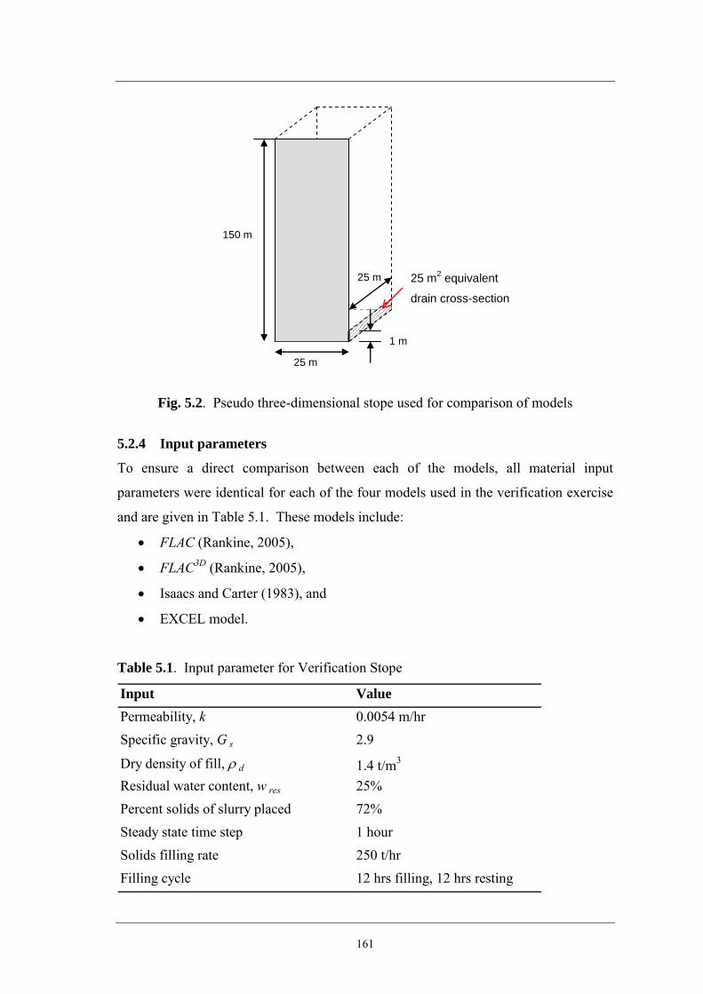
161
Fig. 5.2. Pseudo three-dimensional stope used for comparison of models
5.2.4 Input parameters
To ensure a direct comparison between each of the models, all material input
parameters were identical for each of the four models used in the verification exercise
and are given in Table 5.1. These models include:
• FLAC (Rankine, 2005),
• FLAC3D (Rankine, 2005),
• Isaacs and Carter (1983), and
• EXCEL model.
Table 5.1. Input parameter for Verification Stope
Input ValuePermeability, k 0.0054 m/hrSpecific gravity, G s 2.9
Dry density of fill, ρ d 1.4 t/m3
Residual water content, w res 25%Percent solids of slurry placed 72%Steady state time step 1 hourSolids filling rate 250 t/hrFilling cycle 12 hrs filling, 12 hrs resting
25 m
150 m
1 m
25 m 25 m2 equivalent
drain cross-section

162
5.2.5 Simulation of filling schedule within stope
The filling schedule of the verification stope involved 12 hours of filling followed by
12 hours resting. The spreadsheet was cycled continuously until the fill height reached
the height of the stope. To simulate this process in EXCEL, calculations were carried
out at hourly intervals and the results were used to determine input conditions for the
subsequent hour.
The fill height at each stage of solution was based on the quantity of dry tailings that
had been placed into the stope at that given time. During filling, the fill slurry entered
the stope and the fill height gradually increased by a height equal to the volume of dry
hydraulic fill which would enter the stope for the input filling rate divided by the
cross-sectional area of the stope. The volume of water in the stope was determined as
the total volume of water that had entered the stope minus the total volume that had
exited the stope, and provided the volume of voids within the fill matrix was larger
than the volume of the water in the stope, the water level fell below the height of the
fill. If the volume of water remaining in the stope was larger than the void volume,
then there was decant water above the fill. With due consideration to these cases and
the porosity of the fill, the water height was calculated for each hour. The quantity of
discharge over this hour was recorded and added to the total water discharge from the
stope for the calculation of water height for the next hour. Once the tailings reached
the height of the stope, the EXCEL model was solved as a continuously draining stope
with calculations continued every hour.
It is important to note that no discharge calculations are performed until the hydraulic
fill height passes the height of the drain i.e. in the very early stages of filling. Also, if
decant water is present at the end of filling, it is assumed that the decant water drains
from the top of the stope. i.e. the free water present as decant water is removed at the
top of the stope.
5.2.6 Fill and water heights
Fig. 5.3 illustrates the water and fill heights during the first 500 hours of the filling
schedule and the results compare very well for the verification exercise. As shown in

163
Fig 5.3, the results illustrate a ‘step-like’ pattern which represents the pouring and
resting of the hydraulic fill during the filling schedule. To amplify the difference
between the programs, Fig. 5.3 was magnified over a 24 hour period and is shown in
Fig. 5.4. Even when magnified, the comparison between all four models (EXCEL,
FLAC, FLAC3D and Isaacs and Carter) shows excellent agreement.
0
10
20
30
40
50
60
70
80
0 50 100 150 200 250 300 350 400 450 500
Time (hrs)
Hei
ght (
m)
FLAC - water heightFLAC - fill heightFLAC3D - water heightFLAC3D - fill heightIsaacs and Carter - water heightIsaacs and Carter - fill heightEXCEL - water heightEXCEL - fill height
rest
pour
Fig. 5.3. Fill and water height comparison between Isaacs and Carter, FLAC, FLAC3D,
EXCEL for the verification problem
Fig. 5.5 illustrates the discharge comparisons for the first 500 hours of filling and
resting of the verification stope. For the two-dimensional simulations (Isaacs and
Carter and FLAC), the drain is modeled by extending it to the full length of the stope
with sufficient height to give an equivalent cross-sectional area as the corresponding
three-dimensional models as shown in Fig. 5.2. Thus, with the drain area located
closer to the base and stretching the full depth of the stope, it is expected (and shown
in Fig. 5.5) that the two-dimensional simulations would produce slightly higher
discharge rates than the three-dimensional simulations.

164
8
10
12
14
16
60 65 70 75 80Time (hrs)
Hei
ght (
m)
FLAC - water heightFLAC - fill heightFLAC3D - water heightFLAC3D - fill heightIsaacs and Carter - water heightIsaacs and Carter - fill heightEXCEL - water heightEXCEL - fill height
Fig. 5.4. Magnified fill and water heights for a 24 hour period
0.0
0.5
1.0
1.5
2.0
2.5
3.0
0 100 200 300 400 500
Time (hrs)
Dis
char
ge (m
3 /hr)
Isaacs and CarterFLACFLAC 3DEXCEL
Fig. 5.5. Discharge rate comparison for between Isaacs and Carter, FLAC, FLAC3D and
EXCEL
rest pour

165
To magnify the difference in discharge, Fig. 5.6 illustrates the initial 100 hours of the
filling cycle.
0.0
0.2
0.4
0.6
0.8
1.0
0 10 20 30 40 50 60 70 80 90 100
Time (hrs)
Dis
char
ge (m
3 /hr)
Isaacs and CarterFLACFLAC 3DEXCEL
Fig. 5.6. Magnified discharge rate comparison for between Isaacs and Carter, FLAC,
FLAC3D and EXCEL
The discharge represents only a small proportion of the water in the stope; therefore
the slight differences shown in Fig 5.5 and Fig 5.6 have little effect on the maximum
pore water pressure measurements which are compared later in this chapter.
To investigate the effect of various filling schedules, numerous simulations of a three-
dimensional stope with randomly selected values of geometry, filling schedules and
geotechnical parameters were performed. Table 5.2 illustrates the inputs, for the range
of stopes investigated, whilst Table 5.3 summarizes the results.
As shown from these tables, there is minimal difference in the maximum pore water
pressure between the EXCEL and FLAC3D simulations. The discharge values are also
satisfactory, with a maximum variation of 8.2% between the two models.

166
Table 5.2. Input data for FLAC3D and EXCEL comparison
Hw B W X D F
Solids Filling Rate t/m3
No. of hrs pouring
No. of hrs resting
k (m/hr) Gsρd
t/m3 wres
% Solids of Slurry
1 40 16 16 4 6 6 240 8 16 5.40E-03 2.9 1.4 0.25 72
2 50 16 16 4 4 4 200 12 12 5.40E-03 3.5 1.7 0.25 75
3 40 20 20 4 4 4 240 12 12 5.40E-03 2.9 1.4 0.25 72
4 60 20 20 4 6 6 300 16 8 3.20E-03 4.3 1.7 0.25 70
5 40 16 16 4 6 6 240 12 12 5.40E-03 3.2 1.6 0.25 72
Case
Dimensions (m) Filling Cycle Input Parmaters
Table 5.3. Results for various simulations described in Table 5.2
Q (m3/hr) umax (kPa) Q (m3/hr) umax (kPa) Q umax
1 0.596 251.7 0.631 250.2 5.9 0.6
2 0.470 347.3 0.488 345.1 3.9 0.6
3 0.440 330.2 0.449 334.3 2.0 1.2
4 0.536 374.1 0.580 361.3 8.2 3.4
5 0.596 251.7 0.616 246.6 3.4 2.0
CaseFLAC 3D EXCEL % Difference
5.3 Sequential Filling and Draining for Hydraulic Fill Stope Calculations
The fill and water heights for a particular filling schedule were calculated using simple
phase relations, provided the material properties such as specific gravity, permeability,
porosity of a settled fill and slurry water content are given. The input data of the
EXCEL model can be broken down into three parts: dimensions, input parameters and
filling schedule.

167
The input dimensions of the three-dimensional stope investigated within the EXCEL
model are described below and are illustrated in Fig. 5.7.
• Height of stope, Hw, (m)
• Stope width, B, (m)
• Stope thickness, W, (m)
• Drain length, X, (m)
• Drain height, D, (m)
• Drain width, F, (m)
Fig. 5.7. Input dimensions of EXCEL model
From the geometry inputs, the EXCEL model calculates the stope base area (A), the
equivalent drain height (G) and the head loss within the stope (hL). These are given
by:
Stope base area, BWA ×=
B
Hw
W
D
F
X

168
Equivalent drain height, FDG ×=
Total head loss, GHh wL −= (assuming datum at top of drain)
The geotechnical input parameters of the stope include:
• Permeability, k, (m/s)
• Specific gravity, Gs
• Dry density, ρd, (t/m3)
• Residual moisture content, wres
• % Solids of slurry, Cslurry
From the input parameters given above, the following properties were calculated:
Hydraulic fill void ratio, n
ne−
=1
(5.1)
Hydraulic fill porosity, S
d
Gn
ρ−= 1 (5.2)
Saturation water content, s
sat Gew = (5.3)
When the stope has fully drained, with all the free water removed, the water content is
termed the residual water content (wres). The residual water is not removed in
engineering time and remains within the stope held within the voids. Previous
recorded values range from 20% - 30%, therefore a residual moisture content of 25%
was used for all models, unless otherwise specified.
The effective porosity (ne) represents the voids that are effectively available to conduct
water. The effective porosity can be written as:

169
ress
e we
Gnn+
−=1
(5.4)
The third section of input data is the filling cycle and includes the following inputs:
• Filling rate, Rs, (t/hr)
• Number of hours pouring, (hr)
• Number of hours resting, (hr)
Based on the input properties, geometry of the stope and the filling schedule the
steady-state analysis of the filling and draining of the three-dimensional stope can be
determined.
For a given stope arrangement,
Volume of fill, ff AHV = (5.5)
Volume of solids, )1( nAHV fs −= (5.6)
Mass of solids, wsfs GnAHm ρ)1( −= (5.7)
Water content of slurry, %100)1(
×−
=slurry
slurry
CC
w (5.8)
Mass of water entering the stope, wmm sw = (5.9)
Volume of water entering the stope, AnHC
CGnAHV w
slurry
slurrysfw =⎟
⎟⎠
⎞⎜⎜⎝
⎛ −−=
1)1( (5.10)
To analyze the filling and draining of the stope, the EXCEL model performs
calculations at hourly intervals, with each row in the spreadsheet assigned the values

170
for that specific hour. During the filling cycle, when the slurry is being poured into the
stope, the fill height will increase by a constant height of J per hour. During the
resting period fill height does not increase, but water height decreases due to the
drainage from the stope drain. Assuming a constant filling rate i.e. the mass of solids
poured per hour is Rs (t/hr)
The volume of solids poured per hour (Vs) is:
)1()/( 3 nAHG
RhrmV fws
ss −==
ρ (5.11)
Rearranging Eq. 5.11, we can calculate the fill height increase per hour (J) in meters
as:
)1()(
nAGR
mJws
s
−=
ρ (5.12)
To determine amount of water entering and leaving the stope, a water mass balance is
analyzed. Refer to Fig. 5.8.
Fig. 5.8. Water mass balance
Vin
Vfree Vresidual
Vdrained Vto-drain

171
where:
Vin = total volume of water in the stope,
Vfree = total free water that is drainable,
Vresidual = volume of residual water that remains within the stope and will not drain in
engineering time,
Vdrained = volume of water that has drained so far,
Vto-drain = volume of water that is yet to drain.
The volume of water entering the stope per hour can be calculated as:
slurrys
in wR
hrmVρ
=)/( 3 (5.13)
The volume of water exiting the stope through drainage is calculated using the
analytical solutions developed in Chapter 4 for a three-dimensional stope.
The volume of residual water is determined by:
residualsresidual wmV = (5.14)
where ms represents the total mass of solids in the stope at a specific time and wresidual
is the residual water content of the fill.
The volume of free water is calculated using:
draintodrainedfree VVV −+= (5.15)
At each time step, for example hourly intervals, calculations are undertaken with the
new fill and water heights. Fill heights change during filling, however remain the
same when in the resting part of the filling cycle. Water heights continually vary i.e.
during filling and resting, until all free water has been completely removed.

172
After entering all the required inputs, the EXCEL model automatically gives the user
the required time to fill the stope, the maximum pore water pressure and maximum
discharge. Plots of water height, tailings height, maximum pore water pressure
development and discharge during the filling cycle are also automatically given once
the required inputs are entered.
5.4 Sensitivity Analysis
Using EXCEL the variation and sensitivity in drainage behaviour and pore water
pressure measurements with the variation of the input properties can be determined.
Initially the variation in geometry was undertaken, followed by variation in soil
properties and finally the variation of filling schedule. This sensitivity analysis will
provide a broader understanding of the varying effects of geometry, filling schedule
and properties on discharge and pore water pressure developments within the stope.
5.4.1 Geometry
The geometry of the stope significantly affects the discharge and pore water pressure
developments. The analytical solutions developed in Chapter 4 for calculating
discharge and maximum pore water pressure are functions of the stope geometry and
permeability. However, when considering the entire filling and draining of a three-
dimensional stope other geotechnical properties including, specific gravity, residual
water content, percent solids etc also effect these measurements. This is due to the
properties affecting the amount of water and/or fill entering the stope. Using the
analytical solutions described in chapter 4, design charts were developed to investigate
the effect of varying geometries.
Typical geometric aspect ratios for a three dimensional stope were investigated and are
illustrated in Fig 5.9 and Fig 5.10. These included Hw/B ratios ranging from 0 to 5;
X/D ratios ranging from 0.5 to 2 and D/B ratios ranging from 0.2 to 0.3. The effect of
stope dimensions on discharge and maximum pore water pressure were studied in this
chapter and best presented by non-dimensionalizing the results such that the data may
be presented in the form of design charts. From these charts, a user is able to

173
determine the discharge rate and maximum pore pressure values for stopes scaled from
the ones used to develop the charts. The flow rate was represented by the
dimensionless parameter k(HW)2/Q which is equivalent to sum of the three-
dimensional form factors (ΣΓ), where k, Hw, Q and ΣΓ are the permeability, height of
water in the hydraulic fill stope, flow rate and sum of the three-dimensional form
factors respectively. The maximum pore water pressure (umax) for varying geometries
was represented by the parameterWwH
uγ
max , where γw is the unit weight of water which
equals 9.81 kN/m3 and Hw represents the height of water for the specified geometry.
As shown in Fig. 5.9, the geometry of a specified stope has significant influence on the
pore pressure distribution. The pore water pressure coefficient wwH
uγ
max lies in the
range of 0 – 1. For given stope and drain geometries and for a specific height of water,
the maximum pore water pressure can be estimated using Fig. 5.9.
1.0
1.5
2.0
2.5
3.0
3.5
4.0
4.5
5.0
0.0 0.2 0.4 0.6 0.8 1.0umax/γwHW
Hw
/B
D/B = 0.2 D/B = 0.2 D/B = 0.2D/B = 0.25 D/B = 0.25 D/B = 0.25D/B = 0.3 D/B = 0.3 D/B = 0.3
X/D = 0.5 X/D = 1 X/D = 2
Fig. 5.9. Sensitivity analysis for varying geometries versus maximum pore water
pressure

174
Fig. 5.9 also illustrates several other trends relating maximum pore pressure and
geometry. For example, increasing drain length and/or decreasing drain height (i.e.
increasing the X/D ratio) results in an increase in the maximum pore water pressure.
Also when X/D ≥ 1 the pore pressure increases with decreasing D/B ratios. However
in the case of X/D = 0.5, there is a slight increase in pore pressure with increasing D/B
ratios.
The variation of geometry with discharge is illustrated in Fig. 5.10.
0.0
0.5
1.0
1.5
2.0
2.5
3.0
3.5
4.0
4.5
5.0
0 10 20 30 40 50 60
khL2/Q
Hw/B
D/B = 0.2 D/B = 0.2 D/B = 0.2
D/B = 0.25 D/B = 0.25 D/B = 0.25
D/B = 0.3 D/B = 0.3 D/B = 0.3
X/D = 0.5 X/D = 1 X/D = 2
Fig. 5.10. Sensitivity analysis for varying geometries versus discharge
From this chart the following trends were observed.
• An increase in the X/D ratio results in an increase in the khL2/Q ratio.
• Increasing the drain length results in a reduction in drain discharge. This can
be intuitively explained because as the barricade gets further from the stope,
the flow path increases and the hydraulic gradient across the entire model
decreases, resulting in reduced flow velocity, hence discharge.
• As the drain gets larger for a specific geometry, the discharge increases, thus
reducing the khL2/Q ratio for a specified geometry.

175
• For increasing D/B ratios, there is a reduction in the khL2/Q ratio.
• Another trend also present in Fig. 5.10 shows that for increased X/D ratios,
there is a more prominent increase in variation of khL2/Q for the increased D/B
ratios. For instance when X/D is equal to 0.5, there is minimal variation for the
three curves of D/B ratios. However, when X/D is increased to 2, there is a
more distinct variation of khL2/Q ratios for the varying D/B ratios.
5.4.2 Geotechnical Properties
Using the EXCEL model, a sensitivity analysis of the geotechnical properties was
undertaken. These properties included permeability of the fill material, specific
gravity, dry density, residual moisture content and percent solids of slurry. Previous
laboratory testing carried out at James Cook University (Rankine et al. 2004) provided
a range of values for the majority of the properties investigated. Residual moisture
content has not been tested and previously published values are only estimates based
on experience. For each of the parameters investigated, a sample stope with the
dimensions shown in Fig. 5.11 was used. A filling schedule of 12 hours pour at 250
t/hr followed by 12 hours rest was assumed.
Fig 5.11. Dimensions of sample stope used in the geotechnical property sensitivity
analysis
25 m
100 m
25 m
5 m
5 m
5 m

176
5.4.2.1 Permeability
The effect of permeability on the discharge and pore water pressure developments
were investigated using previously published permeability values. Constant head and
falling head permeability testing conducted at James Cook University on over 25
hydraulic fill samples, recorded a range between 2 mm/hr and 35 mm/hr which was
used in the sensitivity analysis. For a given geometry, velocity is proportional to the
permeability, thus, it can be expected that the rate of discharge also would be
proportional to permeability. This is clearly evident in Fig 5.12 and Fig 5.13 below.
The effect of permeability values of 2 mm/hr, 10mm/hr, 20mm/hr, 30mm/hr and 36
mm/hr were investigated and results are summarised in Fig. 5.12 and Fig. 5.13.
0
2
4
6
8
10
12
14
0 200 400 600 800 1000
Time (hrs)
Dis
char
ge (m
3 /hr)
2mm/hr
6mm/hr
10mm/hr
15mm/hr
20mm/hr
30mm/hr
36mm/hr
Fig. 5.12. Permeability versus discharge
The discharge with time plot (Fig 5.12) illustrates a marked difference in the water
discharge rate from the stope for the typical range of fill permeability values. Velocity
is proportional to the permeability (Darcy’s law), thus, it can be expected that the rate
of discharge also would be proportional to the permeability. This is clearly evident in

177
Fig. 5.12. For all cases of permeability, the trend lines recorded for the discharge
measurements, did not produce a smooth parabolic shape. Between approximately 168
– 184 hrs, each of the trend-lines showed a significant variation, and a step-like
parabolic pattern was observed. This can be attributed to the analytical equations
developed in Chapter 4. When the water height is less than the stope width,
i.e. 1<B
H w , the equipotential surfaces are not horizontal and new equations (Eq. 4.13
to Eq. 4.15) were required to calculate the form factor for fragment 2 for the three-
dimensional stope.
However, the maximum pore pressure over time plot (Fig 5.13) shows little variation
in permeability sensitivity. Since discharge water represents only a small proportion
of the water placed into the stope, the relative influence the drainage rate has on the
water height may be very small, as shown in Fig 5.13 by the minimal variation in pore
pressure measurements between the ranges of permeability values.
0
100
200
300
400
500
600
700
0 100 200 300 400 500 600 700 800 900 1000
Time (hrs)
Max
imum
Por
e Pr
essu
re (k
Pa)
2mm/hr
6mm/hr
10mm/hr
15mm/hr
20mm/hr
30mm/hr
36mm/hr
Fig. 5.13. Permeability versus maximum pore pressure

178
5.4.2.2 Specific gravity and dry density
Chapter 2 details the linear relationship developed between the dry density of the
settled fill and the specific gravity of the hydraulic fill soil grains of previously tested
hydraulic fills. This relationship is given in Fig 2.7 for hydraulic fills from several
Australian and US mines. From the figure, it is shown that the dry density of the
hydraulic fill is directly proportional to the specific gravity and can be approximated
by:
Laboratory dry density (g/cm3) = 0.56 x Specific gravity (2.1)
Implying a void ratio of 0.786 and porosity of 44%. Therefore when analysing the
sensitivity of the specific gravity within the drainage analysis, the dry density was
approximated using Eq. 2.1 and a porosity of 44% was assumed for the settled
hydraulic fill.
Hydraulic fill slurry is generally pumped at specific solid contents (e.g. 75% solids by
weight). Therefore the quantity of water entering the stope is significantly influenced
by specific gravity of the fill material. As the specific gravity increases, so does the
quantity of water entering the stope for a specific slurry density. Fig 5.14 illustrates
the fill and water heights versus time for various specific gravities for the specified
stope at a specific solids content. From Fig 5.14 it can deduced that the water heights
and the drainage times during any particular filling schedule will vary significantly
with various specific gravities. In all three cases (Gs = 2.9 - 4.2) there was decant
water present throughout the filling operations for the first 100 hours analyzed in Fig.
5.14. The rise in decant height relative to fill height with time increases with specific
gravity. The maximum pore water pressure is dependent on the water height in the
stope, therefore during filling; the maximum pore pressure will also be affected. From
Fig 5.14, it is shown that the height of water is the greatest when the specific gravity is
the lowest, therefore producing the greatest maximum pore pressure. However at
higher specific gravities, the amount of decant water is greatest which can be of greater
concern in the drainage of hydraulic fill stopes.

179
0
4
8
12
16
0 20 40 60 80 100
Time (hrs)
Hei
ght (
m)
SG =2.9; Fill heightSG = 2.9; Water heightSG = 3.5; Fill heightSG = 3.5; Water heightSG = 4.2; Fill heightSG = 4.2; Water height
Decant Water
Fig. 5.14. Fill and water heights for varying specific gravity values at a constant solids
content
It is important to note that there is significant difference between the rates at which the
fill and water levels rise with the variation in specific gravity and therefore it is
meaningful to also analyze the results when the stope is filled to a certain height (i.e.
not at a certain time). For instance at an 8 m fill height, the decant water for the
various specific gravities of 2.9, 3.5 and 4.2 are 8.2 m, 9.4 m and 10.3 m respectively,
resulting in 0.2 m, 1.4 m and 2.3 m of decant water for the respective specific gravities
(as shown in Fig. 5.14).
Fig 5.15 illustrates the maximum pore water pressure versus specific gravity for the
first 500 hours of the filling cycle. As shown in the figure, for increasing specific
gravity there is a decrease in the maximum pore water pressure within the fill. This can
be expected since water height increases with decreasing specific gravity (see Fig.
5.14.). However, as noted previously, if the stope is analyzed at a certain height,

180
(rather than a certain time), the pore pressure would be greatest at higher specific
gravities.
0
100
200
300
400
500
0 100 200 300 400 500
Time (hrs)
Max
imum
Por
e Pr
essu
re (k
Pa)
SG = 2.9
SG = 3.5
SG = 4.2
Fig. 5.15. Maximum pore pressure versus specific gravity
Fig. 5.16 illustrates discharge versus time for the various specific gravities
investigated. Although the variation in discharge is minimal between the specific
gravities, it is clear that the lower the specific gravity, the greater the discharge. From
Fig. 5.14, we know that the lowest specific gravity produces the greatest fill and water
heights. Therefore, applying these heights to the analytical equations developed in
chapter 4 will result in increased discharge as shown in the figure.
5.4.2.3 Solids Content
For optimal economic advantage, stopes should be filled with a solids content that
maximizes solid waste disposal, minimizes the quantity of water requiring removal,
while still being sufficiently moist to meet rheological requirements. The tailings

181
0.0
0.2
0.4
0.6
0.8
1.0
1.2
1.4
0 100 200 300 400 500
Time (hrs)
Dis
char
ge (m
3 /hr)
SG = 2.9
SG = 3.5
SG = 4.2
Fig. 5.16. Discharge versus specific gravity
slurry is dewatered to minimize the quantity of water that will be placed underground
and must drain out of the fill during and after fill placement. However if the slurry is
pumped at too high a solids content, the mine runs the risk of additional costs and
schedule delays associated with blocked pipes. Each fill material has a specific
optimum solids content for which the slurry best meets the balance between
maximized solids disposal and minimized water added.
Tailings are supplied to the hydraulic fill plant at low density slurry. Hydrocyclones
are commonly used to dewater the slurry to between 45% solid by volume and 50%
solids by volume
Potvin et al. (2005) suggest a range of slurry densities that correspond to the common
range of specific gravities encountered in hydraulic fill and these are illustrated in Fig.
5.17.

182
60
64
68
72
76
80
84
2 2.5 3 3.5 4 4.5 5
Specific gravity of solids
Perc
ent s
olid
s by
wei
ght
Upper limit 50% solids by volumeTarget density 47.5% solids by volumeLower limit 45% solids by volume
Fig 5.17. Hydraulic fill Slurry density ranges (Potvin et al. 2005)
Fig 5.18 illustrates the details of the fill and water heights for the first 500 hours of the
filling schedule. As can be expected, as the percent solids content is increased, the
volume of tailings is also increased. For each of the percent solids contents
investigated, the mass of tailings entering the stope remained the same (250 t/hr)
however; the amount of water was decreased with increased percent solids. This
results in decreased water height in the stope with increased percent solids. To
magnify the effect, Fig 5.19 illustrates the fill and water heights over a 24 hour period
from 240 – 264 hours. As shown in the figure, at 70% and 72% solids content, the
decant water is present in the stope contains, however, for the 74% solids content,
there is minimal decant water and the tailings height and water height are roughly
equal over the selected time period.

183
0
10
20
30
40
50
60
70
80
0 100 200 300 400 500
Time (hrs)
Hei
ght (
m)
70% solids content - fill height70% solids content - water height72% solids content - fill height72% solids content - water height74% solids content - fill height74% solids content - water height
Fig. 5.18. Fill and water heights for varying solids content
32
34
36
38
40
42
240 248 256 264
Time (hrs)
Hei
ght (
m)
70% solids content - fill height70% solids content - water height72% solids content - fill height72% solids content - water height74% solids content - fill height74% solids content - water height
Fig. 5.19. Magnified fill and water heights for varying solids content

184
Fig. 5.20 and Fig. 5.21 illustrate the effect of solids content on discharge and pore
water pressure within the three-dimensional stope.
0
0.1
0.2
0.3
0.4
35 55 75 95
Time (hrs)
Dis
char
ge (m
3 /hr)
70% Solids content
72% Solids content
74% Solids content
Fig. 5.20. Discharge versus solids content
0
100
200
300
400
500
600
0 100 200 300 400 500
Time (hrs)
umax
(kPa
)
70% solids content
72% solids content
74% solids content
Fig. 5.21. Maximum pore water pressure versus solids content
185
Fig 5.20 illustrates the results for discharge versus time for the various percent solids
investigated for the initial 35 – 100 hours of filling. (A smaller time interval was
chosen for this figure, to magnify the effect of percent solids on discharge results).
The discharge rates between the various percent solids does not vary significantly,
however when magnified (as in Fig 5.20) it can be shown that with decreased percent
solids there is a slight increase in discharge. Fig 5.21 illustrates the maximum pore
pressure for the three solids contents investigated over the first 500 hours of the filling
schedule. As illustrated, there is a slight increase in maximum pore water pressure
with decreasing percent solids content, which would be a consequence of the increased
water heights for the decreased solids content.
From these figures (Fig 5.18 – Fig 5.21), it can be concluded that the lower solids
contents results in higher water levels, discharge rates and maximum pore pressures at
a specific time, simply because more water has entered the stope. For the 72% solids
content case, the results illustrated a slightly lower water level, lower discharge rate
and marginally lower maximum pore water pressures. The pronounced step like
pattern observed in all figures, is due to the fill and rest periods in the filling cycle.
5.4.2.4 Residual water content
Residual water content is the water content present within the stope, when the stope
has fully drained. The residual water content is not removed in engineering time and
remains within the stope held within the voids. When modeling the three-dimensional
stope, the EXCEL simulation only models the flow of drainable water and not all the
water that enters the stope.
Cowling et al. (1988) records the presence of residual moisture in a sample calculation.
In his calculation, for every 200 t of hydraulic fill placed in a stope, 90 t of water is
added, for a pulp density of 69% solids. During drainage only 40 t of water is
discharged from the stope for every 90 t that are input. The difference, 50 t, is retained
in the fill as residual moisture content, which is equivalent to 25 % residual moisture.
Due to the generally large dimensions in hydraulic fill stopes, there is significant
amount of immobile water that will not be drained in engineering times.

186
Using the EXCEL model, several simulations of a three-dimensional stope with
dimensions given in Fig 5.11, where analyzed with varying residual moisture contents.
As shown in the Fig. 5.22, the filling of the stope is not affected by the residual
moisture content, however the drainage time required to completely remove all the free
water from the stope is dependent upon this parameter. Once, the free water has been
removed, the adjacent works may commence - thus providing a very valuable tool to
assist with mine scheduling.
0
20
40
60
80
100
120
0 2000 4000 6000 8000 10000
Time (hrs)
Hei
ght (
m)
Fill height
20%
25%
35%
30%
water heights
Fig. 5.22. Water and fill heights during filling and draining of three-dimensional stope
with varying residual moisture contents
5.4.3 Filling Schedule
The EXCEL model was used to study the effect of varying filling schedules on the
discharge and pore pressure measurements. When the slurry is placed into
underground stopes, it is imperative that the stope be allowed to drain to remove the

187
transport water from the stope, reducing pore pressure build-up within the stope that
could lead to barricade failure. For a particular stope at any mine, there will be a rate
of fill placement and resting time for drainage, which should not be exceeded.
Cowling et al. (1988) proposed a filling schedule for underground stopes at Mount Isa
Mines. These guidelines were based on a filling rate of 300 t/hr at 72% + 2% solids
content with specific gravity of 2.9 and the stopes where characterized by tall sublevel
open stopes. Table 5.4 summarizes the suggested filling cycles.
Table 5.4 Suggested filling schedules (Cowling et al. 1988)
Stope plan area Pouring time Resting time
m2 (hrs) (hrs)
< 400 8 16
<1000 12 12
< 1600 16 8
> 1600 Unrestricted N/A
Fig 5.23 presents the fill and water heights for the various filling schedules suggested
by Cowling et al. (1988) for the 100 m high stope given in Fig. 5.9 and with properties
given in Table 5.2.
From the figure it is shown that provided the quantity of water discharged from the
stope represents only a small percentage of the overall water placed into the stope, the
filling schedule has little effect on discharge rates or pore pressures; it merely changes
the time in which these values are experienced.
5.4.4. Filling Rate
As can be expected, the filling rate will influence the rate at which the fill and water
levels raise, but have minimal effect on their heights relative to each other provided the
discharge quantity represents only a small proportion of the total water placed in the
stope. Also, the rate at which the stope is filled will have almost no influence on the

188
0
10
20
30
40
50
60
70
80
90
100
0 200 400 600 800 1000
Time (hrs)
Hei
ght (
m)
Water Ht: 16hr pour / 8 hr rest
Tailings Ht: 16 hr pour / 8 hr rest
Water Ht: 12 hr pour / 12 hr rest
Tailings Ht: 12 hour pour / 12 hour rest
Water Ht: 8 hr pour / 12 hr rest
Tailings Ht: 8 hr pour / 12 hr rest
Fig. 5.23. Fill and water heights during filling for various filling schedules
values of discharge and pore water pressure at any given height, it will only influence
the time in which these values are recorded (because the fill height increases more
rapidly with increased filling rate).
5.5. Two-dimensional versus Three-dimensional Stopes
The two-dimensional models and analytical solutions discussed in chapter 3 provide
valuable information in the understanding of hydraulic fill drainage in underground
stopes. However, due to the geometrical simplification in the two-dimensional
modeling, several shortfalls are present. These include:
• The distance between the drain exit and point of maximum pore water pressure
is smaller for a two-dimensional analysis than for an identical sized stope in
three-dimensions due to the geometrical simplification involved. Therefore,
the maximum pore pressure measurements will be lower for two-dimensional
analysis than it is for three-dimensional analysis, and hence the pore water
pressure is lower.

189
• When comparing the two and three-dimensional solutions, the two-dimensional
drain is modelled at the full depth of the stope with sufficient height to give an
equivalent cross-sectional area of the corresponding three-dimensional models.
Thus, with the drain area located more closely to the base and stretching the
full depth of the stope, the two-dimensional simulations produce higher
discharge rates than the three-dimensional simulations.
5.6. Summary and Conclusions
This chapter has developed, verified and implemented a three-dimensional model to
simulate the complete filling and draining of a hydraulic filled stope. The EXCEL
model is used to predict the fill and water levels, discharge rates and pore pressures
within a three-dimensional hydraulic fill stope as they are being filled and drained.
Using the model a sensitivity analysis on the drainage behavior and pore water
pressure measurements with the fill properties, geometries and typical filling schedules
of a three-dimensional hydraulic fill stope was undertaken.
To verify the EXCEL model, a hypothetical problem was designed and results from
EXCEL were verified against results obtained from the identical simulation done in the
existing two and three dimensional programs previously validated against in situ data.
The verification exercise was designed to compare the water and tailings levels, the
discharge during a specific filling schedule and the maximum pore water pressure
development within the three-dimensional stope and results showed excellent
agreement.
Using the EXCEL model a sensitivity analysis was undertaken for varying geometries,
geotechnical properties and filling schedules. Several trends were observed and are
briefly described below:
• As drain length increases and the drain cross-section area decreases, the
maximum pore water pressure increases.
• As the barricade gets further from the stope, the flow path increases and the
hydraulic gradient across the entire model decreases, resulting in reduced flow
velocity, hence discharge.

190
• An increase in drain length results in a reduction in drain discharge and a slight
decrease in the maximum pore pressure. Also, for increasing drain cross-
sectional area discharge increases and pore water pressure decreases.
• Permeability has a significant influence on discharge. However, shows little
variation in pore pressure measurements. For a given geometry, velocity is
proportional to permeability, thus it is expected and illustrated in this chapter
that the rate of discharge is also proportional to the permeability. Since the
discharge water represents only a small proportion of the water placed into the
stope, the relative influence the drainage has on the water height may be small,
thus resulting in minimal variation in the pore pressure measurements.
• Also, the solids content and specific gravity of the slurry will have a significant
influence on the relative fill and water heights with time, within the specified
stope and minimal variation in discharge measurements. With all other
parameters equal, the higher the specific gravity of the slurry, the greater the
quantity of water entering the stope for a specific slurry density. Also,
increasing the solids content decreases the excess water requiring removal
within the stope. However, it is important that stopes be filled with a solids
content that maximises the solids waste disposal, minimises the quantity of
water requiring removal, while still being sufficiently moist to meet
rheological requirements.
• The effect of residual moisture content was also investigated in the chapter.
Results indicate that the filling of the stope is not affected by the residual
moisture content, however the drainage time required to completely removing
all the free water from the stope is dependent upon this parameter.
• Using EXCEL, several filling schedules and filling rates were analysed.
Provided the quantity of water discharged from the stope represents only a
small percentage of the overall water placed into the stope, the filling schedule
and filling rate has little effect on the discharge rates or pore pressures, it
merely changes the time in which these values are experienced. Careful
attention should be directed towards these properties to prevent pore pressure
build-up within the stope that could lead to barricade failure.

191
CHAPTER 6
SUMMARY AND CONCLUSIONS
This chapter presents a summary of the research carried out in this dissertation,
conclusions and recommendations for future research.
6.1 Summary
The extraction and processing of most mineral ores, result in the generation of large
volumes of finer residue or tailings. The safe disposal of such material is of prime
environmental, safety and economical concern to the management of mining
operations. Recent barricade failures, resulting from poor drainage, have led to need
for an increased understanding of the pore pressure developments and flow rates
throughout the filling operation. This dissertation is considers the drainage
characteristics of hydraulic fill which is one of the most popular minefilling methods
used in Australia and worldwide.
Hydraulic fills produced from tailings, are man-made and can therefore much more
uniform in their characteristics than are most natural deposits. However, due to the
wide range of geological conditions and mineralogical compositions from which the
hydraulic fills may be sourced a wide range of specific gravity values for hydraulic
fills has been observed across Australia. To ensure good drainage, backfilling
operations typically ensure that the by-product (usually by hydrocyclones) has an
effective grain size (D10), no smaller than 10 μm. Commonly accepted industry rule-
of-thumb standard suggests that the permeability of the hydraulic fill should be no less
than 100 mm/hr but many Australian and worldwide mines that have operated
satisfactorily for years quote hydraulic fill permeability values substantially less than
this value. A review was presented on previous research conducted on the
characterization of hydraulic fills and barricade bricks. An overview of the current

192
practices and developments reported in the literature with regard to the placement of
hydraulic fill material in underground stopes was also undertaken. The review briefly
discusses some of the details with regard to the design and construction of the
barricades used to contain the hydraulic fill within the stope as it is being placed, the in
situ monitoring techniques that have been used on site to study pore pressure
developments and barricade loading, as well as some of the numerical and laboratory
modeling techniques that have been used in the past to predict drainage behavior
within hydraulic fill stopes.
In recent years, there has been an increasing trend to use numerical modeling as a
prediction tool in studying the drainage of hydraulic fill stopes. Although these
models provide valuable information, they are often time-consuming and require
specialist knowledge of the numerical package used to model the stope. Using a
parametric study carried out using the numerical packages FLAC and FLAC3D and the
method of fragments (Harr 1962, 1977), this dissertation presents analytical solutions
for studying the drainage of hydraulic fills in two and three-dimensional stopes.
Initially a two-dimensional hydraulic fill stope was analyzed. It was shown that the
flow region of the two-dimensional hydraulic fill stope can be divided into three
fragments, for which the form factors can be determined from the dimensions of the
stope and drain. The flow is vertical at heights above the stope width (B), and is
horizontal within the drain a short distance (0.5D) from the stope face. At the bottom
of the stope, up to a height of the stope width, flow is two-dimensional. Since the
bottom of the stope (fragment 2) does not conform to any of the fragments suggested
by Harr (1962), a new fragment was developed. The dimensionless form factor of the
new fragments was expressed as a function of the dimensions of the stope and drain.
Analytical solutions were proposed for determining the entry hydraulic gradient at the
top of the stope, flow rate and maximum pore water pressure that occurs at the bottom
corner of the stope. The model was verified through several numerical examples of
hydraulic fill stopes with randomly selected dimensions and was found to be in
excellent agreement.

193
Underground stope arrangements are very much three-dimensional in geometry and
although the two-dimensional solutions provide a valuable tool for drainage prediction,
the inherent approximations required, substantially reduce the value of the model when
dealing with complex three-dimensional stopes. Using FLAC3D and method of
fragments simple analytical solutions and design charts were developed to estimate the
maximum pore water pressure and discharge within three-dimensional hydraulic fill
stopes of varying geometries. Shape factors were developed to account for the
inherent individuality associated with stope and drain geometry and the influence of
scaling on discharge and pore water pressure measurements were also investigated.
The proposed solutions were validated using the finite difference program FLAC3D and
physical modeling of a scaled stope and results were found to be satisfactory.
Using the analytical solutions developed for flow through three-dimensional hydraulic
fill stopes, an EXCEL model was developed to accurately and efficiently model the
drainage behavior in three-dimensional stopes. The model simulates the complete
filling and draining of the stopes and was verified using previously validated two and
three-dimensional models and results showed excellent agreement. The model
incorporates the complete filling and draining of the stopes and enables the user inputs
such as filling schedule, varying stope geometries and geotechnical properties (e.g.
specific gravity, slurry solids content, residual water content, void ratio etc). The
variation and sensitivity of drainage behaviour and pore water pressure measurements
with the fill properties, filling schedules and geometries was undertaken using the
EXCEL model.
Catastrophic fill barricade failures in underground hydraulic fill mines in Australia and
overseas have resulted in significant economic loss and loss of lives. The increased
knowledge into the drainage behaviours of underground hydraulic fill stopes and the
improved tools for analysis presented in this dissertation should produce an increased
level of confidence in design of hydraulic fills, more efficient mining, increased cost
savings and safer mine filling practices.

194
6.2 Conclusions
Initially this thesis applied the method of fragments to two-dimensional hydraulic fill
stopes. The method, originally developed by Pavlovsky (1956) was used to divide the
flow region into three fragments, for which the form factors were determined from the
dimensions of the stope and the drain. Two simple expressions were developed for
determining the discharge through the drain and the maximum pore water pressure
within the stope. The proposed solutions were verified against solutions derived from
the finite difference software package FLAC and results were found to be in excellent
agreement. Later this method was applied to several other points within the two-
dimensional stope and equations of maximum pore water pressure developed for each
of the points considered. Using these analytical solutions, the use of ancillary drains
and anisotropy was investigated. From the analysis the following conclusions were
made:
• It was shown that ancillary drainage was effective in accelerating the
drainage process within a two-dimensional hydraulically filled stope.
Consequently, this accelerated drainage reduces the build-up of pore
pressure behind the barricades.
• The horizontal ancillary drain provided at the bottom of the drain
reduces the pore pressure at all points within the fill, with the reduction
being proportional to the length of the drain
• Preliminary laboratory testing was undertaken to determine the degree
of anisotropic permeability on several hydraulic fills. Using these
results in combination with previously published values, varying
degrees of anisotropic permeability was investigated using FLAC and
method of fragments. From the results, it is evident that the anisotropic
permeability has a significant effect on pore pressure development and
discharge within the stope. As the anisotropy in permeability is
increased there is a substantial reduction in pore pressure. Several
design charts were created to quantify the effect of varying anisotropic
ratios and geometries on pore pressure and discharge within the stope.

195
Using the method of fragment concepts and the three-dimensional finite difference
software FLAC3D simple analytical solutions and design charts were developed for
estimating the maximum pore water pressure and discharge within a three-dimensional
stope of varying geometry. The three-dimensional solutions were verified using the
finite difference software package FLAC3D and physical modeling of a scaled stope
and results were deemed acceptable. It was clear from several FLAC3D runs that the
flow within the upper region of the stope, approximately above a height of the stope
width (B), is one-dimensional and vertical. Similarly within the drain, at a distance
greater than half the drain height, the flow is one dimensional and horizontal. As was
the case for the two-dimensional stope. On the basis of this observation, the flow
domain was divided into three fragments, separated by equipotential surfaces and form
factors were developed for each fragment. Initially the solutions were developed for a
square based stope with a square drain outlet located centrally along the base of one of
the stope faces. Using the three-dimensional analytical solutions, the following
conclusions were drawn.
• Initially when the height of water is greater than the stope width the
location of the drain on the base of the stope wall and the shape of the
drain have little effect on the computed values of discharge and
maximum pore pressure. However during the filling and drainage of
the stope when the height of water is less than the stope width the
location and shape of the drain have a noticeable influence on discharge
and negligible effect on maximum pore water pressure.
• To take account of varying stope geometry, a shape factor was
developed for non-square stopes, which is simply a multiplication factor
on the flow rate and maximum pore water pressures computed
assuming a square base stope and square drain outlet.
• By considering the symmetry of drain arrangements, values of
discharge and maximum pressure can be computed for a wide variety of
multiple-drain arrangements.
• For a given plan area, as the height of saturated material is increased in
the model, the discharge increases. Also, as observed by previous

196
authors, as the position of the barricade progresses further from the
stope face, the rate of discharge decreases.
The final part of this thesis consisted of developing an accurate and efficient three-
dimensional model that can be used to simulate the complete filling and draining of a
hydraulic filled stope. Previous models were often time consuming and in most cases,
specialist knowledge of the corresponding software package is required. Therefore a
quicker and less complicated solution was desirable. The well-known and user friendly
package EXCEL was used to model the three-dimensional stope. The model is
capable of predicting the fill and water levels, discharge rates and pore pressures
within a three-dimensional hydraulic fill stope as they are being filled and drained.
Using the model a sensitivity analysis on the drainage behavior and pore water
pressure developments with fill properties, geometries and typical filling schedules of
a three-dimensional hydraulic fill stope was undertaken.
To verify the EXCEL model, a hypothetical problem was designed and results from
EXCEL were verified against results obtained from the identical simulation done in the
existing two and three dimensional programs that have been previously validated
against in situ data. The verification exercise was designed to compare the water and
tailings levels, the discharge during a specific filling schedule and the maximum pore
water pressure development within the three-dimensional stope and results showed
excellent agreement.
Using the EXCEL model a sensitivity analysis was undertaken for varying geometries,
geotechnical properties and filling schedules. Several trends were observed and are
briefly described below:
• As drain length increases and the drain cross-section area decreases, the
maximum pore water pressure increases.
• As the barricade gets further from the stope, the flow path increases and
the hydraulic gradient across the entire model decreases, resulting in
reduced flow velocity, hence discharge.

197
• An increase in drain length results in a reduction in drain discharge and
a slight decrease in the maximum pore pressure. Also, for increasing
drain cross-sectional area discharge increases and pore water pressure
decreases.
• Permeability has a significant influence on discharge however shows
little variation in pore pressure measurements. For a given geometry,
velocity is proportional to permeability, thus it is expected and
illustrated that the rate of discharge is also proportional to the
permeability. Since the discharge water represents only a small
proportion of the water placed into the stope, the relative influence the
drainage has on the water height may be small, thus resulting in
minimal variation in the pore pressure measurements.
• It was shown that the solids content and specific gravity of the slurry
will have a significant influence on the relative fill and water heights
with time, within the specified stope and minimal variation in discharge
measurements. With all other parameters equal, the higher the specific
gravity of the slurry, the greater the quantity of water entering the stope
for a specific slurry density. Also, increasing the solids content
decreases the excess water requiring removal within the stope.
However, it is important that stopes be filled with a solids content that
maximises the solids waste disposal, minimises the quantity of water
requiring removal, while still being sufficiently moist to meet
rheological requirements.
• The effect of residual moisture content was also investigated in the
chapter. Results indicate that the filling of the stope is not affected by
the residual moisture content, however the drainage time required to
completely remove all the free water from the stope is dependent upon
this parameter.
• Using the EXCEL model, several filling schedules and filling rates
were analysed. Provided the quantity of water discharged from the
stope represents only a small percentage of the overall water placed into
the stope, the filling schedule and filling rate has little effect on the

198
discharge rates or pore water pressures, it merely changes the time in
which these values are experienced. More attention should be directed
towards these properties to prevent pore pressure build-up within the
stope that could lead to barricade failure.
6.3 Recommendations for Future Research
Whilst there have been considerable advancements in understanding the drainage
performance of hydraulic fill, there are still many areas that are deserving of further
study. Recommendations for future research include:
• Only rectangular based and/or square based stopes were analyzed when
developing the shape factor coefficient. It is recommended that shape
factors be developed for more irregular shaped stopes.
• This thesis as assumed tight-filling in its analysis – it is recommended
that several design charts be developed for stopes which have not been
tight-filled.
• Extend the two-dimensional model described in chapter three to take
into account multiple level access drives (i.e. more than one drain) and
derive analytical solutions.
• The effects of cemented hydraulic fill be incorporated into the EXCEL
model. i.e. the variation of permeability with respect to cement content
and curing time would be investigated and applied to the EXCEL
model. Although preliminary testing was conducted, further
permeability testing on cemented hydraulic fills would be required to
obtain a better understanding on the effect of varying cement contents
on permeability; and the effect of curing on permeability.
• The effects of arching on the three-dimensional stope be investigated
and implemented into the spreadsheet. Studies are currently being
undertaken by a postgraduate student from James Cook University on
the effect of arching on hydraulic fill material.
• Modeling of the bearing capacity of hydraulic fill i.e. the value of
hydraulic fill as a working surface for underground personnel and
machinery.

199
• Further investigation into the effect of consolidation on fill masses.
Any attempt to incorporate coupling into the numerical model would
require a thorough understanding of the consolidation characteristics of
the hydraulic fills. Due to the rapid consolidation of the hydraulic fills
observed in the standard oedometer tests at James Cook University, it is
suggested that consolidation tests be carried out on much thicker
samples (e.g. in a 150 mm diameter compaction mould) which would
prolong the consolidation process, and enable determination of
coefficient of consolidation cv.
• The use of ancillary drainage in three-dimensional stopes. It was shown
that ancillary drainage in two-dimensional stopes was effective in
accelerating the drainage process within a hydraulically filled stopes,
consequently, reducing the build-up of pore pressure behind the
barricades. It is recommended that the use and placement of ancillary
drainage in three-dimensions be investigated to enable the most
effective and efficient drainage to be obtained. i.e. length and
placement of ancillary drains
• Further investigation is suggested into the potential of migration of
fines and the influence on the barricade drainage performance.
• It is recommended that the EXCEL model developed in this dissertation
be modified to take into account inhomogeneity in the fill.
• Although the EXCEL model was verified against previously validated
models, it is recommended that a direct comparison of in situ data be
used in validation.
• The EXCEL model developed only considers the behaviour in
hydraulic filled stopes. By understanding the behavior and
requirements of other fill types, EXCEL models could be developed for
each of the fill types and tied into the one spreadsheet.
It is anticipated that the EXCEL model developed in this dissertation will provide the
building block for additional features (such as the static and dynamic requirements) in

200
understanding the behavior of three-dimensional hydraulic filled stopes with varying
properties, geometries and filling schedules.

201
REFERENCES
Amer A.M., and Awad, A.A. (1974). “Permeability of cohesionless soils.” Journal
Geotechnical Engineering Division ASCE, 100(12), 1309-1216.
Aubertin, M., Li, L., Arnoldi, S., Simon, R., Belem, T., Bussiere, B. and
Benzaazoua, M. (2003). “Interaction between backfill and rockmass in narrow
stopes.” Soil & Rock America 2003, Cambridge, Massachusetts, AA Balkema,
Roterdam, 1157-1164.
Aubertin, M., Mbonimpa, M., Bussiere, B., and Chapius, R.P. (2003). “A model to
predict the water retention curve from basic geotechnical properties.” Canadian
Geotechnical Journal, 40(6), 1104 – 1122.
Azizi F. (2000). Applied Analysis in Geotechnics, E & FN Spon, Taylor and Francis
Group, New York, Chapter 13.
Barkley, E., (1927). “Stope filling at north Mount Lyell Mine.” The AusIMM
Proceedings, 66, 157-164.
Bear, J. (1972). Dynamics of fluids in porous media, Elsevier, New York, USA.
Black, A.B. (1941). “Pneumatic stowing of mill residues in underground stopes.”
Broken Hill South Limited, Proc. Australian Institute Mining Metallurgy, 123, 141-
154.
Barnes, G.E. (2000). Soil Mechanics – Principles and Practice, 2nd Edition,
MacMillan Press Ltd., London, 476.
Barrett, J.R. and Cowling, R. (1980). “Investigation of cemented fill stability in 1100
orebody, Mount Isa Mines, Ltd., Queensland, Australia.” Transactions, Institute of
Mining and Metallurgy, Section A, 89, A118-A128.
Barrett, J.R., Coulthard, M.A. and Dight, P.M. (1978). “Determination of fill
stability.” Mining with Backfill, Proceedings of 12th Canadian Rock Mechanics
Symposium, CIM, 19, Sudbury, Ontario, Canada.
Belem, T., Harvey, A., Simon, R., and Aubertin, M. (2004). “Measurement and
prediction of internal stresses in an underground opening during its filling with
cemented fill,” Proceedings of the 5th International Symposium on Ground Support,
Ground Support in Mining and Underground Construction, Perth, Western

202
Australia, 619-130.
Bloss, M.L. (1992). Prediction of cemented rock fill stability design procedures and
modelling techniques. PhD Thesis, Department of Mining and Metallurgical
Engineering, University of Queensland, Brisbane, Australia.
Bloss, M.L. and Chen, J. (1998). “Drainage research at Mount Isa Mines Limited
1992 – 1997.” Proceedings of the 6th International Symposium on Mining with
Backfill: Minefill ’98, Ed. M. Bloss, Brisbane, Australia, 111-116.
Brady, B.H.G. and Brown, E.T. (1985). Rock mechanics for underground mining,
George Allen and Unwin, London.
Brady, A.C. and Brown, J.A. (2002). “Hydraulic fill at Osborne mine.” Proceedings
of the 7th Underground Operators’ Conference, Townsville, Australia, 161-165.
Brandon T., Clough G., and Rahardjo P. (1991). “Fabrication of Silty Sand
Specimens for Large-and Small-Scale Tests” Geotechnical Testing Journal, ASTM,
14, 46-55.
Bridges, M.C. (2003). “A New Era of Fill-Retaining Barricades,” Digging Deeper,
AMC Consultants, October, www.amcconsultants.com.au , 2-5.
Budhu, M. (2000). Soil Mechanics and Foundations, John Wiley and sons Inc., New
York, USA, 557 pp.
Butterfield, R. (1999). Dimensional analysis for geotechnical Engineers,
Geotechnique, 49(3), 357-366.
Butterfield, R. (2000). Scale-Modelling of Fluid Flow in Geotechnial Centrifuges,
Soils and Foundations, Japanese Geotechnical Society, 40(6), 39-45.
Carman, P.C. (1938). “The determination of specific surface of powders.” J. Soc.
Chem. Ind. Trans., 57, 225 pp.
Carman, P.C. (1956). Flow of gases through porous media, Butterworths scientific
Publications, London, U.K.
Carrier III, D.W., Bromwell, L.G. and Somogyi, F. (1983). “Design capacity of
slurried mineral waste ponds.” Journal of Geotechnical Engineering, 109(5), 699-
716
Cedegren, H. R. (1989). Seepage, drainage and flownets, Wiley, 3rd Edition, New
York, USA.
Chapius, R.P. (2004). “Predicting the saturated hydraulic conductivity of sand and

203
gravel using effective diameter and void ratio.” Canadian Geotechnical Journal,
41(5), 787-795.
Chapius, R.P. and Aubertin M. (2003). “On the use of the Kozeny Carman equation
to predict the hydraulic conductivity of soils.” Canadian Geotechncial Journal,
40(3), 616-628.
Chapius, R.P., Gill D.E. and Bass K. (1989). Laboratory permeability tests on sand:
Influence of the compaction method on anisotropy.” Canadian Geotechnical Journal,
26(4), 614 -622,
Clarke, I.H. (1988). “The properties of hydraulically placed backfill.” Proceedings
of Backfill South African Mines, Johannesburg, SAIMM, 15-33.
Coduto D.P. (1999). Geotechnical engineering: Principles and practice, Prentice-
Hall, Upper Saddle River, N.J.
Corson, D.R., Dorman, R.K. and Sprute, R.H. (1981). “Improving the support
characteristics of hydraulic fill.” Application of Rock Mechanics to Cut and Fill
Mining, The Institute of Mining and Metallurgy, Eds. O. Stephansson and M.J.
Jones, 93-99.
Cowling, R. (1998). “Twenty-five Years of Mine Filling: Developments and
Directions.” Proceedings of Minefill ’98, Brisbane, 3-10.
Cowling, R., Grice, A.G. and Isaacs, L.T. (1988), “Simulation of hydraulic filling of
large underground mining excavations.” Proceedings of 6th International Conference
on Numerical Methods in Geomechanics, Innsbruck, Austria, 1869-1876.
Cowling R., Voboril A., Isaacs L.T., Meek J.L. and Beer G. (1989). “Computer
models for Improved fill performance.” Proceedings of Innovations in Mining
Backfill Technology, Balkema, Rotterdam, 165 – 174.
Darcy, H. (1856). Les fontaines publiques de la ville de Dijon. Victor Dalmont,
Paris, France.
Das, B.M. (2002). Principles of Geotechnical Engineering, 5th Edition, Brooks/Cole
– Thomsom Learning, USA. 578 pp.
Das, B.M. (1985). Advanced soil mechanics, Hemisphere Publishing, Corporation,
Singapore.
Das, B.M. (1997). Advanced soil mechanics, Taylor and Francis, Washington, D.C.
Douglas J.F., Gasiorek J.M. and Swaffield J.A. (2001). Fluid Mechanics 4th Edition,

204
Pearson, Essex, England.
Dorricott M.G., and Grice A.G. (2002). “Backfill – The environmentally Friendly
Tailings Disposal System.” Proceedings Green Processing 02, Australian Institute
of mining and metallurgy, 265-270.
Duffield, C., Gad, E., and Bamford, W. (2003). “Investigation into the structural
behaviour of mine brick barricades.” AusIMM Bulletin, Institute of Engineers,
March/ April, 45-50.
Franklin J.A. and Dusseault M.B. (1991). Rock Engineering Applications 1st Edition.
McGraw Hill Professional, New York, USA.
Freeze, R.A. and Cherry, J.A. (1979). Groundwater, Prentice-Hall, Englewoods
Cliffs, N.J.
Fourie, A.B., Hofmann, B.A., Mikula, R.J., Lord, E.R.F. and Robertson, P.K.
(2001). “Partially saturated tailings sand below the Phreatic surface.” Geotechnique,
51(7) 577 – 585.
Garett, W.S. and Campbell Pitt, L.T. (1961). “Design and Construction of
Underground Bulkheads and Water Barriers.” 7th CMMI Congress, SAIMM,
Johannesburg, 1285-1301
Grice, A.G. (1989). “Fill Research at Mount Isa Mines Limited.” Innovations in
Mining Backfill Technology, Balkema, Rotterdam, 15-22.
Grice, A.G. (1998 a). “Stability of hydraulic backfill barricades.” Proceedings of the
6th International Symposium on Mining with Backfill, AusIMM, Brisbane, Australia.
Grice, A.G. (1998 b). “Underground mining with backfill.” Proceedings of the 2nd
Annual Summit – Mine Tailings Disposal Systems, Brisbane, Australia.
Grice, T. (2001). “Recent minefill developments in Australia.” Proceedings of the
7th International Symposium on Mining with Backfill: Minefill ’01, Seattle, USA,
351-357.
Grice, A.G., Wilwain, A, and Urquhart, K. (1993). “Backfilling operations at Mount
Isa Mines 1998-1992.” Proceedings of the 5th International Symposium on Mining
with Backfill: Minefill ’93, Johannesburg, South Africa, 369-373.
Grice, A.G. and Fountain, L.J. (1991). “The fill information system.” Second
Australian Conference on Computer Applications in the Mineral Industry,
University of Wollongong, NSW, Australia.

205
Griffiths, D.V. (1984). “Rationalized charts for the method of fragments applied to
confined seepage.” Geotechnique., 34(2), 229 – 238.
Hall W.K. (2006). “Permeability Characteristics of Granular soils and hydraulic fill
Drainage Modeling,” B.E. Thesis, James Cook University.
Hansbo, S. (1960). “Consolidation of Clay with Special Reference to Influence of
Vertical Sand Drains,” Proceedings No. 14, Sweedish Geotechnical Institute.
Sweeden.
Hatanaka, M., Uchida, A., Taya, Y., Takehara, N., Hagisawa, T., Sakou, N. and
Ogawa, S. (2001). “Permeability characteristics of high-quality undisturbed gravely
soils measured in laboratory tests.” Soils and Foundations, 41(3), 45–55.
Harr, M.E. (1962). Ground Water and Seepage, McGraw Hill Book Company, New
York.
Harr, M.E. (1977). Mechanics of Particulate Media, McGraw Hill Book Company,
New York.
Hazen, A. (1892). “Some physical properties of sands and gravels, with special
reference to their use in filtration.” 24th Annual Rep., Massachusetts State Board of
Health, Pub. Doc. No. 34, 539 – 556.
Hazen, A. (1930). Water supply. American Civil Engineers Handbook, Wiley, New
York, USA.
Head, K.H. (1980-1996). Manual of Soil Laboratory Testing, John Wiley and Sons;
Vol. 1-3.
Herget, G. and De Korompay, V. (1988). “In situ drainage properties of hydraulic
backfills,” Proceedings of Mining with Backfill, Research and Innovations, CIM, 19,
117 – 123.
Hinde A.L. (1993). “Advances in Particle Sizing of Backfill.” Minefill 93, SAIMM
Johannesburg, 181 – 188.
Holtz, R.D. and Broms, B.B., (1972). “Long-Term Loading Tests at Ska-Edeby
Sweeden.” Proceedings of the ASCE Speciality Conference on Performance of Earth
and Earth-Supported Structures, Purdue University, Vol 1, Part 1, 435 – 444.
Holtz, R.D., and Kovacs, W.D. (1981). An introduction to geotechnical engineering,
Prentice-Hall, Englewood Cliffs, New Jersey, USA.
Hansbo, S. (1960). “Consolidation of Clay with Special Reference to Influence of

206
Vertical Sand Drains,” Proceedings No. 14, Sweedish Geotechnical Institute.
Isaacs, L. T., Carter, J. P. (1983). “Theoretical study of pore water pressures
developed in hydraulic fill in mine stopes,” Transactions of Institution of Mining
and Metallurgy (Section A: Mining Industry), 92, A93-A102.
Itasca, (2002). FLAC version 4.0 Users Manuals. Itasca Consulting Group, Thresher
Square East, 708 South Third Street, Suite 310, Minneapolis, Minnesota, 55415
USA.
Itasca, (2002). FLAC3D version 2.1 Users Manuals. Itasca Consulting Group,
Thresher Square East, 708 South Third Street, Suite 310, Minneapolis, Minnesota,
55415 USA.
Keren, L. and Kainain, S. (1983). “Influence of tailings particles on physical and
mechanical properties of fill.” Proceedings of the International Symposium on
Mining with Backfill, Eds. S Granholm, A.A. Balkema, Sweden, 21-29.
Karol, R.H., (1960). Soils and Soil Engineering. Prentice-Hall, Englewood Cliffs,
New Jersey, USA.
Kozeny, J. (1927). “Ueber kapillare Leitung des Wassers im Boden.” Wien, Akad.
Wiss., 136(2a), 271.
Kuganathan, K. (2001 a). “Design and Construction of Shotcrete Bulkheads with
Engineered Drainage System for Mine Backfilling.” International Seminar on
Surface Support Liners, Australian Centre for Geomechanics, Section 8, 1-15.
Kuganathan K. (2001 b). “Mine backfilling, backfill drainage and bulkhead
construction – A safety first approach.” Australia’s mining monthly, February, 58-
64.
Kuganathan, K. (2002). “A method to design efficient mine backfill drainage
systems to improve safety and stability of backfill bulkheads and fills.” Proceedings
of the 7th Underground Operators’ Conference, Townsville, Australia, 181-188.
Kupper A., Morgenstern N, Sego D., (1992). “Laboratory tests to study hydraulic
fill.” Canadian Geotechnical Journal, 29, 405-417.
Lambe, T.W. (1951). Soil Testing for Engineers, John Wiley and Sons, New York,
USA.
Lambe, T.W., and Whitman, R.V. (1969). Soil Mechanics, Wiley, New York, USA.
Lambe, T.W. and Whitman R.V. (1979). Soil Mechanics, SI Version, Series in Soil
207
Engineering, John Wiley and Sons, New York, USA.
Lamos, A.W. (1993). “An assessment of the effects of ultrafine aggregate
components on the properties of mine backfills.” Proceedings of the 5th
International Symposium on Mining with Backfill: Minefill ’01, Johannesburg, South
Africa, 173-179.
Leonards, G.A. (1962). Engineering properties of soils. Foundation engineering,
G.A. Leonards, ed., McGraw-Hill, New York, USA, 66 – 240.
Manoharan S., Pirahas B., Pirapakanara K. (2002). An experimental Study on the
effect of Cement Stabilization on the Permeability and Compressive strength of a
soil, not published.
Martin, D.M., (2001). Effective drainage of Hydraulic Mine Backfill, B Eng. Thesis,
Western Australian School of Mines, Kalgoorlie, Australia.
Mansur, C.I. and Dietrich, R.S. (1965). “Pumping tests to determine permeability
ratio.” Journal of Soil Mechanics and Foundations, ASCE, 91(SM4), 151-183.
Martys, N., Masad, E., and Muhunthan, B. (2000). “Simulation of fluid flow and
permeability in cohesionless soils.” Water Resources Research, 36(4), 851 – 864.
McKinstry, J.D. (1989). “Backfilling operations at Mount Isa Mines Limited.”
Proceedings of the fourth International Symposium on Mining with Backfill,
Montreal.
Mbonimpa, M., Aubertin, M., Chapius, R.P., Bussiere, B. (2002). “Practical
pedaotransfer functions for estimating the saturated hydraulic conductivity.”
Geotechnical and Geological Engineering, 20, 235 – 259.
Mishra, G.C., and A.K. Singh. (2005). “Seepage through a Levee.” International
Journal of Geomechanics., 5(1), 74-79.
Mitchell, J.K. (1976), Fundamentals of Soil Behavior, John Wiley and Sons, New
York, 422.
Mitchell, R.J. (1998). “The Eleventh Annual R.M. Hardy Keynote Address, 1997:
Centrifugation in Geoenvironmental Practice and Education.” Canadian
Geotechnical Journal, 35(4), 630-640.
Mitchell, R.J., Smith, J.D. and Libby, D.J. (1975). “Bulkhead Pressures Due to
Cemented Hydraulic Mine Backfills.” Canadian Geotechnical Journal, 12(3), 362-
371.

208
Murray, R.M. (1915). “Mining methods at Mount Lyell.” The AusIME Proceedings,
19, 125-139.
Murphy, G. (1950). Similitude in Engineering, Ronal Press Company, New York.
Nantel, J. (1998). “Recent Developments and Trends in Backfill Practices in
Canada.” Proceedings of AusIMM ’98 – The Mining Cycle, Mt Isa, Australia, 11 –
14.
NAVFAC. (1974). “Soil mechanics, foundations and earth structures.” Naval
Facilities Engineering Command (NAVFAC) design manual DM7. U.S.
Government Printing Office. Washington D.C.
Neindorf, L.B. (1983). “Fill Operating Practices at Mount Isa Mines.” Proceedings,
Symposium ‘Mining with Backfill, Lulea, Sweeden, 179 – 187.
Nicholson, D.E. and Wayment, W.R. (1964). “Properties of hydraulic backfills and
preliminary vibratory compaction tests.” United States Department of the Interior,
Bureau of Mines, 6477.
Nnadi, G.N. and Mitchell, R.J. (1991). “Use of centrifuge models to study simulated
blast loadings on backfills.” Canadian Institute of Mining and Metallurgy, Rock
Mechnaics Bulletin, 84(951), 58-63.
Ouellet, J. and Servant, S. (1998). “Numerical simulation of the drainage in a mining
stope filled with hydraulic backfill.” Proceedings of the 6th International Symposium
on Mining with Backfill: Minefill ’98, Ed. M. Bloss, Brisbane, Australia, 105-110.
Park R.T. and Gamble, W.L. (2000). Reinforced Concrete Slabs. 2nd Edition, John
Wiley and Sons, New York, USA.
Patton, F.E. (1957). Backfilling at Noranda. Mining in Canada, 6th Comm. Min.
and Met. Congr: Toronto, Canada, 229 – 236.
Pavlovsky, N. N. (1956). Collected Works, Akad. Nauk USSR, Leningrad.
Peele, J. (1941). Mining Engineers Handbook, John Wiley & Sons, Inc. Canada.
Pettibone, H.C. and Kealy, C.D. (1971). “Engineering properties of mine tailings.”
Journal of Soil Mechanics and Foundations Division, ASCE, 97(SM9), 1207-1225.
Potvin Y., Thomas E., and Fourie A., (2005) Handbook on Minefill, Australian
Centre for Geomechanics, Nedlands, Australia.
Qiu, Y. and Sego, D.C. (2001). “Laboratory properties of mine tailings.” Canadian
Geotechnical Journal, 38(1), 183-190.

209
Rankine, K. S. (2002). “Permeability and Drainage Characteristics of Hydraulic Fills
in Underground Mines” B Eng. Undergraduate thesis, Department of Civil and
Environmental Engineering, James Cook University, Townsville, Australia.
Rankine, K.J., Rankine, K.S., and Sivakugan, N. (2003). "Three-dimensional
drainage modelling of hydraulic fill mines," Proc. 12th Asian Regional Conf. on Soil
Mech. and Geotech. Engineering, Eds. CF Leung, KK Phoon, YK Chow, CI Teh
and KY Yong, Singapore, 937-940.
Rankine, K.J., Sivakugan, N. and Rankine, K.S. (2004). Laboratory tests for mine
fills and barricade bricks, Proceedings of 9th ANZ Conference on Geomechanics,
Auckland, Vol. 1, 218–224.
Rankine, K.J. (2005). An investigation into the drainage characteristics and
behaviour of hydraulically placed mine backfill and permeable minefill barricades.
PhD Thesis, Department of Civil and Environmental Engineering, James Cook
University, Townsville, Australia.
Rankine, K.J., Sivakugan, N. and Cowling, R. (2006). "Emplaced geotechnical
characteristics of hydraulic fills in a number of Australian mines," Geotechnical and
Geological Engineering, Springer, 24(1), 1-14.
Reddi, L.N. (2004). Seepage in Soils – Principles and applications, John Wiley and
Sons, Inc., Hoboken, New Jersey, 383.
Reedman J.H. (1979). Techniques in Mineral Exploration. Applied Science
Publishers, London, England.
Samarasinghe, A.M., Huang, Y.H. and Drnevich, V.P. (1982). “Permeability and
consolidation of normally consolidated soils.” Journal of the Geotechnical
Engineering Division, ASCE, 108(GT1), 55-60.
Scheideeger, A.E. (1953). Theoretical models of porous matter. Producers Monthly,
10(17), 17-23.
Scheideeger, A.E. (1954). “Statistical hydrodynamics in porous media.” Journal of
Applied Physics, 25, 994-1001.
Scheidegger, A. E. (1974). The physics of flow through porous media, University of
Toronto Press, Toronto, Canada.
Singh, S. (2007). Personal Communication
Singh, D.N. and Gupta, A.K. (2000). “Modelling hydraulic conductivity in a small

210
centrifuge.” Canadian Geotechnical Journal, 37(5), 1150-1155.
Sivakugan, N. and Al-Aghbari, M.Y.S. (1993 a). “An Optimization Study on
Seepage Beneath a Concrete Dam.” Proceedings of Structural Optimization '93,
The World Congress on Optimal Design of Structural Systems, Rio de Janeiro, 343-
350.
Sivakugan, N., and Al-Aghbari, M.Y.S. (1993 b). “Method of fragments – quick
solutions to seepage problems.” Environmental Management, Geo-Water &
Engineering Aspects, Balkema, 491-496.
Sivakugan, N., Rankine, K., and Rankine, R. (2006). "Permeability of hydraulic fills
and barricade bricks." Geotechnical and Geological Engineering, Springer, 24(3),
661-673.
Sivakugan, N., Rankine, K.J. and Rankine, K.S. (2006). "Study of drainage through
hydraulic fill stopes using method of fragments." Journal of Geotechnical and
Geological Engineering, Springer, 24(1), 79-89.
Sivakugan, N., and Rankine, K.S. (2006). “A simple solution for drainage through a
2-dimensional hydraulic fill stope,” Journal of Geotechnical and Geological
Engineering, Springer, 24(5), 1229-1241.
Sivakugan, N., Rankine, R.M., Rankine, K.J., and Rankine, K.S. (2006).
"Geotechnical considerations in mine backfilling in Australia," Journal of Cleaner
Production, Elsevier, 14, 1168-1175.
Sivakugan, N., Rankine, K.J., and Rankine, R.M. (2005). Geotechnical Aspects of
Hydraulic Filling of Underground Mine Stopes in Australia, Chapter 18, Ground
Improvements - Case Histories, Eds. B. Indraratna & J. Chu, Elseveir, Netherlands,
515-540.
Taylor, D.W. (1948). Fundamentals of soil mechanics, Wiley, New York, USA.
Terzaghi, K., and Peck, R.B. (1964). Soil mechanics in engineering practice, Wiley,
New York, USA.
Terzaghi, K., Peck, R.B., and Mesri, G. (1996). Soil mechanics in engineering
practice, Wiley, New York, USA.
Terzaghi, C. (1925). Determination of the permeability of clay. Engng News Rec. 95,
832-836, 510.
Thomas, E.G. (1969). Characteristics and Behaviour of Hydraulic Fill Material,

211
PhD Thesis, Department of Mining and Metallurgical Engineering of the University
of Queensland, Brisbane, Australia.
Thomas, E.G. (1978). “Fill permeability and its significance in mine fill practice.”
Mining with Backfill, 12th Canadian Rock Mechanics Symposium, Montreal,
CIMM.
Thomas, E.G., (1979). “Fill permeability and its significance in mine fill practice.”
Proc. Symp. Mining with Backfill, Sunbury, Canada.
Thomas, E.G. and Holtham, P.N. (1989). “The basics of preparation of deslimed
mill tailing hydraulic fill.” Innovations in Mining Backfill Technology, Ed. Hassani
et al., Rotterdam, Balkerna, 425-431.
Thomas, E.G., Nantel J.H. and Notley K.R. (1979). “Backfill technology in
underground metalliferous mines.” International Academic Services, Kinston,
Ontario, Canada.
Torlach, J. (2000) Potential hazards associated with minefill, Safety Bulletin 55,
Department of Minerals and Energy of Western Australia.
Traves, W.H. (1988). A three dimensional model of the drainage of back-filled open
stopes, Masters Thesis, Department of Civil Engineering, University of Queensland,
Brisbane, Australia.
Traves, W.H. and Isaacs, L.T. (1991). “Three-dimensional modelling of fill drainage
in mine stopes.” Transactions of the Institution of Mining and Metallurgy, Section A
(Mining Industry), The Institution of Mining and Metallurgy, A66-A71.
Tritton, D.J. (1988). Physical Fluid Dynamics 2nd Edition.
Udd, J.E. and Annor, A. (1993). “Backfill Research in Canada.” Proceedings of the
5th International Symposium on Mining with Backfill: Minefill ’93, SAIMM,
Johannesburg, South Africa, 361 – 368.
Uys, C.J. (1993). “The production of better backfill by the removal of ultrafine
material.” Proceedings of the 5th International Symposium on Mining with Backfill:
Minefill ’93, SAIMM, Johannesburg, South Africa, 159 – 167.
Vukovic, M., and Soro A. (1992). “Determination of hydraulic conductivity of
porous media from grain size composition.” Water Resources Publications,
Littleton, Colorado, USA.
Wallace, K. (1975). “A procedure for numerical analysis of transient moisture in

212
saturated and unsaturated earth structures.” Report, James Cook University,
Townsville, Qld.
Wayment, W.R. and Nicholson D.E. (1964). “A proposed modified percolation-rate
test for use in physical property testing of mine backfill” Rep. Invest. U.S. Bureau
Mines 6562, 24 p.
Wen, B., Aydin, A. and Duzgoren-Aydin, N.S. (2002). “A comparative study of
particle size analysis by sieve-hydrometer and laser diffraction methods.”
Geotechnical Testing Journal, ASTM, Dec, 25(4), 434-442.
Witt K.J., and Brauns J. (1983). “Permeability-anisotropy due to particle shape.”
Journal of Geotechnical Engineering, 109(9), 1181 -1187.
Hypertext References
www.civil.uwa.edu.au/teaching/MINE4162?f=130747
http://www.minerals.org.au/corporate
http://www.australianmineralsatlas.gov.au
Ore-age: a hybrid system for assisting and teaching mining method selection

213
APPENDIX A
Cemented hydraulic fill laboratory testing

214
A.1. Initial and Final Parameters for Copper Tailings A.2. Initial and Final parameters for Zinc Tailings
A.3. Grain Size Distribution Curves for Copper and Zinc Tailings tested in cemented hydraulic fill permeability testing
0
10
20
30
40
50
60
70
80
90
100
1 10 100 1000 10000
Grain Size (μm)
Perc
ent F
iner
Copper (HF)
Zinc (HF)
Copper (CHF)
Zinc (CHF)
CHF 1 CHF 2 CHF 3 CHF1 CHF 2 CHF 3 HFw Water Content 0.33 0.33 0.33 0.196 0.19 0.194 0.171G s Specific Gravity 3.69 3.69 3.69 3.69 3.69 3.69 3.69e Void Ratio 1.218 1.218 1.218 0.723 0.701 0.716 0.631n Porosity 0.55 0.55 0.55 0.42 0.41 0.42 0.39
ρ d Dry Density(t/m3) 1.85 1.85 1.85 2.14 2.17 2.15 2.26ρ m Bulk Density(t/m3) 2.45 2.45 2.45 2.56 2.58 2.57 2.65
Parameters Initial slurry Final (At 28 days)
CHF 1 CHF 2 CHF 3 CHF1 CHF 2 CHF 3 HFw Water Content 0.33 0.33 0.33 0.18 0.198 0.197 0.194
G s Specific Gravity 3.02 3.02 3.02 3.02 3.02 3.02 3.02e Void ratio 1.00 1.00 1.00 0.54 0.60 0.59 0.59n Porosity 0.50 0.50 0.50 0.35 0.37 0.37 0.37
ρ d Dry Density 1.51 1.51 1.51 1.96 1.89 1.89 1.90ρ m Bulk Density 2.01 2.01 2.01 2.31 2.26 2.27 2.27
Initial SlurryParameters Final (At 28 days)

215
A.4. Summary of Copper Permeability Results
days hours const.headfall.head const.headfall.head const.headfall.head const.headfall.head const.headfall.head const.headfall.head0.00 0 1.85E-04 1.98E-04 1.91E-04 6.67 7.14 6.880.04 1 1.71E-04 1.80E-04 1.93E-04 6.15 6.48 6.940.08 2 2.11E-04 1.89E-04 1.79E-04 7.58 6.80 6.450.13 3 2.06E-04 1.84E-04 2.24E-04 7.41 6.62 8.080.17 4 2.19E-04 1.79E-04 2.19E-04 7.89 6.44 7.890.21 5 1.93E-04 1.74E-04 1.77E-04 6.94 6.25 6.370.25 6 1.88E-04 1.66E-04 1.68E-04 6.75 5.99 6.060.29 7 1.81E-04 1.61E-04 1.63E-04 6.50 5.80 5.870.33 8 1.77E-04 1.54E-04 1.58E-04 6.37 5.55 5.680.38 9 1.68E-04 1.51E-04 1.50E-04 6.06 5.43 5.410.42 10 1.56E-04 1.51E-04 1.54E-04 5.62 5.43 5.550.46 11 1.54E-04 1.37E-04 1.40E-04 5.55 4.92 5.050.50 12 1.52E-04 1.28E-04 1.38E-04 5.49 4.61 4.980.54 13 1.47E-04 1.40E-04 1.33E-04 5.30 5.05 4.800.58 14 1.14E-04 1.38E-04 1.19E-04 4.10 4.98 4.290.63 15 9.81E-05 1.47E-04 1.16E-04 3.53 5.30 4.160.67 16 1.05E-04 1.24E-04 1.09E-04 3.79 4.48 3.910.71 17 1.21E-04 9.81E-05 1.07E-04 4.35 3.53 3.850.75 18 1.07E-04 9.81E-05 1.01E-04 3.85 3.53 3.650.79 19 7.94E-05 9.31E-05 7.62E-05 2.86 3.35 2.740.83 20 9.64E-05 9.11E-05 8.76E-05 3.47 3.28 3.150.88 21 9.64E-05 1.09E-04 8.76E-05 3.47 3.91 3.150.92 22 9.81E-05 8.41E-05 8.76E-05 3.53 3.03 3.150.96 23 8.59E-05 8.24E-05 8.59E-05 3.09 2.97 3.093.00 72 3.51E-05 2.98E-05 1.84E-05 1.26 1.07 0.667.00 168 9.64E-06 8.76E-06 1.68E-05 0.35 0.32 0.6014.00 336 1.13E-05 1.10E-05 5.52E-06 0.41 0.40 0.2028.00 672 3.92E-06 3.48E-06 6.08E-07 0.14 0.13 0.02
CHF2 CHF3Time Permeability (mm/hour)CHF1 CHF2 CHF3
Permeability (cm/s)CHF1
Permeability of (uncemented) hydraulic fill = 4.94E-04 cm/s = 17.79 mm/hr (approx)

216
A.5. Summary of Zinc Permeability Results
days hours const.head fall.head const.head fall.head const.head fall.head const.head fall.head const.head fall.head const.head fall.head0.00 0 3.38E-04 3.13E-04 3.63E-04 12.18 11.25 13.050.04 1 3.04E-04 3.07E-04 3.57E-04 10.96 11.06 12.860.08 2 3.06E-04 3.13E-04 3.58E-04 11.01 11.25 12.880.13 3 2.74E-04 3.04E-04 3.41E-04 9.85 10.93 12.280.17 4 2.79E-04 2.82E-04 2.82E-04 10.06 10.15 10.140.21 5 2.68E-04 2.69E-04 2.85E-04 9.64 9.69 10.270.25 6 2.31E-04 2.60E-04 2.76E-04 8.31 9.37 9.950.29 7 2.25E-04 2.53E-04 2.87E-04 8.10 9.11 10.340.33 8 2.10E-04 2.40E-04 2.63E-04 7.57 8.65 9.480.38 9 2.31E-04 2.35E-04 2.53E-04 8.32 8.46 9.110.42 10 2.08E-04 2.49E-04 2.72E-04 7.48 8.98 9.800.46 11 1.95E-04 2.15E-04 2.03E-04 7.03 7.74 7.300.50 12 2.01E-04 2.10E-04 2.23E-04 7.22 7.55 8.010.54 13 2.12E-04 2.06E-04 2.01E-04 7.62 7.42 7.240.58 14 1.99E-04 2.02E-04 2.14E-04 7.15 7.29 7.690.63 15 1.73E-04 1.97E-04 1.87E-04 6.22 7.09 6.720.67 16 1.61E-04 1.95E-04 1.71E-04 5.81 7.03 6.140.71 17 1.58E-04 1.92E-04 1.97E-04 5.67 6.90 7.110.75 18 1.39E-04 1.92E-04 1.97E-04 5.02 6.90 7.110.79 19 1.49E-04 1.90E-04 1.81E-04 5.35 6.83 6.530.83 20 1.62E-04 1.92E-04 1.79E-04 5.82 6.90 6.460.88 21 1.49E-04 1.83E-04 1.81E-04 5.35 6.57 6.530.92 22 1.49E-04 1.81E-04 1.78E-04 5.36 6.51 6.400.96 23 1.40E-04 1.79E-04 1.78E-04 5.02 6.44 6.403.00 72 9.57E-05 1.17E-04 1.53E-04 3.45 4.23 5.497.00 168 5.38E-05 7.22E-05 5.88E-05 1.94 2.60 2.12
14.00 336 8.47E-05 4.29E-05 3.80E-05 3.05 1.54 1.3728.00 672 3.07E-05 1.60E-05 1.78E-05 1.10 0.57 0.64
CHF2 CHF3Time CHF1 CHF2 CHF3 CHF1Permeability (cm/s) Permeability (mm/hour)
Permeability of (uncemented) hydraulic fill = 6.2582E-04 cm/s = 22.53 mm/hr (approx)

217
APPENDIX B
FLAC/FLAC3D Codes

218
B.1. Source listing FISH and FLAC code for program used to develop the two-
dimensional form factor
;Program for validating Method of fragments in two-dimenisonal stopes ; Kelda Rankine ; James Cook University config gw grid 26,60 ; Change set up i-col j-row model mohr prop dens=1800 bulk=1e8 shear=0.3e8 coh=0 ten=0 prop perm=2e-10 set gravity=9.81 set flow = on mech = off water dens=1000 bulk=2e9 gen 0,0 0,60 26,60 26,0 model null i=21,26 j=6,60 ; Change for stope dimensions apply pp=0 j=61 i=1,21 ; Change set pp top of stope fix sat j=61 i=1,21 ; Change sat at top of stope apply pp = 49.05e3 var 0 -49.05e3 i=53 j=1,6 ; Change set pp at drain exit fix sat i=27 j=1,6 ; Change sat at drain exit set datum = 6 ; Change datum plot hold model grid gn bou his gpp i=1 j=1 ; Change max pp history solve sratio = 1e-3 save kelflow.sav plot hold fix bou ; Plots results plot hold pp fill ; Calculating form factors for two-dimensional stopes restore kelflow.sav def formfac perm=2e-10 sumflow=0 loop j (1,6) ; Change height of drain

219
sumflow = sumflow + gflow(27,j) ; Change gridpoints height of drain end_loop formfactor = perm*9810*55/sumflow ; Change head loss for specified geometry end formfac print formfactor ;**************** def formfaccheck perm=2e-10 sumflow1=0 loop i (1,21) ; Change gridpoints widtth of stope sumflow1 = sumflow1 + gflow(i,61) ; Change gridpoints stope height end_loop formfactorcheck = perm*9810*55/sumflow1 ; Change head loss for specified geometry end formfaccheck print formfactorcheck ;**************** def porepressures ua=gpp(1,1) ; Maximum pore pressure end porepressures print ua

220
B.2. Source listing FISH and FLAC code for two-dimensional Anisotropic
Permeability Analysis
; Anisotropic Permeability Investigation ; Kelda Rankine ; James Cook University new ;SET UP MODEL config gw grid 42, 120 ; Change stope geometry model mohr ; SET UP PROPERTIES prop den=1500 shear=3e8 bulk=5e8 coh=5e5 tens=1e10 prop k11=3e-9 ;Change horizontal permeability prop k22=1e-9 ;Change vertical permeability model null i=41,42 j=3,120 plot hold model grid bou set gravity=9.81 flow=on mech=off ; Flow only problem water dens=1000 bulk=1e5 title VERIFICATION OF SPREADSHEET ;SET UP PORE PRESSURE AND SATURATION ALONG BOUDNARIES apply pp=0 j=121 i=1,41 ;Change set pp at top of stope apply pp=0 i=43 j=1,3 ;Change set pp at drain fix sat j=121 i=1,41 ;Change fix sat at top of stope fix sat i=43 j=1,3 ;Change fix sat at drain outlet plot hold fix bou set sratio 1e-3 step 140000 plot hold pp fill bou black ; TO COMPUTE FORM FACTOR AND FLOW def flowout

221
outflow=0 loop j (1,3) ;Change height of drain outflow=outflow+gflow(43,j) ;Change gp at drain outlet end_loop end def flowin inflow=0 loop i (1,81) ;Change gp at top of stope inflow = inflow + gflow(i, jgp) end_loop end flowout flowin hist gpp i=1 j=1 plot hist 1 print outflow inflow print gpp i=1 j=1 save anisoF3.sav

222
B.3. Source listing FISH and FLAC3D code for program used to develop three-
dimensional form factor
; Steady State Stope ; ; CASE 1 - Single drain, modelled in half symmetry ; Steady state simulations to develop design charts ; ; Kirralee Rankine modified by Kelda Rankine ; James Cook University ; ; *** Initial Input Parameters *** ; Specify Input Parameters Define inputparameters realfillperm=0.0054 ; m/hr fillperm=(realfillperm/(60*60))/9810 ; FLAC3D units for permeability fillspecgrav=2.9 ; Specific Gravity filldrydens=0.5*fillspecgrav ; Dry Density of Fill (t/m3) fillmoistcont=0.25 ; moisture content fillpor=1-(filldrydens/fillspecgrav) ; fill porosity fillvoidratio=fillpor/(1-fillpor) ; fill void ratio satmoistcont=fillvoidratio/fillspecgrav ; saturated moisture content of fill percentsolids=0.72 ; slurry percent solids filleffpor=fillpor-(fillmoistcont*fillspecgrav/(1+fillvoidratio)) ; effective porosity ; B=20 ; stope width (m) hb=B/2 ; half stope width for half symmetry x=4 ; drain length (m) dw=2 ; square drain width (m) hdw=dw/2 fullheight=100 ; ; use 1 m grid spacing throughout zonespace=1 xzones=x/zonespace dwzones=dw/zonespace hdwzones=hdw/zonespace bzones=b/zonespace hbzones=hb/zonespace fullzones=fullheight/zonespace ; ; number of nodes dwnodes=dwzones+1 hdwnodes=hdwzones+1 hbnodes=hbzones+1

223
bnodes=bzones+1 fullnodes=fullzones+1 ; ; boundaries xbound1=B+x+0.1 xbound2=B+x-0.1 xbound=B+x stpoint=(B-dw)/2 endpoint=stpoint+dw ppatbase=height*9.81*1000 ; end inputparameters ; run inputparamters ; ; FISH program to calculate discharge and store results in a table ; TABLE 1 => x=row number, y=water height ; TABLE 2 => x=row number, y=Discharge rate ; TABLE 3 => x=Hour number, y=Maximum Pore pressure ; define calculatedischarge cumflow=0 cumdischarge=0 xcord=xbound ; x co-ordinate for drain node loop ynode (1,hdwnodes) ycord=((ynode-1)*zonespace) ; y co-ordinate for drain node loop znode (1,dwnodes) zcord=(znode-1)*zonespace ; z co-ordinate for drain node thenode=gp_near(xcord,ycord,zcord) thenodeflow=gp_flow(thenode) cumflow=cumflow+(-1*(thenodeflow)) end_loop end_loop hrdischarge=cumflow*3600*2 ; half symmetry ; ; Find Position and Value for Maximum Pore Pressure maxpp = 0 xcount=Bzones+1 ycount=hbzones+1 heightcount=heightzones+1 loop zpos(1,heightcount) zz=((zpos-1)*zonespace) loop xpos (1,xcount) xx=(xpos-1)*zonespace loop ypos (1,ycount) yy=(ypos-1)*zonespace

224
pppoint=gp_near(xx,yy,zz) ppatpoint=gp_pp(pppoint) if ppatpoint > maxpp then maxpp = ppatpoint end_if end_loop end_loop end_loop ; table(1,heightfac)=Height table(2,heightfac)=hrdischarge table(3,heightfac)=maxpp ; end ; ; *** Model geometry *** ; Geomety config fl gen zone brick size Bzones,hBzones,fullzones p0 (0,0,0) p1 add (B,0,0) p2 add (0,hB,0) p3 add (0,0,fullheight) gen zone brick size xzones,hdwzones,dwzones p0 (B,0,0) p1 add (x,0,0) p2 add (0,hdw,0) p3 add (0,0,dw) ; ; define solveit ; loop heightfac (1,20) height=heightfac*B/2 Heightbound1=height+0.1 Heightbound2=height-0.1 ppatbase=1000*9.81*height Heightzones=height/zonespace Heightnodes=Heightzones+1 ; command title Case 1 - Single Drain with Half Symmetry ; group fill range z -0.1 heightbound1 model mohr range group fill model null range group fill not prop dens=1500 shear=3e8 bulk=5e8 coh=5e5 fric=0 tens=0 range group fill model fl_iso range group fill prop perm fillperm por fillpor range group fill set fl biot off

225
; ; --- Initial Conditions --- ini fmod 1e3 ini sat 1 range group fill ini pp ppatbase grad 0 0 -9.81e3 range group fill apply pp=0 range x xbound1 xbound2 y 0 hdw z 0 dw fix pp range x xbound1 xbound2 y 0 hdw z 0 dw apply pp=0.001 range z heightbound2 heightbound1 fix pp range z heightbound1 heightbound2 ; ; --- settings --- set grav 0 0 -9.81 ini fdensity 1e3 ini ftens 0.0 set mech off set fl on ; set fluid ratio 1e-5 solve calculatedischarge print hrdischarge maxpp height ; apply remove gp range x xbound2 xbound1 y 0 hdw z 0 dw apply remove gp range z heightbound1 heightbound2 save stopeA.sav end_command end_loop end solveit ; set logfile case stopeA set log on print table 1 print table 2 print table 3 set log

226
APPENDIX C
Validation plots for additional points on two-dimensional stope

227
C.1. Validation graphs for Point A and B on two dimensional stope
0
100
200
300
400
500
600
700
0 100 200 300 400 500 600 700
Max. pore pressure from FLAC (kPa)
Max
. por
e pr
essu
re fr
om M
OF
(kPa
)
Hw>B

228
C.2. Validation graphs for Point C on two-dimensional hydraulic fill stope
0
100
200
300
400
500
600
700
800
0 100 200 300 400 500 600 700 800
Max. pore pressure from FLAC (kPa)
Max
. por
e pr
essu
re fr
om M
OF
(kPa
)
Hw>B
Hw<B

229
C.3. Validation graph for Point D on two-dimensional hydraulic fill stope
0
100
200
300
400
500
600
700
0 100 200 300 400 500 600 700
Max. pore pressure from FLAC (kPa)
Max
. por
e pr
essu
re fr
om M
OF
(kPa
)
Hw>BHw<B

230
C.4. Validation graph for Point E and F on two-dimensional hydraulic fill stope
0
100
200
300
400
500
600
0 100 200 300 400 500 600
Max. pore pressure from FLAC (kPa)
Max
. por
e pr
essu
re fr
om M
OF
(kPa
)
Hw>BHw<B

231
APPENDIX D
Anisotropic Permeability Cell Testing Results

232
D.1. Permeability Cell Testing on Sample D3
Trial Flow Direction Run # Collection
TimeBeaker mass
Beaker + water Volume Head kavg kavg
(mins) (g) (g) (cm3) (cm) (cm/s) (mm/hr) mm/hr mm/hr1 3.00 200 481 281 56 0.00183 66.012 3.00 228 498 270 56 0.00176 63.433 4.00 200 552 352 56 0.00172 62.024 3.00 228 528 300 56 0.00196 70.48
1 3.00 228 498 270 71 0.00139 50.032 3.00 200 499 299 71 0.00154 55.403 3.00 200 467 267 71 0.00137 49.474 3.00 228 509 281 71 0.00145 52.07
1 3.00 228 563 335 85 0.00144 51.852 3.00 200 514 314 85 0.00135 48.603 3.00 228 577 349 85 0.00150 54.024 3.00 200 525 325 85 0.00140 50.30 51.19
1 3.00 200 495 295 55 0.00196 70.562 3.00 228 528 300 55 0.00199 71.763 3.00 228 552 324 55 0.00215 77.504 3.00 200 473 273 55 0.00181 65.30
1 3.00 228 590 362 65 0.00204 73.272 3.00 200 587 387 65 0.00218 78.333 4.20 228 734 506 65 0.00203 73.154 4.50 200 677 477 65 0.00179 64.36
kh/kv
71.7871.28
Head 1
Head 2
k
Horizontal
Head 3
Head 2 Vertical
65.48
51.74
56.14
1.28
72.28
Head 1

233
D.2. Permeability Cell Testing on Sample D4
Sample ID - D4 ~ Permeability Cell (Anisotropic permeability) Date 17/01/2006
Sample Height 14.8 cm Comments:Sample Length 15
Sample width 15 cmSample Area 225.00 cm2
Trial Flow Direction Run # Collection Time
Beaker mass
Beaker + water Volume Head kavg kavg
(mins) (g) (g) (cm3) (cm) (cm/s) (mm/hr) mm/hr mm/hr1 5.00 228 388 160 58 0.00060 21.772 5.00 200 359 159 58 0.00060 21.643 5.00 228 396 168 58 0.00064 22.861 5.00 228 496 268 87.5 0.00067 24.182 5.00 228 511 283 87.5 0.00071 25.533 3.00 228 393 165 87.5 0.00069 24.814 3.00 200 368 168 87.5 0.00070 25.261 3.00 228 371 143 55 0.00095 34.202 3.00 228 379 151 55 0.00100 36.123 3.00 228 370 142 55 0.00094 33.971 5.00 228 598 370 87.5 0.00093 33.382 5.00 200 568 368 87.5 0.00092 33.203 5.00 228 596 368 87.5 0.00092 33.20
k
Vertical
Horizontal
kh/kv
23.52
34.21
1.45524.94
22.09
35.16
33.26
Head 2
Head 1
Head 1
Head 2

234
D.3. Permeability Cell Testing on Sample A1
Sample ID - A1 ~ Permeability Cell (Anisotropic permeability) Date 24/01/2006
Sample Height 14.6 cm Comments:Sample Length 15
Sample width 15 cmSample Area 225.00 cm2
Trial Flow Direction Run # Collection
TimeBeaker mass
Beaker + water Volume Head kavg kavg
(mins) (g) (g) (cm3) (cm) (cm/s) (mm/hr) mm/hr mm/hr1 3.00 200 555 355 50 0.00256 92.14
Head 1 2 3.00 228 595 367 50 0.00265 95.263 3.00 200 568 368 50 0.00265 95.52 94.311 3.00 200 736 536 70 0.00276 99.37
Head 2 2 3.00 228 761 533 70 0.00274 98.823 3.00 200 672 472 70 0.00243 87.51 95.23 94.771 3.00 228 721 493 50 0.00355 127.96
Head 1 2 3.00 200 689 489 50 0.00353 126.923 3.00 200 674 474 50 0.00342 123.03 125.971 2.50 200 747 547 70 0.00338 121.69
Head 2 2 3.00 228 867 639 70 0.00329 118.473 3.00 228 835 607 70 0.00313 112.54 117.57 121.77
kh/kv
1.28
k
Vertical
Horizontal
235
APPENDIX E
Physical Modelling Results

236
E.1. Scaled Stope Analysis: Numerical / Laboratory / MOF3D results for scaled stope
Experimental FLAC3D
Γ1 (from eqn) Γ3 (from eqn) Γ2 (from eqn) ΣΓ Eqn αQfull size Eqn
(m3/hr)Qscaled Eqn
(m3/hr)Q (m3/hr) Q (m3/hr)
S11 20 20 5 4 16 6.58E-05 0.20 1.25 1.00 0.00 3.00 4.99 7.99 0.89 7.587 0.21 0.250 0.253S12 60 20 5 4 56 6.58E-05 0.20 1.25 3.00 5.60 10.50 14.98 31.08 0.89 23.902 0.66 0.773 0.482S13 100 20 5 4 96 6.58E-05 0.20 1.25 5.00 19.20 18.00 24.96 62.16 0.89 35.118 0.98 1.147 0.965S14 20 20 10 4 16 6.58E-05 0.20 2.5 1.00 0.00 8.00 4.99 12.99 0.89 4.667 0.13 0.103 0.152S15 60 20 10 4 56 6.58E-05 0.20 2.5 3.00 5.60 28.00 14.98 48.58 0.89 15.292 0.42 0.387 0.433S16 100 20 10 4 96 6.58E-05 0.20 2.5 5.00 19.20 48.00 24.96 92.16 0.89 23.687 0.66 0.657 0.658S17 20 20 14 4 16 6.58E-05 0.20 3.5 1.00 0.00 12.00 4.99 16.99 0.89 3.569 0.10 0.073 0.115S18 60 20 14 4 56 6.58E-05 0.20 3.5 3.00 5.60 42.00 14.98 62.58 0.89 11.871 0.33 0.263 0.338S19 100 20 14 4 96 6.58E-05 0.20 3.5 5.00 19.20 72.00 24.96 116.16 0.89 18.793 0.52 0.470 0.524S21 20 20 5 4 16 8.76E-05 0.20 1.25 1.00 0.00 3.00 4.99 7.99 0.89 10.100 0.28 0.357 0.337S22 60 20 5 4 56 8.76E-05 0.20 1.25 3.00 5.60 10.50 14.98 31.08 0.89 31.821 0.88 0.987 0.894S23 100 20 5 4 96 8.76E-05 0.20 1.25 5.00 19.20 18.00 24.96 62.16 0.89 46.753 1.30 1.453 1.285S24 20 20 10 4 16 8.76E-05 0.20 2.5 1.00 0.00 8.00 4.99 12.99 0.89 6.214 0.17 0.163 0.202S25 60 20 10 4 56 8.76E-05 0.20 2.5 3.00 5.60 28.00 14.98 48.58 0.89 20.358 0.57 0.527 0.744S26 100 20 10 4 96 8.76E-05 0.20 2.5 5.00 19.20 48.00 24.96 92.16 0.89 31.534 0.88 0.920 0.875S27 20 20 14 4 16 8.76E-05 0.20 3.5 1.00 0.00 12.00 4.99 16.99 0.89 4.751 0.13 0.177 0.153S28 60 20 14 4 56 8.76E-05 0.20 3.5 3.00 5.60 42.00 14.98 62.58 0.89 15.804 0.44 0.517 0.449S29 100 20 14 4 96 8.76E-05 0.20 3.5 5.00 19.20 72.00 24.96 116.16 0.89 25.019 0.69 0.780 0.698S31 20 20 5 4 16 0.00008 0.20 1.25 1.00 0.00 3.00 4.99 7.99 0.89 9.224 0.26 0.433 0.031S32 60 20 5 4 56 0.00008 0.20 1.25 3.00 5.60 10.50 14.98 31.08 0.89 29.061 0.81 0.883 0.816S33 100 20 5 4 96 0.00008 0.20 1.25 5.00 19.20 18.00 24.96 62.16 0.89 42.696 1.19 1.370 1.173S34 20 20 10 4 16 0.00008 0.20 2.5 1.00 0.00 8.00 4.99 12.99 0.89 5.674 0.16 0.143 0.185S35 60 20 10 4 56 0.00008 0.20 2.5 3.00 5.60 28.00 14.98 48.58 0.89 18.592 0.52 0.490 0.527S36 100 20 10 4 96 0.00008 0.20 2.5 5.00 19.20 48.00 24.96 92.16 0.89 28.799 0.80 0.783 0.799S37 20 20 14 4 16 0.00008 0.20 3.5 1.00 0.00 12.00 4.99 16.99 0.89 4.339 0.12 0.137 0.140S38 60 20 14 4 56 0.00008 0.20 3.5 3.00 5.60 42.00 14.98 62.58 0.89 14.432 0.40 0.380 0.410S39 100 20 14 4 96 0.00008 0.20 3.5 5.00 19.20 72.00 24.96 116.16 0.89 22.849 0.63 0.697 0.637
D/B X/D Hw/BMOF3D
D hL k (m/s)Case Hw B X
Related Documents