Random Walk Integrals - Borwein (2010)

8/3/2019 Random Walk Integrals - Borwein (2010)

http://slidepdf.com/reader/full/random-walk-integrals-borwein-2010 1/25

Random Walk IntegralsJonathan M. Borwein∗, Dirk Nuyens†, Armin Straub‡, and James Wan§

October 19, 2010

Abstract

We study the expected distance of a two-dimensional walk in the plane with unitsteps in random directions. A series evaluation and recursions are obtained, makingit possible to explicitly formulate this distance for small number of steps. Closed form

expressions for all the moments of a 2-step and a 3-step walk are given, and a formulais conjectured for the 4-step walk. Our interest is on closed forms and efficientlycomputable forms. Heavy use is made of the analytic continuation of the underlyingintegral.

1 Introduction, History and Preliminaries

We consider, for various values of s, the n-dimensional integral

W n(s) :=

� [0,1]n

nk=1

e2πxki

s

dx (1)

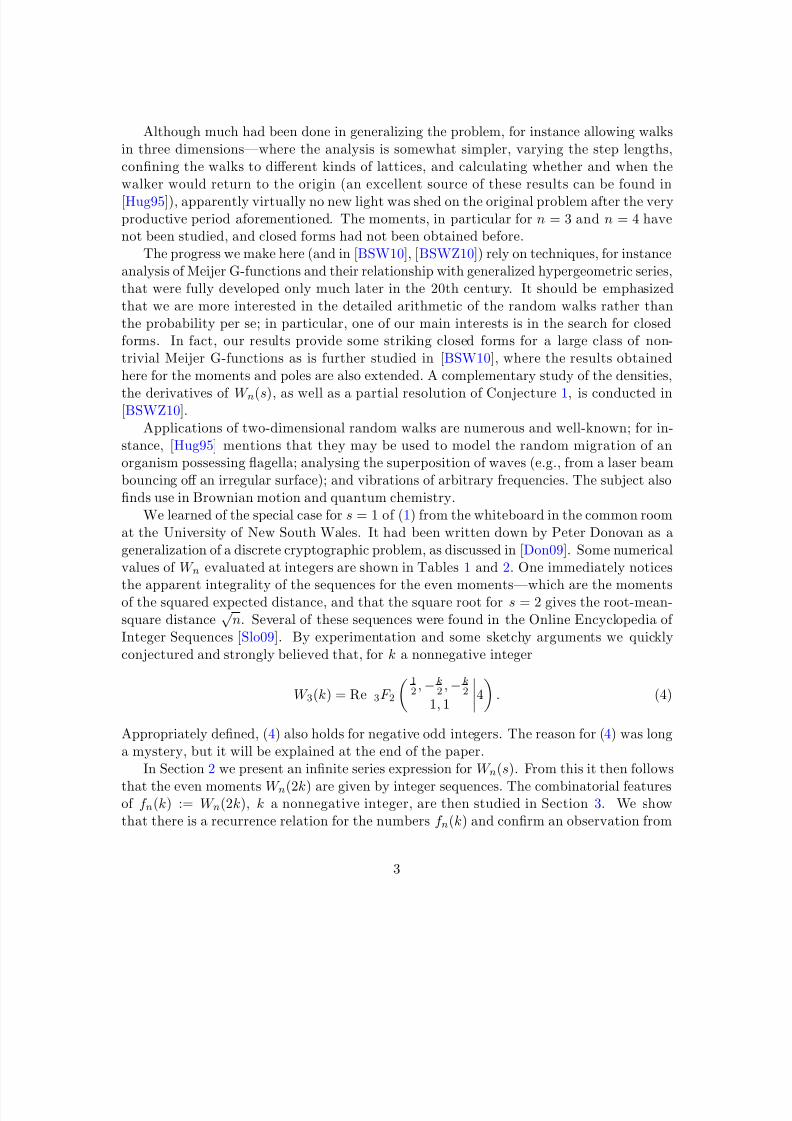
which occurs in the theory of uniform random walk integrals in the plane, where at each stepa unit-step is taken in a random direction, see Figure 1. As such, the integral (1) expressesthe s-th moment of the distance to the origin after n steps. Particularly interesting is thespecial case W n(1) of the expected distance after n steps.

A lot is known about the one-dimensional random walk. For instance, its expecteddistance after n unit-steps is (n − 1)!!/(n − 2)!! when n is even, and n!!/(n − 1)!! when nis odd. Here n!! is the double factorial. Asymptotically this distance behaves like

2n/π.

For the two-dimensional walk no such explicit expressions were known, though theexpected value for the root-mean-square distance is well-known to be just

√n; in this case

the implicit square root in (1) disappears which greatly simplifies the problem.

∗CARMA, University of Newcastle, Australia. Email: [email protected].†K.U.Leuven, Belgium. Email: [email protected]; part of this work done while a research

associate at the Department of Mathematics and Statistics, University of New South Wales, Australia.‡Tulane University, New Orleans, USA. Email: [email protected].§CARMA, University of Newcastle, Australia. Email: [email protected].

1



The term “random walk” first appears in a question by Karl Pearson in Nature in1905 [Pea1905]. He asked for the probability density of a two-dimensional random walkcouched in the language of how far a “rambler” (hill walker) might walk. This triggereda response by Lord Rayleigh [Ray1905] just one week later. Rayleigh replied that he had

considered the problem earlier in the context of the composition of vibrations of randomphases, and gave the probability distribution 2x

n e−x2/n for large n. This quickly leads to a

good approximation for W n(s) for large n and fixed s = 1, 2, 3, . . ..Another week later, Pearson again wrote in Nature, see [Pea1905b], to note that G. J.

Bennett had given a solution for the probability distribution for n = 3 which can be writtenin terms of the complete elliptic integral of the first kind K . This density function can bewritten as

p3(x) = Re

√x

π2K

(x + 1)3(3 − x)

16x

, (2)

see, e.g., [Hug95] and [Pea1906]. Pearson concluded that there was still great interest in

the case of small n which as he had noted is dramatically diff

erent from that of large n.It transpires that the solution of (2) is quite clumsy to work with; a much improvedhypergeometric solution is obtained in [BSWZ10]: for 0 � x � 4,

p3(x) =2√

3x

π (3 + x2)2F 1

1

3,

2

3; 1;

x2

9− x22

(3 + x2)3

. (3)

In further response to Pearson, Kluyver [Klu1906] made a lovely analysis of the cumu-lative distribution function of the distance traveled by a rambler in the plane for variouschoices of step length.

(a) Several 4-step walks (b) A 500-step walk

Figure 1: Random walks in the plane.

2



Although much had been done in generalizing the problem, for instance allowing walksin three dimensions—where the analysis is somewhat simpler, varying the step lengths,confining the walks to diff erent kinds of lattices, and calculating whether and when thewalker would return to the origin (an excellent source of these results can be found in

[Hug95]), apparently virtually no new light was shed on the original problem after the veryproductive period aforementioned. The moments, in particular for n = 3 and n = 4 havenot been studied, and closed forms had not been obtained before.

The progress we make here (and in [BSW10], [BSWZ10]) rely on techniques, for instanceanalysis of Meijer G-functions and their relationship with generalized hypergeometric series,that were fully developed only much later in the 20th century. It should be emphasizedthat we are more interested in the detailed arithmetic of the random walks rather thanthe probability per se; in particular, one of our main interests is in the search for closedforms. In fact, our results provide some striking closed forms for a large class of non-trivial Meijer G-functions as is further studied in [BSW10], where the results obtainedhere for the moments and poles are also extended. A complementary study of the densities,

the derivatives of W n(s), as well as a partial resolution of Conjecture 1, is conducted in[BSWZ10].

Applications of two-dimensional random walks are numerous and well-known; for in-stance, [Hug95] mentions that they may be used to model the random migration of anorganism possessing flagella; analysing the superposition of waves (e.g., from a laser beambouncing off an irregular surface); and vibrations of arbitrary frequencies. The subject alsofinds use in Brownian motion and quantum chemistry.

We learned of the special case for s = 1 of (1) from the whiteboard in the common roomat the University of New South Wales. It had been written down by Peter Donovan as ageneralization of a discrete cryptographic problem, as discussed in [Don09]. Some numericalvalues of W n evaluated at integers are shown in Tables 1 and 2. One immediately notices

the apparent integrality of the sequences for the even moments—which are the momentsof the squared expected distance, and that the square root for s = 2 gives the root-mean-square distance

√n. Several of these sequences were found in the Online Encyclopedia of

Integer Sequences [Slo09]. By experimentation and some sketchy arguments we quicklyconjectured and strongly believed that, for k a nonnegative integer

W 3(k) = Re 3F 2

12 ,−k

2 ,−k2

1, 1

4

. (4)

Appropriately defined, (4) also holds for negative odd integers. The reason for (4) was longa mystery, but it will be explained at the end of the paper.

In Section 2 we present an infinite series expression for W n(s). From this it then follows

that the even moments W n(2k) are given by integer sequences. The combinatorial featuresof f n(k) := W n(2k), k a nonnegative integer, are then studied in Section 3. We showthat there is a recurrence relation for the numbers f n(k) and confirm an observation from

3



n s = 2 s = 4 s = 6 s = 8 s = 10 [Slo09]

2 2 6 20 70 252 A000984

3 3 15 93 639 4653 A002893

4 4 28 256 2716 31504 A002895

5 5 45 545 7885 1279056 6 66 996 18306 384156

Table 1: W n(s) at even integers.

n s = 1 s = 3 s = 5 s = 7 s = 9

2 1.27324 3.39531 10.8650 37.2514 132.4493 1.57460 6.45168 36.7052 241.544 1714.624 1.79909 10.1207 82.6515 822.273 9169.625 2.00816 14.2896 152.316 2037.14 31393.16 2.19386 18.9133 248.759 4186.19 82718.9

Table 2: W n(s) at odd integers.

Table 1 that the last digit in the column for s = 10 is always n mod 10. The discovery of (4) was precipitated by the form of f 3 given in (10).

In Section 4 some analytic results are given, and the recursions for f n(k) are lifted toW n(s) by the use of Carlson’s theorem. The recursions for n = 2, 3, 4, 5 are given explicitlyas an example. These recursions then give further information regarding the pole structureof W n(s). Plots of the analytic continuation of W n(s) on the negative real axis are givenin Figure 2. From here we conjecture the recursion

W 2n(s)

?

= j0

s/2

j2

W 2n−1(s − 2 j).

In Section 6 we explore the underlying probability model more closely starting withwork of Kluyver [Klu1906]. This leads to an alternative tractable form for W 3(s) thateventually allows us to prove (4).

The ability to compute the moments (and the densities) accurately to reasonably highaccuracy was central to our work. This is not easy, and so some comments on obtaininghigh precision numerical evaluations of W n(s) are given in Appendix A.2. In fact, morethan 70 years after the problem was posed, [Merz79] remarks that for the densities of 4,5 and 6-steps walks, “it has remained difficult to obtain reliable values.” In [BSWZ10] aclosed hypergeometric form for the 4-step density is given, while in [BB10], a summary of

closed forms related to the walk integrals are given, as well as a more comprehensive studyof the numerics of such integrations.

4



�6

�4

�2 2

�3

�2

�1

1

2

3

4

(a) W 3

�6

�4

�2 2

�3

�2

�1

1

2

3

4

(b) W 4

�6 �4 �2 2

�3

�2

�1

1

2

3

4

(c) W 5

�6 �4 �2 2

�3

�2

�1

1

2

3

4

(d) W 6

Figure 2: Various W n and their analytic continuations.

2 A Series Evaluation of W n(s)

In this section a series evaluation of W n(s) is presented. For our purposes, its main interestlies in the fact that it specializes to an expression for W n(2k), k 0 an integer, as afinite sum. This sum and its combinatorics will be studied in Section 3. We thereforerestrict ourselves here to give a short formal proof of the series evaluation which ignoresany convergence issues; note that these don’t arise when s is an even integer. A morecomplete and elementary proof is given in Appendix A.1. Chronologically our first one, asa side-product it yields other interesting integral evaluations.

Theorem 1. For n = 1, 2, . . . and Re s 0 one has

W n(s) = nsm0

(−1)m

s/2

m

mk=0

(−1)k

n2k

m

k

a1+···+an=k

k

a1, . . . , an

2. (5)

Proof. In the spirit of the residue theorem of complex analysis, if f (x1, . . . , xn) has aLaurent expansion around the origin then

ct f (x1, . . . , xn) =

� [0,1]n

f (e2πix1 , . . . , e2πixn) dx (6)

5



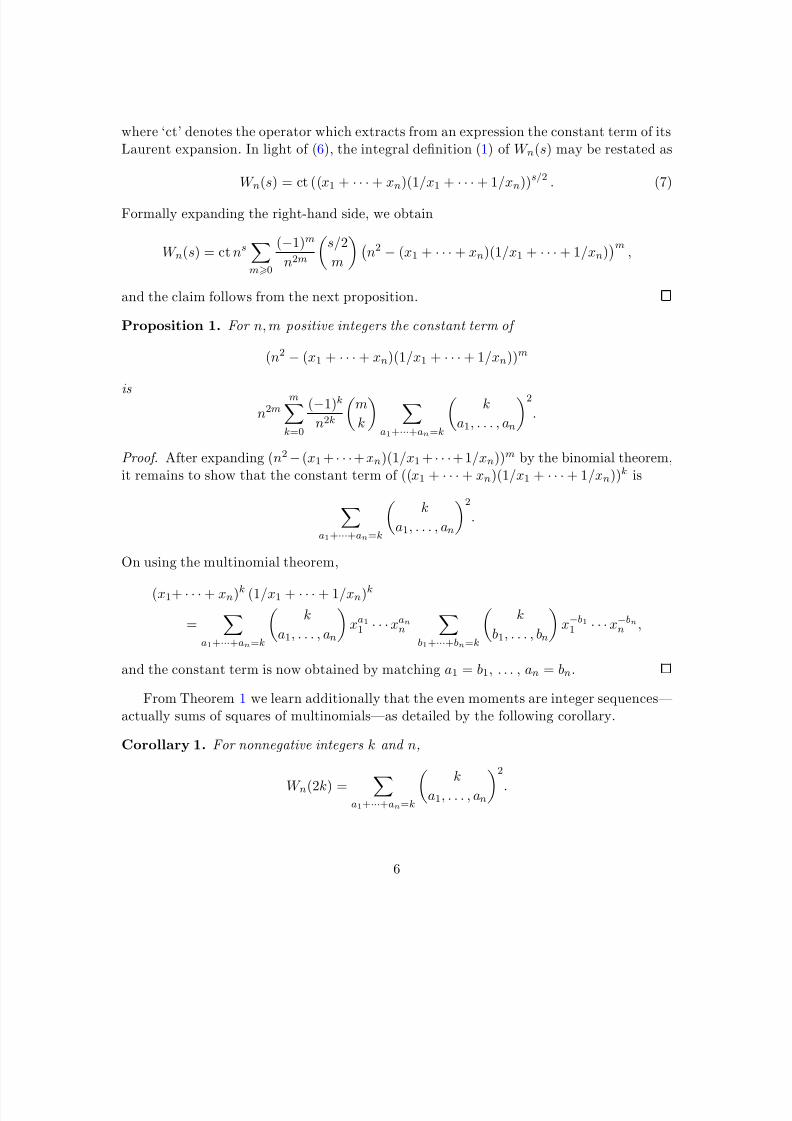
where ‘ct’ denotes the operator which extracts from an expression the constant term of itsLaurent expansion. In light of (6), the integral definition (1) of W n(s) may be restated as

W n(s) = ct ((x1 + · · · + xn)(1/x1 + · · · + 1/xn))s/2 . (7)

Formally expanding the right-hand side, we obtain

W n(s) = ct nsm0

(−1)m

n2m

s/2

m

n2 − (x1 + · · · + xn)(1/x1 + · · · + 1/xn)

m,

and the claim follows from the next proposition.

Proposition 1. For n, m positive integers the constant term of

(n2 − (x1 + · · · + xn)(1/x1 + · · · + 1/xn))m

isn2m

mk=0

(−1)k

n2k

m

k

a1+···+an=k

k

a1, . . . , an

2.

Proof. After expanding (n2−(x1 + · · ·+ xn)(1/x1 + · · ·+ 1/xn))m by the binomial theorem,it remains to show that the constant term of ((x1 + · · · + xn)(1/x1 + · · · + 1/xn))k is

a1+···+an=k

k

a1, . . . , an

2.

On using the multinomial theorem,

(x1+ · · · + xn)k (1/x1 + · · · + 1/xn)k

=

a1+···+an=k

k

a1, . . . , an

xa11 · · ·xan

n

b1+···+bn=k

k

b1, . . . , bn

x−b11 · · ·x−bnn ,

and the constant term is now obtained by matching a1 = b1, . . . , an = bn.

From Theorem 1 we learn additionally that the even moments are integer sequences—actually sums of squares of multinomials—as detailed by the following corollary.

Corollary 1. For nonnegative integers k and n,

W n(2k) =

a1+···+an=k

k

a1, . . . , an2

.

6



Proof. This follows easily from (7) since in that case the right-hand side can be finitelyexpanded.

Alternatively, the result is a consequence of Theorem 1 and the fact that the binomial transform , {bm}m0, of a sequence {ak}k0, where

bm :=mk=0

(−1)k

m

k

ak,

is an involution [CG96].

3 Combinatorial Features

In light of Corollary 1, we consider the combinatorial sums

f n(k) = a1+···+an=k k

a1, . . . , an2

. (8)

of multinomial coefficients squared. These numbers also appear in [RS09] in the followingway: f n(k) counts the number of abelian squares of length 2k over an alphabet with nletters (that is strings xx� of length 2k from an alphabet with n letters such that x� is apermutation of x). It is not hard to see that

f n1+n2(k) =k

j=0

k

j

2f n1( j) f n2(k − j), (9)

for two non-overlapping alphabets with n1 and n2 letters. In particular, we may use (9) toobtain f 1(k) = 1, f 2(k) = 2k

k, as well as

f 3(k) =k

j=0

k

j

22 j j

= 3F 2

12 ,−k,−k

1, 1

4

=

2k

k

3F 2

−k,−k,−k

1,−k + 12

14

, (10)

f 4(k) =k

j=0

k

j

22 j j

2(k − j)

k − j

=

2k

k

4F 3

12 ,−k,−k,−k

1, 1,−k + 12

1

. (11)

Here and below pF q notates the generalised hypergeometric function. In general, (9) canbe used to write f n as a sum with at most �n/2 − 1 summation indices.

We recall a generating function for (f n(k))∞k=0 used in [BBBG08]. Let I n(z) denote themodified Bessel function of the first kind. Then

k0

f n(k)zk

(k!)2=

k0

zk

(k!)2

n

= 0F 1(1; z)n = I 0(2√

z)n.

7



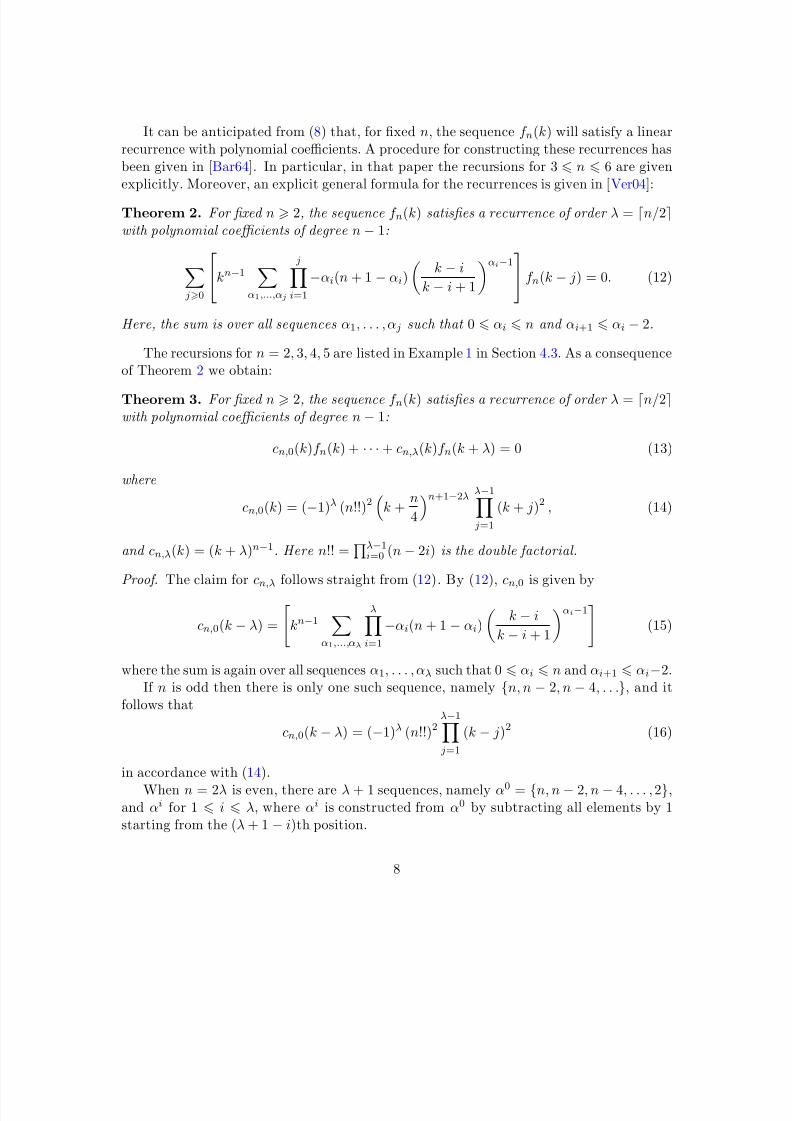
It can be anticipated from (8) that, for fixed n, the sequence f n(k) will satisfy a linearrecurrence with polynomial coefficients. A procedure for constructing these recurrences hasbeen given in [Bar64]. In particular, in that paper the recursions for 3 � n � 6 are givenexplicitly. Moreover, an explicit general formula for the recurrences is given in [Ver04]:

Theorem 2. For fixed n 2, the sequence f n(k) satisfies a recurrence of order λ = �n/2with polynomial coe ffi cients of degree n− 1:

j0

kn−1

α1,...,αj

ji=1

−αi(n + 1 − αi)

k − i

k − i + 1

αi−1 f n(k − j) = 0. (12)

Here, the sum is over all sequences α1, . . . ,α j such that 0 � αi � n and αi+1 � αi − 2.

The recursions for n = 2, 3, 4, 5 are listed in Example 1 in Section 4.3. As a consequenceof Theorem 2 we obtain:

Theorem 3. For fixed n 2, the sequence f n(k) satisfies a recurrence of order λ = �n/2with polynomial coe ffi cients of degree n− 1:

cn,0(k)f n(k) + · · · + cn,λ(k)f n(k + λ) = 0 (13)

where

cn,0(k) = (−1)λ (n!!)2

k +n

4

n+1−2λλ−1 j=1

(k + j)2 , (14)

and cn,λ(k) = (k + λ)n−1. Here n!! =λ−1i=0 (n− 2i) is the double factorial.

Proof. The claim for cn,λ follows straight from (12). By (12), cn,0 is given by

cn,0(k − λ) =

kn−1

α1,...,αλ

λi=1

−αi(n + 1 − αi)

k − i

k − i + 1

αi−1

(15)

where the sum is again over all sequences α1, . . . ,αλ such that 0 � αi � n and αi+1 � αi−2.If n is odd then there is only one such sequence, namely {n, n − 2, n − 4, . . .}, and it

follows that

cn,0(k − λ) = (−1)λ (n!!)2λ−1 j=1

(k − j)2 (16)

in accordance with (14).

When n = 2λ is even, there are λ + 1 sequences, namely α0 = {n, n− 2, n − 4, . . . , 2},and α

i for 1 � i � λ, where αi is constructed from α

0 by subtracting all elements by 1starting from the (λ + 1 − i)th position.

8



Now by (15), we have

cn,0(k − λ) = (−1)λλ−1

i=1

(k − i)2λ

j=0

λ

i=1

a ji (n + 1 − a ji ) (k − λ + j), (17)

where a ji denotes the ith element of a j.We make the key observation that the sum in (17) is symmetric, so writing it backwards

and adding that to itself, we factor out the term involving k:

2λ

j=0

λ

i=1

a ji (n + 1 − a ji )

(k − λ + j) = (2k − λ)

λ j=0

λi=1

a ji (n + 1 − a ji ). (18)

As we know the sequences a j explicitly, the product on the right of (18) simplifies to

(2λ)!2 j j2λ−2 jλ− j 2λ

λ

.

Hence the sum on the right of (18) is

λ j=0

(2λ)!

2 j j

2λ−2 jλ− j2λλ

= 22λλ!2, (19)

which can be verified, for instance, using the snake oil method ([Wil93]). Substituting thisinto (17) gives (14) for even n.

Remark 1. For fixed k, the map n

→f n(k) can be given by the evaluation of a polynomial

in n of degree k. This follows from

f n(k) =k

j=0

n

j

a1+···+aj=k

ai>0

k

a1, . . . , a j

2, (20)

because the right-hand side is a linear combination (with positive coefficients only depend-

ing on k) of the polynomialsn j

= n(n−1)···(n− j+1)

j! in n of degree j for j = 0, 1, . . . , k.

From (20) the coefficient of nk

is seen to be (k!)2. We therefore formally obtain the

first-order approximation W n(s) ≈n ns/2Γ(s/2+1) for n going to infinity, see also [Klu1906].

In particular, W n(1)

≈n√

nπ/2. Similarly, the coefficient of nk−1 isk−14 (k!)2 which gives

rise to the second-order approximation

(k!)2

n

k

+

k − 1

4(k!)2

n

k − 1

= k!nk − k(k − 1)

4k!nk−1 + O(nk−2)

9



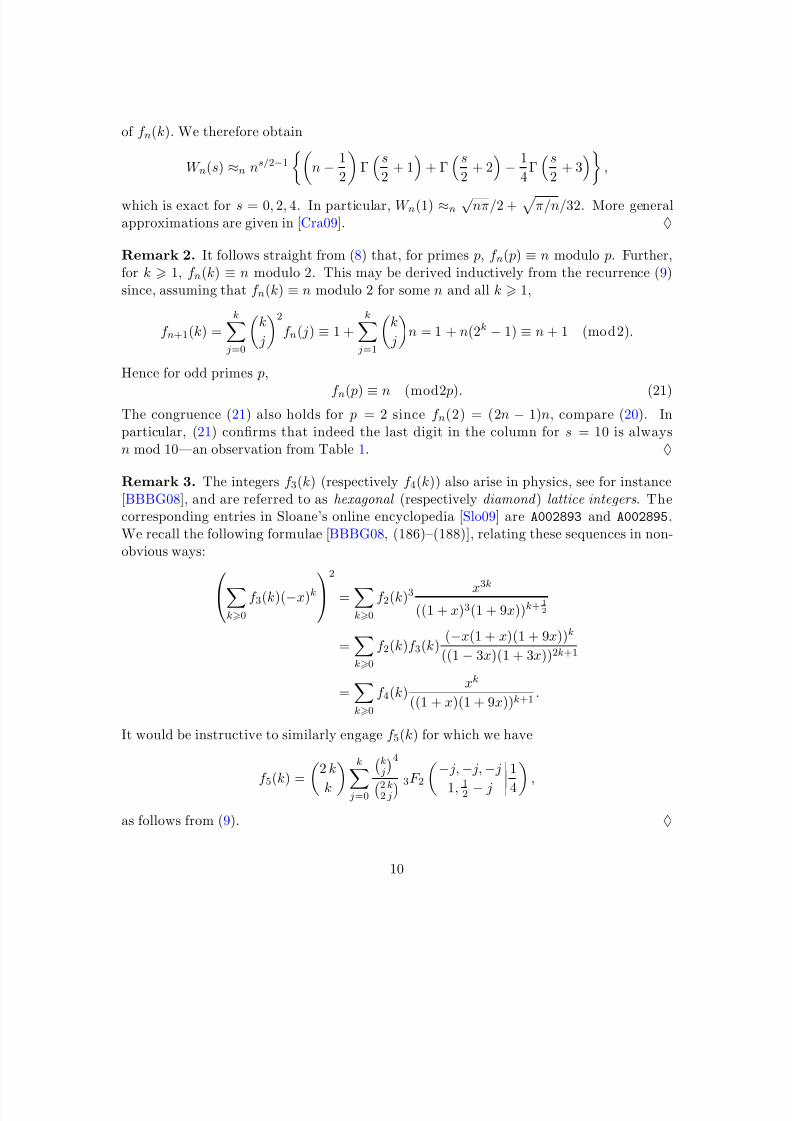
of f n(k). We therefore obtain

W n(s) ≈n ns/2−1

n− 1

2

Γ

s

2+ 1

+ Γ

s

2+ 2

− 1

4Γ

s

2+ 3

,

which is exact for s = 0, 2, 4. In particular, W n(1) ≈n √nπ/2 + π/n/32. More general

approximations are given in [Cra09]. ♦

Remark 2. It follows straight from (8) that, for primes p, f n( p) ≡ n modulo p. Further,for k 1, f n(k) ≡ n modulo 2. This may be derived inductively from the recurrence (9)since, assuming that f n(k) ≡ n modulo 2 for some n and all k 1,

f n+1(k) =

k j=0

k

j

2f n( j) ≡ 1 +

k j=1

k

j

n = 1 + n(2k − 1) ≡ n + 1 (mod2).

Hence for odd primes p,

f n( p) ≡ n (mod2 p). (21)The congruence (21) also holds for p = 2 since f n(2) = (2n − 1)n, compare (20). Inparticular, (21) confirms that indeed the last digit in the column for s = 10 is alwaysn mod 10—an observation from Table 1. ♦

Remark 3. The integers f 3(k) (respectively f 4(k)) also arise in physics, see for instance[BBBG08], and are referred to as hexagonal (respectively diamond ) lattice integers. Thecorresponding entries in Sloane’s online encyclopedia [Slo09] are A002893 and A002895.We recall the following formulae [BBBG08, (186)–(188)], relating these sequences in non-obvious ways:

k0

f 3(k)(−x)k

2

=k0

f 2(k)3 x3k

((1 + x)3(1 + 9x))k+1

2

=k0

f 2(k)f 3(k)(−x(1 + x)(1 + 9x))k

((1− 3x)(1 + 3x))2k+1

=k0

f 4(k)xk

((1 + x)(1 + 9x))k+1.

It would be instructive to similarly engage f 5(k) for which we have

f 5(k) =2 k

k

k

j=0k j

4

2k2 j3F 2−

j,

− j,

− j

1, 12 − j1

4

,

as follows from (9). ♦

10



4 Analytic Results

4.1 Analyticity

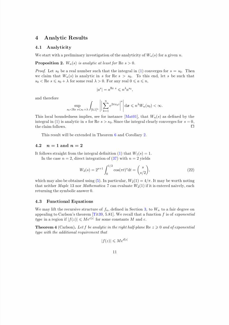
We start with a preliminary investigation of the analyticity of W n(s) for a given n.Proposition 2. W n(s) is analytic at least for Re s > 0.

Proof. Let s0 be a real number such that the integral in (1) converges for s = s0. Thenwe claim that W n(s) is analytic in s for Re s > s0. To this end, let s be such thats0 < Re s � s0 + λ for some real λ > 0. For any real 0 � a � n,

|as| = aRe s � nλas0 ,

and therefore

sups0<Re s�s0+λ

� [0,1]n

n

k=1

e2πxkis

dx � nλW n(s0) < ∞.

This local boundedness implies, see for instance [Mat01], that W n(s) as defined by theintegral in (1) is analytic in s for Re s > s0. Since the integral clearly converges for s = 0,the claim follows.

This result will be extended in Theorem 6 and Corollary 2.

4.2 n = 1 and n = 2

It follows straight from the integral definition (1) that W 1(s) = 1.In the case n = 2, direct integration of (37) with n = 2 yields

W 2(s) = 2s+1 � 1/2

0 cos(πt)s

dt = s

s/2

, (22)

which may also be obtained using (5). In particular, W 2(1) = 4/π. It may be worth notingthat neither Maple 13 nor Mathematica 7 can evaluate W 2(1) if it is entered naively, eachreturning the symbolic answer 0.

4.3 Functional Equations

We may lift the recursive structure of f n, defined in Section 3, to W n to a fair degree onappealing to Carlson’s theorem [Tit39, 5.81]. We recall that a function f is of exponential type in a region if |f (z)| � Mec|z| for some constants M and c.

Theorem 4 (Carlson). Let f be analytic in the right half-plane Re z 0 and of exponential type with the additional requirement that

|f (z)| � M ed|z|

11



for some d < π on the imaginary axis Re z = 0. If f (k) = 0 for k = 0, 1, 2, . . . then f (z) = 0 identically.

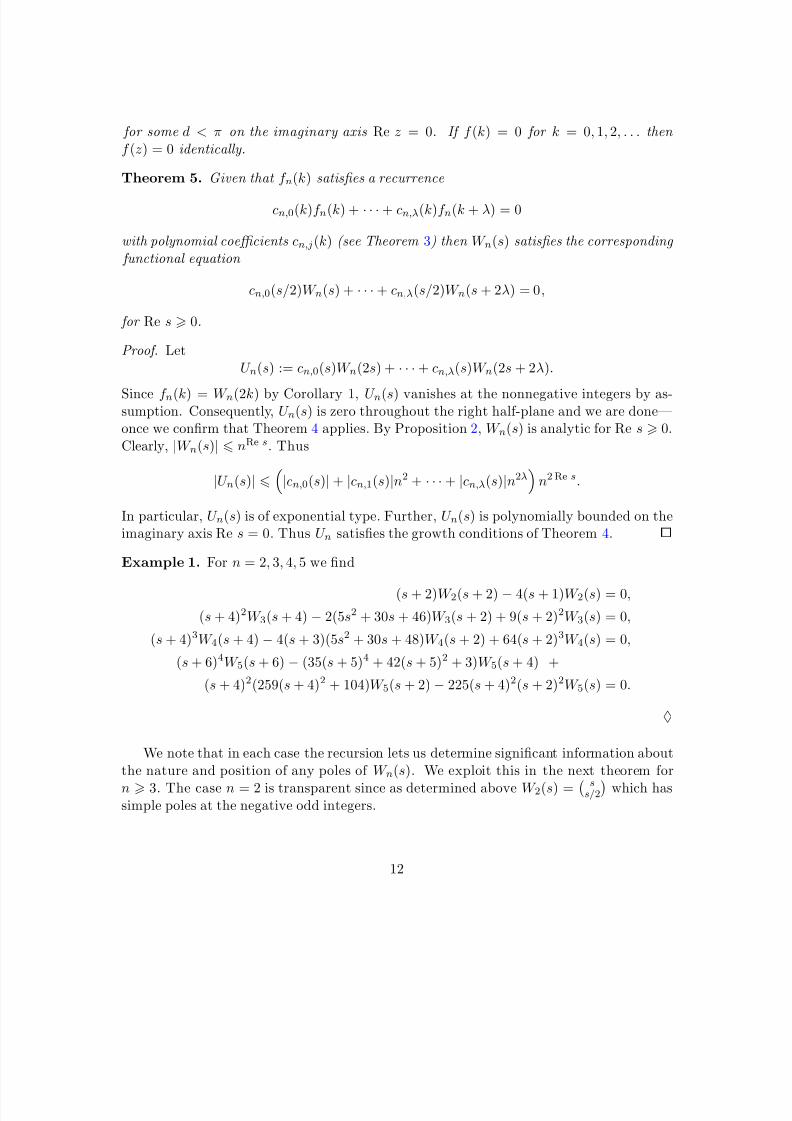
Theorem 5. Given that f n(k) satisfies a recurrence

cn,0(k)f n(k) + · · · + cn,λ(k)f n(k + λ) = 0

with polynomial coe ffi cients cn,j(k) (see Theorem 3) then W n(s) satisfies the corresponding functional equation

cn,0(s/2)W n(s) + · · · + cn,λ(s/2)W n(s + 2λ) = 0,

for Re s 0.

Proof. LetU n(s) := cn,0(s)W n(2s) + · · · + cn,λ(s)W n(2s + 2λ).

Since f n(k) = W n(2k) by Corollary 1, U n(s) vanishes at the nonnegative integers by as-sumption. Consequently, U n(s) is zero throughout the right half-plane and we are done—once we confirm that Theorem 4 applies. By Proposition 2, W n(s) is analytic for Re s 0.Clearly, |W n(s)| � nRe s. Thus

|U n(s)| �|cn,0(s)| + |cn,1(s)|n2 + · · · + |cn,λ(s)|n2λ

n2Re s.

In particular, U n(s) is of exponential type. Further, U n(s) is polynomially bounded on theimaginary axis Re s = 0. Thus U n satisfies the growth conditions of Theorem 4.

Example 1. For n = 2, 3, 4, 5 we find

(s + 2)W 2(s + 2) − 4(s + 1)W 2(s) = 0,

(s + 4)2W 3(s + 4) − 2(5s2 + 30s + 46)W 3(s + 2) + 9(s + 2)2W 3(s) = 0,

(s + 4)3W 4(s + 4) − 4(s + 3)(5s2 + 30s + 48)W 4(s + 2) + 64(s + 2)3W 4(s) = 0,

(s + 6)4W 5(s + 6) − (35(s + 5)4 + 42(s + 5)2 + 3)W 5(s + 4) +

(s + 4)2(259(s + 4)2 + 104)W 5(s + 2) − 225(s + 4)2(s + 2)2W 5(s) = 0.

♦

We note that in each case the recursion lets us determine significant information aboutthe nature and position of any poles of W n(s). We exploit this in the next theorem for

n 3. The case n = 2 is transparent since as determined above W 2(s) =

ss/2

which hassimple poles at the negative odd integers.

12



Theorem 6. Let an integer n 3 be given. The recursion guaranteed by Theorem 5provides an analytic continuation of W n(s) to all of the complex plane with poles of at most order two at certain negative integers.

Proof. Proposition 2 proves analyticity in the right halfplane. It is clear that the recursiongiven by Theorem 5 ensures an analytic continuation with poles only possible at negativeinteger values compatible with the recursion. Indeed, with λ = �n/2 we have

W n(s) = −cn,1(s/2)W n(s + 2) + · · · + cn,λ(s/2)W n(s + 2λ)

cn,0(s/2)(23)

with the cn,j as in (13). We observe that the right side of (23) only involves W n(s + 2k)for k 1. Therefore the least negative pole can only occur at a zero of cn,0(s/2) whichis explicitly given in (14). We then note that the recursion forces poles to be simple or of order two, and to be replicated as claimed.

Corollary 2. If n 3 then W n(s), as given by (1), is analytic for Re s > −2.

Proof. This follows directly from Theorem 6, the fact that cn,0(s/2) given in (14) has nozero for s = −1, and the proof of Proposition 2.

In Figure 2 the analytic continuations for each of W 3, W 4, W 5, and W 6 are plotted onthe real line.

Example 2. Using the recurrence given in Example 1 we find that W 3(s) has simple polesat s = −2,−4,−6, . . ., compare Figure 2(a). Moreover, the residue at s = −2 is given byRes−2(W 3) = 2√

3π, and all other residues of W 3 are rational multiples thereof. This may

be obtained from the integral representation given in (26) observing that, at s a negativeeven integer, the residue contributions are entirely from the first term. ♦

Example 3. Similarly, we find that W 4 has double poles at

−2,

−4,

−6, . . ., compare

Figure 2(b). With more work, it is also possible to show that

lims→−2

(s + 2)2 W 4(s) =3

2π2.

♦

Remark 4. More generally, it would appear that Theorem 6 can be extended to show that

• for n odd W n has simple poles at −2 p for p = 1, 2, 3 . . ., while

• for n even W n has simple poles at −2 p and 2(1 − p) − n/2 for p = 1, 2, 3 . . . whichwill overlap when 4|n.

This conjecture is further investigated in [BSW10]. ♦

We close this section by remarking that the knowledge about the poles of W n forinstance reveals the asymptotic behaviour of the densities pn at 0. This is detailed in[BSWZ10] where closed forms for the densities are investigated.

13



4.4 Convolution Series

Next, we tried to lift the convolution sum (9) to W n(s). Our conjecture is:

Conjecture 1. For positive integers n and complex s,

W 2n(s)?= j0

s/2

j

2W 2n−1(s − 2 j). (24)

It is understood that the right-hand side of (24) refers to the analytic continuation of W n as guaranteed by Theorem 6. Conjecture 1, which is consistent with the pole structuredescribed in Remark 4, has been confirmed by David Broadhurst [Bro09] using a Besselintegral representation for W n, given in (25), for n = 2, 3, 4, 5 and odd integers s < 50 toa precision of 50 digits. By (9) the conjecture clearly holds for s an even positive integer.For n = 1 it is confirmed next.

Example 4. For n = 1 we obtain from (24) using W 1(s) = 1,

W 2(s) = j0

s/2

j

2=

s

s/2

which agrees with (22). ♦

5 Bessel integral representations

As noted such problems have a long lineage. In response to the questions posed by Pearsonin Nature, Kluyver [Klu1906] made a lovely analysis of the cumulative distribution functionof the distance traveled by a “rambler” in the plane for various fixed step lengths. In

particular, for our uniform walk Kluyver provides the Bessel function representation

P n(t) = t

� ∞0

J 1(xt) J n0 (x) dx.

Thus, W n(s) = n0 ts pn(t) dt, where pn = P �n. From here, Broadhurst [Bro09] obtains

W n(s) = 2s+1−k Γ(1 + s2)

Γ(k − s2)

� ∞0

x2k−s−1−1

x

d

dx

kJ n0 (x) dx (25)

for real s; valid as long as 2k > s > max(−2,−n2 ).

Remark 5. For n = 3, 4, symbolic integration in Mathematica of (25) leads to interestinganalytic continuations [Cra09] such as

W 3(s) =1

22s+1tanπs

2

ss−12

23F 2

12 , 1

2 , 12

s+32 , s+3

2

14

+

ss2

3F 2

− s

2 ,− s2 ,− s

2

1,−s−12

14

, (26)

14



and

W 4(s) =1

22stan

πs

2 s

s−12

3

4F 3

12 , 1

2 , 12 , s

2 + 1s+32 , s+3

2 , s+32 1

+ss24F 3

12 ,− s

2 ,− s2 ,− s

2

1, 1,

−s−12 1

.

(27)

We note that for s = 2k = 0, 2, 4, . . . the first term in (26) (resp. (27)) is zero andthe second is a formula given in (10) (resp. (11)). Thence, one can in principle prove (26)and (27) by applying Carlson’s theorem—after showing the singularities at 1, 3, 5, . . . areremovable. A rigorous proof and more details appear in [BSW10]. ♦

6 A Probabilistic Approach

In this section, we will take a probabilistic approach so as to be able to express our quanti-

ties of interest in terms of special functions which eventually allows us to explicitly evaluateW 3(s) at odd integers. The results of the previous sections are here taken together to finallyproof (4) in Theorem 7.

It is elementary to express the distance y of an (n +1)-step walk conditioned on a givendistance x of an n-step walk. By a simple application of the cosine rule we find

y2 = x2 + 1 + 2x cos(θ),

where θ is the outside angle of the triangle with sides of lengths x, 1, and y:

� θx

y � � � � � � � � �

� � � �

� � � � � � � � � � � � � 1

It follows that the s-th moment of an (n + 1)-step walk conditioned on a given distance xof an n-step walk is

gs(x) :=1

π

� π

0ys dθ = |x− 1|s 2F 1

12 ,− s

2

1

− 4x

(x− 1)2

. (28)

Here we appealed to symmetry to restrict the angle to θ ∈ [0,π). We then evaluatedthe integral in hypergeometric form which, for instance, can be done with the help of Mathematica . Observe that gs(x) does not depend on n. Since W n+1(s) is the s-th moment

of the distance of an (n + 1)-step walk, we obtain

W n+1(s) =

� n0

gs(x) pn(x) dx, (29)

15



where pn(x) is the density of the distance x for an n-step walk. Clearly, for the 1-step walkwe have p1(x) = δ1(x), a Dirac delta function at x = 1. It is also easily shown that theprobability density for a 2-step walk is given by p2(x) = 2(π

√4− x2)−1 for 0 � x � 2 and

0 otherwise. The density p3(x) is given in (2).

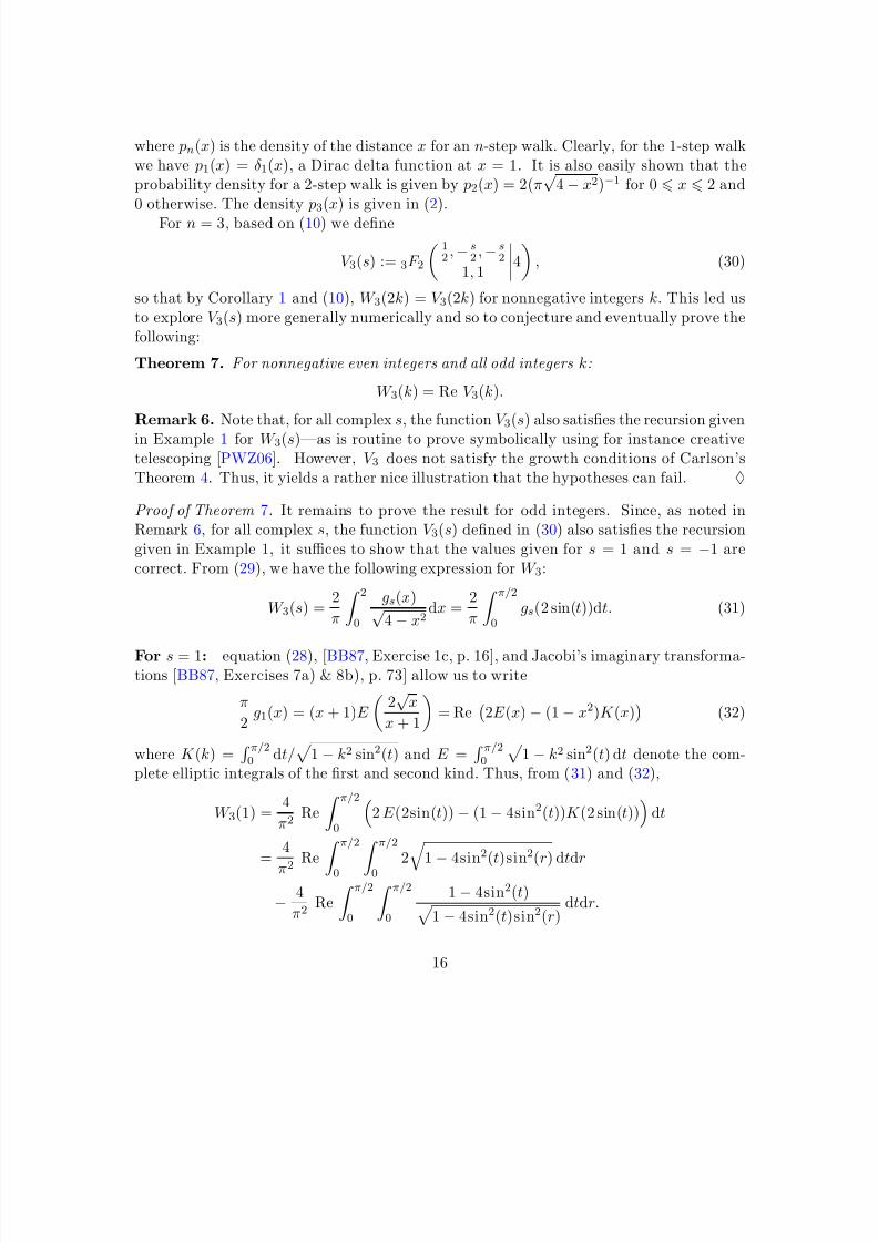
For n = 3, based on (10) we define

V 3(s) := 3F 2

12 ,− s

2 ,− s2

1, 1

4

, (30)

so that by Corollary 1 and (10), W 3(2k) = V 3(2k) for nonnegative integers k. This led usto explore V 3(s) more generally numerically and so to conjecture and eventually prove thefollowing:

Theorem 7. For nonnegative even integers and all odd integers k:

W 3(k) = Re V 3(k).

Remark 6. Note that, for all complex s, the function V 3(s) also satisfies the recursion given

in Example 1 for W 3(s)—as is routine to prove symbolically using for instance creativetelescoping [PWZ06]. However, V 3 does not satisfy the growth conditions of Carlson’sTheorem 4. Thus, it yields a rather nice illustration that the hypotheses can fail. ♦

Proof of Theorem 7. It remains to prove the result for odd integers. Since, as noted inRemark 6, for all complex s, the function V 3(s) defined in (30) also satisfies the recursiongiven in Example 1, it suffices to show that the values given for s = 1 and s = −1 arecorrect. From (29), we have the following expression for W 3:

W 3(s) =2

π

� 20

gs(x)√4− x2

dx =2

π

� π/2

0gs(2 sin(t))dt. (31)

For s = 1: equation (28), [BB87, Exercise 1c, p. 16], and Jacobi’s imaginary transforma-tions [BB87, Exercises 7a) & 8b), p. 73] allow us to write

π

2g1(x) = (x + 1)E

2√

x

x + 1

= Re

2E (x)− (1− x2)K (x)

(32)

where K (k) = π/20 dt/

1 − k2 sin2(t) and E = π/20

1− k2 sin2(t) dt denote the com-

plete elliptic integrals of the first and second kind. Thus, from ( 31) and (32),

W 3(1) =4

π2Re

� π/2

0

2 E (2sin(t)) − (1− 4sin2(t))K (2 sin(t))

dt

=4

π2

Re � π/2

0�

π/2

0

2 1− 4sin2(t)sin2(r) dtdr

− 4

π2Re

� π/2

0

� π/2

0

1− 4sin2(t) 1− 4sin2(t)sin2(r)

dtdr.

16



Amalgamating the two last integrals and parameterizing, we consider

Q(a) :=4

π2 � π/2

0 � π/2

0

1 + a2 sin2(t)− 2 a2 sin2(t)sin2(r)

1− a2 sin2(t)sin2(r)dtdr. (33)

We now use the binomial theorem to integrate (33) term-by-term for |a| < 1 and

substitute 2π

π/20 sin2m(t) dt = (−1)m−1/2

m

throughout. Moreover, (−1)m

−αm

= (α)m/m!

where the later denotes the Pochhammer symbol. Evaluation of the consequent infinitesum produces:

Q(a) =k0

(−1)k−1/2

k

a2k−1/2

k

2− a2k+2

−1/2

k

−1/2

k + 1

− 2a2k+2

−1/2

k + 1

2

=k0

(−1)ka2k−1/2

k

3 1

(1− 2k)2

= 3F 2

−12 ,−1

2 , 12

1, 1

a2

.

Analytic continuation to a = 2 yields the claimed result as per for s = 1.

For s = −1: we similarly and more easily use (28) and (31) to derive

W 3(−1) = Re4

π2

� π/2

0K (2 sin(t)) dt

= Re4

π2 � π/2

0 � π/2

0

1

1− 4sin2(t)sin2(r)dtdr = V 3(−1).

Example 5. Theorem 7 allows us to establish the following equivalent expressions forW 3(1):

W 3(1) =4√

3

3

3F 2

−12 ,−1

2 ,−12

1, 1

14− 1

π

+

√3

243F 2

12 , 1

2 , 12

2, 2

14

= 2√

3K 2 (k3)

π2+√

31

K 2 (k3)

=3

16

21/3

π

4Γ61

3+ 27

4

22/3

π

4Γ62

3 .

These rely on using Legendre’s identity and several Clausen-like product formulae, plus

Legendre’s evaluation of K (k3) where k3 :=√ 3−12√ 2

is the third singular value as in [BB87].

17



More simply but similarly, we have

W 3(−1) = 2√

3K 2 (k3)

π2=

3

16

21/3

π4Γ6

1

3 .Using the recurrence presented in Example 1 it follows that similar expressions can begiven for W 3 evaluated at odd integers.

In [BSW10] corresponding hypergeometric closed forms for W 4 are presented. ♦

7 Conclusion

The behaviour of these two-dimensional walks provides a fascinating blend of probabilistic,analytic, algebraic and combinatorial challenges.

Acknowledgements We are grateful to David Bailey, David Broadhurst and RichardCrandall for helpful suggestions, to Bruno Salvy for reminding us of the existence of [Bar64],Michael Mossinghoff for showing us [Klu1906], and to Peter Donovan for stimulating thisresearch and for much subsequent useful discussion. We also thank the referees for theircareful reading and comments. The work of the third author, as a graduate student, waspartially funded by NSF-DMS 0070567.

A Appendix

A.1 A rigorous proof of Theorem 1

We begin with:

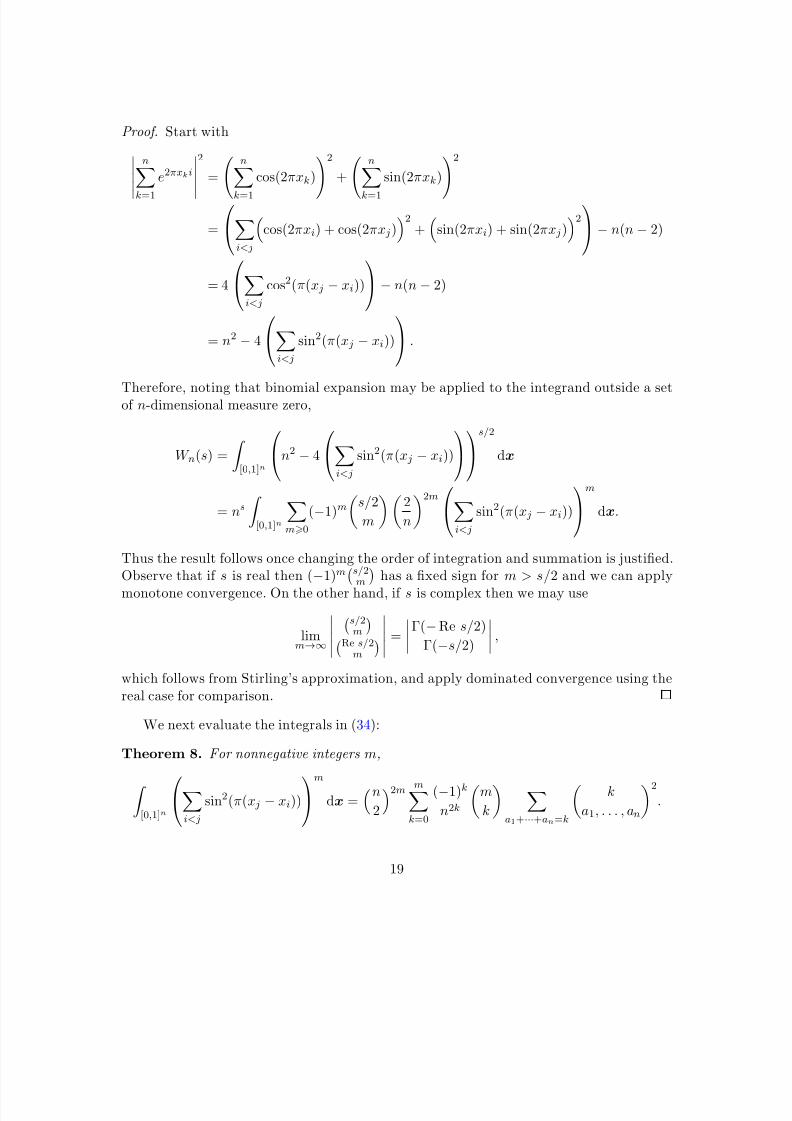
Proposition 3. For complex s with Re s 0,

W n(s) = nsm0

(−1)m

s/2

m

2

n

2m � [0,1]n

1�i<j�n

sin2(π(x j − xi))

m

dx. (34)

18



Proof. Start with

n

k=1

e2πxki2

= n

k=1

cos(2πxk)2

+n

k=1

sin(2πxk)2

=

i<j

cos(2πxi) + cos(2πx j)2

+

sin(2πxi) + sin(2πx j)2− n(n− 2)

= 4

i<j

cos2(π(x j − xi))

− n(n− 2)

= n2 − 4

i<j


.

Therefore, noting that binomial expansion may be applied to the integrand outside a setof n-dimensional measure zero,

W n(s) =

� [0,1]n

n2 − 4

i<j


s/2

dx

= ns

� [0,1]n

m0

(−1)m

s/2

m

2

n

2mi<j


m

dx.

Thus the result follows once changing the order of integration and summation is justified.Observe that if s is real then (

−1)ms/2m has a fixed sign for m > s/2 and we can apply

monotone convergence. On the other hand, if s is complex then we may use

limm→∞

s/2m

Re s/2

m

=Γ(−Re s/2)

Γ(−s/2)

,which follows from Stirling’s approximation, and apply dominated convergence using thereal case for comparison.

We next evaluate the integrals in (34):

Theorem 8. For nonnegative integers m,

� [0,1]n

i<j


m

dx =n

2

2m mk=0

(−1)k

n2k

m

k

a1+···+an=k

k

a1, . . . , an

2

.

19



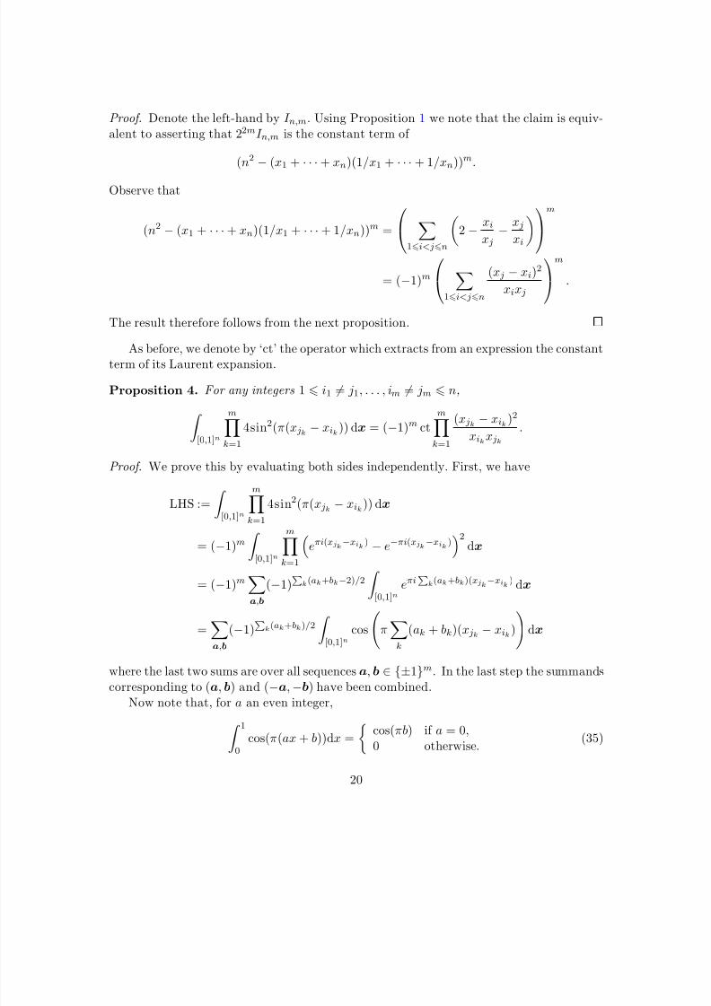
Proof. Denote the left-hand by I n,m. Using Proposition 1 we note that the claim is equiv-alent to asserting that 22mI n,m is the constant term of

(n2

−(x1 + · · · + xn)(1/x1 + · · · + 1/xn))m.

Observe that

(n2 − (x1 + · · · + xn)(1/x1 + · · · + 1/xn))m =

1�i<j�n

2− xi

x j− x j

xi

m

= (−1)m

1�i<j�n

(x j − xi)2

xix j

m

.

The result therefore follows from the next proposition.

As before, we denote by ‘ct’ the operator which extracts from an expression the constantterm of its Laurent expansion.

Proposition 4. For any integers 1 � i1 = j1, . . . , im = jm � n,

� [0,1]n

mk=1

4sin2(π(x jk − xik)) dx = (−1)m ctmk=1

(x jk − xik)2

xikx jk.

Proof. We prove this by evaluating both sides independently. First, we have

LHS :=

� [0,1]n

m

k=1

4sin2(π(x jk − xik)) dx

= (−1)m� [0,1]n

mk=1

eπi(xjk−xik ) − e−πi(xjk−xik )2

dx

= (−1)ma,b

(−1)�

k(ak+bk−2)/2� [0,1]n

eπi�

k(ak+bk)(xjk−xik ) dx

=a,b

(−1)�

k(ak+bk)/2

� [0,1]n

cos

π

k

(ak + bk)(x jk − xik)

dx

where the last two sums are over all sequences a, b ∈ {±1}m. In the last step the summandscorresponding to (a, b) and (−a,−b) have been combined.

Now note that, for a an even integer,� 10

cos(π(ax + b))dx =

cos(πb) if a = 0,0 otherwise.

(35)

20



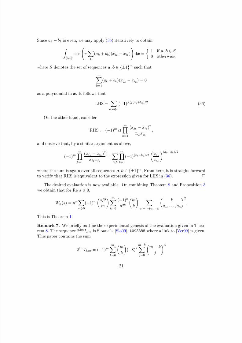
Since ak + bk is even, we may apply (35) iteratively to obtain

� [0,1]n cosπk

(ak + bk)(x jk − xik)dx = 1 if a, b ∈ S,0 otherwise,

where S denotes the set of sequences a, b ∈ {±1}m such that

mk=1

(ak + bk)(x jk − xik) = 0

as a polynomial in x. It follows that

LHS =a,b∈S

(−1)�

k(ak+bk)/2 (36)

On the other hand, consider

RHS := (−1)m ctmk=1

(x jk − xik)2

xikx jk,

and observe that, by a similar argument as above,

(−1)mmk=1

(x jk − xik)2

xikx jk=a,b

mk=1

(−1)(ak+bk)/2

x jkxik

(ak+bk)/2

where the sum is again over all sequences a, b ∈ {±1}m. From here, it is straight-forwardto verify that RHS is equivalent to the expression given for LHS in (36).

The desired evaluation is now available. On combining Theorem 8 and Proposition 3we obtain that for Re s 0,

W n(s) = nsm0

(−1)m

s/2

m

mk=0

(−1)k

n2k

m

k

a1+···+an=k

k

a1, . . . , an

2.

This is Theorem 1.

Remark 7. We briefly outline the experimental genesis of the evaluation given in Theo-rem 8. The sequence 22mI 3,m is Sloane’s, [Slo09], A093388 where a link to [Ver99] is given.This paper contains the sum

22mI 3,m = (−1)mmk=0

m

k

(−8)k

m−k j=0

m − k

j

3

21



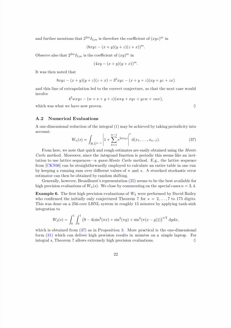
and further mentions that 22mI 3,m is therefore the coefficient of (xyz)m in

(8xyz − (x + y)(y + z)(z + x))m.

Observe also that 2

2m

I 2,m is the coeffi

cient of (xy)

m

in(4xy − (x + y)(y + x))m.

It was then noted that

8xyz − (x + y)(y + z)(z + x) = 32xyz − (x + y + z)(xy + yz + zx)

and this line of extrapolation led to the correct conjecture, so that the next case wouldinvolve

42wxyz − (w + x + y + z)(wxy + xyz + yzw + zwx),

which was what we have now proven. ♦

A.2 Numerical Evaluations

A one-dimensional reduction of the integral (1) may be achieved by taking periodicity intoaccount:

W n(s) =

� [0,1]n−1

1 +n−1k=1

e2πxki

s

d(x1, . . . , xn−1). (37)

From here, we note that quick and rough estimates are easily obtained using the MonteCarlo method. Moreover, since the integrand function is periodic this seems like an invi-tation to use lattice sequences—a quasi-Monte Carlo method. E.g., the lattice sequencefrom [CKN06] can be straightforwardly employed to calculate an entire table in one run

by keeping a running sum over diff

erent values of n and s. A standard stochastic errorestimator can then be obtained by random shifting.Generally, however, Broadhurst’s representation (25) seems to be the best available for

high precision evaluations of W n(s). We close by commenting on the special cases n = 3, 4.

Example 6. The first high precision evaluations of W 3 were performed by David Baileywho confirmed the initially only conjectured Theorem 7 for s = 2, . . . , 7 to 175 digits.This was done on a 256-core LBNL system in roughly 15 minutes by applying tanh-sinhintegration to

W 3(s) =

� 10

� 10

9− 4(sin2(πx) + sin2(πy) + sin2(π(x− y)))

s/2dydx,

which is obtained from (37) as in Proposition 3. More practical is the one-dimensionalform (31) which can deliver high precision results in minutes on a simple laptop. Forintegral s, Theorem 7 allows extremely high precision evaluations. ♦

22



Example 7. Assuming that Conjecture 1 holds for n = 2 (for a proof, see [BSWZ10]),Theorem 7 implies that for nonnegative integers k

W 4(k)

?

= Re j0

s/2

j2

3F 2 12 ,

−k2 + j,

−k2 + j

1, 14

.

This representation is very suitable for high precision evaluations of W 4 since, roughly, onecorrect digit is added by each term of the sum. Formula (27) by Crandall also lends itself quite well for numerical work (by slightly perturbing s even for integral arguments). ♦

References

[BB10] D. H. Bailey and J. M. Borwein. “Hand-to-hand combat with thousand-digitintegrals.” Preprint, 2010.

[BBBG08] D. H. Bailey, J. M. Borwein, D. J. Broadhurst, and M. L. Glasser. “Ellipticintegral evaluations of Bessel moments and applications.” J. Phys. A: Math.Theor., 41, 5203–5231, 2008.

[Bar64] P. Barrucand. “Sur la somme des puissances des coefficients multinomiaux etles puissances successives d’une fonction de Bessel.” Comptes rendus hebdo-madaires des seances de l’Academie des sciences, 258, 5318–5320, 1964.

[BBC07] J. M. Borwein, D. Bailey, N. Calkin, R. Girgensohn, R. Luke, and V. Moll.Experimental Mathematics in Action . A.K. Peters, 2007.

[BB87] J. M. Borwein and P. B. Borwein. Pi and the AGM: A Study in Analytic

Number Theory and Computational Complexity . Wiley, 1987.

[BS08] J. M. Borwein and B. Salvy. “A proof of a recursion for Bessel moments.”Experimental Mathematics, 17, 223–230, 2008. [D-drive Preprint 346.]

[BSW10] J. M. Borwein, A. Straub, and J. Wan. “Three-Step and Four-Step RandomWalk Integrals.” Experimental Mathematics, in press, 2010.

[BSWZ10] J. M. Borwein, A. Straub, J. Wan, and W. Zudilin. “Densities of short uniformrandom walks.” Preprint, September 2010.

[Bro09] D. Broadhurst. “Bessel moments, random walks and Calabi-Yau equations.”Preprint, November 2009.

[CKN06] R. Cools, F. Y. Kuo, and D. Nuyens. “Constructing embedded lattice rules formultivariate integration.” SIAM J. Sci. Comput., 28, 2162–2188, 2006.

23



[Cra09] R. E. Crandall. “Analytic representations for circle-jump moments.” Preprint,October 2009.

[CG96] J. H. Conway and R. K. Guy. The Book of Numbers. Springer-Verlag, 1996.

[Don09] P. Donovan. “The flaw in the JN-25 series of ciphers, II.” Cryptologia , in press,2010.

[Hug95] B. D. Hughes. “Random Walks and Random Environments,” Volume 1. Ox-ford, 1995.

[Klu1906] J. C. Kluyver. “A local probability problem.” Nederl. Acad. Wetensch. Proc.,8, 341–350, 1906.

[Mat01] L. Mattner. “Complex diff erentiation under the integral.” Nieuw Arch. Wisk.,IV. Ser. 5/2(1), 32–35, 2001.

[Merz79] E. Merzbacher, J. M. Feagan, and T-H. Wu. “Superposition of the radiationfrom N independent sources and the problem of random flights.” American Journal of Physics. Vol. 45, No. 10, 1977.

[Pea1905] K. Pearson. “The random walk.” Nature, 72, 294, 1905.

[Pea1905b] K. Pearson. “The problem of the random walk.” Nature, 72, 342, 1905.

[Pea1906] K. Pearson. A Mathematical Theory of Random Migration , Mathematical Con-tributions to the Theory of Evolution XV. Drapers, 1906.

[PWZ06] M. Petkovsek, H. Wilf and D. Zeilberger. A=B , AK Peters, 3rd printing,(2006).

[Ray1905] Lord Rayleigh. “The problem of the random walk.” Nature, 72, 318, 1905.

[RS09] L. B. Richmond and J. Shallit. “Counting abelian squares.” The ElectronicJournal of Combinatorics, 16, 2009.

[Slo09] N. J. A. Sloane. The On-Line Encyclopedia of Integer Sequences. Publishedelectronically at http://www.research.att.com/sequences , 2009.

[Tit39] E. Titchmarsh. The Theory of Functions. Oxford University Press, 2nd edition,1939.

[Ver99] H. A. Verrill. “Some congruences related to modular forms.” Preprint MPI-

1999-26, Max-Planck-Institut, 1999.

[Ver04] H. A. Verrill. “Sums of squares of binomial coefficients, with applications toPicard-Fuchs equations.” 2004. arXiv:math/0407327v1[math.CO].

24



[Wil93] H. Wilf. generatingfunctionology , Academic Press, 2nd edition, 1993.

25

Random Walk Integrals - Borwein (2010)

Documents