Random walk analysis with multiple structural breaks: Case study in emerging market of S&P BSE sectoral indices stocks

503

Random walk analysis with multiple structural breaks: Case study in emerging

market of S&P BSE sectoral indices stocks

G. Sheelapriya and R. Murugesan

Department of Humanities, National Institute of Technology, Tiruchirappalli, India

Abstract

As the consequences of high volatile and time varying mean in the financial series, it causes

behavioural changes in the stochastic trend is known as a structural break. The aim is to

investigate the number of unknown structural breaks for the emerging market of S&P 500 indices

which are listed on BSE, by employing BP unit root tests. This empirical study examines the

random walk hypothesis by testing the unit root in the presence of unknown structural breaks.

The concern in the traditional unit root test is to fail the rejection of null hypothesis. This issue

has been trounced by the BP tests and it significantly locates the unknown structural breaks in the

data containing differed error distribution and error heteroskedasticity. In this paper, ADF,

Phillips Perron and KPSS tests have been employed to examine the unit root hypothesis, and

hence to predict the unknown structural breaks. Then all the sectoral indices have been forecasted

in the presence of the structural breaks using Markov switching AR (1) process.

Keywords: Multiple structural breaks, unit root, random walk, efficient market hypothesis, Markov

switching AR (1) model

Introduction1

The objective of the study is to investigate the random walk hypothesis and the numbers of

unknown multiple structural breaks for the emerging market in India for the twelve sectors which

are listed on BSE. Recent research has focussed on testing the efficiency of the emerging market

countries due to the fact that, for the past decade the rate of growth returning in the emerging

markets are all together relatively higher than in the emergent countries. Such kind of this

occasional trend has been increasing the attention of researchers to investigate the efficiency of

the market testing by the random walk hypothesis. So far the vast numbers of literature have been

investigated about the random walk hypothesis by applying unit root test. The main issue in the

unit root test is unable to reject the null hypothesis of unit root in the presence of unknown

structural breaks in the stock prices. Initially this idea was proposed by Perron (1989) for known

structural breaks date. Later studies by Zivot and Andrews (1992), Papell (1997), Perron (2006)

and Narayan and Popp (2010) have investigated one or two endogenous structural breaks.

The study focuses on contributing the literature in the following way; first we extend the

literature on the Indian stock market efficiency by examining the random walk hypothesis using

the unit root test. Secondly we are extending the literature on testing the multiple structural

breaks in the Indian stock market data. And this each sectoral indices stock has been split into

Corresponding author's

Name: G. Sheelapriya

Email address: [email protected]

Asian Journal of Empirical Research

journal homepage: http://aessweb.com/journal-detail.php?id=5004

mailto:[email protected]

Asian Journal of Empirical Research, 4(11)2014: 503-513

504

regions based on their occurrence of possible unknown structural breaks. Then the movements of

each sectoral stock in the region have estimated using the Markov Switching model. Indian stock

market efficiency has been investigated in many literatures, Bhunia (2012), Rabbani et al. (2013),

Mahajan and Luthra (2013), Srinivasan (2010), Mishra (2011), and Mishra et al. (2014).

Similarly a study on testing the efficient market hypothesis for European stock markets have been

done by Borges (2010), and a model comparison approach on testing the random walk hypothesis

in the China stock market has been investigated by Darrat and Zhong (2000). However the above

mentioned authors have used the traditional ADF test and/or Phillips Perron and /or Kpss unit

root tests which are unable to identify the presence of unknown breaks in the stock prices, while

examining the null hypothesis of unit root in their literatures. Further the estimation of structural

breaks can be done to the models of pure and partial changes by applying the principle of

dynamic algorithm which yields efficient global minimisers for the sum squared residuals that is

given in Bai and Perron (2003).

Therefore BP test (Bai and Perron, 2003 test) has been employed to get a better goodness of fit

and the minimum level of committing type II error in the data containing error distribution. There

is a scarce of literatures on testing the multiple structural breaks. However a few studies dealt

about the multiple structural breaks in the stock prices, explained in the following literatures,

Andrews et al. (1996), Lumsdaine and Papell (1997), Lee and Strazicich (2003, 2004), Glynn and

Verma (2007). Based on LWE and Schwarz criteria, the BP estimation of structural break has

been done using the sequential or partial, 𝑈𝐷𝑀𝐴𝑋 and 𝑊𝐷𝑀𝐴𝑋 tests, by Bai and Perron (2003).

Markov switching models by Hamilton (1989) have modelled many nonlinear applications of

financial economics. Markove switching Model estimation has dealt the estimation of multiple

structural breaks.

The rest of this paper is arranged as follows; section 2 discusses the traditional unit root tests in

the context of the emerging market efficiency. Section 3, provides an outline of the data set. In

section 4, the empirical estimation of breaks and the prediction of forecasting error are explained

in detail. Section 5, presents the summary of results and conclusions which provides a significant

evidence of the current study on market efficiency of emerging market.

Market efficiency

Efficient market hypothesis (EMH) states that a market is one in which prices are always fully

reflected the all available information at any time by Fama (1970). EMH can be categorised into

three forms; first weak form of EMH implies that a market is efficient by providing all the

available information. However the prediction is impossible due to the integrated shocks which

make often the historical prices to move into a new orbit. Second the semi strong of EMH states

that a market is one where the stocks are adopted quickly to attract all the new publically

available information. Even if an investor possibly gets all the information, he couldn’t get

benefit through it in the market. The third strong form of EMH incorporates both the weak and

semi strong form, and states that the stocks are reflected all information privately as well as

publically in a market by Fama(1970).

The random walk theory states that the stock price movements/ trend are based on the past

available information which cannot be used to predict the future movement. The reason behind

the random walk hypothesis represents the stock prices are independent to each other; perhaps the

flow of all information adequately reflecting on the today’s stocks has an influence only on today

prices. Malkiel (2003) suggested that, due to the random changes in the current stock prices, the

future stock prices should not be predicted, even all news and its definitions are available without

hindrance. Thus an uninformed investor achieves the average profits buying a diversified

portfolio getting all information in the market.


505

Our interest is to test the stock index prices that often encounters the issue of non-stationarity (i.e.

stock price does not tend to return to its mean). Such kind of situation is known as unit root

synonymous as random walk hypothesis that is explained in Gujarati (2003). Initially Dickey and

Fuller (1979) as well as Dickey and Fuller (1981) developed the unit root test which can mainly

satisfy the demands of trend stationary and different stationary behaviour of stock index prices.

Later Phillips and Perron (1988) have introduced the PP test which takes care of possible serial

correlation in the error terms without adding the lagged different terms of the regress and. Again

an alternative procedure for the unit root test is known as KPSS test or contrary stationary test

(i.e. null hypothesis is not the existence of a unit toot), which tries to discriminate the purely

trend stationary process and the process with an additive random walk, is given in Kirchgässner

et al. (2012).

The above mentioned tests usually tests, whether series possess unit root or not. The procedure of

sequential test, global minimizing test and the global information criteria test were proposed by

Perron (1989) to identify the presence of unknown multiple structural breaks in the stock price.

Recently Bai and Perron (2003) proposed an alternative refining procedure for finding the unit

root in the stock indexes with multiple structural changes that are estimated by the ordinary least

squares.

S&P BSE Sectoral indices data

BSE Ltd was established in 1875, and it is the Asia’s fastest stock exchanges with a speed of 200

microseconds, and the world’s third largest leading exchange for Index option trading (in March

2014 onwards, source: World Federation of Exchange). The total market capitalization is of USD

1.151 Trillion for the companies which listed on BSE Ltd as of May 2014, given in Wikipedia,

and the Free Encyclopedia (2014). S&P BSE Index consists of the following sector names as

follows Auto, Banks, Consumer Durables, Capital Goods, FMCG, Healthcare, IT, Metal, Oil&

Gas, Power, Realty, and Technology. These sectoral indices have significantly received a large

amount of money from FIIs and also have a large number of subsets contained in these twelve

broad sectoral indices, which provide a great trade-off platform for the intercontinental traders to

invest their stocks in the Indian market. The highlight of the increasing SENSEX aids the sectoral

indices that have outperformed others from 1 January 2013 to March 2014, by Priyanka (2014

March 12).

The data for the investigation of multiple structural breaks were downloaded from BSE website

(http://www.bseindia.com/indices/indexarchivedata.aspx) for the periods (January 1999- July

2014). The data for the sectors name as Power was available for the periods (January 2005-July

2014), the data for the sector Realty was available for (January 2006- July 2014) and the data for

the sector Bank was available for (January 2002- July 2014). Similarly the data for Tech was

available for (April 2001- July 2014).

Methodology

Bai and Perron (2003) derived linear model estimation for the multiple unknown structural

breaks. The rate of convergence has greatly achieved the minimum level of sum squared

residuals using least squares. This model employs the principle of dynamic programming

computations of order two 𝑂(𝑇2) for any number of changes ‘m’ whereas the principle of

standard grid search procedure necessitate the order 𝑂(𝑇𝑚), given by Guthery (1974).

𝑦𝑡 = 𝑋𝑡′𝛽 + 𝑍𝑡

′ 𝛿𝑗 + 𝑢𝑡 𝑡 = 𝑇𝑗−1 + 1, … , 𝑇𝑗 …………………. (1)

http://www.bseindia.com/indices/indexarchivedata.aspx


506

𝑋𝑡(𝑝 ∗ 1) & 𝑍𝑡(𝑞 ∗ 1) are vectors of covariance and 𝛽 and 𝛿𝑗 (j=1... m+1) are corresponding

vector coefficients. 𝑢𝑡 The residual error term at time t.

𝑦 = 𝑋𝛽 + �̅�∗𝛿 + 𝑈 ……………………… (2)

�̅�∗ , the diagonal partition of Z at the ‘m’ partition {𝑇∗} = (𝑇1∗ … 𝑇𝑚

∗ )

Multiple break tests statistics

Sequential ‘𝒍 + 𝟏’ breaks vs. ‘𝒍’ break

This sequential testing procedure of ′𝑙 + 1′ vs. ′𝑙′ break has been proposed by Bai (1997) and

Bai and Perron (2003). Here the test has been applied over the range of all sets that contain the

samples from �̂�𝑖−1 to 𝑇�̂� where i=1... 𝑙+1. The breaks have been calculated using the method of

global minimum. The overall minimum value of sum squared residuals of ′𝑙 + 1′ breaks is

smaller than the overall minimum value of sum squared residuals of ′𝑙′ break.

Global Bai and Perron ′𝒍′ break vs. No break

In BP method, using 𝑈𝐷𝑀𝐴𝑋 , 𝑊𝐷𝑀𝐴𝑋 tests, at least one break can be found in the data. The ‘m’

number of breaks has been detected through the procedure of sequential statistics SupF (𝑙 + 1|𝑙)

using the global optimizer test. Therefore this method has indeed produced the best results of

multiple structural breaks for the time series applications.

Global information criteria

The Global information Criteria such as Schwarz and LWZ have searched a better value of

optimized information based on the sum of squared residuals. It has been estimated using the

likelihood function, is explained in Bai and Perron (2003).

Markov switching model

Hamilton (1989), described the Markov process which explains the sample that has been split

into ‘m+1‘regime, based on the occurrences of possible unknown breaks ‘m ‘. Thus the markov

switching model has been constructed for each split region and the unknown parameters. They

are estimated using the method of maximum likelihood, which is also evolving in the process of

auto regression AR (1). The forecasting value can be found, under this Markov switching

approach, when there are multiple shifts from one set of behaviour to another in the region. This

can be expressed as flows

𝑦𝑡 = (1 − 𝑝11) + 𝜌𝑦𝑡−1 + 휀𝑡 …………………. (3)

𝑦𝑡 = (𝜇1 + 𝜇2)𝑦𝑡−1 + (𝜎12 + 𝜑𝑦𝑡)1/2𝑢𝑡 …………………. (4)

𝜌 = 𝑝11 + 𝑝22 − 1. (1 − 𝑝11), defines the probability of a shift from state 1 to state 2 between

times ‘ t-1 ’ and ‘ t ‘. 𝜌11 and 𝜌22 denote the probability of being in regions one and two.

Where 𝜇𝑡~𝑁(0,1), and 휀𝑡 is the error at time‘t’. The expected values and variances of the series

are 𝜇1 and 𝜎12 respectively in state one, and (𝜇1 + 𝜇2) and (𝜎1

2 + 𝜑) are mean and variance in

state two, is given in Hamilton (1989).

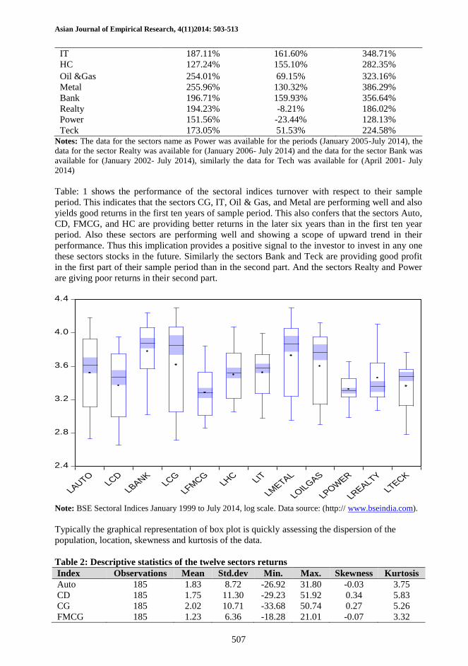
Table 1: Returns on the sectoral indices for the given years

Sectoral indices 𝑹𝟏𝟎 Years 𝑹𝟔 Years Overall Return

Auto 137.02% 202.99% 340%

CG 251.72% 121.82% 373.54%

CD 138% 185.42% 324.35%

FMCG 96.60% 131.41% 228.02%


507

IT 187.11% 161.60% 348.71%

HC 127.24% 155.10% 282.35%

Oil &Gas 254.01% 69.15% 323.16%

Metal 255.96% 130.32% 386.29%

Bank 196.71% 159.93% 356.64%

Realty 194.23% -8.21% 186.02%

Power 151.56% -23.44% 128.13%

Teck 173.05% 51.53% 224.58% Notes: The data for the sectors name as Power was available for the periods (January 2005-July 2014), the

data for the sector Realty was available for (January 2006- July 2014) and the data for the sector Bank was

available for (January 2002- July 2014), similarly the data for Tech was available for (April 2001- July

2014)

Table: 1 shows the performance of the sectoral indices turnover with respect to their sample

period. This indicates that the sectors CG, IT, Oil & Gas, and Metal are performing well and also

yields good returns in the first ten years of sample period. This also confers that the sectors Auto,

CD, FMCG, and HC are providing better returns in the later six years than in the first ten year

period. Also these sectors are performing well and showing a scope of upward trend in their

performance. Thus this implication provides a positive signal to the investor to invest in any one

these sectors stocks in the future. Similarly the sectors Bank and Teck are providing good profit

in the first part of their sample period than in the second part. And the sectors Realty and Power

are giving poor returns in their second part.

2.4

2.8

3.2

3.6

4.0

4.4

LAUTOLCD

LBANKLCG

LFMCG

LHC LIT

LMETAL

LOIL

GAS

LPOW

ER

LREALTY

LTECK

Note: BSE Sectoral Indices January 1999 to July 2014, log scale. Data source: (http:// www.bseindia.com).

Typically the graphical representation of box plot is quickly assessing the dispersion of the

population, location, skewness and kurtosis of the data.

Table 2: Descriptive statistics of the twelve sectors returns

Index Observations Mean Std.dev Min. Max. Skewness Kurtosis

Auto 185 1.83 8.72 -26.92 31.80 -0.03 3.75

CD 185 1.75 11.30 -29.23 51.92 0.34 5.83

CG 185 2.02 10.71 -33.68 50.74 0.27 5.26

FMCG 185 1.23 6.36 -18.28 21.01 -0.07 3.32

http://www.bseindia.com/


508

IT 185 1.88 12.38 -41.71 61.48 0.44 6.62

HC 185 1.52 7.22 -24.33 22.33 -0.38 4.19

Oil & Gas 185 1.74 8.98 -31.46 30.42 0.20 4.83

Metal 185 2.09 12.22 -40.31 57.98 0.33 5.02

Bank 152 0.23 1.12 -3.61 4.32 -0.19 4.70

Realty 103 0.04 2.27 -7.02 7.62 0.36 4.37

Power 116 0.09 1.25 -4.61 4.05 -0.13 4.99

Teck 161 0.15 1.11 -4.74 4.10 -0.54 5.63 Notes: (Using Return value the summary statistics has been calculated. Abbreviations: Automobile,

Consumer Durables, Capital Goods, Fast Moving Consumer Goods, Information Technology, Health Care,

Bank, and Technology stocks)

The table: 2 present the summary of individual statistics of monthly returns for all sector indices

over the sample period. The expected returns have been consistently moved in the range between

0.04 to 2.09.The monthly returns of risk measures are relatively high for the sectors Auto,

FMCG, HC, Oil & Gas, IT, CD, CG, and Metal. It shows that the sectors have been significantly

affected by the volatility of sampling. Furthermore, the monthly returns are low for the following

sectors, Bank, Realty, Power and Teck. The sectors, Auto, FMCG, HC, Bank, Power and Teck

have small negative skewness and also have significantly quite high kurtosis for all sectors.

Finally, the residual ARCH LM test has confirmed that the monthly returns of sector indices are

been affected by the volatility.

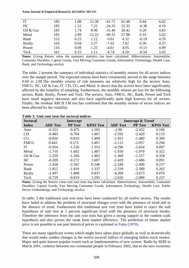
Table 3: Unit root tests for sectoral indices

Sectoral Intercept Intercept & Trend

Index ADF Test PP Test KPSS Test ADF Test PP Test KPSS Test

Auto -0.553 -0.475 1.503 -2.80 -2.452 0.106

CD -0.485 -0.704 1.407 -2.592 -2.420 0.119

CG -0.820 -0.810 1.400 -1.455 -1.480 0.300

FMCG 0.443 0.575 1.497 -2.113 -2.057 0.294

IT -0.954 -1.536 1.353 -4.296 -2.654 0.097

Metal -1.710 -1.602 1.487 -1.939 -1.970 0.322

Oil & Gas -1.259 -1.266 1.483 -1.368 -1.557 0.328

HC -0.209 -0.272 1.697 -2.429 -2.686 0.091

Power -2.458 -2.502 0.246 -2.349 -2.400 0.237

Bank -1.815 -1.810 1.337 -2.339 -2.389 0.262

Realty -1.497 -1.808 0.837 -4.369 -3.673 0.070

Teck -0.729 -0.819 1.295 -2.026 -2.089 0.237 Notes: (Using the Return value unit root tests has been calculated. Abbreviations: Automobile, Consumer

Durables, Capital Goods, Fast Moving Consumer Goods, Information Technology, Health Care, Public

Sector Undertakings, and Technology stocks)

In table: 3 the traditional unit root tests have been conducted for all twelve sectors. The results

have failed to address the problem of structural changes even with the presence of trend and in

the absence of trend. Furthermore this traditional unit root tests have failed to reject the null

hypothesis of unit root at 5 percent significant level with the presence of structural breaks.

Therefore the inference from the unit root tests has given a strong support to the random walk

hypothesis and also proves the weak form market efficiency. The prediction of future market

price is not possible to use past historical prices is explained in Fama (1970).

There are many significant events which might have taken place globally as well as domestically

that would make sudden changes in the twelve sectoral indices of emerging Indian stock market.

Major and quite known popular events such as Implementation of new system Badla by SEBI in

March 2001, violence between two communal people in February 2002, due to the new economic


509

policy as a results of election in May 2004, climate change which could have caused for a storm

floods and landslides in July 2005, Mumbai terrorist attack in November 2008, re-election of

Indian Government in May 2009, anti corruption activities led by Anna Hazare in 2011 -2012,

Uttarakh and floods and landslides in June 2013 and bombs blast in Hyderabad in February 2013,

general election with the new prime minister Narendra Modi leading the BJP Government in May

2014 and the split of two new states Telangana and Andhra Pradesh with Hyderabad according to

the Andra Pradesh recognition act in June 2014 entailed an impact on the Indian stock market.

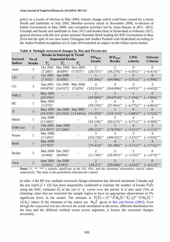
Table 4: Multiple structural changes by Bai and Perron test

Breaks in Intercept & Trend 𝑼𝑫𝑴𝑨𝑿

breaks

𝑾𝑫𝑴𝑨𝑿

Breaks

LWE

criteria

Schwarz

Criteria Sectoral

Indices No of

breaks

Sequential breaks

𝑻�̂� 𝑻�̂� 𝑻�̂�

Auto 3 Oct 2001

(7.285)∗

Mar 2009

(8.089)∗

Nov 2005

(7.557)∗-

2

(28.757)∗∗

5

(36.278)∗∗

0

(−6.501)∗∗∗

0

(−6.414)∗∗∗

CD 2 Oct 2001

(7.415)∗

Jan 2008

(5.858)∗ -

5

(37.346)∗∗

5

(69.986)∗∗

0

(−5.911)∗∗∗

0

(−5.998)∗∗∗

CG 3 Sep 2001

(49.874)∗

Oct 2005

(14.917)∗

Mar 2008

(7.829)∗

4

(153.514)∗∗

4

(244.896)∗∗

3

(−4.953)∗∗∗

3

(−4.632)∗∗∗

FMCG 1 May 2003

(23.196)∗ - -

1

(69.589)∗∗

5

(94.0714)∗∗

1

(−7.194)∗∗∗

0

(−7.056)∗∗∗

HC 1 May 2003

(7.272)∗

3

(39.139)∗∗

4

(57.964)∗∗

0

(−6.775)∗∗∗

0

(−6.863)∗∗∗

IT 3 May 2005

(53.339)∗

Jan 2008

(31.910)∗

Sep 2003

(113.816)∗

1

(76.358)∗∗

1

(104.765)∗∗

0

(−5.809)∗∗∗

0

(−5.723)∗∗∗

Metal 1 July 2008

(11.682)∗ -

5

(42.136)∗∗

5

(82.615)∗∗

4

(−4.711)∗∗∗

3

(−4.384)∗∗∗

Oil& Gas 2 Feb 2002

(11.967)∗

June 2008

(17.260)∗ -

2

(98.122)∗∗

5

(178.704)∗∗

4

(−5.513)∗∗∗

2

(−5.133)∗∗∗

Power 1 Mar 2008

(17.693)∗ -

3

(254.720)∗∗

5

(499.425)∗∗

3

(−5.432)∗∗∗

4

(−5.928)∗∗∗

Bank 1 Mar 2008

(37.707)∗

1

(75.414)∗∗

4

(81.586)∗∗

2

(−5.313)∗∗∗

4

(−5.716)∗∗∗

Realty 2 Mar 2009

(4.968)∗

Dec 2007

(8.096)∗ -

2

(21.249)∗∗

3

(25.947)∗∗

2

(−5.105)∗∗∗

0

(−4.979)∗∗∗

Teck 2 June 2001

(8.041)∗

Jan 2008

(8.965)∗ -

2

(18.37)∗∗

5

(29.046)∗∗

1

(−6.628)∗∗∗

0

(−6.523)∗∗∗ Notes: (*, **, *** a statistic significant at the 5%, 10%, and the minimum information criteria values

respectively. The value in the parentheses indicates the t ratios)

In table: 4 the BP test, multiple structural change estimation has allowed maximum 5 breaks and

the test 𝑠𝑢𝑝𝐹𝑇(𝑙 + 1|𝑙) has been sequentially conducted to estimate the number of breaks �̂�(�̂�)

using the HAC estimator 𝑘�̂� of the (m+1) ‘q’ vector over the period. It is also used 15% of

trimming value that are restricted the sample region to have an appropriate observations at 5%

significant level, in the model. The estimate is �̂�(�̂�) = (𝑇−1�̅�′𝑀𝑋�̅�)−1𝑘�̂� ((𝑇−1�̅�′𝑀𝑋�̅�)−1

{𝑍𝑡∗�̂�𝑡} where 𝑍𝑡

∗ the elements of the matrix are 𝑀𝑋�̅� given in Bai and Perron (2003). Even

though the sequential test has allowed the serial correlation in the errors, different distribution for

the data and the different residual errors across segments, it locates the structural changes

accurately.


510

Therefore this test has been performed for the twelve sectoral indices over the sample period, for

finding the multiple structural breaks in the case of no stationary data. The sectors CD, Oil& Gas,

Realty, and Teck were found that they have indentified two structural breaks in the given sample

period. The test statistics (𝐹𝑇(2|1) ,𝐹𝑇(3|2)) for these sectors were found to be (7.415, 5.858),

(11.967, 17.260), (4.968, 8.096) and (8.041, 8.965). These results were compared with their

respective critical values suggested in Bai and Perron (2003) at 5 % significant level. The

(𝑈𝐷𝑀𝑎𝑥 𝑎𝑛𝑑 𝑊𝐷𝑀𝑎𝑥 ) tests values for the above mentioned sectors were (37.346, 69.986),

(98.122, 178.704), (21.249, 25.947), (18.370, 29.046). Similarly, the sectors Auto, CG, and IT

have three structural breaks and the test statistics. ( 𝐹𝑇(2|1), 𝐹𝑇(3|2), 𝐹𝑇(4|3)) were obtained as

(7.285, 8.089, 7.557), (49.874, 14.917, 7.829), and (53.339, 31.910, 113.816). Also

the(𝑈𝐷𝑀𝑎𝑥 𝑎𝑛𝑑 𝑊𝐷𝑀𝑎𝑥) tests statistics values were found to be (28.757, 36.278), (153.514,

244.896) and (76.358, 104.765). Furthermore these results have been compared with their

respective critical values (suggested in Bai and Perron) at 5% significant level. Finally the sectors

FMCG, HC, Metal, Power, and Bank have captured one structural break with the test statistics

(𝐹𝑇(2|1) values (23.196), (7.272), (11.682), (17.693), (37.707). Alike the

(𝑈𝐷𝑀𝑎𝑥 𝑎𝑛𝑑 𝑊𝐷𝑀𝑎𝑥) test statistics values were found to be (69.589, 94.074), (39.139, 57.964),

(42.136, 182.615), (254.720, 499.425), (75.414, 81.586).

Finding the location of multiple structural changes in intercept & trend for the twelve sectoral

indices has mainly fallen into two different ranges. First the range from 2000 to 2005, many

sectoral indices such as Auto, CD, CG, FMCG, IT, Oil& Gas, and Teck have shown major

multiple significant breaks in the following years 2001, 2002, 2003 and 2005 over the sample

period. Similarly in the range from 2006 to 2012, there are structural changes in the sectoral

indices Auto, CD, CG, IT, Metal, Power and Realty in the years 2007, 2008, & 2009. Also it is

found from the table: 4, that the tests 𝑈𝐷𝑀𝐴𝑋 , 𝑊𝐷𝑀𝐴𝑋 , LWE criteria and Schwarz criteria are

significantly locating major structural breaks at 5% level. The breaks from these tests have

showed the impact on the Indian stocks due to the domestic events which could have caused

sudden changes in the market. Global events also have an impact on the occurrence of structural

breaks. The global events of financial crisis and the domestic event of Mumbai terrorist attack

happened in the same year of 2008.Therefore the impact of these events would be reflected on

the following sectors CD, CG, IT, Oil& Gas, and Power, Metal, Bank and Teck.

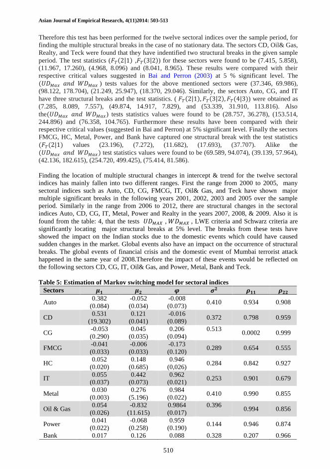
Table 5: Estimation of Markov switching model for sectoral indices

Sectors 𝝁𝟏 𝝁𝟐 𝝋 𝝈𝟐 𝝆𝟏𝟏 𝝆𝟐𝟐

Auto 0.382

(0.084)

-0.052

(0.034)

-0.008

(0.073) 0.410 0.934 0.908

CD 0.531

(19.302)

0.121

(0.041)

-0.016

(0.089) 0.372 0.798 0.959

CG -0.053

(0.290)

0.045

(0.035)

0.206

(0.094)

0.513

0.0002 0.999

FMCG -0.041

(0.033)

-0.006

(0.033)

-0.173

(0.120) 0.289 0.654 0.555

HC 0.052

(0.020)

0.148

(0.685)

0.946

(0,026) 0.284 0.842 0.927

IT 0.055

(0.037)

0.442

(0.073)

0.962

(0.021) 0.253 0.901 0.679

Metal 0.030

(0.003)

0.276

(5.196)

0.984

(0.022) 0.410 0.990 0.855

Oil & Gas 0.054

(0.026)

-0.832

(11.615)

0.9864

(0.017)

0.396

0.994 0.856

Power 0.041

(0.022)

-0.068

(0.258)

0.959

(0.190) 0.144 0.946 0.874

Bank 0.017 0.126 0.088 0.328 0.207 0.966


511

(0.459) (0.034) (0.094)

Realty -0.648

(12.881)

-0.098

(0.050)

0.835

(0.040)

0.273 0.848 0.984

Teck -0.029

(7.317)

-0.020

(0.022)

0.967

(0.021)

0.258 0.591 0.972

Note: Standard error in parentheses

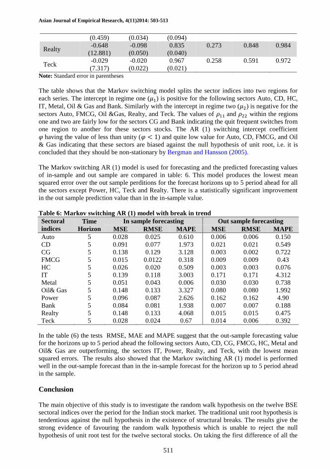
The table shows that the Markov switching model splits the sector indices into two regions for

each series. The intercept in regime one (𝜇1) is positive for the following sectors Auto, CD, HC,

IT, Metal, Oil & Gas and Bank. Similarly with the intercept in regime two (𝜇2) is negative for the

sectors Auto, FMCG, Oil &Gas, Realty, and Teck. The values of 𝜌11 and 𝜌22 within the regions

one and two are fairly low for the sectors CG and Bank indicating the quit frequent switches from

one region to another for these sectors stocks. The AR (1) switching intercept coefficient

𝜑 having the value of less than unity (𝜑 < 1) and quite low value for Auto, CD, FMCG, and Oil

& Gas indicating that these sectors are biased against the null hypothesis of unit root, i.e. it is

concluded that they should be non-stationary by Bergman and Hansson (2005).

The Markov switching AR (1) model is used for forecasting and the predicted forecasting values

of in-sample and out sample are compared in table: 6. This model produces the lowest mean

squared error over the out sample perditions for the forecast horizons up to 5 period ahead for all

the sectors except Power, HC, Teck and Realty. There is a statistically significant improvement

in the out sample prediction value than in the in-sample value.

Table 6: Markov switching AR (1) model with break in trend

Sectoral

indices

Time

Horizon

In sample forecasting Out sample forecasting

MSE RMSE MAPE MSE RMSE MAPE

Auto 5 0.028 0.025 0.610 0.006 0.006 0.150

CD 5 0.091 0.077 1.973 0.021 0.021 0.549

CG 5 0.138 0.129 3.128 0.003 0.002 0.722

FMCG 5 0.015 0.0122 0.318 0.009 0.009 0.43

HC 5 0.026 0.020 0.509 0.003 0.003 0.076

IT 5 0.139 0.118 3.003 0.171 0.171 4.312

Metal 5 0.051 0.043 0.006 0.030 0.030 0.738

Oil& Gas 5 0.148 0.133 3.327 0.080 0.080 1.992

Power 5 0.096 0.087 2.626 0.162 0.162 4.90

Bank 5 0.084 0.081 1.938 0.007 0.007 0.188

Realty 5 0.148 0.133 4.068 0.015 0.015 0.475

Teck 5 0.028 0.024 0.67 0.014 0.006 0.392

In the table (6) the tests RMSE, MAE and MAPE suggest that the out-sample forecasting value

for the horizons up to 5 period ahead the following sectors Auto, CD, CG, FMCG, HC, Metal and

Oil& Gas are outperforming, the sectors IT, Power, Realty, and Teck, with the lowest mean

squared errors. The results also showed that the Markov switching AR (1) model is performed

well in the out-sample forecast than in the in-sample forecast for the horizon up to 5 period ahead

in the sample.

Conclusion

The main objective of this study is to investigate the random walk hypothesis on the twelve BSE

sectoral indices over the period for the Indian stock market. The traditional unit root hypothesis is

tendentious against the null hypothesis in the existence of structural breaks. The results give the

strong evidence of favouring the random walk hypothesis which is unable to reject the null

hypothesis of unit root test for the twelve sectoral stocks. On taking the first difference of all the


512

sectoral indices data, the BSE sectoral indices stocks are mean reverting. Aftermath these stocks

are able to predict the future stock prices based on the available past information.

It is analyzed that the multiple structural break using BP test has been allowing the serial

correlation, heteroskedasicity, and the different distribution for the residuals across the region. It

is investigated that greatly captured the behavioural changes in the stock price with the presence

of structural breaks. Also found that the BP test yields minimum one and maximum three

structural breaks in the BSE sectoral indices stocks. Finally this breaks are estimated using the

Markov switching AR (1) model which has effectively predicted the frequent changes in the

variance as well as in the mean between the regions for all the sectors in the given period. The

minimum forecasting error for the out-sample values are out performed the in-sample forecasting

value for the chosen stock market data.

References

Andrews, D. W., Lee, I., & Ploberger, W. (1996). Optimal change point tests for normal linear

regression. Journal of Econometrics, 70(1), 9-38.

Bai, J. (1997). Estimation of a change point in multiple regression models. Review of Economics

and Statistics, 79(4), 551-563.

Bai, J., & Perron, P. (2003). Computation and analysis of multiple structural change models.

Journal of Applied Econometrics, 18(1), 1-22.

Bergman, U. M., & Hansson, J. (2005). Real exchange rates and switching regimes. Journal of

International Money and Finance, 24(1), 121-138.

Bhunia, A. (2012). Association between crude price and stock indices: empirical evidence from

Bombay stock exchange. Journal of Economics and Sustainable Development, 3(3), 25-

34.

Borges, M. R. (2010). Efficient market hypothesis in European stock markets. The European

Journal of Finance, 16(7), 711-726.

Darrat, A. F., & Zhong, M. (2000). On testing the random‐walk Hypothesis: A

model‐comparison approach. Financial Review, 35(3), 105-124.

Dickey, D. A., & Fuller, W. A. (1981). Likelihood ratio statistics for autoregressive time series

with a unit root. Econometrica: Journal of the Econometric Society, 49(4), 1057-1072.

Dickey, D. A., & Fuller, W. A. (1979). Distribution of the estimators for autoregressive time

series with a unit root. Journal of the American Statistical Association, 74(366a), 427-431.

Fama, E. F. (1970). Efficient capital markets: A review of theory and empirical work. The

journal of Finance, 25(2), 383-417.

Glynn, J. P. N., & Verma, R. (2007), Unit root tests and structural breaks: A survey with

applications. Journal of Quantitative Methods for Economics and Business Administration,

3(1), 63-79.

Gujarati, D. N. (2003). Basic econometrics. Fourth edition, McGraw-Hill, New York.

Guthery, S. B. (1974). A transformation theorem for one-dimensional< i> F</i>-

expansions. Journal of Number Theory, 6(3), 201-210.

Hamilton, J. D. (1989). A new approach to the economic analysis of no stationary time series and

the business cycle. Econometrica: Journal of the Econometric Society, 57(2), 357-384.

Kirchgässner, G., Wolters, J., & Hassler, U. (2012). Introduction to modern time series analysis.

Springer.

Lee, J., & Strazicich, M. C. (2003). Minimum Lagrange multiplier unit root test with two

structural breaks. Review of Economics and Statistics, 85(4), 1082-1089.

Lee, J., & Strazicich, M. C. (2004). Minimum LM unit root test with one structural break (No.

04-17). Department of Economics, Appalachian State University.

Lumsdaine, R. L., & Papell, D. H. (1997). Multiple trend breaks and the unit-root hypothesis.

Review of Economics and Statistics, 79(2), 212-218.


513

Mahajan, S., & Luthra, M. (2013). Testing weak form efficiency of BSE bankex. Methodology.

International Journal of Research in Commerce & Management, 4(9), 976-2183.

Malkiel, B. G. (2003). The efficient market hypothesis and its critics. Journal of Economic

Perspectives, 17(1), 59-82.

Mishra, A., Mishra, V., & Smyth, R. (2014). The Random-Walk Hypothesis on the Indian stock

market (No. 07-14). Monash University, Department of Economics.

Mishra, P. K. (2011). Weak-form market efficiency: evidence from emerging and developed

world. The Journal of Commerce, 3(2), 26-34.

Narayan, P. K., & Popp, S. (2010). A new unit root test with two structural breaks in level and

slope at unknown time. Journal of Applied Statistics, 37(9), 1425-1438.

Papell, D. H. (1997). Searching for stationarity: Purchasing power parity under the current float.

Journal of International Economics, 43(3), 313-332.

Perron, P. (1989). The great crash, the oil price shock, and the unit root

hypothesis. Econometrica: Journal of the Econometric Society, 57(6), 1361-1401.

Perron, P. (2006). Dealing with structural breaks. Palgrave Handbook of Econometrics, 1, 278-

352.

Phillips, P. C., & Perron, P. (1988). Testing for a unit root in time series regression. Biometrika,

75(2), 335-346.

Priyanka, K. (2014). In dalal street investment journal, Top Five Performing S&P Sectoral Index

since January 1, 2013. Retrieved 11:23, September 23, 2014 from

http://www.dsij.in/article-details/articleid/9855/top-five-best-performing-s-p-bse-sectoral-

index-since-january-1-2013.aspx.

Rabbani, S., Kamal, N., & Salim, M. (2013). Testing the weak-form efficiency of the stock

market: Pakistan as an emerging economy. Journal of Basic and Applied Scientific

Research, 3(4), 136-142.

Srinivasan, P. (2010). Testing weak-form efficiency of Indian stock markets. Asia Pacific

Journal of Research in Business Management, 1(2), 134-140.

Zivot, E., & Andrews, D. W. K. (2002). Further evidence on the great crash, the oil-price shock,

and the unit-root hypothesis. Journal of Business & Economic Statistics, 20(1), 25-44.

http://www.dsij.in/article-details/articleid/9855/top-five-best-performing-s-p-bse-sectoral-index-since-january-1-2013.aspx

http://www.dsij.in/article-details/articleid/9855/top-five-best-performing-s-p-bse-sectoral-index-since-january-1-2013.aspx

Random walk analysis with multiple structural breaks: Case study in emerging market of S&P BSE sectoral indices stocks

Documents