28-1 ©2008 Raj Jain CSE567M Washington University in St. Louis Random Variate Random Variate Generation Generation Raj Jain Washington University in Saint Louis Saint Louis, MO 63130 [email protected] Audio/Video recordings of this lecture are available at: http://www.cse.wustl.edu/~jain/cse567-08/

Welcome message from author
This document is posted to help you gain knowledge. Please leave a comment to let me know what you think about it! Share it to your friends and learn new things together.
Transcript

28-1©2008 Raj JainCSE567MWashington University in St. Louis
Random Variate Random Variate GenerationGeneration
Raj Jain Washington University in Saint Louis
Saint Louis, MO [email protected]
Audio/Video recordings of this lecture are available at:http://www.cse.wustl.edu/~jain/cse567-08/

28-2©2008 Raj JainCSE567MWashington University in St. Louis
OverviewOverview
1. Inverse transformation2. Rejection3. Composition4. Convolution5. Characterization

28-3©2008 Raj JainCSE567MWashington University in St. Louis
RandomRandom--Variate GenerationVariate Generation
! General Techniques! Only a few techniques may apply to a particular
distribution! Look up the distribution in Chapter 29

28-4©2008 Raj JainCSE567MWashington University in St. Louis
Inverse TransformationInverse Transformation! Used when F-1 can be determined either analytically or
empirically.
0
0.5
u
1.0
x
CDFF(x)
28-5©2008 Raj JainCSE567MWashington University in St. Louis
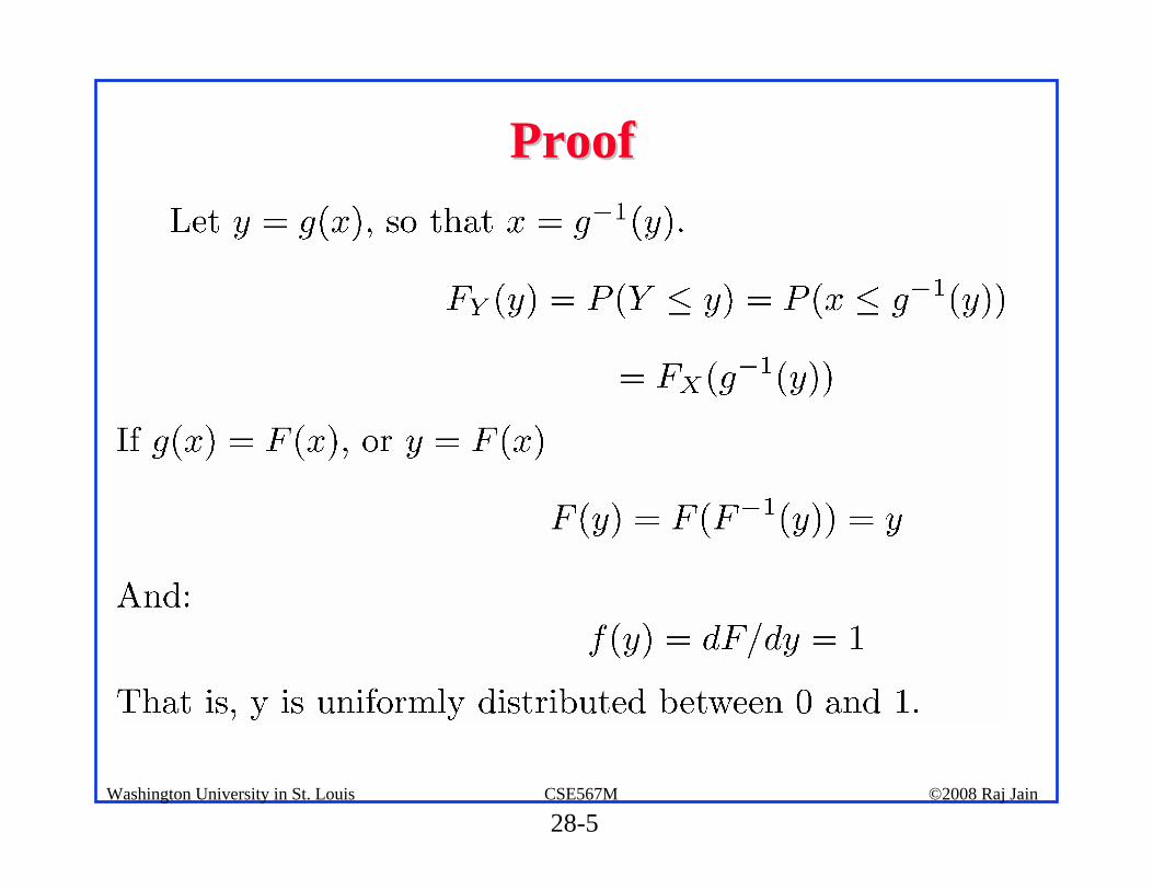
ProofProof

28-6©2008 Raj JainCSE567MWashington University in St. Louis
Example 28.1Example 28.1! For exponential variates:
! If u is U(0,1), 1-u is also U(0,1)! Thus, exponential variables can be generated by:
28-7©2008 Raj JainCSE567MWashington University in St. Louis
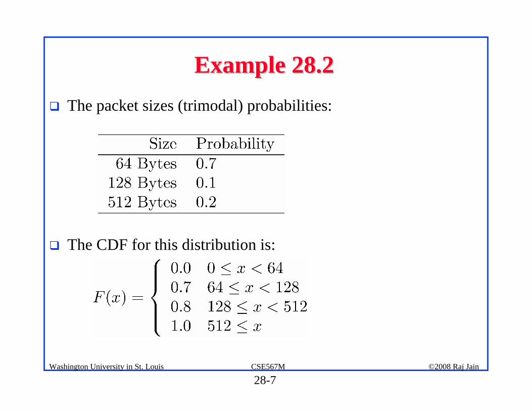
Example 28.2Example 28.2! The packet sizes (trimodal) probabilities:
! The CDF for this distribution is:

28-8©2008 Raj JainCSE567MWashington University in St. Louis
Example 28.2 (Cont)Example 28.2 (Cont)
! The inverse function is:
! Note: CDF is continuous from the right⇒ the value on the right of the discontinuity is used⇒ The inverse function is continuous from the left⇒ u=0.7 ⇒ x=64

28-9©2008 Raj JainCSE567MWashington University in St. Louis
Applications of the InverseApplications of the Inverse--Transformation Transformation TechniqueTechnique

28-10©2008 Raj JainCSE567MWashington University in St. Louis
RejectionRejection! Can be used if a pdf g(x) exists such that c g(x) majorizes the
pdf f(x) ⇒ c g(x) > f(x) ∀ x! Steps:1. Generate x with pdf g(x).2. Generate y uniform on [0, cg(x)].3. If y < f(x), then output x and return.
Otherwise, repeat from step 1.⇒ Continue rejecting the random variates x and y until y > f(x)
! Efficiency = how closely c g(x) envelopes f(x)Large area between c g(x) and f(x) ⇒ Large percentage of (x, y) generated in steps 1 and 2 are rejected
! If generation of g(x) is complex, this method may not be efficient.

28-11©2008 Raj JainCSE567MWashington University in St. Louis
Example 28.2Example 28.2! Beta(2,4) density function:
! Bounded inside a rectangle of height 2.11⇒ Steps:" Generate x uniform on
[0, 1]." Generate y uniform on
[0, 2.11]." If y < 20 x(1-x)3, then
output x and return. Otherwise repeat from step 1.

28-12©2008 Raj JainCSE567MWashington University in St. Louis
CompositionComposition! Can be used if CDF F(x) = Weighted sum of n other CDFs.
! Here, , and Fi's are distribution functions. ! n CDFs are composed together to form the desired CDF
Hence, the name of the technique. ! The desired CDF is decomposed into several other CDFs⇒ Also called decomposition.
! Can also be used if the pdf f(x) is a weighted sum of n other pdfs:
28-13©2008 Raj JainCSE567MWashington University in St. Louis
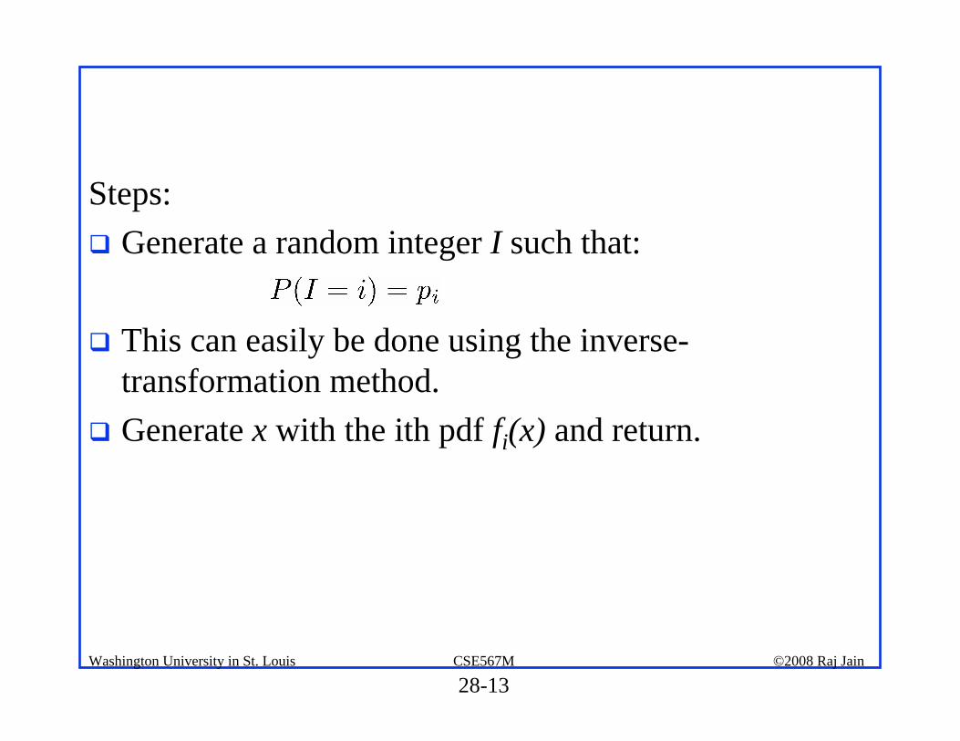
Steps:! Generate a random integer I such that:
! This can easily be done using the inverse-transformation method.
! Generate x with the ith pdf fi(x) and return.

28-14©2008 Raj JainCSE567MWashington University in St. Louis
Example 28.4Example 28.4! pdf:! Composition of two
exponential pdf's! Generate
! If u1<0.5, return; otherwise return x=a ln u2.
! Inverse transformation better for Laplace
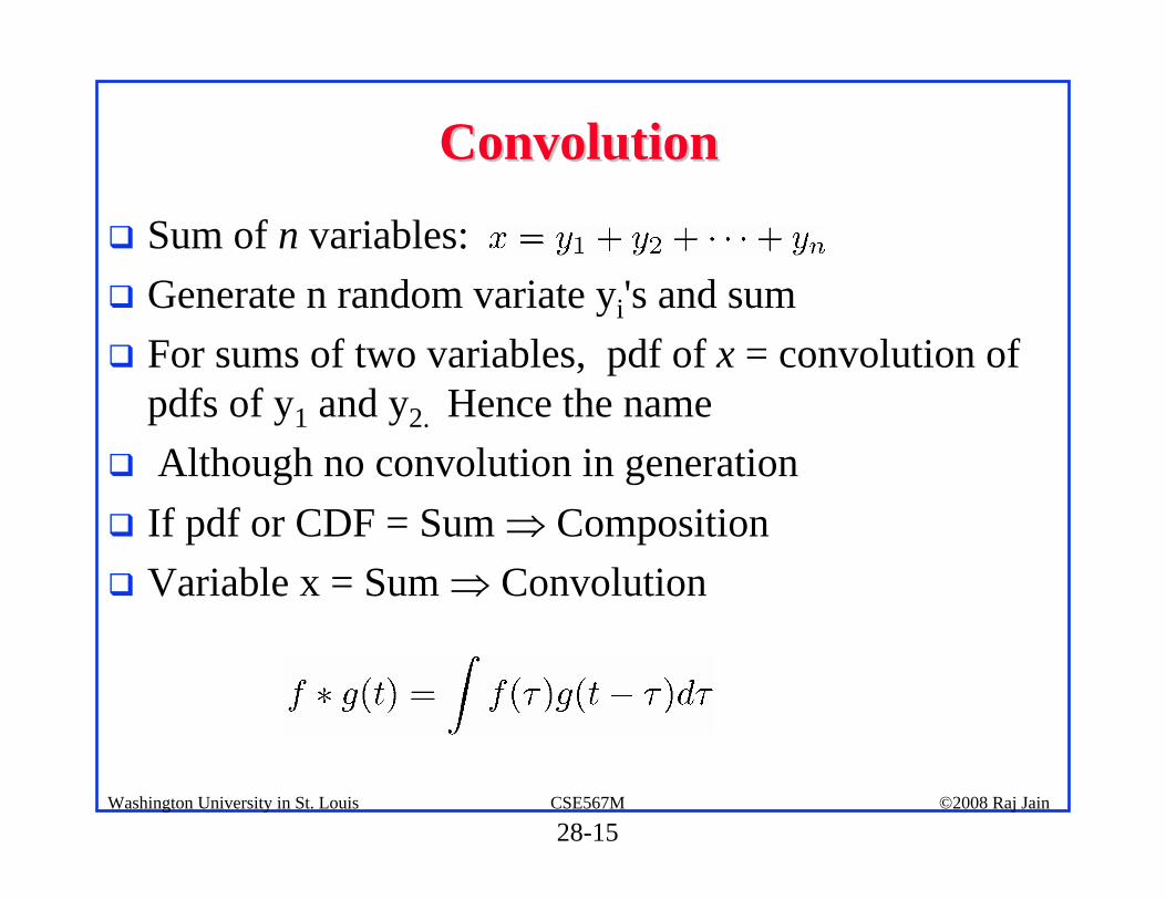
28-15©2008 Raj JainCSE567MWashington University in St. Louis
ConvolutionConvolution
! Sum of n variables:! Generate n random variate yi's and sum! For sums of two variables, pdf of x = convolution of
pdfs of y1 and y2. Hence the name! Although no convolution in generation! If pdf or CDF = Sum ⇒ Composition! Variable x = Sum ⇒ Convolution

28-16©2008 Raj JainCSE567MWashington University in St. Louis
Convolution: ExamplesConvolution: Examples! Erlang-k = ∑i=1
k Exponentiali! Binomial(n, p) = ∑i=1
n Bernoulli(p)⇒ Generated n U(0,1), return the number of RNs less than p
! χ2(ν) = ∑i=1ν N(0,1)2
! Γ(a, b1)+Γ(a,b2)=Γ(a,b1+b2)⇒ Non-integer value of b = integer + fraction
! ∑ι=1n Any = Normal ⇒∑ U(0,1) = Normal
! ∑ι=1m Geometric = Pascal
! ∑ι=12 Uniform = Triangular

28-17©2008 Raj JainCSE567MWashington University in St. Louis
CharacterizationCharacterization! Use special characteristics of distributions ⇒ characterization! Exponential inter-arrival times ⇒ Poisson number of arrivals⇒ Continuously generate exponential variates until their sum exceeds T and return the number of variates generated as the Poisson variate.
! The ath smallest number in a sequence of a+b+1 U(0,1) uniform variates has a β(a, b) distribution.
! The ratio of two unit normal variates is a Cauchy(0, 1) variate.! A chi-square variate with even degrees of freedom χ2(ν) is the
same as a gamma variate γ(2,ν/2).! If x1 and x2 are two gamma variates γ(a,b) and γ(a,c),
respectively, the ratio x1/(x1+x2) is a beta variate β(b,c).! If x is a unit normal variate, eμ+σ x is a lognormal(μ, σ) variate.

28-18©2008 Raj JainCSE567MWashington University in St. Louis
SummarySummary
Is pdf a sumof other pdfs? Use CompositionYes
Is CDF a sumof other CDFs? Use compositionYes
Is CDFinvertible? Use inversionYes

28-19©2008 Raj JainCSE567MWashington University in St. Louis
Summary (Cont)Summary (Cont)
Doesa majorizing function
exist?Use rejectionYes
Is thevariate related to other
variates?Use characterizationYes
Is thevariate a sum of other
variatesUse convolutionYes
Use empirical inversion
No

28-20©2008 Raj JainCSE567MWashington University in St. Louis
Exercise 28.1Exercise 28.1! A random variate has the following triangular density:
! Develop algorithms to generate this variate using each of the following methods:
a. Inverse-transformationb. Rejectionc. Compositiond. Convolution
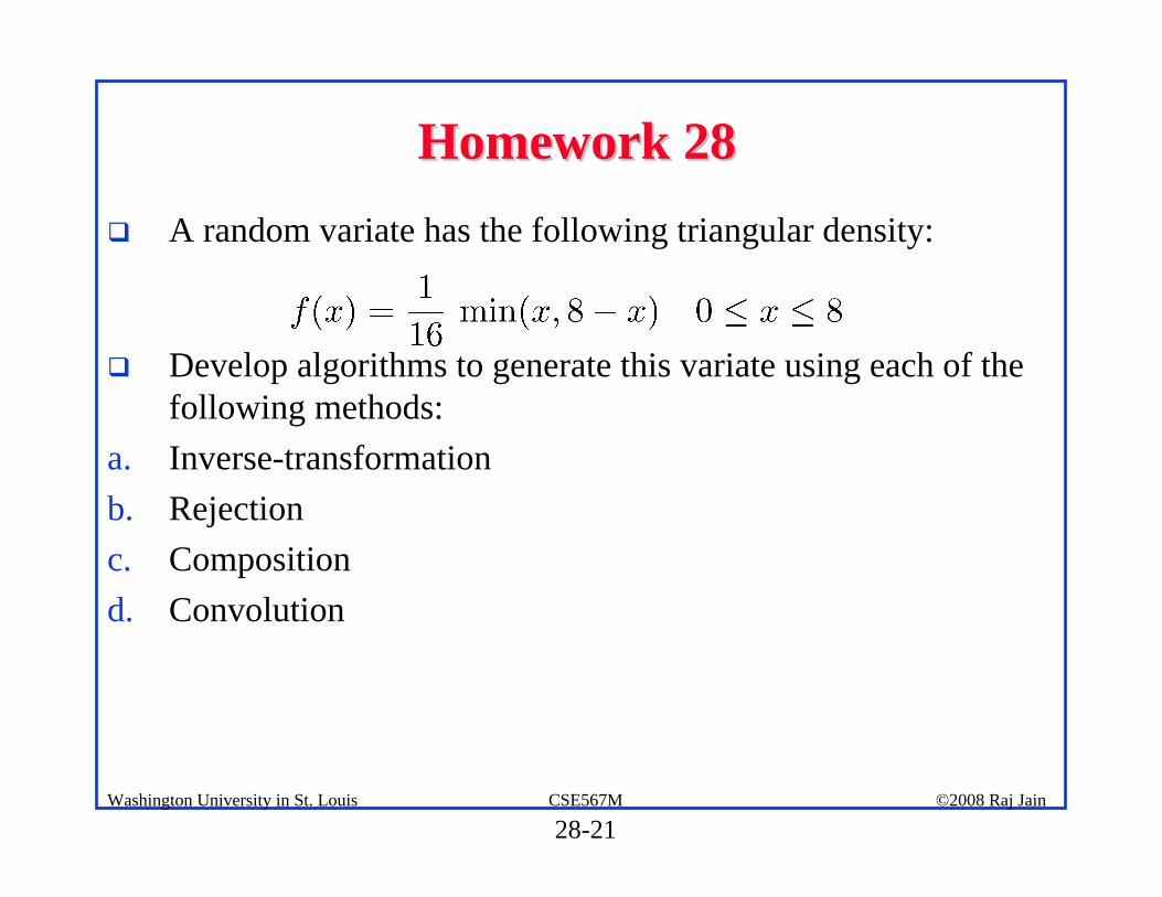
28-21©2008 Raj JainCSE567MWashington University in St. Louis
Homework 28Homework 28! A random variate has the following triangular density:
! Develop algorithms to generate this variate using each of the following methods:
a. Inverse-transformationb. Rejectionc. Compositiond. Convolution
Related Documents