Random (Stochastic) Processesdsp/dsp2013/slides/Course 12 - Random Signals, Oversampling...Random (or Stochastic) Process (or Signal) A random process is random ‘function’, not

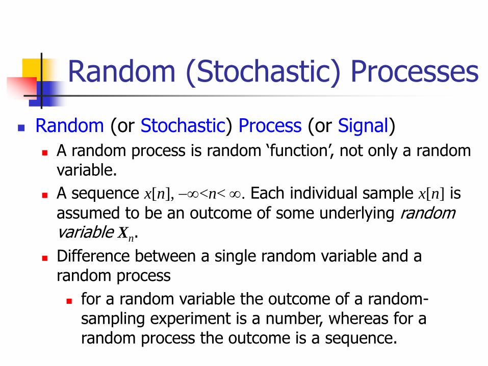
Random (or Stochastic) Process (or Signal)

A random process is random ‘function’, not only a random variable.

A sequence x[n], <n< . Each individual sample x[n] is

assumed to be an outcome of some underlying random variable Xn.

Difference between a single random variable and a random process

for a random variable the outcome of a random-sampling experiment is a number, whereas for a random process the outcome is a sequence.

Random (Stochastic) Processes

Consider a random process x[n], <n< , where each x[n] is drawn from the random variable Xn.

Hence, there are infinite random variables, Xn, <n< .

Strictly speaking, its joint distribution,

p(…, X-2=x[-2], X-1=x[-1],, X0=x[0],, X1=x[1], X2=x[2], …)

is a probability distribution in an infinite-dimensional space.

Random (Stochastic) Processes

However, it is impractical and somewhat infeasible to represent the random (or stochastic) process as a distribution in an infinite-dimensional space.

The most common way to describe a random process is to characterize the distributions for some finite samples, say, {n1, n2, …, nk}, and specify their probability distributions in finite-dimensional spaces:

p(Xn1=x[n1], Xn2=x[n2], …, Xnk=x[nk])

Random (Stochastic) Processes

For example, the Gaussian process is defined as follows:

If for any set of samples n1, n2, …, nk (niZ, kN+), the random process satisfies that the joint distribution of these samples

p(Xn1=x[n1], Xn2=x[n2], …, Xnk=x[nk])

is a multivariate Gaussian distribution, then this process is called a Gaussian process.

Gaussian process is often used in machine learning for nonlinear regression.

Example: Gaussian Process

In signal processing, the random process considered focused more on the joint distributions of two samples, p(Xn1=x[n1], Xn2=x[n2]).

In addition, the shift-invariant property is further imposed (called ‘stationary’ process).

Details will be given below.

Random process in signal processing

Why random process or random signals?

Until now, we have assumed that the signals are deterministic, i.e., each value of a sequence is uniquely determined.

In many situations, the processes that generate signals are so complex as to make precise description of a signal extremely difficult or undesirable.

A random or stochastic signal is considered to be characterized by a set of probability density functions.

Discrete-time random process: A sequence x[n], <n< . Each individual sample x[n] is assumed to be an outcome of some underlying random variable Xn.

Discrete-time Random Signals

A continuous-time random signal is a signal x(t) whose value at each time is a random variable.

Random signals appear often in real life.

Examples include:

1. The noise heard from a radio receiver that is not tuned to an operating channel

2. The noise heard from a helicopter rotor.

3. Electrical signals recorded from a human brain through electrodes put in contact with the skull (these are called electroencephalograms, or EEGs).

Continuous-time Random Signals

4. Mechanical vibrations sensed in a vehicle moving on a rough terrain.

5. Angular motion of a boat in the sea caused by waves and wind.

6. Television signal

7. Radar signal

Probability density function of x[n]:

The pdf is varying with the time index n.

Joint distribution of two samples x[n] and x[m]:

The joint pdf of time indices n and m

Eg., x1[n] = Ancos(wn+n), where An and n are random variables for all < n < , then x1[n] is a

random process.

Definitions (Oppenheim, Appendix)

nxp n ,

mxnxp mn ,,,

x[n] and x[m] are independent iff

x is a stationary process iff

for all k.

That is, the joint distribution of x[n] and x[m] depends only on the time difference m n.

Independence and Stationary

mxpnxpmxnxp mnmn ,,,,,

mxnxpkmxknxp mnkmkn ,,,,,,

In particular, the above definition of stationary process is also applicable to the situation of m=n.

Hence, a stationary random process should also satisfy

That is, the pdf of a stationary process is not varying with the time index n.

Implies that x[n] is shift invariant.

Stationary (continue)

nxpknxp nkn ,,

In many applications of DSP, random processes serve as signal-source models in the sense that a particular signal can be considered a sample sequence of a random process.

Although such a signals are unpredictable – making a deterministic approach to signal representation is inappropriate – certain average properties of the ensemble can be determined, given the probability law of the process.

Stochastic Processes vs. Deterministic Signal

Mean (or average)

denotes the expectation operator

For independent random variables

Average Ensembles: Expectation

nnnnx dxnxpxxm

n,

nnnn dxnxpxgxg ,

mnmn yxyx

Defined in association with the time index n

Mean squared value (also called power of the random signal)

Variance:

Statistics: Mean Square Value and Variance

nnnn dxnxpxx ,

22}{

2

nxnn mxx var

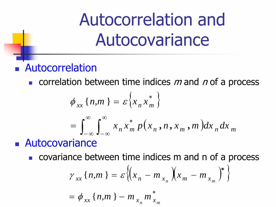
Autocorrelation

correlation between time indices m and n of a process

Autocovariance

covariance between time indices m and n of a process

Autocorrelation and Autocovariance

mnmnmn

mnxx

dxdxmxnxpxx

xxn,m

,,,

}{

mn

mn

xxxx

xmxnxx

mmn,m

mxmxn,m

}{

}{

*

According to the definition of stationary process, the autocorrelation of a stationary process is dependent only on the time difference m n.

Hence, for stationary process, we have

If we denote the time difference by k, we have

Stationary Process

22

xnx

nxx

mx

xmmn

nknxxxx xxknkn ,

Mean and variance are independent to n

Autocorrelation is dependent only to the time difference k

In the above, the stationary property is defined in the strict sense that the pdf should remain the same for all time.

However, for many instances, we encounter random processes that are not stationary in the strict sense. Instead, only the statistics up to the 2-nd order are invariant with time.

To relax the definition, if the following equations hold, we call the process wide-sense stationary (w. s. s.).

Wide-sense Stationary

22

xnx

nxx

mx

xmmn

nknxxxx xxknkn ,

As we see, intuitively, a WSS signal looks more or less the same at different time intervals.

Although its detailed form varies, its overall (or macroscopic) shape does not.

Example of stationary

An example of a random signal that is not WSS. is a seismic wave during an earthquake.

As we see, the amplitude of the wave shortly before the beginning of the earthquake is small. At the start of the earthquake the amplitude grows suddenly, sustains its amplitude for a certain time, then decays.

Example of nonstationary

For any single sample sequence x[n], define their

time average to be

Similarly, time-average autocorrelation is

Time Averages

L

LnL

nxL

nx12

1lim

nxmnxL

nxmnx

L

LnL

12

1lim

Defined by averaging all time indices for an arbitrary instance of the random process

Note that the above time average is defined for a deterministic signal sampled from the random process.

A stationary random process for which time averages equal ensemble averages is called an ergodic process:

Ergodic Process

xmnx

mnxmnx xx

It is common to assume that a given sequence is a sample sequence of an ergodic random process, so that averages can be computed from only a single sequence.

Ergodic Process (continue)

1

0

1

0

22

1

0

1

1

1

L

nL

L

n

xx

L

n

x

nxmnxL

nxmnx

mnxL

nxL

m

ˆ

ˆ

In practice, we cannot compute with the limits, but instead the finite-sum quantities for approximation

W. S. S. correlation sequences

xx n m n

xy n m n

m x x

m x y

Definition: Autocorrelation and cross-correlation sequences (or functions) of W. S. S. random process

Note that, due to the stationary property, the above definitions exist and are independent to the time indices n.

Autocorrelation sequence (or function) is a deterministic signal (not a random signal), which cannot be well defined for a random process that is not W. S. S.

Hence, it specifies unique quantities for W. S. S. signals.

Property (similar properties have already been

shown in the deterministic case)

The above implies

Properties of correlation and covariance sequences (continue)

2

0 0xy xx yy

m

0xx xx

m

Property: (shift invariance)

If

Property

Properties of correlation and covariance sequences (continue)

yy xxm m

0nnn xy

2

0 M ean Squared V aluexx n

x

Since the autocorrelation sequence of a random process is a deterministic signal, its DTFT exists and are bounded in |w|.

Let the DTFT of the autocorrelation sequence be

By doing so, we can view a W. S. S. random process in the spectral domain.

Fourier Transform Representation of Random Signals

jw

xx xxm e

Applying the inverse Fourier Transform:

Recall that

Consequently,

Fourier Transform Representation of Random Signals (continue)

1

2

jw jwm

xx xxm e e dw

2 1

02

jw

xx xxx n e dw

2

0xx

x n

also called the power of the random signal.

Denote

to be the power spectral density; power density spectrum (or power spectrum) of the random process x.

Hence, we have

That is, the total area under power density in [,]

is the total power of the signal.

Fourier Transform Representation of Random Signals (continue)

jw

xxxx ewP

dwwPnx xx

2

12

In sum, from

Pxx(w) can be treated as the “density” at the

frequency w of the total power.

Integrating all the densities from to then constitutes the total energy of a w.s.s. random signal.

This is why Pxx(w) is called power spectral density.

Power Spectral Density

dwwPnx xx

2

12

Property of the power density spectrum:

Pxx(w) is always real-valued since xx(n) is

conjugate symmetric.

For real-valued random processes, Pxx(w) = xx(ejw)

is both real and even.

When the ergodic property is available, we can realize more nature about the power density spectrum.

Power Density Spectrum

Suppose we sample a deterministic signal y from the random process x.

Remember the autocorrelation sequence defined for a deterministic signal is

Power Spectral Density Estimation from Deterministic Signal

yy

n

r l y n y n l

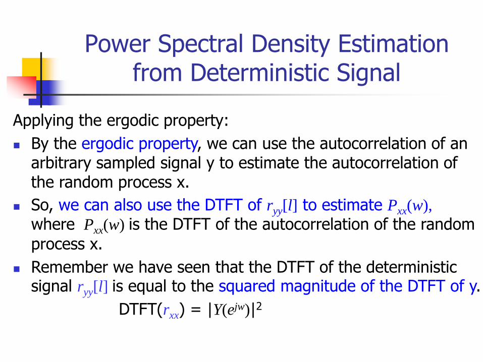
Applying the ergodic property:

By the ergodic property, we can use the autocorrelation of an arbitrary sampled signal y to estimate the autocorrelation of the random process x.

So, we can also use the DTFT of ryy[l] to estimate Pxx(w),

where Pxx(w) is the DTFT of the autocorrelation of the random

process x.

Remember we have seen that the DTFT of the deterministic signal ryy[l] is equal to the squared magnitude of the DTFT of y.

DTFT(rxx) = |Y(ejw)|2

Power Spectral Density Estimation from Deterministic Signal

Hence, the power spectral density Pxx(w) of a

random process x is equal to the squared magnitude spectrum of any of its instance y when the ergodic assumption is hold.

So, the power spectral density is the squared magnitude frequency response of a random process, which does not contain phase information and is always positive.

Power Spectral Density and Squared Magnitude of DTFT

We have seen that a random process is actually a collection of signals, instead of a single or unique signal.

To apply a random process as input to a LTI system, we mean that each signal in this collection serves as input, and we obtain a collection of output signals.

We want to characterize the output collection of signals. What are their ensemble properties?

Input W.S.S. random process to a LTI system

Consider a linear system with the impulse response h[n]. If x[n] is a stationary random signal with mean mx, then the output y[n] is also a stationary random signal with mean my equaling to

Since the input is stationary, mx[nk] = mx , and

consequently,

Mean of the output process

knmkhknxkhnynm x

kk

y

x

j

k

xy meHkhmm0

If x[n] is a real and stationary random signal, the

autocorrelation function of the output process is

Since x[n] is stationary , {x[nk]x[n+mr] } depends only on the time difference m+kr.

Stationary and Linear System

k r

k r

yy

rmnxknxrhkh

rmnxknxrhkh

mnynymnn

,

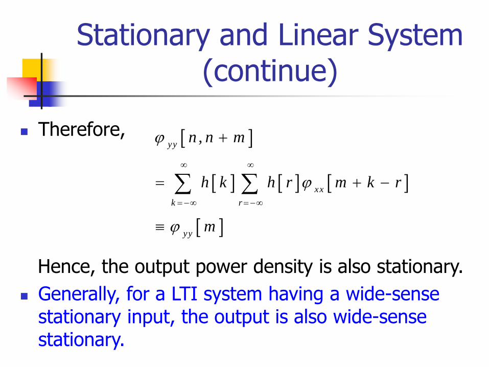
Therefore,

Hence, the output power density is also stationary.

Generally, for a LTI system having a wide-sense stationary input, the output is also wide-sense stationary.

Stationary and Linear System (continue)

,yy

xx

k r

yy

n n m

h k h r m k r

m

Furthermore, by substituting l = rk in the above,

where

A sequence of the form of chh[l] is called a

deterministic autocorrelation sequence.

Power Density Spectrum and Linear System

yy xx

l k

xx hh

l

m m l h k h l k

m l c l

k

hh klhkhlc

Hence,

That is, the autocorrelation sequence of the output random process is the convolution of that of the input random process and chh[l].

So, in the DTFT domain,

where Chh(ejw) is the Fourier transform of chh[l].

Power Density Spectrum and Linear System

yy xx hh

l

m m l c l

jw

xx

jw

hh

jw

yy eeCe

For real chh[l],

So

What is ?

jwjwjw

hh

hh

eHeHeC

lhlhlc

2

jwjw

hheHeC

Correlation of a[n] and b[n] is the convolution of a[n[ and b[-n]

jw

hheC

We have the relation of the input and the output power spectra as follows:

Power Density Spectrum and Linear System (continue)

jw

xx

jwjw

yy eeHe 2

output theofpower average total

2

10

input theofpower average total2

10

22

2

dweeHny

dwenx

jw

xx

jw

yy

jw

xxxx

We have seen that Pxx(w)=xx(ejw) can be viewed as “density.”

Property: The area over a band of frequencies, wa<|w|<wb, is

proportional to the power in the signal in that band.

We can explain this again from the linear-system property above.

Consider an ideal band-pass filter. Let Hbp(ejw) be the

frequency response of the ideal band pass filter for the band wa<|w|<wb.

Power Density Property

1 | |

0 otherw ise

a bjw

bp

w w wH e

Consider the power of the output random signal y when the ideal band-pass filter is applied:

is just equivalent to the power of the random signal x in the band wa<|w|<wb.

Power Density Property

1 1

2 2

a b

b a

w wjw jw

xx xxw w

e dw e dw

1

02

jw

yy yye dw

A white noise signal is a signal for which

Because its autocorrelation is a delta function, its samples at different instants of time are uncorrelated.

The power spectrum of a white noise is a constant

White Noise (or White Gaussian Noise)

2

x

jw

xx e

mm xxx 2

delta function

White noise is very useful in quantization error analysis.

White Gaussian noise: if a random process is both white noise and Gaussian process it is called a white Gaussian noise.

White Noise (or White Gaussian Noise)

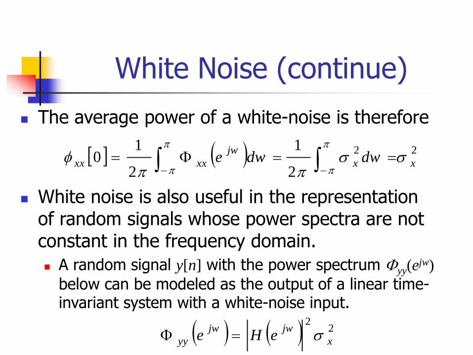
The average power of a white-noise is therefore

White noise is also useful in the representation of random signals whose power spectra are not constant in the frequency domain.

A random signal y[n] with the power spectrum yy(ejw)

below can be modeled as the output of a linear time-invariant system with a white-noise input.

White Noise (continue)

22

2

1

2

10 xx

jw

xxxx dwdwe

22

x

jwjw

yy eHe

Review of Quantization Error

8-bit quantization error

The signal is sufficiently complex and the quantization steps are sufficiently small, so that the amplitude of the signal is likely to traverse many quantization steps from sample to sample.

Review: Assumptions about e[n]

e[n] is a sample sequence of a stationary random process.

e[n] is uncorrelated with the sequence x[n].

The random variables of the error process e[n] are uncorrelated; i.e., the error is a white-noise process.

The probability distribution of the error process is uniform over the range of quantization error (i.e., without being clipped).

Experiments have shown that, as the signal becomes more complicated, the measured correlation between the signal and the quantization error decreases, and the error also becomes uncorrelated.

Review: Quantization error analysis

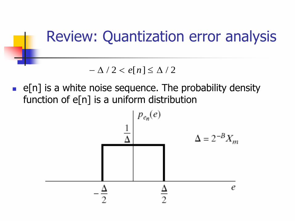
2/][2/ ne

e[n] is a white noise sequence. The probability density function of e[n] is a uniform distribution

Review: quantization error vs. quantization bits

The mean value of e[n] is zero, and its variance is

Since

For a (B+1)-bit quantizer with full-scale value Xm, the noise variance, or power, is

12

122/

2/

22

deee

B

mX

2

12

222

2 m

B

e

X

Review: Quantization error analysis

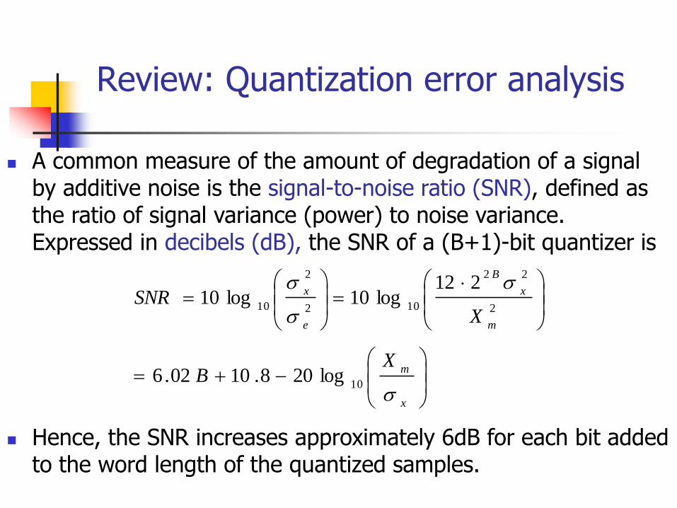
A common measure of the amount of degradation of a signal by additive noise is the signal-to-noise ratio (SNR), defined as the ratio of signal variance (power) to noise variance. Expressed in decibels (dB), the SNR of a (B+1)-bit quantizer is

Hence, the SNR increases approximately 6dB for each bit added to the word length of the quantized samples.

x

m

m

x

B

e

x

XB

XSNR

10

2

22

102

2

10

log208.1002.6

212log10log10

We consider the analog signal xa(t) as zero-mean, wide-sense-stationary, random process with power-spectral density denoted by and the autocorrelation function by .

To simplify our discussion, assume that xa(t) is already bandlimited to N, i.e.,

Oversampling vs. quantization (Oppenheim, Chap. 4)

)(jw

xxe

aa

)(aa xx

,0)( jaa xx

,||N

j

Oversampling: We assume that 2/T = 2MN.

M is an integer, called the oversampling ratio.

Oversampling

Oversampled A/D conversion with simple quantization and down-sampling

Decimation with ideal low-pass filter

Using the additive noise model, the system can be replaced by

Its output xd[n] has two components, one from the signal input xa(t) and the other from the quantization noise input e[n]. Denote them as xda[n] and xde[n], respectively.

Additive noise model

Decimation with ideal low-pass filter

Goal: determine the signal-to noise ratio of signal power {xda

2} to the quantization-noise power {xde

2}. ({.} denotes the expectation value.)

As xa(t) is converted into x[n], and then xda[n], we focus on the power of x[n] first.

Let us analyze this in the time domain. Denote xx[n] and xx(e

jw) to be the autocorrelation and power spectral density of x[n], respectively.

By definition, xx[m]= {x[n+m]x[n]}.

Signal component (assume e[n]=0)

Power of x[n] (assume e[n]=0)

Since x[n]= xa(nT), it is easy to see that

That is, the autocorrelation function of the sequence of samples is a sampled version of the autocorrelation function.

The wide-sense-stationary assumption implies that {xa2(t)}

is a constant independent of t. It then follows that

for all n or t.

]}[][{][ nxmnxmxx

)}())(({ nTxTmnxaa

)(mTaa xx

)}({)}({]}[{222

txnTxnxaa

Power of xda[n] (assume e[n]=0)

Since the decimation filter is an ideal lowpass filter with cutoff frequency wc = /M, the signal x[n] passes unaltered through the filter.

Therefore, the downsampled signal component at the output, xda[n]=x[nM]=xa(nMT), also has the same power.

In sum, the above analyses show that

which shows that the power of the signal component stays the same as it traverses the entire system from the input xa(t) to the corresponding output component xda[n].

)}({]}[{]}[{222

txnxnxada

Power of the noise component

According to previous studies, let us assume that e[n] is a wide-sense-stationary white-noise process with zero mean and variance

Consequently, the autocorrelation function and power density spectrum for e[n] are,

The power spectral density is the DTFT of the autocorrelation function. So,

12

2

2

e

][][2

nneee

white noise

2( ) ,

jw

ee ee w

Power of the noise component (assume xa(t)=0)

Although we have shown that the power in xda[n] does not depend on M, we will show that the noise component xde[n] does not keep the same noise power.

It is because that, as the oversampling ratio M increases, less of the quantization noise spectrum overlaps with the signal spectrum, as shown below.

Review of Downsampling in the Frequency domain (without aliasing)

(over) sampling

Down-sampling (power remains the same for the integral from - to .

CTFT domain

CTFT domain

Illustration of frequency and amplitude scaling

So, when oversampled by M, the power spectrum of xa(t) and x[n] in the frequency domain are illustrated as follows.

Illustration of frequency for noise

By considering both the signal and the quantization noise, the power spectra of x[n] and e[n] in the frequency domain are illustrated as

Noise component power

Then, by ideal low pass with cutoff wc=/M in the decimation, the noise power at the output becomes

Mdwne e

M

Me

2/

/

22

2

1]}[{

Powers after downsampling

Next, the lowpass filtered signal is downsampled, and as we have seen, the signal power remains the same. Hence, the power spectrum of xda[n] and xde[n] in the frequency domain are illustrated as follows:

Noise power reduction

Conclusion: The quantization-noise power {xde2[n]} has

been reduced by a factor of M through the decimation (low-pass filtering + downsampling), while the signal power has remained the same.

For a given quantization noise power, there is a clear tradeoff between the oversampling factor M and the quantization step .

MMdw

Mx ee

de122

1}{

222

2

Oversampling for noise power reduction

Remember that

Therefore

The above equation shows that for a fixed quantizer, the noise power can be decreased by increasing the oversampling ratio M.

Since the signal power is independent of M, increasing M will increase the signal-to-quantization-noise ratio.

B

mX

2

22)

2(

12

1}{

B

m

de

X

Mx

Tradeoff between oversampling and quantization bits

Alternatively, for a fixed quantization noise power,

the required value for B is

From the equation, every doubling of the oversampling ratio M, we need ½ bit less to achieve a given signal-to-quantization-noise ratio.

In other words, if we oversample by a factor M=4, we need one less bit to achieve a desired accuracy in representing the signal.

22)

2(

12

1}{

B

m

dede

X

MxP

mdeXPMB

2222loglog

2

112log

2

1log

2

1