Random Process Model for Urban Traffic Flow Using a Wavelet-Bayesian Hierarchical Technique

Seediscussions,stats,andauthorprofilesforthispublicationat:https://www.researchgate.net/publication/220373617

RandomProcessModelforUrbanTrafficFlowUsingaWavelet-BayesianHierarchicalTechnique.

Article·January2010

Source:DBLP

CITATIONS

2

READS

8

3authors,including:

BidishaGhosh

TrinityCollegeDublin

61PUBLICATIONS340CITATIONS

SEEPROFILE

BiswajitBasu

TrinityCollegeDublin

193PUBLICATIONS1,875CITATIONS

SEEPROFILE

AllcontentfollowingthispagewasuploadedbyBidishaGhoshon16January2015.

Theuserhasrequestedenhancementofthedownloadedfile.Allin-textreferencesunderlinedinbluearelinkedtopublicationsonResearchGate,lettingyouaccessandreadthemimmediately.

Computer-Aided Civil and Infrastructure Engineering 25 (2010) 613–624

Random Process Model for Urban Traffic Flow Usinga Wavelet-Bayesian Hierarchical Technique

Bidisha Ghosh, Biswajit Basu∗ & Margaret O’Mahony

Department of Civil, Structural and Environmental Engineering, Trinity College Dublin,Dublin 2, Ireland

Abstract: The existing well-known short-term trafficforecasting algorithms require large traffic flow data sets,including information on current traffic scenarios to pre-dict the future traffic conditions. This article proposes arandom process traffic volume model that enables esti-mation and prediction of traffic volume at sites wheresuch large and continuous data sets of traffic condi-tion related information are unavailable. The proposedmodel is based on a combination of wavelet analysis(WA) and Bayesian hierarchical methodology (BHM).The average daily “trend” of urban traffic flow obser-vations can be reliably modeled using discrete WA. Theremaining fluctuating parts of the traffic volume observa-tions are modeled using BHM. This BHM modeling con-siders that the variance of the urban traffic flow observa-tions from an intersection vary with the time-of-the-day.A case study has been performed at two busy junctionsat the city-centre of Dublin to validate the effectiveness ofthe strategy.

1 INTRODUCTION

Continuous collection of traffic condition related infor-mation is of critical importance for real-time monitor-ing and operational purposes in an intelligent trans-portation systems (ITS) equipped transport network.In this regard short-term traffic forecasting algorithmshave been developed and applied to assist the continu-ous flow of traffic-related information in near-term fu-ture (Vlahogianni et al., 2004, 2007; Stathopoulos etal., 2008; Boto-Giralda et al., 2010). The basis of allsuch prediction algorithms is that the traffic condition

∗To whom correspondence should be addressed. E-mail: [email protected].

variables are dependent on measurements from previ-ous time intervals and can be used to predict the sub-sequent values of the variables (Vlahogianni, 2008a,b;Kesting and Treiber, 2008; Yang and Recker, 2008).This is also the main drawback of these algorithms asthey require considerably large data sets of previous ob-servations as well as observations from the recent pastavailable through continuous monitoring of traffic con-ditions. To alleviate this drawback, the article employs arandom process traffic volume model to estimate trafficflow at a signalized junction. The model can be used forsituations where measurements related to traffic condi-tions (e.g., volume, speed, or density) are not collectedregularly or where the data collection system (inductiveloop-detector or video-imaging system) is out of ser-vice for a considerable period of time and the existingshort-term traffic forecasting algorithms cannot be ap-plied due to unavailability of data on real-time trafficconditions.

The model is formulated based on a combination ofdiscrete wavelet transform (DWT) (Mallat, 1998) andBayesian hierarchical methodology (BHM). This in-volves modeling the trend underlying the traffic flow ob-servations over a day in a nonfunctional manner usingdiscrete wavelet analysis (WA) and subsequently cap-turing the time-varying variations of the traffic flow overthe trend implementing a BHM.

In transport modeling, WA was introduced primarilyfor developing automatic incident detection algorithms(Samant and Adeli, 2000, 2001; Adeli and Samant, 2000;Adeli and Karim, 2000; Karim and Adeli, 2002a,b, 2003;Teng and Qi, 2003; Adeli and Karim, 2005). In recentyears, DWT technique has been applied by researchersin many different areas of traffic modeling. In highwaytraffic modeling, WA has been used to explore self-similarity1 in vehicular fluctuations (Huang, 2003). Inshort-term traffic flow forecasting algorithms (Hamad

C© 2010 Computer-Aided Civil and Infrastructure Engineering.DOI: 10.1111/j.1467-8667.2010.00681.x

614 Ghosh, Basu & O’Mahony

et al., 2009), DWT has been used by researchers as ade-noising technique (Jiang and Adeli, 2004, 2005; Sunet al., 2005) and as a decomposition technique (Xieet al., 2007). In the field of traffic pattern modeling,varied studies on optimized aggregation level (Qiaoet al., 2003), data reduction (Venkatanarayana et al.,2006), mesoscopic-wavelet modeling (Adeli and Ghosh-Dastidar, 2004), and neural network-wavelet microsim-ulation modeling (Ghosh-Dastidar and Adeli, 2006)have been carried out. In WA-based traffic flow model-ing, DWT using multiresolution analysis (MRA) tech-nique has the potential to decompose the fluctuationsin the traffic flow observations at multiple time-scales(within a day). In this article, this feature of the MRAhas been used to capture the “approximate” variationof the traffic flow observations at a time-scale of the or-der of a day, smoothing out the short-term fluctuations,leading to the nonfunctional “trend” of the traffic flowtime-series data set. The function-free form of the trendhas better flexibility in accommodating the variationsas compared to the trends in functional forms associ-ated with most of the existing time-series models. Therandom fluctuations over the “trend” in traffic flow ob-servations may be considered as a random process inaddition to the modeled “trend.” The characterizationof these random fluctuations is carried out following aBayesian statistical approach.

Application of Bayesian statistics in traffic flow mod-eling and forecasting is a recent phenomenon. Short-term traffic flow forecasting using Bayesian inference-based hierarchical regression models (Tebaldi et al.,2002), Bayesian SARIMA models (Ghosh et al., 2007),and Bayesian networks (Zhang et al., 2004; Queen andAlbers, 2009) are a few available examples of researchin this area. The model discussed in the article utilizesthe concept of BHM in modeling the time-varying vari-ations of traffic flow over the daily trend. Previously, re-searchers have modeled time-dependant flows (Ashokand Ben-Akiva, 2000) and time-varying mean and vari-ances (Cetin and Comert, 2006; Kamarianakis et al.,2005; Tsekeris and Stathopoulos, 2006). This article con-centrates on proposing time-varying variability in mod-eling random fluctuations over “trend” and is unique tosuch modeling. This article establishes the superiority ofthe BHM technique in describing the fluctuations overa regular Gaussian noise model as done in the case ofmost of the existing forecasting algorithms. The studyadditionally establishes the effectiveness of the BHMmodel in dealing with extreme value situations whichare unnaturally high or low values of traffic volume ob-servations brought about by recurrent congestion. Alsothe article assures successful application of the method-ology in both critical and noncritical junctions in the ur-ban arterials.

2 METHODOLOGY

2.1 Multiresolution wavelet analysis

Wavelet transform provides a time–frequency repre-sentation of any signal/time-series data. The basis ofwavelet analysis is decomposing a signal into shifted andscaled components of the original (or mother) wavelet.Multiresolution wavelet analysis (MRWA) uses tech-niques by which the contribution of different frequen-cies of a signal over time can be isolated by using anefficient numerical algorithm. The DWT (Mallat, 1998)of a signal X(t) consists of the collection of coefficients{

cJ (k) =< X, ϕJ k (t) >

dj (k) =< X, ψ j k (t) >

}j, k ∈ Z

where, Z = 1, 2, 3 . . .

(1)

where <∗, ∗> denotes inner product, t is time, {dj (k)}are the detail coefficients at level j (j = 1, 2, . . . , J), and{cJ (k)} are the approximate coefficients at level J. Thesignal X to be analyzed is integral-transformed using aset of basis functions

ψ j k(t) = 2− j/2ψ(2− j t − k) (2)

The set of bases in Equation (2) is constructed fromthe mother-wavelet ψ(t) by a time-shift operation (k)and a dilation operation (j). The function ϕJ k(t) is atime-shifted version of the mother-wavelet scaling func-tion ϕJ (t) : ϕJ k(t) = ϕJ (t − k). ϕJ (t) is a low-pass func-tion, which can separate the low-frequency componentof the signal. Thus, DWT decomposes a signal, at eachlevel, into a low-frequency approximation and a high-frequency detail. In this study, the DWT associated withthe basis Daubechies’ 4 (db4) (Daubechies, 1992) isused to decompose a signal.

The original signal can be reconstructed back fromthe decomposed approximation and the detail compo-nents. Thus, the original signal can be represented as

X(t) = AJ (t) +∑j ≤ J

Dj (t) (3)

where AJ (t) is the reconstruction of the approxima-tion coefficients cJ at level J and Dj (t) is the recon-struction obtained from the detail coefficients dj at levelj. In the reconstructed approximation (AJ ) and in thereconstructed details obtained at each stage/level (D1,D2, D3, . . . , DJ), the numbers of data points remain thesame as the original data set.

2.2 The daily trend model

The “trend” of a time-series data can loosely be definedas the “long-term” change of the mean level of the data

Random process model for urban traffic flow using a wavelet-Bayesian hierarchical technique 615

(Chatfield, 2001). In the daily trend model of the traf-fic flow time-series observations from an urban signal-ized intersection, the word “long-term” indicates stabil-ity over time on a daily basis. In this study, MRWA isused to develop a representative daily trend model un-derlying the traffic flow observations over a day (Ghoshet al., 2006).

In this study, the traffic flow time-series observa-tions are decomposed into different time-scales us-ing the MRWA technique. Initially, the original sig-nal is decomposed into approximation coefficients c1

(low-frequency/fluctuations or variability) and detailcoefficients d1 (high-frequency/fluctuations or variabil-ity). The approximation coefficients c1 (relative low-frequency components) are again decomposed to ap-proximation coefficients c2 and detail coefficients d2 atthe next level. This procedure is repeated for further de-compositions. The aim of repeating the decompositionprocedure is to find an optimum approximation level forextracting the trend in the data. At optimum approx-imation level, the reconstructed approximation coeffi-cients, Am (m is the optimum approximation level), be-come the optimal smoothed estimate of the traffic flowdata set which can truly represent the traffic flow pat-tern on an average day. This is essentially an averag-ing or smoothing technique in a statistical sense and iscomputationally similar to de-noising technique in sig-nal processing. The local variation in traffic flow ob-servations due to signal control in the urban arterialsis considered as fluctuations to be smoothed (for themathematical treatment) in this methodology. The traf-fic flow pattern at any particular approach at any inter-section in an urban transport network is similar for theweekdays. However, there can be some day-to-day vari-ability due to other factors such as the day of the week,accidents, or recurrent congestion in other parts of thetransport network, etc. These factors are uncontrollableand cannot be modeled as such. So, to obtain a “regu-lar trend over an average day,” the Am values over someregular days (approximately 20 days in this study) are tobe averaged. In their previous work, the authors havealready established that this “nonfunctional” averagedaily trend model is superior to the existing well-knownshort-term traffic volume prediction technique the Holt-Winter’s Exponential Smoothing method (Ghosh et al.,2008).

2.3 Residual model

The residuals are obtained by subtracting the “reg-ular trend over an average day” from the orig-inal traffic volume observations. The modeling ofthe residuals helps to establish a confidence intervalover the “nonfunctional trend model.” In this arti-

cle, the residuals are modeled using the following twoapproaches.

a. Crude residual modelb. Bayesian hierarchical residual model

2.3.1 Crude residual model. In statistical analysis,residuals represent the portion of the validation datawhich could not be explained by the model. In thisstudy, the portion of the traffic flow time-series obser-vations which could not be modeled using the “dailytrend model” is treated as the residual. Assuming ran-domness, this residual data set is modeled as Gaussiandistribution. A crude model of the residuals is devel-oped accordingly. This crude model helps to calculatea confidence interval on the “regular trend over an av-erage day” to accommodate the variability of the traf-fic flow in addition to the variations represented by thetrend. The following equation is used in calculating theconfidence limit.

yt = At + μ res + εres where εres ∼ N (0, σ ) (4)

where yt is the estimated traffic volume from the pro-posed model; At is the average value of level three ap-proximation obtained from the trend model; μ res is themean of the residual data set and ε res is the randompart of the residuals. ε res values are randomly generatedfrom a normal distribution with mean zero and standarddeviation σ which is the sample standard deviation ofthe residuals. A 95% confidence interval of the residu-als is used to form the confidence limit.

2.3.2 Bayesian hierarchical residual model. The BHMis a parametric statistical model with a tree-like struc-ture based on the dependencies of the variables. Theparameters of the model at each stage are representedby other parametric statistical models at the next stage.In this study, the variance of the residual is dependenton time and has to be modeled accordingly using an-other parametric statistical model. If R is the vector ofthe residuals averaged over multiple days (say, 20 daysin this study), then in a normal hierarchical model,

Rt ∼ N(m, σ 2

t

)t = 1, 2, . . . ., T (5)

where m is the sample mean of the residuals and σt isthe standard deviation of the residuals for each timeinstant denoted by a subscript t. The vectors σ and Rare both of dimension {T×1} where T is the number oftime intervals or time instants in a day (for 5 min aggre-gate traffic flow observations as used in this study, T =288). The variance σ 2 of the residual data set R changeswith the time of the day. To model this time-varyingvariance, the following parametric prior distribution isproposed.

σ ∼ LN(log( y), τ 2) (6)

616 Ghosh, Basu & O’Mahony

As σ is always positive, a lognormal distribution istaken in Equation (6) to ensure that all σt lie within(0,∞). The lognormal distribution for each σt is cen-tered at log(yt) with standard deviation of τ . The vari-ances of the high-resolution components (sum of level1, 2, and 3 reconstructed from detail coefficients) fromtraffic flow observations over multiple days are calcu-lated over each hour of a day are considered as the ini-tial estimates of the standard deviation of the residual(yt) for that hour of the day. The values of the vectory of dimension {T×1} are constant and site specific. Atthe next stage of the tree-structure of the BHM the vari-ance τ 2 of the lognormal distribution is assumed to fol-low a uniform distribution as its prior, within a range(0, k)

τ ∼ U (0,k) k < ∞ (7)

where k is an arbitrary constant signifying the maxi-mum limit of the values of τ . The exact value of k doesnot influence the estimation process. In this study, theEquations (5)–(7) define the BHM for the residuals. Inthe model, the unknown parameters to be estimatedare σ (σ1, σ2, . . . , σT) and τ . They are represented bya vector ξ = (τ, σ1, σ2, . . . , σT)T and are estimated bythe Bayesian estimation technique (Lee, 1997). For theBayesian inference, the posterior density of the normalhierarchical model is

p(ξ |R, t ) = p(τ )L(σ | R, t)L(τ | σ , t) (8)

where p(ξ |R, t) is the posterior density of ξ ; L(σ | R, t)is the likelihood function of σ and L(τ |σ , t) is the like-lihood function of τ ; p(τ ) is the prior density of param-eter τ . As R is assumed to follow a normal distribution,the likelihood function of σ given R and the time instantvector t (unit time interval = 5 min) is

L(σ | R, t) =T∏

t=1

1√2πσ 2

t

exp(

− R2t

2σ 2t

)(9)

Similarly, the likelihood function of τ given σ , y and tis

L(τ | σ , t) =T∏

t=1

1

σtτ√

2πexp

[− (log σt − log yt )

2

2τ 2

]

(10)

p(τ ) is equal to a constant as the prior density of τ isassumed as flat on the range (0, k). Hence, the posteriordensity from Equation (7) is

p(ξ | R, t) ∝T∏

t=1

1σt

exp(

− R2t

2σ 2t

) T∏t=1

1σtτ

× exp

[− (log σt − log yt )

2

2τ 2

](11a)

which yields

p(ξ | R, t) ∝(

1τ T

) T∏t=1

1

σ 2t

× exp

(− R2

t

2σ 2t

− (log σt − log yt )2

2τ 2

)(11b)

The posterior distribution

F(ξ) =∫ ∞

0. . .

∫ ∞

0

∫ ∞

0

(1τ T

) T∏t=1

1

σ 2t

× exp

(− R2

t

2σ 2t

− (log σt − log yt )2

2τ 2

)dτdσ1 . . . dσT

(12)

By integrating out the other unknown parameters ex-cept for the one whose distribution is to be estimated,the “marginal distributions” of each of the unknown pa-rameters can be determined from the integral in Equa-tion (12). The computation of the marginal distributionsof the unknown parameters in ξ involves evaluation ofa complex integral with problems of high dimensional-ity. In Bayesian estimation, numerical integrations areoften performed to compute the integrations for whichthe analytical solution is intractable. However, numer-ical integration may lead to too large approximationsand may even become intractable for large models. Inmany high-dimensional cases of Bayesian analysis, cer-tain noniterative and iterative refinements of MonteCarlo integration methods are often used (Carlin andLouis, 1996). Markov Chain Monte Carlo (MCMC) isthe particular iterative variation of Monte Carlo methodin which the simulated values are not in iid but are in aMarkov chain. In summary, the goal of the MCMC is,given a target distribution �(x), a Markov chain {xn}is required to be constructed whose limiting distribu-tion is �(x). There are two popular MCMC algorithms:(i) Gibbs sampler (Geman and Geman, 1984) and (ii)Metropolis-Hastings algorithm (Metropolis et al., 1953;Hastings, 1970).

In MCMC method, to simulate the marginal prob-ability distributions for the unknown parameters inthe vector ξ(τ, σ1, σ2, . . . , σT), given an initial condition(τ (0), σ

(0)1 , σ

(0)2 , . . . , σ

(0)T ) the following two steps are to

be iterated (i denotes the number of iteration):

1. Sample τ i+1 from p(τ i+1|σ (i)1 , σ

(i)2 , . . . ., σ

(i)T , yt, t)

using Gibbs sampler technique.2. Sample σ i+1

1 to σ i+1T using Metropolis-Hastings

technique.

The initial conditions (τ (0), σ(0)1 , σ

(0)2 , . . . , σ

(0)T ) are as

follows:

Random process model for urban traffic flow using a wavelet-Bayesian hierarchical technique 617

⎧⎪⎪⎪⎪⎪⎪⎨⎪⎪⎪⎪⎪⎪⎩

σ (0) = |y − 0.5|

τ (0) ∼ Inverse-gamma

⎡⎢⎢⎢⎢⎢⎣

T − 12

,

T∑t=1

(log σ

(0)t − log yt

)2

2

⎤⎥⎥⎥⎥⎥⎦

−1

(13)

In step 1, the Gibbs sampler technique is used to sim-ulate the distribution of τ . From the posterior density inEquation (12), a full conditional distribution for τ is asfollows:

p (τ |σ , R, t ) ∝(

1τ T

)exp

⎛⎜⎜⎜⎜⎜⎝−

T∑t=1

(log σt − log yt )2

2τ 2

⎞⎟⎟⎟⎟⎟⎠

(14)

The full conditional distribution of τ is observed as aninverse-gamma distribution with parameters

α = T2

− 0.5; β = 0.5T∑

t=1

(log σt − log yt )2 (15a)

where the density function of the inverse-gamma distri-bution is as follows:

p (τ ) = βα

� (α)τ−(α+1) exp

(−β

τ

)(15b)

For simplicity, the superscript denoting the numberof iteration is not used in Equations (14) and (15). Step2 is used to simulate the values of σ using Metropolis-Hastings technique. The candidate values of each of theelements of the vector σ are simulated from following

proposal distribution:

σ i ∼ LN[log( y),(τ i )2] (16)

The simulated value of σ i in each iteration is acceptedfollowing the Metropolis algorithm. According to thisalgorithm, each simulated value of the elements of thevector σ i in each iteration is accepted with a probability

�p(σ t )

= p(σ i

t | τ i , σ i−11 , σ i−1

2 , . . . , σ i−1t−1 , σ i−1

t+1 , . . . , σ i−1T , R, t

)p(σ i−1

t | τ i , σ i−11 , σ i−1

2 , . . . , σ i−1t−1 , σ i−1

t+1 , . . . , σ i−1T , R, t

)(17)

or 1 whichever is minimum, with an acceptance crite-ria (Ghosh et al., 2007). The steps 1 and 2 are repeateduntil convergence is achieved. The Equations (12)–(17)are used to simulate the marginal distributions of theunknown parameters. Finally, using these distributionsa 95% confidence interval is calculated over the dailytrend of the traffic volume observations. The BHM gen-erates a different probability distribution for residualsat each different time interval within a day.

3 TRAFFIC FLOW OBSERVATIONS

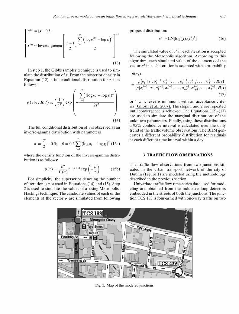
The traffic flow observations from two junctions sit-uated in the urban transport network of the city ofDublin (Figure 1) are modeled using the methodologydescribed in the previous section.

Univariate traffic flow time-series data used for mod-eling are obtained from the inductive loop-detectorsembedded in the streets of both the junctions. The junc-tion TCS 183 is four-armed with one-way traffic on two

Fig. 1. Map of the modeled junctions.

618 Ghosh, Basu & O’Mahony

Fig. 2. Traffic flow observations at junction TCS 183and TCS 439.

approaches. Tara Street (one-way) has four lanes, withtraffic flowing from south to north. The traffic volumepassing through Tara Street is continuously recorded onthe four loop-detectors situated on the four lanes. Thejunction TCS 439 is a comparatively quiet four-armedjunction with one-way traffic on both approaches. Sim-ilar to Tara Street, the traffic volume passing throughTownsend Street is continuously measured using loop-detectors. These flow observations are used in describ-ing and evaluating the proposed traffic volume model.

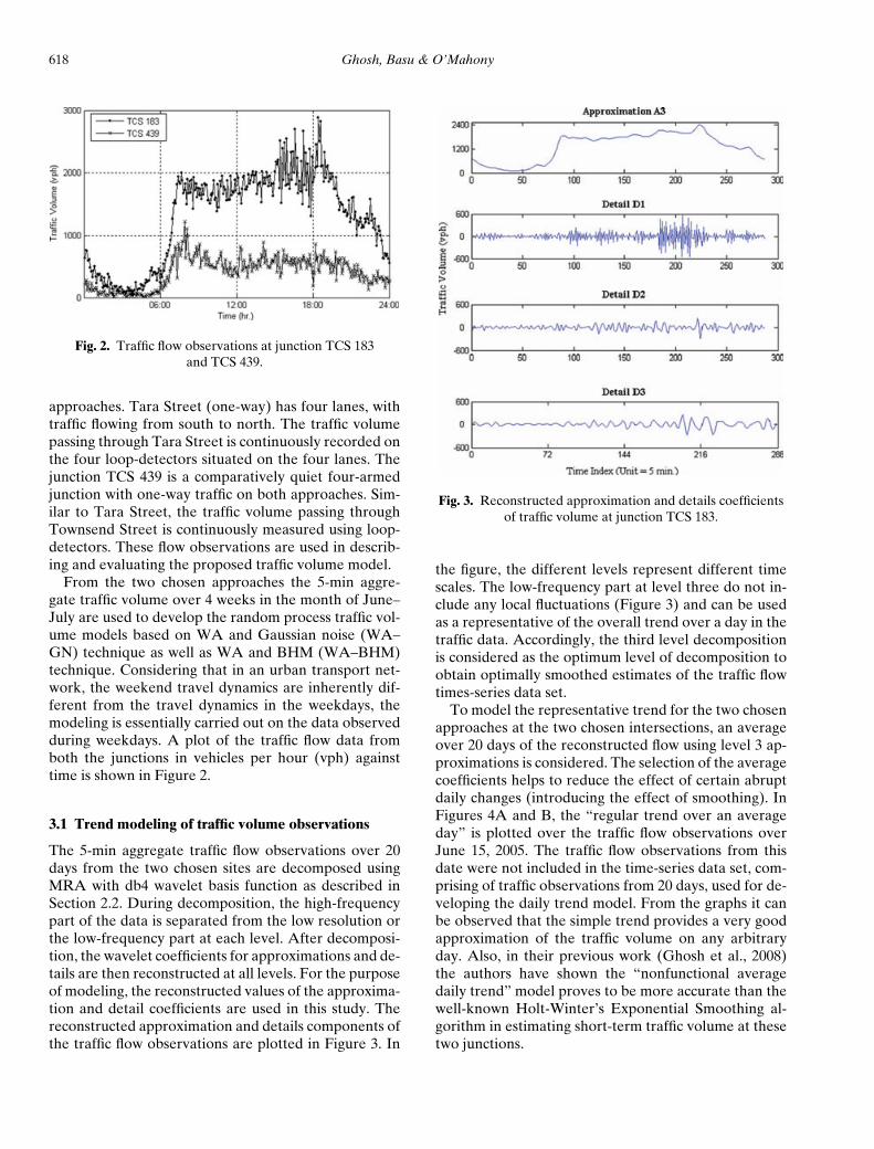
From the two chosen approaches the 5-min aggre-gate traffic volume over 4 weeks in the month of June–July are used to develop the random process traffic vol-ume models based on WA and Gaussian noise (WA–GN) technique as well as WA and BHM (WA–BHM)technique. Considering that in an urban transport net-work, the weekend travel dynamics are inherently dif-ferent from the travel dynamics in the weekdays, themodeling is essentially carried out on the data observedduring weekdays. A plot of the traffic flow data fromboth the junctions in vehicles per hour (vph) againsttime is shown in Figure 2.

3.1 Trend modeling of traffic volume observations

The 5-min aggregate traffic flow observations over 20days from the two chosen sites are decomposed usingMRA with db4 wavelet basis function as described inSection 2.2. During decomposition, the high-frequencypart of the data is separated from the low resolution orthe low-frequency part at each level. After decomposi-tion, the wavelet coefficients for approximations and de-tails are then reconstructed at all levels. For the purposeof modeling, the reconstructed values of the approxima-tion and detail coefficients are used in this study. Thereconstructed approximation and details components ofthe traffic flow observations are plotted in Figure 3. In

Fig. 3. Reconstructed approximation and details coefficientsof traffic volume at junction TCS 183.

the figure, the different levels represent different timescales. The low-frequency part at level three do not in-clude any local fluctuations (Figure 3) and can be usedas a representative of the overall trend over a day in thetraffic data. Accordingly, the third level decompositionis considered as the optimum level of decomposition toobtain optimally smoothed estimates of the traffic flowtimes-series data set.

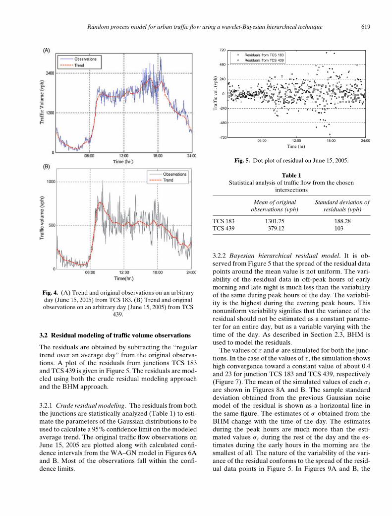
To model the representative trend for the two chosenapproaches at the two chosen intersections, an averageover 20 days of the reconstructed flow using level 3 ap-proximations is considered. The selection of the averagecoefficients helps to reduce the effect of certain abruptdaily changes (introducing the effect of smoothing). InFigures 4A and B, the “regular trend over an averageday” is plotted over the traffic flow observations overJune 15, 2005. The traffic flow observations from thisdate were not included in the time-series data set, com-prising of traffic observations from 20 days, used for de-veloping the daily trend model. From the graphs it canbe observed that the simple trend provides a very goodapproximation of the traffic volume on any arbitraryday. Also, in their previous work (Ghosh et al., 2008)the authors have shown the “nonfunctional averagedaily trend” model proves to be more accurate than thewell-known Holt-Winter’s Exponential Smoothing al-gorithm in estimating short-term traffic volume at thesetwo junctions.

Random process model for urban traffic flow using a wavelet-Bayesian hierarchical technique 619

Fig. 4. (A) Trend and original observations on an arbitraryday (June 15, 2005) from TCS 183. (B) Trend and originalobservations on an arbitrary day (June 15, 2005) from TCS

439.

3.2 Residual modeling of traffic volume observations

The residuals are obtained by subtracting the “regulartrend over an average day” from the original observa-tions. A plot of the residuals from junctions TCS 183and TCS 439 is given in Figure 5. The residuals are mod-eled using both the crude residual modeling approachand the BHM approach.

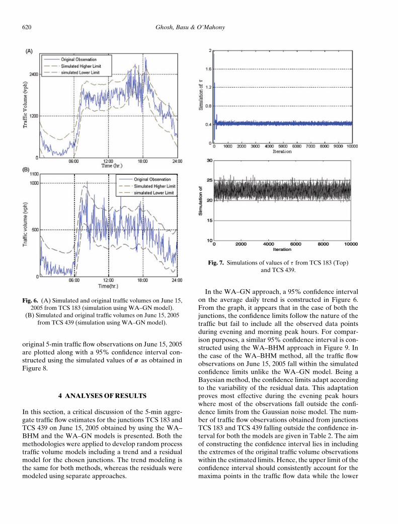
3.2.1 Crude residual modeling. The residuals from boththe junctions are statistically analyzed (Table 1) to esti-mate the parameters of the Gaussian distributions to beused to calculate a 95% confidence limit on the modeledaverage trend. The original traffic flow observations onJune 15, 2005 are plotted along with calculated confi-dence intervals from the WA–GN model in Figures 6Aand B. Most of the observations fall within the confi-dence limits.

Fig. 5. Dot plot of residual on June 15, 2005.

Table 1Statistical analysis of traffic flow from the chosen

intersections

Mean of original Standard deviation ofobservations (vph) residuals (vph)

TCS 183 1301.75 188.28TCS 439 379.12 103

3.2.2 Bayesian hierarchical residual model. It is ob-served from Figure 5 that the spread of the residual datapoints around the mean value is not uniform. The vari-ability of the residual data in off-peak hours of earlymorning and late night is much less than the variabilityof the same during peak hours of the day. The variabil-ity is the highest during the evening peak hours. Thisnonuniform variability signifies that the variance of theresidual should not be estimated as a constant parame-ter for an entire day, but as a variable varying with thetime of the day. As described in Section 2.3, BHM isused to model the residuals.

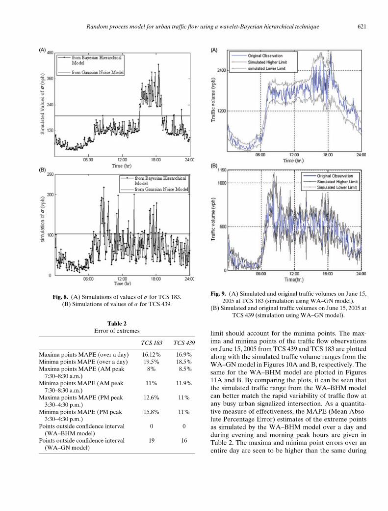
The values of τ and σ are simulated for both the junc-tions. In the case of the values of τ , the simulation showshigh convergence toward a constant value of about 0.4and 23 for junction TCS 183 and TCS 439, respectively(Figure 7). The mean of the simulated values of each σ t

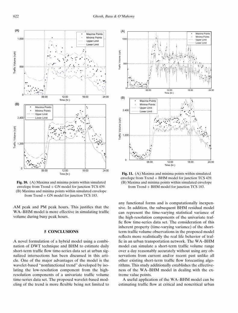
are shown in Figures 8A and B. The sample standarddeviation obtained from the previous Gaussian noisemodel of the residual is shown as a horizontal line inthe same figure. The estimates of σ obtained from theBHM change with the time of the day. The estimatesduring the peak hours are much more than the esti-mated values σ t during the rest of the day and the es-timates during the early hours in the morning are thesmallest of all. The nature of the variability of the vari-ance of the residual conforms to the spread of the resid-ual data points in Figure 5. In Figures 9A and B, the

620 Ghosh, Basu & O’Mahony

Fig. 6. (A) Simulated and original traffic volumes on June 15,2005 from TCS 183 (simulation using WA–GN model).

(B) Simulated and original traffic volumes on June 15, 2005from TCS 439 (simulation using WA–GN model).

original 5-min traffic flow observations on June 15, 2005are plotted along with a 95% confidence interval con-structed using the simulated values of σ as obtained inFigure 8.

4 ANALYSES OF RESULTS

In this section, a critical discussion of the 5-min aggre-gate traffic flow estimates for the junctions TCS 183 andTCS 439 on June 15, 2005 obtained by using the WA–BHM and the WA–GN models is presented. Both themethodologies were applied to develop random processtraffic volume models including a trend and a residualmodel for the chosen junctions. The trend modeling isthe same for both methods, whereas the residuals weremodeled using separate approaches.

Fig. 7. Simulations of values of τ from TCS 183 (Top)and TCS 439.

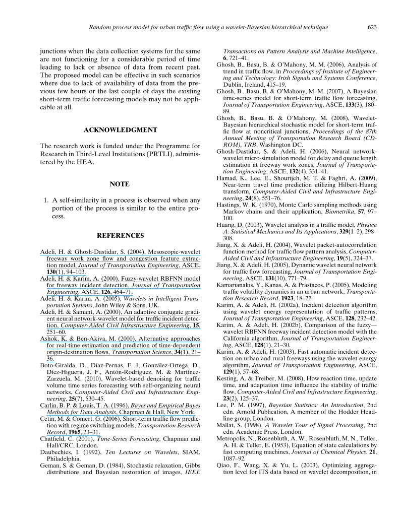
In the WA–GN approach, a 95% confidence intervalon the average daily trend is constructed in Figure 6.From the graph, it appears that in the case of both thejunctions, the confidence limits follow the nature of thetraffic but fail to include all the observed data pointsduring evening and morning peak hours. For compar-ison purposes, a similar 95% confidence interval is con-structed using the WA–BHM approach in Figure 9. Inthe case of the WA–BHM method, all the traffic flowobservations on June 15, 2005 fall within the simulatedconfidence limits unlike the WA–GN model. Being aBayesian method, the confidence limits adapt accordingto the variability of the residual data. This adaptationproves most effective during the evening peak hourswhere most of the observations fall outside the confi-dence limits from the Gaussian noise model. The num-ber of traffic flow observations obtained from junctionsTCS 183 and TCS 439 falling outside the confidence in-terval for both the models are given in Table 2. The aimof constructing the confidence interval lies in includingthe extremes of the original traffic volume observationswithin the estimated limits. Hence, the upper limit of theconfidence interval should consistently account for themaxima points in the traffic flow data while the lower

Random process model for urban traffic flow using a wavelet-Bayesian hierarchical technique 621

Fig. 8. (A) Simulations of values of σ for TCS 183.(B) Simulations of values of σ for TCS 439.

Table 2Error of extremes

TCS 183 TCS 439

Maxima points MAPE (over a day) 16.12% 16.9%Minima points MAPE (over a day) 19.5% 18.5%Maxima points MAPE (AM peak

7:30–8:30 a.m.)8% 8.5%

Minima points MAPE (AM peak7:30–8:30 a.m.)

11% 11.9%

Maxima points MAPE (PM peak3:30–4:30 p.m.)

12.6% 11%

Minima points MAPE (PM peak3:30–4:30 p.m.)

15.8% 11%

Points outside confidence interval(WA–BHM model)

0 0

Points outside confidence interval(WA–GN model)

19 16

Fig. 9. (A) Simulated and original traffic volumes on June 15,2005 at TCS 183 (simulation using WA–GN model).

(B) Simulated and original traffic volumes on June 15, 2005 atTCS 439 (simulation using WA–GN model).

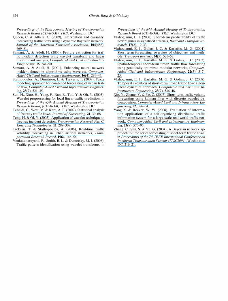
limit should account for the minima points. The max-ima and minima points of the traffic flow observationson June 15, 2005 from TCS 439 and TCS 183 are plottedalong with the simulated traffic volume ranges from theWA–GN model in Figures 10A and B, respectively. Thesame for the WA–BHM model are plotted in Figures11A and B. By comparing the plots, it can be seen thatthe simulated traffic range from the WA–BHM modelcan better match the rapid variability of traffic flow atany busy urban signalized intersection. As a quantita-tive measure of effectiveness, the MAPE (Mean Abso-lute Percentage Error) estimates of the extreme pointsas simulated by the WA–BHM model over a day andduring evening and morning peak hours are given inTable 2. The maxima and minima point errors over anentire day are seen to be higher than the same during

622 Ghosh, Basu & O’Mahony

Fig. 10. (A) Maxima and minima points within simulatedenvelope from Trend + GN model for junction TCS 439.

(B) Maxima and minima points within simulated envelopefrom Trend + GN model for junction TCS 183.

AM peak and PM peak hours. This justifies that theWA–BHM model is more effective in simulating trafficvolume during busy peak hours.

5 CONCLUSIONS

A novel formulation of a hybrid model using a combi-nation of DWT technique and BHM to estimate dailyshort-term traffic flow time-series data set at urban sig-nalized intersections has been discussed in this arti-cle. One of the major advantages of the model is thewavelet-based “nonfunctional trend” developed by iso-lating the low-resolution component from the high-resolution components of a univariate traffic volumetime-series data set. The proposed wavelet-based mod-eling of the trend is more flexible being not limited to

(A)

(B)

Fig. 11. (A) Maxima and minima points within simulatedenvelope from Trend + BHM model for junction TCS 439.(B) Maxima and minima points within simulated envelope

from Trend + BHM model for junction TCS 183.

any functional forms and is computationally inexpen-sive. In addition, the subsequent BHM residual modelcan represent the time-varying statistical variance ofthe high-resolution components of the univariate traf-fic flow time-series data set. The consideration of thisinherent property (time-varying variance) of the short-term traffic volume observations in the proposed modelreflects more realistically the real life behavior of traf-fic in an urban transportation network. The WA–BHMmodel can simulate a short-term traffic volume rangeover a day reasonably accurately without using any ob-servations from current and/or recent past unlike allother existing short-term traffic flow forecasting algo-rithms. This study additionally establishes the effective-ness of the WA–BHM model in dealing with the ex-treme value points.

A useful application of the WA–BHM model can beestimating traffic flow at critical and noncritical urban

Random process model for urban traffic flow using a wavelet-Bayesian hierarchical technique 623

junctions when the data collection systems for the sameare not functioning for a considerable period of timeleading to lack or absence of data from recent past.The proposed model can be effective in such scenarioswhere due to lack of availability of data from the pre-vious few hours or the last couple of days the existingshort-term traffic forecasting models may not be appli-cable at all.

ACKNOWLEDGMENT

The research work is funded under the Programme forResearch in Third-Level Institutions (PRTLI), adminis-tered by the HEA.

NOTE

1. A self-similarity in a process is observed when anyportion of the process is similar to the entire pro-cess.

REFERENCES

Adeli, H. & Ghosh-Dastidar, S. (2004), Mesoscopic-waveletfreeway work zone flow and congestion feature extrac-tion model, Journal of Transportation Engineering, ASCE,130(1), 94–103.

Adeli, H. & Karim, A. (2000), Fuzzy-wavelet RBFNN modelfor freeway incident detection, Journal of TransportationEngineering, ASCE, 126, 464–71.

Adeli, H. & Karim, A. (2005), Wavelets in Intelligent Trans-portation Systems, John Wiley & Sons, UK.

Adeli, H. & Samant, A. (2000), An adaptive conjugate gradi-ent neural network-wavelet model for traffic incident detec-tion, Computer-Aided Civil Infrastructure Engineering, 15,251–60.

Ashok, K. & Ben-Akiva, M. (2000), Alternative approachesfor real-time estimation and prediction of time-dependentorigin-destination flows, Transportation Science, 34(1), 21–36.

Boto-Giralda, D., Dıaz-Pernas, F. J, Gonzalez-Ortega, D.,Dıez-Higuera, J. F., Anton-Rodrıguez, M. & Martınez-Zarzuela, M. (2010), Wavelet-based denoising for trafficvolume time series forecasting with self-organizing neuralnetworks, Computer-Aided Civil and Infrastructure Engi-neering, 25(7), 530–45.

Carlin, B. P. & Louis, T. A. (1996), Bayes and Empirical BayesMethods for Data Analysis, Chapman & Hall, New York.

Cetin, M. & Comert, G. (2006), Short-term traffic flow predic-tion with regime switching models, Transportation ResearchRecord, 1965, 23–31.

Chatfield, C. (2001), Time-Series Forecasting, Chapman andHall/CRC, London.

Daubechies, I. (1992), Ten Lectures on Wavelets, SIAM,Philadelphia.

Geman, S. & Geman, D. (1984), Stochastic relaxation, Gibbsdistributions and Bayesian restoration of images, IEEE

Transactions on Pattern Analysis and Machine Intelligence,6, 721–41.

Ghosh, B., Basu, B. & O’Mahony, M. M. (2006), Analysis oftrend in traffic flow, in Proceedings of Institute of Engineer-ing and Technology: Irish Signals and Systems Conference,Dublin, Ireland, 415–19.

Ghosh, B., Basu, B. & O’Mahony, M. M. (2007), A Bayesiantime-series model for short-term traffic flow forecasting,Journal of Transportation Engineering, ASCE, 133(3), 180–89.

Ghosh, B., Basu, B. & O’Mahony, M. (2008), Wavelet-Bayesian hierarchical stochastic model for short-term traf-fic flow at noncritical junctions, Proceedings of the 87thAnnual Meeting of Transportation Research Board (CD-ROM), TRB, Washington DC.

Ghosh-Dastidar, S. & Adeli, H. (2006), Neural network-wavelet micro-simulation model for delay and queue lengthestimation at freeway work zones, Journal of Transporta-tion Engineering, ASCE, 132(4), 331–41.

Hamad, K., Lee, E., Shourijeh, M. T. & Faghri, A. (2009),Near-term travel time prediction utilizing Hilbert-Huangtransform, Computer-Aided Civil and Infrastructure Engi-neering, 24(8), 551–76.

Hastings, W. K. (1970), Monte Carlo sampling methods usingMarkov chains and their application, Biometrika, 57, 97–100.

Huang, D. (2003), Wavelet analysis in a traffic model, PhysicaA: Statistical Mechanics and Its Applications, 329(1–2), 298–308.

Jiang, X. & Adeli, H. (2004), Wavelet packet-autocorrelationfunction method for traffic flow pattern analysis, Computer-Aided Civil and Infrastructure Engineering, 19(5), 324–37.

Jiang, X. & Adeli, H. (2005), Dynamic wavelet neural networkfor traffic flow forecasting, Journal of Transportation Engi-neering, ASCE, 131(10), 771–79.

Kamarianakis, Y., Kanas, A. & Prastacos, P. (2005), Modelingtraffic volatility dynamics in an urban network, Transporta-tion Research Record, 1923, 18–27.

Karim, A. & Adeli, H. (2002a), Incident detection algorithmusing wavelet energy representation of traffic patterns,Journal of Transportation Engineering, ASCE, 128, 232–42.

Karim, A. & Adeli, H. (2002b), Comparison of the fuzzy—wavelet RBFNN freeway incident detection model with theCalifornia algorithm, Journal of Transportation Engineer-ing, ASCE, 128(1), 21–30.

Karim, A. & Adeli, H. (2003), Fast automatic incident detec-tion on urban and rural freeways using the wavelet energyalgorithm, Journal of Transportation Engineering, ASCE,129(1), 57–68.

Kesting, A. & Treiber, M. (2008), How reaction time, updatetime, and adaptation time influence the stability of trafficflow, Computer-Aided Civil and Infrastructure Engineering,23(2), 125–37.

Lee, P. M. (1997), Bayesian Statistics: An Introduction, 2ndedn. Arnold Publication, A member of the Hodder Head-line group, London.

Mallat, S. (1998), A Wavelet Tour of Signal Processing, 2ndedn. Academic Press, London.

Metropolis, N., Rosenbluth, A. W., Rosenbluth, M. N., Teller,A. H. & Teller, E. (1953), Equation of state calculations byfast computing machines, Journal of Chemical Physics, 21,1087–92.

Qiao, F., Wang, X. & Yu, L. (2003), Optimizing aggrega-tion level for ITS data based on wavelet decomposition, in

624 Ghosh, Basu & O’Mahony

Proceedings of the 82nd Annual Meeting of TransportationResearch Board (CD-ROM), TRB, Washington DC.

Queen, C. & Albers, C. (2009), Intervention and causality:forecasting traffic flows using a dynamic Bayesian network,Journal of the American Statistical Association, 104(486),669–81.

Samant, A. & Adeli, H. (2000), Feature extraction for traf-fic incident detection using wavelet transform and lineardiscriminant analysis, Computer-Aided Civil InfrastructureEngineering, 15, 241–50.

Samant, A. & Adeli, H. (2001), Enhancing neural networkincident detection algorithms using wavelets, Computer-Aided Civil and Infrastructure Engineering, 16(4), 239–45.

Stathopoulos, A., Dimitriou, L. & Tsekeris, T. (2008), Fuzzymodeling approach for combined forecasting of urban traf-fic flow, Computer-Aided Civil and Infrastructure Engineer-ing, 23(7), 521–35.

Sun, H., Xiao, H., Yang, F., Ran, B., Tao, Y. & Oh, Y. (2005),Wavelet preprocessing for local linear traffic prediction, inProceedings of the 85th Annual Meeting of TransportationResearch Board, (CD-ROM), TRB, Washington DC.

Tebaldi, C., West, M. & Karr, A. F. (2002), Statistical analysisof freeway traffic flows, Journal of Forecasting, 21, 39–68.

Teng, H. & Qi, Y. (2003), Application of wavelet technique tofreeway incident detection, Transportation Research Part C:Emerging Technologies, 11, 289–308.

Tsekeris, T. & Stathopoulos, A. (2006), Real-time trafficvolatility forecasting in urban arterial networks, Trans-portation Research Record, 1964, 146–56.

Venkatanarayana, R., Smith, B. L. & Demetsky, M. J. (2006),Traffic pattern identification using wavelet transforms, in

Proceedings of the 84th Annual Meeting of TransportationResearch Board (CD-ROM), TRB, Washington DC.

Vlahogianni, E. I. (2008), Short-term predictability of trafficflow regimes in signalised arterials, Road and Transport Re-search, 17(2), 19–33.

Vlahogianni, E. I., Golias, J. C. & Karlaftis, M. G. (2004),Short-term forecasting: overview of objectives and meth-ods, Transport Reviews, 24(5), 533–57.

Vlahogianni, E. I., Karlaftis, M. G. & Golias, J. C. (2007),Spatio-temporal short-term urban traffic flow forecastingusing genetically-optimized modular networks, Computer-Aided Civil and Infrastructure Engineering, 22(5), 317–25.

Vlahogianni, E. I., Karlaftis, M. G. & Golias, J. C. (2008),Temporal evolution of short-term urban traffic flow: a non-linear dynamics approach, Computer-Aided Civil and In-frastructure Engineering, 23(7), 536–48.

Xie, Y., Zhang, Y. & Ye, Z. (2007), Short-term traffic volumeforecasting using kalman filter with discrete wavelet de-composition, Computer-Aided Civil and Infrastructure En-gineering, 22, 326–34.

Yang X. & Recker, W. W. (2008), Evaluation of informa-tion applications of a self-organizing distributed trafficinformation system for a large-scale real-world traffic net-work, Computer-Aided Civil and Infrastructure Engineer-ing, 23(8), 575–95.

Zhang, C., Sun, S. & Yu, G. (2004), A Bayesian network ap-proach to time series forecasting of short-term traffic flows,in Proceedings of the 7th IEEE International Conference onIntelligent Transportation Systems (ITSC2004), WashingtonDC, 216–21.