Notes for ECE 534 An Exploration of Random Processes for Engineers Bruce Hajek January 1, 2014 c 2014 by Bruce Hajek All rights reserved. Permission is hereby given to freely print and circulate copies of these notes so long as the notes are left intact and not reproduced for commercial purposes. Email to [email protected], pointing out errors or hard to understand passages or providing comments, is welcome.

Welcome message from author
This document is posted to help you gain knowledge. Please leave a comment to let me know what you think about it! Share it to your friends and learn new things together.
Transcript

8/11/2019 Random process by B. Hajek
http://slidepdf.com/reader/full/random-process-by-b-hajek 1/448
Notes for ECE 534
An Exploration of Random Processes for Engineers
Bruce Hajek
January 1, 2014
c 2014 by Bruce HajekAll rights reserved. Permission is hereby given to freely print and circulate copies of these notes so long as the notes are left
intact and not reproduced for commercial purposes. Email to [email protected], pointing out errors or hard to understand
passages or providing comments, is welcome.

8/11/2019 Random process by B. Hajek
http://slidepdf.com/reader/full/random-process-by-b-hajek 2/448
Contents
1 Getting Started 1
1.1 The axioms of probability theory . . . . . . . . . . . . . . . . . . . . . . . . . . . . . 1
1.2 Independence and conditional probability . . . . . . . . . . . . . . . . . . . . . . . . 5
1.3 Random variables and their distribution . . . . . . . . . . . . . . . . . . . . . . . . . 8
1.4 Functions of a random variable . . . . . . . . . . . . . . . . . . . . . . . . . . . . . . 111.5 Expectation of a random variable . . . . . . . . . . . . . . . . . . . . . . . . . . . . . 16
1.6 Frequently used distributions . . . . . . . . . . . . . . . . . . . . . . . . . . . . . . . 211.7 Failure rate functions . . . . . . . . . . . . . . . . . . . . . . . . . . . . . . . . . . . . 25
1.8 Jointly distributed random variables . . . . . . . . . . . . . . . . . . . . . . . . . . . 26
1.9 Conditional densities . . . . . . . . . . . . . . . . . . . . . . . . . . . . . . . . . . . . 271.10 Correlation and covariance . . . . . . . . . . . . . . . . . . . . . . . . . . . . . . . . . 28
1.11 Transformation of random vectors . . . . . . . . . . . . . . . . . . . . . . . . . . . . 29
1.12 Problems . . . . . . . . . . . . . . . . . . . . . . . . . . . . . . . . . . . . . . . . . . 32
2 Convergence of a Sequence of Random Variables 43
2.1 Four definitions of convergence of random variables . . . . . . . . . . . . . . . . . . . 432.2 Cauchy criteria for convergence of random variables . . . . . . . . . . . . . . . . . . 54
2.3 Limit theorems for sums of independent random variables . . . . . . . . . . . . . . . 58
2.4 Convex functions and Jensen’s inequality . . . . . . . . . . . . . . . . . . . . . . . . 612.5 Chernoff bound and large deviations theory . . . . . . . . . . . . . . . . . . . . . . . 63
2.6 Problems . . . . . . . . . . . . . . . . . . . . . . . . . . . . . . . . . . . . . . . . . . 67
3 Random Vectors and Minimum Mean Squared Error Estimation 79
3.1 Basic definitions and properties . . . . . . . . . . . . . . . . . . . . . . . . . . . . . . 79
3.2 The orthogonality principle for minimum mean square error estimation . . . . . . . . 813.3 Conditional expectation and linear estimators . . . . . . . . . . . . . . . . . . . . . . 85
3.3.1 Conditional expectation as a projection . . . . . . . . . . . . . . . . . . . . . 853.3.2 Linear estimators . . . . . . . . . . . . . . . . . . . . . . . . . . . . . . . . . . 873.3.3 Comparison of the estimators . . . . . . . . . . . . . . . . . . . . . . . . . . . 88
3.4 Joint Gaussian distribution and Gaussian random vectors . . . . . . . . . . . . . . . 90
3.5 Linear innovations sequences . . . . . . . . . . . . . . . . . . . . . . . . . . . . . . . 963.6 Discrete-time Kalman filtering . . . . . . . . . . . . . . . . . . . . . . . . . . . . . . 97
iii

8/11/2019 Random process by B. Hajek
http://slidepdf.com/reader/full/random-process-by-b-hajek 3/448
iv CONTENTS
3.7 Problems . . . . . . . . . . . . . . . . . . . . . . . . . . . . . . . . . . . . . . . . . . 101
4 Random Processes 111
4.1 Definition of a random process . . . . . . . . . . . . . . . . . . . . . . . . . . . . . . 1114.2 Random walks and gambler’s ruin . . . . . . . . . . . . . . . . . . . . . . . . . . . . 114
4.3 Processes with independent increments and martingales . . . . . . . . . . . . . . . . 1164.4 Brownian motion . . . . . . . . . . . . . . . . . . . . . . . . . . . . . . . . . . . . . . 1184.5 Counting processes and the Poisson process . . . . . . . . . . . . . . . . . . . . . . . 119
4.6 Stationarity . . . . . . . . . . . . . . . . . . . . . . . . . . . . . . . . . . . . . . . . . 1234.7 Joint properties of random processes . . . . . . . . . . . . . . . . . . . . . . . . . . . 1264.8 Conditional independence and Markov processes . . . . . . . . . . . . . . . . . . . . 126
4.9 Discrete-state Markov processes . . . . . . . . . . . . . . . . . . . . . . . . . . . . . . 1304.10 Space-time structure of discrete-state Markov processes . . . . . . . . . . . . . . . . 136
4.11 Problems . . . . . . . . . . . . . . . . . . . . . . . . . . . . . . . . . . . . . . . . . . 139
5 Inference for Markov Models 1535.1 A bit of estimation theory . . . . . . . . . . . . . . . . . . . . . . . . . . . . . . . . . 1535.2 The expectation-maximization (EM) algorithm . . . . . . . . . . . . . . . . . . . . . 1585.3 Hidden Markov models . . . . . . . . . . . . . . . . . . . . . . . . . . . . . . . . . . . 163
5.3.1 Posterior state probabilities and the forward-backward algorithm . . . . . . . 1 6 45.3.2 Most likely state sequence – Viterbi algorithm . . . . . . . . . . . . . . . . . 1675.3.3 The Baum-Welch algorithm, or EM algorithm for HMM . . . . . . . . . . . . 168
5.4 Notes . . . . . . . . . . . . . . . . . . . . . . . . . . . . . . . . . . . . . . . . . . . . 1705.5 Problems . . . . . . . . . . . . . . . . . . . . . . . . . . . . . . . . . . . . . . . . . . 170
6 Dynamics of Countable-State Markov Models 179
6.1 Examples with finite state space . . . . . . . . . . . . . . . . . . . . . . . . . . . . . 1796.2 Classification and convergence of discrete-time Markov processes . . . . . . . . . . . 1816.3 Classification and convergence of continuous-time Markov processes . . . . . . . . . 1846.4 Classification of birth-death processes . . . . . . . . . . . . . . . . . . . . . . . . . . 187
6.5 Time averages vs. statistical averages . . . . . . . . . . . . . . . . . . . . . . . . . . 1896.6 Queueing systems, M/M/1 queue and Little’s law . . . . . . . . . . . . . . . . . . . . 191
6.7 Mean arrival rate, distributions seen by arrivals, and PASTA . . . . . . . . . . . . . 1946.8 More examples of queueing systems modeled as Markov birth-death processes . . . 1966.9 Foster-Lyapunov stability criterion and moment bounds . . . . . . . . . . . . . . . . 198
6.9.1 Stability criteria for discrete-time processes . . . . . . . . . . . . . . . . . . . 1986.9.2 Stability criteria for continuous time processes . . . . . . . . . . . . . . . . . 206
6.10 Problems . . . . . . . . . . . . . . . . . . . . . . . . . . . . . . . . . . . . . . . . . . 209
7 Basic Calculus of Random Processes 2197.1 Continuity of random processes . . . . . . . . . . . . . . . . . . . . . . . . . . . . . . 219
7.2 Mean square differentiation of random processes . . . . . . . . . . . . . . . . . . . . 2257.3 Integration of random processes . . . . . . . . . . . . . . . . . . . . . . . . . . . . . . 229

8/11/2019 Random process by B. Hajek
http://slidepdf.com/reader/full/random-process-by-b-hajek 4/448
CONTENTS v
7.4 Ergodicity . . . . . . . . . . . . . . . . . . . . . . . . . . . . . . . . . . . . . . . . . . 2367.5 Complexification, Part I . . . . . . . . . . . . . . . . . . . . . . . . . . . . . . . . . . 2427.6 The Karhunen-Loeve expansion . . . . . . . . . . . . . . . . . . . . . . . . . . . . . . 244
7.7 Periodic WSS random processes . . . . . . . . . . . . . . . . . . . . . . . . . . . . . . 2527.8 Problems . . . . . . . . . . . . . . . . . . . . . . . . . . . . . . . . . . . . . . . . . . 254
8 Random Processes in Linear Systems and Spectral Analysis 2638.1 Basic definitions . . . . . . . . . . . . . . . . . . . . . . . . . . . . . . . . . . . . . . 264
8.2 Fourier transforms, transfer functions and power spectral densities . . . . . . . . . . 2678.3 Discrete-time processes in linear systems . . . . . . . . . . . . . . . . . . . . . . . . . 2748.4 Baseband random processes . . . . . . . . . . . . . . . . . . . . . . . . . . . . . . . . 276
8.5 Narrowband random processes . . . . . . . . . . . . . . . . . . . . . . . . . . . . . . 2798.6 Complexification, Part II . . . . . . . . . . . . . . . . . . . . . . . . . . . . . . . . . 285
8.7 Problems . . . . . . . . . . . . . . . . . . . . . . . . . . . . . . . . . . . . . . . . . . 287
9 Wiener filtering 2979.1 Return of the orthogonality principle . . . . . . . . . . . . . . . . . . . . . . . . . . . 2979.2 The causal Wiener filtering problem . . . . . . . . . . . . . . . . . . . . . . . . . . . 3009.3 Causal functions and spectral factorization . . . . . . . . . . . . . . . . . . . . . . . 300
9.4 Solution of the causal Wiener filtering problem for rational power spectral densities . 3059.5 Discrete time Wiener filtering . . . . . . . . . . . . . . . . . . . . . . . . . . . . . . . 3099.6 Problems . . . . . . . . . . . . . . . . . . . . . . . . . . . . . . . . . . . . . . . . . . 314
10 Martingales 323
10.1 Conditional expectation revisited . . . . . . . . . . . . . . . . . . . . . . . . . . . . . 32310.2 Martingales with respect to filtrations . . . . . . . . . . . . . . . . . . . . . . . . . . 328
10.3 Azuma-Hoeffding inequaltity . . . . . . . . . . . . . . . . . . . . . . . . . . . . . . . 33110.4 Stopping times and the optional sampling theorem . . . . . . . . . . . . . . . . . . . 33510.5 Notes . . . . . . . . . . . . . . . . . . . . . . . . . . . . . . . . . . . . . . . . . . . . 33910.6 Problems . . . . . . . . . . . . . . . . . . . . . . . . . . . . . . . . . . . . . . . . . . 340
11 Appendix 345
11.1 Some notation . . . . . . . . . . . . . . . . . . . . . . . . . . . . . . . . . . . . . . . 34511.2 Convergence of sequences of numbers . . . . . . . . . . . . . . . . . . . . . . . . . . . 34611.3 Continuity of functions . . . . . . . . . . . . . . . . . . . . . . . . . . . . . . . . . . . 350
11.4 Derivatives of functions . . . . . . . . . . . . . . . . . . . . . . . . . . . . . . . . . . 35111.5 Integration . . . . . . . . . . . . . . . . . . . . . . . . . . . . . . . . . . . . . . . . . 353
11.5.1 Riemann integration . . . . . . . . . . . . . . . . . . . . . . . . . . . . . . . . 35311.5.2 Lebesgue integration . . . . . . . . . . . . . . . . . . . . . . . . . . . . . . . . 35511.5.3 Riemann-Stieltjes integration . . . . . . . . . . . . . . . . . . . . . . . . . . . 35611.5.4 Lebesgue-Stieltjes integration . . . . . . . . . . . . . . . . . . . . . . . . . . . 356
11.6 On convergence of the mean . . . . . . . . . . . . . . . . . . . . . . . . . . . . . . . . 35711.7 Matrices . . . . . . . . . . . . . . . . . . . . . . . . . . . . . . . . . . . . . . . . . . . 359

8/11/2019 Random process by B. Hajek
http://slidepdf.com/reader/full/random-process-by-b-hajek 5/448
CONTENTS v
12 Solutions to Problems 365

8/11/2019 Random process by B. Hajek
http://slidepdf.com/reader/full/random-process-by-b-hajek 6/448
vi CONTENTS
8/11/2019 Random process by B. Hajek
http://slidepdf.com/reader/full/random-process-by-b-hajek 7/448
Preface
From an applications viewpoint, the main reason to study the subject of these notes is to helpdeal with the complexity of describing random, time-varying functions. A random variable canbe interpreted as the result of a single measurement. The distribution of a single random vari-able is fairly simple to describe. It is completely specified by the cumulative distribution functionF (x), a function of one variable. It is relatively easy to approximately represent a cumulativedistribution function on a computer. The joint distribution of several random variables is muchmore complex, for in general, it is described by a joint cumulative probability distribution function,F (x1, x2, . . . , xn), which is much more complicated than n functions of one variable. A randomprocess, for example a model of time-varying fading in a communication channel, involves many,possibly infinitely many (one for each time instant t within an observation interval) random vari-ables. Woe the complexity!
These notes help prepare the reader to understand and use the following methods for dealingwith the complexity of random processes:
• Work with moments, such as means and covariances.
• Use extensively processes with special properties. Most notably, Gaussian processes are char-acterized entirely be means and covariances, Markov processes are characterized by one-steptransition probabilities or transition rates, and initial distributions. Independent incrementprocesses are characterized by the distributions of single increments.
• Appeal to models or approximations based on limit theorems for reduced complexity descrip-tions, especially in connection with averages of independent, identically distributed randomvariables. The law of large numbers tells us that, in a certain context, a probability distri-bution can be characterized by its mean alone. The central limit theorem, similarly tells usthat a probability distribution can be characterized by its mean and variance. These limittheorems are analogous to, and in fact examples of, perhaps the most powerful tool ever dis-covered for dealing with the complexity of functions: Taylor’s theorem, in which a function
in a small interval can be approximated using its value and a small number of derivatives ata single point.
• Diagonalize. A change of coordinates reduces an arbitrary n-dimensional Gaussian vectorinto a Gaussian vector with n independent coordinates. In the new coordinates the jointprobability distribution is the product of n one-dimensional distributions, representing a great
vii
8/11/2019 Random process by B. Hajek
http://slidepdf.com/reader/full/random-process-by-b-hajek 8/448
viii CONTENTS
reduction of complexity. Similarly, a random process on an interval of time, is diagonalized bythe Karhunen-Loeve representation. A periodic random process is diagonalized by a Fourierseries representation. Stationary random processes are diagonalized by Fourier transforms.
• Sample. A narrowband continuous time random process can be exactly represented by itssamples taken with sampling rate twice the highest frequency of the random process. Thesamples offer a reduced complexity representation of the original process.
• Work with baseband equivalent. The range of frequencies in a typical radio transmissionis much smaller than the center frequency, or carrier frequency, of the transmission. Thesignal could be represented directly by sampling at twice the largest frequency component.However, the sampling frequency, and hence the complexity, can be dramatically reduced bysampling a baseband equivalent random process.
These notes were written for the first semester graduate course on random processes, offeredby the Department of Electrical and Computer Engineering at the University of Illinois at Urbana-Champaign. Students in the class are assumed to have had a previous course in probability, whichis briefly reviewed in the first chapter of these notes. Students are also expected to have somefamiliarity with real analysis and elementary linear algebra, such as the notions of limits, definitionsof derivatives, Riemann integration, and diagonalization of symmetric matrices. These topics arereviewed in the appendix. Finally, students are expected to have some familiarity with transformmethods and complex analysis, though the concepts used are reviewed in the relevant chapters.
Each chapter represents roughly two weeks of lectures, and includes homework problems. Solu-tions to the even numbered problems without stars can be found at the end of the notes. Studentsare encouraged to first read a chapter, then try doing the even numbered problems before lookingat the solutions. Problems with stars, for the most part, investigate additional theoretical issues,and solutions are not provided.
Hopefully some students reading these notes will find them useful for understanding the diversetechnical literature on systems engineering, ranging from control systems, signal and image process-ing, communication theory, and analysis of a variety of networks. Hopefully some students will goon to design systems, and define and analyze stochastic models. Hopefully others will be motivatedto continue study in probability theory, going on to learn measure theory and its applications toprobability and analysis in general.
A brief comment is in order on the level of rigor and generality at which these notes are written.Engineers and scientists have great intuition and ingenuity, and routinely use methods that arenot typically taught in undergraduate mathematics courses. For example, engineers generally havegood experience and intuition about transforms, such as Fourier transforms, Fourier series, andz-transforms, and some associated methods of complex analysis. In addition, they routinely use
generalized functions, in particular the delta function is frequently used. The use of these conceptsin these notes leverages on this knowledge, and it is consistent with mathematical definitions,but full mathematical justification is not given in every instance. The mathematical backgroundrequired for a full mathematically rigorous treatment of the material in these notes is roughly atthe level of a second year graduate course in measure theoretic probability, pursued after a courseon measure theory.

8/11/2019 Random process by B. Hajek
http://slidepdf.com/reader/full/random-process-by-b-hajek 9/448
CONTENTS ix
The author gratefully acknowledges the students and faculty (Todd Coleman, Christoforos Had- jicostis, Andrew Singer, R. Srikant, and Venu Veeravalli) in the past five years for their commentsand corrections.
Bruce HajekJanuary 2014

8/11/2019 Random process by B. Hajek
http://slidepdf.com/reader/full/random-process-by-b-hajek 10/448
x CONTENTS
Organization
The first four chapters of the notes are used heavily in the remaining chapters, so that mostreaders should cover those chapters before moving on.
Chapter 1 is meant primarily as a review of concepts found in a typical first course on probabilitytheory, with an emphasis on axioms and the definition of expectation. Readers desiring amore extensive review of basic probability are referred to the author’s notes for ECE 313 atUniversity of Illinois.
Chapter 2 focuses on various ways in which a sequence of random variables can converge, andthe basic limit theorems of probability: law of large numbers, central limit theorem, and theasymptotic behavior of large deviations.
Chapter 3 focuses on minimum mean square error estimation and the orthogonality principle.
Chapter 4 introduces the notion of random process, and briefly covers several examples and classesof random processes. Markov processes and martingales are introduced in this chapter, butare covered in greater depth in later chapters.
The following four additional topics can be covered independently of each other.
Chapter 5 describes the use of Markov processes for modeling and statistical inference. Applica-tions include natural language processing.
Chapter 6 describes the use of Markov processes for modeling and analysis of dynamical systems.Applications include the modeling of queueing systems.
Chapters 7-9 develop calculus for random processes based on mean square convergence, moving to
linear filtering, orthogonal expansions, and ending with causal and noncausal Wiener filtering.
Chapter 10 explores martingales with respect to filtrations, with emphasis on elementary concen-tration inequalities, and on the optional sampling theorem
In recent one-semester course offerings, the author covered Chapters 1-5, Sections 6.1-6.8, Chap-ter 7, Sections 8.1-8.4, and Section 9.1. Time did not permit to cover the Foster-Lyapunov stabilitycriteria, noncausal Wiener filtering, and the chapter on martingales.
A number of background topics are covered in the appendix, including basic notation.
8/11/2019 Random process by B. Hajek
http://slidepdf.com/reader/full/random-process-by-b-hajek 11/448
Chapter 1
Getting Started
This chapter reviews many of the main concepts in a first level course on probability theory with
more emphasis on axioms and the definition of expectation than is typical of a first course.
1.1 The axioms of probability theory
Random processes are widely used to model systems in engineering and scientific applications.These notes adopt the most widely used framework of probability and random processes, namelythe one based on Kolmogorov’s axioms of probability. The idea is to assume a mathematically soliddefinition of the model. This structure encourages a modeler to have a consistent, if not accurate,model.
A probability space is a triplet (Ω, F , P ). The first component, Ω, is a nonempty set. Eachelement ω of Ω is called an outcome and Ω is called the sample space . The second component,
F ,
is a set of subsets of Ω called events. The set of events F is assumed to be a σ-algebra, meaning itsatisfies the following axioms: (See Appendix 11.1 for set notation).
A.1 Ω ∈ F
A.2 If A ∈ F then Ac ∈ F
A.3 If A, B ∈ F then A ∪ B ∈ F . Also, if A1, A2, . . . is a sequence of elements in F then∞i=1 Ai ∈ F
If F is a σ-algebra and A, B ∈ F , then AB ∈ F by A.2, A.3 and the fact AB = (Ac ∪ Bc)c. By
the same reasoning, if A1, A2, . . . is a sequence of elements in a σ-algebra F , then ∞i=1 Ai ∈ F .Events Ai, i ∈ I , indexed by a set I are called mutually exclusive if the intersection AiA j = ∅for all i, j ∈ I with i = j . The final component, P , of the triplet (Ω, F , P ) is a probability measureon F satisfying the following axioms:
P.1 P (A) ≥ 0 for all A ∈ F
1
8/11/2019 Random process by B. Hajek
http://slidepdf.com/reader/full/random-process-by-b-hajek 12/448
2 CHAPTER 1. GETTING STARTED
P.2 If A, B ∈ F and if A and B are mutually exclusive, then P (A∪B) = P (A) + P (B). Also,if A1, A2, . . . is a sequence of mutually exclusive events in F then P (
∞i=1 Ai) =
∞i=1 P (Ai).
P.3 P (Ω) = 1.
The axioms imply a host of properties including the following. For any subsets A, B , C of F :• If A ⊂ B then P (A) ≤ P (B)
• P (A ∪ B) = P (A) + P (B) − P (AB)
• P (A ∪ B ∪ C ) = P (A) + P (B) + P − P (AB) − P (AC ) − P (BC ) + P (ABC )
• P (A) + P (Ac) = 1
• P (∅) = 0.
Example 1.1.1 (Toss of a fair coin) Using “H ” for “heads” and “T ” for “tails,” the toss of a faircoin is modelled by
Ω = H, T F = H , T , H, T , ∅
P H = P T = 1
2, P H, T = 1, P (∅) = 0
Note that, for brevity, we omitted the parentheses and wrote P H instead of P (H ).
Example 1.1.2 (Standard unit-interval probability space) Take Ω = θ : 0 ≤ θ ≤ 1. Imagine anexperiment in which the outcome ω is drawn from Ω with no preference towards any subset. Inparticular, we want the set of events F to include intervals, and the probability of an interval [a, b]with 0 ≤ a ≤ b ≤ 1 to be given by:
P ( [a, b] ) = b − a. (1.1)
Taking a = b, we see that F contains singleton sets a, and these sets have probability zero. SinceF is to be a σ-algrebra, it must also contain all the open intervals (a, b) in Ω, and for such an openinterval, P ( (a, b) ) = b − a. Any open subset of Ω is the union of a finite or countably infinite set
of open intervals, so that F should contain all open and all closed subsets of Ω. Thus, F mustcontain the intersection of any set that is the intersection of countably many open sets, and soon. The specification of the probability function P must be extended from intervals to all of F .It is not a priori clear how large F can be. It is tempting to take F to be the set of all subsetsof Ω. However, that idea doesn’t work–see Problem 1.37 showing that the length of all subsets of R can’t be defined in a consistent way. The problem is resolved by taking F to be the smallest
8/11/2019 Random process by B. Hajek
http://slidepdf.com/reader/full/random-process-by-b-hajek 13/448
1.1. THE AXIOMS OF PROBABILITY THEORY 3
σ-algebra containing all the subintervals of Ω, or equivalently, containing all the open subsets of Ω. This σ-algebra is called the Borel σ-algebra for [0, 1], and the sets in it are called Borel sets.While not every subset of Ω is a Borel subset, any set we are likely to encounter in applications
is a Borel set. The existence of the Borel σ-algebra is discussed in Problem 1.38. Furthermore,extension theorems of measure theory1 imply that P can be extended from its definition (1.1) forinterval sets to all Borel sets.
The smallest σ-algebra, B, containing the open subsets of R is called the Borel σ-algebra for R,and the sets in it are called Borel sets. Similarly, the Borel σ-algebra Bn of subsets of Rn is thesmallest σ-algebra containing all sets of the form [a1, b1] × [a2, b2] × · · · × [an, bn]. Sets in Bn arecalled Borel subsets of Rn. The class of Borel sets includes not only rectangle sets and countableunions of rectangle sets, but all open sets and all closed sets. Virtually any subset of Rn arising inapplications is a Borel set.
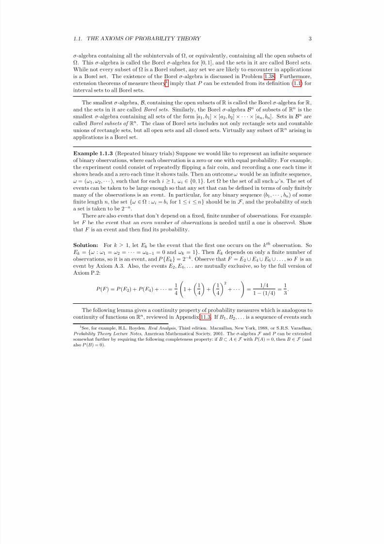
Example 1.1.3 (Repeated binary trials) Suppose we would like to represent an infinite sequenceof binary observations, where each observation is a zero or one with equal probability. For example,the experiment could consist of repeatedly flipping a fair coin, and recording a one each time itshows heads and a zero each time it shows tails. Then an outcome ω would be an infinite sequence,ω = (ω1, ω2, · · · ), such that for each i ≥ 1, ωi ∈ 0, 1. Let Ω be the set of all such ω ’s. The set of events can be taken to be large enough so that any set that can be defined in terms of only finitelymany of the observations is an event. In particular, for any binary sequence (b1, · · · , bn) of somefinite length n, the set ω ∈ Ω : ωi = bi for 1 ≤ i ≤ n should be in F , and the probability of sucha set is taken to be 2−n.
There are also events that don’t depend on a fixed, finite number of observations. For example,let F be the event that an even number of observations is needed until a one is observed. Showthat F is an event and then find its probability.
Solution: For k ≥ 1, let E k be the event that the first one occurs on the kth observation. SoE k = ω : ω1 = ω2 = · · · = ωk−1 = 0 and ωk = 1. Then E k depends on only a finite number of observations, so it is an event, and P E k = 2−k. Observe that F = E 2 ∪ E 4 ∪ E 6 ∪ . . . , so F is anevent by Axiom A.3. Also, the events E 2, E 4, . . . are mutually exclusive, so by the full version of Axiom P.2:
P (F ) = P (E 2) + P (E 4) + · · · = 1
4
1 +
1
4
+
1
4
2
+ · · ·
= 1/4
1 − (1/4) =
1
3.
The following lemma gives a continuity property of probability measures which is analogous tocontinuity of functions on Rn, reviewed in Appendix 11.3. If B1, B2, . . . is a sequence of events such
1See, for example, H.L. Royden, Real Analysis , Third edition. Macmillan, New York, 1988, or S.R.S. Varadhan,Probability Theory Lecture Notes , American Mathematical Society, 2001. The σ-algebra F and P can be extendedsomewhat further by requiring the following completeness property: if B ⊂ A ∈ F with P (A) = 0, then B ∈ F (andalso P (B) = 0).
8/11/2019 Random process by B. Hajek
http://slidepdf.com/reader/full/random-process-by-b-hajek 14/448
4 CHAPTER 1. GETTING STARTED
that B1 ⊂ B2 ⊂ B3 ⊂ · · · , then we can think that B j converges to the set ∪∞i=1Bi as j → ∞. The
lemma states that in this case, P (B j) converges to the probability of the limit set as j → ∞.
Lemma 1.1.4 (Continuity of Probability) Suppose B1, B2, . . . is a sequence of events.(a) If B1 ⊂ B2 ⊂ · · · then lim j→∞ P (B j) = P (∞i=1 Bi)
(b) If B1 ⊃ B2 ⊃ · · · then lim j→∞ P (B j) = P (∞
i=1 Bi)
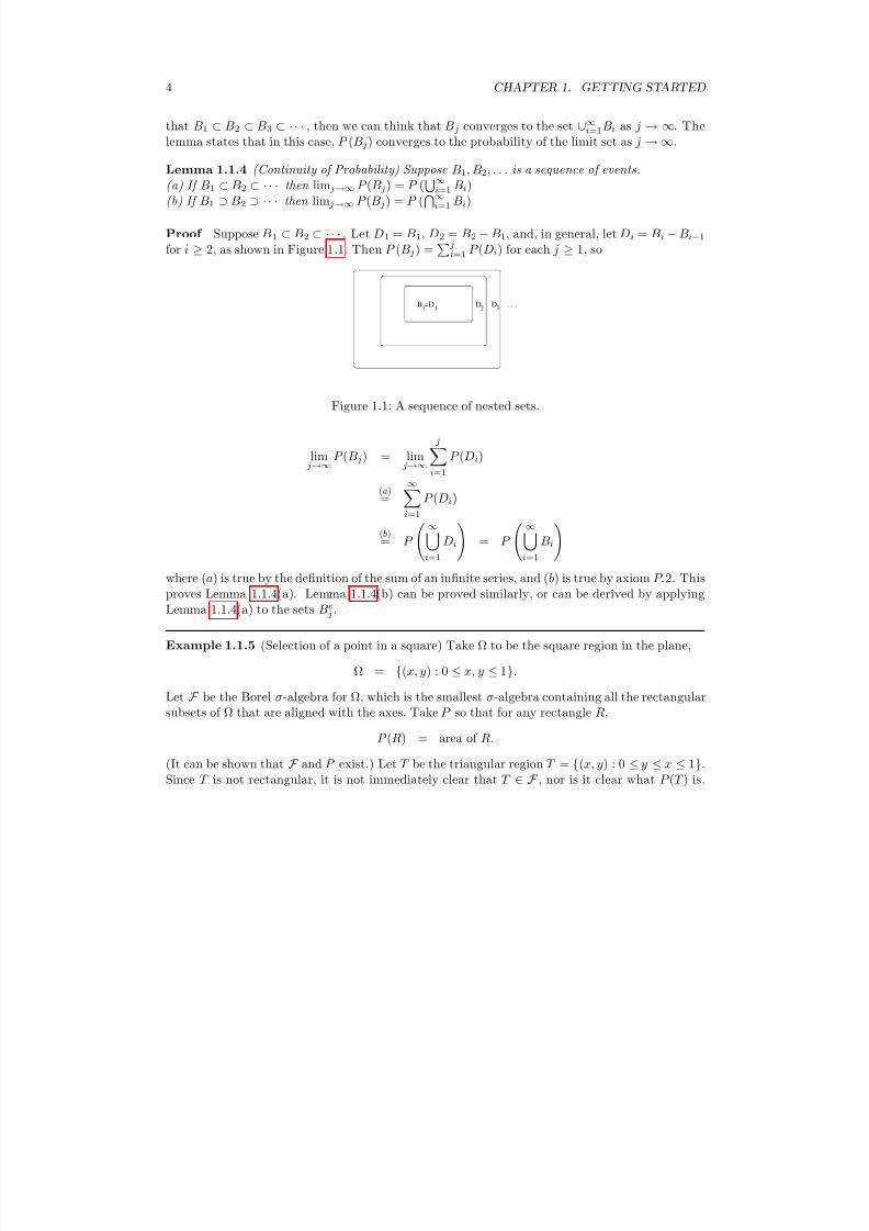
Proof Suppose B1 ⊂ B2 ⊂ · · · . Let D1 = B1, D2 = B2 − B1, and, in general, let Di = Bi − Bi−1
for i ≥ 2, as shown in Figure 1.1. Then P (B j) = j
i=1 P (Di) for each j ≥ 1, so
B =D D1 1
D2 3
. . .
Figure 1.1: A sequence of nested sets.
lim j→∞
P (B j) = lim j→∞
ji=1
P (Di)
(a)=
∞i=1
P (Di)
(b)= P
∞i=1
Di
= P ∞
i=1
Bi
where (a) is true by the definition of the sum of an infinite series, and ( b) is true by axiom P.2. Thisproves Lemma 1.1.4(a). Lemma 1.1.4(b) can be proved similarly, or can be derived by applyingLemma 1.1.4(a) to the sets Bc
j .
Example 1.1.5 (Selection of a point in a square) Take Ω to be the square region in the plane,
Ω = (x, y) : 0 ≤ x, y ≤ 1.
Let F
be the Borel σ-algebra for Ω, which is the smallest σ-algebra containing all the rectangularsubsets of Ω that are aligned with the axes. Take P so that for any rectangle R,
P (R) = area of R.
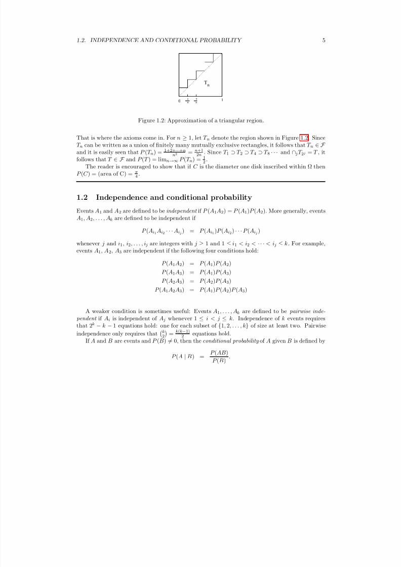
(It can be shown that F and P exist.) Let T be the triangular region T = (x, y) : 0 ≤ y ≤ x ≤ 1.Since T is not rectangular, it is not immediately clear that T ∈ F , nor is it clear what P (T ) is.
8/11/2019 Random process by B. Hajek
http://slidepdf.com/reader/full/random-process-by-b-hajek 15/448
1.2. INDEPENDENCE AND CONDITIONAL PROBABILITY 5
Tn
1 2
nn 10
Figure 1.2: Approximation of a triangular region.
That is where the axioms come in. For n ≥ 1, let T n denote the region shown in Figure 1.2. SinceT n can be written as a union of finitely many mutually exclusive rectangles, it follows that T n ∈ F and it is easily seen that P (T n) = 1+2+···+n
n2 = n+1
2n . Since T 1 ⊃ T 2 ⊃ T 4 ⊃ T 8 · · · and ∩ jT 2j = T , it
follows that T ∈ F and P (T ) = limn→∞ P (T n) =
1
2 .The reader is encouraged to show that if C is the diameter one disk inscribed within Ω thenP (C ) = (area of C) = π
4 .
1.2 Independence and conditional probability
Events A1 and A2 are defined to be independent if P (A1A2) = P (A1)P (A2). More generally, eventsA1, A2, . . . , Ak are defined to be independent if
P (Ai1Ai2 · · · Aij ) = P (Ai1)P (Ai2) · · · P (Aij )
whenever j and i1, i2, . . . , i j are integers with j ≥ 1 and 1 ≤ i1 < i2 < · · · < i j ≤ k . For example,events A1, A2, A3 are independent if the following four conditions hold:
P (A1A2) = P (A1)P (A2)
P (A1A3) = P (A1)P (A3)
P (A2A3) = P (A2)P (A3)
P (A1A2A3) = P (A1)P (A2)P (A3)
A weaker condition is sometimes useful: Events A1, . . . , Ak are defined to be pairwise inde-pendent if Ai is independent of A j whenever 1
≤ i < j
≤ k. Independence of k events requires
that 2k − k − 1 equations hold: one for each subset of 1, 2, . . . , k of size at least two. Pairwiseindependence only requires that
k2
= k(k−1)
2 equations hold.If A and B are events and P (B) = 0, then the conditional probability of A given B is defined by
P (A | B) = P (AB)
P (B) .

8/11/2019 Random process by B. Hajek
http://slidepdf.com/reader/full/random-process-by-b-hajek 16/448
6 CHAPTER 1. GETTING STARTED
It is not defined if P (B) = 0, which has the following meaning. If you were to write a computerroutine to compute P (A | B) and the inputs are P (AB) = 0 and P (B) = 0, your routine shouldn’tsimply return the value 0. Rather, your routine should generate an error message such as “input
error–conditioning on event of probability zero.” Such an error message would help you or othersfind errors in larger computer programs which use the routine.
As a function of A for B fixed with P (B) = 0, the conditional probability of A given B is itself a probability measure for Ω and F . More explicitly, fix B with P (B) = 0. For each event A defineP (A) = P (A | B). Then (Ω, F , P ) is a probability space, because P satisfies the axioms P 1− P 3.(Try showing that).
If A and B are independent then Ac and B are independent. Indeed, if A and B are independentthen
P (AcB) = P (B) − P (AB) = (1 − P (A))P (B) = P (Ac)P (B).
Similarly, if A, B, and C are independent events then AB is independent of C . More generally,
suppose E 1, E 2, . . . , E n are independent events, suppose n = n1 +· · ·+nk with ni ≥ 1 for each i, andsuppose F 1 is defined by Boolean operations (intersections, complements, and unions) of the first n1
events E 1, . . . , E n1, F 2 is defined by Boolean operations on the next n2 events, E n1+1, . . . , E n1+n2 ,and so on, then F 1, . . . , F k are independent.
Events E 1, . . . , E k are said to form a partition of Ω if the events are mutually exclusive andΩ = E 1 ∪ · · · ∪ E k. Of course for a partition, P (E 1) + · · · + P (E k) = 1. More generally, for anyevent A, the law of total probability holds because A is the union of the mutually exclusive setsAE 1, AE 2, . . . , A E k:
P (A) = P (AE 1) + · · · + P (AE k).
If P (E i) = 0 for each i, this can be written as
P (A) = P (A | E 1)P (E 1) + · · · + P (A | E k)P (E k).
Figure 1.3 illustrates the condition of the law of total probability.
E
E
E
E1
2
3
4
Ω
A
Figure 1.3: Partitioning a set A using a partition of Ω.
Judicious use of the definition of conditional probability and the law of total probability leadsto Bayes’ formula for P (E i | A) (if P (A) = 0) in simple form
P (E i | A) = P (AE i)
P (A) =
P (A | E i)P (E i)
P (A) ,
8/11/2019 Random process by B. Hajek
http://slidepdf.com/reader/full/random-process-by-b-hajek 17/448
1.2. INDEPENDENCE AND CONDITIONAL PROBABILITY 7
or in expanded form:
P (E i | A) = P (A | E i)P (E i)
P (A
| E 1)P (E 1) +
· · ·+ P (A
| E k)P (E k)
.
The remainder of this section gives the Borel-Cantelli lemma. It is a simple result based oncontinuity of probability and independence of events, but it is not typically encountered in a firstcourse on probability. Let (An : n ≥ 0) be a sequence of events for a probability space (Ω, F , P ).
Definition 1.2.1 The event An infinitely often is the set of ω ∈ Ω such that ω ∈ An for infinitely many values of n.
Another way to describe An infinitely often is that it is the set of ω such that for any k , there isan n ≥ k such that ω ∈ An. Therefore,
An infinitely often = ∩k≥1 (∪n≥kAn) .
For each k, the set ∪n≥kAn is a countable union of events, so it is an event, and An infinitely oftenis an intersection of countably many such events, so that An infinitely often is also an event.
Lemma 1.2.2 (Borel-Cantelli lemma) Let (An : n ≥ 1) be a sequence of events and let pn =P (An).
(a) If ∞
n=1 pn < ∞, then P An infinitely often = 0.
(b) If ∞
n=1 pn = ∞ and A1, A2, · · · are mutually independent, then P An infinitely often = 1.
Proof. (a) Since An infinitely often is the intersection of the monotonically nonincreasing se-quence of events ∪n≥kAn, it follows from the continuity of probability for monotone sequences of events (Lemma 1.1.4) that P An infinitely often = limk→∞ P (∪n≥kAn). Lemma 1.1.4, the fact
that the probability of a union of events is less than or equal to the sum of the probabilities of theevents, and the definition of the sum of a sequence of numbers, yield that for any k ≥ 1,
P (∪n≥kAn) = limm→∞ P (∪m
n=kAn) ≤ limm→∞
mn=k
pn =∞
n=k
pn
Combining the above yields P An infinitely often ≤ limk→∞∞
n=k pn. If ∞
n=1 pn < ∞, thenlimk→∞
∞n=k pn = 0, which implies part (a) of the lemma.
(b) Suppose that ∞
n=1 pn = +∞ and that the events A1, A2, . . . are mutually independent. Forany k ≥ 1, using the fact 1 − u ≤ exp(−u) for all u,
P (∪n≥kAn) = limm
→∞
P (∪mn=kAn) = lim
m
→∞
1 −m
n=k
(1 − pn)
≥ limm→∞ 1 − exp
−
mn=k
pn
= 1 − exp
−
∞n=k
pn
= 1 − exp(−∞) = 1.
Therefore, P An infinitely often = limk→∞ P (∪n≥kAn) = 1.
8/11/2019 Random process by B. Hajek
http://slidepdf.com/reader/full/random-process-by-b-hajek 18/448
8 CHAPTER 1. GETTING STARTED
Example 1.2.3 Consider independent coin tosses using biased coins, such that P (An) = pn = 1n ,
where An is the event of getting heads on the nth toss. Since ∞n=1
1n = +
∞, the part of the
Borel-Cantelli lemma for independent events implies that P An infinitely often = 1.
Example 1.2.4 Let (Ω, F , P ) be the standard unit-interval probability space defined in Example1.1.2, and let An = [0, 1
n). Then pn = 1n and An+1 ⊂ An for n ≥ 1. The events are not independent,
because for m < n, P (AmAn) = P (An) = 1n = P (Am)P (An). Of course 0 ∈ An for all n. But
for any ω ∈ (0, 1], ω ∈ An for n > 1ω . Therefore, An infinitely often = 0. The single point
set 0 has probability zero, so P An infinitely often = 0. This conclusion holds even though∞n=1 pn = +∞, illustrating the need for the independence assumption in Lemma 1.2.2(b).
1.3 Random variables and their distribution
Let a probability space (Ω, F , P ) be given. By definition, a random variable is a function X fromΩ to the real line R that is F measurable, meaning that for any number c,
ω : X (ω) ≤ c ∈ F . (1.2)
If Ω is finite or countably infinite, then F can be the set of all subsets of Ω, in which case anyreal-valued function on Ω is a random variable.
If (Ω, F , P ) is the standard unit-interval probability space described in Example 1.1.2, then therandom variables on (Ω, F , P ) are called the Borel measurable functions on Ω. Since the Borelσ-algebra contains all subsets of [0, 1] that come up in applications, for practical purposes we can
think of any function on [0, 1] as being a random variable. For example, any piecewise continuous orpiecewise monotone function on [0, 1] is a random variable for the standard unit-interval probabilityspace.
The cumulative distribution function (CDF) of a random variable X is denoted by F X . It isthe function, with domain the real line R, defined by
F X (c) = P ω : X (ω) ≤ c= P X ≤ c (for short)
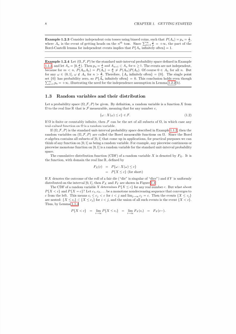
If X denotes the outcome of the roll of a fair die (“die” is singular of “dice”) and if Y is uniformlydistributed on the interval [0, 1], then F X and F Y are shown in Figure 1.4
The CDF of a random variable X determines P
X
≤ c
for any real number c. But what about
P X < c and P X = c? Let c1, c2, . . . be a monotone nondecreasing sequence that converges toc from the left. This means ci ≤ c j < c for i < j and lim j→∞ c j = c. Then the events X ≤ c jare nested: X ≤ ci ⊂ X ≤ c j for i < j, and the union of all such events is the event X < c.Thus, by Lemma 1.1.4
P X < c = limi→∞
P X ≤ ci = limi→∞
F X (ci) = F X (c−).
8/11/2019 Random process by B. Hajek
http://slidepdf.com/reader/full/random-process-by-b-hajek 19/448
1.3. RANDOM VARIABLES AND THEIR DISTRIBUTION 9
64
FYX1
53210 0 1
1
Figure 1.4: Examples of CDFs.
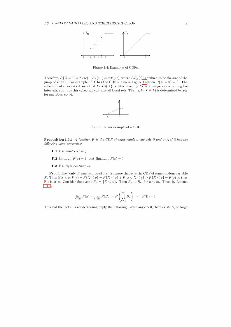
Therefore, P X = c = F X (c) − F X (c−) = F X (c), where F X (c) is defined to be the size of the jump of F at c. For example, if X has the CDF shown in Figure 1.5 then P X = 0 = 1
2 . Thecollection of all events A such that P X ∈ A is determined by F X is a σ-algebra containing theintervals, and thus this collection contains all Borel sets. That is, P
X
∈ A
is determined by F X
for any Borel set A.
0−1
0.5
1
Figure 1.5: An example of a CDF.
Proposition 1.3.1 A function F is the CDF of some random variable if and only if it has the following three properties:
F.1 F is nondecreasing
F.2 limx→+∞ F (x) = 1 and limx→−∞ F (x) = 0
F.3 F is right continuous
Proof. The “only if” part is proved first. Suppose that F is the CDF of some random variableX . Then if x < y, F (y) = P X ≤ y = P X ≤ x + P x < X ≤ y ≥ P X ≤ x = F (x) so thatF.1 is true. Consider the events Bn = X ≤ n. Then Bn ⊂ Bm for n ≤ m. Thus, by Lemma
1.1.4,
limn→∞ F (n) = lim
n→∞ P (Bn) = P
∞n=1
Bn
= P (Ω) = 1.
This and the fact F is nondecreasing imply the following. Given any > 0, there exists N so large
8/11/2019 Random process by B. Hajek
http://slidepdf.com/reader/full/random-process-by-b-hajek 20/448
10 CHAPTER 1. GETTING STARTED
that F (x) ≥ 1 − for all x ≥ N . That is, F (x) → 1 as x → +∞. Similarly,
limn
→−∞
F (n) = limn
→∞
P (B−n) = P ∞
n=1
B−n = P (∅) = 0.
so that F (x) → 0 as x → −∞. Property F.2 is proved.The proof of F.3 is similar. Fix an arbitrary real number x. Define the sequence of events An
for n ≥ 1 by An = X ≤ x + 1n. Then An ⊂ Am for n ≥ m so
limn→∞ F (x +
1
n) = lim
n→∞ P (An) = P
∞k=1
Ak
= P X ≤ x = F X (x).
Convergence along the sequence x + 1n , together with the fact that F is nondecreasing, implies that
F (x+) = F (x). Property F.3 is thus proved. The proof of the “only if” portion of Proposition1.3.1 is complete
To prove the “if” part of Proposition 1.3.1, let F be a function satisfying properties F.1-F.3. It
must be shown that there exists a random variable with CDF F . Let Ω = R and let F be the setB of Borel subsets of R. Define P on intervals of the form (a, b] by P ((a, b]) = F (b) − F (a). It canbe shown by an extension theorem of measure theory that P can be extended to all of F so thatthe axioms of probability are satisfied. Finally, let X (ω) = ω for all ω ∈ Ω. Then
P ( X ∈ (a, b]) = P ((a, b]) = F (b) − F (a).
Therefore, X has CDF F . So F is a CDF, as was to be proved.
The vast majority of random variables described in applications are one of two types, to bedescribed next. A random variable X is a discrete random variable if there is a finite or countablyinfinite set of values xi : i ∈ I such that P X ∈ xi : i ∈ I = 1. The probability mass function(pmf) of a discrete random variable X , denoted pX (x), is defined by pX (x) = P
X = x
. Typically
the pmf of a discrete random variable is much more useful than the CDF. However, the pmf andCDF of a discrete random variable are related by pX (x) = F X (x) and conversely,
F X (x) =y:y≤x
pX (y), (1.3)
where the sum in (1.3) is taken only over y such that pX (y) = 0. If X is a discrete random variablewith only finitely many mass points in any finite interval, then F X is a piecewise constant function.
A random variable X is a continuous random variable if the CDF is the integral of a function:
F X (x) =
x−∞
f X (y)dy
The function f X is called the probability density function (pdf). If the pdf f X is continuous at apoint x, then the value f X (x) has the following nice interpretation:
f X (x) = limε→0
1
ε
x+ε
xf X (y)dy
= limε→0
1
εP x ≤ X ≤ x + ε.
8/11/2019 Random process by B. Hajek
http://slidepdf.com/reader/full/random-process-by-b-hajek 21/448
1.4. FUNCTIONS OF A RANDOM VARIABLE 11
If A is any Borel subset of R, then
P X ∈ A =
Af X (x)dx. (1.4)
The integral in (1.4) can be understood as a Riemann integral if A is a finite union of intervals andf is piecewise continuous or monotone. In general, f X is required to be Borel measurable and theintegral is defined by Lebesgue integration.2
Any random variable X on an arbitrary probability space has a CDF F X . As noted in the proof of Proposition 1.3.1 there exists a probability measure P X (called P in the proof) on the Borelsubsets of R such that for any interval (a, b],
P X ((a, b]) = P X ∈ (a, b].
We define the probability distribution of X to be the probability measure P X . The distribution P X
is determined uniquely by the CDF F X . The distribution is also determined by the pdf f X if X
is continuous type, or the pmf pX if X is discrete type. In common usage, the response to thequestion “What is the distribution of X ?” is answered by giving one or more of F X , f X , or pX , orpossibly a transform of one of these, whichever is most convenient.
1.4 Functions of a random variable
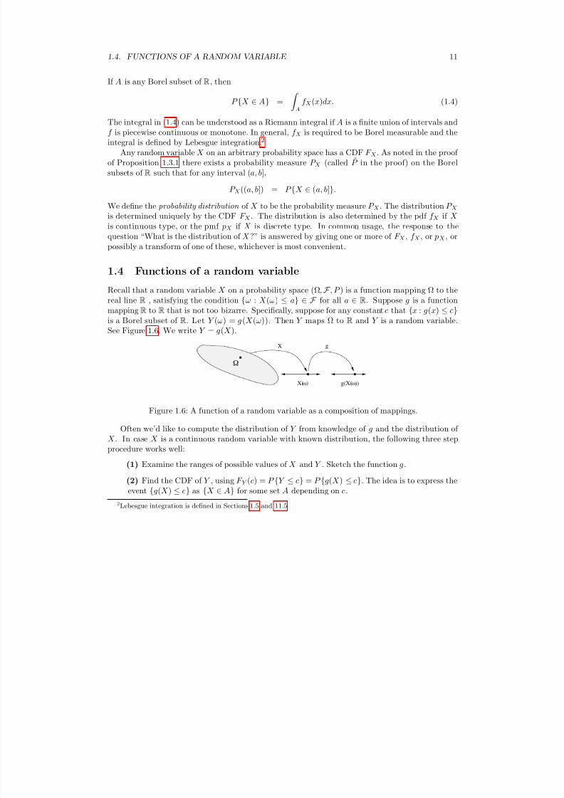
Recall that a random variable X on a probability space (Ω, F , P ) is a function mapping Ω to thereal line R , satisfying the condition ω : X (ω) ≤ a ∈ F for all a ∈ R. Suppose g is a functionmapping R to R that is not too bizarre. Specifically, suppose for any constant c that x : g(x) ≤ cis a Borel subset of R. Let Y (ω) = g (X (ω)). Then Y maps Ω to R and Y is a random variable.See Figure 1.6. We write Y = g(X ).
Ω
g(X( ))X( )ω ω
gX
Figure 1.6: A function of a random variable as a composition of mappings.
Often we’d like to compute the distribution of Y from knowledge of g and the distribution of X . In case X is a continuous random variable with known distribution, the following three stepprocedure works well:
(1) Examine the ranges of possible values of X and Y . Sketch the function g .
(2) Find the CDF of Y , using F Y (c) = P Y ≤ c = P g(X ) ≤ c. The idea is to express theevent g(X ) ≤ c as X ∈ A for some set A depending on c.
2Lebesgue integration is defined in Sections 1.5 and 11.5
8/11/2019 Random process by B. Hajek
http://slidepdf.com/reader/full/random-process-by-b-hajek 22/448
12 CHAPTER 1. GETTING STARTED
(3) If F Y has a piecewise continuous derivative, and if the pdf f Y is desired, differentiate F Y .
If instead X is a discrete random variable then step 1 should be followed. After that the pmf of Y can be found from the pmf of X using
pY (y) = P g(X ) = y =
x:g(x)=y
pX (x)
Example 1.4.1 Suppose X is a N (µ = 2, σ2 = 3) random variable (see Section 1.6 for the defini-tion) and Y = X 2. Let us describe the density of Y . Note that Y = g(X ) where g(x) = x2. Thesupport of the distribution of X is the whole real line, and the range of g over this support is R+.Next we find the CDF, F Y . Since P Y ≥ 0 = 1, F Y (c) = 0 for c < 0. For c ≥ 0,
F Y (c) = P
X 2
≤ c
= P −
√ c ≤
X ≤
√ c
= P −√ c − 2√
3≤ X − 2√
3≤
√ c − 2√ 3
= Φ
√ c − 2√
3
− Φ
−√ c − 2√
3
Differentiate with respect to c, using the chain rule and the fact, Φ(s) = 1√
2π exp(− s2
2 ) to obtain
f Y (c) =
1√ 24πc
exp
−√
c−2√ 6
2
+ exp
−−√
c−2√ 6
2
if c ≥ 0
0 if c < 0(1.5)
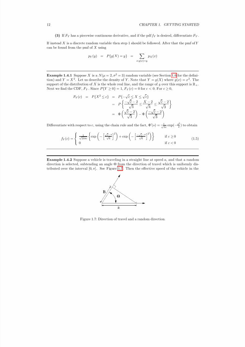
Example 1.4.2 Suppose a vehicle is traveling in a straight line at speed a, and that a randomdirection is selected, subtending an angle Θ from the direction of travel which is uniformly dis-tributed over the interval [0, π]. See Figure 1.7. Then the effective speed of the vehicle in the
B
a
Θ
Figure 1.7: Direction of travel and a random direction.
8/11/2019 Random process by B. Hajek
http://slidepdf.com/reader/full/random-process-by-b-hajek 23/448
1.4. FUNCTIONS OF A RANDOM VARIABLE 13
random direction is B = a cos(Θ). Let us find the pdf of B.The range of a cos(θ), as θ ranges over [0, π], is the interval [−a, a]. Therefore, F B(c) = 0
for c ≤ −a and F B(c) = 1 for c ≥ a. Let now −a < c < a. Then, because cos is monotone
nonincreasing on the interval [0, π],
F B(c) = P a cos(Θ) ≤ c = P
cos(Θ) ≤ c
a
= P
Θ ≥ cos−1
c
a
= 1 − cos−1
ca
π
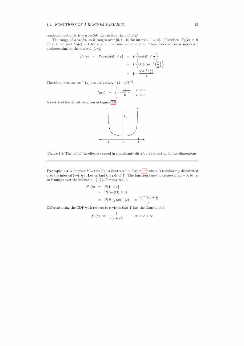
Therefore, because cos−1(y) has derivative, −(1 − y2)−12 ,
f B(c) =
1
π√ a2−c2
| c |< a
0
| c
|> a
A sketch of the density is given in Figure 1.8.
−a a
f B
0
Figure 1.8: The pdf of the effective speed in a uniformly distributed direction in two dimensions.
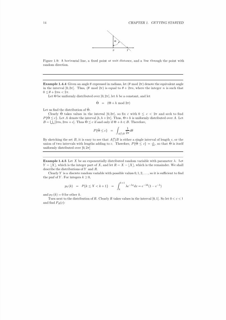
Example 1.4.3 Suppose Y = tan(Θ), as illustrated in Figure 1.9, where Θ is uniformly distributedover the interval (−π
2 , π2 ) . Let us find the pdf of Y . The function tan(θ) increases from −∞ to ∞as θ ranges over the interval (−π
2 , π2 ). For any real c,
F Y (c) = P Y ≤ c= P tan(Θ) ≤ c
= P Θ ≤ tan−1(c) = tan−1
(c) + π2
π
Differentiating the CDF with respect to c yields that Y has the Cauchy pdf:
f Y (c) = 1
π(1 + c2) − ∞ < c < ∞
8/11/2019 Random process by B. Hajek
http://slidepdf.com/reader/full/random-process-by-b-hajek 24/448
14 CHAPTER 1. GETTING STARTED
Y 0
Θ
Figure 1.9: A horizontal line, a fixed point at unit distance, and a line through the point withrandom direction.
Example 1.4.4 Given an angle θ expressed in radians, let (θ mod 2π) denote the equivalent anglein the interval [0, 2π]. Thus, (θ mod 2π) is equal to θ + 2πn, where the integer n is such that
0 ≤ θ + 2πn < 2π.Let Θ be uniformly distributed over [0, 2π], let h be a constant, and let
Θ = (Θ + h mod 2π)
Let us find the distribution of Θ.Clearly Θ takes values in the interval [0, 2π], so fix c with 0 ≤ c < 2π and seek to find
P Θ ≤ c. Let A denote the interval [h, h + 2π]. Thus, Θ + h is uniformly distributed over A. LetB =
n[2πn, 2πn + c]. Thus Θ ≤ c if and only if Θ + h ∈ B. Therefore,
P Θ ≤ c =
AT
B
1
2πdθ
By sketching the set B, it is easy to see that AB is either a single interval of length c, or theunion of two intervals with lengths adding to c. Therefore, P Θ ≤ c = c
2π , so that Θ is itself uniformly distributed over [0, 2π]
Example 1.4.5 Let X be an exponentially distributed random variable with parameter λ. LetY = X , which is the integer part of X , and let R = X − X , which is the remainder. We shalldescribe the distributions of Y and R.
Clearly Y is a discrete random variable with possible values 0, 1, 2, . . . , so it is sufficient to findthe pmf of Y . For integers k ≥ 0,
pY (k) = P k ≤ X < k + 1 = k+1
kλe−λxdx = e−λk(1 − e−λ)
and pY (k) = 0 for other k.Turn next to the distribution of R. Clearly R takes values in the interval [0, 1]. So let 0 < c < 1
and find F R(c):
8/11/2019 Random process by B. Hajek
http://slidepdf.com/reader/full/random-process-by-b-hajek 25/448
1.4. FUNCTIONS OF A RANDOM VARIABLE 15
F R(c) = P
X
− X
≤ c
= P X
∈
∞
k=0
[k, k + c]=
∞k=0
P k ≤ X ≤ k + c =∞k=0
e−λk(1 − e−λc) = 1 − e−λc
1 − e−λ
where we used the fact 1 + α + α2 + · · · = 11−α for | α |< 1. Differentiating F R yields the pmf:
f R(c) =
λe−λc
1−e−λ 0 ≤ c ≤ 1
0 otherwise
What happens to the density of R as λ
→ 0 or as λ
→ ∞? By l’Hospital’s rule,
limλ→0
f R(c) =
1 0 ≤ c ≤ 10 otherwise
That is, in the limit as λ → 0, the density of X becomes more and more evenly spread out, and Rbecomes uniformly distributed over the interval [0, 1]. If λ is very large then the factor 1 − e−λ isnearly one , and the density of R is nearly the same as the exponential density with parameter λ.
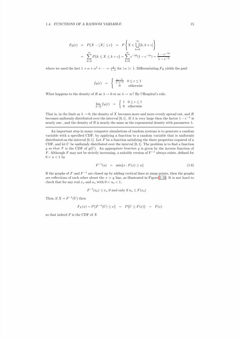
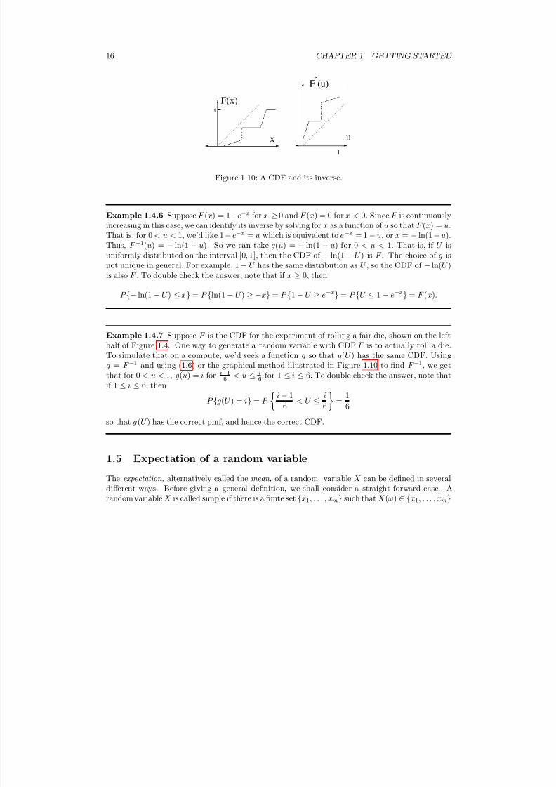
An important step in many computer simulations of random systems is to generate a randomvariable with a specified CDF, by applying a function to a random variable that is uniformlydistributed on the interval [0, 1]. Let F be a function satisfying the three properties required of a
CDF, and let U be uniformly distributed over the interval [0, 1]. The problem is to find a functiong so that F is the CDF of g(U ). An appropriate function g is given by the inverse function of F . Although F may not be strictly increasing, a suitable version of F −1 always exists, defined for0 < u < 1 by
F −1(u) = minx : F (x) ≥ u (1.6)
If the graphs of F and F −1 are closed up by adding vertical lines at jump points, then the graphsare reflections of each other about the x = y line, as illustrated in Figure 1.10. It is not hard tocheck that for any real xo and uo with 0 < uo < 1,
F −1(uo)
≤ xo if and only if uo
≤ F (xo)
Thus, if X = F −1(U ) then
F X (x) = P F −1(U ) ≤ x = P U ≤ F (x) = F (x)
so that indeed F is the CDF of X
8/11/2019 Random process by B. Hajek
http://slidepdf.com/reader/full/random-process-by-b-hajek 26/448
16 CHAPTER 1. GETTING STARTED
! #$%
&
&
!&
!#'%
' $
Figure 1.10: A CDF and its inverse.
Example 1.4.6 Suppose F (x) = 1
−e−x for x
≥ 0 and F (x) = 0 for x < 0. Since F is continuously
increasing in this case, we can identify its inverse by solving for x as a function of u so that F (x) = u.That is, for 0 < u < 1, we’d like 1 − e−x = u which is equivalent to e−x = 1 − u, or x = − ln(1 − u).Thus, F −1(u) = − ln(1 − u). So we can take g(u) = − ln(1 − u) for 0 < u < 1. That is, if U isuniformly distributed on the interval [0, 1], then the CDF of − ln(1 − U ) is F . The choice of g isnot unique in general. For example, 1 − U has the same distribution as U , so the CDF of − ln(U )is also F . To double check the answer, note that if x ≥ 0, then
P − ln(1 − U ) ≤ x = P ln(1 − U ) ≥ −x = P 1 − U ≥ e−x = P U ≤ 1 − e−x = F (x).
Example 1.4.7 Suppose F is the CDF for the experiment of rolling a fair die, shown on the lefthalf of Figure 1.4. One way to generate a random variable with CDF F is to actually roll a die.To simulate that on a compute, we’d seek a function g so that g(U ) has the same CDF. Usingg = F −1 and using (1.6) or the graphical method illustrated in Figure 1.10 to find F −1, we getthat for 0 < u < 1, g(u) = i for i−1
6 < u ≤ i6 for 1 ≤ i ≤ 6. To double check the answer, note that
if 1 ≤ i ≤ 6, then
P g(U ) = i = P
i − 1
6 < U ≤ i
6
=
1
6
so that g(U ) has the correct pmf, and hence the correct CDF.
1.5 Expectation of a random variable
The expectation, alternatively called the mean, of a random variable X can be defined in severaldifferent ways. Before giving a general definition, we shall consider a straight forward case. Arandom variable X is called simple if there is a finite set x1, . . . , xm such that X (ω) ∈ x1, . . . , xm
8/11/2019 Random process by B. Hajek
http://slidepdf.com/reader/full/random-process-by-b-hajek 27/448
1.5. EXPECTATION OF A RANDOM VARIABLE 17
for all ω. The expectation of such a random variable is defined by
E [X ] =m
i=1
xiP
X = xi
(1.7)
The definition (1.7) clearly shows that E [X ] for a simple random variable X depends only on thepmf of X .
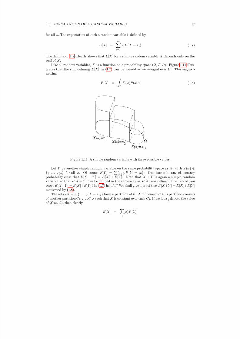
Like all random variables, X is a function on a probability space (Ω, F , P ). Figure 1.11 illus-trates that the sum defining E [X ] in (1.7) can be viewed as an integral over Ω. This suggestswriting
E [X ] =
Ω
X (ω)P (dω) (1.8)
X( )=x X( )=x
X( )=x
1
2
3
Ωω
ω
ω
Figure 1.11: A simple random variable with three possible values.
Let Y be another simple random variable on the same probability space as X , with Y (ω) ∈y1, . . . , yn for all ω. Of course E [Y ] =
ni=1 yiP Y = yi. One learns in any elementary
probability class that E [X + Y ] = E [X ] + E [Y ]. Note that X + Y is again a simple randomvariable, so that E [X + Y ] can be defined in the same way as E [X ] was defined. How would youprove E [X +Y ] = E [X ]+E [Y ]? Is (1.7) helpful? We shall give a proof that E [X +Y ] = E [X ]+E [Y ]motivated by (1.8).
The sets X = x1, . . . , X = xm form a partition of Ω. A refinement of this partition consistsof another partition C 1, . . . , C m such that X is constant over each C j . If we let x
j denote the valueof X on C j , then clearly
E [X ] = j
x jP (C j ]
8/11/2019 Random process by B. Hajek
http://slidepdf.com/reader/full/random-process-by-b-hajek 28/448
18 CHAPTER 1. GETTING STARTED
Now, it is possible to select the partition C 1, . . . , C m so that both X and Y are constant over eachC j. For example, each C j could have the form X = xi ∩ Y = yk for some i, k. Let y j denotethe value of Y on C j . Then x
j + y j is the value of X + Y on C j. Therefore,
E [X + Y ] = j
(x j + y j)P (C j) =
j
x jP (C j) +
j
y jP (C j) = E [X ] + E [Y ]
While the expression (1.8) is rather suggestive, it would be overly restrictive to interpret itas a Riemann integral over Ω. For example, if X is a random variable for the standard unit-interval probability space defined in Example 1.1.2, then it is tempting to define E [X ] by Riemannintegration (see the appendix):
E [X ] =
1
0X (ω)dω (1.9)
However, suppose X is the simple random variable such that X (w) = 1 for rational values of ω andX (ω) = 0 otherwise. Since the set of rational numbers in Ω is countably infinite, such X satisfiesP X = 0 = 1. Clearly we’d like E [X ] = 0, but the Riemann integral (1.9) is not convergent forthis choice of X .
The expression (1.8) can be used to define E [X ] in great generality if it is interpreted as aLebesgue integral, defined as follows: Suppose X is an arbitrary nonnegative random variable.Then there exists a sequence of simple random variables X 1, X 2, . . . such that for every ω ∈ Ω,X 1(ω) ≤ X 2(ω) ≤ · · · and X n(ω) → X (ω) as n → ∞. Then E [X n] is well defined for each n andis nondecreasing in n, so the limit of E [X n] as n → ∞ exists with values in [0, +∞]. Furthermoreit can be shown that the value of the limit depends only on (Ω , F , P ) and X , not on the particularchoice of the approximating simple sequence. We thus define E [X ] = limn→∞ E [X n]. Thus, E [X ]is always well defined in this way, with possible value +
∞, if X is a nonnegative random variable.
Suppose X is an arbitrary random variable. Define the positive part of X to be the randomvariable X + defined by X +(ω) = max0, X (ω) for each value of ω. Similarly define the negativepart of X to be the random variable X −(ω) = max0, −X (ω). Then X (ω) = X +(ω) − X −(ω)for all ω, and X + and X − are both nonnegative random variables. As long as at least one of E [X +] or E [X −] is finite, define E [X ] = E [X +] − E [X −]. The expectation E [X ] is undefined if E [X +] = E [X −] = +∞. This completes the definition of E [X ] using (1.8) interpreted as a Lebesgueintegral.
We will prove that E [X ] defined by the Lebesgue integral (1.8) depends only on the CDF of X . It suffices to show this for a nonnegative random variable X . For such a random variable, andn ≥ 1, define the simple random variable X n by
X n(ω) = k2−n if k2−n
≤ X (ω) < (k + 1)2−n, k = 0, 1, . . . , 22n
−1
0 else
Then
E [X n] =22n−1k=0
k2−n(F X ((k + 1)2−n) − F X (k2−n)
8/11/2019 Random process by B. Hajek
http://slidepdf.com/reader/full/random-process-by-b-hajek 29/448
1.5. EXPECTATION OF A RANDOM VARIABLE 19
so that E [X n] is determined by the CDF F X for each n. Furthermore, the X n’s are nondecreasingin n and converge to X . Thus, E [X ] = limn→∞ E [X n], and therefore the limit E [X ] is determinedby F X .
In Section 1.3 we defined the probability distribution P X of a random variable such that thecanonical random variable X (ω) = ω on (R, B, P X ) has the same CDF as X . Therefore E [X ] =E [ X ], or
E [X ] =
∞−∞
xP X (dx) (Lebesgue) (1.10)
By definition, the integral (1.10) is the Lebesgue-Stieltjes integral of x with respect to F X , so that
E [X ] =
∞−∞
xdF X (x) (Lebesgue-Stieltjes) (1.11)
Expectation has the following properties. Let X, Y be random variables and c be a constant.
E.1 (Linearity) E [cX ] = cE [X ]. If E [X ], E [Y ] and E [X ] + E [Y ] are well defined, thenE [X + Y ] is well defined and E [X + Y ] = E [X ] + E [Y ].
E.2 (Preservation of order) If P X ≥ Y = 1 and E [Y ] is well defined with E [Y ] > −∞,then E [X ] is well defined and E [X ] ≥ E [Y ].
E.3 If X has pdf f X then
E [X ] =
∞
−∞
xf X (x)dx (Lebesgue)
E.4 If X has pmf pX then
E [X ] =x>0
xpX (x) +x<0
xpX (x).
E.5 (Law of the unconscious statistician (LOTUS) ) If g is Borel measurable,
E [g(X )] =
Ω
g(X (ω))P (dω) (Lebesgue)
= ∞
−∞g(x)dF
X (x) (Lebesgue-Stieltjes)
and in case X is a continuous type random variable
E [g(X )] =
∞−∞
g(x)f X (x)dx (Lebesgue)
8/11/2019 Random process by B. Hajek
http://slidepdf.com/reader/full/random-process-by-b-hajek 30/448
20 CHAPTER 1. GETTING STARTED
E.6 (Integration by parts formula)
E [X ] = ∞
0
(1
−F X (x))dx
− 0
−∞F X (x)dx, (1.12)
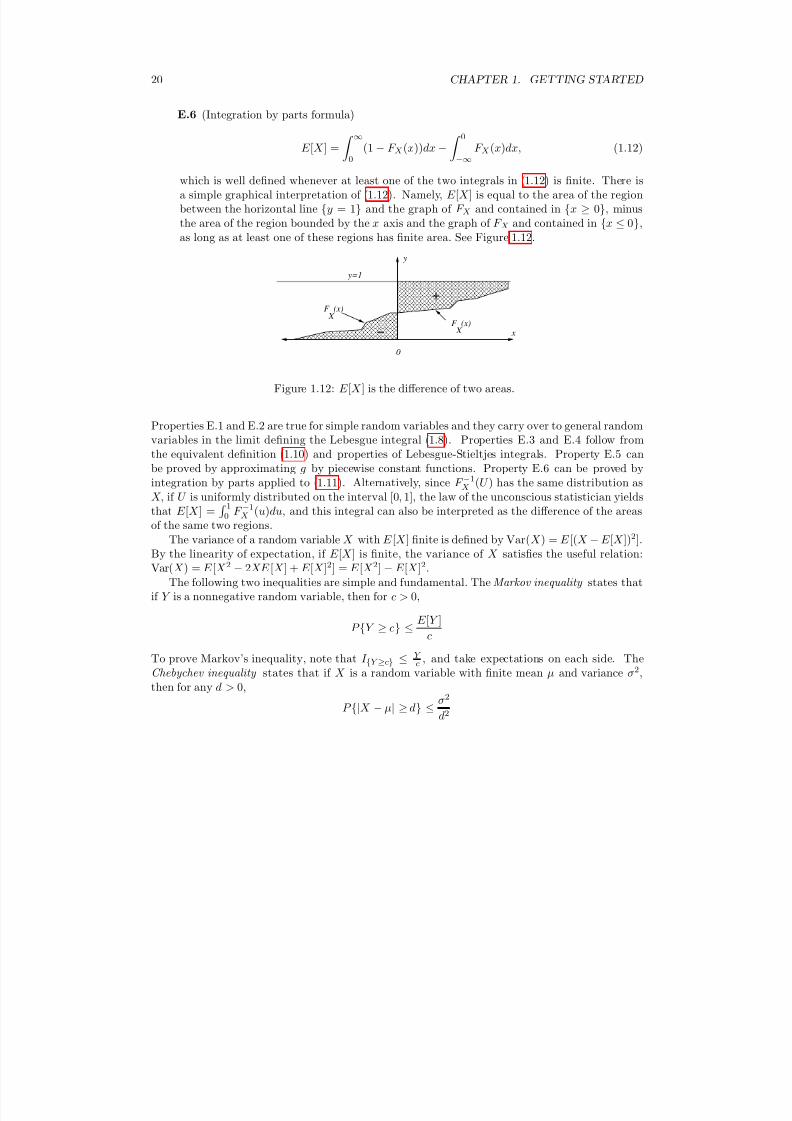
which is well defined whenever at least one of the two integrals in (1.12) is finite. There isa simple graphical interpretation of (1.12). Namely, E [X ] is equal to the area of the regionbetween the horizontal line y = 1 and the graph of F X and contained in x ≥ 0, minusthe area of the region bounded by the x axis and the graph of F X and contained in x ≤ 0,as long as at least one of these regions has finite area. See Figure 1.12.
X x
y
y=1
F (x) X
0
!
!
F (x)
Figure 1.12: E [X ] is the difference of two areas.
Properties E.1 and E.2 are true for simple random variables and they carry over to general randomvariables in the limit defining the Lebesgue integral (1.8). Properties E.3 and E.4 follow fromthe equivalent definition (1.10) and properties of Lebesgue-Stieltjes integrals. Property E.5 canbe proved by approximating g by piecewise constant functions. Property E.6 can be proved by
integration by parts applied to (1.11). Alternatively, since F −1X (U ) has the same distribution asX, if U is uniformly distributed on the interval [0, 1], the law of the unconscious statistician yieldsthat E [X ] =
10 F −1
X (u)du, and this integral can also be interpreted as the difference of the areasof the same two regions.
The variance of a random variable X with E [X ] finite is defined by Var(X ) = E [(X − E [X ])2].By the linearity of expectation, if E [X ] is finite, the variance of X satisfies the useful relation:Var(X ) = E [X 2 − 2XE [X ] + E [X ]2] = E [X 2] − E [X ]2.
The following two inequalities are simple and fundamental. The Markov inequality states thatif Y is a nonnegative random variable, then for c > 0,
P
Y
≥ c
≤
E [Y ]
cTo prove Markov’s inequality, note that I Y ≥c ≤ Y
c , and take expectations on each side. TheChebychev inequality states that if X is a random variable with finite mean µ and variance σ2,then for any d > 0,
P |X − µ| ≥ d ≤ σ2
d2
8/11/2019 Random process by B. Hajek
http://slidepdf.com/reader/full/random-process-by-b-hajek 31/448
1.6. FREQUENTLY USED DISTRIBUTIONS 21
The Chebychev inequality follows by applying the Markov inequality with Y = |X −µ|2 and c = d2.The characteristic function ΦX of a random variable X is defined by
ΦX (u) = E [e juX ]
for real values of u, where j =√ −1. For example, if X has pdf f , then
ΦX (u) =
∞−∞
exp( jux)f X (x)dx,
which is 2π times the inverse Fourier transform of f X .Two random variables have the same probability distribution if and only if they have the same
characteristic function. If E [X k] exists and is finite for an integer k ≥ 1, then the derivatives of ΦX up to order k exist and are continuous, and
Φ(k)X (0) = jkE [X k]
For a nonnegative integer-valued random variable X it is often more convenient to work with thez transform of the pmf, defined by
ΨX (z) = E [zX ] =∞k=0
zk pX (k)
for real or complex z with | z |≤ 1. Two such random variables have the same probability dis-tribution if and only if their z transforms are equal. If E [X k] is finite it can be found from thederivatives of ΨX up to the kth order at z = 1,
Ψ(k)X (1) = E [X (X − 1) · · · (X − k + 1)]
1.6 Frequently used distributionsThe following is a list of the most basic and frequently used probability distributions. For eachdistribution an abbreviation, if any, and valid parameter values are given, followed by either theCDF, pdf or pmf, then the mean, variance, a typical example and significance of the distribution.
The constants p, λ, µ, σ, a, b, and α are real-valued, and n and i are integer-valued, except ncan be noninteger-valued in the case of the gamma distribution.
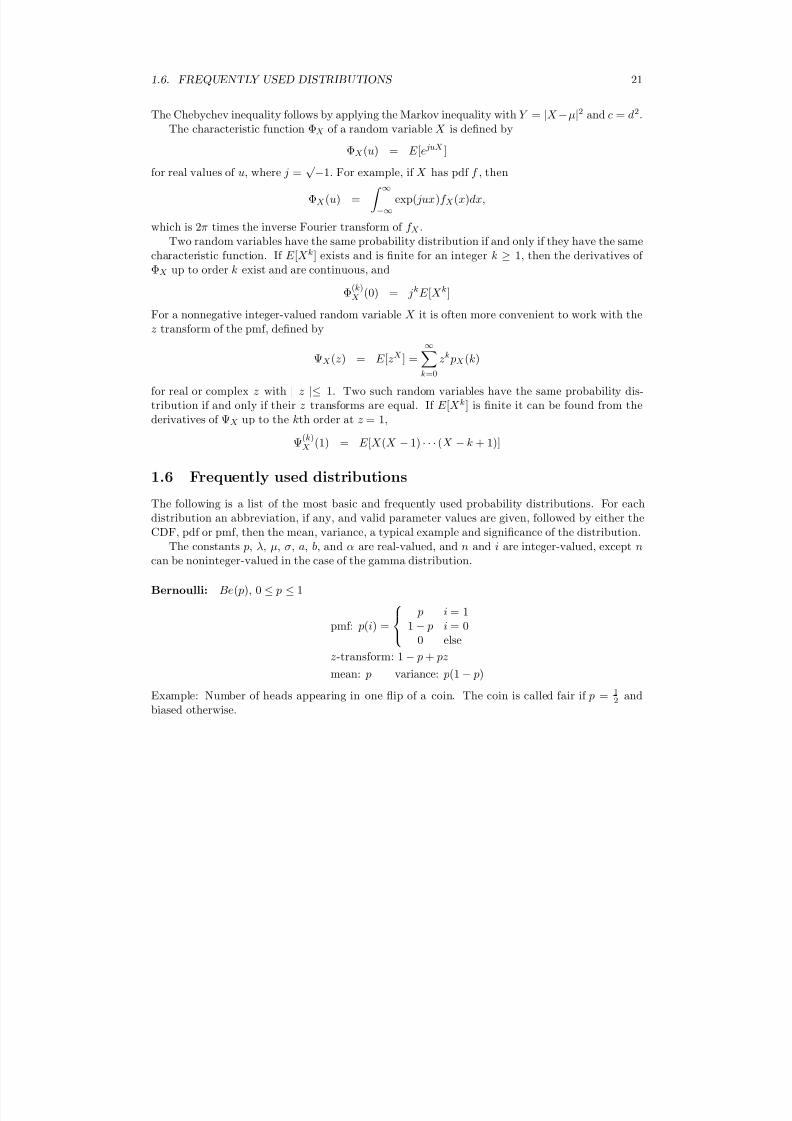
Bernoulli: Be( p), 0 ≤ p ≤ 1
pmf: p(i) =
p i = 11 − p i = 0
0 elsez-transform: 1 − p + pz
mean: p variance: p(1 − p)
Example: Number of heads appearing in one flip of a coin. The coin is called fair if p = 12 and
biased otherwise.
8/11/2019 Random process by B. Hajek
http://slidepdf.com/reader/full/random-process-by-b-hajek 32/448
22 CHAPTER 1. GETTING STARTED
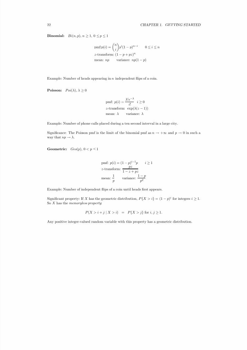
Binomial: Bi(n, p), n ≥ 1, 0 ≤ p ≤ 1
pmf: p(i) = n
i pi(1
− p)n−i 0
≤ i
≤ n
z-transform: (1 − p + pz)n
mean: np variance: np(1 − p)
Example: Number of heads appearing in n independent flips of a coin.
Poisson: P oi(λ), λ ≥ 0
pmf: p(i) = λi
e−λ
i! i ≥ 0
z-transform: exp(λ(z − 1))
mean: λ variance: λ
Example: Number of phone calls placed during a ten second interval in a large city.
Significance: The Poisson pmf is the limit of the binomial pmf as n → +∞ and p → 0 in such away that np → λ.
Geometric: Geo( p), 0 < p ≤ 1
pmf: p(i) = (1 − p)i−1 p i ≥ 1
z-transform: pz
1 − z + pz
mean: 1
p variance:
1 − p
p2
Example: Number of independent flips of a coin until heads first appears.
Significant property: If X has the geometric distribution, P X > i = (1 − p)
i
for integers i ≥ 1.So X has the memoryless property :
P (X > i + j | X > i) = P X > j for i, j ≥ 1.
Any positive integer-valued random variable with this property has a geometric distribution.
8/11/2019 Random process by B. Hajek
http://slidepdf.com/reader/full/random-process-by-b-hajek 33/448
1.6. FREQUENTLY USED DISTRIBUTIONS 23
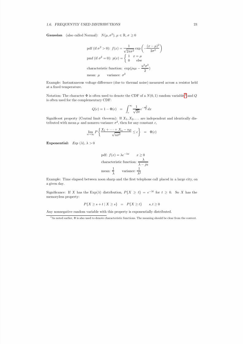
Gaussian (also called Normal): N (µ, σ2), µ ∈ R, σ ≥ 0
pdf (if σ2
> 0): f (x) =
1
√ 2πσ2 exp−(x
−µ)2
2σ2 pmf (if σ2 = 0): p(x) =
1 x = µ0 else
characteristic function: exp( juµ − u2σ2
2 )
mean: µ variance: σ2
Example: Instantaneous voltage difference (due to thermal noise) measured across a resistor heldat a fixed temperature.
Notation: The character Φ is often used to denote the CDF of a N (0, 1) random variable,3 and Qis often used for the complementary CDF:
Q(c) = 1 − Φ(c) =
∞c
1√ 2π
e−x2
2 dx
Significant property (Central limit theorem): If X 1, X 2, . . . are independent and identically dis-tributed with mean µ and nonzero variance σ2, then for any constant c,
limn→∞ P
X 1 + · · · + X n − nµ√
nσ2≤ c
= Φ(c)
Exponential: Exp (λ), λ > 0
pdf: f (x) = λe−λx x ≥ 0
characteristic function: λ
λ − ju
mean: 1
λ variance:
1
λ2
Example: Time elapsed between noon sharp and the first telephone call placed in a large city, ona given day.
Significance: If X has the Exp(λ) distribution, P X ≥ t = e−λt for t ≥ 0. So X has the
memoryless property:
P X ≥ s + t | X ≥ s = P X ≥ t s, t ≥ 0
Any nonnegative random variable with this property is exponentially distributed.
3As noted earlier, Φ is also used to denote characteristic functions. The meaning should be clear from the context.
8/11/2019 Random process by B. Hajek
http://slidepdf.com/reader/full/random-process-by-b-hajek 34/448
24 CHAPTER 1. GETTING STARTED
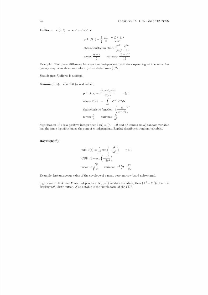
Uniform: U (a, b) − ∞ < a < b < ∞
pdf: f (x) = 1b−a a ≤ x ≤ b
0 else
characteristic function: e jub − e jua
ju(b − a)
mean: a + b
2 variance:
(b − a)2
12
Example: The phase difference between two independent oscillators operating at the same fre-quency may be modeled as uniformly distributed over [0, 2π]
Significance: Uniform is uniform.
Gamma(n, α): n, α > 0 (n real valued)
pdf: f (x) = αnxn−1e−αx
Γ(n) x ≥ 0
where Γ(n) =
∞0
sn−1e−sds
characteristic function:
α
α − ju
n
mean: n
α variance:
n
α2
Significance: If n is a positive integer then Γ(n) = (n−
1)! and a Gamma (n, α) random variablehas the same distribution as the sum of n independent, Exp(α) distributed random variables.
Rayleigh(σ2):
pdf: f (r) = r
σ2 exp
− r2
2σ2
r > 0
CDF : 1 − exp
− r2
2σ2
mean: σ π2 variance: σ2 2
− π
2Example: Instantaneous value of the envelope of a mean zero, narrow band noise signal.
Significance: If X and Y are independent, N (0, σ2) random variables, then (X 2 + Y 2)12 has the
Rayleigh(σ2) distribution. Also notable is the simple form of the CDF.
8/11/2019 Random process by B. Hajek
http://slidepdf.com/reader/full/random-process-by-b-hajek 35/448
1.7. FAILURE RATE FUNCTIONS 25
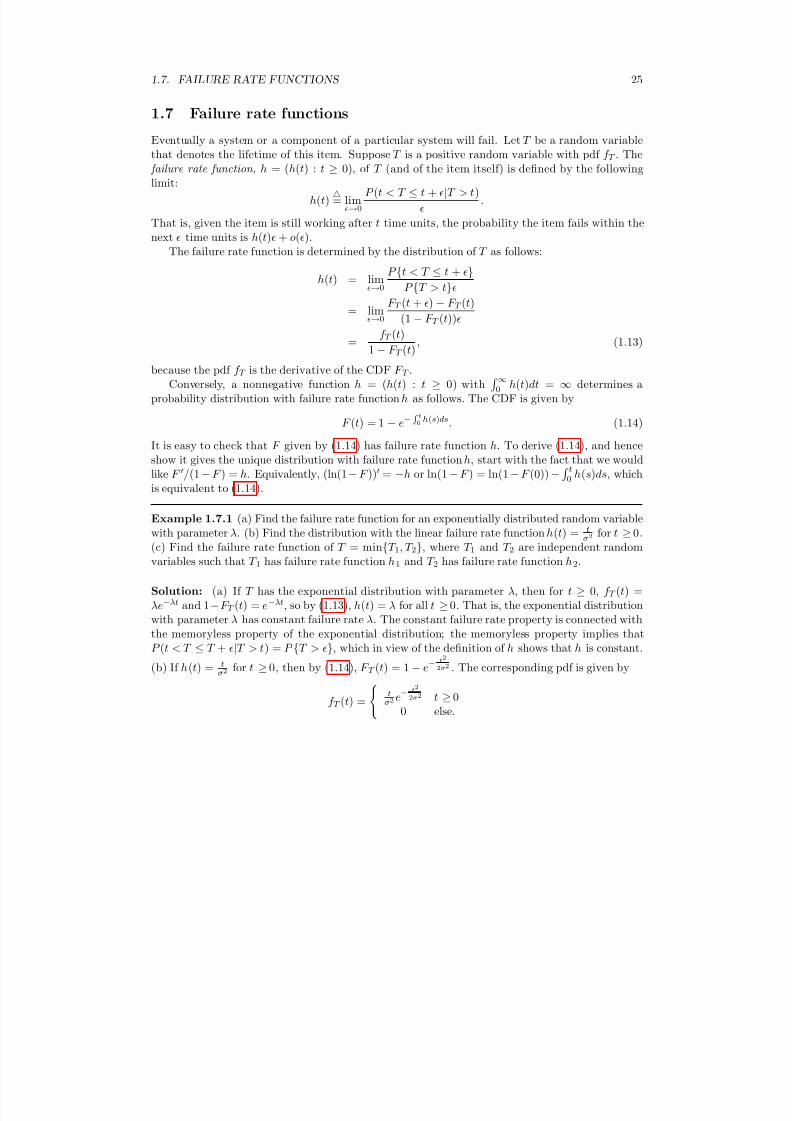
1.7 Failure rate functions
Eventually a system or a component of a particular system will fail. Let T be a random variable
that denotes the lifetime of this item. Suppose T is a positive random variable with pdf f T . The failure rate function, h = (h(t) : t ≥ 0), of T (and of the item itself) is defined by the followinglimit:
h(t) = lim
→0
P (t < T ≤ t + |T > t)
.
That is, given the item is still working after t time units, the probability the item fails within thenext time units is h(t) + o().
The failure rate function is determined by the distribution of T as follows:
h(t) = lim→0
P t < T ≤ t + P T > t
= lim→0
F T (t + ) − F T (t)
(1 − F T (t))
= f T (t)
1 − F T (t), (1.13)
because the pdf f T is the derivative of the CDF F T .Conversely, a nonnegative function h = (h(t) : t ≥ 0) with
∞0 h(t)dt = ∞ determines a
probability distribution with failure rate function h as follows. The CDF is given by
F (t) = 1 − e−R t0 h(s)ds. (1.14)
It is easy to check that F given by (1.14) has failure rate function h. To derive (1.14), and henceshow it gives the unique distribution with failure rate function h, start with the fact that we wouldlike F
/(1
−F ) = h. Equivalently, (ln(1
−F ))
=
−h or ln(1
−F ) = ln(1
−F (0))
− t0 h(s)ds, whichis equivalent to (1.14).
Example 1.7.1 (a) Find the failure rate function for an exponentially distributed random variablewith parameter λ. (b) Find the distribution with the linear failure rate function h(t) = t
σ2 for t ≥ 0.(c) Find the failure rate function of T = minT 1, T 2, where T 1 and T 2 are independent randomvariables such that T 1 has failure rate function h1 and T 2 has failure rate function h2.
Solution: (a) If T has the exponential distribution with parameter λ, then for t ≥ 0, f T (t) =λe−λt and 1−F T (t) = e−λt, so by (1.13), h(t) = λ for all t ≥ 0. That is, the exponential distributionwith parameter λ has constant failure rate λ. The constant failure rate property is connected withthe memoryless property of the exponential distribution; the memoryless property implies thatP (t < T ≤ T + |T > t) = P T > , which in view of the definition of h shows that h is constant.
(b) If h(t) = tσ2 for t ≥ 0, then by (1.14), F T (t) = 1 − e−
t2
2σ2 . The corresponding pdf is given by
f T (t) =
tσ2 e−
t2
2σ2 t ≥ 00 else.
8/11/2019 Random process by B. Hajek
http://slidepdf.com/reader/full/random-process-by-b-hajek 36/448
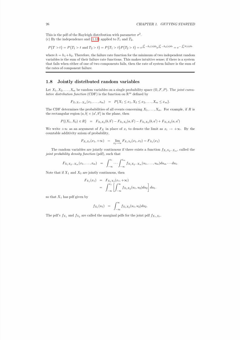
26 CHAPTER 1. GETTING STARTED
This is the pdf of the Rayleigh distribution with parameter σ2.(c) By the independence and (1.13) applied to T 1 and T 2,
P T > t = P T 1 > t and T 2 > t = P T 1 > tP T 2 > t = eR t0
−h1(s)ds
eR t0
−h2(s)ds
= e− R t0 h(s)ds
where h = h1 +h2. Therefore, the failure rate function for the minimum of two independent randomvariables is the sum of their failure rate functions. This makes intuitive sense; if there is a systemthat fails when either of one of two components fails, then the rate of system failure is the sum of the rates of component failure.
1.8 Jointly distributed random variables
Let X 1, X 2, . . . , X m be random variables on a single probability space (Ω, F , P ). The joint cumu-lative distribution function (CDF) is the function on Rm defined by
F X 1X 2···X m(x1, . . . , xm) = P X 1 ≤ x1, X 2 ≤ x2, . . . , X m ≤ xm.
The CDF determines the probabilities of all events concerning X 1, . . . , X m. For example, if R isthe rectangular region (a, b] × (a, b] in the plane, then
P (X 1, X 2) ∈ R = F X 1X 2(b, b) − F X 1X 2(a, b) − F X 1X 2(b, a) + F X 1X 2(a, a)
We write +∞ as an argument of F X in place of xi to denote the limit as xi → +∞. By thecountable additivity axiom of probability,
F X 1X 2(x1, +∞) = limx2
→∞
F X 1X 2(x1, x2) = F X 1(x1)
The random variables are jointly continuous if there exists a function f X 1X 2···X m, called the joint probability density function (pdf), such that
F X 1X 2···X m(x1, . . . , xm) =
x1−∞
· · · xm
−∞f X 1X 2···X m(u1, . . . , um)dum · · · du1.
Note that if X 1 and X 2 are jointly continuous, then
F X 1(x1) = F X 1X 2(x1, +∞)
=
x1−∞
∞−∞
f X 1X 2(u1, u2)du2
du1.
so that X 1 has pdf given by
f X 1(u1) =
∞−∞
f X 1X 2(u1, u2)du2.
The pdf’s f X 1 and f X 2 are called the marginal pdfs for the joint pdf f X 1,X 2.
8/11/2019 Random process by B. Hajek
http://slidepdf.com/reader/full/random-process-by-b-hajek 37/448
1.9. CONDITIONAL DENSITIES 27
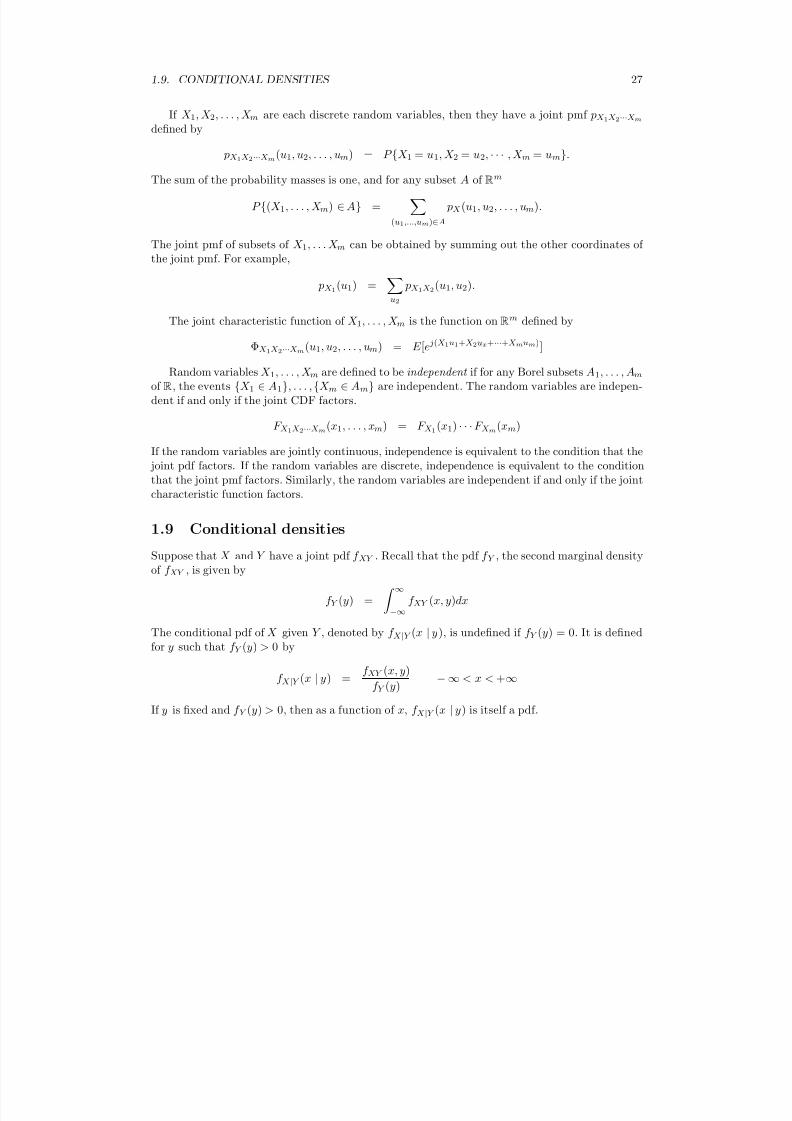
If X 1, X 2, . . . , X m are each discrete random variables, then they have a joint pmf pX 1X 2···X m
defined by
pX 1X 2···X m(u1, u2, . . . , um) = P X 1 = u1, X 2 = u2, · · · , X m = um.
The sum of the probability masses is one, and for any subset A of Rm
P (X 1, . . . , X m) ∈ A =
(u1,...,um)∈A
pX (u1, u2, . . . , um).
The joint pmf of subsets of X 1, . . . X m can be obtained by summing out the other coordinates of the joint pmf. For example,
pX 1(u1) =u2
pX 1X 2(u1, u2).
The joint characteristic function of X 1, . . . , X m is the function on Rm defined by
ΦX 1X 2···X m(u1, u2, . . . , um) = E [e j(X 1u1+X 2ux+···+X mum)]
Random variables X 1, . . . , X m are defined to be independent if for any Borel subsets A1, . . . , Am
of R, the events X 1 ∈ A1, . . . , X m ∈ Am are independent. The random variables are indepen-dent if and only if the joint CDF factors.
F X 1X 2···X m(x1, . . . , xm) = F X 1(x1) · · · F X m(xm)
If the random variables are jointly continuous, independence is equivalent to the condition that the joint pdf factors. If the random variables are discrete, independence is equivalent to the condition
that the joint pmf factors. Similarly, the random variables are independent if and only if the jointcharacteristic function factors.
1.9 Conditional densities
Suppose that X and Y have a joint pdf f XY . Recall that the pdf f Y , the second marginal densityof f XY , is given by
f Y (y) =
∞−∞
f XY (x, y)dx
The conditional pdf of X given Y , denoted by f X |Y (x
| y), is undefined if f Y (y) = 0. It is defined
for y such that f Y (y) > 0 by
f X |Y (x | y) = f XY (x, y)
f Y (y) − ∞ < x < +∞
If y is fixed and f Y (y) > 0, then as a function of x, f X |Y (x | y) is itself a pdf.
8/11/2019 Random process by B. Hajek
http://slidepdf.com/reader/full/random-process-by-b-hajek 38/448
28 CHAPTER 1. GETTING STARTED
The expectation of the conditional pdf is called the conditional expectation (or conditionalmean) of X given Y = y, written as
E [X | Y = y] = ∞−∞ xf X |Y (x | y)dx
If the deterministic function E [X | Y = y] is applied to the random variable Y , the result is arandom variable denoted by E [X | Y ].
Note that conditional pdf and conditional expectation were so far defined in case X and Y havea joint pdf. If instead, X and Y are both discrete random variables, the conditional pmf pX |Y andthe conditional expectation E [X | Y = y] can be defined in a similar way. More general notions of conditional expectation are considered in a later chapter.
1.10 Correlation and covariance
Let X and Y be random variables on the same probability space with finite second moments. Threeimportant related quantities are:
the correlation: E [XY ]
the covariance: Cov(X, Y ) = E [(X − E [X ])(Y − E [Y ])]
the correlation coefficient: ρXY = Cov(X, Y )
Var(X )Var(Y )
A fundamental inequality is Schwarz’s inequality:
| E [XY ] | ≤ E [X 2]E [Y 2] (1.15)
Furthermore, if E [Y 2] = 0, equality holds if and only if P (X = cY ) = 1 for some constant c.Schwarz’s inequality (1.15) is equivalent to the L2 triangle inequality for random variables:
E [(X + Y )2]12 ≤ E [X 2]
12 + E [Y 2]
12 (1.16)
Schwarz’s inequality can be proved as follows. If P Y = 0 = 1 the inequality is trivial, so supposeE [Y 2] > 0. By the inequality (a + b)2 ≤ 2a2 + 2b2 it follows that E [(X − λY )2] < ∞ for anyconstant λ. Take λ = E [XY ]/E [Y 2] and note that
0 ≤ E [(X − λY )2
] = E [X 2
] − 2λE [XY ] + λ2
E [Y 2
]
= E [X 2] − E [XY ]2
E [Y 2] ,
which is clearly equivalent to the Schwarz inequality. If P (X = cY ) = 1 for some c then equalityholds in (1.15), and conversely, if equality holds in (1.15) then P (X = cY ) = 1 for c = λ.
8/11/2019 Random process by B. Hajek
http://slidepdf.com/reader/full/random-process-by-b-hajek 39/448
1.11. TRANSFORMATION OF RANDOM VECTORS 29
Application of Schwarz’s inequality to X − E [X ] and Y − E [Y ] in place of X and Y yields that
| Cov(X, Y ) | ≤
Var(X )Var(Y )
Furthermore, if Var(Y ) = 0 then equality holds if and only if X = aY + b for some constants a andb. Consequently, if Var(X ) and Var(Y ) are not zero, so that the correlation coefficient ρXY is welldefined, then | ρXY |≤ 1 with equality if and only if X = aY + b for some constants a, b.
The following alternative expressions for Cov(X, Y ) are often useful in calculations:
Cov(X, Y ) = E [X (Y − E [Y ])] = E [(X − E [X ])Y ] = E [XY ] − E [X ]E [Y ]
In particular, if either X or Y has mean zero then E [XY ] = Cov(X, Y ).Random variables X and Y are called orthogonal if E [XY ] = 0 and are called uncorrelated
if Cov(X, Y ) = 0. If X and Y are independent then they are uncorrelated. The converse is far
from true. Independence requires a large number of equations to be true, namely F XY (x, y) =F X (x)F Y (y) for every real value of x and y. The condition of being uncorrelated involves only asingle equation to hold.
Covariance generalizes variance, in that Var(X ) = Cov(X, X ). Covariance is linear in each of its two arguments:
Cov(X + Y, U + V ) = Cov(X, U ) + Cov(X, V ) + Cov(Y, U ) + Cov(Y, V )
Cov(aX + b,cY + d) = acCov(X, Y )
for constants a, b, c, d. For example, consider the sum S m = X 1 + · · · + X m, such that X 1, · · · , X mare (pairwise) uncorrelated with E [X i] = µ and Var(X i) = σ2 for 1 ≤ i ≤ m. Then E [S m] = mµ
and
Var(S m) = Cov(S m, S m)
=i
Var(X i) +
i,j:i= jCov(X i, X j)
= mσ2.
Therefore, S m−mµ√ mσ2
has mean zero and variance one.
1.11 Transformation of random vectors
A random vector X of dimension m has the form
X =
X 1X 2
...X m
8/11/2019 Random process by B. Hajek
http://slidepdf.com/reader/full/random-process-by-b-hajek 40/448
30 CHAPTER 1. GETTING STARTED
where X 1, . . . , X m are random variables. The joint distribution of X 1, . . . , X m can be consideredto be the distribution of the vector X . For example, if X 1, . . . , X m are jointly continuous, the jointpdf f X 1X 2···X m(x1, . . . , xm) can as well be written as f X (x), and be thought of as the pdf of the
random vector X .Let X be a continuous type random vector on Rm. Let g be a one-to-one mapping from Rm
to Rm. Think of g as mapping x-space (here x is lower case, representing a coordinate value) intoy-space. As x varies over Rn, y varies over the range of g. All the while, y = g(x) or, equivalently,x = g−1(y).
Suppose that the Jacobian matrix of derivatives ∂y∂x (x) is continuous in x and nonsingular for
all x. By the inverse function theorem of vector calculus, it follows that the Jacobian matrix of theinverse mapping (from y to x) exists and satisfies ∂x
∂y (y) = (∂y∂x (x))−1. Use | K | for a square matrix
K to denote | det(K )|.
Proposition 1.11.1 Under the above assumptions, Y is a continuous type random vector and for
y in the range of g:
f Y (y) = f X (x)
| ∂y∂x (x) | = f X (x)
∂x
∂y(y)
Example 1.11.2 Let U , V have the joint pdf:
f UV (u, v) =
u + v 0 ≤ u, v ≤ 1
0 else
and let X = U 2 and Y = U (1 + V ). Let’s find the pdf f XY . The vector (U, V ) in the u − v plane istransformed into the vector (X, Y ) in the x
−y plane under a mapping g that maps u, v to x = u2
and y = u(1 + v). The image in the x − y plane of the square [0, 1]2 in the u − v plane is the set Agiven by
A = (x, y) : 0 ≤ x ≤ 1, and√
x ≤ y ≤ 2√
x
See Figure 1.13 The mapping from the square is one to one, for if (x, y) ∈ A then (u, v) can berecovered by u =
√ x and v = y√
x − 1. The Jacobian determinant is
∂x∂u
∂x∂v
∂y∂u
∂y∂v
=
2u 01 + v u
= 2u2
Therefore, using the transformation formula and expressing u and V in terms of x and y yields
f XY (x, y) =
√ x+( y√
x−1)
2x if (x, y) ∈ A0 else
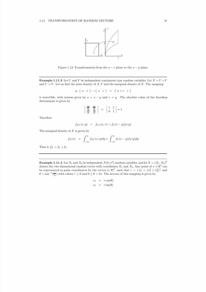
8/11/2019 Random process by B. Hajek
http://slidepdf.com/reader/full/random-process-by-b-hajek 41/448
1.11. TRANSFORMATION OF RANDOM VECTORS 31
xu
v
1
1 1
2
y
Figure 1.13: Transformation from the u − v plane to the x − y plane.
Example 1.11.3 Let U and V be independent continuous type random variables. Let X = U + V
and Y = V . Let us find the joint density of X, Y and the marginal density of X . The mapping
g :
u v →
u v
=
u + v v
is invertible, with inverse given by u = x − y and v = y. The absolute value of the Jacobiandeterminant is given by ∂x
∂u∂x∂v
∂y∂u
∂y∂v
=
1 10 1
= 1
Therefore
f XY (x, y) = f UV (u, v) = f U (x − y)f V (y)
The marginal density of X is given by
f X (x) =
∞−∞
f XY (x, y)dy =
∞−∞
f U (x − y)f V (y)dy
That is f X = f U ∗ f V .
Example 1.11.4 Let X 1 and X 2 be independent N (0, σ2) random variables, and let X = (X 1, X 2)T
denote the two-dimensional random vector with coordinates X 1 and X 2. Any point of x ∈R2
canbe represented in polar coordinates by the vector (r, θ)T such that r = x = (x2
1 + x22)
12 and
θ = tan−1(x2x1
) with values r ≥ 0 and 0 ≤ θ < 2π. The inverse of this mapping is given by
x1 = r cos(θ)
x2 = r sin(θ)
8/11/2019 Random process by B. Hajek
http://slidepdf.com/reader/full/random-process-by-b-hajek 42/448
32 CHAPTER 1. GETTING STARTED
We endeavor to find the pdf of the random vector ( R, Θ)T , the polar coordinates of X . The pdf of X is given by
f X (x) = f X 1(x1)f X 2(x2) =
1
2πσ2 e− r2
2σ2
The range of the mapping is the set r > 0 and 0 < θ ≤ 2π. On the range,∂x
∂
rθ
=
∂x1∂r
∂x1∂θ
∂x2∂r
∂x2∂θ
=
cos(θ) −r sin(θ)sin(θ) r cos(θ)
= r
Therefore for (r, θ)T in the range of the mapping,
f R,Θ(r, θ) = f X (x) ∂x
∂
rθ
= r2πσ2
e− r2
2σ2
Of course f R,Θ(r, θ) = 0 off the range of the mapping. The joint density factors into a function of r and a function of θ, so R and Θ are independent. Moreover, R has the Rayleigh density withparameter σ2, and Θ is uniformly distributed on [0, 2π].
1.12 Problems
1.1 Simple events
A register contains 8 random binary digits which are mutually independent. Each digit is a zero ora one with equal probability. (a) Describe an appropriate probability space (Ω, F , P ) correspondingto looking at the contents of the register.(b) Express each of the following four events explicitly as subsets of Ω, and find their probabilities:E 1=“No two neighboring digits are the same”E 2=“Some cyclic shift of the register contents is equal to 01100110”E 3=“The register contains exactly four zeros”E 4=“There is a run of at least six consecutive ones”(c) Find P (E 1|E 3) and P (E 2|E 3).
1.2 A ballot problem
Suppose there is an election with two candidates and six ballots turned in, such that four of theballots are for the winning candidate and two of the ballots are for the other candidate. Theballots are opened and counted one at a time, in random order, with all orders equally likely. Findthe probability that from the time the first ballot is counted until all the ballots are counted, thewinning candidate has the majority of the ballots counted. (“Majority” means there are strictlymore votes for the winning candidate than for the other candidate.)

8/11/2019 Random process by B. Hajek
http://slidepdf.com/reader/full/random-process-by-b-hajek 43/448
1.12. PROBLEMS 33
1.3 Ordering of three random variablesSuppose X,Y, and U are mutually independent, such that X and Y are each exponentially dis-tributed with some common parameter λ > 0, and U is uniformly distributed on the interval [0, 1].
Express P X < U < Y in terms of λ. Simplify your answer.
1.4 Independent vs. mutually exclusive(a) Suppose that an event E is independent of itself. Show that either P (E ) = 0 or P (E ) = 1.(b) Events A and B have probabilities P (A) = 0.3 and P (B) = 0.4. What is P (A ∪ B) if A and Bare independent? What is P (A ∪ B) if A and B are mutually exclusive?(c) Now suppose that P (A) = 0.6 and P (B) = 0.8. In this case, could the events A and B beindependent? Could they be mutually exclusive?
1.5 Congestion at output portsConsider a packet switch with some number of input ports and eight output ports. Suppose fourpackets simultaneously arrive on different input ports, and each is routed toward an output port.Assume the choices of output ports are mutually independent, and for each packet, each outputport has equal probability.(a) Specify a probability space (Ω, F , P ) to describe this situation.(b) Let X i denote the number of packets routed to output port i for 1 ≤ i ≤ 8. Describe the jointpmf of X 1, . . . , X 8.(c) Find Cov(X 1, X 2).(d) Find P X i ≤ 1 for all i.(e) Find P X i ≤ 2 for all i.
1.6 Frantic searchAt the end of each day Professor Plum puts her glasses in her drawer with probability .90, leaves
them on the table with probability .06, leaves them in her briefcase with probability 0.03, and sheactually leaves them at the office with probability 0.01. The next morning she has no recollectionof where she left the glasses. She looks for them, but each time she looks in a place the glasses areactually located, she misses finding them with probability 0.1, whether or not she already lookedin the same place. (After all, she doesn’t have her glasses on and she is in a hurry.)(a) Given that Professor Plum didn’t find the glasses in her drawer after looking one time, what isthe conditional probability the glasses are on the table?(b) Given that she didn’t find the glasses after looking for them in the drawer and on the tableonce each, what is the conditional probability they are in the briefcase?(c) Given that she failed to find the glasses after looking in the drawer twice, on the table twice,and in the briefcase once, what is the conditional probability she left the glasses at the office?
1.7 Conditional probability of failed device given failed attemptsA particular webserver may be working or not working. If the webserver is not working, any attemptto access it fails. Even if the webserver is working, an attempt to access it can fail due to networkcongestion beyond the control of the webserver. Suppose that the a priori probability that the serveris working is 0.8. Suppose that if the server is working, then each access attempt is successful with
8/11/2019 Random process by B. Hajek
http://slidepdf.com/reader/full/random-process-by-b-hajek 44/448
34 CHAPTER 1. GETTING STARTED
probability 0.9, independently of other access attempts. Find the following quantities.(a) P ( first access attempt fails)(b) P (server is working | first access attempt fails )
(c) P (second access attempt fails | first access attempt fails )(d) P (server is working | first and second access attempts fail ).
1.8 Conditional probabilities–basic computations of iterative decodingSuppose B1, . . . , Bn, Y 1, . . . , Y n are discrete random variables with joint pmf
p(b1, . . . , bn, y1, . . . , yn) =
2−n
ni=1 q i(yi|bi) if bi ∈ 0, 1 for 1 ≤ i ≤ n
0 else
where q i(yi|bi) as a function of yi is a pmf for bi ∈ 0, 1. Finally, let B = B1⊕· · ·⊕Bn represent themodulo two sum of B1, · · · , Bn. Thus, the ordinary sum of the n +1 random variables B1, . . . , Bn, Bis even. Express P (B = 1
|Y 1 = y1,
· · · .Y n = yn) in terms of the yi and the functions q i. Simplify
your answer.(b) Suppose B and Z 1, . . . , Z k are discrete random variables with joint pmf
p(b, z1, . . . , zk) =
1
2
k j=1 r j(z j |b) if b ∈ 0, 1
0 else
where r j(z j |b) as a function of z j is a pmf for b ∈ 0, 1 fixed. Express P (B = 1|Z 1 = z1, . . . , Z k =zk) in terms of the z j and the functions r j.
1.9 Conditional lifetimes and the memoryless property of the geometric distribution(a) Let X represent the lifetime, rounded up to an integer number of years, of a certain car battery.
Suppose that the pmf of X is given by pX (k) = 0.2 if 3 ≤ k ≤ 7 and pX (k) = 0 otherwise. (i)Find the probability, P X > 3, that a three year old battery is still working. (ii) Given that thebattery is still working after five years, what is the conditional probability that the battery willstill be working three years later? (i.e. what is P (X > 8|X > 5)?)(b) A certain Illini basketball player shoots the ball repeatedly from half court during practice.Each shot is a success with probability p and a miss with probability 1 − p, independently of theoutcomes of previous shots. Let Y denote the number of shots required for the first success. (i)Express the probability that she needs more than three shots for a success, P Y > 3, in terms of p. (ii) Given that she already missed the first five shots, what is the conditional probability thatshe will need more than three additional shots for a success? (i.e. what is P (Y > 8|Y > 5))?(iii) What type of probability distribution does Y have?
1.10 Blue cornersSuppose each corner of a cube is colored blue, independently of the other corners, with someprobability p. Let B denote the event that at least one face of the cube has all four corners coloredblue. (a) Find the conditional probability of B given that exactly five corners of the cube arecolored blue. (b) Find P (B), the unconditional probability of B.
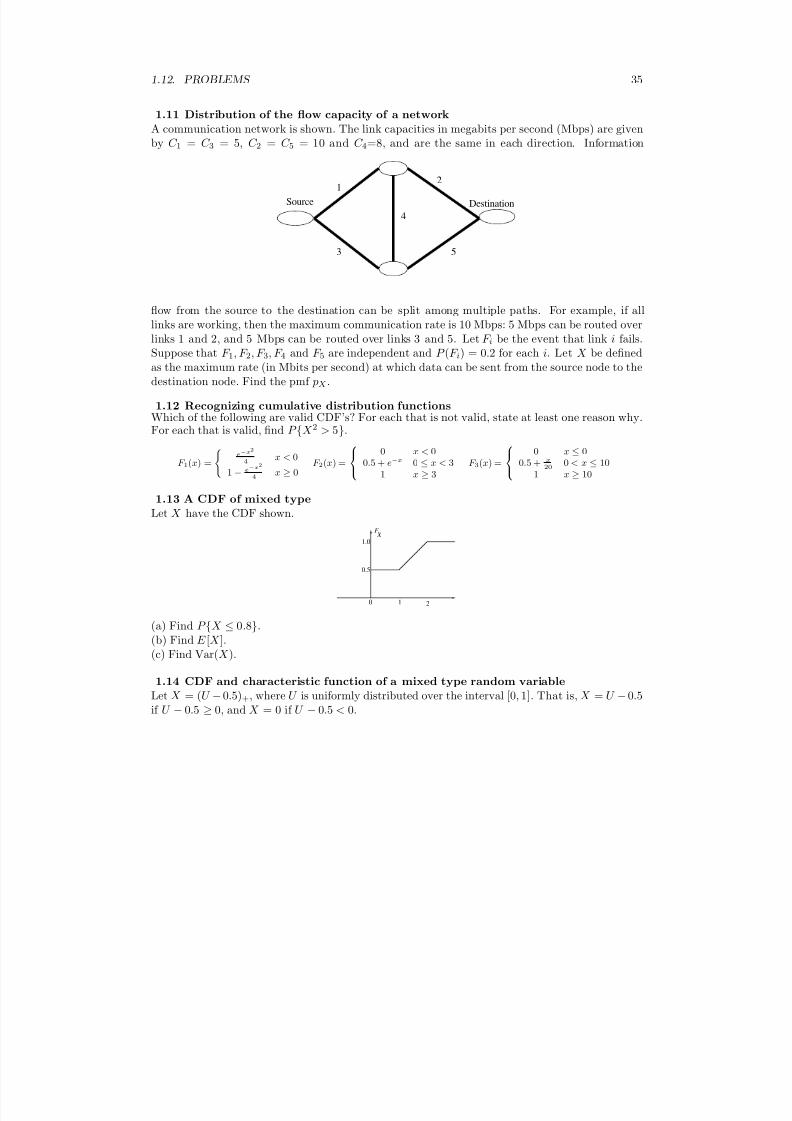
8/11/2019 Random process by B. Hajek
http://slidepdf.com/reader/full/random-process-by-b-hajek 45/448
1.12. PROBLEMS 35
1.11 Distribution of the flow capacity of a networkA communication network is shown. The link capacities in megabits per second (Mbps) are givenby C 1 = C 3 = 5, C 2 = C 5 = 10 and C 4=8, and are the same in each direction. Information
Source
12
3
4
5
Destination
flow from the source to the destination can be split among multiple paths. For example, if all
links are working, then the maximum communication rate is 10 Mbps: 5 Mbps can be routed overlinks 1 and 2, and 5 Mbps can be routed over links 3 and 5. Let F i be the event that link i fails.Suppose that F 1, F 2, F 3, F 4 and F 5 are independent and P (F i) = 0.2 for each i. Let X be definedas the maximum rate (in Mbits per second) at which data can be sent from the source node to thedestination node. Find the pmf pX .
1.12 Recognizing cumulative distribution functionsWhich of the following are valid CDF’s? For each that is not valid, state at least one reason why.For each that is valid, find P X 2 > 5.
F 1(x) =
( e−x
2
4 x < 0
1− e−x2
4 x ≥ 0
F 2(x) =
8<:
0 x < 00.5 + e−x 0 ≤ x < 3
1 x ≥ 3F 3(x) =
8<:
0 x ≤ 00.5 + x
20 0 < x ≤ 10
1 x ≥ 10
1.13 A CDF of mixed typeLet X have the CDF shown.
1 20
F X
1.0
0.5
(a) Find P X ≤ 0.8.
(b) Find E [X ].(c) Find Var(X ).
1.14 CDF and characteristic function of a mixed type random variableLet X = (U − 0.5)+, where U is uniformly distributed over the interval [0, 1]. That is, X = U − 0.5if U − 0.5 ≥ 0, and X = 0 if U − 0.5 < 0.
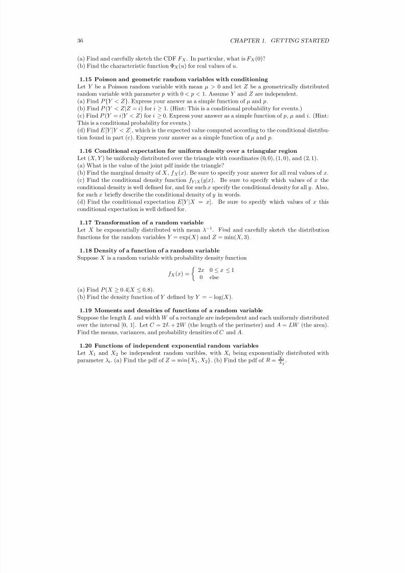
8/11/2019 Random process by B. Hajek
http://slidepdf.com/reader/full/random-process-by-b-hajek 46/448
36 CHAPTER 1. GETTING STARTED
(a) Find and carefully sketch the CDF F X . In particular, what is F X (0)?(b) Find the characteristic function ΦX (u) for real values of u.
1.15 Poisson and geometric random variables with conditioningLet Y be a Poisson random variable with mean µ > 0 and let Z be a geometrically distributedrandom variable with parameter p with 0 < p < 1. Assume Y and Z are independent.(a) Find P Y < Z . Express your answer as a simple function of µ and p.(b) Find P (Y < Z |Z = i) for i ≥ 1. (Hint: This is a conditional probability for events.)(c) Find P (Y = i|Y < Z ) for i ≥ 0. Express your answer as a simple function of p, µ and i. (Hint:This is a conditional probability for events.)(d) Find E [Y |Y < Z ], which is the expected value computed according to the conditional distribu-tion found in part (c). Express your answer as a simple function of µ and p.
1.16 Conditional expectation for uniform density over a triangular regionLet (X, Y ) be uniformly distributed over the triangle with coordinates (0, 0), (1, 0), and (2, 1).
(a) What is the value of the joint pdf inside the triangle?(b) Find the marginal density of X , f X (x). Be sure to specify your answer for all real values of x.(c) Find the conditional density function f Y |X (y|x). Be sure to specify which values of x theconditional density is well defined for, and for such x specify the conditional density for all y. Also,for such x briefly describe the conditional density of y in words.(d) Find the conditional expectation E [Y |X = x]. Be sure to specify which values of x thisconditional expectation is well defined for.
1.17 Transformation of a random variableLet X be exponentially distributed with mean λ−1. Find and carefully sketch the distributionfunctions for the random variables Y = exp(X ) and Z = min(X, 3).
1.18 Density of a function of a random variableSuppose X is a random variable with probability density function
f X (x) =
2x 0 ≤ x ≤ 1
0 else
(a) Find P (X ≥ 0.4|X ≤ 0.8).(b) Find the density function of Y defined by Y = − log(X ).
1.19 Moments and densities of functions of a random variableSuppose the length L and width W of a rectangle are independent and each uniformly distributed
over the interval [0, 1]. Let C = 2L + 2W (the length of the perimeter) and A = LW (the area).Find the means, variances, and probability densities of C and A.
1.20 Functions of independent exponential random variablesLet X 1 and X 2 be independent random varibles, with X i being exponentially distributed withparameter λi. (a) Find the pdf of Z = minX 1, X 2. (b) Find the pdf of R = X 1
X 2.
8/11/2019 Random process by B. Hajek
http://slidepdf.com/reader/full/random-process-by-b-hajek 47/448
1.12. PROBLEMS 37
1.21 Using the Gaussian Q functionExpress each of the given probabilities in terms of the standard Gaussian complementary CDF Q.(a) P X ≥ 16, where X has the N (10, 9) distribution.
(b) P X 2
≥ 16, where X has the N (10, 9) distribution.(c) P |X − 2Y | > 1, where X and Y are independent, N (0, 1) random variables. (Hint: Linearcombinations of independent Gaussian random variables are Gaussian.)
1.22 Gaussians and the Q functionLet X and Y be independent, N (0, 1) random variables.(a) Find Cov(3X + 2Y, X + 5Y + 10).(b) Express P X + 4Y ≥ 2 in terms of the Q function.(c) Express P (X − Y )2 > 9 in terms of the Q function.
1.23 Correlation of histogram valuesSuppose that n fair dice are independently rolled. Let
X i = 1 if a 1 shows on the ith roll
0 else Y i =
1 if a 2 shows on the ith roll0 else
Let X denote the sum of the X i’s, which is simply the number of 1’s rolled. Let Y denote the sumof the Y i’s, which is simply the number of 2’s rolled. Note that if a histogram is made recordingthe number of occurrences of each of the six numbers, then X and Y are the heights of the firsttwo entries in the histogram.(a) Find E [X 1] and Var(X 1).(b) Find E [X ] and Var(X ).(c) Find Cov(X i, Y j) if 1 ≤ i, j ≤ n (Hint: Does it make a difference if i = j?)(d) Find Cov(X, Y ) and the correlation coefficient ρ(X, Y ) = Cov(X, Y )/ Var(X )Var(Y ).
(e) Find E [Y |X = x] for any integer x with 0 ≤ x ≤ n. Note that your answer should depend onx and n, but otherwise your answer is deterministic.
1.24 Working with a joint densitySuppose X and Y have joint density function f X,Y (x, y) = c(1 + xy) if 2 ≤ x ≤ 3 and 1 ≤ y ≤ 2,and f X,Y (x, y) = 0 otherwise. (a) Find c. (b) Find f X and f Y . (c) Find f X |Y .
1.25 A function of jointly distributed random variablesSuppose (U, V ) is uniformly distributed over the square with corners (0,0), (1,0), (1,1), and (0,1),and let X = U V . Find the CDF and pdf of X .
1.26 Density of a difference
Let X and Y be independent, exponentially distributed random variables with parameter λ, suchthat λ > 0. Find the pdf of Z = |X − Y |.
1.27 Working with a two dimensional densityLet the random variables X and Y be jointly uniformly distributed over the region shown.
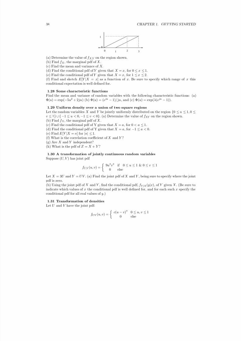
8/11/2019 Random process by B. Hajek
http://slidepdf.com/reader/full/random-process-by-b-hajek 48/448
38 CHAPTER 1. GETTING STARTED
0 1 2 3
1
0
(a) Determine the value of f X,Y on the region shown.(b) Find f X , the marginal pdf of X.(c) Find the mean and variance of X.(d) Find the conditional pdf of Y given that X = x, for 0 ≤ x ≤ 1.(e) Find the conditional pdf of Y given that X = x, for 1 ≤ x ≤ 2.(f) Find and sketch E [Y |X = x] as a function of x. Be sure to specify which range of x thisconditional expectation is well defined for.
1.28 Some characteristic functionsFind the mean and variance of random variables with the following characteristic functions: (a)Φ(u) = exp(−5u2 + 2 ju) (b) Φ(u) = (e ju − 1)/ju, and (c) Φ(u) = exp(λ(e ju − 1)).
1.29 Uniform density over a union of two square regionsLet the random variables X and Y be jointly uniformly distributed on the region 0 ≤ u ≤ 1, 0 ≤v ≤ 1∪−1 ≤ u < 0, −1 ≤ v < 0. (a) Determine the value of f XY on the region shown.(b) Find f X , the marginal pdf of X .(c) Find the conditional pdf of Y given that X = a, for 0 < a ≤ 1.(d) Find the conditional pdf of Y given that X = a, for −1 ≤ a < 0.(e) Find E [Y |X = a] for |a| ≤ 1.(f) What is the correlation coefficient of X and Y ?(g) Are X and Y independent?
(h) What is the pdf of Z = X + Y ?
1.30 A transformation of jointly continuous random variablesSuppose (U, V ) has joint pdf
f U,V (u, v) =
9u2v2 if 0 ≤ u ≤ 1 & 0 ≤ v ≤ 1
0 else
Let X = 3U and Y = U V . (a) Find the joint pdf of X and Y , being sure to specify where the jointpdf is zero.(b) Using the joint pdf of X and Y , find the conditional pdf, f Y |X (y|x), of Y given X . (Be sure toindicate which values of x the conditional pdf is well defined for, and for each such x specify the
conditional pdf for all real values of y.)
1.31 Transformation of densitiesLet U and V have the joint pdf:
f UV (u, v) =
c(u − v)2 0 ≤ u, v ≤ 1
0 else
8/11/2019 Random process by B. Hajek
http://slidepdf.com/reader/full/random-process-by-b-hajek 49/448
1.12. PROBLEMS 39
for some constant c. (a) Find the constant c. (b) Suppose X = U 2 and Y = U 2V 2. Describe the joint pdf f X,Y (x, y) of X and Y . Be sure to indicate where the joint pdf is zero.
1.32 Opening a bicycle combination lockA certain bicycle combination lock has 104 possible combinations, ranging from 0000 to 9999.Suppose the combination required to open the lock takes any one of the possible values with equalprobability. Suppose it takes two seconds to try opening the lock with a given combination. Findthe mean and standard deviation of the amount of time, each to within a minute, of how long itwould take to open the lock by cycling through the combinations without repetition. (Hint: Youcan approximate the random amount of time required by a continuous type random variable.)
1.33 Transformation of joint densitiesAssume X and Y are independent, each with the exponential pdf with parameter λ > 0. LetW = X − Y and Z = X 2 + X − Y. Find the joint pdf of (W, Z ). Be sure to specify its support (i.e.where it is not zero).
1.34 Computing some covariancesSuppose X,Y, and Z are random variables, each with mean zero and variance 20, such thatCov(X, Y ) = Cov(X, Z ) = 10 and Cov(Y, Z ) = 5. (a) Find Cov(X + Y, X − Y ). (b) FindCov(3X+Z,3X+Y). (c) Find E [(X + Y )2].
1.35 Conditional densities and expectationsSuppose that random variables X and Y have the joint pdf:
f XY (u, v) =
4u2, 0 < v < u < 10, elsewhere
(a) Find E [XY ]. (b) Find f Y (v). Be sure to specify it for all values of v. (c) Find f X |Y (u|v). Besure to specify where it is undefined, and where it is zero. (d) Find E [X 2|Y = v] for 0 < v < 1.
1.36 Jointly distributed variablesLet U and V be independent random variables, such that U is uniformly distributed over theinterval [0, 1], and V has the exponential probability density function
(a) Calculate E [ V 2
1+U ].(b) Calculate P U ≤ V .(c) Find the joint probability density function of Y and Z, where Y = U 2 and Z = U V .
1.37 * Why not every set has a length
Suppose a length (actually, “one-dimensional volume” would be a better name) of any subset A ⊂ Rcould be defined, so that the following axioms are satisfied:
L0: 0 ≤ length(A) ≤ ∞ for any A ⊂ RL1: length([a, b]) = b − a for a < b
8/11/2019 Random process by B. Hajek
http://slidepdf.com/reader/full/random-process-by-b-hajek 50/448
40 CHAPTER 1. GETTING STARTED
L2: length(A) = length(A + y), for any A ⊂ R and y ∈ R, where A + y represents the translationof A by y , defined by A + y = x + y : x ∈ A
L3: If A = ∪
∞i=1
Bi such that B1, B2,· · ·
are disjoint, then length(A) = ∞i=1
length(Bi).
The purpose of this problem is to show that the above supposition leads to a contradiction. LetQ denote the set of rational numbers, Q = p/q : p, q ∈ Z, q = 0. (a) Show that the set of rational numbers can be expressed as Q = q 1, q 2, . . ., which means that Q is countably infinite.Say that x, y ∈ R are equivalent, and write x ∼ y, if x − y ∈ Q. (b) Show that ∼ is an equivalence relation , meaning it is reflexive (a ∼ a for all a ∈ R), symmetric (a ∼ b implies b ∼ a), andtransitive (a ∼ b and b ∼ c implies a ∼ c). For any x ∈ R, let Qx = Q + x. (c) Show that forany x, y ∈ R, either Qx = Qy or Qx ∩ Qy = ∅. Sets of the form Qx are called equivalence classes of the equivalence relation ∼. (d) Show that Qx ∩ [0, 1] = ∅ for all x ∈ R, or in other words, eachequivalence class contains at least one element from the interval [0, 1]. Let V be a set obtainedby choosing exactly one element in [0, 1] from each equivalence class (by accepting that V is well
defined, you’ll be accepting what is called the Axiom of Choice ). So V is a subset of [0, 1]. Supposeq 1, q 2, . . . is an enumeration of all the rational numbers in the interval [−1, 1], with no numberappearing twice in the list. Let V i = V + q i for i ≥ 1. (e) Verify that the sets V i are disjoint, and[0, 1] ⊂ ∪∞
i=1V i ⊂ [−1, 2]. Since the V i’s are translations of V , they should all have the same lengthas V . If the length of V is defined to be zero, then [0, 1] would be covered by a countable unionof disjoint sets of length zero, so [0, 1] would also have length zero. If the length of V were strictlypositive, then the countable union would have infinite length, and hence the interval [−1, 2] wouldhave infinite length. Either way there is a contradiction.
1.38 * On sigma-algebras, random variables, and measurable functionsProve the seven statements lettered (a)-(g) in what follows.Definition. Let Ω be an arbitrary set. A nonempty collection
F of subsets of Ω is defined to be
an algebra if: (i) Ac ∈ F whenever A ∈ F and (ii) A ∪ B ∈ F whenever A, B ∈ F .(a) If F is an algebra then ∅ ∈ F , Ω ∈ F , and the union or intersection of any finite collection of sets in F is in F .Definition. F is called a σ-algebra if F is an algebra such that whenever A1, A2,... are each in F ,so is the union, ∪Ai.(b) If F is a σ-algebra and B1, B2, . . . are in F , then so is the intersection, ∩Bi.(c) Let U be an arbitrary nonempty set, and suppose that F u is a σ-algebra of subsets of Ω foreach u ∈ U . Then the intersection ∩u∈U F u is also a σ-algebra.(d) The collection of all subsets of Ω is a σ-algebra.(e) If F o is any collection of subsets of Ω then there is a smallest σ-algebra containing F o (Hint:use (c) and (d).)
Definitions. B(R) is the smallest σ-algebra of subsets of R which contains all sets of the form(−∞, a]. Sets in B(R) are called Borel sets. A real-valued random variable on a probability space(Ω, F , P ) is a real-valued function X on Ω such that ω : X (ω) ≤ a ∈ F for any a ∈ R.(f) If X is a random variable on (Ω, F , P ) and A ∈ B(R) then ω : X (ω) ∈ A ∈ F . (Hint: Fixa random variable X . Let D be the collection of all subsets A of B(R) for which the conclusion istrue. It is enough (why?) to show that D contains all sets of the form (−∞, a] and that D is a

8/11/2019 Random process by B. Hajek
http://slidepdf.com/reader/full/random-process-by-b-hajek 51/448
1.12. PROBLEMS 41
σ-algebra of subsets of R. You must use the fact that F is a σ-algebra.)Remark. By (f), P ω : X (ω) ∈ A, or P X ∈ A for short, is well defined for A ∈ B(R).Definition. A function g mapping R to R is called Borel measurable if x : g(x) ∈ A ∈ B(R)
whenever A ∈ B(R).(g) If X is a real-valued random variable on (Ω, F , P ) and g is a Borel measurable function, thenY defined by Y = g(X ) is also a random variable on (Ω, F , P ).

8/11/2019 Random process by B. Hajek
http://slidepdf.com/reader/full/random-process-by-b-hajek 52/448
42 CHAPTER 1. GETTING STARTED
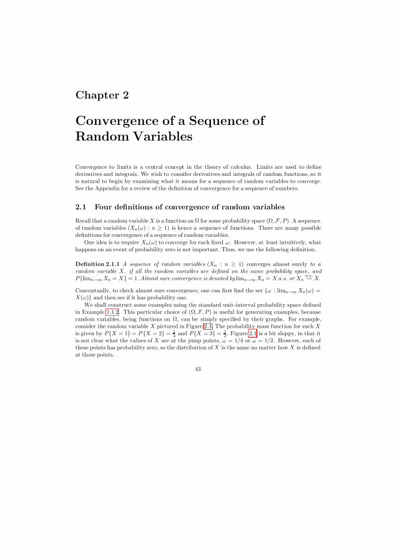
8/11/2019 Random process by B. Hajek
http://slidepdf.com/reader/full/random-process-by-b-hajek 53/448
Chapter 2
Convergence of a Sequence of Random Variables
Convergence to limits is a central concept in the theory of calculus. Limits are used to definederivatives and integrals. We wish to consider derivatives and integrals of random functions, so itis natural to begin by examining what it means for a sequence of random variables to converge.See the Appendix for a review of the definition of convergence for a sequence of numbers.
2.1 Four definitions of convergence of random variables
Recall that a random variable X is a function on Ω for some probability space (Ω, F , P ). A sequenceof random variables (X n(ω) : n ≥ 1) is hence a sequence of functions. There are many possibledefinitions for convergence of a sequence of random variables.
One idea is to require X n(ω) to converge for each fixed ω. However, at least intuitively, whathappens on an event of probability zero is not important. Thus, we use the following definition.
Definition 2.1.1 A sequence of random variables (X n : n ≥ 1) converges almost surely to a random variable X , if all the random variables are defined on the same probability space, and P limn→∞ X n = X = 1. Almost sure convergence is denoted by limn→∞ X n = X a.s. or X n
a.s.→ X.
Conceptually, to check almost sure convergence, one can first find the set ω : limn→∞ X n(ω) =X (ω) and then see if it has probability one.
We shall construct some examples using the standard unit-interval probability space definedin Example 1.1.2. This particular choice of (Ω, F , P ) is useful for generating examples, because
random variables, being functions on Ω, can be simply specified by their graphs. For example,consider the random variable X pictured in Figure 2.1. The probability mass function for such X is given by P X = 1 = P X = 2 = 1
4 and P X = 3 = 12 . Figure 2.1 is a bit sloppy, in that it
is not clear what the values of X are at the jump points, ω = 1/4 or ω = 1/2. However, each of these points has probability zero, so the distribution of X is the same no matter how X is definedat those points.
43
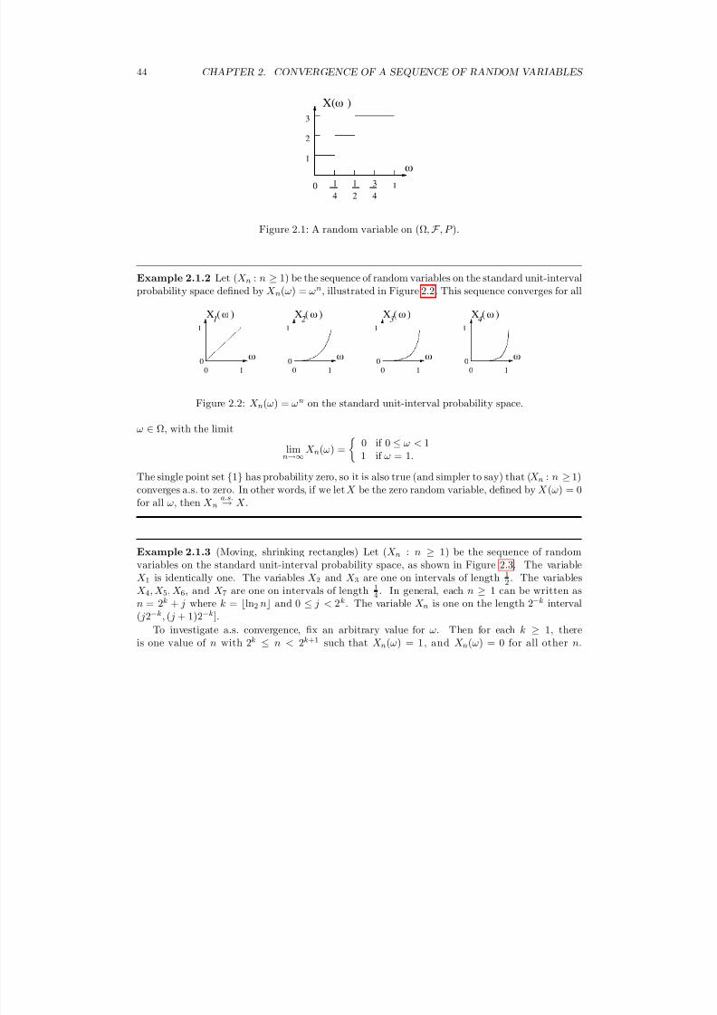
8/11/2019 Random process by B. Hajek
http://slidepdf.com/reader/full/random-process-by-b-hajek 54/448
44 CHAPTER 2. CONVERGENCE OF A SEQUENCE OF RANDOM VARIABLES
1
2
3
0 1
4
1
2
ω
ω
X( )
13
4
Figure 2.1: A random variable on (Ω, F , P ).
Example 2.1.2 Let (X n : n
≥ 1) be the sequence of random variables on the standard unit-interval
probability space defined by X n(ω) = ωn, illustrated in Figure 2.2. This sequence converges for all
4
0 1
0
1
!
X ( )!
0 1
0
1
!
X ( )!
0 1
0
1
!
X ( )!
0 1
0
1
!
X ( )!1 2 3
Figure 2.2: X n(ω) = ωn on the standard unit-interval probability space.
ω ∈
Ω, with the limit
limn→∞ X n(ω) =
0 if 0 ≤ ω < 11 if ω = 1.
The single point set 1 has probability zero, so it is also true (and simpler to say) that (X n : n ≥ 1)converges a.s. to zero. In other words, if we let X be the zero random variable, defined by X (ω) = 0for all ω, then X n
a.s.→ X .
Example 2.1.3 (Moving, shrinking rectangles) Let (X n : n ≥ 1) be the sequence of randomvariables on the standard unit-interval probability space, as shown in Figure 2.3. The variable
X 1 is identically one. The variables X 2 and X 3 are one on intervals of length 1
2 . The variablesX 4, X 5, X 6, and X 7 are one on intervals of length 14 . In general, each n ≥ 1 can be written as
n = 2k + j where k = ln2 n and 0 ≤ j < 2k. The variable X n is one on the length 2−k interval( j2−k, ( j + 1)2−k].
To investigate a.s. convergence, fix an arbitrary value for ω. Then for each k ≥ 1, thereis one value of n with 2k ≤ n < 2k+1 such that X n(ω) = 1, and X n(ω) = 0 for all other n.
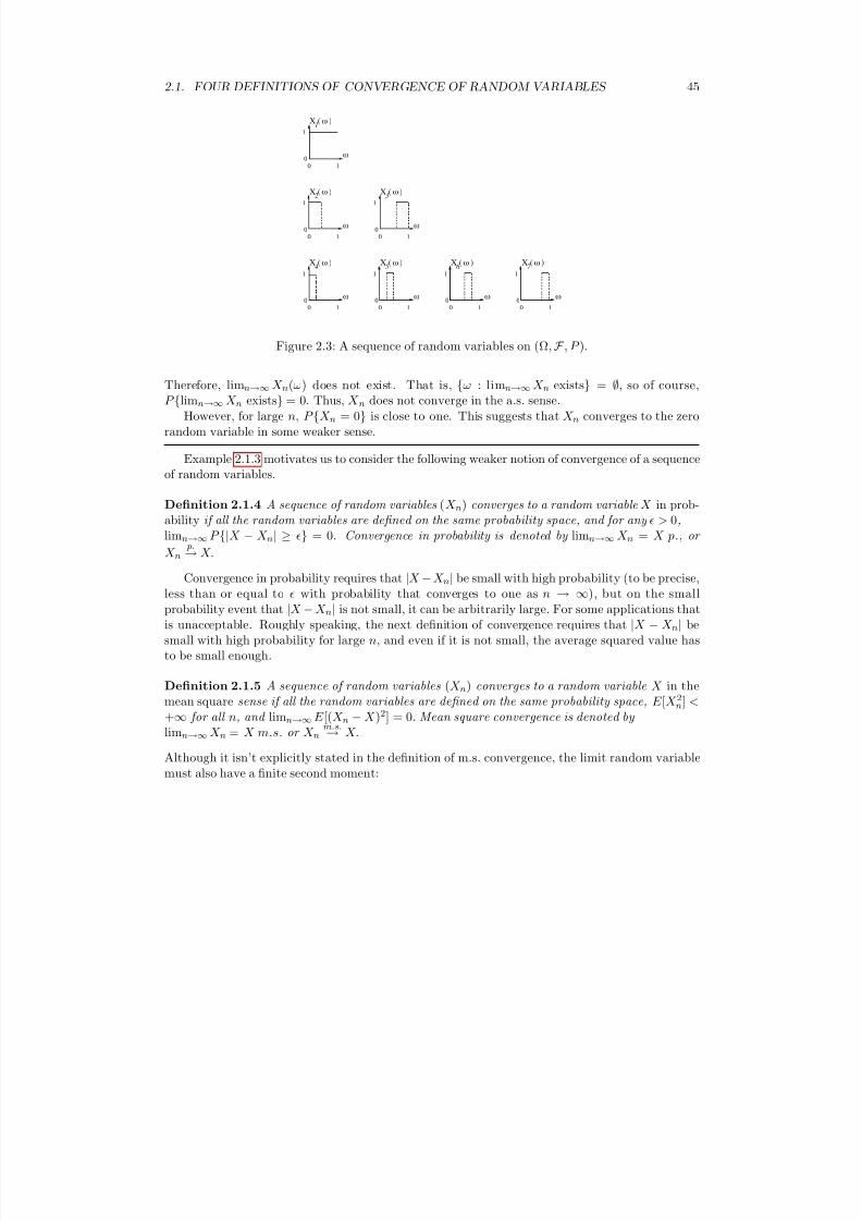
8/11/2019 Random process by B. Hajek
http://slidepdf.com/reader/full/random-process-by-b-hajek 55/448
2.1. FOUR DEFINITIONS OF CONVERGENCE OF RANDOM VARIABLES 45
0 1
0
1
ω
X ( )ω
0 1
0
1
ω
X ( )ω
0 1
0
1
ω
X ( )ω
0 1
0
1
ω
X ( )ω
0 1
0
1
ω
X ( )ω
0 1
0
1
ω
X ( )ω
0 1
0
1
ω
X ( )ω6 7
1
2 3
54
Figure 2.3: A sequence of random variables on (Ω, F , P ).
Therefore, limn→∞ X n(ω) does not exist. That is, ω : limn→∞ X n exists = ∅, so of course,P limn→∞ X n exists = 0. Thus, X n does not converge in the a.s. sense.
However, for large n, P X n = 0 is close to one. This suggests that X n converges to the zerorandom variable in some weaker sense.
Example 2.1.3 motivates us to consider the following weaker notion of convergence of a sequenceof random variables.
Definition 2.1.4 A sequence of random variables (X n) converges to a random variable X in prob-
ability if all the random variables are defined on the same probability space, and for any > 0,limn→∞ P |X − X n| ≥ = 0. Convergence in probability is denoted by limn→∞ X n = X p., or
X n p.→ X.
Convergence in probability requires that |X −X n| be small with high probability (to be precise,less than or equal to with probability that converges to one as n → ∞), but on the smallprobability event that |X − X n| is not small, it can be arbitrarily large. For some applications thatis unacceptable. Roughly speaking, the next definition of convergence requires that |X − X n| besmall with high probability for large n, and even if it is not small, the average squared value hasto be small enough.
Definition 2.1.5 A sequence of random variables (X n) converges to a random variable X in the
mean square sense if all the random variables are defined on the same probability space, E [X 2n] <+∞ for all n, and limn→∞ E [(X n − X )2] = 0. Mean square convergence is denoted by limn→∞ X n = X m.s. or X n
m.s.→ X.
Although it isn’t explicitly stated in the definition of m.s. convergence, the limit random variablemust also have a finite second moment:
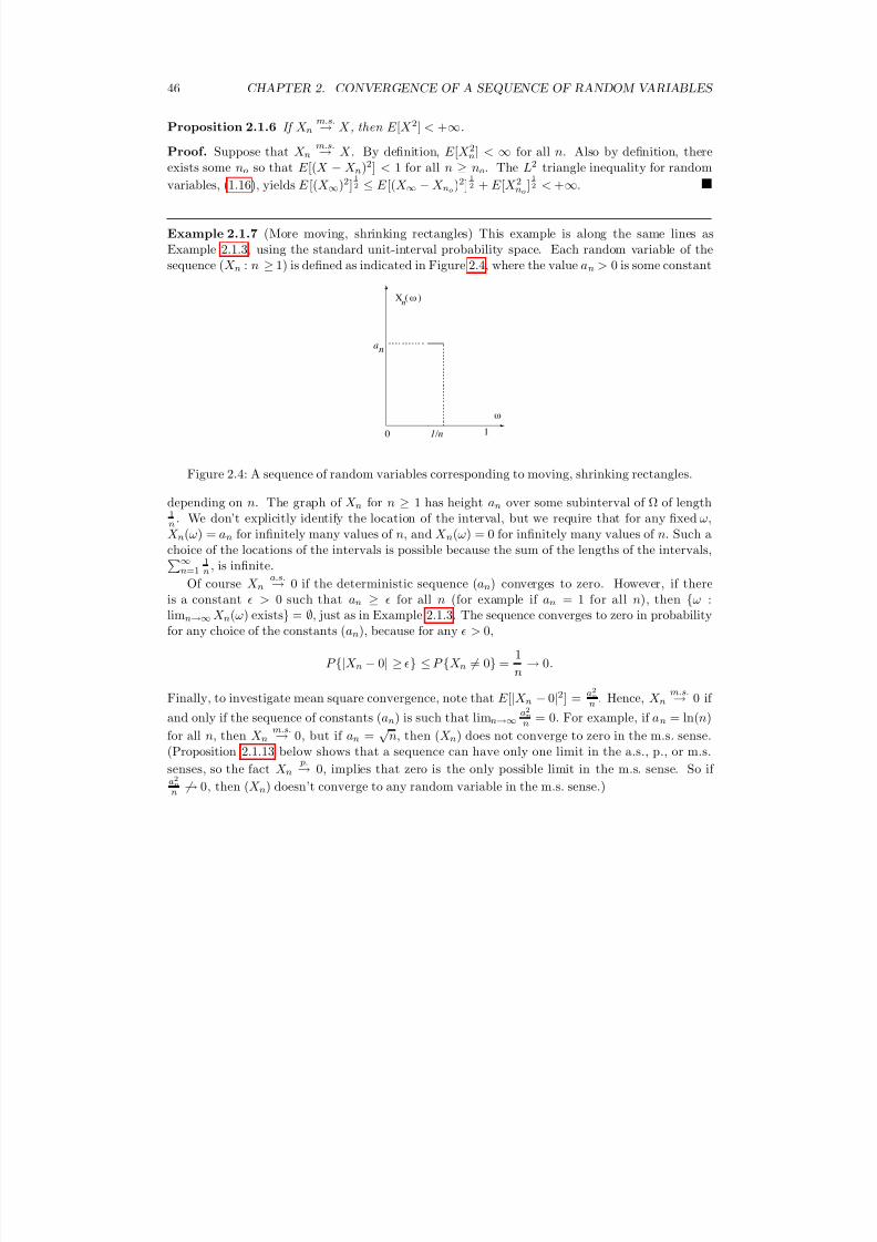
8/11/2019 Random process by B. Hajek
http://slidepdf.com/reader/full/random-process-by-b-hajek 56/448
46 CHAPTER 2. CONVERGENCE OF A SEQUENCE OF RANDOM VARIABLES
Proposition 2.1.6 If X nm.s.→ X , then E [X 2] < +∞.
Proof. Suppose that X nm.s.→ X . By definition, E [X 2n] < ∞ for all n. Also by definition, there
exists some no so that E [(X −
X n)2] < 1 for all n ≥
no. The L2 triangle inequality for random
variables, (1.16), yields E [(X ∞)2] 12 ≤ E [(X ∞ − X no)2] 12 + E [X 2no] 12 < +∞.
Example 2.1.7 (More moving, shrinking rectangles) This example is along the same lines asExample 2.1.3, using the standard unit-interval probability space. Each random variable of thesequence (X n : n ≥ 1) is defined as indicated in Figure 2.4, where the value an > 0 is some constant
a
X ( )!
!
1/n0 1
n
n
Figure 2.4: A sequence of random variables corresponding to moving, shrinking rectangles.
depending on n. The graph of X n for n ≥ 1 has height an over some subinterval of Ω of length1n . We don’t explicitly identify the location of the interval, but we require that for any fixed ω,
X n(ω) = an for infinitely many values of n, and X n(ω) = 0 for infinitely many values of n. Such achoice of the locations of the intervals is possible because the sum of the lengths of the intervals,∞
n=11n , is infinite.
Of course X na.s.→ 0 if the deterministic sequence (an) converges to zero. However, if there
is a constant > 0 such that an ≥ for all n (for example if an = 1 for all n), then ω :limn→∞ X n(ω) exists = ∅, just as in Example 2.1.3. The sequence converges to zero in probabilityfor any choice of the constants (an), because for any > 0,
P |X n − 0| ≥ ≤ P X n = 0 = 1
n → 0.
Finally, to investigate mean square convergence, note that E [
|X n
−0
|2] = a2n
n . Hence, X nm.s.
→ 0 if
and only if the sequence of constants (an) is such that limn→∞ a2nn = 0. For example, if an = ln(n)
for all n, then X nm.s.→ 0, but if an =
√ n, then (X n) does not converge to zero in the m.s. sense.
(Proposition 2.1.13 below shows that a sequence can have only one limit in the a.s., p., or m.s.
senses, so the fact X n p.→ 0, implies that zero is the only possible limit in the m.s. sense. So if
a2nn → 0, then (X n) doesn’t converge to any random variable in the m.s. sense.)
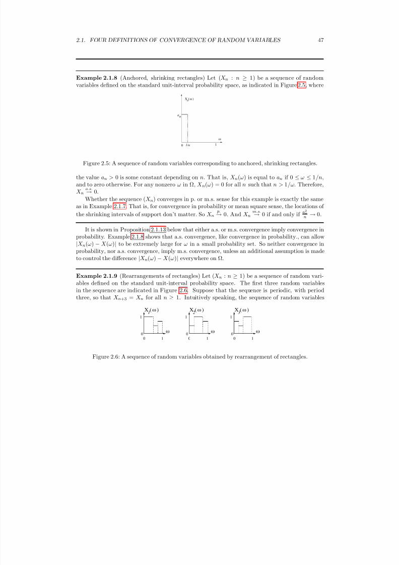
8/11/2019 Random process by B. Hajek
http://slidepdf.com/reader/full/random-process-by-b-hajek 57/448
2.1. FOUR DEFINITIONS OF CONVERGENCE OF RANDOM VARIABLES 47
Example 2.1.8 (Anchored, shrinking rectangles) Let (X n : n ≥ 1) be a sequence of randomvariables defined on the standard unit-interval probability space, as indicated in Figure 2.5, where
1/n
X ( )!
!
0 1
na
n
Figure 2.5: A sequence of random variables corresponding to anchored, shrinking rectangles.
the value an > 0 is some constant depending on n. That is, X n(ω) is equal to an if 0 ≤ ω ≤ 1/n,and to zero otherwise. For any nonzero ω in Ω, X n(ω) = 0 for all n such that n > 1/ω. Therefore,X n
a.s.→ 0.
Whether the sequence (X n) converges in p. or m.s. sense for this example is exactly the sameas in Example 2.1.7. That is, for convergence in probability or mean square sense, the locations of
the shrinking intervals of support don’t matter. So X n p.→ 0. And X n
m.s.→ 0 if and only if a2nn → 0.
It is shown in Proposition 2.1.13 below that either a.s. or m.s. convergence imply convergence inprobability. Example 2.1.8 shows that a.s. convergence, like convergence in probability., can allow
|X n(ω) − X (ω)| to be extremely large for ω in a small probability set. So neither convergence inprobability, nor a.s. convergence, imply m.s. convergence, unless an additional assumption is madeto control the difference |X n(ω) − X (ω)| everywhere on Ω.
Example 2.1.9 (Rearrangements of rectangles) Let (X n : n ≥ 1) be a sequence of random vari-ables defined on the standard unit-interval probability space. The first three random variablesin the sequence are indicated in Figure 2.6. Suppose that the sequence is periodic, with periodthree, so that X n+3 = X n for all n ≥ 1. Intuitively speaking, the sequence of random variables
3
0 1
0
1
!
X ( )!
0 1
0
1
!
X ( )!
0 1
0
1
!
X ( )!1 2
Figure 2.6: A sequence of random variables obtained by rearrangement of rectangles.
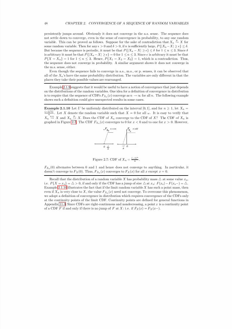
8/11/2019 Random process by B. Hajek
http://slidepdf.com/reader/full/random-process-by-b-hajek 58/448
48 CHAPTER 2. CONVERGENCE OF A SEQUENCE OF RANDOM VARIABLES
persistently jumps around. Obviously it does not converge in the a.s. sense. The sequence doesnot settle down to converge, even in the sense of convergence in probability, to any one randomvariable. This can be proved as follows. Suppose for the sake of contradiction that X n
p.→ X for
some random variable. Then for any > 0 and δ > 0, if n is sufficiently large, P |X n−X | ≥ ≤ δ.But because the sequence is periodic, it must be that P |X n − X | ≥ ≤ δ for 1 ≤ n ≤ 3. Since δ is arbitrary it must be that P |X n −X | ≥ = 0 for 1 ≤ n ≤ 3. Since is arbitrary it must be thatP X = X n = 1 for 1 ≤ n ≤ 3. Hence, P X 1 = X 2 = X 3 = 1, which is a contradiction. Thus,the sequence does not converge in probability. A similar argument shows it does not converge inthe m.s. sense, either.
Even though the sequence fails to converge in a.s., m.s., or p. senses, it can be observed thatall of the X n’s have the same probability distribution. The variables are only different in that theplaces they take their possible values are rearranged.
Example 2.1.9 suggests that it would be useful to have a notion of convergence that just dependson the distributions of the random variables. One idea for a definition of convergence in distribution
is to require that the sequence of CDFs F X n(x) converge as n → ∞ for all n. The following exampleshows such a definition could give unexpected results in some cases.
Example 2.1.10 Let U be uniformly distributed on the interval [0, 1], and for n ≥ 1, let X n =(−1)nU
n . Let X denote the random variable such that X = 0 for all ω. It is easy to verify that
X na.s.→ X and X n
p.→ X. Does the CDF of X n converge to the CDF of X ? The CDF of X n isgraphed in Figure 2.7. The CDF F X n(x) converges to 0 for x < 0 and to one for x > 0. However,
F X n
F X
n
1 −1
n n
n even n odd
0 0
Figure 2.7: CDF of X n = (−1)n
n .
F X n(0) alternates between 0 and 1 and hence does not converge to anything. In particular, itdoesn’t converge to F X (0). Thus, F X n(x) converges to F X (x) for all x except x = 0.
Recall that the distribution of a random variable X has probability mass at some value xo,i.e. P X = xo = > 0, if and only if the CDF has a jump of size at xo: F (xo) − F (xo−) = .
Example 2.1.10 illustrates the fact that if the limit random variable X has such a point mass, theneven if X n is very close to X , the value F X n(x) need not converge. To overcome this phenomenon,we adopt a definition of convergence in distribution which requires convergence of the CDFs onlyat the continuity points of the limit CDF. Continuity points are defined for general functions inAppendix 11.3. Since CDFs are right-continuous and nondecreasing, a point x is a continuity pointof a CDF F if and only if there is no jump of F at X : i.e. if F X (x) = F X (x−).
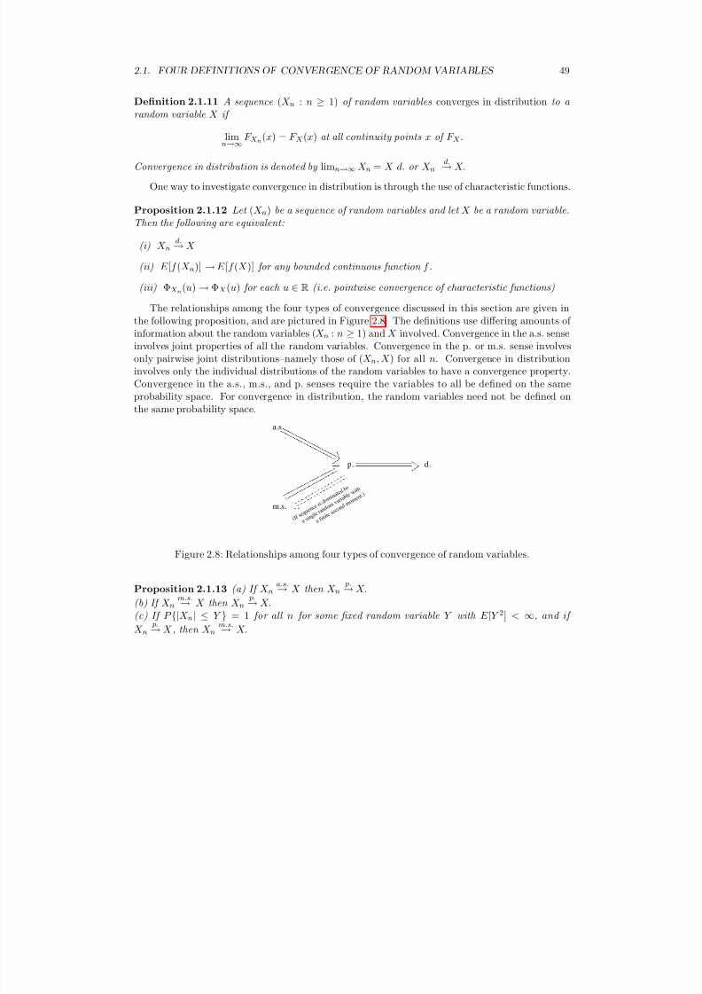
8/11/2019 Random process by B. Hajek
http://slidepdf.com/reader/full/random-process-by-b-hajek 59/448
2.1. FOUR DEFINITIONS OF CONVERGENCE OF RANDOM VARIABLES 49
Definition 2.1.11 A sequence (X n : n ≥ 1) of random variables converges in distribution to a random variable X if
limn→∞ F X n(x) = F X (x) at all continuity points x of F X .
Convergence in distribution is denoted by limn→∞ X n = X d. or X nd.→ X.
One way to investigate convergence in distribution is through the use of characteristic functions.
Proposition 2.1.12 Let (X n) be a sequence of random variables and let X be a random variable.Then the following are equivalent:
(i) X nd.→ X
(ii) E [f (X n)] → E [f (X )] for any bounded continuous function f .
(iii) ΦX n(u) → ΦX (u) for each u ∈ R (i.e. pointwise convergence of characteristic functions)
The relationships among the four types of convergence discussed in this section are given inthe following proposition, and are pictured in Figure 2.8. The definitions use differing amounts of information about the random variables (X n : n ≥ 1) and X involved. Convergence in the a.s. senseinvolves joint properties of all the random variables. Convergence in the p. or m.s. sense involvesonly pairwise joint distributions–namely those of (X n, X ) for all n. Convergence in distributioninvolves only the individual distributions of the random variables to have a convergence property.Convergence in the a.s., m.s., and p. senses require the variables to all be defined on the sameprobability space. For convergence in distribution, the random variables need not be defined onthe same probability space.
m.s.
p. d.
a.s.
( I f s e q u
e n c e i s
d o m i
n a t e d
b y
a f i n i
t e s e c
o n d m
o m e n t
. )
a s i n g
l e r a n
d o m v a
r i a b l e
w i t h
Figure 2.8: Relationships among four types of convergence of random variables.
Proposition 2.1.13 (a) If X na.s.→ X then X n
p.→ X.
(b) If X nm.s.→ X then X n
p.→ X.(c) If P |X n| ≤ Y = 1 for all n for some fixed random variable Y with E [Y 2] < ∞, and if
X n p.→ X , then X n
m.s.→ X.
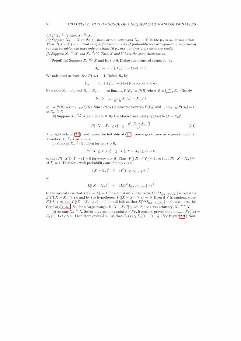
8/11/2019 Random process by B. Hajek
http://slidepdf.com/reader/full/random-process-by-b-hajek 60/448
50 CHAPTER 2. CONVERGENCE OF A SEQUENCE OF RANDOM VARIABLES
(d) If X n p.→ X then X n
d.→ X .(e) Suppose X n → X in the p., m.s., or a.s. sense and X n → Y in the p., m.s., or a.s. sense.Then P X = Y = 1. That is, if differences on sets of probability zero are ignored, a sequence of
random variables can have only one limit (if p., m.s., and/or a.s. senses are used).(f) Suppose X n
d.→ X and X nd.→ Y. Then X and Y have the same distribution.
Proof. (a) Suppose X na.s.→ X and let > 0. Define a sequence of events An by
An = ω :| X n(ω) − X (ω) |<
We only need to show that P (An) → 1. Define Bn by
Bn = ω :| X k(ω) − X (ω) |< for all k ≥ n
Note that Bn ⊂ An and B1 ⊂ B2 ⊂ · · · so limn→∞ P (Bn) = P (B) where B =
∞n=1 Bn. Clearly
B ⊃ ω : limn→∞ X n(ω) = X (ω)
so 1 = P (B) = limn→∞P (Bn). Since P (An) is squeezed between P (Bn) and 1, limn→∞ P (An) = 1,
so X n p.→ X .
(b) Suppose X nm.s.→ X and let > 0. By the Markov inequality applied to |X − X n|2,
P | X − X n |≥ ≤ E [| X − X n |2]
2 (2.1)
The right side of (2.1), and hence the left side of (2.1), converges to zero as n goes to infinity.
Therefore X n p.→ X as n → ∞.
(c) Suppose X n p.
→ X . Then for any > 0,
P | X |≥ Y + ≤ P | X − X n |≥ → 0
so that P | X |≥ Y + = 0 for every > 0. Thus, P | X |≤ Y = 1, so that P | X − X n |2≤4Y 2 = 1. Therefore, with probability one, for any > 0,
| X − X n |2 ≤ 4Y 2I |X −X n|≥ + 2
so
E [| X − X n |2] ≤ 4E [Y 2I |X −X n|≥] + 2
In the special case that P
Y = L
= 1 for a constant L, the term E [Y 2I |X −X n|≥
] is equal toL2P |X − X n| ≥ , and by the hypotheses, P |X − X n| ≥ → 0. Even if Y is random, sinceE [Y 2] < ∞ and P |X − X n| ≥ → 0, it still follows that E [Y 2I |X −X n|≥] → 0 as n → ∞, by
Corollary 11.6.5. So, for n large enough, E [|X − X n|2] ≤ 22. Since was arbitrary, X nm.s.→ X.
(d) Assume X n p.→ X. Select any continuity point x of F X . It must be proved that limn→∞ F X n(x) =
F X (x). Let > 0. Then there exists δ > 0 so that F X (x) ≤ F X (x − δ ) + 2 . (See Figure 2.9.) Now
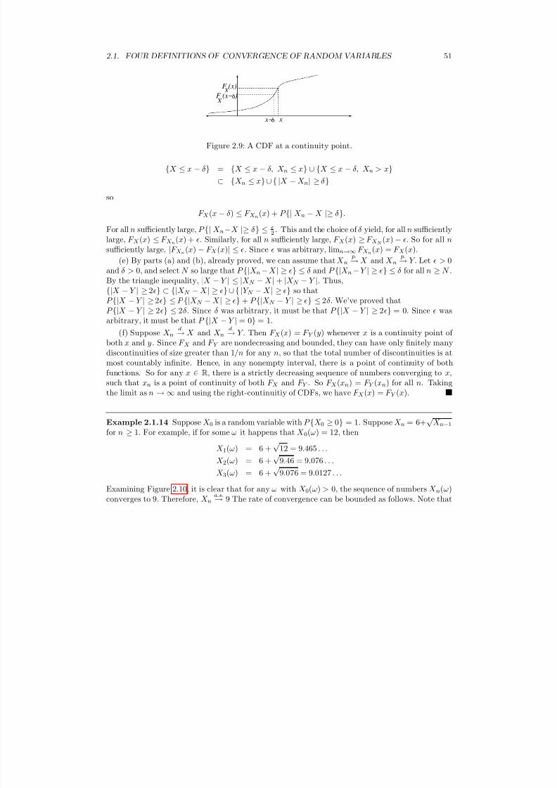
8/11/2019 Random process by B. Hajek
http://slidepdf.com/reader/full/random-process-by-b-hajek 61/448
2.1. FOUR DEFINITIONS OF CONVERGENCE OF RANDOM VARIABLES 51
!
!
"! "!
! # %"! &
# %"&
Figure 2.9: A CDF at a continuity point.
X ≤ x − δ = X ≤ x − δ, X n ≤ x ∪ X ≤ x − δ, X n > x⊂ X n ≤ x∪ |X − X n| ≥ δ
so
F X (x − δ ) ≤ F X n(x) + P | X n − X |≥ δ .
For all n sufficiently large, P | X n−X |≥ δ ≤ 2 . This and the choice of δ yield, for all n sufficiently
large, F X (x) ≤ F X n(x) + . Similarly, for all n sufficiently large, F X (x) ≥ F X N (x) − . So for all nsufficiently large, |F X n(x) − F X (x)| ≤ . Since was arbitrary, limn→∞ F X n(x) = F X (x).
(e) By parts (a) and (b), already proved, we can assume that X n p.→ X and X n
p.→ Y. Let > 0and δ > 0, and select N so large that P |X n −X | ≥ ≤ δ and P |X n −Y | ≥ ≤ δ for all n ≥ N .By the triangle inequality, |X − Y | ≤ |X N − X | + |X N − Y |. Thus,|X − Y | ≥ 2 ⊂ |X N − X | ≥ ∪ |Y N − X | ≥ so thatP |X − Y | ≥ 2 ≤ P |X N − X | ≥ + P |X N − Y | ≥ ≤ 2δ . We’ve proved thatP |X − Y | ≥ 2 ≤ 2δ . Since δ was arbitrary, it must be that P |X − Y | ≥ 2 = 0. Since wasarbitrary, it must be that P |X − Y | = 0 = 1.
(f) Suppose X nd.
→ X and X n
d.
→ Y . Then F X (x) = F Y (y) whenever x is a continuity point of
both x and y . Since F X and F Y are nondecreasing and bounded, they can have only finitely manydiscontinuities of size greater than 1/n for any n, so that the total number of discontinuities is atmost countably infinite. Hence, in any nonempty interval, there is a point of continuity of bothfunctions. So for any x ∈ R, there is a strictly decreasing sequence of numbers converging to x,such that xn is a point of continuity of both F X and F Y . So F X (xn) = F Y (xn) for all n. Takingthe limit as n → ∞ and using the right-continuitiy of CDFs, we have F X (x) = F Y (x).
Example 2.1.14 Suppose X 0 is a random variable with P X 0 ≥ 0 = 1. Suppose X n = 6+√
X n−1
for n ≥ 1. For example, if for some ω it happens that X 0(ω) = 12, then
X 1(ω) = 6 + √ 12 = 9.465 . . .X 2(ω) = 6 +
√ 9.46 = 9.076 . . .
X 3(ω) = 6 +√
9.076 = 9.0127 . . .
Examining Figure 2.10, it is clear that for any ω with X 0(ω) > 0, the sequence of numbers X n(ω)converges to 9. Therefore, X n
a.s.→ 9 The rate of convergence can be bounded as follows. Note that
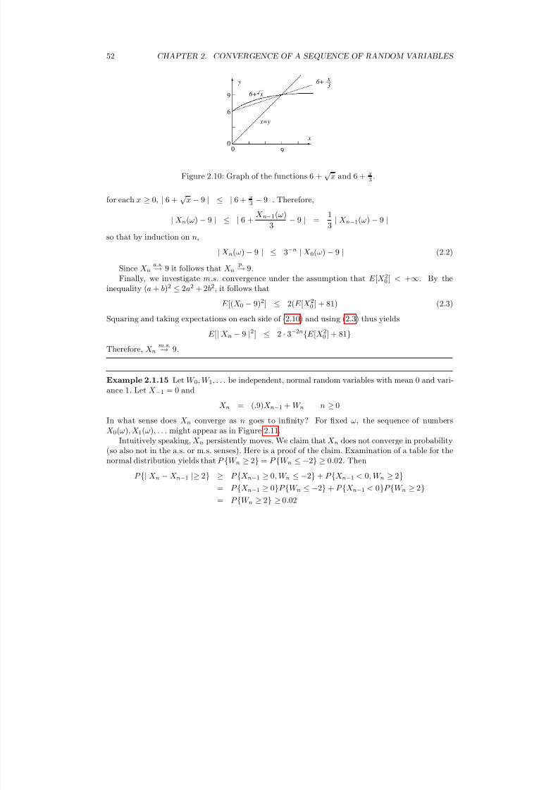
8/11/2019 Random process by B. Hajek
http://slidepdf.com/reader/full/random-process-by-b-hajek 62/448
52 CHAPTER 2. CONVERGENCE OF A SEQUENCE OF RANDOM VARIABLES
6
x=y
6+ x
6+ x3
x
y
9
900
Figure 2.10: Graph of the functions 6 +√
x and 6 + x3 .
for each x ≥ 0, | 6 +√
x − 9 | ≤ | 6 + x3 − 9 |. Therefore,
| X n(ω)
−9 | ≤ |
6 + X n−1(ω)
3 −9 |
= 1
3 | X n
−1(ω)
−9 |
so that by induction on n,
| X n(ω) − 9 | ≤ 3−n | X 0(ω) − 9 | (2.2)
Since X na.s.→ 9 it follows that X n
p.→ 9.Finally, we investigate m.s. convergence under the assumption that E [X 20 ] < +∞. By the
inequality (a + b)2 ≤ 2a2 + 2b2, it follows that
E [(X 0 − 9)2] ≤ 2(E [X 20 ] + 81) (2.3)
Squaring and taking expectations on each side of (2.10) and using (2.3) thus yields
E [| X
n −9 |
2] ≤
2·
3−2n
E [X 2
0] + 81
Therefore, X n
m.s.→ 9.
Example 2.1.15 Let W 0, W 1, . . . be independent, normal random variables with mean 0 and vari-ance 1. Let X −1 = 0 and
X n = (.9)X n−1 + W n n ≥ 0
In what sense does X n converge as n goes to infinity? For fixed ω, the sequence of numbersX 0(ω), X 1(ω), . . . might appear as in Figure 2.11.
Intuitively speaking, X n persistently moves. We claim that X n does not converge in probability
(so also not in the a.s. or m.s. senses). Here is a proof of the claim. Examination of a table for thenormal distribution yields that P W n ≥ 2 = P W n ≤ −2 ≥ 0.02. Then
P | X n − X n−1 |≥ 2 ≥ P X n−1 ≥ 0, W n ≤ −2 + P X n−1 < 0, W n ≥ 2= P X n−1 ≥ 0P W n ≤ −2 + P X n−1 < 0P W n ≥ 2= P W n ≥ 2 ≥ 0.02
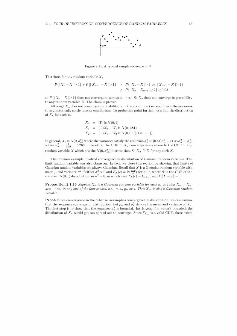
8/11/2019 Random process by B. Hajek
http://slidepdf.com/reader/full/random-process-by-b-hajek 63/448
2.1. FOUR DEFINITIONS OF CONVERGENCE OF RANDOM VARIABLES 53
k X
k
Figure 2.11: A typical sample sequence of X .
Therefore, for any random variable X ,
P | X n − X |≥ 1 + P | X n−1 − X |≥ 1 ≥ P | X n − X |≥ 1 or | X n−1 − X |≥ 1≥ P | X n − X n−1 |≥ 2 ≥ 0.02
so P | X n − X |≥ 1 does not converge to zero as n → ∞. So X n does not converge in probabilityto any random variable X . The claim is proved.
Although X n does not converge in probability, or in the a.s. or m.s.) senses, it nevertheless seemsto asymptotically settle into an equilibrium. To probe this point further, let’s find the distributionof X n for each n.
X 0 = W 0 is N (0, 1)
X 1 = (.9)X 0 + W 1 is N (0, 1.81)
X 2 = (.9)X 1 + W 2 is N (0, (.81)(1.81 + 1))
In general, X n is N (0, σ2n) where the variances satisfy the recursion σ2
n = (0.81)σ2n
−1 +1 so σ2
n
→ σ2
∞where σ2∞ = 10.19 = 5.263. Therefore, the CDF of X n converges everywhere to the CDF of any
random variable X which has the N (0, σ2∞) distribution. So X nd.→ X for any such X .
The previous example involved convergence in distribution of Gaussian random variables. Thelimit random variable was also Gaussian. In fact, we close this section by showing that limits of Gaussian random variables are always Gaussian. Recall that X is a Gaussian random variable withmean µ and variance σ2 if either σ2 > 0 and F X (c) = Φ( c−µ
σ ) for all c, where Φ is the CDF of thestandard N (0, 1) distribution, or σ2 = 0, in which case F X (c) = I c≥µ and P X = µ = 1.
Proposition 2.1.16 Suppose X n is a Gaussian random variable for each n, and that X n → X ∞as n
→ ∞, in any one of the four senses, a.s., m.s., p., or d. Then X
∞ is also a Gaussian random
variable.
Proof. Since convergence in the other senses implies convergence in distribution, we can assumethat the sequence converges in distribution. Let µn and σ2
n denote the mean and variance of X n.The first step is to show that the sequence σ2
n is bounded. Intuitively, if it weren’t bounded, thedistribution of X n would get too spread out to converge. Since F X ∞ is a valid CDF, there exists
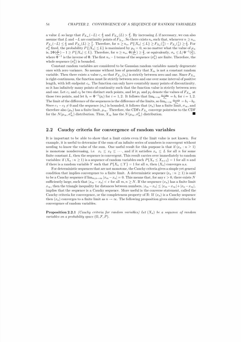
8/11/2019 Random process by B. Hajek
http://slidepdf.com/reader/full/random-process-by-b-hajek 64/448
54 CHAPTER 2. CONVERGENCE OF A SEQUENCE OF RANDOM VARIABLES
a value L so large that F X ∞(−L) < 13 and F X ∞(L) > 2
3 . By increasing L if necessary, we can alsoassume that L and −L are continuity points of F X ∞ . So there exists no such that, whenever n ≥ no,F X n(−L) ≤ 1
3 and F X n(L) ≥ 23 . Therefore, for n ≥ no, P |X n| ≤ L ≥ F X n( 2
3 ) − F X n( 13 ) ≥ 1
3 . For
σ2n fixed, the probability P |X n| ≤ L is maximized by µn = 0, so no matter what the value of µn
is, 2Φ( Lσn) − 1 ≥ P |X n| ≤ L. Therefore, for n ≥ no, Φ( Lσn
) ≥ 23 , or equivalently, σn ≤ L/Φ−1( 2
3 ),
where Φ−1 is the inverse of Φ. The first no − 1 terms of the sequence (σ2n) are finite. Therefore, the
whole sequence (σ2n) is bounded.
Constant random variables are considered to be Gaussian random variables–namely degenerateones with zero variance. So assume without loss of generality that X ∞ is not a constant randomvariable. Then there exists a value co so that F X ∞(co) is strictly between zero and one. Since F X ∞is right-continuous, the function must lie strictly between zero and one over some interval of positivelength, with left endpoint co. The function can only have countably many points of discontinuity,so it has infinitely many points of continuity such that the function value is strictly between zeroand one. Let c1 and c2 be two distinct such points, and let p1 and p2 denote the values of F X ∞ at
those two points, and let bi = Φ−1
( pi) for i = 1, 2. It follows that limn→∞ci
−µn
σn = bi for i = 1, 2.The limit of the difference of the sequences is the difference of the limits, so limn→∞ c1−c2σn
= b1 −b2.Since c1 − c2 = 0 and the sequence (σn) is bounded, it follows that (σn) has a finite limit, σ∞, andtherefore also (µn) has a finite limit, µ∞. Therefore, the CDFs F X n converge pointwise to the CDFfor the N (µ∞, σ2∞) distribution. Thus, X ∞ has the N (µ∞, σ2∞) distribution.
2.2 Cauchy criteria for convergence of random variables
It is important to be able to show that a limit exists even if the limit value is not known. Forexample, it is useful to determine if the sum of an infinite series of numbers is convergent without
needing to know the value of the sum. One useful result for this purpose is that if (xn : n ≥ 1)is monotone nondecreasing, i.e. x1 ≤ x2 ≤ · · · , and if it satisfies xn ≤ L for all n for somefinite constant L, then the sequence is convergent. This result carries over immediately to randomvariables: if (X n : n ≥ 1) is a sequence of random variables such P X n ≤ X n+1 = 1 for all n andif there is a random variable Y such that P X n ≤ Y = 1 for all n, then (X n) converges a.s.
For deterministic sequences that are not monotone, the Cauchy criteria gives a simple yet generalcondition that implies convergence to a finite limit. A deterministic sequence (xn : n ≥ 1) is saidto be a Cauchy sequence if limm,n→∞ |xm − xn| = 0. This means that, for any > 0, there exists N sufficiently large, such that |xm − xn| < for all m, n ≥ N . If the sequence (xn) has a finite limitx∞, then the triangle inequality for distances between numbers, |xm−xn| ≤ |xm −x∞|+ |xn −x∞|,implies that the sequence is a Cauchy sequence. More useful is the converse statement, called the
Cauchy criteria for convergence, or the completeness property of R: If (xn) is a Cauchy sequencethen (xn) converges to a finite limit as n → ∞. The following proposition gives similar criteria forconvergence of random variables.
Proposition 2.2.1 (Cauchy criteria for random variables) Let (X n) be a sequence of random variables on a probability space (Ω, F , P ).
8/11/2019 Random process by B. Hajek
http://slidepdf.com/reader/full/random-process-by-b-hajek 65/448
2.2. CAUCHY CRITERIA FOR CONVERGENCE OF RANDOM VARIABLES 55
(a) X n converges a.s. to some random variable if and only if
P ω : limm,n→∞ |X m(ω) − X n(ω)| = 0 = 1.
(b) X n converges m.s. to some random variable if and only if (X n) is a Cauchy sequence in the m.s. sense, meaning E [X 2n] < +∞ for all n and
limm,n→∞ E [(X m − X n)2] = 0. (2.4)
(c) X n converges p. to some random variable if and only if for every > 0,
limm,n→∞ P |X m − X n| ≥ = 0. (2.5)
Proof. (a) For any ω fixed, (X n(ω) : n ≥
1) is a sequence of numbers. So by the Cauchy criterionfor convergence of a sequence of numbers, the following equality of sets holds:
ω : limn→∞ X n(ω) exists and is finite = ω : lim
m,n→∞ |X m(ω) − X n(ω)| = 0.
Thus, the set on the left has probability one (i.e. X converges a.s. to a random variable) if andonly if the set on the right has probability one. Part (a) is proved.
(b) First the “only if” part is proved. Suppose X nm.s.→ X ∞. By the L2 triangle inequality for
random variables,
E [(X n − X m)2]12 ≤ E [(X m − X ∞)2]
12 + E [(X n − X ∞)2]
12 (2.6)
Since X nm.s.
→ X ∞. the right side of (2.6) converges to zero as m, n → ∞, so that (2.4) holds. The“only if” part of (b) is proved.
Moving to the proof of the “if” part, suppose (2.4) holds. Choose the sequence k1 < k2 < . . .recursively as follows. Let k1 be so large that E [(X n−X k1)2] ≤ 1/2 for all n ≥ k1. Once k1, . . . , ki−1
are selected, let ki be so large that ki > ki−1 and E [(X n−X ki)2] ≤ 2−i for all n ≥ ki. It follows fromthis choice of the ki’s that E [(X ki+1
−X ki)2] ≤ 2−i for all i ≥ 1. Let S n = |X k1|+n−1
i=1 |X ki+1−X ki
|.Note that |X ki
| ≤ S n for 1 ≤ i ≤ k by the triangle inequality for differences of real numbers. Bythe L2 triangle inequality for random variables (1.16),
E [S 2n]12 ≤ E [X 2k1]
12 +
n−1
i=1
E [(X ki+1 − X ki)2]
12 ≤ E [X 2k1]
12 + 1.
Since S n is monotonically increasing, it converges a.s. to a limit S ∞. Note that |X ki| ≤ S ∞ for
all i ≥ 1. By the monotone convergence theorem, E [S 2∞] = limn→∞ E [S 2n] ≤ (E [X 2k1]12 + 1)2. So,
S ∞ is in L2(Ω, F , P ). In particular, S ∞ is finite a.s., and for any ω such that S ∞(ω) is finite, thesequence of numbers (X ki
(ω) : i ≥ 1) is a Cauchy sequence. (See Example 11.2.3 in the appendix.)By completeness of R, for ω in that set, the limit X ∞(ω) exists. Let X ∞(ω) = 0 on the zero
8/11/2019 Random process by B. Hajek
http://slidepdf.com/reader/full/random-process-by-b-hajek 66/448
56 CHAPTER 2. CONVERGENCE OF A SEQUENCE OF RANDOM VARIABLES
probability event that (X ki(ω) : i ≥ 1) does not converge. Summarizing, we have limi→∞ X ki = X ∞a.s. and |X ki
| ≤ S ∞ where S ∞ ∈ L2(Ω, F , P ). It therefore follows from Proposition 2.1.13(c) that
X ki
m.s.→ X ∞.
The final step is to prove that the entire sequence (X n) converges in the m.s. sense to X ∞.For this purpose, let > 0. Select i so large that E [(X n − X ki)2] < 2 for all n ≥ ki, andE [(X ki
− X ∞)2] ≤ 2. Then, by the L2 triangle inequality, for any n ≥ ki,
E [(X n − X ∞)2]12 ≤ E (X n − X ki)2]
12 + E [(X ki
− X ∞)2]12 ≤ 2
Since was arbitrary, X nm.s.→ X ∞. The proof of (b) is complete.
(c) First the “only if” part is proved. Suppose X n p.→ X ∞. Then for any > 0,
P |X m − X n| ≥ 2 ≤ P |X m − X ∞| ≥ + P |X m − X ∞| ≥ → 0
as m, n
→ ∞, so that (2.5) holds. The “only if” part is proved.
Moving to the proof of the “if” part, suppose (2.5) holds. Select an increasing sequence of integers ki so that P |X n − X m| ≥ 2−i ≤ 2−i for all m, n ≥ ki. It follows, in particular, thatP |X ki+1
− X ki| ≥ 2−i ≤ 2−i. Since the sum of the probabilities of these events is finite, the prob-
ability that infinitely many of the events is true is zero, by the Borel-Cantelli lemma (specifically,Lemma 1.2.2(a)). Thus, P |X ki+1
− X ki| ≤ 2−i for all large enough i = 1. Thus, for all ω is a
set with probability one, (X ki(ω) : i ≥ 1) is a Cauchy sequence of numbers. By completeness of R, for ω in that set, the limit X ∞(ω) exists. Let X ∞(ω) = 0 on the zero probability event that
(X ki(ω) : i ≥ 1) does not converge. Then, X ki
a.s.→ X ∞. It follows that X ki
p.→ X ∞ as well.The final step is to prove that the entire sequence (X n) converges in the p. sense to X ∞. For
this purpose, let > 0. Select i so large that P ||X n − X ki|| ≥ < for all n ≥ ki, and
P |X ki − X ∞| ≥ < . Then P |X n − X ∞| ≥ 2 ≤ 2 for all n ≥ ki. Since was arbitrary,
X n p.
→ X ∞. The proof of (c) is complete.
The following is a corollary of Proposition 2.2.1(c) and its proof.
Corollary 2.2.2 If X n p.→ X ∞, then there is a subsequence (X ki : i ≥ 1) such that limi→∞ X ki =
X ∞ a.s.
Proof. By Proposition 2.2.1(c), the sequence satisfies (2.2.1). By the proof of Proposition 2.2.1(c)there is a subsequence (X ki) that converges a.s. By uniqueness of limits in the p. or a.s. senses, thelimit of the subsequence is the same random variable, X ∞ (up to differences on a set of measurezero).
Proposition 2.2.1(b), the Cauchy criteria for mean square convergence, is used extensively inthese notes. The remainder of this section concerns a more convenient form of the Cauchy criteriafor m.s. convergence.
Proposition 2.2.3 (Correlation version of the Cauchy criterion for m.s. convergence) Let (X n)be a sequence of random variables with E [X 2n] < +∞ for each n. Then there exists a random
8/11/2019 Random process by B. Hajek
http://slidepdf.com/reader/full/random-process-by-b-hajek 67/448
2.2. CAUCHY CRITERIA FOR CONVERGENCE OF RANDOM VARIABLES 57
variable X such that X nm.s.→ X if and only if the limit limm,n→∞ E [X nX m] exists and is finite.
Furthermore, if X nm.s.→ X , then limm,n→∞ E [X nX m] = E [X 2].
Proof. The “if” part is proved first. Suppose limm,n→∞
E [X nX m] = c for a finite constant c.Then
E (X n − X m)2 = E [X 2n] − 2E [X nX m] + E [X 2m]
→ c − 2c + c = 0 as m, n → ∞Thus, X n is Cauchy in the m.s. sense, so X n
m.s.→ X for some random variable X .To prove the “only if” part, suppose X n
m.s.→ X . Observe next that
E [X mX n] = E [(X + (X m − X ))(X + (X n − X ))]
= E [X 2 + (X m − X )X + X (X n − X ) + (X m − X )(X n − X )]
By the Cauchy-Schwarz inequality,
E [| (X m − X )X |] ≤ E [(X m − X )2]12 E [X 2]
12 → 0
E [| (X m − X )(X n − X ) |] ≤ E [(X m − X )2]12 E [(X n − X )2]
12 → 0
and similarly E [| X (X n − X ) |] → 0. Thus E [X mX n] → E [X 2]. This establishes both the “only if”part of the proposition and the last statement of the proposition. The proof of the proposition iscomplete.
Corollary 2.2.4 Suppose X nm.s.→ X and Y n
m.s.→ Y . Then E [X nY n] → E [XY ].
Proof. By the inequality (a + b)2 ≤ 2a2 + 2b2, it follows that X n + Y n m.s.→ X + Y as n → ∞.Proposition 2.2.3 therefore implies that E [(X n + Y n)2] → E [(X + Y )2], E [X 2n] → E [X 2], andE [Y 2n ] → E [Y 2]. Since X nY n = ((X n + Y n)2 − X 2n − Y 2n )/2, the corollary follows.
Corollary 2.2.5 Suppose X nm.s.→ X. Then E [X n] → E [X ].
Proof. Corollary 2.2.5 follows from Corollary 2.2.4 by taking Y n = 1 for all n.
Example 2.2.6 This example illustrates the use of Proposition 2.2.3. Let X 1, X 2, . . . be meanzero random variables such that
E [X iX j] =
1 if i = j0 else
Does the series∞
k=1X kk converge in the mean square sense to a random variable with a finite second
moment? Let Y n = n
k=1X kk . The question is whether Y n converges in the mean square sense to
8/11/2019 Random process by B. Hajek
http://slidepdf.com/reader/full/random-process-by-b-hajek 68/448
58 CHAPTER 2. CONVERGENCE OF A SEQUENCE OF RANDOM VARIABLES
a random variable with finite second moment. The answer is yes if and only if limm,n→∞ E [Y mY n]exists and is finite. Observe that
E [Y mY n] =
min(m,n)k=1
1k2
→∞k=1
1
k2 as m, n → ∞
This sum is smaller than 1 + ∞
11x2 dx = 2 < ∞.1 Therefore, by Proposition 2.2.3, the series∞
k=1X kk indeed converges in the m.s. sense.
2.3 Limit theorems for sums of independent random variables
Sums of many independent random variables often have distributions that can be characterizedby a small number of parameters. For engineering applications, this represents a low complexitymethod for describing the random variables. An analogous tool is the Taylor series approximation.A continuously differentiable function f can be approximated near zero by the first order Taylor’sapproximation
f (x) ≈ f (0) + xf (0)
A second order approximation, in case f is twice continuously differentiable, is
f (x) ≈ f (0) + xf (0) +
x2
2 f (0)
Bounds on the approximation error are given by Taylor’s theorem, found in Appendix 11.4. Inessence, Taylor’s approximation lets us represent the function by the numbers f (0), f (0) andf (0). We shall see that the law of large numbers and central limit theorem can be viewed not justas analogies of the first and second order Taylor’s approximations, but actually as consequences of them.
Lemma 2.3.1 Let (zn : n ≥ 1) be a sequence of real or complex numbers with limit z. Then 1 + zn
n
n → ez as n → ∞.
Proof. The basic idea is to note that (1 + s)n = exp(n ln(1 + s)), and apply a power series
expansion of ln(1 + s) about the point s = 0. The details are given next. Since the sequence (zn)converges to a finite limit, |znn | ≤ 1
2 for all sufficiently large n, so it suffices to consider ln(1 + s) for
complex s with |s| ≤ 12 . Note that the kth derivative of ln(1+s) evaluated at s = 0 is (−1)(k−1)(k−1)!
1In fact, the sum is equal to π2
6 , but the technique of comparing the sum to an integral to show the sum is finite
is the main point here.
8/11/2019 Random process by B. Hajek
http://slidepdf.com/reader/full/random-process-by-b-hajek 69/448
8/11/2019 Random process by B. Hajek
http://slidepdf.com/reader/full/random-process-by-b-hajek 70/448
60 CHAPTER 2. CONVERGENCE OF A SEQUENCE OF RANDOM VARIABLES
Turn next to part (b). If in addition to the conditions of (b) it is assumed that Var(X 1) < +∞,then the conditions of part (a) are true. Since mean square convergence implies convergence inprobability, the conclusion of part (b) follows. An extra credit problem shows how to use the same
approach to verify (b) even if Var(X 1) = +∞.Here a second approach to proving (b) is given. The characteristic function of X i
n is given by
E
exp
juX i
n
= E
exp
ju
n
X i
= ΦX
u
n
where ΦX denotes the characteristic function of X 1. Since the characteristic function of the sumof independent random variables is the product of the characteristic functions,
Φ Snn
(u) =
ΦX
u
n
n.
Since E [X 1] = m it follows that ΦX is differentiable with ΦX (0) = 1, ΦX (0) = jm and Φ is
continuous. By Taylor’s theorem (Theorem 11.4.1) applied separately to the real and imaginaryparts of ΦX , for any u fixed,
ΦX
u
n
= 1 +
u
n
Re(Φ
X (un)) + jI m(ΦX (vn))
for some un and vn between 0 and u
n for all n. Since Φ(un) → j m and Φ(vn) → jm as n → ∞,it follows that Re(Φ
X (un)) + jIm(ΦX (vn)) → jm as n → ∞. So Lemma 2.3.1 yields ΦX (
un)n →
exp( jum) as n → ∞. Note that exp( jum) is the characteristic function of a random variableequal to m with probability one. Since pointwise convergence of characteristic functions to a valid
characteristic function implies convergence in distribution, it follows that S nn
d.→ m. However,convergence in distribution to a constant implies convergence in probability, so (b) is proved.
Part (c) is proved under the additional assumption that E [X 41 ] < +∞. Without loss of generalitywe assume that EX 1 = 0. Consider expanding S 4n. There are n terms of the form X 4i and 3n(n−1)terms of the form X 2i X 2 j with 1 ≤ i, j ≤ n and i = j . The other terms have the form X 3i X j, X 2i X jX kor X iX jX kX l for distinct i, j, k,l, and these terms have mean zero. Thus,
E [S 4n] = nE [X 41 ] + 3n(n − 1)E [X 21 ]2
Let Y =∞
n=1(S nn )4. The value of Y is well defined but it is a priori possible that Y (ω) = +∞ for
some ω. However, by the monotone convergence theorem, the expectation of the sum of nonnegativerandom variables is the sum of the expectations, so that
E [Y ] =
∞n=1
E S nn 4 =
∞n=1
nE [X
4
1 ] + 3n(n − 1)E [X
2
1 ]
2
n4 < +∞
Therefore, P Y < +∞ = 1. However, Y < +∞ is a subset of the event of convergence
w : S n(w)n → 0 as n → ∞, so the event of convergence also has probability one. Thus, part (c)
under the extra fourth moment condition is proved.
8/11/2019 Random process by B. Hajek
http://slidepdf.com/reader/full/random-process-by-b-hajek 71/448
2.4. CONVEX FUNCTIONS AND JENSEN’S INEQUALITY 61
Proposition 2.3.3 (Central Limit Theorem) Suppose that X 1, X 2, . . . are i.i.d., each with mean µ and variance σ2. Let S n = X 1 + · · · + X n. Then the normalized sum
S n −
nµ
√ nconverges in distribution to the N (0, σ2) distribution as n → ∞.
Proof. Without loss of generality, assume that µ = 0. Then the characteristic function of the normalized sum S n√
n is given by ΦX (
u√ n
)n, where ΦX denotes the characteristic function of X 1.
Since X 1 has mean 0 and finite second moment σ2, it follows that ΦX is twice differentiable withΦX (0) = 1, Φ
X (0) = 0, ΦX (0) = −σ2, and Φ
X is continuous. By Taylor’s theorem (Theorem11.4.1) applied separately to the real and imaginary parts of ΦX , for any u fixed,
ΦX
u√
n = 1 +
u2
2n Re(Φ
X (un)) + jI m(ΦX (vn))
for some un and vn between 0 and u√ n
for all n. Note that un → 0 and vn → 0 as n → ∞, so
Φ(un) → −σ2 and Φ(vn) → −σ2 as n → ∞. It follows that Re(ΦX (un)) + jI m(Φ
X (vn)) → −σ2
as n → ∞. Lemma 2.3.1 yields ΦX ( u√ n
)n → exp(−u2σ2
2 ) as n → ∞. Since pointwise convergence
of characteristic functions to a valid characteristic function implies convergence in distribution, theproposition is proved.
2.4 Convex functions and Jensen’s inequality
Let ϕ be a function on R with values in R
∪ +
∞ such that ϕ(x) <
∞ for at least one value of x.
Then ϕ is said to be convex if for any a, b and λ with a < b and 0 ≤ λ ≤ 1
ϕ(aλ + b(1 − λ)) ≤ λϕ(a) + (1 − λ)ϕ(b).
This means that the graph of ϕ on any interval [a, b] lies below the line segment equal to ϕ at theendpoints of the interval.
Proposition 2.4.1 Suppose f is a function with domain R. (a) If f is continuously differentiable,f is convex if and only if f is nondecreasing. (b) If f is twice continuously differentiable, f is convex if and only if f (v) ≥ 0 for all v.
Proof. (a) (if) Suppose f is continuously differentiable. (if part) Given s ≤ t, defineD
s,t = λf (s) + (1
−λ)f (t)
−f (λs + (1
−λ)t). We claim that
Ds,t = (1 − λ)
ts
f (x) − f (λs + (1 − λ)x
dx. (2.7)
To verify (2.7), fix s and note that (2.7) is true if t = s, for then both sides are zero, and the deriva-tive with respect to t of each side of (2.7) is the same, equal to (1 − λ) (f (t) − f (λs + (1 − λ)t)) .
8/11/2019 Random process by B. Hajek
http://slidepdf.com/reader/full/random-process-by-b-hajek 72/448
62 CHAPTER 2. CONVERGENCE OF A SEQUENCE OF RANDOM VARIABLES
If f is nondecreasing, then the integrand in (2.7) is nonnegative, so Ds,t ≥ 0, so f is convex.(only if) Turning to the “only if” part of (a), suppose f is convex, and let s < t. For any h > 0small enough that s < s + h < t < t + h,
f (s + h)(t − s + h) ≤ (t − s)f (s) + hf (t + h) (2.8)
f (t)(t − s + h) ≤ hf (s) + (t − s)f (t + h) (2.9)
by the convexity of f. Combining (2.8) and (2.9) by summing the left hand sides and right handsides, rearranging, and multiplying by a positive constant, yields
f (s + h) − f (s)
h ≤ f (t + h) − f (t)
h . (2.10)
Letting h → 0 in (2.10) yields f (s) ≤ f (t), so f is nondecreasing. Part (a) is proved.(b) Suppose f is twice continuously differentiable. Part (b) follows from part (a) and the fact f isnondecreasing if and only if f (v) ≥ 0 for all v.
Examples of convex functions include:
ax2 + bx + c for constants a,b,c with a ≥ 0,
eλx for λ constant,
ϕ(x) =
− ln x x > 0+∞ x ≤ 0,
ϕ(x) =
x ln x x > 0
0 x = 0+∞ x < 0.
Theorem 2.4.2 (Jensen’s inequality) Let ϕ be a convex function and let X be a random variable such that E [X ] is finite. Then E [ϕ(X )] ≥ ϕ(E [X ]).
For example, Jensen’s inequality implies that E [X 2] ≥ E [X ]2, which also follows from the factVar(X ) = E [X 2] − E [X ]2.
Proof. Since ϕ is convex, there is a tangent to the graph of ϕ at E [X ], meaning there is afunction L of the form L(x) = a + bx such that ϕ(x) ≥ L(x) for all x and ϕ(E [X ]) = L(E [X ]).See the illustration in Figure 2.12. Therefore E [ϕ(X )] ≥ E [L(X )] = L(E [X ]) = ϕ(E [X ]), whichestablishes the theorem.
A function ϕ is called concave if −ϕ is convex. If ϕ is concave then E [ϕ(X )] ≤ ϕ(E [X ]).
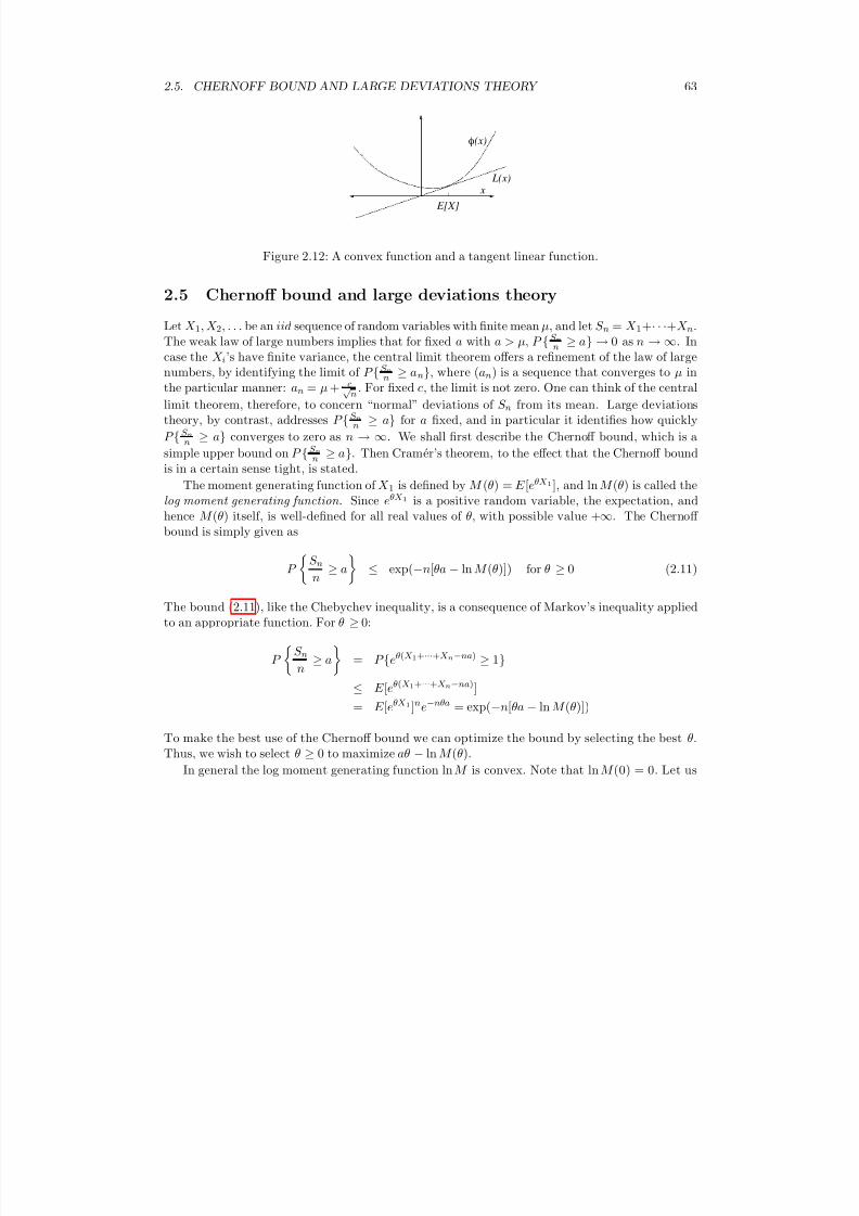
8/11/2019 Random process by B. Hajek
http://slidepdf.com/reader/full/random-process-by-b-hajek 73/448
2.5. CHERNOFF BOUND AND LARGE DEVIATIONS THEORY 63
(x)
L(x)
x
E[X]
φ
Figure 2.12: A convex function and a tangent linear function.
2.5 Chernoff bound and large deviations theory
Let X 1, X 2, . . . be an iid sequence of random variables with finite mean µ, and let S n = X 1+· · ·+X n.
The weak law of large numbers implies that for fixed a with a > µ, P S n
n ≥ a → 0 as n → ∞. Incase the X i’s have finite variance, the central limit theorem offers a refinement of the law of largenumbers, by identifying the limit of P S n
n ≥ an, where (an) is a sequence that converges to µ inthe particular manner: an = µ + c√
n. For fixed c, the limit is not zero. One can think of the central
limit theorem, therefore, to concern “normal” deviations of S n from its mean. Large deviationstheory, by contrast, addresses P S n
n ≥ a for a fixed, and in particular it identifies how quickly
P S nn ≥ a converges to zero as n → ∞. We shall first describe the Chernoff bound, which is a
simple upper bound on P S nn ≥ a. Then Cramer’s theorem, to the effect that the Chernoff bound
is in a certain sense tight, is stated.
The moment generating function of X 1 is defined by M (θ) = E [eθX 1], and ln M (θ) is called thelog moment generating function. Since eθX 1 is a positive random variable, the expectation, and
hence M (θ) itself, is well-defined for all real values of θ, with possible value +∞. The Chernoff bound is simply given as
P
S nn
≥ a
≤ exp(−n[θa − ln M (θ)]) for θ ≥ 0 (2.11)
The bound (2.11), like the Chebychev inequality, is a consequence of Markov’s inequality appliedto an appropriate function. For θ ≥ 0:
P
S nn
≥ a
= P eθ(X 1+···+X n−na) ≥ 1
≤ E [eθ(X 1+···+X n−na)]
= E [eθX 1]ne−nθa = exp(−n[θa − ln M (θ)])
To make the best use of the Chernoff bound we can optimize the bound by selecting the best θ.Thus, we wish to select θ ≥ 0 to maximize aθ − ln M (θ).
In general the log moment generating function ln M is convex. Note that ln M (0) = 0. Let us
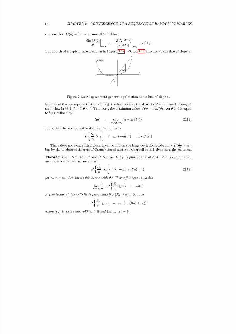
8/11/2019 Random process by B. Hajek
http://slidepdf.com/reader/full/random-process-by-b-hajek 74/448
64 CHAPTER 2. CONVERGENCE OF A SEQUENCE OF RANDOM VARIABLES
suppose that M (θ) is finite for some θ > 0. Then
d ln M (θ)
dθ θ=0
= E [X 1eθX 1]
E [eθX 1] θ=0
= E [X 1]
The sketch of a typical case is shown in Figure 2.13. Figure 2.13 also shows the line of slope a.
ln M( )
!
a!
l(a)
!
Figure 2.13: A log moment generating function and a line of slope a.
Because of the assumption that a > E [X 1], the line lies strictly above ln M (θ) for small enough θand below ln M (θ) for all θ < 0. Therefore, the maximum value of θa − ln M (θ) over θ ≥ 0 is equalto l(a), defined by
l(a) = sup−∞<θ<∞
θa − ln M (θ) (2.12)
Thus, the Chernoff bound in its optimized form, is
P
S nn
≥ a
≤ exp(−nl(a)) a > E [X 1]
There does not exist such a clean lower bound on the large deviation probability P S nn ≥ a,
but by the celebrated theorem of Cramer stated next, the Chernoff bound gives the right exponent.
Theorem 2.5.1 (Cramer’s theorem) Suppose E [X 1] is finite, and that E [X 1] < a. Then for > 0there exists a number n such that
P
S nn
≥ a
≥ exp(−n(l(a) + )) (2.13)
for all n ≥ n. Combining this bound with the Chernoff inequality yields
limn
→∞
1
n ln P
S nn
≥ a
= −l(a)
In particular, if l(a) is finite (equivalently if P X 1 ≥ a > 0) then
P
S nn
≥ a
= exp(−n(l(a) + n))
where (n) is a sequence with n ≥ 0 and limn→∞ n = 0.
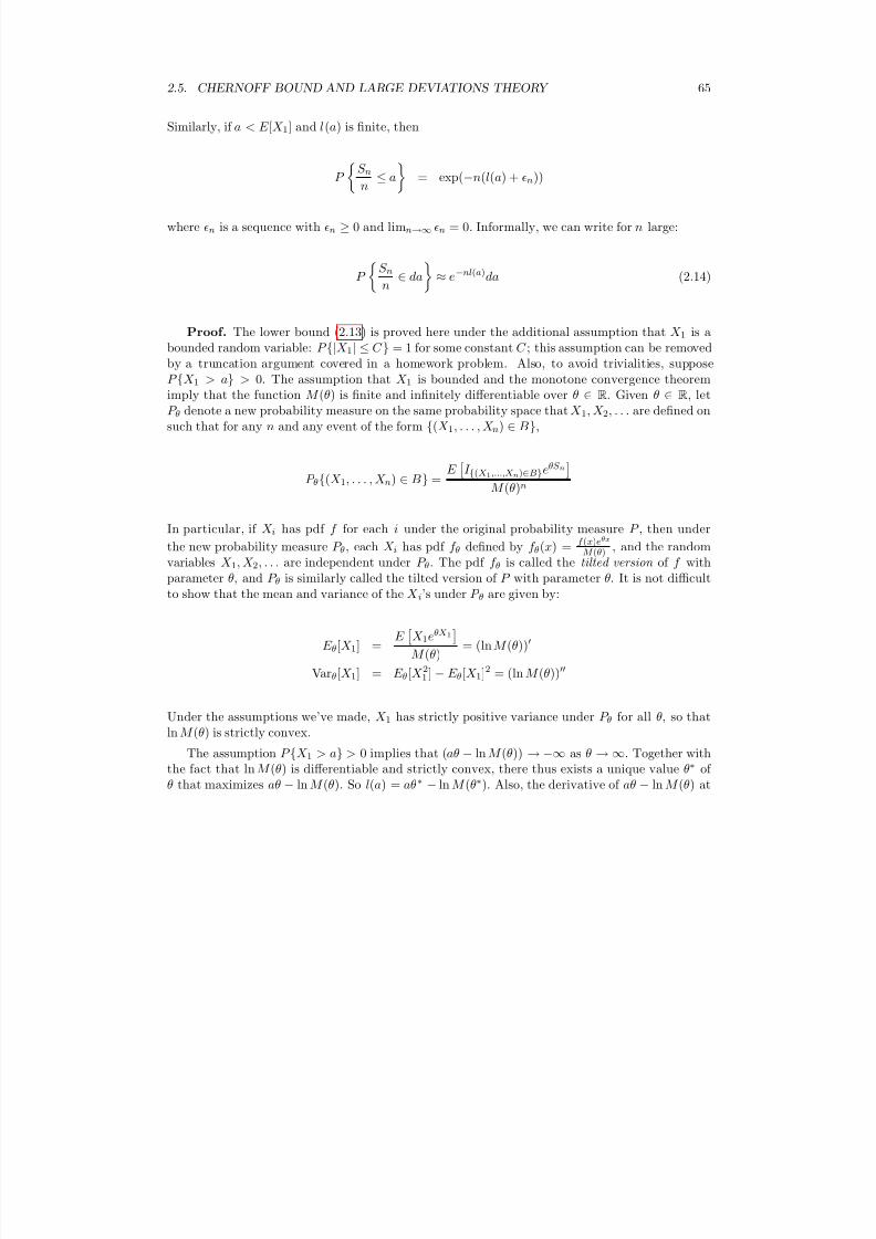
8/11/2019 Random process by B. Hajek
http://slidepdf.com/reader/full/random-process-by-b-hajek 75/448
2.5. CHERNOFF BOUND AND LARGE DEVIATIONS THEORY 65
Similarly, if a < E [X 1] and l(a) is finite, then
P S nn ≤ a = exp(−n(l(a) + n))
where n is a sequence with n ≥ 0 and limn→∞ n = 0. Informally, we can write for n large:
P
S nn
∈ da
≈ e−nl(a)da (2.14)
Proof. The lower bound (2.13) is proved here under the additional assumption that X 1 is a
bounded random variable: P |X 1| ≤ C = 1 for some constant C ; this assumption can be removedby a truncation argument covered in a homework problem. Also, to avoid trivialities, supposeP X 1 > a > 0. The assumption that X 1 is bounded and the monotone convergence theoremimply that the function M (θ) is finite and infinitely differentiable over θ ∈ R. Given θ ∈ R, letP θ denote a new probability measure on the same probability space that X 1, X 2, . . . are defined onsuch that for any n and any event of the form (X 1, . . . , X n) ∈ B,
P θ(X 1, . . . , X n) ∈ B =E
I (X 1,...,X n)∈BeθS n
M (θ)n
In particular, if X i has pdf f for each i under the original probability measure P , then underthe new probability measure P θ, each X i has pdf f θ defined by f θ(x) = f (x)eθx
M (θ) , and the randomvariables X 1, X 2, . . . are independent under P θ. The pdf f θ is called the tilted version of f withparameter θ, and P θ is similarly called the tilted version of P with parameter θ. It is not difficultto show that the mean and variance of the X i’s under P θ are given by:
E θ[X 1] = E
X 1eθX 1
M (θ)
= (ln M (θ))
Varθ[X 1] = E θ[X 21 ] − E θ[X 1]2 = (ln M (θ))
Under the assumptions we’ve made, X 1 has strictly positive variance under P θ for all θ, so thatln M (θ) is strictly convex.
The assumption P X 1 > a > 0 implies that (aθ − ln M (θ)) → −∞ as θ → ∞. Together withthe fact that ln M (θ) is differentiable and strictly convex, there thus exists a unique value θ∗ of θ that maximizes aθ − ln M (θ). So l(a) = aθ∗ − ln M (θ∗). Also, the derivative of aθ − ln M (θ) at
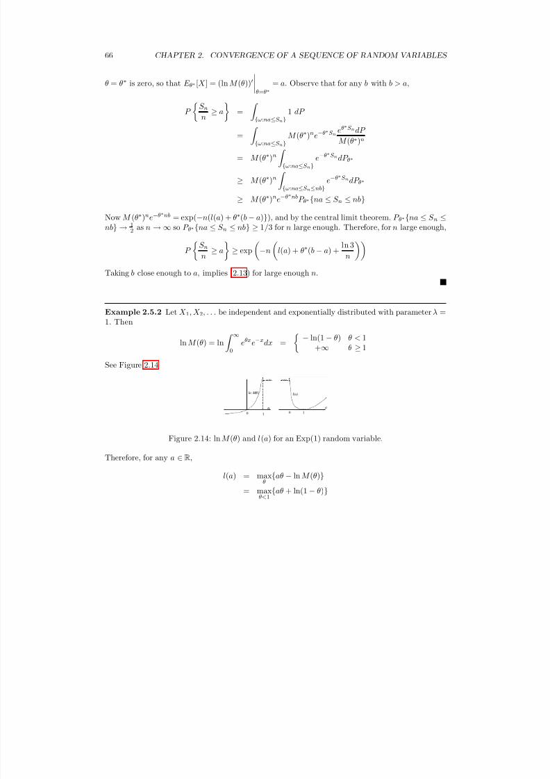
8/11/2019 Random process by B. Hajek
http://slidepdf.com/reader/full/random-process-by-b-hajek 76/448
66 CHAPTER 2. CONVERGENCE OF A SEQUENCE OF RANDOM VARIABLES
θ = θ∗ is zero, so that E θ∗ [X ] = (ln M (θ))θ=θ∗
= a. Observe that for any b with b > a,
P S nn ≥ a = ω:na≤S n 1 dP
=
ω:na≤S n
M (θ∗)ne−θ∗S n eθ∗S ndP
M (θ∗)n
= M (θ∗)n ω:na≤S n
e−θ∗S ndP θ∗
≥ M (θ∗)n ω:na≤S n≤nb
e−θ∗S ndP θ∗
≥ M (θ∗)ne−θ∗nbP θ∗na ≤ S n ≤ nb
Now M (θ∗)ne−θ∗nb = exp(−
n(l(a) + θ∗(b−
a)
), and by the central limit theorem, P θ∗
na ≤
S n ≤nb → 1
2 as n → ∞ so P θ∗na ≤ S n ≤ nb ≥ 1/3 for n large enough. Therefore, for n large enough,
P
S nn
≥ a
≥ exp
−n
l(a) + θ∗(b − a) +
ln 3
n
Taking b close enough to a, implies (2.13) for large enough n.
Example 2.5.2 Let X 1, X 2, . . . be independent and exponentially distributed with parameter λ =1. Then
ln M (θ) = ln ∞
0eθxe−xdx =
− ln(1 − θ) θ < 1+∞ θ ≥ 1
See Figure 2.14
!
10
!"
!
0
""!
1
l(a)
a
"
ln M( )
Figure 2.14: ln M (θ) and l(a) for an Exp(1) random variable.
Therefore, for any a ∈R,
l(a) = maxθ
aθ − ln M (θ)= max
θ<1aθ + ln(1 − θ)
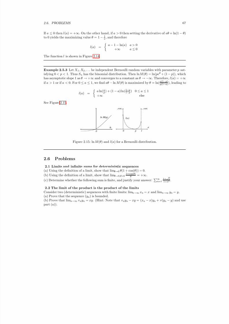
8/11/2019 Random process by B. Hajek
http://slidepdf.com/reader/full/random-process-by-b-hajek 77/448
2.6. PROBLEMS 67
If a ≤ 0 then l(a) = +∞. On the other hand, if a > 0 then setting the derivative of aθ + ln(1 − θ)to 0 yields the maximizing value θ = 1 − 1
a , and therefore
l(a) = a − 1 − ln(a) a > 0+∞ a ≤ 0
The function l is shown in Figure 2.14.
Example 2.5.3 Let X 1, X 2, . . . be independent Bernoulli random variables with parameter p sat-isfying 0 < p < 1. Thus S n has the binomial distribution. Then ln M (θ) = ln( peθ + (1 − p)), whichhas asymptotic slope 1 as θ → +∞ and converges to a constant as θ → −∞. Therefore, l(a) = +∞if a > 1 or if a < 0. For 0 ≤ a ≤ 1, we find aθ − ln M (θ) is maximized by θ = ln(
a(1− p) p(1−a) ), leading to
l(a) = a ln(
a
p ) + (1 − a)ln(
1
−a
1− p ) 0 ≤ a ≤ 1+∞ else
See Figure 2.15.
ln M( )
0
!!!
l(a)
a
1
!!!
p
"
"
0
Figure 2.15: ln M (θ) and l(a) for a Bernoulli distribution.
2.6 Problems
2.1 Limits and infinite sums for deterministic sequences(a) Using the definition of a limit, show that limθ→0 θ(1 + cos(θ)) = 0.
(b) Using the definition of a limit, show that limθ→0,θ>01+cos(θ)
θ = +∞.
(c) Determine whether the following sum is finite, and justify your answer:
∞n=1
1+√ n
1+n2 .
2.2 The limit of the product is the product of the limitsConsider two (deterministic) sequences with finite limits: limn→∞ xn = x and limn→∞ yn = y.(a) Prove that the sequence (yn) is bounded.(b) Prove that limn→∞ xnyn = xy. (Hint: Note that xnyn − xy = (xn − x)yn + x(yn − y) and usepart (a)).
8/11/2019 Random process by B. Hajek
http://slidepdf.com/reader/full/random-process-by-b-hajek 78/448
68 CHAPTER 2. CONVERGENCE OF A SEQUENCE OF RANDOM VARIABLES
2.3 The reciprocal of the limit is the limit of the reciprocalUsing the definition of converence for deterministic sequences, prove that if (xn) is a sequence witha nonzero finite limit x∞, then the sequence (1/xn) converges to 1/x∞.
2.4 Limits of some deterministic seriesDetermine which of the following series are convergent (i.e. have partial sums converging to a finitelimit). Justify your answers.
(a)∞n=0
3n
n! (b)
∞n=1
(n + 2) ln n
(n + 5)3 (c)
∞n=1
1
(ln(n + 1))5.
2.5 On convergence of deterministic sequences and functions(a) Let xn = 8n2+n
3n2 for n ≥ 1. Prove that limn→∞ xn = 83 .
(b) Suppose f n is a function on some set D for each n ≥ 1, and suppose f is also a function onD. Then f
n is defined to converge to f uniformly if for any > 0, there exists an n
such that
|f n(x) − f (x)| ≤ for all x ∈ D whenever n ≥ n. A key point is that n does not depend on x.Show that the functions f n(x) = xn on the semi-open interval [0, 1) do not converge uniformly tothe zero function.(c) The supremum of a function f on D, written supD f , is the least upper bound of f . Equivalently,supD f satisfies supD f ≥ f (x) for all x ∈ D, and given any c < supD f , there is an x ∈ D suchthat f (x) ≥ c. Show that | supD f − supD g| ≤ supD |f − g|. Conclude that if f n converges to f uniformly on D , then supD f n converges to supD f .
2.6 Convergence of alternating seriesSuppose b0 ≥ b1 ≥ · · · and that bk → 0 as k → ∞. The purpose of this problem is to prove, usingthe Cauchy criteria, that the infinite sum
∞k=0(
−1)kbk exists and is finite. By definition, the sum
is equal to the limit of the partial sums sn = nk=0(−1)kbk as n → ∞, so it is to be proved that thesequence (sn) has a finite limit. Please work to make your proof as simple and clean as possible.(a) Show if m ≥ n then sm is contained in the interval with endpoints sn and sn+1.(b) Show that (sn) is a Cauchy sequence. In particular, given > 0, specify how N can be selectedso that |sn − sm| < whenever m ≥ N and n ≥ N .
2.7 On the Dirichlet criterion for convergence of a seriesLet (ak) be a sequence with ak ≥ 0 for all k ≥ 0 such that
∞k=0 ak is finite, and let L be a finite
positive constant.(a) Use the Cauchy criterion to show that if (dk) is a sequence with |dk| ≤ Lak for all k then theseries
∞k=0 dk converges to a finite value.
Let An = ∞
k=n ak. Then ak = Ak − Ak+1 and the assumptions above about (ak) are equiva-lent to the condition that (Ak) is a nonincreasing sequence converging to zero. Assume (Bk) is asequence with |Bk| ≤ L for all k ≥ 0. Let S n =
nk=0 Ak(Bk −Bk−1), with the convention B−1 = 0.
(b) Prove the summation by parts formula: S n = (n
k=0 akBk) + An+1Bn.(c) Prove
∞k=0 Ak(Bk − Bk−1) converges to a finite limit.
8/11/2019 Random process by B. Hajek
http://slidepdf.com/reader/full/random-process-by-b-hajek 79/448
2.6. PROBLEMS 69
(Note: If Bn = 1 for n even and Bn = 0 for n odd, the result of this problem provides an alternativeproof of the result of the previous problem.)
2.8 Convergence of sequences of random variablesLet Θ be uniformly distributed on the interval [0, 2π]. In which of the four senses (a.s., m.s., p.,d.) do each of the following two sequences converge? Identify the limits, if they exist, and justifyyour answers.(a) (X n : n ≥ 1) defined by X n = cos(nΘ).(b) (Y n : n ≥ 1) defined by Y n = |1 − Θ
π |n.
2.9 Convergence of a random sequenceSuppose U n for n ≥ 1 are independent random variables, each uniformly distributed on the interval[0, 1]. Let X 0 = 0, and define X n for n ≥ 1 by the following recursion:
X n = maxX n−1, X n−1 + U n
2 .
(a) Does limn→∞ X n exist in the a.s. sense?(b) Does limn→∞ X n exist in the m.s. sense?(c) Identify the random variable Z such that X n → Z in probability as n → ∞. (Justify youranswer.)
2.10 Convergence of random variables on (0,1]Let Ω = (0, 1], let F be the Borel σ algebra of subsets of (0, 1], and let P be the probability measureon F such that P ([a, b]) = b − a for 0 < a ≤ b ≤ 1. For the following sequences of random variableson (Ω, F , P ), determine in which of the four senses (a.s., p., m.s, d.), if any, each of the followingsequences of random variables converges. Justify your answers.(a) X n(ω) = nω
− nω
, where
x
is the largest integer less than or equal to x.
(b) X n(ω) = n2ω if 0 < ω < 1/n, and X n(ω) = 0 otherwise.(c) X n(ω) =
(−1)n
n√ ω
.
(d) X n(ω) = nωn.(e) X n(ω) = ω sin(2πnω). (Try at least for a heuristic justification.)
2.11 Convergence of some sequences of random variablesLet V have the exponential distribution with parameter λ = 3. Determine which of the four sense(s),a.s., m.s., p., or d., that each of the following three sequences of random variables converges, to a finite limit random variable .(a) X n = cos
V n
for n ≥ 1.
(b) Y n = V n
n for n
≥ 1.
(c) Z n = 1 + V n n for n ≥ 1.
2.12 A Gaussian sequenceSuppose W 1, W 2, · · · are independent Gaussian random variables with mean zero and varianceσ2 > 0. Define the sequence (X n : n ≥ 0) recursively by X 0 = 0 and X k+1 = X k+W k
2 . Determine inwhich one(s) of the four senses, a.s., m.s., p., and d., the sequence ( X n) converges.
8/11/2019 Random process by B. Hajek
http://slidepdf.com/reader/full/random-process-by-b-hajek 80/448
70 CHAPTER 2. CONVERGENCE OF A SEQUENCE OF RANDOM VARIABLES
2.13 On the maximum of a random walk with negative driftLet X 1, X 2, . . . be independent, identically distributed random variables with mean E [X i] = −1.Let S 0 = 0, and for n ≥ 1, let S n = X 1 + · · · + X n. Let Z = maxS n : n ≥ 0.
(a) Show that Z is well defined with probability one, and P Z < +∞ = 1.(b) Does there exist a finite constant L, depending only on the above assumptions, such thatE [Z ] ≤ L? Justify your answer. (Hint: Z ≥ maxS 0, S 1 = max0, X 1.)
2.14 Convergence of a sequence of discrete random variablesLet X n = X + (1/n) where P X = i = 1/6 for i = 1, 2, 3, 4, 5 or 6, and let F n denote thedistribution function of X n.(a) For what values of x does F n(x) converge to F (x) as n tends to infinity?(b) At what values of x is F X (x) continuous?(c) Does the sequence (X n) converge in distribution to X ?
2.15 Convergence in distribution to a nonrandom limit
Let (X n, n ≥ 1) be a sequence of random variables and let X be a random variable such thatP X = c = 1 for some constant c. Prove that if limn→∞ X n = X d., then limn→∞ X n = X p.That is, prove that convergence in distribution to a constant implies convergence in probability tothe same constant.
2.16 Convergence of a minimumLet U 1, U 2, . . . be a sequence of independent random variables, with each variable being uniformlydistributed over the interval [0, 1], and let X n = minU 1, . . . , U n for n ≥ 1.(a) Determine in which of the senses (a.s., m.s., p., d.) the sequence (X n) converges as n → ∞,and identify the limit, if any. Justify your answers.(b) Determine the value of the constant θ so that the sequence (Y n) defined by Y n = nθX n convergesin distribution as n
→ ∞ to a nonzero limit, and identify the limit distribution.
2.17 Convergence of a productLet U 1, U 2, . . . be a sequence of independent random variables, with each variable being uniformlydistributed over the interval [0, 2], and let X n = U 1U 2 · · · U n for n ≥ 1.(a) Determine in which of the senses (a.s., m.s., p., d.) the sequence (X n) converges as n → ∞,and identify the limit, if any. Justify your answers.(b) Determine the value of the constant θ so that the sequence (Y n) defined by Y n = nθ ln(X n)converges in distribution as n → ∞ to a nonzero limit.
2.18 Limits of functions of random variablesLet g and h be functions defined as follows:
g(x) = −1 if x ≤ −1
x if − 1 ≤ x ≤ 11 if x ≥ 1
h(x) = −1 if x ≤ 0
1 if x > 0.
Thus, g represents a clipper and h represents a hard limiter. Suppose that (X n : n ≥ 0) is asequence of random variables, and that X is also a random variable, all on the same underlying
8/11/2019 Random process by B. Hajek
http://slidepdf.com/reader/full/random-process-by-b-hajek 81/448
2.6. PROBLEMS 71
probability space. Give a yes or no answer to each of the four questions below. For each yes answer,identify the limit and give a justification. For each no answer, give a counterexample.(a) If limn→∞ X n = X a.s., then does limn→∞ g(X n) a.s. necessarily exist?
(b) If limn→∞ X n = X m.s., then does limn→∞ g(X n) m.s. necessarily exist?(c) If limn→∞ X n = X a.s., then does limn→∞ h(X n) a.s. necessarily exist?(d) If limn→∞ X n = X m.s., then does limn→∞ h(X n) m.s. necessarily exist?
2.19 Sums of i.i.d. random variables, IA gambler repeatedly plays the following game: She bets one dollar and then there are threepossible outcomes: she wins two dollars back with probability 0.4, she gets just the one dollar backwith probability 0.1, and otherwise she gets nothing back. Roughly what is the probability thatshe is ahead after playing the game one hundred times?
2.20 Sums of i.i.d. random variables, IILet X 1, X 2, . . . be independent random variable with P
X i = 1
= P
X i =
−1
= 0.5.
(a) Compute the characteristic function of the following random variables: X 1, S n = X 1 + · · ·+ X n,and V n = S n/
√ n.
(b) Find the pointwise limits of the characteristic functions of S n and V n as n → ∞.(c) In what sense(s), if any, do the sequences (S n) and (V n) converge?
2.21 Sums of i.i.d. random variables, IIIFix λ > 0. For each integer n > λ, let X 1,n, X 2,n, . . . , X n,n be independent random variables suchthat P [X i,n = 1] = λ/n and P X i,n = 0 = 1 − (λ/n). Let Y n = X 1,n + X 2,n + · · · + X n,n.(a) Compute the characteristic function of Y n for each n.(b) Find the pointwise limit of the characteristic functions as n → ∞ tends. The limit is thecharacteristic function of what probability distribution?
(c) In what sense(s), if any, does the sequence (Y n) converge?
2.22 Convergence and robustness of the sample medianSuppose F is a CDF such that there is a unique value c∗ such that F (c∗) = 0.5. Let X 1, X 2, . . .be independent random variables with CDF F. For n ≥ 1, let Y n denote the sample medianof X 1, . . . , X 2n+1. That is, for given ω ∈ Ω, if the numbers X 1(ω), . . . , X 2n+1(ω) are sorted innondecreasing order, then Y n(ω) is the n + 1st number.(a) Show that Y n converges almost surely (a.s.) as n → ∞, and identify the limit. (It follows thatY n also converges in the p. and d. senses.)(b) Show that P |Y n| ≥ c ≤ 22n+1P |X 1| ≥ cn+1 for all c > 0. This shows the tails of thedistribution of Y n are smaller than the tales of the distribution represented by F. (Hint: The unionbound is sufficient. Specifically, the event
|Y n
| ≥ c
is contained in the union of 2n+1
n+1 overlapping
events (what are they?), each having probability P |X 1| ≥ cn+1, and 2n+1n+1
≤ 22n+1. )
(c) Show that if F is the CDF for the Cauchy distribution, with pdf f (u) = 1π(1+u2) , then E [|Y 1||] <
∞. So E [Y 1] is well defined, and by symmetry, is equal to zero, even though E [X 1] is not welldefined. (Hint: Try finding a simple upper bound for P |Y n| ≥ c and use the area rule forexpectation: E [|Y 1|] =
∞0 P |Y 1| ≥ cdc.)
8/11/2019 Random process by B. Hajek
http://slidepdf.com/reader/full/random-process-by-b-hajek 82/448
72 CHAPTER 2. CONVERGENCE OF A SEQUENCE OF RANDOM VARIABLES
2.23 On the growth of the maximum of n independent exponentialsSuppose that X 1, X 2, . . . are independent random variables, each with the exponential distributionwith parameter λ = 1. For n ≥ 2, let Z n = maxX 1,...,X n
ln(n) .
(a) Find a simple expression for the CDF of Z n.(b) Show that (Z n) converges in distribution to a constant, and find the constant. (Note: It followsimmediately that Z n converges in p. to the same constant. It can also be shown that (Z n) convergesin the a.s. and m.s. senses to the same constant.)
2.24 Normal approximation for quantization errorSuppose each of 100 real numbers are rounded to the nearest integer and then added. Assume theindividual roundoff errors are independent and uniformly distributed over the interval [−0.5, 0.5].Using the normal approximation suggested by the central limit theorem, find the approximateprobability that the absolute value of the sum of the errors is greater than 5.
2.25 Limit behavior of a stochastic dynamical systemLet W 1, W 2, . . . be a sequence of independent, N (0, 0.5) random variables. Let X 0 = 0, and defineX 1, X 2, . . . recursively by X k+1 = X 2k + W k. Determine in which of the senses (a.s., m.s., p., d.)the sequence (X n) converges as n → ∞, and identify the limit, if any. Justify your answer.
2.26 Applications of Jensen’s inequalityExplain how each of the inequalties below follows from Jensen’s inequality. Specifically, identifythe convex function and random variable used.(a) E [ 1
X ] ≥ 1E [X ] , for a positive random variable X with finite mean.
(b) E [X 4] ≥ E [X 2]2, for a random variable X with finite second moment.(c) D(f
|g)
≥ 0, where f and g are positive probability densities on a set A, and D is the divergence
distance defined by D(f |g) = A f (x) ln f (x)
g(x) dx. (The base used in the logarithm is not relevant.)
2.27 Convergence analysis of successive averagingLet U 1, U 2,... be independent random variables, each uniformly distributed on the interval [0,1].Let X 0 = 0 and X 1 = 1, and for n ≥ 1 let X n+1 = (1 − U n)X n + U nX n−1. Note that given X n−1
and X n, the variable X n+1 is uniformly distributed on the interval with endpoints X n−1 and X n.(a) Sketch a typical sample realization of the first few variables in the sequence.(b) Find E [X n] for all n.(c) Show that X n converges in the a.s. sense as n goes to infinity. Explain your reasoning. (Hint:Let Dn = |X n − X n−1|. Then Dn+1 = U nDn, and if m > n then |X m − X n| ≤ Dn.)
2.28 Understanding the Markov inequalitySuppose X is a random variable with E [X 4] = 30.(a) Derive an upper bound on P |X | ≥ 10. Show your work.(b) (Your bound in (a) must be the best possible in order to get both parts (a) and (b) correct).Find a distribution for X such that the bound you found in part (a) holds with equality.
8/11/2019 Random process by B. Hajek
http://slidepdf.com/reader/full/random-process-by-b-hajek 83/448
2.6. PROBLEMS 73
2.29 Mean square convergence of a random seriesThe sum of infinitely many random variables, X 1 + X 2 + · · · is defined as the limit as n tends toinfinity of the partial sums X 1 + X 2 + · · · + X n. The limit can be taken in the usual senses (in
probability, in distribution, etc.). Suppose that the X i are mutually independent with mean zero.Show that X 1 + X 2 + · · · exists in the mean square sense if and only if the sum of the variances,Var(X 1)+Var(X 2) + · · · , is finite. (Hint: Apply the Cauchy criteria for mean square convergence.)
2.30 Portfolio allocationSuppose that you are given one unit of money (for example, a million dollars). Each day you beta fraction α of it on a coin toss. If you win, you get double your money back, whereas if you lose,you get half of your money back. Let W n denote the wealth you have accumulated (or have left)after n days. Identify in what sense(s) the limit limn→∞ W n exists, and when it does, identify thevalue of the limit(a) for α = 0 (pure banking),(b) for α = 1 (pure betting),(c) for general α.(d) What value of α maximizes the expected wealth, E [W n]? Would you recommend using thatvalue of α?(e) What value of α maximizes the long term growth rate of W n (Hint: Consider ln(W n) and applythe LLN.)
2.31 A large deviationLet X 1, X 2,... be independent, N(0,1) random variables. Find the constant b such that
P X 21 + X 22 + . . . + X 2n ≥ 2n = exp(−n(b + n))
where n →
0 as n
→ ∞. What is the numerical value of the approximation exp(
−nb) if n = 100.
2.32 Some large deviationsLet U 1, U 2, . . . be a sequence of independent random variables, each uniformly distributed on theinterval [0, 1].(a) For what values of c ≥ 0 does there exist b with b > 0 (depending on c) so that P U 1 +· · ·+U n ≥cn ≤ e−bn for all n ≥ 1?(b) For what values of c ≥ 0 does there exist b with b > 0 (depending on c) so that P U 1 +· · ·+U n ≥c(U n+1 + · · · + U 2n) ≤ e−bn for all n ≥ 1?
2.33 Sums of independent Cauchy random variablesLet X 1, X 2, . . . be independent, each with the standard Cauchy density function. The standard
Cauchy density and its characteristic function are given by f (x) = 1
π(1+x2) and Φ(u) = exp(−|u|).Let S n = X 1 + X 2 + · · · + X n.(a) Find the characteristic function of S n
nθ for a constant θ .
(b) Does S nn converge in distribution as n → ∞? Justify your answer, and if the answer is yes,
identify the limiting distribution.(c) Does S n
n2 converge in distribution as n → ∞? Justify your answer, and if the answer is yes,
8/11/2019 Random process by B. Hajek
http://slidepdf.com/reader/full/random-process-by-b-hajek 84/448
74 CHAPTER 2. CONVERGENCE OF A SEQUENCE OF RANDOM VARIABLES
identify the limiting distribution.(d) Does S n√
n converge in distribution as n → ∞? Justify your answer, and if the answer is yes,
identify the limiting distribution.
2.34 A rapprochement between the central limit theorem and large deviationsLet X 1, X 2, . . . be independent, identically distributed random variables with mean zero, varianceσ2, and probability density function f . Suppose the moment generating function M (θ) is finite forθ in an open interval I containing zero.(a) Show that for θ ∈ I , (ln M (θ)) is the variance for the “tilted” density function f θ defined byf θ(x) = f (x)exp(θx − ln M (θ)). In particular, since (ln M (θ)) is nonnegative, ln M is a convexfunction. (The interchange of expectation and differentiation with respect to θ can be justified forθ ∈ I . You needn’t give details.)Let b > 0 and let S n = X 1 + · · · + X n for n any positive integer. By the central limit theorem,P (S n ≥ b
√ n) → Q(b/σ) as n → ∞. An upper bound on the Q function is given by Q(u) =
∞u 1
√ 2πe−s2/2ds
≤ ∞u s
u√ 2πe−s2/2ds = 1
u√ 2πe−u2/2. This bound is a good approximation if u is
moderately large. Thus, Q(b/σ) ≈ σb√
2πe−b2/2σ2 if b/σ is moderately large.
(b) The large deviations upper bound yields P S n ≥ b√
n ≤ exp(−n(b/√
n)). Identify thelimit of the large deviations upper bound as n → ∞, and compare with the approximation givenby the central limit theorem. (Hint: Approximate ln M near zero by its second order Taylor’sapproximation.)
2.35 Chernoff bound for Gaussian and Poisson random variables(a) Let X have the N (µ, σ2) distribution. Find the optimized Chernoff bound on P X ≥ E [X ] +cfor c ≥ 0.(b) Let Y have the P oi(λ) distribution. Find the optimized Chernoff bound on P Y ≥ E [Y ] + cfor c
≥ 0.
(c) (The purpose of this problem is to highlight the similarity of the answers to parts (a) and (b).)
Show that your answer to part (b) can be expressed as P Y ≥ E [Y ]+c ≤ exp(− c2
2λψ( cλ )) for c ≥ 0,
where ψ(u) = 2g(1 + u)/u2, with g(s) = s(ln s − 1) + 1. (Note: Y has variance λ, so the essentialdifference between the normal and Poisson bounds is the ψ term. The function ψ is strictly positiveand strictly decreasing on the interval [−1, +∞), with ψ(−1) = 2 and ψ(0) = 1. Also, uψ(u) isstrictly increasing in u over the interval [−1, +∞). )
2.36 Large deviations of a mixed sumLet X 1, X 2, . . . have the E xp(1) distribution, and Y 1, Y 2, . . . have the P oi(1) distribution. Supposeall these random variables are mutually independent. Let 0 ≤ f ≤ 1, and suppose S n = X 1 + · · · +X nf + Y 1 + · · · + Y (1−f )n. Define l(f, a) = limn→∞ 1
n ln P S nn ≥ a for a > 1. Cramers theorem can
be extended to show that l(f, a) can be computed by replacing the probability P S nn ≥ a by itsoptimized Chernoff bound. (For example, if f = 1/2, we simply view S n as the sum of the n
2 i.i.d.random variables, X 1 + Y 1, . . . , X n
2+ Y n
2.) Compute l(f, a) for f ∈ 0, 1
3 , 23 , 1 and a = 4.
2.37 Large deviation exponent for a mixture distributionProblem 2.36 concerns an example such that 0 < f < 1 and S n is the sum of n independent random
8/11/2019 Random process by B. Hajek
http://slidepdf.com/reader/full/random-process-by-b-hajek 85/448
2.6. PROBLEMS 75
variables, such that a fraction f of the random variables have a CDF F Y and a fraction 1 − f havea CDF F Z . It is shown in the solutions that the large deviations exponent for S n
n is given by:
l(a) = maxθ
θa−
f M Y
(θ)−
(1−
f )M Z
(θ)
where M Y (θ) and M Z (θ) are the log moment generating functions for F Y and F Z respectively.Consider the following variation. Let X 1, X 2, . . . , X n be independent, and identically distributed,each with CDF given by F X (c) = f F Y (c) + (1 − f )F Z (c). Equivalently, each X i can be generatedby flipping a biased coin with probability of heads equal to f , and generating X i using CDF F Y if heads shows and generating X i with CDF F Z if tails shows. Let S n = X 1 + · · · + X n, and let ldenote the large deviations exponent for
eS nn .
(a) Express the function l in terms of f , M Y , and M Z .(b) Determine which is true and give a proof: l(a) ≤ l(a) for all a, or l(a) ≥ l(a) for all a. Can youalso offer an intuitive explanation?
2.38 Bennett’s inequality and Bernstein’s inequalityThis problem illustrates that the proof of the Chernoff inequality is very easy to extend in manydirections. Suppose it is known that X 1, X 2, . . . are independent with mean zero. Also, supposethat for some known positive constants L and d2
i for i ≥ 1, Var(X i) ≤ d2i and P |X i| ≤ L = 1.
(a) Prove for θ > 0 that E [eθX i ] ≤ exp
d2iL2 (eθL − 1 − θL)
. (Hint: Use the Taylor series
expansion of eu about u = 0, the fact |X i|k ≤ |X i|2Lk−2 for k ≥ 2, and the fact 1 + y ≤ ey for ally.)(b) For α > 0, find θ that maximizes
θα − ni=1 d2
i
L2 (eθL − 1 − θL)
(c) Prove Bennett’s inequality: For α > 0,
P
ni=1
X i ≥ α
≤ exp
−n
i=1 d2i
L2 φ
αL
i d2i
,
where φ(u) = (1 + u) ln(1 + u) − u.(d) Show that φ(u)/(u2/2) → 1 as u → 0 with u ≥ 0. (Hint: Expand ln(1+ u) in a Taylor series
about u = 0.)
(e) Using the fact φ(u) ≥ u2
2(1+ u3
) for u > 0 (you needn’t prove it), prove Bernstein’s inequality:
P ni=1
X i ≥ α ≤ exp−1
2 α2n
i=1 d2i + αL
3
.
2.39 Bernstein’s inequality in various asymptotic regimesIn the special case that the X i’s are independent and identically distributed with variance σ2
(and mean zero and there exists L such that P |X 1| ≤ L = 1) Berntein’s inequality becomes
8/11/2019 Random process by B. Hajek
http://slidepdf.com/reader/full/random-process-by-b-hajek 86/448
76 CHAPTER 2. CONVERGENCE OF A SEQUENCE OF RANDOM VARIABLES
P S n ≥ α ≤ exp
−
12α2
nσ2+ αL3
. See how the bound behaves for each of the following asymptotic
regimes as n → ∞:(a) The values of σ2 and L are fixed, and α = θ
√ n for some fixed θ. (i.e. the central limit theorem
regime)(b) The values of σ2 and L are fixed, and α = cn for some fixed c. (i.e. the large deviations regime)(c) The values of L and α are fixed and σ2 = γ
n for some constant γ . (This regime is similar to the
convergence of the binomial distribution with p = λn to the Poisson distribution; the distribution
of the X ’s depends on n.)
2.40 The limit of a sum of cumulative products of a sequence of uniform randomvariablesLet A1, A2, . . . be a sequence of independent random variables, withP (Ai = 1) = P (Ai =
12 ) = 1
2 for all i. Let Bk = A1 · · · Ak.(a) Does limk→∞ Bk exist in the m.s. sense? Justify your answer.
(b) Does limk→∞ Bk exist in the a.s. sense? Justify your answer.(c) Let S n = B1 + . . . + Bn. Show that limm,n→∞ E [S mS n] = 35
3 , which implies that limn→∞ S nexists in the m.s. sense.(d) Find the mean and variance of the limit random variable.(e) Does limn→∞ S n exist in the a.s. sense? Justify your answer.
2.41 * Distance measures (metrics) for random variablesFor random variables X and Y , define
d1(X, Y ) = E [| X − Y | /(1+ | X − Y |)]
d2(X, Y ) = min ≥ 0 : F X (x + ) + ≥ F Y (x) and F Y (x + ) + ≥ F X (x) for all xd3(X, Y ) = (E [(X
−Y )2])1/2,
where in defining d3(X, Y ) it is assumed that E [X 2] and E [Y 2] are finite.
(a) Show that di is a metric for i = 1, 2 or 3. Clearly di(X, X ) = 0 and di(X, Y ) = di(Y, X ).Verify in addition the triangle inequality. (The only other requirement of a metric is thatdi(X, Y ) = 0 only if X = Y . For this to be true we must think of the metric as being definedon equivalence classes of random variables.)
(b) Let X 1, X 2, . . . be a sequence of random variables and let Y be a random variable. Show thatX n converges to Y
(i) in probability if and only if d1(X, Y ) converges to zero,
(ii) in distribution if and only if d2(X, Y ) converges to zero,
(iii) in the mean square sense if and only if d3(X, Y ) converges to zero (assume E [Y 2] < ∞).
(Hint for (i): It helps to establish that
d1(X, Y ) − /(1 + ) ≤ P | X − Y |≥ ≤ d1(X, Y )(1 + )/.
The “only if” part of (ii) is a little tricky. The metric d2 is called the Levy metric.
8/11/2019 Random process by B. Hajek
http://slidepdf.com/reader/full/random-process-by-b-hajek 87/448
2.6. PROBLEMS 77
2.42 * Weak Law of Large NumbersLet X 1, X 2, . . . be a sequence of random variables which are independent and identically distributed.Assume that E [X i] exists and is equal to zero for all i. If Var(X i) is finite, then Chebychev’s
inequality easily establishes that (X 1 + · · · + X n)/n converges in probability to zero. Taking thatresult as a starting point, show that the convergence still holds even if Var( X i) is infinite. (Hint:Use “truncation” by defining U k = X kI | X k |≥ c and V k = X kI | X k |< c for some constant c.E [| U k |] and E [V k] don’t depend on k and converge to zero as c tends to infinity. You might alsofind the previous problem helpful.
2.43 * Completing the proof of Cramer’s theoremProve Theorem 2.5.1 without the assumption that the random variables are bounded. To begin,select a large constant C and let X i denote a random variable with the conditional distribution of X i given that |X i| ≤ C. Let S n = X 1 + · · · + X n and let l denote the large deviations exponent for
X i. Then
P S nn ≥ n ≥ P |X 1| ≤ C nP S n
n ≥ nOne step is to show that l(a) converges to l(a) as C → ∞. It is equivalent to showing that if apointwise monotonically increasing sequence of convex functions converges pointwise to a nonneg-ative convex function that is strictly positive outside some bounded set, then the minima of theconvex functions converges to a nonnegative value.

8/11/2019 Random process by B. Hajek
http://slidepdf.com/reader/full/random-process-by-b-hajek 88/448
78 CHAPTER 2. CONVERGENCE OF A SEQUENCE OF RANDOM VARIABLES
8/11/2019 Random process by B. Hajek
http://slidepdf.com/reader/full/random-process-by-b-hajek 89/448
Chapter 3
Random Vectors and Minimum MeanSquared Error Estimation
The reader is encouraged to review the section on matrices in the appendix before reading thischapter.
3.1 Basic definitions and properties
A random vector X of dimension m has the form
X =
X 1X 2
...
X m
where the X i’s are random variables all on the same probability space. The expectation of X (alsocalled the mean of X ) is the vector E [X ] defined by
E [X ] =
E [X 1]E [X 2]
...E [X m]
Suppose Y is another random vector on the same probability space as X , with dimension n. The
cross correlation matrix of X and Y is the m × n matrix E [XY T
], which has ijth
entry E [X iY j].The cross covariance matrix of X and Y , denoted by Cov(X, Y ), is the matrix with ijth entryCov(X i, Y j). Note that the correlation matrix is the matrix of correlations, and the covariancematrix is the matrix of covariances.
In the particular case that n = m and Y = X , the cross correlation matrix of X with itself, issimply called the correlation matrix of X , and is written as E [XX T ], and it has ijth entry E [X iX j].
79
8/11/2019 Random process by B. Hajek
http://slidepdf.com/reader/full/random-process-by-b-hajek 90/448
80CHAPTER 3. RANDOM VECTORS AND MINIMUM MEAN SQUARED ERROR ESTIMATION
The cross covariance matrix of X with itself, Cov(X, X ), has ijth entry Cov(X i, X j). This matrixis called the covariance matrix of X , and it is also denoted by Cov(X ). So the notations Cov(X )and Cov(X, X ) are interchangeable. While the notation Cov(X ) is more concise, the notation
Cov(X, X ) is more suggestive of the way the covariance matrix scales when X is multiplied by aconstant.
Elementary properties of expectation, correlation, and covariance for vectors follow immediatelyfrom similar properties for ordinary scalar random variables. These properties include the following(here A and C are nonrandom matrices and b and d are nonrandom vectors).
1. E [AX + b] = AE [X ] + b
2. Cov(X, Y ) =E [X (Y − E [Y ])T ] =E [(X − E [X ])Y T ] = E [XY T ] − (E [X ])(E [Y ])T
3. E [(AX )(CY )T ] = AE [XY T ]C T
4. Cov(AX + b,CY + d) = ACov(X, Y )C T
5. Cov(AX + b) = ACov(X )AT
6. Cov(W + X, Y + Z ) = Cov(W, Y ) + Cov(W, Z ) + Cov(X, Y ) + Cov(X, Z )
In particular, the second property above shows the close connection between correlation matricesand covariance matrices. In particular, if the mean vector of either X or Y is zero, then the crosscorrelation and cross covariance matrices are equal.
Not every square matrix is a correlation matrix. For example, the diagonal elements must benonnegative. Also, Schwarz’s inequality (see Section 1.10) must be respected, so that |Cov(X i, X j)| ≤
Cov(X i, X i)Cov(X j, X j). Additional inequalities arise for consideration of three or more randomvariables at a time. Of course a square diagonal matrix is a correlation matrix if and only if its
diagonal entries are nonnegative, because only vectors with independent entries need be considered.But if an m×m matrix is not diagonal, it is not a priori clear whether there are m random variableswith all m(m + 1)/2 correlations matching the entries of the matrix. The following propositionneatly resolves these issues.
Proposition 3.1.1 Correlation matrices and covariance matrices are symmetric positive semidef-inite matrices. Conversely, if K is a symmetric positive semidefinite matrix, then K is the covari-ance matrix and correlation matrix for some mean zero random vector X .
Proof. If K is a correlation matrix, then K = E [XX T ] for some random vector X . Given anyvector α, αT X is a scaler random variable, so
α
T
Kα = E [α
T
XX
T
α] = E [(α
T
X )(X
T
α)] = E [(α
T
X )
2
] ≥ 0.Similarly, if K = Cov(X, X ) then for any vector α,
αT Kα = αT Cov(X, X )α = Cov(αT X, αT X ) = Var(αT X ) ≥ 0.
The first part of the proposition is proved.
8/11/2019 Random process by B. Hajek
http://slidepdf.com/reader/full/random-process-by-b-hajek 91/448
3.2. THE ORTHOGONALITY PRINCIPLE FOR MINIMUM MEAN SQUARE ERROR ESTIMATION 8
For the converse part, suppose that K is an arbitrary symmetric positive semidefinite matrix.Let λ1, . . . , λm and U be the corresponding set of eigenvalues and orthonormal matrix formed bythe eigenvectors. (See Section 11.7 in the appendix.) Let Y 1, . . . , Y m be independent, mean 0
random variables with Var(Y i) = λi, and let Y be the random vector Y = (Y 1, . . . , Y m)T
. ThenCov(Y, Y ) = Λ, where Λ is the diagonal matrix with the λi’s on the diagonal. Let X = U Y . ThenE [X ] = 0 and
Cov(X, X ) = Cov(U Y , U Y ) = U ΛU T = K.
Therefore, K is both the covariance matrix and the correlation matrix of X .
The characteristic function ΦX of X is the function on Rm defined by
ΦX (u) = E [exp( juT X )].
3.2 The orthogonality principle for minimum mean square errorestimation
Let X be a random variable with some known distribution. Suppose X is not observed but thatwe wish to estimate X . If we use a constant b to estimate X , the estimation error will be X − b.The mean square error (MSE) is E [(X − b)2]. Since E [X − E [X ]] = 0 and E [X ] − b is constant,
E [(X − b)2] = E [((X − E [X ]) + (E [X ] − b))2]
= E [(X − E [X ])2 + 2(X − E [X ])(E [X ] − b) + (E [X ] − b)2]
= Var(X ) + (E [X ] − b)2.
From this expression it is easy to see that the mean square error is minimized with respect to b if and only if b = E [X ]. The minimum possible value is Var(X ).
Random variables X and Y are called orthogonal if E [XY ] = 0. Orthogonality is denoted by“X ⊥ Y .”
The essential fact E [X − E [X ]] = 0 is equivalent to the following condition: X − E [X ] isorthogonal to constants: (X − E [X ]) ⊥ c for any constant c. Therefore, the choice of constant byielding the minimum mean square error is the one that makes the error X − b orthogonal to allconstants. This result is generalized by the orthogonality principle, stated next.
Fix some probability space and let L2(Ω, F , P ) be the set of all random variables on the proba-bility space with finite second moments. Let X be a random variable in L2(Ω, F , P ), and let V bea collection of random variables on the same probability space as X such that
V.1 V ⊂ L2(Ω, F , P )
V.2 V is a linear class: If Z 1 ∈ V and Z 2 ∈ V and a1, a2 are constants, then a1Z 1 + a2Z 2 ∈ V V.3 V is closed in the mean square sense: If Z 1, Z 2, . . . is a sequence of elements of V and if
Z n → Z ∞ m.s. for some random variable Z ∞, then Z ∞ ∈ V .
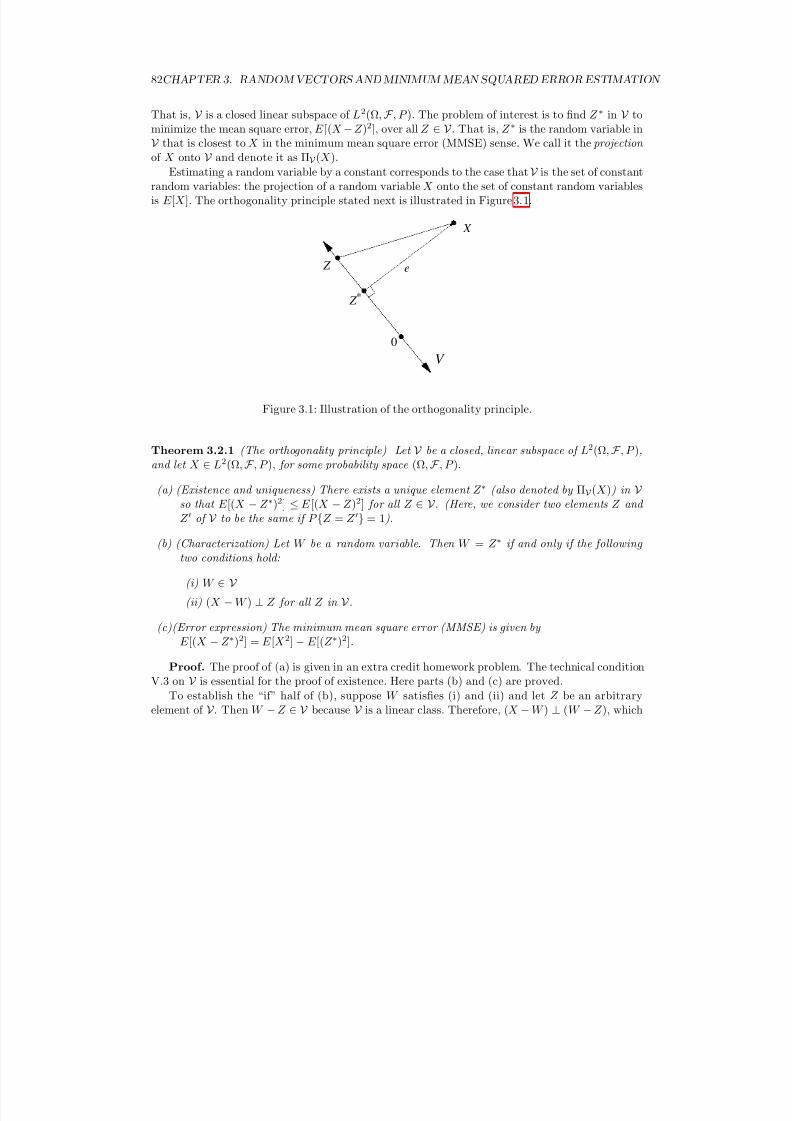
8/11/2019 Random process by B. Hajek
http://slidepdf.com/reader/full/random-process-by-b-hajek 92/448
82CHAPTER 3. RANDOM VECTORS AND MINIMUM MEAN SQUARED ERROR ESTIMATION
That is, V is a closed linear subspace of L2(Ω, F , P ). The problem of interest is to find Z ∗ in V tominimize the mean square error, E [(X −Z )2], over all Z ∈ V . That is, Z ∗ is the random variable inV that is closest to X in the minimum mean square error (MMSE) sense. We call it the projection
of X onto V and denote it as ΠV (X ).Estimating a random variable by a constant corresponds to the case that V is the set of constant
random variables: the projection of a random variable X onto the set of constant random variablesis E [X ]. The orthogonality principle stated next is illustrated in Figure 3.1.
*
Z
Z
X
e
0
V
Figure 3.1: Illustration of the orthogonality principle.
Theorem 3.2.1 (The orthogonality principle) Let V be a closed, linear subspace of L2(Ω, F , P ),and let X ∈ L2(Ω, F , P ), for some probability space (Ω, F , P ).
(a) (Existence and uniqueness) There exists a unique element Z ∗ (also denoted by ΠV (X )) in V so that E [(X − Z ∗)2] ≤ E [(X − Z )2] for all Z ∈ V . (Here, we consider two elements Z and Z of V to be the same if P Z = Z = 1).
(b) (Characterization) Let W be a random variable. Then W = Z ∗ if and only if the following two conditions hold:
(i) W ∈ V (ii) (X − W ) ⊥ Z for all Z in V .
(c)(Error expression) The minimum mean square error (MMSE) is given by
E [(X − Z ∗)2] = E [X 2] − E [(Z ∗)2].
Proof. The proof of (a) is given in an extra credit homework problem. The technical conditionV.3 on V is essential for the proof of existence. Here parts (b) and (c) are proved.
To establish the “if” half of (b), suppose W satisfies (i) and (ii) and let Z be an arbitraryelement of V . Then W − Z ∈ V because V is a linear class. Therefore, (X − W ) ⊥ (W − Z ), which
8/11/2019 Random process by B. Hajek
http://slidepdf.com/reader/full/random-process-by-b-hajek 93/448
3.2. THE ORTHOGONALITY PRINCIPLE FOR MINIMUM MEAN SQUARE ERROR ESTIMATION 8
implies that
E [(X − Z )2] = E [(X − W + W − Z )2]
= E [(X − W )2
+ 2(X − W )(W − Z ) + (W − Z )2
]= E [(X − W )2] + E [(W − Z )2].
Thus E [(X − W )2] ≤ E [(X − Z )2]. Since Z is an arbitrary element of V , it follows that W = Z ∗,and the “if” half of (b) is proved.
To establish the “only if” half of (b), note that Z ∗ ∈ V by the definition of Z ∗. Let Z ∈ V andlet c ∈ R. Then Z ∗ + cZ ∈ V , so that E [(X − (Z ∗ + cZ ))2] ≥ E [(X − Z ∗)2]. But
E [(X − (Z ∗ + cZ ))2] = E [(X − Z ∗) − cZ )2] = E [(X − Z ∗)2] − 2cE [(X − Z ∗)Z ] + c2E [Z 2],
so that
− 2cE [(X − Z ∗)Z ] + c2
E [Z 2
] ≥ 0. (3.1)As a function of c the left side of (3.1) is a parabola with value zero at c = 0. Hence its derivativewith respect to c at 0 must be zero, which yields that (X − Z ∗) ⊥ Z . The “only if” half of (b) isproved.
The expression of (c) is proved as follows. Since X − Z ∗ is orthogonal to all elements of V ,including Z ∗ itself,
E [X 2] = E [((X − Z ∗) + Z ∗)2] = E [(X − Z ∗)2] + E [(Z ∗)2].
This proves (c).
The following propositions give some properties of the projection mapping ΠV , with proofsbased on the orthogonality principle.
Proposition 3.2.2 (Linearity of projection) Suppose V is a closed linear subspace of L2(Ω, F , P ),X 1 and X 2 are in L2(Ω, F , P ), and a1 and a2 are constants. Then
ΠV (a1X 1 + a2X 2) = a1ΠV (X 1) + a2ΠV (X 2). (3.2)
Proof. By the characterization part of the orthogonality principle ( (b) of Theorem 3.2.1), theprojection ΠV (a1X 1 + a2X 2) is characterized by two properties. So, to prove (3.2), it sufficesto show that a1ΠV 1(X 1) + a2ΠV 2(X 2) satisfies these two properties. First, we must check that
a1ΠV 1(X 1) + a2ΠV 2(X 2) ∈ V . This follows immediately from the fact that ΠV (X i) ∈ V , for i = 1, 2,and V is a linear subspace, so the first property is checked. Second, we must check that e ⊥ Z , wheree = a1X 1+a2X 2−(a1ΠV (X 1)+a2ΠV (X 2)), and Z is an arbitrary element of V . Now e = a1e1+a2e2,where ei = X i − ΠV (X i) for i = 1, 2, and ei ⊥ Z for i = 1, 2. So E [eZ ] = a1E [e1Z ] + a2E [e2Z ] = 0,or equivalently, e ⊥ Z. Thus, the second property is also checked, and the proof is complete.
8/11/2019 Random process by B. Hajek
http://slidepdf.com/reader/full/random-process-by-b-hajek 94/448
84CHAPTER 3. RANDOM VECTORS AND MINIMUM MEAN SQUARED ERROR ESTIMATION
Proposition 3.2.3 (Projections onto nested subspaces) Suppose V 1 and V 2 are closed linear sub-spaces of L2(Ω, F , P ) such that V 2 ⊂ V 1. Then for any X ∈ L2(Ω, F , P ), ΠV 2(X ) = ΠV 2ΠV 1(X ). (In words, the projection of X onto V 2 can be found by first projecting X onto V 1, and then projecting
the result onto V 2.) Furthermore,E [(X − ΠV 2(X ))2] = E [(X − ΠV 1(X ))2] + E [(ΠV 1(X ) − ΠV 2(X ))2]. (3.3)
In particular, E [(X − ΠV 2(X ))2] ≥ E [(X − ΠV 1(X ))2].
Proof. By the characterization part of the orthogonality principle (Theorem 3.2.1(b)), the pro- jection ΠV 2(X ) is characterized by two properties. So, to prove ΠV 2(X ) = ΠV 2ΠV 1(X ), it sufficesto show that ΠV 2ΠV 1(X ) satisfies the two properties. First, we must check that ΠV 2ΠV 1(X ) ∈ V 2.This follows immediately from the fact that ΠV 2(X ) maps into V 2, so the first property is checked.Second, we must check that e ⊥ Z , where e = X − ΠV 2ΠV 1(X ), and Z is an arbitrary element of V 2. Now e = e1 + e2, where e1 = X − ΠV 1(X ) and e2 = ΠV 1(X ) − ΠV 2ΠV 1(X ). By the characteri-zation of Π
V 1(X ), e1 is perpendicular to any random variable in
V 1. In particular, e1
⊥ Z , because
Z ∈ V 2 ⊂ V 1. The characterization of the projection of ΠV 1(X ) onto V 2 implies that e2 ⊥ Z . Sinceei ⊥ Z for i = 1, 2, it follows that e ⊥ Z . Thus, the second property is also checked, so it is provedthat ΠV 2(X ) = ΠV 2ΠV 1(X ).
As mentioned above, e1 is perpendicular to any random variable in V 1, which implies thate1 ⊥ e2. Thus, E [e2] = E [e2
1] + E [e22], which is equivalent to (3.3). Therefore, (3.3) is proved. The
last inequality of the proposition follows, of course, from (3.3). The inequality is also equivalent tothe inequality minW ∈V 2 E [(X −W )2] ≥ minW ∈V 1 E [(X − W )2], and this inequality is true becausethe minimum of a set of numbers cannot increase if more numbers are added to the set.
The following proposition is closely related to the use of linear innovations sequences, discussedin Sections 3.5 and 3.6.
Proposition 3.2.4 (Projection onto the span of orthogonal subspaces) Suppose V 1 and V 2 are closed linear subspaces of L2(Ω, F , P ) such that V 1 ⊥ V 2, which means that E [Z 1Z 2] = 0 for any Z 1 ∈ V 1 and Z 2 ∈ V 2. Let V = V 1 ⊕ V 2 = Z 1 + Z 2 : Z i ∈ V i denote the span of V 1 and V 2. Then for any X ∈ L2(Ω, F , P ), ΠV (X ) = ΠV 1(X ) + ΠV 2(X ). The minimum mean square error satisfies
E [(X − ΠV (X ))2] = E [X 2] − E [(ΠV 1(X ))2] − E [(ΠV 2(X ))2].
Proof. The space V is also a closed linear subspace of L2(Ω, F , P ) (see a starred homeworkproblem). By the characterization part of the orthogonality principle (Theorem 3.2.1(b)), theprojection ΠV (X ) is characterized by two properties. So to prove ΠV (X ) = ΠV 1(X ) + ΠV 2(X ), itsuffices to show that ΠV 1(X ) + ΠV 2(X ) satisfies these two properties. First, we must check thatΠV 1(X )+ΠV 2(X )
∈ V . This follows immediately from the fact that ΠV i(X )
∈ V i, for i = 1, 2, so the
first property is checked. Second, we must check that e ⊥ Z , where e = X − (ΠV 1(X ) + ΠV 2(X )),and Z is an arbitrary element of V . Now any such Z can be written as Z = Z 1 + Z 2 where Z i ∈ V ifor i = 1, 2. Observe that ΠV 2(X ) ⊥ Z 1 because ΠV 2(X ) ∈ V 2 and Z 1 ∈ V 1. Therefore,
E [eZ 1] = E [(X − (ΠV 1(X ) + ΠV 2(X ))Z 1]
= E [(X − ΠV 1(X ))Z 1] = 0,
8/11/2019 Random process by B. Hajek
http://slidepdf.com/reader/full/random-process-by-b-hajek 95/448
3.3. CONDITIONAL EXPECTATION AND LINEAR ESTIMATORS 85
where the last equality follows from the characterization of ΠV 1(X ). Thus, e ⊥ Z 1, and similarlye ⊥ Z 2, so e ⊥ Z. Thus, the second property is also checked, so ΠV (X ) = ΠV 1(X ) + ΠV 2(X ) isproved.
Since ΠV i(X ) ∈ V i for i = 1, 2, ΠV 1(X ) ⊥ ΠV 2(X ). Therefore, E [(ΠV (X ))2
] = E [(ΠV 1(X ))2
] +E [(ΠV 2(X ))2], and the expression for the MMSE in the proposition follows from the error expressionin the orthogonality principle.
3.3 Conditional expectation and linear estimators
In many applications, a random variable X is to be estimated based on observation of a randomvariable Y . Thus, an estimator is a function of Y . In applications, the two most frequentlyconsidered classes of functions of Y used in this context are essentially all functions, leading to the
best unconstrained estimator, or all linear functions, leading to the best linear estimator. Thesetwo possibilities are discussed in this section.
3.3.1 Conditional expectation as a projection
Suppose a random variable X is to be estimated using an observed random vector Y of dimensionm. Suppose E [X 2] < +∞. Consider the most general class of estimators based on Y , by setting
V = g(Y ) : g : Rm → R, E [g(Y )2] < +∞. (3.4)
There is also the implicit condition that g is Borel measurable so that g(Y ) is a random variable.The projection of X onto this class V is the unconstrained minimum mean square error (MMSE)
estimator of X given Y .Let us first proceed to identify the optimal estimator by conditioning on the value of Y , thereby
reducing this example to the estimation of a random variable by a constant, as discussed at thebeginning of Section 3.2. For technical reasons we assume for now that X and Y have a joint pdf.Then, conditioning on Y ,
E [(X − g(Y ))2] =
Rm
E [(X − g(Y ))2|Y = y]f Y (y)dy
where
E [(X − g(Y ))2|Y = y] = ∞
−∞(x − g(y))2f X |Y (x | y)dx
Since the mean is the MMSE estimator of a random variable among all constants, for each fixed y ,the minimizing choice for g(y) is
g∗(y) = E [X |Y = y] =
∞−∞
xf X |Y (x | y)dx. (3.5)
8/11/2019 Random process by B. Hajek
http://slidepdf.com/reader/full/random-process-by-b-hajek 96/448
86CHAPTER 3. RANDOM VECTORS AND MINIMUM MEAN SQUARED ERROR ESTIMATION
Therefore, the optimal estimator in V is g∗(Y ) which, by definition, is equal to the random variableE [X |Y ].
What does the orthogonality principle imply for this example? It implies that there exists an
optimal estimator g∗(Y ) which is the unique element of V such that
(X − g∗(Y )) ⊥ g(Y )
for all g(Y ) ∈ V . If X, Y have a joint pdf then we can check that E [X | Y ] satisfies the requiredcondition. Indeed,
E [(X − E [X | Y ])g(Y )] =
(x − E [X | Y = y])g(y)f X |Y (x | y)f Y (y)dxdy
=
(x − E [X | Y = y])f X |Y (x | y)dx
g(y)f Y (y)dy
= 0,
because the expression within the braces is zero.In summary, if X and Y have a joint pdf (and similarly if they have a joint pmf) then the
MMSE estimator of X given Y is E [X | Y ]. Even if X and Y don’t have a joint pdf or joint pmf,we define the conditional expectation E [X | Y ] to be the MMSE estimator of X given Y. By theorthogonality principle E [X | Y ] exists as long as E [X 2] < ∞, and it is the unique function of Ysuch that
E [(X − E [X | Y ])g(Y )] = 0
for all g(Y ) in V .Estimation of a random variable has been discussed, but often we wish to estimate a random
vector. A beauty of the MSE criteria is that it easily extends to estimation of random vectors,because the MSE for estimation of a random vector is the sum of the MSEs of the coordinates:
E [ X − g(Y ) 2] =
mi=1
E [(X i − gi(Y ))2]
Therefore, for most sets of estimators V typically encountered, finding the MMSE estimator of arandom vector X decomposes into finding the MMSE estimators of the coordinates of X separately.
Suppose a random vector X is to be estimated using estimators of the form g(Y), where here gmaps Rn into Rm. Assume E [X 2] < +∞ and seek an estimator to minimize the MSE. As seenabove, the MMSE estimator for each coordinate X i is E [X i|Y ], which is also the projection of X ionto the set of unconstrained estimators based on Y , defined in (3.4). So the optimal estimator
g∗(Y ) of the entire vector X is given by
g∗(Y ) = E [X | Y ] =
E [X 1 | Y ]E [X 2 | Y ]
...E [X m | Y ]
8/11/2019 Random process by B. Hajek
http://slidepdf.com/reader/full/random-process-by-b-hajek 97/448
3.3. CONDITIONAL EXPECTATION AND LINEAR ESTIMATORS 87
Let the estimation error be denoted by e, e = X − E [X | Y ]. (Even though e is a random vectorwe use lower case for it for an obvious reason.)
The mean of the error is given by Ee = 0. As for the covariance of the error, note that
E [X j | Y ] is in V for each j, so ei ⊥ E [X j | Y ] for each i, j. Since Eei = 0, it follows thatCov(ei, E [X j | Y ]) = 0 for all i, j. Equivalently, Cov(e, E [X | Y ]) = 0. Using this and the factX = E [X | Y ] + e yields
Cov(X ) = Cov(E [X | Y ] + e)
= Cov(E [X | Y ]) + Cov(e) + Cov(E [X |Y ], e) + Cov(e, E [X |Y ])
= Cov(E [X | Y ]) + Cov(e)
Thus, Cov(e) = Cov(X ) − Cov(E [X | Y ]).In practice, computation of E [X | Y ] (for example, using (3.5) in case a joint pdf exists) may
be too complex or may require more information about the joint distribution of X and Y than
is available. For both of these reasons, it is worthwhile to consider classes of estimators that areconstrained to smaller sets of functions of the observations. A widely used set is the set of all linearfunctions, leading to linear estimators, described next.
3.3.2 Linear estimators
Let X and Y be random vectors with E [X 2] < +∞ and E [Y 2] < +∞. Seek estimators of the form AY + b to minimize the MSE. Such estimators are called linear estimators because eachcoordinate of AY + b is a linear combination of Y 1, Y 2, . . . , Y m and 1. Here “1” stands for therandom variable that is always equal to 1.
To identify the optimal linear estimator we shall apply the orthogonality principle for eachcoordinate of X with
V = c0 + c1Y 1 + c2Y 2 + . . . + cnY n : c0, c1, . . . , cn ∈ R
Let e denote the estimation error e = X − (AY + b). We must select A and b so that ei ⊥ Z for allZ ∈ V . Equivalently, we must select A and b so that
ei ⊥ 1 all iei ⊥ Y j all i,j.
The condition ei ⊥ 1, which means Eei = 0, implies that E [eiY j] = Cov(ei, Y j). Thus, therequired orthogonality conditions on A and b become Ee = 0 and Cov(e, Y ) = 0. The conditionEe = 0 requires that b = E [X ]
− AE [Y ], so we can restrict our attention to estimators of the
form E [X ] + A(Y − E [Y ]), so that e = X − E [X ] − A(Y − E [Y ]). The condition Cov(e, Y ) = 0becomes Cov(X, Y ) − ACov(Y, Y ) = 0. If Cov(Y, Y ) is not singular, then A must be given byA = Cov(X, Y )Cov(Y, Y )−1. In this case the optimal linear estimator, denoted by E [X | Y ], isgiven by
E [X | Y ] = E [X ] + Cov(X, Y )Cov(Y, Y )−1(Y − E [Y ]) (3.6)
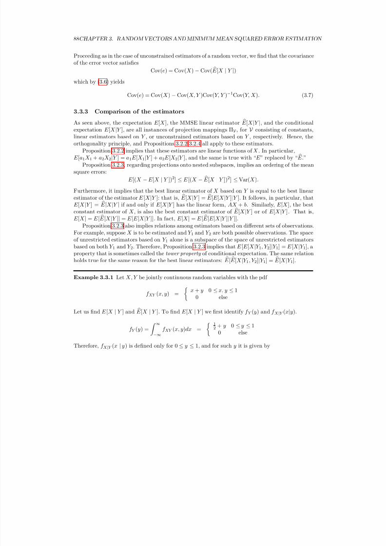
8/11/2019 Random process by B. Hajek
http://slidepdf.com/reader/full/random-process-by-b-hajek 98/448
88CHAPTER 3. RANDOM VECTORS AND MINIMUM MEAN SQUARED ERROR ESTIMATION
Proceeding as in the case of unconstrained estimators of a random vector, we find that the covarianceof the error vector satisfies
Cov(e) = Cov(X ) − Cov( E [X | Y ])
which by (3.6) yields
Cov(e) = Cov(X ) − Cov(X, Y )Cov(Y, Y )−1Cov(Y, X ). (3.7)
3.3.3 Comparison of the estimators
As seen above, the expectation E [X ], the MMSE linear estimator E [X |Y |, and the conditionalexpectation E [X |Y ], are all instances of projection mappings ΠV , for V consisting of constants,linear estimators based on Y , or unconstrained estimators based on Y , respectively. Hence, theorthogonality principle, and Propositions 3.2.2-3.2.4 all apply to these estimators.
Proposition 3.2.2 implies that these estimators are linear functions of X . In particular,
E [a1X 1 + a2X 2|Y ] = a1E [X 1|Y ] + a2E [X 2|Y ], and the same is true with “E ” replaced by “ E .”Proposition 3.2.3, regarding projections onto nested subspaces, implies an ordering of the mean
square errors:
E [(X − E [X | Y ])2] ≤ E [(X − E [X | Y ])2] ≤ Var(X ).
Furthermore, it implies that the best linear estimator of X based on Y is equal to the best linearestimator of the estimator E [X |Y ]: that is, E [X |Y ] = E [E [X |Y ]|Y ]. It follows, in particular, thatE [X |Y ] = E [X |Y ] if and only if E [X |Y ] has the linear form, AX + b. Similarly, E [X ], the bestconstant estimator of X , is also the best constant estimator of E [X |Y ] or of E [X |Y ]. That is,E [X ] = E [
E [X |Y ]] = E [E [X |Y ]]. In fact, E [X ] = E [
E [E [X |Y ]|Y ]].
Proposition 3.2.3 also implies relations among estimators based on different sets of observations.
For example, suppose X is to be estimated and Y 1 and Y 2 are both possible observations. The spaceof unrestricted estimators based on Y 1 alone is a subspace of the space of unrestricted estimatorsbased on both Y 1 and Y 2. Therefore, Proposition 3.2.3 implies that E [E [X |Y 1, Y 2]|Y 1] = E [X |Y 1], aproperty that is sometimes called the tower property of conditional expectation. The same relationholds true for the same reason for the best linear estimators: E [ E [X |Y 1, Y 2]|Y 1] = E [X |Y 1].
Example 3.3.1 Let X, Y be jointly continuous random variables with the pdf
f XY (x, y) =
x + y 0 ≤ x, y ≤ 1
0 else
Let us find E [X | Y ] and E [X | Y ]. To find E [X | Y ] we first identify f Y (y) and f X |Y (x|y).
f Y (y) =
∞−∞
f XY (x, y)dx =
1
2 + y 0 ≤ y ≤ 10 else
Therefore, f X |Y (x | y) is defined only for 0 ≤ y ≤ 1, and for such y it is given by
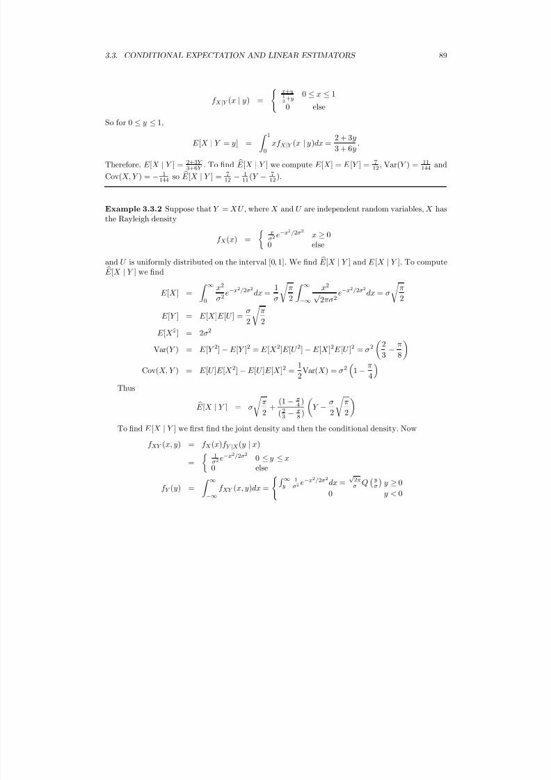
8/11/2019 Random process by B. Hajek
http://slidepdf.com/reader/full/random-process-by-b-hajek 99/448
3.3. CONDITIONAL EXPECTATION AND LINEAR ESTIMATORS 89
f X |Y (x | y) = x+y12
+y 0 ≤ x ≤ 1
0 else
So for 0 ≤ y ≤ 1,
E [X | Y = y] =
1
0xf X |Y (x | y)dx =
2 + 3y
3 + 6y.
Therefore, E [X | Y ] = 2+3Y 3+6Y . To find E [X | Y ] we compute E [X ] = E [Y ] = 7
12 , Var(Y ) = 11144 and
Cov(X, Y ) = − 1144 so E [X | Y ] = 7
12 − 111 (Y − 7
12 ).
Example 3.3.2 Suppose that Y = X U , where X and U are independent random variables, X has
the Rayleigh density
f X (x) =
xσ2 e−x2/2σ2 x ≥ 00 else
and U is uniformly distributed on the interval [0, 1]. We find E [X | Y ] and E [X | Y ]. To compute E [X | Y ] we find
E [X ] =
∞0
x2
σ2e−x2/2σ2dx =
1
σ
π
2
∞−∞
x2
√ 2πσ2
e−x2/2σ2dx = σ
π
2
E [Y ] = E [X ]E [U ] = σ
2
π
2
E [X 2
] = 2σ2
Var(Y ) = E [Y 2] − E [Y ]2 = E [X 2]E [U 2] − E [X ]2E [U ]2 = σ2
2
3 − π
8
Cov(X, Y ) = E [U ]E [X 2] − E [U ]E [X ]2 =
1
2Var(X ) = σ2
1 − π
4
Thus
E [X | Y ] = σ
π
2 +
(1 − π4 )
( 23 − π
8 )
Y − σ
2
π
2
To find E [X | Y ] we first find the joint density and then the conditional density. Now
f XY (x, y) = f X (x)f Y |X (y | x)
=
1σ2 e−x2/2σ2 0 ≤ y ≤ x0 else
f Y (y) =
∞−∞
f XY (x, y)dx =
∞y
1σ2 e−x2/2σ2dx =
√ 2πσ Q
yσ
0
y ≥ 0
y < 0
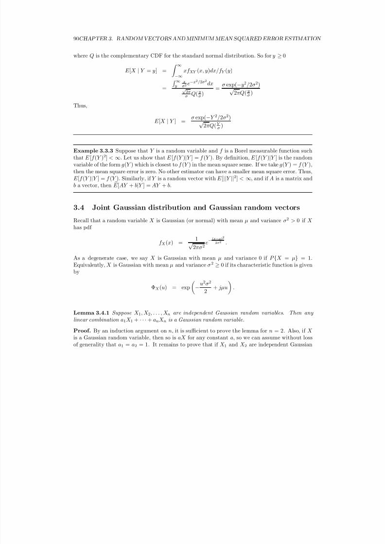
8/11/2019 Random process by B. Hajek
http://slidepdf.com/reader/full/random-process-by-b-hajek 100/448
90CHAPTER 3. RANDOM VECTORS AND MINIMUM MEAN SQUARED ERROR ESTIMATION
where Q is the complementary CDF for the standard normal distribution. So for y ≥ 0
E [X | Y = y] = ∞
−∞xf XY (x, y)dx/f Y (y)
=
∞y
xσ2 e−x2/2σ2dx√
2πσ Q( y
σ )=
σ exp(−y2/2σ2)√ 2πQ( y
σ )
Thus,
E [X | Y ] = σ exp(−Y 2/2σ2)√
2πQ(Y σ )
Example 3.3.3 Suppose that Y is a random variable and f is a Borel measurable function such
that E [f (Y )2] < ∞. Let us show that E [f (Y )|Y ] = f (Y ). By definition, E [f (Y )|Y ] is the randomvariable of the form g(Y ) which is closest to f (Y ) in the mean square sense. If we take g(Y ) = f (Y ),then the mean square error is zero. No other estimator can have a smaller mean square error. Thus,E [f (Y )|Y ] = f (Y ). Similarly, if Y is a random vector with E [||Y ||2] < ∞, and if A is a matrix andb a vector, then E [AY + b|Y ] = AY + b.
3.4 Joint Gaussian distribution and Gaussian random vectors
Recall that a random variable X is Gaussian (or normal) with mean µ and variance σ2 > 0 if X has pdf
f X (x) = 1√
2πσ2e−
(x−µ)2
2σ2 .
As a degenerate case, we say X is Gaussian with mean µ and variance 0 if P X = µ = 1.Equivalently, X is Gaussian with mean µ and variance σ 2 ≥ 0 if its characteristic function is givenby
ΦX (u) = exp
−u2σ2
2 + jµu
.
Lemma 3.4.1 Suppose X 1, X 2, . . . , X n are independent Gaussian random variables. Then any linear combination a1X 1 + · · · + anX n is a Gaussian random variable.
Proof. By an induction argument on n, it is sufficient to prove the lemma for n = 2. Also, if X is a Gaussian random variable, then so is aX for any constant a, so we can assume without lossof generality that a1 = a2 = 1. It remains to prove that if X 1 and X 2 are independent Gaussian
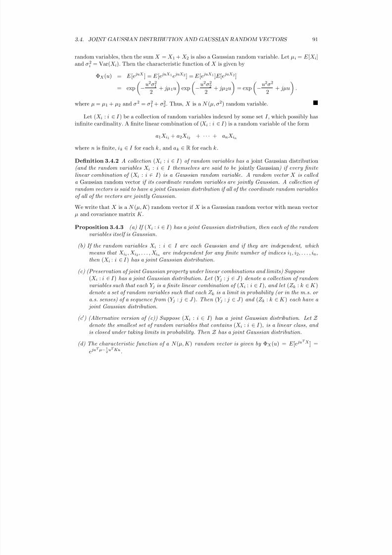
8/11/2019 Random process by B. Hajek
http://slidepdf.com/reader/full/random-process-by-b-hajek 101/448
3.4. JOINT GAUSSIAN DISTRIBUTION AND GAUSSIAN RANDOM VECTORS 91
random variables, then the sum X = X 1 + X 2 is also a Gaussian random variable. Let µi = E [X i]and σ 2
i = Var(X i). Then the characteristic function of X is given by
ΦX
(u) = E [e juX ] = E [e juX 1e juX 2] = E [e juX 1 ]E [e juX 2]
= exp
−u2σ21
2 + jµ1u
exp
−u2σ2
2
2 + jµ2u
= exp
−u2σ2
2 + jµu
.
where µ = µ1 + µ2 and σ 2 = σ21 + σ2
2. Thus, X is a N (µ, σ2) random variable.
Let (X i : i ∈ I ) be a collection of random variables indexed by some set I , which possibly hasinfinite cardinality. A finite linear combination of (X i : i ∈ I ) is a random variable of the form
a1X i1 + a2X i2 + · · · + anX in
where n is finite, ik ∈ I for each k , and ak ∈ R for each k .
Definition 3.4.2 A collection (X i : i ∈ I ) of random variables has a joint Gaussian distribution(and the random variables X i : i ∈ I themselves are said to be jointly Gaussian) if every finite linear combination of (X i : i ∈ I ) is a Gaussian random variable. A random vector X is called a Gaussian random vector if its coordinate random variables are jointly Gaussian. A collection of random vectors is said to have a joint Gaussian distribution if all of the coordinate random variables of all of the vectors are jointly Gaussian.
We write that X is a N (µ, K ) random vector if X is a Gaussian random vector with mean vectorµ and covariance matrix K .
Proposition 3.4.3 (a) If (X i : i ∈ I ) has a joint Gaussian distribution, then each of the random variables itself is Gaussian.
(b) If the random variables X i : i ∈ I are each Gaussian and if they are independent, which means that X i1, X i2, . . . , X in are independent for any finite number of indices i1, i2, . . . , in,then (X i : i ∈ I ) has a joint Gaussian distribution.
(c) (Preservation of joint Gaussian property under linear combinations and limits) Suppose (X i : i ∈ I ) has a joint Gaussian distribution. Let (Y j : j ∈ J ) denote a collection of random variables such that each Y j is a finite linear combination of (X i : i ∈ I ), and let (Z k : k ∈ K )denote a set of random variables such that each Z k is a limit in probability (or in the m.s. or a.s. senses) of a sequence from (Y j : j ∈ J ). Then (Y j : j ∈ J ) and (Z k : k ∈ K ) each have a joint Gaussian distribution.
(c ) (Alternative version of (c)) Suppose (X i : i ∈ I ) has a joint Gaussian distribution. Let Z denote the smallest set of random variables that contains (X i : i ∈ I ), is a linear class, and is closed under taking limits in probability. Then Z has a joint Gaussian distribution.
(d) The characteristic function of a N (µ, K ) random vector is given by ΦX (u) = E [e juT X ] =
e juT µ− 1
2uT Ku .
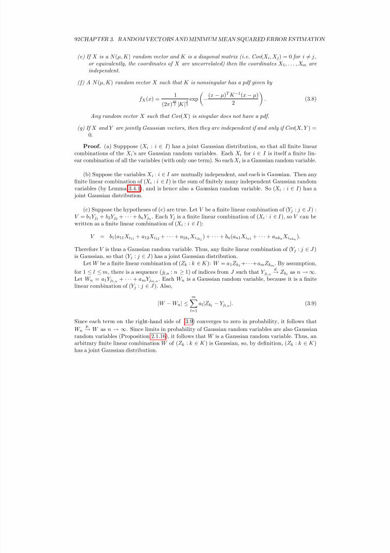
8/11/2019 Random process by B. Hajek
http://slidepdf.com/reader/full/random-process-by-b-hajek 102/448
92CHAPTER 3. RANDOM VECTORS AND MINIMUM MEAN SQUARED ERROR ESTIMATION
(e) If X is a N (µ, K ) random vector and K is a diagonal matrix (i.e. Cov (X i, X j) = 0 for i = j ,or equivalently, the coordinates of X are uncorrelated) then the coordinates X 1, . . . , X m are independent.
(f) A N (µ, K ) random vector X such that K is nonsingular has a pdf given by
f X (x) = 1
(2π)m2 |K | 12
exp
−(x − µ)T K −1(x − µ)
2
. (3.8)
Any random vector X such that Cov (X ) is singular does not have a pdf.
(g) If X and Y are jointly Gaussian vectors, then they are independent if and only if Cov (X, Y ) =0.
Proof. (a) Supppose (X i : i ∈ I ) has a joint Gaussian distribution, so that all finite linearcombinations of the X i’s are Gaussian random variables. Each X i for i
∈ I is itself a finite lin-
ear combination of all the variables (with only one term). So each X i is a Gaussian random variable.
(b) Suppose the variables X i : i ∈ I are mutually independent, and each is Gaussian. Then anyfinite linear combination of (X i : i ∈ I ) is the sum of finitely many independent Gaussian randomvariables (by Lemma 3.4.1), and is hence also a Gaussian random variable. So (X i : i ∈ I ) has a joint Gaussian distribution.
(c) Suppose the hypotheses of (c) are true. Let V be a finite linear combination of (Y j : j ∈ J ) :V = b1Y j1 + b2Y j2 + · · · + bnY jn. Each Y j is a finite linear combination of (X i : i ∈ I ), so V can bewritten as a finite linear combination of (X i : i ∈ I ):
V = b1(a11X i11 + a12X i12 + · · · + a1k1X i1k1 ) + · · · + bn(an1X in1 + · · · + anknX inkn ).
Therefore V is thus a Gaussian random variable. Thus, any finite linear combination of (Y j : j ∈ J )is Gaussian, so that (Y j : j ∈ J ) has a joint Gaussian distribution.
Let W be a finite linear combination of (Z k : k ∈ K ): W = a1Z k1 +· · ·+amZ km . By assumption,
for 1 ≤ l ≤ m, there is a sequence ( jl,n : n ≥ 1) of indices from J such that Y jl,nd.→ Z kl
as n → ∞.Let W n = a1Y j1,n + · · · + amY jm,n. Each W n is a Gaussian random variable, because it is a finitelinear combination of (Y j : j ∈ J ). Also,
|W − W n| ≤ml=1
al|Z kl − Y jl,n|. (3.9)
Since each term on the right-hand side of (3.9) converges to zero in probability, it follows that
W n p.→ W as n → ∞. Since limits in probability of Gaussian random variables are also Gaussian
random variables (Proposition 2.1.16), it follows that W is a Gaussian random variable. Thus, anarbitrary finite linear combination W of (Z k : k ∈ K ) is Gaussian, so, by definition, (Z k : k ∈ K )has a joint Gaussian distribution.
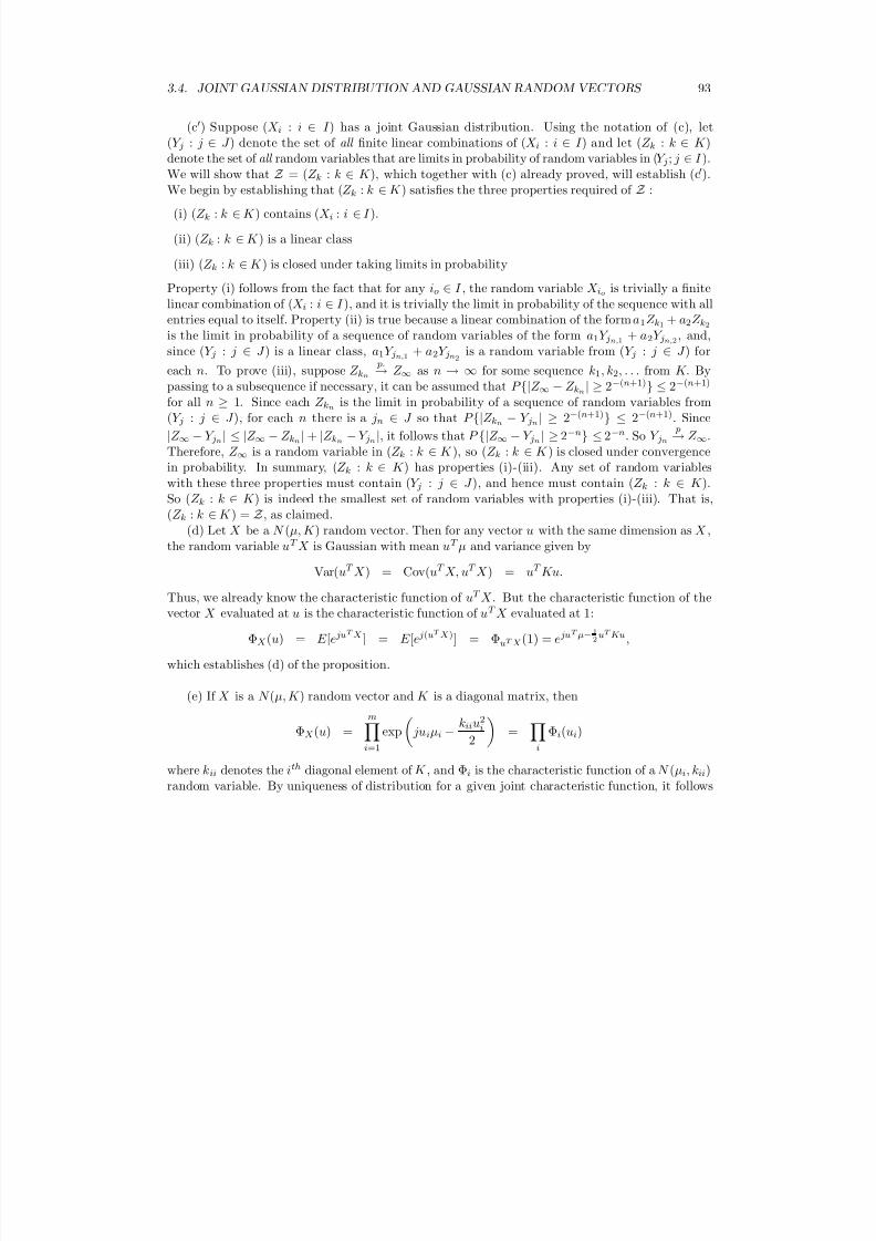
8/11/2019 Random process by B. Hajek
http://slidepdf.com/reader/full/random-process-by-b-hajek 103/448
3.4. JOINT GAUSSIAN DISTRIBUTION AND GAUSSIAN RANDOM VECTORS 93
(c) Suppose (X i : i ∈ I ) has a joint Gaussian distribution. Using the notation of (c), let(Y j : j ∈ J ) denote the set of all finite linear combinations of (X i : i ∈ I ) and let (Z k : k ∈ K )denote the set of all random variables that are limits in probability of random variables in (Y j; j ∈ I ).
We will show that Z = (Z k : k ∈ K ), which together with (c) already proved, will establish (c).We begin by establishing that (Z k : k ∈ K ) satisfies the three properties required of Z :
(i) (Z k : k ∈ K ) contains (X i : i ∈ I ).
(ii) (Z k : k ∈ K ) is a linear class
(iii) (Z k : k ∈ K ) is closed under taking limits in probability
Property (i) follows from the fact that for any io ∈ I , the random variable X io is trivially a finitelinear combination of (X i : i ∈ I ), and it is trivially the limit in probability of the sequence with allentries equal to itself. Property (ii) is true because a linear combination of the form a1Z k1 + a2Z k2is the limit in probability of a sequence of random variables of the form a1Y jn,1 + a2Y jn,2, and,
since (Y j : j ∈ J ) is a linear class, a1Y jn,1 + a2Y jn2 is a random variable from (Y j : j ∈ J ) foreach n. To prove (iii), suppose Z kn
p.→ Z ∞ as n → ∞ for some sequence k1, k2, . . . from K. Bypassing to a subsequence if necessary, it can be assumed that P |Z ∞ − Z kn | ≥ 2−(n+1) ≤ 2−(n+1)
for all n ≥ 1. Since each Z kn is the limit in probability of a sequence of random variables from(Y j : j ∈ J ), for each n there is a jn ∈ J so that P |Z kn − Y jn| ≥ 2−(n+1) ≤ 2−(n+1). Since
|Z ∞ − Y jn| ≤ |Z ∞ − Z kn | + |Z kn − Y jn |, it follows that P |Z ∞ − Y jn| ≥ 2−n ≤ 2−n. So Y jn p→ Z ∞.
Therefore, Z ∞ is a random variable in (Z k : k ∈ K ), so (Z k : k ∈ K ) is closed under convergencein probability. In summary, (Z k : k ∈ K ) has properties (i)-(iii). Any set of random variableswith these three properties must contain (Y j : j ∈ J ), and hence must contain (Z k : k ∈ K ).So (Z k : k ∈ K ) is indeed the smallest set of random variables with properties (i)-(iii). That is,(Z k : k ∈ K ) = Z , as claimed.
(d) Let X be a N (µ, K ) random vector. Then for any vector u with the same dimension as X ,the random variable uT X is Gaussian with mean uT µ and variance given by
Var(uT X ) = Cov(uT X, uT X ) = uT Ku.
Thus, we already know the characteristic function of uT X . But the characteristic function of thevector X evaluated at u is the characteristic function of uT X evaluated at 1:
ΦX (u) = E [e juT X ] = E [e j(uT X )] = ΦuT X (1) = e ju
T µ− 12uT Ku ,
which establishes (d) of the proposition.
(e) If X is a N (µ, K ) random vector and K is a diagonal matrix, then
ΦX (u) =mi=1
exp
juiµi − kiiu2i
2
=
i
Φi(ui)
where kii denotes the ith diagonal element of K , and Φi is the characteristic function of a N (µi, kii)random variable. By uniqueness of distribution for a given joint characteristic function, it follows
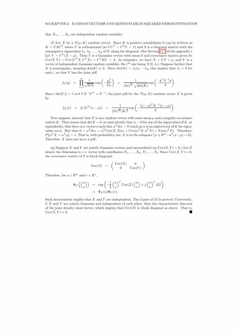
8/11/2019 Random process by B. Hajek
http://slidepdf.com/reader/full/random-process-by-b-hajek 104/448
94CHAPTER 3. RANDOM VECTORS AND MINIMUM MEAN SQUARED ERROR ESTIMATION
that X 1, . . . , X m are independent random variables.
(f) Let X be a N (µ, K ) random vector. Since K is positive semidefinite it can be written as
K = U ΛU T
where U is orthonormal (so UU T
= U T
U = I ) and Λ is a diagonal matrix with thenonnegative eigenvalues λ1, λ2, . . . , λm of K along the diagonal. (See Section 11.7 of the appendix.)Let Y = U T (X − µ). Then Y is a Gaussian vector with mean 0 and covariance matrix given byCov(Y, Y ) = Cov(U T X, U T X ) = U T KU = Λ. In summary, we have X = U Y + µ, and Y is avector of independent Gaussian random variables, the ith one being N (0, λi). Suppose further thatK is nonsingular, meaning det(K ) = 0. Since det(K ) = λ1λ2 · · · λm this implies that λi > 0 foreach i, so that Y has the joint pdf
f Y (y) =mi=1
1√ 2πλi
exp
− y 2
i
2λi
=
1
(2π)m2
det(K )exp
−yT Λ−1y
2
.
Since |
det(U )| = 1 and U Λ
−1U T = K
−1, the joint pdf for the N (µ, K ) random vector X is given
by
f X (x) = f Y (U T (x − µ)) = 1
(2π)m2 |K | 12
exp
−(x − µ)T K −1(x − µ)
2
.
Now suppose, instead, that X is any random vector with some mean µ and a singular covariancematrix K . That means that det K = 0, or equivalently that λi = 0 for one of the eigenvalues of K , orequivalently, that there is a vector α such that αT Kα = 0 (such an α is an eigenvector of K for eigen-value zero). But then 0 = αT Kα = αT Cov(X, X )α = Cov(αT X, αT X ) = Var(αT X ). Therefore,P αT X = αT µ = 1. That is, with probability one, X is in the subspace x ∈ Rm : αT (x−µ) = 0.Therefore, X does not have a pdf.
(g) Suppose X and Y are jointly Gaussian vectors and uncorrelated (so Cov(X, Y ) = 0.) Let Z denote the dimension m + n vector with coordinates X 1, . . . , X m, Y 1, . . . , Y n. Since Cov(X, Y ) = 0,the covariance matrix of Z is block diagonal:
Cov(Z ) =
Cov(X ) 0
0 Cov(Y )
.
Therefore, for u ∈ Rm and v ∈ Rn,
ΦZ
u
v = exp
−1
2 u
vT
Cov(Z )
u
v+ j
u
vT
EZ
= ΦX (u)ΦY (v).
Such factorization implies that X and Y are independent. The if part of (f) is proved. Conversely,if X and Y are jointly Gaussian and independent of each other, then the characteristic functionof the joint density must factor, which implies that Cov( Z ) is block diagonal as above. That is,Cov(X, Y ) = 0.
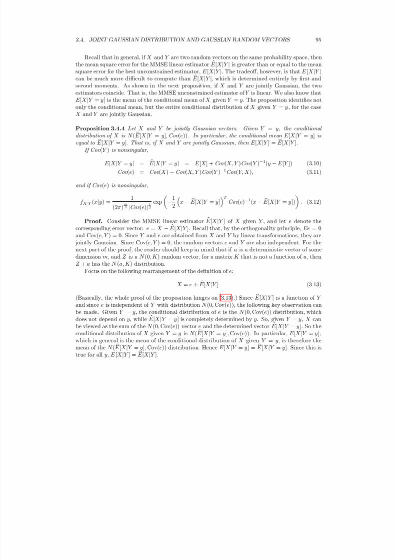
8/11/2019 Random process by B. Hajek
http://slidepdf.com/reader/full/random-process-by-b-hajek 105/448
3.4. JOINT GAUSSIAN DISTRIBUTION AND GAUSSIAN RANDOM VECTORS 95
Recall that in general, if X and Y are two random vectors on the same probability space, thenthe mean square error for the MMSE linear estimator
E [X |Y | is greater than or equal to the mean
square error for the best unconstrained estimator, E [X |Y |. The tradeoff, however, is that E [X |Y |can be much more difficult to compute than E [X |Y |, which is determined entirely by first andsecond moments. As shown in the next proposition, if X and Y are jointly Gaussian, the twoestimators coincide. That is, the MMSE unconstrained estimator of Y is linear. We also know thatE [X |Y = y] is the mean of the conditional mean of X given Y = y. The proposition identifies notonly the conditional mean, but the entire conditional distribution of X given Y = y , for the caseX and Y are jointly Gaussian.
Proposition 3.4.4 Let X and Y be jointly Gaussian vectors. Given Y = y, the conditional distribution of X is N ( E [X |Y = y], Cov (e)). In particular, the conditional mean E [X |Y = y] is equal to E [X |Y = y]. That is, if X and Y are jointly Gaussian, then E [X |Y ] = E [X |Y ].
If Cov (Y ) is nonsingular,
E [X |Y = y] = E [X |Y = y] = E [X ] + Cov (X, Y )Cov (Y )−1(y − E [Y ]) (3.10)
Cov (e) = Cov (X ) − Cov (X, Y )Cov (Y )−1Cov (Y, X ), (3.11)
and if Cov (e) is nonsingular,
f X |Y (x|y) = 1
(2π)m2 |Cov (e)| 12
exp
−1
2
x − E [X |Y = y]
T Cov (e)−1(x − E [X |Y = y])
. (3.12)
Proof. Consider the MMSE linear estimator E [X |Y ] of X given Y , and let e denote thecorresponding error vector: e = X −
E [X |Y ]. Recall that, by the orthogonality principle, Ee = 0
and Cov(e, Y ) = 0. Since Y and e are obtained from X and Y by linear transformations, they are
jointly Gaussian. Since Cov(e, Y ) = 0, the random vectors e and Y are also independent. For thenext part of the proof, the reader should keep in mind that if a is a deterministic vector of somedimension m, and Z is a N (0, K ) random vector, for a matrix K that is not a function of a, thenZ + a has the N (a, K ) distribution.
Focus on the following rearrangement of the definition of e:
X = e + E [X |Y ]. (3.13)
(Basically, the whole proof of the proposition hinges on (3.13).) Since E [X |Y ] is a function of Y and since e is independent of Y with distribution N (0, Cov(e)), the following key observation canbe made. Given Y = y, the conditional distribution of e is the N (0, Cov(e)) distribution, which
does not depend on y, while E [X |Y = y ] is completely determined by y. So, given Y = y , X canbe viewed as the sum of the N (0, Cov(e)) vector e and the determined vector E [X |Y = y]. So theconditional distribution of X given Y = y is N ( E [X |Y = y], Cov(e)). In particular, E [X |Y = y ],which in general is the mean of the conditional distribution of X given Y = y, is therefore themean of the N ( E [X |Y = y], Cov(e)) distribution. Hence E [X |Y = y] = E [X |Y = y]. Since this istrue for all y, E [X |Y ] = E [X |Y ].
8/11/2019 Random process by B. Hajek
http://slidepdf.com/reader/full/random-process-by-b-hajek 106/448
96CHAPTER 3. RANDOM VECTORS AND MINIMUM MEAN SQUARED ERROR ESTIMATION
Equations (3.10) and (3.11), respectively, are just the equations (3.6) and (3.7) derived for theMMSE linear estimator,
E [X |Y ], and its associated covariance of error. Equation (3.12) is just the
formula (3.8) for the pdf of a N (µ, K ) vector, with µ =
E [X |Y = y] and K = Cov(e).
Example 3.4.5 Suppose X and Y are jointly Gaussian mean zero random variables such that the
vector
X Y
has covariance matrix
4 33 9
. Let us find simple expressions for the two random
variables E [X 2|Y ] and P (X ≥ c|Y ). Note that if W is a random variable with the N (µ, σ2)distribution, then E [W 2] = µ2 + σ2 and P W ≥ c = Q( c−µ
σ ), where Q is the standard Gaussiancomplementary CDF. The idea is to apply these facts to the conditional distribution of X given Y .
Given Y = y, the conditional distribution of X is N ( Cov(X,Y )
Var(Y ) y, Cov(X ) − Cov(X,Y )2
Var(Y ) ), or N (y
3 , 3).
Therefore, E [X 2|Y = y] = (y3 )2 + 3 and P (X ≥ c|Y = y) = Q( c−(y/3)√
3 ). Applying these two
functions to the random variable Y yields E [X 2|Y ] = (Y 3 )2 + 3 and P (X ≥ c|Y ) = Q( c−(Y/3)√
3 ).
3.5 Linear innovations sequences
Let X, Y 1, . . . , Y n be random vectors with finite second moments, all on the same probability space.In general, computation of the joint projection E [X |Y 1, . . . , Y n] is considerably more complicatedthan computation of the individual projections E [X |Y i], because it requires inversion of the covari-ance matrix of all the Y ’s. However, if E [Y i] = 0 for all i and E [Y iY T j ] = 0 for i = j (i.e., allcoordinates of Y i are orthogonal to constants and to all coordinates of Y j for i = j), then
E [X |Y 1, . . . , Y n] = X +n
i=1
E [X − X |Y i], (3.14)
where we write X for E [X ]. The orthogonality principle can be used to prove (3.14) as follows. Itsuffices to prove that the right side of (3.14) satisfies the two properties that together characterizethe left side of (3.14). First, the right side is a linear combination of 1, Y 1, . . . , Y n. Secondly, let edenote the error when the right side of (3.14) is used to estimate X :
e = X − X −n
i=1
E [X − X |Y i].
It must be shown that E [e(Y T
1 c1 + Y T
2 c2 + · · · + Y T n cn + b)] = 0 for any constant vectors c1, . . . , cn
and constant b. It is enough to show that E [e] = 0 and E [eY T j ] = 0 for all j . But E [X − X |Y i] has
the form BiY i, because X − X and Y i have mean zero. Thus, E [e] = 0. Furthermore,
E [eY T j ] = E
X − E [X |Y j ]
Y T j
−i:i= j
E [BiY iY T j ].
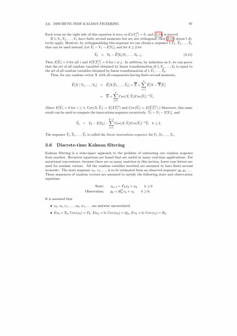
8/11/2019 Random process by B. Hajek
http://slidepdf.com/reader/full/random-process-by-b-hajek 107/448
3.6. DISCRETE-TIME KALMAN FILTERING 97
Each term on the right side of this equation is zero, so E [eY T j ] = 0, and (3.14) is proved.If 1, Y 1, Y 2, . . . , Y n have finite second moments but are not orthogonal, then (3.14) doesn’t di-
rectly apply. However, by orthogonalizing this sequence we can obtain a sequence 1,
Y 1,
Y 2, . . . ,
Y n
that can be used instead. Let Y 1 = Y 1 − E [Y 1], and for k ≥ 2 letY k = Y k − E [Y k|Y 1, . . . , Y k−1]. (3.15)
Then E [Y i] = 0 for all i and E [Y i Y T j ] = 0 for i = j . In addition, by induction on k, we can provethat the set of all random variables obtained by linear transformation of 1 , Y 1, . . . , Y k is equal tothe set of all random variables obtained by linear transformation of 1, Y 1, . . . , Y k.
Thus, for any random vector X with all components having finite second moments,
E [X | Y 1, . . . , Y n] = E [X |Y 1, . . . , Y n] = X +n
i=1
E [X − X |Y i]
= X +
ni=1
Cov(X, Y i)Cov(Y i)−1 Y i.
(Since E [Y i] = 0 for i ≥ 1, Cov(X, Y i) = E [X Y T i ] and Cov(Y i) = E [Y i Y T i ].) Moreover, this same
result can be used to compute the innovations sequence recursively: Y 1 = Y 1 − E [Y 1], and
Y k = Y k − E [Y k] −k−1i=1
Cov(X, Y i)Cov(Y i)−1Y i k ≥ 2.
The sequence
Y 1,
Y 2, . . . ,
Y n is called the linear innovations sequence for Y 1, Y 2, . . . , Y n.
3.6 Discrete-time Kalman filtering
Kalman filtering is a state-space approach to the problem of estimating one random sequencefrom another. Recursive equations are found that are useful in many real-time applications. Fornotational convenience, because there are so many matrices in this section, lower case letters areused for random vectors. All the random variables involved are assumed to have finite secondmoments. The state sequence x0, x1, . . ., is to be estimated from an observed sequence y0, y1, . . ..These sequences of random vectors are assumed to satisfy the following state and observationequations.
State: xk+1 = F kxk + wk k ≥ 0
Observation: yk = H T
k xk + vk k ≥ 0.
It is assumed that
• x0, v0, v1, . . . , w0, w1, . . . are pairwise uncorrelated.
• Ex0 = x0, Cov(x0) = P 0, Ewk = 0, Cov(wk) = Qk, E vk = 0, Cov(vk) = Rk.
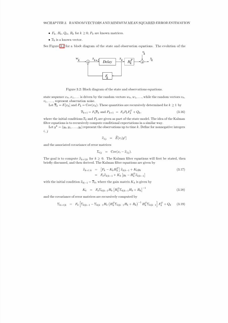
8/11/2019 Random process by B. Hajek
http://slidepdf.com/reader/full/random-process-by-b-hajek 108/448
98CHAPTER 3. RANDOM VECTORS AND MINIMUM MEAN SQUARED ERROR ESTIMATION
• F k, H k, Qk, Rk for k ≥ 0; P 0 are known matrices.
• x0 is a known vector.
See Figure 3.2 for a block diagram of the state and observation equations. The evolution of the
+ + H k T
wk
yk k
x Delay
k+1 x
Fk
k v
Figure 3.2: Block diagram of the state and observations equations.
state sequence x0, x1, . . . is driven by the random vectors w0, w1, . . ., while the random vectors v0,v1, . . . , represent observation noise.
Let xk = E [xk] and P k = Cov(xk). These quantities are recursively determined for k ≥ 1 by
xk+1 = F kxk and P k+1 = F kP kF T k + Qk, (3.16)
where the initial conditions x0 and P 0 are given as part of the state model. The idea of the Kalmanfilter equations is to recursively compute conditional expectations in a similar way.
Let yk = (y0, y1, . . . , yk) represent the observations up to time k. Define for nonnegative integersi, j
xi| j = E [xi|y j
]
and the associated covariance of error matrices
Σi| j = Cov(xi − xi| j).
The goal is to compute xk+1|k for k ≥ 0. The Kalman filter equations will first be stated, thenbriefly discussed, and then derived. The Kalman filter equations are given by
xk+1|k =
F k − K kH T k
xk|k−1 + K kyk (3.17)
= F k
xk|k−1 + K k
yk − H T k
xk|k−1
with the initial condition x0
|−1 = x0, where the gain matrix K k is given by
K k = F kΣk|k−1H k
H T k Σk|k−1H k + Rk
−1(3.18)
and the covariance of error matrices are recursively computed by
Σk+1|k = F k
Σk|k−1 − Σk|k−1H k
H T k Σk|k−1H k + Rk
−1H T k Σk|k−1
F T k + Qk (3.19)
8/11/2019 Random process by B. Hajek
http://slidepdf.com/reader/full/random-process-by-b-hajek 109/448
3.6. DISCRETE-TIME KALMAN FILTERING 99
x x
F −K H k k k
T
K k Delayk+1 k k k −1+k
y
Figure 3.3: Block diagram of the Kalman filter.
with the initial condition Σ0|−1 = P 0. See Figure 3.3 for the block diagram.
We comment briefly on the Kalman filter equations, before deriving them. First, observe whathappens if H k is the zero matrix, H k = 0, for all k. Then the Kalman filter equations reduce to(3.16) with
xk|k−1 = xk, Σk|k−1 = P k and K k = 0. Taking H k = 0 for all k is equivalent to having
no observations available.In many applications, the sequence of gain matrices can be computed ahead of time according
to (3.18) and (3.19). Then as the observations become available, the estimates can be computedusing only (3.17). In some applications the matrices involved in the state and observation models,including the covariance matrices of the vk’s and wk’s, do not depend on k. The gain matricesK k could still depend on k due to the initial conditions, but if the model is stable in some sense,then the gains converge to a constant matrix K , so that in steady state the filter equation (3.17)becomes time invariant: xk+1|k = (F − KH T ) xk|k−1 + Kyk.
In other applications, particularly those involving feedback control, the matrices in the stateand/or observation equations might not be known until just before they are needed.
The Kalman filter equations are now derived. Roughly speaking, there are two considerations
for computing xk+1|k once xk|k−1 is computed: (1) the information update , accounting for theavailability of the new observation yk, enabling the calculation of xk|k, and (2) the time update ,accounting for the change in state from xk to xk+1.
Information update: The observation yk is not totally new because it can be predicted in partfrom the previous observations, or simply by its mean in the case k = 0. Specifically, we consideryk = yk − E [yk | yk−1] to be the new part of the observation yk. Here, y0, y1, . . . is the linearinnovation sequence for the observation sequence y0, y1, . . ., as defined in Section 3.5 (with the minordifference that here the vectors are indexed from time k = 0 on, rather than from time k = 1). Letyk−1 = (y0, y1, . . . , yk−1). Since the linear span of the random variables in (1, yk−1, yk) is the sameas the linear span of the random variables in (1, yk−1, yk), for the purposes of incorporating the newobservation we can pretend that yk is the new observation rather than yk. From the observation
equation, the fact E [vk] = 0, and the fact wk is orthogonal to all the random variables of yk−1, itfollows that
E [yk | yk−1] = E
H T k xk + wk|yk−1
= H T k xk|k−1,
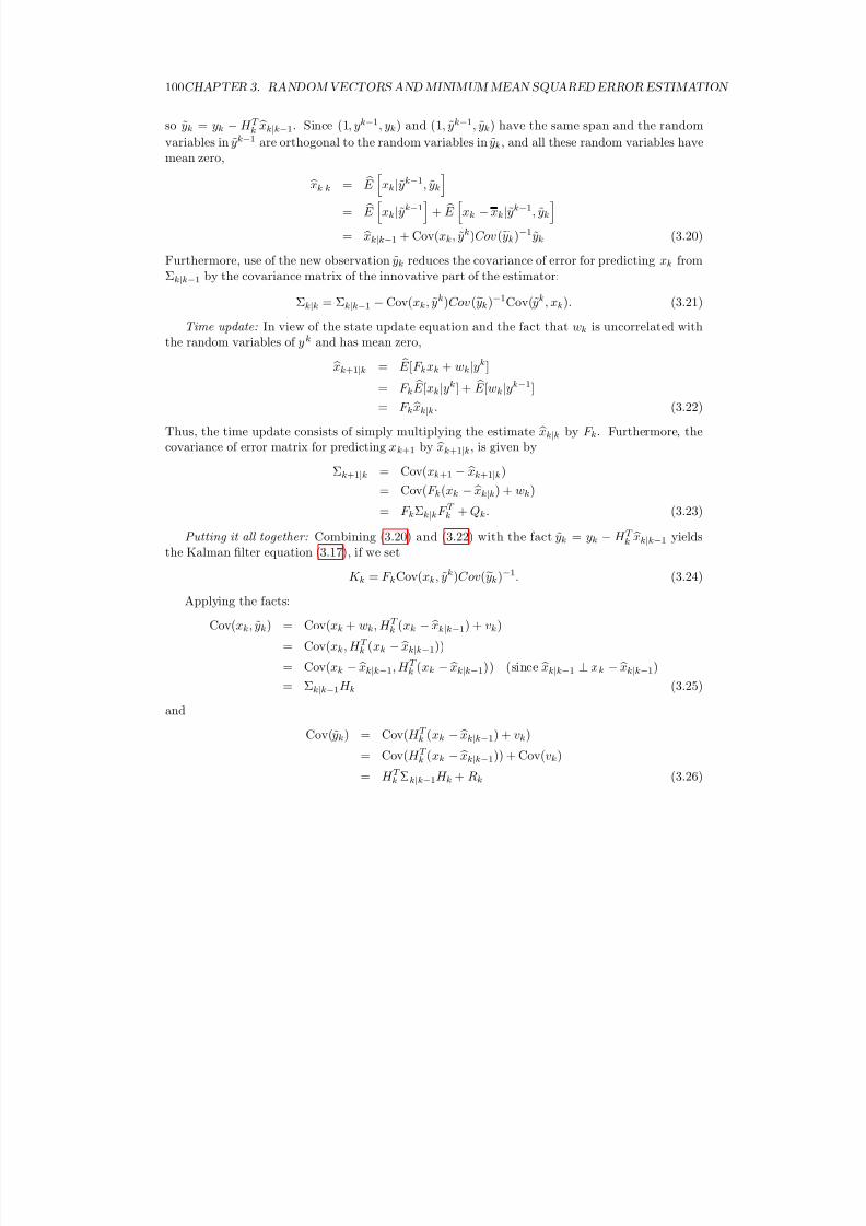
8/11/2019 Random process by B. Hajek
http://slidepdf.com/reader/full/random-process-by-b-hajek 110/448
100CHAPTER 3. RANDOM VECTORS AND MINIMUM MEAN SQUARED ERROR ESTIMATION
so yk = yk − H T k xk|k−1. Since (1, yk−1, yk) and (1, yk−1, yk) have the same span and the random
variables in yk−1 are orthogonal to the random variables in yk, and all these random variables havemean zero,
xk|k = E xk|yk−1, yk
= E
xk|yk−1
+ E
xk − xk|yk−1, yk
= xk|k−1 + Cov(xk, yk)Cov(yk)−1yk (3.20)
Furthermore, use of the new observation yk reduces the covariance of error for predicting xk fromΣk|k−1 by the covariance matrix of the innovative part of the estimator:
Σk|k = Σk|k−1 − Cov(xk, yk)Cov(yk)−1Cov(yk, xk). (3.21)
Time update: In view of the state update equation and the fact that wk is uncorrelated withthe random variables of yk and has mean zero,
xk+1|k = E [F kxk + wk|yk]
= F k E [xk|yk] + E [wk|yk−1]
= F k xk|k. (3.22)
Thus, the time update consists of simply multiplying the estimate xk|k by F k. Furthermore, thecovariance of error matrix for predicting xk+1 by xk+1|k, is given by
Σk+1|k = Cov(xk+1 − xk+1|k)
= Cov(F k(xk −
xk|k) + wk)
= F kΣk
|kF T k + Qk. (3.23)
Putting it all together: Combining (3.20) and (3.22) with the fact yk = yk − H T k xk|k−1 yieldsthe Kalman filter equation (3.17), if we set
K k = F kCov(xk, yk)Cov(yk)−1. (3.24)
Applying the facts:
Cov(xk, yk) = Cov(xk + wk, H T k (xk − xk|k−1) + vk)
= Cov(xk, H T k (xk − xk|k−1))
= Cov(xk −
xk|k−1, H T k (xk −
xk|k−1)) (since
xk|k−1 ⊥ xk −
xk|k−1)
= Σk|k−1H k (3.25)
and
Cov(yk) = Cov(H T k (xk − xk|k−1) + vk)
= Cov(H T k (xk − xk|k−1)) + Cov(vk)
= H T k Σk|k−1H k + Rk (3.26)
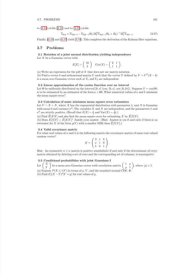
8/11/2019 Random process by B. Hajek
http://slidepdf.com/reader/full/random-process-by-b-hajek 111/448
3.7. PROBLEMS 101
to (3.24) yields (3.18) and to (3.21) yields
Σk|k = Σk|k−1 − Σk|k−1H k(H T k Σk|k−1H k + Rk)−1H T k Σk|k−1. (3.27)
Finally, (3.23) and (3.27) yield (3.19). This completes the derivation of the Kalman filter equations.
3.7 Problems
3.1 Rotation of a joint normal distribution yielding independenceLet X be a Gaussian vector with
E [X ] =
10
5
Cov(X ) =
2 11 1
.
(a) Write an expression for the pdf of X that does not use matrix notation.(b) Find a vector b and orthonormal matrix U such that the vector Y defined by Y = U T (X
−b)
is a mean zero Gaussian vector such at Y 1 and Y 2 are independent.
3.2 Linear approximation of the cosine function over an intervalLet Θ be uniformly distributed on the interval [0, π] (yes, [0, π], not [0, 2π]). Suppose Y = cos(Θ)is to be estimated by an estimator of the form a + bΘ. What numerical values of a and b minimizethe mean square error?
3.3 Calculation of some minimum mean square error estimatorsLet Y = X + N , where X has the exponential distribution with parameter λ, and N is Gaussianwith mean 0 and variance σ 2. The variables X and N are independent, and the parameters λ andσ2 are strictly positive. (Recall that E [X ] = 1
λ and Var(X ) = 1λ2 .)
(a) Find E [X |Y ] and also find the mean square error for estimating X by E [X
|Y ].
(b) Does E [X |Y ] = E [X |Y ]? Justify your answer. (Hint: Answer is yes if and only if there is noestimator for X of the form g(Y ) with a smaller MSE than E [X |Y ].)
3.4 Valid covariance matrixFor what real values of a and b is the following matrix the covariance matrix of some real-valuedrandom vector?
K =
2 1 ba 1 0b 0 1
.
Hint: An symmetric n × n matrix is positive semidefinite if and only if the determinant of everymatrix obtained by deleting a set of rows and the corresponding set of columns, is nonnegative.
3.5 Conditional probabilities with joint Gaussians I
Let
X Y
be a mean zero Gaussian vector with correlation matrix
1 ρρ 1
, where |ρ| < 1.
(a) Express P (X ≤ 1|Y ) in terms of ρ, Y , and the standard normal CDF, Φ.(b) Find E [(X − Y )2|Y = y] for real values of y .
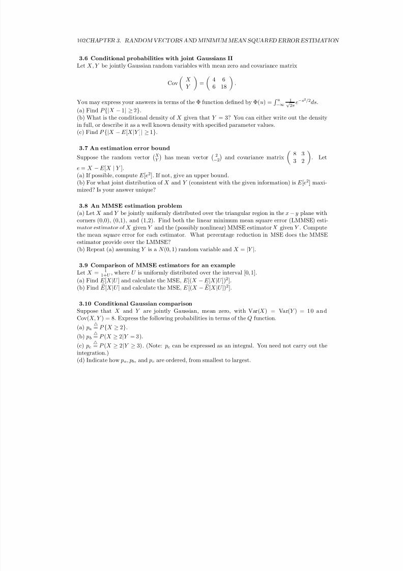
8/11/2019 Random process by B. Hajek
http://slidepdf.com/reader/full/random-process-by-b-hajek 112/448
102CHAPTER 3. RANDOM VECTORS AND MINIMUM MEAN SQUARED ERROR ESTIMATION
3.6 Conditional probabilities with joint Gaussians IILet X, Y be jointly Gaussian random variables with mean zero and covariance matrix
Cov X Y = 4 66 18 .
You may express your answers in terms of the Φ function defined by Φ(u) = u−∞
1√ 2π
e−s2/2ds.
(a) Find P |X − 1| ≥ 2.(b) What is the conditional density of X given that Y = 3? You can either write out the densityin full, or describe it as a well known density with specified parameter values.(c) Find P |X − E [X |Y ]| ≥ 1.
3.7 An estimation error bound
Suppose the random vector X Y has mean vector
2
−2 and covariance matrix
8 3
3 2 . Let
e = X − E [X | Y ].(a) If possible, compute E [e2]. If not, give an upper bound.(b) For what joint distribution of X and Y (consistent with the given information) is E [e2] maxi-mized? Is your answer unique?
3.8 An MMSE estimation problem(a) Let X and Y be jointly uniformly distributed over the triangular region in the x − y plane withcorners (0,0), (0,1), and (1,2). Find both the linear minimum mean square error (LMMSE) esti-mator estimator of X given Y and the (possibly nonlinear) MMSE estimator X given Y . Computethe mean square error for each estimator. What percentage reduction in MSE does the MMSE
estimator provide over the LMMSE?(b) Repeat (a) assuming Y is a N (0, 1) random variable and X = |Y |.
3.9 Comparison of MMSE estimators for an exampleLet X = 1
1+U , where U is uniformly distributed over the interval [0, 1].
(a) Find E [X |U ] and calculate the MSE, E [(X − E [X |U ])2].(b) Find E [X |U ] and calculate the MSE, E [(X − E [X |U ])2].
3.10 Conditional Gaussian comparisonSuppose that X and Y are jointly Gaussian, mean zero, with Var(X ) = Var(Y ) = 10 andCov(X, Y ) = 8. Express the following probabilities in terms of the Q function.
(a) pa = P X ≥ 2.(b) pb
= P (X ≥ 2|Y = 3).
(c) pc= P (X ≥ 2|Y ≥ 3). (Note: pc can be expressed as an integral. You need not carry out the
integration.)(d) Indicate how pa, pb, and pc are ordered, from smallest to largest.
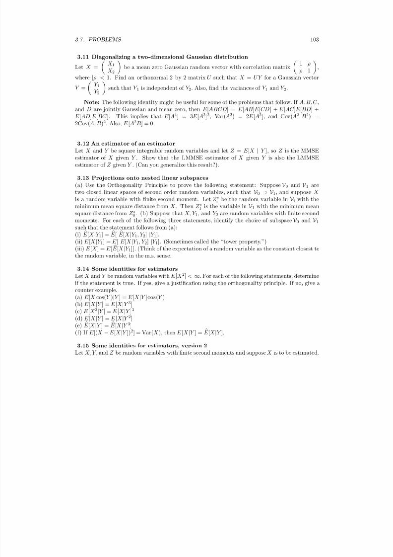
8/11/2019 Random process by B. Hajek
http://slidepdf.com/reader/full/random-process-by-b-hajek 113/448
3.7. PROBLEMS 103
3.11 Diagonalizing a two-dimensional Gaussian distribution
Let X =
X 1X 2
be a mean zero Gaussian random vector with correlation matrix
1 ρρ 1
,
where |ρ| < 1. Find an orthonormal 2 by 2 matrix U such that X = U Y for a Gaussian vectorY =
Y 1Y 2
such that Y 1 is independent of Y 2. Also, find the variances of Y 1 and Y 2.
Note: The following identity might be useful for some of the problems that follow. If A,B,C,and D are jointly Gaussian and mean zero, then E [ABCD] = E [AB]E [CD ] + E [AC ]E [BD] +E [AD]E [BC ]. This implies that E [A4] = 3E [A2]2, Var(A2) = 2E [A2], and Cov(A2, B2) =2Cov(A, B)2. Also, E [A2B] = 0.
3.12 An estimator of an estimatorLet X and Y be square integrable random variables and let Z = E [X | Y ], so Z is the MMSE
estimator of X given Y . Show that the LMMSE estimator of X given Y is also the LMMSEestimator of Z given Y . (Can you generalize this result?).
3.13 Projections onto nested linear subspaces(a) Use the Orthogonality Principle to prove the following statement: Suppose V 0 and V 1 aretwo closed linear spaces of second order random variables, such that V 0 ⊃ V 1, and suppose X is a random variable with finite second moment. Let Z ∗i be the random variable in V i with theminimum mean square distance from X . Then Z ∗1 is the variable in V 1 with the minimum meansquare distance from Z ∗0 . (b) Suppose that X, Y 1, and Y 2 are random variables with finite secondmoments. For each of the following three statements, identify the choice of subspace V 0 and V 1such that the statement follows from (a):(i) E [X
|Y 1] = E [ E [X
|Y 1, Y 2]
|Y 1].
(ii) E [X |Y 1] = E [ E [X |Y 1, Y 2] |Y 1]. (Sometimes called the “tower property.”)(iii) E [X ] = E [ E [X |Y 1]]. (Think of the expectation of a random variable as the constant closest tothe random variable, in the m.s. sense.
3.14 Some identities for estimatorsLet X and Y be random variables with E [X 2] < ∞. For each of the following statements, determineif the statement is true. If yes, give a justification using the orthogonality principle. If no, give acounter example.(a) E [X cos(Y )|Y ] = E [X |Y ]cos(Y )(b) E [X |Y ] = E [X |Y 3](c) E [X 3|Y ] = E [X |Y ]3
(d) E [X |Y ] = E [X |Y 2](e) E [X |Y ] = E [X |Y 3](f) If E [(X − E [X |Y ])2] = Var(X ), then E [X |Y ] = E [X |Y ].
3.15 Some identities for estimators, version 2Let X,Y, and Z be random variables with finite second moments and suppose X is to be estimated.
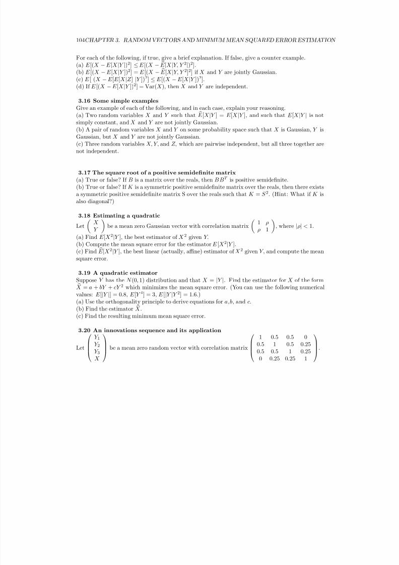
8/11/2019 Random process by B. Hajek
http://slidepdf.com/reader/full/random-process-by-b-hajek 114/448
104CHAPTER 3. RANDOM VECTORS AND MINIMUM MEAN SQUARED ERROR ESTIMATION
For each of the following, if true, give a brief explanation. If false, give a counter example.(a) E [(X − E [X |Y ])2] ≤ E [(X −
E [X |Y, Y 2])2].
(b) E [(X − E [X |Y ])2] = E [(X − E [X |Y, Y 2]2] if X and Y are jointly Gaussian.
(c) E [ (X − E [E [X |Z ] |Y ])2
] ≤ E [(X − E [X |Y ])2
].(d) If E [(X − E [X |Y ])2] = Var(X ), then X and Y are independent.
3.16 Some simple examplesGive an example of each of the following, and in each case, explain your reasoning.(a) Two random variables X and Y such that E [X |Y ] = E [X |Y ], and such that E [X |Y | is notsimply constant, and X and Y are not jointly Gaussian.(b) A pair of random variables X and Y on some probability space such that X is Gaussian, Y isGaussian, but X and Y are not jointly Gaussian.(c) Three random variables X, Y, and Z, which are pairwise independent, but all three together arenot independent.
3.17 The square root of a positive semidefinite matrix(a) True or false? If B is a matrix over the reals, then B BT is positive semidefinite.(b) True or false? If K is a symmetric positive semidefinite matrix over the reals, then there existsa symmetric positive semidefinite matrix S over the reals such that K = S 2. (Hint: What if K isalso diagonal?)
3.18 Estimating a quadratic
Let
X Y
be a mean zero Gaussian vector with correlation matrix
1 ρρ 1
, where |ρ| < 1.
(a) Find E [X 2
|Y ], the best estimator of X 2 given Y.
(b) Compute the mean square error for the estimator E [X 2|Y ].(c) Find E [X 2|Y ], the best linear (actually, affine) estimator of X 2 given Y, and compute the meansquare error.
3.19 A quadratic estimatorSuppose Y has the N (0, 1) distribution and that X = |Y |. Find the estimator for X of the form X = a + bY + cY 2 which minimizes the mean square error. (You can use the following numericalvalues: E [|Y |] = 0.8, E [Y 4] = 3, E [|Y |Y 2] = 1.6.)(a) Use the orthogonality principle to derive equations for a,b, and c.(b) Find the estimator
X .
(c) Find the resulting minimum mean square error.
3.20 An innovations sequence and its application
Let
Y 1Y 2Y 3X
be a mean zero random vector with correlation matrix
1 0.5 0.5 0
0.5 1 0.5 0.250.5 0.5 1 0.250 0.25 0.25 1
.
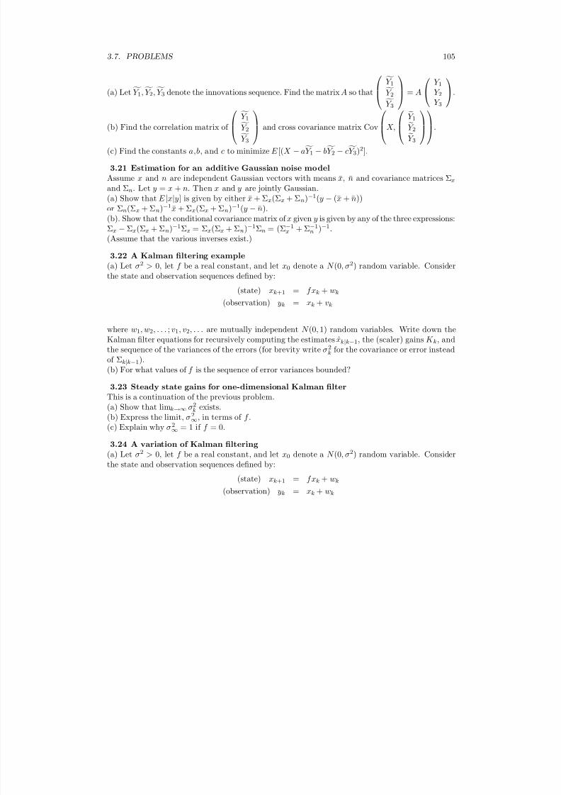
8/11/2019 Random process by B. Hajek
http://slidepdf.com/reader/full/random-process-by-b-hajek 115/448
3.7. PROBLEMS 105
(a) Let
Y 1,
Y 2,
Y 3 denote the innovations sequence. Find the matrix A so that
Y 1
Y 2
Y 3
= A
Y 1Y 2Y 3
.
(b) Find the correlation matrix of Y 1Y 2Y 3
and cross covariance matrix CovX,
Y 1Y 2Y 3
.
(c) Find the constants a,b, and c to minimize E [(X − aY 1 − bY 2 − cY 3)2].
3.21 Estimation for an additive Gaussian noise modelAssume x and n are independent Gaussian vectors with means x, n and covariance matrices Σx
and Σn. Let y = x + n. Then x and y are jointly Gaussian.(a) Show that E [x|y] is given by either x + Σx(Σx + Σn)−1(y − (x + n))or Σn(Σx + Σn)−1x + Σx(Σx + Σn)−1(y − n).(b). Show that the conditional covariance matrix of x given y is given by any of the three expressions:
Σx − Σx(Σx + Σn)−1Σx = Σx(Σx + Σn)−1Σn = (Σ−1x + Σ−1n )−1.(Assume that the various inverses exist.)
3.22 A Kalman filtering example(a) Let σ2 > 0, let f be a real constant, and let x0 denote a N (0, σ2) random variable. Considerthe state and observation sequences defined by:
(state) xk+1 = f xk + wk
(observation) yk = xk + vk
where w1, w2, . . . ; v1, v2, . . . are mutually independent N (0, 1) random variables. Write down the
Kalman filter equations for recursively computing the estimates xk|k−1, the (scaler) gains K k, andthe sequence of the variances of the errors (for brevity write σ 2
k for the covariance or error insteadof Σk|k−1).(b) For what values of f is the sequence of error variances bounded?
3.23 Steady state gains for one-dimensional Kalman filterThis is a continuation of the previous problem.(a) Show that limk→∞ σ2
k exists.(b) Express the limit, σ 2∞, in terms of f .(c) Explain why σ 2∞ = 1 if f = 0.
3.24 A variation of Kalman filtering
(a) Let σ2 > 0, let f be a real constant, and let x0 denote a N (0, σ2) random variable. Considerthe state and observation sequences defined by:
(state) xk+1 = f xk + wk
(observation) yk = xk + wk
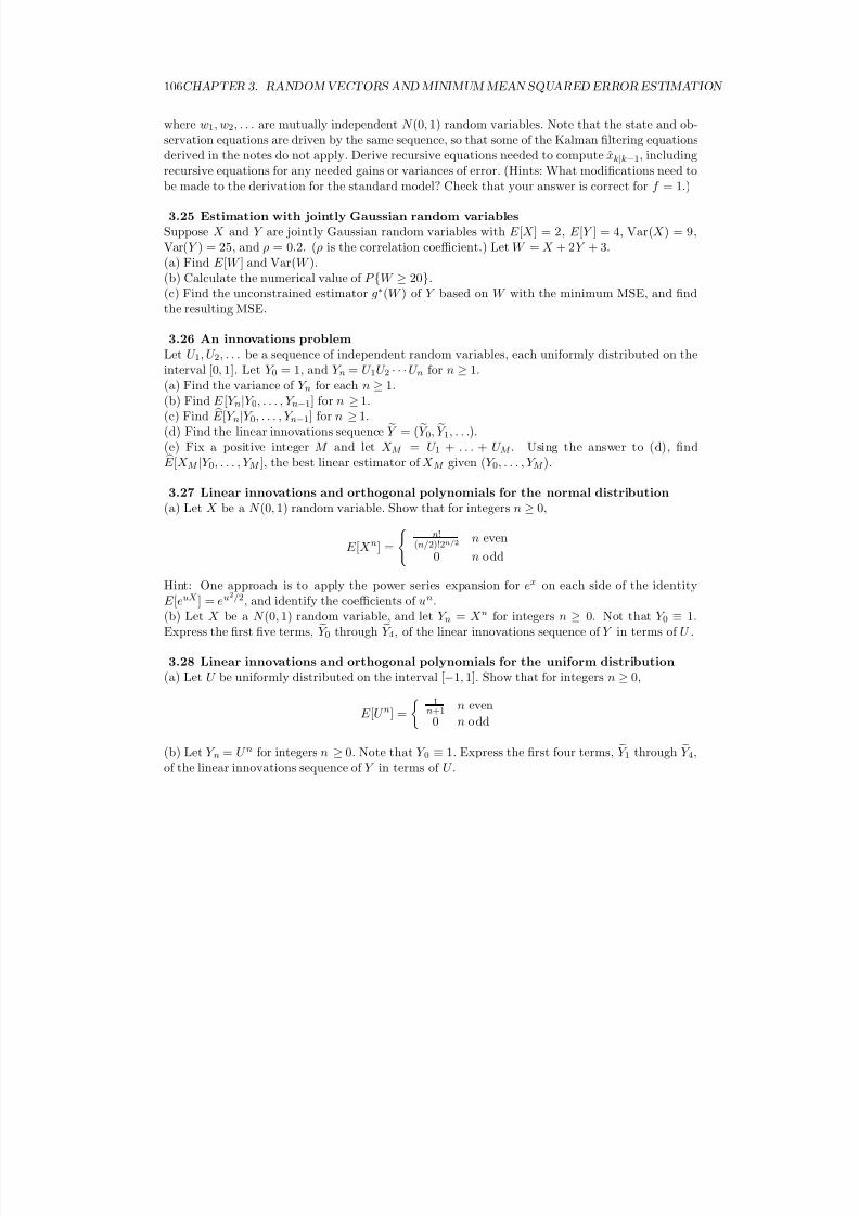
8/11/2019 Random process by B. Hajek
http://slidepdf.com/reader/full/random-process-by-b-hajek 116/448
106CHAPTER 3. RANDOM VECTORS AND MINIMUM MEAN SQUARED ERROR ESTIMATION
where w1, w2, . . . are mutually independent N (0, 1) random variables. Note that the state and ob-servation equations are driven by the same sequence, so that some of the Kalman filtering equationsderived in the notes do not apply. Derive recursive equations needed to compute xk|k−1, including
recursive equations for any needed gains or variances of error. (Hints: What modifications need tobe made to the derivation for the standard model? Check that your answer is correct for f = 1.)
3.25 Estimation with jointly Gaussian random variablesSuppose X and Y are jointly Gaussian random variables with E [X ] = 2, E [Y ] = 4, Var(X ) = 9,Var(Y ) = 25, and ρ = 0.2. (ρ is the correlation coefficient.) Let W = X + 2Y + 3.(a) Find E [W ] and Var(W ).(b) Calculate the numerical value of P W ≥ 20.(c) Find the unconstrained estimator g∗(W ) of Y based on W with the minimum MSE, and findthe resulting MSE.
3.26 An innovations problemLet U 1, U 2, . . . be a sequence of independent random variables, each uniformly distributed on theinterval [0, 1]. Let Y 0 = 1, and Y n = U 1U 2 · · · U n for n ≥ 1.(a) Find the variance of Y n for each n ≥ 1.(b) Find E [Y n|Y 0, . . . , Y n−1] for n ≥ 1.(c) Find E [Y n|Y 0, . . . , Y n−1] for n ≥ 1.(d) Find the linear innovations sequence Y = (Y 0, Y 1, . . .).(e) Fix a positive integer M and let X M = U 1 + . . . + U M . Using the answer to (d), find E [X M |Y 0, . . . , Y M ], the best linear estimator of X M given (Y 0, . . . , Y M ).
3.27 Linear innovations and orthogonal polynomials for the normal distribution(a) Let X be a N (0, 1) random variable. Show that for integers n
≥ 0,
E [X n] =
n!
(n/2)!2n/2 n even
0 n odd
Hint: One approach is to apply the power series expansion for ex on each side of the identityE [euX ] = eu2/2, and identify the coefficients of un.(b) Let X be a N (0, 1) random variable, and let Y n = X n for integers n ≥ 0. Not that Y 0 ≡ 1.Express the first five terms, Y 0 through Y 4, of the linear innovations sequence of Y in terms of U .
3.28 Linear innovations and orthogonal polynomials for the uniform distribution(a) Let U be uniformly distributed on the interval [−1, 1]. Show that for integers n ≥ 0,
E [U n] = 1
n+1 n even
0 n odd
(b) Let Y n = U n for integers n ≥ 0. Note that Y 0 ≡ 1. Express the first four terms, Y 1 through Y 4,of the linear innovations sequence of Y in terms of U .
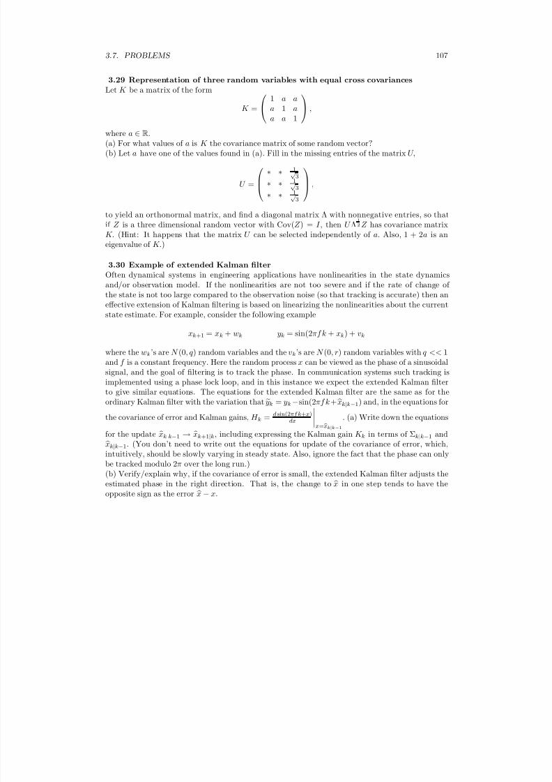
8/11/2019 Random process by B. Hajek
http://slidepdf.com/reader/full/random-process-by-b-hajek 117/448
3.7. PROBLEMS 107
3.29 Representation of three random variables with equal cross covariancesLet K be a matrix of the form
K = 1 a a
a 1 aa a 1 ,
where a ∈ R.(a) For what values of a is K the covariance matrix of some random vector?(b) Let a have one of the values found in (a). Fill in the missing entries of the matrix U,
U =
∗ ∗ 1√ 3
∗ ∗ 1√ 3
∗ ∗ 1√ 3
,
to yield an orthonormal matrix, and find a diagonal matrix Λ with nonnegative entries, so that
if Z is a three dimensional random vector with Cov(Z ) = I, then U Λ12 Z has covariance matrix
K. (Hint: It happens that the matrix U can be selected independently of a. Also, 1 + 2a is aneigenvalue of K.)
3.30 Example of extended Kalman filterOften dynamical systems in engineering applications have nonlinearities in the state dynamicsand/or observation model. If the nonlinearities are not too severe and if the rate of change of the state is not too large compared to the observation noise (so that tracking is accurate) then aneffective extension of Kalman filtering is based on linearizing the nonlinearities about the currentstate estimate. For example, consider the following example
xk+1 = xk + wk yk = sin(2πf k + xk) + vk
where the wk’s are N (0, q ) random variables and the vk’s are N (0, r) random variables with q << 1and f is a constant frequency. Here the random process x can be viewed as the phase of a sinusoidalsignal, and the goal of filtering is to track the phase. In communication systems such tracking isimplemented using a phase lock loop, and in this instance we expect the extended Kalman filterto give similar equations. The equations for the extended Kalman filter are the same as for theordinary Kalman filter with the variation that yk = yk−sin(2πf k + xk|k−1) and, in the equations for
the covariance of error and Kalman gains, H k = d sin(2πfk+x)dx
x= bxk|k−1
. (a) Write down the equations
for the update
xk|k−1 →
xk+1|k, including expressing the Kalman gain K k in terms of Σk|k−1 and
xk|k−1. (You don’t need to write out the equations for update of the covariance of error, which,intuitively, should be slowly varying in steady state. Also, ignore the fact that the phase can onlybe tracked modulo 2π over the long run.)(b) Verify/explain why, if the covariance of error is small, the extended Kalman filter adjusts theestimated phase in the right direction. That is, the change to x in one step tends to have theopposite sign as the error x − x.
8/11/2019 Random process by B. Hajek
http://slidepdf.com/reader/full/random-process-by-b-hajek 118/448
108CHAPTER 3. RANDOM VECTORS AND MINIMUM MEAN SQUARED ERROR ESTIMATION
3.31 Kalman filter for a rotating stateConsider the Kalman state and observation equations for the following matrices, where θo = 2π/10(the matrices don’t depend on time, so the subscript k is omitted):
F = (0.99) cos(θo) − sin(θo)
sin(θo) cos(θo)
H =
10
Q =
1 00 1
R = 1
(a) Explain in words what successive iterates F nxo are like, for a nonzero initial state xo (this isthe same as the state equation, but with the random term wk left off).(b) Write out the Kalman filter equations for this example, simplifying as much as possible (butno more than possible! The equations don’t simplify all that much.)
3.32 * Proof of the orthogonality principleProve the seven statements lettered (a)-(g) in what follows.Let X be a random variable and let V be a collection of random variables on the same probability
space such that(i) E [Z 2] < +∞ for each Z ∈ V (ii) V is a linear class, i.e., if Z, Z ∈ V then so is aZ + bZ for any real numbers a and b.(iii) V is closed in the sense that if Z n ∈ V for each n and Z n converges to a random variable Z inthe mean square sense, then Z ∈ V .The Orthogonality Principle is that there exists a unique element Z ∗ ∈ V so that E [(X − Z ∗)2] ≤E [(X − Z )2] for all Z ∈ V . Furthermore, a random variable W ∈ V is equal to Z ∗ if and only if (X − W ) ⊥ Z for all Z ∈ V . ((X − W ) ⊥ Z means E [(X − W )Z ] = 0.)The remainder of this problem is aimed at a proof. Let d = inf E [(X −Z )2] : Z ∈ V. By definitionof infimum there exists a sequence Z n ∈ V so that E [(X − Z n)2] → d as n → +∞.(a) The sequence Z n is Cauchy in the mean square sense.(Hint: Use the “parallelogram law”: E [(U
−V )2] + E [(U + V )2] = 2(E [U 2] + E [V 2]). Thus, by the
Cauchy criteria, there is a random variable Z ∗ such that Z n converges to Z ∗ in the mean squaresense.(b) Z ∗ satisfies the conditions advertised in the first sentence of the principle.(c) The element Z ∗ satisfying the condition in the first sentence of the principle is unique. (Considertwo random variables that are equal to each other with probability one to be the same.) Thiscompletes the proof of the first sentence.(d) (“if” part of second sentence). If W ∈ V and (X − W ) ⊥ Z for all Z ∈ V , then W = Z ∗.(The “only if” part of second sentence is divided into three parts:)(e) E [(X − Z ∗ − cZ )2] ≥ E [(X − Z ∗)2] for any real constant c.(f) −2cE [(X − Z ∗)Z ] + c2E [Z 2] ≥ 0 for any real constant c.(g) (X
−Z ∗)
⊥ Z , and the principle is proved.
3.33 * The span of two closed subspaces is closedCheck that the span, V 1 ⊕V 2, of two closed orthogonal linear spaces (defined in Proposition 3.2.4) isalso a closed linear space. A hint for showing that V is closed is to use the fact that if (Z n) is a m.s.convergent sequence of random variables in V , then each variable in the sequence can be representedas Z n = Z n,1 + Z n,2, where Z n,i ∈ V i, and E [(Z n − Z m)2] = E [(Z n,1 − Z m,1)2] + E [(Z n,2 − Z m,2)2].
8/11/2019 Random process by B. Hajek
http://slidepdf.com/reader/full/random-process-by-b-hajek 119/448
3.7. PROBLEMS 109
3.34 * Von Neumann’s alternating projections algorithmLet V 1 and V 2 be closed linear subspaces of L2(Ω, F , P ), and let X ∈ L2(Ω, F , P ). Define a sequence(Z n : n ≥ 0) recursively, by alternating projections onto V 1 and V 2, as follows. Let Z 0 = X , and
for k ≥ 0, let Z 2k+1 = ΠV 1(Z 2k) and Z 2k+2 = ΠV 2(Z 2k+1). The goal of this problem is to show thatZ n
m.s.→ ΠV 1∩V 2(X ). The approach will be to establish that (Z n) converges in the m.s. sense, byverifying the Cauchy criteria, and then use the orthogonality principle to identify the limit. DefineD(i, j) = E [(Z i − Z j)]2 for i ≥ 0 and j ≥ 0, and let i = D(i + 1, i) for i ≥ 0.(a) Show that i = E [(Z i)
2] − E [(Z i+1)2].(b) Show that
∞i=0 i ≤ E [X 2] < ∞.
(c) Use the orthogonality principle to show that for n ≥ 1 and k ≥ 0:
D(n, n + 2k + 1) = n + D(n + 1, n + 2k + 1)
D(n, n + 2k + 2) = D(n, n + 2k + 1) − n+2k+1.
(d) Use the above equations to show that for n ≥
1 and k ≥
0,
D(n, n + 2k + 1) = n + · · · + n+k − (n+k+1 + · · · + n+2k)
D(n, n + 2k + 2) = n + · · · + n+k − (n+k+1 + · · · + n+2k+1).
Consequently, D(n, m) ≤m−1i=n i for 1 ≤ n < m, and therefore (Z n : n ≥ 0) is a Cauchy sequence,
so Z nm.s.→ Z ∞ for some random variable Z ∞.
(e) Verify that Z ∞ ∈ V 1 ∩ V 2.(f) Verify that (X − Z ∞) ⊥ Z for any Z ∈ V 1 ∩ V 2. (Hint: Explain why (X − Z n) ⊥ Z for all n,and let n → ∞.)By the orthogonality principle, (e) and (f) imply that Z ∞ = ΠV 1∩V 2(X ).

8/11/2019 Random process by B. Hajek
http://slidepdf.com/reader/full/random-process-by-b-hajek 120/448
110CHAPTER 3. RANDOM VECTORS AND MINIMUM MEAN SQUARED ERROR ESTIMATION
8/11/2019 Random process by B. Hajek
http://slidepdf.com/reader/full/random-process-by-b-hajek 121/448
Chapter 4
Random Processes
4.1 Definition of a random process
A random process X is an indexed collection X = (X t : t ∈ T) of random variables, all on thesame probability space (Ω, F , P ). In many applications the index set T is a set of times. If T = Z,or more generally, if T is a set of consecutive integers, then X is called a discrete-time randomprocess. If T = R or if T is an interval of R, then X is called a continuous-time random process.Three ways to view a random process X = (X t : t ∈ T) are as follows:
• For each t fixed, X t is a function on Ω.
• X is a function on T × Ω with value X t(ω) for given t ∈ T and ω ∈ Ω.
• For each ω fixed with ω ∈ Ω, X t(ω) is a function of t, called the sample path corresponding
to ω.
Example 4.1.1 Suppose W 1, W 2, . . . are independent random variables withP W k = 1 = P W k = −1 = 1
2 for each k, and suppose X 0 = 0 and X n = W 1 + · · · + W nfor positive integers n. Let W = (W k : k ≥ 1) and X = (X n : n ≥ 0). Then W and X areboth discrete-time random processes. The index set T for X is Z+. A sample path of W and acorresponding sample path of X are shown in Figure 4.1.
The following notation is used:
µX (t) = E [X t]
RX
(s, t) = E [X s
X t]
C X (s, t) = Cov(X s, X t)
F X,n(x1, t1; . . . ; xn, tn) = P X t1 ≤ x1, . . . , X tn ≤ xn
and µX is called the mean function , RX is called the correlation function, C X is called the covariancefunction, and F X,n is called the nth order CDF. Sometimes the prefix “auto,” meaning “self,” is
111
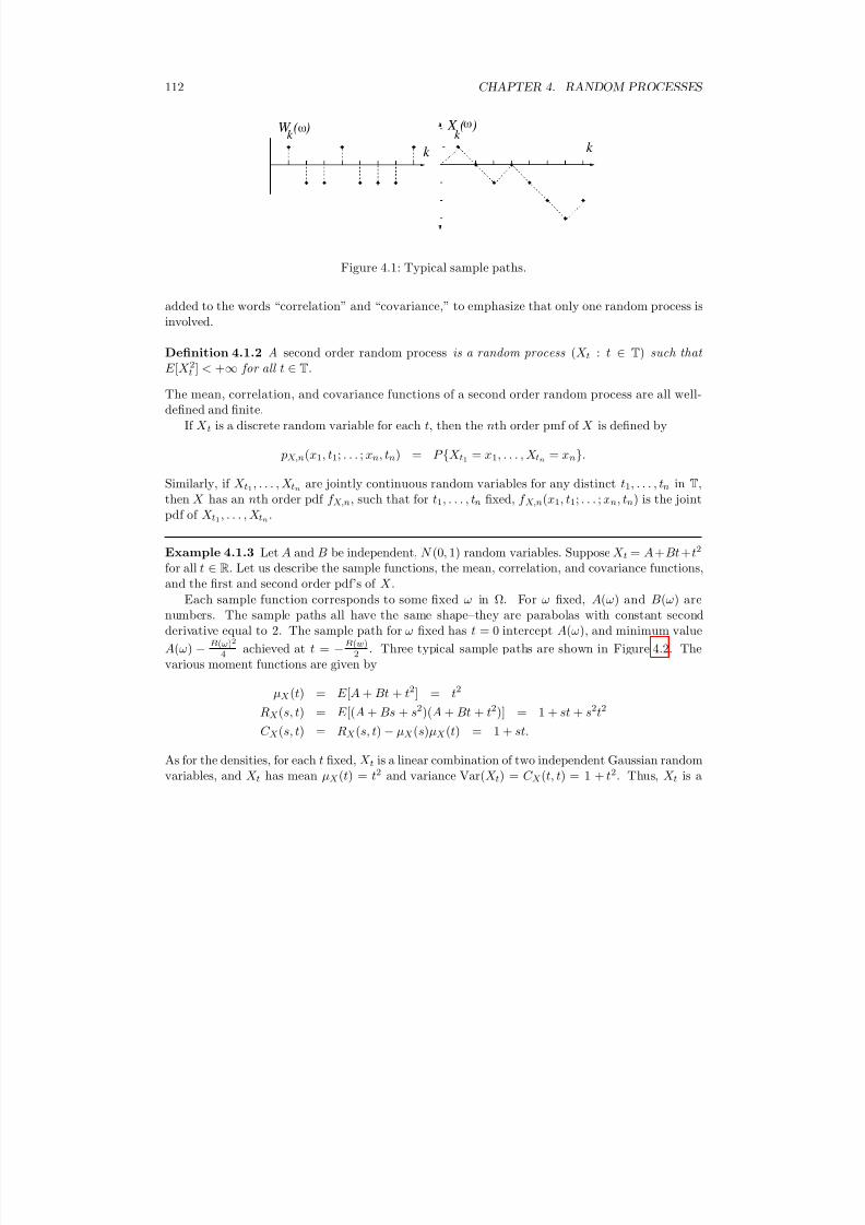
8/11/2019 Random process by B. Hajek
http://slidepdf.com/reader/full/random-process-by-b-hajek 122/448
112 CHAPTER 4. RANDOM PROCESSES
k
W ( )k ω
k X ( )ω
k
Figure 4.1: Typical sample paths.
added to the words “correlation” and “covariance,” to emphasize that only one random process isinvolved.
Definition 4.1.2 A second order random process is a random process (X t : t ∈ T) such that E [X 2t ] < +∞ for all t ∈ T.
The mean, correlation, and covariance functions of a second order random process are all well-defined and finite.
If X t is a discrete random variable for each t, then the nth order pmf of X is defined by
pX,n(x1, t1; . . . ; xn, tn) = P X t1 = x1, . . . , X tn = xn.
Similarly, if X t1, . . . , X tn are jointly continuous random variables for any distinct t1, . . . , tn in T,then X has an nth order pdf f X,n, such that for t1, . . . , tn fixed, f X,n(x1, t1; . . . ; xn, tn) is the jointpdf of X t1, . . . , X tn.
Example 4.1.3 Let A and B be independent, N (0, 1) random variables. Suppose X t = A +Bt +t2
for all t ∈ R. Let us describe the sample functions, the mean, correlation, and covariance functions,and the first and second order pdf’s of X .
Each sample function corresponds to some fixed ω in Ω. For ω fixed, A(ω) and B(ω) arenumbers. The sample paths all have the same shape–they are parabolas with constant secondderivative equal to 2. The sample path for ω fixed has t = 0 intercept A(ω), and minimum value
A(ω) − B(ω)2
4 achieved at t = −B(w)2 . Three typical sample paths are shown in Figure 4.2. The
various moment functions are given by
µX
(t) = E [A + Bt + t2] = t2
RX (s, t) = E [(A + Bs + s2)(A + Bt + t2)] = 1 + st + s2t2
C X (s, t) = RX (s, t) − µX (s)µX (t) = 1 + st.
As for the densities, for each t fixed, X t is a linear combination of two independent Gaussian randomvariables, and X t has mean µX (t) = t2 and variance Var(X t) = C X (t, t) = 1 + t2. Thus, X t is a
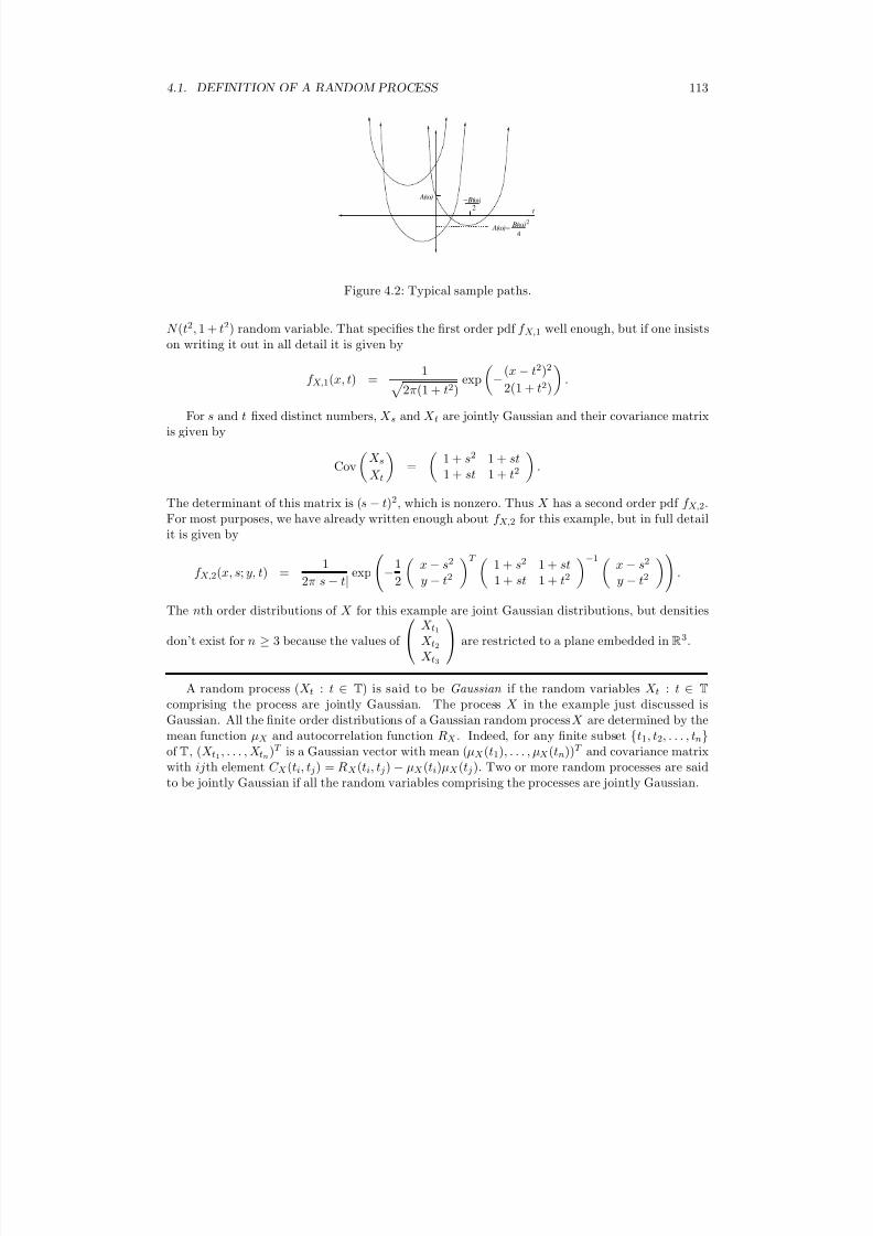
8/11/2019 Random process by B. Hajek
http://slidepdf.com/reader/full/random-process-by-b-hajek 123/448
4.1. DEFINITION OF A RANDOM PROCESS 113
ω A( )ω
− B( )2 t
A( )−ω4
ω B( )2
Figure 4.2: Typical sample paths.
N (t2, 1 + t2) random variable. That specifies the first order pdf f X,1 well enough, but if one insistson writing it out in all detail it is given by
f X,1(x, t) = 1 2π(1 + t2)
exp
−(x − t2)2
2(1 + t2)
.
For s and t fixed distinct numbers, X s and X t are jointly Gaussian and their covariance matrixis given by
Cov
X sX t
=
1 + s2 1 + st1 + st 1 + t2
.
The determinant of this matrix is (s − t)2, which is nonzero. Thus X has a second order pdf f X,2.For most purposes, we have already written enough about f X,2 for this example, but in full detail
it is given by
f X,2(x, s; y, t) = 1
2π|s − t| exp
−1
2
x − s2
y − t2
T 1 + s2 1 + st1 + st 1 + t2
−1 x − s2
y − t2
.
The nth order distributions of X for this example are joint Gaussian distributions, but densities
don’t exist for n ≥ 3 because the values of
X t1X t2X t3
are restricted to a plane embedded in R3.
A random process (X t : t ∈ T) is said to be Gaussian if the random variables X t : t ∈ Tcomprising the process are jointly Gaussian. The process X in the example just discussed isGaussian. All the finite order distributions of a Gaussian random process X are determined by themean function µX and autocorrelation function RX . Indeed, for any finite subset t1, t2, . . . , tnof T, (X t1, . . . , X tn)T is a Gaussian vector with mean (µX (t1), . . . , µX (tn))T and covariance matrixwith ijth element C X (ti, t j) = RX (ti, t j) − µX (ti)µX (t j). Two or more random processes are saidto be jointly Gaussian if all the random variables comprising the processes are jointly Gaussian.
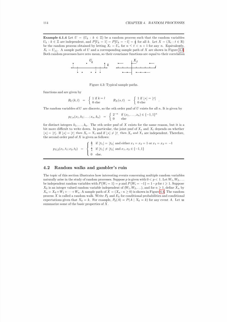
8/11/2019 Random process by B. Hajek
http://slidepdf.com/reader/full/random-process-by-b-hajek 124/448
114 CHAPTER 4. RANDOM PROCESSES
Example 4.1.4 Let U = (U k : k ∈ Z) be a random process such that the random variablesU k : k ∈ Z are independent, and P [U k = 1] = P [U k = −1] = 1
2 for all k. Let X = (X t : t ∈ R)
be the random process obtained by letting X t = U n for n ≤ t < n + 1 for any n. Equivalently,X t = U t. A sample path of U and a corresponding sample path of X are shown in Figure 4.3.Both random processes have zero mean, so their covariance functions are equal to their correlation
k
U k
X t
t
Figure 4.3: Typical sample paths.
functions and are given by
RU (k, l) =
1 if k = l0 else
RX (s, t) =
1 if s = t0 else
.
The random variables of U are discrete, so the nth order pmf of U exists for all n. It is given by
pU,n(x1, k1; . . . ; xn, kn) =
2−n if (x1, . . . , xn) ∈ −1, 1n0 else
for distinct integers k1, . . . , kn. The nth order pmf of X exists for the same reason, but it is abit more difficult to write down. In particular, the joint pmf of X s and X t depends on whethers = t. If s = t then X s = X t and if s = t then X s and X t are independent. Therefore,
the second order pmf of X is given as follows:
pX,2(x1, t1; x2, t2) =
12 if t1 = t2 and either x1 = x2 = 1 or x1 = x2 = −1
14 if t1 = t2 and x1, x2 ∈ −1, 10 else.
4.2 Random walks and gambler’s ruin
The topic of this section illustrates how interesting events concerning multiple random variablesnaturally arise in the study of random processes. Suppose p is given with 0 < p < 1. Let W 1, W 2, . . .
be independent random variables with P W i = 1 = p and P W i = −1 = 1− p for i ≥ 1. SupposeX 0 is an integer valued random variable independent of (W 1, W 2, . . .), and for n ≥ 1, define X n byX n = X 0 + W 1 + · · ·+ W n. A sample path of X = (X n : n ≥ 0) is shown in Figure 4.4. The randomprocess X is called a random walk. Write P k and E k for conditional probabilities and conditionalexpectations given that X 0 = k. For example, P k(A) = P (A | X 0 = k) for any event A. Let ussummarize some of the basic properties of X .
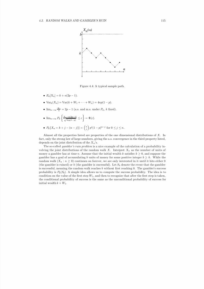
8/11/2019 Random process by B. Hajek
http://slidepdf.com/reader/full/random-process-by-b-hajek 125/448
4.2. RANDOM WALKS AND GAMBLER’S RUIN 115
k
b
ω
n
X ( )n
Figure 4.4: A typical sample path.
• E k[X n] = k + n(2 p − 1).
• Vark(X n) = Var(k + W 1 + · · · + W n) = 4np(1 − p).
• limn→∞ X nn = 2 p − 1 (a.s. and m.s. under P k, k fixed).
• limn→∞ P k
X n−n(2 p−1)√
4np(1− p)≤ c
= Φ(c).
• P kX n = k + j − (n − j) =n j
p j(1 − p)n− j for 0 ≤ j ≤ n.
Almost all the properties listed are properties of the one dimensional distributions of X . Infact, only the strong law of large numbers, giving the a.s. convergence in the third property listed,depends on the joint distribution of the X n’s.
The so-called gambler’s ruin problem is a nice example of the calculation of a probability in-volving the joint distributions of the random walk X . Interpret X n as the number of units of money a gambler has at time n. Assume that the initial wealth k satisfies k ≥ 0, and suppose thegambler has a goal of accumulating b units of money for some positive integer b ≥ k. While therandom walk (X n : n ≥ 0) continues on forever, we are only interested in it until it hits either 0
(the gambler is ruined) or b (the gambler is successful). Let S b denote the event that the gambleris successful, meaning the random walk reaches b without first reaching 0. The gambler’s successprobability is P k(S b). A simple idea allows us to compute the success probability. The idea is tocondition on the value of the first step W 1, and then to recognize that after the first step is taken,the conditional probability of success is the same as the unconditional probability of success forinitial wealth k + W 1.
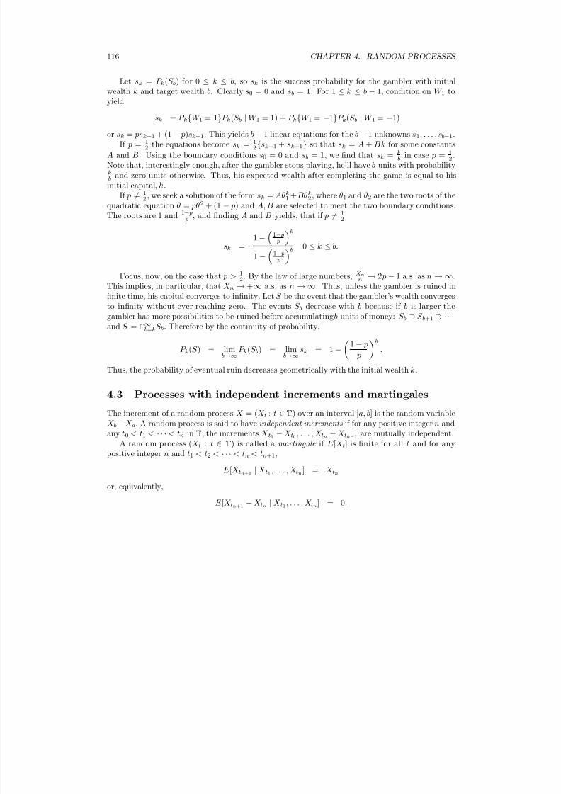
8/11/2019 Random process by B. Hajek
http://slidepdf.com/reader/full/random-process-by-b-hajek 126/448
116 CHAPTER 4. RANDOM PROCESSES
Let sk = P k(S b) for 0 ≤ k ≤ b, so sk is the success probability for the gambler with initialwealth k and target wealth b. Clearly s0 = 0 and sb = 1. For 1 ≤ k ≤ b − 1, condition on W 1 toyield
sk = P kW 1 = 1P k(S b | W 1 = 1) + P kW 1 = −1P k(S b | W 1 = −1)
or sk = psk+1 + (1 − p)sk−1. This yields b − 1 linear equations for the b − 1 unknowns s1, . . . , sb−1.If p = 1
2 the equations become sk = 12sk−1 + sk+1 so that sk = A + Bk for some constants
A and B. Using the boundary conditions s0 = 0 and sb = 1, we find that sk = kb in case p = 1
2 .Note that, interestingly enough, after the gambler stops playing, he’ll have b units with probabilitykb and zero units otherwise. Thus, his expected wealth after completing the game is equal to hisinitial capital, k .
If p = 12 , we seek a solution of the form sk = Aθk
1 +Bθk2 , where θ1 and θ2 are the two roots of the
quadratic equation θ = pθ2 + (1 − p) and A, B are selected to meet the two boundary conditions.The roots are 1 and 1− p
p , and finding A and B yields, that if p = 12
sk =1 − 1− p
p
k1 −
1− p p
b 0 ≤ k ≤ b.
Focus, now, on the case that p > 12 . By the law of large numbers, X n
n → 2 p − 1 a.s. as n → ∞.This implies, in particular, that X n → +∞ a.s. as n → ∞. Thus, unless the gambler is ruined infinite time, his capital converges to infinity. Let S be the event that the gambler’s wealth convergesto infinity without ever reaching zero. The events S b decrease with b because if b is larger thegambler has more possibilities to be ruined before accumulating b units of money: S b ⊃ S b+1 ⊃ · · ·and S = ∩∞
b=kS b. Therefore by the continuity of probability,
P k(S ) = limb→∞
P k(S b) = limb→∞
sk = 1 −1 − p
p
k.
Thus, the probability of eventual ruin decreases geometrically with the initial wealth k .
4.3 Processes with independent increments and martingales
The increment of a random process X = (X t : t ∈ T) over an interval [a, b] is the random variableX b −X a. A random process is said to have independent increments if for any positive integer n andany t0 < t1 < · · · < tn in T, the increments X t1 − X t0, . . . , X tn − X tn−1 are mutually independent.
A random process (X t : t ∈ T) is called a martingale if E [X t] is finite for all t and for any
positive integer n and t1 < t2 < · · · < tn < tn+1,
E [X tn+1 | X t1 , . . . , X tn ] = X tn
or, equivalently,
E [X tn+1 − X tn | X t1, . . . , X tn] = 0.
8/11/2019 Random process by B. Hajek
http://slidepdf.com/reader/full/random-process-by-b-hajek 127/448
4.3. PROCESSES WITH INDEPENDENT INCREMENTS AND MARTINGALES 117
If tn is interpreted as the present time, then tn+1 is a future time and the value of (X t1 , . . . , X tn)represents information about the past and present values of X . With this interpretation, themartingale property is that the future increments of X have conditional mean zero, given the past
and present values of the process.An example of a martingale is the following. Suppose a gambler has initial wealth X 0. Suppose
the gambler makes bets with various odds, such that, as far as the past history of X can determine,the bets made are all for fair games in which the expected net gains are zero. Then if X t denotesthe wealth of the gambler at any time t ≥ 0, then (X t : t ≥ 0) is a martingale.
Suppose (X t) is an independent increment process with index set T = R+ or T = Z+, with X 0equal to a constant and with mean zero increments. Then X is a martingale, as we now show.Let t1 < · · · < tn+1 be in T. Then (X t1, . . . , X tn) is a function of the increments X t1 − X 0, X t2 −X t1, . . . , X tn − X tn−1 , and hence it is independent of the increment X tn+1 − X tn. Thus
E [X tn+1 − X tn | X t1 , . . . , X tn ] = E [X tn+1 − X tn] = 0.
The random walk (X n : n ≥ 0) arising in the gambler’s ruin problem is an independent incrementprocess, and if p = 1
2 it is also a martingale.
The following proposition is stated, without proof, to give an indication of some of the usefuldeductions that follow from the martingale property.
Proposition 4.3.1 (a) (Doob’s maximal inequality) Let X 0, X 1, X 2, ...be nonnegative random variables such that E [X k+1 | X 0, . . . , X k] ≤ X k for k ≥ 0 (such X is a nonnegative supermartingale). Then
P
max0≤k≤n
X k
≥ γ
≤ E [X 0]
γ .
(b) (Doob’s L2 Inequality) Let X 0, X 1, ...be a martingale sequence with E [X 2n] < +∞ for some n. Then
E
max0≤k≤n
X k
2
≤ 4E [X 2n].
Martingales can be used to derive concentration inequalities involving sums of dependent ran-dom variables, as shown next. A random sequence X 1, X 2, . . . is called a martingale difference sequence if the process of partial sums defined by S n = X 1 + · · ·+ X n (with S 0 = 0) is a martingale,or equivalently, if E [X n|X 1, · · · , X n−1] = 0 for each n ≥ 1. The following proposition shows that
Bennett’s inequality and Bernstein’s inequality given in Problem 2.38 readily extend from the caseof sums of independent random variables to sums of martingale difference random variables. Arelated analysis in Section 10.3 yields the Azuma-Hoeffding inequality.
Proposition 4.3.2 (Bennett’s and Bernstein’s inequalities for martingale difference sequences)Suppose X 1, X 2, . . . is a martingale difference sequence such that for some constant L and constants
8/11/2019 Random process by B. Hajek
http://slidepdf.com/reader/full/random-process-by-b-hajek 128/448
118 CHAPTER 4. RANDOM PROCESSES
d2i , i ≥ 1: P |X i| ≤ L = 1 and E [X 2i |X 1, . . . , X i−1] ≤ d2
i for i ≥ 1. Then for α > 0 and n ≥ 1 :
P n
i=1
X i ≥
α ≤ exp−
ni=1 d2
i
L2
φ αL
i d2i (Bennett’s inequality)
≤ exp
−
12 α2n
i=1 d2i + αL
3
(Bernstein’s inequality),
where φ(u) = (1 + u) ln(1 + u) − u.
Proof. Problem 2.38(a) yields that E [eθX i |X 1, . . . , X i−1] ≤ exp
d2i (eθL−1−θL)
L2
for θ > 0. Then
E [eθS n] = E [E [eθX neθS n−1|X 1, . . . , X n−1]]
= E [E [eθX n|X 1, . . . , X n−1]eθS n−1 ]
≤ expd
2
n(e
θL
− 1 − θL)L2 E [eθS n−1],
which by induction on n implies
E [eθS n ] ≤ exp
ni=1 d2
i
(eθL − 1 − θL)
L2
,
just as if the X i’s were independent. The remainder of the proof is identical to the proof of theChernoff bound, as in Problem 2.38.
4.4 Brownian motion
A Brownian motion , also called a Wiener process , with parameter σ2 > 0, is a random processW = (W t : t ≥ 0) such that
B.0 P W 0 = 0 = 1.
B.1 W has independent increments.
B.2 W t − W s has the N (0, σ2(t − s)) distribution for t ≥ s.
B.3 P W t is a continuous function of t = 1, or in other words, W is sample path continuous withprobability one.
A typical sample path of a Brownian motion is shown in Figure 4.5. A Brownian motion, being amean zero independent increment process with P W 0 = 0 = 1, is a martingale.
The mean, correlation, and covariance functions of a Brownian motion W are given by
µW (t) = E [W t] = E [W t − W 0] = 0
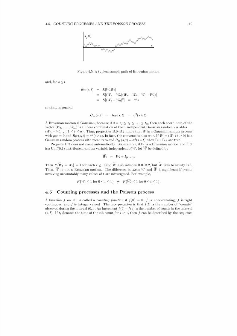
8/11/2019 Random process by B. Hajek
http://slidepdf.com/reader/full/random-process-by-b-hajek 129/448
4.5. COUNTING PROCESSES AND THE POISSON PROCESS 119
X ( )ωt
t
Figure 4.5: A typical sample path of Brownian motion.
and, for s ≤ t,
RW (s, t) = E [W sW t]
= E [(W s − W 0)(W s − W 0 + W t − W s)]= E [(W s − W 0)2] = σ2s
so that, in general,
C W (s, t) = RW (s, t) = σ2(s ∧ t).
A Brownian motion is Gaussian, because if 0 = t0 ≤ t1 ≤ ·· · ≤ tn, then each coordinate of thevector (W t1, . . . , W tn) is a linear combination of the n independent Gaussian random variables(W ti − W ti−1 : 1 ≤ i ≤ n). Thus, properties B.0–B.2 imply that W is a Gaussian random processwith µW = 0 and RW (s, t) = σ2(s ∧ t). In fact, the converse is also true. If W = (W t : t ≥ 0) is aGaussian random process with mean zero and RW (s, t) = σ2(s
∧t), then B.0–B.2 are true.
Property B.3 does not come automatically. For example, if W is a Brownian motion and if U is a Unif(0,1) distributed random variable independent of W , let W be defined by
W t = W t + I U =t.
Then P W t = W t = 1 for each t ≥ 0 and W also satisfies B.0–B.2, but W fails to satisfy B.3.
Thus, W is not a Brownian motion. The difference between W and W is significant if eventsinvolving uncountably many values of t are investigated. For example,
P W t ≤ 1 for 0 ≤ t ≤ 1 = P W t ≤ 1 for 0 ≤ t ≤ 1.
4.5 Counting processes and the Poisson processA function f on R+ is called a counting function if f (0) = 0, f is nondecreasing, f is rightcontinuous, and f is integer valued. The interpretation is that f (t) is the number of “counts”observed during the interval (0, t]. An increment f (b)−f (a) is the number of counts in the interval(a, b]. If ti denotes the time of the ith count for i ≥ 1, then f can be described by the sequence
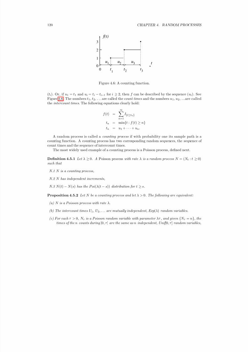
8/11/2019 Random process by B. Hajek
http://slidepdf.com/reader/full/random-process-by-b-hajek 130/448
120 CHAPTER 4. RANDOM PROCESSES
t
t t t 1 2 3
u u u31 2
3
2
1
0
0
f(t)
Figure 4.6: A counting function.
(ti). Or, if u1 = t1 and ui = ti − ti−1 for i ≥ 2, then f can be described by the sequence (ui). SeeFigure 4.6. The numbers t
1, t
2, . . . are called the count times and the numbers u
1, u
2, ...are called
the intercount times . The following equations clearly hold:
f (t) =∞
n=1
I t≥tn
tn = mint : f (t) ≥ ntn = u1 + · · · + un.
A random process is called a counting process if with probability one its sample path is acounting function. A counting process has two corresponding random sequences, the sequence of count times and the sequence of intercount times.
The most widely used example of a counting process is a Poisson process, defined next.
Definition 4.5.1 Let λ ≥ 0. A Poisson process with rate λ is a random process N = (N t : t ≥ 0)such that
N.1 N is a counting process,
N.2 N has independent increments,
N.3 N (t) − N (s) has the P oi(λ(t − s)) distribution for t ≥ s.
Proposition 4.5.2 Let N be a counting process and let λ > 0. The following are equivalent:
(a) N is a Poisson process with rate λ.
(b) The intercount times U 1, U 2, . . . are mutually independent, Exp(λ) random variables.
(c) For each τ > 0, N τ is a Poisson random variable with parameter λτ , and given N τ = n, the times of the n counts during [0, τ ] are the same as n independent, Unif [0, τ ] random variables,
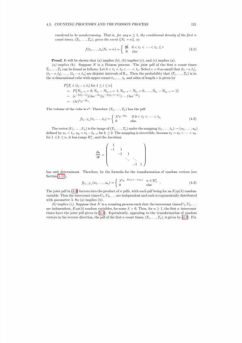
8/11/2019 Random process by B. Hajek
http://slidepdf.com/reader/full/random-process-by-b-hajek 131/448
4.5. COUNTING PROCESSES AND THE POISSON PROCESS 121
reordered to be nondecreasing. That is, for any n ≥ 1, the conditional density of the first ncount times, (T 1, . . . , T n), given the event N τ = n, is:
f (t1, . . . , tn|N τ = n) = n!
τ n 0 < t1 < · · · < tn ≤ τ 0 else (4.1)
Proof. It will be shown that (a) implies (b), (b) implies (c), and (c) implies (a).(a) implies (b). Suppose N is a Poisson process. The joint pdf of the first n count times
T 1, . . . , T n can be found as follows. Let 0 < t1 < t2 < · · · < tn. Select > 0 so small that (t1 − , t1],(t2 − , t2], . . . , (tn − , tn] are disjoint intervals of R+. Then the probability that (T 1, . . . , T n) is inthe n-dimensional cube with upper corner t1, . . . , tn and sides of length is given by
P T i ∈ (ti − , ti] for 1 ≤ i ≤ n= P N t1− = 0, N t1 − N t1− = 1, N t2− − N t1 = 0, . . . , N tn − N tn− = 1= (e
−λ(t1
−))(λe
−λ)(e
−λ(t2
−
−t1))
· · ·(λe
−λ)
= (λ)ne−λtn.
The volume of the cube is n. Therefore (T 1, . . . , T n) has the pdf
f T 1···T n(t1, . . . , tn) =
λne−λtn if 0 < t1 < · · · < tn0 else.
(4.2)
The vector (U 1, . . . , U n) is the image of (T 1, . . . , T n) under the mapping (t1, . . . , tn) → (u1, . . . , un)defined by u1 = t1, uk = tk − tk−1 for k ≥ 2. The mapping is invertible, because tk = u1 + · · · + uk
for 1 ≤ k ≤ n, it has range Rn+, and the Jacobian
∂u
∂t =
1
−1 1−1 1
. . . . . .
−1 1
has unit determinant. Therefore, by the formula for the transformation of random vectors (seeSection 1.11),
f U 1...U n(u1, . . . , un) =
λne−λ(u1+···+un) u ∈Rn
+
0 else . (4.3)
The joint pdf in (4.3) factors into the product of n pdfs, with each pdf being for an Exp(λ) random
variable. Thus the intercount times U 1, U 2, . . . are independent and each is exponentially distributedwith parameter λ. So (a) implies (b).
(b) implies (c). Suppose that N is a counting process such that the intercount times U 1, U 2, . . .are independent, E xp(λ) random variables, for some λ > 0. Thus, for n ≥ 1, the first n intercounttimes have the joint pdf given in (4.3). Equivalently, appealing to the transformation of randomvectors in the reverse direction, the pdf of the first n count times, (T 1, . . . , T n), is given by (4.2). Fix
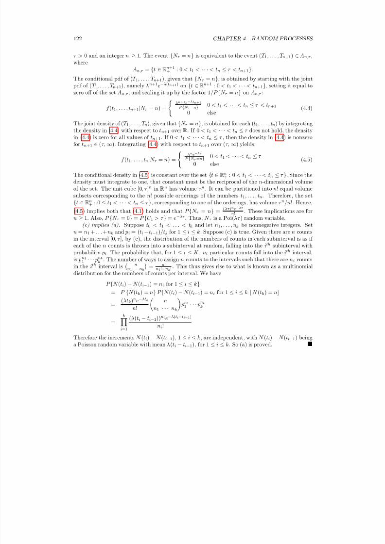
8/11/2019 Random process by B. Hajek
http://slidepdf.com/reader/full/random-process-by-b-hajek 132/448
122 CHAPTER 4. RANDOM PROCESSES
τ > 0 and an integer n ≥ 1. The event N τ = n is equivalent to the event (T 1, . . . , T n+1) ∈ An,τ ,where
An,τ = t ∈Rn+1+ : 0 < t1 < · · · < tn ≤ τ < tn+1.
The conditional pdf of (T 1, . . . , T n+1), given that N τ = n, is obtained by starting with the jointpdf of (T 1, . . . , T n+1), namely λn+1e−λ(tn+1) on t ∈Rn+1 : 0 < t1 < · · · < tn+1, setting it equal tozero off of the set An,τ , and scaling it up by the factor 1/P N τ = n on An,τ :
f (t1, . . . , tn+1|N τ = n) =
λn+1e−λtn+1
P N τ =n 0 < t1 < · · · < tn ≤ τ < tn+1
0 else(4.4)
The joint density of (T 1, . . . , T n), given that N τ = n, is obtained for each (t1, . . . , tn) by integratingthe density in (4.4) with respect to tn+1 over R. If 0 < t1 < · · · < tn ≤ τ does not hold, the densityin (4.4) is zero for all values of tn+1. If 0 < t1 < · · · < tn ≤ τ , then the density in (4.4) is nonzerofor tn+1 ∈ (τ, ∞). Integrating (4.4) with respect to tn+1 over (τ, ∞) yields:
f (t1, . . . , tn|N τ = n) = λn
e−λτ
P N τ =n 0 < t1 < · · · < tn ≤ τ 0 else
(4.5)
The conditional density in (4.5) is constant over the set t ∈ Rn+ : 0 < t1 < · · · < tn ≤ τ . Since the
density must integrate to one, that constant must be the reciprocal of the n-dimensional volumeof the set. The unit cube [0, τ ]n in Rn has volume τ n. It can be partitioned into n! equal volumesubsets corresponding to the n! possible orderings of the numbers t1, . . . , tn. Therefore, the sett ∈Rn
+ : 0 ≤ t1 < · · · < tn ≤ τ , corresponding to one of the orderings, has volume τ n/n!. Hence,
(4.5) implies both that (4.1) holds and that P N τ = n = (λτ )ne−λτ
n! . These implications are forn ≥ 1. Also, P N τ = 0 = P U 1 > τ = e−λτ . Thus, N τ is a Poi(λτ ) random variable.
(c) implies (a). Suppose t0 < t1 < . . . < tk and let n1, . . . , nk be nonnegative integers. Set
n = n1 + . . . + nk and pi = (ti−ti−1)/tk for 1 ≤ i ≤ k. Suppose (c) is true. Given there are n countsin the interval [0, τ ], by (c), the distribution of the numbers of counts in each subinterval is as if each of the n counts is thrown into a subinterval at random, falling into the ith subinterval withprobability pi. The probability that, for 1 ≤ i ≤ K , ni particular counts fall into the ith interval,is pn1
1 · · · pnkk . The number of ways to assign n counts to the intervals such that there are ni counts
in the ith interval is
nn1 · ·· nk
= n!
n1!···nk! . This thus gives rise to what is known as a multinomialdistribution for the numbers of counts per interval. We have
P N (ti) − N (ti−1) = ni for 1 ≤ i ≤ k= P N (tk) = n P [N (ti) − N (ti−1) = ni for 1 ≤ i ≤ k | N (tk) = n]
= (λtk)ne−λtk
n! n
n1 · · ·
nk pn1
1
· · · pnk
k
=k
i=1
(λ(ti − ti−1))nie−λ(ti−ti−1)
ni!
Therefore the increments N (ti) − N (ti−1), 1 ≤ i ≤ k, are independent, with N (ti) − N (ti−1) beinga Poisson random variable with mean λ(ti − ti−1), for 1 ≤ i ≤ k. So (a) is proved.
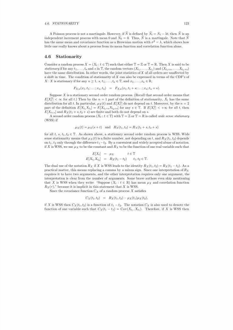
8/11/2019 Random process by B. Hajek
http://slidepdf.com/reader/full/random-process-by-b-hajek 133/448
4.6. STATIONARITY 123
A Poisson process is not a martingale. However, if N is defined by N t = N t − λt, then N is anindependent increment process with mean 0 and
N 0 = 0. Thus,
N is a martingale. Note that
N
has the same mean and covariance function as a Brownian motion with σ2 = λ, which shows how
little one really knows about a process from its mean function and correlation function alone.
4.6 Stationarity
Consider a random process X = (X t : t ∈ T) such that either T = Z or T = R. Then X is said to bestationary if for any t1, . . . , tn and s in T, the random vectors (X t1, . . . , X tn) and (X t1+s, . . . , X tn+s)have the same distribution. In other words, the joint statistics of X of all orders are unaffected bya shift in time. The condition of stationarity of X can also be expressed in terms of the CDF’s of X : X is stationary if for any n ≥ 1, s, t1, . . . , tn ∈ T, and x1, . . . , xn ∈ R,
F X,n(x1, t1; . . . ; xn, tn) = F X,n(x1, t1 + s; . . . ; xn; tn + s).
Suppose X is a stationary second order random process. (Recall that second order means thatE [X 2t ] < ∞ for all t.) Then by the n = 1 part of the definition of stationarity, X t has the samedistribution for all t. In particular, µX (t) and E [X 2t ] do not depend on t. Moreover, by the n = 2part of the definition E [X t1X t2] = E [X t1+sX t2+s] for any s ∈ T. If E [X 2t ] < +∞ for all t, thenE [X t+s] and RX (t1 + s, t2 + s) are finite and both do not depend on s.
A second order random process (X t : t ∈ T) with T = Z or T = R is called wide sense stationary (WSS) if
µX (t) = µX (s + t) and RX (t1, t2) = RX (t1 + s, t2 + s)
for all t, s, t1, t2 ∈ T. As shown above, a stationary second order random process is WSS. Widesense stationarity means that µX (t) is a finite number, not depending on t, and RX (t1, t2) depends
on t1, t2 only through the difference t1 −t2. By a convenient and widely accepted abuse of notation,if X is WSS, we use µX to be the constant and RX to be the function of one real variable such that
E [X t] = µX t ∈ TE [X t1X t2] = RX (t1 − t2) t1, t2 ∈ T.
The dual use of the notation RX if X is WSS leads to the identity RX (t1, t2) = RX (t1 − t2). As apractical matter, this means replacing a comma by a minus sign. Since one interpretation of RX
requires it to have two arguments, and the other interpretation requires only one argument, theinterpretation is clear from the number of arguments. Some brave authors even skip mentioningthat X is WSS when they write: “Suppose (X t : t ∈ R) has mean µX and correlation functionRX (τ ),” because it is implicit in this statement that X is WSS.
Since the covariance function C X of a random process X satisfies
C X (t1, t2) = RX (t1, t2) − µX (t1)µX (t2),
if X is WSS then C X (t1, t2) is a function of t1 − t2. The notation C X is also used to denote thefunction of one variable such that C X (t1 − t2) = Cov(X t1 , X t2). Therefore, if X is WSS then
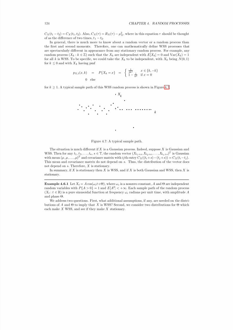
8/11/2019 Random process by B. Hajek
http://slidepdf.com/reader/full/random-process-by-b-hajek 134/448
124 CHAPTER 4. RANDOM PROCESSES
C X (t1 − t2) = C X (t1, t2). Also, C X (τ ) = RX (τ ) − µ2X , where in this equation τ should be thought
of as the difference of two times, t1 − t2.In general, there is much more to know about a random vector or a random process than
the first and second moments. Therefore, one can mathematically define WSS processes thatare spectacularly different in appearance from any stationary random process. For example, anyrandom process (X k : k ∈ Z) such that the X k are independent with E [X k] = 0 and Var(X k) = 1for all k is WSS. To be specific, we could take the X k to be independent, with X k being N (0, 1)for k ≤ 0 and with X k having pmf
pX,1(x, k) = P X k = x =
12k2 x ∈ k, −k1 − 1
k2 if x = 0
0 else
for k ≥ 1. A typical sample path of this WSS random process is shown in Figure 4.7.
k
k X
Figure 4.7: A typical sample path.
The situation is much different if X is a Gaussian process. Indeed, suppose X is Gaussian andWSS. Then for any t1, t2, . . . , tn, s ∈ T, the random vector (X t1+s, X t2+s, . . . , X tn+s)T is Gaussianwith mean (µ , µ , . . . , µ)T and covariance matrix with ijth entry C X ((ti +s)−(t j +s)) = C X (ti−t j).This mean and covariance matrix do not depend on s. Thus, the distribution of the vector doesnot depend on s. Therefore, X is stationary.
In summary, if X is stationary then X is WSS, and if X is both Gaussian and WSS, then X isstationary.
Example 4.6.1 Let X t = A cos(ωct+Θ), where ωc is a nonzero constant, A and Θ are independent
random variables with P A > 0 = 1 and E [A2
] < +∞. Each sample path of the random process(X t : t ∈ R) is a pure sinusoidal function at frequency ωc radians per unit time, with amplitude Aand phase Θ.
We address two questions. First, what additional assumptions, if any, are needed on the distri-butions of A and Θ to imply that X is WSS? Second, we consider two distributions for Θ whicheach make X WSS, and see if they make X stationary.
8/11/2019 Random process by B. Hajek
http://slidepdf.com/reader/full/random-process-by-b-hajek 135/448
4.6. STATIONARITY 125
To address whether X is WSS, the mean and correlation functions can be computed as follows.Since A and Θ are independent and since cos(ωct + Θ) = cos(ωct) cos(Θ) − sin(ωct) sin(Θ),
µX (t) = E [A] (E [cos(Θ)] cos(ωct)−
E [sin(Θ)] sin(ωct)) .
Thus, the function µX (t) is a linear combination of cos(ωct) and sin(ωct). The only way such alinear combination can be independent of t is if the coefficients of both cos(ωct) and sin(ωct) arezero (in fact, it is enough to equate the values of µX (t) at ωct = 0, π2 , and π). Therefore, µX (t)does not depend on t if and only if E [cos(Θ)] = E [sin(Θ)] = 0.
Turning next to RX , using the trigonometric identity cos(a) cos(b) = (cos(a − b)+cos(a + b))/2yields
RX (s, t) = E [A2]E [cos(ωcs + Θ) cos(ωct + Θ)]
= E [A2]
2 cos(ωc(s − t)) + E [cos(ωc(s + t) + 2Θ)] .
Since s + t can be arbitrary for s − t fixed, in order that RX (s, t) be a function of s − t alone it isnecessary that E [cos(ωc(s + t) + 2Θ)] be a constant, independent of the value of s + t. Arguing justas in the case of µX , with Θ replaced by 2Θ, yields that RX (s, t) is a function of s − t if and onlyif E [cos(2Θ)] = E [sin(2Θ)] = 0.
Combining the findings for µX and RX , yields that X is WSS, if and only if,
E [cos(Θ)] = E [sin(Θ)] = E [cos(2Θ)] = E [sin(2Θ)] = 0.
There are many distributions for Θ in [0, 2π] such that the four moments specified are zero. Twopossibilities are (a) Θ is uniformly distributed on the interval [0, 2π], or, (b) Θ is a discrete randomvariable, taking the four values 0, π
2 , π, 3π2 with equal probability. Is X stationary for either
possibility?
We shall show that X is stationary if Θ is uniformly distributed over [0, 2π]. Stationarity meansthat for any fixed constant s, the random processes (X t : t ∈ R) and (X t+s : t ∈ R) have the samefinite order distributions. For this example,
X t+s = A cos(ωc(t + s) + Θ) = A cos(ωct + Θ)
where Θ = ((ωcs +Θ) mod 2π). By Example 1.4.4, Θ is again uniformly distributed on the interval[0, 2π]. Thus (A, Θ) and (A, Θ) have the same joint distribution, so A cos(ωct+Θ) and A cos(ωct+Θ)have the same finite order distributions. Hence, X is indeed stationary if Θ is uniformly distributedover [0, 2π].
Assume now that Θ takes on each of the values of 0, π2 , π , and 3π
2 with equal probability. Is X stationary? If X were stationary then, in particular, X t would have the same distribution for all t.On one hand, P
X
0 = 0
= P
Θ = π
2 or Θ = 3π
2 = 1
2. On the other hand, if ω
ct is not an integer
multiple of π2 , then ωct + Θ cannot be an integer multiple of π2 , so P X t = 0 = 0. Hence X is notstationary.
(With more work it can be shown that X is stationary, if and only if, (Θ mod 2π) is uniformlydistributed over the interval [0, 2π].)
8/11/2019 Random process by B. Hajek
http://slidepdf.com/reader/full/random-process-by-b-hajek 136/448
8/11/2019 Random process by B. Hajek
http://slidepdf.com/reader/full/random-process-by-b-hajek 137/448
4.8. CONDITIONAL INDEPENDENCE AND MARKOV PROCESSES 127
for all i, j, k with P X = i, Y = j > 0. The forms (4.6) and (4.7) make it clear that the conditionX − Y − Z is symmetric in X and Z : thus X − Y − Z is the same condition as Z − Y − X .The form (4.7) does not involve conditional probabilities, so no requirement about conditioning
on events having positive probability is needed. The form (4.8) shows that X − Y − Z meansthat knowing Y alone is as informative as knowing both X and Y , for the purpose of determiningconditional probabilities of Z . Intuitively, the condition X − Y − Z means that the randomvariable Y serves as a state.
If X, Y , and Z have a joint pdf, then the condition X − Y − Z can be defined using thepdfs and conditional pdfs in a similar way. For example, the conditional independence conditionX − Y − Z holds by definition if
f XZ |Y (x, z|y) = f X |Y (x|y)f Z |Y (z|y) whenever f Y (y) > 0
An equivalent condition is
f Z
|XY (z
|x, y) = f Z
|Y (z
|y) whenever f XY (x, y) > 0. (4.9)
Example 4.8.1 Suppose X, Y,Z are jointly Gaussian vectors. Let us see what the conditionX − Y − Z means in terms of the covariance matrices. Assume without loss of generality that thevectors have mean zero. Because X, Y , and Z are jointly Gaussian, the condition (4.9) is equivalentto the condition that E [Z |X, Y ] = E [Z |Y ] (because given X, Y , or just given Y , the conditionaldistribution of Z is Gaussian, and in the two cases the mean and covariance of the conditionaldistribution of Z is the same.) The idea of linear innovations applied to the length two sequence(Y, X ) yields E [Z |X, Y ] = E [Z |Y ] + E [Z | X ] where X = X −E [X |Y ]. Thus X −Y −Z if and only if E [Z | X ] = 0, or equivalently, if and only if Cov( X, Z ) = 0. Since X = X − Cov(X, Y )Cov(Y )−1Y ,if follows that
Cov( X, Z ) = Cov(X, Z )
−Cov(X, Y )Cov(Y )−1Cov(Y, Z ).
Therefore, X − Y − Z if and only if
Cov(X, Z ) = Cov(X, Y )Cov(Y )−1Cov(Y, Z ). (4.10)
In particular, if X, Y , and Z are jointly Gaussian random variables with nonzero variances, thecondition X − Y − Z holds if and only if the correlation coefficients satisfy ρXZ = ρXY ρY Z .
A general definition of conditional probabilities and conditional independence, based on thegeneral definition of conditional expectation given in Chapter 3, is given next. Recall thatP (F ) = E [I F ] for any event F , where I F denotes the indicator function of F . If Y is a randomvector, we define P (F |Y ) to equal E [I F |Y ]. This means that P (F |Y ) is the unique (in the sensethat any two versions are equal with probability one) random variable such that
(1) P (F |Y ) is a function of Y and it has finite second moments, and(2) E [g(Y )P (F |Y )] = E [g(Y )I F ] for any g(Y ) with finite second moment.
Given arbitrary random vectors, we define X and Z to be conditionally independent given Y ,(written X − Y − Z ) if for any Borel sets A and B ,
P (X ∈ AZ ∈ B|Y ) = P (X ∈ A|Y )P (Z ∈ B|Y ).
8/11/2019 Random process by B. Hajek
http://slidepdf.com/reader/full/random-process-by-b-hajek 138/448
128 CHAPTER 4. RANDOM PROCESSES
Equivalently, X − Y − Z holds if for any Borel set B, P (Z ∈ B|X, Y ) = P (Z ∈ B|Y ).
Definition 4.8.2 A random process X = (X t : t ∈ T) is said to be a Markov process if for any
t1, . . . , tn+1 in T with t1 < · · · < tn, the following conditional independence condition holds:(X t1, · · · , X tn) − X tn − X tn+1 (4.11)
It turns out that the Markov property is equivalent to the following conditional independenceproperty: For any t1, . . . , tn+m in T with t1 < · · · < tn+m,
(X t1 , · · · , X tn) − X tn − (X tn, · · · , X tn+m) (4.12)
The definition (4.11) is easier to check than condition (4.12), but (4.12) is appealing because it issymmetric in time. In words, thinking of tn as the present time, the Markov property means thatthe past and future of X are conditionally independent given the present state X tn.
Example 4.8.3 (Markov property of independent increment processes ) Let (X t : t ≥ 0) be anindependent increment process such that X 0 is a constant. Then for any t1, . . . , tn+1 with 0 ≤ t1 ≤· · · ≤ tn+1, the vector (X t1, . . . , X tn) is a function of the n increments X t1 − X 0, X t2 − X t1 , X tn −X tn−1, and is thus independent of the increment V = X tn+1 − X tn. But X tn+1 is determined byV and X tn. Thus, X is a Markov process. In particular, random walks, Brownian motions, andPoisson processes are Markov processes.
Example 4.8.4 (Gaussian Markov processes ) Suppose X = (X t : t
∈ T) is a Gaussian random
process with Var(X t) > 0 for all t. By the characterization of conditional independence for jointlyGaussian vectors (4.10), the Markov property (4.11) is equivalent to
Cov
X t1X t2
...X tn
, X tn+1
= Cov
X t1X t2
...X tn
, X tn
Var(X tn)−1Cov(X tn, X tn+1)
which, letting ρ(s, t) denote the correlation coefficient between X s and X t, is equivalent to therequirement
ρ(t1, tn+1)ρ(t2, tn+1))
...ρ(tn, tn+1)
= ρ(t1, tn)ρ(t2, tn)
...ρ(tn, tn)
ρ(tn, tn+1)
Therefore a Gaussian process X is Markovian if and only if
ρ(r, t) = ρ(r, s)ρ(s, t) whenever r, s, t ∈ T with r < s < t. (4.13)
8/11/2019 Random process by B. Hajek
http://slidepdf.com/reader/full/random-process-by-b-hajek 139/448
4.8. CONDITIONAL INDEPENDENCE AND MARKOV PROCESSES 129
If X = (X k : k ∈ Z ) is a discrete-time stationary Gaussian process, then ρ(s, t) may be writtenas ρ(k), where k = s − t. Note that ρ(k) = ρ(−k). Such a process is Markovian if and only if ρ(k1 + k2) = ρ(k1)ρ(k2) for all positive integers k1 and k2. Therefore, X is Markovian if and only if
ρ(k) = b|k| for all k, for some constant b with |b| ≤ 1. Equivalently, a stationary Gaussian process
X = (X k : k ∈ Z ) with V ar(X k) > 0 for all k is Markovian if and only if the covariance functionhas the form C X (k) = Ab|k| for some constants A and b with A > 0 and |b| ≤ 1.
Similarly, if (X t : t ∈ R) is a continuous-time stationary Gaussian process with V ar(X t) > 0for all t, X is Markovian if and only if ρ(s + t) = ρ(s)ρ(t) for all s, t ≥ 0. The only bounded real-valued functions satisfying such a multiplicative condition are exponential functions. Therefore, astationary Gaussian process X with V ar(X t) > 0 for all t is Markovian if and only if ρ has theform ρ(τ ) = exp(−α|τ |), for some constant α ≥ 0, or equivalently, if and only if C X has the formC X (τ ) = A exp(−α|τ |) for some constants A > 0 and α ≥ 0.
The following proposition should be intuitively clear, and it often applies in practice.
Proposition 4.8.5 (Markov property of a sequence determined by a recursion driven by inde-pendent random variables) Suppose X 0, U 1, U 2, . . . are mutually independent random variables and suppose (X n : n ≥ 1) is determined by a recursion of the form X n+1 = hn+1(X n, U n+1) for n ≥ 0.Then (X n : n ≥ 0) is a Markov process.
Proof. The Proposition will first be proved in case the random variables are all discrete type.Let n ≥ 1, let B ⊂ R, and let φ be the function defined by φ(xn) = P hn+1(xn, U n+1) ∈ B.The random vector (X 0, . . . , X n) is determined by (X 0, U 1, . . . , U n), and is therefore independentof U n+1. Thus, for any possible value (x0, . . . , xn) of (X 0, . . . , X n),
P (X n+1 ∈ B |X 0 = xo, . . . , X n = xn) = P (hn+1(xn, U n+1) ∈ B|X 0 = xo, . . . , X n = xn)
= φ(xn)
So the conditional distribution of X n+1 given (X 0, . . . , X n) depends only on X n, establishing theMarkov property.
For the general case we use the general version of conditional probability. Let n ≥ 1, let B bea Borel subset of R, and let φ be defined as before. We will show that P (X n+1 ∈ B|X 0, . . . , X n) =φ(X n) by checking that φ(X n) has the two properties that characterize P (X n+1 ∈ B |X 0, . . . , X n).First, φ(X n) is a function of X 0, . . . , X n with finite second moments. Secondly, if g is an arbitraryBorel function such that g(X 0, . . . , X n) has a finite second moment, then
E
I X n+1∈Bg(X 0, . . . , X n)
=
Rn
u:hn+1(xn,u)∈B
g(x0, . . . , xn)dF U n+1(u)dF X 0,...,X n(x0, . . . , xn)
= Rn
u:hn+1(xn,u)∈B
dF U n+1(u)
g(x0, . . . , xn)dF X 0,...,X n(x0, . . . , xn)
=
Rn
φ(xn)g(x0, . . . , xn)dF X 0,...,X n(x0, . . . , xn)
= E [φ(X n)g(X 0, . . . , X n)] .
8/11/2019 Random process by B. Hajek
http://slidepdf.com/reader/full/random-process-by-b-hajek 140/448
130 CHAPTER 4. RANDOM PROCESSES
Therefore, P (X n+1 ∈ B|X 0, . . . X n) = φ(X n). In particular, P (X n+1 ∈ B|X 0, . . . X n) is a func-tion of X n so that P (X n+1 ∈ B|X 0, . . . X n) = P (X n+1 ∈ B|X n). Since B is arbitrary it implies(X 0, . . . , X n) − X n − X n+1, so (X n : n ≥ 0) is a Markov process.
For example, if the driving terms wk : k ≥ 0 used for discrete-time Kalman filtering are in-dependent (rather than just being pairwise uncorrelated), then the state process of the Kalmanfiltering model has the Markov property.
4.9 Discrete-state Markov processes
This section delves further into the theory of Markov processes in the technically simplest case of a discrete state space. Let S be a finite or countably infinite set, called the state space. Given aprobability space (Ω, F , P ), an S valued random variable is defined to be a function Y mapping Ωto S such that ω : Y (ω) = s ∈ F for each s ∈ S . Assume that the elements of S are orderedso that
S =
a
1, a
2, . . . , a
n in case
S has finite cardinality, or
S =
a
1, a
2, a
3, . . .
in case
S has
infinite cardinality. Given the ordering, an S valued random variable is equivalent to a positiveinteger valued random variable, so it is nothing exotic. Think of the probability distribution of an S valued random variable Y as a row vector of possibly infinite dimension, called a probabilityvector: pY = (P Y = a1, P Y = a2, . . .). Similarly think of a deterministic function g on S asa column vector, g = (g(a1), g(a2), . . .)T . Since the elements of S may not even be numbers, itmight not make sense to speak of the expected value of an S valued random variable. However,if g is a function mapping S to the reals, then g(Y ) is a real-valued random variable and itsexpectation is given by the inner product of the probability vector pY and the column vector g:E [g(Y )] =
i∈S pY (i)g(i) = pY g. A random process X = (X t : t ∈ T) is said to have state space
S if X t is an S valued random variable for each t ∈ T, and the Markov property of such a randomprocess is defined just as it is for a real valued random process.
Let (X t : t ∈ T) be a be a Markov process with state space S . For brevity we denote the firstorder pmf of X at time t as π(t) = (πi(t) : i ∈ S ). That is, πi(t) = pX (i, t) = P X (t) = i. Thefollowing notation is used to denote conditional probabilities:
P (X t1 = j1, . . . , X tn = jn|X s1 = i1, . . . , X sm = im) = pX ( j1, t1; . . . ; jn, tn|i1, s1; . . . ; im, sm)
For brevity, conditional probabilities of the form P (X t = j |X s = i) are written as pij(s, t), and arecalled the transition probabilities of X .
The first order pmfs π(t) and the transition probabilities pij(s, t) determine all the finite orderdistributions of the Markov process as follows. Given
t1 < t2 < . . . < tn in T,ii, i2,...,in
∈ S (4.14)
one writes
pX (i1, t1; · · · ; in, tn)
= pX (i1, t1; · · · ; in−1, tn−1) pX (in, tn|i1, t1; · · · ; in−1, tn−1)
= pX (i1, t1; · · · ; in−1, tn−1) pin−1in(tn−1, tn)
8/11/2019 Random process by B. Hajek
http://slidepdf.com/reader/full/random-process-by-b-hajek 141/448
4.9. DISCRETE-STATE MARKOV PROCESSES 131
Application of this operation n − 2 more times yields that
pX (i1, t1; · · · ; in, tn) = πi1(t1) pi1i2(t1, t2) · · · pin−1in(tn−1, tn) (4.15)
which shows that the finite order distributions of X are indeed determined by the first order pmfsand the transition probabilities. Equation (4.15) can be used to easily verify that the form (4.12)of the Markov property holds.
Given s < t, the collection H (s, t) defined by H (s, t) = ( pij(s, t) : i, j ∈ S ) should be thoughtof as a matrix, and it is called the transition probability matrix for the interval [ s, t]. Let e denotethe column vector with all ones, indexed by S . Since π(t) and the rows of H (s, t) are probabilityvectors, it follows that π(t)e = 1 and H (s, t)e = e. Computing the distribution of X t by summingover all possible values of X s yields that π j(t) =
i P (X s = i, X t = j) =
i πi(s) pij(s, t), which in
matrix form yields that π(t) = π(s)H (s, t) for s, t ∈ T, s ≤ t. Similarly, given s < τ < t, computingthe conditional distribution of X t given X s by summing over all possible values of X τ yields
H (s, t) = H (s, τ )H (τ, t) s ,τ,t ∈T, s < τ < t. (4.16)
The relations (4.16) are known as the Chapman-Kolmogorov equations.A Markov process is time-homogeneous if the transition probabilities pij(s, t) depend on s and
t only through t − s. In that case we write pij(t − s) instead of pij(s, t), and H ij(t − s) instead of H ij(s, t). If the Markov process is time-homogeneous, then π(s+τ ) = π(s)H (τ ) for s, s+τ ∈ T andτ ≥ 0. A probability distribution π is called an equilibrium (or invariant) distribution if πH (τ ) = πfor all τ ≥ 0.
Recall that a random process is stationary if its finite order distributions are invariant withrespect to translation in time. On one hand, referring to (4.15), we see that a time-homogeneousMarkov process is stationary if and only if π(t) = π for all t for some equilibrium distribution π.On the other hand, a Markov random process that is stationary is time homogeneous.
Repeated application of the Chapman-Kolmogorov equations yields that pij(s, t) can be ex-pressed in terms of transition probabilities for s and t close together. For example, considerMarkov processes with index set the integers. Then H (n, k + 1) = H (n, k)P (k) for n ≤ k , whereP (k) = H (k, k + 1) is the one-step transition probability matrix. Fixing n and using forward re-cursion starting with H (n, n) = I , H (n, n + 1) = P (n), H (n, n + 2) = P (n)P (n + 1), and so forthyields
H (n, l) = P (n)P (n + 1) · · · P (l − 1)
In particular, if the chain is time-homogeneous then H (k) = P k for all k, where P is the timeindependent one-step transition probability matrix, and π(l) = π(k)P l−k for l ≥ k. In this case aprobability distribution π is an equilibrium distribution if and only if πP = π.
Example 4.9.1 Consider a two-stage pipeline through which packets flow, as pictured in Figure4.8. Some assumptions about the pipeline will be made in order to model it as a simple discrete-time Markov process. Each stage has a single buffer. Normalize time so that in one unit of timea packet can make a single transition. Call the time interval between k and k + 1 the kth “timeslot,” and assume that the pipeline evolves in the following way during a given slot.
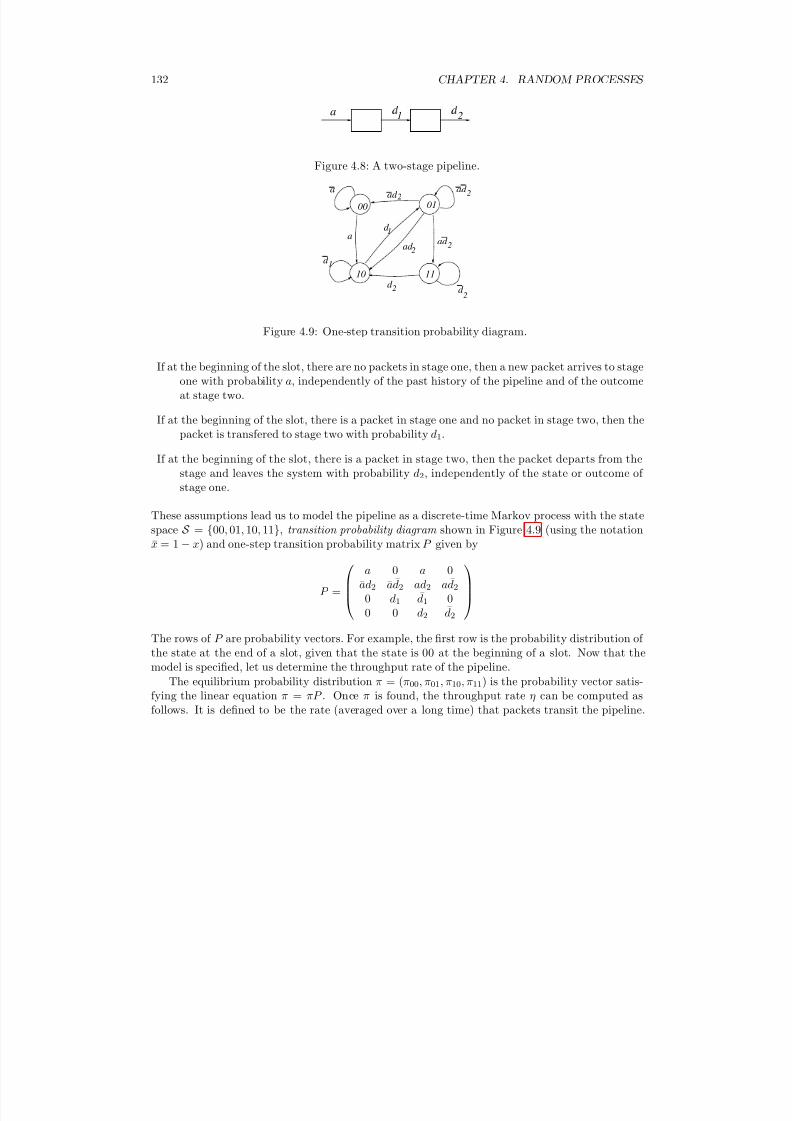
8/11/2019 Random process by B. Hajek
http://slidepdf.com/reader/full/random-process-by-b-hajek 142/448
132 CHAPTER 4. RANDOM PROCESSES
1 2a
Figure 4.8: A two-stage pipeline.
aad
a
d
d d
ad
ad
10
00 01
11
2
2
2
22
1
1
ad 2
d
Figure 4.9: One-step transition probability diagram.
If at the beginning of the slot, there are no packets in stage one, then a new packet arrives to stageone with probability a, independently of the past history of the pipeline and of the outcomeat stage two.
If at the beginning of the slot, there is a packet in stage one and no packet in stage two, then thepacket is transfered to stage two with probability d1.
If at the beginning of the slot, there is a packet in stage two, then the packet departs from thestage and leaves the system with probability d2, independently of the state or outcome of stage one.
These assumptions lead us to model the pipeline as a discrete-time Markov process with the statespace S = 00, 01, 10, 11, transition probability diagram shown in Figure 4.9 (using the notationx = 1 − x) and one-step transition probability matrix P given by
P =
a 0 a 0
ad2 ad2 ad2 ad2
0 d1 d1 0
0 0 d2 d2
The rows of P are probability vectors. For example, the first row is the probability distribution of the state at the end of a slot, given that the state is 00 at the beginning of a slot. Now that themodel is specified, let us determine the throughput rate of the pipeline.
The equilibrium probability distribution π = (π00, π01, π10, π11) is the probability vector satis-fying the linear equation π = πP . Once π is found, the throughput rate η can be computed asfollows. It is defined to be the rate (averaged over a long time) that packets transit the pipeline.
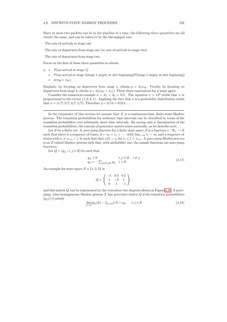
8/11/2019 Random process by B. Hajek
http://slidepdf.com/reader/full/random-process-by-b-hajek 143/448
4.9. DISCRETE-STATE MARKOV PROCESSES 133
Since at most two packets can be in the pipeline at a time, the following three quantities are allclearly the same, and can be taken to be the throughput rate.
The rate of arrivals to stage one
The rate of departures from stage one (or rate of arrivals to stage two)
The rate of departures from stage two
Focus on the first of these three quantities to obtain
η = P an arrival at stage 1= P (an arrival at stage 1|stage 1 empty at slot beginning)P (stage 1 empty at slot beginning)
= a(π00 + π01).
Similarly, by focusing on departures from stage 1, obtain η = d1π10. Finally, by focusing on
departures from stage 2, obtain η = d2(π01 + π11). These three expressions for η must agree.Consider the numerical example a = d1 = d2 = 0.5. The equation π = πP yields that π isproportional to the vector (1, 2, 3, 1). Applying the fact that π is a probability distribution yieldsthat π = (1/7, 2/7, 3/7, 1/7). Therefore η = 3/14 = 0.214 . . ..
In the remainder of this section we assume that X is a continuous-time, finite-state Markovprocess. The transition probabilities for arbitrary time intervals can be described in terms of thetransition probabilites over arbitrarily short time intervals. By saving only a linearization of thetransition probabilities, the concept of generator matrix arises naturally, as we describe next.
Let S be a finite set. A pure-jump function for a finite state space S is a function x : R+ → S such that there is a sequence of times, 0 = τ 0 < τ 1 <
· · · with limi
→∞τ i =
∞, and a sequence of
states with si = si+1, i ≥ 0, such that that x(t) = si for τ i ≤ t < τ i+1. A pure-jump Markov process is an S valued Markov process such that, with probability one, the sample functions are pure-jumpfunctions.
Let Q = (q ij : i, j ∈ S ) be such that
q ij ≥ 0 i, j ∈ S , i = jq ii = − j∈S ,j=i q ij i ∈ S . (4.17)
An example for state space S = 1, 2, 3 is
Q =
−1 0.5 0.51 −2 1
0 1 −1
,
and this matrix Q can be represented by the transition rate diagram shown in Figure 4.10. A pure- jump, time-homogeneous Markov process X has generator matrix Q if the transition probabilities( pij(τ )) satisfy
limh0
( pij(h) − I i= j)/h = q ij i, j ∈ S (4.18)
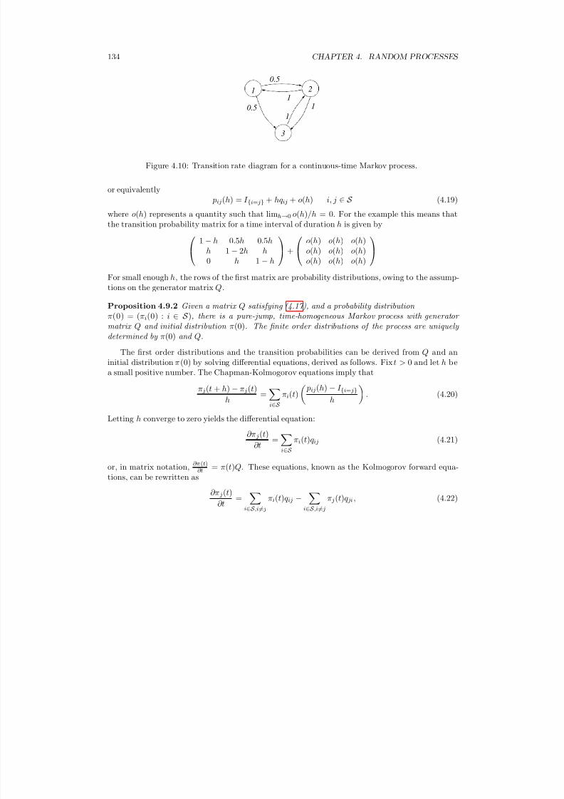
8/11/2019 Random process by B. Hajek
http://slidepdf.com/reader/full/random-process-by-b-hajek 144/448
134 CHAPTER 4. RANDOM PROCESSES
21
3
0.5
1
1
10.5
Figure 4.10: Transition rate diagram for a continuous-time Markov process.
or equivalently pij(h) = I i= j + hq ij + o(h) i, j ∈ S (4.19)
where o(h) represents a quantity such that limh→0 o(h)/h = 0. For the example this means that
the transition probability matrix for a time interval of duration h is given by 1 − h 0.5h 0.5hh 1 − 2h h0 h 1 − h
+
o(h) o(h) o(h)o(h) o(h) o(h)o(h) o(h) o(h)
For small enough h, the rows of the first matrix are probability distributions, owing to the assump-tions on the generator matrix Q.
Proposition 4.9.2 Given a matrix Q satisfying ( 4.17 ), and a probability distribution π(0) = (πi(0) : i ∈ S ), there is a pure-jump, time-homogeneous Markov process with generator matrix Q and initial distribution π(0). The finite order distributions of the process are uniquely determined by π(0) and Q.
The first order distributions and the transition probabilities can be derived from Q and aninitial distribution π(0) by solving differential equations, derived as follows. Fix t > 0 and let h bea small positive number. The Chapman-Kolmogorov equations imply that
π j(t + h) − π j(t)
h =
i∈S
πi(t)
pij(h) − I i= j
h
. (4.20)
Letting h converge to zero yields the differential equation:
∂π j(t)
∂t =
i∈S πi(t)q ij (4.21)
or, in matrix notation, ∂π(t)∂t = π(t)Q. These equations, known as the Kolmogorov forward equa-
tions, can be rewritten as
∂π j(t)
∂t =
i∈S ,i= j
πi(t)q ij −
i∈S ,i= j
π j(t)q ji , (4.22)
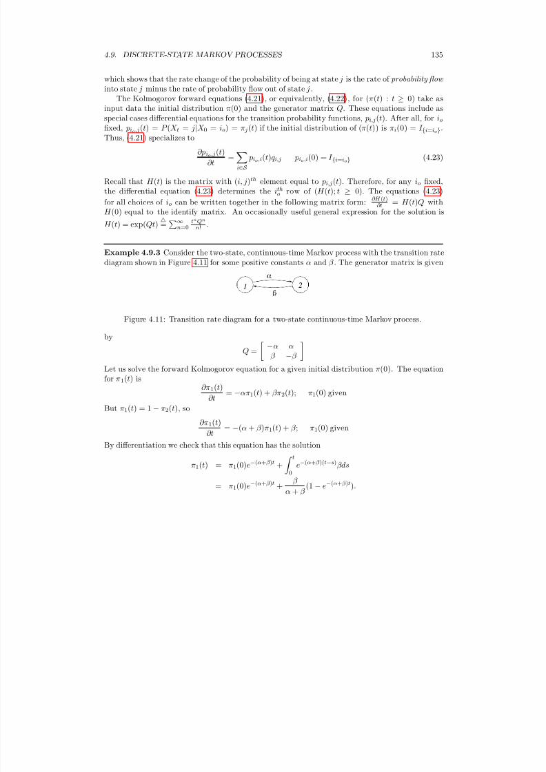
8/11/2019 Random process by B. Hajek
http://slidepdf.com/reader/full/random-process-by-b-hajek 145/448
4.9. DISCRETE-STATE MARKOV PROCESSES 135
which shows that the rate change of the probability of being at state j is the rate of probability flow into state j minus the rate of probability flow out of state j .
The Kolmogorov forward equations (4.21), or equivalently, (4.22), for (π(t) : t ≥ 0) take as
input data the initial distribution π(0) and the generator matrix Q. These equations include asspecial cases differential equations for the transition probability functions, pi,j(t). After all, for iofixed, pio,j(t) = P (X t = j|X 0 = io) = π j(t) if the initial distribution of (π(t)) is πi(0) = I i=io.Thus, (4.21) specializes to
∂pio,j(t)
∂t =
i∈S
pio,i(t)q i,j pio,i(0) = I i=io (4.23)
Recall that H (t) is the matrix with (i, j)th element equal to pi,j(t). Therefore, for any io fixed,the differential equation (4.23) determines the itho row of (H (t); t ≥ 0). The equations (4.23)
for all choices of io can be written together in the following matrix form: ∂H (t)
∂t = H (t)Q withH (0) equal to the identify matrix. An occasionally useful general expression for the solution is
H (t) = exp(Qt) = ∞n=0
tnQnn! .
Example 4.9.3 Consider the two-state, continuous-time Markov process with the transition ratediagram shown in Figure 4.11 for some positive constants α and β . The generator matrix is given
21
α
Figure 4.11: Transition rate diagram for a two-state continuous-time Markov process.
by
Q =
−α αβ −β
Let us solve the forward Kolmogorov equation for a given initial distribution π(0). The equationfor π1(t) is
∂π1(t)
∂t = −απ1(t) + βπ2(t); π1(0) given
But π1(t) = 1 − π2(t), so
∂π1(t)
∂t = −(α + β )π1(t) + β ; π1(0) given
By differentiation we check that this equation has the solution
π1(t) = π1(0)e−(α+β )t +
t0
e−(α+β )(t−s)βds
= π1(0)e−(α+β )t + β
α + β (1 − e−(α+β )t).
8/11/2019 Random process by B. Hajek
http://slidepdf.com/reader/full/random-process-by-b-hajek 146/448
136 CHAPTER 4. RANDOM PROCESSES
so that
π(t) = π(0)e−(α+β )t +
β
α + β ,
α
α + β
(1 − e−(α+β )t) (4.24)
For any initial distribution π(0),
limt→∞ π(t) =
β
α + β ,
α
α + β
.
The rate of convergence is exponential, with rate parameter α + β , and the limiting distribution isthe unique probability distribution satisfying πQ = 0.
By specializing (4.24) we determine H (t). Specifically, H (t) is a 2 × 2 matrix; its top row is π(t)for the initial condition π(0) = (1, 0); its bottom row is π(t) for the initial condition π(0) = (0, 1);the result is:
H (t) =
αe−(α+β)t+β
α+β α(1−e−(α+β)t)
α+β β (1−e−(α+β)t)
α+β
α+βe−(α+β)t
α+β
. (4.25)
Note that H (t) is a transition probability matrix for each t ≥ 0, H (0) is the 2 × 2 identity matrix;each row of limt→∞ H (t) is equal to limt→∞ π(t).
4.10 Space-time structure of discrete-state Markov processes
The previous section showed that the distribution of a time-homogeneous, discrete-state Markovprocess can be specified by an initial probability distribution, and either a one-step transitionprobability matrix P (for discrete-time processes) or a generator matrix Q (for continuous-timeprocesses). Another way to describe these processes is to specify the space-time structure, which is
simply the sequences of states visited and how long each state is visited. The space-time structureis discussed first for discrete-time processes, and then for continuous-time processes. One benefitis to show how little difference there is between discrete-time and continuous-time processes.
Let (X k : k ∈ Z+) be a time-homogeneous Markov process with one-step transition probabilitymatrix P . Let T k denote the time that elapses between the kth and k + 1th jumps of X , and letX J (k) denote the state after k jumps. See Fig. 4.12 for illustration. More precisely, the holding times are defined by
T 0 = mint ≥ 0 : X (t) = X (0) (4.26)
T k = mint ≥ 0 : X (T 0 + . . . + T k−1 + t) = X (T 0 + . . . + T k−1) (4.27)
and the jump process X J = (X J (k) : k
≥ 0) is defined by
X J (0) = X (0) and X J (k) = X (T 0 + . . . + T k−1) (4.28)
Clearly the holding times and jump process contain all the information needed to construct X , andvice versa. Thus, the following description of the joint distribution of the holding times and the jump process characterizes the distribution of X .
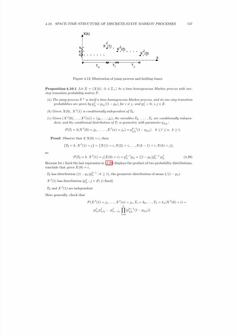
8/11/2019 Random process by B. Hajek
http://slidepdf.com/reader/full/random-process-by-b-hajek 147/448
4.10. SPACE-TIME STRUCTURE OF DISCRETE-STATE MARKOV PROCESSES 137
! !! " #
!
X (3)
X(k)
J
k
X (1)X (2)J Js
ss123
Figure 4.12: Illustration of jump process and holding times.
Proposition 4.10.1 Let X = (X (k) : k ∈ Z+) be a time-homogeneous Markov process with one-step transition probability matrix P .
(a) The jump process X J is itself a time-homogeneous Markov process, and its one-step transition probabilities are given by pJ
ij = pij/(1 − pii) for i = j, and pJ ii = 0, i, j ∈ S .
(b) Given X (0), X J (1) is conditionally independent of T 0.
(c) Given (X J (0), . . . , X J (n)) = ( j0, . . . , jn), the variables T 0, . . . , T n are conditionally indepen-dent, and the conditional distribution of T l is geometric with parameter p jl jl:
P (T l = k|X J (0) = j0, . . . , X J (n) = jn) = pk−1 jl jl
(1 − p jl jl) 0 ≤ l ≤ n, k ≥ 1.
Proof. Observe that if X (0) = i, then
T 0 = k, X J (1) = j = X (1) = i, X (2) = i, . . . , X (k − 1) = i, X (k) = j,
soP (T 0 = k, X J (1) = j |X (0) = i) = pk−1
ii pij = [(1 − pii) pk−1ii ] pJ
ij (4.29)
Because for i fixed the last expression in (4.29) displays the product of two probability distributions,conclude that given X (0) = i,
T 0 has distribution ((1 − pii) pk−1ii : k ≥ 1), the geometric distribution of mean 1/(1 − pii)
X J (1) has distribution ( pJ ij : j ∈ S ) (i fixed)
T 0 and X J (1) are independent
More generally, check that
P (X J (1) = j1, . . . , X J (n) = jn, T o = k0, . . . , T n = kn|X J (0) = i) =
pJ ij1 p
J j1 j2 . . . pJ
jn−1 jn
nl=0
( pkl−1 jl jl
(1 − p jl jl))
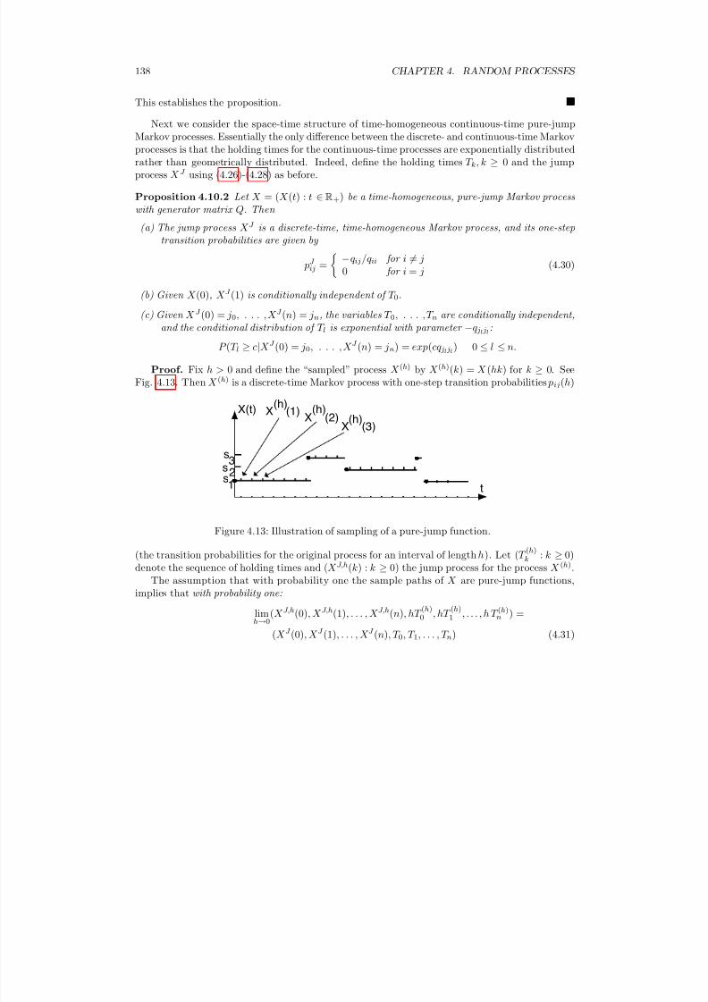
8/11/2019 Random process by B. Hajek
http://slidepdf.com/reader/full/random-process-by-b-hajek 148/448
138 CHAPTER 4. RANDOM PROCESSES
This establishes the proposition.
Next we consider the space-time structure of time-homogeneous continuous-time pure-jumpMarkov processes. Essentially the only difference between the discrete- and continuous-time Markovprocesses is that the holding times for the continuous-time processes are exponentially distributedrather than geometrically distributed. Indeed, define the holding times T k, k ≥ 0 and the jumpprocess X J using (4.26)-(4.28) as before.
Proposition 4.10.2 Let X = (X (t) : t ∈ R+) be a time-homogeneous, pure-jump Markov process with generator matrix Q. Then
(a) The jump process X J is a discrete-time, time-homogeneous Markov process, and its one-steptransition probabilities are given by
pJ ij =
−q ij/q ii for i = j0 for i = j
(4.30)
(b) Given X (0), X J (1) is conditionally independent of T 0.
(c) Given X J (0) = j0, . . . ,X J (n) = jn, the variables T 0, . . . ,T n are conditionally independent,and the conditional distribution of T l is exponential with parameter −q jl jl:
P (T l ≥ c|X J (0) = j0, . . . , X J (n) = jn) = exp(cq jl jl) 0 ≤ l ≤ n.
Proof. Fix h > 0 and define the “sampled” process X (h) by X (h)(k) = X (hk) for k ≥ 0. SeeFig. 4.13. Then X (h) is a discrete-time Markov process with one-step transition probabilities pij(h)
X(t)
t
(h)X (1)
X (2)(h)
X (3)
(h)
s
ss123
Figure 4.13: Illustration of sampling of a pure-jump function.
(the transition probabilities for the original process for an interval of length h). Let (T (h)k : k ≥ 0)
denote the sequence of holding times and (X J,h(k) : k ≥
0) the jump process for the process X (h).The assumption that with probability one the sample paths of X are pure-jump functions,
implies that with probability one:
limh→0
(X J,h(0), X J,h(1), . . . , X J,h(n), hT (h)0 , hT
(h)1 , . . . , h T (h)
n ) =
(X J (0), X J (1), . . . , X J (n), T 0, T 1, . . . , T n) (4.31)
8/11/2019 Random process by B. Hajek
http://slidepdf.com/reader/full/random-process-by-b-hajek 149/448
4.11. PROBLEMS 139
Since convergence with probability one implies convergence in distribution, the goal of identifyingthe distribution of the random vector on the righthand side of (4.31) can be accomplished byidentifying the limit of the distribution of the vector on the left.
First, the limiting distribution of the process X J,h
is identified. Since X (h)
has one-step transi-tion probabilities pij(h), the formula for the jump process probabilities for discrete-time processes
(see Proposition 4.10.1, part a) yields that the one step transition probabilities pJ,hij for X (J,h) are
given by
pJ,hij =
pij(h)
1 − pii(h)
= pij(h)/h
(1 − pii(h))/h → q ij
−q iias h → 0 (4.32)
for i = j , where the limit indicated in (4.32) follows from the definition (4.18) of the generator matrixQ. Thus, the limiting distribution of X J,h is that of a Markov process with one-step transition
probabilities given by (4.30), establishing part (a) of the proposition. The conditional independenceproperties stated in (b) and (c) of the proposition follow in the limit from the correspondingproperties for the jump process X J,h guaranteed by Proposition 4.10.1. Finally, since log(1 + θ) =θ + o(θ) by Taylor’s formula, we have for all c ≥ 0 that
P (hT (h)l > c|X J,h(0) = j0, . . . , X J,h = jn) = ( p jl jl(h))c/h
= exp(c/h log( p jl jl(h)))
= exp(c/h(q jl jlh + o(h)))
→ exp(q jl jlc) as h → 0
which establishes the remaining part of (c), and the proposition is proved.
4.11 Problems
4.1 Event probabilities for a simple random processDefine the random process X by X t = 2A + Bt where A and B are independent random variableswith P A = 1 = P A = −1 = P B = 1 = P B = −1 = 0.5. (a) Sketch the possible samplefunctions. (b) Find P X t ≥ 0 for all t. (c) Find P X t ≥ 0 for all t.
4.2 Correlation function of a productLet Y and Z be independent random processes with RY (s, t) = 2 exp(−|s − t|) cos(2πf (s − t)) and
RZ (s, t) = 9 + exp(−3|s − t|4). Find the autocorrelation function RX (s, t) where X t = Y tZ t.
4.3 A sinusoidal random processLet X t = A cos(2πV t + Θ) where the amplitude A has mean 2 and variance 4, the frequency V inHertz is uniform on [0, 5], and the phase Θ is uniform on [0, 2π]. Furthermore, suppose A, V and Θare independent. Find the mean function µX (t) and autocorrelation function RX (s, t). Is X WSS?
8/11/2019 Random process by B. Hajek
http://slidepdf.com/reader/full/random-process-by-b-hajek 150/448
8/11/2019 Random process by B. Hajek
http://slidepdf.com/reader/full/random-process-by-b-hajek 151/448
4.11. PROBLEMS 141
(d) Show that B is independent of the random variable W 1. (This means that for any finite collec-tion, t1, . . . , tn ∈ [0, 1], the random vector (Bt1, . . . , Btn)T is independent of W 1.)(e) (Due to J.L. Doob.) Let X t = (1 − t)W t
1−t, for 0 ≤ t < 1 and let X 1 = 0. Let X denote the
random process X = (X t : 0 ≤ t ≤ 1). Like W , X is a mean zero, Gaussian random process. Findthe autocorrelation function of X. Can you draw any conclusions?
4.10 Empirical distribution functions as random processesLet X 1, X 2, . . . be independent random variables, all with the same CDF F. For n ≥ 1, the empiricalCDF for n observations is defined by F n(t) = 1
n
nk=1 I X k≤t for t ∈R.
(a) Find the mean function and autocovariance function of the random process ( F n(t) : t ∈ R) forfixed n. (Hint: For computing the autocovariance, it may help to treat the cases s ≤ t and s ≥ tseparately.)(b) Explain why, for each t ∈R, limn→∞
F n(t) = F (t) almost surely.
(c) Let Dn = supt∈R |
F n(t) −F (t)|, so that Dn is a measure of distance between
F n and F. Suppose
the CDF F is continuous and strictly increasing. Show that the distribution of Dn is the same asit would be if the X n’s were all uniformly distributed on the interval [0, 1]. (Hint: Let U k = F (X k).Show that the U ’s are uniformly distributed on the interval [0, 1], let Gn be the empirical CDF forthe U ’s and let G be the CDF of the U ’s. Show that if F (t) = v, then | F n(t)−F (t)| = | Gn(v)−G(v)|.Then complete the proof.)(d) Let X n(t) =
√ n( F n(t) − F (t)) for t ∈ R. Find the limit in distribution of X n(t) for t fixed as
n → ∞.(e) (Note that
√ nDn = supt∈R |X n(t)|. ) Show that in the case the X ’s are uniformly distributed
on the interval [0, 1], the autocorrelation function of the process (X n(t) : 0 ≤ t ≤ 1) is the same asfor a Brownian bridge (discussed in the previous problem). (Note: The distance Dn is known as theKolmogorov-Smirnov statistic, and by pursuing the method of this problem further, the limitingdistribution of
√ nDn can be found and it is equal to the distribution of the maximum magnitude
of a Brownian bridge, a result due to J.L. Doob. )
4.11 Some Poisson process calculationsLet N = (N t : t ≥ 0) be a Poisson process with rate λ > 0.(a) Give a simple expression for P (N 1 ≥ 1|N 2 = 2) in terms of λ.(b) Give a simple expression for P (N 2 = 2|N 1 ≥ 1) in terms of λ.(c) Let X t = N 2t . Is X = (X t : t ≥ 0) a time-homogeneous Markov process? If so, give thetransition probabilities pij(τ ). If not, explain.
4.12 MMSE prediction for a Gaussian process based on two observationsLet X be a stationary Gaussian process with mean zero and RX (τ ) = 5 cos(πτ 2 )3−|τ |. (a) Find the
covariance matrix of the random vector (X (2), X (3), X (4))T . (b) Find E [X (4)|X (2)]. (c) FindE [X (4)|X (2), X (3)].
4.13 A simple discrete-time random processLet U = (U n : n ∈ Z) consist of independent random variables, each uniformly distributed on theinterval [0, 1]. Let X = (X k : k ∈ Z be defined by X k = maxU k−1, U k. (a) Sketch a typical
8/11/2019 Random process by B. Hajek
http://slidepdf.com/reader/full/random-process-by-b-hajek 152/448
142 CHAPTER 4. RANDOM PROCESSES
sample path of the process X . (b) Is X stationary? (c) Is X Markov? (d) Describe the first orderdistributions of X . (e) Describe the second order distributions of X .
4.14 Poisson process probabilitiesConsider a Poisson process with rate λ > 0.(a) Find the probability that there is (exactly) one count in each of the three intervals [0,1], [1,2],and [2,3].(b) Find the probability that there are two counts in the interval [0, 2] and two counts in the interval[1, 3]. (Note: your answer to part (b) should be larger than your answer to part (a)).(c) Find the probability that there are two counts in the interval [1,2], given that there are twocounts in the interval [0,2] and two counts in the the interval [1,3].
4.15 Sliding function of an i.i.d. Poisson sequenceLet X = (X k : k ∈ Z ) be a random process such that the X i are independent, Poisson randomvariables with mean λ, for some λ > 0. Let Y = (Y k : k
∈ Z ) be the random process defined by
Y k = X k + X k+1.(a) Show that Y k is a Poisson random variable with parameter 2λ for each k .(b) Show that X is a stationary random process.(c) Is Y a stationary random process? Justify your answer.
4.16 Adding jointly stationary Gaussian processesLet X and Y be jointly stationary, jointly Gaussian random processes with mean zero, autocorre-lation functions RX (t) = RY (t) = exp(−|t|), and cross-correlation functionRXY (t) = (0.5) exp(−|t − 3|).(a) Let Z (t) = (X (t) + Y (t))/2 for all t. Find the autocorrelation function of Z .(b) Is Z a stationary random process? Explain.(c) Find P
X (1)
≤ 5Y (2) + 1
. You may express your answer in terms of the standard normal
cumulative distribution function Φ.
4.17 Invariance of properties under transformationsLet X = (X n : n ∈ Z), Y = (Y n : n ∈ Z), and Z = (Z n : n ∈ Z) be random processes such thatY n = X 2n for all n and Z n = X 3n for all n. Determine whether each of the following statements isalways true. If true, give a justification. If not, give a simple counter example.(a) If X is Markov then Y is Markov.(b) If X is Markov then Z is Markov.(c) If Y is Markov then X is Markov.(d) If X is stationary then Y is stationary.(e) If Y is stationary then X is stationary.
(f) If X is wide sense stationary then Y is wide sense stationary.(g) If X has independent increments then Y has independent increments.(h) If X is a martingale then Z is a martingale.
4.18 A linear evolution equation with random coefficientsLet the variables Ak, Bk, k ≥ 0 be mutually independent with mean zero. Let Ak have variance σ2
A
8/11/2019 Random process by B. Hajek
http://slidepdf.com/reader/full/random-process-by-b-hajek 153/448
4.11. PROBLEMS 143
and let Bk have variance σ 2B for all k. Define a discrete-time random process Y by
Y = (Y k : k ≥ 0), such that Y 0 = 0 and Y k+1 = AkY k + Bk for k ≥ 0.(a) Find a recursive method for computing P k = E [(Y k)2] for k ≥ 0.
(b) Is Y a Markov process? Explain.(c) Does Y have independent increments? Explain.(d) Find the autocorrelation function of Y . ( You can use the second moments (P k) in expressingyour answer.)
(e) Find the corresponding linear innovations sequence (Y k : k ≥ 1).
4.19 On an M/D/infinity systemSuppose customers enter a service system according to a Poisson point process on R of rate λ,meaning that the number of arrivals, N (a, b], in an interval (a, b], has the Poisson distributionwith mean λ(b − a), and the numbers of arrivals in disjoint intervals are independent. Supposeeach customer stays in the system for one unit of time, independently of other customers. Because
the arrival process is memoryless, because the service times are deterministic, and because thecustomers are served simultaneously, corresponding to infinitely many servers, this queueing systemis called an M/D/∞ queueing system. The number of customers in the system at time t is givenby X t = N (t − 1, t].(a) Find the mean and autocovariance function of X .(b) Is X stationary? Is X wide sense stationary?(c) Is X a Markov process?(d) Find a simple expression for P X t = 0 for t ∈ [0, 1] in terms of λ.(e) Find a simple expression for P X t > 0 for t ∈ [0, 1] in terms of λ.
4.20 A Poisson spacing probability
Let N = (N t : t ≥ 0) be a Poisson process with some rate λ > 0. For t ≥ 0, let At be the eventthat during the interval [0, t] no two arrivals in the interval are closer than one unit of time apart.Let x(t) = P (At).(a) Find x(t) for 0 ≤ t ≤ 1.(b) Derive a differential equation for (x(t) : t ≥ 1) which expresses x(t) as a function of x(t) andx(t − 1). Begin by supposing t ≥ and h is a small positive constant, and writing an expression forx(t + h) in terms of x(t) and x(t−1). (This is a linear differential equation with a delay term. Fromthe viewpoint of solving such differential equations, we view the initial condition of the equationas the waveform (x(t) : 0 ≤ t ≤ 1). Since x is determined over [0, 1] in part (a), the differentialequation can then be used to solve, at least numerically, for x over the interval [1, 2], then over theinterval [2, 3], and so on, to determine x(t) for all t ≥ 0. Moreover, this shows that the solution
(x(t) : t ≥ 0) is an increasing function of its initial value, (x(t) : 0 ≤ t ≤ 1). This monotonicity isdifferent from monotonicity with respect to time. )(c) Give equations that identify θ∗ > 0 and constants c0 and c1 so that c0 ≤ x(t)eθ
∗t ≤ c1 for allt ≥ 0. (Hint: Use the fact that there is a solution of the differential equation found in part (b), butnot satisfying the initial condition over [0, 1] found in part (a), of the form y(t) = e−θ∗t for someθ∗ > 0, and use the monotonicity property identified in part (b).)
8/11/2019 Random process by B. Hajek
http://slidepdf.com/reader/full/random-process-by-b-hajek 154/448
144 CHAPTER 4. RANDOM PROCESSES
(d) The conditional probability of At, given there are exactly k arrivals during [0, t], ist−k+1
t
kfor 0 ≤ k ≤ t (Why?). Use that fact to give a series representation for (x(t) : t ≥ 0).
4.21 Hitting the corners of a triangleConsider a discrete-time Markov process (X k : k ≥ 0), with state space 1, 2, 3, 4, 5, 6. Supposethe states are arranged in the triangle shown,
6
1
2
3 4 5
and given X k = i, the next state X k+1 is one of the two neighbors of i, selected with probability0.5 each. Suppose P X 0 = 1 = 1.
(a) Let τ B = mink : X k ∈ 3, 4, 5. So τ B is the time the base of the triangle is first reached.Find E [τ B ].(b) Let τ 3 = mink : X k = 3. Find E [τ 3].(c) Let τ C be the first time k ≥ 1 such that both states 3 and 5 have been visited by time k . FindE [τ C ]. (Hint: Use results of (a) and (b) and symmetry.)(d) Let τ R denote the first time k ≥ τ C such that X k = 1. That is, τ R is the first time the processreturns to vertex 1 of the triangle after reaching both of the other vertices. Find E [τ R]. (Hint: Useresults of (c) and (b) and symmetry.)
4.22 A fly on a cubeConsider a cube with vertices 000, 001, 010, 100, 110, 101. 011, 111. Suppose a fly walks alongedges of the cube from vertex to vertex, and for any integer t
≥ 0, let X t denote which vertex the
fly is at at time t. Assume X = (X t : t ≥ 0) is a discrete-time Markov process, such that given X t,the next state X t+1 is equally likely to be any one of the three vertices neighboring X t.(a) Sketch the one step transition probability diagram for X .(b) Let Y t denote the distance of X t, measured in number of hops, between vertex 000 and X t. Forexample, if X t = 101, then Y t = 2. The process Y is a Markov process with states 0,1,2, and 3.Sketch the one-step transition probability diagram for Y .(c) Suppose the fly begins at vertex 000 at time zero. Let τ be the first time that X returns tovertex 000 after time 0, or equivalently, the first time that Y returns to 0 after time 0. Find E [τ ].
4.23 Time elapsed since Bernoulli renewalsLet U = (U k : k ∈ Z) be such that for some p ∈ (0, 1), the random variables U k are independent,
with each having the Bernoulli distribution with parameter p. Interpret U k = 1 to mean that arenewal, or replacement, of some part takes place at time k . For k ∈ Z, letX k = mini ≥ 1 : U k−i = 1. In words, X k is the time elapsed since the last renewal strictly beforetime k .(a) The process X is a time-homogeneous Markov process. Indicate a suitable state space, anddescribe the one-step transition probabilities.
8/11/2019 Random process by B. Hajek
http://slidepdf.com/reader/full/random-process-by-b-hajek 155/448
4.11. PROBLEMS 145
(b) Find the distribution of X k for k fixed.(c) Is X a stationary random process? Explain.(d) Find the k-step transition probabilities, pi,j(k) = P X n+k = j |X n = i.
4.24 A random process created by interpolationLet U = (U k : k ∈ Z) such that the U k are independent, and each is uniformly distributed onthe interval [0, 1]. Let X = (X t : t ∈ R) denote the continuous time random process obtained bylinearly interpolating between the U ’s. Specifically, X n = U n for any n ∈ Z, and X t is affine oneach interval of the form [n, n + 1] for n ∈ Z.(a) Sketch a sample path of U and a corresponding sample path of X.(b) Let t ∈ R. Find and sketch the first order marginal density, f X,1(x, t). (Hint: Let n = t anda = t − n, so that t = n + a. Then X t = (1 − a)U n + aU n+1. It’s helpful to consider the cases0 ≤ a ≤ 0.5 and 0.5 < a < 1 separately. For brevity, you need only consider the case 0 ≤ a ≤ 0.5.)(c) Is the random process X WSS? Justify your answer.
(d) Find P max0≤t≤10 X t ≤ 0.5.
4.25 Reinforcing samples(Due to G. Polya) Suppose at time k = 2, there is a bag with two balls in it, one orange and oneblue. During each time step between k and k + 1, one of the balls is selected from the bag atrandom, with all balls in the bag having equal probability. That ball, and a new ball of the samecolor, are both put into the bag. Thus, at time k there are k balls in the bag, for all k ≥ 2. Let X kdenote the number of blue balls in the bag at time k.(a) Is X = (X k : k ≥ 2) a Markov process?(b) Let M k = X k
k . Thus, M k is the fraction of balls in the bag at time k that are blue. Determinewhether M = (M k : k
≥ 2) is a martingale.
(c) By the theory of martingales, since M is a bounded martingale, it converges a.s. to somerandom variable M ∞. Let V k = M k(1 − M k). Show that E [V k+1|V k] = k(k+2)
(k+1)2 V k, and therefore that
E [V k] = (k+1)
6k . It follows that Var(limk→∞ M k) = 112 .
(d) More concretely, find the distribution of M k for each k, and then identify the distribution of the limit random variable, M ∞.
4.26 Restoring samplesSuppose at time k = 2, there is a bag with two balls in it, one orange and one blue. During eachtime step between k and k + 1, one of the balls is selected from the bag at random, with all ballsin the bag having equal probability. That ball, and a new ball of the other color, are both put into
the bag. Thus, at time k there are k balls in the bag, for all k ≥ 2. Let X k denote the number of blue balls in the bag at time k.(a) Is X = (X k : k ≥ 2) a Markov process? If so, describe the one-step transition probabilities.(b) Compute E [X k+1|X k] for k ≥ 2.(c) Let M k = X k
k . Thus, M k is the fraction of balls in the bag at time k that are blue. Determinewhether M = (M k : k ≥ 2) is a martingale.
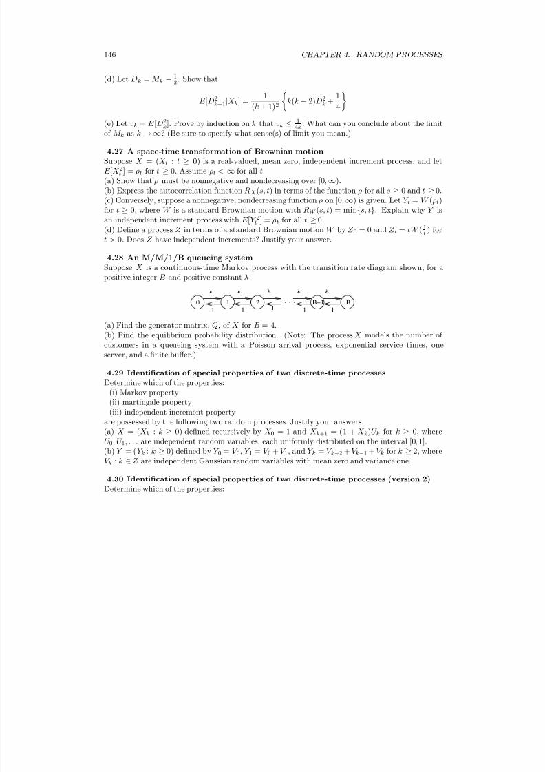
8/11/2019 Random process by B. Hajek
http://slidepdf.com/reader/full/random-process-by-b-hajek 156/448
146 CHAPTER 4. RANDOM PROCESSES
(d) Let Dk = M k − 12 . Show that
E [D2k+1
|X k] =
1
(k + 1)2 k(k
−2)D2
k + 1
4(e) Let vk = E [D2
k]. Prove by induction on k that vk ≤ 14k . What can you conclude about the limit
of M k as k → ∞? (Be sure to specify what sense(s) of limit you mean.)
4.27 A space-time transformation of Brownian motionSuppose X = (X t : t ≥ 0) is a real-valued, mean zero, independent increment process, and letE [X 2t ] = ρt for t ≥ 0. Assume ρt < ∞ for all t.(a) Show that ρ must be nonnegative and nondecreasing over [0, ∞).(b) Express the autocorrelation function RX (s, t) in terms of the function ρ for all s ≥ 0 and t ≥ 0.(c) Conversely, suppose a nonnegative, nondecreasing function ρ on [0, ∞) is given. Let Y t = W (ρt)for t ≥ 0, where W is a standard Brownian motion with RW (s, t) = mins, t. Explain why Y is
an independent increment process with E [Y 2t ] = ρt for all t ≥ 0.(d) Define a process Z in terms of a standard Brownian motion W by Z 0 = 0 and Z t = tW ( 1
t ) fort > 0. Does Z have independent increments? Justify your answer.
4.28 An M/M/1/B queueing systemSuppose X is a continuous-time Markov process with the transition rate diagram shown, for apositive integer B and positive constant λ.
! ! !
# # # ##
! ! ! ! !
$ # % &!# &
(a) Find the generator matrix, Q, of X for B = 4.(b) Find the equilibrium probability distribution. (Note: The process X models the number of customers in a queueing system with a Poisson arrival process, exponential service times, oneserver, and a finite buffer.)
4.29 Identification of special properties of two discrete-time processesDetermine which of the properties:
(i) Markov property(ii) martingale property(iii) independent increment property
are possessed by the following two random processes. Justify your answers.(a) X = (X k : k ≥ 0) defined recursively by X 0 = 1 and X k+1 = (1 + X k)U k for k ≥ 0, where
U 0, U 1, . . . are independent random variables, each uniformly distributed on the interval [0, 1].(b) Y = (Y k : k ≥ 0) defined by Y 0 = V 0, Y 1 = V 0 + V 1, and Y k = V k−2 + V k−1 + V k for k ≥ 2, whereV k : k ∈ Z are independent Gaussian random variables with mean zero and variance one.
4.30 Identification of special properties of two discrete-time processes (version 2)Determine which of the properties:
8/11/2019 Random process by B. Hajek
http://slidepdf.com/reader/full/random-process-by-b-hajek 157/448
4.11. PROBLEMS 147
(i) Markov property(ii) martingale property(iii) independent increment property
are possessed by the following two random processes. Justify your answers.(a) (X k : k ≥ 0), where X k is the number of cells alive at time k in a colony that evolves asfollows. Initially, there is one cell, so X 0 = 1. During each discrete time step, each cell either diesor splits into two new cells, each possibility having probability one half. Suppose cells die or splitindependently. Let X k denote the number of cells alive at time k.(b) (Y k : k ≥ 0), such that Y 0 = 1 and, for k ≥ 1, Y k = U 1U 2 . . . U k, where U 1, U 2, . . . are independentrandom variables, each uniformly distributed over the interval [0, 2]
4.31 Identification of special properties of two continuous-time processesAnswer as in the previous problem, for the following two random processes:(a) Z = (Z t : t ≥ 0), defined by Z t = exp(W t− σ2t
2 ), where W is a Brownian motion with parameterσ2. (Hint: Observe that E [Z t] = 1 for all t.)
(b) R = (Rt : t ≥ 0) defined by Rt = D1 + D2 + · · · + DN t, where N is a Poisson process with rateλ > 0 and Di : i ≥ 1 is an iid sequence of random variables, each having mean 0 and variance σ2.
4.32 Identification of special properties of two continuous-time processes (version 2)Answer as in the previous problem, for the following two random processes:(a) Z = (Z t : t ≥ 0), defined by Z t = W 3t , where W is a Brownian motion with parameter σ2.(b) R = (Rt : t ≥ 0), defined by Rt = cos(2πt +Θ), where Θ is uniformly distributed on the interval[0, 2π].
4.33 A branching processLet p = ( pi : i ≥ 0) be a probability distribution on the nonnegative integers with mean m.Consider a population beginning with a single individual, comprising generation zero. The offspring
of the initial individual comprise the first generation, and, in general, the offspring of the kthgeneration comprise the k + 1st generation. Suppose the number of offspring of any individual hasthe probability distribution p, independently of how many offspring other individuals have. LetY 0 = 1, and for k ≥ 1 let Y k denote the number of individuals in the kth generation.(a) Is Y = (Y k : k ≥ 0) a Markov process? Briefly explain your answer.(b) Find constants ck so that Y k
ckis a martingale.
(c) Let am = P Y m = 0, the probability of extinction by the mth generation. Express am+1
in terms of the distribution p and am (Hint: condition on the value of Y 1, and note that the Y 1subpopulations beginning with the Y 1 individuals in generation one are independent and statisticallyidentical to the whole population.)(d) Express the probability of eventual extinction, a
∞ = limm
→∞am, in terms of the distribution
p. Under what condition is a∞ = 1?(e) Find a∞ in terms of θ in case pk = θk(1 − θ) for k ≥ 0 and 0 ≤ θ < 1. (This distribution issimilar to the geometric distribution, and it has mean m = θ
1−θ .)
4.34 Moving ballsConsider the motion of three indistinguishable balls on a linear array of positions, indexed by the
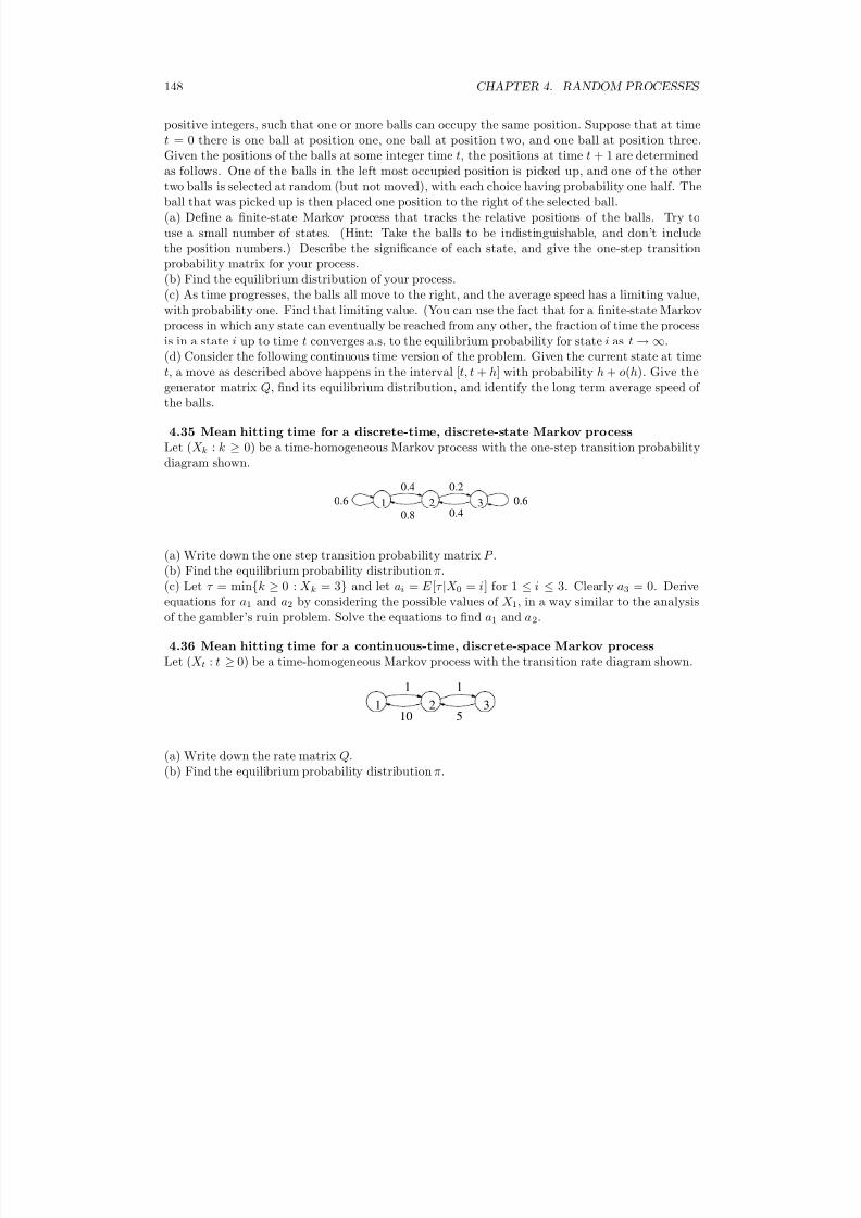
8/11/2019 Random process by B. Hajek
http://slidepdf.com/reader/full/random-process-by-b-hajek 158/448
148 CHAPTER 4. RANDOM PROCESSES
positive integers, such that one or more balls can occupy the same position. Suppose that at timet = 0 there is one ball at position one, one ball at position two, and one ball at position three.Given the positions of the balls at some integer time t, the positions at time t + 1 are determined
as follows. One of the balls in the left most occupied position is picked up, and one of the othertwo balls is selected at random (but not moved), with each choice having probability one half. Theball that was picked up is then placed one position to the right of the selected ball.(a) Define a finite-state Markov process that tracks the relative positions of the balls. Try touse a small number of states. (Hint: Take the balls to be indistinguishable, and don’t includethe position numbers.) Describe the significance of each state, and give the one-step transitionprobability matrix for your process.(b) Find the equilibrium distribution of your process.(c) As time progresses, the balls all move to the right, and the average speed has a limiting value,with probability one. Find that limiting value. (You can use the fact that for a finite-state Markovprocess in which any state can eventually be reached from any other, the fraction of time the processis in a state i up to time t converges a.s. to the equilibrium probability for state i as t
→ ∞.
(d) Consider the following continuous time version of the problem. Given the current state at timet, a move as described above happens in the interval [t, t + h] with probability h + o(h). Give thegenerator matrix Q, find its equilibrium distribution, and identify the long term average speed of the balls.
4.35 Mean hitting time for a discrete-time, discrete-state Markov processLet (X k : k ≥ 0) be a time-homogeneous Markov process with the one-step transition probabilitydiagram shown.
1 2 3
0.2
0.6 0.6
0.4
0.4
0.8
(a) Write down the one step transition probability matrix P .(b) Find the equilibrium probability distribution π.(c) Let τ = mink ≥ 0 : X k = 3 and let ai = E [τ |X 0 = i] for 1 ≤ i ≤ 3. Clearly a3 = 0. Deriveequations for a1 and a2 by considering the possible values of X 1, in a way similar to the analysisof the gambler’s ruin problem. Solve the equations to find a1 and a2.
4.36 Mean hitting time for a continuous-time, discrete-space Markov processLet (X t : t ≥ 0) be a time-homogeneous Markov process with the transition rate diagram shown.
1 2 3
10
1
5
1
(a) Write down the rate matrix Q.(b) Find the equilibrium probability distribution π.

8/11/2019 Random process by B. Hajek
http://slidepdf.com/reader/full/random-process-by-b-hajek 159/448
4.11. PROBLEMS 149
(c) Let τ = mint ≥ 0 : X t = 3 and let ai = E [τ |X 0 = i] for 1 ≤ i ≤ 3. Clearly a3 = 0. Deriveequations for a1 and a2 by considering the possible values of X t(h) for small values of h > 0 andtaking the limit as h → 0. Solve the equations to find a1 and a2.
4.37 Poisson mergerSumming counting processes corresponds to “merging” point processes. Show that the sum of K independent Poisson processes, having rates λ1, . . . , λK , respectively, is a Poisson process with rateλ1 + . . . + λK . (Hint: First formulate and prove a similar result for sums of random variables,and then think about what else is needed to get the result for Poisson processes. You can use thedefinition of a Poisson process or one of the equivalent descriptions given by Proposition 4.5.2 inthe notes. Don’t forget to check required independence properties.)
4.38 Poisson splittingConsider a stream of customers modeled by a Poisson process, and suppose each customer is oneof K types. Let ( p
1, . . . , p
K ) be a probability vector, and suppose that for each k, the kth customer
is type i with probability pi. The types of the customers are mutually independent and alsoindependent of the arrival times of the customers. Show that the stream of customers of a giventype i is again a Poisson stream, and that its rate is λpi. (Same hint as in the previous problemapplies.) Show furthermore that the K substreams are mutually independent.
4.39 Poisson method for coupon collector’s problem(a) Suppose a stream of coupons arrives according to a Poisson process ( A(t) : t ≥ 0) with rateλ = 1, and suppose there are k types of coupons. (In network applications, the coupons could bepieces of a file to be distributed by some sort of gossip algorithm.) The type of each coupon in thestream is randomly drawn from the k types, each possibility having probability 1
k , and the types of different coupons are mutually independent. Let p(k, t) be the probability that at least one coupon
of each type arrives by time t. (The letter “ p” is used here because the number of coupons arrivingby time t has the Poisson distribution). Express p(k, t) in terms of k and t.(b) Find limk→∞ p(k, k ln k+kc) for an arbitrary constant c. That is, find the limit of the probabilitythat the collection is complete at time t = k ln k + kc. (Hint: If ak → a as k → ∞, then (1 + ak
k )k →ea.)(c) The rest of this problem shows that the limit found in part (b) also holds if the total number of coupons is deterministic, rather than Poisson distributed. One idea is that if t is large, then A(t)is not too far from its mean with high probability. Show, specifically, that
limk→∞ P A(k ln k + kc) ≥ k ln k + kc =
0 if c < c
1 if c > c
(d) Let d(k, n) denote the probability that the collection is complete after n coupon arrivals. (The
letter “d” is used here because the number of coupons, n, is deterministic.) Show that for any k, t,and n fixed, d(k, n)P A(t) ≥ n ≤ p(k, t) ≤ P A(t) ≥ n + P A(t) ≤ nd(k, n).(e) Combine parts (c) and (d) to identify limk→∞ d(k, k ln k + kc).
4.40 Some orthogonal martingales based on Brownian motion(Related to Problem 3.27.) Let W = (W t : t ≥ 0) be a Brownian motion with σ2 = 1 (called a
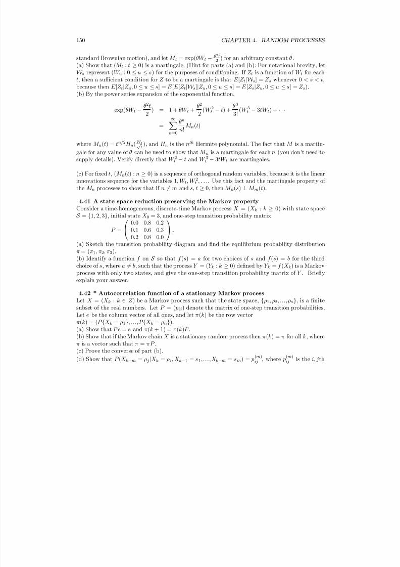
8/11/2019 Random process by B. Hajek
http://slidepdf.com/reader/full/random-process-by-b-hajek 160/448
150 CHAPTER 4. RANDOM PROCESSES
standard Brownian motion), and let M t = exp(θW t − θ2t2 ) for an arbitrary constant θ .
(a) Show that (M t : t ≥ 0) is a martingale. (Hint for parts (a) and (b): For notational brevity, letW s represent (W u : 0 ≤ u ≤ s) for the purposes of conditioning. If Z t is a function of W t for each
t, then a sufficient condition for Z to be a martingale is that E [Z t|W s] = Z s whenever 0 < s < t,because then E [Z t|Z u, 0 ≤ u ≤ s] = E [E [Z t|W s]|Z u, 0 ≤ u ≤ s] = E [Z s|Z u, 0 ≤ u ≤ s] = Z s).(b) By the power series expansion of the exponential function,
exp(θW t − θ2t
2 ) = 1 + θW t +
θ2
2 (W 2t − t) +
θ 3
3!(W 3t − 3tW t) + · · ·
=∞
n=0
θn
n!M n(t)
where M n(t) = tn/2H n(W t√ t
), and H n is the nth Hermite polynomial. The fact that M is a martin-
gale for any value of θ can be used to show that M n is a martingale for each n (you don’t need to
supply details). Verify directly that W
2
t − t and W
3
t − 3tW t are martingales.
(c) For fixed t, (M n(t) : n ≥ 0) is a sequence of orthogonal random variables, because it is the linearinnovations sequence for the variables 1, W t, W 2t , . . .. Use this fact and the martingale property of the M n processes to show that if n = m and s, t ≥ 0, then M n(s) ⊥ M m(t).
4.41 A state space reduction preserving the Markov propertyConsider a time-homogeneous, discrete-time Markov process X = (X k : k ≥ 0) with state spaceS = 1, 2, 3, initial state X 0 = 3, and one-step transition probability matrix
P =
0.0 0.8 0.20.1 0.6 0.30.2 0.8 0.0
.
(a) Sketch the transition probability diagram and find the equilibrium probability distributionπ = (π1, π2, π3).(b) Identify a function f on S so that f (s) = a for two choices of s and f (s) = b for the thirdchoice of s, where a = b, such that the process Y = (Y k : k ≥ 0) defined by Y k = f (X k) is a Markovprocess with only two states, and give the one-step transition probability matrix of Y . Brieflyexplain your answer.
4.42 * Autocorrelation function of a stationary Markov processLet X = (X k : k ∈ Z ) be a Markov process such that the state space, ρ1, ρ2,...,ρn, is a finitesubset of the real numbers. Let P = ( pij) denote the matrix of one-step transition probabilities.Let e be the column vector of all ones, and let π(k) be the row vector
π(k) = (P X k = ρ1,...,P X k = ρn).(a) Show that P e = e and π(k + 1) = π(k)P .(b) Show that if the Markov chain X is a stationary random process then π(k) = π for all k, whereπ is a vector such that π = πP .(c) Prove the converse of part (b).
(d) Show that P (X k+m = ρ j|X k = ρi, X k−1 = s1,...,X k−m = sm) = p(m)ij , where p
(m)ij is the i, jth

8/11/2019 Random process by B. Hajek
http://slidepdf.com/reader/full/random-process-by-b-hajek 161/448
4.11. PROBLEMS 151
element of the mth power of P , P m, and s1, . . . , sm are arbitrary states.(e) Assume that X is stationary. Express RX (k) in terms of P , (ρi), and the vector π of parts (b)and (c).

8/11/2019 Random process by B. Hajek
http://slidepdf.com/reader/full/random-process-by-b-hajek 162/448
152 CHAPTER 4. RANDOM PROCESSES
8/11/2019 Random process by B. Hajek
http://slidepdf.com/reader/full/random-process-by-b-hajek 163/448
Chapter 5
Inference for Markov Models
This chapter gives a glimpse of the theory of iterative algorithms for graphical models, as well as an
introduction to statistical estimation theory. It begins with a brief introduction to estimation the-ory: maximum likelihood and Bayes estimators are introduced, and an iterative algorithm, knownas the expectation-maximization algorithm, for computation of maximum likelihood estimators incertain contexts, is described. This general background is then focused on three inference problemsposed using Markov models.
5.1 A bit of estimation theory
The two most commonly used methods for producing estimates of unknown quantities are themaximum likelihood (ML) and Bayesian methods. These two methods are briefly described in thissection, beginning with the ML method.
Suppose a parameter θ is to be estimated, based on observation of a random variable Y . Anestimator of θ based on Y is a function θ, which for each possible observed value y, gives theestimate θ(y). The ML method is based on the assumption that Y has a pmf pY (y|θ) (if Y isdiscrete type) or a pdf f Y (y|θ) (if Y is continuous type), where θ is the unknown parameter to beestimated, and the family of functions pY (y|θ) or f Y (y|θ), is known.
Definition 5.1.1 For a particular value y and parameter value θ, the likelihood of y for θ is pY (y|θ), if Y is discrete type, or f Y (y|θ), if Y is continuous type. The maximum likelihood estimateof θ given Y = y for a particular y is the value of θ that maximizes the likelihood of y. That is, the maximum likelihood estimator
θML is given by
θML(y) = argmaxθ pY (y|θ), or
θML(y) =
arg maxθ f Y (y|θ).
Note that the maximum likelihood estimator is not defined as one maximizing the likelihoodof the parameter θ to be estimated. In fact, θ need not even be a random variable. Rather, themaximum likelihood estimator is defined by selecting the value of θ that maximizes the likelihoodof the observation.
153
8/11/2019 Random process by B. Hajek
http://slidepdf.com/reader/full/random-process-by-b-hajek 164/448
154 CHAPTER 5. INFERENCE FOR MARKOV MODELS
Example 5.1.2 Suppose Y is assumed to be a N (θ, σ2) random variable, where σ2 is known.Equivalently, we can write Y = θ + W , where W is a N (0, σ2) random variable. Given a value
y is observed, the ML estimator is obtained by maximizing f Y (y
|θ) = 1√
2πσ2 exp −
(y−θ)2
2σ2 with
respect to θ. By inspection, θML(y) = y.
Example 5.1.3 Suppose Y is assumed to be a P oi(θ) random variable, for some θ > 0. Given theobservation Y = k for some fixed k ≥ 0, the ML estimator is obtained by maximizing pY (k|θ) =e−θθk
k! with respect to θ. Equivalently, dropping the constant k! and taking the logarithm, θ is tobe selected to maximize −θ + k ln θ. The derivative is −1 + k/θ, which is positive for θ < k andnegative for θ > k . Hence, θML(k) = k.
Note that in the ML method, the quantity to be estimated, θ, is not assumed to be random.
This has the advantage that the modeler does not have to come up with a probability distributionfor θ, and the modeler can still impose hard constraints on θ. But the ML method does not permitincorporation of soft probabilistic knowledge the modeler may have about θ before any observationis used.
The Bayesian method is based on estimating a random quantity. Thus, in the end, the variableto be estimated, say Z , and the observation, say Y , are jointly distributed random variables.
Definition 5.1.4 The Bayes estimator of Z given Y, for jointly distributed random variables Z and Y, and cost function C (z, y), is the function Z = g(Y ) of Y which minimizes the average cost,E [C (Z, Z )].
The assumed distribution of Z is called the prior or a priori distribution, whereas the conditional
distribution of Z given Y is called the posterior or a posteriori distribution. In particular, if Z isdiscrete, there is a prior pmf, pZ , and a posterior pmf, pZ |Y , or if Z and Y are jointly continuous,there is a prior pdf, f Z , and a posterior pdf, f Z |Y .
One of the most common choices of the cost function is the squared error, C (z, z) = (z − z)2, forwhich the Bayes estimators are the minimum mean squared error (MMSE) estimators, examinedin Chapter 3. Recall that the MMSE estimators are given by the conditional expectation, g(y) =E [Z |Y = y], which, given the observation Y = y, is the mean of the posterior distribution of Z given Y = y.
A commonly used choice of C in case Z is a discrete random variable is C (z, z) = I z= bz. In
this case, the Bayesian objective is to select Z to minimize P Z = Z , or equivalently, to maximizeP
Z = Z
. For an estimator Z = g(Y ),
P Z = Z =y
P (Z = g(y)|Y = y) pY (y) =y
pZ |Y (g(y)|y) pY (y).
So a Bayes estimator for C (z, z) = I z= bz is one such that g(y) maximizes P (Z = g(y)|Y = y) foreach y. That is, for each y, g(y) is a maximizer of the posterior pmf of Z . The estimator, called
8/11/2019 Random process by B. Hajek
http://slidepdf.com/reader/full/random-process-by-b-hajek 165/448
5.1. A BIT OF ESTIMATION THEORY 155
the maximum a posteriori probability (MAP) estimator, can be written concisely as
Z MAP (y) = arg max
z pZ |Y (z|y).
Suppose there is a parameter θ to be estimated based on an observation Y, and suppose thatthe pmf of Y, pY (y|θ), is known for each θ. This is enough to determine the ML estimator, butdetermination of a Bayes estimator requires, in addition, a choice of cost function C and a priorprobability distribution (i.e. a distribution for θ). For example, if θ is a discrete variable, theBayesian method would require that a prior pmf for θ be selected. In that case, we can view theparameter to be estimated as a random variable, which we might denote by the upper case symbolΘ, and the prior pmf could be denoted by pΘ(θ). Then, as required by the Bayesian method, thevariable to be estimated, Θ, and the observation, Y , would be jointly distributed random variables.The joint pmf would be given by pΘ,Y (θ, Y ) = pΘ(θ) pY (y|θ). The posterior probability distributioncan be expressed as a conditional pmf, by Bayes’ formula:
pΘ|Y (θ|y) = pΘ(θ) pY (y|θ) pY (y)
(5.1)
where pY (y) =
θ pΘ,Y (θ, y). Given y, the value of the MAP estimator is a value of θ thatmaximizes pΘ|Y (θ|y) with respect to θ. For that purpose, the denominator in the right-hand sideof (5.1) can be ignored, so that the MAP estimator is given by
ΘMAP (y) = arg m axθ
pΘ|Y (θ|y)
= arg maxθ
pΘ(θ) pY (y|θ). (5.2)
The expression, (5.2), for ΘMAP (y) is rather similar to the expression for the ML estimator, θML(y) = arg maxθ pY (y|θ). In fact, the two estimators agree if the prior pΘ(θ) is uniform , meaningit is the same for all θ.
The MAP criterion for selecting estimators can be extended to the case that Y and θ are jointlycontinuous variables, leading to the following:
ΘMAP (y) = arg m axθ
f Θ|Y (θ|y)
= arg maxθ
f Θ(θ)f Y (y|θ). (5.3)
In this case, the probability that any estimator is exactly equal to θ is zero, but taking ΘMAP (y)to maximize the posterior pdf maximizes the probability that the estimator is within of the truevalue of θ , in an asymptotic sense as
→ 0.
Example 5.1.5 Suppose Y is assumed to be a N (θ, σ2) random variable, where the variance σ2 isknown and θ is to be estimated. Using the Bayesian method, suppose the prior density of θ is theN (0, b2) density for some known parameter b2. Equivalently, we can write Y = Θ+ W , where Θ is aN (0, b2) random variable and W is a N (0, σ2) random variable, independent of Θ. By the properties
8/11/2019 Random process by B. Hajek
http://slidepdf.com/reader/full/random-process-by-b-hajek 166/448
156 CHAPTER 5. INFERENCE FOR MARKOV MODELS
of joint Gaussian densities given in Chapter 3, given Y = y, the posterior distribution (i.e. the
conditional distribution of Θ given y) is the normal distribution with mean
E [Θ|Y = y] = b2y
b2+σ2
and variance b2σ2
b2+σ2 . The mean and maximizing value of this conditional density are both equal to E [Θ|Y = y]. Therefore, ΘMMSE (y) = ΘMAP (y) = E [Θ|Y = y]. It is interesting to compare thisexample to Example 5.1.2. The Bayes estimators (MMSE and MAP) are both smaller in magnitude
than θML(y) = y, by the factor b2
b2+σ2 . If b2 is small compared to σ2, the prior information indicatesthat |θ| is believed to be small, resulting in the Bayes estimators being smaller in magnitude thanthe ML estimator. As b2 → ∞, the priori distribution gets increasingly uniform, and the Bayesestimators coverge to the ML estimator.
Example 5.1.6 Suppose Y is assumed to be a P oi(θ) random variable. Using the Bayesianmethod, suppose the prior distribution for θ is the uniformly distribution over the interval [0, θmax],for some known value θ
max. Given the observation Y = k for some fixed k
≥ 0, the MAP estimator
is obtained by maximizing
pY (k|θ)f Θ(θ) = e−θθk
k!
I 0≤θ≤θθmaxθmax
with respect to θ. As seen in Example 5.1.3, the term e−θθk
k! is increasing in θ for θ < k anddecreasing in θ for θ > k. Therefore, ΘMAP (k) = mink, θmax.
It is interesting to compare this example to Example 5.1.3. Intuitively, the prior probability distri-bution indicates knowledge that θ ≤ θmax, but no more than that, because the prior restricted toθ
≤ θmax is uniform. If θmax is less than k , the MAP estimator is strictly smaller than θML(k) = k.
As θmax → ∞, the MAP estimator converges to the ML estimator. Actually, deterministic priorknowledge, such as θ ≤ θmax, can also be incorporated into ML estimation as a hard constraint.
The next example makes use of the following lemma.
Lemma 5.1.7 Suppose ci ≥ 0 for 1 ≤ i ≤ n and that c = n
i=1 ci > 0. Then n
i=1 ci log pi is maximized over all probability vectors p = ( p1. . . . , pn) by pi = ci/c.
Proof. If c j = 0 for some j, then clearly p j = 0 for the maximizing probability vector. Byeliminating such terms from the sum, we can assume without loss of generality that ci > 0 forall i. The function to be maximized is a strictly concave function of p over a region with linearconstraints. The positivity constraints, namely pi ≥ 0, will be satisfied with strict inequality.
The remaining constraint is the equality constraint, ni=1 pi = 1. We thus introduce a Lagrange
multiplier λ for the equality constraint and seek the stationary point of the Lagrangian L( p, λ) =ni=1 ci log pi−λ((
ni=1 pi)−1). By definition, the stationary point is the point at which the partial
derivatives with respect to the variables pi are all zero. Setting ∂L∂pi
= ci pi
− λ = 0 yields that pi = ciλ
for all i. To satisfy the linear constraint, λ must equal c.
8/11/2019 Random process by B. Hajek
http://slidepdf.com/reader/full/random-process-by-b-hajek 167/448
5.1. A BIT OF ESTIMATION THEORY 157
Example 5.1.8 Suppose b = (b1, b2, . . . , bn) is a probability vector to be estimated by observingY = (Y 1, . . . , Y T ). Assume Y 1, . . . , Y T are independent, with each Y t having probability distribution
b: P Y t = i = bi for 1 ≤ t ≤ T and 1 ≤ i ≤ n. We shall determine the maximum likelihoodestimate, bML(y), given a particular observation y = (y1, . . . , yT ). The likelihood to be maximizedwith respect to b is p(y|b) = by1 · · · byT
= n
i=1 bkii where ki = |t : yt = i|. The log likelihood is
ln p(y|b) = n
i=1 ki ln(bi). By Lemma 5.1.7, this is maximized by the empirical distribution of the
observations, namely bi = kiT for 1 ≤ i ≤ n. That is, bML = (k1
T , . . . , knT ).
Example 5.1.9 This is a Bayesian version of the previous example. Suppose b = (b1, b2, . . . , bn)is a probability vector to be estimated by observing Y = (Y 1, . . . , Y T ), and assume Y 1, . . . , Y T areindependent, with each Y t having probability distribution b. For the Bayesian method, a distribution
of the unknown distribution b must be assumed. That is right, a distribution of the distributionis needed. A convenient choice is the following. Suppose for some known numbers di ≥ 1 that(b1, . . . , bn−1) has the prior density:
f B(b) =
Qni=1 b
di−1i
Z (d) if bi ≥ 0 for 1 ≤ i ≤ n − 1, and n−1
i=1 bi ≤ 1
0 else
where bn = 1 − b1 − · · ·− bn−1, and Z (d) is a constant chosen so that f B integrates to one. A largervalue of di for a fixed i expresses an a priori guess that the corresponding value bi may be larger. Itcan be shown, in particular, that if B has this prior distribution, then E [Bi] =
did1+···dn
. The MAP
estimate, bMAP (y), for a given observation vector y , is given by:
bMAP (y) = arg maxb
ln (f B(b) p(y|b)) = arg maxb
− ln(Z (d)) +
ni=1
(di − 1 + ki)ln(bi)
By Lemma 5.1.7, bMAP (y) = ( d1−1+k1eT , . . . , dn−1+kneT ), where T =n
i=1(di−1+ki) = T −n+n
i=1 di.
Comparison with Example 5.1.8 shows that the MAP estimate is the same as the ML estimate,except that di − 1 is added to ki for each i. If the di’s are integers, the MAP estimate is the MLestimate with some prior observations mixed in, namely, di − 1 prior observations of outcome i foreach i. A prior distribution such that the MAP estimate has the same algebraic form as the MLestimate is called a conjugate prior , and the specific density f B for this example is a called theDirichlet density with parameter vector d.
Example 5.1.10 Suppose Y = (Y 1, . . . , Y T ) is observed, and it is assumed that the Y i are inde-pendent, with the binomial distribution with parameters n and q. Suppose n is known, and q isan unknown parameter to be estimated from Y . Let us find the maximum likelihood estimate,
8/11/2019 Random process by B. Hajek
http://slidepdf.com/reader/full/random-process-by-b-hajek 168/448
158 CHAPTER 5. INFERENCE FOR MARKOV MODELS
q ML(y), for a particular observation y = (y1, . . . , yT ). The likelihood is
p(y
|q ) =
T
t=1 n
ytq yt(1
−q )n−yt = cq s(1
−q )nT −s,
where s = y1 + · · · + yT , and c depends on y but not on q. The log likelihood is ln c + s ln(q ) +(nT − s)ln(1 − q ). Maximizing over q yields q ML = s
nT . An alternative way to think about this isto realize that each Y t can be viewed as the sum of n independent Bernoulli(q ) random variables,and s can be viewed as the observed sum of nT independent Bernoulli(q ) random variables.
5.2 The expectation-maximization (EM) algorithm
The expectation-maximization algorithm is a computational method for computing maximum like-lihood estimates in contexts where there are hidden random variables, in addition to observed dataand unknown parameters. The following notation will be used.
θ, a parameter to be estimated
X, the complete data
pcd(x|θ), the pmf of the complete data, which is a known function for each value of θ
Y = h(X ), the observed random vector
Z, the unobserved data (This notation is used in the common case that X has the form X =(Y, Z ).)
We write p(y|θ) to denote the pmf of Y for a given value of θ. It can be expressed in terms of thepmf of the complete data by:
p(y|θ) =
x:h(x)=y pcd(x|θ) (5.4)
In some applications, there can be a very large number of terms in the sum in ( 5.4), making itdifficult to numerically maximize p(y|θ) with respect to θ (i.e. to compute θML(y)).
Algorithm 5.2.1 (Expectation-maximization (EM) algorithm) An observation y is given, along with an intitial estimate θ(0). The algorithm is iterative. Given θ(k), the next value θ(k+1) is com-puted in the following two steps:
(Expectation step) Compute Q(θ|θ(k)
) for all θ, where
Q(θ|θ(k)) = E [ log pcd(X |θ) | y, θ(k)]. (5.5)
(Maximization step) Compute θ(k+1) ∈ arg maxθ Q(θ|θ(k)). In other words, find a value θ(k+1) of θ that maximizes Q(θ|θ(k)) with respect to θ.
8/11/2019 Random process by B. Hajek
http://slidepdf.com/reader/full/random-process-by-b-hajek 169/448
5.2. THE EXPECTATION-MAXIMIZATION (EM) ALGORITHM 159
Some intuition behind the algorithm is the following. If a vector of complete data x couldbe observed, it would be reasonable to estimate θ by maximizing the pmf of the complete data, pcd(x|θ), with respect to θ. This plan is not feasible if the complete data is not observed. The idea is
to estimate log pcd(X |θ) by its conditional expectation, Q(θ|θ(k)
), and then find θ to maximize thisconditional expectation. The conditional expectation is well defined if some value of the parameterθ is fixed. For each iteration of the algorithm, the expectation step is completed using the latestvalue of θ , θ (k), in computing the expectation of log pcd(X |θ).
In most applications there is some additional structure that helps in the computation of Q(θ|θ(k)).This typically happens when pcd factors into simple terms, such as in the case of hidden Markovmodels discussed in this chapter, or when pcd has the form of an exponential raised to a low degreepolynomial, such as the Gaussian or exponential distribution. In some cases there are closed formexpressions for Q(θ|θ(k)). In others, there may be an algorithm that generates samples of X withthe desired pmf pcd(x|θ(k)) using random number generators, and then log pcd(X |θ) is used as anapproximation to Q(θ|θ(k)).
Example 5.2.2 (Estimation of the variance of a signal) An observation Y is modeled as Y = S +N,where the signal S is assumed to be a N (0, θ) random variable, where θ is an unknown parameter,assumed to satisfy θ ≥ 0, and the noise N is a N (0, σ2) random variable where σ2 is known andstrictly positive. Suppose it is desired to estimate θ, the variance of the signal. Let y be a particularobserved value of Y. We consider two approaches to finding θML : a direct approach, and the EMalgorithm.
For the direct approach, note that for θ fixed, Y is a N (0, θ + σ2) random variable. Therefore,the pdf of Y evaluated at y , or likelihood of y, is given by
f (y|θ) =exp(− y2
2(θ+σ2) )
2π(θ + σ2).
The natural log of the likelihood is given by
log f (y|θ) = − log(2π)
2 − log(θ + σ2)
2 − y2
2(θ + σ2).
Maximizing over θ yields θML = (y2 − σ2)+. While this one-dimensional case is fairly simple, thesituation is different in higher dimensions, as explored in Problem 5.7. Thus, we examine use of the EM algorithm for this example.
To apply the EM algorithm for this example, take X = (S, N ) as the complete data. Theobservation is only the sum, Y = S + N, so the complete data is not observed. For given θ , S andN are independent, so the log of the joint pdf of the complete data is given as follows:
log pcd(s, n|θ) = −log(2πθ)
2 − s2
2θ − log(2πσ2)
2 − n2
2σ2 .
For the expectation step, we find
Q(θ|θ(k)) = E [ log pcd(S, N |θ) |y, θ(k)]
= − log(2πθ)
2 − E [S 2|y, θ(k)]
2θ − log(2πσ2)
2 − E [N 2|y, θ(k)]
2σ2 .
8/11/2019 Random process by B. Hajek
http://slidepdf.com/reader/full/random-process-by-b-hajek 170/448
160 CHAPTER 5. INFERENCE FOR MARKOV MODELS
For the maximization step, we find
∂Q(θ|θ(k))
∂θ
=
−
1
2θ
+ E [S 2|y, θ(k)]
2θ2
from which we see that θ(k+1) = E [S 2|y, θ(k)]. Computation of E [S 2|y, θ(k)] is an exercise inconditional Gaussian distributions, similar to Example 3.4.5. The conditional second moment isthe sum of the square of the conditional mean and the variance of the estimation error. Thus, theEM algorithm becomes the following recursion:
θ(k+1) =
θ(k)
θ(k) + σ2
2
y2 + θ(k)σ2
θ(k) + σ2 (5.6)
Problem 5.5 shows that if θ (0) > 0, then θ (k) →
θML as k → ∞.
Proposition 5.2.5 below shows that the likelihood p(y|θ(k)) is nondecreasing in k. In the idealcase, the likelihood converges to the maximum possible value of the likelihood, and limk→∞ θ(k) = θML(y). However, the sequence could converge to a local, but not global, maximizer of the likelihood,or possibly even to an inflection point of the likelihood. This behavior is typical of gradient typenonlinear optimization algorithms, which the EM algorithm is similar to. Note that even if theparameter set is convex (as it is for the case of hidden Markov models), the corresponding setsof probability distributions on Y are not convex. It is the geometry of the set of probabilitydistributions that really matters for the EM algorithm, rather than the geometry of the space of the parameters. Before the proposition is stated, the divergence between two probability vectorsand some of its basic properties are discussed.
Definition 5.2.3 The divergence between probability vectors p = ( p1, . . . , pn) and q = (q 1, . . . , q n),denoted by D( p||q ), is defined by D( p||q ) =
i pi log( pi/q i), with the understanding that pi log( pi/q i) =
0 if pi = 0 and pi log( pi/q i) = +∞ if pi > q i = 0.
Lemma 5.2.4 (Basic properties of divergence)
(i) D( p||q ) ≥ 0, with equality if and only if p = q
(ii) D is a convex function of the pair ( p, q ).
Proof. Property (i) follows from Lemma 5.1.7. Here is another proof. In proving (i), we can
assume that q i > 0 for all i. The function φ(u) = u log u u > 0
0 u = 0 is convex. Thus, by Jensen’s
inequality,
D( p||q ) =i
φ
pi
q i
q i ≥ φ
i
pi
q i· q i
= φ(1) = 0,
so (i) is proved.
8/11/2019 Random process by B. Hajek
http://slidepdf.com/reader/full/random-process-by-b-hajek 171/448
5.2. THE EXPECTATION-MAXIMIZATION (EM) ALGORITHM 161
The proof of (ii) is based on the log-sum inequality , which is the fact that for nonnegativenumbers a1, . . . , an, b1, . . . , bn :
i ai log ai
bi ≥ a log
a
b
, (5.7)
where a =
i ai and b =
i bi. To verify (5.7), note that it is true if and only if it is true with eachai replaced by cai, for any strictly positive constant c. So it can be assumed that a = 1. Similarly,it can be assumed that b = 1. For a = b = 1, (5.7) is equivalent to the fact D(a||b) ≥ 0, alreadyproved. So (5.7) is proved.
Let 0 < α < 1. Suppose p j = ( p j1, . . . , p jn) and q j = (q j1, . . . , q jn) are probability distributions for j = 1, 2, and let pi = αp1
i + (1 − α) p2i and q i = αq 1i + (1 − α)q 2i , for 1 ≤ i ≤ n. That is, ( p1, q 1) and
( p2, q 2) are two pairs of probability distributions, and ( p, q ) = α( p1, q 1)+(1 − α)( p2, q 2). For i fixedwith 1 ≤ i ≤ n, the log-sum inequality (5.7) with (a1, a2, b1, b2) = (αp1
i , (1 − α) p2i , αq 1i , (1 − α)q 2i )
yields
αp1i log p1
iq 1i+ (1 − α) p2i log
p2
iq 2i= αp1i log
αp1
iαq 1i+ (1 − α) p2i log
(1−
α) p2
i(1 − α)q 2i
≥ pi log pi
q i.
Summing each side of this inequality over i yields αD( p1||q 1) + ( 1 − α)D( p2||q 2) ≥ D( p||q ), so thatD( p||q ) is a convex function of the pair ( p, q ).
Proposition 5.2.5 (Convergence of the EM algorithm) Suppose that the complete data pmf can be factored as pcd(x|θ) = p(y|θ)k(x|y, θ) such that
(i) log p(y|θ) is differentiable in θ
(ii) E log k(X |y, θ) | y, θ is finite for all θ
(iii) D(k(·|y, θ)||k(·|y, θ)) is differentiable with respect to θ for fixed θ.
(iv) D(k(·|y, θ)||k(·|y, θ)) is continuous in θ for fixed θ.
and suppose that p(y|θ(0)) > 0. Then the likelihood p(y|θ(k)) is nondecreasing in k, and any limit point θ∗ of the sequence (θ(k)) is a stationary point of the objective function p(y|θ), which by definition means
∂p(y|θ)
∂θ |θ=θ∗ = 0. (5.8)
Proof. Using the factorization pcd(x|θ) = p(y|θ)k(x|y, θ),
Q(θ|θ(k)) = E [log pcd(X |θ)|y, θ(k)]= log p(y|θ) + E [ log k(X |y, θ) |y, θ(k)]
= log p(y|θ) + E [ log k(X |y, θ)
k(X |y, θ(k)) |y, θ(k)] + R
= log p(y|θ) − D(k(·|y, θ(k))||k(·|y, θ)) + R, (5.9)
8/11/2019 Random process by B. Hajek
http://slidepdf.com/reader/full/random-process-by-b-hajek 172/448
162 CHAPTER 5. INFERENCE FOR MARKOV MODELS
whereR = E [ log k(X |y, θ(k)) |y, θ(k)].
By assumption (ii), R is finite, and it depends on y and θ(k), but not on θ. Therefore, the maxi-
mization step of the EM algorithm is equivalent to:
θ(k+1) = arg maxθ
log p(y|θ) − D(k(·|y, θ(k))||k(·|y, θ))
(5.10)
Thus, at each step, the EM algorithm attempts to maximize the log likelihood ratio log p(y|θ) itself,minus a term which penalizes large differences between θ and θ (k).
The definition of θ(k+1) implies that Q(θ(k+1)|θ(k)) ≥ Q(θ(k)|θ(k)). Therefore, using (5.9) andthe fact D(k(·|y, θ(k))||k(·|y, θ(k))) = 0, yields
log p(y|θ(k+1)) − D(k(·|y, θ(k))||k(·|y, θ(k+1))) ≥ log p(y|θ(k)) (5.11)
In particular, since the divergence is nonnegative, p(y|θ(k)) is nondecreasing in k. Therefore,limk→∞ log p(y|θ(k)) exists.
Suppose now that the sequence (θ(k)) has a limit point, θ∗. By continuity, implied by thedifferentiability assumption (i), limk→∞ p(y|θ(k)) = p(y|θ∗) < ∞. For each k ,
0 ≤ maxθ
log p(y|θ) − D
k(·|y, θ(k)) || k(·|y, θ)
− log p(y|θ(k)) (5.12)
≤ log p(y|θ(k+1)) − log p(y|θ(k)) → 0 as k → ∞, (5.13)
where (5.12) follows from the fact that θ(k) is a possible value of θ in the maximization, and theinequality in (5.13) follows from (5.10) and the fact that the divergence is always nonnegative.Thus, the quantity on the right-hand side of (5.12) converges to zero as k → ∞. So by continuity,for any limit point θ∗ of the sequence (θk),
maxθ
[log p(y|θ) − D (k(·|y, θ∗) || k(·|y, θ))] − log p(y|θ∗) = 0
and therefore,
θ∗ ∈ arg maxθ
[log p(y|θ) − D (k(·|y, θ∗) || k(·|y, θ))]
So the derivative of log p(y|θ) − D (k(·|y, θ∗) || k(·|y, θ)) with respect to θ at θ = θ∗ is zero. Thesame is true of the term D (k(·|y, θ∗) || k(·|y, θ)) alone, because this term is nonnegative, it hasvalue 0 at θ = θ∗, and it is assumed to be differentiable in θ. Therefore, the derivative of the firstterm, log p(y|θ), must be zero at θ∗.
Remark 5.2.6 In the above proposition and proof, we assume that θ∗ is unconstrained. If thereare inequality constraints on θ and if some of them are tight for θ∗, then we still find that if
θ∗ is a limit point of θ
(k)
, then it is a maximizer of f (θ) = log p(y|θ) − D (k(·|y, θ) || k(·|y, θ∗)) .Thus, under regularity conditions implying the existence of Lagrange multipliers, the Kuhn-Tuckeroptimality conditions are satisfied for the problem of maximizing f (θ). Since the derivatives of D (k(·|y, θ) || k(·|y, θ∗)) with respect to θ at θ = θ∗ are zero, and since the Kuhn-Tucker optimalityconditions only involve the first derivatives of the objective function, those conditions for theproblem of maximizing the true log likelihood function, log p(y|θ), also hold at θ∗.
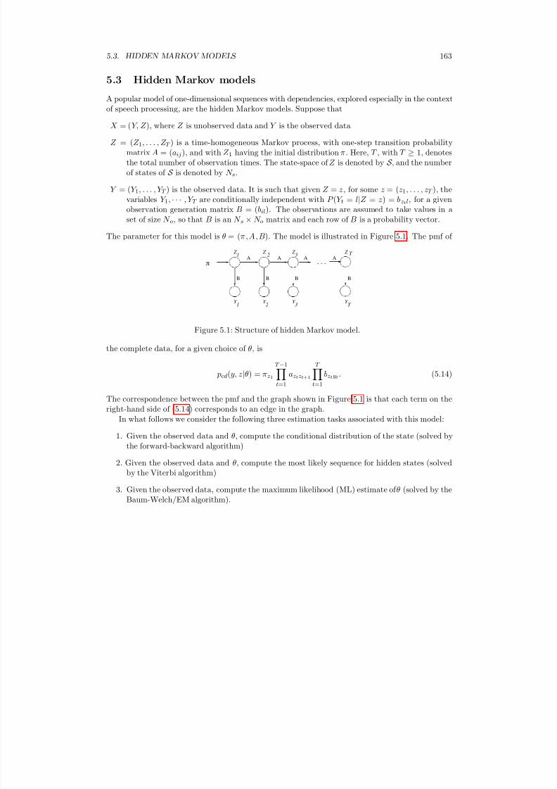
8/11/2019 Random process by B. Hajek
http://slidepdf.com/reader/full/random-process-by-b-hajek 173/448
5.3. HIDDEN MARKOV MODELS 163
5.3 Hidden Markov models
A popular model of one-dimensional sequences with dependencies, explored especially in the context
of speech processing, are the hidden Markov models. Suppose thatX = (Y, Z ), where Z is unobserved data and Y is the observed data
Z = (Z 1, . . . , Z T ) is a time-homogeneous Markov process, with one-step transition probabilitymatrix A = (aij), and with Z 1 having the initial distribution π. Here, T , with T ≥ 1, denotesthe total number of observation times. The state-space of Z is denoted by S , and the numberof states of S is denoted by N s.
Y = (Y 1, . . . , Y T ) is the observed data. It is such that given Z = z, for some z = (z1, . . . , zT ), thevariables Y 1, · · · , Y T are conditionally independent with P (Y t = l|Z = z) = bztl, for a givenobservation generation matrix B = (bil). The observations are assumed to take values in aset of size N o, so that B is an N s
×N o matrix and each row of B is a probability vector.
The parameter for this model is θ = (π,A ,B). The model is illustrated in Figure 5.1. The pmf of
T
!
Y
1
1 Y
2 Y
3 Y
Z Z 2
Z 3
. . .
Z
A A A A
B B B B
T
Figure 5.1: Structure of hidden Markov model.
the complete data, for a given choice of θ, is
pcd(y, z|θ) = πz1
T −1t=1
aztzt+1
T t=1
bztyt. (5.14)
The correspondence between the pmf and the graph shown in Figure 5.1 is that each term on theright-hand side of (5.14) corresponds to an edge in the graph.
In what follows we consider the following three estimation tasks associated with this model:
1. Given the observed data and θ, compute the conditional distribution of the state (solved bythe forward-backward algorithm)
2. Given the observed data and θ, compute the most likely sequence for hidden states (solvedby the Viterbi algorithm)
3. Given the observed data, compute the maximum likelihood (ML) estimate of θ (solved by theBaum-Welch/EM algorithm).
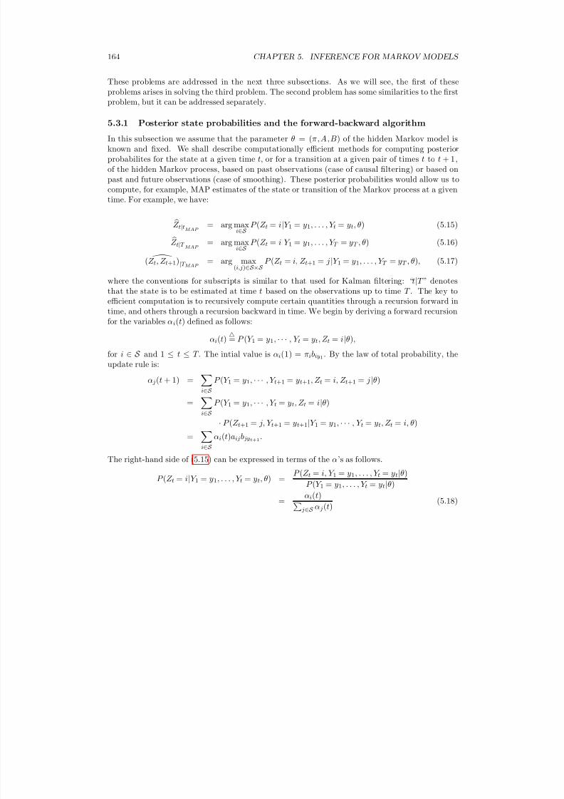
8/11/2019 Random process by B. Hajek
http://slidepdf.com/reader/full/random-process-by-b-hajek 174/448
164 CHAPTER 5. INFERENCE FOR MARKOV MODELS
These problems are addressed in the next three subsections. As we will see, the first of theseproblems arises in solving the third problem. The second problem has some similarities to the firstproblem, but it can be addressed separately.
5.3.1 Posterior state probabilities and the forward-backward algorithm
In this subsection we assume that the parameter θ = (π,A,B) of the hidden Markov model isknown and fixed. We shall describe computationally efficient methods for computing posteriorprobabilites for the state at a given time t, or for a transition at a given pair of times t to t + 1,of the hidden Markov process, based on past observations (case of causal filtering) or based onpast and future observations (case of smoothing). These posterior probabilities would allow us tocompute, for example, MAP estimates of the state or transition of the Markov process at a giventime. For example, we have:
Z t|tMAP = arg maxi∈S P (Z t = i|Y 1 = y1, . . . , Y t = yt, θ) (5.15) Z t|T MAP = arg max
i∈S P (Z t = i|Y 1 = y1, . . . , Y T = yT , θ) (5.16)
(Z t, Z t+1)|T MAP = arg max
(i,j)∈S×S P (Z t = i, Z t+1 = j |Y 1 = y1, . . . , Y T = yT , θ), (5.17)
where the conventions for subscripts is similar to that used for Kalman filtering: “t|T ” denotesthat the state is to be estimated at time t based on the observations up to time T . The key toefficient computation is to recursively compute certain quantities through a recursion forward intime, and others through a recursion backward in time. We begin by deriving a forward recursionfor the variables αi(t) defined as follows:
αi(t)
= P (Y 1 = y1, · · · , Y t = yt, Z t = i|θ),
for i ∈ S and 1 ≤ t ≤ T. The intial value is αi(1) = πibiy1 . By the law of total probability, theupdate rule is:
α j(t + 1) =i∈S
P (Y 1 = y1, · · · , Y t+1 = yt+1, Z t = i, Z t+1 = j |θ)
=i∈S
P (Y 1 = y1, · · · , Y t = yt, Z t = i|θ)
· P (Z t+1 = j, Y t+1 = yt+1|Y 1 = y1, · · · , Y t = yt, Z t = i, θ)
=i∈S
αi(t)aijb jyt+1.
The right-hand side of (5.15) can be expressed in terms of the α’s as follows.
P (Z t = i|Y 1 = y1, . . . , Y t = yt, θ) = P (Z t = i, Y 1 = y1, . . . , Y t = yt|θ)
P (Y 1 = y1, . . . , Y t = yt|θ)
= αi(t)
j∈S α j(t) (5.18)
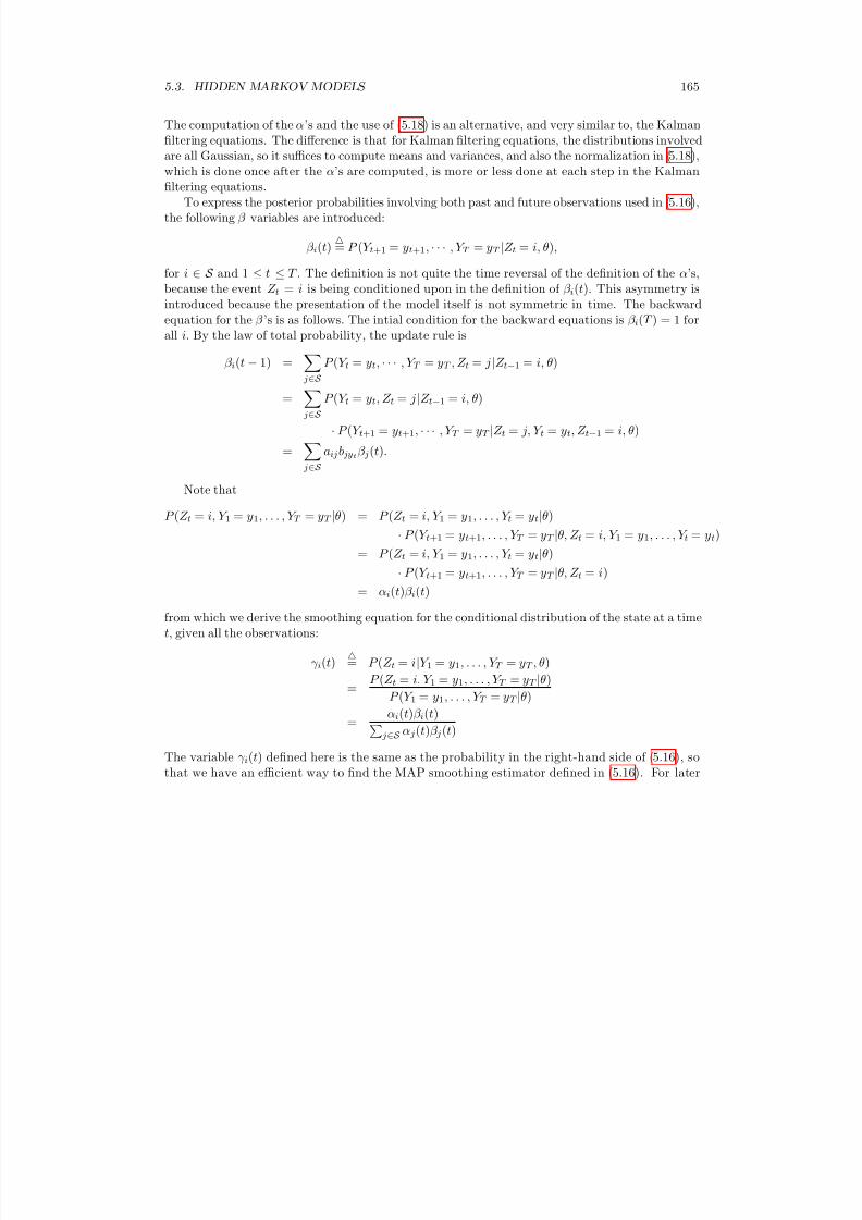
8/11/2019 Random process by B. Hajek
http://slidepdf.com/reader/full/random-process-by-b-hajek 175/448
5.3. HIDDEN MARKOV MODELS 165
The computation of the α’s and the use of (5.18) is an alternative, and very similar to, the Kalmanfiltering equations. The difference is that for Kalman filtering equations, the distributions involvedare all Gaussian, so it suffices to compute means and variances, and also the normalization in (5.18),
which is done once after the α’s are computed, is more or less done at each step in the Kalmanfiltering equations.
To express the posterior probabilities involving both past and future observations used in (5.16),the following β variables are introduced:
β i(t) = P (Y t+1 = yt+1, · · · , Y T = yT |Z t = i, θ),
for i ∈ S and 1 ≤ t ≤ T . The definition is not quite the time reversal of the definition of the α’s,because the event Z t = i is being conditioned upon in the definition of β i(t). This asymmetry isintroduced because the presentation of the model itself is not symmetric in time. The backwardequation for the β ’s is as follows. The intial condition for the backward equations is β i(T ) = 1 forall i. By the law of total probability, the update rule is
β i(t − 1) = j∈S
P (Y t = yt, · · · , Y T = yT , Z t = j |Z t−1 = i, θ)
= j∈S
P (Y t = yt, Z t = j |Z t−1 = i, θ)
· P (Y t+1 = yt+1, · · · , Y T = yT |Z t = j, Y t = yt, Z t−1 = i, θ)
= j∈S
aijb jytβ j(t).
Note that
P (Z t = i, Y
1 = y
1, . . . , Y
T = y
T |θ) = P (Z
t = i, Y
1 = y
1, . . . , Y
t = y
t|θ)
· P (Y t+1 = yt+1, . . . , Y T = yT |θ, Z t = i, Y 1 = y1, . . . , Y t = yt)
= P (Z t = i, Y 1 = y1, . . . , Y t = yt|θ)
· P (Y t+1 = yt+1, . . . , Y T = yT |θ, Z t = i)
= αi(t)β i(t)
from which we derive the smoothing equation for the conditional distribution of the state at a timet, given all the observations:
γ i(t)
= P (Z t = i|Y 1 = y1, . . . , Y T = yT , θ)
= P (Z t = i, Y 1 = y1, . . . , Y T = yT |θ)
P (Y 1 = y1, . . . , Y T = yT |θ)
= αi(t)β i(t)
j∈S α j(t)β j(t)
The variable γ i(t) defined here is the same as the probability in the right-hand side of (5.16), sothat we have an efficient way to find the MAP smoothing estimator defined in ( 5.16). For later
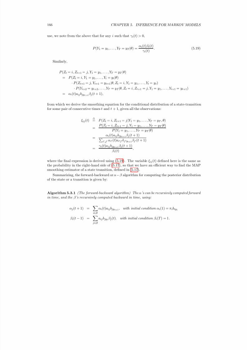
8/11/2019 Random process by B. Hajek
http://slidepdf.com/reader/full/random-process-by-b-hajek 176/448
166 CHAPTER 5. INFERENCE FOR MARKOV MODELS
use, we note from the above that for any i such that γ i(t) > 0,
P (Y 1 = y1, . . . , Y T = yT |θ) =
αi(t)β i(t)
γ i(t) . (5.19)
Similarly,
P (Z t = i, Z t+1 = j, Y 1 = y1, . . . , Y T = yT |θ)
= P (Z t = i, Y 1 = y1, . . . , Y t = yt|θ)
· P (Z t+1 = j, Y t+1 = yt+1|θ, Z t = i, Y 1 = y1, . . . , Y t = yt)
· P (Y t+2 = yt+2, . . . , Y T = yT |θ, Z t = i, Z t+1 = j, Y 1 = y1, . . . , Y t+1 = yt+1)
= αi(t)aijb jyt+1β j(t + 1),
from which we derive the smoothing equation for the conditional distribution of a state-transitionfor some pair of consecutive times t and t + 1, given all the observations:
ξ ij(t)
= P (Z t = i, Z t+1 = j |Y 1 = y1, . . . , Y T = yT , θ)
= P (Z t = i, Z t+1 = j, Y 1 = y1, . . . , Y T = yT |θ)
P (Y 1 = y1, . . . , Y T = yT |θ)
= αi(t)aijb jyt+1β j(t + 1)
i,j αi(t)ai jb jyt+1β j(t + 1)
=
γ i(t)aijb jyt+1β j(t + 1)
β i(t) ,
where the final expression is derived using (5.19). The variable ξ ij(t) defined here is the same asthe probability in the right-hand side of (5.17), so that we have an efficient way to find the MAPsmoothing estimator of a state transition, defined in (5.17).
Summarizing, the forward-backward or α−β algorithm for computing the posterior distributionof the state or a transition is given by:
Algorithm 5.3.1 (The forward-backward algorithm) The α’s can be recursively computed forward in time, and the β ’s recursively computed backward in time, using:
α j(t + 1) =i∈S
αi(t)aijb jyt+1, with initial condition αi(1) = πibiy1
β i(t − 1) = j∈S
aijb jytβ j(t), with initial condition β i(T ) = 1.
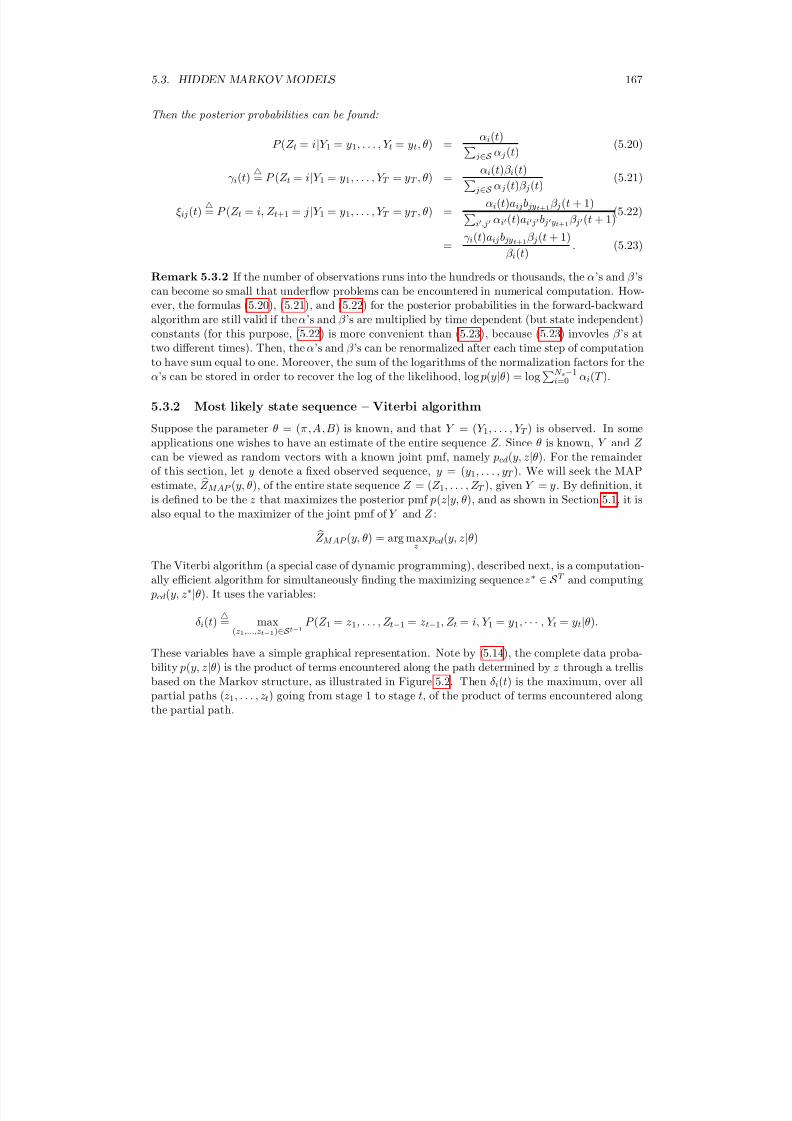
8/11/2019 Random process by B. Hajek
http://slidepdf.com/reader/full/random-process-by-b-hajek 177/448
5.3. HIDDEN MARKOV MODELS 167
Then the posterior probabilities can be found:
P (Z t = i|Y 1 = y1, . . . , Y t = yt, θ) = αi(t)
j∈S α j(t)
(5.20)
γ i(t) = P (Z t = i|Y 1 = y1, . . . , Y T = yT , θ) =
αi(t)β i(t) j∈S α j(t)β j(t)
(5.21)
ξ ij(t) = P (Z t = i, Z t+1 = j |Y 1 = y1, . . . , Y T = yT , θ) =
αi(t)aijb jyt+1β j(t + 1)i,j αi(t)ai jb jyt+1β j(t + 1)
(5.22)
= γ i(t)aijb jyt+1β j(t + 1)
β i(t) . (5.23)
Remark 5.3.2 If the number of observations runs into the hundreds or thousands, the α’s and β ’scan become so small that underflow problems can be encountered in numerical computation. How-ever, the formulas (5.20), (5.21), and (5.22) for the posterior probabilities in the forward-backward
algorithm are still valid if the α’s and β ’s are multiplied by time dependent (but state independent)constants (for this purpose, (5.22) is more convenient than (5.23), because (5.23) invovles β ’s attwo different times). Then, the α’s and β ’s can be renormalized after each time step of computationto have sum equal to one. Moreover, the sum of the logarithms of the normalization factors for theα’s can be stored in order to recover the log of the likelihood, log p(y|θ) = log
N s−1i=0 αi(T ).
5.3.2 Most likely state sequence – Viterbi algorithm
Suppose the parameter θ = (π,A,B) is known, and that Y = (Y 1, . . . , Y T ) is observed. In someapplications one wishes to have an estimate of the entire sequence Z. Since θ is known, Y and Z can be viewed as random vectors with a known joint pmf, namely pcd(y, z|θ). For the remainderof this section, let y denote a fixed observed sequence, y = (y1, . . . , yT ). We will seek the MAP
estimate, Z MAP (y, θ), of the entire state sequence Z = (Z 1, . . . , Z T ), given Y = y. By definition, itis defined to be the z that maximizes the posterior pmf p(z|y, θ), and as shown in Section 5.1, it isalso equal to the maximizer of the joint pmf of Y and Z : Z MAP (y, θ) = arg max
z pcd(y, z|θ)
The Viterbi algorithm (a special case of dynamic programming), described next, is a computation-ally efficient algorithm for simultaneously finding the maximizing sequence z∗ ∈ S T and computing pcd(y, z∗|θ). It uses the variables:
δ i(t) = max
(z1,...,zt−1)
∈S t−1
P (Z 1 = z1, . . . , Z t−1 = zt−1, Z t = i, Y 1 = y1, · · · , Y t = yt|θ).
These variables have a simple graphical representation. Note by (5.14), the complete data proba-bility p(y, z|θ) is the product of terms encountered along the path determined by z through a trellisbased on the Markov structure, as illustrated in Figure 5.2. Then δ i(t) is the maximum, over allpartial paths (z1, . . . , zt) going from stage 1 to stage t, of the product of terms encountered alongthe partial path.
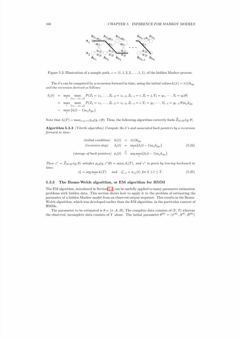
8/11/2019 Random process by B. Hajek
http://slidepdf.com/reader/full/random-process-by-b-hajek 178/448
168 CHAPTER 5. INFERENCE FOR MARKOV MODELS
Figure 5.2: Illustration of a sample path, z = (1, 1, 2, 2, . . . , 1, 1), of the hidden Markov process.
The δ ’s can be computed by a recursion forward in time, using the initial values δ i(1) = π(i)biy1and the recursion derived as follows:
δ j(t) = maxi maxz1,...,zt−2 P (Z 1 = z1, . . . , Z t−2 = zt−2, Z t−1 = i, Z t = j, Y 1 = y1, · · · , Y t = yt|θ)= max
imax
z1,...,zt−2P (Z 1 = z1, . . . , Z t−2 = zt−2, Z t−1 = i, Y 1 = y1, · · · , Y t−1 = yt−1|θ)aijb jyt
= maxi
δ i(t − 1)aijb jyt
Note that δ i(T ) = maxz:zT =i pcd(y, z|θ). Thus, the following algorithm correctly finds Z MAP (y, θ).
Algorithm 5.3.3 (Viterbi algorithm) Compute the δ ’s and associated back pointers by a recursion forward in time:
(initial condition) δ i(1) = π(i)biy1
(recursive step) δ j(t) = maxi δ i(t − 1)aijb jyt (5.24)
(storage of back pointers) φ j(t)
= arg maxi
δ i(t − 1)aijb jyt
Then z∗ = Z MAP (y, θ) satisfies pcd(y, z∗|θ) = maxi δ i(T ), and z∗ is given by tracing backward in time:
z∗T = arg maxi
δ i(T ) and z∗t−1 = φz∗t (t) for 2 ≤ t ≤ T . (5.25)
5.3.3 The Baum-Welch algorithm, or EM algorithm for HMM
The EM algorithm, introduced in Section 5.2, can be usefully applied to many parameter estimation
problems with hidden data. This section shows how to apply it to the problem of estimating theparameter of a hidden Markov model from an observed output sequence. This results in the Baum-Welch algorithm, which was developed earlier than the EM algorithm, in the particular context of HMMs.
The parameter to be estimated is θ = (π,A ,B). The complete data consists of (Y, Z ) whereasthe observed, incomplete data consists of Y alone. The initial parameter θ(0) = (π(0), A(0), B(0))
8/11/2019 Random process by B. Hajek
http://slidepdf.com/reader/full/random-process-by-b-hajek 179/448
5.3. HIDDEN MARKOV MODELS 169
should have all entries strictly positive, because any entry that is zero will remain zero at the endof an iteration. Suppose θ(k) is given. The first half of an iteration of the EM algorithm is tocompute, or determine in closed form, Q(θ|θ(k)). Taking logarithms in the expression (5.14) for the
pmf of the complete data yields
log pcd(y, z|θ) = log πz1 +T −1t=1
log aztzt+1 +T
t=1
log bztyt
Taking the expectation yields
Q(θ|θ(k)) = E [log pcd(y, Z |θ)|y, θ(k)]
=i∈S
γ i(1) log πi +T −1t=1
i,j
ξ ij(t)log aij +T
t=1
i∈S
γ i(t)log biyt,
where the variables γ i(t) and ξ ij(t) are defined using the model with parameter θ(k). In view of this
closed form expression for Q(θ|θ(k)), the expectation step of the EM algorithm essentially comesdown to computing the γ ’s and the ξ ’s. This computation can be done using the forward-backwardalgorithm, Algorithm 5.3.1, with θ = θ(k).
The second half of an iteration of the EM algorithm is to find the value of θ that maximizesQ(θ|θ(k)), and set θ (k+1) equal to that value. The parameter θ = (π,A ,B) for this problem can beviewed as a set of probability vectors. Namely, π is a probability vector, and, for each i fixed, aij
as j varies, and bil as l varies, are probability vectors. Therefore, Example 5.1.8 and Lemma 5.1.7will be of use. Motivated by these, we rewrite the expression found for Q(θ|θ(k)) to get
Q(θ|θ(k)) =
i∈S γ i(1) log πi +
i,jT −1
t=1
ξ ij(t)log aij +
i∈S T
t=1
γ i(t)log biyt
=i∈S
γ i(1) log πi +i,j
T −1t=1
ξ ij(t)
log aij
+i∈S
l
T t=1
γ i(t)I yt=l
log bil (5.26)
The first summation in (5.26) has the same form as the sum in Lemma 5.1.7. Similarly, for eachi fixed, the sum over j involving aij, and the sum over l involving bil, also have the same form asthe sum in Lemma 5.1.7. Therefore, the maximization step of the EM algorithm can be written inthe following form:
π(k+1)
i = γ i(1) (5.27)
a(k+1)ij =
T −1t=1 ξ ij(t)T −1t=1 γ i(t)
(5.28)
b(k+1)il =
T t=1 γ i(t)I yt=lT
t=1 γ i(t)(5.29)

8/11/2019 Random process by B. Hajek
http://slidepdf.com/reader/full/random-process-by-b-hajek 180/448
170 CHAPTER 5. INFERENCE FOR MARKOV MODELS
The update equations (5.27)-(5.29) have a natural interpretation. Equation (5.27) means that thenew value of the distribution of the initial state, π (k+1), is simply the posterior distribution of theinitial state, computed assuming θ (k) is the true parameter value. The other two update equations
are similar, but are more complicated because the transition matrix A and observation generationmatrix B do not change with time. The denominator of (5.28) is the posterior expected number of times the state is equal to i up to time T − 1, and the numerator is the posterior expected numberof times two consecutive states are i,j. Thus, if we think of the time of a jump as being random,the right-hand side of (5.28) is the time-averaged posterior conditional probability that, given thestate at the beginning of a transition is i at a typical time, the next state will be j. Similarly, theright-hand side of (5.29) is the time-averaged posterior conditional probability that, given the stateis i at a typical time, the observation will be l.
Algorithm 5.3.4 (Baum-Welch algorithm, or EM algorithm for HMM) Select the state space S ,and in particular, the cardinality, N s, of the state space, and let θ(0) denote a given initial choice of parameter. Given θ(k), compute θ(k+1) by using the forward-backward algorithm (Algorithm 5.3.1) with θ = θ(k) to compute the γ ’s and ξ ’s. Then use (5.27)-(5.29) to compute θ(k+1) =(π(k+1), A(k+1), B(k+1)).
5.4 Notes
The EM algorithm is due to A.P. Dempster, N.M. Laird, and B.D. Rubin [3]. The paper includesexamples and a proof that the likelihood is increased with each iteration of the algorithm. Anarticle on the convergence of the EM algorithm is given in [16]. Earlier related work includes thatof Baum et al. [2], giving the Baum-Welch algorithm. A tutorial on inference for HMMs andapplications to speech recognition is given in [11].
5.5 Problems
5.1 Estimation of a Poisson parameterSuppose Y is assumed to be a P oi(θ) random variable. Using the Bayesian method, suppose theprior distribution of θ is the exponential distribution with some known parameter λ > 0. (a) Find ΘMAP (k), the MAP estimate of θ given that Y = k is observed, for some k ≥ 0.(b) For what values of λ is ΘMAP (k) ≈ θML(k)? (The ML estimator was found in Example 5.1.3.)Why should that be expected?
5.2 A variance estimation problem with Poisson observation
The input voltage to an optical device is X and the number of photons observed at a detector isN . Suppose X is a Gaussian random variable with mean zero and variance σ2, and that givenX , the random variable N has the Poisson distribution with mean X 2. (Recall that the Poissondistribution with mean λ has probability mass function λne−λ/n! for n ≥ 0.)(a) Express P N = n in terms of σ2. You can express this as an integral, which you do not haveto evaluate.
8/11/2019 Random process by B. Hajek
http://slidepdf.com/reader/full/random-process-by-b-hajek 181/448
5.5. PROBLEMS 171
(b) Find the maximum likelihood estimator of σ2 given N . (Caution: Estimate σ2, not X . Be asexplicit as possible–the final answer has a simple form. Hint: You can first simplify your answer to
part (a) by using the fact that if X is a N (0, σ2) random variable, then E [X 2n] = eσ2n(2n)!
n!2n . )
5.3 ML estimation of covariance matrixSuppose n independently generated p dimensional random vectors X 1, . . . , X n, are observed, eachassumed to have the N (0, K ) distribution for some unknown positive semidefinite matrix K. Let S denote the sample covariance function, defined by S = 1
n
ni=1 X iX T i . The goal of this problem is
to prove that S is the ML estimator of K. Let the observations be fixed for the remainder of thisproblem, and for simplicity, assume S has full rank. Therefore S is symmetric and positive definite.(a) First, show that ln f (X 1, . . . , X n|K ) = −n
2 ( p ln(2π)+lndet(K )+Tr(SK −1)), where Tr denotesthe trace function.(b) Then, using the diagonalization of S, explain why there is a symmetric positive definite matrix
S 12 so that S = S
12 S
12 .
(c) Complete the proof by using the change of variables K = S −12
KS −12
and finding the value of K that maximizes the likelihood. Since the transformation from K to K is invertible, applyingthe inverse mapping to the maximizing value of K yields the ML estimator for K. (At somepoint you may need to use the fact that for matrices A and B such that AB is a square matrix,Tr(AB) = Tr(BA).)
5.4 Estimation of parameter of Bernoulli random variables in Gaussian noise by EMalgorithmSuppose Y = (Y 1, . . . , Y T ), W = (W 1, . . . , W T ), and Z = (Z 1, . . . , Z T ) Let θ ∈ [0, 1] be a parameterto be estimated. Suppose W 1. . . . , W T are independent, N (0, 1) random variables, and Z 1, . . . Z T are independent random variables with P Z t = 1 = θ and P Z t = −1 = 1 − θ for 1 ≤ t ≤ T.Suppose Y t = Z t + W t.
(a) Find a simple formula for the function φ(t, θ) defined by φ(u, θ) = E [Z 1|Y 1 = u, θ].(b) Using the function φ found in part (a) in your answer, derive the EM algorithm for calcu-
lation of θML(y).
5.5 Convergence of the EM algorithm for an exampleThe purpose of this exercise is to verify for Example 5.2.2 that if θ(0) > 0, then θ(k) → θML
as k → ∞. As shown in the example, θML = (y2 − σ2)+. Let F (θ) =
θθ+σ2
2y2 + θσ2
θ+σ2 so
that the recursion (5.6) has the form θ(k+1) = F (θ(k)). Clearly, over R+, F is increasing andbounded. (a) Show that 0 is the only nonnegative solution of F (θ) = θ if y ≤ σ2 and that 0 andy − σ2 are the only nonnegative solutions of F (θ) = θ if y > σ2. (b) Show that for small θ > 0,
F (θ) = θ +
θ2(y2
−σ2)
σ4 + o(θ
3
). (Hint: For 0 < θ < σ
2
,
θ
θ+σ2 =
θ
σ2
1
1+θ/σ2 =
θ
σ2 (1 − θ
σ2 + (
θ
σ2 )
2
− . . .).(c) Sketch F and argue, using the above properties of F, that if θ(0) > 0, then θ(k) → θML.
5.6 Transformation of estimators and estimators of transformationsConsider estimating a parameter θ ∈ [0, 1] from an observation Y . A prior density of θ is availablefor the Bayes estimators, MAP and MMSE, and the conditional density of Y given θ is known.
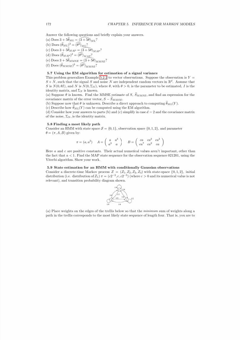
8/11/2019 Random process by B. Hajek
http://slidepdf.com/reader/full/random-process-by-b-hajek 182/448
172 CHAPTER 5. INFERENCE FOR MARKOV MODELS
Answer the following questions and briefly explain your answers.
(a) Does 3 + 5
θML = (3 + 5θ)ML?
(b) Does ( θML)3 = (θ3)ML?
(c) Does 3 + 5 θMAP = (3 + 5θ)MAP ?
(d) Does ( θMAP )3 = (θ3)MAP ?
(e) Does 3 + 5 θMMSE = (3 + 5θ)MMSE ?
(f) Does ( θMMSE )3 = (θ3)MMSE ?
5.7 Using the EM algorithm for estimation of a signal varianceThis problem generalizes Example 5.2.2 to vector observations. Suppose the observation is Y =S + N , such that the signal S and noise N are independent random vectors in Rd. Assume thatS is N (0, θI ), and N is N (0, ΣN ), where θ, with θ > 0, is the parameter to be estimated, I is theidentity matrix, and ΣN is known.(a) Suppose θ is known. Find the MMSE estimate of S , S MMSE , and find an espression for thecovariance matrix of the error vector, S − S MMSE .(b) Suppose now that θ is unknown. Describe a direct approach to computing θML(Y ).(c) Describe how θML(Y ) can be computed using the EM algorithm.(d) Consider how your answers to parts (b) and (c) simplify in case d = 2 and the covariance matrixof the noise, ΣN , is the identity matrix.
5.8 Finding a most likely pathConsider an HMM with state space S = 0, 1, observation space 0, 1, 2, and parameterθ = (π,A,B) given by:
π = (a, a3) A = a a3
a
3
a B = ca ca2 ca3
ca
2
ca
3
ca Here a and c are positive constants. Their actual numerical values aren’t important, other thanthe fact that a < 1. Find the MAP state sequence for the observation sequence 021201, using theViterbi algorithm. Show your work.
5.9 State estimation for an HMM with conditionally Gaussian observationsConsider a discrete-time Markov process Z = (Z 1, Z 2, Z 3, Z 4) with state-space 0, 1, 2, initialdistribution (i.e. distribution of Z 1) π = (c2−3, c , c2−5) (where c > 0 and its numerical value is notrelevant), and transition probability diagram shown.
1/41/4
1/21/2 1/4
1/21/4
1/4
1/4
0
1
2
(a) Place weights on the edges of the trellis below so that the minimum sum of weights along apath in the trellis corresponds to the most likely state sequence of length four. That is, you are to
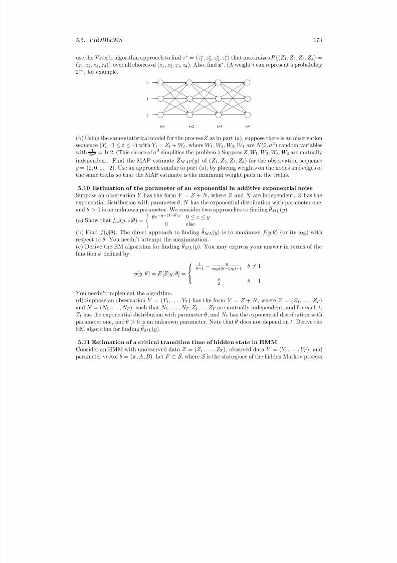
8/11/2019 Random process by B. Hajek
http://slidepdf.com/reader/full/random-process-by-b-hajek 183/448
5.5. PROBLEMS 173
use the Viterbi algorithm approach to find z∗ = (z∗1, z∗2 , z∗3, z∗4 ) that maximizes P (Z 1, Z 2, Z 3, Z 4) =(z1, z2, z3, z4) over all choices of (z1, z2, z3, z4). Also, find z∗. (A weight i can represent a probability2−i, for example.
2
1
t=1 t=2 t=3 t=4
0
(b) Using the same statistical model for the process Z as in part (a), suppose there is an observationsequence (Y t : 1 ≤ t ≤ 4) with Y t = Z t + W t, where W 1, W 2, W 3, W 4 are N (0, σ2) random variableswith 1
2σ2 = ln2. (This choice of σ2 simplifies the problem.) Suppose Z, W 1, W 2, W 3, W 4 are mutually
independent. Find the MAP estimate Z MAP (y) of (Z 1, Z 2, Z 3, Z 4) for the observation sequencey = (2, 0, 1, −2). Use an approach similar to part (a), by placing weights on the nodes and edges of the same trellis so that the MAP estimate is the minimum weight path in the trellis.
5.10 Estimation of the parameter of an exponential in additive exponential noiseSuppose an observation Y has the form Y = Z + N, where Z and N are independent, Z has theexponential distribution with parameter θ, N has the exponential distribution with parameter one,and θ > 0 is an unknown parameter. We consider two approaches to finding θML(y).
(a) Show that f cd(y, z|θ) =
θe−y+(1−θ)z 0 ≤ z ≤ y
0 else
(b) Find f (y|θ). The direct approach to finding
θML(y) is to maximize f (y|θ) (or its log) with
respect to θ. You needn’t attempt the maximization.(c) Derive the EM algorithm for finding θML(y). You may express your answer in terms of thefunction φ defined by:
φ(y, θ) = E [Z |y, θ] =
1
θ−1 − yexp((θ−1)y)−1 θ = 1
y2 θ = 1
You needn’t implement the algorithm.(d) Suppose an observation Y = (Y 1, . . . , Y T ) has the form Y = Z + N, where Z = (Z 1, . . . , Z T )and N = (N 1, . . . , N T ), such that N 1, . . . , N T , Z 1, . . . Z T are mutually independent, and for each t,Z t has the exponential distribution with parameter θ, and N t has the exponential distribution with
parameter one, and θ > 0 is an unknown parameter. Note that θ does not depend on t. Derive theEM algorithm for finding θML(y).
5.11 Estimation of a critical transition time of hidden state in HMMConsider an HMM with unobserved data Z = (Z 1, . . . , Z T ), observed data Y = (Y 1, . . . , Y T ), andparameter vector θ = (π,A ,B). Let F ⊂ S , where S is the statespace of the hidden Markov process
8/11/2019 Random process by B. Hajek
http://slidepdf.com/reader/full/random-process-by-b-hajek 184/448
174 CHAPTER 5. INFERENCE FOR MARKOV MODELS
Z , and let τ F be the first time t such that Z t ∈ F with the convention that τ F = T + 1 if (Z t ∈ F for 1 ≤ t ≤ T ).(a) Describe how to find the conditional distribution of τ F given Y, under the added assumption
that (aij = 0 for all (i, j) such that i ∈ F and j ∈ F ), i.e. under the assumption that F is anabsorbing set for Z.(b) Describe how to find the conditional distribution of τ F given Y , without the added assumptionmade in part (a).
5.12 Maximum likelihood estimation for HMMsConsider an HMM with unobserved data Z = (Z 1, . . . , Z T ), observed data Y = (Y 1, . . . , Y T ),and parameter vector θ = (π,A,B). Explain how the forward-backward algorithm or the Viterbialgorithm can be used or modified to compute the following:(a) The ML estimator, Z ML, of Z based on Y, assuming any initial state and any transitions i → jare possible for Z. (Hint: Your answer should not depend on π or A.)(b) The ML estimator, Z ML, of Z based on Y , subject to the constraints that Z ML takes values inthe set z : P Z = z > 0. (Hint: Your answer should depend on π and A only through whichcoordinates of π and A are nonzero.)(c) The ML estimator, Z 1,ML, of Z 1 based on Y.
(d) The ML estimator, Z to,ML, of Z to based on Y, for some fixed to with 1 ≤ to ≤ T .
5.13 An underconstrained estimation problemSuppose the parameter θ = (π,A ,B) for an HMM is unknown, but that it is assumed that thenumber of states N s in the statespace S for (Z t) is equal to the number of observations, T . Describea trivial choice of the ML estimator θML(y) for a given observation sequence y = (y1, . . . , yT ). Whatis the likelihood of y for this choice of θ?
5.14 Specialization of Baum-Welch algorithm for no hidden data(a) Determine how the Baum-Welch algorithm simplifies in the special case that B is the identitymatrix, so that X t = Y t for all t. (b) Still assuming that B is the identity matrix, suppose thatS = 0, 1 and the observation sequence is 0001110001110001110001. Find the ML estimator for πand A.
5.15 Bayes estimation for a simple product form distribution
Let A be the three by three matrix with entries aij =
2 i = j1 i = j
. Suppose X, Y 1, Y 2, Y 3 have the
joint pmf P X = i, Y 1 = j, Y 2 = k, Y 3 = l = aijaikail
Z , where Z is a normalizing constant so thatthe sum of P X = i, Y 1 = j, Y 2 = k, Y 3 = l over all i, j, k,l ∈ 1, 2, 3 is equal to one.
(a) Find the maximum a posteriori (MAP) estimate of X given (Y 1, Y 2, Y 3) = 122.(b) Find the conditional probability distribution of X given (Y 1, Y 2, Y 3) = 122.
5.16 Extending the forward-backward algorithmThe forward-backward algorithm is a form of belief propagation (or message passing) algorithmfor the special case of graph structure that is a one-dimensional chain. It is easy to generalize
8/11/2019 Random process by B. Hajek
http://slidepdf.com/reader/full/random-process-by-b-hajek 185/448
5.5. PROBLEMS 175
the algorithm when the graph structure is a tree. For even more general graphs, with cycles, itis often useful to ignore the cycles and continue to use the same local computations, resulting ingeneral belief propagation algorithms. To help explain how belief propagation equations can be
derived for general graphs without a given linear ordering of nodes, this problem focuses on asymmetric version of the forward backward algorithm. If the initial distribution π is uniform, thenthe complete probability distribution function can be written as
pcd(y, z|θ) =
T −1t=1 aztzt+1
T t=1 biyt
G (5.30)
where G is the number of states in S . Taking θ = (A, B), and dropping the requirement that therow sums of A and B be normalized to one, (5.30) still defines a valid joint distribution for Y andZ, with the understanding that the constant G is selected to make the sum over all pairs (y, z) sumto one. Note that G depends on θ. This representation of joint probability distributions for (Y, Z )is symmetric forward and backward in time.
(a) Assuming the distribution in (5.30), derive a symmetric variation of the forward backwardalgorithm for computation of γ i(t) = P (Z t = i|y, θ). Instead of α’s and β ’s, use variables of theform µi(t, t + 1) to replace the α’s; these are messages passed to the right, and variables of the formµi(t + 1, t) to replace the β ’s; these are messages passed to the left. Here the notation u(s, t) fortwo adjacent times s and t is for a message to be passed from node s to node t. A better notationmight be u(s → t). The message u(s, t) is a vector u(s, t) = (ui(s, t) : i ∈ S ) of likelihoods, aboutthe distribution of Z t that has been collected from the direction s is from t. Give equations forcalculating the µ’s and an equation to calculate the γ ’s from the µ’s. (Hint: The backward variableµ(t + 1, t) can be taken to be essentially identical to β (t) for all t, whereas the forward variableµ(t, t +1) will be somewhat different from α(t) for all t. Note that α(t) depends on yt but β (t) doesnot. This asymmetry is used when α(t) and β (t) are combined to give γ (t). )(b) Give expressions for µi(t, t + 1) and µ(t + 1, t) for 1
≤ t
≤ T that involve multiple summations
but no recursion. (These expressions can be verified by induction.)(c) Explain using your answer to part (b) the correctness of your algorithm in part (a).
5.17 Free energy and the Boltzmann distributionLet S denote a finite set of possible states of a physical system, and suppose the (internal) energyof any state s ∈ S is given by V (s) for some function V on S . Let T > 0. The Helmholtz freeenergy of a probability distribution Q on S is defined to be the average (internal) energy minus thetemperature times entropy: F (Q) =
i Q(i)V (i) + T
i Q(i)log Q(i). Note that F is a convex
function of Q. (We’re assuming Boltzmann’s constant is normalized to one, so that T shouldactually be in units of energy, but by abuse of notation we will call T the temperature.)(a) Use the method of Lagrange multipliers to show that the Boltzmann distribution defined by
BT (i) = 1Z (T ) exp(−V (i)/T ) minimizes F (Q). Here Z (T ) is the normalizing constant required to
make BT a probability distribution.(b) Describe the limit of the Boltzmann distribution as T → ∞.(c) Describe the limit of the Boltzmann distribution as T → 0. If it is possible to simulate a randomvariable with the Boltzmann distribution, does this suggest an application?(d) Show that F (Q) = T D(Q||BT ) + (term not depending on Q). Therefore, given an energy
8/11/2019 Random process by B. Hajek
http://slidepdf.com/reader/full/random-process-by-b-hajek 186/448
176 CHAPTER 5. INFERENCE FOR MARKOV MODELS
function V on S and temperature T > 0, minimizing free energy over Q in some set is equivalentto minimizing the divergence D(Q||BT ) over Q in the same set.
5.18 Baum-Welch saddlepointSuppose that the Baum-Welch algorithm is run on a given data set with initial parameter θ(0) =(π(0), A(0), B(0)) such that π(0) = π(0)A(0) (i.e., the initial distribution of the state is an equilibriumdistribution of the state) and every row of B(0) is identical. Explain what happens, assuming anideal computer with infinite precision arithmetic is used.
5.19 Inference for a mixture model(a) An observed random vector Y is distributed as a mixture of Gaussian distributions in d dimen-sions. The parameter of the mixture distribution is θ = (θ1, . . . , θJ ), where θ j is a d-dimensionalvector for 1 ≤ j ≤ J . Specifically, to generate Y a random variable Z, called the class label forthe observation, is generated. The variable Z is uniformly distributed on 1, . . . , J , and the con-ditional distribution of Y given (θ, Z ) is Gaussian with mean vector θ
Z and covariance the d
×d
identity matrix. The class label Z is not observed. Assuming that θ is known, find the posteriorpmf p(z|y, θ). Give a geometrical interpretation of the MAP estimate Z for a given observationY = y.(b) Suppose now that the parameter θ is random with the uniform prior over a very large regionand suppose that given θ, n random variables are each generated as in part (a), independently, toproduce(Z (1), Y (1), Z (2), Y (2), . . . , Z (n), Y (n)). Give an explicit expression for the joint distributionP (θ, z(1), y(1), z(2), y(2), . . . , z(n), y(n)).(c) The iterative conditional modes (ICM) algorithm for this example corresponds to taking turnsmaximizing P (
θ,
z(1), y(1),
z(2), y(2), . . . ,
z(n), y(n)) with respect to
θ for
z fixed and with respect to
z
for θ fixed. Give a simple geometric description of how the algorithm works and suggest a method
to initialize the algorithm (there is no unique answer for the later).(d) Derive the EM algorithm for this example, in an attempt to compute the maximum likelihoodestimate of θ given y (1), y(2), . . . , y(n).
5.20 Constraining the Baum-Welch algorithmThe Baum-Welch algorithm as presented placed no prior assumptions on the parameters π, A, B,other than the number of states N s in the state space of (Z t). Suppose matrices A and B are givenwith the same dimensions as the matrices A and B to be esitmated, with all elements of A andB having values 0 and 1. Suppose that A and B are constrained to satisfy A ≤ A and B ≤ B , inthe element-by-element ordering (for example, aij ≤ aij for all i,j.) Explain how the Baum-Welchalgorithm can be adapted to this situation.
5.21 MAP estimation of parameters of a Markov processLet Z be a Markov process with state space S = 0, 1, initial time t = 1, initial distribution π,and one-step transition probability matrix A.
(a) Suppose it is known that A =
2/3 1/31/3 2/3
and it is observed that (Z (1), Z (4)) = (0, 1). Find

8/11/2019 Random process by B. Hajek
http://slidepdf.com/reader/full/random-process-by-b-hajek 187/448
5.5. PROBLEMS 177
the MAP estimate of Z (2).(b) Suppose instead θ = (π, A) and θ is unknown, and three independent observations of (Z (1), Z (2), Z (3), Zare generated using θ. Assuming the observations are 0001, 1011, 1110, find
θML.
5.22 * Implementation of algorithmsWrite a computer program to (a) simulate a HMM on a computer for a specified value of theparamter θ = (π,A,B), (b) To run the forward-backward algorithm and compute the α’s, β ’s, γ ’s,and ξ ’s , (c) To run the Baum-Welch algorithm. Experiment a bit and describe your results. Forexample, if T observations are generated, and then if the Baum-Welch algorithm is used to estimatethe paramter, how large does T need to be to insure that the estimates of θ are pretty accurate.

8/11/2019 Random process by B. Hajek
http://slidepdf.com/reader/full/random-process-by-b-hajek 188/448
178 CHAPTER 5. INFERENCE FOR MARKOV MODELS
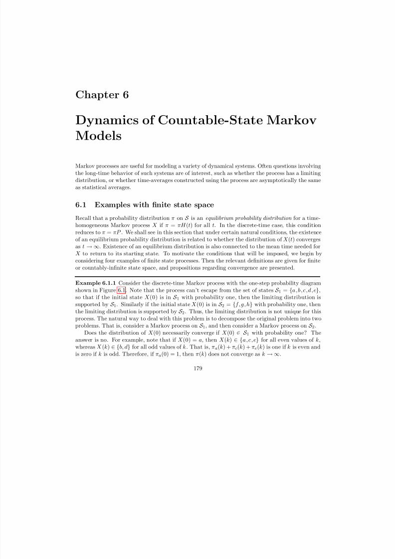
8/11/2019 Random process by B. Hajek
http://slidepdf.com/reader/full/random-process-by-b-hajek 189/448
Chapter 6
Dynamics of Countable-State MarkovModels
Markov processes are useful for modeling a variety of dynamical systems. Often questions involvingthe long-time behavior of such systems are of interest, such as whether the process has a limitingdistribution, or whether time-averages constructed using the process are asymptotically the sameas statistical averages.
6.1 Examples with finite state space
Recall that a probability distribution π on S is an equilibrium probability distribution for a time-homogeneous Markov process X if π = πH (t) for all t. In the discrete-time case, this conditionreduces to π = πP . We shall see in this section that under certain natural conditions, the existence
of an equilibrium probability distribution is related to whether the distribution of X (t) convergesas t → ∞. Existence of an equilibrium distribution is also connected to the mean time needed forX to return to its starting state. To motivate the conditions that will be imposed, we begin byconsidering four examples of finite state processes. Then the relevant definitions are given for finiteor countably-infinite state space, and propositions regarding convergence are presented.
Example 6.1.1 Consider the discrete-time Markov process with the one-step probability diagramshown in Figure 6.1. Note that the process can’t escape from the set of states S 1 = a,b,c,d,e,so that if the initial state X (0) is in S 1 with probability one, then the limiting distribution issupported by S 1. Similarly if the initial state X (0) is in S 2 = f ,g ,h with probability one, thenthe limiting distribution is supported by S 2. Thus, the limiting distribution is not unique for this
process. The natural way to deal with this problem is to decompose the original problem into twoproblems. That is, consider a Markov process on S 1, and then consider a Markov process on S 2.
Does the distribution of X (0) necessarily converge if X (0) ∈ S 1 with probability one? Theanswer is no. For example, note that if X (0) = a, then X (k) ∈ a,c,e for all even values of k,whereas X (k) ∈ b, d for all odd values of k . That is, πa(k) + πc(k) + πe(k) is one if k is even andis zero if k is odd. Therefore, if πa(0) = 1, then π(k) does not converge as k → ∞.
179
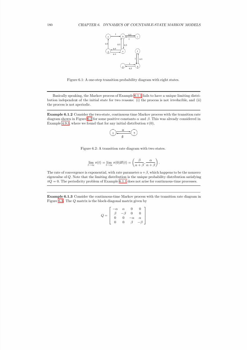
8/11/2019 Random process by B. Hajek
http://slidepdf.com/reader/full/random-process-by-b-hajek 190/448
180 CHAPTER 6. DYNAMICS OF COUNTABLE-STATE MARKOV MODELS
0.5
1
0.50.5
0.5
0.5
1
1 0.5
0.5
b c
d e f
g h
a
0.5
1
Figure 6.1: A one-step transition probability diagram with eight states.
Basically speaking, the Markov process of Example 6.1.1 fails to have a unique limiting distri-
bution independent of the initial state for two reasons: (i) the process is not irreducible, and (ii)the process is not aperiodic.
Example 6.1.2 Consider the two-state, continuous time Markov process with the transition ratediagram shown in Figure 6.2 for some positive constants α and β . This was already considered inExample 4.9.3, where we found that for any initial distribution π(0),
!1 2
Figure 6.2: A transition rate diagram with two states.
limt→∞ π(t) = lim
t→∞ π(0)H (t) =
β
α + β ,
α
α + β
.
The rate of convergence is exponential, with rate parameter α +β , which happens to be the nonzeroeigenvalue of Q. Note that the limiting distribution is the unique probability distribution satisfyingπQ = 0. The periodicity problem of Example 6.1.1 does not arise for continuous-time processes.
Example 6.1.3 Consider the continuous-time Markov process with the transition rate diagram in
Figure 6.3. The Q matrix is the block-diagonal matrix given by
Q =
−α α 0 0
β −β 0 00 0 −α α0 0 β −β
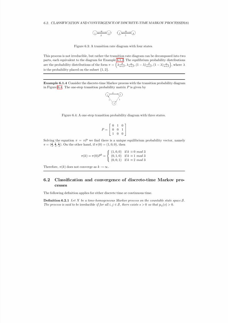
8/11/2019 Random process by B. Hajek
http://slidepdf.com/reader/full/random-process-by-b-hajek 191/448
6.2. CLASSIFICATION AND CONVERGENCE OF DISCRETE-TIME MARKOV PROCESSES 181
!1 2
!3 4
Figure 6.3: A transition rate diagram with four states.
This process is not irreducible, but rather the transition rate diagram can be decomposed into twoparts, each equivalent to the diagram for Example 6.1.2. The equilibrium probability distributions
are the probability distributions of the form π =
λ β α+β , λ α
α+β , (1 − λ) β α+β , (1 − λ) α
α+β
, where λ
is the probability placed on the subset 1, 2.
Example 6.1.4 Consider the discrete-time Markov process with the transition probability diagramin Figure 6.4. The one-step transition probability matrix P is given by
1 2
3
11
Figure 6.4: A one-step transition probability diagram with three states.
P =
0 1 00 0 11 0 0
Solving the equation π = πP we find there is a unique equilibrium probability vector, namelyπ = ( 1
3 , 13 , 1
3 ). On the other hand, if π(0) = (1, 0, 0), then
π(k) = π(0)P k =
(1, 0, 0) if k ≡ 0 mod 3(0, 1, 0) if k ≡ 1 mod 3(0, 0, 1) if k ≡ 2 mod 3
Therefore, π(k) does not converge as k → ∞.
6.2 Classification and convergence of discrete-time Markov pro-
cesses
The following definition applies for either discrete time or continuous time.
Definition 6.2.1 Let X be a time-homogeneous Markov process on the countable state space S .The process is said to be irreducible if for all i, j ∈ S , there exists s > 0 so that pij(s) > 0.
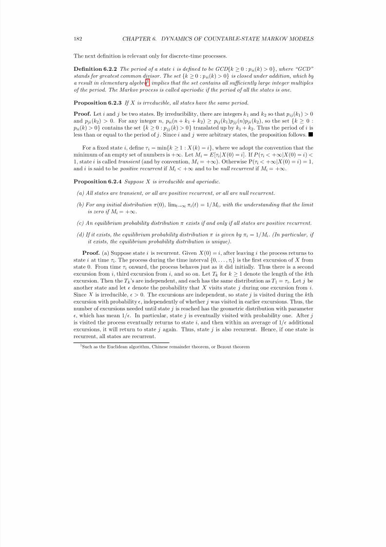
8/11/2019 Random process by B. Hajek
http://slidepdf.com/reader/full/random-process-by-b-hajek 192/448
182 CHAPTER 6. DYNAMICS OF COUNTABLE-STATE MARKOV MODELS
The next definition is relevant only for discrete-time processes.
Definition 6.2.2 The period of a state i is defined to be GCD k ≥ 0 : pii(k) > 0, where “GCD”
stands for greatest common divisor. The set k ≥ 0 : pii(k) > 0 is closed under addition, which by a result in elementary algebra 1 implies that the set contains all sufficiently large integer multiples of the period. The Markov process is called aperiodic if the period of all the states is one.
Proposition 6.2.3 If X is irreducible, all states have the same period.
Proof. Let i and j be two states. By irreducibility, there are integers k1 and k2 so that pij(k1) > 0and p ji(k2) > 0. For any integer n, pii(n + k1 + k2) ≥ pij(k1) p jj (n) p ji(k2), so the set k ≥ 0 : pii(k) > 0 contains the set k ≥ 0 : p jj (k) > 0 translated up by k1 + k2. Thus the period of i isless than or equal to the period of j . Since i and j were arbitrary states, the proposition follows.
For a fixed state i, define τ i = mink ≥ 1 : X (k) = i, where we adopt the convention that the
minimum of an empty set of numbers is +∞. Let M i = E [τ i|X (0) = i]. If P (τ i < +∞|X (0) = i) <1, state i is called transient (and by convention, M i = +∞). Otherwise P(τ i < +∞|X (0) = i) = 1,and i is said to be positive recurrent if M i < +∞ and to be null recurrent if M i = +∞.
Proposition 6.2.4 Suppose X is irreducible and aperiodic.
(a) All states are transient, or all are positive recurrent, or all are null recurrent.
(b) For any initial distribution π(0), limt→∞ πi(t) = 1/M i, with the understanding that the limit is zero if M i = +∞.
(c) An equilibrium probability distribution π exists if and only if all states are positive recurrent.
(d) If it exists, the equilibrium probability distribution π is given by πi = 1/M i. (In particular, if it exists, the equilibrium probability distribution is unique).
Proof. (a) Suppose state i is recurrent. Given X (0) = i, after leaving i the process returns tostate i at time τ i. The process during the time interval 0, . . . , τ i is the first excursion of X fromstate 0. From time τ i onward, the process behaves just as it did initially. Thus there is a secondexcursion from i, third excursion from i, and so on. Let T k for k ≥ 1 denote the length of the kthexcursion. Then the T k’s are independent, and each has the same distribution as T 1 = τ i. Let j beanother state and let denote the probability that X visits state j during one excursion from i.Since X is irreducible, > 0. The excursions are independent, so state j is visited during the kthexcursion with probability , independently of whether j was visited in earlier excursions. Thus, thenumber of excursions needed until state j is reached has the geometric distribution with parameter, which has mean 1/. In particular, state j is eventually visited with probability one. After jis visited the process eventually returns to state i, and then within an average of 1/ additionalexcursions, it will return to state j again. Thus, state j is also recurrent. Hence, if one state isrecurrent, all states are recurrent.
1Such as the Euclidean algorithm, Chinese remainder theorem, or Bezout theorem
8/11/2019 Random process by B. Hajek
http://slidepdf.com/reader/full/random-process-by-b-hajek 193/448
6.2. CLASSIFICATION AND CONVERGENCE OF DISCRETE-TIME MARKOV PROCESSES 183
The same argument shows that if i is positive recurrent, then j is positive recurrent. GivenX (0) = i, the mean time needed for the process to visit j and then return to i is M i/, since onaverage 1/ excursions of mean length M i are needed. Thus, the mean time to hit j starting from
i, and the mean time to hit i starting from j , are both finite. Thus, j is positive recurrent. Hence,if one state is positive recurrent, all states are positive recurrent.
(b) Part (b) of the proposition follows by an application of the renewal theorem, which can befound in [1].
(c) Suppose all states are positive recurrent. By the law of large numbers, for any state j, thelong run fraction of time the process is in state j is 1/M j with probability one. Similarly, for anystates i and j, the long run fraction of time the process is in state j is γ ij/M i, where γ ij is themean number of visits to j in an excursion from i. Therefore 1/M j = γ ij/M i. This implies that
i 1/M i = 1. That is, π defined by πi = 1/M i is a probability distribution. The convergence foreach i separately given in part (b), together with the fact that π is a probability distribution, implythat
i |πi(t) − πi| → 0. Thus, taking s to infinity in the equation π(s)H (t) = π(s + t) yields
πH (t) = π, so that π is an equilibrium probability distribution.Conversely, if there is an equilibrium probability distribution π, consider running the process
with initial state π. Then π(t) = π for all t. So by part (b), for any state i, πi = 1/M i. Taking astate i such that πi > 0, it follows that M i < ∞. So state i is positive recurrent. By part (a), allstates are positive recurrent.
(d) Part (d) was proved in the course of proving part (c).
We conclude this section by describing a technique to establish a rate of convergence to theequilibrium distribution for finite-state Markov processes. Define δ (P ) for a one-step transitionprobability matrix P by
δ (P ) = mini,k j p
ij ∧ p
kj,
where a ∧ b = mina, b. The number δ (P ) is known as Dobrushin’s coefficient of ergodicity. Sincea + b − 2(a ∧ b) = |a − b| for a, b ≥ 0, we also have
1 − 2δ (P ) = mini,k
j
| pij − pkj |.
Let µ1 for a vector µ denote the L1 norm: µ1 =
i |µi|.
Proposition 6.2.5 For any probability vectors π and σ, πP − σP 1 ≤ (1 − δ (P ))π − σ1.Furthermore, if δ (P ) > 0 there is a unique equilibrium distribution π∞, and for any other probability distribution π on S , πP l − π∞1 ≤ 2(1 − δ (P ))l.
Proof. Let πi = πi − πi ∧ σi and σi = σi − πi ∧ σi. Note that if πi ≥ σi then πi = πi − σi
and σi = 0, and if πi ≤ σi then σi = σi − πi and πi = 0. Also, π1 and σ1 are both equal to
8/11/2019 Random process by B. Hajek
http://slidepdf.com/reader/full/random-process-by-b-hajek 194/448
184 CHAPTER 6. DYNAMICS OF COUNTABLE-STATE MARKOV MODELS
1 −i πi ∧ σi. Therefore, π − σ1 = π − σ1 = 2π1 = 2σ1. Furthermore,
πP − σP 1 = πP − σP 1
= j
i
πiP ij −k
σkP kj1
= (1/π1) j
i,k
πi σk(P ij − P kj)
≤ (1/π1)
i,k
πi σk
j
|P ij − P kj |
≤ π1(2 − 2δ (P )) = π − σ1(1 − δ (P )),
which proves the first part of the proposition. Iterating the inequality just proved yields that
πP l
−σP l
1
≤ (1
−δ (P ))l
π
−σ
1
≤ 2(1
−δ (P ))l. (6.1)
This inequality for σ = πP n yields that πP l − πP l+n1 ≤ 2(1 − δ (P ))l. Thus the sequence πP l
is a Cauchy sequence and has a limit π∞, and π∞P = π∞. Finally, taking σ in (6.1) equal to π∞
yields the last part of the proposition.
Proposition 6.2.5 typically does not yield the exact asymptotic rate that πl − π∞1 tends tozero. The asymptotic behavior can be investigated by computing (I −zP )−1, and matching powersof z in the identity (I − zP )−1 =
∞n=0 znP n.
6.3 Classification and convergence of continuous-time Markov pro-
cessesChapter 4 discusses Markov processes in continuous time with a finite number of states. Herewe extend the coverage of continuous-time Markov processes to include countably infinitely manystates. For example, the state of a simple queue could be the number of customers in the queue,and if there is no upper bound on the number of customers that can be waiting in the queue, thestate space is Z+. One possible complication, that rarely arises in practice, is that a continuoustime process can make infinitely many jumps in a finite amount of time.
Let S be a finite or countably infinite set, and let ∈ S . A pure-jump function is a functionx : R+ → S ∪ such that there is a sequence of times, 0 = τ 0 < τ 1 < . . . , and a sequence of states, s0, s1, . . . with si ∈ S , and si = si+1, i ≥ 0, so that
x(t) = si if τ i ≤ t < τ i+1 i ≥ 0 if t ≥ τ ∗ (6.2)
where τ ∗ = limi→∞ τ i. If τ ∗ is finite it is said to be the explosion time of the function x, and if τ ∗ = +∞ the function is said to be nonexplosive. The example corresponding to S = 0, 1, . . .,τ i = i/(i + 1) and si = i is pictured in Fig. 6.5. Note that τ ∗ = 1 for this example.
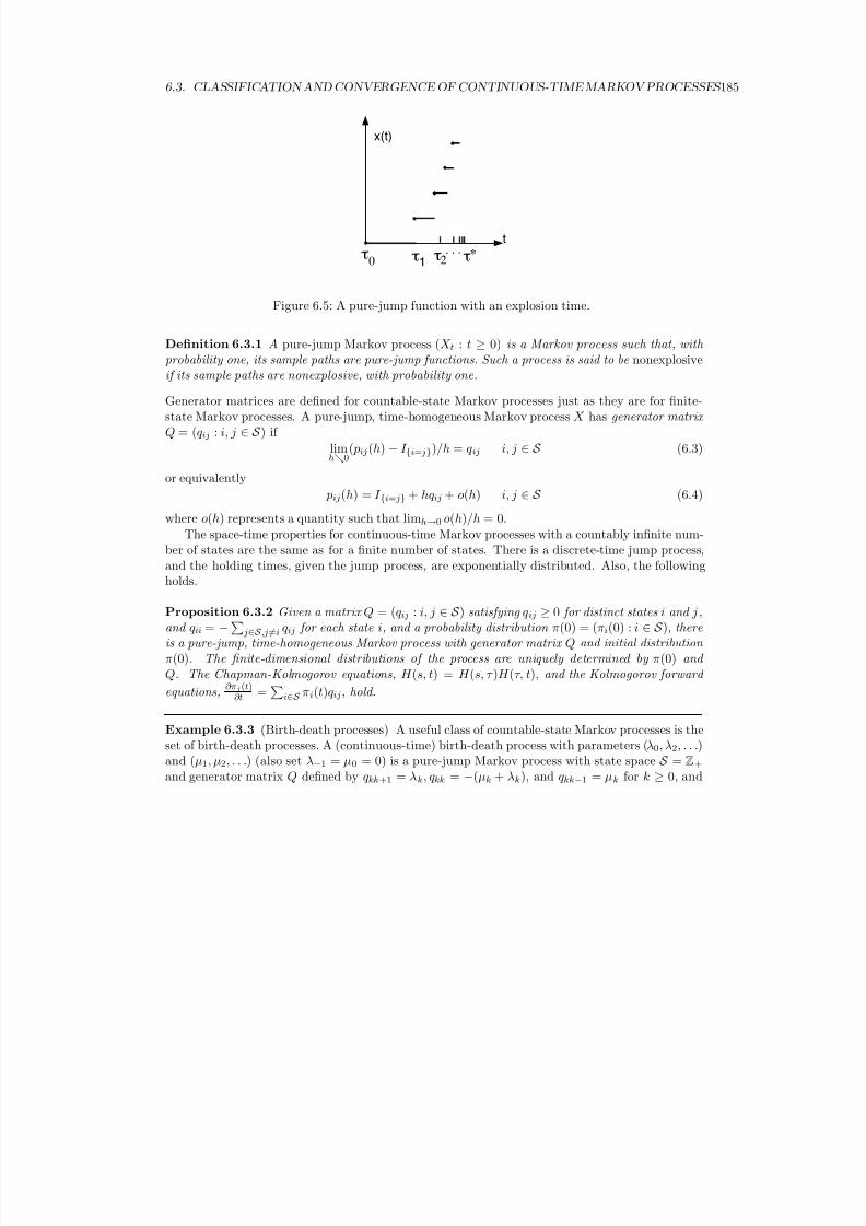
8/11/2019 Random process by B. Hajek
http://slidepdf.com/reader/full/random-process-by-b-hajek 195/448
6.3. CLASSIFICATION AND CONVERGENCE OF CONTINUOUS-TIME MARKOV PROCESSES 185
x(t)
!1! "
# # # "
t
! ! !
Figure 6.5: A pure-jump function with an explosion time.
Definition 6.3.1 A pure-jump Markov process (X t : t ≥ 0) is a Markov process such that, with probability one, its sample paths are pure-jump functions. Such a process is said to be nonexplosiveif its sample paths are nonexplosive, with probability one.
Generator matrices are defined for countable-state Markov processes just as they are for finite-state Markov processes. A pure-jump, time-homogeneous Markov process X has generator matrix Q = (q ij : i, j ∈ S ) if
limh0
( pij(h) − I i= j)/h = q ij i, j ∈ S (6.3)
or equivalently
pij(h) = I i= j + hq ij + o(h) i, j ∈ S (6.4)
where o(h) represents a quantity such that limh→0
o(h)/h = 0.
The space-time properties for continuous-time Markov processes with a countably infinite num-ber of states are the same as for a finite number of states. There is a discrete-time jump process,and the holding times, given the jump process, are exponentially distributed. Also, the followingholds.
Proposition 6.3.2 Given a matrix Q = (q ij : i, j ∈ S ) satisfying q ij ≥ 0 for distinct states i and j ,and q ii = − j∈S ,j=i q ij for each state i, and a probability distribution π(0) = (πi(0) : i ∈ S ), there is a pure-jump, time-homogeneous Markov process with generator matrix Q and initial distribution π(0). The finite-dimensional distributions of the process are uniquely determined by π(0) and Q. The Chapman-Kolmogorov equations, H (s, t) = H (s, τ )H (τ, t), and the Kolmogorov forward
equations, ∂πj(t)
∂t
= i∈S πi(t)q ij , hold.
Example 6.3.3 (Birth-death processes) A useful class of countable-state Markov processes is theset of birth-death processes. A (continuous-time) birth-death process with parameters (λ0, λ2, . . .)and (µ1, µ2, . . .) (also set λ−1 = µ0 = 0) is a pure-jump Markov process with state space S = Z+
and generator matrix Q defined by q kk+1 = λk, q kk = −(µk + λk), and q kk−1 = µk for k ≥ 0, and
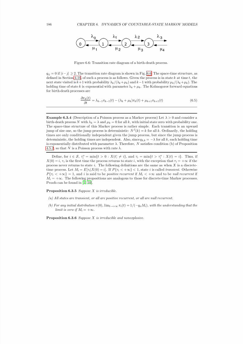
8/11/2019 Random process by B. Hajek
http://slidepdf.com/reader/full/random-process-by-b-hajek 196/448
186 CHAPTER 6. DYNAMICS OF COUNTABLE-STATE MARKOV MODELS
1 2 30
1
1 2
2 3
3
0
4!
!
!!!
!!!
Figure 6.6: Transition rate diagram of a birth-death process.
q ij = 0 if |i− j| ≥ 2. The transition rate diagram is shown in Fig. 6.6. The space-time structure, asdefined in Section 4.10, of such a process is as follows. Given the process is in state k at time t, thenext state visited is k +1 with probability λk/(λk +µk) and k −1 with probability µk/(λk +µk). Theholding time of state k is exponential with parameter λk + µk. The Kolmogorov forward equationsfor birth-death processes are
∂πk(t)∂t
= λk−1πk−1(t) − (λk + µk)πk(t) + µk+1πk+1(t) (6.5)
Example 6.3.4 (Description of a Poisson process as a Markov process) Let λ > 0 and consider abirth-death process N with λk = λ and µk = 0 for all k, with initial state zero with probability one.The space-time structure of this Markov process is rather simple. Each transition is an upward jump of size one, so the jump process is deterministic: N J (k) = k for all k . Ordinarily, the holdingtimes are only conditionally independent given the jump process, but since the jump process isdeterministic, the holding times are independent. Also, since q k,k = −λ for all k, each holding timeis exponentially distributed with parameter λ. Therefore, N satisfies condition (b) of Proposition
4.5.2, so that N is a Poisson process with rate λ.
Define, for i ∈ S , τ oi = mint > 0 : X (t) = i, and τ i = mint > τ oi : X (t) = i. Thus, if X (0) = i, τ i is the first time the process returns to state i, with the exception that τ i = +∞ if theprocess never returns to state i. The following definitions are the same as when X is a discrete-time process. Let M i = E [τ i|X (0) = i]. If P τ i < +∞ < 1, state i is called transient . OtherwiseP τ i < +∞ = 1, and i is said to be positive recurrent if M i < +∞ and to be null recurrent if M i = +∞. The following propositions are analogous to those for discrete-time Markov processes.Proofs can be found in [1, 10].
Proposition 6.3.5 Suppose X is irreducible.
(a) All states are transient, or all are positive recurrent, or all are null recurrent.
(b) For any initial distribution π(0), limt→+∞ πi(t) = 1/(−q iiM i), with the understanding that the limit is zero if M i = +∞.
Proposition 6.3.6 Suppose X is irreducible and nonexplosive.
8/11/2019 Random process by B. Hajek
http://slidepdf.com/reader/full/random-process-by-b-hajek 197/448
8/11/2019 Random process by B. Hajek
http://slidepdf.com/reader/full/random-process-by-b-hajek 198/448
188 CHAPTER 6. DYNAMICS OF COUNTABLE-STATE MARKOV MODELS
Finally, investigate whether X is recurrent. This step is not necessary if we already know thatX is positive recurrent, because a positive recurrent process is recurrent. The following test forrecurrence is valid whether or not X is explosive. Since all states have the same classification,
the process is recurrent if and only if state 0 is recurrent. Thus, the process is recurrent if theprobability the process never hits 0, for initial state 1, is zero. We shall first find the probabilityof never hitting state zero for a modified process, which stops upon reaching a large state n, andthen let n → ∞ to find the probability the original process never hits state 0. Let bin denote theprobability, for initial state i, the process does not reach zero before reaching n. Set the boundaryconditions, b0n = 0 and bnn = 1. Fix i with 1 ≤ i ≤ n − 1, and derive an expression for bin by firstconditioning on the state reached by the first jump of the process, starting from state i. By thespace-time structure, the probability the first jump is up is λi/(λi + µi) and the probability thefirst jump is down is µi/(λi + µi). Thus,
bin = λi
λi + µibi+1,n +
µi
λi + µibi−1,n,
which can be rewritten as µi(bin − bi−1,n) = λi(bi+1,n − bi,n). In particular, b2n − b1n = b1nµ1/λ1
and b3n − b2n = b1nµ1µ2/(λ1λ2), and so on, which upon summing yields the expression
bkn = b1n
k−1i=0
µ1µ2 . . . µi
λ1λ2 . . . λi.
with the convention that the i = 0 term in the sum is one. Finally, the condition bnn = 1 yieldsthe solution
b1n = 1
n−1i=0
µ1µ2...µiλ1λ2...λi
. (6.8)
Note that b1n is the probability, for initial state 1, of the event Bn that state n is reached withoutan earlier visit to state 0. Since Bn+1 ⊂ Bn for all n ≥ 1,
P (∩n≥1Bn|X (0) = 1) = limn→∞ b1n = 1/S 2 (6.9)
where
S 2 =
∞i=0
µ1µ2 . . . µi
λ1λ2 . . . λi,
with the understanding that the i = 0 term in the sum defining S 2 is one. Due to the definition of pure jump processes used, whenever X visits a state in S the number of jumps up until that timeis finite. Thus, on the event ∩n≥1Bn, state zero is never reached. Conversely, if state zero is never
reached, either the process remains bounded (which has probability zero) or ∩n≥1Bn is true. Thus,P (zero is never reached|X (0) = 1) = 1/S 2. Consequently, X is recurrent if and only if S 2 = ∞.
In summary, the following proposition is proved.
Proposition 6.4.1 Suppose X is a continuous-time birth-death process with strictly positive birth rates and death rates. If X is nonexplosive (for example, if the rates are bounded or grow at most
8/11/2019 Random process by B. Hajek
http://slidepdf.com/reader/full/random-process-by-b-hajek 199/448
6.5. TIME AVERAGES VS. STATISTICAL AVERAGES 189
linearly with n, or if S 2 = ∞) then X is positive recurrent if and only if S 1 < +∞. If X is positive recurrent the equilibrium probability distribution is given by πn = (λ0 . . . λn−1)/(S 1µ1 . . . µn).The process X is recurrent if and only if S 2 = ∞.
Discrete-time birth-death processes have a similar characterization. They are discrete-time,time-homogeneous Markov processes with state space equal to the set of nonnegative integers. Letnonnegative birth probabilities (λk : k ≥ 0) and death probabilities (µk : k ≥ 1) satisfy λ0 ≤ 1, andλk + µk ≤ 1 for k ≥ 1. The one-step transition probability matrix P = ( pij : i, j ≥ 0) is given by
pij =
λi if j = i + 1µi if j = i − 1
1 − λi − µi if j = i ≥ 11 − λ0 if j = i = 0
0 else.
(6.10)
Implicit in the specification of P is that births and deaths can’t happen simultaneously. If the birthand death probabilities are strictly positive, Proposition 6.4.1 holds as before, with the exceptionthat the discrete-time process cannot be explosive.2
6.5 Time averages vs. statistical averages
Let X be a positive recurrent, irreducible, time-homogeneous Markov process with equilibriumprobability distribution π. To be definite, suppose X is a continuous-time process, with pure-jumpsample paths and generator matrix Q. The results of this section apply with minor modificationsto the discrete-time setting as well. Above it is noted that limt→∞ πi(t) = πi = 1/(−q iiM i), whereM i is the mean “cycle time” of state i. A related consideration is convergence of the empirical distribution of the Markov process, where the empirical distribution is the distribution observedover a (usually large) time interval.
For a fixed state i, the fraction of time the process spends in state i during [0, t] is
1
t
t0
I X (s)=ids
Let T 0 denote the time that the process is first in state i, and let T k for k ≥ 1 denote the timethat the process jumps to state i for the kth time after T 0. The cycle times T k+1 − T k, k ≥ 0 areindependent and identically distributed, with mean M i. Therefore, by the law of large numbers,with probability one,
limk→∞
T k/(kM i) = limk→∞
1
kM i
k−1l=0
(T l+1 − T l)
= 1
2If in addition λi + µi = 1 for all i, the discrete-time process has period 2.
8/11/2019 Random process by B. Hajek
http://slidepdf.com/reader/full/random-process-by-b-hajek 200/448
190 CHAPTER 6. DYNAMICS OF COUNTABLE-STATE MARKOV MODELS
Furthermore, during the kth cycle interval [T k, T k+1), the amount of time spent by the processin state i is exponentially distributed with mean −1/q ii, and the time spent in the state duringdisjoint cycles is independent. Thus, with probability one,
limk→∞
1
kM i
T k0
I X (s)=ids = limk→∞
1
kM i
k−1l=0
T l+1T l
I X (s)=ids
= 1
M iE
T 1T 0
I X (s)=ids
= 1/(−q iiM i)
Combining these two observations yields that
limt→∞
1
t t
0
I X (s)=i
ds = 1/(
−q iiM i) = πi (6.11)
with probability one. In short, the limit (6.11) is expected, because the process spends on average−1/q ii time units in state i per cycle from state i, and the cycle rate is 1/M i. Of course, since statei is arbitrary, if j is any other state
limt→∞
1
t
t0
I X (s)= jds = 1/(−q jjM j) = π j (6.12)
By considering how the time in state j is distributed among the cycles from state i, it follows thatthe mean time spent in state j per cycle from state i is M iπ j.
So for any nonnegative function φ on S
,
limt→∞
1
t
t0
φ(X (s))ds = limk→∞
1
kM i
T k0
φ(X (s))ds
= 1
M iE
T 1T 0
φ(X (s))ds
= 1
M iE
j∈S
φ( j)
T 1T 0
I X (s)= jds
=
1
M i j∈S φ( j)E
T 1
T 0
I X (s)= j
ds
= j∈S
φ( j)π j (6.13)
Finally, if φ is a function of S such that either
j∈S φ+( j)π j < ∞ or
j∈S φ−( j)π j < ∞, thensince (6.13) holds for both φ+ and φ−, it must hold for φ itself.
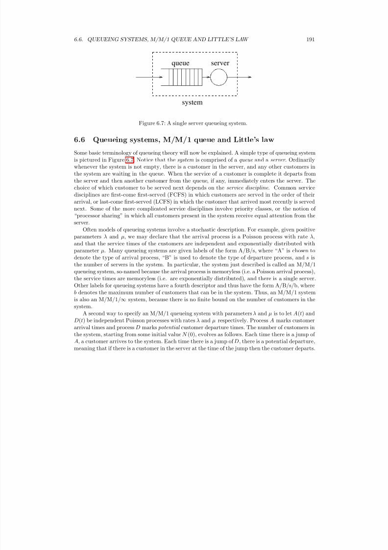
8/11/2019 Random process by B. Hajek
http://slidepdf.com/reader/full/random-process-by-b-hajek 201/448
6.6. QUEUEING SYSTEMS, M/M/1 QUEUE AND LITTLE’S LAW 191
queue server
system
Figure 6.7: A single server queueing system.
6.6 Queueing systems, M/M/1 queue and Little’s law
Some basic terminology of queueing theory will now be explained. A simple type of queueing systemis pictured in Figure 6.7. Notice that the system is comprised of a queue and a server . Ordinarilywhenever the system is not empty, there is a customer in the server, and any other customers inthe system are waiting in the queue. When the service of a customer is complete it departs fromthe server and then another customer from the queue, if any, immediately enters the server. Thechoice of which customer to be served next depends on the service discipline . Common servicedisciplines are first-come first-served (FCFS) in which customers are served in the order of theirarrival, or last-come first-served (LCFS) in which the customer that arrived most recently is servednext. Some of the more complicated service disciplines involve priority classes, or the notion of “processor sharing” in which all customers present in the system receive equal attention from theserver.
Often models of queueing systems involve a stochastic description. For example, given positive
parameters λ and µ, we may declare that the arrival process is a Poisson process with rate λ,and that the service times of the customers are independent and exponentially distributed withparameter µ. Many queueing systems are given labels of the form A/B/s, where “A” is chosen todenote the type of arrival process, “B” is used to denote the type of departure process, and s isthe number of servers in the system. In particular, the system just described is called an M/M/1queueing system, so-named because the arrival process is memoryless (i.e. a Poisson arrival process),the service times are memoryless (i.e. are exponentially distributed), and there is a single server.Other labels for queueing systems have a fourth descriptor and thus have the form A/B/s/b, whereb denotes the maximum number of customers that can be in the system. Thus, an M/M/1 systemis also an M/M/1/∞ system, because there is no finite bound on the number of customers in thesystem.
A second way to specify an M/M/1 queueing system with parameters λ and µ is to let A(t) andD(t) be independent Poisson processes with rates λ and µ respectively. Process A marks customerarrival times and process D marks potential customer departure times. The number of customers inthe system, starting from some initial value N (0), evolves as follows. Each time there is a jump of A, a customer arrives to the system. Each time there is a jump of D, there is a potential departure,meaning that if there is a customer in the server at the time of the jump then the customer departs.
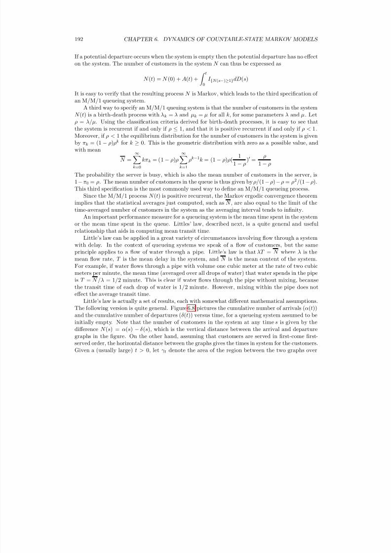
8/11/2019 Random process by B. Hajek
http://slidepdf.com/reader/full/random-process-by-b-hajek 202/448
192 CHAPTER 6. DYNAMICS OF COUNTABLE-STATE MARKOV MODELS
If a potential departure occurs when the system is empty then the potential departure has no effecton the system. The number of customers in the system N can thus be expressed as
N (t) = N (0) + A(t) + t0
I N (s−)≥1dD(s)
It is easy to verify that the resulting process N is Markov, which leads to the third specification of an M/M/1 queueing system.
A third way to specify an M/M/1 queuing system is that the number of customers in the systemN (t) is a birth-death process with λk = λ and µk = µ for all k, for some parameters λ and µ. Letρ = λ/µ. Using the classification criteria derived for birth-death processes, it is easy to see thatthe system is recurrent if and only if ρ ≤ 1, and that it is positive recurrent if and only if ρ < 1.Moreover, if ρ < 1 the equilibrium distribution for the number of customers in the system is givenby πk = (1 − ρ)ρk for k ≥ 0. This is the geometric distribution with zero as a possible value, andwith mean
N = ∞k=0
kπk = (1 − ρ)ρ ∞k=1
ρk−1k = (1 − ρ)ρ( 11 − ρ
) = ρ1 − ρ
The probability the server is busy, which is also the mean number of customers in the server, is1−π0 = ρ. The mean number of customers in the queue is thus given by ρ/(1−ρ)−ρ = ρ2/(1−ρ).This third specification is the most commonly used way to define an M/M/1 queueing process.
Since the M/M/1 process N (t) is positive recurrent, the Markov ergodic convergence theoremimplies that the statistical averages just computed, such as N , are also equal to the limit of thetime-averaged number of customers in the system as the averaging interval tends to infinity.
An important performance measure for a queueing system is the mean time spent in the systemor the mean time spent in the queue. Littles’ law, described next, is a quite general and usefulrelationship that aids in computing mean transit time.
Little’s law can be applied in a great variety of circumstances involving flow through a systemwith delay. In the context of queueing systems we speak of a flow of customers, but the sameprinciple applies to a flow of water through a pipe. Little’s law is that λT = N where λ is themean flow rate, T is the mean delay in the system, and N is the mean content of the system.For example, if water flows through a pipe with volume one cubic meter at the rate of two cubicmeters per minute, the mean time (averaged over all drops of water) that water spends in the pipeis T = N /λ = 1/2 minute. This is clear if water flows through the pipe without mixing, becausethe transit time of each drop of water is 1/2 minute. However, mixing within the pipe does noteffect the average transit time.
Little’s law is actually a set of results, each with somewhat different mathematical assumptions.The following version is quite general. Figure 6.8 pictures the cumulative number of arrivals (α(t))
and the cumulative number of departures (δ (t)) versus time, for a queueing system assumed to beinitially empty. Note that the number of customers in the system at any time s is given by thedifference N (s) = α(s) − δ (s), which is the vertical distance between the arrival and departuregraphs in the figure. On the other hand, assuming that customers are served in first-come first-served order, the horizontal distance between the graphs gives the times in system for the customers.Given a (usually large) t > 0, let γ t denote the area of the region between the two graphs over
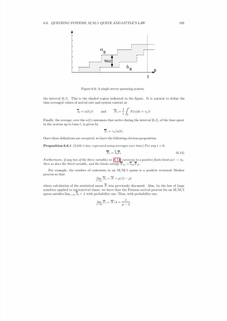
8/11/2019 Random process by B. Hajek
http://slidepdf.com/reader/full/random-process-by-b-hajek 203/448
6.6. QUEUEING SYSTEMS, M/M/1 QUEUE AND LITTLE’S LAW 193
t
!
"ss
s
N(s)
Figure 6.8: A single server queueing system.
the interval [0, t]. This is the shaded region indicated in the figure. It is natural to define thetime-averaged values of arrival rate and system content as
λt = α(t)/t and N t = 1
t
t0
N (s)ds = γ t/t
Finally, the average, over the α(t) customers that arrive during the interval [0, t], of the time spentin the system up to time t, is given by
T t = γ t/α(t).
Once these definitions are accepted, we have the following obvious proposition.
Proposition 6.6.1 (Little’s law, expressed using averages over time) For any t > 0,
N t = λtT t (6.14)
Furthermore, if any two of the three variables in (6.14) converge to a positive finite limit as t → ∞,then so does the third variable, and the limits satisfy N ∞ = λ∞T ∞.
For example, the number of customers in an M/M/1 queue is a positive recurrent Markovprocess so that
limt→∞ N t = N = ρ/(1 − ρ)
where calculation of the statistical mean N was previously discussed. Also, by the law of largenumbers applied to interarrival times, we have that the Poisson arrival process for an M/M/1queue satisfies limt→∞ λt = λ with probability one. Thus, with probability one,
limt→∞ T t = N /λ =
1
µ − λ.
8/11/2019 Random process by B. Hajek
http://slidepdf.com/reader/full/random-process-by-b-hajek 204/448
194 CHAPTER 6. DYNAMICS OF COUNTABLE-STATE MARKOV MODELS
In this sense, the average waiting time in an M/M/1 system is 1/(µ−λ). The average time in serviceis 1/µ (this follows from the third description of an M/M/1 queue, or also from Little’s law appliedto the server alone) so that the average waiting time in queue is given by W = 1/(µ − λ) − 1/µ =
ρ/(µ − λ). This final result also follows from Little’s law applied to the queue alone.
6.7 Mean arrival rate, distributions seen by arrivals, and PASTA
The mean arrival rate for the M/M/1 system is λ, the parameter of the Poisson arrival process.However for some queueing systems the arrival rate depends on the number of customers in thesystem. In such cases the mean arrival rate is still typically meaningful, and it can be used inLittle’s law.
Suppose the number of customers in a queuing system is modeled by a birth death processwith arrival rates (λk) and departure rates (µk). Suppose in addition that the process is positiverecurrent. Intuitively, the process spends a fraction of time πk in state k and while in state k the
arrival rate is λk. Therefore, the average arrival rate is
λ =∞k=0
πkλk
Similarly the average departure rate is
µ =
∞k=1
πkµk
and of course λ = µ because both are equal to the throughput of the system.
Often the distribution of a system at particular system-related sampling times are more impor-tant than the distribution in equilibrium. For example, the distribution seen by arriving customersmay be the most relevant distribution, as far as the customers are concerned. If the arrival ratedepends on the number of customers in the system then the distribution seen by arrivals need notbe the same as the equilibrium distribution. Intuitively, πkλk is the long-term frequency of arrivalswhich occur when there are k customers in the system, so that the fraction of customers that seek customers in the system upon arrival is given by
rk = πkλk
λ.
The following is an example of a system with variable arrival rate.
Example 6.7.1 (Single-server, discouraged arrivals) Suppose λk = α/(k + 1) and µk = µ for allk, where µ and α are positive constants. Then
S 2 =∞k=0
(k + 1)!µk
αk = ∞ and S 1 =
∞k=0
αk
k!µk = exp
α
µ
< ∞
8/11/2019 Random process by B. Hajek
http://slidepdf.com/reader/full/random-process-by-b-hajek 205/448
6.7. MEAN ARRIVAL RATE, DISTRIBUTIONS SEEN BY ARRIVALS, AND PASTA 195
so that the number of customers in the system is a positive recurrent Markov process, with noadditional restrictions on α and µ. Moreover, the equilibrium probability distribution is given byπk = (α/µ)k exp(−α/µ)/k!, which is the Poisson distribution with mean N = α/µ. The mean
arrival rate is
λ =∞k=0
πkα
k + 1 = µ exp(−α/µ)
∞k=0
(α/µ)k+1
(k + 1)! = µ exp(−α/µ)(exp(α/µ) − 1) = µ(1 − exp(−α/µ)).
(6.15)This expression derived for λ is clearly equal to µ, because the departure rate is µ with probability1 − π0 and zero otherwise. The distribution of the number of customers in the system seen byarrivals, (rk) is given by
rk = πkα
(k + 1)λ=
(α/µ)k+1 exp(−α/µ)
(k + 1)!(1 − exp(−α/µ)) for k ≥ 0
which in words can be described as the result of removing the probability mass at zero in the
Poisson distribution, shifting the distribution down by one, and then renormalizing. The meannumber of customers in the queue seen by a typical arrival is therefore (α/µ − 1)/(1 − exp(−α/µ)).This mean is somewhat less than N because, roughly speaking, the customer arrival rate is higherwhen the system is more lightly loaded.
The equivalence of time-averages and statistical averages for computing the mean arrival rateand the distribution seen by arrivals can be shown by application of ergodic properties of theprocesses involved. The associated formal approach is described next, in slightly more generality.Let X denote an irreducible, positive-recurrent pure-jump Markov process. If the process makes a jump from state i to state j at time t, say that a transition of type (i, j) occurs. The sequence of transitions of X forms a new Markov process, Y . The process Y is a discrete-time Markov process
with state space (i, j) ∈ S ×S : q ij > 0, and it can be described in terms of the jump process forX , by Y (k) = (X J (k − 1), X J (k)) for k ≥ 0. (Let X J (−1) be defined arbitrarily.)The one-step transition probability matrix of the jump process X J is given by πJ
ij = q ij/(−q ii),
and X J is recurrent because X is recurrent. Its equilibrium distribution πJ (if it exists) is propor-tional to −πiq ii (see Problem 6.3), and X J is positive recurrent if and only if this distribution canbe normalized to make a probability distribution, i.e. if and only if R = −i πiq ii < ∞. Assumefor simplicity that X J is positive recurrent. Then πJ
i = −πiq ii/R is the equilibrium probabilitydistribution of X J . Furthermore, Y is positive recurrent and its equilibrium distribution is givenby
πY ij = πJ
i pJ ij
= −πiq ii
R
q ij
−q ii
= πiq ij
R
Since limiting time averages equal statistical averages for Y ,
limn→∞(number of first n transitions of X that are type (i, j))/n = πiq ij/R
8/11/2019 Random process by B. Hajek
http://slidepdf.com/reader/full/random-process-by-b-hajek 206/448
196 CHAPTER 6. DYNAMICS OF COUNTABLE-STATE MARKOV MODELS
with probability one. Therefore, if A ⊂ S ×S , and if (i, j) ∈ A,
limn
→∞
number of first n transitions of X that are type (i, j)
number of first n transitions of X with type in A =
πiq ij
(i,j)∈A πi
q i j
(6.16)
To apply this setup to the special case of a queueing system in which the number of customersin the system is a Markov birth-death processes, let the set A be the set of transitions of the form(i, i + 1). Then deduce that the fraction of the first n arrivals that see i customers in the systemupon arrival converges to πiλi/
j π jλ j with probability one.
Note that if λi = λ for all i, then λ = λ and π = r. The condition λi = λ also implies that thearrival process is Poisson. This situation is called “Poisson Arrivals See Time Averages” (PASTA).
6.8 More examples of queueing systems modeled as Markov birth-
death processesFor each of the four examples of this section it is assumed that new customers are offered to thesystem according to a Poisson process with rate λ, so that the PASTA property holds. Also, whenthere are k customers in the system then the service rate is µk for some given numbers µk. Thenumber of customers in the system is a Markov birth-death process with λk = λ for all k. Sincethe number of transitions of the process up to any given time t is at most twice the number of customers that arrived by time t, the Markov process is not explosive. Therefore the process ispositive recurrent if and only if S 1 is finite, where
S 1 =∞
k=0
λk
µ1µ2 . . . µk
Special cases of this example are presented in the next four examples.
Example 6.8.1 (M/M/m systems) An M/M/m queueing system consists of a single queue andm servers. The arrival process is Poisson with some rate λ and the customer service times areindependent and exponentially distributed with mean µ for some µ > 0. The total number of customers in the system is a birth-death process with µk = µ min(k, m). Let ρ = λ/(mµ). Sinceµk = mµ for all k large enough it is easy to check that the process is positive recurrent if and onlyif ρ < 1. Assume now that ρ < 1. Then the equilibrium distribution is given by
πk = (λ/µ)k
S 1k! for 0 ≤ k ≤ m
πm+ j = πmρ j for j ≥ 1
where S 1 is chosen to make the probabilities sum to one (use the fact 1 + ρ + ρ2 . . . = 1/(1 − ρ)):
S 1 =
m−1k=0
(λ/µ)k
k!
+
(λ/µ)m
m!(1 − ρ).
8/11/2019 Random process by B. Hajek
http://slidepdf.com/reader/full/random-process-by-b-hajek 207/448
6.8. MORE EXAMPLES OF QUEUEING SYSTEMS MODELED AS MARKOV BIRTH-DEATH PROCE
An arriving customer must join the queue (rather that go directly to a server) if and only if thesystem has m or more customers in it. By the PASTA property, this is the same as the equilibriumprobability of having m or more customers in the system:
P Q =∞
j=0
πm+ j = πm/(1 − ρ)
This formula is called the Erlang C formula for probability of queueing.
Example 6.8.2 (M/M/m/m systems) An M/M/m/m queueing system consists of m servers. Thearrival process is Poisson with some rate λ and the customer service times are independent andexponentially distributed with mean µ for some µ > 0. Since there is no queue, if a customerarrives when there are already m customers in the system, the arrival is blocked and cleared fromthe system. The total number of customers in the system is a birth death process, but with the
state space reduced to 0, 1, . . . , m, and with µk = kµ for 1 ≤ k ≤ m. The unique equilibriumdistribution is given by
πk = (λ/µ)k
S 1k! for 0 ≤ k ≤ m
where S 1 is chosen to make the probabilities sum to one.An arriving customer is blocked and cleared from the system if and only if the system already
has m customers in it. By the PASTA property, this is the same as the equilibrium probability of having m customers in the system:
P B = πm =(λ/µ)m
m!
m j=0
(λ/µ)j
j!
This formula is called the Erlang B formula for probability of blocking.
Example 6.8.3 (A system with a discouraged server) The number of customers in this system is abirth-death process with constant birth rate λ and death rates µk = 1/k. It is is easy to check thatall states are transient for any positive value of λ (to verify this it suffices to check that S 2 < ∞).It is not difficult to show that N (t) converges to +∞ with probability one as t → ∞.
Example 6.8.4 (A barely stable system) The number of customers in this system is a birth-death
process with constant birth rate λ and death rates µk = λ(1+k2)1+(k−1)2 for all k ≥ 1. Since the departure
rates are barely larger than the arrival rates, this system is near the borderline between recurrenceand transience. However, we see that
S 1 =∞k=0
1
1 + k2 < ∞
8/11/2019 Random process by B. Hajek
http://slidepdf.com/reader/full/random-process-by-b-hajek 208/448
198 CHAPTER 6. DYNAMICS OF COUNTABLE-STATE MARKOV MODELS
so that N (t) is positive recurrent with equilibrium distribution πk = 1/(S 1(1 + k2)). Note that themean number of customers in the system is
N = ∞k=0
k/(S 1(1 + k2)) = ∞
By Little’s law the mean time customers spend in the system is also infinity. It is debatable whetherthis system should be thought of as “stable” even though all states are positive recurrent and allwaiting times are finite with probability one.
6.9 Foster-Lyapunov stability criterion and moment bounds
Communication network models can become quite complex, especially when dynamic scheduling,
congestion, and physical layer effects such as fading wireless channel models are included. It is thususeful to have methods to give approximations or bounds on key performance parameters. Thecriteria for stability and related moment bounds discussed in this chapter are useful for providingsuch bounds.
Aleksandr Mikhailovich Lyapunov (1857-1918) contributed significantly to the theory of stabil-ity of dynamical systems. Although a dynamical system may evolve on a complicated, multipledimensional state space, a recurring theme of dynamical systems theory is that stability questionscan often be settled by studying the potential of a system for some nonnegative potential functionV . Potential functions used for stability analysis are widely called Lyapunov functions. Similarstability conditions have been developed by many authors for stochastic systems. Below we presentthe well known criteria due to Foster [4] for recurrence and positive recurrence. In addition wepresent associated bounds on the moments, which are expectations of some functions on the statespace, computed with respect to the equilibrium probability distribution.3
Subsection 6.9.1 discusses the discrete-time tools, and presents examples involving load balanc-ing routing, and input queued crossbar switches. Subsection 6.9.2 presents the continuous timetools, and an example.
6.9.1 Stability criteria for discrete-time processes
Consider an irreducible discrete-time Markov process X on a countable state space S , with one-steptransition probability matrix P . If f is a function on S , P f represents the function obtained bymultiplication of the vector f by the matrix P : P f (i) =
j∈S pijf ( j). If f is nonnegative, P f
is well defined, with the understanding that P f (i) = +∞ is possible for some, or all, values of i.
An important property of P f is that P f (i) = E [f (X (t + 1)|X (t) = i]. Let V be a nonnegativefunction on S , to serve as the Lyapunov function. The drift vector of V (X (t)) is defined by
3 A version of these moment bounds was given by Tweedie [15], and a version of the moment bound methodwas used by Kingman [5] in a queueing context. As noted in [9], the moment bound method is closely related toDynkin’s formula. The works [13, 14, 6, 12], and many others, have demonstrated the wide applicability of thestability methods in various queueing network contexts, using quadratic Lyapunov functions.
8/11/2019 Random process by B. Hajek
http://slidepdf.com/reader/full/random-process-by-b-hajek 209/448
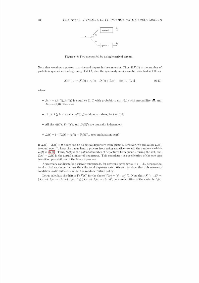
8/11/2019 Random process by B. Hajek
http://slidepdf.com/reader/full/random-process-by-b-hajek 210/448
200 CHAPTER 6. DYNAMICS OF COUNTABLE-STATE MARKOV MODELS
u
queue 1
queue 22
d
1d
au
Figure 6.9: Two queues fed by a single arrival stream.
Note that we allow a packet to arrive and depart in the same slot. Thus, if X i(t) is the number of packets in queue i at the beginning of slot t, then the system dynamics can be described as follows:
X i(t + 1) = X i(t) + Ai(t) − Di(t) + Li(t) for i ∈ 0, 1 (6.20)
where
• A(t) = (A1(t), A2(t)) is equal to (1, 0) with probability au, (0, 1) with probability au, andA(t) = (0, 0) otherwise.
• Di(t) : t ≥ 0, are Bernoulli(di) random variables, for i ∈ 0, 1
• All the A(t)’s, D1(t)’s, and D2(t)’s are mutually independent
• Li(t) = (−(X i(t) + Ai(t) − Di(t)))+ (see explanation next)
If X i(t) + Ai(t) = 0, there can be no actual departure from queue i. However, we still allow Di(t)to equal one. To keep the queue length process from going negative, we add the random variableLi(t) in (6.20). Thus, Di(t) is the potential number of departures from queue i during the slot, andDi(t) − Li(t) is the actual number of departures. This completes the specification of the one-steptransition probabilities of the Markov process.
A necessary condition for positive recurrence is, for any routing policy, a < d1 + d2, because thetotal arrival rate must be less than the total depature rate. We seek to show that this necessarycondition is also sufficient, under the random routing policy.
Let us calculate the drift of V (X (t)) for the choice V (x) = (x21 +x2
2)/2. Note that (X i(t+1))2 =(X i(t) + Ai(t) − Di(t) + Li(t))2 ≤ (X i(t) + Ai(t) − Di(t))2, because addition of the variable Li(t)
8/11/2019 Random process by B. Hajek
http://slidepdf.com/reader/full/random-process-by-b-hajek 211/448
6.9. FOSTER-LYAPUNOV STABILITY CRITERION AND MOMENT BOUNDS 201
can only push X i(t) + Ai(t) − Di(t) closer to zero. Thus,
P V (x) − V (x) = E [V (X (t + 1))|X (t) = x] − V (x)
≤ 12
2i=1
E [(xi + Ai(t) − Di(t))2 − x2i |X (t) = x]
=2
i=1
xiE [Ai(t) − Di(t)|X (t) = x] + 1
2E [(Ai(t) − Di(t))2|X (t) = x] (6.21)
≤
2i=1
xiE [Ai(t) − Di(t)|X (t) = x]
+ 1
= − (x1(d1 − au) + x2(d2 − au)) + 1 (6.22)
Under the necessary condition a < d1 + d2, there are choices of u so that au < d1 and au < d2, andfor such u the conditions of Corollary 6.9.3 are satisfied, with f (x) = x1(d1
−au) + x2(d2
−au),
g(x) = 1, and any > 0, implying that the Markov process is positive recurrent. In addition, thefirst moments under the equlibrium distribution satisfy:
(d1 − au)X 1 + (d2 − au)X 2 ≤ 1. (6.23)
In order to deduce an upper bound on X 1 + X 2, we select u∗ to maximize the minimum of thetwo coefficients in (6.23). Intuitively, this entails selecting u to minimize the absolute value of thedifference between the two coefficients. We find:
= max0≤u≤1
mind1 − au,d2 − au
= mind1, d2, d1 + d2 − a
2
and the corresponding value u∗ of u is given by
u∗ =
0 if d1 − d2 < −a
12 + d1−d2
2a if |d1 − d2| ≤ a1 if d1 − d2 > a
For the system with u = u∗, (6.23) yields
X 1 + X 2 ≤ 1
. (6.24)
We remark that, in fact,
X 1 + X 2
≤
2
d1 + d2 − a
(6.25)
If |d1 − d2| ≤ a then the bounds (6.24) and (6.25) coincide, and otherwise, the bound (6.25) isstrictly tighter. If d1 − d2 < −a then u∗ = 0, so that X 1 = 0, and (6.23) becomes (d2 − a)X 2 ≤ 1, which implies (6.25). Similarly, if d1 − d2 > a, then u∗ = 1, so that X 2 = 0, and (6.23) becomes(d1 − a)X 1 ≤ 1, which implies (6.25). Thus, (6.25) is proved.

8/11/2019 Random process by B. Hajek
http://slidepdf.com/reader/full/random-process-by-b-hajek 212/448
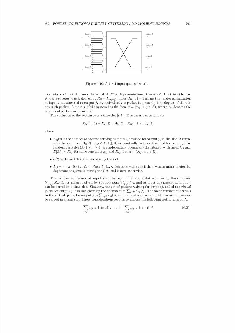
8/11/2019 Random process by B. Hajek
http://slidepdf.com/reader/full/random-process-by-b-hajek 213/448
6.9. FOSTER-LYAPUNOV STABILITY CRITERION AND MOMENT BOUNDS 203
input 4
1,3
1,4
1,2
1,1
2,1
2,2
2,3
2,4
3,1
3,2
3,3
3,4
4,1
4,2
4,3
4,4
output 1
output 2
output 3
output 4
input 1
input 2
input 3
Figure 6.10: A 4 × 4 input queued switch.
elements of E . Let Π denote the set of all N ! such permutations. Given σ ∈ Π, let R(σ) be theN × N switching matrix defined by Rij = I σi= j. Thus, Rij(σ) = 1 means that under permutationσ, input i is connected to output j, or, equivalently, a packet in queue i, j is to depart, if there isany such packet. A state x of the system has the form x = (xij : i, j ∈ E ), where xij denotes thenumber of packets in queue i, j.
The evolution of the system over a time slot [t, t + 1) is described as follows:
X ij(t + 1) = X ij(t) + Aij(t) − Rij(σ(t)) + Lij(t)
where
• Aij(t) is the number of packets arriving at input i, destined for output j , in the slot. Assume
that the variables (Aij(t) : i, j ∈ E, t ≥ 0) are mutually independent, and for each i, j, therandom variables (Aij(t) : t ≥ 0) are independent, identically distributed, with mean λij andE [A2
ij] ≤ K ij , for some constants λij and K ij. Let Λ = (λij : i, j ∈ E ).
• σ(t) is the switch state used during the slot
• Lij = (−(X ij(t) +Aij(t)−Rij(σ(t)))+, which takes value one if there was an unused potentialdeparture at queue ij during the slot, and is zero otherwise.
The number of packets at input i at the beginning of the slot is given by the row sum
j∈E X ij(t), its mean is given by the row sum
j∈E λij , and at most one packet at input i
can be served in a time slot. Similarly, the set of packets waiting for output j, called the virtual
queue for output j, has size given by the column sum i∈E X ij(t). The mean number of arrivalsto the virtual queue for output j is
i∈E λij(t), and at most one packet in the virtual queue can
be served in a time slot. These considerations lead us to impose the following restrictions on Λ: j∈E
λij < 1 for all i andi∈E
λij < 1 for all j (6.26)
8/11/2019 Random process by B. Hajek
http://slidepdf.com/reader/full/random-process-by-b-hajek 214/448
204 CHAPTER 6. DYNAMICS OF COUNTABLE-STATE MARKOV MODELS
Except for trivial cases involving deterministic arrival sequences, the conditions (6.26) are necessaryfor stable operation, for any choice of the switch schedule (σ(t) : t ≥ 0).
Let’s first explore random, independent and identically distributed (i.i.d.) switching. That is,
given a probability distribution u on Π, let (σ(t) : t ≥ 0) be independent with common probabilitydistribution u. Once the distributions of the Aij ’s and u are fixed, we have a discrete-time Markovprocess model. Given Λ satisfying (6.26), we wish to determine a choice of u so that the processwith i.i.d. switch selection is positive recurrent.
Some standard background from switching theory is given in this paragraph. A line sum of amatrix M is either a row sum,
j M ij , or a column sum,
i M ij . A square matrix M is called
doubly stochastic if it has nonnegative entries and if all of its line sums are one. Birkhoff’s theorem,celebrated in the theory of switching, states that any doubly stochastic matrix M is a convexcombination of switching matrices. That is, such an M can be represented as M =
σ∈Π R(σ)u(σ),
where u = (u(σ) : σ ∈ Π) is a probability distribution on Π. If
M is a nonnegative matrix with all
line sums less than or equal to one, then if some of the entries of M are increased appropriately,
a doubly stochastic matrix can be obtained. That is, there exists a doubly stochastic matrix M so that M ij ≤ M ij for all i, j. Applying Birkhoff’s theorem to M yields that there is a probability
distribution u so that M ij ≤
σ∈Π R(σ)u(σ) for all i, j.
Suppose Λ satisfies the necessary conditions (6.26). That is, suppose that all the line sums of Λ are less than one. Then with defined by
= 1 − (maximum line sum of Λ)
N ,
each line sum of (λij + : i, j ∈ E ) is less than or equal to one. Thus, by the observation at theend of the previous paragraph, there is a probability distribution u∗ on Π so that λij + ≤ µij(u∗),where
µij(u) = σ∈Π
Rij(σ)u(σ).
We consider the system using probability distribution u∗ for the switch states. That is, let (σ(t) :t ≥ 0) be independent, each with distribution u∗. Then for each ij , the random variables Rij(σ(t))are independent, Bernoulli(µij(u∗)) random variables.
Consider the quadratic Lyapunov function V given by V (x) = 12
i,j x2
ij . As in (6.21),
P V (x) − V (x) ≤i,j
xijE [Aij(t) − Rij(σ(t))|X ij(t) = x] + 1
2
i,j
E [(Aij(t) − Rij(σ(t)))2|X (t) = x].
NowE [Aij(t) − Rij(σ(t))|X ij(t) = x] = E [Aij(t) − Rij(σ(t))] = λij − µij(u∗) ≤ −
and1
2
i,j
E [(Aij(t) − Rij(σ(t)))2|X (t) = x] ≤ 1
2
i,j
E [(Aij(t))2 + (Rij(σ(t)))2] ≤ K
8/11/2019 Random process by B. Hajek
http://slidepdf.com/reader/full/random-process-by-b-hajek 215/448
6.9. FOSTER-LYAPUNOV STABILITY CRITERION AND MOMENT BOUNDS 205
where K = 12 (N +
i,j K ij). Thus,
P V (x) − V (x) ≤ −ij
xij+ K (6.27)
Therefore, by Corollary 6.9.3, the process is positive recurrent, andij
X ij ≤ K
(6.28)
That is, the necessary condition (6.26) is also sufficient for positive recurrence and finite mean queuelength in equilibrium, under i.i.d. random switching, for an appropriate probability distribution u∗
on the set of permutations.
Example 6.9.7 (An input queued switch with maximum weight switching) The random switchingpolicy used in Example 2a depends on the arrival rate matrix Λ, which may be unknown a priori.Also, the policy allocates potential departures to a given queue ij, whether or not the queue isempty, even if other queues could be served instead. This suggests using a dynamic switchingpolicy, such as the maximum weight switching policy, defined by σ(t) = σMW (X (t)), where for astate x,
σMW (x) = arg maxσ∈Π
ij
xijRij(σ). (6.29)
The use of “arg max” here means that σMW (x) is selected to be a value of σ that maximizes the
sum on the right hand side of (6.29), which is the weight of permutation σ with edge weights xij . Inorder to obtain a particular Markov model, we assume that the set of permutations Π is numberedfrom 1 to N ! in some fashion, and in case there is a tie between two or more permutations for havingthe maximum weight, the lowest numbered permutation is used. Let P MW denote the one-steptransition probability matrix when the route-to-shorter policy is used.
Letting V and K be as in Example 2a, we find under the maximum weight policy that
P MW V (x) − V (x) ≤ij
xij(λij − Rij(σMW (x))) + K
The maximum of a function is greater than or equal to the average of the function, so that for any
probability distribution u on Πij
xijRij(σMW (t)) ≥σ
u(σ)ij
xijRij(σ) (6.30)
=ij
xijµij(u)
8/11/2019 Random process by B. Hajek
http://slidepdf.com/reader/full/random-process-by-b-hajek 216/448
206 CHAPTER 6. DYNAMICS OF COUNTABLE-STATE MARKOV MODELS
with equality in (6.30) if and only if u is concentrated on the set of maximum weight permutations.In particular, the choice u = u∗ shows that
ij xijRij(σ
MW
(t)) ≥ ij xijµij(u∗) ≥ ij xij(λij + )
Therefore, if P is replaced by P MW , (6.27) still holds. Therefore, by Corollary 6.9.3, the processis positive recurrent, and the same moment bound, (6.28), holds, as for the randomized switchingstrategy of Example 2a. On one hand, implementing the maximum weight algorithm does notrequire knowledge of the arrival rates, but on the other hand, it requires that queue length infor-mation be shared, and that a maximization problem be solved for each time slot. Much recentwork has gone towards reduced complexity dynamic switching algorithms.
6.9.2 Stability criteria for continuous time processes
Here is a continuous time version of the Foster-Lyapunov stability criteria and the moment bounds.Suppose X is a time-homegeneous, irreducible, continuous-time Markov process with generatormatrix Q. The drift vector of V (X (t)) is the vector QV . This definition is motivated by the factthat the mean drift of X for an interval of duration h is given by
dh(i) = E [V (X (t + h))|X (t) = i] − V (i)
h
= j∈S
pij(h) − δ ij
h
V ( j)
= j∈S q ij + o(h)
h V ( j), (6.31)
so that if the limit as h → 0 can be taken inside the summation in (6.31), then dh(i) → QV (i) ash → 0. The following useful expression for QV follows from the fact that the row sums of Q arezero:
QV (i) = j: j=i
q ij(V ( j) − V (i)). (6.32)
Formula (6.32) is quite similar to the formula (6.17) for the drift vector for a discrete-time process.
Proposition 6.9.8 (Foster-Lyapunov stability criterion–continuous time) Suppose V : S → R+
and C is a finite subset of S .(a) If QV
≤ 0 on
S −C , and
i : V (i)
≤ K
is finite for all K then X is recurrent.
(b) Suppose for some b > 0 and > 0 that
QV (i) ≤ − + bI C (i) for all i ∈ S . (6.33)
Suppose further that i : V (i) ≤ K is finite for all K , or that X is nonexplosive. Then X is positive recurrent.
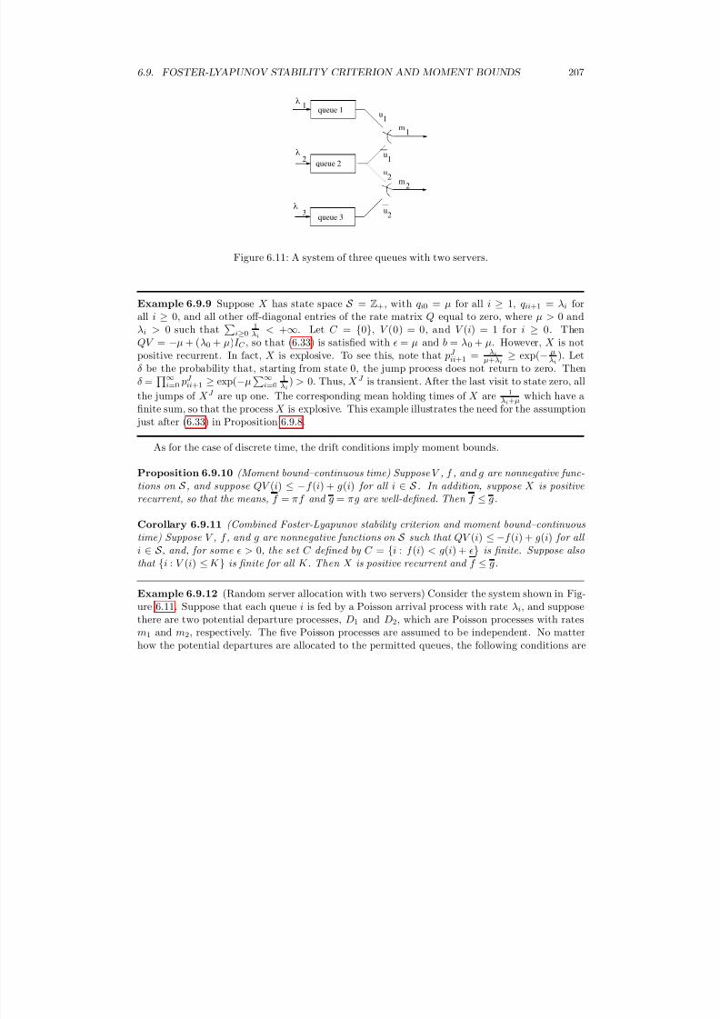
8/11/2019 Random process by B. Hajek
http://slidepdf.com/reader/full/random-process-by-b-hajek 217/448
6.9. FOSTER-LYAPUNOV STABILITY CRITERION AND MOMENT BOUNDS 207
2
queue 1
queue 2
queue 3
1
2
3
2
1
!
!
!
m
m
u1
1u
u2
u
Figure 6.11: A system of three queues with two servers.
Example 6.9.9 Suppose X has state space S = Z+, with q i0 = µ for all i ≥ 1, q ii+1 = λi forall i ≥ 0, and all other off-diagonal entries of the rate matrix Q equal to zero, where µ > 0 andλi > 0 such that
i≥0
1λi
< +∞. Let C = 0, V (0) = 0, and V (i) = 1 for i ≥ 0. ThenQV = −µ + (λ0 + µ)I C , so that (6.33) is satisfied with = µ and b = λ0 + µ. However, X is notpositive recurrent. In fact, X is explosive. To see this, note that pJ
ii+1 = λiµ+λi
≥ exp(− µλi
). Letδ be the probability that, starting from state 0, the jump process does not return to zero. Thenδ =
∞i=0 pJ
ii+1 ≥ exp(−µ∞
i=01λi
) > 0. Thus, X J is transient. After the last visit to state zero, all
the jumps of X J are up one. The corresponding mean holding times of X are 1λi+µ which have a
finite sum, so that the process X is explosive. This example illustrates the need for the assumption just after (6.33) in Proposition 6.9.8.
As for the case of discrete time, the drift conditions imply moment bounds.
Proposition 6.9.10 (Moment bound–continuous time) Suppose V , f , and g are nonnegative func-tions on S , and suppose QV (i) ≤ −f (i) + g(i) for all i ∈ S . In addition, suppose X is positive recurrent, so that the means, f = πf and g = πg are well-defined. Then f ≤ g.
Corollary 6.9.11 (Combined Foster-Lyapunov stability criterion and moment bound–continuous time) Suppose V , f , and g are nonnegative functions on S such that QV (i) ≤ −f (i) + g(i) for all i ∈ S , and, for some > 0, the set C defined by C = i : f (i) < g(i) + is finite. Suppose alsothat i : V (i) ≤ K is finite for all K . Then X is positive recurrent and f ≤ g.
Example 6.9.12 (Random server allocation with two servers) Consider the system shown in Fig-ure 6.11. Suppose that each queue i is fed by a Poisson arrival process with rate λi, and supposethere are two potential departure processes, D1 and D2, which are Poisson processes with ratesm1 and m2, respectively. The five Poisson processes are assumed to be independent. No matterhow the potential departures are allocated to the permitted queues, the following conditions are
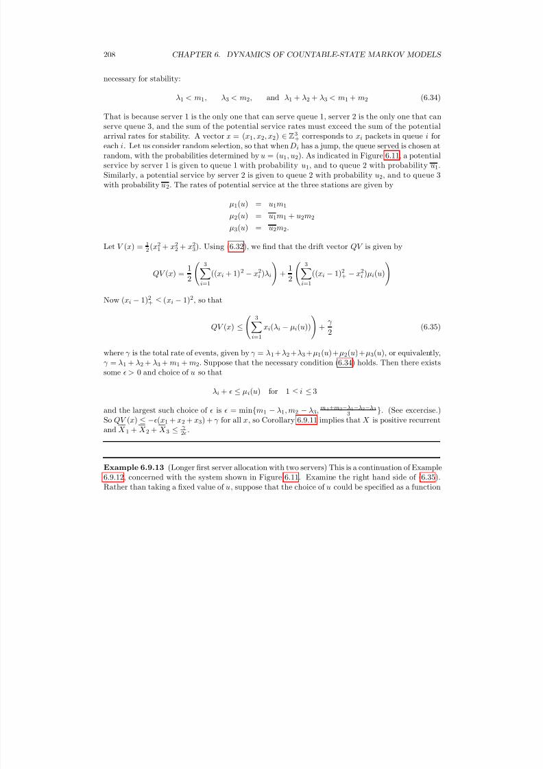
8/11/2019 Random process by B. Hajek
http://slidepdf.com/reader/full/random-process-by-b-hajek 218/448
208 CHAPTER 6. DYNAMICS OF COUNTABLE-STATE MARKOV MODELS
necessary for stability:
λ1 < m1, λ3 < m2, and λ1 + λ2 + λ3 < m1 + m2 (6.34)
That is because server 1 is the only one that can serve queue 1, server 2 is the only one that canserve queue 3, and the sum of the potential service rates must exceed the sum of the potentialarrival rates for stability. A vector x = (x1, x2, x2) ∈ Z3
+ corresponds to xi packets in queue i foreach i. Let us consider random selection, so that when Di has a jump, the queue served is chosen atrandom, with the probabilities determined by u = (u1, u2). As indicated in Figure 6.11, a potentialservice by server 1 is given to queue 1 with probability u1, and to queue 2 with probability u1.Similarly, a potential service by server 2 is given to queue 2 with probability u2, and to queue 3with probability u2. The rates of potential service at the three stations are given by
µ1(u) = u1m1
µ2(u) = u1m1 + u2m2µ3(u) = u2m2.
Let V (x) = 12 (x2
1 + x22 + x2
3). Using (6.32), we find that the drift vector QV is given by
QV (x) = 1
2
3i=1
((xi + 1)2 − x2i )λi
+
1
2
3i=1
((xi − 1)2+ − x2
i )µi(u)
Now (xi − 1)2+ ≤ (xi − 1)2, so that
QV (x) ≤ 3
i=1 xi(λi − µi(u))+
γ
2 (6.35)
where γ is the total rate of events, given by γ = λ1 +λ2 +λ3 +µ1(u)+µ2(u)+µ3(u), or equivalently,γ = λ1 + λ2 + λ3 + m1 + m2. Suppose that the necessary condition (6.34) holds. Then there existssome > 0 and choice of u so that
λi + ≤ µi(u) for 1 ≤ i ≤ 3
and the largest such choice of is = minm1 − λ1, m2 − λ3, m1+m2−λ1−λ2−λ33 . (See excercise.)
So QV (x) ≤ −(x1 + x2 + x3) + γ for all x, so Corollary 6.9.11 implies that X is positive recurrentand X 1 + X 2 + X 3 ≤ γ
2 .
Example 6.9.13 (Longer first server allocation with two servers) This is a continuation of Example6.9.12, concerned with the system shown in Figure 6.11. Examine the right hand side of (6.35).Rather than taking a fixed value of u, suppose that the choice of u could be specified as a function
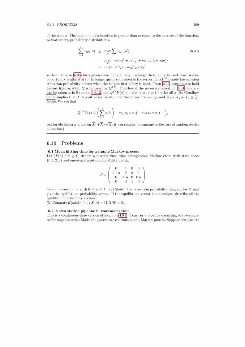
8/11/2019 Random process by B. Hajek
http://slidepdf.com/reader/full/random-process-by-b-hajek 219/448
6.10. PROBLEMS 209
of the state x. The maximum of a function is greater than or equal to the average of the function,so that for any probability distribution u,
3i=1
xiµi(u) ≤ maxui
xiµi(u) (6.36)
= maxu
m1(x1u1 + x2u
1) + m2(x2u2 + x3u
2)
= m1(x1 ∨ x2) + m2(x2 ∨ x3)
with equality in (6.36) for a given state x if and only if a longer first policy is used: each serviceopportunity is allocated to the longer queue connected to the server. Let QLF denote the one-steptransition probability matrix when the longest first policy is used. Then (6.35) continues to holdfor any fixed u, when Q is replaced by QLF . Therefore if the necessary condition (6.34) holds, can be taken as in Example 6.9.12, and QLF V (x) ≤ −(x1 + x2 + x3) + γ for all x. So Corollary6.9.11 implies that X is positive recurrent under the longer first policy, and X
1 + X
2 + X
3 ≤ γ
2.
(Note: We see that
QLF V (x) ≤
3i=1
xiλi
− m1(x1 ∨ x2) − m2(x2 ∨ x3) +
γ
2,
but for obtaining a bound on X 1 +X 2 +X 3 it was simpler to compare to the case of random serviceallocation.)
6.10 Problems
6.1 Mean hitting time for a simple Markov processLet (X (n) : n ≥ 0) denote a discrete-time, time-homogeneous Markov chain with state space0, 1, 2, 3 and one-step transition probability matrix
P =
0 1 0 0
1 − a 0 a 00 0.5 0 0.50 0 1 0
for some constant a with 0 ≤ a ≤ 1. (a) Sketch the transition probability diagram for X andgive the equilibrium probability vector. If the equilibrium vector is not unique, describe all the
equilibrium probability vectors.(b) Compute E [minn ≥ 1 : X (n) = 3|X (0) = 0].
6.2 A two station pipeline in continuous timeThis is a continuous-time version of Example 4.9.1. Consider a pipeline consisting of two single-buffer stages in series. Model the system as a continuous-time Markov process. Suppose new packets
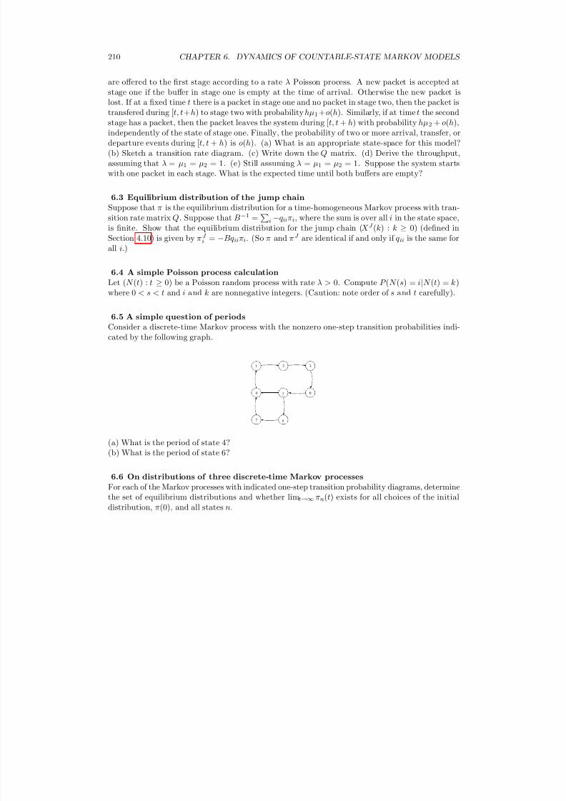
8/11/2019 Random process by B. Hajek
http://slidepdf.com/reader/full/random-process-by-b-hajek 220/448
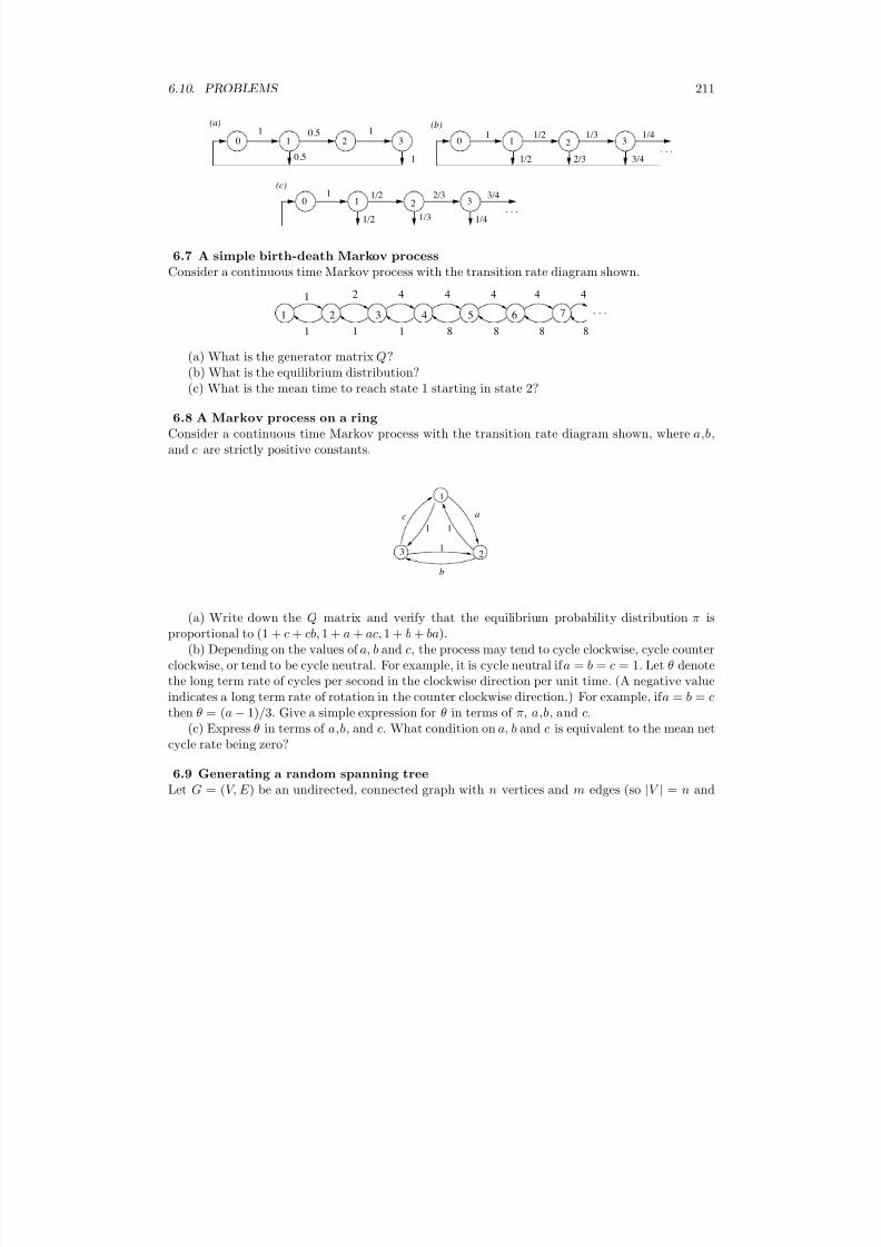
8/11/2019 Random process by B. Hajek
http://slidepdf.com/reader/full/random-process-by-b-hajek 221/448
6.10. PROBLEMS 211
1
1 1
1
0.5
0.5
0 1 2 3
(a)
. . .0 1 2 3
(b)1/2
2/3
1/31
1/2 3/4
1/4
. . .0 1 2 3
3/4
1/4
2/3
1/3
1/2
1/2
(c)
6.7 A simple birth-death Markov processConsider a continuous time Markov process with the transition rate diagram shown.
4
. . .1 765432
1 4
1 1 1 8 8 8 8
4 4 42
(a) What is the generator matrix Q?(b) What is the equilibrium distribution?(c) What is the mean time to reach state 1 starting in state 2?
6.8 A Markov process on a ringConsider a continuous time Markov process with the transition rate diagram shown, where a,b,and c are strictly positive constants.
2
a
3
c
1
b
11
1
(a) Write down the Q matrix and verify that the equilibrium probability distribution π isproportional to (1 + c + cb, 1 + a + ac, 1 + b + ba).
(b) Depending on the values of a, b and c, the process may tend to cycle clockwise, cycle counterclockwise, or tend to be cycle neutral. For example, it is cycle neutral if a = b = c = 1. Let θ denotethe long term rate of cycles per second in the clockwise direction per unit time. (A negative valueindicates a long term rate of rotation in the counter clockwise direction.) For example, if a = b = c
then θ = (a − 1)/3. Give a simple expression for θ in terms of π, a,b, and c.(c) Express θ in terms of a,b, and c. What condition on a, b and c is equivalent to the mean net
cycle rate being zero?
6.9 Generating a random spanning treeLet G = (V, E ) be an undirected, connected graph with n vertices and m edges (so |V | = n and
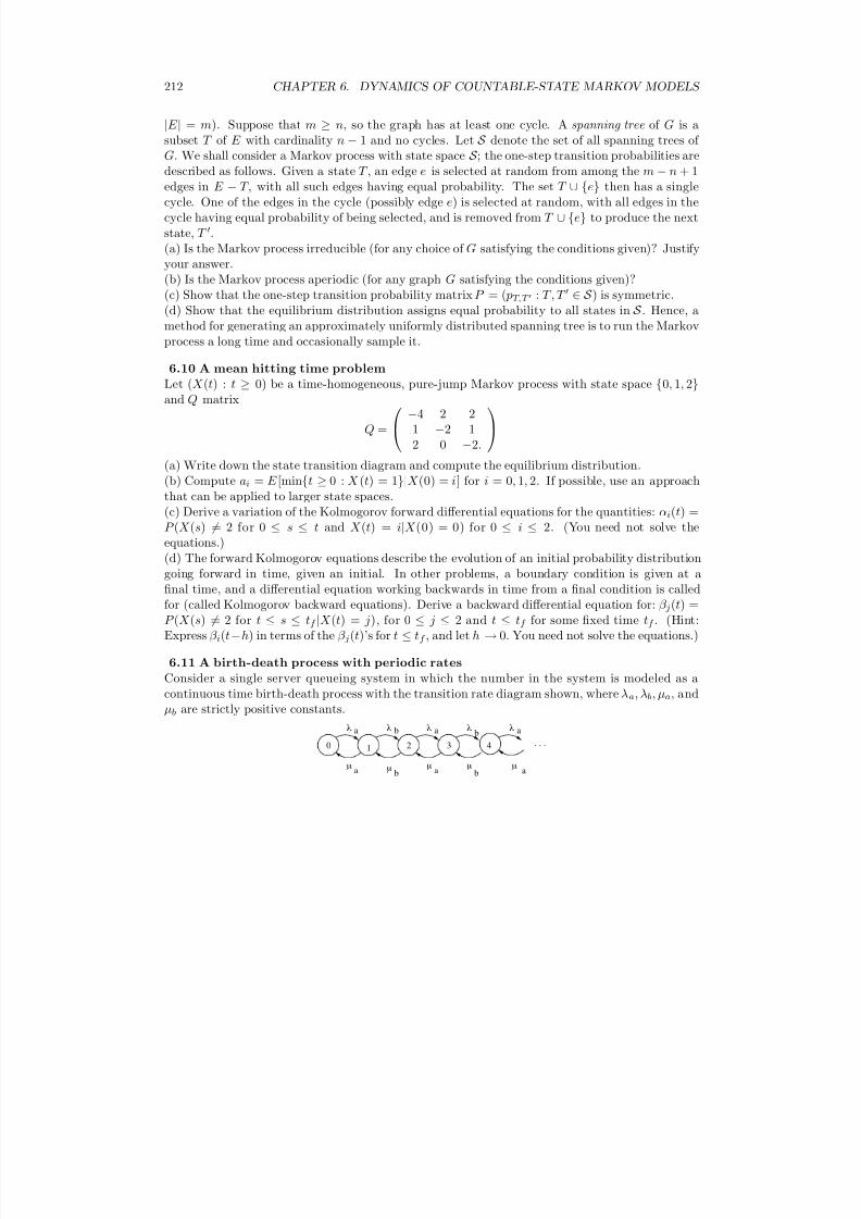
8/11/2019 Random process by B. Hajek
http://slidepdf.com/reader/full/random-process-by-b-hajek 222/448
212 CHAPTER 6. DYNAMICS OF COUNTABLE-STATE MARKOV MODELS
|E | = m). Suppose that m ≥ n, so the graph has at least one cycle. A spanning tree of G is asubset T of E with cardinality n − 1 and no cycles. Let S denote the set of all spanning trees of G. We shall consider a Markov process with state space S ; the one-step transition probabilities are
described as follows. Given a state T , an edge e is selected at random from among the m − n + 1edges in E − T, with all such edges having equal probability. The set T ∪ e then has a singlecycle. One of the edges in the cycle (possibly edge e) is selected at random, with all edges in thecycle having equal probability of being selected, and is removed from T ∪ e to produce the nextstate, T .(a) Is the Markov process irreducible (for any choice of G satisfying the conditions given)? Justifyyour answer.(b) Is the Markov process aperiodic (for any graph G satisfying the conditions given)?(c) Show that the one-step transition probability matrix P = ( pT,T : T , T ∈ S ) is symmetric.(d) Show that the equilibrium distribution assigns equal probability to all states in S . Hence, amethod for generating an approximately uniformly distributed spanning tree is to run the Markovprocess a long time and occasionally sample it.
6.10 A mean hitting time problemLet (X (t) : t ≥ 0) be a time-homogeneous, pure-jump Markov process with state space 0, 1, 2and Q matrix
Q =
−4 2 21 −2 12 0 −2.
(a) Write down the state transition diagram and compute the equilibrium distribution.(b) Compute ai = E [mint ≥ 0 : X (t) = 1|X (0) = i] for i = 0, 1, 2. If possible, use an approachthat can be applied to larger state spaces.(c) Derive a variation of the Kolmogorov forward differential equations for the quantities: αi(t) =
P (X (s) = 2 for 0 ≤ s ≤ t and X (t) = i|X (0) = 0) for 0 ≤ i ≤ 2. (You need not solve theequations.)(d) The forward Kolmogorov equations describe the evolution of an initial probability distributiongoing forward in time, given an initial. In other problems, a boundary condition is given at afinal time, and a differential equation working backwards in time from a final condition is calledfor (called Kolmogorov backward equations). Derive a backward differential equation for: β j(t) =P (X (s) = 2 for t ≤ s ≤ tf |X (t) = j), for 0 ≤ j ≤ 2 and t ≤ tf for some fixed time tf . (Hint:Express β i(t−h) in terms of the β j(t)’s for t ≤ tf , and let h → 0. You need not solve the equations.)
6.11 A birth-death process with periodic ratesConsider a single server queueing system in which the number in the system is modeled as a
continuous time birth-death process with the transition rate diagram shown, where λa, λb, µa, andµb are strictly positive constants.
a
31 20 . . .4
! ! !!
!
!
!! ! !
a a ab b
a b a b
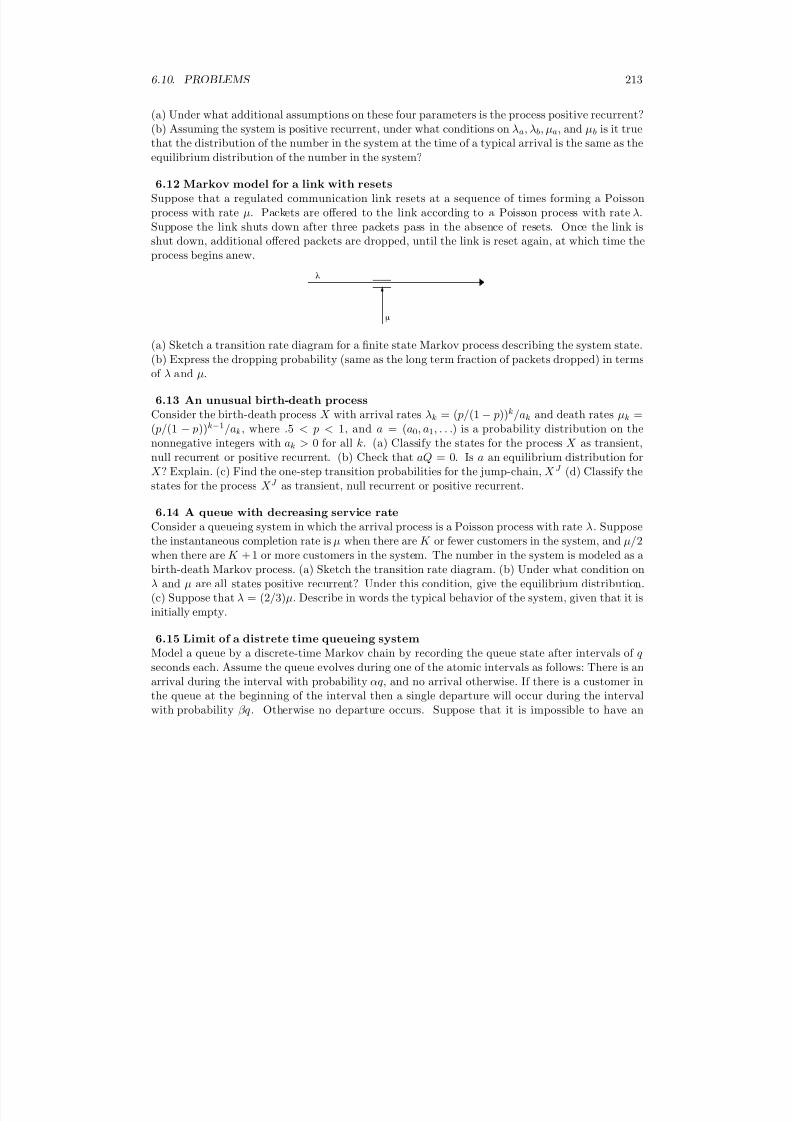
8/11/2019 Random process by B. Hajek
http://slidepdf.com/reader/full/random-process-by-b-hajek 223/448
6.10. PROBLEMS 213
(a) Under what additional assumptions on these four parameters is the process positive recurrent?(b) Assuming the system is positive recurrent, under what conditions on λa, λb, µa, and µb is it truethat the distribution of the number in the system at the time of a typical arrival is the same as the
equilibrium distribution of the number in the system?
6.12 Markov model for a link with resetsSuppose that a regulated communication link resets at a sequence of times forming a Poissonprocess with rate µ. Packets are offered to the link according to a Poisson process with rate λ.Suppose the link shuts down after three packets pass in the absence of resets. Once the link isshut down, additional offered packets are dropped, until the link is reset again, at which time theprocess begins anew.
!
!
(a) Sketch a transition rate diagram for a finite state Markov process describing the system state.(b) Express the dropping probability (same as the long term fraction of packets dropped) in termsof λ and µ.
6.13 An unusual birth-death processConsider the birth-death process X with arrival rates λk = ( p/(1 − p))k/ak and death rates µk =( p/(1 − p))k−1/ak, where .5 < p < 1, and a = (a0, a1, . . .) is a probability distribution on thenonnegative integers with ak > 0 for all k. (a) Classify the states for the process X as transient,null recurrent or positive recurrent. (b) Check that aQ = 0. Is a an equilibrium distribution forX ? Explain. (c) Find the one-step transition probabilities for the jump-chain, X J (d) Classify the
states for the process X J as transient, null recurrent or positive recurrent.
6.14 A queue with decreasing service rateConsider a queueing system in which the arrival process is a Poisson process with rate λ. Supposethe instantaneous completion rate is µ when there are K or fewer customers in the system, and µ/2when there are K + 1 or more customers in the system. The number in the system is modeled as abirth-death Markov process. (a) Sketch the transition rate diagram. (b) Under what condition onλ and µ are all states positive recurrent? Under this condition, give the equilibrium distribution.(c) Suppose that λ = (2/3)µ. Describe in words the typical behavior of the system, given that it isinitially empty.
6.15 Limit of a distrete time queueing systemModel a queue by a discrete-time Markov chain by recording the queue state after intervals of q seconds each. Assume the queue evolves during one of the atomic intervals as follows: There is anarrival during the interval with probability αq , and no arrival otherwise. If there is a customer inthe queue at the beginning of the interval then a single departure will occur during the intervalwith probability βq . Otherwise no departure occurs. Suppose that it is impossible to have an

8/11/2019 Random process by B. Hajek
http://slidepdf.com/reader/full/random-process-by-b-hajek 224/448
214 CHAPTER 6. DYNAMICS OF COUNTABLE-STATE MARKOV MODELS
arrival and a departure in a single atomic interval. (a) Find ak=P(an interarrival time is kq ) andbk=P(a service time is kq ). (b) Find the equilibrium distribution, p = ( pk : k ≥ 0), of the numberof customers in the system at the end of an atomic interval. What happens as q → 0?
6.16 An M/M/1 queue with impatient customersConsider an M/M/1 queue with parameters λ and µ with the following modification. Each customerin the queue will defect (i.e. depart without service) with probability αh + o(h) in an interval of length h, independently of the other customers in the queue. Once a customer makes it to theserver it no longer has a chance to defect and simply waits until its service is completed and thendeparts from the system. Let N (t) denote the number of customers in the system (queue plusserver) at time t. (a) Give the transition rate diagram and generator matrix Q for the Markovchain N = (N (t) : t ≥ 0). (b) Under what conditions are all states positive recurrent? Under thiscondition, find the equilibrium distribution for N . (You need not explicitly sum the series.) (c)Suppose that α = µ. Find an explicit expression for pD, the probability that a typical arriving
customer defects instead of being served. Does your answer make sense as λ/µ converges to zeroor to infinity?
6.17 Statistical multiplexingConsider the following scenario regarding a one-way link in a store-and-forward packet commu-nication network. Suppose that the link supports eight connections, each generating traffic at 5kilobits per second (kbps). The data for each connection is assumed to be in packets exponentiallydistributed in length with mean packet size 1 kilobit. The packet lengths are assumed mutuallyindependent and the packets for each stream arrive according to a Poisson process. Packets arequeued at the beginning of the link if necessary, and queue space is unlimited. Compute the meandelay (queueing plus transmission time–neglect propagation delay) for each of the following three
scenarios. Compare your answers. (a) (Full multiplexing) The link transmit speed is 50 kbps. (b)The link is replaced by two 25 kbps links, and each of the two links carries four sessions. (Of coursethe delay would be larger if the sessions were not evenly divided.) (c) (Multiplexing over two links)The link is replaced by two 25 kbps links. Each packet is transmitted on one link or the other, andneither link is idle whenever a packet from any session is waiting.
6.18 A queue with blocking(M/M/1/5 system) Consider an M/M/1 queue with service rate µ, arrival rate λ, and the modifi-cation that at any time, at most five customers can be in the system (including the one in service,if any). If a customer arrives and the system is full (i.e. already has five customers in it) then thecustomer is dropped, and is said to be blocked. Let N (t) denote the number of customers in the
system at time t. Then (N (t) : t ≥ 0) is a Markov chain. (a) Indicate the transition rate diagram of the chain and find the equilibrium probability distribution. (b) What is the probability, pB , that atypical customer is blocked? (c) What is the mean waiting time in queue, W , of a typical customerthat is not blocked? (d) Give a simple method to numerically calculate, or give a simple expressionfor, the mean length of a busy period of the system. (A busy period begins with the arrival of acustomer to an empty system and ends when the system is again empty.)
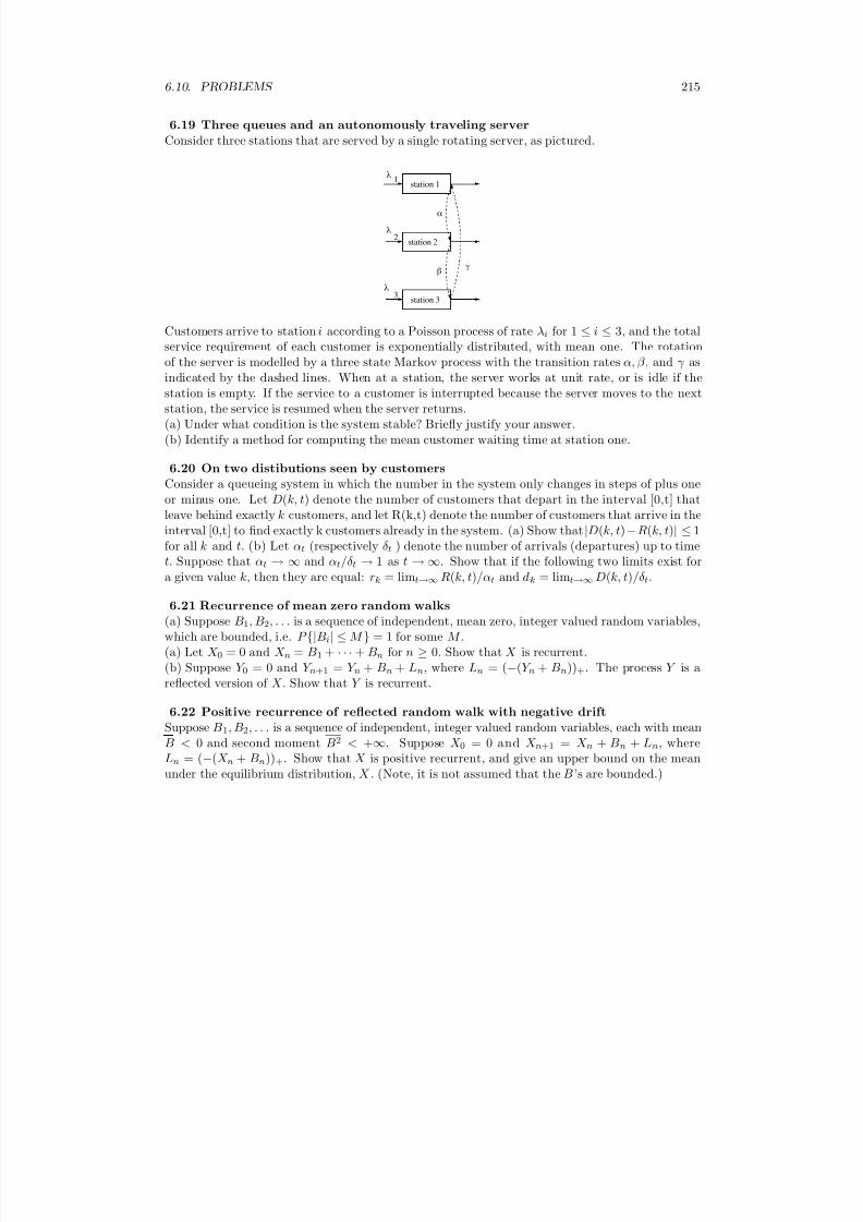
8/11/2019 Random process by B. Hajek
http://slidepdf.com/reader/full/random-process-by-b-hajek 225/448
6.10. PROBLEMS 215
6.19 Three queues and an autonomously traveling serverConsider three stations that are served by a single rotating server, as pictured.
!
1
2
3"
"
"station 1
station 2
station 3
#$
Customers arrive to station i according to a Poisson process of rate λi for 1 ≤ i ≤ 3, and the total
service requirement of each customer is exponentially distributed, with mean one. The rotationof the server is modelled by a three state Markov process with the transition rates α, β, and γ asindicated by the dashed lines. When at a station, the server works at unit rate, or is idle if thestation is empty. If the service to a customer is interrupted because the server moves to the nextstation, the service is resumed when the server returns.(a) Under what condition is the system stable? Briefly justify your answer.(b) Identify a method for computing the mean customer waiting time at station one.
6.20 On two distibutions seen by customersConsider a queueing system in which the number in the system only changes in steps of plus oneor minus one. Let D(k, t) denote the number of customers that depart in the interval [0,t] thatleave behind exactly k customers, and let R(k,t) denote the number of customers that arrive in theinterval [0,t] to find exactly k customers already in the system. (a) Show that |D(k, t)−R(k, t)| ≤ 1for all k and t. (b) Let αt (respectively δ t ) denote the number of arrivals (departures) up to timet. Suppose that αt → ∞ and αt/δ t → 1 as t → ∞. Show that if the following two limits exist fora given value k, then they are equal: rk = limt→∞ R(k, t)/αt and dk = limt→∞ D(k, t)/δ t.
6.21 Recurrence of mean zero random walks(a) Suppose B1, B2, . . . is a sequence of independent, mean zero, integer valued random variables,which are bounded, i.e. P |Bi| ≤ M = 1 for some M .(a) Let X 0 = 0 and X n = B1 + · · · + Bn for n ≥ 0. Show that X is recurrent.(b) Suppose Y 0 = 0 and Y n+1 = Y n + Bn + Ln, where Ln = (−(Y n + Bn))+. The process Y is areflected version of X . Show that Y is recurrent.
6.22 Positive recurrence of reflected random walk with negative driftSuppose B1, B2, . . . is a sequence of independent, integer valued random variables, each with meanB < 0 and second moment B2 < +∞. Suppose X 0 = 0 and X n+1 = X n + Bn + Ln, whereLn = (−(X n + Bn))+. Show that X is positive recurrent, and give an upper bound on the meanunder the equilibrium distribution, X . (Note, it is not assumed that the B ’s are bounded.)
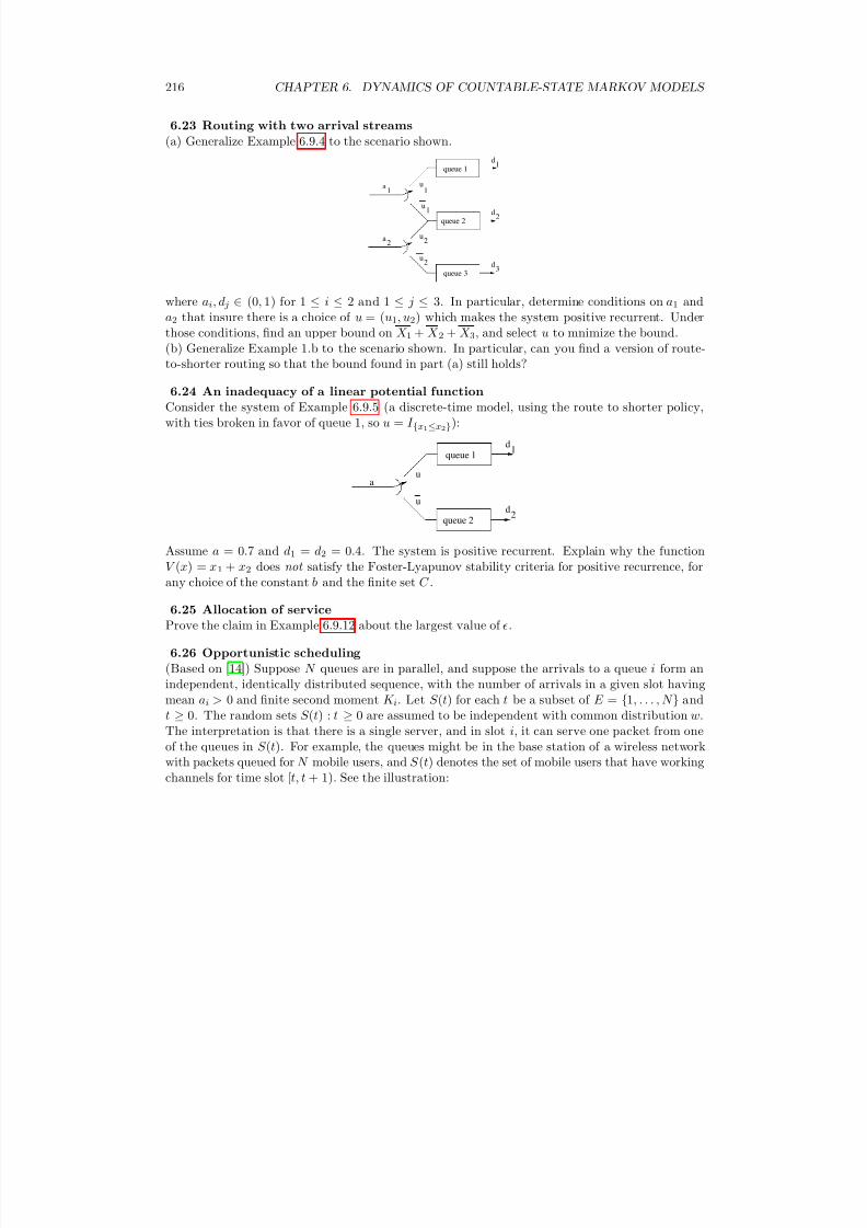
8/11/2019 Random process by B. Hajek
http://slidepdf.com/reader/full/random-process-by-b-hajek 226/448
216 CHAPTER 6. DYNAMICS OF COUNTABLE-STATE MARKOV MODELS
6.23 Routing with two arrival streams(a) Generalize Example 6.9.4 to the scenario shown.
1
queue 1
queue 22
d
1d
d
1
2
u
u
u
u2
queue 33
2a
a1
where ai, d j ∈ (0, 1) for 1 ≤ i ≤ 2 and 1 ≤ j ≤ 3. In particular, determine conditions on a1 anda2 that insure there is a choice of u = (u1, u2) which makes the system positive recurrent. Underthose conditions, find an upper bound on X 1 + X 2 + X 3, and select u to mnimize the bound.
(b) Generalize Example 1.b to the scenario shown. In particular, can you find a version of route-to-shorter routing so that the bound found in part (a) still holds?
6.24 An inadequacy of a linear potential functionConsider the system of Example 6.9.5 (a discrete-time model, using the route to shorter policy,with ties broken in favor of queue 1, so u = I x1≤x2):
u
queue 1
queue 22
d
1d
au
Assume a = 0.7 and d1 = d2 = 0.4. The system is positive recurrent. Explain why the functionV (x) = x1 + x2 does not satisfy the Foster-Lyapunov stability criteria for positive recurrence, forany choice of the constant b and the finite set C .
6.25 Allocation of serviceProve the claim in Example 6.9.12 about the largest value of .
6.26 Opportunistic scheduling(Based on [14]) Suppose N queues are in parallel, and suppose the arrivals to a queue i form anindependent, identically distributed sequence, with the number of arrivals in a given slot having
mean ai > 0 and finite second moment K i. Let S (t) for each t be a subset of E = 1, . . . , N andt ≥ 0. The random sets S (t) : t ≥ 0 are assumed to be independent with common distribution w.The interpretation is that there is a single server, and in slot i, it can serve one packet from oneof the queues in S (t). For example, the queues might be in the base station of a wireless networkwith packets queued for N mobile users, and S (t) denotes the set of mobile users that have workingchannels for time slot [t, t + 1). See the illustration:
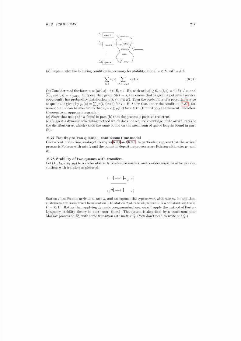
8/11/2019 Random process by B. Hajek
http://slidepdf.com/reader/full/random-process-by-b-hajek 227/448
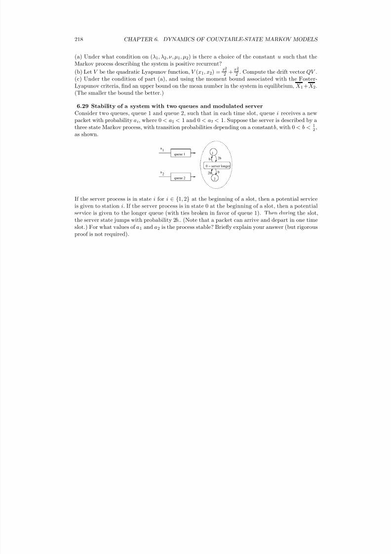
8/11/2019 Random process by B. Hajek
http://slidepdf.com/reader/full/random-process-by-b-hajek 228/448
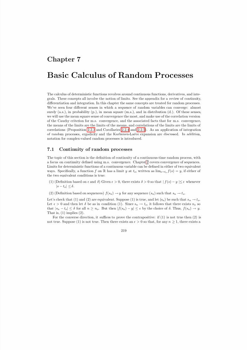
8/11/2019 Random process by B. Hajek
http://slidepdf.com/reader/full/random-process-by-b-hajek 229/448
Chapter 7
Basic Calculus of Random Processes
The calculus of deterministic functions revolves around continuous functions, derivatives, and inte-
grals. These concepts all involve the notion of limits. See the appendix for a review of continuity,differentiation and integration. In this chapter the same concepts are treated for random processes.We’ve seen four different senses in which a sequence of random variables can converge: almostsurely (a.s.), in probability (p.), in mean square (m.s.), and in distribution (d.). Of these senses,we will use the mean square sense of convergence the most, and make use of the correlation versionof the Cauchy criterion for m.s. convergence, and the associated facts that for m.s. convergence,the means of the limits are the limits of the means, and correlations of the limits are the limits of correlations (Proposition 2.2.3 and Corollaries 2.2.4 and 2.2.5). As an application of integrationof random processes, ergodicity and the Karhunen-Loeve expansion are discussed. In addition,notation for complex-valued random processes is introduced.
7.1 Continuity of random processesThe topic of this section is the definition of continuity of a continuous-time random process, witha focus on continuity defined using m.s. convergence. Chapter 2 covers convergence of sequences.Limits for deterministic functions of a continuous variable can be defined in either of two equivalentways. Specifically, a function f on R has a limit y at to, written as lims→to f (s) = y, if either of the two equivalent conditions is true:
(1) (Definition based on and δ ) Given > 0, there exists δ > 0 so that | f (s) − y |≤ whenever|s − to| ≤ δ .
(2) (Definition based on sequences) f (sn) → y for any sequence (sn) such that sn → to.
Let’s check that (1) and (2) are equivalent. Suppose (1) is true, and let (sn) be such that sn → to.Let > 0 and then let δ be as in condition (1). Since sn → to, it follows that there exists no sothat |sn − to| ≤ δ for all n ≥ no. But then |f (sn) − y| ≤ by the choice of δ. Thus, f (sn) → y.That is, (1) implies (2).
For the converse direction, it suffices to prove the contrapositive: if (1) is not true then (2) isnot true. Suppose (1) is not true. Then there exists an > 0 so that, for any n ≥ 1, there exists a
219
8/11/2019 Random process by B. Hajek
http://slidepdf.com/reader/full/random-process-by-b-hajek 230/448
8/11/2019 Random process by B. Hajek
http://slidepdf.com/reader/full/random-process-by-b-hajek 231/448
7.1. CONTINUITY OF RANDOM PROCESSES 221
Therefore, if the first of these sets contains an event which has probability one, the second of thesesets is an event which has probability one. The proposition then follows from the same relationsfor convergence of sequences. In particular, a.s. convergence for continuous time implies a.s.
convergence along sequences (as just shown), which implies convergence in p. along sequences, whichis the same as convergence in probability. The other implications of the proposition follow directlyfrom the same implications for sequences, and the fact the first three definitions of convergence forcontinuous time have a form based on sequences.
The following example shows that a.s. convergence as s → to is strictly stronger than a.s.convergence along sequences.
Example 7.1.3 Let U be uniformly distributed on the interval [0, 1]. Let X t = 1 if t − U is arational number, and X t = 0 otherwise. Each sample path of X takes values zero and one in anyfinite interval, so that X is not a.s. convergent at any to. However, for any fixed t, P X t = 0 = 1.
Therefore, for any sequence sn, since there are only countably many terms, P X sn = 0 for all n = 1so that X sn → 0 a.s.
Definition 7.1.4 (Four types of continuity at a point for a random process) For each to ∈ T fixed,the random process X = (X t : t ∈ T) is continuous at to in any one of the four senses: m.s., p.,a.s., or d., if lims→to X s = X to in the corresponding sense.
The following is immediately implied by Proposition 7.1.2. It shows that for convergence of arandom process at a single point, the relations illustrated in Figure 2.8 again hold.
Corollary 7.1.5 If X is continuous at to in either the a.s. or m.s. sense, then X is continuous at
to in probability. If X is continuous at to in probability, then X is continuous at to in distribution.Also, if there is a random variable Z with E [Z 2] < ∞ and |X t| ≤ Z for all t, and if X is continuous at to in probability, then it is continuous at to in the m.s. sense.
A deterministic function f on R is simply called continuous if it is continuous at all points. Sincewe have four senses of continuity at a point for a random process, this gives four types of continuityfor random processes. Before stating them formally, we describe a fifth type of continuity of randomprocesses, which is often used in applications. Recall that for a fixed ω ∈ Ω, the random processX gives a sample path, which is a function on T. Continuity of a sample path is thus defined asit is for any deterministic function. The subset of Ω, ω : X t(ω) is a continuous function of t, ormore concisely, X t is a continuous function of t, is the set of ω such that the sample path for ωis continuous. The fifth type of continuity requires that the sample paths be continuous, if a set of
probability zero is ignored.
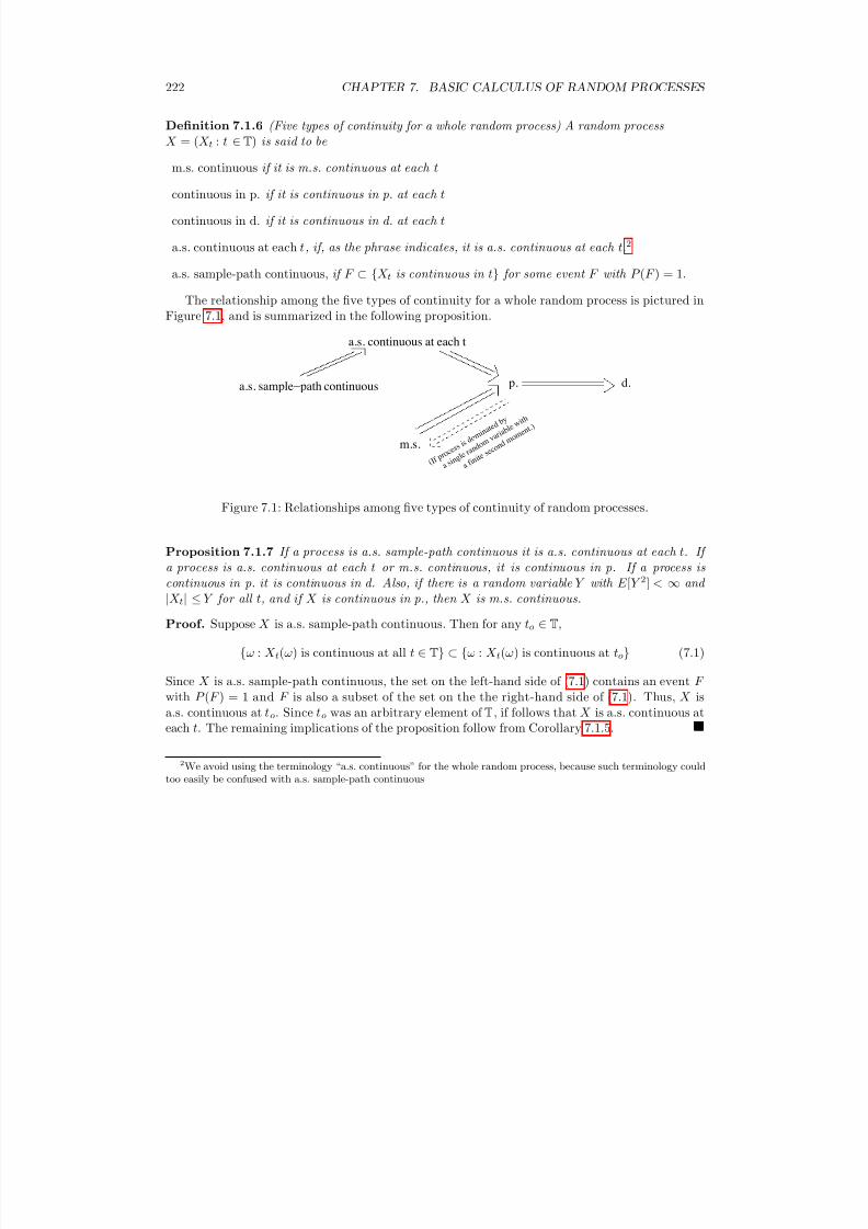
8/11/2019 Random process by B. Hajek
http://slidepdf.com/reader/full/random-process-by-b-hajek 232/448
8/11/2019 Random process by B. Hajek
http://slidepdf.com/reader/full/random-process-by-b-hajek 233/448
7.1. CONTINUITY OF RANDOM PROCESSES 223
Example 7.1.8 (Shows a.s. sample-path continuity is strictly stronger than a.s. continuity at eacht.) Let X = (X t : 0 ≤ t ≤ t) be given by X t = I t≥U for 0 ≤ t ≤ 1, where U is uniformly distributed
over [0, 1]. Thus, each sample path of X has a single upward jump of size one, at a random time U uniformly distributed over [0, 1]. So every sample path is discontinuous, and therefore X is not a.s.sample-path continuous. For any fixed t and ω , if U (ω) = t (i.e. if the jump of X is not exactly attime t) then X s(ω) → X t(ω) as s → t. Since P U = t = 1, it follows that X is a.s. continuous ateach t. Therefore X is also continuous in p. and d. senses. Finally, since |X t| ≤ 1 for all t and X iscontinuous in p., it is also m.s. continuous.
The remainder of this section focuses on m.s. continuity. Recall that the definition of m.s.convergence of a sequence of random variables requires that the random variables have finite secondmoments, and consequently the limit also has a finite second moment. Thus, in order for a randomprocess X = (X t : t ∈ T) to be continuous in the m.s. sense, it must be a second order process:
E [X
2
t ] < ∞ for all t ∈ T
. Whether X is m.s. continuous depends only on the correlation functionRX , as shown in the following proposition.
Proposition 7.1.9 Suppose (X t : t ∈ T) is a second order process. The following are equivalent:
(i) RX is continuous at all points of the form (t, t) (This condition involves RX for points in and near the set of points of the form (t, t). It is stronger than requiring RX (t, t) to be continuous in t–see example 7.1.10 .)
(ii) X is m.s. continuous
(iii) RX is continuous over T× T.
If X is m.s. continuous, then the mean function, µX (t), is continuous. If X is wide sense stationary,the following are equivalent:
( i) RX (τ ) is continuous at τ = 0
( ii) X is m.s. continuous
( iii) RX (τ ) is continuous over all of R.
Proof. ((i) implies (ii)) Fix t ∈ T and suppose that RX is continuous at the point (t, t). ThenRX (s, s), RX (s, t), and RX (t, s) all converge to RX (t, t) as s → t. Therefore, lims→t E [(X s−X t)2] =lims→t(RX (s, s) − RX (s, t) − RX (t, s) + RX (t, t)) = 0. So X is m.s. continuous at t. Therefore if
RX is continuous at all points of the form (t, t) ∈ T × T, then X is m.s. continuous at all t ∈ T.Therefore (i) implies (ii).
((ii) implies (iii)) Suppose condition (ii) is true. Let (s, t) ∈ T×T, and suppose (sn, tn) ∈ T×Tfor all n ≥ 1 such that limn→∞(sn, tn) = (s, t). Therefore, sn → s and tn → t as n → ∞. Bycondition (b), it follows that X sn
m.s.→ X s and X tnm.s.→ X t as n → ∞. Since the limit of the
correlations is the correlation of the limit for a pair of m.s. convergent sequences (Corollary 2.2.4)
8/11/2019 Random process by B. Hajek
http://slidepdf.com/reader/full/random-process-by-b-hajek 234/448
224 CHAPTER 7. BASIC CALCULUS OF RANDOM PROCESSES
it follows that RX (sn, tn) → RX (s, t) as n → ∞. Thus, RX is continuous at (s, t), where (s, t) wasan arbitrary point of T × T. Therefore RX is continuous over T × T, proving that (ii) implies (iii).
Obviously (iii) implies (i), so the proof of the equivalence of (i)-(iii) is complete.
If X is m.s. continuous, then, by definition, for any t ∈ T, X sm.s.
→ X t as s → t. It thus followsthat µX (s) → µX (t), because the limit of the means is the mean of the limit, for a m.s. convergentsequence (Corollary 2.2.5). Thus, m.s. continuity of X implies that the deterministic mean function,µX , is continuous.
Finally, if X is WSS, then RX (s, t) = RX (τ ) where τ = s − t, and the three conditions (i)-(iii)become (i)-(iii), so the equivalence of (i)-(iii) implies the equivalence of (i)-(iii).
Example 7.1.10 Let X = (X t : t ∈ R) be defined by X t = U for t < 0 and X t = V for t ≥ 0,where U and V are independent random variables with mean zero and variance one. Let tn be asequence of strictly negative numbers converging to 0. Then X tn = U for all n and X 0 = V . Since
P |U − V | ≥ = 0 for small enough, X tn does not converge to X 0 in p. sense. So X is notcontinuous in probability at zero. It is thus not continuous in the m.s or a.s. sense at zero either. Theonly one of the five senses that the whole process could be continuous is continuous in distribution.The process X is continuous in distribution if and only if U and V have the same distribution.Finally, let us check the continuity properties of the autocorrelation function. The autocorrelationfunction is given by RX (s, t) = 1 if either s,t < 0 or if s, t ≥ 0, and RX (s, t) = 0 otherwise. So RX
is not continuous at (0, 0), because R( 1n , − 1
n) = 0 for all n ≥ 1, so R( 1n , − 1
n) → RX (0, 0) = 1. asn → ∞. However, it is true that RX (t, t) = 1 for all t, so that RX (t, t) is a continuous function of t. This illustrates the fact that continuity of the function of two variables, RX (s, t), at a particularpoint of the form (to, to), is a stronger requirement than continuity of the function of one variable,RX (t, t), at t = to.
Example 7.1.11 Let W = (W t : t ≥ 0) be a Brownian motion with parameter σ 2. Then E [(W t −W s)2] = σ2|t − s| → 0 as s → t. Therefore W is m.s. continuous. Another way to show W ism.s. continuous is to observe that the autocorrelation function, RW (s, t) = σ2(s ∧ t), is continuous.Since W is m.s. continuous, it is also continuous in the p. and d. senses. As we stated in definingW , it is a.s. sample-path continuous, and therefore a.s. continuous at each t ≥ 0, as well.
Example 7.1.12 Let N = (N t : t ≥ 0) be a Poisson process with rate λ > 0. Then for fixed t,E [(N t
−N s)2] = λ(t
−s) + (λ(t
−s))2
→ 0 as s
→ t. Therefore N is m.s. continuous. As required,
RN , given by RN (s, t) = λ(s ∧ t) + λ2st, is continuous. Since N is m.s. continuous, it is alsocontinuous in the p. and d. senses. N is also a.s. continuous at any fixed t, because the probabilityof a jump at exactly time t is zero for any fixed t. However, N is not a.s. sample continuous. Infact, N is continuous on [0, a] = e−λa and so P N is continuous on R+ = 0.
8/11/2019 Random process by B. Hajek
http://slidepdf.com/reader/full/random-process-by-b-hajek 235/448
7.2. MEAN SQUARE DIFFERENTIATION OF RANDOM PROCESSES 225
Definition 7.1.13 A random process (X t : t ∈ T), such that T is a bounded interval (open, closed,or mixed) in R with endpoints a < b, is piecewise m.s. continuous, if there exist n ≥ 1 and a = t0 < t1 < · · · < tn = b, such that, for 1 ≤ k ≤ n: X is m.s. continuous over (tk−1, tk) and has
m.s. limits at the endpoints of (tk−1, tk).More generally, if T is all of R or an interval in R, X is piecewise m.s. continuous over T if it is piecewise m.s. continuous over every bounded subinterval of T.
7.2 Mean square differentiation of random processes
Before considering the m.s. derivative of a random process, we review the definition of the derivativeof a function (also, see Appendix 11.4). Let the index set T be either all of R or an interval inR. Suppose f is a deterministic function on T. Recall that for a fixed t in T, f is differentiableat t if lims→t
f (s)−f (t)s−t exists and is finite, and if f is differentiable at t, the value of the limit is
the derivative, f (t). The whole function f is called differentiable if it is differentiable at all t. The
function f is called continuously differentiable if f is differentiable, and the derivative function f is continuous.
In many applications of calculus, it is important that a function f be not only differentiable,but continuously differentiable. In much of the applied literature, when there is an assumptionthat a function is differentiable, it is understood that the function is continuously differentiable.For example, by the fundamental theorem of calculus ,
f (b) − f (a) =
ba
f (s)ds (7.2)
holds if f is a continuously differentiable function with derivative f . Example 11.4.2 shows that(7.2) might not hold if f is simply assumed to be differentiable.
Let X = (X t : t ∈ T) be a second order random process such that the index set T is equal toeither all of R or an interval in R. The following definition for m.s. derivatives is analogous to thedefinition of derivatives for deterministic functions.
Definition 7.2.1 For each t fixed, the random process X = (X t : t ∈ T) is mean square (m.s.)differentiable at t if the following limit exists
lims→t
X s−X ts−t m.s.
The limit, if it exists, is the m.s. derivative of X at t, denoted by X t. The whole random process X is said to be m.s. differentiable if it is m.s. differentiable at each t, and it is said to be m.s. continuouslydifferentiable if it is m.s. differentiable and the derivative process X is m.s. continuous.
Let ∂ i denote the operation of taking the partial derivative with respect to the ith argument.For example, if f (x, y) = x2y3 then ∂ 2f (x, y) = 3x2y2 and ∂ 1∂ 2f (x, y) = 6xy2. The partialderivative of a function is the same as the ordinary derivative with respect to one variable, withthe other variables held fixed. We shall be applying ∂ 1 and ∂ 2 to an autocorrelation functionRX = (RX (s, t) : (s, t) ∈ T× T, which is a function of two variables.
8/11/2019 Random process by B. Hajek
http://slidepdf.com/reader/full/random-process-by-b-hajek 236/448
226 CHAPTER 7. BASIC CALCULUS OF RANDOM PROCESSES
Proposition 7.2.2 (a) (The derivative of the mean is the mean of the derivative) If X is m.s.differentiable, then the mean function µX is differentiable, and µ
X (t) = µX (t). (i.e. the operations of (i) taking expectation, which basically involves integrating over ω, and (ii) dif-
ferentiation with respect to t, can be done in either order.)(b) If X is m.s. differentiable, the cross correlation functions are given by RX X = ∂ 1RX and
RXX = ∂ 2RX , and the autocorrelation function of X is given by RX = ∂ 1∂ 2RX = ∂ 2∂ 1RX .(In particular, the indicated partial derivatives exist.)
(c) X is m.s. differentiable at t if and only if the following limit exists and is finite:
lims,s→t
RX (s, s) − RX (s, t) − RX (t, s) + RX (t, t)
(s − t)(s − t) . (7.3)
(Therefore, the whole process X is m.s. differentiable if and only if the limit in (7.3) exists and is finite for all t ∈ T.)
(d) X is m.s. continuously differentiable if and only if RX , ∂ 2RX , and ∂ 1∂ 2RX exist and are continuous. (By symmetry, if X is m.s. continuously differentiable, then also ∂ 1RX is con-tinuous.)
(e) (Specialization of (d) for WSS case) Suppose X is WSS. Then X is m.s. continuously differ-entiable if and only if RX (τ ), R
X (τ ), and RX (τ ) exist and are continuous functions of τ . If
X is m.s. continuously differentiable then X and X are jointly WSS, X has mean zero (i.e.µX = 0) and autocorrelation function given by RX (τ ) = −R
X (τ ), and the cross correlation functions are given by RX X (τ ) = R
X (τ ) and RXX (τ ) = −RX (τ ).
(f) (A necessary condition for m.s. differentiability) If X is WSS and m.s. differentiable, then R
X (0) exists and RX (0) = 0.
(g) If X is a m.s. differentiable Gaussian process, then X and its derivative process X are jointly Gaussian.
Proof. (a) Suppose X is m.s. differentiable. Then for any t fixed,
X s − X ts − t
m.s.→ X t as s → t.
It thus follows thatµX (s) − µX (t)
s − t → µX (t) as s → t, (7.4)
because the limit of the means is the mean of the limit, for a m.s. convergent sequence (Corol-lary 2.2.5). But (7.4) is just the definition of the statement that the derivative of µX at t is equalto µX (t). That is, dµX
dt (t) = µX (t) for all t, or more concisely, µ X = µX .
(b) Suppose X is m.s. differentiable. Since the limit of the correlations is the correlation of thelimits for m.s. convergent sequences (Corollary 2.2.4), for t, t ∈ T,
RX X (t, t) = lims→t
E
X (s) − X (t)
s − t
X (t)
= lim
s→t
RX (s, t) − RX (t, t)s − t
= ∂ 1RX (t, t)
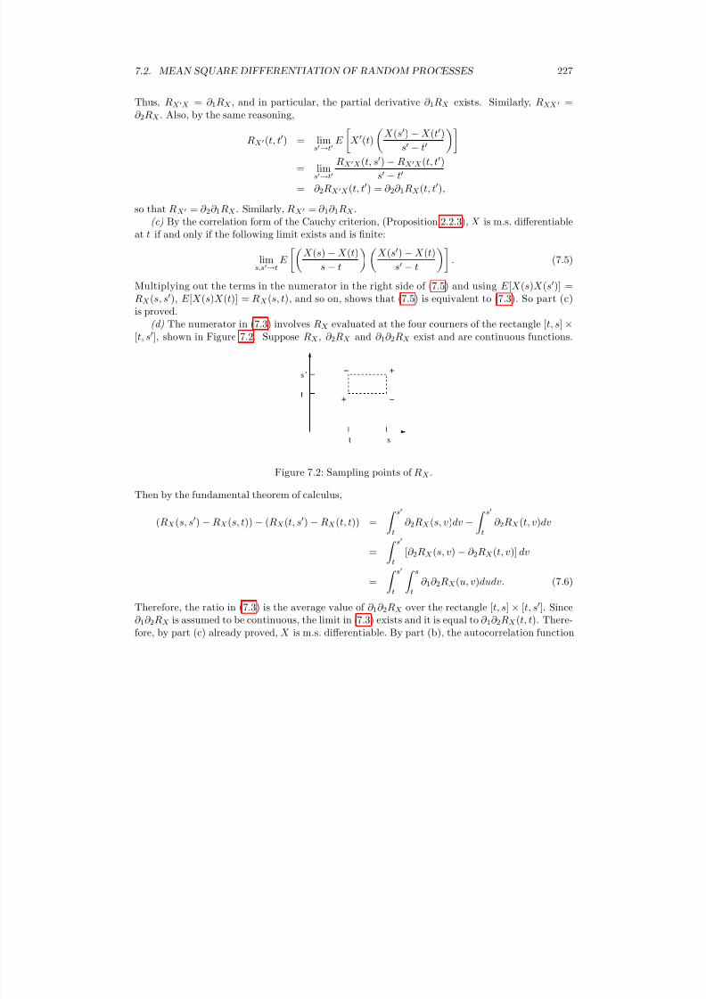
8/11/2019 Random process by B. Hajek
http://slidepdf.com/reader/full/random-process-by-b-hajek 237/448
7.2. MEAN SQUARE DIFFERENTIATION OF RANDOM PROCESSES 227
Thus, RX X = ∂ 1RX , and in particular, the partial derivative ∂ 1RX exists. Similarly, RXX =∂ 2RX . Also, by the same reasoning,
RX (t, t) = lims→t E X (t)X (s)−
X (t)s − t
= lims→t
RX X (t, s) − RX X (t, t)s − t
= ∂ 2RX X (t, t) = ∂ 2∂ 1RX (t, t),
so that RX = ∂ 2∂ 1RX . Similarly, RX = ∂ 1∂ 1RX .(c) By the correlation form of the Cauchy criterion, (Proposition 2.2.3), X is m.s. differentiable
at t if and only if the following limit exists and is finite:
lims,s→t
E
X (s) − X (t)
s − t
X (s) − X (t)
s − t
. (7.5)
Multiplying out the terms in the numerator in the right side of (7.5) and using E [X (s)X (s)] =RX (s, s), E [X (s)X (t)] = RX (s, t), and so on, shows that (7.5) is equivalent to (7.3). So part (c)is proved.
(d) The numerator in (7.3) involves RX evaluated at the four courners of the rectangle [t, s] ×[t, s], shown in Figure 7.2. Suppose RX , ∂ 2RX and ∂ 1∂ 2RX exist and are continuous functions.
!"
# !
#"
!
!
!
Figure 7.2: Sampling points of RX .
Then by the fundamental theorem of calculus,
(RX (s, s) − RX (s, t)) − (RX (t, s) − RX (t, t)) =
st
∂ 2RX (s, v)dv − st
∂ 2RX (t, v)dv
=
st
[∂ 2RX (s, v) − ∂ 2RX (t, v)] dv
= st
st
∂ 1∂ 2RX (u, v)dudv. (7.6)
Therefore, the ratio in (7.3) is the average value of ∂ 1∂ 2RX over the rectangle [t, s] × [t, s]. Since∂ 1∂ 2RX is assumed to be continuous, the limit in (7.3) exists and it is equal to ∂ 1∂ 2RX (t, t). There-fore, by part (c) already proved, X is m.s. differentiable. By part (b), the autocorrelation function
8/11/2019 Random process by B. Hajek
http://slidepdf.com/reader/full/random-process-by-b-hajek 238/448
228 CHAPTER 7. BASIC CALCULUS OF RANDOM PROCESSES
of X is ∂ 1∂ 2RX . Since this is assumed to be continuous, it follows that X is m.s. continuous. Thus,X is m.s. continuously differentiable.
(e) If X is WSS, then RX (s − t) = RX (τ ) where τ = s − t. Suppose RX (τ ), RX (τ ) and R
X (τ )
exist and are continuous functions of τ . Then
∂ 1RX (s, t) = RX (τ ) and ∂ 2∂ 1RX (s, t) = −R
X (τ ). (7.7)
The minus sign in (7.7) appears because RX (s, t) = RX (τ ) where τ = s − t, and the derivative of with respect to t is −1. So, the hypotheses of part (d) hold, so that X is m.s. differentiable. SinceX is WSS, its mean function µX is constant, which has derivative zero, so X has mean zero. Alsoby part (c) and (7.7), RX X (τ ) = R
X (τ ) and RX X = −RX . Similarly, RXX (τ ) = −R
X (τ ). Notethat X and X are each WSS and the cross correlation functions depend on τ alone, so X and X
are jointly WSS.(f ) If X is WSS then
E X (t) − X (0)t 2 = −2(RX (t) − RX (0))t2 (7.8)
Therefore, if X is m.s. differentiable then the right side of (7.8) must converge to a finite limit ast → 0, so in particular it is necessary that (RX (t) − RX (0))/t → 0 as t → 0. Therefore R
X (0) = 0.(g) The derivative process X is obtained by taking linear combinations and m.s. limits of
random variables in X = (X t; t ∈ T). Therefore, (g) follows from the fact that the joint Gaussianproperty is preserved under linear combinations and limits (Proposition 3.4.3(c)).
Example 7.2.3 Let f (t) = t2 sin(1/t2) for t = 0 and f (0) = 0 as in Example 11.4.2, and letX = (X t : t
∈R) be the deterministic random process such that X (t) = f (t) for all t
∈R. Since X
is differentiable as an ordinary function, it is also m.s. differentiable, and its m.s. derivative X isequal to f . Since X , as a deterministic function, is not continuous at zero, it is also not continuousat zero in the m.s. sense. We have RX (s, t) = f (s)f (t) and ∂ 2RX (s, t) = f (s)f (t), which is notcontinuous. So indeed the conditions of Proposition 7.2.2(d) do not hold, as required.
Example 7.2.4 A Brownian motion W = (W t : t ≥ 0) is not m.s. differentiable. If it were, then
for any fixed t ≥ 0, W (s)−W (t)s−t would converge in the m.s. sense as s → t to a random variable
with a finite second moment. For a m.s. convergent seqence, the second moments of the variablesin the sequence converge to the second moment of the limit random variable, which is finite. ButW (s)
−W (t) has mean zero and variance σ 2
|s
−t
|, so that
lims→t
E
W (s) − W (t)
s − t
2= lim
s→t
σ2
|s − t| = +∞. (7.9)
Thus, W is not m.s. differentiable at any t. For another approach, we could appeal to Proposition7.2.2 to deduce this result. The limit in (7.9) is the same as the limit in (7.5), but with s and s
8/11/2019 Random process by B. Hajek
http://slidepdf.com/reader/full/random-process-by-b-hajek 239/448
7.3. INTEGRATION OF RANDOM PROCESSES 229
restricted to be equal. Hence (7.5), or equivalently (7.3), is not a finite limit, implying that W isnot differentiable at t.
Similarly, a Poisson process is not m.s. differentiable at any t. A WSS process X with RX (τ ) =
e−α|τ | is not m.s. differentiable because RX (0) does not exist. A WSS process X with RX (τ ) =
11+τ 2
is m.s. differentiable, and its derivative process X is WSS with mean 0 and covariance function
RX (τ ) = −
1
1 + τ 2
=
2 − 6τ 2
(1 + τ 2)3.
Proposition 7.2.5 Suppose X is a m.s. differentiable random process and f is a differentiable function. Then the product Xf = (X (t)f (t) : t ∈ R) is mean square differentiable and (Xf ) =X f + Xf .
Proof: Fix t. Then for each s = t,
X (s)f (s) − X (t)f (t)
s − t =
(X (s) − X (t))f (s)
s − t +
X (t)(f (s) − f (t))
s − tm.s.→ X (t)f (t) + X (t)f (t) as s → t.
Definition 7.2.6 A random process X on a bounded interval (open, closed, or mixed) with end-points a < b is continuous and piecewise continuously differentiable in the m.s. sense, if X is m.s.continuous over the interval, and if there exists n ≥ 1 and a = t0 < t1 < · · · < tn = b, such that, for 1 ≤ k ≤ n: X is m.s. continuously differentiable over (tk−1, tk) and X has finite limits at the endpoints of (tk−1, tk).
More generally, if T is all of R or a subinterval of R, then a random process X = (X t : t ∈ T)is continuous and piecewise continuously differentiable in the m.s. sense if its restriction to any bounded interval is continuous and piecewise continuously differentiable in the m.s. sense.
7.3 Integration of random processes
Let X = (X t : a ≤ t ≤ b) be a random process and let h be a function on a finite interval [a, b].How shall we define the following integral? b
a X th(t)dt. (7.10)
One approach is to note that for each fixed ω, X t(ω) is a deterministic function of time, and sothe integral can be defined as the integral of a deterministic function for each ω. We shall focuson another approach, namely mean square (m.s.) integration. An advantage of m.s. integration isthat it relies much less on properties of sample paths of random processes.
As for integration of deterministic functions, the m.s. Riemann integrals are based on Riemannsums, defined as follows. Given:
8/11/2019 Random process by B. Hajek
http://slidepdf.com/reader/full/random-process-by-b-hajek 240/448
230 CHAPTER 7. BASIC CALCULUS OF RANDOM PROCESSES
• A partition of (a, b] of the form (t0, t1], (t1, t2], · · · , (tn−1, tn], where n ≥ 0 anda = t0 < t1 · · · < tn = b
• A sampling point from each subinterval, vk ∈ (tk−1, tk], for 1 ≤ k ≤ n,
the corresponding Riemann sum for X h is defined by
nk=1
X vkh(vk)(tk − tk−1).
The norm of the partition is defined to be maxk |tk − tk−1|.
Definition 7.3.1 The Riemann integral ba X th(t)dt is said to exist in the m.s. sense and its
value is the random variable I if the following is true. Given any > 0, there is a δ > 0 so that E [(n
k=1X
vkh(v
k)(t
k −tk−1
)−
I )2] ≤
whenever the norm of the partition is less than or equal toδ . This definition is equivalent to the following condition, expressed using convergence of sequences.The m.s. Riemann integral exists and is equal to I , if for any sequence of partitions, specified by ((tm1 , tm2 , . . . , tmnm
) : m ≥ 1), with corresponding sampling points ((vm1 , . . . , vm
nm) : m ≥ 1), such that
norm of the mth partition converges to zero as m → ∞, the corresponding sequence of Riemann sums converges in the m.s. sense to I as m → ∞. The process X th(t) is said to be m.s. Riemann
integrable over (a, b] if the integral ba X th(t)dt exists and is finite.
Next, suppose X th(t) is defined over the whole real line. If X th(t) is m.s. Riemann integrable over every bounded interval [a, b], then the Riemann integral of X th(t) over R is defined by
∞
−∞
X th(t)dt = lima,b
→∞ b
−a
X th(t)dt m.s.
provided that the indicated limit exist as a, b jointly converge to +∞.
Whether an integral exists in the m.s. sense is determined by the autocorrelation function of the random process involved, as shown next. The condition involves Riemann integration of adeterministic function of two variables. As reviewed in Appendix 11.5, a two-dimensional Riemannintegral over a bounded rectangle is defined as the limit of Riemann sums corresponding to apartition of the rectangle into subrectangles and choices of sampling points within the subrectangles.If the sampling points for the Riemann sums are required to be horizontally and vertically alligned,then we say the two-dimensional Riemann integral exists with aligned sampling.
Proposition 7.3.2 The integral ba X th(t)dt exists in the m.s. Riemann sense if and only if ba
ba RX (s, t)h(s)h(t)dsdt (7.11)
exists as a two dimensional Riemann integral with aligned sampling. The m.s. integral exists, in particular, if X is m.s. piecewise continuous over [a, b] and h is piecewise continuous over [a, b].
8/11/2019 Random process by B. Hajek
http://slidepdf.com/reader/full/random-process-by-b-hajek 241/448
7.3. INTEGRATION OF RANDOM PROCESSES 231
Proof. By definition, the m.s. integral of X th(t) exists if and only if the Riemann sums convergein the m.s. sense for an arbitary sequence of partitions and sampling points, such that the normsof the partitions converge to zero. So consider an arbitrary sequence of partitions of (a, b] into
intervals specified by the collection of endpoints, ((tm0 , t
m1 , . . . , t
mnm) : m ≥ 1), with corresponding
sampling point vmk ∈ (tmk−1, tmk ] for each m and 1 ≤ k ≤ nm, such that the norm of the mth partition
converges to zero as m → ∞. For each m ≥ 1, let S m denote the corresponding Riemann sum:
S m =nmk=1
X vmk
h(vmk )(tmk − tmk−1).
By the correlation form of the Cauchy criterion for m.s. convergence (Proposition 2.2.3), (S m :m
≥ 1) converges in the m.s. sense if and only if limm,m
→∞E [S mS m
] exists and is finite. Now
E [S mS m ] =nm j=1
nmk=1
RX (vm j , vm
k )h(vm j )h(vm
k )(tm j − tm j−1)(tm
k − tm
k−1), (7.12)
and the right-hand side of (7.12) is the Riemann sum for the integral (7.11), for the partition of (a, b] × (a, b] into rectangles of the form (tm j−1, tm j ] × (tm
k−1, tm
k ] and the sampling points (vm
j , vmk ).
Note that the mm sampling points are aligned, in that they are determined by the m + m num-bers vm
1
, . . . , vm
nm , vm
1
, . . . , vm
nm. Moreover, any Riemann sum for the integral (7.11) with aligned
sampling can arise in this way. Further, as m, m → ∞, the norm of this partition, which is themaximum length or width of any rectangle of the partition, converges to zero. Thus, the limitlimm,m→∞ E [S mS m ] exists for any sequence of partitions and sampling points if and only if theintegral (7.11) exists as a two-dimensional Riemann integral with aligned sampling.
Finally, if X is piecewise m.s. continuous over [a, b] and h is piecewise continuous over [a, b], thenthere is a partition of [a, b] into intervals of the form (sk−1, sk] such that X is m.s. continuous over(sk−1, sk) with m.s. limits at the endpoints, and h is continuous over (sk−1, sk) with finite limitsat the endpoints. Therefore, RX (s, t)h(s)h(t) restricted to each rectangle of the form (s j−1, s j) ×(sk−1, sk), is the restriction of a continuous function on [s j−1, s j ]× [sk−1, sk]. Thus RX (s, t)h(s)h(t)is Riemann integrable over [a, b] × [a, b].
8/11/2019 Random process by B. Hajek
http://slidepdf.com/reader/full/random-process-by-b-hajek 242/448
232 CHAPTER 7. BASIC CALCULUS OF RANDOM PROCESSES
Proposition 7.3.3 Suppose X th(t) and Y tk(t) are both m.s. integrable over [a, b]. Then
E b
a
X th(t)dt = b
a
µX (t)h(t)dt (7.13)
E
ba
X th(t)dt
2
=
ba
ba
RX (s, t)h(s)h(t)dsdt (7.14)
Var
ba
X th(t)dt
=
ba
ba
C X (s, t)h(s)h(t)dsdt. (7.15)
E
ba
X sh(s)ds
ba
Y tk(t)dt
=
ba
ba
RXY (s, t)h(s)k(t)dsdt (7.16)
Cov
ba
X sh(s)ds,
ba
Y tk(t)dt
=
ba
ba
C XY (s, t)h(s)k(t)dsdt (7.17)
ba
X th(t) + Y tk(t)dt = ba
X th(t)dt + ba
Y tk(t))dt (7.18)
Proof. Let (S m) denote the sequence of Riemann sums appearing in the proof of Proposition7.3.2. Since the mean of a m.s. convergent sequence of random variables is the limit of the means(Corollary 2.2.5),
E
ba
X th(t)dt
= lim
m→∞ E [S m]
= limm→∞
nmk=1
µX (vmk )h(vm
k )(tmk − tmk−1). (7.19)
The right-hand side of (7.19) is a limit of Riemann sums for the integral ba µX (t)h(t)dt. Since this
limit exists and is equal to E b
a X th(t)dt
for any sequence of partitions and sample points, it
follows that ba µX (t)h(t)dt exists as a Riemann integral, and is equal to E
ba X th(t)dt
, so (7.13)
is proved.
The second moment of the m.s. limit of (S m : m ≥ 0) is equal to limm,m→∞ E [S mS m ], by thecorrelation form of the Cauchy criterion for m.s. convergence (Proposition 2.2.3), which implies(7.14). It follows from (7.13) that
E b
a
X th(t)dt2
= b
a b
a
µX (s)µX (t)h(s)h(t)dsdt
Subtracting each side of this from the corresponding side of (7.14) yields (7.15). The proofs of (7.16) and (7.17) are similar to the proofs of (7.14) and (7.15), and are left to the reader.
For any partition of [a, b] and choice of sampling points, the Riemann sums for the three integralsappearing (7.17) satisfy the corresponding additivity condition, implying (7.17).
8/11/2019 Random process by B. Hajek
http://slidepdf.com/reader/full/random-process-by-b-hajek 243/448
7.3. INTEGRATION OF RANDOM PROCESSES 233
The fundamental theorem of calculus, stated in Appendix 11.5, states the increments of acontinuous, piecewise continuously differentiable function are equal to integrals of the derivative of the function. The following is the generalization of the fundamental theorem of calculus to the m.s.
calculus.
Theorem 7.3.4 (Fundamental Theorem of m.s. Calculus) Let X be a m.s. continuously differen-tiable random process. Then for a < b,
X b − X a =
ba
X tdt (m.s. Riemann integral ) (7.20)
More generally, if X is continuous and piecewise continuously differentiable, (11.4) holds with X treplaced by the right-hand derivative, D+X t. (Note that D+X t = X t whenever X t is defined.)
Proof. The m.s. Riemann integral in (7.20) exists because X is assumed to be m.s. continuous.
Let B = X b
−X a
− ba X tdt, and let Y be an arbitrary random variable with a finite second moment.
It suffices to show that E [Y B] = 0, because a possible choice of Y is B itself. Let φ(t) = E [Y X t].Then for s = t,
φ(s) − φ(t)
s − t = E
Y
X s − X t
s − t
Taking a limit as s → t and using the fact the correlation of a limit is the limit of the correlationsfor m.s. convergent sequences, it follows that φ is differentiable and φ(t) = E [Y X t]. Since X ism.s. continuous, it similarly follows that φ is continuous.
Next, we use the fact that the integral in (7.20) is the m.s. limit of Riemann sums, with eachRiemann sum corresponding to a partition of (a, b] specified by some n ≥ 1 and a = t0 < · · · < tn = band sampling points vk ∈ (tk−1, tk] for a ≤ k ≤ n. Since the limit of the correlation is the correlationof the limt for m.s. convergence,
E
Y ba
X tdt
= lim|tk−tk−1|→0
E
Y n
k=1
X vk(tk − tk−1)
= lim
|tk−tk−1|→0
nk=1
φ(vk)(tk − tk−1) =
ba
φ(t)dt
Therefore, E [Y B] = φ(b) − φ(a) − ba φ(t)dt, which is equal to zero by the fundamental theorem
of calculus for deterministic continuously differentiable functions. This establishes (7.20) in caseX is m.s. continuously differentiable. If X is m.s. continuous and only piecewise continuouslydifferentiable, we can use essentially the same proof, observing that φ is continuous and piecewisecontinuously differentiable, so that E [Y B] = φ(b)
− φ(a)
− ba φ(t)dt = 0 by the fundamental
theorem of calculus for deterministic continuous, piecewise continuously differential functions.
Proposition 7.3.5 Suppose X is a Gaussian random process. Then X , together with all mean square derivatives of X that exist, and all m.s. Riemann integrals of X of the form I (a, b) = ba X th(t)dt that exist, are jointly Gaussian.
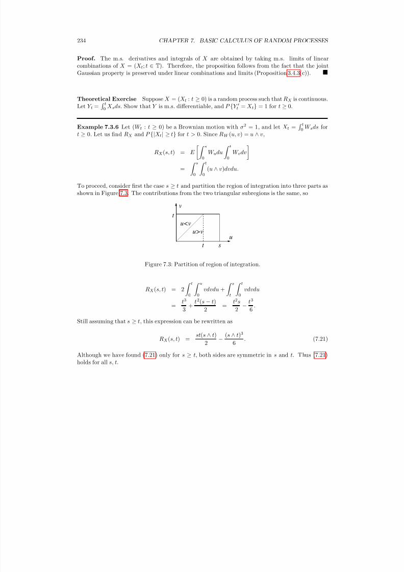
8/11/2019 Random process by B. Hajek
http://slidepdf.com/reader/full/random-process-by-b-hajek 244/448
234 CHAPTER 7. BASIC CALCULUS OF RANDOM PROCESSES
Proof. The m.s. derivatives and integrals of X are obtained by taking m.s. limits of linearcombinations of X = (X t; t ∈ T). Therefore, the proposition follows from the fact that the jointGaussian property is preserved under linear combinations and limits (Proposition 3.4.3(c)).
Theoretical Exercise Suppose X = (X t : t ≥ 0) is a random process such that RX is continuous.Let Y t =
t0 X sds. Show that Y is m.s. differentiable, and P Y t = X t = 1 for t ≥ 0.
Example 7.3.6 Let (W t : t ≥ 0) be a Brownian motion with σ2 = 1, and let X t = t
0 W sds fort ≥ 0. Let us find RX and P |X t| ≥ t for t > 0. Since RW (u, v) = u ∧ v,
RX (s, t) = E
s0
W udu
t0
W vdv
= s
0
t0
(u ∧ v)dvdu.
To proceed, consider first the case s ≥ t and partition the region of integration into three parts asshown in Figure 7.3. The contributions from the two triangular subregions is the same, so
u
v
s
u<v
u>v
t
t
Figure 7.3: Partition of region of integration.
RX (s, t) = 2
t0
u0
vdvdu +
st
t0
vdvdu
= t3
3 +
t2(s − t)
2 =
t2s
2 − t3
6 .
Still assuming that s
≥ t, this expression can be rewritten as
RX (s, t) = st(s ∧ t)
2 − (s ∧ t)3
6 . (7.21)
Although we have found (7.21) only for s ≥ t, both sides are symmetric in s and t. Thus (7.21)holds for all s, t.
8/11/2019 Random process by B. Hajek
http://slidepdf.com/reader/full/random-process-by-b-hajek 245/448
7.3. INTEGRATION OF RANDOM PROCESSES 235
Since W is a Gaussian process, X is a Gaussian process. Also, E [X t] = 0 (because W is mean
zero) and E [X 2t ] = RX (t, t) = t3
3 . Thus,
P |X t| ≥ t = 2P X t
t3
3
≥ t t3
3
= 2Q 3
t
.
Note that P X t| ≥ t → 1 as t → +∞.
Example 7.3.7 Let N = (N t : t ≥ 0) be a second order process with a continuous autocorrelationfunction RN and let x0 be a constant. Consider the problem of finding a m.s. differentiable randomprocess X = (X t : t ≥ 0) satisfying the linear differential equation
X t = −X t + N t, X 0 = x0. (7.22)
Guided by the case that N t is a smooth nonrandom function, we write
X t = x0e−t +
t0
e−(t−v)N vdv (7.23)
or
X t = x0e−t + e−t
t0
evN vdv. (7.24)
Using Proposition 7.2.5, it is not difficult to check that (7.24) indeed gives the solution to (7.22).Next, let us find the mean and autocovariance functions of X in terms of those of N . Taking
the expectation on each side of (7.23) yields
µX (t) = x0e−t +
t0
e−(t−v)µN (v)dv. (7.25)
A different way to derive (7.25) is to take expectations in (7.22) to yield the deterministic lineardifferential equation:
µX (t) = −µX (t) + µN (t); µX (0) = x0
which can be solved to yield (7.25). To summarize, we found two methods to start with thestochastic differential equation (7.23) to derive (7.25), thereby expressing the mean function of thesolution X in terms of the mean function of the driving process N . The first is to solve (7.22) toobtain (7.23) and then take expectations, the second is to take expectations first and then solvethe deterministic differential equation for µX .
8/11/2019 Random process by B. Hajek
http://slidepdf.com/reader/full/random-process-by-b-hajek 246/448
236 CHAPTER 7. BASIC CALCULUS OF RANDOM PROCESSES
The same two methods can be used to express the covariance function of X in terms of thecovariance function of N . For the first method, we use (7.23) to obtain
C X (s, t) = Cov x0e−s + s0
e−(s−u)N udu, x0e−t + t0
e−(t−v)N vdv=
s0
t0
e−(s−u)e−(t−v)C N (u, v)dvdu. (7.26)
The second method is to derive deterministic differential equations. To begin, note that
∂ 1C X (s, t) = Cov (X s, X t) = Cov (−X s + N s, X t)
so
∂ 1C X (s, t) =
−C X (s, t) + C NX (s, t). (7.27)
For t fixed, this is a differential equation in s. Also, C X (0, t) = 0. If somehow the cross covariancefunction C NX is found, (7.27) and the boundary condition C X (0, t) = 0 can be used to find C X .So we turn next to finding a differential equation for C NX .
∂ 2C NX (s, t) = Cov(N s, X t) = Cov(N s, −X t + N t)
so
∂ 2C NX (s, t) = −C NX (s, t) + C N (s, t). (7.28)
For s fixed, this is a differential equation in t with initial condition C NX (s, 0) = 0. Solving (7.28)
yields
C NX (s, t) =
t0
e−(t−v)C N (s, v)dv. (7.29)
Using (7.29) to replace C NX in (7.27) and solving (7.27) yields (7.26).
7.4 Ergodicity
Let X be a stationary or WSS random process. Ergodicity generally means that certain time
averages are asymptotically equal to certain statistical averages. For example, supposeX = (X t : t ∈ R) is WSS and m.s. continuous. The mean µX is defined as a statistical average:µX = E [X t] for any t ∈R.
The time average of X over the interval [0, t] is given by
1t
t0 X udu.
8/11/2019 Random process by B. Hajek
http://slidepdf.com/reader/full/random-process-by-b-hajek 247/448
7.4. ERGODICITY 237
Of course, for t fixed, the time average is a random variable, and is typically not equal to thestatistical average µX . The random process X is called mean ergodic (in the m.s. sense) if
limt→∞ 1
t t
0X udu = µX m.s.
A discrete time WSS random process X is similarly called mean ergodic (in the m.s. sense) if
limn→∞
1
n
ni=1
X i = µX m.s. (7.30)
For example, by the m.s. version of the law of large numbers, if X = (X n : n ∈ Z) is WSS withC X (n) = I n=0 (so that the X i’s are uncorrelated) then (7.30) is true. For another example, if C X (n) = 1 for all n, it means that X 0 has variance one and P X k = X 0 = 1 for all k (because
equality holds in the Schwarz inequality: C X (n) ≤ C X (0)). Then for all n ≥ 1,
1
n
nk=1
X k = X 0.
Since X 0 has variance one, the process X is not ergodic if C X (n) = 1 for all n. In general, whetherX is m.s. ergodic in the m.s. sense is determined by the autocovariance function, C X . The resultis stated and proved next for continuous time, and the discrete-time version is true as well.
Proposition 7.4.1 Let X be a real-valued, WSS, m.s. continuous random process. Then X is mean ergodic (in the m.s. sense) if and only if
limt→∞
2
t
t0
t − τ
t
C X (τ )dτ = 0. (7.31)
Sufficient conditions are
(a) limτ →∞ C X (τ ) = 0. (This condition is also necessary if limτ →∞ C X (τ ) exists.)
(b) ∞−∞ |C X (τ )|dτ < +∞.
(c) limτ →∞ RX (τ ) = 0.
(d) ∞−∞ |RX (τ )|dτ < +∞.
Proof. By the definition of m.s. convergence, X is mean ergodic if and only if
limt→∞ E
1
t
t0
X udu − µX
2
= 0. (7.32)

8/11/2019 Random process by B. Hajek
http://slidepdf.com/reader/full/random-process-by-b-hajek 248/448
238 CHAPTER 7. BASIC CALCULUS OF RANDOM PROCESSES
Since E
1t
t0 X udu
= 1
t
t0 µX du = µX , (7.32) is the same as Var
1t
t0 X udu
→ 0 as t → ∞. By
the properties of m.s. integrals,
Var 1t t
0X udu = Cov 1
t t
0X udu, 1
t t
0X vdv
= 1
t2
t0
t0
C X (u − v)dudv (7.33)
= 1
t2
t0
t−v
−vC X (τ )dτdv (7.34)
= 1
t2
t0
t−τ
0C X (τ )dvdτ +
0
−t
t−τ
C X (τ )dvdτ (7.35)
= 1
t
t−t
t − |τ |
t
C X (τ )dτ
= 2t t
0
t − τ tC X (τ )dτ,
where for v fixed the variable τ = u − v was introduced, and we use the fact that in both (7.34)and (7.35), the pair (v, τ ) ranges over the region pictured in Figure 7.4. This establishes the first
!!
!
!
"
!
Figure 7.4: Region of integration for (7.34) and (7.35).
statement of the proposition.For the remainder of the proof, it is important to keep in mind that the integral in (7.33) is
simply the average of C X (u − v) over the square [0, t] × [0, t]. The function C X (u − v) is equal toC X (0) along the diagonal of the square, and the magnitude of the function is bounded by C X (0)
everywhere in the square. Thus, if C X (u, v) is small for u − v larger than some constant, if t islarge, the average of C X (u − v) over the square will be small. The integral in (7.31) is equivalentto the integral in (7.33), and both can be viewed as a weighted average of C X (τ ), with a triangularweighting function.
It remains to prove the assertions regarding (a)-(d). Suppose C X (τ ) → c as τ → ∞. We claimthe left side of (7.31) is equal to c. Indeed, given ε > 0 there exists L > 0 so that |C X (τ ) − c| ≤ ε
8/11/2019 Random process by B. Hajek
http://slidepdf.com/reader/full/random-process-by-b-hajek 249/448
7.4. ERGODICITY 239
whenever τ ≥ L. For 0 ≤ τ ≤ L we can use the Schwarz inequality to bound C X (τ ), namely|C X (τ )| ≤ C X (0). Therefore for t ≥ L,
2t t0
t − τ t C X (τ )dτ − c = 2
t t0 t − τ
t (C X (τ ) − c) dτ ≤ 2
t
t0
t − τ
t
|C X (τ ) − c| dτ
≤ 2
t
L0
(C X (0) + |c|) dτ + 2ε
t
tL
t − τ
t dτ
≤ 2L (C X (0) + |c|)t
+ 2ε
L
t0
t − τ
t dτ =
2L (C X (0) + |c|)t
+ ε
≤ 2ε for t large enough
Thus the left side of (7.31) is equal to c, as claimed. Hence if limτ
→∞C X (τ ) = c, (7.31) holds if
and only if c = 0. It remains to prove that (b), (c) and (d) each imply ( 7.31).Suppose condition (b) holds. Then2
t
t0
t − τ
t
C X (τ )dτ
≤ 2
t
t0
|C X (τ )|dτ
≤ 1
t
∞−∞
|C X (τ )|dτ → 0 as t → ∞
so that (7.31) holds.
Suppose either condition (c) or condition (d) holds. By the same arguments applied to C X forparts (a) and (b), it follows that
2
t
t0
t − τ
t
RX (τ )dτ → 0 as t → ∞.
Since the integral in (7.31) is the variance of a random variable, it is nonnegative. Also, the integralis a weighted average of C X (τ ), and C X (τ ) = RX (τ ) − µ2
X . Therefore,
0 ≤ 2
t
t0
t − τ
t
C X (τ )dt = −µ2
X + 2
t
t0
t − τ
t
RX (τ )dτ → −µ2
X as t → ∞.
Thus, (7.31) holds, so that X is mean ergodic in the m.s. sense. In addition, we see that conditions(c) and (d) also each imply that µX = 0.
Example 7.4.2 Let f c be a nonzero constant, let Θ be a random variable such that cos(Θ), sin(Θ),cos(2Θ), and sin(2Θ) have mean zero, and let A be a random variable independent of Θ such thatE [A2] < +∞. Let X = (X t : t ∈ R) be defined by X t = A cos(2πf ct + Θ). Then X is WSS with
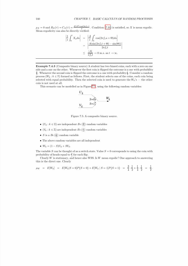
8/11/2019 Random process by B. Hajek
http://slidepdf.com/reader/full/random-process-by-b-hajek 250/448
8/11/2019 Random process by B. Hajek
http://slidepdf.com/reader/full/random-process-by-b-hajek 251/448
7.4. ERGODICITY 241
So the question is whether
1
n
n
k=1
W k?
→ 1
2
m.s.
But by the strong law of large numbers
1
n
nk=1
W k = 1
n
nk=1
((1 − S )U k + SV k)
= (1 − S )
1
n
nk=1
U k
+ S
1
n
nk=1
V k
m.s.→ (1 − S )
3
4 + S
1
4 =
3
4 − S
2.
Thus, the limit is a random variable, rather than the constant 12 . Intuitively, the process W has
such strong memory due to the switch mechanism that even averaging over long time intervals doesnot diminish the randomness due to the switch.
Another way to show that W is not mean ergodic is to find the covariance function C W and usethe necessary and sufficient condition (7.31) for mean ergodicity. Note that for k fixed, W 2k = W kwith probability one, so E [W 2k ] = 1
2 . If k = l, then
E [W kW l] = E [W kW l | S = 0]P S = 0 + E [W kW l | S = 1]P S = 1= E [U kU l]
1
2 + E [V kV l]
1
2
= E [U k]E [U l]
1
2 + E [V k]E [V l]
1
2
=
3
4
2 1
2 +
1
4
2 1
2 =
5
16.
Therefore,
C W (n) =
1
4 if n = 01
16 if n = 0
Since limn→∞ C W (n) exists and is not zero, W is not mean ergodic.
In many applications, we are interested in averages of functions that depend on multiple randomvariables. We discuss this topic for a discrete time stationary random process, (X n : n ∈ Z). Let hbe a bounded, Borel measurable function on Rk for some k. What time average would we expectto be a good approximation to the statistical average E [h(X 1, . . . , X k)]? A natural choice is
1n
n j=1 h(X j, X j+1, . . . , X j+k−1).
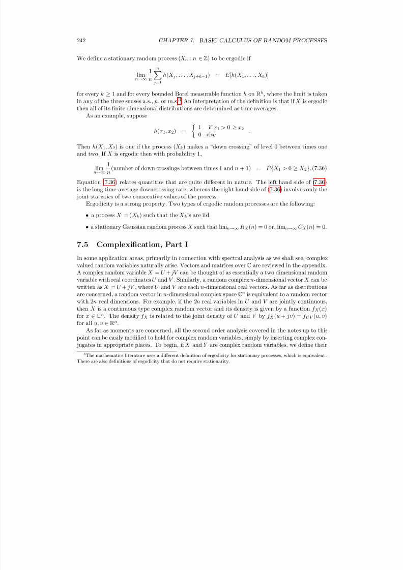
8/11/2019 Random process by B. Hajek
http://slidepdf.com/reader/full/random-process-by-b-hajek 252/448
242 CHAPTER 7. BASIC CALCULUS OF RANDOM PROCESSES
We define a stationary random process (X n : n ∈ Z) to be ergodic if
limn→∞
1
n
n
j=1
h(X j, . . . , X j+k
−1) = E [h(X 1, . . . , X k)]
for every k ≥ 1 and for every bounded Borel measurable function h on Rk, where the limit is takenin any of the three senses a.s., p. or m.s.3 An interpretation of the definition is that if X is ergodicthen all of its finite dimensional distributions are determined as time averages.
As an example, suppose
h(x1, x2) =
1 if x1 > 0 ≥ x2
0 else .
Then h(X 1, X 2) is one if the process (X k) makes a “down crossing” of level 0 between times oneand two. If X is ergodic then with probability 1,
limn→∞
1n
(number of down crossings between times 1 and n + 1) = P X 1 > 0 ≥ X 2. (7.36)
Equation (7.36) relates quantities that are quite different in nature. The left hand side of (7.36)is the long time-average downcrossing rate, whereas the right hand side of ( 7.36) involves only the joint statistics of two consecutive values of the process.
Ergodicity is a strong property. Two types of ergodic random processes are the following:
• a process X = (X k) such that the X k’s are iid.
• a stationary Gaussian random process X such that limn→∞ RX (n) = 0 or, limn→∞ C X (n) = 0.
7.5 Complexification, Part IIn some application areas, primarily in connection with spectral analysis as we shall see, complexvalued random variables naturally arise. Vectors and matrices over C are reviewed in the appendix.A complex random variable X = U + jV can be thought of as essentially a two dimensional randomvariable with real coordinates U and V . Similarly, a random complex n-dimensional vector X can bewritten as X = U + jV , where U and V are each n-dimensional real vectors. As far as distributionsare concerned, a random vector in n-dimensional complex space Cn is equivalent to a random vectorwith 2n real dimensions. For example, if the 2n real variables in U and V are jointly continuous,then X is a continuous type complex random vector and its density is given by a function f X (x)for x ∈ Cn. The density f X is related to the joint density of U and V by f X (u + jv) = f UV (u, v)
for all u, v ∈Rn
.As far as moments are concerned, all the second order analysis covered in the notes up to thispoint can be easily modified to hold for complex random variables, simply by inserting complex con- jugates in appropriate places. To begin, if X and Y are complex random variables, we define their
3The mathematics literature uses a different definition of ergodicity for stationary processes, which is equivalent.There are also definitions of ergodicity that do not require stationarity.
8/11/2019 Random process by B. Hajek
http://slidepdf.com/reader/full/random-process-by-b-hajek 253/448
7.5. COMPLEXIFICATION, PART I 243
correlation by E [XY ∗] and similarly their covariance as E [(X −E [X ])(Y −E [Y ])∗], where ∗ is usedto denote the operation on vectors or matrices of taking the transpose and then taking the complexconjugate of each coordinate. The Schwarz inequality becomes |E [XY ∗]| ≤
E [|X |2]E [|Y |2] and
its proof is essentially the same as for real valued random variables. The cross correlation matrixfor two complex random vectors X and Y is given by E [XY ∗], and similarly the cross covariancematrix is given by Cov(X, Y ) = E [(X − E [X ])(Y − E [Y ])∗]. As before, Cov(X ) = Cov(X, X ). Thevarious formulas for covariance still apply. For example, if A and C are complex matrices and band d are complex vectors, then Cov(AX + b,CY + d) = ACov(X, Y )C ∗. Just as in the case of realvalued random variables, a matrix K is a valid covariance matrix (in other words, there exits somerandom vector X such that K = Cov(X )) if and only if K is Hermitian symmetric and positivesemidefinite.
Complex valued random variables X and Y with finite second moments are said to be orthogonal if E [XY ∗] = 0, and with this definition the orthogonality principle holds for complex valued randomvariables. If X and Y are complex random vectors, then again E [X |Y ] is the MMSE estimator of X given Y , and the covariance matrix of the error vector is given by Cov(X )
−Cov(E [X
|Y ]). The
MMSE estimator for X of the form AY + b (i.e. the best linear estimator of X based on Y ) andthe covariance of the corresponding error vector are given just as for vectors made of real randomvariables:
E [X |Y ] = E [X ] + Cov(X, Y )Cov(Y )−1(Y − E [Y ])
Cov(X − E [X |Y ]) = Cov(X ) − Cov(X, Y )Cov(Y )−1Cov(Y, X )
By definition, a sequence X 1, X 2, . . . of complex valued random variables converges in the m.s.sense to a random variable X if E [|X n|2] < ∞ for all n and if limn→∞ E [|X n − X |2] = 0. Thevarious Cauchy criteria still hold with minor modification. A sequence with E [|X n|2] < ∞ for alln is a Cauchy sequence in the m.s. sense if limm,n
→∞E [
|X n
−X m
|2] = 0. As before, a sequence
converges in the m.s. sense if and only if it is a Cauchy sequence. In addition, a sequence X 1, X 2, . . .of complex valued random variables with E [|X n|2] < ∞ for all n converges in the m.s. sense if and only if limm,n→∞ E [X mX ∗n] exits and is a finite constant c. If the m.s. limit exists, then thelimiting random variable X satisfies E [|X |2] = c.
Let X = (X t : t ∈ T) be a complex random process. We can write X t = U t + jV t where U andV are each real valued random processes. The process X is defined to be a second order processif E [|X t|2] < ∞ for all t. Since |X t|2 = U 2t + V 2
t for each t, X being a second order process isequivalent to both U and V being second order processes. The correlation function of a secondorder complex random process X is defined by RX (s, t) = E [X sX ∗t ]. The covariance function isgiven by C X (s, t) = Cov(X s, X t) where the definition of Cov for complex random variables is used.The definitions and results given for m.s. continuity, m.s. differentiation, and m.s. integration all
carry over to the case of complex processes, because they are based on the use of the Cauchy criteriafor m.s. convergence which also carries over. For example, a complex valued random process is m.s.continuous if and only if its correlation function RX is continuous. Similarly the cross correlationfunction for two second order random processes X and Y is defined by RXY (s, t) = E [X sY ∗t ]. Notethat RXY (s, t) = R∗
Y X (t, s).Let X = (X t : t ∈ T) be a complex random process such that T is either the real line or
8/11/2019 Random process by B. Hajek
http://slidepdf.com/reader/full/random-process-by-b-hajek 254/448
244 CHAPTER 7. BASIC CALCULUS OF RANDOM PROCESSES
the set of integers, and write X t = U t + jV t where U and V are each real valued random pro-cesses. By definition, X is stationary if and only if for any t1, . . . , tn ∈ T, the joint distribution of (X t1+s, . . . , X tn+s) is the same for all s ∈ T. Equivalently, X is stationary if and only if U and V
are jointly stationary. The process X is defined to be WSS if X is a second order process such thatE [X t] does not depend on t, and RX (s, t) is a function of s − t alone. If X is WSS we use RX (τ ) todenote RX (s, t), where τ = s − t. A pair of complex-valued random processes X and Y are definedto be jointly WSS if both X and Y are WSS and if the cross correlation function RXY (s, t) is afunction of s − t. If X and Y are jointly WSS then RXY (−τ ) = R∗
Y X (τ ).In summary, everything we’ve discussed in this section regarding complex random variables,
vectors, and processes can be considered a simple matter of notation. One simply needs to use|X |2 instead of X 2, and to use a star “∗” for Hermitian transpose in place of “T ” for transpose.We shall begin using the notation at this point, and return to a discussion of the topic of complexvalued random processes in Section 8.6. In particular, we will examine complex normal randomvectors and their densities, and we shall see that there is somewhat more to complexification than just notation.
7.6 The Karhunen-Loeve expansion
We’ve seen that under a change of coordinates, an n-dimensional random vector X is transformedinto a vector Y = U ∗X such that the coordinates of Y are orthogonal random variables. HereU is the unitary matrix such that E [XX ∗] = U ΛU ∗. The columns of U are eigenvectors of theHermitian symmetric matrix E [XX ∗] and the corresponding nonnegative eigenvalues of E [XX ∗]comprise the diagonal of the diagonal matrix Λ. The columns of U form an orthonormal basis forCn. The Karhunen-Loeve expansion gives a similar change of coordinates for a random process ona finite interval, using an orthonormal basis of functions instead of an othonormal basis of vectors.
Fix a finite interval [a, b]. The L2 norm of a real or complex valued function f on the interval[a, b] is defined by
||f || = b
a|f (t)|2dt
We write L2[a, b] for the set of all functions on [a, b] which have finite L2 norm. The inner productof two functions f and g in L2[a, b] is defined by
f, g =
ba
f (t)g∗(t)dt
The functions f and g are said to be orthogonal if f, g = 0. Note that ||f || = f, f and the
Schwarz inequality holds:
|f, g
| ≤ ||f
| | · | |g
||. A finite or infinite set of functions (φn) in L2[a, b]
is said to be an orthonormal system if the functions in the set are mutually orthogonal and havenorm one, or in other words, φi, φ j = I i= j for all i and j .
In many applications it is useful to use representations of the form
f (t) =N
n=1
cnφn(t), (7.37)
8/11/2019 Random process by B. Hajek
http://slidepdf.com/reader/full/random-process-by-b-hajek 255/448
7.6. THE KARHUNEN-LO EVE EXPANSION 245
for some orthonormal system φ1, . . . , φN . In such a case, we think of (c1, . . . , cN ) as the coordinatesof f relative to the orthonormal system (φn), and we might write f ↔ (c1, . . . , cN ). For example,transmitted signals in many digital communication systems have this form, where the coordinate
vector (c1, , . . . , cN ) represents a data symbol. The geometry of the space of all functions f of the form (7.37) for the fixed orthonormal system φ1, . . . , φN is equivalent to the geometry of thecoordinates vectors. For example, if g has a similar representation,
g(t) =N
n=1
dnφn(t),
or equivalently g ↔ (d1, . . . , dN ), then f + g ↔ (c1, . . . , cN ) + (d1, . . . , dN ) and
f, g =
ba
N m=1
cmφm(t)
N n=1
d∗nφ∗n(t)
dt
=
N m=1
N n=1
cmd∗n ba
φm(t)φ∗n(t)dt
=N
m=1
N n=1
cmd∗nφm, φn
=N
m=1
cmd∗m (7.38)
That is, the inner product of the functions, f, g, is equal to the inner product of their coordinatevectors. Note that for 1 ≤ n ≤ N , φn ↔ (0, . . . , 0, 1, 0, . . . , 0), such that the one is in the nth
position. If f ↔ (c1, . . . , cN ), then the nth coordinate of f is the inner product of f and φn :
f, φn = ba
N m=1
cmφm(t)
φ∗n(t)dt =
N m=1
cmφm, φn = cn.
Another way to derive that f, φn = cn is to note that f ↔ (c1, . . . , cN ) and φn ↔ (0, . . . , 0, 1, 0, . . . , 0),so f, φn is the inner product of (c1, . . . , cN ) and (0, . . . , 0, 1, 0, . . . , 0), or cn. Thus, the coordinatevector for f is given by f ↔ (f, φ1, . . . , f, φN ).
The dimension of the space L2[a, b] is infinite, meaning that there are orthonormal systems(φn : n ≥ 1) with infinitely many functions. For such a system, a function f can have therepresentation
f (t) =∞
n=1
cnφn(t). (7.39)
In many instances encountered in practice, the sum (7.39) converges for each t, but in general whatis meant is that the convergence is in the sense of the L2[a, b] norm:
limN →∞
ba
f (t) −N
n=1
cnφn(t)
2dt = 0,
8/11/2019 Random process by B. Hajek
http://slidepdf.com/reader/full/random-process-by-b-hajek 256/448
246 CHAPTER 7. BASIC CALCULUS OF RANDOM PROCESSES
or equivalently,
limN →∞
f −
N
n=1
cnφn
= 0
The span of a set of functions φ1, . . . , φN is the set of all functions of the form a1φ1(t) +· · · + aN φN (t). If the functions φ1, . . . , φN form an orthonormal system and if f ∈ L2[a, b], then thefunction f in the span of φ1, . . . , φN that minimizes ||f −f || is given by f (t) =
N n=1f, φnφn(t).
In fact, it is easy to check that f − f is orthogonal to φn for all n, implying that for any complexnumbers a1, . . . , aN ,
||f −N
n=1
anφn||2 = ||f − f ||2 +N
n=1
|f , φn − an|2.
Thus, the closest approximation is indeed given by an = f , φn. That is, f given by f (t) =
N n=1f, φnφn(t) is the projection of f onto the span of the φ’s. Furthermore,
||f − f ||2 = ||f ||2 − ||f ||2 = ||f ||2 −N
n=1
|f, φn|2. (7.40)
The above reasoning is analogous to that in Proposition 3.2.4.An orthonormal system (φn) is said to be an orthonormal basis for L2[a, b], if any f ∈ L2[a, b]
can be represented as in (7.39). If (φn) is an orthonormal system then for any f, g ∈ L2[a, b], (7.38)still holds with N replaced by ∞ and is known as Parseval’s relation :
f, g =∞
n=1
f, φng, φn∗
In particular,
||f ||2 =∞
n=1
|f, φn|2.
A commonly used orthonormal basis is the following (with [a, b] = [0, T ] for some T ≥ 0):
φ1(t) = 1√ T
, φ2(t) =
2T cos( 2πt
T ), φ3(t) =
2T sin( 2πt
T ),
φ2k(t) =
2T cos( 2πkt
T ), φ2k+1(t) =
2T sin( 2πkt
T ) for k ≥ 1.(7.41)
Next, consider what happens if f is replaced by a random process X = (X t : a ≤ t ≤ b). Suppose(φn : 1 ≤ n ≤ N ) is an orthonormal system consisting of continuous functions, with N ≤ ∞. Thesystem does not have to be a basis for L2[a, b], but if it is then there are infinitely many functionsin the system. Suppose that X is m.s. continuous, or equivalently, that RX is continuous as a
function on [a, b] × [a, b]. In particular, RX is bounded. Then E ba |X t|2dt = ba RX (t, t)dt < ∞,
so that ba |X t|2dt is finite with probability one. Suppose that X can be represented as
X t =N
n=1
C nφn(t). (7.42)

8/11/2019 Random process by B. Hajek
http://slidepdf.com/reader/full/random-process-by-b-hajek 257/448
7.6. THE KARHUNEN-LO EVE EXPANSION 247
Such a representation exists if (φn) is a basis for L2[a, b], but some random processes have the form(7.42) even if N is finite or if N is infinite but the system is not a basis. The representation ( 7.42)reduces the description of the continuous-time random process to the description of the coefficients,
(C n). This representation of X is much easier to work with if the coordinate random variables areorthogonal.
Definition 7.6.1 A Karhunen-Loeve (KL) expansion for a random process X = (X t : a ≤ t ≤ b)is a representation of the form (7.42) with N ≤ ∞ such that:(1) the functions (φn) are orthonormal: φm, φn = I m=n, and (2) the coordinate random variables C n are mutually orthogonal: E [C mC ∗n] = 0.
Example 7.6.2 Let X t = A for 0 ≤ t ≤ T, where A is a random variable with 0 < E [A2] < ∞.
Then X has the form in (7.42) for [a, b] = [0, T ], N = 1, C 1 = A√
T , and φ1(t) = I 0≤t≤T √
T . This is
trivially a KL expansion, with only one term.
Example 7.6.3 Let X t = A cos(2πt/T +Θ) for 0 ≤ t ≤ T , where A is a real-valued random variablewith 0 < E [A2] < ∞, and Θ is a random variable uniformly distributed on [0, 2π] and independentof A. By the cosine angle addition formula, X t = A cos(Θ) cos(2πt/T ) − A sin(Θ) sin(2πt/T ). ThenX has the form in (7.42) for [a, b] = [0, T ], N = 2,
C 1 = A√
2T cos(Θ), C 2 = −A√
2T sin(Θ), φ1(t) = cos(2πt/T )√
2T , φ2(t) =
sin(2πt/T )√ 2T
.
In particular, φ1 and φ2 form an orthonormal system with N = 2 elements. To check whether
this is a KL expansion, we see if E [C 1C ∗2 ] = 0. Since E [C 1C ∗2 ] = −2T E [A
2
]E [cos(Θ) sin(Θ)] =−T E [A2]E [sin(2Θ)] = 0, this is indeed a KL expansion, with two terms.
An important property of Karhunen-Loeve (KL) expansions in practice is that they identify themost accurate finite dimensional approximations of a random process, as described in the followingproposition. A random process Z = (Z t : a ≤ t ≤ b) is said to be N -dimensional if it has the formZ t =
N n=1 Bnψn(t) for some N random variables B1, . . . , BN and N functions ψ1, . . . , ψN .
Proposition 7.6.4 Suppose X has a Karhunen-Loeve (KL) expansion X t = ∞
n=1 C nφn(t) (See Definition 7.6.1). Let λn = E [|C n|2] and suppose the terms are indexed so that λ1 ≥ λ2 ≥ · · · . For any finite N ≥ 1, the N th partial sum, X (N )(t) =
N n=1 C nφn(t), is a choice for Z that minimizes
E [
||X
−Z
||2] over all N -dimensional random processes Z.
Proof. Suppose Z is a random linear combination of N functions, ψ1, . . . , ψN . Without loss of generality, assume that ψ1, . . . , ψN is an orthonormal system. (If not, the Gram-Schmidt procedurecould be applied to get an orthonormal system of N functions with the same span.) We firstidentify the optimal choice of random coefficients for the ψ’s fixed, and then consider the optimalchoice of the ψ’s. For a given choice of ψ’s and a sample path of X, the L2 norm ||X − Z ||2
8/11/2019 Random process by B. Hajek
http://slidepdf.com/reader/full/random-process-by-b-hajek 258/448
248 CHAPTER 7. BASIC CALCULUS OF RANDOM PROCESSES
is minimized by projecting the sample path of X onto the span of the ψ’s, which means takingZ t =
N j=1X, ψ jψ j(t). That is, the sample path of Z has the form of f above, if f is the sample
path of X. This determines the coefficients to be used for a given choice of ψ’s; it remains to
determine the ψ’s. By (7.40), the (random) approximation error is
||X − Z ||2 = ||X ||2 −N
j=1
|X, ψ j|2
Using the KL expansion for X yields
E [|X, ψ j|2] = E
∞n=1
C nφn, ψ j2
=
∞n=1
λn|φn, ψ j|2
Therefore,
E ||X − Z ||2 = E ||X ||
2−∞
n=1 λnbn (7.43)
where bn =N
j=1 |φn, ψ j|2. Note that (bn) satisfies the constraints 0 ≤ bn ≤ 1, and∞
n=1 bn = N.The right hand side of (7.43) is minimized over (bn) subject to these constraints by taking bn =I 1≤n≤N . That can be achieved by taking ψ j = φ j for 1 ≤ j ≤ N , in which case X, ψ j = C j, and
Z becomes X (N ).
Proposition 7.6.5 Suppose X = (X t : a ≤ t ≤ b) is m.s. continuous and (φn) is an orthonormal system of continuous functions. If (7.42) holds for some random variables (C n), it is a KL expan-sion (i.e., the coordinate random variables are orthogonal) if and only if the φn’s are eigenfunctions of RX :
RX φn = λnφn, (7.44)
where for a function φ ∈ L2[a, b], RX φ denotes the function (RX φ)(s) = ba RX (s, t)φ(t)dt. In case
(7.42) is a KL expansion, the eigenvalues are given by λn = E [|C n|2].
Proof. Suppose (7.42) holds. Then C n = X, φn = ba X tφ
∗n(t)dt, so that
E [C mC ∗n] = E [X, φmX, φn∗]
= E
ba
X sφ∗m(s)ds
ba
X tφ∗n(t)dt
∗
= b
a b
aR
X (s, t)φ∗
m(s)φ
n(t)dsdt
= RX φn, φm (7.45)
Now, if the φn’s are eigenfunctions of RX , then E [C mC ∗n] = RX φn, φm = λnφn, φm = λnφn, φm =λnI m=n. In particular, E [C mC ∗n] = 0 if n = m, so that (7.42) is a KL expansion. Also, takingm = n yields E [|C n|2] = λn.
8/11/2019 Random process by B. Hajek
http://slidepdf.com/reader/full/random-process-by-b-hajek 259/448
7.6. THE KARHUNEN-LO EVE EXPANSION 249
Conversely, suppose (7.42) is a KL expansion. Without loss of generality, suppose that thesystem (φn) is a basis of L2[a, b]. (If it weren’t, it could be extended to a basis by augmenting itwith functions from another basis and applying the Gramm-Schmidt method of orthogonalizing.)
Then for n fixed, RX φn, φm = 0 for all m = n. By the fact (φn) is a basis, the function RX φn hasan expansion of the form (7.39), but all terms except possibly the nth are zero. Hence, Rnφn = λnφn
for some constant λn, so the eigenrelations (7.44) hold. Again, E [|C n|2] = λn by the computationabove.
The following theorem is stated without proof.
Theorem 7.6.6 (Mercer’s theorem) If RX is the autocorrelation function of a m.s. continuous random process X = (X t : a ≤ t ≤ b) (equivalently, if RX is a continuous function on [a, b] × [a, b]that is positive semi-definite, i.e. RX (ti, t j) is a positive semidefinite matrix for any n and any a ≤ t1 < t2 < · · · < tn ≤ b), then there exists an orthonormal basis for L2[a, b], (φn : n ≥ 1), of continuous eigenfunctions and corresponding nonnegative eigenvalues ( λn : n
≥ 1) for RX , and RX
is given by the following series expansion:
RX (s, t) =
∞n=1
λnφn(s)φ∗n(t). (7.46)
The series converges uniformly in s, t, meaning that
limN →∞
maxs,t∈[a,b]
RX (s, t) −N
n=1
λnφn(s)φ∗n(t)
= 0.
Theorem 7.6.7 ( Karhunen-Loeve expansion) If X = (X t : a ≤ t ≤ b) is a m.s. continuous random process it has a KL expansion,
X t =
∞n=1
φn(t)X, φn,
and the series converges in the m.s. sense, uniformly over t ∈ [a, b].
Proof. Use the orthonormal basis (φn) guaranteed by Mercer’s theorem. By (7.45), E [X, φm∗X, φn]RX φn, φm = λnI n=m. Also,
E [X tX, φn∗] = E [X t
ba
X ∗s φn(s)ds]
= b
aRX (t, s)φn(s)ds = λnφn(t).
These facts imply that for finite N ,
E
X t −N
n=1
φn(t)X, φn
2 = RX (t, t) −
N n=1
λn|φn(t)|2, (7.47)
8/11/2019 Random process by B. Hajek
http://slidepdf.com/reader/full/random-process-by-b-hajek 260/448
250 CHAPTER 7. BASIC CALCULUS OF RANDOM PROCESSES
which, since the series on the right side of (7.47) converges uniformly in t as n → ∞, implies thestated convergence property for the representation of X .
Remarks (1) The means of the coordinates of X in a KL expansion can be expressed using themean function µX (t) = E [X t] as follows:
E [X, φn] =
ba
µX (t)φ∗n(t)dt = µX , φn
Thus, the mean of the nth coordinate of X is the nth coordinate of the mean function of X.(2) Symbolically, mimicking matrix notation, we can write the representation (7.46) of RX as
RX (s, t) = [φ1(s)|φ2(s)| · · · ]
λ1
λ2
λ3
.. .
φ∗1(t)
φ∗2(t)...
(3) If f ∈ L2[a, b] and f (t) represents a voltage or current across a resistor, then the energydissipated during the interval [a, b] is, up to a multiplicative constant, given by
(Energy of f ) = ||f ||2 =
ba
|f (t)|2dt =
∞n=1
|f, φn|2.
The mean total energy of (X t : a < t < b) is thus given by
E b
a |X t|2
dt = b
a RX (t, t)dt
=
ba
∞n=1
λn|φn(t)|2dt
=∞
n=1
λn
(4) If (X t : a ≤ t ≤ b) is a real valued mean zero Gaussian process and if the orthonormal basisfunctions are real valued, then the coordinates X, φn are uncorrelated, real valued, jointly Gaus-sian random variables, and therefore are independent.
Example 7.6.8 Let W = (W t : t ≥ 0) be a Brownian motion with parameter σ2. Let us find theKL expansion of W over the interval [0, T ]. Substituting RX (s, t) = σ2(s ∧ t) into the eigenrelation(7.44) yields t
0σ2sφn(s)ds +
T t
σ2tφn(s)ds = λnφn(t) (7.48)
8/11/2019 Random process by B. Hajek
http://slidepdf.com/reader/full/random-process-by-b-hajek 261/448
7.6. THE KARHUNEN-LO EVE EXPANSION 251
Differentiating (7.48) with respect to t yields
σ2tφn(t)
−σ2tφn(t) +
T
t
σ2φn(s)ds = λnφn(t), (7.49)
and differentiating a second time yields that the eigenfunctions satisfy the differential equationλφ = −σ2φ. Also, setting t = 0 in (7.48) yields the boundary condition φn(0) = 0, and settingt = T in (7.49) yields the boundary condition φ
n(T ) = 0. Solving yields that the eigenvalue andeigenfunction pairs for W are
λn = 4σ2T 2
(2n + 1)2π2 φn(t) =
2
T sin
(2n + 1)πt
2T
n ≥ 0
It can be shown that these functions form an orthonormal basis for L2[0, T ].
Example 7.6.9 Let X be a white noise process. Such a process is not a random process as definedin these notes, but can be defined as a generalized process in the same way that a delta function canbe defined as a generalized function. Generalized random processes, just like generalized functions,only make sense when multiplied by a suitable function and then integrated. For example, thedelta function δ is defined by the requirement that for any function f that is continuous at t = 0, ∞
−∞f (t)δ (t)dt = f (0)
A white noise process X is such that integrals of the form ∞−∞ f (t)X (t)dt exist for functions f with
finite L2 norm ||f ||. The integrals are random variables with finite second moments, mean zero andcorrelations given by
E
∞−∞
f (s)X sds
∞−∞
g(t)X tdt
∗= σ2
∞−∞
f (t)g∗(t)dt
In a formal or symbolic sense, this means that X is a WSS process with mean µX = 0 andautocorrelation function RX (s, t) = E [X sX ∗t ] given by RX (τ ) = σ2δ (τ ).
What would the KL expansion be for a white noise process over some fixed interval [a,b]?The eigenrelation (7.44) becomes simply σ2φ(t) = λnφ(t) for all t in the interval. Thus, all theeigenvalues of a white noise process are equal to σ2, and any function φ with finite norm is aneigenfunction. Thus, if (φn : n ≥ 1) is an arbitrary orthonormal basis for L2[a, b], then thecoordinates of the white noise process X , formally given by X n = X, φn, satisfy
E [X nX ∗m] = σ2
I n=m. (7.50)
This offers a reasonable interpretation of white noise. It is a generalized random process such thatits coordinates (X n : n ≥ 1) relative to an arbitrary orthonormal basis for a finite interval havemean zero and satisfy (7.50).
8/11/2019 Random process by B. Hajek
http://slidepdf.com/reader/full/random-process-by-b-hajek 262/448
252 CHAPTER 7. BASIC CALCULUS OF RANDOM PROCESSES
7.7 Periodic WSS random processes
Let X = (X t : t ∈R) be a WSS random process and let T be a positive constant.
Proposition 7.7.1 The following three conditions are equivalent:(a) RX (T ) = RX (0)(b) P X T +τ = X τ = 1 for all τ ∈ R(c) RX (T + τ ) = RX (τ ) for all τ ∈ R (i.e. RX (τ ) is periodic with period T.)
Proof. Suppose (a) is true. Since RX (0) is real valued, so is RX (T ), yielding
E [|X T +τ − X τ |2] = E [X T +τ X ∗T +τ − X T +τ X ∗τ − X τ X ∗T +τ + X τ X ∗τ ]= RX (0) − RX (T ) − R∗
X (T ) + RX (0) = 0
Therefore, (a) implies (b). Next, suppose (b) is true and let τ ∈ R. Since two random variablesthat are equal with probability one have the same expectation, (b) implies that
RX (T + τ ) = E [X T +τ X ∗0 ] = E [X τ X ∗0 ] = RX (τ ).
Therefore (b) imples (c). Trivially (c) implies (a), so the equivalence of (a) through (c) is proved.
Definition 7.7.2 We call X a periodic, WSS process of period T if X is WSS and any of the three equivalent properties (a), (b), or (c) of Proposition 7.7.1 hold.
Property (b) almost implies that the sample paths of X are periodic. However, for each τ it canbe that X τ = X τ +T on an event of probability zero, and since there are uncountably many realnumbers τ , the sample paths need not be periodic. However, suppose (b) is true and define aprocess Y by Y t = X (t mod T ). (Recall that by definition, (t mod T ) is equal to t + nT , where n
is selected so that 0 ≤ t + nT < T .) Then Y has periodic sample paths, and Y is a version of X ,which by definition means that P X t = Y t = 1 for any t ∈ R. Thus, the properties (a) through(c) are equivalent to the condition that X is WSS and there is a version of X with periodic samplepaths of period T .
Suppose X is a m.s. continuous, periodic, WSS random process. Due to the periodicity of X ,it is natural to consider the restriction of X to the interval [0, T ]. The Karhunen-Loeve expansionof X restricted to [0, T ] is described next. Let φn be the function on [0, T ] defined by
φn(t) = e2πjnt/T
√ T
8/11/2019 Random process by B. Hajek
http://slidepdf.com/reader/full/random-process-by-b-hajek 263/448
7.7. PERIODIC WSS RANDOM PROCESSES 253
The functions (φn : n ∈ Z) form an orthonormal basis for L2[0, T ].4 In addition, for any n fixed,both RX (τ ) and φn are periodic with period dividing T , so
T 0
RX (s, t)φn(t)dt = T 0
RX (s − t)φn(t)dt
=
ss−T
RX (t)φn(s − t)dt
=
T 0
RX (t)φn(s − t)dt
= 1√
T
T 0
RX (t)e2πjns/T e−2πjnt/T dt
= λnφn(s).
where λn is given by
λn = T
0RX (t)e−2πjnt/T dt =
√ T RX , φn. (7.51)
Therefore φn is an eigenfunction of RX with eigenvalue λn. The Karhunen-Loeve expansion (5.20)of X over the interval [0, T ] can be written as
X t =∞
n=−∞X ne2πjnt/T (7.52)
where X n is defined by
X n = 1
√ T X, φn
=
1
T T
0
X te−2πjnt/T dt
Note that
E [ X m X ∗n] = 1
T E [X, φmX, φn∗] =
λn
T I m=n
Although the representation (7.52) has been derived only for 0 ≤ t ≤ T , both sides of (7.52) areperiodic with period T . Therefore, the representation (7.52) holds for all t. It is called the spectral representation of the periodic, WSS process X .
By (7.51), the series expansion (7.39) applied to the function RX over the interval [0, T ] can bewritten as
RX (t) =
∞
n=−∞
λn
T e2πjnt/T
=ω
pX (ω)e jωt , (7.53)
4Here it is more convenient to index the functions by the integers, rather than by the nonnegative integers. Sumsof the form
P∞n=−∞ should be interpreted as limits of
PN n=−N as N → ∞.
8/11/2019 Random process by B. Hajek
http://slidepdf.com/reader/full/random-process-by-b-hajek 264/448
254 CHAPTER 7. BASIC CALCULUS OF RANDOM PROCESSES
where pX is the function on the real line R = (ω : −∞ < ω < ∞),5 defined by
pX (ω) = λn/T ω = 2πn
T for some integer n
0 elseand the sum in (7.53) is only over ω such that pX (ω) = 0. The function pX is called the power spectral mass function of X . It is similar to a probability mass function, in that it is positive forat most a countable infinity of values. The value pX (
2πnT ) is equal to the power of the nth term in
the representation (7.52):
E [| X ne2πjnt/T |2] = E [| X n|2] = pX
2πn
T
and the total mass of pX is the total power of X , RX (0) = E [|X t|2].
Periodicity is a rather restrictive assumption to place on a WSS process. In the next chapter we
shall further investigate spectral properties of WSS processes. We shall see that many WSS randomprocesses have a power spectral density. A given random variable might have a pmf or a pdf, andit definitely has a CDF. In the same way, a given WSS process might have a power spectral massfunction or a power spectral density function, and it definitely has a cumulative power spectraldistribution function. The periodic WSS processes of period T are precisely those WSS processesthat have a power spectral mass function that is concentrated on the integer multiples of 2π
T .
7.8 Problems
7.1 Calculus for a simple Gaussian random processDefine X = (X t : t ∈ R) by X t = A + Bt + C t2, where A,B, and C are independent, N (0, 1)
random variables. (a) Verify directly that X is m.s. differentiable. (b) Express P 10 X sds ≥ 1in terms of Q, the standard normal complementary CDF.
7.2 Lack of sample path continuity of a Poisson processLet N = (N t : t ≥ 0) be a Poisson process with rate λ > 0. (a) Find the following two probabilities,explaining your reasoning: P N is continuous over the interval [0,T] for a fixed T > 0, andP N is continuous over the interval [0, ∞). (b) Is N sample path continuous a.s.? Is N m.s.continuous?
7.3 Properties of a binary valued processLet Y = (Y t : t ≥ 0) be given by Y t = (−1)N t , where N is a Poisson process with rate λ > 0.(a) Is Y a Markov process? If so, find the transition probability function p
i,j(s, t) and the transition
rate matrix Q. (b) Is Y mean square continuous? (c) Is Y mean square differentiable? (d) Does
limT →∞ 1T
T 0 ytdt exist in the m.s. sense? If so, identify the limit.
5The Greek letter ω is used here as it is traditionally used for frequency measured in radians per second. It isrelated to the frequency f measured in cycles per second by ω = 2πf . Here ω is not the same as a typical elementof the underlying space of all outcomes, Ω. The meaning of ω should be clear from the context.
8/11/2019 Random process by B. Hajek
http://slidepdf.com/reader/full/random-process-by-b-hajek 265/448
7.8. PROBLEMS 255
7.4 Some statements related to the basic calculus of random processesClassify each of the following statements as either true (meaning always holds) or false, and justifyyour answers.
(a) Let X t = Z , where Z is a Gaussian random variable. Then X = (X t : t ∈ R) is mean ergodicin the m.s. sense.
(b) The function RX defined by RX (τ ) =
σ2 |τ | ≤ 1
0 τ > 1 is a valid autocorrelation function.
(c) Suppose X = (X t : t ∈R) is a mean zero stationary Gaussian random process, and suppose X is m.s. differentiable. Then for any fixed time t, X t and X t are independent.
7.5 Differentiation of the square of a Gaussian random process(a) Show that if random variables (An : n ≥ 0) are mean zero and jointly Gaussian and if limn→∞ An = A m.s., then limn→∞ A2
n = A2 m.s. (Hint: If A, B,C , and D are mean zero and jointly Gaussian, then E [ABCD] = E [AB]E [CD ] + E [AC ]E [BD] + E [AD]E [BC ].)(b) Show that if random variables (An, Bn : n
≥ 0) are jointly Gaussian and limn
→∞An = A m.s.
and limn→∞ Bn = B m.s. then limn→∞ AnBn = AB m.s. (Hint: Use part (a) and the identity
ab = (a+b)2−a2−b2
2 .)(c) Let X be a mean zero, m.s. differentiable Gaussian random process, and let Y t = X 2t for all t.Is Y m.s. differentiable? If so, justify your answer and express the derivative in terms of X t andX t.
7.6 Continuity of a process passing through a nonlinearitySuppose X is a m.s. continuous random process and G is a bounded, continuous function on R.Let Y t = G(X t) for all t ∈R.(a) Prove Y is m.s. continuous. (Hint: Use the connections between continuity in m.s. and p.senses. Also, a continuous function is uniformly continuous over any finite interval, so for any
interval [a, b] and > 0, there is a δ > 0 so that |G(x) − G(x)| ≤ whenever x, x ∈ [a, b] with|x − x| ≤ δ.)(b) Give an example with G bounded but not continuous, such that Y is not m.s. continuous.(c) Give an example with G continuous but not bounded, such that Y is not m.s. continuous.
7.7 Mean square differentiability of some random processesFor each process described below, determine whether the process is m.s. differentiable in the m.s.sense. Justify your reasoning.(a) X t =
t0 N sds, where N is a Poisson random process with rate parameter one.
(b) Process Y, assumed to be a mean-zero Gaussian process with autocorrelation function RY (s, t) =
1 if s = t0 else.
Here “
x
” denotes the greatest integer less than or equal to x.
(c) Process Z defined by the series (which converges uniformly in the m.s. sense)
Z t =∞
n=1V n sin(nt)
n2 where the V n’s are independent, N (0, 1) random variables.
7.8 Integral of OU processSuppose X is a stationary continuous-time Gaussian process with autocorrelation function RX (τ ) =
8/11/2019 Random process by B. Hajek
http://slidepdf.com/reader/full/random-process-by-b-hajek 266/448
256 CHAPTER 7. BASIC CALCULUS OF RANDOM PROCESSES
Ae−|τ |, and let Y t = t
0 X udu for t ≥ 0. (It follows that X has mean zero and is a Markov process.It is sometimes called the standard Ornstein-Uhlenbeck process, and it provides a model for thevelocity of a particle moving in one dimension subject to random disturbances and friction, and
thus Y would denote the position of the particle.)(a) Find the mean and autocorrelation function of (Y t : t ≥ 0).(b) Find g(t) for t > 0 so that P |Y t| ≥ g(t) = 0.5. (Hint: Q(0.81) ≈ 0.25, where Q is thecomplementary CDF of the standard Gaussian distribution.)(c) Find a function f (α) so that as α → ∞, the finite dimensional distributions of the process
Z t= f (α)Y αt converge to the finite dimensional distributions of the standard Brownian motion
process. (An interpretation is that f (α)X αt converges to white Gaussian noise.)
7.9 A two-state stationary Markov processSuppose X is a stationary Markov process with mean zero, state space −1, 1, and transition rate
matrix Q = −α α
α −α , where α
≥ 0. Note that α = 0 is a possible case.
(a) Find the autocorrelation function, RX (τ ).(b) For what value(s) of α ≥ 0 is X m.s. continuous?(c) For what value(s) of α ≥ 0 is X m.s. continuously differentiable?(d) For what value(s) of α ≥ 0 is X mean ergodic in the m.s. sense?
7.10 Cross correlation between a process and its m.s. derivativeSuppose X is a m.s. differentiable random process. Show that RX X = ∂ 1RX . (It follows, inparticular, that ∂ 1RX exists.)
7.11 Fundamental theorem of calculus for m.s. calculus
Suppose X = (X t : t ≥ 0) is a m.s. continuous random process. Let Y be the process defined byY t =
t0 X udu for t ≥ 0. Show that X is the m.s. derivative of Y . (It follows, in particular, that Y
is m.s. differentiable.)
7.12 A windowed Poisson processLet N = (N t : t ≥ 0) be a Poisson process with rate λ > 0, and let X = (X t : t ≥ 0) be defined byX t = N t+1 − N t. Thus, X t is the number of counts of N during the time window (t, t + 1].(a) Sketch a typical sample path of N , and the corresponding sample path of X .(b) Find the mean function µX (t) and covariance function C X (s, t) for s, t ≥ 0. Express youranswer in a simple form.(c) Is X Markov? Why or why not?
(d) Is X mean-square continuous? Why or why not?(e) Determine whether 1
t
t0 X sds converges in the mean square sense as t → ∞.
7.13 An integral of white noise times an exponentialLet X t =
t0 Z ue−udu, for t ≥ 0, where Z is white Gaussian noise with autocorrelation function
δ (τ )σ2, for some σ2 > 0. (a) Find the autocorrelation function, RX (s, t) for s, t ≥ 0. (b) Is X
8/11/2019 Random process by B. Hajek
http://slidepdf.com/reader/full/random-process-by-b-hajek 267/448
7.8. PROBLEMS 257
mean square differentiable? Justify your answer. (c) Does X t converge in the mean square senseas t → ∞? Justify your answer.
7.14 A singular integral with a Brownian motionConsider the integral 10 wtt dt, where w = (wt : t ≥ 0) is a standard Brownian motion. Since
Var(wtt ) = 1
t diverges as t → 0, we define the integral as lim→0
1
wtt dt m.s. if the limit exists.
(a) Does the limit exist? If so, what is the probability distribution of the limit?
(b) Similarly, we define ∞
1wtt dt to be limT →∞
T 1
wtt dt m.s. if the limit exists. Does the limit
exist? If so, what is the probability distribution of the limit?
7.15 An integrated Poisson processLet N = (N t : t ≥ 0) denote a Poisson process with rate λ > 0, and let Y t =
t0 N sds for s ≥ 0. (a)
Sketch a typical sample path of Y . (b) Compute the mean function, µY (t), for t ≥ 0. (c) ComputeVar(Y t) for t ≥ 0. (d) Determine the value of the limit, limt→∞ P Y t < t.
7.16 Recognizing m.s. propertiesSuppose X is a mean zero random process. For each choice of autocorrelation function shown, indi-cate which of the following properties X has: m.s. continuous, m.s. differentiable, m.s. integrableover finite length intervals, and mean ergodic in the the m.s. sense.(a) X is WSS with RX (τ ) = (1 − |τ |)+,(b) X is WSS with RX (τ ) = 1 + (1 − |τ |)+,(c) X is WSS with RX (τ ) = cos(20πτ ) exp(−10|τ |),
(d) RX (s, t) =
1 if s = t0 else
, (not WSS, you don’t need to check for mean ergodic property)
(e) RX (s, t) =√
s ∧ t for s, t ≥ 0. (not WSS, you don’t need to check for mean ergodic property)
7.17 A random Taylor’s approximationSuppose X is a mean zero WSS random process such that RX is twice continuously differentiable.Guided by Taylor’s approximation for deterministic functions, we might propose the followingestimator of X t given X 0 and X 0: X t = X 0 + tX 0.(a) Express the covariance matrix for the vector (X 0, X 0, X t)
T in terms of the function RX and itsderivatives.(b) Express the mean square error E [(X t − X t)
2] in terms of the function RX and its derivatives.(c) Express the optimal linear estimator E [X t|X 0, X 0] in terms of X 0, X 0, and the function RX andits derivatives.(d) (This part is optional - not required.) Compute and compare limt→0 (mean square error)/t4
for the two estimators, under the assumption that RX is four times continuously differentiable.
7.18 A stationary Gaussian processLet X = (X t : t ∈ Z) be a real stationary Gaussian process with mean zero and RX (t) = 1
1+t2 .Answer the following unrelated questions.(a) Is X a Markov process? Justify your anwer.(b) Find E [X 3|X 0] and express P |X 3 − E [X 3|X 0]| ≥ 10 in terms of Q, the standard Gaussian
8/11/2019 Random process by B. Hajek
http://slidepdf.com/reader/full/random-process-by-b-hajek 268/448
258 CHAPTER 7. BASIC CALCULUS OF RANDOM PROCESSES
complementary cumulative distribution function.(c) Find the autocorrelation function of X , the m.s. derivative of X .(d) Describe the joint probability density of (X 0, X 0, X 1)T . You need not write it down in detail.
7.19 Integral of a Brownian bridgeA standard Brownian bridge B can be defined by Bt = W t − tW 1 for 0 ≤ t ≤ 1, where W is aBrownian motion with parameter σ2 = 1. A Brownian bridge is a mean zero, Gaussian randomprocess which is a.s. sample path continuous, and has autocorrelation function RB(s, t) = s(1 − t)for 0 ≤ s ≤ t ≤ 1.(a) Why is the integral X =
10 Btdt well defined in the m.s. sense?
(b) Describe the joint distribution of the random variables X and W 1.
7.20 Correlation ergodicity of Gaussian processes(a) A WSS random process X is called correlation ergodic (in the m.s. sense) if for any constant h,
limt→∞ m.s. 1
t t
0X s+hX sds = E [X s+hX s]
Suppose X is a mean zero, real-valued Gaussian process such that RX (τ ) → 0 as |τ | → ∞. Showthat X is correlation ergodic. (Hints: Let Y t = X t+hX t. Then correlation ergodicity of X isequivalent to mean ergodicity of Y . If A,B,C, and D are mean zero, jointly Gaussian randomvariables, then E [ABCD] = E [AB]E [CD] + E [AC ]E [BD] + E [AD]E [BC ].(b) Give a simple example of a WSS random process that is mean ergodic in the m.s. sense but isnot correlation ergodic in the m.s. sense.
7.21 A random process which changes at a random time
Let Y = (Y t : t ∈R
) and Z = (Z t : t ∈R
) be stationary Gaussian Markov processes with mean zeroand autocorrelation functions RY (τ ) = RZ (τ ) = e−|τ |. Let U be a real-valued random variable andsuppose Y , Z , and U , are mutually independent. Finally, let X = (X t : t ∈ R) be defined by
X t =
Y t t < U Z t t ≥ U
(a) Sketch a typical sample path of X .(b) Find the first order distributions of X .(c) Express the mean and autocorrelation function of X in terms of the CDF, F U , of U .(d) Under what condition on F U is X m.s. continuous?(e) Under what condition on F U is X a Gaussian random process?
7.22 Gaussian review questionLet X = (X t : t ∈ R) be a real-valued stationary Gauss-Markov process with mean zero andautocorrelation function C X (τ ) = 9exp(−|τ |).(a) A fourth degree polynomial of two variables is given by p(x, y) = a+bx+cy+dxy+ex2y+f xy2+...such that all terms have the form cxiy j with i + j ≤ 4. Suppose X 2 is to be estimated by an

8/11/2019 Random process by B. Hajek
http://slidepdf.com/reader/full/random-process-by-b-hajek 269/448
7.8. PROBLEMS 259
estimator of the form p(X 0, X 1). Find the fourth degree polynomial p to minimize the MSE:E [(X 2 − p(X 0, X 1))2] and find the resulting MMSE. (Hint: Think! Very little computation isneeded.)
(b) Find P (X 2 ≥ 4|X 0 = 1π , X 1 = 3). You can express your answer using the Gaussian Q function
Q(c) = ∞c
1√ 2π
e−u2/2du. (Hint: Think! Very little computation is needed.)
7.23 First order differential equation driven by Gaussian white noiseLet X be the solution of the ordinary differential equation X = −X + N , with initial condition x0,where N = (N t : t ≥ 0) is a real valued Gaussian white noise with RN (τ ) = σ 2δ (τ ) for some con-stant σ2 > 0. Although N is not an ordinary random process, we can interpret this as the conditionthat N is a Gaussian random process with mean µN = 0 and correlation function RN (τ ) = σ2δ (τ ).(a) Find the mean function µX (t) and covariance function C X (s, t).(b) Verify that X is a Markov process by checking the necessary and sufficient condition: C X (r, s)C X (s, t) =C X (r, t)C X (s, s) whenever r < s < t. (Note: The very definition of X also suggests that X is a
Markov process, because if t is the “present time,” the future of X depends only on X t and thefuture of the white noise. The future of the white noise is independent of the past (X s : s ≤ t).Thus, the present value X t contains all the information from the past of X that is relevant to thefuture of X . This is the continuous-time analog of the discrete-time Kalman state equation.)(c) Find the limits of µX (t) and RX (t + τ, t) as t → ∞. (Because these limits exist, X is said to beasymptotically WSS.)
7.24 KL expansion of a simple random processLet X be a WSS random process with mean zero and autocorrelation functionRX (τ ) = 100(cos(10πτ ))2 = 50 + 50 cos(20πτ ).(a) Is X mean square differentiable? (Justify your answer.)(b) Is X mean ergodic in the m.s. sense? (Justify your answer.)
(c) Describe a set of eigenfunctions and corresponding eigenvalues for the Karhunen-Loeve expan-sion of (X t : 0 ≤ t ≤ 1).
7.25 KL expansion of a finite rank processSuppose Z = (Z t : 0 ≤ t ≤ T ) has the form Z t =
N n=1 X nξ n(t) such that the functions ξ 1, . . . , ξ N
are orthonormal over the interval [0, T ], and the vector X = (X 1,...,X N )T has a correlation matrix
K with det(K ) = 0. The process Z is said to have rank N . Suppose K is not diagonal. Describethe Karhunen-Loeve expansion of Z . That is, describe an orthornormal basis (φn : n ≥ 1), andeigenvalues for the K-L expansion of X , in terms of the given functions (ξ n) and correlation matrixK . Also, describe how the coordinates Z, φn are related to X .
7.26 KL expansion for derivative processSuppose that X = (X t : 0 ≤ t ≤ 1) is a m.s. continuously differentiable random process on theinterval [0, 1]. Differentiating the KL expansion of X yields X (t) =
nX, φnφ
n(t), which lookssimilar to a KL expansion for X , but it may be that the functions φ
n are not orthonormal. For somecases it is not difficult to identify the KL expansion for X . To explore this, let (φn(t)), (X, φn),and (λn) denote the eigenfunctions, coordinate random variables, and eigenvalues, for the KL
8/11/2019 Random process by B. Hajek
http://slidepdf.com/reader/full/random-process-by-b-hajek 270/448
8/11/2019 Random process by B. Hajek
http://slidepdf.com/reader/full/random-process-by-b-hajek 271/448
7.8. PROBLEMS 261
7.31 Application of the KL expansion to estimationLet X = (X t : 0 ≤ T ) be a random process given by X t = AB sin(πt
T ), where A and T are positiveconstants and B is a N (0, 1) random variable. Think of X as an amplitude modulated random
signal.(a) What is the expected total energy of X ?(b) What are the mean and covariance functions of X ?(c) Describe the Karhunen-Loeve expansion of X . (Hint: Only one eigenvalue is nonzero, call itλ1. What are λ1, the corresponding eigenfunction φ1, and the first coordinate X 1 = X, φ1? Youdon’t need to explicitly identify the other eigenfunctions φ2, φ3, . . .. They can simply be taken tofill out an orthonormal basis.)(d) Let N = (X t : 0 ≤ T ) be a real-valued Gaussian white noise process independent of X withRN (τ ) = σ2δ (τ ), and let Y = X + N . Think of Y as a noisy observation of X . The same basisfunctions used for X can be used for the Karhunen-Loeve expansions of N and Y . Let N 1 = N, φ1and Y 1 = Y, φ1. Note that Y 1 = X 1 + N 1. Find E [B|Y 1] and the resulting mean square error.(Remark: The other coordinates Y
2, Y
3, . . . are independent of both X and Y
1, and are thus useless
for the purpose of estimating B . Thus, E [B|Y 1] is equal to E [B|Y ], the MMSE estimate of B giventhe entire observation process Y .)
7.32 * An autocorrelation function or not?Let RX (s, t) = cosh(a(|s − t| − 0.5)) for −0.5 ≤ s, t ≤ 0.5 where a is a positive constant. Is RX
the autocorrelation function of a random process of the form X = (X t : −0.5 ≤ t ≤ 0.5)? If not,explain why not. If so, give the Karhunen-Loeve expansion for X .
7.33 * On the conditions for m.s. differentiability
(a) Let f (t) =
t2 sin(1/t2) t = 0
0 t = 0 . Sketch f and show that f is differentiable over all of R, and
find the derivative function f . Note that f is not continuous, and 1−1 f (t)dt is not well defined,whereas this integral would equal f (1) − f (−1) if f were continuous.(b) Let X t = Af (t), where A is a random variable with mean zero and variance one. Show that X is m.s. differentiable.(c) Find RX . Show that ∂ 1RX and ∂ 2∂ 1RX exist but are not continuous.

8/11/2019 Random process by B. Hajek
http://slidepdf.com/reader/full/random-process-by-b-hajek 272/448
262 CHAPTER 7. BASIC CALCULUS OF RANDOM PROCESSES
8/11/2019 Random process by B. Hajek
http://slidepdf.com/reader/full/random-process-by-b-hajek 273/448
Chapter 8
Random Processes in Linear Systemsand Spectral Analysis
Random processes can be passed through linear systems in much the same way as deterministicsignals can. A time-invariant linear system is described in the time domain by an impulse responsefunction, and in the frequency domain by the Fourier transform of the impulse response function.In a sense we shall see that Fourier transforms provide a diagonalization of WSS random processes, just as the Karhunen-Loeve expansion allows for the diagonalization of a random process definedon a finite interval. While a m.s. continuous random process on a finite interval has a finite averageenergy, a WSS random process has a finite mean average energy per unit time, called the power.
Nearly all the definitions and results of this chapter can be carried through in either discretetime or continuous time. The set of frequencies relevant for continuous-time random processes is allof R, while the set of frequencies relevant for discrete-time random processes is the interval [−π, π].For ease of notation we shall primarily concentrate on continuous-time processes and systems inthe first two sections, and give the corresponding definition for discrete time in the third section.
Representations of baseband random processes and narrowband random processes are discussedin Sections 8.4 and 8.5. Roughly speaking, baseband random processes are those which have poweronly in low frequencies. A baseband random process can be recovered from samples taken at asampling frequency that is at least twice as large as the largest frequency component of the process.Thus, operations and statistical calculations for a continuous-time baseband process can be reduced
to considerations for the discrete time sampled process. Roughly speaking, narrowband randomprocesses are those processes which have power only in a band (i.e. interval) of frequencies. Anarrowband random process can be represented as baseband random processes that is modulatedby a deterministic sinusoid. Complex random processes naturally arise as baseband equivalentprocesses for real-valued narrowband random processes. A related discussion of complex randomprocesses is given in the last section of the chapter.
263
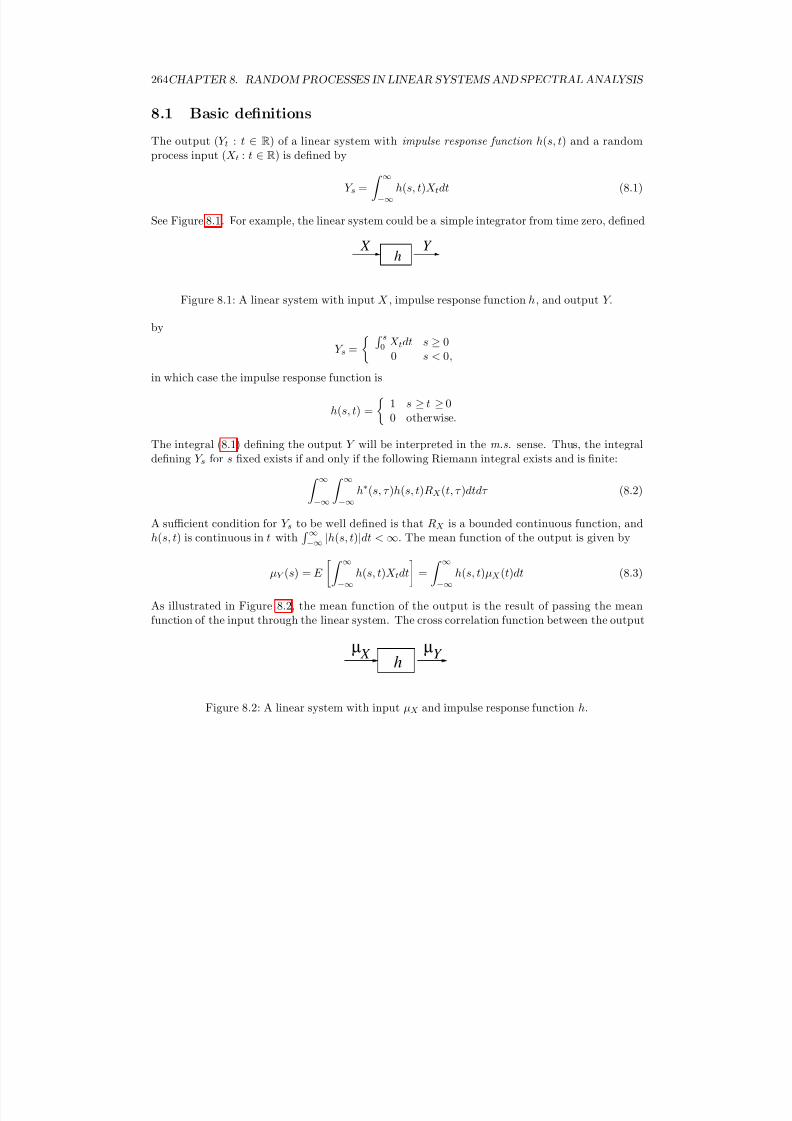
8/11/2019 Random process by B. Hajek
http://slidepdf.com/reader/full/random-process-by-b-hajek 274/448
264CHAPTER 8. RANDOM PROCESSES IN LINEAR SYSTEMS AND SPECTRAL ANALYSIS
8.1 Basic definitions
The output (Y t : t ∈ R) of a linear system with impulse response function h(s, t) and a random
process input (X t : t ∈ R) is defined by
Y s =
∞−∞
h(s, t)X tdt (8.1)
See Figure 8.1. For example, the linear system could be a simple integrator from time zero, defined
h X Y
Figure 8.1: A linear system with input X , impulse response function h, and output Y.
by
Y s =
s0 X tdt s ≥ 0
0 s < 0,
in which case the impulse response function is
h(s, t) =
1 s ≥ t ≥ 00 otherwise.
The integral (8.1) defining the output Y will be interpreted in the m.s. sense. Thus, the integraldefining Y s for s fixed exists if and only if the following Riemann integral exists and is finite:
∞−∞
∞−∞
h∗(s, τ )h(s, t)RX (t, τ )dtdτ (8.2)
A sufficient condition for Y s to be well defined is that RX is a bounded continuous function, andh(s, t) is continuous in t with
∞−∞ |h(s, t)|dt < ∞. The mean function of the output is given by
µY (s) = E
∞−∞
h(s, t)X tdt
=
∞−∞
h(s, t)µX (t)dt (8.3)
As illustrated in Figure 8.2, the mean function of the output is the result of passing the meanfunction of the input through the linear system. The cross correlation function between the output
h X
µ µY
Figure 8.2: A linear system with input µX and impulse response function h.
8/11/2019 Random process by B. Hajek
http://slidepdf.com/reader/full/random-process-by-b-hajek 275/448
8.1. BASIC DEFINITIONS 265
and input processes is given by
RY X (s, τ ) = E
∞
−∞
h(s, t)X tdtX ∗τ =
∞−∞
h(s, t)RX (t, τ )dt (8.4)
and the correlation function of the output is given by
RY (s, u) = E
Y s
∞−∞
h(u, τ )X τ dτ
∗=
∞−∞
h∗(u, τ )RY X (s, τ )dτ (8.5)
=
∞−∞
∞−∞
h∗(u, τ )h(s, t)RX (t, τ )dtdτ (8.6)
Recall that Y s is well defined as a m.s. integral if and only if the integral ( 8.2) is well defined andfinite. Comparing with (8.6), it means that Y s is well defined if and only if the right side of (8.6)with u = s is well defined and gives a finite value for E [|Y s|2].
The linear system is time invariant if h(s, t) depends on s, t only through s − t. If the system istime invariant we write h(s − t) instead of h(s, t), and with this substitution the defining relation(8.1) becomes a convolution: Y = h ∗ X .
A linear system is called bounded input bounded output (bibo) stable if the output is boundedwhenever the input is bounded. In case the system is time invariant, bibo stability is equivalent tothe condition ∞
−∞|h(τ )|dτ < ∞. (8.7)
In particular, if (8.7) holds and if an input signal x satisfies |xs| < L for all s, then the outputsignal y = x ∗ h satisfies
|y(t)| ≤ ∞−∞
|h(t − s)|Lds = L
∞−∞
|h(τ )|dτ
for all t. If X is a WSS random process then by the Schwarz inequality, RX is bounded by RX (0).Thus, if X is WSS and m.s. continuous, and if the linear system is time-invariant and bibo stable,the integral in (8.2) exists and is bounded by
RX (0)
∞−∞
∞−∞
|h(s − τ )||h(s − t)|dtdτ = RX (0)
∞−∞
|h(τ )|dτ
2
< ∞
Thus, the output of a linear, time-invariant bibo stable system is well defined in the m.s. sense if the input is a stationary, m.s. continuous process.
A paragraph about convolutions is in order. It is useful to be able to recognize convolutionintegrals in disguise. If f and g are functions on R, the convolution is the function f ∗g defined by
f ∗ g(t) =
∞−∞
f (s)g(t − s)ds
8/11/2019 Random process by B. Hajek
http://slidepdf.com/reader/full/random-process-by-b-hajek 276/448
266CHAPTER 8. RANDOM PROCESSES IN LINEAR SYSTEMS AND SPECTRAL ANALYSIS
or equivalently
f ∗ g(t) =
∞−∞
f (t − s)g(s)ds
or equivalently, for any real a and b
f ∗ g(a + b) =
∞−∞
f (a + s)g(b − s)ds.
A simple change of variable shows that the above three expressions are equivalent. However, inorder to immediately recognize a convolution, the salient feature is that the convolution is theintegral of the product of f and g, with the arguments of both f and g ranging over R in such away that the sum of the two arguments is held constant. The value of the constant is the value atwhich the convolution is being evaluated. Convolution is commutative: f ∗g = g ∗f and associative:(f ∗ g) ∗ k = f ∗ (g ∗ k) for three functions f ,g ,k. We simply write f ∗ g ∗ k for (f ∗ g) ∗ k. Theconvolution f
∗g
∗k is equal to a double integral of the product of f ,g, and k , with the arguments
of the three functions ranging over all triples in R3 with a constant sum. The value of the constantis the value at which the convolution is being evaluated. For example,
f ∗ g ∗ k(a + b + c) =
∞−∞
∞−∞
f (a + s + t)g(b − s)k(c − t)dsdt.
Suppose that X is WSS and that the linear system is time invariant. Then (8.3) becomes
µY (s) =
∞−∞
h(s − t)µX dt = µX
∞−∞
h(t)dt
Observe that µY (s) does not depend on s. Equation (8.4) becomes
RY X (s, τ ) = ∞−∞
h(s − t)RX (t − τ )dt
= h ∗ RX (s − τ ), (8.8)
which in particular means that RY X (s, τ ) is a function of s − τ alone. Equation (8.5) becomes
RY (s, u) =
∞−∞
h∗(u − τ )RY X (s − τ )dτ. (8.9)
The right side of (8.9) looks nearly like a convolution, but as τ varies the sum of the two argumentsis u − τ + s − τ , which is not constant as τ varies. To arrive at a true convolution, define the newfunction h by h(v) = h∗(
−v). Using the definition of h and (8.8) in (8.9) yields
RY (s, u) = ∞−∞
h(τ − u)(h ∗ RX )(s − τ )dτ
= h ∗ (h ∗ RX )(s − u) = h ∗ h ∗ RX (s − u)
which in particular means that RY (s, u) is a function of s − u alone.
8/11/2019 Random process by B. Hajek
http://slidepdf.com/reader/full/random-process-by-b-hajek 277/448
8.2. FOURIER TRANSFORMS, TRANSFER FUNCTIONS AND POWER SPECTRAL DENSITIES 267
To summarize, if X is WSS and if the linear system is time invariant, then X and Y are jointlyWSS with
µY = µX ∞
−∞h(t)dt RY X = h
∗RX RY = h
∗ h ∗RX . (8.10)
The convolution h ∗ h, equal to h ∗ h, can also be written as
h ∗ h(t) =
∞−∞
h(s)h(t − s)ds
=
∞−∞
h(s)h∗(s − t)ds (8.11)
The expression shows that h ∗ h(t) is the correlation between h and h∗ translated by t from theorigin.
The equations derived in this section for the correlation functions RX , RY X and RY also hold for
the covariance functions C X , C Y X , and C Y . The derivations are the same except that covariancesrather than correlations are computed. In particular, if X is WSS and the system is linear andtime invariant, then C Y X = h ∗ C X and C Y = h ∗ h ∗ C X .
8.2 Fourier transforms, transfer functions and power spectral den-sities
Fourier transforms convert convolutions into products, so this is a good point to begin using Fouriertransforms. The Fourier transform of a function g mapping R to the complex numbers C is formallydefined by
g(ω) = ∞
−∞e− jωtg(t)dt (8.12)
Some important properties of Fourier transforms are stated next.
Linearity: ag + bh = a g + b hInversion: g(t) =
∞−∞ e jωt g(ω)dω
2π
Convolution to multiplication: g ∗ h = g h and g ∗ h = 2π gh
Parseval’s identity: ∞−∞ g(t)h∗(t)dt =
∞−∞ g(ω) h∗(ω)dω
2π
Transform of time reversal: h = h∗, where h(t) = h∗(
−t)
Differentiation to multiplication by jω: dgdt (ω) = ( jω) g(ω)
Pure sinusoid to delta function: For ωo fixed: e jωot(ω) = 2πδ (ω − ωo)
Delta function to pure sinusoid: For to fixed: δ (t − to)(ω) = e− jωto
8/11/2019 Random process by B. Hajek
http://slidepdf.com/reader/full/random-process-by-b-hajek 278/448
268CHAPTER 8. RANDOM PROCESSES IN LINEAR SYSTEMS AND SPECTRAL ANALYSIS
The inversion formula above shows that a function g can be represented as an integral (basicallya limiting form of linear combination) of sinusoidal functions of time e jωt, and
g(ω) is the coefficient
in the representation for each ω. Paresval’s identity applied with g = h yields that the total
energy of g (the square of the L2
norm) can be computed in either the time or frequency domain:||g||2 = ∞−∞ |g(t)|2dt =
∞−∞ | g(ω)|2 dω
2π . The factor 2π in the formulas can be attributed to the use
of frequency ω in radians. If ω = 2πf , then f is the frequency in Hertz (Hz) and dω2π is simply df .
The Fourier transform can be defined for a very large class of functions, including generalizedfunctions such as delta functions. In these notes we won’t attempt a systematic treatment, but willuse Fourier transforms with impunity. In applications, one is often forced to determine in whatsenses the transform is well defined on a case-by-case basis. Two sufficient conditions for the Fouriertransform of g to be well defined are mentioned in the remainder of this paragraph. The relation(8.12) defining a Fourier transform of g is well defined if, for example, g is a continuous functionwhich is integrable:
∞−∞ |g(t)|dt < ∞, and in this case the dominated convergence theorem implies
that
g is a continuous function. The Fourier transform can also be naturally defined whenever g
has a finite L2
norm, through the use of Parseval’s identity. The idea is that if g has finite L2
norm,then it is the limit in the L2 norm of a sequence of functions gn which are integrable. Owing toParseval’s identity, the Fourier transforms gn form a Cauchy sequence in the L2 norm, and hencehave a limit, which is defined to be g.
Return now to consideration of a linear time-invariant system with an impulse response functionh = (h(τ ) : τ ∈ R). The Fourier transform of h is used so often that a special name and notationis used: it is called the transfer function and is denoted by H (ω).
The output signal y = (yt : t ∈ R) for an input signal x = (xt : t ∈ R) is given in the timedomain by the convolution y = x ∗ h. In the frequency domain this becomes y(ω) = H (ω) x(ω).For example, given a < b let H [a,b](ω) be the ideal bandpass transfer function for frequency band[a, b], defined by
H [a,b](ω) = 1 a ≤ ω ≤ b0 otherwise. (8.13)
If x is the input and y is the output of a linear system with transfer function H [a,b], then therelation y(ω) = H [a,b](ω) x(ω) shows that the frequency components of x in the frequency band[a, b] pass through the filter unchanged, and the frequency components of x outside of the band arecompletely nulled. The total energy of the output function y can therefore be interpreted as theenergy of x in the frequency band [a, b]. Therefore,
Energy of x in frequency interval [a, b] = ||y||2 =
∞−∞
|H [a,b](ω)|2| x(ω)|2 dω
2π =
ba
| x(ω)|2 dω
2π.
Consequently, it is appropriate to call | x(ω)|2
the energy spectral density of the deterministic signalx.
Given a WSS random process X = (X t : t ∈R), the Fourier transform of its correlation functionRX is denoted by S X . For reasons that we will soon see, the function S X is called the power spectral density of X . Similarly, if Y and X are jointly WSS, then the Fourier transform of RY X is denotedby S Y X , called the cross power spectral density function of Y and X . The Fourier transform of
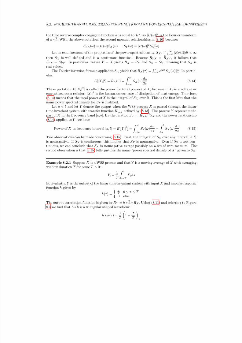
8/11/2019 Random process by B. Hajek
http://slidepdf.com/reader/full/random-process-by-b-hajek 279/448
8.2. FOURIER TRANSFORMS, TRANSFER FUNCTIONS AND POWER SPECTRAL DENSITIES 269
the time reverse complex conjugate function h is equal to H ∗, so |H (ω)|2 is the Fourier transformof h ∗
h. With the above notation, the second moment relationships in ( 8.10) become:
S Y X (ω) = H (ω)S X (ω) S Y (ω) =
|H (ω)
|2S X (ω)
Let us examine some of the properties of the power spectral density, S X . If ∞−∞ |RX (t)|dt < ∞
then S X is well defined and is a continuous function. Because RY X = RXY , it follows thatS Y X = S ∗XY . In particular, taking Y = X yields RX = RX and S X = S ∗X , meaning that S X isreal-valued.
The Fourier inversion formula applied to S X yields that RX (τ ) = ∞−∞ e jωτ S X (ω)dω
2π . In partic-ular,
E [|X t|2] = RX (0) =
∞−∞
S X (ω)dω
2π. (8.14)
The expectation E [|X t|2] is called the power (or total power) of X , because if X t is a voltage orcurrent accross a resistor, |X t|2 is the instantaneous rate of dissipation of heat energy. Therefore,
(8.14) means that the total power of X is the integral of S X over R. This is the first hint that thename power spectral density for S X is justified.
Let a < b and let Y denote the output when the WSS process X is passed through the lineartime-invariant system with transfer function H [a,b] defined by (8.13). The process Y represents thepart of X in the frequency band [a, b]. By the relation S Y = |H [a,b]|2S X and the power relationship(8.14) applied to Y , we have
Power of X in frequency interval [a, b] = E [|Y t|2] =
∞−∞
S Y (ω)dω
2π =
ba
S X (ω)dω
2π (8.15)
Two observations can be made concerning (8.15). First, the integral of S X over any interval [a, b]is nonnegative. If S X is continuous, this implies that S X is nonnegative. Even if S X is not con-
tinuous, we can conclude that S X is nonnegative except possibly on a set of zero measure. Thesecond observation is that (8.15) fully justifies the name “power spectral density of X ” given to S X .
Example 8.2.1 Suppose X is a WSS process and that Y is a moving average of X with averagingwindow duration T for some T > 0:
Y t = 1
T
tt−T
X sds
Equivalently, Y is the output of the linear time-invariant system with input X and impulse responsefunction h given by
h(τ ) = 1T 0 ≤ τ ≤ T
0 else
The output correlation function is given by RY = h ∗ h ∗ RX . Using (8.11) and referring to Figure8.3 we find that h ∗ h is a triangular shaped waveform:
h ∗ h(τ ) = 1
T
1 − |τ |
T
+
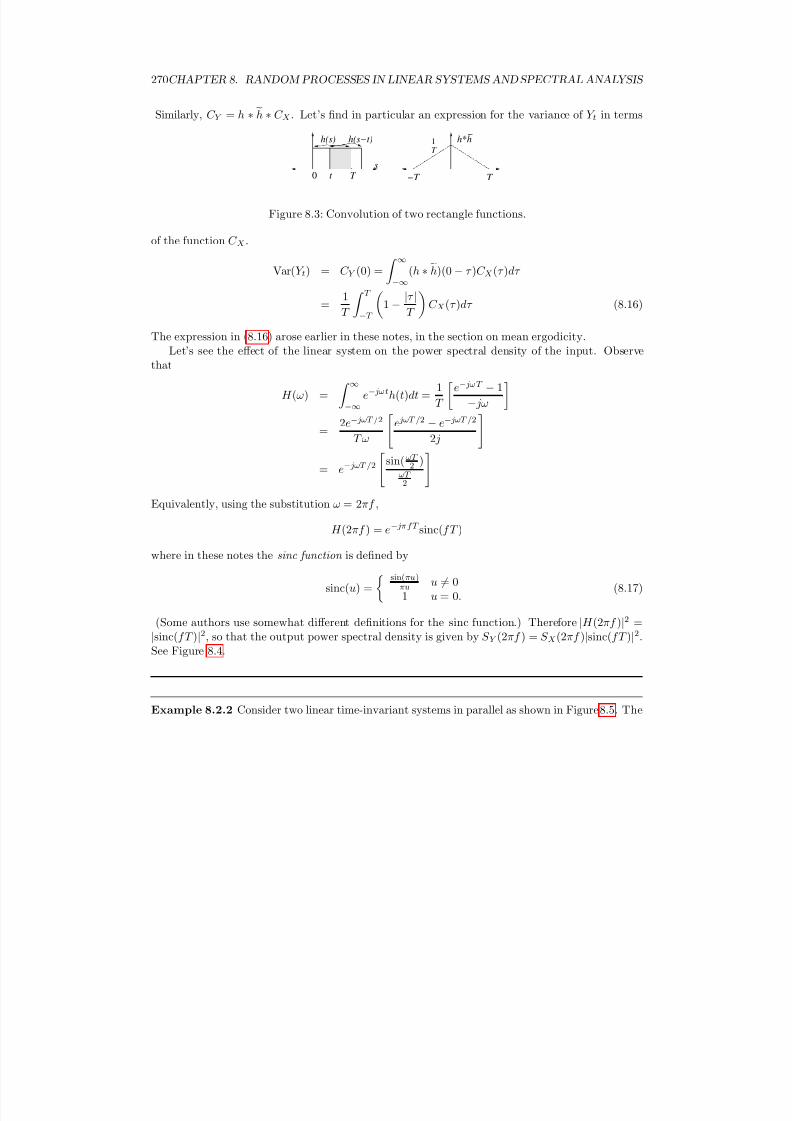
8/11/2019 Random process by B. Hajek
http://slidepdf.com/reader/full/random-process-by-b-hajek 280/448
270CHAPTER 8. RANDOM PROCESSES IN LINEAR SYSTEMS AND SPECTRAL ANALYSIS
Similarly, C Y = h ∗ h ∗ C X . Let’s find in particular an expression for the variance of Y t in terms
T s
h(s−t)h(s) h*h~
1
T
0 t T −T
Figure 8.3: Convolution of two rectangle functions.
of the function C X .
Var(Y t) = C Y (0) =
∞−∞
(h ∗ h)(0 − τ )C X (τ )dτ
= 1
T T
−T
1 − |τ |T
C X (τ )dτ (8.16)
The expression in (8.16) arose earlier in these notes, in the section on mean ergodicity.Let’s see the effect of the linear system on the power spectral density of the input. Observe
that
H (ω) =
∞−∞
e− jωth(t)dt = 1
T
e− jωT − 1
− jω
=
2e− jωT /2
T ω
e jωT /2 − e− jωT /2
2 j
= e− jωT /2
sin(ωT
2 )ωT
2 Equivalently, using the substitution ω = 2πf ,
H (2πf ) = e− jπfT sinc(f T )
where in these notes the sinc function is defined by
sinc(u) =
sin(πu)
πu u = 01 u = 0.
(8.17)
(Some authors use somewhat different definitions for the sinc function.) Therefore |H (2πf )|2 =
|sinc(f T )|2
, so that the output power spectral density is given by S Y (2πf ) = S X (2πf )|sinc(f T )|2
.See Figure 8.4.
Example 8.2.2 Consider two linear time-invariant systems in parallel as shown in Figure 8.5. The
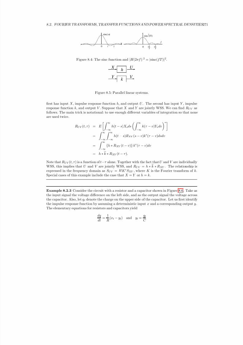
8/11/2019 Random process by B. Hajek
http://slidepdf.com/reader/full/random-process-by-b-hajek 281/448
8.2. FOURIER TRANSFORMS, TRANSFER FUNCTIONS AND POWER SPECTRAL DENSITIES 271
2
u1
T
2
T
f
1 20 0
usinc( )sinc (fT)
Figure 8.4: The sinc function and |H (2πf )|2 = |sinc(f T )|2.
h
Y
X U
V k
Figure 8.5: Parallel linear systems.
first has input X , impulse response function h, and output U . The second has input Y , impulseresponse function k, and output V . Suppose that X and Y are jointly WSS. We can find RUV asfollows. The main trick is notational: to use enough different variables of integration so that noneare used twice.
RUV (t, τ ) = E
∞−∞
h(t − s)X sds
∞−∞
k(τ − v)Y vdv
∗=
∞−∞
∞−∞
h(t − s)RXY (s − v)k∗(τ − v)dsdv
= ∞
−∞ h
∗RXY (t
−v)
k∗(τ
−v)dv
= h ∗ k ∗ RXY (t − τ ).
Note that RUV (t, τ ) is a function of t−τ alone. Together with the fact that U and V are individuallyWSS, this implies that U and V are jointly WSS, and RUV = h ∗ k ∗ RXY . The relationship isexpressed in the frequency domain as S UV = HK ∗S XY , where K is the Fourier transform of k.Special cases of this example include the case that X = Y or h = k.
Example 8.2.3 Consider the circuit with a resistor and a capacitor shown in Figure 8.6. Take asthe input signal the voltage difference on the left side, and as the output signal the voltage acrossthe capacitor. Also, let q t denote the charge on the upper side of the capacitor. Let us first identifythe impulse response function by assuming a deterministic input x and a corresponding output y .The elementary equations for resistors and capacitors yield
dq
dt =
1
R(xt − yt) and yt =
q tC
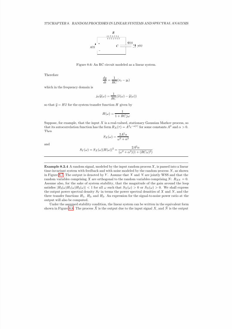
8/11/2019 Random process by B. Hajek
http://slidepdf.com/reader/full/random-process-by-b-hajek 282/448
272CHAPTER 8. RANDOM PROCESSES IN LINEAR SYSTEMS AND SPECTRAL ANALYSIS
R
C
q
x(t)
(t)
−
+
y(t)−
+
Figure 8.6: An RC circuit modeled as a linear system.
Thereforedy
dt =
1
RC (xt − yt)
which in the frequency domain is
jω y(ω) = 1RC
( x(ω) − y(ω))
so that y = H x for the system transfer function H given by
H (ω) = 1
1 + RCjω
Suppose, for example, that the input X is a real-valued, stationary Gaussian Markov process, sothat its autocorrelation function has the form RX (τ ) = A2e−α|τ | for some constants A2 and α > 0.Then
S X (ω) = 2A2α
ω2 + α2
and
S Y (ω) = S X (ω)|H (ω)|2 = 2A2α
(ω2 + α2)(1 + (RCω)2)
Example 8.2.4 A random signal, modeled by the input random process X , is passed into a lineartime-invariant system with feedback and with noise modeled by the random process N , as shownin Figure 8.7. The output is denoted by Y . Assume that X and N are jointly WSS and that therandom variables comprising X are orthogonal to the random variables comprising N : RXN = 0.Assume also, for the sake of system stability, that the magnitude of the gain around the loop
satisfies |H 3(ω)H 1(ω)H 2(ω)| < 1 for all ω such that S X (ω) > 0 or S N (ω) > 0. We shall expressthe output power spectral density S Y in terms the power spectral densities of X and N , and thethree transfer functions H 1, H 2, and H 3. An expression for the signal-to-noise power ratio at theoutput will also be computed.
Under the assumed stability condition, the linear system can be written in the equivalent formshown in Figure 8.8. The process X is the output due to the input signal X , and N is the output
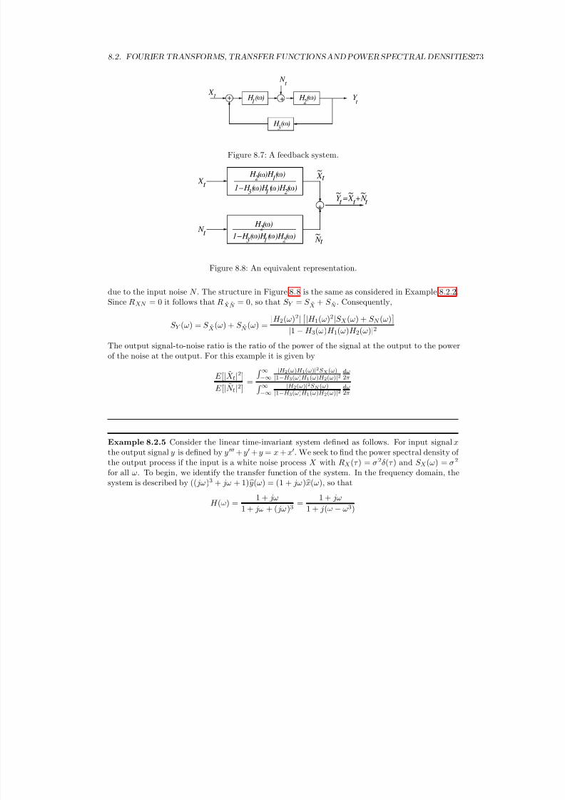
8/11/2019 Random process by B. Hajek
http://slidepdf.com/reader/full/random-process-by-b-hajek 283/448
8.2. FOURIER TRANSFORMS, TRANSFER FUNCTIONS AND POWER SPECTRAL DENSITIES 273
+ H ( ) H ( )
H ( )
1 2
3
!
!
!
X +
N
Y t
t
t
Figure 8.7: A feedback system.
!
!! " $ %" $ %" $ %
" $ %
!! " $ %" $ %" $ %
" $ %" $ %
! !& ! '
'
& ! '
(
)
*
+
+
, ( +
+ * ,
, , ,- .( )* + + +
! !
!
! !!
!
'
Figure 8.8: An equivalent representation.
due to the input noise N . The structure in Figure 8.8 is the same as considered in Example 8.2.2.Since RXN = 0 it follows that RX N = 0, so that S Y = S X + S N . Consequently,
S Y (ω) = S X (ω) + S N (ω) = |H 2(ω)2| |H 1(ω)2|S X (ω) + S N (ω)
|1 − H 3(ω)H 1(ω)H 2(ω)|2
The output signal-to-noise ratio is the ratio of the power of the signal at the output to the powerof the noise at the output. For this example it is given by
E [| X t|2]
E [| N t|2]=
∞−∞
|H 2(ω)H 1(ω)|2S X(ω)|1−H 3(ω)H 1(ω)H 2(ω)|2
dω2π ∞
−∞|H 2(ω)|2S N (ω)
|1−H 3(ω)H 1(ω)H 2(ω)|2dω2π
Example 8.2.5 Consider the linear time-invariant system defined as follows. For input signal xthe output signal y is defined by y + y + y = x + x. We seek to find the power spectral density of the output process if the input is a white noise process X with RX (τ ) = σ 2δ (τ ) and S X (ω) = σ 2
for all ω. To begin, we identify the transfer function of the system. In the frequency domain, thesystem is described by (( jω)3 + jω + 1) y(ω) = (1 + jω) x(ω), so that
H (ω) = 1 + jω
1 + jω + ( jω)3 =
1 + jω
1 + j(ω − ω3)
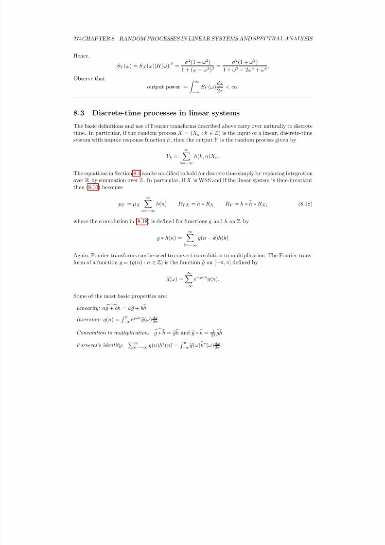
8/11/2019 Random process by B. Hajek
http://slidepdf.com/reader/full/random-process-by-b-hajek 284/448
274CHAPTER 8. RANDOM PROCESSES IN LINEAR SYSTEMS AND SPECTRAL ANALYSIS
Hence,
S Y (ω) = S X (ω)|H (ω)|2 = σ2(1 + ω2)
1 + (ω − ω3)2 =
σ2(1 + ω2)
1 + ω2 − 2ω4 + ω6.
Observe thatoutput power =
∞−∞
S Y (ω)dω
2π < ∞.
8.3 Discrete-time processes in linear systems
The basic definitions and use of Fourier transforms described above carry over naturally to discretetime. In particular, if the random process X = (X k : k ∈ Z) is the input of a linear, discrete-timesystem with impule response function h, then the output Y is the random process given by
Y k =
∞n=−∞
h(k, n)X n.
The equations in Section 8.1 can be modified to hold for discrete time simply by replacing integrationover R by summation over Z. In particular, if X is WSS and if the linear system is time-invariantthen (8.10) becomes
µY = µX
∞n=−∞
h(n) RY X = h ∗ RX RY = h ∗ h ∗ RX , (8.18)
where the convolution in (8.18) is defined for functions g and h on Z by
g ∗ h(n) = ∞k=−∞
g(n − k)h(k)
Again, Fourier transforms can be used to convert convolution to multiplication. The Fourier trans-form of a function g = (g(n) : n ∈ Z) is the function g on [−π, π] defined by
g(ω) =
∞−∞
e− jωng(n).
Some of the most basic properties are:
Linearity: ag + bh = a g + b hInversion: g(n) =
π−π e jωn g(ω)dω
2π
Convolution to multiplication: g ∗ h = g h and g ∗ h = 12π gh
Parseval’s identity: ∞
n=−∞ g(n)h∗(n) = π−π g(ω) h∗(ω)dω
2π
8/11/2019 Random process by B. Hajek
http://slidepdf.com/reader/full/random-process-by-b-hajek 285/448
8.3. DISCRETE-TIME PROCESSES IN LINEAR SYSTEMS 275
Transform of time reversal: h = h∗, where h(t) = h(−t)∗
Pure sinusoid to delta function: For ωo ∈ [−π, π] fixed: e jωon(ω) = 2πδ (ω − ωo)
Delta function to pure sinusoid: For no fixed: I n=no(ω) = e− jωno
The inversion formula above shows that a function g on Z can be represented as an integral(basically a limiting form of linear combination) of sinusoidal functions of time e jωn, and g(ω) isthe coefficient in the representation for each ω. Paresval’s identity applied with g = h yields thatthe total energy of g (the square of the L2 norm) can be computed in either the time or frequencydomain: ||g||2 =
∞n=−∞ |g(n)|2 =
π−π | g(ω)|2 dω
2π .The Fourier transform and its inversion formula for discrete-time functions are equivalent to
the Fourier series representation of functions in L2[−π, π] using the complete orthogonal basis(e jωn : n ∈ Z) for L2[−π, π], as discussed in connection with the Karhunen-Loeve expansion. Thefunctions in this basis all have norm 2π. Recall that when we considered the Karhunen-Loeve
expansion for a periodic WSS random process of period T , functions on a time interval wereimportant and the power was distributed on the integers Z scaled by 1
T . In this section, Z isconsidered to be the time domain and the power is distributed over an interval. That is, the roleof Z and a finite interval are interchanged. The transforms used are essentially the same, but with j replaced by − j.
Given a linear time-invariant system in discrete time with an impulse response function h =(h(τ ) : τ ∈ Z), the Fourier transform of h is denoted by H (ω). The defining relation for thesystem in the time domain, y = h ∗ x, becomes y(ω) = H (ω) x(ω) in the frequency domain. For−π ≤ a < b ≤ π,
Energy of x in frequency interval [a, b] =
ba
|
x(ω)|2 dω
2π.
so it is appropriate to call | x(ω)|2 the energy spectral density of the deterministic, discrete-timesignal x.
Given a WSS random process X = (X n : n ∈ Z), the Fourier transform of its correlationfunction RX is denoted by S X , and is called the power spectral density of X . Similarly, if Y andX are jointly WSS, then the Fourier transform of RY X is denoted by S Y X , called the cross powerspectral density function of Y and X . With the above notation, the second moment relationshipsin (8.18) become:
S Y X (ω) = H (ω)S X (ω) S Y (ω) = |H (ω)|2S X (ω)
The Fourier inversion formula applied to S X yields that RX (n) = π−π e jωnS X (ω)dω
2π . In partic-ular,
E [|X n|2
] = RX (0) = π
−π S X (ω)
dω
2π .
The expectation E [|X n|2] is called the power (or total power) of X , and for −π < a < b ≤ π wehave
Power of X in frequency interval [a, b] =
ba
S X (ω)dω
2π
8/11/2019 Random process by B. Hajek
http://slidepdf.com/reader/full/random-process-by-b-hajek 286/448
276CHAPTER 8. RANDOM PROCESSES IN LINEAR SYSTEMS AND SPECTRAL ANALYSIS
8.4 Baseband random processes
Deterministic baseband signals are considered first. Let x be a continuous-time signal (i.e. a
function on R
) such that its energy, ∞−∞ |x(t)|2
dt, is finite. By the Fourier inversion formula, thesignal x is an integral, which is essentially a sum, of sinusoidal functions of time, e jωt. The weightsare given by the Fourier transform x(w). Let f o > 0 and let ωo = 2πf o. The signal x is called abaseband signal, with one-sided band limit f o Hz, or equivalently ωo radians/second, if x(ω) = 0for |ω| ≥ ωo. For such a signal, the Fourier inversion formula becomes
x(t) =
ωo
−ωo
e jωt x(ω)dω
2π (8.19)
Equation (8.19) displays the baseband signal x as a linear combination of the functions e jωt indexedby ω ∈ [−ωo, ωo].
A celebrated theorem of Nyquist states that the baseband signal x is completely determined by
its samples taken at sampling frequency 2f o. Specifically, define T by
1
T = 2f o. Then
x(t) =∞
n=−∞x(nT ) sinc
t − nT
T
. (8.20)
where the sinc function is defined by (8.17). Nyquist’s equation (8.20) is indeed elegant. It obviouslyholds by inspection if t = mT for some integer m, because for t = mT the only nonzero term inthe sum is the one indexed by n = m. The equation shows that the sinc function gives the correctinterpolation of the narrowband signal x for times in between the integer multiples of T . We shallgive a proof of (8.20) for deterministic signals, before considering its extension to random processes.
A proof of (8.20) goes as follows. Henceforth we will use ωo more often than f o, so it is worthremembering that ωoT = π. Taking t = nT in (8.19) yields
x(nT ) = ωo
−ωo
e jωnT x(ω)dω
2π
=
ωo
−ωo
x(ω)(e− jωnT )∗dω
2π (8.21)
Equation (8.21) shows that x(nT ) is given by an inner product of x and e− jωnT . The functionse− jωnT , considered on the interval −ωo < ω < ωo and indexed by n ∈ Z, form a complete orthogonalbasis for L2[−ωo, ωo], and
ωo
−ωoT |e− jωnT |2 dω
2π = 1. Therefore, x over the interval [−ωo, ωo] has thefollowing Fourier series representation:
x(ω) = T ∞
n=−∞e− jωnT x(nT ) ω
∈ [−
ωo
, ωo
] (8.22)
Plugging (8.22) into (8.19) yields
x(t) =∞
n=−∞x(nT )T
ωo
−ωo
e jωte− jωnT dω
2π. (8.23)
8/11/2019 Random process by B. Hajek
http://slidepdf.com/reader/full/random-process-by-b-hajek 287/448
8.4. BASEBAND RANDOM PROCESSES 277
The integral in (8.23) can be simplified using
T ωo
−ωo
e jωτ dω
2π = sinc
τ
T . (8.24)
with τ = t − nT to yield (8.20) as desired.The sampling theorem extends naturally to WSS random processes. A WSS random process
X with spectral density S X is said to be a baseband random process with one-sided band limit ωo
if S X (ω) = 0 for | ω |≥ ωo.
Proposition 8.4.1 Suppose X is a WSS baseband random process with one-sided band limit ωo
and let T = π/ωo. Then for each t ∈ R
X t =
∞n=−∞
X nT sinc
t − nT
T
m.s. (8.25)
If B is the process of samples defined by Bn = X nT , then the power spectral densities of B and X are related by
S B(ω) = 1
T S X
ω
T
for | ω |≤ π (8.26)
Proof. Fix t ∈ R. It must be shown that N defined by the following expectation converges tozero as N → ∞:
εN = E
X t −
N n=−N
X nT sinc
t − nT
t
2
When the square is expanded, terms of the form E [X aX ∗b ] arise, where a and b take on the valuest or nT for some n. But
E [X aX ∗b ] = RX (a − b) =
∞−∞
e jωa(e jωb)∗S X (ω)dω
2π.
Therefore, εN can be expressed as an integration over ω rather than as an expectation:
εN =
∞−∞
e jωt −N
n=−N
e jωnT sinc
t − nT
T
2
S X (ω)dω
2π. (8.27)
For t fixed, the function (e jωt :
−ωo < ω < ωo) has a Fourier series representation (use (8.24))
e jωt = T
∞−∞
e jωnT ωo
−ωo
e jωte− jωnT dω
2π
=∞−∞
e jωnT sinc
t − nT
T
.
8/11/2019 Random process by B. Hajek
http://slidepdf.com/reader/full/random-process-by-b-hajek 288/448
278CHAPTER 8. RANDOM PROCESSES IN LINEAR SYSTEMS AND SPECTRAL ANALYSIS
so that the quantity inside the absolute value signs in (8.27) is the approximation error for theN th partial Fourier series sum for e jωt . Since e jωt is continuous in ω, a basic result in the theoryof Fourier series yields that the Fourier approximation error is bounded by a single constant for
all N and ω, and as N → ∞ the Fourier approximation error converges to 0 uniformly on sets of the form | ω |≤ ωo − ε. Thus εN → 0 as N → ∞ by the dominated convergence theorem. Therepresentation (8.25) is proved.
Clearly B is a WSS discrete time random process with µB = µX and
RB(n) = RX (nT ) =
∞−∞
e jnT ωS X (ω)dω
2π
=
ωo
−ωo
e jnT ωS X (ω)dω
2π,
so, using a change of variable ν = T ω and the fact T = πωo
yields
RB(n) =
π−π
e jnν 1
T S X
ν
T
dν
2π. (8.28)
But S B(ω) is the unique function on [−π, π] such that
RB(n) =
π−π
e jnωS B(ω)dω
2π
so (8.26) holds. The proof of Proposition 8.4.1 is complete.
As a check on (8.26), we note that B(0) = X (0), so the processes have the same total power.Thus, it must be that π
−πS B(ω)
dω
2π =
∞−∞
S X (ω)dω
2π, (8.29)
which is indeed consistent with (8.26).
Example 8.4.2 If µX = 0 and the spectral density S X of X is constant over the interval [−ωo, ωo],then µB = 0 and S B(ω) is constant over the interval [−π, π]. Therefore RB(n) = C B(n) = 0 for
n = 0, and the samples (B(n)) are mean zero, uncorrelated random variables.
Theoretical Exercise What does (8.26) become if X is W SS and has a power spectral density,but X is not a baseband signal?
8/11/2019 Random process by B. Hajek
http://slidepdf.com/reader/full/random-process-by-b-hajek 289/448
8.5. NARROWBAND RANDOM PROCESSES 279
8.5 Narrowband random processes
As noted in the previous section, a signal – modeled as either a deterministic finite energy signal
or a WSS random process – can be reconstructed from samples taken at a sampling rate twice thehighest frequency of the signal. For example, a typical voice signal may have highest frequency 5KHz. If such a signal is multiplied by a signal with frequency 109 Hz, the highest frequency of theresulting product is about 200,000 times larger than that of the original signal. Naıve applicationof the sampling theorem would mean that the sampling rate would have to increase by the samefactor. Fortunately, because the energy or power of such a modulated signal is concentrated in anarrow band, the signal is nearly as simple as the original baseband signal. The motivation of thissection is to see how signals and random processes with narrow spectral ranges can be analyzed interms of equivalent baseband signals. For example, the effects of filtering can be analyzed usingbaseband equivalent filters. As an application, an example at the end of the section is given whichdescribes how a narrowband random process (to be defined) can be simulated using a sampling rateequal to twice the one-sided width of a frequency band of a signal, rather than twice the highest
frequency of the signal.Deterministic narrowband signals are considered first, and the development for random pro-
cesses follows a similar approach. Let ωc > ωo > 0. A narrowband signal (relative to ωo andωc) is a signal x such that x(ω) = 0 unless ω is in the union of two intervals: the upper band,(ωc − ωo, ωc + ωo), and the lower band, (−ωc − ωo, −ωc + ωo). More compactly, x(ω) = 0 if || ω | −ωc| ≥ ωo.
A narrowband signal arises when a sinusoidal signal is modulated by a narrowband signal, asshown next. Let u and v be real-valued baseband signals, each with one-sided bandwidth less thanωo, as defined at the beginning of the previous section. Define a signal x by
x(t) = u(t)cos(ωct) − v(t)sin(ωct). (8.30)
Since cos(ωct) = (e jωct + e− jωct)/2 and − sin(ωct) = ( je jωct − je− jωct)/2, (8.30) becomes
x(ω) = 1
2 u(ω − ωc) + u(ω + ωc) + j v(ω − ωc) − j v(ω + ωc) (8.31)
Graphically, x is obtained by sliding 12 u to the right by ωc, 1
2 u to the left by ωc, j2 v to the right by
ωc, and − j2 v to the left by ωc, and then adding. Of course x is real-valued by its definition. The
reader is encouraged to verify from (8.31) that x(ω) = x∗(−ω). Equation (8.31) shows that indeedx is a narrowband signal.
A convenient alternative expression for x is obtained by defining a complex valued basebandsignal z by z(t) = u(t) + jv(t). Then x(t) = Re(z(t)e jωct). It is a good idea to keep in mind the
case that ωc is much larger than ωo (written ωc ωo). Then z varies slowly compared to thecomplex sinusoid e jωct. In a small neighborhood of a fixed time t, x is approximately a sinusoidwith frequency ωc, peak amplitude |z(t)|, and phase given by the argument of z (t). The signal z iscalled the complex envelope of x and |z(t)| is called the real envelope of x.
So far we have shown that a real-valued narrowband signal x results from modulating sinusoidalfunctions by a pair of real-valued baseband signals, or equivalently, modulating a complex sinusoidal
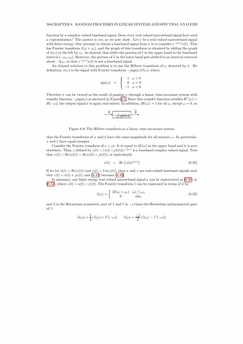
8/11/2019 Random process by B. Hajek
http://slidepdf.com/reader/full/random-process-by-b-hajek 290/448
280CHAPTER 8. RANDOM PROCESSES IN LINEAR SYSTEMS AND SPECTRAL ANALYSIS
function by a complex-valued baseband signal. Does every real-valued narrowband signal have sucha representation? The answer is yes, as we now show. Let x be a real-valued narrowband signalwith finite energy. One attempt to obtain a baseband signal from x is to consider e− jωctx(t). This
has Fourier transform x(ω + ωc), and the graph of this transform is obtained by sliding the graphof x(ω) to the left by ωc. As desired, that shifts the portion of x in the upper band to the basebandinterval (−ωo, ωo). However, the portion of x in the lower band gets shifted to an interval centeredabout −2ωc, so that e− jωctx(t) is not a baseband signal.
An elegant solution to this problem is to use the Hilbert transform of x, denoted by x. Bydefinition, x(ω) is the signal with Fourier transform − jsgn(ω) x(ω), where
sgn(ω) =
1 ω > 00 ω = 0
−1 ω < 0
Therefore x can be viewed as the result of passing x through a linear, time-invariant system with
transfer function − jsgn(ω) as pictured in Figure 8.9. Since this transfer function satisfies H ∗(ω) =H (−ω), the output signal x is again real-valued. In addition, |H (ω)| = 1 for all ω, except ω = 0, so
− j sgn( )ω x x
Figure 8.9: The Hilbert transform as a linear, time-invariant system.
that the Fourier transforms of x and x have the same magnitude for all nonzero ω. In particular,x and x have equal energies.
Consider the Fourier transform of x + jx. It is equal to 2 x(ω) in the upper band and it is zeroelsewhere. Thus, z defined by z(t) = (x(t) + jx(t))e− jωct is a baseband complex valued signal. Notethat x(t) = Re(x(t)) = Re(x(t) + jx(t)), or equivalently
x(t) = Re
z(t)e jωct
(8.32)
If we let u(t) = Re(z(t)) and v(t) = I m(z(t)), then u and v are real-valued baseband signals suchthat z (t) = u(t) + jv(t), and (8.32) becomes (8.30).
In summary, any finite energy real-valued narrowband signal x can be represented as (8.30) or(8.32), where z (t) = u(t) + jv(t). The Fourier transform z can be expressed in terms of x by
z(ω) = 2
x(ω + ωc) |ω| ≤ ωo
0 else, (8.33)
and u is the Hermetian symmetric part of z and v is − j times the Hermetian antisymmetric partof z:
u(ω) = 1
2 ( z(ω) + z∗(−ω)) v(ω) =
− j
2 ( z(ω) − z∗(−ω))
8/11/2019 Random process by B. Hajek
http://slidepdf.com/reader/full/random-process-by-b-hajek 291/448
8.5. NARROWBAND RANDOM PROCESSES 281
In the other direction, x can be expressed in terms of u and v by (8.31).
If x1 and x2 are each narrowband signals with corresponding complex envelope processes z1 andz2, then the convolution x = x1 ∗ x2 is again a narrowband signal, and the corresponding complex
envelope is 1
2 z1 ∗ z2. To see this, note that the Fourier transform, z, of the complex envelope z forx is given by (8.33). Similar equations hold for zi in terms of xi for i = 1, 2. Using these equationsand the fact x(ω) = x1(ω) x2(ω), it is readily seen that z(ω) = 1
2 z1(ω) z2(ω) for all ω, establishingthe claim. Thus, the analysis of linear, time invariant filtering of narrowband signals can be carriedout in the baseband equivalent setting.
A similar development is considered next for WSS random processes. Let U and V be jointlyWSS real-valued baseband random processes, and let X be defined by
X t = U t cos(ωct) − V t sin(ωct) (8.34)
or equivalently, defining Z t by Z t = U t + jV t,
X t = Re Z te jωct (8.35)
In some sort of generalized sense, we expect that X is a narrowband process. However, suchan X need not even be WSS. Let us find the conditions on U and V that make X WSS. First, inorder that µX (t) not depend on t, it must be that µU = µV = 0.
Using the notation ct = cos(ωct), st = sin(ωct), and τ = a − b,
RX (a, b) = RU (τ )cacb − RUV (τ )casb − RV U (τ )sacb + RV (τ )sasb.
Using the trigonometric identities such as cacb = (ca−b + ca+b)/2, this can be rewritten as
RX (a, b) = RU (τ ) + RV (τ )
2 ca−b + RUV (τ )
−RV U (τ )
2 sa−b
+
RU (τ ) − RV (τ )
2
ca+b −
RUV (τ ) + RV U (τ )
2
sa+b.
Therefore, in order that RX (a, b) is a function of a−b, it must be that RU = RV and RUV = −RV U .Since in general RUV (τ ) = RV U (−τ ), the condition RUV = −RV U means that RUV is an oddfunction: RUV (τ ) = −RUV (−τ ).
We summarize the results as a proposition.
Proposition 8.5.1 Suppose X is given by ( 8.34) or ( 8.35 ), where U and V are jointly WSS. Then X is WSS if and only if U and V are mean zero with RU = RV and RUV =
−RV U . Equivalently,
X is WSS if and only if Z = U + jV is mean zero and E [Z aZ b] = 0 for all a, b. If X is WSS then
RX (τ ) = RU (τ )cos(ωcτ ) + RUV (τ )sin(ωcτ )
S X (ω) = 1
2[S U (ω − ωc) + S U (ω + ωc) − jS UV (ω − ωc) + jS UV (ω + ωc)]
8/11/2019 Random process by B. Hajek
http://slidepdf.com/reader/full/random-process-by-b-hajek 292/448
282CHAPTER 8. RANDOM PROCESSES IN LINEAR SYSTEMS AND SPECTRAL ANALYSIS
and, with RZ (τ ) defined by RZ (a − b) = E [Z aZ ∗b ],
RX (τ ) = 1
2Re(RZ (τ )e jωcτ )
The functions S X , S U , and S V are nonnegative, even functions, and S UV is a purely imaginary odd function (i.e. S UV (ω) = I m(S UV (ω)) = −S UV (−ω).)
Let X by any WSS real-valued random process with a spectral density S X , and continue tolet ωc > ωo > 0. Then X is defined to be a narrowband random process if S X (ω) = 0 whenever| |ω| − ωc |≥ ωo. Equivalently, X is a narrowband random process if RX (t) is a narrowbandfunction. We’ve seen how such a process can be obtained by modulating a pair of jointly WSSbaseband random processes U and V . We show next that all narrowband random processes havesuch a representation.
To proceed as in the case of deterministic signals, we first wish to define the Hilbert transformof X , denoted by X . A slight concern about defining X is that the function
− jsgn(ω) does not
have finite energy. However, we can replace this function by the function given by
H (ω) = − jsgn(ω)I |ω|≤ωo+ωc,
which has finite energy and it has a real-valued inverse transform h. Define X as the output whenX is passed through the linear system with impulse response h. Since X and h are real valued, therandom process X is also real valued. As in the deterministic case, define random processes Z , U ,and V by Z t = (X t + j X t)e− jωct, U t = Re(Z t), and V t = I m(Z t).
Proposition 8.5.2 Let X be a narrowband WSS random process, with spectral density S X satis- fying S X (ω) = 0 unless ωc − ωo ≤ |ω| ≤ ωc + ωo, where ωo < ωc. Then µX = 0 and the following representations hold
X t = Re(Z te jωct) = U t cos(ωct) − V t sin(ωct)
where Z t = U t + jV t, and U and V are jointly WSS real-valued random processes with mean zeroand
S U (ω) = S V (ω) = [S X (ω − ωc) + S X (ω + ωc)] I |ω|≤ωo (8.36)
and S UV (ω) = j [S X (ω + ωc) − S X (ω − ωc)] I |ω|≤ωo
(8.37)
Equivalently,
RU (τ ) = RV (τ ) = RX (τ ) cos(ωcτ ) + RX (τ )sin(ωcτ ) (8.38)
and
RUV (τ ) = RX (τ )sin(ωcτ ) − RX (τ ) cos(ωcτ ) (8.39)
.
8/11/2019 Random process by B. Hajek
http://slidepdf.com/reader/full/random-process-by-b-hajek 293/448
8.5. NARROWBAND RANDOM PROCESSES 283
Proof To show that µX = 0, consider passing X through a linear, time-invariant system withtransfer function K (ω) = 1 if ω is in either the upper band or lower band, and K (ω) = 0 otherwise.Then µY = µX
∞−∞ h(τ )dτ = µX K (0) = 0. Since K (ω) = 1 for all ω such that S X (ω) > 0, it
follows that RX = RY = RXY = RY X . Therefore E [|X t − Y t|2
] = 0 so that X t has the same meanas Y t, namely zero, as claimed.
By the definitions of the processes Z , U , and V , using the notation ct = cos(ωct) and st =sin(ωct), we have
U t = X tct + X tst V t = −X tst + X tct
The remainder of the proof consists of computing RU , RV , and RUV as functions of two variables,because it is not yet clear that U and V are jointly WSS.
By the fact X is WSS and the definition of X , the processes X and X are jointly WSS, andthe various spectral densities are given by
S XX = H S X S X X = H ∗S X = −HS X S X = |H |2
S X = S X
Therefore,
RXX = RX RX X = −RX RX = RX
Thus, for real numbers a and b,
RU (a, b) = E
X (a)ca + X (a)sa
X (b)cb + X (b)sb
= RX (a − b)(cacb + sasb) + RX (a − b)(sacb − casb)
= RX (a − b)ca−b + RX (a − b)sa−b
Thus, RU (a, b) is a function of a − b, and RU (τ ) is given by the right side of (8.38). The proof thatRV also satisfies (8.38), and the proof of (8.39) are similar. Finally, it is a simple matter to derive(8.36) and (8.37) from (8.38) and (8.39), respectively.
Equations (8.36) and (8.37) have simple graphical interpretations, as illustrated in Figure 8.10.Equation (8.36) means that S U and S V are each equal to the sum of the upper lobe of S X shiftedto the left by ωc and the lower lobe of S X shifted to the right by ωc. Similarly, equation (8.36)means that S UV is equal to the sum of j times the upper lobe of S X shifted to the left by ωc and− j times the lower lobe of S X shifted to the right by ωc. Equivalently, S U and S V are each twicethe symmetric part of the upper lobe of S X , and S UV is j times the antisymmetric part of theupper lobe of S X . Since RUV is an odd function of τ , if follows that RUV (0) = 0. Thus, for any
fixed time t, U t and V t are uncorrelated. That does not imply that U s and V t are uncorrelated forall s and t, for the cross correlation function RXY is identically zero if and only if the upper lobeof S X is symmetric about ωc.
Example 8.5.3 ( Baseband equivalent filtering of a random process) As noted above, filtering of narrowband deterministic signals can be described using equivalent baseband signals, namely the
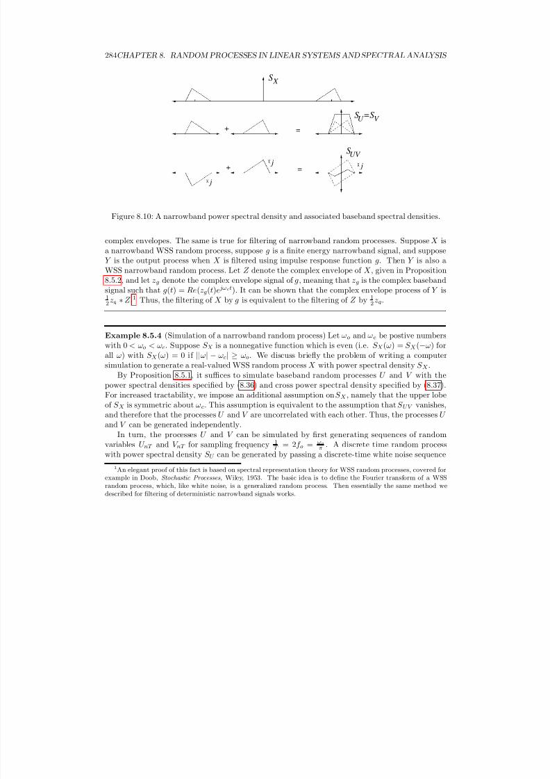
8/11/2019 Random process by B. Hajek
http://slidepdf.com/reader/full/random-process-by-b-hajek 294/448
284CHAPTER 8. RANDOM PROCESSES IN LINEAR SYSTEMS AND SPECTRAL ANALYSIS
S X
j j
j
S
S =S U V
UV
+
+
=
=
Figure 8.10: A narrowband power spectral density and associated baseband spectral densities.
complex envelopes. The same is true for filtering of narrowband random processes. Suppose X isa narrowband WSS random process, suppose g is a finite energy narrowband signal, and supposeY is the output process when X is filtered using impulse response function g. Then Y is also aWSS narrowband random process. Let Z denote the complex envelope of X , given in Proposition8.5.2, and let zg denote the complex envelope signal of g, meaning that zg is the complex basebandsignal such that g(t) = Re(zg(t)e jωct). It can be shown that the complex envelope process of Y is12 zg ∗ Z .1 Thus, the filtering of X by g is equivalent to the filtering of Z by 1
2 zg.
Example 8.5.4 (Simulation of a narrowband random process) Let ωo and ωc be postive numberswith 0 < ωo < ωc. Suppose S X is a nonnegative function which is even (i.e. S X (ω) = S X (−ω) forall ω) with S X (ω) = 0 if ||ω| − ωc| ≥ ωo. We discuss briefly the problem of writing a computersimulation to generate a real-valued WSS random process X with power spectral density S X .
By Proposition 8.5.1, it suffices to simulate baseband random processes U and V with thepower spectral densities specified by (8.36) and cross power spectral density specified by (8.37).For increased tractability, we impose an additional assumption on S X , namely that the upper lobeof S X is symmetric about ωc. This assumption is equivalent to the assumption that S UV vanishes,and therefore that the processes U and V are uncorrelated with each other. Thus, the processes U and V can be generated independently.
In turn, the processes U and V can be simulated by first generating sequences of random
variables U nT and V nT for sampling frequency 1T = 2f o =
ωoπ . A discrete time random process
with power spectral density S U can be generated by passing a discrete-time white noise sequence
1An elegant proof of this fact is based on spectral representation theory for WSS random processes, covered forexample in Doob, Stochastic Processes , Wiley, 1953. The basic idea is to define the Fourier transform of a WSSrandom process, which, like white noise, is a generalized random process. Then essentially the same method wedescribed for filtering of deterministic narrowband signals works.
8/11/2019 Random process by B. Hajek
http://slidepdf.com/reader/full/random-process-by-b-hajek 295/448
8.6. COMPLEXIFICATION, PART II 285
with unit variance through a discrete-time linear time-invariant system with real-valued impulseresponse function such that the transfer function H satisfies S U = |H |2. For example, takingH (ω) =
S U (ω) works, though it might not be the most well behaved linear system. (The
problem of finding a transfer function H with additional properties such that S U = |H |2
is calledthe problem of spectral factorization, which we shall return to in the next chapter.) The samplesV kT can be generated similarly.
For a specific example, suppose that (using kHz for kilohertz, or thousands of Hertz)
S X (2πf ) =
1 9, 000 kHz < |f | < 9, 020 kH z0 else
. (8.40)
Notice that the parameters ωo and ωc are not uniquely determined by S X . They must simply bepositive numbers with ωo < ωc such that
(9, 000 kHz, 9, 020 kH z) ⊂ (f c − f o, f c + f o)
However, only the choice f c = 9, 010 kH z makes the upper lobe of S X symmetric around f c.Therefore we take f c = 9, 010 kHz. We take the minmum allowable value for f o, namely f o =10 kHz. For this choice, (8.36) yields
S U (2πf ) = S V (2πf ) =
2 |f | < 10 kHz0 else
(8.41)
and (8.37) yields S UV (2πf ) = 0 for all f . The processes U and V are continuous-time basebandrandom processes with one-sided bandwidth limit 10 kH z. To simulate these processes it is thereforeenough to generate samples of them with sampling period T = 0.5×10⁻⁴, and then use the Nyquistsampling representation described in Section 8.4. The processes of samples will, according to (8.26),
have power spectral density equal to 4 × 10
4
over the interval [−π, π]. Consequently, the samplescan be taken to be uncorrelated with E [|Ak|2] = E [|Bk|2] = 4 × 10⁴. For example, these variablescan be taken to be independent real Gaussian random variables. Putting the steps together, wefind the following representation for X :
X t = cos(ωct)
∞n=−∞
Ansinc
t − nT
T
− sin(ωct)
∞n=−∞
Bnsinc
t − nT
T
8.6 Complexification, Part II
A complex random variable Z is said to be circularly symmetric if Z has the same distributionas e jθZ for every real value of θ. If Z has a pdf f Z , circular symmetry of Z means that f Z (z)is invariant under rotations about zero, or, equivalently, f Z (z) depends on z only through |z|. Acollection of random variables (Z i : i ∈ I ) is said to be jointly circularly symmetric if for every realvalue of θ , the collection (Z i : i ∈ I ) has the same finite dimensional distributions as the collection(Z ie
jθ : i ∈ I ). Note that if (Z i : i ∈ I ) is jointly circularly symmetric, and if (Y j : j ∈ J ) is another
8/11/2019 Random process by B. Hajek
http://slidepdf.com/reader/full/random-process-by-b-hajek 296/448
286CHAPTER 8. RANDOM PROCESSES IN LINEAR SYSTEMS AND SPECTRAL ANALYSIS
collection of random variables such that each Y j is a linear combination of Z i’s (with no constantsadded in) then the collection (Y j : j ∈ J ) is also jointly circularly symmetric.
Recall that a complex random vector Z , expressed in terms of real random vectors U and V as
Z = U + jV , has mean E Z = EU + jE V and covariance matrix Cov(Z ) = E [(Z − EZ )(Z − EZ )∗].The pseudo-covariance matrix of Z is defined by Cov p(Z ) = E [(Z − EZ )(Z − EZ )T ], and it differsfrom the covariance of Z in that a transpose, rather than a Hermitian transpose, is involved. Notethat Cov(Z ) and Cov p(Z ) are readily expressed in terms of Cov(U ), Cov(V ), and Cov(U, V ) as:
Cov(Z ) = Cov(U ) + Cov(V ) + j (Cov(V, U ) − Cov(U, V ))
Cov p(Z ) = Cov(U ) − Cov(V ) + j (Cov(V, U ) + Cov(U, V ))
where Cov(V, U ) = Cov(U, V )T . Conversely,
Cov(U ) = Re (Cov(Z ) + Cov p(Z )) /2, Cov(V ) = Re (Cov(Z ) − Cov p(Z )) /2,
andCov(U, V ) = I m (−Cov(Z ) + Cov p(Z )) /2.
The vector Z is defined to be Gaussian if the random vectors U and V are jointly Gaussian.Suppose that Z is a complex Gaussian random vector. Then its distribution is fully determined
by its mean and the matrices Cov(U ), Cov(V ), and Cov(U, V ), or equivalently by its mean andthe matrices Cov(Z ) and Cov p(Z ). Therefore, for a real value of θ, Z and e jθZ have the samedistribution if and only if they have the same mean, covariance matrix, and pseudo-covariancematrix. Since E [e jθZ ] = e jθEZ , Cov(e jθZ ) = Cov(Z ), and Cov p(e jθZ ) = e j2θCov p(Z ), Z and e jθZ have the same distribution if and only if (e jθ − 1)EZ = 0 and (e j2θ − 1)Cov p(Z ) = 0. Hence, if θ isnot a multiple of π, Z and e jθZ have the same distribution if and only if EZ = 0 and Cov p(Z ) = 0.Consequently, a Gaussian random vector Z is circularly symmetric if and only if its mean vector
and pseudo-covariance matrix are zero.The joint density function of a circularly symmetric complex random vector Z with n complex
dimensions and covariance matrix K , with det K = 0, has the particularly elegant form:
f Z (z) = exp(−z∗K −1z)
πn det(K ) . (8.42)
Equation (8.42) can be derived in the same way the density for Gaussian vectors with real com-ponents is derived. Namely, (8.42) is easy to verify if K is diagonal. If K is not diagonal, theHermetian symmetric positive definite matrix K can be expressed as K = U ΛU ∗, where U is aunitary matrix and Λ is a diagonal matrix with strictly positive diagonal entries. The random
vector Y defined by Y = U ∗Z is Gaussian and circularly symmetric with covariance matrix Λ, andsince det(Λ) = det(K ), it has pdf f Y (y) = exp(−y∗Λ−1y)πn det(K ) . Since | det(U )| = 1, f Z (z) = f Y (U ∗x),
which yields (8.42).Let us switch now to random processes. Let Z be a complex-valued random process and let U
and V be the real-valued random processes such that Z t = U t + jV t. Recall that Z is Gaussian if U and V are jointly Gaussian, and the covariance function of Z is defined by C Z (s, t) = Cov(Z s, Z t).
8/11/2019 Random process by B. Hajek
http://slidepdf.com/reader/full/random-process-by-b-hajek 297/448
8/11/2019 Random process by B. Hajek
http://slidepdf.com/reader/full/random-process-by-b-hajek 298/448
288CHAPTER 8. RANDOM PROCESSES IN LINEAR SYSTEMS AND SPECTRAL ANALYSIS
8.3 On filtering a WSS random processSuppose Y is the output of a linear time-invariant system with WSS input X , impulse responsefunction h, and transfer function H . Indicate whether the following statements are true or false.
Justify your answers. (a) If |H (ω)| ≤ 1 for all ω then the power of Y is less than or equal to thepower of X . (b) If X is periodic (in addition to being WSS) then Y is WSS and periodic. (c) If X has mean zero and strictly positive total power, and if ||h||2 > 0, then the output power is strictlypositive.
8.4 On the cross spectral densitySuppose X and Y are jointly WSS such that the power spectral densities S X , S Y , and S XY arecontinuous. Show that for each ω, |S XY (ω)|2 ≤ S X (ω)S Y (ω). Hint: Fix ωo, let > 0, and let J
denote the interval of length centered at ωo. Consider passing both X and Y through a lineartime-invariant system with transfer function H (ω) = I J (ω). Apply the Schwarz inequality to theoutput processes sampled at a fixed time, and let → 0.
8.5 Modulating and filtering a stationary processLet X = (X t : t ∈ Z ) be a discrete-time mean-zero stationary random process with power E [X 20 ] =1. Let Y be the stationary discrete time random process obtained from X by modulation as follows:
Y t = X t cos(80πt + Θ),
where Θ is independent of X and is uniformly distributed over [0, 2π]. Let Z be the stationarydiscrete time random process obtained from Y by the linear equations:
Z t+1 = (1 − a)Z t + aY t+1
for all t, where a is a constant with 0 < a < 1. (a) Why is the random process Y stationary?(b) Express the autocorrelation function of Y , RY (τ ) = E [Y τ Y 0], in terms of the autocorrelationfunction of X . Similarly, express the power spectral density of Y , S Y (ω), in terms of the powerspectral density of X , S X (ω). (c) Find and sketch the transfer function H (ω) for the linear systemdescribing the mapping from Y to Z . (d) Can the power of Z be arbitrarily large (depending ona)? Explain your answer. (e) Describe an input X satisfying the assumptions above so that thepower of Z is at least 0.5, for any value of a with 0 < a < 1.
8.6 Filtering a Gauss Markov processLet X = (X t : −∞ < t < +∞) be a stationary Gauss Markov process with mean zero and
autocorrelation function RX (τ ) = exp(−|τ |). Define a random process Y = (Y t : t ∈ R
) by thedifferential equation Y t = X t − Y t.(a) Find the cross correlation function RXY . Are X and Y jointly stationary?(b) Find E [Y 5|X 5 = 3]. What is the approximate numerical value?(c) Is Y a Gaussian random process? Justify your answer.(d) Is Y a Markov process? Justify your answer.
8/11/2019 Random process by B. Hajek
http://slidepdf.com/reader/full/random-process-by-b-hajek 299/448
8.7. PROBLEMS 289
8.7 Slight smoothingSuppose Y is the output of the linear time-invariant system with input X and impulse responsefunction h, such that X is WSS with RX (τ ) = exp(−|τ |), and h(τ ) = 1
aI |τ |≤ a2 for a > 0. If a
is small, then h approximates the delta function δ (τ ), and consequently Y t ≈ X t. This problemexplores the accuracy of the approximation.(a) Find RY X (0), and use the power series expansion of eu to show that RY X (0) = 1 − a
4 + o(a) asa → 0. Here, o(a) denotes any term such that o(a)/a → 0 as a → 0.(b) Find RY (0), and use the power series expansion of eu to show that RY (0) = 1 − a
3 + o(a) asa → 0.(c) Show that E [|X t − Y t|2] = a
6 + o(a) as a → 0.
8.8 A stationary two-state Markov processLet X = (X k : k ∈ Z) be a stationary Markov process with state space S = 1, −1 and one-steptransition probability matrix
P = 1−
p p p 1 − p ,
where 0 < p < 1. Find the mean, correlation function and power spectral density function of X .Hint: For nonnegative integers k :
P k =
1
212
12
12
+ (1 − 2 p)k
1
2 −12
−12
12
.
8.9 A stationary two-state Markov process in continuous timeLet X = (X t : t ∈R) be a stationary Markov process with state space S = 1, −1 and Q matrix
Q = −α α
α −α ,
where α > 0. Find the mean, correlation function and power spectral density function of X . (Hint:Recall from the example in the chapter on Markov processes that for s < t, the matrix of transitionprobabilities pij(s, t) is given by H (τ ), where τ = t − s and
H (τ ) =
1+e−2ατ
21−e−2ατ
21−e−2ατ
21+e−2ατ
2
.
8.10 A linear estimation problemSuppose X and Y are possibly complex valued jointly WSS processes with known autocorrelation
functions, cross-correlation function, and associated spectral densities. Suppose Y is passed througha linear time-invariant system with impulse response function h and transfer function H , and letZ be the output. The mean square error of estimating X t by Z t is E [|X t − Z t|2].(a) Express the mean square error in terms of RX , RY , RXY and h.(b) Express the mean square error in terms of S X , S Y , S XY and H .(c) Using your answer to part (b), find the choice of H that minimizes the mean square error. (Hint:
8/11/2019 Random process by B. Hajek
http://slidepdf.com/reader/full/random-process-by-b-hajek 300/448
290CHAPTER 8. RANDOM PROCESSES IN LINEAR SYSTEMS AND SPECTRAL ANALYSIS
Try working out the problem first assuming the processes are real valued. For the complex case,
note that for σ2 > 0 and complex numbers z and zo, σ2|z|2 −2Re(z∗zo) is equal to |σz − zoσ |2 − |zo|2
σ2 ,
which is minimized with respect to z by z = zoσ2 .)
8.11 Linear time invariant, uncorrelated scattering channelA signal transmitted through a scattering environment can propagate over many different pathson its way to a receiver. The channel gains along distinct paths are often modeled as uncorrelated.The paths may differ in length, causing a delay spread. Let h = (hu : u ∈ Z) consist of uncorrelated,possibly complex valued random variables with mean zero and E [|hu|2] = gu. Assume that G =
u gu < ∞. The variable hu is the random complex gain for delay u, and g = (gu : u ∈ Z) isthe energy gain delay mass function with total gain G. Given a deterministic signal x, the channeloutput is the random signal Y defined by Y i =
∞u=−∞ huxi−u.
(a) Determine the mean and autocorrelation function for Y in terms of x and g .(b) Express the average total energy of Y : E [
i Y 2i ], in terms of x and g .
(c) Suppose instead that the input is a WSS random process X with autocorrelation function RX
.The input X is assumed to be independent of the channel h. Express the mean and autocorrelationfunction of the output Y in terms of RX and g. Is Y WSS?(d) Since the impulse response function h is random, so is its Fourier transform, H = (H (ω) : −π ≤ω ≤ π). Express the autocorrelation function of the random process H in terms of g.
8.12 The accuracy of approximate differentiationLet X be a WSS baseband random process with power spectral density S X , and let ωo be theone-sided band limit of X . The process X is m.s. differentiable and X can be viewed as theoutput of a time-invariant linear system with transfer function H (ω) = jω.(a) What is the power spectral density of X ?(b) Let Y t = X t+a−X t−a
2a , for some a > 0. We can also view Y = (Y t : t
∈ R) as the output of
a time-invariant linear system, with input X . Find the impulse response function k and transferfunction K of the linear system. Show that K (ω) → jω as a → 0.(c) Let Dt = X t − Y t. Find the power spectral density of D .(d) Find a value of a, depending only on ωo, so that E [|Dt|2] ≤ (0.01)E [|X t|]2. In other words, forsuch a, the m.s. error of approximating X t by Y t is less than one percent of E [|X t|2]. You can use
the fact that 0 ≤ 1 − sin(u)u ≤ u2
6 for all real u. (Hint: Find a so that S D(ω) ≤ (0.01)S X (ω) for|ω| ≤ ωo.)
8.13 Some linear transformations of some random processesLet U = (U n : n ∈ Z) be a random process such that the variables U n are independent, identicallydistributed, with E [U n] = µ and Var(U n) = σ2, where µ = 0 and σ 2 > 0. Please keep in mind that
µ = 0. Let X = (X n : n ∈ Z) be defined by X n = ∞k=0 U n−kak
, for a constant a with 0 < a < 1.(a) Is X stationary? Find the mean function µX and autocovariance function C X for X .(b) Is X a Markov process ? (Hint: X is not necessarily Gaussian. Does X have a state represen-tation driven by U ?)(c) Is X mean ergodic in the m.s. sense?Let U be as before, and let Y = (Y n : n ∈ Z) be defined by Y n =
∞k=0 U n−kAk, where A is a
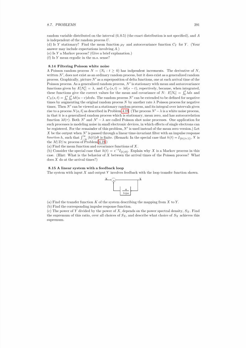
8/11/2019 Random process by B. Hajek
http://slidepdf.com/reader/full/random-process-by-b-hajek 301/448
8.7. PROBLEMS 291
random variable distributed on the interval (0, 0.5) (the exact distribution is not specified), and Ais independent of the random process U .(d) Is Y stationary? Find the mean function µY and autocovariance function C Y for Y . (Your
answer may include expectations involving A.)(e) Is Y a Markov process? (Give a brief explanation.)(f) Is Y mean ergodic in the m.s. sense?
8.14 Filtering Poisson white noiseA Poisson random process N = (N t : t ≥ 0) has indpendent increments. The derivative of N ,written N , does not exist as an ordinary random process, but it does exist as a generalized randomprocess. Graphically, picture N as a superposition of delta functions, one at each arrival time of thePoisson process. As a generalized random process, N is stationary with mean and autocovariancefunctions given by E [N t] = λ, and C N (s, t) = λδ (s − t), repectively, because, when integrated,these functions give the correct values for the mean and covariance of N : E [N t] =
t
0 λds and
C N (s, t) = s0 t0 λδ (u − v)dvdu. The random process N can be extended to be defined for negativetimes by augmenting the original random process N by another rate λ Poisson process for negativetimes. Then N can be viewed as a stationary random process, and its integral over intervals givesrise to a process N (a, b] as described in Problem 4.19. (The process N − λ is a white noise process,in that it is a generalized random process which is stationary, mean zero, and has autocorrelationfunction λδ (τ ). Both N and N − λ are called Poisson shot noise processes. One application forsuch processes is modeling noise in small electronic devices, in which effects of single electrons canbe registered. For the remainder of this problem, N is used instead of the mean zero version.) LetX be the output when N is passed through a linear time-invariant filter with an impulse responsefunction h, such that
∞−∞ |h(t)|dt is finite. (Remark: In the special case that h(t) = I 0≤t<1, X is
the M/D/∞ process of Problem 4.19.)(a) Find the mean function and covariance functions of X .
(b) Consider the special case that h(t) = e−tI t≥0. Explain why X is a Markov process in thiscase. (Hint: What is the behavior of X between the arrival times of the Poisson process? Whatdoes X do at the arrival times?)
8.15 A linear system with a feedback loopThe system with input X and output Y involves feedback with the loop transfer function shown.
Y
!
1+j"
X+
(a) Find the transfer function K of the system describing the mapping from X to Y .(b) Find the corresponding impulse response function.(c) The power of Y divided by the power of X , depends on the power spectral density, S X . Findthe supremum of this ratio, over all choices of S X , and describe what choice of S X achieves thissupremum.
8/11/2019 Random process by B. Hajek
http://slidepdf.com/reader/full/random-process-by-b-hajek 302/448
292CHAPTER 8. RANDOM PROCESSES IN LINEAR SYSTEMS AND SPECTRAL ANALYSIS
8.16 Linear and nonlinear reconstruction from samplesSuppose X t =
∞n=−∞ g(t−n−U )Bn, where the Bn’s are independent with mean zero and variance
σ2 > 0, g is a function with finite energy
|g(t)|2dt and Fourier transform G(ω), U is a random
variable which is independent of B and uniformly distributed on the interval [0, 1]. The process X is a typical model for a digital baseband signal, where the Bn’s are random data symbols.(a) Show that X is WSS, with mean zero and RX (t) = σ2g ∗ g(t).(b) Under what conditions on G and T can the sampling theorem be used to recover X from itssamples of the form (X (nT ) : n ∈ Z)?(c) Consider the particular case g(t) = (1 − |t|)+ and T = 0.5. Although this falls outside theconditions found in part (b), show that by using nonlinear operations, the process X can berecovered from its samples of the form (X (nT ) : n ∈ Z). (Hint: Consider a sample path of X )
8.17 Sampling a cubed Gaussian processLet X = (X t : t ∈ R) be a baseband mean zero stationary real Gaussian random process with
one-sided band limit f o Hz. Thus, X t = ∞n=−∞ X nT sinc t−nT
T where 1
T = 2f o. Let Y t = X 3
t foreach t.(a) Is Y stationary? Express RY in terms of RX , and S Y in terms of S X and/or RX . (Hint: If A, B are jointly Gaussian and mean zero, Cov(A3, B3) = 6Cov(A, B)3 + 9E [A2]E [B2]Cov(A, B).)
(b) At what rate 1T should Y be sampled in order that Y t =
∞n=−∞ Y nT sinc
t−nT T
?
(c) Can Y be recovered with fewer samples than in part (b)? Explain.
8.18 An approximation of white noiseWhite noise in continuous time can be approximated by a piecewise constant process as follows.Let T be a small positive constant, let AT be a positive scaling constant depending on T , and let(Bk : k
∈Z) be a discrete-time white noise process with RB(k) = σ2I
k=0
. Define (N t : t
∈R) by
N t = AT Bk for t ∈ [kT , (k + 1)T ).(a) Sketch a typical sample path of N and express E [| 10 N sds|2] in terms of AT , T and σ2. Forsimplicity assume that T = 1
K for some large integer K .(b) What choice of AT makes the expectation found in part (a) equal to σ2? This choice makesN a good approximation to a continuous-time white noise process with autocorrelation functionσ2δ (τ ).(c) What happens to the expectation found in part (a) as T → 0 if AT = 1 for all T ?
8.19 Simulating a baseband random processSuppose a real-valued Gaussian baseband process X = (X t : t ∈ R) with mean zero and powerspectral density
S X (2πf ) = 1 if |f | ≤ 0.50 else
is to be simulated over the time interval [−500, 500] through use of the sampling theorem withsampling time T = 1. (a) What is the joint distribution of the samples, X n : n ∈ Z ? (b) Of coursea computer cannot generate infinitely many random variables in a finite amount of time. Therefore,
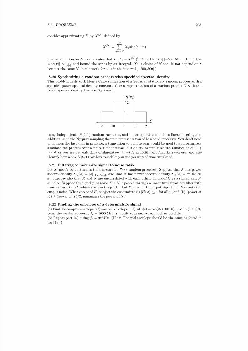
8/11/2019 Random process by B. Hajek
http://slidepdf.com/reader/full/random-process-by-b-hajek 303/448
8.7. PROBLEMS 293
consider approximating X by X (N ) defined by
X (N )t =
N
n=−N
X nsinc(t
−n)
Find a condition on N to guarantee that E [(X t − X (N )t )2] ≤ 0.01 for t ∈ [−500, 500]. (Hint: Use
|sinc(τ )| ≤ 1π|τ | and bound the series by an integral. Your choice of N should not depend on t
because the same N should work for all t in the interval [−500, 500] ).
8.20 Synthesizing a random process with specified spectral densityThis problem deals with Monte Carlo simulation of a Gaussian stationary random process with aspecified power spectral density function. Give a representation of a random process X with thepower spectral density function S X shown,
f
S(2 f)
!" #" " #" !"
#
!
using independent, N (0, 1) random variables, and linear operations such as linear filtering andaddition, as in the Nyquist sampling theorem representation of baseband processes. You don’t needto address the fact that in practice, a truncation to a finite sum would be used to approximatelysimulate the process over a finite time interval, but do try to minimize the number of N (0, 1)variables you use per unit time of simulation. Identify explicitly any functions you use, and alsoidentify how many N (0, 1) random variables you use per unit of time simulated.
8.21 Filtering to maximize signal to noise ratioLet X and N be continuous time, mean zero WSS random processes. Suppose that X has powerspectral density S X (ω) = |ω|I |ω|≤ωo, and that N has power spectral density S N (ω) = σ 2 for allω. Suppose also that X and N are uncorrelated with each other. Think of X as a signal, and N as noise. Suppose the signal plus noise X + N is passed through a linear time-invariant filter withtransfer function H , which you are to specify. Let X denote the output signal and N denote theoutput noise. What choice of H , subject the constraints (i) |H (ω)| ≤ 1 for all ω, and (ii) (power of
X ) ≥ (power of X )/2, minimizes the power of N ?
8.22 Finding the envelope of a deterministic signal(a) Find the complex envelope z(t) and real envelope |z(t)| of x(t) = cos(2π(1000)t)+cos(2π(1001)t),using the carrier frequency f c = 1000.5Hz. Simplify your answer as much as possible.(b) Repeat part (a), using f c = 995Hz. (Hint: The real envelope should be the same as found inpart (a).)
8/11/2019 Random process by B. Hajek
http://slidepdf.com/reader/full/random-process-by-b-hajek 304/448
294CHAPTER 8. RANDOM PROCESSES IN LINEAR SYSTEMS AND SPECTRAL ANALYSIS
(c) Explain why, in general, the real envelope of a narrowband signal does not depend on whichfrequency f c is used to represent the signal (as long as f c is chosen so that the upper band of thesignal is contained in an interval [f c − a, f c + a] with a << f c.)
8.23 Sampling a signal or process that is not band limited(a) Fix T > 0 and let ωo = π/T . Given a finite energy signal x, let xo be the band-limited signalwith Fourier transform xo(ω) = I |ω|≤ωo
∞n=−∞ x(ω + 2nωo). Show that x(nT ) = xo(nT ) for all
integers n. (b) Explain why xo(t) =∞
n=−∞ x(nT )sinct−nT
T
.
(c) Let X be a mean zero WSS random process, and let RoX be the autocorrelation function for
power spectral density S oX (ω) defined by S oX (ω) = I |ω|≤ωo∞
n=−∞ S X (ω + 2nωo). Show thatRX (nT ) = Ro
X (nT ) for all integers n. (d) Explain why the random process Y defined by Y t =∞n=−∞ X nT sinc
t−nT T
is WSS with autocorrelation function Ro
X . (e) Find S oX in case S X (ω) =exp(−α|ω|) for ω ∈ R.
8.24 A narrowband Gaussian process
Let X be a real-valued stationary Gaussian process with mean zero and RX (τ ) = cos(2π(30τ ))(sinc(6τ ))2.(a) Find and carefully sketch the power spectral density of X . (b) Sketch a sample path of X . (c)The process X can be represented by X t = Re(Z te2πj30t), where Z t = U t + jV t for jointly stationarynarrowband real-valued random processes U and V . Find the spectral densities S U , S V , and S UV .(d) Find P |Z 33| > 5. Note that |Z t| is the real envelope process of X .
8.25 Another narrowband Gaussian processSuppose a real-valued Gaussian random process R = (Rt : t ∈ R) with mean 2 and power spectraldensity S R(2πf ) = e−|f |/104 is fed through a linear time-invariant system with transfer function
H (2πf ) =
0.1 5000 ≤ |f | ≤ 6000
0 else
(a) Find the mean and power spectral density of the output process X = (X t : t ∈ R). (b) FindP X 25 > 6. (c) The random process X is a narrowband random process. Find the power spectraldensities S U , S V and the cross spectral density S UV of jointly WSS baseband random processes U and V so that
X t = U t cos(2πf ct) − V t sin(2πf ct),
using f c = 5500. (d) Repeat part (c) with f c = 5000.
8.26 Another narrowband Gaussian process (version 2)Suppose a real-valued Gaussian white noise process N (we assume white noise has mean zero) withpower spectral density S N (2πf ) ≡ N o
2 for f ∈ R is fed through a linear time-invariant system with
transfer function H specified as follows, where f represents the frequency in gigahertz (GHz) anda gigahertz is 109 cycles per second.
H (2πf ) =
1 19.10 ≤ |f | ≤ 19.11
19.12−|f |0.01 19.11 ≤ |f | ≤ 19.12
0 else
8/11/2019 Random process by B. Hajek
http://slidepdf.com/reader/full/random-process-by-b-hajek 305/448
8.7. PROBLEMS 295
(a) Find the mean and power spectral density of the output process X = (X t : t ∈ R).(b) Express P X 25 > 2 in terms of N o and the standard normal complementary CDF function Q.(c) The random process X is a narrowband random process. Find and sketch the power spectral
densities S U , S V and the cross spectral density S UV of jointly WSS baseband random processes U and V so that
X t = U t cos(2πf ct) − V t sin(2πf ct),
using f c = 19.11 GHz.(d) The complex envelope process is given by Z = U + jV and the real envelope process is givenby |Z |. Specify the distributions of Z t and |Z t| for t fixed.
8.27 Declaring the center frequency for a given random processLet a > 0 and let g be a nonnegative function on R which is zero outside of the interval [a, 2a].Suppose X is a narrowband WSS random process with power spectral density function S X (ω) =g(|ω|), or equivalently, S X (ω) = g(ω) + g(−ω). The process X can thus be viewed as a narrowband
signal for carrier frequency ωc, for any choice of ωc in the interval [a, 2a]. Let U and V be thebaseband random processes in the usual complex envelope representation: X t = Re((U t+ jV t)e jωct).(a) Express S U and S UV in terms of g and ωc.(b) Describe which choice of ωc minimizes
∞−∞ |S UV (ω)|2 dω
dπ . (Note: If g is symmetric arroundsome frequency ν , then ωc = ν . But what is the answer otherwise?)
8.28 * Cyclostationary random processesA random process X = (X t : t ∈ R) is said to be cyclostationary with period T , if whenever s isan integer multiple of T , X has the same finite dimensional distributions as (X t+s : t ∈ R). Thisproperty is weaker than stationarity, because stationarity requires equality of finite dimensionaldistributions for all real values of s.(a) What properties of the mean function µX and autocorrelation function RX does any secondorder cyclostationary process possess? A process with these properties is called a wide sensecyclostationary process.(b) Suppose X is cyclostationary and that U is a random variable independent of X that is uniformlydistributed on the interval [0, T ]. Let Y = (Y t : t ∈ R) be the random process defined by Y t = X t+U .Argue that Y is stationary, and express the mean and autocorrelation function of Y in terms of the mean function and autocorrelation function of X . Although X is not necessarily WSS, it isreasonable to define the power spectral density of X to equal the power spectral density of Y .(c) Suppose B is a stationary discrete-time random process and that g is a deterministic function.Let X be defined by
X t =
∞
−∞
g(t − nT )Bn.
Show that X is a cyclostationary random process. Find the mean function and autocorrelationfunction of X in terms g, T , and the mean and autocorrelation function of B. If your answer iscomplicated, identify special cases which make the answer nice.(d) Suppose Y is defined as in part (b) for the specific X defined in part (c). Express the meanµY , autocorrelation function RY , and power spectral density S Y in terms of g, T , µB, and S B .

8/11/2019 Random process by B. Hajek
http://slidepdf.com/reader/full/random-process-by-b-hajek 306/448
8/11/2019 Random process by B. Hajek
http://slidepdf.com/reader/full/random-process-by-b-hajek 307/448
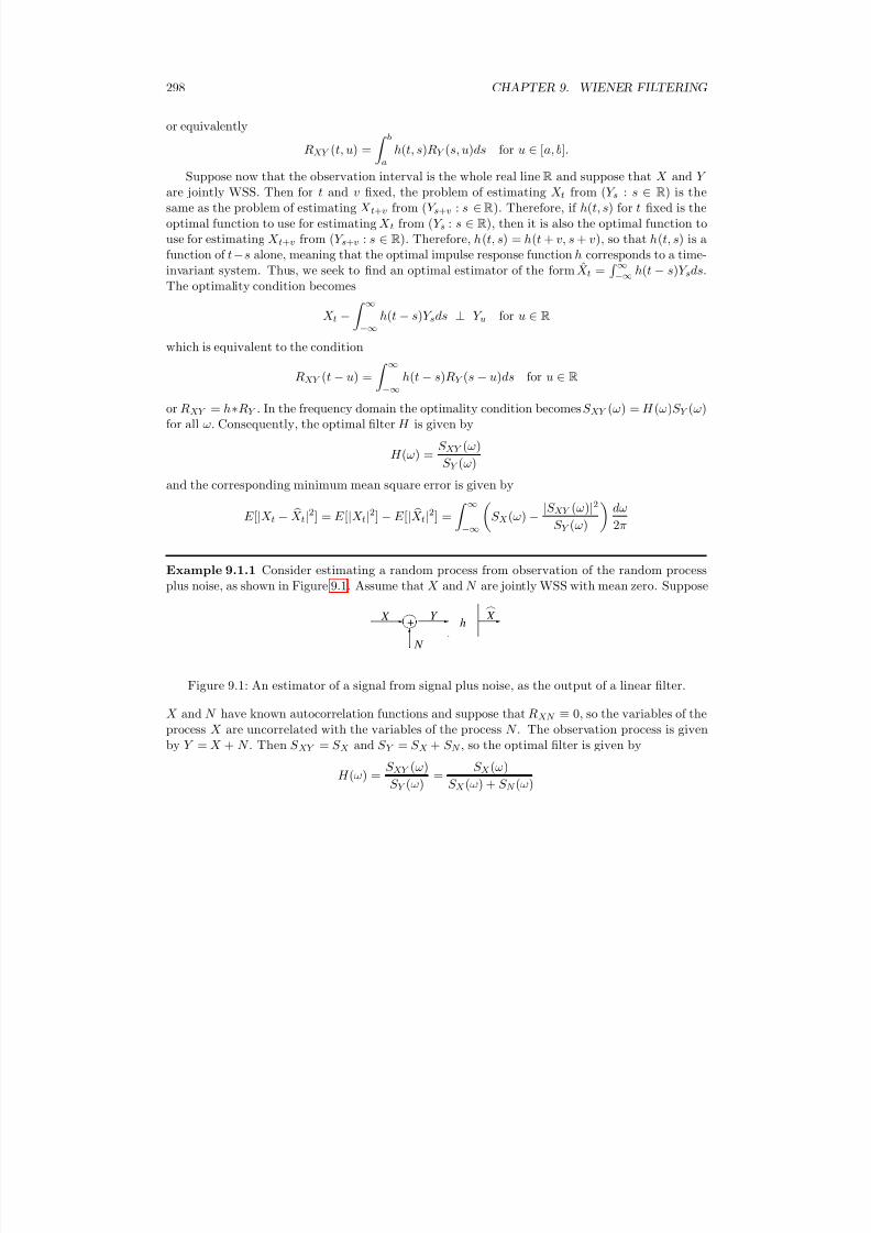
8/11/2019 Random process by B. Hajek
http://slidepdf.com/reader/full/random-process-by-b-hajek 308/448
298 CHAPTER 9. WIENER FILTERING
or equivalently
RXY (t, u) =
ba
h(t, s)RY (s, u)ds for u ∈ [a, b].
Suppose now that the observation interval is the whole real line R and suppose that X and Y are jointly WSS. Then for t and v fixed, the problem of estimating X t from (Y s : s ∈ R) is thesame as the problem of estimating X t+v from (Y s+v : s ∈ R). Therefore, if h(t, s) for t fixed is theoptimal function to use for estimating X t from (Y s : s ∈ R), then it is also the optimal function touse for estimating X t+v from (Y s+v : s ∈ R). Therefore, h(t, s) = h(t + v, s + v), so that h(t, s) is afunction of t−s alone, meaning that the optimal impulse response function h corresponds to a time-invariant system. Thus, we seek to find an optimal estimator of the form X t =
∞−∞ h(t − s)Y sds.
The optimality condition becomes
X t − ∞−∞
h(t − s)Y sds ⊥ Y u for u ∈ R
which is equivalent to the condition
RXY (t − u) =
∞−∞
h(t − s)RY (s − u)ds for u ∈ R
or RXY = h∗RY . In the frequency domain the optimality condition becomes S XY (ω) = H (ω)S Y (ω)for all ω. Consequently, the optimal filter H is given by
H (ω) = S XY (ω)
S Y (ω)
and the corresponding minimum mean square error is given by
E [
|X t
− X t
|2] = E [
|X t
|2]
−E [
| X t
|2] =
∞
−∞S X (ω)
− |S XY (ω)|2
S Y (ω) dω
2π
Example 9.1.1 Consider estimating a random process from observation of the random processplus noise, as shown in Figure 9.1. Assume that X and N are jointly WSS with mean zero. Suppose
X
N
+ h X Y
Figure 9.1: An estimator of a signal from signal plus noise, as the output of a linear filter.
X and N have known autocorrelation functions and suppose that RXN ≡ 0, so the variables of theprocess X are uncorrelated with the variables of the process N . The observation process is givenby Y = X + N . Then S XY = S X and S Y = S X + S N , so the optimal filter is given by
H (ω) = S XY (ω)
S Y (ω) =
S X (ω)
S X (ω) + S N (ω)
8/11/2019 Random process by B. Hajek
http://slidepdf.com/reader/full/random-process-by-b-hajek 309/448
9.1. RETURN OF THE ORTHOGONALITY PRINCIPLE 299
The associated minimum mean square error is given by
E [|X t − X t|2] =
∞
−∞S X (ω) − S X (ω)2
S X (ω) + S N (ω)dω
2π
= ∞−∞
S X (ω)S N (ω)
S X (ω) + S N (ω)
dω
2π
Example 9.1.2 This example is a continuation of the previous example, for a particular choiceof power spectral densities. Suppose that the signal process X is WSS with mean zero and powerspectral density S X (ω) = 1
1+ω2 , suppose the noise process N is WSS with mean zero and power
spectral density 44+ω2 , and suppose S XN ≡ 0. Equivalently, RX (τ ) = e−|τ |
2 , RN (τ ) = e−2|τ | andRXN ≡ 0. We seek the optimal linear estimator of X t given (Y s : s ∈ R), where Y = X + N .Seeking an estimator of the form
X t = ∞−∞ h(t − s)Y sds
we find from the previous example that the transform H of h is given by
H (ω) = S X (ω)
S X (ω) + S N (ω) =
11+ω2
11+ω2
+ 44+ω2
= 4 + ω2
8 + 5ω2
We will find h by finding the inverse transform of H . First, note that
4 + ω2
8 + 5ω2 =
85 + ω2
8 + 5ω2 +
125
8 + 5ω2 =
1
5 +
125
8 + 5ω2
We know that 15 δ (t) ↔ 1
5 . Also, for any α > 0,
e−α|t| ↔ 2αω2 + α2
, (9.1)
so
1
8 + 5ω2 =
15
85 + ω2
=
1
5 · 2
5
8
2
85
( 85 + ω2)
↔
1
4√
10
e−q
85|t|
Therefore the optimal filter is given in the time domain by
h(t) = 1
5δ (t) +
3
5√
10
e−q
85|t|
The associated minimum mean square error is given by (one way to do the integration is to use thefact that if k
↔ K then ∞−∞
K (ω)dω2π = k(0)):
E [|X t − X t|2] =
∞−∞
S X (ω)S N (ω)
S X (ω) + S N (ω)
dω
2π =
∞−∞
4
8 + 5ω2
dω
2π = 4
1
4√
10
=
1√ 10
In an example later in this chapter we will return to the same random processes, but seek the bestlinear estimator of X t given (Y s : s ≤ t).
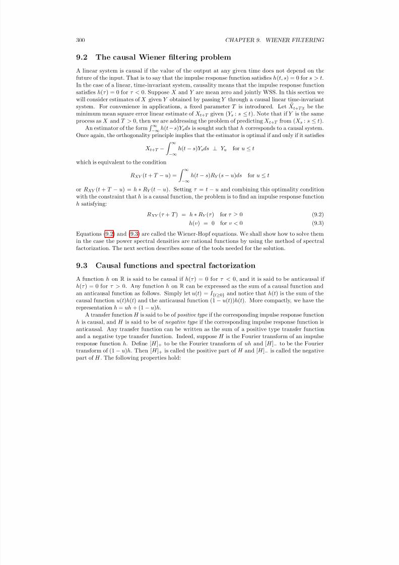
8/11/2019 Random process by B. Hajek
http://slidepdf.com/reader/full/random-process-by-b-hajek 310/448
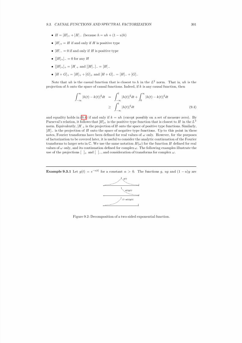
8/11/2019 Random process by B. Hajek
http://slidepdf.com/reader/full/random-process-by-b-hajek 311/448
9.3. CAUSAL FUNCTIONS AND SPECTRAL FACTORIZATION 301
• H = [H ]+ + [H ]− (because h = uh + (1 − u)h)
• [H ]+ = H if and only if H is positive type
• [H ]− = 0 if and only if H is positive type
• [[H ]+]− = 0 for any H
• [[H ]+]+ = [H ]+ and [[H ]−]− = [H ]−
• [H + G]+ = [H ]+ + [G]+ and [H + G]− = [H ]− + [G]−
Note that uh is the casual function that is closest to h in the L2 norm. That is, uh is theprojection of h onto the space of causal functions. Indeed, if k is any causal function, then
∞
−∞ |h(t) − k(t)|2
dt = 0
−∞ |h(t)|2
dt + ∞
0 |h(t) − k(t)|2
dt
≥ 0
−∞|h(t)|2dt (9.4)
and equality holds in (9.4) if and only if k = uh (except possibly on a set of measure zero). ByParseval’s relation, it follows that [H ]+ is the positive type function that is closest to H in the L2
norm. Equivalently, [H ]+ is the projection of H onto the space of positive type functions. Similarly,[H ]− is the projection of H onto the space of negative type functions. Up to this point in thesenotes, Fourier transforms have been defined for real values of ω only. However, for the purposesof factorization to be covered later, it is useful to consider the analytic continuation of the Fouriertransforms to larger sets in C. We use the same notation H (ω) for the function H defined for real
values of ω only, and its continuation defined for complex ω . The following examples illustrate theuse of the projections [ ]+ and [ ]−, and consideration of transforms for complex ω.
Example 9.3.1 Let g(t) = e−α|t| for a constant α > 0. The functions g, ug and (1 − u)g are
g(t)
u(t)g(t)
(1−u(t))g(t)
t
t
t
Figure 9.2: Decomposition of a two-sided exponential function.
8/11/2019 Random process by B. Hajek
http://slidepdf.com/reader/full/random-process-by-b-hajek 312/448
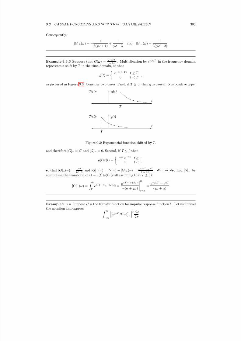
8/11/2019 Random process by B. Hajek
http://slidepdf.com/reader/full/random-process-by-b-hajek 313/448
9.3. CAUSAL FUNCTIONS AND SPECTRAL FACTORIZATION 303
Consequently,
[G]+(ω) = − 1
3( jω + 1) +
1
jω + 3 and [G]−(ω) =
1
3( jω
−2)
Example 9.3.3 Suppose that G(ω) = e−jωT
( jω+α) . Multiplication by e− jωT in the frequency domainrepresents a shift by T in the time domain, so that
g(t) =
e−α(t−T ) t ≥ T
0 t < T ,
as pictured in Figure 9.3. Consider two cases. First, if T ≥ 0, then g is causal, G is positive type,
g(t)
t
T>0:
T
T
g(t)
t
T<0:
Figure 9.3: Exponential function shifted by T.
and therefore [G]+ = G and [G]− = 0. Second, if T ≤ 0 then
g(t)u(t) =
eαT e−αt t ≥ 0
0 t < 0
so that [G]+(ω) = eαT
jω+α and [G]−(ω) = G(ω) − [G]+(ω) = e−jωT −eαT
( jω+α) . We can also find [G]− by
computing the transform of (1 − u(t))g(t) (still assuming that T ≤ 0):
[G]−(ω) =
0
T eα(T −t)e− jωtdt =
eαT −(α+ jω)t
−(α + jω)
0
t=T
= e− jωT − eαT
( jω + α)
Example 9.3.4 Suppose H is the transfer function for impulse response function h. Let us unravelthe notation and express ∞
−∞
e jωT H (ω)
+
2 dω
2π
8/11/2019 Random process by B. Hajek
http://slidepdf.com/reader/full/random-process-by-b-hajek 314/448
304 CHAPTER 9. WIENER FILTERING
in terms of h and T . (Note that the factor e jωT is used, rather than e− jωT as in the previousexample.) Multiplication by e jωT in the frequency domain corresponds to shifting by −T in thetime domain, so that
e jωT
H (ω) ↔ h(t + T )and thus
e jωT H (ω)
+ ↔ u(t)h(t + T )
Applying Parseval’s identity, the definition of u, and a change of variables yields ∞−∞
e jωT H (ω)
+
2 dω
2π =
∞−∞
|u(t)h(t + T )|2dt
=
∞0
|h(t + T )|2dt
= ∞
T |h(t)
|2dt
The integral decreases from the energy of h to zero as T ranges from −∞ to ∞.
Example 9.3.5 Suppose [H ]− = [K ]− = 0. Let us find [HK ]−. As usual, let h denote the inversetransform of H , and k denote the inverse transform of K . The supposition implies that h and kare both causal functions. Therefore the convolution h ∗ k is also a causal function. Since HK isthe transform of h ∗ k, it follows that HK is a positive type function. Equivalently, [HK ]− = 0.
The decomposition H = [H ]+ + [H ]− is an additive one. Next we turn to multiplicative
decomposition, concentrating on rational functions. A function H is said to be rational if it canbe written as the ratio of two polynomials. Since polynomials can be factored over the complexnumbers, a rational function H can be expressed in the form
H (ω) = γ ( jω + β 1)( jω + β 2) · · · ( jω + β K )
( jω + α1)( jω + α2) · · · ( jω + αN )
for complex constants γ , α1, . . . , αN , β 1, . . . , β K . Without loss of generality, we assume that αi ∩β j = ∅. We also assume that the real parts of the constants α1, . . . , αN , β 1, . . . , β K are nonzero.The function H is positive type if and only if Re(αi) > 0 for all i, or equivalently, if and only if allthe poles of H (ω) are in the upper half plane I m(ω) > 0.
A positive type function H is said to have minimum phase if Re(β i) > 0 for all i. Thus, a
positive type function H is minimum phase if and only if 1/H is also positive type.Suppose that S Y is the power spectral density of a WSS random process and that S Y is a
rational function. The function S Y , being nonnegative, is also real-valued, so S Y = S ∗Y . Thus, if the denominator of S Y has a factor of the form jω + α then the denominator must also have afactor of the form − jω + α∗. Similarly, if the numerator of S Y has a factor of the form j ω + β thenthe numerator must also have a factor of the form − jω + β ∗.
8/11/2019 Random process by B. Hajek
http://slidepdf.com/reader/full/random-process-by-b-hajek 315/448
9.4. SOLUTION OF THE CAUSAL WIENER FILTERING PROBLEM FOR RATIONAL POWER SPEC
Example 9.3.6 The function S Y given by
S Y (ω) = 8 + 5ω2
(1 + ω2)(4 + ω2)
can be factored as
S Y (ω) =√
5( jω +
85 )
( jω + 2)( jω + 1) S +Y (ω)
√ 5
(− jω +
85 )
(− jω + 2)(− jω + 1) S −Y (ω)
(9.5)
where S +Y is a positive type, minimum phase function and S −Y is a negative type function withS −Y = (S +Y )
∗.
Note that the operators [ ]+ and [ ]− give us an additive decomposition of a function H intothe sum of a positive type and a negative type function, whereas spectral factorization has to dowith products. At least formally, the factorization can be accomplished by taking a logarithm,doing an additive decomposition, and then exponentiating:
S X (ω) = exp([ln S X (ω)]+) S +X(ω)
exp([ln S X (ω)]−) S −X(ω)
. (9.6)
Notice that if h ↔ H then, formally,
1 + h +
h
∗h
2! +
h
∗h
∗h
3! · · · ↔ exp(H ) = 1 + H +
H 2
2! +
H 2
3! · · ·so that if H is positive type, then exp(H ) is also positive type. Thus, the factor S +X in (9.6) isindeed a positive type function, and the factor S −X is a negative type function. Use of (9.6) is calledthe cepstrum method. Unfortunately, there is a host of problems, both numerical and analytical,in using the method, so that it will not be used further in these notes.
9.4 Solution of the causal Wiener filtering problem for rationalpower spectral densities
The Wiener-Hopf equations (9.2) and ( 9.3) can be formulated in the frequency domain as follows:
Find a positive type transfer function H such thate jωT S XY − HS Y
+
= 0 (9.7)
Suppose S Y is factored as S Y = S +Y S −Y such that S +Y is a minimum phase, positive type transferfunction and S −Y = (S +Y )
∗. Then S −Y and 1S −Y
are negative type functions. Since the product of
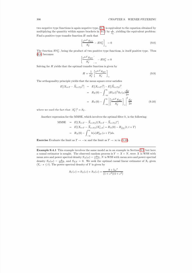
8/11/2019 Random process by B. Hajek
http://slidepdf.com/reader/full/random-process-by-b-hajek 316/448
306 CHAPTER 9. WIENER FILTERING
two negative type functions is again negative type, (9.7) is equivalent to the equation obtained bymultiplying the quantity within square brackets in (9.7) by 1
S −Y
, yielding the equivalent problem:
Find a positive type transfer function H such thate jωT S XY
S −Y − HS +Y
+
= 0 (9.8)
The function HS +Y , being the product of two positive type functions, is itself positive type. Thus(9.8) becomes
e jωT S XY
S −Y
+
− HS +Y = 0
Solving for H yields that the optimal transfer function is given by
H = 1
S +Y e jωT S XY
S −Y +
(9.9)
The orthogonality principle yields that the mean square error satisfies
E [|X t+T − X t+T |t|2] = E [|X t+T |2] − E [| X t+T |t|2]
= RX (0) − ∞−∞
|H (ω)|2S Y (ω)dω
2π
= RX (0) − ∞−∞
e jωT S XY
S −Y
+
2
dω
2π (9.10)
where we used the fact that |S +Y |2 = S Y .
Another expression for the MMSE, which involves the optimal filter h, is the following:
MMSE = E [(X t+T − X t+T |t)(X t+T − X t+T |t)∗]
= E [(X t+T − X t+T |t)X ∗t+T ] = RX (0) − R bXX (t, t + T )
= RX (0) − ∞−∞
h(s)R∗XY (s + T )ds.
Exercise Evaluate the limit as T → −∞ and the limit as T → ∞ in (9.10).
Example 9.4.1 This example involves the same model as in an example in Section 9.1, but herea causal estimator is sought. The observed random process is Y = X + N , were X is WSS with
mean zero and power spectral density S X (ω) = 11+ω2 , N is WSS with mean zero and power spectral
density S N (ω) = 44+ω2 , and S XN = 0. We seek the optimal casual linear estimator of X t given
(Y s : s ≤ t). The power spectral density of Y is given by
S Y (ω) = S X (ω) + S N (ω) = 8 + 5ω2
(1 + ω2)(4 + ω2)
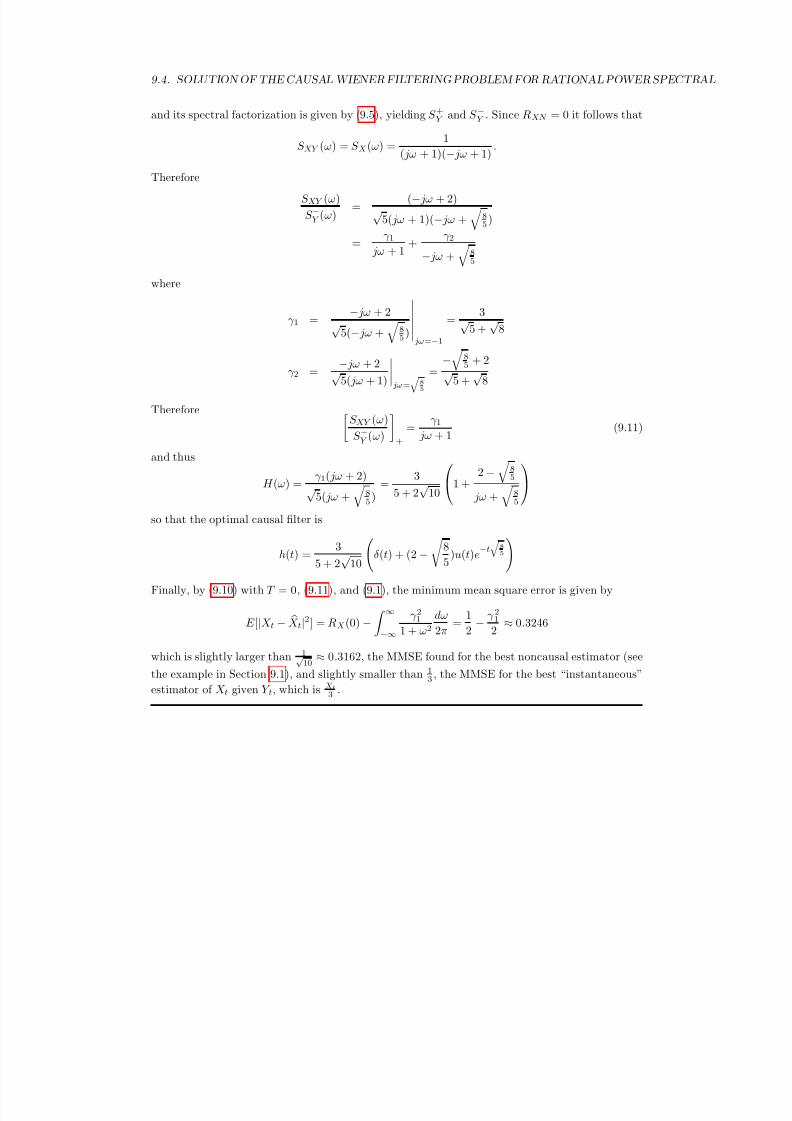
8/11/2019 Random process by B. Hajek
http://slidepdf.com/reader/full/random-process-by-b-hajek 317/448
9.4. SOLUTION OF THE CAUSAL WIENER FILTERING PROBLEM FOR RATIONAL POWER SPEC
and its spectral factorization is given by (9.5), yielding S +Y and S −Y . Since RXN = 0 it follows that
S XY (ω) = S X (ω) = 1
( jω + 1)(− jω + 1)
.
Therefore
S XY (ω)
S −Y (ω)=
(− jω + 2)√
5( jω + 1)(− jω +
85 )
= γ 1 jω + 1
+ γ 2
− jω +
85
where
γ 1 = − jω + 2
√ 5(− jω +
85 ) jω=−1
= 3
√ 5 + √ 8
γ 2 = − jω + 2√
5( jω + 1)
jω=
q 85
=−
85 + 2
√ 5 +
√ 8
Therefore S XY (ω)
S −Y (ω)
+
= γ 1
jω + 1 (9.11)
and thus
H (ω) = γ 1( jω + 2)√ 5( jω +
85 )
= 35 + 2
√ 101 +
2− 85
jω +
85
so that the optimal causal filter is
h(t) = 3
5 + 2√
10
δ (t) + (2 −
8
5)u(t)e
−tq
85
Finally, by (9.10) with T = 0, (9.11), and (9.1), the minimum mean square error is given by
E [|X t − X t|2] = RX (0) −
∞
−∞
γ 211 + ω2
dω
2π =
1
2 − γ 21
2 ≈ 0.3246
which is slightly larger than 1√ 10
≈ 0.3162, the MMSE found for the best noncausal estimator (see
the example in Section 9.1), and slightly smaller than 13 , the MMSE for the best “instantaneous”
estimator of X t given Y t, which is X t3 .
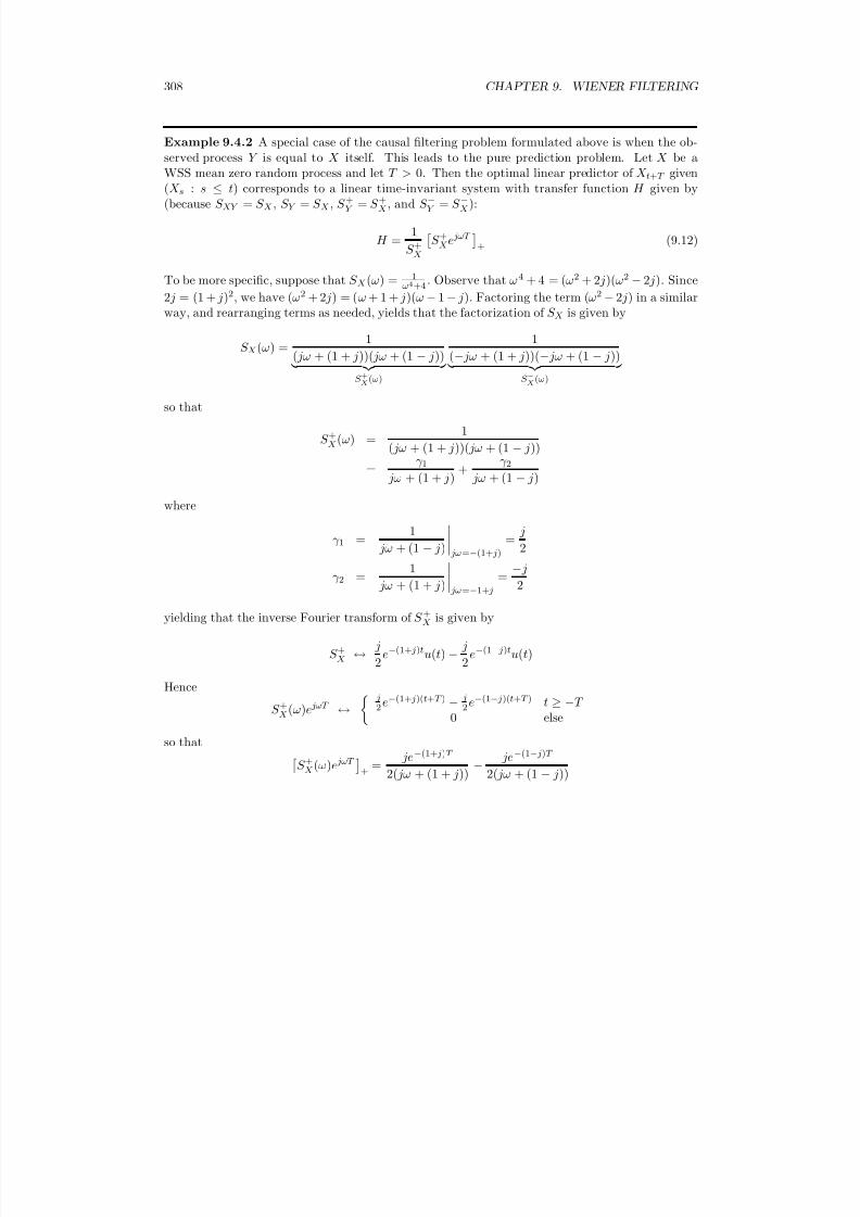
8/11/2019 Random process by B. Hajek
http://slidepdf.com/reader/full/random-process-by-b-hajek 318/448
308 CHAPTER 9. WIENER FILTERING
Example 9.4.2 A special case of the causal filtering problem formulated above is when the ob-served process Y is equal to X itself. This leads to the pure prediction problem. Let X be a
WSS mean zero random process and let T > 0. Then the optimal linear predictor of X t+T given(X s : s ≤ t) corresponds to a linear time-invariant system with transfer function H given by(because S XY = S X , S Y = S X , S +Y = S +X , and S −Y = S −X ):
H = 1
S +X
S +X e
jωT
+ (9.12)
To be more specific, suppose that S X (ω) = 1ω4+4 . Observe that ω 4 + 4 = (ω2 + 2 j)(ω2 − 2 j). Since
2 j = (1 + j)2, we have (ω2 + 2 j) = (ω + 1 + j)(ω − 1 − j). Factoring the term (ω2 − 2 j) in a similarway, and rearranging terms as needed, yields that the factorization of S X is given by
S X (ω) = 1
( jω + (1 + j))( jω + (1 − j)) S +X(ω)
1
(− jω + (1 + j))(− jω + (1 − j)) S −X(ω)
so that
S +X (ω) = 1
( jω + (1 + j))( jω + (1 − j))
= γ 1
jω + (1 + j) +
γ 2 jω + (1 − j)
where
γ 1 = 1
jω + (1 − j)
jω=−(1+ j)
= j
2
γ 2 = 1
jω + (1 + j)
jω=−1+ j
= − j
2
yielding that the inverse Fourier transform of S +X is given by
S +X ↔ j
2e−(1+ j)tu(t) − j
2e−(1− j)tu(t)
Hence
S +X (ω)e jωT ↔ j2 e−(1+ j)(t+T ) − j
2 e−(1− j)(t+T ) t ≥ −T 0 else
so that S +X (ω)e jωT
+
= je−(1+ j)T
2( jω + (1 + j)) − je−(1− j)T
2( jω + (1 − j))
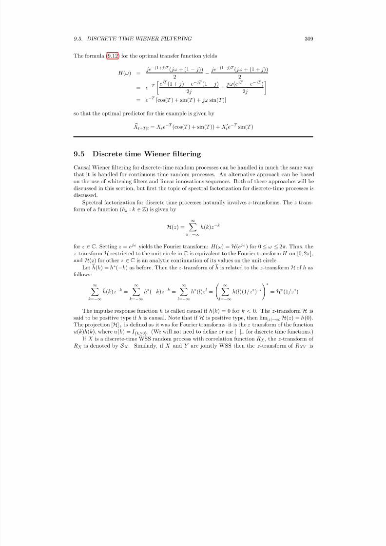
8/11/2019 Random process by B. Hajek
http://slidepdf.com/reader/full/random-process-by-b-hajek 319/448
9.5. DISCRETE TIME WIENER FILTERING 309
The formula (9.12) for the optimal transfer function yields
H (ω) = je−(1+ j)T ( jω + (1 − j))
2 − je−(1− j)T ( jω + (1 + j))
2= e−T
e jT (1 + j) − e− jT (1 − j)
2 j +
j ω(e jT − e− jT )2 j
= e−T [cos(T ) + sin(T ) + jω sin(T )]
so that the optimal predictor for this example is given by
X t+T |t = X te−T (cos(T ) + sin(T )) + X te−T sin(T )
9.5 Discrete time Wiener filteringCausal Wiener filtering for discrete-time random processes can be handled in much the same waythat it is handled for continuous time random processes. An alternative approach can be basedon the use of whitening filters and linear innovations sequences. Both of these approaches will bediscussed in this section, but first the topic of spectral factorization for discrete-time processes isdiscussed.
Spectral factorization for discrete time processes naturally involves z-transforms. The z trans-form of a function (hk : k ∈ Z) is given by
H(z) =
∞
k=−∞h(k)z−k
for z ∈ C. Setting z = e jω yields the Fourier transform: H (ω) = H(e jω) for 0 ≤ ω ≤ 2π. Thus, thez-transform H restricted to the unit circle in C is equivalent to the Fourier transform H on [0, 2π],and H(z) for other z ∈ C is an analytic continuation of its values on the unit circle.
Let h(k) = h∗(−k) as before. Then the z-transform of h is related to the z-transform H of h asfollows:
∞k=−∞
h(k)z−k =∞
k=−∞h∗(−k)z−k =
∞l=−∞
h∗(l)zl =
∞l=−∞
h(l)(1/z∗)−l
∗= H∗(1/z∗)
The impulse response function h is called causal if h(k) = 0 for k < 0. The z-transform H issaid to be positive type if h is causal. Note that if H is positive type, then lim|z|→∞ H(z) = h(0).The projection [H]+ is defined as it was for Fourier transforms–it is the z transform of the functionu(k)h(k), where u(k) = I k≥0. (We will not need to define or use [ ]− for discrete time functions.)
If X is a discrete-time WSS random process with correlation function RX , the z-transform of RX is denoted by S X . Similarly, if X and Y are jointly WSS then the z-transform of RXY is
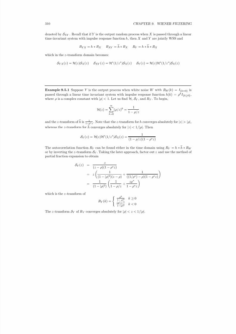
8/11/2019 Random process by B. Hajek
http://slidepdf.com/reader/full/random-process-by-b-hajek 320/448
310 CHAPTER 9. WIENER FILTERING
denoted by S XY . Recall that if Y is the output random process when X is passed through a lineartime-invariant system with impulse response function h, then X and Y are jointly WSS and
RY X = h ∗ RX RXY = h ∗ RX RY = h ∗ h ∗ RX
which in the z -transform domain becomes:
S Y X (z) = H(z)S X (z) S XY (z) = H∗(1/z∗)S X (z) S Y (z) = H(z)H∗(1/z∗)S X (z)
Example 9.5.1 Suppose Y is the output process when white noise W with RW (k) = I k=0 is
passed through a linear time invariant system with impulse response function h(k) = ρk
I k≥0,where ρ is a complex constant with |ρ| < 1. Let us find H, S Y , and RY . To begin,
H(z) =∞k=0
(ρ/z)k = 1
1 − ρ/z
and the z-transform of h is 11−ρ∗z . Note that the z-transform for h converges absolutely for |z| > |ρ|,
whereas the z-transform for h converges absolutely for |z| < 1/|ρ|. Then
S Y (z) = H(z)H∗(1/z∗)S X (z) = 1
(1
−ρ/z)(1
−ρ∗z)
The autocorrelation function RY can be found either in the time domain using RY = h ∗ h ∗ RW
or by inverting the z -transform S Y . Taking the later approach, factor out z and use the method of partial fraction expansion to obtain
S Y (z) = z
(z − ρ)(1 − ρ∗z)
= z
1
(1 − |ρ|2)(z − ρ) +
1
((1/ρ∗) − ρ)(1 − ρ∗z)
=
1
(1 − |ρ|2)
1
1 − ρ/z +
zρ∗
1 − ρ∗z
which is the z -transform of
RY (k) =
ρk
1−|ρ|2 k ≥ 0(ρ∗)−k
1−|ρ|2 k < 0
The z -transform S Y of RY converges absolutely for |ρ| < z < 1/|ρ|.
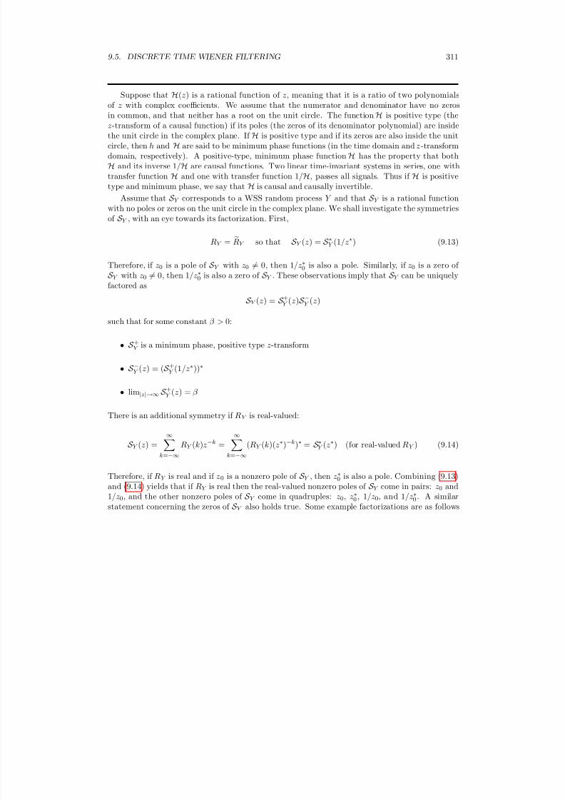
8/11/2019 Random process by B. Hajek
http://slidepdf.com/reader/full/random-process-by-b-hajek 321/448
9.5. DISCRETE TIME WIENER FILTERING 311
Suppose that H(z) is a rational function of z, meaning that it is a ratio of two polynomialsof z with complex coefficients. We assume that the numerator and denominator have no zeros
in common, and that neither has a root on the unit circle. The function H is positive type (thez-transform of a causal function) if its poles (the zeros of its denominator polynomial) are insidethe unit circle in the complex plane. If H is positive type and if its zeros are also inside the unitcircle, then h and H are said to be minimum phase functions (in the time domain and z -transformdomain, respectively). A positive-type, minimum phase function H has the property that bothH and its inverse 1/H are causal functions. Two linear time-invariant systems in series, one withtransfer function H and one with transfer function 1/H, passes all signals. Thus if H is positivetype and minimum phase, we say that H is causal and causally invertible.
Assume that S Y corresponds to a WSS random process Y and that S Y is a rational functionwith no poles or zeros on the unit circle in the complex plane. We shall investigate the symmetriesof
S Y , with an eye towards its factorization. First,
RY = RY so that S Y (z) = S ∗Y (1/z∗) (9.13)
Therefore, if z0 is a pole of S Y with z0 = 0, then 1/z∗0 is also a pole. Similarly, if z0 is a zero of S Y with z0 = 0, then 1/z∗0 is also a zero of S Y . These observations imply that S Y can be uniquelyfactored as
S Y (z) = S +Y (z)S −Y (z)
such that for some constant β > 0:
• S +Y is a minimum phase, positive type z-transform
• S −Y (z) = (S +Y (1/z∗))∗
• lim|z|→∞ S +Y (z) = β
There is an additional symmetry if RY is real-valued:
S Y (z) =
∞
k=−∞
RY (k)z−k =
∞
k=−∞
(RY (k)(z∗)−k)∗ = S ∗Y (z∗) (for real-valued RY ) (9.14)
Therefore, if RY is real and if z0 is a nonzero pole of S Y , then z∗0 is also a pole. Combining (9.13)and (9.14) yields that if RY is real then the real-valued nonzero poles of S Y come in pairs: z0 and1/z0, and the other nonzero poles of S Y come in quadruples: z0, z∗0 , 1/z0, and 1/z∗0 . A similarstatement concerning the zeros of S Y also holds true. Some example factorizations are as follows
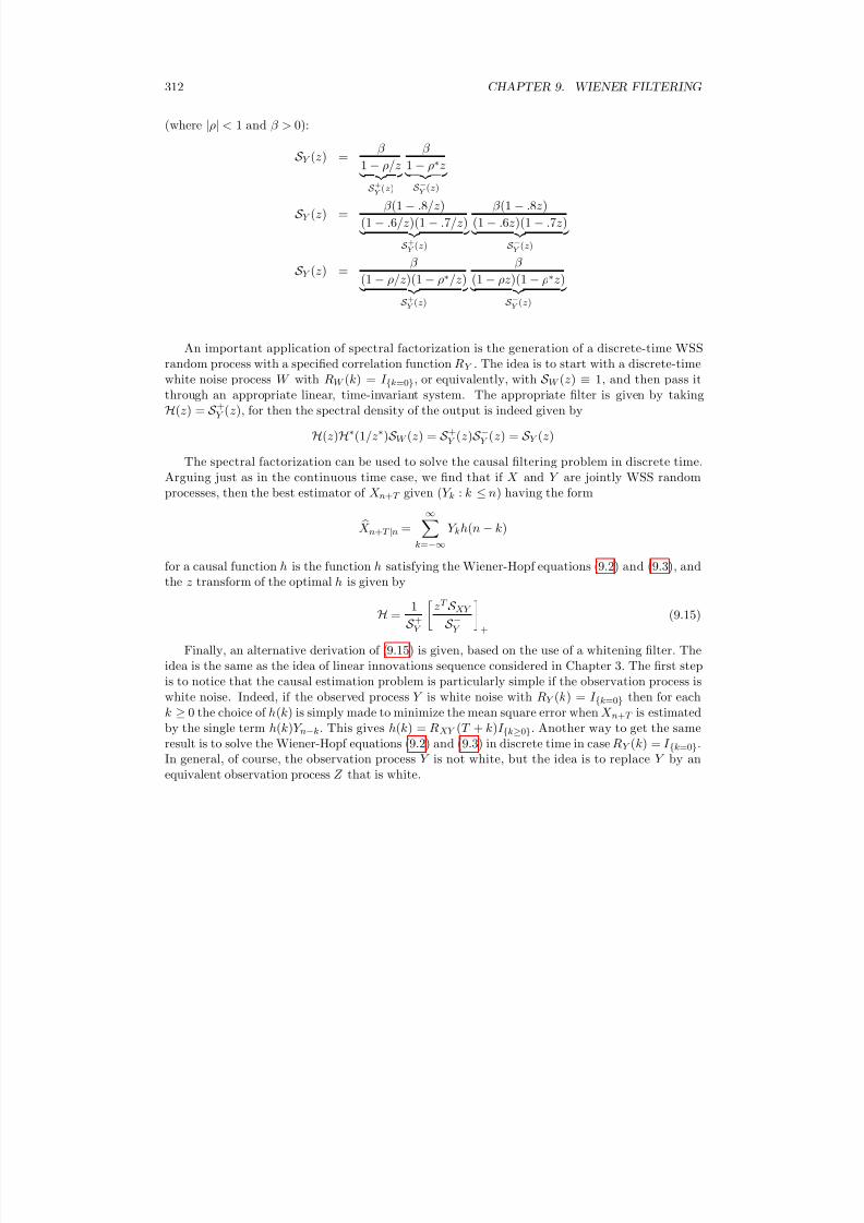
8/11/2019 Random process by B. Hajek
http://slidepdf.com/reader/full/random-process-by-b-hajek 322/448
312 CHAPTER 9. WIENER FILTERING
(where |ρ| < 1 and β > 0):
S Y (z) = β
1−
ρ/z S +Y (z)
β
1−
ρ∗z S −Y (z)
S Y (z) = β (1 − .8/z)
(1 − .6/z)(1 − .7/z) S +Y (z)
β (1 − .8z)
(1 − .6z)(1 − .7z) S −Y (z)
S Y (z) = β
(1 − ρ/z)(1 − ρ∗/z) S +Y (z)
β
(1 − ρz)(1 − ρ∗z) S −Y (z)
An important application of spectral factorization is the generation of a discrete-time WSSrandom process with a specified correlation function RY . The idea is to start with a discrete-timewhite noise process W with RW (k) = I k=0, or equivalently, with S W (z) ≡ 1, and then pass itthrough an appropriate linear, time-invariant system. The appropriate filter is given by takingH(z) = S +Y (z), for then the spectral density of the output is indeed given by
H(z)H∗(1/z∗)S W (z) = S +Y (z)S −Y (z) = S Y (z)
The spectral factorization can be used to solve the causal filtering problem in discrete time.Arguing just as in the continuous time case, we find that if X and Y are jointly WSS randomprocesses, then the best estimator of X n+T given (Y k : k ≤ n) having the form
X n+T |n = ∞k=−∞
Y kh(n − k)
for a causal function h is the function h satisfying the Wiener-Hopf equations (9.2) and (9.3), andthe z transform of the optimal h is given by
H = 1
S +Y
zT S XY
S −Y
+
(9.15)
Finally, an alternative derivation of (9.15) is given, based on the use of a whitening filter. Theidea is the same as the idea of linear innovations sequence considered in Chapter 3. The first stepis to notice that the causal estimation problem is particularly simple if the observation process is
white noise. Indeed, if the observed process Y is white noise with RY (k) = I k=0 then for eachk ≥ 0 the choice of h(k) is simply made to minimize the mean square error when X n+T is estimatedby the single term h(k)Y n−k. This gives h(k) = RXY (T + k)I k≥0. Another way to get the sameresult is to solve the Wiener-Hopf equations (9.2) and (9.3) in discrete time in case RY (k) = I k=0.In general, of course, the observation process Y is not white, but the idea is to replace Y by anequivalent observation process Z that is white.
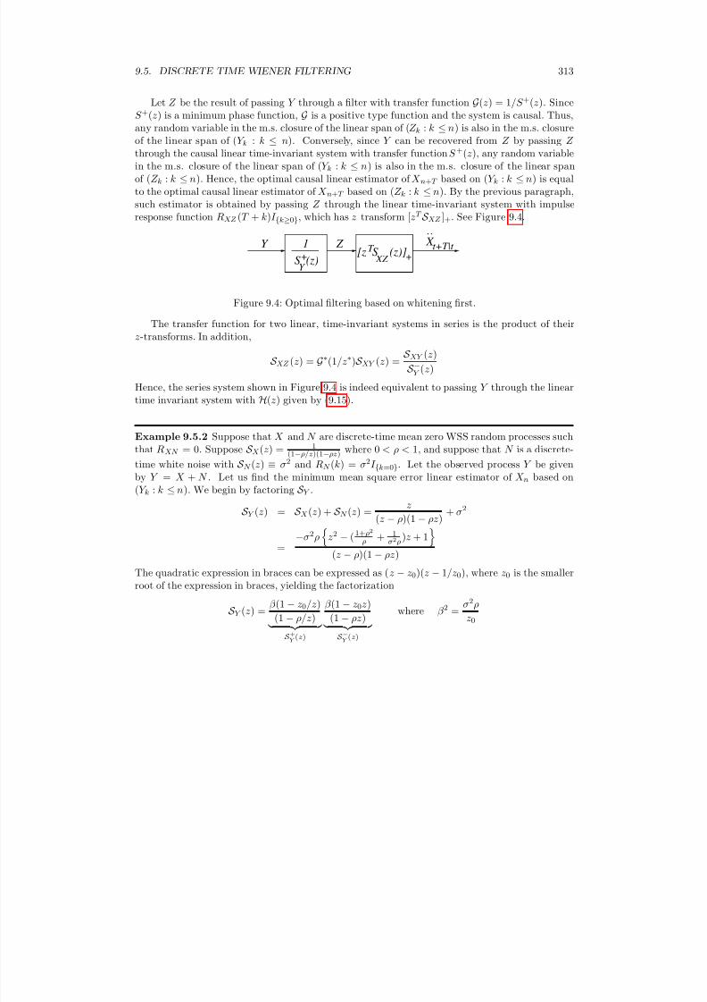
8/11/2019 Random process by B. Hajek
http://slidepdf.com/reader/full/random-process-by-b-hajek 323/448
9.5. DISCRETE TIME WIENER FILTERING 313
Let Z be the result of passing Y through a filter with transfer function G(z) = 1/S +(z). SinceS +(z) is a minimum phase function, G is a positive type function and the system is causal. Thus,any random variable in the m.s. closure of the linear span of (Z k : k ≤ n) is also in the m.s. closure
of the linear span of (Y k : k ≤ n). Conversely, since Y can be recovered from Z by passing Z through the causal linear time-invariant system with transfer function S +(z), any random variablein the m.s. closure of the linear span of (Y k : k ≤ n) is also in the m.s. closure of the linear spanof (Z k : k ≤ n). Hence, the optimal causal linear estimator of X n+T based on (Y k : k ≤ n) is equalto the optimal causal linear estimator of X n+T based on (Z k : k ≤ n). By the previous paragraph,such estimator is obtained by passing Z through the linear time-invariant system with impulseresponse function RXZ (T + k)I k≥0, which has z transform [zT S XZ ]+. See Figure 9.4.
1
S (z)Y
Z Y
++
X t+T|t
[z S (z)]T XZ
Figure 9.4: Optimal filtering based on whitening first.
The transfer function for two linear, time-invariant systems in series is the product of theirz-transforms. In addition,
S XZ (z) = G∗(1/z∗)S XY (z) = S XY (z)
S −Y (z)
Hence, the series system shown in Figure 9.4 is indeed equivalent to passing Y through the lineartime invariant system with H(z) given by (9.15).
Example 9.5.2 Suppose that X and N are discrete-time mean zero WSS random processes suchthat RXN = 0. Suppose S X (z) = 1
(1−ρ/z)(1−ρz) where 0 < ρ < 1, and suppose that N is a discrete-
time white noise with S N (z) ≡ σ2 and RN (k) = σ2I k=0. Let the observed process Y be givenby Y = X + N . Let us find the minimum mean square error linear estimator of X n based on(Y k : k ≤ n). We begin by factoring S Y .
S Y (z) = S X (z) + S N (z) = z
(z − ρ)(1 − ρz) + σ2
=−σ2ρ
z2 − ( 1+ρ2
ρ + 1σ2ρ)z + 1
(z − ρ)(1 − ρz)
The quadratic expression in braces can be expressed as ( z − z0)(z − 1/z0), where z0 is the smallerroot of the expression in braces, yielding the factorization
S Y (z) = β (1 − z0/z)
(1 − ρ/z) S +Y (z)
β (1 − z0z)
(1 − ρz) S −Y (z)
where β 2 = σ2ρ
z0
8/11/2019 Random process by B. Hajek
http://slidepdf.com/reader/full/random-process-by-b-hajek 324/448
314 CHAPTER 9. WIENER FILTERING
Using the fact S XY = S X , and appealing to a partial fraction expansion yields
S XY (z)
S −Y (z)
= 1
β (1−
ρ/z)(1−
z0
z)
= 1
β (1 − ρ/z)(1 − z0ρ) +
z
β ((1/z0) − ρ)(1 − z0z) (9.16)
The first term in (9.16) is positive type, and the second term in (9.16) is the z transform of a
function that is supported on the negative integers. Thus, the first term is equal toS XY
S −Y
+
.
Finally, dividing by S +Y yields that the z-transform of the optimal filter is given by
H(z) = 1
β 2(1 − z0ρ)(1 − z0/z)
or in the time domain
h(n) = zn0 I n≥0
β 2(1 − z0ρ)
9.6 Problems
9.1 A quadratic predictorSuppose X is a mean zero, stationary discrete-time random process and that n is an integer withn ≥ 1. Consider estimating X n+1 by a nonlinear one-step predictor of the form
X n+1
= h0
+n
k=1
h1
(k)X k
+n
j=1
j
k=1
h2
( j, k)X j
X k
(a) Find equations in term of the moments (second and higher, if needed) of X for the triple(h0, h1, h2) to minimize the one step prediction error: E [(X n+1 − X n+1)2].(b) Explain how your answer to part (a) simplifies if X is a Gaussian random process.
9.2 A smoothing problemSuppose X and Y are mean zero, second order random processes in continuous time. Suppose theMMSE estimator of X 5 is to be found based on observation of (Y u : u ∈ [0, 3]∪[7, 10]). Assuming theestimator takes the form of an integral, derive the optimality conditions that must be satisfied bythe kernal function (the function that Y is multiplied by before integrating). Use the orthogonality
principle.
9.3 A simple prediction problemLet X be a Gaussian stationary process with RX (τ ) = e−|τ | and mean zero. Suppose X T is to beestimated given (X t : t ≤ 0) where T is a fixed positive constant, and the mean square error is to
be minimized. Without loss of generality, suppose the estimator has the form X T = T
0 g(t)X tdt
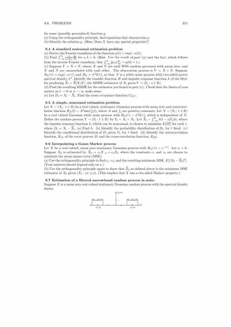
8/11/2019 Random process by B. Hajek
http://slidepdf.com/reader/full/random-process-by-b-hajek 325/448
9.6. PROBLEMS 315
for some (possibly generalized) function g.(a) Using the orthogonality principle, find equations that characterize g.(b) Identify the solution g. (Hint: Does X have any special properties?)
9.4 A standard noncausal estimation problem(a) Derive the Fourier transform of the function g (t) = exp(−α|t|).(b) Find
∞−∞
1a+bω2
dω2π for a, b > 0. (Hint: Use the result of part (a) and the fact, which follows
from the inverse Fourier transform, that ∞−∞ g(ω)dω
2π = g(0) = 1.)(c) Suppose Y = X + N , where X and N are each WSS random processes with mean zero, andX and N are uncorrelated with each other. The observation process is Y = X + N. SupposeRX (τ ) = exp(−α|τ |) and RN = σ2δ (τ ), so that N is a white noise process with two-sided powerspectral density σ2. Identify the transfer function H and impulse response function h of the filterfor producing X t = E [X t|Y ], the MMSE estimator of X t given Y = (Y s : s ∈ R).(d) Find the resulting MMSE for the estimator you found in part (c). Check that the limits of youranswer as σ
→ 0 or σ
→ ∞ make sense.
(e) Let Dt = X t − X t. Find the cross covariance function C D,Y .
9.5 A simple, noncausal estimation problemLet X = (X t : t ∈ R) be a real valued, stationary Gaussian process with mean zero and autocorre-lation function RX (t) = A2sinc(f ot), where A and f o are positive constants. Let N = (N t : t ∈ R)be a real valued Gaussian white noise process with RN (τ ) = σ2δ (τ ), which is independent of X .Define the random process Y = (Y t : t ∈ R) by Y t = X t + N t. Let X t =
∞−∞ h(t − s)Y sds, where
the impulse response function h, which can be noncausal, is chosen to minimize E [D2t ] for each t,
where Dt = X t − X t. (a) Find h. (b) Identify the probability distribution of Dt, for t fixed. (c)Identify the conditional distribution of Dt given Y t, for t fixed. (d) Identify the autocorrelationfunction, RD, of the error process D, and the cross correlation function, RDY .
9.6 Interpolating a Gauss Markov processLet X be a real-valued, mean zero stationary Gaussian process with RX (τ ) = e−|τ |. Let a > 0.Suppose X 0 is estimated by X 0 = c1X −a + c2X a where the constants c1 and c2 are chosen tominimize the mean square error (MSE).(a) Use the orthogonality principle to find c1, c2, and the resulting minimum MSE, E [(X 0 − X 0)2].(Your answers should depend only on a.)(b) Use the orthogonality principle again to show that X 0 as defined above is the minimum MSEestimator of X 0 given (X s : |s| ≥ a). (This implies that X has a two-sided Markov property.)
9.7 Estimation of a filtered narrowband random process in noiseSuppose X is a mean zero real-valued stationary Gaussian random process with the spectral density
shown.
1
f
8 Hz
S (2 f)π X
8 Hz
10 Hz4
10 Hz4
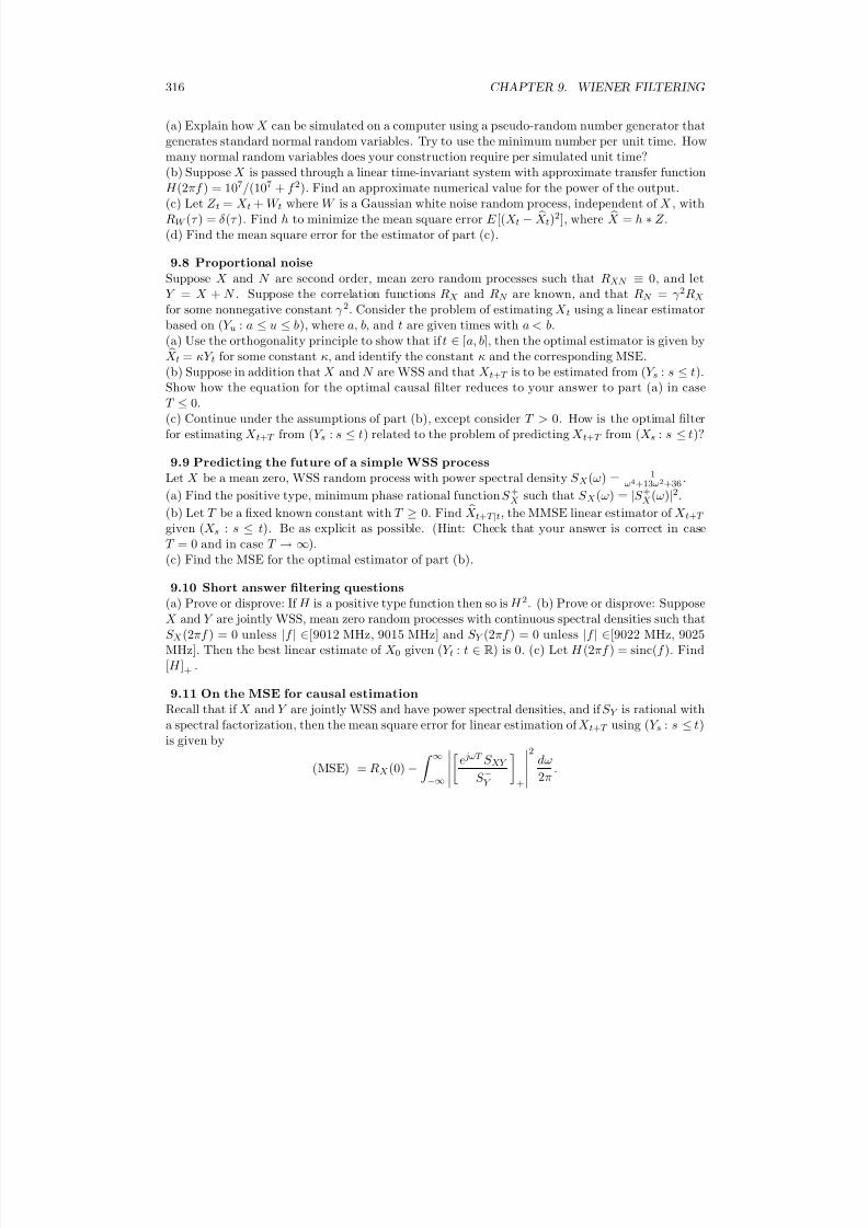
8/11/2019 Random process by B. Hajek
http://slidepdf.com/reader/full/random-process-by-b-hajek 326/448
316 CHAPTER 9. WIENER FILTERING
(a) Explain how X can be simulated on a computer using a pseudo-random number generator thatgenerates standard normal random variables. Try to use the minimum number per unit time. Howmany normal random variables does your construction require per simulated unit time?
(b) Suppose X is passed through a linear time-invariant system with approximate transfer functionH (2πf ) = 107/(107 + f 2). Find an approximate numerical value for the power of the output.(c) Let Z t = X t + W t where W is a Gaussian white noise random process, independent of X , withRW (τ ) = δ (τ ). Find h to minimize the mean square error E [(X t − X t)2], where X = h ∗ Z .(d) Find the mean square error for the estimator of part (c).
9.8 Proportional noiseSuppose X and N are second order, mean zero random processes such that RXN ≡ 0, and letY = X + N . Suppose the correlation functions RX and RN are known, and that RN = γ 2RX
for some nonnegative constant γ 2. Consider the problem of estimating X t using a linear estimatorbased on (Y u : a ≤ u ≤ b), where a, b, and t are given times with a < b.(a) Use the orthogonality principle to show that if t
∈ [a, b], then the optimal estimator is given by X t = κY t for some constant κ, and identify the constant κ and the corresponding MSE.
(b) Suppose in addition that X and N are WSS and that X t+T is to be estimated from (Y s : s ≤ t).Show how the equation for the optimal causal filter reduces to your answer to part (a) in caseT ≤ 0.(c) Continue under the assumptions of part (b), except consider T > 0. How is the optimal filterfor estimating X t+T from (Y s : s ≤ t) related to the problem of predicting X t+T from (X s : s ≤ t)?
9.9 Predicting the future of a simple WSS processLet X be a mean zero, WSS random process with power spectral density S X (ω) = 1
ω4+13ω2+36 .
(a) Find the positive type, minimum phase rational function S +X such that S X (ω) = |S +X (ω)|2.
(b) Let T be a fixed known constant with T
≥ 0. Find X t+T
|t, the MMSE linear estimator of X t+T
given (X s : s ≤ t). Be as explicit as possible. (Hint: Check that your answer is correct in caseT = 0 and in case T → ∞).(c) Find the MSE for the optimal estimator of part (b).
9.10 Short answer filtering questions(a) Prove or disprove: If H is a positive type function then so is H 2. (b) Prove or disprove: SupposeX and Y are jointly WSS, mean zero random processes with continuous spectral densities such thatS X (2πf ) = 0 unless |f | ∈[9012 MHz, 9015 MHz] and S Y (2πf ) = 0 unless |f | ∈[9022 MHz, 9025MHz]. Then the best linear estimate of X 0 given (Y t : t ∈ R) is 0. (c) Let H (2πf ) = sinc(f ). Find[H ]+ .
9.11 On the MSE for causal estimationRecall that if X and Y are jointly WSS and have power spectral densities, and if S Y is rational witha spectral factorization, then the mean square error for linear estimation of X t+T using (Y s : s ≤ t)is given by
(MSE) = RX (0) − ∞−∞
e jωT S XY
S −Y
+
2
dω
2π.
8/11/2019 Random process by B. Hajek
http://slidepdf.com/reader/full/random-process-by-b-hajek 327/448
9.6. PROBLEMS 317
Evaluate and interpret the limits of this expression as T → −∞ and as T → ∞.
9.12 A singular estimation problem
Let X t = Ae j2πf ot
, where f o > 0 and A is a mean zero complex valued random variable withE [A2] = 0 and E [|A|2] = σ2A. Let N be a white noise process with RN (τ ) = σ2
N δ (τ ). Let
Y t = X t + N t. Let X denote the output process when Y is filtered using the impulse responsefunction h(τ ) = αe−(α− j2πf o)tI t≥0.(a) Verify that X is a WSS periodic process, and find its power spectral density (the power spectraldensity only exists as a generalized function–i.e. there is a delta function in it).(b) Give a simple expression for the output of the linear system when the input is X .(c) Find the mean square error, E [|X t − X t|2]. How should the parameter α be chosen to approxi-mately minimize the MSE?
9.13 Filtering a WSS signal plus noiseSuppose X and N are jointly WSS, mean zero, continuous time random processes with RXN
≡ 0.
The processes are the inputs to a system with the block diagram shown, for some transfer functionsK 1(ω) and K 2(ω):
N
K 2
+1
K
Y=X +Nout out X
Suppose that for every value of ω , K i(ω) = 0 for i = 1 and i = 2. Because the two subsystems arelinear, we can view the output process Y as the sum of two processes, X out, due to the input X ,plus N out, due to the input N . Your answers to the first four parts should be expressed in termsof K 1, K 2, and the power spectral densities S X and S N .(a) What is the power spectral density S Y ?
(b) Find the signal-to-noise ratio at the output (the power of X out divided by the power of N out).(c) Suppose Y is passed into a linear system with transfer function H , designed so that the outputat time t is X t, the best linear estimator of X t given (Y s : s ∈ R). Find H .(d) Find the resulting minimum mean square error.(e) The correct answer to part (d) (the minimum MSE) does not depend on the filter K 2. Why?
9.14 A prediction problemLet X be a mean zero WSS random process with correlation function RX (τ ) = e−|τ |. Using theWiener filtering equations, find the optimal linear MMSE estimator (i.e. predictor) of X t+T basedon (X s : s ≤ t), for a constant T > 0. Explain why your answer takes such a simple form.
9.15 Properties of a particular Gaussian processLet X be a zero-mean, wide-sense stationary Gaussian random process in continuous time withautocorrelation function RX (τ ) = (1 + |τ |)e−|τ | and power spectral density S X (ω) = (2/(1 + ω2))2.Answer the following questions, being sure to provide justification.(a) Is X mean ergodic in the m.s. sense?(b) Is X a Markov process?
8/11/2019 Random process by B. Hajek
http://slidepdf.com/reader/full/random-process-by-b-hajek 328/448
318 CHAPTER 9. WIENER FILTERING
(c) Is X differentiable in the m.s. sense?(d) Find the causal, minimum phase filter h (or its transform H ) such that if white noise withautocorrelation function δ (τ ) is filtered using h then the output autocorrelation function is RX .
(e) Express X as the solution of a stochastic differential equation driven by white noise.
9.16 Spectral decomposition and factorization(a) Let x be the signal with Fourier transform given by x(2πf ) =
sinc(100f )e j2πfT
+
. Find theenergy of x for all real values of the constant T .(b) Find the spectral factorization of the power spectral density S (ω) = 1
ω4+16ω2+100 . (Hint: 1+3 jis a pole of S .)
9.17 A continuous-time Wiener filtering problemLet (X t) and (N t) be uncorrelated, mean zero random processes with RX (t) = exp(−2|t|) andS N (ω) ≡ N o/2 for a positive constant N o. Suppose that Y t = X t + N t.(a) Find the optimal (noncausal) filter for estimating X t given (Y s :
−∞ < s < +
∞) and find the
resulting mean square error. Comment on how the MMSE depends on N o.(b) Find the optimal causal filter with lead time T , that is, the Wiener filter for estimating X t+T
given (Y s : −∞ < s ≤ t), and find the corresponding MMSE. For simplicity you can assume thatT ≥ 0. Comment on the limiting value of the MMSE as T → ∞, as N o → ∞, or as N o → 0.
9.18 Estimation of a random signal, using the KL expansionSuppose that X is a m.s. continuous, mean zero process over an interval [a, b], and suppose N isa white noise process, with RXN ≡ 0 and RN (s, t) = σ2δ (s − t). Let (φk : k ≥ 1) be a completeorthonormal basis for L2[a, b] consisting of eigenfunctions of RX , and let (λk : k ≥ 1) denote thecorresponding eigenvalues. Suppose that Y = (Y t : a ≤ t ≤ b) is observed.(a) Fix an index i. Express the MMSE estimator of (X, φi) given Y in terms of the coordinates,
(Y, φ1), (Y, φ2), . . . of Y , and find the corresponding mean square error.(b) Now suppose f is a function in L2[a, b]. Express the MMSE estimator of (X, f ) given Y interms of the coordinates ((f, φ j) : j ≥ 1) of f , the coordinates of Y , the λ’s, and σ. Also, find themean square error.
9.19 Noiseless prediction of a baseband random processFix positive constants T and ωo, suppose X = (X t : t ∈ R) is a baseband random process with
one-sided frequency limit ωo, and let H (n)(ω) = n
k=0( jωT )k
k! , which is a partial sum of the power
series of e jωT . Let X (n)t+T |t denote the output at time t when X is passed through the linear time
invariant system with transfer function H (n). As the notation suggests,
X
(n)t+T |t is an estimator (not
necessarily optimal) of X t+T given (X s : s
≤ t).
(a) Describe X (n)t+T |t in terms of X in the time domain. Verify that the linear system is causal.
(b) Show that limn→∞ an = 0, where an = max|ω|≤ωo|e jωT − H (n)(ω)|. (This means that the power
series converges uniformly for ω ∈ [−ωo, ωo].)(c) Show that the mean square error can be made arbitrarily small by taking n sufficiently large.
In other words, show that limn→∞ E [|X t+T − X (n)t+T |t|2] = 0.
8/11/2019 Random process by B. Hajek
http://slidepdf.com/reader/full/random-process-by-b-hajek 329/448
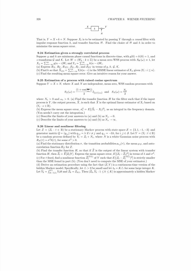
8/11/2019 Random process by B. Hajek
http://slidepdf.com/reader/full/random-process-by-b-hajek 330/448
320 CHAPTER 9. WIENER FILTERING
k + X
N
Y
That is, Y = X ∗ k + N . Suppose X t is to be estimated by passing Y through a causal filter withimpulse response function h, and transfer function H . Find the choice of H and h in order tominimize the mean square error.
9.24 Estimation given a strongly correlated processSuppose g and k are minimum phase causal functions in discrete-time, with g(0) = k(0) = 1, andz-transforms G and K. Let W = (W k : k ∈ Z) be a mean zero WSS process with S W (ω) ≡ 1, letX n =
∞i=−∞ g(n − i)W i and Y n =
∞i=−∞ k(n − i)W i.
(a) Express RX , RY , RXY , S X , S Y , and S XY in terms of g , k , G, K.(b) Find h so that
X n|n =
∞i=−∞ Y ih(n− i) is the MMSE linear estimator of X n given (Y i : i ≤ n).
(c) Find the resulting mean square error. Give an intuitive reason for your answer.
9.25 Estimation of a process with raised cosine spectrumSuppose Y = X + N, where X and N are independent, mean zero, WSS random processes with
S X (ω) =(1 + cos(πω
ωo))
2 I |ω|≤ωo and S N (ω) =
N o2
where N o > 0 and ωo > 0. (a) Find the transfer function H for the filter such that if the inputprocess is Y , the output process, X, is such that X is the optimal linear estimator of X t based on(Y s : s ∈R).(b) Express the mean square error, σ2
e = E [(
X t − X t)
2], as an integral in the frequency domain.(You needn’t carry out the integration.)
(c) Describe the limits of your answers to (a) and (b) as N o → 0.(c) Describe the limits of your answers to (a) and (b) as N o → ∞.
9.26 Linear and nonlinear filteringLet Z = (Z t : t ∈ R) be a stationary Markov process with state space S = 3, 1, −1, −3 andgenerator matrix Q = (q i,j) with q i,j = λ if i = j and q i,i = −3λ, for i, j ∈ S . Let Y = (Y t : t ∈ R)be a random process defined by Y t = Z t + N t, where N is a white Gaussian noise process withRN (τ ) = σ2δ (τ ), for some σ 2 > 0.(a) Find the stationary distribution π, the transition probabilities pi,j(τ ), the mean µZ , and auto-correlation function RZ for Z .(b) Find the transfer function H, so that if
Z is the output of the linear system with transfer
function H, then Z t = E [Z t|Y ]. Express the mean square error, E [(Z t − Z t)2
] in terms of λ and σ2
.(c) For t fixed, find a nonlinear function Z
(NL)t of Y such that E [(Z t − Z
(NL)t )2] is strictly smaller
than the MSE found in part (b). (You don’t need to compute the MSE of your estimator.)(d) Derive an estimation procedure using the fact that (Z, Y ) is a continuous-time version of thehidden Markov model. Specifically, let > 0 be small and let t0 = K for some large integer K .Let Y k =
k(k−1) Y tdt and Z k = Z k. Then ( Z k, Y k : 1 ≤ k ≤ K ) is approximately a hidden Markov
8/11/2019 Random process by B. Hajek
http://slidepdf.com/reader/full/random-process-by-b-hajek 331/448
9.6. PROBLEMS 321
model with observation space R instead of a finite observation space. Identify the (approximate)parameter (π,A ,B) of this Markov model (note that bi,y for i fixed should be a pdf as a functionof y.) (Using this model, the forward backward algorithm could be used to approximately compute
the conditional pmf of X at a fixed time given Y , which becomes asymptotically exact as → 0.An alternative to this approach is to simply start with a discrete-time model. Another alternativeis to derive a continuous-time version of the forward backward algorithm.)
9.27 * Resolution of Wiener and Kalman filteringConsider the state and observation models:
X n = F X n−1 + W n
Y n = H T X n + V n
where (W n : −∞ < n < +∞) and (V n : −∞ < n < +∞) are independent vector-valued randomsequences of independent, identically distributed mean zero random variables. Let ΣW and ΣV
denote the respective covariance matrices of W n and V n. (F , H and the covariance matrices mustsatisfy a stability condition. Can you find it? ) (a) What are the autocorrelation function RX andcrosscorrelation function RXY ?(b) Use the orthogonality principle to derive conditions for the causal filter h that minimizesE [ X n+1 −
∞ j=0 h( j)Y n− j 2]. (i.e. derive the basic equations for the Wiener-Hopf method.)
(c) Write down and solve the equations for the Kalman predictor in steady state to derive anexpression for h, and verify that it satisfies the orthogonality conditions.

8/11/2019 Random process by B. Hajek
http://slidepdf.com/reader/full/random-process-by-b-hajek 332/448
322 CHAPTER 9. WIENER FILTERING
8/11/2019 Random process by B. Hajek
http://slidepdf.com/reader/full/random-process-by-b-hajek 333/448

8/11/2019 Random process by B. Hajek
http://slidepdf.com/reader/full/random-process-by-b-hajek 334/448
324 CHAPTER 10. MARTINGALES
(a) Ω ∈ D,
(b) if A ∈ D then Ac ∈ D,
(c) if A, B ∈ D then AB ∈ D, and more generally, if A1, A2,... is such that Ai ∈ D for i ≥ 1, then∪∞i=1Ai ∈ D.
In particular, the set of events, F , in a probability space (Ω, F , P ), is required to be a σ-algebra.The original motivation for introducing F in this context was a technical one, related to theimpossibility of extending P to be defined on all subsets of Ω, for important examples such asΩ = [0, 1] and P ((a, b)) = b − a for all intervals (a, b). However, σ-algebras are also useful forrepresenting information available to an observer. We call D a sub-σ-algebra of F if D is a σ-algebra such that D ⊂ F . A random variable Z is said to be D-measurable if Z ≤ c ⊂ D forall c. By definition, random variables are functions on Ω that are F -measurable. The smaller theσ-algebra D is, the fewer the set of D measurable random variables. In practice, sub-σ-algebras areusually generated by collections of random variables:
Definition 10.1.1 The σ-algebra generated by a collection of random variables (Y i : i ∈ I ), denoted by σ(Y i : i ∈ I ), is the smallest σ-algebra containing all sets of the form Y i ≤ c.1 The σ-algebra generated by a single random variable Y is denoted by σ(Y ), and sometimes as F Y .An equivalent definition would be that σ(Y i : i ∈ I ) is the smallest σ-algebra such that each Y i ismeasurable with respect to it.
A sub-σ-algebra of F represents knowledge about the probability experiment modeled by theprobability space (Ω, F , P ). In Chapter 3, the information gained from observing a random variableY was modeled by requiring estimators to be random variables of the form g(Y ), for a Borelmeasurable function g. An equivalent condition would be to allow any estimator that is a σ(Y )-measurable random variable. That is, as shown in a starred homework problem, if Y and Z arerandom variables on the same probability space, then Z = g(Y ) for some Borel measurable functiong if and only if Z is σ(Y ) measurable. Using sub-σ-algebras is more general, because some σ-algebrason some probability spaces are not generated by random variables. Using σ-algebras to representinformation also works better when there is an uncountably infinite number of observations, suchas observation of a continuous random process over an interval of time. But in engineering practice,the main difference between the two ways to model information is simply a matter of notation.
Example 10.1.2 (The trivial σ-algebra) Let (Ω, F , P ) be a probability space. Suppose X is arandom variable such that, for some constant co, X (ω) = co for all ω ∈ Ω. Then X is measurablewith respect to the trivial σ-algebra D defined by D = ∅, Ω. That is, constant random variablesare
∅, Ω
-measurable.
Conversely, suppose Y is a ∅, Ω-measurable random variable. Select an arbitrary ωo ∈ Ω andlet co = Y (ωo). On one hand, ω : Y (ω) ≤ c can’t be empty for c ≥ co, so ω : Y (ω) ≤ c = Ω forc ≥ co. On the other hand, ω : Y (ω) ≤ co doesn’t contain ωo for c < co, so ω : Y (ω) ≤ co = ∅ forc < co. Therefore, Y (ω) = co for all ω. That is, ∅, Ω-measurable random variables are constant.
1The smallest one exists–it is equal to the intersection of all σ-algebras which contain all sets of the form Y i ≤ c.
8/11/2019 Random process by B. Hajek
http://slidepdf.com/reader/full/random-process-by-b-hajek 335/448
10.1. CONDITIONAL EXPECTATION REVISITED 325
Definition 10.1.3 If X is a random variable on (Ω, F , P ) with finite mean and D is a sub-σ-
algebra of F , the conditional expectation of X given D, E [X |D], is the unique (two versions equal with probability one are considered to be the same) random variable on (Ω, F , P ) such that
(i) E [X |D] is D-measurable
(ii) E [(X − E [X |D])I D] = 0 for all D ∈ D. (Here I D is the indicator function of D).
We remark that a possible choice of D in property (ii) of the definition is D = Ω, so E [X |D]should satisfy E [X − E [X |D]] = 0, or equivalently, since E [X ] is assumed to be finite, E [X ] =E [E [X |D]]. In particular, an implication of the definition is that E [X |D] also has a finite mean.
Proposition 10.1.4 Definition 10.1.3 is well posed. Specifically, there exits a random variable
satisfying conditions (i) and (ii), and it is unique.
Proof. (Uniqueness) Suppose U and V are each D-measurable random variables such thatE [(X − U )I D] = 0 and E [(X − V )I D] = 0 for all D ∈ D. It follows that E [(U − V )I D] = E [(X −V )I D]−E [(X −U )I D] = 0 for any D ∈ D. A possible choice of D is U > V , so E [(U −V )I U>V ] =0. Since (U − V )I U>V is nonnegative and is strictly positive on the event U > V , it must bethat P U > V = 0. Similarly, P U < V = 0. So P U = V = 1.
(Existence ) Existence is first proved under the added assumption that P X ≥ 0 = 1. LetL2(D) be the space of D-measurable random variables with finite second moments. Then D isa closed, linear subspace of L2(Ω, F , P ), so the orthogonality principle can be applied. For anyn ≥ 0, the random variable X ∧ n is bounded and thus has a finite second moment. Let
X n be the
projection of X
∧n onto L2(
D). Then by the orthogonality principle, X
∧n
− X n is orthogonal
to any random variable in L2(D). In particular, X ∧ n − X n is orthogonal to I D for any D ∈ D.Therefore, E [(X ∧ n − X n)I D] = 0 for all D ∈ D. Equivalently,
E [(X ∧ n)I D] = E [ X nI D]. (10.1)
The next step is to take a limit as n → ∞. Since E [(X ∧ n)I D] is nondecreasing in n for eachD ∈ D, the same is true of E [ X nI D]. Thus, for any n ≥ 0, E [( X n+1 − X n)I D] ≥ 0 for any D ∈ D.Taking D = X n+1 − X n < 0 implies that P X n+1 ≥ X n = 1. Therefore, the sequence ( X n)converges a.s., and we denote the limit by X ∞. We show that X ∞ satisfies the two properties,(i) and (ii), required of E [X |D]. First,
X ∞ is D-measurable because it is the limit of a sequence
of D-measurable random variables. Secondly, for any D ∈ D, the sequences of random variables
(X ∧ n)I D and X nI D are a.s. nondecreasing and nonnegative, so by the monotone convergencetheorem (Theorem 11.6.6) and (10.1):
E [XI D] = limn→∞ E [(X ∧ n)I D] = lim
n→∞ E [ X nI D] = E [ X ∞I D].
So property (ii), E [(X − X ∞)I D] = 0, is also satisfied. Existence is proved in case P X ≥ 0 = 1.
8/11/2019 Random process by B. Hajek
http://slidepdf.com/reader/full/random-process-by-b-hajek 336/448
326 CHAPTER 10. MARTINGALES
For the general case, X can be represented as X = X +−X −, where X + and X − are nonnegativewith finite means. By the case already proved, E [X +|D] and E [X −|D] exist, and, of course, theysatisfy conditions (i) and (ii) in Definition 10.1.3. Therefore, with E [X |D] = E [X +|D] − E [X −|D],
it is a simple matter to check that E ]X |D] also satisfies conditions (i) and (ii), as required.
Proposition 10.1.5 Let X and Y be random variables on (Ω, F , P ) and let A and D be sub-σ-algebras of F .
1. (Consistency with definition based on projection) If E [X 2] < ∞ and V = g(Y ) : g is Borel measurable such that E [g(Y )2] < ∞, then E [X |Y ], defined as the MMSE projection of X onto V (also written as ΠV (X )) is equal to E [X |σ(Y )].
2. (Linearity) If E [X ] and E [Y ] are finite, then aE [X |D] + bE [Y |D] = E [aX + bY |D].
3. (Tower property) If E [X ] is finite and
A ⊂ D ⊂ F , then E [E [X
|D]
|A] = E [X
|A]. (In
particular, E [E [X |D]] = E [X ].)
4. (Positivity preserving) If E [X ] is finite and X ≥ 0 a.s. then E [X |D] ≥ 0 a.s.
5. ( L1 contraction property) E [|E |X |D]|] ≤ E [|X |].6. ( L1 continuity) If E [X n] is finite for all n and E [|X n − X ∞|] → 0, then
E [|E [X n|D] − E [X ∞|D]|] → 0.
7. (Pull out property) If X is D-measurable and E [XY ] and E [Y ] are finite, then E [XY |D] =XE [Y |D].
Proof. (Consistency with definition based on projection) Suppose X and V
are as in part 1.Then, by definition, E [X |Y ] ∈ V and E [(X − E [X |Y ])Z ] = 0 for any Z ∈ V . As mentioned above,a random variable has the form g(Y ) if and only if it is σ(Y )-measurable. In particular, V is simplythe set of σ(Y )-measurable random variables Z such that E [Z 2] < ∞. Thus, E [X |Y ] is σ(Y )measurable, and E [(X − E [X |Y ])Z ] = 0 for any σ(Y )-measurable random variable Z such thatE [Z 2] < ∞. As a special case, E [(X − E [X |Y ])I D] = 0 for any D ∈ σ(Y ). Thus, E [X |Y ] satisfiesconditions (i) and (ii) in Definition 10.1.3 of E [X |σ(Y )]. So E [X |Y ] = E [X |σ(Y )].
(Linearity Property) (This is similar to the proof of linearity for projections, Proposition 3.2.2.)It suffices to check that the linear combination aE [X |D] + bE [Y |D] satisfies the two conditions thatdefine E [aX +bY |D]. First, E [X |D] and E [Y |D] are both D measurable, so their linear combinationis also D-measurable. Secondly, if D ∈ D, then E [(X − E [X |D])I D] = E [(Y − E [Y |D])I D] = 0,from which if follows that
E [(aX + bY − E [aX + bY |D]) I D] = aE [(X − E [X |D])I D] + bE [(Y − E [Y |D])I D] = 0.
Therefore, aE [X |D] + bE [Y |D] = E [aX + bY |D].(Tower Property) (This is similar to the proof of Proposition 3.2.3, about projections onto nested
subspaces.) It suffices to check that E [E [X |D]|A] satisfies the two conditions that define E [X |A].
8/11/2019 Random process by B. Hajek
http://slidepdf.com/reader/full/random-process-by-b-hajek 337/448
8/11/2019 Random process by B. Hajek
http://slidepdf.com/reader/full/random-process-by-b-hajek 338/448
328 CHAPTER 10. MARTINGALES
In the general case, X = X + − X −, where X + = X ∨ 0 and X − = (−X ) ∨ 0, and similarly Y =Y + − Y −. The hypotheses imply E [X ±Y ±] and E [Y ±] are finite so that E [X ±Y ±|D] = X ±E [Y ±|D],and therefore
E [X ±Y ±I D] = E [X ±E [Y ±|D]I D], (10.4)
where in these equations, the sign on both appearances of X should be the same, and the sign onboth appearances of Y should be the same. The left side of (10.2) can be expressed as a linearcombination of terms of the form E [X ±Y ±I D]:
E [XY I D] = E [X +Y +I D] − E [X +Y −I D] − E [X −Y +I D] + E [X −Y −I D].
Similarly, the right side of (10.2) can be expressed as a linear combination of terms of the formE [X ±E [Y ±|D]I D]. Therefore, (10.2) follows from (10.4).
10.2 Martingales with respect to filtrations
A filtration of a σ-algebra F is a sequence of sub-σ-algebras F F F = (F n : n ≥ 0) of F , such thatF n ⊂ F n+1 for n ≥ 0. If Y = (Y n : n ≥ 0) or Y = (Y n : n ≥ 1) is a sequence of random variables on(Ω, F , P ), the filtration generated by Y , often written as F F F Y = (F Y n : n ≥ 0), is defined by lettingF Y n = σ(Y k : k ≤ n). (If there is no variable Y 0 defined, we take F Y 0 to be the trivial σ-algebra,F Y 0 = ∅, Ω, representing no observations.)
In practice, a filtration represents an sequence of observations or measurements. If the filtrationis generated by a random process, then the information available at time n is represents observationof the random process up to time n.
A random process (X n : n
≥ 0) is adapted to a filtration
F F F if X n is
F n measurable for each
n ≥ 0.
Definition 10.2.1 Let (Ω, F , P ) be a probability space with a filtration F F F = (F n : n ≥ 0). Let Y = (Y n : n ≥ 0) be a sequence of random variables adapted to F F F . Then Y is a martingale with respect to F F F if for all n ≥ 0:
(i) Y n is F n measurable (i.e. the process Y is adapted to F F F )
(ii) E [|Y n|] < ∞,
(iii) E [Y n+1|F n] = Y n a.s.
Similarly, Y is a submartingale relative to F F F if (0) and (i) are true and E [Y n+1|F n] ≥ Y n, a.s.,and Y is a supermartingale relative to F F F if (0) and (i) are true and E [Y n+1|F n] ≤ Y n a.s.
Some comments are in order. Note that if Y = (Y n : n ≥ 0) is a martingale with respect to afiltration F F F = (F n : n ≥ 0), then Y is also a martingale with respect to the filtration generated byY itself. Indeed, for each n, Y n is F n measurable, whereas F Y n is the smallest σ-algebra with respect
8/11/2019 Random process by B. Hajek
http://slidepdf.com/reader/full/random-process-by-b-hajek 339/448
10.2. MARTINGALES WITH RESPECT TO FILTRATIONS 329
to which Y n is measurable, so F Y n ⊂ F n. Therefore, the tower property of conditional expectation,the fact Y is a margtingale with respect to F F F , and the fact Y n is F Y n measurable, imply
E [Y n+1|F Y
n ] = E [E [Y n+1|F n]|F Y
n ] = E [Y n|F Y
n ] = Y n.
Thus, in practice, if Y is said to be a martingale and no filtration F is specified, at least Y is amartingale with respect to the filtration it generates.
Note that if Y is a martingale with respect to a filtration F F F , then for any n, k ≥ 0,
E [Y n+k+1|F n] = E [E [Y n+k+1|F n+k|F n] = E [Y n+k|F n]
Therefore, by induction on k for n fixed:
E [X n+k|F n] = X n, (10.5)
for n, k ≥ 0.
Example 10.2.2 Suppose (U i : i ≥ 1) is a collection of independent random variables, each withmean zero. Let S 0 = 0 and for n ≥ 1, S n =
ni=1 U i. Let F F F = (F n : n ≥ 0) denote the filtration
generated by S : F n = σ(S 0, . . . , S n). Equivalently, F is the filtration generated by (U i : i ≥ 1):F 0 = ∅, Ω and F n = σ(S 0, . . . , S n). for n ≥ 1. Then S = (S n : n ≥ 0) is a martingale with respectto F F F :
E [S n+1|F n] = E [U n+1|F n] + E [S n|F n] = 0 + S n = S n.
Example 10.2.3 Suppose S = (S n : n ≥ 0) and F F F = (F n : n ≥ 0) are defined as in Example10.2.2 in terms of a sequence of independent random variables U = (U i : i ≥ 1). Suppose inaddition that Var(U i) = σ2 for some finite constant σ2. Finally, let M n = S 2n −nσ2 for n ≥ 0. ThenM = (M n : n ≥ 0) is a martingale relative to F F F . Indeed, M is adapted to F F F . Since S n+1 = S n + U n,we have M n+1 = M n + 2S nU n+1 + U 2n+1 − σ2 so that
E [M n+1|F n] = E [M n|F n] + 2S nE [U n|F n]] + E [U 2n − σ2|F n]]
= M n + 2S nE [U n] + E [U 2n − σ2]
= M n
Example 10.2.4 Suppose X 1, X 2, . . . is a sequence of independent, identically distributed randomvariables and θ is a number such that E [eθX 1] < ∞. Let S 0 = 0 and S n = X 1 + · · · + X n for n ≥ 1.Then (M n) defined by M n = eθS n/E [eθX 1]n for n ≥ 0 is a martingale.
8/11/2019 Random process by B. Hajek
http://slidepdf.com/reader/full/random-process-by-b-hajek 340/448
330 CHAPTER 10. MARTINGALES
Example 10.2.5 (Galton-Watson branching process) A Galton-Watson branching process startswith an initial set of individuals, called the zeroth generation. For example, there may be just one
individual in the zeroth generation. The (n + 1)st generation is the set of all offspring of individualsin the nth generation. The number of offspring of each individual has the same distribution asa given discrete random variable X, with the numbers of offspring of different individuals beingmutually independent. Let Gn denote the number of individuals in the nth generation of a branchingprocess. Select a > 0 so that E [aX ] = 1 and suppose E [aG0 ] < ∞. Then, aGn is a martingale.
Example 10.2.6 (Doob martingale) Let M n = E [Φ|F n] for n ≥ 0, where Φ is a random variablewith finite mean, and F F F = (F n : n ≥ 0) is a filtration. Then, by the tower property of conditionalexpectation, M = (M n : n ≥ 0) is a martingale with respect to F F F .
Definition 10.2.7 A martingale difference sequence (Dn : n ≥ 1) relative to a filtration F F F = (F n :n ≥ 0) is a sequence of random variables (Dn : n ≥ 1) such that
(i) (Dn : n ≥ 1) is adapted to F F F (i.e. Dn is F n-measurable for each n ≥ 1)
(ii) E [|Dn|] < ∞ for n ≥ 1
(iii) E [Dn+1|F n] = 0 a.s. for all n ≥ 0.
Equivalently, (Dn : n ≥ 1) has the form Dn = M n − M n−1 for n ≥ 1, for some (M n : n ≥ 0) which is a martingale with respect to
F F F .
Definition 10.2.8 A random process (H n : n ≥ 1) is said to be predictable with respect to afiltration F F F = (F n : n ≥ 0) if H n is F n−1 measurable for all n ≥ 1. (Sometimes this is called “one-step” predictable, because F n determines H one step ahead.)
Example 10.2.9 (Nonlinear innovations process, a.k.a. Doob decomposition) Suppose X = (X n :n ≥ 1) is a sequence of random variables with finite means that is adapted to a filtration F F F . LetH n = E [X n|F n−1] for n ≥ 0. Then H = (H n : n ≥ 1) is a predictable process and D = (Dn : n ≥ 1),defined by Dk = X k − H k, is a martingale difference sequence with respect to F F F . In summary, anysuch process X is the sum of a predicable process H and a martingale difference sequence D.Moreover, for given X and
F F F , this decomposition is unique up to events of measure zero, because
a predictable martingale difference sequence is almost surely identically zero.
Example 10.2.10 Suppose (Dn : n ≥ 1) is a martingale difference sequence and (H k : k ≥ 1) isa bounded predictable process, both relative to a filtration F F F = (F n : n ≥ 0). We claim that the
8/11/2019 Random process by B. Hajek
http://slidepdf.com/reader/full/random-process-by-b-hajek 341/448
10.3. AZUMA-HOEFFDING INEQUALTITY 331
new process D = ( Dn : n ≥ 1) defined by Dn = H nDn is also a martingale difference sequence withrespect to F F F . Indeed, it is adapted, has finite means, and
E [H n+1Dn+1|F n] = H n+1E [Dn+1|F n] = 0,
where we pulled out the F n measurable random variable H n+1 from the conditional expectationgiven F n. An interpretation is that Dn is the net gain to a gambler if one dollar is staked on theoutcome of a fair game in round n, and so H nDn is the net stake if H n dollars are staked on roundn. The requirement that (H k : k ≥ 1) be predictable means that the gambler must decide howmuch to stake in round n based only on information available at the end of round n − 1. It wouldbe an unfair advantage if the gambler already knew Dn when deciding how much money to stakein round n.
If the initial reserves of the gambler were some constant M 0, then the reserves of the gamblerafter n rounds would be given by:
M n = M 0 +n
k=1
H kDk
Then (M n : n ≥ 0) is a margingale with respect to F F F . The random variables are H kDk, 1 ≤ k ≤ nare orthogonal. Also, E [(H kDk)2] = E [E [(H kDk)2|F k−1]] = E [H 2kE [D2
k|F k−1]]. Therefore,
E [(M n − M 0)2] =n
k=1
E [H 2kE [D2k|F k−1]].
10.3 Azuma-Hoeffding inequaltity
One of the most simple inequalities for martingales is the Azuma-Hoeffding inequality. It is provenin this section, and applications to prove concentration inequalities for some combinatorial problemsare given.2
Lemma 10.3.1 Suppose D is a random variable with E [D] = 0 and P |D − b| ≤ d = 1 for some constant b. Then for any α ∈R, E [eαD] ≤ e(αd)2/2.
Proof. Since D has mean zero and D lies in the interval [b − d, b + d] with probability one, theinterval must contain zero, so |b| ≤ d. To avoid trivial cases we assume that |b| < d. Since eαx is
convex in x, the value of e
αx
for x ∈ [b − d, b + d] is bounded above by the linear function that isequal to eαx at the endpoints, x = b ± d, of the interval:
eαx ≤ x − b + d
2d eα(b+d) +
b + d − x
2d eα(b−d). (10.6)
2See McDiarmid survey paper
8/11/2019 Random process by B. Hajek
http://slidepdf.com/reader/full/random-process-by-b-hajek 342/448
332 CHAPTER 10. MARTINGALES
Since D lies in that interval with probability one, (10.6) remains true if x is replaced by the randomvariable D. Taking expectations on both sides and using E [D] = 0 yields
E [eαD
] ≤ d
−b
2d eα(b+d)
+ b + d
2d eα(b
−d)
. (10.7)
The proof is completed by showing that the right side of ( 10.7) is less than or equal to e(αd)2/2 forany |b| < d. Letting u = αd and θ = b/d, the inequality to be proved becomes f (u) ≤ eu
2/2, foru ∈ R and |θ| < 1, where
f (u) = ln
(1 − θ)eu(1+θ) + (1 + θ)eu(−1+θ)
2
.
Taylor’s formula implies that f (u) = f (0)+f (0)u+f (v)u2
2 for some v in the interval with endpoints0 and u. Elementary, but somewhat tedious, calculations show that
f (u) = (1 − θ2)(eu − e−u)
(1 − θ)eu + (1 + θ)e−u
and
f (u) = 4(1 − θ2)
[(1 − θ)eu + (1 + θ)e−u]2
= 1
cosh2(u + β ),
where β = 12 ln( 1−θ
1+θ ). Note that f (0) = f (0) = 0, and f (u) ≤ 1 for all u ∈ R. Therefore,
f (u) ≤
u2/2 for all u ∈R, as was to be shown.
Proposition 10.3.2 (Azuma-Hoeffding inequality with centering) Let (Y n : n ≥ 0) be a martingale and (Bn : n ≥ 1) be a predictable process, both with respect to a filtration F F F = (F n : n ≥ 0), such that P |Y n+1 − Bn+1| ≤ dn = 1 for all n ≥ 0. Then
P |Y n − Y 0| ≥ λ ≤ 2exp
− λ2
2n
i=1 d2i
.
Proof. Let n ≥ 0. The idea is to write Y n = Y n − Y n−1 + Y n−1, to use the tower property of conditional expectation, and to apply Lemma 10.3.1 to the random variable Y n − Y n−1 for d = dn.This yields:
E [eα(Y n−Y 0)] = E [E [eα(Y n−Y n−1+Y n−1−Y 0)|F n−1]]
= E [eα(Y n−1−Y 0)E [eα(Y n−Y n−1 |F n−1]]
≤ E [eα(Y n−1−Y 0)]e(αdn)2/2.
8/11/2019 Random process by B. Hajek
http://slidepdf.com/reader/full/random-process-by-b-hajek 343/448
10.3. AZUMA-HOEFFDING INEQUALTITY 333
Thus, by induction on n,
E [eα(Y n−Y 0)] ≤ e(α2/2)Pn
i=1 d2i .
The remainder of the proof is essentially the Chernoff inequality:
P Y n − Y 0 ≥ λ ≤ E [eα(Y n−Y 0−λ)] ≤ e(α2/2)Pn
i=1 d2i−αλ.
Finally, taking α to make this bound as tight as possible, i.e. α = λPni=1 d
2i
, yields
P Y n − Y 0 ≥ λ ≤ exp
− λ2
2n
i=1 d2i
.
Similarly, P Y n − Y 0 ≤ −λ satisfies the same bound because the previous bound applies for (Y n)replaced by (−Y n), yielding the proposition.
Definition 10.3.3 A function f of n variables x1, . . . , xn is said to satisfy the Lipschitz condition with constant c if |f (x1, . . . , xn) − f (x1, . . . , xn−1, yi, xi+1, . . . , xn)| ≤ c for any x1, . . . , xn, i, and yi.
3
Proposition 10.3.4 (McDiarmid’s inequality) Suppose F = f (X 1, . . . , X n), where f satisfies the Lipschitz condition with constant c, and X 1, . . . , X n are independent random variables. Then P |F − E [F ]| ≥ λ ≤ 2exp(−2λ2
nc2 ).
Proof. Let (Z k : 0 ≤ k ≤ n) denote the Doob martingale defined by Z k = E [F |F X k ], where,
as usual, F X k = σ(X k : 1 ≤ k ≤ n) is the filtration generated by (X k). Note that F X
0 is the trivialσ-algebra ∅, Ω, corresponding to no observations, so Z 0 = E [F ]. Also, Z n = F . In words, Z k is
the expected value of F , given that the first k X ’s are revealed.For 0 ≤ k ≤ n − 1, let
gk(x1, . . . , xk, xk+1) = E [f (x1, . . . , xk+1, X k+2, . . . , X n)].
Note that Z k+1 = gk(X 1, . . . , X k+1). Since f satisfies the Lipschitz condition with constant c, thesame is true of gk. In particular, for x1, . . . , xk fixed, the set of possible values (i.e. range) of gk(x1, . . . , xk+1) as xk+1 varies, lies within some interval (depending on x1, . . . , xk) with length atmost c. We define mk(x1, · · · , xk) to be the midpoint of the smallest such interval:
mk(x1, . . . , xk) =supxk+1
gk(x1, . . . , xk+1) + inf xk+1 gk(x1, . . . , xk+1)
2
and let Bk+1 = mk(X 1, . . . , X k). Then B is a predictable process and
|Z k+1
− Bk+1
| ≤ c
2 with
probability one. Thus, the Azuma-Hoeffding inequality with centering can be applied with di = c2for all i, giving the desired result.
3Equivalently, f (x) − f (y) ≤ cdH (x, y), where dH (x, y) denotes the Hamming distance, which is the number of coordinates in which x and y differ. In the analysis of functions of a continuous variable, the Euclidean distance isused instead of the Hamming distance.
8/11/2019 Random process by B. Hajek
http://slidepdf.com/reader/full/random-process-by-b-hajek 344/448
334 CHAPTER 10. MARTINGALES
Example 10.3.5 Let V = v1, . . . , vn be a finite set of cardinality n ≥ 1. For each i, j with1 ≤ i < j ≤ n, suppose that Z i,j is a Bernoulli random variable with parameter p, where 0 ≤ p ≤ 1.
Suppose that the Z ’s are mutually independent. Let G = (V, E ) be a random graph, such that fori < j, there is an undirected edge between vertices vi and v j (i.e. vi and v j are neighbors) if andonly if Z i,j = 1. Equivalently, the set of edges is E = i, j : i < j and Z i,j = 1. An independentset in the graph is a set of vertices such that no two of the vertices in the set are neighbors. Let
I = I (G) denote the maximum of the cardinalities of all independent sets for G. Note that I isa random variable, because the graph is random. We shall apply McDiarmid’s inequality to finda concentration bound for I (G). Note that I (G) = f ((Z i,j : 1 ≤ i < j ≤ n)), for an appropriatefunction f. We could write a computer program for computing f, for example by cycling throughall subsets of V , seeing which ones are independent sets, and reporting the largest cardinality of the independent. The running time for this algorithm is exponential in n. However, there is noneed to be so explicit about how to compute f. Observe next that changing any one of the Z ’s
would change I (G) by at most one. In particular, if there is an independent set in a graph, andif one edge is added to the graph, then at most one vertex would have to be removed from theindependent set for the original graph to obtain an independent set for the new graph. Thus, f satisfies the Lipschitz condition with constant c = 1. Thus, by McDiarmid’s inequality with c = 1and m variables, where m = n(n − 1)/2,
P |I − E [ I ]| ≥ λ ≤ 2exp(− 4λ2
n(n − 1)).
More thought yields a tighter bound. For 1 ≤ i ≤ n, let X i = (Z 1,i, Z i2,i, . . . , Z i−1,i). In words, foreach i, X i determines which vertices with index less than i are neighbors of vertex vi. Of course I is also determined by X 1, . . . , X n. Moreover, if any one of the X ’s changes, I changes by at mostone. That is,
I can be expressed as a function of the n variables X
1, . . . , X
n, such that the function
satisfies the Lipschitz condition with constant c = 1. Therefore, by McDiarmid’s inequality withc = 1 and n variables,4
P |I − E [ I ]| ≥ λ ≤ 2exp(−2λ2
n ).
For example, if λ = a√
n, we have
P |I − E [ I ]| ≥ a√
n ≤ 2 exp(−2a2)
whenever n ≥ 1, 0 ≤ p ≤ 1, and a > 0.
Note that McDiarmid’s inequality, as illustrated in the above example, gives an upper boundabout how spread out the distribution of a random variable F is, without requiring specific knowl-edge about the value of the mean, E [F ]. Inequalities of this form are known as concentration inequalities . McDiarmid’s inequality can similarly be applied to obtain concentration inequalitiesfor many other numbers associated with graphs, such as the size of a maximum matching (a match-ing is a set of edges, no two of which have a node in common), chromatic index (number of colors
4Since X n is degenerate, we could use n − 1 instead of n, but it makes little difference.
8/11/2019 Random process by B. Hajek
http://slidepdf.com/reader/full/random-process-by-b-hajek 345/448
10.4. STOPPING TIMES AND THE OPTIONAL SAMPLING THEOREM 335
needed to color all edges so that all edges containing a single vertex are different colors), chromaticnumber (number of colors needed to color all vertices so that neighbors are different colors), mini-mum number of edges that need to be cut to break graph into two equal size components, and so
on.
10.4 Stopping times and the optional sampling theorem
Let X = (X k : k ≥ 0) be a martingale with respect to a filtration F F F = (F k : k ≥ 0). Note thatE [X k+1] = E [E [X k+1|F k] = E [X k]. So, by induction on n, E [X n] = E [X 0] for all n ≥ 0.
A useful interpretation of a martingale X = (X k : k ≥ 0) is that X k is the reserve (amount of money on hand) that a gambler playing a fair game at each time step, has after k time steps, if X 0is the initial reserve. (If the gambler is allowed to go into debt, the reserve can be negative.) Thecondition E [X k+1|F k] = X k means that, given the knowledge that is observable up to time k, theexpected reserve after the next game is equal to the reserve at time k. The equality E [X n] = E [X 0]
has the natural interpretation that the expected reserve of the gambler after n games have beenplayed, is equal to the inital reserve X 0.
This section focuses on the following question. What happens if the gambler stops after arandom number, T , of games? Is it true that E [X T ] = E [X 0]?
Example 10.4.1 Suppose that X n = W 1 + · · · + W n where P W k = 1 = P W k = −1 = 0.5 forall k, and the W ’s are independent. Let T be the random time:
T =
3 if W 1 + W 2 + W 3 = 10 else
Then X T = 3 with probability 1/8, and X T = 0 otherwise. Hence, E [X T ] = 3/8.
Does example 10.4.1 give a realistic strategy for a gambler to obtain a strictly positive expectedpayoff from a fair game? To implement the strategy, the gambler should stop gambling after T games. However, the event T = 0 depends on the outcomes W 1, W 2, and W 3. Thus, at timezero, the gambler is required to make a decision about whether to stop before any games are playedbased on the outcomes of the first thee games. Unless the gambler can somehow predict the future,the gambler will be unable to implement the strategy of stopping play after T games.
Intuitively, a random time corresponds to an implementable stopping strategy if the gamblerhas enough information after n games to tell whether to play future games. That type of conditionis captured by the notion of optional stopping time, defined as follows.
Definition 10.4.2 An optional stopping time T relative to a filtration F F F = (F k : k ≥ 0) is a random variable with values in Z+ such that for any n ≥ 0, T ≤ n ∈ F n.
The intuitive interpretation of the condition T ≤ n ∈ F n is that, the gambler should have enoughinformation by time n to know whether to stop by time n. Since σ-algebras are closed under setcomplements, the condition in the definition of an optional stopping time is equivalent to requiring
8/11/2019 Random process by B. Hajek
http://slidepdf.com/reader/full/random-process-by-b-hajek 346/448
336 CHAPTER 10. MARTINGALES
that, for any n ≥ 0, T > n ∈ F n. This means that the gambler should have enough informationby time n to know whether to continue gambling strictly beyond time n.
Example 10.4.3 Let (X n : n ≥ 0) be a random process adapted to a filtration F F F = (F n : n ≥ 0).Let A be some fixed (Borel measurable) set, and let T = minn ≥ 0 : X n ∈ A. Then T is astopping time relative to F F F . Indeed, T ≤ n = X k ∈ A for some k with 0 ≤ k ≤ n. So T ≤ nis an event determined by (X 0, . . . , X n), which is in F n because X is adapted to the filtration.
Example 10.4.4 Suppose W 1, W 2, . . . are independent Bernoulli random variables with p = 0.5,modeling fair coin flips. Suppose that if a gambler stakes some money at the beginning of thenth round, then if W n = 1, the gambler wins back the stake and an additional equal amount. If W n = 0, the gambler loses the money staked. Let X n denote the reserve of the gambler after n
rounds. For simplicity, we assume that the gambler can borrow money as needed, and that theinitial reserve of the gambler is zero. So X 0 = 0. Suppose the gambler adopts the following strategy.The gambler continues playing until the first win, and in each round until stopping, the gamblerstakes the amount of money needed to insure that the reserve at the time the gambler stops, is onedoller. For example, the gambler initially borrows one dollar, and stakes it on the first outcome.If W 1 = 1 the gambler’s reserve (money in hand minus the amount borrowed) is one dollar, andthe gambler stops, so T = 1 and X T = 1. Since no money is staked after time T , X k = X T forall k ≥ T . If the gambler loses in the first round (i.e. W 1 = 0), then X 1 = −1. In that case,the gambler keeps playing, and, next, borrows two more dollars and stakes them on the secondoutcome. If W 2 = 1 the gambler’s reserve is one dollar, and the gambler stops. So T = 2 andX T = 1. If the gambler loses in the second round (i.e. W 2 = 0), then X 2 = −3. In that case, thegambler keeps playing, and, next, borrows four more dollars and stakes them on the third outcome,and so on. The random process (X n : n ≥ 0) is a martingale. For this strategy, the number of rounds, T , that the gambler plays has the geometric distribution with parameter p = 0.5. Thus,E [T ] = 2. In particular, T is finite with probability one. Thus, X T = 1 a.s., while X 0 = 0. Thus,E [X T ] = E [X 0]. This strategy does not require the gambler to be able to predict the future, andthe gambler is always up one dollar after stopping.
But don’t run out and start playing this strategy, expecting to make money for sure. There isa catch–the amount borrowed can be very large. Indeed, let us compute the expectation of B , thetotal amount borrowed before the final win. If T = 1 then B = 1 (only the dollar borrowed in thefirst round is counted). If T = 2 then B = 3 (the first dollar in the first round, and two more inthe second). In general, B = 2T − 1. Thus,
E [B] =∞
n=1
(2n − 1)P T = n =∞n=1
(2n − 1)2−n =∞
n=1
(1 − 2−n) = +∞
That is, the expected amount of money the gambler will need to borrow is infinite.
8/11/2019 Random process by B. Hajek
http://slidepdf.com/reader/full/random-process-by-b-hajek 347/448
10.4. STOPPING TIMES AND THE OPTIONAL SAMPLING THEOREM 337
Proposition 10.4.5 If X is a martingale and T is an optional stopping time, relative to (Ω,F F F , P ),then E [X T ∧n] = E [X 0] for any n.
Proof. Note that
X T ∧(n+1) − X T ∧n =
0 if T ≤ n
X ∧ (n + 1) − X ∧ n if T > n
= (X ∧ (n + 1) − X ∧ n)I T>n
Using this and the tower property of conditional expectation yields
E [X T ∧(n+1) − X T ∧n] = E [E [(X ∧ (n + 1) − X ∧ n)I T>n|F n]]
= E [E [(X ∧ (n + 1) − X ∧ n)|F n]I T>n] = 0
because E [(X ∧
(n + 1)−
X ∧
n)|F
n] = 0. Therefore, E [X ∧
(n + 1)] = E [X ∧
n] for all n ≥
0. Soby induction on n, E [X T ∧n] = E [X 0] for all n ≥ 0.
The following corollary follows immediately from Proposition 10.4.5.
Corollary 10.4.6 If X is a martingale and T is an optional stopping time, relative to (Ω,F F F , P ),then E [X 0] = limn→∞ E [X T ∧n]. In particular, if
limn→∞ E [X T ∧n] = E [X T ] (10.8)
then E [X T ] = E [X 0].
By Corollary 10.4.6, the trick to establishing E [X T ] = E [X 0] comes down to proving (10.8). Notethat X T ∧n
a.s.→ X T as n → ∞, so (10.8) is simply requiring the convergence of the means to themean of the limit, for an a.s. convergent sequence of random variables. There are several differentsufficient conditions for this to happen, involving conditions on the martingale X , the stoppingtime T , or both. For example:
Corollary 10.4.7 If X is a martingale and T is an optional stopping time, relative to (Ω,F F F , P ),and if T is bounded (so P T ≤ n = 1 for some n) then E [X T ] = E [X 0].
Proof. If P T ≤ n = 1 then T ∧ n = T with probability one, so E [X T ∧n = X T ]. Therefore, thecorollary follows from Proposition 10.4.5.
Corollary 10.4.8 If X is a martingale and T is an optional stopping time, relative to (Ω,F F F , P ),and if there is a random variable Z such that |X n| ≤ Z a.s. for all n, and E [Z ] < ∞, then E [X T ] = E [X 0].
8/11/2019 Random process by B. Hajek
http://slidepdf.com/reader/full/random-process-by-b-hajek 348/448
338 CHAPTER 10. MARTINGALES
Proof. Let > 0. Since E [Z ] < ∞, there exists δ > 0 so that if A is any set with P (A) < δ , then
E [ZI A] < . Since X T ∧na.s.→ X T , we also have X T ∧n
p.→ X T . Therefore, if n is sufficiently large,P |X T ∧n − X T | ≥ ≤ δ . For such n,
|X T ∧n − X T | ≤ + |X T ∧n − X T |I |X T ∧n−X T |>≤ + 2|Z |I |X T ∧n−X T |> (10.9)
Now E [|Z |I |X T ∧n−X T |>] < by the choice of δ and n. So taking expectations of each side of (10.9)yields E [|X T ∧n − X T |] ≤ 3. Both X T ∧n and X T have finite means, because both have absolutevalues less than or equal to Z , so
|E [X T ∧n] − E [X T ]| = |E [X T ∧n − X T ]| ≤ E [|X T ∧n − X T |] < 3
Since was an arbitrary positive number, the corollary is proved.
Corollary 10.4.9 Suppose (X n : n
≥ 0) is a martingale relative to (Ω,
F F F , P ). Suppose
(i) there is a constant c such that E [ |X n+1 − X n| |F n] ≤ c for n ≥ 0,(ii) T is stopping time such that E [T ] < ∞.Then E [X T ] = E [X 0]. If, instead, (X n : n ≥ 0) is a submartingale relative to (Ω,F F F , P ), satisfying (i) and (ii), then E [X T ] ≥ E [X 0].
Proof. Suppose (X n : n ≥ 0) is a martingale relative to (Ω,F F F , P ), satisfying (i) and (ii). Lookingat the proof of Corollary 10.4.8, we see that it is enough to show that there is a random variable Z such that E [Z ] < +∞ and |X T ∧n| ≤ Z for all n ≥ 0. Let
Z = |X 0| + |X 1 − X 0| + · · · + |X T − X T −1|Obviously, |X T ∧n| ≤ Z for all n ≥ 0, so it remains to show that E [Z ] < ∞. But
E [Z ] = E [|X 0] + E ∞i=1
|X i − X i−1|I i≤T = E [|X 0|] + E
∞i=1
E |X i − X i−1|I i≤T | F i−1
= E [|X 0|] + E
∞i=1
I i≤T E [|X i − X i−1| | F i−1]
= E [|X 0|] + cE [T ] < ∞
The first statement of the Corollary is proved. If instead X is a submartingale, then a minorvariation of Proposition 10.4.5 yields that E [X T
∧n]
≥ E [X 0]. The proof for the first part of the
corollary, already given, shows that conditions (i) and (ii) imply that E [X T ∧n] → E [X T ] as n → ∞.Therefore, E [X T ] ≥ E [X 0].
Martingale inequalities offer a way to provide upper and lower bounds on the completion timesof algorithms. The following example shows how a lower bound can be found for a particular game.
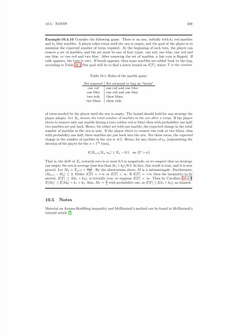
8/11/2019 Random process by B. Hajek
http://slidepdf.com/reader/full/random-process-by-b-hajek 349/448
10.5. NOTES 339
Example 10.4.10 Consider the following game. There is an urn, initially with k1 red marblesand k2 blue marbles. A player takes turns until the urn is empty, and the goal of the player is to
minimize the expected number of turns required. At the beginning of each turn, the player canremove a set of marbles, and the set must be one of four types: one red, one blue, one red andone blue, or two red and two blue. After removing the set of marbles, a fair coin is flipped. If tails appears, the turn is over. If heads appears, then some marbles are added back to the bag,according to Table 10.1 Our goal will be to find a lower bound on E [T ], where T is the number
Table 10.1: Rules of the marble game
Set removed Set returned to bag on “heads”
one red one red and one blueone blue one red and one blue
two reds three bluestwo blues three reds
of turns needed by the player until the urn is empty. The bound should hold for any strategy theplayer adopts. Let X n denote the total number of marbles in the urn after n turns. If the playerelects to remove only one marble during a turn (either red or blue) then with probability one half,two marbles are put back. Hence, for either set with one marble, the expected change in the totalnumber of marbles in the urn is zero. If the player elects to remove two reds or two blues, thenwith probability one half, three marbles are put back into the urn. For these turns, the expectedchange in the number of marbles in the urn is -0.5. Hence, for any choice of un (representing the
decision of the player for the n + 1th
turn),
E [X n+1|X n, un] ≥ X n − 0.5 on T > n
That is, the drift of X n towards zero is at most 0.5 in magnitude, so we suspect that no strategycan empty the urn in average time less than (k1 + k2)/0.5. In fact, this result is true, and it is nowproved. Let M n = X n∧T + n∧T
2 . By the observations above, M is a submartingale. Furthermore,|M n+1 − M n| ≤ 2. Either E [T ] = +∞ or E [T ] < ∞. If E [T ] = +∞ then the inequality to beproved, E [T ] ≥ 2(k1 + k2), is trivially true, so suppose E [T ] < ∞. Then by Corollary 10.4.9,E [M T ] ≥ E [M 0] = k1 + k2. Also, M T = T
2 with probability one, so E [T ] ≥ 2(k1 + k2), as claimed.
10.5 Notes
Material on Azuma-Hoeffding inequality and McDiarmid’s method can be found in McDiarmid’stutorial article [7].
8/11/2019 Random process by B. Hajek
http://slidepdf.com/reader/full/random-process-by-b-hajek 350/448
340 CHAPTER 10. MARTINGALES
10.6 Problems
10.1 Two martingales associated with a simple branching process
Let Y = (Y n : n ≥ 0) denote a simple branching process. Thus, Y n is the number of individuals inthe nth generation, Y 0 = 1, the numbers of offspring of different individuals are independent, andeach has the same distribution as a random variable X .(a) Identify a constant θ so that Gn = Y n
θn is a martingale.(b) Let E denote the event of eventual extinction, and let α = P E. Show that P (E|Y 0, . . . , Y n) =αY n. Thus, M n = αY n is a martingale.(c) Using the fact E [M 1] = E [M 0], find an equation for α. (Note: Problem 4.33 shows that α isthe smallest positive solution to the equation, and α < 1 if and only if E [X ] > 1.)
10.2 A covering problemConsider a linear array of n cells. Suppose that m base stations are randomly placed among thecells, such that the locations of the base stations are independent, and uniformly distributed amongthe n cell locations. Let r be a positive integer. Call a cell i covered if there is at least one basestation at some cell j with |i − j| ≤ r − 1. Thus, each base station (unless those near the edge of the array) covers 2r − 1 cells. Note that there can be more than one base station at a given cell,and interference between base stations is ignored.(a) Let F denote the number of cells covered. Apply the method of bounded differences based onthe Azuma-Hoeffding inequality to find an upper bound on P |F − E [F ]| ≥ γ .(b) (This part is related to the coupon collector problem and may not have anything to do withmartingales.) Rather than fixing the number of base stations, m, let X denote the number of basestations needed until all cells are covered. In case r = 1 we have seen that P X ≥ n ln n + cn →exp(−e−c) (the coupon collectors problem). For general r ≥ 1, find g1(r) and g2(r) to so that forany > 0, P
X
≥ (g2(r) + )n ln n
→ 0 and P
X
≤ (g1(r)
−)n ln n
→ 0. (Ideally you can find
g1 = g2, but if not, it’d be nice if they are close.)
10.3 Doob decompositionSuppose X = (X k : k ≥ 0) is an integrable (meaning E [|X k|] < ∞ for each k) sequence adapted toa filtration F F F = (F k : k ≥ 1). (a) Show that there is sequence B = (Bk : k ≥ 0) which is predictablerelative to F F F (which means that B0 is a constant and Bk is F k−1 measurable for k ≥ 1) and a meanzero martingale M = (M k : k ≥ 0), such that X k = Bk + M k for all k. (b) Are the sequences Band M uniquely determined by X and F F F ?
10.4 Stopping time properties(a) Show that if S and T are stopping times for some filtration F F F , then S ∧ T , S ∨ T , and S + T ,
are also stopping times.(b) Show that if F F F is a filtration and X = (X k : k ≥ 0) is the random sequence defined byX k = I T ≤k for some random time T with values in Z+, then T is a stopping time if and only if X is F F F -adapted.(c) If T is a stopping time for a filtration F F F , recall that F T is the set of events A such thatA ∩ T ≤ n ∈ F n for all n. (Or, for discrete time, the set of events A such that A ∩T = n ∈ F n
8/11/2019 Random process by B. Hajek
http://slidepdf.com/reader/full/random-process-by-b-hajek 351/448
10.6. PROBLEMS 341
for all n.) Show that (i) F T is a σ-algebra, (ii) T is F T measurable, and (iii) if X is an adaptedprocess then X T is F T measurable.
10.5 A stopped random walkLet W 1, W 2, . . . be a sequence of independent, identically distributed mean zero random variables.To avoid triviality, assume P W 1 = 0 = 0. Let S 0 = 0 and S n = W 1 + . . . W n for n ≥ 1. Fixa constant c > 0 and let τ = minn ≥ 0 : |S n| ≥ c. The goal of this problem is to show thatE [S τ ] = 0.(a) Show that E [S τ ] = 0 if there is a constant D so that P |W i| > D = 0. (Hint: Invoke a versionof the optional stopping theorem).
(b) In view of part (a), we need to address the case that the W ’s are not bounded. Let W n =
W n if |W n| ≤ 2ca if W n > 2c
−b if W n < −2cwhere the constants a and b are selected so that a ≥ 2c, b ≥ 2c, and
E [W i] = 0. Note that if τ < n and if W n = W n, then τ = n. Thus, τ defined above alsosatisfies τ = minn ≥ 0 : |S n| ≥ c. Let σ2 = Var(W i). Let S n = W 1 + . . .W n for n ≥ 0 and letM n = S 2n − nσ2. Show that M is a martingale. Hence, E [M τ ∧n] = 0 for all n. Conclude thatE [τ ] < ∞(c) Show that E [S τ ] = 0. (Hint: Use part (b) and invoke a version of the optional stoppingtheorem).
10.6 Bounding the value of a gameConsider the following game. Initially a jar has ao red marbles and bo blue marbles. On each turn,the player removes a set of marbles, consisting of either one or two marbles of the same color, andthen flips a fair coin. If heads appears on the coin, then if one marble was removed, one of each
color is added to the jar, and if two marbles were removed, then three marbles of the other colorare added back to the jar. If tails appears, no marbles are added back to the jar. The turn is thenover. Play continues until the jar is empty after a turn, and then the game ends. Let τ be thenumber of turns in the game. The goal of the player is to minimize E [τ ]. A strategy is a rule todecide what set of marbles to remove at the beginning of each turn.(a) Find a lower bound on E [τ ] that holds no matter what strategy the player selects.(b) Suggest a strategy that approximately minimizes E [τ ], and for that strategy, find an upperbound on E [τ ].
10.7 On the size of a maximum matching in a random bipartite graphGiven 1 ≤ d < n, let U = u1, . . . , un and V = v1, . . . , vn be disjoint sets of cardinality n, and let
G be a bipartite random graph with vertex set U ∪ V , such that if V i denotes the set of neighborsof ui, then V 1, . . . , V n are independent, and each is uniformly distributed over the set of all
nd
subsets of V of cardinality d. A matching for G is a subset of edges M such that no two edges inM have a common vertex. Let Z denote the maximum of the cardinalities of the matchings for G.(a) Find bounds a and b, with 0 < a ≤ b < n, so that a ≤ E [Z ] ≤ b.(b) Give an upper bound on P |Z − E [Z ]| ≥ γ
√ n, for γ > 0, showing that for fixed d, the
8/11/2019 Random process by B. Hajek
http://slidepdf.com/reader/full/random-process-by-b-hajek 352/448
342 CHAPTER 10. MARTINGALES
distribution of Z is concentrated about its mean as n → ∞.(c) Suggest a greedy algorithm for finding a large cardinality matching.
10.8 * Equivalence of having the form g(Y ) and being measurable relative to the sigmaalgebra generated by Y .Let Y and Z be random variables on the same probability space. The purpose of this problem is toestablish that Z = g(Y ) for some Borel measurable function g if and only if Z is σ(Y ) measurable.
(“only if” part) Suppose Z = g(Y ) for a Borel measurable function g, and let c ∈ R. Itmust be shown that Z ≤ c ∈ σ(Y ). Since g is a Borel measurable function, by definition,A = y : g(y) ≤ c is a Borel subset of R. (a) Show that Z ≤ c = Y ∈ A. (b) Using thedefinition of Borel sets, show that Y ∈ A ∈ σ(Y ) for any Borel set A. The “only if” part follows.
(“if” part) Suppose Z is σ(Y ) measurable. It must be shown that Z has the form g(Y ) forsome Borel measurable function g. (c) Prove this first in the special case that Z has the form of an indicator function: Z = I B , for some event B, which satisfies B ∈ σ(Y ). (Hint: Appeal to thedefinition of σ(Y ).) (d) Prove the “if” part in general. (Hint: Z can be written as the supremum
of a countable set of random variables, with each being a constant times an indicator function:Z = supn q nI Z ≤qn, where q 1, q 2, . . . is an enumeration of the set of rational numbers.)
10.9 * Regular conditional distributionsLet X be a random variable on (Ω, F , P ) and let D be a sub-σ-algebra of F . A conditional prob-ability such as P (X ≤ c|D) for a fixed constant c can sometimes have different versions, but anytwo such versions are equal with probability one. Roughly speaking, the idea of regular conditionaldistributions, defined next, is to select a version of P (X ≤ c|D) for every real number c so that,as a function of c for ω fixed, the result is a valid CDF (i.e. nondecreasing, right-continuous, withlimit zero at −∞ and limit one at +∞.) The difficulty is that there are uncountably many choicesof c. Here is the definition. A regular conditional CDF of X given D, denoted by F X |D(c|ω), is a
function of (c, ω) ∈R× Ω such that:(1) for each c ∈ R fixed, F X |D(c|ω) is a D measurable function of ω ,
(2) for each ω fixed, as a function of c, F X |D(c|ω) is a valid CDF,
(3) for any c ∈ R, F X |D(c|ω) is a version of P (X ≤ c|D).
The purpose of this problem is to prove the existence of a regular conditional CDF. For eachrational number q , let Φ(q ) = P (X ≤ q |D). That is, for each rational number q , we pick Φ(q ) to beone particular version of P (X ≤ q |D). Thus, Φ(q ) is a random variable, and so we can also writeit at as Φ(q, ω) to make explicit the dependence on ω. By the positivity preserving property of conditional expectations, P Φ(q ) > Φ(q ) = 0 if q < q . Let q 1, q 2, . . . denote the set of rationalnumbers, listed in some order. The event N defined by
N = ∩n,m:qn<qmΦ(q n) > Φ(q m).thus has probability zero. Modify Φ(q, ω) for ω ∈ N by letting Φ(q, ω) = F o(q ) for ω ∈ N and allrational q , where F o is an arbitrary, fixed CDF. Then for any c ∈ I R and ω ∈ Ω, let
Φ(c, ω) = inf q≥c
Φ(q, ω)

8/11/2019 Random process by B. Hajek
http://slidepdf.com/reader/full/random-process-by-b-hajek 353/448
10.6. PROBLEMS 343
Show that Φ so defined is a regular, condtional CDF of X given D.
10.10 * An even more general definition of conditional expectation, and the condi-
tional version of Jensen’s inequalityLet X be a random variable on (Ω, F , P ) and let D be a sub-σ-algebra of F . Let F X |D(c|ω) be aregular conditional CDF of X given D. Then for each ω, we can define E [X |D] at ω to equal themean for the CDF F X |D(c|ω) : c ∈ R, which is contained in the extended real line R∪−∞, +∞.Symbollically: E [X |D](ω) =
R
cF X |D(dc|ω). Show that, in the special case that E [|X |] < ∞, thisdefinition is consistent with the one given previously. As an application, the following conditionalversion of Jensen’s inequality holds: If φ is a convex function on R, then E [φ(X )|D] ≥ φ(E [X |D])a.s. The proof is given by applying the ordinary Jensen’s inequality for each ω fixed, for the regularconditional CDF of X given D evaluated at ω .

8/11/2019 Random process by B. Hajek
http://slidepdf.com/reader/full/random-process-by-b-hajek 354/448
344 CHAPTER 10. MARTINGALES
8/11/2019 Random process by B. Hajek
http://slidepdf.com/reader/full/random-process-by-b-hajek 355/448
Chapter 11
Appendix
11.1 Some notation
The following notational conventions are used in these notes.
Ac = complement of A
AB = A ∩ B
A ⊂ B ↔ any element of A is also an element of B
A − B = ABc
∞i=1
Ai = a : a ∈ Ai for some i∞i=1
Ai = a : a ∈ Ai for all i
a ∨ b = maxa, b =
a if a ≥ bb if a < b
a ∧ b = mina, ba+ = a ∨ 0 = maxa, 0
I A(x) =
1 if x ∈ A0 else
(a, b) = x : a < x < b (a, b] = x : a < x ≤ b[a, b) = x : a ≤ x < b [a, b] = x : a ≤ x ≤ b
Z − set of integersZ+ − set of nonnegative integers
R − set of real numbers
R+ − set of nonnegative real numbers
C = set of complex numbers
345
8/11/2019 Random process by B. Hajek
http://slidepdf.com/reader/full/random-process-by-b-hajek 356/448
346 CHAPTER 11. APPENDIX
A1 × · · · × An = (a1, . . . , an)T : ai ∈ Ai for 1 ≤ i ≤ nAn = A × · · · × A
n times
t = greatest integer n such that n ≤ t
t = least integer n such that n ≥ t
A = expression − denotes that A is defined by the expression
All the trigonometric identities required in these notes can be easily derived from the twoidentities:
cos(a + b) = cos(a)cos(b) − sin(a)sin(b)
sin(a + b) = sin(a)cos(b) + cos(a)sin(b)
and the facts cos(−a) = cos(a) and sin(−b) = −sin(b).
A set of numbers is countably infinite if the numbers in the set can be listed in a sequencexi : i = 1, 2, . . .. For example, the set of rational numbers is countably infinite, but the set of allreal numbers in any interval of positive length is not countably infinite.
11.2 Convergence of sequences of numbers
We begin with some basic definitions. Let (xn) = (x1, x2, . . .) and (yn) = (y1, y2, . . .) be sequencesof numbers and let x be a number. By definition, xn converges to x as n goes to infinity if for each > 0 there is an integer n so that | xn − x |< for every n ≥ n. We write limn→∞ xn = x todenote that xn converges to x.
Example 11.2.1 Let xn = 2n+4n2+1 . Let us verify that limn→∞ xn = 0. The inequality | xn |< holds if 2n + 4 ≤ (n2 + 1). Therefore it holds if 2n + 4 ≤ n2. Therefore it holds if both 2n ≤
2 n2
and 4 ≤ 2 n2. So if n =
max
4 ,
8
then n ≥ n implies that | xn |< . So limn→∞ xn = 0.
By definition, (xn) converges to +∞ as n goes to infinity if for every K > 0 there is an integernK so that xn ≥ K for every n ≥ nK . Convergence to −∞ is defined in a similar way.1 Forexample, n3 → ∞ as n → ∞ and n3 − 2n4 → −∞ as n → ∞.
Occasionally a two-dimensional array of numbers (am,n : m ≥ 1, n ≥ 1) is considered. Bydefinition, am,n converges to a number a∗ as m and n jointly go to infinity if for each > 0 thereis n > 0 so that | am,n − a∗ |< for every m, n ≥ n. We write limm,n→∞ am,n = a to denote thatam,n converges to a as m and n jointly go to infinity.
Theoretical Exercise Let am,n = 1 if m = n and am,n = 0 if m = n. Show that limn→∞(limm→∞ am,n) =limm→∞(limn→∞ amn) = 0 but that limm,n→∞ am,n does not exist.
1Some authors reserve the word “convergence” for convergence to a finite limit. When we say a sequence convergesto +∞ some would say the sequence diverges to +∞.
8/11/2019 Random process by B. Hajek
http://slidepdf.com/reader/full/random-process-by-b-hajek 357/448
8/11/2019 Random process by B. Hajek
http://slidepdf.com/reader/full/random-process-by-b-hajek 358/448
348 CHAPTER 11. APPENDIX
A sequence (xn) is a Cauchy sequence if limm,n→∞ | xm − xn |= 0. It is not hard to show thatif xn converges to a finite limit x then (xn) is a Cauchy sequence. More useful is the converse
statement, called the Cauchy criteria for convergence, or the completeness property of R: If (xn)is a Cauchy sequence then xn converges to a finite limit as n goes to infinity.
Example 11.2.3 Suppose (xn : n ≥ 1) is a sequence such that∞
i=1 |xi+1 − xi| < ∞. The Cauchycriteria can be used to show that the sequence (xn : n ≥ 1) is convergent. Suppose 1 ≤ m < n.Then by the triangle inequality for absolute values:
|xn − xm| ≤n−1i=m
|xi+1 − xi|
or, equivalently,
|xn − xm| ≤ n
−1
i=1
|xi+1 − xi| −m
−1
i=1
|xi+1 − xi| . (11.1)
Inequality (11.1) also holds if 1 ≤ n ≤ m. By the definition of the sum, ∞
i=1 |xi+1 − xi|, both sumson the right side of (11.1) converge to
∞i=1 |xi+1 − xi| as m, n → ∞, so the right side of (11.1)
converges to zero as m, n → ∞. Thus, (xn) is a Cauchy sequence, and it is hence convergent.
Theoretical Exercise
1. Show that if limn→∞ xn = x and limn→∞ yn = y then limn→∞ xnyn = xy.
2. Find the limits and prove convergence as n → ∞
for the following sequences:
(a) xn = cos(n2)n2+1 , (b) yn = n2
log n (c) zn = nk=2
1k log k
The minimum of a set of numbers, A, written min A, is the smallest number in the set, if thereis one. For example, min3, 5, 19, −2 = −2. Of course, min A is well defined if A is finite (i.e. hasfinite cardinality). Some sets fail to have a minimum, for example neither 1, 1/2, 1/3, 1/4, . . . nor0, −1, −2, . . . have a smallest number. The infimum of a set of numbers A, written inf A, is thegreatest lower bound for A. If A is bounded below, then inf A = maxc : c ≤ a for all a ∈ A. Forexample, inf 1, 1/2, 1/3, 1/4, . . . = 0. If there is no finite lower bound, the infimum is −∞. Forexample, inf 0, −1, −2, . . . = −∞. By convention, the infimum of the empty set is +∞. Withthese conventions, if A ⊂ B then inf A ≥ inf B. The infimum of any subset of R exists, and if min Aexists, then min A = inf A, so the notion of infimum extends the notion of minimum to all subsets
of R.Similarly, the maximum of a set of numbers A, written max A, is the largest number in the set,
if there is one. The supremum of a set of numbers A, written sup A, is the least upper bound forA. We have sup A = − inf −a : a ∈ A. In particular, sup A = +∞ if A is not bounded above, andsup ∅ = −∞. The supremum of any subset of R exists, and if max A exists, then max A = sup A,so the notion of supremum extends the notion of maximum to all subsets of R.

8/11/2019 Random process by B. Hajek
http://slidepdf.com/reader/full/random-process-by-b-hajek 359/448
11.2. CONVERGENCE OF SEQUENCES OF NUMBERS 349
The notions of infimum and supremum of a set of numbers are useful because they exist for anyset of numbers. There is a pair of related notions that generalizes the notion of limit. Not everysequence has a limit, but the following terminology is useful for describing the limiting behavior of
a sequence, whether or not the sequence has a limit.
Definition 11.2.4 The liminf (also called limit inferior) of a sequence (xn : n ≥ 1), is defined by
liminf n→∞ xn = lim
n→∞ [inf xk : k ≥ n] , (11.2)
and the limsup (also called limit superior) is defined by
limsupn→∞
xn = limn→∞ [supxk : k ≥ n] , (11.3)
The possible values of the liminf and limsup of a sequence are R ∪−∞, +∞.
The limit on the right side of (11.2) exists because the infimum inside the square brackets ismonotone nondecreasing in n. Similarly, the limit on the right side of (11.3) exists. So everysequence of numbers has a liminf and limsup.
Definition 11.2.5 A subsequence of a sequence (xn : n ≥ 1) is a sequence of the form (xki : i ≥ 1),where k1, k2, . . . is a strictly increasing sequence of integers. The set of limit points of a sequence is the set of all limits of convergent subsequences. The values −∞ and +∞ are possible limit points.
Example 11.2.6 Suppose yn = 121 − 25n2 for n ≤ 100 and yn = 1/n for n ≥ 101. The liminf andlimsup of a sequence do not depend on any finite number of terms of the sequence, so the valuesof yn for n
≤ 100 are irrelevant. For all n
≥ 101, inf
xk : k
≥ n
= inf
1/n, 1/(n + 1), . . .
= 0,
which trivially converges to 0 as n → ∞. So the liminf of (yn) is zero. For all n ≥ 101, supxk :k ≥ n = sup1/n, 1/(n + 1), . . . = 1
n , which converges also to 0 at n → ∞. So the limsup of (yn)is also zero. Zero is also the only limit point of (yn).
Example 11.2.7 Consider the sequence of numbers (2, −3/2, 4/3, −5/4, 6/5, . . .), which we also
write as (xn : n ≥ 1) such that xn = (n+1)(−1)n+1
n . The maximum (and supremum) of the sequence is2, and the minimum (and infimum) of the sequence is −3/2. But for large n, the sequence alternatesbetween numbers near one and numbers near minus one. More precisely, the subsequence of oddnumbered terms, (x2i−1 : i ≥ 1), converges to 1, and the subsequence of even numbered terms,
(x2i : i ≥ 1, has limit +1. Thus, both 1 and -1 are limit points of the sequence, and there aren’tany other limit points. The overall sequence itself does not converge (i.e. does not have a limit)but lim inf n→∞ xn = −1 and lim supn→∞ xn = +1.
Some simple facts about the limit, liminf, limsup, and limit points of a sequence are collectedin the following proposition. The proof is left to the reader.

8/11/2019 Random process by B. Hajek
http://slidepdf.com/reader/full/random-process-by-b-hajek 360/448
8/11/2019 Random process by B. Hajek
http://slidepdf.com/reader/full/random-process-by-b-hajek 361/448
11.4. DERIVATIVES OF FUNCTIONS 351
left-hand limit f (xo−) = limxxo f (x) is defined similarly. If f is monotone nondecreasing, thenthe left-hand and right-hand limits exist, and f (xo−) ≤ f (xo) ≤ f (xo+) for all xo.
A function f is called right-continuous at xo if f (xo) = f (xo+). A function f is simply called
right-continuous if it is right-continuous at all points.
Definition 11.3.1 A function f on a bounded interval (open, closed, or mixed) with endpoints a < b is piecewise continuous, if there exist n ≥ 1 and a = t0 < t1 < · · · < tn = b, such that, for 1 ≤ k ≤ n: f is continuous over (tk−1, tk) and has finite limits at the endpoints of (tk−1, tk).More generally, if T is all of R or an interval in R, f is piecewise continuous over T if it is piecewise continuous over every bounded subinterval of T.
11.4 Derivatives of functions
Let f be a function on R and let xo ∈ R. Then f is differentiable at xo if the following limit exists
and is finite:
limx→xo
f (x) − f (xo)
x − xo.
The value of the limit is the derivative of f at xo, written as f (xo). In more detail, this conditionthat f is differentiable at xo means there is a finite value f (xo) so that, for any > 0, there existsδ > 0, so that f (x) − f (xo)
x − xo− f (xo)
≤ δ
whenever 0 < |x − xo| < . Alternatively, in terms of convergence of sequences, it means there is afinite value f (xo) so that
limn→∞
f (xn) − f (xo)xn − xo
= f (xo)
whenever (xn : n ≥ 1) is a sequence with values in R − xo converging to xo. The function f isdifferentiable if it is differentiable at all points.
The right-hand derivative of f at a point xo, denoted by D+f (xo), is defined the same way asf (xo), except the limit is taken using only x such that x > xo. The extra condition x > xo isindicated by using a slanting arrow in the limit notation:
D+f (x0) = limxxo
f (x) − f (xo)
x − xo.
Similarly, the left-hand derivative of f at a point xo is D−f (x0) = limxxo
f (x)−f (xo)
x−xo .
Theoretical Exercise
1. Suppose f is defined on an open interval containing xo, then f (xo) exists if and only if D+f (xo) = D−f (x0). If f (xo) exists then D+f (xo) = D−f (x0) = f (xo).
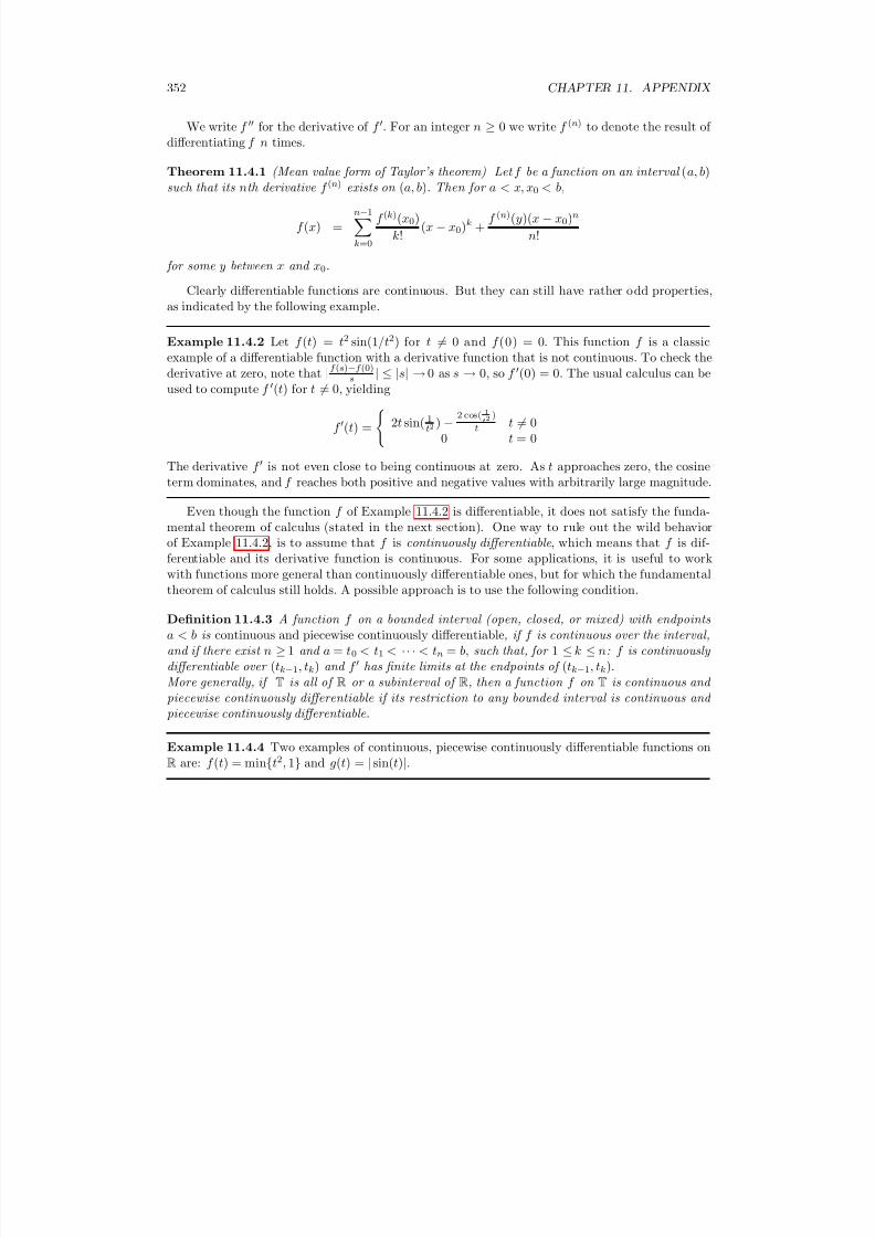
8/11/2019 Random process by B. Hajek
http://slidepdf.com/reader/full/random-process-by-b-hajek 362/448
352 CHAPTER 11. APPENDIX
We write f for the derivative of f . For an integer n ≥ 0 we write f (n) to denote the result of differentiating f n times.
Theorem 11.4.1 (Mean value form of Taylor’s theorem) Let f be a function on an interval (a, b)such that its nth derivative f (n) exists on (a, b). Then for a < x, x0 < b,
f (x) =n−1k=0
f (k)(x0)
k! (x − x0)k +
f (n)(y)(x − x0)n
n!
for some y between x and x0.
Clearly differentiable functions are continuous. But they can still have rather odd properties,as indicated by the following example.
Example 11.4.2 Let f (t) = t2 sin(1/t2) for t
= 0 and f (0) = 0. This function f is a classic
example of a differentiable function with a derivative function that is not continuous. To check thederivative at zero, note that |f (s)−f (0)
s | ≤ |s| → 0 as s → 0, so f (0) = 0. The usual calculus can beused to compute f (t) for t = 0, yielding
f (t) =
2t sin( 1
t2 ) − 2 cos( 1t2
)
t t = 00 t = 0
The derivative f is not even close to being continuous at zero. As t approaches zero, the cosineterm dominates, and f reaches both positive and negative values with arbitrarily large magnitude.
Even though the function f of Example 11.4.2 is differentiable, it does not satisfy the funda-
mental theorem of calculus (stated in the next section). One way to rule out the wild behaviorof Example 11.4.2, is to assume that f is continuously differentiable , which means that f is dif-ferentiable and its derivative function is continuous. For some applications, it is useful to workwith functions more general than continuously differentiable ones, but for which the fundamentaltheorem of calculus still holds. A possible approach is to use the following condition.
Definition 11.4.3 A function f on a bounded interval (open, closed, or mixed) with endpoints a < b is continuous and piecewise continuously differentiable, if f is continuous over the interval,and if there exist n ≥ 1 and a = t0 < t1 < · · · < tn = b, such that, for 1 ≤ k ≤ n: f is continuously differentiable over (tk−1, tk) and f has finite limits at the endpoints of (tk−1, tk).More generally, if T is all of R or a subinterval of R, then a function f on T is continuous and piecewise continuously differentiable if its restriction to any bounded interval is continuous and
piecewise continuously differentiable.
Example 11.4.4 Two examples of continuous, piecewise continuously differentiable functions onR are: f (t) = mint2, 1 and g(t) = | sin(t)|.
8/11/2019 Random process by B. Hajek
http://slidepdf.com/reader/full/random-process-by-b-hajek 363/448
11.5. INTEGRATION 353
Example 11.4.5 The function given in Example 11.4.2 is not considered to be piecewise contin-uously differentiable because the derivative does not have finite limits at zero.
Theoretical Exercise
1. Suppose f is a continuously differentiable function on an open bounded interval ( a, b). Showthat if f has finite limits at the endpoints, then so does f .
2. Suppose f is a continuous function on a closed, bounded interval [a, b] such that f existsand is continuous on the open subinterval (a, b). Show that if the right-hand limit of thederviative at a, f (a+) = limxa f (x), exists, then the right-hand derivative at a, defined by
D+f (a) = limx
a
f (x) − f (a)
x − aalso exists, and the two limits are equal.
Let g be a function from Rn to Rm. Thus for each vector x ∈ Rn, g(x) is an m vector. Thederivative matrix of g at a point x, ∂g∂x (x), is the n×m matrix with ijth entry ∂gi
∂xj(x). Sometimes for
brevity we write y = g(x) and think of y as a variable depending on x, and we write the derivativematrix as ∂y
∂x (x).
Theorem 11.4.6 (Implicit function theorem) If m = n and if ∂y∂x is continuous in a neighborhood
of x0 and if ∂y∂x (x0) is nonsingular, then the inverse mapping x = g−1(y) is defined in a neighborhood of y0 = g(x0) and
∂x
∂y(y0) =
∂y
∂x(x0)
−1
11.5 Integration
11.5.1 Riemann integration
Let g be a bounded function on a bounded interval of the form (a, b]. Given:
• An partition of (a, b] of the form (t0, t1], (t1, t2], · · · , (tn−1, tn], where n ≥ 0 anda = t0 ≤ t1 · · · < tn = b
• A sampling point from each subinterval, vk ∈ (tk−1, tk], for 1 ≤ k ≤ n,
the corresponding Riemann sum for g is defined by
nk=1
g(vk)(tk − tk−1).
8/11/2019 Random process by B. Hajek
http://slidepdf.com/reader/full/random-process-by-b-hajek 364/448
354 CHAPTER 11. APPENDIX
The norm of the partition is defined to be maxk |tk − tk−1|. The Riemann integral ba g(x)dx is
said to exist and its value is I if the following is true. Given any > 0, there is a δ > 0 so that|
nk=1 g(vk)(tk − tk−1) − I | ≤ whenever the norm of the partition is less than or equal to δ .
This definition is equivalent to the following condition, expressed using convergence of sequences.The Riemann integral exists and is equal to I , if for any sequence of partitions, specified by((tm1 , tm2 , . . . , tmnm
) : m ≥ 1), with corresponding sampling points ((vm1 , . . . , vm
nm) : m ≥ 1), such that
norm of the mth partition converges to zero as m → ∞, the corresponding sequence of Riemannsums converges to I as m → ∞. The function g is said to be Reimann integrable over (a, b] if the
integral ba g(x)dx exists and is finite.
Next, suppose g is defined over the whole real line. If for every interval (a, b], g is bounded over[a, b] and Riemann integrable over (a, b], then the Riemann integral of g over R is defined by ∞
−∞g(x)dx = lim
a,b→∞
b−a
g(x)dx
provided that the indicated limit exist as a, b jointly converge to +∞. The values +∞ or −∞ arepossible.
A function that is continuous, or just piecewise continuous, is Riemann integrable over anybounded interval. Moreover, the following is true for Riemann integration:
Theorem 11.5.1 (Fundamental theorem of calculus) Let f be a continuously differentiable function on R. Then for a < b,
f (b) − f (a) =
ba
f (x)dx. (11.4)
More generally, if f is continuous and piecewise continuously differentiable, (11.4) holds with f (x)
replaced by the right-hand derivative, D+f (x). (Note that D+f (x) = f (x) whenever f (x) is de- fined.)
We will have occasion to use Riemann integrals in two dimensions. Let g be a bounded functionon a bounded rectangle of the form (a1, b1] × (a2, b2]. Given:
• A partition of (a1, b1] × (a2, b2] into n1 × n2 rectangles of the form (t1 j , t1
j−1] × (t2k, t2
k−1], where
ni ≥ 1 and ai = ti0 < ti1 < · · · < tini = bi for i = 1, 2
• A sampling point (v1 jk , v2
jk) inside (t1 j , t1
j−1] × (t2k, t2
k−1] for 1 ≤ j ≤ n1 and 1 ≤ k ≤ n2,
the corresponding Riemann sum for g is
n1 j=1
n2k=1
g(v1 j,k, v2
j,k)(t1 j − t1
j−1)(t2k − t2
k−1).
The norm of the partition is maxi∈1,2 maxk | tik − tik−1|. As in the case of one dimension, g is saidto be Riemann integrable over (a1, b1] × (a2, b2], and
(a1,b1]×(a2,b2] g(x1, x2)dsdt = I , if the value
8/11/2019 Random process by B. Hajek
http://slidepdf.com/reader/full/random-process-by-b-hajek 365/448
11.5. INTEGRATION 355
of the Riemann sum converges to I for any sequence of partitions and sampling point pairs, withthe norms of the partitions converging to zero.
The above definition of a Riemann sum allows the n1 × n2 sampling points to be selected
arbitrarily from the n1
× n2
rectangles. If, instead, the sampling points are restricted to have theform (v1
j , v2k), for n1 + n2 numbers v1
1, . . . , v1n1, v2
1, . . . v2n2 , we say the corresponding Riemann sum
uses aligned sampling. We define a function g on [a, b]× [a, b] to be Riemann integrable with aligned sampling in the same way as we defined g to be Riemann integrable, except the family of Riemannsums used are the ones using aligned sampling. Since the set of sequences that must converge ismore restricted for aligned sampling, a function g on [a, b] × [a, b] that is Riemann integrable is alsoRiemann integrable with aligned sampling.
Proposition 11.5.2 A sufficient condition for g to be Riemann integrable (and hence Riemann integrable with aligned sampling) over (a1, b1] × (a2, b2] is that g be the restriction to (a1, b1] ×(a2, b2] of a continuous function on [a1, b1]
×[a2, b2]. More generally, g is Riemann integrable over
(a1, b1]×(a2, b2] if there is a partition of (a1, b1]×(a2, b2] into finitely many subrectangles of the form (t1 j , t1
j−1] × (t2k, t2
k−1], such that g on (t1 j , t1
j−1] × (t2k, t2
k−1] is the restriction to (t1 j , t1
j−1] × (t2k, t2
k−1]
of a continuous function on [t1 j , t1
j−1] × [t2k, t2
k−1].
Proposition 11.5.2 is a standard result in real analysis. It’s proof uses the fact that continuousfunctions on bounded, closed sets are uniformly continuous, from which if follows that, for any > 0, there is a δ > 0 so that the Riemann sums for any two partitions with norm less than orequal to δ differ by most . The Cauchy criteria for convergence of sequences of numbers is alsoused.
11.5.2 Lebesgue integration
Lebesgue integration with respect to a probability measure is defined in the section defining theexpectation of a random variable X and is written as
E [X ] =
Ω
X (ω)P (dω)
The idea is to first define the expectation for simple random variables, then for nonnegative randomvariables, and then for general random variables by E [X ] = E [X +] − E [X −]. The same approachcan be used to define the Lebesgue integral
∞−∞ g(ω)dω
for Borel measurable functions g on R. Such an integral is well defined if either ∞−∞ g+(ω)dω < +∞
or ∞−∞ g−(ω)dω < +∞.
8/11/2019 Random process by B. Hajek
http://slidepdf.com/reader/full/random-process-by-b-hajek 366/448
356 CHAPTER 11. APPENDIX
11.5.3 Riemann-Stieltjes integration
Let g be a bounded function on a closed interval [a, b] and let F be a nondecreasing function on[a, b]. The Riemann-Stieltjes integral
ba
g(x)dF (x) (Riemann-Stieltjes)
is defined the same way as the Riemann integral, except that the Riemann sums are changed to
nk=1
g(vk)(F (tk) − F (tk−1))
Extension of the integral over the whole real line is done as it is for Riemann integration. An
alternative definition of ∞−∞ g(x)dF (x), preferred in the context of these notes, is given next.
11.5.4 Lebesgue-Stieltjes integration
Let F be a CDF. As seen in Section 1.3, there is a corresponding probability measure P on theBorel subsets of R. Given a Borel measurable function g on R, the Lebesgue-Stieltjes integral of gwith respect to F is defined to be the Lebesgue integral of g with respect to P :
(Lebesgue-Stieltjes)
∞−∞
g(x)dF (x) =
∞−∞
g(x) P (dx) (Lebesgue)
The same notation ∞−∞ g(x)dF (x) is used for both Riemann-Stieltjes (RS) and Lebesgue-Stieltjes(LS) integration. If g is continuous and the LS integral is finite, then the integrals agree. Inparticular,
∞−∞ xdF (x) is identical as either an LS or RS integral. However, for equivalence of the
integrals Ω
g(X (ω))P (dω) and
∞−∞
g(x)dF (x),
even for continuous functions g, it is essential that the integral on the right be understood as anLS integral. Hence, in these notes, only the LS interpretation is used, and RS integration is notneeded.
If F has a corresponding pdf f , then
(Lebesgue-Stieltjes)
∞−∞
g(x)dF (x) =
∞−∞
g(x)f (x)dx (Lebesgue)
for any Borel measurable function g.
8/11/2019 Random process by B. Hajek
http://slidepdf.com/reader/full/random-process-by-b-hajek 367/448
11.6. ON CONVERGENCE OF THE MEAN 357
11.6 On convergence of the mean
Suppose (X n : n ≥ 1) is a sequence of random variables such that X n p.→ X ∞, for some random
variable X ∞. The theorems in this section address the question of whether E [X n] → E [X ∞]. Thehypothesis X n
p.→ X ∞ means that for any > 0 and δ > 0, P |X n − X ∞| ≤ ≥ 1 − δ . Thus, theevent that X n is close to X ∞ has probability close to one. But the mean of X n can differ greatlyfrom the mean of X if, in the unlikely event that |X n − X ∞| is not small, it is very, very large.
Example 11.6.1 Suppose U is a random variable with a finite mean, and suppose A1, A2, . . . is asequence of events, each with positive probability, but such that P (An) → 0, and let b1, b2, · · · bea sequence of nonzero numbers. Let X n = U + bnI An for n ≥ 1. Then for any > 0, P |X n − U | ≥ ≤ P X n = U = P (An) → 0 as n → ∞, so X n
p.→ U . However, E [X n] = E [U ] + bnP (An). Thus,if the bn have very large magnitude, the mean E [X n] can be far larger or far smaller than E [U ],for all large n.
The simplest way to rule out the very, very large values of |X n − X ∞| is to require the sequence(X n) to be bounded. That would rule out using constants bn with arbitrarily large magnitudesin Example 11.6.1. The following result is a good start–it is generalized to yield the dominatedconvergence theorem further below.
Theorem 11.6.2 (Bounded convergence theorem) Let X 1, X 2, . . . be a sequence of random vari-
ables such that for some finite L, P |X n| ≤ L = 1 for all n ≥ 1, and such that X n p.→ X as
n → ∞. Then E [X n] → E [X ].
Proof. For any > 0, P | X |≥ L + ≤ P | X − X n |≥ → 0, so that P | X |≥ L + = 0.Since was arbitrary, P | X |≤ L = 1. Therefore, P |X − X n| ≤ 2L = 1 for all n ≥ 1. Again let
> 0. Then |X − X n| ≤ + 2LI |X −X n|≥, (11.5)
so that |E [X ] − E [X n]| = |E [X − X n]| ≤ E [|X − X n|] ≤ + 2LP |X − X n| ≥ . By the hypotheses,P |X − X n| ≥ → 0 as n → ∞. Thus, for n large enough, |E [X ] − E [X n]| < 2. Since isarbitrary, E [X n] → E [X ].
Equation (11.5) is central to the proof just given. It bounds the difference |X − X n| by onthe event |X − X n| < , which has probability close to one for n large, and on the complementof this event, the difference |X − X n| is still bounded so that its contribution is small for n largeenough.
The following lemma, used to establish the dominated convergence theorem, is similar to the
bounded convergence theorem, but the variables are assumed to be bounded only on one side:specifically, the random variables are restricted to be greater than or equal to zero. The result isthat E [X n] for large n can still be much larger than E [X ∞], but cannot be much smaller. Therestriction to nonnegative X n’s would rule out using negative constants bn with arbitrarily largemagnitudes in Example 11.6.1. The statement of the lemma uses “liminf,” which is defined inAppendix 11.2.
8/11/2019 Random process by B. Hajek
http://slidepdf.com/reader/full/random-process-by-b-hajek 368/448
8/11/2019 Random process by B. Hajek
http://slidepdf.com/reader/full/random-process-by-b-hajek 369/448
11.7. MATRICES 359
Theorem 11.6.6 (Monotone convergence theorem) Let X 1, X 2, . . . be a sequence of random vari-ables such that E [X 1] > −∞ and such that X 1(ω) ≤ X 2(ω) ≤ · · · . Then the limit X ∞ given by X ∞(ω) = limn→∞ X n(ω) for all ω is an extended random variable (with possible value ∞) and
E [X n] → E [X ∞] as n → ∞.Proof. By adding min0, −X 1 to all the random variables involved if necessary, we can assumewithout loss of generality that X 1, X 2, . . . , and therefore also X , are nonnegative. Recall that E [X ]is equal to the supremum of the expectation of simple random variables that are less than or equalto X . So let γ be any number such that γ < E [X ]. Then, there is a simple random variable X less than or equal to X with E [ X ] ≥ γ . The simple random variable X takes only finitely manypossible values. Let L be the largest. Then X ≤ X ∧ L, so that E [X ∧ L] > γ . By the boundedconvergence theorem, E [X n ∧ L] → E [X ∧ L]. Therefore, E [X n ∧ L] > γ for all large enough n.Since E [X n ∧ L] ≤ E [X n] ≤ E [X ], if follows that γ < E [X n] ≤ E [X ] for all large enough n. Sinceγ is an arbitrary constant with γ < E [X ], the desired conclusion, E [X n] → E [X ], follows.
11.7 Matrices
An m × n matrix over the reals R has the form
A =
a11 a12 · · · a1n
a21 a22 · · · a2n...
... ...
am1 am2 · · · amn
where aij ∈ R for all i, j. This matrix has m rows and n columns. A matrix over the complexnumbers C has the same form, with aij
∈C for all i, j. The transpose of an m
×n matrix A = (aij)
is the n × m matrix AT = (a ji). For example 1 0 32 1 1
T
=
1 20 13 1
The matrix A is symmetric if A = AT . Symmetry requires that the matrix A be square: m = n.
The diagonal of a matrix is comprised by the entries of the form aii. A square matrix A is calleddiagonal if the entries off of the diagonal are zero. The n × n identity matrix is the n × n diagonalmatrix with ones on the diagonal. We write I to denote an identity matrix of some dimension n.
If A is an m × k matrix and B is a k × n matrix, then the product AB is the m × n matrix withijth element
kl=1 ailblj. A vector x is an m
×1 matrix, where m is the dimension of the vector.
Thus, vectors are written in column form:
x =
x1
x2...
xm
8/11/2019 Random process by B. Hajek
http://slidepdf.com/reader/full/random-process-by-b-hajek 370/448
360 CHAPTER 11. APPENDIX
The set of all dimension m vectors over R is the m dimensional Euclidean space Rm. The inner product of two vectors x and y of the same dimension m is the number xT y, equal to
mi=1 xiyi.
The vectors x and y are orthogonal if xT y = 0. The Euclidean length or norm of a vector x is given
by x = (xT
x)
1
2 . A set of vectors ϕ1, . . . , ϕn is orthonormal if the vectors are orthogonal to eachother and ϕi = 1 for all i.
A set of vectors v1, . . . , vn in Rm is said to span Rm if any vector in Rm can be expressed as alinear combination α1v1 +α2v2 + · · ·+ αnvn for some α1, . . . , αn ∈ R. An orthonormal set of vectorsϕ1, . . . , ϕn in Rm spans Rm if and only if n = m. An orthonormal basis for Rm is an orthonormalset of m vectors in Rm. An orthonormal basis ϕ1, . . . , ϕm corresponds to a coordinate system forRm. Given a vector v in Rm, the coordinates of v relative to ϕ1, . . . , ϕm are given by αi = ϕT
i v.The coordinates α1, . . . , αm are the unique numbers such that v = α1ϕ1 + · · · + αmϕm.
A square matrix U is called orthonormal if any of the following three equivalent conditions issatisfied:
1. U T U = I
2. U U T = I
3. the columns of U form an orthonormal basis.
Given an m × m orthonormal matrix U and a vector v ∈ Rm, the coordinates of v relative to U aregiven by the vector U T v. Given a square matrix A, a vector ϕ is an eigenvector of A and λ is aneigenvalue of A if the eigen relation Aϕ = λϕ is satisfied.
A permutation π of the numbers 1, . . . , m is a one-to-one mapping of 1, 2, . . . , m onto itself.That is (π(1), . . . , π(m)) is a reordering of (1, 2, . . . , m). Any permutation is either even or odd.A permutation is even if it can be obtained by an even number of transpositions of two elements.Otherwise a permutation is odd. We write
(−1)π = 1 if π is even
−1 if π is odd
The determinant of a square matrix A, written det(A), is defined by
det(A) =π
(−1)πmi=1
aiπ(i)
The absolute value of the determinant of a matrix A is denoted by | A |. Thus | A |=| det(A) |.Some important properties of determinants are the following. Let A and B be m × m matrices.
1. If B is obtained from A by multiplication of a row or column of A by a scaler constant c,then det(B) = c det(A).
2. If U is a subset of Rm and V is the image of U under the linear transformation determinedby A:
V = Ax : x ∈ U
8/11/2019 Random process by B. Hajek
http://slidepdf.com/reader/full/random-process-by-b-hajek 371/448
11.7. MATRICES 361
then
(the volume of U ) = | A | × (the volume of V )
3. det(AB) = det(A) det(B)
4. det(A) = det(AT )
5. |U | = 1 if U is orthonormal.
6. The columns of A span Rn if and only if det(A) = 0.
7. The equation p(λ) = det(λI − A) defines a polynomial p of degree m called the characteristic polynomial of A.
8. The zeros λ1, λ2, . . . , λm of the characteristic polynomial of A, repeated according to mul-tiplicity, are the eigenvalues of A, and det(A) = n
i=1λi. The eigenvalues can be complex
valued with nonzero imaginary parts.
If K is a symmetric m × m matrix, then the eigenvalues λ1, λ2, . . . , λm, are real-valued (notnecessarily distinct) and there exists an orthonormal basis consisting of the corresponding eigen-vectors ϕ1, ϕ2, . . . , ϕm. Let U be the orthonormal matrix with columns ϕ1, . . . , ϕm and let Λ bethe diagonal matrix with diagonal entries given by the eigenvalues
Λ =
λ10∼
λ2
. . .0
∼ λm
Then the relations among the eigenvalues and eigenvectors may be written as K U = U Λ. Therefore
K = U ΛU T and Λ = U T KU . A symmetric m × m matrix A is positive semidefinite if αT Aα ≥ 0for all m-dimensional vectors α. A symmetric matrix is positive semidefinite if and only if itseigenvalues are nonnegative.
The remainder of this section deals with matrices over C. The Hermitian transpose of a matrixA is the matrix A∗, obtained from AT by taking the complex conjugate of each element of AT . Forexample,
1 0 3 + 2 j2 j 1
∗=
1 20 − j
3
−2 j 1
The set of all dimension m vectors over C is the m-complex dimensional space Cm. The inner product of two vectors x and y of the same dimension m is the complex number y∗x, equal tom
i=1 xiy∗i . The vectors x and y are orthogonal if x∗y = 0. The length or norm of a vector x is
given by x = (x∗x)12 . A set of vectors ϕ1, . . . , ϕn is orthonormal if the vectors are orthogonal to
each other and ϕi = 1 for all i.
8/11/2019 Random process by B. Hajek
http://slidepdf.com/reader/full/random-process-by-b-hajek 372/448
362 CHAPTER 11. APPENDIX
A set of vectors v1, . . . , vn in Cm is said to span Cm if any vector in Cm can be expressed as alinear combination α1v1 +α2v2 + · · ·+ αnvn for some α1, . . . , αn ∈ C. An orthonormal set of vectorsϕ1, . . . , ϕn in Cm spans Cm if and only if n = m. An orthonormal basis for Cm is an orthonormal
set of m vectors in Cm
. An orthonormal basis ϕ1, . . . , ϕm corresponds to a coordinate system forCm. Given a vector v in Rm, the coordinates of v relative to ϕ1, . . . , ϕm are given by αi = ϕ∗
i v.The coordinates α1, . . . , αm are the unique numbers such that v = α1ϕ1 + · · · + αmϕm.
A square matrix U over C is called unitary (rather than orthonormal) if any of the followingthree equivalent conditions is satisfied:
1. U ∗U = I
2. U U ∗ = I
3. the columns of U form an orthonormal basis.
Given an m × m unitary matrix U and a vector v ∈ Cm, the coordinates of v relative to U are
given by the vector U ∗v. Eigenvectors, eigenvalues, and determinants of square matrices over Care defined just as they are for matrices over R. The absolute value of the determinant of a matrixA is denoted by | A |. Thus | A |=| det(A) |.
Some important properties of determinants of matrices over C are the following. Let A and Bby m × m matrices.
1. If B is obtained from A by multiplication of a row or column of A by a constant c ∈ C, thendet(B) = c det(A).
2. If U is a subset of Cm and V is the image of U under the linear transformation determinedby A:
V =
Ax : x
∈ Uthen
(the volume of U ) = | A |2 × (the volume of V )
3. det(AB) = det(A) det(B)
4. det∗(A) = det(A∗)
5. | U |= 1 if U is unitary.
6. The columns of A span Cn if and only if det(A) = 0.
7. The equation p(λ) = det(λI − A) defines a polynomial p of degree m called the characteristic polynomial of A.
8. The zeros λ1, λ2, . . . , λm of the characteristic polynomial of A, repeated according to mul-tiplicity, are the eigenvalues of A, and det(A) =
ni=1 λi. The eigenvalues can be complex
valued with nonzero imaginary parts.
8/11/2019 Random process by B. Hajek
http://slidepdf.com/reader/full/random-process-by-b-hajek 373/448
11.7. MATRICES 363
A matrix K is called Hermitian symmetric if K = K ∗. If K is a Hermitian symmetric m × mmatrix, then the eigenvalues λ1, λ2, . . . , λm, are real-valued (not necessarily distinct) and thereexists an orthonormal basis consisting of the corresponding eigenvectors ϕ1, ϕ2, . . . , ϕm. Let U be
the unitary matrix with columns ϕ1, . . . , ϕm and let Λ be the diagonal matrix with diagonal entriesgiven by the eigenvalues
Λ =
λ1
0∼
λ2
. . .0∼ λm
Then the relations among the eigenvalues and eigenvectors may be written as K U = U Λ. ThereforeK = U ΛU ∗ and Λ = U ∗KU . A Hermitian symmetric m × m matrix A is positive semidefinite if α∗Aα ≥ 0 for all α ∈ Cm. A Hermitian symmetric matrix is positive semidefinite if and only if itseigenvalues are nonnegative.
Many questions about matrices over C can be addressed using matrices over R. If Z is an m×mmatrix over C, then Z can be expressed as Z = A + Bj , for some m × m matrices A and B over R.Similarly, if x is a vector in Cm then it can be written as x = u + jv for vectors u, v ∈ Rm. ThenZx = (Au − Bv) + j(Bu + Av). There is a one-to-one and onto mapping from Cm to R2m definedby u + jv →
uv
. Multiplication of x by the matrix Z is thus equivalent to multiplication of
uv
byZ =
A −BB A
. We will show that
|Z |2 = det( Z ) (11.6)
so that Property 2 for determinants of matrices over C follows from Property 2 for determinantsof matrices over R.
It remains to prove (11.6). Suppose that A−1 exists and examine the two 2m
×2m matrices
A −BB A
and
A 0B A + BA−1B
. (11.7)
The second matrix is obtained from the first by left multiplying each sub-block in the right column of the first matrix by A−1B, and adding the result to the left column. Equivalently, the second matrix
is obtained by right multiplying the first matrix by
I A−1B0 I
. But det
I A−1B0 I
= 1, so
that the two matrices in (11.7) have the same determinant. Equating the determinants of the two
matrices in (11.7) yields det( Z ) = det(A)det(A + BA−1B). Similarly, the following four matriceshave the same determinant:
A + Bj 0
0 A − Bj A + Bj A
−Bj
0 A − Bj 2A A
−Bj
A − Bj A − Bj 2A 0
A − Bj A+BA
−1
B2 (11.8)
Equating the determinants of the first and last of the matrices in (11.8) yields that |Z |2 =det(Z )det∗(Z ) = det(A + B j) det(A − B j) = det(A)det(A + B A−1B). Combining these ob-servations yields that (11.6) holds if A−1 exists. Since each side of (11.6) is a continuous functionof A, (11.6) holds in general.

8/11/2019 Random process by B. Hajek
http://slidepdf.com/reader/full/random-process-by-b-hajek 374/448
364 CHAPTER 11. APPENDIX

8/11/2019 Random process by B. Hajek
http://slidepdf.com/reader/full/random-process-by-b-hajek 375/448
Chapter 12
Solutions to Problems
1.2 A ballot problem
There are 64 = 15 possibilities for the positions of the winning ballots, and the event in questioncan be written as 110110, 110101, 111001, 111010, 111100, so the event has probability 5
15 = 13 .
It can be shown in general that if k of the ballots are for the winning candidate and n − k arefor the losing candidate, then the winning candidate has a strict majority throughout the countingwith probability 2k−n
n . This remains true even if the cyclic order of the ballots counted is fixed,with only the identify of the first ballot counted being random and uniform over the n possibilities.
1.4 Independent vs. mutually exclusive(a) If E is an event independent of itself, then P (E ) = P (E ∩ E ) = P (E )P (E ). This can happen if P (E ) = 0. If P (E ) = 0 then cancelling a factor of P (E ) on each side yields P (E ) = 1. In summary,either P (E ) = 0 or P (E ) = 1.
(b) In general, we have P (A∪B) = P (A) + P (B)−P (AB). If the events A and B are independent,then P (A∪B) = P (A)+P (B)−P (A)P (B) = 0.3+0.4−(0.3)(0.4) = 0.58. On the other hand, if theevents A and B are mutually exclusive, then P (AB) = 0 and therefore P (A ∪ B) = 0.3 + 0.4 = 0.7.(c) If P (A) = 0.6 and P (B) = 0.8, then the two events could be independent. However, if A andB were mutually exclusive, then P (A) + P (B) = P (A ∪ B) ≤ 1, so it would not possible for A andB to be mutually exclusive if P (A) = 0.6 and P (B) = 0.8.
1.6 Frantic searchLet D,T ,B, and O denote the events that the glasses are in the drawer, on the table, in the brief-case, or in the office, respectively. These four events partition the probability space.(a) Let E denote the event that the glasses were not found in the first drawer search.
P (T |E ) = P (TE )P (E ) = P (E |T )P (T )P (E |D)P (D)+P (E |Dc)P (Dc) = (1)(0.06)(0.1)(0.9)+(1)(0.1) = 0.060.19 ≈ 0.315(b) Let F denote the event that the glasses were not found after the first drawer search and first
table search. P (B|F ) = P (BF )P (F ) =
P (F |B)P (B)P (F |D)P (D)+P (F |T )P (T )+P (F |B)P (B)+P (F |O)P (O)
= (1)(0.03)(0.1)(0.9)+(0.1)(0.06)+(1)(0.03)+(1)(0.01) ≈ 0.22
(c) Let G denote the event that the glasses were not found after the two drawer searches, two table
365
8/11/2019 Random process by B. Hajek
http://slidepdf.com/reader/full/random-process-by-b-hajek 376/448
366 CHAPTER 12. SOLUTIONS TO PROBLEMS
searches, and one briefcase search.P (O|G) =
P (OG)P (G) =
P (G|O)P (O)P (G|D)P (D)+P (G|T )P (T )+P (G|B)P (B)+P (G|O)P (O)
= (1)(0.01)(0.1)2(0.9)+(0.1)2(0.06)+(0.1)(0.03)+(1)(0.01)
≈ 0.4225
1.8 Conditional probabilities–basic computations of iterative decoding(a) Here is one of several approaches to this problem. Note that the n pairs (B1, Y 1), . . . , (Bn, Y n)
are mutually independent, and λi(bi) def
= P (Bi = bi|Y i = yi) = qi(yi|bi)
qi(yi|0)+qi(yi|1) . Therefore
P (B = 1|Y 1 = y1, . . . , Y n = yn) =
b1,...,bn:b1⊕···⊕bn=1
P (B1 = b1, . . . , Bn = bn|Y 1 = y1, . . . , Y n = yn)
=
b1,...,bn:b1⊕···⊕bn=1
ni=1
λi(bi).
(b) Using the definitions,
P (B = 1|Z 1 = z1, . . . , Z k = zk) = p(1, z1, . . . , zk)
p(0, z1, . . . , zk) + p(1, z1, . . . , zk)
=12
k j=1 r j(1|z j)
12
k j=1 r j(0|z j) + 1
2
k j=1 r j(1|z j)
= η
1 + η where η =
k j=1
r j(1|z j)
r j(0|z j).
1.10 Blue corners(a) There are 24 ways to color 5 corners so that at least one face has four blue corners (there are 6choices of the face, and for each face there are four choices for which additional corner to color blue.)Since there are
85
= 56 ways to select 5 out of 8 corners, P (B|exactly 5 corners colored blue) =
24/56 = 3/7.(b) By counting the number of ways that B can happen for different numbers of blue corners wefind P (B) = 6 p4(1 − p)4 + 24 p5(1 − p)3 + 24 p6(1 − p)2 + 8 p7(1 − p) + p8.
1.12 Recognizing cumulative distribution functions
(a) Valid (draw a sketch) P X
2
≤ 5 = P X ≤ −√
5 + P X ≥√
5 = F 1(−√
5) + 1 − F 1(
√ 5) =e−5
2 .(b) Invalid. F (0) > 1. Another reason is that F is not nondecreasing(c) Invalid, not right continuous at 0.
1.14 CDF and characteristic function of a mixed type random variable
8/11/2019 Random process by B. Hajek
http://slidepdf.com/reader/full/random-process-by-b-hajek 377/448
367
(a) Range of X is [0, 0.5]. For 0 ≤ c ≤ 0.5, P X ≤ c] = P U ≤ c + 0.5 = c + 0.5 Thus,
F X (c) = 0 c < 0
c + 0.5 0
≤ c
≤ 0.5
1 c ≥ 0.5
(b) ΦX (u) = 0.5 + 0.5
0 e juxdx = 0.5 + eju/2−1 ju
1.16 Conditional expectation for uniform density over a triangular region(a) The triangle has base and height one, so the area of the triangle is 0.5. Thus the joint pdf is 2inside the triangle.(b)
f X (x) =
∞−∞
f XY (x, y)dy =
x/20 2dy = x if 0 < x < 1 x/2
x−1 2dy = 2 − x if 1 < x < 2
0 else
(c) In view of part (c), the conditional density f Y |X (y|x) is not well defined unless 0 < x < 2. Ingeneral we have
f Y |X (y|x) =
2x if 0 < x ≤ 1 and y ∈ [0, x2 ]0 if 0 < x ≤ 1 and y ∈ [0, x2 ]2
2−x if 1 < x < 2 and y ∈ [x − 1, x2 ]
0 if 1 < x < 2 and y ∈ [x − 1, x2 ]not defined if x ≤ 0 or x ≥ 2
Thus, for 0 < x ≤ 1, the conditional distribution of Y is uniform over the interval [0, x2 ]. For1 < x ≤ 2, the conditional distribution of Y is uniform over the interval [x − 1, x2 ].(d) Finding the midpoints of the intervals that Y is conditionally uniformly distributed over, or
integrating x against the conditional density found in part (c), yields:
E [Y |X = x] =
x4 if 0 < x ≤ 1
3x−24 if 1 < x < 2
not defined if x ≤ 0 or x ≥ 2
1.18 Density of a function of a random variable(a) P (X ≥ 0.4|X ≤ 0.8) = P (0.4 ≤ X ≤ 0.8|X ≤ 0.8) = (0.82 − 0.42)/0.82 = 3
4 .(b) The range of Y is the interval [0, +∞). For c ≥ 0,P − ln(X ) ≤ c = P ln(X ) ≥ −c = P X ≥ e−c =
1e−c 2xdx = 1 − e−2c so
f Y (c) = 2exp(−2c) c ≥ 0
0 else
That is, Y is an exponential random variable with parameter 2.
1.20 Functions of independent exponential random variables(a) Z takes values in the positive real line. So let z ≥ 0.
P Z ≤ z) = P minX 1, X 2 ≤ z = P X 1 ≤ z or X 2 ≤ z= 1 − P X 1 > z and X 2 > z = 1 − P (X 1 > z]P X 2 > z = 1 − e−λ1ze−λ2z = 1 − e−(λ1+λ
8/11/2019 Random process by B. Hajek
http://slidepdf.com/reader/full/random-process-by-b-hajek 378/448
368 CHAPTER 12. SOLUTIONS TO PROBLEMS
Differentiating yields that
f Z (z) = (λ1 + λ2)e−(λ1+λ2)z , z ≥ 00, z < 0
That is, Z has the exponential distribution with parameter λ1 + λ2.(b) R takes values in the positive real line and by independence the joint pdf of X 1 and X 2 is theproduct of their individual densities. So for r ≥ 0 ,
P R ≤ r = P
X 1X 2
≤ r
= P X 1 ≤ rX 2
=
∞0
rx20
λ1e−λ1x1λ2e−λ2x2dx1dx2
=
∞0
(1 − e−rλ1x2)λ2e−λ2x2dx2 = 1 − λ2
rλ1 + λ2.
Differentiating yields that
f R(r) =
λ1λ2(λ1r+λ2)2 r ≥ 0
0, r < 0
1.22 Gaussians and the Q function(a) Cov(3X + 2Y, X + 5Y + 10) = 3Cov(X, X ) + 10Cov(Y, Y ) = 3Var(X ) + 10Var(Y ) = 13.(b) X + 4Y is N (0, 17), so P X + 4Y ≥ 2 = P X +4Y √
17 ≥ 2√
17 = Q( 2√
17).
(c) X − Y is N (0, 2), so P (X − Y )2 > 9 = P (X − Y ) ≥ 3 orX − Y ≤ −3 = 2P X −Y √ 2 ≥ 3√
2 =
2Q( 3√ 2
).
1.24 Working with a joint density(a) The density must integrate to one, so c = 4/19.(b)
f X (x) =
419
21 (1 + xy)dy = 4
19 [1 + 3x2 ] 2 ≤ x ≤ 3
0 else
f Y (y) =
419
32 (1 + xy)dx = 4
19 [1 + 5y2 ] 1 ≤ y ≤ 2
0 else
Therefore f X |Y (x|y) is well defined only if 1 ≤ y ≤ 2. For 1 ≤ y ≤ 2:
f X |Y (x|y) = 1+xy
1+5
2y
2 ≤
x ≤
3
0 for other x
1.26 Density of a difference(a) Method 1 The joint density is the product of the marginals, and for any c ≥ 0, the probability
8/11/2019 Random process by B. Hajek
http://slidepdf.com/reader/full/random-process-by-b-hajek 379/448
369
P |X − Y | ≤ c is the integral of the joint density over the region of the positive quadrant suchthat |x−y| ≤ c, which by symmetry is one minus twice the integral of the density over the regiony ≥ 0 and y ≤ y+c. Thus, P X −Y | ≤ c = 1−2
∞
0 exp(−λ(y+c))λ exp(−λy)dy = 1−exp(−λc).
Thus, f Z (c) = λ exp(−λc) c ≥ 00 else
That is, Z has the exponential distribution with parameter
λ.(Method 2 The problem can be solved without calculation by the memoryless property of the ex-ponential distribution, as follows. Suppose X and Y are lifetimes of identical lightbulbs which areturned on at the same time. One of them will burn out first. At that time, the other lightbulb willbe the same as a new light bulb, and |X − Y ] is equal to how much longer that lightbulb will last.
1.28 Some characteristic functions(a) Differentiation is straight-forward, yielding jE [X ] = Φ(0) = 2 j or E [X ] = 2, and j2E [X 2] =Φ
(0) = −
14, so Var(x) = 14−
22 = 10. In fact, this is the characteristic function of a N (10, 22)random variable.(b) Evaluation of the derivatives at zero requires l’Hospital’s rule, and is a little tedious. A simplerway is to use the Taylor series expansion exp( ju) = 1 + ( ju) + ( ju)2/2! + ( ju)3/3!... The result isE [X ] = 0.5 and Var(X ) = 1/12. In fact, this is the characteristic function of a U (0, 1) randomvariable.(c) Differentiation is straight-forward, yielding E [X ] = Var(X ) = λ. In fact, this is the character-istic function of a P oi(λ) random variable.
1.30 A transformation of jointly continuous random variables(a) We are using the mapping, from the square region (u, v) : 0 ≤ u, v ≤ 1 in the u − v plane tothe triangular region with corners (0,0), (3,0), and (3,1) in the x
−y plane, given by
x = 3u
y = uv.
The mapping is one-to-one, meaning that for any (x, y) in the range we can recover (u, v). Indeed,the inverse mapping is given by
u = x
3
v = 3y
x .
The Jacobian determinant of the transformation is
J (u, v) = det ∂x∂u
∂x∂v
∂y∂u
∂y∂v
= det 3 0v u
= 3u = 0, for all u, v ∈ (0, 1)2.
Therefore the required pdf is
f X,Y (x, y) = f U,V (u, v)
|J (u, v)| = 9u2v2
|3u| = 3uv2 = 9y2
x
8/11/2019 Random process by B. Hajek
http://slidepdf.com/reader/full/random-process-by-b-hajek 380/448
370 CHAPTER 12. SOLUTIONS TO PROBLEMS
within the triangle with corners (0,0), (3,0), and (3,1), and f X,Y (x, y) = 0 elsewhere.(b) Integrating out y from the joint pdf yields
f X (x) = x30
9y2
x dy = x2
9 if 0 ≤ x ≤ 30 else
Therefore the conditional density f Y |X (y|x) is well defined only if 0 ≤ x ≤ 3. For 0 ≤ x ≤ 3,
f Y |X (y|x) = f X,Y (x, y)
f X (x) =
81y2
x3 if 0 ≤ y ≤ x3
0 else
1.32 Opening a bicycle combination lockThe time required has possible values from 2 seconds to 20, 000 seconds. It is well approximated
(within 2 seconds) by a continuous type random variable T that is uniformly distributed on theinterval [0, 20, 000]. In fact, if we were to round T up to the nearest multiple of 2 seconds we would
get a random variable with the exact distribution of time required. Then E [T ] = 2×10⁴
2 seconds
= 10,000 seconds = 166.66 minutes, and the standard deviation of T is 20,000√ 12
= 5773.5 seconds =96.22 minutes.
1.34 Computing some covariances(a) Cov(X + Y, X − Y ) = Cov(X,X) − Cov(X,Y) + Cov(Y,X)− Cov(Y,Y) = Var(X ) − Var(Y ) = 0.(b) Cov(3X+Z,3X+Y) = 9Var(X )+3Cov(X, Y )+3Cov(Z, X )+Cov(Z, Y ) = 9·20+3·10+3·10+5 =245.(c) Since E [X + Y ] = 0, E [(X + Y )2] = Var(X + Y ) = Var(X ) + 2Cov(X, Y ) + Var(Y ) =20 + 2
·10 + 20 = 60.
1.36 Jointly distributed variables(a) E [ V
2
1+U ] = E [V 2]E [ 11+U ] =
∞0 v2λe−λvdv
10
11+udu = ( 2
λ2)(ln(2)) = 2 l n 2
λ2 .
(b) P U ≤ V = 1
0
∞u λe−λvdvdu =
10 e−λudu = (1 − e−λ)/λ.
(c) The support of both f UV and f Y Z is the strip [0, 1]× [0, ∞), and the mapping (u, v) → (y, z)
defined by y = u2 and z = uv is one-to-one. Indeed, the inverse mapping is given by u = y12 and
v = zy− 12 . The absolute value of the Jacobian determinant of the forward mapping is | ∂ (x,y)
∂ (u,v) | =
2u 0v u = 2u2 = 2y. Thus,
f Y,Z (y, z) =
λ2ye−λzy−
12 (y, z) ∈ [0, 1] × [0, ∞)
0 otherwise.
8/11/2019 Random process by B. Hajek
http://slidepdf.com/reader/full/random-process-by-b-hajek 381/448
371
2.2 The limit of the product is the product of the limits(a) There exists n1 so large that |yn − y | ≤ 1 for n ≥ n1. Thus, |yn| ≤ L for all n, whereL = max|y1|, |y2|, . . . , |yn1−1|, |y| + 1..
(b) Given > 0, there exists n so large that |xn−x| ≤ 2L and |yn−y| ≤
2(|x|+1) . Thus, for n ≥ n,
|xnyn − xy| ≤ |(xn − x)yn| + |x(yn − y)| ≤ |xn − x|L + |x||yn − y| ≤
2 +
2 ≤ .
So xnyn → xy as n → ∞.
2.4 Limits of some deterministic series(a) Convergent. This is the power series expansion for ex, which is everywhere convergent, evalu-ated at x = 3. The value of the sum is thus e3. Another way to show the series is convergent is tonotice that for n ≥ 3 the nth term can be bounded above by 3n
n! = 33
3!34
35 · · · 3
n ≤ (4.5)( 34 )n−3. Thus,
the sum is bounded by a constant plus a geometric series, so it is convergent.(b) Convergent. Let 0 < η < 1. Then ln n < nη for all large enough n. Also, n + 2
≤ 2n for all large
enough n, and n+5 ≥ n for all n. Therefore, the nth term in the series is bounded above, for all suffi-ciently large n, by 2n·nη
n3 = 2nη−2. Therefore, the sum in (b) is bounded above by finitely many termsof the sum, plus 2
∞n=1 nη−2, which is finite, because, for α > 1,
∞n=1 n−α < 1 +
∞1 x−αdx = α
α−1 ,as shown in an example in the appendix of the notes.(c) Not convergent. Let 0 < η < 0.2. Then log(n + 1) ≤ nη for all n large enough, so for n largeenough the nth term in the series is greater than or equal to n−5η. The series is therefore divergent.We used the fact that
∞n=1 n−α is infinite for any 0 ≤ α ≤ 1, because it is greater than or equal
to the integral ∞
1 x−αdx, which is infinite for 0 ≤ α ≤ 1.
2.6 Convergence of alternating series(a) For n
≥ 0, let I n denote the interval with endpoints sn and sn+1. It suffices to show that
I 0 ⊃ I 1 ⊃ I 2 ⊃ · · · . If n is even, then I n = [sn+1, sn+1 + bn+1] ⊃ [sn+1, sn+1 + bn+2] = I n+1.Similarly, if n is odd, I n = [sn+1 − bn+1, sn+1] ⊃ [sn+1 − bn+2, sn+1] = I n+1. So in general, for anyn, I n ⊃ I n+1.(b) Given > 0, let N be so large that bN < . It remains to prove that |sn − sm| ≤ whenevern ≥ N and m ≥ N . Without loss of generality, we can assume that n ≤ m. Since I m ⊂ I n itfollows that sm ∈ I n and therefore that |sm − sn| ≤ bn+1 ≤ .
2.8 Convergence of sequences of random variables(a) The distribution of X n is the same for all n, so the sequence converges in distribution to anyrandom variable with the distribution of X 1. To check for mean square convergence, use the factcos(a)cos(b) = (cos(a+b)+cos(a−b))/2 to calculate that E [X nX m] = 1
2 if n = m and E [X nX m] = 0
if n = m. Therefore, limn,m→∞ E [X nX m] does not exist, so the sequence (X n) does not satisfythe Cauchy criteria for m.s. convergence, so it doesn’t converge in the m.s. sense. Since it is abounded sequence, it therefore does not converge in the p. sense either. (Because for boundedsequences, convergence p. implies convergence m.s.) Therefore the sequence doesn’t converge inthe a.s. sense either. In summary, the sequence converges in distribution but not in the other threesenses. (Another approach is to note that the distribution of X n − X 2n is the same for all n, so
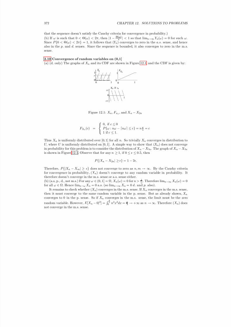
8/11/2019 Random process by B. Hajek
http://slidepdf.com/reader/full/random-process-by-b-hajek 382/448
372 CHAPTER 12. SOLUTIONS TO PROBLEMS
that the sequence doesn’t satisfy the Cauchy criteria for convergence in probability.)
(b) If ω is such that 0 < Θ(ω) < 2π, then |1 − Θ(ω)π | < 1 so that limn→∞ Y n(ω) = 0 for such ω.
Since P 0 < Θ(ω) < 2π = 1, it follows that (Y n) converges to zero in the a.s. sense, and hence
also in the p. and d. senses. Since the sequence is bounded, it also converges to zero in the m.s.sense.
2.10 Convergence of random variables on (0,1](a) (d. only) The graphs of X n and its CDF are shown in Figure 12.1, and the CDF is given by:
c
0
0
1
X n
1 0 1
1
0
n X F
0
-1/2
1/2
1
X -X n 2n
Figure 12.1: X n, F xn , and X n − X 2n
F X n(c) =
0, if c ≤ 0P ω : nω − nω ≤ c = n c
n = c1 if c ≤ 1.
Thus X n is uniformly distributed over [0, 1] for all n. So trivially X n converges in distribution toU, where U is uniformly distributed on [0, 1]. A simple way to show that (X n) does not convergein probability for this problem is to consider the distribution of X n − X 2n. The graph of X n − X 2nis shown in Figure 12.1. Observe that for any n ≥ 1, if 0 ≤ ≤ 0.5, then
P |X n − X 2n| ≥ = 1 − 2.
Therefore, P |X n − X m| ≥ does not converge to zero as n, m → ∞. By the Cauchy criteriafor convergence in probability, (X n) doesn’t converge to any random variable in probability. Ittherefore doesn’t converge in the m.s. sense or a.s. sense either.(b) (a.s, p., d., not m.s.) For any ω ∈ (0, 1] = Ω, X n(ω) = 0 for n > 1
ω . Therefore limn→∞ X n(ω) = 0for all ω
∈ Ω. Hence lim
n→ω X
n = 0 a.s. (so lim
n→∞X
n = 0 d. and p. also).
It remains to check whether (X n) converges in the m.s. sense. If X n converges in the m.s. sense,then it must converge to the same random variable in the p. sense. But as already shown, X nconverges to 0 in the p. sense. So if X n converges in the m.s. sense, the limit must be the zero
random variable. However, E [X n − 0|2] = 1
n0 n4x2dx = n
3 → +∞ as n → ∞. Therefore (X n) doesnot converge in the m.s. sense.
8/11/2019 Random process by B. Hajek
http://slidepdf.com/reader/full/random-process-by-b-hajek 383/448
373
(c) (a.s, p., d., not m.s.) For any ω ∈ Ω fixed, the deterministic sequence X n(ω) converges tozero. So X n → 0 a.s. The sequence thus also converges in p. and d. If the sequence converged inthe m.s. sense, the limit would also have to be zero, but
E [|X n − 0|2] = E [X n|2] = 1
n2
1
0
1
ωdω = +∞ → 0.
The sequence thus does not converge in the m.s. sense.(d) (a.s, p., d., not m.s.) For any ω ∈ Ω fixed, except the single point 1 which has zero probability,the deterministic sequence X n(ω) converges to zero. So X n → 0 a.s. The sequence also convergesin p. and d. If the sequence converged in the m.s. sense, the limit would also have to be zero, but
E [|X n − 0|2] = E [X n|2] = n2
1
0ω2ndω =
n2
2n + 1 → 0.
The sequence thus does not converge in the m.s. sense.
(e) (d. only) For ω fixed and irrational, the sequence does not even come close to settling down,so intuitively we expect the sequence does not converge in any of the three strongest senses: a.s.,m.s., or p. To prove this, it suffices to prove that the sequence doesn’t converge in p. Since thesequence is bounded, convergence in probability is equivalent to convergence in the m.s. sense, so italso would suffice to prove the sequence does not converge in the m.s. sense. The Cauchy criteriafor m.s. convergence would be violated if E [(X n − X 2n)2] → 0 as n → ∞. By the double angleformula, X 2n(ω) = 2ω sin(2πnω) cos(2πnω) so that
E [(X n − X 2n)2] =
1
0ω2(sin(2πnω))2(1 − 2 cos(2πnω))2dω
and this integral clearly does not converge to zero as n → ∞. In fact, following the heuristicreasoning below, the limit can be shown to equal E [sin2(Θ)(1
−2 cos(Θ))2]/3, where Θ is uniformly
distributed over the interval [0, 2π]. So the sequence (X n) does not converge in m.s., p., or a.s.senses.The sequence does converge in the distribution sense. We shall give a heuristic derivation of thelimiting CDF. Note that the CDF of X n is given by
F X n(c) =
1
0I f (ω) sin(2πnω)≤cdω (12.1)
where f is the function defined by f (ω) = ω. As n → ∞, the integrand in (12.1) jumps betweenzero and one more and more frequently. For any small > 0, we can imagine partitioning [0, 1] intointervals of length . The number of oscillations of the integrand within each interval converges toinfinity, and the factor f (ω) is roughly constant over each interval. The fraction of a small intervalfor which the integrand is one nearly converges to P f (ω) sin(Θ) ≤ c , where Θ is a randomvariable that is uniformly distributed over the interval [0, 2π], and ω is a fixed point in the smallinterval. So the CDF of X n converges for all constants c to: 1
0P f (ω) sin(Θ) ≤ c dω. (12.2)
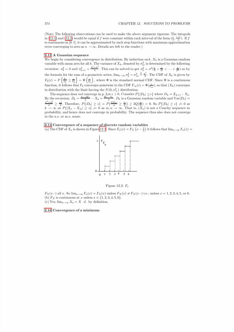
8/11/2019 Random process by B. Hajek
http://slidepdf.com/reader/full/random-process-by-b-hajek 384/448
8/11/2019 Random process by B. Hajek
http://slidepdf.com/reader/full/random-process-by-b-hajek 385/448
375
(a) The sequence (X n) converges to zero in all four senses. Here is one proof, and there are others.For any with 0 < < 1, P |X n − 0| ≥ = P U 1 ≥ , . . . , U n ≥ = (1 − )n, which convergesto zero as n → ∞. Thus, by definition, X n → 0 p. Thus, the sequence converges to zero in d.
sense and, since it is bounded, in the m.s. sense. For each ω, as a function of n, the sequence of numbers X 1(ω), X 2(ω), . . . is a nonincreasing sequence of numbers bounded below by zero. Thus,the sequence X n converges in the a.s. sense to some limit random variable. If a limit of randomvariables exists in different senses, the limit random variable has to be the same, so the sequence(X n) converges a.s. to zero.(b) For n fixed, the variable Y n is distributed over the interval [0, nθ], so let c be a number in thatinterval. Then P Y n ≤ c = P X n ≤ cn−θ = 1−P X n > cn−θ = 1−(1−cn−θ)n. Thus, if θ = 1,limn→∞ P Y n ≤ c = 1 − limn→∞(1 − c
n)n = 1 − exp(−c) for any c ≥ 0. Therefore, if θ = 1, thesequence (Y n) converges in distribution, and the limit distribution is the exponential distributionwith parameter one.
2.18 Limits of functions of random variables(a) Yes. Since g is a continuous function, if a sequence of numbers an converges to a limit a, theng(an) converges to g(a). Therefore, for any ω such that limn→∞ X n(ω) = X (ω), it holds thatlimn→∞ g(X n(ω)) = g(X (ω)). If X n → X a.s., then the set of all such ω has probability one, sog(X n) → g(X ) a.s.(b) Yes. A direct proof is to first note that |g(b) − g(a)| ≤ |b − a| for any numbers a and b. So, if X n → X m.s., then E [|g(X n) − g(X )|2] ≤ E [|X − X n|2] → 0 as n → ∞. Therefore g(X n) → g(X )m.s. A slightly more general proof would be to use the continuity of g (implying uniform continuityon bounded intervals) to show that g(X n) → g(X ) p., and then, since g is bounded, use the factthat convergence in probability for a bounded sequence implies convergence in the m.s. sense.)(c) No. For a counter example, let X n = (−1)n/n. Then X n → 0 deterministically, and hence inthe a.s. sense. But h(X n) = (
−1)n, which converges with probability zero, not with probability
one.(d) No. For a counter example, let X n = (−1)n/n. Then X n → 0 deterministically, and hence inthe m.s. sense. But h(X n) = (−1)n does not converge in the m.s. sense. (For a proof, note thatE [h(X m)h(X n)] = (−1)m+n, which does not converge as m, n → ∞. Thus, h(X n) does not satisfythe necessary Cauchy criteria for m.s. convergence.)
2.20 Sums of i.i.d. random variables, II(a) ΦX 1(u) = 1
2 e ju+ 12 e− ju = cos(u), so ΦS n(u) = ΦX 1(u)n = (cos(u))n, and ΦV n(u) = ΦS n(u/
√ n) =
cos(u/√
n)n.(b)
limn→∞ ΦS n(u) = 1 if u is an even multiple of π
does not exist if u is an odd multiple of π0 if u is not a multiple of π .
limn→∞ ΦV n(u) = lim
n→∞
1 − 1
2
u√
n
2
+ o
u2
n
n
= e−u2
2 .
8/11/2019 Random process by B. Hajek
http://slidepdf.com/reader/full/random-process-by-b-hajek 386/448
376 CHAPTER 12. SOLUTIONS TO PROBLEMS
(c) S n does not converge in distribution, because, for example, limn→∞ ΦS n(π) = limn→∞(−1)n
does not exist. So S n does not converge in the m.s., a.s. or p. sense either. The limit of ΦV n is
the characteristic function of the N (0, 1) distribution, so that (V n) converges in distribution andthe limit distribution is N (0, 1). It will next be proved that V n does not converge in probability.The intuitive idea is that if m is much larger than n, then most of the random variables in the sumdefining V m are independent of the variables defining V n. Hence, there is no reason for V m to beclose to V n with high probability. The proof below looks at the case m = 2n. Note that
V 2n − V n = X 1 + · · · + X 2n√
2n− X 1 + · · · + X n√
n
=
√ 2 − 2
2
X 1 + · · · + X n√
n
+
1√ 2
X n+1 + · · · + X 2n√
n
The two terms within the two pairs of braces are independent, and by the central limit theo-
rem, each converges in distribution to the N (0, 1) distribution. Thus limn→∞ d. V 2n − V n = W,
where W is a normal random variable with mean 0 and Var(W ) =√
2−22
2+
1√ 2
2= 2 − √
2.
Thus, limn→∞ P (|V 2n − V n| > ) = 0 so by the Cauchy criteria for convergence in probability, V ndoes not converge in probability. Hence V n does not converge in the a.s. sense or m.s. sense either.
2.22 Convergence and robustness of the sample median(a) We show that Y n
a.s.→ c∗. It suffices to prove that for any c0 and c1 with c0 < c∗ < c1,
P Y n ≤ c1 for all n sufficiently large = 1 (12.3)
P Y n ≥ c0 for all n sufficiently large = 1 (12.4)
Since c∗ is the unique solution to F (c∗) = 0.5, it follows that F (c1) > 0.5. By the strong law of large numbers,
I X 1≤c1 + · · · + I X 2n+1≤c12n + 1
a.s.→ F X (c1)
In words, it means that the fraction of the variables X 1, . . . , X 2n+1 that are less than or equal toc1 converges to F X (c1). Since F X (c1) > 0.5, it follows that
P
I X 1≤c1 + · · · + I X 2n+1≤c1
2n + 1 > 0.5 for all n large enough
= 1,
which, in turn, implies (12.3). The proof of (12.4) is similar, and omitted.
(b) The event |Y n| > c is a subset of the union of the events |X i| ≥ c for all i ∈ A over allA ⊂ 1, · · · , 2n + 1 with |A| = n + 1. There are less than 2n+1n+1
such subsets A of 1, · · · , 2n + 1,
and for any one of them, P |X i| ≥ c for all i ∈ A = P |X 1| ≥ cn+1. Now2n+1n+1
≤ 22n+1 becausethe number of subsets of 1, . . . , 2n+1 of cardinality n +1 is less than or equal to the total numberof subsets. Thus (b) follows by the union bound.(c) Note that for c > 0, P |X 1| ≥ c = 2
∞c
1π(1+u2) du ≤ 2
π
∞c
1u2 du = 2
πc . By the result of part
8/11/2019 Random process by B. Hajek
http://slidepdf.com/reader/full/random-process-by-b-hajek 387/448
377
(b) with n = 1, P |Y 1| ≥ c ≤ 8
2πc
2= 32
(πc)2 . Thus,
E [|Y 1|] =
∞
0 P |Y 1| ≥ cdc ≤ 1 +
∞
1 P |Y 1| ≥ cdc ≤ 1 +
∞
132
(πc)2 dc ≤ 1 + 32π2 .
2.24 Normal approximation for quantization errorThe mean of each roundoff error is zero and the variance is
0.5−0.5 u2du = 1
12 . Thus, E [S ] = 0 and
Var(S ) = 10012 = 8.333. Thus, P |S | ≥ 5 = P
S √ 8.333
≥ 5√ 8.333
≈ 2Q( 5√
8.333) = 2Q(1.73) =
2(1 − Φ(1.732)) = 0.083.
2.26 Applications of Jensen’s inequality(a) Convex function: ϕ(u) = 1
u . Random variable X .(b) Convex function: ϕ(u) = u2, Random variable X 2.(c) Convex function: ϕ(u) = u ln u, Random variable L=f(Y)/g(Y) where Y has probabil-ity density g. Indeed, in this case, Jensen’s inequality is E [ϕ(L)] ≥ ϕ(E [L]). But E [ϕ(L)] =
A f (y)g(y) ln f (y)g(y) g(y)dy = D(f |g), and E [Y ] = A f (y)g(y) g(y)dy = A f (y)dy = 1 and ϕ(1) = 0, sothat Jensen’s inequality becomes D(f |g) ≥ 0.Another solution is to use the function ϕ(u) = − ln u and the random variable Z = g(X )/f (X ),where X has density f . Indeed, in this case, Jensen’s inequality is E [ϕ(Z )] ≥ ϕ(E [Z ]). But
E [ϕ(Z )] = A − ln g(x)
f (x) f (x)dx = D(f |g), and E [Z ] = A
g(x)f (x)
f (x)dx =
A g(x)dx = 1 and
ϕ(1) = 0, so that Jensen’s inequality becomes D(f |g) ≥ 0.
2.28 Understanding the Markov inequality
(a) P |X | ≥ 10 = P X 4 ≥ 104 ≤ E [X 4]104 = 0.003.
(b) Equality holds if P X = 10 = 0.003 and P X = 0 = 0.997. (We could have guessed thisanswer as follows. The inequality in part (a) is obtained by taking expectations on each side of the
following inequaltiy: I |X |≥10 ≤ X 4
104. In order for equality to hold, we need I |X |≥10 = X 4
104 with
probability one. This requires X ∈ −10, 0, 10 with probability one.
2.30 Portfolio allocationLet
Z n =
2 if you win on day n,
12 if you lose on day n.
Then W n =n
k=1(1 − α + αZ n).(a) For α = 0, W n ≡ 1 (so W n → 1 a.s., m.s., p., d.)
(b) For α = 1, W n = exp (n
k=1 ln(Z k)). The exponent is a simple random walk-same as S n in *6.(Does not converge in any sense. It can be show that with probability one, W n is bounded neitherbelow nor above.)(c) ln W n =
nk=1 ln(1 − α + αZ k). By the strong law of large numbers, limn→∞ ln W n
n = R(α)a.s., where R(α) = E [ln(1 − α + αZ n)] = 1
2 [ln(1 + α) + ln(1 − α2 )]. Intuitively, this means that
W n ≈ enR(α) as n → ∞ in some sense. To be precise, it means there is a set of ω with prob-
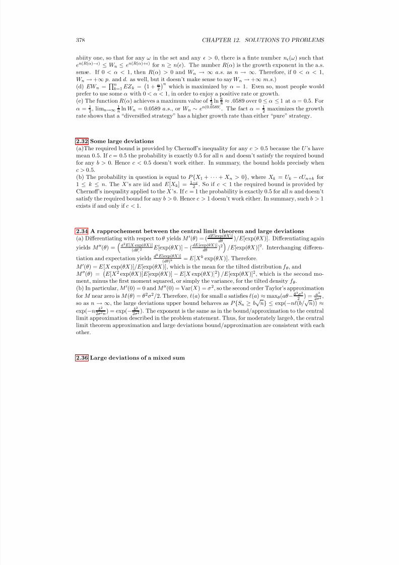
8/11/2019 Random process by B. Hajek
http://slidepdf.com/reader/full/random-process-by-b-hajek 388/448
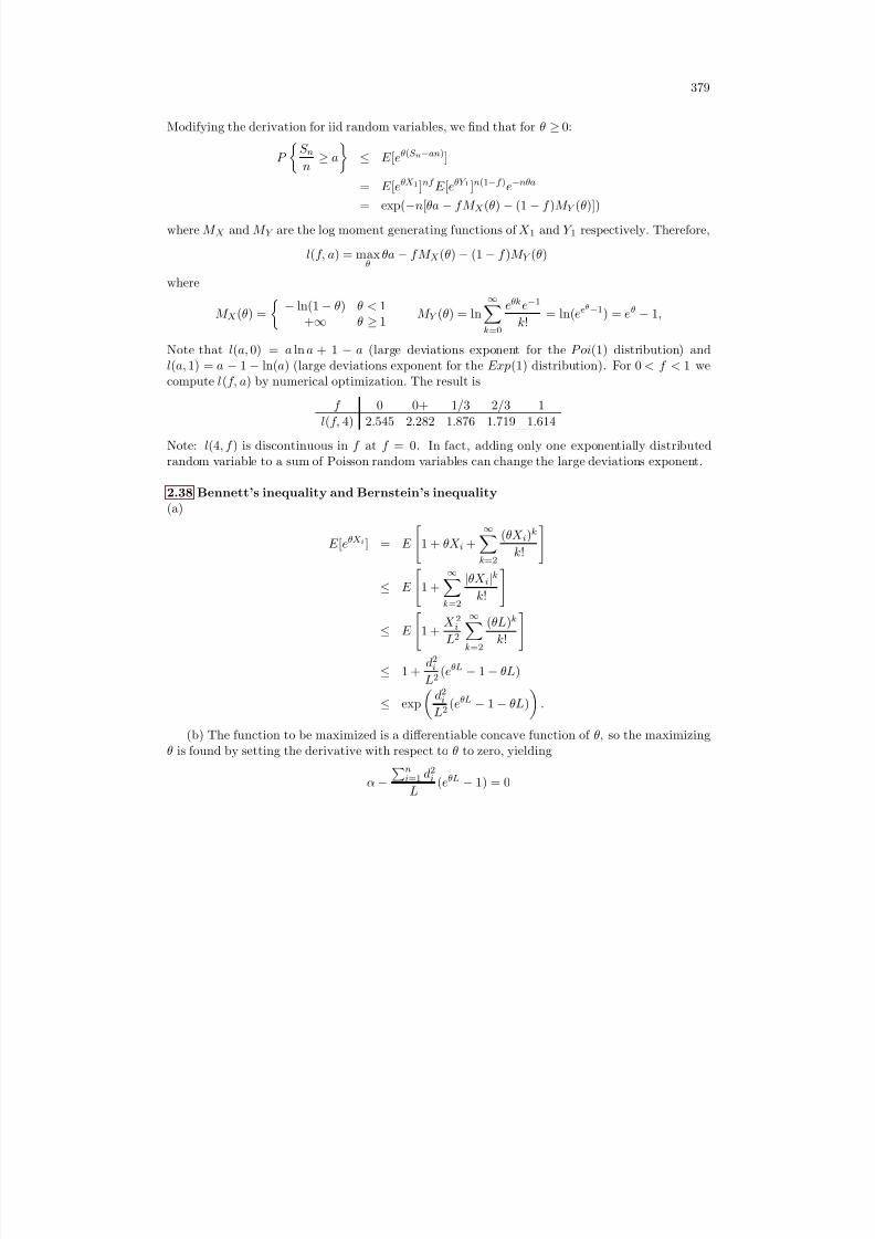
8/11/2019 Random process by B. Hajek
http://slidepdf.com/reader/full/random-process-by-b-hajek 389/448
379
Modifying the derivation for iid random variables, we find that for θ ≥ 0:
P
S nn
≥ a
≤ E [eθ(S n−an)]
= E [eθX 1]nf E [eθY 1 ]n(1−f )e−nθa
= exp(−n[θa − f M X (θ) − (1 − f )M Y (θ)])
where M X and M Y are the log moment generating functions of X 1 and Y 1 respectively. Therefore,
l(f, a) = maxθ
θa − f M X (θ) − (1 − f )M Y (θ)
where
M X (θ) =
− ln(1 − θ) θ < 1+∞ θ ≥ 1
M Y (θ) = ln
∞k=0
eθke−1
k! = ln(ee
θ−1) = eθ − 1,
Note that l(a, 0) = a ln a + 1 − a (large deviations exponent for the P oi(1) distribution) andl(a, 1) = a − 1 − ln(a) (large deviations exponent for the Exp(1) distribution). For 0 < f < 1 wecompute l(f, a) by numerical optimization. The result is
f 0 0+ 1/3 2/3 1
l(f, 4) 2.545 2.282 1.876 1.719 1.614
Note: l(4, f ) is discontinuous in f at f = 0. In fact, adding only one exponentially distributedrandom variable to a sum of Poisson random variables can change the large deviations exponent.
2.38 Bennett’s inequality and Bernstein’s inequality(a)
E [eθX i ] = E 1 + θX i +∞k=2
(θX i)k
k!
≤ E
1 +
∞k=2
|θX i|kk!
≤ E
1 +
X 2iL2
∞k=2
(θL)k
k!
≤ 1 + d2
i
L2(eθL − 1 − θL)
≤ exp d2i
L2 (e
θL
− 1 − θL) .
(b) The function to be maximized is a differentiable concave function of θ, so the maximizingθ is found by setting the derivative with respect to θ to zero, yielding
α −n
i=1 d2i
L (eθL − 1) = 0
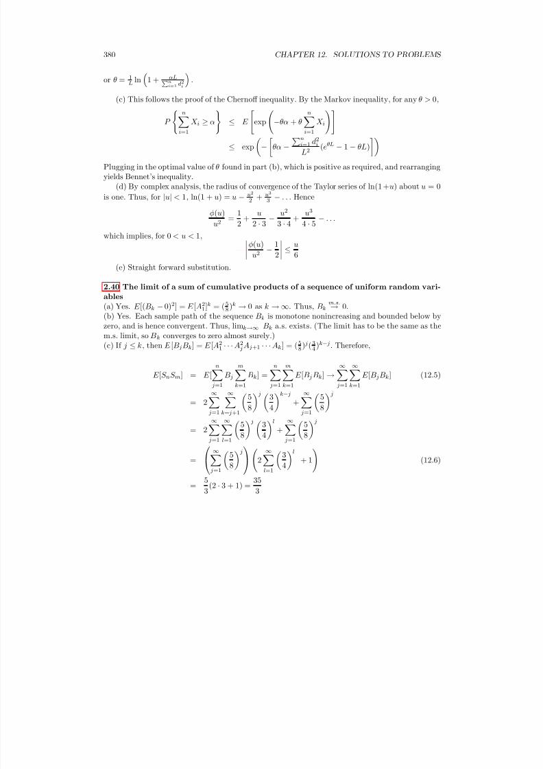
8/11/2019 Random process by B. Hajek
http://slidepdf.com/reader/full/random-process-by-b-hajek 390/448
380 CHAPTER 12. SOLUTIONS TO PROBLEMS
or θ = 1L ln
1 + αLPn
i=1 d2i
.
(c) This follows the proof of the Chernoff inequality. By the Markov inequality, for any θ > 0,
P n
i=1
X i ≥ α
≤ E
exp
−θα + θn
i=1
X i
≤ exp
−
θα −n
i=1 d2i
L2 (eθL − 1 − θL)
Plugging in the optimal value of θ found in part (b), which is positive as required, and rearrangingyields Bennet’s inequality.
(d) By complex analysis, the radius of convergence of the Taylor series of ln(1 + u) about u = 0
is one. Thus, for |u| < 1, ln(1 + u) = u − u2
2 + u3
3 − . . . Hence
φ(u)
u2 =
1
2 +
u
2 · 3 − u2
3 · 4 +
u3
4 · 5 − . . .
which implies, for 0 < u < 1, φ(u)
u2 − 1
2
≤ u
6
(e) Straight forward substitution.
2.40 The limit of a sum of cumulative products of a sequence of uniform random vari-ables(a) Yes. E [(Bk − 0)2] = E [A2
1]k = ( 58 )k → 0 as k → ∞. Thus, Bk
m.s.→ 0.(b) Yes. Each sample path of the sequence Bk is monotone nonincreasing and bounded below by
zero, and is hence convergent. Thus, limk→∞ Bk a.s. exists. (The limit has to be the same as them.s. limit, so Bk converges to zero almost surely.)(c) If j ≤ k, then E [B jBk] = E [A2
1 · · · A2 jA j+1 · · · Ak] = ( 5
8 ) j( 34 )k− j. Therefore,
E [S nS m] = E [n
j=1
B j
mk=1
Bk] =n
j=1
mk=1
E [B jBk] →∞
j=1
∞k=1
E [B jBk] (12.5)
= 2
∞ j=1
∞k= j+1
5
8
j 3
4
k− j+
∞ j=1
5
8
j= 2
∞
j=1
∞
l=1 5
8 j
3
4l
+∞
j=15
8 j
=
∞ j=1
5
8
j2∞l=1
3
4
l
+ 1
(12.6)
= 5
3(2 · 3 + 1) =
35
3
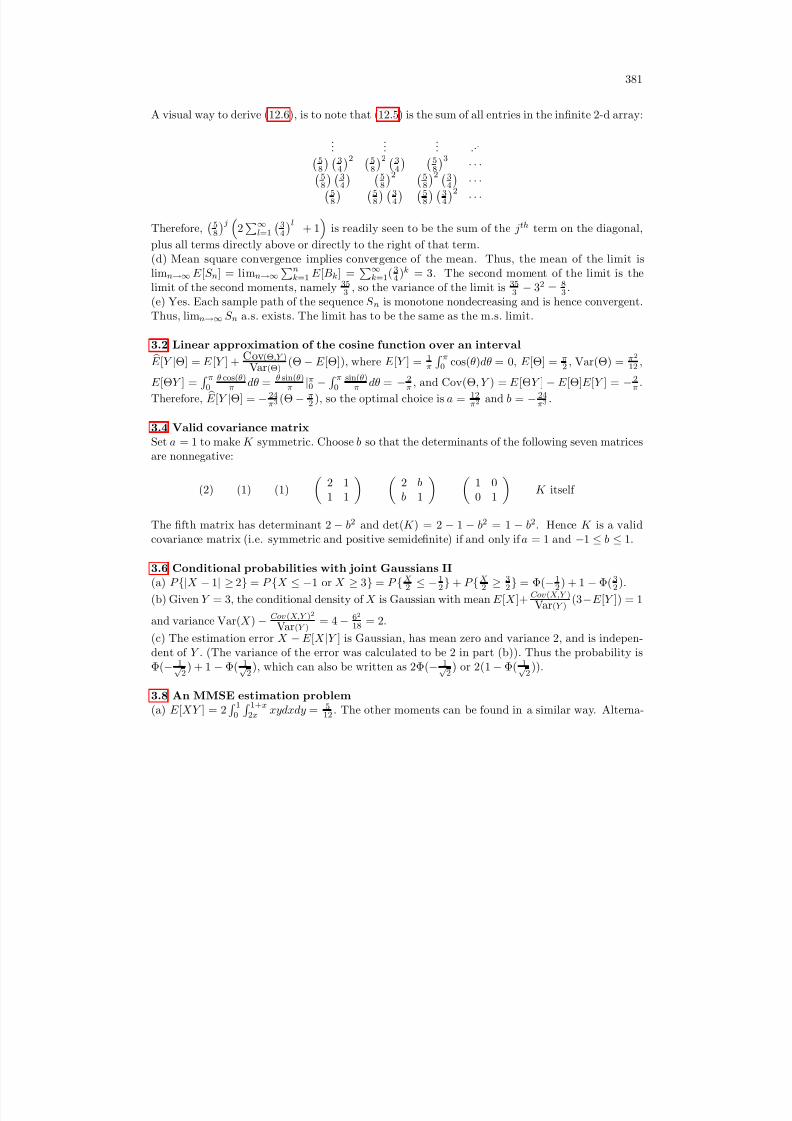
8/11/2019 Random process by B. Hajek
http://slidepdf.com/reader/full/random-process-by-b-hajek 391/448
381
A visual way to derive (12.6), is to note that (12.5) is the sum of all entries in the infinite 2-d array:
... ...
... .
·.
58 3
42 582 3
4 583 · · ·
58
34
58
2 58
2 34
· · ·58
58
34
58
34
2 · · ·
Therefore,
58
j 2∞
l=1
34
l+ 1
is readily seen to be the sum of the jth term on the diagonal,
plus all terms directly above or directly to the right of that term.(d) Mean square convergence implies convergence of the mean. Thus, the mean of the limit islimn→∞ E [S n] = limn→∞
nk=1 E [Bk] =
∞k=1( 3
4 )k = 3. The second moment of the limit is thelimit of the second moments, namely 35
3 , so the variance of the limit is 353 − 32 = 8
3 .(e) Yes. Each sample path of the sequence S n is monotone nondecreasing and is hence convergent.
Thus, limn→∞ S n a.s. exists. The limit has to be the same as the m.s. limit.
3.2 Linear approximation of the cosine function over an interval E [Y |Θ] = E [Y ] + Cov(Θ,Y )
Var(Θ) (Θ − E [Θ]), where E [Y ] = 1
π
π0 cos(θ)dθ = 0, E [Θ] = π
2 , Var(Θ) = π2
12 ,
E [ΘY ] = π
0θ cos(θ)
π dθ = θ sin(θ)π |π0 −
π0
sin(θ)π dθ = −2
π , and Cov(Θ, Y ) = E [ΘY ] − E [Θ]E [Y ] = −2π .
Therefore, E [Y |Θ] = − 24π3 (Θ − π
2 ), so the optimal choice is a = 12π2 and b = − 24
π3 .
3.4 Valid covariance matrixSet a = 1 to make K symmetric. Choose b so that the determinants of the following seven matricesare nonnegative:
(2) (1) (1) 2 11 1
2 bb 1
1 00 1
K itself
The fifth matrix has determinant 2 − b2 and det(K ) = 2 − 1 − b2 = 1 − b2. Hence K is a validcovariance matrix (i.e. symmetric and positive semidefinite) if and only if a = 1 and −1 ≤ b ≤ 1.
3.6 Conditional probabilities with joint Gaussians II(a) P |X − 1| ≥ 2 = P X ≤ −1 or X ≥ 3 = P X
2 ≤ −12 + P X
2 ≥ 32 = Φ(−1
2 ) + 1 − Φ( 32 ).
(b) Given Y = 3, the conditional density of X is Gaussian with mean E [X ]+ Cov(X,Y )
Var(Y ) (3−E [Y ]) = 1
and variance Var(X ) − Cov(X,Y )2
Var(Y ) = 4 − 62
18 = 2.
(c) The estimation error X − E [X |Y ] is Gaussian, has mean zero and variance 2, and is indepen-dent of Y . (The variance of the error was calculated to be 2 in part (b)). Thus the probability isΦ(− 1√
2) + 1 − Φ( 1√
2), which can also be written as 2Φ(− 1√
2) or 2(1 − Φ( 1√
2)).
3.8 An MMSE estimation problem(a) E [XY ] = 2
10
1+x2x xydxdy = 5
12 . The other moments can be found in a similar way. Alterna-
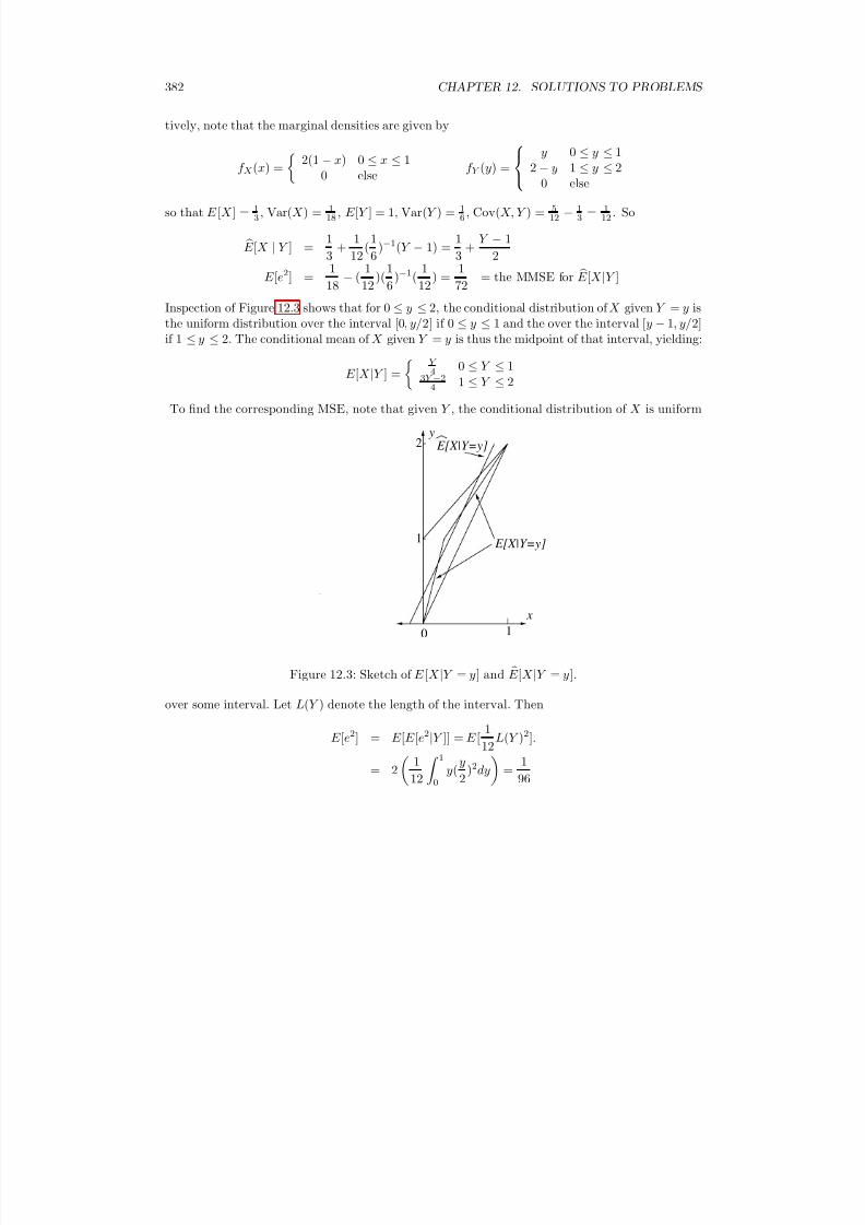
8/11/2019 Random process by B. Hajek
http://slidepdf.com/reader/full/random-process-by-b-hajek 392/448
382 CHAPTER 12. SOLUTIONS TO PROBLEMS
tively, note that the marginal densities are given by
f X
(x) = 2(1
−x) 0
≤ x
≤ 1
0 else f
Y (y) =
y 0 ≤ y ≤ 12
−y 1
≤ y
≤ 2
0 else
so that E [X ] = 13 , Var(X ) = 1
18 , E [Y ] = 1, Var(Y ) = 16 , Cov(X, Y ) = 5
12 − 13 = 1
12 . So
E [X | Y ] = 1
3 +
1
12(
1
6)−1(Y − 1) =
1
3 +
Y − 1
2
E [e2] = 1
18 − (
1
12)(
1
6)−1(
1
12) =
1
72 = the MMSE for E [X |Y ]
Inspection of Figure 12.3 shows that for 0 ≤ y ≤ 2, the conditional distribution of X given Y = y isthe uniform distribution over the interval [0, y/2] if 0 ≤ y ≤ 1 and the over the interval [y − 1, y/2]if 1
≤ y
≤ 2. The conditional mean of X given Y = y is thus the midpoint of that interval, yielding:
E [X |Y ] =
Y
4 0 ≤ Y ≤ 13Y −2
4 1 ≤ Y ≤ 2
To find the corresponding MSE, note that given Y , the conditional distribution of X is uniform
E[X|Y=y]
E[X|Y=y]
y
x
2
1
0 1
Figure 12.3: Sketch of E [X |Y = y] and
E [X |Y = y].
over some interval. Let L(Y ) denote the length of the interval. Then
E [e2] = E [E [e2|Y ]] = E [ 1
12L(Y )2].
= 2
1
12
1
0y(
y
2)2dy
=
1
96
8/11/2019 Random process by B. Hajek
http://slidepdf.com/reader/full/random-process-by-b-hajek 393/448
383
For this example, the MSE for the best estimator is 25% smaller than the MSE for the best linearestimator.(b)
E [X ] = ∞−∞
|y| 1√ 2π
e−y2/2dy = 2 ∞
0
y√ 2π
e−12y2dy =
2π
and E [Y ] = 0,
Var(Y ) = 1, Cov(X, Y ) = E [|Y |Y ] = 0 so E [X |Y ] =
2
π +
0
1Y ≡
2
π
That is, the best linear estimator is the constant E [X ]. The corresponding MSE is Var(X ) =E [X 2] − E [X ]2 = E [Y 2] − 2
π = 1 − 2π . Note that |Y | is a function of Y with mean square error
E [(X − |Y |)2] = 0. Nothing can beat that, so |Y | is the MMSE estimator of X given Y . So
|Y | = E [X |Y ]. The corresponding MSE is 0, or 100% smaller than the MSE for the best linearestimator.
3.10 Conditional Gaussian comparison(a) pa = P X ≥ 2 = P X √
10 ≥ 2√
10 = Q( 2√
10) = Q(0.6324).
(b) By the theory of conditional distributions for jointly Gaussian random variables, the conditionaldistribution of X given Y = y is Gaussian, with mean E [X |Y = y ] and variance σ2
e , which is the
MSE for estimation of X by E [X |Y ]. Since X and Y are mean zero and Cov(X,Y )
Var(Y ) = 0.8, we have
E [X |Y = y] = 0.8y, and σ2
e = Var(X ) − Cov(X,Y )2
Var(Y ) = 3.6. Hence, given Y = y, the conditional
distribution of X is N (0.8y, 3.6). Therefore, P (X
≥ 2
|Y = y) = Q( 2−(0.8)y√
3.6
). In particular, pb =
P (X ≥ 2|Y = 3) = Q( 2−(0.8)3√ 3.6
) = Q(−0.2108).
(c) Given the event Y ≥ 3, the conditional pdf of Y is obtained by setting the pdf of Y to zero onthe interval (−∞, 3), and then renormalizing by P Y ≥ 3 = Q( 3√
10) to make the density integrate
to one. We can write this as
f Y |Y ≥3(y) =
f Y (y)1−F Y (3) = e−y2/20
Q( 3√ 10
)√
20π y ≥ 3
0 else.
Using this density, by considering the possible values of Y , we have
pc = P (X ≥ 2|Y ≥ 3) =
∞3
P (X ≥ 2, Y ∈ dy|Y ≥ 3) =
∞3
P (X ≥ 2|Y = y)P (Y ∈ dy|Y ≥ 3)
=
∞3
Q(2 − (0.8)y√
3.6)f Y |Y ≥3(y)dy
8/11/2019 Random process by B. Hajek
http://slidepdf.com/reader/full/random-process-by-b-hajek 394/448
384 CHAPTER 12. SOLUTIONS TO PROBLEMS
(ALTERNATIVE) The same expression can be derived in a more conventional fashion as follows:
pe = P (X ≥ 2|Y ≥ 3) = P X ≥ 2, Y ≥ 3
P
Y ≥
3
= ∞
3
∞2
f X |Y (x|y)dx
f Y (y)dy/P Y ≥ 3
=
∞3
Q
2 − (0.8)y√
3.6
f Y (y)dy/(1 − F Y (3)) =
∞3
Q(2 − (0.8)y√
3.6)f Y |Y ≥3(y)dy
(d) We will show that pa < pb < pc. The inequality pa < pb follows from parts (a) and (b) and
the fact the function Q is decreasing. By part (c), pc is an average of Q( 2−(0.8)y√ 3.6
) with respect to y
over the region y ∈ [3, ∞) (using the pdf f Y |Y ≥3). But everywhere in that region, Q( 2−(0.8)y√ 3.6
) > pb,
showing that pc > pb.
3.12 An estimator of an estimatorTo show that E [X |Y ] is the LMMSE estimator of E [X |Y ], it suffices by the orthogonality principleto note that E [X |Y ] is linear in (1, Y ) and to prove that E [X |Y ] − E [X |Y ] is orthogonal to 1and to Y . However E [X |Y ] − E [X |Y ] can be written as the difference of two random variables(X − E [X |Y ]) and (X −E [X |Y ]), which are each orthogonal to 1 and to Y . Thus, E [X |Y ]− E [X |Y ]is also orthogonal to 1 and to Y , and the result follows.
Here is a generalization, which can be proved in the same way. Suppose V 0 and V 1 are twoclosed linear subspaces of random variables with finite second moments, such that V 0 ⊃ V 1. LetX be a random variable with finite second moment, and let X ∗i be the variable in V i with theminimum mean square distance to X , for i = 0 or i = 1. Then X ∗1 is the variable in V 1 with theminimum mean square distance to X ∗0 .
Another solution to the original problem can be obtained by using the formula for E [Z |Y ]
applied to Z = E [X |Y ]: E [E [X |Y ]|Y ] = E [E [X |Y ]] + Cov(Y, E [X |Y ])Var(Y )−1(Y − E [Y ])
which can be simplified using E [E [X |Y ]] = E [X ] and
Cov(Y, E [X |Y ]) = E [Y (E [X |Y ] − E [X ])]
= E [Y E [X |Y ]] − E [Y ]E [X ]
= E [E [XY |Y ]] − E [Y ]E [X ]
= E [XY ] − E [X ]E [Y ] = Cov(X, Y )
to yield the desired result.
3.14 Some identities for estimators(a) True. The random variable E [X |Y ] cos(Y ) has the following two properties:
• It is a function of Y with finite second moments (because E [X |Y ] is a function of Y withfinite second moment and cos(Y ) is a bounded function of Y )
8/11/2019 Random process by B. Hajek
http://slidepdf.com/reader/full/random-process-by-b-hajek 395/448
385
• (X cos(Y ) − E [X |Y ]cos(Y )) ⊥ g(Y ) for any g with E [g(Y )2] < ∞ (because for any such g,E [(X cos(Y )−E [X |Y ]cos(Y ))g(Y )] = E [(X −E [X |Y ])
g(Y )] = 0, where
g(Y ) = g(Y )cos(Y ).)
Thus, by the orthogonality principle, E [X
|Y ]cos(Y ) is equal to E [X cos(Y )
|Y ].
(b) True. The left hand side is the projection of X onto the space g(Y ) : E [g(Y )2] < ∞ and theright hand side is the projection of X onto the space f (Y 3) : E [f (Y 3)2] < ∞. But these twospaces are the same, because for each function g there is the function f (u) = g(u1/3). The point isthat the function y3 is an invertible function, so any function of Y can also be written as a functionof Y 3.(c) False. For example, let X be uniform on the interval [0, 1] and let Y be identically zero. ThenE [X 3|Y ] = E [X 3] = 1
4 and E [X |Y ]3 = E [X ]3 = 18 .
(d) False. For example, let P X = Y = 1 = P X = Y = −1 = 0.5. Then E [X |Y ] = Y whileE [X |Y 2] = 0. The point is that the function y2 is not invertible, so that not every function of Y can be written as a function of Y 2. Equivalently, Y 2 can give less information than Y .(e) False. For example, let X be uniformly distributed on [−1, 1], and let Y = X . Then E [X |Y ] = Y
while E [X |Y 3] = E [X ] + Cov(X,Y 3
)Var(Y 3) (Y 3 − E [Y 3]) = E [X 4
]E [X 6] Y 3 = 75 Y 3.(f)) True. The given implies that the mean, E [X ] has the minimum MSE over all possible functionsof Y. (i.e. E [X ] = E [X |Y ]) Therefore, E [X ] also has the minimum MSE over all possible affinefunctions of Y , so E [X |Y ] = E [X ]. Thus, E [X |Y ] = E [X ] = E [X |Y ].
3.16 Some simple examplesOf course there are many valid answers for this problem–we only give one.(a) Let X denote the outcome of a roll of a fair die, and let Y = 1 if X is odd and Y = 2 if X iseven. Then E [X |Y ] has to be linear. In fact, since Y has only two possible values, any functionof Y can be written in the form a + bY. That is, any function of Y is linear. (There is no need toeven calculate E [X
|Y ] here, but we note that is is given by E [Y
|X ] = X + 2.)
(b) Let X be a N(0,1) random variable, and let W be indpendent of X , with P W = 1 = P W =−1 = 1
2 . Finally, let Y = XW . The conditional distribution of Y given W is N (0, 1), for eitherpossible value of W , so the unconditional value of Y is also N (0, 1). However, P X −Y = 0 = 0.5,so that X − Y is not a Gaussian random variable, so X and Y are not jointly Gaussian.(c) Let the triplet (X,Y,Z ) take on the four values (0, 0, 0), (1, 1, 0), (1, 0, 1), (0, 1, 1) with equalprobability. Then any pair of these variables takes the values (0, 0), (0, 1), (1, 0), (1, 1) with equalprobability, indicating pairwise independence. ButP (X,Y,Z = (0, 0, 1) = 0 = P X = 0P Y = 0P Z = 1 = 1
8 . So the three random variablesare not independent.
3.18 Estimating a quadratic
(a) Recall the fact that E [Z 2
] = E [Z ]2
+ Var(Z ) for any second order random variable Z . Theidea is to apply the fact to the conditional distribution of X given Y . Given Y , the conditionaldistribution of X is Gaussian with mean ρY and variance 1 − ρ2. Thus, E [X 2|Y ] = (ρY )2 + 1 − ρ2.(b) The MSE=E [(X 2)2]−E [(E [X 2|Y ])2] = E [X 4]−ρ4E [Y 4]−2ρ2E [Y 2](1−ρ2)−(1−ρ2)2 = 2(1−ρ4)(c) Since Cov(X 2, Y ) = E [X 2Y ] = 0, it follows that E [X 2|Y ] = E [X 2] = 1. That is, the best linearestimator in this case is just the constant estimator equal to 1.
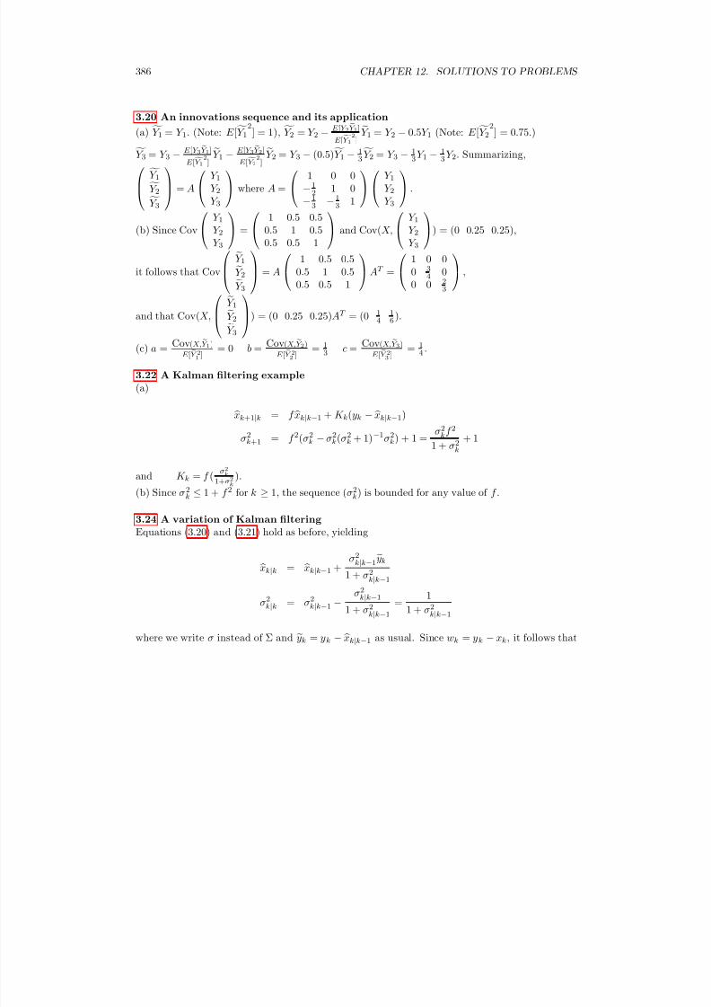
8/11/2019 Random process by B. Hajek
http://slidepdf.com/reader/full/random-process-by-b-hajek 396/448
386 CHAPTER 12. SOLUTIONS TO PROBLEMS
3.20 An innovations sequence and its application
(a) Y 1 = Y 1. (Note: E [Y 12
] = 1), Y 2 = Y 2
− E [Y 2 eY 1]
E [fY 12
] Y 1 = Y 2
−0.5Y 1 (Note: E [Y 2
2] = 0.75.)
Y 3 = Y 3 − E [Y 3 eY 1]
E [fY 12]
Y 1 − E [Y 3 eY 2]
E [fY 22]
Y 2 = Y 3 − (0.5)Y 1 − 13Y 2 = Y 3 − 1
3 Y 1 − 13 Y 2. Summarizing, Y 1Y 2Y 3
= A
Y 1Y 2Y 3
where A =
1 0 0−1
2 1 0−1
3 −13 1
Y 1Y 2Y 3
.
(b) Since Cov
Y 1Y 2Y 3
=
1 0.5 0.50.5 1 0.50.5 0.5 1
and Cov(X,
Y 1Y 2Y 3
) = (0 0.25 0.25),
it follows that Cov
Y 1
Y 2Y 3
= A
1 0.5 0.50.5 1 0.5
0.5 0.5 1
AT =
1 0 00 3
4 0
0 0 2
3
,
and that Cov(X,
Y 1Y 2Y 3
) = (0 0.25 0.25)AT = (0 14
16 ).
(c) a = Cov(X,eY 1)
E [eY 21 ] = 0 b = Cov(X,eY 2)
E [eY 22 ] = 1
3 c = Cov(X,eY 3)
E [eY 23 ] = 1
4 .
3.22 A Kalman filtering example(a)
xk+1|k = f
xk|k−1 + K k(yk −
xk|k−1)
σ2k+1 = f 2(σ2
k − σ2k(σ2
k + 1)−1σ2k) + 1 = σ2kf 2
1 + σ2k
+ 1
and K k = f ( σ2k1+σ2k
).
(b) Since σ 2k ≤ 1 + f 2 for k ≥ 1, the sequence (σ2
k) is bounded for any value of f .
3.24 A variation of Kalman filteringEquations (3.20) and (3.21) hold as before, yielding
xk|k = xk
|k−
1 +σ2k|k−1
yk
1 + σ2k|k−1
σ2k|k = σ2
k|k−1 −σ2k|k−1
1 + σ2k|k−1
= 1
1 + σ2k|k−1
where we write σ instead of Σ and yk = yk − xk|k−1 as usual. Since wk = yk − xk, it follows that
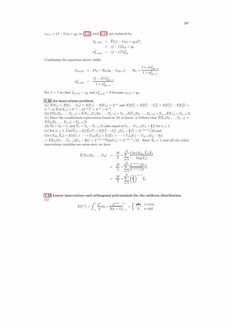
8/11/2019 Random process by B. Hajek
http://slidepdf.com/reader/full/random-process-by-b-hajek 397/448
387
xk+1 = (f − 1)xk + yk, so (3.22) and (3.23) get replaced by
xk+1|k =
E [(f − 1)xk + yk|yk]
= (f − 1) xk|k + yk
σ2k+1|k = (f − 1)2σ2
k|k
Combining the equations above yields
xk+1|k = f xk + K k(yk − xk|k−1) K k =1 + f σ2
k|k−1
1 + σ2k|k−1
σ2k+1|k =
(f − 1)2σ2k|k−1
1 + σ2k|k−1
For f = 1 we find xk+1|k = yk and σ
2
k+1|k = 0 because xk+1 = yk.
3.26 An innovations problem(a) E [Y n] = E [U 1 · · · U n] = E [U 1] · · · E [U n] = 2−n and E [Y 2n ] = E [U 21 · · · U 2n] = E [U 21 ] · · · E [U 2n] =3−n, so Var(Y n) = 3−n − (2−n)2 = 3−n − 4−n.(b) E [Y n|Y 0, . . . , Y n−1] = E [Y n−1U n|Y 0, . . . , Y n−1] = Y n−1E [U n|Y 0, . . . , Y n−1] = Y n−1E [U n] = Y n−1/2.(c) Since the conditional expectation found in (b) is linear, it follows that E [Y n|Y 0, . . . , Y n−1] =E [Y n|Y 0, . . . , Y n−1] = Y n−1/2.(d) Y 0 = Y 0 = 1, and Y n = Y n − Y n−1/2 (also equal to U 1 · · · U n−1(U n − 1
2 )) for n ≥ 1.
(e) For n ≥ 1, Var(Y n) = E [(Y n)2] = E [U 21 · · · U 2n−1(U n − 12 )2] = 3−(n−1)/12 and
Cov(X M ,
Y n) = E [(U 1 + · · · + U M )
Y n] = E [(U 1 + · · · + U M )U 1 · · · U n−1(U n − 1
2 )]
= E [U n(U 1 · · · U n−1)(U n − 1
2 )] = 2−(n
−1)
Var(U n) = 2−(n−
1)
/12. Since Y 0 = 1 and all the otherinnovations variables are mean zero, we have
E [X M |Y 0, . . . , Y M ] = M
2 +
M n=1
Cov(X M , Y n)Y n
Var(Y n)
= M
2 +
M n=1
2−n+1/12
3−n+1/12Y n
= M
2 +
M n=1
3
2
n−1
Y n
3.28 Linear innovations and orthogonal polynomials for the uniform distribution(a)
E [U n] =
1
−1
un
2 du =
un+1
2(n + 1)
1−1
=
1n+1 n even
0 n odd
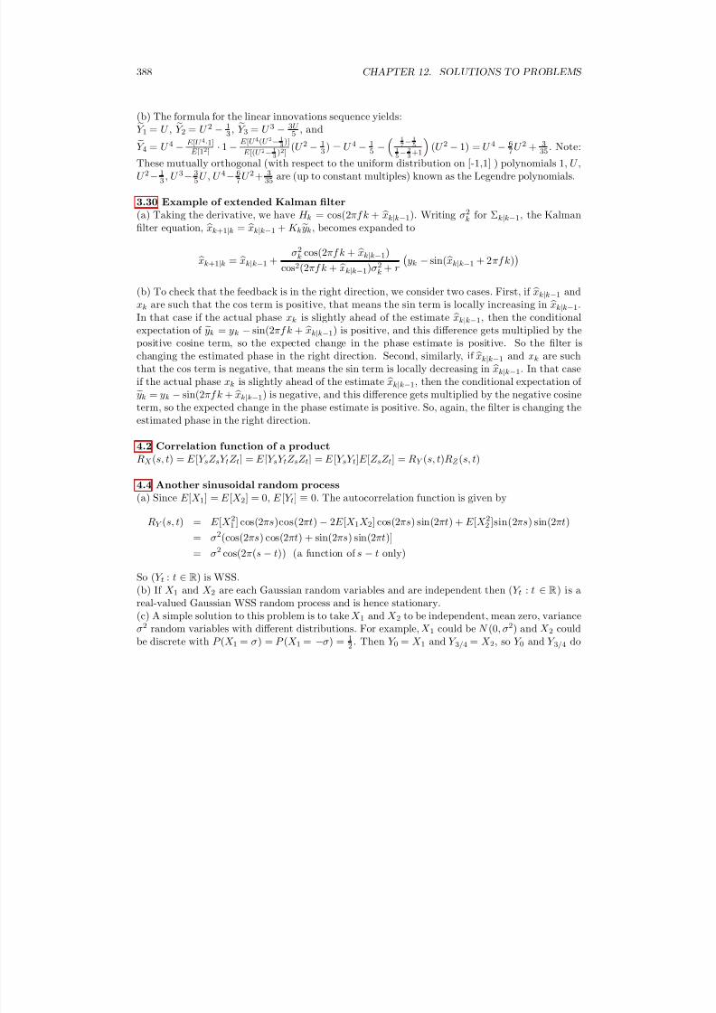
8/11/2019 Random process by B. Hajek
http://slidepdf.com/reader/full/random-process-by-b-hajek 398/448
388 CHAPTER 12. SOLUTIONS TO PROBLEMS
(b) The formula for the linear innovations sequence yields:
Y 1 = U ,
Y 2 = U 2 − 1
3 ,
Y 3 = U 3 − 3U
5 , and
Y 4 = U 4 − E [U 4
·1]E [12] · 1 − E [U 4
(U 2
−1
3 )]E [(U 2− 1
3)2] (U 2 − 13 ) = U 4 − 15 − 1
7−1
515− 23
+1 (U 2 − 1) = U 4 − 67 U 2 + 335 . Note:
These mutually orthogonal (with respect to the uniform distribution on [-1,1] ) polynomials 1, U ,U 2− 1
3 , U 3− 35 U , U 4− 6
7 U 2 + 335 are (up to constant multiples) known as the Legendre polynomials.
3.30 Example of extended Kalman filter(a) Taking the derivative, we have H k = cos(2πf k + xk|k−1). Writing σ2
k for Σk|k−1, the Kalmanfilter equation, xk+1|k = xk|k−1 + K kyk, becomes expanded to
xk+1|k =
xk|k−1 +
σ2k cos(2πf k + xk|k−1)
cos2(2πf k +
xk|k−1)σ2
k + r
yk − sin(
xk|k−1 + 2πf k)
(b) To check that the feedback is in the right direction, we consider two cases. First, if xk|k−1 andxk are such that the cos term is positive, that means the sin term is locally increasing in xk|k−1.In that case if the actual phase xk is slightly ahead of the estimate xk|k−1, then the conditionalexpectation of yk = yk − sin(2πf k + xk|k−1) is positive, and this difference gets multiplied by thepositive cosine term, so the expected change in the phase estimate is positive. So the filter ischanging the estimated phase in the right direction. Second, similarly, if xk|k−1 and xk are suchthat the cos term is negative, that means the sin term is locally decreasing in xk|k−1. In that caseif the actual phase xk is slightly ahead of the estimate xk|k−1, then the conditional expectation of yk = yk − sin(2πf k + xk|k−1) is negative, and this difference gets multiplied by the negative cosineterm, so the expected change in the phase estimate is positive. So, again, the filter is changing theestimated phase in the right direction.
4.2 Correlation function of a productRX (s, t) = E [Y sZ sY tZ t] = E [Y sY tZ sZ t] = E [Y sY t]E [Z sZ t] = RY (s, t)RZ (s, t)
4.4 Another sinusoidal random process(a) Since E [X 1] = E [X 2] = 0, E [Y t] ≡ 0. The autocorrelation function is given by
RY (s, t) = E [X 21 ] cos(2πs)cos(2πt) − 2E [X 1X 2] cos(2πs) sin(2πt) + E [X 22 ]sin(2πs) sin(2πt)
= σ2(cos(2πs) cos(2πt) + sin(2πs) sin(2πt)]
= σ2 cos(2π(s − t)) (a function of s − t only)
So (Y t : t ∈ R) is WSS.(b) If X 1 and X 2 are each Gaussian random variables and are independent then (Y t : t ∈ R) is areal-valued Gaussian WSS random process and is hence stationary.(c) A simple solution to this problem is to take X 1 and X 2 to be independent, mean zero, varianceσ2 random variables with different distributions. For example, X 1 could be N (0, σ2) and X 2 couldbe discrete with P (X 1 = σ) = P (X 1 = −σ) = 1
2 . Then Y 0 = X 1 and Y 3/4 = X 2, so Y 0 and Y 3/4 do
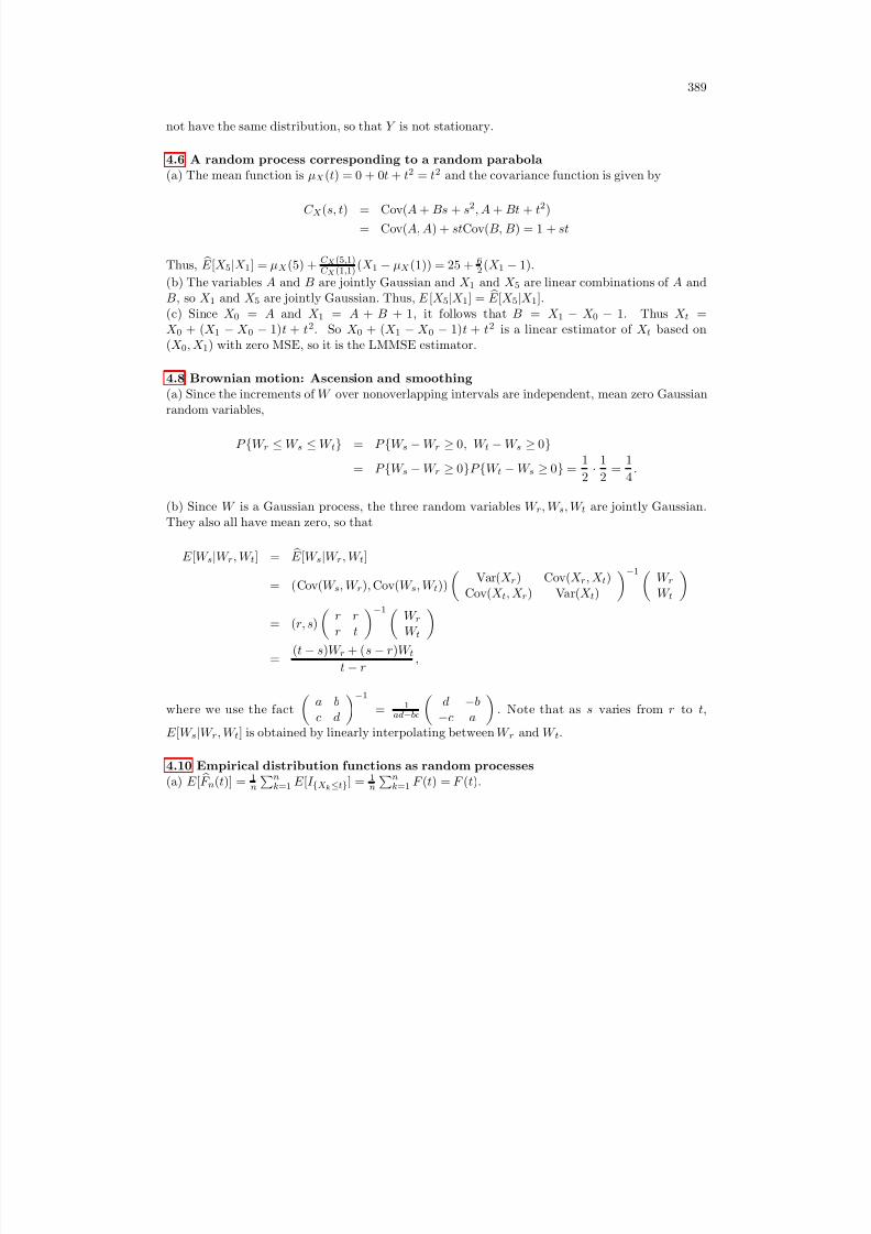
8/11/2019 Random process by B. Hajek
http://slidepdf.com/reader/full/random-process-by-b-hajek 399/448
389
not have the same distribution, so that Y is not stationary.
4.6 A random process corresponding to a random parabola
(a) The mean function is µX (t) = 0 + 0t + t2 = t2 and the covariance function is given by
C X (s, t) = Cov(A + Bs + s2, A + Bt + t2)
= Cov(A, A) + stCov(B, B) = 1 + st
Thus, E [X 5|X 1] = µX (5) + C X(5,1)C X(1,1) (X 1 − µX (1)) = 25 + 6
2 (X 1 − 1).
(b) The variables A and B are jointly Gaussian and X 1 and X 5 are linear combinations of A andB, so X 1 and X 5 are jointly Gaussian. Thus, E [X 5|X 1] = E [X 5|X 1].(c) Since X 0 = A and X 1 = A + B + 1, it follows that B = X 1 − X 0 − 1. Thus X t =X 0 + (X 1 − X 0 − 1)t + t2. So X 0 + (X 1 − X 0 − 1)t + t2 is a linear estimator of X t based on(X
0, X
1) with zero MSE, so it is the LMMSE estimator.
4.8 Brownian motion: Ascension and smoothing(a) Since the increments of W over nonoverlapping intervals are independent, mean zero Gaussianrandom variables,
P W r ≤ W s ≤ W t = P W s − W r ≥ 0, W t − W s ≥ 0= P W s − W r ≥ 0P W t − W s ≥ 0 =
1
2 · 1
2 =
1
4.
(b) Since W is a Gaussian process, the three random variables W r, W s, W t are jointly Gaussian.They also all have mean zero, so that
E [W s|W r, W t] = E [W s|W r, W t]
= (Cov(W s, W r), Cov(W s, W t))
Var(X r) Cov(X r, X t)Cov(X t, X r) Var(X t)
−1 W rW t
= (r, s)
r rr t
−1 W rW t
=
(t − s)W r + (s − r)W tt − r
,
where we use the fact a bc d −1
= 1ad−bc d −b−c a . Note that as s varies from r to t,
E [W s|W r, W t] is obtained by linearly interpolating between W r and W t.
4.10 Empirical distribution functions as random processes(a) E [ F n(t)] = 1
n
nk=1 E [I X k≤t] = 1
n
nk=1 F (t) = F (t).
8/11/2019 Random process by B. Hajek
http://slidepdf.com/reader/full/random-process-by-b-hajek 400/448
390 CHAPTER 12. SOLUTIONS TO PROBLEMS
C (s, t) = Cov
1
n
n
k=1
I X k≤s, 1
n
n
l=1
I X l≤t=
1
n2
nk=1
nl=1
Cov
I X k≤s, I X l≤t
= 1
n2
nk=1
Cov
I X k≤s, I X k≤t
= 1
nCov
I X 1≤s, I X 1≤t
where we used the fact that for k = l, the random variables I X k≤s and I X l≤t are independent,and hence, uncorrelated, and the random variables X k are identically distributed. If s
≤ t, then
Cov I X 1≤s, I X 1≤t = E I X 1≤sI X 1≤t− E I X 1≤sE I X 1≤t= E
I X 1≤s
− F (s)F (t) = F (s) − F (s)F (t).
Similarly, if s ≥ t,Cov
I X 1≤s, I X 1≤t
= F (t) − F (s)F (t).
Thus, in general, Cov
I X 1≤s, I X 1≤t
= F (s ∧ t) − F (s)F (t), where s ∧ t = mins, t, and so
C (s, t) = F (s∧t)−F (s)F (t)
n .(b) The convergence follows by the strong law of large numbers applied to the iid random
variables I X k≤t, k ≥ 1.(c) Let U k = F (X k) for all k ≥ 1 and suppose that F is a continuous CDF. Fix v ∈ (0, 1). Then,
since F is a continuous CDF, there exits a value t such that F (t) = v. Then P F (X k) ≤ v =P X k ≤ t = F (t) = v. Therefore, as suggested in the hint, the U ’s are uniformly distributed over[0, 1]. For any k, under the assumptions on F, X k ≤ t and F (X k) ≤ v are the same events.Summing the indicator functions over k and dividing by n yields that F n(t) = Gn(v), and thereforethat | F n(t) − F (t)| = | Gn(v) − v|.
Taking the supremum over all all t ∈ R, or over all v ∈ (0, 1), while keeping F (t) = v, showsthat Dn = sup0<v<1 | Gn(v) − v|, and, since G(v) = v, the LHS of this equation is just Dn for thecase of the uniformly distributed random variables U k, k ≥ 1.
(d) Observe, for t fixed, that X n(t) =Pn
k=1(I Xn≤t−F (t))√ n
and the random variables I X n≤t−F (t)
have mean zero and variance F (t)(1 − F (t)). Therefore, by the central limit theorem, for each tfixed, X n(t) converges in distribution and the limit is Gaussian with mean zero and variance
C (t, t) = F (t)(1 − F (t)).(e) The covariance is n times the covariance function found in part (a), with F (t) = t. The
result is s ∧ t − st, as claimed in the problem statement.(Note: The distance Dn is known as the Kolmogorov-Smirnov statistic, and by pursuing the
method of this problem further, the limiting distribution of √
nDn can be found and it is equal tothe distribution of the maximum of a Brownian bridge, a result due to J.L. Doob. )
8/11/2019 Random process by B. Hajek
http://slidepdf.com/reader/full/random-process-by-b-hajek 401/448
391
4.12 MMSE prediction for a Gaussian process based on two observations
(a) Since RX (0) = 5, RX (1) = 0, and RX (2) = −59 , the covariance matrix is
5 0 −590 5 0
−59 0 5
.
(b) As the variables are all mean zero, E [X (4)|X (2)] = Cov(X (4),X (2))
Var(X (2) X (2) = −X (2)
9 .
(c) The variable X (3) is uncorrelated with (X (2), X (4))T . Since the variables are jointly Gaussian,
X (3) is also independent of (X (2), X (4))T . So E [X (4)|X (2)] = E [X (4)|X (2), X (3)] = −X (2)9 .
4.14 Poisson process probabilities(a) The numbers of arrivals in the disjoint intervals are independent, Poisson random variables withmean λ. Thus, the probability is (λe−λ)3 = λ3e−3λ.
(b) The event is the same as the event that the numbers of counts in the intervals [0,1], [1,2], and[2,3] are 020, 111, or 202. The probability is thus e−λ(λ2
2 e−λ)e−λ + (λe−λ)3 + (λ2
2 e−λ)e−λ(λ2
2 e−λ) =
(λ2
2 + λ3 + λ4
4 )e−3λ.(c) This is the same as the probability the counts are 020, divided by the answer to part (b), orλ2
2 /(λ2
2 + λ3 + λ4
4 ) = 2λ2/(2 + 4λ + λ2).
4.16 Adding jointly stationary Gaussian processes
(a) RZ (s, t) = E
X (s)+Y (s)2
X (t)+Y (t)
2
= 1
4 [RX (s − t) + RY (s − t) + RXY (s − t) + RY X (s − t)].
So RZ (s, t) is a function of s − t. Also, RY X (s, t) = RXY (t, s). Thus,
RZ (τ ) = 14 [2e−|τ | + e−|τ −3|
2 + e−|τ +3|2 ].
(b) Yes, the mean function of Z is constant (µZ
≡ 0) and RZ (s, t) is a function of s
−t only, so Z
is WSS. However, Z is obtained from the jointly Gaussian processes X and Y by linear operations,so Z is a Gaussian process. Since Z is Gaussian and WSS, it is stationary.
(c) P X (1) < 5Y (2) + 1 = P
X (1)−5Y (2)σ ≤ 1
σ
= Φ
1σ
, where
σ2 = Var(X (1) − 5Y (2)) = RX (0) − 10RXY (1 − 2) + 25RY (0) = 1 − 10e−42 + 25 = 26 − 5e−4.
4.18 A linear evolution equation with random coefficients(a) P k+1 = E [(AkX k + Bk)2] = E [A2
kX 2k ] + 2E [AkX k]E [Bk] + E [B2k] = σ2
AP k + σ2B.
(b) Yes. Think of n as the present time. The future values X n+1, X n+2, . . . are all functions of X nand (Ak, Bk : k ≥ n). But the variables (Ak, Bk : k ≥ n) are independent of X 0, X 1, . . . X n. Thus,the future is conditionally independent of the past, given the present.
(c) No. For example, X 1−X 0 = X 1 = B1, and X 2−X 1 = A2B1 +B2, and clearly B1 and A2B1 +B2
are not independent. (Given B1 = b, the conditional distribution of A2B1 + B2 is N (0, σ2Ab2 + σ2
B),which depends on b.)(d) Suppose s and t are integer times with s < t. Then RY (s, t) = E [Y s(At−1Y t−1 + Bt−1)] =
E [At−1]E [Y sY t−1] + E [Y s]E [Bt−1] = 0. Thus, RY (s, t) =
P k if s = t = k
0 else.
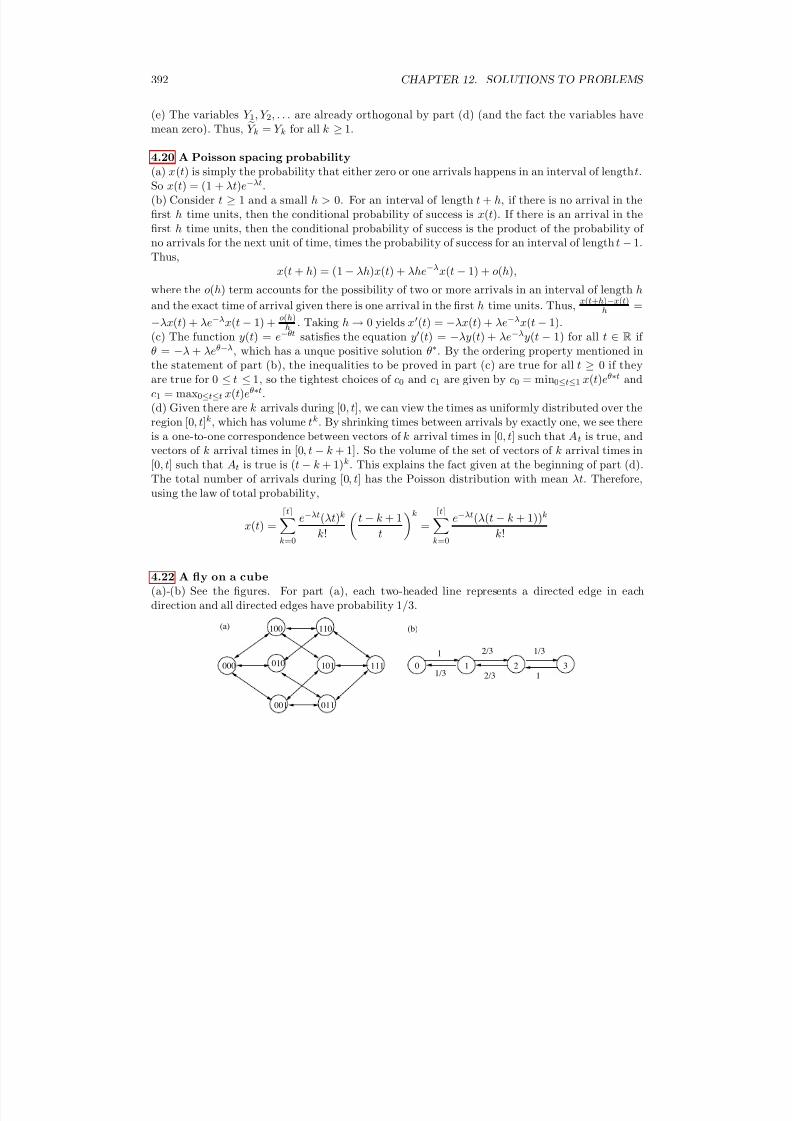
8/11/2019 Random process by B. Hajek
http://slidepdf.com/reader/full/random-process-by-b-hajek 402/448
392 CHAPTER 12. SOLUTIONS TO PROBLEMS
(e) The variables Y 1, Y 2, . . . are already orthogonal by part (d) (and the fact the variables havemean zero). Thus,
Y k = Y k for all k ≥ 1.
4.20 A Poisson spacing probability(a) x(t) is simply the probability that either zero or one arrivals happens in an interval of length t.So x(t) = (1 + λt)e−λt.(b) Consider t ≥ 1 and a small h > 0. For an interval of length t + h, if there is no arrival in thefirst h time units, then the conditional probability of success is x(t). If there is an arrival in thefirst h time units, then the conditional probability of success is the product of the probability of no arrivals for the next unit of time, times the probability of success for an interval of length t − 1.Thus,
x(t + h) = (1 − λh)x(t) + λhe−λx(t − 1) + o(h),
where the o(h) term accounts for the possibility of two or more arrivals in an interval of length h
and the exact time of arrival given there is one arrival in the first h time units. Thus, x(t+h)−x(t)h =
−λx(t) + λe−λx(t − 1) + o(h)h . Taking h → 0 yields x(t) = −λx(t) + λe−λx(t − 1).(c) The function y(t) = e−θt satisfies the equation y(t) = −λy(t) + λe−λy(t − 1) for all t ∈ R if θ = −λ + λeθ−λ, which has a unque positive solution θ∗. By the ordering property mentioned inthe statement of part (b), the inequalities to be proved in part (c) are true for all t ≥ 0 if theyare true for 0 ≤ t ≤ 1, so the tightest choices of c0 and c1 are given by c0 = min0≤t≤1 x(t)eθ∗t andc1 = max0≤t≤t x(t)eθ∗t.(d) Given there are k arrivals during [0, t], we can view the times as uniformly distributed over theregion [0, t]k, which has volume tk. By shrinking times between arrivals by exactly one, we see thereis a one-to-one correspondence between vectors of k arrival times in [0, t] such that At is true, andvectors of k arrival times in [0, t − k + 1]. So the volume of the set of vectors of k arrival times in[0, t] such that At is true is (t − k + 1)k. This explains the fact given at the beginning of part (d).
The total number of arrivals during [0, t] has the Poisson distribution with mean λt. Therefore,using the law of total probability,
x(t) =
tk=0
e−λt(λt)k
k!
t − k + 1
t
k
=
tk=0
e−λt(λ(t − k + 1))k
k!
4.22 A fly on a cube(a)-(b) See the figures. For part (a), each two-headed line represents a directed edge in eachdirection and all directed edges have probability 1/3.
(b)
000 010
001
110100
101
011
111 1 2 30
1 2/3 1/3
12/31/3
(a)
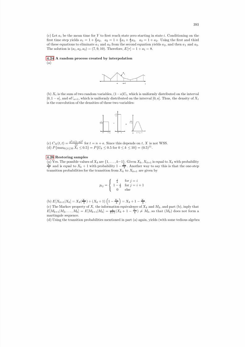
8/11/2019 Random process by B. Hajek
http://slidepdf.com/reader/full/random-process-by-b-hajek 403/448
393
(c) Let ai be the mean time for Y to first reach state zero starting in state i. Conditioning on thefirst time step yields a1 = 1 + 2
3 a2, a2 = 1 + 23 a1 + 1
3 a3, a3 = 1 + a2. Using the first and thirdof these equations to eliminate a1 and a3 from the second equation yields a2, and then a1 and a3.
The solution is (a1, a2, a3) = (7, 9, 10). Therefore, E [τ ] = 1 + a1 = 8.
4.24 A random process created by interpolation(a)
tn+1n
Xt
(b) X t is the sum of two random variables, (1 − a)U t, which is uniformly distributed on the interval
[0, 1 − a], and aU n+1, which is uniformly distributed on the interval [0, a]. Thus, the density of X tis the convolution of the densities of these two variables:
!
!!"
!
!!"
!
# !!" # " " !!"
!
"
$ %
#
(c) C X (t, t) = a2+(1−a)2
12 for t = n + a. Since this depends on t, X is not WSS.
(d) P max0≤t≤10 X t ≤ 0.5 = P U k ≤ 0.5 for 0 ≤ k ≤ 10 = (0.5)11
.
4.26 Restoring samples(a) Yes. The possible values of X k are 1, . . . , k−1. Given X k, X k+1 is equal to X k with probabilityX kk and is equal to X k + 1 with probability 1 − X k
k . Another way to say this is that the one-steptransition probabilities for the transition from X k to X k+1 are given by
pij =
ik for j = i
1 − ik for j = i + 1
0 else
(b) E [X k+1|X k] = X k(X kk ) + (X k + 1) 1 − X k
k = X k + 1 − X k
k .
(c) The Markov property of X, the information equivalence of X k and M k, and part (b), inply thatE [M k+1|M 2, . . . , M k] = E [M k+1|M k] = 1
k+1 (X k + 1 − X kk ) = M k, so that (M k) does not form a
martingale sequence.(d) Using the transition probabilities mentioned in part (a) again, yields (with some tedious algebra
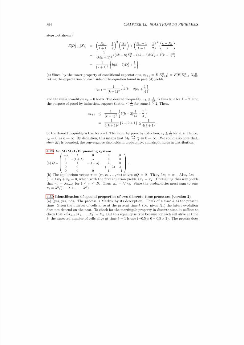
8/11/2019 Random process by B. Hajek
http://slidepdf.com/reader/full/random-process-by-b-hajek 404/448
394 CHAPTER 12. SOLUTIONS TO PROBLEMS
steps not shown)
E [D2k+1
|X k] =
X k
k + 1 − 1
22
X k
k +X k + 1
k + 1 − 1
22
k − X k
k =
1
4k(k + 1)2
(4k − 8)X 2k − (4k − 8)kX k + k(k − 1)2
=
1
(k + 1)2
k(k − 2)D2
k + 1
4
(e) Since, by the tower property of conditional expectations, vk+1 = E [D2
k+1] = E [E [D2k+1|X k]],
taking the expectation on each side of the equation found in part (d) yields
vk+1 = 1
(k + 1)2
k(k − 2)vk +
1
4
and the initial condition v2 = 0 holds. The desired inequality, vk ≤ 14k , is thus true for k = 2. Forthe purpose of proof by induction, suppose that vk ≤ 1
4k for some k ≥ 2. Then,
vk+1 ≤ 1
(k + 1)2
k(k − 2)
1
4k +
1
4
=
1
4(k + 1)2 k − 2 + 1 ≤ 1
4(k + 1).
So the desired inequality is true for k +1. Therefore, by proof by induction, vk ≤ 14k for all k. Hence,
vk → 0 as k → ∞. By definition, this means that M km.s.→ 1
2 as k → ∞. (We could also note that,since M k is bounded, the convergence also holds in probability, and also it holds in distribution.)
4.28 An M/M/1/B queueing system
(a) Q =
−λ λ 0 0 0
1 −(1 + λ) λ 0 00 1 −(1 + λ) λ 00 0 1 −(1 + λ) λ0 0 0 1 −1
.
(b) The equilibrium vector π = (π0, π1, . . . , πB) solves πQ = 0. Thus, λπ0 = π1. Also, λπ0 −(1 + λ)π1 + π2 = 0, which with the first equation yields λπ1 = π2. Continuing this way yieldsthat πn = λπn−1 for 1 ≤ n ≤ B. Thus, πn = λnπ0. Since the probabilities must sum to one,πn = λn/(1 + λ + · · · + λB).
4.30 Identification of special properties of two discrete-time processes (version 2)(a) (yes, yes, no). The process is Markov by its description. Think of a time k as the presenttime. Given the number of cells alive at the present time k (i.e. given X k) the future evolutiondoes not depend on the past. To check for the martingale property in discrete time, it suffices tocheck that E [X k+1|X 1, . . . , X k] = X k. But this equality is true because for each cell alive at timek, the expected number of cells alive at time k + 1 is one (=0.5 × 0 + 0.5 × 2). The process does
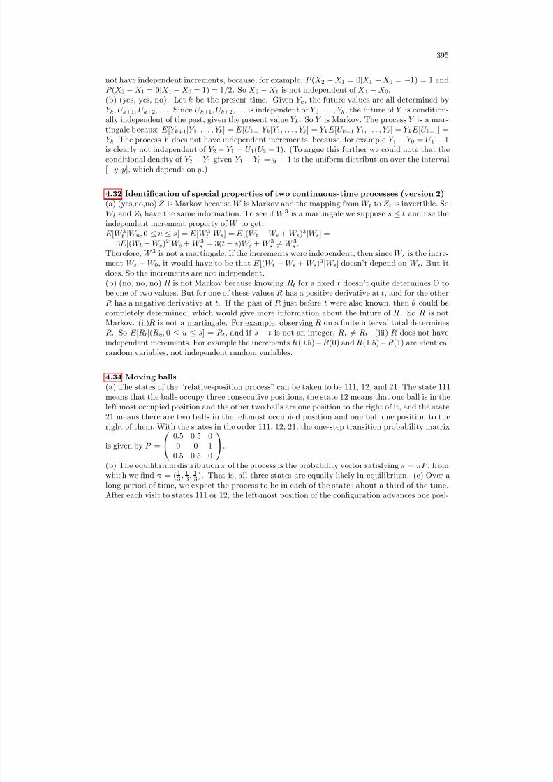
8/11/2019 Random process by B. Hajek
http://slidepdf.com/reader/full/random-process-by-b-hajek 405/448
395
not have independent increments, because, for example, P (X 2 − X 1 = 0|X 1 − X 0 = −1) = 1 andP (X 2 − X 1 = 0|X 1 − X 0 = 1) = 1/2. So X 2 − X 1 is not independent of X 1 − X 0.(b) (yes, yes, no). Let k be the present time. Given Y k, the future values are all determined by
Y k, U k+1, U k+2, . . .. Since U k+1, U k+2, . . . is independent of Y 0, . . . , Y k, the future of Y is condition-ally independent of the past, given the present value Y k. So Y is Markov. The process Y is a mar-tingale because E [Y k+1|Y 1, . . . , Y k] = E [U k+1Y k|Y 1, . . . , Y k] = Y kE [U k+1|Y 1, . . . , Y k] = Y kE [U k+1] =Y k. The process Y does not have independent increments, because, for example Y 1 − Y 0 = U 1 − 1is clearly not independent of Y 2 − Y 1 = U 1(U 2 − 1). (To argue this further we could note that theconditional density of Y 2 − Y 1 given Y 1 − Y 0 = y − 1 is the uniform distribution over the interval[−y, y], which depends on y .)
4.32 Identification of special properties of two continuous-time processes (version 2)(a) (yes,no,no) Z is Markov because W is Markov and the mapping from W t to Z t is invertible. SoW t and Z t have the same information. To see if W 3 is a martingale we suppose s
≤ t and use the
independent increment property of W to get:E [W 3t |W u, 0 ≤ u ≤ s] = E [W 3t |W s] = E [(W t − W s + W s)3|W s] =
3E [(W t − W s)2]W s + W 3s = 3(t − s)W s + W 3s = W 3s .Therefore, W 3 is not a martingale. If the increments were independent, then since W s is the incre-ment W s − W 0, it would have to be that E [(W t − W s + W s)3|W s] doesn’t depend on W s. But itdoes. So the increments are not independent.(b) (no, no, no) R is not Markov because knowing Rt for a fixed t doesn’t quite determines Θ tobe one of two values. But for one of these values R has a positive derivative at t, and for the otherR has a negative derivative at t. If the past of R just before t were also known, then θ could becompletely determined, which would give more information about the future of R. So R is notMarkov. (ii)R is not a martingale. For example, observing R on a finite interval total determines
R. So E [Rt|(Ru, 0 ≤ u ≤ s] = Rt, and if s − t is not an integer, Rs = Rt. (iii) R does not haveindependent increments. For example the increments R(0.5)−R(0) and R(1.5)−R(1) are identicalrandom variables, not independent random variables.
4.34 Moving balls(a) The states of the “relative-position process” can be taken to be 111, 12, and 21. The state 111means that the balls occupy three consecutive positions, the state 12 means that one ball is in theleft most occupied position and the other two balls are one position to the right of it, and the state21 means there are two balls in the leftmost occupied position and one ball one position to theright of them. With the states in the order 111, 12, 21, the one-step transition probability matrix
is given by P = 0.5 0.5 0
0 0 10.5 0.5 0
.
(b) The equilibrium distribution π of the process is the probability vector satisfying π = πP , fromwhich we find π = ( 1
3 , 13 , 1
3 ). That is, all three states are equally likely in equilibrium. (c) Over along period of time, we expect the process to be in each of the states about a third of the time.After each visit to states 111 or 12, the left-most position of the configuration advances one posi-
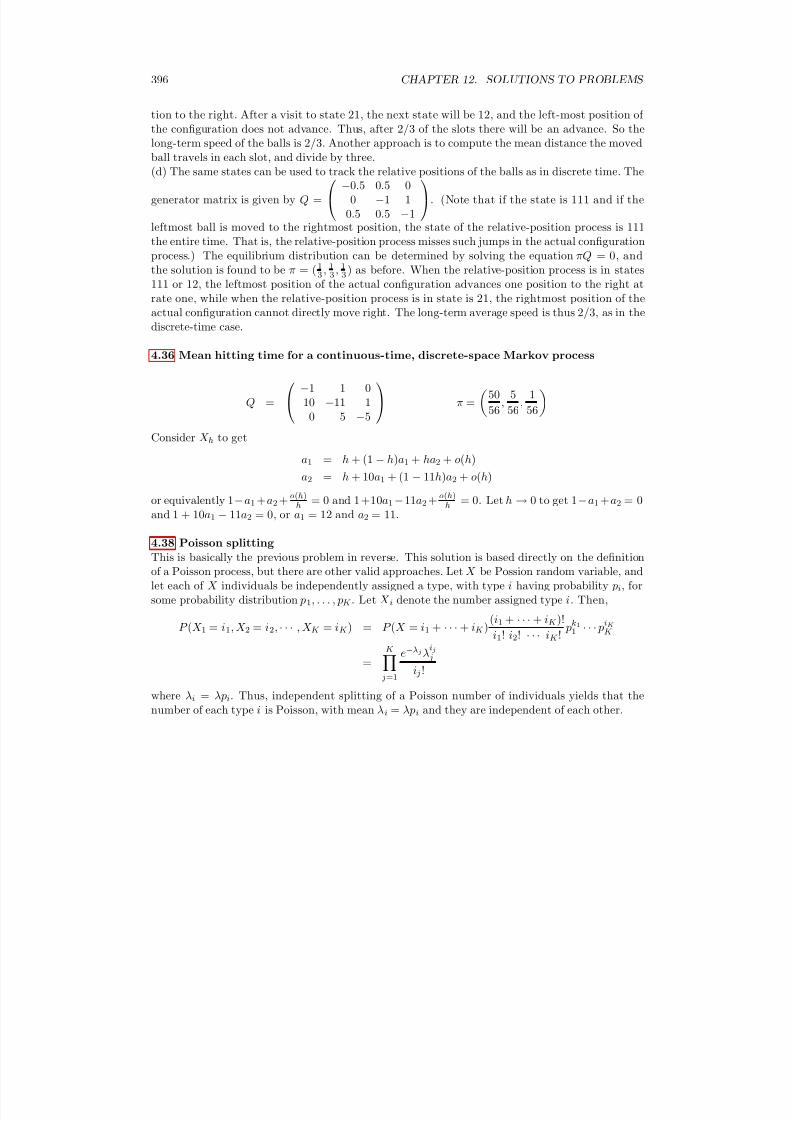
8/11/2019 Random process by B. Hajek
http://slidepdf.com/reader/full/random-process-by-b-hajek 406/448
396 CHAPTER 12. SOLUTIONS TO PROBLEMS
tion to the right. After a visit to state 21, the next state will be 12, and the left-most position of the configuration does not advance. Thus, after 2/3 of the slots there will be an advance. So thelong-term speed of the balls is 2/3. Another approach is to compute the mean distance the moved
ball travels in each slot, and divide by three.(d) The same states can be used to track the relative positions of the balls as in discrete time. The
generator matrix is given by Q =
−0.5 0.5 00 −1 1
0.5 0.5 −1
. (Note that if the state is 111 and if the
leftmost ball is moved to the rightmost position, the state of the relative-position process is 111the entire time. That is, the relative-position process misses such jumps in the actual configurationprocess.) The equilibrium distribution can be determined by solving the equation πQ = 0, andthe solution is found to be π = ( 1
3 , 13 , 1
3 ) as before. When the relative-position process is in states111 or 12, the leftmost position of the actual configuration advances one position to the right atrate one, while when the relative-position process is in state is 21, the rightmost position of theactual configuration cannot directly move right. The long-term average speed is thus 2/3, as in thediscrete-time case.
4.36 Mean hitting time for a continuous-time, discrete-space Markov process
Q =
−1 1 010 −11 1
0 5 −5
π =
50
56,
5
56,
1
56
Consider X h to get
a1 = h + (1 − h)a1 + ha2 + o(h)
a2 = h + 10a1 + (1 − 11h)a2 + o(h)or equivalently 1−a1 +a2 + o(h)
h = 0 and 1 +10a1 −11a2 + o(h)h = 0. Let h → 0 to get 1−a1 +a2 = 0
and 1 + 10a1 − 11a2 = 0, or a1 = 12 and a2 = 11.
4.38 Poisson splittingThis is basically the previous problem in reverse. This solution is based directly on the definitionof a Poisson process, but there are other valid approaches. Let X be Possion random variable, andlet each of X individuals be independently assigned a type, with type i having probability pi, forsome probability distribution p1, . . . , pK . Let X i denote the number assigned type i. Then,
P (X 1 = i1, X 2 = i2,
· · · , X K = iK ) = P (X = i1 +
· · ·+ iK )
(i1 + · · · + iK )!
i1
! i2
! · · ·
iK
! pk1
1
· · · piK
K
=K
j=1
e−λj λij j
i j !
where λi = λpi. Thus, independent splitting of a Poisson number of individuals yields that thenumber of each type i is Poisson, with mean λi = λpi and they are independent of each other.
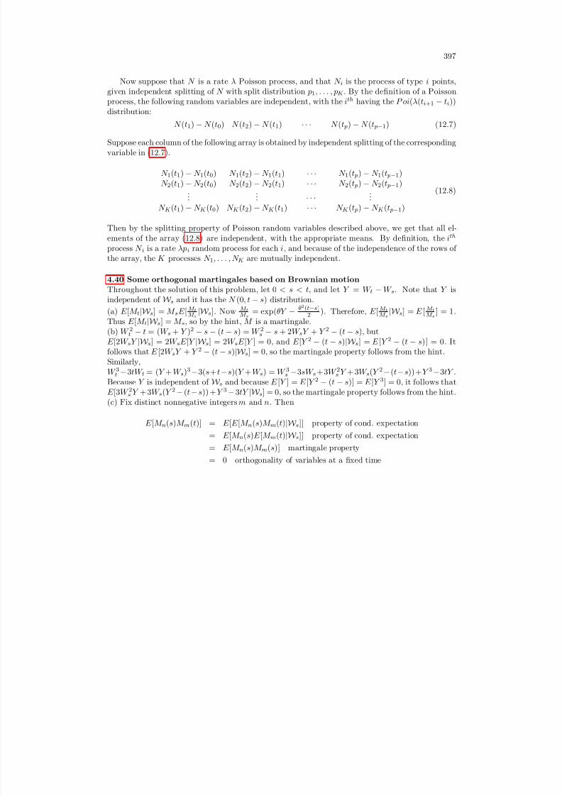
8/11/2019 Random process by B. Hajek
http://slidepdf.com/reader/full/random-process-by-b-hajek 407/448
397
Now suppose that N is a rate λ Poisson process, and that N i is the process of type i points,given independent splitting of N with split distribution p1, . . . , pK . By the definition of a Poissonprocess, the following random variables are independent, with the ith having the P oi(λ(ti+1 − ti))
distribution:N (t1) − N (t0) N (t2) − N (t1) · · · N (t p) − N (t p−1) (12.7)
Suppose each column of the following array is obtained by independent splitting of the correspondingvariable in (12.7).
N 1(t1) − N 1(t0) N 1(t2) − N 1(t1) · · · N 1(t p) − N 1(t p−1)N 2(t1) − N 2(t0) N 2(t2) − N 2(t1) · · · N 2(t p) − N 2(t p−1)
... ... · · · ...
N K (t1) − N K (t0) N K (t2) − N K (t1) · · · N K (t p) − N K (t p−1)
(12.8)
Then by the splitting property of Poisson random variables described above, we get that all el-ements of the array (12.8) are independent, with the appropriate means. By definition, the ith
process N i is a rate λpi random process for each i, and because of the independence of the rows of the array, the K processes N 1, . . . , N K are mutually independent.
4.40 Some orthogonal martingales based on Brownian motionThroughout the solution of this problem, let 0 < s < t, and let Y = W t − W s. Note that Y isindependent of W s and it has the N (0, t − s) distribution.
(a) E [M t|W s] = M sE [M tM s
|W s]. Now M tM s
= exp(θY − θ2(t−s)2 ). Therefore, E [M t
M s|W s] = E [ M t
M s] = 1.
Thus E [M t|W s] = M s, so by the hint, M is a martingale.(b) W 2t
−t = (W s + Y )2
−s
−(t
−s) = W 2s
−s + 2W sY + Y 2
−(t
−s), but
E [2W sY |W s] = 2W sE [Y |W s] = 2W sE [Y ] = 0, and E [Y 2 − (t − s)|W s] = E [Y 2 − (t − s)] = 0. Itfollows that E [2W sY + Y 2 − (t − s)|W s] = 0, so the martingale property follows from the hint.Similarly,W 3t −3tW t = (Y + W s)3 −3(s+t−s)(Y + W s) = W 3s −3sW s+3W 2s Y + 3W s(Y 2 −(t−s))+Y 3 −3tY .Because Y is independent of W s and because E [Y ] = E [Y 2 − (t − s)] = E [Y 3] = 0, it follows thatE [3W 2s Y + 3W s(Y 2 − (t−s)) + Y 3 −3tY |W s] = 0, so the martingale property follows from the hint.(c) Fix distinct nonnegative integers m and n. Then
E [M n(s)M m(t)] = E [E [M n(s)M m(t)|W s]] property of cond. expectation
= E [M n(s)E [M m(t)|W s]] property of cond. expectation
= E [M n(s)M m(s)] martingale property
= 0 orthogonality of variables at a fixed time
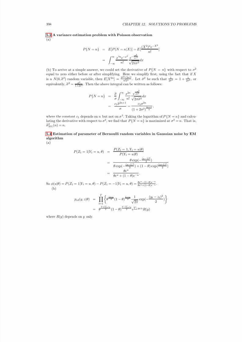
8/11/2019 Random process by B. Hajek
http://slidepdf.com/reader/full/random-process-by-b-hajek 408/448
398 CHAPTER 12. SOLUTIONS TO PROBLEMS
5.2 A variance estimation problem with Poisson observation(a)
P N = n = E [P (N = n|X )] = E [(X 2)ne
−X 2
n! ]
=
∞−∞
x2ne−x2
n!
e− x2
2σ2√ 2πσ2
dx
(b) To arrive at a simple answer, we could set the derivative of P N = n with respect to σ2
equal to zero either before or after simplifying. Here we simplify first, using the fact that if X
is a N (0, σ2) random variable, then E [X 2n] = eσ2n(2n)!
n!2n . Let σ2 be such that 12σ2 = 1 + 1
2σ2 , or
equivalently, σ2 = σ2
1+2σ2 . Then the above integral can be written as follows:
P N = n = σσ ∞
−∞x2n
n!
e−x2
2eσ2
√ 2πσ2 dx
= c1σ2n+1
σ =
c1σ2n
(1 + 2σ2)2n+12
,
where the constant c1 depends on n but not on σ 2. Taking the logarithm of P N = n and calcu-lating the derivative with respect to σ2, we find that P N = n is maximized at σ2 = n. That is, σ2ML(n) = n.
5.4 Estimation of parameter of Bernoulli random variables in Gaussian noise by EMalgorithm(a)
P (Z 1 = 1|Y 1 = u, θ) = P (Z 1 = 1, Y 1 = u|θ)
P (Y 1 = u|θ)
= θ exp(− (u−1)2
2 )
θ exp(− (u−1)2
2 ) + (1 − θ) exp((u+1)2
2 )
= θeu
θeu + (1 − θ)e−u.
So φ(u|θ) = P (Z 1 = 1|Y 1 = u, θ) − P (Z 1 = −1|Y 1 = u, θ) = θeu−(1−θ)e−u
θeu+(1−θ)e−u .
(b)
pcd(y, z|θ) =T
t=1
θ1+zt2 (1 − θ)
1−zt2
1√ 2π
exp(−(yt − zt)2
2 )
= θT +P
t zt2 (1 − θ)
T −Pt zt2 e
Pt ytztR(y)
where R(y) depends on y only.
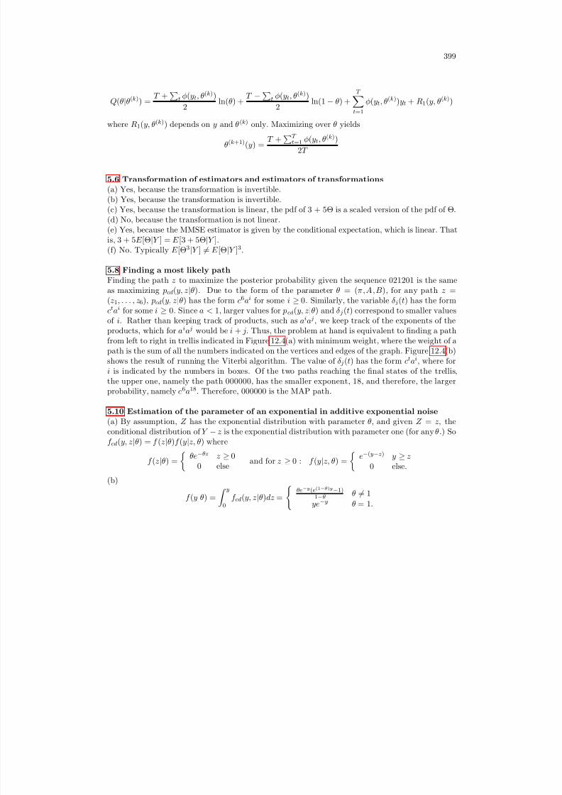
8/11/2019 Random process by B. Hajek
http://slidepdf.com/reader/full/random-process-by-b-hajek 409/448
399
Q(θ|θ(k)) = T +
t φ(yt, θ(k))
2 ln(θ) +
T −
t φ(yt, θ(k))
2 ln(1 − θ) +
T
t=1
φ(yt, θ(k))yt + R1(y, θ(k))
where R1(y, θ(k)) depends on y and θ (k) only. Maximizing over θ yields
θ(k+1)(y) = T +
T t=1 φ(yt, θ(k))
2T
5.6 Transformation of estimators and estimators of transformations(a) Yes, because the transformation is invertible.(b) Yes, because the transformation is invertible.(c) Yes, because the transformation is linear, the pdf of 3 + 5Θ is a scaled version of the pdf of Θ .(d) No, because the transformation is not linear.
(e) Yes, because the MMSE estimator is given by the conditional expectation, which is linear. Thatis, 3 + 5E [Θ|Y ] = E [3 + 5Θ|Y ].(f) No. Typically E [Θ3|Y ] = E [Θ|Y ]3.
5.8 Finding a most likely pathFinding the path z to maximize the posterior probability given the sequence 021201 is the sameas maximizing pcd(y, z|θ). Due to the form of the parameter θ = (π,A,B), for any path z =(z1, . . . , z6), pcd(y, z|θ) has the form c6ai for some i ≥ 0. Similarly, the variable δ j(t) has the formctai for some i ≥ 0. Since a < 1, larger values for pcd(y, z|θ) and δ j(t) correspond to smaller valuesof i. Rather than keeping track of products, such as aia j, we keep track of the exponents of theproducts, which for aia j would be i + j. Thus, the problem at hand is equivalent to finding a path
from left to right in trellis indicated in Figure 12.4(a) with minimum weight, where the weight of apath is the sum of all the numbers indicated on the vertices and edges of the graph. Figure 12.4(b)shows the result of running the Viterbi algorithm. The value of δ j(t) has the form ctai, where fori is indicated by the numbers in boxes. Of the two paths reaching the final states of the trellis,the upper one, namely the path 000000, has the smaller exponent, 18, and therefore, the largerprobability, namely c6a18. Therefore, 000000 is the MAP path.
5.10 Estimation of the parameter of an exponential in additive exponential noise(a) By assumption, Z has the exponential distribution with parameter θ, and given Z = z, theconditional distribution of Y − z is the exponential distribution with parameter one (for any θ.) Sof cd(y, z|θ) = f (z|θ)f (y|z, θ) where
f (z|θ) = θe−θz z ≥ 00 else
and for z ≥ 0 : f (y|z, θ) = e−(y−z) y ≥ z0 else.
(b)
f (y|θ) =
y0
f cd(y, z|θ)dz =
θe−y(e(1−θ)y−1)
1−θ θ = 1
ye−y θ = 1.
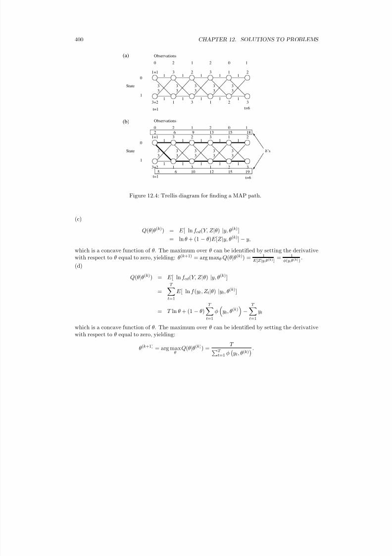
8/11/2019 Random process by B. Hajek
http://slidepdf.com/reader/full/random-process-by-b-hajek 410/448
400 CHAPTER 12. SOLUTIONS TO PROBLEMS
’s
3
1
1
3
3
1
1
3
3
1
1
3
3
1
1
3
3
1
1
3
3
1
1
3
3
1
1
3
3
1
1
3
3
1
1
3
3
1
1
3
0 2 1 2 0 1
0
1
Observations
State
t=1 t=6
3 2 3 1 2
3 23+2 1 1 3
1+1
(a)
(b)
186 9 13 15
6 10 12 15
2
0 2 1 2 0 1
0
1
Observations
State
3 2 3 1 2
3 23+2 1 1 3
1+1
t=1 t=6
195
!
Figure 12.4: Trellis diagram for finding a MAP path.
(c)
Q(θ|θ(k)) = E [ ln f cd(Y, Z |θ) |y, θ(k)]
= ln θ + (1 − θ)E [Z |y, θ(k)] − y,
which is a concave function of θ. The maximum over θ can be identified by setting the derivativewith respect to θ equal to zero, yielding: θ(k+1) = arg maxθ Q(θ|θ(k)) = 1
E [Z |y,θ(k)] = 1
φ(y,θ(k)).
(d)
Q(θ|θ(k)) = E [ ln f cd(Y, Z |θ) |y, θ(k)]
=
T t=1
E [ ln f (yt, Z t|θ) |yt, θ(k)]
= T ln θ + (1
−θ)
T
t=1
φyt, θ(k)
−
T
t=1
yt
which is a concave function of θ. The maximum over θ can be identified by setting the derivativewith respect to θ equal to zero, yielding:
θ(k+1) = arg maxθ
Q(θ|θ(k)) = T T t=1 φ
yt, θ(k)
.
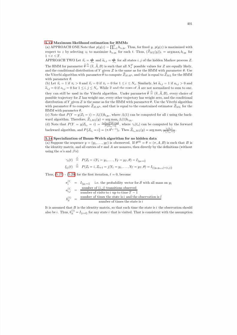
8/11/2019 Random process by B. Hajek
http://slidepdf.com/reader/full/random-process-by-b-hajek 411/448
8/11/2019 Random process by B. Hajek
http://slidepdf.com/reader/full/random-process-by-b-hajek 412/448
402 CHAPTER 12. SOLUTIONS TO PROBLEMS
that B is the identify matrix. (Alternatively, since B is fixed to be the identity matrix, we could just work with estimating π and A, and simply not consider B as part of the parameter to be esti-mated.) The next iteration will give the same values of π and A. Thus, the Baum-Welch algorithm
converges in one iteration to the final value θ(1)
= (π(1)
, A(1)
, B(1)
) already described. Note that,by Lemma 5.1.7, θ (1) is the ML estimate.
(b) In view of part (a), the ML estimates are π = (1, 0) and A =
2
313
13
23
. This estimator of A
results from the fact that, of the first 21 times, the sate was zero 12 times, and 8 of those 12 timesthe next state was a zero. So a00 = 8/12 = 2/3 is the ML estimate. Similarly, the ML estimate of a11 is 6/9, which simplifies to 2/3.
5.16 Extending the forward-backward algorithm(a) Forward equations: µ j(t, t + 1) =
i∈S µi(t − 1, t)biytaij µi(−1, 0) = 1
Backward equations: µ j(t, t − 1) =
i∈S µi(t + 1, t)biyta ji µi(T + 1, T ) = 1
γ i(t) = µi(t − 1, t)µi(t + 1, t)biyt j µ j(t − 1, t)µ j(t + 1, t)b jyt
(12.9)
(b)
µi(t − 1, t) =
z1,··· ,zt−1
az1z2az2z3 · · · azt−1i
t−1s=1
bzs,ys
(12.10)
µi(t + 1, t) =
zt+1,··· ,zT
aizt+1azt+1zt+2 · · · azT −1zT
T s=t+1
bzs,ys
(12.11)
(To bring out the symmetry more, we could let aij = a ji (corresponds to AT ) and rewrite (12.11)as
µi(t + 1, t) =
zT ,··· ,zt+1
azT zT −1azT −1zT −2 · · ·azt+2zt+1azt+1i
T s=t+1
bzs,ys
(12.12)
Observe that (12.10) and (12.12) are the same up to time reversal.)
A partially probabilistic interpretation can be given to the messages as follows. First, considerhow to find the marginal distribution of Z t for some t. It is obtained by summing out all values of the other variables in the complete data probability function, with Z t fixed at i. For Z t = i fixed,the numerator in the joint probability function factors into three terms involving disjoint sets of
variables:bz1y1az1,z2bz2,y2 · · · azt−2zt−1bzt−1yt−1azt−1i
(biyt)
aizt+1bzt+1yt+1azt+1,zt+2 · · · azT −1zT
bzT yT
Let Gi(t−1, t)i denote the sum of the first factor over all (z1, y1, z2, · · · , zt−1, yt−1), let Go
i (t) denotethe sum of the second factor over all yt and let Gi(t + 1, t) denote the sum of the third factor over

8/11/2019 Random process by B. Hajek
http://slidepdf.com/reader/full/random-process-by-b-hajek 413/448
403
all (zt+1, yt+1, . . . , zT , yT ). Then the marginal distribution of Z t can be represented as
P
Z t = i
=
Gi(t − 1, t)Goi (t)Gi(t + 1, t)
G
,
and the constant G can be expressed as G =
j G j(t − 1, t)Go j(t)G j(t + 1, t). Note that the G’s
depend on the joint distribution but do not depend on specific values of the observation. They aresimply factors in the prior (i.e. before observations are incorporated) distribution of Z t.
For fixed y1, · · · yt−1, using the definition of conditional probability yields that
P (Y 1 = y1, . . . , Y t−1 = yt−1|Z t = i) = µi(t − 1, t)
Gi(t − 1, t),
or equivalently,
µi(t
−1, t) = P (Y 1 = y1, . . . , Y t
−1 = yt
−1
|Z t = i)Gi(t
−1, t) (12.13)
Equation (12.13) gives perhaps the closest we can get to a probabilistic interpretation of µi(t −1, t). In words, µi(t − 1, t) is the product of the likelihood of the observations (y1, . . . , yt−1) and afactor Gt(t − 1, t), not depending on the observations, that contributes to the unconditional priordistribution of Z t. A similar interpretation holds for µi(t + 1, t). Also, byti can be thought of as amessage from the observation node of the graph at time t to the node for zt, and byti = P (Y t =yt|Z t = i)Go
i (t). Combining these observations shows that the numerator in (12.9) is given by:
µi(t − 1, t)µi(t + 1, t)biyt = P (Y 1 = y1, . . . , Y T = Y T |Z t = i)Gi(t − 1, t)Goi (t)Gi(t + 1, t)
= P (Y 1 = y1, . . . , Y T = Y T |Z t = i)P (Z t = i)G
= P (Y 1 = y1, . . . , Y T = Y T , Z t = i)G.
(c) Comparison of the numerator in (12.9) to the definition of pcd(y, z|θ) given in the problemstatement shows that the numerator in (12.9) is the sum of pcd(y, z|θ)G over all values of z : zt = ifor y fixed, so it is P (Y = y, Z t = i|θ)G. Thus,
RHS of (12.9) = P (Y = y, Z t = i|θ)G
j P (Y = y, Z t = j |θ)G =
P (Y = y, Z t = i|θ)
P (Y = y|θ) = γ i(t).
5.18 Baum-Welch saddlepointIt turns out that π(k) = π(0) and A(k) = A(0), for each k ≥ 0. Also, B(k) = B(1) for each k ≥ 1,
where B(1)
is the matrix with identical rows, such that each row of B(1)
is the empirical distributionof the observation sequence. For example, if the observations are binary valued, and if there areT = 100 observations, of which 37 observations are zero and 63 are 1, then each row of B (1) wouldbe (0.37, 0.63). Thus, the EM algorithm converges in one iteration, and unless θ(0) happens tobe a local maximum or local minimum, the EM algorithm converges to an inflection point of thelikelihood function.
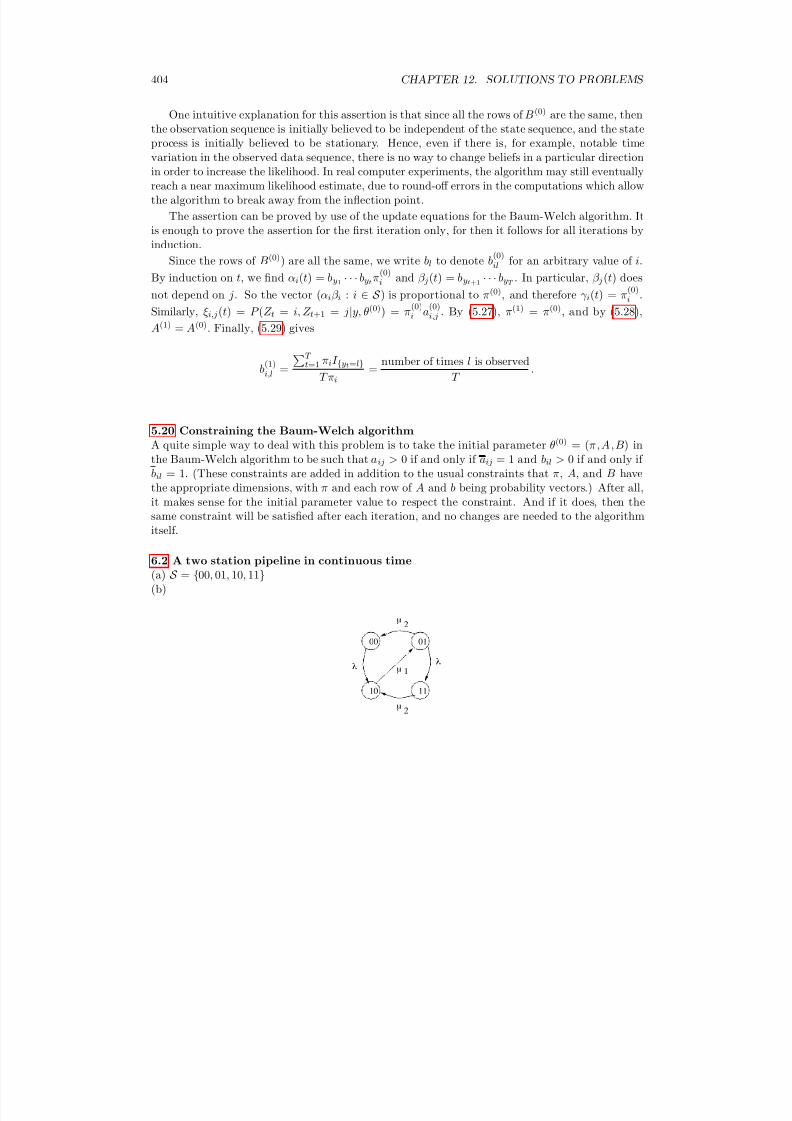
8/11/2019 Random process by B. Hajek
http://slidepdf.com/reader/full/random-process-by-b-hajek 414/448
404 CHAPTER 12. SOLUTIONS TO PROBLEMS
One intuitive explanation for this assertion is that since all the rows of B (0) are the same, thenthe observation sequence is initially believed to be independent of the state sequence, and the stateprocess is initially believed to be stationary. Hence, even if there is, for example, notable time
variation in the observed data sequence, there is no way to change beliefs in a particular directionin order to increase the likelihood. In real computer experiments, the algorithm may still eventuallyreach a near maximum likelihood estimate, due to round-off errors in the computations which allowthe algorithm to break away from the inflection point.
The assertion can be proved by use of the update equations for the Baum-Welch algorithm. Itis enough to prove the assertion for the first iteration only, for then it follows for all iterations byinduction.
Since the rows of B(0)) are all the same, we write bl to denote b(0)il for an arbitrary value of i.
By induction on t, we find αi(t) = by1 · · · bytπ(0)i and β j(t) = byt+1 · · · byT
. In particular, β j(t) does
not depend on j. So the vector (αiβ i : i ∈ S ) is proportional to π(0), and therefore γ i(t) = π(0)i .
Similarly, ξ i,j(t) = P (Z t = i, Z t+1 = j|y, θ(0)) = π
(0)i a
(0)i,j . By (5.27), π(1) = π(0), and by (5.28),
A(1) = A(0). Finally, (5.29) gives
b(1)i,l =
T t=1 πiI yt=l
T πi=
number of times l is observed
T .
5.20 Constraining the Baum-Welch algorithmA quite simple way to deal with this problem is to take the initial parameter θ(0) = (π,A ,B) inthe Baum-Welch algorithm to be such that aij > 0 if and only if aij = 1 and bil > 0 if and only if bil = 1. (These constraints are added in addition to the usual constraints that π, A, and B havethe appropriate dimensions, with π and each row of A and b being probability vectors.) After all,it makes sense for the initial parameter value to respect the constraint. And if it does, then thesame constraint will be satisfied after each iteration, and no changes are needed to the algorithmitself.
6.2 A two station pipeline in continuous time(a) S = 00, 01, 10, 11(b)
!
00 01
10 11
!!!"
!#
#
8/11/2019 Random process by B. Hajek
http://slidepdf.com/reader/full/random-process-by-b-hajek 415/448
405
(c) Q =
−λ 0 λ 0µ2 −µ2 − λ 0 λ0 µ1 −µ1 0
0 0 µ2 −µ2
.
(d) η = (π00 + π01)λ = (π01 + π11)µ2 = π10µ1. If λ = µ1 = µ2 = 1.0 then π = (0.2, 0.2, 0.4, 0.2) andη = 0.4.(e) Let τ = mint ≥ 0 : X (t) = 00, and define hs = E [τ |X (0) = s], for s ∈ S . We wish to find
h11.
h00 = 0
h01 = 1µ2+λ + µ2h00
µ2+λ + λh11µ2+λ
h10 = 1µ1
+ h01
h11 = 1µ2
+ h10
For If λ = µ1 = µ2 = 1.0 this yields
h00
h01
h10
h11
=
0345
. Thus,
h11 = 5 is the required answer.
6.4 A simple Poisson process calculation
Suppose 0 < s < t and 0 ≤ i ≤ k.
P (N (s) = i|N (t) = k) = P N (s) = i, N (t) = k
P N (t) = k
=
e−λs(λs)i
i!
e−λ(t−s)(λ(t − s))k−i
(k − i)!
e−λt(λt)k
k!
−1
=
k
i
s
t
i t − s
t
k−1
That is, given N (t) = k, the conditional distribution of N (s) is binomial. This could have beendeduced with no calculation, using the fact that given N (t) = k , the locations of the k points areuniformly and independently distributed on the interval [0, t].
6.6 On distributions of three discrete-time Markov processes(a) A probability vector π is an equilibrium distribution if and only if π satisfies the balanceequations: π = πP. This yields π1 = π0 and π2 = π3 = π1/2. Thus, π =
13 , 1
3 , 16 , 1
6
is the unique
equilibrium distribution. However, this Markov process is periodic with period 2, so limt→∞ π(t)does not necessarily exit. (The limit exists if and only if π0(0) + π2(0) = 0.5.)(b) The balance equations yield πn = 1
nπn−1 for all n ≥ 1, so that πn = π0n! . Thus, the Poisson
distribution with mean one, πn = e−1n! , is the unique equilibrium distribution. Since there is
an equilibrium distribution and the process is irreducible and aperiodic, all states are positiverecurrent and limt→∞ π(t) exits and is equal to the equilibrium distribution for any choice of initialdistribution.
(c) The balance equations yield πn = n−1n πn−1 for all n ≥ 1, so that πn = π0n . But since ∞n=1 1n =∞, there is no way to normalize this distribution to make it a probability distribution. Thus,
there does not exist an equilibrium distribution. The process is thus transient or null recurrent:limt→∞ πn(t) = 0 for each state n. (It can be shown that the process is recurrent. Indeed,
P (not return to 0|X (0) = 0) = limn→∞ P (hit n before return to 0|X (0) = 0) = lim
n→∞ 1·1
2·2
3· · · · ·n − 1
n = 0.)
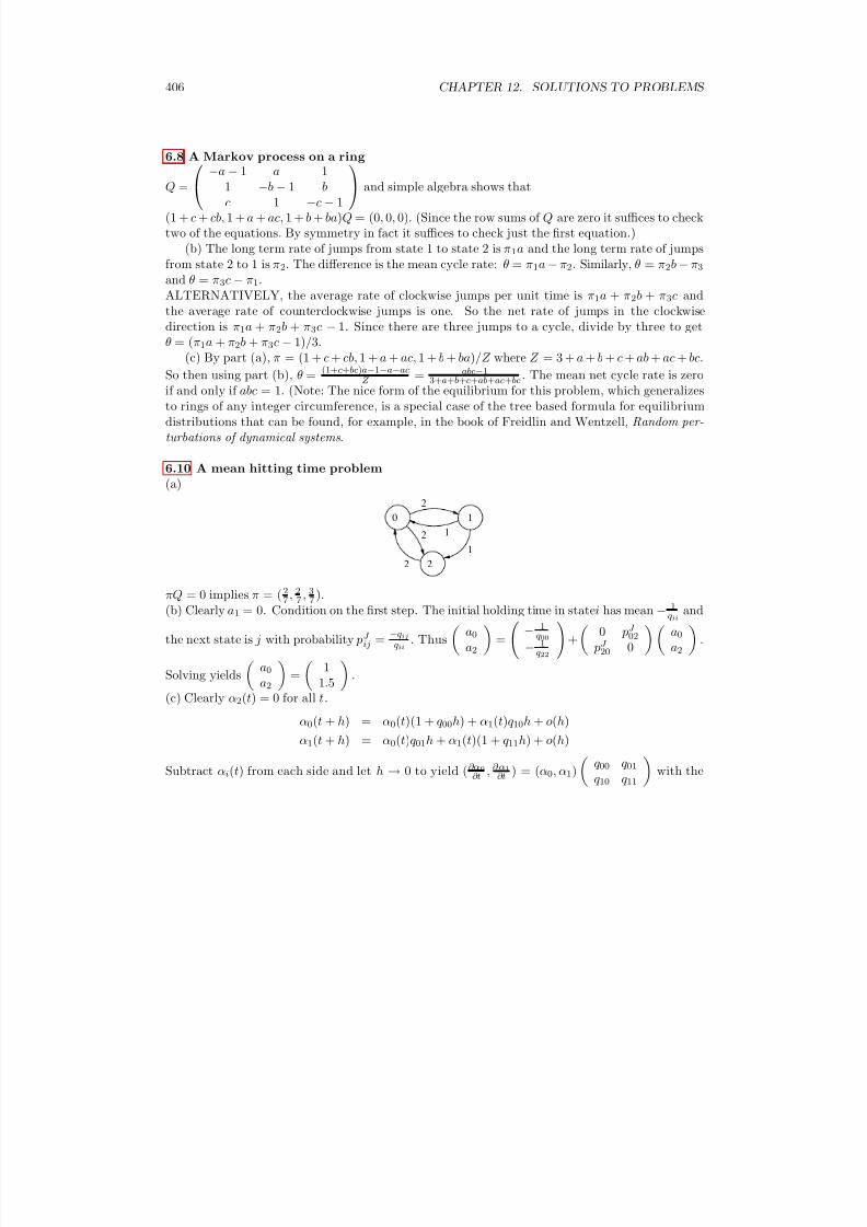
8/11/2019 Random process by B. Hajek
http://slidepdf.com/reader/full/random-process-by-b-hajek 416/448
406 CHAPTER 12. SOLUTIONS TO PROBLEMS
6.8 A Markov process on a ring
Q = −a − 1 a 11 −b − 1 bc 1 −c − 1
and simple algebra shows that
(1 + c + cb, 1 + a + ac, 1 + b + ba)Q = (0, 0, 0). (Since the row sums of Q are zero it suffices to checktwo of the equations. By symmetry in fact it suffices to check just the first equation.)
(b) The long term rate of jumps from state 1 to state 2 is π1a and the long term rate of jumpsfrom state 2 to 1 is π2. The difference is the mean cycle rate: θ = π1a − π2. Similarly, θ = π2b − π3
and θ = π3c − π1.ALTERNATIVELY, the average rate of clockwise jumps per unit time is π1a + π2b + π3c andthe average rate of counterclockwise jumps is one. So the net rate of jumps in the clockwisedirection is π1a + π2b + π3c − 1. Since there are three jumps to a cycle, divide by three to getθ = (π1a + π2b + π3c
−1)/3.
(c) By part (a), π = (1 + c + cb, 1 + a + ac, 1 + b + ba)/Z where Z = 3 + a + b + c + ab + ac + bc.
So then using part (b), θ = (1+c+bc)a−1−a−acZ = abc−1
3+a+b+c+ab+ac+bc . The mean net cycle rate is zeroif and only if abc = 1. (Note: The nice form of the equilibrium for this problem, which generalizesto rings of any integer circumference, is a special case of the tree based formula for equilibriumdistributions that can be found, for example, in the book of Freidlin and Wentzell, Random per-turbations of dynamical systems .
6.10 A mean hitting time problem(a)
2
0 1
2
1
1
2
2
πQ = 0 implies π = ( 27 , 2
7 , 37 ).
(b) Clearly a1 = 0. Condition on the first step. The initial holding time in state i has mean − 1qii
and
the next state is j with probability pJ ij =
−qijqii
. Thus
a0
a2
=
− 1
q00− 1
q22
+
0 pJ
02
pJ 20 0
a0
a2
.
Solving yields
a0
a2
=
11.5
.
(c) Clearly α2(t) = 0 for all t.α0(t + h) = α0(t)(1 + q 00h) + α1(t)q 10h + o(h)
α1(t + h) = α0(t)q 01h + α1(t)(1 + q 11h) + o(h)
Subtract αi(t) from each side and let h → 0 to yield (∂α0∂t , ∂α1
∂t ) = (α0, α1)
q 00 q 01
q 10 q 11
with the

8/11/2019 Random process by B. Hajek
http://slidepdf.com/reader/full/random-process-by-b-hajek 417/448
407
inital condition (α0(0), α1(0)) = (1, 0). (Note: the matrix involved here is the Q matrix with therow and column for state 2 removed.)(d) Similarly,
β 0(t − h) = (1 + q 00h)β 0(t) + q 01hβ 1(t) + o(h)
β 1(t − h) = q 10hβ 0(t) + (1 + q 11h)β 1(t)) + o(h)
Subtract β i(t)’s, divide by h and let h → 0 to get:
− ∂β 0∂t
−∂β 1∂t
=
q 00 q 01
q 10 q 11
β 0β 1
with
β 0(tf )β 1(tf )
=
11
6.12 Markov model for a link with resets(a) Let S = 0, 1, 2, 3, where the state is the number of packets passed since the last reset.
!
0 1 2 3
!
! !!
(b) By the PASTA property, the dropping probability is π3. We can find the equilibrium distribu-tion π by solving the equation πQ = 0. The balance equation for state 0 is λπ0 = µ(1 − π0) so thatπ0 = µ
λ+µ . The balance equation for state i ∈ 1, 2 is λπi−1 = (λ + µ)πi, so that π1 = π0( λλ+µ)
and π2 = π0( λλ+µ)2. Finally, λπ2 = µπ3 so that π3 = π0( λ
λ+µ)2 λµ = λ3
(λ+µ)3 . The dropping prob-
ability is π3 = λ3
(λ+µ)3 . (This formula for π3 can be deduced with virtually no calculation from
the properties of merged Poisson processes. Fix a time t. Each event is a packet arrival withprobability λ
λ+µ and is a reset otherwise. The types of different events are independent. Finally,π3(t) is the probability that the last three events before time t were arrivals. The formula follows.)
6.14 A queue with decreasing service rate(a)
X(t)
0 . . . . . .
! ! ! ! ! !
" " " "#$ "#$ "#$
1 K K+2K+1
K
t
(b) S 2 = ∞
k=0( µ2λ)k2k∧K , where k ∧ K = mink, K . Thus, if λ < µ2 then S 2 < +∞ and the
process is recurrent. S 1 =∞
k=0( 2λµ )k2−k∧K , so if λ < µ
2 then S 1 < +∞ and the process is positive
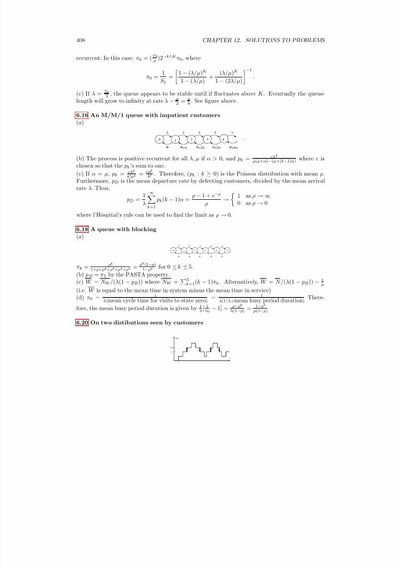
8/11/2019 Random process by B. Hajek
http://slidepdf.com/reader/full/random-process-by-b-hajek 418/448
408 CHAPTER 12. SOLUTIONS TO PROBLEMS
recurrent. In this case, πk = ( 2λµ )2−k∧K π0, where
π0 = 1
S 1= 1 − (λ/µ)K
1 − (λ/µ) +
(λ/µ)K
1 − (2λ/µ)−1
.
(c) If λ = 2µ3 , the queue appears to be stable until if fluctuates above K . Eventually the queue-
length will grow to infinity at rate λ − µ2 = µ
6 . See figure above.
6.16 An M/M/1 queue with impatient customers(a)
!
31 20 . . .4
! !
"" "#" "$" "%"
!!
(b) The process is positive recurrent for all λ, µ if α > 0, and pk
= cλk
µ(µ+α)···(µ+(k−1)α) where c is
chosen so that the pk’s sum to one.
(c) If α = µ, pk = cλk
k!µk = cρk
k! . Therefore, ( pk : k ≥ 0) is the Poisson distribution with mean ρ.Furthermore, pD is the mean departure rate by defecting customers, divided by the mean arrivalrate λ. Thus,
pD = 1
λ
∞k=1
pk(k − 1)α = ρ − 1 + e−ρ
ρ →
1 as ρ → ∞0 as ρ → 0
where l’Hospital’s rule can be used to find the limit as ρ → 0.
6.18 A queue with blocking(a)
531 20 4
! ! !!
!
!
!!!!
πk = ρk
1+ρ+ρ2+ρ3+ρ4+ρ5 = ρk(1−ρ)1−ρ6 for 0 ≤ k ≤ 5.
(b) pB = π5 by the PASTA property.(c) W = N W /(λ(1 − pB)) where N W =
5k=1(k − 1)πk. Alternatively, W = N/(λ(1 − pB)) − 1
µ
(i.e. W is equal to the mean time in system minus the mean time in service)(d) π0 = 1
λ(mean cycle time for visits to state zero) = 1
λ(1/λ+mean busy period duration) There-
fore, the mean busy period duration is given by 1λ [ 1
π0− 1] = ρ−ρ6
λ(1−ρ) = 1−ρ5
µ(1−ρ)
6.20 On two distibutions seen by customers
t
k
k+1
N(t)
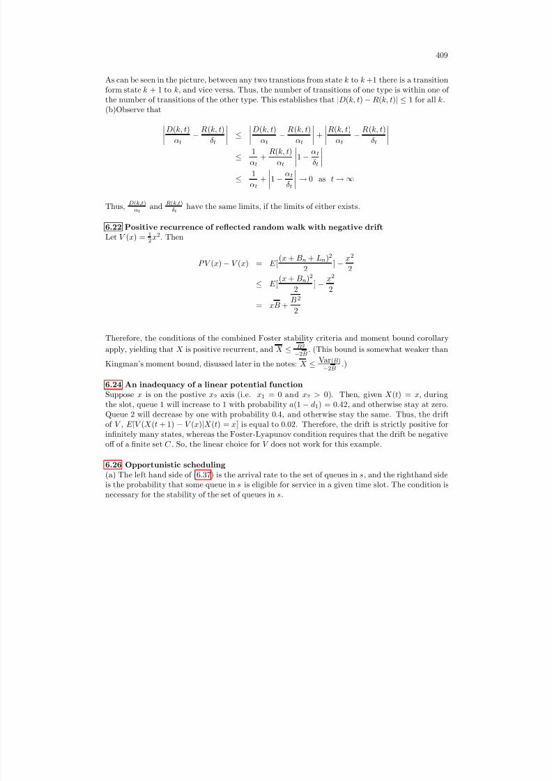
8/11/2019 Random process by B. Hajek
http://slidepdf.com/reader/full/random-process-by-b-hajek 419/448
409
As can be seen in the picture, between any two transtions from state k to k +1 there is a transitionform state k + 1 to k, and vice versa. Thus, the number of transitions of one type is within one of the number of transitions of the other type. This establishes that |D(k, t) − R(k, t)| ≤ 1 for all k .
(b)Observe that D(k, t)
αt− R(k, t)
δ t
≤D(k, t)
αt− R(k, t)
αt
+
R(k, t)
αt− R(k, t)
δ t
≤ 1
αt+
R(k, t)
αt
1 − αt
δ t
≤ 1
αt+
1 − αt
δ t
→ 0 as t → ∞
Thus, D(k,t)
αtand
R(k,t)δt
have the same limits, if the limits of either exists.
6.22 Positive recurrence of reflected random walk with negative driftLet V (x) = 1
2 x2. Then
P V (x) − V (x) = E [(x + Bn + Ln)2
2 ] − x2
2
≤ E [(x + Bn)2
2 ] − x2
2
= xB + B 2
2
Therefore, the conditions of the combined Foster stability criteria and moment bound corollary
apply, yielding that X is positive recurrent, and X ≤ B2
−2B. (This bound is somewhat weaker than
Kingman’s moment bound, disussed later in the notes: X ≤ Var(B)
−2B .)
6.24 An inadequacy of a linear potential functionSuppose x is on the postive x2 axis (i.e. x1 = 0 and x2 > 0). Then, given X (t) = x, duringthe slot, queue 1 will increase to 1 with probability a(1 − d1) = 0.42, and otherwise stay at zero.Queue 2 will decrease by one with probability 0.4, and otherwise stay the same. Thus, the driftof V , E [V (X (t + 1) − V (x)|X (t) = x] is equal to 0.02. Therefore, the drift is strictly positive forinfinitely many states, whereas the Foster-Lyapunov condition requires that the drift be negative
off of a finite set C . So, the linear choice for V does not work for this example.
6.26 Opportunistic scheduling(a) The left hand side of (6.37) is the arrival rate to the set of queues in s, and the righthand sideis the probability that some queue in s is eligible for service in a given time slot. The condition isnecessary for the stability of the set of queues in s.
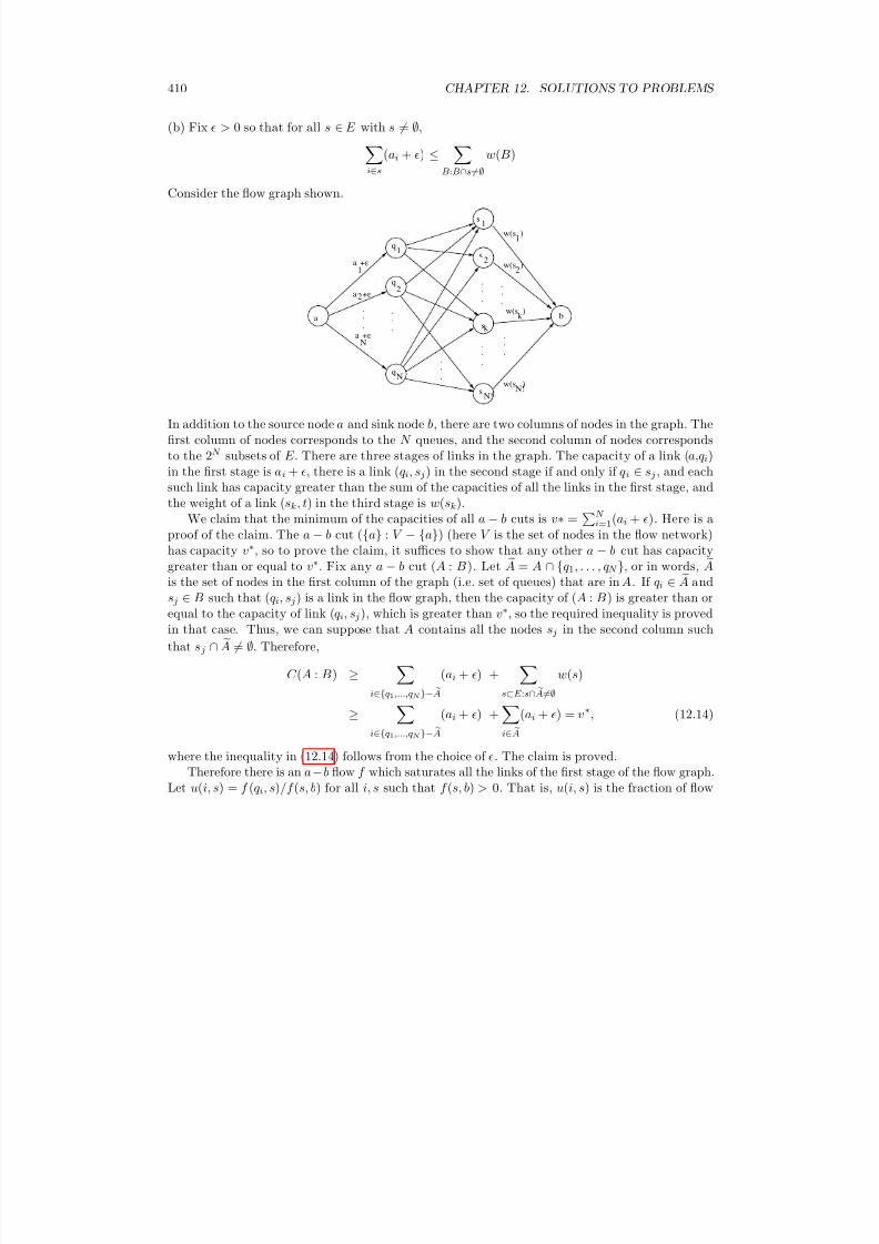
8/11/2019 Random process by B. Hajek
http://slidepdf.com/reader/full/random-process-by-b-hajek 420/448
410 CHAPTER 12. SOLUTIONS TO PROBLEMS
(b) Fix > 0 so that for all s ∈ E with s = ∅,
i∈s(ai + ) ≤
B:B∩s=∅
w(B)
Consider the flow graph shown.
.
a b
q1
q2
qN
s1
s2
sN!
a2
a1
aN
sk
N!
2
1w(s )
w(s )
w(s )
w(s )k
!!
!!
!!
.
.
...
.
..
.
.
.
.
.
.
.
.
.
...
In addition to the source node a and sink node b, there are two columns of nodes in the graph. Thefirst column of nodes corresponds to the N queues, and the second column of nodes correspondsto the 2N subsets of E . There are three stages of links in the graph. The capacity of a link (a,q i)in the first stage is ai + , there is a link (q i, s j) in the second stage if and only if q i ∈ s j , and eachsuch link has capacity greater than the sum of the capacities of all the links in the first stage, andthe weight of a link (sk, t) in the third stage is w(sk).
We claim that the minimum of the capacities of all a
−b cuts is v
∗ =
N i=1(ai + ). Here is a
proof of the claim. The a − b cut (a : V − a) (here V is the set of nodes in the flow network)has capacity v∗, so to prove the claim, it suffices to show that any other a − b cut has capacitygreater than or equal to v∗. Fix any a − b cut (A : B ). Let A = A ∩ q 1, . . . , q N , or in words, Ais the set of nodes in the first column of the graph (i.e. set of queues) that are in A. If q i ∈ A ands j ∈ B such that (q i, s j) is a link in the flow graph, then the capacity of ( A : B) is greater than orequal to the capacity of link (q i, s j), which is greater than v∗, so the required inequality is provedin that case. Thus, we can suppose that A contains all the nodes s j in the second column such
that s j ∩ A = ∅. Therefore,
C (A : B) ≥
i∈q1,...,qN − eA(ai + ) +
s⊂E :s∩ eA=∅
w(s)
≥ i∈q1,...,qN − eA
(ai + ) +i∈ eA
(ai + ) = v∗, (12.14)
where the inequality in (12.14) follows from the choice of . The claim is proved.Therefore there is an a−b flow f which saturates all the links of the first stage of the flow graph.
Let u(i, s) = f (q i, s)/f (s, b) for all i, s such that f (s, b) > 0. That is, u(i, s) is the fraction of flow
8/11/2019 Random process by B. Hajek
http://slidepdf.com/reader/full/random-process-by-b-hajek 421/448
411
on link (s, b) which comes from link (q i, s). For those s such that f (s, b) = 0, define u(i, s) in somearbitrary way, respecting the requirements u(i, s) ≥ 0, u(i, s) = 0 if i ∈ s, and
i∈E u(i, s) = I s=∅.
Then ai + = f (a, q i) =
s f (q i, s) =
s f (s, b)u(i, s) ≤s w(s)u(i, s) = µi(u), as required.
(c) Let V (x) = 1
2 i∈E x2i . Let δ (t) denote the identity of the queue given a potential service at
time t, with δ (t) = 0 if no queue is given potential service. Then P (δ (t) = i|S (t) = s) = u(i, s). Thedynamics of queue i are given by X i(t + 1) = X i(t) + Ai(t) − Ri(δ (t)) + Li(t), where Ri(δ ) = I δ=i.Since
i∈E (Ai(t) − Ri(δ i(t)))2 ≤
i∈E (Ai(t))2 + (Ri(δ i(t)))2 ≤ N +
i∈E Ai(t)2 we have
P V (x) − V (x) ≤
i∈E
xi(ai − µi(u))
+ K (12.15)
≤ −
i∈E
xi
+ K (12.16)
where K = N
2 + N
i=1 K i. Thus, under the necessary stability conditions we have that under thevector of scheduling probabilities u, the system is positive recurrent, andi∈E
X i ≤ K
(12.17)
(d) If u could be selected as a function of the state, x, then the right hand side of (12.15) would beminimized by taking u(i, s) = 1 if i is the smallest index in s such that xi = max j∈s x j. This sug-gests using the longest connected first (LCF) policy, in which the longest connected queue is servedin each time slot. If P LCF denotes the one-step transition probability matrix for the LCF policy,then (12.15) holds for any u, if P is replaced by P LCF . Therefore, under the necessary condition and as in part (b), (12.16) also holds with P replaced by P LCF , and (12.17) holds for the LCF policy.
6.28 Stability of two queues with transfers(a) System is positive recurrent for some u if and only if λ1 < µ1 +ν, λ2 < µ2, and λ1 +λ2 < µ1 +µ2.(b)
QV (x) =y:y=x
q xy (V (y) − V (x))
= λ1
2 [(x1 + 1)2 − x2
1] + λ2
2 [(x2 + 1)2 − x2
2] + µ1
2 [(x1 − 1)2
+ − x21] +
µ2
2 [(x2 − 1)2
+ − x22] +
uνI x1≥12
[(x1 − 1)2 − x21 + (x2 + 1)2 − x2
2] (12.18)
(c) If the righthand side of (12.18) is changed by dropping the positive part symbols and droppingthe factor I x1≥1, then it is not increased, so that
QV (x) ≤ x1(λ1 − µ1 − uν ) + x2(λ2 + uν − µ2) + K
≤ −(x1 + x2)minµ1 + uν − λ1, µ2 − λ2 − uν + K (12.19)
8/11/2019 Random process by B. Hajek
http://slidepdf.com/reader/full/random-process-by-b-hajek 422/448
412 CHAPTER 12. SOLUTIONS TO PROBLEMS
where K = λ1+λ2+µ1+µ2+2ν 2 . To get the best bound on X 1 + X 2, we select u to maximize the min
term in (12.19), or u = u∗, where u∗ is the point in [0, 1] nearest to µ1+µ2−λ1−λ22ν . For u = u∗, we
find QV (x)
≤ −(x1 + x2) + K where = min
µ1 + ν
−λ1, µ2
−λ2, µ1+µ2−λ1−λ2
2
. Which of the
three terms is smallest in the expression for corresponds to the three cases u∗ = 1, u∗ = 0, and0 < u∗ < 1, respectively. It is easy to check that this same is the largest constant such that thestability conditions (with strict inequality relaxed to less than or equal) hold with (λ1, λ2) replacedby (λ1 + , λ2 + ).
7.2 Lack of sample path continuity of a Poisson process(a) The sample path of N is continuous over [0, T ] if and only if it has no jumps in the in-terval, equivalently, if and only if N (T ) = 0. So P (N is continuous over the interval [0,T] ) =exp(−λT ). Since N is continuous over [0, +∞) = ∩∞
n=1N is continuous over [0, n], it followsthat P (N is continuous over [0, +∞)) = limn→∞ P (N is continuous over [0, n]) = limn→∞ e−λn =0.
(b) Since P (N is continuous over [0, +∞)) = 1, N is not a.s. sample continuous. However N ism.s. continuous. One proof is to simply note that the correlation function, given by RN (s, t) =λ(s ∧ t) + λ2st, is continuous. A more direct proof is to note that for fixed t, E [|N s − N t|2] =λ|s − t| + λ2|s − t|2 → 0 as s → t.
7.4 Some statements related to the basic calculus of random processes(a) False. limt→∞ 1
t
t0 X sds = Z = E [Z ] (except in the degenerate case that Z has variance zero).
(b) False. One reason is that the function is continuous at zero, but not everywhere. For another,we would have Var(X 1 − X 0 − X 2) = 3RX (0) − 4RX (1) + 2RX (2) = 3 − 4 + 0 = −1.(c) True. In general, RX X (τ ) = R
X (τ ). Since RX is an even function, RX (0) = 0. Thus, for
any t, E [X tX t] = RX X (0) = RX (0) = 0. Since the process X has mean zero, it follows that
Cov(X t, X
t) = 0 as well. Since X is a Gaussian process, and differentiation is a linear operation,
X t and X t are jointly Gaussian. Summarizing, for t fixed, X t and X t are jointly Gaussian anduncorrelated, so they are independent. (Note: X s is not necessarily independent of X t if s = t. )
7.6 Continuity of a process passing through a nonlinearity(a) Fix t ∈ R and let (sn) be a sequence converging to t. Let > 0 be arbitrary. Let [a, b] be aninterval so large that P X t ∈ [a, b] ≥ . Let δ with 0 < δ < 1 be so small that |G(x) − G(x)| ≤ whenever x, x ∈ [a − 1, b + 1] with |x − x| ≤ δ. Since X sn → X t m.s. it follows that X sn → X tin probability, so there exits N so large that P |X sn − X t| > δ ≤ whenever n ≥ N. Then forn ≥ N ,
P |Y sn − Y t| > ≤ P |Y sn − Y t| > , X t ∈ [a, b] + P X t ∈ [a, b]≤ P |X sn − X t| > δ + ≤ 2
Therefore, Y sn → Y t in probability as n → ∞. Since the Y ’s are bounded, the convergence alsoholds in the m.s. sense. Thus, Y is m.s. continuous at an arbitrary t, so Y is a m.s. continuousprocess.
8/11/2019 Random process by B. Hajek
http://slidepdf.com/reader/full/random-process-by-b-hajek 423/448
413
(b) Let X t = t (a deterministic process) and G(x) = I x≥0. Then Y t = I t≥0 which is not contin-uous at t = 0, and so is not a m.s. continuous process.(c) Let X t ≡ U, (a process content in time) where U has the exponential distribution with param-
eter one. Let G(x) = ex
. Then E [Y 2t ] = ∞0 (e
u
)2
e−u
du = ∞, so that Y is not even a second orderrandom process, so Y is not m.s. continuous random process.
7.8 Integral of OU process(a) The process Y has mean zero because X has mean zero. For s ≤ t,
RY (s, t) =
s0
t0
e−|u−v|dvdu
=
s0
u0
dv−udv +
tu
eu−vdv
du
= s
0
1
−e−u + 1
−eu−tdu
= 2s − 1 + e−s + e−t − es−t,
so in general, RY (s, t) = 2(s ∧ t) − 1 + e−s + e−t − e−|s−t|.(b) For t > 0, Y t is a N (0, σ2
t ) random variable where σ2t = RY (t, t) = 2(t − 1 + e−t). Therefore,
P |Y t| ≥ g(t) = 2Q
g(t)σt
, which, since Q(0.81) ≈ 0.25, means we want g(t) = Q−1(0.25)σt ≈
(0.81)
2(t − 1 + e−t) ≈ (1.15)√
t − 1 + e−t.(c) Since
RZ (s, t) = f (α)2RY (αs, αt)
= f (α)2
2α(s
∧t)
−1 + e−αs + e−αt
−e−α|s−t|
∼ f (α)22α(s ∧ t) as α → ∞,
the choice f (α) = 1√ 2α
works. Intuitively, speeding up the process X causes the duration of the
memory in X to decrease.
7.10 Cross correlation between a process and its m.s. derivative
Fix t, u ∈ T . By assumption, lims→tX s−s−t = X t m.s. Therefore, by Corollary 2.2.4, E
X s−X ts−t
X u
→E [X tX u] as s → t. Equivalently,
RX (s, u) − RX (t, u)
s
−t
→ RX X (t, u) as s → t.
Hence ∂ 1RX (s, u) exists, and ∂ 1RX (t, u) = RX X (t, u).
7.12 A windowed Poisson process(a) The sample paths of X are piecewise constant, integer valued with initial value zero. They jump by +1 at each jump of N , and jump by -1 one time unit after each jump of N .
8/11/2019 Random process by B. Hajek
http://slidepdf.com/reader/full/random-process-by-b-hajek 424/448
414 CHAPTER 12. SOLUTIONS TO PROBLEMS
(b) Method 1: If |s−t| ≥ 1 then X s and X t are increments of N over disjoint intervals, and are there-fore independent, so C X (s, t) = 0. If |s−t| < 1, then there are three disjoint intervals, I 0, I 1, and I 2,with I 0 = [s, s+1]∪ [t, t+1], such that [s, s+1] = I 0 ∪I 1 and [t, t+1] = I 0 ∪I 2. Thus, X s = D0 +D1
and X t = D0 + D2, where Di is the increment of N over the interval I i. The three incrementsD1, D2, and D3 are independent, and D0 is a Poisson random variable with mean and variance equalto λ times the length of I 0, which is 1 − |s − t|. Therefore, C X (s, t) = Cov(D0 + D1, D0 + D2) =
Cov(D0, D0) = λ(1 − |s − t|). Summarizing, C X (s, t) =
λ(1 − |s − t|) if |s − t| < 1
0 elseMethod 2: C X (s, t) = Cov(N s+1 − N s, N t+1 − N t) = λ[min(s + 1, t + 1) − min(s + 1, t) − min(s, t +1) − min(s, t)]. This answer can be simplified to the one found by Method 1 by considering thecases |s − t| > 1, t < s < t + 1, and s < t < s + 1 separately.(c) No. X has a -1 jump one time unit after each +1 jump, so the value X t for a “present” time ttells less about the future, (X s : s ≥ t), than the past, (X s : 0 ≤ s ≤ t), tells about the future .(d) Yes, recall that RX (s, t) = C X (s, t) − µX (s)µX (t). Since C X and µX are continuous functions,so is RX , so that X is m.s. continuous.(e) Yes. Using the facts that C X (s, t) is a function of s − t alone, and C X (s) → 0 as s → ∞, wefind as in the section on ergodicity, Var( 1
t
t0 X sds) = 2
t
t0 (1 − s
t )C X (s)ds → 0 as t → ∞.
7.14 A singular integral with a Brownian motion(a) The integral
1
wtt dt exists in the m.s. sense for any > 0 because wt/t is m.s. continuous over
[, 1]. To see if the limit exists we apply the correlation form of the Cauchy criteria (Proposition2.2.2). Using different letters as variables of integration and the fact Rw(s, t) = s ∧ t (the minimumof s and t), yields that as , → 0,
E
1
ws
s ds
1
wt
t dt
=
1
1
s ∧ t
st dsdt
→ 1
0
1
0
s ∧ t
st dsdt
= 2
1
0
t0
s ∧ t
st dsdt = 2
1
0
t0
s
stdsdt
= 2 1
0 t
0
1
tdsdt = 2
1
0
1dt = 2.
Thus the m.s. limit defining the integral exits. The integral has the N (0, 2) distribution.
8/11/2019 Random process by B. Hajek
http://slidepdf.com/reader/full/random-process-by-b-hajek 425/448
415
(b) As a, b → ∞,
E a
1
ws
s
ds b
1
wt
t
dt = a
1 b
1
s ∧ t
st
dsdt
→ ∞
1
∞1
s ∧ t
st dsdt
= 2
∞1
t1
s ∧ t
st dsdt = 2
∞1
t1
s
stdsdt
= 2
∞1
t1
1
tdsdt = 2
∞1
t − 1
t dt = ∞,
so that the m.s. limit does not exist, and the integral is not well defined.
7.16 Recognizing m.s. properties
(a) Yes m.s. continuous since RX is continuous. No not m.s. differentiable since RX (0) doesn’texist. Yes, m.s. integrable over finite intervals since m.s. continuous. Yes mean ergodic in m.s.since RX (T ) → 0 as |T | → ∞.(b) Yes, no, yes, for the same reasons as in part (a). Since X is mean zero, RX (T ) = C X (T ) for allT . Thus
lim|T |→∞
C X (T ) = lim|T |→∞
RX (T ) = 1
Since the limit of C X exists and is net zero, X is not mean ergodic in the m.s. sense.(c) Yes, no, yes, yes, for the same reasons as in (a).(d) No, not m.s. continuous since RX is not continuous. No, not m.s. differentiable since X is
not even m.s. continuous. Yes, m.s. integrable over finite intervals, because the Riemann integral ba ba RX (s, t)dsdt exists and is finite, for the region of integration is a simple bounded region and
the integrand is piece-wise constant.(e) Yes, m.s. continuous since RX is continuous. No, not m.s. differentiable. For example,
E
X t − X 0
t
2
= 1
t2 [RX (t, t) − RX (t, 0) − RX (0, t) + RX (0, 0)]
= 1
t2
√ t − 0 − 0 + 0
→ +∞ as t → 0.
Yes, m.s. integrable over finite intervals since m.s. continuous.
7.18 A stationary Gaussian process(a) No. All mean zero stationary, Gaussian Markov processes have autocorrelation functions of theform RX (t) = Aρ|t|, where A ≥ 0 and 0 ≤ ρ ≤ 1 for continuous time (or |ρ| ≤ 1 for discrete time).
(b) E [X 3|X 0] = E [X 3|X 0] = RX(3)RX(0) X 0 = X 0
10 . The error is Gaussian with mean zero and variance
MSE = Var(X 3) − Var(X 010 ) = 1 − 0.01 = 0.99. So P |X 3 − E [X 3|X 0]| ≥ 10 = 2Q( 10√
0.99).
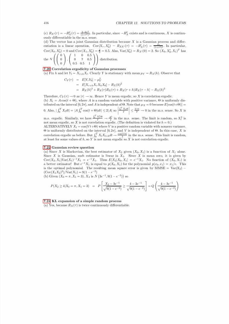
8/11/2019 Random process by B. Hajek
http://slidepdf.com/reader/full/random-process-by-b-hajek 426/448
416 CHAPTER 12. SOLUTIONS TO PROBLEMS
(c) RX (τ ) = −RX (τ ) = 2−6τ 2
(1+τ 2)3 . In particular, since −RX exists and is continuous, X is continu-
ously differentiable in the m.s. sense.(d) The vector has a joint Gaussian distribution because X is a Gaussian process and differ-
entiation is a linear operation. Cov(X τ , X 0) = RXX (τ ) = −RX (τ ) = 2τ (1+τ 2)2 . In particular,
Cov(X 0, X 0) = 0 and Cov(X 1, X 0) = 24 = 0.5. Also, Var(X 0) = RX (0) = 2. So (X 0, X 0, X 1)T has
the N
000
,
1 0 0.50 2 0.5
0.5 0.5 1
distribution.
7.20 Correlation ergodicity of Gaussian processes(a) Fix h and let Y t = X t+hX t. Clearly Y is stationary with mean µY = RX (h). Observe that
C Y (τ ) = E [Y τ Y 0] − µ2Y
= E [X τ +hX τ X hX 0] − RX (h)2
= RX (h)2 + RX (τ )RX (τ ) + RX (τ + h)RX (τ
−h)
−RX (h)2
Therefore, C Y (τ ) → 0 as |τ | → ∞. Hence Y is mean ergodic, so X is correlation ergodic.(b) X t = A cos(t + Θ), where A is a random variable with positive variance, Θ is uniformly dis-tributed on the interval [0, 2π], and A is independent of Θ. Note that µX = 0 because E [cos(t+Θ)] =
0. Also, | T 0 X tdt| = |A T 0 cos(t + Θ)dt| ≤ 2|A| so
R T 0 X tdt
T
≤ 2|A|T → 0 in the m.s. sense. So X is
m.s. ergodic. Similarly, we haveR T 0 X 2t dt
T → A2
2 in the m.s. sense. The limit is random, so X 2t isnot mean ergodic, so X is not correlation ergodic. (The definition is violated for h = 0.)ALTERNATIVELY X t = cos(V t+Θ) where V is a positive random variable with nonzero variance,Θ is uniformly distributed on the interval [0, 2π], and V is independent of Θ. In this case, X is
correlation ergodic as before. But T
0 X tX t+hdt
→ cos(V h)
2 in the m.s. sense. This limit is random,
at least for some values of h, so Y is not mean ergodic so X is not correlation ergodic.
7.22 Gaussian review question(a) Since X is Markovian, the best estimator of X 2 given (X 0, X 1) is a function of X 1 alone.Since X is Gaussian, such estimator is linear in X 1. Since X is mean zero, it is given byCov(X 2, X 1)Var(X 1)−1X 1 = e−1X 1. Thus E [X 2|X 0, X 1] = e−1X 1. No function of (X 0, X 1) isa better estimator! But e−1X 1 is equal to p(X 0, X 1) for the polynomial p(x0, x1) = x1/e. Thisis the optimal polynomial. The resulting mean square error is given by MMSE = Var(X 2) −(Cov(X 1X 2)2)/Var(X 1) = 9(1 − e−2)(b) Given (X 0 = π, X 1 = 3), X 2 is N
3e−1, 9(1 − e−2)
so
P (X 2 ≥ 4|X 0 = π, X 1 = 3) = P X 2 − 3e−1
9(1 − e−2)≥ 4 − 3e−
1 9(1 − e−2)
= Q 4 − 3e−1
9(1 − e−2)
7.24 KL expansion of a simple random process(a) Yes, because RX (τ ) is twice continuously differentiable.
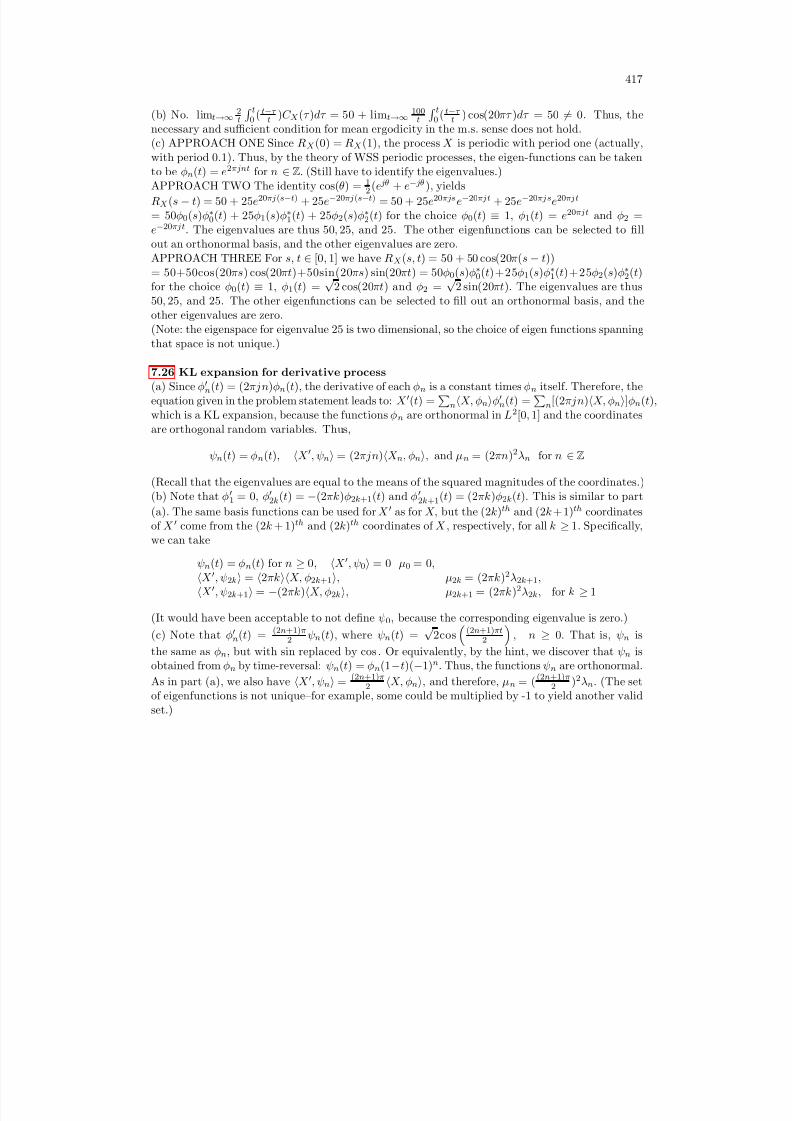
8/11/2019 Random process by B. Hajek
http://slidepdf.com/reader/full/random-process-by-b-hajek 427/448
417
(b) No. limt→∞ 2t
t0 ( t−τ
t )C X (τ )dτ = 50 + limt→∞ 100t
t0 ( t−τ
t ) cos(20πτ )dτ = 50 = 0. Thus, thenecessary and sufficient condition for mean ergodicity in the m.s. sense does not hold.(c) APPROACH ONE Since RX (0) = RX (1), the process X is periodic with period one (actually,
with period 0.1). Thus, by the theory of WSS periodic processes, the eigen-functions can be takento be φn(t) = e2πjnt for n ∈ Z. (Still have to identify the eigenvalues.)APPROACH TWO The identity cos(θ) = 1
2 (e jθ + e− jθ), yields
RX (s − t) = 50 + 25e20πj(s−t) + 25e−20πj(s−t) = 50 + 25e20πjse−20πjt + 25e−20πjse20πjt
= 50φ0(s)φ∗0(t) + 25φ1(s)φ∗
1(t) + 25φ2(s)φ∗2(t) for the choice φ0(t) ≡ 1, φ1(t) = e20πjt and φ2 =
e−20πjt. The eigenvalues are thus 50, 25, and 25. The other eigenfunctions can be selected to fillout an orthonormal basis, and the other eigenvalues are zero.APPROACH THREE For s, t ∈ [0, 1] we have RX (s, t) = 50 + 50 cos(20π(s − t))= 50+50cos(20πs) cos(20πt)+50sin(20πs) sin(20πt) = 50φ0(s)φ∗
0(t)+25φ1(s)φ∗1(t)+25φ2(s)φ∗
2(t)for the choice φ0(t) ≡ 1, φ1(t) =
√ 2 cos(20πt) and φ2 =
√ 2 sin(20πt). The eigenvalues are thus
50, 25, and 25. The other eigenfunctions can be selected to fill out an orthonormal basis, and the
other eigenvalues are zero.(Note: the eigenspace for eigenvalue 25 is two dimensional, so the choice of eigen functions spanningthat space is not unique.)
7.26 KL expansion for derivative process(a) Since φ
n(t) = (2πjn)φn(t), the derivative of each φn is a constant times φn itself. Therefore, theequation given in the problem statement leads to: X (t) =
nX, φnφ
n(t) =
n[(2πjn)X, φn]φn(t),which is a KL expansion, because the functions φn are orthonormal in L2[0, 1] and the coordinatesare orthogonal random variables. Thus,
ψn(t) = φn(t), X , ψn = (2πjn)X n, φn, and µn = (2πn)2λn for n ∈ Z
(Recall that the eigenvalues are equal to the means of the squared magnitudes of the coordinates.)(b) Note that φ
1 = 0, φ2k(t) = −(2πk)φ2k+1(t) and φ
2k+1(t) = (2πk)φ2k(t). This is similar to part
(a). The same basis functions can be used for X as for X, but the (2k)th and (2k +1)th coordinatesof X come from the (2k + 1)th and (2k)th coordinates of X , respectively, for all k ≥ 1. Specifically,we can take
ψn(t) = φn(t) for n ≥ 0, X , ψ0 = 0 µ0 = 0,X , ψ2k = 2πkX, φ2k+1, µ2k = (2πk)2λ2k+1,X , ψ2k+1 = −(2πk)X, φ2k, µ2k+1 = (2πk)2λ2k, for k ≥ 1
(It would have been acceptable to not define ψ0, because the corresponding eigenvalue is zero.)
(c) Note that φn
(t) = (2n+1)π
2 ψ
n(t), where ψ
n(t) =
√ 2cos (2n+1)πt
2 , n ≥
0. That is, ψn
is
the same as φn, but with sin replaced by cos . Or equivalently, by the hint, we discover that ψn isobtained from φn by time-reversal: ψn(t) = φn(1−t)(−1)n. Thus, the functions ψn are orthonormal.
As in part (a), we also have X , ψn = (2n+1)π
2 X, φn, and therefore, µn = ((2n+1)π
2 )2λn. (The setof eigenfunctions is not unique–for example, some could be multiplied by -1 to yield another validset.)
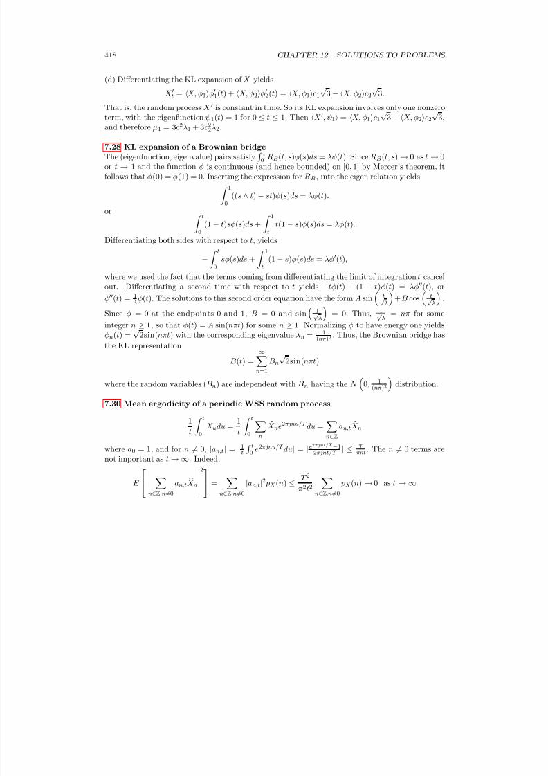
8/11/2019 Random process by B. Hajek
http://slidepdf.com/reader/full/random-process-by-b-hajek 428/448
418 CHAPTER 12. SOLUTIONS TO PROBLEMS
(d) Differentiating the KL expansion of X yields
X t = X, φ1φ1(t) + X, φ2φ
2(t) = X, φ1c1
√ 3 − X, φ2c2
√ 3.
That is, the random process X is constant in time. So its KL expansion involves only one nonzeroterm, with the eigenfunction ψ1(t) = 1 for 0 ≤ t ≤ 1. Then X , ψ1 = X, φ1c1√ 3 − X, φ2c2
√ 3,and therefore µ1 = 3c2
1λ1 + 3c22λ2.
7.28 KL expansion of a Brownian bridgeThe (eigenfunction, eigenvalue) pairs satisfy
10 RB(t, s)φ(s)ds = λφ(t). Since RB(t, s) → 0 as t → 0
or t → 1 and the function φ is continuous (and hence bounded) on [0, 1] by Mercer’s theorem, itfollows that φ(0) = φ(1) = 0. Inserting the expression for RB , into the eigen relation yields 1
0((s ∧ t) − st)φ(s)ds = λφ(t).
or t0
(1 − t)sφ(s)ds + 1
tt(1 − s)φ(s)ds = λφ(t).
Differentiating both sides with respect to t, yields
− t
0sφ(s)ds +
1
t(1 − s)φ(s)ds = λφ(t),
where we used the fact that the terms coming from differentiating the limit of integration t cancelout. Differentiating a second time with respect to t yields −tφ(t) − (1 − t)φ(t) = λφ(t), or
φ(t) = 1λφ(t). The solutions to this second order equation have the form A sin
t√ λ
+B cos
t√ λ
.
Since φ = 0 at the endpoints 0 and 1, B = 0 and sin
1√ λ
= 0. Thus, 1√
λ = nπ for some
integer n
≥ 1, so that φ(t) = A sin(nπt) for some n
≥ 1. Normalizing φ to have energy one yields
φn(t) = √ 2sin(nπt) with the corresponding eigenvalue λn = 1(nπ)2 . Thus, the Brownian bridge has
the KL representation
B(t) =
∞n=1
Bn
√ 2sin(nπt)
where the random variables (Bn) are independent with Bn having the N
0, 1(nπ)2
distribution.
7.30 Mean ergodicity of a periodic WSS random process
1
t
t0
X udu = 1
t
t0 n
X ne2πjnu/T du =
n∈Zan,t
X n
where a0 = 1, and for n = 0, |an,t| = |1t t
0 e2πjnu/T du| = | e2πjnt/T −12πjnt/T | ≤ T
πnt . The n = 0 terms arenot important as t → ∞. Indeed,
E
n∈Z,n=0
an,t X n
2 =
n∈Z,n=0
|an,t|2 pX (n) ≤ T 2
π2t2
n∈Z,n=0
pX (n) → 0 as t → ∞
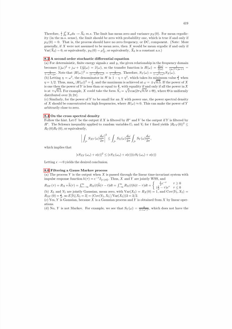
8/11/2019 Random process by B. Hajek
http://slidepdf.com/reader/full/random-process-by-b-hajek 429/448
419
Therefore, 1t
t0 X udu → X 0 m.s. The limit has mean zero and variance pX (0). For mean ergodic-
ity (in the m.s. sense), the limit should be zero with probability one, which is true if and only if pX (0) = 0. That is, the process should have no zero frequency, or DC, component. (Note: More
generally, if X were not assumed to be mean zero, then X would be mean ergodic if and only if Var( X 0) = 0, or equivalently, pX (0) = µ2
X , or equivalently, X 0 is a constant a.s.)
8.2 A second order stochastic differential equation(a) For deterministic, finite energy signals x and y, the given relationship in the frequency domain
becomes (( jω)2 + jω + 1) y(ω) = x(ω), so the transfer function is H (ω) = by(ω) bx(ω) = 1
( jω)2+ jω+1 =1
1−ω2+ jω . Note that |H (ω)|2 = 1(1−ω2)2+ω2 = 1
1−ω2+ω4 . Therefore, S Y (ω) = 11−ω2+ω4 S X (ω).
(b) Letting η = ω2, the denominator in H is 1 − η + η2, which takes its minimum value 34 when
η = 1/2. Thus, maxω |H (ω)|2 = 43 , and the maximum is achieved at ω = ±√
0.5. If the power of X is one then the power of Y is less than or equal to 4
3 , with equality if and only if all the power in X
is at
±
√ 0.5. For example, X could take the form X t =
√ 2 cos(2π
√ 0.5t + Θ), where Θ is uniformly
distributed over [0, 2π].(c) Similarly, for the power of Y to be small for an X with power one, the power spectral densityof X should be concentrated on high frequencies, where H (ω) ≈ 0. This can make the power of Y arbitrarily close to zero.
8.4 On the cross spectral densityFollow the hint. Let U be the output if X is filtered by H and V be the output if Y is filtered byH . The Schwarz inequality applied to random variables U t and V t for t fixed yields |RUV (0)|2 ≤RU (0)RV (0), or equivalently,
J S XY (ω)dω
2π 2
≤ J S X (ω)dω
2π J S Y (ω)dω
2π
,
which implies that
|S XY (ωo) + o()|2 ≤ (S X (ωo) + o())(S Y (ωo) + o())
Letting → 0 yields the desired conclusion.
8.6 Filtering a Gauss Markov process(a) The process Y is the output when X is passed through the linear time-invariant system withimpulse response function h(τ ) = e−τ I τ ≥0. Thus, X and Y are jointly WSS, and
RXY (τ ) = RX
∗ h(τ ) = ∞t=−∞
RX (t)h(τ
−t)dt = ∞−∞
RX (t)h(t
−τ )dt =
12 e−τ τ ≥ 0
(12 − τ )e
τ
τ ≤ 0(b) X 5 and Y 5 are jointly Gaussian, mean zero, with Var(X 5) = RX (0) = 1, and Cov(Y 5, X 5) =RXY (0) = 1
2 , so E [Y 5|X 5 = 3] = (Cov(Y 5, X 5)/Var(X 5))3 = 3/2.(c) Yes, Y is Gaussian, because X is a Gaussian process and Y is obtained from X by linear oper-ations.(d) No, Y is not Markov. For example, we see that S Y (ω) = 2
(1+ω2)2 , which does not have the
8/11/2019 Random process by B. Hajek
http://slidepdf.com/reader/full/random-process-by-b-hajek 430/448
420 CHAPTER 12. SOLUTIONS TO PROBLEMS
form required for a stationary mean zero Gaussian process to be Markov (namely 2Aα2+ω2 ). Another
explanation is that, if t is the present time, given Y t, the future of Y is determined by Y t and(X s : s ≥ t). The future could be better predicted by knowing something more about X t than Y t
gives alone, which is provided by knowing the past of Y .(Note: the R2-valued process ((X t, Y t) : t ∈ R) is Markov.)
8.8 A stationary two-state Markov processπP = π implies π = ( 1
2 , 12 ) is the equilibrium distribution so P X n = 1 = P X n = −1 = 1
2 forall n. Thus µX = 0. For n ≥ 1
RX (n) = P (X n = 1, X 0 = 1) + P (X n = −1, X 0 = −1) − P (X n = −1, X 0 = 1) − P (X n = 1, X 0 = −1)
= 1
2
1
2 +
1
2(1 − 2 p)n
+
1
2
1
2 +
1
2(1 − 2 p)n
− 1
2
1
2 − 1
2(1 − 2 p)n
− 1
2
1
2 − 1
2(1 − 2 p)n
= (1 − 2 p)n
So in general, RX (n) = (1 − 2 p)|n|. The corresponding power spectral density is given by:
S X (ω) =
∞n=−∞
(1 − 2 p)ne− jωn =
∞n=0
((1 − 2 p)e− jω)n +
∞n=0
((1 − 2 p)e jω)n − 1
= 1
1 − (1 − 2 p)e− jω +
1
1 − (1 − 2 p)e jω − 1
= 1 − (1 − 2 p)2
1 − 2(1 − 2 p) cos(ω) + (1 − 2 p)2
8.10 A linear estimation problem
E [|X t − Z t|2] = E [(X t − Z t)(X t − Z t)∗]
= RX (0) + RZ (0) − RXZ (0) − RZX (0)
= RX (0) + h ∗ h ∗ RY (0) − 2Re(h ∗ RXY (0))
=
∞−∞
S X (ω) + |H (ω)|2S Y (ω) − 2Re(H ∗(ω)S XY (ω))dω
2π
The hint with σ 2 = S Y (ω), zo = S (XY (ω), and z = H (ω) implies H opt(ω) = S XY (ω)S Y (ω) .
8.12 The accuracy of approximate differentiation(a) S X (ω) = S X (ω)|H (ω)|2 = ω2S X (ω).
(b) k(τ ) = 12a(δ (τ + a) − δ (τ − a)) and K (ω) =
∞−∞ k(τ )e− jωtdτ = 1
2a(e jωa − e− jωa) = j sin(aω)a . By
l’Hospital’s rule, lima→0 K (ω) = lima→0 jω cos(aω)
1 = jω.(c) D is the output of the linear system with input X and transfer function H (ω) − K (ω). The
8/11/2019 Random process by B. Hajek
http://slidepdf.com/reader/full/random-process-by-b-hajek 431/448
421
output thus has power spectral density S D(ω) = S X (ω)|H (ω) − K (ω)|2 = S X (ω)|ω − sin(aω)a |2.
(d) Or, S D(ω) = S X (ω)|1 − sin(aω)aω |2. Suppose 0 < a ≤
√ 0.6ωo
(≈ 0.77ωo
). Then by the bound given
in the problem statement, if |
ω| ≤
ωo then 0 ≤
1 −
sin(aω)
aω ≤ (aω)2
6 ≤ (aωo)2
6 ≤ 0.1, so that
S D(ω) ≤ (0.01)S X (ω) for ω in the base band. Integrating this inequality over the band yields thatE [|Dt|2] ≤ (0.01)E [|X t|2].
8.14 Filtering Poisson white noise(a) Since µN = λ, µX = λ
∞−∞ h(t)dt. Also, C X = h ∗ h ∗ C N = λh ∗ h. (In particular, if
h(t) = I 0≤t<1, then C X (τ ) = λ(1 − |τ |)+, as already found in Problem 4.19.)(b) In the special case, in between arrival times of N , X decreases exponentially, following theequation X = −X. At each arrival time of N , X has an upward jump of size one. Formally, we canwrite, X = −X + N . For a fixed time to, which we think of as the present time, the process aftertime to is the solution of the above differential equation, where the future of N is independent of X up to time to. Thus, the future evolution of X depends only on the current value, and random
variables independent of the past. Hence, X is Markov.
8.16 Linear and nonlinear reconstruction from samples(a) We first find the mean function and autocorrelation function of X. E [X t] =
n E [g(t − n −
U )]E [Bn] = 0 because E [Bn] = 0 for all n.
RX (s, t) = E
∞n=−∞
g(s − n − U )Bn
∞m=−∞
g(t − m − U )Bm
= σ2∞
n=−∞E [g(s − n − U )g(t − n − U )] = σ2
∞n=−∞
1
0g(s − n − u)g(t − n − u)du
= σ2 ∞n=−∞
n+1
ng(s − v)g(t − v)dv = σ2 ∞
−∞g(s − v)g(t − v)dv
= σ2
∞−∞
g(s − v)g(v − t)dv = σ2(g ∗ g)(s − t)
So X is WSS with mean zero and RX = σ2g ∗ g.(b) By part (a), the power spectral density of X is σ2|G(ω)|2. If g is a baseband signal, so that|G(ω)2| = 0 for ω ≥ ωo. then by the sampling theorem for WSS baseband random processes, X canbe recovered from the samples (X (nT ) : n ∈ Z) as long as T ≤ π
ωo.
(c) For this case, G(2πf ) = sinc2(f ), which is not supported in any finite interval. So part (a) doesnot apply. The sample paths of X are continuous and piecewise linear, and at least two sample
points fall within each linear portion of X. Either all pairs of samples of the form (X n, X n+0.5) fallwithin linear regions (happens when 0.5 ≤ U ≤ 1), or all pairs of samples of the form (X n+0.5, X n+1)fall within linear regions (happens when 0 ≤ U ≤ 0.5). We can try reconstructing X using bothcases. With probability one, only one of the cases will yield a reconstruction with change pointshaving spacing one. That must be the correct reconstruction of X. The algorithm is illustratedin Figure 12.5. Figure 12.5(a) shows a sample path of B and a corresponding sample path of X ,
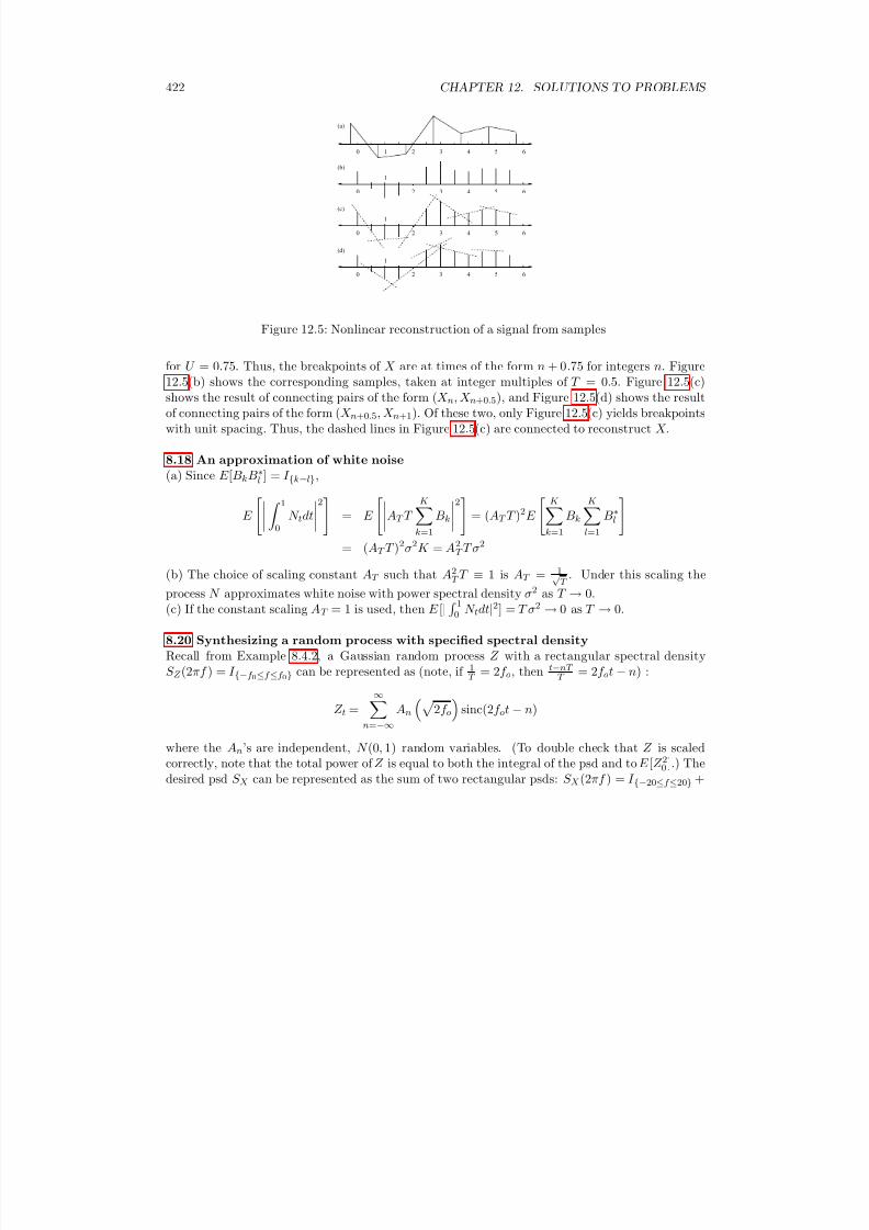
8/11/2019 Random process by B. Hajek
http://slidepdf.com/reader/full/random-process-by-b-hajek 432/448
422 CHAPTER 12. SOLUTIONS TO PROBLEMS
1
1 32 4 60 5
(b)
(a)
(c)
(d)
32 4 60 5
1
32 4 60 5
1
32 4 60 5
Figure 12.5: Nonlinear reconstruction of a signal from samples
for U = 0.75. Thus, the breakpoints of X are at times of the form n + 0.75 for integers n. Figure12.5(b) shows the corresponding samples, taken at integer multiples of T = 0.5. Figure 12.5(c)shows the result of connecting pairs of the form (X n, X n+0.5), and Figure 12.5(d) shows the resultof connecting pairs of the form (X n+0.5, X n+1). Of these two, only Figure 12.5(c) yields breakpointswith unit spacing. Thus, the dashed lines in Figure 12.5(c) are connected to reconstruct X.
8.18 An approximation of white noise(a) Since E [BkB∗
l ] = I k=l,
E 1
0
N tdt2
= E AT T K
k=1
Bk2
= (AT T )2E K
k=1
Bk
K
l=1
B∗l
= (AT T )2σ2K = A2T T σ2
(b) The choice of scaling constant AT such that A2T T ≡ 1 is AT = 1√
T . Under this scaling the
process N approximates white noise with power spectral density σ2 as T → 0.(c) If the constant scaling AT = 1 is used, then E [| 10 N tdt|2] = T σ2 → 0 as T → 0.
8.20 Synthesizing a random process with specified spectral densityRecall from Example 8.4.2, a Gaussian random process Z with a rectangular spectral densityS Z (2πf ) = I −f 0≤f ≤f 0 can be represented as (note, if 1
T = 2f o, then t−nT T = 2f ot − n) :
Z t = ∞n=−∞
An 2f o sinc(2f ot − n)
where the An’s are independent, N (0, 1) random variables. (To double check that Z is scaledcorrectly, note that the total power of Z is equal to both the integral of the psd and to E [Z 20 ].) Thedesired psd S X can be represented as the sum of two rectangular psds: S X (2πf ) = I −20≤f ≤20 +
8/11/2019 Random process by B. Hajek
http://slidepdf.com/reader/full/random-process-by-b-hajek 433/448
423
I −10≤f ≤10, and the psd of the sum of two independent WSS processes is the sum of the psds, soX could be represented as:
X t =
∞n=−∞
An √ 40 sinc(40t − n) +
∞n=−∞
Bn √ 20 sinc(20t − n)
where the A’s and B’s are independent N (0, 1) random variables. This requires 60 samples perunit simulation time.
An approach using fewer samples is to generate a random process Y with psd S Y (ω) =I −20≤f ≤20 and then filter Y using a filter with impulse response H with |H |2 = S X . For ex-
ample, we could simply take H (2πf ) =
S X (2πf ) = I −20≤f ≤20 +√
2 − 1
I −10≤f ≤10, so X could be represented as:
X =
∞
n=−∞
An √
40
sinc(40t − n)
∗ h
where h(t) = (40)sinc(40t) +√
2 − 1
(20)sinc(20t). This approach requires 40 samples per unitsimulation time.
8.22 Finding the envelope of a deterministic signal(a) z(2πf ) = 2[ x(2π(f + f c))]LP = δ (f + f c − 1000) + δ (f + f c − 1001). If f c = 1000.5 then z(2πf ) = δ (f + 0.5) + δ (f − 0.5). Therefore z (t) = 2cos(πt) and |z(t)| = 2| cos(πt)|.(b) If f c = 995 then z(2πf ) = δ (f − 5) + δ (f − 6). Therefore z(t) = e j2π(5.5)t2 cos(πt) and|z(t)| = 2| cos(πt)|.(c) In general, the complex envelope in the frequency domain is given by
z(2πf ) = 2[
x(2π(f +
f c))]LP . If a somewhat different carrier frequency f c = f c +
f c is used, the complex envelope of x
using f c is the original complex envelope, shifted to the left in the frequency domain by f . Thisis equivalent to multiplication by e− j2π(f )t in the time domain. Since |e− j2π(f )t| ≡ 1, the realenvelope is unchanged.
8.24 A narrowband Gaussian process(a) The power spectral density S X , which is the Fourier transform of RX , can be found graphicallyas follows.(b) A sample path of X generated by computer simulation is pictured in Figure 12.7.Several features of the sample path are apparent. The carrier frequency is 30 Hz, so for a period of time on the order of a tenth of a second, the signal resembles a pure sinusiodal signal with frequencynear 30 Hz. On the other hand, the one sided root mean squared bandwidth of the baseband signals
U and V is 2.7 Hz, so that the envelope of X varies significantly over intervals of length 1/3 of a second or more. The mean square value of the real envelope is given by E [|Z t|2] = 2, so theamplitude of the real envelope process |Z t| fluctuates about
√ 2 ≈ 1.41.
(c) The power spectral densities S U (2πf ) and S V (2πf ) are equal, and are equal to the Fouriertranform of sinc(6τ )2, shown in Figure 12.6. The cross spectral density S UV is zero since the upperlobe of S X is symmetric about 30Hz.
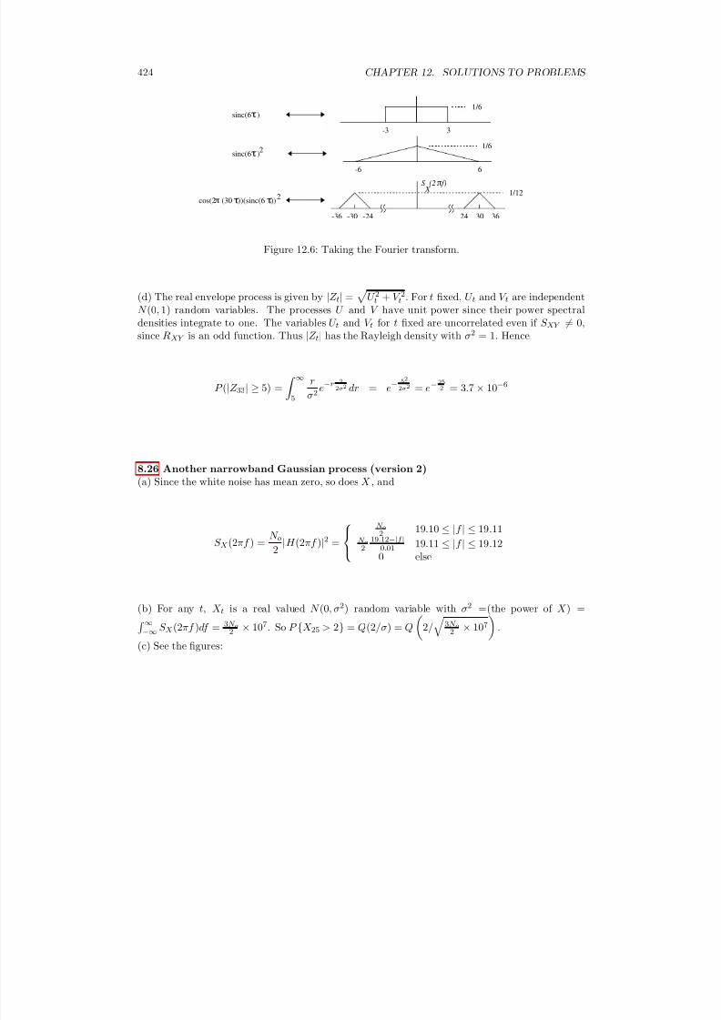
8/11/2019 Random process by B. Hajek
http://slidepdf.com/reader/full/random-process-by-b-hajek 434/448
424 CHAPTER 12. SOLUTIONS TO PROBLEMS
π τ
τsinc(6 )
sinc(6 ) τ
2
πS (2 f) X
-6
-3 3
6
1/12
1/6
1/6
-24-30-36 363024
cos(2 (30 ))(sinc(6 ))2
τ
Figure 12.6: Taking the Fourier transform.
(d) The real envelope process is given by |Z t| = U 2t + V 2t . For t fixed, U t and V t are independentN (0, 1) random variables. The processes U and V have unit power since their power spectraldensities integrate to one. The variables U t and V t for t fixed are uncorrelated even if S XY = 0,since RXY is an odd function. Thus |Z t| has the Rayleigh density with σ2 = 1. Hence
P (|Z 33| ≥ 5) =
∞5
r
σ2e−r 2
2σ2 dr = e− 52
2σ2 = e−252 = 3.7 × 10⁻⁶
8.26 Another narrowband Gaussian process (version 2)(a) Since the white noise has mean zero, so does X , and
S X (2πf ) = N o
2 |H (2πf )|2 =
N o
2 19.10 ≤ |f | ≤ 19.11N o
219.12−|f |
0.01 19.11 ≤ |f | ≤ 19.120 else
(b) For any t, X t is a real valued N (0, σ2) random variable with σ2 =(the power of X ) = ∞−∞ S X (2πf )df = 3N o
2 × 10⁷. So P X 25 > 2 = Q(2/σ) = Q
2/
3N o2 × 107
.
(c) See the figures:
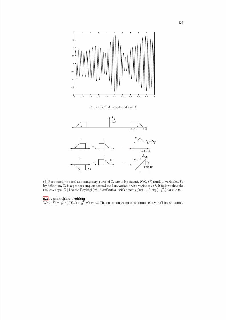
8/11/2019 Random process by B. Hajek
http://slidepdf.com/reader/full/random-process-by-b-hajek 435/448
425
0 0.1 0.2 0.3 0.4 0.5 0.6 0.7 0.8 0.9 1−2
−1.5
−1
−0.5
0
0.5
1
1.5
2
Figure 12.7: A sample path of X
0.01 GHz
j j
S X No/2
S
S =S U V
UV
+
+
=
=
j
No/2
No
19.10 19.12
0.01 GHz
(d) For t fixed, the real and imaginary parts of Z t are independent, N (0, σ
2
) random variables. Soby definition, Z t is a proper complex normal random variable with variance 2σ2. It follows that thereal envelope |Z t| has the Rayleigh(σ2) distribution, with density f (r) = r
σ2 exp(− r2
2σ2 ) for r ≥ 0.
9.2 A smoothing problemWrite X 5 =
30 g(s)Y sds +
107 g(s)ysds. The mean square error is minimized over all linear estima-
8/11/2019 Random process by B. Hajek
http://slidepdf.com/reader/full/random-process-by-b-hajek 436/448
426 CHAPTER 12. SOLUTIONS TO PROBLEMS
tors if and only if (X 5 − X 5) ⊥ Y u for u ∈ [0, 3] ∪ [7, 10], or equivalently
RXY (5, u) = 3
0
g(s)RY (s, u)ds + 10
7
g(s)RY (s, u)ds for u
∈ [0, 3]
∪[7, 10].
9.4 A standard noncausal estimation problem(a) g(ω) =
∞0 g(t)e− jωtdt +
0−∞ g(t)e− jωtdt = 1
α+ jω + 1α− jω = 2α
ω2+α2 .
(So ∞−∞
1ω2+α2
dω2π = 1
2α .)
(b) ∞−∞
1a+bω2
dω2π =
∞−∞
1/ba/b+ω2
dω2π =
1/b
2√
a/b= 1
2√ ab
.
(c) By Example 9.1.1 in the notes, H (ω) = S X(ω)S X(ω)+S N (ω) . By the given and part (a),
S X (ω) = 2αω2+α2
and S N (ω) = σ2. So
H (ω) = 2α2α + σ2(α2 + ω2)
= 2α/σ2
(2α/σ2 + α2) + ω2 ↔ α
2ασ2 + (ασ2)2 exp
−
2α/σ2 + α2t
(d) By Example 9.1.1 in the notes and part (b),
MSE =
∞−∞
H (ω)S N (ω)dω
2π =
∞−∞
2α
(2α/σ2 + α2) + ω2
dω
2π
= α
2α/σ2 + α2 =
1
1 + 2/(ασ2).
MSE→ 0 as σ2 → 0 and MSE→ 1 = E [X 2t ] as σ2 → ∞, as expected.(e) The estimation error Dt is orthogonal to constants and to Y s for all s by the orthogonalityprinciple, so C D,Y ≡ 0.
9.6 Interpolating a Gauss Markov process(a) The constants must be selected so that X 0 − X 0 ⊥ X a and X 0 − X 0 ⊥ X −a, or equivalentlye−a − [c1e−2a + c2] = 0 and e−a − [c1 + c2e−2a] = 0. Solving for c1 and c2 (one could begin by
subtracting the two equations) yields c1 = c2 = c where c = e−a
1+e−2a = 1ea+e−a = 1
2 cosh(a) . The corre-
sponding minimum MSE is given by E [X 20 ] − E [
X 20 ] = 1 − c2E [(X −a + X a)2] = 1 − c2( 2 + 2e−2a) =
e2a−e−2a
(ea
+e−a
)2 = (ea−e−a)(ea+e−a)
(ea
+e−a
)2 = tanh(a).
(b) The claim is true if (X 0 − X 0) ⊥ X u whenever |u| ≥ a. If u ≥ a thenE [(X 0 − c(X −a + X a))X u] = e−u − 1
ea+e−a (e−a−u + ea+u) = 0. Similarly if u ≤ −a then
E [(X 0 − c(X −a + X a))X u] = eu − 1ea+e−a (ea+u + e−a+u) = 0. The orthogonality condition is thus
true whenever |u| ≥ a as required.
8/11/2019 Random process by B. Hajek
http://slidepdf.com/reader/full/random-process-by-b-hajek 437/448
427
9.8 Proportional noise(a) In order that κY t be the optimal estimator, by the orthogonality principle, it suffices to checktwo things:
1. κY t must be in the linear span of (Y u : a ≤ u ≤ b). This is true since t ∈ [a, b] is assumed.
2. Orthogonality condition: (X t − κY t) ⊥ Y u for u ∈ [a, b]
It remains to show that κ can be chosen so that the orthogonality condition is true. The condition isequivalent to E [(X t−κY t)Y ∗u ] = 0 for u ∈ [a, b], or equivalently RXY (t, u) = κRY (t, u) for u ∈ [a, b].The assumptions imply that RY = RX + RN = (1 + γ 2)RX and RXY = RX , so the orthogonalitycondition becomes RX (t, u) = κ(1 + γ 2)RX (t, u) for u ∈ [a, b], which is true for κ = 1/(1 + γ 2).The form of the estimator is proved. The MSE is given by E [|X t − X t|2] = E [|X t|2] − E [| X t|]2 =γ 2
1+γ 2 RX (t, t).
(b) Since S Y is proportional to S X , the factors in the spectral factorization of S Y are proportional
to the factors in the spectral factorization of X :
S Y = (1 + γ 2)S X =
1 + γ 2S +X
S +Y
1 + γ 2S −X
S −Y
.
That and the fact S XY = S X imply that
H (ω) = 1
S +Y
e jωT S XY
S −Y
+
= 1 1 + γ 2S +X
e jωT S +X
1 + γ 2
+
= κ
S +X (ω)
e jωT S +X (ω)
+
Therefore H is simply κ times the optimal filter for predicting X t+T from (X s : s ≤ t). In par-
ticular, if T < 0 then H (ω) = κe
jωT
, and the estimator of X t+T is simply X t+T |t = κY t+T , whichagrees with part (a).(c) As already observed, if T > 0 then the optimal filter is κ times the prediction filter for X t+T
given (X s : s ≤ t).
9.10 Short answer filtering questions(a) The convolution of a causal function h with itself is causal, and H 2 has transform h ∗ h. So if H is a positive type function then H 2 is positive type.(b) Since the intervals of support of S X and S Y do not intersect, S X (2πf )S Y (2πf ) ≡ 0. Since|S XY (2πf )|2 ≤ S X (2πf )S Y (2πf ) (by the first problem in Chapter 6) it follows that S XY ≡ 0.Hence the assertion is true.(c) Since sinc(f ) is the Fourier transform of I [
−1
2, 12
], it follows that
[H ]+(2πf ) =
12
0e−2πfjtdt =
1
2e−πjf/2sinc
f
2
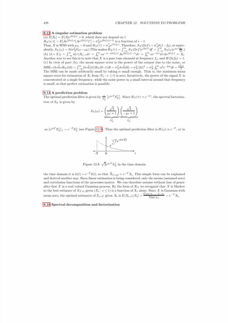
8/11/2019 Random process by B. Hajek
http://slidepdf.com/reader/full/random-process-by-b-hajek 438/448
428 CHAPTER 12. SOLUTIONS TO PROBLEMS
9.12 A singular estimation problem(a) E [X t] = E [A]e j2πf ot = 0, which does not depend on t.RX (s, t) = E [Ae j2πf os(Ae j2πf ot)∗] = σ2
Ae j2πf o(s−t) is a function of s − t.
Thus, X is WSS with µX = 0 and RX (τ ) = σ2Ae
j2πf oτ
. Therefore, S X (2πf ) = σ2Aδ (f −f 0), or equiv-
alently, S X (ω) = 2πσ2Aδ (ω−ω0) (This makes RX (τ ) =
∞−∞ S X (2πf )e j2πfτ df =
∞−∞ S X (ω)e jωτ dω
2π .)
(b) (h ∗ X )t = ∞−∞ h(τ )X t−τ dτ =
∞0 αe−α− j2πf o)τ Ae j2πf o(t−τ )dτ =
∞0 αe−(ατ dτAe j2πf ot = X t.
Another way to see this is to note that X is a pure tone sinusoid at frequency f o, and H (2πf 0) = 1.(c) In view of part (b), the mean square error is the power of the output due to the noise, or
MSE=(h∗h∗RN )(0) = ∞−∞(h∗h)(t)RN (0−t)dt = σ2
N h∗h(0) = σ2N ||h||2 = σ2
N
∞0 α2e−2αtdt =
σ2N α2 .
The MSE can be made arbitrarily small by taking α small enough. That is, the minimum meansquare error for estimation of X t from (Y s : s ≤ t) is zero. Intuitively, the power of the signal X isconcentrated at a single frequency, while the noise power in a small interval around that frequencyis small, so that perfect estimation is possible.
9.14 A prediction problemThe optimal prediction filter is given by 1
S +X
e jωT S +X
. Since RX (τ ) = e−|τ |, the spectral factoriza-
tion of S X is given by
S X (ω) =
√ 2
jω + 1
S +X
√ 2
− jω + 1
S −X
so [e jωT S +X ]+ = e−T S +X (see Figure 12.8). Thus the optimal prediction filter is H (ω) ≡ e−T , or in
2 e
-T
-(t+T)
t 0
Figure 12.8:√
2e jωT S +X in the time domain
the time domain it is h(t) = e−T δ (t), so that X T +t|t = e−T X t. This simple form can be explainedand derived another way. Since linear estimation is being considered, only the means (assumed zero)and correlation functions of the processes matter. We can therefore assume without loss of gener-ality that X is a real valued Gaussian process. By the form of RX we recognize that X is Markovso the best estimate of X T +t given (X s : s ≤ t) is a function of X t alone. Since X is Gaussian with
mean zero, the optimal estimator of X t+T given X t is E [X t+T |X t] = Cov(X t+T ,X t)X t
Var(X t) = e−T X t.
9.16 Spectral decomposition and factorization
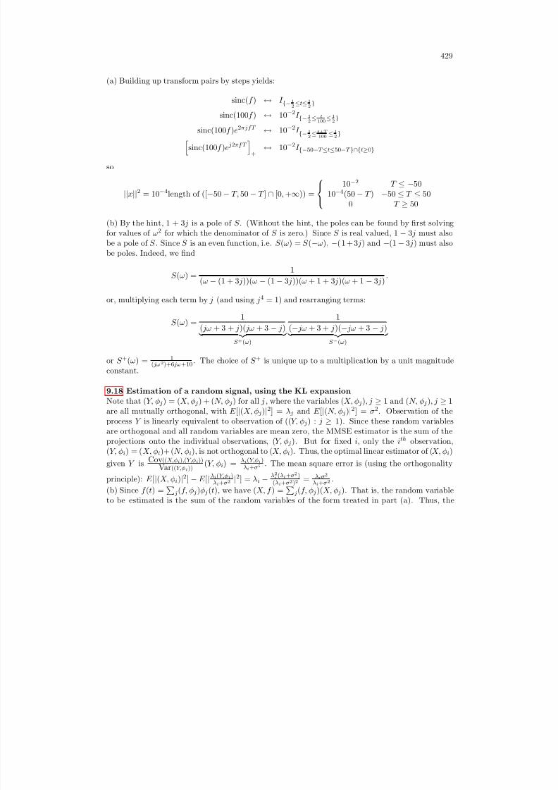
8/11/2019 Random process by B. Hajek
http://slidepdf.com/reader/full/random-process-by-b-hajek 439/448
429
(a) Building up transform pairs by steps yields:
sinc(f ) ↔ I − 12≤t≤ 1
2
sinc(100f ) ↔ 10−2I − 12≤ t100
≤ 12
sinc(100f )e2πjfT ↔ 10−2I − 12≤ t+T
100 ≤ 1
2
sinc(100f )e j2πfT
+↔ 10−2I −50−T ≤t≤50−T ∩t≥0
so
||x||2 = 10−4length of ([−50 − T, 50 − T ] ∩ [0, +∞)) =
10−2 T ≤ −50
10−4(50 − T ) −50 ≤ T ≤ 500 T ≥ 50
(b) By the hint, 1 + 3 j is a pole of S . (Without the hint, the poles can be found by first solvingfor values of ω2 for which the denominator of S is zero.) Since S is real valued, 1 − 3 j must alsobe a pole of S . Since S is an even function, i.e. S (ω) = S (−ω), −( 1 + 3 j) and −(1 − 3 j) must alsobe poles. Indeed, we find
S (ω) = 1
(ω − (1 + 3 j))(ω − (1 − 3 j))(ω + 1 + 3 j)(ω + 1 − 3 j).
or, multiplying each term by j (and using j4 = 1) and rearranging terms:
S (ω) = 1
( jω + 3 + j)( jω + 3 − j) S +(ω)
1
(− jω + 3 + j)(− jω + 3 − j) S −(ω)
or S +(ω) = 1( jω2)+6 jω+10 . The choice of S + is unique up to a multiplication by a unit magnitude
constant.
9.18 Estimation of a random signal, using the KL expansionNote that (Y, φ j) = (X, φ j) + (N, φ j) for all j , where the variables (X, φ j), j ≥ 1 and (N, φ j), j ≥ 1are all mutually orthogonal, with E [|(X, φ j)|2] = λ j and E [|(N, φ j)|2] = σ2. Observation of theprocess Y is linearly equivalent to observation of ((Y, φ j) : j ≥ 1). Since these random variablesare orthogonal and all random variables are mean zero, the MMSE estimator is the sum of theprojections onto the individual observations, (Y, φ j). But for fixed i, only the ith observation,
(Y, φi) = (X, φi)+(N, φi), is not orthogonal to (X, φi). Thus, the optimal linear estimator of (X, φi)given Y is Cov((X,φi),(Y,φi))
Var((Y,φi)) (Y, φi) = λi(Y,φi)
λi+σ2 . The mean square error is (using the orthogonality
principle): E [|(X, φi)|2] − E [|λi(Y,φi)λi+σ2
|2] = λi − λ2i (λi+σ2)(λi+σ2)2 = λiσ
2
λi+σ2 .
(b) Since f (t) =
j(f, φ j)φ j(t), we have (X, f ) =
j(f, φ j)(X, φ j). That is, the random variableto be estimated is the sum of the random variables of the form treated in part (a). Thus, the
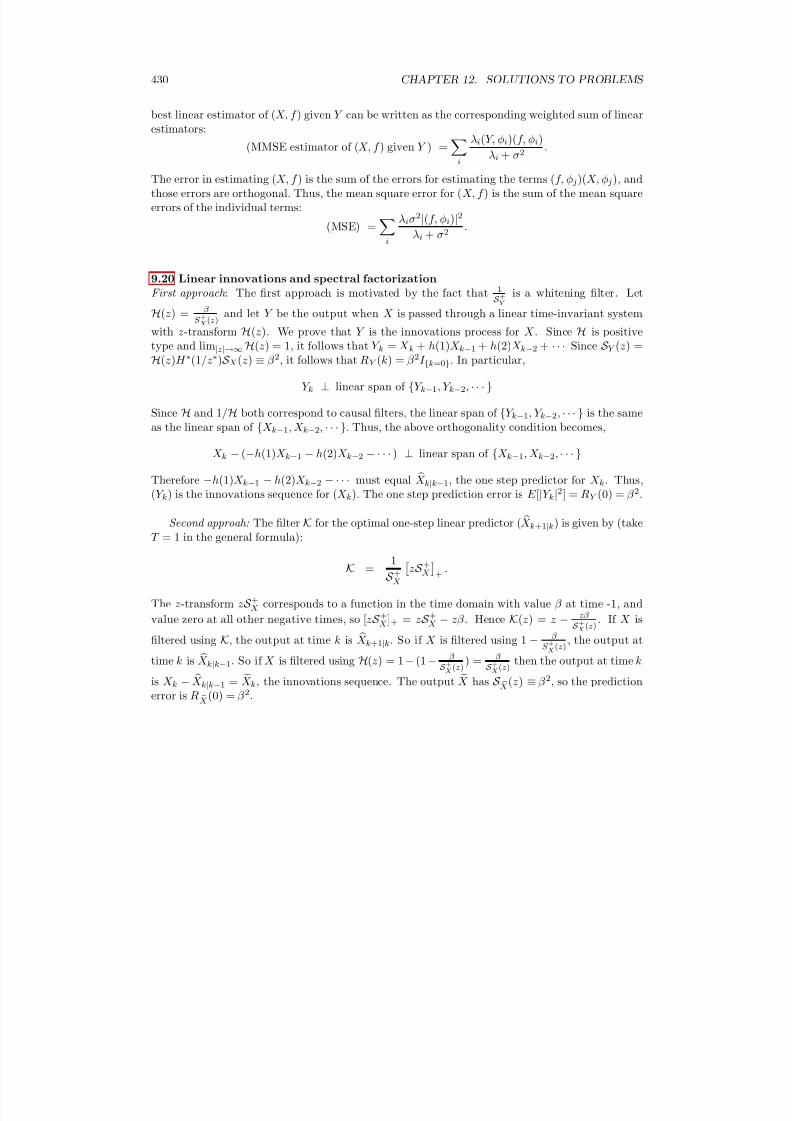
8/11/2019 Random process by B. Hajek
http://slidepdf.com/reader/full/random-process-by-b-hajek 440/448
430 CHAPTER 12. SOLUTIONS TO PROBLEMS
best linear estimator of (X, f ) given Y can be written as the corresponding weighted sum of linearestimators:
(MMSE estimator of (X, f ) given Y ) = iλi(Y, φi)(f, φi)
λi + σ2
.
The error in estimating (X, f ) is the sum of the errors for estimating the terms (f, φ j)(X, φ j), andthose errors are orthogonal. Thus, the mean square error for ( X, f ) is the sum of the mean squareerrors of the individual terms:
(MSE) =i
λiσ2|(f, φi)|2
λi + σ2 .
9.20 Linear innovations and spectral factorizationFirst approach : The first approach is motivated by the fact that 1
S +Y
is a whitening filter. Let
H(z) = β
S +X(z)
and let Y be the output when X is passed through a linear time-invariant system
with z-transform H(z). We prove that Y is the innovations process for X . Since H is positivetype and lim|z|→∞ H(z) = 1, it follows that Y k = X k + h(1)X k−1 + h(2)X k−2 + · · · Since S Y (z) =H(z)H ∗(1/z∗)S X (z) ≡ β 2, it follows that RY (k) = β 2I k=0. In particular,
Y k ⊥ linear span of Y k−1, Y k−2, · · ·
Since H and 1/H both correspond to causal filters, the linear span of Y k−1, Y k−2, · · · is the sameas the linear span of X k−1, X k−2, · · · . Thus, the above orthogonality condition becomes,
X k − (−h(1)X k−1 − h(2)X k−2 − · · · ) ⊥ linear span of X k−1, X k−2, · · ·
Therefore −h(1)X k−1 − h(2)X k−2 − · · · must equal X k|k−1, the one step predictor for X k. Thus,(Y k) is the innovations sequence for (X k). The one step prediction error is E [|Y k|2] = RY (0) = β 2.
Second approah: The filter K for the optimal one-step linear predictor ( X k+1|k) is given by (takeT = 1 in the general formula):
K = 1
S +X
zS +X
+
.
The z-transform zS +X corresponds to a function in the time domain with value β at time -1, and
value zero at all other negative times, so [zS +X ]+ = zS +X − zβ . Hence K(z) = z − zβ
S +X(z). If X is
filtered using K, the output at time k is X k+1|k. So if X is filtered using 1 − β
S +X(z) , the output attime k is X k|k−1. So if X is filtered using H(z) = 1 − (1 − β
S +X(z)) = β
S +X(z) then the output at time k
is X k − X k|k−1 = X k, the innovations sequence. The output X has S eX (z) ≡ β 2, so the predictionerror is R eX (0) = β 2.
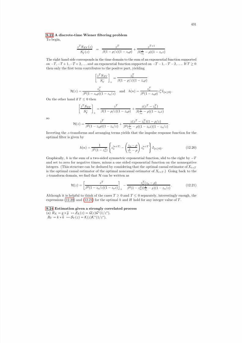
8/11/2019 Random process by B. Hajek
http://slidepdf.com/reader/full/random-process-by-b-hajek 441/448
431
9.22 A discrete-time Wiener filtering problemTo begin,
zT S XY
(z)
S −Y (z) = zT
β (1 − ρ/z)(1 − zoρ) + zT +1
β ( 1zo
− ρ)(1 − zoz)
The right hand side corresponds in the time domain to the sum of an exponential function supportedon −T, −T + 1, −T + 2, . . . and an exponential function supported on −T −1, −T −2, . . .. If T ≥ 0then only the first term contributes to the positve part, yielding
zT S XY
S −Y
+
= zT
o
β (1 − ρ/z)(1 − zoρ)
H(z) = zT
o
β 2(1 − zoρ)(1 − zo/z) and h(n) =
zT o
β 2(1 − zoρ)zno I n≥0.
On the other hand if T ≤ 0 thenzT S XY
S −Y
+
= zT
β (1 − ρ/z)(1 − zoρ) +
z(zT − zT o )
β ( 1zo
− ρ)(1 − zoz)
so
H(z) = zT
β 2(1 − zoρ)(1 − zo/z) +
z(zT − zT o )(1 − ρ/z)
β 2( 1zo
− ρ)(1 − zoz)(1 − zo/z).
Inverting the z-transforms and arranging terms yields that the impulse response function for theoptimal filter is given by
h(n) = 1
β 2(1 − z2o) z|n+T |o − z
o −ρ
1zo
− ρ zn+T o I n≥0. (12.20)
Graphically, h is the sum of a two-sided symmetric exponential function, slid to the right by −T and set to zero for negative times, minus a one sided exponential function on the nonnegativeintegers. (This structure can be deduced by considering that the optimal casual estimator of X t+T
is the optimal causal estimator of the optimal noncausal estimator of X t+T .) Going back to thez-transform domain, we find that H can be written as
H(z) =
zT
β 2(1 − zo/z)(1 − zoz)
+
− zT o (zo − ρ)
β 2(1 − z2o)( 1
zo− ρ)(1 − zo/z)
. (12.21)
Although it is helpful to think of the cases T ≥ 0 and T ≤ 0 separately, interestingly enough, theexpressions (12.20) and (12.21) for the optimal h and H hold for any integer value of T .
9.24 Estimation given a strongly correlated process(a) RX = g ∗ g ↔ S X (z) = G(z)G∗(1/z∗),RY = k ∗ k ↔ S Y (z) = K(z)K∗(1/z∗),
8/11/2019 Random process by B. Hajek
http://slidepdf.com/reader/full/random-process-by-b-hajek 442/448
8/11/2019 Random process by B. Hajek
http://slidepdf.com/reader/full/random-process-by-b-hajek 443/448
433
(d) The initial distribution π for the hidden Markov model should be the equilibrium distribution,π = (0.25, 0.25.0.25, 0.25). By the definition of the generator matrix Q, the one step transitionprobabilities for a length time step are given by pi,j() = δ i,j + q i,j + o(). So we ignore the
o() term and let ai,j = λ if i = j and ai,i = 1− 3λ for i, j ∈ S . (ALTERNATIVELY, we couldlet ai,j = pi,j(), that is, use the exact transition probability matrix for time duration .) If is small enough, then Z will be constant over most of the intervals of length . Given Z = i overthe time interval [(k − 1), k], Y k = i +
k(k−1) N tdt which has the N (i, σ2) distribution.
Thus, we set bi,y = 1√ 2πσ2
exp− (y−i)2
2σ2
.
10.2 A covering problem(a) Let X i denote the location of the ith base station. Then F = f (X 1, . . . , X m), where f satisfiesthe Lipschitz condition with constant (2r − 1). Thus, by the method of bounded differences based
on the Azuma-Hoeffding inequality, P |F − E [F ]| ≥ γ ≤ 2 exp(− γ 2
m(2r−1)2 ).
(b) Using the Possion method and associated bound technique, we compare to the case that the
number of stations has a Poisson distribution with mean m. Note that the mean number of stationsthat cover cell i is m(2r−1)
n , unless cell i is near one of the boundaries. If cells 1 and n are covered,then all the other cells within distance r of either boundary are covered. Thus,
P X ≥ m ≤ 2P Poi(m) stations is not enough≤ 2ne−m(2r−1)/n + P cell 1 or cell n is not covered→ 0 as n → ∞ if m =
(1 + )n ln n
2r − 1
For a bound going the other direction, note that if cells differ by 2r − 1 or more then the eventsthat they are covered are independent. Hence,
P X ≤ m ≤ 2P Poi(m) stations cover all cells≤ 2P
Poi(m) stations cover cells 1 + (2r − 1) j, 1 ≤ j ≤ n − 1
2r − 1
≤ 2
1 − e−
m(2r−1)n
n−12r−1
≤ 2exp
−e−
m(2r−1)n · n − 1
2r − 1
→ 0 as n → ∞ if m =
(1 − )n ln n
2r − 1
Thus, in conclusion, we can take g1(r) = g2(r) = 12r−1 .
10.4 Stopping time properties(a) Suppose S and T are optional stopping times for some filtration F F F . Then it suffices to notethat:S ∧ T ≤ n = S ≤ n ∪ T ≤ n ∈ F n, and
8/11/2019 Random process by B. Hajek
http://slidepdf.com/reader/full/random-process-by-b-hajek 444/448
434 CHAPTER 12. SOLUTIONS TO PROBLEMS
S ∨ T ≤ n = S ≤ n ∩ T ≤ n ∈ F n.S + T ≤ n = ∪0≤k≤nS ≤ k ∩ T ≤ n − k ∈ F n,(b) Since X takes on values 0 and 1 only, events of the form X n ≤ c are either empty or the
whole probability space if c < 0 or if c ≥ 1, so we can ignore such values of c. I f 0 ≤ c < 1 andn ≥ 0, then X n ≤ c = T > n. Thus, for each n X n ≤ c ∈ F n if and only if T ≤ n ∈ F n.Therefore, T is a stopping time if and only if X is adapted.(c) (i)
A.1 ∅ ∩ T ≤ n = ∅ ∈ F n for all n, so that ∅ ∈ F T .A.2 If A ∈ F T then A ∩ T ≤ n ∈ F n for all n. Also, T ≤ n ∈ F n.So [A ∩ T ≤ n]c ∩ T ≤ n = Ac ∩ T ≤ n ∈ F n for all n. Therefore, Ac ∈ F T
A.3 If Ai ∈ F T for all i ≥ 1, then Ai ∩ T ≤ n ∈ F n for all i, n. Therefore∩i (Ai ∩ T ≤ n) = (∩iAi) ∩ T ≤ n ∈ F n for all n. Therefore, ∩iAi ∈ F n.
Thus F T satisfies all three axioms of a σ-algebra so it is a σ-algebra.(ii) To show that T is measurable with respect to a σ-algebra, we need events of the form T ≤ mto be in the σ algebra, for any m ≥ 0. For this event to be in F T , we need T ≤ m∩T ≤ n ∈ F nfor any n ≥ 0. But T ≤ m ∩ T ≤ n = T ≤ m ∧ n ∈ F m∧n ∈ F n, as desired.(iii) Fix a constant c. Then for any n ≥ 0, X T ≤ c ∩ T = n = X n ≤ c ∩ T = n ∈ F n.Therefore, the event X T ≤ c is in F T . Since c is arbitrary, X T is F T measurable.
10.6 Bounding the value of a gameLet X t = (Rt, Bt), where Rt denotes the number of red marbles in the jar after t turns and Bt
denotes the number of blue marbles in the jar after t turns, let ut denote the decision taken by theplayer at the beginning of turn t +1, and let F t = σ(X 0, . . . , X t, u0, . . . , ut). Then X is a controlled
Markov process relative to the filtration F F F .(a) Suppose an initial state (ro, bo) and strategy (ut : t ≥ 0) are fixed. Let N t = Rt + Bt (or equiva-lently, N = V (X t) for the potential function V (r, b) = r + b). Note that E [N t+1 − N t|F t] ≥ −1
2 forall t. Therefore the process M defined by M t = N t +
t2 is a submartingale relative to F F F . Observe
that |M t+1 − M t| ≤ 2, so that E [|M t+1 − M t||F t] ≤ 2. If E [τ ] = +∞ then any lower bound on E [τ ]is valid, so we can and do assume without loss of generality that E [τ ] < ∞. Therefore, by a versionof the optional stopping theorem, E [M τ ] ≥ E [M 0]. But M τ = τ
2 and M 0 = ao + bo. Thus, we findthat E [τ ] ≥ 2(ao + bo) for any strategy of the player.(b) Consider the strategy that selects two balls of the same color whenever possible. Let V (X t) =f (N t) where f (0) = 0, f (1) = 3, and f (n) = n + 3 for n ≥ 2. The function V was selected so thatE [V (X t+1) − V (X t)|F t] ≤ −1
2 whenever X t = (0, 0). Therefore, M is a supermartingale, where
M t = V (X t∧τ ) +
t
∧τ
2 . Consequently, E [M t] ≤ E [M 0] for all t ≥ 0. That is, E [V (X t∧τ )] + E [
t
∧τ
2 ] ≤2f (ao + bo). Using this and the facts E [V (X t∧τ )] ≥ 0 and f (ao + bo) ≤ 3 + ao + bo yields thatE [t ∧ τ ] ≤ 2(ao + bo)+6. Finally, E [t ∧ τ ] → E [τ ] as t → ∞ by the monotone convergence theorem,so that E [τ ] ≤ 2(ao + bo) + 6 for the specified strategy of the player.

8/11/2019 Random process by B. Hajek
http://slidepdf.com/reader/full/random-process-by-b-hajek 445/448
Index
adapted random process, 328autocorrelation function, see correlation functionautocovariance function, see covariance function
basebandrandom process, 277signal, 276
Baum-Welch algorithm, 170Bayes’ formula, 6belief propagation, 174Bernoulli distribution, 21binomial distribution, 22Borel sets, 3Borel-Cantelli lemma, 7bounded convergence theorem, 357bounded input bounded output (bibo) stability,
265branching process, 147, 330
Brownian motion, 118
Cauchycriterion for convergence, 54, 348criterion for m.s. convergence in correlation
form, 56sequence, 55, 348
central limit theorem, 61characteristic function
of a random variable, 21of a random vector, 81
Chebychev inequality, 20circular symmetry, 285
joint, 285completeness
of a probability space, 220of the real numbers, 348
conditional
expectation, 28, 86
mean, see conditional expectation
pdf, 27
probability, 5
conjugate prior, 157
continuityof a function, 350
of a function at a point, 350
of a random process, 222
of a random process at a point, 221
piecewise m.s., 225
convergence of sequences
almost sure, 43
deterministic, 346
in distribution, 49
in probability, 45
mean square, 45, 243convex function, 61
convolution, 265
correlation
coefficient, 28
cross correlation matrix, 79
function, 111
matrix, 79
count times, 120
countably infinite, 346
counting process, 120
covariancecross covariance matrix, 79
function, 111, 287
matrix, 80
pseudo-covariance function, 287
pseudo-covariance matrix, 286
435

8/11/2019 Random process by B. Hajek
http://slidepdf.com/reader/full/random-process-by-b-hajek 446/448
436 INDEX
Cramer’s theorem, 64cumulative distribution function (CDF), 8, 26,
111
derivativeright-hand, 351
differentiable, 351at a point, 351continuous and piecewise continuously, 352continuously, 352m.s. at a point, 225m.s. continuous and piecewise continuously,
229m.s. continuously, 225m.s. sense, 225
Dirichlet density, 157discrete-time random process, 111dominated convergence theorem, 358Doob decomposition, 330Doob martingale, 330drift vector, 198, 206
energy spectral density, 268Erlang B formula, 197Erlang C formula, 197expectation, 16
of a random vector, 79expectation-maximization (EM) algorithm, 158exponential distribution, 23
failure rate function, 25Fatou’s lemma, 358filtration of σ-algebras, 328forward-backard algorithm, 166Foster-Lyapunov stability criterion, 199Fourier transform, 267
inversion formula, 267Parseval’s identity, 267
fundamental theorem of calculus, 354
gambler’s ruin problem, 115gamma distribution, 24Gaussian
distribution, 23
joint pdf, 92random vector, 91
geometric distribution, 22
implicit function theorem, 353impulse response function, 264independence
events, 5pairwise, 5
independent increment process, 116inequalities
Azuma-Hoeffding inequality, 332Bennett’s inequality, 75, 117Bernstein’s inequality, 75, 117Chebychev inequality, 20
Chernoff bound, 63concentration, 334Doob’s L2 inequality, 117Doob’s maximal inequality, 117Foster-Lyapunov moment bound, 199Jensen’s inequality, 62Markov inequality, 20McDiarmid’s inequality, 333Schwarz’s inequality, 28
infimum, 348information update, 99
inner product, 360, 362integration
Riemann-Stieltjes, 356Lebesgue, 355Lebesgue-Stieltjes, 356m.s. Riemann, 230Riemann, 353
intercount times, 120
Jacobian matrix, 30Jensen’s inequality, 62 joint Gaussian distribution, 91 jointly Gaussian random variables, 91
Kalman filter, 97Kolmogorov-Smirnov statistic, 141
law of total probability, 6

8/11/2019 Random process by B. Hajek
http://slidepdf.com/reader/full/random-process-by-b-hajek 447/448
INDEX 437
law of large numbers, 59strong law, 59weak law, 59
liminf, or limit inferior, 349, 350limit points, 349, 350limsup, or limit superior, 349, 350linear innovations sequence, 97Lipschitz condition, 333Little’s law, 193log moment generating function, 63log-sum inequality, 161
Markov inequality, 20Markov process, 128
aperiodic, 182
birth-death process, 185Chapman-Kolmogorov equations, 131equilibrium distribution, 131generator matrix, 133holding times, 136irreducible, 181 jump process, 136Kolmogorov forward equations, 134nonexplosive, 185null recurrent, 182, 186one-step transition probability matrix, 131
period of a state, 182positive recurrent, 182, 186pure-jump for a countable state space, 185pure-jump for a finite state space, 133space-time structure, 137, 138stationary, 131time homogeneous, 131transient, 182, 186transition probabilities, 130transition probability diagram, 132transition rate diagram, 133
martingale, 116martingale difference sequence, 330matrices, 359
characteristic polynomial, 361, 363determinant, 360diagonal, 359
eigenvalue, 360, 361, 363eigenvector, 360Hermitian symmetric, 363
Hermitian transpose, 361identity matrix, 359positive semidefinite, 361, 363symmetric, 359unitary, 362
maximum, 348maximum a posteriori probability (MAP) esti-
mator, 154maximum likelihood (ML) estimator, 153mean, see expectationmean ergodic, 237
mean function, 111mean square closure, 297memoryless property of the geometric distribu-
tion, 22message passing, 174minimum, 348monotone convergence theorem, 359
narrowbandrandom process, 282signal, 279
norm
of a vector, 360of an interval partition, 354
normal distribution, see Gaussian distributionNyquist sampling theorem, 276
optional stopping time, 335orthogonal, 362
complex random variables, 243random variables, 81vectors, 360
orthogonality principle, 82
orthonormal, 360basis, 360, 362matrix, 360system, 244
Parseval’s relation, 246

8/11/2019 Random process by B. Hajek
http://slidepdf.com/reader/full/random-process-by-b-hajek 448/448
438 INDEX
partition, 6periodic WSS random processes, 252permutation, 360
piecewise continuous, 351Poisson arrivals see time averages (PASTA), 196Poisson distribution, 22Poisson process, 120posterior, or a posteriori, 154power
of a random process, 269spectral density, 268
predictable random process, 330prior, or a priori, 154probability density function (pdf), 26projection, 82
Rayleigh distribution, 24, 26Riemann sum, 353
sample path, 111Schwarz’s inequality, 28second order random process, 112sinc function, 270span, 360spectral representation, 253stationary, 123, 244
wide sense, 123, 287strictly increasing, 347
b 349
wide sense sationary, 287wide sense stationary, 123Wiener process, see Brownian motion
Related Documents