Random forest and stochastic gradient tree boosting based approach for the prediction of airfoil self-noise

Available online at www.sciencedirect.com

ScienceDirect Procedia Computer Science 00 (2014) 000–000

www.elsevier.com/locate/procedia

1877-0509 © 2014 The Authors. Published by Elsevier B.V. Peer-review under responsibility of organizing committee of the International Conference on Information and Communication Technologies (ICICT 2014).

International Conference on Information and Communication Technologies (ICICT 2014)

Random forest and stochastic gradient tree boosting based approach for the prediction of airfoil self-noise

Ashutosh Patria,0F*, Yugesh Patnaikb

aDepartment of Mining Engineering, National Institute of Technology, Rourkela-769008, India bDepartment of Mechanical Engineering, National Institute of Technology, Rourkela-769008, India

Abstract

Due to the complex nature of turbulent fluid flow, which is the source of airfoil self-noise generation, prediction of airfoil self-noise is a challenging problem, crucial for designing silent airfoils. In this paper, models for prediction of airfoil self-noise using two different algorithms namely Random Forest and Stochastic Gradient Tree Boosting have been proposed and tested on the NACA0012 airfoil data set, published by NASA. The parameters used to build these models were studied extensively and 10-fold cross validation was performed on the data set. The models predict with significantly higher accuracy compared to results reported by earlier computational models. © 2014 The Authors. Published by Elsevier B.V. Peer-review under responsibility of organizing committee of the International Conference on Information and Communication Technologies (ICICT 2014).

Keywords: airfoil self-noise; prediction; Random Forest; Stochastic Gradient Boosting; CART; regression; NACA0012.

1. Introduction

Airfoil self-noise is produced when an airfoil obstructs a uniform and steady fluid flow resulting in turbulence and formation of fluctuating eddies. These eddies are a source of noise which get amplified when they interact with the airfoil surface. There are five mechanisms of generation of self-noise as described by Brooks et al. 1, which are illustrated in Fig.1. At high Reynolds number ( CR ), Turbulent Boundary Layers (TBL) develop over most of the airfoil. Noise is generated as the turbulence passes over the Trailing Edge (TE). At low CR , largely Laminar

* Corresponding author. Tel.: +91-993-885-7511

E-mail address: [email protected]

http://www.sciencedirect.com/science/journal/22120173

2 Ashutosh Patri, Yugesh Patnaik/ Procedia Computer Science 00 (2014) 000–000

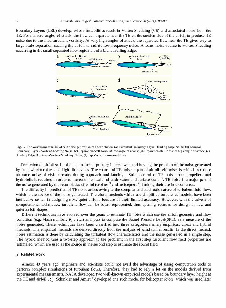
Boundary Layers (LBL) develop, whose instabilities result in Vortex Shedding (VS) and associated noise from the TE. For nonzero angles of attack, the flow can separate near the TE on the suction side of the airfoil to produce TE noise due to the shed turbulent vorticity. At very high angles of attack, the separated flow near the TE gives way to large-scale separation causing the airfoil to radiate low-frequency noise. Another noise source is Vortex Shedding occurring in the small separated flow region aft of a blunt Trailing Edge.

Fig. 1. The various mechanism of self-noise generation has been shown: (a) Turbulent Boundary Layer -Trailing Edge Noise; (b) Laminar Boundary Layer - Vortex-Shedding Noise; (c) Separation-Stall Noise at low angle of attack; (d) Separation-stall Noise at high angle of attack; (e) Trailing Edge Bluntness-Vortex- Shedding Noise; (f) Tip Vortex Formation Noise.

Prediction of airfoil self-noise is a matter of primary interest when addressing the problem of the noise generated by fans, wind turbines and high-lift devices. The control of TE noise, a part of airfoil self-noise, is critical to reduce airframe noise of civil aircrafts during approach and landing. Strict control of TE noise from propellers and hydrofoils is required in order to increase the stealth of underwater and surface crafts 2. TE noise is a major part of the noise generated by the rotor blades of wind turbines 3 and helicopters 4, limiting their use in urban areas.

The difficulty in prediction of TE noise arises owing to the complex and stochastic nature of turbulent fluid flow, which is the source of the noise generated. Therefore, methods which use simplified turbulence models, have been ineffective so far in designing new, quiet airfoils because of their limited accuracy. However, with the advent of computational techniques, turbulent flow can be better represented, thus opening avenues for design of new and quiet airfoil shapes.

Different techniques have evolved over the years to estimate TE noise which use the airfoil geometry and flow condition (e.g. Mach number, CR , etc.) as inputs to compute the Sound Pressure Level(SPL), as a measure of the noise generated. These techniques have been classified into three categories namely empirical, direct and hybrid methods. The empirical methods are derived directly from the analysis of wind tunnel results. In the direct method, noise estimation is done by calculating the turbulent flow characteristics and the noise generated in a single step. The hybrid method uses a two-step approach to the problem; in the first step turbulent flow field properties are estimated, which are used as the source in the second step to estimate the sound field.

2. Related work

Almost 40 years ago, engineers and scientists could not avail the advantage of using computation tools to perform complex simulations of turbulent flows. Therefore, they had to rely a lot on the models derived from experimental measurements. NASA developed two well-known empirical models based on boundary layer height at the TE and airfoil CR . Schinkler and Amiet 5 developed one such model for helicopter rotors, which was used later

Ashutosh Patri, Yugesh Patnaik/ Procedia Computer Science 00 (2014) 000–000 3

to predict the noise of wind turbine blades very successfully 6. Other empirical methods of noise prediction were developed based on fluctuating surface pressure. Correct estimation of turbulence properties is the key to accurate TE noise prediction. Brooks and Hodgson used data obtained from measuring noise and surface pressure simultaneously to produce good results 7.

The recent emergence of Computational Aero Acoustics (CAA) is a direct result of the enormous increase in computing power. CAA has been used effectively in direct and hybrid methods of predicting airfoil self-noise. Turbulent flow is most commonly simulated by solving the Reynolds Averaged Navier Stokes (RANS) equations, Leipmann or Von Kármán spectra 8, for instance. Large Eddy Simulation (LES), in spite of its capability to model turbulent flow field more accurately than RANS, has not been employed in academic research, until recently, because of its high computational cost. Eddy viscosity models have been used in attempts to model turbulence and as a result reduce computational expense by coupling turbulence and TE noise calculations 9-11. But, these models perform poorly when predicting noise levels at high frequencies 12. High frequency noise components must be correctly accounted for, because they cause discomfort to the human ear and are heavily regulated.

In recent years, numerical simulation has also been used most effectively in various studies to predict the self-noise by modelling the turbulent fluid flow. Greschner et al. 13 used an advanced method of modelling the turbulent boundary layer for an attached flow, which uses a novel variant of Detached Eddy Simulation (DES), called Improved Delayed Detached Eddy Simulation (IDDES). Jiang et al. 14 employed a numerical simulation for flow past NACA0018 airfoil at low Mach number to find out the hydrodynamic properties of the boundary layer and the noise generated thence; their reported results agree well with experimental results. Kamruzzaman et al. 15 devised a method to find out the properties of the anisotropic and non-homogenous flow near the trailing edge, using standard RANS simulation, which may be further used to predict the self-noise. Direct Numerical Simulation (DNS) of the flow around a NACA0012 air foil was employed in 16 by Sandberg and Jones to investigate the hydrodynamic behaviour of the turbulent flow causing the self-noise in detail and subsequently reduce self-noise. Hutcheson et al. 17 studied the effect of trailing edge bluntness and angle of attack on the self-noise generated using a NACA63-215 air foil model. Fuglsang et al. 18 predicted and optimised the self-noise generated by wind turbines. Leloudas et al. 19 undertook a similar effort in prediction and reduction of self-noise by wind turbines. Sarradj and Geyer 20 have employed genetic programming and symbolic regression to analyse and predict self-noise. Very recently, Albarracin et al. 21 used an aero-acoustic method to predict TE noise in a turbulent flow field using three different Computational Fluid Dynamics codes and compared these results.

Brooks, Pope and Marcolini 1, developed a more detailed model, known as the BPM model, which incorporated airfoil self-noise generated by various other sources (i.e. bluntness, separation, etc.). The BPM model is comprehensive, easily programmable and can quickly estimate TE noise. It is based on a semi-empirical approach formulated by analysis of acoustic wind tunnel tests performed by NASA, using NACA0012 airfoil sections of varying lengths. The BPM model predicts the self-noise of an airfoil blade as a function of the angle of attack, the free-stream velocity and other geometric parameters of the air foil. The BPM model lacks in accuracy and underestimates the air foil self-noise at low values, thus creating the need for a more accurate model.

González 22 attempted to remove this drawback of BPM model by using Artificial Neural Network (ANN) based approach to airfoil self-noise prediction. He split the NASA (NACA0012) data set into training, validation and testing subsets, which represent 50%, 25% and 25% of the full data set, respectively and then proceeded to train three different neural networks with 6, 9 and 12 neurons in the hidden layer with the normalized squared error objective functional and the quasi-Newton method training algorithm with Broyden-Fletcher-Goldfarb-Shanno train direction and Brent train rate. The generalization performance of each neural network was estimated by measuring the error between the outputs from the trained neural networks and the target values in the validation data set, which served as an indicator for under or over-fitting. He found that the validation error showed a minimum value for the neural network with 9 hidden neurons, therefore the optimal network architecture for the problem as suggested by him, included 9 hidden neurons, and was denoted as a 5: 9: 1 multilayer perceptron.

The neural network designed, as a part of a later effort by Gonzalez 23 is composed of the following parts: Inputs, Scaling layer, Multilayer Perceptron, Unscaling layer, Outputs. The scaling layer section utilises the minimum and maximum method to scale the inputs calculated from the data file. The number of parameters in this neural network is 64. The unscaling layer unscales the outputs, using the same method as used by the scaling layer to scale the inputs. The normalized squared error divides the squared error between the outputs from the neural network and the


targets in the data set by a normalization coefficient. The neural parameters norm is used as regularization term with a weight of 0.001 in the functional performance, to control the complexity of the neural network by reducing the value of the parameters.

In this paper, an attempt has been made to design models which predict with a greater accuracy than earlier models. The rest of the paper is divided into 5 sections. Section 3 gives a brief introduction to Random Forest and Stochastic Gradient Tree Boosting algorithms which have been used to model and predict the self-noise. Section 4 describes in detail the data set used for training and testing of the models proposed. Section 5 details the designing aspect of the classifiers along with result analysis. Section 6 discusses and critically analyses the results obtained. Section 7 concludes the study undertaken.

3. Random Forest and Stochastic Gradient Boosting

3.1. Random Forest

Random Forest (RF) algorithm, proposed by Breiman 24, is a collection of tree predictors where the trees are formulated on the basis of various random features, hence the name “Random Forest”. It is an example of an ensemble learner wherein each base learner is a Classification and Regression Tree (CART). Random vectors are generated to depict the growth of the trees; the trees are never pruned. A random combination of features is selected at each and every node to perform splitting. The training process consists of generation of K number of Bootstrap sample data sets, with replacement, for K number of trees. Let the training data set be

( ) ( ) ( ){ }1 1 2 2, , , , ., ,N ND X Y X Y X Y= … and each feature vector is ( )1 2 , , ..,p p p pnX x x x= … where, nX D∈ ∈R . For the growth of each tree with respective Bootstrap sample data used for training, Independently and Identically Distributed (IID) random set of vectors { }1 2, , ., KΦ Φ … Φ are generated; each tree predictor is denoted by ( ) ,h X Φ and the random forest is the collection of such predictors 1 2, , ., Kh h h… .

In order to select random features and monitor error, Breiman incorporated a technique called Bootstrap Aggregating or Bagging. The Bagging method claims to increase the accuracy of the RF algorithm by reducing the ongoing generalization error for the ensemble trees owing to the use of random features. This generalization error estimates are done using Out of Bag (OOB) method. In this method, trees which didn’t use a particular data ( ),p pX Y for training are used to predict the value of the same data ( ),p pX Y and average predicted value is calculated. Hence it follows that if a third of the data of the entire training data set is left out in each bootstrap sample data set, then the OOB estimates are based on one third of the total classifiers present in the main combination; in order to decrease the OOB error, number of combinations must be increased, and at the same time to get unbiased OOB estimates the test error must converge to a certain finite value. It has been proven that the generalization error almost certainly converges when the number of trees grown tends to infinity. The mean square generalization error for regression analysis, the main focus of this model, is given by ( )( )2, X YE Y h X− .

The error rate of RF mainly depends on the degree of correlation between any two trees and the prediction accuracy of an individual tree. The error rate decreases as the trees become increasingly uncorrelated and the prediction accuracy of each tree increases. Ease of parallelization, robustness and indifference to noise and outliers in most of the data set are the basic advantages of this method. The method is said to avoid over-fitting due to its unbiased nature of execution 25.

Algorithm 1: Random Forest

• Let the number of instances be N and the number of features be n • The number of features at a node of the decision tree is determined to be m ( m n< ) • The following steps are repeated for each decision tree:

• A subset of training data is set with replacement that represents the N instances and the rest of the data is used to measure the error of the tree

• The following step is repeated for each of node of this tree • In order to determine the decision at this node and calculate the best split accordingly,

m number of features is selected randomly. Tree pruning is prohibited. • End.


3.2. Stochastic Gradient Boosting

Boosting method for both classification and regression, developed by Freund and Schapire 26, was reinterpreted so as to make it statistically convenient by Friedman 27, which in turn came to be known as Stochastic Gradient Tree Boosting (SGTB). It is a generalized method that boosts the accuracy of any learning algorithm by considering a series of models and then producing a weighted sum of the said models. Hence it can be interpreted as a series ensemble learner consisting of many simple base learners. In this paper the base learner is same as that used in the RF algorithm i.e. CART. This method progressively fits the base learner to the current pseudo- residual by least square method in every iteration. Initially the average Y value is used as an assumption for predicting all the observations, which is similar to fitting a linear regression model. Subsequently the residuals from the current model are calculated and another regression tree is fit to these residuals and this process continues till the loss function is minimized. The model is gradually updated by taking the sum of all previous regression trees and at the end of all the iterations the functional relationship can be represented as

( ) ( ) ( ) ( )0 1 1 1 2 2 2 ; ; ;k k kF X F h X a h X a h X aβ β β= + + +…+ (1)

Where, the 0F is the initial guess function, pβ is the expansion coefficient, 1h represents a regression tree, pa represents the parameter for jointly fitting the training data in a forward sequential manner. The loss function can be expressed as ( )( ), L Y F X= Ψ and the function ( )F X is modified in such a way as to minimize L . For solving the differentiable loss function L the function ( );h X a is fit by least square to the current pseudo residuals i.e.

( )( )( )

( ) ( )1

,

p

i iip

iF X F X

Y F Xy

F X−=

∂Ψ =−

∂

(2)

and the value of pa can be calculated; here, m is the number of iteration. For a given ( ); ph X a the optimal value of pβ can be calculated as

( ) ( )( )11

arg , ; N

p i p i i pi

min Y F X h X aββ β−=

= Ψ +∑ (3)

The model employs a regression tree in each iteration to partition the X space i.e. the predictor variables nR into J disjoint regions{ } 1

Jjp j

R=

, where J is the number of terminal nodes present in the regression tree. Then for each of the subdivided regions a separate constant value is predicted and this can be denoted as

{ } ( )1 1;

JJjp jpjpj j

h X R y I X R= =

= ∈∑

(4)

Where, i jpX Rjp ipy Mean y∈

−=

and I is the indicator function. So the regression trees can be solved separately within each region jpR by the corresponding thj node of the thp iteration. Now the tree predicts a constant value of jpy

− in each region jpR and the solution to the eqn. 3 reduces into

( )( )1

arg , i jp

jp i p iX R

min Y F Xγγ γ−∈

= Ψ +∑ (5)

The estimation function can simply be written as


( ) ( ) ( )1 . p p jp jpF X F X v I X Rγ−= + ∈ (6)

In order to control the learning rate a Shrinkage parameter ] ]0,1v∈ is multiplied in each step and low values of this parameter avoid overfitting at time of training and lead to better generalization error.

In SGTB, bagging concept is also incorporated to create randomness in function estimation procedure. In each iteration, a subsample 1S of training data is chosen without replacement from the total training data set D and the base learner fits this data set instead of full training data set and in the next iteration the updated base learner of previous step fits another subsample 2S taken at random.

Algorithm 2: Stochastic Gradient Boosting • The initial guess is set to average of Y • The following steps are repeated for all regression trees:

• The residuals are computed based on the current model • A regression tree (with a fixed number of nodes) is fit to the residuals • The average residual is computed for each terminal node. The average value is the estimate for

all residuals that fall in the corresponding node • The regression tree of the residuals is added to the current best fit

• End.

4. Description of the data set

The self-noise data set used was compiled by extensive aerodynamic and acoustic testing on airfoil blade sections, conducted in an anechoic wind tunnel by NASA in 1989 1, 28, referred hereinafter as the NASA data set. The NASA data set consists of different size NACA0012 airfoils with a constant span exposed to various wind tunnel speeds at varying angles of attack. The observer position remained the same in all of the experiments. The acoustic measurements were used to determine spectra for self-noise from airfoils encountering smooth airflow. This data was suitably processed to remove extraneous contributions and the results were presented as 1/3-octave spectra. The NASA data set contains 1503 entries and consists of the following variables:

• Frequency (Hz) • Angle of attack (deg.) • Chord length (m) • Free-stream velocity (ms−1) • Suction side displacement thickness (m) • Scaled sound pressure level, SPL1/3 (dB)

The suction side displacement thickness was determined using an expression derived from boundary layer experimental data from 1.

5. System design and result analysis

The simulations of the proposed models were done using MATLAB Version 7.6.0.324 r2008a. It was executed on a PC with an Intel Core-i7 3630QM 2.4 GHz processor and 8GB RAM running on 64-bit Windows 7 operating system.

In CART, the space of input variables is partitioned into smaller rectangular regions, with the help of a regression tree, and a constant is assigned to each such region. The partitions can be represented by a series of IF-THEN decisions at each node which continues until a leaf node or a terminal node is encountered; during the splitting at each node, usually the right side branch is chosen when the IF condition is satisfied else the left branch is chosen. In this paper, the original data set is divided into 75% and 25% for training and testing respectively. The results


obtained from the test data are the object of all the analysis done and parameter criteria check. The Mean Square Error (MSE) calculated pertains to the test data, unless mentioned otherwise.

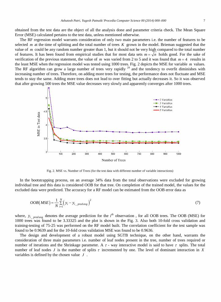
The RF regression model warrants consideration of only two main parameters i.e. the number of features to be selected m at the time of splitting and the total number of trees K grown in the model. Brieman suggested that the value of m could be any random number greater than 1, but it should not be very high compared to the total number of features. It has been found from empirical studies that for most data sets m n= holds good. For the sake of verification of the previous statement, the value of m was varied from 2 to 5 and it was found that 4m = results in the least MSE when the regression model was tested using 1000 trees. Fig. 2 depicts the MSE for variable m values. The RF algorithm can grow a large number of trees very rapidly 29 and the tendency to overfit diminishes with increasing number of trees. Therefore, on adding more trees for testing, the performance does not fluctuate and MSE tends to stay the same. Adding more trees does not lead to over fitting but actually decreases it. So it was observed that after growing 500 trees the MSE value decreases very slowly and apparently converges after 1000 trees.

Fig. 2. MSE vs. Number of Trees (for the test data with different number of variable interactions)

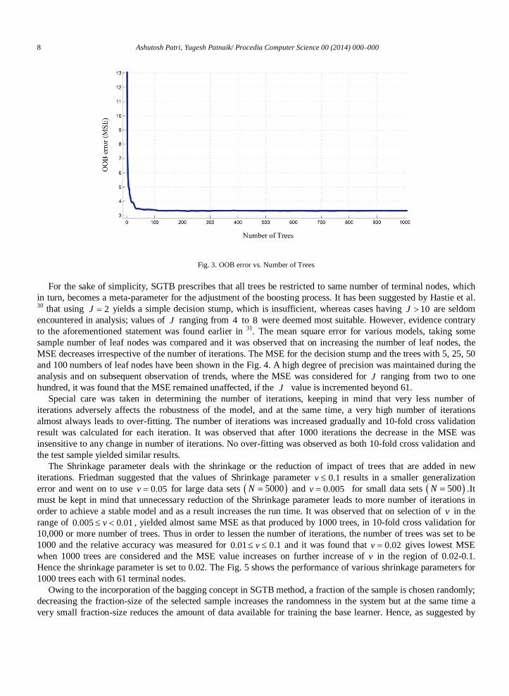
In the bootstrapping process, on an average 34% data from the total observations were excluded for growing individual tree and this data is considered OOB for that tree. On completion of the trained model, the values for the excluded data were predicted. The accuracy for a RF model can be estimated from the OOB error data as

( ) ( )2_1

1 N

i i pred avgi

OOB MSE y yN =

= −∑ (7)

where, _i pred avgy denotes the average prediction for the thi observation , for all OOB trees. The OOB (MSE) for 1000 trees was found to be 3.33325 and the plot is shown in the Fig. 3. Also both 10-fold cross validation and training-testing of 75-25 was performed on the RF model built. The correlation coefficient for the test sample was found to be 0.9639 and for the 10-fold cross validation MSE was found to be 0.9636.

The design and development of a robust model using SGTB technique, on the other hand, warrants the consideration of three main parameters i.e. number of leaf nodes present in the tree, number of trees required or number of iterations and the Shrinkage parameter. A τ - way interactive model is said to have τ splits. The total number of leaf nodes J is the number of splits τ incremented by one. The level of dominant interaction in X variables is defined by the chosen value J .


Fig. 3. OOB error vs. Number of Trees

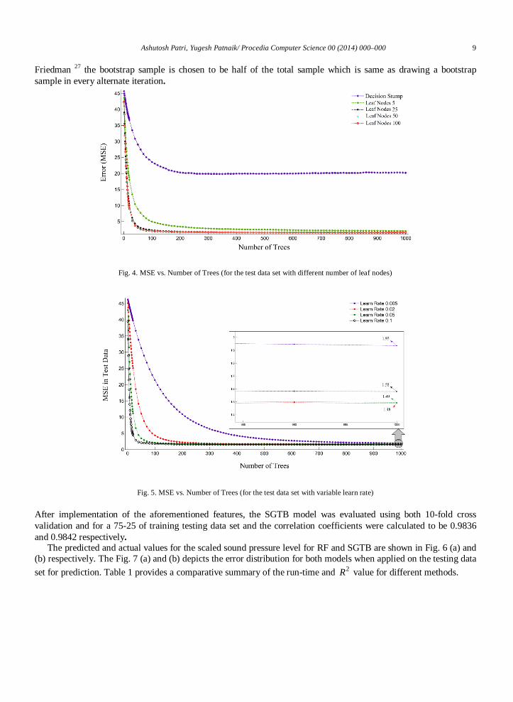
For the sake of simplicity, SGTB prescribes that all trees be restricted to same number of terminal nodes, which in turn, becomes a meta-parameter for the adjustment of the boosting process. It has been suggested by Hastie et al. 30 that using 2J = yields a simple decision stump, which is insufficient, whereas cases having 10J > are seldom encountered in analysis; values of J ranging from 4 to 8 were deemed most suitable. However, evidence contrary to the aforementioned statement was found earlier in 31. The mean square error for various models, taking some sample number of leaf nodes was compared and it was observed that on increasing the number of leaf nodes, the MSE decreases irrespective of the number of iterations. The MSE for the decision stump and the trees with 5, 25, 50 and 100 numbers of leaf nodes have been shown in the Fig. 4. A high degree of precision was maintained during the analysis and on subsequent observation of trends, where the MSE was considered for J ranging from two to one hundred, it was found that the MSE remained unaffected, if the J value is incremented beyond 61.

Special care was taken in determining the number of iterations, keeping in mind that very less number of iterations adversely affects the robustness of the model, and at the same time, a very high number of iterations almost always leads to over-fitting. The number of iterations was increased gradually and 10-fold cross validation result was calculated for each iteration. It was observed that after 1000 iterations the decrease in the MSE was insensitive to any change in number of iterations. No over-fitting was observed as both 10-fold cross validation and the test sample yielded similar results.

The Shrinkage parameter deals with the shrinkage or the reduction of impact of trees that are added in new iterations. Friedman suggested that the values of Shrinkage parameter 0.1v ≤ results in a smaller generalization error and went on to use 0.05v = for large data sets ( )5000N = and 0.005v = for small data sets ( )500N = .It must be kept in mind that unnecessary reduction of the Shrinkage parameter leads to more number of iterations in order to achieve a stable model and as a result increases the run time. It was observed that on selection of v in the range of 0.005 0.01v≤ < , yielded almost same MSE as that produced by 1000 trees, in 10-fold cross validation for 10,000 or more number of trees. Thus in order to lessen the number of iterations, the number of trees was set to be 1000 and the relative accuracy was measured for 0.01 0.1v≤ ≤ and it was found that 0.02v = gives lowest MSE when 1000 trees are considered and the MSE value increases on further increase of v in the region of 0.02-0.1. Hence the shrinkage parameter is set to 0.02. The Fig. 5 shows the performance of various shrinkage parameters for 1000 trees each with 61 terminal nodes.

Owing to the incorporation of the bagging concept in SGTB method, a fraction of the sample is chosen randomly; decreasing the fraction-size of the selected sample increases the randomness in the system but at the same time a very small fraction-size reduces the amount of data available for training the base learner. Hence, as suggested by


Friedman 27 the bootstrap sample is chosen to be half of the total sample which is same as drawing a bootstrap sample in every alternate iteration.

Fig. 4. MSE vs. Number of Trees (for the test data set with different number of leaf nodes)

Fig. 5. MSE vs. Number of Trees (for the test data set with variable learn rate)

After implementation of the aforementioned features, the SGTB model was evaluated using both 10-fold cross validation and for a 75-25 of training testing data set and the correlation coefficients were calculated to be 0.9836 and 0.9842 respectively.

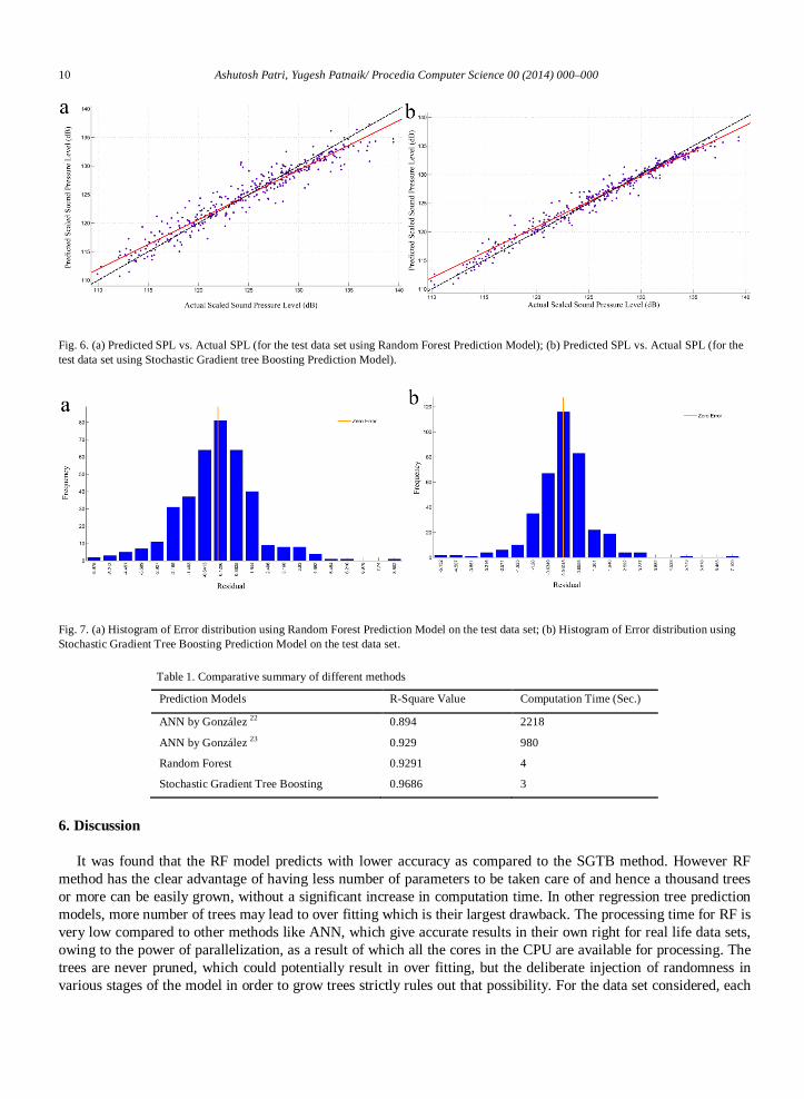
The predicted and actual values for the scaled sound pressure level for RF and SGTB are shown in Fig. 6 (a) and (b) respectively. The Fig. 7 (a) and (b) depicts the error distribution for both models when applied on the testing data set for prediction. Table 1 provides a comparative summary of the run-time and 2R value for different methods.


Fig. 6. (a) Predicted SPL vs. Actual SPL (for the test data set using Random Forest Prediction Model); (b) Predicted SPL vs. Actual SPL (for the test data set using Stochastic Gradient tree Boosting Prediction Model).

Fig. 7. (a) Histogram of Error distribution using Random Forest Prediction Model on the test data set; (b) Histogram of Error distribution using Stochastic Gradient Tree Boosting Prediction Model on the test data set.

Table 1. Comparative summary of different methods

Prediction Models R-Square Value Computation Time (Sec.)

ANN by González 22 0.894 2218

ANN by González 23 0.929 980

Random Forest 0.9291 4

Stochastic Gradient Tree Boosting 0.9686 3

6. Discussion

It was found that the RF model predicts with lower accuracy as compared to the SGTB method. However RF method has the clear advantage of having less number of parameters to be taken care of and hence a thousand trees or more can be easily grown, without a significant increase in computation time. In other regression tree prediction models, more number of trees may lead to over fitting which is their largest drawback. The processing time for RF is very low compared to other methods like ANN, which give accurate results in their own right for real life data sets, owing to the power of parallelization, as a result of which all the cores in the CPU are available for processing. The trees are never pruned, which could potentially result in over fitting, but the deliberate injection of randomness in various stages of the model in order to grow trees strictly rules out that possibility. For the data set considered, each


data consisted of five input variables and one output variable; careful perusal of previous works of Brieman brought to light that best results are achieved on selecting two or three features at the time of splitting at each node, but it has been found in our study, that consideration of four features resulted in best prediction accuracy.

6.1. Complexity

The running time for RF and stochastic tree boosting method to grow 1000 trees was found to be 4 seconds and 3 seconds respectively, much lower than that of the ANN approach. A salient characteristic of an ensemble method is that the complexity of the method is directly proportional to the complexity of growing each tree present in the model. The complexity of RF cannot be exactly stated, but for a data set of N instances and n attributes the computational cost can very nearly be approximated to ( ) O nN log N and hence for growing K trees the expression becomes ( )( )logO K nN N 32. However this is no exact manner of expressing the complexity of RF, as this does not take into account the case when partial number of features is selected, or when additional time is required to inject randomness into the model. The complexity of SGTB algorithms mostly depends on the number of leaf nodes defined for each tree and the number of iterations or the maximum number of trees to be grown. However due to the introduction of bagging concept to increase randomness, a smaller sample is drawn in each iteration which subsequently decreases the complexity.

6.2. Variable importance

The variable importance criterion, which indicates the relative importance or contribution of input variables in model building and their interaction among each other, was evaluated for both the algorithms. For calculating the variable importance in first step for each tree t , its tOOB sample was selected and prediction error for that tree for the OOB sample denoted by _t errOOB was calculated. Then the values of iX (where, i denotes the X values of a

thi selected feature) in tOOB are randomly permuted and a perturbed sample itOOB is used to compute the

prediction error by the same tree 33. So, the Variable Importance (VI ) can be defined as

( ) ( )1i it t

tVI X errOOB errOOB

K= −∑ (8)

In SGTB method, VI is defined by the number of times a variable is selected for splitting, which is weighted by the squared improvement to the model as a result of each split, and then averaged over all the trees 34. The predictors present in a tree are used as a Primary Splitter and/or a Surrogate Splitter. The VI is decided accounting not only the primary splitting but also the surrogate splitting criteria of the predictor, as surrogate splitters are very essential in tree growing process.

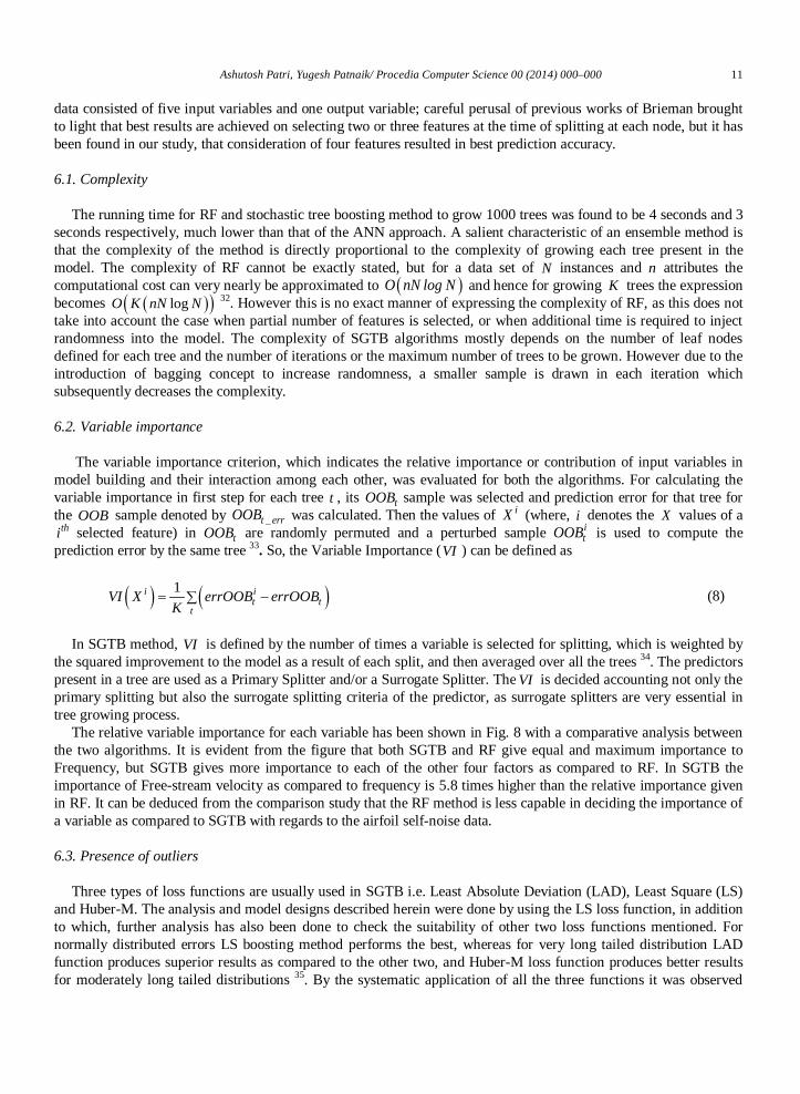
The relative variable importance for each variable has been shown in Fig. 8 with a comparative analysis between the two algorithms. It is evident from the figure that both SGTB and RF give equal and maximum importance to Frequency, but SGTB gives more importance to each of the other four factors as compared to RF. In SGTB the importance of Free-stream velocity as compared to frequency is 5.8 times higher than the relative importance given in RF. It can be deduced from the comparison study that the RF method is less capable in deciding the importance of a variable as compared to SGTB with regards to the airfoil self-noise data.

6.3. Presence of outliers

Three types of loss functions are usually used in SGTB i.e. Least Absolute Deviation (LAD), Least Square (LS) and Huber-M. The analysis and model designs described herein were done by using the LS loss function, in addition to which, further analysis has also been done to check the suitability of other two loss functions mentioned. For normally distributed errors LS boosting method performs the best, whereas for very long tailed distribution LAD function produces superior results as compared to the other two, and Huber-M loss function produces better results for moderately long tailed distributions 35. By the systematic application of all the three functions it was observed


that LAD loss function resulted in lesser prediction accuracy as compared to other two functions. By changing the percentage of error to be squared (σ) in Huber-M loss function, it was observed that the σ value ranging from 85% to 100% proves almost as accurate in prediction when compared to the LS boosting but not higher than that. It was thus concluded from the study that there are only a few outliers in the NASA data set. González came to the very same conclusion regarding the outliers of the data set, which has been further corroborated in our study. The outlier detection in RF was also done using proximity analysis and no variations in results were found. As the outliers have very less influence on both the prediction models, in depth analysis of outliers has not been presented in this paper.

Fig. 8. Comparison of Relative Importance of variables in Random Forest and Stochastic Gradient Tree Boosting

7. Conclusion

On implementation of both ensemble methods, it was found that SGTB is superior to RF as far as the NASA airfoil self-noise data set is concerned. According to the authors’ knowledge based on literature available, this level of accuracy has not been attained before. Although the RF method predicts with an accuracy equal to that of the ANN method, the RF method is more convenient owing to the fact that it has a much lesser computational time and lesser parameters to deal with. In this paper, only CART was used in prediction for both models. But as the boosting and bagging methods are the meta-algorithms, they can be used with various types of trees or other regression models. The higher level of accuracy and the robustness of these models will play a vital role in optimizing the noise generated by various airfoil-based devices and hence will be of enormous significance in the designing of new silent airfoils.

References

1. Brooks TF, Pope DS, Marcolini MA. Airfoil self-noise and prediction. Vol. 1218. National Aeronautics and Space Administration, Office of Management: Scientific and Technical Information Division; 1989.

2. Blake WK. Mechanics of Flow-Induced Sound and Vibration V2: Complex Flow-Structure Interactions. Vol. 2. Elsevier; 2012. 3. Oerlemans S, Sijtsma P, Méndez López B. Location and quantification of noise sources on a wind turbine. Journal of sound and vibration

2007; 299(4): 869-883. 4. Chou ST, George AR. Effect of blunt trailing edge on rotor broadband noise. AIAA journal 1986; 24(8): 1380-1382. 5. Schlinker RH, Amiet RK. Helicopter rotor trailing edge noise. In: Proc 7th AIAA Aeroacoustics Conference, Vol. 1. Palo Alto, CA, October

1981, p. 1-26. 6. Grosveld FW. Prediction of broadband noise from horizontal axis wind turbines. Journal of Propulsion and Power 1985; 1(4): 292-299. 7. Brooks TF, Hodgson TH. Trailing edge noise prediction from measured surface pressures. Journal of Sound and Vibration 1981; 78(1): 69-

117. 8. Moreau S, Roger M. Competing broadband noise mechanisms in low-speed axial fans. AIAA journal 2007; 45(1): 48-57.


9. Marsden AL, Wang M, Dennis JE, Moin P. Trailing-edge noise reduction using derivative-free optimization and large-eddy simulation. Journal of Fluid Mechanics 2007; 572: 13-36.

10. Wang M, Moin P. Computation of trailing-edge flow and noise using large-eddy simulation. AIAA journal 2000; 38(12): 2201-2209. 11. Manoha E, Troff B, Sagaut P. Trailing-edge noise prediction using large-eddy simulation and acoustic analogy. AIAA journal 2000; 38(4):

575-583. 12. Wang M, Freund JB, Lele SK. Computational prediction of flow-generated sound. Annual Review of Fluid Mechanics 2006; 38: 483-512. 13. Greschner B, Thiele F, Grilliat J, Jacob MC. Broadband Noise Prediction of Trailing Edge Noise Caused By a Turbulent Boundary Layer

Using an Improved Delayed Detached Eddy Simulation (IDDES). In: Proc 6th International Congress on Sound and Vibration, ICSV 16. Krakow, Poland, 2009, p. 1-12.

14. Jiang M, Li X, Bai B, Lin D. Numerical simulation on the NACA0018 airfoil self-noise generation. Theoretical and Applied Mechanics Letters 2012; 2(5): 052004.

15. Kamruzzaman M, Lutz T, Herrig A, Krämer E. Semi-Empirical Modeling of Turbulent Anisotropy for Airfoil Self-Noise Predictions. AIAA journal 2012; 50(1): 46-60.

16. Sandberg RD, Jones LE. Direct numerical simulations of airfoil self-noise. Procedia Engineering 2010; 6: 274-282. 17. Hutcheson FV, Brooks TF. Effects of angle of attack and velocity on trailing edge noise determined using microphone array measurements.

International Journal of Aeroacoustics 2006; 5(1): 39-66. 18. Fuglsang P, Aagaard Madsen H. Implementation and verification of an aeroacoustic noise prediction model for wind turbines. Risø National

laboratory, Roskilde, Denmark; 1996. 19. Leloudas G, Zhu WJ, Sørensen JN, Shen WZ, Hjort S. Prediction and reduction of noise from a 2.3 MW wind turbine. The Science of Making

Torque from Wind, Journal of Physics: Conference Series 2007; 75(1): 1-9. 20. Sarradj E, Geyer T. Airfoil noise analysis using symbolic regression. In: Proc. 19th AIAA/CEAS Aeroacoustics Conference. Berlin, Germany,

2013, p. 1-15. 21. Albarracin CA, Marshallsay P, Brooks LA, Cederholm A, Chen L, Doolan CJ. Comparison of aeroacoustic predictions of turbulent trailing

edge noise using three different flow solutions. In: Proc 18th Australasian Fluid Mechanics Conference. Launceston, Australia, December 2012, p. 3-7.

22. González RL. Neural Networks for Variational Problems in Engineering. PhD Thesis, Department of Computer Languages and Systems, Technical University of Catalonia, Barcelona, Spain, 2008.

23. Airfoil self-noise prediction, Available: http://www.intelnics.com/intelnics/neuraldesigner/doc/airfoil_self_noise_prediction.html, accessed 2nd July 2014.

24. Breiman L. Random forests. Machine learning 2001; 45(1): 5-32. 25. Random Forest, Available: https://www.stat.berkeley.edu/~breiman/RandomForests/, accessed 15th July 2014. 26. Freund Y, Schapire R, Abe N. A short introduction to boosting. Journal of Japanese Society for Artificial Intelligence 1999; 14(5): 771-780. 27. Friedman JH. Stochastic gradient boosting. Computational Statistics & Data Analysis 2002; 38(4): 367-378. 28. Brooks TF, Pope DS, Marcolini MA, Lopez R. Airfoil Self-Noise Data Set, UCI Machine Learning Repository. Available:

https://archive.ics.uci.edu/ml/datasets/Airfoil+Self-Noise, accessed 2nd July 2014. 29. Random Forests, Available:http://www.stat.berkeley.edu/~breiman/Using_random_forests_V3.1.pdf, accessed 14th July 2014. 30. Hastie T, Tibshirani R, Friedman J. The elements of statistical learning. 2nd ed. New York: Springer; 2009. 31. Bernard S, Adam S, Heutte L. Using random forests for handwritten digit recognition. In: Proc 9th IEEE International Conference on

Document Analysis and Recognition, ICDAR 2007, Vol. 2. Parana, Brazil, September 2007, p. 1043-1047. 32. Witten IH, Frank E. Data Mining: Practical machine learning tools and techniques. 2nd ed. San Francisco: Morgan Kaufmann; 2005. 33. Cutler A, Cutler DR, Stevens JR. Tree-based methods. In: High-Dimensional Data Analysis in Cancer Research. Springer New York, 2009,

p. 1-19. 34. Friedman JH, Meulman JJ. Multiple additive regression trees with application in epidemiology. Statistics in medicine 2003; 22(9): 1365-

1381. 35. Friedman JH. Greedy function approximation: a gradient boosting machine. Annals of Statistics 2001; 29(5): 1189-1232.

http://www.intelnics.com/intelnics/neuraldesigner/doc/airfoil_self_noise_prediction.html

https://archive.ics.uci.edu/ml/datasets/Airfoil+Self-Noise

Random forest and stochastic gradient tree boosting based approach for the prediction of airfoil self-noise

Documents