RAL-93-072 MA48, a Fortran code for direct solution of sparse ... · If the matrix is rectangular or square but structurally singular (there is no set of entries that can be permuted

RAL-93-072

MA48, a Fortran code for direct solution of sparse unsymmetric linearsystems of equations

by

I. S. Duff and J. K. Reid

Abstract

We describe the design of a new code that supersedes the HarwellSubroutine Library (HSL) code MA28 for the direct solution ofsparse unsymmetric linear systems of equations. The principaldifferences lie in a new factorization entry that includes rowpermutations for stability without an overhead of greatercomplexity than that of the factorization itself, switching to fullprocessing including the use of all three levels of BLAS, bettertreatment of rectangular or rank-deficient matrices, partialrefactorization, and integrated facilities for iterative refinementand error estimation.

Categories and subject descriptors: G.1.3 [Numerical Linear Algebra]: Linear systems (directmethods), Sparse and very large systems.

General Terms: Algorithms, performance.

Additional Key Words and Phrases: sparse unsymmetric matrices, Gaussian elimination, blocktriangular form, error estimation, BLAS.

Central Computing Department,Rutherford Appleton Laboratory,Oxon OX11 0QX.

October 1993.

CONTENTS

1 Introduction …………………………………………………………………… 1

2 The MA50 package …………………………………………………………… 32.1 MA50A: analyse……………………………………………………… 3

2.1.1 Main description……………………………………………… 32.1.2 Markowitz pivoting ………………………………………… 62.1.3 Drop tolerances ……………………………………………… 72.1.4 Singular and rectangular matrices …………………………… 7

2.2 MA50B: factorize …………………………………………………… 82.2.1 First factorization …………………………………………… 92.2.2 Drop tolerances ……………………………………………… 112.2.3 Subsequent factorizations …………………………………… 112.2.4 Singular and rectangular matrices …………………………… 112.2.5 Insufficient storage …………………………………………… 12

2.3 MA50C: solve………………………………………………………… 122.4 MA50D: compress the data structure ………………………………… 132.5 MA50E, MA50F, MA50G, MA50H: solving full sets of linear

equations ……………………………………………………………… 132.6 MA50I: initialization ………………………………………………… 14

3 The MA48 Package …………………………………………………………… 153.1 MA48A: analysis …………………………………………………… 153.2 MA48B: factorization………………………………………………… 183.3 MA48C: solve………………………………………………………… 183.4 MA48D: solution of block system …………………………………… 203.5 MA48I: control parameter initialization……………………………… 21

4 Performance results …………………………………………………………… 214.1 Density threshold for the switch to full code ………………………… 244.2 The choices within the full code …………………………………… 254.3 The choice of strategy for pivot choice ……………………………… 274.4 The block triangular form …………………………………………… 274.5 Comparison with calling MA50 directly …………………………… 304.6 Iterative refinement and error estimation …………………………… 304.7 Comparison with MA28 ……………………………………………… 31

5 Complex versions …………………………………………………………… 33

i

Appendix A. Solving full sets of linear equations …………………………… 34A.1 MA50E: factorization using Level 1 BLAS ………………… 35A.2 MA50F: factorization using Level 2 BLAS ………………… 35A.3 MA50G: factorization using Level 3 BLAS ………………… 36A.4 MA50H: solution …………………………………………… 36

Appendix B. The specification document for MA48 ………………………… 37

Appendix C. The specification document for MA50 ………………………… 50

References …………………………………………………………………… 61

ii

1 IntroductionThis report describes a collection of Fortran subroutines for the direct solution of a sparseunsymmetric set of linear equations

Ax = b. (1.1)

It is intended primarily for the case that is square and nonsingular, but there are some facilitiesfor rectangular and rank-deficient cases.

For the specification of the matrix A, we follow the practice of MA28 (Duff 1977, Duff andReid 1979) and require the values of the entries and their row and column indices to be specified,in any order, as A(k), IRN(k), ICN(k), k = 1, 2, ..., NE. We use the term entry rather than nonzerobecause sometimes a value may happen to be zero.

While this data structure is very convenient for the user, it does not allow efficient processing.MA48 therefore sorts the entries so that those in column 1 precede those in column 2, whichprecede those in column 3, etc. We have chosen to work by columns instead of rows (MA28works by rows) because this makes it much easier to switch to full-matrix processing, given thecolumn-major ordering used by Fortran. It also means that the inner loops of the code to solveequation (1.1) once the matrix has been factorized will vectorize more readily because theyinvolve adding a multiple of one vector to another, rather than a dot product (see Table 2, inSection 4).

Since computer memories are now much larger than they were when MA28 was written, wehave adopted a design philosophy of requiring more storage when this leads to worthwhileperformance improvements. An example of this is to construct a map array when first permutinga matrix of a given pattern. This means that subsequent matrices can be permuted by a singlevectorizable loop of length the number of entries.

As well as using the same initial data structure, MA48 follows MA28 in seeking to permute asquare matrix to block triangular form, which is done by calling the Harwell Subroutine Library(HSL) code MC21 to permute entries onto the main diagonal and the HSL code MC13 tosymmetrically permute to the block form. Holding the matrix by columns makes it natural topermute to the block upper triangular form

A A . . . .11 12

A . . . .22

PAQ = A . . . , (1.2)33

. . .

. .

A ll

rather than to block lower triangular form. The blocks A , i = 1, 2, ..., l are all square. If the matrixii

is reducible (that is, if l > 1), many blocks are often of very small order, particularly one. Forefficiency, we merge adjacent blocks of order one and note that the resulting diagonal block istriangular and so does not need factorization. We also merge adjacent blocks of order greaterthan one until they have a specified minimum size. This latter merging does affect the sparsity ofthe subsequent factorization and is performed solely to avoid procedure-call overheads for smallblocks.

1

If the matrix is rectangular or square but structurally singular (there is no set of entries that canbe permuted onto the diagonal), we treat the matrix as a single block. Block triangularization canbe extended to these cases (see, for example, Pothen and Fan 1990), but time did not permit us toincorporate such an extension here.

Iterative refinement was not included in the original design of MA28, but was added later inthe form of an additional subroutine. We have taken the opportunity in MA48 to build iterativerefinement into the solve subroutine as an option. We also provide options for calculatingestimates of the relative backward error and of the error in the solution (Arioli, Demmel, andDuff 1989).

A separate HSL package, MA30, was provided with MA28 for users willing to order theirmatrix entries by rows. It was called by MA28 to perform the fundamental tasks of matrixfactorization and actual solution. We have followed the same model for the new code, with MA50providing the fundamental facilities. One significant change is that MA50 is passed just one blockof the block triangular form at a time which leads to worthwhile simplifications. It also has theadvantage that it will be straightforward to multitask since the factorization of each diagonalblock is an independent operation. For efficiency of execution of MA50, duplicate entries are notpermitted there, but they are permitted by MA48 (they are summed).

MA28 and MA30 make extensive use of COMMON for parameters that control the actions orprovide information for the user. Default values are set by BLOCK DATA so that the user has totake action only for any controlling parameter for which the default value is unsuitable or anyinformation parameter really wanted. This format is not well-matched to the requirements ofparallel processing, where several copies of the routines may be executing at once. We havetherefore changed to having array arguments for this purpose, with an initialization routine toprovide default values. We have found this to be more convenient when MA48 calls MA50, too,since now MA48 has its own versions of the arrays and does not have to save and restore the datain the case when the user is interspersing calls to MA48 with direct calls to MA50.

The subroutines are named according to the naming convention of the Harwell SubroutineLibrary (Anon 1993). We describe the single-precision versions, whose names all commencewith MA48 or MA50 and have one more letter. The corresponding double-precision versions havethe same names with an additional letter D.

The heart of the package lies in MA50. This is where the actual factorization is performed andso we begin by describing this in Section 2. MA48 provides sorting facilities and calls to theblock triangularization and iterative refinement subroutines of the Harwell Subroutine Library aswell as calls to MA50 itself. It is expected that most users will call MA48 rather than MA50. Theinterface is more user friendly and there are more checks on the input data. We describe it inSection 3. Section 4 is devoted to our experience of the actual running of the codes. Thespecification documents are included as appendices. The code itself is available from AEATechnology, Harwell; the contact is Libby Thick, Theoretical Studies Department, AEATechnology, 424 Harwell, Didcot, Oxon OX11 0RA, tel (44) 235 432688, fax (44) 235 436579,email [email protected], who will provide details of price and conditions of use.

2

2 The MA50 package

MA50 accepts an m×n sparse matrix whose entries are stored by columns. For column j,j = 1, 2, ..., n, the values and corresponding row indices of the entries are stored contiguously in Aand IRN, say in A(k), IRN(k), k = k , k +1, ..., l . We do not allow repeated indices within aj j j

column, since knowing that there are no duplicates allows us to write more efficient code forhandling fill-ins. The columns must be contiguous, that is, k = l + 1, j = 2, 3, ..., n.j j−1

There are four subroutines that are called directly by the user:

Initialize. MA50I provides default values for the arrays CNTL and ICNTL that together controlthe execution of the package.

Analyse. MA50A is given a matrix A and finds permutations P and Q suitable for the triangularfactorization PAQ = LU, where L is block lower triangular and U is unit upper triangular.Only the final block of L is of order greater than unity. This block is intended forfull-matrix processing and MA50A chooses its size. MA50A aims to preserve sparsity andcontrol numerical stability. There is an option for dropping small entries from thefactorization and an option for providing Q together with a recommendation for P.

Factorize. MA50B accepts a matrix A together with recommended permutations and size for thefinal block. It performs the factorization PAQ = LU and the factorization of the final blockof L, including additional row permutations when needed for numerical stability. Optionsexist for subsequent calls for matrices with the same sparsity pattern to be made faster onthe assumption that exactly the same permutations are suitable, that no change has beenmade to the leading columns of PAQ, or both.

Solve. MA50C uses the factorization produced by MA50B to solve the equation Ax = b or theTequation A x = b.

A significant change from MA30 is the inclusion of row interchanges for stability in thefactorize subroutine, based on the work of Gilbert and Peierls (1988), which allows these to beincluded without an increase in overall complexity. In turn, this has allowed us to simplify theanalyse subroutine so that it provides the permutations without the actual factors. This savesstorage during analyse since only the active submatrix need be stored and will often save timesince the vectors that hold the active columns are shorter and data compressions are much lesslikely to be needed.

2.1 MA50A: analyse

MA50A chooses row and column permutations suitable for the factorization

PAQ = LU. (2.1.1)

At each pivotal stage, the reduced matrix is updated and then the pivotal row and column arediscarded. Once the reduced matrix becomes sufficiently dense for the switch to full processing,the whole reduced matrix is discarded since the remaining ordering is not based on any sparsityconsiderations. Thus MA50A does not provide the actual factors.

2.1.1 Main description

In this subsection, we describe the most important case, where the matrix is square andnonsingular, the default pivotal strategy is in operation, and the option for dropping small entriesis not in operation. We defer the other cases to the following subsections.

3

The column-oriented storage scheme is suitable for the active processing of the matrixprovided we do not insist that the columns remain contiguous and supplement it by also holdingthe pattern by rows.

The row-oriented storage is set up as follows:

(i) sweep the column-oriented storage to count the numbers of entries in the rows;

(ii) accumulate the counts to give pointers to just beyond the row ends; and

(iii) sweep the column-oriented storage again, storing the column indices in appropriatepositions for each row while decrementing the pointers.

The opportunity is taken to check for duplicate entries. They will never be present when MA50Ais called from the MA48 package, but we need to allow for independent calls. The additionaloverhead for MA48 is not severe. The check is done efficiently by initializing the integer workarray IW to zero and setting IW(i) = j when an entry for row i in column j is found. If the value ofIW(i) is already j, a duplicate will have been identified; in such a case, a message is optionallyprinted and an immediate return is made with an error flag set.

For stability, each pivot is required to satisfy the column threshold test

|a | ≥ u max |a | (2.1.2)pj iji

within the reduced matrix, where u is a threshold (with default value 0.1). We also require pivotsto be greater than an absolute tolerance with default value zero.

For sparsity, we follow the recommendation of Zlatev (1980) to search the columns of thereduced matrix in order of increasing numbers of entries and limit the search to a given numberof columns (with default value 3). Actually, he recommended a limit by rows, but this was in thecontext of a row-oriented algorithm. We say that the Markowitz cost of an entry of the reducedmatrix is the product of the number of other entries in the row of the reduced matrix and thenumber of other entries in the column. Zlatev looks for the least Markowitz cost among entriesthat satisfy the stability criteria in the columns searched.

In order to be able to find quickly which columns to search, we maintain doubly-linked chainsof columns with equal numbers of entries. The storage needed for the links and their headers ism + 2n integers. They are constructed by inspecting the columns in reverse order and placingeach in turn at the head of the chain for its number of entries. Searching in reverse order ensuresthat the chains are in forward order, which gives an initial bias towards keeping to the naturalordering.

We allow the user the option of specifying that all pivots be chosen from the main diagonal. Itshould be noted that this restriction may mean significant loss of sparsity. We implement it bysearching the columns in the same order but restricting the search to the diagonal entry, if any. Aspecial-purpose data structure could allow more efficient execution of this option, but we judgethat it is sufficient to offer comparable efficiency to that of the ordinary case. If the restriction todiagonal entries and the stability test (2.1.2) together mean that no pivot can be found, weabandon the attempt and signal that the switch to full-matrix processing be made at this point.The full-matrix processing (see section 2.5) uses row interchanges and pays no particularattention to the diagonal.

There is an option for specifying that a given number of columns at the end of A are also at the

4

end of PAQ. This allows for rapid refactorizations when entries in only these columns change.We refer to them as late columns. This rule may be inconvenient for the user, but it makes thecode simple and saves storage for the calls from MA48 since only one integer is needed for eachblock of the block triangular form. In MA48 itself, we provide a general facility in which any setof columns may be labelled as the only ones to change.

We also allow the user to specify the column permutation Q together with a recommended rowpermutation P. In this case, it is convenient to work with the data structures of a one-columnZlatev search, so we require the number of Zlatev columns to be 1. The entries in the specifiedcolumn that satisfy the stability test (2.1.2) are candidates for the pivot and we take the one that isearliest in the recommended row sequence.

The main elimination loop begins with a check on the density of the reduced matrix. If thematrix is full or the ratio of its number of entries to its total size is at least as great as a thresholdwith default value 0.5, an exit from the loop is executed. This exit corresponds to the switch tofull-matrix processing in the factorize subroutine MA48B.

Assuming that the density is low enough to continue, we now look for the next pivot. If Q hasbeen specified, a simple search of the given column is made. Otherwise, a search is made of thecolumns in order of increasing numbers of entries. During this search, we maintain a record ofthe candidate pivot that satisfies the threshold test, is greater than the pivot tolerance, and hasleast Markowitz cost. If two entries have the same Markowitz cost, we prefer the one whosenumerical value has a larger ratio to the largest entry in its column. We first execute a loop to findthe least number MINC of entries in a column. By looping from the previous count (or 0 initially),the overheads of this loop are kept low.

Once the pivot has been found, the active columns (the pivotal column and any column withan entry in the pivot row) are removed from their column-ordering chains, and the pivot is movedto the front of the pivot column.

The integer work array IW is used for flags when adding multiples of the pivot column to othercolumns in the main elimination loop. It is initialized to zero and reset to zero after each use.Here, for each entry of the pivot column, say with row index I, we set IW(I) to the position ofthe entry within the column in packed storage.

The entries of the pivot column are now removed from the row-oriented storage.Unfortunately, this requires a row search for each entry. Once found, the entry is overwritten bythe final entry of the row and the final entry is given the artificial column index 0 as a flag thatthe storage is available for later use.

Each active column, other than the pivot column, is now updated. A search of the column ismade for the pivot row entry. Once this has been found, the multiplier can be calculated, theentry overwritten by the final entry of the column, and the final entry is given the artificial rowindex 0 as a flag that the storage is available for later use.

Unless the pivot column is a singleton, the active column is now updated and the necessaryrevisions to the rest of the data structure are made. For each entry of the active column, say withrow index I, a positive value of IW(I) tell us that the entry needs to be revised because thepivot column has an entry with row index I. IW(I) also indicates where the correspondingentry of the pivot column is stored. Once the revision is done, IW(I) is negated to flag that it hasbeen done.

5

By counting the number of revisions done for the active column, we know whether all entriesof the pivot column have been used. If so, there is no fill-in and the only remaining action for theactive column is to restore the signs of IW ready for the next active column. If there is fill-in, welook at the end of the column to see if there is room for the fill-ins; if there is not enough, we alsolook at the front of the column to see if together there is enough room at the front and back;failing this, we see if there is room in the free space at the end of the data structure; failing this,we compress the data structure by calling MA50D and then try again; if even this fails, we leaveMA50A with an error message. Unless enough space is available at its end, the column has to bemoved to its new position.

There follows a loop through the pivot column to add the fill-ins. An entry with row index Ihas been used if IW(I) is negative and does not cause a fill-in; all that is needed is to restore thesign of IW(I). Otherwise, the fill-in value is calculated and the new entry is placed at the end ofthe active column and an addition is made to the row-oriented storage. This addition is made atthe end of the row, if possible, or at the front if that is possible. Otherwise, we see if there is roomto copy the row to the end of the data structure; failing this, we compress the data structure bycalling MA50D and then try again; if even this fails, we leave MA50A with an error message.

Once all the active columns have been updated, a loop through the pivot row frees this part ofrow-oriented storage and places each active column that still has one or more entries at the frontof its new column-ordering chain. Note that this means that columns with the same number ofentries are no longer in their natural order. To have maintained this ordering would have been tooexpensive.

A loop through the pivot column now resets IW to zero and removes the column from thecolumn-oriented storage. The main elimination loop is completed by recording which columnwas chosen as pivotal.

The main elimination loop is usually left through the test on the density of the reduced matrix.There remains only the tasks of completing the permutation vectors and inverting the columnpermutation (MA50B needs to have easy access to the columns in pivotal order).

2.1.2 Markowitz pivoting

For sparsity, we also offer the strategy of Markowitz (1957). To obtain this, the user must setthe number of Zlatev columns to zero. The pivot is chosen to minimize the Markowitz cost overall entries that satisfy inequality (2.1.2) and the pivot tolerance. In order to be able to find such apivot quickly, we maintain doubly-linked chains of rows with equal numbers of entries as well ascolumns. MA28 (see Duff and Reid 1979) held a single chain for each length, which began withrows and continued with columns. Any link from a row to a column or vice-versa was negated, aswas the header pointer if no rows were present. Checking the signs and resetting themappropriately when a row or column enters or leaves the chain complicates the code and slows itsexecution. We have therefore decided in MA50 to use separate chains. This increases the storagefor the links and their headers slightly, by min(m,n) to 3(m+n) integers. As we did for thecolumns, we construct the chains of rows with equal numbers of entries in forward order to givean initial bias towards keeping to the natural ordering.

As with the Zlatev strategy, we allow the user to specify that all pivots be chosen from themain diagonal. We implement this by leaving unchanged the choice of each row or column to besearched but restricting the search to the diagonal entry, if any.

6

If Q has not been specified, a search is made of the columns and rows in order of increasingnumbers of entries. MINC now holds the least number of entries in a row or column. We firstsearch the columns with MINC entries, then the rows with MINC entries, then the columns withone more entry, then the rows with one more entry, and so on. Each loop is left as soon as it canbe determined that further executions could not find a pivot with a better Markowitz cost. Thus,

2the loop on columns with l entries can be left if the candidate pivot has cost no more than (l−1)since all rows with less than l entries will have been searched already. Similarly, the row loop canbe left if the candidate pivot has cost no more than l(l−1). The row searches are generally moreexpensive than the column searches because a single column scan is need for the stability test forany entry of a column but a separate scan is needed of the column of any entry tested in a rowsearch. We therefore do such a scan only if the entry has lower Markowitz cost than thecandidate.

This procedure usually ensures that the pivot with the best Markowitz cost is found quickly.Our original intention was to offer this strategy by default, since it is a more thorough search thanZlatev’s and is what MA28 does. Unfortunately, it can occasionally be very slow. In one case,provided by Norm Schryer of Bell Laboratories (private communication) and discussed at theend of Section 4.3, the code reached a situation where there were hundreds of columns of countMINC and the best pivot had Markowitz cost MINC*(MINC-1). For each such pivot all thosehundreds of columns were searched, and the code was intolerably slow. This is our reason formaking the Zlatev strategy our default.

2.1.3 Drop tolerances

There is an option for dropping (that is regarding as having the value zero and removing from thedata structure) any entry of the original matrix or a reduced matrix if its absolute value is lessthan a tolerance. If this option is active (the tolerance changed from its default value zero), thefirst action of MA50A is to drop any such small entries from the original matrix. Note thatactivating this option may be inappropriate if such entries might be less small during a laterfactorization of a matrix of the same pattern.

Whenever the entries of a column are updated, a separate loop is used to remove any entrywith absolute value below the tolerance from the column and also its column index from therow-oriented storage. Using a separate loop avoids overheads in the case without drop tolerances,which we expect to be the usual one. In the loop that handles fill-ins, each fill-in value is checkedagainst the drop tolerance and is added to the data structure only if it is sufficiently large.

2.1.4 Singular and rectangular matrices

It is straightforward to factorize a singular or rectangular matrix and we decided that MA50should do this. If it finds r pivots, its factorization can be written in the form

L U Wr r rP A Q = , (2.1.3)M E Ir

where L is lower triangular of order r, U is unit upper triangular of order r, and all the elementsr r

of E are less than the pivot tolerance or the drop tolerance (see Section 2.1.3). Replacing E by 0corresponds to perturbing the elements of A by at most the pivot or drop tolerance and gives us arank r matrix. The corresponding set of equations is

7

L U L W x br r r r 1 1= , (2.1.4)M U M W x br r r r 2 2

and we solve this by solving

L U x = b (2.1.5)r r 1 1

and setting x = 0. If the whole system is consistent, this will be a solution. If the whole system2is underdetermined, the choice of 0 for x means that the solution has a reasonably small norm,2though in general it will not be of minimum norm.

A key problem is the identification of the rank r. It can quite easily happen that it isoverestimated by this procedure and the user should verify the solution, for example by using theiterative refinement option of MA48. An overestimate leads to equation (2.1.5) beingill-conditioned and usually having a solution of large norm.

At any stage of the MA50A processing, we may encounter a row or column that is eitherstructurally or numerically zero. Such a row or column is ordered immediately without choosinga pivot. The natural place to put it is at the end of the pivot sequence, as in (2.1.3), and this isdone for the rows. It cannot be done for the columns since this may put a column that is not ‘late’among the late columns. Also, MA50B needs to be able to tolerate being unable to pivot in anycolumn since it is likely to be receiving different numerical values. Therefore, MA50A orders acolumn in which it cannot find a pivot in the same way as one in which it finds one. It is placedin the next pivotal position or the next position among the ‘late’ columns. In both cases, weeffectively continue with a matrix with one less row or column.

A row or column is regarded as numerically zero if all its entries are less than the pivottolerance. If the pivot tolerance is less than the drop tolerance, it will never come into play sinceany small enough entries will already have been dropped. It may, however, be important whenthe drop tolerance is zero.

Any row found to be of zero length is immediately ordered and is not placed in a chain. Whenthe Zlatev strategy is in use, no chains of rows with equal numbers of entries are constructed forthe original matrix, but we still look for zero-length rows and order them at once. Since MA50Bworks column by column, it cannot recognize zero rows until its processing is complete. Ittherefore includes zero rows in the part that it processes as a full matrix. When choosing the pointfor switching to full-matrix processing in MA50A, we need to add the number of zero rows to thenumber of active rows in order to calculate the number of entries needed in full storage.

2.2 MA50B: factorize

MA50B is given an m×n sparse matrix A, recommended permutations, and the number ofcolumns p to be processed as packed sparse vectors. It calculates the actual factorization

PAQ = LU, (2.2.1)

where L is block lower triangular and U is unit upper triangular. Only the final block of L is oforder greater than unity. The permutations and the value of p may have been calculated by a priorcall of MA50A, but any choice is acceptable. We provide an option for the special case Q = I.This is used by MA48 since the column permutations for the blocks of the block triangular formand the permutations chosen by MA50 within the blocks can be integrated into a single overallpermutation, thereby saving storage.

8

Once one matrix has been factorized, other matrices may be factorized more economically ifonly the numerical values have changed or if the changes are confined to late columns.

2.2.1 First factorization

We begin by considering a first factorization when the rank is n. The operations are performedcolumn by column because the technique of Gilbert and Peierls (1988) then allows rowinterchanges to be introduced while ensuring that the organizational overheads are proportionalto the number of floating-point operations. It also means that the factorization, including fill-ins,can be built progressively by columns with very simple data management.

A packed vector with an associated vector of row indices holds the upper-triangular part ofcolumn k of U (excluding the diagonal), for k = 1, 2,..., n. Similarly, a packed vector holds thelower-triangular part of column k of L (including the diagonal), for k = 1, 2,..., p. The final blockof L is held by columns as a full matrix, together with a single vector of row indices. These arepacked together in the order: column 1 of U, column 1 of L, column 2 of U, column 2 of L,...,column p of U, column p of L, column p+1 of U, column p+2 of U,..., column n of U, final blockof L. This allows the use of just two vectors to indicate where each packed column is stored andhow many entries it has (we hold the positions of the ends of the vectors). The only datamanagement needed is for the full part to be generated at the end of the arrays and movedforward once all the entries of U have been found.

To understand the technique of Gilbert and Peierls, it is convenient to regard the packedrepresentation of L as a representation of the product

L = D L D L ...D L D (2.2.2)1 1 2 2 p p n

where each D , k = 1, 2,..., p, is diagonal and equal to the unit matrix except in position (k,k), eachk

L is lower triangular and equal to the unit matrix except below the diagonal in column k, and Dk n

is equal to the unit matrix except in the final block of order n−p. To calculate column k of L andU requires the premultiplication of column k of PAQ by

−1 −1 −1 −1L D ...L D , l = min(k−1, p) (2.2.3)l l 1 1

−1 −1In the sparse case, many of these operations may be omitted since the application of L D to ai i

vector whose i–th component is zero does not alter the vector. Furthermore, there is freedom toreorder them provided no modification of component i is performed after the application of

−1 −1L D . Thus, any order suffices for the entries of column k of L, but the list of entries ofi i

column k of U needs to be ordered. We choose to ensure that j precedes i if L has an entry in rowj

i and use a backward loop to do the actual operations later. Gilbert and Peierls construct such listsof entries using a stack to record the active columns, as shown in Figure 1.

At any one moment, the stack will consist of k, j , j , ..., j , where j < j < ... < j , and L has1 2 t 1 2 tentries L , L , ... If column j of L has no further entries, all its entries (if any) must havej j j j t2 1 3 2

already have been placed in L-list or U-list. It is therefore safe now to add j to the U-list and wetcan backtrack to column j .t−1

When the inner loop revisits a column j, it starts at the next entry from the last encounteredduring the previous visit. Thus each entry of column k of A and each entry of each column of Lthat is involved in the column k calculation is visited just once and the overall complexity is thatof the number of entries involved.

For efficient execution of the actual floating-point operations, we load the entries of column k

9

set stack, U-list, and L-list to be empty push k on stack do until stack empty copy stack top to j do i = each unsearched index of column j if (i not in U-list or L-list) then if (i > k) then add i to L-list else push i on stack; cycle outer do end if end if end do add j to U-list and pop stack end do

Figure 1. Pseudocode for the Gilbert-Peierls algorithm

of A into a real work vector W that has previously been set to zero. Appropriate multiples of theactive columns of L are added into this vector in the order given by traversing the U-listbackwards. Once this has been done, the entries of the upper-triangular part of the column can beunloaded into the packed vector using the known pattern in the U-list and the entries of W reset tozero ready for their next use. At the same time, each row index is replaced by the correspondingposition of the row in the row order because this is needed for the forward and back-substitution.The other entries of the column are now treated similarly, except that the indices are left asoriginal row indices. A search for the pivot is included for columns 1, 2,..., p. The pivot is theentry that lies earliest in the recommended row order among those that satisfy the pivot toleranceand threshold test (2.1.2). So that it can be found easily, it is moved to the leading position in thepacked vector. The row is recorded as having been pivotal in column k.

A very worthwhile improvement to the Gilbert-Peierls algorithm has been suggested byEisenstat and Liu (1993). Suppose that column k is the first column updated by column j. Anyentries of column j that lie beyond k in the pivot sequence will also be entries in column k. Weplace these physically at the end of column j and mark the boundary. When a later column l isupdated by column j, it is also updated by column k, so the entries beyond the boundary incolumn j are not needed to find the pattern of column l. Thus, when the operations for column khave been completed and the pivot chosen, we examine all the columns active in the step lookingfor columns not already marked and involving the pivot row. For any such column, the entriesare physically reordered and the column is marked.

The columns of the final block of L, corresponding to columns p+1,..., n of A, need only asingle vector of row indices. This is constructed when column p+1 is reached and corresponds toall the rows not so far ordered. We run through the rows in order, i = 1, 2,..., m placing each inturn in the vector if it has not been ordered. This makes the indices monotonic, which allows anin-place sort during the solution (see Section 2.3). For each remaining column, we need to applythe operations of the first p pivotal steps and find the sparsity pattern of the U-part. This is doneefficiently by the Gilbert-Peierls algorithm, as for the previous columns. The differences are thatno pivot need be chosen and the single vector of row indices of the full block is used to unloadthe L-part of the column.

Once the processing of column n is complete, the full block is moved forward to its finalposition. It is then factorized by full-matrix processing, see Section 2.5. The resultingfactorization has the form

10

L U Vp p p , (2.2.4)M F Ip

where L is a p×p lower-triangular matrix, U is a p×p unit upper-triangular matrix, M has pp p pcolumns, and V has p rows.p

2.2.2 Drop tolerances

If the option for dropping small entries is active, checks are made as the entries are unloadedfrom the work vector W following the updating of column k. For efficient execution in the defaultcase, we use separate loops for the default and non-default cases. In the default case, no entriesare dropped, not even those with the value zero. This is in order to ensure that the correctstructure is generated for a subsequent matrix having the same pattern but different numericalvalues.

If any entries are dropped from column k, it cannot be relied upon to supply any of the patternof an earlier column j, so the technique of Eisenstat and Liu (1993) is not applicable. We keep alogical variable DROP to flag this and do not mark and set boundaries for any columns active inthe step. If any column that would have been treated is active in a later pivotal step in which noentries are dropped, the technique may be applied then.

2.2.3 Subsequent factorizations

MA50B has an integer argument JOB that must be given the value 1 when an initial factorizationis wanted. For a subsequent factorization, if drop tolerances are not in use, if the pattern isunchanged, and if the pivotal sequence is numerically stable for the new values, the factorizationmay be accelerated by not needing to find the pattern and choose the pivots. The user must setJOB to 2 for this option. Separate code is executed, but the algorithm is unchanged from thatused for calculating the numerical values during the first factorization. An error return is made ifany pivot is smaller than the pivot threshold.

The user may specify that only a certain number of late columns have changed values so thatprocessing can be confined to these columns, because the factorization in the leading columnswill be exactly as previously. If the pattern is unchanged and the previous pivot sequence isexpected to be satisfactory, this processing may be that of the previous paragraph (JOB must beset to 2 for this option). Otherwise, the processing may be exactly as for the first factorization,with Gilbert-Peierls calculation of the pattern and pivoting within each column (JOB must be setto 3 for this option).

2.2.4 Singular and rectangular matrices

If the rank is less than n, we may fail to find a pivot for column k. The L-part may be null or allits entries may be smaller than the pivot or drop tolerance. This is handled by recording theL-part of the column as null and not recording any row as pivotal. The rest of the reduction iseffectively treated as if column k were omitted.

The column by column processing makes it impossible to recognize a zero row until allcolumns have been processed. It would have been possible to remove such rows from the fullmatrix before passing it to the full-matrix factorization subroutine, but we felt that coding thiswas not justified given that the full-matrix code needs anyway to handle the possibility of zerorows occurring during its processing. We note that MA50A takes into account that zero rows arehandled explicitly when choosing the point for switching to full-matrix processing, which caneven mean that p is given the value n. Also, the user may set p to the value n if all-packedprocessing is wanted. Thus the code has to allow for the possibility of the final block having

11

some rows but no columns. We need the vector of row indices, but do not actually call thefull-matrix factorization subroutine.

To explain the mathematics, it is convenient to permute each column in which no pivot isfound to just ahead of the columns holding the full block, though we emphasize that in the actualcode these columns are left in place. This gives us the factorization

U V Wq q qLq I . (2.2.5)M 0 Fq I

It is also convenient (see Section 2.3) to regard this as the factorization

L U V Wq q q q . (2.2.6)M I 0 Fq

2.2.5 Insufficient storage

If the user provides insufficient storage for the factorization, a serious attempt is made tocalculate how much is needed for a successful factorization. This is done by retaining the first pcolumns of L so that processing of column k can take place as in the successful case, butdiscarding the rest of the factorization. A count is kept of the number of discarded entries. Ofcourse, there may be insufficient storage to finish the factorization even in this mode, in whichcase it is not possible to provide a value for the amount of additional storage that is sure to beadequate. We return the value that is sufficient for the factorization to proceed to the same pointwithout any discards.

2.3 MA50C: solve

MA50C uses the factorization produced by MA50B to solve the equation

Ax = b (2.3.1)

or the equationTA x = b. (2.3.2)

In the square nonsingular case, this involves simple forward and back-substitution using thefactorization (2.2.4). We use a work vector W to avoid altering b. Note that the row indices storedfor L are those of the original matrix, whereas those for U are of the permuted matrix. MA50H iscalled for full-matrix processing of the final block. It is helpful that the row indices of the fullblock are monotonic, as noted in the penultimate paragraph of Section 2.2.1. When solvingAx = b, this permits an in-place sort for loading the required components of the right-hand side;

Twhen solving A x = b, it permits an in-place sort for placing the solution in the requiredpositions.

The permutation Q is treated separately. When solving Ax = b, the solution is permuted justTbefore return and when solving A x = b, the right-hand side is permuted on entry. We provide

an option for these permutations to be omitted when Q = I, which is the case when MA50C iscalled from MA48 since the column permutations are integrated into an overall columnpermutation.

The rectangular or rank-deficient case is not so straightforward. For (2.3.1), we use the form(2.2.6) and begin by solving the system

L y bq 1 1= (2.3.3)M I y bq 2 2

12

by forward substitution and then solve the system

x1 yU V W 1q q q x = (2.3.4)2 y0 F 2x3

by back-substitution. Mathematically, we solve Fx = y , set x = 0, and then solve3 2 2U x = y − W x , but the two final steps are merged in the coding since the columns areq 1 1 q 3interspersed. We traverse the columns backwards either calculating a component of x and doingthe corresponding back-substitution updating, or setting a component of x to zero.

For (2.3.2), we use the form (2.2.5) and begin by solving the system

TU y bq 1 1TV I y = b (2.3.5)q 2 2T y bW I 3 3q

by forward substitution, and then we solve the system

T T yL M 1q q x1 = y (2.3.6)0 2x2T yF 3

by back-substitution. Here, we ignore the middle block row.

2.4 MA50D: compress the data structure

Only in the analysis subroutine can the storage become fragmented so that data compression(garbage collection) may be necessary. Subroutine MA50 called both for the column-oriented androw-oriented storage. The logical argument REALS controls whether real values are to be movedalong with integer values or not. For definiteness, we will describe the action for therow-oriented file.

The processing consists of an initialization loop of length n, followed by a loop that moves thewanted entries forward, of length equal to the size of the array. The initial loop moves the firstentry of each row to the vector IPTR and replaces it by the negation of the row index. Thisenables the start of each row to be recognized in the scan that follows, since all the row indicesare positive and any free location has been given the value 0. This scan now takes place. It skipsany free locations and moves the row indices forward. The first entry of each row is restoredfrom IPTR and the corresponding element of IPTR is set to hold its position.

2.5 MA50E, MA50F, MA50G, MA50H: solving full sets of linear equations

For sufficiently dense matrices, it is more efficient to use full-matrix processing and we thereforeswitch to this towards the end of the factorization. We had hoped to use the LAPACK routinesSGETRF and SGETRS for this purpose, but their treatment of the rank-deficient case isunsatisfactory since no column interchanges are included. For example, the matrix

0 1 1A = 0 1

0

will be factorized as A = LU with L = I and U = A, which is of no help for solving the consistentset of equations

13

0 1 1 20 1 x = 1 .

0 0

On the other hand, interchanging columns 1 and 3 gives

1 1 0 1 1 1 0AQ = 1 0 0 = 1 1 −1 0

0 0 0 0 0 1 0

and the reduced set of equations

x1 1 0 23−1 0 x = −1 .2

0 0x1

The value of x is arbitrary and we may choose 0. By back-substitution, we then get the solution1

0x = 1 .

1

Another reason for rejecting SGETRF is that it tests only for exact zeros. We test for exactzeros by default, but wish to offer the option of a test against a threshold. The final factorizationwill be as if we had started with a matrix whose entries differ from those of A by at most thethreshold.

In our early tests, we found that factorization routines using Basic Linear Algebra Subroutines(BLAS) at Level 1 (Lawson et al. 1979) and Level 2 (Dongarra et al. 1988) sometimesperformed better than those at Level 3 (Dongarra et al. 1990), and have therefore included themall. They are, respectively, MA50E, MA50F, and MA50G. A parameter controls which of them iscalled. In the tests reported in Section 4, we found that the Level 3 versions performed best on allthree of our test platforms, so the default parameter value chooses them.

MA50H solves a set of equations using the factorization produced by MA50E, MA50F, orMA50G, whose output data are identical. Each actual forward or back-substitution operationassociated with L or U is performed either with the Level 2 BLAS STRSV or by a loop involvingcalls to SAXPY or SDOT. An argument controls which of these happens. Unlike the case forfactorization, the logic is very similar for the two cases, so there is no need for separatesubroutines.

We defer a more detailed description of our modifications of the LAPACK subroutines toAppendix A.

2.6 MA50I: initialization

Subroutine MA50I provides default values for the arrays CNTL and ICNTL that together controlthe execution of the package. Their purposes and default values are given in Appendix C.

14

3 The MA48 Package

We anticipate that most users will access the codes described in this report through calls to theMA48 subroutines. The data interface is much simpler than that of MA50. MA48 accepts an m×nsparse matrix whose entries are stored in any order, as A(k), IRN(k), ICN(k), k = 1, 2, ..., NE.Multiple entries are permitted and are summed. Any entry with an out-of-range index is ignored.

There are four subroutines that are called directly by the user:

Initialize. MA48I provides default values for the arrays CNTL and ICNTL that together controlthe execution of the package.

Analyse. MA48A prepares data structures for factorization and chooses permutations P and Qthat provide a suitable pivot sequence and optionally permute the matrix A to block uppertriangular form. There is an option for dropping small entries from the factorization, anoption for limiting pivoting to the diagonal, and an option for providing Q together with arecommendation for P. Any set of columns may be specified as sometimes beingunchanged when refactorizing.

Factorize. MA48B factorizes a matrix A, given data provided by MA48A. On an initial call, itperforms additional row permutations when needed for numerical stability. Options existfor subsequent calls for matrices with the same sparsity pattern to be made faster on theassumption that exactly the same permutations are suitable, that no change has been madeto certain columns of PAQ, or both.

Solve. MA48C uses the factorization produced by MA48B to solve the equation Ax = b or theTequation A x = b with the option of using iterative refinement. Estimates of both

backward and forward error can also be provided.

The data structure is arranged so that the user with a single problem to solve can provide thematrix to MA48A, pass the MA48A output data on to MA48B, and finally pass the MA48B outputdata and the vector b to MA48C. Further calls to MA48C can then be made for other vectors b.The first of a sequence whose matrices have the same pattern is treated similarly, and forsubsequent matrices MA48B can be called with just the array of reals having a different value.For efficient performance of the sorting needed for the later factorizations, we use a map array sothat a single vectorizable loop is all that is needed. Note also that a representation of both theoriginal matrix and its factorization is needed by MA48C since it performs iterative refinement.

3.1 MA48A: analysis

The action of MA48A is controlled by the argument JOB, which must have one of the values:

1 Unrestricted pivot choice.

2 Column permutation provided by the user, together with a recommended row permutation.

3 Pivots to be restricted to the diagonal.

The subroutine first checks the validity of the scalar data and, if JOB=2, of the permutations. Ifthere is a problem, it prints a message and exits. If the data checks are passed, informativeprinting is optionally performed, followed by initializations and the generation of a linked listthat holds the entries of each column as a chain. A vector of length n is needed for the headers butthe links themselves can be held in JCN, overwriting the column indices. During this loop, a

15

check is made on whether any entry has a row or column index outside its permitted range. Suchan entry is not placed in a linked list but is flagged by setting its JCN component to zero.Messages are optionally printed for the first 10 such entries.

An attempt is made to order the matrix to block triangular form as long as the matrix is square,the minimum block size (default value 10) is less than n, and JOB=1. It is conventional (see, forexample, Chapter 6 of Duff, Erisman, and Reid 1986) to do this in two stages: first find a columnpermutation such that the permuted matrix has entries on its diagonal and then find a symmetricpermutation that permutes the resulting matrix to block triangular form. We use the HSLsubroutines MC21A and MC13D for these two stages.

Since MC21A requires the structure of the matrix by columns, we begin by constructing it byusing the linked list by columns to run through the entries of each column in turn. For the sake ofefficiency, the new list of indices is constructed in a separate part of the array. While this takesplace, duplicates are identified efficiently with the help of an integer flag array, in a similarfashion to that discussed in Section 2.1.1. The duplicates are not added to the column structure,of course. MC21A uses a depth-first search algorithm with look ahead and is described by Duff(1981a, 1981b). If it fails to permute entries onto the whole of the diagonal, the matrix must bestructurally singular and the block triangularization is abandoned.

If the matrix is structurally nonsingular, MC13D is used to symmetrically permute the resultingmatrix to block triangular form. It employs the algorithm of Tarjan (1972) and is described byDuff and Reid (1978a, 1978b). The block sizes are calculated from the pointers to block startsprovided by MC13D. Adjacent blocks of size one are amalgamated into triangular blocks in asingle pass that amalgamates the current block with the previous one if the current block is 1 × 1and the previous block is either 1 × 1 or is itself an amalgamation of 1 × 1 blocks. The triangularcase is indicated by negating the block size. A second pass through the blocks is made to mergethe current block with its predecessor (which may itself be a merged block) if the predecessor isof size less than the minimum block size.

Since permutations for the block triangular form may conflict with the user’s permutations ormay move diagonal entries away from the diagonal, we do not perform block triangularization ifJOB has the value 2 or 3.

The final step of block triangularization is to set the permutation arrays.

The user may specify that, for some refactorizations, changes are confined to a set of columnsidentified by zero entries in the array IW. These columns must be placed at the end of anynon-triangular block in order that MA50 handles them appropriately as ‘late’ columns. If thecolumn sequence has been specified (JOB=2), all we can do is scan for the first of the set ofcolumns and treat all subsequent columns as if they too were columns that change. Theappropriate value is recorded for MA50A. If no column sequence is specified (JOB=1 or JOB=3),the IW array is checked for each block in turn and the columns of the set are moved to the end ofthe block. The permutation arrays are adjusted accordingly and the number of late columns ineach block recorded for subsequent use by MA50A. Note that the late-column convention inMA50 not only leads to simplifications in MA50 but also limits the MA48 storage overhead forthis feature to one integer per block.

A reordered copy of the input matrix is now constructed in positions NE+1 to 2*NE of A andIRN. The columns are placed in the chosen order and the diagonal blocks are separated from therest. The columns are accessed through the column links set up earlier, the diagonal blocks are

16

stored from position NE+1 up and the off-diagonal parts of each column from position 2*NEdown. As the entries are placed in position, JCN(1:NE) is overwritten by the mapping array,which holds the new positions. Duplicates are identified in a similar way to previously, but herethe numerical values are accumulated with the help of a pointer for each i to the position of themost recent entry for row i. Finally IRN(NE+1:2*NE) is copied to IRN(1:NE) so that MA50can work within IRN(NE+1:2*NE).

The factorization now proceeds block by block starting with the last block and workingbackwards. This order allows the rest of arrays A, IRN, and JCN to be used as workspace byMA50. Note that the blocks processed late are given more ‘elbow-room’ than those processedearly. No action, other than recording the pivot ordering, is performed for triangular blocks(which have been flagged appropriately), but the others are passed to MA50A. The row indiceshave to be shifted so that they refer to positions within the block rather than within the wholematrix and similarly the pointers to column starts must be shifted to refer to the subarray. If thecolumn sequence and a recommended row sequence have been specified (JOB=2), they too mustbe shifted so that they refer to positions within the block. On return from MA50A, thepermutations that it has calculated must be shifted back.

After completing all calls to MA50A, the row indices are revised to those of the permutedmatrix and are reordered to the new column order. Also the map array is revised to correspond.This is done for the sake of simplicity in MA48B and MA48C. MA48B does not have to beconcerned with the permutations since it works entirely with the permuted matrix and MA48Chas only to apply one permutation to the incoming vector and the other to the outgoing solution.This revision is performed out of place by first copying the indices back from positions 1 to NE toNE+1 to 2*NE. The columns are then scanned in the new order. For each column, the partcorresponding to the diagonal block is accessed before the part corresponding to the off-diagonalblock. We now know how many entries there are in the diagonal blocks, NZD, so we can start theoff-diagonal blocks from NZD+1 and do not need to work backwards. The permuted value foreach row index in turn is placed in the next available location in IRN(1:NZD) orIRN(NZD+1:NE) and the entry in IRN(NE+1:2*NE) holding the unpermuted row index isset to the position to which the permuted row index has just been written. After processing all thecolumns, the permutation arrays are then updated to include the permutations from MA50A andthe map array is updated using the information in IRN(NE+1:2*NE) and the previous mapvalues in JCN(1:NE). Any invalid entries will have been flagged with a zero value in JCN andare now given the map value NE which is a harmless position and allows the mapping to beperformed by MA48B without any test for invalid entries. We flag the presence of multipleentries by negating JCN(1), since a more expensive mapping loop is needed in this case.

The main storage requirement is for the arrays A, IRN, and JCN, whose length LA must be atleast 2*NE and which we recommend to be of length at least 3*NE. The reason for the 2*NElower limit is the use of out-of-place sorting prior to block triangularization, following blocktriangularization, and following the call to MA50A. We have made this choice for the sake ofefficiency and because, for most problems, more storage is needed when the diagonal blocks arebeing analysed by MA50A. The original matrix is preserved unaltered in A(1:NE) so that it canbe passed to MA48B and so that MA48B can treat it in exactly the same way as a matrix with thesame pattern but changed numerical values. IRN(1:NE) holds the permuted row numbers andJCN(1:NE) holds the map array. Locations NE+1 onwards are therefore available to hold thediagonal blocks waiting to be processed and the working space for MA50A. By working from the

17

back, we are able to give successively more space to each block, but often there is only one blockor one of the blocks is very large so that more than NE locations from NE+1 onwards are likely tobe needed.

3.2 MA48B: factorization

MA48B factorizes a sparse matrix, given data from MA48A and possibly changed numericalvalues for the entries. The action of the subroutine is controlled by the argument JOB that musthave one of the values:

1 Initial call, with pivoting.

2 Faster subsequent call for changed numerical values, using exactly the same pivotsequence.

3 Faster subsequent call for changed numerical values only in certain columns, with freshpivoting in those columns.

After simple data checks on the scalar data and optional informative printing, MA48B first usesthe map array in JCN to place the real input array (which must be in the same order as thecorresponding array passed to MA48A) immediately in the correct order for the factorization. Wefirst copy A(1:NE) to A(NE+1,NE*2) and then map back to the appropriate positions inA(1:NE). Separate code is executed according to whether or not duplicates were found byMA48A. With duplicates, A(1:NE) is initialized to zero and used to accumulate the result.Without duplicates, no initialization is needed and the values can be placed directly in position.

Having reordered the data in this very easy way, it is now a simple matter to work through theblock triangular structure, calling the factorize routine MA50B for each non-triangular diagonalblock. We also call the factorize routine MA50B for any triangular diagonal block that has adiagonal entry smaller than the pivot threshold CNTL(4) (MA50B has facilities for includinginterchanges in such a case). The row indices have to be shifted so that they refer to positionswithin the block rather than within the whole matrix and the pointers to column starts must beshifted to refer to the subarray. On return form MA50B, these shifts must be reversed. It might bethought that these shifts should be done once and for all by MA48A, but they are needed in theiroriginal form by MA48C for iterative refinement. The factors found are placed in A and IRNimmediately following the sorted input matrix, and now it is natural to work forwards. Once allthe diagonal blocks have been processed the factorized matrix is optionally printed in a readableformat.

3.3 MA48C: solve

MA48C solves a system of equations, given data from MA48B. The action of the subroutine iscontrolled by the argument JOB that must have one of the values:

1 No iterative refinement or error estimation.

2 No iterative refinement but with estimation of relative backward errors.

3 With iterative refinement and estimation of relative backward errors.

4 With iterative refinement and estimation of relative backward errors and relative error inthe solution.

18

We separate the tasks of solution using the block triangular factorization from permutation of theincoming vector, iterative refinement, error estimation, and permutation of the solution. Theformer task is performed by a separate routine MA48D. For the special case where there is onlyone block and it is not triangular, we save procedure call overheads by calling MA50C directlyrather than calling MA48D.

MA48C begins with simple data checks on the scalar data and optional informative printing,and then permutes the right-hand side vector appropriately into a work vector.

If no iterative refinement or error estimation has been requested (JOB=1), the permutedsolution is computed by calling MA50C or MA48D, as appropriate.

Otherwise, the iterative refinement and error estimation is performed on the permuted systemso the code is uncluttered by permutations. The initial solution is set to zero and the permutedright-hand side stored to enable the residual calculation. In the iterative refinement loop, theresidual equations

(k) (k)Ax = r = b − Axor (3.1)

T (k) T (k)A x = r = b − A x(k)where x is the current estimate of the solution, are solved using MA48D or MA50C as

appropriate, and the solution to these residual equations is used to correct the current estimate.We then use the theory developed by Arioli, Demmel, and Duff (1989) to decide whether to stopthe iterative refinement. In the following discussion, modulus signs round a matrix or vectorindicate the matrix or vector, respectively, obtained by setting all entries equal to the modulus ofthe corresponding entry of the matrix or vector.

In Arioli et al. (1989), the scaled residual

(k)|r |ω = max (3.2)1 (k)i |A| |x | + |b| i

(k)is used as a measure of the backward error, in the sense that the estimated solution x can beshown to be the exact solution of a set of equations

(A + δA)x = b + δ b

where the perturbations δA and δ b are bounded according to

δA ≤ ω |A| and δ b ≤ ω |b|.1 1

This follows directly from the work of Oettli and Prager (1964) and Skeel (1980). Sparsity,however, can cause an added complication since it is possible for the denominator in (3.2) to bezero or very small. We follow the theory developed by Arioli et al. (1989) by monitoring thedenominator. If nvar is the number of variables in the equation, τ is 1000 times machine

(k)precision, A is row i of A, and the denominator is less than nvar τ(|b| + ||A || ||x || ), wei. i i. ∞ 1(k) (k)replace the denominator by |A| |x | + ||A || ||x || , define ω as before for the equations withi i. ∞ max 1

large denominators, and define ω as2

(k)r iω = max2 (k) (k)i |A| |x | + ||A || ||x ||i i. ∞ max

for these other equations. The calculated backward error is then the sum of ω and ω and the1 2

19

iterative refinement is terminated if this is at roundoff level or has not decreased sufficiently fromthe previous iteration step. The amount of decrease required is given by the parameter CNTL(5).If the refinement is being terminated, the solution is set to either the current or previous iterate,depending which had the lower value for ω + ω ; otherwise, the current estimate is saved and1 2we proceed to the next step of iterative refinement.

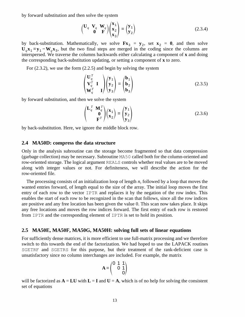
MA48C now optionally proceeds to estimate the error in the solution, using the backwarderrors just calculated and an estimate of the condition number obtained by using the HSL normestimation routine MC41, which uses a method based on that developed by Hager (1984),incorporating the modifications suggested by Higham (1987). Condition numbers are estimatedcorresponding to the two ω s. That corresponding to ω is given by1

(1) (k) (1)−1 |A | |x |+|b ||A |0 ∞κ = ,ω (k)1 ||x ||∞

(1)where |b | are the components of b corresponding to the equations determining ω , and that1corresponding to ω by2

0−1|A | (2) (k) (2)|A | |x |+f ∞κ = ,ω (k)2 ||x ||∞

(2) (2) (k)where f = |A |e||x || , with e the vector of all 1s. In each case, the norm in the numerator is of∞−1 −1

1 2the form |||A |g|| which is equivalent to ||A G|| , with G = diag{g , g , ...}, whence the∞ ∞subroutine MC41 can be applied directly.

||δ x||∞The bound for the error in the solution , , is then given by||x||∞

ω κ +ω κ .1 ω 2 ω1 2

All that remains is to permute the solution appropriately and exit.

3.4 MA48D: solution of block system

MA48D solves a system of equations using the block structure and calls to MA50C for eachnon-triangular diagonal block.

For the solution when the matrix A is not transposed, the block form is block upper-triangularand the blocks are solved in reverse order. For each block, either MA50C is used or a simpletriangular system is solved and then the new values are substituted in earlier equations using theoff-diagonal parts of the columns in the current block. Because of the column-oriented storage,the inner loop of the back-substitution for the triangular diagonal blocks and for the off-diagonalblocks involves the addition of a multiple of one vector to another with indirect addressing forthe vector being accumulated.

For the transposed problem, the system is block lower-triangular and the solution starts withthe (1,1) block and goes forward through the block form. Now the forward substitution loops aredot products with indirect addressing of one of the vectors, which are less likely to vectorize well(see Table 2 in Section 4).

20

3.5 MA48I: control parameter initialization

Subroutine MA48I provides default values for the arrays CNTL and ICNTL that together controlthe execution of the package. In many cases, these values are used to set the correspondingparameters of MA50. Their purposes and default values are given in Appendix B.

4 Performance results

For performance testing, we have taken two subsets of the problems in the Harwell-Boeingcollection (see Duff, Grimes, and Lewis 1989 and 1992). The first subset is summarized in Table1 and was chosen to be representative of the kinds of problems likely to be solved by our codes.

Case Identifier Order Number Descriptionof entries

1 SHL 400 663 1712 Basis matrix obtained after the application by J. K.Reid of 400 steps of the simplex method to a linearprogramming problem. This matrix is apermutation of a triangular matrix.

2 FS 541 1 541 4285 A matrix that arose in FACSIMILE (a stiff ODEpackage) in solving an atmospheric pollutionproblem involving chemical kinetics and two-dimensional transport.

3 FS 680 3 680 2646 Mixed kinetics diffusion problem from radiationchemistry. 17 chemical species and one spacedimension with 40 mesh points.

4 MCFE 765 24382 Radiative transfer and statistical equilibrium inastrophysics.

5 BCSSTK19 817 6853 Part of a suspension bridge.6 ORSIRR 2 886 5970 Oil reservoir simulation.7 WEST0989 989 3537 Chemical engineering plant model.8 JPWH 991 991 6027 Circuit physics model.9 GRE 1107 1107 5664 Matrix produced by the package QNAP written by

CII-HB for simulation modelling of computersystems.

10 ERIS1176 1176 18552 Large electrical network.11 PORES 2 1224 9613 Oil reservoir simulation. Matrix pattern is

symmetric.12 BCSSTK27 1224 56126 Buckling analysis, symmetric half of an engine

inlet from a modern Boeing jetliner.13 NNC1374 1374 8606 Model of an advanced gas-cooled nuclear reactor

core.14 BP 1600 822 4841 Basis matrix obtained after the application of 1600

steps of the simplex method to a linearprogramming problem.

15 WATT 1 1856 11360 Petroleum engineering problem.16 WEST2021 2021 7353 Chemical engineering plant model.17 ORSREG 1 2205 14133 Oil reservoir simulation.18 ORANI678 2529 90158 Economic model of Australasia.19 GEMAT11 4929 33185 Initial basis of an optimal power flow problem with

2400 buses.20 BCSPWR10 5300 21842 Eastern US Power Network – 5300 Bus.

Table 1. The matrices used for performance testing.

21

We have used the Table 1 matrices to choose default values for parameters and to judge theperformance on

(i) one processor of a Cray YMP-8I/8128 using Release 5.0 of the cf77 compilingsystem with the option –Zv (maximum vectorization) and vendor-supplied BLAS,

(ii) a SUN SPARCstation 1 using Release 4.1 of the f77 compiler with the option –O(optimization) and Fortran 77 BLAS, and

(iii) an IBM RS/6000 model 550 using Release 2.3 of the xlf compiler with the option –O(optimization) and vendor-supplied BLAS.

We believe that these are representative of the likely runtime environments, but it must bestressed that other platforms, other compilers, or other implementations of the BLAS may requiredifferent parameter values for good performance. Also, tuning for particular requirements maybe worthwhile; for example, the choice of density threshold for the switch to full code is affectedby whether a single problem is to be solved or many problems with the same pattern are to besolved.

We have been hampered somewhat by the variability of the cpu timers on the IBM RS/6000and the SUN. To alleviate this, we have embedded each call to MA48 in a loop of length 1000that is left as soon as the accumulated time exceeds one second and the average time is thencalculated. We can judge the repeatability of the timings by the variation of the analysis timewhen variations of the block size used for the BLAS are made since this does not affect theanalysis phase. Occasional individual variations could be as high as 25% on the IBM RS/6000and 20% on the SUN. The median change over the twenty problems could be as high as 3% onthe IBM RS/6000 and 8% on the SUN. The Cray is much better with all times within 1%. TheIBM RS/6000 and the SUN figures presented here were obtained with runs on lightly loadedmachines to avoid such extreme variations, but we rely mainly on the Cray times for ourconclusions.

Case Array Analyse Fact. Analyse Fast Solve SolveTsize reqd + Fact. Fact. Ax = b A x = b

1 3424 0.012 0.000 0.012 0.000 0.0007 0.00142 20229 0.123 0.051 0.175 0.023 0.0013 0.00213 7120 0.044 0.017 0.061 0.006 0.0010 0.00174 111853 0.762 0.281 1.043 0.175 0.0039 0.00525 35507 0.247 0.104 0.351 0.044 0.0021 0.00346 61014 0.383 0.139 0.522 0.082 0.0023 0.00367 8992 0.069 0.026 0.095 0.008 0.0021 0.00378 70973 0.331 0.128 0.458 0.097 0.0029 0.00479 72140 0.382 0.170 0.552 0.102 0.0037 0.0054

10 49920 0.176 0.086 0.263 0.042 0.0026 0.004411 63840 0.382 0.154 0.536 0.084 0.0030 0.004612 216228 1.499 0.561 2.060 0.329 0.0059 0.008513 78056 0.483 0.208 0.690 0.108 0.0048 0.007514 9682 0.059 0.018 0.076 0.008 0.0022 0.003615 167763 1.315 0.504 1.820 0.344 0.0071 0.010016 19317 0.150 0.056 0.206 0.017 0.0043 0.007617 298348 1.753 0.886 2.639 0.703 0.0092 0.015718 182012 0.901 0.263 1.163 0.148 0.0083 0.013019 89295 0.595 0.236 0.831 0.073 0.0121 0.020820 100810 0.742 0.305 1.047 0.114 0.0115 0.0191

Table 2. Performance on Cray with default settings.

22


1 3424 0.06 0.01 0.07 0.01 0.009 0.0102 20364 0.99 0.56 1.55 0.38 0.040 0.0303 6823 0.27 0.12 0.39 0.06 0.017 0.0164 111875 10.56 7.34 17.90 6.42 0.175 0.1315 37518 2.61 1.20 3.81 0.85 0.072 0.0536 65625 3.59 4.06 7.65 3.68 0.121 0.0907 8986 0.35 0.15 0.50 0.06 0.022 0.0218 69726 2.34 5.13 7.47 4.81 0.120 0.0959 72140 4.19 4.83 9.02 4.40 0.138 0.103

10 49920 1.27 1.23 2.50 0.98 0.071 0.05611 65984 3.68 3.01 6.69 2.56 0.126 0.09112 218066 23.76 12.32 36.08 10.67 0.353 0.24013 76941 4.68 3.89 8.57 3.26 0.151 0.11314 9682 0.28 0.11 0.39 0.06 0.025 0.02315 169546 20.19 13.69 33.88 12.40 0.330 0.23416 19314 0.79 0.34 1.12 0.15 0.051 0.04617 285175 27.23 38.36 65.59 36.47 0.530 0.38318 182012 10.58 7.10 17.68 6.39 0.292 0.25019 89329 3.70 1.76 5.46 0.92 0.180 0.15320 102676 5.60 3.40 9.00 2.36 0.228 0.182

Table 3. Performance on SUN with default settings.


1 3424 0.013 0.001 0.013 0.000 0.0007 0.00082 20364 0.173 0.057 0.231 0.032 0.0033 0.00343 6823 0.052 0.016 0.068 0.007 0.0016 0.00174 111875 1.900 0.483 2.383 0.353 0.0111 0.01145 37518 0.453 0.132 0.586 0.071 0.0066 0.00586 65625 0.590 0.236 0.826 0.180 0.0075 0.00747 8986 0.071 0.023 0.093 0.008 0.0024 0.00228 69726 0.427 0.236 0.663 0.208 0.0067 0.00669 72140 0.635 0.308 0.942 0.202 0.0089 0.0088

10 49920 0.232 0.118 0.350 0.082 0.0050 0.004911 65984 0.680 0.204 0.884 0.172 0.0078 0.007612 218066 3.800 0.945 4.745 0.730 0.0220 0.024913 76129 0.975 0.307 1.283 0.187 0.0103 0.010714 9682 0.060 0.019 0.079 0.012 0.0028 0.002915 169546 3.120 1.030 4.150 0.800 0.0229 0.021716 19314 0.160 0.050 0.210 0.020 0.0051 0.005617 285175 4.500 1.780 6.280 1.550 0.0312 0.030018 182012 2.190 0.410 2.600 0.312 0.0191 0.017119 89329 0.685 0.224 0.909 0.100 0.0177 0.017720 102676 1.080 0.393 1.473 0.193 0.0220 0.0213

Table 4. Performance on IBM RS/6000 with default settings.

For all three environments, we have chosen the value 0.5 for the density threshold for theswitch to full code and Level 3 BLAS with block size 32. We are able to use the same defaultsbecause the performance is very flat around the optimum values, as the results later in thissection demonstrate. Tables 2, 3, and 4 summarize the performance of the code with these defaultvalues.

The effect of our use of Level 3 BLAS in the full code is most apparent in the solve phase.Since we have chosen a column orientation for the storage of numerical values of the matrix andfactors, the solution of the equations Ax = b will be performed using a SAXPY kernel in the

23

Tinnermost loop while the solution of A x = b uses an SDOT operation. On the Cray, the former ismore efficient than the latter and this is clearly reflected in the fact that the times for solving thesystem are up to 50% less than for the solution of the transposed equations. This was one of thereasons why we chose column orientation in the first place. On the IBM, the different relativeperformance of the two Level 1 BLAS means that times for solution of the system and itstranspose are about the same while on the Sun the position is reversed with the faster SDOTroutine giving a faster solution time for the transposed equations.

We examine the relative performance when a single parameter is changed by means of themedian, upper-quartile and lower-quartile ratios over the 20 problems. We use these values ratherthan means and variances to give some protection against stray results caused either by the timeror by particular features of the problems. We remind the reader that half the results lie betweenthe quartile values. Full tables of ratios are available by anonymous ftp fromnumerical.cc.rl.ac.uk (130.246.8.23) in the file pub/reports/ma48.tables.

4.1 Density threshold for the switch to full code

Which value is best for the density threshold for the switch to full code depends on the relativeimportance of analysis time as opposed to factorization time and to the importance of storage.Any reduction will save time in the analyse phase since no further sparsity processing isperformed once the threshold is reached. Usually, there is a penalty in the need for more storage.Too low a value leads to such an increase in factorize time that we lose even if only a singleproblem is to be solved. We have also been influenced in our choice of default value by theconvenience of a single value on all platforms. Our value of 0.5 is based on slightly differentpriorities on the three platforms.

Table 5 shows the effect of decreasing the value of the density threshold for the switch to fullcode to 0.4. The factorization times are increased, though only slightly for the first factorizationon the Cray. A smaller value may be preferred if a single problem is to be solved, as may bejudged from the sum of the analyse and factorization times (see Table 5). Table 6 shows similareffects from the further reduction to 0.3. For the SUN, this is too low even if only a singleproblem is to be solved.

Array Analyse Fact. Analyse Fast Solve SolveTsize reqd + Fact. Fact. Ax = b A x = b

Cray lower q. 1.03 0.90 0.99 0.94 1.02 1.00 0.99median 1.09 0.96 1.01 0.97 1.09 1.00 1.00upper q. 1.11 0.98 1.05 0.99 1.13 1.02 1.03

SUN lower q. 1.02 0.85 1.05 0.98 1.08 1.03 1.02median 1.09 0.91 1.12 1.00 1.18 1.06 1.07upper q. 1.11 0.98 1.24 1.02 1.28 1.09 1.10

IBM lower q. 1.02 0.80 1.02 0.85 1.04 0.93 0.97median 1.09 0.89 1.04 0.92 1.08 0.98 0.99upper q. 1.11 0.94 1.07 0.97 1.15 1.03 1.03

Table 5. Results with density threshold value 0.4 divided by those with value 0.5.

24
















Tables 7 and 8 show the effect of increasing the value of the density threshold for the switch tofull code. On the Cray, the performance is very flat, a credit to its success nowadays invectorizing loops with indirect addressing. The IBM RS/6000 performance is also rather flat. Forthe SUN and the IBM, there is a loss of performance for the single problem, but some reductionin factorization time. It is unlikely that there would be such reduction in factorization time withoptimized versions of the BLAS, not currently available to us.

4.2 The choices within the full code

We have available to us Level 1 BLAS, Level 2 BLAS, and Level 3 BLAS with a choice of blocksize. Tables 9 and 10 demonstrate that there is some advantage in using Level three BLAS on allthree platforms.

25

Fact. Analyse Fast Solve SolveT+ Fact. Fact. Ax = b A x = b

Cray lower q. 1.03 1.01 1.09 1.07 1.07median 1.13 1.04 1.24 1.18 1.21upper q. 1.26 1.06 1.43 1.30 1.40

SUN lower q. 1.01 1.00 1.06 1.02 1.00median 1.19 1.08 1.22 1.04 1.00upper q. 1.33 1.15 1.37 1.07 1.01

IBM lower q. 1.00 0.99 1.08 0.98 0.96median 1.22 1.04 1.33 1.09 1.05upper q. 1.53 1.09 1.76 1.18 1.07

Table 9. Results with Level 1 BLAS divided by those with Level 3 BLAS and block size 32.





Table 10. Results with Level 2 BLAS divided by those with Level 3 BLAS and block size 32.





Table 11. Results with Level 3 BLAS with block size 16 divided by those with block size 32.





Table 12. Results with Level 3 BLAS with block size 64 divided by those with block size 32.

26

The performance is very flat as the block size is varied around the size 32. Table 11 shows thatwith block size 16 we get slightly worse performance on the Cray and on the IBM and unchangedperformance on the SUN. Table 12 shows that with block size 64 we get slightly worseperformance on the SUN and IBM and unchanged performance on the Cray. We have chosen 32for the default block size because it appears to be near optimal in all three cases and because ofthe convenience of having the same value on the different machines.

4.3 The choice of strategy for pivot choice

We have followed the recommendation of Zlatev (1980) that the search for pivots be limited tothree columns. We have found that, compared with the Markowitz strategy, this does indeed saveworthwhile analyse time without significant loss of sparsity in the factors, as Table 13 illustrates.To check the sensitivity of the choice of number of columns, we have also tried two- andfour-column searches. The results in Table 13 show that there is little sensitivity.


Markowitz lower q. 0.93 1.51 0.89 1.38 0.86 0.97 0.96median 0.99 2.10 0.97 1.76 0.96 0.99 0.99upper q. 1.04 4.18 1.02 3.20 1.02 1.00 1.00

Zlatev 2-col. lower q. 1.00 0.95 0.99 0.96 0.99 1.00 0.99median 1.00 0.97 1.01 0.98 1.01 1.00 1.00upper q. 1.03 1.00 1.02 1.01 1.04 1.00 1.00

Zlatev 2-col. lower q. 0.99 1.00 0.98 1.00 0.99 0.99 1.00median 1.00 1.03 1.00 1.02 1.00 1.00 1.00upper q. 1.04 1.06 1.01 1.04 1.04 1.01 1.01

Table 13. Cray results with different pivot strategies divided bythose with Zlatev’s 3-column search.

The example provided by Norm Schryer of Bell Laboratories (private communication), whichwas mentioned in Section 2.1.2, illustrates the possibility of very slow Markowitz processing.The problem is of order 138409 and has 434918 entries. The largest block of the block triangularform has order 63554 and dominates the analysis time. Compiling as usual on the SPARCstation1, but running on a SPARCstation 10 in order to get a feasible run, we found that the analyse timeincreased from 82 seconds to 8901 seconds when we switched to the Markowitz option. Thefactorization time was 15 seconds and the solve time was 0.02 seconds.

4.4 The block triangular form

Table 14 shows the statistics produced by MA48 on the block triangular form, namely

(i) the order of the largest non-triangular block on the diagonal of the block triangularform,

(ii) the sum of the orders of all the non-triangular blocks on the diagonal of the blocktriangular form, and

(iii) the total number of entries in all the non-triangular blocks on the diagonal of theblock triangular form (these are the entries that are passed to MA50 for analysis).

27

Case Order Order of Sum of Number Number of entrieslargest block of entries in non-triangularblock orders diagonal blocks

1 663 0 0 1712 02 541 540 540 4285 37443 680 235 235 2646 14344 765 697 765 24382 243425 817 817 817 6853 68536 886 886 886 5970 59707 989 720 720 3537 26228 991 846 846 6027 55629 1107 1107 1107 5664 5664

10 1176 1174 1176 18552 1855211 1224 1224 1224 9613 961312 1224 1224 1224 56126 5612613 1374 1318 1318 8606 835014 822 217 392 4841 199715 1856 1728 1728 11360 1110416 2021 1500 1500 7353 549517 2205 2205 2205 14133 1413318 2529 1830 1830 90158 4782319 4929 4578 4578 33185 3150020 5300 5300 5300 21842 21842Table 14. Statistics on the block triangularization.

Case Identifier Order Number Descriptionof entries

21 FS 680 1 680 2646 Mixed kinetics diffusion problem from radiationchemistry. 17 chemical species and one spacedimension with 40 mesh points.

22 SHL 400 663 1712 Basis matrix obtained after the application by J. K.Reid of 400 steps of the simplex method to a linearprogramming problem. This matrix is apermutation of a triangular matrix. (Also case 1.)

23 BP 1600 822 4841 Basis matrix obtained after the application of 1600steps of the simplex method to a linearprogramming problem. (Also case 14.)

24 IMPCOL D 425 1339 Matrix extracted from a run of the chemicalengineering package SPEED UP modelling a nitricacid plant.

25 IMPCOL E 225 1308 Matrix extracted from a run of the chemicalengineering package SPEED UP modelling ahydrocarbon separation problem.

26 WEST0497 497 1727 Chemical engineering plant model.27 WEST2021 2021 7353 Chemical engineering plant model. (Also case 16.)28 WEST0989 989 3537 Chemical engineering plant model. (Also case 7.)29 MAHINDAS 1258 7682 Economic model of Victoria, Australia.30 ORANI678 2529 90158 Economic model of Australasia. (Also case 18.)

Table 15. The matrices used for testing the block triangular form.

For comparison, we also show the matrix order and the number of entries in the matrix. It may beseen that there are only six (cases 1, 3, 7, 14, 16, and 18) where less than 75% of the entries lie inthe diagonal blocks. Seven of the matrices (cases 5, 6, 9, 11, 12, 17, and 20) are irreducible, whileseveral more are nearly so. We felt that more than six very reducible cases would be needed tojudge the block triangularization, so we constructed another set of matrices from theHarwell-Boeing collection, summarized in Table 15. The block triangularization statistics forthis collection are shown in Table 16.

28

Case Order Order of Sum of Number Number of entrieslargest block of entries in non-triangularblock orders diagonal blocks

21 680 235 235 2646 143422 663 0 0 1712 023 822 217 392 4841 199724 425 199 199 1339 56225 225 47 78 1308 40326 497 92 206 1727 76927 2021 1500 1500 7353 549528 989 720 720 3537 262229 1258 589 589 7682 474430 2529 1830 1830 90158 47823

Table 16. Statistics on the block triangularization for the second collection.

Table 17 shows that worthwhile gains are available from block triangularization, though onlyin one case is the gain dramatic and this is because the matrix is a permutation of a triangularmatrix. There are some worthwhile storage gains, too.


21 1.19 1.13 1.59 1.25 1.33 1.16 0.8622 1.20 2.18 161.51 3.30 40.96 1.70 1.1223 1.36 1.28 2.31 1.52 1.51 0.77 0.7724 1.33 0.94 2.00 1.15 1.68 1.07 0.8625 1.23 0.91 2.87 1.24 1.65 0.83 0.7326 1.39 1.24 2.19 1.45 1.70 1.03 1.0027 1.14 0.93 1.28 1.02 1.23 0.97 0.9628 1.15 0.95 1.27 1.04 1.22 0.97 0.9729 1.23 1.08 1.54 1.21 1.33 1.03 0.9130 1.31 1.20 1.96 1.37 1.68 0.98 0.90

lower q. 1.19 0.94 1.54 1.15 1.33 0.97 0.86median 1.23 1.10 1.98 1.24 1.58 1.00 0.91upper q. 1.33 1.24 2.31 1.45 1.68 1.07 0.97

Table 17. Cray results without block triangularization divided bythose with it.

We found that the technique of merging blocks smaller than a threshold size came intooperation in only two cases when the threshold value was 10, our tentative default. In both cases,there was a loss of performance, see Table 18. In the absence of further data, we have changedour default value to 1. Note that the runs reported in Sections 4.1, 4.2, and 4.3 used the value 10.This is not likely to affect the conclusions about other aspects of the code, particularly since onlyone case is affected (case 14, which is also case 23).


Cray 23 1.00 1.08 1.19 1.10 1.16 1.00 0.9825 1.00 1.14 1.47 1.19 1.21 1.08 1.03

IBM 23 1.00 1.14 1.16 1.15 1.18 0.96 1.0125 1.00 1.08 1.33 1.14 1.09 1.16 1.06

Table 18. Results with amalgamation threshold 10 divided by thosewithout block amalgamation.

29

4.5 Comparison with calling MA50 directly

A user with a matrix that is irreducible or only slightly reducible may wish to consider callingMA50 directly, provided the less convenient interface is acceptable and the additional facilities ofiterative refinement and error estimation are not required. Comparisons are shown in Table 19.Note that the cases that we noted as being significantly reducible (cases 1, 3, 7, 14, 16, 18)constitute the upper quartile of factorization ratios. Overall, judging by the median ratios, usingMA50 directly displayed a need for less storage and a reduction in analysis time, but an increasein both factorization times.


1 0.70 1.72 164.21 2.85 40.79 1.67 1.102 0.79 0.92 1.01 0.95 0.92 0.99 0.993 0.94 0.97 1.57 1.14 1.44 1.15 0.844 0.92 0.72 1.10 0.82 1.19 0.91 0.955 1.01 0.97 1.16 1.03 1.24 1.03 1.016 0.81 0.68 0.87 0.73 0.81 0.95 0.937 0.76 0.81 1.27 0.94 1.21 0.96 0.968 1.14 0.67 1.24 0.83 1.24 1.09 1.029 0.91 0.96 1.06 0.99 1.04 0.98 0.9810 0.63 0.54 1.00 0.69 1.02 0.98 0.9811 0.76 0.82 1.01 0.87 0.93 1.00 1.0012 0.75 0.72 1.00 0.80 0.98 0.98 1.0113 0.87 0.79 0.95 0.84 0.97 0.89 0.9214 0.86 1.10 2.32 1.38 1.50 0.77 0.7615 0.98 0.79 1.04 0.86 1.06 0.99 0.9716 0.76 0.80 1.28 0.93 1.21 0.96 0.9517 0.67 0.74 0.73 0.74 0.66 0.92 0.7318 0.81 1.04 1.94 1.24 1.70 0.98 0.9019 0.65 0.72 1.03 0.81 0.99 0.87 0.8720 0.81 0.82 1.03 0.88 1.04 1.00 0.99

lower q. 0.75 0.72 1.01 0.82 0.98 0.93 0.91median 0.81 0.80 1.05 0.88 1.05 0.98 0.96upper q. 0.92 0.97 1.28 1.01 1.24 1.00 1.00

Table 19. Cray results with MA50 divided by those with MA48.

4.6 Iterative refinement and error estimation

Table 20 summarizes the performance when the following options for the solve subroutineMA48C are invoked:

(i) Calculate the solution without iterative refinement but with the calculation of therelative backward errors.

(ii) Calculate the solution with iterative refinement and calculation of the relativebackward errors.

(iii) Calculate the solution with iterative refinement, calculation of the relative backwarderrors and estimation of the ∞–norm of the relative error in the solution.

30

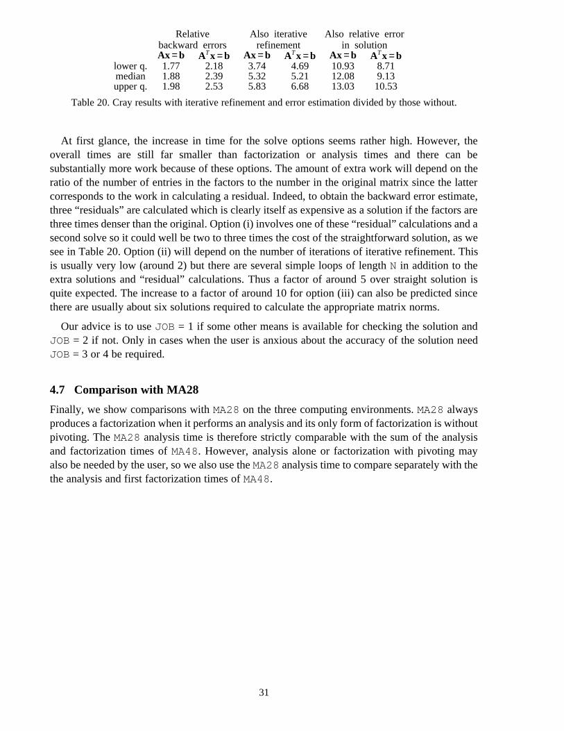
Relative Also iterative Also relative errorbackward errors refinement in solution

T T TAx = b Ax = b Ax = bA x = b A x = b A x = blower q. 1.77 2.18 3.74 4.69 10.93 8.71median 1.88 2.39 5.32 5.21 12.08 9.13upper q. 1.98 2.53 5.83 6.68 13.03 10.53

Table 20. Cray results with iterative refinement and error estimation divided by those without.

At first glance, the increase in time for the solve options seems rather high. However, theoverall times are still far smaller than factorization or analysis times and there can besubstantially more work because of these options. The amount of extra work will depend on theratio of the number of entries in the factors to the number in the original matrix since the lattercorresponds to the work in calculating a residual. Indeed, to obtain the backward error estimate,three “residuals” are calculated which is clearly itself as expensive as a solution if the factors arethree times denser than the original. Option (i) involves one of these “residual” calculations and asecond solve so it could well be two to three times the cost of the straightforward solution, as wesee in Table 20. Option (ii) will depend on the number of iterations of iterative refinement. Thisis usually very low (around 2) but there are several simple loops of length N in addition to theextra solutions and “residual” calculations. Thus a factor of around 5 over straight solution isquite expected. The increase to a factor of around 10 for option (iii) can also be predicted sincethere are usually about six solutions required to calculate the appropriate matrix norms.

Our advice is to use JOB = 1 if some other means is available for checking the solution andJOB = 2 if not. Only in cases when the user is anxious about the accuracy of the solution needJOB = 3 or 4 be required.

4.7 Comparison with MA28

Finally, we show comparisons with MA28 on the three computing environments. MA28 alwaysproduces a factorization when it performs an analysis and its only form of factorization is withoutpivoting. The MA28 analysis time is therefore strictly comparable with the sum of the analysisand factorization times of MA48. However, analysis alone or factorization with pivoting mayalso be needed by the user, so we also use the MA28 analysis time to compare separately with thethe analysis and first factorization times of MA48.

31

Case Array Analyse Fact. Analyse Fast Solvesize reqd + Fact. Fact.

1 0.50 1.38 196.73 1.37 154.50 3.902 0.69 2.64 6.36 1.87 2.04 3.143 0.71 2.35 6.20 1.70 3.43 3.224 0.62 6.15 16.67 4.49 2.02 1.425 0.66 3.92 9.29 2.76 1.81 2.276 0.68 4.30 11.81 3.15 1.82 2.187 0.54 3.64 9.46 2.63 3.06 2.338 0.91 16.51 42.68 11.90 3.54 2.139 0.65 7.81 17.50 5.40 1.64 1.74

10 0.42 3.98 8.13 2.67 3.29 2.4811 0.68 8.68 21.52 6.18 1.82 2.3212 0.63 4.64 12.40 3.38 2.23 1.5913 0.98 21.39 49.73 14.95 2.49 1.8414 0.59 1.65 5.49 1.27 3.81 1.9315 1.53 29.64 77.33 21.43 2.74 1.9616 0.54 6.62 17.61 4.81 3.03 2.3517 0.51 5.40 10.68 3.59 0.96 1.4418 0.58 6.22 21.31 4.81 5.53 1.7519 0.58 1.84 4.63 1.31 3.38 2.2220 0.60 3.10 7.55 2.20 2.03 2.36

lower q. 0.50 2.87 7.84 2.03 1.92 1.79median 0.69 4.47 12.10 3.26 2.61 2.20upper q. 0.71 7.21 21.41 5.11 3.41 2.35

Table 21. Cray results with MA28 divided by those with MA48.


1 0.50 2.06 21.67 1.88 18.33 1.482 0.68 2.14 3.77 1.37 1.59 0.803 0.74 2.31 5.17 1.60 2.22 1.914 0.62 3.06 4.40 1.80 1.31 0.675 0.63 3.29 7.16 2.25 1.27 0.736 0.63 2.96 2.61 1.39 1.07 0.707 0.54 3.66 8.30 2.54 2.00 1.158 0.93 21.82 9.95 6.84 2.60 1.049 0.65 5.99 5.19 2.78 1.06 0.66

10 0.42 3.37 3.48 1.71 1.74 0.7511 0.66 7.74 9.46 4.26 1.27 0.7112 0.62 1.90 3.66 1.25 1.67 0.6413 1.00 22.81 27.44 12.46 2.20 0.9514 0.59 1.68 4.36 1.22 2.81 0.9415 1.51 21.71 32.01 12.94 6.63 1.2616 0.54 6.79 15.68 4.74 1.84 1.0317 0.53 2.26 1.61 0.94 0.65 0.5218 0.58 3.33 4.96 1.99 2.20 0.7019 0.58 1.90 3.99 1.29 2.02 1.0120 0.59 3.04 5.01 1.89 1.07 0.86


Table 22. SUN results with MA28 divided by those with MA48.

32


1 0.50 1.58 35.71 1.52 61.22 2.742 0.68 2.65 8.04 2.00 1.86 1.113 0.74 2.50 7.98 1.90 4.16 1.404 0.62 3.72 14.61 2.96 2.55 1.215 0.63 3.62 12.38 2.80 2.12 0.856 0.63 4.14 10.34 2.95 1.94 1.237 0.54 3.54 11.00 2.68 2.44 1.178 0.93 24.59 44.45 15.83 5.77 1.949 0.65 7.45 15.38 5.02 2.18 1.02

10 0.42 3.71 7.30 2.46 2.67 1.1611 0.66 8.12 27.06 6.24 2.33 1.3212 0.62 2.69 10.84 2.16 2.82 1.2013 1.01 19.56 62.02 14.87 4.18 1.6214 0.59 1.33 4.12 1.01 1.68 0.9915 1.51 26.07 78.97 19.60 9.21 2.1416 0.54 6.69 21.61 5.11 3.50 1.1417 0.53 2.90 7.33 2.08 1.37 0.8918 0.58 3.08 16.46 2.60 7.23 1.0919 0.58 2.00 6.12 1.51 3.30 1.0420 0.59 2.92 8.01 2.14 1.81 0.85


Table 23. IBM results with MA28 divided by those with MA48.

5 Complex versions

We have made complex versions of MA48 and MA50. They are called ME48 and ME50 and keepTclose to the real versions. In ME48C and ME50C, we offer the solution of Ax = b, A x = b, or

HA x = b, and have therefore used an integer argument KIND in place of the logical argumentTRANS. Since this is the only significant change to the interface, we do not include copies of thespecification documents in Appendices A and B.

Extensive use is made of complex absolute values, particularly in connection with iterativerefinement, so we decided against using the BLAS ICAMAX and IZAMAX, which returnmax(|re(x )|+|im(x )|) instead of max(|x |). We believe that any efficiency gain from changing toi i i

i isuch an absolute value would be slight on modern hardware, and would not justify thealgorithmic changes and possible confusion of the user.

33

Appendix A. Solving full sets of linear equations

For the full-matrix processing we use towards the end of the factorization, we need to considerthe solution of dense systems

Ax = b, (A.1)

where A is of order m by n. The mathematical notation used in this appendix is independent ofthat of the main part of the paper. The matrix A here is the matrix F of equation (2.3.4) and thevector b is the vector y . We feel that it is easier to understand the ideas using uncluttered ‘local’2notation. For consistency with LAPACK (Anderson et al., 1992), we work here with afactorization in which the lower-triangular matrix has a unit diagonal.

We had hoped to use the LAPACK routines SGETRF and SGETRS for this purpose, but theirtreatment of the rank-deficient case is unsatisfactory since no column interchanges are included.

Our factorization algorithm proceeds as follows. At a typical stage, we look at a column for apivot and either find one and perform the pivotal operations or interchange the column with thelast column that has not already been interchanged. At the start of step k, we have thefactorization

L U V Wk k k kP A Q = , (A.2)k k M I S 0k k

where P and Q are permutation matrices, L is unit lower triangular and of order j − 1, U isk k k k k

upper triangular of order j − 1, and W has k − j columns. Initially, k = 1; j = 1; P and Q arek k k 1 1 1identity matrices; L , M , and W have no columns; U and V have no rows; and S = A. We1 1 1 1 1 1find the largest entry of the first column of S . If this is nonzero, we interchange rows to make itk

the leading entry of S and perform the pivotal operations; otherwise, we interchange the firstk

and last columns of S . In the former case, j has the value j + 1; in the latter case, j has thek k+1 k k+1value j . The row interchange is also performed in M and the column interchange is alsok k

performed in V . The final factorization isk

L U WP A Q = . (A.3)M I 0

Solving A x = b consists of the steps

c = P b (A.4)

d cL 1 1= (A.5)M I d c2 2

e dU W 1 1= (A.6)0 e d2 2

x = Q e. (A.7)

We solve (A.6) by setting e = 0 and finding e by back-substitution through U. This means that2 1d is not needed so that in (A.5) we need only forward substitute through L to find d .2 1

TSimilarly, solving A x = b consists of the steps

Tc = Q b (A.8)T d cU 1 1= (A.9)T d cW 0 2 2

34

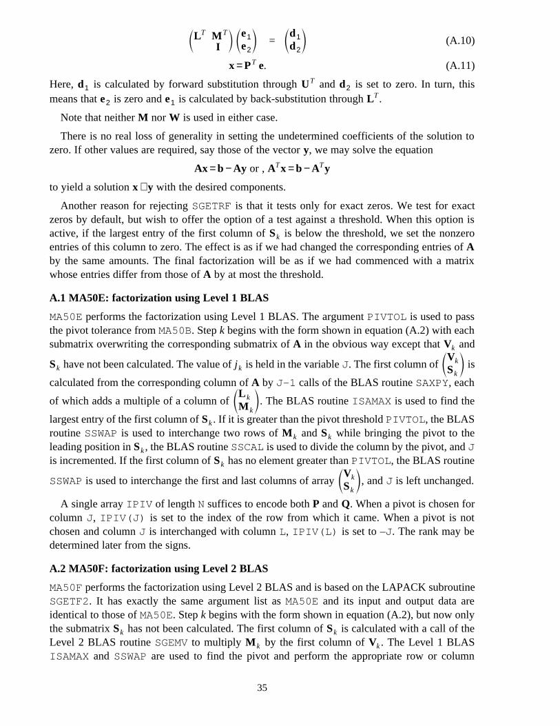
T T e d1 1L M = (A.10)e dI 2 2

Tx = P e. (A.11)THere, d is calculated by forward substitution through U and d is set to zero. In turn, this1 2

Tmeans that e is zero and e is calculated by back-substitution through L .2 1

Note that neither M nor W is used in either case.

There is no real loss of generality in setting the undetermined coefficients of the solution tozero. If other values are required, say those of the vector y, we may solve the equation

T TAx = b − Ay or , A x = b − A y

to yield a solution x + y with the desired components.

Another reason for rejecting SGETRF is that it tests only for exact zeros. We test for exactzeros by default, but wish to offer the option of a test against a threshold. When this option isactive, if the largest entry of the first column of S is below the threshold, we set the nonzerok

entries of this column to zero. The effect is as if we had changed the corresponding entries of Aby the same amounts. The final factorization will be as if we had commenced with a matrixwhose entries differ from those of A by at most the threshold.

A.1 MA50E: factorization using Level 1 BLAS

MA50E performs the factorization using Level 1 BLAS. The argument PIVTOL is used to passthe pivot tolerance from MA50B. Step k begins with the form shown in equation (A.2) with eachsubmatrix overwriting the corresponding submatrix of A in the obvious way except that V andk

VkS have not been calculated. The value of j is held in the variable J. The first column of isk k Skcalculated from the corresponding column of A by J-1 calls of the BLAS routine SAXPY, each

Lkof which adds a multiple of a column of . The BLAS routine ISAMAX is used to find theMklargest entry of the first column of S . If it is greater than the pivot threshold PIVTOL, the BLASk

routine SSWAP is used to interchange two rows of M and S while bringing the pivot to thek k

leading position in S , the BLAS routine SSCAL is used to divide the column by the pivot, and Jk

is incremented. If the first column of S has no element greater than PIVTOL, the BLAS routinekVkSSWAP is used to interchange the first and last columns of array , and J is left unchanged.Sk

A single array IPIV of length N suffices to encode both P and Q. When a pivot is chosen forcolumn J, IPIV(J) is set to the index of the row from which it came. When a pivot is notchosen and column J is interchanged with column L, IPIV(L) is set to –J. The rank may bedetermined later from the signs.

A.2 MA50F: factorization using Level 2 BLAS

MA50F performs the factorization using Level 2 BLAS and is based on the LAPACK subroutineSGETF2. It has exactly the same argument list as MA50E and its input and output data areidentical to those of MA50E. Step k begins with the form shown in equation (A.2), but now onlythe submatrix S has not been calculated. The first column of S is calculated with a call of thek k

Level 2 BLAS routine SGEMV to multiply M by the first column of V . The Level 1 BLASk k

ISAMAX and SSWAP are used to find the pivot and perform the appropriate row or column

35

interchange, as in MA50E. If a pivot is found, the Level 2 BLAS SGEMV is used to form the lastrow of V . It does this by subtracting the first row of M times V , excluding its first column,k+1 k k

from the first row of S , excluding its first entry.k

A simple calculation shows that the number of operations performed within a step outside theLevel 2 BLAS is O(m + n).

A.3 MA50G: factorization using Level 3 BLAS

MA50G performs the factorization using Level 3 BLAS and is based on the LAPACK subroutineSGETRF. Apart from the additional argument NB that specifies the block size, MA50G has thesame argument list as MA50E and MA50F, and its other input and output data are identical totheirs. The matrix is processed in blocks of NB columns, apart from the final block which mayhave less columns. The processing of a block begins with the form shown in equation (A.2), nowwith all submatrices calculated. The leading NB columns of S are treated in just the same way ask

A itself is treated by MA50F, except that when no entry of a column is big enough to be a pivot,an interchange is made with the last column of S rather than the last column of the block. At thek

completion of the block (that is, when NB pivots have been found), the row interchangesgenerated within it are applied to the other columns of M and S (column by column to avoidk k

data movement), and the operations of the block are applied to the remaining columns of V andk

S using the Level 3 BLAS STRSM and SGEMM.k

A simple calculation shows that the total number of operations performed outside the Level 3BLAS is O( n(NBm + n) ).

Note also that the column interchange that follows a failure to find a pivot does not usuallylead to a reduction of the block size, since a column from outside the block is brought in.However, this is not the case for the final block, where the block size is reduced by one for eachsuch interchange.

A.4 MA50H: solutionTMA50H solves a set of equations A x = b or A x = b using the factorization produced by MA50E,

MA50F, or MA50G, whose output data are identical. Each actual forward or back-substitutionoperation associated with L or U is performed either with the Level 2 BLAS STRSV or by a loopinvolving calls to SAXPY or SDOT. An argument controls which of these happens. Unlike thecase for factorization, the logic is very similar for the two cases, so there is no need for separatesubroutines.

MA50H begins by finding the rank r by searching IPIV from the back for a positive value. Weexpect this search to be short on the assumption that a rank much less than min(m,n) is unusual.

If A x = b is to be solved, we first apply r interchanges to the incoming vector to produce thevector c of equation (A.4). The row operations encoded in L are applied to calculate d from c ,1 1see equation (A.5). Back-substitution through U is used to calculate e and e is set to zero, see1 2equation (A.6). Finally, the column interchanges, if any, are applied, see equation (A.7).

TA similar sequence of steps is applied when A x = b is to be solved.

For the Level 1 BLAS code, we have followed the lead of LAPACK in accessing L and U bycolumns with SAXPY inner loops such as

B(1:K-1) = B(1:K-1) – A(1:K-1,K)*B(K)

36

T Twhen solving A x = b, and accessing L and U by rows with SDOT inner loops such as

DOT_PRODUCT(A(1:K-1,K),B(1:K-1))

in order to access contiguous elements of the array A.

Appendix B. The specification document for MA48

In this appendix, we include a copy of the specification document for MA48. The code itself isavailable from AEA Technology, Harwell; the contact is Libby Thick, Theoretical StudiesDepartment, AEA Technology, 424 Harwell, Didcot, Oxon OX11 0RA, tel (44) 235 432688, fax(44) 235 436579, email [email protected], who will provide details of price andconditions of use.

37

Appendix C. The specification document for MA50

In this appendix, we include a copy of the specification document for MA50. The code itself isavailable from AEA Technology, Harwell; the contact is Libby Thick, Theoretical StudiesDepartment, AEA Technology, 424 Harwell, Didcot, Oxon OX11 0RA, tel (44) 235 432688, fax(44) 235 436579, email [email protected], who will provide details of price andconditions of use.

50

References

Anderson, E., Bai, Z., Bischof, C., Demmel, J., Dongarra, J., Du Croz, J., Greenbaum, A.,Hammarling, S., McKenney, A., Ostrouchov, S., and Sorensen, D. (1992). LAPACK users’guide. SIAM, Philadelphia.

Anon (1993). Harwell Subroutine Library Catalogue (Release 11). Theoretical StudiesDepartment, AEA Technology, Harwell.

Arioli, M. Demmel, J. W., and Duff, I. S. (1989). Solving sparse linear systems with sparsebackward error. SIAM J. Matrix Anal. Appl. 10, 165-190.

Dongarra, J. J., Du Croz, J., Duff, I. S., and Hammarling, S. (1990). A set of Level 3 basic linearalgebra subroutines. ACM Trans. Math. Softw. 16, 1-17.

Dongarra, J. J., Du Croz, J., Hammarling, S., and Hanson, R. J. (1988). An extended set ofFortran Basic Linear Algebra Subprograms. ACM Trans. Math. Softw. 14, 1-17 and 18-32.

Duff, I. S. (1977). MA28 – a set of Fortran subroutines for sparse unsymmetric linear equations.Report AERE R8730, HMSO, London.

Duff, I. S. (1981a). On algorithms for obtaining a maximum transversal. ACM Trans. Math.Softw. 7, 315-330.

Duff, I. S. (1981b). Algorithm 575. Permutations for a zero-free diagonal. ACM Trans. Math.Softw. 7, 387-390.

Duff, I. S. and Reid, J. K. (1978a). An implementation of Tarjan’s algorithm for the blocktriangularization of a matrix. ACM Trans. Math. Softw. 4, 137-147.

Duff, I. S. and Reid, J. K. (1978b). Algorithm 529. Permutations to block triangular form. ACMTrans. Math. Softw. 4, 189-192.

Duff, I. S. and Reid, J. K. (1979). Some design features of a sparse matrix code. ACM Trans.Math. Softw. 5, 18-35.

Duff, I. S., Erisman, A. M., and Reid, J. K. (1986). Direct methods for sparse matrices. OxfordUniversity Press, London.

Duff, I. S., Grimes, R. G., and Lewis, J. G. (1989). Sparse matrix test problems. ACM Trans.Math. Softw. 15 1-14.

Duff, I. S., Grimes, R. G., and Lewis, J. G. (1992). Users’ guide for the Harwell-Boeing sparsematrix collection (Release 1). Report RAL-92-086 Rutherford Appleton Laboratory,Oxfordshire.

Eisenstat, S. C. and Liu, J. W. H. (1993). Exploiting structural symmetry in a sparse partialpivoting code. SIAM J. Sci. Stat. Comput. 14, 253-257.

Gilbert, J. R. and Peierls, T. (1988). Sparse partial pivoting in time proportional to arithmeticoperations. SIAM J. Sci. Stat. Comput. 9, 862-874.

Hager, W. W. (1984). Condition estimators, SIAM J. Sci. Stat. Comput. 5, 311-316

Higham, N. J. (1987). Fortran codes for estimating the one-norm of a real or complex matrix,with applications to condition estimation. ACM Trans. Math. Softw. 14, 381-396.

Lawson, C. L., Hanson, R. J., Kincaid, D. R., and Krogh, F. T. (1979). Basic linear algebrasubprograms for Fortran use. ACM Trans. Math. Softw. 5, 308-325.

61

Markowitz, H. M. (1957). The elimination form of the inverse and its application to linearprogramming. Management Sci. 3, 255-269.

Oettli, W. and Prager, W. (1964). Compatibility of approximate solution of linear equations withgiven error bounds for coefficients and right-hand sides. Numerische Math. 6, 405-409.

Pothen, A. and Fan, C-J. (1990). Computing the block triangular form of a sparse matrix. ACMTrans. Math. Softw. 16, 303-324.

Skeel, R. D. (1980). Iterative refinement implies numerical stability for Gaussian elimination.Math. Comp. 35, 817-832.

Tarjan, R. E. (1972). Depth-first search and linear graph algorithms. SIAM J. Computing 1,146-160.

Zlatev, Z. (1980). On some pivotal strategies in Gaussian elimination by sparse technique. SIAMJ. Numer. Anal. 17, 18-30.

62

RAL-93-072 MA48, a Fortran code for direct solution of sparse ... · If the matrix is rectangular or square but structurally singular (there is no set of entries that can be permuted

Documents