Rainfall Measurements Using Underwater Ambient Noisemixing.coas.oregonstate.edu/Oc679/Nystuen 1986.pdf · Rainfall measurements using underwater ambient noise ... include earthquakes

Rainfall measurements using underwater ambient noise Jeffrey A. Nystuen Scripps Institution of Oceanography, University of California at San Diego, La Jolla, California 92093

(Received 26 August 1985; accepted for publication 10 December 1985)

Observations are made which show that the underwater ambient noise spectrum generated by rain has a unique spectral shape which can be distinguished from other noise sources. Furthermore, the relationship between spectral level and rainfall is quantifiable. The spectral shape is dominated by a broad peak at 15 kHz, but also depends on the drop size distribution in the rain. A numerical study of the acoustic physics of a drop splash is used to explain the observed spectra. There are two contributions to underwater sound from the impact. The first contribution is from an initial acoustic water hammer pulse. The magnitude of this pulse depends on drop size, shape, and impact velocity. The contribution to the underwater sound spectrum is white and is very large for large drops. The second contribution occurs because at impact the incompressible continuity equation is not satisfied. Once this equation is satisfied, the splash is no longer an acoustic source. Numerically, the time required to closely satisfy this equation is roughly constant for all drop sizes at their terminal velocity. This time interval causes a low-frequency rolloff at roughly i 5 kHz in the sound spectrum.

PACS numbers: 43.30.Pc, 43.50.Pn, 43.50.Vt, 92.60.Jq

INTRODUCTION

Rainfall is one of the important variables used to describe the climate of a region. It plays a major role iq regional and global heat and water budgets. When rain occurs, latent heat is released. Knowledge of global rainfall would be an indicator for amount and distribution of latent heat release, upward mass flux, and spatial organization of convection. Such knowledge is vital to understanding the general circu- lation of the atmosphere.

Unfortunately, rainfall measurements are very difficult to make because rainfall is sharply discontinuous in both time and space. This makes adequate sampling with point measurement type instruments such as rain gauges, radio- sondes, and aircraft difficult. Weather radars are also used and do provide a more complete spatial coverage but are not very accurate. Furthermore, weather radars are limited, in general, to the developed countries of the world. In short, our knowledge of rainfall patterns over land is limited.

Over the ocean, the situation is much worse. It has been estimated that 80% of the Earth's precipitation occurs over the ocean where only about 10% of the weather stations are located. • These weather stations are located mostly on is- lands, which, from the point of view of sampling the oceanic rainfall, are poorly distributed. Furthermore, orographic effects, especially in the tropics, bias the measurements. Accu- rate rainfall measurements from ships are very difficult to make. Shipboard rain gauges are widely used but are affected by sea spray, platform instabilities, and ship-induced wind effects. In fact, over the ocean accurate rainfall measurements are very rare.

In the future, the best chance of obtaining global oceanic rainfall statistics will come from satellite measurements. A

satellite technique would have the advantage of providing relatively complete and uniform coverage. Regardless of the technique, all satellite methods suffer from an almost complete lack of accurate surface measurements of rainfall need-

ed to calibrate the satellite methods. One possible method to provide surface measurements of rainfall rate over water is to monitor the ambient noise generated by the raindrops striking the surface during rainstorms. 2-•

As a method of measuring rain, monitoring the underwater ambient noise has several advantages over more con- ventional systems. An underwater hydrophone will not have any surface platform problems. Measurementscan be made anywhere a hydrophone can be deployed (by mooring, buoy, or ship). This would reduce fair weather bias. A hydrophone would provide a large spatial average of rainfall which is very important since the spatial variability of rainfall is large. Furthermore, from the point of view of calibrat- ing satellite systems, spatial averaging is desirable as satellite instruments also make spatially averaged observations of rainfall. The principal difficulty with using underwater ambient noise to measure rainfall is that there are other noise

sources in the ocean. The noise spectrum generated by rain must have a spectral shape that allows it to be distinguished from other noise sources.

There are, of course, many sound sources in the ocean. The ambient noise generated by some of these sources has been extensively measured. Wenz s'6 wrote two review papers about oceanic ambient noise and discusses the presumed sources of that noise over a wide range of frequencies (Fig. 1).

In the band from 500 Hz to 25 kHz, the empirical Knud- sen relation is used to describe the wind-generated noise? ? In recent years, various experiments s-• have verified the spectral shape described by Knudsen et aL ? The observations show that the spectra of wind-generated noise are uniformly red with a slope of -- 17 dB per decade. The amplitude at any particular frequency depends on the strength of the wind. What Wenz meant by "surface agitation" has not been clearly described.

The sound spectrum from heavy rain (Fig. 1 ) shows

972 J. Acoust. Soc. Am. 79 (4), April 1986 0001-4966/86/040972-11500.80 ¸ 1986 Acoustical Society of America 972

• % explosions and • \ earthquakes

• :-p ...... • • •'• '•.shipping •fluct a•ions• •. heavy p•ecipitation

• .

•eq•e•e• •

FIG. 1. Summary of ambient noise sources and the spectral levels associated with each source. Prevailin S noise sources include turbulent pressure fluctuations in the ocean and atmosphere, oceanic traffic, surface agitation from wind, and thermal molecular agitation. Intermittent and local noise sources include earthquakes and explosions, biological sources, ships, sea ice, and precipitation (from Wenz, 1962).

rain as the dominant source of noise between 1 and 15 kHz, well above noise due to high winds. There are, however, very few measurements of ambient noise from rain. Wenz's curve is based on observations 2'3 as well as a study by Franz 12 of sound from splashes. Lemon et al. •o and Farmer and Lem- on 13 note that deviations from the Knudsen spectral shape in which excess high-frequency energy is observed can be attri- buted to precipitation. These observations suggest that the spectral shape of rain-generated noise is different from wind- generated noise and so it should be possible to separate rain noise from wind noise.

There are few published measurements above 15 kHz. In fact, the curves shown in Fig. 1 are extrapolated from lower frequencies. Since the shape of the rain-generated noise spectra was poorly documented, but critical, if rain is to be monitored using ambient noise, a series of observations of the noise spectra during rain were made at several different locations to identify the shape of the spectrum and to show that the features of the spectrum are independent of location. They are described in Sec. I, and show that the rain- generated noise spectrum is different than the wind-gener at- ed noise spectrum. The main feature of the rain-generated spectrum is a broadband peak at about 15 kHz. Prior to these observations, this peak had not been reported. In order to have confidence in the relationship between noise and rainfall rate, it is necessary to understand the physics which ex- plains the peak and the spectral level in general. In Sec. II, Franz's laboratory study of sound from splashes is discussed. Rather than try to improve on that experiment, the physics of a drop splash is studied numerically. That numerical study of the acoustic physics of a drop splash is described in Sec. IIl. Section IV is a discussion explaining the spectra observed.

973 J. Acoust. So½. Am., Vol. 79, No. 4, April 1986

I. FIELD OBSERVATIONS

A. Instruments

The principal instrument was a Gould/Clevite hydrophone system CS-131ABB(P). This system consists of a lithium surfate monohydrate sensor with a preamplifier and a decoupling transformer, all enclosed in one housing. The system is very sensitive ( -- 169 dB tel I V//•Pa) and has a self-noise of 8 dB tel I/•Pa2/I-Iz, well below the quietest ambient noise levels expected under normal conditions. The hydrophone system has a relatively flat frequency response ( + 3 dB) between 3 Hz and 150 kHz. Below 20 kHz, the hydrophone is very nearly omnidirectional. Above 50 kHz, the horizontal sensitivity remains essentially omnidirectional but in the vertical plane the directional sensitivity shows significant variability. While some observations were made between 50 and 100 kHz, the most interesting features of the rain-generated noise spectrum are at lower frequencies, between 1 and 30 kHz, where the hydrophone sensitivity characteristics are very good.

The spectrum analyzer was a GenRad model 2512. It performs a fast Fourier transform of the incoming signal for a chosen frequency band. The spectrum analyzer uses a Han- ning window and low-pass filters to sharply reduce aliasing. It also averages consecutive spectra together. Most of the spectra displayed in this paper are the average of 64 individual spectra and therefore have 128 degrees of freedom.

The best quantitative data that were obtained to compare with the hydrophone data came from a Joss-Waldvogel distrometer. The distrometer is an instrument which is de-

signed to identify drop size by measuring the pressure pulse from a drop striking the surface of the instrument. The distrometer counted the number of drops in each of 20 drop size categories during a 30-s interval. The data presented in this paper are the average of three consecutive 30-s periods and so each point represents a 90-s average. Knowing the drop size distribution is important since drop size distributions vary during a rain storm and this variation affects the shape of the underwater ambient noise spectrum. From the drop size distribution data, it is possible to calculate rainfall rate, total number of drops striking the surface, volumetric mean drop diameter, and kinetic energy of the drops in the rain.

The distrometer does bias against smaller drops, especially when the rainfall rate is high, since it is an acoustic device which constantly monitors the background noise level. If the pulse from a small drop is below this fluctuating noise level, then it is not recorded. Naturally, the background noise level is highest when the rainfall rate is high. Numerically, smaller drops make up most of the-drops in a typical drop size distribution; however, they do not contribute significantly to the total rainfall rate, the volumetric mean drop size, or to the total kinetic drop energy in the rain, nor do they contribute much energy into the underwater ambient noise spectrum, especially below 10 kHz. Because of this, the instrument's bias against small drops is not a serious problem.

At other locations, the ra'mfall rate was measured using cylinder style rain gaugei which measured accumulated rainfall in a 10-cm 2 area. By frequently recording the total, it was possible to estimate rainfall rate. At all locations, a

Jeffrey A. Nystuen: Underwater ambient noise from rainfall 973

qualitative assessment of the rainfall was made both visually and by listening directly to the hydrophone signal with ear- phones. At some locations, the rainfall rate was too light for the rain gauges to record significant totals, yet there was a strong underwater noise response.

B. Clinton Lake observations

In October 1982, a rain monitoring experiment took place at Clinton Lake in central Illinois. This lake is large and shallow, with a maximum depth of 8 m. The visibility in the water was low, roughly half a meter, and the lake had a thick, soft mud bottom. The hydrophone was mounted on a tripod 0.5 m above the lake bottom in 8 m of water 30 m from shore. The cable ran along the lake bottom and through a forested area to the spectrum analyzer located in a shelter about 50 m from the lake shore. The distrometers were set in a field 20 m from the shelter and from the nearest trees. The

distance between the hydrophone and the distrometers was about 100 m (Fig. 2).

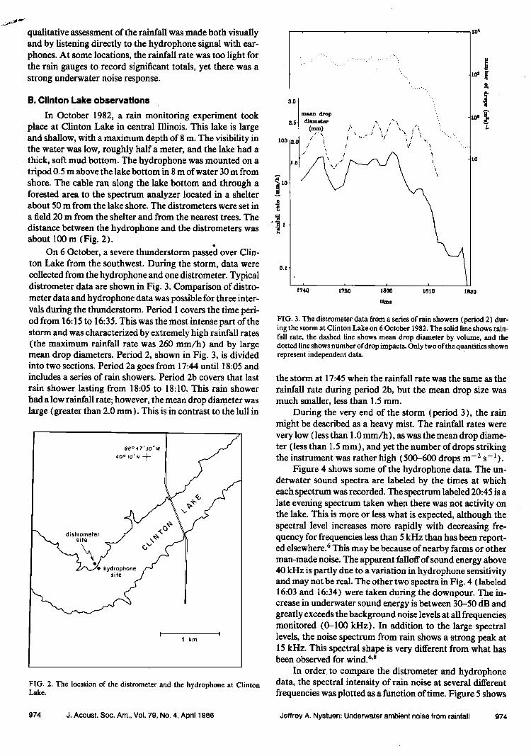
On 6 October, a severe thunderstorm passe•l over Clin- ton Lake from the southwest. During the storm, data were collected from the hydrophone and one distrometer. Typical distrometer data are shown in Fig. 3. Comparison of distrometer data and hydrophone data was possible for three inter- vals during the thunderstorm. Period 1 covers the time period from 16:15 to 16:35. This was the most intense part of the storm and was characterized by extremely high rainfall rates (the maximum rainfall rate was 260 mm/h) and by large mean drop diameters. Period 2, shown in Fig. 3, is divided into two sections. Period 2a goes from 17:44 until 18:05 and includes a series of rain showers. Period 2b covers that last

rain shower lasting from 18:05 to 18:10. This rain shower had a low rainfall rate; however, the mean drop diameter was large (greater than 2.0 mm). This is in contrast to the lull in

88ø 47' 50 TM 40 ø fO' N -•-

• distrometer •/

I

FIG. 2. The location of the distrometer and the hydrophone at Clinton Lake.

too

o.t

L0 ½

3.0 •

2.õ'

2.0

1.5

FIG. 3. The distrometer data from a series of rain showers (period 2) during the storm at Clinton Lake on 6 October 1982. The solid line shows rainfall rate, the dashed line shows mean drop diameter by volume, and the dotted line shows number of drop impacts. Only two of the quantifies shown represent independent data.

the storm at 17:45 when the rainfall rate was the same as the

rainfall rate during period 2b, but the mean drop size was much smaller, less than 1.5 mm.

During the very end of the storm (period 3), the rain might be described as a heavy mist. The rainfall rates were very low (less than 1.0 mm/h), as was the mean drop diameter (less than 1.5 mm), and yet the number of drops striking the instrument was rather high (500-600 drops m

Figure 4 shows some of the hydrophone data. The underwater sound spectra are labeled by the times at which each spectrum was recorded. The spectrum labeled 20:45 is a late evening spectrum taken when there was not activity on the lake. This is more or less what is expected, although the spectral level increases more rapidly with decreasing frequency for frequencies less than 5 kHz than has been reported elsewhere. 6 This may be because of nearby farms or other man-made noise. The apparent falloff of sound energy above 40 kHz is partly due to a variation in hydrophone sensitivity and may not be real. The other two spectra in Fig. 4 (labeled 16:03 and 16:34) were taken during the downpour. The increase in underwater sound energy is between 30-50 dB and greatly exceeds the background noise levels at all frequencies monitored (0-100 kHz). In addition to the large spectral levels, the noise spectrum from rain shows a strong peak at 15 kHz. This spectral shape is very different from what has been observed for wind. 6's

In order. to compare the distrometer and hydrophone data, the spectral intensity of rain noise at several different frequencies was plotted as a function of time. Figure 5 shows

974 J. Acoust. Sec. Am., Vol. 79, No. 4, April 1986 Jeffrey A. Nystuen: Underwater ambient noise from rainfall 974

I

10 BO •0 r•

Frequency in Kilohertz

FIG. 4. The underwater ambient noise spectra for three different times during the day at ClinWn Lake on 6 October 1982. The late night ambient noise spectrum (solid line) at 20:45 is for a quiet period with no activity on the lake. The other two spectra are during the heaviest rain period of the storm.

the spectral levels at 14.5 kHz during period 2. Also shown is the time series of rainfall rate from the distrometer for the

same period. For period 2, the correlation between distrometer rainfall rate and spectral level was highest at 14.5 kHz; however, for all periods of the storm, the relationship was best at 4.5 kHz. Figure 6 shows the comparison of rainfall rate with spectral level at 4.5 kHz for the entire storm. Dur- ing period 3 and during the lull in the rain in period 2a, the

lOO

lO

7O

•o g

FIG. 5. A comparison of the time series of spectral level at 14.5 kHz and the distrometer rainfall rate during period 2 of the storm at Clinton Lake. The solid line shows the rainfall rate data and the q- symbols show spectal level

00

S0

++

A AA

&

ambient noi•e early m'"ter'naon

o o o o

lO-I 10o

RAJxdA/I. ]b,f.e Lu mm/h

I ' I IllIll ' I ' IlllIt I I IIIII

lo • lO ß tos

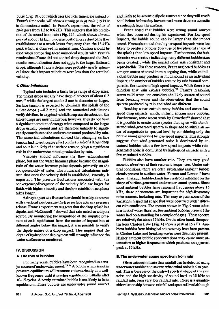
FIG. 6. A comparison of spectrai level at 4.5 kHz and rainfall rate. The late night and early afternoon background ambient noise leveh are also shown. Data poinL• are shown for all three rain periods. The + symbol indicates a data point from period 1, A for period 2a, • for period 2b, and O for period 3.

mean drop diameter in the rain was less than 1.5 ram, indicating the absence of large drops. Figure 6 shows that, at 4.5 kHz, rain consisting mostly of small drops does not cause the spectral level to rise above the ambient background noise level. On the other hand, at 14.5 kHz (Fig. 7), there is a large

9O

S0

• 70

-/6o

t+

o

o A

amb/ent •oile e•rly

ambient noise

late

10-"' 10 -• 10 0 101 10 • 10 • Ra/•fall Rate la mm/h

FIG. 7. Same as Fig. 6 except for spectral level at 14.5 kHz.


increase in spectral level. Apparently, small drops are effi- cient at producing sound near 1 $ kHz but do not produce significant sound energy at a lower frequency.

During period 2b, the rainfall rate was low and the mean drop diameter was large. Figures 6 and 7 show that during this period the spectral level was significantly above the spectral levels observed during other rain periods with similar rainfall rates. Together with the'preceding observation, this suggests that large drops produce sound energy below 5 kHz. Large drops do contain most of the kinetic energy in a typical rain. The kinetic energy of a raindrop increases dra- matically with drop size (KE = • mv:• •const.a 4, where m is the drop mass, a is the drop radius, and v T is the terminal drop velocity, which is roughly proportional to a a•/2). A rain shower, such as that during period 2b, that has the same rainfall rate as another rain shower but in which there are

more large drops, will have more kinetic energy than the other rain period. Since the sound levels were uniformly higher in period 2b than at other times with similar rainfall rates, this observation suggests that the sound level may be better correlated with kinetic energy than with rainfall rate. Figure 8 shows the relationship between kinetic energy and spectral level at 4.5 kHz. This figure should be compared with Fig. 6. The correlation is better with .kinetic energy than with rainfall rate but only slightly.

C. Observations at other locations

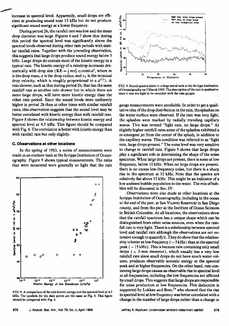
In the spring of 1983, a series of measurements were made in an outdoor tank at the Scripps Institution of Ocean- ography. Figure 9 shows typical measurements. The rains that were measured were generally so light that the rain

8O

• so

++

o o o ̧ o A A

10-u 10-4 10-a 10-a 10-t 10 0 [Clr•tAe gladrAy of the liaimirope (J/m $,•)

FIG. 8. A comparison of the rain kinetic energy and the spectral level at 4.5 kHz. The symbols for the data points are the same as Fig. 6. This figure should be compared with Fig. 6.

0 10 20 30 40

Frequency in Kilohertz

FIG. 9. Sound spectra taken in a large metal tank at the Scripps Institution of Oceanography on 3 March 1983• The description of the rain is qualitative since it was too light to be recorded with the rain gauges.

gauge measurements were unreliable. In order to get a qualitative idea of the drop distribution in the rain, the splashes on the water surface were observed. If the rain was very light, the splashes were marked by radially traveling capillary waves. This was termed "light rain• no large drops." At slightly higher rainfall rates some of the splashes exhibited a re-emergent jet from the center of the splash, in addition to the capillary waves. This condition was referred to as "light rain, large drops present." The noise level was very sensitive to change in rainfall rate. FigUre 9 shows that large drops play a significant role in determining the shape of the noise spectrum. When large drops are present, there is noise at low frequency, below 10 kHz. When no large drops are present, there is no excess low-frequency noise, but there is a sharp rise in the spectrum at 15 kHz. Note that the spectra are relatively flat above 15 kHz. This might be an indicator of a low ambient bubble population in the water. The role of bubbles will be discussed in Sec. IV.

Observations were also made at other locations at the

Scripps Institution of Oceanography, including in the ocean at the end of the pier, at San Vicente Reservoir in San Diego county, and from the pier at the Institute of Ocean Sciences in British Columbia. At all locations, the observations show that the rainfall spectrum has a unique shape which can be distinguished from other noise sources, even when the rainfall rate is very light. There is a relationship between spectral level and rainfall rate although the observations are not ex- tensive enough to quantify it. They do show that the relationship is better at low frequency ( • 5 kHz) than at the spectral peak ( • 15 kHz). This is because rain containing •mly small drops ( < 2-ram diameter), which usually has a very low rainfall rate since small drops do not have much water volume, produces observable acoustic energy at the spectral peak and at higher frequencies. On the other hand, rain con- mining large drops causes an observable rise in spectral level at all frequencies, including the low frequencies not affected by small drops. This suggests that large drops are responsible for noise production at low frequencies. This deduction is supported by Lokken and Born, •4 who showed that the rise in spectral level at low frequency was better correlated with a change in the number of large drops rather than a change in


the total number of drops. Since large drops contribute most of the water volume in the rain, rainfall rate is better correlated with their presence than the presence of small drops. Thus a rise in the spectral level at low frequency (due to large drops) is better correlated with rainfall rate than a rise in the spectral level at the spectral peak (which can be caused by rain containing only small drops). These observations do not identify the sound producing mechanisms in rain. They do indicate that the mechanisms for sound production from large drop and small drop splashes are different. In order to have confidence in the relationship between noise and rain rate, it is necessary to understand the mechanisms which cause the peak and the spectral shape in general.

II. A REVIEW OF FRANZ'S "SPLASHES AS SOURCES OF SOUND IN LIQUIDS"

Franz '2 used high-speed photography with simulta- neous underwater sound recordings to investigate possible mechanisms of sound production from falling individual water drops. These mechanisms included the impact at the surface, the vibration of the drop as it enters the water, secon- dary splashes from droplets thrown up by the initial drop, resonant vibration of cavities open to the air, and the oscillation of air bubbles entrained by the drop. Franz concluded that only the impact at the surface, which he referred to as the "flow establishment" phase, and the oscillation of entrained air bubbles, contribute significantly to the underwater noise. He verified that impacts at the surface and oscillating bubbles near the surface act as acoustic dipole sou.rces with vertical axes and not as simple sources.

For a given drop, ifs bubble occurs, then the impact and bubble contributions to the sound field can be of similar

magnitude. In fact, at low impact velocities, the bubble sound can dominate. However, bubbles are not usually formed, especially at high impact velocities, and so Franz argued that a theory for the sound generated by rain could be formed considering only the sound from the impact. Because the impact noise and the bubble noise were separated in time, Franz could study each phenomena separately. Figure 10 shows the typical shape of the sound-pressure pulse radiated into the water as Franz observed it. The nondimensionaliza-

tion in pressure comes from the assumptions that the drop impact is an acoustic dipole and that a drop can be modeled initially as a rigid sphere entering the water. These two assumptions allowed him to predict that

Pt = (P cos O /rc )v3( a -- zd), (1) where Pt is the acoustic pressure at a distance r and angle 0 below the impact point, p is the water density, c is the speed of sound in water, v is the downward impact velocity (positive downward), a is the drop radius, and zd = zd (t) is the instantaneous depth of penetration by the drop into the water. This equation predicts that the initial impact pressure will be proportional to v s and that the duration of the positive part of the initial pulse will be about t = a/o s long. It also predicts that as c --• oo the initial pulse magnitude goes to zero.

The numerical analysis of the drop impact described in

3.0

4 6

Non dimensional Time (tv/a)

FIG. 10. The typical nondimensional shape of the acoustic pressure pulse recorded under a drop splash. Here, a is the drop radius, v is the impact velocity, p is the density, r is the distance from the impact to the hydrophone, and 0 is the angle below the impact of the drop (from Franz, 1959).

Sec. III does not support Eq. ( 1 ). The initial impact pressure is proportional to v, not 0 3, and the duration of the peak is very short. It also shows that as c -• oo the pulse magnitude increases. The assumption that the drop impact is an acoustic dipole is confirmed, but the assumption that a drop can be modeled as a rigid sphere entering the water is not, even for very short times after impact.

In Franz's experiment, the underwater sound recordings of individual drops were converted to sound spectra by filtering the signal through half-octave bandpass filters. From these data, Franz attempted to find a universal curve showing the conversion of kinetic energy of a drop into underwater sound energy. Using this curve and assuming typical drop size distributions for given rainfall rates, Franz made predictions for the sound from rain. His spectral levels (Fig. 11 ) agree with the Clinton Lake observations at low

101 lO s los tO • los Prequeney (Hz)

FIG. 11. The spectral levels predicted by Franz for four different rainfall rates are shown along with some background wind-generated spectra. The wind-generated spectra (dashed lines) have a "Knudsen" spectral shape. The wind- and rain-generated spectra have differera shapes but the peak predicted in the rain-generated spectra is at about 3 ld4z rather than at 15 kHz.

977 J. Acoust. Sec. Am., Vol. 79, No. 4, April 1986 Jeffrey A. Nystuon.' Underwater ambient noise from rainfall 977

frequency (4.5 kHz). However, they are lower than levels observed by Born 3 and are lower than levels described in this paper at high frequency (14.5 kHz). Franz's prediction shows a broad spectral peak at roughly 3 kHz but does not show a peak near 15 kHz.

If Franz's individual drop size data are replotted in energy density ($/Hz) instead of nondimensional half-octaves (by dividing the half-octave energy by the bandwidth of the particular half-octave), they indicate that his nondimensionalization is not universal. In order to recover a universal

curve, it is necessary to include an additional factor of m•/2 in the nondimensionalization where m is the drop mass. This correction to Franz's nondimensionalization does imply that his results will be modified, but probably not by much. More importantly, the new scaling implies that mechanisms other than those considered by Franz influence sound production.

Franz controlled only two parameters in his experiments, drop size and impact velocity. He used four drop sizes, 11, 56, 103, and 182 mg (equivalent spherical diameters of 2.8, 4.8, 5.8, and 7.0 ram, respectively) and six different impact velocities ranging from 2-7 m/s. His results may be misleading because these drop sizes are all large when compared with drop sizes found in a typical rain, and the impact velocities are all below the terminal fall velocities for such drops. Not considered were the possible influences of surface tension, viscosity, and drop shape.

IlL THE ACOUSTIC PHYSICS OF A DROP SPLASH

A. Method of study

Harlow and Shannon ]5 showed that it is possible to realistically model the flow field of a drop splash numerically. In recent years, even more complete numerical codes have been developed to model general fluid flow. One of these codes, the SOLA-VOF code, •6 is a descendant of the code that Harlow and Shannon used, and is based on a finite difference approximation to the Navier-Stokes equations. The code allows multiple free surfaces and permits variation in surface tension, viscosity, and drop shape, all of which are parameters that Franz had not been able to study. Because the code is two dimensional, it is necessary to use cylindrical coordinates to model a drop splash. Hence, only normal angles of incidence can be studied. A variable cell size was used with the highest density of cells in the drop (to get an accurate drop shape) and in the region directly beneath the drop.

B. Numerical results

Figure 12 shows nine "snapshots" from one of the com- puter simulations. This particular calculation used a large (4.8 mm) nonspherical drop. Since the splash is symmetri- cal, only half of the drop splash is shown in each frame. The first frame (marked t --- 0.0) is the initial condition. A realistic drop shape with an appropriate impact velocity has been placed in contact with a quiescent pool of water. The time step in this run was 0.001 ms, and so the second frame (mid- die top) shows the fluid flow after just one time step. The flow at the base of the drop and in the fluid beneath the drop has already been strongly deformed. This is in contrast to

FIG. 12. Nine flames from the simulation of a 4.8-mm drop impact are shown. The center of each cell is shown with a velocity vector proportional to the magnitude of the velocity. The solid line shows the position of the free surface.

Franz's idea that a drop can be initially modeled as a rigid sphere entering the water.

Since velocity an d pressure are the primary code variables, the method of study was to monitor the pressure in selected cells at different locations below the impact. Figure 13 shows the time series from a cell beneath the impact of a spherical 0.9-ram drop for several different impact velocities. These are typical of the pressure time series from all drop impacts where the drop was larger than 0.5 ram. The

2000

1500

lO0O

500

0

-500

o.o o.'• o 2 o 3 o.4 0.5

'r'•e • ui11iseco•2ds

FIG. 13. The pressure time series beneath a 0.9-mm drop is shown for different impact velocities. The realistic terminal impact velocity for a 0.9-mm drop is 3.5 m/s.


main features are a very short, high amplitude positive pulse which will be called the impulse pressure. This is followed by an oscillating pressure which leads into a slowly changing pressure which will be called the dynamic pressure. The dynamic pressure is defined as a pressure associated with the

nonlinear advective terms in the momentum equation. It does not propagate acoustically. An acoustic pressure requires that there is a balance of the linear terms in the momentum equation and that the fluid is compressible; i.e., the incompressible continuity equation is not satisfied. The tran- sition from the initial acoustic pulse into the dynamic pressure is the "flow establishment" phase. Figure 13 can be compared with Franz's typical'acoustic pulse from a drop splash (Fig. 10). Both pulses show the impulse pressure peak followed by an oscillating pressure. However, the time scales are different. One unit of Franz's nondimensional

time scale is equal to 0.12 ms for the splash shown in Fig. 13. In addition, Franz's pulse does not show a dynamic pressure.

This is because his pulse was measured away from the splash (many drop diameters). Since the dynam.ic pressure does not propagate acoustically, it can only be detected in the immediate vicinity of the impact (one or two drop diameters). This is where the pressure was monitored during the numerical calculations and so the numerical results include

the nonacoustic dynamic pressure.

1. Ttm Initial water hammer pulse

The physics ofthe initial pressure impulse can be under- stood by considering the conservation of mass equation:

0p +v. (pu) =0. (2) ot

The incompressible part of Eq. (2), given in symmetric cylindrical coordinates (the geometry used in this study) is

u, + u/r + v z =0, (3)

where u is the radial horizontal velocity and v is the vertical velocity. At the instant of impact, there is a vertical velocity discontinuity and no horizontal velocities. The incompressible part of the continuity equation (3) is not satisfied and so the drop density must change. The kinetic energy of the drop is changed into compressional energy. This is exactly what happens in elassical acoustic water hammer theory.

In classical acoustic water hammer theory,•7'•s the fluid flow in a rigid pipe is stopped instantly. The pressure increase is given as

P -- Po ---- poVC, (4)

where Po is the background (atmospheric) pressure, Po is the initial density, v is the velocity, and c is the speed of sound. In the numerical calculations, Po = 0 and so P -- Po is just the impulse pressure P•. For a real drop splash, Po is the atmospheric pressure (usually 10 • Pa). This means that, although the numerical calculations and Franz's typical pulse occasionally show negative pressures, these are fluctuating pressures associated with the splash and not the absolute pressure present during a real splash. Of course, Po is a constant pressure and plays no role in the acoustic physics of a drop splash.

A drop splash does not conform exactly to the alescrip-

to

(b)

•pact VaZcx:lty (m/a)

FIG. 14. The effect of variable impact velocity on the initial pulse pressure Pt ( + ) and dynamic pressure Po ( X ) from numerical calculations is shown. The dashed line shows Pt •c v dependence and the solid line shows Po ,x v • dependence. In (a), a 0.9-ram drop, the best fits to the data are P• •c v ø•ø and Po •c d -a9. In (b), a 3.0-mtn drop, the best fits are P• •c v •92 and pD oc /)1.72.

tion of a classical water hammer since lateral fluid flow is

possible. at the base of the drop and the fluid beneath the drop can be compressed and accelerated. However, the mecha- nism is the same and Pz is proportional to povc although it is less than this value. Figure 14 shows the variation of P• with impact velocity for two different drop sizes.

2. Flow establishment

The flow establishment phase of the drop splash is also a source of acoustic energy. The water hammer pressure pulse creates a diverging velocity field proportional to the magnitude of the pulse. The water hammer pressure quickly radi- ates away leaving the diverging velocity field. This diverging velocity field causes the pressure to become negative, which, in turn, modifies the velocity field. This oscillation (convergence, divergence,...) continues several cycles until the velocity field is in equilibrium with the pressure field. This oscillation is the "flow establishment" phase. At the end of the flow establishment phase, the incompressible continuity equation (3) is closely satisfied. The energy of the drop splash is now in the velocity field.

Once the velocity field is no longer rapidly changing with time, the principal balance in the vertical 'momentum equation,

979 d. Acoust. Sec. Am., Vol. 79, No. 4, April 1986 Jeffrey A. Nystuen: Underwater ambient noise from rainfall 979

o, + uor + ooz = - (1/p)pz, (5)

directly below the drop (where uo, -- 0) is

vo, = - (6)

This equation leads immediately to Bernoulli's equation which predicts that the pressure is proportional to 02 . This is the dynamic pressure Pz•. Figure 14 shows the relationship between Pv and the impact velocity for two different drop sizes.

The idea that the pressure created by a drop splash can be described as a water hammer followed by a quasisteady state dynamic pressure is supported by studies of erosion caused by high-speed impacts.•9 That study and other similar studies generally involve the high-speed (35-300 m/s) impact of water jets against rigid surfaces. They show that the initial pressure is proportional to poVC followed immedi - ately by a pressure proportional to v 2. There is no "flow establishment" when a drop hits a rigid surface.

Once the energy of the drop splash is in the velocity field, the splash should be thought of as an energetic surface capillary wave. Such waves have pressure fields associated with them but the radiating acoustic pressure is very small. The drop splash is no longer an acoustic source.

Because the splash is an acoustic source only during the flow establishment period, the duration of the flow establishment sets a low-frequency cutoff for acoustic energy associated with the rapidly fluctuating velocity field. The duration of the flow establishment phase is determined primarily by the magnitude of the water hammer pulse. This pressure pulse sets up the initial diverging velocity field. The influence of a higher initial impulse pressure is shown very clearly in Fig. 13. Four different impact velocities are used. The different magnitudes of the initial pulse are not apparent in this figure but are proportional to the impact velocity as shown in Fig. 14. Similar distinctive features are present in the flow establishment phase of each pressure time series. These events occur more quickly for the high-speed impacts (with larger initial pressures).

3. Drop shape

Drop shape has a dramatic influence on the magnitude of the water hammer pulse and therefore on the duration of the flow establishment phase. Drops less than 1 mm in diameter are nearly spherical but larger drops at their terminal velocity are strongly deformed by air drag. 2ø Changing the drop shape from spherical to a realistic shape for a 4.8-ram drop caused the initial pressure impulse to be seven times larger in amplitude (Fig. 15). The reason the pressure is higher at the base of a flattened drop is that it is more like the classical water hammer than a spherical drop. For the water particles at the base of the flattened drop, the free surface is further away. It is harder to create lateral flow (there is fluid in the way) and so more energy goes into compression.

There are two implications for the influence of drop shape on the sound spectrum generated by a drop splash. For larger drops, a much higher proportion of the acoustic energy is in the water hammer pulse and the magnitude of the pulse is much higher. Hence, these drops contribute a significant amount of white noise to the underwater sound spec-

10oo0

• o

-õ000 • '

0.00 0.04 0.08 0.12 0. iS 0.20

Time in Milliseconds

FIG. 15. The solid line shows the preasure pulse from a sphedcul 4.8-ram drop. The dashed line shows the pressure pulse from a realistically flattened 4. i-ram drop. The peak pressure was 1.02 X I(P Pa in the spherical case and 7.35X 10 • Pa in the flattened case.

trum. Second, the duration of the flow establishment phase is roughly constant for all drop sizes having realistic shapes and impacting at their terminal velocities. Figure 13 shows a spherical 0.9-ram drop and Fig. 15 shows a flattened 4.8-ram drop (both shapes are realistic). Both drops show a flow establishment phase which is over (for the most part) after 0.05-0.06 ms. An oscillating pulse which lasts 0.06 ms will cause a broad peak in the sound spectrum at 15 kHz [ (0.06 ms)-1]. In the flow establishment phase, there are higher frequency oscillations present and so sound energy is also produced above 15 kHz. This means that the sound spectrum produced by the flow establishment phase should show a rise at roughly 15 kHz (the lower limit of the broad peak) and a gradual decrease above 15 kHz (depending on the actual higher frequency oscillations which are present). The Fourier transform of the pressure pulse from the 4.8-ram drop impact (Fig. 16) shows a rise in the spectrum at 10 kHz (actually a broad peak) and a gradual decrease in spectral level above 10 kHz. There is also a very large low-frequency component from the dynamic pressure in the time series which is not acoustic energy.

For the smaller, spherical drops, the duration of the flow establishment can be scaled nondimensionally as a/2v, where a is the drop radius and v is the impact velocity (the flow is established by the time the drop is one-quarter of the way into the water). The Fourier transform of a simplified pressure pulse that has a shape similar to Franz's typical

10 20 30 40 5

Frequency

FIG. 16. The Fourier transform of the pressure time series recorded in a computational cell beneath a 4.8-ram drop impact is shown. Note the peak at 10 kHz.

980 J. Acoust. Soc. Am., Vol. 79, No. 4, April 1986 Jeffrey A. Nystuon: Underwater ambient noise from rainfall 980

pulse (Fig. 10), but which uses thea/2v time scale instead of Franz's time scale, will show a strong peak.at 2v/a ( 15 kHz in dimensional units). In Franz's experiment, the value of 2v/a goes from 1.2 to 8:6 kHz. This suggests that his prediction of the sound from rain (Fig. 11), which shows a broad peak at about 3 kHz, includes acoustic energy due to the flow establishment at a much lower frequency than the 15-kHz peak which is observed in natural rain. Caution should be used when comparing these numerical results with Franz's results since Franz did not control drop shape and the 2v/a nondimensionalization does not apply to the larger flattened drops, although Franz's drops were probably nearly spherical since their impact velocities were less than the terminal velocity.

4. Other influences

Typical rain includes a fairly large range •f drop sizes. The tiniest drops usually have drop diameters of about 0.2 ram, 21 while the largest can be 5 mm in dianleter or larger. Surface tension is expected to dominate the splash of the tiniest drops (•0.2 ram) and the numerical calculations verify this fact. In a typical r_•iv fall drop size distribution, the tiniest drops are most numerous; however, they do not have a significant amount of energy when compared to the larger drops usually present and are therefore unlikely to signiti- cantly contribute to the underwater sound produced by rain. The numerical calculations showed that changing surface tension had no noticeable effect on the splash of a larger drop and so it is unlikely that surface tension plays a significant role in the underwater sound production by rain.

Viscosity should influence the flow establishment phase, but not the water hammer phase because the magnitude of the water hammer pulse depends primarily on the compressibility of water. The numerical calculations indicate that once the velocity field is established, viscosity is important. The pressure fluctuations associated with the convergence/divergence of the velocity field are larger for fluids with higher viscosity and the flow establishment phase takes longer.

A drop impact at a free surface should be a dipole source with a vertical axis because the free surface acts as a pressure release. Franz's experiment suggests that the drop splash is a dipole, and McConnel122 showed that rain acted as a dipole source. By monitoring the magnitude of the impulse pressure at cells equidistant from the center of impact but at different angles below the impact, it was possible to verify the dipole nature of a drop impact. This implies that the depth of hydrophone deployment will strongly influence the water surface area monitored.

IV. DISCUSSION

A. The role of bubbles

For many years, bubbles have been recognized as a major source of underwater sound. 23'• A bubble which is not in pressure equilibrium will resonate volumetrically at a well- known frequency until it reaches equilibrium, usually after 10-15 cycles. A newly entrained bubble is not likely to be in equilibrium. These bubbles are underwater sound sources

and likely to be acoustic dipole sources since they will reach equilibrium before they have moved more than one acoustic wavelength from the surface.

Franz noted that bubbles were strong sound sources when they occurred during his experiment. For low-speed impacts, the bubble sound can be larger than the impact sound. Franz also noted that higher speed impacts were less likely to produce bubbles (because of the physical shape of the splash) than low-speed impacts. Furthermore, the bubble noise was erratic (indicating many different bubble sizes being created), while the impact noise was consistent and reproducible. For these reasons, Franz neglected bubbles as a major source of.sound in rain arguing that, while an individual bubble may produce as much sound as an individual impact, the number of bubbles created by rain is small compared to the number of high-speed impacts. While there is no question that rain creates bubbles, 25 Franz's reasoning seems valid when one considers the likely source of sound from breaking waves and the observation that the sound spectra produced by rain and wind are different.

Breaking waves entrain many bubbles and create low- speed drop impacts, which, in.turn, entrain more bubbles. Furthermore, some recent work by Crowther 26 showed that it is possible to create noise spectra that agree with the observed wind-generated spectra in shape and to within an order of magnitude in spectral level by considering only the bubble sound generated by low-speed impacts. This strongly suggests that wind-generated noise is dominated by entrained bubbles with a few low-speed impacts while rain- generated noise is dominated by high-speed impacts with a few entrained bubbles.

Bubbles also have another role. They are very good acoustic absorbers at their resonant frequencies. Under natural conditions, there are often substantial ambient bubble clouds present in surface water. Farmer and Lemon •3 have shown that such bubble clouds have a strong influence on the shape of surface-generated underwater sound spectra. Since most ambient bubbles have resonant frequencies above 15 kHz, these phenomena are important for high-frequency noise sources, including rain. This may explain some of the variation in spectral shape that were observed under different rain conditions. The spectra shown in Fig. 9 were taken in a tank of water than had few ambient bubbles present (the water had been standing for a couple of days). These spectra are relatively flat above 15 kHz. On the other hand, the spectra from Clinton Lake (Fig. 4 ) show a peak at 15 kHz. Am- bient bubbles from biological sources may have been present in Clinton Lake, and breaking waves were definitely present. Higher ambient bubble concentrations may cause more attenuation at higher frequencies which produces an apparent peak at 15 kHz.

B. The underwater sound spectrum from rain

Observations indicate that rainfall can be detected using underwater ambient noise even when wind noise is also present. This is because of the distinct spectral shape of the rain noise and the high sensitivity of sound level at 15 kHz to rainfall rate, even very low rainfall rate. There is a quantifiable relationship between rainfall and spectral level although


more experiments are necessary to determine exactly that relationship. The underwater sound spectrum also contains information about the drop size distribution in the rain. The large drops in the rain create observable low-frequency ( • 5 kHz) energy; the smaller drops do not.

The typical background ambient noise spectrum in the absence of rain has a uniform red spectral slope similar to the observed wind noise spectra. During light rain, the raindrops are mostly small. These drops produce acoustic noise associated with splash flow establishment, which has a 15- kHz low-frequency cutoff. The water hammer pulse from these drops is weak and so the white spectral noise associated with the water hammer is not observed above the red back-

ground spectrum. In situations where there are no ambient bubbles in the water, the spectral shape above 15 kHz is relatively flat (Fig. 9).

In heavier rain, large flattened drops (larger than 2.0 mm in diameter) are likely to be present. Because of their, larger size, higher impact velocity and deformed shape, the acoustic energy of the water hammer pulse from these drops is much larger and can be detected as a rise in spectral level at all frequencies. The spectral peak from the flow establishment noise is still present because the large drops also contribute flow establishment energy at 15 kHz and because there are usually a much larger number of small drops present during heavier rain.

Rain can be detected when wind is present but the sound spectrum that it produces may be modified. This is partly because of the increased ambient bubble populations in the water but also because of what the wind does to the rain-

drops. The drop impact is no longer vertical. Franz suggest- ed that this means the impact should be thought of as an acoustic quadrupole, but that is not necessary. The flow establishment is over by the time the drop is one-fourth of the way into the water. The impact is still an acoustic dipole. However, the wind may modify the velocity of the drop normal to the surface. Since water hammer theory requires that the kinetic energy normal to the surface be converted into compressional energy, modifying the normal velocity will change the water hammer pulse height, and therefore the energy transmitted into the water will be different. Further- more, the wind has changed the flow field of the air sur- rounding the drop and so the drop shape may be modified. This effect is most important for large drops which are present in heavy precipitation. In addition, heavy precipitation is observed to suppress wind waves? This suggests that heavy rain will modify wind-generated noise. Obviously, the noise generated by heavy rain together with high winds will be difficult to interpret.

ACKNOWLEDGMENTS

During this project, I received useful comments from Robert Stewart, Walter Munk, Myrl Hendershott, Bill Hodgkiss, and Victor Anderson. Tom Seliga invited me to participate in the Illinois experiment and provided the distrometer data. Gene Mueller hosted that experiment. Frank Harlow provided the numerical code used to analyze a drop

splash. Financial support was provided by NASA through a contract to the Jet Propulsion Laboratory in Pasadena.

IS. Q. Kidder and T. H. Vender Haur, "Seasonal oceanic precipitation frequencies from Nimbus 5 microwave data," J. Geephys. Res. 82, 2083- 2086 (1977).

2T. E. Heindsman, R. H. Smith, and A.D. Ameson, "Effect of rain upon underwater noise levels," J. Acoust. Sec. Am. 27, 378-379 (1955).

aN. Born, "Effect of rain on underwater noise level," J. Acoust. Sec. Am. 4•, 150-156 (1968).

4j. A. Nystuen, "Underwater ambient noise measurements of rainfall," Ph.D. thesis, University of California at San Diego (1985).

sO}. M. Wenz, "Acoustic ambient noise in the oceans: Spectra and sources," I. Acoust. Sec. Am. 34, 1936--1956 (1962).

6G. M. Wenz, "Review of underwater acoustics research: Noise," J. Acoust. Sec. Am. Sl, 1010-1024 (1971).

?V. O. Knudsen, R. S. Afford, and J. W. Eraling, "Underwater ambient noise," J. Mar. Res. 1, 410429 (1948).

ap. T. Shaw, D. R. Watts, and H. T. Rossby, "On the estimation of oceanic wind speed and stress from ambient noise measurements," Deep Sea Res. 25, 1225-1233 (1978).

•D. L. Evans and D. R. Watts, "Wind speed and stress at the sea surface from ambient noise measurements," in Proceedings of the International Symposium on .4coustic Remote Sensing of the .4tmosphere and Oceans, Calgary, Alberta ( University of Calgary, Calgary, 1981 ).

reD. D. Lemon, D. M. Farmer, and D. R. Watts, "Acoustic measurements of wind speed and precipitation over a continental sheif," J. Geephys. Res. 89, 3462-3472 (1984).

IID. L. Evans, D. R. Watts, D. Halpern, and S. Bourassa, "Oceanic winds measured from the seafloor," J. Geephys. Res. 89, 3457-3461 (1984).

•2G. J. Franz, "Splashes as sources of sound in liquids," J. Acoust. So:. Am. 31, 1080-1096 (1959).

•3D. M. Farmer and D. D. Lemon, "The influence of bubbles on ambient noise in the ocean at high wind speeds," J. Phys. Ocean. 14, 1762-1778 (1984).

•4j. E. Lokken and N. Bom, "Changes in raindrop size inferred from underwater noise," J. Appl. Meteorel. 11, 553-554 (1972).

t•F. H. Harlow and J.P. Shannon, "The splash of a liquid drop," J. Appl. Phys. 38, 3855-3866 (1967).

•6B. D. Nichols, C. W. Hirt, and R. $. Hotchkiss, "SOLA-VOF: A solution algorithm for transient fluid flow with multiple free boundaries," Los Ala- mos Scientific Laboratory Report LA-8355 (1980).

•?N. E. Joukowsky, "Ueber den Hydraulischen Stoas in Wasserleitungroh- ten," Mere. Acad. Imp. Sci. St. Petersbourg 9 (1898).

taO. Simini "Water hammer," Proc. Am. Water Works Assoc. 24, 335422 (1904).

l•s. A. L. Salem, S. T. S. AI-Hassani, and W. Johnson, "Measurements of surface pressure distribution during jet impact by a pressure pin technique," in Proceedings of the 5th International Conference on Erosion by Solid and Liquid Impact, Cambridge, England ( University of Cambridge, Cambridge, England, 1979).

2øH. R. Proppacher and R. L. Pitter, " semi-empirical determination of the shape of cloud and rain drops," J. Atmos. Sci. 28, 86-94 ( 1971 ).

2•H. R. Pruppacher and J. D. Kiett, Microphysics of Clouds and Precipita- tion (Reidel, Holland, 1978).

•S. O. McConnell and J. G. Lilly, "Surface reverberation and ambient noise measured in the open ocean and Dabab Bay (u)," Applied Physics Laboratory Report APL-UW'/727 (1978).

•SM. Minnaert, "On musical air bubbles and the sounds of running water," Philos. Mag. 16, 235-248 (1933).

•4M. Strasberg, "Gas bubbles as sources of sound in liquids," J. Acoust. Sec. Am. 28, 20-26 (1956).

2aS. A. Thorpe and A. J. Hall, "The characteristics of breaklng waves, bubble clouds and near-surface currents observed using fide-scan sonar," Cont. ShefiRes. 1, 353-384 (1983).

•P. A. Crowther, "Near surface bubble excitation and noise in the ocean," in.4doances in Underwater•coustics, Proc. Inst. Acoustics Conference in Portland, Dorset, U.K. (Institute of Acoustics, Edinburgh, Scotland, 1981).

e?M. J. Manton, "On the attenuation of sea waves by rain," Geephys. Fluid Dyn. $, 249-260 (1973).


Rainfall Measurements Using Underwater Ambient Noisemixing.coas.oregonstate.edu/Oc679/Nystuen 1986.pdf · Rainfall measurements using underwater ambient noise ... include earthquakes

Documents