Rainfall Changes over Southwestern Australia and Their ...users.monash.edu.au/~cjakob/Papers/raut_etal_jcl2014.pdf · Rainfall Changes over Southwestern Australia and Their Relationship

Rainfall Changes over Southwestern Australia and Their Relationship to the SouthernAnnular Mode and ENSO

BHUPENDRA A. RAUT

Monash Weather and Climate Group, School of Mathematical Sciences, Monash University, Clayton, Victoria, Australia

CHRISTIAN JAKOB AND MICHAEL J. REEDER

Australian Research Council Centre of Excellence for Climate System Science, School of Mathematical Sciences, Monash University,

Clayton, Victoria, Australia

(Manuscript received 13 December 2013, in final form 8 April 2014)

ABSTRACT

Since the 1970s, winter rainfall over coastal southwestern Australia (SWA) has decreased by 10%–20%,

while summer rainfall has been increased by 40%–50% in the semiarid inland area. In this paper, a K-means

algorithm is used to cluster rainfall patterns directly as opposed to the more conventional approach of

clustering synoptic conditions (usually the mean sea level pressure) and inferring the associated rainfall. It is

shown that the reduction in the coastal rainfall during winter is mainly due to fewer westerly fronts in June and

July. The reduction in the frequency of strong fronts in June is responsible for half of the decreased rainfall in

June–August (JJA), whereas the reduction in the frequency of weaker fronts in June and July accounts for

a third of the total decrease. The increase in rainfall inland in December–February (DJF) is due to an in-

creased frequency of easterly troughs in December and February. These rainfall patterns are linked to the

southern annular mode (SAM) index and Southern Oscillation index (SOI). The reduction in coastal rainfall

and the increase in rainfall inland are both related to the predominantly positive phase of SAM, especially

when the phase of ENSO is neutral.

1. Introduction

Winter rainfall over coastal southwestern Australia

(SWA) has declined by about 10%–20% since the 1970s

(IOCI 2002) and seasonal-scale droughts have increased

in intensity and longevity in the region (Gallant et al.

2013). This reduction in rainfall has also reduced the

dam flows by more than 50% in the region (Bates et al.

2008). In contrast, the total rainfall and frequency of

extreme rainfall events has increased during the summer

over inland SWA (Suppiah and Hennessy 1998; Fierro

and Leslie 2013).

A number of studies have sought to explain the

mechanisms behind the coastal rainfall variability and

declining winter rainfall since the 1970s (see IOCI 2002;

Nicholls 2006, and references therein). The earliest of

the studies have explored the role of large-scale climate

modes, including but not limited to the El Niño–Southern Oscillation (ENSO), the southern annular

mode (SAM), and the Indian Ocean temperatures, in

annual and seasonal rainfall variability (McBride and

Nicholls 1983; IOCI 2002; Pezza et al. 2008). Although,

the connection between rainfall and ENSO is weak

over the coastal region of SWA compared to rest of

the Australia (McBride and Nicholls 1983), Allan and

Haylock (1993) found a strong relationship between

declining rainfall along the SWA coast and long-term

mean sea level pressure (MSLP) anomalies. They

speculated that the fluctuations in the circulation driving

these MSLP anomalies may have been influenced by

ENSO. Consistent with their speculation, a weak but

significant correlation of June–August (JJA) rainfall

with the Southern Oscillation index (SOI) and the di-

pole mode index (DMI) has been reported by Risbey

et al. (2009). Nonetheless, during the period over which

SWA rainfall has decreased there has been no significant

trend in the SOI and therefore it cannot be linked to the

long-term trends in rainfall over the region (Chowdhury

and Beecham 2010; Nicholls 2010).

Corresponding author address: Bhupendra A. Raut, School of

Mathematical Sciences, Monash University, Clayton Campus,

Melbourne VIC 3800, Australia.

E-mail: [email protected]

1 AUGUST 2014 RAUT ET AL . 5801

DOI: 10.1175/JCLI-D-13-00773.1

� 2014 American Meteorological Society

On the other hand, the reduction in winter rainfall over

the coastal region has been found to be associatedwith the

positive phase of the daily SAM index (Hendon et al.

2007), although the correlation of the coastal JJA rainfall

with the monthly SAM index was found to be in-

significant; a significant positive correlation with the

monthly indexwas found only during SONover the inland

region (Risbey et al. 2009). Similarly, Meneghini et al.

(2007) found no long-term association between the sea-

sonal SAM index and seasonal rainfall in SWA.However,

year-to-year variations in southern Australian rainfall are

correlatedwith the SAM index (Nicholls 2010). Feng et al.

(2010) reported that the correlation of rainfall with SAM

is insignificant when the year of 1964 is excluded from the

time series. Thus, it appears that the effect of SAMon the

changing rainfall over SWA is still uncertain. Moreover,

the various correlations between climate indices and

rainfall in all the above studies are either insignificant or

barely exceed 0.35 and consequently cannot explainmore

than 12% of the variance in the SWA rainfall.

Some studies have sought to explain the decrease in

rainfall through changes in the frequency and the

strength of synoptic systems in the region. A strong in-

verse relationship has been found between coastal SWA

rainfall and the MSLP over the region (Allan and

Haylock 1993; Ansell et al. 2000; Li et al. 2005), in-

dicating the role of large-scale circulation pattern

in controlling the rainfall. In particular, the decline in

winter rainfall has been associated with the reduced fre-

quency of front-like low pressure systems over the region

(Hope et al. 2006; Alexander et al. 2010) and the increases

in both station MSLP over SWA and sea surface tem-

perature (SST) over the southern Indian Ocean (Smith

et al. 2000). For example, Risbey et al. (2013) found that

the reduction in coastal JJA rainfall during 1985–2009 is

mostly associated with the frontal systems. Despite a de-

crease in the number of low pressure systems, the mean

annual frequency of fronts in the region, as deduced from

several reanalyses, has increased during 1989–2009 (Berry

et al. 2011a). It is likely that these conflicting conclusions

can be attributed to the different methods used to

identify and classify rain-bearing synoptic systems such

as fronts, troughs, and cutoff lows (Hope et al. 2014).

In addition to fronts, cutoff lows frequently affect

SWA during winter (Qi et al. 1999). Although, cutoff

lows produce approximately one-third of the SWA

rainfall during April and October, their contribution to

rainfall in June and July is less than that at any other

time of the year (Pook et al. 2013). Pook et al. (2012)

reported a negative trend in the intensity of the cutoff

lows but no significant trend in their frequency. Similarly

Risbey et al. (2013) found that the rainfall over inland

SWA from cutoff lows has decreased during 1985–2009.

Local changes in the land-cover type are also thought

to contribute the reduced rainfall along the coast and

the increased rainfall over inland area (Pitman et al.

2004), although the magnitude of their contribution is

difficult to quantify. It is also difficult to explain how

local changes in the land-cover change the frequency of

fronts and troughs as summarized in the cluster analysis

of Hope et al. (2006) or change the midlatitude storm

tracks and position and strength of the jet stream, as

reported by Frederiksen and Frederiksen (2007) and

Frederiksen et al. (2011).

Cluster analysis is amethod commonly used to classify

synoptic and surface conditions (Stone 1989; Hope et al.

2006) or radiosonde profiles (Pope et al. 2009) into dis-

tinct weather regimes. From the properties of these

weather regimes and their trends, inferences are drawn

about the physical processes responsible for the associ-

ated rainfall and its trend. This approach works well

when synoptic regimes are the main focus of the study

and the relationship between the defined weather re-

gimes and rainfall is strong. Clustering by Euclidean

distance characterizes both the magnitude and the pat-

tern. In addition, for a normally distributed variable like

MSLP, the patterns change smoothly from cluster to

cluster and clusters are of comparable size. Experience

shows that it takes many more clusters to separate the

synoptic patterns associated with heavy rainfall. For

seasonal rainfall, changes in a few heavy rain events may

lead to large changes in the accumulation.

In contrast to this conventional approach, the work

described here takes a simple and more direct approach

and clusters the daily rainfall directly. Because of gamma-

like distribution of rainfall, K-means clustering always

produces a large cluster for the light rain and compara-

tively smaller clusters for themoderate and heavy rainfall

events, automatically separating light rain days from

the extreme events. Thus, there is an advantage in

clustering on rainfall compared with other variables.

The technique is explained in section 2. The results of

the clustering are discussed in section 3. The composite

MSLP and horizontal wind are inferred for each cluster.

The trends in each of the rainfall clusters are calculated

and the monthly changes in rainfall are attributed to the

changes in frequency and intensity of the clusters. The

combined effects of SOI and SAM are also studied with

the help of the rainfall clusters. The results are sum-

marized and conclusions are drawn in section 4.

2. Data and methodology

a. Data

Gridded daily rainfall at 0.058 3 0.058 resolution are

taken from the Australian Water Availability Project

5802 JOURNAL OF CL IMATE VOLUME 27

(AWAP; Raupach et al. 2008; Jones et al. 2009). The

base rain gauge data used in the AWAP analysis were

collected at 0900 local time, which over Western Aus-

tralia corresponds to 0100 UTC. The dataset is only

available over the land, and the domain used in this

study is shown in Fig. 1a. Before clustering, all the days

on which the mean area precipitation is less than

0.1mm are excluded.

The effect of the resolution of data on the resulting

K-means clusters has been investigated. The original

0.058-resolution data were regridded to 0.18 and 0.28horizontal resolutions. Coarsening the resolution from

0.058 to 0.18 had no significant effect on the cluster

members; less than 1% of the days changed cluster.

However, for the 0.28-resolution data, clusters with

high rain rates and low populations lost more than 1%

of their members to the lighter rain clusters. Using

coarser data is computationally more efficient and

hence allows the analysis to be repeated with varying

configurations. For this study, we have used 0.18 3 0.18resolution data.

Daily sea level pressure (SLP) and 925-hPa wind

vectors from the National Centers for Environmental

Prediction–National Center for Atmospheric Research

(NCEP–NCAR) Reanalysis-1 (Kalnay et al. 1996) are

used here. The accumulation period of AWAP rain and

the day of the reanalysis data coincides to within 1 h of

each other. Monthly SOI data, based on the pressure

differences between Tahiti and Darwin, are obtained

from the Australian Bureau of Meteorology (http://

www.bom.gov.au/climate/current/soihtm1.shtml). A

monthly SAM index representing the difference in the

normalized zonal MSLP between 408 and 658S (Gong

and Wang 1999) for the period 1948–2010 are obtained

online (from http://ljp.lasg.ac.cn/dct/page/65572).

b. Cluster analysis

The K-means clustering algorithm is a method that

objectively groups n vectors of any dimensionality, into

k clusters using the Euclidean distance as the metric of

similarity (Anderberg 1973). Each cluster has an asso-

ciated centroid, with the members of each cluster lying

closer to the centroid than the nonmembers.

Let xi be a vector representing the ith data point and

let mj be the geometric centroid of the data points in Sj.

Then the K-means algorithm partitions the data into k

clusters Sj such that d is minimized, where

d5 �k

j51�i2S

j

jxi 2mjj2 . (1)

The days on which the area-averaged rainfall is at

least 0.1mm are grouped into 5 clusters according to Eq.

(1). The number of clusters k was varied between 3 and

9. Although the judgment was subjective, it was found

that 5 clusters is a suitable choice for the current study as

the most important synoptic and rainfall patterns are

captured. Fewer than 5 clusters may not capture all

the key patterns while more than 5 clusters only divided

the existing clusters into further clusters with similar

properties.

c. Trend and breakpoint analysis

Following Catto et al. (2012b), the change in the total

rainfall can be attributed to changes in the intensity and

frequency of each cluster. The change in rainfall DR

FIG. 1. (a) Percent change in rainfall over southwesternAustralia

between the two periods 1941–75 and 1976–2010. Time series of

annual and seasonal mean area rainfall (land only) over (b) coast

and (c) inland regions are as in (a). The seasonal and annual time

series are smoothed using 5-point spline.

1 AUGUST 2014 RAUT ET AL . 5803

between the two periods over a given area can be de-

composed as

DR5 �k

i51

Ni � DPi 1 �k

i51

Pi � DNi 1 �k

i51

DNi � DPi , (2)

where Ni and Pi are the frequency of occurrence and

rainfall intensity of ith regime, respectively and DNi and

DPi are the change in the frequency and the intensity for

each regime. The first and second terms in Eq. (2) de-

scribe the changes in rainfall due to intensity alone and

frequency alone, respectively. The third term represents

the changes in rainfall due to the combination of

changing intensity and frequency. As it is the product of

the two changes, it will be small if the changes are much

smaller than the values themselves.

As pointed out in section 1 and shown in Fig. 1b,

rainfall in JJA along the west coast has declined sharply

since 1970s. For this reason, the two consecutive periods

chosen for the trend analysis are 1940–74 and 1975–2010.

A breakpoint analysis on the annual time series of oc-

currences of each cluster is used to find abrupt changes

in the mean occurrences between these two periods.

3. Results

a. Overview of the changing rainfall

Changes in the rainfall over SWA between the two

periods 1941–74 and 1975–2009 and the smoothed time

series of the mean area rainfall from 1940 to 2010 are

shown in Fig. 1. Most of coastal SWA received 10%–

15% less annual rainfall during the later period, with the

reduction being up to 20% south of Perth. In contrast,

a large area to the east received around 25% more an-

nual rainfall compared to the period before 1975.

Figures 1b and 1c are 5-point smoothed time series over

the coastal and inland areas, respectively. The time se-

ries of the mean coastal area precipitation shows a de-

crease in JJA during the 1970s and a gradual decline

after the 1990s. The change in the mean precipitation

over the inland area is more gradual and spread across

the seasons, although a few extreme events skew the

distribution in this comparatively arid region.

The seasonal rainfall patterns and the rainfall changes

between 1940–74 and 1975–2010 are shown as percent-

ages and in millimeters per day in Fig. 2. The highest

seasonal mean rainfall (.5mmday21) is in JJA and is

confined to a narrow coastal strip approximately 100 km

in width along the southwest of Western Australia. The

rain rate decreases eastward to about 1mmday21. The

same pattern is followed in SON, although the rain

rates along the coast lie in the range of 2–3mmday21. In

summer [December–February (DJF)], comparatively

more rain falls over the inland area than along the coast,

where totals are typically less than 0.5mmday21. Thus,

the rainfall in the region shows a distinct geographic

distribution and pronounced seasonal cycle. The pat-

terns are also imprinted on the changes in post-1970s

period. The reduction in March–May (MAM) and JJA

rainfall is mostly confined to the coastal area while the

increase to the east is prominent during DJF but nearly

absent during JJA.

b. Rainfall patterns

The five rainfall clusters obtained from the K-means

algorithm and their associated MSLP composites and

wind vectors are shown in Fig. 3. The monthly occur-

rences of each cluster type (except dry days) are shown

in Fig. 4. Dry days (38%) are designated as cluster 0 and

are associated with a persistent high pressure area over

the domain. Cluster 1 is the most frequent (47%) and is

characterized by light rain rates (,0.5mmday21) over

most of the region with the moderate rain rates (1–

2mmday21) over the narrow coastal strip to the south

and the west. A region of high pressure is located west of

the western coast and the winds are predominantly

southerly over the domain with westerlies over the

Southern Ocean.

Although cluster 1 is the most frequent and occurs

throughout the year, it contributes only about 25–30%

to the annual rainfall (see Fig. 4). Clusters 2 (9%) and 3

(2%) are associated with heavy coastal rainfall over the

southwest, decreasing northeastward. Both clusters are

associated with front-like features in their MSLP pat-

terns with predominantly northwesterly flow over

SWA. As shown in Fig. 4, the occurrence of clusters 2

and 3 is highly seasonal (with winter maxima). They

contribute approximately 70% of the JJA rainfall and

60% of the annual rainfall for the coastal area shown

in the Fig. 1. Although clusters 1 (47%), 4 (3.5%), and 5

(0.3%) show light to heavy rainfall over the inland

area, clusters 1 and 4 contribute approximately 30%

and 35% of the annual rainfall over the inland region,

respectively. Both clusters 4 and 5 are associated with

easterly winds over the domain and a southward-

extending easterly trough. Cluster 5 occurs exclu-

sively in mid- and late summer (January–March) and is

the least frequent of all the clusters. Although cluster

4 occurs throughout the year, it is more frequent in

summer than in winter.

c. Trends in rainfall patterns

The reduction in total annual rainfall over the coastal

region between the two periods is approximately 10%

(.50mm), and the increase over the inland area is about

5804 JOURNAL OF CL IMATE VOLUME 27

25% (.60mm). A large part of the reduction in coastal

rainfall (up to 45mm) occurs in JJA, and the largest

increase (.35mm) over inland area is in DJF. Figure 5

shows the contribution of each cluster to the total rain-

fall change between the two consecutive periods 1940–

74 and 1975–2010 [see Eq. (2)]. The major change in the

rainfall is largely due to the changes in the frequency of

different regimes, while contributions from the changes

in the rainfall intensity are small. As expected, the

second-order correction term is negligible and hence its

effect is ignored here.

Cluster 1 is the cluster that changes the least each

month; however, it contributes .20% of reduction in

the annual rainfall along the coast. The large reduction

(up to 75%) in June and July rainfall along the west

coast is due to the decreasing frequency of clusters 2 and

3, while the increase of up to 90%over the inland area in

the summer months is due to the increased frequency of

FIG. 2. (left) Mean seasonal rainfall for 1940–2010 and changes over southwestern Australia between two periods 1941–75 and 1976–2010

shown (middle) in millimeters per day and (right) as a percentage change.

1 AUGUST 2014 RAUT ET AL . 5805

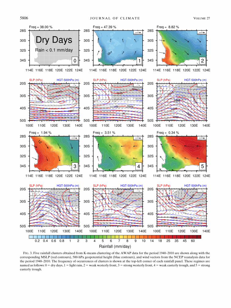
FIG. 3. Five rainfall clusters obtained from K-means clustering of the AWAP data for the period 1940–2010 are shown along with the

corresponding MSLP (red contours), 500-hPa geopotential height (blue contours), and wind vectors from the NCEP reanalysis data for

the period 1948–2010. The frequency of occurrences of clusters is shown at the top-left corner of each rainfall panel. These regimes are

named as follows: 05 dry days, 15 light rain, 25weak westerly front, 35 strong westerly front, 45weak easterly trough, and 55 strong

easterly trough.

5806 JOURNAL OF CL IMATE VOLUME 27

clusters 4 and 5. The rainfall reduction in May and Oc-

tober in clusters 2 and 3 is more or less compensated by

an increase in the frequency of cluster 4. The frequency

of cluster 4 has also increased in the winter months of

July and August, which may have increased the inland

rainfall at the expense of the coastal rainfall in the

winter.

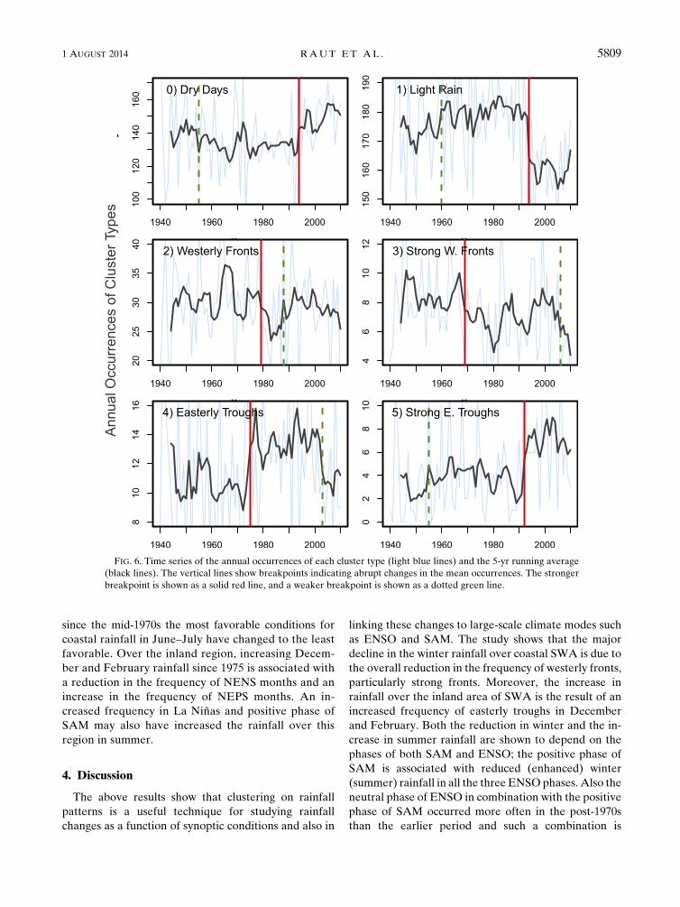
Figure 6 shows the annual occurrences of each cluster

with the vertical lines showing breakpoints in the time

series defined by the rapid changes in the means of the

distributions. The red (solid) line marks the location of

the most abrupt change in the mean and the green

(dashed) line indicates the second strongest change.

Cluster 2 has a breakpoint in the late 1970s, whereas

cluster 3 has a breakpoint in the late 1960s. The fre-

quency of both clusters has fallen after the breakpoint

year. However, cluster 2 recovered from the decline in

the late 1980s while the occurrences of cluster 3 re-

mained low and fell further after the year 2000. Thus, the

reduction in the frequencies of clusters 2 and 3 explains

the abrupt decrease in the winter rainfall in the 1970s.

Note that the breakpoint in the occurrences of cluster 3

after 2000 is the weaker of the two. A large reduction in

the light rain days during the 1990s suggests that the

reduction in rainfall over last two decades is largely due

to the reduction in light rain days associated with west-

erlies and it may include very weak fronts. A reduction

(increase) of approximately 15 light rain (dry) days per

annumhas occurred since 1990, implying the frequency of

dry days has increased at the expense of light rain days.

The breakpoints of clusters 4 and 5 more or less co-

incide with the breakpoints found in other clusters. In

particular, there is an increase in the occurrence of

cluster 4 around 1975 and a reduction after 2000; there is

also a considerable (.50%) increase in cluster 5 in the

early 1990s. Thus, the increment in summer rainfall over

the inland area is due to the increased frequency of rainy

days associated with easterly troughs.

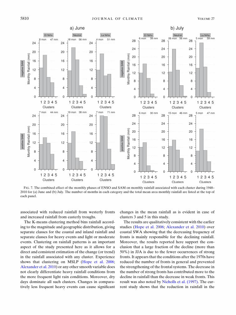
d. Effect of SAM and ENSO on the rainfall

To assess the effect of the SOI and SAM on the

rainfall clusters, the monthly rainfall from each cluster

is plotted for each combination of the three phases of

ENSO and two phases of SAM. Amonth is categorized

as neutral when the SOI lies between 68, El Niñowhen the SOI is less than 28, and La Niña when theSOI exceeds 8. For the brevity, only 4 months—namely, June, July, December, and February—are

shown in Figs. 7 and 8. The effect of the ENSO and

SAM combination is dramatically different in some

adjacent months.

In June (Fig. 7), a positive phase of SAM coupled with

a neutral ENSO phase is associated with reduced rain-

fall along the coast from clusters 2 and 3. The rainfall

from cluster 3 is approximately 5mm per month when

the SAM is positive but 16mm per month when it is

negative. Similarly, the rainfall from cluster 2 changes

from 22 to 17mm per month when SAM shifts from

a negative to a positive phase. In a La Niña phasehowever, rainfall from the light rain cluster and thewesterly fronts clusters (clusters 1 and 2) increases tomore than double that in the positive SAM phase. Incontrast, the coastal rainfall in July for a positive phase ofSAM is approximately 20% lower than in a negativephase of SAM, irrespective of the phase of ENSO.Overall, a positive phase of SAM is associated with thereduction of the coastal rainfall in all the ENSO phases.El Niño is the least favorable condition for coastalrainfall when SAM is negative, although, when SAM ispositive, neutral ENSO and El Niño phases are bothassociated with lower coastal rainfall, thus increasing thefrequency of drier periods over the region.In December (Fig. 8), a positive phase of SAM is as-

sociated with an increase in the rainfall from cluster 4 by

2–6 times in all the phases of ENSO. Except during an El

Niño phase, the positive phase of SAM also tends toincrease the light rainfall from cluster 1. Similarly, Feb-ruary rainfall from cluster 4 increases in positive phasesof SAM.During an El Niño, however, a negative SAM isaccompanied by increases in the coastal rainfall from thestrong westerly fronts (cluster 3). Thus, the effect ofENSO phases on the SWA rainfall is highly dependenton the phase of SAM.

FIG. 4. (a) Mean monthly occurrences of the rainfall clusters.

(b) Mean monthly accumulation of rainfall associated with

the clusters.

1 AUGUST 2014 RAUT ET AL . 5807

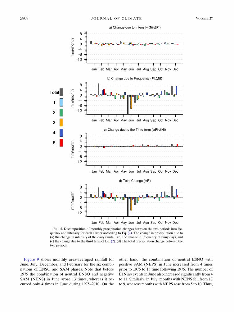
Figure 9 shows monthly area-averaged rainfall for

June, July, December, and February for the six combi-

nations of ENSO and SAM phases. Note that before

1975 the combination of neutral ENSO and negative

SAM (NENS) in June arose 13 times, whereas it oc-

curred only 4 times in June during 1975–2010. On the

other hand, the combination of neutral ESNO with

positive SAM (NEPS) in June increased from 4 times

prior to 1975 to 15 time following 1975. The number of

El Niño events in June also increased significantly from 4to 11. Similarly, in July, months with NENS fell from 17to 9, whereas months with NEPS rose from 5 to 10. Thus,

FIG. 5. Decomposition of monthly precipitation changes between the two periods into fre-

quency and intensity for each cluster according to Eq. (2). The change in precipitation due to

(a) the change in intensity of the daily rainfall, (b) the change in frequency of rainy days, and

(c) the change due to the third term of Eq. (2). (d) The total precipitation change between the

two periods.

5808 JOURNAL OF CL IMATE VOLUME 27

since the mid-1970s the most favorable conditions forcoastal rainfall in June–July have changed to the least

favorable. Over the inland region, increasing Decem-

ber and February rainfall since 1975 is associated with

a reduction in the frequency of NENS months and an

increase in the frequency of NEPS months. An in-

creased frequency in La Niñas and positive phase ofSAM may also have increased the rainfall over thisregion in summer.

4. Discussion

The above results show that clustering on rainfall

patterns is a useful technique for studying rainfall

changes as a function of synoptic conditions and also in

linking these changes to large-scale climate modes such

as ENSO and SAM. The study shows that the major

decline in the winter rainfall over coastal SWA is due to

the overall reduction in the frequency of westerly fronts,

particularly strong fronts. Moreover, the increase in

rainfall over the inland area of SWA is the result of an

increased frequency of easterly troughs in December

and February. Both the reduction in winter and the in-

crease in summer rainfall are shown to depend on the

phases of both SAM and ENSO; the positive phase of

SAM is associated with reduced (enhanced) winter

(summer) rainfall in all the threeENSOphases. Also the

neutral phase of ENSO in combination with the positive

phase of SAM occurred more often in the post-1970s

than the earlier period and such a combination is

FIG. 6. Time series of the annual occurrences of each cluster type (light blue lines) and the 5-yr running average

(black lines). The vertical lines show breakpoints indicating abrupt changes in the mean occurrences. The stronger

breakpoint is shown as a solid red line, and a weaker breakpoint is shown as a dotted green line.

1 AUGUST 2014 RAUT ET AL . 5809

associated with reduced rainfall from westerly fronts

and increased rainfall from easterly troughs.

The K-means clustering method bins rainfall accord-

ing to the magnitude and geographic distribution, giving

separate classes for the coastal and inland rainfall and

separate classes for heavy events and light or moderate

events. Clustering on rainfall patterns is an important

aspect of the study presented here as it allows for a

direct and consistent estimation of the change (or trend)

in the rainfall associated with any cluster. Experience

shows that clustering on MSLP (Hope et al. 2006;

Alexander et al. 2010) or any other smooth variable does

not clearly differentiate heavy rainfall conditions from

the more frequent light rain conditions. Moreover, dry

days dominate all such clusters. Changes in compara-

tively less frequent heavy events can cause significant

changes in the mean rainfall as is evident in case of

clusters 3 and 5 in this study.

The results are qualitatively consistent with the earlier

studies (Hope et al. 2006; Alexander et al. 2010) over

coastal SWA showing that the decreasing frequency of

fronts is mainly responsible for the declining rainfall.

Moreover, the results reported here support the con-

clusion that a large fraction of the decline (more than

50%) in JJA is due to the fewer occurrences of strong

fronts. It appears that the conditions after the 1970s have

reduced the number of fronts in general and prevented

the strengthening of the frontal systems. The decrease in

the number of strong fronts has contributed more to the

decline in rainfall than the decrease in weak fronts. This

result was also noted by Nicholls et al. (1997). The cur-

rent study shows that the reduction in rainfall in the

FIG. 7. The combined effect of the monthly phases of ENSO and SAM on monthly rainfall associated with each cluster during 1948–

2010 for (a) June and (b) July. The number of months in each category and the total mean area monthly rainfall are listed at the top of

each panel.

5810 JOURNAL OF CL IMATE VOLUME 27

1970s was mainly due to fewer fronts, whereas an in-

crease in the number of dry days, associated with the

persistent high, is responsible for the recent decline in

the 1990s (see Fig. 6). A reduction in the frequency of

fronts did not increase the number of dry days in the

1970s and the change in light rain days was also small.

The increased rainfall over the inland area is due to an

increase in the frequency of raining easterly troughs,

although, without any objective method to identify such

troughs, it is difficult to know whether the frequency of

all troughs (both wet and dry) changed during this pe-

riod. Recently, a front detection method used in Berry

et al. (2011b) showed a higher frequency of fronts inDJF

as compared to JJA and an increasing trend in annual

frequency of fronts over SWA (Berry et al. 2011a).

Using the same method Catto et al. (2012a) showed that

a large fraction of the DJF rainfall is connected to warm

fronts, whereas JJA rainfall is mainly connected to cold

fronts. It is likely that many of the fronts over Western

Australia detected by Berry et al. (2011b) are associated

with the easterly troughs and the increase in the number

of summertime easterly troughs is reflected in the annual

increase of the number of fronts. As the frequency of

frontal clusters (i.e., clusters 2 and 3) fell in the 1970s and

the data used by Berry et al. (2011a) only start in 1989,

this reduction is not evident in their study. A more fo-

cused study using objective analysis is required to de-

termine the seasonal trends in fronts, troughs, and cutoff

lows in this area.

Hendon et al. (2007) concluded that the effect of SAM

is comparable to the effect of the ESNOon coastal SWA

rainfall in winter. Moreover, the current results suggest

that a positive phase of SAM dramatically affects the

development of fronts in winter and also strengthens

easterly troughs in summer, producing up to 5 times the

rainfall in some situations (Fig. 8). The effect of SAMon

FIG. 8. As in Fig. 7, but for (a) December and (b) February.

1 AUGUST 2014 RAUT ET AL . 5811

rainfall is most pronounced during the neutral phase of

ENSO, which occurs more often than the El Niño andLa Niña phases combined. For example, during 1948–2010 only 22 Julys were classified as El Niño or La Niñabut 41 Julys were neutral. Consequently, the phase ofSAM has much greater influence during these neutralmonths, resulting in a long-term trend in SWA rainfall.In addition, the change in ENSO from El Niño to neu-tral condition significantly affects the monthly rainfallwhereas the change from neutral to La Niña only slightlyaffects it. In contrast to the results of Meneghini et al.

(2007) and Risbey et al. (2009), the monthly SAM index

is shown to strongly influence SWA rainfall. This dif-

ference could be due to the inability of correlation

analysis to capture the exact strength of the nonlinear

and interdependent relationship between rainfall and

the SAM index.

A reduction in the strength of the southern hemi-

spheric subtropical jet stream and an associated pole-

ward displacement of the storm tracks is linked to the

declining coastal rainfall in winter (Frederiksen and

Frederiksen 2007; Frederiksen et al. 2011) and enhanc-

ing the inland rainfall in summer. During the positive

phase of SAM, the poleward shift in the subtropical jet

increases the precipitation at the poleward flank of the

jet and decreases it over the subtropical latitudes in

winter (Hendon et al. 2014). In summer, a southward

shift in the westerlies associated with positive phase of

SAM allows easterly troughs to penetrate more fre-

quently into higher latitudes.

The recent phase 5 of the Climate Model Intercom-

parison Project (CMIP5) simulations for this century,

using the representative concentration pathway 4.5

(RCP4.5) greenhouse gas emission scenario, show a very

weak negative trend in the SAM index, in contrast

a strong positive trend is projected when the RCP8.5

scenario is used (Zheng et al. 2013). Polade et al. (2014)

also showed 10–20 fewer rainy days and at least a 10%

reduction in the total annual rainfall over SWA in

CMIP5 models for the RCP8.5 emission scenario,

compared to the historical simulations. In the light of

these results, the current study should be extended

using CMIP5 simulations of SAM, ENSO, and rainfall

over SWA.

Acknowledgments. This work received funding from

Cooperative Research Centre for Water Sensitive Cit-

ies. NCEP–NCAR reanalysis data were obtained from

NOAA portal. AWAP data were obtained from Bureau

of Meteorology with the help of Ailie Gallant. The au-

thors thank Michael J. Murphy and Jackson Tan for

valuable suggestions they offered during the scientific

writing workshop conducted by ARC Centre of Excel-

lence for Climate System Science. The NCAR Command

FIG. 9. A 5-point running average of the monthly rainfall time series for (a) June, (b) July, (c) December, and

(d) February. Monthly rainfall accumulations are plotted with the colored symbols corresponding to SAM–ENSO

combinations as shown in Fig. 7 and 8.

5812 JOURNAL OF CL IMATE VOLUME 27

Language (NCL; http://dx.doi.org/10.5065/D6WD3XH5),

R Programming language (http://www.R-project.org),

and Climate Data Operators (CDO) were used for data

analysis and plotting purposes. We are grateful to James

Risbey and an anonymous reviewer for their insightful

comments.

REFERENCES

Alexander, L. V., P. Uotila, N. Nicholls, and A. Lynch, 2010: A

new daily pressure dataset for Australia and its applica-

tion to the assessment of changes in synoptic patterns during

the last century. J. Climate, 23, 1111–1126, doi:10.1175/

2009JCLI2972.1.

Allan, R. J., and M. R. Haylock, 1993: Circulation features asso-

ciatedwith thewinter rainfall decrease in southwesternAustralia.

J. Climate, 6, 1356–1367, doi:10.1175/1520-0442(1993)006,1356:

CFAWTW.2.0.CO;2.

Anderberg, M. R., 1973: Cluster Analysis for Applications. Aca-

demic Press, 359 pp.

Ansell, T. J., C. J. C. Reason, I. N. Smith, and K. Keay, 2000: Ev-

idence for decadal variability in southern Australian rainfall

and relationships with regional pressure and sea surface tem-

perature. Int. J. Climatol., 20, 1113–1129, doi:10.1002/

1097-0088(200008)20:10,1113::AID-JOC531.3.0.CO;2-N.

Bates, B. C., P. Hope, B. Ryan, I. Smith, and S. Charles, 2008: Key

findings from the Indian Ocean Climate Initiative and their

impact on policy development in Australia. Climatic Change,

89, 339–354, doi:10.1007/s10584-007-9390-9.Berry, G., C. Jakob, andM. Reeder, 2011a: Recent global trends in

atmospheric fronts.Geophys. Res. Lett., 38, L21812, doi:10.1029/

2011GL049481.

——, M. J. Reeder, and C. Jakob, 2011b: A global climatology

of atmospheric fronts. Geophys. Res. Lett., 38, L04809,

doi:10.1029/2010GL046451.

Catto, J. L., C. Jakob, G. Berry, and N. Nicholls, 2012a: Relating

global precipitation to atmospheric fronts. Geophys. Res.

Lett., 39, L10805, doi:10.1029/2012GL051736.

——, ——, and N. Nicholls, 2012b: The influence of changes in

synoptic regimes on north Australian wet season rainfall

trends. J. Geophys. Res., 117, D10102, doi:10.1029/

2012JD017472.

Chowdhury, R. K., and S. Beecham, 2010: Australian rainfall

trends and their relation to the Southern Oscillation index.

Hydrol. Processes, 24, 504–514, doi:10.1002/hyp.7504.Feng, J., J. Li, and Y. Li, 2010: Is there a relationship between the

SAM and southwest Western Australian winter rainfall?

J. Climate, 23, 6082–6089, doi:10.1175/2010JCLI3667.1.Fierro, A. O., and L. M. Leslie, 2013: Links between central

west Western Australian rainfall variability and large-scale

climate drivers. J. Climate, 26, 2222–2246, doi:10.1175/

JCLI-D-12-00129.1.

Frederiksen, J. S., and C. S. Frederiksen, 2007: Interdecadal

changes in Southern Hemisphere winter storm track modes.

Tellus, 59A, 599–617, doi:10.1111/j.1600-0870.2007.00264.x.——, ——, S. L. Osbrough, and J. M. Sisson, 2011: Changes in

Southern Hemisphere rainfall, circulation and weather sys-

tems. Proc. 19th Int. Congress on Modelling and Simulation,

Perth, WA, Australia, Modelling and Simulation Society of

Australia and New Zealand, 2712–2718. [Available online at

http://www.mssanz.org.au/modsim2011/index.htm.]

Gallant, A. J. E., M. J. Reeder, J. S. Risbey, and K. J. Hennessy,

2013: The characteristics of seasonal-scale droughts in Aus-

tralia, 1911–2009. Int. J. Climatol., 33, 1658–1672, doi:10.1002/

joc.3540.

Gong, D., and S. Wang, 1999: Definition of Antarctic oscillation

index. Geophys. Res. Lett., 26, 459–462, doi:10.1029/

1999GL900003.

Hendon, H. H., D. W. J. Thompson, and M. C. Wheeler, 2007:

Australian rainfall and surface temperature variations asso-

ciated with the Southern Hemisphere annular mode. J. Cli-

mate, 20, 2452–2467, doi:10.1175/JCLI4134.1.

——, E.-P. Lim, and H. Nguyen, 2014: Seasonal variations

of subtropical precipitation associated with the southern an-

nular mode. J. Climate, 27, 3446–3460, doi: 10.1175/JCLI-D-13-

00550.1.

Hope, P., W. Drosdowsky, and N. Nicholls, 2006: Shifts in the

synoptic systems influencing southwest Western Australia.

Climate Dyn., 26, 751–764, doi:10.1007/s00382-006-0115-y.

——, andCoauthors, 2014:A comparison of automatedmethods of

front recognition for climate studies: A case study in southwest

WesternAustralia.Mon.Wea. Rev., 142, 343–363, doi:10.1175/

MWR-D-12-00252.1.

IOCI, 2002: Climate variability and change in south west Western

Australia. IOCI Rep., 34 pp.

Jones, D., W. Wang, and R. Fawcett, 2009: High-quality spatial

climate data-sets for Australia.Aust. Meteor. Oceanogr. J., 58,

233–248.

Kalnay, E., and Coauthors, 1996: The NCEP/NCAR 40-Year Re-

analysis Project. Bull. Amer. Meteor. Soc., 77, 437–471,

doi:10.1175/1520-0477(1996)077,0437:TNYRP.2.0.CO;2.

Li, F., L. E. Chambers, and N. Nicholls, 2005: Relationships be-

tween rainfall in the southwest ofWestern Australia and near-

global patterns of sea-surface temperature and mean sea-level

pressure variability. Aust. Meteor. Mag., 54, 23–33.McBride, J. L., and N. Nicholls, 1983: Seasonal relationships be-

tween Australian rainfall and the Southern Oscillation. Mon.

Wea.Rev.,111,1998–2004, doi:10.1175/1520-0493(1983)111,1998:

SRBARA.2.0.CO;2.

Meneghini, B., I. Simmonds, and I. N. Smith, 2007: Association

between Australian rainfall and the southern annular mode.

Int. J. Climatol., 27, 109–121, doi:10.1002/joc.1370.Nicholls, N., 2006: Detecting and attributing Australian climate

change: A review. Aust. Meteor. Mag., 55, 199–211.

——, 2010: Local and remote causes of the southern Australian

autumn–winter rainfall decline, 1958–2007. Climate Dyn., 34,

835–845, doi:10.1007/s00382-009-0527-6.

——, L. Chambers, M. Haylock, C. S. Frederiksen, D. Jones, and

W. Drosdowsky, 1997: Climate variability and predictability

for south-west Western Australia. IOCI Phase 1 Rep., 52 pp.

Pezza, A. B., T. Durrant, I. Simmonds, and I. Smith, 2008: Southern

hemisphere synoptic behavior in extreme phases of SAM,

ENSO, sea ice extent, and southern Australia rainfall. J. Cli-

mate, 21, 5566–5584, doi:10.1175/2008JCLI2128.1.

Pitman, A. J., G. T. Narisma, R. A. Pielke Sr., and N. J. Holbrook,

2004: Impact of land cover change on the climate of southwest

WesternAustralia. J. Geophys. Res., 109,D18109, doi:10.1029/

2003JD004347.

Polade, S. D., D.W. Pierce, D. R. Cayan, A. Gershunov, andM. D.

Dettinger, 2014: The key role of dry days in changing regional

climate and precipitation regimes. Sci. Rep., 4, 4364,

doi:10.1038/srep04364.

Pook, M. J., J. S. Risbey, and P. C. McIntosh, 2012: The synoptic

climatology of cool-season rainfall in the central wheatbelt of

1 AUGUST 2014 RAUT ET AL . 5813

Western Australia. Mon. Wea. Rev., 140, 28–43, doi:10.1175/

MWR-D-11-00048.1.

——, ——, and ——, 2013: A comparative synoptic climatology

of cool-season rainfall in major grain-growing regions of

southern Australia. Theor. Appl. Climatol., doi:10.1007/

s00704-013-1021-y.

Pope, M., C. Jakob, and M. J. Reeder, 2009: Regimes of the north

Australian wet season. J. Climate, 22, 6699–6715, doi:10.1175/2009JCLI3057.1.

Qi, L., L. M. Leslie, and S. X. Zhao, 1999: Cut-off low pres-

sure systems over southern Australia: Climatology and

case study. Int. J. Climatol., 19, 1633–1649, doi:10.1002/

(SICI)1097-0088(199912)19:15,1633::AID-JOC445.3.0.CO;2-0.

Raupach, M. R., P. Briggs, V. Haverd, E. King, M. Paget, and

C. Trudinger, 2008: Australian Water Availability Project:

CSIROMarine and Atmospheric Research component: Final

report for phase 3. CAWCR Tech. Rep. 013, 67 pp. [Avail-

able online at http://www.csiro.au/awap/doc/CTR_013_

online_FINAL.pdf.]

Risbey, J. S., M. J. Pook, P. C. McIntosh, M. C.Wheeler, and H. H.

Hendon, 2009: On the remote drivers of rainfall variability in

Australia. Mon. Wea. Rev., 137, 3233–3253, doi:10.1175/

2009MWR2861.1.

——, ——, and ——, 2013: Spatial trends in synoptic rainfall

in southern Australia. Geophys. Res. Lett., 40, 3781–3785,doi:10.1002/grl.50739.

Smith, I. N., P. C. McIntosh, T. J. Ansell, C. J. C. Reason, and

K. McInnes, 2000: Southwest Western Australian winter

rainfall and its association with Indian Ocean climate vari-

ability. Int. J. Climatol., 20, 1913–1930, doi:10.1002/

1097-0088(200012)20:15,1913::AID-JOC594.3.0.CO;2-J.

Stone, R. C., 1989: Weather types at Brisbane, Queensland: An

example of the use of principal components and cluster anal-

ysis. Int. J. Climatol., 9, 3–32, doi:10.1002/joc.3370090103.

Suppiah, R., and K. J. Hennessy, 1998: Trends in total rainfall,

heavy rain events and number of dry days in Australia,

1910–1990. Int. J. Climatol., 18, 1141–1164, doi:10.1002/

(SICI)1097-0088(199808)18:10,1141::AID-JOC286.3.0.CO;2-P.

Zheng, F., J. Li, R. T. Clark, and H. C. Nnamchi, 2013: Simulation

and projection of the Southern Hemisphere annular mode

in CMIP5 models. J. Climate, 26, 9860–9879, doi:10.1175/

JCLI-D-13-00204.1.

5814 JOURNAL OF CL IMATE VOLUME 27