Radiometric cross-calibration of spaceborne scatterometers: first results

Radiometric Cross-Calibration of Spaceborne Scatterometers- First Results

Anis Elyouncha, Xavier Neyt and Marc Acheroy

Royal Military Academy, Brussels, Belgium

ABSTRACTThe main application of a scatterometer is the determination of the wind speed and direction at the sea surface. Thisis achieved by measuring the radar backscattering coefficient in three different directions and inverting these measure-ments using a geophysical model function (GMF). The scientific value of the data is directly related to the quality of theradiometric calibration.

There are currently two european C-band scatterometers operating, one on-board the ERS-2 spacecraft launched in1995 and the other on-board METOP-A, launched in 2006. The similarity of the two scatterometers is an opportunityto ensure the continuity of more than 15 years of global scatterometer measurements. To achieve the consistency of thebackscattering coefficients data sets, required for long-term climate studies, an accurate cross-calibration is vital. Thecross-calibration is made possible since the two spacecrafts operate simultaneously from 2006 up to now.

As the backscattering coefficients measured by the scatterometers depend on acquisition time, location on the groundand on the geometry of the measurements (incidence and look angle), a direct comparison of measurements made by bothinstruments is practically impossible.

In particular cases, models can be used to cope with measurement differences. On the rain forest, assumed to betime-invariant, homogeneous and isotropic, the backscattering coefficient depends only on the incidence angle, and theconstant gamma model can be used to cope with the incidence angle effects. On some ice covered areas (e.g. Greenlandand Antarctica), assuming that the ice surface is isotropic, the ice line model can be used. It is a function of incidenceangle and ice age and depends on the location. On the ocean, which is inherently not stable in time, the CMOD5 GMFis used. CMOD5 relates the observed backscatter to the geophysical parameters which are the wind speed and winddirection. Using the last model, measurement biases can be assessed making simultaneous observations unnecessary.

In this article, we present a cross-calibration methodology and present first results.

Keywords: Cross-calibration, Ocean calibration, Scatterometer

1. INTRODUCTIONThe increasing number of spaceborne sensors measuring wind fields (scatterometers) has made it desirable to integratewind data from various sources to achieve improved accuracy. To assure data continuity and consistency, it’s necessary toperform cross-calibrations of these sources.

The main objective of a scatterometer is the determination of backscattering coefficients of the Earth. ASCAT andAMI are spaceborne active real aperture C-band radars, operating on-board METOP-A and ERS-2 respectively. ERS-2was launched in April 1995 to continue the ERS-1 mission and METOP was launched in October 2006. Both satelliteshave a sun-synchronous near polar orbit.

Several studies have been carried out to assess the consistency of the wind data provided by various instruments,1 and2

performed a statistical comparison of wind estimates whereas other studies3 and4 compared the measured backscatterusing calibration targets and models.1 compared the winds obtained from the microwave radiometer IRS-P4 and the ERS-2 scatterometer, the mean bias was shown to be dependent on regions where it ranges from 3ms−1 in the tropics and 6ms−1

at high latitudes, and on wind speed range, being highest for the low wind speed range (6ms−1) and low for high wind

Further author information: (Send correspondence to Anis Elyouncha) E-mail: [email protected], Telephone: +32 2 7376665, Address: Signal and Image Center, Electrical Engineering Dept, Royal Military Academy, 30 av de la Renaissance, B-1000Brussels, Belgium

speed ranges (2.3ms−1).2 compared three wind data sources TOPEX, NSCAT and ECMWF, the satellite derived windspeeds (TOPEX and NSCAT) are found to have a large overall bias but a smaller variance compared to ECMWF winds,implying that errors associated with satellite data are mostly systematic, the largest bias (0.63ms−1) reported in this studywas between TOPEX and NSCAT and the smallest bias (−0.23ms−1) is between NSCAT and ECMWF winds.

3 performed a cross-calibration between an airborne SAR and ground-based polarimetric scatterometer measurementsat L and C bands. In that work, both distributed and point targets were employed. The distributed surfaces were of typebare surfaces (with varying roughness) and surfaces covered with vegetation (short and tall grass). A trihedral cornerreflector was used for calibrating the airborne SAR. The ground scatterometer was calibrated using a metallic sphere.A comparison of the backscattering coefficients measured by the SAR system and the ground scatterometer using pointtargets showed a maximum discrepancy of 5 dB at C-band. Whereas using the roughest area as calibration target was themost accurate solution with a deviation of about 1 dB.

The calibration of SeaWinds and Quikscat Scatterometers (Ku band) using two land regions, the Amazon rain forestand the Sahara desert is reported in.4 A first order polynomial model was used for both regions in order to remove theincidence angle dependence of σ0. For QuikSCAT, in the Amazon region a maximum difference of backscatter of 0.5dBhas been observed between the morning (6-7 AM) and the evening (6-7 PM) passes at low incidence angles and 0.6dB athigh incidence angles. This difference is due to the presence of dew in the early morning on the rain forest foliage at theoverpass time of QuikSCAT.4 SeaWinds showed a difference of 0.1dB between the 10-11 AM and the 10-11 PM passeswhich is consistent with the results of previous investigations.5, 6 It was shown that the Sahara region was temporallystable with no daily moisture variation but less homogeneous and much noisier than the Amazon region. This means thatthe daily standard deviation of 1.8dB over the desert is larger than over the Amazon region (0.5dB).4 For a given localtime of day the standard deviation of the daily mean backscatter is less than 0.18dB for both regions which is an additionalproof of their temporal stability. The results indicate that the QuikSCAT and SeaWinds scatterometers are calibrated towithin 0.05dB.4

The first section is dedicated to the cross-calibration using collocated measurements, the methodology will be de-scribed, examples of intersections will be shown and results of comparison of the winds will be presented, in sectin 2the ocean calibration method will be presented and applied to the two scatterometers measurements for cross-calibrationpurpose, in the last section comparison of the pair of data in measurements space will be shown and methods of correctionwill be proposed, finally conclusions will be given.

2. CROSS-CALIBRATION USING COLLOCATED MEASUREMENTS2.1. IntroductionThe cross-calibration of two instruments in general requires simultaneous observation of the same area on ground. Theimplicit assumption is that both measurements will be comparable. This imply that the geometry, such as the incidenceangle, is similar (or that the measured quantity is insensitive to the geometry).

Assuming the sensors have the same spatial resolution, even in the case of simultaneous observation of the same areaon the ground, a direct comparison of sigma naught measured by instruments will only be possible on extremely rareoccasions as the sigma naught depends on the geometry (incidence angle, look angle).

2.2. Method overviewThis method is motivated by the fact that a way to deal with the temporal variation of sigma naught is to bypass that vari-ability by comparing (near) simultaneous measurements. Stricto sensu, simultaneous measurements will never occur, sothe constraint is relaxed by requiring near simultaneous measurements. It is assumed that the variations of the backscatterdue to the acquisition time difference is negligible if the time difference between the measurements is small.

This method imply determining when swath intersections occur. Swath intersections are defined as (near) simultane-ous observation of the same spot by ERS-2/AMI and METOP/ASCAT instruments.

The acquisition geometry (incidence angle, look angle) will however typically be different and must be accounted forin a comparison. Over open ocean, this can be performed by comparing the wind speed and the wind direction, using theCMOD5 model.

2.3. Predicting simultaneous overpasses of two satellitesERS-2 has shorter orbital period (100 min) than METOP (101 min), this due to the higher altitude of METOP, henceslower angular velocity and longer orbital period. Consequently the lower-altitude satellite (ERS-2) will catch up with thehigher altitude (METOP). As a result, the two satellites will be approaching until the intersection and then start movingaway from each other until the next intersection. This will be regularly repeated.

The time between two successive intersections can be estimated using the expression7

T =1f1

τ2

τ2− τ1(1)

where T is the intersection period (days), τ1 and τ2 are the orbital periods for the two satellites and f1 is the number oforbits per day for the lower-altitude satellite.

As an example the exact∗ orbital period of ERS-2 is 100.53 min and the exact orbital period of METOP is 101.3 min.It follows that the time between successive intersections of ERS-2 and METOP is approximately 9.18 days.

2.4. Predicting the swath intersectionsAs was discussed above, the two scatterometers may view the same target area at nearly the same time.

ASCAT has two swaths (right and left) and ESCAT has only one swath on the right. The few minutes preceding theintersection of the two nadirs, ERS-2’s nadir is on the right of METOP’s nadir at the North pole and at the left at the Southpole. This implies that ERS-2’s swath overlaps first with the right swath of METOP then with the left swath. The oppositescenario happens at the South pole.

In order to conduct the computations of the intersection of the swath, the distance between the middle of each satellite’sswath is taken into account. For simplicity, the middle of the swath is taken as the intersection of the earth with a rayin the pointing direction of the mid-antenna. The angle between the normal to nadir and that direction is respectively ofγ = 29.3◦ and γ = 39◦ for ERS-2 and METOP/ASCAT.

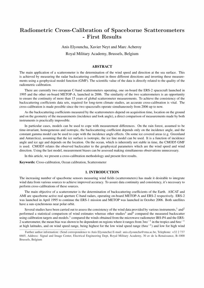
2.5. Examples of orbits intersectionsTo illustrate the locations of these intersections, the mid-beam swath intersections occurring between 01 December 2008and 30 November 2009 have been computed (using SGP4 and TLE’s as described above†). The results are depicted infigure 1. These plots confirm that the intersections occur at −76o and 85o (right swath) and around ±50o (left swath).

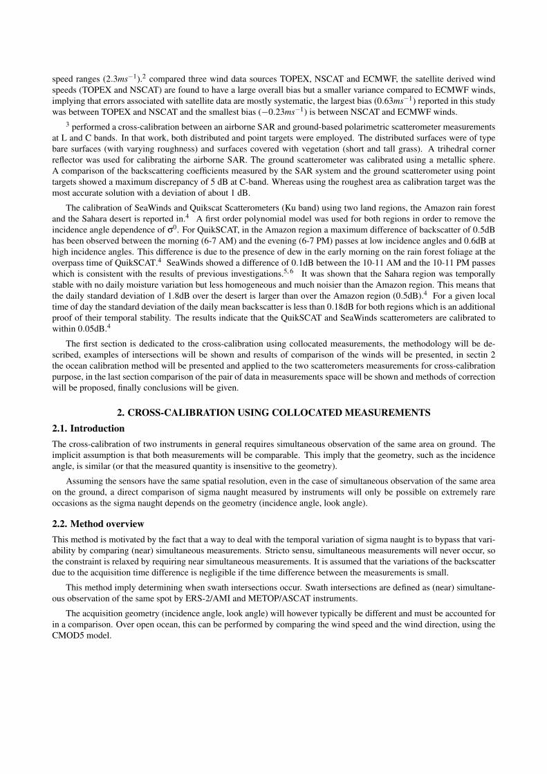
2.6. Cross-comparison of the inverted windsBackscattering coefficients from ERS-ASPS2.0 and ASCAT-L1b data were compared for the intersection of the 5 Dec2009. The node locations are depicted on figure 2.

The ASCAT nodes are pairwise matched to the ERS nodes which are within 30 sec and 25 km. Temporal differencesand spatial differences are neglected. The ASCAT nodes retained for comparison with ERS nodes are represented in greenon Figure 2. A total of approximately 2348 nodes where retained. All nodes are located over the ocean.

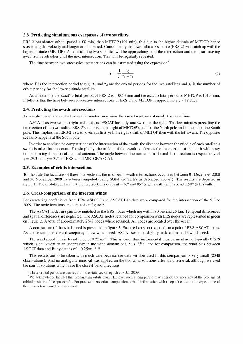
A comparison of the wind speed is presented in figure 3. Each red cross corresponds to a pair of ERS-ASCAT nodes.As can be seen, there is a discrepancy at low wind speed: ASCAT seems to slightly underestimate the wind speed.

The wind speed bias is found to be of 0.22ms−1. This is lower than instrumental measurement noise typically 0.2dBwhich is equivalent to an uncertainty in the wind domain of 0.5ms−1,8, 9 and for comparison, the wind bias betweenASCAT data and Buoy data is of −0.25ms−1.10

This results are to be taken with much care because the data set size used in this comparison is very small (2348observations). And no ambiguity removal was applied on the two wind solutions after wind retrieval, although we usedthe pair of solutions which have the closest wind directions.

∗These orbital period are derived from the state vector, epoch of 8 Jan 2009.†We acknowledge the fact that propagating orbits from TLE over such a long period may degrade the accuracy of the propagated

orbital position of the spacecrafts. For precise intersection computation, orbital information with an epoch closer to the expect time ofthe intersection would be considered.

Figure 1. ERS-2 - METOP intersections locations - North Pole (left) - South Pole (right) - (red: nadir; green: right swath; blue: leftswath)

3. CROSS-CALIBRATION USING OCEAN CALIBRATION METHODTo perform an ocean calibration the average of the measured backscatter measurements is divided by the mean simulatedbackscatter. In order to compute a simulated backscatter, background winds and geophysical model function (GMF) areneeded. The GMF links the observed backscatter to the geophysical parameters which are the wind speed and winddirection with respect to the radar beam φ. The model used in this paper is called CMOD5. It’s formulation is11

z(θ,V,φ) = B0(θ,V )(1+B1(θ,V )cosφ+B2(θ,V )cos2φ) (2)

where z = (σo)0.625

The current use of ocean calibration consists in the evaluation of the difference between the measurements of a givenscatterometer and the model CMOD5, in order to correct the antennas patterns of the instrument. We aim to use thismethod in order to cross-calibrate two scatterometers, i.e. to assess the difference between measurements.

3.1. OverviewWhen reference background winds are available they can be used to compute “reference” backscattering coefficientsto which the measured coefficients are compared. The CMOD5 geophysical model function is used to transform thewinds into backscatter triplets. The backscattering coefficients are averaged resolved per antenna and per node number orincidence angle. This is a direct application of the so-called ocean calibration.10–12

The disadvantage of this method is that it relies on the accuracy of the model. Since the model was obtained usingERS-2 winds, a methodological issue arises. Moreover, the range of incidence angles spanned by ASCAT is different(larger) than that of ERS/AMI. The effect of this on the model is uncertain.

The method used in this article is based on the method described in11 and.13 We will give a short description of themethod here, more details can be found in the two references cited above.

CMOD-5 GMF (2) is characterized by three parameters B0, B1 and B2. B0 is called the bias term, is monotonouslyincreasing with wind speed and represents the central axis of the cone. B1 and B2 are respectively the upwind/downwindand upwind/crosswind terms.

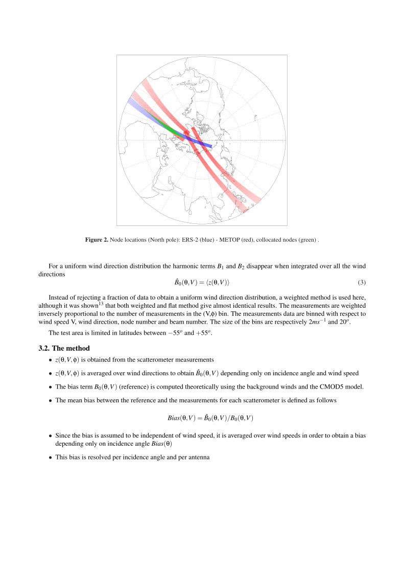
Figure 2. Node locations (North pole): ERS-2 (blue) - METOP (red), collocated nodes (green) .

For a uniform wind direction distribution the harmonic terms B1 and B2 disappear when integrated over all the winddirections

B̂0(θ,V ) = 〈z(θ,V )〉 (3)

Instead of rejecting a fraction of data to obtain a uniform wind direction distribution, a weighted method is used here,although it was shown13 that both weighted and flat method give almost identical results. The measurements are weightedinversely proportional to the number of measurements in the (V,φ) bin. The measurements data are binned with respect towind speed V, wind direction, node number and beam number. The size of the bins are respectively 2ms−1 and 20o.

The test area is limited in latitudes between −55o and +55o.

3.2. The method• z(θ,V,φ) is obtained from the scatterometer measurements

• z(θ,V,φ) is averaged over wind directions to obtain B̂0(θ,V ) depending only on incidence angle and wind speed

• The bias term B0(θ,V ) (reference) is computed theoretically using the background winds and the CMOD5 model.

• The mean bias between the reference and the measurements for each scatterometer is defined as follows

Bias(θ,V ) = B̂0(θ,V )/B0(θ,V )

• Since the bias is assumed to be independent of wind speed, it is averaged over wind speeds in order to obtain a biasdepending only on incidence angle Bias(θ)

• This bias is resolved per incidence angle and per antenna

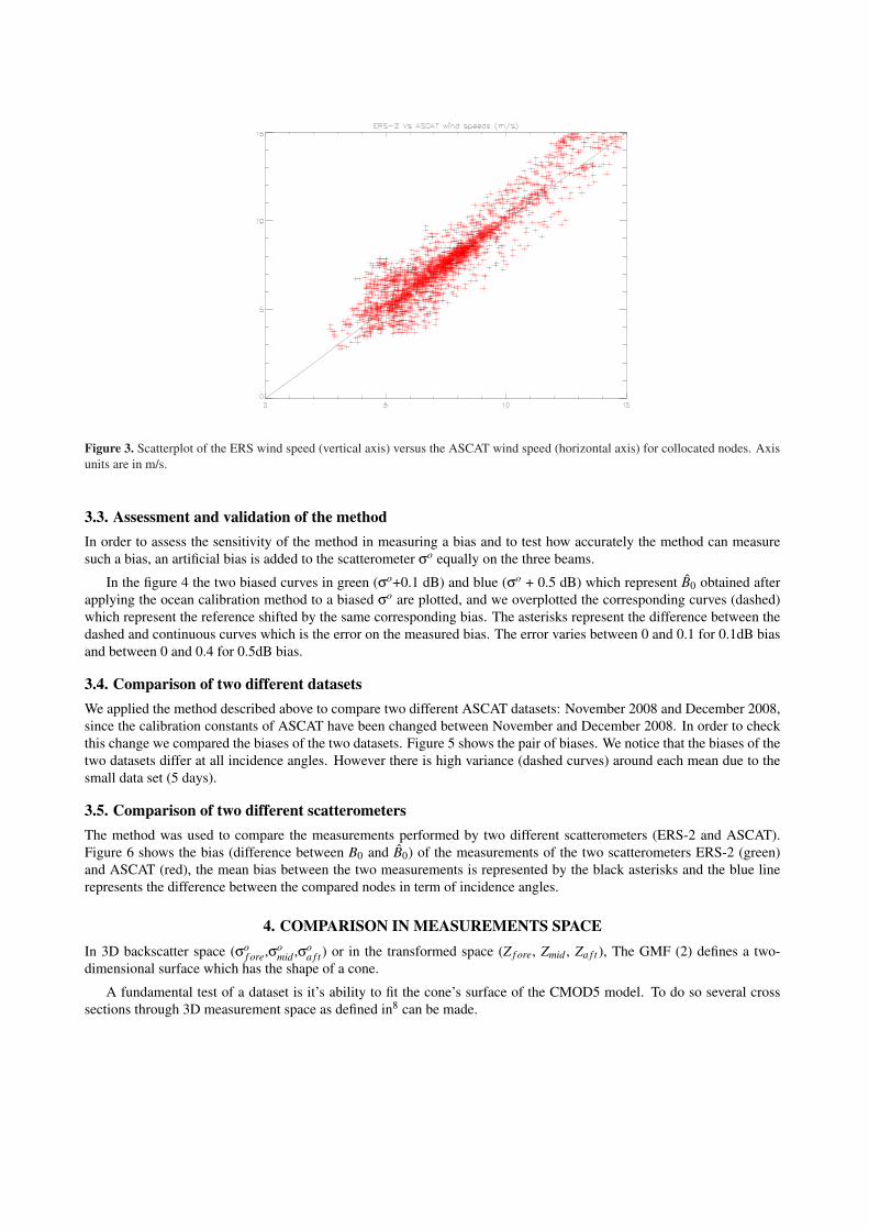
Figure 3. Scatterplot of the ERS wind speed (vertical axis) versus the ASCAT wind speed (horizontal axis) for collocated nodes. Axisunits are in m/s.

3.3. Assessment and validation of the methodIn order to assess the sensitivity of the method in measuring a bias and to test how accurately the method can measuresuch a bias, an artificial bias is added to the scatterometer σo equally on the three beams.

In the figure 4 the two biased curves in green (σo+0.1 dB) and blue (σo + 0.5 dB) which represent B̂0 obtained afterapplying the ocean calibration method to a biased σo are plotted, and we overplotted the corresponding curves (dashed)which represent the reference shifted by the same corresponding bias. The asterisks represent the difference between thedashed and continuous curves which is the error on the measured bias. The error varies between 0 and 0.1 for 0.1dB biasand between 0 and 0.4 for 0.5dB bias.

3.4. Comparison of two different datasetsWe applied the method described above to compare two different ASCAT datasets: November 2008 and December 2008,since the calibration constants of ASCAT have been changed between November and December 2008. In order to checkthis change we compared the biases of the two datasets. Figure 5 shows the pair of biases. We notice that the biases of thetwo datasets differ at all incidence angles. However there is high variance (dashed curves) around each mean due to thesmall data set (5 days).

3.5. Comparison of two different scatterometersThe method was used to compare the measurements performed by two different scatterometers (ERS-2 and ASCAT).Figure 6 shows the bias (difference between B0 and B̂0) of the measurements of the two scatterometers ERS-2 (green)and ASCAT (red), the mean bias between the two measurements is represented by the black asterisks and the blue linerepresents the difference between the compared nodes in term of incidence angles.

4. COMPARISON IN MEASUREMENTS SPACEIn 3D backscatter space (σo

f ore,σomid ,σo

a f t ) or in the transformed space (Z f ore, Zmid , Za f t ), The GMF (2) defines a two-dimensional surface which has the shape of a cone.

A fundamental test of a dataset is it’s ability to fit the cone’s surface of the CMOD5 model. To do so several crosssections through 3D measurement space as defined in8 can be made.

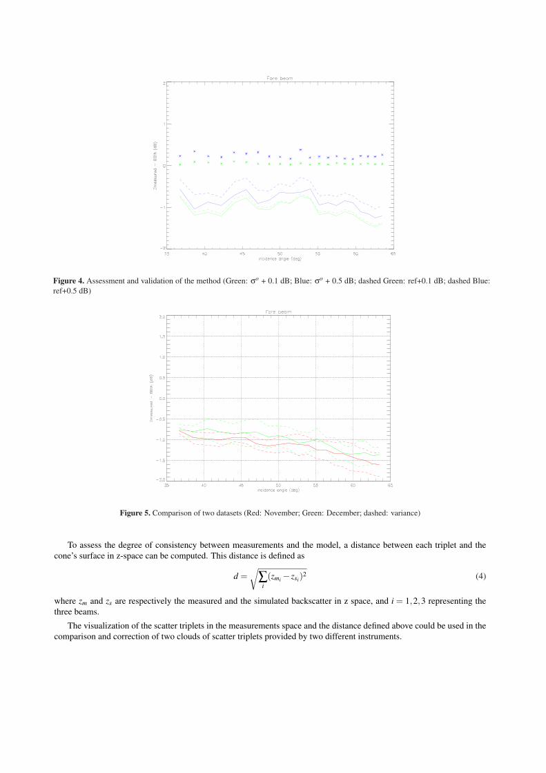
Figure 4. Assessment and validation of the method (Green: σo + 0.1 dB; Blue: σo + 0.5 dB; dashed Green: ref+0.1 dB; dashed Blue:ref+0.5 dB)

Figure 5. Comparison of two datasets (Red: November; Green: December; dashed: variance)

To assess the degree of consistency between measurements and the model, a distance between each triplet and thecone’s surface in z-space can be computed. This distance is defined as

d =√

∑i(zmi − zsi)2 (4)

where zm and zs are respectively the measured and the simulated backscatter in z space, and i = 1,2,3 representing thethree beams.

The visualization of the scatter triplets in the measurements space and the distance defined above could be used in thecomparison and correction of two clouds of scatter triplets provided by two different instruments.

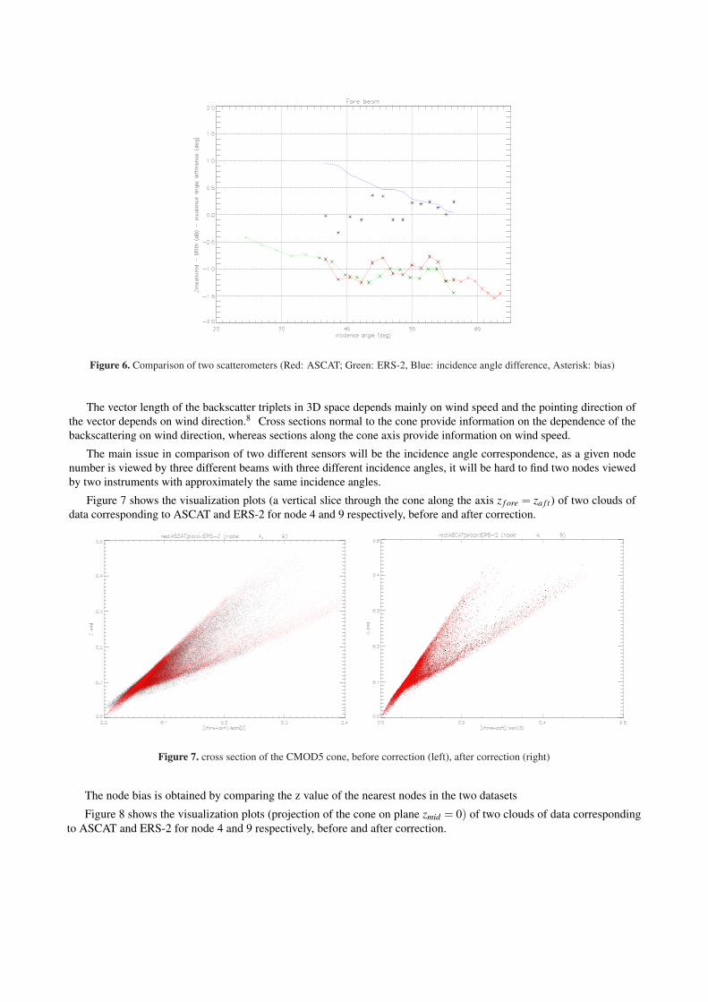
Figure 6. Comparison of two scatterometers (Red: ASCAT; Green: ERS-2, Blue: incidence angle difference, Asterisk: bias)

The vector length of the backscatter triplets in 3D space depends mainly on wind speed and the pointing direction ofthe vector depends on wind direction.8 Cross sections normal to the cone provide information on the dependence of thebackscattering on wind direction, whereas sections along the cone axis provide information on wind speed.

The main issue in comparison of two different sensors will be the incidence angle correspondence, as a given nodenumber is viewed by three different beams with three different incidence angles, it will be hard to find two nodes viewedby two instruments with approximately the same incidence angles.

Figure 7 shows the visualization plots (a vertical slice through the cone along the axis z f ore = za f t ) of two clouds ofdata corresponding to ASCAT and ERS-2 for node 4 and 9 respectively, before and after correction.

Figure 7. cross section of the CMOD5 cone, before correction (left), after correction (right)

The node bias is obtained by comparing the z value of the nearest nodes in the two datasets

Figure 8 shows the visualization plots (projection of the cone on plane zmid = 0) of two clouds of data correspondingto ASCAT and ERS-2 for node 4 and 9 respectively, before and after correction.

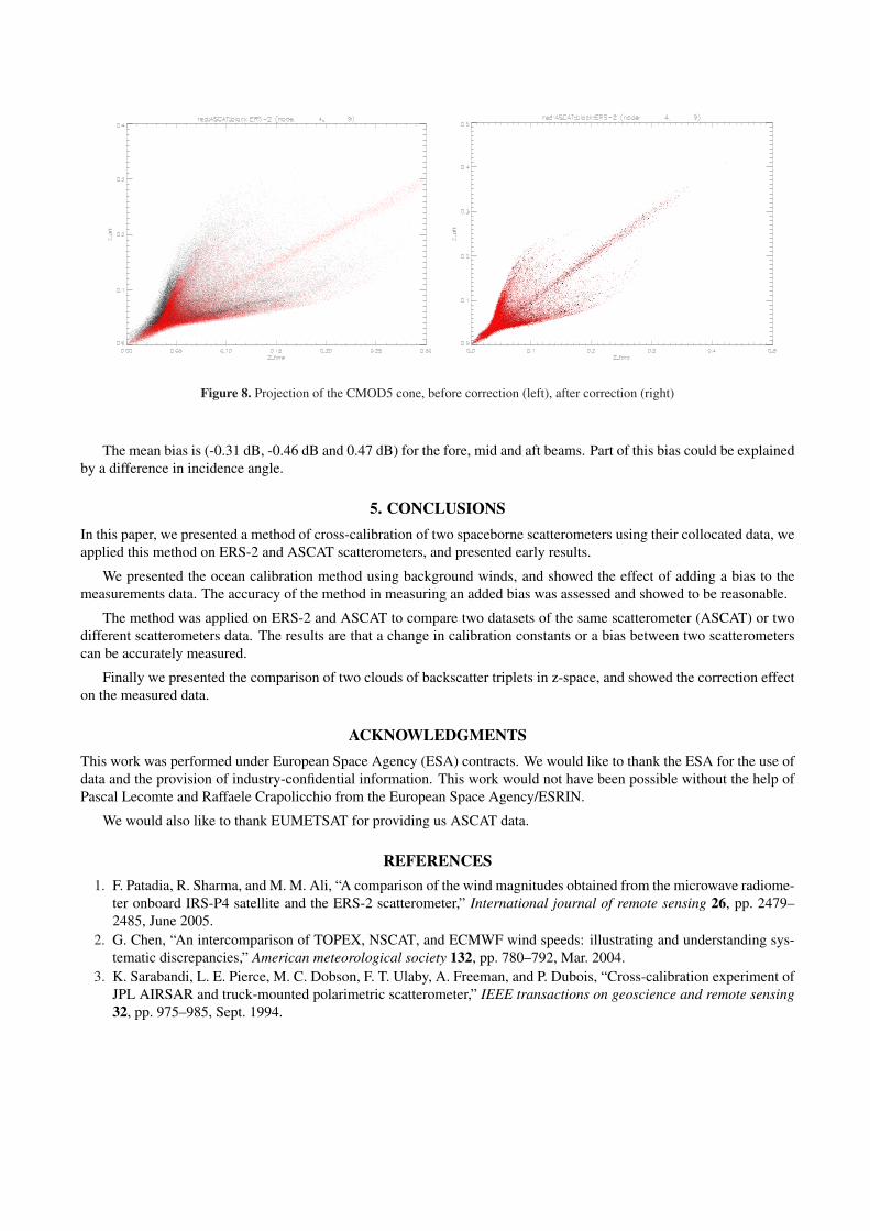
Figure 8. Projection of the CMOD5 cone, before correction (left), after correction (right)

The mean bias is (-0.31 dB, -0.46 dB and 0.47 dB) for the fore, mid and aft beams. Part of this bias could be explainedby a difference in incidence angle.

5. CONCLUSIONSIn this paper, we presented a method of cross-calibration of two spaceborne scatterometers using their collocated data, weapplied this method on ERS-2 and ASCAT scatterometers, and presented early results.

We presented the ocean calibration method using background winds, and showed the effect of adding a bias to themeasurements data. The accuracy of the method in measuring an added bias was assessed and showed to be reasonable.

The method was applied on ERS-2 and ASCAT to compare two datasets of the same scatterometer (ASCAT) or twodifferent scatterometers data. The results are that a change in calibration constants or a bias between two scatterometerscan be accurately measured.

Finally we presented the comparison of two clouds of backscatter triplets in z-space, and showed the correction effecton the measured data.

ACKNOWLEDGMENTSThis work was performed under European Space Agency (ESA) contracts. We would like to thank the ESA for the use ofdata and the provision of industry-confidential information. This work would not have been possible without the help ofPascal Lecomte and Raffaele Crapolicchio from the European Space Agency/ESRIN.

We would also like to thank EUMETSAT for providing us ASCAT data.

REFERENCES1. F. Patadia, R. Sharma, and M. M. Ali, “A comparison of the wind magnitudes obtained from the microwave radiome-

ter onboard IRS-P4 satellite and the ERS-2 scatterometer,” International journal of remote sensing 26, pp. 2479–2485, June 2005.

2. G. Chen, “An intercomparison of TOPEX, NSCAT, and ECMWF wind speeds: illustrating and understanding sys-tematic discrepancies,” American meteorological society 132, pp. 780–792, Mar. 2004.

3. K. Sarabandi, L. E. Pierce, M. C. Dobson, F. T. Ulaby, A. Freeman, and P. Dubois, “Cross-calibration experiment ofJPL AIRSAR and truck-mounted polarimetric scatterometer,” IEEE transactions on geoscience and remote sensing32, pp. 975–985, Sept. 1994.

4. L. B. Kunz and D. G. Long, “Calibrating SeaWinds and quikSCAT scatterometers using natural land targets,” IEEEGeoscience and Remote sensing letters 2, pp. 182–186, Apr. 2005.

5. R. Crapolicchio and P. Lecomte, “On the stability of amazon rainforest backscattering during the ERS-2 scatterom-eter mission lifetime,” in Proc. of the 2004 Envisat and ERS Symposium, (Salzburg, Austria), Sept. 2004.

6. R. Hawkins, E. Attema, R. Crapolicchio, P. Lecomte, J. Closa, P. J. Meadows, and S. K. Srivastava, “Stability ofamazon backscatter at C-band: Spaceborne results from ERS-1/2 and RADARSAT-1,” in Proc. of the CEOS SARWorkshop, ESA-SP450, (Toulouse, France), Oct. 1999.

7. C. Cao, M. Weinreb, and H. Xu, “Predicting simultaneous nadir overpasses among polar-orbiting meteorologi-cal satellites for the intersatellite calibration of radiometers,” Journal of Atmospheric and Oceanic Technology 21,pp. 537–542, Apr. 2004.

8. A. Stoffelen and D. Anderson, “Scatterometer data interpretation: Measurement space and inversion,” Journal ofatmospheric and oceanic technology 14, pp. 1298–1313, Feb. 1997.

9. A. Stoffelen and D. Anderson, “Scatterometer data interpretation: Estimation and validation of the transfer functionCMOD4,” Journal of geophysical research 102, pp. 5767–5780, Mar. 1997.

10. J. Verspeek, A. Stoffelen, M. Portabella, A. Verhoef, and J. Vogelzang, “ASCAT scatterometer ocean calibration,”in Proceedings of the IEEE International Geoscience and Remote Sensing Symposium, 5, pp. 248–251, July 2008.

11. A. Stoffelen, “A simple method for calibration of a scatterometer over the ocean,” Journal of atmospheric andoceanic technology 16, pp. 275–282, Feb. 1999.

12. M. Portabella, A. Stoffelen, J. Verspeek, A. Verhoef, and J. Vogelzang, “ASCAT scatterometer ocean calibration,”in Proceedings of the IEEE International Geoscience and Remote Sensing Symposium, pp. 2539 – 2542, July 2007.

13. J. Verspeek, “Scatterometer calibration tool development,” Tech. Rep. SAF/OSI/KNMI/TEC/RP/092, KNMI, Aug.2006.