Radiocoloring in planar graphs: Complexity and approximations

Theoretical Computer Science 340 (2005) 514–538www.elsevier.com/locate/tcs

Radiocoloring in planar graphs: Complexity andapproximations�

D.A. Fotakis, S.E. Nikoletseas∗, V.G. Papadopoulou, P.G. SpirakisComputer Technology Institute and Patras University, Riga Fereou 61, 26221 Patras, Greece

Abstract

The Frequency Assignment Problem (FAP) in radio networks is the problem of assigning frequen-cies to transmitters, by exploiting frequency reuse while keeping signal interference to acceptablelevels. The FAP is usually modelled by variations of the graph coloring problem. A Radiocoloring(RC) of a graphG(V,E) is an assignment function� : V → N such that|�(u)− �(v)|�2, whenu, v are neighbors inG, and|�(u) − �(v)|�1 when the distance ofu, v in G is two. The numberof discrete frequencies and the range of frequencies used are called order and span, respectively. Theoptimization versions of the Radiocoloring Problem (RCP) are to minimize the span or the order. Inthis paper we prove that the radiocoloring problem for general graphs is hard to approximate (unlessNP= ZPP) within a factor ofn1/2−� (for any� > 0), wheren is the number of vertices of the graph.However, when restricted to some special cases of graphs, the problem becomes easier. We provethatthe min span RCP isNP-complete for planar graphs. Next, we provide an O(n�) time algorithm(|V | = n) which obtains a radiocoloring of a planar graphG thatapproximates the minimum orderwithin a ratio which tends to2 (where� the maximum degree ofG). Finally, we provide afullypolynomial randomized approximation scheme(fpras) for thenumber of valid radiocolorings of aplanar graph Gwith � colors, in the case where��4� + 50.© 2005 Elsevier B.V. All rights reserved.

Keywords:Mobile computing; Radio communication; Coloring; Computational complexity; Approximations;Planar graphs; Rapid mixing; Coupling

� A preliminary version of this work [8] has appeared in the Proceedings of the 25th International Symposiumon Mathematical Foundations of Computer Science (MFCS 2000). This research is partially supported by theEuropean Union Fifth Framework Programme Projects ALCOM-FT, ARACNE and the Greek GSRT PENED’99Project ALKAD.

∗ Corresponding author.E-mail addresses:[email protected](D.A. Fotakis),[email protected](S.E. Nikoletseas),

[email protected] (V.G. Papadopoulou),[email protected](P.G. Spirakis).

0304-3975/$ - see front matter © 2005 Elsevier B.V. All rights reserved.doi:10.1016/j.tcs.2005.03.013

http://www.elsevier.com/locate/tcs

mailto:[email protected]




D.A. Fotakis et al. / Theoretical Computer Science 340 (2005) 514–538 515

1. Introduction, previous work and our results

The Frequency Assignment Problem (FAP) in radio networks is a well-studied, inter-esting problem, aiming at assigning frequencies to transmitters exploiting frequency reusewhile keeping signal interference to acceptable levels. The interference between transmit-ters are modeled by an interference graphG(V,E), whereV (|V | = n) corresponds tothe set of transmitters andE represents distance constraints (e.g. if two neighbor nodes inG get the same or close frequencies then this causes unacceptable levels of interference).In most real life cases the network topology formed has some special properties, e.g.Gis a lattice network or a planar graph. Planar graphs are mainly the object of study inthis work.The FAP is usually modeled by variations of the graph coloring problem. The set of col-

ors represents the available frequencies. In addition, each color in a particular assignmentgets an integer value which has to satisfy certain inequalities compared to the values ofcolors of nearby nodes inG (frequency-distance constraints). The FAP has been consid-ered in, e.g.[9–10,18]. Despite the important work done in either lattices or general net-works, almost nothing has been reported forplanar interference graphs, with the exceptionof [3,20].In the sequel, we denote byD(u, v) the distance ofu, v in G. A discrete version of FAP

is thek-coloring problem:

Definition 1 (k-coloring problem, Hale[12] ). Given a graphG(V,E) find a function� :V → {1, . . . ,∞} such that∀u, v ∈ V, x ∈ {0,1, . . . , k}: if D(u, v)�k − x + 1 then|�u − �v| = x. This function is called ak-coloring ofG. Let |�(V )| = �. Then� is thenumber of colorsthat� actually uses (it is usually calledorderofG under�). The number� = maxv∈V �(v)−minu∈V �(u)+ 1 is usually called thespanof G under�.

Note that the casek = 1 corresponds to thewell-knownproblemof vertex graph coloring.Thus,k-coloring problem (withk as an input) is NP-complete. Here we study the case ofk-coloring problem wherek = 2, called the Radiocoloring problem.

Definition 2 (Radiocoloring problem). GivenagraphG(V,E)finda function� : V →N∗such that|�(u) − �(v)|�2 if D(u, v) = 1 and|�(u) − �(v)|�1 if D(u, v) = 2. Theleast possible number� (order) needed to radiocolorG is denoted byXorder(G). The leastpossible number� = maxv∈V �(v)−minu∈V �(u)+1 (span) needed for the radiocoloringof G is denoted asXspan(G).

Real networks reserve bandwidth (range of frequencies) rather than distinct frequencies.In this case, an assignment seeks to use as small range of frequencies as possible. It issometimes desirable to use as few distinct frequencies of a given bandwidth (span) aspossible, since the unused frequencies are available for other use. However, there are caseswhere the primary objective is to minimize the number of frequencies used and the spanis a secondary objective, since we do not want to reserve unnecessary large span. Theseoptimization versions of the Radiocoloring Problem (RCP) are the main objects of study inthis work and are defined as follows.

516 D.A. Fotakis et al. / Theoretical Computer Science 340 (2005) 514–538

Definition 3 (Min span RCP). The optimization version of the RCP that tries to minimizethe span. The optimal span is calledXspan.

Definition 4 (Min span order RCP). The optimization version of the RCP that tries to findfrom all minimum span assignments, one that uses as few colors as possible. The order ofsuch an assignment is calledX′

order.

Definition 5 (Min order RCP). The optimization version of the RCP that tries to minimizethe order. The optimal order is calledXorder.

Definition 6 (Min order span RCP). The optimization version of the RCP that tries to find,from all minimum order assignments, one that uses a minimum span. The span of such anassignment is calledX′

span.

It easy to see thatXorder�X′order andXspan�X′

span. Also, it holds thatXorder�Xspan.Another variation of FAP is related to the square of a graphG, which is definedas follows:

Definition 7. Given a graphG(V,E),G2 is the graph having the same vertex setV and anedge setE′ : {u, v} ∈ E′ iff D(u, v)�2 inG.

The related variation of FAP is to color the square of a graphG,G2, with the minimumnumber of colors, denoted asX(G2).Observe that for any graphG,Xorder(G) is the same as the (vertex) chromatic number of

G2, i.e.Xorder(G) = X(G2).To see this assume to the contrary thatX(G2)<Xorder(G). Then, from an optimal color-

ing ofG2, we can obtain a radiocoloring ofGwith X(G2) colors by doubling the assignedcolor of each node. In this way we get a new radiocoloring assignment ofG with lessthanXorder(G) colors, which contradicts the definition ofXorder(G). Assume now thatX(G2)>Xorder(G). From an optimal min order radiocoloring we can easily get a coloringof G2 assigning to each node the same color as in the radiocoloring assignment. Such anassignment is valid for the coloring ofG2 since both distance one and two constraints holdin any feasible radiocoloring. Thus, we find a new coloringG2 with less thanX(G2) colors,which contradicts the definition ofX(G2). Concluding,X(G2) = Xorder(G).However, notice that although the number of colors used in aminimal coloring ofG2 and

a min order span radiocoloring is the same, the set of colors in the two solutions may not bethe same. To see this recall the previous argument showing that from an optimal coloringof G2 we can obtain an optimal min order radiocoloring by doubling the assigned color toeach node.Observe also thatX(G2)�Xspan�2X(G2). It is obvious thatX(G2)�Xspan. Further-

more, notice that from a valid coloring ofG2 we can always obtain a valid radiocoloringof G by multiplying the assigned color of every vertex by two. The resulting radiocoloringhas span 2X(G2).In [10,9] it has been proved that the problem of min span RCP is NP-complete, even for

graphs of diameter 2. The reductions use highly non-planar graphs. In [19] it is proved thatthe problem of coloring the square of a general graph is NP-complete.


In [3] a similar problem forplanargraphshasbeenconsidered. This is thehidden terminalinterference avoidance(HTIA) problem, which requests to color a planar graphG so thatvertices at distanceexactly2 get different colors. In [3] this problem is shown to be NP-complete.However, the above-mentioned result does not imply the NP-hardness of the min span

order RCP which is proved here to be NP-complete. This so because HTIA is a differentproblem; in HTIA it is allowed to color neighbors inGwith the same color while in RCPthe colors of neighbor vertices should be at frequency distance at least two apart. Thus, theminimum number of colors as well as the span needed for HTIA can vary arbitrarily fromXorder(G) andXspan(G). To see this consider e.g. thet-size clique graphKt . In HTIA thiscan be colored with only one color. In our case (RCP) we needt colors and span of size 2tfor Kt . In addition, the reduction used by [3], heavily exploits the fact that neighbors inGget the same colorin the component substitution part of the reduction. Consequently, thereduction in [3] considers a different problem and it cannot be easily modified to producean NP-hardness proof of RCP.Note more specifically that, any polynomial time decision procedure for RCP does not

imply a decision procedure for HTIA in the case of “No” answers. Also, any polynomialtime decision procedure for HTIA does not give a decision for RCP in the case of “Yes”answers. In fact, the minimum number of colors needed for HTIA is the chromatic numberofG2−G. To our knowledge, the relation betweenX(G2) andX(G2−G) for a planarGhas not been investigated.Another variation of FAP for planar graphs, calleddistance-2-coloring is studied in

[20]. This is the problem of coloring a given graphG with the minimum number ofcolors so that the vertices of distanceat most two get different colors. Note that thisproblem is equivalent to coloring the square of the graphG, G2. In the above workit is proved that the distance-2-coloring problem for planar graphs is NP-complete. Aswe show, this problem is different from the min span order RCP considered here. Thus,the NP-completeness proof in [20] certainly does not imply the NP-completeness of minspan order RCP proved here. Additionally, the NP-completeness proof of [20] does notwork for planar graphs of maximum degree�>7. Hence, their proof gives no infor-mation on the complexity of distance-2-coloring of planar graphs of maximum degree>7. In contrast, our NP-completeness proof works for planar graphs of all maximum de-grees. In [20] a 9-approximation algorithm for the distance-2-coloring of planar graphs isalso provided.In this paper, we are interested inmin span order, min orderandmin spanRCP of a

planargraphG. We prove the following four basic results:(a) We first show that the number of colorsX′

order(G) used in themin span order RCPof graphG is different from the chromatic number of the square of the graph,X(G2).(b) We prove that the radiocoloring problem for general graphs is hard to approximate

(unless NP= ZPP, the class of problems with polynomial time zero-error randomizedalgorithms) within a factor ofn1/2−� (for any�>0), wheren is the number of vertices ofthe graph. However, when restricted to some special cases of graphs, the problem becomeseasier. We show thatthe min span RCPandmin span order RCPare NP-completeforplanar graphs. Note that few combinatorial problems remain hard forplanar graphs andtheir proofs of hardness are not easy since they have to use planar gadgets which are difficult


to find and understand[18]. As we argued above, this result isnot implied by the knownNP-completeness results of similar problems [3,20].(c) We then present an O(n�) algorithm thatapproximatesthe minimum order of RCP,

Xorder, of a planar graphG by a constant ratio which tends to2 as the maximum degree�of G increases.Our algorithm ismotivated by a constructive coloring theorem of Heuvel andMcGuiness

[13]. Their construction can lead (as we show) to anO(n2) technique assuming that a planarembedding ofG is given. We improve the time complexity of the approximation, and wepresent a much more simple algorithm to verify and implement. Our algorithm does notneed any planar embedding as input.(d) Finally, we study the problemofestimating the number of different radiocoloringsof a

planar graphG. This is a #P-complete problem (as can be easily seen fromour completenessreduction that can be done parsimonious). We employ here standard techniques of rapidlymixing Markov Chains and thenew method of couplingfor purposes of provingrapidconvergence(see e.g. [14]) and we presenta fully polynomial randomized approximationschemefor estimating the number of radiocolorings with� colors for a planar graphG,when��4� + 50.Very recently and independently, Agnarsson and Halldórsson in [2] presented approxi-

mations for the chromatic number of square and power graphs(Gk). Their method doesnot explicitly present an algorithm. A straightforward implementation is difficult and notefficient. Also, the performance ratio for planar graphs of general� obtained in [2] is 2, i.e.it is the same as the approximation ratio obtained by our algorithm.Wenote thatBodlaender et al. [4] provedvery recently and independently that theproblem

of min span radiocoloring, they call it�-labeling, is NP-complete for planar graphs, usinga reduction which is very similar to our reduction. In the same work the authors presentedapproximations for the best� for some interesting families of graphs: outerplanar graphs,graphs of treewidthk, permutation and split graphs.Another relevantwork is that of Formannet al. [7],where theauthorsproved thechromatic

number of the square of any planar graphs is at most(13�/7) + �(�2/3). However, thisbound is bigger than the bound of Agnarsson et al. [2] and it does not improve the boundobtained by our algorithm since it holds only for graphs of quite large(>749) maximumdegree. Also their method is non-constructive.Apreliminary versionof thisworkhasappeared in theProceedingsof th25th International

Symposium on Mathematical Foundations of Computer Science (MFCS 2000) [8].

2. The difference between radiocoloring and distance-2-coloring in planar graphs

The distance-2-coloring problem, discussed above, is formally defined as follows:

Definition 8. TheDistance-2-coloringof a graphG is the problem of coloring the verticesof the graphGwith the minimum number of colors such that every pair of vertices that arelocated at distance at most two get different colors.

The following theorem states that theminimumorder ofmin span order RCPof a graphGmay be different (larger) from the order of distance-2-coloring problem (or the coloring of


distance-2-colorinng(coloring the square) of G:

4

3

2

5

2

2

3

3

5

6

6

order=6 (min order)

1

11

span=8 (min span)order=8 (min order)

min span order radio coloring:

42

8 6

5

3

7

8

4

5

3

7

1

1

Fig. 1. An instance where the problem of min span order radiocoloring and the problem of distance-2-coloringhave different orders.

G2). Thus, the two problems are different. Hence-forth, the NP-completeness of distance-2-coloring problem does not imply the NP-completeness of min span order RCP provedhere.

Theorem 9. There is at least one instance(a graph G) where the minimum order of minspan order RCP of G is different from the minimum order of distance-2-coloring of G(coloring the square of the graph).

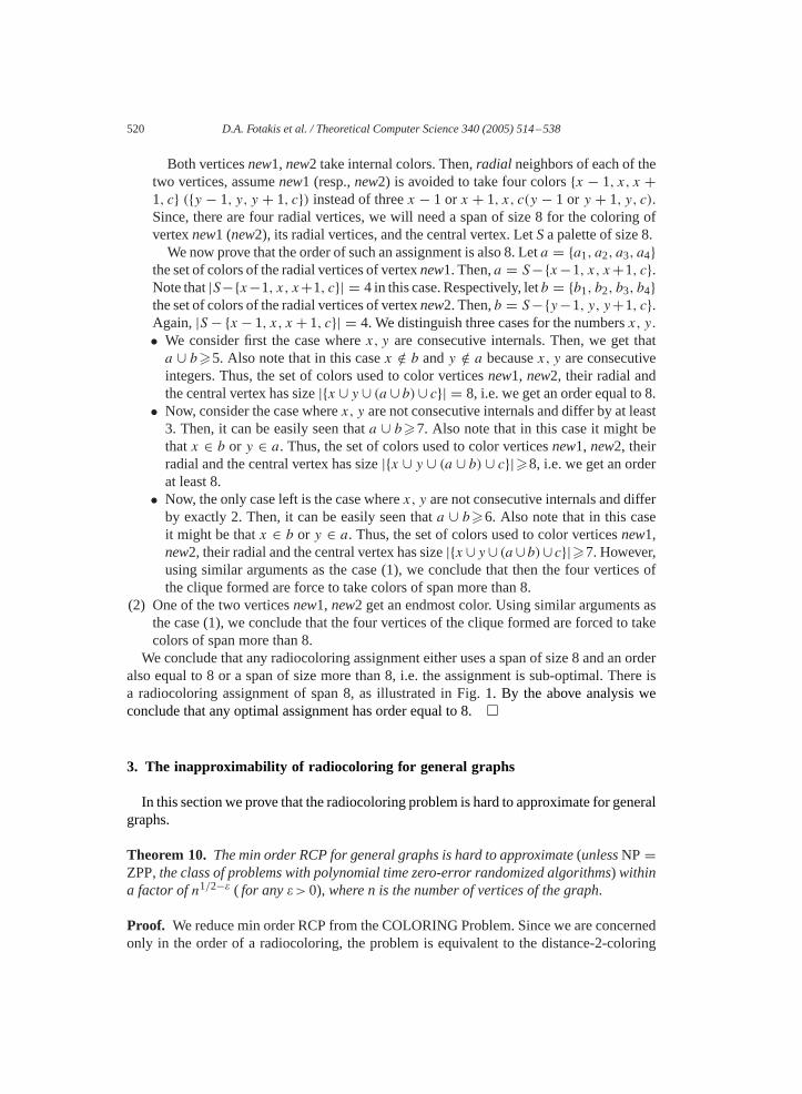
Proof. Consider the instance of the two problems appearing in Fig.1. The vertices of thegraph are named as shown in Fig. 1. Given a palette of colors (integers)S, used in anassignment, we callendmost colorsthe smallest and largest integer of the setS. We call therest of the colors asinternal colors. For example in the setS = {1, . . . ,8} the colors 1, 8are the two endmost colors of setS.It is easy to see that the minimum number of colors (order) needed for the distance-2-

coloring ofG is 6 colors, while the minimum span of the min span order RCP ofG is atleast 7 (consider the colors needed to radiocolor vertexnew1, the central vertex neighborto it, and its radial vertices).We assert that any optimal min span order radiocoloring assignment needs a span of size

at least 8 and the order of such an assignment is also 8.We distinguish three cases based on the colors of verticesnew1,new2. Letx, y the colors

of verticesnew1, new2, respectively (note thatx �= y). Let alsoc the color of the centralvertex. Note that|c − x|�2 and|c − y|�2.(1) Both verticesnew1, new2 get endmost colors. We prove that then, the four vertices of

the clique formed are forced to take colors of spanmore than 8. This because the cliquevertices should take a consecutive sequence of odd (or even) colors. In other case, theywill leave more colors unused increasing the span more than 8. Thus, assume that theclique vertices take consecutive odds (evens). We will need four consecutive numbers,hence we will need a range of size 8. Also, we should use an endmost color. But, thisis not possible, since we allocated the endmost colors to the verticesnew1,new2.


Both verticesnew1,new2 take internal colors. Then,radial neighbors of each of thetwo vertices, assumenew1 (resp.,new2) is avoided to take four colors{x − 1, x, x +1, c} ({y − 1, y, y + 1, c}) instead of threex − 1 orx + 1, x, c(y − 1 or y + 1, y, c).Since, there are four radial vertices, we will need a span of size 8 for the coloring ofvertexnew1 (new2), its radial vertices, and the central vertex. LetSa palette of size 8.We now prove that the order of such an assignment is also 8. Leta = {a1, a2, a3, a4}

the set of colors of the radial vertices of vertexnew1. Then,a = S−{x−1, x, x+1, c}.Note that|S−{x−1, x, x+1, c}| = 4 in this case. Respectively, letb = {b1, b2, b3, b4}the set of colors of the radial vertices of vertexnew2. Then,b = S−{y−1, y, y+1, c}.Again,|S− {x− 1, x, x+ 1, c}| = 4. We distinguish three cases for the numbersx, y.

• We consider first the case wherex, y are consecutive internals. Then, we get thata ∪ b�5. Also note that in this casex /∈ b andy /∈ a becausex, y are consecutiveintegers. Thus, the set of colors used to color verticesnew1, new2, their radial andthe central vertex has size|{x ∪ y ∪ (a ∪ b)∪ c}| = 8, i.e. we get an order equal to 8.

• Now, consider the case wherex, y are not consecutive internals and differ by at least3. Then, it can be easily seen thata ∪ b�7. Also note that in this case it might bethatx ∈ b or y ∈ a. Thus, the set of colors used to color verticesnew1, new2, theirradial and the central vertex has size|{x ∪ y ∪ (a ∪ b) ∪ c}|�8, i.e. we get an orderat least 8.

• Now, the only case left is the case wherex, y are not consecutive internals and differby exactly 2. Then, it can be easily seen thata ∪ b�6. Also note that in this caseit might be thatx ∈ b or y ∈ a. Thus, the set of colors used to color verticesnew1,new2, their radial and the central vertex has size|{x ∪y ∪ (a∪b)∪ c}|�7. However,using similar arguments as the case (1), we conclude that then the four vertices ofthe clique formed are force to take colors of span more than 8.

(2) One of the two verticesnew1, new2 get an endmost color. Using similar arguments asthe case (1), we conclude that the four vertices of the clique formed are forced to takecolors of span more than 8.

We conclude that any radiocoloring assignment either uses a span of size 8 and an orderalso equal to 8 or a span of size more than 8, i.e. the assignment is sub-optimal. There isa radiocoloring assignment of span 8, as illustrated in Fig.1. By the above analysis weconclude that any optimal assignment has order equal to 8.�

3. The inapproximability of radiocoloring for general graphs

In this section we prove that the radiocoloring problem is hard to approximate for generalgraphs.

Theorem 10. The min order RCP for general graphs is hard to approximate(unlessNP=ZPP,the class of problems with polynomial time zero-error randomized algorithms) withina factor ofn1/2−� ( for any�>0),where n is the number of vertices of the graph.

Proof. We reduce min order RCP from the COLORING Problem. Since we are concernedonly in the order of a radiocoloring, the problem is equivalent to the distance-2-coloring


2 1

1 2 1

2

ba

b

ab

a

the graph G

the graph H

N

Fig. 2. GraphH obtained byG.

(d2c) problem. We use the term distance-2-coloring or d2c when referring to a min orderradiocoloring assignment, for terminology convenience purposes.We start with an arbitrary graphG(V,E) with |V | = N . Let n = O(N2 + N). We

construct a graphH of O(n) vertices as follows:

Vertex set of H:(1) For each vertexui of Gwe add a new vertexui in H, which we callexisting vertex.(2) For each edge ofE(G) we add inH a new vertex, calledintermediate vertexand

denoteduij , whereui , uj are the end vertices constituting the edge.(3) Finally, for each vertexui of G, we addN new vertices, calledauxiliary verticesand

denoted asyij : 1� i, j�N .

Edge set of H:(1) For each intermediate vertexuij , obtained by end verticesui , uj , we add the edges

(ui, uij ), (uij , uj ).(2) We connect each auxiliary vertexyij with all neighbor intermediate vertices of the

existing vertexui from which the auxiliary vertex is obtained. Formally, the derivedgraphH can be described as follows:

V (H) = {ui : 1� i�N} ∪ {uij : (ui, uj ) ∈ E(G)} ∪ {yi,j : 1� i�N,1�j�N}.E(H) = {(ui, uij ), (uij , uj ) : (ui, uj ) ∈ E(G)} ∪ {(uij , yi,j ) : (ui, uj ) ∈ E(G)}

An example of the graphH derived by a graphG is presented in the Fig.2.Observe thatif G is k-colorable then H is((k+1)N+�+1)-distance-2-colorable. Such

a coloring can be obtained as follows:First,k-color each set{y1j , y2j , . . . , yNj }, where 1�j�N . To show that the radiocol-

oring is valid, for anyj consider the corresponding set{y1j , y2j , . . . , yNj }. Its distance-oneconstraints inG are inH distance-two constraints. For each auxiliary vertex in this set, its


coloring inG is equivalent to its distance-2-coloring inH. Therefore,kcolors are enough foreach such set to be distance-2-colored. Since we haveN such sets, we needk ·N colors fortheir coloring. Next, color the existing vertices withk additional colors (this is valid, basedon similar arguments as above) and color the intermediate vertices with� + 1 additionalcolors (valid, since it is equivalent to an edge coloring ofG).Summing up,weused, for the coloring of the auxiliary, existing and intermediate vertices,

i.e. the graphH (k + 1)N + � + 1 colors.On the other hand, from a distance-2-coloring ofH we can get a coloring ofG by the

following procedure:For each existing vertexui ∈ V (G) we select one color from the set ofN distinct colors

of the set{yi1, yi2, . . . , yiN } and color the vertexui with this color. This color result to avalid coloring ofG as proved here: A neighbor ofui , a vertexuj will also take one color ofitsN yj1, yj2, . . . , yjN auxiliary vertices. Since allyj1, yj2, . . . , yjN vertices are distance-two neighbors with verticesyi1, yi2, . . . , yiN in H, they all get different colors. Hence, theresulting coloring of verticesui, uj is a valid coloring ofG.Thus, whenH is distance-2-colorable withqN colors, whereq = N�(1), G is O(q)-

colorable.We know that it is NP-hard to determine ifG needs at most O(N �) or at least�(N1−�)

colors to be colored[6]. Thus, it is also NP-hard to determine whether the optimal distance-2-coloring of a given graph (H in our case) with O(n) vertices needs at most O(N �N) or atleast�(N1−�N) colors, i.e. the inapproximability ratio of distance-2-coloring (of a graphH) is

�(N1−�N)

O(N �N)� �(N2−�)

O(N1+�)� �(n1−�/2)

O(n1/2+�/2)��(n1/2−�). �

4. The NP-completeness of the RCP for planar graphs

In the previous section we proved that the radiocoloring problem for general graphsis hard to approximate within a factor ofn1/2−� (for any �>0), wheren is the numberof vertices of the graph. However, the problem, when restricted to some special cases ofgraphs, such as planar graphs, becomes, as we prove, easier.In this section, we show that the decision version of min span RCP remains NP-complete

for planar graphs. This version asks given a planar graphG and an integerB, to decidewhether there exists a valid radiocoloring forG of span no more thanB. Therefore, theoptimization version of min span RCP remains NP-hard for planar graphs.In the sequel the degree of vertexv in a graphG is denoted bydG(v) and when there is

no confusion simply asd(v). We also denote the subtraction operation between sets as\.Theorem 11. The following decision problem is NP-complete:Input: A planar graphG(V,E) and an integer B.Question: Does there exist a radiocoloring for G with span no more than B?

Proof. It can be easily shown that the decision version of min span RCP, where we seek todecidewhether a radiocoloring assignmentwith span�exists, is inNP (guess the assignment


0,8-vertices

0,8-vertices0,8-vertices

1,7-vertex 1,7-vertex

common-internal-vertex

common-internal-vertex

0,8-vertices

Out

0,8'-vertices

Group i

internal-vertex internal-vertex

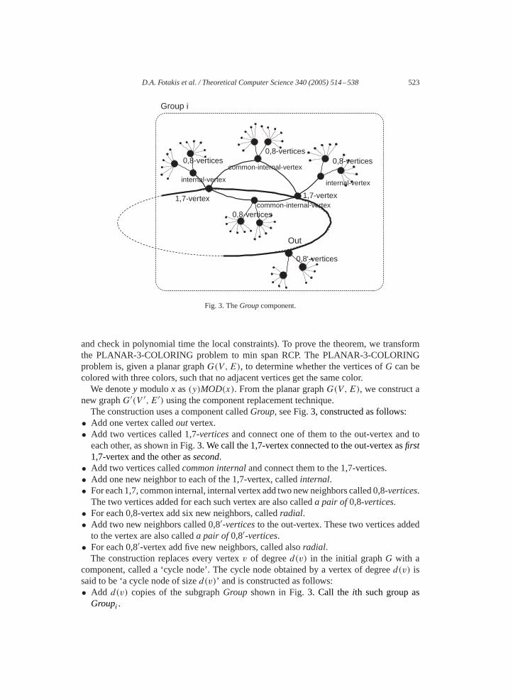
Fig. 3. TheGroupcomponent.

and check in polynomial time the local constraints). To prove the theorem, we transformthe PLANAR-3-COLORING problem to min span RCP. The PLANAR-3-COLORINGproblem is, given a planar graphG(V,E), to determine whether the vertices ofG can becolored with three colors, such that no adjacent vertices get the same color.We denoteymodulox as(y)MOD(x). From the planar graphG(V,E), we construct a

new graphG′(V ′, E′) using the component replacement technique.The construction uses a component calledGroup, see Fig.3, constructed as follows:

• Add one vertex calledoutvertex.• Add two vertices called 1,7-verticesand connect one of them to the out-vertex and toeach other, as shown in Fig.3. We call the 1,7-vertex connected to the out-vertex asfirst1,7-vertex and the other assecond.

• Add two vertices calledcommon internaland connect them to the 1,7-vertices.• Add one new neighbor to each of the 1,7-vertex, calledinternal.• For each 1,7, common internal, internal vertex add two newneighbors called 0,8-vertices.The two vertices added for each such vertex are also calleda pair of0,8-vertices.

• For each 0,8-vertex add six new neighbors, calledradial.• Add two new neighbors called 0,8′-verticesto the out-vertex. These two vertices addedto the vertex are also calleda pair of0,8′-vertices.

• For each 0,8′-vertex add five new neighbors, called alsoradial.The construction replaces every vertexv of degreed(v) in the initial graphG with a

component, called a ‘cycle node’. The cycle node obtained by a vertex of degreed(v) issaid to be ‘a cycle node of sized(v)’ and is constructed as follows:• Add d(v) copies of the subgraphGroup shown in Fig.3. Call theith such group asGroupi .


1,7-vertex 1,7-vertex

Out

a cycle node of degree 1

a cycle node of degree 2

1,7-vertex

OutOut

1,7-vertex

1,7-vertex1,7-vertex

Group 1

Group 2

Fig. 4. The cycle nodes of size 1 and 2 in abbreviation (the radial vertices attached to the 0,8 and 0,8′-vertices arenot shown).

• Connect consecutive groups as follows: Connect the second 1,7-vertex ofGroupi to theout-vertex ofGroup(i)MOD(d(v))+1, for i = 1 : d(v).

For example, the cycle nodes of size 1 and 2 are illustrated in Fig.4 in abbreviation (theradial vertices attached to the 0,8 and 0,8′-vertices are not shown).Now the graphG′(V ′, E′) is defined as follows:

(1) Replace each vertexv of degreed(v) in the graphGwith a cycle node of sized(v).(2) For each vertexv of the graphG, number the edges incident tov in increasing clockwise

order.(3) For every edge of the initial graphe = (u, v) connectingu andv, letue be the number

of edgeegiven by vertexu and letve be the number of the edgeegiven by vertexv.Then, take one of the 0,8′-vertices of theueth group of the cycle node of vertexuand

one of the 0,8′-vertices of theveth group of the cycle node of vertexv and collapse themto a single vertex named also as 0,8′-vertex. Do the same for the second 0,8′-vertex ofu and the second 0,8′-vertex ofv.

An example of a graphG and the new graphG′ obtained is shown in Fig.5 (depicted in acompact way). It can easily be seen that the new graphG′ is a planar graph. We next provetwo lemmas showing thatG′ can be radiocolored using a span of size at most 9 if and onlyif the initial graphG is 3-colorable.


G'G

Fig. 5. TheG′ obtained by the graphG in abbreviation.

Lemma 12. If �(G)�3 thenXspan(G′)�9.

Proof. Consider a 3-coloring of the initial graphG, using colors{1,2,3}. Let the followingradiocoloring assignment on the graphG′ using a paletteS = {0,1,2,3,4,5,6,7,8} ofsize 9:(i) For each vertexu of the graphG coloredi, i ∈ {1,2,3}, color all out-vertices of thecycle node of vertexu in G′, with color i + 2 (i.e. a color from set{3,4,5}).For eachu ∈ V , color each groupGroupi , 1� i�d(u) of the cycle node ofu asfollows:

(ii) Color the first 1,7-vertex of the group with the color 1 and second with color 7.(iii) Color 0,8-vertices and 0,8′-vertices with colors 0,8.(iv) Assuming that the out-vertices of the group are coloredi, i ∈ {3,4,5}, color the

common-internal vertices of the group with colors of set{3,4,5}\{i}.(v) Color the internal-vertex neighbor to the 1,7-vertex colored 1, with color 6 and the

internal-vertex neighbor to the 1,7-vertex colored 7, with color 1.(vi) Consider a 0,8-vertex and the neighbor to it (common)-internal vertex coloredi, i ∈

{2,3,4,5,6}. If the 0,8-vertex is colored0, color the six uncolor neighborswith colors{2,3,4,5,6,7,8}\{i}. If the 0,8-vertex is colored 8, color the six uncolor neighborswith colors{0,1,2,3,4,5,6}\{i}.

(vii) Consider a 0,8′-vertex and the neighbors to it out-verticesu, v coloredi, j, i, j ∈{3,4,5}. If the 0,8-vertex is colored 0, color the five uncolor neighbors with col-ors {2,3,4,5,6,7,8}\{i, j}. If the 0,8-vertex is colored 8, color the five uncolorneighbors with colors{0,1,2,3,4,5,6}\{i, j}.

(viii) Color the radial vertices of 0,8 and 0,8′-vertices with the unused colors from setS.

Claim 13. The suggested radiocoloring assignment is valid.

Proof. The following hold for the suggested radiocoloring assignment:Considering any cycle node, we have the following observations:• Note first that, internal, common-internal, out-vertices are colored using colors fromset{2,3,4,5,6}. Note also that common-internal, out-vertices are colored using colors{3,4,5}.

• Radial vertices neighbors to a 0,8-vertex: These are six vertices. They are neighbors toa (common)-internal vertex colored using a colori, i ∈ {2,3,4,5,6}. The vertices are


also neighbors to a 0,8-vertex colored 0 or 8. Thus, if the 0,8-vertex is colored 0, theycan be colored with the six colors of set{2,3,4,5,6}\{i} ∪ {7,8}, else (the 0,8-vertextakes color 8) with the six colors of set{2,3,4,5,6}\{i} ∪ {0,1}.

• Radial vertices neighbors to a 0,8′-vertex: These are five vertices. They are neighbors totwo out-vertices of neighbor cycle nodes coloredi, j, i �= j, i, j ∈ {2,3,4,5,6}. Thevertices are also neighbors to a 0,8-vertex colored 0 or 8. Thus, if the 0,8-vertex is colored0, they can be colored with the five colors of set{2,3,4,5,6}\{i, j} ∪ {7,8}, else (the0,8-vertex takes color 8) with the five colors of set{2,3,4,5,6}\{i, j} ∪ {0,1}.

• 1,7-vertices: Each of them is connected to four vertices (internal, common-internal, out)colored using colors of set{2,3,4,5,6}. The vertex is at distance one from the other1,7-vertex of the group and at distance two from one 1,7-vertex of the next group. Recallthat all 1,7-vertices of the cycle node are colored by alternating between colors 1, 7. Alsothe vertex is at distance two from at least one pair of 0,8-vertices. So, one of the colors1, 7 is available for each such vertex.

• Common-internal vertices: Each of them is at distance two from the two internal verticescolored{2,6} and the out-vertices of the same cycle node coloredi, i ∈ {3,4,5}. It is atdistance one from the 1,7-vertices of the group, hence it cannot take colors 1,2,6,7. Alsothe vertex is at distance two from at least a pair 0,8-vertices. Hence, in the set{3,4,5}\{i}there are two colors free for the two common-internal vertices.

• Internal vertices: Each of them is at distance two from three vertices (common-internal,out) colored using the colors of set{3,4,5}. Also, the vertex is at distance two from atleast one pair of 0,8-vertices. It is at distance one from one of 1,7-vertex, hence it cannottake colors{0,1,2} or {6,7,8} and at distance two from the other 1,7-vertex. Hence, oneof the colors 6 or 2 is available for each such vertex.

• Out-vertices: Each of them is at distance two from the two common-internal verticescolored using two colors of set{3,4,5}. The vertex is also at distance two from twointernal vertices, one of its group and the other of the next group, colored 2 and 6. Also,the vertex is at distance one from a pair of 0,8′-vertices colored 0,8 and at distance onefrom two 1,7-vertices colored 1,7. Hence, one of the colors of set{3,4,5} is availablefor each such vertex.

Now, consider any two out-vertices connecting two neighbor cycle nodesu, v. Since theytake the corresponding colors as the verticesu, v in the 3-coloring ofG, there is no conflictbetween any two of them.Thus, the suggested radiocoloring assignment is valid.�

Lemma 14. If Xspan(G′)�9 then�(G)�3.

Proof. Consider any radiocoloring assignment of size 9 ofG′. Then, we get that,

Claim 15. Each pair of0,8-vertices or0,8′-vertices, neighbors to a vertex are colored0,8.

Proof. Each 0,8-vertex, 0,8′-vertex has even neighbors. In a setSof colors of range 9, if thevertex takes a color other than 0 or 8, then there will not be enough colors for its neighbors.Considering a pair of 0,8-vertices neighbors to a vertex, they take colors 0,8.�


Claim 16. The common-internal, internal, out-vertices of any Groupi ,1� i�d(v) of acycle nodev are colored using colors from set{2,3,4,5,6}.

Proof. Each such vertex is connected to at least one pair of 0,8-vertices colored 0,8. Thus,they can take one of the colors from setS\{0,1,7,8} = {2,3,4,5,6}. �

Claim 17. Each pair of1,7-vertices of any Groupi ,1� i�d(v), of a cycle nodev arecolored1,7.

Proof. Each 1,7-vertex, has four neighbors ((common)-internal, out) colored using fourcolors from set{2,3,4,5,6} by claim 16. Moreover, the vertex is at distance two from atleast one pair of 0,8-vertices. If the vertex takes a color other than 1 or 7, then there will notbe enough colors for its neighbors from the setS. Since, the two 1,7-vertices of aGroupiare at distance one apart they take colors 1,7.�

Claim 18. Anyout-vertex or common-internal vertex of anyGroupi ,1� i�d(v),of a cyclenodev is colored using one color from the set{3,4,5}.

Proof. Any out-vertex (common-internal vertex) is at distance one from a pair of 0,8′-vertices (0,8-vertices). The vertex is at distance one from two 1,7-vertices at distance two(one) apart each other. Thus, the vertex cannot take colors 0,1,2,6,7,8. Thus, it can takeone of the colors 3,4,5. �

Claim 19. Any internal vertex of anyGroupi ,1� i�d(v) of a cycle nodev is colored usingeither2 or 6.

Proof. Any internal vertex is at distance one from a pair of 0,8-vertices. The vertex is atdistance one from a 1,7-vertex and at distance two from the other 1,7-vertex of the group.Also, the vertex is at distance two from the two common-internal vertices and the out-vertexcolored{3,4,5} (by Claim 18). Thus, it can take the color 2 or 6, depending on the colorof the 1,7-vertex neighbor to it.�

Claim 20. For any cycle nodev, assuming that one out-vertex is colored i, i ∈ {3,4,5},then all out-vertices of the cycle node ofv are colored i.

Proof. Consider the next out-vertex of the cycle node ofv. By Claim 18, the vertex isat distance one from the two common-internal vertices colored{3,4,5}\{i}. Also, it is atdistance one from two 1,7-vertices colored 1,7, and from a pair of 0,8′-vertices colored 0,8.Hence, it cannot take colors{0,1,2,6,7,8} ∪ {3,4,5}\{i}. Thus the only color availablefor it is i. The argument holds for all consecutive out-vertices of the cycle node.We now compute a 3-coloring ofG as follows: Assign to each vertexu of the graphG

the color that any out-vertex of the cycle node corresponding to it takes inG′. We arguethat this is a valid 3-coloring ofG. First note that, by Claim18 we know that the computedassignment onGuses only 3 colors. Moreover, recall also that, by Claim 20, all out-verticesof a cycle node get the same colori, i ∈ {3,4,5}. Thus, for each cycle nodeuofG′, all of its


out-vertices (colored with the same color) ‘see’ the colors of the corresponding out-verticesof all neighbor cycle nodes ofu. This is equivalent to the colors that the correspondingto u vertex inG ‘see’ by all of its neighbors. Hence, since the out-vertices ofG′ have noconflicts with their neighbor out-vertices, there is no conflict with the colors of any vertexin G and its neighbors. Thus, ifG′ can be radiocolored with a span of size 9, then there isa 3-coloring ofG. �(End of proof of Theorem11). �

Corollary 21. The following decision problem isNP-complete:Input: A planar graphG(V,E) and integersB1, B2, B1�B2.Question: Does there exist a radiocoloring for G with span no more thanB1 and order

no more thanB2?

5. A constant ratio approximation algorithm for min order RCP

We provide here an approximation algorithm for min order RCP for planar graphs bymodifying the constructive proof of the theorem presented by Heuvel and McGuiness in[13]. Our algorithm is easier to verify with respect to correctness than what the proof givenin [13] suggests. It also has better time complexity (i.e. O(n�)) compared to the (implicit)algorithm in [13] which needs time O(n2). The improvement was achieved by performingthe heavy part of the computation of the algorithm only in some instances ofG instead of allas in [13]. This enables less checking and computations in the algorithm. Also, the behaviorof our algorithm is very simple andmore time efficient for graphs of smallmaximumdegree.Finally, the algorithm provided here needs no planar embedding ofG, as opposed to thealgorithm implied in [13].Very recently and independently, Agnarsson and Halldórsson in [2] presented approxi-

mations for the chromatic number of square and power graphs(Gk). Their method doesnot explicitly present an algorithm. A straightforward implementation is difficult and notefficient. Also, the approximation ratio for planar graphs of general� obtained is also 2.The main theorem of Heuvel and McGuiness [13] states that a planar graphG can be

radiocoloredwithatmost 2�+25colors.Morespecifically, theauthors consider theproblemof L−(p, q)-Labeling, which is defined as follows:

Definition 22 (L−(p, q)-Labeling). Find an assignmentL:V −→ {0,1, . . . , �}, calledL−(p, q)-Labeling, which satisfies|L(u)−L(v)|�p if D(u, v) = 1 and|L(u)−L(v)|�qif D(u, v) = 2.

Definition 23. The minimum number� for which anL−(p, q)-labeling exists is denotedby �(G;p, q) and is calledp, q-span ofG.

In other words, when the two vertices are at distance one apart, they should take colors(integers) that differ by at leastp, and when they are located at distance two apart, theyshould take colors that differ by at leastq. Note thatL−(p, q)-labeling is a generalizationof radiocoloring sinceL−(p, q)-labeling is equal to radiocoloring whenp = 2 andq = 1.The main theorem of[13] is the following:


Theorem 24(Heuvel and McGuiness[13] ). If G is a planar graph with maximum degree� andp, q are positive integers withp�q, then�(G;p, q)�(4q−2)�+10p+38q−23.

By settingp = q = 1 and using the observation�(G;1,1) = �(G2), where�(G2) is thechromatic number of the graphG2 (defined in the Introduction section), we get immediately,as also[13] notices, that:

Corollary 25 (Heuvel and McGuiness[13] ). If G is a planar graph with maximum degree� then�(G2)�2� + 25.

The theorem of[13] is proved using two lemmata. For an edgee ∈ E(G), let t (e) thenumber of triangular faces containing edgee and for a vertexv ∈ V (G), let t (v) be thenumber of triangular faces containingv, in the maximal planar graph ofG. The first of thetwo lemmata, used to prove the theorem for the case where�(G)�12, is the following:

Lemma 26(Heuvel and McGuiness[13] ). Let G be a simple planar graph. Then thereexists a vertexv with k neighborsv1, v2, . . . , vk with d(v1)� · · · �d(vk) such that one ofthe following is true:(i) k�2;(ii) k = 3with d(v1)�11;(iii) k = 4with d(v1)�7 andd(v2)�11;(iv) k = 5with d(v1)�6, d(v2)�7,andd(v3)�11.

The second lemma, used to prove the theorem for the case where�(G)�11, is quitesimilar.

Lemma 27(Heuvel and McGuiness[13] ). Let G be a simple planar graph with maximumdegree�. Then there exists a vertexv with k neighborsv1, v2, . . . , vk with d(v1)� · · · �d(vk) such that one of the following is true:(i) k�2;(ii) k = 3with d(v1)�5;(iii) k = 3with t (vvi)�1 for some i;(iv) k = 4with d(v1)�4;(v) k = 4with t (vvi) = 2 for some i;(vi) k = 5with d(vi)�4 andt (vvi)�1 for some i;(vii) k = 5with d(vi)�5 andt (vvi) = 2 for some i;(viii) k = 5with d(v1)�7 andt (vvi)�1 for all i ;(ix) k = 5withd(v1)�5,d(v2)�7,and for each i witht (vvi) = 0 it holds thatd(vi)�5.

These two lemmata give the so-calledunavoidable configurationsof G. The followingoperations apply toG: For an edgee ∈ E let G/e denote the graph obtained fromG bycontractinge. For a vertexv ∈ V letG ∗ v denote the graph obtained by deletingv and foreachu ∈ N(v) adding an edge betweenu andu− and betweenu andu+ (if these edges donot exist inGalready). The notationN(v) denotes the neighbors ofv. The notationu−, with


u− ∈ N(v), denotes the edgevu− which directly precedes edgevu (moving clockwise),andu+, with u+ ∈ N(v), refers to the edgevu+ which directly succeeds edgevu (movingclockwise).The two lemmataare used to define thegraphH, a vertexv ∈ V (G)andanedgee ∈ E(G)

using the following rules:• If ��12, then letv be as described in Lemma 26, and sete = vv1 andH = G/e.• If 6��11 and one of 27 (i), (ii), or (iv) holds, then letv be as described, and sete = vv1 andH = G/e.

• If 6��11 and Lemma27 (iii) holds, then letv be as described, sete = vvi witht (vvi)�1, and setH = G/e.

• If 6��11 and Lemma27 (v) holds, then letv be as described, sete = vvi witht (vvi) = 2 and setH = G/e.

• If 6��11 and Lemma27 (vi) holds, then letv be as described, sete = vvi withd(vi)�4 andt (vvi)�1, and setH = G/e.

• If 6��11 and Lemma27 (vii) holds, then letv be as described, sete = vvi withd(vi)�5 andt (vvi) = 2, and setH = G/e.

• If 6��11 and Lemma27 (viii) holds, then letv be as described and setH = G ∗ v.• If 6��11 and Lemma27 (ix) holds, then letv be as described and setH = G ∗ v.Themain idea of theorem of [13] is to defineH to beH = G/e orH = G∗v, with e = vv1andd(v)�5, depending onwhich case of the two Lemmata holds, so that always�(H)��.Using these observations it is proved, by induction, that the minimum(p, q)-span neededfor theL−(p, q)-labeling ofH is �(H ;p, q)�(4q − 2)� + 10p + 38q − 23.FromH we can easily return toG as follows. IfH = G/e then letv′ the new vertex

created from the contraction of edgee. In this case, inG we setv1 = v′ (this is a validassumption sinced(v1)�d(v′)) and colorv1 with the color ofv′. Now we only need tocolor vertexv (for both cases ofH = G/e orH = G ∗ v). From the wayv was chosen, itcan be easily seen that there is always one color free for the vertex in the set of colors ofspan�(4q − 2)� + 10p + 38q − 23 as concluded forH.For the case of radiocoloring of a planar graphG, we can usep = 1 andq = 1 for the

order. Thus, the above theorem states that we need at most 2� + 25 colors.

5.1. The algorithm

We will use only Lemma 26 and the operationG/e in order to provide a much moresimple and more efficient algorithm than what implied in [14]. We provide below a high-level description of our algorithm.

Algorithm Radiocoloring (G)[I] Sort the vertices of the graph G by their degree .[II] If ��12 then follow Procedure (1) below:

Procedure(1):Compute graph G2.Consider the next vertex of theorder. Delete v from G2 to get G2,. Now recursively color G2,

with 145colors. The number of colors that v has to avoid isat most �2 = 144.Thus , in a set of 145colors , there is one freecolor for v.


[III] If �>12 then(1) Find a vertex v and a neighbor v1of it ,as described in Lemma

26, and set e = vv1.(2) Form G′ = G/e (G′ = (V ′, E′) with |V ′| = n − 1, while |V | = n) and

denote the new vertex in G′ obtained by the contraction ofedge e as v′.Modify the sorted degrees of G by deleting v, v1, and in-

serting v′ at the appropriate place , and also modify thepossible affected degrees of the neighbors of both v and v1.

(3) �(G′) = Radiocoloring(G′)(4) Extend �(G′) to a valid radiocoloring of G:(a) Set v1 = v′ and give to v1 the color of v′.(b) Color v with one of the colors used in the radiocoloring

� of G′.

5.2. Analysis of the algorithm

5.2.1. CorrectnessNotice first that Procedure[1] implies a radiocoloring ofGwithX = 145 colors: Assign

frequencies 1,3, . . . ,2X − 1 to the obtained color classes ofG.

Proposition 28. The algorithmRadiocoloring(G) outputs a valid radiocoloring for Gusing no more thanmax{66,2� + 25} colors.

Proof. By induction assume that, the recursive step 3 in [III] outputs a radiocoloring ofG

using at most max{66,2� + 25} colors. Note that�(G′) = �(G), because of the wayvande = vv1 are chosen.At step 4, the radiocoloring�(G′) ofG′ is extended to a valid radiocoloring ofG, using

no more colors than those used in the previous step. This extension procedure is validas explained here: At step (a) the vertexv1 of G takes the color of the vertexv′ of G′.This assignment is valid sincev1 has only a subset of the neighbors ofv′ at distance oneand two.Also, at step (b), the vertexv ofG is colored with one of the colors used in the radiocol-

oring�(G′) of G′. These colors are enough forv to get a valid color. The correctness ofthis claim is explained below.For any vertexv ∈ V (G), the number of vertices at distance two fromv is equal to∑u∈N(v) d(u) − d(v) − 2t (v). By the wayv was chosen, it holds thatd(v)�5 and the

above sum gives that there are at most 2� + 19 vertices at distance two fromv. In total,the number of distance one and two neighbors of the vertex is 5+ (2� + 19) = 2� +24. Assuming that a palette of 2� + 25 colors is given, there is always one color freefor v.Thus, algorithmRadiocoloring(G) gives a valid radiocoloring toG using no more than

max{66,2� + 25} colors. �


5.2.2. Time efficiency and approximation ratio

Lemma 29. OuralgorithmapproximatesXorder(G)byaconstant factor of atmostmax{2+25� ,

66� }.

Proof. Obviously, Xorder(G)>�(G). By Proposition 28, our algorithm uses at mostmax{66,2� + 25} colors, i.e.

1<Xorder(G)

�� max

{66

�,2+ 25

�

}. � (1)

Lemma 30. Our algorithm runs inO(n�) sequential time.

Proof. Step [I] takes O(n logn) time and Step [II] takes O(n) time. LetS be the set ofneighbors of bothv, v1. Each implementation of [III].1, 2 needs timed(v) + d(v1) +∑

x∈S d(x) in order to perform the operationG/e and O(logn) time to modify the sorteddegree list. The total time spent recursively is then just O(

∑v∈V d(v) · logn) = O(n logn).

Each implementation of [III].4 needs O(�) time at most and this step is executed at mostn times. Thus, the total time for all executions of [III].4 is O(n�). This dominates the totalexecution time. �

A more sophisticated and efficient implementation of the contraction operation can befound in[16].

6. An FPRAS for the number of radiocolorings of a planar graph

6.1. Sampling and counting

LetG be aplanargraph ofmaximumdegree� = �(G) on vertex setV = {0,1, . . . , n−1} andC be a set of� colors. Let�:V →C be a (proper) radiocoloring assignment of thevertices ofG. Such a radiocoloring always exists if��2� + 25 and can be found by ourO(n�) time algorithm of the previous section.Consider the Markov Chain(Xt ) whose state spaceR = R�(G) is the set of all radio-

colorings ofG with � colors and whose transition probabilities from state (radiocoloring)Xt are modelled by:1. Choose a vertexv ∈ V and a colorc ∈ C uniformly at random (u.a.r.)2. Recolor vertexv with color c. If the resulting coloringX′ is avalid radiocoloring as-signment then letXt+1 = X′ elseXt+1 = Xt .The procedure above is similar to the “Glauber Dynamics” of an antiferromagnetic Potts

model at zero temperature, and was used in[14] to estimate the number of proper coloringsof any low degree graph withk colors.The Markov Chain(Xt ), which we refer to in the sequel asM(G, �), is ergodic(as we

showed below), provided��2� + 26, in which case its stationary distribution isuniformoverR. We show here thatM(G, �) is rapidly mixing, i.e. converges, in time polynomialin n, to a close approximation of the stationary distribution, provided that��2(2� + 25).


This can be used to get a fully polynomial randomized approximation scheme (fpras) for thenumber of radiocolorings of a planar graphGwith � colors, in the case where��4�+50.

6.2. Some definitions and measures

For t ∈ N let P t :R2→ [0,1] denote thet-step transition probabilities of the MarkovChainM(G, �) so thatP t(x, y) = Pr{Xt = y|X0 = x},∀x, y ∈ R. It is easy to verify thatM(G, �) is (a) irreducibleand (b)aperiodic. The irreducibility ofM(G, �) follows fromthe observation that any radiocoloringxmay be transformed to any other radiocoloringy bysequentially assigning new colors to the verticesV in ascending sequence; before assigninga new colorc to vertexv it is necessary to recolor all verticesu>v that have colorc. Ifwe assume that��2� + 26 colors are given, removing the colorc from this set, we areleft with �2� + 25 for the coloring of the rest of the graph. The algorithm presented inprevious section shows that the remaining graph can by radiocolored with a set of colors ofthis size. Hence, colorc can be assigned tov.Aperiodicity follows from the fact that the loop probabilities areP(x, x) �= 0,∀x ∈ R.Thus, the finite Markov ChainM(G, �) is ergodic, i.e. it has a stationary distribution

�:R→ [0,1] such that limt→∞ P t(x, y) = �(y),∀x, y ∈ R. Now if �′:R→ [0,1] is anyfunction satisfying “local balance”, i.e.�′(x)P (x, y) = �′(y)P (y, x) then if

∑x∈R �′(x) =

1 it follows that�′ is indeed the stationary distribution. In our caseP(y, x) = P(x, y), thusthe stationary distribution ofM(G, �) is uniform.The efficiency of any approach like this to sample radiocolorings crucially depends on the

rate of convergence ofM(G, �) to stationarity. There are various ways to define closenessto stationarity but all are essentially equivalent in this case and we will use the “variationdistance” at timet with respect to initial vertexx

x(t) = maxS⊆R |P t(x, S)− �(S)| = 1

2

∑y∈R

|P t(x, y)− �(y)|,

whereP t(x, S) = ∑y∈S P t (x, y) and�(S) = ∑

x∈S �(x).Note that this is auniform boundover all eventsS ⊆ R of the difference of probabilities

of eventS under the stationary andt-step distributions.Therate of convergence to stationarityfrom initial vertexx is

x(�) = min{t : x(t ′)��,∀t ′ � t}.We also give the following definition:

Definition 31. � randomized approximation scheme for radiocolorings with� colors ofa planar graphG is a probabilistic algorithm that takes as input the graphG and an errorbound�>0 and outputs a numberY (a random variable) such that

Pr{(1− �)|R�(G)�Y�(1+ �) |R�(G)|}� 34.

Such a scheme is said to befully polynomialif it runs in time polynomial inn and�−1. Weabbreviate such schemes tofpras.


6.3. Rapid mixing

As indicated by the (by now standard) techniques for showing rapid mixing bycoupling[14,15], our strategy here is to construct a coupling forM = M(G, �), i.e. a stochasticprocess(Xt , Yt ) onR×R such that each of the processes(Xt ), (Yt ), considered in isolation,is a faithful copy ofM. We will arrange a joint probability space for(Xt ), (Yt ) so that, farfrombeing independent, the two processes tend tocoupleso thatXt = Yt for t large enough.If coupling can occur rapidly (independently of the initial statesX0, Y0), we can infer thatM is rapidly mixing, because the variation distance ofM from the stationary distributionis bounded above by the probability that(Xt ) and(Yt ) have not coupledby timet .The key result we use here is theCoupling Lemma(see [11, Chapter 4] by Jerrum), which

apparently makes its first explicit appearance in the work of Aldous [1, Lemma 3.6] (seealso Diaconis [5, Chapter 4, Lemma 5]).

Lemma 32. Suppose thatM is a countable,ergodicMarkov chainwith transition probabil-itiesP(·, ·) and let((Xt , Yt ), t ∈ N) be a coupling ofM. Suppose further thatt : (0,1] → N

is a function such thatPr(Xt(�) �= Yt(�))��, ∀� ∈ (0,1],uniformly over the choice of initialstate(X0, Y0). Then the mixing time(�) of M is bounded above byt (�).

The transition(Xt , Yt )→ (Xt+1, Yt+1) in the coupling is defined by the following ex-periment:1. Selectv ∈ V uniformly at random (u.a.r.).2. Compute a permutationg(G,Xt , Yt ) of C according to a procedure to be explained.3. Choose a colorc ∈ C u.a.r.4. In the radiocoloringXt (respectivelyYt ) recolor vertexv with colorc (respectivelyg(c))to get a new radiocoloringX′ (respectivelyY ′).

5. If X′ (respectivelyY ′) is a (valid) radiocoloring thenXt+1 = X′ (respectivelyYt+1 =Y ′), else letXt+1 = Xt (respectivelyYt+1 = Yt ).

Note that, whatever procedure is used to select the permutationg, the distribution ofg(c)is uniform, thus(Xt ) and(Yt ) are both faithful copies ofM.We now remark that any set of verticesF ⊆ V can have the same color in the graph

G2 only if they can have the same color in some radiocoloring ofG. Thus, given a propercoloring ofG2 with �′ colors, we can construct a proper radiocoloring ofG by giving thevalues (new colors) 1,3, . . . ,2�′−1 in the color classes ofG2. Note that this transformationpreserves the number of colors (but not the span).Now letA = At ⊆ V be the set of vertices on which the colorings ofG2 implied by

Xt, Yt agree andD = Dt ⊆ V be the set on which they disagree. Letd ′(v) be the numberof edges incident atv in G2 that have one point inA and one inD. Clearly, ifm′ is thenumber of edges ofG2 spanningA,D, we get

∑v∈A d ′(v) = ∑

v∈D d ′(v) = m′.The procedure to computeg(G,Xt , Yt ) is as follows:

(a) If v ∈ D theng is the identity.(b) If v ∈ A then proceed as follows: Denote byN the set of neighbors ofv in G2.

DefineCx ⊆ C to be the set of all colorsc, such that some vertex inN receivesc inradiocoloringYt but no vertex inN receivesc in radiocoloringYt . LetCy be defined asCx with the roles ofXt, Yt interchanged. ObserveCx ∩Cy = ∅ and|Cx |, |Cy |�d ′(v).


Let, w.l.o.g.,|Cx |� |Cy |. Choose any subsetC′y ⊆ Cy with |C′

y |� |Cx | and letCx ={c1, . . . , cr}, C′

y = {c′1, . . . , c′r} be enumerations ofCx,Cy′ coming from the orderingsofXt, Yt . Finally, letg be the permutation(c1, c′1), . . . , (cr , c′r )which interchanges thecolor setsCx,Cy′ and leaves all other colors fixed.

It is clear that|Dt+1| − |Dt | ∈ {−1,0,1}.(i) Consider first the probability that|Dt+1| = |Dt |+1. For this event to occur, the vertex

v selected in step (1) of the procedure forg must lie inA and hence we follow (b). Ifthe new radiocolorings are to disagree at vertexv then the colorc selected in line (3)must be an element ofCy . But |Cy |�d ′(v) hence

Pr{|Dt+1| = |Dt | + 1}� 1

n

∑v∈A

d ′(v)�

= m′

� · n (2)

(ii) Now consider the probability that|Dt+1| = |Dt |−1. For this to occur, the vertexvmustlie inD and hence the permutationg selected in line (2) is the identity. ForXt+1, Yt+1to agree atv, it is enough that colorc selected in step (3) is different from all the colorsthatXt, Yt imply for the neighbors ofv inG2. The number of colorsc that satisfy thisis (by our previous results) at least� − 2(2� + 25)+ d ′(v). Hence

Pr{|Dt+1| = |Dt | − 1} � 1

n

∑v∈D

� − 2(2� + 25)+ d ′(v)�

� � − 2(2� + 25)

�n|D| + m′

�n. (3)

Define now

� = � − 2(2� + 25)

�nand = m′

�n.

So

Pr{|Dt+1| = |Dt | + 1}�

and Pr{|Dt+1| = |Dt | − 1}��|Dt | + . Given�>0, i.e.�>2(2� + 25), from Eqs. (2)and (3), we get

E(|Dt+1|) � (|Dt | + 1)+ (�|Dt | + )(|Dt | − 1)+ (1− �|Dt | − 2 )|Dt |= (1− �)|Dt |.

Thus, from Bayes, we getE(|Dt+1|)�(1− �)t |D0|�n(1− �)t and since|Dt | is a non-negative random variable, we get, by Markov inequality, that

Pr{Dt �= 0}�n(1− �)t �ne−�t .

So, we note that,∀�>0, Pr{Dt �= ∅}�� provided thatt�(1/�) ln(n/�) thus proving:Theorem 33. Let G be a planar graph of maximum degree� on n vertices. Assuming��2(2� + 25) the convergence time(�) of the Markov ChainM(G, �) is boundedabove by

x(�)��

� − 2(2� + 25)n ln

(n�

)regardless of the initial state x.


6.4. An fpras for radiocolorings with� colors

The technique we employ is as in[14] and is fairly standard in the area. By using it weget the following theorem:

Theorem 34. There is a fully polynomial randomized approximation scheme(fpars) forthe number of radiocolorings of a planar graph G with� colors, provided�>2(2� + 25),where� is the maximum degree of G.

Proof. Recall thatR�(G) is the set of all radiocolorings ofG with � colors. Letm be thenumber of edges inG and let

G = Gm ⊇ Gm−1 ⊇ · · · ⊇ G1 ⊇ G0

be any sequence of graphs whereGi−1 is obtained byGi by removing a single edge. Wecan always erase an edge whose one node is of degree at most 5 inGi . Clearly

|R�(G)| = |R�(Gm)||R�(Gm−1)|

|R�(Gm−1)||R�(Gm−2)| · · · |R�(G1)|

|R�(G0)| |R�(G0)|.

But |R�(G0)| = �n for all kinds of colorings. The standard strategy is to estimate the ratio

�i = |R�(Gi)||R�(Gi−1)|

for eachi, 1� i�m.Suppose that graphsGi,Gi−1 differ in the edge{u, v} which is present inGi but not

in Gi−1. Clearly,R�(Gi) ⊆ R�(Gi−1). Any radiocoloring inR�(Gi−1)\R�(Gi) assignseither the same color tou, v or the color values ofu, v differ by only 1. Let deg(v)�5 inGi . So, we now have to recoloruwith one of at least� − (2� + 25), i.e. at least 2� + 25,colors (from Section5 of this paper). Each radiocoloring ofR�(Gi) can be obtained in atmost one way by our algorithm of the previous section as the result of such a perturbation.Thus,

1

2� 2� + 25

2(� + 1)+ 25��i <1. (4)

To avoid trivialities, assume 0< ��1, n�3 and�>2. Let Zi ∈ {0,1} be the randomvariable obtained by simulating the Markov ChainM(Gi−1, �) from any certain fixedinitial state for

T = �� − 2(2� + 25)

n ln

(4nm

�

)

steps and returning to 1 if the final state is a member ofR�(Gi) and 0 else.Let �i = E(Zi). By our theorem of rapid mixing, we have

�i − �4m

��i��i + �4m


and by Eq. (4), we get(1− �

2m

)�i��i�

(1+ �

2m

)�i .

As our estimator for|R�(G)| we useY = �nZ1Z2 · · ·Zm.

Note thatE(Y ) = �n�1�2 · · ·�m. But

Var(Y )� Var(Z1Z2 · · ·Zm)(�1�2 · · ·�m)2

=m∏i=1

(1+ Var(Zi)

�2i

)− 1.

Bystandardwaysofworking (as in[14]) onecaneasily show thatYsatisfies the requirementsfor an fpras for the number of radiocolorings of graphGwith � colors|R�(G)|. �

References

[1] D. Aldous, Random walks in finite groups and rapidly mixing Markov chains, in: A. Dold, B. Eckmann(Eds.), Seminaire de Probabilites XVII 1981/82, Springer Lecture Notes in Mathematics, Vol. 986, Springer,Berlin, 1982, pp. 243–297.

[2] G. Agnarsson, M.M. Halldorsson, Coloring squares of graphs, SIAM J. Discrete Math., to appear.[3] A.A. Bertossi, M.A. Bonuccelli, Code assignment for hidden terminal interference avoidance in multihop

packet radio networks, IEEE/ACM Trans. Networking 3 (4) (1995) 441–449.[4] H.L.Bodlaender, T.Kloks,R.B.Tan, J. vanLeeuwen,Approximations for�-coloringof graphs, in:H.Reichel,

S. Tison (Eds.), STACS2000, Proc. 17th Annual Symp. on Theoretical Aspects of Computer Science, LectureNotes in Computer Science, Vol. 1770, Springer, Berlin, 2000, pp. 395–406.

[5] P. Diaconis, Group Representations in Probability and Statistics, Institute of Mathematical Statistics,Hayward, CA, 1988.

[6] U. Feige, J. Kilian, Zero knowledge proofs and the chromatic number, J. Comput. Syst. Sci. 57 (1998)187–199. Springer, New York, 1993, pp. 250–260.

[7] M. Formann, T. Hagerup, J. Haralambides, M. Kaufmann, F.T. Leighton, A. Symvonis, E. Welzl, G.Woeginger, Drawing graphs in the plane with high resolution, SIAM J. Comput. 22 (5) (1993) 1035–1052.

[8] D. Fotakis, S. Nikoletseas, V. Papadopoulou, P. Spirakis, NP-completeness results and efficientapproximations for radiocoloring in planar graphs, 25th Internat. Symp. on Mathematical Foundations ofComputer Science (MFCS), Lecture Notes in Computer Science, Vol. 1893, Springer, Berlin, 2000, pp.363–372.

[9] D. Fotakis, G. Pantziou, G. Pentaris, P. Spirakis, Frequency assignment in mobile and radio networks,Networks in Distributed Computing, DIMACS Series in Discrete Mathematics and Theoretical ComputerScience, Vol. 45, American Mathematical Society, Providence, RI, 1999, pp. 73–90.

[10] J. Griggs, D. Liu, Minimum span channel assignments, Recent Advances in Radio Channel Assignments.Invited Minisymposium, Discrete Mathematics, 1998.

[11] M. Habib, C. McDiarmid, J. Ramirez-Alfonsin, B. Reed (Eds.), Probabilistic Methods for AlgorithmicDiscrete Mathematics, Algorithms and Combinatorics, Vol. 16, Springer, Berlin, 1998.

[12] W.K. Hale, Frequency assignment: theory and applications, Proc. IEEE 68 (12) (1980) 1497–1514.[13] J.VanD. Heuvel, S. McGuiness, Colouring the square of a planar graph, CDAMResearch Report Series, July

1999.[14] M. Jerrum, A very simple algorithm for estimating the number ofk-colourings of a low degree graph, Random

Struct. Algorithms 7 (1994) 157–165.[15] M. Jerrum, Markov chain Monte Carlo method, in: Probabilistic Methods for Algorithmic Discrete

Mathematics, Springer, Berlin, 1998.


[16] D.R. Karger, C. Steinm, A new approach to the minimum cut problem, J. ACM 43 (4) (1996) 601–640.[17] I. Katsela,M.Nagshineh, Channel assignment schemes for cellularmobile telecommunication systems, IEEE

Personal Communication Complexity 1070 (1996).[18] D. Lichtenstein, Planar formulae and their uses, SIAM J. Comput. 11 (2) (1982) 329–343.[19] Y.L. Lin, S. Skiena, Algorithms for square roots of graphs, SIAM J. Discrete Math. 8 (1995) 99–118.[20] S. Ramanathan, E.R. Loyd, The complexity of distance2-coloring, 4th Internat. Conf. of Comput. Inform.

1992, pp. 71–74.

Further reading

[21] S. Ramanathan, E.R. Loyd, Scheduling algorithms for multi-hop radio networks, IEEE/ACM Trans.Networking 1 (2) (1993) 166–172.

Radiocoloring in planar graphs: Complexity and approximations

Documents