Radio channel characterisation and system-level modelling for ultra wideband body-centric wireless communications Abbasi, Qammer Hussain The copyright of this thesis rests with the author and no quotation from it or information derived from it may be published without the prior written consent of the author For additional information about this publication click this link. http://qmro.qmul.ac.uk/jspui/handle/123456789/2406 Information about this research object was correct at the time of download; we occasionally make corrections to records, please therefore check the published record when citing. For more information contact [email protected]

Welcome message from author
This document is posted to help you gain knowledge. Please leave a comment to let me know what you think about it! Share it to your friends and learn new things together.
Transcript
Radio channel characterisation and system-level modelling for ultra
wideband body-centric wireless communicationsAbbasi, Qammer Hussain
The copyright of this thesis rests with the author and no quotation from it or information
derived from it may be published without the prior written consent of the author
For additional information about this publication click this link.
http://qmro.qmul.ac.uk/jspui/handle/123456789/2406
Information about this research object was correct at the time of download; we occasionally
make corrections to records, please therefore check the published record when citing. For
more information contact [email protected]
Radio Channel Characterisation andSystem-Level Modelling for UltraWideband Body-Centric Wireless
Communications
Qammer Hussain Abbasi
A thesis submitted to the faculty of the University of London in partialfulfillment of the requirements for the degree of
Doctor of Philosophy
School of Electronic Engineering and Computer ScienceQueen Mary, University of London
London E1 4NSUnited Kingdom
January 2012

2011 c© Queen Mary, University of London. All rights reserved.
To my family
Abstract
The next generation of wireless communication is evolving towards user-centric net-
works, where constant and reliable connectivity and services are essential. Body-
centric wireless network (BCWN) is the most exciting and emerging 4G technology
for short (1-5 m) and very short (below 1 m) range communication systems. It has
got numerous applications including healthcare, entertainment, surveillance, emer-
gency, sports and military. The major difference between the BCWN and conventional
wireless systems is the radio channel over which the communication takes place. The
human body is a hostile medium from the radio propagation perspective and it is
therefore important to understand and characterise the effect of the human body on
the antenna elements, the radio propagation channel parameters and hence the sys-
tem performance. In addition, fading is another concern that affects the reliability and
quality of the wireless link, which needs to be taken into account for a low cost and
reliable wireless communication system for body-centric networks.
The complex nature of the BCWN requires operating wireless devices to provide
low power requirements, less complexity, low cost and compactness in size. Apart
from these characteristics, scalable data rates and robust performance in most fad-
ing conditions and jamming environment, even at low signal to noise ratio (SNR) is
needed. Ultra-wideband (UWB) technology is one of the most promising candidate for
BCWN as it tends to fulfill most of these requirements. The thesis focuses on the char-
acterisation of ultra wideband body-centric radio propagation channel using single
and multiple antenna techniques. Apart from channel characterisation, system level
modelling of potential UWB radio transceivers for body-centric wireless network is
also proposed. Channel models with respect to large scale and delay analysis are de-
rived from measured parameters. Results and analyses highlight the consequences
of static and dynamic environments in addition to the antenna positions on the per-
formance of body-centric wireless communication channels. Extensive measurement
i
campaigns are performed to analyse the significance of antenna diversity to combat
the channel fading in body-centric wireless networks. Various diversity combining
techniques are considered in this process. Measurement data are also used to pre-
dict the performance of potential UWB systems in the body-centric wireless networks.
The study supports the significance of single and multiple antenna channel charac-
terisation and modelling in producing suitable wireless systems for ultra low power
body-centric wireless networks.
ii

Acknowledgement
First and the foremost, I would like to thank Almighty Allah for bestowing, His bless-
ings upon me and giving me the strength to carry out and complete this work.
My most sincere and deep gratitude goes to my supervisor’s Prof. Yang Hao &
Dr. Akram Alomainy, their support, guidance and encouragement have given me the
strength and confidence necessary for the development of the work. Apart from their
valuable academic advice and guidelines, they have been extremely kind, friendly,
and helpful as a human being. I would also like to thank Prof. Clive Parini for his
positive and fruitful comments, and Mr. John Dupuy for his assistance in the experi-
mental part of the work.
A special mention goes to Dr. Akram Alomainy, his knowledge, and willingness
to meet and help at anytime have facilitated not only my research, but every aspect of
my PhD.
Many thanks to University of Engineering and Technology, Lahore, Pakistan for
the financial support. I would like also to thank all my colleagues in Queen Mary
University of London for providing a good working atmosphere and making my time
an enjoyable one.
Above all, I would like to thank my family, my relatives and all my friends. Re-
gardless of physical distance, their support and affection have always been with me.
My last thought goes to my family: my Mum and Dad who have stood by me through
thick and thin; my brothers, Qasim, Kashif, Qaiser and Yasir, my wife, my sisters in-
law, nephews and niece. I wish to thank them for their prayers and their encourage-
ment throughout my PhD. I dedicate this thesis to my parents and family, to honour
their love, encouragement and patience during these years.
Qammer Hussain Abbasi
London, January 2012
iii
List of Publications
Journal Publications
1. Q. H. Abbasi, A. Sani, A. Alomainy and Y. Hao, “On-Body Radio Channel Char-
acterisation and System-Level Modelling for Multiband OFDM Ultra Wideband
Body-Centric Wireless Network”, IEEE Transactions on Microwave Theory and
Techniques, Vol. 58, no. 12, pp. 3485-3492, Dec. 2010. .
2. X. D. Yang, A. Rahman, Q. H. Abbasi, Y. Hao, “Electrically Coupled Tapered Slot
Ultra Wideband Antenna with Tunable Notch”, IEEE Microwave and Optical
Technology Letters, Volume 53, no. 7, pp. 1558 1561, July 2011.
3. Q. H. Abbasi, A. Sani , A. Alomainy and Y. Hao, “Experimental Characterisation
and Statistical Analysis of the Pseudo-Dynamic Ultra Wideband On-Body Radio
Channel”, IEEE Antenna and Wireless Propagation letter, Volume 10, pp. 748-
751, August 2011.
4. X. D. Yang, Q. H. Abbasi, A. Alomainy and Y. Hao, “2-D Spatial Pattern Mod-
eling and Characterization of On-body Radio Propagation Channel”, IEEE An-
tenna and Wireless Propagation letter, Volume 10, pp. 780-783, August 2011.
5. Q. H. Abbasi, A. Sani, A. Alomainy and Y. Hao, “Numerical Characterisation
and Modelling of Subject-Specific Ultra Wideband Body-Centric Radio Chan-
nels and Systems for Healthcare Applications”,in press in IEEE Transaction on
Information and Technology In Biomedicine.
6. Q. H. Abbasi, A. Alomainy, Y. Hao, “Characterisation of MB-OFDM based Ultra
Wideband Systems for Body-Centric Wireless Communications ”, IEEE Antenna
and Wireless Propagation letter, Volume 10, pp. 1401-1404, December 2011.
7. Q. H. Abbasi, A. Alomainy and Y. Hao, “Experimental Investigation of Ultra
iv
Wideband Diversity Techniques for Antennas and Radio Propagation in Body-
Centric Wireless Communications”, under final revision in IEEE Transactions on
Antennas and Propagation.
8. R. Di Bari, Q. H. Abbasi, A. Alomainy and Y. Hao, “Statistical Analysis of Chan-
nel Parameters for Ultra Wideband Radio Channels in Body-Centric Wireless
Networks”, under review in IEEE Transactions on Wireless communications.
9. Q. H. Abbasi, A. Alomainy and Y. Hao, “Ultra Wideband Off-Body Antenna
Diversity for Body-Centric Wireless Communications”, to be submitted in IEEE
Transactions on Wireless Communications.
10. Q. H. Abbasi, A. Alomainy and Y. Hao, “Ultra Wideband On-Body and Off-
Body Spatial Diversity Comparison on the basis of UWB OFDM based System
Modeling”, to be submitted in IEEE Antenna and Wireless Propagation letter.
11. Q. H. Abbasi, A. Alomainy and Y. Hao, “Angular and Spatial Dependency of Ul-
tra Wideband Off-Body Radio Channels”, to be submitted in Electronics Letters.
Conference Presentations
1. Richa Bharadwaj, Q. H. Abbasi, A. Alomainy and C. G. Parini, “Ultra Wide-
band Sub-band Time of Arrival Estimation for Location Detection”, accepted in
Loughborough Antennas and Propagation Conference (LAPC2011), 14-15 Nov.,
Loughborough, UK.
2. Q. H. Abbasi, Wenxuan Tang, A. Alomainy and Y. Hao, “Characterisation and
Modelling of Ultra Wideband Radio Propagation Links for Low Power Body-
Centric Wireless Network”, Sep 12-16, 2011, The 30th PIERS in Suzhou, China.
3. M. M. Khan, Q. H. Abbasi, A. Alomainy and Y. Hao, “Investigation of Body
Shape Variations Effect on the Ultra-Wideband On-Body Radio Propagation Chan-
nel”, International Conference on Electromagnetics in Advanced Applications
(ICEAA),Sep. 12-17, 2011, Torino, Itlay.
4. Q. H. Abbasi, M. M. Khan, A. Alomainy and Y. Hao, “Characterisation of Ul-
tra Wideband Body-Centric Radio Channel Dependency on Angular and Spatial
v
Variations ”, European Microwave Week, October 9-14, 2011, Manchester Cent-
ral, Manchester, UK.
5. M. M. Khan, Q. H. Abbasi, A. Alomainy and Y. Hao, “Ultra Wideband Wire-
less Tags for Off-Body Radio Channel Characterisation with Varying Subject
Postures”,European Microwave Week, October 9-14, 2011, Manchester Central,
Manchester, UK.
6. Q. H. Abbasi, M. M. Khan, A. Alomainy and Y. Hao, “Ultra Wideband Low
Power System Modelling for Body-Centric Wireless Networks ”, IET Seminar
on Body-Centric Wireless Communications, June 2011, London, UK.
7. M. M. Khan, Q. H. Abbasi, A. Alomainy and Y. Hao, “ Effect of Various Subject
Postures on Ultra Wideband Body Sensor Network Performance”, IET Seminar
on Body-Centric Wireless Communications, June 2011, London,UK.
8. A. Alomainy, Q. H. Abbasi, R. Di Bari and Y. Hao, “Antennas and radio propaga-
tion for low-power cooperative Body Centric Wireless Networks”, Invited Present-
ation at IET Seminar on Body-Centric Wireless Communications, June 2011, Lon-
don, UK.
9. Q. H. Abbasi, M. M. Khan, A. Alomainy and Y. Hao, “Diversity Antenna Tech-
niques for Enhanced Ultra Wideband Body-Centric Communications”, the 2011
IEEE International Symposium on Antennas and Propagation (APS 2011), July
3-8, 2011, Spokane, Washington, USA.
10. R. Di Bari, Q. H. Abbasi, A. Alomainy and Y. Hao, “Statistical Analysis of Small-
Scale Channel Parameters for Ultra Wideband Radio Channels in Body-Centric
Wireless Networks”, the 2011 IEEE International Symposium on Antennas and
Propagation (APS 2011), July 3-8, 2011, Spokane, Washington, USA.
11. M. M. Khan, Q. H. Abbasi, A. Alomainy C. Parini and Y. Hao, “Dual Band
and Dual Mode Antenna for Power Efficient Body-Centric Wireless Communic-
ations”, The 2011 IEEE International Symposium on Antennas and Propagation
(APS 2011), July 3-8, 2011, Spokane, Washington, USA.
vi
12. Q. H. Abbasi, M. M. Khan, A. Alomainy and Y. Hao, “Radio Channel Character-
isation and OFDM-based Ultra Wideband System Modelling for Body-Centric
Wireless Networks”, 2011 International Conference on Body Sensor Networks
(BSN 2011), 23-25 May 2011, Dallas, Texas, USA.
13. Q. H. Abbasi, A. Sani, A. Alomainy and Y. Hao, “Numerical analysis of posture
variation effect on the Ultra Wideband on-body radio propagation channels us-
ing advanced modelling techniques”, Eighth International Conference on Com-
putation in Electromagnetics (CEM 2011), Wroclaw, Poland, 11-15 April 2011.
14. Q. H. Abbasi, M. M. Khan, A. Alomainy and Y. Hao, “Sectorial Radio Channel
Characterisation for Ultra Wideband Body-centric Wireless Communications”,
the 5th European Conference on Antennas and Propagation (EuCAP), 11-15 April
2011, Rome, Italy.
15. M. H. Sagor, Q. H. Abbasi, A. Alomainy and Y. Hao, “Compact and Conformal
Ultra Wideband Antenna for Wearable Applications”, the 5th European Confer-
ence on Antennas and Propagation (EuCAP), 11-15 April 2011, Rome, Italy.
16. X. D. Yang, Q. H. Abbasi, A. Alomainy and Y. Hao, “K-Weight Based Spatial
Autocorrelation Model for On-body Communication”, the 5th European Con-
ference on Antennas and Propagation (EuCAP), 11-15 April 2011, Rome, Italy.
17. M. M. Khan, Q. H. Abbasi, A. Alomainy and Y. Hao, “Study of Line-of-Sight
(LoS) and Non-Line-of-Sight (NLoS) Ultra Wideband Off-Body Radio Propaga-
tion for Body Centric Wireless Communications in Indoor”, the 5th European
Conference on Antennas and Propagation (EuCAP), 11-15 April 2011, Rome,
Italy.
18. Q. H. Abbasi, M. M. Khan, A. Alomainy and Y. Hao, “Characterization and Mod-
elling Of Ultra Wideband Radio Links For Optimum Performance Of Body Area
Network In Health Care Applications”, 2011 IEEE International Workshop on
Antenna Technology 7-9 March, Hong Kong, IWAT 2011.
19. M. M. Khan, Q. H. Abbasi, A. Alomainy and Y. Hao, “Radio Propagation Chan-
nel Characterisation Using Ultra Wideband Wireless Tags for Body-Centric Wire-
less Networks in Indoor Environment”, 2011 IEEE International Workshop on
vii
Antenna Technology 7-9 March, Hong Kong, IWAT 2011.
20. Q. H. Abbasi, A. Alomainy and Y. Hao, “Effect of Human Body Movements on
Performance of Multiband OFDM based Ultra Wideband Wireless Communica-
tion System”, Loughborough Antennas and Propagation Conference (LAPC2010),
8-9 Nov. 2010, Loughborough, UK.
21. Q. H. Abbasi, A. Alomainy, and Y. Hao, “Antenna Diversity technique for en-
hanced UWB Radio performance in Body-Centric wireless communications”,
European Wireless Technology Conference 2010, September 27-28, 2010, Paris.
22. Q. H. Abbasi, A. Alomainy and Y. Hao, “Recent Development of Ultra Wideband
Body-Centric Wireless Communications”, IEEE international conference of Ultra
Wideband technology (ICUWB), September 20-23, 2010, Nanjing, China.
23. Q. H. Abbasi, Akram Alomainy and Y. Hao, “On-body radio channel modelling
for power efficient RF transceiver design”, invited presentation at MOBIMEDIA
6th International Mobile Multimedia Communications Conference, 6-8 Septem-
ber 2010, Lisbon, Portugal.
24. Q. H. Abbasi, A. Alomainy and Y. Hao, “Characterization of Spatial Diversity for
Ultra Wideband Body-Centric Wireless Networks”, invited presentation at 2010
URSI EMTS (Electromagnetic Theory Symposium), August 16-19, 2010, Berlin.
25. A. Alomainy, Q. H. Abbasi, A. sani and Y. Hao, “System-Level Modelling of Op-
timal Ultra Wideband Body-Centric Wireless Network”, Asia Pacific Microwave
Conference (APMC2009), 7-10 December, 2009, Singapore.
26. Q. H. Abbasi, A. Alomainy and Y. Hao, “Effect of Human Body Movements on
Performance of Multiband OFDM based Ultra Wideband Wireless Communica-
tion System”, Loughborough Antennas and Propagation Conference (LAPC2009),
8-9 Nov., 2009, Loughborough, UK.
viii
Contents
Abstract i
Acknowledgement iii
List of Publications iv
Contents ix
List of Abbreviations xiv
List of Figures xviii
List of Tables xxvi
1 Introduction 1
1.1 Frequency Band Allocation for Body Area Networks . . . . . . . . . . . . 3
1.2 Ultra Wideband Radio Technology . . . . . . . . . . . . . . . . . . . . . . 6
1.2.1 History of Ultra Wideband . . . . . . . . . . . . . . . . . . . . . . 6
1.2.2 Basics of Ultra Wideband . . . . . . . . . . . . . . . . . . . . . . . 7
1.2.3 UWB System Limits and Capacity . . . . . . . . . . . . . . . . . . 8
1.2.4 Pros and Cons of UWB for BCWN . . . . . . . . . . . . . . . . . . 8
1.3 Research Motivation . . . . . . . . . . . . . . . . . . . . . . . . . . . . . . 10
1.4 Research Objectives . . . . . . . . . . . . . . . . . . . . . . . . . . . . . . . 10
1.5 Thesis Organisation . . . . . . . . . . . . . . . . . . . . . . . . . . . . . . . 11
References 13
2 Preliminaries of Ultra Wideband Communication Systems 14
2.1 UWB Communication Systems . . . . . . . . . . . . . . . . . . . . . . . . 14
2.1.1 Signal Representations . . . . . . . . . . . . . . . . . . . . . . . . . 15
ix
2.1.2 Pulse Waveforms . . . . . . . . . . . . . . . . . . . . . . . . . . . . 15
2.1.3 Data Modulation . . . . . . . . . . . . . . . . . . . . . . . . . . . . 17
2.1.4 Multiple Access Transmission Schemes . . . . . . . . . . . . . . . 19
2.1.5 Radiation of Ultra Wideband Signal . . . . . . . . . . . . . . . . . 20
2.1.6 Radio Channel Model . . . . . . . . . . . . . . . . . . . . . . . . . 20
2.1.7 Receiver Architectures . . . . . . . . . . . . . . . . . . . . . . . . . 22
2.2 Ultra Wideband Spectrum Regulations and Standards . . . . . . . . . . . 24
2.2.1 UWB Spectrum Regulations . . . . . . . . . . . . . . . . . . . . . . 24
2.2.2 UWB Standards . . . . . . . . . . . . . . . . . . . . . . . . . . . . . 25
2.3 UWB Example Applications . . . . . . . . . . . . . . . . . . . . . . . . . . 27
2.4 UWB State-of-the-Art . . . . . . . . . . . . . . . . . . . . . . . . . . . . . . 27
2.5 Summary . . . . . . . . . . . . . . . . . . . . . . . . . . . . . . . . . . . . . 30
References 31
3 Fundamentals of UWB Antennas and Propagation for Body-Centric Wireless
Networks 33
3.1 UWB Antenna for Body-Centric Applications . . . . . . . . . . . . . . . . 33
3.1.1 Radiation and Pulse Fidelity . . . . . . . . . . . . . . . . . . . . . 36
3.2 Radio Propagation Channel Characterisation . . . . . . . . . . . . . . . . 38
3.2.1 Fading . . . . . . . . . . . . . . . . . . . . . . . . . . . . . . . . . . 38
3.2.2 Doppler Spread . . . . . . . . . . . . . . . . . . . . . . . . . . . . . 39
3.2.3 Path Loss Characterisation . . . . . . . . . . . . . . . . . . . . . . 40
3.2.4 Transient and Spectral Characteristics of Radio Channel . . . . . 41
3.2.5 UWB Radio Channel Characterisation for Body-Centric Wireless
Network . . . . . . . . . . . . . . . . . . . . . . . . . . . . . . . . . 43
3.3 Overview of Diversity Antenna Techniques for BCWN . . . . . . . . . . 46
3.3.1 Diversity Combining Techniques . . . . . . . . . . . . . . . . . . . 47
3.3.2 Diversity Gain . . . . . . . . . . . . . . . . . . . . . . . . . . . . . . 50
3.3.3 Envelope correlation . . . . . . . . . . . . . . . . . . . . . . . . . . 50
3.3.4 Power Imbalance . . . . . . . . . . . . . . . . . . . . . . . . . . . . 51
3.3.5 Types of Diversity . . . . . . . . . . . . . . . . . . . . . . . . . . . 52
3.3.6 Diversity Antenna Design . . . . . . . . . . . . . . . . . . . . . . . 53
x
3.3.7 Diversity for Body-Centric Wireless Network . . . . . . . . . . . . 54
3.4 Summary . . . . . . . . . . . . . . . . . . . . . . . . . . . . . . . . . . . . . 56
References 58
4 Ultra Wideband Body-Centric Radio Channel Characterisation Based on Hu-
man Body Sectors and Pseudo-Dynamic Movements 64
4.1 Analysis Methodology Applied for Body-Centric Radio Channel Mod-
elling . . . . . . . . . . . . . . . . . . . . . . . . . . . . . . . . . . . . . . . 65
4.2 UWB Antennas for Body-Centric Radio Propagation Measurements . . . 66
4.3 Antenna Placement and Orientation for UWB On-Body Radio Channel
Characterisation . . . . . . . . . . . . . . . . . . . . . . . . . . . . . . . . . 71
4.4 Measurement Procedure For UWB On-Body Radio Channel Character-
isation . . . . . . . . . . . . . . . . . . . . . . . . . . . . . . . . . . . . . . 73
4.5 UWB On-Body Propagation Channel Analysis . . . . . . . . . . . . . . . 75
4.5.1 On-Body Radio Channel Characterisation for Static Subjects . . . 77
4.5.2 Transient Characterisation of UWB On-Body Radio Channel . . . 79
4.5.3 Pulse Fidelity . . . . . . . . . . . . . . . . . . . . . . . . . . . . . . 83
4.6 UWB Off-Body Radio Propagation Channel Characterisation . . . . . . . 83
4.6.1 Antenna Placement and Measurement Procedure . . . . . . . . . 83
4.6.2 Path Loss Characterisation . . . . . . . . . . . . . . . . . . . . . . 85
4.6.3 Transient Characterisation . . . . . . . . . . . . . . . . . . . . . . . 90
4.6.4 Pulse Fidelity . . . . . . . . . . . . . . . . . . . . . . . . . . . . . . 92
4.6.5 Angular and Spatial Variation of UWB Off-Body Radio Channel . 92
4.7 UWB On-Body Radio Channel Characterisation for Pseudo-dynamic
Motion . . . . . . . . . . . . . . . . . . . . . . . . . . . . . . . . . . . . . . 95
4.7.1 Channel Path Loss Variations as a Function of Link and Move-
ments . . . . . . . . . . . . . . . . . . . . . . . . . . . . . . . . . . . 96
4.7.2 Time Delay and Small Scale Fading Analysis . . . . . . . . . . . . 96
4.8 Summary . . . . . . . . . . . . . . . . . . . . . . . . . . . . . . . . . . . . . 101
References 103
xi
5 Diversity Antenna Techniques for UWB Body-Centric Wireless Networks 105
5.1 Ultra Wideband Diversity Antennas . . . . . . . . . . . . . . . . . . . . . 106
5.2 Measurement Equipment for UWB On/Off-Body Spatial Diversity . . . 106
5.2.1 Measurement Procedure for UWB On/Off-Body Antenna Di-
versity Characterisation . . . . . . . . . . . . . . . . . . . . . . . . 108
5.3 Diversity Technique Analysis . . . . . . . . . . . . . . . . . . . . . . . . . 112
5.3.1 Doppler Shift . . . . . . . . . . . . . . . . . . . . . . . . . . . . . . 112
5.3.2 Envelope Correlation Coefficients . . . . . . . . . . . . . . . . . . 112
5.3.3 Mutual Coupling between Diversity Branch Antennas . . . . . . 113
5.3.4 Diversity Combining and Diversity Gain Calculation . . . . . . . 114
5.4 Ultra Wideband On-Body Diversity Radio Channel Characterisation . . 117
5.4.1 Impact of Branch Spacing on Diversity Parameters . . . . . . . . 117
5.4.2 Reliability of Diversity Measurements with respect to Small On-
Body Position Changes . . . . . . . . . . . . . . . . . . . . . . . . 118
5.4.3 Comparison of Diversity Gain for the Free Space and Indoor En-
vironments . . . . . . . . . . . . . . . . . . . . . . . . . . . . . . . 121
5.4.4 Effect of Indoor Locations on the UWB Diversity Gain . . . . . . 121
5.4.5 Conclusion . . . . . . . . . . . . . . . . . . . . . . . . . . . . . . . 123
5.5 UWB Off-Body Diversity Performance Analysis . . . . . . . . . . . . . . 124
5.5.1 Reliability of Diversity Measurements vs. Small variations in
on-body Diversity Receiver Position . . . . . . . . . . . . . . . . . 124
5.5.2 UWB Diversity Gain Variations vs. Different Locations in an In-
door Environment . . . . . . . . . . . . . . . . . . . . . . . . . . . 125
5.5.3 Diversity Branch Spacing vs. Diversity Parameters . . . . . . . . 126
5.5.4 Diversity Parameters vs. Orientation of Off-body Tx and on-
body diversity branch Receivers . . . . . . . . . . . . . . . . . . . 128
5.5.5 Uplink and Downlink Diversity Comparison . . . . . . . . . . . . 128
5.5.6 Subject Specific Diversity Analysis . . . . . . . . . . . . . . . . . . 130
5.5.7 Comparison between Off-Body and On-Body Diversity . . . . . . 132
5.5.8 Conclusion . . . . . . . . . . . . . . . . . . . . . . . . . . . . . . . 133
5.6 Summary . . . . . . . . . . . . . . . . . . . . . . . . . . . . . . . . . . . . . 133
References 135
xii
6 Ultra Wideband Multiband-OFDM based System Modelling and Perform-
ance Evaluation for Body-Centric Wireless Communications 136
6.1 MultiBand-OFDM Based UWB Body-Centric Wireless System Model-
ling and Analysis . . . . . . . . . . . . . . . . . . . . . . . . . . . . . . . . 138
6.1.1 System Validation . . . . . . . . . . . . . . . . . . . . . . . . . . . 140
6.1.2 Measurement Setup for Capturing Channel Responses . . . . . . 140
6.1.3 Selection of Eb/No . . . . . . . . . . . . . . . . . . . . . . . . . . . 142
6.2 UWB Body-Centric System Performance Evaluation . . . . . . . . . . . . 143
6.3 System Modelling for Stationary Subject . . . . . . . . . . . . . . . . . . . 145
6.3.1 UWB On-Body System Modelling . . . . . . . . . . . . . . . . . . 145
6.3.2 UWB Off-Body System Performance Evaluation . . . . . . . . . . 148
6.4 UWB On-Body System Modelling for Pseudo-Dynamic Movement of
Subject . . . . . . . . . . . . . . . . . . . . . . . . . . . . . . . . . . . . . . 150
6.4.1 System Performance Analysis . . . . . . . . . . . . . . . . . . . . . 152
6.5 System Performance Comparison of UWB Spatial Diversity for Body-
Centric Wireless Networks . . . . . . . . . . . . . . . . . . . . . . . . . . . 157
6.6 Summary . . . . . . . . . . . . . . . . . . . . . . . . . . . . . . . . . . . . . 157
References 160
7 Conclusions and Future Work 161
7.1 Conclusions . . . . . . . . . . . . . . . . . . . . . . . . . . . . . . . . . . . 161
7.2 Key Contributions . . . . . . . . . . . . . . . . . . . . . . . . . . . . . . . . 162
7.3 Future Work . . . . . . . . . . . . . . . . . . . . . . . . . . . . . . . . . . . 163
A Diversity Combining Techniques 166
B Multiband OFDM Ultra Wideband System 170
B.1 Standard Proposal For IEEE 802.15.3a WPAN . . . . . . . . . . . . . . . . 171
B.1.1 Channel Coding . . . . . . . . . . . . . . . . . . . . . . . . . . . . 172
B.1.2 Constellation Mapping . . . . . . . . . . . . . . . . . . . . . . . . . 172
B.1.3 OFDM Modulation . . . . . . . . . . . . . . . . . . . . . . . . . . . 174
References 178
xiii
List of Abbreviations
AP Access Point
A-Rake All Rake
AWGN Additive White Gaussian Noise
BAN Body Area Network
BCWN Body-Centric wireless networks
BER Bit Error Rate
BMI Body Mass Index
B-OPM Bi-Orthogonal Phase Shift Keying Modulation
BPSK Binary Phase-Shift Keying
BWCS Body-centric Wireless Communication Systems
CDF Cumulative Distribution Function
CPW Co-Planar Waveguide
CIR Channel Impulse Response
DAA Detect and Avoidance
dBm Decibels relative to 1mW
DC Direct Current
DG Diversity Gain
DS-UWB Direct Spread Sequence Ultra Wideband
Eb/No Energy per bit to noise power spectral density
EGC Equal Gain Combining
EIRP Effective Isotropic Radiated Power
EM Electromagnetic
ETRI Electronic & Telecommunications Research Institute
EU European Union
EXT-WHDMI Extended-Wireless High Definition Multimedia In-
terface
xiv
FCC Federal Communications Commission
FDTD Finite-Difference Time-Domain
FFT Fast Fourier Transform
FIT Finite Integral Technique
FR Frequency Response
FR4 Flame Resistance 4
IEEE Institute of Electrical & Electronics Engineers
IFFT Inverse Fast Fourier Transform
GPR Ground Penetrating Radar
HDMI High-Definition Multimedia Interface
HDTV High-Definition Television
HSCA Horn Shaped Self Complementary Antenna
IDFT Inverse Discrete Fourier Transform
IFFT Inverse Fast Fourier Transform
IR Impulse Response
IR-UWB Impulse Radio Ultra Wideband
ISM Industrial, Scientific and Medical
ISO International Organisation for Standardisation
ITU International Telecommunication Union
LCD Liquid Crystal Display
LED Light Emitting Diode
LOS Line Of Sight
MBOA Multiband OFDM Alliance
MB-OFDM Multiband Orthogonal Frequency Division Multi-
plexing
M-BOK M-ary Bi-Orthogonal Keying
MC-UWB Multi-Carrier Ultra Wideband
MIC Ministry of Internal Affairs and Communications
MICS Medical Implant Communications Services
MIMO Multiple Input Multiple Output
MISO Multiple Input Single Output
MRC Maximum Ratio Combining
xv
NLOS Non Line-Of-Sight
OFCOM Officially the Office of Communications
OFDM Orthogonal Frequency Division Multiplexing
PAM Pulse Amplitude Modulation
PAR Peak to Average Ratio
PCs Personal Computers
PDF Probability Density Function
PDP Power Delay Profile
PICA Planar Inverted Cone Antenna
PIFA Planar Inverted F Antenna
PL Path Loss
PLUS Precision Location Ultra Wideband Systems
PN Pseudo Noise
PNA Programmable network analyser
PPM Pulse Position Modulation
P-Rake Partial Rake
PSD Power Spectral Density
QOS Quality of Service
QPSK Quadrature Phase Shift Keying
RF Radio Frequency
RMS Root Mean Square
RTLS Real Time Location System
Rx Receiver
SAR Specific Absorption Rate
SC Selection Combining
SIMO Single Input Multiple Output
SISO Single Input Single Output
SNR Signal-to-Noise Ratio
S-Rake Selective Rake
S-V Saleh-Valenzuela
TGs Task Groups
TH-UWB Time Hopped Ultra Wideband
xvi
TR Transmit Reference
TSA Tapered Slot Antenna
Tx Transmitter
USB Universal Serial Bus
UWB Ultra WideBand
VNA Vector Network Analyser
WMTS Wireless Medical Telemetry System
WBAN Wireless Body Area Network
WPAN Wireless Personal Area Network
WSN Wireless Sensor Network
WUSB Wirless Universal Serial Bus
XPD Cross Polaristaion Discrimination
xvii
List of Figures
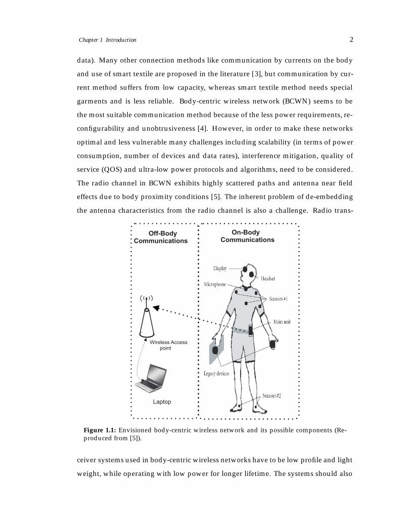
1.1 Envisioned body-centric wireless network and its possible components
(Reproduced from [5]). . . . . . . . . . . . . . . . . . . . . . . . . . . . . . 2
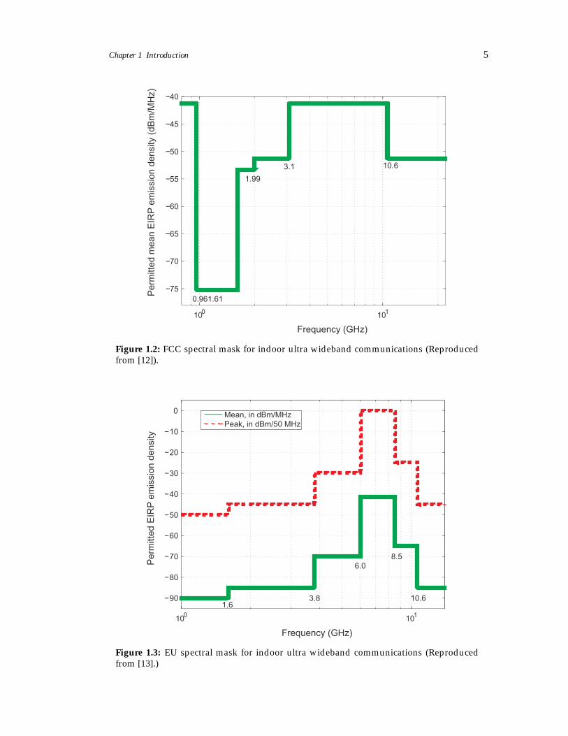
1.2 FCC spectral mask for indoor ultra wideband communications (Repro-
duced from [12]). . . . . . . . . . . . . . . . . . . . . . . . . . . . . . . . . 5
1.3 EU spectral mask for indoor ultra wideband communications (Repro-
duced from [13].) . . . . . . . . . . . . . . . . . . . . . . . . . . . . . . . . 5
2.1 A Gaussian doublet pulse of duration Tp = 0.5 ns [9]. . . . . . . . . . . . 17
2.2 Wireless services matrix showing where UWB fits in the current spec-
trum of wireless technologies mainly intended for consumers (Repro-
duced from [31]). . . . . . . . . . . . . . . . . . . . . . . . . . . . . . . . . 26
2.3 Possible home networking applications using UWB (Reproduced from
[6]). . . . . . . . . . . . . . . . . . . . . . . . . . . . . . . . . . . . . . . . . 28
2.4 Different commercial UWB enabled products [33–36]. . . . . . . . . . . . 29
2.5 Commercial UWB enabled product [37]. . . . . . . . . . . . . . . . . . . . 30
3.1 Antennas for body worn applications. From left to right tapered slot,
swan shaped monopole and planar inverted cone antenna [10]. . . . . . 35
3.2 Examples of transmitted UWB pulses to illustrate pulse fidelity concept.
Fidelity of reference pulse compared to Received A is 100% and com-
pared to Received B is 85% to demonstrate that fidelity compares pulse
shape only regardless of pulse amplitude and phase offsets [4]. . . . . . 37
3.3 Different types of fading, their subtypes and relationship (Reproduced
from [17]). . . . . . . . . . . . . . . . . . . . . . . . . . . . . . . . . . . . . 38
3.4 Block diagram of diversity combiner [41]. . . . . . . . . . . . . . . . . . . 48
3.5 Cophasing circuit for MRC and EGC [41] . . . . . . . . . . . . . . . . . . 50
3.6 An example of Diversity Gain calculation from CDF plots. . . . . . . . . 51
3.7 A printed Ultra-Wideband diversity monopole antenna [56]. . . . . . . . 54
xviii
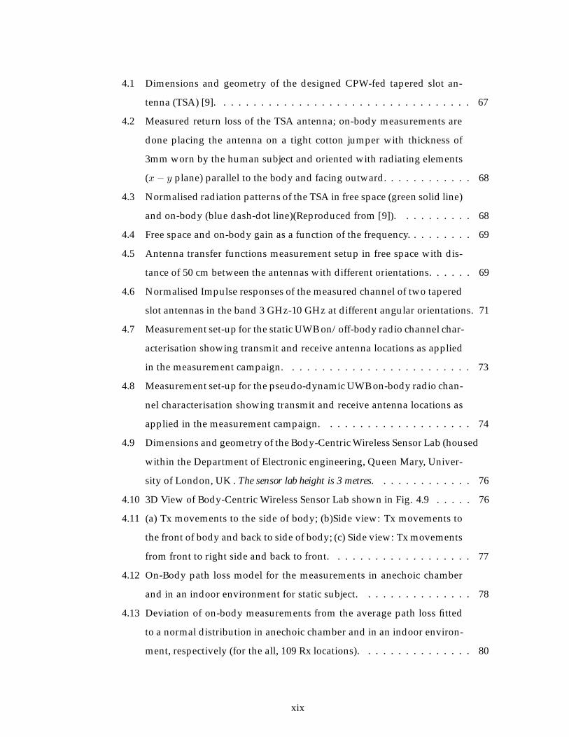
4.1 Dimensions and geometry of the designed CPW-fed tapered slot an-
tenna (TSA) [9]. . . . . . . . . . . . . . . . . . . . . . . . . . . . . . . . . . 67
4.2 Measured return loss of the TSA antenna; on-body measurements are
done placing the antenna on a tight cotton jumper with thickness of
3mm worn by the human subject and oriented with radiating elements
(x− y plane) parallel to the body and facing outward. . . . . . . . . . . . 68
4.3 Normalised radiation patterns of the TSA in free space (green solid line)
and on-body (blue dash-dot line)(Reproduced from [9]). . . . . . . . . . 68
4.4 Free space and on-body gain as a function of the frequency. . . . . . . . . 69
4.5 Antenna transfer functions measurement setup in free space with dis-
tance of 50 cm between the antennas with different orientations. . . . . . 69
4.6 Normalised Impulse responses of the measured channel of two tapered
slot antennas in the band 3 GHz-10 GHz at different angular orientations. 71
4.7 Measurement set-up for the static UWB on/off-body radio channel char-
acterisation showing transmit and receive antenna locations as applied
in the measurement campaign. . . . . . . . . . . . . . . . . . . . . . . . . 73
4.8 Measurement set-up for the pseudo-dynamic UWB on-body radio chan-
nel characterisation showing transmit and receive antenna locations as
applied in the measurement campaign. . . . . . . . . . . . . . . . . . . . 74
4.9 Dimensions and geometry of the Body-Centric Wireless Sensor Lab (housed
within the Department of Electronic engineering, Queen Mary, Univer-
sity of London, UK . The sensor lab height is 3 metres. . . . . . . . . . . . . 76
4.10 3D View of Body-Centric Wireless Sensor Lab shown in Fig. 4.9 . . . . . 76
4.11 (a) Tx movements to the side of body; (b)Side view: Tx movements to
the front of body and back to side of body; (c) Side view: Tx movements
from front to right side and back to front. . . . . . . . . . . . . . . . . . . 77
4.12 On-Body path loss model for the measurements in anechoic chamber
and in an indoor environment for static subject. . . . . . . . . . . . . . . 78
4.13 Deviation of on-body measurements from the average path loss fitted
to a normal distribution in anechoic chamber and in an indoor environ-
ment, respectively (for the all, 109 Rx locations). . . . . . . . . . . . . . . 80
xix
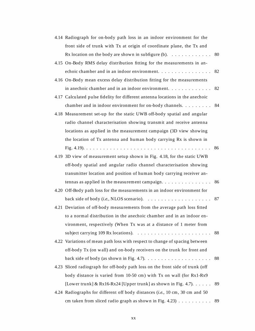
4.14 Radiograph for on-body path loss in an indoor environment for the
front side of trunk with Tx at origin of coordinate plane, the Tx and
Rx location on the body are shown in subfigure (b). . . . . . . . . . . . . 80
4.15 On-Body RMS delay distribution fitting for the measurements in an-
echoic chamber and in an indoor environment. . . . . . . . . . . . . . . . 82
4.16 On-Body mean excess delay distribution fitting for the measurements
in anechoic chamber and in an indoor environment. . . . . . . . . . . . . 82
4.17 Calculated pulse fidelity for different antenna locations in the anechoic
chamber and in indoor environment for on-body channels. . . . . . . . . 84
4.18 Measurement set-up for the static UWB off-body spatial and angular
radio channel characterisation showing transmit and receive antenna
locations as applied in the measurement campaign (3D view showing
the location of Tx antenna and human body carrying Rx is shown in
Fig. 4.19). . . . . . . . . . . . . . . . . . . . . . . . . . . . . . . . . . . . . . 86
4.19 3D view of measurement setup shown in Fig. 4.18, for the static UWB
off-body spatial and angular radio channel characterisation showing
transmitter location and position of human body carrying receiver an-
tennas as applied in the measurement campaign. . . . . . . . . . . . . . . 86
4.20 Off-Body path loss for the measurements in an indoor environment for
back side of body (i.e., NLOS scenario). . . . . . . . . . . . . . . . . . . . 87
4.21 Deviation of off-body measurements from the average path loss fitted
to a normal distribution in the anechoic chamber and in an indoor en-
vironment, respectively (When Tx was at a distance of 1 meter from
subject carrying 109 Rx locations). . . . . . . . . . . . . . . . . . . . . . . 88
4.22 Variations of mean path loss with respect to change of spacing between
off-body Tx (on wall) and on-body receivers on the trunk for front and
back side of body (as shown in Fig. 4.7). . . . . . . . . . . . . . . . . . . . 88
4.23 Sliced radiograph for off-body path loss on the front side of trunk (off
body distance is varied from 10-50 cm) with Tx on wall (for Rx1-Rx9
[Lower trunk] & Rx16-Rx24 [Upper trunk] as shown in Fig. 4.7). . . . . . 89
4.24 Radiographs for different off body distances (i.e., 10 cm, 30 cm and 50
cm taken from sliced radio graph as shown in Fig. 4.23) . . . . . . . . . . 89
xx
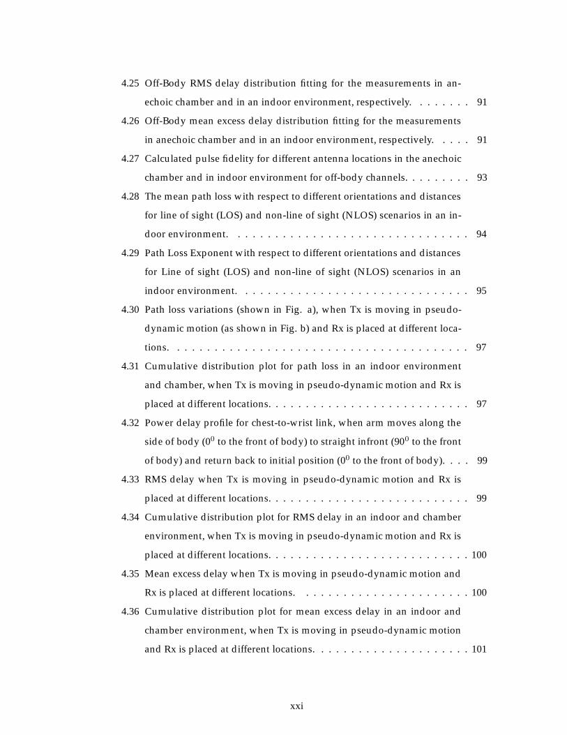
4.25 Off-Body RMS delay distribution fitting for the measurements in an-
echoic chamber and in an indoor environment, respectively. . . . . . . . 91
4.26 Off-Body mean excess delay distribution fitting for the measurements
in anechoic chamber and in an indoor environment, respectively. . . . . 91
4.27 Calculated pulse fidelity for different antenna locations in the anechoic
chamber and in indoor environment for off-body channels. . . . . . . . . 93
4.28 The mean path loss with respect to different orientations and distances
for line of sight (LOS) and non-line of sight (NLOS) scenarios in an in-
door environment. . . . . . . . . . . . . . . . . . . . . . . . . . . . . . . . 94
4.29 Path Loss Exponent with respect to different orientations and distances
for Line of sight (LOS) and non-line of sight (NLOS) scenarios in an
indoor environment. . . . . . . . . . . . . . . . . . . . . . . . . . . . . . . 95
4.30 Path loss variations (shown in Fig. a), when Tx is moving in pseudo-
dynamic motion (as shown in Fig. b) and Rx is placed at different loca-
tions. . . . . . . . . . . . . . . . . . . . . . . . . . . . . . . . . . . . . . . . 97
4.31 Cumulative distribution plot for path loss in an indoor environment
and chamber, when Tx is moving in pseudo-dynamic motion and Rx is
placed at different locations. . . . . . . . . . . . . . . . . . . . . . . . . . . 97
4.32 Power delay profile for chest-to-wrist link, when arm moves along the
side of body (00 to the front of body) to straight infront (900 to the front
of body) and return back to initial position (00 to the front of body). . . . 99
4.33 RMS delay when Tx is moving in pseudo-dynamic motion and Rx is
placed at different locations. . . . . . . . . . . . . . . . . . . . . . . . . . . 99
4.34 Cumulative distribution plot for RMS delay in an indoor and chamber
environment, when Tx is moving in pseudo-dynamic motion and Rx is
placed at different locations. . . . . . . . . . . . . . . . . . . . . . . . . . . 100
4.35 Mean excess delay when Tx is moving in pseudo-dynamic motion and
Rx is placed at different locations. . . . . . . . . . . . . . . . . . . . . . . 100
4.36 Cumulative distribution plot for mean excess delay in an indoor and
chamber environment, when Tx is moving in pseudo-dynamic motion
and Rx is placed at different locations. . . . . . . . . . . . . . . . . . . . . 101
xxi
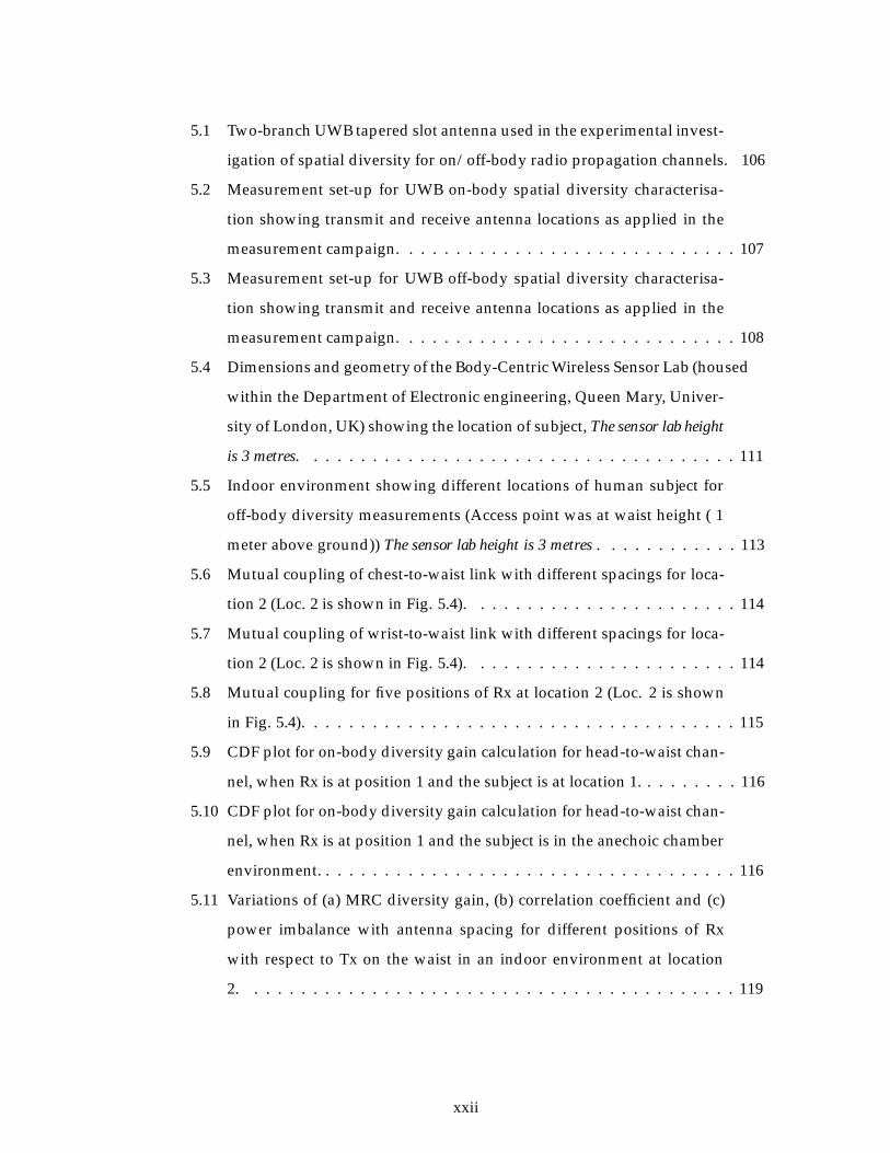
5.1 Two-branch UWB tapered slot antenna used in the experimental invest-
igation of spatial diversity for on/off-body radio propagation channels. 106
5.2 Measurement set-up for UWB on-body spatial diversity characterisa-
tion showing transmit and receive antenna locations as applied in the
measurement campaign. . . . . . . . . . . . . . . . . . . . . . . . . . . . . 107
5.3 Measurement set-up for UWB off-body spatial diversity characterisa-
tion showing transmit and receive antenna locations as applied in the
measurement campaign. . . . . . . . . . . . . . . . . . . . . . . . . . . . . 108
5.4 Dimensions and geometry of the Body-Centric Wireless Sensor Lab (housed
within the Department of Electronic engineering, Queen Mary, Univer-
sity of London, UK) showing the location of subject, The sensor lab height
is 3 metres. . . . . . . . . . . . . . . . . . . . . . . . . . . . . . . . . . . . . 111
5.5 Indoor environment showing different locations of human subject for
off-body diversity measurements (Access point was at waist height ( 1
meter above ground)) The sensor lab height is 3 metres . . . . . . . . . . . . 113
5.6 Mutual coupling of chest-to-waist link with different spacings for loca-
tion 2 (Loc. 2 is shown in Fig. 5.4). . . . . . . . . . . . . . . . . . . . . . . 114
5.7 Mutual coupling of wrist-to-waist link with different spacings for loca-
tion 2 (Loc. 2 is shown in Fig. 5.4). . . . . . . . . . . . . . . . . . . . . . . 114
5.8 Mutual coupling for five positions of Rx at location 2 (Loc. 2 is shown
in Fig. 5.4). . . . . . . . . . . . . . . . . . . . . . . . . . . . . . . . . . . . . 115
5.9 CDF plot for on-body diversity gain calculation for head-to-waist chan-
nel, when Rx is at position 1 and the subject is at location 1. . . . . . . . . 116
5.10 CDF plot for on-body diversity gain calculation for head-to-waist chan-
nel, when Rx is at position 1 and the subject is in the anechoic chamber
environment. . . . . . . . . . . . . . . . . . . . . . . . . . . . . . . . . . . . 116
5.11 Variations of (a) MRC diversity gain, (b) correlation coefficient and (c)
power imbalance with antenna spacing for different positions of Rx
with respect to Tx on the waist in an indoor environment at location
2. . . . . . . . . . . . . . . . . . . . . . . . . . . . . . . . . . . . . . . . . . 119
xxii
5.12 Comparison of MRC diversity gain for different links for position 2 and
three locations at 0.34λo spacing in an indoor environment in compar-
ison with narrow band in an indoor environment presented in [7]. . . . . 122
5.13 Variations of Maximum Ratio combined DG and Correlation coefficient
with respect to variation in spacing between on-body diversity branch
antennas (when diversity branch antenna is on wrist). . . . . . . . . . . . 127
5.14 Variations of Maximum Ratio combined DG and Power imbalance with
respect to variation in spacing between on-body diversity branch anten-
nas (when diversity branch antenna is on wrist). . . . . . . . . . . . . . . 128
5.15 Variations of Maximum Ratio combined DG, Power imbalance and Cor-
relation coefficient with respect to variation in spacing between on-
body diversity branch antennas (when diversity branch antenna is on
wrist). . . . . . . . . . . . . . . . . . . . . . . . . . . . . . . . . . . . . . . . 130
5.16 Variations of Correlation coefficient with respect to different orienta-
tions between Off-body Tx and five on-body Rx locations at Loc. 2 (Loc.
2 is shown in Fig. 5.5). . . . . . . . . . . . . . . . . . . . . . . . . . . . . . 131
5.17 Variations of Maximum Ratio combined DG with respect to different
orientations between Off-body Tx and five on-body Rx locations at Loc.
2 (Loc. 2 is shown in Fig. 5.5). . . . . . . . . . . . . . . . . . . . . . . . . . 131
5.18 Maximum Ratio combined DG for five on-body Rx locations, for three
different Subjects at 0.34λo spacing between diversity branch Rx in an
indoor environment at Loc. 2 (Loc. 2 is at distance of 1 m from off-body
Tx as shown in Fig. 5.5). . . . . . . . . . . . . . . . . . . . . . . . . . . . . 132
6.1 Simplified block diagram illustrating the various stages of the mult-
iband OFDM UWB radio transceiver applied in the system-level mod-
elling for body-centric wireless networks. . . . . . . . . . . . . . . . . . . 138
6.2 A UWB OFDM model for Body-Centric wireless communications without
any channel model. . . . . . . . . . . . . . . . . . . . . . . . . . . . . . . . 140
6.3 A UWB OFDM model for Body-Centric wireless communications using
AWGN channel model. . . . . . . . . . . . . . . . . . . . . . . . . . . . . . 141
6.4 A comparison of theoretical and measured BER for AWGN channel. . . 141
xxiii
6.5 On-body locations used in the measurement campaign for UWB on-
body radio channel characterisation when the subject is stationary. . . . 142
6.6 On-body locations used in the measurement campaign for UWB on-
body system performance evaluation, when the subject is in pseudo-
dynamic motion with Tx is fixed in relation to mobile Rx and then Tx is
mobile with respect to Rx positions. . . . . . . . . . . . . . . . . . . . . . 143
6.7 On-Body BER performance for different receiver locations (position of
Rx is shown in Fig. 4.7 in Chapter 4) at Eb/No = 4 dB. . . . . . . . . . . . 144
6.8 On-Body BER performance for different receiver locations (position of
Rx is shown in Fig. 4.7 in Chapter 4) at Eb/No = 4 dB. . . . . . . . . . . . 144
6.9 BER variations for different locations (Fig. 6.5) on the body for Eb/No=4
dB in the anechoic chamber. . . . . . . . . . . . . . . . . . . . . . . . . . . 145
6.10 BER variations for different locations (Fig. 6.5) on the body for Eb/No=4
dB in the indoor environment. . . . . . . . . . . . . . . . . . . . . . . . . . 146
6.11 Illustration of the on-body radio link classification for different propaga-
tion channels based on system performance analysis. Good link: BER
less than 1.0 x 10⁻⁴, Acceptable link: BER between 1.0 x 10⁻⁴ and 1.0 x
10−3 and Bad link: BER greater than 1.0 x 10⁻³ at Eb/No=4 dB . . . . . . 147
6.12 Illustration of the off-body radio link classification for different propaga-
tion channels based on system performance analysis. Good link: BER
less than 1.0 x 10⁻⁴, Acceptable link: BER between 1.0 x 10⁻⁴ and 1.0 x
10−3 and Bad link: BER greater than 1.0 x 10⁻³ at Eb/No=4 dB. . . . . . 149
6.13 Comparison of BER performance for various Rx locations taken ran-
domly (from Rx locations as shown in Fig. 4.7) for different Off-body
distances at Eb/No = 4 dB. . . . . . . . . . . . . . . . . . . . . . . . . . . 149
6.14 Comparison of BER for on-body and off-body receivers for front side of
body (as shown in Fig. 4.7) at Eb/No = 4 dB. . . . . . . . . . . . . . . . . 151
6.15 Comparison of BER for on-body and off-body receivers for back side of
body (as shown in Fig. 4.7) at Eb/No = 4 dB. . . . . . . . . . . . . . . . . 151
6.16 Bit error rate (BER) as a function of Eb/No for five different UWB on-
body channels (Fig.6.6) in the indoor environment. . . . . . . . . . . . . . 152
xxiv
6.17 Variations of BER as a function of on-body channels when Tx antenna
is placed on the waist in an indoor environment (Fig. 6.6) . . . . . . . . . 153
6.18 Variations of BER as a function of on-body channels when Tx antenna
is placed on the wrist in the indoor environment (Fig. 6.6) . . . . . . . . 155
6.19 Bit Error Rate Performance of five different locations with respect to
Tx on waist (on-body communications) at Eb/No = 4 dB in an indoor
environment. . . . . . . . . . . . . . . . . . . . . . . . . . . . . . . . . . . . 156
6.20 Bit Error Rate Performance of five different locations with respect to Tx
on wall at waist height at distance of 1 m (off-body communications) at
Eb/No = 4 dB in an indoor environment. . . . . . . . . . . . . . . . . . . 158
B.1 UWB Spectrum Division in 14 subbands . . . . . . . . . . . . . . . . . . . 171
B.2 Convolutional encoder: code rate 1/3, constraint length 7 . . . . . . . . . 172
B.3 Bit-stealing and bit-insertion procedure (R = 3/4) . . . . . . . . . . . . . 173
B.4 QPSK Constellation Bit Map . . . . . . . . . . . . . . . . . . . . . . . . . . 174
B.5 Frequency overlapping of OFDM orthogonal sub-carriers . . . . . . . . . 175
B.6 Input and output of IFFT . . . . . . . . . . . . . . . . . . . . . . . . . . . . 177
xxv
List of Tables
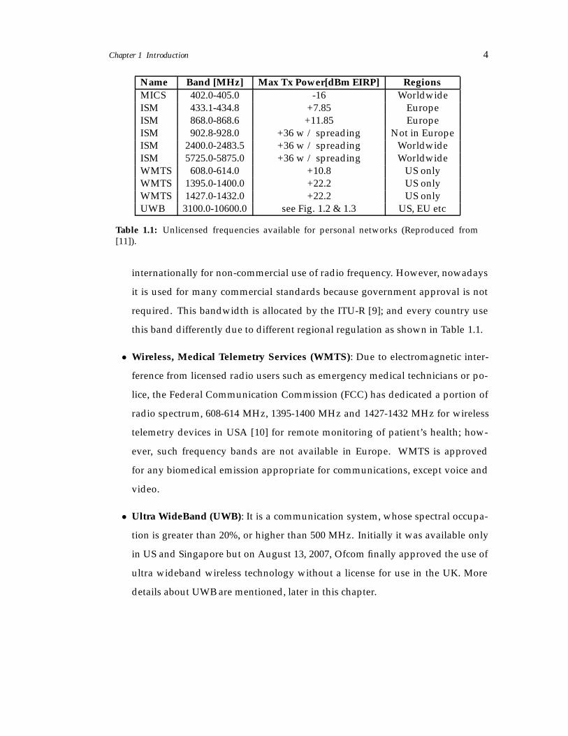
1.1 Unlicensed frequencies available for personal networks (Reproduced
from [11]). . . . . . . . . . . . . . . . . . . . . . . . . . . . . . . . . . . . . 4
2.1 Comparison of different modulation schemes used for UWB. . . . . . . . 18
3.1 Path loss parameters obtained for channel model with respect to an-
tenna directivity [21]. . . . . . . . . . . . . . . . . . . . . . . . . . . . . . . 44
4.1 On-Body path loss exponent (calculated in similar manner using em-
pirical model as shown in Fig. 4.12) and mean path loss for different
sectors of body. . . . . . . . . . . . . . . . . . . . . . . . . . . . . . . . . . 78
4.2 Average value and standard deviation of Log-normal distribution ap-
plied to RMS delay for on-body communications with respect to differ-
ent threshold levels in the chamber and indoor environment. . . . . . . . 82
4.3 Average value and standard deviation of Log-normal distribution ap-
plied to mean excess delay for on-body communications with respect
to different threshold levels in the chamber and indoor environment. . . 83
4.4 Off-Body path loss exponent (calculated in similar manner using em-
pirical model as shown in Fig. 4.20) and mean path loss for different
sectors of body (at distance of 100 cm). . . . . . . . . . . . . . . . . . . . . 90
4.5 Average value and standard deviation of Log-normal distribution ap-
plied to RMS delay for off-body communications with respect to differ-
ent threshold levels in the chamber and indoor environment. . . . . . . . 92
4.6 Average value and standard deviation of Log-normal distribution ap-
plied to mean excess delay for off-body communications with respect
to different threshold levels in the chamber and indoor environment. . . 92
4.7 The mean path loss for different scenarios and orientations. . . . . . . . . 94
xxvi
4.8 Mean and standard deviation of path loss using normal distribution for
different channels and environments (whereas, running is performed in
an indoor environment). . . . . . . . . . . . . . . . . . . . . . . . . . . . . 98
4.9 Mean and standard deviation of RMS delay using log-normal distribu-
tion for different channels and environments (nsec) (whereas, running
is performed in an indoor environment). . . . . . . . . . . . . . . . . . . . 100
4.10 Mean and standard deviation of mean excess delay using log-normal
distribution for different channels and environments (nsec) (whereas,
running is performed in an indoor environment). . . . . . . . . . . . . . 100
5.1 Movements performed for different Channels during UWB on/off An-
tenna Diversity Measurements . . . . . . . . . . . . . . . . . . . . . . . . 110
5.2 The dimensions of Three subjects (F – Female, M – Male). . . . . . . . . . 110
5.3 Diversity parameters for 5 different links at location 2 with different
spacings in an indoor environment. . . . . . . . . . . . . . . . . . . . . . . 117
5.4 Diversity parameters for different Rx positions with respect to Tx on
waist in an indoor environment for location 1 at 0.34λo spacing (all units
are in dB except ρe, r1 and r2 are mean powers and I is the power
imbalance). . . . . . . . . . . . . . . . . . . . . . . . . . . . . . . . . . . . . 120
5.5 Diversity parameters for different Rx positions with respect to Tx on
waist in an anechoic chamber at .34λo spacing (all units are in dB except
ρe, r1 and r2 are mean powers and I is the power imbalance). . . . . . . 121
5.6 On-Body Uplink Downlink Diversity at Loc. 1 (Loc. 1 is shown in Fig.
5.4) at 0.34λo spacing between diversity branch Rx antennas in an in-
door environment (I – power imbalance, MRC and I are in dB units). . . 122
5.7 Diversity parameters for three different locations at 0.34λo spacing between
diversity branch Rx in an indoor environment (L – Location no, all units
are in dB except ρe, r1 and r2 are mean powers and I is the power im-
balance). . . . . . . . . . . . . . . . . . . . . . . . . . . . . . . . . . . . . . 122
5.8 Diversity parameters for different Rx positions with respect to Tx on
wall (At Loc. 2 in an indoor environment as shown in Fig. 5.5) at .34λo
spacing (all units are in dB except ρe, where I is the power imbalance). . 125
xxvii
5.9 Diversity parameters for 5 different links at 8 different locations in an
indoor environment with spacing of 0.34 λo between Rx antenna. . . . . 127
5.10 Diversity parameters for 5 different links at Loc. 2 (as shown in Fig.
5.5) with different spacings between diversity antennas in an indoor
environment. . . . . . . . . . . . . . . . . . . . . . . . . . . . . . . . . . . . 129
5.11 Off-Body Downlink Diversity at Loc. 2 (at 1 meter distance between Tx
and Rx, Loc. 2 is shown in Fig. 5.5) at 0.34λo spacing between diversity
branch Rx in an indoor environment (I – power imbalance, MRC and I
are in dB units) . . . . . . . . . . . . . . . . . . . . . . . . . . . . . . . . . 131
6.1 Specifications for MB-OFDM UWB body-centric system for Bit Error
rate calculation . . . . . . . . . . . . . . . . . . . . . . . . . . . . . . . . . 139
6.2 Classification of the on-body radio link quality for various sectors of the
human body (the upper body, lower body (legs) and arms) for BER less
than 1.0 X10⁻⁴ for good links, and between 1.0 x 10⁻³ and 1.0 X10⁻⁴ for
acceptable links and bad links where BER is greater than 1.0 x 10⁻³ at
Eb/No = 4dB. All units in %. . . . . . . . . . . . . . . . . . . . . . . . . . 146
6.3 System outage percentage at the threshold of 1.0 x 10⁻³ for different
parts of body for on-body and off-body cases (off-body Tx is at distance
of 100 cm) at Eb/No = 4 dB. . . . . . . . . . . . . . . . . . . . . . . . . . . 150
6.4 Percentage of system outage rate as a function of on-body radio chan-
nels for pseudo-dynamic scenarios of the MB-OFDM UWB system with
BER greater than 1.0 x 10⁻³ indicating bad quality links. All units in %. . 154
B.1 Quadrature phase shift keying (QPSK) encoding table . . . . . . . . . . . 173
xxviii
Chapter 1
Introduction
According to Media Lab, MIT, USA,“By 2015, wearables will have virtually eliminated
desktop, laptop, and handheld solutions altogether...” [1].
Body-centric wireless networks (BCWNs) refers to networking over the body and
body-to-body with the use of wearable and implantable wireless sensor nodes. This
subject combines, Wireless Body Area Networks (WBANs), Wireless Sensor Networks
(WSNs) and Wireless Personal Area Networks (WPANs) [2]. Body-centric wireless
network (BCWN) has got numerous applications in everyday’s life including health-
care, entertainment, space exploration, military and so forth [3]. The topic of BCWN
can be divided into three domains based on wireless sensor nodes placement i.e.: com-
munication between the nodes that are on the body surface; communication from the
body-surface to nearby base station; atleast one node may be implanted within the
body. These three domains have been called on-body, off-body and in-body respect-
ively [2]. Figure 1.1 shows an example of on- and off-body system only; for in-body
communications, one of the node should be implanted within the body. The major
drawback with current on body systems is the wired or limited wireless communica-
tion that is not suitable for some user and the restrictions on the data rate (like video
streaming and heavy data communication, where we need to transfer large amount of
1
Chapter 1 Introduction 2
data). Many other connection methods like communication by currents on the body
and use of smart textile are proposed in the literature [3], but communication by cur-
rent method suffers from low capacity, whereas smart textile method needs special
garments and is less reliable. Body-centric wireless network (BCWN) seems to be
the most suitable communication method because of the less power requirements, re-
configurability and unobtrusiveness [4]. However, in order to make these networks
optimal and less vulnerable many challenges including scalability (in terms of power
consumption, number of devices and data rates), interference mitigation, quality of
service (QOS) and ultra-low power protocols and algorithms, need to be considered.
The radio channel in BCWN exhibits highly scattered paths and antenna near field
effects due to body proximity conditions [5]. The inherent problem of de-embedding
the antenna characteristics from the radio channel is also a challenge. Radio trans-
Off-BodyCommunications
On-BodyCommunications
Wireless Accesspoint
Laptop
Figure 1.1: Envisioned body-centric wireless network and its possible components (Re-produced from [5]).
ceiver systems used in body-centric wireless networks have to be low profile and light
weight, while operating with low power for longer lifetime. The systems should also
Chapter 1 Introduction 3
be designed with minimal restriction for the user, so that they can be used during reg-
ular day-to-day activities without inhibition. They should be easily integrated with
the human body, or as a part of the clothing. Many currently existing short-range
wireless technologies provide communication medium and cable replacement tech-
nologies for different transmission types. To design a suitable efficient radio interface
for the wireless body-centric network, the understanding and integration of existing
standards are required in order to bring to light the main areas in which new tech-
niques are required to meet the harsh and demanding communication environment.
As mentioned earlier, the main characteristics of BCWN operating device should be,
low power requirements, less complexity, low cost, robustness to jamming, low prob-
ability of detection, scalable data rates from low (1-10 kbps) to very high (100-400
Mbps) and very small and compact in size [5]. Ultra wideband (UWB) technology is
the most promising candidate for BCWN due to its potential of meeting the essen-
tial requirements needed to deploy an efficient and reliable system. The wideband
nature of UWB technology permits a very fine time resolution which helps in provid-
ing immunity to multipath fading and robustness against jamming [6]. High timing
resolution property makes UWB very beneficial to biomedical application e.g. health
monitoring and real time diagnosis by accurate tracking of small variation in limbs or
object movements for post-operation rehabilitation etc. Vital features including ultra-
low power (-2.5 dBm) and fine time resolution makes UWB a prime candidate for
BCWN [7].
1.1 Frequency Band Allocation for Body Area Networks
Wireless communications systems can operate in the unlicensed portions of the spec-
trum. However the allocation of unlicensed frequencies is not the same in every coun-
try. Important frequency bands for BCWN are reported in Table1.1 and they are:
• Medical Implanted Communication System (MICS): In 1998, the International
Telecommunication Radio sector (ITU-R) allocated the bandwidth 402-405 MHz
for medical implants [8]. MICS devices can use up to 300 KHz of bandwidth at
a time to accommodate future higher data rate communications.
• Industrial, Scientific, and Medical (ISM): ISM bands were originally preserved
Chapter 1 Introduction 4
Name Band [MHz] Max Tx Power[dBm EIRP] RegionsMICS 402.0-405.0 -16 WorldwideISM 433.1-434.8 +7.85 EuropeISM 868.0-868.6 +11.85 EuropeISM 902.8-928.0 +36 w / spreading Not in EuropeISM 2400.0-2483.5 +36 w / spreading WorldwideISM 5725.0-5875.0 +36 w / spreading WorldwideWMTS 608.0-614.0 +10.8 US onlyWMTS 1395.0-1400.0 +22.2 US onlyWMTS 1427.0-1432.0 +22.2 US onlyUWB 3100.0-10600.0 see Fig. 1.2 & 1.3 US, EU etc
Table 1.1: Unlicensed frequencies available for personal networks (Reproduced from[11]).
internationally for non-commercial use of radio frequency. However, nowadays
it is used for many commercial standards because government approval is not
required. This bandwidth is allocated by the ITU-R [9]; and every country use
this band differently due to different regional regulation as shown in Table 1.1.
• Wireless, Medical Telemetry Services (WMTS): Due to electromagnetic inter-
ference from licensed radio users such as emergency medical technicians or po-
lice, the Federal Communication Commission (FCC) has dedicated a portion of
radio spectrum, 608-614 MHz, 1395-1400 MHz and 1427-1432 MHz for wireless
telemetry devices in USA [10] for remote monitoring of patient’s health; how-
ever, such frequency bands are not available in Europe. WMTS is approved
for any biomedical emission appropriate for communications, except voice and
video.
• Ultra WideBand (UWB): It is a communication system, whose spectral occupa-
tion is greater than 20%, or higher than 500 MHz. Initially it was available only
in US and Singapore but on August 13, 2007, Ofcom finally approved the use of
ultra wideband wireless technology without a license for use in the UK. More
details about UWB are mentioned, later in this chapter.
Chapter 1 Introduction 5
100
101
−75
−70
−65
−60
−55
−50
−45
−40
Frequency (GHz)
Perm
itte
d m
ean E
IRP
em
issio
n d
ensity (
dB
m/M
Hz)
0.961.61
1.99
3.1 10.6
Figure 1.2: FCC spectral mask for indoor ultra wideband communications (Reproducedfrom [12]).
100
101
−90
−80
−70
−60
−50
−40
−30
−20
−10
0
Frequency (GHz)
Pe
rmitte
d E
IRP
em
issio
n d
en
sity
1.63.8
6.0
8.5
10.6
Mean, in dBm/MHz
Peak, in dBm/50 MHz
Figure 1.3: EU spectral mask for indoor ultra wideband communications (Reproducedfrom [13].)
Chapter 1 Introduction 6
1.2 Ultra Wideband Radio Technology
Federal Communications Commission approved a promising radio technology that is
Ultra Wideband. It operates primarily in the frequency range between 3.1 GHz to 10.6
GHz with a 7.5 GHz band, maximum power spectral density of -41.25 dBm/MHz
and a maximum transmit power of -2.5 dBm [14]. UWB can be regarded as an ex-
treme case of spread spectrum technology which offers flexibility, robustness, high-
precision (upto 5 cm), location tracking with accuracy in the sub-centimetre range.
Moreover, critical factors like extremely low power consumption, scalable data rates,
high throughput and extended communication range can also be principally achieved
with the UWB technology. Due to long spreading code sequence, UWB devices work
below the noise floor so that jamming becomes extremely difficult, a property bene-
ficial particularly for applications such as intrusion detection. UWB has excellent po-
tential for radio reusability as well.
1.2.1 History of Ultra Wideband
Historically UWB radar systems were first developed for military purpose because
they could be seen beneath ground surfaces, through walls and trees [15]. The era
of UWB starts from Hertzian Spark gap experiment in 1880, because his experiment
came up with a very large RF bandwidth. In 1948, Shannon’s observation led to spread
spectrum modulation [16]. After that, scientists worked to develop short impulse sig-
nals between antennas. Short impulse signaling experiment led to the development
of Impulse Radio later called UWB radio. After development of impulse radio, this
area again attracted people in 1950 when UWB and impulse technology is heavily in-
vestigated for communication, radar and other applications. In 1960s, the first patent
appeared using UWB technique and digital techniques were applied on UWB. In the
late 1970s and 1980s, UWB spread spectrum impulse techniques were demonstrated
by Fullerton for communication and positioning [16]. After that UWB became an area
of greater interest and in 1990s admirers of UWB started attempts to make UWB legal.
FCC noticed the first enquiry about UWB in 1998. UWB communication has drawn
such attention in 2000 that, it is described in popular magazine by monikers such as′one of the ten technologies that will change your world′ [4]. In 2002 FCC approved
Chapter 1 Introduction 7
UWB for commercial use and presented a first report on UWB systems. Finally, the
Hertz spark gap experiment has now re-emerged as an ultra wideband technology.
After the UWB approval by FCC, it attracted many companies and in 2004, the FCC
granted the first modular certification to freescale’s XS110 chipset to Freescale Semi-
conductor, which means commercial shipments can begin immediately. The deadlock
between direct sequence UWB proposal and multiband OFDM alliance slowed down
the standardisation and commercialisation process. On March, 2007, finally interna-
tional standards based on the Wi-Media UWB common radio platform were approved
for release by the international organization for standardization (ISO). Soon after ISO
approval, the British standard body, Ofcom also approved the use of UWB wireless
technology without a license for use in the UK [13]. Recent standards and develop-
ments about UWB technology will be discussed at the end of Chapter 2 in Section 2.2.2
and Section 2.4 respectively.
1.2.2 Basics of Ultra Wideband
The FCC UWB rulings issued in February 2002 provided the initial radiation restric-
tions for UWB, and also allowed the commercialisation of the technology. According
to the FCC rulings, a signal is recognised as UWB if its instantaneous spectral occu-
pancy is in excess of 500 MHz or has a fractional bandwidth greater than 20% [17].
The formula proposed by the FCC for calculating the fractional bandwidth is given by
[17]:
Bf =B
fc(1.1)
where B = fH − fL represents the impedance bandwidth and fc =fH+fL
2 is the centre
frequency with fH denoting the upper frequency of the -10 dB emission limit, and fL
the lower frequency of the -10 dB emission limit. According to the first FCC report
and order, UWB systems with fc> 2.5 GHz are required to have a -10 bandwidth of
no less than 500 MHz while UWB systems with fc< 2.5 GHz ought to have fractional
bandwidth of at least 20% [17].
Chapter 1 Introduction 8
1.2.3 UWB System Limits and Capacity
UWB like any other radio systems are not perfect. Both thermal noise and human
caused interference limit wireless system performance. A theoretical maximum limit
on UWB system gain per bit per second is 173 dB/bps provides a simple mean by
which the performance and capabilities of practical radio links can be estimated. This
system gain limit is by nature [16] (UWB System gain = EIRP − N − eb, whereas
EIRP=-2.55 dBm, N is thermal noise floor, which is -174 dBm/Hz and eb is shannon’s
communication efficiency limit and is given by -1.59 dB). Besides regulatory limits of
power spectral density and frequency band, modulation efficiency is one of the funda-
mental limitations of the UWB system. The antenna also plays a very important role
in defining the effectiveness of the UWB link. Over the frequency band, the antenna
may exhibit constant aperture or constant gain characteristic. The distinction is very
important because the antenna choice can render one end of the band more effective
than the other end in UWB link [16]. UWB link capacity is simply a measure of how
many bits per second can be transferred over the link in the absence of interference
and with no multipath dispersion; this capacity is bounded by Shannon’s limit (-1.59
dBm). In practice additive white gaussian noise (AWGN) is not the only problem but
the time delay copies of transmitted signal is also a problem that limits the system
capacity.
1.2.4 Pros and Cons of UWB for BCWN
In the UWB systems, the transmission of short nanoseconds pulses allow pulse gen-
erators and the whole system to work in on and off mode rather than in continuous
operation resulting in low power requirements per bit [15]. In addition to this, the
combination of high data rate and intermitting signal reduces average power con-
sumption, which makes it possible for UWB systems to have smaller and cheaper bat-
tery systems. This is very important for ensuring, longer operational time of BCWN
and hence greener radio systems. Furthermore due to carrierless capability of UWB
impulse radio systems, it requires less analog components resulting in smaller chip
size [17], which is another very important feature in the context of small and low cost
BCWN.
Chapter 1 Introduction 9
A typical problem in wireless communications is the multipath fading. In a typ-
ical complex indoor environment, presence of many scatterers produces reflected sig-
nals causing a destructive interference in the direct signal (the received power de-
creases resulting in degradation of bit error rate or signal to noise ratio of system). In
UWB, there is an inherent property of multipath fading due to fine time resolutions
[6], which makes it easy to separate the direct component from each single reflection,
hence it is possible to achieve higher range with the same power level. The power
spectrum of UWB signal pulse is spread across the wide band of 7.5 GHz with a very
low signal power that leads to less power absorption by human tissues. Combination
of short duration pulses, low power requirement and random code spreading makes
the UWB robust to jamming as it is difficult to distinguish original signal from noise
signal. Finally, UWB systems are more scalable and flexible in terms of data rate from
low to very high (1-10 kbps and 100-400 Mbps). The combination of all these features
makes UWB, the most favorable candidate for BCWN.
The biggest challenge for the BCWN system is the requirement of low power re-
ceivers to provide reliable transmission. The design of low power receivers for UWB
system is challenging for three reasons [18]:
1. Multipath spreading increases the system complexity
2. Acquisition of data is difficult
3. Its in-band interference issue
UWB is robust to multipaths, but this advantage comes at the significant receiver
hardware cost due to very highly sampling requirement. As UWB operates below
noise floor, its difficult to recognise and synchronise UWB signal at the receiver end.
Moreover, ultra narrow pulses of UWB represents the sensitivity of timing for accurate
measurement otherwise a small timing error may cause a considerable degradation.
Finally the narrow band signal does not blend with noise like UWB, so interfere with
UWB system [18].
Chapter 1 Introduction 10
1.3 Research Motivation
The design of ideal wireless system for body-centric communication needs accurate
and thorough analysis of the radio propagation channel. Any discrepancy in radio
channel characterisation due to the factors including postures, frequency of opera-
tion and antenna polarization can lead to error in the calculation of the system link
budget, which in turn severely degrades the performance of the designed system. The
changes in transmission path of the received signal give rise to fading in BCWN. It
badly affects the overall received power and hence reduces the system performance
and efficiency. Therefore, to improve system performance, fading needs to be mitig-
ated and this is usually achieved using diversity. In the past, researchers have been
actively involved in investigating UWB on-body radio channels but very limited work
for UWB off-body radio channel is being presented. Previous UWB body-centric radio
channel studies are limited, because of considering limited antenna locations for both
on/off-body case. As different tissues have different properties, hence consideration
of more antenna locations on the body with inclusion of body movements are required
to better understand the UWB on/off-body radio channels. From the system perform-
ance perspective, very limited work is present in the literature and that is only for
UWB on-body communications using impulse based UWB systems. Hence, the actual
system performance evaluation needs to be addressed for both on/off-body commu-
nications based on real experimental results, before the concept can be deployed for
commercial applications. As fading is overcome by diversity, in past several efforts
have been made to investigate body-centric diversity for narrow band communica-
tions but applicability of UWB body-centric diversity needs further investigation, as
there is hardly any literature around to validate the applicability of UWB diversity in
body-centric wireless networks.
1.4 Research Objectives
The aim of the research work presented in this thesis, is to analyse and characterise
the radio propagation using single and multiple antennas, and their impact on the
system performance of body-centric wireless communications. This was done through
Chapter 1 Introduction 11
a combination of measurement campaigns and simulations. In this study multiband-
UWB (i.e. OFDM based UWB) system is used, due to its advantage of overcoming the
problem of spectrum flexibility and complexity in comparison to impulse based UWB
system. The main objectives of the study include:
• Characterisation of ultra wideband on/off-body radio channel considering nu-
merous receiver locations, body posture and body movements.
• Investigation of ultra wideband antenna diversity for both on/off-body radio
channel.
• OFDM-UWB system performance evaluation on the basis of bit error rate (BER)
for both UWB on/off-body radio channel measurements.
• System performance improvement comparison for UWB on-body and off-body
antenna diversity.
According to the author’s knowledge, the above mentioned objectives have yet to be
analysed and investigated thoroughly for the accelerated introduction of reliable and
efficient body-centric wireless communications.
1.5 Thesis Organisation
Following the research objectives, the rest of the thesis is organised as follows:
Chapter 2 presents fundamentals of UWB communication systems with a brief intro-
duction of signal representations, pulse shapes, channel models, modulation schemes,
multiple access transmission schemes and receiver architecture. UWB spectrum regu-
lations and standards with its applications are also discussed.
Chapter 3 gives an introduction to UWB antenna for BCWN, wireless channel propaga-
tion and diversity in addition to literature review covering the main areas analysed
and discussed in this thesis.
Chapter 4 presents a thorough investigation of sectorised ultra wideband on/off-body
radio channel in both the anechoic chamber and indoor environments including ef-
fects of time varying movements of various body parts on the channel characterist-
ics. Radio channel parameters are extracted for different sectors of the body from the
Chapter 1 Introduction 12
measurement data and statistically analysed to provide a preliminary radio propaga-
tion model with the inclusion of dynamic body movements.
Chapter 5 presents some studies for the analysis of antenna diversity in ultra wide-
band on/off-body radio channel. Various diversity techniques are applied to highlight
the benefit of employing such methods in enhancing the overall system performance.
Chapter 6 presents system-level modelling of UWB BAN based on experimental in-
vestigation of ultra wideband on/off-body radio channel in both the anechoic cham-
ber and indoor environments. The effects of time varying movements of various body
parts on potential BCWN system performance is also analysed. Apart from this, sys-
tem level comparison of both on-body and off-body diversity is also presented to-
wards the end of the chapter.
Chapter 7 provides a summary of the main contributions and findings of the study
and concludes the accomplished work. It also introduces the potential future research
activities.
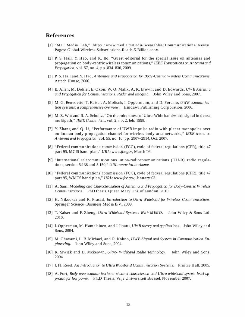
References
[1] “MIT Media Lab,” http://www.media.mit.edu/wearables/Communications/News/Pages/Global-Wireless-Subscriptions-Reach-5-Billion.aspx.
[2] P. S. Hall, Y. Hao, and K. Ito, “Guest editorial for the special issue on antennas andpropagation on body-centric wireless communications,” IEEE Transcations on Antenna andPropagation, vol. 57, no. 4, pp. 834–836, 2009.
[3] P. S. Hall and Y. Hao, Antennas and Propagation for Body-Centric Wireless Communications.Artech House, 2006.
[4] B. Allen, M. Dohler, E. Okon, W. Q. Malik, A. K. Brown, and D. Edwards, UWB Antennaand Propagation for Communications, Radar and Imaging. John Wiley and Sons, 2007.
[5] M. G. Benedetto, T. Kaiser, A. Molisch, I. Oppermann, and D. Porcino, UWB communica-tion systems: a comprehensive overview. Hindawi Publishing Corporation, 2006.
[6] M. Z. Win and R. A. Scholtz, “On the robustness of Ultra-Wide bandwidth signal in densemultipath,” IEEE Comm. lett., vol. 2, no. 2, feb. 1998.
[7] Y. Zhang and Q. Li, “Performance of UWB impulse radio with planar monopoles overon human body propagation channel for wireless body area networks,” IEEE trans. onAntenna and Propagation, vol. 55, no. 10, pp. 2907–2914, Oct. 2007.
[8] “Federal communications commission (FCC), code of federal regulations (CFR), title 47part 95, MCIS band plan,” URL: www.fcc.gov, March’03.
[9] “International telecommunications union-radiocommunications (ITU-R), radio regula-tions, section 5.138 and 5.150,” URL: www.itu.int/home.
[10] “Federal communications commission (FCC), code of federal regulations (CFR), title 47part 95, WMTS band plan,” URL: www.fcc.gov, January’03.
[11] A. Sani, Modeling and Characterisation of Antenna and Propagation for Body-Centric WirelessCommunications. PhD thesis, Queen Mary Uni. of London, 2010.
[12] H. Nikookar and R. Prasad, Introduction to Ultra Wideband for Wireless Communications.Springer Science+Business Media B.V., 2009.
[13] T. Kaiser and F. Zheng, Ultra Wideband Systems With MIMO. John Wiley & Sons Ltd,2010.
[14] I. Opperman, M. Hamalainen, and J. Iinatti, UWB theory and applications. John Wiley andSons, 2004.
[15] M. Ghavami, L. B. Michael, and R. Kohno, UWB Signal and System in Communication En-gineering. John Wiley and Sons, 2004.
[16] K. Siwiak and D. Mckeown, Ultra- Wideband Radio Technology. John Wiley and Sons,2004.
[17] J. H. Reed, An Introduction to Ultra Wideband Communication Systems. Printce Hall, 2005.
[18] A. Fort, Body area communications: channel characterion and Ultra-wideband system level ap-proach for low power. Ph.D Thesis, Vrije Universiteit Brussel, November 2007.
13
Chapter 2
Preliminaries of Ultra Wideband
Communication Systems
In this chapter, the fundamentals of UWB communication systems are discussed. In
addition, UWB spectrum regulations and its standards across different parts of the
world with its applications are also introduced briefly with emphasis on the state-of-
art.
2.1 UWB Communication Systems
In literature two different types of UWB communication systems exist; namely, Impulse-
Radio UWB (IR-UWB) and Multi-Carrier UWB (MC-UWB). IR-UWB employs a base-
band signal with pulse duration in the order of sub-nanoseconds and with signal en-
ergy spread over several gigahertz. One of the key benefits of IR-UWB is its carrier-
less transmission, which can substantially reduce the development costs. On the other
hand, MC-UWB employs multiple simultaneous sub-carriers, and the information is
transmitted using OFDM. This technique exhibit advantages including the efficient
multipath energy capturing with a single RF chain. The drawback is the slight in-
crease in complexity since the transmitter requires an Inverse Fast Fourier Transform
14
(IFFT) [1].
2.1.1 Signal Representations
An IR-UWB communication is based on the emission of a train of very short duration
base-band pulses, where each pulse has the ultra-wide spectral requirement in the fre-
quency domain [2]. This form of transmission does not need the use of additional
carrier modulation. For an IR-UWB system, the basic model for an unmodulated
transmitted pulse train signal sIR(t) as observed by the receiver, in a distortion-less
and noiseless channel, can be given as [3]:
sIR(t) =√E
∞∑i=0
w(t− iTf ) (2.1)
where, t is time,√E is the energy per pulse at the transmitter end, w(t) represents the
applied pulse waveform of duration Tp, and Tf is the frame duration. A UWB frame
is defined as the time period in which one pulse is transmitted. The pulse waveform
has normalised energy, i.e.,∫∞−∞ |w(t)|2 dt = 1. With Tp at the sub-nanosecond level,
w(t) occupies UWB with bandwidth B = 1/Tp. Such an ultra short duration pulse
yields multiple resolvable components, and thus allow rich multipath diversity [4].
MC-UWB is quite different from IR-UWB. The transmit MC-UWB signal sMC(t) has
the following complex baseband form [3]:
sMC(t) =
√Eb
Mf
∞∑u=−∞
Mf−1∑v=0
bu,v exp
(j2πvu
Mf
)w(t− uTf ) (2.2)
where, Eb represent the energy per bit, Mf is the number of subcarriers, and bu,v is the
symbol that is transmitted in the uth transmission interval over the vth sub-carrier.
2.1.2 Pulse Waveforms
Nowadays UWB uses non-sinusoidal wave shapes. Emission in UWB systems is
constrained by FCC [5], which states that radiators that produce class B emission
(damped waves) are prohibited. Damped waves are not perfect for UWB because of
the possibility of interfering with other systems. So, there are a variety of non-damped
UWB waveforms that have been proposed in literature already such as Gaussian,
15
Rayleigh, cubic, rectangular, spherical, prolate spheroidal [6]. For all these waveforms,
the ultimate goal is to obtain a DC component free, flat frequency domain spectrum
in the whole UWB range. The most popular and fascinating waveform is the Gaus-
sian waveform along with its derivatives [7]. The well-known Gaussian monocycle
(first derivative of Gaussian pulse) is a member of this class of pulses, as well as all
the high-order derivatives of the Gaussian pulse. The Gaussian pulse has advantage
over rectangular and cosine pulses because of the lower power in side lobes that is
approximately 20 dB and 10 dB less, respectively [2]. The reason behind the popular-
ity of Gaussian pulses is three-fold: i) Gaussian pulses are easy to describe and work
with [3]; ii) Gaussian pulses have the smallest possible time-bandwidth product of 0.5,
which increases the range resolution [4];iii) the Gaussian pulses are easily obtainable
from the antenna pattern, which means that the UWB antenna may simply differenti-
ate the generated pulse with respect to time [3] [4]. It should however be noted that,
the Gaussian pulse contains a DC (direct current) term making it impractical for being
applied in wireless systems because it reduces the antenna radiating efficiency (this is
the radiation efficiency, not the dc efficiency). On the other hand, the higher derivat-
ives of the Gaussian pulse do not entail such a term and are thus applicable for any
communication system [7]. The first derivative of the Gaussian pulse, called a Gaus-
sian monocycle, is a commonly used pulse waveform. It does not contain a DC term
and has a single zero crossing in the time domain, making it a useful pulse waveform.
The second derivative of the Gaussian pulse, namely a Gaussian doublet, has addi-
tional zero crossings, which yields to a lower relative bandwidth and a higher centre
frequencies but is still a potential waveform. This waveform is more appropriate for
geo-location and positioning application due to the longer total bi-pulse width [2].
The time domain representation of the Gaussian doublet is expressed mathematically
as [8]:
w(t) =
[1− 4π
[t
τw
]2]exp
(−2π
[t
τw
]2)(2.3)
where, τw is a constant that determines the pulse width. The pulse width is defined as
the interval in which 99.99 % of the pulse energy is contained. The Gaussian doublet
pulse is depicted in Figure 2.1. It is paramount that the pulse waveform parameters,
such as pulse order and pulse width, are carefully selected so that the transmitted
16
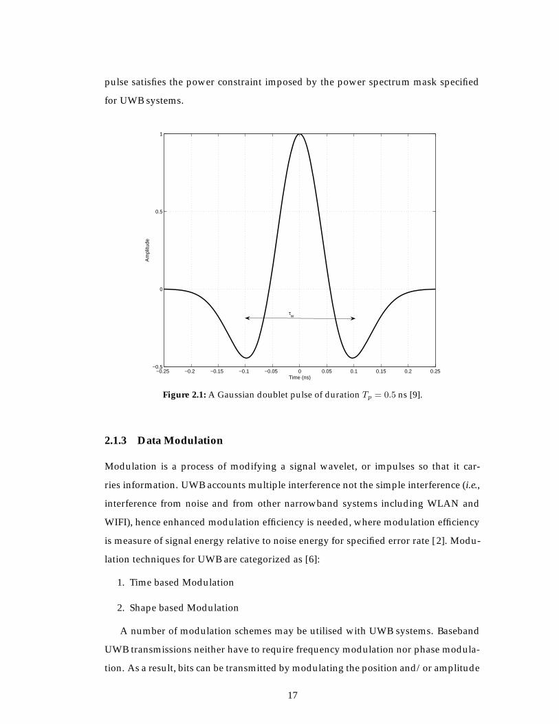
pulse satisfies the power constraint imposed by the power spectrum mask specified
for UWB systems.
−0.25 −0.2 −0.15 −0.1 −0.05 0 0.05 0.1 0.15 0.2 0.25−0.5
0
0.5
1
Time (ns)
Am
plitu
de
τw
Figure 2.1: A Gaussian doublet pulse of duration Tp = 0.5 ns [9].
2.1.3 Data Modulation
Modulation is a process of modifying a signal wavelet, or impulses so that it car-
ries information. UWB accounts multiple interference not the simple interference (i.e.,
interference from noise and from other narrowband systems including WLAN and
WIFI), hence enhanced modulation efficiency is needed, where modulation efficiency
is measure of signal energy relative to noise energy for specified error rate [2]. Modu-
lation techniques for UWB are categorized as [6]:
1. Time based Modulation
2. Shape based Modulation
A number of modulation schemes may be utilised with UWB systems. Baseband
UWB transmissions neither have to require frequency modulation nor phase modula-
tion. As a result, bits can be transmitted by modulating the position and/or amplitude
17
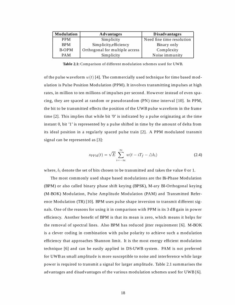
Modulation Advantages DisadvantagesPPM Simplicity Need fine time resolutionBPM Simplicity,efficiency Binary only
B-OPM Orthogonal for multiple access ComplexityPAM Simplicity Noise immunity
Table 2.1: Comparison of different modulation schemes used for UWB.
of the pulse waveform w(t) [4]. The commercially used technique for time based mod-
ulation is Pulse Position Modulation (PPM). It involves transmitting impulses at high
rates, in million to ten millions of impulses per second. However instead of even spa-
cing, they are spaced at random or pseudorandom (PN) time interval [10]. In PPM,
the bit to be transmitted effects the position of the UWB pulse waveform in the frame
time [2]. This implies that while bit ’0’ is indicated by a pulse originating at the time
instant 0, bit ’1’ is represented by a pulse shifted in time by the amount of delta from
its ideal position in a regularly spaced pulse train [2]. A PPM modulated transmit
signal can be represented as [3]:
sPPM(t) =√E
∞∑i=−∞
w(t− iTf −�bi) (2.4)
where, bi denote the set of bits chosen to be transmitted and takes the value 0 or 1.
The most commonly used shape based modulations are the Bi-Phase Modulation
(BPM) or also called binary phase shift keying (BPSK), M-ary BI-Orthogonal keying
(M-BOK) Modulation, Pulse Amplitude Modulation (PAM) and Transmitted Refer-
ence Modulation (TR) [10]. BPM uses pulse shape inversion to transmit different sig-
nals. One of the reasons for using it in comparison with PPM is its 3 dB gain in power
efficiency. Another benefit of BPM is that its mean is zero, which means it helps for
the removal of spectral lines. Also BPM has reduced jitter requirement [6]. M-BOK
is a clever coding in combination with pulse polarity to achieve such a modulation
efficiency that approaches Shannon limit. It is the most energy efficient modulation
technique [6] and can be easily applied in DS-UWB system. PAM is not preferred
for UWB as small amplitude is more susceptible to noise and interference while large
power is required to transmit a signal for larger amplitude. Table 2.1 summarises the
advantages and disadvantages of the various modulation schemes used for UWB [6].
18
A vital feature of UWB communication systems is its low power spectral density
[3]. In a typical UWB system, to maintain sufficiently low power spectral density
while attaining adequate energy per symbol, each single information-bearing symbol
is symbolised by a number of pulses, each transmitted in a frame of duration Tf � Tp
[4]. This means that multiple frames consist of a single symbol. In this respect, the
PPM modulated transmit signal can now be given as [3]:
sPPM(t) =√E
∞∑i=−∞
w(t− iTf −�b�i/N�) (2.5)
where, b�i/N� represents the data bit over the ith frame, N is the number of pulses per
symbol, and �·� is the floor function. Similarly, the BPSK modulated transmit signal is
represented as [3]:
sBPSK(t) =√E
∞∑i=−∞
b�i/N�w(t− iTf ) (2.6)
Where, in this case bi denotes the antipodal binary bit stream consisting of -1’s or +1’s.
2.1.4 Multiple Access Transmission Schemes
In the presence of multiple nodes or users, there are a number of UWB transmission
schemes that can support multiple access. To allow for multiple access in the IR-
UWB systems, TH-UWB and DS-UWB transmission schemes have been introduced.
Whereas in, MC-UWB system, multiple access is introduced by using OFDM. With
TH-UWB, each pulse waveform is placed within a chip in each frame duration ac-
cording to a user-specific TH spreading code sequence. In DS-UWB, multiple access
is enabled by modifying the pulse polarity from chip to chip depending on a pseudor-
andom spreading code sequence. For MC-UWB an OFDM-UWB transmit signal for
the kth user takes the form [11]:
s(k)OFDM(t) =
√Eb
Nf
∞∑u=−∞
x(k)�u/Nf �w
(t− uTf − c(k)u Tc
)(2.7)
Where t is time, s(k)(t) is the transmit signal of the kth node, and w(t) is a pulse wave-
form, which can take arbitrary time-limited pulse shapes proposed specifically for
19
UWB systems. Eb is the transmitted energy per information bit.√
Eb/Nf is norm-
alisation factor. Nf is the length of the hopping code in OFDM-UWB. The sequence
c(k)u for OFDM-UWB represents the TH spreading code sequence for the kth node; it
is pseudorandom with each element taking an integer in the range 0 ≤ c(k)u ≤ Nh for
OFDM-UWB, where Nh is the number of chips. Tf denotes the frame time. Tc is the
chip time. In OFDM-UWB, the bit duration is Tb = NfTf . �·� is the floor function
(Whereas, �x� is the largest integer not greater than x). In (2.7), x(k)u represents the
inverse discrete Fourier transform (IDFT) of the data stream sent over Mf sub-carriers
by the kth node, it is given by:
x(k)u =1
Mf
Mf−1∑v=0
b(k)u,v exp
(j2πvκ
Mf
), 0 ≤ κ < Mf (2.8)
2.1.5 Radiation of Ultra Wideband Signal
Short UWB pulse signals, when radiated show some interesting differences as com-
pared to narrowband signals. UWB signal obeys Maxwell’s equations like narrow-
band signal, but instead of considering them in frequency domain, they are represen-
ted in time domain due to interest in transient response. The radiated UWB signal are
related to transmitted signal by partial time delay derivative, and the received UWB
signal is proportional to the weighted sum of time delay copies of radiated signals.
The design of UWB antennas with a constant gain (e.g., dipole) or constant aperture
(like horn) plays an important role in the performance of the UWB link [10]. UWB
antennas must be understood in their time domain behaviour rather than in the fre-
quency domain, because the effects of short pulses become observable, whenever the
propagation delay and the retardation time, on the antenna is similar to the impulse
rise time [10]. A number of UWB antennas have been proposed already for different
applications in literature including WBAN [12–16].
2.1.6 Radio Channel Model
A comprehensive channel model should comprise of the path loss model and the mul-
tipath model. The path loss is defined as the reduction in power density of an elec-
tromagnetic wave as it propagates through free space. The multipath model describes
20
how the signal energy is dispersed over the multipath components.
Path Loss Model
The effect of link distance on the signal energy obtained at the receiver can be determ-
ined by propagation loss computations which describe the fraction of the transmitted
power that can be received at a distance D . The longer the link distance, the lower is
the received signal energy. This relationship can simply be described by the path loss
model [2]. The path loss model signifies the local average received signal power (Pr)
relative to the transmit power (Pt).
A more general distance dependent path loss model represents the power law re-
lationship between the transmitter-receiver separation D and the received power. It
can be expressed as [2]:Pr
Pt=
(D
D0
)−δe
(2.9)
where D0 is the reference distance, should be larger than the wavelength of lower
frequency limit, in order to minimise the mutual coupling effect when antennas placed
near each other and δe is the path loss exponent or decaying factor.
Multipath Model
The extremely large signal bandwidth occupied by UWB usually exceeds the coher-
ence bandwidth of the propagation channel for most scenarios. Accordingly, the
propagation channel for UWB radio experiences notable frequency selectivity, and can
be described by a tap delay line channel model. Since the UWB signal has a very wide
bandwidth (in the order of GHz), the multipath components tend to form clusters of
rays caused by building structures and other large reflectors. The rays within a cluster
are attributable to reflections from objects in close proximity to the transmitter and
receiver [17]. A well-known tap delay line channel model, called the Saleh-Valenzuela
(S-V) channel model, is widely used in research for UWB systems as it takes into con-
sideration the clustering phenomenon of the multipath components.
In the S-V model, multipath components arrive at the receiver in clusters. Cluster
arrivals are Poisson distributed and so are the subsequent arrivals in each cluster. The
21
discrete time multipath channel impulse response can be presented as [4] [18]:
h(t) =
L∑l=1
αlδ(t− τl)
=M∑
m=0
H∑h=0
αm,hδ(t− Tl − τm,h) (2.10)
where, αm,h denotes the fading gain of the hth multipath component of themth cluster,
δ(t) is the Dirac delta function, Tm is the delay of the mth cluster, and τm,h represents
the delay of the hth multipath component relative to the mth cluster arrival time.
Standardisation of UWB Channel Models
The IEEE 802.15.4 task group was formed to target applications of long-range (up to
hundred of meters), low data rate (between 1 kbps to several Mbps), and low com-
plexity. UWB have been a strong candidate for the physical layer design in this task
group. A comprehensive standardised model described for UWB propagation chan-
nels that is valid for a frequency range from 3 - 10 GHz is given in [18]. The model is
independent of the used antennas and includes the frequency dependence of the path
loss, as well as many generalisations of the S-V model, like mixed Poisson times of ar-
rival and delay-dependent cluster decay constants. The model was acknowledged by
the IEEE 802.15.4a task group as a standard for evaluation of UWB system proposals.
Since the clustering phenomenon has been experimentally recognised, the standard-
ised channel model is essentially a modified version of the S-V channel model.
2.1.7 Receiver Architectures
Rake Reception
The large bandwidth taken up by UWB results in both a frequency selective propaga-
tion channel for wireless communication systems and, innumerable resolvable mul-
tipath components at the receiver end. This frequency selective propagation channel
can be represented as a tap delay line S-V channel model, and the optimum receiver
can be created by utilising a set of matched filters with appropriate time delays for
delay taps. The most commonly employed UWB receiver is a correlation (matched
22
filter) receiver, where the received signal is correlated with the template pulse wave-
form w(t). UWB transmissions sending information with extremely narrow pulses
are able to resolve many paths, and are hence rich in multipath diversity. To im-
prove performance in multipath environments by exploiting this diversity, UWB use
correlation-based rake receivers [4]. Rake receivers combine different signal compon-
ents that have propagated through the mutipath channel by different paths [2].
A rake receiver captures the signal energy conveyed by having a number of fin-
gers equal to the number of multipath components [2]. The rake receiver then con-
structively combines these signal arrivals from multiple paths. Applying additional
fingers helps to capture more signal energy. However, increasing the number of fin-
gers can add to complexity and increase energy consumption [17]. Thus, a realistic
rake receiver may only use a portion of the resolved multipath components to capture
a desirable amount of signal energy from the channel [19].
There are three types of rake receivers that have been investigated in the literature.
The All-rake (A-rake) receivers theoretically give the best energy collection since they
assume an unlimited number of rake fingers, which means an unlimited number of
correlators. The Selective-rake (S-rake) receivers only use a subset of the available re-
solved multipath components with the highest signal energies. Finally, Partial-rake (P-
rake) receivers only combine the first few arriving multipath components [2]. All the
three types of rake receivers can use the Maximal Ratio Combining (MRC) method to
coherently combine all the signal components to achieve optimal performance [2][4].
OFDM-UWB Receiver
Orthogonal frequency division multiplexing (OFDM) is a special case of multicarrier
(MC) transmission that allows subcarriers to overlap in the frequency without mu-
tual interference, resulting in increased spectral efficiency. As compared to earlier
carrierless UWB, OFDM-UWB is a multicarrier UWB system that relies on splitting
orthogonal carriers in a train of short pulses by sending them over the channel and
reassembling them at the receiver side to get orthogonality and to recover each sub-
carrier separately [3]. OFDM-UWB is a MC-UWB system that uses a frequency coded
pulse train as a shaping signal. A novel method for generating and detecting OFDM-
UWB signals using sigma-delta modulator is proposed in [20]. Unlike narrowband
23
OFDM, the OFDM-UWB spectrum can have gaps between subcarriers. In OFDM
based UWB, inverse fast fourier transform/fast fourier transform (IFFT/FFT) cannot
be applied directly to generate and receive UWB-OFDM signals because of high data
rate unlike narrowband OFDM [3]. To solve this problem, a procedure is mentioned
in [20] to move the bulk of processing data from analog to digital baseband. Sigma-
Delta A/D and D/A converts are good choice for high data rate communications.
Traditional sigma-delta modulators can’t be used in OFDM-UWB due to requirement
of high sampling rate. A modified sigma-delta modulator called N-tone sigma-delta
modulator (receiver architecture is proposed in [21]) enables the efficient use of IFFT
and FFT to generate and demodulate OFDM-UWB and helps in avoiding high peak
to average ratio (PAR) problem that occurs with OFDM system [3].
2.2 Ultra Wideband Spectrum Regulations and Standards
2.2.1 UWB Spectrum Regulations
At the national level, the USA was the first country to authorise UWB for commercial
use. In February 2002, the FCC has mandated that UWB radio transmission can legally
operate in the range of 3.1 to 10.6 GHz, with the power spectral density (PSD) satisfy-
ing a specific spectral mask assigned by the FCC. In general, the spectral mask related
with the FCCs UWB regulation was designed to prevent other spectrum users from
undesirable interference caused by UWB operations. For wireless communications,
the power levels regulated by the FCC are extremely low (i.e., -41.3 dBm/MHz), which
permits UWB technology to overlay with existing services [22]. Figure 1.2 shows the
FCCs indoor emission masks [23]. In the UK, the regulatory body, called the Office
of Communications (Ofcom), opened a consultation on UWB matters in January 2005.
The consultation consisted of 15 questions, asking opinions from those who are af-
fected by the UWB technology. Ofcom sees, UWB as a positive technology that if
correctly regulated can bring economic growth to the UK. On August 13, 2007, Ofcom
finally approved the use of ultra wideband wireless technology without a license for
use in the UK (Fig. 1.3 [23]).
The regulatory body that set the policy on UWB in Japan is called the Ministry
of Internal Affairs and Communications (MIC). The Japanese UWB radiation mask for
24
indoor devices has two bands; from 3.4 to 4.8 GHz and from 7.25 to 10.25 GHz. For the
3.4 to 4.8 GHz band, it is required to use a technology to reduce interference with other
radio systems. This interference mitigation technology is called Detect And Avoidance
(DAA) [24] to ascertain the coexistence with incumbent systems and new services such
as 4G systems. However, temporary measures are taken by now to permit the use
of 4.2 to 4.8 GHz band without an interference reduction technology. It should be
noted that no DAA is required for the band 7.25 to 10.25 GHz. Similar to the FCC
mask, the power spectral density is limited to -41.3 dBm/MHz or lower on both bands
[25]. In Korea and Singapore emission level is -66.5 dBm/MHz (for 1-10 GHz) and -35
dBm/MHz (for 2.2-10.6 GHz) respectively.
2.2.2 UWB Standards
Different standards exist for different kind of technologies and processes. Figure 2.2
shows the place of UWB across different wireless standards. Standards are defined to
provide uniform technical methods, processes, and understanding. Standards enable
multi-vendor interoperability and allow competitive products to market quickly from
different vendors. Especially in wireless communication systems, standards provide
interoperability and interfaces for components and products from different vendors,
so products can co-exist and co-work with each other without any problem [10].
In UWB matters, the IEEE is active in making standards. Within the IEEE 802
standard, the UWB standardisation activities initiate in the IEEE 802.15 Work Groups
(WGs). The IEEE 802.15.3a (TG3a) and IEEE 802.15.4a (TG4a) and IEEE 802.15.6 are
three Task Groups (TGs) within 802.15 WG that develop their standards based on
UWB technology. The TG4a is focused on low rate alternative physical layer for
WPANs. The technical requirements for the TG4a include low cost, low data rate, low
complexity and low power consumption. The TG3a is aimed at developing high rate
alternative physical layer for WPANs. The group targeted developing Physical Layer
(PHY) standards to support data rates between 110 to 450 Mbps over short ranges (i.e.,
< 10m) [25, 26]. IEEE 802.15.6 is focused on WBAN technologies. Its goal is to provide
low power and low frequency short range wireless standard [27].
There are two competitive proposals for the TG3a, i.e., the Direct Sequence UWB
(DS-UWB) and the Multiband Orthogonal Frequency Division Multiplexing (MB-OFDM).
25
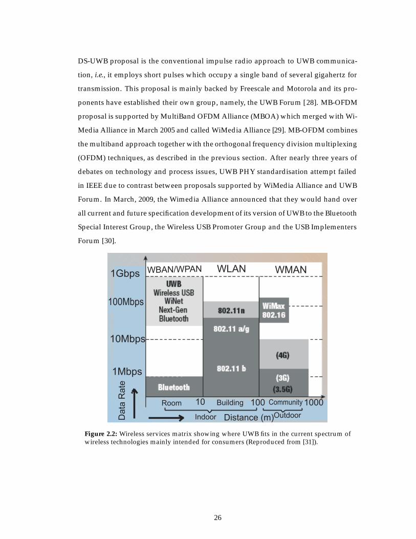
DS-UWB proposal is the conventional impulse radio approach to UWB communica-
tion, i.e., it employs short pulses which occupy a single band of several gigahertz for
transmission. This proposal is mainly backed by Freescale and Motorola and its pro-
ponents have established their own group, namely, the UWB Forum [28]. MB-OFDM
proposal is supported by MultiBand OFDM Alliance (MBOA) which merged with Wi-
Media Alliance in March 2005 and called WiMedia Alliance [29]. MB-OFDM combines
the multiband approach together with the orthogonal frequency division multiplexing
(OFDM) techniques, as described in the previous section. After nearly three years of
debates on technology and process issues, UWB PHY standardisation attempt failed
in IEEE due to contrast between proposals supported by WiMedia Alliance and UWB
Forum. In March, 2009, the Wimedia Alliance announced that they would hand over
all current and future specification development of its version of UWB to the Bluetooth
Special Interest Group, the Wireless USB Promoter Group and the USB Implementers
Forum [30].
WBAN/WPAN WLAN WMAN
10 100 1000
Data
Rate
Distance (m)Indoor Outdoor
Room Building Community
1Mbps
10Mbps
100Mbps
1Gbps
Figure 2.2: Wireless services matrix showing where UWB fits in the current spectrum ofwireless technologies mainly intended for consumers (Reproduced from [31]).
26
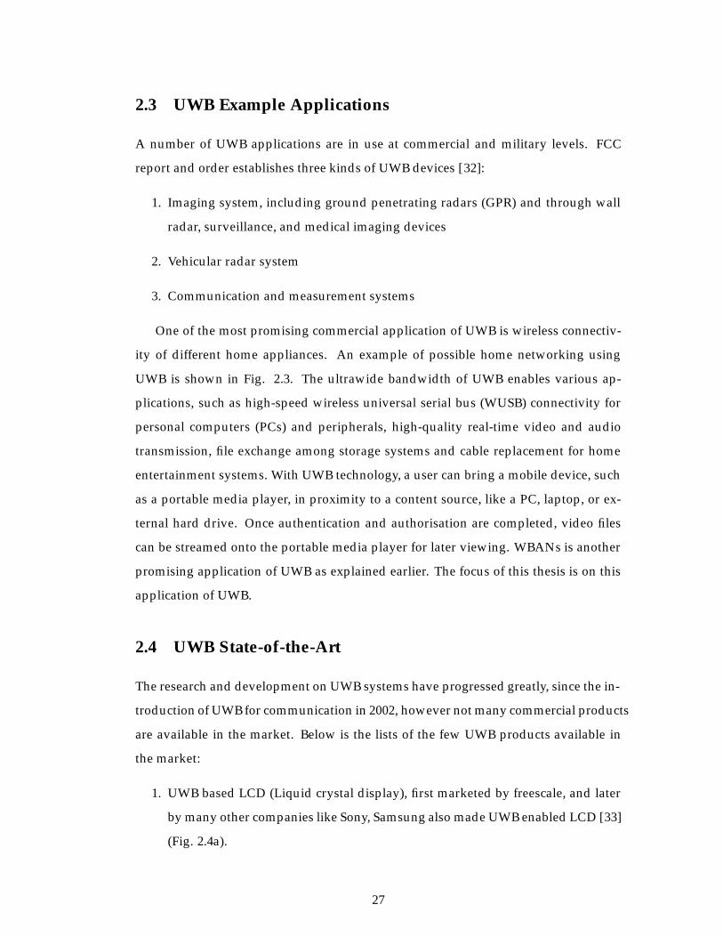
2.3 UWB Example Applications
A number of UWB applications are in use at commercial and military levels. FCC
report and order establishes three kinds of UWB devices [32]:
1. Imaging system, including ground penetrating radars (GPR) and through wall
radar, surveillance, and medical imaging devices
2. Vehicular radar system
3. Communication and measurement systems
One of the most promising commercial application of UWB is wireless connectiv-
ity of different home appliances. An example of possible home networking using
UWB is shown in Fig. 2.3. The ultrawide bandwidth of UWB enables various ap-
plications, such as high-speed wireless universal serial bus (WUSB) connectivity for
personal computers (PCs) and peripherals, high-quality real-time video and audio
transmission, file exchange among storage systems and cable replacement for home
entertainment systems. With UWB technology, a user can bring a mobile device, such
as a portable media player, in proximity to a content source, like a PC, laptop, or ex-
ternal hard drive. Once authentication and authorisation are completed, video files
can be streamed onto the portable media player for later viewing. WBANs is another
promising application of UWB as explained earlier. The focus of this thesis is on this
application of UWB.
2.4 UWB State-of-the-Art
The research and development on UWB systems have progressed greatly, since the in-
troduction of UWB for communication in 2002, however not many commercial products
are available in the market. Below is the lists of the few UWB products available in
the market:
1. UWB based LCD (Liquid crystal display), first marketed by freescale, and later
by many other companies like Sony, Samsung also made UWB enabled LCD [33]
(Fig. 2.4a).
27
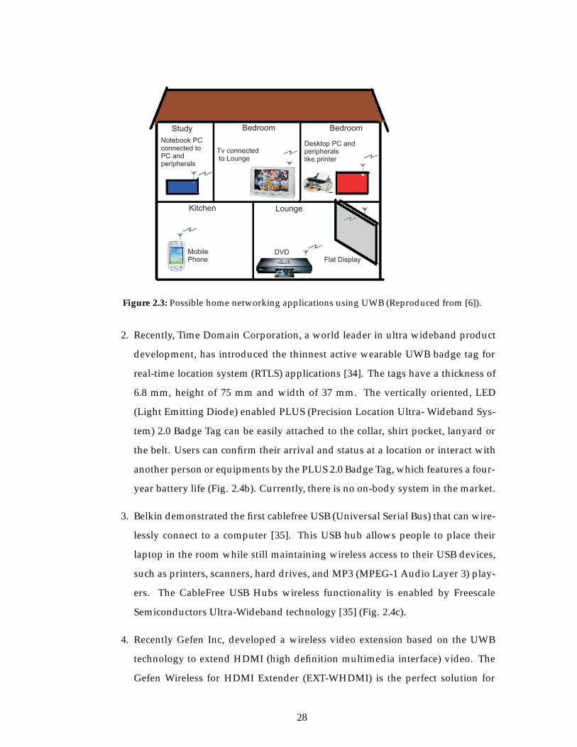
Study Bedroom Bedroom
LoungeKitchen
DVDFlat Display
MobilePhone
Tv connectedto Lounge
Desktop PC andperipheralslike printer
Notebook PCconnected toPC andperipherals
Figure 2.3: Possible home networking applications using UWB (Reproduced from [6]).
2. Recently, Time Domain Corporation, a world leader in ultra wideband product
development, has introduced the thinnest active wearable UWB badge tag for
real-time location system (RTLS) applications [34]. The tags have a thickness of
6.8 mm, height of 75 mm and width of 37 mm. The vertically oriented, LED
(Light Emitting Diode) enabled PLUS (Precision Location Ultra- Wideband Sys-
tem) 2.0 Badge Tag can be easily attached to the collar, shirt pocket, lanyard or
the belt. Users can confirm their arrival and status at a location or interact with
another person or equipments by the PLUS 2.0 Badge Tag, which features a four-
year battery life (Fig. 2.4b). Currently, there is no on-body system in the market.
3. Belkin demonstrated the first cablefree USB (Universal Serial Bus) that can wire-
lessly connect to a computer [35]. This USB hub allows people to place their
laptop in the room while still maintaining wireless access to their USB devices,
such as printers, scanners, hard drives, and MP3 (MPEG-1 Audio Layer 3) play-
ers. The CableFree USB Hubs wireless functionality is enabled by Freescale
Semiconductors Ultra-Wideband technology [35] (Fig. 2.4c).
4. Recently Gefen Inc, developed a wireless video extension based on the UWB
technology to extend HDMI (high definition multimedia interface) video. The
Gefen Wireless for HDMI Extender (EXT-WHDMI) is the perfect solution for
28
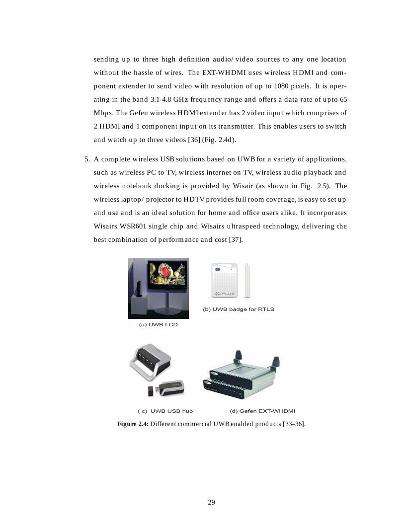
sending up to three high definition audio/video sources to any one location
without the hassle of wires. The EXT-WHDMI uses wireless HDMI and com-
ponent extender to send video with resolution of up to 1080 pixels. It is oper-
ating in the band 3.1-4.8 GHz frequency range and offers a data rate of upto 65
Mbps. The Gefen wireless HDMI extender has 2 video input which comprises of
2 HDMI and 1 component input on its transmitter. This enables users to switch
and watch up to three videos [36] (Fig. 2.4d).
5. A complete wireless USB solutions based on UWB for a variety of applications,
such as wireless PC to TV, wireless internet on TV, wireless audio playback and
wireless notebook docking is provided by Wisair (as shown in Fig. 2.5). The
wireless laptop/projector to HDTV provides full room coverage, is easy to set up
and use and is an ideal solution for home and office users alike. It incorporates
Wisairs WSR601 single chip and Wisairs ultraspeed technology, delivering the
best combination of performance and cost [37].
(b) UWB badge for RTLS
( c) UWB USB hub
(a) UWB LCD
(d) Gefen EXT-WHDMI
Figure 2.4: Different commercial UWB enabled products [33–36].
29
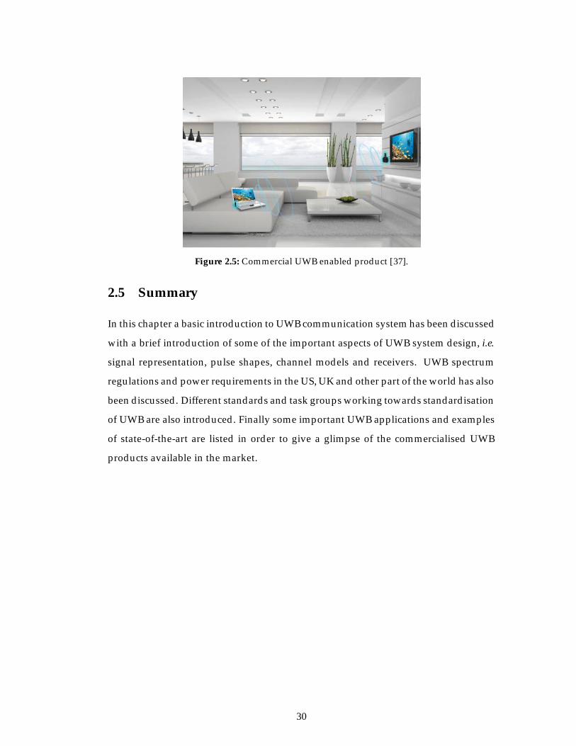
Figure 2.5: Commercial UWB enabled product [37].
2.5 Summary
In this chapter a basic introduction to UWB communication system has been discussed
with a brief introduction of some of the important aspects of UWB system design, i.e.
signal representation, pulse shapes, channel models and receivers. UWB spectrum
regulations and power requirements in the US, UK and other part of the world has also
been discussed. Different standards and task groups working towards standardisation
of UWB are also introduced. Finally some important UWB applications and examples
of state-of-the-art are listed in order to give a glimpse of the commercialised UWB
products available in the market.
30
References
[1] X. Shen, W. Zhuang, H. Jiang, and J. Cai, “Medium access control in ultra-widebandwireless networks,” Vehicular Technology, IEEE Transactions on, vol. 54, no. 5, pp. 1663–1677, Septmber 2005.
[2] I. Opperman, M. Hamalainen, and J. Iinatti, UWB theory and applications. John Wiley andSons, 2004.
[3] J. H. Reed, An Introduction to Ultra Wideband Communication Systems. Printce Hall, 2005.
[4] L. Yang and G. Giannakis, “Ultra-wideband communications: an idea whose time hascome,” Signal Processing Magazine, IEEE, vol. 21, no. 6, pp. 26–54, Nov. 2004.
[5] “Federal communications commission (FCC), code of federal regulations (CFR), title 47part 95, MCIS band plan,” URL: http://www.fcc.gov, March’03.
[6] M. Ghavami, L. B. Michael, and K. R., UWB Signal and System in Communication Engineer-ing. John Wiley and Sons, 2004.
[7] M. G. Benedetto, T. Kaiser, A. Molisch, I. Oppermann, and D. Porcino, UWB Communica-tion Systems: A Comprehensive Overview. Hindawi Publishing Corporation, May 2006.
[8] B. Hu and N. Beaulieu, “Accurate evaluation of multiple-access performance in TH-PPMand TH-BPSK UWB systems,” IEEE Transactions on Communications, vol. 52, no. 10, pp.1758–1766, Oct. 2004.
[9] N. Riaz, “Energy efficient adaptive aroaches for reliable communication and routing inUWB based wireless sensor networks,” Ph.D. dissertation, Kings college, University ofLondon, 2008.
[10] K. Siwiak and D. Mckeown, Ultra- Wideband Radio Technology. John Wiley and Sons,2004.
[11] H. J. Park, M. J. Kim, Y. J. So, Y. H. You, and H. K. Song, “UWB communication systemfor home entertainment network,” IEEE Transactions on Consumer Electronics, vol. 49, pp.302–311, May 2003.
[12] B. Allen, M. Dohler, E. Okon, W. Q. Malik, A. K. Brown, and D. Edwards, UWB Antennaand Propagation for Communications, Radar and Imaging. John Wiley and Sons, 2007.
[13] P. S. Hall and Y. Hao, Antennas and Propagation for Body-Centric Wireless Communications.Artech House, 2006.
[14] L. Guo, “Study and miniaturisation of antennas for ultra wideband communication sys-tems,” Ph.D. dissertation, Queen Mary, University of London, 2009.
[15] M. Klemm, I. Kovcs, G. Pedersen, and G. Troster, “Novel small-size directional antennnafor uwb wban/wpan applications,” IEEE Trans on Antenna and Propagation, vol. 53, no. 12,pp. 3884–3896, Dec. 2005.
[16] A. Alomainy, Y. Hao, X. Hu, C. G. Parini, and P. S. Hall, “Uwb on-body radiopropagation and system modelling for wireless body-centric networks,” IEE ProceedingsCommunications-Special Issue on Ultra Wideband Systems, Technologies and Applications, vol.153, no. 1, pp. 107– 114, Feb. 2006.
[17] K. Colling and P. Ciorciari, “Ultra wideband communications for sensor networks,” inMilitary Communications Conference, 2005. MILCOM 2005. IEEE, 2005, pp. 2384–2390 Vol.4.
31
[18] A. F. Molisch, D. Cassioli, C.-C. Chong, S. Emami, A. Fort, B. Kannan, J. Karedal,J. Kunisch, H. G. Schantz, K. Siwiak, and M. Z. Win, “A comprehensive standard-ized model for ultrawideband propagation channels,” IEEE Transactions on Antennas andPropagation, vol. 54, no. 11, pp. 3151–3166, Dec. 2006.
[19] M. Win and R. Scholtz, “Characterization of ultra-wide bandwidth wireless indoor chan-nels: a communication-theoretic view,” IEEE Journal on Selected Areas in Communications,vol. 20, no. 9, pp. 1613–1627, Dec. 2002.
[20] E. Saberinia and A. H. Tewfik, “N-tone sigma-delta UWB-OFDM transmitter and re-ceiver,” in IEEE International Conference on Acoustics, Speech and Signal Processing (ICASSP),vol. 4, 6, pp. 129–132.
[21] Saberinia and A. Tewfik, “Generating UWB-OFDM signal using sigma-delta modulator,”in IEEE Vehicular Technology Conference (VTC), vol. 2, 2003, pp. 1425–1429.
[22] FCC First Report and Order, Revision of the Part 15 Commission’s Rules Regarding Ultra-Wideband Transmission Systems, pp. ETDocket 98–153, April 22, 2003.
[23] T. Kaiser and F. Zheng, Ultra Wideband Systems With MIMO. John Wiley & Sons Ltd,2010.
[24] “Detect and avoid technology for ultra wideband (uwb) spectrum usage,” Wisair WhitePaper, URL: http://www.wisair.com.
[25] H. Nikookar and R. Prasad, Introduction to Ultra Wideband for Wireless Communications.Springer Science+Business Media B.V., 2009.
[26] R. Aiello and A. Batra, Ultra Wideband Systems Technologies and Applications. Elsevier Inc,2006.
[27] “IEEE 802.15,an international standards working group, IEEE 802.15,” URL:http://grouper.ieee.org/groups/802/15/ .
[28] “UWB forum,” URL: http://www.uwbforum.org.
[29] “Wimedia alliance,” URL: http://www.wimedia.org.
[30] “Wimedia folds: hands UWB spec to bluetooth, usb groups, wimedia alliance,” URL:http://www.wimedia.org.
[31] “Wimedia UWB PHY design and testing,” URL: http://www.mwjournal.com.
[32] F. C. Commission, “First order and report: Revision of part 15 of the commission’s rulesregarding uwb transmission systems,” Tech. Rep., Apr. 22 2002.
[33] “Freescale technology forum,” URL: http://www.freescale.com.
[34] “Time domain RTLS UWB tags,” URL: http://www.timedomain.com.
[35] “Belkin UWB enabled USB hub,” URL: http://www.belkin.com.
[36] “Gefen wireless HDMI extender with ultra-wideband technology,” URL:http://www.gefen.com.
[37] “Wireless usb solutions,” URL: http://www.wisair.com/products.
32
Chapter 3
Fundamentals of UWB Antennas
and Propagation for Body-Centric
Wireless Networks
In this chapter an introduction to UWB antennas for BCWN and a discussion of the
basics of antenna engineering and radio channel propagation principles are given. In
addition, a literature review and analysis of the state-of-the-art is presented with em-
phasis on compact antennas, radio channel characterisation and diversity techniques.
3.1 UWB Antenna for Body-Centric Applications
In a UWB radio system, the antenna plays a more important role than the one com-
pared to a conventional narrow-band system. In such a system, the antenna behaves
33
like a filter in both spatial and frequency domains and tends to introduce signal dis-
tortion and degradation, if not carefully designed [1, 2]. Unlike its narrow-band coun-
terpart, the design of UWB antenna is determined not only by its return loss char-
acteristics but also by its ability to preserve the pulse shape as it employs the un-
orthodox carrier-free modulation. Antennas for UWB systems are required to have a
very broad impedance bandwidth, as well as a stable and constant channel transfer
response. Ordinary wide-band antennas will cause the distortion to the transmitted
short pulses since they radiate various components from different parts and hence
experience severe frequency dependent changes in their phase centers [3]. When
designing UWB antennas, group delay must be taken into account. If the phase is
linear throughout the frequency range, the group delay will be constant and hence the
delivered pulses will be transmitted with no distortion in all directions. Any strong
resonance at any frequency of the UWB antenna response causes large group delay
variation and thus causes distortion in the pulse shape which in turn affects the pulse
fidelity factor of the antenna performance [4]. So it is not reasonable to design ultra-
wideband antenna with multiple deep resonance as far as pulse fidelity is concerned.
A very wide operational fractional bandwidth of UWB systems makes the design and
evaluation of antennas more difficult than in narrowband systems.
For more specific applications, such as WBANs, the antenna design becomes more
complicated than for simple free space operation scenarios, due to the presence of the
complex human body medium. Most examples in the literature consider the antennas
as part of the propagation system and apply common and widely available antenna
types to characterise the channel. However, as discussed in [5], antennas with different
radiation characteristics lead to different channel parameters. In particular, the use
of a vertically polarised UWB monopole, rather than a planar antenna, reduces the
attenuation but increases the time spread of the signal. Therefore, it was concluded
that the hybrid use of different antennas can improve the channel performances. In
[6], a similar study was conducted considering three types of UWB antennas. From
the comparison of a directional and an omnidirectional antenna, it was deduced that
the omnidirectional antenna presents an improved radio link. A further improvement
of radio link was achieved by using two element diversity antenna.
In [7], Klemm et al. presented time domain characteristics of an aperture-stacked
34
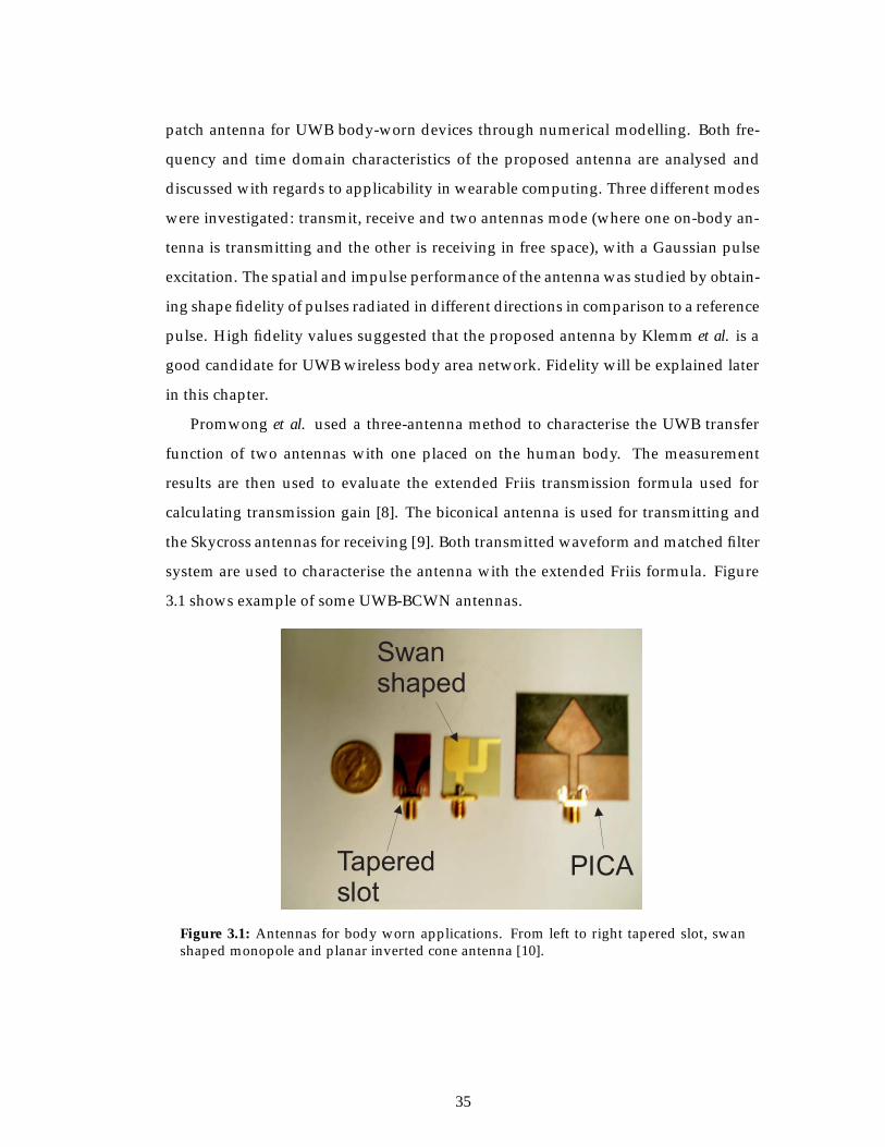
patch antenna for UWB body-worn devices through numerical modelling. Both fre-
quency and time domain characteristics of the proposed antenna are analysed and
discussed with regards to applicability in wearable computing. Three different modes
were investigated: transmit, receive and two antennas mode (where one on-body an-
tenna is transmitting and the other is receiving in free space), with a Gaussian pulse
excitation. The spatial and impulse performance of the antenna was studied by obtain-
ing shape fidelity of pulses radiated in different directions in comparison to a reference
pulse. High fidelity values suggested that the proposed antenna by Klemm et al. is a
good candidate for UWB wireless body area network. Fidelity will be explained later
in this chapter.
Promwong et al. used a three-antenna method to characterise the UWB transfer
function of two antennas with one placed on the human body. The measurement
results are then used to evaluate the extended Friis transmission formula used for
calculating transmission gain [8]. The biconical antenna is used for transmitting and
the Skycross antennas for receiving [9]. Both transmitted waveform and matched filter
system are used to characterise the antenna with the extended Friis formula. Figure
3.1 shows example of some UWB-BCWN antennas.
Figure 3.1: Antennas for body worn applications. From left to right tapered slot, swanshaped monopole and planar inverted cone antenna [10].
35
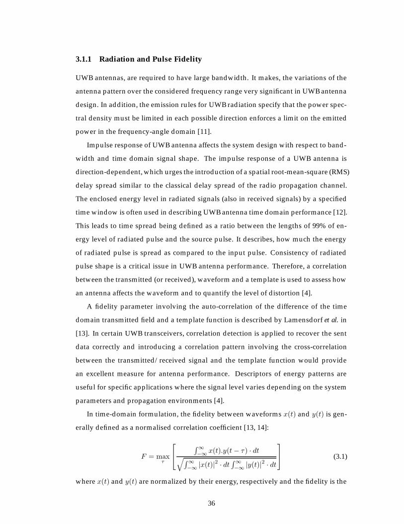
3.1.1 Radiation and Pulse Fidelity
UWB antennas, are required to have large bandwidth. It makes, the variations of the
antenna pattern over the considered frequency range very significant in UWB antenna
design. In addition, the emission rules for UWB radiation specify that the power spec-
tral density must be limited in each possible direction enforces a limit on the emitted
power in the frequency-angle domain [11].
Impulse response of UWB antenna affects the system design with respect to band-
width and time domain signal shape. The impulse response of a UWB antenna is
direction-dependent, which urges the introduction of a spatial root-mean-square (RMS)
delay spread similar to the classical delay spread of the radio propagation channel.
The enclosed energy level in radiated signals (also in received signals) by a specified
time window is often used in describing UWB antenna time domain performance [12].
This leads to time spread being defined as a ratio between the lengths of 99% of en-
ergy level of radiated pulse and the source pulse. It describes, how much the energy
of radiated pulse is spread as compared to the input pulse. Consistency of radiated
pulse shape is a critical issue in UWB antenna performance. Therefore, a correlation
between the transmitted (or received), waveform and a template is used to assess how
an antenna affects the waveform and to quantify the level of distortion [4].
A fidelity parameter involving the auto-correlation of the difference of the time
domain transmitted field and a template function is described by Lamensdorf et al. in
[13]. In certain UWB transceivers, correlation detection is applied to recover the sent
data correctly and introducing a correlation pattern involving the cross-correlation
between the transmitted/received signal and the template function would provide
an excellent measure for antenna performance. Descriptors of energy patterns are
useful for specific applications where the signal level varies depending on the system
parameters and propagation environments [4].
In time-domain formulation, the fidelity between waveforms x(t) and y(t) is gen-
erally defined as a normalised correlation coefficient [13, 14]:
F = maxτ
⎡⎣ ∫∞
−∞ x(t).y(t− τ) · dt√∫∞−∞ |x(t)|2 · dt ∫∞
−∞ |y(t)|2 · dt
⎤⎦ (3.1)
where x(t) and y(t) are normalized by their energy, respectively and the fidelity is the
36
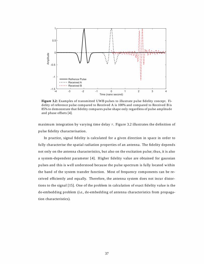
-4 -3 -2 -1 0 1 2 3 4-1.5
-1
-0.5
0
0.5
1
Time (nano second)
Am
plit
ude
Refrence Pulse
Received A
Received B
Figure 3.2: Examples of transmitted UWB pulses to illustrate pulse fidelity concept. Fi-delity of reference pulse compared to Received A is 100% and compared to Received B is85% to demonstrate that fidelity compares pulse shape only regardless of pulse amplitudeand phase offsets [4].
maximum integration by varying time delay τ . Figure 3.2 illustrates the definition of
pulse fidelity characterisation.
In practice, signal fidelity is calculated for a given direction in space in order to
fully characterise the spatial radiation properties of an antenna. The fidelity depends
not only on the antenna characteristics, but also on the excitation pulse; thus, it is also
a system-dependent parameter [4]. Higher fidelity value are obtained for gaussian
pulses and this is well understood because the pulse spectrum is fully located within
the band of the system transfer function. Most of frequency components can be re-
ceived efficiently and equally. Therefore, the antenna system does not incur distor-
tions to the signal [15]. One of the problem in calculation of exact fidelity value is the
de-embedding problem (i.e., de-embedding of antenna characteristics from propaga-
tion characteristics).
37
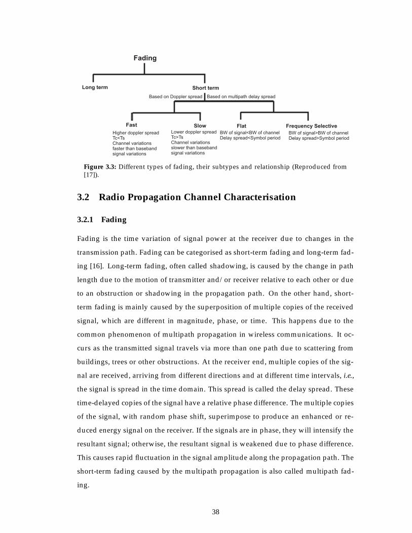
Based on Doppler spread Based on multipath delay spread
Higher doppler spreadTc<TsChannel variationsfaster than basebandsignal variations
Lower doppler spreadTc>TsChannel variationsslower than basebandsignal variations
BW of signal<BW of channelDelay spread<Symbol period
BW of signal>BW of channelDelay spread>Symbol period
Figure 3.3: Different types of fading, their subtypes and relationship (Reproduced from[17]).
3.2 Radio Propagation Channel Characterisation
3.2.1 Fading
Fading is the time variation of signal power at the receiver due to changes in the
transmission path. Fading can be categorised as short-term fading and long-term fad-
ing [16]. Long-term fading, often called shadowing, is caused by the change in path
length due to the motion of transmitter and/or receiver relative to each other or due
to an obstruction or shadowing in the propagation path. On the other hand, short-
term fading is mainly caused by the superposition of multiple copies of the received
signal, which are different in magnitude, phase, or time. This happens due to the
common phenomenon of multipath propagation in wireless communications. It oc-
curs as the transmitted signal travels via more than one path due to scattering from
buildings, trees or other obstructions. At the receiver end, multiple copies of the sig-
nal are received, arriving from different directions and at different time intervals, i.e.,
the signal is spread in the time domain. This spread is called the delay spread. These
time-delayed copies of the signal have a relative phase difference. The multiple copies
of the signal, with random phase shift, superimpose to produce an enhanced or re-
duced energy signal on the receiver. If the signals are in phase, they will intensify the
resultant signal; otherwise, the resultant signal is weakened due to phase difference.
This causes rapid fluctuation in the signal amplitude along the propagation path. The
short-term fading caused by the multipath propagation is also called multipath fad-
ing.
38
When all the spectral components of a transmitted signal are affected the same
way by the channel, the fading is referred to as flat fading, whereas if different spec-
tral components come across different amplitude and phase variation, the fading is
not the same for all the spectral components, and is called frequency selective fading
[16]. If a signal is composed of various frequency components (having a certain band-
width as in the case of real modulated carriers transmitted from the transmitter), the
relative phase shift is different for different frequency components of the signal and as
a result, the signal becomes distorted. If the frequency components are close enough,
the electrical path for the different frequency components is almost the same. Figure
3.3 shows the different types of fading.
3.2.2 Doppler Spread
In a situation where the transmitter and/or receiver move relative to each other, the
frequency of the received signal is increased or decreased due to the rate of change of
phase with motion. This change in frequency is called Doppler shift, which produces a
frequency spread in the spectrum of the signal called Doppler spread. The maximum
Doppler shift, fm, can be calculated as [17]:
fm =vλo
(3.2)
Here v is velocity of motion of human body in m/s and λo is the wavelength in meters.
Due to the rapid variation of the signal and deep fades, multipath fading effectively
reduces the signal to noise ratio (SNR) of the system and the bit-error-rate (BER) is
increased. This degrades the quality of service. Besides the multipath fading, the
transmitted signal on its way to the receiver comes across various impairments that
affect the quality of reception. These may include degradation of signal strength with
distance, addition of noise in the channel, noise produced by the transmitter/receiver
circuits, and interference etc. These impairments put a limit on the increasing demand
for data rate, quality of service, and reliability.
39
3.2.3 Path Loss Characterisation
One of the most important aspects of statistical characterisation is the derivation of a
model describing the fluctuations of the received signal with respect to the distance.
Models of this kind are called large-scale propagation models and the output of these
models is usually the estimation of the path loss at a certain distance. The path loss
represents the attenuation of the signal and it is defined as:
PL =Pr
Pt, (3.3)
where Pr and Pt are received and transmitted power respectively.
Prediction of the average received signal strength at a given distance from the trans-
mitter has been traditionally applied in obtaining radio channel models. Path loss
is usually examined using the Friis transmission formula, which provides a means
for predicting the received power. It states that signal power decreases at a rate of
frequency squared (which has little effect on narrowband systems) and the square of
separation distance between transmitter and receiver. The free space path loss for
distance d between transmitter and receiver is given by [17]:
PL(d) =GtGrλ
2
(4πd)2L(3.4)
where Gt and Gr are the transmitter and receiver antenna gain, respectively. L is the
system loss.
Many studies presented in the literature have shown that the average received
signal decreases logarithmically with distance (for both indoor and outdoor environ-
ments) [17–20]. Therefore, the average path loss is expressed as:
PL(d) ∝(
d
d0
)γ
for d ≥ d0 (3.5)
where γ is the path loss exponent that indicates the rate at which the path loss in-
creases with distance and d0 is a reference distance set in measurement and normally
set to 1 meter for indoor channels. In this case, d0 equals to 1 meter is larger than the
lower frequency wavelength (i.e., 10 cm), in order to minimise the mutual coupling ef-
fect when antennas placed near each other. The average path loss can be represented
40
in dB as:
PLdB(d) = PLdB(d0) + 10γ log
(++
d
d0
)(3.6)
This leads to the average received power represented as:
Pr(d) = Pr(d0)
(d
d0
)γ
(3.7)
The path loss observed at any given point will deviate from this average value due
to variations in the environment as reported in and this variation has been shown to
follow a log-normal distribution in many measurements [17]. Therefore, the average
path loss can be represented as:
PLdB(d) = PLdB(d0) + 10γ log
(d
d0
)+Xσ (3.8)
where Xσ is a zero-mean Gaussian distributed random variable with standard devi-
ation σ, both values in dB.
In UWB systems the path loss is obtained by averaging the received signal across
the band for the specified number of sweeps and was calculated by [21]:
PL(d) =1
NK
N∑i=1
K∑j=1
|H(fi, xj ; d)|2 (3.9)
where H(fi, xj ; d) is the frequency response of the channel, which represents the
received power relative to the transmitted power per frequency component. N repres-
ents the number of frequency components f measured in the channel, K is the number
of sweeps defined by x.
3.2.4 Transient and Spectral Characteristics of Radio Channel
The effects of the wireless channel are commonly modelled by a linear filter where the
received signal is given by:
r(t) = s(t)⊗ h(t) + n(t) (3.10)
41
where s(t) is the transmitted signal, h(t) is the channel impulse response and n(t) is
complex-valued additive Gaussian noise. The channel impulse response changes as
a function of time-spatial variation due to the motion of the transmitter, receiver or
changes in the channel. The channel response is modelled as a linear filter with a
complex-valued low-pass equivalent impulse response, and the channel response at
the time t is given by:
h(τ, t) =K∑k=1
ak(t)δ(τ − τk)ejθk(t) (3.11)
where δ is the Dirac delta function, K is the number of resolvable multipath compon-
ents, τk are the delays of the multipath components, ak are the path amplitude values
and θk are the path phase values.
The power delay profile (PDP) is the squared magnitude of the impulse response,
defined as:
P (τ, t) = h(τ, t)h∗(τ, t) =K∑k=1
a2kδ(τ − τk) (3.12)
The radio channel is usually characterised by the first and second central moment of
the PDP respectively i.e., the mean excess delay and the RMS delay spread, and by the
maximum excess delay. Mean excess delay τm and RMS delay spread τrms (which can
be used as a figure of merit for estimating data rates for multipath channels) describe
the time dispersive properties of the channel. The mean excess delay is given as [17]:
τm =
∑k a
2kτk∑
k a2k
=
∑k τk · |h(τk; d)|2∑
k |h(τk; d)|2(3.13)
and the RMS delay spread is defined as:
τrms =
√∑k a
2kτ
2k∑
k a2k
− (τm)2 =
√∑k(τk − τm)2 · |h(τk; d)|2∑
k |h(τk; d)|2(3.14)
where ak are the multipath amplitudes and τk are the multipath delays relative to the
first arriving multipath component.
42
3.2.5 UWB Radio Channel Characterisation for Body-Centric Wireless Net-
work
The propagation of narrow-band electromagnetic waves for indoor environment at
dedicated narrow-band frequency ranges has been presented widely in literature [18,
22–24]. In narrowband measurements, most of the times only the magnitude of the
transmission transfer function has been collected and recorded as value of interest.
On the other hand, study of UWB propagation characteristics always require the mag-
nitude and the phase information along with delay. This makes narrowband meas-
urements insufficent for UWB radio propagation modelling.
The UWB propagation channel has been characterised and modelled in a number
of previous studies including [11, 21, 25–27]. The UWB channels are experimentally in-
vestigated applying direct time domain measurements using digitised scopes and in-
direct frequency domain measurements using vector network analyser. More realistic
channel characteristics are usually obtained by applying direct time domain measure-
ment techniques [28], however such a method requires more complicated equipments
and settings. On the other hand, frequency domain sounding requires only a vector
network analyser collecting wireless channel responses and post-processing proced-
ures to obtain the impulse response of the channel, which is considered adequate for
propagation characterisation and obtaining radio propagation models with the chan-
nel being the main concern [21, 26, 29].
Rusch et al. in [26] has investigated UWB radio channel experimentally using the
vector network analyser. Statistics on UWB propagation channels in a residential en-
vironment have been presented in 2 GHz - 8 GHz band with frequency resolution of
3.75 MHz and time resolution of 62.5 ps. The measured data provides good coverage
of the possible home propagation paths. In addition to the frequency domain meas-
urement, time domain pulse-based measurements were obtained and post-processed
to deduce channel statistics. Results showed that NLOS multipath environment exhib-
ited a path loss exponent of 4.1 and for LOS equals to 1.7 with shadow fading variance
of 3.6 dB and 1.5 dB, respectively.
The effect of antenna directivity on path loss and multipath propagation in UWB
indoor channel was analysed for different Tx/Rx antenna combinations in the band
from 2 GHz to 6 GHz in [21] by Dabin et al. A statistical channel model including
43
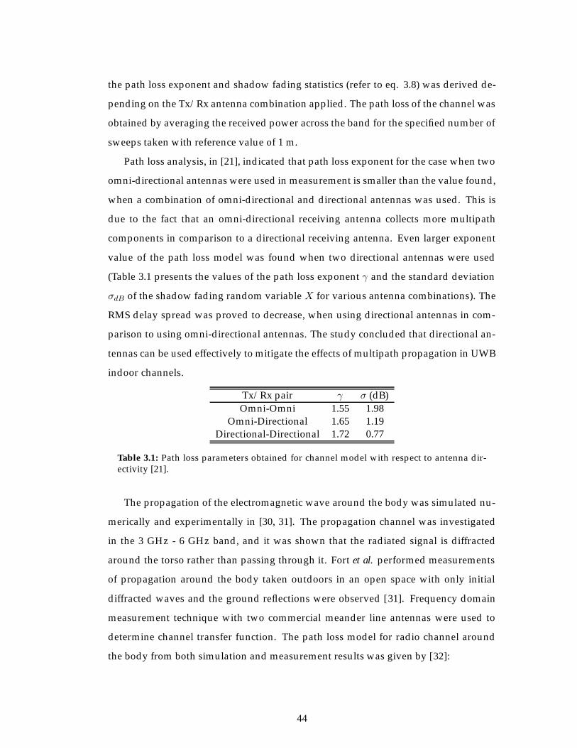
the path loss exponent and shadow fading statistics (refer to eq. 3.8) was derived de-
pending on the Tx/Rx antenna combination applied. The path loss of the channel was
obtained by averaging the received power across the band for the specified number of
sweeps taken with reference value of 1 m.
Path loss analysis, in [21], indicated that path loss exponent for the case when two
omni-directional antennas were used in measurement is smaller than the value found,
when a combination of omni-directional and directional antennas was used. This is
due to the fact that an omni-directional receiving antenna collects more multipath
components in comparison to a directional receiving antenna. Even larger exponent
value of the path loss model was found when two directional antennas were used
(Table 3.1 presents the values of the path loss exponent γ and the standard deviation
σdB of the shadow fading random variable X for various antenna combinations). The
RMS delay spread was proved to decrease, when using directional antennas in com-
parison to using omni-directional antennas. The study concluded that directional an-
tennas can be used effectively to mitigate the effects of multipath propagation in UWB
indoor channels.
Tx/Rx pair γ σ (dB)Omni-Omni 1.55 1.98
Omni-Directional 1.65 1.19Directional-Directional 1.72 0.77
Table 3.1: Path loss parameters obtained for channel model with respect to antenna dir-ectivity [21].
The propagation of the electromagnetic wave around the body was simulated nu-
merically and experimentally in [30, 31]. The propagation channel was investigated
in the 3 GHz - 6 GHz band, and it was shown that the radiated signal is diffracted
around the torso rather than passing through it. Fort et al. performed measurements
of propagation around the body taken outdoors in an open space with only initial
diffracted waves and the ground reflections were observed [31]. Frequency domain
measurement technique with two commercial meander line antennas were used to
determine channel transfer function. The path loss model for radio channel around
the body from both simulation and measurement results was given by [32]:
44
PLdB(d) = 50.5dB + 7.4 · 10log(d/0.1) (3.15)
In addition, Fort et al. presented the BAN channel model for propagation on the front
of the torso, which is given by:
PLdB(d) = 44.6dB + 3.1 · 10log(d/0.1) (3.16)
Fort et al. has also proposed a procedure for measuring body area propagation
in an indoor environment, where the body area channel included an initial cluster of
components diffracting around the body, followed by subsequent clusters of compon-
ents reflecting from surrounding objects in the room. Components diffracting around
the body were best described by a high path loss exponent and correlated lognor-
mal variables [31, 32]. The authors presented a generalised radio channel model for
body area network communication in UWB band based on frequency domain meas-
urements and commercially available antennas. Only static radio channels are con-
sidered for standing still scenarios with arm swinging applied; however, frequency
domain measurements still require static channels for the sweeping duration and the
system model provided is more scenario specific rather than generic [31, 33].
In [34], Wang et al. proposed a channel model which is a modified version of the
one proposed by Saleh-Valanzuela for radio propagation in indoor environment [22].
This model, is specific to some representative body links, and it is based on a set of
dispersive-FDTD simulations. Wang et al. concluded that one cluster is sufficient for
describing the PDPs of the five on-body links considered. It was also shown that the
PDP decays exponentially with the time, however, no reflections from the surrounding
environment were considered. In [5], a measurement campaign was performed using
pairs of a printed horn shaped self complementary antenna (HSCA) and a vertical
version of the printed PICA, exhibiting different radiation characteristics were used.
The measurements were carried out on six different links, and including several body
postures using the reference distance do equals to 1 meter. Results demonstrated the
impact of the antenna radiation pattern on the received power. For HSCA:
PLdB(d) = 86.5 + 10 · (4.4) · log(
d
d0
)for 40cm ≤ d ≤ 100cm (3.17)
45
and for PICA as:
PLdB(d) = 70.3 + 10 · (2.7) · log(
d
d0
)for 40cm ≤ d ≤ 100cm (3.18)
where γ=4.4 and 2.7 are the path loss exponents for HSCA and PICA models, respect-
ively.
Few efforts have been made for UWB off-body channel characterisation in the
open literature [35–40]. UWB off-body signal power strength in the hospital environ-
ment (for both static and dynamic cases) using RF-optical fibre measurement setup is
presented in [36]. In [35, 38], a statistical UWB off-body channel model and time delay
analysis are presented for an indoor environment (in frequency band 3.5-6.5 GHz). A
separate tapped-delay-line model for each region of body (i.e., front, back and side) is
shown due to the dependence of the radio propagation link on the human body lossy
tissue structure. Results show that for the static case, the signal strength is not only
dependant on the radio channel behavior but also dependant on user postures and
movement modes. In [39], an experimental investigation of off-body radio propaga-
tion channels based on commercially available UWB wireless tags at the frequency
band of 5.9-7.2 GHz using nine different channels is presented.
3.3 Overview of Diversity Antenna Techniques for BCWN
By using more than one communication channel, the fading in wireless propagation
channels can be minimised, hence achieving reliable and efficient transmission. Di-
versity works on the principle of using two or more uncorrelated branches with inde-
pendent fading statistics. If two or more channels are separated sufficiently in time,
frequency, space, radiation pattern, and/or polarization, the fading on the individual
channels is independent due to the different channel conditions [41]. It is highly im-
probable that all the branch signals will be at the same fade level at a certain instant.
Therefore, if the branch signals are combined properly, the deep fades can be minim-
ised thus yielding an overall improved SNR. In principle, diversity works at its best if
fading at the branches is uncorrelated and the branch signals have the same average
power level [42].
Antenna diversity generally refers to the implementation of diversity system in
46
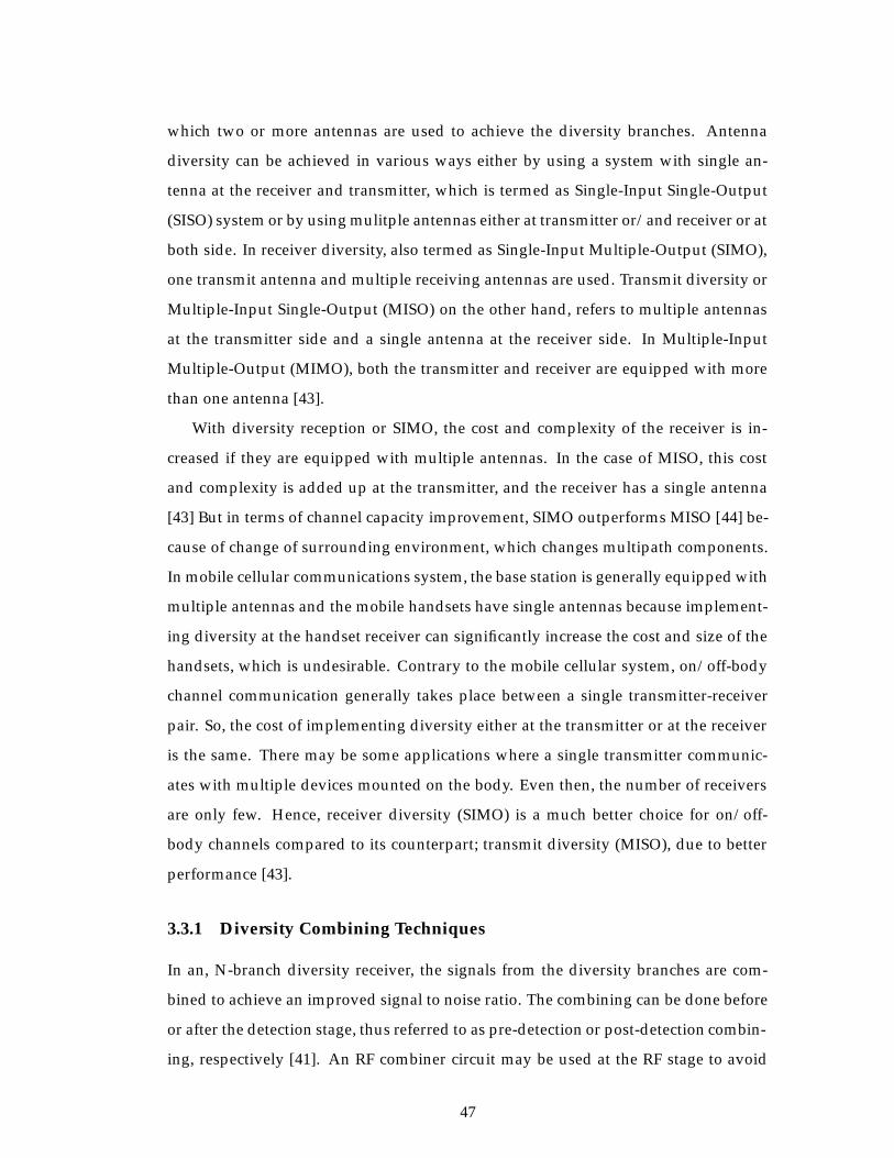
which two or more antennas are used to achieve the diversity branches. Antenna
diversity can be achieved in various ways either by using a system with single an-
tenna at the receiver and transmitter, which is termed as Single-Input Single-Output
(SISO) system or by using mulitple antennas either at transmitter or/and receiver or at
both side. In receiver diversity, also termed as Single-Input Multiple-Output (SIMO),
one transmit antenna and multiple receiving antennas are used. Transmit diversity or
Multiple-Input Single-Output (MISO) on the other hand, refers to multiple antennas
at the transmitter side and a single antenna at the receiver side. In Multiple-Input
Multiple-Output (MIMO), both the transmitter and receiver are equipped with more
than one antenna [43].
With diversity reception or SIMO, the cost and complexity of the receiver is in-
creased if they are equipped with multiple antennas. In the case of MISO, this cost
and complexity is added up at the transmitter, and the receiver has a single antenna
[43] But in terms of channel capacity improvement, SIMO outperforms MISO [44] be-
cause of change of surrounding environment, which changes multipath components.
In mobile cellular communications system, the base station is generally equipped with
multiple antennas and the mobile handsets have single antennas because implement-
ing diversity at the handset receiver can significantly increase the cost and size of the
handsets, which is undesirable. Contrary to the mobile cellular system, on/off-body
channel communication generally takes place between a single transmitter-receiver
pair. So, the cost of implementing diversity either at the transmitter or at the receiver
is the same. There may be some applications where a single transmitter communic-
ates with multiple devices mounted on the body. Even then, the number of receivers
are only few. Hence, receiver diversity (SIMO) is a much better choice for on/off-
body channels compared to its counterpart; transmit diversity (MISO), due to better
performance [43].
3.3.1 Diversity Combining Techniques
In an, N-branch diversity receiver, the signals from the diversity branches are com-
bined to achieve an improved signal to noise ratio. The combining can be done before
or after the detection stage, thus referred to as pre-detection or post-detection combin-
ing, respectively [41]. An RF combiner circuit may be used at the RF stage to avoid
47
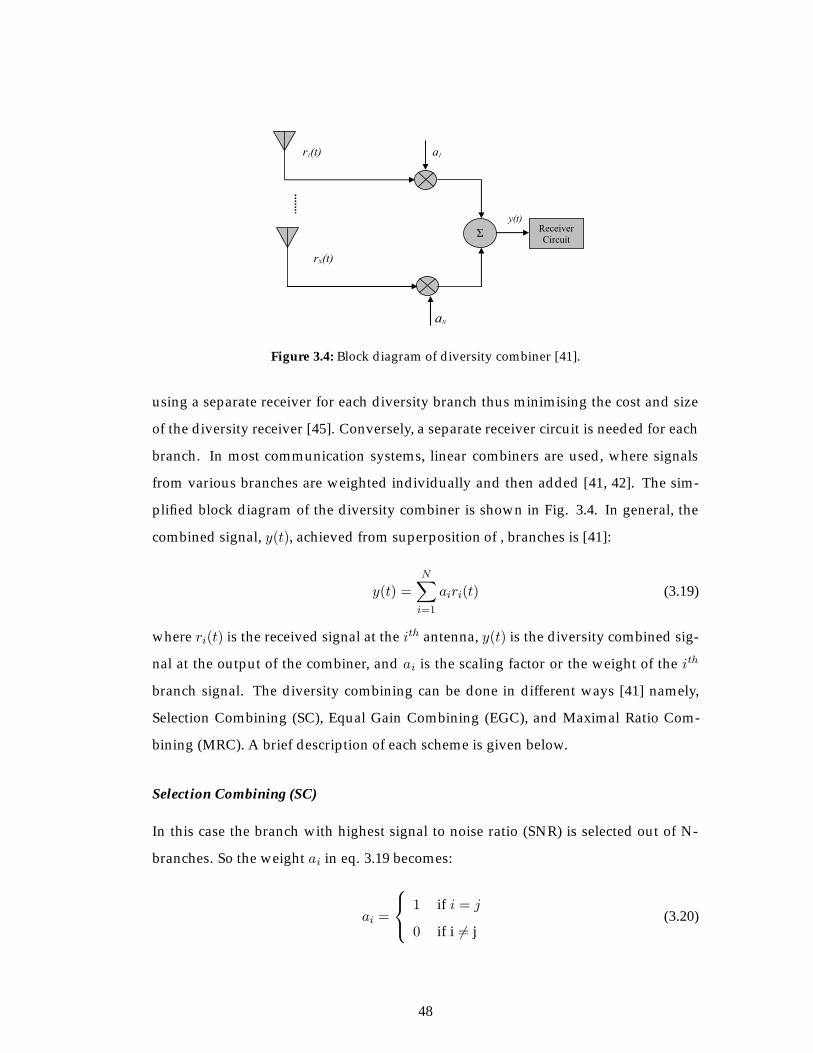
Σ
a
a1
y(t)
r (t)
r1(t)
Receiver Circuit
Figure 3.4: Block diagram of diversity combiner [41].
using a separate receiver for each diversity branch thus minimising the cost and size
of the diversity receiver [45]. Conversely, a separate receiver circuit is needed for each
branch. In most communication systems, linear combiners are used, where signals
from various branches are weighted individually and then added [41, 42]. The sim-
plified block diagram of the diversity combiner is shown in Fig. 3.4. In general, the
combined signal, y(t), achieved from superposition of , branches is [41]:
y(t) =
N∑i=1
airi(t) (3.19)
where ri(t) is the received signal at the ith antenna, y(t) is the diversity combined sig-
nal at the output of the combiner, and ai is the scaling factor or the weight of the ith
branch signal. The diversity combining can be done in different ways [41] namely,
Selection Combining (SC), Equal Gain Combining (EGC), and Maximal Ratio Com-
bining (MRC). A brief description of each scheme is given below.
Selection Combining (SC)
In this case the branch with highest signal to noise ratio (SNR) is selected out of N-
branches. So the weight ai in eq. 3.19 becomes:
ai =
⎧⎨⎩ 1 if i = j
0 if i �= j(3.20)
48
Equal Gain Combining (EGC) and Maximum Ration Combining (MRC)
The EGC and MRC use the combined effect of all the signals. In these two techniques,
the signals are weighted and then added. Before combining, the branch signals must
be cophased. Cophasing of the branch signals in a two-branch diversity receiver can
be done by adjusting the phase of one branch signal according to the relative phase
difference between the two branch signals, as shown in Fig. 3.5. Other methods of
cophasing are also given in [41]. EGC is simple in a sense that the weight for all the
branches is set to 1, i.e., all the branch signals are simply added together. Assuming
that the cophasing has been done, the weight for EGC is, ai = 1 in eq. 3.19. In MRC,
first proposed by Kahn and termed as ratio squarer [46], branch signals are weighted
proportional to their signal voltage to noise power ratio such that the output is the
sum of their SNR’s. The weight ai = 1 in eq. 3.19 is thus directly proportional to the
RMS value of the branch signal and inversely proportional to the average noise power
at the ith branch [42, 47] i.e.,
ai =ri(RMS)
n2i
(3.21)
ri(RMS) =√
r2i is RMS value of the signal and n2i is the average noise power at the
ith branch. The simplified expressions to obtain the diversity-combined signal with
SC, EGC and MRC for an, two branch diversity combiner are given in [48] as:
SC(t) = max(r1(t), r2(t)) (3.22)
EGC(t) =r1(t) + r2(t)√
2(3.23)
MRC(t) =√
r21(t) + r22(t) (3.24)
where r1(t) and r2(t) are the two received branch signal envelopes. Amongst all the
combining schemes, selection combining and switched combining are the simplest
and cheapest methods. They do not rely on the phase information of the received
signals and are thus easy to implement. The performance is though not as good as the
49
Signal 2Phase
ComparatorLO
PhaseShifter
Signal 1
Figure 3.5: Cophasing circuit for MRC and EGC [41]
EGC and MRC schemes. MRC is the optimum combining technique in terms of the
diversity improvement [42] but is complicated and expensive.
3.3.2 Diversity Gain
Diversity gain (DG) is a figure of merit to measure the improvement in signal qual-
ity as a result of applying diversity techniques. It is an improvement in the signal
strength, or SNR, or bit error rate (BER), over a single antenna with no diversity, at a
certain level of outage probability [42, 49]. It is a common practice to calculate the di-
versity gain as the difference in signal levels (or SNR) of the diversity combined signal
and the strongest branch signal (taken as a reference) among all the diversity branches
at some outage probability, as depicted in eq. 3.25. Probability level of 10 % and 1 %
are commonly used. Figure 3.6 shows the Cumulative Distribution Function (CDF) of
two branch signals and a diversity combined signal with diversity gain calculated at
10 % probability.
DG = Pdiv − Ps (3.25)
wherePdiv is the power level of the diversity combined signal and Ps is the power level
of the reference signal (which is strongest among the branch signals). These values are
in dB.
3.3.3 Envelope correlation
The performance of a diversity receiver greatly depends upon the correlation between
the received signals at the diversity branches. Low correlation is desirable to assure
the different fading of branch signals. A correlation coefficient of 0.7 is considered
suitable for most of the mobile communication scenarios [42].
50
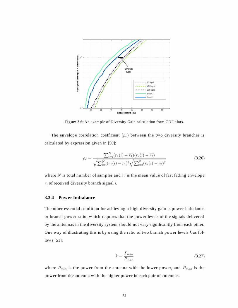
−85 −80 −75 −70 −65 −60 −55 −5010
−2
10−1
Signal strength (dB)
P (
Sig
na
l S
tre
ng
th <
ab
sc
iss
a)
SC signal
MRC signal
EGC signal
Branch 1
Branch 2
Diversity Gain
Figure 3.6: An example of Diversity Gain calculation from CDF plots.
The envelope correlation coefficient (ρe) between the two diversity branches is
calculated by expression given in [50]:
ρe =
∑Ni=i(r1(i)− r1)(r2(i)− r2)√∑N
i=i(r1(i)− r1)2√∑N
i=i(r2(i)− r2)2(3.26)
where N is total number of samples and ri is the mean value of fast fading envelope
ri of received diversity branch signal i.
3.3.4 Power Imbalance
The other essential condition for achieving a high diversity gain is power imbalance
or branch power ratio, which requires that the power levels of the signals delivered
by the antennas in the diversity system should not vary significantly from each other.
One way of illustrating this is by using the ratio of two branch power levels k as fol-
lows [51]:
k =Pmin
Pmax(3.27)
where Pmin is the power from the antenna with the lower power, and Pmax is the
power from the antenna with the higher power in each pair of antennas.
51
3.3.5 Types of Diversity
Diversity can be achieved in various ways, e.g. space (spatial) diversity, polarisation
diversity, and pattern (angle) diversity [41] etc. A brief description of the antenna
diversity types is given below.
Space Diversity
This diversity scheme uses multiple antennas on transmit and/or receive side to get
diversity branches distributed in space. Two or more identical antennas are separated
by certain spacing between them to achieve a space diversity antenna. This technique
does not consume extra spectrum [41, 42]. The spacing of the antennas, determines the
amount of mutual coupling between the adjacent branch antennas and the correlation
among the branch signals. The spacing between the antennas should be such that the
mutual coupling and correlation is minimised and the received signals on the antenna
are faded independently. A spacing of λ/2 is sufficient for most of the applications
[41, 42]. The correlation between two branch signals varies with the spacing between
the antennas in a space diversity receiver.
Angle Diversity
If directional antennas are used either at transmitter or at receiver, another kind of
diversity is achieved, called radiation pattern diversity or angle diversity. The di-
versity branches are produced by directing the radiation pattern in different angles.
The most desirable situation is where the overlap between the adjacent radiation pat-
terns is minimal and the combination gives an omni-directional pattern. The signals
radiated in different directions undergo different fading and hence are uncorrelated.
In most cases, an array with appropriate beam switching is used at either transmitter,
or receiver, or both. Pattern diversity is more effective in situation when the angle of
arrival has more spread and variation [52].
Polarisation Diversity
This diversity scheme exploits the fact that if two signals are transmitted or received
with orthogonal polarisation, the fading in the signals is uncorrelated [41, 42]. Thus,
52
two antennas with different polarisation or a single dual-polarised antenna can be
used to constitute a two-branch diversity system. It has an advantage over space di-
versity that it does not always require two antennas separated by some distance, as a
single dual-polarised antenna can be used to implement it and thus offers size and cost
reduction compared to the space diversity receiver [48]. In case of a single polarisation
transmitted, the difference between the co-polar and the cross-polar components re-
ceived at the receiver is supposed to be very high if the environment does not provide
significant depolarization. This difference, often called the cross-polarisation discrim-
ination (XPD), is required to be lower for polarization diversity to work effectively;
otherwise, the power imbalance between the two diversity branches will be large, res-
ulting in low diversity gain. Full benefits of polarisation diversity can be achieved in
a scenario where the scattering environment causes significant amount of depolarisa-
tion of the transmitted signal and hence the XPD at the receiver is low.
3.3.6 Diversity Antenna Design
There are various issues related to the design of antennas for use in diversity sys-
tems. Some of these are general issues such as size, mutual coupling, radiation pat-
tern, and radiation efficiency etc., whereas, some are specific to the on-body channels,
like specific absorption rate (SAR), detuning due to placement on the body, compact-
ness and structure. Different types of diversity schemes also render specific design
requirements, like spacing between the antennas and similar radiation patterns for
space diversity systems, XPD for polarization diversity, radiation pattern shape and
the overlap between the patterns of the branches for pattern diversity systems. The di-
versity antenna must be as compact as possible due to the trend of miniaturization of
modern communication devices. For body-worn devices, it is desired to be low-profile
as well, along with the small size.In spatial and pattern diversity, spacing between the
antenna elements proved to be the main obstruction in miniaturisation. A reduction
in space results in an increased correlation between the two branch signals thus de-
creasing capacity gain and overall system performance. However, it has been reported
in the literature that for very closely spaced antennas, mutual coupling can actually
cause de-correlation of the branch signals and thus increase the capacity [53–55].
In general, the diversity antenna should be designed such that it is compact, have
53
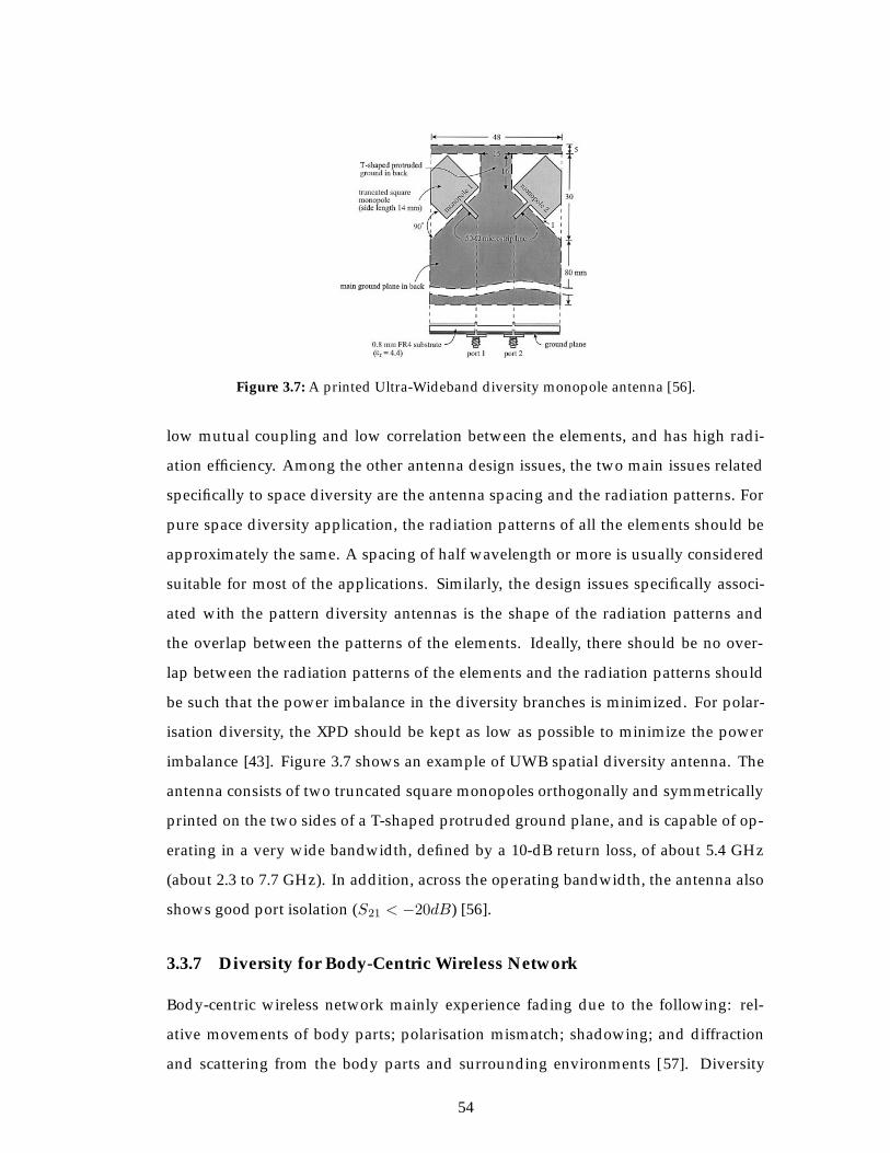
Figure 3.7: A printed Ultra-Wideband diversity monopole antenna [56].
low mutual coupling and low correlation between the elements, and has high radi-
ation efficiency. Among the other antenna design issues, the two main issues related
specifically to space diversity are the antenna spacing and the radiation patterns. For
pure space diversity application, the radiation patterns of all the elements should be
approximately the same. A spacing of half wavelength or more is usually considered
suitable for most of the applications. Similarly, the design issues specifically associ-
ated with the pattern diversity antennas is the shape of the radiation patterns and
the overlap between the patterns of the elements. Ideally, there should be no over-
lap between the radiation patterns of the elements and the radiation patterns should
be such that the power imbalance in the diversity branches is minimized. For polar-
isation diversity, the XPD should be kept as low as possible to minimize the power
imbalance [43]. Figure 3.7 shows an example of UWB spatial diversity antenna. The
antenna consists of two truncated square monopoles orthogonally and symmetrically
printed on the two sides of a T-shaped protruded ground plane, and is capable of op-
erating in a very wide bandwidth, defined by a 10-dB return loss, of about 5.4 GHz
(about 2.3 to 7.7 GHz). In addition, across the operating bandwidth, the antenna also
shows good port isolation (S21 < −20dB) [56].
3.3.7 Diversity for Body-Centric Wireless Network
Body-centric wireless network mainly experience fading due to the following: rel-
ative movements of body parts; polarisation mismatch; shadowing; and diffraction
and scattering from the body parts and surrounding environments [57]. Diversity
54
is a powerful technique to combat fading and multipath effects [58]. As the spatial
diversity does not need any additional spectrum; in addition, UWB is inherently a fre-
quency diversity technology. This makes the spatial arrangement of multiple antennas
a promising technique to enhance the performance of UWB body-centric wireless net-
works [59].
There has been an increasing interest in diversity and multiple-input, multiple-
output (MIMO) techniques for enhanced mobile and wireless communications in re-
cent years [50, 60–64]. Much work has been done on the use of diversity at the mobile
hand-held devices and the base station. The performance benefits of diversity for
portable wireless systems have been reported in [52]. Dietrich et. al [53] shows an
experimental investigation of various diversity configurations and a diversity gain of
up to 10 dB at 1 % probability for none line-of-sight scenario. Karaboikis et. al [45]
gives an experimental study of three-branch diversity system with various antennas.
The correlation coefficients and the effect of mutual coupling are also discussed there.
Colburn et. al [49]has presented diversity performance with experimental data using
PIFA, monopole and other antenna combinations for mobile hand-held terminals in
Rayleigh and Rician fading environments.
There are some studies presented in the open literature where the benefits of di-
versity techniques for body-centric communications in narrow-band systems have
been investigated [57, 59, 65–73]. The effect of human body, especially the head and
the hand, on the performance of diversity antenna at the mobile handset was dis-
cussed in [65] by presenting the change in diversity gain and envelope correlation
with angle of inclination of the antenna and its distance from the head. Introduct-
ory studies for on-body diversity measurements at 2.45 GHz were presented in [66].
The diversity performances were evaluated in terms of DG, power imbalance and en-
velope correlation coefficients between the two receiving channels. A comprehensive
study of diversity for an on-body channel at 2.45 GHz was presented in [57], using
different antennas and diversity types. A significant gain was observed for NLOS
channels and dynamic channels involving large body movements. The uplink and
downlink diversities were also calculated and found to be similar. A comparison of
spatial and pattern diversity was presented in [67]. It was observed that spatial di-
versity gave a greater improvement than pattern diversity, in terms of DG. Cotton and
55
Scanlon [69, 70] have presented first- and second-order statistics and some diversity
results for off-body and on-body channels, at 2.45 GHz and 868 MHz, respectively.
On-body diversity at 868 MHz has been thoroughly investigated in [70], with ap-
plication to medical implants. Off-body spatial diversity and correlation coefficient
evaluation was performed in [71, 72] at 868 MHz and 5.8 GHz respectively. Diversity
performance using textile antennas for firefighters was presented in [73].
Other studies on UWB-MIMO and UWB diversity were presented in [74–83]. An-
tenna diversity results for the UWB indoor channel are presented in [77], with an em-
phasis on differences between virtual and real compact arrays, including mutual coup-
ling effects. UWB-MIMO for on-body has been investigated in [75], using frequency-
space polarization. The key findings in [75] were that, in BCWN, the MIMO channel
capacity is mainly determined by the power imbalance for both spatial arrays and po-
lar arrays. It was also found that the MIMO capacity decreases with the frequency.
Roy et. al presented an innovative space-time spatial model for UWB multi-sensor,
multi-antenna BANs in [83]. However, to the authors’ knowledge, UWB spatial di-
versity for on/off-body communications has not yet been investigated systematically
and thoroughly. In this thesis, the spatial diversity is investigated for UWB on/off-
body communication channels. The improvement due to diversity is often measured
in terms of diversity gain; this is basically an improvement in signal strength (or, equi-
valently, signal-to-noise ratio or bit-error rate) compared with that observed with a
single antenna at a certain outage probability [57, 58, 60, 63, 64]. The outage probabil-
ity is the probability that the system performance falls below a minimum performance
threshold (typically defined in terms of signal-to-noise ratio) within a specified time
period [17].
3.4 Summary
In this chapter, a brief introduction to UWB antennas was presented with respect to
their applicability in body-centric wireless communications. Radio channel charac-
terisation including transient and spectral characteristics have also been discussed for
56
UWB radio technology. A literature review on the state-of-the-art on UWB radio chan-
nel characterisation for body-centric network is also presented. Apart from UWB an-
tenna and radio propagation, the issues related to fading in wireless channel with its
different types was also discussed. An overview of diversity antenna systems includ-
ing different combining techniques (i.e. selection combining, equal gain combining
and maximum ratio combining) and types of diversity (i.e. space, angle and polarisa-
tion diversity) has been presented. Diversity parameters (i.e. diversity gain, power
imbalance and correlation) are briefly introduced including their relationship with di-
versity performance. Towards, the end of the chapter a brief introduction about the
requirements for diversity antenna and existing literature on the use of diversity in
body-centric network has been highlighted.
Based on the background reading and literature review, the following challenges,
still needs to be tackled, i.e., UWB radio channel characterisation for body-centric wire-
less commmunications needs to be fully charaterised, taking into account the dynamic
nature of the channel, the effect of indoor environment and the effect of different sec-
tors of the body. Apart from UWB body-centric radio channel characterisation, ap-
plicability of UWB diversity analysis needs to be investigated as well. Furthermore, a
system level performance analysis of UWB body-centric radio channel and diversity
techniques is required. The above mentioned problems will be analysed and studied
in the following chapters and in this thesis generally.
57
References
[1] W. Soergel, C. Waldschmidt, and W. Wiesbeck, “Antenna characterization for ultra wide-band communications,” IWUWBS, Oulu, Finland, June 2003.
[2] S. Licul, J. A. N. Noronha, W. A. Davis, D. G. Sweeney, C. R. Anderson, and T. M. Bielawa,“A parametric study of time-domain characteristics of possible UWB antenna architec-tures,” 2003 IEEE 58th Vehicular Technology Conference, Fall 2003, vol. 5, pp. 3110–3114,October 2003.
[3] T. Yang, S.-Y. Suh, R. Nealy, W. Davis, and W. L. Stutzman, “Compact antennas for UWBapplications,” 2003 IEEE Ultra Wideband Systems and Technologies, pp. 205–208, November2003.
[4] A. Sani, Modeling and Characterisation of Antenna and Propagation for Body-Centric WirelessCommunications. PhD thesis, Queen Mary Uni. of London, 2010.
[5] A. Alomainy, Y. Hao, C. G. Parini, and P. S. Hall, “Comparison between two differ-ent antennas for UWB on-body propagation measurements,” IEEE Antennas and WirelessPropagation Letter, vol. 4, no. 1, pp. 31–34, December 2005.
[6] T. See and Z. Chen, “Experimental characterization of UWB antennas for on-body com-munications,” IEEE Transactions on Antennas and Propagation, vol. 57, no. 4, pp. 866–874,2009.
[7] M. Klemm and G. Troster, “Characterisation of an aperture-stacked patch antenna forultra-wideband wearable radio systems,” 15th International Conference on Microwaves,Radar and Wireless Communications, 2004, vol. 2, pp. 395–398, May 2004.
[8] S. Promwong, W. Hachitani, G. S. Ching, and J. Takada, “Characterization of ultra-wideband antenna with human body,” Internationa Symposium on Communications andInformation Technology (ISCIT 2004), Sapporo, Japan, pp. 1213–1217, October 2004.
[9] I. Skycross, “3.1-10 GHz UWB antenna for commercial UWB applications,”http://www.skycross.com/.
[10] Q. H. Abbasi, A. Alomainy, and Y. Hao, “Recent development of ultra wideband body-centric wireless communications,” in IEEE international conference on Ultra Wideband Tech-nology (ICUWB), Nanjing, China, 20-23 Sep. 2010.
[11] FCC First Report and Order, Revision of the Part 15 Commission’s Rules Regarding Ultra-Wideband Transmission Systems, pp. 98–153, April 22, 2003.
[12] T. Zasowski, F. Althaus, M. Stager, A. Wittneben, and G. Troster, “UWB for noninvasivewireless body area networks: channel measurements and results,” Proceedings of IEEEConference on Ultra Wideband Systems and Technologies, Reston, Virginia, vol. 55, no. 1, pp.285–289, November 2003.
[13] D. Lamensdorf and L. Susman, “Baseband-pulse-antenna techniques,” IEEE Antennas andPropagation Magazine, vol. 36, no. 1, February 1994.
[14] J. S. McLean, H. Foltz, and R. Sutton, “Pattern descriptors for UWB antennas,” IEEETransactions on Antennas and Propagation, vol. 53, no. 1, January 2005.
[15] L. Guo, Study and Miniaturisation of Antennas for Ultra Wideband Communication Systems.PhD thesis, Queen Mary Uni. of London, 2009.
[16] P. Prasad, Universal Wireless Personal Communications. Artech House, London, 1998.
58
[17] T. S. Rappaport, Wireless Communications Principles and Practice. Prentice Hall, Inc., NewJersey, 1996.
[18] H. Hashemi, “The indoor radio propagation channel,” Proceedings of IEEE, vol. 81, no. 7,pp. 943–968, 1993.
[19] S. R. Saunders, Antennas and Propagation for Wireless Communication Systems. John Wiley& Sons, Ltd., 2004.
[20] S. R., Antennas and Propagation for Wireless Communication Systems, 2nd Edition. JohnWiley & Sons, Ltd., 2007.
[21] J. A. Dabin, N. Ni, A. M. Haimovich, E. Niver, and H. Grebel, “The effects of antennadirectivity on path loss and multipath propagation in UWB indoor wireless channels,” inProc. IEEE Conf. Ultra Wideband Systems and Technologies, Newark, NJ,, pp. 305–309, 2003.
[22] A. Saleh and R. A. Valenzuela, “A statistical model for indoor multipath propagation,”IEEE J. Selected Areas Commun, vol. JSAC-5, no. 3, pp. 128–137, February 1987.
[23] H. Suzuki, “A statistical model for urban radio propagation,” IEEE Transactions on Com-munications, vol. 25, no. 7, pp. 673–680, July 1977.
[24] M. Z. Win and R. A. Scholtz, “Impulse radio: how it works,” IEEE Communications Letters,pp. 36–38, February 1998.
[25] M. Win and R. Scholtz, “Characterization of ultra-wide bandwidth wireless indoor chan-nels: A communication-theoretic view,” IEEE Journal on Selected Areas in Communications,vol. 20, no. 9, pp. 1613–1627, December 2002.
[26] L. Rusch, C. Prettie, D. Cheung, Q. Li, and M. Ho, “Characterization of UWB propagationfrom 2 to 8 GHz in a residential environment,” Intel Corporation, Intel Research Labs.
[27] W. Ciccognani, A. Durantini, and D. Cassioli, “Time domain propagation measurementsof the UWB indoor channel using PN sequence in the FCC-compliant band 3.66 GHz,”IEEE Transactions on Antenna and Propagation, vol. 53, no. 4, April 2005.
[28] M. Z. Win and R. A. Scholtz, “Characterization of ultra-wide bandwidth wireless indoorchannels: A communication-theoretic view,” IEEE Journal on Selected Areas in Communic-ations, vol. 20, no. 9, pp. 1613–1627, December 2002.
[29] S. Ghassemzadeh and V. Tarokh, “A statistical path loss model for in-home UWB chan-nels,” IEEE Conference on Ultra Wideband Systems and Technologies, pp. 59–64, May 2002.
[30] A. Fort, C. Desset, J. Ryckaert, P. D. Doncker, and L. V. Biesen, “Ultra wideband body areachannel model,” International Conference on Communications, ICC05, Seoul, South Korea,May 2005.
[31] A. Fort, C. Desset, P. D. Doncker, and L. V. Biesen, “Ultra wideband body area propaga-tion: from statistics to implementation,” IEEE Transactions on Microwave Theory and Tech-nique, vol. 54, no. 4, pp. 1820–1826, June 2006.
[32] A. Fort, P. D. Doncker, and L. V. Biesen, “An ultra wideband channel model for commu-nication around the body,” IEEE Journal on selcted area of comms, vol. 24, no. 4, pp. 927–933,April 2006.
[33] A. F. Molisch, D. Cassioli, C.-C. Chong, S. Emami, A. Fort, B. Kannan, J. Karedal,J. Kunisch, H. G. Schantz, K. Siwiak, and M. Z. Win, “A comprehensive standardizedmodel for ultra wideband propagation channels,” IEEE Transactions on Antennas andPropagation, vol. 54, no. 11, pp. 3151–3166, 2006.
59
[34] Q. Wang, T. Tayamachi, I. Kimura, and J. Wang, “An on-body channel model for UWBbody area communications for various postures,” IEEE Journal on Selected Areas in Com-munications, vol. 57, no. 4, pp. 991–998, April 2009.
[35] A. A. Goulianos, T. W. C. Brown, B. G. Evans, and S. Stavrou, “Wideband power mod-elling and time dispersion analysis for UWB indoor off-body communications,” IEEETransactions on Antenna and Propagation, vol. 57, no. 7, pp. 2162–2171, July 2009.
[36] P. A. Catherwood and W. G. Scanlon, “Link characteristics for an off-body UWB transmit-ter in a hospital environment,” in Loughborough Antennas & Propagation Conference, 2009.
[37] A. Goulianos, T. Brown, and S. Stavrou, “A novel path loss model for UWB off-bodypropagation,” in IEEE Vehicular Technology Conference (VTC Spring).
[38] G. A., T. W. Brown, B. G. Evans, and S. Stavrou, “Power delay profile modelling of ultrawideband off-body propagation channel,” IET Microw. Antennas Propag., vol. 4, no. 1, pp.62–71, Jan. 2010.
[39] M. M. Khan, Q. H. Abbasi, A. Alomainy, and Y. Hao, “Radio propagation channel char-acterisation using ultra wideband wireless tags for body-centric wireless networks in in-door environment,” in 2011 IEEE International Workshop on Antenna Technology, IWAt 2011,Hong Kong, 7-9 March 2011.
[40] A. Goulianos, T. Brown, and S. Stavrou, “Ultra-wideband measurements and results forsparse off-body communication channels,” in Loughborough Antennas & Propagation Con-ference, UK, 17-18 March 2008, pp. 213–216.
[41] W. C. Jakes, Microwave Mobile Communications. New York:Wiley, 1974.
[42] J. B. A. R G. Vaughan, “Antenna diversity in mobile communications,” IEEE transactionOn Vehicular Technology, vol. VT-36, no. 4, Nov. 1987.
[43] I. Khan, Diveristy and MIMO for Body-Centric Wireless Channels. Phd thesis, University ofBirmingham, Sep. 2009.
[44] J. Gong, F. J. Hayes, and M. R. Soleymani, “Comparison of capacities of the transmitantenna diversity with the receive antenna diversity in the MIMO scheme,” Proc. IEEECanadian Conference on Electrical and Computer Engineering (CCECE), vol. 1, pp. 179–182,May 47, 2003.
[45] M. Karaboikis, C. Soras, G. Tsachtsiris, and V. Makios, “Three-branch antenna diversitysystems on wireless devices using various printed monopoles,” IEEE International Sym-posium on Electromagnetic Compatibility, Istanbul (May 11-16, 2003).
[46] L. R. Kahn, “Ratio squarer,” Proc. IRE, vol. 42, p. 1704, Nov. 1954.
[47] D. G. Brennan, “Linear diversity combining techniques,” Proceedings of the IEEE, vol. 91,no. 2, Feb. 2003.
[48] Turkmani, Arowojolu, P. Jefford, and C. Kellett, “An experimental evaluation of the per-formance of two branch space and polarization diversity schemes at 1800 mhz,” IEEETrans. on Vehc. Tech., vol. 44, no. 2, pp. 318–325, May 1995.
[49] J. S. Colburn, Y. Rahmat-Samii, M. A. Jensen, and G. J. Pottie, “Evaluation of personalcommunications dual-antenna handset diversity performance,” IEEE Transactions OnVehicular Technology,, vol. 47, no. 3, Aug. 1998.
60
[50] A. M. D. Turkmani, A. Arowojolu, P. A. Jefford, and C. J. Kellett, “An experimental evalu-ation of the performance of two branch space and polarization diversity schemes at 1800MHz,” IEEE Trans. on Vehc. Tech., vol. 44, no. 2, pp. 318–325, May 1995.
[51] Y. Gao, Characterisation of Multiple Antennas and Channel for Small Mobile Terminals. Phdthesis, Queen Mary University of London, June 2007.
[52] P. Irazoqui-Pastor and J. T. Bernhard, “Examining the performance benefits of antennadiversity systems in portable wireless environments,” IEEE Antenna Applications Sym-posium, Allerton Park, Sep 15-17, 1999.
[53] C. B. J. Dietrich, K. Dietze, J. R. Nealy, and W. L. Stutzman, “Spatial,polarization, andpattern diversity for wireless handheld terminals,” IEEE Transactions on Antennas andPropagation, vol. 49, no. 9, pp. 1271–1281, Sep. 2001.
[54] T. Svantesson and A. Ranheim, “Mutual coupling effects on the capacity of multi-elementantenna systems,” Proc. IEEE Int. Conf. Acoustics, Speech, and Signal Processing (ICASSP)01,vol. 4, pp. 2485–2488, May 2001.
[55] R. G. Vaughan and N. L. Scott, “Terminated in-line monopoles for vehicular diversity,”Proc. Int. Union of Radio Science (USRI) Triennial Symp. Electromagnetic Theory, Sydney, Aus-tralia, pp. 111–113, Aug. 1992.
[56] K.-L. Wong, S.-W. Su, and Y.-L. Kuo, “A printed ultra wideband diversity monopole an-tenna,” IEEE Microwave and Optical Technology Letter, vol. 38, no. 4, pp. 257–259, 20 August2003.
[57] I. Khan, P. S. Hall, A. A. Serra, A. R. Guraliuc, and P. Nepa, “Diversity performanceanalysis for on-body communication channels at 2.45 GHz,” IEEE Transactions in Antennaand Propagation, vol. 57, no. 4, pp. 956–963, April 2009.
[58] W. C. Jakes, Microwave Mobile Communications. New York:Wiley, 1974.
[59] I. Khan and P. S. Hall, “Multiple antenna reception at 5.8 and 10 GHz for body-centricwireless communication channels,” IEEE Transactions in Antenna and Propagation, vol. 57,no. 1, pp. 248–255, Jan 2009.
[60] L. M. Correia, Mobile Broadband Multimedia Networks Techniques, Models and Tools for 4G.Elsevier Ltd, 2006.
[61] C. B. J. Dietrich, K. Dietze, J. R. Nealy, and W. L. Stutzman, “Spatial, polarization, andpattern diversity for wireless handheld terminals,” IEEE Transactions on Antennas andPropagation, vol. 49, no. 9, pp. 1271–1281, September 2001.
[62] M. Karaboikis, C. Soras, G. Tsachtsiris, and V. Makios, “Three-branch antenna diversitysystems on wireless devices using various printed monopoles,” in IEEE International Sym-posium on Electromagnetic Compatibility, May 11-16 2003.
[63] J. S. Colburn, Y. Rahmat-Samii, M. A. Jensen, and G. J. Pottie, “Evaluation of personalcommunications dual-antenna handset diversity performance,” IEEE Transactions OnVehicular Technology, vol. 47, no. 3, pp. 737–746, August 1998.
[64] R. G. Vaughan and J. B. Andersen, “Antenna diversity in mobile communications,” IEEETransactions On Vehicular Technology, vol. VT-36, no. 4, pp. 149–172, May Nov. 1987.
[65] T. M. K Ogawa and K. Monma, “An analysis of the performance of a handset diversityantenna influenced by head, hand, and shoulder effects at 900 MHz: Part II correlationcharacteristics,” IEEE Transactions on Vehicular Technology, vol. 50, no. 3, May 2001.
61
[66] A. A. Serra, P. Nepa, G. Manara, and P. Hall, “Diversity measurements for on-body com-munication systems,” IEEE Antennas and Wireless Propagation Letters, vol. 6, no. 1, pp.361–363, Jan 2007.
[67] I. Khan, M. R. Kamarudin, L. Yu, Y. I. Nechayev, and H. P. S., “Comparison of space andpattern diveristy for on-body channels,” in 5th Eur. Workshop Conformal Antennas, Bristol,U.K., 10-11 Sep. 2007, pp. 47–50.
[68] M. R. Kamarudin, Y. I. Nechayev, and H. P. S., “Performance of antenna in on-body en-vironment,” IEEE Antenna and Propagation Soc. Int. Symp., vol. 3A, pp. 475–478, 3-8 Jul.2009.
[69] S. L. Cotton and W. G. Scanlon, “Channel characterization for single and multiple-antenna wearable systems used for indoor body-to-body communications,” IEEE Trans-actions in Antenna and Propagation, vol. 57, no. 4, pp. 980–990, Jan. 2009.
[70] L. Cotton and G. Scanlon, “Characterization and modeling of on-body spatial diversitywithin indoor environments at 868 MHz,” IEEE Transactions on Wireless Communications,vol. 8, no. 1, pp. 176–185, Jan. 2009.
[71] S. Cotton and W. Scanlon, “Spatial diversity and correlation for off-body communicationsin indoor environments at 868 MHz,” in IEEE 65th, Vehicular Technology Conference, 2007.VTC2007-Spring., 2007, pp. 372–376.
[72] A. J. Ali, S. Cotton, and W. Scanlon, “Spatial diversity for off-body communications inan indoor populated environment at 5.8 GHz,” in Loughborough Antennas & PropagationConference, 2009. LAPC 2009., Loughborough, UK, 16-17 Nov. 2009, pp. 641–644.
[73] P. Van Torre, L. Vallozzi, H. Rogier, and J. Verhaevert, “Diversity textile antenna systemsfor firefighters,” in Proceedings of the Fourth European Conference on Antennas and Propaga-tion (EuCAP, Barcelona, Spain, 12-16 April 2010, pp. 1–5.
[74] T. Kaiser and F. Zheng, Ultra Wideband Systems With MIMO. John Wiley & Sons Ltd,2010.
[75] W. J. Chang, J. H. Tarng, and S. Y. Peng, “Frequency-space-polarization on UWB MIMOperformance for body area network applications,” IEEE Antennas and Wireless PropagationLetters, vol. 7, pp. 577–580, Jan. 2009.
[76] A. Sibille and S. Bories, “Spatial diversity for UWB communications,” in 5th European(Conf. Publ. No. 492) Personal Mobile Communications Conference, 2003, pp. 367 – 370.
[77] R. D’Errico, A. Sibille, A. Giorgetti, and M. Chiani, “Antenna diversity in UWB indoorchannel,” in IEEE International Conference on Ultra-Wideband ICUWB, 2008, pp. 13–16.
[78] R. D’Errico and A. Sibille, “Multiple antennas effect in UWB spatial multiplexing,” inEuropean Conference on Antennas and Propagation EUCAP, Berlin, Germany, 23-27 March2009.
[79] A. Sibille, “Diversity combining for enhanced multi-user throughput in pulse based UWBcommunications,” in 11th European Wireless conference, Nicosia, Cyprus, 10-13 Apr. 2005.
[80] C. Yifan, T. Jianqi, J. Lai, E. Gunawan, S. L. Kay, B. S. Cheong, and P. Rapajic, “Cooperativecommunications in ultra-wideband wireless body area networks: Channel modeling andsystem diversity analysis,” IEEE Journal on Selected Areas in Communications, vol. 27, no. 1,pp. 5–16, Jan. 2009.
[81] M. G. Benedetto, T. Kaiser, A. Molisch, I. Oppermann, and D. Porcino, UWB communica-tion systems: a comprehensive overview. Hindawi Publishing Corporation, 2006.
62
[82] V. Roy, S. Oestges, C. Horlin, F. Doncker, and P. Opera, “Ultra-wideband spatial channelcharacterization for body area networks,” in European Conference on Antennas and Propaga-tion (EuCAP 2007), Edinburgh, U.K., 11-16 Nov. 2007.
[83] S. Van Roy, C. Oestges, F. Horlin, and P. De Doncker, “A comprehensive channel modelfor UWB multisensor multiantenna body area networks,” IEEE Transactions On Antennasand Propagation, vol. 58, no. 1, pp. 163–170, Jan. 2010.
63
Chapter 4
Ultra Wideband Body-Centric Radio
Channel Characterisation Based on
Human Body Sectors and
Pseudo-Dynamic Movements
This chapter discusses the various experimental investigations undertaken to thor-
oughly understand the UWB on/off-body radio propagation channels. These charac-
terisation measurement campaigns were performed in both the anechoic chamber and
a typical indoor environment (cluttered laboratory). Effect of human body movements
on the channel parameters is evaluated. Apart from measurements in an anechoic
chamber and in an indoor environment, when body parts were moving, measure-
ments were also taken on a treadmill machine in order to mimic the scenario of UWB
body-centric system applied in performance monitoring for sport and exercise medi-
cine. Radio channel parameters are extracted from the measurement data and statist-
ically analysed to provide a preliminary radio propagation model with the inclusion
of pseudo-dynamic body movements. In addition, angular and spatial dependency
64
of the UWB off-body radio channels is experimentally characterised by considering
different angles and distances between off-body transmitter and on-body receivers.
4.1 Analysis Methodology Applied for Body-Centric Radio Chan-
nel Modelling
To investigate and analyse the performance of single and multiple antennas for body-
centric wireless communication channels, various approaches can be adopted. It can
either be predicted through detailed simulations using numerical digital phantom,
by real time measurements or by using a statistical channel model, which completely
characterises the channels and the environment. The simulation approach is compu-
tationally intensive and becomes even more complex, when UWB technology is con-
sidered, because of frequency dependance characteristic of human body and larger
bandwidth of UWB. It seems almost unrealistic if random body movement is intro-
duced in the simulations, and seems much less valuable for static postures with no
movements at all, as system design is typically based on statistical channel models.
The statistical channel approach cannot be adopted due to the absence of a standard
statistical channel model for on/off-body radio channels. Hence, on/off-body radio
propagation channel measurements seems useful in real environments with natural-
istic movements of a real human body to quantify the significance of single and mul-
tiple antenna systems for body-worn devices. To do so in this work, antennas were
placed on a human subject to perform single and multiple antenna channel character-
isation and system modelling, while taking safety limits in consideration.
Different propagation measurement setups have been presented in the open liter-
ature to characterise the radio channel. The measurement techniques can be generally
characterised as time domain measurements, and frequency domain measurements
[1–5]. These two techniques are the basis for many other radio propagation sounders
commonly used in characterising wideband radio channels for indoor, outdoor and
body-area network scenarios [6–8].
In time domain measurements, a digital oscilloscope is used to receive the signal,
and is relatively easy to detect multipath components, if their delay with respect to
65
the direct component is greater than the UWB pulse duration [9]. Channel measure-
ments can also be performed using a vector network analyser (VNA) in the frequency
domain. In this case, antennas are connected to the ports of the analyser and a sweep
of discrete frequency tones is performed and S21 is measured from one antenna to the
other which represents the channel frequency response (H(ω)). Analyzing both, mag-
nitude and phase of S21, enables a transition to the time domain by simply applying
an Inverse Discrete Fourier Transform (IDFT). However, one of the problem with fre-
quency domain method is the restriction applied on measurement area freedom since
both transmit and receive antennas are connected to the same VNA; nevertheless, such
problem can be avoided by the use of ultra low-loss long cables and applying advance
calibration techniques [10]. This problem can also be overcome by applications of
VNA measurement set-up using RF on fibre optic connection in scenarios, where elec-
trically small antennas are used [6].
4.2 UWB Antennas for Body-Centric Radio Propagation Meas-
urements
For UWB-BCWN, the antenna design becomes more complicated due to the presence
of the human body. In this thesis, a miniaturised coplanar waveguide (CPW) fed
tapered slot antenna (TSA) for ultra-wideband applications [11] is used for all meas-
urements, as shown in Fig. 4.1. While designing UWB antenna, a broadband imped-
ance matching network is needed and it can be achieved by employing two tapered
radiating slots at the end of the CPW feeding line [12] or by gradually varying the
feed-gap [13] or with the help of a pair of tapered radiating slots [14]. The tapered
slot antenna (TSA) used in this thesis is using a similar approach presented in [12].
However, the difference is that here the waveguide and radiating slot is inseparable.
The antenna is fabricated on RT/Duroid board (with thickness h=1.524 mm, relative
permittivity εr=3, and loss tangent tan(δ)=0.0013). The total antenna size is 27 mm
x 16 mm which is around 0.27λ0 x 0.16λ0 in electrical length, where λ0 is the free
space wavelength at 3 GHz. Unlike the traditional CPW-fed antenna (such as the
PICA aforementioned), the tapered slot antenna is designed to allow for the smooth
transition of line impedance. The length of the semi-major and semi-minor axis of the
66
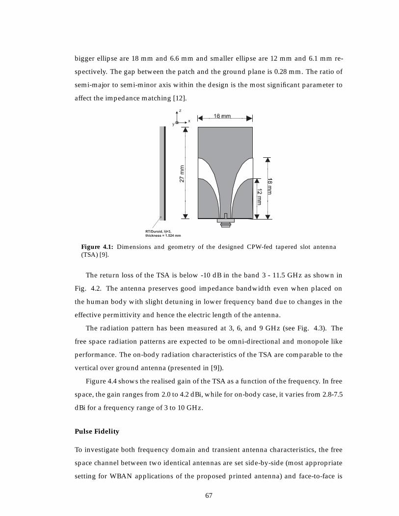
bigger ellipse are 18 mm and 6.6 mm and smaller ellipse are 12 mm and 6.1 mm re-
spectively. The gap between the patch and the ground plane is 0.28 mm. The ratio of
semi-major to semi-minor axis within the design is the most significant parameter to
affect the impedance matching [12].
xy
z
Figure 4.1: Dimensions and geometry of the designed CPW-fed tapered slot antenna(TSA) [9].
The return loss of the TSA is below -10 dB in the band 3 - 11.5 GHz as shown in
Fig. 4.2. The antenna preserves good impedance bandwidth even when placed on
the human body with slight detuning in lower frequency band due to changes in the
effective permittivity and hence the electric length of the antenna.
The radiation pattern has been measured at 3, 6, and 9 GHz (see Fig. 4.3). The
free space radiation patterns are expected to be omni-directional and monopole like
performance. The on-body radiation characteristics of the TSA are comparable to the
vertical over ground antenna (presented in [9]).
Figure 4.4 shows the realised gain of the TSA as a function of the frequency. In free
space, the gain ranges from 2.0 to 4.2 dBi, while for on-body case, it varies from 2.8-7.5
dBi for a frequency range of 3 to 10 GHz.
Pulse Fidelity
To investigate both frequency domain and transient antenna characteristics, the free
space channel between two identical antennas are set side-by-side (most appropriate
setting for WBAN applications of the proposed printed antenna) and face-to-face is
67
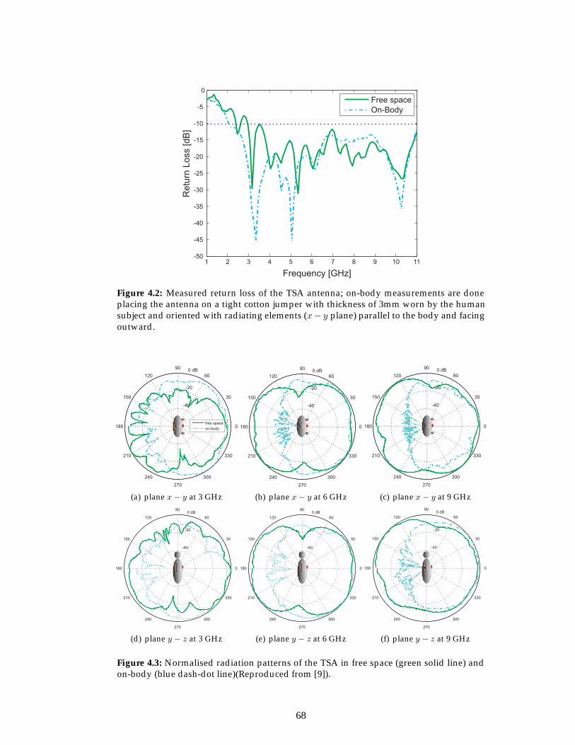
1 2 3 4 5 6 7 8 9 10 11-50
-45
-40
-35
-30
-25
-20
-15
-10
-5
0
Frequency [GHz]
Retu
rn L
oss [dB
]
Free space
On-Body
Figure 4.2: Measured return loss of the TSA antenna; on-body measurements are doneplacing the antenna on a tight cotton jumper with thickness of 3mm worn by the humansubject and oriented with radiating elements (x− y plane) parallel to the body and facingoutward.
(a) plane x− y at 3 GHz (b) plane x− y at 6 GHz (c) plane x− y at 9 GHz
(d) plane y − z at 3 GHz (e) plane y − z at 6 GHz (f) plane y − z at 9 GHz
Figure 4.3: Normalised radiation patterns of the TSA in free space (green solid line) andon-body (blue dash-dot line)(Reproduced from [9]).
68
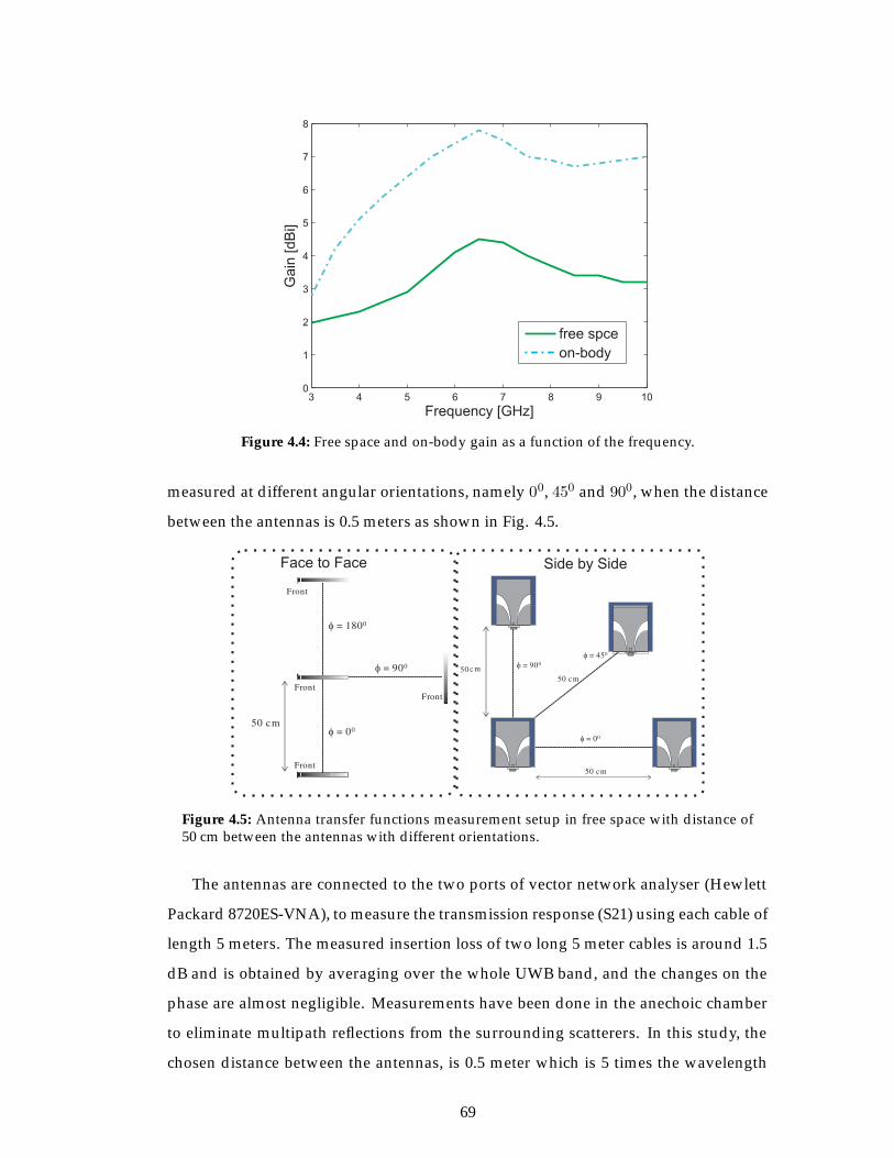
3 4 5 6 7 8 9 100
1
2
3
4
5
6
7
8
Frequency [GHz]
Gain
[dB
i]
free spce
on-body
Figure 4.4: Free space and on-body gain as a function of the frequency.
measured at different angular orientations, namely 00, 450 and 900, when the distance
between the antennas is 0.5 meters as shown in Fig. 4.5.
Figure 4.5: Antenna transfer functions measurement setup in free space with distance of50 cm between the antennas with different orientations.
The antennas are connected to the two ports of vector network analyser (Hewlett
Packard 8720ES-VNA), to measure the transmission response (S21) using each cable of
length 5 meters. The measured insertion loss of two long 5 meter cables is around 1.5
dB and is obtained by averaging over the whole UWB band, and the changes on the
phase are almost negligible. Measurements have been done in the anechoic chamber
to eliminate multipath reflections from the surrounding scatterers. In this study, the
chosen distance between the antennas, is 0.5 meter which is 5 times the wavelength
69
at the lower frequency in the band (3 GHz). Thus, the interaction between the an-
tennas is minimal and most of the distortion in frequency channel responses is due
to impedance mismatch and inherent radiation properties of the antenna. The time
domain responses of the free space radio channel with the antennas are obtained by
direct application of IFFT on the measured real frequency responses S21 [15].
Figure 4.6(a) shows the impulse responses in the band 3-10 GHz when the anten-
nas are set side-by-side. The pulse fidelity is calculated adopting the eq. 3.1, and
using a reference pulse, the one obtained when both antennas are set face-to-face in
free space. The fidelity values for the measured band 3-10 GHz are 96.04% and 72.43%
for 450 and 900, respectively (the pulses used here are from the VNA, and not the
gaussian pulses). The fidelity of the impulse response at different directions (with ref-
erence to the response at 00 when the antennas are facing each other) is 91.06% and
95.35% for 900 and 1800, respectively. Fidelity of 77.1% is obtained when comparing
side-by-side and face-to-face scenarios (Fig. 4.6(c)).
Fidelity studies of commonly used antennas such as monopoles and resistively
loaded dipoles presented in [16–20] has shown that spatially averaged fidelity factor
as low as 70 % is often deduced. In wireless BAN specific study presented in [16], a
value of 76-99% is derived for fidelity when numerically comparing input pulse to a
transmitted pulses for various antenna types. This indicates that the acceptable min-
imum value for fidelity is application and environment specific. In the study presen-
ted here, the average values obtained for TSA (around 86%) is considered sufficient for
the indoor body-centric wireless communication application when considering 99%
of energy windowed pulse [16, 18]. In order to determine a specific threshold fidelity
factor for generic application (or even for body-centric networks), further evaluations
and more in depth system-level analysis is required. The TSA presents similar radi-
ation characteristics compared with the PICA (PICA presented in [9]), with a signific-
ative size reduction that makes it an ideal candidate for BANs. However for on-body
applications, the behavior of the antenna as a part of the on-body radio channel needs
to be investigated.
70
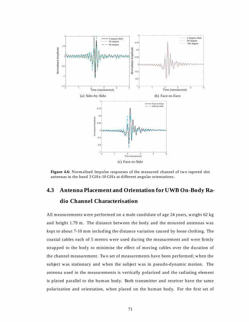
0 1 2 3 4 5-1.5
-1
-0.5
0
0.5
1
Time (nanosecond)
No
rma
lise
dA
mp
litu
de
0 degree (Ref)
45 degree
90 degree
(a) Side-by-Side
0 1 2 3 4 5
Time (nanosecond)
0 degree (Ref)
90 degree
180 degree
-1
-0.6
-0.3
0
0.25
0.5
0.75
1
No
rmalis
ed
Am
plit
ud
e
(b) Face-to-Face
0 1 2 3 4 5-1
-0.6
-0.3
0
0.25
0.5
0.75
1
Time (nanosecond)
Norm
alis
ed
Am
plit
ude
Face-to-Face
Side-by-Side
(c) Face-to-Side
Figure 4.6: Normalised Impulse responses of the measured channel of two tapered slotantennas in the band 3 GHz-10 GHz at different angular orientations.
4.3 Antenna Placement and Orientation for UWB On-Body Ra-
dio Channel Characterisation
All measurements were performed on a male candidate of age 24 years, weight 62 kg
and height 1.79 m. The distance between the body and the mounted antennas was
kept to about 7-10 mm including the distance variation caused by loose clothing. The
coaxial cables each of 5 meters were used during the measurement and were firmly
strapped to the body to minimise the effect of moving cables over the duration of
the channel measurement. Two set of measurements have been performed; when the
subject was stationary and when the subject was in pseudo-dynamic motion. The
antenna used in the measurements is vertically polarized and the radiating element
is placed parallel to the human body. Both transmitter and receiver have the same
polarization and orientation, when placed on the human body. For the first set of
71
on-body measurements (when the subject was stationary), the transmitting antenna
(Tx) was placed at the waist (belt) position on the left side of the body, about 200 mm
away from the body centre line and the receiving antennas (Rx) were placed at 109
different locations as shown in Figure 4.7. For the second set of measurements, the
effect of pseudo-dynamic body movements on the UWB on-body radio channels was
considered. Two measurement scenarios for Tx were considered for pseudo-dynamic
on-body radio channel characterisation:
• When Tx was static with respect to Rx (Tx on waist).
• When Tx was moving in pseudo-dynamic manner with respect to Rx (Tx on
wrist).
The receiving antenna was placed at five different positions: on the right chest; right
wrist; right ankle; on the centre of the back; and on the right side of the head, thus
forming five on-body channels as shown in Fig. 4.8 (named belt-chest, belt-back, belt-
head, belt-wrist and belt-ankle, respectively). The belt-chest channel represents the
line-of-sight scenario. The belt-back channel is a good representation of the NLOS
scenario. Both of these channels (i.e., belt-chest and belt-back) are static channels in
which the distance between the transmitting and receiving antennas is almost con-
stant. To mimic a dynamic channel, in which the path length varies randomly with
movement of the body, the belt-wrist channel was selected. Most often, there are scen-
arios where there is partial LOS or a transition of LOS and NLOS. The belt-head and
belt-ankle channels are good examples of this.
An Agilent two-port vector network analyzer (Hewlett Packard 8720ES-VNA) was
used for UWB on/off-body radio propagation channel measurements. The two an-
tennas (Tx and Rx) were connected to the VNA by a pair of low loss coaxial cables.
For all UWB on/off-body radio propagation channel measurements, a two-port vec-
tor network analyzer (VNA) was used to measure the transmission response (S21). A
Labview programme written by the author is used to control the VNA remotely. The
data measured by the VNA was stored in a computer hard disk by the software in
the form of a text file containing the magnitude (in dB) and the phase (in degrees) of
the transmission response (S21). During the measurements, the VNA was always cal-
ibrated to exclude the losses that incurred in the cables and thus the measured data
72
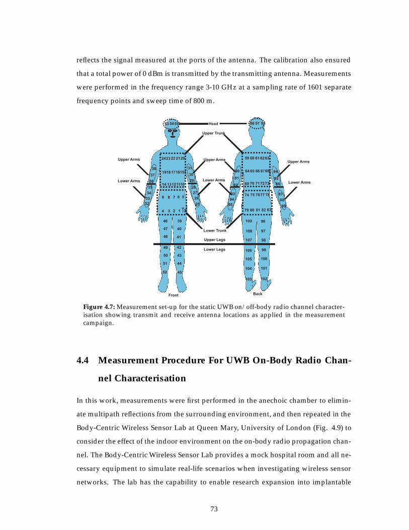
reflects the signal measured at the ports of the antenna. The calibration also ensured
that a total power of 0 dBm is transmitted by the transmitting antenna. Measurements
were performed in the frequency range 3-10 GHz at a sampling rate of 1601 separate
frequency points and sweep time of 800 m.
Tx1234
5
10
20
15
6
11
16
21
789
121314
171819
222324
25
26
27
28
29
30
31
32
33
34
35
36
37
38
39
40
41
42
43
44
45
46
47
48
49
50
51
52
5453 55 56 57 58
59 60 61 6263
64 65 66 6768
69 70 717273
74 75 7677 78
79 80 81 82 8389
88
87
86
85
84
95
94
93
92
91
90
96
97
98
99
100
101
102
109
108
107
106
105
104
103
Front Back
Upper Trunk
Lower Arms
Upper Legs
Lower Legs
Upper Arms
Head
Lower Trunk
Upper ArmsUpper Arms
Lower Arms Lower Arms
Figure 4.7: Measurement set-up for the static UWB on/off-body radio channel character-isation showing transmit and receive antenna locations as applied in the measurementcampaign.
4.4 Measurement Procedure For UWB On-Body Radio Chan-
nel Characterisation
In this work, measurements were first performed in the anechoic chamber to elimin-
ate multipath reflections from the surrounding environment, and then repeated in the
Body-Centric Wireless Sensor Lab at Queen Mary, University of London (Fig. 4.9) to
consider the effect of the indoor environment on the on-body radio propagation chan-
nel. The Body-Centric Wireless Sensor Lab provides a mock hospital room and all ne-
cessary equipment to simulate real-life scenarios when investigating wireless sensor
networks. The lab has the capability to enable research expansion into implantable
73
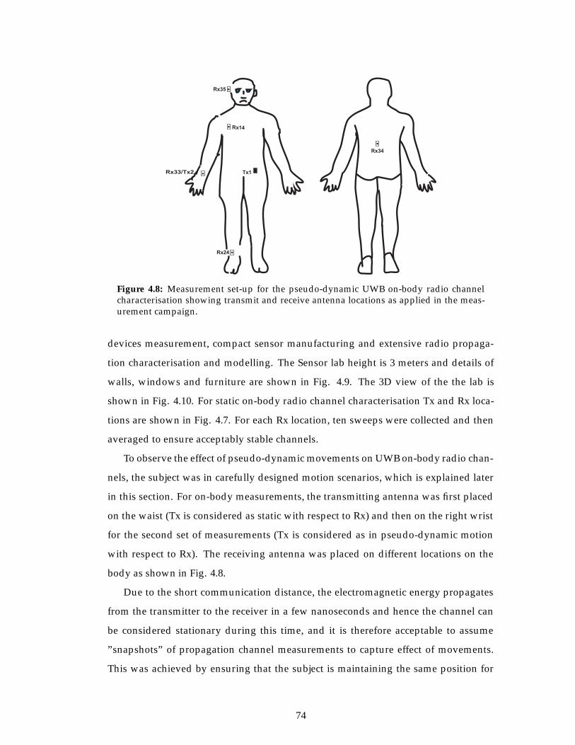
Tx1Rx33/Tx2
Rx14
Rx35
Rx24
Rx34
Figure 4.8: Measurement set-up for the pseudo-dynamic UWB on-body radio channelcharacterisation showing transmit and receive antenna locations as applied in the meas-urement campaign.
devices measurement, compact sensor manufacturing and extensive radio propaga-
tion characterisation and modelling. The Sensor lab height is 3 meters and details of
walls, windows and furniture are shown in Fig. 4.9. The 3D view of the the lab is
shown in Fig. 4.10. For static on-body radio channel characterisation Tx and Rx loca-
tions are shown in Fig. 4.7. For each Rx location, ten sweeps were collected and then
averaged to ensure acceptably stable channels.
To observe the effect of pseudo-dynamic movements on UWB on-body radio chan-
nels, the subject was in carefully designed motion scenarios, which is explained later
in this section. For on-body measurements, the transmitting antenna was first placed
on the waist (Tx is considered as static with respect to Rx) and then on the right wrist
for the second set of measurements (Tx is considered as in pseudo-dynamic motion
with respect to Rx). The receiving antenna was placed on different locations on the
body as shown in Fig. 4.8.
Due to the short communication distance, the electromagnetic energy propagates
from the transmitter to the receiver in a few nanoseconds and hence the channel can
be considered stationary during this time, and it is therefore acceptable to assume
”snapshots” of propagation channel measurements to capture effect of movements.
This was achieved by ensuring that the subject is maintaining the same position for
74
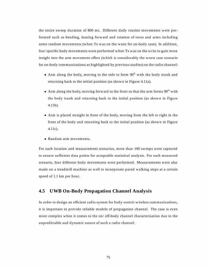
the entire sweep duration of 800 ms. Different daily routine movements were per-
formed such as bending, leaning forward and rotation of torso and arms including
some random movements (when Tx was on the waist for on-body case). In addition,
four specific body movements were performed when Tx was on the wrist to gain more
insight into the arm movement effect (which is considerably the worst case scenario
for on-body communications as highlighted by previous studies) on the radio channel:
• Arm along the body, moving to the side to form 900 with the body trunk and
returning back to the initial position (as shown in Figure 4.11a).
• Arm along the body, moving forward to the front so that the arm forms 900 with
the body trunk and returning back to the initial position (as shown in Figure
4.11b).
• Arm is placed straight in front of the body, moving from the left to right in the
front of the body and returning back to the initial position (as shown in Figure
4.11c).
• Random arm movements.
For each location and measurement scenarios, more than 100 sweeps were captured
to ensure sufficient data points for acceptable statistical analysis. For each measured
scenario, four different body movements were performed. Measurements were also
made on a treadmill machine as well to incorporate paced walking steps at a certain
speed of 1.1 km per hour.
4.5 UWB On-Body Propagation Channel Analysis
In order to design an efficient radio system for body-centric wireless communications,
it is important to provide reliable models of propagation channel. The case is even
more complex when it comes to the on/off-body channel characterisation due to the
unpredictable and dynamic nature of such a radio channel.
75
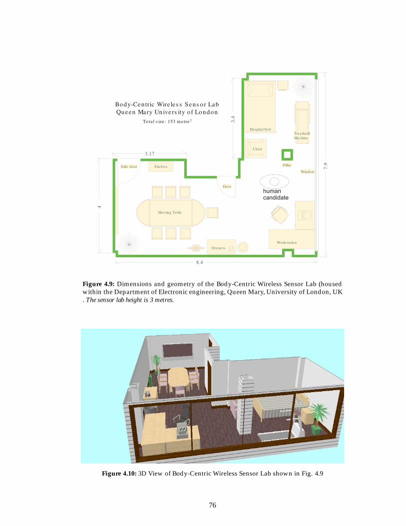
Figure 4.9: Dimensions and geometry of the Body-Centric Wireless Sensor Lab (housedwithin the Department of Electronic engineering, Queen Mary, University of London, UK. The sensor lab height is 3 metres.
Figure 4.10: 3D View of Body-Centric Wireless Sensor Lab shown in Fig. 4.9
76
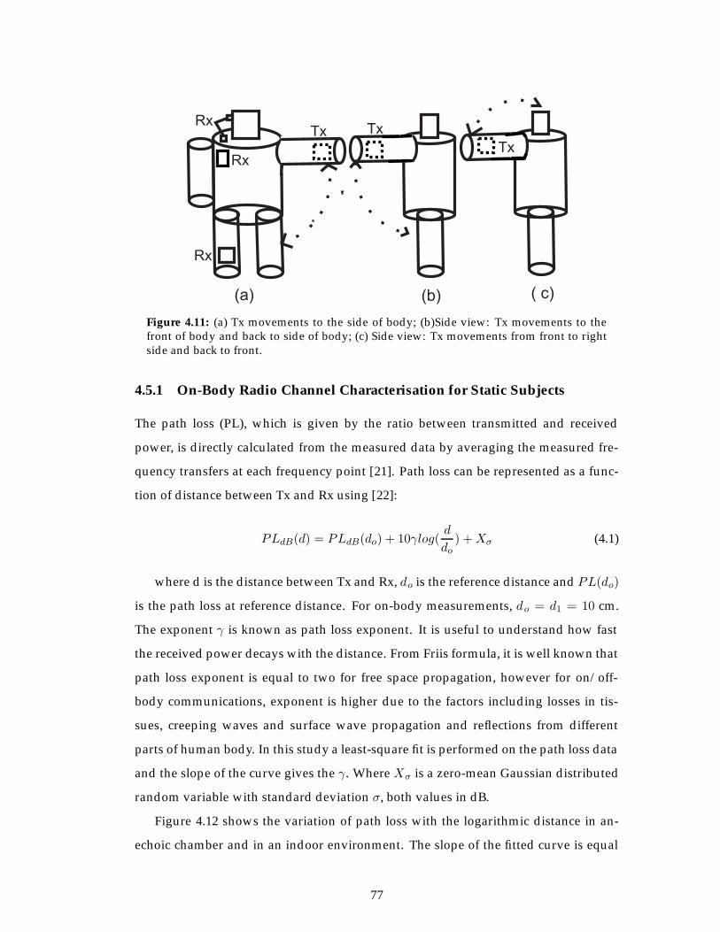
Figure 4.11: (a) Tx movements to the side of body; (b)Side view: Tx movements to thefront of body and back to side of body; (c) Side view: Tx movements from front to rightside and back to front.
4.5.1 On-Body Radio Channel Characterisation for Static Subjects
The path loss (PL), which is given by the ratio between transmitted and received
power, is directly calculated from the measured data by averaging the measured fre-
quency transfers at each frequency point [21]. Path loss can be represented as a func-
tion of distance between Tx and Rx using [22]:
PLdB(d) = PLdB(do) + 10γlog(d
do) +Xσ (4.1)
where d is the distance between Tx and Rx, do is the reference distance and PL(do)
is the path loss at reference distance. For on-body measurements, do = d1 = 10 cm.
The exponent γ is known as path loss exponent. It is useful to understand how fast
the received power decays with the distance. From Friis formula, it is well known that
path loss exponent is equal to two for free space propagation, however for on/off-
body communications, exponent is higher due to the factors including losses in tis-
sues, creeping waves and surface wave propagation and reflections from different
parts of human body. In this study a least-square fit is performed on the path loss data
and the slope of the curve gives the γ. Where Xσ is a zero-mean Gaussian distributed
random variable with standard deviation σ, both values in dB.
Figure 4.12 shows the variation of path loss with the logarithmic distance in an-
echoic chamber and in an indoor environment. The slope of the fitted curve is equal
77

0 2 4 6 8 10 1235
40
45
50
55
60
65
70
75
80
10 log(d/d0)
Pa
th L
oss (
dB
)
γ =2.48
ChamberLeast Square FitIndoor
Least Square Fit
γ =2.96
Figure 4.12: On-Body path loss model for the measurements in anechoic chamber and inan indoor environment for static subject.
On-BodyLOS NLOS
Body Parts γ Mean PL (dB) γ Mean PL (dB)Trunk 3.39 59.41 2.64 62.56Arms 4.31 59.10 3.34 67.98Legs 1.16 59.76 2.35 69.78Head 1.17 70.92 2.57 69.83
All Parts 2.8 60.05 1.34 66.04LOS+NLOS γ=2.48 and Mean PL=63.02 dB
Table 4.1: On-Body path loss exponent (calculated in similar manner using empiricalmodel as shown in Fig. 4.12) and mean path loss for different sectors of body.
78
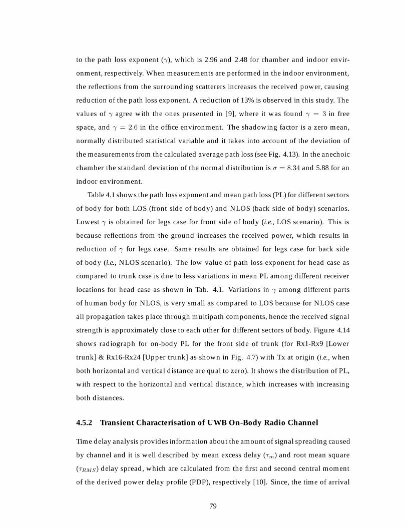
to the path loss exponent (γ), which is 2.96 and 2.48 for chamber and indoor envir-
onment, respectively. When measurements are performed in the indoor environment,
the reflections from the surrounding scatterers increases the received power, causing
reduction of the path loss exponent. A reduction of 13% is observed in this study. The
values of γ agree with the ones presented in [9], where it was found γ = 3 in free
space, and γ = 2.6 in the office environment. The shadowing factor is a zero mean,
normally distributed statistical variable and it takes into account of the deviation of
the measurements from the calculated average path loss (see Fig. 4.13). In the anechoic
chamber the standard deviation of the normal distribution is σ = 8.34 and 5.88 for an
indoor environment.
Table 4.1 shows the path loss exponent and mean path loss (PL) for different sectors
of body for both LOS (front side of body) and NLOS (back side of body) scenarios.
Lowest γ is obtained for legs case for front side of body (i.e., LOS scenario). This is
because reflections from the ground increases the received power, which results in
reduction of γ for legs case. Same results are obtained for legs case for back side
of body (i.e., NLOS scenario). The low value of path loss exponent for head case as
compared to trunk case is due to less variations in mean PL among different receiver
locations for head case as shown in Tab. 4.1. Variations in γ among different parts
of human body for NLOS, is very small as compared to LOS because for NLOS case
all propagation takes place through multipath components, hence the received signal
strength is approximately close to each other for different sectors of body. Figure 4.14
shows radiograph for on-body PL for the front side of trunk (for Rx1-Rx9 [Lower
trunk] & Rx16-Rx24 [Upper trunk] as shown in Fig. 4.7) with Tx at origin (i.e., when
both horizontal and vertical distance are qual to zero). It shows the distribution of PL,
with respect to the horizontal and vertical distance, which increases with increasing
both distances.
4.5.2 Transient Characterisation of UWB On-Body Radio Channel
Time delay analysis provides information about the amount of signal spreading caused
by channel and it is well described by mean excess delay (τm) and root mean square
(τRMS ) delay spread, which are calculated from the first and second central moment
of the derived power delay profile (PDP), respectively [10]. Since, the time of arrival
79
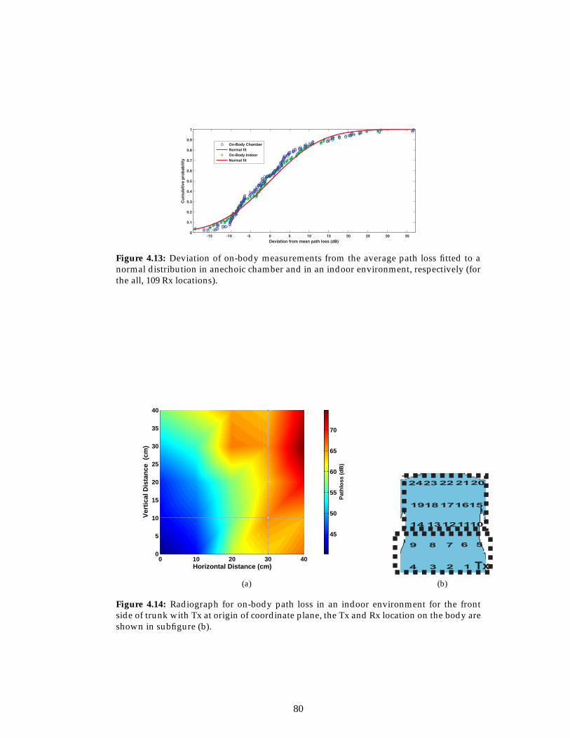
Figure 4.13: Deviation of on-body measurements from the average path loss fitted to anormal distribution in anechoic chamber and in an indoor environment, respectively (forthe all, 109 Rx locations).
0 10 20 30 400
5
10
15
20
25
30
35
40
Horizontal Distance (cm)
Ver
tica
l Dis
tan
ce (
cm)
Pat
hlo
ss (
dB
)
45
50
55
60
65
70
(a) (b)
Figure 4.14: Radiograph for on-body path loss in an indoor environment for the frontside of trunk with Tx at origin of coordinate plane, the Tx and Rx location on the body areshown in subfigure (b).
80
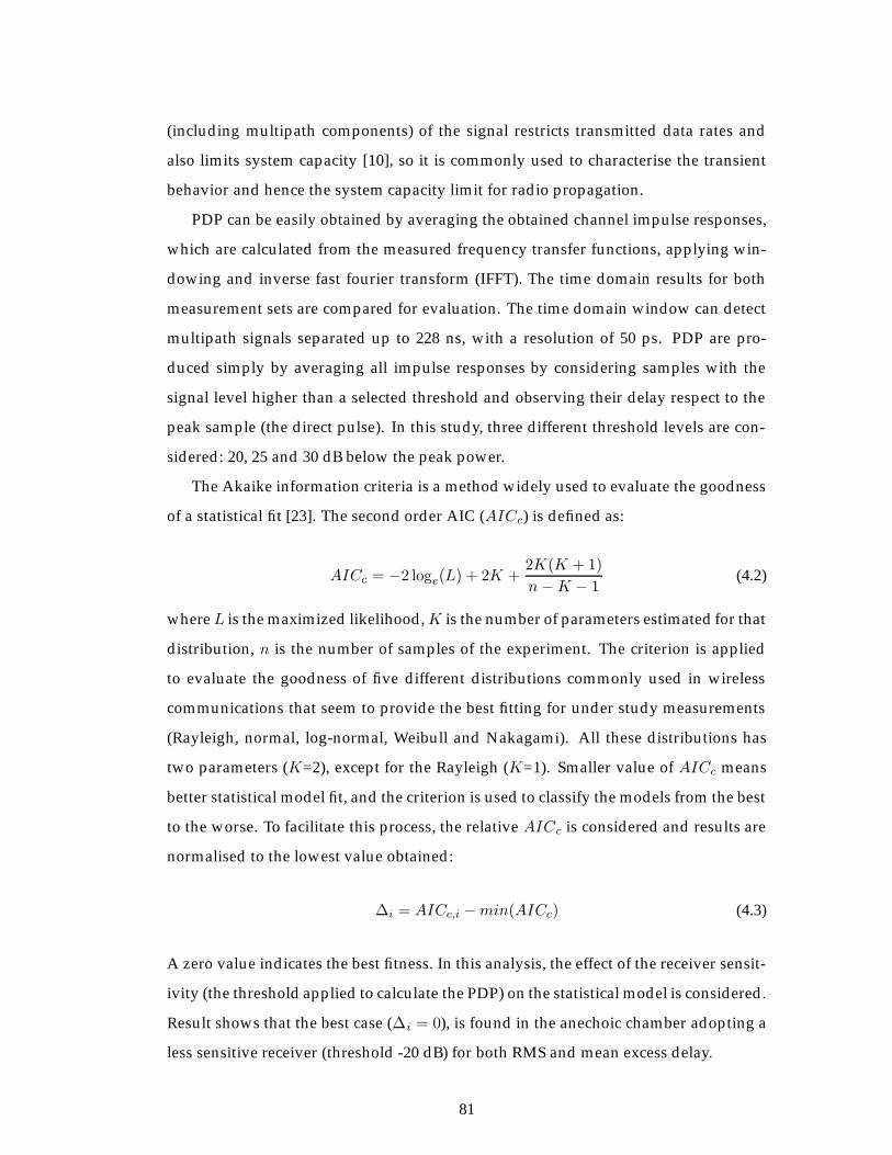
(including multipath components) of the signal restricts transmitted data rates and
also limits system capacity [10], so it is commonly used to characterise the transient
behavior and hence the system capacity limit for radio propagation.
PDP can be easily obtained by averaging the obtained channel impulse responses,
which are calculated from the measured frequency transfer functions, applying win-
dowing and inverse fast fourier transform (IFFT). The time domain results for both
measurement sets are compared for evaluation. The time domain window can detect
multipath signals separated up to 228 ns, with a resolution of 50 ps. PDP are pro-
duced simply by averaging all impulse responses by considering samples with the
signal level higher than a selected threshold and observing their delay respect to the
peak sample (the direct pulse). In this study, three different threshold levels are con-
sidered: 20, 25 and 30 dB below the peak power.
The Akaike information criteria is a method widely used to evaluate the goodness
of a statistical fit [23]. The second order AIC (AICc) is defined as:
AICc = −2 loge(L) + 2K +2K(K + 1)
n−K − 1(4.2)
whereL is the maximized likelihood, K is the number of parameters estimated for that
distribution, n is the number of samples of the experiment. The criterion is applied
to evaluate the goodness of five different distributions commonly used in wireless
communications that seem to provide the best fitting for under study measurements
(Rayleigh, normal, log-normal, Weibull and Nakagami). All these distributions has
two parameters (K=2), except for the Rayleigh (K=1). Smaller value of AICc means
better statistical model fit, and the criterion is used to classify the models from the best
to the worse. To facilitate this process, the relative AICc is considered and results are
normalised to the lowest value obtained:
Δi = AICc,i −min(AICc) (4.3)
A zero value indicates the best fitness. In this analysis, the effect of the receiver sensit-
ivity (the threshold applied to calculate the PDP) on the statistical model is considered.
Result shows that the best case (Δi = 0), is found in the anechoic chamber adopting a
less sensitive receiver (threshold -20 dB) for both RMS and mean excess delay.
81
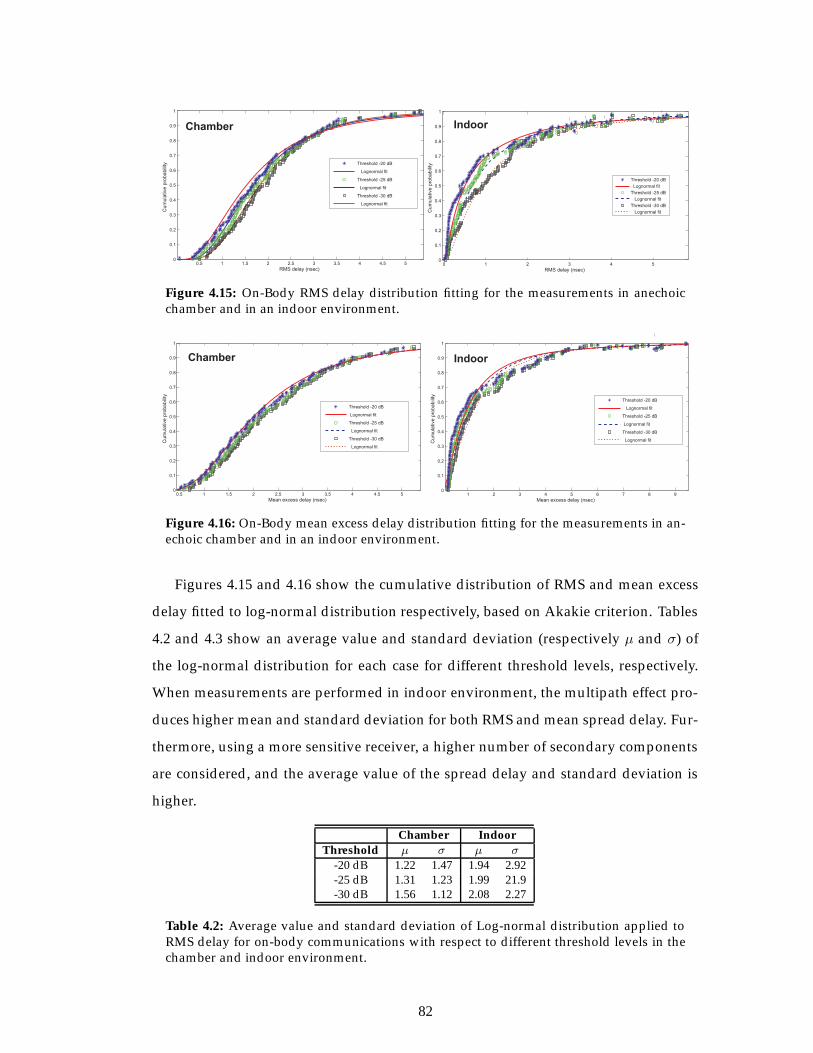
0 1 2 3 4 50
0.1
0.2
0.3
0.4
0.5
0.6
0.7
0.8
0.9
1
RMS delay (nsec)
Cu
mu
lative
pro
ba
bili
ty
Threshold -20 dB
Lognormal fit
Threshold -25 dB
Lognormal fit
Threshold -30 dB
Lognormal fit
0.5 1 1.5 2 2.5 3 3.5 4 4.5 50
0.1
0.2
0.3
0.4
0.5
0.6
0.7
0.8
0.9
1
RMS delay (nsec)
Cu
mu
lative
pro
ba
bili
ty Threshold -20 dB
Lognormal fit
Threshold -25 dB
Lognormal fit
Threshold -30 dB
Lognormal fit
Chamber Indoor
Figure 4.15: On-Body RMS delay distribution fitting for the measurements in anechoicchamber and in an indoor environment.
1 2 3 4 5 6 7 8 90
0.1
0.2
0.3
0.4
0.5
0.6
0.7
0.8
0.9
1
Mean excess delay (nsec)
Cu
mu
lative
pro
ba
bili
ty
Threshold -20 dB
Lognormal fit
Threshold -25 dB
Lognormal fit
Threshold -30 dB
Lognormal fit
0.5 1 1.5 2 2.5 3 3.5 4 4.5 50
0.1
0.2
0.3
0.4
0.5
0.6
0.7
0.8
0.9
1
Mean excess delay (nsec)
Cu
mu
lative
pro
ba
bili
ty
Threshold -20 dB
Lognormal fit
Threshold -25 dB
Lognormal fit
Threshold -30 dB
Lognormal fit
Chamber Indoor
Figure 4.16: On-Body mean excess delay distribution fitting for the measurements in an-echoic chamber and in an indoor environment.
Figures 4.15 and 4.16 show the cumulative distribution of RMS and mean excess
delay fitted to log-normal distribution respectively, based on Akakie criterion. Tables
4.2 and 4.3 show an average value and standard deviation (respectively μ and σ) of
the log-normal distribution for each case for different threshold levels, respectively.
When measurements are performed in indoor environment, the multipath effect pro-
duces higher mean and standard deviation for both RMS and mean spread delay. Fur-
thermore, using a more sensitive receiver, a higher number of secondary components
are considered, and the average value of the spread delay and standard deviation is
higher.
Chamber IndoorThreshold μ σ μ σ
-20 dB 1.22 1.47 1.94 2.92-25 dB 1.31 1.23 1.99 21.9-30 dB 1.56 1.12 2.08 2.27
Table 4.2: Average value and standard deviation of Log-normal distribution applied toRMS delay for on-body communications with respect to different threshold levels in thechamber and indoor environment.
82
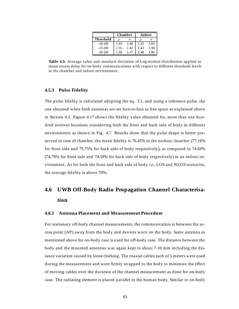
Chamber IndoorThreshold μ σ μ σ
-20 dB 1.43 1.46 2.35 2.03-25 dB 1.55 1.42 2.43 1.98-30 dB 1.69 1.37 2.48 1.96
Table 4.3: Average value and standard deviation of Log-normal distribution applied tomean excess delay for on-body communications with respect to different threshold levelsin the chamber and indoor environment.
4.5.3 Pulse Fidelity
The pulse fidelity is calculated adopting the eq. 3.1, and using a reference pulse, the
one obtained when both antennas are set face-to-face in free space as explained above
in Section 4.2. Figure 4.17 shows the fidelity value obtained for, more than one hun-
dred receiver locations considering both the front and back side of body in different
environments as shown in Fig. 4.7. Results show that the pulse shape is better pre-
served in case of chamber, the mean fidelity is 76.45% in the nechoic chamber (77.16%
for front side and 75.75% for back side of body respectively), as compared to 74.69%
(74.79% for front side and 74.59% for back side of body respectively) in an indoor en-
vironment. As for both the front and back side of body i.e., LOS and NLOS scenarios,
the average fidelity is above 70%.
4.6 UWB Off-Body Radio Propagation Channel Characterisa-
tion
4.6.1 Antenna Placement and Measurement Procedure
For stationary off-body channel measurements, the communication is between the ac-
cess point (AP) away from the body and devices worn on the body. Same antenna as
mentioned above for on-body case is used for off-body case. The distance between the
body and the mounted antennas was again kept to about 7-10 mm including the dis-
tance variation caused by loose clothing. The coaxial cables each of 5 meters were used
during the measurement and were firmly strapped to the body to minimize the effect
of moving cables over the duration of the channel measurement as done for on-body
case. The radiating element is placed parallel to the human body. Similar to on-body
83
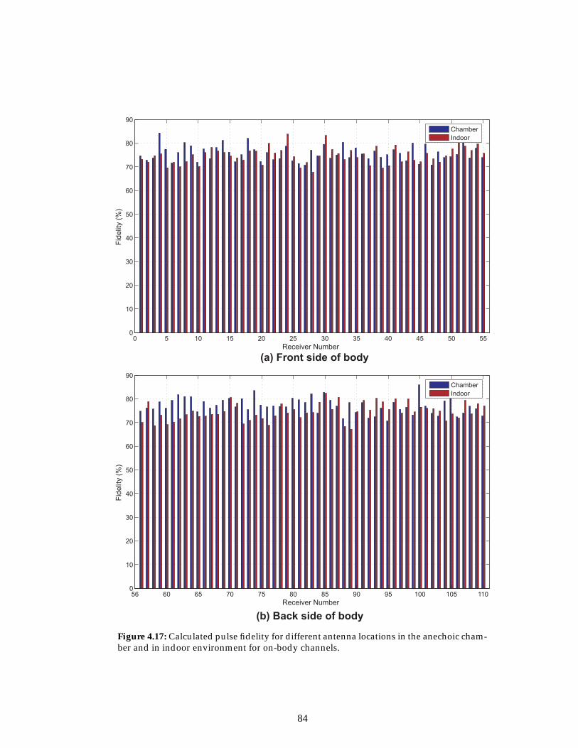
0 5 10 15 20 25 30 35 40 45 50 550
10
20
30
40
50
60
70
80
90
Receiver Number
Fid
elit
y (
%)
Chamber
Indoor
56 60 65 70 75 80 85 90 95 100 105 1100
10
20
30
40
50
60
70
80
90
Receiver Number
Fid
elit
y (
%)
Chamber
Indoor
(a) Front side of body
(b) Back side of body
Figure 4.17: Calculated pulse fidelity for different antenna locations in the anechoic cham-ber and in indoor environment for on-body channels.
84
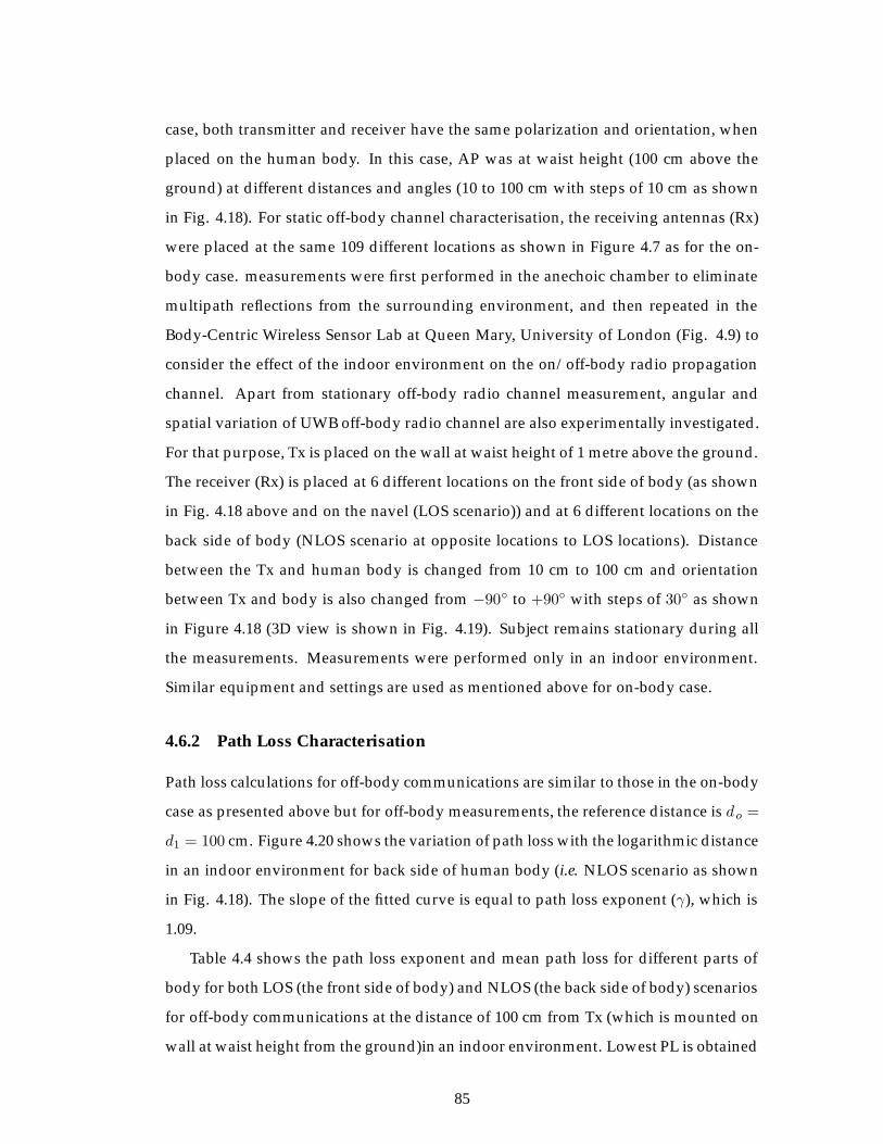
case, both transmitter and receiver have the same polarization and orientation, when
placed on the human body. In this case, AP was at waist height (100 cm above the
ground) at different distances and angles (10 to 100 cm with steps of 10 cm as shown
in Fig. 4.18). For static off-body channel characterisation, the receiving antennas (Rx)
were placed at the same 109 different locations as shown in Figure 4.7 as for the on-
body case. measurements were first performed in the anechoic chamber to eliminate
multipath reflections from the surrounding environment, and then repeated in the
Body-Centric Wireless Sensor Lab at Queen Mary, University of London (Fig. 4.9) to
consider the effect of the indoor environment on the on/off-body radio propagation
channel. Apart from stationary off-body radio channel measurement, angular and
spatial variation of UWB off-body radio channel are also experimentally investigated.
For that purpose, Tx is placed on the wall at waist height of 1 metre above the ground.
The receiver (Rx) is placed at 6 different locations on the front side of body (as shown
in Fig. 4.18 above and on the navel (LOS scenario)) and at 6 different locations on the
back side of body (NLOS scenario at opposite locations to LOS locations). Distance
between the Tx and human body is changed from 10 cm to 100 cm and orientation
between Tx and body is also changed from −90◦ to +90◦ with steps of 30◦ as shown
in Figure 4.18 (3D view is shown in Fig. 4.19). Subject remains stationary during all
the measurements. Measurements were performed only in an indoor environment.
Similar equipment and settings are used as mentioned above for on-body case.
4.6.2 Path Loss Characterisation
Path loss calculations for off-body communications are similar to those in the on-body
case as presented above but for off-body measurements, the reference distance is do =
d1 = 100 cm. Figure 4.20 shows the variation of path loss with the logarithmic distance
in an indoor environment for back side of human body (i.e. NLOS scenario as shown
in Fig. 4.18). The slope of the fitted curve is equal to path loss exponent (γ), which is
1.09.
Table 4.4 shows the path loss exponent and mean path loss for different parts of
body for both LOS (the front side of body) and NLOS (the back side of body) scenarios
for off-body communications at the distance of 100 cm from Tx (which is mounted on
wall at waist height from the ground)in an indoor environment. Lowest PL is obtained
85
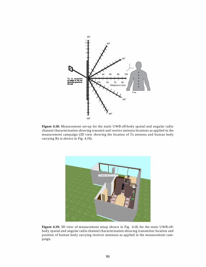
Tx
Tx
Z
Y
X
60º
90º
30º
-30
-60
-90º
30 50 70
100
Distance in (cm)
º
º
40 60 80
90
T x i s m o u n t e dat height of 100 cmabove the ground onthe wall
T x i s m o u n t e dat height of 100 cmabove the ground onthe wall.
Rx
Figure 4.18: Measurement set-up for the static UWB off-body spatial and angular radiochannel characterisation showing transmit and receive antenna locations as applied in themeasurement campaign (3D view showing the location of Tx antenna and human bodycarrying Rx is shown in Fig. 4.19).
Sensor Lab
Tx
Figure 4.19: 3D view of measurement setup shown in Fig. 4.18, for the static UWB off-body spatial and angular radio channel characterisation showing transmitter location andposition of human body carrying receiver antennas as applied in the measurement cam-paign.
86
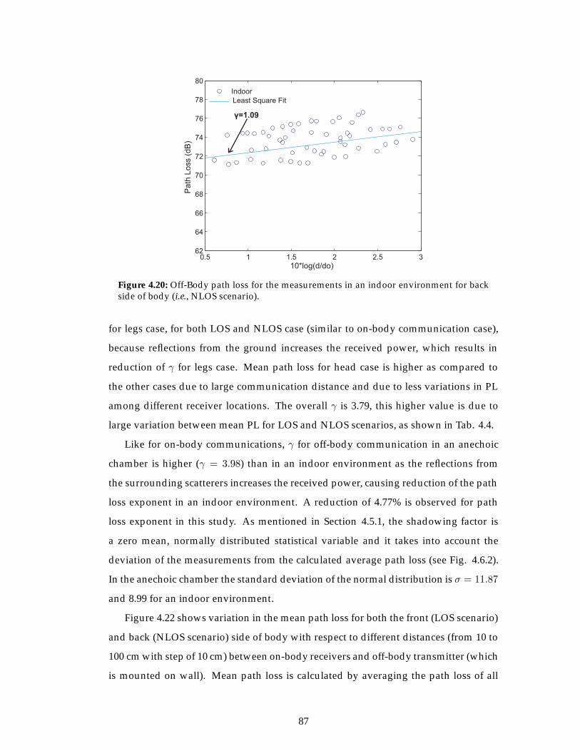
0.5 1 1.5 2 2.5 362
64
66
68
70
72
74
76
78
80
10*log(d/do)
Pa
th L
oss (
dB
)
Indoor
Least Square Fit
γ=1.09
Figure 4.20: Off-Body path loss for the measurements in an indoor environment for backside of body (i.e., NLOS scenario).
for legs case, for both LOS and NLOS case (similar to on-body communication case),
because reflections from the ground increases the received power, which results in
reduction of γ for legs case. Mean path loss for head case is higher as compared to
the other cases due to large communication distance and due to less variations in PL
among different receiver locations. The overall γ is 3.79, this higher value is due to
large variation between mean PL for LOS and NLOS scenarios, as shown in Tab. 4.4.
Like for on-body communications, γ for off-body communication in an anechoic
chamber is higher (γ = 3.98) than in an indoor environment as the reflections from
the surrounding scatterers increases the received power, causing reduction of the path
loss exponent in an indoor environment. A reduction of 4.77% is observed for path
loss exponent in this study. As mentioned in Section 4.5.1, the shadowing factor is
a zero mean, normally distributed statistical variable and it takes into account the
deviation of the measurements from the calculated average path loss (see Fig. 4.6.2).
In the anechoic chamber the standard deviation of the normal distribution is σ = 11.87
and 8.99 for an indoor environment.
Figure 4.22 shows variation in the mean path loss for both the front (LOS scenario)
and back (NLOS scenario) side of body with respect to different distances (from 10 to
100 cm with step of 10 cm) between on-body receivers and off-body transmitter (which
is mounted on wall). Mean path loss is calculated by averaging the path loss of all
87
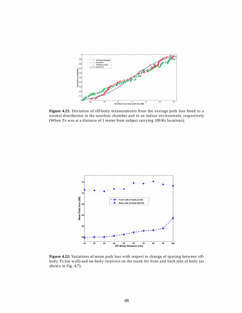
Figure 4.21: Deviation of off-body measurements from the average path loss fitted to anormal distribution in the anechoic chamber and in an indoor environment, respectively(When Tx was at a distance of 1 meter from subject carrying 109 Rx locations).
10 20 30 40 50 60 70 80 90 100
50
55
60
65
70
75
Off−Body Distance (cm)
Mea
n P
ath
loss
(d
B)
Front side of body (LOS)
Back side of body (NLOS)
Figure 4.22: Variations of mean path loss with respect to change of spacing between off-body Tx (on wall) and on-body receivers on the trunk for front and back side of body (asshown in Fig. 4.7).
88
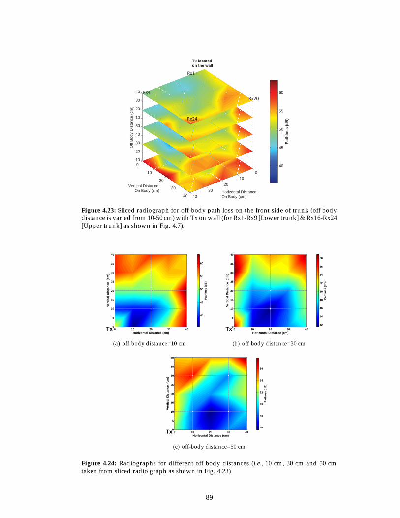
4030
2010
0
40
30
20
10
010
20
30
40
50
10
20
30
40
Off
Bod
y D
ista
nce
(cm
)
Horizontal Distance On Body (cm)
Vertical Distance On Body (cm)
Path
loss
(dB
)
40
45
50
55
60
Tx locatedon the wall
Rx1
Rx4Rx20
Rx24
Figure 4.23: Sliced radiograph for off-body path loss on the front side of trunk (off bodydistance is varied from 10-50 cm) with Tx on wall (for Rx1-Rx9 [Lower trunk] & Rx16-Rx24[Upper trunk] as shown in Fig. 4.7).
0 10 20 30 400
5
10
15
20
25
30
35
40
Horizontal Distance (cm)
Ver
tica
l Dis
tan
ce (
cm)
Pat
hlo
ss (
dB
)
40
45
50
55
60
Tx
(a) off-body distance=10 cm
0 10 20 30 400
5
10
15
20
25
30
35
40
Horizontal Distance (cm)
Ver
tica
l Dis
tan
ce (
cm)
Pat
hlo
ss (
dB
)42
44
46
48
50
52
54
56
58
Tx
(b) off-body distance=30 cm
0 10 20 30 400
5
10
15
20
25
30
35
40
Horizontal Distance (cm)
Ver
tica
l Dis
tan
ce (
cm)
Pat
hlo
ss (
dB
)
46
48
50
52
54
56
Tx
(c) off-body distance=50 cm
Figure 4.24: Radiographs for different off body distances (i.e., 10 cm, 30 cm and 50 cmtaken from sliced radio graph as shown in Fig. 4.23)
89
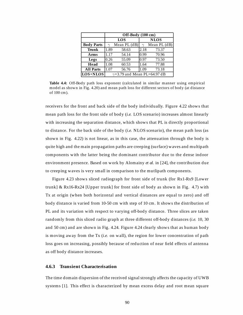
Off-Body (100 cm)LOS NLOS
Body Parts γ Mean PL (dB) γ Mean PL (dB)Trunk 1.89 58.63 2.18 73.37Arms 1.17 54.14 0.99 70.96Legs 0.26 55.09 0.97 73.50Head 1.08 60.53 1.64 77.88
All Parts 1.07 56.76 1.09 73.18LOS+NLOS γ=3.79 and Mean PL=64.97 dB
Table 4.4: Off-Body path loss exponent (calculated in similar manner using empiricalmodel as shown in Fig. 4.20) and mean path loss for different sectors of body (at distanceof 100 cm).
receivers for the front and back side of the body individually. Figure 4.22 shows that
mean path loss for the front side of body (i.e. LOS scenario) increases almost linearly
with increasing the separation distance, which shows that PL is directly proportional
to distance. For the back side of the body (i.e. NLOS scenario), the mean path loss (as
shown in Fig. 4.22) is not linear, as in this case, the attenuation through the body is
quite high and the main propagation paths are creeping (surface) waves and multipath
components with the latter being the dominant contributor due to the dense indoor
environment presence. Based on work by Alomainy et al. in [24], the contribution due
to creeping waves is very small in comparison to the mutlipath components.
Figure 4.23 shows sliced radiograph for front side of trunk (for Rx1-Rx9 [Lower
trunk] & Rx16-Rx24 [Upper trunk] for front side of body as shown in Fig. 4.7) with
Tx at origin (when both horizontal and vertical distances are equal to zero) and off
body distance is varied from 10-50 cm with step of 10 cm. It shows the distribution of
PL and its variation with respect to varying off-body distance. Three slices are taken
randomly from this sliced radio graph at three different off-body distances (i.e. 10, 30
and 50 cm) and are shown in Fig. 4.24. Figure 4.24 clearly shows that as human body
is moving away from the Tx (i.e. on wall), the region for lower concentration of path
loss goes on increasing, possibly because of reduction of near field effects of antenna
as off body distance increases.
4.6.3 Transient Characterisation
The time domain dispersion of the received signal strongly affects the capacity of UWB
systems [1]. This effect is characterized by mean excess delay and root mean square
90
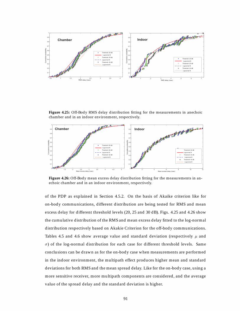
RMS delay (nsec)0.5 1 1.5 2 2.5 3 3.5 4
0
0.1
0.2
0.3
0.4
0.5
0.6
0.7
0.8
0.9
1
Cum
ula
tive p
robabili
ty
Threshold -20 dB
Lognormal fit
Threshold -25 dB
Lognormal fit
Threshold -30 dB
Lognormal fit
1 2 3 4 5 6 70
0.1
0.2
0.3
0.4
0.5
0.6
0.7
0.8
0.9
1
RMS delay (nsec)
Cum
ula
tive p
robabili
ty
Threshold -20 dB
Lognormal fit
Threshold -25 dB
Lognormal fit
Threshold -30 dB
Lognormal fit
Chamber Indoor
Figure 4.25: Off-Body RMS delay distribution fitting for the measurements in anechoicchamber and in an indoor environment, respectively.
Mean excess delay (nsec)1 1.5 2 2.5 3 3.5 4 4.5 5
0
0.1
0.2
0.3
0.4
0.5
0.6
0.7
0.8
0.9
1
Cu
mu
lative
pro
ba
bili
ty
Threshold -20 dB
Lognormal fit
Threshold -25 dB
Lognormal fit
Threshold -30 dB
Lognormal fit
2 4 6 8 10 120
0.1
0.2
0.3
0.4
0.5
0.6
0.7
0.8
0.9
1
Mean excess delay (nsec)
Cu
mu
lative
pro
ba
bili
ty
Threshold -20 dB
Lognormal fit
Threshold -25 dB
Lognormal fit
Threshold -30 dB
Lognormal fit
Chamber Indoor
Figure 4.26: Off-Body mean excess delay distribution fitting for the measurements in an-echoic chamber and in an indoor environment, respectively.
of the PDP as explained in Section 4.5.2. On the basis of Akaike criterion like for
on-body communications, different distribution are being tested for RMS and mean
excess delay for different threshold levels (20, 25 and 30 dB). Figs. 4.25 and 4.26 show
the cumulative distribution of the RMS and mean excess delay fitted to the log-normal
distribution respectively based on Akakie Criterion for the off-body communications.
Tables 4.5 and 4.6 show average value and standard deviation (respectively μ and
σ) of the log-normal distribution for each case for different threshold levels. Same
conclusions can be drawn as for the on-body case when measurements are performed
in the indoor environment, the multipath effect produces higher mean and standard
deviations for both RMS and the mean spread delay. Like for the on-body case, using a
more sensitive receiver, more multipath components are considered, and the average
value of the spread delay and the standard deviation is higher.
91
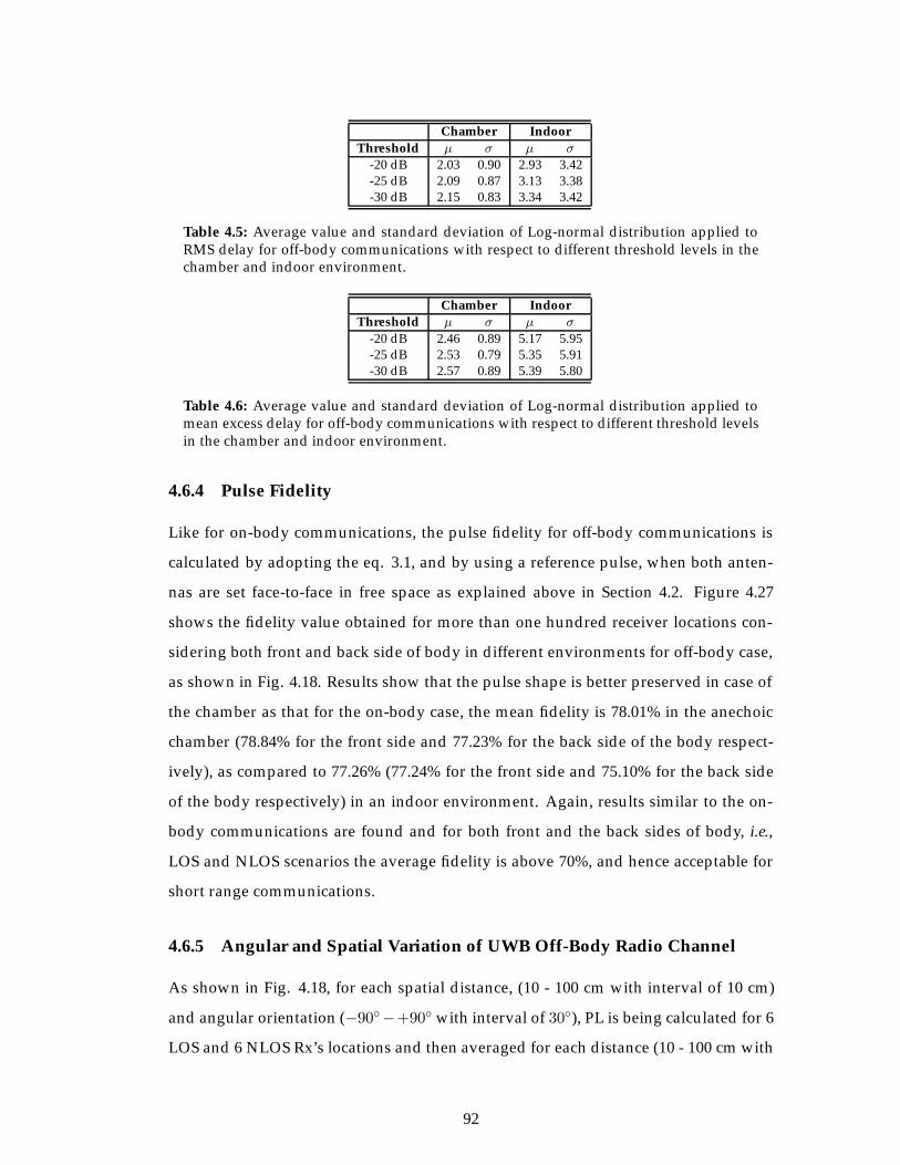
Chamber IndoorThreshold μ σ μ σ
-20 dB 2.03 0.90 2.93 3.42-25 dB 2.09 0.87 3.13 3.38-30 dB 2.15 0.83 3.34 3.42
Table 4.5: Average value and standard deviation of Log-normal distribution applied toRMS delay for off-body communications with respect to different threshold levels in thechamber and indoor environment.
Chamber IndoorThreshold μ σ μ σ
-20 dB 2.46 0.89 5.17 5.95-25 dB 2.53 0.79 5.35 5.91-30 dB 2.57 0.89 5.39 5.80
Table 4.6: Average value and standard deviation of Log-normal distribution applied tomean excess delay for off-body communications with respect to different threshold levelsin the chamber and indoor environment.
4.6.4 Pulse Fidelity
Like for on-body communications, the pulse fidelity for off-body communications is
calculated by adopting the eq. 3.1, and by using a reference pulse, when both anten-
nas are set face-to-face in free space as explained above in Section 4.2. Figure 4.27
shows the fidelity value obtained for more than one hundred receiver locations con-
sidering both front and back side of body in different environments for off-body case,
as shown in Fig. 4.18. Results show that the pulse shape is better preserved in case of
the chamber as that for the on-body case, the mean fidelity is 78.01% in the anechoic
chamber (78.84% for the front side and 77.23% for the back side of the body respect-
ively), as compared to 77.26% (77.24% for the front side and 75.10% for the back side
of the body respectively) in an indoor environment. Again, results similar to the on-
body communications are found and for both front and the back sides of body, i.e.,
LOS and NLOS scenarios the average fidelity is above 70%, and hence acceptable for
short range communications.
4.6.5 Angular and Spatial Variation of UWB Off-Body Radio Channel
As shown in Fig. 4.18, for each spatial distance, (10 - 100 cm with interval of 10 cm)
and angular orientation (−90◦−+90◦ with interval of 30◦), PL is being calculated for 6
LOS and 6 NLOS Rx’s locations and then averaged for each distance (10 - 100 cm with
92
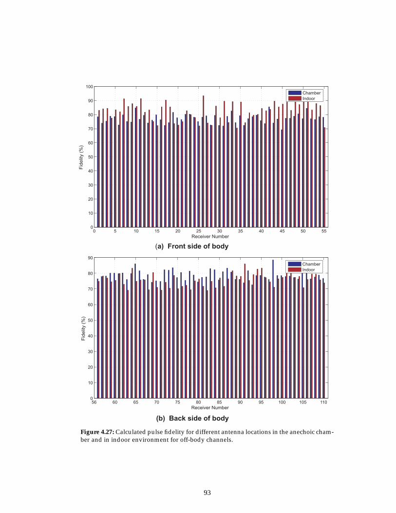
0 5 10 15 20 25 30 35 40 45 50 550
10
20
30
40
50
60
70
80
90
100
Receiver Number
Fid
elit
y (
%)
Chamber
Indoor
56 60 65 70 75 80 85 90 95 100 105 1100
10
20
30
40
50
60
70
80
90
Receiver Number
Fid
elit
y (
%)
Chamber
Indoor
(a) Front side of body
(b) Back side of body
Figure 4.27: Calculated pulse fidelity for different antenna locations in the anechoic cham-ber and in indoor environment for off-body channels.
93
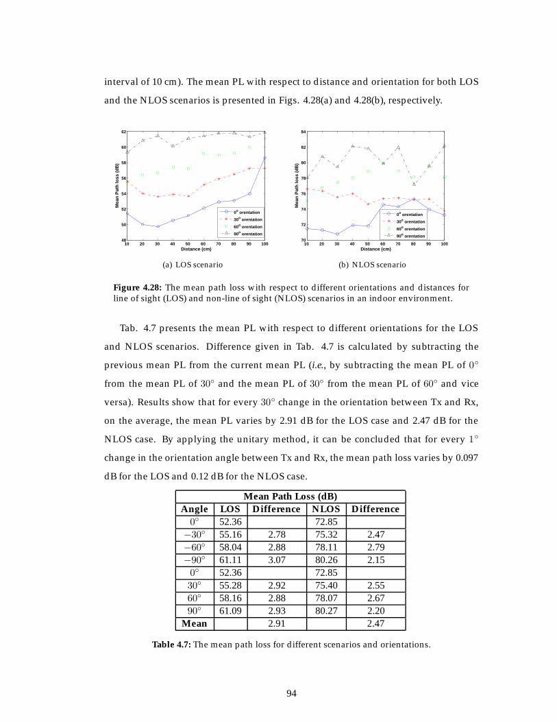
interval of 10 cm). The mean PL with respect to distance and orientation for both LOS
and the NLOS scenarios is presented in Figs. 4.28(a) and 4.28(b), respectively.
10 20 30 40 50 60 70 80 90 10048
50
52
54
56
58
60
62
Distance (cm)
Mea
n P
ath
loss
(d
B)
0o orentation
30o orentation
60o orentation
90o orentation
(a) LOS scenario
10 20 30 40 50 60 70 80 90 10070
72
74
76
78
80
82
84
Distance (cm)
Mea
n P
ath
loss
(d
B)
0o orentation
30o orentation
60o orentation
90o orentation
(b) NLOS scenario
Figure 4.28: The mean path loss with respect to different orientations and distances forline of sight (LOS) and non-line of sight (NLOS) scenarios in an indoor environment.
Tab. 4.7 presents the mean PL with respect to different orientations for the LOS
and NLOS scenarios. Difference given in Tab. 4.7 is calculated by subtracting the
previous mean PL from the current mean PL (i.e., by subtracting the mean PL of 0◦
from the mean PL of 30◦ and the mean PL of 30◦ from the mean PL of 60◦ and vice
versa). Results show that for every 30◦ change in the orientation between Tx and Rx,
on the average, the mean PL varies by 2.91 dB for the LOS case and 2.47 dB for the
NLOS case. By applying the unitary method, it can be concluded that for every 1◦
change in the orientation angle between Tx and Rx, the mean path loss varies by 0.097
dB for the LOS and 0.12 dB for the NLOS case.
Mean Path Loss (dB)Angle LOS Difference NLOS Difference0◦ 52.36 72.85
−30◦ 55.16 2.78 75.32 2.47−60◦ 58.04 2.88 78.11 2.79−90◦ 61.11 3.07 80.26 2.150◦ 52.36 72.8530◦ 55.28 2.92 75.40 2.5560◦ 58.16 2.88 78.07 2.6790◦ 61.09 2.93 80.27 2.20
Mean 2.91 2.47
Table 4.7: The mean path loss for different scenarios and orientations.
94
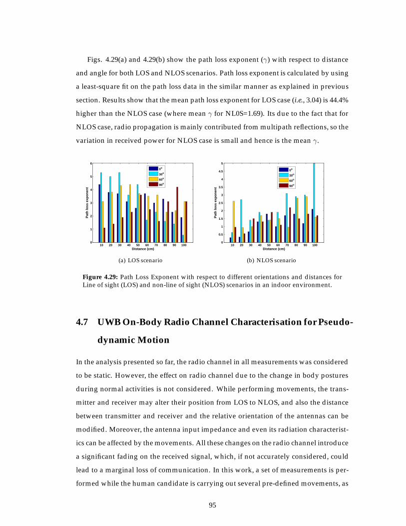
Figs. 4.29(a) and 4.29(b) show the path loss exponent (γ) with respect to distance
and angle for both LOS and NLOS scenarios. Path loss exponent is calculated by using
a least-square fit on the path loss data in the similar manner as explained in previous
section. Results show that the mean path loss exponent for LOS case (i.e., 3.04) is 44.4%
higher than the NLOS case (where mean γ for NL0S=1.69). Its due to the fact that for
NLOS case, radio propagation is mainly contributed from multipath reflections, so the
variation in received power for NLOS case is small and hence is the mean γ.
10 20 30 40 50 60 70 80 90 1000
1
2
3
4
5
6
Pat
h lo
ss e
xpo
nen
t
Distance (cm)
0o
30o
60o
90o
(a) LOS scenario
10 20 30 40 50 60 70 80 90 1000
0.5
1
1.5
2
2.5
3
3.5
4
4.5
5
Pat
h lo
ss e
xpo
nen
t
Distance (cm)
0o
30o
60o
90o
(b) NLOS scenario
Figure 4.29: Path Loss Exponent with respect to different orientations and distances forLine of sight (LOS) and non-line of sight (NLOS) scenarios in an indoor environment.
4.7 UWB On-Body Radio Channel Characterisation for Pseudo-
dynamic Motion
In the analysis presented so far, the radio channel in all measurements was considered
to be static. However, the effect on radio channel due to the change in body postures
during normal activities is not considered. While performing movements, the trans-
mitter and receiver may alter their position from LOS to NLOS, and also the distance
between transmitter and receiver and the relative orientation of the antennas can be
modified. Moreover, the antenna input impedance and even its radiation characterist-
ics can be affected by the movements. All these changes on the radio channel introduce
a significant fading on the received signal, which, if not accurately considered, could
lead to a marginal loss of communication. In this work, a set of measurements is per-
formed while the human candidate is carrying out several pre-defined movements, as
95
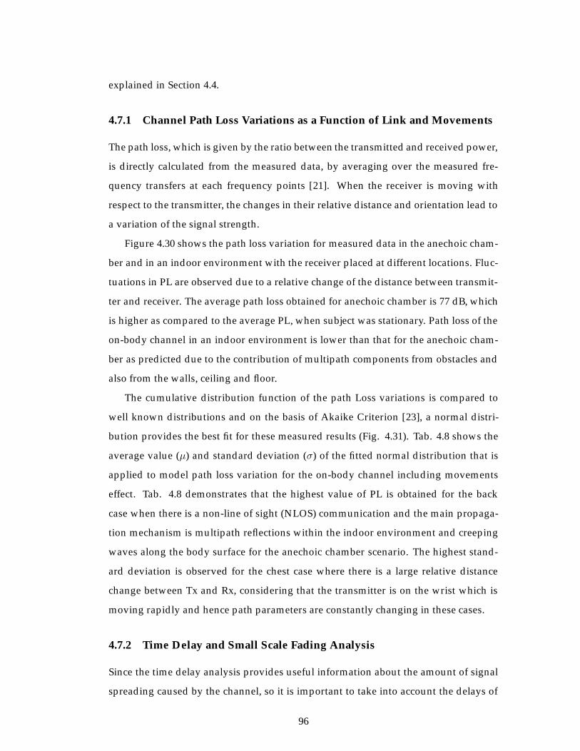
explained in Section 4.4.
4.7.1 Channel Path Loss Variations as a Function of Link and Movements
The path loss, which is given by the ratio between the transmitted and received power,
is directly calculated from the measured data, by averaging over the measured fre-
quency transfers at each frequency points [21]. When the receiver is moving with
respect to the transmitter, the changes in their relative distance and orientation lead to
a variation of the signal strength.
Figure 4.30 shows the path loss variation for measured data in the anechoic cham-
ber and in an indoor environment with the receiver placed at different locations. Fluc-
tuations in PL are observed due to a relative change of the distance between transmit-
ter and receiver. The average path loss obtained for anechoic chamber is 77 dB, which
is higher as compared to the average PL, when subject was stationary. Path loss of the
on-body channel in an indoor environment is lower than that for the anechoic cham-
ber as predicted due to the contribution of multipath components from obstacles and
also from the walls, ceiling and floor.
The cumulative distribution function of the path Loss variations is compared to
well known distributions and on the basis of Akaike Criterion [23], a normal distri-
bution provides the best fit for these measured results (Fig. 4.31). Tab. 4.8 shows the
average value (μ) and standard deviation (σ) of the fitted normal distribution that is
applied to model path loss variation for the on-body channel including movements
effect. Tab. 4.8 demonstrates that the highest value of PL is obtained for the back
case when there is a non-line of sight (NLOS) communication and the main propaga-
tion mechanism is multipath reflections within the indoor environment and creeping
waves along the body surface for the anechoic chamber scenario. The highest stand-
ard deviation is observed for the chest case where there is a large relative distance
change between Tx and Rx, considering that the transmitter is on the wrist which is
moving rapidly and hence path parameters are constantly changing in these cases.
4.7.2 Time Delay and Small Scale Fading Analysis
Since the time delay analysis provides useful information about the amount of signal
spreading caused by the channel, so it is important to take into account the delays of
96
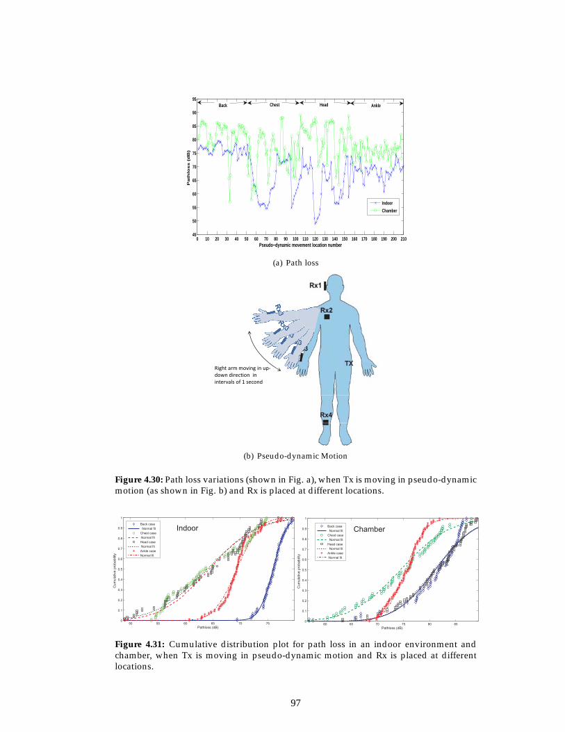
0 10 20 30 40 50 60 70 80 90 100 110 120 130 140 150 160 170 180 190 200 21045
50
55
60
65
70
75
80
85
90
95
Pseudo−dynamic movement location number
Path
loss (
dB
)
Indoor
Chamber
Back Chest Head Ankle
(a) Path loss
Right arm moving in upRight�arm�moving�in�up�down�direction��in�intervals�of�1�second
(b) Pseudo-dynamic Motion
Figure 4.30: Path loss variations (shown in Fig. a), when Tx is moving in pseudo-dynamicmotion (as shown in Fig. b) and Rx is placed at different locations.
50 55 60 65 70 750
0.1
0.2
0.3
0.4
0.5
0.6
0.7
0.8
0.9
1
Pathloss (dB)
Cu
mu
lative
pro
ba
bili
ty
Back case
Normal fit
Chest case
Normal fit
Head case
Normal fit
Ankle case
Normal fit
Indoor
60 65 70 75 80 850
0.1
0.2
0.3
0.4
0.5
0.6
0.7
0.8
0.9
1
Pathloss (dB)
Cu
mu
lative
pro
ba
bili
ty
Back case
Normal fit
Chest case
Normal fit
Head case
Normal fit
Ankle case
Normal fit
Chamber
Figure 4.31: Cumulative distribution plot for path loss in an indoor environment andchamber, when Tx is moving in pseudo-dynamic motion and Rx is placed at differentlocations.
97
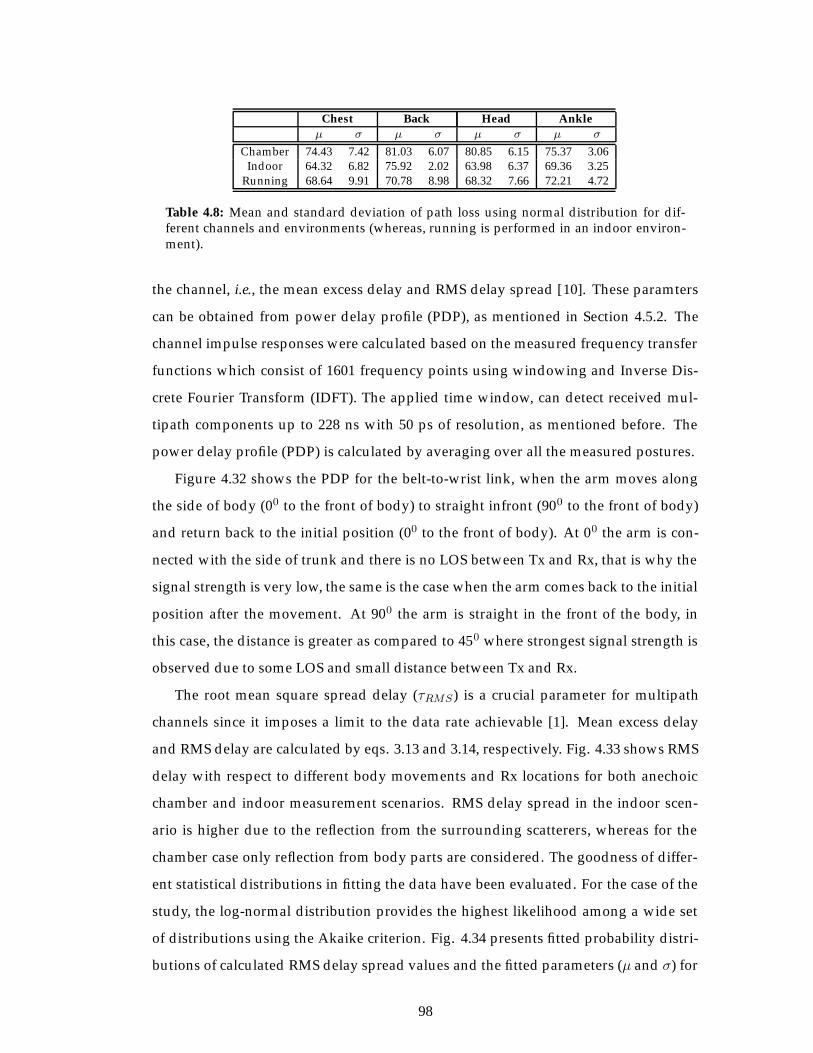
Chest Back Head Ankleμ σ μ σ μ σ μ σ
Chamber 74.43 7.42 81.03 6.07 80.85 6.15 75.37 3.06Indoor 64.32 6.82 75.92 2.02 63.98 6.37 69.36 3.25
Running 68.64 9.91 70.78 8.98 68.32 7.66 72.21 4.72
Table 4.8: Mean and standard deviation of path loss using normal distribution for dif-ferent channels and environments (whereas, running is performed in an indoor environ-ment).
the channel, i.e., the mean excess delay and RMS delay spread [10]. These paramters
can be obtained from power delay profile (PDP), as mentioned in Section 4.5.2. The
channel impulse responses were calculated based on the measured frequency transfer
functions which consist of 1601 frequency points using windowing and Inverse Dis-
crete Fourier Transform (IDFT). The applied time window, can detect received mul-
tipath components up to 228 ns with 50 ps of resolution, as mentioned before. The
power delay profile (PDP) is calculated by averaging over all the measured postures.
Figure 4.32 shows the PDP for the belt-to-wrist link, when the arm moves along
the side of body (00 to the front of body) to straight infront (900 to the front of body)
and return back to the initial position (00 to the front of body). At 00 the arm is con-
nected with the side of trunk and there is no LOS between Tx and Rx, that is why the
signal strength is very low, the same is the case when the arm comes back to the initial
position after the movement. At 900 the arm is straight in the front of the body, in
this case, the distance is greater as compared to 450 where strongest signal strength is
observed due to some LOS and small distance between Tx and Rx.
The root mean square spread delay (τRMS) is a crucial parameter for multipath
channels since it imposes a limit to the data rate achievable [1]. Mean excess delay
and RMS delay are calculated by eqs. 3.13 and 3.14, respectively. Fig. 4.33 shows RMS
delay with respect to different body movements and Rx locations for both anechoic
chamber and indoor measurement scenarios. RMS delay spread in the indoor scen-
ario is higher due to the reflection from the surrounding scatterers, whereas for the
chamber case only reflection from body parts are considered. The goodness of differ-
ent statistical distributions in fitting the data have been evaluated. For the case of the
study, the log-normal distribution provides the highest likelihood among a wide set
of distributions using the Akaike criterion. Fig. 4.34 presents fitted probability distri-
butions of calculated RMS delay spread values and the fitted parameters (μ and σ) for
98
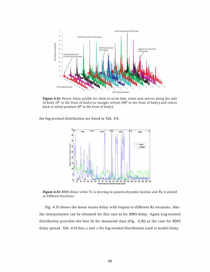
Figure 4.32: Power delay profile for chest-to-wrist link, when arm moves along the sideof body (00 to the front of body) to straight infront (900 to the front of body) and returnback to initial position (00 to the front of body).
the log-normal distribution are listed in Tab. 4.9.
0 10 20 30 40 50 60 70 80 90 100 110 120 130 140 150 160 170 180 190 200 2100
5
10
15
20
25
30
35
40
45
Pseudo−dynamic movement location number
Mean
excess d
ela
y (
nsec)
IndoorChamber
Back Chest Head Ankle
Figure 4.33: RMS delay when Tx is moving in pseudo-dynamic motion and Rx is placedat different locations.
Fig. 4.35 shows the mean excess delay with respect to different Rx locations. Sim-
ilar interpretation can be obtained for this case as for RMS delay. Again Log-normal
distribution provides the best fit for measured data (Fig. 4.36) as the case for RMS
delay spread. Tab. 4.10 lists μ and σ for log-normal distribution used to model delay.
99
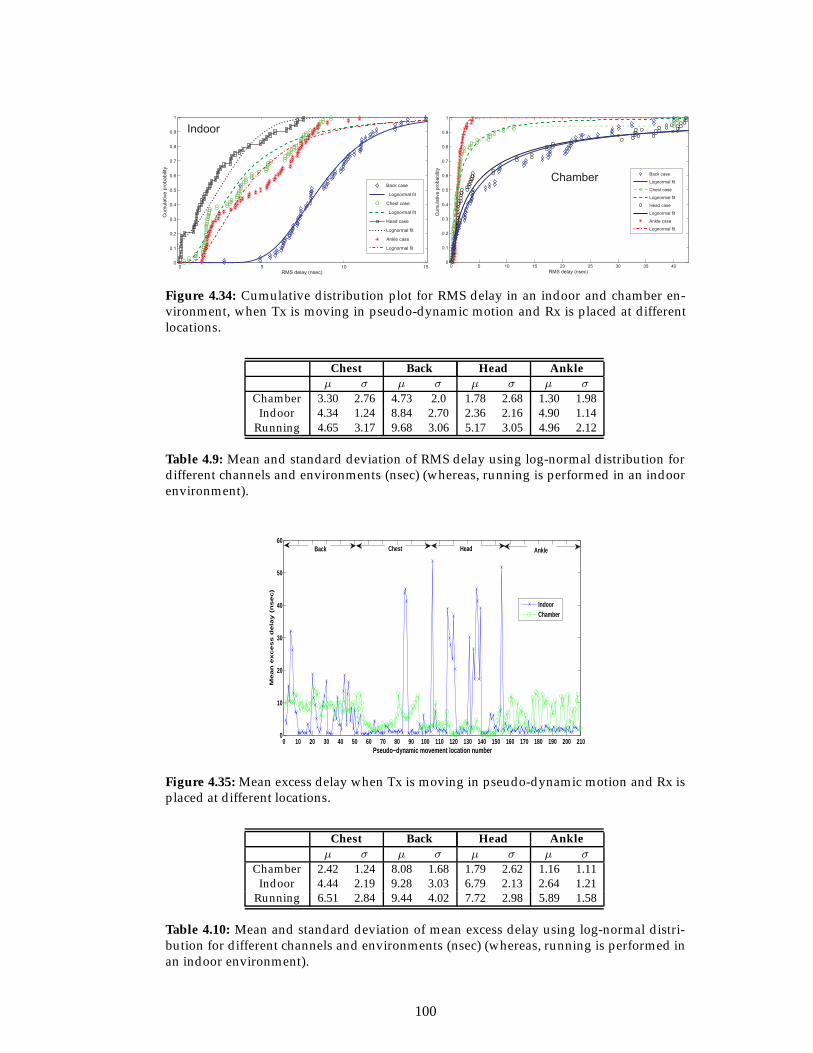
0 5 10 150
0.1
0.2
0.3
0.4
0.5
0.6
0.7
0.8
0.9
1
RMS delay (nsec)
Cu
mu
lative
pro
ba
bili
ty
Back case
Lognormal fit
Chest case
Lognormal fit
Head case
Lognormal fit
Ankle case
Lognormal fit
0 5 10 15 20 25 30 35 400
0.1
0.2
0.3
0.4
0.5
0.6
0.7
0.8
0.9
1
RMS delay (nsec)
Cu
mu
lative
pro
ba
bili
ty
Back case
Lognormal fit
Chest case
Lognormal fit
Head case
Lognormal fit
Ankle case
Lognormal fit
Indoor
Chamber
Figure 4.34: Cumulative distribution plot for RMS delay in an indoor and chamber en-vironment, when Tx is moving in pseudo-dynamic motion and Rx is placed at differentlocations.
Chest Back Head Ankleμ σ μ σ μ σ μ σ
Chamber 3.30 2.76 4.73 2.0 1.78 2.68 1.30 1.98Indoor 4.34 1.24 8.84 2.70 2.36 2.16 4.90 1.14
Running 4.65 3.17 9.68 3.06 5.17 3.05 4.96 2.12
Table 4.9: Mean and standard deviation of RMS delay using log-normal distribution fordifferent channels and environments (nsec) (whereas, running is performed in an indoorenvironment).
0 10 20 30 40 50 60 70 80 90 100 110 120 130 140 150 160 170 180 190 200 2100
10
20
30
40
50
60
Pseudo−dynamic movement location number
Mean
excess d
ela
y (
nsec)
IndoorChamber
Back Chest Head Ankle
Figure 4.35: Mean excess delay when Tx is moving in pseudo-dynamic motion and Rx isplaced at different locations.
Chest Back Head Ankleμ σ μ σ μ σ μ σ
Chamber 2.42 1.24 8.08 1.68 1.79 2.62 1.16 1.11Indoor 4.44 2.19 9.28 3.03 6.79 2.13 2.64 1.21
Running 6.51 2.84 9.44 4.02 7.72 2.98 5.89 1.58
Table 4.10: Mean and standard deviation of mean excess delay using log-normal distri-bution for different channels and environments (nsec) (whereas, running is performed inan indoor environment).
100
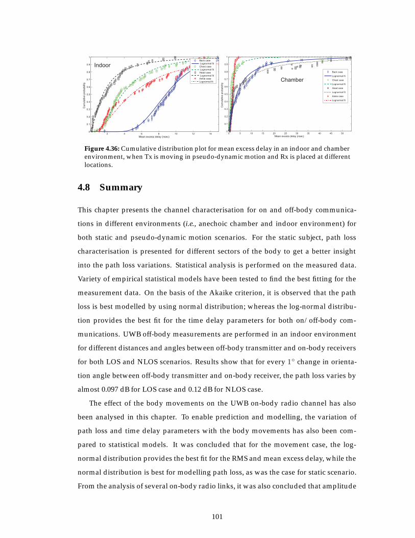
2 4 6 8 10 12 140
0.1
0.2
0.3
0.4
0.5
0.6
0.7
0.8
0.9
1
Mean excess delay (nsec)
Cum
ula
tive p
robabili
ty
Back case
Lognormal fit
Chest case
Lognormal fit
Head case
Lognormal fit
Ankle case
Lognormal fit
Indoor
Mean excess delay (nsec)0 5 10 15 20 25 30 35 40 45 50
0
0.1
0.2
0.3
0.4
0.5
0.6
0.7
0.8
0.9
1
Cum
ula
tive p
robabili
ty
Back case
Lognormal fit
Chest case
Lognormal fit
Head case
Lognormal fit
Ankle case
Lognormal fit
Chamber
Figure 4.36: Cumulative distribution plot for mean excess delay in an indoor and chamberenvironment, when Tx is moving in pseudo-dynamic motion and Rx is placed at differentlocations.
4.8 Summary
This chapter presents the channel characterisation for on and off-body communica-
tions in different environments (i.e., anechoic chamber and indoor environment) for
both static and pseudo-dynamic motion scenarios. For the static subject, path loss
characterisation is presented for different sectors of the body to get a better insight
into the path loss variations. Statistical analysis is performed on the measured data.
Variety of empirical statistical models have been tested to find the best fitting for the
measurement data. On the basis of the Akaike criterion, it is observed that the path
loss is best modelled by using normal distribution; whereas the log-normal distribu-
tion provides the best fit for the time delay parameters for both on/off-body com-
munications. UWB off-body measurements are performed in an indoor environment
for different distances and angles between off-body transmitter and on-body receivers
for both LOS and NLOS scenarios. Results show that for every 1◦ change in orienta-
tion angle between off-body transmitter and on-body receiver, the path loss varies by
almost 0.097 dB for LOS case and 0.12 dB for NLOS case.
The effect of the body movements on the UWB on-body radio channel has also
been analysed in this chapter. To enable prediction and modelling, the variation of
path loss and time delay parameters with the body movements has also been com-
pared to statistical models. It was concluded that for the movement case, the log-
normal distribution provides the best fit for the RMS and mean excess delay, while the
normal distribution is best for modelling path loss, as was the case for static scenario.
From the analysis of several on-body radio links, it was also concluded that amplitude
101

and delay spread of the received signal can vary significatively with the changes in the
posture and position of antennas on the body.
102
References
[1] T. S. Rappaport, Wireless Communications Principles and Practice. Prentice Hall, Inc., NewJersey, 1996.
[2] H. Hashemi, “The indoor radio propagation channel,” Proceedings of IEEE, vol. 81, no. 7,pp. 943–968, 1993.
[3] A. A. Saleh and R. A. Valenzuela, “A statistical model for indoor multipath propagation,”IEEE Journal on Selected Areas in Communications, vol. 5, no. 2, pp. 128–137, February 1987.
[4] H. Suzuki, “A statistical model for urban radio propagation,” IEEE Transactions on Com-munications, vol. 25, no. 7, pp. 673–680, July 1977.
[5] M. Z. Win and R. A. Scholtz, “Impulse radio: how it works,” IEEE Communications Letters,pp. 36–38, February 1998.
[6] I. S. Kovacs, G. Pedersen, P. Eggers, and K. Olesen, “Ultra wideband radio propagationin body area network scenarios,” in ISSSTA Proceedings, pp. 102–106, 2004.
[7] S. L. Cotton and W. Scanlon, “A statistical analysis of indoor multipath fading for a nar-rowband wireless body area network,” IEEE 17th International Symposium on Personal,Indoor and Mobile Radio Communications, pp. 1–5, September 2006.
[8] D. Neirynck, Channel Characterisation and Physical Layer Analysis for Body and Personal AreaNetwork Development. Ph.D Thesis, University of Bristol, November 2006.
[9] A. Sani, Modeling and Characterisation of Antenna and Propagation for Body-Centric WirelessCommunications. PhD thesis, Queen Mary Uni. of London, 2010.
[10] J. H. Reed, An Introduction to Ultra Wideband Communication Systems. Printce Hall, 2005.
[11] A. Rahman, A. Alomainy, and Y. Hao, “Compact body-worn coplanar waveguide fedantenna for UWB body-centric wireless communications,” in European Conference on An-tennas and Propagation (EuCAP 2007), 11.
[12] T.-G. Ma and C.-H. Tseng, “An ultra wideband coplanar waveguide-fed tapered slot ringantenna,” IEEE Transactions on Antenna and Propagation, vol. 54, no. 4, April 2006.
[13] L. Liang, L. Guo, C. C. Chiau, X. Chen, and C. G. Parini, “Study of CPW fed circulardisc monopole antenna for ultra wideband application,” IEE Proceedings on Microwave,Antennas and Propagataion, vol. 152, no. 6, pp. 520–526, Nov. 2005.
[14] H. G. Schantz and M. Barnes, “Ieee ap-s int. symp.” in The COTAB UWB magnetic slotantenna, Boston, MA, 2001, pp. 104–107.
[15] T. Yang, S.-Y. Suh, R. Nealy, W. Davis, and W. L. Stutzman, “Compact antennas for UWBapplications,” 2003 IEEE Ultra Wideband Systems and Technologies, pp. 205–208, November2003.
[16] M. Klemm, I. Z. Kovacs, F. G. Pedersen, and G. Troester, “Novel small-size directional an-tenna for UWB WBAN/WPAN applications,” IEEE Transactions on Antennas and Propaga-tion, vol. 53, no. 12, pp. 3884–3896, 2005.
[17] D. Lamensdorf and L. Susman, “Baseband-pulse-antenna techniques,” IEEE Antennas andPropagation Magazine, vol. 36, no. 1, February 1994.
[18] J. McLean, H. Foltz, and R. Sutton, “Pattern descriptors for UWB antennas,” IEEE trans-actions on antennas and propagation, vol. 53, no. 1 Part 2, pp. 553–559, 2005.
103
[19] T. Dissanayake and K. Esselle, “Correlation-based pattern stability analysis and a figureof merit for UWB antennas,” IEEE Transactions on Antennas and Propagation, vol. 54, no. 11Part 1, pp. 3184–3191, 2006.
[20] M. Kanda, “A relatively short cylindrical broadband antenna with tapered resistive load-ing for picosecond pulse measurements,” IEEE Transactions on Antennas and Propagation,vol. 26, no. 3, pp. 439–447, 1978.
[21] J. A. Dabin, N. Ni, A. M. Haimovich, E. Niver, and H. Grebel, “The effects of antennadirectivity on path loss and multipath propagation in UWB indoor wireless channels,” inProc. IEEE Conf. Ultra Wideband Systems and Technologies, Newark, NJ,, pp. 305–309, 2003.
[22] S. S. Ghassemzadeh, R. Jana, C. W. Rice, W. Turin, and V. Tarokh, “A Statistical PathLoss Model for in-home UWB Channels,” in IEEE Conf. on Ultra wideband Systems andTechnologies (UWBST), 2002, pp. 59–64.
[23] K. P. Burnham and D. R. Anderson, Model Selection and Multimodel Inference: A PracticalInformation-Theoretic Approach. New York: Springer-Verlag, 2002.
[24] A. Alomainy, Y. Hao, and W. F. Pasveer, “Numerical and experimental evaluation of acompact sensor antenna performance for healthcare devices,” IEEE Transactions on Bio-medical Circuits and Systems, vol. 1, no. 4, pp. 242–249, Dec. 2007.
104
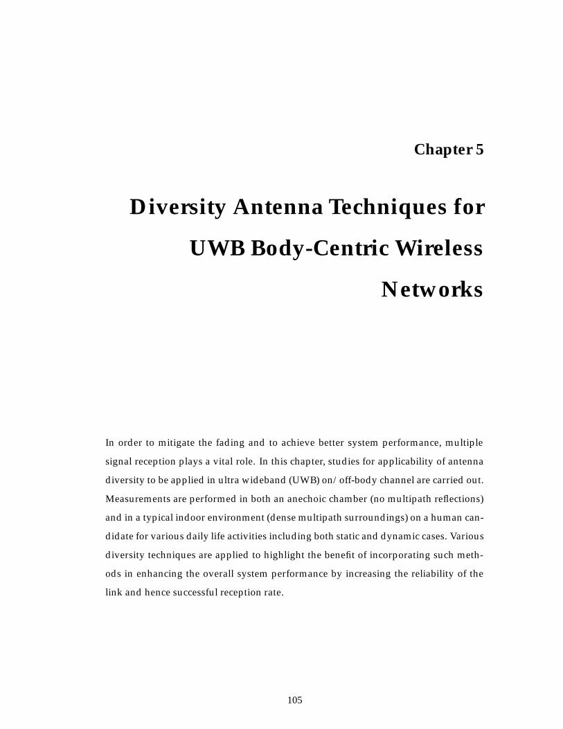
Chapter 5
Diversity Antenna Techniques for
UWB Body-Centric Wireless
Networks
In order to mitigate the fading and to achieve better system performance, multiple
signal reception plays a vital role. In this chapter, studies for applicability of antenna
diversity to be applied in ultra wideband (UWB) on/off-body channel are carried out.
Measurements are performed in both an anechoic chamber (no multipath reflections)
and in a typical indoor environment (dense multipath surroundings) on a human can-
didate for various daily life activities including both static and dynamic cases. Various
diversity techniques are applied to highlight the benefit of incorporating such meth-
ods in enhancing the overall system performance by increasing the reliability of the
link and hence successful reception rate.
105
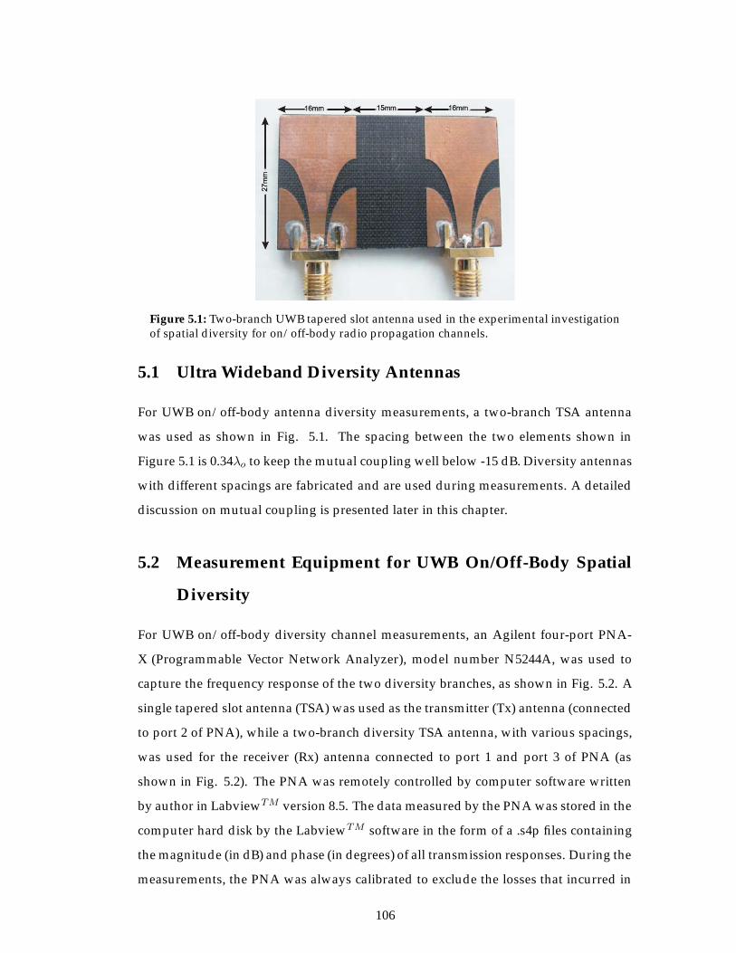
Figure 5.1: Two-branch UWB tapered slot antenna used in the experimental investigationof spatial diversity for on/off-body radio propagation channels.
5.1 Ultra Wideband Diversity Antennas
For UWB on/off-body antenna diversity measurements, a two-branch TSA antenna
was used as shown in Fig. 5.1. The spacing between the two elements shown in
Figure 5.1 is 0.34λo to keep the mutual coupling well below -15 dB. Diversity antennas
with different spacings are fabricated and are used during measurements. A detailed
discussion on mutual coupling is presented later in this chapter.
5.2 Measurement Equipment for UWB On/Off-Body Spatial
Diversity
For UWB on/off-body diversity channel measurements, an Agilent four-port PNA-
X (Programmable Vector Network Analyzer), model number N5244A, was used to
capture the frequency response of the two diversity branches, as shown in Fig. 5.2. A
single tapered slot antenna (TSA) was used as the transmitter (Tx) antenna (connected
to port 2 of PNA), while a two-branch diversity TSA antenna, with various spacings,
was used for the receiver (Rx) antenna connected to port 1 and port 3 of PNA (as
shown in Fig. 5.2). The PNA was remotely controlled by computer software written
by author in LabviewTM version 8.5. The data measured by the PNA was stored in the
computer hard disk by the LabviewTM software in the form of a .s4p files containing
the magnitude (in dB) and phase (in degrees) of all transmission responses. During the
measurements, the PNA was always calibrated to exclude the losses that incurred in
106
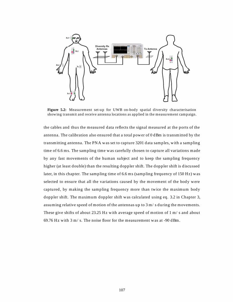
Diversity RxAntennas Tx Antenna
Figure 5.2: Measurement set-up for UWB on-body spatial diversity characterisationshowing transmit and receive antenna locations as applied in the measurement campaign.
the cables and thus the measured data reflects the signal measured at the ports of the
antenna. The calibration also ensured that a total power of 0 dBm is transmitted by the
transmitting antenna. The PNA was set to capture 3201 data samples, with a sampling
time of 6.6 ms. The sampling time was carefully chosen to capture all variations made
by any fast movements of the human subject and to keep the sampling frequency
higher (at least double) than the resulting doppler shift. The doppler shift is discussed
later, in this chapter. The sampling time of 6.6 ms (sampling frequency of 150 Hz) was
selected to ensure that all the variations caused by the movement of the body were
captured, by making the sampling frequency more than twice the maximum body
doppler shift. The maximum doppler shift was calculated using eq. 3.2 in Chapter 3,
assuming relative speed of motion of the antennas up to 3 m/s during the movements.
These give shifts of about 23.25 Hz with average speed of motion of 1 m/s and about
69.76 Hz with 3 m/s. The noise floor for the measurement was at -90 dBm.
107
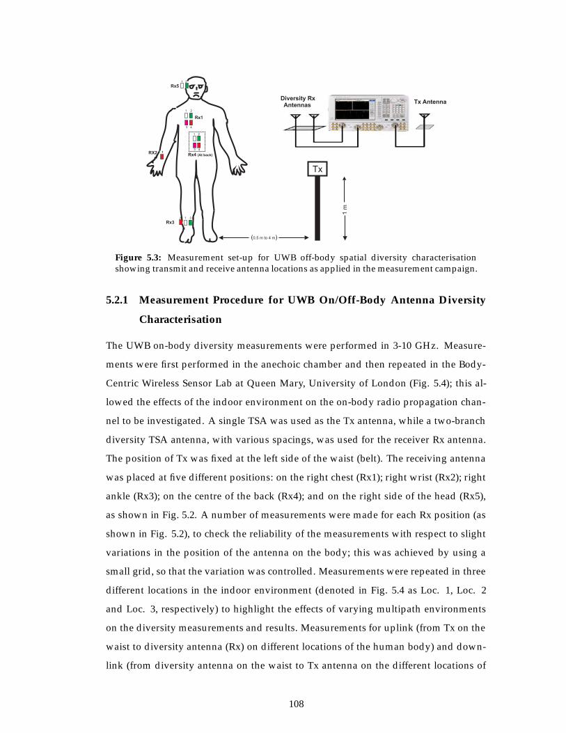
Diversity RxAntennas
Tx Antenna
Tx
1 m
1 2
3 4
1
1
11
12 3
2
2
3 4
Rx1
RX2
Rx3
Rx4 (At back)
Rx5
( )0.5 m to 4 m
Figure 5.3: Measurement set-up for UWB off-body spatial diversity characterisationshowing transmit and receive antenna locations as applied in the measurement campaign.
5.2.1 Measurement Procedure for UWB On/Off-Body Antenna Diversity
Characterisation
The UWB on-body diversity measurements were performed in 3-10 GHz. Measure-
ments were first performed in the anechoic chamber and then repeated in the Body-
Centric Wireless Sensor Lab at Queen Mary, University of London (Fig. 5.4); this al-
lowed the effects of the indoor environment on the on-body radio propagation chan-
nel to be investigated. A single TSA was used as the Tx antenna, while a two-branch
diversity TSA antenna, with various spacings, was used for the receiver Rx antenna.
The position of Tx was fixed at the left side of the waist (belt). The receiving antenna
was placed at five different positions: on the right chest (Rx1); right wrist (Rx2); right
ankle (Rx3); on the centre of the back (Rx4); and on the right side of the head (Rx5),
as shown in Fig. 5.2. A number of measurements were made for each Rx position (as
shown in Fig. 5.2), to check the reliability of the measurements with respect to slight
variations in the position of the antenna on the body; this was achieved by using a
small grid, so that the variation was controlled. Measurements were repeated in three
different locations in the indoor environment (denoted in Fig. 5.4 as Loc. 1, Loc. 2
and Loc. 3, respectively) to highlight the effects of varying multipath environments
on the diversity measurements and results. Measurements for uplink (from Tx on the
waist to diversity antenna (Rx) on different locations of the human body) and down-
link (from diversity antenna on the waist to Tx antenna on the different locations of
108
the human body) diversity were also carried out. Moreover, the repeatability of the
measurements with respect to time was investigated by repeating the measurement
procedures on different days. During the UWB on-body diversity channel character-
isation, a variety of movements were included as shown in Table 5.1 for each channel.
Five sweeps were carried out, thus a total of 16005 data points were considered dur-
ing each channel measurement. Measurements were performed in a controlled indoor
environment (i.e. not in the real environment) on time varying human body channel,
when the surrounding environment was completely static. Measurements were taken
during the evening in the Body-Centric Wireless Sensor Lab at Queen Mary, Univer-
sity of London (Fig. 5.4), to avoid any variations in the surrounding environment due
to moving people. The goal was to investigate the potential improvement achieved by
using diversity for BCWN.
For the UWB off-body diversity measurements, the same antenna was used as
for on-body diversity case. Measurements were performed only in the Body-Centric
Wireless Sensor Lab at Queen Mary, University of London (Fig. 5.5). Similar to on-
body diversity case, a single TSA (i.e. Access point (AP)) was used as the transmitter
(Tx) antenna, while a two-branch diversity TSA antenna, with various spacings, was
used as the receiver (Rx) antenna. The AP was fixed at waist height (1 meter above
the ground). The receiving antenna was placed at same five positions as for on-body
diveristy. The distance between the subject carrying diversity branch receivers and
AP is varied from 0.5 meters to 4 meters (Tx and Rx locations are as shown in Fig. 5.3).
For the off-body diversity case, like for the on-body diversity; the number of meas-
urements were made for each Rx position, a small grid was assigned to check the reli-
ability of measurements with respect to small variations in the position of the antenna
on the body. Measurements were repeated in eight different locations in an indoor
environment, each with a step of 0.5 meter (denoted in Fig. 5.5 as Loc. 1 to Loc. 8 re-
spectively). This was done to highlight the effect of varying multipath environments
and the distance between the off-body access point (AP) and the human body carrying
diversity antennas, on the diversity measurements and results. In addition, for spa-
cing of 1 meter between the AP and the human subject carrying the diversity receivers,
measurements were performed for three different angles (i.e. 0◦, 45◦ and 90◦), in or-
der to observe the impact of orientation on diversity performance (The orientation is
109
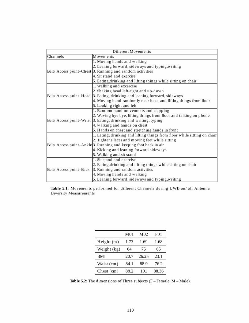
Different MovementsChannels Movements
Belt/Access point–Chest
1. Moving hands and walking2. Leaning forward, sideways and typing,writing3. Running and random activities4. Sit stand and exercise5. Eating,drinking and lifting things while sitting on chair
Belt/Access point–Head
1. Walking and excercise2. Shaking head left-right and up-down3. Eating, drinking and leaning forward, sideways4. Moving hand randomly near head and lifting things from floor5. Looking right and left
Belt/Access point–Wrist
1. Random hand movements and clapping2. Waving bye bye, lifting things from floor and talking on phone3. Eating, drinking and writing, typing4. walking and hands on chest5. Hands on chest and stretching hands in front
Belt/Access point–Ankle
1. Eating, drinking and lifting things from floor while sitting on chair2. Tightens laces and moving feet while sitting3. Running and keeping foot back in air4. Kicking and leaning forward sideways5. Walking and sit stand
Belt/Access point–Back
1. Sit stand and exercise2. Eating,drinking and lifting things while sitting on chair3. Running and random activities4. Moving hands and walking5. Leaning forward, sideways and typing,writing
Table 5.1: Movements performed for different Channels during UWB on/off AntennaDiversity Measurements
M01 M02 F01
Height (m) 1.73 1.69 1.68
Weight (kg) 64 75 65
BMI 20.7 26.25 23.1
Waist (cm) 84.1 88.9 76.2
Chest (cm) 88.2 101 88.36
Table 5.2: The dimensions of Three subjects (F – Female, M – Male).
110
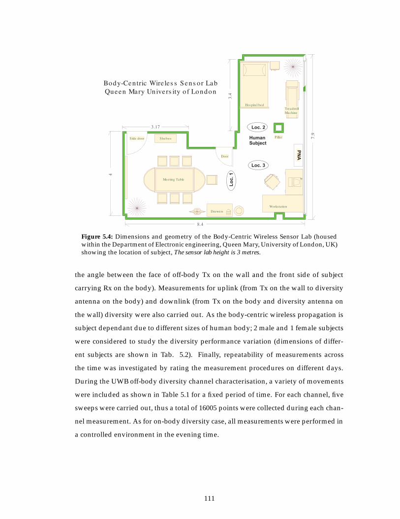
HumanSubject
Loc. 2
Lo
c.
1
Loc. 3
PN
A
Figure 5.4: Dimensions and geometry of the Body-Centric Wireless Sensor Lab (housedwithin the Department of Electronic engineering, Queen Mary, University of London, UK)showing the location of subject, The sensor lab height is 3 metres.
the angle between the face of off-body Tx on the wall and the front side of subject
carrying Rx on the body). Measurements for uplink (from Tx on the wall to diversity
antenna on the body) and downlink (from Tx on the body and diversity antenna on
the wall) diversity were also carried out. As the body-centric wireless propagation is
subject dependant due to different sizes of human body; 2 male and 1 female subjects
were considered to study the diversity performance variation (dimensions of differ-
ent subjects are shown in Tab. 5.2). Finally, repeatability of measurements across
the time was investigated by rating the measurement procedures on different days.
During the UWB off-body diversity channel characterisation, a variety of movements
were included as shown in Table 5.1 for a fixed period of time. For each channel, five
sweeps were carried out, thus a total of 16005 points were collected during each chan-
nel measurement. As for on-body diversity case, all measurements were performed in
a controlled environment in the evening time.
111
5.3 Diversity Technique Analysis
5.3.1 Doppler Shift
In mobile communications, a doppler shift in the signal frequency occurs due to the
relative speed of motion between the transmitter and receiver; this is also true for the
on-body case. In order to capture all movements made by the human body during
measurements, the sampling frequency of the measurement should be greater than
twice the maximum expected doppler shift. This shift is calculated for all channels
using eq. 5.1, as given in [1]:
fm =v
λo(5.1)
where v is the velocity of motion of the human body in metres per second and λo is the
wavelength in metres. For the UWB band (3.1 to 10.6 GHz), with a centre frequency of
6.85 GHz, fm = 22.83 Hz for an average speed of 1 m/s and fm = 68.5 Hz for a speed
of 3 m/s. The maximum doppler shift is observed for the waist-to-wrist channel,
compared to the other channels. During measurements, the sampling time was set
to 6.6 ms on the PNA, to capture even the fastest movement of 3 m/s by keeping
the sampling frequency equal to 150 Hz, which is greater than twice the maximum
expected doppler shift (i.e., 68.5 Hz).
5.3.2 Envelope Correlation Coefficients
For a diversity scheme to be effective, each antenna element should receive statist-
ically independent versions of the transmitted signal reducing the likelihood that all
branches are experiencing correlated fading. Two signals are said to be suitably uncor-
related if their correlation is less than 0.7 [2]. Signal decorrelation is usually introduced
by multipath components. The envelope correlation coefficient (ρe) between the two
diversity branches is calculated by the following expression [3]:
ρe =
∑Ni=i(r1(i)− r1)(r2(i)− r2)√∑N
i=i(r1(i)− r1)2√∑N
i=i(r2(i)− r2)2(5.2)
where N is total number of samples and ri is the mean value of fast fading envelope
ri of received diversity branch signal i. Using Tab. 5.4 for the chest case for position
112
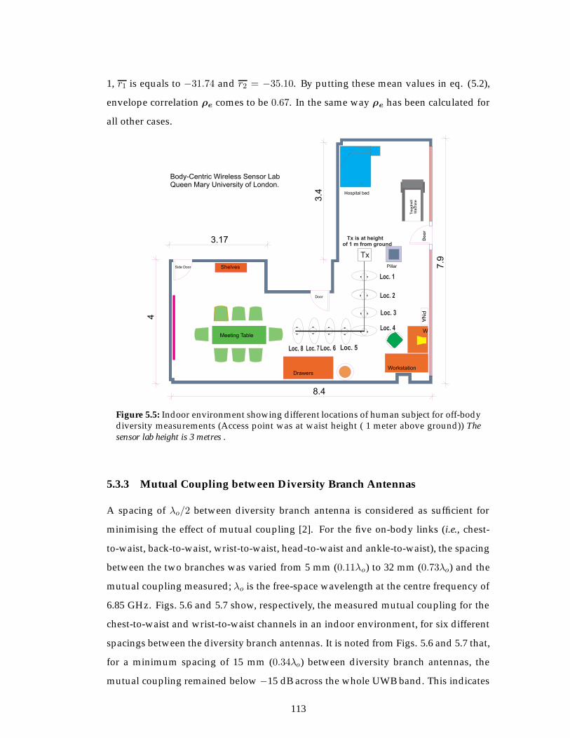
1, r1 is equals to −31.74 and r2 = −35.10. By putting these mean values in eq. (5.2),
envelope correlation ρe comes to be 0.67. In the same way ρe has been calculated for
all other cases.
Shelves
Workstation
W
PN
A
Drawers
T
Door
Side Door
Tre
ad
mill
Ma
ch
ine
Pillar
Hospital bed
Body-Centric Wireless Sensor LabQueen Mary University of London.
8.4
3.17
3.4
7.9
4
Tx
Loc. 2
Loc. 3
Loc. 4
Loc. 5Loc. 6Loc. 7Loc. 8
Do
or
Loc. 1
Tx is at heightof 1 m from ground
Meeting Table
Figure 5.5: Indoor environment showing different locations of human subject for off-bodydiversity measurements (Access point was at waist height ( 1 meter above ground)) Thesensor lab height is 3 metres .
5.3.3 Mutual Coupling between Diversity Branch Antennas
A spacing of λo/2 between diversity branch antenna is considered as sufficient for
minimising the effect of mutual coupling [2]. For the five on-body links (i.e., chest-
to-waist, back-to-waist, wrist-to-waist, head-to-waist and ankle-to-waist), the spacing
between the two branches was varied from 5 mm (0.11λo) to 32 mm (0.73λo) and the
mutual coupling measured; λo is the free-space wavelength at the centre frequency of
6.85 GHz. Figs. 5.6 and 5.7 show, respectively, the measured mutual coupling for the
chest-to-waist and wrist-to-waist channels in an indoor environment, for six different
spacings between the diversity branch antennas. It is noted from Figs. 5.6 and 5.7 that,
for a minimum spacing of 15 mm (0.34λo) between diversity branch antennas, the
mutual coupling remained below −15 dB across the whole UWB band. This indicates
113
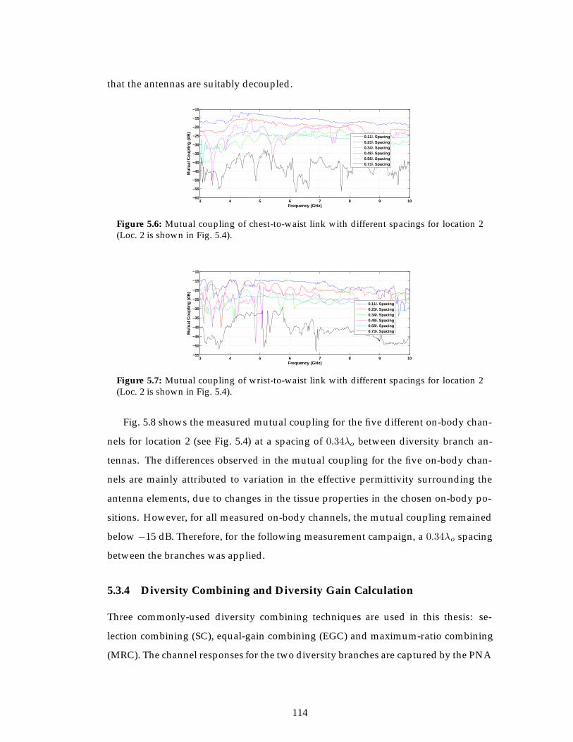
that the antennas are suitably decoupled.
3 4 5 6 7 8 9 10−60
−55
−50
−45
−40
−35
−30
−25
−20
−15
−10
Frequency (GHz)
Mu
tual
Co
up
ling
(d
B)
0.11λ Spacing0.23λ Spacing0.34λ Spacing0.48λ Spacing0.58λ Spacing0.73λ Spacing
Figure 5.6: Mutual coupling of chest-to-waist link with different spacings for location 2(Loc. 2 is shown in Fig. 5.4).
3 4 5 6 7 8 9 10−55
−50
−45
−40
−35
−30
−25
−20
−15
−10
Frequency (GHz)
Mu
tual
Co
up
ling
(d
B)
0.11λ Spacing0.23λ Spacing0.34λ Spacing0.48λ Spacing0.58λ Spacing0.73λ Spacing
Figure 5.7: Mutual coupling of wrist-to-waist link with different spacings for location 2(Loc. 2 is shown in Fig. 5.4).
Fig. 5.8 shows the measured mutual coupling for the five different on-body chan-
nels for location 2 (see Fig. 5.4) at a spacing of 0.34λo between diversity branch an-
tennas. The differences observed in the mutual coupling for the five on-body chan-
nels are mainly attributed to variation in the effective permittivity surrounding the
antenna elements, due to changes in the tissue properties in the chosen on-body po-
sitions. However, for all measured on-body channels, the mutual coupling remained
below −15 dB. Therefore, for the following measurement campaign, a 0.34λo spacing
between the branches was applied.
5.3.4 Diversity Combining and Diversity Gain Calculation
Three commonly-used diversity combining techniques are used in this thesis: se-
lection combining (SC), equal-gain combining (EGC) and maximum-ratio combining
(MRC). The channel responses for the two diversity branches are captured by the PNA
114
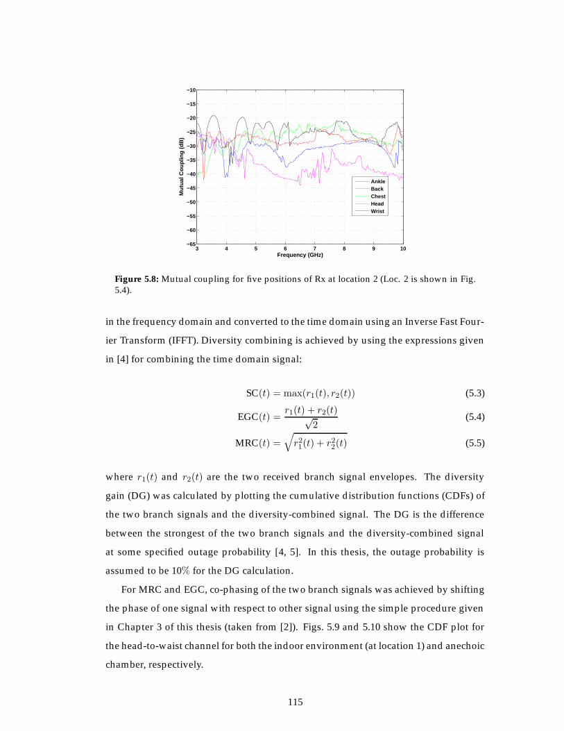
3 4 5 6 7 8 9 10−65
−60
−55
−50
−45
−40
−35
−30
−25
−20
−15
−10
Frequency (GHz)
Mu
tual
Co
up
ling
(d
B)
AnkleBackChestHeadWrist
Figure 5.8: Mutual coupling for five positions of Rx at location 2 (Loc. 2 is shown in Fig.5.4).
in the frequency domain and converted to the time domain using an Inverse Fast Four-
ier Transform (IFFT). Diversity combining is achieved by using the expressions given
in [4] for combining the time domain signal:
SC(t) = max(r1(t), r2(t)) (5.3)
EGC(t) =r1(t) + r2(t)√
2(5.4)
MRC(t) =√
r21(t) + r22(t) (5.5)
where r1(t) and r2(t) are the two received branch signal envelopes. The diversity
gain (DG) was calculated by plotting the cumulative distribution functions (CDFs) of
the two branch signals and the diversity-combined signal. The DG is the difference
between the strongest of the two branch signals and the diversity-combined signal
at some specified outage probability [4, 5]. In this thesis, the outage probability is
assumed to be 10% for the DG calculation.
For MRC and EGC, co-phasing of the two branch signals was achieved by shifting
the phase of one signal with respect to other signal using the simple procedure given
in Chapter 3 of this thesis (taken from [2]). Figs. 5.9 and 5.10 show the CDF plot for
the head-to-waist channel for both the indoor environment (at location 1) and anechoic
chamber, respectively.
115
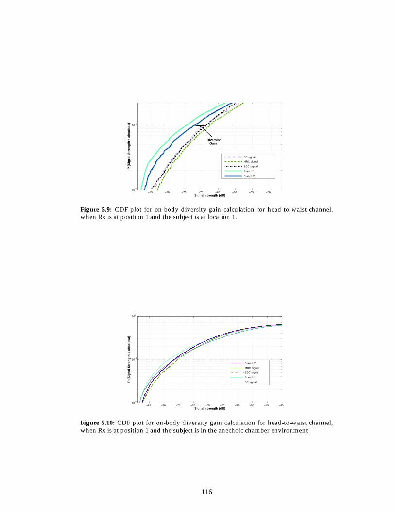
−85 −80 −75 −70 −65 −60 −55 −5010
−2
10−1
Signal strength (dB)
P (
Sig
nal
Str
eng
th <
ab
scis
sa)
SC signal
MRC signal
EGC signal
Branch 1
Branch 2
Diversity Gain
Figure 5.9: CDF plot for on-body diversity gain calculation for head-to-waist channel,when Rx is at position 1 and the subject is at location 1.
−85 −80 −75 −70 −65 −60 −55 −50 −45 −4010
−2
10−1
100
Signal strength (dB)
P (
Sig
nal
Str
eng
th <
ab
scis
sa)
Branch 2
MRC signal
EGC signal
Branch 1
SC signal
Figure 5.10: CDF plot for on-body diversity gain calculation for head-to-waist channel,when Rx is at position 1 and the subject is in the anechoic chamber environment.
116
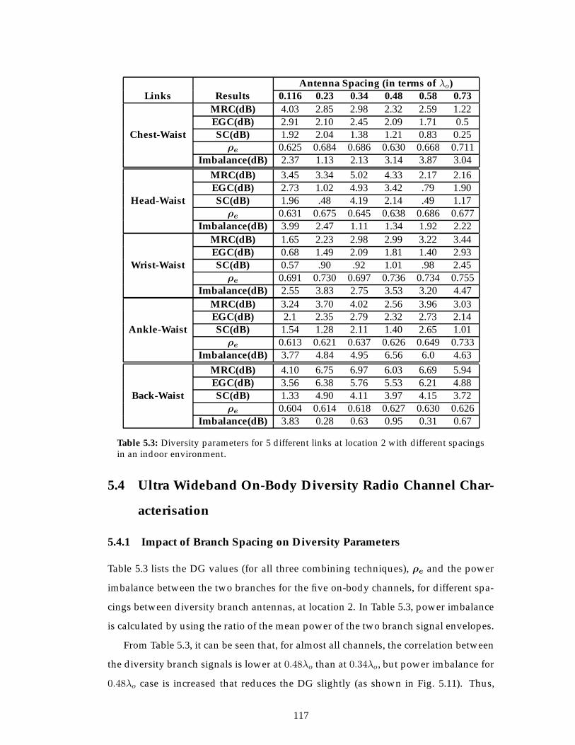
Antenna Spacing (in terms of λo)Links Results 0.116 0.23 0.34 0.48 0.58 0.73
Chest-Waist
MRC(dB) 4.03 2.85 2.98 2.32 2.59 1.22EGC(dB) 2.91 2.10 2.45 2.09 1.71 0.5SC(dB) 1.92 2.04 1.38 1.21 0.83 0.25
ρe 0.625 0.684 0.686 0.630 0.668 0.711Imbalance(dB) 2.37 1.13 2.13 3.14 3.87 3.04
Head-Waist
MRC(dB) 3.45 3.34 5.02 4.33 2.17 2.16EGC(dB) 2.73 1.02 4.93 3.42 .79 1.90SC(dB) 1.96 .48 4.19 2.14 .49 1.17
ρe 0.631 0.675 0.645 0.638 0.686 0.677Imbalance(dB) 3.99 2.47 1.11 1.34 1.92 2.22
Wrist-Waist
MRC(dB) 1.65 2.23 2.98 2.99 3.22 3.44EGC(dB) 0.68 1.49 2.09 1.81 1.40 2.93SC(dB) 0.57 .90 .92 1.01 .98 2.45
ρe 0.691 0.730 0.697 0.736 0.734 0.755Imbalance(dB) 2.55 3.83 2.75 3.53 3.20 4.47
Ankle-Waist
MRC(dB) 3.24 3.70 4.02 2.56 3.96 3.03EGC(dB) 2.1 2.35 2.79 2.32 2.73 2.14SC(dB) 1.54 1.28 2.11 1.40 2.65 1.01
ρe 0.613 0.621 0.637 0.626 0.649 0.733Imbalance(dB) 3.77 4.84 4.95 6.56 6.0 4.63
Back-Waist
MRC(dB) 4.10 6.75 6.97 6.03 6.69 5.94EGC(dB) 3.56 6.38 5.76 5.53 6.21 4.88SC(dB) 1.33 4.90 4.11 3.97 4.15 3.72
ρe 0.604 0.614 0.618 0.627 0.630 0.626Imbalance(dB) 3.83 0.28 0.63 0.95 0.31 0.67
Table 5.3: Diversity parameters for 5 different links at location 2 with different spacingsin an indoor environment.
5.4 Ultra Wideband On-Body Diversity Radio Channel Char-
acterisation
5.4.1 Impact of Branch Spacing on Diversity Parameters
Table 5.3 lists the DG values (for all three combining techniques), ρe and the power
imbalance between the two branches for the five on-body channels, for different spa-
cings between diversity branch antennas, at location 2. In Table 5.3, power imbalance
is calculated by using the ratio of the mean power of the two branch signal envelopes.
From Table 5.3, it can be seen that, for almost all channels, the correlation between
the diversity branch signals is lower at 0.48λo than at 0.34λo, but power imbalance for
0.48λo case is increased that reduces the DG slightly (as shown in Fig. 5.11). Thus,
117
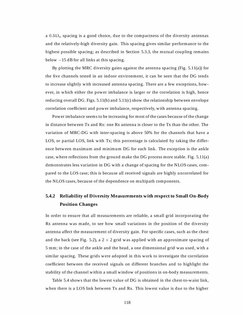
a 0.34λo spacing is a good choice, due to the compactness of the diversity antennas
and the relatively-high diversity gain. This spacing gives similar performance to the
highest possible spacing; as described in Section 5.3.3, the mutual coupling remains
below −15 dB for all links at this spacing.
By plotting the MRC diversity gains against the antenna spacing (Fig. 5.11(a)) for
the five channels tested in an indoor environment, it can be seen that the DG tends
to increase slightly with increased antenna spacing. There are a few exceptions, how-
ever, in which either the power imbalance is larger or the correlation is high, hence
reducing overall DG. Figs. 5.11(b) and 5.11(c) show the relationship between envelope
correlation coefficient and power imbalance, respectively, with antenna spacing.
Power imbalance seems to be increasing for most of the cases because of the change
in distance between Tx and Rx: one Rx antenna is closer to the Tx than the other. The
variation of MRC-DG with inter-spacing is above 50% for the channels that have a
LOS, or partial LOS, link with Tx; this percentage is calculated by taking the differ-
ence between maximum and minimum DG for each link. The exception is the ankle
case, where reflections from the ground make the DG process more stable. Fig. 5.11(a)
demonstrates less variation in DG with a change of spacing for the NLOS cases, com-
pared to the LOS case; this is because all received signals are highly uncorrelated for
the NLOS cases, because of the dependence on multipath components.
5.4.2 Reliability of Diversity Measurements with respect to Small On-Body
Position Changes
In order to ensure that all measurements are reliable, a small grid incorporating the
Rx antenna was made, to see how small variations in the position of the diversity
antenna affect the measurement of diversity gain. For specific cases, such as the chest
and the back (see Fig. 5.2), a 2 × 2 grid was applied with an approximate spacing of
5 mm; in the case of the ankle and the head, a one dimensional grid was used, with a
similar spacing. These grids were adopted in this work to investigate the correlation
coefficient between the received signals on different branches and to highlight the
stability of the channel within a small window of positions in on-body measurements.
Table 5.4 shows that the lowest value of DG is obtained in the chest-to-waist link,
when there is a LOS link between Tx and Rx. This lowest value is due to the higher
118
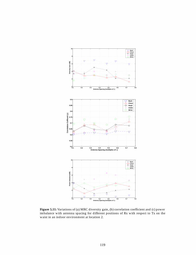
0.1 0.2 0.3 0.4 0.5 0.6 0.7 0.80
2
4
6
8
10
Antenna Spacing (multiples of λ)
Div
ersi
ty G
ain
(d
B)
BackChestHeadAnkleWrist
0.1 0.2 0.3 0.4 0.5 0.6 0.7 0.80.5
0.55
0.6
0.65
0.7
0.75
0.8
0.85
0.9
Antenna Spacing (multiples of λ)
Co
rrel
atio
n C
off
icen
t (ρ
)
BackChestHeadAnkleWrist
0.1 0.2 0.3 0.4 0.5 0.6 0.7 0.80
2
4
6
8
10
Antenna Spacing (multiples of λ)
Po
wer
Imb
alan
ce(d
B)
BackChestHeadAnkleWrist
Figure 5.11: Variations of (a) MRC diversity gain, (b) correlation coefficient and (c) powerimbalance with antenna spacing for different positions of Rx with respect to Tx on thewaist in an indoor environment at location 2.
119
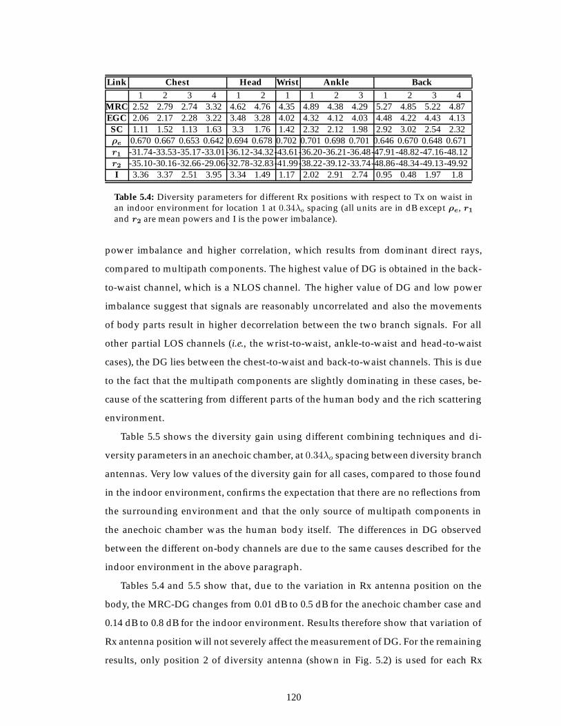
Link Chest Head Wrist Ankle Back1 2 3 4 1 2 1 1 2 3 1 2 3 4
MRC 2.52 2.79 2.74 3.32 4.62 4.76 4.35 4.89 4.38 4.29 5.27 4.85 5.22 4.87EGC 2.06 2.17 2.28 3.22 3.48 3.28 4.02 4.32 4.12 4.03 4.48 4.22 4.43 4.13SC 1.11 1.52 1.13 1.63 3.3 1.76 1.42 2.32 2.12 1.98 2.92 3.02 2.54 2.32ρe 0.670 0.667 0.653 0.642 0.694 0.678 0.702 0.701 0.698 0.701 0.646 0.670 0.648 0.671r1 -31.74-33.53-35.17-33.01-36.12-34.32-43.61-36.20-36.21-36.48-47.91-48.82-47.16-48.12r2 -35.10-30.16-32.66-29.06-32.78-32.83-41.99-38.22-39.12-33.74-48.86-48.34-49.13-49.92I 3.36 3.37 2.51 3.95 3.34 1.49 1.17 2.02 2.91 2.74 0.95 0.48 1.97 1.8
Table 5.4: Diversity parameters for different Rx positions with respect to Tx on waist inan indoor environment for location 1 at 0.34λo spacing (all units are in dB except ρe, r1and r2 are mean powers and I is the power imbalance).
power imbalance and higher correlation, which results from dominant direct rays,
compared to multipath components. The highest value of DG is obtained in the back-
to-waist channel, which is a NLOS channel. The higher value of DG and low power
imbalance suggest that signals are reasonably uncorrelated and also the movements
of body parts result in higher decorrelation between the two branch signals. For all
other partial LOS channels (i.e., the wrist-to-waist, ankle-to-waist and head-to-waist
cases), the DG lies between the chest-to-waist and back-to-waist channels. This is due
to the fact that the multipath components are slightly dominating in these cases, be-
cause of the scattering from different parts of the human body and the rich scattering
environment.
Table 5.5 shows the diversity gain using different combining techniques and di-
versity parameters in an anechoic chamber, at 0.34λo spacing between diversity branch
antennas. Very low values of the diversity gain for all cases, compared to those found
in the indoor environment, confirms the expectation that there are no reflections from
the surrounding environment and that the only source of multipath components in
the anechoic chamber was the human body itself. The differences in DG observed
between the different on-body channels are due to the same causes described for the
indoor environment in the above paragraph.
Tables 5.4 and 5.5 show that, due to the variation in Rx antenna position on the
body, the MRC-DG changes from 0.01 dB to 0.5 dB for the anechoic chamber case and
0.14 dB to 0.8 dB for the indoor environment. Results therefore show that variation of
Rx antenna position will not severely affect the measurement of DG. For the remaining
results, only position 2 of diversity antenna (shown in Fig. 5.2) is used for each Rx
120
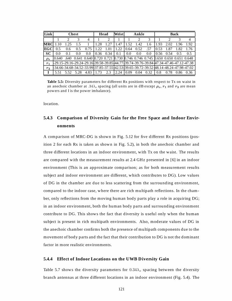
Link Chest Head Wrist Ankle Back1 2 3 4 1 2 1 1 2 3 1 2 3 4
MRC 1.10 1.25 1.5 1 1.28 1.27 1.47 1.52 1.42 1.6 1.93 2.02 1.96 1.92EGC 0.5 0.6 0.5 0.75 1.22 1.01 1.22 0.64 0.52 .57 0.53 1.87 1.82 1.76SC 0.0 0.1 0.0 0.0 0.36 0.34 0.1 0.0 0.0 0.0 0.56 0.54 0.5 0.5ρe 0.640 .640 0.641 0.640 0.720 0.721 0.730 0.746 0.746 0.745 0.650 0.650 0.651 0.648r1 -29.15-29.16-29.24-29.16-39.58-39.85-44.77-39.74-39.76-39.84-47.34-47.46-47.12-47.38r2 -34.66-34.68-34.52-33.99-37.85-37.55-42.53-39.65-39.72-39.52-48.14-48.24-47.98-47.02I 5.51 5.52 5.28 4.83 1.73 2.3 2.24 0.09 0.04 0.32 0.8 0.78 0.86 0.36
Table 5.5: Diversity parameters for different Rx positions with respect to Tx on waist inan anechoic chamber at .34λo spacing (all units are in dB except ρe, r1 and r2 are meanpowers and I is the power imbalance).
location.
5.4.3 Comparison of Diversity Gain for the Free Space and Indoor Envir-
onments
A comparison of MRC-DG is shown in Fig. 5.12 for five different Rx positions (pos-
ition 2 for each Rx is taken as shown in Fig. 5.2), in both the anechoic chamber and
three different locations in an indoor environment, with Tx on the waist. The results
are compared with the measurement results at 2.4 GHz presented in [6] in an indoor
environment (This is an approximate comparison; as for both measurement results
subject and indoor environment are different, which contributes to DG). Low values
of DG in the chamber are due to less scattering from the surrounding environment,
compared to the indoor case, where there are rich multipath reflections. In the cham-
ber, only reflections from the moving human body parts play a role in acquiring DG;
in an indoor environment, both the human body parts and surrounding environment
contribute to DG. This shows the fact that diversity is useful only when the human
subject is present in rich multipath environments. Also, moderate values of DG in
the anechoic chamber confirms both the presence of multipath components due to the
movement of body parts and the fact that their contribution to DG is not the dominant
factor in more realistic environments.
5.4.4 Effect of Indoor Locations on the UWB Diversity Gain
Table 5.7 shows the diversity parameters for 0.34λo spacing between the diversity
branch antennas at three different locations in an indoor environment (Fig. 5.4). The
121
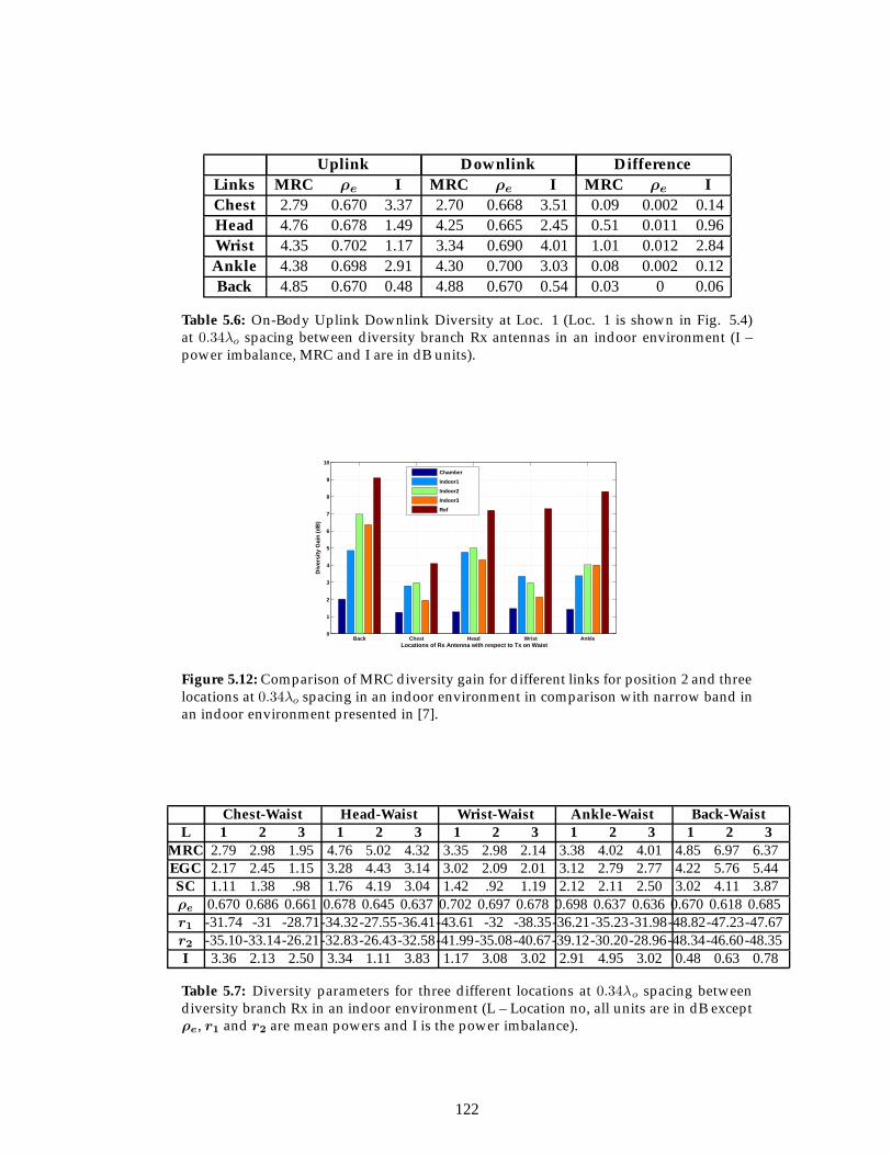
Uplink Downlink DifferenceLinks MRC ρe I MRC ρe I MRC ρe IChest 2.79 0.670 3.37 2.70 0.668 3.51 0.09 0.002 0.14Head 4.76 0.678 1.49 4.25 0.665 2.45 0.51 0.011 0.96Wrist 4.35 0.702 1.17 3.34 0.690 4.01 1.01 0.012 2.84Ankle 4.38 0.698 2.91 4.30 0.700 3.03 0.08 0.002 0.12Back 4.85 0.670 0.48 4.88 0.670 0.54 0.03 0 0.06
Table 5.6: On-Body Uplink Downlink Diversity at Loc. 1 (Loc. 1 is shown in Fig. 5.4)at 0.34λo spacing between diversity branch Rx antennas in an indoor environment (I –power imbalance, MRC and I are in dB units).
Back Chest Head Wrist Ankle0
1
2
3
4
5
6
7
8
9
10
Locations of Rx Antenna with respect to Tx on Waist
Div
ersi
ty G
ain
(d
B)
Chamber
Indoor1
Indoor2
Indoor3
Ref
Figure 5.12: Comparison of MRC diversity gain for different links for position 2 and threelocations at 0.34λo spacing in an indoor environment in comparison with narrow band inan indoor environment presented in [7].
Chest-Waist Head-Waist Wrist-Waist Ankle-Waist Back-WaistL 1 2 3 1 2 3 1 2 3 1 2 3 1 2 3
MRC 2.79 2.98 1.95 4.76 5.02 4.32 3.35 2.98 2.14 3.38 4.02 4.01 4.85 6.97 6.37EGC 2.17 2.45 1.15 3.28 4.43 3.14 3.02 2.09 2.01 3.12 2.79 2.77 4.22 5.76 5.44SC 1.11 1.38 .98 1.76 4.19 3.04 1.42 .92 1.19 2.12 2.11 2.50 3.02 4.11 3.87ρe 0.670 0.686 0.661 0.678 0.645 0.637 0.702 0.697 0.678 0.698 0.637 0.636 0.670 0.618 0.685r1 -31.74 -31 -28.71-34.32-27.55-36.41-43.61 -32 -38.35-36.21-35.23-31.98-48.82-47.23-47.67r2 -35.10-33.14-26.21-32.83-26.43-32.58-41.99-35.08-40.67-39.12-30.20-28.96-48.34-46.60-48.35I 3.36 2.13 2.50 3.34 1.11 3.83 1.17 3.08 3.02 2.91 4.95 3.02 0.48 0.63 0.78
Table 5.7: Diversity parameters for three different locations at 0.34λo spacing betweendiversity branch Rx in an indoor environment (L – Location no, all units are in dB exceptρe, r1 and r2 are mean powers and I is the power imbalance).
122
highest DG values are obtained for location 2, because the subject is close to the walls
and pillar in this case, leading to stronger multipath reflections. The wrist-to-waist
channel is the exception: here, DG is low, compared to other locations, due to the
higher power imbalance and higher correlation in this case, as the wrist was very
close to the wall.
The highest value of DG (i.e., 6.97 dB using MRC) is obtained for the back-to-waist
link (NLOS case), compared to the other links for location 2. The higher value of DG
and lower power imbalance (0.63 dB) for the back-to-waist link suggests that signals
are reasonably uncorrelated and also that movements of body parts result in a higher
decorrelation between the two branch signals. The same reasoning as described in
Section 5.4.2 can be applied to account for DG variation for all other links.
The results obtained for UWB on-body diversity at location 2 are compared with
the results of Khan et al. at 2.4 GHz presented in [7] in an indoor environment (com-
parison plot is shown in Fig. 5.12). This is an approximate comparison; as for both
measurement results, human subject and indoor environment were different). Results
approximately agree for the chest-to-waist link (where there is direct LOS communic-
ation between Tx and Rx). However, there is disagreement for partial LOS cases and
NLOS case (i.e., the head-to-waist, wrist-to-waist and back-to-waist links); this is due
to the fact that, for NLOS cases, the reflections and contributions by the environment
have a large effect on the quality of the signal and the measurements were done in dif-
ferent environments. In addition, the subject-specific behaviour of the UWB on-body
channel (see, for example, the work of Sani et al. [8]) will also play role in explaining
the disagreement between the results.
5.4.5 Conclusion
Spatial diversity techniques for ultra wideband on-body radio channels have been in-
vestigated and analysed. Various scenarios, including changes in antenna on-body
positions, the location of subject in the indoor environment and also variation in
the inter-spacing between antenna element branches, have been considered. Results
showed that, for dense multipath environments, the benefits of applying diversity
techniques were significant for the non-line-of-sight cases, where there are low power
imbalances due to uncorrelated signals, in comparison to the line-of-sight scenarios.
123
Maximum variations of 0.5 dB and 0.8 dB, for the anechoic chamber and the indoor
environment cases, respectively, have been observed in response to slight changes in
the on-body antenna position. This demonstrated the potentially negligible effect of
accidental and inherited on-body element location shift due to the subject’s sudden
movement. The results presented here gave indications of the beneficial applications
of diversity antenna techniques for potential performance enhancement of UWB body-
centric wireless communications as experienced in narrowband technologies. This
will be increasingly appreciated for off-body communications, due to the variation in
the spatial and angular parameters of the multipath components that will contribute
to enhanced diversity gain. Hence in the next section UWB off-body spatial diversity
is being investigated.
5.5 UWB Off-Body Diversity Performance Analysis
5.5.1 Reliability of Diversity Measurements vs. Small variations in on-
body Diversity Receiver Position
In order to ensure that all measurements are reliable, for each channel a small grid
incorporating in the Rx antenna was made to see how the small variation in position
of diversity antenna will affect the measurement of diversity gain. For specific cases
such as the chest and the back (see Fig. 5.3), a 2 × 2 grid was applied with approximate
spacing of 5 mm and in the case for the ankle and the head a one dimensional grid
was used with similar spacing. Table 5.8 shows diversity gain (DG) values based
on different combining techniques, envelope correlation (ρe) and power imbalance
between two branches for Loc. 2 in an indoor environment (as shown in Fig. 5.5)
at 0.34λo spacing between diversity branch antennas (whereas, power imbalance is
calculated by using the ratio of mean power of two branch signal envelopes).
Results show that the value of DG are lower, when Rx is placed at chest and ankle
as compared to other links, because there is a direct LOS link between Tx and Rx.
Higher power imbalance and relatively higher value of correlation are the factor that
plays a role in reducing diversity gain. The highest value of DG is obtained in NLOS
channel i.e. when Rx is placed at the back. Higher value of DG and low power im-
balance suggest that movements of body parts result in higher decorrelation between
124
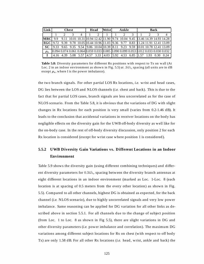
Link Chest Head Wrist Ankle Back1 2 3 4 1 2 1 1 2 3 1 2 3 4
MRC 9.9 9.11 10.01 10.31 10.94 12.42 11.90 9.74 10.04 9.45 13.46 14.39 14.93 14.28EGC 9.72 9.39 9.78 10.05 10.44 10.96 11.03 9.36 9.77 8.83 11.24 11.91 12.41 13.09SC 9.33 9.65 9.35 9.54 9.86 10.04 10.39 8.11 9.23 9.59 10.01 10.78 12.41 13.09ρe 0.094 0.074 0.061 0.064 0.059 0.033 0.085 0.090 0.099 0.053 0.012 0.033 0.030 0.032I 4.16 4.39 5.08 5.57 4.57 3.33 4.03 5.92 4.53 6.85 1.57 1.93 0.30 0.24
Table 5.8: Diversity parameters for different Rx positions with respect to Tx on wall (AtLoc. 2 in an indoor environment as shown in Fig. 5.5) at .34λo spacing (all units are in dBexcept ρe, where I is the power imbalance).
the two branch signals. For other partial LOS Rx locations, i.e. wrist and head cases,
DG lies between the LOS and NLOS channels (i.e. chest and back). This is due to the
fact that for partial LOS cases, branch signals are less uncorrelated as for the case of
NLOS scenario. From the Table 5.8, it is obvious that the variations of DG with slight
changes in Rx locations for each position is very small (varies from 0.2-1.46 dB). It
leads to the conclusion that accidental variations in receiver locations on the body has
negligible effects on the diversity gain for the UWB off-body diversity as well like for
the on-body case. In the rest of off-body diversity discussion, only position 2 for each
Rx location is considered (except for wrist case where position 1 is considered).
5.5.2 UWB Diversity Gain Variations vs. Different Locations in an Indoor
Environment
Table 5.9 shows the diversity gain (using different combining techniques) and differ-
ent diversity parameters for 0.34λo spacing between the diversity branch antennas at
eight different locations in an indoor environment (marked as Loc. 1-Loc. 8 (each
location is at spacing of 0.5 meters from the every other location) as shown in Fig.
5.5). Compared to all other channels, highest DG is obtained as expected, for the back
channel (i.e. NLOS scenario), due to highly uncorrelated signals and very low power
imbalance. Same reasoning can be applied for DG variation for all other links as de-
scribed above in section 5.5.1. For all channels due to the change of subject position
(from Loc. 1 to Loc. 8 as shown in Fig 5.5), there are slight variations in DG and
other diversity parameters (i.e. power imbalance and correlation). The maximum DG
variations among different subject locations for Rx on chest (with respect to off body
Tx) are only 1.58 dB. For all other Rx locations (i.e. head, wrist, ankle and back) the
125
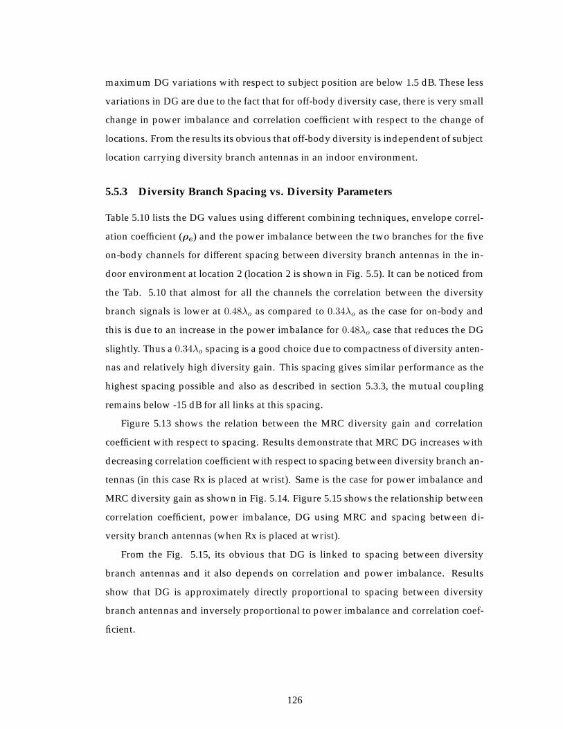
maximum DG variations with respect to subject position are below 1.5 dB. These less
variations in DG are due to the fact that for off-body diversity case, there is very small
change in power imbalance and correlation coefficient with respect to the change of
locations. From the results its obvious that off-body diversity is independent of subject
location carrying diversity branch antennas in an indoor environment.
5.5.3 Diversity Branch Spacing vs. Diversity Parameters
Table 5.10 lists the DG values using different combining techniques, envelope correl-
ation coefficient (ρe) and the power imbalance between the two branches for the five
on-body channels for different spacing between diversity branch antennas in the in-
door environment at location 2 (location 2 is shown in Fig. 5.5). It can be noticed from
the Tab. 5.10 that almost for all the channels the correlation between the diversity
branch signals is lower at 0.48λo as compared to 0.34λo as the case for on-body and
this is due to an increase in the power imbalance for 0.48λo case that reduces the DG
slightly. Thus a 0.34λo spacing is a good choice due to compactness of diversity anten-
nas and relatively high diversity gain. This spacing gives similar performance as the
highest spacing possible and also as described in section 5.3.3, the mutual coupling
remains below -15 dB for all links at this spacing.
Figure 5.13 shows the relation between the MRC diversity gain and correlation
coefficient with respect to spacing. Results demonstrate that MRC DG increases with
decreasing correlation coefficient with respect to spacing between diversity branch an-
tennas (in this case Rx is placed at wrist). Same is the case for power imbalance and
MRC diversity gain as shown in Fig. 5.14. Figure 5.15 shows the relationship between
correlation coefficient, power imbalance, DG using MRC and spacing between di-
versity branch antennas (when Rx is placed at wrist).
From the Fig. 5.15, its obvious that DG is linked to spacing between diversity
branch antennas and it also depends on correlation and power imbalance. Results
show that DG is approximately directly proportional to spacing between diversity
branch antennas and inversely proportional to power imbalance and correlation coef-
ficient.
126
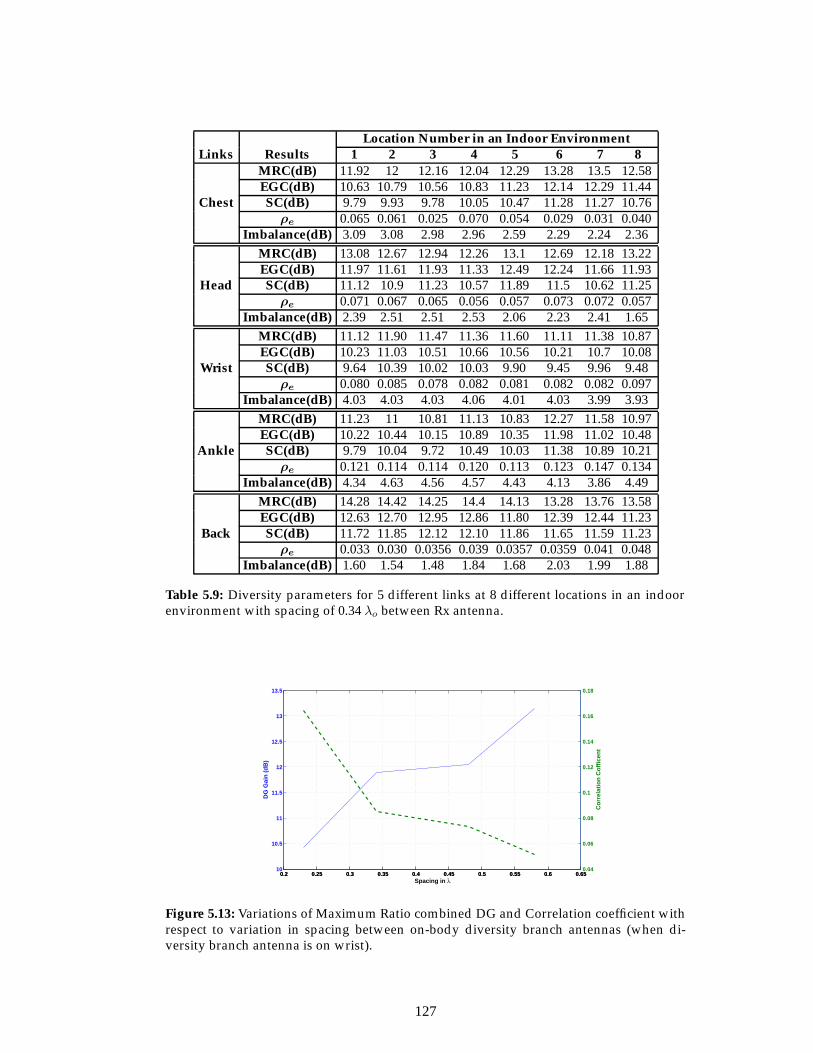
Location Number in an Indoor EnvironmentLinks Results 1 2 3 4 5 6 7 8
Chest
MRC(dB) 11.92 12 12.16 12.04 12.29 13.28 13.5 12.58EGC(dB) 10.63 10.79 10.56 10.83 11.23 12.14 12.29 11.44SC(dB) 9.79 9.93 9.78 10.05 10.47 11.28 11.27 10.76
ρe 0.065 0.061 0.025 0.070 0.054 0.029 0.031 0.040Imbalance(dB) 3.09 3.08 2.98 2.96 2.59 2.29 2.24 2.36
Head
MRC(dB) 13.08 12.67 12.94 12.26 13.1 12.69 12.18 13.22EGC(dB) 11.97 11.61 11.93 11.33 12.49 12.24 11.66 11.93SC(dB) 11.12 10.9 11.23 10.57 11.89 11.5 10.62 11.25
ρe 0.071 0.067 0.065 0.056 0.057 0.073 0.072 0.057Imbalance(dB) 2.39 2.51 2.51 2.53 2.06 2.23 2.41 1.65
Wrist
MRC(dB) 11.12 11.90 11.47 11.36 11.60 11.11 11.38 10.87EGC(dB) 10.23 11.03 10.51 10.66 10.56 10.21 10.7 10.08SC(dB) 9.64 10.39 10.02 10.03 9.90 9.45 9.96 9.48
ρe 0.080 0.085 0.078 0.082 0.081 0.082 0.082 0.097Imbalance(dB) 4.03 4.03 4.03 4.06 4.01 4.03 3.99 3.93
Ankle
MRC(dB) 11.23 11 10.81 11.13 10.83 12.27 11.58 10.97EGC(dB) 10.22 10.44 10.15 10.89 10.35 11.98 11.02 10.48SC(dB) 9.79 10.04 9.72 10.49 10.03 11.38 10.89 10.21
ρe 0.121 0.114 0.114 0.120 0.113 0.123 0.147 0.134Imbalance(dB) 4.34 4.63 4.56 4.57 4.43 4.13 3.86 4.49
Back
MRC(dB) 14.28 14.42 14.25 14.4 14.13 13.28 13.76 13.58EGC(dB) 12.63 12.70 12.95 12.86 11.80 12.39 12.44 11.23SC(dB) 11.72 11.85 12.12 12.10 11.86 11.65 11.59 11.23
ρe 0.033 0.030 0.0356 0.039 0.0357 0.0359 0.041 0.048Imbalance(dB) 1.60 1.54 1.48 1.84 1.68 2.03 1.99 1.88
Table 5.9: Diversity parameters for 5 different links at 8 different locations in an indoorenvironment with spacing of 0.34 λo between Rx antenna.
0.2 0.25 0.3 0.35 0.4 0.45 0.5 0.55 0.6 0.6510
10.5
11
11.5
12
12.5
13
13.5
Spacing in λ
DG
Gai
n (
dB
)
0.2 0.25 0.3 0.35 0.4 0.45 0.5 0.55 0.6 0.650.04
0.06
0.08
0.1
0.12
0.14
0.16
0.18
Co
rrel
atio
n C
off
icen
t
Figure 5.13: Variations of Maximum Ratio combined DG and Correlation coefficient withrespect to variation in spacing between on-body diversity branch antennas (when di-versity branch antenna is on wrist).
127
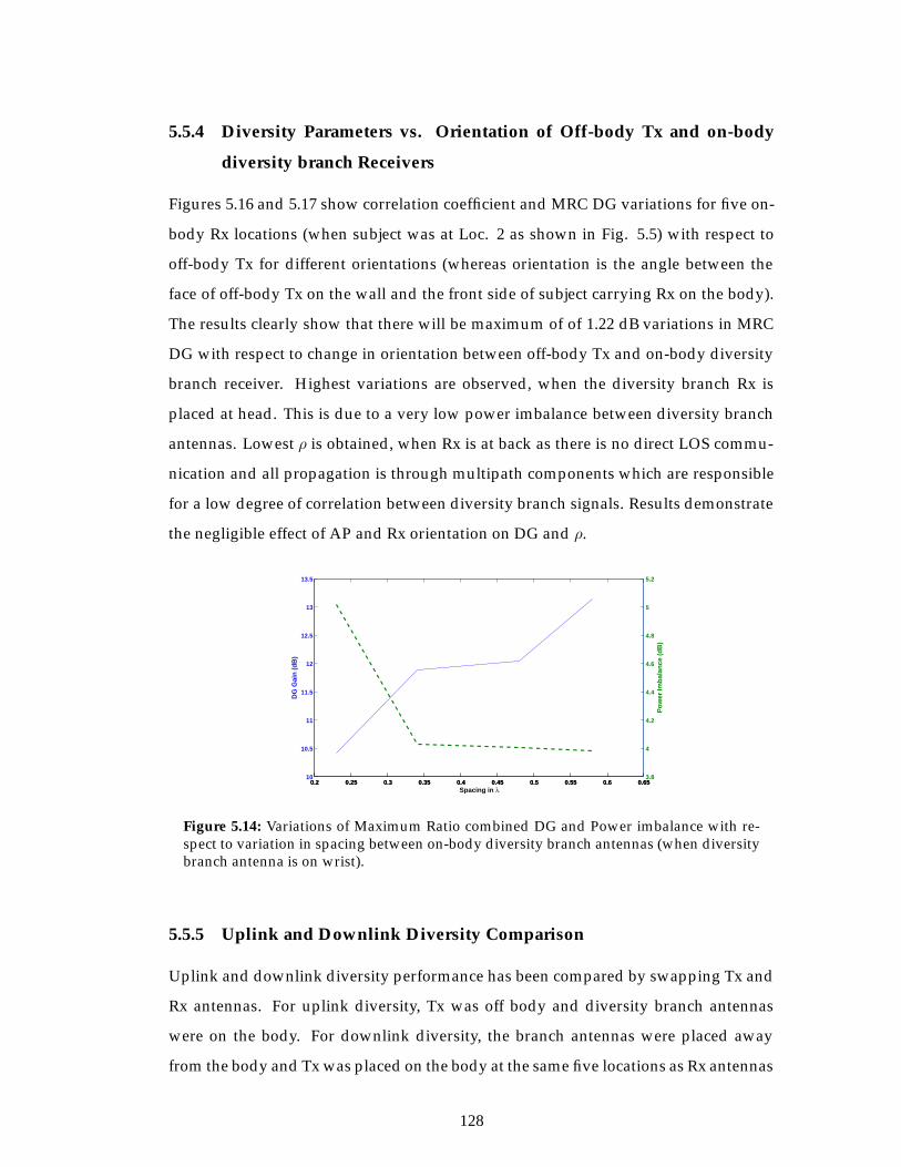
5.5.4 Diversity Parameters vs. Orientation of Off-body Tx and on-body
diversity branch Receivers
Figures 5.16 and 5.17 show correlation coefficient and MRC DG variations for five on-
body Rx locations (when subject was at Loc. 2 as shown in Fig. 5.5) with respect to
off-body Tx for different orientations (whereas orientation is the angle between the
face of off-body Tx on the wall and the front side of subject carrying Rx on the body).
The results clearly show that there will be maximum of of 1.22 dB variations in MRC
DG with respect to change in orientation between off-body Tx and on-body diversity
branch receiver. Highest variations are observed, when the diversity branch Rx is
placed at head. This is due to a very low power imbalance between diversity branch
antennas. Lowest ρ is obtained, when Rx is at back as there is no direct LOS commu-
nication and all propagation is through multipath components which are responsible
for a low degree of correlation between diversity branch signals. Results demonstrate
the negligible effect of AP and Rx orientation on DG and ρ.
0.2 0.25 0.3 0.35 0.4 0.45 0.5 0.55 0.6 0.6510
10.5
11
11.5
12
12.5
13
13.5
Spacing in λ
DG
Gai
n (
dB
)
0.2 0.25 0.3 0.35 0.4 0.45 0.5 0.55 0.6 0.653.8
4
4.2
4.4
4.6
4.8
5
5.2
Po
wer
Imb
alan
ce (
dB
)
Figure 5.14: Variations of Maximum Ratio combined DG and Power imbalance with re-spect to variation in spacing between on-body diversity branch antennas (when diversitybranch antenna is on wrist).
5.5.5 Uplink and Downlink Diversity Comparison
Uplink and downlink diversity performance has been compared by swapping Tx and
Rx antennas. For uplink diversity, Tx was off body and diversity branch antennas
were on the body. For downlink diversity, the branch antennas were placed away
from the body and Tx was placed on the body at the same five locations as Rx antennas
128
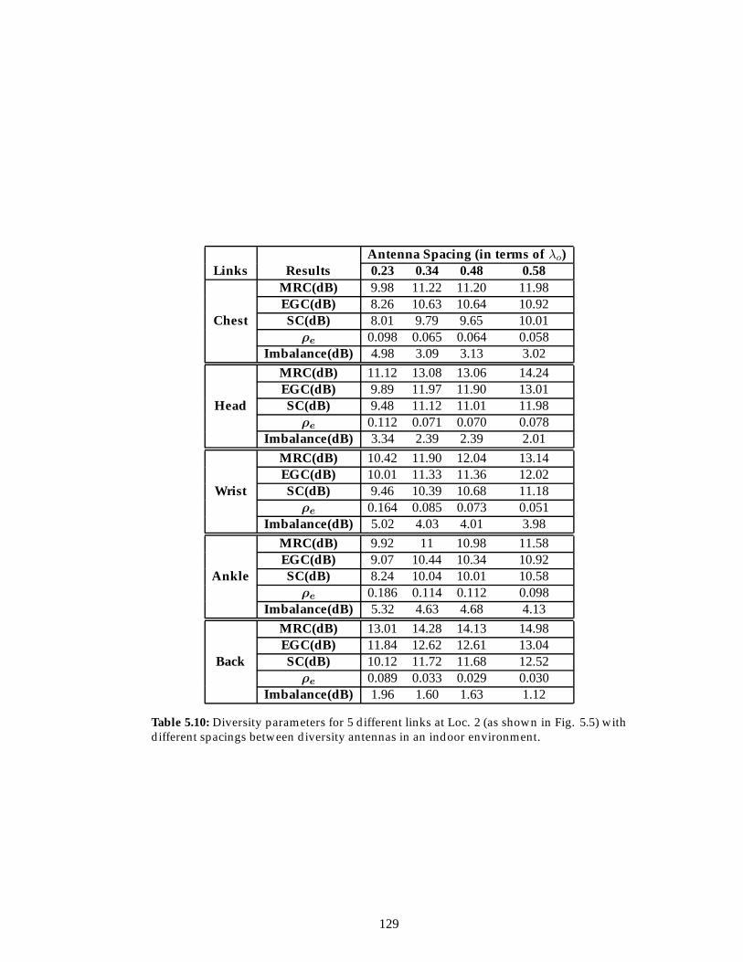
Antenna Spacing (in terms of λo)Links Results 0.23 0.34 0.48 0.58
Chest
MRC(dB) 9.98 11.22 11.20 11.98EGC(dB) 8.26 10.63 10.64 10.92SC(dB) 8.01 9.79 9.65 10.01
ρe 0.098 0.065 0.064 0.058Imbalance(dB) 4.98 3.09 3.13 3.02
Head
MRC(dB) 11.12 13.08 13.06 14.24EGC(dB) 9.89 11.97 11.90 13.01SC(dB) 9.48 11.12 11.01 11.98
ρe 0.112 0.071 0.070 0.078Imbalance(dB) 3.34 2.39 2.39 2.01
Wrist
MRC(dB) 10.42 11.90 12.04 13.14EGC(dB) 10.01 11.33 11.36 12.02SC(dB) 9.46 10.39 10.68 11.18
ρe 0.164 0.085 0.073 0.051Imbalance(dB) 5.02 4.03 4.01 3.98
Ankle
MRC(dB) 9.92 11 10.98 11.58EGC(dB) 9.07 10.44 10.34 10.92SC(dB) 8.24 10.04 10.01 10.58
ρe 0.186 0.114 0.112 0.098Imbalance(dB) 5.32 4.63 4.68 4.13
Back
MRC(dB) 13.01 14.28 14.13 14.98EGC(dB) 11.84 12.62 12.61 13.04SC(dB) 10.12 11.72 11.68 12.52
ρe 0.089 0.033 0.029 0.030Imbalance(dB) 1.96 1.60 1.63 1.12
Table 5.10: Diversity parameters for 5 different links at Loc. 2 (as shown in Fig. 5.5) withdifferent spacings between diversity antennas in an indoor environment.
129
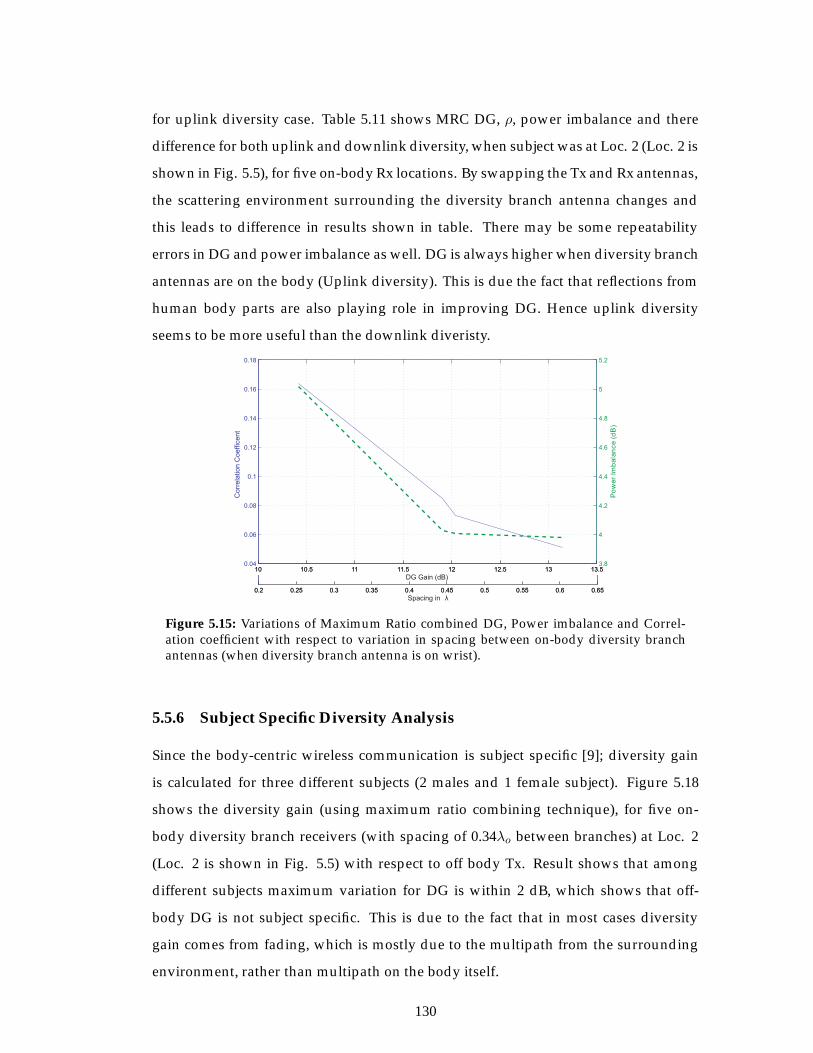
for uplink diversity case. Table 5.11 shows MRC DG, ρ, power imbalance and there
difference for both uplink and downlink diversity, when subject was at Loc. 2 (Loc. 2 is
shown in Fig. 5.5), for five on-body Rx locations. By swapping the Tx and Rx antennas,
the scattering environment surrounding the diversity branch antenna changes and
this leads to difference in results shown in table. There may be some repeatability
errors in DG and power imbalance as well. DG is always higher when diversity branch
antennas are on the body (Uplink diversity). This is due the fact that reflections from
human body parts are also playing role in improving DG. Hence uplink diversity
seems to be more useful than the downlink diveristy.
0.2 0.25 0.3 0.35 0.4 0.45 0.5 0.55 0.6 0.65
Spacing in λ0.2 0.25 0.3 0.35 0.4 0.45 0.5 0.55 0.6 0.65
10 10.5 11 11.5 12 12.5 13 13.50.04
0.06
0.08
0.1
0.12
0.14
0.16
0.18
DG Gain (dB)
Co
rre
latio
n C
oe
ffic
en
t
10 10.5 11 11.5 12 12.5 13 13.53.8
4
4.2
4.4
4.6
4.8
5
5.2
Figure 5.15: Variations of Maximum Ratio combined DG, Power imbalance and Correl-ation coefficient with respect to variation in spacing between on-body diversity branchantennas (when diversity branch antenna is on wrist).
5.5.6 Subject Specific Diversity Analysis
Since the body-centric wireless communication is subject specific [9]; diversity gain
is calculated for three different subjects (2 males and 1 female subject). Figure 5.18
shows the diversity gain (using maximum ratio combining technique), for five on-
body diversity branch receivers (with spacing of 0.34λo between branches) at Loc. 2
(Loc. 2 is shown in Fig. 5.5) with respect to off body Tx. Result shows that among
different subjects maximum variation for DG is within 2 dB, which shows that off-
body DG is not subject specific. This is due to the fact that in most cases diversity
gain comes from fading, which is mostly due to the multipath from the surrounding
environment, rather than multipath on the body itself.
130
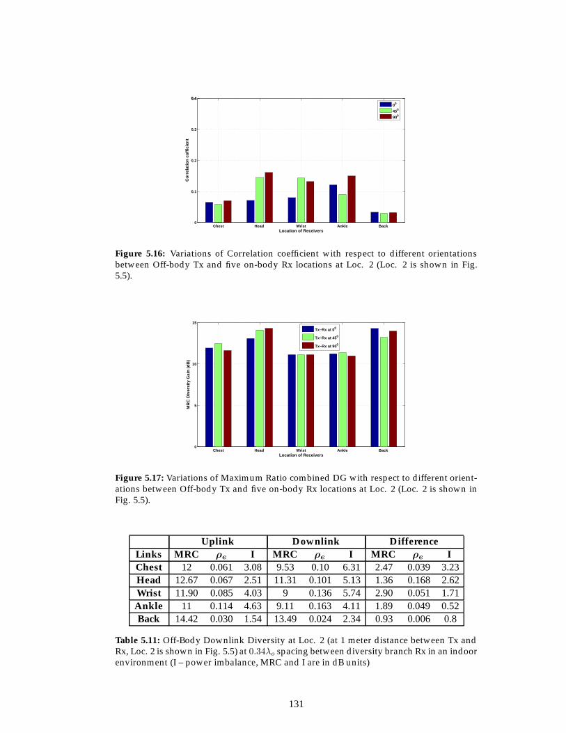
Chest Head Wrist Ankle Back 0
0.1
0.2
0.3
0.40.4
Location of Receivers
Co
rrel
atio
n c
off
icie
nt
00
450
900
Figure 5.16: Variations of Correlation coefficient with respect to different orientationsbetween Off-body Tx and five on-body Rx locations at Loc. 2 (Loc. 2 is shown in Fig.5.5).
Chest Head Wrist Ankle Back 0
5
10
15
Location of Receivers
MR
C D
iver
sity
Gai
n (
dB
)
Tx−Rx at 00
Tx−Rx at 450
Tx−Rx at 900
Figure 5.17: Variations of Maximum Ratio combined DG with respect to different orient-ations between Off-body Tx and five on-body Rx locations at Loc. 2 (Loc. 2 is shown inFig. 5.5).
Uplink Downlink DifferenceLinks MRC ρe I MRC ρe I MRC ρe IChest 12 0.061 3.08 9.53 0.10 6.31 2.47 0.039 3.23Head 12.67 0.067 2.51 11.31 0.101 5.13 1.36 0.168 2.62Wrist 11.90 0.085 4.03 9 0.136 5.74 2.90 0.051 1.71Ankle 11 0.114 4.63 9.11 0.163 4.11 1.89 0.049 0.52Back 14.42 0.030 1.54 13.49 0.024 2.34 0.93 0.006 0.8
Table 5.11: Off-Body Downlink Diversity at Loc. 2 (at 1 meter distance between Tx andRx, Loc. 2 is shown in Fig. 5.5) at 0.34λo spacing between diversity branch Rx in an indoorenvironment (I – power imbalance, MRC and I are in dB units)
131
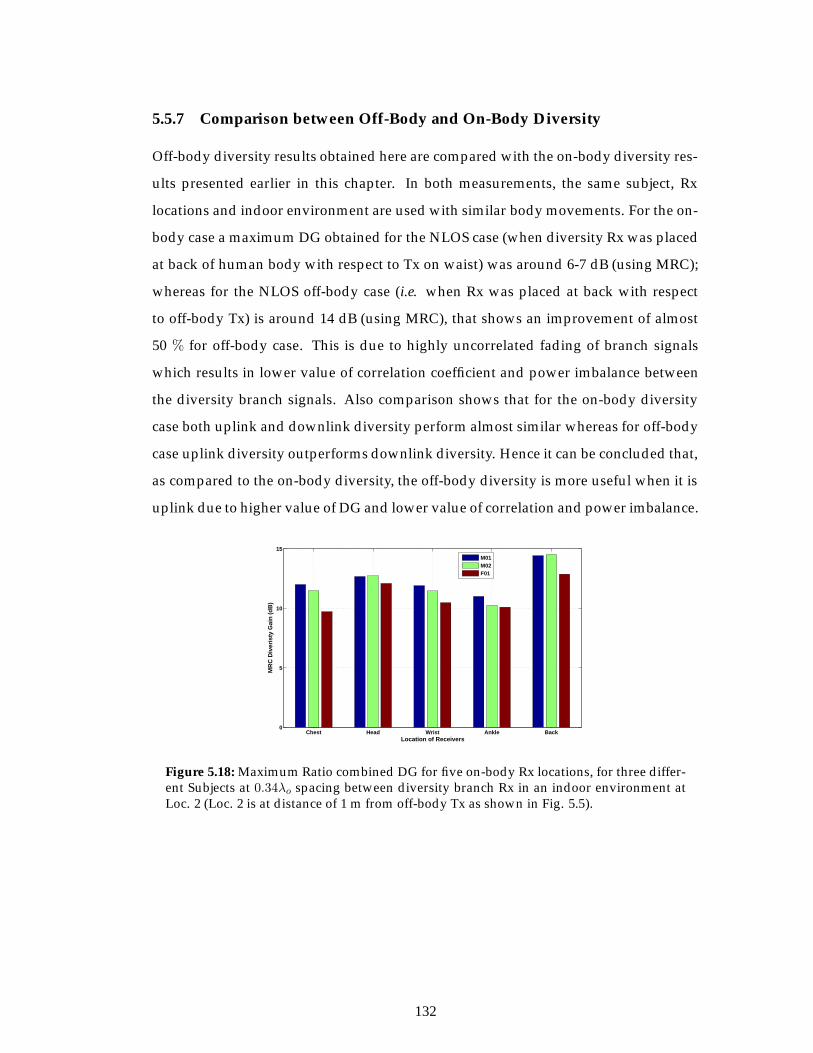
5.5.7 Comparison between Off-Body and On-Body Diversity
Off-body diversity results obtained here are compared with the on-body diversity res-
ults presented earlier in this chapter. In both measurements, the same subject, Rx
locations and indoor environment are used with similar body movements. For the on-
body case a maximum DG obtained for the NLOS case (when diversity Rx was placed
at back of human body with respect to Tx on waist) was around 6-7 dB (using MRC);
whereas for the NLOS off-body case (i.e. when Rx was placed at back with respect
to off-body Tx) is around 14 dB (using MRC), that shows an improvement of almost
50 % for off-body case. This is due to highly uncorrelated fading of branch signals
which results in lower value of correlation coefficient and power imbalance between
the diversity branch signals. Also comparison shows that for the on-body diversity
case both uplink and downlink diversity perform almost similar whereas for off-body
case uplink diversity outperforms downlink diversity. Hence it can be concluded that,
as compared to the on-body diversity, the off-body diversity is more useful when it is
uplink due to higher value of DG and lower value of correlation and power imbalance.
Chest Head Wrist Ankle Back0
5
10
15
Location of Receivers
MR
C D
iver
isty
Gai
n (
dB
)
M01M02F01
Figure 5.18: Maximum Ratio combined DG for five on-body Rx locations, for three differ-ent Subjects at 0.34λo spacing between diversity branch Rx in an indoor environment atLoc. 2 (Loc. 2 is at distance of 1 m from off-body Tx as shown in Fig. 5.5).
132
5.5.8 Conclusion
Spatial diversity techniques for ultra wideband off-body radio channels have been
analysed. Various scenarios including changes in the on-body diversity branch an-
tenna positions, location of subject in the indoor environment, variation in the inter-
spacing between antenna elements, change of subject, uplink and downlink (i.e. swap-
ping of Tx and Rx) are considered. Results show that for rich multipath environment,
the diversity gain is higher for the non line-of-sight cases where there is low power
imbalance due to highly uncorrelated signals in comparison to the line-of-sight scen-
arios. Maximum variation of 1 dB has been observed due to slight changes in the
on-body antenna position. This demonstrates the potentially negligible effect of acci-
dental and inherited on-body element location shift due to sudden movement of the
subject.
Higher diversity gain were obtained as inter-spacing between diversity antenna
branches increased with a few exceptions where either the power imbalance or the
correlation is high. Small variations in DG due to changes in subject location within
the indoor environment and orientation between AP and on-body diversity receiver
shows that off-body diversity is independent of subject location and orientation in an
indoor environment. Results also demonstrate that off-body diversity is almost 50%
more efficient than on-body diversity and off-body diversity is more useful when it
is considered as uplink (i.e. diversity branch antennas are on-body with respect to
off-body Tx) as compared to downlink diversity.
5.6 Summary
Diversity for UWB body area networks is analysed, using various measurements scen-
arios. Diversity gain is calculated for five different on/off-body channels by plotting
cumulative distribution functions and it is found that diversity gain value is very low
for chamber due to no reflections from surroundings as compared to indoor environ-
ment. Also in indoor environment and chamber, diversity gain is lowest for line-of-
sight case. There are significant benefits of diversity techniques for non line-of-sight
case as compared to LOS cases due to low power imbalance and low correlation coef-
ficient between the branch signals. Comparison of on-body and off-body diversity
133
shows a significance improvement for the off-body case. It also reveals that the on-
body diversity has almost similar impact for both uplink and downlink diversity,
whereas uplink is preferable over downlink diversity for the off-body diversity case.
Analysis also shows that diversity gain is independent of subject specific behavior.
The results presented in this chapter gave indications of the beneficial applications
of diversity antenna techniques for potential performance enhancement of the ultra
wideband body-centric wireless communications.
134
References
[1] T. S. Rappaport, Wireless Communications Principles and Practice. Prentice Hall, Inc., NewJersey, 1996.
[2] W. C. Jakes, Microwave Mobile Communications. New York:Wiley, 1974.
[3] A. M. D. Turkmani, A. A. Arowojolu, P. A. Jefford, and C. J. Kellett, “An experimentalevaluation of the performance of two-branch space and polarization diversity schemes at1800 MHz,” IEEE Transactions On Vehicular Technology, vol. 44, no. 2, pp. 318–326, May1995.
[4] I. Khan and P. S. Hall, “Multiple antenna reception at 5.8 and 10 GHz for body-centricwireless communication channels,” IEEE Transactions on Antenna and Propagation, vol. 57,no. 1, pp. 248–255, Jan 2009.
[5] L. M. Correia, Mobile Broadband Multimedia Networks Techniques, Models and Tools for 4G.Elsevier Ltd, 2006.
[6] I. Khan, Diveristy and MIMO for Body-Centric Wireless Channels. Phd thesis, University ofBirmingham, Sep. 2009.
[7] I. Khan, P. S. Hall, A. A. Serra, A. R. Guraliuc, and P. Nepa, “Diversity performance ana-lysis for on-body communication channels at 2.45 GHz,” IEEE Transactions on Antenna andPropagation, vol. 57, no. 4, pp. 956–963, April 2009.
[8] A. Sani, Y. Hao, Y. Zhao, S. L. Lee, and G. Z. Yang, “A subject-specific numerical study inUWB body-centric wireless communications,” in Proceedings of the Fourth European Confer-ence on Antennas and Propagation (EuCAP), Barcelona, Spain, 12-16 Apr. 2010.
[9] A. Sani, Modeling and Characterisation of Antenna and Propagation for Body-Centric WirelessCommunications. PhD thesis, Queen Mary Uni. of London, 2010.
135
Chapter 6
Ultra Wideband Multiband-OFDM
based System Modelling and
Performance Evaluation for
Body-Centric Wireless
Communications
The wireless transceiver systems used in body-centric networks needs to have some
special and user friendly features including small and compact size and longer bat-
tery life. To design a suitable and efficient radio interface for the wireless body-centric
network, understanding of existing standards are required. The UWB radio front-end
could be used for the same applications as targeted for other short-range wireless sys-
tems; however, at higher data rates, with lower emitted Radio Frequency (RF) power
and less complexity in transceiver designs. In this chapter, system modelling and per-
formance evaluation of potential UWB radio transceivers for body-centric network is
proposed.
136
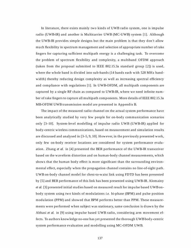
In literature, there exists mainly two kinds of UWB radio system, one is impulse
radio (UWB-IR) and another is Multicarrier UWB (MC-UWB) system [1]. Although
the UWB-IR provides simple designs but the main problem is that they don’t allow
much flexibility in spectrum management and selection of appropriate number of rake
fingers for capturing sufficient multipath energy is a challenging task. To overcome
the problem of spectrum flexibility and complexity, a multiband OFDM approach
(taken from the proposal submitted to IEEE 802.15.3a standard group [2]) is used,
where the whole band is divided into sub-bands (14 bands each with 528 MHz band-
width) thereby reducing design complexity as well as increasing spectral efficiency
and compliance with regulations [1]. In UWB-OFDM, all multipath components are
captured by a single RF chain as compared to UWB-IR, where we need infinite num-
ber of rake fingers to capture all multipath components. More details of IEEE 802.15.3a
MB-OFDM UWB transmission model are presented in Appendix B.
The impact of the measured radio channel on the actual system performance have
been analytically studied by very few people for on-body communication scenarios
only [3–10]. System-level modelling of impulse radio UWB (UWB-IR) applied for
body-centric wireless communications, based on measurement and simulation results
are discussed and analysed in [3–5, 9, 10]. However, in the previously presented work,
only few on-body receiver locations are considered for system performance evalu-
ation. Zhang et al. in [4] presented the BER performance of the UWB-IR transceiver
based on the waveform distortion and on human-body channel measurements, which
shows that the human body effect is more significant than the surrounding environ-
mental effect, especially when the propagation channel contains no line-of-sight path.
UWB on-body channel model for chest-to-waist link using FDTD has been presented
by [5] and BER performance of this link has been presented using UWB-IR. Alomainy
et al. [3] presented initial studies based on measured result for impulse based UWB on-
body system using two kinds of modulations i.e. bi-phase (BPM) and pulse position
modulation (PPM) and showed that BPM performs better than PPM. These measure-
ments were performed when subject was stationary, same conclusion is drawn by the
Abbasi et al. in [9] using impulse based UWB radio, considering arm movement ef-
fects. To authors knowledge no-one has yet presented the thorough UWB body-centric
system performance evaluation and modelling using MC-OFDM UWB.
137
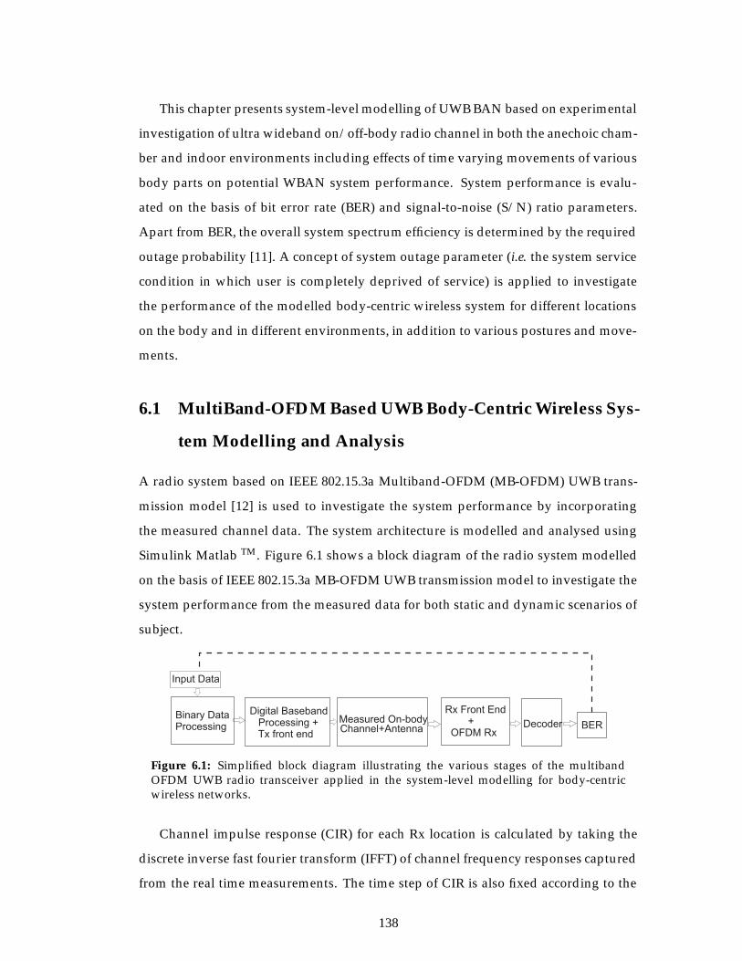
This chapter presents system-level modelling of UWB BAN based on experimental
investigation of ultra wideband on/off-body radio channel in both the anechoic cham-
ber and indoor environments including effects of time varying movements of various
body parts on potential WBAN system performance. System performance is evalu-
ated on the basis of bit error rate (BER) and signal-to-noise (S/N) ratio parameters.
Apart from BER, the overall system spectrum efficiency is determined by the required
outage probability [11]. A concept of system outage parameter (i.e. the system service
condition in which user is completely deprived of service) is applied to investigate
the performance of the modelled body-centric wireless system for different locations
on the body and in different environments, in addition to various postures and move-
ments.
6.1 MultiBand-OFDM Based UWB Body-Centric Wireless Sys-
tem Modelling and Analysis
A radio system based on IEEE 802.15.3a Multiband-OFDM (MB-OFDM) UWB trans-
mission model [12] is used to investigate the system performance by incorporating
the measured channel data. The system architecture is modelled and analysed using
Simulink Matlab TM. Figure 6.1 shows a block diagram of the radio system modelled
on the basis of IEEE 802.15.3a MB-OFDM UWB transmission model to investigate the
system performance from the measured data for both static and dynamic scenarios of
subject.
Figure 6.1: Simplified block diagram illustrating the various stages of the multibandOFDM UWB radio transceiver applied in the system-level modelling for body-centricwireless networks.
Channel impulse response (CIR) for each Rx location is calculated by taking the
discrete inverse fast fourier transform (IFFT) of channel frequency responses captured
from the real time measurements. The time step of CIR is also fixed according to the
138
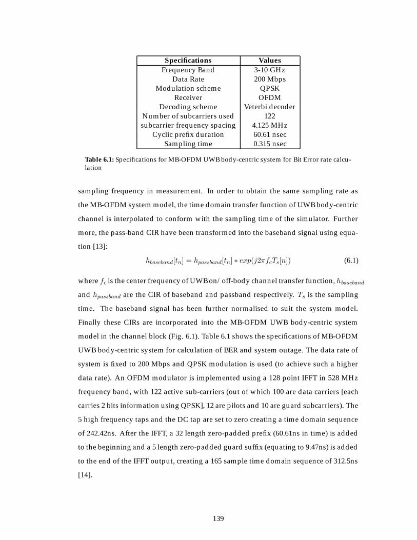
Specifications ValuesFrequency Band 3-10 GHz
Data Rate 200 MbpsModulation scheme QPSK
Receiver OFDMDecoding scheme Veterbi decoder
Number of subcarriers used 122subcarrier frequency spacing 4.125 MHz
Cyclic prefix duration 60.61 nsecSampling time 0.315 nsec
Table 6.1: Specifications for MB-OFDM UWB body-centric system for Bit Error rate calcu-lation
sampling frequency in measurement. In order to obtain the same sampling rate as
the MB-OFDM system model, the time domain transfer function of UWB body-centric
channel is interpolated to conform with the sampling time of the simulator. Further
more, the pass-band CIR have been transformed into the baseband signal using equa-
tion [13]:
hbaseband[tn] = hpassband[tn] ∗ exp(j2πfcTs[n]) (6.1)
where fc is the center frequency of UWB on/off-body channel transfer function, hbaseband
and hpassband are the CIR of baseband and passband respectively. Ts is the sampling
time. The baseband signal has been further normalised to suit the system model.
Finally these CIRs are incorporated into the MB-OFDM UWB body-centric system
model in the channel block (Fig. 6.1). Table 6.1 shows the specifications of MB-OFDM
UWB body-centric system for calculation of BER and system outage. The data rate of
system is fixed to 200 Mbps and QPSK modulation is used (to achieve such a higher
data rate). An OFDM modulator is implemented using a 128 point IFFT in 528 MHz
frequency band, with 122 active sub-carriers (out of which 100 are data carriers [each
carries 2 bits information using QPSK], 12 are pilots and 10 are guard subcarriers). The
5 high frequency taps and the DC tap are set to zero creating a time domain sequence
of 242.42ns. After the IFFT, a 32 length zero-padded prefix (60.61ns in time) is added
to the beginning and a 5 length zero-padded guard suffix (equating to 9.47ns) is added
to the end of the IFFT output, creating a 165 sample time domain sequence of 312.5ns
[14].
139
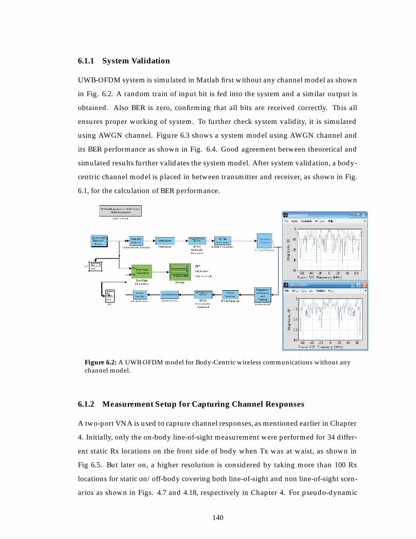
6.1.1 System Validation
UWB-OFDM system is simulated in Matlab first without any channel model as shown
in Fig. 6.2. A random train of input bit is fed into the system and a similar output is
obtained. Also BER is zero, confirming that all bits are received correctly. This all
ensures proper working of system. To further check system validity, it is simulated
using AWGN channel. Figure 6.3 shows a system model using AWGN channel and
its BER performance as shown in Fig. 6.4. Good agreement between theoretical and
simulated results further validates the system model. After system validation, a body-
centric channel model is placed in between transmitter and receiver, as shown in Fig.
6.1, for the calculation of BER performance.
Figure 6.2: A UWB OFDM model for Body-Centric wireless communications without anychannel model.
6.1.2 Measurement Setup for Capturing Channel Responses
A two-port VNA is used to capture channel responses, as mentioned earlier in Chapter
4. Initially, only the on-body line-of-sight measurement were performed for 34 differ-
ent static Rx locations on the front side of body when Tx was at waist, as shown in
Fig 6.5. But later on, a higher resolution is considered by taking more than 100 Rx
locations for static on/off-body covering both line-of-sight and non line-of-sight scen-
arios as shown in Figs. 4.7 and 4.18, respectively in Chapter 4. For pseudo-dynamic
140
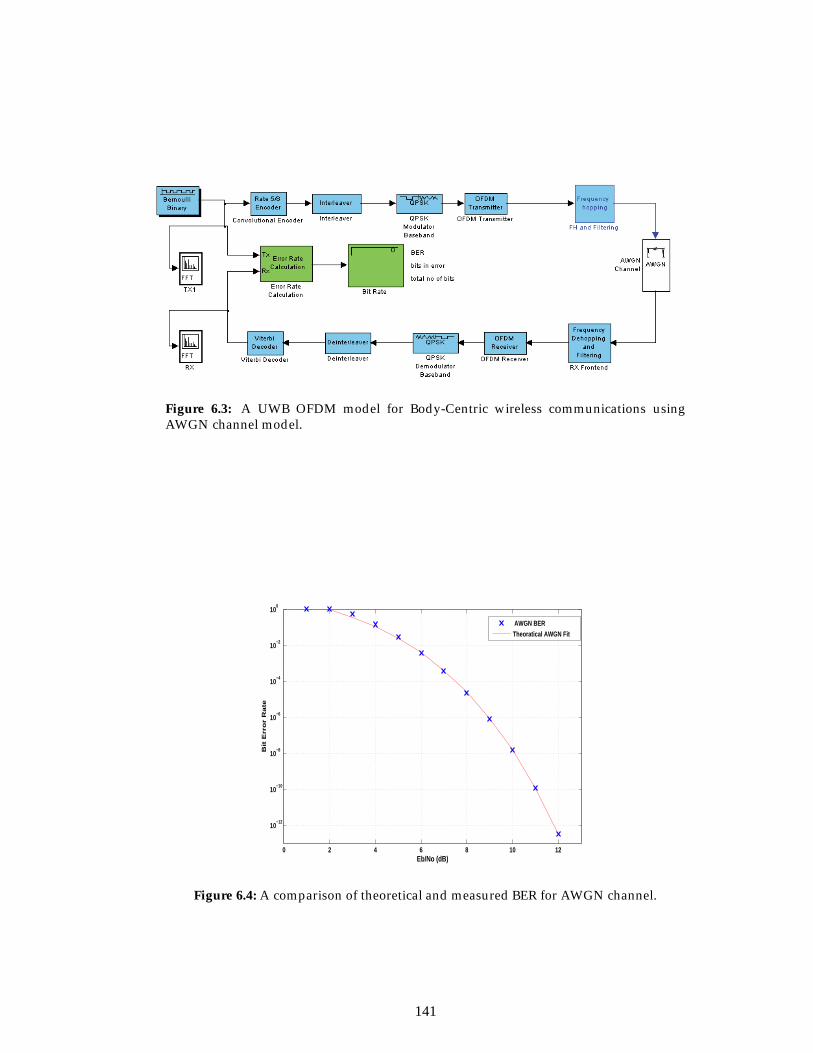
Figure 6.3: A UWB OFDM model for Body-Centric wireless communications usingAWGN channel model.
0 2 4 6 8 10 12
10−12
10−10
10−8
10−6
10−4
10−2
100
Eb/No (dB)
Bit
Err
or
Ra
te
AWGN BERTheoratical AWGN Fit
Figure 6.4: A comparison of theoretical and measured BER for AWGN channel.
141
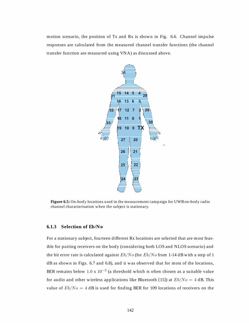
motion scenario, the position of Tx and Rx is shown in Fig. 6.6. Channel impulse
responses are calculated from the measured channel transfer functions (the channel
transfer function are measured using VNA) as discussed above.
19 10 9
18 11 8 1
17 12 7 2
16 13 6 3
15 14 5 4
20
21
22
2324
25
26
27
28
29
30
31
32
33
TX
34
Figure 6.5: On-body locations used in the measurement campaign for UWB on-body radiochannel characterisation when the subject is stationary.
6.1.3 Selection of Eb/No
For a stationary subject, fourteen different Rx locations are selected that are most feas-
ible for putting receivers on the body (considering both LOS and NLOS scenario) and
the bit error rate is calculated against Eb/No (for Eb/No from 1-14 dB with a step of 1
dB as shown in Figs. 6.7 and 6.8), and it was observed that for most of the locations,
BER remains below 1.0 x 10⁻³ (a threshold which is often chosen as a suitable value
for audio and other wireless applications like Bluetooth [15]) at Eb/No = 4 dB. This
value of Eb/No = 4 dB is used for finding BER for 109 locations of receivers on the
142
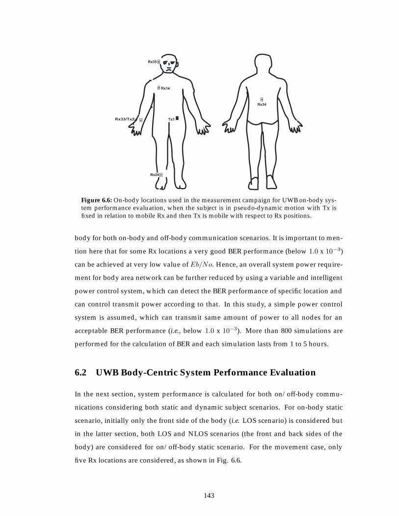
Tx1Rx33/Tx2
Rx14
Rx35
Rx24
Rx34
Figure 6.6: On-body locations used in the measurement campaign for UWB on-body sys-tem performance evaluation, when the subject is in pseudo-dynamic motion with Tx isfixed in relation to mobile Rx and then Tx is mobile with respect to Rx positions.
body for both on-body and off-body communication scenarios. It is important to men-
tion here that for some Rx locations a very good BER performance (below 1.0 x 10⁻³)
can be achieved at very low value of Eb/No. Hence, an overall system power require-
ment for body area network can be further reduced by using a variable and intelligent
power control system, which can detect the BER performance of specific location and
can control transmit power according to that. In this study, a simple power control
system is assumed, which can transmit same amount of power to all nodes for an
acceptable BER performance (i.e., below 1.0 x 10⁻³). More than 800 simulations are
performed for the calculation of BER and each simulation lasts from 1 to 5 hours.
6.2 UWB Body-Centric System Performance Evaluation
In the next section, system performance is calculated for both on/off-body commu-
nications considering both static and dynamic subject scenarios. For on-body static
scenario, initially only the front side of the body (i.e. LOS scenario) is considered but
in the latter section, both LOS and NLOS scenarios (the front and back sides of the
body) are considered for on/off-body static scenario. For the movement case, only
five Rx locations are considered, as shown in Fig. 6.6.
143
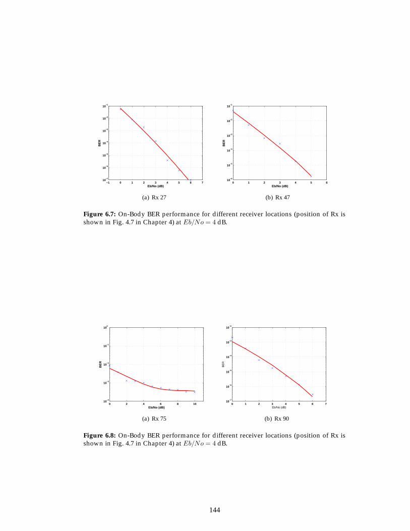
−1 0 1 2 3 4 5 6 710
−7
10−6
10−5
10−4
10−3
10−2
10−1
Eb/No (dB)
BE
R
(a) Rx 27
0 1 2 3 4 5 610
−6
10−5
10−4
10−3
10−2
10−1
Eb/No (dB)
BE
R
(b) Rx 47
Figure 6.7: On-Body BER performance for different receiver locations (position of Rx isshown in Fig. 4.7 in Chapter 4) at Eb/No = 4 dB.
0 2 4 6 8 1010
−4
10−3
10−2
10−1
100
Eb/No (dB)
BE
R
(a) Rx 75
0 1 2 3 4 5 6 710
−7
10−6
10−5
10−4
10−3
10−2
Eb/No (dB)
BE
R
(b) Rx 90
Figure 6.8: On-Body BER performance for different receiver locations (position of Rx isshown in Fig. 4.7 in Chapter 4) at Eb/No = 4 dB.
144
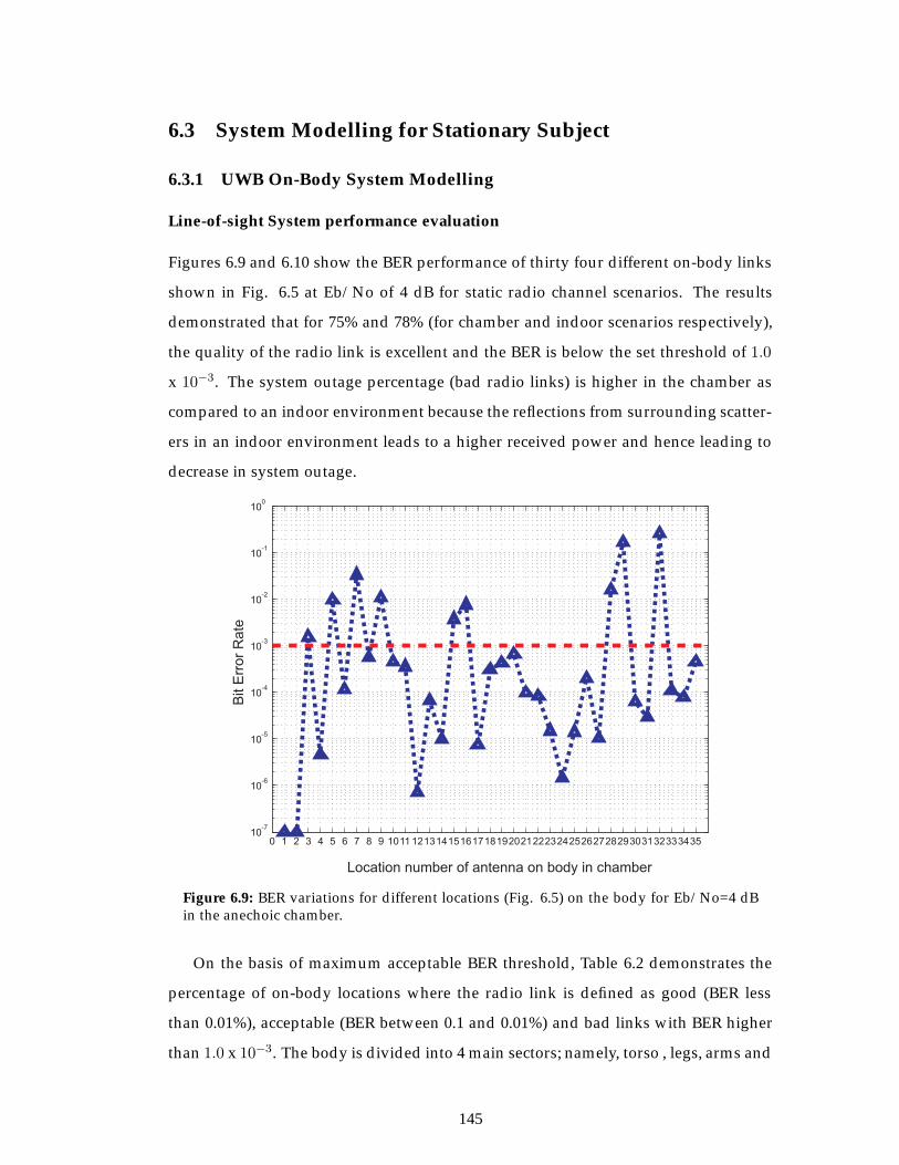
6.3 System Modelling for Stationary Subject
6.3.1 UWB On-Body System Modelling
Line-of-sight System performance evaluation
Figures 6.9 and 6.10 show the BER performance of thirty four different on-body links
shown in Fig. 6.5 at Eb/No of 4 dB for static radio channel scenarios. The results
demonstrated that for 75% and 78% (for chamber and indoor scenarios respectively),
the quality of the radio link is excellent and the BER is below the set threshold of 1.0
x 10−3. The system outage percentage (bad radio links) is higher in the chamber as
compared to an indoor environment because the reflections from surrounding scatter-
ers in an indoor environment leads to a higher received power and hence leading to
decrease in system outage.
Figure 6.9: BER variations for different locations (Fig. 6.5) on the body for Eb/No=4 dBin the anechoic chamber.
On the basis of maximum acceptable BER threshold, Table 6.2 demonstrates the
percentage of on-body locations where the radio link is defined as good (BER less
than 0.01%), acceptable (BER between 0.1 and 0.01%) and bad links with BER higher
than 1.0 x 10⁻³. The body is divided into 4 main sectors; namely, torso , legs, arms and
145
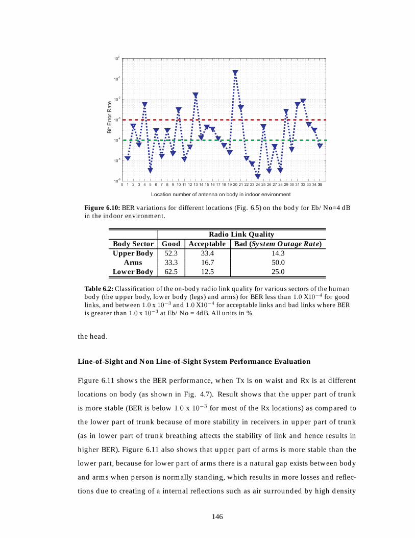
Figure 6.10: BER variations for different locations (Fig. 6.5) on the body for Eb/No=4 dBin the indoor environment.
Radio Link QualityBody Sector Good Acceptable Bad (System Outage Rate)Upper Body 52.3 33.4 14.3
Arms 33.3 16.7 50.0Lower Body 62.5 12.5 25.0
Table 6.2: Classification of the on-body radio link quality for various sectors of the humanbody (the upper body, lower body (legs) and arms) for BER less than 1.0 X10⁻⁴ for goodlinks, and between 1.0 x 10⁻³ and 1.0 X10⁻⁴ for acceptable links and bad links where BERis greater than 1.0 x 10⁻³ at Eb/No = 4dB. All units in %.
the head.
Line-of-Sight and Non Line-of-Sight System Performance Evaluation
Figure 6.11 shows the BER performance, when Tx is on waist and Rx is at different
locations on body (as shown in Fig. 4.7). Result shows that the upper part of trunk
is more stable (BER is below 1.0 x 10⁻³ for most of the Rx locations) as compared to
the lower part of trunk because of more stability in receivers in upper part of trunk
(as in lower part of trunk breathing affects the stability of link and hence results in
higher BER). Figure 6.11 also shows that upper part of arms is more stable than the
lower part, because for lower part of arms there is a natural gap exists between body
and arms when person is normally standing, which results in more losses and reflec-
tions due to creating of a internal reflections such as air surrounded by high density
146
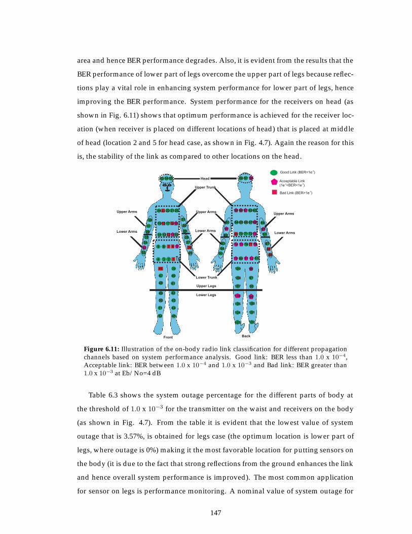
area and hence BER performance degrades. Also, it is evident from the results that the
BER performance of lower part of legs overcome the upper part of legs because reflec-
tions play a vital role in enhancing system performance for lower part of legs, hence
improving the BER performance. System performance for the receivers on head (as
shown in Fig. 6.11) shows that optimum performance is achieved for the receiver loc-
ation (when receiver is placed on different locations of head) that is placed at middle
of head (location 2 and 5 for head case, as shown in Fig. 4.7). Again the reason for this
is, the stability of the link as compared to other locations on the head.
7776
108
100
101
102
6768
7273
78
89
88
87
86
85
84
96
97
98
99
Lower Arms
105
104
103
15
46
47
48
49
50
51
52
Tx1234
5
10
20
6
11
16
21
789
121314
171819
222324
25
26
27
28
29
30
31
32
33
34
35
36
37
38
39
40
41
42
43
44
45
5453 55 56 57 58
59 60 61 6263
64 65 66
70 71
74 75
79 80
95
94
93
92
91
90
109
107
106
Front Back
69
81 8382
Upper Trunk
Lower Arms
Upper Legs
Lower Legs
Upper Arms
Head
Lower Trunk
Upper ArmsUpper Arms
Lower Arms
Figure 6.11: Illustration of the on-body radio link classification for different propagationchannels based on system performance analysis. Good link: BER less than 1.0 x 10⁻⁴,Acceptable link: BER between 1.0 x 10⁻⁴ and 1.0 x 10⁻³ and Bad link: BER greater than1.0 x 10−3 at Eb/No=4 dB
Table 6.3 shows the system outage percentage for the different parts of body at
the threshold of 1.0 x 10⁻³ for the transmitter on the waist and receivers on the body
(as shown in Fig. 4.7). From the table it is evident that the lowest value of system
outage that is 3.57%, is obtained for legs case (the optimum location is lower part of
legs, where outage is 0%) making it the most favorable location for putting sensors on
the body (it is due to the fact that strong reflections from the ground enhances the link
and hence overall system performance is improved). The most common application
for sensor on legs is performance monitoring. A nominal value of system outage for
147
the head case as compared to other body parts makes it the second optimum location
after the legs for locating sensors on the body for on-body communications.
6.3.2 UWB Off-Body System Performance Evaluation
Figure 6.12 shows the off-body (when Tx is on the wall, at the waist height and at a
distance of 100 cm from the human body), BER performance for the upper and lower
part of the trunk (as shown in Fig. 4.7). The lower part of the trunk is more stable
(the BER is less than 1.0 x 10⁻³ for most of the Rx locations) as compared to the upper
part of the trunk contrary to the on-body communications, as discussed above. This
may be due to the fact that the lower part of the trunk is exactly at the same level of
transmitter on wall, thus making direct LOS and hence improves the overall system
performance. Figure 6.12 also shows the off-body BER performance for the upper and
lower parts of arms and legs respectively (as shown in Fig. 4.7). The upper part of
legs performs better than lower part of legs as upper part of legs is in direct sight of
off-body transmitter (which is on wall at a waist height from the ground). The BER
performance for the head case in the off-body link is also shown in Fig. 6.12. For
the head case, the same interpretation and reasoning can be applied as discussed for
on-body case in section 6.3.1.
Table 6.3 shows the system outage percentage for different human body parts at
the threshold of 1.0 x 10⁻³ for Tx on the wall at a waist height with a distance of 100
cm from the on-body receivers. The lowest system outage percentage of 16.32% for
the trunk case indicates that the trunk is the most favorable part of body for locating
sensors on the body for off-body communications (optimum locations are the lower
part of trunk and upper part of legs due to strong direct LOS communications). The
second favorable location for the off-body communication is again on the head as for
the on-body communication. Figure 6.13 shows the comparison of BER for different
distances between off-body Tx and on-body Rx for some randomly selected Rx loca-
tions (from both the front side of body (LOS) and the back side of body (NLOS)). It
shows that for most of the cases, the system performance degrades as off-body dis-
tance is increased except for very few Rx locations, where multipath reflections are
high.
Figure 6.14 shows the comparison of BER performance for Tx on the waist and
148
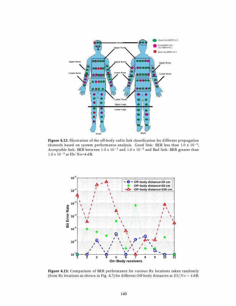
1234
5
10
20
15
6
11
16
21
789
121314
171819
222324
25
26
27
28
29
30
31
32
33
34
35
36
37
38
39
40
41
42
43
44
45
46
47
48
49
50
51
52
5453 55 56 57 58
59 60 61 6263
64 65 66 6768
69 70 717273
74 75 7677 78
79 80 81 82 8389
88
87
86
85
84
95
94
93
92
91
90
96
97
98
99
100
101
102
109
108
107
106
105
104
103
Front Back
Upper Trunk
Lower Arms
Upper Legs
Lower Legs
Upper Arms
Head
Lower Trunk
Upper ArmsUpper Arms
Lower Arms Lower Arms
Figure 6.12: Illustration of the off-body radio link classification for different propagationchannels based on system performance analysis. Good link: BER less than 1.0 x 10⁻⁴,Acceptable link: BER between 1.0 x 10⁻⁴ and 1.0 x 10⁻³ and Bad link: BER greater than1.0 x 10−3 at Eb/No=4 dB.
1 2 3 4 5 6 7 8 9 10 1110
−7
10−6
10−5
10−4
10−3
10−2
10−1
On−Body receivers
Bit
Err
or
Rat
e
Off−body distance=20 cmOff−body distance=50 cmOff−body distance=100 cm
Figure 6.13: Comparison of BER performance for various Rx locations taken randomly(from Rx locations as shown in Fig. 4.7) for different Off-body distances at Eb/No = 4 dB.
149
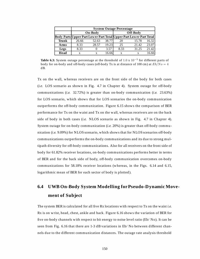
System Outage PercentageOn-Body Off-Body
Body Parts Upper Part Lower Part Total Upper Part Lower Part TotalTrunk 26.66 52.63 38.77 20 15.78 16.32Arms 8.33 28.57 19.23 25 21.42 23.07Legs 8.33 0 3.57 8.33 31.25 21.42Head x x 16.66 x x 16.66
Table 6.3: System outage percentage at the threshold of 1.0 x 10⁻³ for different parts ofbody for on-body and off-body cases (off-body Tx is at distance of 100 cm) at Eb/No = 4dB.
Tx on the wall, whereas receivers are on the front side of the body for both cases
(i.e. LOS scenario as shown in Fig. 4.7 in Chapter 4). System outage for off-body
communications (i.e. 32.72%) is greater than on-body communication (i.e. 23.63%)
for LOS scenario, which shows that for LOS scenarios the on-body communication
outperforms the off-body communication. Figure 6.15 shows the comparison of BER
performance for Tx on the waist and Tx on the wall, whereas receivers are on the back
side of body in both cases (i.e. NLOS scenario as shown in Fig. 4.7 in Chapter 4).
System outage for on-body communication (i.e. 20%) is greater than off-body commu-
nication (i.e. 9.09%) for NLOS scenario, which shows that for NLOS scenarios off-body
communications outperforms the on-body communications and its due to strong mul-
tipath diversity for off-body communications. Also for all receivers on the front side of
body for 61.82% receiver locations, on-body communications performs better in terms
of BER and for the back side of body, off-body communication overcomes on-body
communications for 58.18% receiver locations (whereas, in the Figs. 6.14 and 6.15,
logarithmic mean of BER for each sector of body is plotted).
6.4 UWB On-Body System Modelling for Pseudo-Dynamic Move-
ment of Subject
The system BER is calculated for all five Rx locations with respect to Tx on the waist i.e.
Rx is on wrist, head, chest, ankle and back. Figure 6.16 shows the variation of BER for
five on-body channels with respect to bit energy to noise level ratio (Eb/No). It can be
seen from Fig. 6.16 that there are 1-3 dB variations in Eb/No between different chan-
nels due to the different communication distances. The outage rate analysis threshold
150
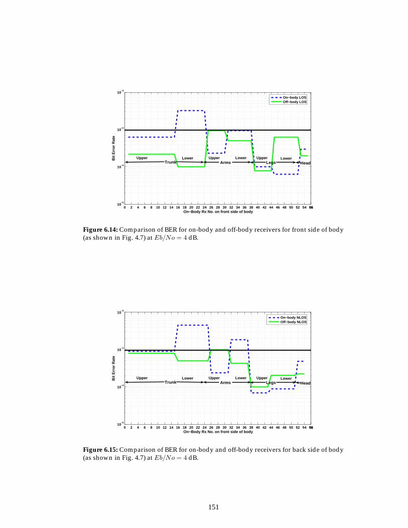
0 2 4 6 8 10 12 14 16 18 20 22 24 26 28 30 32 34 36 38 40 42 44 46 48 50 52 54 565610
−5
10−4
10−3
10−2
On−Body Rx No. on front side of body
Bit
Err
or
Rat
e
On−body LOSOff−body LOS
Trunk Arms Legs HeadUpper Upper UpperLower Lower Lower
Figure 6.14: Comparison of BER for on-body and off-body receivers for front side of body(as shown in Fig. 4.7) at Eb/No = 4 dB.
0 2 4 6 8 10 12 14 16 18 20 22 24 26 28 30 32 34 36 38 40 42 44 46 48 50 52 54 565610
−5
10−4
10−3
10−2
On−Body Rx No. on front side of body
Bit
Err
or
Rat
e
On−body NLOSOff−body NLOS
Trunk Arms Legs HeadUpper Upper UpperLower Lower Lower
Figure 6.15: Comparison of BER for on-body and off-body receivers for back side of body(as shown in Fig. 4.7) at Eb/No = 4 dB.
151
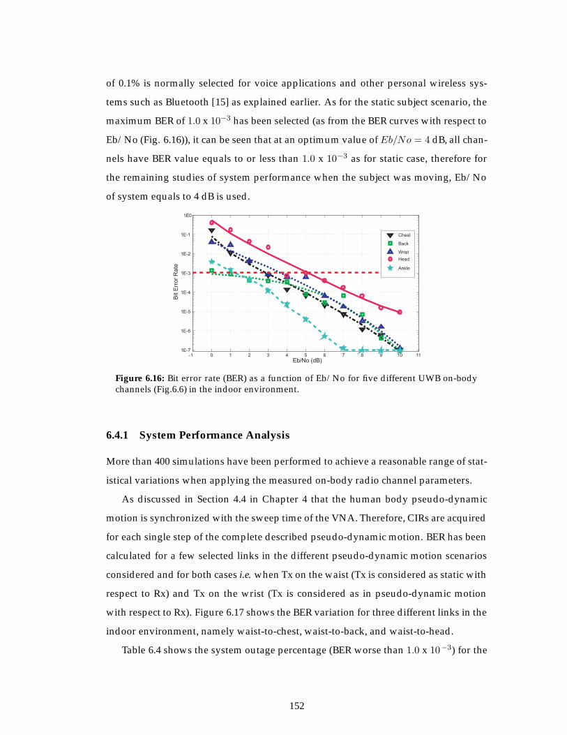
of 0.1% is normally selected for voice applications and other personal wireless sys-
tems such as Bluetooth [15] as explained earlier. As for the static subject scenario, the
maximum BER of 1.0 x 10⁻³ has been selected (as from the BER curves with respect to
Eb/No (Fig. 6.16)), it can be seen that at an optimum value of Eb/No = 4 dB, all chan-
nels have BER value equals to or less than 1.0 x 10⁻³ as for static case, therefore for
the remaining studies of system performance when the subject was moving, Eb/No
of system equals to 4 dB is used.
Figure 6.16: Bit error rate (BER) as a function of Eb/No for five different UWB on-bodychannels (Fig.6.6) in the indoor environment.
6.4.1 System Performance Analysis
More than 400 simulations have been performed to achieve a reasonable range of stat-
istical variations when applying the measured on-body radio channel parameters.
As discussed in Section 4.4 in Chapter 4 that the human body pseudo-dynamic
motion is synchronized with the sweep time of the VNA. Therefore, CIRs are acquired
for each single step of the complete described pseudo-dynamic motion. BER has been
calculated for a few selected links in the different pseudo-dynamic motion scenarios
considered and for both cases i.e. when Tx on the waist (Tx is considered as static with
respect to Rx) and Tx on the wrist (Tx is considered as in pseudo-dynamic motion
with respect to Rx). Figure 6.17 shows the BER variation for three different links in the
indoor environment, namely waist-to-chest, waist-to-back, and waist-to-head.
Table 6.4 shows the system outage percentage (BER worse than 1.0 x 10⁻³) for the
152
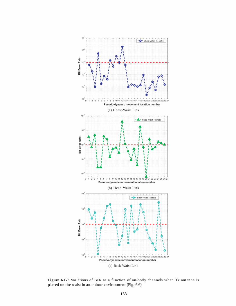
Pseudo-dynamic movement location number
Bit
Err
or
Rate
(a) Chest-Waist Link
Pseudo-dynamic movement location number
Bit
Err
or
Ra
te
(b) Head-Waist Link
Pseudo-dynamic movement location number
Bit
Err
or
Rate
(c) Back-Waist Link
Figure 6.17: Variations of BER as a function of on-body channels when Tx antenna isplaced on the waist in an indoor environment (Fig. 6.6)
153
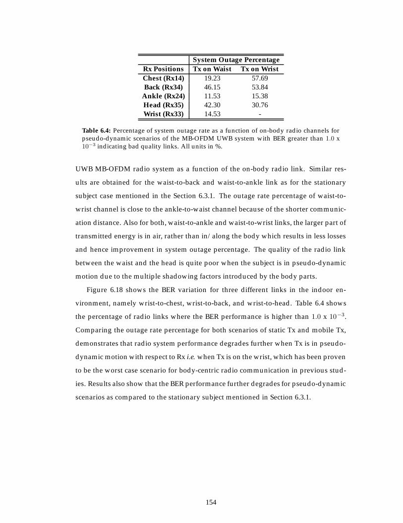
System Outage PercentageRx Positions Tx on Waist Tx on WristChest (Rx14) 19.23 57.69Back (Rx34) 46.15 53.84
Ankle (Rx24) 11.53 15.38Head (Rx35) 42.30 30.76Wrist (Rx33) 14.53 -
Table 6.4: Percentage of system outage rate as a function of on-body radio channels forpseudo-dynamic scenarios of the MB-OFDM UWB system with BER greater than 1.0 x10⁻³ indicating bad quality links. All units in %.
UWB MB-OFDM radio system as a function of the on-body radio link. Similar res-
ults are obtained for the waist-to-back and waist-to-ankle link as for the stationary
subject case mentioned in the Section 6.3.1. The outage rate percentage of waist-to-
wrist channel is close to the ankle-to-waist channel because of the shorter communic-
ation distance. Also for both, waist-to-ankle and waist-to-wrist links, the larger part of
transmitted energy is in air, rather than in/along the body which results in less losses
and hence improvement in system outage percentage. The quality of the radio link
between the waist and the head is quite poor when the subject is in pseudo-dynamic
motion due to the multiple shadowing factors introduced by the body parts.
Figure 6.18 shows the BER variation for three different links in the indoor en-
vironment, namely wrist-to-chest, wrist-to-back, and wrist-to-head. Table 6.4 shows
the percentage of radio links where the BER performance is higher than 1.0 x 10⁻³.
Comparing the outage rate percentage for both scenarios of static Tx and mobile Tx,
demonstrates that radio system performance degrades further when Tx is in pseudo-
dynamic motion with respect to Rx i.e. when Tx is on the wrist, which has been proven
to be the worst case scenario for body-centric radio communication in previous stud-
ies. Results also show that the BER performance further degrades for pseudo-dynamic
scenarios as compared to the stationary subject mentioned in Section 6.3.1.
154
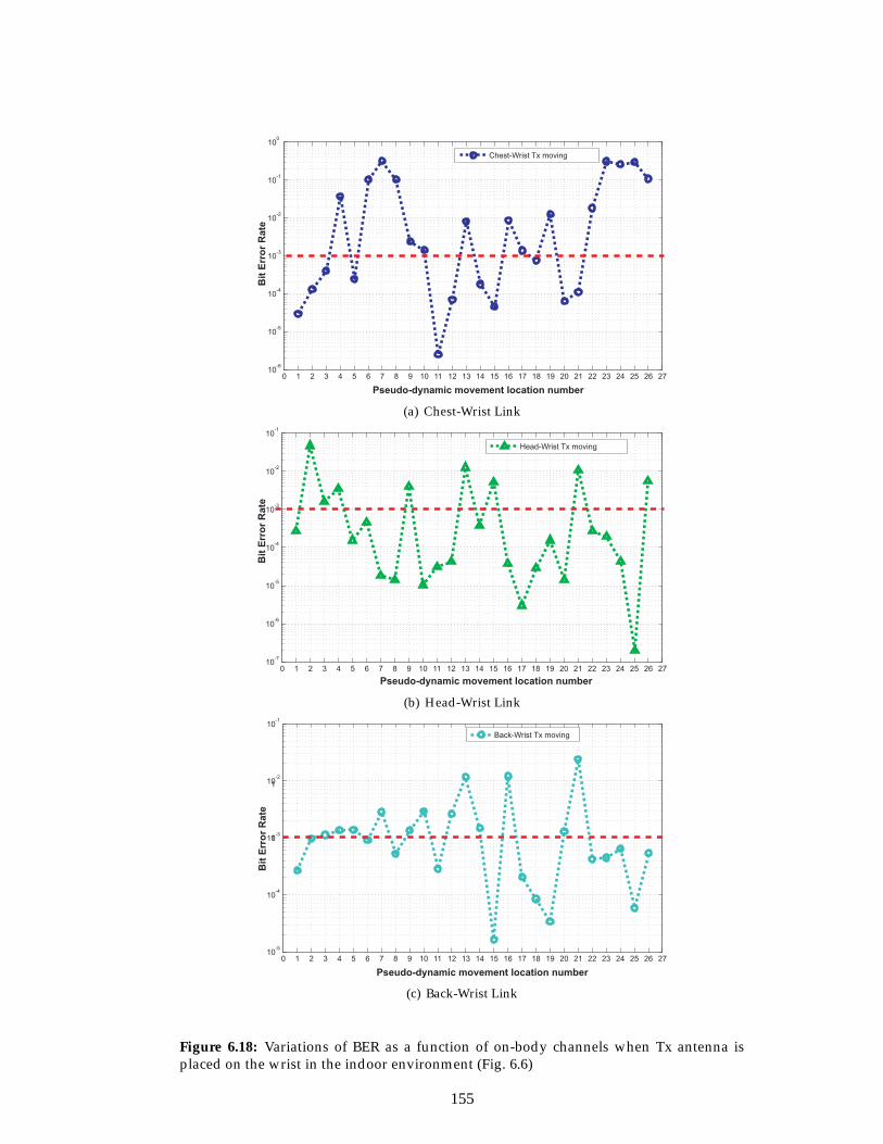
Pseudo-dynamic movement location number
Bit
Err
or
Ra
te
(a) Chest-Wrist Link
Pseudo-dynamic movement location number
Bit
Err
or
Ra
te
(b) Head-Wrist Link
Pseudo-dynamic movement location number
Bit
Err
or
Rate
(c) Back-Wrist Link
Figure 6.18: Variations of BER as a function of on-body channels when Tx antenna isplaced on the wrist in the indoor environment (Fig. 6.6)
155
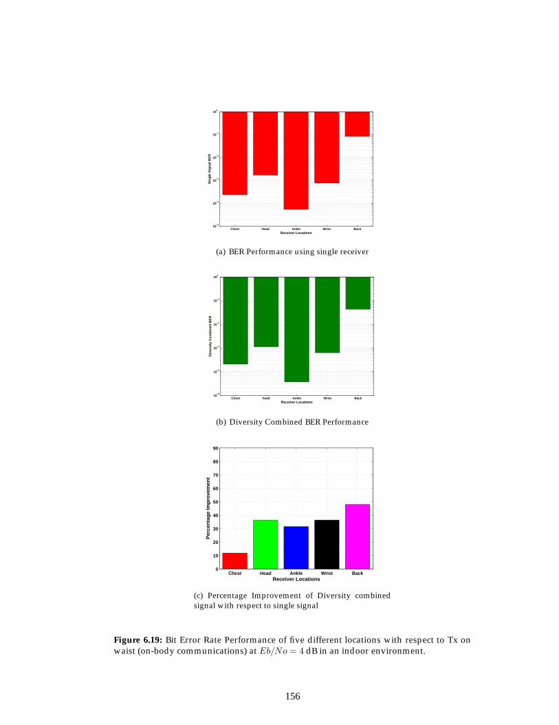
Chest Head Ankle Wrist Back10
−5
10−4
10−3
10−2
10−1
100
Receiver Locations
Sin
gle
Sig
nal
BE
R
(a) BER Performance using single receiver
Chest head Ankle Wrist Back10
−5
10−4
10−3
10−2
10−1
100
Receiver Locations
Div
ersi
ty C
om
bin
ed B
ER
(b) Diversity Combined BER Performance
Chest Head Ankle Wrist Back0
10
20
30
40
50
60
70
80
90
Receiver Locations
Per
cen
tag
e Im
pro
vem
ent
(c) Percentage Improvement of Diversity combinedsignal with respect to single signal
Figure 6.19: Bit Error Rate Performance of five different locations with respect to Tx onwaist (on-body communications) at Eb/No = 4 dB in an indoor environment.
156
6.5 System Performance Comparison of UWB Spatial Diversity
for Body-Centric Wireless Networks
In Chapter 5, spatial diversity for both UWB on-body and off-body communication
is being studied using different combining techniques. Two branch signals are meas-
ured using PNA-X as mentioned in Chapter 5. These measured signals are converted
to time domain signals as mentioned earlier. After converting to the time domain,
these responses are combined using the maximum ratio combination technique (de-
tail is given in Chapter 5). The BER performance is being calculated at Eb/No = 4 dB
by inputting each branch signal and MRC combined signal, one by one to the OFDM
based system, all other settings of the system are the same as those mentioned above.
Figures 6.19 and 6.20 show the BER performance of branch signal (out of two branch
signals r1&r2, the signal with better BER performance is chosen) and MRC combined
signal with a percentage improvement of MRC combined signal over the branch sig-
nal for five different on-body diversity branch receiver locations with respect to Tx
on the waist for on-body and Tx on wall at waist height (1 meter above the ground),
at distance of 1 meter from the body carrying diversity receivers in an indoor envir-
onment for off-body diversity respectively (Tx and Rx locations are shown in Figs.
5.2 and 5.3 for on-body and off-body diversity respectively; the spacing between the
diversity branch antennas is 0.34λ).
Results show that for both cases i.e. on and off-body diversity case, system per-
formance improvement is significant, when Rx is placed on the back side i.e. NLOS
scenario (as already explained in chapter 5 in terms of diversity gain). The percentage
improvement in the system performance with respect to the single antenna shows,
that in case of off-body diversity, improvement is 25-65% higher than that of on-body
diversity. This shows the dominance of off-body diversity over on-body diversity as
mentioned in Chapter 5.
6.6 Summary
In this chapter a UWB body-centric system modelling has been presented based on
measured data. System-level modelling is analytically and numerically performed on
157
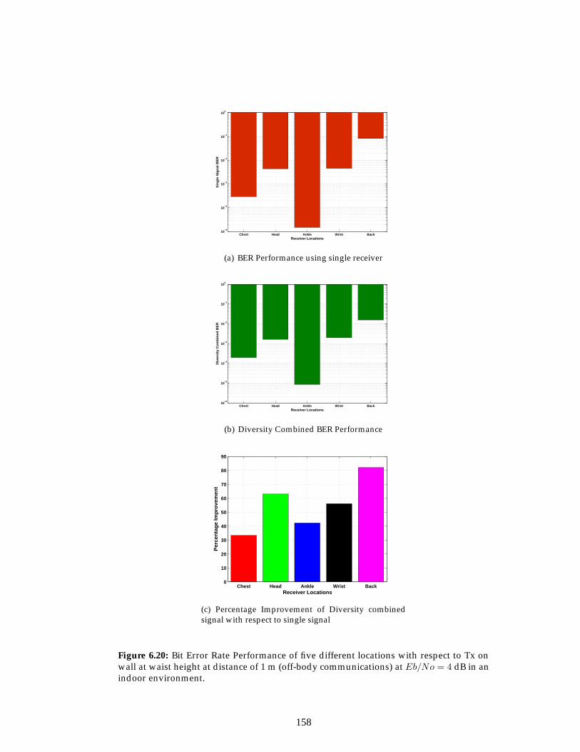
Chest Head Ankle Wrist Back10
−5
10−4
10−3
10−2
10−1
100
Receiver Locations
Sin
gle
Sig
nal
BE
R
(a) BER Performance using single receiver
Chest Head Ankle Wrist Back10
−6
10−5
10−4
10−3
10−2
10−1
100
Receiver Locations
Div
ersi
ty C
om
bin
ed B
ER
(b) Diversity Combined BER Performance
Chest Head Ankle Wrist Back0
10
20
30
40
50
60
70
80
90
Receiver Locations
Per
cen
tag
e Im
pro
vem
ent
(c) Percentage Improvement of Diversity combinedsignal with respect to single signal
Figure 6.20: Bit Error Rate Performance of five different locations with respect to Tx onwall at waist height at distance of 1 m (off-body communications) at Eb/No = 4 dB in anindoor environment.
158
the basis of multiband orthogonal frequency division multiplexed (OFDM) system for
both on/off-body communications. System performance is evaluated for the different
sectors of the body based on real time measurements using bit error rate and system
outage rate calculation. Results and analysis, based on signal to noise ratio and bit er-
ror rate, demonstrated that BER is less than or equal to 0.1%, for 96.43% of lower body
locations (for on-body communications) and 83.68% of the human trunk ones (for off-
body communications) respectively, with low power requirements. System perform-
ance is also evaluated, when subject was in the pseudo-dynamic motion. The conduc-
ted system analysis demonstrated that for pseudo-dynamic motion scenario; the BER
is equal to or less than 0.1% for 75% of stable and 61% of unstable transmitter locations.
Results demonstrated that the system performance is highly affected by the position
of the sensors on the body and by the changes in postures, thus showing the import-
ance of considering these parameters when designing optimal UWB radio systems
for body-centric wireless communications. Based on the results in this chapter, clear
recommendations are given for best on/off-body locations leading to optimal body-
centric wireless system performance. Apart from this, towards the end of chapter, a
comparison of system performance for on/off-body diversity is also presented. Res-
ults showed that off-body diversity performance improvement with respect to single
antenna vary from 25-65% as compared to on-body diversity, hence, making the UWB
off-body diversity more useful than the UWB on-body diversity.
159
References
[1] J. H. Reed, An Introduction to Ultra Wideband Communication Systems. Printce Hall, 2005.
[2] M. Wylie-Green, A. R. Pekka, and J. Salokannel, “Multi-band OFDM UWB solution forieee 802.15.3a wpans,” in IEEE/Sarnoff Symposium on Advances in Wired and Wireless Com-munication, 2005, pp. 102–105.
[3] A. Alomainy, Y. Hao, X. Hu, C. G. Parini, and P. S. Hall, “UWB on-body radiopropagation and system modelling for wireless body-centric networks,” IEE ProceedingsCommunications-Special Issue on Ultra Wideband Systems, Technologies and Applications, vol.153, no. 1, pp. 107– 114, Feb. 2006.
[4] Y. Zhang and Q. Li, “Performance of UWB impulse radio with planar monopoles over onhuman body propagation channel for wireless body area networks,” IEEE Transaction onAntenna and Propagation, vol. 55, no. 10, pp. 2907–2914, Oct. 2007.
[5] Q. Wang and J. Wang, “Performance of on-body chest-to-waist UWB communicationlink,” IEEE microwave and wireless components lett., vol. 19, no. 2, Feb. 2009.
[6] Q. Wang, T. Tayamachi, I. Kimura, and J. Wang, “An on-body channel model for uwbbody area communications for various postures,” IEEE Journal on Selected Areas in Com-munications, vol. 57, no. 4, pp. 991–998, Apr. 2009.
[7] I. Kovacs, G. pedersen, P. Eggers, and K. Olesen, “Ultra wideband radio propagation inbody area network scenarios,” in IEEE Int. Symp. on spread spectrum techniques and applic-ations techniques and applications, Sydney, Australia, 2004, pp. 102–106.
[8] A. Fort, C. Desset, J. Ryckaert, P. D. Doncker, L. V. Biesen, and S. Donnay, “Ultra widebandbody area channel model,” in International Conference on Communications, ICC05, Seoul,South Korea, May 2005.
[9] Q. H. Abbasi, A. Sani, A. Alomainy, and Y. Hao, “Arm movements effect on ultra wide-band on-body propagation channels and radio systems,” in Loughborough Antennas andPropagation Conference (LAPC2009), Loughborough, UK, 16-17 Nov. 2009.
[10] A. Alomainy, Q. H. Abbasi, A. Sani, and Y. Hao, “System-level modelling of optimal ultrawideband body-centric wireless network,” in Asia Pacific Microwave Conference (APMC),Singapore, 7-10 December 2009.
[11] M. Guizani, Wireless Communications Systems and Networks. Kluwer Academic/PlenumPublishers New York, 2004.
[12] A. Batra, “Multi-band OFDM physical layer proposal for IEEE 802.15 task group 3a,”Texas Instruments, Tech. Rep., November 2003.
[13] B. Sklar, Digital communications: fundamentals and applications. Prentice Hall, 2001.
[14] W. P. Siriwongpairat and K. J. Ray Liu, Ultra-Wideband Communications Systems: MultibandOFDM Approach. John Wiley & Sons, Ltd., 2007.
[15] M. H. I. Opperman and J. Iinatti, UWB theory and applications. John Wiley & Sons, 2004.
160
Chapter 7
Conclusions and Future Work
7.1 Conclusions
Recently, there have been many efforts made to characterise the on-body radio channel
and impulse based UWB system model in both anechoic chamber and indoor environ-
ment. In the presented work, both the on/off-body radio channel and system model
are characterised more thoroughly by taking over 100 receiver locations for static scen-
arios. In addition to the static scenarios, channel and system performance is evaluated
by taking into account the movement of human body parts. Path loss calculation is
performed for different sectors of body instead of taking the body as a whole to better
understand the path loss trend. Radiographs were used in this thesis for character-
ising on-body and off-body communications, to get more closer insight into the path
loss distribution. To enable prediction and modelling, a statistical analysis was per-
formed on the both spectral and transient parameters of the channel. The received
power was proven to be dependent on the antenna positions, distances and on the
dynamic behaviour of the body environment.
Multiple antenna techniques are commonly used in wireless commmunication
to overcome fading. In this work, the spatial diversity has been analysed for both
on/off-body communications with the fixed spacing between receiver antennas. The
161
diversity gain using different combining techniques like SC, EGC and MRC have been
calculated. Power imbalance and correlation coefficients between branch signals have
also been evaluated for different environments (anechoic chamber and indoor). In
addition to this, different measurement scenarios, subjects, angles etc are considered
to check the effect of such scenarios on antenna diversity performance. It has been
observed that the diversity gain is low for the chamber due to no reflections from sur-
roundings as compared to indoor environment. Results show that for rich multipath
environment, the diversity gain is higher for the non line-of-sight case, where there is
low power imbalance due to highly uncorrelated signals. Comparison of on-body and
off-body diversity is performed and results showed significant improvement for the
off-body case. Results presented in this thesis gave indications of the beneficial applic-
ations of diversity antenna techniques for potential enhancement of UWB body-centric
wireless network performance.
Finally, the measured and analysed data was used for evaluating the perform-
ance of potential UWB transceivers that could be applied in the wireless body-centric
networks. The system-level modelling is analytically and numerically performed us-
ing a multiband orthogonal frequency division multiplexed (OFDM) system for both
on/off-body communications. System performance is evaluated for different sectors
of the body based on the real time measurements using the bit error rate and sys-
tem outage rate calculation under both static and dynamic scenarios. Results demon-
strated that the system performance is highly affected by the position of antennas on
the body and changes in postures, thus it shows the importance of considering these
parameters when designing optimal UWB radio systems for the body-centric wireless
communications. In addition to this, results presented in this thesis supports the ap-
plicability of UWB diversity for BCWN and also highlights the dominance of UWB
off-body diversity over on-body diversity, making UWB off-body diversity more use-
ful for the body-centric wireless networks.
7.2 Key Contributions
The major contributions of this work are:
• Analysis of the spectral and transient characteristics of ultra wideband radio
162
channel for body-centric wireless networks (both on-body and off-body), based
on different sectors of human body. Effect of pseudo-dynamic motion and pos-
ture of human body on body-centric channel were considered. To enable predic-
tion and modelling, statistical models based on measured data were derived.
• Study of ultra wideband on-body antenna diversity considering various diversity
combining techniques. The impact of variation of spacing between diversity
branch antennas and indoor locations is discussed, with an emphasis on mutual
coupling, correlation and power imbalance of received signals.
• Study of ultra wideband off-body antenna diversity is performed. Different
scenarios i.e. effect of change of subject locations in an indoor environment and
the impact of variation of inter-spacing between diversity branch antennas on
mutual coupling, correlation and power imbalance were highlighted. Variations
in diversity gain (DG) with respect to, small changes of antenna position on the
body and DG behavior with change of orientation between off-body transmitter
and on-body diversity receiver were discussed. Also subject specific off-body
diversity and uplink, downlink diversity were explored.
• System-level modelling of potential multiband orthogonal frequency division
multiplexed UWB system has been conducted and system performance is meas-
ured using bit error rate and signal-to-noise ratio for both static and pseudo-
dynamic scenarios, for the different sectors of the body based on real time meas-
urements. The system performance is being evaluated for both on-body and off-
body communications. Recommendations for optimum locations of ultra wide-
band nodes placement on the body for reliable and energy efficient body-centric
wireless communications were proposed.
7.3 Future Work
Based on the conclusions drawn and the limitations of the work presented, the fol-
lowing research aspects and issues would provide potential and natural progression
to the accomplished work in the thesis:
163
UWB Radio Channel Characterisation and System level Modelling for BCWN
• Time Domain UWB Radio Channel Characterisation: Performing UWB meas-
urements with a time-domain channel sounder to provide a cross-reference for
a comprehensive understanding of the channel characteristics. Using time do-
main measurements a comprehensive channel models including calculation of
time of arrival and angle of arrival will also be performed.
• UWB Radio Channel Characterisation Using Wireless Sensors: The use of wire-
less sensors for realistic channel measurements. So far, measurement campaigns
have been done by connecting two stand-alone antennas to the VNA through
coaxial cables. However, cables do not allow freedom of movement to the user,
and, it has been proven that, when connected to small antennas, those cables
may radiate and hence produce measurements errors.
• Characterisation of UWB Body-to-Body channel: The body to body communic-
ation link can offer wireless communication between individuals by seamless
exchange of information. For example, patients could exchange vital informa-
tion with their doctors by merely transmitting their medical history files to the
doctor’s personal base station or may be soliders exchanging information with
the base station. However, from channel modelling point of view, the character-
isation of UWB body to body channels presents increased complexity compared
to other wireless BCWN systems and some data reduction techniques should be
applied where applicable.
• Characterisation of UWB Body Proximity Channel: Measurements must be car-
ried out to characterise the scenario, where a body is shadowed by other bodies.
This type of measurement can be performed by moving a group of people in a
specific route and measuring the alteration of received signal with respect to Tx
and Rx separation and orientation.
UWB Diversity for BCWN
• Transmit Diversity and Alamouti Codes: The use of diversity antenna at the
transmitter side can be carried out and compared to receive diversity. The con-
ventional Alamouti codes can be used and there is scope in defining some new
164
algorithm for transmit diversity.
• Exploring UWB pattern and polarisation diversity for body-centric wireless net-
works: It includes designing of compact antenna for UWB pattern and polarisa-
tion diversity as well.
• UWB-MIMO: Investigation of UWB-MIMO for BCWN and its comparison in
terms of performance and capacity improvement with respect to SISO, SIMO
and MISO.
• Higher order Diversity: Use of higher-order diversity and MIMO system per-
formance can be a potential future work.
• Water-filling Technique for MIMO: The use of water-filling technique is quite
useful for MIMO system with non-uniform power distribution among trans-
mitting antennas. Through water-filling, the power can be distributed to avoid
channel with high impairments. This needs investigation for UWB on-body ra-
dio channels and also suitable water-filling schemes is required to be proposed
and compared with the narrow-band water-filling schemes as well.
UWB Radio Channel Characterisation and System Modelling based on Numerical
Modelling for BCWN
• UWB On/Off-Body Radio Channel Characterisation: The use of numerical mod-
elling for UWB on/off-body propagation channel characterisation based on dif-
ferent sectors of body using the dispersive FDTD. Subject specific radio chan-
nel characterisation needs to be investigated for both on/off-body radio channel
characterisation and validation of both results after comparison with measure-
ments.
• UWB Dynamic On-Body Radio Channels: Based on numerical modelling, dif-
ferent posture and movement scenarios needs to be consider to investigate its
effect on the UWB radio channel.
• Numerical Modelling of UWB Body-to-Body Channel: Characterisation of body
to body radio channel using dispersive FDTD modelling and its validation by
measurements.
165
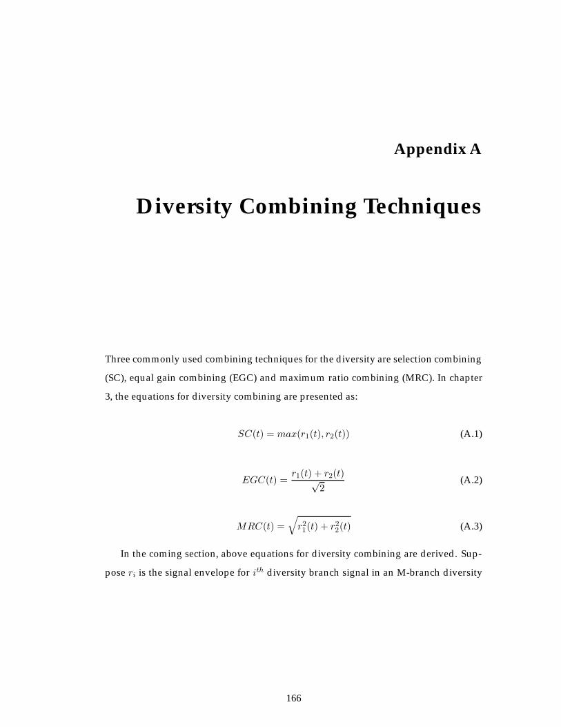
Appendix A
Diversity Combining Techniques
Three commonly used combining techniques for the diversity are selection combining
(SC), equal gain combining (EGC) and maximum ratio combining (MRC). In chapter
3, the equations for diversity combining are presented as:
SC(t) = max(r1(t), r2(t)) (A.1)
EGC(t) =r1(t) + r2(t)√
2(A.2)
MRC(t) =√
r21(t) + r22(t) (A.3)
In the coming section, above equations for diversity combining are derived. Sup-
pose ri is the signal envelope for ith diversity branch signal in an M-branch diversity
166
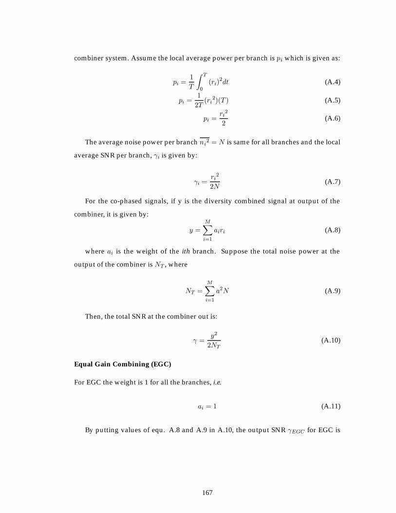
combiner system. Assume the local average power per branch is pi which is given as:
pi =1
T
∫ T
0(ri)
2dt (A.4)
pi =1
2T(ri
2)(T ) (A.5)
pi =ri
2
2(A.6)
The average noise power per branch ni2 = N is same for all branches and the local
average SNR per branch, γi is given by:
γi =ri
2
2N(A.7)
For the co-phased signals, if y is the diversity combined signal at output of the
combiner, it is given by:
y =
M∑i=1
airi (A.8)
where ai is the weight of the ith branch. Suppose the total noise power at the
output of the combiner is NT , where
NT =
M∑i=1
a2N (A.9)
Then, the total SNR at the combiner out is:
γ =y2
2NT(A.10)
Equal Gain Combining (EGC)
For EGC the weight is 1 for all the branches, i.e.
ai = 1 (A.11)
By putting values of equ. A.8 and A.9 in A.10, the output SNR γEGC for EGC is
167
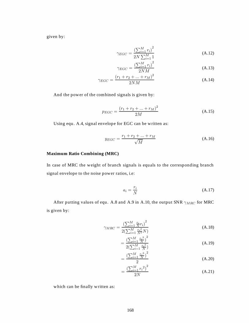
given by:
γEGC =(∑M
i=1 ri)2
2N∑M
i=1 1(A.12)
γEGC =(∑M
i=1 ri)2
2NM(A.13)
γEGC =(r1 + r2 + ...+ rM )2
2NM(A.14)
And the power of the combined signals is given by:
pEGC =(r1 + r2 + ...+ rM )2
2M(A.15)
Using equ. A.4, signal envelope for EGC can be written as:
yEGC =r1 + r2 + ...+ rM√
M(A.16)
Maximum Ratio Combining (MRC)
In case of MRC the weight of branch signals is equals to the corresponding branch
signal envelope to the noise power ratios, i.e:
ai =riN
(A.17)
After putting values of equ. A.8 and A.9 in A.10, the output SNR γMRC for MRC
is given by:
γMRC =(∑M
i=1riN ri)
2
2(∑M
i=1ri2
N2N)(A.18)
=(∑M
i=1ri2
N )2
2(∑M
i=1ri2
N )(A.19)
=(∑M
i=1ri2
N )2
2(A.20)
=(∑M
i=1 ri2)
2
2N(A.21)
which can be finally written as:
168
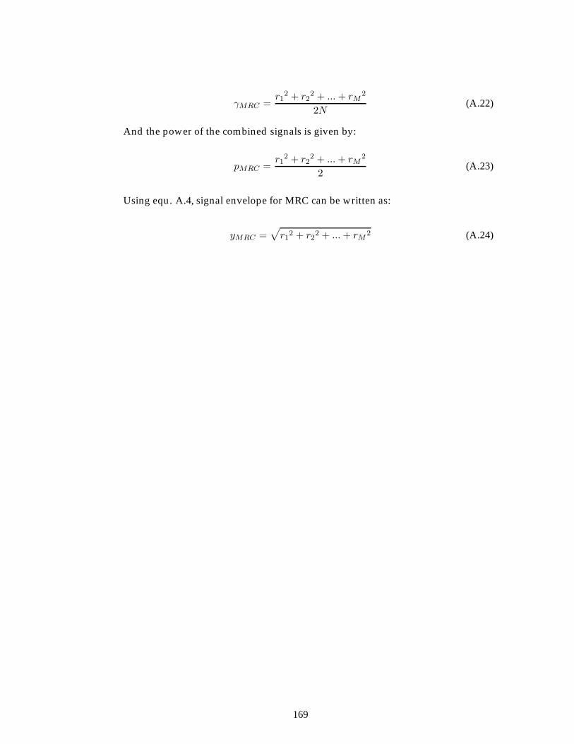
γMRC =r1
2 + r22 + ...+ rM
2
2N(A.22)
And the power of the combined signals is given by:
pMRC =r1
2 + r22 + ...+ rM
2
2(A.23)
Using equ. A.4, signal envelope for MRC can be written as:
yMRC =√
r12 + r22 + ...+ rM 2 (A.24)
169
Appendix B
Multiband OFDM Ultra Wideband
System
The principal idea of multiband approaches is to divide the UWB frequency band (3.1
to 10.6 GHz) into multiple smaller frequency bands (also referred to as subbands) and
uses multiple carrier frequencies to transmit the information. Each subband has a
bandwidth greater than 500 MHz to comply with the FCC definition of a UWB signal
[1]. Using multiband OFDM approach, smaller bands are used to process the data
which in turn reduces overall design complexity and improves spectral flexibility and
worldwide compliance. Specifically, reduction of sampling rate for A/D converters
are achieved due to reduction in bandwidth. Moreover, due to smaller bands more
fine-grained control of the power spectral density (i.e. the average transmitter power
can be maximised), according to the FCC spectral mask. In order to capture the mul-
tipath energy efficiently (as UWB has inherent rich multipath diveristy), the OFDM
technique has been used to modulate the information in each subband. The major
difference between multiband OFDM and traditional OFDM schemes is that the mult-
iband OFDM symbols are not sent continually on one frequency band; instead, they
170
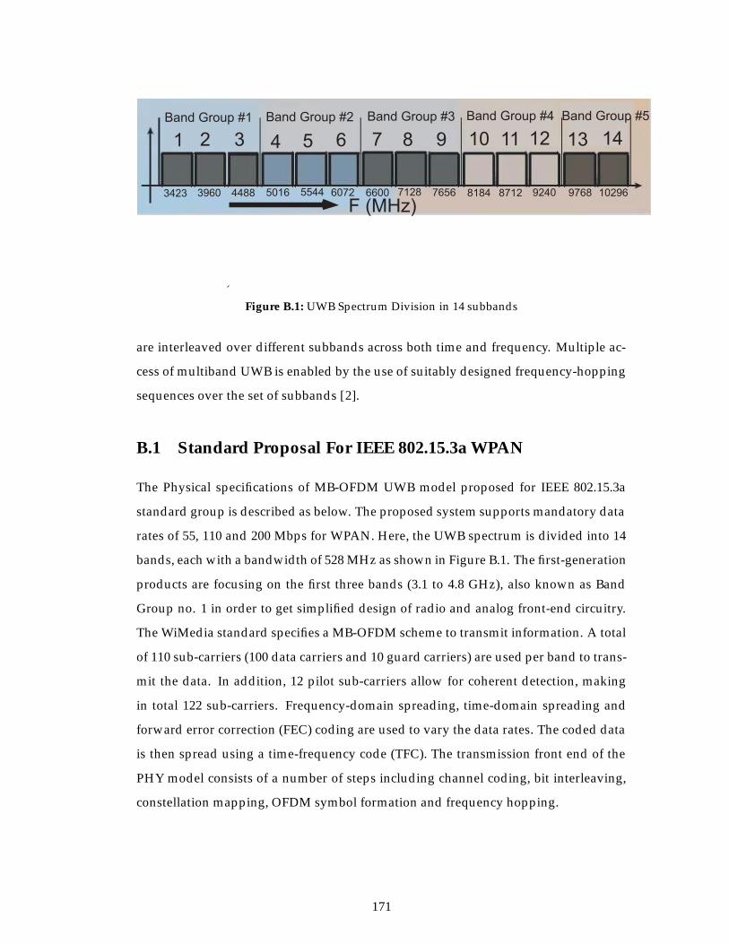
Band Group #1 Band Group #2 Band Group #3 Band Group #4 Band Group #5
1 2 3 4 5 6 7 8 9 10 11 12 13 14
F (MHz)3423 3960 4488 55445016 6072 6600 7128 7656 8184 8712 9240 9768 10296
Figure B.1: UWB Spectrum Division in 14 subbands
are interleaved over different subbands across both time and frequency. Multiple ac-
cess of multiband UWB is enabled by the use of suitably designed frequency-hopping
sequences over the set of subbands [2].
B.1 Standard Proposal For IEEE 802.15.3a WPAN
The Physical specifications of MB-OFDM UWB model proposed for IEEE 802.15.3a
standard group is described as below. The proposed system supports mandatory data
rates of 55, 110 and 200 Mbps for WPAN. Here, the UWB spectrum is divided into 14
bands, each with a bandwidth of 528 MHz as shown in Figure B.1. The first-generation
products are focusing on the first three bands (3.1 to 4.8 GHz), also known as Band
Group no. 1 in order to get simplified design of radio and analog front-end circuitry.
The WiMedia standard specifies a MB-OFDM scheme to transmit information. A total
of 110 sub-carriers (100 data carriers and 10 guard carriers) are used per band to trans-
mit the data. In addition, 12 pilot sub-carriers allow for coherent detection, making
in total 122 sub-carriers. Frequency-domain spreading, time-domain spreading and
forward error correction (FEC) coding are used to vary the data rates. The coded data
is then spread using a time-frequency code (TFC). The transmission front end of the
PHY model consists of a number of steps including channel coding, bit interleaving,
constellation mapping, OFDM symbol formation and frequency hopping.
171
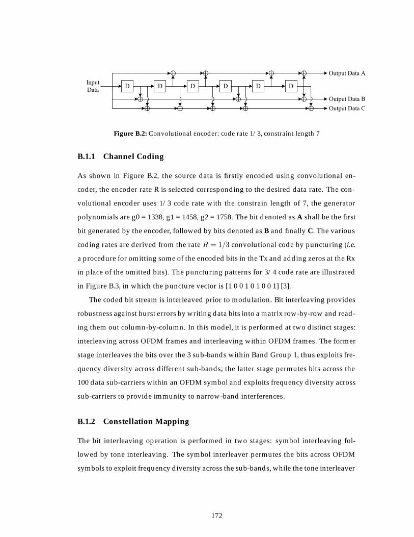
D D D D D DInputData
Output Data A
Output Data BOutput Data C
Figure B.2: Convolutional encoder: code rate 1/3, constraint length 7
B.1.1 Channel Coding
As shown in Figure B.2, the source data is firstly encoded using convolutional en-
coder, the encoder rate R is selected corresponding to the desired data rate. The con-
volutional encoder uses 1/3 code rate with the constrain length of 7, the generator
polynomials are g0 = 1338, g1 = 1458, g2 = 1758. The bit denoted as A shall be the first
bit generated by the encoder, followed by bits denoted as B and finally C. The various
coding rates are derived from the rate R = 1/3 convolutional code by puncturing (i.e.
a procedure for omitting some of the encoded bits in the Tx and adding zeros at the Rx
in place of the omitted bits). The puncturing patterns for 3/4 code rate are illustrated
in Figure B.3, in which the puncture vector is [1 0 0 1 0 1 0 0 1] [3].
The coded bit stream is interleaved prior to modulation. Bit interleaving provides
robustness against burst errors by writing data bits into a matrix row-by-row and read-
ing them out column-by-column. In this model, it is performed at two distinct stages:
interleaving across OFDM frames and interleaving within OFDM frames. The former
stage interleaves the bits over the 3 sub-bands within Band Group 1, thus exploits fre-
quency diversity across different sub-bands; the latter stage permutes bits across the
100 data sub-carriers within an OFDM symbol and exploits frequency diversity across
sub-carriers to provide immunity to narrow-band interferences.
B.1.2 Constellation Mapping
The bit interleaving operation is performed in two stages: symbol interleaving fol-
lowed by tone interleaving. The symbol interleaver permutes the bits across OFDM
symbols to exploit frequency diversity across the sub-bands, while the tone interleaver
172
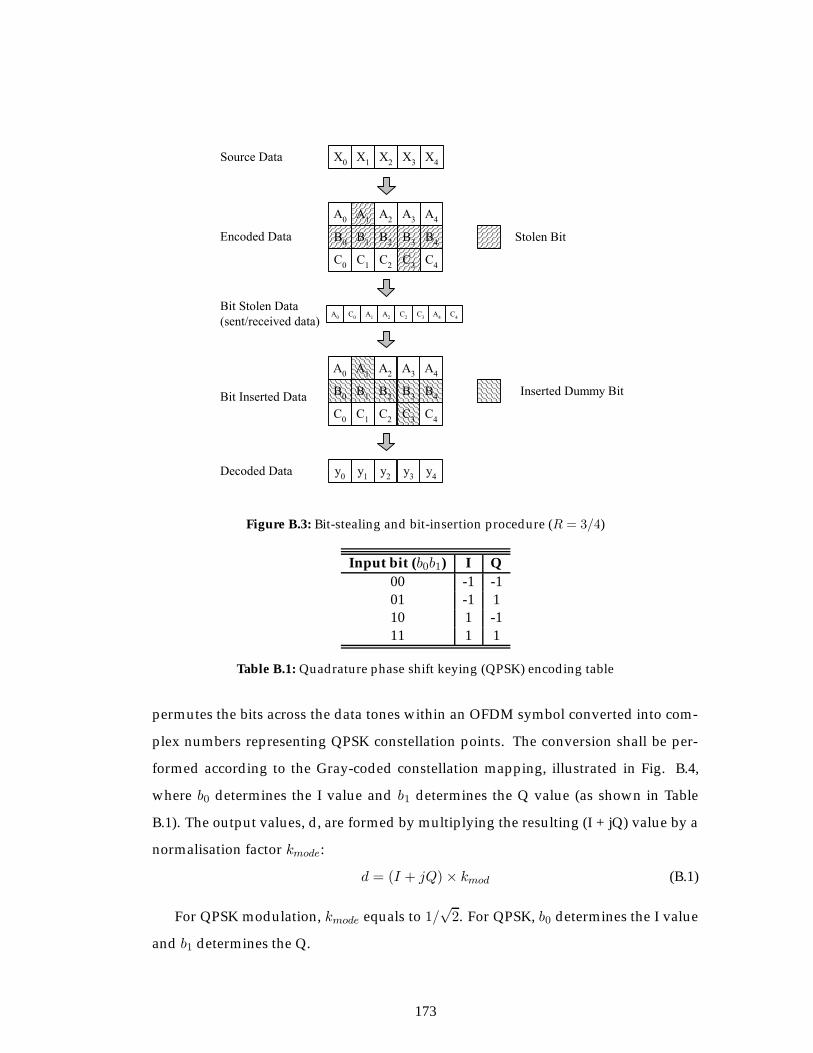
X4X3X2X1X0
A4A3A2A1
B4B3B2B1B0
C4C3C2C1C0
A4A3A2A1A0
B4B3B2B1B0
C4C3C2C1C0
y4y3y2y1y0
Stolen Bit
Inserted Dummy Bit
A0
Source Data
Encoded Data
Bit Stolen Data(sent/received data)
Bit Inserted Data
Decoded Data
A0 C0 A1 A2 C2 C3 A4 C4
Figure B.3: Bit-stealing and bit-insertion procedure (R = 3/4)
Input bit (b0b1) I Q00 -1 -101 -1 110 1 -111 1 1
Table B.1: Quadrature phase shift keying (QPSK) encoding table
permutes the bits across the data tones within an OFDM symbol converted into com-
plex numbers representing QPSK constellation points. The conversion shall be per-
formed according to the Gray-coded constellation mapping, illustrated in Fig. B.4,
where b0 determines the I value and b1 determines the Q value (as shown in Table
B.1). The output values, d, are formed by multiplying the resulting (I + jQ) value by a
normalisation factor kmode:
d = (I + jQ)× kmod (B.1)
For QPSK modulation, kmode equals to 1/√2. For QPSK, b0 determines the I value
and b1 determines the Q.
173
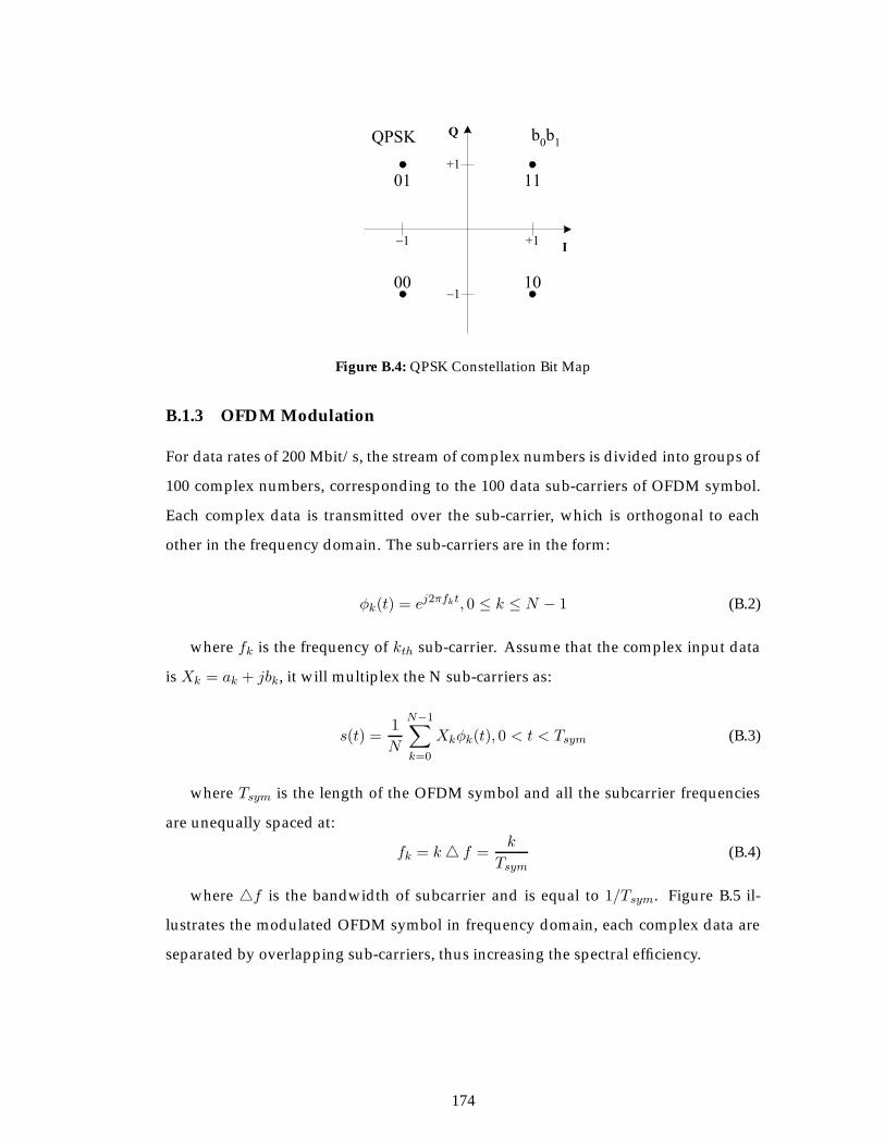
+11
+1
1
Q
I
QPSK
01 11
b0b1
00 10
Figure B.4: QPSK Constellation Bit Map
B.1.3 OFDM Modulation
For data rates of 200 Mbit/s, the stream of complex numbers is divided into groups of
100 complex numbers, corresponding to the 100 data sub-carriers of OFDM symbol.
Each complex data is transmitted over the sub-carrier, which is orthogonal to each
other in the frequency domain. The sub-carriers are in the form:
φk(t) = ej2πfkt, 0 ≤ k ≤ N − 1 (B.2)
where fk is the frequency of kth sub-carrier. Assume that the complex input data
is Xk = ak + jbk, it will multiplex the N sub-carriers as:
s(t) =1
N
N−1∑k=0
Xkφk(t), 0 < t < Tsym (B.3)
where Tsym is the length of the OFDM symbol and all the subcarrier frequencies
are unequally spaced at:
fk = k� f =k
Tsym(B.4)
where �f is the bandwidth of subcarrier and is equal to 1/Tsym. Figure B.5 il-
lustrates the modulated OFDM symbol in frequency domain, each complex data are
separated by overlapping sub-carriers, thus increasing the spectral efficiency.
174
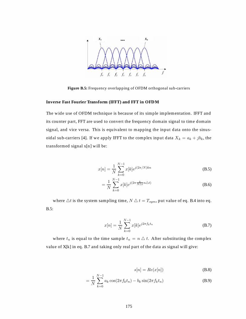
X1 X6
Figure B.5: Frequency overlapping of OFDM orthogonal sub-carriers
Inverse Fast Fourier Transform (IFFT) and FFT in OFDM
The wide use of OFDM technique is because of its simple implementation. IFFT and
its counter part, FFT are used to convert the frequency domain signal to time domain
signal, and vice versa. This is equivalent to mapping the input data onto the sinus-
oidal sub-carriers [4]. If we apply IFFT to the complex input data Xk = ak + jbk, the
transformed signal x[n] will be:
x[n] =1
N
N−1∑k=0
x[k]ej(2π/N)kn (B.5)
=1
N
N−1∑k=0
x[k]ej(2π k
N�tn�t) (B.6)
where �t is the system sampling time, N � t = Tsym, put value of eq. B.4 into eq.
B.5:
x[n] =1
N
N−1∑k=0
x[k]ej2πfktn (B.7)
where tn is equal to the time sample tn = n � t. After substituting the complex
value of X[k] in eq. B.7 and taking only real part of the data as signal will give:
s[n] = Re(x[n]) (B.8)
=1
N
N−1∑k=0
ak cos(2πfktn)− bk sin(2πfktn) (B.9)
175
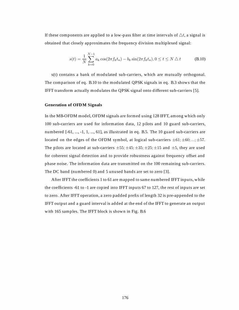
If these components are applied to a low-pass filter at time intervals of �t, a signal is
obtained that closely approximates the frequency division multiplexed signal:
s(t) =1
N
N−1∑k=0
ak cos(2πfktn)− bk sin(2πfktn), 0 ≤ t ≤ N � t (B.10)
s(t) contains a bank of modulated sub-carriers, which are mutually orthogonal.
The comparison of eq. B.10 to the modulated QPSK signals in eq. B.3 shows that the
IFFT transform actually modulates the QPSK signal onto different sub-carriers [5].
Generation of OFDM Signals
In the MB-OFDM model, OFDM signals are formed using 128 IFFT, among which only
100 sub-carriers are used for information data, 12 pilots and 10 guard sub-carriers,
numbered [-61, ..., -1, 1, ..., 61], as illustrated in eq. B.5. The 10 guard sub-carriers are
located on the edges of the OFDM symbol, at logical sub-carriers ±61;±60; ...;±57.
The pilots are located at sub-carriers ±55;±45;±35;±25;±15 and ±5, they are used
for coherent signal detection and to provide robustness against frequency offset and
phase noise. The information data are transmitted on the 100 remaining sub-carriers.
The DC band (numbered 0) and 5 unused bands are set to zero [3].
After IFFT the coefficients 1 to 61 are mapped to same numbered IFFT inputs, while
the coefficients -61 to -1 are copied into IFFT inputs 67 to 127, the rest of inputs are set
to zero. After IFFT operation, a zero padded prefix of length 32 is pre-appended to the
IFFT output and a guard interval is added at the end of the IFFT to generate an output
with 165 samples. The IFFT block is shown in Fig. B.6
176

IFF
T T
ransfo
rm
Figure B.6: Input and output of IFFT
177
References
[1] W. P. Siriwongpairat and K. J. Ray Liu, Ultra-Wideband Communications Systems: MultibandOFDM Approach. John Wiley & Sons, Ltd., 2007.
[2] M. H. I. Opperman and J. Iinatti, UWB theory and applications. John Wiley & Sons, 2004.
[3] A. Batra, “Multi-band OFDM physical layer proposal for IEEE 802.15 task group 3a,” TexasInstruments, Tech. Rep., November 2003.
[4] Litwin and M. Pugel, “RF signal processing: The principles of OFDM, RF design,” pp.30–48, Jan 2001.
[5] D. Matiae, “OFDM as a possible modulation technique for multimedia applications in therange of mm waves:introduction to OFDM,” 1998.
178
Related Documents