RADIATIVE TRANSFER IN STELLAR ATMOSPHERESbaron/ast4303/afy1-2.pdf · RADIATIVE TRANSFER IN STELLAR ATMOSPHERES R.J. Rutten Sterrekundig Instituut Utrecht Institute of Theoretical

RADIATIVE TRANSFER

IN

STELLAR ATMOSPHERES

R.J. Rutten

Sterrekundig Instituut Utrecht

Institute of Theoretical Astrophysics Oslo

May 8, 2003

ESMN

Copyright c! 1995 Robert J. Rutten, Sterrekundig Instuut Utrecht, The Netherlands.Copying permitted for non-commercial educational purposes only. R.J. Rutten asserts themoral right to be identified as the author of these notes. In no way can he be held responsiblefor any liability with respect to these notes.

First Utrecht edition: March 7, 1995. Based on “Stellar Atmospheres” lecture notes by C. Zwaan.First WWW edition: June 1, 1995 for the 1995 Oslo Summer School. Figures scanned by Sake

Hogeveen. Corrections from Louis Strous, Bart-Jan van Tent, Guus Oonincx, Dan Kiselman,Mats Carlsson.

Second WWW edition: June 22, 1995. Corrections from Carine Briand, Kees Dullemond, MartijnSmit.

Third edition: March 11, 1996. Corrections from Ferdi Hulleman. Section “Exercises” started.Fourth WWW edition: October 1, 1997. Corrections from Hans Akkerman, Thijs Krijger, Nils

Ryde, Bob Stein.Fourth SIU edition: January 6, 1998. Corrections from Oliver Ryan; new figures from Thijs Krijger.Fifth SIU/WWW edition: January 4, 1999. Corrections from Mark Gieles, Jorrit Wiersma, Marc

van der Sluys, Niels Zagers.Sixth edition: May 20, 1999, for the ESMN Summer School at Oslo. Corrections from Wouter

Bergmann Tiest.Seventh edition: December 1, 2000. Corrections from Karin Jonsell, Torgny Karlsson, Hans van

Rijn, Louis Strous.Eighth edition: May 8, 2003. Corrections from Else van den Besselaar, Jacqueline Mout, Jelle de

Plaa, Remco Scheepmaker.

These lecture notes are freely available as a service of the European Solar MagnetismNetwork (http://esmn.astro.uu.nl). There are also corresponding equation viewgraphsfor classroom display.Details on how to get printable files are given at http://www.astro.uu.nl/"rutten.These lecture notes still evolve; the WWW information contains an update on theirstatus. Major renewals are announced to those who request to be put on the noti-fication email list. Corrections and additions are very welcome; please send them toR.J.Rutten@ astro.uu.nl.You are also most welcome to cite these lecture notes. Please do so as: Rutten, R.J., 2003,Radiative Transfer in Stellar Atmospheres, Utrecht University lecture notes, 8th edition.

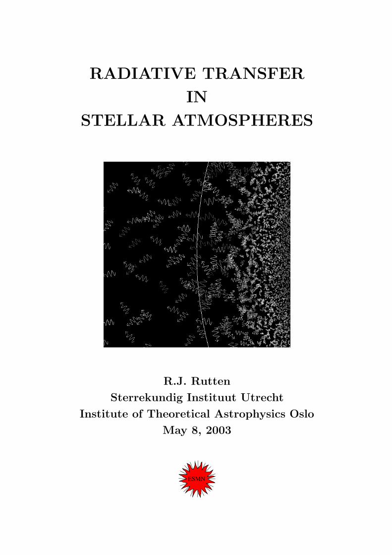
Cover: a stellar atmosphere is where photons leave the star, a dramatic transition fromwarm dense comfort in near-thermal enclosure to bare isolation in the cold emptiness ofspace — su!ciently traumatic to make stellar atmospheres highly interesting to astro-physicists. On average, photons get scarcer, longer, and more outwards directed furtherout in the atmosphere until they escape. Copied from Mats Carlsson’s poster for the 1995Oslo “Intensive Summer School on Radiative Transfer and Radiation Hydrodynamics”.

Contents

Preface xv

Bibliography xvii

1 Brief History of Stellar Spectrometry 1Fraunhofer lines . . . . . . . . . . . . . . . . . . . . . . . . . . . . . . . . . . . . . 1Lines as element encoders . . . . . . . . . . . . . . . . . . . . . . . . . . . . . . . . 2Stellar classification . . . . . . . . . . . . . . . . . . . . . . . . . . . . . . . . . . . 2Abundance determination . . . . . . . . . . . . . . . . . . . . . . . . . . . . . . . . 4Reversing-layer line formation . . . . . . . . . . . . . . . . . . . . . . . . . . . . . . 5LTE line formation . . . . . . . . . . . . . . . . . . . . . . . . . . . . . . . . . . . . 5NLTE line formation . . . . . . . . . . . . . . . . . . . . . . . . . . . . . . . . . . . 5Numerical line formation . . . . . . . . . . . . . . . . . . . . . . . . . . . . . . . . 5Diagnostic line formation . . . . . . . . . . . . . . . . . . . . . . . . . . . . . . . . 5

2 Basic Radiative Transfer 92.1 Radiation . . . . . . . . . . . . . . . . . . . . . . . . . . . . . . . . . . . . . . . . . 9

2.1.1 Local amount . . . . . . . . . . . . . . . . . . . . . . . . . . . . . . . . . . . 9Intensity . . . . . . . . . . . . . . . . . . . . . . . . . . . . . . . . . . . 9Mean intensity . . . . . . . . . . . . . . . . . . . . . . . . . . . . . . . . 10Flux . . . . . . . . . . . . . . . . . . . . . . . . . . . . . . . . . . . . . . 10Density . . . . . . . . . . . . . . . . . . . . . . . . . . . . . . . . . . . . 11Pressure . . . . . . . . . . . . . . . . . . . . . . . . . . . . . . . . . . . . 12Moments of the intensity . . . . . . . . . . . . . . . . . . . . . . . . . . 12

2.1.2 Local change . . . . . . . . . . . . . . . . . . . . . . . . . . . . . . . . . . . 12Emission . . . . . . . . . . . . . . . . . . . . . . . . . . . . . . . . . . . 12Extinction . . . . . . . . . . . . . . . . . . . . . . . . . . . . . . . . . . 13Source function . . . . . . . . . . . . . . . . . . . . . . . . . . . . . . . . 13

2.2 Transport equation . . . . . . . . . . . . . . . . . . . . . . . . . . . . . . . . . . . . 142.2.1 Transport along a ray . . . . . . . . . . . . . . . . . . . . . . . . . . . . . . 14

Discussion . . . . . . . . . . . . . . . . . . . . . . . . . . . . . . . . . . 14Optical length and thickness . . . . . . . . . . . . . . . . . . . . . . . . 14Homogeneous medium . . . . . . . . . . . . . . . . . . . . . . . . . . . . 15

2.2.2 Transport through an atmosphere . . . . . . . . . . . . . . . . . . . . . . . 17Optical depth . . . . . . . . . . . . . . . . . . . . . . . . . . . . . . . . . 17Standard plane-parallel transport equation . . . . . . . . . . . . . . . . 17Formal solution . . . . . . . . . . . . . . . . . . . . . . . . . . . . . . . . 17Eddington-Barbier approximation . . . . . . . . . . . . . . . . . . . . . 18

2.3 Line transitions . . . . . . . . . . . . . . . . . . . . . . . . . . . . . . . . . . . . . . 182.3.1 Einstein coe!cients . . . . . . . . . . . . . . . . . . . . . . . . . . . . . . . 19

Spontaneous deexcitation . . . . . . . . . . . . . . . . . . . . . . . . . . 19Radiative excitation . . . . . . . . . . . . . . . . . . . . . . . . . . . . . 21Induced deexcitation . . . . . . . . . . . . . . . . . . . . . . . . . . . . . 22

iii

iv CONTENTS

Collisional excitation and deexcitation . . . . . . . . . . . . . . . . . . . 22Einstein relations . . . . . . . . . . . . . . . . . . . . . . . . . . . . . . . 23

2.3.2 Volume coe!cients . . . . . . . . . . . . . . . . . . . . . . . . . . . . . . . . 23Extinction . . . . . . . . . . . . . . . . . . . . . . . . . . . . . . . . . . 23Emission . . . . . . . . . . . . . . . . . . . . . . . . . . . . . . . . . . . 24Source function . . . . . . . . . . . . . . . . . . . . . . . . . . . . . . . . 24

2.4 Continuum transitions . . . . . . . . . . . . . . . . . . . . . . . . . . . . . . . . . . 252.4.1 Inelastic processes . . . . . . . . . . . . . . . . . . . . . . . . . . . . . . . . 25

Bound-free transitions . . . . . . . . . . . . . . . . . . . . . . . . . . . . 25Discussion . . . . . . . . . . . . . . . . . . . . . . . . . . . . . . . . . . 25Free-free transitions . . . . . . . . . . . . . . . . . . . . . . . . . . . . . 26

2.4.2 Elastic processes . . . . . . . . . . . . . . . . . . . . . . . . . . . . . . . . . 27Thomson scattering . . . . . . . . . . . . . . . . . . . . . . . . . . . . . 27Rayleigh scattering . . . . . . . . . . . . . . . . . . . . . . . . . . . . . . 28Redistribution . . . . . . . . . . . . . . . . . . . . . . . . . . . . . . . . 28

2.5 LTE . . . . . . . . . . . . . . . . . . . . . . . . . . . . . . . . . . . . . . . . . . . . 282.5.1 Matter in LTE . . . . . . . . . . . . . . . . . . . . . . . . . . . . . . . . . . 28

Maxwell distribution . . . . . . . . . . . . . . . . . . . . . . . . . . . . . 28Boltzmann distribution . . . . . . . . . . . . . . . . . . . . . . . . . . . 29Saha distribution . . . . . . . . . . . . . . . . . . . . . . . . . . . . . . . 30Saha-Boltzmann distribution . . . . . . . . . . . . . . . . . . . . . . . . 30

2.5.2 Radiation in LTE . . . . . . . . . . . . . . . . . . . . . . . . . . . . . . . . . 30Planck function . . . . . . . . . . . . . . . . . . . . . . . . . . . . . . . . 30Wien and Rayleigh-Jeans approximations . . . . . . . . . . . . . . . . . 31Stefan-Boltzmann law . . . . . . . . . . . . . . . . . . . . . . . . . . . . 31Induced emission . . . . . . . . . . . . . . . . . . . . . . . . . . . . . . . 31Line extinction . . . . . . . . . . . . . . . . . . . . . . . . . . . . . . . . 31Discussion . . . . . . . . . . . . . . . . . . . . . . . . . . . . . . . . . . 31

2.6 NLTE . . . . . . . . . . . . . . . . . . . . . . . . . . . . . . . . . . . . . . . . . . . 322.6.1 Statistical equilibrium . . . . . . . . . . . . . . . . . . . . . . . . . . . . . . 32

Rate equations . . . . . . . . . . . . . . . . . . . . . . . . . . . . . . . . 32Transport equations . . . . . . . . . . . . . . . . . . . . . . . . . . . . . 32Time-dependent transfer . . . . . . . . . . . . . . . . . . . . . . . . . . 33Multi-dimensional transfer . . . . . . . . . . . . . . . . . . . . . . . . . 33

2.6.2 NLTE descriptions . . . . . . . . . . . . . . . . . . . . . . . . . . . . . . . . 33Departure coe!cients . . . . . . . . . . . . . . . . . . . . . . . . . . . . 33Bound-bound source function . . . . . . . . . . . . . . . . . . . . . . . . 33Bound-bound extinction . . . . . . . . . . . . . . . . . . . . . . . . . . . 34Laser regime . . . . . . . . . . . . . . . . . . . . . . . . . . . . . . . . . 35Bound-free source function . . . . . . . . . . . . . . . . . . . . . . . . . 35Bound-free extinction . . . . . . . . . . . . . . . . . . . . . . . . . . . . 35Bound-free emission . . . . . . . . . . . . . . . . . . . . . . . . . . . . . 35Free-free source function, extinction, emission . . . . . . . . . . . . . . . 36Discussion . . . . . . . . . . . . . . . . . . . . . . . . . . . . . . . . . . 36Warning . . . . . . . . . . . . . . . . . . . . . . . . . . . . . . . . . . . . 36Formal temperatures . . . . . . . . . . . . . . . . . . . . . . . . . . . . . 37

2.6.3 Coherent scattering . . . . . . . . . . . . . . . . . . . . . . . . . . . . . . . 38Two-level atoms . . . . . . . . . . . . . . . . . . . . . . . . . . . . . . . 38Coherently scattering medium . . . . . . . . . . . . . . . . . . . . . . . 39Destruction probability . . . . . . . . . . . . . . . . . . . . . . . . . . . 39E"ective path, thickness, depth . . . . . . . . . . . . . . . . . . . . . . . 40Source function . . . . . . . . . . . . . . . . . . . . . . . . . . . . . . . . 40Transport equation . . . . . . . . . . . . . . . . . . . . . . . . . . . . . . 41

2.6.4 Multi-level interlocking . . . . . . . . . . . . . . . . . . . . . . . . . . . . . 41

CONTENTS v

2.6.5 Coronal conditions . . . . . . . . . . . . . . . . . . . . . . . . . . . . . . . . 41

3 Bound-Bound and Bound-Free Transitions 433.1 Photonic transitions . . . . . . . . . . . . . . . . . . . . . . . . . . . . . . . . . . . 43

3.1.1 Atomic transitions . . . . . . . . . . . . . . . . . . . . . . . . . . . . . . . . 433.1.2 Molecular transitions . . . . . . . . . . . . . . . . . . . . . . . . . . . . . . . 433.1.3 Two-electron transitions . . . . . . . . . . . . . . . . . . . . . . . . . . . . . 43

Dielectronic recombination . . . . . . . . . . . . . . . . . . . . . . . . . 43Autoionization . . . . . . . . . . . . . . . . . . . . . . . . . . . . . . . . 44Bound-free resonances . . . . . . . . . . . . . . . . . . . . . . . . . . . . 44

3.1.4 Charge-transfer transitions . . . . . . . . . . . . . . . . . . . . . . . . . . . 443.2 Transition rates . . . . . . . . . . . . . . . . . . . . . . . . . . . . . . . . . . . . . . 44

3.2.1 Bound-bound radiative rates . . . . . . . . . . . . . . . . . . . . . . . . . . 443.2.2 Bound-free radiative rates . . . . . . . . . . . . . . . . . . . . . . . . . . . . 45

Physics . . . . . . . . . . . . . . . . . . . . . . . . . . . . . . . . . . . . 45Einstein-Milne equations . . . . . . . . . . . . . . . . . . . . . . . . . . 46Photoionization . . . . . . . . . . . . . . . . . . . . . . . . . . . . . . . 46Spontaneous recombination . . . . . . . . . . . . . . . . . . . . . . . . . 46Discussion . . . . . . . . . . . . . . . . . . . . . . . . . . . . . . . . . . 47Induced recombination . . . . . . . . . . . . . . . . . . . . . . . . . . . 47Total radiative recombination . . . . . . . . . . . . . . . . . . . . . . . . 47

3.2.3 Unified radiative rates . . . . . . . . . . . . . . . . . . . . . . . . . . . . . . 48Discussion . . . . . . . . . . . . . . . . . . . . . . . . . . . . . . . . . . 48

3.2.4 Net radiative rates . . . . . . . . . . . . . . . . . . . . . . . . . . . . . . . . 48Net radiative recombination . . . . . . . . . . . . . . . . . . . . . . . . . 48Net radiative deexcitation . . . . . . . . . . . . . . . . . . . . . . . . . . 49Discussion . . . . . . . . . . . . . . . . . . . . . . . . . . . . . . . . . . 49

3.2.5 Collision rates . . . . . . . . . . . . . . . . . . . . . . . . . . . . . . . . . . 50Net collision rates . . . . . . . . . . . . . . . . . . . . . . . . . . . . . . 51Collisional coupling . . . . . . . . . . . . . . . . . . . . . . . . . . . . . 52Collisional LTE . . . . . . . . . . . . . . . . . . . . . . . . . . . . . . . . 52

3.3 Spectral line broadening . . . . . . . . . . . . . . . . . . . . . . . . . . . . . . . . . 523.3.1 Radiation broadening . . . . . . . . . . . . . . . . . . . . . . . . . . . . . . 53

Damping profile . . . . . . . . . . . . . . . . . . . . . . . . . . . . . . . 53Extinction profile . . . . . . . . . . . . . . . . . . . . . . . . . . . . . . . 53Derivation . . . . . . . . . . . . . . . . . . . . . . . . . . . . . . . . . . 53Multiple levels and transitions . . . . . . . . . . . . . . . . . . . . . . . 54

3.3.2 Collision broadening . . . . . . . . . . . . . . . . . . . . . . . . . . . . . . . 54Elastic collisions . . . . . . . . . . . . . . . . . . . . . . . . . . . . . . . 54Impact approximation . . . . . . . . . . . . . . . . . . . . . . . . . . . . 55Quasi-static approximation . . . . . . . . . . . . . . . . . . . . . . . . . 55Classification . . . . . . . . . . . . . . . . . . . . . . . . . . . . . . . . . 55Linear Stark e"ect (n = 2) . . . . . . . . . . . . . . . . . . . . . . . . . 55Resonance broadening (n = 3) . . . . . . . . . . . . . . . . . . . . . . . 56Quadratic Stark e"ect (n = 4) . . . . . . . . . . . . . . . . . . . . . . . 56Van der Waals broadening (n = 6) . . . . . . . . . . . . . . . . . . . . . 56Van der Waals enhancement factor . . . . . . . . . . . . . . . . . . . . . 57

3.3.3 Doppler broadening . . . . . . . . . . . . . . . . . . . . . . . . . . . . . . . 57Doppler shift . . . . . . . . . . . . . . . . . . . . . . . . . . . . . . . . . 57Thermal motions . . . . . . . . . . . . . . . . . . . . . . . . . . . . . . . 57Thermal broadening . . . . . . . . . . . . . . . . . . . . . . . . . . . . . 58Voigt profile . . . . . . . . . . . . . . . . . . . . . . . . . . . . . . . . . 59Rotational broadening . . . . . . . . . . . . . . . . . . . . . . . . . . . . 60Deconvolution . . . . . . . . . . . . . . . . . . . . . . . . . . . . . . . . 61

vi CONTENTS

Turbulent broadening . . . . . . . . . . . . . . . . . . . . . . . . . . . . 62Warning . . . . . . . . . . . . . . . . . . . . . . . . . . . . . . . . . . . . 63

3.3.4 Other broadening . . . . . . . . . . . . . . . . . . . . . . . . . . . . . . . . . 63Hyperfine structure . . . . . . . . . . . . . . . . . . . . . . . . . . . . . 63Isotope splitting . . . . . . . . . . . . . . . . . . . . . . . . . . . . . . . 63Zeeman splitting . . . . . . . . . . . . . . . . . . . . . . . . . . . . . . . 63

3.3.5 Spectral edge broadening . . . . . . . . . . . . . . . . . . . . . . . . . . . . 64Near-edge line blending . . . . . . . . . . . . . . . . . . . . . . . . . . . 64

3.4 Spectral line redistribution . . . . . . . . . . . . . . . . . . . . . . . . . . . . . . . 643.4.1 Monochromatic redistribution . . . . . . . . . . . . . . . . . . . . . . . . . . 64

Sharp-line atoms . . . . . . . . . . . . . . . . . . . . . . . . . . . . . . . 64Up-down sequences . . . . . . . . . . . . . . . . . . . . . . . . . . . . . 65Transport equation . . . . . . . . . . . . . . . . . . . . . . . . . . . . . . 66Extinction . . . . . . . . . . . . . . . . . . . . . . . . . . . . . . . . . . 67Emission . . . . . . . . . . . . . . . . . . . . . . . . . . . . . . . . . . . 67Source function . . . . . . . . . . . . . . . . . . . . . . . . . . . . . . . . 68Destruction probability . . . . . . . . . . . . . . . . . . . . . . . . . . . 68Discussion . . . . . . . . . . . . . . . . . . . . . . . . . . . . . . . . . . 69Thomson and Rayleigh scattering . . . . . . . . . . . . . . . . . . . . . 69

3.4.2 Complete redistribution . . . . . . . . . . . . . . . . . . . . . . . . . . . . . 70Two-level statistical equilibrium . . . . . . . . . . . . . . . . . . . . . . 70Frequency dependence . . . . . . . . . . . . . . . . . . . . . . . . . . . . 71Angle dependence . . . . . . . . . . . . . . . . . . . . . . . . . . . . . . 71Absence of lasering . . . . . . . . . . . . . . . . . . . . . . . . . . . . . . 71

3.4.3 Partial redistribution . . . . . . . . . . . . . . . . . . . . . . . . . . . . . . . 72Qualitative summary . . . . . . . . . . . . . . . . . . . . . . . . . . . . 72Formulation . . . . . . . . . . . . . . . . . . . . . . . . . . . . . . . . . . 72

3.4.4 Angle redistribution . . . . . . . . . . . . . . . . . . . . . . . . . . . . . . . 723.4.5 Spectral edge redistribution . . . . . . . . . . . . . . . . . . . . . . . . . . . 72

Bound-free scattering . . . . . . . . . . . . . . . . . . . . . . . . . . . . 72One-level-plus-continuum atoms . . . . . . . . . . . . . . . . . . . . . . 73Discussion . . . . . . . . . . . . . . . . . . . . . . . . . . . . . . . . . . 74

4 Analytical Radiative Transfer 754.1 Formal solutions . . . . . . . . . . . . . . . . . . . . . . . . . . . . . . . . . . . . . 75

4.1.1 General transport equation . . . . . . . . . . . . . . . . . . . . . . . . . . . 75Spherical geometry . . . . . . . . . . . . . . . . . . . . . . . . . . . . . . 75Plane-parallel geometry . . . . . . . . . . . . . . . . . . . . . . . . . . . 76More transport equations . . . . . . . . . . . . . . . . . . . . . . . . . . 76Discussion . . . . . . . . . . . . . . . . . . . . . . . . . . . . . . . . . . 77

4.1.2 Exponential integrals . . . . . . . . . . . . . . . . . . . . . . . . . . . . . . . 77Formal solution . . . . . . . . . . . . . . . . . . . . . . . . . . . . . . . . 77Exponential integrals . . . . . . . . . . . . . . . . . . . . . . . . . . . . 77Schwarzschild-Milne equations . . . . . . . . . . . . . . . . . . . . . . . 78Discussion . . . . . . . . . . . . . . . . . . . . . . . . . . . . . . . . . . 79Surface values . . . . . . . . . . . . . . . . . . . . . . . . . . . . . . . . 81

4.1.3 Operators . . . . . . . . . . . . . . . . . . . . . . . . . . . . . . . . . . . . . 81Classical Lambda operator . . . . . . . . . . . . . . . . . . . . . . . . . 81Phi and Chi operators . . . . . . . . . . . . . . . . . . . . . . . . . . . . 82Kourgano" graphs . . . . . . . . . . . . . . . . . . . . . . . . . . . . . . 82Generalized Lambda operators . . . . . . . . . . . . . . . . . . . . . . . 82

4.2 Approximate solutions . . . . . . . . . . . . . . . . . . . . . . . . . . . . . . . . . . 854.2.1 Approximations at the surface . . . . . . . . . . . . . . . . . . . . . . . . . 85

Eddington-Barbier approximations . . . . . . . . . . . . . . . . . . . . . 85

CONTENTS vii

Second Eddington approximation . . . . . . . . . . . . . . . . . . . . . . 864.2.2 Approximations at large depth . . . . . . . . . . . . . . . . . . . . . . . . . 87

Taylor expansion . . . . . . . . . . . . . . . . . . . . . . . . . . . . . . . 87Large depth . . . . . . . . . . . . . . . . . . . . . . . . . . . . . . . . . . 88Di"usion approximation . . . . . . . . . . . . . . . . . . . . . . . . . . . 89Rosseland mean extinction . . . . . . . . . . . . . . . . . . . . . . . . . 90Total radiative energy di"usion . . . . . . . . . . . . . . . . . . . . . . . 90

4.2.3 The Eddington approximation . . . . . . . . . . . . . . . . . . . . . . . . . 91Validity . . . . . . . . . . . . . . . . . . . . . . . . . . . . . . . . . . . . 91Second-order transport equation . . . . . . . . . . . . . . . . . . . . . . 92

4.3 Illustrative solutions . . . . . . . . . . . . . . . . . . . . . . . . . . . . . . . . . . . 924.3.1 Coherent scattering in the Eddington approximation . . . . . . . . . . . . . 92

Transport equation . . . . . . . . . . . . . . . . . . . . . . . . . . . . . . 93Boundary conditions . . . . . . . . . . . . . . . . . . . . . . . . . . . . . 93Solutions . . . . . . . . . . . . . . . . . . . . . . . . . . . . . . . . . . . 93

4.3.2 Isothermal atmosphere . . . . . . . . . . . . . . . . . . . . . . . . . . . . . . 94Solutions . . . . . . . . . . . . . . . . . . . . . . . . . . . . . . . . . . . 94Without scattering . . . . . . . . . . . . . . . . . . . . . . . . . . . . . . 94With scattering . . . . . . . . . . . . . . . . . . . . . . . . . . . . . . . . 95Surface values . . . . . . . . . . . . . . . . . . . . . . . . . . . . . . . . 95Discussion . . . . . . . . . . . . . . . . . . . . . . . . . . . . . . . . . . 97

4.3.3 Thermalization depth . . . . . . . . . . . . . . . . . . . . . . . . . . . . . . 99E"ectively thick regime . . . . . . . . . . . . . . . . . . . . . . . . . . . 99Optically thick regime . . . . . . . . . . . . . . . . . . . . . . . . . . . . 100Optically thin regime . . . . . . . . . . . . . . . . . . . . . . . . . . . . 100

4.3.4 Gradients and splits . . . . . . . . . . . . . . . . . . . . . . . . . . . . . . . 100Continuum splits . . . . . . . . . . . . . . . . . . . . . . . . . . . . . . . 102Overionization . . . . . . . . . . . . . . . . . . . . . . . . . . . . . . . . 102Strong-line splits . . . . . . . . . . . . . . . . . . . . . . . . . . . . . . . 102

4.3.5 Applications . . . . . . . . . . . . . . . . . . . . . . . . . . . . . . . . . . . 104Resonance lines . . . . . . . . . . . . . . . . . . . . . . . . . . . . . . . . 104Lines with thermal background continuum . . . . . . . . . . . . . . . . 104Thermalization depth . . . . . . . . . . . . . . . . . . . . . . . . . . . . 106Continuum scattering . . . . . . . . . . . . . . . . . . . . . . . . . . . . 106Bound-bound redistribution . . . . . . . . . . . . . . . . . . . . . . . . . 107Bound-free redistribution . . . . . . . . . . . . . . . . . . . . . . . . . . 110Discussion . . . . . . . . . . . . . . . . . . . . . . . . . . . . . . . . . . 111

5 Numerical Radiative Transfer 1135.1 Numerical modeling . . . . . . . . . . . . . . . . . . . . . . . . . . . . . . . . . . . 113

5.1.1 Introduction . . . . . . . . . . . . . . . . . . . . . . . . . . . . . . . . . . . 113Aims . . . . . . . . . . . . . . . . . . . . . . . . . . . . . . . . . . . . . 113References . . . . . . . . . . . . . . . . . . . . . . . . . . . . . . . . . . 114

5.1.2 Discretization . . . . . . . . . . . . . . . . . . . . . . . . . . . . . . . . . . . 114Angles . . . . . . . . . . . . . . . . . . . . . . . . . . . . . . . . . . . . . 114Angle quadrature . . . . . . . . . . . . . . . . . . . . . . . . . . . . . . 115Frequencies . . . . . . . . . . . . . . . . . . . . . . . . . . . . . . . . . . 116Depths . . . . . . . . . . . . . . . . . . . . . . . . . . . . . . . . . . . . 116Non-plane-parallel grids . . . . . . . . . . . . . . . . . . . . . . . . . . . 116

5.2 Feautrier method . . . . . . . . . . . . . . . . . . . . . . . . . . . . . . . . . . . . . 117Boundary problems . . . . . . . . . . . . . . . . . . . . . . . . . . . . . 117Antisymmetric averages . . . . . . . . . . . . . . . . . . . . . . . . . . . 118Transport equation . . . . . . . . . . . . . . . . . . . . . . . . . . . . . . 118Boundary conditions . . . . . . . . . . . . . . . . . . . . . . . . . . . . . 119

viii CONTENTS

Di"erence equations . . . . . . . . . . . . . . . . . . . . . . . . . . . . . 119Forward-backward solution . . . . . . . . . . . . . . . . . . . . . . . . . 121Two-level solution . . . . . . . . . . . . . . . . . . . . . . . . . . . . . . 121Rybicki version . . . . . . . . . . . . . . . . . . . . . . . . . . . . . . . . 121Feautrier solver as Lambda operator . . . . . . . . . . . . . . . . . . . . 121

5.3 Lambda iteration . . . . . . . . . . . . . . . . . . . . . . . . . . . . . . . . . . . . . 1225.3.1 Classical Lambda iteration . . . . . . . . . . . . . . . . . . . . . . . . . . . 122

Formal solution . . . . . . . . . . . . . . . . . . . . . . . . . . . . . . . . 122Discretization . . . . . . . . . . . . . . . . . . . . . . . . . . . . . . . . . 123Lambda iteration . . . . . . . . . . . . . . . . . . . . . . . . . . . . . . . 123Multi-level iteration . . . . . . . . . . . . . . . . . . . . . . . . . . . . . 123Convergence . . . . . . . . . . . . . . . . . . . . . . . . . . . . . . . . . 124

5.3.2 Approximate Lambda iteration . . . . . . . . . . . . . . . . . . . . . . . . . 125Operator perturbation . . . . . . . . . . . . . . . . . . . . . . . . . . . . 125

5.3.3 Approximate Lambda operators . . . . . . . . . . . . . . . . . . . . . . . . 126Core saturation operator . . . . . . . . . . . . . . . . . . . . . . . . . . 126Scharmer operator . . . . . . . . . . . . . . . . . . . . . . . . . . . . . . 128Partial redistribution . . . . . . . . . . . . . . . . . . . . . . . . . . . . 130Local operator . . . . . . . . . . . . . . . . . . . . . . . . . . . . . . . . 130

5.4 Multi-level iteration . . . . . . . . . . . . . . . . . . . . . . . . . . . . . . . . . . . 131Equivalent two-level atom method . . . . . . . . . . . . . . . . . . . . . 131Complete linearization . . . . . . . . . . . . . . . . . . . . . . . . . . . . 131Newton-Raphson iteration . . . . . . . . . . . . . . . . . . . . . . . . . . 131Rate equations . . . . . . . . . . . . . . . . . . . . . . . . . . . . . . . . 133Perturbations . . . . . . . . . . . . . . . . . . . . . . . . . . . . . . . . . 133Linearization . . . . . . . . . . . . . . . . . . . . . . . . . . . . . . . . . 133Auer–Mihalas second-order solution . . . . . . . . . . . . . . . . . . . . 134Scharmer–Carlsson first-order solution . . . . . . . . . . . . . . . . . . . 134Preconditioning . . . . . . . . . . . . . . . . . . . . . . . . . . . . . . . 135Start-up trick . . . . . . . . . . . . . . . . . . . . . . . . . . . . . . . . . 135

6 Polarised Radiative Transfer 1376.1 Stokes parameters . . . . . . . . . . . . . . . . . . . . . . . . . . . . . . . . . . . . 137

Stokes parameters for a single wave . . . . . . . . . . . . . . . . . . . . 137Stokes parameters for actual radiation . . . . . . . . . . . . . . . . . . . 138Stokes parameters for observations . . . . . . . . . . . . . . . . . . . . . 138

6.2 More detail . . . . . . . . . . . . . . . . . . . . . . . . . . . . . . . . . . . . . . . . 140

7 Atmospheres of Plane-Parallel Stars 1417.1 Classical modeling . . . . . . . . . . . . . . . . . . . . . . . . . . . . . . . . . . . . 141

Assumptions . . . . . . . . . . . . . . . . . . . . . . . . . . . . . . . . . 141Model parameters . . . . . . . . . . . . . . . . . . . . . . . . . . . . . . 142

7.2 Pressure stratification . . . . . . . . . . . . . . . . . . . . . . . . . . . . . . . . . . 1427.2.1 Gas law . . . . . . . . . . . . . . . . . . . . . . . . . . . . . . . . . . . . . . 1427.2.2 Particle densities . . . . . . . . . . . . . . . . . . . . . . . . . . . . . . . . . 143

Chemical composition . . . . . . . . . . . . . . . . . . . . . . . . . . . . 143Electron donors . . . . . . . . . . . . . . . . . . . . . . . . . . . . . . . 143Electron and gas pressure . . . . . . . . . . . . . . . . . . . . . . . . . . 145

7.2.3 Hydrostatic equilibrium . . . . . . . . . . . . . . . . . . . . . . . . . . . . . 146Model completion . . . . . . . . . . . . . . . . . . . . . . . . . . . . . . 147Plane-parallel layers . . . . . . . . . . . . . . . . . . . . . . . . . . . . . 147Solar limb . . . . . . . . . . . . . . . . . . . . . . . . . . . . . . . . . . . 148

7.3 Temperature stratification . . . . . . . . . . . . . . . . . . . . . . . . . . . . . . . . 1487.3.1 Empirical models . . . . . . . . . . . . . . . . . . . . . . . . . . . . . . . . . 148

CONTENTS ix

Center-limb variation . . . . . . . . . . . . . . . . . . . . . . . . . . . . 150Line intensities . . . . . . . . . . . . . . . . . . . . . . . . . . . . . . . . 150Continuum intensities . . . . . . . . . . . . . . . . . . . . . . . . . . . . 153

7.3.2 Radiative equilibrium . . . . . . . . . . . . . . . . . . . . . . . . . . . . . . 153Flux constancy . . . . . . . . . . . . . . . . . . . . . . . . . . . . . . . . 153Radiative equilibrium (RE) . . . . . . . . . . . . . . . . . . . . . . . . . 154Discussion . . . . . . . . . . . . . . . . . . . . . . . . . . . . . . . . . . 155Line cooling . . . . . . . . . . . . . . . . . . . . . . . . . . . . . . . . . . 155Continuum cooling . . . . . . . . . . . . . . . . . . . . . . . . . . . . . . 156

7.3.3 The grey approximation . . . . . . . . . . . . . . . . . . . . . . . . . . . . . 156Grey RE source function . . . . . . . . . . . . . . . . . . . . . . . . . . 156Grey RE temperature stratification . . . . . . . . . . . . . . . . . . . . 157Grey RE scattering . . . . . . . . . . . . . . . . . . . . . . . . . . . . . 157Grey RE limb darkening . . . . . . . . . . . . . . . . . . . . . . . . . . . 158Grey extinction and mean extinction . . . . . . . . . . . . . . . . . . . . 158Flux-weighted mean and Rosseland mean . . . . . . . . . . . . . . . . . 159

7.3.4 Line blanketing . . . . . . . . . . . . . . . . . . . . . . . . . . . . . . . . . . 160Backwarming . . . . . . . . . . . . . . . . . . . . . . . . . . . . . . . . . 160Surface e"ects . . . . . . . . . . . . . . . . . . . . . . . . . . . . . . . . 161Strong LTE lines . . . . . . . . . . . . . . . . . . . . . . . . . . . . . . . 162Strong scattering lines . . . . . . . . . . . . . . . . . . . . . . . . . . . . 162Scattering continua . . . . . . . . . . . . . . . . . . . . . . . . . . . . . 162

7.4 Numerical modeling . . . . . . . . . . . . . . . . . . . . . . . . . . . . . . . . . . . 1647.4.1 LTE–RE modeling of cool stars . . . . . . . . . . . . . . . . . . . . . . . . . 164

Sample models . . . . . . . . . . . . . . . . . . . . . . . . . . . . . . . . 164Line haze . . . . . . . . . . . . . . . . . . . . . . . . . . . . . . . . . . . 164

7.4.2 NLTE–RE modeling of hot stars . . . . . . . . . . . . . . . . . . . . . . . . 167Two-level atom with Lyman alpha . . . . . . . . . . . . . . . . . . . . . 168Three-level atom with Balmer alpha . . . . . . . . . . . . . . . . . . . . 168

8 Continua from Plane-Parallel Stars 1718.1 Solar continua . . . . . . . . . . . . . . . . . . . . . . . . . . . . . . . . . . . . . . . 171

Observations . . . . . . . . . . . . . . . . . . . . . . . . . . . . . . . . . 171Continuous extinction . . . . . . . . . . . . . . . . . . . . . . . . . . . . 171Vitense diagram . . . . . . . . . . . . . . . . . . . . . . . . . . . . . . . 176Dominance of H! . . . . . . . . . . . . . . . . . . . . . . . . . . . . . . 178

8.2 VALIII continua . . . . . . . . . . . . . . . . . . . . . . . . . . . . . . . . . . . . . 180VALIII modeling . . . . . . . . . . . . . . . . . . . . . . . . . . . . . . . 180VALIII as a star . . . . . . . . . . . . . . . . . . . . . . . . . . . . . . . 183VALIII atmosphere . . . . . . . . . . . . . . . . . . . . . . . . . . . . . 189VALIII radiative transfer . . . . . . . . . . . . . . . . . . . . . . . . . . 189VALIII energy budget . . . . . . . . . . . . . . . . . . . . . . . . . . . . 189

8.3 Stellar continua . . . . . . . . . . . . . . . . . . . . . . . . . . . . . . . . . . . . . . 190Stellar classification . . . . . . . . . . . . . . . . . . . . . . . . . . . . . 190Continuous extinction . . . . . . . . . . . . . . . . . . . . . . . . . . . . 190Vitense diagrams . . . . . . . . . . . . . . . . . . . . . . . . . . . . . . . 190Hydrogen and helium edges . . . . . . . . . . . . . . . . . . . . . . . . . 201Balmer jump . . . . . . . . . . . . . . . . . . . . . . . . . . . . . . . . . 201Thomson scattering . . . . . . . . . . . . . . . . . . . . . . . . . . . . . 202Kurucz flux spectra . . . . . . . . . . . . . . . . . . . . . . . . . . . . . 202

9 Lines from Plane-Parallel Stars 2039.1 Classical abundance determination . . . . . . . . . . . . . . . . . . . . . . . . . . . 203

9.1.1 Abundance . . . . . . . . . . . . . . . . . . . . . . . . . . . . . . . . . . . . 203

x CONTENTS

9.1.2 Curve of growth methods . . . . . . . . . . . . . . . . . . . . . . . . . . . . 204Equivalent width . . . . . . . . . . . . . . . . . . . . . . . . . . . . . . . 204Schuster-Schwarzschild atmosphere . . . . . . . . . . . . . . . . . . . . . 204Weak lines . . . . . . . . . . . . . . . . . . . . . . . . . . . . . . . . . . 205Saturated lines . . . . . . . . . . . . . . . . . . . . . . . . . . . . . . . . 206Strong lines . . . . . . . . . . . . . . . . . . . . . . . . . . . . . . . . . . 206Milne-Eddington atmosphere . . . . . . . . . . . . . . . . . . . . . . . . 207Curve of growth fitting . . . . . . . . . . . . . . . . . . . . . . . . . . . 208

9.1.3 LTE line synthesis . . . . . . . . . . . . . . . . . . . . . . . . . . . . . . . . 209Parameters . . . . . . . . . . . . . . . . . . . . . . . . . . . . . . . . . . 209HOLMUL photosphere . . . . . . . . . . . . . . . . . . . . . . . . . . . 210Validity . . . . . . . . . . . . . . . . . . . . . . . . . . . . . . . . . . . . 210Invalidity . . . . . . . . . . . . . . . . . . . . . . . . . . . . . . . . . . . 211

9.2 NLTE line synthesis . . . . . . . . . . . . . . . . . . . . . . . . . . . . . . . . . . . 2119.2.1 Pictorial guide to solar NLTE mechanisms . . . . . . . . . . . . . . . . . . . 211

10 Lines from Non-Plane-Parallel Stars 21310.1 The solar NaD lines . . . . . . . . . . . . . . . . . . . . . . . . . . . . . . . . . . . 213

Atomic structure . . . . . . . . . . . . . . . . . . . . . . . . . . . . . . . 213VALIII formation . . . . . . . . . . . . . . . . . . . . . . . . . . . . . . 214HOLMUL formation . . . . . . . . . . . . . . . . . . . . . . . . . . . . . 216Atom-size experiments . . . . . . . . . . . . . . . . . . . . . . . . . . . . 216Solar granulation . . . . . . . . . . . . . . . . . . . . . . . . . . . . . . . 218Quasi-plane-parallel formation . . . . . . . . . . . . . . . . . . . . . . . 218Non-plane-parallel formation . . . . . . . . . . . . . . . . . . . . . . . . 220

10.2 Solar and stellar CaII H and K lines . . . . . . . . . . . . . . . . . . . . . . . . . . 22110.3 Coronal lines . . . . . . . . . . . . . . . . . . . . . . . . . . . . . . . . . . . . . . . 22110.4 Wind lines . . . . . . . . . . . . . . . . . . . . . . . . . . . . . . . . . . . . . . . . . 223

Exercises 224

References 241

Index 246

Radiative Transfer Rap 255

List of Figures

1.1 Pickering with harem . . . . . . . . . . . . . . . . . . . . . . . . . . . . . . . . . . . 31.2 Definition of equivalent width . . . . . . . . . . . . . . . . . . . . . . . . . . . . . . 51.3 Solar spectrum atlases . . . . . . . . . . . . . . . . . . . . . . . . . . . . . . . . . . 61.4 M.G.J. Minnaert . . . . . . . . . . . . . . . . . . . . . . . . . . . . . . . . . . . . . 71.5 Secchi and Harvard classifications . . . . . . . . . . . . . . . . . . . . . . . . . . . . 8

2.1 Solid angle in polar coordinates . . . . . . . . . . . . . . . . . . . . . . . . . . . . . 102.2 Spectral lines from a homogeneous medium . . . . . . . . . . . . . . . . . . . . . . 162.3 Eddington-Barbier approximation . . . . . . . . . . . . . . . . . . . . . . . . . . . . 182.4 Solar limb darkening . . . . . . . . . . . . . . . . . . . . . . . . . . . . . . . . . . . 192.5 Schematic line formation diagrams . . . . . . . . . . . . . . . . . . . . . . . . . . . 202.6 Hydrogen bound-free extinction . . . . . . . . . . . . . . . . . . . . . . . . . . . . . 262.7 Saha-Boltzmann distributions for elementE . . . . . . . . . . . . . . . . . . . . . . 292.8 NLTE source functions . . . . . . . . . . . . . . . . . . . . . . . . . . . . . . . . . . 34

3.1 Voigt function . . . . . . . . . . . . . . . . . . . . . . . . . . . . . . . . . . . . . . . 603.2 Voigt line strength . . . . . . . . . . . . . . . . . . . . . . . . . . . . . . . . . . . . 613.3 Two-level-atom sequences . . . . . . . . . . . . . . . . . . . . . . . . . . . . . . . . 65

4.1 Exponential integrals . . . . . . . . . . . . . . . . . . . . . . . . . . . . . . . . . . . 794.2 Schwarzschild equation . . . . . . . . . . . . . . . . . . . . . . . . . . . . . . . . . . 804.3 Milne equation . . . . . . . . . . . . . . . . . . . . . . . . . . . . . . . . . . . . . . 814.4 Kourgano" plots for the Lambda operator . . . . . . . . . . . . . . . . . . . . . . . 834.5 Kourgano" plots for the phi operator . . . . . . . . . . . . . . . . . . . . . . . . . . 844.6 Radiation field at large depth . . . . . . . . . . . . . . . . . . . . . . . . . . . . . . 894.7 Eddington approximation for an isothermal LTE atmosphere . . . . . . . . . . . . 954.8 B, S and J in plane-parallel atmospheres . . . . . . . . . . . . . . . . . . . . . . . . 964.9 Continuum splits . . . . . . . . . . . . . . . . . . . . . . . . . . . . . . . . . . . . . 1014.10 Source function gradient for strong lines . . . . . . . . . . . . . . . . . . . . . . . . 1034.11 Schematic formation of resonance lines . . . . . . . . . . . . . . . . . . . . . . . . . 1054.12 Avrett results for redistributed two-level lines . . . . . . . . . . . . . . . . . . . . . 1084.13 Avrett results for redistributed two-level lines with a background continuum . . . . 109

5.1 Structure of Feautrier matrix . . . . . . . . . . . . . . . . . . . . . . . . . . . . . . 1225.2 Convergence for di"erent ALI methods . . . . . . . . . . . . . . . . . . . . . . . . . 1275.3 Newton-Raphson iteration . . . . . . . . . . . . . . . . . . . . . . . . . . . . . . . . 132

6.1 Elliptical polarization . . . . . . . . . . . . . . . . . . . . . . . . . . . . . . . . . . 1386.2 Zeeman triplet . . . . . . . . . . . . . . . . . . . . . . . . . . . . . . . . . . . . . . 139

7.1 Ionization edges . . . . . . . . . . . . . . . . . . . . . . . . . . . . . . . . . . . . . . 1447.2 Solar flash spectrum . . . . . . . . . . . . . . . . . . . . . . . . . . . . . . . . . . . 1487.3 Solar model atmospheres . . . . . . . . . . . . . . . . . . . . . . . . . . . . . . . . . 149

xi

xii LIST OF FIGURES

7.4 Determination of the variation of the continuum extinction with wavelength . . . . 1517.5 Solar modeling by Pierce & Waddell . . . . . . . . . . . . . . . . . . . . . . . . . . 1527.6 LTE backwarming and surface cooling . . . . . . . . . . . . . . . . . . . . . . . . . 1617.7 NLTE backwarming and surface cooling . . . . . . . . . . . . . . . . . . . . . . . . 1637.8 Photospheric models for cool stars . . . . . . . . . . . . . . . . . . . . . . . . . . . 1657.9 Solar near-ultraviolet line haze . . . . . . . . . . . . . . . . . . . . . . . . . . . . . 1667.10 NLTE-RE modeling of a hot star . . . . . . . . . . . . . . . . . . . . . . . . . . . . 167

8.1 Solar irradiance spectrum . . . . . . . . . . . . . . . . . . . . . . . . . . . . . . . . 1728.2 Solar continua in the far ultraviolet . . . . . . . . . . . . . . . . . . . . . . . . . . . 1738.3 Solar continua in the mid ultraviolet . . . . . . . . . . . . . . . . . . . . . . . . . . 1748.4 Solar continua in the near ultraviolet, visible and near infrared . . . . . . . . . . . 1758.5 Solar continua in the infrared . . . . . . . . . . . . . . . . . . . . . . . . . . . . . . 1778.6 Vitense diagram of the continuous extinction in the solar atmosphere . . . . . . . . 1798.7 VALIII model atmosphere . . . . . . . . . . . . . . . . . . . . . . . . . . . . . . . . 1818.8 VALIII electron densities and electron donors . . . . . . . . . . . . . . . . . . . . . 1838.9 VALIII continua, radio to infrared . . . . . . . . . . . . . . . . . . . . . . . . . . . 1848.10 VALIII continua, near infrared to mid ultraviolet . . . . . . . . . . . . . . . . . . . 1858.11 VALIII continua, mid ultraviolet to far ultraviolet . . . . . . . . . . . . . . . . . . 1868.12 VALIII cooling rates for hydrogen transitions . . . . . . . . . . . . . . . . . . . . . 1878.13 VALIII energy budget . . . . . . . . . . . . . . . . . . . . . . . . . . . . . . . . . . 1888.14 Continuous extinction from H and He . . . . . . . . . . . . . . . . . . . . . . . . . 1918.15 Vitense diagram of the continuous extinction in O1 stars . . . . . . . . . . . . . . . 1928.16 Vitense diagram of the continuous extinction in O5 stars . . . . . . . . . . . . . . . 1938.17 Vitense diagram of the continuous extinction in B9.5 stars . . . . . . . . . . . . . . 1948.18 Vitense diagram of the continuous extinction in K8 stars . . . . . . . . . . . . . . . 1958.19 Kurucz flux spectra for hot stars . . . . . . . . . . . . . . . . . . . . . . . . . . . . 1968.20 Kurucz flux spectra on linear scales . . . . . . . . . . . . . . . . . . . . . . . . . . . 1978.21 Kurucz flux spectra redward of the Lyman limit . . . . . . . . . . . . . . . . . . . 1988.22 Kurucz flux spectra for the optical . . . . . . . . . . . . . . . . . . . . . . . . . . . 1998.23 Kurucz color spectra . . . . . . . . . . . . . . . . . . . . . . . . . . . . . . . . . . . 200

9.1 Schuster-Schwarzschild line profiles and curve of growth . . . . . . . . . . . . . . . 2059.2 Line-to-continuum extinction ratio for solar iron lines . . . . . . . . . . . . . . . . 2079.3 Sensitivities of the curve of growth . . . . . . . . . . . . . . . . . . . . . . . . . . . 2099.4 Empirical solar curve of growth . . . . . . . . . . . . . . . . . . . . . . . . . . . . . 210

10.1 Grotrian diagram for Na I . . . . . . . . . . . . . . . . . . . . . . . . . . . . . . . . 21410.2 Na I line formation in the sun . . . . . . . . . . . . . . . . . . . . . . . . . . . . . . 21510.3 Departure coe!cients for simplified Na I model atoms . . . . . . . . . . . . . . . . 21710.4 Observed solar granulation . . . . . . . . . . . . . . . . . . . . . . . . . . . . . . . 21910.5 Computed solar granulation . . . . . . . . . . . . . . . . . . . . . . . . . . . . . . . 22010.6 Granulation properties . . . . . . . . . . . . . . . . . . . . . . . . . . . . . . . . . . 22110.7 Granulation models and Na I D line formation . . . . . . . . . . . . . . . . . . . . . 22210.8 Departure coe!cient ratio for Na I D . . . . . . . . . . . . . . . . . . . . . . . . . . 22310.9 Computed Na I D profiles from the solar granulation . . . . . . . . . . . . . . . . . 22310.10Redman’s eclipse spectrum . . . . . . . . . . . . . . . . . . . . . . . . . . . . . . . 22610.11Eclipse geometry . . . . . . . . . . . . . . . . . . . . . . . . . . . . . . . . . . . . . 22610.12Solar temperature distribution . . . . . . . . . . . . . . . . . . . . . . . . . . . . . 22710.13Na I D source function . . . . . . . . . . . . . . . . . . . . . . . . . . . . . . . . . . 23010.14Auer-Mihalas results . . . . . . . . . . . . . . . . . . . . . . . . . . . . . . . . . . . 23510.15Auer-Mihalas results . . . . . . . . . . . . . . . . . . . . . . . . . . . . . . . . . . . 236

List of Tables

3.1 Collision broadening mechanisms . . . . . . . . . . . . . . . . . . . . . . . . . . . . 563.2 Inglis-Teller estimate . . . . . . . . . . . . . . . . . . . . . . . . . . . . . . . . . . . 64

4.1 Exponential integrals . . . . . . . . . . . . . . . . . . . . . . . . . . . . . . . . . . . 784.2 Eddington approximation for an isothermal scattering atmosphere . . . . . . . . . 97

7.1 Abundances and ionization energies of major elements . . . . . . . . . . . . . . . . 1447.2 Solar limb darkening and energy transport . . . . . . . . . . . . . . . . . . . . . . . 159

8.1 Spectral features . . . . . . . . . . . . . . . . . . . . . . . . . . . . . . . . . . . . . 1768.2 VALIII model atmosphere . . . . . . . . . . . . . . . . . . . . . . . . . . . . . . . . 1828.3 H I and He II edge wavelengths . . . . . . . . . . . . . . . . . . . . . . . . . . . . . 201

xiii

xiv LIST OF TABLES

Preface

T his is the current version of lecture notes for the Utrecht third-year astronomy courseon stellar atmospheres. The main topic treated in this 30-hour course is the classical

theory of radiative transfer for explaining stellar spectra. The reason to emphasize thistopic over the many newer subjects of astrophysical interest o"ered by stellar atmospheresis that it needs relatively much attention to be mastered. Radiative transfer in gaseousmedia that are neither optically thin nor completely opaque is a key part of astrophysics,but it is not a transparent subject.

This course requires familiarity with the basic quantities and processes of radiative trans-fer. At Utrecht I treat these in a more basic course that follows the first chapter ofRybicki and Lightman (1979) and is summarized in Chapter 2 here. The present lecturenotes are roughly a middle road between Mihalas (1970) and the books by Novotny (1973)and Bohm-Vitense (1989), at about the level of Gray (1992) but emphasizing radiativetransfer rather than observational techniques and data interpretation.

In 1995 these lecture notes replaced former Dutch-language ones that were written byC. Zwaan over the many years in which he developed the Utrecht course. The approachfollows Zwaan’s example, much explanation was taken from him, and many equationswere copied from his LaTeX files. In his course, Zwaan also paid attention to aspects ofcool-star magnetism that are not treated here. They are described in Solar and StellarMagnetic Activity by Schrijver and Zwaan (2000), a book that was completed just beforeZwaan’s untimely death in 1999. He was my lifelong teacher and friend; these lecturenotes bear his stamp.

In addition, various treatments come from other sources, especially from the books men-tioned above and from unpublished Harvard course notes by E.H. Avrett. I gratefullyacknowledge these debts.

These lecture notes still evolve (at present, many sections are yet empty). I welcomesuggestions for improvement.

Rob Rutten

Utrecht, May 8, 2003

xv

xvi PREFACE

Bibliography

T here is a long list of books treating topics discussed here that are worth to have, tostudy, or to have a look at. I frequently refer to the first four of these books in the

text; in various places, the treatment follows the cited book in detail.

The first group consists of the books quoted most:

– Mihalas (1978): Stellar Atmospheres.The bible on NLTE spectral line formation in stellar atmospheres. Comprehensive,highly authorative, well written. The first edition (Mihalas 1970) is somewhat lessformal and sometimes clearer on classical topics than the 1978 edition; the latter hasbeen expanded with the theory of expanding atmospheres, in particular the Sobolevapproximation. The level is for US graduate students and researchers, higher thanthis course. Various sections of these lecture notes follow Mihalas closely, but are inprinciple self-contained. You should study this book if you start graduate research intostellar atmospheres. Out of print, but a new version is being prepared by Mihalas andHubeny.

– Rybicki and Lightman (1979): Radiative Processes in Astrophysics.Excellent general introduction to radiative processes, in particular high-energy ones.Chapter 2 below gives an equation summary of the first chapter, with the same notation.In the context of the other material treated here, Chapters 9 (Atomic Structure), 10(Radiative Transitions) and 11 (Molecular Structure) are of interest. Worth having.

– Gray (1992): Observation and Analysis of Stellar Photospheres.Worth buying and using as complement to these lecture notes. It does not cover NLTEradiative transfer, but it adds much observational flavor which falls outside the scopeof this course. It is clearly written, contains many easy-to-use formulae and recipes,and has good references to the literature.

– Novotny (1973): Introduction to Stellar Atmospheres and Interiors.A bit oldfashioned, but still of interest for its clear and extensive low-level explanationsof atomic structure, atom-photon interactions, extinction coe!cients and classical at-mosphere modeling. Out of print.

– Bohm-Vitense (1989): Introduction to stellar astrophysics II. Stellar Atmospheres.An easy to read textbook on a lower level than this course. Good on Saha-Boltzmannstatistics, extinction processes, curve of growth diagnostics and observational contexts.It also discusses coronae and winds.

Then some general textbooks that also include radiative transfer:

xvii

xviii BIBLIOGRAPHY

– Shu (1991): The Physics of Astrophysics. I. Radiation.Excellent general textbook on astrophysical processes, including radiative ones andatomic and molecular quantum theory. Emphasizes the underlying physics. Compa-rable to Rybicki & Lightman but putting more emphasis on low-energy rather thanhigh-energy processes. Worth buying in general but not specifically needed for thiscourse.

– Osterbrock (1974): Astrophysics of gaseous nebulae.About nebulae rather than about stellar atmospheres, but containing an excellent de-scription of the physics of non-equilibrium radiative transfer.

– Aller (1952): The Atmospheres of the Sun and Stars.Very readable textbook on the physics of stellar atmospheres and stellar spectra, witha good introduction to the physics of atomic and molecular spectral line formation.

– Schatzman and Praderie (1993): The Stars.Excellent general introduction to stellar astrophysics including solar and stellar activity.

– Harwit (1988): Astrophysical Concepts.A good basic astrophysics source in general, not specifically for stellar atmospheres.

– Bowers and Deeming (1984): Astrophysics I.The two books of Bowers and Deeming are useful in that they cover a wide range ofsubjects in substantial detail. However, I don’t like their sections on radiative transfer,nor their tendency to present results rather than explain principles. They are worthbuying if you choose to possess just two books on astronomy.

The next three are compendia rather than textbooks:

– Allen (1976): Astrophysical Quantities.An authorative collection of numbers, units, data and formulae. A book to have andcarry with you when you are a practising astrophysicist. The emphasis is on astronomyand astronomical spectrometry. It is getting out of date in places, especially in its ref-erences; nevertheless, it remains the book to look up the Planck constant, the distanceto the nearest star, the size of Jupiter and of the Galaxy, the definition of oscillatorstrength, the abundance of iron, the refraction of the atmosphere, and lots more.

– Lang (1974): Astrophysical formulae.Intended as the equation counterpart to the previous book, specifying all formulae thatan astrophysicist might need. Useful, but usually you want to know more about theequation you are using. Good references to the original literature.

– Baschek and Scholz (1982): Physics of Stellar Atmospheres.Part of the Landolt-Bornstein reference series giving concise but authorative summariesof whole areas of physics. This 60-page chapter represents a grundliches equationsummary of the classical theory of stellar atmospheres including radiative transfer. Itis particularly good in specifying equation validity limits. It also contains useful tablesof various quantities.

The following group concerns books detailing radiative transfer:

– Menzel (1966): Selected Papers on the Transfer of Radiation.An interesting reprint collection of the classical founding papers by Schuster (1905) on

BIBLIOGRAPHY xix

scattering, Schwarzschild (1906, 1914; both translated from German) on the equilibriumof and the radiation in the solar atmosphere, Eddington (1916) on radiative equilibrium,Rosseland (1924) on the Rosseland-average of stellar extinction, and the review by Milne(1930) in which he formalized the use of exponential integrals in radiative transfertheory. Recommended for more than just the historical context. Often, the originalpapers that laid the groundwork of a field contain well-formulated insights that becometoo condensed in subsequent textbooks or in very dense lecture notes such as these.

– Chandrasekhar (1950): Radiative Transfer.Outdated and hard to read, but nevertheless still valuable as the elegant mathematicalfoundation of analytical radiative transfer, with precise, well-formulated definitions.

– Chandrasekhar (1939): Stellar Structure.Idem. Mostly a treatment of stellar interiors, but Chapter 5 (Radiation and Equilib-rium) is a beautiful and concise formulation of radiative transfer and the thermody-namics of LTE.

– Kourgano" (1952): Basic methods in transfer problems.A readable, still worthwhile text on the mathematics of classical analytical radiativetransfer, with many approximations and examples.

– Je"eries (1968): Spectral Line Formation.A carefully written account of line formation theory at the time when numerical solu-tions began changing the field. It was superseded by Mihalas’ book and is now partiallyoutdated. Its clear formulation of NLTE basics remains valuable, though.

– Athay (1972): Radiation Transport in Spectral Lines.The application-oriented counterpart to Je"eries’ book during the 1970’s. Athay,Thomas and Je"eries constituted the Boulder school of NLTE line formation, usingsolar lines to define NLTE physics. Athay’s book has many model computations fordi"erent types of lines. It is not a good text for students, but its many numericalexamples remain instructive for researchers in the field.

– Cannon (1985): The transfer of spectral line radiation.A specialist book on the foundations of radiative transfer, recommended to researchersrather than to students. The first chapter is an excellent basic introduction, employingtwo-level atoms for insight into the physics of scattering.

– Pomraning (1973): The Equations of Radiation Hydrodynamics.Basics of radiation hydrodynamics. More advanced than this course.

– Mihalas and Mihalas (1984): Foundations of Radiation Hydrodynamics.A new bible for researchers at the frontier of time-dependent radiation hydrodynamics.Much more advanced than this course.

– Stenflo (1994): Solar Magnetic Fields.Not so much a book on solar magnetic fields as a book on polarized radiative transfer,the first authorative textbook on this intricate subject. It gives both classical andquantummechanical derivations. Solar magnetic fields set the context and the examples.

– Unsold (1955): Physik der Sternatmospharen.This was the European stellar spectroscopy bible until the 1960’s. now mostly ofhistorical interest. Take a look at it to get a flavor of German-style stellar astrophysics

xx BIBLIOGRAPHY

in the first half of the 20th century. It was never o!cially translated into English andtherefore lost its value rather rapidly. The Landolt-Bornstein chapter of Baschek andScholz (listed above) represents a concise summary.

For numerical solution methods see:

– Craig and Brown (1986): Inverse Problems in Astronomy.An excellent mathematical “guide to inversion strategies for remotely sensed data”,needed to minimize the noise amplification inherent in astronomy’s intrinsic undersam-pling.

– Kalkofen (1984): Methods in Radiative Transfer.Kalkofen (1987): Numerical Radiative transfer.Two collections of review papers about the tricks of numerical radiative transfer.

The history of astronomical spectroscopy is described in detail by:

– Hearnshaw (1986): The analysis of starlight.Very readable and highly recommended. It covers all of stellar spectrometry and thepeople that developed it, from Newton to Mihalas, up to 1965.

Some books on solar physics, which as “the mother of astrophysics” provided the contextin which most theory treated here was formulated, and from which I draw most of myexamples:

– Foukal (1990): Solar Astrophysics.Excellent overview of modern solar physics, well-balanced and authorative. This is thebook to buy if you want one book on solar physics.

– Stix (1989): The Sun: An Introduction.Good general textbook at the undergraduate level.

– Zirin (1988): Astrophysics of the Sun.Excellent in places, but misleading in other places; the reader has to be able to dis-criminate between insight and conjecture. Its strengths are its unique displays of dataand lively discussions of controversial research topics.

Finally, the book that wraps up much of Kees Zwaan’s work and insights on cool-staractivity. It represents a natural companion to these Zwaan-inspired lecture notes:

– Schrijver and Zwaan (2000): Solar and Stellar Magnetic Activity.Complete review of the field, with very strong solar–stellar links.

Chapter 1

Brief History of StellarSpectrometry

S tellar spectra provide our principal means to quantify stellar constitution and stellarphysics, truly “the astronomer’s treasure chest” (Pannekoek). The history of astro-

nomical spectroscopy is fairly brief, covering less than two centuries, but it is very rich. Itis summarized in this introductory chapter, largely following the excellent book by Hearn-shaw (1986). For the history of astronomy in wider context see Pannekoek’s (1951, 1961)and Dijksterhuis’ (1950, 1969) books (each in Dutch and English, respectively). The firstis a detailed but very readable factual history of astronomy. The second is a review of thecorresponding changes in philosophy. Both are highly recommended.

Fraunhofer lines. William Wollaston was to the first to observe spectral lines, in 1802.He noticed dark gaps in a solar spectrum seen through a prism fed from a narrow slit inthe window shade and thought that these marked the gaps between the di"erent colors.They included the Na I D lines and Ca II H& K. These letters do not come from him butfrom Joseph Fraunhofer, a glass maker who used the solar spectrum to test the qualityand achromaticity of his optical products. He rediscovered the dark lines in 1814:

In a shuttered room I allowed sunlight to pass through a narrow opening in the shutters.[. . . ] I wanted to find out whether in the colour-image of sunlight, a similar bright stripewas to be seen, as in the colour image of lamplight. But instead of this I found with thetelescope almost countless strong and weak vertical lines, which however are darker thanthe remaining part of the colour-image; some seem to be nearly completely black.

and labeled the darkest ones alphabetically. We still call spectral lines in stellar spectra“Fraunhofer lines”, use D for Na I D, H& K for Ca II H& K1, G for the CH band around! = 430.5 nm and b for the Mg I b triplet in the green. Figure 1.3 displays Fraunhofer’sengraving (top). The other lines present in that segment (from D to F) illustrate thathe noted hundreds of fainter lines as well. He measured wavelengths for many, using anobjective di"raction grating made of parallel thin wires. He also achieved spectrometry ofVenus, Sirius and other stars with an objective prism, and noted in 1823 that:

The spectrum of Betelgeuse (" Orionis) contains countless fixed lines which, with a goodatmosphere, are sharply defined; and although at first sight it seems to have no resemblance1Fraunhofer called them H together, the Ca II K line was split o! and called K by Henry Draper.

Fraunhofer’s A and B were for a telluric absorption bands starting at ! = 759 nm and ! = 687 nm, C forH" at ! = 656.3 nm, E for a cluster of metal lines near ! = 527 nm, F for H# at ! = 486.1 nm.

1

2 CHAPTER 1. BRIEF HISTORY OF STELLAR SPECTROMETRY

to the spectrum of Venus, yet similar lines are found in the spectrum of this fixed star inexactly the places where the sunlight D and b come.

Lines as element encoders. William Herschel realized that spectra contain quantita-tive information on the source contents and tried to establish how and what from flamespectroscopy. A quote, also from 1823:

The colours thus communicated by the di"erent bases to flame a"ord, in many cases, a readyand neat way of detecting extremely minute quantities of them.

However, the flames always contained sodium impurities and so produced the yellowishNa I D lines; for decades, these bright lines kept spectroscopists from recognizing otherfainter lines as uniquely determined by other elements. In addition, Brewster and othersthought that the colors of sunlight were due to interference, locally, out of the three basiccolors red, yellow and blue, leaving no clear solar reason for the lines.

Becquerel succeeded in photographing the solar spectrum in 1842, recording manylines in the ultraviolet that can’t be seen. Stokes and others followed his example. Quan-titative solar spectroscopy came of age with Kirchho". He noted first that bright flameemission lines are seen as dark lines against a bright continuum background and then,with Bunsen, that wavelength coincidence between bright flame lines and dark solar linesimplies that flame and sun share the same line-causing substance, whether emitting orabsorbing. Kirchho" and Bunsen recorded flame and spark spectra for many elements.The story goes that they also determined the amount of sodium in flames produced by aMannheim fire, observed from their Heidelberg laboratory window, and that they, whilediscussing that measurement-at-a-distance during a stroll the evening after, realized thatthey had so demonstrated that spectral-line encoding is independent of distance and thuspermits quantitative analysis of sources far more distant than Mannheim. Kirchho" thenascertained that iron, calcium, magnesium, sodium nickel and chromium are certainlypresent in the sun, and cobalt, barium, copper and zinc probably.

Stellar classification. Stellar spectroscopy continued after Fraunhofer at no great paceuntil Father Secchi started a Jesuit observatory in Rome. He wrote 700 papers and twobooks (The Sun and The Stars), all within three decades, and started spectral classification(Figure 1.5). In the hands of Huggins (UK), Henry Draper (USA) and especially AnnieCannon (USA) stellar classification became mature. It centered at Harvard where thephysicist Edward Pickering had become observatory director and was open to directingnew quests on tremendous scales. He started the Harvard plate collection and was selectedby the widow of Henry Draper, the first to photograph a stellar spectrum from his privateobservatory on the Hudson river, to embark on an ambitious spectroscopy program asa memorial to her husband. She donated large sums of money to this end. Pickeringequipped a sequence of telescopes with low-dispersion objective prisms, obtaining spectraof all bright stars in the field simultaneously on one plate (at five-minute exposure for upto sixth magnitude stars per ten-degree square field with the eight-inch Bache telescope).

A sequence of women, most of them hired as “computers”, developed the classificationscheme (Figure 1.5). The first, Williamina Fleming, did most of the work for the DraperMemorial of 10 351 stars. She classified them in a scheme assigning di"erent letters todi"erent types, elaborating on Secchi’s original four-class division. She also noted thestrength of Ca II K and H# for each spectrogram. She later revised the scheme when theelement helium and its lines were identified.

3

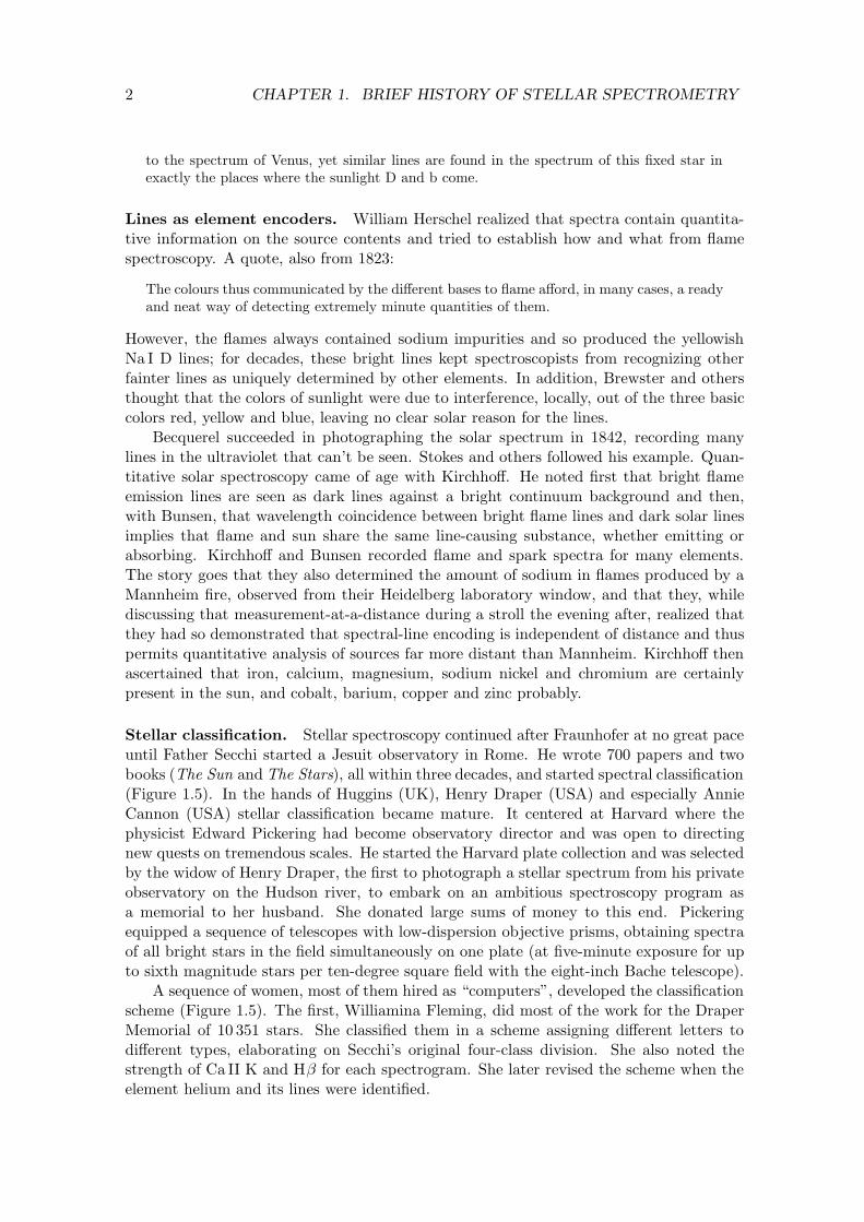
Figure 1.1: Pickering and his “harem”. With his assistants, Pickering undertook spectral classification ofstars on an enormous scale well before the nature of the classification was understood. Taken at Harvardin 1913. Annie Cannon is in the middle row, second to the right of Pickering. From Hearnshaw (1986).

Antonia Maury, a niece of Henry Draper, was the next. Pickering gave her the taskto examine 5000 plates of bright stars with much higher dispersion. She came up with anew classification scheme, in twenty-two classes plus five orthogonal divisions with the linesharpness as criterion. Doppler broadening had been suggested as a mechanism but wasnot yet generally accepted. The large number of classes was severely criticized, especiallyfrom Potsdam. Nevertheless, some of her subsets make sense in hindsight, describing high-luminosity giants and supergiants that are sharp-lined due to small collisional broadening.This distinction was not taken over by Annie Cannon (1863-1941) who

must rank among the most dedicated of astronomers of all time and certainly as one of themost illustrious from the female ranks (Hearnshaw 1986)

and updated Fleming’s original classification scheme by accounting for ionized helium linesas observed from $ Puppis. Pickering had discovered these and found that they obeyedBalmer’s equation for the H I series when including half-integer values, just as for theHe II bound-free edges in Table 8.3 on page 201. He therefore attributed them to a newhydrogen state; only later were they identified as due to He II by Bohr. Miss Cannonconstructed the O–B–A–F–G–K–M sequence with decimal subdivisions that is still inuse. After taking part in classifying some 5000 bright stars, she started on the HenryDraper Catalogue, the successor to the Henry Draper Memorial, in 1911 and completedthe classification of 225 300 stars within four years, at an average of 30 per working hour.She had assistants but must indeed have worked diligently. Her lifetime total amounts to395 000 classifications.

It is interesting to note that this enormous industry was strictly morphological. Theclassification was thought to be evolutionary, hence the terms early- and late-type stars

4 CHAPTER 1. BRIEF HISTORY OF STELLAR SPECTROMETRY

that we still use. Even after Hertzsprung2 and Russell plotted their diagram3 the natureof the spectral classicifation was unclear. That puzzle was solved after the influence ofpressure had been recognized by Pannekoek, Saha had produced his equation for ionizationequilibria, and Fowler and Milne had connected stellar colors with ionization di"erences.The crown came with the 1925 thesis of Cecilia Payne, the first woman to obtain an as-tronomy PhD at Harvard, which was later called “undoubtedly the most brilliant PhDthesis ever written in astronomy” by Struve. She showed that all stars more or less sharethe same composition, but display di"erent line strengths from Saha-Boltzmann sensitiv-ities to temperature and density. Stellar spectroscopy had matured from morphology toastrophysics4.

Abundance determination. Finally, quantitative spectrometry arose from work byRussell, Adams, Charlotte Moore, Unsold, Minnaert, Pannekoek, Struve, Menzel, Allenand others. They took up the pioneering e"orts in understanding stellar line formationby Schuster, Schwarzschild and Milne and turned spectral lines into a tool for stellarabundance determination.

This industry started in the first half of the 20th century; the concepts of the “equiv-alent width” of a spectral line and the “curve of growth” to measure its dependence onthe amount of extinction were introduced by Minnaert and coworkers at Utrecht.

Measuring equivalent widths of spectral lines was an industry by its own. For the Sun,landmark Utrecht publications were the Utrecht Atlas of the solar spectrum5 by Minnaertet al. (1940) and the corresponding line list6 by Moore et al. (1966). The advantage

2Hertzsprung was a Danish amateur astronomer who noted that the intrinsic luminosity of the sharp-line stars in Maury’s classification must be large since they tend, as a group, to have much smaller propermotions than other stars of comparable apparent magnitude. He wrote in 1905 that the sharp-line starsand the “hot Orion-type” stars “shine the brightest, and among the remaining stars not the red but theyellow ones are the faintest”, and two years later continued that “the bright red stars (" Bootis, " Tauri," Orionis etc.) are rare per unit volume of space, and those which belong to the normal solar seriesform by far the greatest number. The bright red stage is therefore quickly traversed.”. He published thesepioneering articles in an obscure journal on photography, but in 1908 visited Karl Schwarzschild who nearlyinstantaneously made him professor at Gottingen and took him along to Potsdam. After Schwarzschild’searly death (from WW I military service), Hertzsprung completed his career at Leiden.

3Hertzsprung and Russell plotted their diagrams independently, Hertzsprung showing an early one toSchwarzschild already in 1908 and Russell displaying one in London in 1913, both with absolute magnitudeplotted horizontally. Later in 1913 Russell showed one with absolute magnitude downwards along the y-axis, as we plot the HRD now. It was called the Russell diagram until Bengt Stromgren, two decades later,renamed it the Hertzsprung–Russell diagram.

4There is an obvious parallel with large-scale surveys of galaxies. The most ambitious one at presentis the Sloan Digital Sky Survey which aims to measure redshifts for one million galaxies and quasarswith multi-fiber spectrometers on a special-purpose telescope at Apache Point in New Mexico. Sofar,fewer galaxy spectra have been obtained over the years than stellar spectra inspected by Miss Cannon.Multi-fiber spectrometry now increases the e"ciency of deep spectrometry to that of objective-prismspectrometry. These extragalactic e!orts are yet rather morphological in nature.

5With a preface by Minnaert in Esperanto. Together with his pupils Houtgast and Mulders, Minnaertproduced the Utrecht Atlas from photographic spectra taken at Mt. Wilson. Houtgast invented an ingeniousmicrodensitometer that converted the blackness of the photographic plates into solar intensity tracingsusing cutout cardboard calibration curves that were scanned by galvanometer beams. The technique isdescribed in the Atlas preface — also in English.

6An equally impressive piece of work. Lots of persons designated “computers” in the Acknowledgementsmeasured the equivalent widths of the 24 000 spectral lines in the Utrecht Atlas by counting the squaremillimeters of the atlas grid covered by each line. I have the original Atlas copy of Hubenet (a personalcomputer, as was De Jager) in my o"ce. You can nearly smell the sweat! Each line was also meticulouslyidentified, by checking laboratory wavelengths and multiplet membership, the multiplet measurements

5

W!

0!

I!

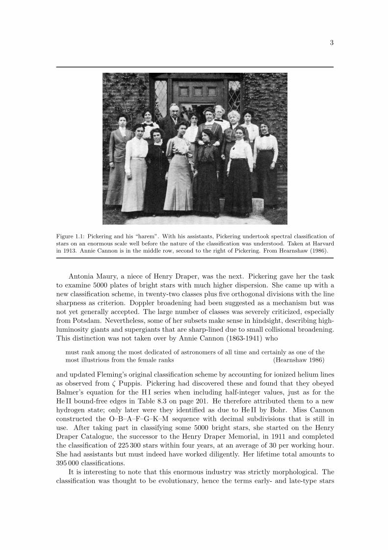
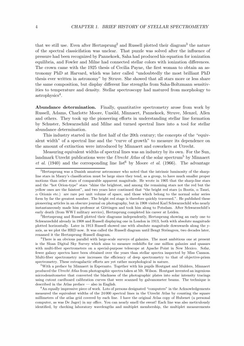
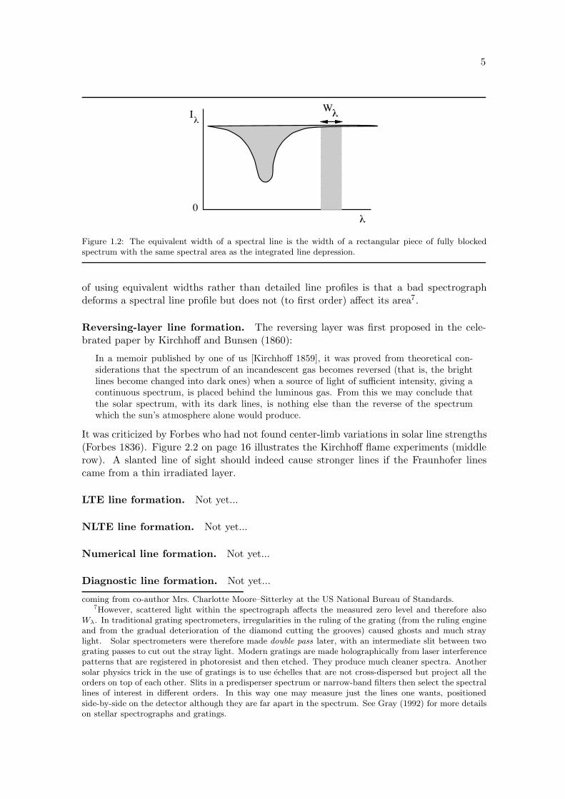
Figure 1.2: The equivalent width of a spectral line is the width of a rectangular piece of fully blockedspectrum with the same spectral area as the integrated line depression.

of using equivalent widths rather than detailed line profiles is that a bad spectrographdeforms a spectral line profile but does not (to first order) a"ect its area7.

Reversing-layer line formation. The reversing layer was first proposed in the cele-brated paper by Kirchho" and Bunsen (1860):

In a memoir published by one of us [Kirchho" 1859], it was proved from theoretical con-siderations that the spectrum of an incandescent gas becomes reversed (that is, the brightlines become changed into dark ones) when a source of light of su!cient intensity, giving acontinuous spectrum, is placed behind the luminous gas. From this we may conclude thatthe solar spectrum, with its dark lines, is nothing else than the reverse of the spectrumwhich the sun’s atmosphere alone would produce.

It was criticized by Forbes who had not found center-limb variations in solar line strengths(Forbes 1836). Figure 2.2 on page 16 illustrates the Kirchho" flame experiments (middlerow). A slanted line of sight should indeed cause stronger lines if the Fraunhofer linescame from a thin irradiated layer.

LTE line formation. Not yet...

NLTE line formation. Not yet...

Numerical line formation. Not yet...

Diagnostic line formation. Not yet...

coming from co-author Mrs. Charlotte Moore–Sitterley at the US National Bureau of Standards.7However, scattered light within the spectrograph a!ects the measured zero level and therefore also

W!. In traditional grating spectrometers, irregularities in the ruling of the grating (from the ruling engineand from the gradual deterioration of the diamond cutting the grooves) caused ghosts and much straylight. Solar spectrometers were therefore made double pass later, with an intermediate slit between twograting passes to cut out the stray light. Modern gratings are made holographically from laser interferencepatterns that are registered in photoresist and then etched. They produce much cleaner spectra. Anothersolar physics trick in the use of gratings is to use echelles that are not cross-dispersed but project all theorders on top of each other. Slits in a predisperser spectrum or narrow-band filters then select the spectrallines of interest in di!erent orders. In this way one may measure just the lines one wants, positionedside-by-side on the detector although they are far apart in the spectrum. See Gray (1992) for more detailson stellar spectrographs and gratings.

6 CHAPTER 1. BRIEF HISTORY OF STELLAR SPECTROMETRY

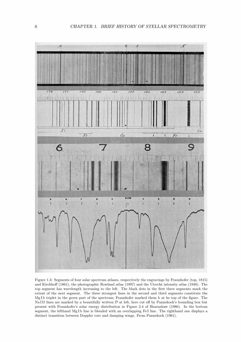
Figure 1.3: Segments of four solar spectrum atlases, respectively the engravings by Fraunhofer (top, 1815)and Kirchho! (1861), the photographic Rowland atlas (1897) and the Utrecht intensity atlas (1940). Thetop segment has wavelength increasing to the left. The black dots in the first three segments mark theextent of the next segment. The three strongest lines in the second and third segments constitute theMg I b triplet in the green part of the spectrum; Fraunhofer marked them b at he top of the figure. TheNa ID lines are marked by a beautifully written D at left, here cut o! by Pannekoek’s bounding box butpresent with Fraunhofer’s solar energy distribution in Figure 2.4 of Hearnshaw (1986). In the bottomsegment, the lefthand Mg I b line is blended with an overlapping Fe I line. The righthand one displays adistinct transition between Doppler core and damping wings. From Pannekoek (1961).

7

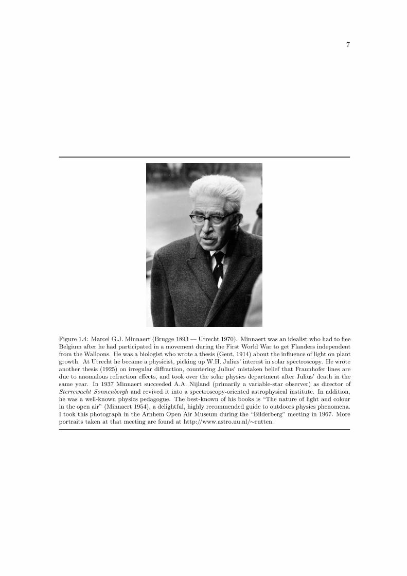
Figure 1.4: Marcel G.J. Minnaert (Brugge 1893 — Utrecht 1970). Minnaert was an idealist who had to fleeBelgium after he had participated in a movement during the First World War to get Flanders independentfrom the Walloons. He was a biologist who wrote a thesis (Gent, 1914) about the influence of light on plantgrowth. At Utrecht he became a physicist, picking up W.H. Julius’ interest in solar spectroscopy. He wroteanother thesis (1925) on irregular di!raction, countering Julius’ mistaken belief that Fraunhofer lines aredue to anomalous refraction e!ects, and took over the solar physics department after Julius’ death in thesame year. In 1937 Minnaert succeeded A.A. Nijland (primarily a variable-star observer) as director ofSterrewacht Sonnenborgh and revived it into a spectroscopy-oriented astrophysical institute. In addition,he was a well-known physics pedagogue. The best-known of his books is “The nature of light and colourin the open air” (Minnaert 1954), a delightful, highly recommended guide to outdoors physics phenomena.I took this photograph in the Arnhem Open Air Museum during the “Bilderberg” meeting in 1967. Moreportraits taken at that meeting are found at http://www.astro.uu.nl/!rutten.

8 CHAPTER 1. BRIEF HISTORY OF STELLAR SPECTROMETRY

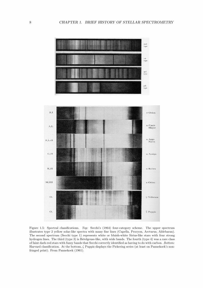
Figure 1.5: Spectral classifications. Top: Secchi’s (1864) four-category scheme. The upper spectrumillustrates type 2 yellow solar-like spectra with many fine lines (Capella, Procyon, Arcturus, Aldebaran).The second spectrum (Secchi type 1) represents white or bluish-white Sirius-like stars with four stronghydrogen lines. The third (type 3) is Betelgeuse-like, with wide bands. The fourth (type 4) was a rare classof faint dark-red stars with fuzzy bands that Secchi correctly identified as having to do with carbon. Bottom:Harvard classification. At the bottom, $ Puppis displays the Pickering series (at least on Pannekoek’s non-fringed print). From Pannekoek (1961).

Chapter 2

Basic Radiative Transfer

T his chapter presents the basic quantities and equations of radiative transfer. It ismainly a summary of Chapter 1 of Rybicki and Lightman (1979) with the same

notation:

– extinction is written in terms of the coe!cient "! per cm rather than the coe!cient %!

per gram that is more commonly employed in books and papers on stellar atmospheres(e.g., Gray 1992) and is also used here in later chapters;

– flux is written as F! rather than &F! (the same as Gray 1992; note that Rybicki andLightman 1979 write F! for F!);

– the Planck function B! is defined in intensity units, per steradian, not as flux orenergy density;

– the Einstein A and B transition probabilities are defined for radiation into or outof the full 4& ster sphere (same as Rybicki and Lightman 1979), rather than perintensity (e.g., Chandrasekhar 1939, Gray 1992). The latter values are smaller by afactor of 4&.

– the photon destruction probability ' is defined per extinction (' = "a/("a + "s) #Cul/(Aul + Cul)), rather than per radiative deexcitation ('! # Cul/Aul).

2.1 Radiation

2.1.1 Local amount

Intensity. The specific intensity (or surface brightness) I! is the proportionality coe!-cient in:

dE! $ I!((r,(l, t) ((l · (n) dA dt d) d# (2.1)= I!(x, y, z, *,+, t) cos * dA dt d) d#,

with dE! the amount of energy transported through the area dA, at the location (r, with(n the normal to dA, between times t and t + dt, in the frequency band between ) and)+d), over the solid angle d# around the direction(l with polar coordinates * and +. Units:erg s"1 cm"2 Hz"1 ster"1 or W m"2 Hz"1 ster"1. Frequency to wavelength conversion:I" = I! c/!2, with d! and d) both positively increasing. This is the monochromaticintensity; the total intensity is I $

! #0 I! d).

9

10 CHAPTER 2. BASIC RADIATIVE TRANSFER

By defining I! per infinitesimally small time interval, area, band width and solid an-gle, I! represents the macroscopic counterpart to specifying the energy carried by a bunchof identical photons along a single “ray”. Since photons are the basic carrier of electro-magnetic interactions, intensity is the basic macroscopic quantity to use in formulatingradiative transfer1. In particular, the definition per steradian ensures that the intensityalong a ray in vacuum does not diminish with travel distance — photons do not decayspontaneously.

"#$

r#"

r sin

$

z

y

x

"

Figure 2.1: Solid angle in polar coordinates. The area of the sphere with radius r limited by (%, % + #%)and (&, & + #&) is r2 sin % #% #' so that #$ = sin % #% #&.

Mean intensity. The mean intensity J! averaged over all directions is:

J!((r, t) $14&

"

I! d# =14&

" 2#

0

" #

0I! sin * d* d+. (2.2)

Units: erg cm"2 s"1 Hz"1 ster"1, just as for I! . In axial symmetry with the z-axis(* $ 0) along the axis of symmetry (vertical stratification only, “plane parallel layers”) J!

simplifies to, using d# = 2& sin * d* = %2& dµ with µ $ cos *:

J!(z) =14&

" #

0I!(z, *) 2& sin * d* =

12

" +1

"1I!(z, µ) dµ. (2.3)

This quantity is the one to use when only the availability of photons is of interest, irrespec-tive of the photon origin, for example when evaluating the amount of radiative excitationand ionization.

Flux. The monochromatic flux F! is:

F!((r,(n, t) $"

I! cos * d# =" 2#

0

" #

0I! cos * sin * d* d+. (2.4)

Units: erg s"1 cm"2 Hz"1 or W m"2 Hz"1. This is the net flow of energy per secondthrough an area placed at location (r perpendicular to (n . It is the quantity to use for spec-ifying the energetics of radiation transfer, through stellar interiors, stellar atmospheres,

1Except for polarimetry, which needs three more Stokes parameters discussed in Section 6.1 on page 137.

2.1. RADIATION 11

planetary atmospheres or space. In principle, flux is a vector. In stellar-atmosphere prac-tice, the radial direction is always implied, outward positive, so that

F!(z) =" 2#

0

" #/2

0I! cos * sin * d* d+ +

" 2#

0

" #

#/2I! cos * sin * d* d+

=" 2#

0

" #/2

0I! cos * sin * d* d+ %

" 2#

0

" #/2

0I!(& % *) cos * sin * d* d+

$ F+! (z) % F"

! (z), (2.5)

with both the outward flux F+! and the inward flux F"

! positive. Isotropic radiation hasF+

! = F"! = &I! and F! = 0. For axial symmetry:

F!(z) = 2&" #

0I! cos * sin * d*

= 2&" 1

0µI! dµ % 2&

" "1

0µI! dµ

= F+! (z) % F"

! (z). (2.6)

The flux emitted by a non-irradiated spherical star per cm2 of its surface at radius r = Ris

F surface! $ F+

! (r=R) = &I+! , (2.7)

with I+! the intensity averaged over the apparent stellar disk that is received by a distant

observer, or the intensity emitted by a Lambert-like star with isotropic I+! for µ > 0. This

equality is the reason that flux is often written as &F $ F so that F = I, with F called the“astrophysical flux”. The flux received at Earth (“irradiance”) from a star with radiusR at distance D is:

R! =4&R2

4&D2F surface

! =&R2

D2I! . (2.8)

Density. The radiation energy density u! is:

u! =1c

"

I! d# (2.9)

with units erg cm"3 Hz"1 or J m"3 Hz"1. integration over $V and over all beam directionsgives the radiative energy E! d) contained within $V across the bandwidth d) as E! d) =(1/c)

!

!V

!

" I! d#dV d). The energy density per unit volume is then given by (2.9) becausefor su!ciently small volume $V , the intensity I! is homogeneous within $V so that thetwo integrations are independent.

Isotropic radiation has u! = (4&/c)J! with I! = J! in all directions, filling a unitsphere in 1/c seconds. The monochromatic energy density has u! = (4&/c)J! and thetotal energy density has u = (4&/c)

! #0 J! d) = (4&/c)J . When LTE and linear anisotropy

are good approximations (as in stellar interiors) J! # B! so that the total energy densityis, with (2.95) on page 31:

u ="

u! d) =1c

" "

B! d# d) =4,c

T 4 (2.10)

and the total photon density is, with T in K (Bowers and Deeming 1984 p. 22):

Nphoton =" #

0

u!

h)d) # 20T 3 cm"3. (2.11)

12 CHAPTER 2. BASIC RADIATIVE TRANSFER

Comparison with Table 8.2 on page 182 shows that the particle density at the bottom ofthe VALIII photosphere (where J! # B! for all )) is much higher.

Pressure. The radiation pressure p! is (Gray p. 95; Rybicki & Lightman p. 6):

p! =1c

"

I! cos2 * d# (2.12)

with units dyne cm"2 Hz"1 or Nm"2 Hz"1. Isotropic radiation has p! = u!/3 and p = u/3.Radiation pressure is analogous to gas pressure, being the pressure of the photon gas. Itis a scalar for isotropic radiation fields; a force is exerted only along a photon pressuregradient2.

Moments of the intensity. For axial symmetry (plane-parallel layers) the first threemoments of the intensity with respect to µ are:

J!(z) $ 12

" +1

"1I! dµ (2.13)

H!(z) $ 12

" +1

"1µ I! dµ (2.14)

K!(z) $ 12

" +1

"1µ2I! dµ (2.15)

Each has the dimension of intensity and each is already familiar. The mean intensity J!

was defined in (2.2). H! is called the Eddington flux and has H! = F!/4& = F!/4, withF! the real flux and F! = F!/& the astrophysical flux. K! is called the K integral and isrelated to radiation pressure by p! = (4&/c)K! . J! and K! are always positive; H! maybe negative. The same definitions produce the spectrum-integrated total J , H and K fromI because the integrations over ) and µ are independent and therefore interchangeable.

2.1.2 Local change

Emission. The monochromatic emissivity j! per cm3 is defined by:

dE! $ j! dV dt d) d#, (2.16)

with dE! the energy locally added to the radiation in volume dV per frequency bandwidthd) during time interval dt in directions d#. Units of j! : erg cm"3 s"1 Hz"1 ster"1. Theintensity contribution from local emission to a beam is

dI!(s) = j!(s) ds, (2.17)

where s measures geometrical path length along the beam in cm.2The term radiation pressure is often used for the mechanical vector force on an object when it absorbs

photons from a single direction. The scalar expression (2.12) is only valid when the radiation behaveslike a gas of particles that locally move at random. The complete definition of radiation pressure is givenin Eq. (16) on page 94 of Baschek and Scholz (1982). It reduces to (2.12) only if the source function isisotropic (no dependence on µ) and if the intensity is not too anisotropic. More precisely, the Eddingtonapproximation (4.54) on page 91 should hold. The latter is exact when I" obeys linear anisotropy in µ.

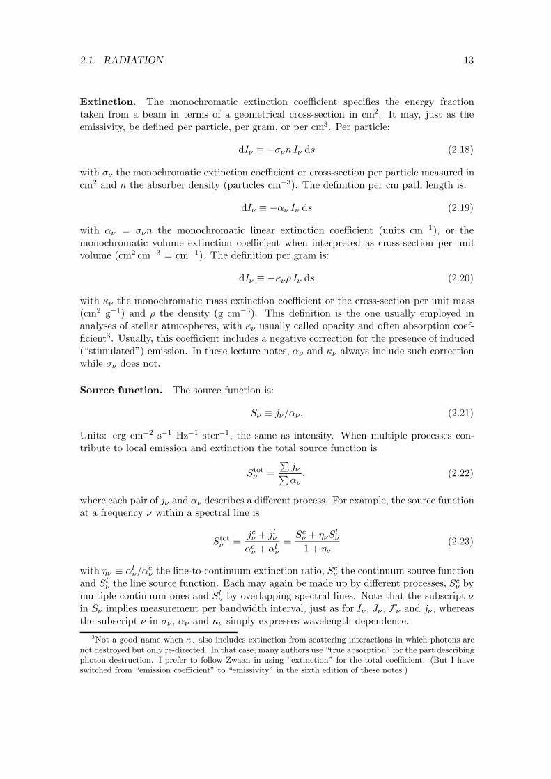
2.1. RADIATION 13

Extinction. The monochromatic extinction coe!cient specifies the energy fractiontaken from a beam in terms of a geometrical cross-section in cm2. It may, just as theemissivity, be defined per particle, per gram, or per cm3. Per particle:

dI! $ %,!n I! ds (2.18)

with ,! the monochromatic extinction coe!cient or cross-section per particle measured incm2 and n the absorber density (particles cm"3). The definition per cm path length is:

dI! $ %"! I! ds (2.19)

with "! = ,!n the monochromatic linear extinction coe!cient (units cm"1), or themonochromatic volume extinction coe!cient when interpreted as cross-section per unitvolume (cm2 cm"3 = cm"1). The definition per gram is:

dI! $ %%!- I! ds (2.20)

with %! the monochromatic mass extinction coe!cient or the cross-section per unit mass(cm2 g"1) and - the density (g cm"3). This definition is the one usually employed inanalyses of stellar atmospheres, with %! usually called opacity and often absorption coef-ficient3. Usually, this coe!cient includes a negative correction for the presence of induced(“stimulated”) emission. In these lecture notes, "! and %! always include such correctionwhile ,! does not.

Source function. The source function is:

S! $ j!/"! . (2.21)

Units: erg cm"2 s"1 Hz"1 ster"1, the same as intensity. When multiple processes con-tribute to local emission and extinction the total source function is

Stot! =

#

j!#

"!, (2.22)

where each pair of j! and "! describes a di"erent process. For example, the source functionat a frequency ) within a spectral line is

Stot! =

jc! + jl

!

"c! + "l

!=

Sc! + .!Sl

!

1 + .!(2.23)

with .! $ "l!/"

c! the line-to-continuum extinction ratio, Sc

! the continuum source functionand Sl

! the line source function. Each may again be made up by di"erent processes, Sc! by

multiple continuum ones and Sl! by overlapping spectral lines. Note that the subscript )

in S! implies measurement per bandwidth interval, just as for I! , J! , F! and j! , whereasthe subscript ) in ,! , "! and %! simply expresses wavelength dependence.

3Not a good name when (" also includes extinction from scattering interactions in which photons arenot destroyed but only re-directed. In that case, many authors use “true absorption” for the part describingphoton destruction. I prefer to follow Zwaan in using “extinction” for the total coe"cient. (But I haveswitched from “emission coe"cient” to “emissivity” in the sixth edition of these notes.)

14 CHAPTER 2. BASIC RADIATIVE TRANSFER

2.2 Transport equation

2.2.1 Transport along a ray

The radiation transport equation is:

dI!(s) = I!(s + ds) % I!(s) = j!(s) ds % "!(s)I!(s) ds (2.24)

ordI!

ds= j! % "!I! (2.25)

ordI!

"! ds= S! % I! , (2.26)

with s measured along the beam in the propagation direction.

Discussion. This basic equation expresses that photons do not decay spontaneously sothat the intensity along a ray does not change unless photons are added to the beam ortaken from it4; without such processes, intensity is invariant along rays.

The versions (2.25) and (2.26) di"er trivially in notation but drastically in their do-main of application. In stellar photospheres one often meets LTE (Local ThermodynamicEquilibrium, see Section 2.5 on page 28") or near-LTE conditions having S! = B!(T ) orS! # B!(T ) with B! the Planck function (2.92). The combination ("! , S!) then presentsa much more “orthogonal” parameter space to describe radiative transfer than the com-bination ("! , j!). The latter two may each vary orders of magnitude over the narrowextent of a spectral line whereas their variations cancel completely or closely in the ratioS! = j!/"! . Photospheric line formation is therefore described in terms of the parameter"! which details atomic particle properties (such as the gas composition, the degree ofionization and excitation, the probability of spectral line transitions at some frequency,the nature and amount of line broadening) and which sets the transparency of the medium(in particular the depth above which the gas is su!ciently transparent that photons mayescape towards our telescope), and the parameter S! which describes the thermodynamicstate of the medium as an ensemble of particles and photons. The two parameters maydepend on each other in highly complex fashion when LTE does not hold, but they areless closely related than "! and j! even then.

In contrast, one doesn’t use source functions to describe radiation in or from tenuousouter atmospheres such as the solar corona. Coronal extinction is often negligible for theX-ray photons emitted there, so that the description is simply in terms of emissivities.The transport than simplifies to photon loss through escape (which constitutes the energydrain that limits the coronal temperature).

Optical length and thickness. The monochromatic optical path length d/! measuredalong the beam across a layer of geometrical thickness ds is:

d/!(s) $ "!(s) ds; (2.27)4It also expresses that photons are bosons which simply add up without pushing one another aside; they

actually like to join together in the same quantum state (stimulated emission). In contrast, Archimedesand the water in his bathtub were made of mutually-exclusive fermions. Neutrinos are much like photons,but they are fermions rather than bosons; they su!er inhibited emission (induced extinction) rather thaninduced emission because excited states cannot emit a fermion where there is one already present (Rybickiand Lightman 1979 p. 316, Shu 1991 p. 8).

2.2. TRANSPORT EQUATION 15

the monochromatic optical thickness5 of a medium with total thickness D is

/!(D) =" D

0"!(s) ds, (2.28)

again measured along the beam. For extinction only (no emission, j! = 0):

I!(D) = I!(0) e"$"(D). (2.29)

The transition between small and large extinction lies at the 1/e value, i.e., at opticalthickness /! = 1. A layer is optically thick for /!(D) > 1 and optically thin for /!(D) < 1.The optical photon mean free path </!(s)> is:

</!(s)> $! #0 /!(s) e"$"(s) d/!(s)

! #0 e"$"(s) d/!(s)

= 1 (2.30)

and the geometrical photon mean free path in a homogeneous medium is:

l! =</!(s)>

"!=

1"!

=1

%!-. (2.31)

In an inhomogeneous medium this estimate represents the local free path. With /! andS! (2.26) becomes

dI!

d/!= S! % I! , (2.32)

from which the integral form of the transport equation follows formally:

I!(/!) = I!(0) e"$" +" $"

0S!(t!) e"($""t") dt! . (2.33)

Homogeneous medium. For a medium in which S! does not vary with location6 (2.33)simplifies to:

I!(D) = I!(0) e"$"(D) + S!

$

1 % e"$"(D)%

. (2.34)

Thus, when the object is optically thick

I!(D) # S!, (2.35)

and when it is optically thin

I!(D) # I!(0) + [S! % I!(0)] /!(D). (2.36)

These basic solutions are illustrated in Figure 2.2 and Exercise 1.5The term “optical” is used in this context for the whole electromagnetic spectrum, from gamma rays

to radio waves, and even for neutrinos.6If scattering or stimulated emission is important, S" depends on the local angle-averaged intensity J"

and may vary with location even if the matter component of the medium is homogeneous.

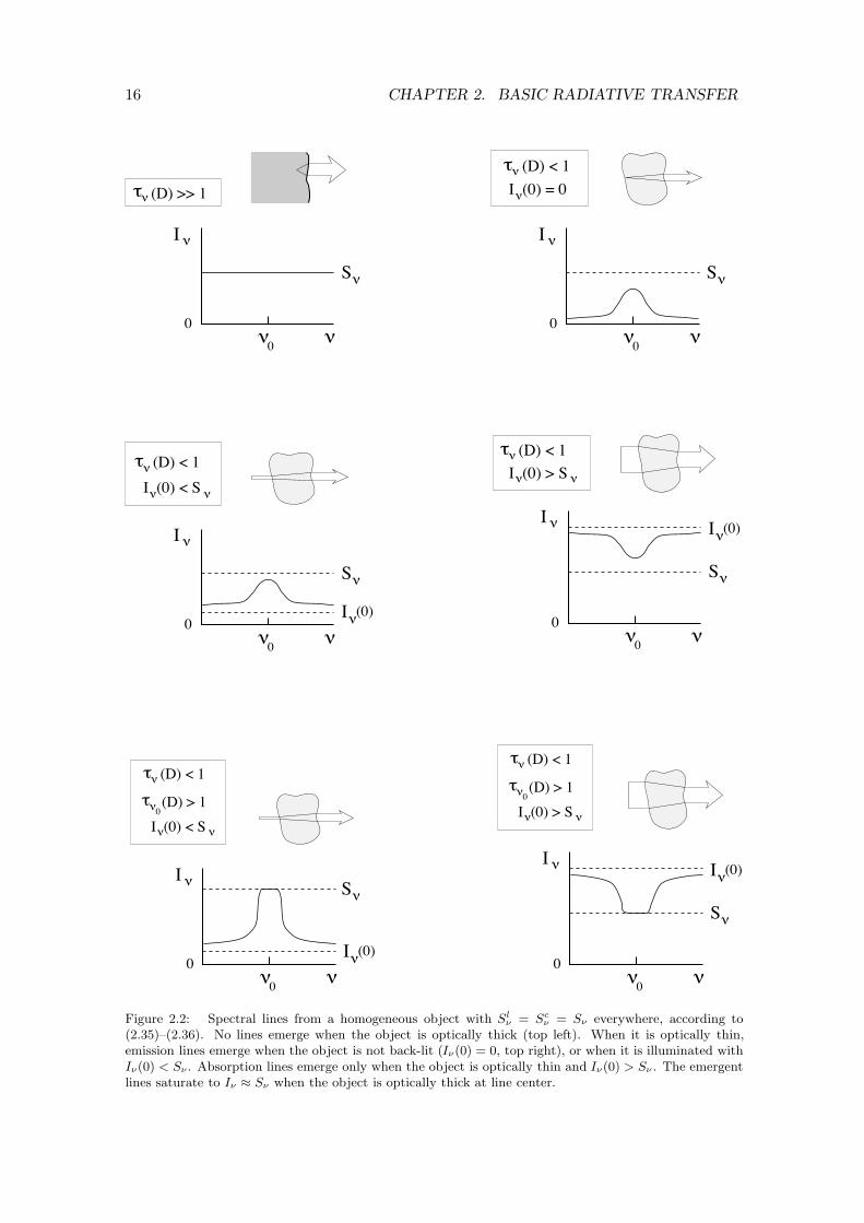
16 CHAPTER 2. BASIC RADIATIVE TRANSFER

% (D) >> 1

%0

I %

S %

0% %

0

I %

S %

0%

&% (D) < 1

I (0) = 0%

%0

I %

S %

I %(0)0

%

I (0) < S% %

&% (D) < 1

%0

I %(0)

S %I %

&

0%

&% (D) > 10

&% (D) < 1

I (0) < S% %

%0

S %

I %(0)I %

0%

&% (D) > 10

&% (D) < 1

% %I (0) > S

%0

S %

I %(0)I %

0%

&% (D) < 1

I (0) > S% %

Figure 2.2: Spectral lines from a homogeneous object with Sl" = Sc

" = S" everywhere, according to(2.35)–(2.36). No lines emerge when the object is optically thick (top left). When it is optically thin,emission lines emerge when the object is not back-lit (I"(0) = 0, top right), or when it is illuminated withI"(0) < S" . Absorption lines emerge only when the object is optically thin and I"(0) > S" . The emergentlines saturate to I" " S" when the object is optically thick at line center.

2.2. TRANSPORT EQUATION 17

2.2.2 Transport through an atmosphere

Optical depth. Sofar, /! has denoted optical thickness, measured along the beam inthe photon propagation direction. Since this course is mostly concerned with objects ofwhich the total optical thickness along the line of sight is far too large to be of any interest,I now switch notation and use /! from here on for radial optical depth, as most authorsdo. In the context of stellar atmospheres, one often adopts axial symmetry with the z-axisradially outward along the axis of symmetry (perpendicular to the surface of a sphericalstar consisting of horizontally homogeneous shells). The viewing angle µ is then defined byµ $ cos * where * specifies the angle between the line of sight and the z-axis. In addition,plane-parallel stratification is usually assumed so that the angle µ does not vary along theline of sight as is the case for curved layers. I do the same throughout this course. In somecases, I will use the angle-dependent optical depth /!µ

d/!µ $ %"!dz

|µ| (2.37)

which is measured along the viewing direction, with µ > 0 outwards for outgoing photonsand µ < 0 inwards for incoming photons. In most cases, however, I will use the radialoptical depth /! which for a geometrical location with z = z0 is given by

/!(z0) =" z0

#%"! dz =

" #

z0

"! dz, (2.38)

and which measures the optical depth along the radial line of sight with µ = 1, from /! = 0at the observer’s eye located at z = &. For a frequency within a spectral line the totaloptical depth is given by

d/ total! = %("c

! + "l!) dz = (1 + .!) d/ c

! (2.39)

with .! $ "l!/"

c! and / c

! the continuum optical depth.

Standard plane-parallel transport equation. The use of radial optical depth de-livers the standard form of the radiation transport equation in plane-parallel geometry:

µdI!

d/!= I! % S! . (2.40)

Formal solution. For axial symmetry the inward directed intensity (µ < 0) is, usingt! $

! z#%"!(z) dz as /!-like integration variable (e.g., Gray 1992 p. 114):

I"! (/! , µ) = %" $"

0S!(t!) e"(t""$")/µ dt!/µ (2.41)

and the outward directed intensity (µ > 0) is:

I+! (/! , µ) = +

" #

$"

S!(t!) e"(t""$")/µ dt!/µ. (2.42)

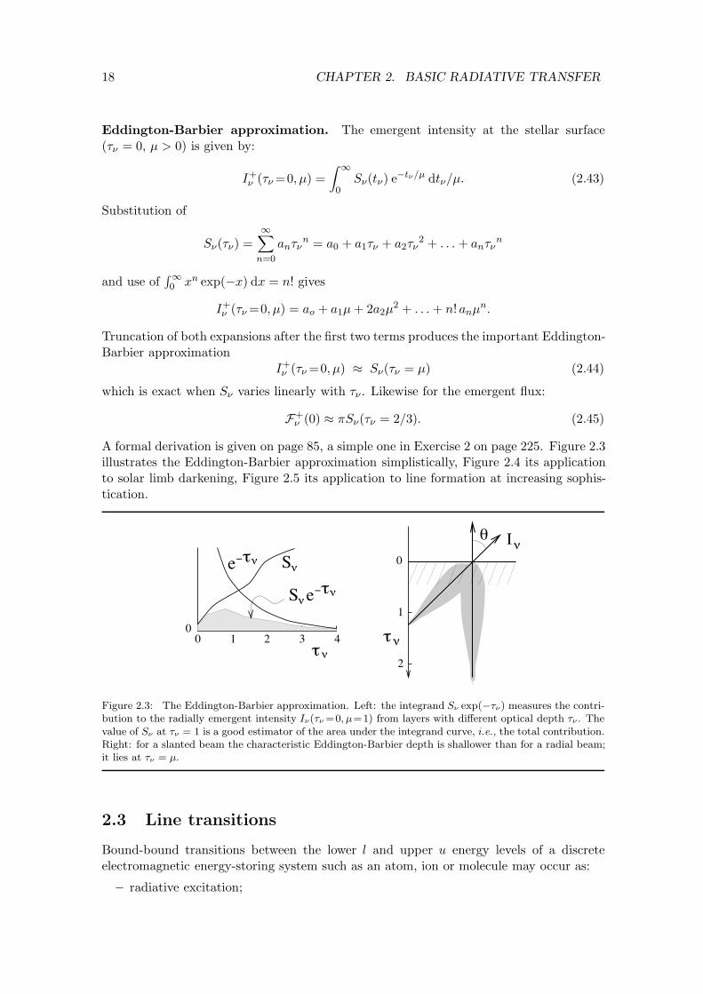
18 CHAPTER 2. BASIC RADIATIVE TRANSFER

Eddington-Barbier approximation. The emergent intensity at the stellar surface(/! = 0, µ > 0) is given by:

I+! (/! =0, µ) =

" #

0S!(t!) e"t"/µ dt!/µ. (2.43)

Substitution of

S!(/!) =#&

n=0

an/!n = a0 + a1/! + a2/!

2 + . . . + an/!n

and use of! #0 xn exp(%x) dx = n! gives

I+! (/! =0, µ) = ao + a1µ + 2a2µ

2 + . . . + n! anµn.

Truncation of both expansions after the first two terms produces the important Eddington-Barbier approximation

I+! (/! =0, µ) # S!(/! = µ) (2.44)

which is exact when S! varies linearly with /! . Likewise for the emergent flux:

F+! (0) # &S!(/! = 2/3). (2.45)

A formal derivation is given on page 85, a simple one in Exercise 2 on page 225. Figure 2.3illustrates the Eddington-Barbier approximation simplistically, Figure 2.4 its applicationto solar limb darkening, Figure 2.5 its application to line formation at increasing sophis-tication.

S% 0

1

2

0 1 2 3 40

'&%e

" I

&%

%

'&%eS%

%&

Figure 2.3: The Eddington-Barbier approximation. Left: the integrand S" exp(#)") measures the contri-bution to the radially emergent intensity I"()" =0, µ=1) from layers with di!erent optical depth )" . Thevalue of S" at )" = 1 is a good estimator of the area under the integrand curve, i.e., the total contribution.Right: for a slanted beam the characteristic Eddington-Barbier depth is shallower than for a radial beam;it lies at )" = µ.

2.3 Line transitions

Bound-bound transitions between the lower l and upper u energy levels of a discreteelectromagnetic energy-storing system such as an atom, ion or molecule may occur as:

– radiative excitation;

2.3. LINE TRANSITIONS 19

S% a

b

h0

I%

0

a

b

10 sin "

"

a

b

Figure 2.4: Solar limb darkening. The viewing angle % increases with the fractional radius r/R! = sin %of the apparent solar disk. The emergent intensity samples shallower layers towards the limb, with smallersource function. The final drop at r/R! = 1 marks the viewing angle at which the sun becomes opticallythin. Note that substantial decrease of µ = cos % is reached only close to the limb, for r/R! = sin % =(1#µ2)1/2 close to unity (Table 7.2 on page 159). The o!-limb extension to this sketch is given in Figure 7.2on page 148.

– spontaneous radiative deexcitation;– induced radiative deexcitation;– collisional excitation;– collisional deexcitation.

2.3.1 Einstein coe!cients

Spontaneous deexcitation. The Einstein coe!cient for spontaneous deexcitation is:

Aul $ transition probability for spontaneous deexcitation fromstate u to state l per sec per particle in state u.

(2.46)

In the absence of collisions and of any other transitions than the ul one, the mean lifetimeof particles in state u is $t = 1/Aul s. The corresponding spread in energy is (Heisenberg):$E = h/(2&$t) or $) = 0rad/(2&) with 0rad $ 1/$t the radiative damping constant.This “natural” broadening process defines an emission probability distribution 1()%)0)around the line center at ) = )0 that is given by the area-normalized Lorentz profile:

1()%)0) =0rad/4&2

()%)0)2 + (0rad/4&)2. (2.47)

The Aul coe!cient is a summation over the profile, describing the transition probabilityfor the whole line; the probability per unit of bandwidth is given by Aul1()%)0) since1()%)0) is measured per Hertz. The spontaneous deexcitation rate per cm3 is given bythe product nuAul.

The emission-profile shape function is discussed in more detail in Section 3.3 onpage 52 " together with other line broadening processes. The latter are usually muchmore important than radiative damping. For a static atmosphere and assuming that each

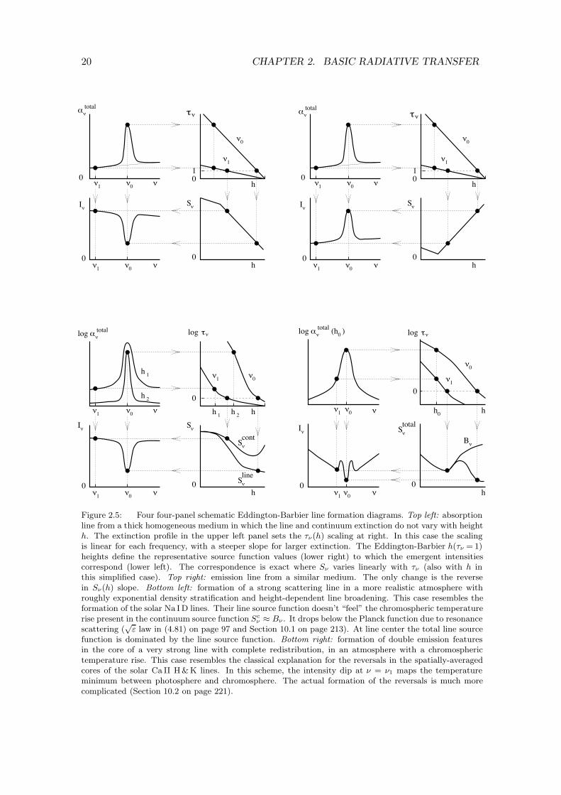
20 CHAPTER 2. BASIC RADIATIVE TRANSFER

%1

%0

%1

%0

I% %

S

(%

total

%0

%1

0 0

01

h

h0

%

%

%&

%1

%0

%1

%0

I% %

S

(%

%0

%1

0 0

01

h

h

total

0%

%

&%

%0

%0

%S

line

%S

cont

I% %

S

(%

logtotal

%1

%1

h1

h2

%1

%0

h1

h2

0 0h

0

%

% h

&%log

0

%0

I%

(%

h0

h0

( )

%0

1%

1%

1%

%S

B%

%

total

0

%

0%

logtotal

0

h

h

&%log

Figure 2.5: Four four-panel schematic Eddington-Barbier line formation diagrams. Top left: absorptionline from a thick homogeneous medium in which the line and continuum extinction do not vary with heighth. The extinction profile in the upper left panel sets the )"(h) scaling at right. In this case the scalingis linear for each frequency, with a steeper slope for larger extinction. The Eddington-Barbier h()" = 1)heights define the representative source function values (lower right) to which the emergent intensitiescorrespond (lower left). The correspondence is exact where S" varies linearly with )" (also with h inthis simplified case). Top right: emission line from a similar medium. The only change is the reversein S"(h) slope. Bottom left: formation of a strong scattering line in a more realistic atmosphere withroughly exponential density stratification and height-dependent line broadening. This case resembles theformation of the solar Na I D lines. Their line source function doesn’t “feel” the chromospheric temperaturerise present in the continuum source function Sc

" " B" . It drops below the Planck function due to resonancescattering (

$* law in (4.81) on page 97 and Section 10.1 on page 213). At line center the total line source

function is dominated by the line source function. Bottom right: formation of double emission featuresin the core of a very strong line with complete redistribution, in an atmosphere with a chromospherictemperature rise. This case resembles the classical explanation for the reversals in the spatially-averagedcores of the solar Ca II H& K lines. In this scheme, the intensity dip at + = +1 maps the temperatureminimum between photosphere and chromosphere. The actual formation of the reversals is much morecomplicated (Section 10.2 on page 221).

2.3. LINE TRANSITIONS 21

deexcitation is independent of the preceding process(es) that put the atom in state u(“complete redistribution”), the probability distribution is

1()%)0) =H(a, v)'

&$)D(2.48)

with the Doppler width $)D defined as

$)D $ )0

c

'

2kT

m, (2.49)

where m is the particle mass, and with the Voigt function H(a, v) given by (3.68) onpage 59 and shown in Figure 3.1 on page 60. It is Gaussian at line center due to Dopplershifts from Maxwellian motions (“Doppler core”) and it has extended Lorentzian wingscaused by collisional perturbations (“damping wings”).

The emission profile is more complex when the frequency redistribution over the lineprofile is incomplete (“partial redistribution”), which is the case if the photon that isemitted per deexcitation has some correlation with the photon that previously excited theatom in a scattering up-down sequence. Coherent scattering, without frequency change,is the other extreme. I mostly use the two extremes of fully coherent and fully incoherentscattering in this course; partial redistribution is discussed in Section 3.4.3 on page 72".

Radiative excitation. The Einstein coe!cient for radiative excitation Blu is definedby:

BluJ%!0

$ number of radiative excitations from state l to state u persec per particle in state l,

(2.50)

with the index )0 defining a specific spectral line of which the extinction profile +()%)0)is used in the weighting of the angle-averaged exciting radiation field over the spectralextent of the line7

J%!0

$" #

0J! +()%)0) d), (2.51)

where!

+()%)0) d) = 1. A more general expression for this summation is

J%!0

$ 12

" #

0

" +1

"1I! +()%)0) dµ d), (2.52)

which also holds when +() % )0) is anisotropic due to systematic Doppler shifts8 (seepage 71). In the absence of the latter (static atmosphere), the profile function +()%)0)

7Because &(+#+0) is area-normalized, J#"0 represents both the profile-weighted summation and the

profile-weighted average of the radiation field over the line width. The latter is formally defined byJ

#"0 %

!

J" &(+#+0) d+/!

&(+#+0) d+.8A yet more general expression is to integrate also over the azimuthal angle & as in (2.2) on page 10.

This must be done when axial asymmetry is no longer valid (horizontal inhomogeneity). A better option isto define the Einstein coe"cients in terms of the intensity. The coe"cients A and B in (2.46), (2.50) and(2.55) are based on emission into and extinction out of all directions, as done by Rybicki and Lightman(1979), Mihalas (1978), Shu (1991) and Bohm-Vitense (1989). Gray (1992) follows Chandrasekhar (1939)and bases the Einstein coe"cients on intensity, so that they are defined per steradian and are 4, smaller.In our case, they are divided by 4, in (2.62) and (2.69) to produce intensity extinction and emissivities.Je!eries (1968) has the most elegant notation. He defines Aul for radiation into all directions, as fits a“transition probability” for deexcitations that won’t care in which direction they emit photons, but definesBul and Blu as negative and positive extinction of the intensity in a beam, per steradian. His downwardradiative rate per cm3 is nuRul = nuAul + 4, nuBul

! "0

J" -(+#+0) d+.

22 CHAPTER 2. BASIC RADIATIVE TRANSFER

is again set by random Doppler shifts and radiative plus collisional damping and given bythe area-normalized Voigt function as in (2.48):

+()%)0) =H(a, v)'

&$)D. (2.53)

For small damping (Voigt parameter a < 1) the line-center amplitude is

+() =)0) =1 % a'&$)D

, (2.54)

where a = 0 for a purely Gaussian line shape (pure Doppler broadening).

Induced deexcitation. The Einstein coe!cient for induced deexcitation Bul is similarlydefined by:

BulJ&!0

$ number of induced radiative deexcitations from state u tostate l per sec per particle in state u,

(2.55)

similarly to Blu, with frequency averaging

J&!0

$ 12

" #

0

" +1

"1I! 2()%)0) dµ d) =

" #

0J!2()%)0) d) (2.56)

in which 2()%)0) is the area-normalized profile shape for induced emission. The firstversion is the more general one.

Collisional excitation and deexcitation. The Einstein coe!cients for collisional ex-citation and deexcitation are:

Clu $ number of collisional excitations from state l to state u persec per particle in state l.

(2.57)

Cul $ number of collisional deexcitations from state u to state lper sec per particle in state u

(2.58)

Electron collisions (usually the most important ones) causing transitions from state i tostate j have transition rates

niCij = niNe

" #

v0

,ij(v) v f(v) dv, (2.59)

with Ne the electron density, ,ij(v) the electron collision cross-section, f(v) the area-normalized velocity distribution (usually Maxwellian) with mean value

!

v f(v)dv, and v0

the threshold velocity with (1/2)mv20 = h)0. The collision cross-section ,ij is, similarly to

the radiative bb cross-section ,l! and the corresponding Einstein coe!cients Aul, Blu and

Bul, a material property of each transition that is independent of external state parametersexcept the velocity (di"erence) v.

2.3. LINE TRANSITIONS 23

Einstein relations. The Einstein coe!cients are coupled by the Einstein relations:

Blu

Bul=

gu

gl

Aul

Bul=

2h)3

c2(2.60)

andCul

Clu=

gl

gueEul/kT , (2.61)

where Eul is the transition energy. The ratios (2.60) are derived for TE by equatingthe upward and downward radiative rates requiring detailed balance per frequency with+ = 1 = 2 and equating the resulting expression for J! to B! at arbitrary temperature.They then hold universally since they do not depend on any medium property. The ratio(2.61) follows similarly from equating the upward and downward collisional rates in TE.It holds also outside TE if the Maxwell distribution holds.

2.3.2 Volume coe!cients

Extinction. The monochromatic line extinction coe!cient per cm path length expressedin Einstein coe!cients is:

"l! =

h)

4&[nlBlu +()%)0) % nuBul 2()%)0)] (2.62)

=h)

4&nlBlu +()%)0)

(

1 % nu gl 2()%)0)nl gu +()%)0)

)

(2.63)

where the term between square brackets corrects for induced emission, taken into accountas negative extinction. In these lecture notes, volume coe!cients " always contain suchcorrection. The total line extinction coe!cient is

"l!0

$" #

0"l

! d) =h)0

4&(nlBlu % nuBul) (2.64)

using!

h) +() %)0) d) = h)0 and!

h) 2()%)0) d) = h)0 assuming the profile to besymmetric or su!ciently narrow9. Throughout these lecture notes, the subscript )0 de-notes summation over the line profile10 and identifies the particular bound-bound transi-tion. The coe!cients "l

! and "l!0

are rewritten with population departure coe!cients in(2.108)–(2.115) on page 34. The monochromatic line extinction coe!cient per particle, inthese lecture notes always without correction for induced emission, is:

,l! =

h)

4&Blu +()%)0). (2.65)

The total line extinction coe!cient per particle is

,l!0

$" #

0,l

! d) =h)0

4&Blu =

&e2

mecflu = 0.02654 flu cm2 Hz. (2.66)

9Motion along the line of sight implies a shift of +0 and local anisotropy of the monochromatic extinctioncoe"cient. Di!erential motions along the line of sight imply varying shift and anisotropy. Asymmetrymay be caused by hyperfine and isotope structure (page 63).

10Or it denotes averaging over the profile, in the case of profile-weighted summation as in (2.51). Notethat (2.64) does not represent averaging of "l

" over the line profile. The dimension of "l"0 is cm#1 Hz.

24 CHAPTER 2. BASIC RADIATIVE TRANSFER

These coe!cients are ensemble quantities, given per individual particle but sampling,respectively summed over, the ensemble distribution specified by +()%)0). The param-eter flu is the classical dimensionless oscillator strength, a quantity that was historicallyintroduced to correct harmonic-oscillator line strength predictions for unknown quantum-mechanical e"ects. Resonance lines such as H I Ly" have flu # 1. The )-dependences in(2.60) and (2.66) produce

Aul "gl

guflu ($Eul)2 (2.67)

with $Eul = h)0 the transition energy. Numerically:

Aul = 6.67 ( 1013 gl

gu

flu

!2s"1 (2.68)

with ! in nm (Allen 1976). The (absorption) oscillator strength is usually combined withthe lower-level statistical weight into the “gf-value” glflu because this product definesthe e"ective transition probability that one must know11 to evaluate "l

! or %l! . The gl

then comes in when evaluating the lower-level population nl, for example through its LTEBoltzmann-Saha estimate nLTE

l in (9.6) on page 204.

Emission. The monochromatic line emissivity expressed in Einstein coe!cients is, with-out induced emission,

jl! =

h)

4&nuAul 1()%)0). (2.69)

The total line emissivity is

jl!0

=" #

0jl! d) =

h)0

4&nuAul (2.70)

using!

h) 1()%)0) d) = h)0 because 1()%)0) is symmetric around ) = )0 in the absenceof systematic Doppler shifts.

Source function. The monochromatic line source function expressed in Einstein coef-ficients is

Sl! $ jl

!/"l! =

nuAul1()%)0)nlBlu+()%)0) % nuBul2()%)0)

(2.71)

or, using the Einstein relations (2.60)

Sl! =

Aul

Bul

1

+nl

nu

Blu

Bul% 2

+

=2h)3

c2

1/+gunl

glnu% 2

+

. (2.72)

The line source function may vary strongly with frequency across the line when the profileshapes are not equal due to coherent scattering or partial frequency redistribution (Sec-tion 3.4.3 on page 72). They become equal when complete redistribution holds in which

11Direct computation of gf-values is fairly straightforward for hydrogen and hydrogen-like ions but lessso for more complex atomic, ionic or molecular configurations. Chapter 10 of Rybicki and Lightman(1979) presents the hydrogen computation and contains a table of H I gf-values on page 281. Extensivetabulations of experimentally measured transition probabilities used to come in thick volumes producedby the US National Bureau of Standards (e.g., Corliss and Bozman 1962) but better values now resultfrom large-scale computations and become available on the web, e.g., http://vizier.u-strasbg.fr/OP.html(Opacity Project), http://wwwsolar.nrl.navy.mil/chianti.html (CHIANTI database)

2.4. CONTINUUM TRANSITIONS 25

every process takes a fresh sample of the probability distribution, without “memory” forany preceding process, so that +()%)0) = 1()%)0) = 2()%)0). The line source functionthen simplifies to

Sl!0

=nuAul

nlBlu % nuBul=

2h)30

c2

1gunl

glnu% 1

. (2.73)

The index 0 to Sl!0

signifies that the complete-redistribution version of the line sourcefunction is frequency-independent12. The line source function simplifies yet further to toSl

!0= B!0 when the population ratio nl/nu in (2.73) obeys the Boltzmann distribution

(2.86) on page 29 as it does in LTE.

2.4 Continuum transitions

2.4.1 Inelastic processes

Bound-free transitions. For bound-free transitions of hydrogen and hydrogen-like ionsthe extinction cross-section in cm2 per particle is given by Kramers’ formula:

,bf! = 2.815 ( 1029 Z4

n5)3gbf for ) ) )0, (2.74)

with n the principal quantum number of the level i from which the atom or ion is ionized, Zthe ion charge, ) in Hz and gbf the dimensionless Gaunt factor, a quantummechanical cor-rection factor of order unity. The Kramers cross-section decays " )"3 above the threshold(“edge”) frequency )0, being zero below it because the threshold energy is the requiredminimum. For more complex atoms and ions than hydrogen-like ones, the bound-freecross-sections do not have such simple )"3 dependence but possess peaks at “resonances”caused by other electrons in the same shell (Section 3.1.3 on page 43).

For LTE conditions the corresponding volume extinction coe!cient is

"bf! = ,bf

! ni

$

1 % e"h!/kT%

(2.75)

with ni the density of particles in the ionizing level. The negative term corrects for inducedprocesses (stimulated photorecombination, cf. (2.97) on page 31). It is present just asfor bound-bound processes because ionization is also either radiative or collisional whilerecombination may also be achieved spontaneously (ion-electron collision), inducedly (ion-electron plus photon collision), or collisionally without the production of a photon (ion-electron-plus-third-particle collision). Outside LTE the more general expression (2.119)on page 35 holds. Bound-free collision rates are given in (3.36) and (3.37) on page 51.

Discussion. Figure 2.6 from Gray (1992) illustrates the hydrogen bound-free extinctioncoe!cient ,bf

! per particle and per bound-free feature. The peak amplitudes are of theorder of 10"17 cm2 per particle. They increase with n, although Kramers’ law suggests

12At least for su"cient narrow lines over which the frequency variation due to the +3 scaling factor andthe nl/nu ratio can be neglected. For LTE these combine in Planckian frequency dependence. Note thatSl

"0 = jl"0/"l

"0 does not represent a total but the average!

Sl" &(+#+0)d+/

!

&(+#+0)d+ over the line. The“total” source function is the weighted combination of line and continuous source functions as in (2.23) onpage 13. That combination varies with frequency across the line when Sl &= Sc even when Sl and Sc areeach frequency-independent.

26 CHAPTER 2. BASIC RADIATIVE TRANSFER

Figure 2.6: H I bound-free extinction coe"cient .bf" per hydrogen atom in level n (here written as "n)

against wavelength. The Lyman, Balmer, Paschen, Brackett and Pfund edges are marked by the quantumnumber n of the ionizing level. Their amplitudes increase with n and have not been added up in thisfigure. The threshold wavelengths are specified in Table 8.1 on page 176. Figure 8.14 on page 191 showsthe hydrogen and helium bound-free and free-free extinction for the actual mix of particles in three stellaratmospheres. The total extinction from all continuous processes is shown for a grid of stellar atmospheresin the Vitense diagrams on page 179 and page 192!. From Gray (1992).

,bf! " 1/n5, because the Rydberg sequence for the hydrogen ionization thresholds has

h)n = 2cn = E# % En = 13.6/n2 eV so that the factor )"3 converts into a factor n6.The bound-free extinction peaks are much lower than the bound-bound resonance-line

peaks. For example, the Ly" line at ! = 121.5 nm or ) = 2.47 ( 1015 Hz has oscillatorstrength f12 = 0.416 (page 280 of Rybicki and Lightman 1979). Assuming a = 0 in (2.54)and T = 104 K in (2.49) gives with (2.65) and (2.66) a Ly" peak extinction ,Ly'() =)0) =4.0( 10"14 cm2, three orders of magnitude larger than the peaks in Figure 2.6. However,the edges are much wider. The edge-integrated bound-free extinction is )0/2 times largerthan (2.74), so that the full Lyman edge with threshold frequency )0 = 3.3 ( 1015 Hzhas integrated cross-section ,Ly edge = 0.01 cm2 Hz, about the same as the integratedLy" cross-section ,Ly ' = 0.011 cm2 Hz given by (2.66). Note that the actual integratedradiative transiton rates in the two features depend on the radiation field, as specified by(3.4) on page 45 and (3.7) on page 46, respectively.

Free-free transitions. Free-free transitions13 have S! = B! when the Maxwell velocitydistribution holds (“thermal Bremsstrahlung”). A formula for the corresponding extinc-tion coe!cient per particle is (Rybicki and Lightman 1979 p. 162):

,#! = 3.7 ( 108 Ne

Z2

T 1/2)3g# , (2.76)

with Z the ion charge, Ne and Nion the electron and ion densities, and g# a Gaunt factorof order unity. There is no threshold frequency. This expression is derived classically;

13Note the astronomical convention: H I free-free extinction describes photon-absorbing encounters be-tween protons and free electrons with Z = 1 and Nion = Np; H II free-free encounters do not exist; H

!

free-free encounters are between neutral hydrogen atoms and free electrons.

2.4. CONTINUUM TRANSITIONS 27

the Gaunt factor corrects for simple errors relative to the appropriate quantummechanicalresult. It does not hold for more complex systems such as H# ions (which indeed wouldhave Z = 0 in (2.76)).

The corresponding volume extinction coe!cient is:

"#! = ,#

! Nion

$

1 % e"h!/kT%

(2.77)

which holds also out of LTE conditions (as long as the velocities are Maxwellian) becausethe free-free processes are always fully collisional. The negative term again corrects forinduced processes. In the Wien limit defined by (2.93) on page 31 the free-free extinctioncoe!cient simplifies to:

"#! # 3.7 ( 108 NeNion

Z2

T 1/2)3g# (2.78)

with "#! " )"3. In the Rayleigh-Jeans limit defined by (2.94) on page 31 it becomes:

"#! # 0.018NeNion

Z2

T 3/2)2g# (2.79)

with "#! " )"2.

2.4.2 Elastic processes

Thomson scattering. Thomson scattering of photons by free electrons has a frequency-independent extinction cross-section given per electron by:

,T! $ ,T =

8&3

r2e = 6.65 ( 10"25 cm2. (2.80)

The corresponding volume extinction coe!cient is given by

"T! = ,T Ne (2.81)

with Ne the electron density14. These coe!cients hold for low-energy photons and low-energy electrons. For high-energy photons, Thomson scattering is replaced by Comptonscattering; for high-energy electrons, by inverse Compton scattering (e.g., Rybicki andLightman 1979). Thomson scattering is the major source of continuous extinction in theatmospheres of hot stars where hydrogen is ionized (see discussion on page 202 of thecontinuous opacity diagram in Figure 8.15 on page 192). The much larger values of theH I bound-free peaks in (2.74) and Figure 2.6, of order 10"17 cm2 per particle, win fromelectron scattering when hydrogen is not fully ionized (high pressure curves in Figure 8.15).

14There is no (1 # something) correction comparable to the [1 # exp(#h+/kT )] factor used for LTEextinction processes as in (2.77). Induced emission processes are generally not included in elastic electronscattering (e.g., Mihalas 1978, p. 107), corresponding with the Bohr picture in which the free electron has nointernal excitation energy to be released upon outside triggering. Actually, electron scattering does su!erfrom stimulated enhancement because photons are bosons. However, the enhancement cancels betweensource and sink terms when the scattering is coherent. Precisely as many photons are then stimulated toscatter monochromatically into any beam as out of it (Shu 1991 p. 71). This cancelation is discussed inmore detail on page 69.

28 CHAPTER 2. BASIC RADIATIVE TRANSFER

Rayleigh scattering. The extinction cross-section for Rayleigh scattering of photonswith ) * )0 by bound electrons with characteristic bounding energy h)0 is:

,R! # flu ,T

*)

)0

+4

, (2.82)

where the oscillator strength flu and the frequency )0 characterize the major bound-bound“resonance transition” of the bound electron, for example the Ly" transition in neutralhydrogen or a weighted sum over all Lyman lines. The )4 dependence makes our sky blueand sunsets red. The volume extinction coe!cient for Rayleigh scattering by hydrogenatoms with density NH is given by

"R! = ,R

! NH. (2.83)

Rayleigh scattering is included in Vitense’s stellar-atmosphere opacity diagrams onpage 179 and page 192". Its contribution is usually negligible.

Redistribution. Thomson and Rayleigh scattering are coherent, meaning elastic ormonochromatic; the photon gets redirected but it keeps its frequency. The redirection hasphase function " 1 + cos2 *, with su!ciently small departure from isotropy that isotropyis generally assumed. At high temperature, Thomson scattering is not truly coherent dueto the Doppler shifts imposed by the electrons. They move faster by a factor 43 thanprotons, see (3.31) on page 50. In the atmospheres of hot stars and in coronae theseDoppler shifts are appreciable. They obliterate the Fraunhofer lines in the spectrum ofthe solar K corona. For hot stars, Rybicki and Hummer (1994) have formulated a radiativetransfer method which includes the frequency spreading due to the appreciable thermalDoppler shifts.

2.5 LTE

In local thermodynamic equilibrium (LTE) all material energy partitioning, i.e., all atomic,ionic and molecular level populations, is given by Saha-Boltzmann statistics defined by thelocal temperature, just as if that location sits within a TE (thermodynamic equilibrium)enclosure as seen by the matter component of the ensemble (but not altogether by thephotons). The definition of LTE is to assume the validity of all TE material distributionlaws at the local temperature. The equality Sl

!0= B!0 then follows by entering the

Boltzmann distribution into (2.73) on page 2515.

2.5.1 Matter in LTE

Maxwell distribution. Per species of particles with mass m the Maxwell distributionfor the velocity components in the x direction is:

(n(vx)

Ndvx

)

LTE=

*m

2&kT

+1/2

e"(1/2)mv2x/kT dvx, (2.84)

15Often, the LTE equality S" = B" is taken to be the definition of LTE. It is not; the concept requiresstrict coupling of the matter component to the local temperature (Ivanov 1973). This can only be the case ifthe radiation is not too far o!, or unimportant. Otherwise, photon processes will make the level populationsdepart from Saha-Boltzmann statistics. In that case Sl

" &= B" as evident from (2.73). Thus, S" = B"

corresponds to requiring Boltzmann-Saha-Maxwell statistics for the material (fermion) distributions whilepermitting the photon (boson) distributions to depart slightly from the local TE values.

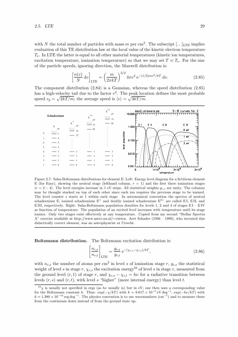
2.5. LTE 29

with N the total number of particles with mass m per cm3. The subscript [. . .]LTE impliesevaluation of this TE distribution law at the local value of the kinetic electron temperatureTe. In LTE the latter is equal to all other material temperatures (kinetic ion temperatures,excitation temperature, ionization temperature) so that we may set T $ Te. For the sizeof the particle speeds, ignoring direction, the Maxwell distribution is:

(n(v)N

dv)

LTE=

*m

2&kT

+3/2

4&v2 e"(1/2)mv2/kT dv. (2.85)

The component distribution (2.84) is a Gaussian, whereas the speed distribution (2.85)has a high-velocity tail due to the factor v2. The peak location defines the most probablespeed vp =

,

2kT/m; the average speed is +v, =,

3kT/m.

eV

1

2

3

4

5

6

7

1

2

3

4

5

6

7

16

15

0

1

31

30

0

1

51

50

0

1

22

33 3

2

0

E

E

E

E+

2

3

+

+

Schadeenium

s

eV

eV

eV

Figure 2.7: Saha-Boltzmann distributions for element E. Left: Energy level diagram for a fictitious elementE (for Easy), showing the neutral stage (lefthand column, r = 1) and the first three ionization stages(r = 2 # 4). The level energies increase in 1 eV steps. All statistical weights gr,s are unity. The columnsmay be thought stacked on top of each other since each ion requires the previous stage to be ionized.The level counter s starts at 1 within each stage. In astronomical convention the spectra of neutralschadeenium E, ionized schadeenium E+ and doubly ionized schadeenium E2+ are called E I, E II, andE III, respectively. Right: Saha-Boltzmann population densities for levels 1, 2 and 4 of stages E I – E IVas function of temperature. The population of an excited level increases with temperature until its stageionizes. Only two stages exist e!ectively at any temperature. Copied from my second “Stellar SpectraA” exercise available at http://www.astro.uu.nl/!rutten. Aert Schadee (1936 – 1999), who invented thisdidactically correct element, was an astrophysicist at Utrecht.

Boltzmann distribution. The Boltzmann excitation distribution is:-

nr,s

nr,t

.

LTE

=gr,s

gr,te"(&r,s"&r,t)/kT , (2.86)

with nr,s the number of atoms per cm3 in level s of ionization stage r, gr,s the statisticalweight of level s in stage r, 2r,s the excitation energy16 of level s in stage r, measured fromthe ground level (r, 1) of stage r, and 2r,s % 2r,t = h) for a radiative transition betweenlevels (r, s) and (r, t), with level s “higher” (more internal energy) than level t.

16- is usually not specified in ergs (as h+ usually is) but in eV; one then uses a corresponding valuefor the Boltzmann constant k. Thus: exp(#-/kT ) with k = 8.617 ' 10#5 eV deg#1, exp(#h+/kT ) withk = 1.380 ' 10#16 erg deg#1. The physics convention is to use wavenumbers (cm#1) and to measure thesefrom the continuum down instead of from the ground state up.

30 CHAPTER 2. BASIC RADIATIVE TRANSFER

Saha distribution. The Saha ionization distribution for the population ratio betweenthe ground levels of successive ionization stages is:

-

nr+1,1

nr,1

.

LTE

=1

Ne

2 gr+1,1

gr,1

*2&mekT

h2

+3/2

e"&r/kT , (2.87)

with Ne the electron density, me the electron mass, nr+1,1 and nr,1 the population densitiesof the two ground states of the successive ionization stages r and r + 1, 2r the ionizationenergy of stage r (the minimum energy needed to free an electron from the ground state ofstage r, with 2r = h)threshold) and gr+1,1 and gr,1 the statistical weights of the two groundlevels. The freed electron has statistical weight 2 due to its choice of spin orientation. Forthe total population of two successive ionization stages the Saha distribution is:

(Nr+1

Nr

)

LTE=

1Ne

2Ur+1

Ur

*2&mekT

h2

+3/2

e"&r/kT , (2.88)

with Nr+1 and Nr the total population densities of the two successive ionization stagesr and r + 1, 2r the ionization energy of stage r and the partition function Ur of stage rgiven by

Ur $&

s

gr,s e"&r,s/kT . (2.89)

Appendix D of Gray (1992) contains polynomial approximations of Ur for many atomsand singly-ionized ions. Other tables are given by Halenka and Grabowski (1984).

Saha-Boltzmann distribution. Combination of the two distributions gives the LTEpopulation ratio between a particular level i and the ion state c to which it ionizes as:

(nc

ni

)

LTE=

1Ne

2 gc

gi

*2&mekT

h2

+3/2

e"&ci/kT (2.90)

with ni the total population density of level i, nc the number of ions in ionization levelc (usually the ground state of the ion term system but sometimes an excited level withexcitation energy 2r+1,c) and 2ci = 2r % 2r,i + 2r+1,c = h)threshold the ionization energyfrom level i to state c.

2.5.2 Radiation in LTE

Planck function. In LTE the Boltzmann distribution holds so that the line sourcefunction simplifies from (2.72) on page 24 to the Planck function:

/

Sl!

0

LTE=

2h)3

c2

1(gunl

glnu

)

LTE% 1

(2.91)

=2h)3

c2

1eh!/kT % 1

$ B!(T ). (2.92)

This equality S! = B! is formally derived here through the Einstein coe!cients for bound-bound processes, thus only for the line source function, but it holds for all LTE (“thermal”)processes in which matter creates and destructs photons.

2.5. LTE 31

Wien and Rayleigh-Jeans approximations. For large h)/kT the numerator hasexp(h)/kT ) - 1 yielding the Wien approximation:

B!(T ) # 2h)3

c2e"h!/kT , (2.93)

expressing the particle-like behavior of photons at high energy by being similar to theBoltzmann distribution. For small h)/kT the approximation exp(h)/kT ) % 1 # h)/kTgives the Rayleigh-Jeans approximation:

B!(T ) # 2)2kT

c2, (2.94)

which is wave-like in character (Shu 1991, p. 7).

Stefan-Boltzmann law. Spectral integration produces the Stefan-Boltzmann law:

B(T ) =" #

0B! d) =

,

&T 4, (2.95)

with, =

2&5k4

15h3c2= 5.67 ( 10"5 erg cm"2 K"4 s"1. (2.96)

Induced emission. The LTE correction factor for bound-bound induced emission in(2.63) on page 23 is:

(

1 % nuBul2()%)0)nlBlu+()%)0)

)

LTE

= 1 % e"h!0/kT . (2.97)

The profile functions + and 2 are equal in LTE because otherwise detailed balancing perwavelength would not be feasible in TE.

Line extinction. The LTE line extinction coe!cient is:/

"l!

0

LTE=

&e2

mecnLTE

l flu +()%)0)/

1 % e"h!0/kT0

(2.98)

with nLTEl $ [nl]LTE given by the Saha-Boltzmann distributions for the local kinetic tem-

perature Te. The classical oscillator strength flu is defined by (2.66) on page 23. It is oftencombined with the lower-level statistical weight gl (which sits in nLTE

l through (2.86)) intothe so-called gf -value measuring transition probability.

Discussion. The essential premise of LTE is that collisions control the energy parti-tioning of the matter in the medium more strictly than that they control the energypartitioning of the radiation. All material energy distributions (velocity, ionization, ex-citation, dissociation) are then fixed by the local kinetic temperature (Maxwell, Saha,Boltzmann), while the radiative energy distributions may depart slightly from the localTE values:

Sl!((r) = B! [T ((r)] I!((r,(l) .= B! [T ((r)] J!((r) .= B! [T ((r)] F!((r) .= 0. (2.99)

32 CHAPTER 2. BASIC RADIATIVE TRANSFER

The LTE equality S! = B! holds when the source function is dominated by collisionsand/or when the frequency- and angle-averaged radiation field is Planckian, as shown fortwo-level atoms by (2.144) and (2.145) on page 41. Deep within stars both conditions arefulfilled. There, the photons are “honorary particles” (Castor) that fully participate in thethermodynamics of the gas. Their mean free paths are much smaller than the scales overwhich state parameters vary appreciably. However, even there I! is not exactly isotropic(as required for I! = B!); therefore, (or rather, because) the net flux has F!((r) .= 0and transports energy outward, a leak that inhibits strict TE even for the very closeconfinement within stars — strict TE doesn’t exist in nature.

2.6 NLTE

Non-local thermodynamical equilibrium (NLTE or non-LTE) is a loose term which impliesthat the assumption of LTE fails. Often one then assumes statistical equilibrium implicitly,usually with the Maxwell distribution and complete redistribution in frequency and angle.However, the populations are now permitted to di"er from the local Saha-Boltzmannequilibrium values.

2.6.1 Statistical equilibrium

Rate equations. Statistical equilibrium (SE) implies that the radiation fields (in alldirections and on all frequencies) and level populations do not vary with time, as expressedin the statistical equilibrium equations (population equations, rate equations):

dni((r)dt

=N

&

j $=i

nj((r)Pji((r) % ni((r)N

&

j $=i

Pij((r) = 0, (2.100)

with ni the population of a particular level, N the total number of levels that are importantfor the population of level ni one way or another, and j stepping over all those levels. Thetransition rates Pij for radiative and collisinal processes, respectively, are given per particlein state i or j by:

Pij = Rij + Cij. (2.101)

For a bound-bound transition the radiative rate per particle is:

Rij = Aij + BijJ!0. (2.102)

A similar expression holds for radiative bound-free rates but with J!0 averaged over theionization edge. General expressions for radiative rates Rij in bound-bound and bound-free transitions are given by (3.17)–(3.22) on page 48. Approximate expressions for bound-bound and bound-free collision rates Cij are given in (3.32)–(3.37) on page 51.

Transport equations. The population equations (2.100) contain the mean intensitiesat all relevant frequencies via J!0 terms as in (2.102). The intensities are given by theradiation transport equations

µdI!((r, µ)d/!((r)

= %S!((r) + I!((r, µ) (2.103)

at all frequencies ), directions µ and locations (r that are important in (2.100) one wayor another. Thus, the rates Pij in (2.100) depend on J! and therefore on I! in other

2.6. NLTE 33

directions, whereas the optical depths /! and the source functions S! in (2.103) dependon the populations nl and nu of the lower and upper levels involved in transitions atthe frequency ). These populations may depend on other transitions and therefore onother populations again, each dependent on radiation fields at other frequencies. Thus,a given transition of interest may be influenced by many other transitions in the sameparticle species, or by transitions in other atoms and molecules if these possess transitionsat overlapping frequencies. The latter include all interactions that cause the continuumbackground at a frequency of interest. This intricate coupling between populations andradiation is non-linear and non-local. It can be very complex, except when the tremendoussimplification of LTE may be assumed.

Time-dependent transfer. When SE does not hold the population equations must sat-isfy overall particle conservation (continuity) rather than population conservation. Theseequations and the transport equations then become time dependent. Systematic flowsmake the source function anisotropic (page 71).

Multi-dimensional transfer. Lateral inhomogeneity is likely to come with time de-pendence so that the geometry of stellar-atmosphere radiative transfer becomes two- orthree-dimensional, instead of the one-dimensional plane-parallel simplification assumedthroughout these lecture notes. Such complexity requires the full sophistication of elabo-rate radiative hydrodynamics (Mihalas and Mihalas 1984).

2.6.2 NLTE descriptions

Departure coe!cients. NLTE population departure coe!cients bi are defined as:

bl = nl/nLTEl bu = nu/nLTE

u (2.104)

with n the actual population and nLTE the Saha-Boltzmann values for the lower and upperlevel, respectively (Wijbenga and Zwaan 1972).

Bound-bound source function. Expressed in departure coe!cients the general linesource function (2.72) becomes

Sl! =

2h)3

c2

1/+bl

bueh!/kT % 2

+

(2.105)

and for complete redistribution with 2! = 1! = +!

Sl!0

=2h)3

0

c2

1bl

bueh!0/kT % 1

, (2.106)

where Sl!0

does not depend on frequency over the extent of a narrow line. In the Wienregime with (bl/bu) exp(h)/kT ) - 1 the fractional departure of the source function fromthe Planck function is given by the inverse fugacity ratio bu/bl:

Sl!0

# bu

blB!0 . (2.107)

34 CHAPTER 2. BASIC RADIATIVE TRANSFER

Bound-bound extinction. The monochromatic line extinction coe!cient (2.63) onpage 23 becomes:

"l! =

h)

4&bl n

LTEl Blu+()%)0)

-

1 % bu nLTEu Bul 2

bl nLTEl Blu +

.

(2.108)

=h)

4&bl n

LTEl Blu+()%)0)

(

1 % bu

bl

2

+e"h!/kT

)

(2.109)

= bl nLTEl ,l

!

(

1 % bu

bl

2

+e"h!/kT

)

(2.110)

=&e2

mecbl n

LTEl flu+()%)0)

(

1 % bu

bl

2

+e"h!/kT

)

(2.111)

with 2/+ = 1 for complete redistribution. In the Wien approximation, using (2.98):

"l! # bl

/

"l!

0

LTE. (2.112)

Similarly, the total line extinction coe!cient (2.64) on page 23 becomes

"l!0

=h)0

4&bl n

LTEl Blu

(

1 % bu

ble"h!0/kT

)

(2.113)

=&e2

mecbl n

LTEl flu

(

1 % bu

ble"h!0/kT

)

(2.114)

# bl

/

"l!0

0

LTE. (2.115)

Figure 2.8: Wavelength variation of the NLTE source functions (2.106) and (2.117) for T = 10 000 K andthe specified ratios bu/bl or bc/bi, respectively, in cgs units with #! = 1 nm. The NLTE source functionscales with the Planck function (solid curve) in the Wien part at left, but reaches the laser regime for largebu/bl in the Rayleigh-Jeans part at right.

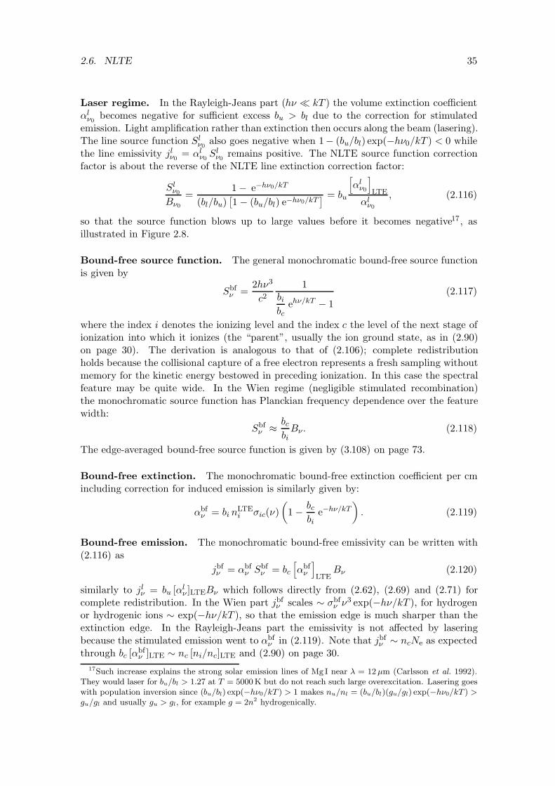
2.6. NLTE 35

Laser regime. In the Rayleigh-Jeans part (h) * kT ) the volume extinction coe!cient"l

!0becomes negative for su!cient excess bu > bl due to the correction for stimulated

emission. Light amplification rather than extinction then occurs along the beam (lasering).The line source function Sl

!0also goes negative when 1% (bu/bl) exp(%h)0/kT ) < 0 while

the line emissivity jl!0

= "l!0

Sl!0

remains positive. The NLTE source function correctionfactor is about the reverse of the NLTE line extinction correction factor:

Sl!0

B!0

=1 % e"h!0/kT

(bl/bu)1

1 % (bu/bl) e"h!0/kT2 = bu

/

"l!0

0

LTE

"l!0

, (2.116)

so that the source function blows up to large values before it becomes negative17, asillustrated in Figure 2.8.

Bound-free source function. The general monochromatic bound-free source functionis given by

Sbf! =

2h)3

c2

1bi

bceh!/kT % 1

(2.117)

where the index i denotes the ionizing level and the index c the level of the next stage ofionization into which it ionizes (the “parent”, usually the ion ground state, as in (2.90)on page 30). The derivation is analogous to that of (2.106); complete redistributionholds because the collisional capture of a free electron represents a fresh sampling withoutmemory for the kinetic energy bestowed in preceding ionization. In this case the spectralfeature may be quite wide. In the Wien regime (negligible stimulated recombination)the monochromatic source function has Planckian frequency dependence over the featurewidth:

Sbf! # bc

biB! . (2.118)

The edge-averaged bound-free source function is given by (3.108) on page 73.

Bound-free extinction. The monochromatic bound-free extinction coe!cient per cmincluding correction for induced emission is similarly given by:

"bf! = bi n

LTEi ,ic())

*

1 % bc

bie"h!/kT

+

. (2.119)

Bound-free emission. The monochromatic bound-free emissivity can be written with(2.116) as

jbf! = "bf

! Sbf! = bc

/

"bf!

0

LTEB! (2.120)

similarly to jl! = bu ["l

! ]LTEB! which follows directly from (2.62), (2.69) and (2.71) forcomplete redistribution. In the Wien part jbf

! scales " ,bf! )3 exp(%h)/kT ), for hydrogen

or hydrogenic ions " exp(%h)/kT ), so that the emission edge is much sharper than theextinction edge. In the Rayleigh-Jeans part the emissivity is not a"ected by laseringbecause the stimulated emission went to "bf

! in (2.119). Note that jbf! " ncNe as expected

through bc ["bf! ]LTE " nc [ni/nc]LTE and (2.90) on page 30.

17Such increase explains the strong solar emission lines of Mg I near ! = 12 µm (Carlsson et al. 1992).They would laser for bu/bl > 1.27 at T = 5000 K but do not reach such large overexcitation. Lasering goeswith population inversion since (bu/bl) exp(#h+0/kT ) > 1 makes nu/nl = (bu/bl)(gu/gl) exp(#h+0/kT ) >gu/gl and usually gu > gl, for example g = 2n2 hydrogenically.

36 CHAPTER 2. BASIC RADIATIVE TRANSFER

Free-free source function, extinction, emission. For completeness the correspond-ing free-free expressions:

S#! = B! (2.121)

"#! = bc nLTE

c ,#!

$

1 % e"h!/kT%

(2.122)

j#! = bc

/

"#!

0

LTEB! (2.123)

where ,#! is given by (2.76) on page 26. The free-free source function and stimulated

emission correction are thermal. Formally, this follows by setting bi = bc in (2.117) and(2.119). Physically, it follows from the assumption of the Maxwell distribution for the ki-netic energy partitioning, sampled afresh by each new bremsstrahlung photon. Departuresfrom LTE in the ion population that are caused by other transitions a"ect the free-freeextinction but not the amount of emission per extinction = source function.

Discussion. These formal expressions do not specify what part of the source functionis controlled by B! or by J! (at this frequency or at other frequencies); they only expressthe overall result in term of population departures relative to the LTE equilibrium values.The actual values of nl and nu may depend on B! and J! at widely di"erent frequenciesthrough other transitions that may feed excess population into these levels or deplete themexcessively. Bound-free transitions contain at least partial thermalization, since part of thephoton energy produces kinetic energy (ionization) or uses kinetic energy (recombination),but they may also depend on J! in the ionization edge or at other frequencies. Thispartial thermalization and sensitivity to radiation is also hidden in the resulting populationdepartures.

Only free-free photon emission and extinction are strictly kinetic, respectively creatingand destroying photons in every interaction, with S#

! = B! and "#! = bc ["#

! ]LTE whereverthe Maxwell distribution holds.

Lasering occurs at su!cient bound-bound overexcitation or bound-free overionization,but only when other transitions provide a mechanism to overpopulate the higher level (seediscussion on page 71 at the end of Section 3.4.2).

Warning. I should add a warning here that the departure coe!cients bi are often de-fined di"erently18 from (2.104), as a generalization of the original introduction by Menzeland Cillie (1937) for H I in which the departure of the neutral hydrogen population wasnormalized by the H II density (free protons). In the Menzel convention, the bi coe!-cients are normalized to the LTE population of the next ionization stage by a partialSaha-Boltzmann evaluation, whereas in the preferable Zwaan convention of Wijbenga andZwaan (1972) used here the bi are normalized by the total particle density (abundance) ofthe element through the complete Saha-Boltzmann relations. The two conventions are:

bZwaani $ ni/n

LTEi (2.124)

bMenzeli $ ni/nLTE

i

nC/nLTEC

(2.125)

where nC is the total population of the next ion. Sometimes its ground state is used insteadby setting nC # nc, also following Menzel and Cillie (1937) who made no distinction

18For example on p. 76 of Shu (1991).

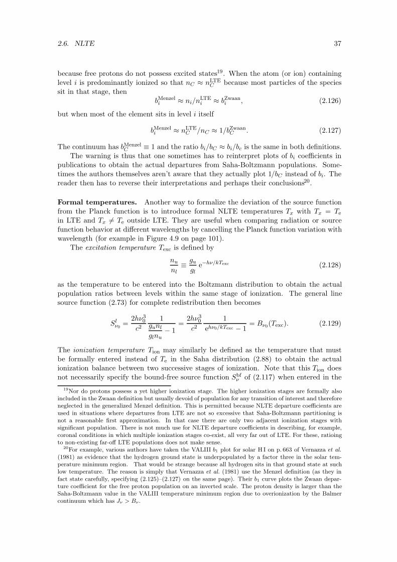
2.6. NLTE 37

because free protons do not possess excited states19. When the atom (or ion) containinglevel i is predominantly ionized so that nC # nLTE

C because most particles of the speciessit in that stage, then

bMenzeli # ni/n

LTEi # bZwaan

i , (2.126)

but when most of the element sits in level i itself

bMenzeli # nLTE

C /nC # 1/bZwaanC . (2.127)

The continuum has bMenzelC $ 1 and the ratio bi/bC # bi/bc is the same in both definitions.

The warning is thus that one sometimes has to reinterpret plots of bi coe!cients inpublications to obtain the actual departures from Saha-Boltzmann populations. Some-times the authors themselves aren’t aware that they actually plot 1/bC instead of bi. Thereader then has to reverse their interpretations and perhaps their conclusions20.

Formal temperatures. Another way to formalize the deviation of the source functionfrom the Planck function is to introduce formal NLTE temperatures Tx with Tx = Te

in LTE and Tx .= Te outside LTE. They are useful when comparing radiation or sourcefunction behavior at di"erent wavelengths by cancelling the Planck function variation withwavelength (for example in Figure 4.9 on page 101).

The excitation temperature Texc is defined by

nu

nl$ gu

gle"h!/kTexc (2.128)

as the temperature to be entered into the Boltzmann distribution to obtain the actualpopulation ratios between levels within the same stage of ionization. The general linesource function (2.73) for complete redistribution then becomes

Sl!0

=2h)3

0

c2

1gunl

glnu% 1

=2h)3

0

c2

1eh!0/kTexc % 1

= B!0(Texc). (2.129)

The ionization temperature Tion may similarly be defined as the temperature that mustbe formally entered instead of Te in the Saha distribution (2.88) to obtain the actualionization balance between two successive stages of ionization. Note that this Tion doesnot necessarily specify the bound-free source function Sbf

! of (2.117) when entered in the19Nor do protons possess a yet higher ionization stage. The higher ionization stages are formally also

included in the Zwaan definition but usually devoid of population for any transition of interest and thereforeneglected in the generalized Menzel definition. This is permitted because NLTE departure coe"cients areused in situations where departures from LTE are not so excessive that Saha-Boltzmann partitioning isnot a reasonable first approximation. In that case there are only two adjacent ionization stages withsignificant population. There is not much use for NLTE departure coe"cients in describing, for example,coronal conditions in which multiple ionization stages co-exist, all very far out of LTE. For these, ratioingto non-existing far-o! LTE populations does not make sense.

20For example, various authors have taken the VALIII b1 plot for solar H I on p. 663 of Vernazza et al.(1981) as evidence that the hydrogen ground state is underpopulated by a factor three in the solar tem-perature minimum region. That would be strange because all hydrogen sits in that ground state at suchlow temperature. The reason is simply that Vernazza et al. (1981) use the Menzel definition (as they infact state carefully, specifying (2.125)–(2.127) on the same page). Their b1 curve plots the Zwaan depar-ture coe"cient for the free proton population on an inverted scale. The proton density is larger than theSaha-Boltzmann value in the VALIII temperature minimum region due to overionization by the Balmercontinuum which has J" > B" .

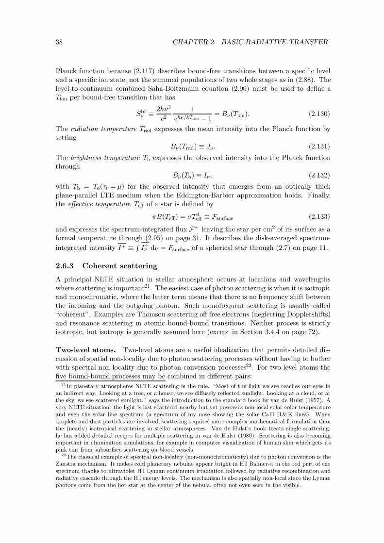
38 CHAPTER 2. BASIC RADIATIVE TRANSFER

Planck function because (2.117) describes bound-free transitions between a specific leveland a specific ion state, not the summed populations of two whole stages as in (2.88). Thelevel-to-continuum combined Saha-Boltzmann equation (2.90) must be used to define aTion per bound-free transition that has

Sbf! $ 2h)3

c2

1eh!/kTion % 1

= B!(Tion). (2.130)

The radiation temperature Trad expresses the mean intensity into the Planck function bysetting

B!(Trad) $ J! . (2.131)

The brightness temperature Tb expresses the observed intensity into the Planck functionthrough

B!(Tb) $ I! , (2.132)

with Tb = Te(/! = µ) for the observed intensity that emerges from an optically thickplane-parallel LTE medium when the Eddington-Barbier approximation holds. Finally,the e!ective temperature Te# of a star is defined by

&B(Te#) = ,T 4e# $ Fsurface (2.133)

and expresses the spectrum-integrated flux F+ leaving the star per cm2 of its surface as aformal temperature through (2.95) on page 31. It describes the disk-averaged spectrum-integrated intensity I+ $

!

I+! d) = Fsurface of a spherical star through (2.7) on page 11.

2.6.3 Coherent scattering

A principal NLTE situation in stellar atmosphere occurs at locations and wavelengthswhere scattering is important21. The easiest case of photon scattering is when it is isotropicand monochromatic, where the latter term means that there is no frequency shift betweenthe incoming and the outgoing photon. Such monofrequent scattering is usually called“coherent”. Examples are Thomson scattering o" free electrons (neglecting Dopplershifts)and resonance scattering in atomic bound-bound transitions. Neither process is strictlyisotropic, but isotropy is generally assumed here (except in Section 3.4.4 on page 72).

Two-level atoms. Two-level atoms are a useful idealization that permits detailed dis-cussion of spatial non-locality due to photon scattering processes without having to botherwith spectral non-locality due to photon conversion processes22. For two-level atoms thefive bound-bound processes may be combined in di"erent pairs:

21In planetary atmospheres NLTE scattering is the rule. “Most of the light we see reaches our eyes inan indirect way. Looking at a tree, or a house, we see di!usely reflected sunlight. Looking at a cloud, or atthe sky, we see scattered sunlight.” says the introduction to the standard book by van de Hulst (1957). Avery NLTE situation: the light is last scattered nearby but yet possesses non-local solar color temperatureand even the solar line spectrum (a spectrum of my nose showing the solar Ca II H& K lines). Whendroplets and dust particles are involved, scattering requires more complex mathematical formulation thanthe (nearly) isotropical scattering in stellar atmospheres. Van de Hulst’s book treats single scattering;he has added detailed recipes for multiple scattering in van de Hulst (1980). Scattering is also becomingimportant in illumination simulations, for example in computer visualization of human skin which gets itspink tint from subsurface scattering on blood vessels.

22The classical example of spectral non-locality (non-monochromaticity) due to photon conversion is theZanstra mechanism. It makes cold planetary nebulae appear bright in H I Balmer-" in the red part of thespectrum thanks to ultraviolet H I Lyman continuum irradiation followed by radiative recombination andradiative cascade through the H I energy levels. The mechanism is also spatially non-local since the Lymanphotons come from the hot star at the center of the nebula, often not even seen in the visible.

2.6. NLTE 39

– photon scattering: radiative excitation followed by spontaneous or induced radiativedeexcitation. The new photon is often described as still being the old one, but it hasbeen re-directed and has possibly been slightly shifted (redistributed) in frequency;

– photon creation: collisional excitation followed by spontaneous or induced radiativedeexcitation. This pair makes a new photon out of kinetic energy;

– photon destruction: radiative excitation followed by collisional deexcitation. Thispair thermalizes a photon into kinetic energy.

Similar pairs hold for bf, " and other processes. The split is treated in more detail inSection 3.4.1 on page 64"; the discussion here is limited to the essentials following Rybickiand Lightman (1979).

Coherently scattering medium. A useful simplification of resonance scattering is toassume that the medium consists purely of two-level atoms and that the scattering iscoherent. Each radiative excitation is then necessarily followed by deexcitation in thesame transition, either a radiative one at exactly the same frequency (spontaneous or in-duced; photon scattering) or a collisional one (photon destruction). In repeated scattering,photons step in random walk through the medium without coupling their energy to thelocal conditions. On the other hand, the photon creation and photon destruction pairscouple the radiation energy to the local kinetic energy; these pairs constitute “thermal”processes23.

The strength of the coupling depends on the relative frequency of the thermal andscattering sequences. The monochromatic bound-bound extinction coe!cient "l

! may inthis case be written as the sum of partial extinction coe!cients "a

! for photon destruction(absorption, often called “true absorption” when “absorption” is used for extinction) and"s

! for photon scattering:"l

! = "a! + "s

! . (2.134)

The continuous extinction coe!cient may similarly be split into a coherent scattering partdue to Thomson or Rayleigh scattering and a thermal destruction part due to free-free24

processes.

Destruction probability. The photon destruction probability per extinction for coher-ently scattering two-level atoms is given by

'! $ "a!

"a! + "s

!. (2.135)

Its complement is the scattering probability per extinction:

1 % '! ="s

!

"a! + "s

!. (2.136)

23When the Maxwell distribution holds so that the local kinetic energy of all material particle species(fermions) is parametrized by the local electron temperature. This is generally the case in stellar atmo-spheres and is assumed tacitly throughout these lecture notes — together with the assumption that allfermions occur exclusively as a gas of free atoms and/or ions plus electrons and/or molecules, without ag-gregation into fluid or solid states or boson condensates. This quite reasonable assumption makes radiativetransfer in stellar atmospheres again simpler than radiative transfer in planetary atmospheres.

24Or bound-free processes, but these may mix thermal and scattering behavior since the part of theenergy jump above the ionization limit is converted into kinetic energy while the remainder representsinternal atomic energy rather like a bound-bound transition. More on this in Section 3.2.2 on page 45 andSection 3.4.5 on page 72.

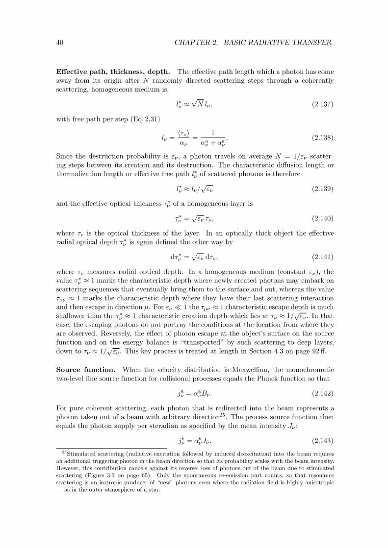
40 CHAPTER 2. BASIC RADIATIVE TRANSFER

E"ective path, thickness, depth. The e"ective path length which a photon has comeaway from its origin after N randomly directed scattering steps through a coherentlyscattering, homogeneous medium is:

l%! #'

N l! , (2.137)

with free path per step (Eq. 2.31)

l! =+/!,"!

=1

"a! + "s

!. (2.138)

Since the destruction probability is '! , a photon travels on average N = 1/'! scatter-ing steps between its creation and its destruction. The characteristic di"usion length orthermalization length or e"ective free path l%! of scattered photons is therefore

l%! # l!/'

'! (2.139)

and the e"ective optical thickness /%! of a homogeneous layer is

/%! =

''! /! , (2.140)

where /! is the optical thickness of the layer. In an optically thick object the e"ectiveradial optical depth /%

! is again defined the other way by

d/%! =

''! d/! , (2.141)

where /! measures radial optical depth. In a homogeneous medium (constant '!), thevalue /%

! # 1 marks the characteristic depth where newly created photons may embark onscattering sequences that eventually bring them to the surface and out, whereas the value/!µ # 1 marks the characteristic depth where they have their last scattering interactionand then escape in direction µ. For '! * 1 the /µ! # 1 characteristic escape depth is muchshallower than the /%

! # 1 characteristic creation depth which lies at /! # 1/''! . In thatcase, the escaping photons do not portray the conditions at the location from where theyare observed. Reversely, the e"ect of photon escape at the object’s surface on the sourcefunction and on the energy balance is “transported” by such scattering to deep layers,down to /! # 1/

''! . This key process is treated at length in Section 4.3 on page 92".

Source function. When the velocity distribution is Maxwellian, the monochromatictwo-level line source function for collisional processes equals the Planck function so that

ja! = "a

!B! . (2.142)

For pure coherent scattering, each photon that is redirected into the beam represents aphoton taken out of a beam with arbitrary direction25. The process source function thenequals the photon supply per steradian as specified by the mean intensity J! :

js! = "s

!J! . (2.143)25Stimulated scattering (radiative excitation followed by induced deexcitation) into the beam requires

an additional triggering photon in the beam direction so that its probability scales with the beam intensity.However, this contribution cancels against its reverse, loss of photons out of the beam due to stimulatedscattering (Figure 3.3 on page 65). Only the spontaneous re-emission part counts, so that resonancescattering is an isotropic producer of “new” photons even where the radiation field is highly anisotropic— as in the outer atmosphere of a star.

2.6. NLTE 41

The combined two-level-atom line source function for a mixture of thermal absorption andcoherent scattering is with (2.22), (2.134) and (2.135):

Sl! =

ja! + js

!

"a! + "s

!= (1 % '!)J! + '!B! . (2.144)

An elaborate derivation in terms of Einstein coe!cients is given in Section 3.4.1 on page 64.The expression holds also for monochromatic (elastic, coherent) Thomson and Rayleighscattering in the presence of thermal bound-free and free-free continuum processes thatcause photon destruction at the frequency ).

A similar expression holds for the case of complete redistribution:

Sl!0

= (1 % '!0)J%!0

+ '!0B!0 , (2.145)

where '!0 is the profile-summed photon destruction probability defined by

'!0 $"a

!0

"a!0

+ "s!0

. (2.146)

The derivation is given in Section 3.4.2 on page 70. Similar expressions hold for bound-freescattering (Section 3.4.5) on page 72 and synchrotron scattering (footnote on page 74).

Transport equation. For a medium made up of two-level atoms, the transport equationalong the propagation direction

dI! = %"a!I! ds % "s

!I! ds + "a!B! ds + "s

!J! ds (2.147)

is, with optical thickness d/! $ "l! ds = ("a

! + "s!) ds, once more given by

dI!

d/!=

dI!

("a! + "s

!) ds= Sl

! % I! (2.148)

and when using /! for radial optical depth in axial symmetry by

µdI!

d/!= I! % Sl

! . (2.149)

In the case of complete redistribution the monofrequent line source function has Sl! = Sl

!0

and does not vary over the line profile26.

2.6.4 Multi-level interlocking

Not yet...

2.6.5 Coronal conditions

Not yet...

26In the more realistic case of a medium containing not only two-level atoms but also other particleswhich contribute continuous extinction at the line wavelength, the total source function replaces Sl

" in thetransport equation. It varies over the line profile, even if Sl does not in the complete-redistribution case,due to the frequency-dependent weighting of any di!erence between Sl and Sc in (2.23) on page 13.