Radar Signal Propagation and Detection Through Ice

Space Sci Rev (2010) 153: 249–271DOI 10.1007/s11214-010-9642-2

Radar Signal Propagation and Detection Through Ice

Wlodek Kofman · Roberto Orosei · Elena Pettinelli

Received: 1 September 2009 / Accepted: 1 March 2010 / Published online: 31 March 2010© Springer Science+Business Media B.V. 2010

Abstract In this paper we describe the existing and planned radar measurements of theplanetary bodies. The dielectric properties of water ice and other potential surface and sub-surface materials are discussed, as well as their dependency on temperature and structure.We then evaluate the performance of subsurface sounding radars using these parameters.Finally we describe some laboratory technique to help interpret the radar data, presentingsome results obtained using dielectric spectroscopy methods.

Keywords Dielectric properties · Radar · Laboratory measurements

1 Introduction—What Can Be Learned from Radar Observations?

Radio-echo sounding (RES), or ice-penetrating radar, is a well established geophysical tech-nique, similar to ground-penetrating radar, which has been employed for more than fivedecades to investigate the structure of ice sheets and glaciers in Antarctica, Greenland, andthe Arctic. It is based on the transmission of radar pulses at frequencies in the MF, HF andVHF portions of the electromagnetic spectrum into the surface to detect reflected signalsfrom subsurface structures (see e.g. Bogorodsky et al. 1985).

Ground-penetrating radar is particularly effective on glaciers because ice is the mosttransparent natural material in this range of frequencies. The ice-covered Lake Vostok in

W. Kofman (�)Laboratoire de Planetologie de Grenoble, CNRS/UJF, BP 53, 38041 Grenoble, Francee-mail: [email protected]

R. OroseiIstituto Nazionale di Astrofisica, Istituto di Fisica dello Spazio Interplanetario,Via del Fosso del Cavaliere, 100, 00133 Roma, Italy

E. PettinelliDipartimento di Fisica “E. Amaldi”, Università Roma Tre, Via della Vasca Navale 84,00146 Roma, Italy

mailto:[email protected]

250 W. Kofman et al.

Antarctica was characterized through more than 4 km of polar ice. Cold ice is more trans-parent than warm ice, so that it is expected that at the temperatures of the outer Solar Systemthis technique could provide detection of much deeper subsurface structures (Blankenshipet al. 2010).

An electromagnetic wave propagating through a medium is attenuated, scattered anddispersed. Its distortion depends on the dielectric characteristics of the medium and its ho-mogeneity at the wavelength scale. The electromagnetic pulse emitted from orbiting ice-penetrating radar would be subject to scattering from the irregular natural surface of an icymoon, and it would be scattered by volume inhomogeneities and attenuated in the dielec-tric subsurface medium before reaching any subsurface dielectric discontinuity causing areflection.

The capability of subsurface sounding radar to detect an underground dielectric discon-tinuity is thus strongly dependent on the medium through which the radar pulse propagates.For icy bodies the physical properties of water ice and the effect of impurities in the ice playa major role.

Radar sounding is the only remote sensing technique allowing the study of the subsurfaceof a planet from orbit. By detecting dielectric discontinuities associated with compositionaland/or structural discontinuities, it is possible to map the stratigraphy, i.e. the distributioncharacteristics of ice and/or rocks vs. depth, which can be of fundamental importance to bet-ter understand the dynamics and the history of the first meters to kilometers of the subsurface(depending on frequency and dielectric properties of the material). On the other hand, theestimation of the propagation time and the signal attenuation, also allows us to retrieve someinformation on the subsurface petrophysical properties like density and material composi-tion. Moreover, the form of the received signal gives some information about the surface andthe volume scattering, from which the size distribution of inhomogeneities can be inferred.All this nonwithstanding, the information obtained with subsurface sounding radars shouldbe compared and integrated with other observations (infrared, visible or in situ analysis) tointerpret inferred petrophysical properties in an unambiguous way.

In this chapter we describe the existing and planned radar measurements of the planetarybodies. The dielectric properties of water ice and other potential surface and subsurfacematerials are discussed, as well as their dependency on temperature and structure. We thenevaluate the performance of subsurface sounding radars using these parameters. Finally wedescribe some laboratory technique to help interpret the radar data, presenting some resultsobtained using dielectric spectroscopy methods.

2 Overview of Radar Observations of Icy Satellites

Radar observations of the icy satellites were obtained from the Earth using the Goldstoneand Arecibo radar (Ostro et al. 1992). The measurements of the reflected signal by thesurface and subsurface of Galilean satellites and of Saturn’s icy satellites were made inthe 3.5–70 cm wavelength range. Recently also observations of the Saturn’s satellites weremade using Cassini 2.2 cm radar. The Arecibo and Goldstone measurements used essen-tially transmitted circularly polarized and, rarely, linearly polarized signals. The receptionof returning signal was in the same circular (SC) (or same linear SL) and opposite circular(OC) (orthogonal linear OL) polarizations. The radar target’s properties are measured by itsalbedo that is defined by the radar cross section divided by the projected area of the observedsurface. The total radar albedo is TP = SL + OL = SC + OC and the polarization ratio isμc = SC/OC (OL/SL). For a polished metal sphere of the radius of the observed bodies the

Radar Signal Propagation and Detection Through Ice 251

single back reflections would be entirely OC (or SL) and the polarization ratios equal zero.In this case the radar albedo would equal the surface’s Fresnel coefficient.

The reflections from rough surfaces (or produced by multiple reflections or refrac-tions) produce power on two polarizations. For instance, for randomly oriented dipoles,SC/OC = 1 and OL/SL = 1/3. The echoes from Earth-like planets are characterised bythe quasi specular reflection having SC/OC ∼= 0.3 due to the much stronger direct reflec-tion compared to the power scattered by the surface and subsurface. The total albedo forEarth-like planets or for asteroids are of the order of TP ∼ 0.1. Figure 1 (Black et al. 2007)summarizes the measurements of total radar albedo and of polarization ratio obtained dur-ing the last three decades for icy satellites. One can see that the results are really differentfrom that obtained for the rocky bodies. The polarization ratio is larger than 1 and the totalalbedo are between 0.3 and 2.6. The total albedo value larger than 1 means that the backreflection is stronger than the reflection from the perfect metal sphere with the same ra-dius as observed body! What is the process responsible for this anomalous high albedo andpolarization ratio? The models proposed in the geometrical optics limit included: buriedcraters effect on the refracted signal (Eshleman 1986), another refraction scattering fromsubsurface lenses (Hagfors et al. 1997) and volume multiple scattering due to the scatter-ers embedded in the ice (Hapke 1990). The models were improved (Baron et al. 2003) andthe present agreement is that this “anomalous” behaviour results from the multiple scatteringwithin a random medium whose intrinsic microwave absorption is very low. The regoliths ofthe planetary bodies are very heterogeneous and that combined with the radio transparencyof icy regoliths gives the observed radar behaviour. Measurements of radar properties andany inter-satellite variations address issues of surface characteristics and formation histo-ries.

The unusual radar properties of icy satellite surfaces are thus determined by a combi-nation of the structure of the regolith, providing many dielectric discontinuities by whichan incident wave is reflected, and its composition, a transparent material that allows severalinternal reflections of the same wave without attenuating it significantly.

Subsurface sounding radars operate at much lower frequencies, and electromagneticpropagation at wavelengths of tens of meters is probably unaffected by the small-scalestructure of the regolith producing the anomalous reflection observed at cm wavelengths.However, the fact that the surface material is so transparent to electromagnetic waves testi-fies to a mostly icy composition with a small content of impurities, a very favorable scenariofor radar sounding experiments.

3 Interpretation of Radar Measurements

Subsurface radar sounding is now an established technique in planetary exploration, withan history of success (see Phillips et al. 1973; Picardi et al. 2004; Seu et al. 2007a; Onoet al. 2009) and a promising future (e.g. Lebreton et al. 2009). The Consert tomographicradar (Kofman et al. 1998, 2007), the next application of this technique, is on the way to itscometary target on the Rosetta mission. However, radar data have features that depend oninstrument characteristics and on the environment in which observations take place, whichhave to be taken into account for a correct interpretation.

The main parameters determining the performance of an orbiting subsurface soundingradar are frequency and bandwidth of the transmitted pulse. Frequency determines the pen-etration capability of the radar, while bandwidth controls resolution.

For a wide range of frequencies ranging from MHz to GHz and beyond, dielectric losses(loss tangent) in most natural materials are independent of frequency, so that the number


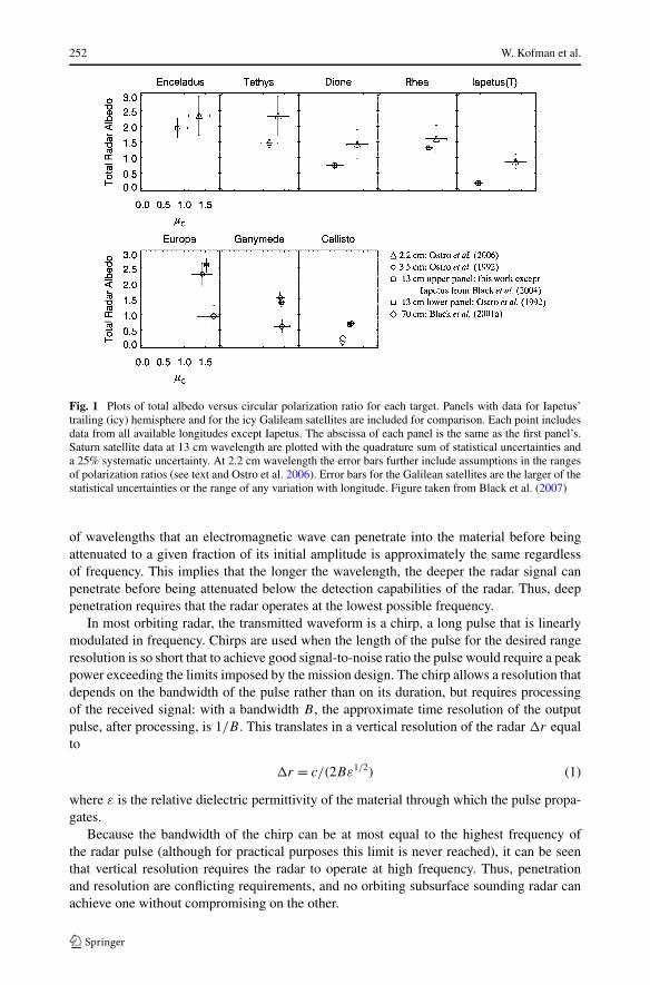
Fig. 1 Plots of total albedo versus circular polarization ratio for each target. Panels with data for Iapetus’trailing (icy) hemisphere and for the icy Galileam satellites are included for comparison. Each point includesdata from all available longitudes except Iapetus. The abscissa of each panel is the same as the first panel’s.Saturn satellite data at 13 cm wavelength are plotted with the quadrature sum of statistical uncertainties anda 25% systematic uncertainty. At 2.2 cm wavelength the error bars further include assumptions in the rangesof polarization ratios (see text and Ostro et al. 2006). Error bars for the Galilean satellites are the larger of thestatistical uncertainties or the range of any variation with longitude. Figure taken from Black et al. (2007)

of wavelengths that an electromagnetic wave can penetrate into the material before beingattenuated to a given fraction of its initial amplitude is approximately the same regardlessof frequency. This implies that the longer the wavelength, the deeper the radar signal canpenetrate before being attenuated below the detection capabilities of the radar. Thus, deeppenetration requires that the radar operates at the lowest possible frequency.

In most orbiting radar, the transmitted waveform is a chirp, a long pulse that is linearlymodulated in frequency. Chirps are used when the length of the pulse for the desired rangeresolution is so short that to achieve good signal-to-noise ratio the pulse would require a peakpower exceeding the limits imposed by the mission design. The chirp allows a resolution thatdepends on the bandwidth of the pulse rather than on its duration, but requires processingof the received signal: with a bandwidth B , the approximate time resolution of the outputpulse, after processing, is 1/B . This translates in a vertical resolution of the radar �r equalto

�r = c/(2Bε1/2) (1)

where ε is the relative dielectric permittivity of the material through which the pulse propa-gates.

Because the bandwidth of the chirp can be at most equal to the highest frequency ofthe radar pulse (although for practical purposes this limit is never reached), it can be seenthat vertical resolution requires the radar to operate at high frequency. Thus, penetrationand resolution are conflicting requirements, and no orbiting subsurface sounding radar canachieve one without compromising on the other.


Fig. 2 (Top) MARSIS radargram for orbit 2682 above Planum Australe, Mars, showing a bright basal reflec-tor (arrow) beneath the ice-rich South Polar Layered Deposits (SPLD). The vertical dimension is round-triptravel time. The apparent curvature of the reflector is an artefact of the time representation of the data. Themaximum depth at which the basal reflector could be detected, converting travel time for propagation throughwater ice, is about 3.5 km. (Bottom) Ground track of the spacecraft during data acquisition, shown on a shadedrelief topographic map of the south polar region of Mars (adapted from Plaut et al. 2007)

An example of this trade off is the design of the two radars currently operating at Mars,MARSIS (Picardi et al. 2004) and SHARAD (Seu et al. 2007a). They are both synthetic-aperture, orbital sounding radars, carried respectively by ESA’s Mars Express and NASA’sMars Reconnaissance Orbiter. MARSIS is capable of transmitting at four different bandsbetween 1.3 MHz and 5.5 MHz, with a 1 MHz bandwidth. SHARAD operates at a centralfrequency of 20 MHz transmitting a 10 MHz bandwidth. Whereas MARSIS is optimizedfor deep penetration, having detected echoes down to a depth of 3.7 km over the SouthPolar Layered Deposits (Plaut et al. 2007), SHARAD is capable of a tenfold-finer verticalresolution, namely 15 m or less, depending on the dielectric constant of the material beingsounded (e.g. Seu et al. 2007b).

The difference in the performance of the two radars can be perhaps better appreciatedthrough the examination of Figs. 2 and 3. Both figures show radargrams that are repre-sentations of radar echoes acquired continuously during the movement of the spacecraft asgrey-scale images, in which the horizontal dimension is distance along the ground track,the vertical dimension is the round trip time of the echo (Fig. 2) or depth (Fig. 3), and thebrightness of the pixel is a function of the strength of the echo.

The capability of MARSIS for deep penetration at the expense of vertical resolution canbe seen in the radargram in Fig. 2, in which subsurface echoes almost as bright as surfaceones are detected down to depths of 3.5 km, but only very faint details of the stratigraphy canbe discerned. The minimal attenuation of subsurface reflections—evident through the veryweak change of the basal echo brightness with depth—allows one to infer that MARSISwould be able to discern the base of the South Polar Layered Deposits of Mars through atleast three or four times their actual thickness.

In Fig. 3 the tenfold-greater vertical resolution of SHARAD, achieved at the expense ofpenetration, is made evident by the richness of details discernible in the subsurface stratigra-phy. The North Polar Layered Deposits of Mars contain much less impurity than the SPLD,and are much more transparent to the radar signal. SHARAD is thus able to see the baseof the NPLD and also part of the Basal Unit through almost 1500 m of material, whereaspenetration in the SPLD has been found to be approximately half this amount (Seu et al.2007b).

Subsurface sounding radar data are affected by a number of artifacts that can make itproblematic to correctly interpret echoes as either surface or subsurface reflections.

Because of the long (10–100 m) wavelength of radar pulses required in subsurface sound-ing, it is extremely challenging to produce an antenna that has both an acceptable gain and


Fig. 3 (Top) Radargram from SHARAD orbit 5192 above Planum Boreum, Mars. Range time delay, theusual ordinate in a radargram, has been converted to depth by assigning real permittivities of 1 (correspondingto vacuum) and 3 (water ice) above and below the detected ground surface, respectively. The North PolarLayered Deposit geological unit (NPLD) and the Basal Unit (BU) beneath the NPLD are labelled. Internalradar reflections arise from boundaries between layers differing in their fractions of ice, dust, and sand. Theradar reflections in Planum Boreum are clustered into distinct packets of reflectors (numbered). (Bottom)Ground track of orbit 5192 shown on a topographic map of the north polar region of Mars (adapted fromPhillips et al. 2008)

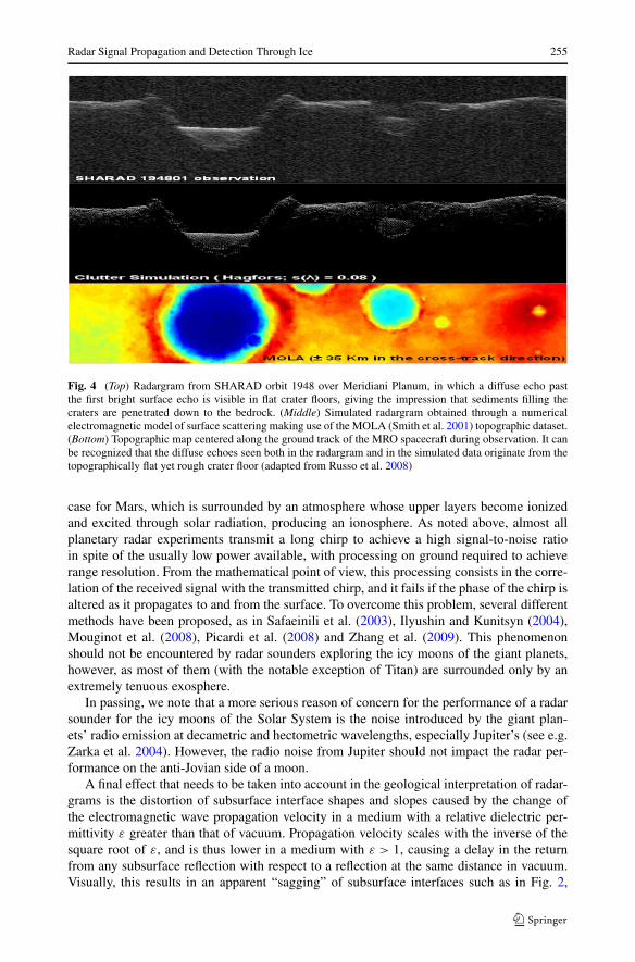
good directivity. Both MARSIS and SHARAD in fact transmit through dipoles, which havenegligible directivity, with the consequence that the radar pulse illuminates the entire surfacebeneath the spacecraft and not only the near-nadir portion from which subsurface echoes areexpected. The electromagnetic wave can then be scattered by any roughness of the surface.If the surface of the body being sounded is not smooth at the wavelength scale, i.e. if ther.m.s. of topographic heights is greater than a fraction of the wavelength, then part of theincident radiation will be scattered in directions different from the specular one. This meansthat areas of the surface that are not directly beneath the radar can scatter part of the in-cident radiation back towards it, and thus produce surface echoes that will reach the radarafter the echo coming from nadir, which can mask, or be mistaken for, subsurface echoes.This surface backscattering from off-nadir directions is called “clutter”. Clutter can pro-duce in a radargram the impression of subsurface structures where there are in fact none.An example is shown in Fig. 4, in which a radargram is compared with a simulated surfaceecho. What appears in the data to be volume scattering from sediments filling a crater isrevealed by simulations to be in fact surface scattering from a crater floor that is flat fromthe topographic point of view, but must possess a relatively high roughness at meter scale.For data shown in Fig. 4, the effect of roughness below the resolution of the Mars OrbitingLaser Altimeter (MOLA) dataset has been simulated through the use of an analytical for-mula for the scattering from a random rough surface, but other methods are possible, suchas interpolation.

Numerical electromagnetic models of surface scattering, such as those by Nouvel et al.(2004) or Russo et al. (2008), have been routinely used to validate the detection of subsurfaceinterfaces in radargrams. To be effective, however, such models require a knowledge of thetopography of the observed surface at scales that are comparable or, better still, much smallerthan the wavelength. For example, the MOLA Martian topographic dataset (Smith et al.2001) has a resolution at the equator of less than 500 m, which is adequate for the MARSISwavelength range (50–100 m) but requires approximations or interpolations at SHARADwavelengths (around 15 m).

The presence of a dispersive medium, such as a plasma, between the radar and its ob-servation target can cause a distortion (dispersion) of the transmitted waveform. Such is the


Fig. 4 (Top) Radargram from SHARAD orbit 1948 over Meridiani Planum, in which a diffuse echo pastthe first bright surface echo is visible in flat crater floors, giving the impression that sediments filling thecraters are penetrated down to the bedrock. (Middle) Simulated radargram obtained through a numericalelectromagnetic model of surface scattering making use of the MOLA (Smith et al. 2001) topographic dataset.(Bottom) Topographic map centered along the ground track of the MRO spacecraft during observation. It canbe recognized that the diffuse echoes seen both in the radargram and in the simulated data originate from thetopographically flat yet rough crater floor (adapted from Russo et al. 2008)

case for Mars, which is surrounded by an atmosphere whose upper layers become ionizedand excited through solar radiation, producing an ionosphere. As noted above, almost allplanetary radar experiments transmit a long chirp to achieve a high signal-to-noise ratioin spite of the usually low power available, with processing on ground required to achieverange resolution. From the mathematical point of view, this processing consists in the corre-lation of the received signal with the transmitted chirp, and it fails if the phase of the chirp isaltered as it propagates to and from the surface. To overcome this problem, several differentmethods have been proposed, as in Safaeinili et al. (2003), Ilyushin and Kunitsyn (2004),Mouginot et al. (2008), Picardi et al. (2008) and Zhang et al. (2009). This phenomenonshould not be encountered by radar sounders exploring the icy moons of the giant planets,however, as most of them (with the notable exception of Titan) are surrounded only by anextremely tenuous exosphere.

In passing, we note that a more serious reason of concern for the performance of a radarsounder for the icy moons of the Solar System is the noise introduced by the giant plan-ets’ radio emission at decametric and hectometric wavelengths, especially Jupiter’s (see e.g.Zarka et al. 2004). However, the radio noise from Jupiter should not impact the radar per-formance on the anti-Jovian side of a moon.

A final effect that needs to be taken into account in the geological interpretation of radar-grams is the distortion of subsurface interface shapes and slopes caused by the change ofthe electromagnetic wave propagation velocity in a medium with a relative dielectric per-mittivity ε greater than that of vacuum. Propagation velocity scales with the inverse of thesquare root of ε, and is thus lower in a medium with ε > 1, causing a delay in the returnfrom any subsurface reflection with respect to a reflection at the same distance in vacuum.Visually, this results in an apparent “sagging” of subsurface interfaces such as in Fig. 2,


in which the basal echo beneath the SPLD (pointed by an arrow) is in reality at the samelevel of the topography surrounding the SPLD, but appears to be sloping because of theincreasing thickness of the SPLD through which the radar signal propagates. When thevalue of ε can be derived through other means, it is possible to correct this distortion,such as in Fig. 3, where the dielectric constant of ice (ε ≈ 3) has been assumed for theNPLD.

4 Radar Signal Propagation and Detection Through Ice

4.1 Dielectric Properties of Ice

The permittivity ε of a material is a property describing how much more energy is storedthrough charge separation than in a vacuum. Charges of opposite signs move in oppositedirections in response to an external field so that the resultant internal field between thecharges opposes the external field. When the external field is removed, the energy stored inthis internal field decays as the charges revert back to their original positions. Frequency de-pendence of permittivity occurs because charge separation does not happen instantaneously.

Charges separate with finite velocities, thus if the external field is reversing polarity tooquickly the charges cannot move fast enough to keep up. The frequency at which the chargesfully separate and are in constant motion is called the relaxation frequency. At frequen-cies below the relaxation frequency the permittivity plateaus at the low frequency, or static,limit εs, and is often call dielectric constant. At high frequencies above the relaxation fre-quency the permittivity plateaus at the high frequency limit ε∞.

The response of the ice crystal is the conduction and the polarization. The polarizationwill develop in time with some delay which duration depends on temperature. The temper-ature dependency is described by the Arrhenius function of the form of exp(E/kT ) whereE is the activation energy (enthalpy) of the formation process, k the Boltzmann’s constantand T temperature.

The classical Debye model takes into account this dependency and the dielectric constantis described by the following equations:

ε = ε∞ + �ε�ε

1 + jωτ, ω = 2πf and �ε = εs − ε∞ (2)

where εs , ε∞ are respectively the static and high frequency values of the permittivity andτ is the dielectric relaxation time. The permittivity is a complex function of frequency andusually is described by its real and imaginary part.

εR = ε∞ + �ε

1 + ω2τ 2, εI = �εωτ

1 + ω2τ 2(3)

The loss tangent tan δ is defined by the ratio of these two parts and characterizes the attenu-ation of the electromagnetic waves in a medium due to ohmic conductivity σ .

tan δd = εI

εR

= σ

ωεR

(4)

The conductivity σ of the medium is directly proportional to the imaginary part of the di-electric constant.


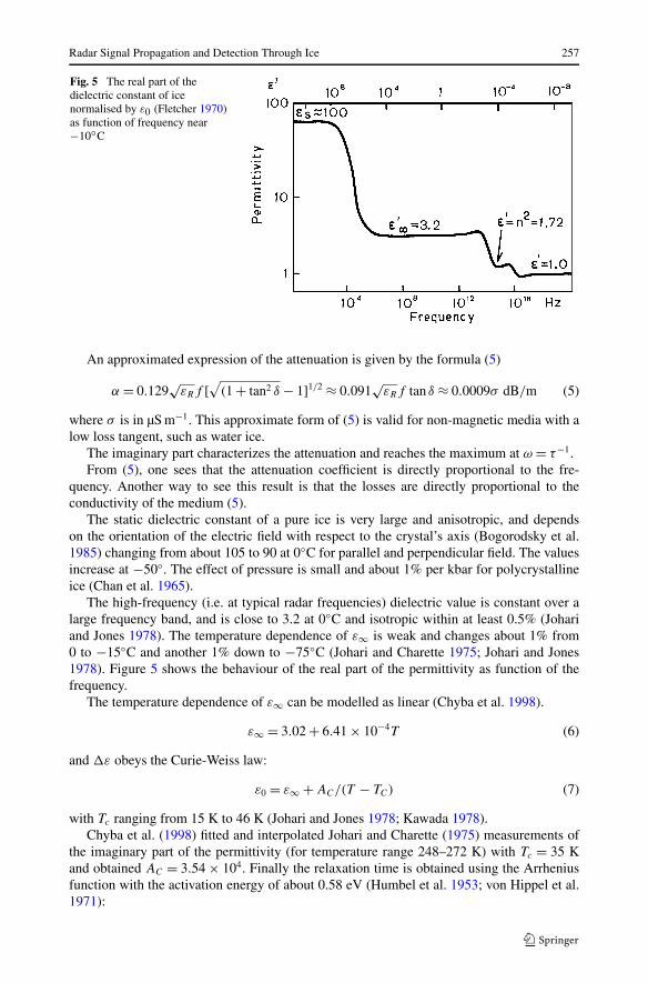
Fig. 5 The real part of thedielectric constant of icenormalised by ε0 (Fletcher 1970)as function of frequency near−10◦C

An approximated expression of the attenuation is given by the formula (5)

α = 0.129√

εRf [√

(1 + tan2 δ − 1]1/2 ≈ 0.091√

εRf tan δ ≈ 0.0009σ dB/m (5)

where σ is in µS m−1. This approximate form of (5) is valid for non-magnetic media with alow loss tangent, such as water ice.

The imaginary part characterizes the attenuation and reaches the maximum at ω = τ−1.From (5), one sees that the attenuation coefficient is directly proportional to the fre-

quency. Another way to see this result is that the losses are directly proportional to theconductivity of the medium (5).

The static dielectric constant of a pure ice is very large and anisotropic, and dependson the orientation of the electric field with respect to the crystal’s axis (Bogorodsky et al.1985) changing from about 105 to 90 at 0◦C for parallel and perpendicular field. The valuesincrease at −50◦. The effect of pressure is small and about 1% per kbar for polycrystallineice (Chan et al. 1965).

The high-frequency (i.e. at typical radar frequencies) dielectric value is constant over alarge frequency band, and is close to 3.2 at 0◦C and isotropic within at least 0.5% (Johariand Jones 1978). The temperature dependence of ε∞ is weak and changes about 1% from0 to −15◦C and another 1% down to −75◦C (Johari and Charette 1975; Johari and Jones1978). Figure 5 shows the behaviour of the real part of the permittivity as function of thefrequency.

The temperature dependence of ε∞ can be modelled as linear (Chyba et al. 1998).

ε∞ = 3.02 + 6.41 × 10−4T (6)

and �ε obeys the Curie-Weiss law:

ε0 = ε∞ + AC/(T − TC) (7)

with Tc ranging from 15 K to 46 K (Johari and Jones 1978; Kawada 1978).Chyba et al. (1998) fitted and interpolated Johari and Charette (1975) measurements of

the imaginary part of the permittivity (for temperature range 248–272 K) with Tc = 35 Kand obtained AC = 3.54 × 104. Finally the relaxation time is obtained using the Arrheniusfunction with the activation energy of about 0.58 eV (Humbel et al. 1953; von Hippel et al.1971):


τ = C exp

(E

kT

)(8)

where C = 5.3 × 10−16 and k = 8.61 × 10−5 eV K−1. The pressure effect is to increase therelaxation time of about 10% between 0 and 500 bars, independent on temperature (Ruepp1973).

Other data were used by Thompson and Squyres (1990) to obtain slightly different for-mulas that were compared in the paper by Chyba et al. (1998). The results are similar and re-main close. For the experiment definition and the estimation of radar capabilities it’s enoughto use the above formulas. The attenuation of the electromagnetic waves in the ice can becalculated for lower temperatures using the previous equations. However, for very low fre-quencies below a few kHz the previous formula can greatly underestimate the attenuation(Chyba et al. 1998). But for a future subsurface sounding radars working at frequencieshigher than a few MHz the formulas are probably correct.

In general the values of dielectric parameters for pure polycrystalline ice are close tothose for single-crystal ice (Bogorodsky et al. 1985).

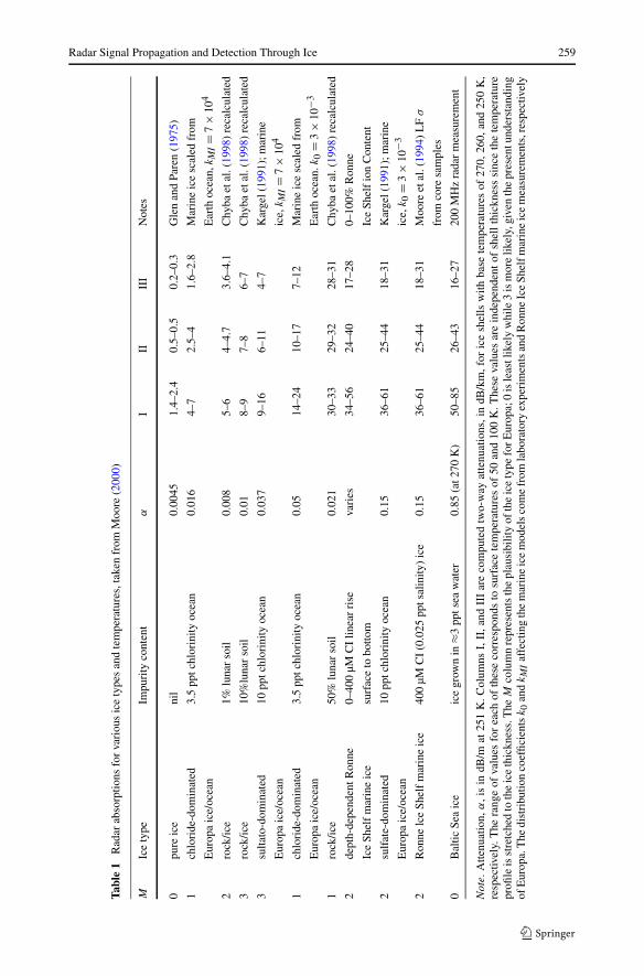
Because of the low losses expected in pure water ice, the major effect on the absorption ofradar waves will in fact depend on the nature and concentration of impurities in the ice. Thisis of course difficult to evaluate due to uncertainties and lack of knowledge of the physicalnature of impurities for icy satellites. For Europan ice this problem was studied by Chybaet al. (1998) and Moore (2000). The latter considered three types of water ice, produced bythree basic processes occurring on Earth: meteoric ice formed by atmospheric precipitations,sea ice formed by the freezing of water close to the atmospheric interface, and marine iceforming beneath ice shelves directly from ocean water. Moore (2000) concluded that similarprocesses are likely to occur on Europa as well, and that the most probable form of ice wouldbe marine ice.

Chyba et al. (1998) studied the electromagnetic properties of a medium resulting from themixing of different impurities (rock, dust) into an ice matrix. They used a mixing formula(Sihvola and Kong 1988, 1989) to calculate the dielectric constant of the mixture and theproperties of lunar materials as a model for the impurities within the Europan ice. This ap-proach requires many assumptions and gives only some estimation of the dielectric constantthat can be used in the evaluation of the radar capabilities.

In addition to the Chyba et al. (1998) approach, Moore (2000) was interested in solubleimpurities in ice like F−, Cl−, NH+

4 , SO2−4 and H+ ions. In Table 1 (Moore 2000) the atten-

uation for different types of impurities in ice is shown, based on laboratory measurements,ice temperature modelling for Europa and some scaling from Earth ice measurements. Thesedata are valid for electromagnetic frequencies of a few tens of MHz.

These calculations are not taking into account a possible scattering of the electromagneticwaves by the ice/pore interfaces that can exist in the crust. The scattering effect plays thesame role as attenuation and depends strongly on the dimension of cavities, (voids) in themedium compared to the wavelength. The Mie or Rayleigh approaches (see e.g. Ishimaru1978) can be used to calculate the extinction of the radar signal.

The scattering of radio waves by surface and by volume irregularities is an importantfactor which one has to take into account to evaluate the penetration of the radar wave, andthe ratio of any subsurface echo to surface clutter. These two parameters are essential topredict the radar performance. The scattering depends strongly, as we wrote above, on theradar wavelength and surface parameters of the body under investigation. This frequencydependence of attenuation requires that subsurface sounding radars operate at low-frequency(<100 MHz) in order to achieve a deep penetration. The choice of the frequency has aninfluence on the instrument characteristics, and especially on the size of the antenna. The


Tabl

e1

Rad

arab

sorp

tions

for

vari

ous

ice

type

san

dte

mpe

ratu

res,

take

nfr

omM

oore

(200

0)

MIc

ety

peIm

puri

tyco

nten

tα

III

III

Not

es

0pu

reic

eni

l0.

0045

1.4–

2.4

0.5–

0.5

0.2–

0.3

Gle

nan

dPa

ren

(197

5)

1ch

lori

de-d

omin

ated

3.5

pptc

hlor

inity

ocea

n0.

016

4–7

2.5–

41.

6–2.

8M

arin

eic

esc

aled

from

Eur

opa

ice/

ocea

nE

arth

ocea

n,k

MI=

7×

104

2ro

ck/ic

e1%

luna

rso

il0.

008

5–6

4–4.

73.

6–4.

1C

hyba

etal

.(19

98)

reca

lcul

ated

3ro

ck/ic

e10

%lu

nar

soil

0.01

8–9

7–8

6–7

Chy

baet

al.(

1998

)re

calc

ulat

ed

3su

ltato

-dom

inat

ed10

pptc

hlor

inity

ocea

n0.

037

9–16

6–11

4–7

Kar

gel(

1991

);m

arin

e

Eur

opa

ice/

ocea

nic

e,k

MI=

7×

104

1ch

lori

de-d

omin

ated

3.5

pptc

hlor

inity

ocea

n0.

0514

–24

10–1

77–

12M

arin

eic

esc

aled

from

Eur

opa

ice/

ocea

nE

arth

ocea

n.k

0=

3×

10−3

1ro

ck/ic

e50

%lu

nar

soil

0.02

130

–33

29–3

228

–31

Chy

baet

al.(

1998

)re

calc

ulat

ed

2de

pth-

depe

nden

tRon

ne0–

400

µMC

Ilin

ear

rise

vari

es34

–56

24–4

017

–28

0–10

0%R

onne

Ice

Shel

fm

arin

eic

esu

rfac

eto

botto

mIc

eSh

elf

ion

Con

tent

2su

lfat

e-do

min

ated

10pp

tchl

orin

ityoc

ean

0.15

36–6

125

–44

18–3

1K

arge

l(19

91);

mar

ine

Eur

opa

ice/

ocea

nic

e,k

0=

3×

10−3

2R

onne

lce

Shel

fm

arin

eic

e40

0µM

CI

(0.0

25pp

tsal

inity

)ic

e0.

1536

–61

25–4

418

–31

Moo

reet

al.(

1994

)L

Fσ

from

core

sam

ples

0B

altic

Sea

ice

ice

grow

nin

≈3pp

tsea

wat

er0.

85(a

t270

K)

50–8

526

–43

16–2

720

0M

Hz

rada

rm

easu

rem

ent

Not

e.A

ttenu

atio

n,α

,is

indB

/mat

251

K.C

olum

nsI,

II,a

ndII

Iar

eco

mpu

ted

two-

way

atte

nuat

ions

,in

dB/k

m,f

oric

esh

ells

with

base

tem

pera

ture

sof

270,

260,

and

250

K,

resp

ectiv

ely.

The

rang

eof

valu

esfo

rea

chof

thes

eco

rres

pond

sto

surf

ace

tem

pera

ture

sof

50an

d10

0K

.The

seva

lues

are

inde

pend

ento

fsh

ellt

hick

ness

sinc

eth

ete

mpe

ratu

repr

ofile

isst

retc

hed

toth

eic

eth

ickn

ess.

The

Mco

lum

nre

pres

ents

the

plau

sibi

lity

ofth

eic

ety

pefo

rEur

opa;

0is

leas

tlik

ely

whi

le3

ism

ore

likel

y,gi

ven

the

pres

entu

nder

stan

ding

ofE

urop

a.T

hedi

stri

butio

nco

effic

ient

sk

0an

dk

MI

affe

ctin

gth

em

arin

eic

em

odel

sco

me

from

labo

rato

ryex

peri

men

tsan

dR

onne

Ice

Shel

fmar

ine

ice

mea

sure

men

ts,r

espe

ctiv

ely


exact choice of the frequency results from a trade-off between science requirements andtechnical limitations.

Due to the lack of knowledge of physical parameters controlling scattering, it israther difficult to predict its effects with accuracy. For example, Eluszkiewicz (2004) con-cluded that the presence of a regolith about 1 km thick with an 1% of cavities whosesize is comparable to the radar wavelength will make radar wave penetration impossi-ble.

In spite of all these uncertainties, experience has demonstrated that data such as thosepresented in Table 1 provide the capability to evaluate the radar performance with sufficientaccuracy. At the time in which the MARSIS (Picardi et al. 2004) and SHARAD (Seu et al.2007a) radar sounding experiments were proposed, radar sounding of planetary bodies wasdeemed problematic if not impossible, in spite of data obtained by the ALSE experimenton board the Apollo 17 spacecraft (Phillips et al. 1973), but results at Mars (e.g. Picardiet al. 2005; Plaut et al. 2007; Seu et al. 2007b; Mouginot et al. 2009) have conclusivelydemonstrated that this technique is effective in the investigation of planetary bodies fromorbit.

4.2 Radar Performance

The data from Table 1 can be used to evaluate penetration depth in the subsurface of icybodies. As we want to use the radar to study interiors using the reflection from discontinu-ities and/or diffraction of signals, the reflection and transmission coefficients are also factorsdetermining how much of the incoming signal amplitude is reflected and transmitted. Thesequantities allow the estimation of the power of the incoming radar signal and therefore theradar capabilities. The following equations summarize the factors affecting radar perfor-mance:

PRx = PTx(1 − |rice|2)τpBGTxGRxλ2r2

layer10−αzLsys

(4π)2(2(R + z))2(9)

SNR = PRx

Pnoise= PTx(1 − |rice|2)τpGTxGRxλ

2r2layer10−αzLsys

(4π)2(2(R + z))2kTref Nf

(10)

where

PTx = peak RF power during transmission of the pulseGTx = antenna gain on transmissionGRx = antenna gain on receptionλ = operating wavelengthrice = effective reflectivity of the ice-atmosphere interfacerlayer = effective reflectivity of an internal layerα = 2-way attenuation through ice of thickness z

Lsys = system losses including internal transmission losses and losses within the antennaduring transmission

R = range from satellite to ice surfacez = depth from the surface to the internal layerPnoise = kTref BNf wherek = Boltzmann constantTref = antenna reference temperatureB = bandwidth of transmitted pulse


Nf = system noise figureτp = pulse duration

Modern radars transmit a modulated signal that provides a compression gain so that theeffective echo power received within the pulse bandwidth is increased by a factor τpB .

This equation is given here only to highlight different factors playing a role in radardetection capabilities. The noise level is one of the factors limiting performance. For lowfrequency radars (1–50 MHz) the galactic noise temperature varies between 107 to 104 K.In the Jovian environment its radio noise increases the noise temperature of about 1010 to106 K but on the anti-Jovian side of a moon the influence is negligible.

The altitude of the spacecraft also plays an important role. For a radar placed on an orbitat 100 km of altitude, at the frequency of 20 MHz (the SHARAD radar frequency), with thenoise temperatures of the order of 5 × 104 K, the antenna gain of 10 dB, the peak power of100 W and a modulated pulse of 200 µs, the signal to noise ratio is:

SNR ≈ 130 − αZ + 20 log rlayer + 10 log(1 − |rice|2) + Lsys (11)

The transmission loss between the air/ice interface is about 1 dB, and the reflection loss atthe interface within the ice is estimated to be between −10 to −20 dB. Lsys is assumed tobe −3 dB.

Finally, as one needs about 20 dB SNR in order to adequately process the signal, theacceptable losses inside the ice are found to be of about 85 dB. Coherent processing canreduce the noise power and then increase the SNR. Typical gains for coherent processing areof the order of 10–20 dB. In this analysis surface clutter effects are not taken into account,but they can easily reduce the signal detection capability by a comparable amount, althoughthey can in turn be reduced through Doppler filtering. This is why the acceptable value forattenuation can still be maintained at 85 dB.

From Table 1 it can be seen that radar penetration inside pure ice can exceed 40 km. Themost probable losses, however, are between 6 and 16 dB/km, which will clearly limit thepenetration to 5 to 15 km.

5 Laboratory Studies Relevant to Interpretation of Radar Observations

As mentioned above, in order to estimate the maximum penetration depth of a subsurfaceradar signal in the icy moons crust of the Solar System, the electromagnetic properties ofthe materials forming the solid and/or liquid layering sequence should be known. Severallaboratory techniques can be used to measure the complex permittivity of ice or icy soilsimulants: some of them operate in the frequency domain (FD) regime, others in the timedomain (TD) regime. The FD techniques (dielectric spectroscopy) allows one to perform astraightforward measurement of both real and imaginary part of the permittivity, in a limitedrange of frequency (in fact, it is not possible to use just one instrument to measure thepermittivity from zero-frequency up to the microwave region). Conversely, to extract thesame parameters as a function of frequency, the TD techniques need a transformation fromtime to frequency domain and a dielectric model to fit the experimental data. However, if nodispersion is observed, time domain analysis can be a very fast and reproducible techniqueto estimate the dielectric permittivity and the DC conductivity of a material.


Fig. 6 (a) Equivalent circuit;(b) Schematic of a capacitancecell to measure electricalproperties of granular or liquidmaterials

5.1 Frequency Domain Measurements

Usually, the laboratory techniques for measuring the electromagnetic properties of granu-lar or liquid materials at hertz-to-megahertz frequencies are based on the equivalent circuitanalysis performed through L-C-R meters (Pettinelli et al. 2003). Conductivity and permit-tivity are obtained by measuring the magnitude and phase of the electrical impedance of acapacitive cell (i.e. Parallel Plate Capacitor—PPC) filled with the material being tested.

With reference to the lumped equivalent circuit shown in Fig. 6a, the current in the cell,can be expressed through its complex admittance Y ∗:

I = Vg · Y ∗ = Vg ·(

1

Rp

+ jωCp

)(12)

Using the geometrical features of the cell the measured values of capacitance Cp and parallelresistance Rp can be related to the real and imaginary parts of the complex permittivity ofthe material enclosed between the electrodes.

In particular, if A is the surface of the guarded electrode (the plate connected to the “low”terminal in Fig. 6) and d is the spacing between the two parallel plates, one obtains:

ε′ = d

A· Cp

ε0= Cp

C0; ε′′ = d

A· 1

ωε0Rp

= 1

ωC0Rp

(13)

Note that, a precise knowledge of the cell geometry is not strictly required to get accuratemeasurements, as both the real and imaginary terms of permittivity can be calculated usingthe previously measured value of the capacitance with the cell empty (i.e. C0). The effectof the fringing field at the edges of the capacitor plates is cancelled by using a guardedelectrode (see Fig. 6).

Several types of capacitive cell can be used to estimate the dielectric parameters of a ma-terial; the choice depends on the material itself (soil, ice or mixtures) and the pressure andtemperature that should be applied to the sample. As an example, Fig. 7a and b show a paral-lel plate cell and a coaxial cell suitable for granular or icy samples measured at atmosphericpressure.

The maximum frequency achievable with the capacitor cell technique is of the orderof few tens of MHz, therefore suitable to support the investigations of orbiting subsurfaceradars like MARSIS or SHARAD. However, if a higher frequency range should be investi-gated (from hundreds of MHz to few GHz), the most common technique used to extract thereal and imaginary part of the permittivity is the measurement of the scattering parameters


Fig. 7 (a) Parallel plate capacitor cell; (b) Coaxial capacitor cell

of a coaxial line, connected to a network analyzer (see for example the review of Stuchlyand Stuchly 1980).

5.2 Time Domain Measurements

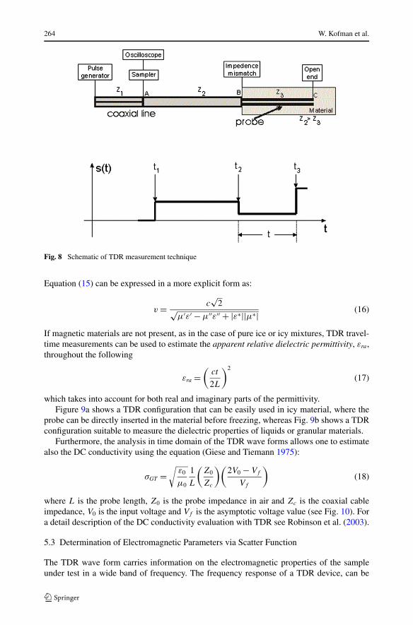
The use of Time Domain Reflectometry (TDR) technique for permittivity measurements isbased on evaluating the velocity of a step-like signal which travels along a transmission linefilled with the material under test or embedded in it (for details see Topp and Ferré 2002,and Robinson et al. 2003). The TDR signal has a broad band and the upper frequency, in asample, can extend up to about 500 MHz.

A basic TDR system consists of a pulse generator, a sampler, an oscilloscope, a coaxialcable, and a transmission line probe (see Fig. 7). The pulse generator applies a fast rise-timevoltage step (∼200 ps) to a 50-ohm coaxial cable and triggers a sampler. The step pulsetravels down the coaxial cable, until it reaches the probe, where part of the signal is reflectedback toward the cable tester due to an impedance mismatch, and part passes along the linein the material itself. The signal traveling in the material ultimately reaches the end of theprobe, sending a reflection back toward the oscilloscope.

The waveform displayed on the oscilloscope represents the superposition of incomingand reflected waves (in phase or in counter phase), generated at every impedance mismatchin the system. From the propagation time of the wave front along the probe, the pulse veloc-ity can be calculated according to the following equation:

v = 2L

t(14)

where t is the two-way travel time (from t2 to t3 in Fig. 8) and L is the probe length.Assuming that the material is homogeneous within the sample, the electromagnetic wavevelocity is given by:

v = c

Re√

ε∗μ∗ (15)

where c is the electromagnetic wave velocity in the vacuum (3 × 108 m/s), and ε∗ andμ∗ are the material complex permittivity and complex magnetic permeability, respectively.


Fig. 8 Schematic of TDR measurement technique

Equation (15) can be expressed in a more explicit form as:

v = c√

2√μ′ε′ − μ′′ε′′ + |ε∗||μ∗| (16)

If magnetic materials are not present, as in the case of pure ice or icy mixtures, TDR travel-time measurements can be used to estimate the apparent relative dielectric permittivity, εra,throughout the following

εra =(

ct

2L

)2

(17)

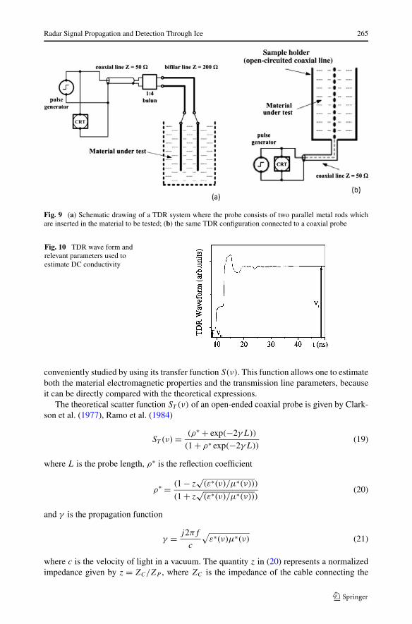
which takes into account for both real and imaginary parts of the permittivity.Figure 9a shows a TDR configuration that can be easily used in icy material, where the

probe can be directly inserted in the material before freezing, whereas Fig. 9b shows a TDRconfiguration suitable to measure the dielectric properties of liquids or granular materials.

Furthermore, the analysis in time domain of the TDR wave forms allows one to estimatealso the DC conductivity using the equation (Giese and Tiemann 1975):

σGT =√

ε0

μ0

1

L

(Z0

Zc

)(2V0 − Vf

Vf

)(18)

where L is the probe length, Z0 is the probe impedance in air and Zc is the coaxial cableimpedance, V0 is the input voltage and Vf is the asymptotic voltage value (see Fig. 10). Fora detail description of the DC conductivity evaluation with TDR see Robinson et al. (2003).

5.3 Determination of Electromagnetic Parameters via Scatter Function

The TDR wave form carries information on the electromagnetic properties of the sampleunder test in a wide band of frequency. The frequency response of a TDR device, can be


Fig. 9 (a) Schematic drawing of a TDR system where the probe consists of two parallel metal rods whichare inserted in the material to be tested; (b) the same TDR configuration connected to a coaxial probe

Fig. 10 TDR wave form andrelevant parameters used toestimate DC conductivity

conveniently studied by using its transfer function S(ν). This function allows one to estimateboth the material electromagnetic properties and the transmission line parameters, becauseit can be directly compared with the theoretical expressions.

The theoretical scatter function ST (ν) of an open-ended coaxial probe is given by Clark-son et al. (1977), Ramo et al. (1984)

ST (ν) = (ρ∗ + exp(−2γL))

(1 + ρ∗ exp(−2γL))(19)

where L is the probe length, ρ∗ is the reflection coefficient

ρ∗ = (1 − z√

(ε∗(ν)/μ∗(ν)))

(1 + z√

(ε∗(ν)/μ∗(ν)))(20)

and γ is the propagation function

γ = j2πf

c

√ε∗(ν)μ∗(ν) (21)

where c is the velocity of light in a vacuum. The quantity z in (20) represents a normalizedimpedance given by z = ZC/ZP , where ZC is the impedance of the cable connecting the


TDR probe to the signal generator and ZP is the impedance of the TDR probe in air. ε∗ =ε′ − jε′′, μ∗ = μ′ − jμ′′ are the e.m. parameters of the test material.

To estimate the probe parameters (Feng et al. 1999; Mattei et al. 2006), calibration mea-surements in some reference materials (such as water, air, ethanol, etc.) should always beperformed. The fitting of the theoretical scatter function ST (ν) to the experimental scatterfunction, allows the evaluation of z and L, since the e.m. properties of the reference materi-als are known from literature.

Once the probe parameters are known, TDR measurements can be performed in the probefilled with the material under test. The fitting of ST (ν) to the experimental scatter functionprovides the e.m. constitutive parameters. In fact, for non magnetic materials, if the polariza-tion process can be modelled with Debye-like relaxation, the relative complex permittivityis given by

ε∗(ν) = ε∞ + (εS − ε∞)

1 + iν/νrel+ i

σdc

2πνε0(22)

where εS is the static value of permittivity, ε∞ its high frequency limit, νrel is the relaxationfrequency, σdc is the static conductivity, and ε0 is the permittivity in a vacuum. ST (ν) can beobtained applying (19) and (20), whereas the minimization procedure allows the evaluationsof the model parameters and, consequently, the frequency dependence of test material e.m.properties.

6 Laboratory Results on Icy Soil Samples

As examples of the information that can be retrieved from dielectric measurements withFD or TD techniques, we present here some data acquired on CO2 ice and some icy mix-tures. The measurements were performed in the frequency domain (100 Hz–1 MHz) usinga capacitive cell (PPC) and in the time domain using a two-prong transmission line. Thesetwo techniques are particularly suitable to perform dielectric measurements on icy samplesbecause they offer several advantages: (i) data acquisition is simple and fast; (ii) sample vol-ume is large (i.e. the bulk properties of a material are measured); and (iii) the experimentaltechniques are reproducible and the results are consistent.

Figure 11a and b show real and imaginary parts of permittivity measured in the samefrequency range on two samples prepared with CO2 ice (ice powder) and CO2 ice mixedwith volcanic sand. For comparison, in the figures the plots for the same dry sand are shownas well. Table 2 summarises volume fractions and density of the materials under test. Thedata confirm the non-polar behaviour of CO2 ice, as the real part of the permittivity is verylow (about 1.4). The ε′ ∼= 2 measured for the mixture CO2 ice and sand is in general agree-ment with what is reasonably expected. Indeed the dielectric constant of the mixture shouldexhibit a sort of average between the ε′ ∼= 1.4 of CO2 ice and that of the anhydrous sand(ε′ ∼= 3).

The plot of the imaginary parts of permittivity shows the general tendency of low tem-perature mixtures to behave like good insulators because the mobility of ions significantlyslowed down by the freezing process.

More extended measurements have been conducted on CO2 ice and icy mixtures withTDR techniques. Table 3 summarises the information on volume fractions and density ofthe samples and the apparent permittivity values (with the uncertainties) measured with theTD method (for detail see Pettinelli et al. 2003). Note that there are little differences in theapparent permittivity values of the samples presented in the table, with different materialshaving approximately the same permittivity.


Fig. 11 Real (a) and imaginary (b) part of permittivity of CO2 ice and volcanic sand. Comparison with thevalues measured for anhydrous volcanic sand at room temperature

Table 2 Volume fractions and density of the samples shown in Figs. 11

Material Volume fractions (%) Density (g cm−3)

CO2 powder (−75°C) VCO2 = 70.3% 1.05

Vair = 29.7%

dry Vulcano sand (24.4°C) Vsand = 55.9% 2.58 (grain density)

Vair = 44.1%

CO2 powder + sand Vsand = 31.7% –

VCO2 = 35.7%

Vair = 32.6%

7 Laboratory Measurements Needed to Support Interpretation of RadarObservations

At the present stage an accurate survey of the literature available, shows a lack of data ondielectric properties of icy materials, gas hydrates (clathrates), and salt doped ice in thefrequency range of interest (i.e. tens of MHz or higher) to define the performance proper-ties (the maximum penetration depth) of future subsurface radars capable of investigatingthe interior structure of the icy moons of the Solar System. The vast majority of dielectricmeasurements, in fact, have been collected at low frequency (below 1 MHz) (Thompsonand Squyres 1990; Lorenz 1998; Chyba et al. 1998; Moore 2000; Pettinelli et al. 2003;Grimm et al. 2008). These data show, in general, that the impurities in the ice have the effectof shifting the relaxation time at higher frequencies, however, never exceeding few tens ofkHz. In the MHz range, the ice or the icy mixtures seem to have low values of the real part ofthe permittivity and small values of the conductivity, behaving like non-polar low-loss mate-rials. Therefore, we should expect a transparent behavior of the icy materials in a broadbandof frequencies well above the relaxation frequency.

Nevertheless, the definition of the best radar frequency to use to investigate the inter-nal structure of an icy moon crust should be strongly supported by adequate and extensive


Table 3 Volume fractions, density and apparent permittivity experimental values, measured by TDR tech-nique for various samples of solid CO2, volcanic sand, and mixtures (Pettinelli et al. 2003)

Material Volume fraction Density (g cm−3) εra ± �εra

CO2 ice – 1.50 2.12 ±0.04

CO2 snow – – 1.48 ±0.04

CO2 powder (1) – 0.99 1.67 ±0.06

CO2 powder (2) – 1.01 1.63 ±0.06

CO2 powder (3) – 1.02 1.67 ±0.06

dry Vulcano sand Vsand = 57.5% 2.58 (grain density) 3.83 ±0.09

Vair = 42.5%

CO2 snow + glass beads (1) Vglass1 = 37.47% – 2.32 ±0.03

VCO2 = 62.53%

CO2 snow + glass beads (2) Vglass2 = 20.75% – 1.56 ±0.03

VCO2 = 79.25%

CO2 powder + sand (1) Vsand1 = 38.2% – 2.6 ±0.2

VCO2 = 23.8%

Vair = 38.0%

CO2 powder + sand (2) Vsand2 = 25.5% – 2.28 ±0.07

VCO2 = 38.6%

Vair = 35.9%

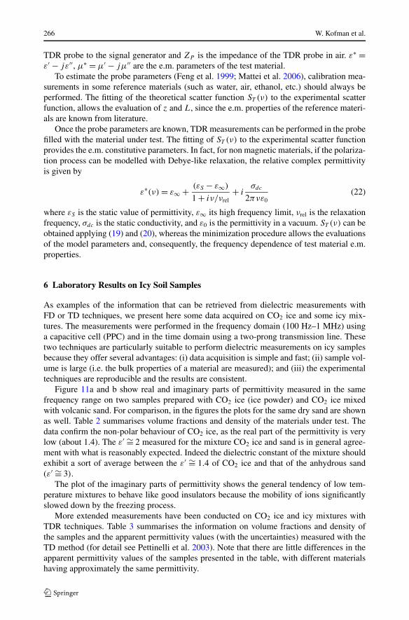
laboratory investigations on a sufficient number of composite ice samples. In particular, be-cause the temperature, the impurities, and the density of the icy materials are the parametersthat affect the most the dielectric behavior of the simulants, these measurements shouldbe performed systematically changing these two parameters. These types of measurements,however, require a certain level of accuracy: in fact, as shown in Table 3, the permittivityvalues obtained in the MHz range for different icy soil, might be very close to each other,and in order to distinguish between different materials a small uncertainty should be asso-ciated to the measurement. This ambiguity in the dielectric properties also affects stronglythe possibility to perform some data inversion and extract some information on the dielec-tric properties of the deeper layers, like an ocean under an icy crust. Moreover, laboratorymeasurements can be used to validate a dielectric model. As an example, Table 4 compares,the apparent permittivity values obtained using TDR technique with those calculated usingdifferent dielectric models (for detail see Pettinelli et al. 2003).

Among the models presented in Table 4 to predict the average dielectric properties ofa mixture, the Tinga model is the most flexible and therefore it was applied to simulatethe dielectric behavior of almost all measured mixtures. The results for mixtures of glassbeads and air or water are in excellent agreement with experimental data, due to the factthat this model is particularly well suited to describe the dielectric properties of a mixtureconsisting of a uniform known host material with homogeneous, equally-sized sphericalinclusions. Note that, also Rayleigh mixing formula is suitable to estimate the real part ofthe permittivity of a material on the basis of its density, if the permittivity value of the solidphase is known. However, many other dielectric mixing formulas are present in the literature(see Sihvola 2000), and in order to assess the prediction capability of such models for theicy mixtures, an extensive study combining laboratory-measured and theoretical permittivityvalues should be performed


Table 4 Comparison between TDR experimental apparent permittivity values and calculated values frommodels

Material εra ± �εra Model

Rayleigh 1892 Tinga et al. 1973 Topp et al. 1980

dry glass beads 3.19 ± 0.08 – 3.0 3.3

saturated glass beads (r.t.) 30.0 ± 0.2 – 30.6 29.6

drained glass beads (r.t.) 4.09 ± 0.08 – – 5.3

CO2 powder (1) 1.67 ± 0.06 1.6 1.6 –

CO2 powder (2) 1.63 ± 0.06 1.7 1.7 –

CO2 powder (3) 1.67 ± 0.06 1.7 1.7 –

dry Vulcano sand 3.83 ± 0.09 – 3.9 3.0

CO2 snow + glass beads (1) 2.32 ± 0.03 – 2.7 –

CO2 snow + glass beads (2) 1.56 ± 0.03 – 1.5 –

CO2 powder + sand (1) 2.6 ± 0.2 – 3.6 –

CO2 powder + sand (2) 2.28 ± 0.07 – 2.8 –

Vulcano sand: εgrain ∼= 17 (calculated with Rayleigh mixing formula)

Glass beads: εgrain = 7.2

Finally, laboratory measurements are fundamental to help calculate the total attenua-tion coefficient (ohmic + volumetric scattering) for an electromagnetic wave propagatingthrough an inhomogeneous medium. Tables 5a and b show the total attenuation and themaximum penetration depth of a 225 MHz radar signal in different icy media with basalticinclusions (for detail see Pettinelli et al. 2007). Again in this case, both dielectric and mag-netic properties of the materials forming the mixtures and the inclusions have been measuredusing the above described FD techniques.

8 Summary and Recommendations

In this chapter, we discussed the application of subsurface radar sounding from orbit to thestudy of icy moons. We first summarized known radar properties of icy moon surfaces, anddiscussed existing subsurface radar observations of other planetary bodies. We then pre-sented the main physical parameters of a planetary crust affecting the performance of aradar sounder, concluding that in icy moons a radar sounder should be able to detect dielec-tric discontinuities at depths of several kilometers to a few tens of kilometers, depending onthe nature of the materials through which the electromagnetic pulse propagates. We finallyreviewed methods and results for the measurements of dielectric properties of natural mate-rials affecting radar performance, providing suggestions for laboratory activities in supportof future subsurface radar observations of icy moons.

Subsurface radar sounding is the only existing remote sensing technique for the study ofplanetary subsurfaces. Radar sounders have been successfully flown to the Moon and arecurrently operating at Mars, while another instrument of this kind is on its way to a cometnucleus. Radar experiments are being considered for future missions to near-Earth asteroids,to Vesta and to the icy moons of giant planets. In spite of this, the body of knowledgeassociated with this technique is still relatively small compared to other remote sensingmethods such as spectroscopy, and notions on the correct use and interpretation of data arenot yet widespread in the planetary community.


Table 5 Maximum penetration depth at which an interface can be detected below an icy soil with 10%volume fraction of basaltic inclusions (a) and 20% volume fraction of basaltic inclusions (b)

a (10% volume fraction)

Scenarios 225 MHz

Radius of the αtot (dB/m) L (m)

inclusions (mm)

CO2/Basalt 200 0.13 43

CO2&DrySoil/Basalt 200 0.11 40

IcySoil/Basalt 200 0.082 22

b (20% volume fraction)

Scenarios 225 MHz

Radius of the αtot (dB/m) L (m)

inclusions (mm)

CO2/Basalt 200 0.49 21

CO2&DrySoil/Basalt 200 0.42 21

IcySoil/Basalt 200 0.084 27

We are convinced that radar sounding has the potential to provide an enormous increasein our knowledge of the geology of planetary bodies, because of its unique capability to ex-plore the third dimension and its yet limited application to planetary exploration. Because ofthe transparency of ice-rich materials to low-frequency electromagnetic waves, we stronglyadvocate the use of this technique in the study of icy bodies in the Solar System. We alsodeem that more work is required to fully utilize radar sounding data for the quantitativedetermination of subsurface properties, an inverse problem of no small complexity. Labora-tory measurements of the dielectric parameters of natural materials occurring on planetarybodies are a key activity towards this end.

References

J.E. Baron, G.L. Tyler, R.A. Simpson, Icarus 164, 404–417 (2003)G.J. Black, D.B. Campbell, L.M. Carter, Icarus 191, 702–711 (2007)D.D. Blankenship, D.A. Young, W.B. Moore, J.C. Moore, in EUROPA, ed. by R.T. Pappalardo, W.B. McK-

innon, K. Khurana (The University of Arizona Press, Tucson, 2010), pp. 631–653V. Bogorodsky, C. Bentley, P. Gudmandsen, Radioglaciology (Reidel, Dordrecht, 1985). ISBN 90-277-1893-

8R.K. Chan, D.W. Davidson, E. Whalley, J. Chem. Phys. 43, 2376–2383 (1965)C.F. Chyba, S.J. Ostro, B.C. Edwards, Icarus 134, 292–302 (1998)T.S. Clarkson, L. Glasser, R.W. Tuxworth, G. Williams, Adv. Mol. Relax. Proc. 10, 173–202 (1977)V.R. Eshleman, Science 234, 587–590 (1986)J. Eluszkiewicz, Icarus 170, 234–236 (2004)N.H. Fletcher, The Chemical Physics of Ice (Cambridge University Press, New York, 1970)W. Feng, C.P. Lin, R.J. Dechamps, V.P. Drnevich, Water Resour. Res. 35, 2321–2331 (1999)K. Giese, R. Tiemann, Adv. Mol. Relax. Proc. 7, 45–59 (1975)J.W. Glen, J.G. Paren, J. Glaciol. 15, 15–37 (1975)R.E. Grimm, D.E. Stillman, S.F. Dec, M.A. Bullock, J. Phys. Chem. B 112, 15382–15390 (2008)T. Hagfors, I. Dahlstrom, T. Gold, S.-E. Hamran, R. Hansen, Icarus 130, 313–322 (1997)B. Hapke, Icarus 88, 407–417 (1990)F. Humbel, F. Jona, P. Scherrer, Helv. Phys. Acta 26, 17–32 (1953)


Y.A. Ilyushin, V.E. Kunitsyn, J. Commun. Technol. Electron. 49, 154–165 (2004)A. Ishimaru, Wave Propagation and Scattering in Random Media (Academic Press, New York, 1978)G.P. Johari, P. Charette, J. Glaciol. 14, 293–303 (1975)G.P. Johari, S.J. Jones, J. Glaciol. 21, 259–276 (1978)J.S. Kargel, Icarus 94, 368–390 (1991)S. Kawada, J. Phys. Soc. Jpn. 44, 1881–1886 (1978)W. Kofman et al., Adv. Space. Res. 21(11), 1589–1598 (1998)W. Kofman, A. Herique, J.-P. Goutail, T. Hagfors, I.P. Williams, E. Nielsen, J.-P. Barriot, Y. Barbin, C. Elachi,

P. Edenhofer, A.-C. Levasseur-Regourd, D. Plettemeier, G. Picardi, R. Seu, V. Svedhem, Space Sci. Rev.128(1–4), 413–432 (2007)

J.-P. Lebreton et al., in Lunar and Planetary Institute Science Conference Abstracts, vol. 40 (2009), p. 2383R.D. Lorenz, Icarus 136(2), 344–348 (1998)E. Mattei, A. Di Matteo, A. De Santis, G. Vannaroni, E. Pettinelli, Water Resour. Res. 42 (2006). doi:

10.1029/2005WR004728J.C. Moore, Icarus 147, 292–300 (2000)J.C. Moore, A.P. Reid, J. Kipfstuhl, J. Geophys. Res., Oceans 99(C3), 5171–5180 (1994)J. Mouginot, W. Kofman, A. Safaeinili, C. Grima, A. Herique, J.J. Plaut, Icarus 201(2), 454–459 (2009)J. Mouginot, W. Kofman, A. Safaeinili, A. Herique, Planet. Space Sci. 56, 917–926 (2008)J.-F. Nouvel, A. Herique, W. Kofman, A. Safaeinili, Radio Sci. 39(2004), 1013 (2004)T. Ono, A. Kumamoto, H. Nakagawa, Y. Yamaguchi, S. Oshigami, A. Yamaji, T. Kobayashi, Y. Kasahara,

H. Oya, Science 323, 909–912 (2009)S.J. Ostro, D.B. Campbell, R.A. Simpson, R.S. Hudson, J.F. Chandler, K.D. Rosema, I.I. Shapiro, E.M. Stan-

dish, R. Winkler, D.K. Yeomans, R. Velez, R.M. Goldstein, J. Geophys. Res. 97, 18227–18244 (1992)S.J. Ostro et al., Icarus 183, 479–490 (2006)E. Pettinelli, G. Vannaroni, A. Cereti, F. Paolucci, G. Della Monica, M. Storini, F. Bella, J. Geophys. Res.,

Planets 108(E4), 8029–8040 (2003)E. Pettinelli, P. Burghignoli, A. Galli, A.R. Pisani, F. Ticconi, G. Vannaroni, F. Bella, in IEEE-TGRS 2007,

vol. 48 (2007), pp. 1271–1281R.J. Phillips et al., NASA Spec. Publ. 330(22), 1–26 (1973)R.J. Phillips et al., Science 320, 1182–1185 (2008)G. Picardi et al., in Mars Express: The Scientific Payload, ed. by A. Wilson, A. Chicarro vol. SP-1240 (ESA,

Noordwijk, 2004), pp. 51–69G. Picardi et al., Science 310, 1925–1928 (2005)G. Picardi et al., in Radar Conference, RADAR’08, IEEE, 26–30 May 2008 (2008), pp. 1–5J.J. Plaut et al., Science 316, 92–95 (2007)S. Ramo, J.R. Whinnery, T.V. Duzer, Fields and Waves in Communication Electronics (Wiley, New York,

1984)Lord Rayleigh J.W. Strutt, Philos. Mag. 4, 481–502 (1892)D.A. Robinson, S.B. Jones, J.M. Wraith, D. Or, R.P. Fredman, Vadose Zone J. 2, 444–475 (2003)R. Ruepp, in Physics and Chemistry of Ice, ed. by E. Whalley, S.J. Jones, L.W. Gold (R. Soc. Can., Ottawa,

1973), pp. 179–186F. Russo, M. Cutigni, R. Orosei, C. Taddei, R. Seu, D. Biccari, E. Giacomoni, O. Fuga, E. Flamini, in Radar

Conference, RADAR’08, IEEE, 26–30 May 2008 (2008), pp. 1–4A. Safaeinili, W. Kofman, J.-F. Nouvel, A. Herique, R.L. Jordan, Planet. Space Sci. 51, 505–515 (2003)D.E. Smith et al., J. Geophys. Res. 106, 23 689–23 722 (2001)R. Seu, R.J. Phillips, D. Biccari, R. Orosei, A. Masdea, G. Picardi, A. Safaeinili, B.A. Campbell, J.J. Plaut,

L. Marinangeli, S.E. Smrekar, D.C. Nunes, J. Geophys. Res. 112, E05S05 (2007a)R. Seu et al., Science 317, 1715–1718 (2007b)M.A. Stuchly, S.S. Stuchly, IEEE Trans. Instrum. Measur. 29(3) (1980)A.H. Sihvola, Subsurf. Sens. Technol. Appl. 1, 393–415 (2000)A.H. Sihvola, J.A. Kong, IEEE Trans. Geosci. Remote Sens. 26, 420–429 (1988)A.H. Sihvola, J.A. Kong, IEEE Trans. Geosci. Remote Sens. 27, 101–102 (1989)W.R. Thompson, S.W. Squyres, Icarus 86, 336–354 (1990)W.R. Tinga, W.A.G. Voss, D.F. Blossey, J. Appl. Phys. 44, 3897–3902 (1973)G.C. Topp, P.A. Ferré, in Methods of Soil Analysis: Part 4, Physical Methods, ed. by J.H. Dane, G.C. Topp,

Soil Sci. Soc. Am. Book Ser, vol. 5 (Springer, Berlin, 2002), pp. 417–421G.C. Topp, J.L. Davis, A.P. Annan, Water Resour. Res. 16(3), 574–582 (1980)P. Zarka, B. Cecconi, W.S. Kurth, J. Geophys. Res. (Space Phys.) 109, 9 (2004)Z. Zhang, E. Nielsen, J.J. Plaut, R. Orosei, G. Picardi, Planet. Space Sci. 57, 393–403 (2009)A. von Hippel, D.B. Knoll, W.B. Westphal, J. Chem. Phys. 54, 134–134 (1971)

http://dx.doi.org/10.1029/2005WR004728

Radar Signal Propagation and Detection Through Ice

Documents