RADAR RESOURCE MANAGEMENT TECHNIQUES FOR MULTI-FUNCTION PHASED ARRAY RADARS A THESIS SUBMITTED TO THE GRADUATE SCHOOL OF NATURAL AND APPLIED SCIENCES OF MIDDLE EAST TECHNICAL UNIVERSITY BY ÖMER ÇAYIR IN PARTIAL FULFILLMENT OF THE REQUIREMENTS FOR THE DEGREE OF MASTER OF SCIENCE IN ELECTRICAL AND ELECTRONICS ENGINEERING SEPTEMBER 2014

Welcome message from author
This document is posted to help you gain knowledge. Please leave a comment to let me know what you think about it! Share it to your friends and learn new things together.
Transcript
RADAR RESOURCE MANAGEMENT TECHNIQUES FORMULTI-FUNCTION PHASED ARRAY RADARS
A THESIS SUBMITTED TOTHE GRADUATE SCHOOL OF NATURAL AND APPLIED SCIENCES
OFMIDDLE EAST TECHNICAL UNIVERSITY
BY
ÖMER ÇAYIR
IN PARTIAL FULFILLMENT OF THE REQUIREMENTSFOR
THE DEGREE OF MASTER OF SCIENCEIN
ELECTRICAL AND ELECTRONICS ENGINEERING
SEPTEMBER 2014


Approval of the thesis:
RADAR RESOURCE MANAGEMENT TECHNIQUES FORMULTI-FUNCTION PHASED ARRAY RADARS
submitted by ÖMER ÇAYIR in partial fulfillment of the requirements for the deg-ree of Master of Science in Electrical and Electronics Engineering Department,Middle East Technical University by,
Prof. Dr. Canan ÖzgenDean, Graduate School of Natural and Applied Sciences
Prof. Dr. Gönül Turhan SayanHead of Department, Electrical and Electronics Engineering
Assoc. Prof. Dr. Çagatay CandanSupervisor, Electrical and Electronics Eng. Dept., METU
Examining Committee Members:
Prof. Dr. Mübeccel DemireklerElectrical and Electronics Engineering Department, METU
Assoc. Prof. Dr. Çagatay CandanElectrical and Electronics Engineering Department, METU
Assoc. Prof. Dr. Umut OrgunerElectrical and Electronics Engineering Department, METU
Assist. Prof. Dr. Fatih KamıslıElectrical and Electronics Engineering Department, METU
Dr. Recep Fırat TigrekREHIS, ASELSAN Inc.
Date: September 3, 2014

I hereby declare that all information in this document has been obtained andpresented in accordance with academic rules and ethical conduct. I also declarethat, as required by these rules and conduct, I have fully cited and referenced allmaterial and results that are not original to this work.
Name, Last Name: ÖMER ÇAYIR
Signature :
iv
ABSTRACT
RADAR RESOURCE MANAGEMENT TECHNIQUES FORMULTI-FUNCTION PHASED ARRAY RADARS
Çayır, Ömer
M.S., Department of Electrical and Electronics Engineering
Supervisor : Assoc. Prof. Dr. Çagatay Candan
September 2014, 147 pages
Multi-function phased array radars (MFPARs) are capable of executing several tasks
without any rotating antenna by jointly optimizing limited time and energy resources.
The allocation of radar time resources is usually referred to as scheduling in radar
resource management (RRM) literature. In this thesis, two scheduling algorithms,
namely multi-type adaptive time-balance scheduler (MTATBS) and knapsack sched-
uler (KS), are proposed for real-time operations. A resource-aided technique called
as the multi-frequency band usage is developed to increase the applicability of task
interleaving.
A simulator for MFPAR system is implemented to apply RRM techniques with differ-
ent optional choices, such as adaptive update-rate, dynamic task prioritization, trac-
king, task interleaving. The simulator is designed in a way that each of the blocks can
be individually modified according to RRM constraints.
Target selection problem emerges when there are more than one target concurrently
requesting track update. It is suggested to adopt the solution methods for the well-
v

known machine replacement problem to the problem of target selection and track
update is solved with the method of decision policy (DecP). In addition to this method,
two other ad hoc methods based on track quality are described.
Keywords: Radar Resource Management, RRM, Multi-Function Radar, MFR, Task
Scheduling, Time-Balance, Adaptive Time-Balance, Knapsack Problem, Task Inter-
leaving, Multi-Frequency Band Usage, Machine Replacement Problem, Target Selec-
tion Problem
vi

ÖZ
ÇOK-ISLEVLI FAZ DIZILI RADARLAR IÇIN RADAR KAYNAK YÖNETIMITEKNIKLERI
Çayır, Ömer
Yüksek Lisans, Elektrik ve Elektronik Mühendisligi Bölümü
Tez Yöneticisi : Doç. Dr. Çagatay Candan
Eylül 2014 , 147 sayfa
Çok-islevli faz dizili radarlar (MFPARs) dönen herhangi bir anten olmadan sınırlı za-
man ve enerji kaynaklarını birlikte eniyileyerek birçok görevi yürütebilme yetenegine
sahiptir. Radar kaynak yönetimi (RRM) literatüründe radar zaman kaynaklarının
ayırtımı genellikle zaman çizelgelemesi olarak adlandırılır. Bu tezde, gerçek zamanlı
operasyonlar için iki tane zaman çizelgelemesi algoritması, yani çok-tipli uyarlanır
zaman-denge çizelgeleyici (MTATBS) ve torba çizelgeleyici (KS) önerilmektedir.
Çoklu frekans bandı kullanımı olarak adlandırılan bir kaynak-destekli teknik görev
serpistirmenin uygulanabilirligini arttırmak için gelistirilmektedir.
Uyarlanır güncelleme-oranı, dinamik görev önceliklendirme, izleme, görev serpis-
tirme gibi farklı seçimli seçenekler ile RRM teknikleri uygulamaya MFPAR sistemi
için bir simülatör gerçeklestirilmektedir. Simülatör, blokların her biri ayrı ayrı RRM
kısıtlarına göre degistirilebilir sekilde tasarımlanmaktadır.
Eszamanlı iz güncelleme talebinde bulunan birden fazla hedef oldugu zaman hedef
seçimi problemi ortaya çıkmaktadır. Karar politikası yöntemi (DecP) ile çözülen
vii

hedef seçimi ve iz güncelleme problemine iyi bilinen makine yerine koyma prob-
lemi için çözüm yöntemlerini benimsemeyi önerilmektedir. Bu yönteme ek olarak, iz
kalitesine dayalı iki diger özel yöntem tanımlanmaktadır.
Anahtar Kelimeler: Radar Kaynak Yönetimi, RRM, Çok-Islevli Radar, MFR, Görev
Zaman Çizelgelemesi, Zaman-Denge, Uyarlanır Zaman-Denge, Torba Problemi, Gö-
rev Serpistirme, Çoklu Frekans Bandı Kullanımı, Makine Yerine Koyma Problemi,
Hedef Seçimi Problemi
viii

To my loving family
Hüseyin Çayır, Elmas Çayır, Kadir Çayır
ix

ACKNOWLEDGMENTS
First of all, I would like to thank my supervisor, Assoc. Prof. Dr. Çagatay Candan,
for his unique encouragement throughout the thesis work. I am deeply indebted for
his guidance and interesting theoretical discussions which are the touchstone of my
academic life.
I’d like to extend my thanks to all the jury members : Prof. Dr. Mübeccel Demirekler
who have taught me the basics of the decision processes for control problems, Assoc.
Prof. Dr. Umut Orguner who shares his intelligent experience on tracking methods,
especially providing us the IMM simulation codes, with us, Assist. Prof. Dr. Fatih
Kamıslı who was one of the evaluators of poster presentation of this work during
the Graduate Research Writing and Presentation Workshop (GRWPW), 2014 and Dr.
Recep Fırat Tigrek who motivates us to research on radar systems by his valuable
discussions.
I am also very grateful to financial support of TÜBITAK-BIDEB National Graduate
Scholarship Programme for MS (2211).
Very special thanks to Prof. Dr. Nevzat Güneri Gençer and the members of biomed-
ical group who I have met in the office, DZ-10, for their joyful talks and smiling
faces.
Lastly, sincerest thanks to my parents, Hüseyin Çayır and Elmas Çayır, and my
brother, Kadir Çayır, for supporting and believing in me all the way through my
academic life.
x

TABLE OF CONTENTS
ABSTRACT . . . . . . . . . . . . . . . . . . . . . . . . . . . . . . . . . . . . v
ÖZ . . . . . . . . . . . . . . . . . . . . . . . . . . . . . . . . . . . . . . . . . vii
ACKNOWLEDGMENTS . . . . . . . . . . . . . . . . . . . . . . . . . . . . . x
TABLE OF CONTENTS . . . . . . . . . . . . . . . . . . . . . . . . . . . . . xi
LIST OF TABLES . . . . . . . . . . . . . . . . . . . . . . . . . . . . . . . . xv
LIST OF FIGURES . . . . . . . . . . . . . . . . . . . . . . . . . . . . . . . . xvi
LIST OF ALGORITHMS . . . . . . . . . . . . . . . . . . . . . . . . . . . . . xx
LIST OF ABBREVIATIONS . . . . . . . . . . . . . . . . . . . . . . . . . . . xxi
CHAPTERS
1 INTRODUCTION . . . . . . . . . . . . . . . . . . . . . . . . . . . 1
1.1 Literature Survey . . . . . . . . . . . . . . . . . . . . . . . 2
1.2 Main Scope of the Thesis . . . . . . . . . . . . . . . . . . . 6
1.3 Outline of the Thesis . . . . . . . . . . . . . . . . . . . . . . 7
2 RADAR SYSTEM MODEL . . . . . . . . . . . . . . . . . . . . . . 9
2.1 Scenario . . . . . . . . . . . . . . . . . . . . . . . . . . . . 10
2.2 Task Parameters . . . . . . . . . . . . . . . . . . . . . . . . 11
2.3 Task Prioritization . . . . . . . . . . . . . . . . . . . . . . . 13
xi
2.4 Scheduler . . . . . . . . . . . . . . . . . . . . . . . . . . . 16
2.4.1 Task Interleaving . . . . . . . . . . . . . . . . . . 16
2.4.2 Multi-Frequency Band Usage . . . . . . . . . . . 18
2.4.3 Adaptive Update-Rate . . . . . . . . . . . . . . . 20
2.5 Surveillance . . . . . . . . . . . . . . . . . . . . . . . . . . 23
2.6 Detection . . . . . . . . . . . . . . . . . . . . . . . . . . . . 23
2.7 Tracking . . . . . . . . . . . . . . . . . . . . . . . . . . . . 23
2.8 Tracker . . . . . . . . . . . . . . . . . . . . . . . . . . . . . 23
2.9 Summary . . . . . . . . . . . . . . . . . . . . . . . . . . . . 24
3 SCHEDULING TECHNIQUES . . . . . . . . . . . . . . . . . . . . 25
3.1 Time-Balance Technique Based Schedulers . . . . . . . . . . 25
3.1.1 Time-Balance Scheduler . . . . . . . . . . . . . . 26
3.1.1.1 Algorithm of TB Scheduler . . . . . . 26
3.1.1.2 An Example . . . . . . . . . . . . . . 28
3.1.2 Scheduler Developed for MESAR . . . . . . . . . 29
3.1.2.1 Algorithm of MESAR . . . . . . . . . 30
3.1.2.2 Modified Algorithm of MESAR . . . 33
3.1.3 Adaptive Time-Balance Scheduler . . . . . . . . . 34
3.1.3.1 Adjusting Task Update Times . . . . . 34
3.1.3.2 Task Prioritization . . . . . . . . . . . 36
3.1.3.3 Quality Measurement for Update Times 36
3.1.3.4 Algorithm of ATB Scheduler . . . . . 37
3.2 Proposed Schedulers . . . . . . . . . . . . . . . . . . . . . . 42
xii
3.2.1 Multi-Type Adaptive Time-Balance Scheduler . . . 44
3.2.1.1 MTATBS-Type 1 . . . . . . . . . . . 44
3.2.1.2 MTATBS-Type 2 . . . . . . . . . . . 45
3.2.1.3 MTATBS-Type 3 . . . . . . . . . . . 45
3.2.1.4 MTATBS-Type 4 . . . . . . . . . . . 45
3.2.1.5 Explanation About TB Schemes . . . 58
3.2.2 Knapsack Scheduler . . . . . . . . . . . . . . . . 60
3.2.2.1 Macro Scheduler . . . . . . . . . . . 61
3.2.2.2 Micro Scheduler . . . . . . . . . . . . 62
3.2.2.3 Time-to-Go Value . . . . . . . . . . . 62
3.2.2.4 An Example . . . . . . . . . . . . . . 63
3.3 Summary . . . . . . . . . . . . . . . . . . . . . . . . . . . . 65
4 DECISION METHODS FOR TIME-BALANCE SCHEDULERS . . 67
4.1 Method of Decision Policy . . . . . . . . . . . . . . . . . . 68
4.1.1 Problem Model . . . . . . . . . . . . . . . . . . . 73
4.1.2 Derivation of Required Expressions . . . . . . . . 74
4.1.3 Cost Parameter . . . . . . . . . . . . . . . . . . . 80
4.1.4 Infinite-Horizon Value Functions . . . . . . . . . . 85
4.1.5 The Threshold Value for Decision Making . . . . . 88
4.1.6 Choosing the Best Target . . . . . . . . . . . . . . 102
4.2 Method of Minimizing the Tracking Error . . . . . . . . . . 108
4.3 Method of Pursuing the Most Maneuvering . . . . . . . . . . 109
4.4 Summary . . . . . . . . . . . . . . . . . . . . . . . . . . . . 109
xiii

5 EXPERIMENTAL RESULTS . . . . . . . . . . . . . . . . . . . . . 111
6 CONCLUSIONS AND FUTURE WORK . . . . . . . . . . . . . . . 123
REFERENCES . . . . . . . . . . . . . . . . . . . . . . . . . . . . . . . . . . 125
APPENDICES
A INTERACTING MULTIPLE MODEL FILTER FOR TRACKING . . 131
A.1 State Space Representations for Target Motion Models . . . . 132
A.2 Interacting Multiple Model Estimator . . . . . . . . . . . . . 133
B PROOFS OF LEMMAS . . . . . . . . . . . . . . . . . . . . . . . . 139
C A VIEW TO THE RADAR SIMULATOR GUI . . . . . . . . . . . . 141
xiv

LIST OF TABLES
TABLES
Table 4.1 Comparison of the threshold value and number of segments for dif-
ferent Knk values with α = 0.99. . . . . . . . . . . . . . . . . . . . . . . . 100
Table 5.1 Comparison of scheduling techniques. . . . . . . . . . . . . . . . . 114
Table 5.2 Effects of multi-frequency band usage technique on scheduling. . . . 115
Table 5.3 Comparison of scheduling techniques for N = 15 and N = 25
targets by disabling task interleaving and adaptive update-rate techniques,
within the duration of tmax = 200 s. . . . . . . . . . . . . . . . . . . . . . 116
Table 5.4 Comparison of scheduling techniques for N = 15 and N = 25
targets by enabling task interleaving technique, and disabling adaptive
update-rate and multi-frequency band usage techniques, within the du-
ration of tmax = 200 s. . . . . . . . . . . . . . . . . . . . . . . . . . . . . 118
Table 5.5 Comparison of the decision methods by enabling adaptive update-
rate and multi-frequency band usage techniques for N = 15 targets. . . . . 120
Table 5.6 Comparison of the decision methods by enabling adaptive update-
rate and multi-frequency band usage techniques for N = 25 targets. . . . . 121
xv
LIST OF FIGURES
FIGURES
Figure 1.1 A ship-mounted MFR. . . . . . . . . . . . . . . . . . . . . . . . . 1
Figure 1.2 Radar system resources. . . . . . . . . . . . . . . . . . . . . . . . 2
Figure 1.3 Classification of the RRM algorithms. . . . . . . . . . . . . . . . . 3
Figure 2.1 Radar system model. . . . . . . . . . . . . . . . . . . . . . . . . . 9
Figure 2.2 A scenario contains N = 15 targets moving for tmax = 500 s. . . . 10
Figure 2.3 Target prioritization regions. . . . . . . . . . . . . . . . . . . . . . 13
Figure 2.4 Detection performance degradation due to task prioritization. . . . 14
Figure 2.5 Effect of dynamic task prioritization. . . . . . . . . . . . . . . . . 15
Figure 2.6 A coupled-task. . . . . . . . . . . . . . . . . . . . . . . . . . . . . 16
Figure 2.7 Task queue by exploiting task interleaving technique. . . . . . . . . 17
Figure 2.8 A scenario for multi-frequency band usage technique. . . . . . . . 18
Figure 2.9 Task queue example for multi-frequency band usage technique. . . 19
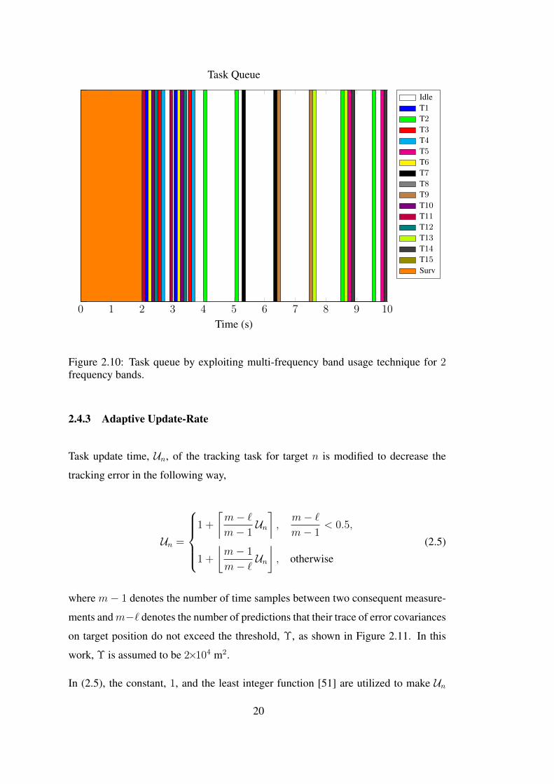
Figure 2.10 Task queue by exploiting multi-frequency band usage technique
for 2 frequency bands. . . . . . . . . . . . . . . . . . . . . . . . . . . . . 20
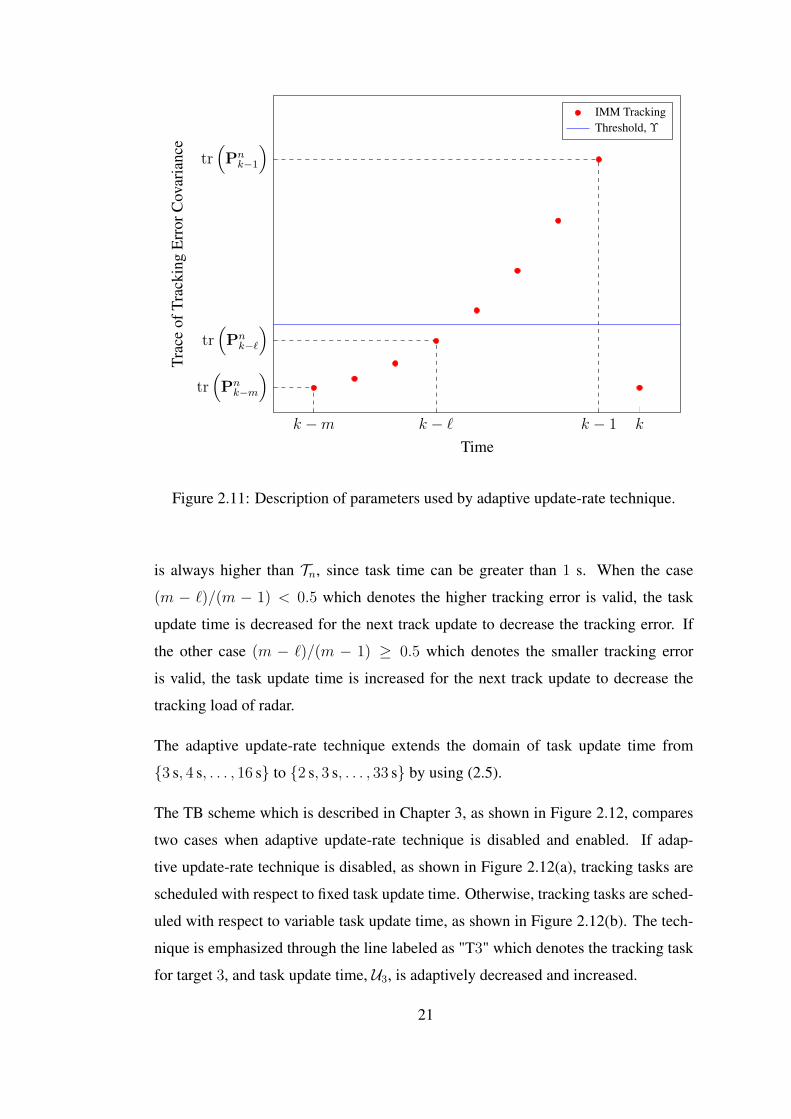
Figure 2.11 Description of parameters used by adaptive update-rate technique. . 21
Figure 2.12 Effect of adaptive update-rate technique on TB scheme. . . . . . . 22
xvi

Figure 2.13 Effects of the sectoring and priority threshold on detections. . . . . 24
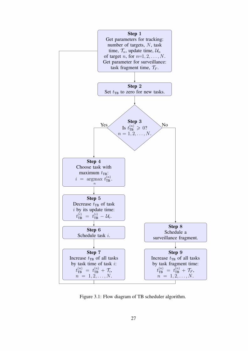
Figure 3.1 Flow diagram of TB scheduler algorithm. . . . . . . . . . . . . . . 27
Figure 3.2 TB scheduler example. . . . . . . . . . . . . . . . . . . . . . . . . 28
Figure 3.3 Flow diagram of scheduler algorithm for MESAR. . . . . . . . . . 31
Figure 3.4 Illustration of job, task, look terms and time intervals. . . . . . . . 32
Figure 3.5 Step 1 of ATB scheduler algorithm. . . . . . . . . . . . . . . . . . 38
Figure 3.6 Step-e of ATB scheduler algorithm. . . . . . . . . . . . . . . . . . 39
Figure 3.7 Step-h of ATB scheduler algorithm. . . . . . . . . . . . . . . . . . 40
Figure 3.8 Flow diagram of ATB scheduler algorithm. . . . . . . . . . . . . . 41
Figure 3.9 ATB scheduler example. . . . . . . . . . . . . . . . . . . . . . . . 43
Figure 3.10 The scenario used to measure the performance of proposed sched-
ulers. . . . . . . . . . . . . . . . . . . . . . . . . . . . . . . . . . . . . . 44
Figure 3.11 Distribution of tasks scheduled with MTATBS-Type 1. . . . . . . . 46
Figure 3.12 TB schemes for MTATBS-Type 1. . . . . . . . . . . . . . . . . . . 47
Figure 3.13 Cumulative distribution of latenesses for MTATBS-Type 1. . . . . . 48
Figure 3.14 Distribution of tasks scheduled with MTATBS-Type 2. . . . . . . . 49
Figure 3.15 TB schemes for MTATBS-Type 2. . . . . . . . . . . . . . . . . . . 50
Figure 3.16 Cumulative distribution of latenesses for MTATBS-Type 2. . . . . . 51
Figure 3.17 Distribution of tasks scheduled with MTATBS-Type 3. . . . . . . . 52
Figure 3.18 TB schemes for MTATBS-Type 3. . . . . . . . . . . . . . . . . . . 53
Figure 3.19 Cumulative distribution of latenesses for MTATBS-Type 3. . . . . . 54
Figure 3.20 Distribution of tasks scheduled with MTATBS-Type 4. . . . . . . . 55
xvii

Figure 3.21 TB schemes for MTATBS-Type 4. . . . . . . . . . . . . . . . . . . 56
Figure 3.22 Cumulative distribution of latenesses for MTATBS-Type 4. . . . . . 57
Figure 3.23 Explanation about TB schemes. . . . . . . . . . . . . . . . . . . . 59
Figure 3.24 Knapsack problem. . . . . . . . . . . . . . . . . . . . . . . . . . . 61
Figure 3.25 Distribution of tasks scheduled with KS. . . . . . . . . . . . . . . 63
Figure 3.26 Time-to-Go scheme and value vs. time graph for KS. . . . . . . . . 64
Figure 4.1 Tracking example of target maneuvers. . . . . . . . . . . . . . . . 71
Figure 4.2 Markov chains for NUPD and UPD actions. . . . . . . . . . . . . . 73
Figure 4.3 Hgt(µnk) andHbt(µ
nk) functions. . . . . . . . . . . . . . . . . . . . 79
Figure 4.4 Flow diagram for unk = 0. . . . . . . . . . . . . . . . . . . . . . . 80
Figure 4.5 Tracking error covariance example for non-maneuvering and ma-
neuvering target. . . . . . . . . . . . . . . . . . . . . . . . . . . . . . . . 81
Figure 4.6 Description of parameters used for the cost value computation. . . . 84
Figure 4.7 The value function of NUPD action for M = 3. . . . . . . . . . . . 90
Figure 4.8 Sample infinite-horizon value functions of NUPD action. . . . . . . 101
Figure 4.9 Tracking example of target maneuvers by using the method of de-
cision policy. . . . . . . . . . . . . . . . . . . . . . . . . . . . . . . . . . 106
Figure 4.10 Tracking error covariance example using the method of decision
policy for non-maneuvering and maneuvering target. . . . . . . . . . . . . 107
Figure 5.1 Comparison of techniques within the distribution of scheduled tasks.113
Figure A.1 Block diagram of a one cycle of IMM estimator for 2-models. . . . 137
Figure C.1 Radar Simulator GUI for MTATBS. . . . . . . . . . . . . . . . . . 142
xviii

Figure C.2 Radar Simulator GUI for KS. . . . . . . . . . . . . . . . . . . . . 143
Figure C.3 Tracking parameters option. . . . . . . . . . . . . . . . . . . . . . 145
xix

LIST OF ALGORITHMS
ALGORITHMS
Algorithm 4.1 Number of segments. . . . . . . . . . . . . . . . . . . . . . . . 93
Algorithm 4.2 The threshold value computation. . . . . . . . . . . . . . . . . 99
xx
LIST OF ABBREVIATIONS
AI artificial intelligenceATB adaptive time-balanceCfTUL method of choosing first target in the update listCPU central processing unitCT coordinated turnCV constant velocityDecP method of decision policyDP dynamic programmingECM electronic countermeasureFA false alarmFCFS first-come, first-servedGUI graphical user interfaceIMM interacting multiple modelIMMPDAF IMM estimator with PDA filterKF Kalman filterKS knapsack schedulerLHS left-hand sideMAB multi-armed banditMFPAR multi-function phased array radarMFR multi-function radarMHT multiple hypothesis trackingMinTE method of minimizing the tracking errorMTATBS multi-type adaptive time-balance schedulerNUPD not updatePAR phased array radarPDA probabilistic data associationPOMDP partially observable Markov decision processPPI plan position indicatorPurMM method of pursuing the most maneuveringQ-RAM QoS based resource allocation modelQoS Quality of Serviceradar RAdio Detection And Ranging
xxi
RHS right-hand side
RRM radar resource management
SNR signal-to-noise ratio
TB time-balance
TPM transition probability matrix
UPD update
xxii
CHAPTER 1
INTRODUCTION
Phased array radar (PAR) can steer the beam electronically. This versatile feature
allows to control beam adaptively without any rotating antenna, and there is no wait-
ing period to direct the beam or inertia to overcome. Thus, PAR, which is especially
employed in military applications [1] owing to capabilities, can carry out multiple
functions by exploiting beam agility.
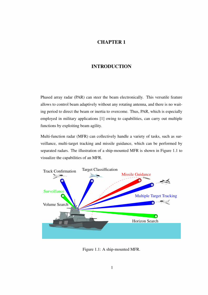
Multi-function radar (MFR) can collectively handle a variety of tasks, such as sur-
veillance, multi-target tracking and missile guidance, which can be performed by
separated radars. The illustration of a ship-mounted MFR is shown in Figure 1.1 to
visualize the capabilities of an MFR.
Multiple Target TrackingSurveillance
Missile GuidanceTarget ClassifficationTrack Confirmation
Volume Search
Horizon Search
Figure 1.1: A ship-mounted MFR.
1

The capabilities of MFR come at a significant cost, since MFR contains numerous
transmit/receive modules which make the overall system expensive. To use the capa-
bilities efficiently, an effective radar resource management (RRM) is required. The
tasks to be executed by MFR, are competing for the limited radar resources which
can be mainly classified as time, energy and computation resources [2], as shown in
Figure 1.2. This raises the problem of how to allocate the limited radar resources to
handle tasks for the best performance.
Radar time resources allocation is generally called scheduling for RRM applications.
The effective scheduling of tasks competing for the radar time resources without sig-
nificant delays [3] is an important research area of RRM. As an example, there are
three targets, an aircraft, an airplane and a missile, to be tracked. There are 3! = 6
permutations of the set {aircraft, airplane, missile} for tracking queue. One of these
will be the worst case operational choice, possibly tracking the missile as the tar-
get of interest. The scheduling is crucial for both of time allocation and sustainable
operation of radar systems.
1.1 Literature Survey
The resource management is a topic of operational research and is widely used in the
area of mathematics, economy, sociology. It can be considered as a planning prob-
lem. RRM utilizes algorithms similar to the ones in operations research with some
modifications. There are many RRM algorithms in the literature, such as artificial in-
telligence (AI), stochastic dynamic programming, Quality of Service based resource
allocation model (Q-RAM). The preliminary survey of the different algorithms which
Radar System Resources
ComputationEnergyTime
Figure 1.2: Radar system resources.
2
are described in the numerous publications is briefly provided in [2] and the majority
of these algorithms are too complex for real-time implementation.
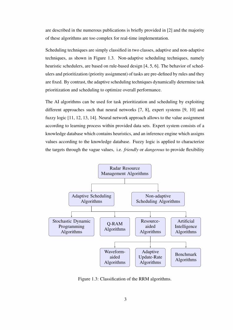
Scheduling techniques are simply classified in two classes, adaptive and non-adaptive
techniques, as shown in Figure 1.3. Non-adaptive scheduling techniques, namely
heuristic schedulers, are based on rule-based design [4, 5, 6]. The behavior of sched-
ulers and prioritization (priority assignment) of tasks are pre-defined by rules and they
are fixed. By contrast, the adaptive scheduling techniques dynamically determine task
prioritization and scheduling to optimize overall performance.
The AI algorithms can be used for task prioritization and scheduling by exploiting
different approaches such that neural networks [7, 8], expert systems [9, 10] and
fuzzy logic [11, 12, 13, 14]. Neural network approach allows to the value assignment
according to learning process within provided data sets. Expert system consists of a
knowledge database which contains heuristics, and an inference engine which assigns
values according to the knowledge database. Fuzzy logic is applied to characterize
the targets through the vague values, i.e. friendly or dangerous to provide flexibility
Radar ResourceManagement Algorithms
Non-adaptiveScheduling Algorithms
Adaptive SchedulingAlgorithms
Resource-aided
Algorithms
Q-RAMAlgorithms
Stochastic DynamicProgrammingAlgorithms
ArtificialIntelligenceAlgorithms
Waveform-aided
Algorithms
AdaptiveUpdate-RateAlgorithms
BenchmarkAlgorithms
Figure 1.3: Classification of the RRM algorithms.
3

in task prioritization and scheduling.
Dynamic programming (DP) is a general approach for sequential optimization where
decisions are made in stages [15]. For each stage, the outcome of each decision is
predictable to some extent before making the next decision through transition prob-
abilities. It is emphasized that the DP comes with heavy of computation load, but
can provide the optimal scheduling as in [16] which is one of the first example of DP
applications for RRM. In addition to heavy computational load, direct utilization of
DP applications, namely without any approximation, can be intractable owing to the
curse of dimensionality which is inherent in DP [17] for some RRM problems. The
stochastic DP algorithms differ in their modeling of the RRM problem, such as multi-
armed bandit (MAB) problem in [18], MAB problem with hidden Markov model in
[19, 20], restless bandit problem in [21]. In [22, ch. 7], an application of MABs is
explained in details of target tracking, and the MAB theory is also briefly explained
in [22, ch. 6]. In [17], the RRM problem that the scheduling is decomposed into fast
and slow timescales, is translated to a constrained Markov decision process and the
algorithm based on Lagrangian relaxation is presented. Further details can be also
found in [23].
Resource-aided algorithms are utilized to improve the performance of the radar by
modifying the parameters or the features. One of the subclass is the waveform-aided
algorithms which provide a noticeable improvement on the radar performance, es-
pecially when there are possible jamming resources. In [24], radar detection perfor-
mance is optimized in a changing environment where performance factors (eclipsing,
clutter, propagation and jamming) are analyzed and utilized to select the optimum
waveform parameters within a neural network approach. In [25], waveforms are
adaptively scheduled to detect a new target by using stochastic DP and it is noted
that the time to detect a new target decreases with described method.
Waveforms can be selected according to the features of tasks by using fixed or variable
waveform libraries. In [26], waveform is selected from a pre-designed library by
using the information states and it is noted that acceptable limits of tracking error are
achieved with the decreased number of revisits. Similarly, the effects of waveform
scheduling is analyzed for target tracking in [27] and target classification in [28].
4

Another subclass of resource-aided algorithms is the adaptive update-rate algorithms
which are studied to improve tracking performance of radars, in comparison to the
traditional trackers that use uniform update-rates for the case of clutters and mane-
uvering targets. In [29], the revisit time, which depends upon the estimated lack of
information corresponding to the target, is computed. In addition, the radar parame-
ters such as signal-to-noise ratio (SNR), track sharpness and detection threshold, are
optimized with respect to the radar load for tracking in the same work. In [30], a
method is proposed to control the revisit time and adjust the energy level of the radar
by exploiting the interacting multiple model (IMM)1. In [31], an adaptive update-rate
algorithm that is based on IMM for target tracking, is proposed. The IMM algo-
rithm has already been capable to estimate target state and tracking error covariance.
Thus, update intervals are computed with respect to these tracking error covariances
to decrease the number of track updates by providing the acceptable beam position-
ing losses, in the same work. In [32], the radar energy resource, which is required for
track maintenance, is minimized by optimally computing track update time and SNR
pairs.
The last subclass of resource-aided algorithms comprises the benchmark algorithms
which are studied to cope with the benchmark problems. The benchmark problem
is a scenario that converts the dynamics of radar environment into a simulation con-
cept, in order to test the behavior of described algorithms without implicitly running
on a radar system. In [33], a benchmark problem is proposed for tracking mane-
uvering targets where the features of a PAR such as beam-shape, finite resolution,
and other restrictions that occur in a real-world environment such as target maneu-
vers, missed detections, track loss are handled by the simulation test-bed. The work,
[33], is extended to cover the effects of false alarms (FAs), namely false detections,
and electronic countermeasures (ECMs) in [34]. Furthermore, multiple waveforms
are included to allocate the radar energy with tracking algorithms in the same work.
Many of the deficiencies which are associated with [34] are rectified in [35, 36]. In
[35], a documentation for the computer program, which is written in MATLAB R©2
to simulate the radar system, is also provided. In [37], IMM/MHT method which
combines IMM for tracking, and MHT for data association, as described in [38],
1 The algorithm is described in Appendix A2 MATLAB is a registered trademark of the The MathWorks, Inc. www.mathworks.com.
5

is presented for the benchmark problem that is given in [34]. In [39], IMMPDAF
method, as described in [38], which combines IMM for tracking, and PDA filter for
data association, is presented for the benchmark problem that is given in [36].
Q-RAM algorithms are utilized to allocate radar resources by managing Quality of
Service (QoS) [40]. The main aim of a Q-RAM model is to allocate system resources
between applications, namely tasks, in order to make overall system utility maximized
while meeting the minimum needs of applications [41]. The Q-RAM approach gets
more complex, when the system has more constraints. Thus, the algorithms have
been developed to approximately solve the problem or to exploit its useful features
in the last decades. The PARs are convenient to present the capabilities of Q-RAM
which is described in the pioneer work [41]. In [42], real-time scheduling of a PAR
system, which is described in [43], is developed by using Q-RAM. In [44], a dwell
scheduling scheme that is based on Q-RAM, is proposed for a radar tracking system
where the physical and environmental factors are incorporated to manage QoS for the
same PAR system. In [45], Q-RAM is evaluated and the shortcomings of the method
are identified for RRM problem.
There is another scheduling method called as the time-balance method which does
not exactly fit into any category shown in Figure 1.3 [2]. This method is described
as a measure of the radar time which is requested by a task to be scheduled. The
algorithms based on this method are presented in [46, 47, 48].
1.2 Main Scope of the Thesis
Main purpose of this thesis is to realize the RRM techniques for a multi-function
phased array radar (MFPAR). The entire of the radar system is taken into account to
attain this purpose. It should be noted that the existing works are usually too specific
such that they consider only task prioritization or revisit time without completely re-
marking the effect of other components on RRM. This makes a comparison of the
suggested algorithms quite difficult. Furthermore most of these methods utilizes spe-
cific test-beds which are insufficient to model stochastic nature of radar environment.
Hence, randomized scenarios are generated and RRM is applied to almost all compo-
6

nents of MFPAR. The simulation environment is built on the MATLAB software, and
contains adaptive update rate, dynamic task prioritization, tracking and task interlea-
ving features.
Here, the problem presented in [17] is studied to understand the main aspects of the
RRM problem. The ideas given in [23], such as target dropping, track quality, two
timescales, utility function are also utilized in this work. The time-balance approach
described in [48] is preferred instead of the DP approaches, owing to its simplicity
and applicability in real-time operation. Moreover, a scheduling method based on
binary integer programming is studied to solve the RRM problem as an optimization
problem and to present comparisons with the previous approach.
1.3 Outline of the Thesis
The radar system model is described in Chapter 2. Then, the time-balance tech-
nique based schedulers in literature, are briefly explained in Chapter 3. Furthermore,
the scheduling algorithms, multi-type adaptive time-balance scheduler and knapsack
scheduler, are described in the same chapter. Next, in Chapter 4, the decision making
problem that occurs, when two or more targets concurrently request track update, is
mentioned and some analytical methods are described to handle this problem. The
experimental results are provided in Chapter 5. Finally, conclusions and future work
are given.
7

8

CHAPTER 2
RADAR SYSTEM MODEL
A general MFR system model shown in Figure 2.1 is used for simulation and ana-
lyzing the scheduling techniques. The given model is mainly focused on surveillance
and tracking tasks, since the other types of tasks (i.e. missile guidance, calibration)
are used less frequently in comparison to these tasks.
In this chapter, every block of the system model is briefly described and a resource-
aided technique, multi-frequency band usage, is presented for the utilization of radar
timeline effectively.
Scenario
TaskParameters
TaskPrioritization
Scheduler
Surveillance
Detection
Tracking
Tracker
Figure 2.1: Radar system model.
9
2.1 Scenario
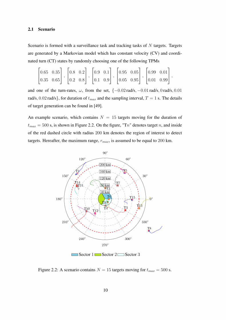
Scenario is formed with a surveillance task and tracking tasks of N targets. Targets
are generated by a Markovian model which has constant velocity (CV) and coordi-
nated turn (CT) states by randomly choosing one of the following TPMs0.65 0.35
0.35 0.65
,
0.8 0.2
0.2 0.8
,
0.9 0.1
0.1 0.9
,
0.95 0.05
0.05 0.95
,
0.99 0.01
0.01 0.99
,
and one of the turn-rates, ω, from the set, {−0.02 rad/s,−0.01 rad/s, 0 rad/s, 0.01
rad/s, 0.02 rad/s}, for duration of tmax and the sampling interval, T = 1 s. The details
of target generation can be found in [49].
An example scenario, which contains N = 15 targets moving for the duration of
tmax = 500 s, is shown in Figure 2.2. On the figure, "Tn" denotes target n, and inside
of the red dashed circle with radius 200 km denotes the region of interest to detect
targets. Hereafter, the maximum range, rmax, is assumed to be equal to 200 km.
0◦
30◦
60◦
90◦
120◦
150◦
180◦
210◦
240◦
270◦
300◦
330◦
40 km
80 km
120 km
160 km
200 km
T1
T2
T3T4
T5
T6
T7
T8
T9
T10
T11
T12T13
T14
T15
Sector 1 Sector 2 Sector 3
Figure 2.2: A scenario contains N = 15 targets moving for tmax = 500 s.
10
2.2 Task Parameters
Task parameters contain task id, task time, task update time, allowable lateness,
scheduling value and priority. By notifying that the declarations may not be real-
istic to reflect the real-world, the parameters are described as follows:
• Task id is an integer between 1 and N and associated with a target. Therefore
the task id, n, is reserved for target n, even if target n is dropped after a while.
It is the only fixed parameter. The task id of a surveillance task is always
associated as N + 1.
• Task time is the elapsed time to complete transmitting and receiving cycle for a
task. Task time of a surveillance task is fixed as 2 s. Task time of tracking task
is thought to depend on the range of corresponding target. This idea is inspired
from the range equation,
R =cTR2, (2.1)
given in [1, ch. 1], where c = 3×10⁸ m/s is the speed of light and TR is the
round-trip travel time which is the elapsed time when pulse has to travel to the
target and back. Task time, Ti, of the tracking task for target i is computed as
Ti = (0.95 s) + (0.05 s)⌈ ri
40 km
⌉. (2.2)
where the constants are intuitively chosen and ri is the range of corresponding
target. Considering the range which can take any value from 0 to 200 km for
detection, Ti can take any value which belongs to the set, {0.95 s, 1.00 s, 1.05 s,
1.10 s, 1.15 s, 1.20 s}, with respect to the range of target i.
• Task update time is the elapsed time between sequential updates for a task,
namely it is the desired period value for a task. Task update time of surveillance
task is assumed to be 25 s, and it can be dynamically changed to decrease idle
time of radar. Task update time of a tracking task is initialized with a value
which depends on the speed of corresponding target, and it can be dynamically
11

changed to keep maneuvers and to track the target more accurately. Task update
time, Ui, of the tracking task for target i is computed as
Ui = (17 s)−⌈ vi
25 m/s2
⌉. (2.3)
where the constants are intuitively chosen and vi is the speed of corresponding
target. Considering the speed which can take any value from 10 to 340 m/s for
detection, Ti can take any value which belongs to the set, {3 s, 4 s, . . . , 16 s},with respect to the speed of target i. Indeed, (2.3) can be modified as
Ui = max(
(17 s)−⌈ vi
25 m/s2
⌉, 3 s). (2.4)
to detect a target, speed of whom is greater than 340 m/s. However, it may be
improper to assign the same task update time for two targets which have the
speeds 340 m/s and 1000 m/s respectively. Hence, it is beyond the scope of this
work at this level.
• Allowable lateness is a tolerable time, in other words, it is the time difference
between update time at which the task can be scheduled, and due time by which
it must be scheduled to successfully accomplish, for late update and it is as-
sumed to be equal to 20% of the task update time. If update time of a tracking
task exceeds the allowable lateness, the tracked target is counted as probably
dropped. Therefore another aim of scheduling is to reduce the number of prob-
able drops.
• Scheduling value refers the state of task, i.e. how much time is left to new
update, after scheduling epochs. Its function is directly related to scheduler.
Hence, it is defined to help scheduler to choose the most convenient task for
scheduling.
• Priority refers the importance of scheduling a task. Its range is defined to be
between 1 and 5. Assuming that the maximum range is 200 km, the priority is
decreased from 5 to 1 by 1 through each ring has 40 km thickness for tracking
tasks. If a target is 50 km away from radar which is at the origin, its priority is
associated as 4. Target prioritization levels according to regions are shown in
Figure 2.3. Surveillance task has the minimum priority that is 1.
12

5 4 3 2 1
40 km
80 km
120 km
160 km
200 km
Figure 2.3: Target prioritization regions.
2.3 Task Prioritization
Task prioritization is applied so that each one of the targets has an initial priority
based on its range for tracking tasks (targets closer to base are more important) and
surveillance task has the minimum priority.
If task prioritization process is not dynamically changed, every aspect of MFR per-
formance may be sub-optimal. For example, assuming surveillance tasks have the
lowest priority level, the total occupancy of surveillance tasks is set as OS and the
remaining part, 100% − OS , of the resource is set as free in case of detection. As-
suming that there is not any initialized track, the system is run. Then, scheduler
allows surveillance tasks to share all of the resource, since there is not any tracking
task to be scheduled. However, as number of tracks becomes higher, available re-
sources may not be sufficient to sustain tracks after the first detection. Since priority
of a tracking task is usually higher than surveillance task, scheduler should transfer
some amount of the resource which is reserved for surveillance to tracking tasks and
the detection performance of system decreases, as shown in Figure 2.4. This simple
example demonstrates the importance of dynamic task prioritization. To avoid such
problems or to reduce their negative effects, task prioritization should be dynamically
13

performed. If surveillance task cannot be scheduled at the desired time, its priority is
increased temporarily to a level which is higher than the highest priority of available
tasks. Similarly, if a tracking task cannot be scheduled at the desired time, its prio-
rity can be increased temporarily to a level which is higher than the highest priority
of available tasks. Thus, the dynamic task prioritization process is applied to avoid
lateness and to enhance system performance.
If a target has a range which is associated with a different priority level, then its
priority is immediately updated. This is explained with a scenario shown in Figure
2.5. By choosing the sector 3 as a region of interest and the priority threshold as 2,
namely the targets with priority levels higher than 1 can be detected, the target 2 and
the target 3 are going to be tracked. Figure 2.5(a) shows that the tracking is handled at
a desired level when the feature, dynamic task prioritization, is enabled. However, the
Figure 2.5(b) shows that the tracking tasks are not scheduled to meet the constraints.
The target 2 is tracked until the maximum range. The target 3 is not tracked until the
detection of target 5, since the system only updates the task list whenever a detection
occurs.
0%
100%
OS
(a)
0%
100%
OS
(b)
Figure 2.4: Detection performance degradation due to task prioritization. (a) Surve-illance task completely utilizes radar resources, since there is initially no tracks toschedule a tracking task. (b) Surveillance task cannot maintain the desired detectionperformance, since radar is overloaded by detections and some amount of reservedresource for surveillance task is transferred to tracking tasks.
14

0◦
30◦
60◦
90◦
120◦
150◦
180◦
210◦
240◦
270◦
300◦
330◦
40 km
80 km
120 km
160 km
200 km
T1
T2T3
T4
T5
T6
Sector 1 Sector 2 Sector 3
(a) Dynamic task prioritization is enabled.
0◦
30◦
60◦
90◦
120◦
150◦
180◦
210◦
240◦
270◦
300◦
330◦
40 km
80 km
120 km
160 km
200 km
T1
T2T3
T4
T5
T6
Sector 1 Sector 2 Sector 3
(b) Dynamic task prioritization is disabled.
Figure 2.5: Effect of dynamic task prioritization.
15

2.4 Scheduler
Scheduler block controls the performance of the radar. Here, the performance is
measured by the factors which are defined as follows:
• The number of probable drops is the number of updates which are too late
to track target accurately. The probable drop occurs when the update interval
exceeds the sum of task update time and allowable lateness.
• Cost is the sum of squared lateness values after each scheduling epochs.
• Average of errors is simply the average of the trace of tracking error covariance
matrices of all targets.
• Occupancy is the ratio of utilized radar time to the total available time interval.
The following sections describe several resource-aided techniques for the scheduling
algorithms which are described in detail in Chapter 3 to enhance the overall perfor-
mance of the radar.
2.4.1 Task Interleaving
Tasks mentioned here are coupled-tasks [50] that consist of transmitting, idle time
and receiving parts, as shown in Figure 2.6. Task interleaving technique is applied
to insert the transmitting and receiving parts of a coupled-task into the idle time part
of other coupled-tasks. The time when radar is idle, can be reduced so that radar
time-line is effectively utilized by this technique. However, it increases the consumed
radar energy, since radar processes more tasks for the same interval.
transmitting receivingidle timeTime0.1 0.2 0.3 0.4 0.5 0.6 0.7 0.8 0.90 1
Figure 2.6: A coupled-task.
16

In this work, transmitting and receiving intervals are assumed to be equal to 10% of
the task time. Thus, idle time interval is assigned as 80% of the task time. Task queue
shown in Figure 2.7 where "Tn" denotes the tracking task for target n, and "Surv"
denotes the surveillance task, is obtained by exploiting task interleaving technique
for a scenario.
The task queue starts with surveillance task which is not interleaved. Then, tracking
tasks for target 11 and target 1 are scheduled respectively. Since task times are not
identical, a gap, which is labeled as "Idle" on the figure, appears between the receiving
parts of these tasks. Task interleaving process continues in this manner.
Task interleaving cannot be always handled in a proper way, as shown in Figure 2.7.
When tasks are closely interleaved, this interleaving may cause interference and other
problems in a real radar systems. A practical method of using multiple frequency
bands is suggested to interleave the tasks without any negative side effects. This
method is described in the next section.
0 1 2 3 4 5 6 7 8 9 10
Time (s)
Task Queue
IdleT1T2T3T4T5T6T7T8T9T10T11T12T13T14T15Surv
Figure 2.7: Task queue by exploiting task interleaving technique.
17

2.4.2 Multi-Frequency Band Usage
The interleaving of tasks is valuable choice to decrease the idle time for radar. How-
ever, the interleaving of tracking tasks between closer targets can bring wrong target
association problems, physical layer problems, etc. There are many methods, i.e.
waveform selection, to solve these problems. Unfortunately, these methods are too
complex for implementation. Thus, the idea of frequency re-usage has emerged to
deal with tracking of the high number of targets and to avoid the track mixing of closer
targets. In this method, it is supposed to have multiple distinct frequency bands. Each
of the frequency bands is reserved for a single tracking task.
The method is explained via a scenario shown in Figure 2.8. It is supposed that there
are 2 frequency bands (f1 and f2), 4 targets and target priorities makes the scheduling
sequence as target 1, target 2, target 3 and target 4 respectively. Here, the critical point
is that the two of targets are referred to as closer targets, if their azimuth difference is
less than the frequency re-usage angle, θfr.
Target 1Target 2
Target 3
Target 4θfr
30◦
30◦
210◦
45◦ 35◦ 20◦
Figure 2.8: A scenario for multi-frequency band usage technique.
18
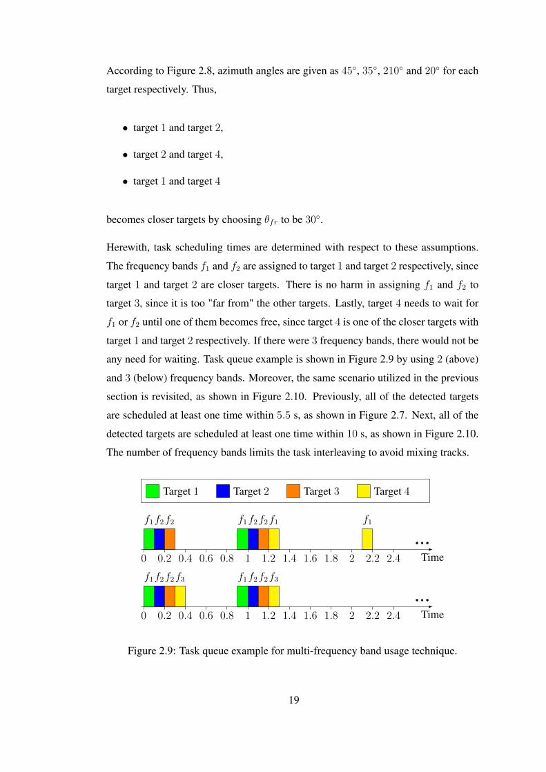
According to Figure 2.8, azimuth angles are given as 45◦, 35◦, 210◦ and 20◦ for each
target respectively. Thus,
• target 1 and target 2,
• target 2 and target 4,
• target 1 and target 4
becomes closer targets by choosing θfr to be 30◦.
Herewith, task scheduling times are determined with respect to these assumptions.
The frequency bands f1 and f2 are assigned to target 1 and target 2 respectively, since
target 1 and target 2 are closer targets. There is no harm in assigning f1 and f2 to
target 3, since it is too "far from" the other targets. Lastly, target 4 needs to wait for
f1 or f2 until one of them becomes free, since target 4 is one of the closer targets with
target 1 and target 2 respectively. If there were 3 frequency bands, there would not be
any need for waiting. Task queue example is shown in Figure 2.9 by using 2 (above)
and 3 (below) frequency bands. Moreover, the same scenario utilized in the previous
section is revisited, as shown in Figure 2.10. Previously, all of the detected targets
are scheduled at least one time within 5.5 s, as shown in Figure 2.7. Next, all of the
detected targets are scheduled at least one time within 10 s, as shown in Figure 2.10.
The number of frequency bands limits the task interleaving to avoid mixing tracks.
f1 f1f2 f2f2 f2f1 f1
Time0.2 0.4 0.6 0.8 1 1.2 1.4 1.6 1.8 2 2.2 2.40
Target 1 Target 2 Target 3 Target 4
f1 f1f2 f2f2 f2f3 f3
Time0.2 0.4 0.6 0.8 1 1.2 1.4 1.6 1.8 2 2.2 2.40
Figure 2.9: Task queue example for multi-frequency band usage technique.
19
0 1 2 3 4 5 6 7 8 9 10
Time (s)
Task Queue
IdleT1T2T3T4T5T6T7T8T9T10T11T12T13T14T15Surv
Figure 2.10: Task queue by exploiting multi-frequency band usage technique for 2frequency bands.
2.4.3 Adaptive Update-Rate
Task update time, Un, of the tracking task for target n is modified to decrease the
tracking error in the following way,
Un =
1 +
⌈m− `m− 1
Un⌉,
m− `m− 1
< 0.5,
1 +
⌊m− 1
m− ` Un⌋, otherwise
(2.5)
where m− 1 denotes the number of time samples between two consequent measure-
ments andm−` denotes the number of predictions that their trace of error covariances
on target position do not exceed the threshold, Υ, as shown in Figure 2.11. In this
work, Υ is assumed to be 2×10⁴ m2.
In (2.5), the constant, 1, and the least integer function [51] are utilized to make Un
20
k −m k − ` k − 1 k
tr(Pn
k−m
)tr(Pn
k−`
)
tr(Pn
k−1
)
Time
Trac
eof
Trac
king
Err
orC
ovar
ianc
e
IMM TrackingThreshold, Υ
Figure 2.11: Description of parameters used by adaptive update-rate technique.
is always higher than Tn, since task time can be greater than 1 s. When the case
(m − `)/(m − 1) < 0.5 which denotes the higher tracking error is valid, the task
update time is decreased for the next track update to decrease the tracking error. If
the other case (m − `)/(m − 1) ≥ 0.5 which denotes the smaller tracking error
is valid, the task update time is increased for the next track update to decrease the
tracking load of radar.
The adaptive update-rate technique extends the domain of task update time from
{3 s, 4 s, . . . , 16 s} to {2 s, 3 s, . . . , 33 s} by using (2.5).
The TB scheme which is described in Chapter 3, as shown in Figure 2.12, compares
two cases when adaptive update-rate technique is disabled and enabled. If adap-
tive update-rate technique is disabled, as shown in Figure 2.12(a), tracking tasks are
scheduled with respect to fixed task update time. Otherwise, tracking tasks are sched-
uled with respect to variable task update time, as shown in Figure 2.12(b). The tech-
nique is emphasized through the line labeled as "T3" which denotes the tracking task
for target 3, and task update time, U3, is adaptively decreased and increased.
21

0 20 40 60 80 100 120 140 160 180 200
−25
−20
−15
−10
−5
0
5
Time (s)
t TB
(s)
TB Scheme
U3T1T2T3T4Surv
(a) Adaptive update-rate technique is disabled.
0 20 40 60 80 100 120 140 160 180 200
−25
−20
−15
−10
−5
0
5
Time (s)
t TB
(s)
TB Scheme
U3 U3T1T2T3T4Surv
(b) Adaptive update-rate technique is enabled.
Figure 2.12: Effect of adaptive update-rate technique on TB scheme.
22

2.5 Surveillance
Surveillance task can be a single task or can be a task that can be fragmented with
tracking tasks [48]. The fragmented surveillance task is supposed to be handled in
the idle time when there is no task to schedule. The fragmented surveillance task is
assumed to be completed when all fragments summed up to a given surveillance task
time. However, task update time for this case is not fixed, if there is not sufficient idle
time for the surveillance.
2.6 Detection
The instrumented detection range of radar is up to rmax, and hence, the targets are
assumed to be detected within this range. It is crucial to remind that the detections in
this work are assumed to be perfectly associated with the targets.
The effects of the sectoring and priority threshold on detections are shown in Figure
2.13. Here, only sector 2 is the region of interest and the priority threshold is 2,
namely the targets with priority levels higher than 1 can be detected.
2.7 Tracking
A tracking task is associated for every target in track mode. A target which is pre-
viously detected is assumed to be perfectly associated, if it stays in the out of range
for a while and comes back to the region of interest. Therefore tracks are not mixed
during the scheduling process.
2.8 Tracker
The utilization of the tracker can be seen as the most important phase of RRM. Be-
cause its performance effects the future tracking load of the radar. The tracker, in this
work, utilizes IMM algorithm which is briefly described in Appendix A. The IMM
23

0◦
30◦
60◦
90◦
120◦
150◦
180◦
210◦
240◦
270◦
300◦
330◦
40 km
80 km
120 km
160 km
200 km
T1
T2
T3
T4
T5
T6
T7
T8
T9
T10
T11
T12
T13
T14
T15
Sector 1 Sector 2 Sector 3
Figure 2.13: Effects of the sectoring and priority threshold on detections.
provides the information about the maneuver state of targets, and this information is
useful for RRM in target selection, adaptive update-rate.
2.9 Summary
In this chapter, the general MFR system and its environment are modeled for simula-
tion. The methods for parameter assignment, task prioritization and adaptive update-
rate are explained. A resource-aided technique called as the multi-frequency band us-
age, is proposed to increase the applicability of task interleaving. Thus, the elements
of the simulation model are described to emphasize each phase of the scheduling.
However, the scheduling techniques are not covered, while describing the scheduler
phase. Hence, they are described in the next chapter.
24

CHAPTER 3
SCHEDULING TECHNIQUES
In this chapter, time-balance technique based schedulers and two suggested schedul-
ing algorithms, namely multi-type adaptive time-balance scheduler (MTATBS) and
knapsack scheduler (KS), are described. MTATBS and KS are implemented on the
simulation model described in the previous chapter.
3.1 Time-Balance Technique Based Schedulers
The time-balance (TB) is described as a measure of how much time which is owed
to a task to perform it by radar [46]. The TB actually indicates the degree of urgency
corresponding to the next scheduling of a task, and hence, TB is continually updated
to indicate the actual and required use of radar time [52].
General idea of TB technique is very simple. Each task is associated with a TB value,
tTB, which is varying with time and there is a TB scheme which maintains tTB’s. A
task is thought to be delayed for scheduling, if it has a positive tTB which indicates
to request radar time. Similarly, a task is thought to wait radar time for scheduling,
if it has a negative tTB to indicate that it is not ready. A task has zero tTB when it is
exactly ready for scheduling. Moreover, new tasks can be inserted to a radar task list
with a negative tTB in order to delay the new task until its due time of execution. If a
task is scheduled, its tTB is decreased by its task update time. The tTB of other tasks
which are not scheduled is increased by an amount that is determined in accordance
with the algorithm of scheduling. This process continues in this way until the end of
operation.
25

In the following sections, the TB technique based algorithms are presented in an
increasing order of complexity and a non-historical order. Various versions of the
suggested TB scheduler are described in the remaining parts of this work.
3.1.1 Time-Balance Scheduler
This type is the simplest scheduler based on TB technique and it is described in
[53]. The TB scheduler chooses the task which has higher tTB than other tasks to
be processed next. The scheduler is designed to schedule mainly tracking tasks, and
hence, surveillance task is not associated with a tTB. The surveillance task is sched-
uled whenever all tracking tasks have negative tTB. Thus, surveillance task can be
scheduled if radar is underloaded. The underloaded radar cannot perform a complete
surveillance task if there is not a sufficient idle time after performing tracking tasks.
Therefore the surveillance task is fragmented by task fragment time, TF , in order to
interleave with tracking tasks. When total time of the scheduled fragments is equal to
task time of surveillance, a surveillance task is completely scheduled.
3.1.1.1 Algorithm of TB Scheduler
Flow diagram of the TB scheduler algorithm is shown in Figure 3.1. The step 1 gets
parameters for each task. Tracking task parameters contain the number of targets, N ,
task time, Tn, and task update time, Un, for n = 1, 2, . . . , N , and surveillance task
parameter is only task fragment time, TF . The step 2 assigns tTB as zero for new tasks.
The step 3 finds out that if there is any task with positive tTB. The step 4 chooses a
task which has the highest tTB, if there is at least one task with positive tTB after step
3. The step 5 decreases tTB of task, which is chosen by step 4, by task update time of
this task. Here, the critical point is that tTB’s of other tasks are not updated. The step
6 schedules task chosen by step 4. The step 7 increases tTB’s of all tasks by task time
of the scheduled task. If there is not any task with positive tTB found by step 3, then
step 8 is executed. The step 8 schedules a surveillance fragment. The step 9 increases
tTB’s of all tasks by TF . After processing step 7 or step 9, the next step is again step
1, and scheduling continues in this way.
26
Step 1Get parameters for tracking:number of targets, N , tasktime, Tn, update time, Un
of target n, for n=1, 2, . . . , N .Get parameter for surveillance:
task fragment time, TF .
Step 2Set tTB to zero for new tasks.
Step 3
Is t(n)TB > 0?
n = 1, 2, . . . , N .
Step 4Choose task with
maximum tTB:i = argmax
nt(n)TB .
Step 5Decrease tTB of taski by its update time:t(i)TB = t
(i)TB − Ui.
Step 6Schedule task i.
Step 7Increase tTB of all tasksby task time of task i:t(n)TB = t
(n)TB + Ti,
n = 1, 2, . . . , N .
Step 8Schedule a
surveillance fragment.
Step 9Increase tTB of all tasksby task fragment time:t(n)TB = t
(n)TB + TF ,
n = 1, 2, . . . , N .
Yes No
Figure 3.1: Flow diagram of TB scheduler algorithm.
27
3.1.1.2 An Example
A scheduling example for two tracking tasks is shown in Figure 3.2. Task time and
task update time for tracking task 1 are assigned as T1 = 6 s and U1 = 24 s, and
for tracking task 2 are assigned as T2 = 9 s and U2 = 15 s. According to these
parameters, the occupancies, On = TnU−1n , are computed as 25% and 60% for each
task respectively. Task fragment time, TF , is assigned as 1 s, so that surveillance task
fragments can be scheduled when both of tracking tasks have negative tTB.
After processing step 1, as given in previous paragraph, step 2 is processed to assign
tTB as 0 for both of tracking tasks, at t = 0. Thus, tTB’s are not negative in step
3 and either task 1 or task 2 can be chosen in step 4. In step 5, tTB of task 1, t(1)TB ,
is decreased with U1, as depicted by blue line on TB scheme shown in Figure 3.2.
Meanwhile, tTB of task 2 is depicted by green line on TB scheme. In step 6, task 1 is
scheduled. In step 7, tTB for both of tracking tasks are increased with T1. The first
0 10 20 30 40 50 60 70 80 90 100
Tracking Task 2 with 60.00% Occupancy0 10 20 30 40 50 60 70 80 90 100
Tracking Task 1 with 25.00% Occupancy
0 10 20 30 40 50 60 70 80 90 100
Task Queue
0 10 20 30 40 50 60 70 80 90 100
−20
0
Time (s)
t TB
(s)
TB Scheme
Task 1 Task 2
Figure 3.2: TB scheduler example.
28
cycle of scheduling ends at t = 6 s, and t(1)TB = −18 s and t(2)TB = 6 s, as shown on TB
scheme. In the second cycle of scheduling, task 2 is chosen since task 1 has a negative
tTB. The second cycle of scheduling ends at t = 15 s, and t(1)TB = −9 s and t(2)TB = 0
s by processing all steps, as shown on TB scheme. Radar time is completely utilized
until t = 39 s. Here, t(1)TB = −9 s and t(2)TB = −6 s, and hence, step 8 is processed
after step 3. Then, a surveillance task fragment, as depicted by the white areas on
task queue shown in Figure 3.2, is scheduled. In step 9, tTB for both of tracking tasks
are increased with TF . Surveillance task fragments are successively scheduled until
t = 45 s, since both of tracking tasks have negative tTB, as shown on TB scheme. The
scheduling process continues in this way.
The requested task queue of each tracking task is individually shown in Figure 3.2,
and task queue after scheduling is also shown in the same figure below of them.
Here, the main aim is compare the actual and requested occupancies. Task 1 and
task 2 actually utilize radar time for 25 s and 63 s respectively until t = 100 s.
These values indicate that the actual occupancies are 25% and 63% for task 1 and
task 2 respectively. Thus, there are minor differences which is negligible for longer
durations between the actual and requested occupancies.
3.1.2 Scheduler Developed for MESAR
A scheduler algorithm which utilizes TB technique is briefly explained in [46] for
real-time control of Multifunction Electronically Scanned Adaptive Radar (MESAR).
In addition to some improvements on this algorithm, the work [47] describes TB tech-
nique in a detailed manner. This section describes the original and modified version
of scheduling algorithms, as explained in [47], developed for real-time task schedul-
ing with MESAR. Before delving into scheduling algorithms, it is more convenient
to give some aspects briefly related to MESAR.
The resource management of MFR can be applied efficiently by achieving the follow-
ing processes.
• All tasks must be ranked in a priority order. Note that the priorities of tasks
may change throughout an engagement.
29

• Tasks must be formed into a timeline for MFR to perform. This is the main task
of the scheduler.
The scheduler’s task in constructing scheduling timeline in real-time is complicated
due to the constraints which apply to each task as follows:
• Tasks vary in the criticality of the time period in which they must be scheduled.
Some may have a small window of opportunity which must be met for the task
to be successful, while others may have looser time constraints.
• Tasks differ significantly in length.
• Tasks may become suddenly necessary or urgent, or may become unnecessary.
• Tasks may have to adhere to some constraint such as close to array broadside
operation in a rotating system.
Thus, the following broad objectives are suggested for resource management and task
scheduling effectively.
• Schedule each task as near to the requested time as possible.
• Schedule each task as close to array broadside as possible.
• Schedule each task to minimize the radar idle time.
• Schedule each task to maximize the tactical benefit of MFR.
3.1.2.1 Algorithm of MESAR
The task is thought as a single entity in Section 3.1.1. However, it is known that
tasks can be divided into subtasks, i.e. coupled-tasks consist of transmitting, idle
time and receiving parts [50]. In addition, the resource manager sometimes needs
interruptions to serve the resources to the tasks with higher priority. Therefore the
algorithm of MESAR allows to divide tasks into subtasks that can be interleaved to
manage radar time efficiently and decrease the delays for the highly prioritized tasks.
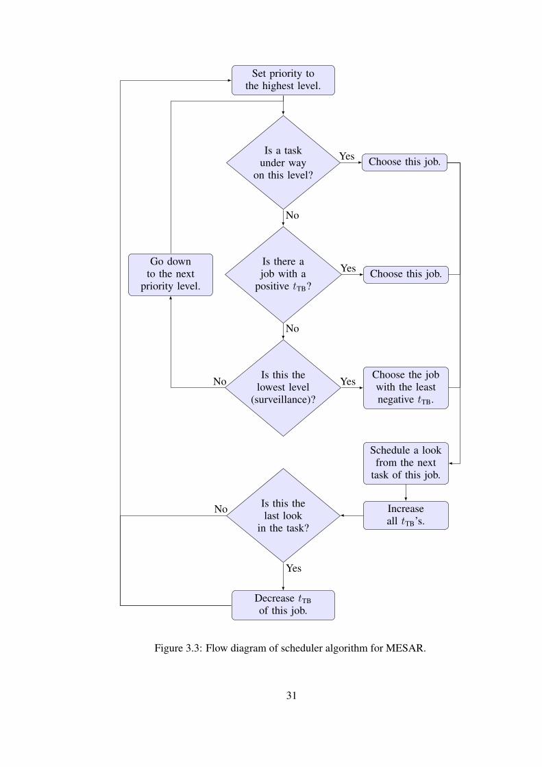
The flow diagram of the algorithm of MESAR is shown in Figure 3.3.
30
Set priority tothe highest level.
Is a taskunder way
on this level?Choose this job.
Is there ajob with a
positive tTB?Choose this job.
Go downto the next
priority level.
Is this thelowest level
(surveillance)?
Choose the jobwith the leastnegative tTB.
Schedule a lookfrom the next
task of this job.
Increaseall tTB’s.
Is this thelast look
in the task?
Decrease tTBof this job.
Yes
No
Yes
No
YesNo
No
Yes
Figure 3.3: Flow diagram of scheduler algorithm for MESAR.
31

According to Figure 3.3, it should be clear that the description of a job, a task and a
look in MESAR must be clarified. A job may be surveillance of a region, or main-
taining track on a specific target and it usually consists of several tasks, i.e. searching
a single surveillance beam position, or performing one track update. Then, each task
usually consists of several activities which are non-coherently integrated to give a
detection. The last definition, a look is one or more activities from a task that are
transmitted coherently by the radar. The described terms and time intervals are illus-
trated in Figure 3.4.
Description of the figure by starting from the highest priority level;
1. If a job is already under the process on that level, then that job is chosen for
scheduling of looks. This means that tasks from each level will be completed
sequentially, rather than many tasks from the same level being interleaved, and
thus drawn out in time.
2. If no task is executed then the task on the same priority level is chosen with the
highest positive tTB.
3. If no task has a positive tTB then move down to the next level and repeat (1)-(3).
4. If no task has a positive tTB on the job table, then choose the surveillance task
with the smallest negative tTB.
5. Schedule one look from the chosen task, and increase all other tTB’s by a frac-
tion of this task.
6. If that was the last look of a task decrease the job’s tTB by the task dwell time.
A look A task
A job
dwell time look intervalTime0.50 1 2 3 4 5
Figure 3.4: Illustration of job, task, look terms and time intervals.
32

The idea is deduced from the given description that resource management, handled
in real-time, schedules jobs (or tasks) within the fixed time intervals. The elapsed
time for a look, and tasks are said to be complete after all of the corresponding looks
processed, while the previous algorithm described in Section 3.1.1 adds task times to
or subtracts task update times from tTB variables. Then, it schedules tasks only after
the task under the process is completely executed.
3.1.2.2 Modified Algorithm of MESAR
It has been mentioned that the simplest TB algorithm only used to determine whether
a task is ready for scheduling, i.e. if the job has a tTB that is not negative then this
job is ready to be executed. Here, the modified version of the algorithm of MESAR
is the same as the algorithm described in Section 3.1.1 with an addition of priority
assignments.
The simplifications of the algorithms with respect to MESAR are as follows:
• The tTB unit is seconds.
• Tasks are scheduled as a single entity.
• Scheduler uses the task look interval (the time between implementations of
successive tasks, e.g. the track update interval, or the surveillance beam revisit
time), and the task time (the dwell time of the task) to control the scheduling of
tasks.
In addition to these simplifications, once a task has been scheduled one of two things
may happen to the task tTB which are different in their result.
• The tTB is decreased by the task look back interval.
• The tTB is reset to minus the task look back interval, so that the next task will
not occur until the desired time has elapsed.
In the first case, if the task was late then it is possible that tTB of that job would still
be positive after it was decreased. Therefore more tasks may be scheduled for that
33
job straight away, without waiting for maximum interval. This case may be useful
when surveillance tasks are considered. For example, where if the search of a region
is running late due to overload, the search may catch up by searching several beams
very rapidly. This is not a useful property for all functions however. When updating
a track for example, there is little benefit accrued from scheduling two or more track
updates in rapid succession. In this instance, tTB should be reset to negative of the task
interval, so that all track updates are scheduled periodically with the look interval. It
should be noted that the look interval can adaptively be changed.
Currently the algorithm resets the tTB of tracking jobs and surveillance job time bal-
ances are decreased by the task look back interval, so that if they are running late,
they may catch up by scheduling several looks.
3.1.3 Adaptive Time-Balance Scheduler
The adaptive time-balance (ATB) scheduler is proposed in [48]. The ATB scheduler
extends some ideas behind the TB technique. Here, surveillance task can be associ-
ated with a tTB so that it is scheduled with respect to task update time to detect new
targets. Task time of surveillance, TS , is not divided into fragments. Furthermore,
task update times can be adaptively changed to mitigate the overload conditions or
to increase the revisit improvement factor. The ATB scheduler supports user defined
priority levels for each task, and tasks are scheduled according to these priority levels
and tTB’s.
3.1.3.1 Adjusting Task Update Times
The occupancy, O, is expressed as T U−1 that is the ratio of task time, T , and task
update time, U , for each task. In this approach, the total occupancy of all tasks is
fixed at 100% so that radar time is completely utilized. That is
OT +OS =N∑
n=1
On +OS = 100%, (3.1)
34
whereOT denotes the total occupancy of all tracking tasks,N is the number of targets,
On = TnU−1n denotes the occupancy of tracking task for target n, andOS denotes the
occupancy of surveillance task. Task time of surveillance, TS , is the elapsed time for
a complete search in the region of interest, and task update time of surveillance, US , is
determined fromOS = TSU−1S . IfOT exceeds 100% then radar is overloaded. Hence,
tracking tasks will be unavoidably delayed and the surveillance task, which usually
runs with a lower priority, will not run until the overload condition disappears. This
becomes a serious problem since it is desired that the surveillance task is executed
within a time interval not too long so that it can keep the current tracks and achieve
early detection of new tracks. Therefore two approaches are presented in [48] to
maintain surveillance execution while handling the overload condition.
The first step to adjust task update times is to set task update time of surveillance equal
to the task update time for a conventional search, UC , namely maximum allowable
task update time for surveillance, and then estimate the remaining occupancy based
on (3.1) as
O∗T = 100%− TSU−1C , (3.2)
where O∗T is the total occupancy available for tracking tasks after allocating the oc-
cupancy for surveillance task. The estimation of O∗T leads to three different radar
resource load conditions. O∗T < OT the radar is said to be overloaded, if O∗T = OTit is fully loaded, otherwise it is underloaded. For the overload condition, it is nec-
essary to decrease the total requested tracking task occupancies. A total occupancy
correction factor, Cf , can be computed as
C−1f OT = O∗T . (3.3)
Then, the new occupancy distribution for N tracking and surveillance tasks is de-
scribed as
O∗T +O∗S =N∑
n=1
Tn(CfUn)−1 + TSU−1C = 100%, (3.4)
35
where the term CfUi is the adjusted task update time for tracking task for target n,
and O∗S is the surveillance occupancy corresponding to UC .
It is simple to understand thatCf > 1 and task update times for tracking tasks increase
for the overloaded case, Cf 6 1 and task update times for tracking tasks decrease for
the underloaded case.
3.1.3.2 Task Prioritization
Task prioritization is critical for the selection the best task within multiple tasks com-
peting for radar resources are present. If there is not sufficient radar time, namely
radar is overloaded, one or more of these tasks have lower priority levels may be exe-
cuted late. Therefore the operator can assign higher priority to some tasks to execute
them on time.
The priority level, Pn ∈ Z+, is associated with tracking task for target n and the
minimum priority level is 1, for n = 1, 2, . . . , N ′. Here, N ′ = N + 1 so there are N
tracking tasks and one surveillance task with associated priority levels.
Priority levels can also be changed according to defined constraints, as described in
Section 2.3. For example, if surveillance has not been executed for a time period of
UC , it must be forced by maximizing its priority level so that the track identification
and tracking can be effective.
3.1.3.3 Quality Measurement for Update Times
The TB algorithm is extended to handle the two overload mitigation approaches de-
scribed above. Approach 1 is adjusting task update times which is described in Sec-
tion 3.1.3.1, and approach 2 is task prioritization which is described in Section 3.1.3.2.
A quality measurement is described as
I =
N∑
i=1
UmU−1i
NUmU−1C. (3.5)
36
This measure shows the improvement on the number of scheduled tasks after adjust-
ing update times. First it is assumed thatN tasks have a constant update time UC , then
the update times are adjusted to individual values, Ui’s and Um is the time interval,
region of interest, for scheduled tasks.
3.1.3.4 Algorithm of ATB Scheduler
The step 1, the process of acquiring and/or setting parameters for surveillance and
tracking tasks is described in Figure 3.5. In step-a, tracking parameters such as num-
ber of tracks , N , task time ,T , task update time U , priority level, P for each track
and the maximum surveillance update time UC are loaded from database. Step-b, if
a tTB is not associated with surveillance, then surveillance is fragmented and update
times are adjusted as suggested by approach 1 is named as step-e and shown in detail
in Figure 3.6. If the requested update times are to be controlled, the update time for
surveillance is estimated based on (3.1), and its value determines whether or not radar
resources are overloaded. For an overload condition, the update time correction fac-
tor is estimated based on (3.3) and update times are increased as shown in (3.4). For
a non-overload condition, if the surveillance update time is set to UC , then tracking
update times are decreased using (3.4). Third, when a tTB is associated with surveil-
lance, (shown in the right branch of Figure 3.5), surveillance is not longer fragmented
and its task time is denoted by TN ′ . Also, priority level assignments are evaluated as
suggested by approach 2 is named as step-h and shown in detail in Figure 3.7. If
the radar resources are insufficient, the surveillance task update time is forced to be
the same as for conventional radar, UC . In addition, if surveillance tTB is positive, its
priority is set to be larger than the maximum of all Pi. Otherwise, surveillance update
time and surveillance priority are not modified.
The ATB scheduler algorithm flow chart is shown in Figure 3.8. After step 1 is pro-
cessed, priority levels and tTB’s for all tasks are evaluated. The output of this process
is indicated by three branches in the same figure. The step 5 runs if there is at least
one task of tracking or surveillance that has a positive tTB at the current priority level.
The task which has the highest positive tTB is scheduled next. Here, it should be noted
that tasks are analyzed in decreasing order of priority. The step 12 runs if all tracking
37
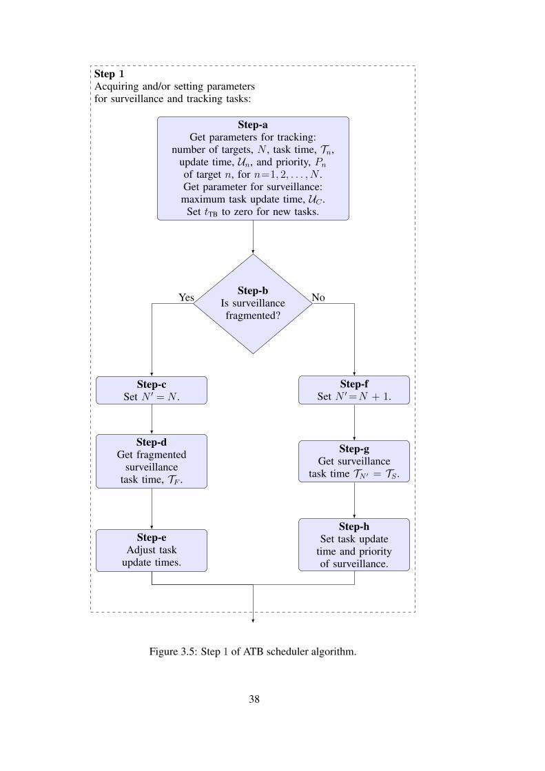
Step-aGet parameters for tracking:
number of targets, N , task time, Tn,update time, Un, and priority, Pn
of target n, for n=1, 2, . . . , N .Get parameter for surveillance:maximum task update time, UC .
Set tTB to zero for new tasks.
Step-bIs surveillancefragmented?
Step-cSet N ′ = N .
Step-dGet fragmented
surveillancetask time, TF .
Step-eAdjust task
update times.
Step-fSet N ′=N + 1.
Step-gGet surveillance
task time TN ′ = TS .
Step-hSet task update
time and priorityof surveillance.
Step 1Acquiring and/or setting parametersfor surveillance and tracking tasks:
Yes No
Figure 3.5: Step 1 of ATB scheduler algorithm.
38

Step-e1Is Ui controlled?i = 1, 2, . . . , N ′.
Step-e2Get surveillance task time, TS , andset surveillance task update time:US = max
{0, TS
[1−∑N ′
n=1On
]−1}.
Step-e3Is US = 0 orUS > UC?
Step-e4Estimate task update
time correction factor:
Cf =OT
100%− TSU−1C
> 1.
Step-e5Adjust task update times:
Un = Un·Cf ,n = 1, 2, . . . , N ′.
Step-e6Is US = UC
forced?
Step-e7Estimate task update
time correction factor:
Cf =OT
100%− TSU−1C
6 1.
Step-eAdjust task update times.
Yes
Yes
No
Yes
No
No
Figure 3.6: Step-e of ATB scheduler algorithm.
39
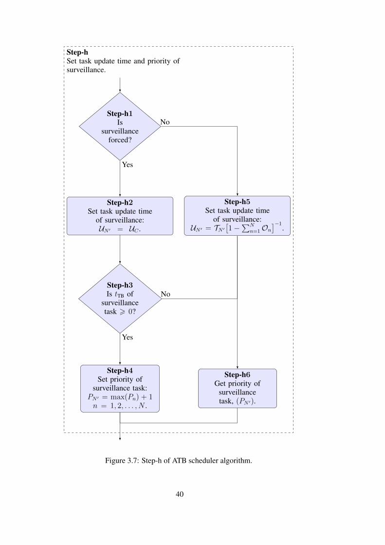
Step-h1Is
surveillanceforced?
Step-h2Set task update time
of surveillance:UN ′ = UC .
Step-h3Is tTB of
surveillancetask > 0?
Step-h4Set priority of
surveillance task:PN ′ = max(Pn) + 1n = 1, 2, . . . , N .
Step-h5Set task update time
of surveillance:UN ′ = TN ′
[1−∑N
n=1On
]−1.
Step-h6Get priority of
surveillancetask, (PN ′).
Step-hSet task update time and priority ofsurveillance.
Yes
Yes
No
No
Figure 3.7: Step-h of ATB scheduler algorithm.
40

Step 1
Step 2P = max(Pn),n = 1, 2, . . . , N ′.
Step 3Establish the
next set of tasks:K = {n : t
(n)TB > 0 ∧ Pn = P}
n = 1, 2, . . . , N ′.
Step 4Is K empty?
Step 9Is P = min(Pn)?n = 1, 2, . . . , N ′.
Step 10Decrease thepriority level:P = P − 1.
Step 5Choose task with
maximum tTB:i = argmax
Kt(K)TB .
Step 6Decrease tTB
of task i by itsupdate time:
t(i)TB = t
(i)TB − Ui.
Step 7Schedule task i.
Step 8Increase tTB of
all tasks by tasktime of task i:t(n)TB = t
(n)TB + Ti,
n = 1, 2, . . . , N ′.
Step 11Is N ′ = N?
Step 12Schedule asurveillancefragment.
Step 13Increase tTB of
all tasks by taskfragment time:t(n)TB = t
(n)TB + TF ,
n = 1, 2, . . . , N ′.
Step 14Set idle time, TI :TI = |max(t
(n)TB )|,
n = 1, 2, . . . , N ′.
Step 15Increase tTBof all tasks
by idle time:t(n)TB = t
(n)TB + TI ,
n = 1, 2, . . . , N ′.
No Yes
Yes
No
Yes No
Figure 3.8: Flow diagram of ATB scheduler algorithm.
41
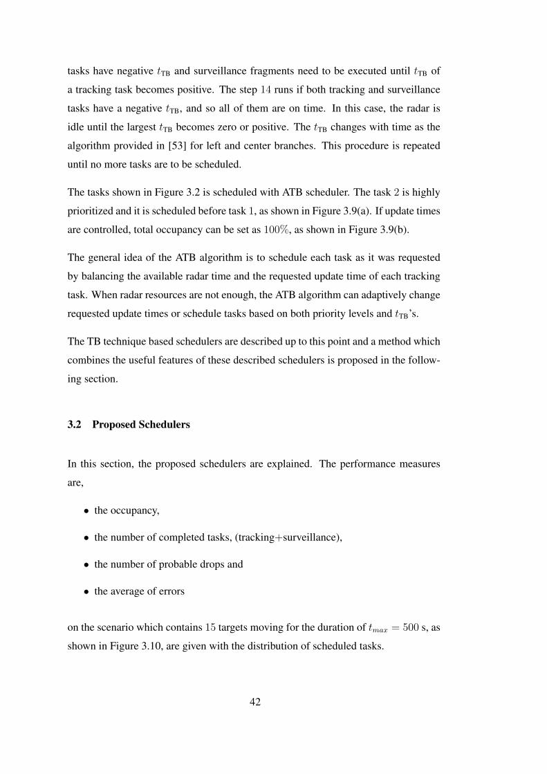
tasks have negative tTB and surveillance fragments need to be executed until tTB of
a tracking task becomes positive. The step 14 runs if both tracking and surveillance
tasks have a negative tTB, and so all of them are on time. In this case, the radar is
idle until the largest tTB becomes zero or positive. The tTB changes with time as the
algorithm provided in [53] for left and center branches. This procedure is repeated
until no more tasks are to be scheduled.
The tasks shown in Figure 3.2 is scheduled with ATB scheduler. The task 2 is highly
prioritized and it is scheduled before task 1, as shown in Figure 3.9(a). If update times
are controlled, total occupancy can be set as 100%, as shown in Figure 3.9(b).
The general idea of the ATB algorithm is to schedule each task as it was requested
by balancing the available radar time and the requested update time of each tracking
task. When radar resources are not enough, the ATB algorithm can adaptively change
requested update times or schedule tasks based on both priority levels and tTB’s.
The TB technique based schedulers are described up to this point and a method which
combines the useful features of these described schedulers is proposed in the follow-
ing section.
3.2 Proposed Schedulers
In this section, the proposed schedulers are explained. The performance measures
are,
• the occupancy,
• the number of completed tasks, (tracking+surveillance),
• the number of probable drops and
• the average of errors
on the scenario which contains 15 targets moving for the duration of tmax = 500 s, as
shown in Figure 3.10, are given with the distribution of scheduled tasks.
42

0 10 20 30 40 50 60 70 80 90 100
Tracking Task 2 with 60.00% Occupancy0 10 20 30 40 50 60 70 80 90 100
Tracking Task 1 with 25.00% Occupancy
0 10 20 30 40 50 60 70 80 90 100
Task Queue
0 10 20 30 40 50 60 70 80 90 100
−20
0
Time (s)
t TB
(s)
TB Scheme
Task 1 Task 2
(a) Task 2 is highly prioritized.
0 10 20 30 40 50 60 70 80 90 100
Tracking Task 2 with 70.59% Occupancy0 10 20 30 40 50 60 70 80 90 100
Tracking Task 1 with 29.41% Occupancy
0 10 20 30 40 50 60 70 80 90 100
Task Queue
0 10 20 30 40 50 60 70 80 90 100
−20
0
Time (s)
t TB
(s)
TB Scheme
Task 1 Task 2
(b) Task 2 is highly prioritized and task update times are controlled.
Figure 3.9: ATB scheduler example.
43

0◦
30◦
60◦
90◦
120◦
150◦
180◦
210◦
240◦
270◦
300◦
330◦
40 km
80 km
120 km
160 km
200 km
T1
T2
T3
T4T5
T6
T7
T8
T9
T10T11T12
T13
T14
T15
Sector 1 Sector 2 Sector 3
Figure 3.10: The scenario used to measure the performance of proposed schedulers.
3.2.1 Multi-Type Adaptive Time-Balance Scheduler
The multi-type adaptive time-balance scheduler (MTATBS) consists of four different
types of ATB scheduler differ with updating tTB’s and task selections. The following
sections describe these types.
3.2.1.1 MTATBS-Type 1
The MTATBS-Type 1 tries to update all available targets for positive tTB. It utilizes
the dynamic task prioritization to temporarily increase the priority of less important
task to the highest priority level. Hence, this task is scheduled for the next cycle of
scheduling. However, the scheduling of less important tasks that have less priority
can cause to increase tTB’s of other more important tasks. Thus, tTB of each target
monotonically increases, and the cost of each target also increases with the time goes
44

on. Since it tries to schedule all of available tasks, lateness values are smaller and the
distribution of scheduled tasks is usually more similar to a uniform distribution.
Figure 3.11, 3.12 and 3.13 show the performance measures of MTATBS-Type 1.
3.2.1.2 MTATBS-Type 2
The MTATBS-Type 2 mainly schedules more important tasks. Thus, tTB and the cost
of less important tasks increase rapidly. Lateness values are higher for MTATBS-Type
2 than MTATBS-Type 1, since MTATBS-Type 2 delays less important tasks.
Figure 3.14, 3.15 and 3.16 show the performance measures of MTATBS-Type 2.
3.2.1.3 MTATBS-Type 3
The MTATBS-Type 3 is similar to MTATBS-Type 1, except the decrement in tTB of
the scheduled task. It assigns the new tTB of the scheduled task as negative of update
time of this task instead of subtracting task update time from current tTB, in other
words, it resets the new tTB, after each update. This process avoids the monotonically
increment of tTB.
Figure 3.17, 3.18 and 3.19 show the performance measures of MTATBS-Type 3.
3.2.1.4 MTATBS-Type 4
The MTATBS-Type 4 is similar to MTATBS-Type 2, except the decrement in tTB of
the scheduled task. It assigns the new tTB of the scheduled task as negative of update
time of this task instead of subtracting task update time from current tTB, in other
words, it resets the new tTB, after each update. Hence, the cost of MTATBS-Type 4 is
always less than the cost of MTATBS-Type 1 and MTATBS-Type 2. The smaller tTB’s
also makes lateness values smaller. Lateness values are higher for MTATBS-Type 4
than MTATBS-Type 3, since MTATBS-Type 4 usually delays less important tasks.
Figure 3.20, 3.21 and 3.22 show the performance measures of MTATBS-Type 4.
45

T1 T2 T3 T4 T5 T6 T8 T9 T10 T11 T12 T13 T14 T15 Surv0
10
20
30
40
50
60
70
Task Id
Num
bero
fCom
plet
esDistribution of Tasks Scheduled with MTATBS-Type 1
Occupancy = 100.00%
# of completed tasks (T+S) = 432(389 + 43)
# of probable drops = 15
Average of errors = 1.70×10⁵ m2
(a) Task interleaving technique is disabled.
T1 T2 T3 T4 T5 T6 T8 T9 T10 T11 T12 T13 T14 T15 Surv0
20
40
60
80
100
120
140
160
Task Id
Num
bero
fCom
plet
es
Distribution of Tasks Scheduled with MTATBS-Type 1
Occupancy = 59.33%
# of completed tasks (T+S) = 1016(973 + 43)
# of probable drops = 15
Average of errors = 3.38×10⁴ m2
(b) Task interleaving technique is enabled.
Figure 3.11: Distribution of tasks scheduled with MTATBS-Type 1.
46

0 50 100 150 200 250 300 350 400 450 500
−20
0
20
40
60
80
100
120
Time (s)
t TB
(s)
TB Scheme for MTATBS-Type 1
T1T2T3T4T5T6T7T8T9T10T11T12T13T14T15Surv
(a) Task interleaving technique is disabled.
0 50 100 150 200 250 300 350 400 450 500−25
−20
−15
−10
−5
0
5
10
15
Time (s)
t TB
(s)
TB Scheme for MTATBS-Type 1
T1T2T3T4T5T6T7T8T9T10T11T12T13T14T15Surv
(b) Task interleaving technique is enabled.
Figure 3.12: TB schemes for MTATBS-Type 1.
47

0 5 10 15 20 25 30 35 400
20
40
60
80
100
Lateness (s)
Perc
enta
geof
Task
s(%
)Cumulative Distribution of Latenesses for MTATBS-Type 1
AllT1T2T3T4T5T8T9T10T11T12T13T14T15
(a) Task interleaving technique is disabled.
−8 −6 −4 −2 0 2 4 6 80
20
40
60
80
100
Lateness (s)
Perc
enta
geof
Task
s(%
)
Cumulative Distribution of Latenesses for MTATBS-Type 1
AllT1T2T3T4T5T6T8T9T10T11T12T13T14T15
(b) Task interleaving technique is enabled.
Figure 3.13: Cumulative distribution of latenesses for MTATBS-Type 1.
48

T1 T2 T3 T4 T5 T6 T8 T9 T10 T11 T12 T13 T14 T15 Surv0
10
20
30
40
50
60
70
Task Id
Num
bero
fCom
plet
es
Distribution of Tasks Scheduled with MTATBS-Type 2
Occupancy = 100.00%
# of completed tasks (T+S) = 438(395 + 43)
# of probable drops = 39
Average of errors = 1.53×10⁵ m2
(a) Task interleaving technique is disabled.
T1 T2 T3 T4 T5 T6 T8 T9 T10 T11 T12 T13 T14 T15 Surv0
20
40
60
80
100
120
140
160
Task Id
Num
bero
fCom
plet
es
Distribution of Tasks Scheduled with MTATBS-Type 2
Occupancy = 60.24%
# of completed tasks (T+S) = 1042(1000 + 42)
# of probable drops = 28
Average of errors = 1.08×10⁵ m2
(b) Task interleaving technique is enabled.
Figure 3.14: Distribution of tasks scheduled with MTATBS-Type 2.
49

0 50 100 150 200 250 300 350 400 450 500
0
50
100
150
200
Time (s)
t TB
(s)
TB Scheme for MTATBS-Type 2
T1T2T3T4T5T6T7T8T9T10T11T12T13T14T15Surv
(a) Task interleaving technique is disabled.
0 50 100 150 200 250 300 350 400 450 500
−20
0
20
40
60
80
Time (s)
t TB
(s)
TB Scheme for MTATBS-Type 2
T1T2T3T4T5T6T7T8T9T10T11T12T13T14T15Surv
(b) Task interleaving technique is enabled.
Figure 3.15: TB schemes for MTATBS-Type 2.
50

−5 0 5 10 15 20 250
20
40
60
80
100
Lateness (s)
Perc
enta
geof
Task
s(%
)
Cumulative Distribution of Latenesses for MTATBS-Type 2
AllT1T2T4T5T8T9T10T11T12T14T15
(a) Task interleaving technique is disabled.
0 10 20 30 40 50 60 700
20
40
60
80
100
Lateness (s)
Perc
enta
geof
Task
s(%
)
Cumulative Distribution of Latenesses for MTATBS-Type 2
AllT1T2T3T4T5T8T9T10T11T12T13T14T15
(b) Task interleaving technique is enabled.
Figure 3.16: Cumulative distribution of latenesses for MTATBS-Type 2.
51
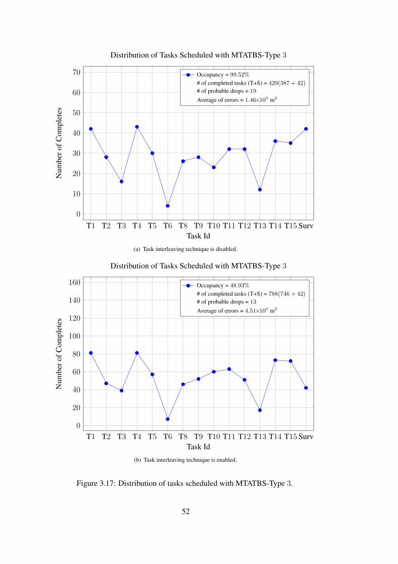
T1 T2 T3 T4 T5 T6 T8 T9 T10 T11 T12 T13 T14 T15 Surv0
10
20
30
40
50
60
70
Task Id
Num
bero
fCom
plet
esDistribution of Tasks Scheduled with MTATBS-Type 3
Occupancy = 99.52%
# of completed tasks (T+S) = 429(387 + 42)
# of probable drops = 19
Average of errors = 1.46×10⁵ m2
(a) Task interleaving technique is disabled.
T1 T2 T3 T4 T5 T6 T8 T9 T10 T11 T12 T13 T14 T15 Surv0
20
40
60
80
100
120
140
160
Task Id
Num
bero
fCom
plet
es
Distribution of Tasks Scheduled with MTATBS-Type 3
Occupancy = 48.93%
# of completed tasks (T+S) = 788(746 + 42)
# of probable drops = 13
Average of errors = 4.51×10⁴ m2
(b) Task interleaving technique is enabled.
Figure 3.17: Distribution of tasks scheduled with MTATBS-Type 3.
52
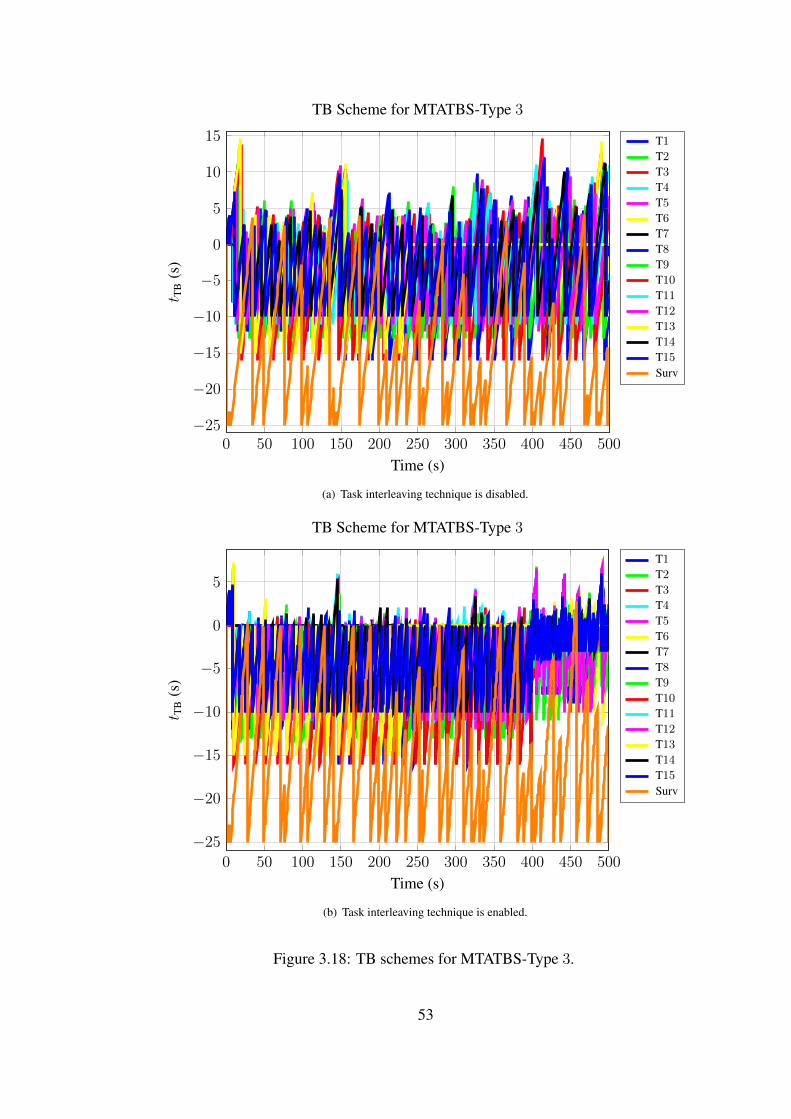
0 50 100 150 200 250 300 350 400 450 500−25
−20
−15
−10
−5
0
5
10
15
Time (s)
t TB
(s)
TB Scheme for MTATBS-Type 3
T1T2T3T4T5T6T7T8T9T10T11T12T13T14T15Surv
(a) Task interleaving technique is disabled.
0 50 100 150 200 250 300 350 400 450 500
−25
−20
−15
−10
−5
0
5
Time (s)
t TB
(s)
TB Scheme for MTATBS-Type 3
T1T2T3T4T5T6T7T8T9T10T11T12T13T14T15Surv
(b) Task interleaving technique is enabled.
Figure 3.18: TB schemes for MTATBS-Type 3.
53
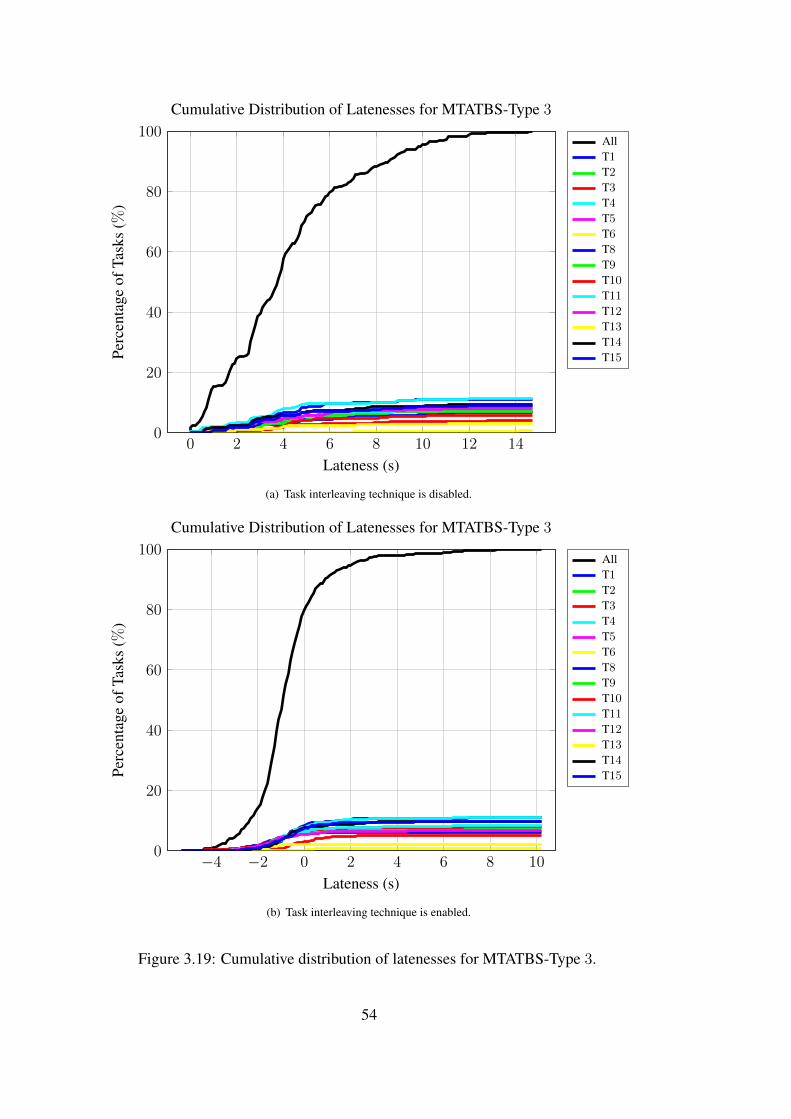
0 2 4 6 8 10 12 140
20
40
60
80
100
Lateness (s)
Perc
enta
geof
Task
s(%
)Cumulative Distribution of Latenesses for MTATBS-Type 3
AllT1T2T3T4T5T6T8T9T10T11T12T13T14T15
(a) Task interleaving technique is disabled.
−4 −2 0 2 4 6 8 100
20
40
60
80
100
Lateness (s)
Perc
enta
geof
Task
s(%
)
Cumulative Distribution of Latenesses for MTATBS-Type 3
AllT1T2T3T4T5T6T8T9T10T11T12T13T14T15
(b) Task interleaving technique is enabled.
Figure 3.19: Cumulative distribution of latenesses for MTATBS-Type 3.
54

T1 T2 T3 T4 T5 T6 T8 T9 T10 T11 T12 T13 T14 T15 Surv0
10
20
30
40
50
60
70
Task Id
Num
bero
fCom
plet
es
Distribution of Tasks Scheduled with MTATBS-Type 4
Occupancy = 98.90%
# of completed tasks (T+S) = 429(385 + 44)
# of probable drops = 37
Average of errors = 1.56×10⁵ m2
(a) Task interleaving technique is disabled.
T1 T2 T3 T4 T5 T6 T8 T9 T10 T11 T12 T13 T14 T15 Surv0
20
40
60
80
100
120
140
160
Task Id
Num
bero
fCom
plet
es
Distribution of Tasks Scheduled with MTATBS-Type 4
Occupancy = 43.05%
# of completed tasks (T+S) = 629(583 + 46)
# of probable drops = 1
Average of errors = 5.83×10⁴ m2
(b) Task interleaving technique is enabled.
Figure 3.20: Distribution of tasks scheduled with MTATBS-Type 4.
55

0 50 100 150 200 250 300 350 400 450 500
−20
−10
0
10
20
30
Time (s)
t TB
(s)
TB Scheme for MTATBS-Type 4
T1T2T3T4T5T6T7T8T9T10T11T12T13T14T15Surv
(a) Task interleaving technique is disabled.
0 50 100 150 200 250 300 350 400 450 500−25
−20
−15
−10
−5
0
5
10
Time (s)
t TB
(s)
TB Scheme for MTATBS-Type 4
T1T2T3T4T5T6T7T8T9T10T11T12T13T14T15Surv
(b) Task interleaving technique is enabled.
Figure 3.21: TB schemes for MTATBS-Type 4.
56

0 5 10 15 20 25 300
20
40
60
80
100
Lateness (s)
Perc
enta
geof
Task
s(%
)
Cumulative Distribution of Latenesses for MTATBS-Type 4
AllT1T2T3T4T5T8T9T10T11T12T13T14T15
(a) Task interleaving technique is disabled.
−6 −4 −2 0 2 4 6 8 10 12 14 160
20
40
60
80
100
Lateness (s)
Perc
enta
geof
Task
s(%
)
Cumulative Distribution of Latenesses for MTATBS-Type 4
AllT1T2T3T4T5T6T8T9T10T11T12T13T14T15
(b) Task interleaving technique is enabled.
Figure 3.22: Cumulative distribution of latenesses for MTATBS-Type 4.
57

3.2.1.5 Explanation About TB Schemes
As a remark to the readers, it should be interpreted that the dropping directly to zero
and not changing after a time level means that the target is dropped at that time.
Furthermore constant tTB’s equal to zero shows that the target is out of radar scope.
The target 2 and target 6, as shown in Figure 3.23(a), are dropped at∼ 420 and∼ 430
s respectively. The target 1, range of whom is always higher than rmax as shown in
Figure 3.23(b), is not detected within the simulation interval.
Negative lateness values usually appear, when type 1 and type 2 of MTATBS is uti-
lized. It is the result of tTB update procedure. Decreasing tTB by task update time does
not guarantee that the task will not be scheduled for a while that is equal to update
time. If it’s current tTB is larger than its update time, new tTB after subtraction will
already be positive. Therefore the same task may be chosen at the next scheduling
cycle. It is very easy to see it from TB scheme shown in Figure 3.23(a). If a task
with a tTB starts to decrease monotonically after a few scheduling cycles, the task
must have negative lateness values. In the Figure 3.23(a), tTB of target 7 decreased
to 0 from ∼ 220 between ∼ 430 and ∼ 480 s. It is the result of frequent scheduling,
namely consecutively updating, of target 7, while there is no need to do so. These
consecutive updates may be viewed as the waste of sources.
The effect of priorities is revisited by using the type 2 scheduler which is said to
schedule only more important tasks. By disabling dynamic task prioritization, the
case is emphasized in Figure 3.23(a). The target 5 and target 14 have the priority
level 1, when they are detected. Then, the scheduler could not share the radar time
resource until ∼ 480 s, while target 7 is unnecessarily scheduled. Hence, tTB of less
important tasks usually increases monotonically.
58

0 50 100 150 200 250 300 350 400 450 500
0
100
200
300
400
Time (s)
t TB
(s)
TB Scheme
Less important tasks
Targets are dropped
Consecutive updates
T1T2T3T4T5T6T7T8T9T10T11T12T13T14T15Surv
(a) TB scheme.
0◦
30◦
60◦
90◦
120◦
150◦
180◦
210◦
240◦
270◦
300◦
330◦
40 km
80 km
120 km
160 km
200 km
T1
T2
T3
T4
T5
T6
T7
T8
T9
T10
T11
T12
T13
T14
T15
Sector 1 Sector 2 Sector 3
(b) Tracking PPI.
Figure 3.23: Explanation about TB schemes.
59

3.2.2 Knapsack Scheduler
In combinatorial optimization field, a well-known problem, knapsack problem, is
studied to make a selection within available items that each item has a value and a
weight so that the total value is maximized and the total weight does not exceed the
allowed weight for selected items [54]. Its name is thought to come from a problem
which usually arises in daily life whenever one wants to pack a suitcase or knapsack
with useful objects in a proper way.
The applicability of knapsack problem for financial and industrial applications where
resource management is the main concern increases the research on solution methods
in many areas, such as applied mathematics, operational research. After the pioneer
work [55] that discusses knapsack problem and presents some solution methods for it,
there are many algorithms, most of them are described in [56], to solve this problem.
A simple example of knapsack problem is shown in Figure 3.24. Here, there are 4
different gifts and a knapsack for carrying them, but it is allowed to carry a maximum
of only 10 kg in knapsack. Thus, the aim is to carry gifts that have maximum total
weight less than 10 kg and maximum ratio of total value per total weight.
Since it is a toy example, its solution is too simple with greedy algorithm. Firstly, the
ratio of value per weight for each gift is computed as follows:
Gift-1 :36
6= 6, Gift-2 :
20
4= 5, Gift-3 :
24
3= 8, Gift-4 :
24
8= 3.
Then, the gift which has the highest ratio, is chosen. After choosing gift-3, gift-1 or
gift-2 can be chosen. As gift-1 has higher ratio than gift-2, gift-1 is chosen.
Knapsack scheduler (KS) is built on the solution methods of knapsack problem. The
scheduling problem is solved by maximizing the total value of N tracking tasks and
the surveillance task. Total value may be referred as the total utility or negative of
the total cost for each scheduling epoch. This method only help to select tasks to be
processed, while sorting the selected tasks is another problem. Thus, KS uses two-
step scheduling method where the first step is macro scheduler and the second step is
micro scheduler, to schedule the tasks. The following sections briefly describe these
schedulers.
60
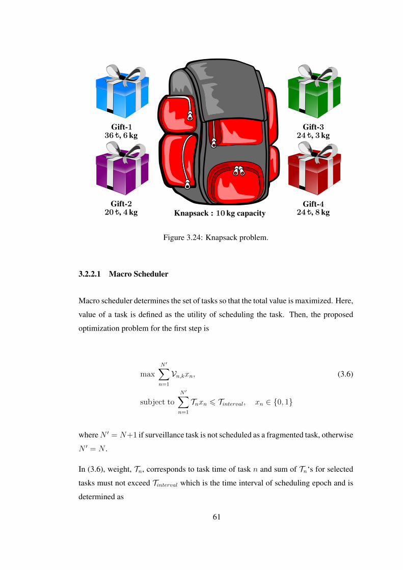
Gift-136 , 6kg
Gift-324 , 3kg
Knapsack : 10kg capacityGift-2
20 , 4kgGift-4
24 , 8kg
Figure 3.24: Knapsack problem.
3.2.2.1 Macro Scheduler
Macro scheduler determines the set of tasks so that the total value is maximized. Here,
value of a task is defined as the utility of scheduling the task. Then, the proposed
optimization problem for the first step is
maxN ′∑
n=1
Vn,kxn, (3.6)
subject toN ′∑
n=1
Tnxn 6 Tinterval, xn ∈ {0, 1}
whereN ′ = N+1 if surveillance task is not scheduled as a fragmented task, otherwise
N ′ = N .
In (3.6), weight, Tn, corresponds to task time of task n and sum of Tn‘s for selected
tasks must not exceed Tinterval which is the time interval of scheduling epoch and is
determined as
61
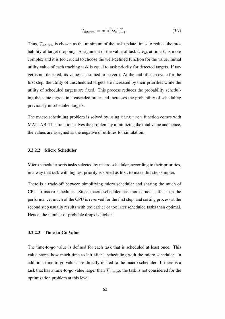
Tinterval = min {Un}N′
n=1 . (3.7)
Thus, Tinterval is chosen as the minimum of the task update times to reduce the pro-
bability of target dropping. Assignment of the value of task i, Vi,k at time k, is more
complex and it is too crucial to choose the well-defined function for the value. Initial
utility value of each tracking task is equal to task priority for detected targets. If tar-
get is not detected, its value is assumed to be zero. At the end of each cycle for the
first step, the utility of unscheduled targets are increased by their priorities while the
utility of scheduled targets are fixed. This process reduces the probability schedul-
ing the same targets in a cascaded order and increases the probability of scheduling
previously unscheduled targets.
The macro scheduling problem is solved by using bintprog function comes with
MATLAB. This function solves the problem by minimizing the total value and hence,
the values are assigned as the negative of utilities for simulation.
3.2.2.2 Micro Scheduler
Micro scheduler sorts tasks selected by macro scheduler, according to their priorities,
in a way that task with highest priority is sorted as first, to make this step simpler.
There is a trade-off between simplifying micro scheduler and sharing the much of
CPU to macro scheduler. Since macro scheduler has more crucial effects on the
performance, much of the CPU is reserved for the first step, and sorting process at the
second step usually results with too earlier or too later scheduled tasks than optimal.
Hence, the number of probable drops is higher.
3.2.2.3 Time-to-Go Value
The time-to-go value is defined for each task that is scheduled at least once. This
value stores how much time to left after a scheduling with the micro scheduler. In
addition, time-to-go values are directly related to the macro scheduler. If there is a
task that has a time-to-go value larger than Tinterval, the task is not considered for the
optimization problem at this level.
62

3.2.2.4 An Example
The scenario shown in Figure 3.25 is scheduled by KS. Time-to-go scheme is shown
in Figure 3.26(a) and value vs. time graph is shown in Figure 3.26(b). The KS always
schedules more tracking tasks, as it is sometimes not aware of scheduling surveillance
tasks.
The KS is slower than the other types of scheduler. Since increasing the number
of detected targets by one, exponentially increases the computation load. Therefore
the maximum number of targets must be limited. Furthermore, a modification is
to schedule the targets with respect to their sectors is proposed. For example, if
there are 30 targets and detection region is bounded by sector 1 and sector 2, KS
considers targets in sector 1 ahead to targets in sector 2 by using common Tinterval.This modification is very useful to schedule more targets in a limited processing time,
since scheduling problem is solved among targets in each sector individually.
T1 T2 T3 T4 T5 T6 T8 T9 T10 T11 T12 T13 T14 T15 Surv0
10
20
30
40
50
60
70
Task Id
Num
bero
fCom
plet
es
Distribution of Tasks Scheduled with KS
Occupancy = 99.60%
# of completed tasks (T+S) = 460(457 + 3)
# of probable drops = 66
Average of errors = 1.45×10⁵ m2
Figure 3.25: Distribution of tasks scheduled with KS.
63
0 50 100 150 200 250 300 350 400 450 500
0
5
10
15
20
25
30
35
Time (s)
t TG
(s)
Time-to-Go Scheme
T1T2T3T4T5T6T7T8T9T10T11T12T13T14T15Surv
(a)
0 50 100 150 200 250 300 350 400 450 5000
20
40
60
80
100
120
140
160
180
Time (s)
Val
ue
Value vs. Time
T1T2T3T4T5T6T7T8T9T10T11T12T13T14T15Surv
(b)
Figure 3.26: (a) Time-to-Go scheme and (b) value vs. time graph for KS.
64
3.3 Summary
In this chapter, time-balance technique based schedulers found in [47, 48, 53] are
described. Then, a scheduler referred to as MTATBS is proposed. The MTATBS
covers the appropriate features of the scheduler described in [48] and handles the
optional techniques described in the previous chapter.
In the final part of this chapter, an optimization-based method, KS, utilizing binary
integer programming, is proposed to make a comparison with MTATBS, and it is seen
that KS is not capable of task interleaving due to computational complexity.
Up to here, MTATBS is not well-defined for target selection, when there are more
than one targets which request track update. Hence, the suggested methods for target
selection are described in the next chapter.
65

66

CHAPTER 4
DECISION METHODS FOR TIME-BALANCE SCHEDULERS
Target selection problem emerges when there are more than one target requesting
track update. If MTATBS is forced to make a selection, it firstly selects the targets
with the highest priority level. Then, it looks for the targets which have the highest tTB
within these targets. If there are more than one target after the second stage, it selects
a target which has smaller task id than the others. This target selection procedure is
not reliable for the real systems, since task id does not reflect track informations.
In this chapter, the methods to handle the target selection problem are described. To
do this, the well-known machine replacement problem is examined. Then, the analo-
gies between target selection and machine replacement problems are emphasized.
The method for target selection is adopted from a solution of the machine replace-
ment problem, found in [57], by conducting the analogies and modifications which
are related to tracking performance. In addition to this method, two other ad hoc
methods which only depend on tracking information are given.
The machine replacement problem is the uncertainty of the time when the existing
machine should be replaced. For example, there is only one oven (machine) at a
bakery and the bread (product) can be delicious (conforming) or tasteless (defective),
if this oven is used. The cooking performance of the oven deteriorates due to aging
(deterioration) process, and the oven can be in good or bad state due to its cooking
performance. Hence, a delicious bread can be cooked by an oven, state of which is
not exactly known. This case is valid, when the bread is tasteless. Therefore it is
possible to say that an oven which is in good state can cook a tasteless bread. The
cost of a new oven (replacement cost) is too expensive to frequently renew the oven.
67
Despite the complexity of problem, the baker can estimate the time when the existing
oven should be replaced with a new one by utilizing one of the solution methods for
the machine replacement problem.
Returning to the target selection problem, a target can be in one of the states, "Good"
and "Bad" owing to track quality during the track updates. The target supposed to be
in "Good" state tells scheduler that there is no need to update its track at that time,
since the update is not necessary, in other words it is a waste of radar time that can
be better put into use by doing another task. The target in a "Bad" state alerts the
scheduler that it is important to do update the track, since the scheduler knows that
the target will be probably dropped for the next scheduling time, if its track is not
updated as soon as possible.
It is easily concluded from above that assigning a state to each target helps the sched-
uler decide which one of the targets currently deserves the track update. Especially,
it will be crucial for the scheduler, when the radar is in overloaded case. Executing
an unnecessary task may decrease the tracking performance by causing an increase in
the delay of other tasks in the queue. Therefore the state dependent target selection is
crucial for both of cases, while the main goal of the state assignment is to deal with
overloaded case.
4.1 Method of Decision Policy
The RRM problem is examined in analogy with machine replacement problem. The
machine replacement, machine maintenance and quality control applications are wi-
dely popular in decision making literature. The discussed method is adopted from
[57] that analyzes the binomial observation model for machine replacement problem.
The binomial observation is the classification of the quality of products as conform-
ing units or defecting units according to measurements while production process is in
either "Good" or "Bad" state. True state of the process is assumed to be unobservable
and only the measured quality of the produced units gives the tips about the true state
which the process is most likely to be in. Thus, the production process is modeled as
a partially observable Markov decision process (POMDP) with control limits.
68

The most interesting part of [57] is the proof for that the infinite-horizon control limit
which is defined as a function of probability of obtaining conforming unit can be
calculated by solving a finite set of linear equations. Because POMDPs are known to
be usually hard to solve due to prohibitively large size of the state space [58]. It is
also known that the length of time horizon effects the tractability of the problem, i.e.
a 5-horizon problem is harder than 2-horizon problem.
One-to-one adoption from the machine replacement problem to the target selection
problem of RRM is really hard. Because procedures of the referred machine replace-
ment problem consider only one machine. In addition, cost of renewing the machine
is fixed and decision making policy can become a degenerate policy, such as always
continue with the same machine when chosen cost value makes the other action, re-
place the machine the worst selection for infinite-horizon case.
In the case of target selection problem, there are many targets and each target is
thought to represent a single machine. At each instant of decision making, only one
target can be chosen to update its track. Therefore decision making process specifies
targets that need track update, and then it selects one of them which improves at most
of the tracking performance of radar.
Another difficulty is to specify the cost value associated with each target. At each
instant, the scheduler can choose only one of available targets to update its track.
Thus, it would be almost impossible to define cost value of each target as independent
from the other targets.
Furthermore, it is necessary to explain how to obtain "Good" or "Bad" state infor-
mation. To do so, IMM algorithm in Appendix A, is utilized through advantage of
providing mode-probabilities. Mode-probabilities tell tracker how motion model of
moving targets is distributed at each instant. For example, it is given that there are
2 motion models which obey the constant velocity model (CV) with different pro-
cess noise covariances, Q1 and Q2. There is a relation between these covariances as
follows:
Q2 = 1002Q1.
Hence, the model-1 with Q1 indicates non-maneuvering motion and the model-2 with
Q2 indicates maneuvering motion. If the mode-probabilities are distributed as 0.7
69

and 0.3 for model-1 and model-2 respectively, tracker presumes that the target is not
probably maneuvering. For both the tracker and scheduler, the main concern is to
know that the target is maneuvering or not maneuvering. Owing to this knowledge,
the tracker can predict tracks of a target with less error for an interval when there is not
any measurement provided, and the scheduler can mostly concentrate on to schedule
tracking tasks of highly maneuvering targets to enhance the tracking performance.
Radar plan position indicator (PPI) displays taken from a simple scenario are shown
in Figure 4.1(a) belongs one of less maneuvering targets and Figure 4.1(b) belongs
one of highly maneuvering targets. These figures are given only to make clear why
the classification of targets as maneuvering and non-maneuvering is required. There-
fore it is not necessary to give the complete scenario with parameters at this point.
The tracking task of each target is competing for radar time and there is not a deci-
sion method which classifies the target as maneuvering or non-maneuvering. Hence,
the scheduler selects a target which has smaller task id than the others, when there
is a target selection problem. Then confidence ellipses shown on the displays point
out how well the tracker predicts positions of moving targets. Larger ellipses indi-
cate worse predictions and smaller ellipses indicate better predictions. Therefore it is
easily deduced that maneuvering targets cause worse predictions.
In this manner, a target classified as non-maneuvering, is indicated to be in Good
state and a target classified as maneuvering, is indicated to be in Bad state. As men-
tioned before, the probability of being in Good state is defined to be equal to mode-
probability of motion model-1 with Q1 provided by IMM estimator.
The decision making process for updating a target track requires to observe (measure)
the quality of target track. The track is referred to as good track when trace of tracking
error covariance is within the allowed values. Otherwise it is referred to as bad track.
Then, the conditional observation probabilities are
• θ0, the probability of obtaining a good track given that corresponding target is
in Good state,
• θ1, the probability of obtaining a good track given that corresponding target is
in Bad state,
70

0◦
30◦
60◦
90◦
120◦
150◦
180◦
210◦
240◦
270◦
300◦
330◦
S1
S2
S3
Initial TrackTrue TracksMeasurementsDetectionsIMM TrackingConfidenceEllipses
(a)
0◦
30◦
60◦
90◦
120◦
150◦
180◦
210◦
240◦
270◦
300◦
330◦
S1
S2
S3
Initial TrackTrue TracksMeasurementsDetectionsIMM TrackingConfidenceEllipses
(b)
Figure 4.1: Tracking example of (a) non-maneuvering and (b) maneuvering targets.
71
• 1− θ0, the probability of obtaining a bad track given that corresponding target
is in Good state,
• 1− θ1, the probability of obtaining a bad track given that corresponding target
is in Bad state,
and it is assumed that θ0 > θ1 due to reliability on measurement process.
The state of a target is probabilistically evolving, such that if the target is in Good
state at time k, it will be in Good state with probability r or it will change its state
to Bad with probability 1 − r at time k + 1. Once the target enters Bad state, it is
assumed to remain that state until its track is updated. The last sentence can be a bit
confusing, since it claims that if a target start maneuvering, the target will continue
maneuvering until a track update. In real world, the targets perform maneuvering in
a random order so that they try to decrease the probability of being tracked.
If a target supposed to maneuver, its bearing (or azimuth) angle will start to change
with higher deviation which cannot be tolerated by prediction. Seeing Figure 4.1(b),
IMM tracking points are not compatible with the true tracks at the points where target
performs maneuvering and prediction error grows up until a measurement is taken at
detection points. Once a target enters to Bad state, it is assumed to stay there until
radar takes a measurement. Thus, the case is summarized with the last statement.
Actions are UPD (update) and NUPD (not update) for the decision making process to
update a target track. UPD action is similar to replace the machine action comes with
a cost K that will be explained later. Again, UPD action may fail to guarantee that a
target will be absolutely in Good state after applying the action. The target will be in
Good state with probability q after taking the UPD action.
If NUPD action is taken, the transition of target states becomes a time-homogeneous
Markov chain with Good state, a transient state, and Bad state, an absorbing state.
Because NUPD action is similar to continue with the same machine action does noth-
ing to change the process environment and the states only change due to evolving of
the process.
In the following sections, the detailed description is presented for this scheme.
72

4.1.1 Problem Model
It is supposed that there are Nk targets at time k. Hence, there are Nk distinct Markov
chains corresponding to each target, and the state transition probabilities of each target
are independent.
Target n obeys a 2-state Markov chain with the following descriptions.
• State is xnk ∈ {1, 2}, where 1 denotes Good state and 2 denotes Bad state, with
initial probability P (xn0 = i) = 0.5 for i = 1, 2.
• Observation is ynk ∈ {gt, bt}, where gt denotes good track and bt denotes bad
track.
• Action is unk ∈ {0, 1}, where 0 denotes NUPD action and 1 denotes UPD action,
at time k for n = 1, 2, . . . , Nk.
The transition probability matrices are
P (0) =
r 1− r
0 1
and P (1) =
q 1− qq 1− q
, (4.1)
where r = P (xnk+1 = 1|xnk = 1, unk = 0) and q = P (xnk+1 = 1|xnk , unk = 1) are the
transition probabilities by taking NUPD and UPD actions respectively.
Markov chains are shown in Figure 4.2 for NUPD and UPD actions.
Taking NUPD action, state-1 represents a transient state and state-2 represents an
absorbing state, shown in Figure 4.2(a) for r ∈ (0, 1). Taking UPD action, both
1 2r 11− r
(a) unk = 0
1 2
1− q
1− q
q q
(b) unk = 1
Figure 4.2: Markov chains for (a) NUPD and (b) UPD actions.
73
state-1 and state-2 become transient state, as shown in Figure 4.2(b), unless q is not
assumed to be equal to 1 which claims the target is exactly in state-1 after UPD action.
Regarding to descriptions, the conditional observation probabilities previously stated
are expressed as follows:
P (ynk = gt|xnk = 1) = θ0, (4.2)
P (ynk = gt|xnk = 2) = θ1, (4.3)
P (ynk = bt|xnk = 1) = 1− θ0, (4.4)
P (ynk = bt|xnk = 2) = 1− θ1. (4.5)
All of the variables essential to model the problem are briefly presented. In the next
section, they are utilized to derive expressions for solving the problem.
4.1.2 Derivation of Required Expressions
It is important to remember that all derivations are originated to [57] and the idea is
given in the same order as in referred work, while notations are changed and addi-
tional details are given to make explanation clearer.
Original notation is not sufficient to denote target id and time information. Hence
a time term, k, and target id term, n, are inserted as subscript and superscript re-
spectively wherever they are required. Functions which depend on observations are
denoted with the observation term inserted as a subscript to a calligraphic letter.
Starting with the mostly used function, the probability of being in Good state is
µnk = P (xnk = 1), (4.6)
where the symbol, µ is chosen to remind that probability of being in Good state is
directly related to mode-probability provided by IMM estimator.
Then, the probability of observing good track is
74
P (ynk = gt) =2∑
i=1
P (ynk = gt|xnk = i)P (xnk = i), (4.7)
= θ0µnk + θ1(1− µnk),
= (θ0 − θ1)µnk + θ1. (4.8)
Similarly, the probability of observing bad track is
P (ynk = bt) =2∑
i=1
P (ynk = bt|xnk = i)P (xnk = i), (4.9)
= (1− θ0)µnk + (1− θ1)(1− µnk),
= 1− (θ0 − θ1)µnk − θ1, (4.10)
= 1− P (ynk = gt). (4.11)
Hereafter, the observation probabilities expressed in (4.8) and (4.10) are defined as a
functions of µnk , since the only time-variant variable is µnk while θ0 and θ1 are depicted
as constants. The observation probabilities are
Pgt(µnk) , P (ynk = gt), (4.12)
= (θ0 − θ1)µnk + θ1, (4.13)
Pbt(µnk) , P (ynk = bt), (4.14)
= 1− (θ0 − θ1)µnk − θ1. (4.15)
By applying Bayes’ theorem, the posterior probabilities for Good state are given
P (xnk = 1|ynk = gt) =P (ynk = gt|xnk = 1)P (xnk = 1)
P (ynk = gt), (4.16)
=θ0µ
nk
Pgt(µnk), (4.17)
P (xnk = 1|ynk = bt) =P (ynk = bt|xnk = 1)P (xnk = 1)
P (ynk = bt), (4.18)
=(1− θ0)µnkPbt(µnk)
. (4.19)
75

The probability of being in Good state given that good track is observed and the
probability of being in Good state given that bad track is observed are given in (4.17)
and (4.19) respectively.
Using Markov property, it is assumed xnk+1 is conditionally independent of ynk [59]
so that the conditional probability of the next state is j given that gt is observed and
NUPD action is taken in the current state is i, can be written as
P (xnk+1 = j|xnk = i, ynk = gt, unk = 0) = P (xnk+1 = j|xnk = i, unk = 0), (4.20)
= Pij(unk), (4.21)
where i, j = 1, 2.
The posterior probabilities of the current state at time k are expressed in (4.17) and
(4.19). Furthermore, it is better to get information about the next state. By using these
expressions and the law of total probability, the conditional probabilities of the next
state are obtained. The probability of being in Good state at next time given that good
track is observed and NUPD action is taken at current time is
P (xnk+1 = 1|ynk = gt, unk = 0) =2∑
i=1
P (xnk+1 = 1, xnk = i|ynk = gt, unk = 0), (4.22)
=2∑
i=1
P (xnk+1 = 1|xnk = i, ynk = gt, unk = 0)
P (xnk = i|ynk = gt, unk = 0),
=2∑
i=1
Pi1(unk)P (xnk = i|ynk = gt),
= r · P (xnk = 1|ynk = gt)
+ 0 · P (xnk = 2|ynk = gt), (4.23)
=rθ0µ
nk
Pgt(µnk), (4.24)
and the probability of being in Good state at next time given that bad track is observed
and NUPD action is taken at current time is
76
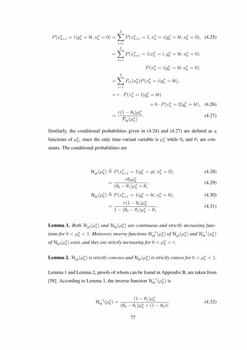
P (xnk+1 = 1|ynk = bt, unk = 0) =2∑
i=1
P (xnk+1 = 1, xnk = i|ynk = bt, unk = 0), (4.25)
=2∑
i=1
P (xnk+1 = 1|xnk = i, ynk = bt, unk = 0)
P (xnk = i|ynk = bt, unk = 0),
=2∑
i=1
Pi1(unk)P (xnk = i|ynk = bt),
= r · P (xnk = 1|ynk = bt)
+ 0 · P (xnk = 2|ynk = bt), (4.26)
=r(1− θ0)µnkPbt(µnk)
. (4.27)
Similarly, the conditional probabilities given in (4.24) and (4.27) are defined as a
functions of µnk , since the only time-variant variable is µnk while θ0 and θ1 are con-
stants. The conditional probabilities are
Hgt(µnk) , P (xnk+1 = 1|ynk = gt, unk = 0), (4.28)
=rθ0µ
nk
(θ0 − θ1)µnk + θ1, (4.29)
Hbt(µnk) , P (xnk+1 = 1|ynk = bt, unk = 0), (4.30)
=r(1− θ0)µnk
1− (θ0 − θ1)µnk − θ1. (4.31)
Lemma 1. Both Hgt(µnk) and Hbt(µ
nk) are continuous and strictly increasing func-
tions for 0 < µnk < 1. Moreover, inverse functionsH−1gt (µnk) ofHgt(µnk) andH−1bt (µnk)
ofHbt(µnk) exist, and they are strictly increasing for 0 < µnk < r.
Lemma 2. Hgt(µnk) is strictly concave andHbt(µ
nk) is strictly convex for 0 < µnk < 1.
Lemma 1 and Lemma 2, proofs of whom can be found in Appendix B, are taken from
[58]. According to Lemma 1, the inverse functionH−1bt (µnk) is
H−1bt (µnk) =(1− θ1)µnk
(θ0 − θ1)µnk + (1− θ0)r(4.32)
77

for 0 < µnk < r. Furthermore, existence of inverse leads to utilize function composi-
tion, such that
Hbt
(H−1bt (µnk)
)= µnk .
Then, a notation can be used
H`bt(µ
nk) = Hbt
(H`−1bt (µnk)
)orH−`bt (µnk) = H−1bt
(H−`+1bt (µnk)
)
for ` ∈ Z+ and it may be necessary to remind that
H0bt(µ
nk) = Hbt
(H−1bt (µnk)
)= µnk .
The functionsHgt(µnk) andHbt(µ
nk) depend on fixed parameters, r, θ0 and θ1 as well.
The critical point for choosing the fixed parameters is to ensure the criteria, rθ0 > θ1,
so thatHgt(µ∗) = µ∗ does exist. The value of µ∗ is computed as
µ∗ =rθ0 − θ1θ0 − θ1
. (4.33)
The point, µ∗, divides the domain of µnk into 2 sub-domains, µ∗ < Hgt(µnk) < µnk for
µnk > µ∗ and Hgt(µnk) > µnk for 0 < µnk < µ∗. If rθ0 6 θ1, then 0 < Hgt(µ
nk) < µnk
for 0 < µnk 6 1, and hence,Hgt(µ∗) = µ∗ does not exist.
Figure 4.3 illustrates both of these conditions for the functionsHgt(µnk) andHbt(µ
nk).
The first condition, rθ0 > θ1, is satisfied with r = 0.8, θ0 = 0.9 and θ1 = 0.4,
as shown in Figure 4.3(a). The value of µ∗ is computed as 0.64 by using (4.33).
According to this value, it is concluded that if the probability of being in Good state
is less than 0.64, then the probability of being in Good state at next time increases
by observing good track at current time. Or vice versa, if the probability of being in
Good state is greater than 0.64, then the probability of being in Good state at next time
decreases by observing good track at current time. The second condition, rθ0 < θ1,
is satisfied with r = 0.6, θ0 = 0.6 and θ1 = 0.4, as shown in Figure 4.3(b). Here, the
linear function µnk does not intersect Hgt(µnk) at any point for µnk > 0. Therefore the
probability of being in Good state at next time always decreases by observing good
track at current time. Then, observations become less valuable to give an idea about
the probability of being in Good state.
78
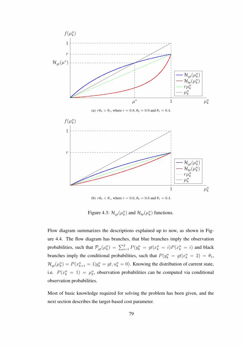
µ∗ 1
Hgt(µ∗)
r
1
µnk
f(µnk)
Hgt(µnk)
Hbt(µnk)
rµnk
µnk
(a) rθ0 > θ1, where r = 0.8, θ0 = 0.9 and θ1 = 0.4.
1
r
1
µnk
f(µnk)
Hgt(µnk)
Hbt(µnk)
rµnk
µnk
(b) rθ0 < θ1, where r = 0.6, θ0 = 0.6 and θ1 = 0.4.
Figure 4.3: Hgt(µnk) andHbt(µ
nk) functions.
Flow diagram summarizes the descriptions explained up to now, as shown in Fig-
ure 4.4. The flow diagram has branches, that blue branches imply the observation
probabilities, such that Pgt(µnk) =∑2
i=1 P (ynk = gt|xnk = i)P (xnk = i) and black
branches imply the conditional probabilities, such that P (ynk = gt|xnk = 2) = θ1,
Hgt(µnk) = P (xnk+1 = 1|ynk = gt, unk = 0). Knowing the distribution of current state,
i.e. P (xnk = 1) = µnk , observation probabilities can be computed via conditional
observation probabilities.
Most of basic knowledge required for solving the problem has been given, and the
next section describes the target-based cost parameter.
79
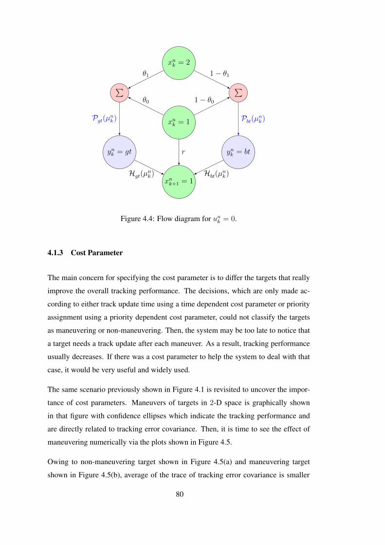
xnk = 1
xnk = 2
xnk+1 = 1
ynk = gt ynk = bt
∑ ∑
r
Pgt(µnk) Pbt(µ
nk)
Hgt(µnk) Hbt(µ
nk)
θ1
θ0
1− θ1
1− θ0
Figure 4.4: Flow diagram for unk = 0.
4.1.3 Cost Parameter
The main concern for specifying the cost parameter is to differ the targets that really
improve the overall tracking performance. The decisions, which are only made ac-
cording to either track update time using a time dependent cost parameter or priority
assignment using a priority dependent cost parameter, could not classify the targets
as maneuvering or non-maneuvering. Then, the system may be too late to notice that
a target needs a track update after each maneuver. As a result, tracking performance
usually decreases. If there was a cost parameter to help the system to deal with that
case, it would be very useful and widely used.
The same scenario previously shown in Figure 4.1 is revisited to uncover the impor-
tance of cost parameters. Maneuvers of targets in 2-D space is graphically shown
in that figure with confidence ellipses which indicate the tracking performance and
are directly related to tracking error covariance. Then, it is time to see the effect of
maneuvering numerically via the plots shown in Figure 4.5.
Owing to non-maneuvering target shown in Figure 4.5(a) and maneuvering target
shown in Figure 4.5(b), average of the trace of tracking error covariance is smaller
80

0 20 40 60 80 100 120 140 160 180 2000
1
2
3
4
5
6
7
8
×105
Time (s)
Trac
eof
Trac
king
Err
orC
ovar
ianc
e(m
2) IMM Tracking
Avg. of IMM TrackingAd Hoc PredictionDetections
(a)
0 20 40 60 80 100 120 140 160 180 2000
1
2
3
4
5
6
7
8
×105
Time (s)
Trac
eof
Trac
king
Err
orC
ovar
ianc
e(m
2) IMM Tracking
Avg. of IMM TrackingAd Hoc PredictionDetections
(b)
Figure 4.5: Tracking error covariance example for (a) non-maneuvering target and(b) maneuvering target.
81

for non-maneuvering target. Then, it is deduced that the overall tracking performance
is better for non-maneuvering target, as it is expected.
It is shown in Figure 4.5(a), non-maneuvering target is almost precisely tracked ex-
cept between 60 − 85 s and the target gets the highest tracking error, ∼ 8 × 10⁵ m2,
during that interval.
The number of red dots between blue and empty dots on the plots indicates the number
of predictions. Tracking error is higher for prediction, since there is not any measure-
ment provided. Especially between 60 − 85 s, system has been probably overloaded
and hence, the target has not been tracked for a while. Moreover, it is concluded that
the target is probably less important than other targets. For the other intervals, red
dots seem as being too squeezed. It means that the predictions are well-matched and
the tracking errors are less.
The maneuvering target shown in Figure 4.5(b) is almost periodically updated and
there is not an interval like that the non-maneuvering target. The maneuvering target
gets the highest tracking error, ∼ 4.5 × 10⁵ m2, which is less than the highest value
of non-maneuvering target.
The scenario given up to here, symbolizes the main problems for tracking. The reason
of these problems is the limited radar resources and capabilities. Hence, the system
can not perform all requested tasks and it selects the most appropriate one at each
instant. To utilize resources effectively, the performing advantages of each task over
the others must be provided to the system in an intelligent way. This can be done
through the cost parameter. Thus, the cost parameter is preferable to contain both
absolute and relative informations of each target.
Briefly, the main properties of the desired cost parameter are
X time dependent,
X maneuvering-based,
X target-based,
X combining all targets.
82
Considering all of them, the cost parameter, Knk , is defined as
Knk ,max
{m
(0,`)k x`requesting,k
}Nk
`=1, ` 6=n
m(1,n)k
· xnrequesting,k, (4.34)
where xnrequesting,k ∈ {0, 1} indicates that if the target n requests a track update or
not, m(1,n)k denotes the estimated improvement on the tracking error covariance of
the target n by taking UPD action(unk = 1
)and max
{m
(0,`)k
}Nk
`=1, ` 6=n denotes the
maximum of estimated deterioration on the tracking error covariances of all targets
which are not updated. Thus, the latter covers all targets except the target n. The
improvement or deterioration issue is simply the change in the trace of the tracking
error covariance. If the trace is thought to be decreased at time k+1, the improvement
will be observed for tracking. Otherwise the deterioration occurs.
Figure 4.6 is given to visualize what is specified by m(0,n)k and m(1,n)
k are
m(0,n)k =
∣∣∣ tr(Pnk+1
)− tr
(Pnk+1
)∣∣∣, (4.35)
m(1,n)k =
∣∣∣ tr(Pnk
)− tr
(Pnk+1
)∣∣∣, (4.36)
where Pnk+1 is predicted, in an ad hoc way, tracking error covariance at next time.
Pnk+1 is computed as the linear combination of current and previous tracking error
covariances as follows:
Pnk+1 = Pn
k +(Pnk −Pn
k−1),
= 2 ·Pnk −Pn
k−1. (4.37)
It is known that system can use all of the available data related to each target and make
predictions when there is not any measurement provided. Thus, track informations,
not provided, have already been predicted at time k − 1 for the current time k. In
fact, prediction process is one of the jobs of tracker and it has a sampling interval,
namely a period, T , i.e. T = 1 s. However, each target can request an update of track,
83

m(0,n)k
m(1,n)k
k − 1 k k + 1
tr(Pn
k+1
)
tr(Pn
k−1
)
tr(Pn
k
)
tr(Pn
k+1
)
Time
Trac
eof
Trac
king
Err
orC
ovar
ianc
eIMM TrackingAd Hoc Prediction
Figure 4.6: Description of parameters used for the cost value computation.
within T . Hence, the term, ad hoc prediction, is more preferable than prediction while
describing (4.37).
It is almost clear howm(0,n)k andm(1,n)
k are obtained by (4.35) and (4.36) respectively,
but the parameter, Pnk+1, makes them a bit confusing to understand. The trace of
tracking error covariance is increasing while time goes on until k, as shown in Figure
4.6. Then, it decreases to a value which is too close to a value at the beginning of the
ad hoc prediction curve. This is the main clue to assign the value of Pnk+1. Owing
to description of m(1,n)k , it is said that the trace of tracking error covariance improves
after UPD action. Fortunately, UPD action comes with a measurement and hence, the
trace of Pnk+1 is assumed to be equal to the trace of measurement noise covariance,
tr (R) = σ2x + σ2
y,
where σx and σy are standard deviations of measurement in x and y directions and
they are known by the tracker.
The next section describes the infinite-horizon value functions.
84
4.1.4 Infinite-Horizon Value Functions
Problem will be solved for infinite-horizon case, since there is not a fixed period
which resets the problem with fixed initial parameters. This is simply the result of
problem modeling of multiple target tracking. Each target has a different motion
characteristics and hence, target-based generalization of initial parameters will be too
complex.
It is claimed in the previous paragraph that process always continues until the target
of interest is out of range. Typically, the duration of scheduling is in the order of hun-
dreds seconds, while the tracking task time is in order of milliseconds. This makes the
time-variant solutions (finite-horizon solutions) become computationally intractable
or unnecessarily comprehensive. The infinite-horizon optimization only refers the so-
lution as a time-invariant solution and it is easier to optimize than its finite-horizon
counterpart. The infinite-horizon case solution has the advantage of requiring less
computation. It only computes a fixed threshold for the probability of being in Good
state at infinite. Then, whenever the probability of being in Good state is less than the
threshold, the optimal action is UPD action in order to avoid dropping the target.
The optimal action is determined via the optimal value function, V n(·), according to
the probability of being in Good state, µnk ,
V n(µnk) = max{V nnupd(µ
nk), V n
upd
}, (4.38)
where V nnupd(µ
nk) and V n
upd are the infinite-horizon value functions for NUPD and UPD
actions respectively as follows:
V nnupd(µ
nk) = µnk + α
∑
i∈{gt,bt}Pi(µnk)V n
(Hi(µ
nk)), (4.39)
= µnk + α[Pgt(µnk)V n
(Hgt(µ
nk))
+ Pbt(µnk)V n(Hbt(µ
nk))], (4.40)
V nupd = −Knk + V n
nupd(q), (4.41)
where α is a discount factor, satisfies 0 < α < 1.
85

The value functions (4.39) and (4.41) are explicitly depend on each other via V n(µnk)
given in (4.38). Furthermore, V nnupd(µ
nk), given in (4.40), is related to the optimal
value function, V n(·) through the functionsHgt(µnk) andHbt(µ
nk), while V n(·), given
in (4.38), is already related to V nnupd(·). It is difficult to express V n
nupd(µnk) without any
assumptions onHgt(µnk) andHbt(µ
nk).
It is previously said that both of Hgt(µnk) and Hbt(µ
nk) are examined within the in-
terval, 0 < µnk < 1, in Lemma 1. Thus, the properties of these functions are valid
for µnk = 0+ but not valid for µnk = 0. Though, it is impossible to define a range
which includes all of the real numbers belong to the interval of [0+, 1−] by a com-
puter program due to the limited precision, while it is trivial to define an interval of
[0, 1]. Considering the intervals, the first is a bit cumbersome and hence, the latter
is more preferable for computer programming. If the latter is chosen, then problems
may occur during a simulation by assigned values to parameters, θ0, θ1 and r. Espe-
cially, the function,Hgt(µnk), becomes 0/0, an indeterminate form [51], at µnk = 0 for
θ1 = 0. That is
Hgt(0)∣∣∣
θ1=0
=rθ0 · 0
(θ0 − θ1) · 0 + θ1
∣∣∣θ1=0
= 0/0.
Choosing θ1 = 0 is a good idea which claims the probability of obtaining a good
track given that corresponding target is in Bad state is 0. In this manner, it is only
possible that a good track is obtained from a target which is in Good state. Moreover,
the idea increases the reliability and validity of measurements. The value assignment
of θ1 can be done during the operation to decrease uncertainty about targets, when the
system is overloaded. In this work, it is assumed that θ1 = 0 in order to simplify the
scheme, and the functions described in Section 4.1.2 become
Pgt(µnk)∣∣
θ1=0
= (θ0 − θ1)µnk + θ1∣∣
θ1=0
,
= θ0µnk , (4.42)
Pbt(µnk)∣∣
θ1=0
= 1− (θ0 − θ1)µnk − θ1∣∣
θ1=0
,
= 1− θ0µnk , (4.43)
86

Hgt(µnk)∣∣∣
θ1=0
=rθ0µ
nk
(θ0 − θ1)µnk + θ1
∣∣∣θ1=0
,
= r, (4.44)
Hbt(µnk)∣∣∣
θ1=0
=r(1− θ0)µnk
1− (θ0 − θ1)µnk − θ1
∣∣∣θ1=0
,
=r(1− θ0)µnk
1− θ0µnk, (4.45)
H−1bt (µnk)∣∣∣
θ1=0
=(1− θ1)µnk
(θ0 − θ1)µnk + (1− θ0)r∣∣∣
θ1=0
,
=µnk
θ0µnk + (1− θ0)r. (4.46)
Substituting (4.42), (4.43) and (4.44) in (4.40), infinite-horizon value function for
NUPD action is expressed by
V nnupd(µ
nk) = µnk + α
[θ0µ
nkV
n(r) + (1− θ0µnk)V n(Hbt(µ
nk))]. (4.47)
Next, there is one more simplification required to handle (4.47) and (4.41). This
simplification is related to q, the probability of transition to Good state by taking
UPD action. There are two main assumptions for specifying q, such that
1. q = 1 means action is perfectly achieved (track is successfully updated) and
2. q = r, (r 6= 1) means action may fail (mixed detection or sharp maneuvering).
For the rest of the work, the second assumption is considered to make the model more
realistic. Then, (4.41) becomes
V nupd = −Knk + V n
nupd(r), (4.48)
while V nnupd(r) can be found as
V nnupd(r) = r + α
[θ0rV
n(r) + (1− θ0r)V n(Hbt(r)
)]. (4.49)
87
Both (4.47) and (4.49) require V n(r),
V n(r) = max{V nnupd(r), V
nupd
},
= max{Knk + V n
upd, Vnupd
}. (4.50)
It is true with certainty that Knk , given in (4.34) cannot be negative, owing that it is a
ratio of absolute differences. Then, (4.50) becomes
V n(r) = Knk + V nupd. (4.51)
Using (4.51), the simplified value function of NUPD action, (4.47) becomes
V nnupd(µ
nk) = µnk + α
[θ0µ
nk
(Knk + V n
upd
)+ (1− θ0µnk)V n
(Hbt(µ
nk))]. (4.52)
In this section, the value functions for each action is obtained. In the next section, the
computation of threshold value, that the update decision depends on, is examined.
4.1.5 The Threshold Value for Decision Making
The threshold value, µnth, is the solution of V nnupd(µ
nk) = V n
upd, where LHS and RHS
are given in (4.52) and (4.48) respectively. According to µnth, the decision policy is
unk =
0, µnk > µnth,
1, otherwise(4.53)
and the action will be not to update the track, if threshold is exceeded.
Up to here, only the formulas of infinite-horizon value functions have been given and
the properties of these functions have not been sufficiently mentioned. Before obtain-
ing the formula of µnth, it is more convenient to describe the properties of value func-
tions by assuming that µnth is already known. Firstly, the effect of µnth on V nnupd(µ
nk) is
88

discussed within a proposition. Meanwhile, it can be better to remind that proofs for
propositions, theorems, etc., are given again in this chapter after revising them owing
to some typos noticed in [57].
Proposition 1. For 0 6 µnk 6 r, the threshold, µnth, generates all breakpoints of
V nnupd(µ
nk) in the manner that, [57, Proposition 3],
(i) V nnupd(µ
nk) has no breakpoints for 0 6 µnk < µnth,
(ii) V nnupd(µ
nk) has breakpoints, B1, B2, . . . , satisfying µnth < B1 < B2 < · · · < r
for µnth 6 µnk 6 r. Breakpoints are computed by inverse function of Hbt(·), i.e.
B1 = H−1bt (µnth), B2 = H−1bt (B1).
Proof. (i) If µnk < µnth, then Hbt(µnk) < µnk < µnth due to convexity explained in
Lemma 2, see Figure 4.3. Thus, there is not breakpoint for this interval.
(ii) If µnk < H−1bt (µnth), then Hbt(µnk) < µnth by applying Hbt(·) to both sides. The
case of Hbt(µnk) < µnth leads the optimal action to be UPD, V n
(Hbt(µ
nk))
= V nupd for
that interval. Then, the value function of NUPD action can be written as
V nnupd(µ
nk) = µnk + α
[θ0µ
nk(Knk + V n
upd) + (1− θ0µnk)V nupd
], (4.54)
= µnk + α[θ0µ
nkKnk + V n
upd
],
= µnk(1 + αθ0Knk ) + αV nupd. (4.55)
If H−1bt (µnth) < µnk < H−2bt (µnth), then µnth < Hbt(µnk) < H−1bt (µnth) by applying Hbt(·)
to both sides of inequalities. The case of µnth < Hbt(µnk) leads the optimal action
to be NUPD, V n(Hbt(µ
nk))
= V nnupd
(Hbt(µ
nk))
for that interval. Replacing µnk with
Hbt(µnk) in (4.55), V n
nupd
(Hbt(µ
nk))
can be obtained as
V nnupd
(Hbt(µ
nk))
= Hbt(µnk)(1 + αθ0Knk ) + αV n
upd. (4.56)
Thus, V n(Hbt(µ
nk))
known from (4.56) can be used to obtain value function of NUPD
action in the following way,
89
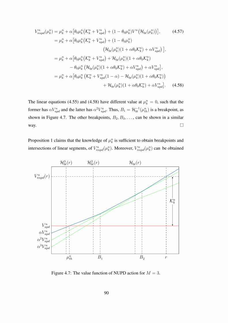
V nnupd(µ
nk) = µnk + α
[θ0µ
nk
(Knk + V n
upd
)+ (1− θ0µnk)V n
(Hbt(µ
nk))], (4.57)
= µnk + α[θ0µ
nk
(Knk + V n
upd
)+ (1− θ0µnk)
(Hbt(µ
nk)(1 + αθ0Knk ) + αV n
upd
) ],
= µnk + α[θ0µ
nk
(Knk + V n
upd
)+Hbt(µ
nk)(1 + αθ0Knk )
− θ0µnk(Hbt(µ
nk)(1 + αθ0Knk ) + αV n
upd
)+ αV n
upd
],
= µnk + α[θ0µ
nk
(Knk + V n
upd(1− α)−Hbt(µnk)(1 + αθ0Knk )
)
+Hbt(µnk)(1 + αθ0Knk ) + αV n
upd
]. (4.58)
The linear equations (4.55) and (4.58) have different value at µnk = 0, such that the
former has αV nupd and the latter has α2V n
upd. Thus, B1 = H−1bt (µnth) is a breakpoint, as
shown in Figure 4.7. The other breakpoints, B2, B3, . . . , can be shown in a similar
way.
Proposition 1 claims that the knowledge of µnk is sufficient to obtain breakpoints and
intersections of linear segments, of V nnupd(µ
nk). Moreover, V n
nupd(µnk) can be obtained
Knk
µnth B1 B2 r
α3V nupd
α2V nupd
αV nupd
V nupd
V nnupd(r)
H3bt(r) H2
bt(r) Hbt(r)
Figure 4.7: The value function of NUPD action for M = 3.
90

explicitly by knowing both V nupd and µnth. It is interesting to note that if V n
nupd(r)
is known, (4.48) can be used to find V nupd. However, if µnth is known, V n
nupd(µnk) for
0 < µnk 6 r can be found from V nupd. Hence, in a system with limited memory, storing
only µnth and V nupd can be more efficient than storing V n
nupd(µnk) for 0 < µnk 6 r.
The properties of V nnupd(µ
nk) deduced from Proposition 1, can be generalized by a
theorem.
Theorem 1. The infinite-horizon value functions for NUPD action, V nnupd(µ
nk), is a
piecewise-linear convex function for θ1 = 0, [57, Theorem 2].
Proof. For θ1 = 0, the infinite-horizon value functions for NUPD action, V nnupd(µ
nk),
is given in (4.52) and V n(Hbt(µ
nk)), in that expression, is obtained as
V n(Hbt(µ
nk))
= max{V nnupd
(Hbt(µ
nk)), V n
upd
}(4.59)
by using (4.38). According to (4.38), V n(·) is composed of upper part of functions
that V nupd is a constant function and V n
nupd(·) consists of the linear segments shown in
Proposition 1. Then, V n(·) is a piecewise-linear convex function. Hence, V nnupd(µ
nk)
is also a piecewise-linear convex function. Further details can be found in [60].
Before continuing discussions about the threshold value, it may be better to mention
that there is a different statement on the proof of Theorem 1. It is noted in [57]
that, to prove V nnupd(µ
nk) to be piecewise-linear, it is required to show the finiteness
of the number of breakpoints. To do so, it is sufficient to show that the length of the
intervals, (B0 = µnth, B1), (B1, B2), . . . , is increasing. To the best our understanding,
the length of interval depends on the starting point,
Bi+1 −Bi = H−1bt (Bi)−Bi, (4.60)
=Bi
θ0Bi + (1− θ0)r−Bi, (4.61)
and the first derivative of (4.61) is always positive with respect to Bi, then it can be
said that the length of interval is increasing.
91
D(Bi) ,Bi
θ0Bi + (1− θ0)r−Bi, (4.62)
D′(Bi) =dD(Bi)
dBi
, (4.63)
=(1− θ0)r[
θ0Bi + (1− θ0)r]2 − 1. (4.64)
The derivative of the function given in (4.64), is not always positive. Hence, it cannot
be said that the length of interval is increasing.
When Figure 4.7 is examined again, to obtain segments of V nnupd(µ
nk), breakpoints,
B1 and B2, are computed by H−1bt (µnth) and H−2bt (µnth) respectively. In fact, µnth, is
not a breakpoint of V nnupd(µ
nk), while it is a breakpoint of V n(µnk) according to (4.38)
for µnth > 0. Hence, µnth can also behave like a breakpoint. Then, H3bt(r), H2
bt(r)
and Hbt(r) come right before µnth, B1 and B2 respectively. These points depend on
r which has a presumed value, while breakpoints are directly related to µnth which
depends on the basic parameters, α, θ0, r, Knk . Thus, it is simpler to compute these
points than breakpoints which require the µnth. One can try to compute other points,
H4bt(r), H5
bt(r), . . . , until they become sufficiently close to zero. Thus, there is no
limit for the number of these points.
The number of segments of V nnupd(µ
nk) can be given with the following corollary.
Corollary 1. Assuming that M is the number of segments of V nnupd(µ
nk), 0 6 µnk 6 r,
there are M − 1 breakpoints from Proposition 1. Then, µnth satisfies the condition,
[57, Corollary 1],
r > Hbt(r) > H2bt(r) > · · · > HM−2
bt (r) > HM−1bt (r) > µnth > HM
bt (r).
Corollary 1 depicts HMbt (r) < µnth which can be used to determine the number of
segments, M , without explicitly finding breakpoints of V nnupd(µ
nk). A simple function
to realize this idea is given in Algorithm 4.1.
Moreover, it is deduced that
µnk > HM−1bt (r) ∧HM−1
bt (r) > µnth =⇒ µnk > µnth,
∴ V nnupd(µ
nk) > V n
upd =⇒ V n(µnk) = V nnupd(µ
nk).
92
Algorithm 4.1 Number of segments.
1: function NOFSEGMENT(α, θ0, r, Knk
)
2: M = 1
3: computeHMbt (r)
4: compute µnth5: whileHM
bt (r) > µnth do
6: M++
7: computeHMbt (r)
8: compute µnth
9: end while
10: return M
11: end
from Corollary 1. Hence, the optimal value function becomes
V n(µnk) = µnk + α[θ0µ
nk
(Knk + V n
upd
)+ (1− θ0µnk)V n
(Hbt(µ
nk))], (4.65)
for µnk > HM−1bt (r).
In the beginning of this section, it is said that µnth is the solution of V nnupd(µ
nk) = V n
upd
so that V nnupd(µ
nth) = V n
upd. It is also added that µnth and V nupd are sufficient to determine
V nnupd(µ
nk) by Proposition 1. Summing them, it is more confident to think that µnth
and V nupd are dependent. The relation between them is clarified with the following
proposition.
Proposition 2. The threshold, µnth, can be computed as
µnth =1− α
1 + αθ0KnkV nupd, (4.66)
if V nupd is known, [57, Proposition 4].
Proof. The threshold value, µnth, satisfies V nnupd(µ
nk) = V n
upd for µnk = µnth. By using
(4.59), V n(Hbt(µ
nth))
= V nupd owing to Hbt(µ
nth) < µnth, as shown in Figure 4.3(a). It
93

is known r > µnth and V n(r) = V nnupd(r) = Knk + V n
upd. Combining all of them, V nupd
becomes
V nupd = µnth + α
[θ0µ
nthV
n(r) + (1− θ0µnth)V nupd
], (4.67)
= µnth + α[θ0µ
nth
(Knk + V n
upd
)+ (1− θ0µnth)V n
upd
],
= µnth + α[θ0µ
nthKnk + V n
upd
],
= µnth(1 + αθ0Knk
)+ αV n
upd,
= µnth
(1 + αθ0Knk
1− α
). (4.68)
The relation, µnth ∝ V nupd, is given in (4.68), and (4.66) can be obtained simply with
this relation.
It is suggested within Proposition 2 that µnth is directly obtained from V nupd. Indeed,
V nupd can be thought as the base point of all functions. Hence, the expression of V n
upd,
which depends only on the basic parameters, is given in the following theorem.
Theorem 2. Supposing that V nnupd(µ
nk) consists ofM segments, V n
upd can be computed
by, [57, Theorem 3 and 4],
V nupd ,
AnM(r)(1 + αθ0Knk )−Knk1− αθ0AnM(r)− BnM(r)
, (4.69)
where AnM(r) is defined as
AnM(r) ,
r, M = 1,
r +M−1∑
i=1
αiHibt(r)
i−1∏
j=0
(1− θ0Hj
bt(r)), M > 2
(4.70)
and BnM(r) is defined as
BnM(r) ,M−1∏
i=0
α(1− θ0Hi
bt(r)), (4.71)
for M > 1.
94

Proof. To compute V nupd, it is necessary and sufficient to solve M + 1 distinct equa-
tions as follows:
V n(r) = r + α[θ0rV
n(r) + (1− θ0r)V n(Hbt(r)
)], (4.72)
V n(Hbt(r)
)= Hbt(r) + α
[θ0Hbt(r)V
n(r)+(1− θ0Hbt(r)
)V n(H2bt(r)
)], (4.73)
V n(H2bt(r)
)= H2
bt(r) + α[θ0H2
bt(r)Vn(r)+
(1− θ0H2
bt(r))V n(H3bt(r)
)], (4.74)
...
V n(HM−2bt (r)
)= HM−2
bt (r) + α[θ0HM−2
bt (r)V n(r)+(1− θ0HM−2
bt (r))V n(HM−1bt (r)
)], (4.75)
V n(HM−1bt (r)
)= HM−1
bt (r) + α[θ0HM−1
bt (r)V n(r)+(1− θ0HM−1
bt (r))V nupd
]. (4.76)
From (4.72) to (4.76), M equations, are obtained directly using (4.65). In (4.76), the
last term becomes V nupd, while it can be written as V n
(HMbt (r)
). This is concluded
from Corollary 1 claims that
HMbt (r) < µnth =⇒ V n
nupd
(HMbt (r)
)< V n
upd,
∴ V n(HMbt (r)
)= V n
upd.
Substituting (4.73) into (4.72), the expression is obtained as
V n(r) = r + α[θ0rV
n(r) + (1− θ0r)(Hbt(r) + α
[θ0Hbt(r)V
n(r) +(1− θ0Hbt(r)
)V n(H2bt(r)
)) ]. (4.77)
Then, (4.77) can be converted into a more compact form,
V n(r) = (r + α(1− θ0r)Hbt(r)) + αθ0 (r + α(1− θ0r)Hbt(r))Vn(r)+
α2(1− θ0r)(1− θ0Hbt(r)
)V n(H2bt(r)
). (4.78)
95
Substituting (4.74) into (4.78), the expression is obtained as
V n(r) =(r + α(1− θ0r)Hbt(r) + α2(1− θ0r)
(1− θ0Hbt(r)
)H2bt(r)
)+
αθ0(r + α(1− θ0r)Hbt(r) + α2(1− θ0r)
(1− θ0Hbt(r)
)H2bt(r)
)
V n(r) + α3(1− θ0r)(1− θ0Hbt(r)
)(1− θ0H2
bt(r))V n(H3bt(r)
). (4.79)
Continuing in this way, (4.72) becomes
V n(r) = AnM(r) + αθ0AnM(r)V n(r) + BnM(r)V nupd, (4.80)
where AnM(r) is
AnM(r) = r + α(1− θ0r
)Hbt(r)
+ α2(1− θ0r
)(1− θ0Hbt(r)
)H2bt(r)
...
+ αM−1(1− θ0r
)(1− θ0Hbt(r)
)(1− θ0H2
bt(r))
· · ·(1− θ0HM−2
bt (r))HM−1bt (r),
= r +M−1∑
i=1
αiHibt(r)
i−1∏
j=0
(1− θ0Hj
bt(r)), (4.81)
and BnM(r) is
BnM(r) = αM(1− θ0r
)(1− θ0Hbt(r)
)(1− θ0H2
bt(r))· · ·(1− θ0HM−1
bt (r)),
=M−1∏
i=0
α(1− θ0Hi
bt(r)). (4.82)
If M = 1, then (4.76) becomes
V n(H0bt(r)
)= H0
bt(r) + α[θ0H0
bt(r)Vn(r) +
(1− θ0H0
bt(r))V nupd
], (4.83)
96
where
H0bt(r) = Hbt
(H−1bt (r)
)= r =⇒ An1 (r) = r.
Here, M of M + 1 equations are presented and the other required equation is (4.51)
to find V nupd. Substituting (4.51) into (4.80), the expression is obtained as
Knk + V nupd = AnM(r) + αθ0AnM(r)
(Knk + V n
upd
)+ BnM(r)V n
upd. (4.84)
By using (4.84), (4.69) can be obtained simply.
The way for obtaining the value V nupd is given by Theorem 2. After carefully exam-
ining (4.69), it is obvious to say that V nupd can be negative with respect to Knk value.
If Knk is high enough, then V nupd is negative and hence, µnth also becomes negative ac-
cording to (4.66). Therefore NUPD action becomes always optimal for the negative
threshold value, since µnk is always positive. This makes computations for decision
making process unnecessary. Because it is explicitly inferred from Knk , whether µnthis negative or not. The upper bound of Knk , which guarantees that µnth is positive, is
discussed in the following proposition.
Proposition 3. If Knk > r/(1 − αr), then the decision policy becomes a degenerate
policy and the optimal action is always NUPD, [61, Proposition 2].
Proof. To begin the proof, the infinite-horizon value functions given in (4.47) and
(4.48) are converted to the finite-horizon case,
V n,tnupd(µ
nk) = µnk + α
[θ0µ
nkV
n,t−1(r) + (1− θ0µnk)V n,t−1(Hbt(µnk))], (4.85)
V n,tupd = −Knk + V n,t
nupd(r), (4.86)
for t > 1.
Assumed initial condition is V n,0(µnk) = 0, i.e. there is not any value or utility at
the initial point for each target. Then, starting from horizon-1 and always choosing
97

NUPD as an optimal action until horizon-t, value functions given in (4.85) and (4.86)
are employed as
V n,1nupd(µ
nk) = µnk ,
V n,1upd = −Knk + r,
V n,1(µnk) = µnk ,
V n,2nupd(µ
nk) = µnk + α
[θ0µ
nkV
n,1(r) + (1− θ0µnk)V n,1(Hbt(µ
nk))]
= µnk + α[θ0µ
nkr + (1− θ0µnk)Hbt(µ
nk)]
= µnk + α
[θ0µ
nkr +������
(1− θ0µnk) · r(1− θ0)µnk
�����1− θ0µnk
],
= µnk +����αθ0µnkr + αrµnk −����αrθ0µ
nk ,
= µnk(1 + αr),
V n,2upd = −Knk + r(1 + αr),
V n,2(µnk) = µnk(1 + αr),
V n,3nupd(µ
nk) = µnk + α
[θ0µ
nkV
n,2(r) + (1− θ0µnk)V n,2(Hbt(µ
nk))]
= µnk + α(1 + αr)[θ0µ
nkr + (1− θ0µnk)Hbt(µ
nk)]
= µnk + α(1 + αr)rµnk ,
= µnk(1 + αr + α2r2
),
V n,3upd = −Knk + r
(1 + αr + α2r2
),
V n,3(µnk) = µnk(1 + αr + α2r2
),
...
V n,tnupd(µ
nk) = µnk
t−1∑
`=0
α`r`, (4.87)
V n,tupd = −Knk + r
t−1∑
`=0
α`r`, (4.88)
V n,t(µnk) = max{V n,tnupd(µ
nk), V n,t
upd
}. (4.89)
As t→∞, (4.88) becomes,
V n,tupd = −Knk + r
t−1∑
`=0
α`r` =t→∞−Knk +
r
1− αr .
98
V n,tnupd(µ
nk) given in (4.87), is always positive. If Knk > r/(1 − αr), then V n,t
upd given
in (4.88), is negative and the optimal action is again NUPD, V n,t(µnk) = V n,tnupd(µ
nk),
at horizon-t for t→∞. Hence, the decision policy becomes a degenerate policy and
the optimal action is always NUPD.
Fortunately, the solution is completed by substituting (4.69) into (4.66). The threshold
value is determined by
µnth =
0, Knk >r
1− αr ,1− α
1 + αθ0Knk
(AnM(r)(1 + αθ0Knk )−Knk1− αθ0AnM(r)− BnM(r)
), otherwise
(4.90)
and the way of computing µnth is given with Algorithm 4.2.
Algorithm 4.2 The threshold value computation.
1: function THRESHOLD(α, θ0, r, Knk
)
2: if Knk > r/(1− αr) then
3: µnth = 0
4: else
5: M = 1
6: computeHMbt (r), AnM(r) and BnM(r)
7: compute V nupd
8: compute µnth9: whileHM
bt (r) > µnth do
10: M++
11: computeHMbt (r), AnM(r) and BnM(r)
12: compute V nupd
13: compute µnth
14: end while
15: end if
16: return µnth17: end
99

Assuming α = 0.99, the other basic parameters, θ0, r and Knk are changed to obtain
distinct infinite-horizon value functions. Then obtained thresholds and the numbers
of segments are given in Table 4.1. Furthermore, Figure 4.8 shows these functions,
when θ0 = 0.60 and r = 0.90.
The comments for the data given in Table 4.1 can be given as follows:
• The higher r makes µnth higher, since AnM(r) increases with r, and V nnupd also
increases. This statement is inferred from Theorem 2.
• The higher Knk makes µnth smaller, as mentioned in Proposition 3. That is
Knk < r/(1− αr) ∧ Knk → r/(1− αr) =⇒ µnth → 0.
• M depends on both θ0 and Knk , as depicted more clearly in Table 4.1(c).
Table4.1: Comparison of the threshold value and number of segments for α = 0.99and (a) Knk = 0.3, (b) Knk = 1.2, (c) Knk = 2.8.
(a)
r = 0.90 r = 0.95
θ0 = 0.60 θ0 = 0.75 θ0 = 0.90 θ0 = 0.60 θ0 = 0.75 θ0 = 0.90
µnth 0.6454 0.6547 0.6633 0.6954 0.7047 0.7133
M 1 1 1 1 1 1
(b)
r = 0.90 r = 0.95
θ0 = 0.60 θ0 = 0.75 θ0 = 0.90 θ0 = 0.60 θ0 = 0.75 θ0 = 0.90
µnth 0.3574 0.3525 0.3369 0.4256 0.4194 0.4017
M 2 2 2 2 2 2
(c)
r = 0.90 r = 0.95
θ0 = 0.60 θ0 = 0.75 θ0 = 0.90 θ0 = 0.60 θ0 = 0.75 θ0 = 0.90
µnth 0.1654 0.1581 0.1507 0.2388 0.2260 0.2083
M 3 3 2 3 3 2
100

0.6454 0.9000
75.2776
76.0380
76.3380
µnth B1
V nupd
V nnupd(r)
(a)
0.3574 0.6222 0.9000
59.9965
60.6025
61.2146
62.4146
µnth B1 r
V nupd
V nnupd(r)
(b)
0.1654 0.3601 0.6251 0.9000
42.730943.162543.598544.0389
46.8389
µnth B1 B2 r
V nupd
V nnupd(r)
(c)
Figure 4.8: Sample infinite-horizon value functions of NUPD action with α = 0.99,θ0 = 0.60, r = 0.90 and (a) Knk = 0.3, (b) Knk = 1.2, (c) Knk = 2.8.
101
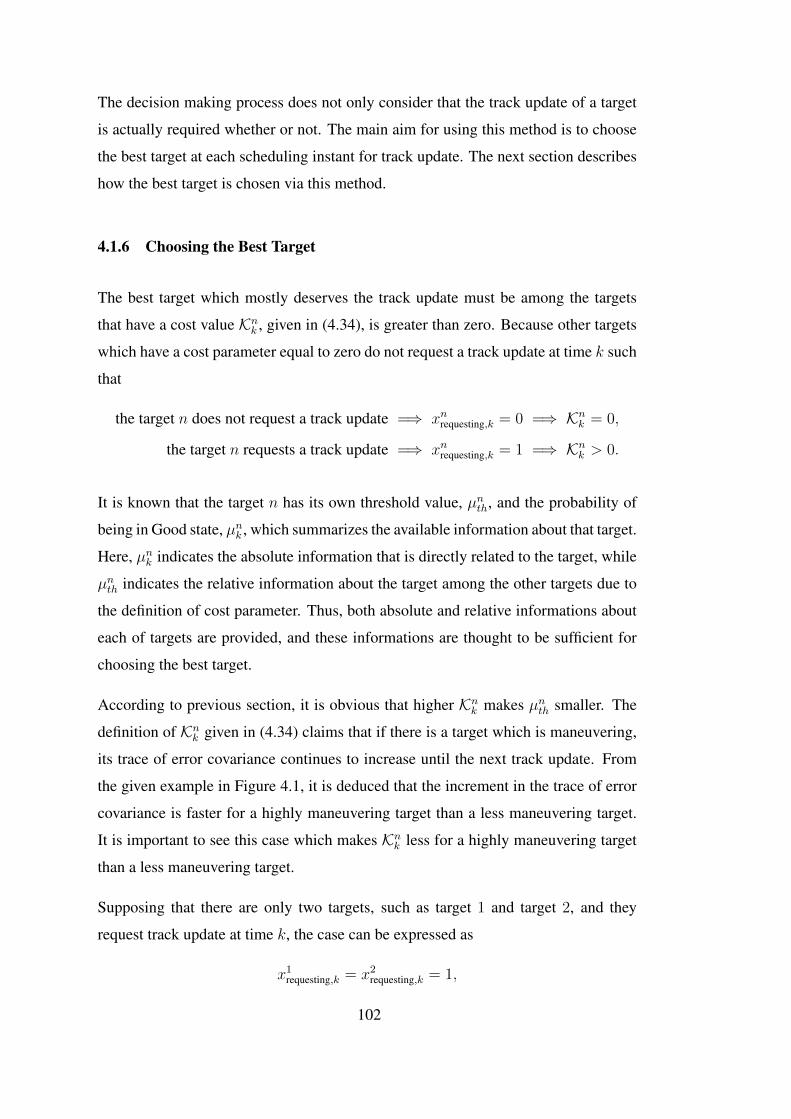
The decision making process does not only consider that the track update of a target
is actually required whether or not. The main aim for using this method is to choose
the best target at each scheduling instant for track update. The next section describes
how the best target is chosen via this method.
4.1.6 Choosing the Best Target
The best target which mostly deserves the track update must be among the targets
that have a cost value Knk , given in (4.34), is greater than zero. Because other targets
which have a cost parameter equal to zero do not request a track update at time k such
that
the target n does not request a track update =⇒ xnrequesting,k = 0 =⇒ Knk = 0,
the target n requests a track update =⇒ xnrequesting,k = 1 =⇒ Knk > 0.
It is known that the target n has its own threshold value, µnth, and the probability of
being in Good state, µnk , which summarizes the available information about that target.
Here, µnk indicates the absolute information that is directly related to the target, while
µnth indicates the relative information about the target among the other targets due to
the definition of cost parameter. Thus, both absolute and relative informations about
each of targets are provided, and these informations are thought to be sufficient for
choosing the best target.
According to previous section, it is obvious that higher Knk makes µnth smaller. The
definition of Knk given in (4.34) claims that if there is a target which is maneuvering,
its trace of error covariance continues to increase until the next track update. From
the given example in Figure 4.1, it is deduced that the increment in the trace of error
covariance is faster for a highly maneuvering target than a less maneuvering target.
It is important to see this case which makes Knk less for a highly maneuvering target
than a less maneuvering target.
Supposing that there are only two targets, such as target 1 and target 2, and they
request track update at time k, the case can be expressed as
x1requesting,k = x2requesting,k = 1,
102

and the cost parameters are determined as
K1k =
m(0,2)k
m(1,1)k
, K2k =
m(0,1)k
m(1,2)k
respectively by using (4.34).
If both targets have track update scheduled at next time, k + 1, it will be true that
tr(P1k+1
)= tr
(P2k+1
)(4.91)
due to tracking process. Moreover, it is assumed that target 1 is less maneuvering,
and target 2 is highly maneuvering. Hence, the statement about the increment in the
trace of error covariance,
tr(P1k −P1
k−1
)< tr
(P2k −P2
k−1
),
implies that
tr(P1k
)< tr
(P2k
)(4.92)
and it is clear to denote that
tr(P1k+1
)< tr
(P2k+1
)(4.93)
by using (4.37).
From (4.36), the estimated improvements on the tracking error covariance of target 1
and target 2 by taking UPD action, are given as
m(1,1)k =
∣∣∣ tr(P1k
)− tr
(P1k+1
)∣∣∣, m(1,2)k =
∣∣∣ tr(P2k
)− tr
(P2k+1
)∣∣∣
respectively. Then, it is deduced that
m(1,1)k < m
(1,2)k (4.94)
by jointly combining (4.91) and (4.92).
103

From (4.35), the estimated changes on the tracking error covariance of target 1 and
target 2 by taking NUPD action, are given as
m(0,1)k =
∣∣∣ tr(P1k+1
)− tr
(P1k+1
)∣∣∣, m(0,2)k =
∣∣∣ tr(P2k+1
)− tr
(P2k+1
)∣∣∣
respectively. Then, it is deduced that
m(0,1)k < m
(0,2)k (4.95)
by jointly combining (4.91) and (4.93).
Lastly, it is seen that
K1k > K2
k
by using (4.94) and (4.95).
The main contribution of this statement is that
K1k > K2
k =⇒ µ1th < µ2
th (4.96)
owing to the common parameters, α, θ0, r.
It is known that µnk also specifies the probability of non-maneuvering which is directly
proportional to the probability of being in Good state. Hence, it is obvious that
µ1k > µ2
k (4.97)
and it is also noticed that
µ1k − µ1
th > µ2k − µ2
th
by jointly combining (4.96) and (4.97). This inequality compares the objective crite-
rion for each target, and ideally helps choose the best target for track update. Because
the utilized objective criterion, i.e. µnk − µnth for target n, combines both absolute and
relative informations about each of targets.
Method described for two targets can be extended by induction. When there are more
than two targets which request track update for the same instant, all targets can be
104
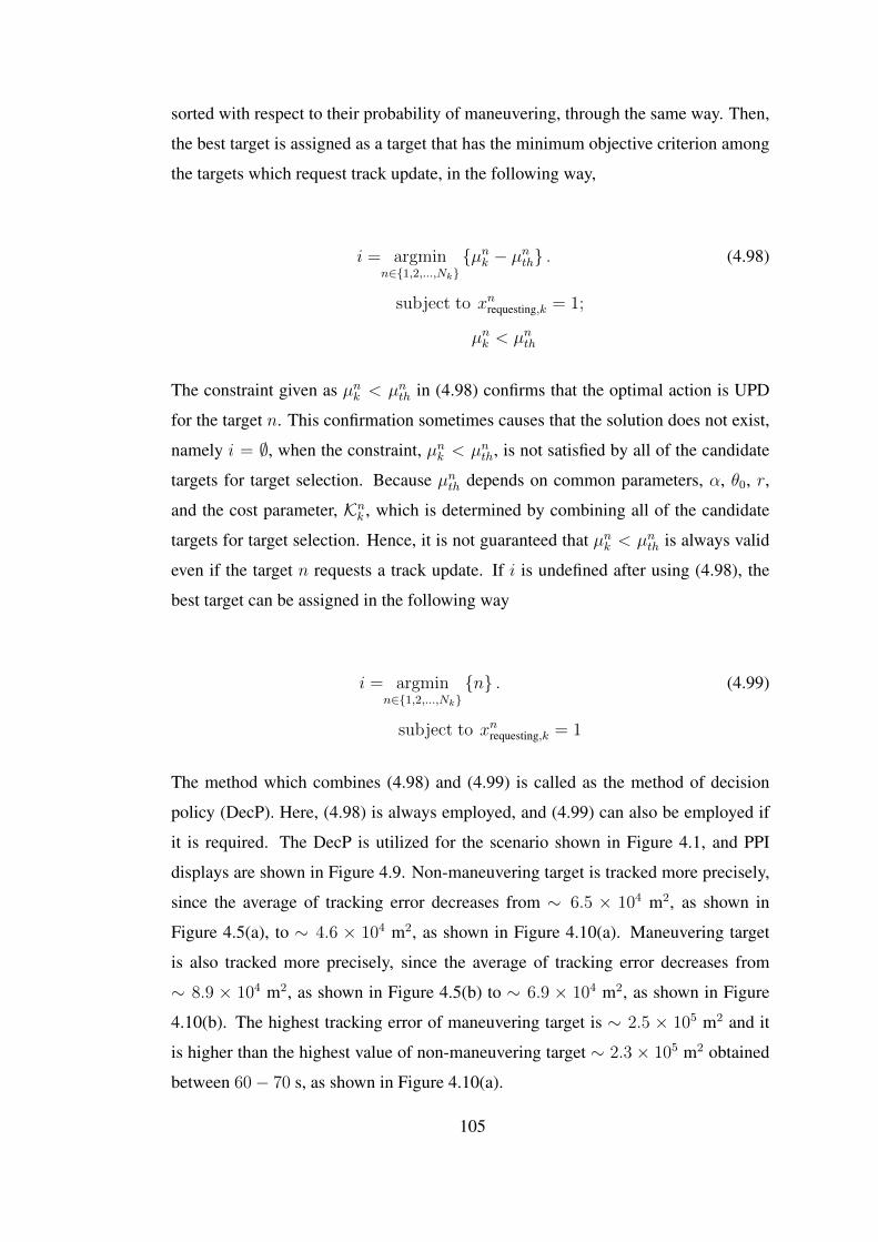
sorted with respect to their probability of maneuvering, through the same way. Then,
the best target is assigned as a target that has the minimum objective criterion among
the targets which request track update, in the following way,
i = argminn∈{1,2,...,Nk}
{µnk − µnth} . (4.98)
subject to xnrequesting,k = 1;
µnk < µnth
The constraint given as µnk < µnth in (4.98) confirms that the optimal action is UPD
for the target n. This confirmation sometimes causes that the solution does not exist,
namely i = ∅, when the constraint, µnk < µnth, is not satisfied by all of the candidate
targets for target selection. Because µnth depends on common parameters, α, θ0, r,
and the cost parameter, Knk , which is determined by combining all of the candidate
targets for target selection. Hence, it is not guaranteed that µnk < µnth is always valid
even if the target n requests a track update. If i is undefined after using (4.98), the
best target can be assigned in the following way
i = argminn∈{1,2,...,Nk}
{n} . (4.99)
subject to xnrequesting,k = 1
The method which combines (4.98) and (4.99) is called as the method of decision
policy (DecP). Here, (4.98) is always employed, and (4.99) can also be employed if
it is required. The DecP is utilized for the scenario shown in Figure 4.1, and PPI
displays are shown in Figure 4.9. Non-maneuvering target is tracked more precisely,
since the average of tracking error decreases from ∼ 6.5 × 10⁴ m2, as shown in
Figure 4.5(a), to ∼ 4.6 × 10⁴ m2, as shown in Figure 4.10(a). Maneuvering target
is also tracked more precisely, since the average of tracking error decreases from
∼ 8.9 × 10⁴ m2, as shown in Figure 4.5(b) to ∼ 6.9 × 10⁴ m2, as shown in Figure
4.10(b). The highest tracking error of maneuvering target is ∼ 2.5 × 10⁵ m2 and it
is higher than the highest value of non-maneuvering target ∼ 2.3 × 10⁵ m2 obtained
between 60− 70 s, as shown in Figure 4.10(a).
105
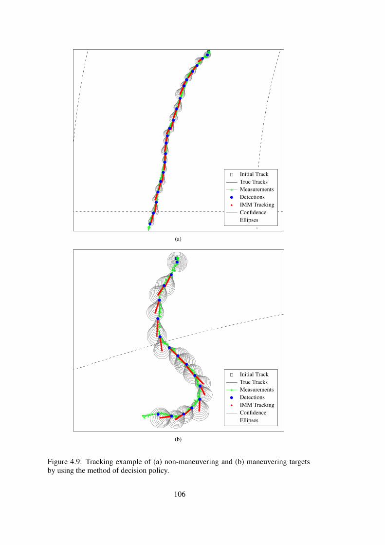
0◦
30◦
60◦
90◦
120◦
150◦
180◦
210◦
240◦
270◦
300◦
330◦
S1
S2
S3
Initial TrackTrue TracksMeasurementsDetectionsIMM TrackingConfidenceEllipses
(a)
0◦
30◦
60◦
90◦
120◦
150◦
180◦
210◦
240◦
270◦
300◦
330◦
S1
S2
S3
Initial TrackTrue TracksMeasurementsDetectionsIMM TrackingConfidenceEllipses
(b)
Figure 4.9: Tracking example of (a) non-maneuvering and (b) maneuvering targetsby using the method of decision policy.
106

0 20 40 60 80 100 120 140 160 180 2000
1
2
3
4
×105
Time (s)
Trac
eof
Trac
king
Err
orC
ovar
ianc
e(m
2) IMM Tracking
Avg. of IMM TrackingAd Hoc PredictionDetections
(a)
0 20 40 60 80 100 120 140 160 180 2000
1
2
3
4
×105
Time (s)
Trac
eof
Trac
king
Err
orC
ovar
ianc
e(m
2) IMM Tracking
Avg. of IMM TrackingAd Hoc PredictionDetections
(b)
Figure 4.10: Tracking error covariance example using the method of decision policyfor (a) non-maneuvering target and (b) maneuvering target.
107
The numbers given in the previous paragraph shows that the described method is
more preferable in this run. However, it is important to remind that DecP does not
guarantee a better operation at every run. After choosing one of the targets, dynamics
(position, velocity) of target environment change and the other targets will wait more
for the track update. Hence, it is not guaranteed to have a better overall performance.
In Chapter 5, additional numerical experiments are given to utilize DecP which is
compared with other methods.
Indeed, the approach given in (4.99) is utilized, when there is not a specific method
for decision making process. For example, assuming that target 3, target 9 and target
14 have the same TB value, tTB, which is higher than other tTB’s at time k, a TB
technique based scheduler verifies that target 9 and target 14 have the same priority
level which is higher than the priority level of target 3. Then, the scheduler assigns
xrequesting,k as 1 for target 9 and target 14, and 0 for other targets. Without utilizing
DecP, the scheduler selects target 9 to schedule a tracking task. This case is origi-
nated to the service policy; first-come, first-served (FCFS) [62], since the scheduler
analyzes targets starting from the target which has the smallest task id, n. Then, the
method is called as the method of choosing first target in the update list (CfTUL).
The PPI displays shown in Figure 4.1 and the numerical results shown in Figure 4.5
are obtained by using CfTUL as a decision method which exploits the help of (4.99)
whenever it is required.
In the following two sections, two different methods which provide other approaches
to the same problem are given.
4.2 Method of Minimizing the Tracking Error
In the previous section, it is stated that increment in the trace of error covariance is
faster for a highly maneuvering target than a less maneuvering target. Hence, it is
thought that the highly maneuvering target increases the average of tracking error
faster. Thus, the best target is assigned as a target, the trace of error covariance
of whom is the highest one among the targets which request track update, in the
following way,
108
i = argmaxn∈{1,2,...,Nk}
{tr(Pnk
)}. (4.100)
subject to xnrequesting,k = 1
This method is called as the method of minimizing the tracking error (MinTE) and
compared with other methods in Chapter 5 which gives the numerical experiments.
4.3 Method of Pursuing the Most Maneuvering
Generally speaking, it is not always valid that the trace of error covariance of a highly
maneuvering target is higher than the target which is less maneuvering. An example
that supports this statement is previously given in Figure 4.5. The method to minimize
the tracking error, described in the previous section, is extended to a novel method by
exploiting µnk .
If the probability of non-maneuvering is directly proportional to µnk , then the probabi-
lity of maneuvering is proportional to 1−µnk . Thus, the target can be chosen to update
its track via the multiplication of the trace of error covariance and the probability of
maneuvering, in the following way,
i = argmaxn∈{1,2,...,Nk}
{(1− µnk + ε) tr
(Pnk
)}, (4.101)
subject to xnrequesting,k = 1
where ε > 0 is added to avoid multiplication by zero.
This method is called as the method of pursuing the most maneuvering (PurMM) and
compared with other methods in Chapter 5 which gives the numerical experiments.
4.4 Summary
In this chapter, the decision process to choose a target among the targets which require
track update concurrently is studied. The method of decision policy based on [57] is
109

presented analytically for the solution of the problem.
In the final parts of this chapter, two other methods; the method of minimizing the
tracking error and the method of pursuing the most maneuvering are proposed as
some other ad hoc methods to the problem. These methods are simpler to implement
and makes more intuitive sense.
110
CHAPTER 5
EXPERIMENTAL RESULTS
In this chapter, the experimental results for the comparisons of proposed schedulers
(described in Chapter 3) with different decision methods (described in Chapter 4)
are given. The simulation environment which supports the described techniques, is
written in MATLAB and its operation is briefly presented in Appendix C. The same
scenarios and parameters are chosen to make a fair comparison between different
methods, unless it is noted otherwise.
For all simulations, the assumptions are as follows:
• Surveillance task is not fragmented and interleaved.
• Surveillance task is periodic and forced to be scheduled whenever it is requested
by using dynamic task prioritization.
• Dynamic task prioritization is utilized.
• The scheduler is forced to schedule the surveillance task, before detecting a
target or dropping the previously tracked target.
The latter is assumed to make the radar system more realistic, since the surveillance
task is scheduled to detect a new target or check one of the existing targets is dropped.
In simulations, all target trajectories are generated before the scheduling. The trajec-
tories show the information where each target is at given time. The trajectory infor-
mation is not known by radar system. The surveillance tasks are scheduled whenever
a scheduling technique declares a target drop.
111
The scenario where N = 15 targets are present in the duration of tmax = 500 s, as
shown in Figure 3.10 is considered. A comparison of the proposed scheduling tech-
niques described in Section 3.2, is given in Table 5.1 and the distribution of scheduled
tasks are shown in Figure 5.1. Here, the main goal is to see the occupancy and task
interleaving capability of the scheduler by using CfTUL as the decision method, and
disabling the adaptive update-rate and multi-frequency band usage techniques. In Ta-
ble 5.1(a), all types of MTATBS and KS are compared when interleaving technique
is not applied. The occupancy values are approximately 100% for all of techniques.
There is a trade off between the number of surveillance and tracking tasks, since task
time of the surveillance is 2 s that is almost 2 times of the task time of a tracking
task. Owing to maximization of the instantaneous value, KS schedules mostly trac-
king tasks and rarely surveillance tasks. All types of MTATBS give similar results.
The number of probable drops is related to the lateness of tasks. The MTATBS-Type
1 and MTATBS-Type 3 that the latter is the modified version of the former, are more
successful for this scenario and KS has the highest number of probable drops owing
to the simpler approach utilized for the micro scheduler.
The cost value depends on the algorithm of scheduler and becomes higher, if there
are tasks which are not properly scheduled. Thus, the updating method of tTB for
MTATBS-Type 1 and MTATBS-Type 2, and the surveillance task for KS increase
their cost. The criterion, average of errors, can be thought to be decreased by in-
creasing the number of tracking tasks. However, this is not always true. Because the
average of errors for a target is to be decreased, when the target is precisely tracked.
Thus, average of errors which combines all of targets, is not proportional to the num-
ber of tracking tasks, as shown the table.
In Table 5.1(b), all types of MTATBS are compared when task interleaving technique
is applied. Here, the cost, the number of probable drops and the occupancy rates
are smaller than the previous case. Hence, the radar seems to be underloaded. The
number of tracking tasks are higher due to task interleaving, while the number of
surveillance tasks which cannot be interleaved, does not significantly change. The
comment about the average of error still holds. The MTATBS-Type 2 has the highest
value for both the number tracking tasks and the average of errors.
112
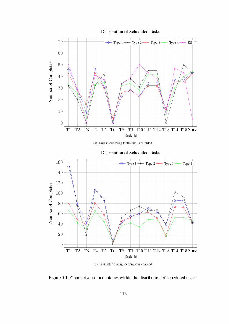
T1 T2 T3 T4 T5 T6 T8 T9 T10 T11 T12 T13 T14 T15 Surv0
10
20
30
40
50
60
70
Task Id
Num
bero
fCom
plet
es
Distribution of Scheduled Tasks
Type 1 Type 2 Type 3 Type 4 KS
(a) Task interleaving technique is disabled.
T1 T2 T3 T4 T5 T6 T8 T9 T10 T11 T12 T13 T14 T15 Surv0
20
40
60
80
100
120
140
160
Task Id
Num
bero
fCom
plet
es
Distribution of Scheduled Tasks
Type 1 Type 2 Type 3 Type 4
(b) Task interleaving technique is enabled.
Figure 5.1: Comparison of techniques within the distribution of scheduled tasks.
113

Table5.1: Comparison of scheduling techniques when task interleaving technique is(a) disabled and (b) enabled by using CfTUL as the decision method, and disablingadaptive update-rate and multi-frequency band usage techniques.
(a)
Type 1 Type 2 Type 3 Type 4 KS
# of tracking tasks 389 395 387 385 457
# of surveillances 43 43 42 44 3
# of prob. drops 15 39 19 37 66
Occupancy (%) 100.00 100.00 99.52 98.90 99.60
Cost (s2) 3.94×10⁷ 9.74×10⁶ 2.20×10⁴ 1.68×10⁴ 2.16×10⁵
Avg. of errors (m2) 1.70×10⁵ 1.53×10⁵ 1.46×10⁵ 1.56×10⁵ 1.45×10⁵
(b)
Type 1 Type 2 Type 3 Type 4
# of tracking tasks 973 1000 746 583
# of surveillances 43 42 42 46
# of prob. drops 15 28 13 1
Occupancy (%) 59.33 60.24 48.93 43.05
Cost (s2) 9.68×10³ 2.61×10⁴ 0.52×10³ 0.49×10³
Avg. of errors (m2) 3.38×10⁴ 1.08×10⁵ 4.51×10⁴ 5.83×10⁴
The effects of the multi-frequency band usage on scheduling is shown in Table 5.2 for
the same scenario shown in Figure 3.10. Here, the main goal is to see the occupancies
provided by the schedulers when task interleaving technique is applied by jointly
using the multi-frequency band usage technique. In Table 5.2(a) and Table 5.2(b),
the number of available frequency bands is set as 2 and 7, respectively. The higher
number of frequency bands increases the scheduling performance; higher number of
scheduled tasks, smaller cost, smaller number of probable drops, higher occupancy,
smaller average of errors due to increment in the utilization of the radar timeline.
Up to here, the simulations are run on a specific scenario. From now on, the compar-
isons are made on the average of the scheduler performance by running them on the
identical scenario with randomly generated targets for 100 times. That is at every run,
N = 15 and N = 25 targets are moving for the duration of tmax = 200 s.
114

Table5.2: Effects of multi-frequency band usage technique on scheduling when thenumber of frequency bands is (a) 2 and (b) 7.
(a)
Type 1 Type 2 Type 3 Type 4
# of tracking tasks 921 759 934 860
# of surveillances 36 36 37 36
# of prob. drops 83 54 70 103
Occupancy (%) 55.41 46.96 56.41 51.94
Cost (s2) 3.21×10⁶ 3.59×10⁶ 3.85×10³ 3.11×10⁵
Avg. of errors (m2) 3.76×10⁴ 3.60×10⁴ 3.15×10⁴ 1.82×10⁵
(b)
Type 1 Type 2 Type 3 Type 4
# of tracking tasks 1447 1492 1307 1335
# of surveillances 42 41 40 40
# of prob. drops 17 30 24 16
Occupancy (%) 81.09 82.67 74.06 75.18
Cost (s2) 3.13×10⁵ 5.44×10⁴ 0.44×10³ 0.55×10³
Avg. of errors (m2) 1.55×10⁴ 2.15×10⁴ 1.71×10⁴ 1.67×10⁴
The distribution of scheduler rankings with respect to average of errors is given at the
end of each table. This ranking given in the tables will denote that average and the
scenario based performance are not proportional which holds the comment about the
average of tracking error.
In Table 5.3, all types of MTATBS and KS are compared when task interleaving
technique is not applied. Here, the main goal is to see the statistics (the average of
errors and the number of probable drops) of the scheduler by using CfTUL as the
decision method, and disabling the adaptive update-rate technique. These optional
techniques are disabled to see core performance of the schedulers. Moreover, all
types of MTATBS are ranked within each other, as shown in parenthesis.
115

Table5.3: Comparison of scheduling techniques for (a) N = 15 and (b) N = 25targets by disabling task interleaving and adaptive update-rate techniques, within theduration of tmax = 200 s.
(a)
Average of statistics after 100 simulations
Type 1 Type 2 Type 3 Type 4 KS
# of tracking tasks 148.16 153.02 148.17 151.12 177.34
# of surveillances 18.54 18.59 18.35 18.45 2.71
# of prob. drops 32.07 10.61 29.53 17.43 9.96
Occupancy (%) 100.00 100.00 99.85 99.76 99.59
Cost (s2) 1.46×10⁶ 8.32×10⁵ 1.14×10⁴ 1.10×10⁵ 2.16×10⁴
Avg. of errors (m2) 3.35×10⁵ 2.54×10⁵ 2.37×10⁵ 3.28×10⁵ 1.77×10⁵
Distributions of rankings with respect to avg. of errors
Best 2(5) 46(59) 3(21) 7(15) 42
Runner-up 5(14) 13(10) 29(59) 11(17) 42
Honorable Mention 14(40) 12(13) 50(20) 16(27) 8
Last 38(41) 18(18) 0(0) 39(41) 5
(b)
Average of statistics after 100 simulations
Type 1 Type 2 Type 3 Type 4 KS
# of tracking tasks 132.51 140.12 132.33 139.08 183.91
# of surveillances 26.90 27.15 26.98 27.09 0.50
# of prob. drops 100.80 16.33 103.99 25.55 13.13
Occupancy (%) 100.00 100.00 100.00 100.00 100.00
Cost (s2) 5.38×10⁶ 2.85×10⁶ 1.96×10⁵ 1.39×10⁶ 3.55×10⁴
Avg. of errors (m2) 1.44×10⁶ 4.09×10⁵ 1.22×10⁶ 6.02×10⁵ 8.44×10⁵
Distributions of rankings with respect to avg. of errors
Best 0(0) 66(68) 0(0) 30(32) 4
Runner-up 1(2) 25(26) 4(15) 39(57) 31
Honorable Mention 5(25) 3(2) 33(70) 21(3) 38
Last 55(73) 3(4) 14(15) 7(8) 21
116
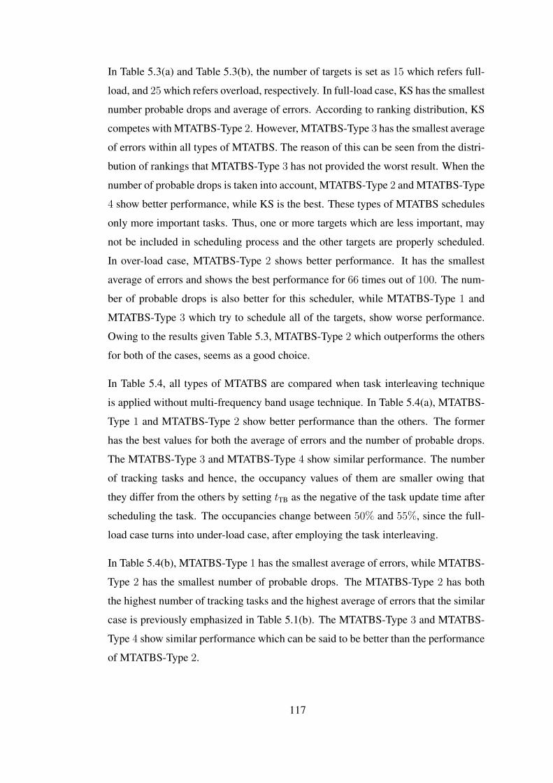
In Table 5.3(a) and Table 5.3(b), the number of targets is set as 15 which refers full-
load, and 25 which refers overload, respectively. In full-load case, KS has the smallest
number probable drops and average of errors. According to ranking distribution, KS
competes with MTATBS-Type 2. However, MTATBS-Type 3 has the smallest average
of errors within all types of MTATBS. The reason of this can be seen from the distri-
bution of rankings that MTATBS-Type 3 has not provided the worst result. When the
number of probable drops is taken into account, MTATBS-Type 2 and MTATBS-Type
4 show better performance, while KS is the best. These types of MTATBS schedules
only more important tasks. Thus, one or more targets which are less important, may
not be included in scheduling process and the other targets are properly scheduled.
In over-load case, MTATBS-Type 2 shows better performance. It has the smallest
average of errors and shows the best performance for 66 times out of 100. The num-
ber of probable drops is also better for this scheduler, while MTATBS-Type 1 and
MTATBS-Type 3 which try to schedule all of the targets, show worse performance.
Owing to the results given Table 5.3, MTATBS-Type 2 which outperforms the others
for both of the cases, seems as a good choice.
In Table 5.4, all types of MTATBS are compared when task interleaving technique
is applied without multi-frequency band usage technique. In Table 5.4(a), MTATBS-
Type 1 and MTATBS-Type 2 show better performance than the others. The former
has the best values for both the average of errors and the number of probable drops.
The MTATBS-Type 3 and MTATBS-Type 4 show similar performance. The number
of tracking tasks and hence, the occupancy values of them are smaller owing that
they differ from the others by setting tTB as the negative of the task update time after
scheduling the task. The occupancies change between 50% and 55%, since the full-
load case turns into under-load case, after employing the task interleaving.
In Table 5.4(b), MTATBS-Type 1 has the smallest average of errors, while MTATBS-
Type 2 has the smallest number of probable drops. The MTATBS-Type 2 has both
the highest number of tracking tasks and the highest average of errors that the similar
case is previously emphasized in Table 5.1(b). The MTATBS-Type 3 and MTATBS-
Type 4 show similar performance which can be said to be better than the performance
of MTATBS-Type 2.
117
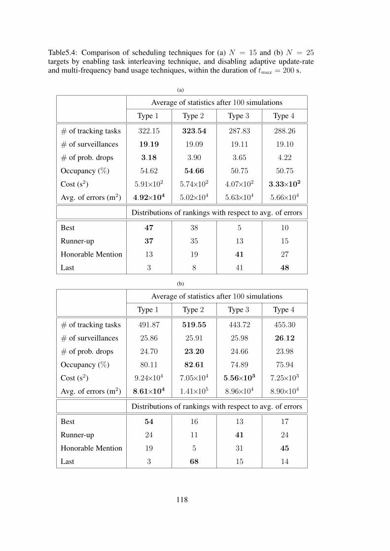
Table5.4: Comparison of scheduling techniques for (a) N = 15 and (b) N = 25targets by enabling task interleaving technique, and disabling adaptive update-rateand multi-frequency band usage techniques, within the duration of tmax = 200 s.
(a)
Average of statistics after 100 simulations
Type 1 Type 2 Type 3 Type 4
# of tracking tasks 322.15 323.54 287.83 288.26
# of surveillances 19.19 19.09 19.11 19.10
# of prob. drops 3.18 3.90 3.65 4.22
Occupancy (%) 54.62 54.66 50.75 50.75
Cost (s2) 5.91×10² 5.74×10² 4.07×10² 3.33×10²
Avg. of errors (m2) 4.92×10⁴ 5.02×10⁴ 5.63×10⁴ 5.66×10⁴
Distributions of rankings with respect to avg. of errors
Best 47 38 5 10
Runner-up 37 35 13 15
Honorable Mention 13 19 41 27
Last 3 8 41 48
(b)
Average of statistics after 100 simulations
Type 1 Type 2 Type 3 Type 4
# of tracking tasks 491.87 519.55 443.72 455.30
# of surveillances 25.86 25.91 25.98 26.12
# of prob. drops 24.70 23.20 24.66 23.98
Occupancy (%) 80.11 82.61 74.89 75.94
Cost (s2) 9.24×10⁴ 7.05×10⁴ 5.56×10³ 7.25×10³
Avg. of errors (m2) 8.61×10⁴ 1.41×10⁵ 8.96×10⁴ 8.90×10⁴
Distributions of rankings with respect to avg. of errors
Best 54 16 13 17
Runner-up 24 11 41 24
Honorable Mention 19 5 31 45
Last 3 68 15 14
118
Owing to the results given Table 5.4, MTATBS-Type 1 which outperforms the oth-
ers for both of the cases, seems as a good choice. Although, MTATBS-Type 1 and
MTATBS-Type 2 are the leading schedulers, they are not suggested to employ on a
real system. Because it is said that the consecutive updates consume vast radar time
resources, in Section 3.2.1.5, and both of these schedulers exploit the consecutive up-
dates. Then, MTATBS-Type 3 and MTATBS-Type 4 are preferable that the former
tries to schedule all tasks and the latter schedules only more important tasks. If the
results given in Table 5.3 and Table 5.4, are revised, it is seen that MTATBS-Type 4
shows better performance for over-load case. Hence, MTATBS-Type 4 is chosen as
the base scheduler for the following comparisons.
In Table 5.5 and Table 5.6, the decision methods are compared when there areN = 15
and N = 25 targets, respectively. Here, the main goal is to see the statistics, the av-
erage of errors and the number of probable drops, of MTATBS-Type 4 by using each
of the decision methods, and applying the adaptive update-rate and multi-frequency
band usage techniques. Furthermore, the effect of multi-frequency band usage tech-
nique on the tracking performance is compared by setting the number of frequency
bands as 2 that the results are given in Table 5.5(a) and Table 5.6(a), and 7 that the
results are given in Table 5.5(b) and Table 5.6(b). The proposed methods, DeCP,
MinTE and PurMM are compared with CfTUL which is assigned as the reference
method. Then, DecP is the unique method which has the smaller number of prob-
able drops and the smaller average of errors than CfTUL owing to the results given
in these tables. Indeed, there is not a significant difference between the results of
the proposed methods. All of them are usually better than CfTUL that is concluded
from the distribution of rankings. The PurMM has the smallest average of errors, and
MinTE shows more frequently the best performance than the others when there are
25 targets, as shown in Table 5.6.
119

Table5.5: Comparison of the decision methods by enabling adaptive update-rate tech-nique and the number of frequency bands is (a) 2 and (b) 7 by scheduling N = 15targets with MTATBS-Type4 within the duration of tmax = 200 s.
(a)
Average of statistics after 100 simulations
CfTUL DecP MinTE PurMM
# of tracking tasks 296.94 296.05 294.24 296.94
# of surveillances 17.55 17.68 17.54 17.57
# of prob. drops 24.98 24.05 24.54 24.68
Occupancy (%) 49.81 49.83 49.46 49.82
Cost (s2) 1.77×10⁴ 2.12×10⁴ 1.68×10⁴ 1.99×10⁴
Avg. of errors (m2) 1.97×10⁵ 1.82×10⁵ 1.95×10⁵ 2.06×10⁵
Distributions of rankings with respect to avg. of errors
Best 27 26 25 22
Runner-up 17 27 25 31
Honorable Mention 20 29 28 23
Last 36 18 22 24
(b)
Average of statistics after 100 simulations
CfTUL DecP MinTE PurMM
# of tracking tasks 365.36 366.98 364.83 367.98
# of surveillances 19.25 19.15 19.25 19.12
# of prob. drops 14.72 14.10 14.92 14.29
Occupancy (%) 59.35 59.46 59.31 59.52
Cost (s2) 0.44×10³ 0.40×10³ 0.41×10³ 0.47×10³
Avg. of errors (m2) 7.12×10⁴ 6.94×10⁴ 7.14×10⁴ 6.92×10⁴
Distributions of rankings with respect to avg. of errors
Best 31 23 17 29
Runner-up 16 30 32 22
Honorable Mention 21 30 20 29
Last 32 17 31 20
120

Table5.6: Comparison of the decision methods by enabling adaptive update-rate tech-nique and the number of frequency bands is (a) 2 and (b) 7 by scheduling N = 25targets with MTATBS-Type 4 within the duration of tmax = 200 s.
(a)
Average of statistics after 100 simulations
CfTUL DecP MinTE PurMM
# of tracking tasks 308.11 305.52 303.14 305.82
# of surveillances 24.53 24.64 24.58 24.75
# of prob. drops 43.81 42.47 43.75 44.03
Occupancy (%) 57.30 57.12 56.81 57.25
Cost (s2) 3.04×10⁵ 3.75×10⁵ 3.46×10⁵ 3.37×10⁵
Avg. of errors (m2) 7.28×10⁵ 6.67×10⁵ 6.93×10⁵ 6.33×10⁵
Distributions of rankings with respect to avg. of errors
Best 17 29 33 21
Runner-up 17 25 20 38
Honorable Mention 33 28 20 19
Last 33 18 27 22
(b)
Average of statistics after 100 simulations
CfTUL DecP MinTE PurMM
# of tracking tasks 511.81 513.66 512.67 512.64
# of surveillances 25.84 25.90 25.88 25.87
# of prob. drops 45.03 43.68 43.40 43.43
Occupancy (%) 81.65 81.91 81.76 81.78
Cost (s2) 2.12×10⁴ 2.59×10⁴ 2.34×10⁴ 2.23×10⁴
Avg. of errors (m2) 1.51×10⁵ 1.46×10⁵ 1.43×10⁵ 1.42×10⁵
Distributions of rankings with respect to avg. of errors
Best 17 25 32 26
Runner-up 21 30 23 26
Honorable Mention 24 27 23 26
Last 38 18 22 22
121

122
CHAPTER 6
CONCLUSIONS AND FUTURE WORK
In this work, two schedulers are examined, namely MTATBS and KS for the real-time
resource management of MFPAR. A resource-aided technique called as the multi-
frequency band usage, is developed to increase the applicability of task interleaving.
The KS which employs the binary integer programming is proposed to suggest a
simple optimization technique for RRM. The KS is compared with TB based tech-
niques. However, it is concluded that the computation time requirement of KS is too
much for real-time operation. The higher number of targets makes the scheduling al-
most intractable for KS. Moreover, the resource-aided techniques except the adaptive
update-rate are not applicable for it. Thus, TB based techniques comprise the main
part of this work.
The MTATBS utilizes the existing ATB scheduler algorithm described in [48] with
some improvements:
1. Scheduling parameters can be dynamically changed by tracker in addition to
scheduler.
2. Scheduling utilizes multi-frequency bands for interleaved tasks.
3. Decision method which is previously the selection of a task with the highest
priority and tTB, of TB technique based schedulers is modified.
The decision process is required when there are at least two targets which satisfy the
maximum priority level and tTB for MTATBS. The traditional method is to choose the
123

target which has the smallest task id among candidate targets for track update. This
does not guarantees an appropriate performance. We suggest to adopt the solution
methods for the well-known machine replacement problem to the problem of target
selection and track update is solved with a method called DecP. In addition to this
method, two other ad hoc methods, namely MinTE and PurMM, are given.
The results show that all TB based techniques provide similar performance with mi-
nor differences. Task interleaving and the multi-frequency band usage techniques
increase the tracking performance and the utilization of radar timeline effectively.
Decision methods based on machine replacement and others increase the tracking
performance and decrease the number probable drops. The MTATBS-Type 4 and
DeCP is suggested as the scheduler and the decision method respectively. It should
be noted minor performance differences not easily reflected in averaged results can
be important for the practical applications. Hence, the decision policy based on track
quality can be important in general.
To conduct experiments, a simulator for MFPAR system is implemented to apply
RRM techniques with different optional choices, such as adaptive update-rate, dy-
namic task prioritization, tracking, task interleaving. The simulator which combines
the model shown in Figure 2.1, is designed in a way that each of the blocks can
be individually modified according to RRM constraints. Hence, the development of
general purpose simulator is one of the main contributions of this work.
Among future works, it can be useful to utilize the optimization-based methods for
the scheduling problem and compare the optimization-based methods and MTATBS
with our simulator. In addition, the simulator can be modified to handle the radar
equation, probability of detection, false alarm values and other related parameters.
124

REFERENCES
[1] M. I. Skolnik. Introduction to radar systems. Tata McGraw Hill, 772 pp., 2003.
[2] Z. Ding. A survey of radar resource management algorithms. In Canadian Con-ference on Electrical and Computer Engineering, 2008. CCECE 2008, pages1559–1564, May 2008.
[3] S. Sabatini and M. Tarantino. Multifunction Array Radar: System Design andAnalysis. The Artech House Radar Library. Artech House, 271 pp., 1994.
[4] B. Gillespie, E. Hughes, and M. Lewis. Scan scheduling of multi-functionphased array radars using heuristic techniques. In IEEE International RadarConference, pages 513–518, May 2005.
[5] A. G. Huizing and A. A. F. Bloemen. An efficient scheduling algorithm for amultifunction radar. In IEEE International Symposium on Phased Array Sys-tems and Technology, 1996, pages 359–364, Oct. 1996.
[6] A. J. Orman, C. N. Potts, A. K. Shahani, and A. R. Moore. Scheduling for amultifunction array radar system. European Journal of Operational Research,90(1):13–25, 1996.
[7] A. Izquierdo-Fuente and J. R. Casar-Corredera. Optimal radar pulse schedulingusing a neural network. In 1994 IEEE International Conference on Neural Net-works. IEEE World Congress on Computational Intelligence, volume 7, pages4588–4591, June 1994.
[8] W. Komorniczak and J. Pietrasiñski. Selected problems of MFR resources man-agement. In Proceedings of the 3rd International Conference on InformationFusion, 2000. FUSION 2000, volume 2, pages WEC1/3–WEC1/8 vol.2, July2000.
[9] R. Popoli and S. Blackman. Expert system allocation for the electronicallyscanned antenna radar. In American Control Conference, 1987, pages 1821–1826, Minneapolis, MN, USA, June 1987.
[10] V. C. Vannicola and J. A. Mineo. Expert system for sensor resource allocation.In Proceedings of the 33rd Midwest Symposium on Circuits and Systems, 1990,volume 2, pages 1005–1008, Aug. 1990.
[11] S. Miranda, C. Baker, K. Woodbridge, and H. Griffiths. Knowledge-based re-source management for multifunction radar: a look at scheduling and task pri-oritization. IEEE Signal Processing Magazine, 23(1):66–76, Jan. 2006.
[12] S. L. C. Miranda, C. J. Baker, K. Woodbridge, and H. D. Griffiths. Simulationmethods for prioritising tasks and sectors of surveillance in phased array radars.International Journal of Simulation, 5(1-2):18–25, 2004.
125
[13] S. L. C. Miranda, C. J. Baker, K. Woodbridge, and H. D. Griffiths. Fuzzy logicapproach for prioritisation of radar tasks and sectors of surveillance in multi-function radar. Radar, Sonar Navigation, IET, 1(2):131–141, Apr. 2007.
[14] M. T. Vine. Fuzzy logic in radar resource management. In IEE MultifunctionRadar and Sonar Sensor Management Techniques (Ref. No. 2001/173), pages5/1–5/4, Nov. 2001.
[15] D. P. Bertsekas. Dynamic Programming and Optimal Control, volume 1.Athena Scientific, 400 pp., Belmont, MA, USA, 1995.
[16] D. Strömberg and P. Grahn. Scheduling of tasks in phased array radar. InProceedings of IEEE International Symposium on Phased Array Systems andTechnology, pages 318–321, 1996.
[17] J. Wintenby and V. Krishnamurthy. Hierarchical resource management in adap-tive airborne surveillance radars. IEEE Transactions on Aerospace and Elec-tronic Systems, 42(2):401–420, Apr. 2006.
[18] R. Washburn, M. Schneider, and J. Fox. Stochastic dynamic programmingbased approaches to sensor resource management. In Proceedings of the 5thInternational Conference on Information Fusion, 2002, volume 1, pages 608–615, Annapolis, MD, USA, 2002.
[19] V. Krishnamurthy and R. J. Evans. Hidden Markov model multiarm bandits: amethodology for beam scheduling in multitarget tracking. IEEE Transactionson Signal Processing, 49(12):2893–2908, Dec. 2001.
[20] V. Krishnamurthy and R. J. Evans. Correction to ’Hidden Markov model multi-arm bandits: a methodology for beam scheduling in multitarget tracking’. IEEETransactions on Signal Processing, 51(6):1662–1663, June 2003.
[21] B. F. La Scala and B. Moran. Optimal target tracking with restless bandits.Digital Signal Processing, 16(5):479–487, Sept. 2006.
[22] A. O. Hero III, D. A. Castañón, D. Cochran, and K. Kastella. Foundations andApplications of Sensor Management. Signals and Communication Technology.Springer, 308 pp., 2008.
[23] J. Wintenby. Resource Allocation in Airborne Surveillance Radar. PhD thesis,Chalmers University Of Technology, Göteborg, Sweden, 2003.
[24] A. G. Huizing and J. A. Spruyt. Adaptive waveform selection with a neuralnetwork. In International Conference Radar 92, pages 419–421, Oct. 1992.
[25] B. F. La Scala, W. Moran, and R. J. Evans. Optimal adaptive waveform selectionfor target detection. In Proceedings of the International Radar Conference,pages 492–496, Sept. 2003.
[26] D. Cochran, S. Suvorova, S. D. Howard, and B. Moran. Waveform libraries:Measures of effectiveness for radar scheduling. IEEE Signal Processing Maga-zine, 26(1):12–21, Jan. 2009.
126
[27] B. La Scala, M. Rezaeian, and B. Moran. Optimal adaptive waveform selectionfor target tracking. In The 8th International Conference on Information Fusion,volume 1, pages 552–557, July 2005.
[28] S. M. Sowelam and A. H. Tewfik. Waveform selection in radar target classifica-tion. IEEE Transactions on Information Theory, 46(3):1014–1029, May 2000.
[29] G. van Keuk and S. S. Blackman. On phased-array radar tracking and parametercontrol. IEEE Transactions on Aerospace and Electronic Systems, 29(1):186–194, Jan. 1993.
[30] G. A. Watson and W. D. Blair. Revisit calculation and waveform control for amultifunction radar. In Proceedings of the 32nd IEEE Conference on Decisionand Control, volume 1, pages 456–460, San Antonio, TX, USA, Dec. 1993.
[31] H.-J. Shin, S.-M. Hong, and D.-H. Hong. Adaptive-update-rate target trac-king for phased-array radar. IEE Proceedings - Radar, Sonar and Navigation,142(3):137–143, June 1995.
[32] S.-M. Hong and Y.-H. Jung. Optimal scheduling of track updates in phasedarray radars. IEEE Transactions on Aerospace and Electronic Systems,34(3):1016–1022, July 1998.
[33] W. D. Blair, G. A. Watson, and S. A. Hoffman. Benchmark problem for beampointing control of phased array radar against maneuvering targets. In Proceed-ings of the American Control Conference, volume 2, pages 2071–2075, Balti-more, MD, USA, June 1994.
[34] W. D. Blair, G. A. Watson, G. L. Gentry, and S. A. Hoffman. Benchmark prob-lem for beam pointing control of phased array radar against maneuvering targetsin the presence of ECM and false alarms. In Proceedings of the American Con-trol Conference, volume 4, pages 2601–2605, Seattle, WA, USA, June 1995.
[35] W. D. Blair and G. A. Watson. Benchmark problem for radar resource allo-cation and tracking maneuvering targets in the presence of ECM. TechnicalReport NSWCDD/TR-96/10, Naval Surface Warfare Center Dahlgren Division,Dahlgren, VA, USA, Sept. 1996.
[36] W. D. Blair, G. A. Watson, T. Kirubarajan, and Y. Bar-Shalom. Benchmark forradar allocation and tracking in ECM. IEEE Transactions on Aerospace andElectronic Systems, 34(4):1097–1114, Oct. 1998.
[37] S. S. Blackman, M. T. Busch, G. Demos, and R. F. Popoli. IMM/MHT trackingand data association for benchmark tracking problem. In Proceedings of theAmerican Control Conference, volume 4, pages 2606–2610, Seattle, WA, USA,June 1995.
[38] Y. Bar-Shalom and X.-R. Li. Multitarget-multisensor Tracking: Principles AndTechniques. YBS Publishing, 615 pp., Storrs, CT, USA, 1995.
[39] T. Kirubarajan, Y. Bar-Shalom, W. D. Blair, and G. A. Watson. IMMPDAF forradar management and tracking benchmark with ECM. IEEE Transactions onAerospace and Electronic Systems, 34(4):1115–1134, Oct. 1998.
127
[40] C. Lee. On Quality of Service Management. PhD thesis, Carnegie MellonUniversity, Pittsburgh, PA, USA, Aug. 1999.
[41] R. Rajkumar, C. Lee, J. Lehoczky, and D. Siewiorek. A resource allocationmodel for QoS management. In Proceedings of the 18th IEEE Real-Time Sys-tems Symposium, 1997, pages 298–307, Dec. 1997.
[42] S. Ghosh, J. Hansen, R. (Raj) Rajkumar, and J. Lehoczky. Integrated resourcemanagement and scheduling with multi-resource constraints. In Proceedings ofthe 25th IEEE International Real-Time Systems Symposium, 2004, pages 12–22,Lisbon, Portugal, Dec. 2004.
[43] S. Ghosh, J. Hansen, R. (Raj) Rajkumar, and J. Lehoczky. Adaptive QoS opti-mizations with applications to radar tracking. Technical Report 18-03-04, Insti-tute for Complex Engineering Systems, Carnegie Mellon University, 2004.
[44] J. Hansen, R. Rajkumar, J. Lehoczky, and S. Ghosh. Resource managementfor radar tracking. In IEEE Conference on Radar, 2006. RADAR ’06, pages140–147, Verona, NY, USA, Apr. 2006.
[45] A. Ircı. On Optimal Resource Allocation in Multifunction Radar Systems. MScthesis, Middle East Technical University, Ankara, Turkey, Sept. 2006.
[46] W. K. Stafford. Real time control of a Multifunction Electronically ScannedAdaptive Radar, (MESAR). IEE Colloquium on Real-Time Management ofAdaptive Radar Systems, pages 7/1–7/5, June 1990.
[47] J. M. Butler. Tracking and Control in Multi-Function Radar. PhD thesis, Uni-versity College London, 1998.
[48] R. Reinoso-Rondinel, T.-Y. Yu, and S. Torres. Task prioritization on phased-array radar scheduler for adaptive weather sensing. The 26th International Con-ference on Interactive Information and Processing Systems (IIPS) for Meteorol-ogy, Oceanography, and Hydrology. American Meteorological Society, Paper14B.6, Atlanta, GA, USA, 2010.
[49] F. Opitz and T. Kausch. UKF controlled variable-structure IMM algorithmsusing coordinated turn models. In Proceedings of the 7th International Confer-ence on Information Fusion, 2004. FUSION 2004, volume I, pages 138–145,Mountain View, CA, USA, June 2004. International Society of Information Fu-sion.
[50] A. J. Orman and C. N. Potts. On the complexity of coupled-task scheduling.Discrete Applied Mathematics, 72(1–2):141–154, 1997.
[51] G. B. Thomas and R. L. Finney. Calculus and Analytic Geometry, 9th ed.Addison-Wesley, 1264 pp., 1995.
[52] M. Wray. Software architecture for real time control of the radar beam withinMESAR. In International Conference Radar 92, pages 38–41, Oct 1992.
[53] R. Reinoso-Rondinel, T.-Y. Yu, and S. Torres. Multifunction phased-arrayradar: Time balance scheduler for adaptive weather sensing. Journal of At-mospheric and Oceanic Technology, 27:1854–1867, 2010.
128

[54] B. Korte and J. Vygen. Combinatorial Optimization: Theory and Algorithms.Algorithms and Combinatorics 21. Springer Berlin Heidelberg, 597 pp., 2006.
[55] G. B. Dantzig. Discrete-variable extremum problems. Operations Research,5(2):266–277, Apr. 1957.
[56] D. Pisinger. Algorithms for Knapsack Problems. PhD thesis, University ofCopenhagen, 1995.
[57] T. Ben-Zvi and A. Grosfeld-Nir. Partially observed Markov decision pro-cesses with binomial observations. Operations Research Letters, 41(2):201–206, 2013.
[58] S. Anily and A. Grosfeld-Nir. An optimal lot-sizing and offline inspection pol-icy in the case of nonrigid demand. Operations Research, 54(2):311–323, 2006.
[59] P. R. Kumar and P. Varaiya. Stochastic Systems: Estimation, Identification, andAdaptive Control. Information and System Sciences Series. Prentice-Hall, Inc.,358 pp., Englewood Cliffs, NJ, USA, 1986.
[60] R. D. Smallwood and E. J. Sondik. The optimal control of partially observablemarkov processes over a finite horizon. Operations Research, 21(5):1071–1088,1973.
[61] M. Givon and A. Grosfeld-Nir. Using partially observed markov processes toselect optimal termination time of TV shows. Omega, 36(3):477–485, 2008.Special Issue on Multiple Criteria Decision Making for Engineering.
[62] A. Silberschatz, P. B. Galvin, and G. Greg. Operating System Concepts. JohnWiley & Sons, Inc., 944 pp., 2013.
[63] Y. Bar-Shalom, X.-R. Li, and T. Kirubarajan. Estimation with Applications toTracking and Navigation. John Wiley & Sons, Inc., 584 pp., New York, NY,USA, July 2001.
129

130

APPENDIX A
INTERACTING MULTIPLE MODEL FILTER FOR
TRACKING
The interacting multiple model (IMM) is an efficient estimation technique for mane-
uvering targets. The possible target maneuvers are described by a finite state model.
The IMM is able to give accurate estimation results, whenever the true target maneu-
ver fits with a single maneuver model of the implemented discrete set. The additional
gain of the IMM is to extend the covered target maneuver by a statistical mixing of
the elements of the model set. A widely used model set contains the constant velocity
model (CV) and coordinated turn model (CT) with fixed angular velocity [49].
The evolution of the target motion model state, rk, is modeled by a time-homogeneous
(time-invariant) r-state Markov chain with the transition probabilities,
πij , Pr{rk+1 = j|rk = i}, ∀ i, j ∈ {1, 2, . . . , r}. (A.1)
The transition probability matrix (TPM), Π = [πij] is a r × r matrix with elements
satisfying πij ≥ 0 and∑r
j=1 πij = 1, ∀ i ∈ {1, 2, . . . , r}. The TPM used in this work
with r = 2 is
Π =
0.99 0.01
0.01 0.99
. (A.2)
131

A.1 State Space Representations for Target Motion Models
State vector for a target moving in a 2-D plane is
xk =[xk xk yk yk
]T, (A.3)
where xk and yk are the target position in Cartesian coordinates, xk and yk are the
target velocities at time k.
The problem addressed is the estimation of the state (position) of the moving target
which obeys 2 possible modes (models) that are CV with different process noise
covariance, Qj , for j = 1, 2. The state space representation is considered as
xk+1 = Ajkxk + Gj
kwjk, (A.4)
yk = Cjkxk + Hj
kvjk, (A.5)
where wjk is the process noise distributed with wj
k ∼ N (wjk; 0,Qj) and vjk is the
measurement noise distributed with vjk ∼ N (vjk; 0,Rj) for model-j.
In (A.5), yk is the 2 × 1 measurement vector consists only position of the moving
target at time k. The coefficient parameters for state and noise vectors shown in (A.4)
and (A.5) are assumed to be known. They are defined as follows:
A1k = A2
k = A =
1 0 T 0
0 1 0 T
0 0 1 0
0 0 0 1
, (A.6)
G1k = G2
k = G =
T 2/2 0
0 T
T 2/2 0
0 T
, (A.7)
132

where the sampling interval is T = 1 s. The other matrices are
Q1 =
0.12 0
0 0.12
(m/s2)2 & Q2 =
102 0
0 102
(m/s2)2, (A.8)
C1k = C2
k = C =
1 0 0 0
0 1 0 0
, (A.9)
H1k = H2
k = H =
1 0
0 1
, (A.10)
R1 = R2 = R =
σ
2x 0
0 σ2y
, (A.11)
where σx and σy are standard deviations of measurement in x and y directions, e.g.
σx = σy = 80 m.
A.2 Interacting Multiple Model Estimator
In the interacting multiple model estimator, at time k the state estimate is computed
under each possible current model using r filters, with each filter using a different
combination of the previous model-conditioned estimates — mixed initial conditions
[63]. The IMM estimates the posterior distribution of the state as follows:
p(xk|y0:k) =r∑
j=1
p(xk|rk = j,y0:k)P (rk = j|y0:k). (A.12)
In (A.12), P (rk = j|y0:k) denotes the mode probability of model-j that will be de-
rived later and p(xk|rk = j,y0:k) is approximated as
p(xk|rk = j,y0:k) ≈ N (xk; xjk|k,P
jk|k), (A.13)
then (A.12) becomes a mixture of Gaussian distributions with weightings mode prob-
abilities,
133

p(xk|y0:k) ≈r∑
j=1
N (xk; xjk|k,P
jk|k)µ
jk, (A.14)
where
µjk , P (rk = j|y0:k). (A.15)
Recursive steps to find the mode-conditioned estimate xjk|k, mode-conditioned covari-
ance Pjk|k and mode probability µjk in (A.14) are briefly given with the knowledge of
xjk−1|k−1, Pjk−1|k−1, µ
jk−1 and Π for j = 1, 2, . . . , r.
Step 1: Mixing probability calculation.
µi|jk−1|k−1 , P (rk−1 = i|rk = j,y0:k−1), (A.16)
=P (rk−1 = i, rk = j|y0:k−1)
P (rk = j|y0:k−1),
=P (rk = j|rk−1 = i,y0:k−1)P (rk−1 = i|y0:k−1)
P (rk = j|y0:k−1),
=P (rk = j|rk−1 = i,y0:k−1)P (rk−1 = i|y0:k−1)
r∑`=1
P (rk = j, rk−1 = `|y0:k−1),
=P (rk = j|rk−1 = i,y0:k−1)P (rk−1 = i|y0:k−1)r∑`=1
P (rk = j|rk−1 = `,y0:k−1)P (rk−1 = `|y0:k−1),
=πijµ
ik−1
r∑`=1
π`jµ`k−1
. (A.17)
Step 2: Interaction (mixing).
x0jk−1|k−1 =
r∑
i=1
xik−1|k−1µi|jk−1|k−1, (A.18)
P0jk−1|k−1 =
r∑
i=1
µi|jk−1|k−1
[Pik−1|k−1+
(xik−1|k−1 − x0j
k−1|k−1)
(xik−1|k−1 − x0j
k−1|k−1)T]
. (A.19)
134

Step 3: Mode-matched filtering.
The estimate (A.18) and covariance (A.19) are used as input to filter Mj at time k.
Step 3a: Time update (prediction update).
xjk|k−1 = Ajk−1x
0jk−1|k−1, (A.20)
Pjk|k−1 = Aj
k−1P0jk−1|k−1A
jk−1
T+ Gj
k−1QjGj
k−1T, (A.21)
yjk|k−1 = Cjkx
jk|k−1. (A.22)
Step 3b: Measurement update.
Sjk = CjkP
jk|k−1C
jk
T+ Hj
kRjHj
k
T, (A.23)
Kjk = Pj
k|k−1Cjk
TSjk−1, (A.24)
xjk|k = xjk|k−1 + Kjk(yk − yjk|k−1), (A.25)
Pjk|k = Pj
k|k−1 −KjkS
jkK
jk
T, (A.26)
= Pjk|k−1 −Kj
kSjk
[Pjk|k−1C
jk
TSjk−1]T
,
=[I−Kj
kCjk
]Pjk|k−1. (A.27)
In (A.23) and (A.24), the measurement prediction covariance (innovation1 covari-
ance) and Kalman filter (KF) gain are given respectively. The KF matched to each
of model that gives the mode-conditioned estimate (A.25) and mode-conditioned co-
variance (A.27).
Step 3c: Likelihood function computation.
Λjk = p(yk|rk = j,y0:k−1), (A.28)
Λjk ∼ N (yk; y
jk|k−1,S
jk), (A.29)
Λjk =
1√(2π)2
∣∣Sjk∣∣
exp
[− 1
2
(yk − yjk|k−1
)T(Sjk)
−1(yk − yjk|k−1
)]. (A.30)
1 yk − yjk|k−1 is called the innovation.
135
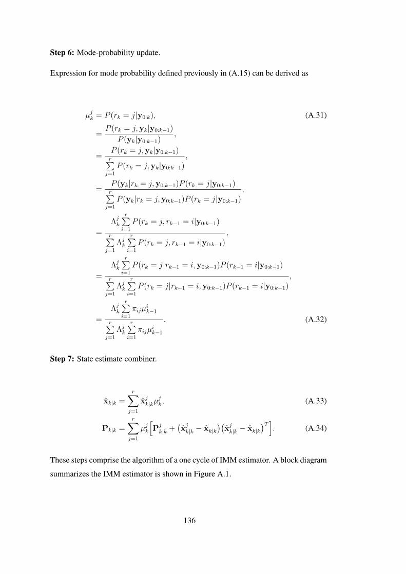
Step 6: Mode-probability update.
Expression for mode probability defined previously in (A.15) can be derived as
µjk = P (rk = j|y0:k), (A.31)
=P (rk = j,yk|y0:k−1)
P (yk|y0:k−1),
=P (rk = j,yk|y0:k−1)r∑j=1
P (rk = j,yk|y0:k−1),
=P (yk|rk = j,y0:k−1)P (rk = j|y0:k−1)r∑j=1
P (yk|rk = j,y0:k−1)P (rk = j|y0:k−1),
=
Λjk
r∑i=1
P (rk = j, rk−1 = i|y0:k−1)
r∑j=1
Λjk
r∑i=1
P (rk = j, rk−1 = i|y0:k−1),
=
Λjk
r∑i=1
P (rk = j|rk−1 = i,y0:k−1)P (rk−1 = i|y0:k−1)
r∑j=1
Λjk
r∑i=1
P (rk = j|rk−1 = i,y0:k−1)P (rk−1 = i|y0:k−1),
=
Λjk
r∑i=1
πijµik−1
r∑j=1
Λjk
r∑i=1
πijµik−1
. (A.32)
Step 7: State estimate combiner.
xk|k =r∑
j=1
xjk|kµjk, (A.33)
Pk|k =r∑
j=1
µjk
[Pjk|k +
(xjk|k − xk|k
)(xjk|k − xk|k
)T]. (A.34)
These steps comprise the algorithm of a one cycle of IMM estimator. A block diagram
summarizes the IMM estimator is shown in Figure A.1.
136
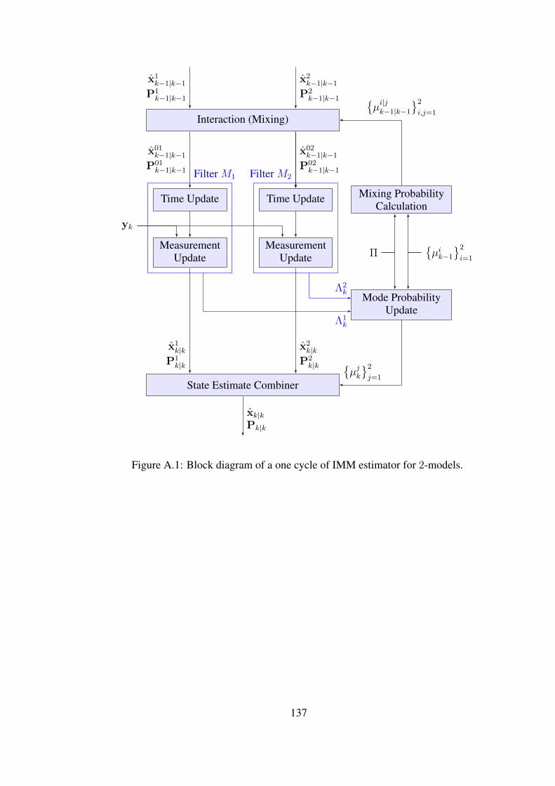
Interaction (Mixing)
Time Update
MeasurementUpdate
Time Update
MeasurementUpdate
Filter M1 Filter M2
Mixing ProbabilityCalculation
Mode ProbabilityUpdate
State Estimate Combiner
x01k−1|k−1
P01k−1|k−1
x02k−1|k−1
P02k−1|k−1
x1k−1|k−1
P1k−1|k−1
x2k−1|k−1
P2k−1|k−1
yk
x1k|k
P1k|k
x2k|k
P2k|k
Π{µik−1
}2
i=1
{µi|jk−1|k−1
}2
i,j=1
Λ1k
Λ2k
xk|kPk|k
{µjk
}2
j=1
Figure A.1: Block diagram of a one cycle of IMM estimator for 2-models.
137

138
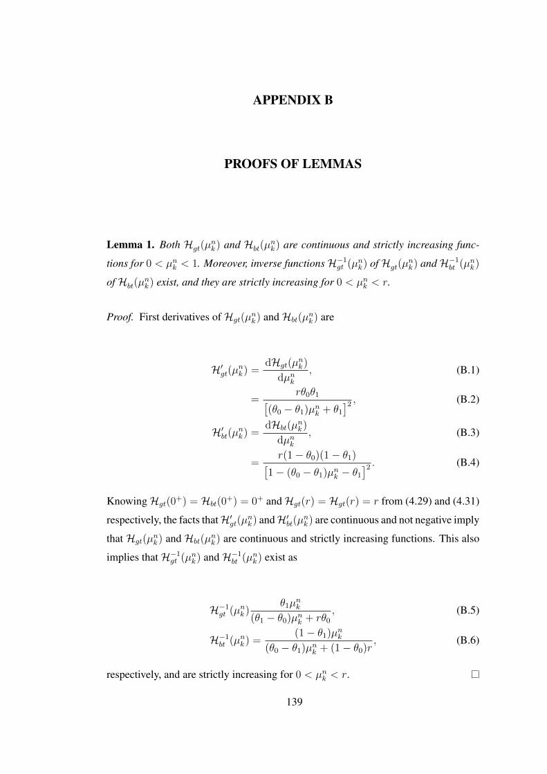
APPENDIX B
PROOFS OF LEMMAS
Lemma 1. Both Hgt(µnk) and Hbt(µ
nk) are continuous and strictly increasing func-
tions for 0 < µnk < 1. Moreover, inverse functionsH−1gt (µnk) ofHgt(µnk) andH−1bt (µnk)
ofHbt(µnk) exist, and they are strictly increasing for 0 < µnk < r.
Proof. First derivatives ofHgt(µnk) andHbt(µ
nk) are
H′gt(µnk) =dHgt(µ
nk)
dµnk, (B.1)
=rθ0θ1[
(θ0 − θ1)µnk + θ1]2 , (B.2)
H′bt(µnk) =dHbt(µ
nk)
dµnk, (B.3)
=r(1− θ0)(1− θ1)[
1− (θ0 − θ1)µnk − θ1]2 . (B.4)
KnowingHgt(0+) = Hbt(0
+) = 0+ andHgt(r) = Hgt(r) = r from (4.29) and (4.31)
respectively, the facts thatH′gt(µnk) andH′bt(µnk) are continuous and not negative imply
that Hgt(µnk) and Hbt(µ
nk) are continuous and strictly increasing functions. This also
implies thatH−1gt (µnk) andH−1bt (µnk) exist as
H−1gt (µnk)θ1µ
nk
(θ1 − θ0)µnk + rθ0, (B.5)
H−1bt (µnk) =(1− θ1)µnk
(θ0 − θ1)µnk + (1− θ0)r, (B.6)
respectively, and are strictly increasing for 0 < µnk < r.
139
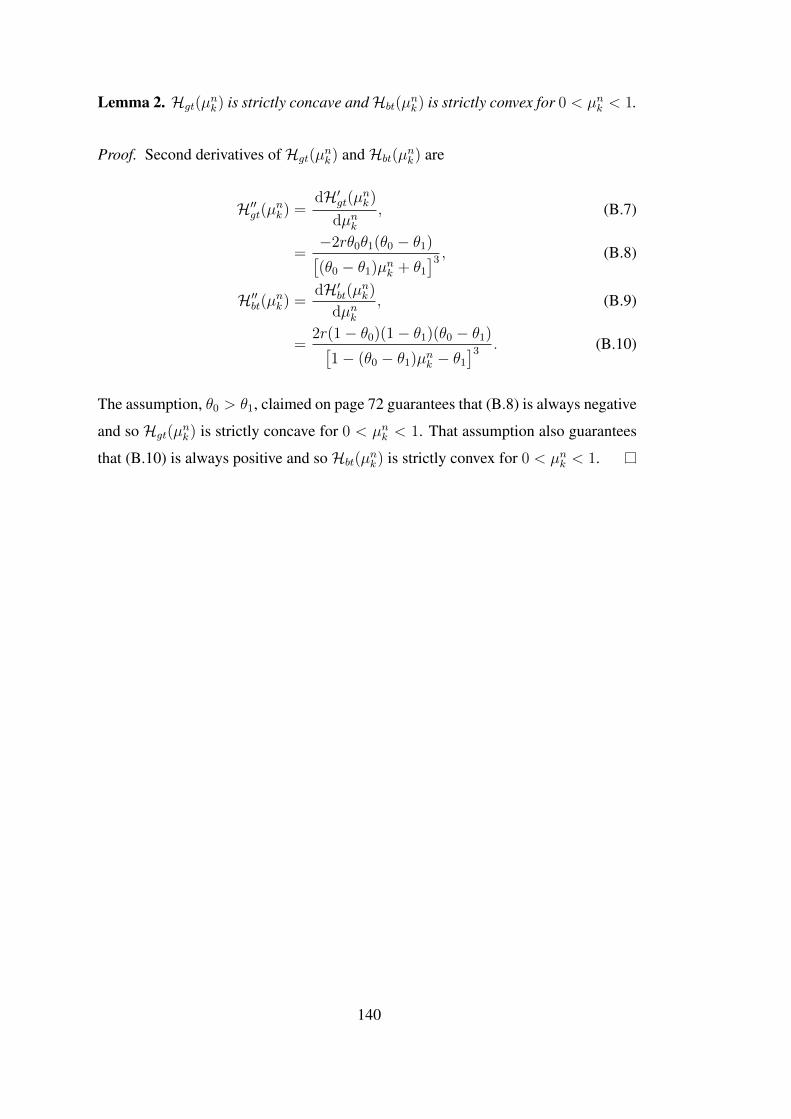
Lemma 2. Hgt(µnk) is strictly concave andHbt(µ
nk) is strictly convex for 0 < µnk < 1.
Proof. Second derivatives ofHgt(µnk) andHbt(µ
nk) are
H′′gt(µnk) =dH′gt(µnk)
dµnk, (B.7)
=−2rθ0θ1(θ0 − θ1)[(θ0 − θ1)µnk + θ1
]3 , (B.8)
H′′bt(µnk) =dH′bt(µnk)
dµnk, (B.9)
=2r(1− θ0)(1− θ1)(θ0 − θ1)[
1− (θ0 − θ1)µnk − θ1]3 . (B.10)
The assumption, θ0 > θ1, claimed on page 72 guarantees that (B.8) is always negative
and so Hgt(µnk) is strictly concave for 0 < µnk < 1. That assumption also guarantees
that (B.10) is always positive and soHbt(µnk) is strictly convex for 0 < µnk < 1.
140
APPENDIX C
A VIEW TO THE RADAR SIMULATOR GUI
The radar simulator GUI is shown in Figure C.1 for MTATBS and Figure C.2 for KS.
There is a plot area supports zoom in/zoom out, data cursor, rotate and pan functions.
This area is very useful and informs the resource manager about how-to use or what
the results. It changes interactively to correspond the operations directed by resource
manager. Options which can be typed by resource manager are as follows:
• Number of targets is allowed between 1 and 40. The number of targets is limited
to 40, since processing time becomes too much for higher values when KS is
utilized. The default value is 15.
• End time of simulation is allowed between 10 and 1000 s. The default value is
500 s.
• Surveillance update time is allowed between 10 and 1000 s. This value corre-
sponds to time that is necessary to a complete search of the region of interest,
so it is namely a conventional update time. The flag named as "Surveillance is
not fragmented" is used to activate this value. If this flag is disabled, the value
of surveillance update time is useless. The default value is 25 s.
• Number of frequency bands can be used when task interleaving technique is
enabled. It is allowed between 2 and 7. The default value is 2.
• Priority threshold is allowed between 1 and 3. The priority threshold can be
set as 3 at most, instead of 5 to decrease the number of undetected targets.
Simulator does not schedule the track updates of targets which have less priority
than the threshold. The default value is 1.
141
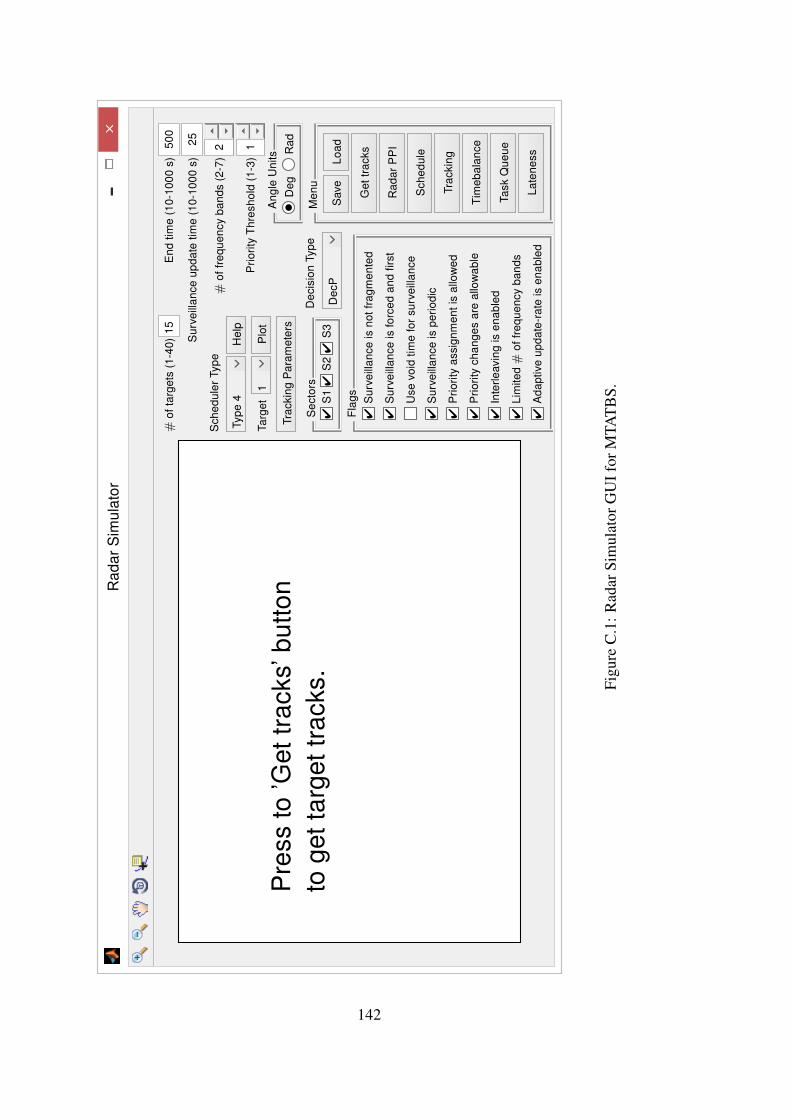
Rad
arS
imul
ator
Pre
ssto
’Get
trac
ks’b
utto
nto
gett
arge
ttra
cks.
#of
targ
ets
(1-4
0)15
End
time
(10-
1000
s)50
0
Sur
veill
ance
upda
tetim
e(1
0-10
00s)
25
#of
freq
uenc
yba
nds
(2-7
)2
Prio
rity
Thr
esho
ld(1
-3)
1
Ang
leU
nits
Deg
Rad
Sch
edul
erTy
pe
Type
4H
elp
Targ
et1
Plo
t
Trac
king
Par
amet
ers
Sec
tors
4S
14
S2
4S
3
Dec
isio
nTy
pe
Dec
P
Fla
gs
4S
urve
illan
ceis
notf
ragm
ente
d
4S
urve
illan
ceis
forc
edan
dfir
st
Use
void
time
for
surv
eilla
nce
4S
urve
illan
ceis
perio
dic
4P
riorit
yas
sign
men
tis
allo
wed
4P
riorit
ych
ange
sar
eal
low
able
4In
terle
avin
gis
enab
led
4Li
mite
d#
offr
eque
ncy
band
s
4A
dapt
ive
upda
te-r
ate
isen
able
d
Men
u
Sav
eLo
ad
Get
trac
ks
Rad
arP
PI
Sch
edul
e
Trac
king
Tim
ebal
ance
Task
Que
ue
Late
ness
Figu
reC
.1:R
adar
Sim
ulat
orG
UIf
orM
TAT
BS.
142

Rad
arS
imul
ator
Pre
ssto
’Get
trac
ks’b
utto
nto
gett
arge
ttra
cks.
#of
targ
ets
(1-4
0)15
End
time
(10-
1000
s)50
0
Sur
veill
ance
upda
tetim
e(1
0-10
00s)
25
#of
freq
uenc
yba
nds
(2-7
)2
Prio
rity
Thr
esho
ld(1
-3)
1
Ang
leU
nits
Deg
Rad
Sch
edul
erTy
pe
Kna
psac
kH
elp
Targ
et1
Plo
t
Trac
king
Par
amet
ers
Sec
tors
4S
14
S2
4S
3
Dec
isio
nTy
pe
Dec
P
Fla
gs
4S
urve
illan
ceis
notf
ragm
ente
d
4S
urve
illan
ceis
forc
edan
dfir
st
Use
void
time
for
surv
eilla
nce
4S
urve
illan
ceis
perio
dic
4P
riorit
yas
sign
men
tis
allo
wed
4P
riorit
ych
ange
sar
eal
low
able
4In
terle
avin
gis
enab
led
4Li
mite
d#
offr
eque
ncy
band
s
4A
dapt
ive
upda
te-r
ate
isen
able
d
Men
u
Sav
eLo
ad
Get
trac
ks
Rad
arP
PI
Sch
edul
e
Trac
king
Tim
e-to
-Go
Task
Que
ue
Val
uevs
.T
ime
Figu
reC
.2:R
adar
Sim
ulat
orG
UIf
orK
S.
143
Scheduler type includes:
• Type 1 for MTATBS-Type 1,
• Type 2 for MTATBS-Type 2,
• Type 3 for MTATBS-Type 3,
• Type 4 for MTATBS-Type 4,
• Knapsack for KS.
Decision type includes:
• CfTUL for the method of choosing first target in the update list,
• DecP for the method of decision policy,
• MinTE the method of minimizing the tracking error,
• PurMM the method of pursuing the most maneuvering.
Angle units selection is used only for visualization of targets on "Radar PPI" and
"Tracking" plots. It only changes the unit of angle for polar coordinates shown on
PPI display from radians to degrees or vice versa. A sample plot is shown in Figure
2.2 when degree option is selected.
Sectors selection panel includes the sectors, where each of them corresponds to 2π/3
radians or 120◦ and all of them are initially enabled. Visualization of sectors is shown
in Figure 2.2.The sectors are
• S1 for sector 1,
• S2 for sector 2,
• S3 for sector 3.
Help button opens a help window for radar simulator.
144
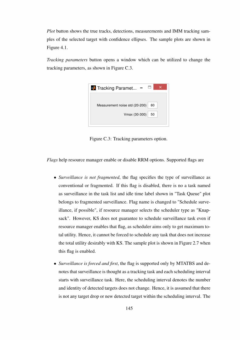
Plot button shows the true tracks, detections, measurements and IMM tracking sam-
ples of the selected target with confidence ellipses. The sample plots are shown in
Figure 4.1.
Tracking parameters button opens a window which can be utilized to change the
tracking parameters, as shown in Figure C.3.
Tracking Paramet...
Measurement noise std (20-200) 80
Vmax (30-300) 50
Figure C.3: Tracking parameters option.
Flags help resource manager enable or disable RRM options. Supported flags are
• Surveillance is not fragmented, the flag specifies the type of surveillance as
conventional or fragmented. If this flag is disabled, there is no a task named
as surveillance in the task list and idle time label shown in "Task Queue" plot
belongs to fragmented surveillance. Flag name is changed to "Schedule surve-
illance, if possible", if resource manager selects the scheduler type as "Knap-
sack". However, KS does not guarantee to schedule surveillance task even if
resource manager enables that flag, as scheduler aims only to get maximum to-
tal utility. Hence, it cannot be forced to schedule any task that does not increase
the total utility desirably with KS. The sample plot is shown in Figure 2.7 when
this flag is enabled.
• Surveillance is forced and first, the flag is supported only by MTATBS and de-
notes that surveillance is thought as a tracking task and each scheduling interval
starts with surveillance task. Here, the scheduling interval denotes the number
and identity of detected targets does not change. Hence, it is assumed that there
is not any target drop or new detected target within the scheduling interval. The
145

time interval between two cascaded surveillance tasks can be less than the sur-
veillance update time, if there is a target drop or detection in that interval. "Task
Queue" plot is shown in Figure 2.7 that the surveillance task is the first task in
radar timeline.
• Use void time for surveillance, the flag is supported only by MTATBS and
denotes the scheduling times of surveillance task updates depend on available
gaps, computed by ATB technique, on the timeline.
• Surveillance is periodic, the flag is supported only by MTATBS and denotes
the surveillance task has a fixed task update time.
• Priority assignment is allowed, the flag enables the task prioritization. If it
is disabled, all tasks have the priority level 1. This flag is provided to check
the performance of decision methods, when there are lots of targets to make a
selection. It is not suggested to disable it for general case, since the scheduling
process time increases too much for target selection.
• Priority changes are allowable, the flag enables the dynamic task prioritiza-
tion to be aware of the priority changes that affect the scheduling performance,
while targets are moving in the region of interests and through the fixed priority
rings. The sample plots are shown in Figure 2.5.
• Interleaving is enabled, the flag enables task interleaving technique.
• Limited number of frequency bands, the flag enables the multi-frequency bands
technique.
• Adaptive update-rate is enabled, the flag enables the adaptive update-rate tech-
nique which modifies task update times to enhance the tracking performance.
Menu panel consists of
• Save button saves the targets data to a file.
• Load button loads the targets data from a file.
• Get tracks button randomly generates the targets which obey the motion models
CV and CT in 2-D space.
146
• Radar PPI button shows tracks of targets. The sample plots are shown in Figure
2.2 and Figure 3.10.
• Schedule button schedules the tasks and shows the distribution of completed
tasks. The sample plots can be found in section 3.2.
• Tracking button plots detected (or updated) tracks of targets. The sample plots
are shown in Figure 2.5 and Figure 2.13.
• Timebalance button plots TB scheme of tracking and surveillance tasks. The
sample plots are shown in Figure 2.12 and are found in section 3.2.1. If resource
manager changes the scheduler type to "Knapsack", button plots the time-to-go
scheme of tracking and surveillance tasks, as shown in Figure 3.26(a).
• Task Queue button plots scheduled task queue. The sample plots are shown in
Figure 2.7 and Figure 2.10.
• Lateness button plots the histogram of lateness of tracking tasks. The sample
plot for individual cumulative distribution of latenesses can be found in section
3.2.1. If resource manager changes the scheduler type to "Knapsack", button
plots value vs. time graph of tracking and surveillance tasks, as shown in Figure
3.26(b).
147
Related Documents