This item was submitted to Loughborough's Research Repository by the author. Items in Figshare are protected by copyright, with all rights reserved, unless otherwise indicated. Racing car coastdown analysis Racing car coastdown analysis PLEASE CITE THE PUBLISHED VERSION PUBLISHER © C.M. Crewe PUBLISHER STATEMENT This work is made available according to the conditions of the Creative Commons Attribution-NonCommercial- NoDerivatives 2.5 Generic (CC BY-NC-ND 2.5) licence. Full details of this licence are available at: http://creativecommons.org/licenses/by-nc-nd/2.5/ LICENCE CC BY-NC-ND 2.5 REPOSITORY RECORD Crewe, Clive M.. 2017. “Racing Car Coastdown Analysis”. figshare. https://hdl.handle.net/2134/26985.

Welcome message from author
This document is posted to help you gain knowledge. Please leave a comment to let me know what you think about it! Share it to your friends and learn new things together.
Transcript
This item was submitted to Loughborough's Research Repository by the author. Items in Figshare are protected by copyright, with all rights reserved, unless otherwise indicated.
Racing car coastdown analysisRacing car coastdown analysis
PLEASE CITE THE PUBLISHED VERSION
PUBLISHER
© C.M. Crewe
PUBLISHER STATEMENT
This work is made available according to the conditions of the Creative Commons Attribution-NonCommercial-NoDerivatives 2.5 Generic (CC BY-NC-ND 2.5) licence. Full details of this licence are available at:http://creativecommons.org/licenses/by-nc-nd/2.5/
LICENCE
CC BY-NC-ND 2.5
REPOSITORY RECORD
Crewe, Clive M.. 2017. “Racing Car Coastdown Analysis”. figshare. https://hdl.handle.net/2134/26985.

This item was submitted to Loughborough University as an MPhil thesis by the author and is made available in the Institutional Repository
(https://dspace.lboro.ac.uk/) under the following Creative Commons Licence conditions.
For the full text of this licence, please go to: http://creativecommons.org/licenses/by-nc-nd/2.5/

LOUGHBOROUGH UNIVERSITY OF TECHNOLOGY
LIBRARY
AUTHOR/FILING TITLE
C(Z.lfwe; C.M. -. -- -----------------)---------------------------
-- ------------------------- -- -- ~~- ----- - --------- I ACCESSION/COPY NO. I ,
___________________ ~_~_~~_Lr_c:~ ______ ~ ___________ i
VOL. NO. CLASS MARK i
11 GEe 15:3
r-040W8031 -
I 111I111I111111I11111
Racing Car Coastdown Analysis·
Department of Aeronautical and Automotive Engineering and Transport Studies
In conjunction with
A Masters Thesis
Submitted in partial fulfilment of the award of the Degree of MPhil
....
C.M.Crewe 1995


"For the understanding may set the imagination into motion or, on the other hand, be set in motion by it"
-Rene Descartes excerpt from 'Rules for the direction of the mind'

The Test Vehicle Benetton B194
Acknowledgements
Acknowledgements
I would like to express my thanks to my supervisor Dr. Martin Passmore for his advice and
assistance during the year.
Mr. Pat Symonds (of Benetton Formula) without whom none of this would have been possible.
All at the Benetton Formula One team, particularly the members of the test and race teams notably Malcolm Tierney, Cristian Silk and Dr Nicklaus Tombazis.
I would also like to thank W. Toet (formerly ofBenetton, now Scuderia Ferrari) for his help and enthusiasm, particularly with wind tunnel data;
Finally I would like to thank Dr. P. Adcock, N. Grange, J.wheals, A Little, P Denrnan, D Sansum, D. Bailey and I. Williams for their friendship and help throughout the past twelve months.
i
Synopsis
Synopsis
Coastdown testing is a proven method for the determination of vehicle drag coefficients for road cars whilst the vehicle is in it's normal operating environment. A method of achieving this has been successfully developed at Loughborough University of Technology over the past few years. This study is concerned with the adaptation of the technique to the specific application of a contemporary Formula One racing car, this work was undertaken in conjunction with the Benetton Formula One racing team.
There are major differences between current Formula One cars and normal road cars. Formula One cars generate very high normal load forces, have very high aerodynamic drag coefficients, and use slick treaded tyres. These aspects have major implications on the use of the coastdown method to estimate drag coefficients. The mathematical model developed for this particular application of the coastdown test includes the aerodynamic, tyre, drivetrain and the undriven wheel drags and accounts for the change in aerodynamic drag due to ambient wind and changes in vehicle ride height during coastdown. The investigation of the use of the vehicle coastdown test included an in depth assessment of the major facets prevalent in the determination of vehicle drag coefficients via computer based simulation. The findings from this were applied in the development of a suitable mathematical drag model, test and analysis methods.
A series of full scale coastdown tests were conducted at Silverstone racing circuit (U.K.) and the Circuit De Catalunya (Spain) and the data analysed to yield the drag coefficients. The agreement between wind tunnel/rig tests and full scale coastdown test derived coefficients was found to be good. The findings from the study and the results are documented in this report.
ii

Nomenclature
Nomenclature Units
A Vehicle frontal area m2
AD Constant tyre loss coefficient A, Transmission loss coefficient N
A. Undriven wheel drag N BD Constant drag term srn-I Bt
Transmission loss coefficient Bu Un driven wheel loss coefficient N/ms- I
Co Drag coefficient Coo Drag coefficient at zero yaw angle CL Lift coefficient
Cw Lift coefficient at zero yaw angle Cp Pitching moment coefficient C Tyre slip coefficient N rad-I
Ct Transmission loss coefficient D Aerodynamic drag N OF Ride Height Front m
OR Ride Height Rear m
FA'", Aerodynamic drag force N FOr Driveline losses N FM Mechanical drag force N
FT)"C Tyre rolling resistance N FT Total rolling resistance N Fu Total undriven wheel drag N GFD Final drive gear ratio g Acceleration due to gravity ms-2
h Numerical integration step length I,. Single wheel inertia kgm2
I,.4 Inertia of four wheels kgm2
I" Gearbox inertia kgm2
Ko Coefficient to modify Co. for yaw angle rad-I
KL Coefficient to modify CLo for yawangle rad-I
L Lift force N 1 Wheelbase m M Vehicle mass kg
M'1f Vehicle effective mass kg P Pressure Nm-2
Re Reynolds number Rr Tyre rolling radius m· T Tyre temperature °C t Time s v Vehicle speed ms-I
v, Total relative air speed ms-I vh Ambient head wind ms-I
Vx Ambient cross wind ms-I
iii
Nomenclature
Vc Calculated Speed ms-!
vm Measured Speed ms-!
a Front wing angle of attack 0
v Kinematic viscosity m2s-!
p Density of air kgm-3
'I' Vehicle yaw angle rad co Wheel angular velocity rads-!
iv
Contents
Contents
Acknowledgements
Synopsis
Nomenclature
Contents
1. Introduction
1.1. Background 1.2. Objectives
2. Mathematical Drag Model
Mechanical contribution
2.1 Tyre Rolling Resistance 2.1.1 Racing car tyre characteristics 2.1.2 Temperature and Frequency 2.1.3 Inflation Pressure and Deflection 2.1.4 Temperature and Speed Sensitivity 2.1.5 Normal Load 2.1.6 Speed 2.1.7 Goodyear Tyre Dynarnometer tests 2.1.8 Tyre Drag Model
2.2 Driveline Losses 2.2.1 Drivetrain Losses 2.2.2 Undriven Wheel Losses
2.3 Mechanical Drag Model
Aerodynamic 2.4 Ambient Wind 2.5 Aerodynamic Yawangle 2.6 Ground Effect 2.7 Reynolds's Number effects 2.8 Open Wheel aerodynamics 2.9 Lift and Drag 2.10 Aerodynamic Drag Model
v
Page Number
i
ii
iii
v
1
2 3
4
4 5 5 6 7 9 9 12 14
15 IS 15
16
17 20 22 27 27 28 30
Contents
Mathematical Drag Model
2.11 Summary ofMathematicaI Model
3. Coastdown Test Method
3.1 Vehicle Set up 3.2 Environmental Conditions 3.3 Test Procedure
3.3.l Pre Test 3.3.2 Tyre conditioning 3.3.3 Test
3 .4 Driveline tests 3.4.1 Drivetrain Tests 3.4.2 Undriven Wheel tests
4. Instrumentation
4.1 On Board data logger 4.1.1 Vehicle Speed 4.1.2 Normal Load 4.1.3 Airspeed 4.1.4 Lateral Acceleration 4.1.5 Ride Height 4.1.6 Gear Oil Temperature
4.2 Measurement and System Noise 4.2.l Measurement Noise 4.2.2 System Noise
4.3 Weather Station
4.4 Ambient Wmd measurement
4.5 Aerodynamic Yaw probe
5. Analysis Method
5.1 Methodology, Coastdown analysis
5.2 Optimisation Methods
5.3 Coastdown Analysis 5.3.1 Minimisation ofafunction 5.3.2 Nelder and Mead's method 5.3.3 Powel\'s method
vi
Page Number
31
32 32 33 34 34 34 35 35 35
38
38 39 40 41 41 42 42
42 42 43
46
47
48
49
49
50
51 51 52 53

Contents
5.4 Signal Processing
5.5 Racing car coastdown analysis methods 5.5.1 Minimisation of a function 5.5. 2 M~Iti term analysis
5.6 Coefficient Sensitivities
5.7 Drivetrain and Undriven wheel Coastdown Analysis
6. Results and Discussion
6.1 Driveline
6.2 Undriven Wheel
6.3 Full Coastdown Tests 6.3.1 Preliminary tests Silverstone 6.3.2 Main tests Circuit De Catalunya
7. Conclusions
8. Recommendations for Further Work
9. References
10. Bibliography
Appendices
Appendix I Appendix 11 Appendix III Appendix IV Appendix V Appendix VI
Track Coastdown test data sheets Simulation details Wheel Inertia Tests/calculations Initial Proposal Ne1der and Mead Method Flow chart Track Survey
vii
Page Number 54
55 55 58
59
61
62
62
64
67 69
76
79
80
86
87
88 91 94 97 104 108
Introduction
1. Introduction
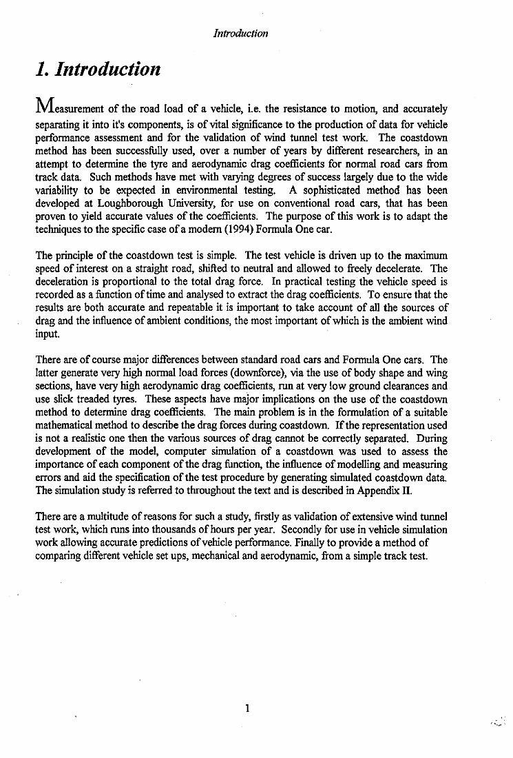
Measurement of the road load of a vehicle, i.e. the resistance to motion, and accurately
separating it into it's components, is of vital significance to the production of data for vehicle performance assessment and for the validation of wind tunnel test work. The coastdown method has been successfully used, over a number of years by different researchers, in an attempt to determine the tyre and aerodynamic drag coefficients for normal road cars from track data. Such methods have met with varying degrees of success largely due to the wide variability to be expected in environmental testing. A sophisticated method has been developed at Loughborough University, for use on conventional road cars, that has been proven to yield accurate values of the coefficients. The purpose of this work is to adapt the techniques to the specific case ofa modern (1994) Formula One car.
The principle of the coastdown test is simple. The test vehicle is driven up to the maximum speed of interest on a straight road, shifted to neutral and allowed to freely decelerate. The deceleration is proportional to the total drag force. In practical testing the vehicle speed is recorded as a function of time and analysed to extract the drag coefficients. To ensure that the results are both accurate and repeatable it is important to take account of all the sources of drag and the influence of ambient conditions, the most important of which is the ambient wind input.
There are of course major differences between standard road cars and Formula One cars. The latter generate very high normal load forces (downforce), via the use of body shape and wing sections, have very high aerodynamic drag coefficients, run at very low ground clearances and use slick treaded tyres. These aspects have major implications on the use of the coastdown method to determine drag coefficients. The main problem is in the formulation of a suitable mathematical method to describe the drag forces during coastdown. If the representation used is not a realistic one then the various sources of drag carmot be correctly separated. During development of the model, computer simulation of a coastdown was used to assess the importance of each component of the drag function, the influence of modelling and measuring errors and aid the specification of the test procedure by generating simulated coastdown data. The simulation study is referred to throughout the text and is described in Appendix n.
There are a multitude of reasons for such a study, firstly as validation of extensive wind tunnel test work, which runs into thousands of hours per year. Secondly for use in vehicle simulation work allowing accurate predictions of vehicle performance. Finally to provide a method of comparing different vehicle set ups, mechanical and aerodynamic, from a simple track test.
1 " ..... '
Introduction
1.1. Background
T here are two well established methods for the determination of road load coefficients for a
road vehicle from data obtained during track tests. These methods are the Coastdown and Steady State Torque tests, it is the development of the former that is considered in this report, since the latter is expensive, requiring highly specialised equipment and necessitates special wind tunnel testing prior to analysis.
The coastdown method has been successfully used to determine road load coefficients of normal road cars for chassis dynamometer calibration for many years.
The method has also been used with varying degrees of success to determine the tyre and aerodynamic drag coefficients for normal road cars. With financial support from SERC, a sophisticated method of the determination of drag coefficients was developed by Dr M.A.Passmore at the department of Transport Technology, Loughborough University. This method successfully produced values ofTransrnission, Undriven wheel (off line in laboratory), Tyre and Aerodynamic drag coefficients (directly from coastdown tests) using a parameter optimisation routine. The aerodynamic lift force generated by the vehicle in coastdown was neglected since it is considered negligible for a road car, therefore no normal load measurements were made. Additionally the effect of vehicle ride height variations were considered negligible. The method developed was for Bi-directional testing using a track with parallel straights linked with banked track. The start speed for a coastdown being approximately 30 m/s.
The method applied in the development of a means of extracting the drag coefficients of a Formula One car builds upon the normal road car method developed at LUT.
2
Introduction
1.1. Background
T here are two well established methods for the determination of road load coefficients for a road vehicle from data obtained during track tests. These methods are the Coastdown and Steady State Torque tests, it is the development of the former that is considered in this report, since the latter is expensive, requiring highly specialised equipment and necessitates special wind tunnel testing prior to analysis.
The coastdown method has been successfully used to determine road load coefficients of normal road cars for chassis dynamometer calibration for many years.
The method has also been used with varying degrees of success to determine the tyre and aerodynamic drag coefficients for normal road cars. With financial support from SERC, a sophisticated method of the determination of drag coefficients . 'r'as developed by Dr M.A.Passmore at the department of Aernautical and Automotive Engineering and Transport Studies, Loughborough University. This method successfully produced values of Transmission, Undriven wheel (off line in laboratory), Tyre and Aerodynamic drag coefficients (directly from coastdown tests) using a parameter optimisation routine. The aerodynamic lift force generated by the vehicle in coastdown was neglected since it is considered negligible for a road car, therefore no normal load measurements were made. Additionally the effect of vehicle ride height variations were considered negligible. The method developed was for Bi-directional testing using a track with parallel straights linked with banked track. The start speed for a coastdown being approximately 30 rnIs.
The method applied in the development of a means of extracting the drag coefficients of a Formula One car builds upon the normal road car method developed at LUT .
. ,
2
.,
Introduction
1.2. Objectives
The major aim of the project was to develop an Uni directional (as distinct from the usual
Bi-directional coastdown test method) coastdown test method that could be routinely used to detennine the drag coefficients of a Formula One car at normal race tracks. This data could then be used for real world comparisons, as distinct from wind tunnel data, of different aerodynamic configurations, mechanical configurations and vehicle set ups. On the aerodynamic side the main objective was to validate extensive wind tunnel test data. Wind tunnel testing of the vehicle often exceeds three thousand hours a year.
Fundamental to the development of a suitable method is the establishment of a suitable mathematical drag model. The model must accurately represent aerodynamic, tyre and driveline drag components. Separate tests were conducted to detennine the undriven wheel and drivetrain losses, subsequently allowing the losses to be directly accounted for in the analysis. Throughout the development of the model a means of assessing the various facets of the model and their relative importance was required. Focal to this was the generation of realistic simulated coastdown data using a suitable simulation code. The third major part of the work is in the development of the analysis method to be used to produce accurate drag coefficients from both simulated and real coastdown data.
The first step, in what one hopes to be an on going process, was to produce repeatable test results from on track Uni directional coastdown testing.
3
Mechanical Contribution
2. Mathematical Model
In this chapter the mathematical model that describes the drag force acting on the
vehicle during coastdown is developed. The equation of motion for a vehicle travelling on a track with grade angle e is a straight forward application of Newton's second law of motion:
Tractive Force
Resistive Force
Mg Sine
Gravitational Force
= M dv • dt
Inertial Force
(1)
It is thus the Fo(v) term, composed of aerodynamic, tyre and driveline drag components that we are concerned with in coastdown since FT = O. The first part of the chapter covers the subject of tyre rolling resistance. This is followed by the development of a suitable driveline drag model, encompassing drivetrain and undriven wheel loss drag models. Lastly the model accounting for the most significant portion of the drag force acting on the vehicle during coastdown, namely aerodynamic drag is developed.
2.1. Tyre Rolling Resistance
Tyre rolling resistance is the dominant form of mechanical loss during a coastdown.
The various mechanisms associated with this type of rolling loss are introduced in the following part of the report, and a mathematical model developed that describes tyre rolling resistance for a Formula One car. Rolling resistance is defined quantitatively as the energy converted into heat per unit distance rolled by the tyre. It has long been understood and confirmed that rolling tyres absorb energy in two principle forms and these derive from the structural deformations of the tyre resulting from contact with the road surface. The first is the cyclic storage and retrieval of elastic energy in parts of the tyre as they deform when passing through the region of road contact. In the course of this process, not all of the energy dissipated by the materials is returned as useful mechanical energy. Instead a large amount is transformed into heat internally in the materials of the tyre. The second form of energy absorption is attributed to sliding in the presence of mctional resistance between the tread and the road. Although sliding throughout the contact patch is not generally apparent, there are local regions where sliding does take place, for free rolling tyres when travelling straight ahead, sliding is restricted to a relatively small zone at the exit of the contact patch. Another, less significant, form of mechanical energy loss is in the formation of vibrations and noise associated with the irregularities of the road surface, this form ofloss is usually neglected. In much of the work done on measuring tyre rolling resistance it is common to neglect the aerodynamic drag of the moving tyre as being unavoidable, exterior to the tyre. In order to reduce the level of energy absorption in the tyre, several methods can be employed. One is the use of construction materials that are better for recovering the
4
, Mechanical Contribution
elastic energy that is cyclically stored within them, however this is limited practically by the materials currently applicable for use, for example, elastomers and textiles. Materials which yield very low rolling resistance are available but they are not conducive to good handling. The materials used must function at the strain cycles, moduli, wear resistance and fatigue lives that are required by the tyre user. The Formula One racing car tyre user requires very different characteristics to the normal road car user.
2.1.1. Racing Car Tyre Characteristics
The modem Formula One racing car tyre is vastly different in size and shape to common road car tyres. Racing car tyres use extremely soft rubber compounds, for high grip, have very low aspect ratios and are designed for as little as one hundred miles usage. Typically a road car tyre yields a coefficient of friction, It of 0.8-1.0, the race car tyre typically produces It values in excess of 1.463
•
A great many factors need to be taken into account before the design of a racecar tyre can be finalised. The basic specification is for a radial ply slick tyre. The actual tyre compound depends on the situation for which the tyre is to be utilised, i.e. soft compounds for race qualifying, harder compounds for race distances not to mention specific compounds for particular race circuits and conditions. However, in recent times the Goodyear tyre monopoly in Formula One has reduced the number of compounds limiting the tyre choice to three or four compounds at a given circuit. In wet conditions the requirements are similar though a heavily treaded tyre is then required.
2.1.2. Temperature And Frequency
Schuring et. al5t studied' the interaction between temperature, frequency and loss modulus of a typical road car tyre. To understand what is meant by frequency consider that a tyre generating a certain amount of heat during one revolution would
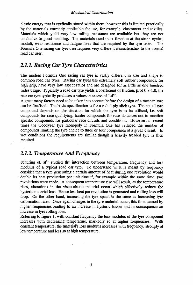
, double its heat production per unit time if, for example within the same time, two revolutions were made. A consequent temperature rise will result, as the temperature rises, alterations in the visco-elastic material occur which effectively reduce the hysteric material loss. Hence less heat per revolution is generated and rolling loss will drop. On the other hand, increasing the tyre speed is the same as increasing tyre deformation rates. Once again changes in the tyre material occur, this time caused by higher frequencies leading to an increase in hysteric losses and in consequence an increase in tyre rolling loss. Referring to figure I, with constant frequency the loss modulus of the tyre compound increases with decreasing temperature, markedly so at higher frequencies. With constant temperature, the material's loss modulus increases with frequency, strongly at low temperature and less so at high temperature.
5
2 1.8
_ 1.6 o Si 1.4 -: 1.2
~ 1 ~ 0.8 ~ 0.6
0.4 0.2 o
1
Mechanical Contribution
Tyre Loss Modulus vs Frequency For Various Tyre Temperature
-+-20degC -+-40 deg C _60degC ~8OdegC
10 Frequency (Hz)
Figure 1
~
100
The material response exhibited in a tyre mimics this behaviour, with rolling loss taking the place ofloss modulus, and speed of frequency.
2.1.3. Inflation Pressure And Deflection
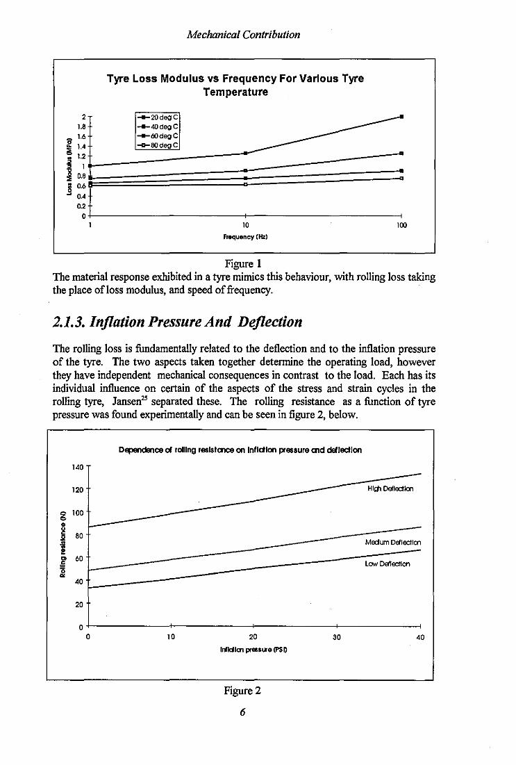
The roIling loss is fundamentally related to the deflection and to the inflation pressure of the tyre. The two aspects taken together detennine the operating load, however they have independent mechanical consequences in contrast to the load. Each has its individual influence on certain of the aspects of the stress and strain cycles in the roIling tyre, Jansen25 separated these. The roIling resistance as a function of tyre pressure was found experimentally and can be seen in figure 2, below.
Dependence 0/ roiling reslstCllce on In"allon pressure CIld deflection
140 -120 HI", D€lIEdloo
g 100 & g
80
t Meclum Da'IEdloo --
r 60 lOW' Detle::tlon
'0 .. 40
20
0 0 10 20 30 40
Irllclloo press ... e (PS D
Figure 2
6
Mechanical Contribution
It is important to note that variations in internal temperature and axle height were prevented during the course of the experiment. The figure shows linear increases in rolling resistance with increase in the inflation pressure and an increase in rolling resistance with vertical deflection. The former of these is in direct contrast to what is normally expected, and this is explained by the controlling of the test parameters as described above. In tests where the vertical load is held constant and the inflation pressure is increased, the deflection of the tyre decreases. Since the decrease in the deflection has a greater influence on the rolling resistance (deflection effects =65% and inflation effects =35%) than the increase in the inflation pressure, the net value of the rolling resistance also decreases.
Several other researchers have concentrated on this aspect, elarle' found that for radial ply tyres an increase of one pound per square inch in the tyre's inflation pressure implied a reduction in the rolling resistance of the order of2%.
2.1.4. Temperature And Speed Sensitivity
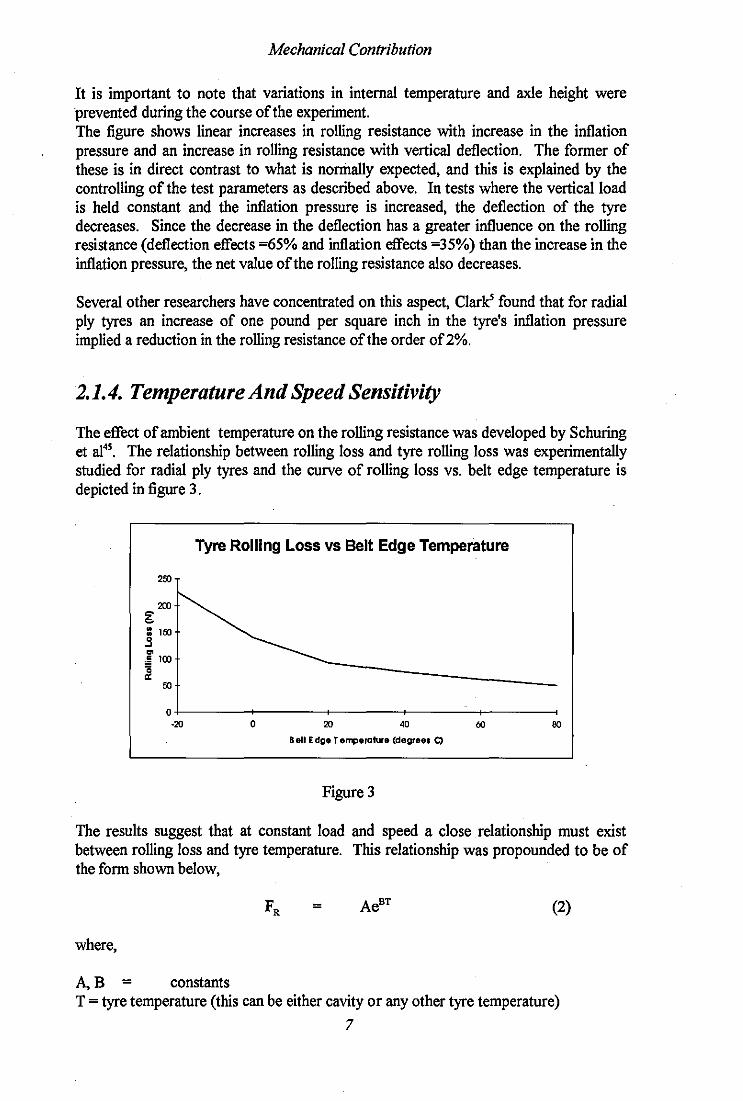
The effect of ambient temperature on the rolling resistance was developed by Schuring et al4S
• The relationship between rolling loss and tyre rolling loss was experimentally studied for radial ply tyres and the curve of rolling loss vs. belt edge temperature is depicted in figure 3.
200
200 g : 150 s '" ~ 100
~
Tyre Rolling Loss vs Belt Edge Temperature
O~------~-------r-------+------~------~ ·20 o 20 40 60
Bell Edge T el'fl)eratur. (degree. C)
Figure 3
The results suggest that at constant load and speed a close relationship must exist between rolling loss and tyre temperature. This relationship was propounded to be of the form shown below,
= (2)
where,
A, B = constants T = tyre temperature (this can be either cavity or any other tyre temperature)
7

Mechanical Contribution
This was simplified, for a small change in temperature, by a truncated Taylor series of the form,
where,
To = T, = Kr =
=
observed ambient temperature standard temperature constant equal to 0.011 /oK for radial ply tyres
(3)
The relationship between tyre temperature, rolling loss and vehicle speed can be described in terms of an RTS (R-rolling loss, T -temperature, S-speed) diagram see figure 4.
eo
75
70
!!:os L, E &55
'" A5
'" "0 Zlo 320 "0 '20 T yr. T errpII'd\I'. rQ
Figure 4
-13.33nw
---0-- 17.nsnW
--22.222rrw
-0-- 26.94 rrVJ
.70
Figure 4 consists of a family of constant-speed curves measured at a given load and tyre pressure and plotted as a function of tyre temperature and rolling loss. This was based on experimental work undertaken on radial ply road car tyres. It is difficult to separate the affects of tyre temperature and speed on rolling loss. An increase in tyre temperature occurs when the speed is increased, this increase lags behind the speed increase typically by 2 seconds6
'. For the coastdown situation after our initial acceleration/cornering period prior to coastdown, during which the tyre temperature increases, we have a cooling period during which the tyre temperature may decay by 25°C, during coastdown, with an accompanying change in tyre rolling loss. Evidently we have a constantly changing situation. Accounting' for this mathematically is evidently dependent on a reliable means of measuring tyre temperature. This was not possible for the tests undertaken for this work, hence an average value was used.
8
Mechanical Contribution
2.1.5. Normal Load
In keeping with the findings outlined previously the increase of the nonnal load on the tyre will bring about an increase in the deflection apparent, and so the hysteresis loss. The roIling resistance coefficient is therefore defined as the ratio of roIling resistance to nonnal load,
FR = -......;;....:.:......-NormalLoad
(4)
The roIling resistance coefficient is a non dimensional one, therefore different types of tyre can be compared under different operating conditions.
2.1. 6. Speed Several researchers have attempted to mathematically quantify the relationship between roIling resistance and speed. The mathematical models proposed by each of the researchers are reviewed in this section.
The method of modelling the tyre rolling resistance variation with speed is varied, some simply model it as a constant tenn, others, Passmore and J enkins44 include a linear dependence with velocity,
= (Nonnal Load) (A" + BDv) (5)
This model has been successfully applied to nonnal road car coastdown data to produce consistent values of all of the coefficients from track tests. The Andreau model·3 was used in a study for the design of the land speed record attempt vehicle by Eyston in 1938, it is an empirical fonnula containing tenns in speed, tyre pressure and weight. Andreau's model is considered to be very dated and was surpassed by Kanun's model·3
•
This model includes tyre pressure in the fonnula for tyre dependent rolling resistance, below,
=
where;
=
=
Mg(O.0051 + 5.5+1SW Pr x 103
+ (S.5+6W)v2
Pr x 103
tyre pressure measured in kg/cm2
weight on wheels in tons
) (6)
Based upon the discussion above on the effect of changing inflation pressure and the higher relative importance of tyre deflection, this model does not truly reflect this. Kanun's model produces values of rolling resistance significantly lower than those in the encountered by use of the Andreau model, emphasising the degree of variability in the values of tyre rolling resistance produced by these early models.
9

Mechanical Contribution
Early work in the field of racing car tyre rolling resistance depended upon the use of formulae such as those proposed by Andreau and Kamm, this was at a time when the now accepted technology was not available to the tyre technicians, additionally the formulae are based upon limited data for fundamentally different types of tyre.
Jante and Saal's model63 has been successfully used in the past to model racing car tyre rolling resistance and is considered to correlate well with experimental data,
where,
=
=
=
value assigned to each type of road surface varying from 0.008 for cement pavement to 0.011-0.018 for various types of tarmac, also dependent on other factors such as tyre type, inflation pressure and axial load.
numerical coefficient, given by Jante and SaaI to be 5xl0·7 for slick racing tyres.
(7)
Yasin69 proposed a similar model correcting the speed term to standard reference conditions. Other models, modelling the Velocity term as a higher order term include those proposed by Emtagel6 and Dayman9
, both are of the form shown below,
= (Normal Load) (Ao+Bov") (8)
Emtage calculated n to be 3.5 and Dayman reported the value of the power ofn to be 4. The model proposed by Yasin is based upon limited test data and is based around treaded road car tyres. Both Emtage and Dayman proposed higher order velocity term models however both models ignore drive-line losses in their studies and this throws a degree of doubt on the validity of the proposed values. The Jante and Saal model is considered valid today, since the quadratic expression has been confirmed by experience and the value of 1\ that is used can be corrected through many statistical observations at the individual tracks.
Mcnay40 details a graph showing force at the contact patch versus speed in the range 140 -250 mph for a 1988 Indy car with slick Goodyear racing tyres. Curve fitting to this data yielded the following relationship between the force (in lbs) at the contact patch and the speed of the car (in mph),
FE = -64846 + 1372.6Y - 10.625y2 + 0.036333y3 - 0.000046354\1" (9)
The model detailed by Mcnay is based around curve fitting of experimental data, added to the fact that it is difficult to separate the terms attributable to the engine (driving forces) and the tyres. However, the inference in the paper is of a higher order dependence of tyre rolling resistance with speed.
10

Mechanical Contribution
Published work undertaken in the field of mathematical modelling of the behaviour of slick racing car tyres is very limited. The work of Metz 41 suggests that there is no velocity term in the tyre rolling resistance model, it is stated that this is a reasonable assumption for modem radial ply slick tyres. Indeed tests conducted by S.P.38 tyres on slick tyres that were used in Audi's German Touring Car Championship cars showed that there is very little change in the rolling resistance of the tyre with respect to speed, i.e. a very small BD term is apparent. This survey has shown that there are three methods of modelling tyre rolling resistance, i.e. with a constant term, linearly or with a higher order term in vehicle speed.
Almost none of the models are actually based upon models of material behaviour. Some of the models found in the literature are empirically based, and several are based on regressions to measured data. The linear Ao+BDv model has been proven as a means of adequately accounting for tyre losses in coastdown44
• The important aim for this study was to accurately account for the tyre rolling resistance of a Formula One car with a suitable mathematical model. In order to achieve this, realistic tyre rolling resistance measurements were required to be made. Hence Goodyear tyres, the sole manufacturer of Formula One car tyres, was contacted, in order to obtain specific rolling resistance information. The aim was to ascertain whether the AD +BD v model was adequate for the purposes of representing tyre losses in coastdown tests.
11

Mechanical Contribution
2.1. 7. Goodyear Tyre Dynamometer Tests
At the start of this research project an approach was made to Goodyear Racing Tyres Akron (Ohio, USA) for tyre dynamometer rolling resistance test data. Goodyear responded favourably to the request, although it was stated that tyre rolling resistance measurement was a difficult and time consuming task to undertake, limiting the data that could realistically be collected. The tyre dynamometer tests themselves were conducted on 1994 specification tyres prior to the start of the 1994 season.
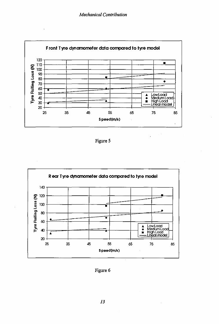
Tyre rolling resistance was measured on a moving flat belt at constant speeds under a variety of loads, inflation pressures, cambers and slip angle conditions. The tyre was supported by an air bearing, and all forces and moments were measured by a balance beam. The rolling resistance tests were conducted at room temperature, 25°C and the tyres were new at the commencement of the tests. Tyre pressure was maintained constantly at the pressure specified at the beginning of the tests. To stabilise the performance of the tyre, conditioning was undertaken on the dynamometer prior to testing. This is considered to be when the tyre's Contained Air Temperature (CAT) is constant. It was found that CAT is the best indicator of the tyre's stability, and therefore suitability for testing. During the test, readings of CAT were made, and it was found that as the speed increased so did CAT, linearly.
Time constraints limited the tyre data to a total of seven measurements, encompassing three speeds and three loads for a front and a rear tyre. The data is detailed graphically in Figures 5 and 6 with the proposed model «An+BDv)(Normal load)), based upon linear dependence of rolling resistance with speed, superimposed. The coefficients for the model, generated from linear regressions to the data are detailed in tables I and 2.
At the higher speeds and loads the model is found to be most in error, with a total error over both tyres of approximately 50 N at the highest speed and load. Although this represents less than I % of the total vehicle drag force at this speed it could be a source of error in the coastdown analysis because of the close relationship between the coefficients. The simulation tests showed that for an unaccounted force of this order, An could be in error by 15.5 %, BD by 90 % and Co by 4 %. This biasing of error reflects the relative sensitivities of the coefficients. However the data from Goodyear is for loads significantly higher than were experienced with the vehicle set-up used in the coastdown tests, (due to mid season rule changes) which are much closer to the medium to low load range. It should be noted that the fit to the data in this region is good with an RMS. error of the order ofless than ION. The validity of the model in terms of accounting for the (yre drag force in coastdown is investigated further in chapters 5 and 6.
Some testing on tyres that were well used was also undertaken and it was found that the rolling resistance decreased with wear by approximately 10%. The tyres used were very well worn it was stated, so this felt to be representative of an extreme case. This underlines the necessity of monitoring the wear rate throughout testing.
12
120
Z' 110 -100 l:: 90 ..9 80 g' 70
=a (IJ a: 50 ~ 40 ~ 30
20
Mechanical Contribution
Front Tyre dynamometer data col'JlXlred to tyre model
•
• • •
• LowLoad • Medlll1 Load • High Load
Linea model
25 35 45 55
Speed(m/s)
65 75 85
140
Z'12O -.. ~ 100 Cl :a 80
~ 60 ., ~40
20
Figure 5
R ear Tyre dynamometer data corrpared to tyre model
•
• 25 35 45
•
•
55
Speed(m/s)
Figure 6
13
-~
• LowLoad • Medium Load • HI(j1Load
- Llnecr rrodel
65 75
l-
85

Mechanical Contribution
Front LOAD(N) AD BD AdjustedR2 Standard Error
2,225 O.oI 13 7.198e-5 0.9994 0.1054
3,560 0.0128 9.638e-5 0.7459 4.396
4,890 0.0133 0.0001 0.442 12.61
Table I
Rear
LOAD(N) AD BD Adjusted R2 Standard Error
2,670 0.0083 0.0001 0.943 2.245
4,450 O.oII7 9.0 I 6ge-5 0.7688 5.47
6,230 0.013 7.253e-5 0.48 10.03
Table 2
Thus our average, simulated tyre rolling resistance coefficients from tyre dynamometer tests were found to be
Ao=0.0117
and BD = 8.85IxI0·5
summarising the tyre model,
(10)
2.1.8. Tyre Model
From all the information researched on the subject of racing car tyre rolling resistance and the measured data for tyre dynamometer tests the tyre rolling resistance mathematical model was determined to be as described in the equation below which includes the aerodynamic lift term L (Y2pAv/CJ, which is a term in V,2. This has major implications for the method applied is discussed further in section 2.9.
14
Mechanical Contribution
2.2 Driveline Losses
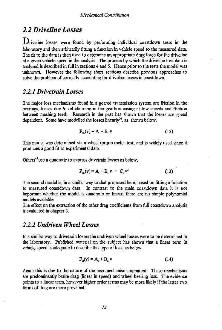
Driveline losses were found by perfonning individual coastdown tests in the laboratory and then arbitrarily fitting a function in vehicle speed to the measured data. The fit to the data is then used to detennine an appropriate drag force for the driveline at a given vehicle speed in the analysis. The process by which the driveline loss data is analysed is described in full in sections 4 and 5. Hence prior to the tests the model was unknown. However the following short sections describe previous approaches to solve the problem of correctly accounting for driveline losses in coastdown.
2.2.1 Drivetrain Losses
The major loss mechanisms found in a geared transmission system are friction in the bearings, losses due to oil churning in the gearbox casing at low speeds and friction between meshing teeth. Research in the past has shown that the losses are speed dependent. Some have modelled the losses linearlY", as shown below,
(12)
This model was determined via a wheel torque meter test, and is widely used since it produces a good fit to experimental data.
Others" use a quadratic to express drivetrain losses as below,
(13)
The second model is, in a similar way to that proposed here, based on fitting a function to measured coastdown data. In contrast to the main coastdown data it is not important whether the model is quadratic or linear, there are no simple polynomial models available. The effect on the extraction of the other drag coefficients from full coastdown analysis is evaluated in chapter 3.
2.2.2 Undriven Wheel Losses
In a similar way to drivetrain losses the undriven wheel losses were to be detennined in the laboratory. Published material on the subject has shown that a linear term in vehicle speed is adequate to describe this type ofloss, as below
(14)
Again this is due to the nature of the loss mechanisms apparent. These mechanisms are predominantly brake drag Oinear in speed) and wheel bearing loss. The evidence points to a linear term, however higher order terms may be more likely if the latter two forms of drag are more prevalent.
15

Mechanical Contribution
2.3 Mechanical Model
The overall mathematical model of the drag force found due to mechanical
components is detailed below,
Expanding,
= ([An + BDv]x[Mg+L]><[1+I<-r(To·TJ]) + (.4, + B, v) + (A" +Bu v)
16
(15)
(16)

Aerodynamics
Aerodynamic Contribution
Aerodynamic drag is the largest single component of the drag acting on the vehicle in
coastdown, it composes almost ninety percent of the drag force at a speed of 150 mph (for a high downforce aerodynamic set-up). In this part of the report the relevant literature, is reviewed in the fields of ambient wind, aerodynamic yaw angle, ground effects, racing car aerodynamics and the relationship between aerodynamic lift and drag. The mathematical model describing the aerodynamic drag force acting on the vehicle during coastdown is developed accounting for the effects of ambient wind and changes in vehicle ride height. Although not specifically required for coastdown testing on conventional vehicles, data from routine wind tunnel tests has been used during the adaptation of the coastdown technique to the FI car. The data was used to assess the importance of ride height changes, yaw angle effects, and for the calibration of the on board anemometer. In addition it also provides a basis for comparison between track and tunnel. The wind tunnel has a high tensioned, high suction belt, with a cooled platen that provides a maximum speed of 40 mls. For the normal 40% scale model arrangement the blockage was calculated to be approximately 4%.
2.4. Ambient wind
T he effects of atmospheric wind cause changes to a vehicle's aerodynamic environment. This
is most obviously perceived by the generation of an aerodynamic yaw angle such that the flow is not aligned with the vehicles direction of motion. The nature of ambient wind and it's induced affects on road vehicles has been the subject of several papers over the last fifteen years. Some are based upon the physical aspects in the field, typically gust measurement on higIt speed roads, others are of a more theoretical nature. Those which are felt to be particularly relevant to this study are outlined in the following text and the implications of the findings for coastdown analysis are considered. Much of the work discussed is based on studies of more extreme wind conditions than usually found during coastdown testing.
The effects of gusts on vehicle drag were discussed by K.R.Coopef. Cooper summarised that the effects are not well understood and are difficult to represent at wind tunnel model scale. High frequency eddies of wavelengths smaller than the major vehicle dimensions cause a tripping up of the boundary layer and Cooper argued that the effects will be small at the higher Reynolds numbers that are relevant to surface vehicles. In conclusion he stated that the gust effects have not been simulated at all and their effects are unknown. He recommended further work in the field to clarifY these shortcomings.
The work of SmithS2 falls in to the first category of papers in this subject. He measured discrete wind gusts experienced by an instrumented car moving along sections of high speed road, near the MIRA proving ground. The aim of the work was to define typical gust characteristics and to correlate upstream conditions with type and shape of gust. The main part of the work was concerned with changes oflateral wind velocities since the research was largely with regard to the safety and stability aspects of a vehicle under gusty conditions. The results were presented mostly graphically and detailed the effects of local topography on gust characteristics. A strong influence of the local terrain was found to be the case, with the wind variations being repeatable under similar ambient conditions along the same stretch of road.
17

Aerodynamics
Seventy per cent of wind changes with half a seconds duration were found to be attributable to features on, or near to the road. Gusts were found to occur near bridges, buildings and entrances to, and exits from, cuttings. The turbulence caused by natural wind was estimated to be of the order of thirty percent. The author recommended that further work be made into investigating the mechanisms by which gusts are caused on roads, and how these rapidly-changing side winds translate into forces acted on the road vehicle.
RK. Cooper7 produced a statistical model of atmospheric turbulence from ground based data compiled from a number of wind engineering sources. Much of the material is referenced to ESDU 7202616. The reason for the study was for suspension and stability studies on trains. One sidewind case was considered in detail, and the turbulent velocities normal to the direction of travel were calculated. The main interest was the excitation of vehicle suspension under the influence of strong winds for worst case situations, hence the turbulence effects in line with vehicle's direction of motion were not considered. The work builds on a simplified model that was detailed by Balzer in 1977. The work incorporated a more comprehensive statistical model of turbulence for strong winds sourced from ESDU data sheet 74031 15, updating and extending the work. It also included the effects ofIateral velocity fluctuations.
Watkins57 maintained that the approach of using natural wind data to predict moving data should be valid if the vehicle is traversing a homogenous turbulence field with no other local factors modifYing the flow. However this is not the case due to the nature of local obstructions that surround most roads. He goes on to state that one of the assumptions underpinning the statistical frameworks which he discusses, is that the flow being considered is removed from the surface roughness that is contributing to the local structure of the turbulent atmospheric boundary layer. Due to the proximity of roads to local roughness this is clearly not the case. A crosswind, even if considered steady, causes local wind effects and wake flows on a road with local roadside roughness. These are experienced by a moving vehicle as a change in wind velocity and direction and can considerably vary from road to road. Smith52 found that the majority of gusts, as measured by an anemometer on a moving car, were attributable to these local wind effects, Watkins57 noted large variations in yaw angle and relative velocity which appeared to be influenced by roadside topography. This underlines the need to choose a suitable test site if no anemometry is to be used during coastdown test work. Smith's study also showed that the effects of traffic will significantly modify both mean and fluctuating velocities. Wakes of other vehicles also interact with the flow field of the vehicle under consideration. In conclusion the effects of wakes will vary considerably with the orientation of the natural wind to the vehicle's direction of motion, and the relative levels of the velocities of both vehicles and the windspeed. For the specific case of a Formula One car the wake effect is extensive, due to the body shape and wing sections used. Indeed the wake of a car in front of a Formula One car can induce major handling problems.
Bearman and Mullarkeyl studied the aerodynamic forces on road vehicles due to steady side winds and gusts using the Davis family of basic vehicle model shapes at a Reynolds number of 4.5 x 10⁵. Measurements were conducted in three types of flow environment, a uniform stream at various yaw angles, sinusoidal transverse gusts (using a pair of flapping aerofoils) and turbulent flows produced by grids. Aerodynamic admittance was used to quantify the effects found, the admittance function being defined as a frequency dependent transfer function that compares measured load or moment to that predicted assuming the unsteady flow is fully correlated over the vehicle and behaves in a
18

Aerodynamics
. quasi steady way. This infers that, if the admittance value exceeds unity then quasi steady theory will underestimate the effects of side gusts. A plot detailing the yawing moment admittance indicated that values slightly greater than unity are prevalent at the highest reduced frequencies but that there was no significant amplification above quasi steady flow predictions. This equates to an equivalent gust frequency of 5 or 6 Hz for a car travelling at motorway speeds. At the lower reduced frequency values where the quasi steady predictions would seem to be most likely to apply, there was evidence of a drop in the admittance value. It is stated that even with wavelengths as long as 20 times the vehicle length it appears that there is insufficient time for the flow to adjust to the varying yaw angle in a quasi steady way. The author goes on to say that it appears that changes in the viscous flow around the body and the wake lag are behind changes in yaw angle resulting in reductions in both side force and yawing moment, this is felt to be significant since it is at these reduced frequencies that the fluctuations experienced by a car at motorway speeds would be between 0.25 and 0.5 Hz and hence likely to be in a range that affects vehicle handling. Due to the nature of the experimental arrangement using the flapping aerofoils and tests at representative Reynolds numbers means that the full spectrum of fluctuations could not be reproduced, since Eddies many times the size of the vehicle may be encountered in full scale, evidently this is impossible to simulate with a reasonable sized model and tunnel. However the authors do state that it is possible to generate sinusoidal gusts with wavelengths equal to many times the model length. In conclusion the effects of gusts at the frequencies described above can be safely estimated using force and moment coefficient results obtained from conventional wind tunnel tests where the car is set at a series of constant aerodynamic yaw angles. However for the case of this work, due to the wind tunnel set up currently used in wind tunnel testing of Formula One cars it would be impossible to test at anything like the range of aerodynamic yaw angles that normal road cars are subject to, hence a minimal amount of testing at one and two degrees yaw was deemed to be the limit.
In the context of this work, the effects of natural wind, gusts and wakes should be considered carefully when undertaking coastdown testing, a knowledge of the behaviour at aerodynamic yaw is required if testing is not to be conducted on a still day, which as outlined above, may be difficult to obtain from wind tunnel tests. For a Formula One car the effect of a similar vehicle's wake can be considerable due to the lifting surfaces used, in fact the wake of any vehicle will have an appreciable effect on this type of vehicle (indeed if the vehicle is passed by a similar vehicle during a coastdown test then that test should be considered null and void). This brief study has highlighted some of the aspects that might be incolPorated into ambient wind simulation methods, the simulation code used is documented in Appendix 11. The test track should ideally be as free as possible from surface obstructions on a macro scale, such as bridges or cuttings for instance. This may be difficult since most circuits have bridges over straights. It is evident from this short study that ambient wind effects could have major implications on the data acquired if coastdown testing is carried out in windy conditions. The effects on the converged values of the drag coefficients due to inaccurate or total inaccountability of natural wind are considered in section 4.4.
19

Aerodynamics
2.5 Aerodynamic Yaw Angle
Researchers who do not incorporate the effects of aerodynamic yaw into coastdown analysis
studies cite it as the major cause of error. The aim here is to determine the expression modifying the aerodynamic drag and lift coefficients for ambient wind in the analysis. To the knowledge of the author, there is no published work in the field of the effect of aerodynamic yaw angle on open wheeled configured racing cars. However there is some literature for the normal road car case, this is reviewed below.
Bucklet, in a paper based on coastdown analysis of an articulated vehicle, details a plot of the variation of aerodynamic drag coefficient with yaw angle, this appears to be parabolic in nature. The difference between steady breeze conditions and gusty wind conditions is then studied. For gusty conditions it is stated that the relative airspeed decreases in an erratic fashion owing to the higher turbulence level present at this condition. The yaw angle again progressively increases with decreasing vehicle speed, however it shows large fluctuations owing to the result of the gusty wind conditions. The results show that there exists a variation of Co with yaw angle. These results are said to be in agreement with findings from work done in the wind tunnel. There was however a fair degree of scatter in the results and this was put down to the unsteadiness of the flow field during the course of the test.
Bearman and Mullarkeyl undertook some test work on an idealised vehicle model (Davis Model) and detailed a plot of variation of the aerodynamic drag coefficient Cn with yaw angle 'V. The vehicle configurations varied with different slope angles at the rear of the body (Le. similar to a fastback, hatchback and notchback) for the more highly sloped shapes the variation of Cn with yaw angle was shown to be of a parabolic nature. The squarer the rear of the shape, the less parabolic the variation.
At the higher operating speeds typically encountered by a Formula One racing car, the size of aerodynamic yaw angle observed is smaller than that found for a normal road car for a given combination of head and cross wind. Thus it may be concluded from this that yaw angle does not have the same order of relevance for the high vehicle velocities applicable to racing cars. However, since we are considering a coastdown situation, over a range of vehicle speeds, it becomes apparent that it is towards the end of the coastdown that yaw angle has an increasing effect. If the coastdown were to be conducted over the speed range 225-100 m.p.h. for example then the case for disregarding the yaw angle effect would be good, for a still day in accordance with the SAE recommended practice50
• It was considered that the coastdown should be performed over the speed range 200 m.p.h. to 40 m.p.h. (this reflects the speeds over which the vehicle normally operates), so although the effect over the higher velocities is minimal for the cross winds usually encountered it becomes more prevalent as the coastdown progresses.
20
Aerodynamics
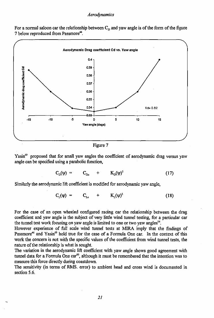
For a nonnal saloon car the relationship between Co and yaw angle is of the fonn of the figure 7 below reproduced from Passmore44
•
AerodynamIc Drag coemclent Cd vs. Vaw angle
0.4
~ 0.39
] 0.38
§ 0.37
'" e ." .11
0.36
Kc;. 0.82 I 0.35
0.34
·15 ·10 -5 o 5 10 15
Vaw angle (degs)
Figure 7
Yasin69 proposed that for small yaw angles the coefficient of aerodynamic drag versus yaw angle can be specified using a parabolic function,
Cno + (17)
Similarly the aerodynamic lift coefficient is modified for aerodynamic yaw angle,
~ + (18)
For the case of an open wheeled configured racing car the relationship between the drag coefficient and yaw angle is the subject of very little wind tunnel testing, for a particular car the tunnel test work focusing on yaw angle is limited to one or two yaw angless4•
However experience of full scale wind tunnel tests at MlRA imply that the findings of Passmore46 and Yasin69 hold true for the case of a Fonnula One car. In the context of this work the concern is not with the specific values of the coefficient from wind tunnel tests, the nature of the relationship is what is sought. The variation in the aerodynamic lift coefficient with yaw angle shows good agreement with tunnel data for a Fonnula One car60
, although it must be remembered that the intention was to measure this force directly during coastdown. The sensitivity (in tenns of RMS. error) to ambient head and cross wind is documented in section 5.6.
21

Aerodynamics
2.6 Ground Effect
During a coastdown test, due to the speed changes involved (200 - 40 mph) the ride height
and attitude of the vehicle are constantly changing implying changes in CD and <;. It is of vital importance that an appreciation of these effects is made. A full study of Formula One type wing sections in ground effect is indeed a major subject in itself, however what we are concerned with here is the effect that variations in ride height of the car during coastdown have on aerodynamic drag and lift. Hence part of the study looks at the effects of the ground on wing performance, in essence a study of ground effect for the modem Formula One car, since the front wing is currently the major component of the vehicle in ground effect. Additionally studied are the effects that ride height and rake of the vehicle have on drag and downforce.
During coastdown, due to the speed range described by the vehicle, the ride height and rake change with deceleration and variation in the normal load force, this is manifested by some pitching motion, and a general increase in ride height. These effects mean that the front wing angle of attack varies and the height above the ground changes. As an example of the important effects apparent for a Formula One car a study by Knowles et al.3
! on a front wing section typical of that used on modem Formula One cars, a GA(W)-l wing section, is considered in the following text.
Lift Coemclent vs incidence ror varyill! height above the ground
HeighUChord
-0-0.84
=-:.-"""--:;;-¥'------:-/"-+t--------1,---1 ....... 0•72
........ 0.6
~~~::::::::r=""""=---1~7oC--..... t----i--1 ....... 0.48 ;: __ 0.36
f-----+----"""C-----M-f-----+----l-a-O.14 ___ 0.12
Figure 8
Referring to Figure 8 proximity to the ground plane (lower height/chord ratio) was found to yield an increases in the lift curve slope. The sharpest increases occurring between the height
22
Aerodynamics
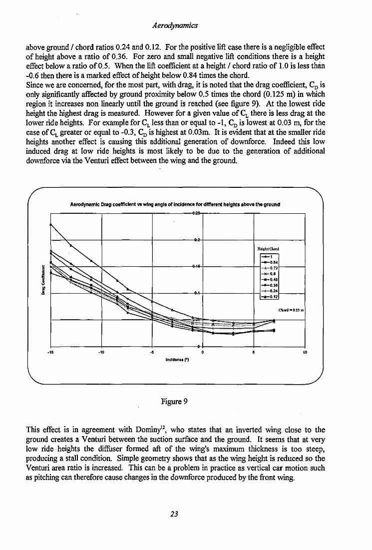
above ground I chord ratios 0.24 and 0.12. For the positive lift case there is a negligible effect of height above a ratio of 0.36. For zero and small negative lift conditions there is a height effect below a ratio of 0.5. When the lift coefficient at a height I chord ratio of 1.0 is less than -0.6 then there is a marked effect of height below 0.84 times the chord. Since we are concerned, for the most part, with drag, it is noted that the drag coefficient, Co is only significantly affected by ground proximity below 0.5 times the chord (0.125 m) in which region it increases non linearly until the ground is reached (see figure 9). At the lowest ride height the highest drag is measured. However for a given value of <;. there is less drag at the lower ride heights. For example for CL less than or equal to -1, Cn is lowest at 0.03 m, for the case of CL greater or equal to -0.3, Cn is highest at 0.03m. It is evident that at the smaller ride heights another effect is causing this additional generation of downforce. Indeed this low induced drag at low ride heights is most likely to be due to the generation of additional downforce via the Venturi effect between the wing and the ground.
Aerodynamic Drag coemclent VI wing angle of Incidence for different heights above the ground
Height/Chord
Chord -us
." -'0 -. o • ,0 Incld.no. C")
Figure 9
This effect is in agreement with Dominyl2, who states that an inverted wing close to the ground creates a Venturi between the suction surface and the ground. It seems that at very low ride heights the diffuser formed aft of the wing's maximum thickness is too steep, producing a stall condition. Simple geometry shows that as the wing height is reduced so the Venturi area ratio is increased. This can be a problem in practice as vertical car motion such as pitching can therefore cause changes in the downforce produced by the front wing.
23

Aerodynamics
It can be concluded from this short study that for the case of the front wing as the ground is approached the lift curve slope increases and the stall angle of the wing increases. Drag increases with decreasing height, however there is less induced drag at low heights. Therefore if the front ride height of the car is reduced and no change is made to the rear ride height we would expect to see a reduction in the drag from the front wing. Previous to the introduction of the now mandatory stepped bottoms a significant amount of the aerodynamic downforce produced by a modern Formula One car was generated by the underbody of the car, interacting with the boundary layer between the car and the road surface. The remaining part of the downforce was produced by the car body itself including the front and rear wing sections. This balance has changed making the car more pitch sensitive, the car is now far more heavily reliant on the wing sections to produce the necessary downforce. This was the result of legislation changes introduced to limit speeds during 1994, which necessitated the use of mandatory stepped bottoms. This implied increased ride heights which severely limited the interaction of the ground with the body of the car, significantly reducing downforce levels. Studies on the effects of changing vehicle ride height and angle of attack (rake) are limited to the pre stepped bottom era, so this must be borne in mind when considering the following points. Wildi67 undertook wind tunnel tests with twenty different ride height configurations varying the front ride height from 10mm to 35 mm and the angle of attack from _0.90 to 0.10 (positive denotes a nose up case). It was found that rake and ride height both have significant effects on downforce. The decreases in downforce appearing at positive or small negative angles of attack at constant ride height are caused by local flow separation on the bottom of the car. The influence of this flow separation again is strongly dependent on ride height. In situations where there is no major flow separation at the bottom of the car, the downforce increases with decreasing ride height at constant angles of attack. While the downforce varies over a range from best to worst of more than 35%, while the body drag varies over a range of 13%. A plot ofe;, for different angles of attack of the vehicle indicated that as the nose goes doWn in relation to the rear the drag increases. This trend is consistent for the range of front ride heights tested (10-32.5 mm). There is no strict correlation between downforce and drag, therefore high downforce doesn't necessarily infer a high drag case, and vice versa.
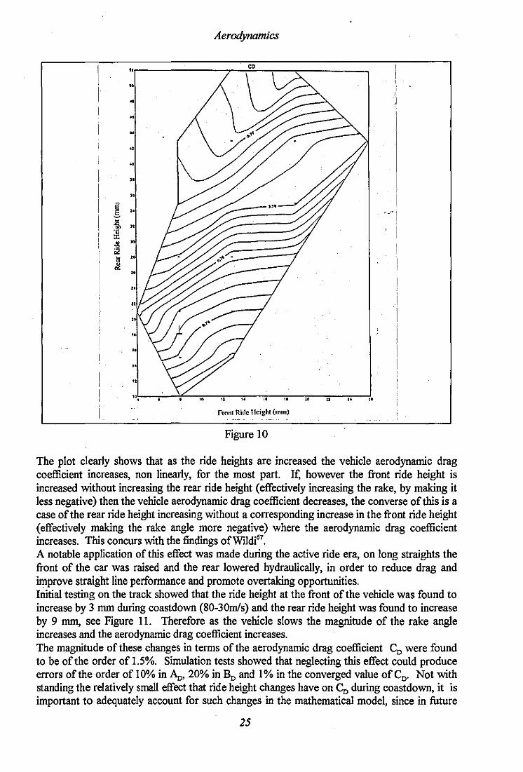
Bearing in mind our situation of an increase in ride height as the speed of the vehicle decreases and a decrease in vehicle angle of attack (i.e. the rear ride height increases more in relation to the front ride height) we could similarly hypothesise that the aerodynamic drag of the vehicle is likely to increase throughout the coastdown. In keeping with the findings of Wildi67 this is likely to be predominantly non linear.
It is clear from both these studies that some account must be made of the change of ride height and/or angle of attack of the vehicle during coastdown. To this end wind tunnel data on the e;, and <;, of the vehicle over the foreseeable range of ride height situations was obtained. This unfortunately was for the car previous to the new rule changes that legislated stepped bottoms or 'planks' fitted to the underside of the car. However the advice from the aerodynamicist61 was that the general trends would be similar. A representation of the contour plot of the e;, for different front and rear ride heights is detailed for a low downforce configuration in figure 10.
24
Aerodynamics
.. ~
d
M
" .. M
" " g ,.
il. " £
c~ ! I
~ »
la " ~ ..
..
.. " ".!--7-¥----;, • ..---.. " -",,--;,;-, -,;0, --;;,,--;,,;--,;0. -; ..
Pront Ride Height (mm)
Figure 10
The plot clearly shows that as the ride heights are increased the vehicle aerodynamic drag coefficient increases, non linearly, for the most part. If, however the front ride height is increased without increasing the rear ride height (effectively increasing the rake, by making it less negative) then the vehicle aerodynamic drag coefficient decreases, the converse of this is a case of the rear ride height increasing without a corresponding increase in the front ride height (effectively making the rake angle more negative) where the aerodynamic drag coefficient increases. This concurs with the findings ofWildi67
•
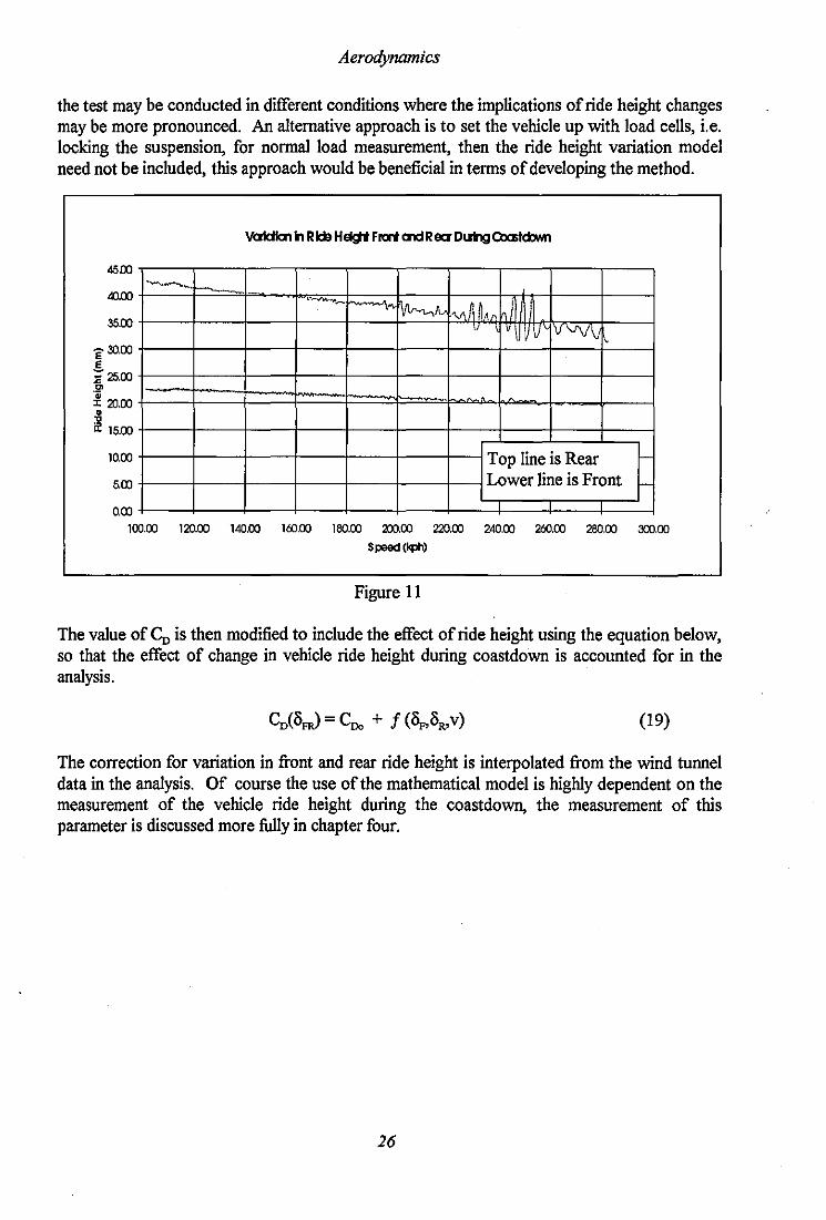
A notable application of this effect was made during the active ride era, on long straights the front of the car was raised and the rear lowered hydraulically, in order to reduce drag and improve straight line performance and promote overtaking opportunities. Initial testing on the track showed that the ride height at the front of the vehicle was found to increase by 3 mm during coastdown (80-30m/s) and the rear ride height was found to increase by 9 mm, see Figure 11. Therefore as the vehicle slows the magnitude of the rake angle increases and the aerodynamic drag coefficient increases. The magnitude of these changes in terms of the aerodynamic drag coefficient CD were found to be of the order of 1.5%. Simulation tests showed that neglecting this effect could produce errors of the order ofl0% in An, 20% in BD and 1% in the converged value of CD' Not with standing the relatively small effect that ride height changes have on Co during coastdown, it is important to adequately account for such changes in the mathematical model, since in future
25
Aerodynamics
the test may be conducted in different conditions where the implications of ride height changes may be more pronounced. An alternative approach is to set the vehicle up with load ceJls, i.e. locking the suspension, for normal load measurement, then the ride height variation model need not be included, this approach would be beneficial in terms of developing the method.
4500
AC.OO
35.00
E 30,00 .s ~ 25.00 ,2' • J: 20,00 -Il if 15,00
10,00
500
0,00
------... .... ~-.
YaIdfcI1 n Ride HeIgI Fm cnd Rea DlIfngOlaslcbi.n
.. ~ VL' ........ A, .V\~ ~AA
I
11 v \I VVV\j
_.
Top line is Rear I-
Lower line is Front f-
100.00 120,00 lAC,oo 160,00 180,00 200,00 220,00 240,00 260,00 280,00 300,00
Speed(kph)
Figure 11
The value of Co is then modified to include the effect of ride height using the equation below, so that the effect of change in vehicle ride height during coastdown is accounted for in the analysis,
(19)
The correction for variation in front and rear ride height is interpolated from the wind tunnel data in the analysis. Of course the use of the mathematical model is highly dependent on the measurement of the vehicle ride height during the coastdown, the measurement of this paraooeter is discussed more fuJly in chapter four.
26

Aerodynamics
2.7 Reynolds Number Effects in Tunnel Testing
However well wind tunnel testing is carried out, no matter how big the model or how fast
the tunnel speed is, there will be differences between what is encountered in the tunnel and on the track. Some of these phenomena can be attributed to Reynolds number effects. The aim of this short section is to review the literature available on the subject of the effects of Reynolds numbers on Co and CL" Wildi67 studied the effect on the total lift force, the front and rear lift force and the aerodynamic drag coefficient CD' of variation of the value of the Reynolds Number. This was undertaken via the reduction in the tunnel speed from the nominal test speed of 40, to 35 and 30 mls. Formula One car wind tunnel testing is typically conducted at Reynolds numbers in excess of 4 x 10⁶
, coastdown tests are conducted over a range of Reynolds numbers from 9 x 10⁶ to 2.1 x 10⁷
•
Wildi67 found that lower Reynolds numbers produce lower lift coeffiCients, the rear lift force being least effected. In contrast the drag shows a tendency to decrease with increasing value of Reynolds's number, the differences were found to be close to measurement accuracy.
This seems to indicate that if anything we would expect to see lower values of the drag coefficient CD on the track due to the higher Reynolds number. Quantifying the differences would be extremely difficult at this point. Moreover at different Reynolds numbers different flow regimes will exist, therefore inducing different lift I drag characteristics. It is indeed not clear cut that the track value of Co would be less than the tunnel value. In conclusion the influence of Reynolds's number in the tested range on the aerodynamic drag coefficient is small for the speed range tested67
, Reynolds number effects on CD during coastdown are likely to be minimal.
2.8 Open Wheel Aerodynamics
No study of a single seater racing car aerodynamics in the context of coastdown testing
would be complete without a study of the effects of the rotating wheels in the flow. Indeed the wheels of a Formula One car account for 0.3 (35 %) of the CD valrie67
, for a 1994 car with a CD estimated to be around 0.85. Dominyl4 put the figure at 50% (one assumes this was for the '93 car regulations, since which tyre width has been reduced). HiIhorsf2 stated that the wheels are responsible for around 40% of the whole vehicle drag and the effect tends to decrease with increasing normal load force. He cites the increased induced drag of the body being large in high downforce configuration as the explanation in the paper. A plot of the variation of the wheel drag as a percentage of the total drag is detailed for high, medium and low downforce vehicle settings. This showed that as the downforce increased so the percentage contribution of the wheels to the total drag decreased. Therefore on a high speed track the greatest amount of wheel drag is noted relative to the total drag, the upper limit was found to be around 36% of the total drag the lower around 23%. Although the wheels of a Formula One car account for significant proportions of the total vehicle drag, the lift force generated by the wheels is significantly smaller. Rotating wheels reduce the vehicle downforce22
, at the same time the wheel body interaction is said to increase the drag. This effect was found to be consistent throughout the vehicle speed range tested. Indeed at higher speeds the interaction is less, i.e. the body downforce increases and the aerodynamic drag increases relatively.
27 "

Aerodynamics
During wind tunnel testing of the vehicle using a moving ground plane, estimation of the wheel lift forces must be undertaken via integration of the pressures acting over the surface of the wheel. For accurate estimation ofthe force the pressure data must be recorded across the full width of the wheel not only since the wheel has a low aspect ratio but also as a consequence of the spanwise asymmetry of the flow arising from external influences such as aerofoils, radiator intakes and brake ducts. Therefore during routine wind tunnel testing the lift force from the wheels is usually not measured. Toees estimated that the wind tunnel value of<;' to be in error due to this by 1%, i.e. 1% over the actual value.
Referring back to the work of Hilhorse2, a diagram in the paper details the vortex system
found in the region of a rotating wheel. It is shown that three pairs of vortices are present, a lower pair close to the ground of the roll down type, a central roll up pair and from the top of the wheel a roll up pair. Wheel speed variations are said to greatly influence the effect, position and intensity of all the vortices present around the wheel. Little is really known about the nature of these variations and their effects overall.
2.9. Lift and Drag
T he chosen route of solution for the analysis of coastdown data was that of simulation and
optimisation in keeping with the findings of Passmore45• This implies that the terrns of a
common order in speed cannot be discerned in the analysis. The basic vehicle drag equation is summarised below to illustrate that the aerodynamic drag and lift contain terms of a common order in airspeed vr •
[(Ao+Bov) (Mg - 'hpAv/<;.)] + ['hpAv/Co] (20)
(neglecting drivetrain and transmission losses)
The implication of this is that the lift and drag terms cannot be separated in the analysis. Thus the aerodynamic lift must be constantly measured during the course of the test. This can be achieved via load cells, or alternatively another suitable method was that of strain gauging of the suspension pushrods front and rear in order to measure the normal load. An alternative approach to the problem is to define the relationship between lift and drag coefficients, thus making the problem resolvable, the coefficient of aerodynamic drag is discerned in the analysis, which subsequently allows the coefficient of aerodynamic lift to be determined via the relevant formula. The purpose of this part of the study is to review the literature concerning the aforementioned link between the aerodynamic drag and lift coefficients for racing cars.
Katz'° in his study into the effect of wing body interaction on the aerodynamics of two generic racing car shapes defined the formula below for the aerodynamic drag coefficient in terms of the aerodynamic lift coefficient and aerodynamic drag coefficient for the car without any wing sections.
Rearranging, .
<;. = «Co - Cno)Ik)~ + CLo
28
(21)
(22) .
Aerodynamics
Thus eliminating <;. from the general drag equation. The values of the constants were found to be as below for an IMSA GTP type racing car.
COo = 0.3, Cu, = 0.2, k = 0.04.
Which is a closed wheel type racing car raced in the United States. This type of relationship is of course unique to each type of vehicle tested, and the determination of the Cno and CLo coefficients is reliant on wind tunnel testing.
Mcnay40 in his study into an approximate lap time minimisation based on Indy style racing car geometry, (Open wheeled wings and slicks racing car) defined a relationship between Drag and Lift coefficients via a curve fit to wind tunnel based experimental data. The data having been published by another author (Katz2).
A curve fit to the data yielded the following formula for the aerodynamic drag coefficient in terms of the aerodynamic lift coefficient,
Co = Cno - 0.10375 + 0.77<;. - 1.3381<;.2 + 1.2478<;.3 (23)
Arbitrarily fitting a high order polynomial function to data can be a dangerous practice, since values determined from the expression outside the experimental range can be very inaccurate, owing to the higher order nature. This also has dubious origins in terms of the type of car upon which the initial wind tunnel tests were conducted. Katz's paper was based upon a generic racing car in 1985, the Mcnay paper is based upon data for a 1988 Indy car. Additionally the curve fitting errors add to the inaccuracy. However the results published in Mcnay's paper seem to indicate that not withstanding these inadequacies, good circuit simulation results can be obtained using this type of relationship. In conclusion there is very little published material on the relationship between lift and drag. What little there is indicates that some major assumptions have to be made in order to define the relationship and the relationship is specific to each vehicle. Wind tunnel dataS8 indicates a very non linear relationship, so measurement of the normal load force is evidently the best method to use, if indeed accurate measurements can be made. This is considered further in section 4 of the report.
29

Aerodynamics
2.10. Aerodynamic drag Model
The aerodynamic drag model determined from research, simulation and test work was deemed to be as expressed below. It includes account for the effects of ambient wind and variation in the vehicle ride height during the coastdown test.
= (24)
Expanding
= (25)
The effect of the lift force (downforce) is not included in this term since it included as a factor in the tyre mathematical drag model.
30

Aerodynamics
2.11. Mathematical Vehicle Drag Model
The complete mathematical drag model is obtained by combining the aerodynamic, tyre, transmission, and undriven wheel loss models described in chapter 2. It is detailed in stages below.
Fo(v) = FAero + F1)Te + FDr + Fu + FGrnde
Fo(v) = (Y2pAv/[CDo + KoC'I") + f (oFA,v)]) +
([Ao + Bov] x [Mg+L] x [l+lCr(To-TJD +
(A, + B,v) + (A. + Buv) + (Mgsin 9)
(26)
(27)
The grade force F Orad. must be determined ifUni-directional testing is to be undertaken, . example grade data (Circuit De Catalunya) can be located in Appendix VI.
31

Test Method
3. Test Method
Based upon the findings from the simulation work and subsequent full scale testing, recommendations for a test method specific to coastdown testing of a Formula One car were made. The test method developed has been designed to be flexible, so that testing may be undertaken at purpose built tracks or airfield sites. All the coastdown tests were eventually conducted on the main straight of existing Grand Prix circuits, namely Silverstone and Barcelona. The test is designed to be as simple as possible to perform so that it can undertaken during routine track testing. This chapter outlines the vehicle set up required for coastdown testing, the environmental conditions necessary, the instrumentation required, and the test procedures recommended.
3.1. Vehicle Set Up
T he following are recommendations for the car set up for coastdown test work based upon the findings made in the course of this study. Vehicle set up is of course dependent on the circuit at which the test is to be conducted for example a high speed track would infer a low downforce vehicle setup. These recommendations therefore do not indicate definitive vehicle configurations for coastdown testing. The transmission system must be set up so that neutral can be selected by the driver at the start of the coastdown. If 'possible appropriate gear ratios should be selected to produce maximum acceleration prior to the start of the coastdown test. The aerodynamic set up is dependent on the track at which the testing is being undertaken. However for the purposes of developing the method the general rule is that a mediumlhigh downforce set-up be used, for two reasons. Firstly the higher the drag, the shorter the straight needed to describe a representative speed range in coastdown. A minimum of four Uni directional coastdowns should be conducted with the standard aerodynamic set up before any changes are made in order to establish a datum for repeatability.
3.2. Environmental Conditions
The EEC regulations for coastdown testing state that, in order for coastdown tests to be performed the track should be dry and the ambient temperature and pressure should be within the limits indicated below:
Ambient Pressure Ambient Temperature
=
= 100±7.5 kPa 293.2±22K
In conventional testing the ambient wind levels must be within the limits detailed below:
Average wind speed Peak wind speed Maximum crosswind component
=
= =
3.0 mls 5.0 mls 2.0 mls
If the intention is to conduct the tests with on board anemometry, it is not necessary to ensure that these limits are met. If only a pitot is used to monitor ambient wind then the tests should
32
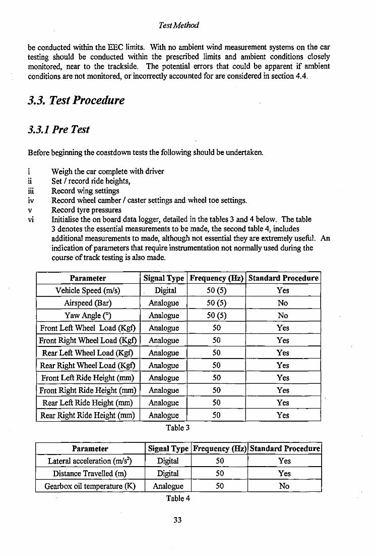
Test Method
be conducted within the EEC limits. With no ambient wind measurement systems on the car testing should be conducted within the prescribed limits and ambient conditions closely monitored, near to the trackside. The potential errors that could be apparent if ambient conditions are not monitored, or incorrectly accounted for are considered in section 4.4.
3.3. Test Procedure
3.3.1 Pre Test
Before beginning the coastdown tests the following should be undertaken.
Weigh the car complete with driver ii Set I record ride heights, iii Record wing settings iv Record wheel camber I caster settings and wheel toe settings. v Record tyre pressures vi Initialise the on board data logger, detailed in the tables 3 and 4 below. The table
3 denotes the essential measurements to be made, the second table 4, includes additional measurements to made, although not essential they are extremely useful. An indication of parameters that require instrumentation not normally used during the course of track testing is also made.
Parameter Signal Type Frequency (Hz) Standard Procedure
Vehicle Speed (rnIs) Digital 50 (5) Yes
Airspeed (Bar) Analogue 50 (5) No
YawAnglee) Analogue 50 (5) No
Front Left Wheel Load (Kgf) Analogue 50 Yes
Front Right Wheel Load (Kgf) Analogue 50 Yes
Rear Left Wheel Load (Kgf) Analogue 50 Yes
Rear Right Wheel Load (Kgf) Analogue 50 Yes
Front Left Ride Height (mm) Analogue 50 Yes
Front Right Ride Height (mm) Analogue 50 Yes
Rear Left Ride Height (mm) Analogue 50 Yes
Rear Right Ride Height (mm) Analogue 50 Yes
Table 3
Parameter Signal Type Frequency (Hz) Standard Procedure
Lateral acceleration (rnIs2) Digital 50 Yes
Distance Travelled (m) Digital 50 Yes
Gearbox oil temperature (K) Analogue 50 No
Table 4
33
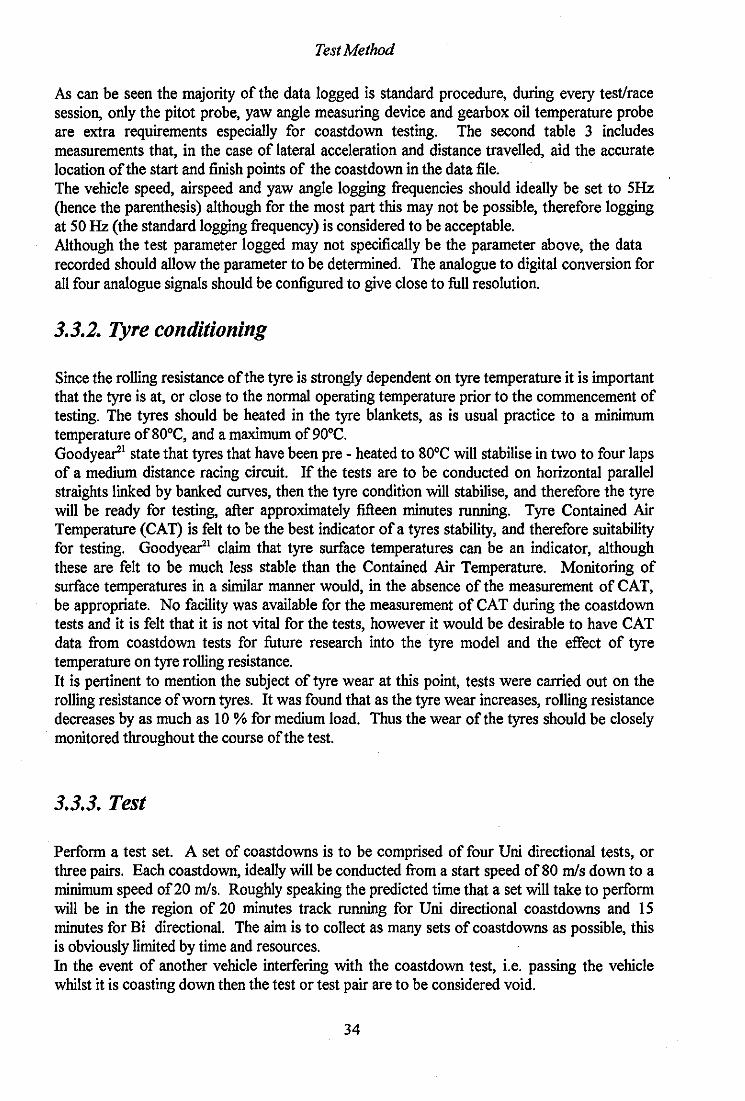
Test Method
As can be seen the majority of the data logged is standard procedure, during every test/race session, only the pitot probe, yaw angle measuring device and gearbox oil temperature probe are extra requirements especially for coastdown testing. The second table 3 includes measurements that, in the case of lateral acceleration and distance travelled, aid the accurate location of the start and finish points of the coastdown in the data file. The vehicle speed, airspeed and yaw angle logging frequencies should ideally be set to 5Hz (hence the parenthesis) although for the most part this may not be possible, therefore logging at 50 Hz (the standard logging frequency) is considered to be acceptable. Although the test parameter logged may not specifically be the parameter above, the data recorded should allow the parameter to be determined. The analogue to digital conversion for all four analogue signals should be configured to give close to full resolution.
3.3.2. Tyre conditioning
Since the rolling resistance of the tyre is strongly dependent on tyre temperature it is important that the tyre is at, or close to the normal operating temperature prior to the commencement of testing. The tyres should be heated in the tyre blankets, as is usual practice to a minimum temperature ofSO°C, and a maximum of 90°C. Goodyear l state that tyres that have been pre - heated to SO°C will stabilise in two to four laps of a medium distance racing circuit. If the tests are to be conducted on horizontal parallel straights linked by banked curves, then the tyre condition will stabilise, and therefore the tyre will be ready for testing, after approximately fifteen minutes running. Tyre Contained Air Temperature (CAT) is felt to be the best indicator of a tyres stability, and therefore suitability for testing. Goodyearl claim that tyre surface temperatures can be an indicator, although these are felt to be much less stable than the Contained Air Temperature. Monitoring of surface temperatures in a similar manner would, in the absence of the measurement of CAT, be appropriate. No facility was available for the measurement of CAT during the coastdown tests and it is felt that it is not vital for the tests, however it would be desirable to have CAT data from coastdown tests for future research into the tyre model and the effect of tyre temperature on tyre rolling resistance. It is pertinent to mention the subject of tyre wear at this point, tests were carried out on the rolling resistance of worn tyres. It was found that as the tyre wear increases, rolling resistance decreases by as much as 10 % for medium load. Thus the wear of the tyres should be closely monitored throughout the course of the test.
3.3.3. Test
Perform a test set. A set of coastdowns is to be comprised of four Uni directional tests, or three pairs. Each coastdown, ideally will be conducted from a start speed of SO m/s down to a minimum speed of 20 m/ s. Roughly speaking the predicted time that a set will take to perform will be in the region of 20 minutes track running for Uni directional coastdowns and 15 minutes for Bi directional. The aim is to collect as many sets of coastdowns as possible, this is obviously limited by time and resources. In the event of another vehicle interfering with the coastdown test, i.e. passing the vehicle whilst it is coasting down then the test or test pair are to be considered void.
34

Test Method
Down load the data from the on board data logger, manipulate the files applying appropriate headers.
Predicted Distances Travelled in Coastdawn Since the length of the straight / runway available to us for coastdown testing may be limited, simulation tests were undertaken in Matrix. in order to determine predicted distances travelled for the vehicle coasting down. Table 5 below shows predicted distances travelled in coastdown for a low downforce aerodynamic set up, these distances do not include the extra track distance required to accelerate to the necessary start speed before commencing a coastdown.
Speed 88-16 85-16 80-15 75-15 80-20 80-25 80-30 range (m/s)
Distance 1,253 1,218.3 1,176.8 1,114.4 1,048 904.7 778.6 travelled
(m)
Table 5
This is included as a guide, if for example a new test site were to be selected.
The test method developed is applicable for testing on normal racetracks, airfields and dedicated test sites such as MIRA (Motor Industry Research Association) or IDIADA (Institute for Applied Automotive Research, Spain). In the event oftests being conducted at the latter sites, marking out of the start and termination points for the driver, should be made prior to commencing the testing using the table above as a guide. Data capture sheets that were used to collect coastdown test data are included in the report in Appendix I.
3.4. Driveline Tests
. T his part of the report is concerned with the test method used to determine the drivetrain and
undriven wheel loss components from laboratory testing. Drivetrain coastdown tests were conducted during testing at Paul Ricard in June (1994). Three tests were undertaken which were run after a days testing, so as to minimise the risk of a curtailment of the main test due to an engine failure, due to overheating. Formula One engines are reliant on airflow for cooling (there being no on board cooling fan). Due to the very high inertia's involved it was deemed unsafe to test at a rear wheel speed in excess of 900 rpm (this equates to a road speed of2Amls). This 'Yas unfortunate but unavoidable Laboratory tests to determine the undriven wheel loss model were conducted at the Benetton factory at Enstone in June (1994). A suitable laboratory test rig was constructed and extensive testing was undertaken at various hub temperatures in order to determine an accurate representation of the losses associated with the undriven wheels during coastdown testing. The test methods used for both these types of test are detailed separately in the following sub sections of the report.
35

Test Method
3.4.1. Drivetrain Tests
The vehicle should be raised from ground level and put onto stands to allow free rotation of the drivetrain, the suspension supported so that it is in it's normal track configuration and the engine started. The engine speed is then increased until an engine speed corresponding to as high a vehicle speed as possible in the appropriate gear is reached. The engine is then de clutched, the gearbox set in neutral, and the drivelrain allowed to coastdown. At each time step the wheel Speed is recorded.
3.4.2. Undriven Wheel Tests
Undriven wheel coastdown tests were conducted at several temperatures, (heating of the assembly being undertaken with a heat gun) felt to reflect the range of temperatures over which the assembly normally operates. The wheel and hub assembly was set up so that the hub and braking system were in their normal operating mode. This is detailed in the photographs below, figures 12 and 13, the first shows the disk calliper assembly in frontal view, the second focuses _on the four pot calliper itself, clearly showing the fou r pads and vented disk.
Figure 12
36
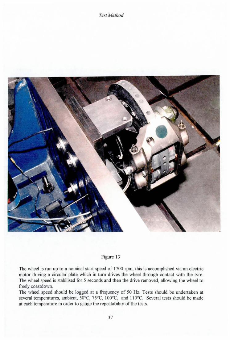
Test Method
Figure 13
The wheel is run up to a nominal start speed of 1700 rpm, this is accomplished via an electric motor driving a circular plate which in turn drives the wheel through contact with the tyre. The wheel speed is stabilised for 5 seconds and then the drive removed, allowing the wheel to freely coastdown. The wheel speed should be logged at a frequency of 50 Hz. Tests should be undertaken at several temperatures, ambient, 50°C, 75°C, lOOoe , and llO°C. Several tests should be made at each temperature in order to gauge the repeatability of the tests.
37

Instrumentation
4. Instrumentation
Accurate measurement of the parameters that are used in coastdown analysis is of vital
importance in order to accurately determine the correct drag coefficients. In this chapter the on board data logging system is detailed, the potential errors induced by inaccurate measurements and system noise and their effect on the converged values of the drag coefficients is described with reference to the simulation (Appendix 11). Additionally the other data acquisition system used, the weather station, is described. The effect of incorrect account of ambient wind is then considered again with reference to simulation tests. Finally recommendations are made for a device to measure aerodynamic yaw angle.
4.1. On Board Data Logger
The on board data logging systems used in Formula One are highly sophisticated, measuring
upto thirty five (not including engine data) parameters continuously during testing I racing.· Data required for coastdown analysis requires only a limited amount of extra instrumentation, for ambient wind measurement.
Transducers were used to measure the following parameters throughout testing unless otherwise stated.
» Vehicle Speed » Normal Load » Airspeed » Lateral acceleration » Ride Height Front and Rear » Gear box oil temperature
The data logging system used was the same one used for normal track testing, the logger module is located near the drivers right shoulder (see Figure 16). The normal test logging frequency is 50 Hz. At the commencement of each track test session the logger is initialised and data is recorded throughout the test. On return to the pits the data is downloaded to a P.C. from which it can be accessed via the GRID (Graphical Race Instrumentation Data system) P.C. package, an in house software package, for use in DOS.
38

Instrl/mentation
4.1.1. Vehicle Speed
Measurement of vehicle speed was made via an inductive pickup mounted in the hub as shown in the photograph below Figure 14.
Figure 14
The speed pickup is positioned in line with a 48 tooth disk which rotates at wheel speed, yielding a digital wheel speed signal. For the maximum speed encountered during a coastdown test the resolution is close to 0.4 rn/s prior to coastdown analysis.
39
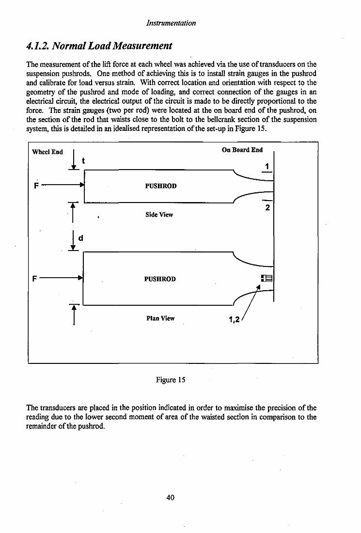
Instrumentation
4.1.2. Normal Load Measurement
The measurement of the lift force at each wheel was achieved via the use of transducers on the suspension pushrods. One method of achieving this is to install strain gauges in the pushrod and calibrate for load versus strain. With correct location and orientation with respect to the geometry of the pushrod and mode of loading, and correct connection of the gauges in an electrical circuit, the electrical output of the circuit is made to be directly proportional to the force. The strain gauges (two per rod) were located at the on board end of the pushrod, on the section of the rod that waists close to the bolt to the bellcrank section of the suspension system, this is detailed in an idealised representation of the set-up in Figure 15.
ee n
t 1
On Board End Wh lE d 1
-F PUSHROD
-·T 2
• Side View
Id F PUSHROD ::§
'---i Plan View 7 1,2
Figure 15
The transducers are placed in the position indicated in order to maximise the precision of the reading due to the lower second moment of area of the waisted section in comparison to the remainder of the pushrod.
40

instromentation
The strain in the pushrod is given by,
£= F Exdxt
(28)
with £1=£2 i.e. strain is equal in both sides of the pushrod.
A Wheatstone bridge circuit is used to produce a voltage signal that is proportional to the Load F. Prior to each test the strain gauges are calibrated by applying a known forces and recording the strains.
4.1.3. Airspeed measurement
Measurement of the vehicle airspeed was carried out using a pitot probe in line with the vehicle's direction of travel, (Figure 16) located at the front of the car, close to the front suspension mounting.
Logger I Airspeed Pitot
O.85m
Accelerometers
Figure 16
Calibration of this device was undertaken in the wind tunnel. The zero setting (i.e. no airspeed) was checked prior to the start of a test session.
4.1.4. Lateral Acceleration
Although not specifically required for coastdown analysis, lateral acceleration was measured in order to correctly determine where the coastdown commenced and terminated. Lateral acceleration is measured by an accelerometer that is located on the floor of the monocoque of the car, below the driver's legs (Figure 16).
4.1.5. Ride Height
Vehicle ride height was measured at each of the four wheels and averaged over each axle in the coastdown to produce front and rear ride height values. Damper deflection is used to determine the wheel deflection from which the ride height is calculated. No account is made
41

Instromentation
of the tyre deflectionlsquish in this calculation. The absolute reading of the vehicle ride height is evidently inaccurate, however for the purposes of coastdown analysis, where we are concerned with ride height changes it is adequate.
4.1.6. GearBox Oil Temperature
For the preliminary tests at Silverstone the gearbox oil temperature was measured, this was undertaken since it was felt that the drivetrain losses were variable with gear oil temperature. However it was found that the gear oil temperature was fairly stable throughout the test, showing a maximum change of 3-4 °C. This implied that measurement was not critical, although useful.
4.2. Measurement and System Noise
To gain an appreciation of the inevitable problems associated with real world testing, tests
were undertaken in order to gauge the effect of measurement and system noise. This was achieved by adding Gaussian (zero mean, known standard deviation) white noise to the measured signals, and then analysing the simulated coastdowns to yield the drag coefficients. Secondly in a similar way the effects of system noise were determined. System noise is noise connected with factors that have not been included in the analysis. These usually manifest themselves in the form of track surface irregularities and suspension motions.
4.2.1. Measurement Noise
The simulation methodology is described in Appendix II of the report, and details of the vehicle configuration are documented. Tests were conducted with various levels of noise imposed on the measured signals to quantifY the permissible noise levels for each of the four measured signals. The permissible maximum noise levels based on an acceptable coefficient tolerance are,
Vehicle Speed YawAngle Relative Airspeed Normal Load
0.5 rnls 0.001 rad 0.1 rnls 400N
The acceptable tolerance to these noise levels was deemed to be errors of <1 % in AD' <1 % in BD' <0.5% in Co and <5% in Ko.
Considering each case individually, the effect on the converged values of the coefficients of applying noise to vehicle speed was limited. No coefficient was in error by more than 1%, An being closest at 0.89 %. The effect of imposing noise on the measured value of yaw angle was limited for AD' BD and CD' no coefficient being any more than 0.09 % in error, however the resulting error in KD was 3.4%. The case of imposed noise on relative airspeed produced the most dramatic effects on the converged coefficients. Noise levels above 0.1 produced intolerable errors in the converged
42

Instrumentation
coefficients, over 1 % in the tyre loss coefficients. Finally the effect of imposing noise on the normal load force was considered, it was found that noise levels up to 400 N could be tolerated with little effect on An, Bo and Co. Ko was found to be in error by more than the nominal 5% when the noise level was over 400 N.
4.2.2. System Noise
Additional Constant drag
To determine the implications of an additional constant drag force that is not accounted for in the analysis, simulations tests were conducted with a range of extra constant drag forces added to the total drag force. The magnitudes of these forces are small in comparison with the total drag force, being little greater than 1 %. This additional drag could take the form of clutch drag or incorrect gradient force (50 N is equivalent to a grade of 0.5%), for example. The effect of not accounting for the force on the converged coefficients was then determined, these are displayed in table 6 below. Percentage errors are in parenthesis.
Drag(N) An Bo(x10-s) Co Ko
25 0.0131 0.0139 0.851 4.714 (12.93) (-99.85) (3.402) (6.51)
50 0.0134 0.0933 0.859 4.788 (15.5) (0.0093) (4.374) (8.179)
75 0.0138 0.0007 0.866 4.858 (18.966) (-99.9926) (5.225) (9.761)
100 0.0141 0.0006 0.873 4.928 (21.55) (-99.9993) (6.075) (11.34)
Table 6
The results show that additional constant drag can induce large errors in the converged values of the coefficients, notably Bo and An. It would be expected that these coefficients would be most affected due to their lower sensitivity with respect to Co. If we are considering the normal road car case of zero lift force where there was a constant term (mgxAn), as opposed to the V/ term in the lift force, we would expect that the additional drag term would be accounted for by a high converged value of Ao. Since the normal load force is speed dependent the error is distributed among the coefficients, although as can be seen it is biased towards the more sensitive coefficients, such as Bo and An. These additional forces are relatively high however and are unlikely to be consistent throughout a test. It is unlikely that modelling errors could cause errors of the order of 100 N, 50 N would however be possible and thus this underlines the importance of an accurate mathematical model.
Effective Mass Error
Every effort was made to accurately determine the vehicle's effective mass during testing however, the pace of development of the cars is such that development parts are being tried consistently, therefore it was deemed entirely possible for the effective mass to be slightly different from the pre determined value. The nominal value of the effective mass was
43

Instrumentation
therefore varied during the analysis of simulated data by ±O.S, ±l.O and ±2%, the effect on the converged values of the coefficients is shown in figure 17.
Effective mass error
8
~ 6
___ Bd ___ Cd
4 ~
C-c 2 " 'u is
" 8 -2 -1.5 0.5 1.5 2 .5 -2 ~ 0 t:
UJ -4
-6
.s E lIorln effecHv8 moss (%)
Figure 17
The net effect is that, if the effective mass of the vehicle is over estimated, then the resultant converged values of the drag coefficients will be positively in error, or over estimated. One percent equates to over six kilos for the vehicle in test set-up. Conversely underestimating the vehicle's effective mass decreases the values of the converged drag coefficients. Considering the change in the converged value of Co by linearly increasing the assumed effective mass, it can been seen that Co linearly increases with increased assumed effective mass.
Error In Normal Load Measurement
Since the normal load was to be measured on line during the tests, the effect of an error in the measurement of the force was investigated. This error could be due to inaccurate calibration of the strain gauge system, surface irregularities or an error due to suspension movement. This latter cause of error falls into the realms of system noise. These tests were undertaken by simulating additional lift forces applied to the vehicle and not accounting for this change in the analysis. The results are shown in Figure 18.
44
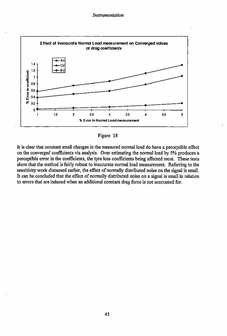
lA
1: 1.2 m '0 1
Instromentation
E fleet of InacaJrale Normal Load measurement on Converged values of drag coefficients
[3Ad ___ Cd
___ Bd
m 0.8 ~ t __ --------------~------=::= .! Oht:=====:==---------Ji OA
~ O.~ b===+====f===i===::==:::;:::===:======: 1.5 2 2.5 3 3.5 4 4.5 5
% Error In Normal Load measurement
Figure 18
It is clear that constant small changes in the measured normal load do have a perceptible effect on the converged coefficients via analysis. Over estimating the normal load by 5% produces a perceptible error in the coefficients, the tyre loss coefficients being affected most. These tests show that the method is fairly robust to inaccurate normal load measurement. Referring to the sensitivity work discussed earlier, the effect of normally distributed noise on the signal is small. It can be concluded that the effect of normally distributed noise on a signal is small in relation to errors that are induced when an additional constant drag force is not accounted for.
45

Instrumentation
4.3. Weather Station
The detailed schematic of the equipment is shown below in Figure 19.
Barometric Pressure Sensor
Temperature Humidity Sensor
Figure 19
Display Unit
IUIIBIB
+
12 v D.e. supply
The weather station has the facility to measure the following parameters;
".. Wind Speed (Knots) ".. Wind Direction e from head on, cw +ve) ".. Temperature eC) ".. Barometric Pressure (mBar) ".. Relative Humidity (%)
Prior to testing the station is set up on a flat piece of ground close to the trackside and remote from any large obstacles, such as bridges or buildings. The wind direction vane is zeroed in the direction of travel of the vehicle and the following readings are taken at the indicated intervals;
46
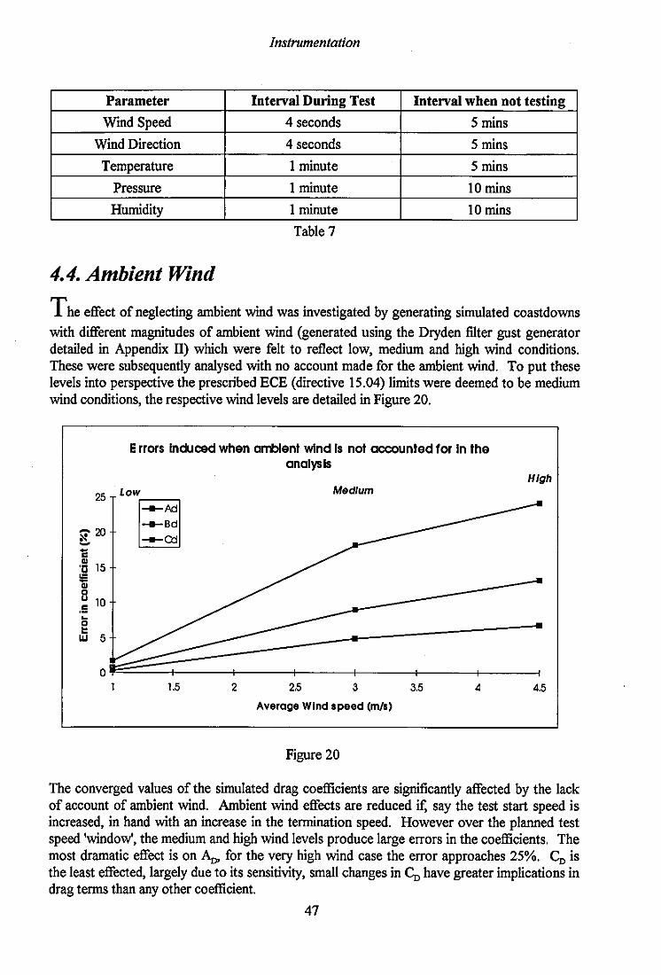
Instrnmentation
Parameter Interval During Test Interval when not testing
Wind Speed 4 seconds 5 mins
Wind Direction 4 seconds 5 mins
Temperature 1 minute 5 mins
Pressure 1 minute 10 mins
Humidity 1 minute 10 mins
Table 7
4.4. Ambient Wind
The effect of neglecting ambient wind was investigated by generating simulated coastdowns
with different magnitudes of ambient wind (generated using the Dryden filter gust generator detailed in Appendix 11) which were felt to reflect low, medium and high wind conditions. These were subsequently analysed with no account made for the ambient wind. To put these levels into perspective the prescribed ECE (directive 15.04) limits were deemed to be medium wind conditions, the respective wind levels are detailed in Figure 20.
E nors Induced when ambient wind Is not accounted for In the analysis
The converged values of the simulated drag coefficients are significantly affected by the lack of account of ambient wind. Ambient wind effects are reduced if, say the test start speed is increased, in hand with an increase in the termination speed. However over the planned test speed 'window', the medium and high wind levels produce large errors in the coefficients. The most dramatic effect is on An, for the very high wind case the error approaches 25%. Cn is the least effected, largely due to its sensitivity, small changes in Co have greater implications in drag terms than any other coefficient.
47

Instromentation
Additional simulation / analysis work was undertaken for the case of simulated data generated with simulated natural wind, with constant wind values assumed in the analysis. This was intended to be a simulation of the case when on board anemometry is not available - implying weather station measurements. It was found that assuming constant high wind values for a high wind case produced errors in the converged values of the coefficients of the order 0.5% in Co, 2.2% in Ao, and 26% in BD. The results were similar when mean values were assumed. In conclusion weather station wind readings can cause appreciable errors in the coefficients, which are largely manifested in the form of over estimates.
4.5. Aerodynamic Yaw Probe
Aerodynamic yaw is usually measured with a micro response vane during the coastdown
testing of normal road cars. The devices used are cumbersome, requiring a 1.5m boom extending from the front of the vehicle in order to minimise the effect of both instrumentation on the flow field upstream of the car and the effect of the flow field around the car on the instrument. Owing to the very sensitive nature of the devices employed at the front of a Formula One car and the absence of any suitable means of mounting a boom on the front of the car, this sort of device is totally inappropriate for a Formula One car, hence a pitot probe type ofyawmeter is recommended. A normal pitot probe is to some extent sensitive to aerodynamic yaw, but by virtue of its design the aim is to produce a probe with the smallest possible sensitivity. A yaw meter is specifically designed to produce a high yaw sensitivity. In the aeronautical field yaw meters are split into two categories, the 'sawn off pitot tube' or the 'bent tube' type. Measurement of the aerodynamic yaw angle during the coastdown should be undertaken using the 450 sawn off pitot tube type of yaw meter, as opposed to the bent tube type of device. The reasoning behind this is that the former type yields the flow desired in a given plane and is simple and easy to manufacture. Figure 21 represents a suitable type of yaw meter for this purpose.
Sawn Off Tube Y,wmeter -
-
Figure 21
48

Analysis Method
5. Analysis Method
5.1. Methodology
The type of analysis method employed to extract the drag coefficients from coastdown data is varied. Lucas3S proffered the opinion that the raw speed - time data should be fitted with a high order polynomial, and the polynomial be differentiated to obtain a smoothed force - speed characteristic. A quadratic curve fit then yields An, BD and CD' This method is straight forward but as detailed by Emtagel6
, the coefficients extracted from the drag force - speed curve are very sensitive to errors in the high order curve fit. Passmore4S showed the effect in terms of the inherent error found when an inappropriate mathematical drag model is employed, in addition to a similar order of error for the case when no account is made for crosswind effects.
A method used to resolve the problem of differentiation of the coastdown equation is that of analytically integrating the coastdown equation to obtain an expression for the speed time function, Lucas3S, details this method. This has inherent drawbacks in that it is extremely inflexible and very difficult to implement if all the facets of the drag force acting on the vehicle are to be accounted for.
These conventional methods of attacking the problem have been superseded by the method used by Passmore4S
,46 and Buckely2-3. Passmore states that, 'In general these methods have been designed for the analysis of data acquired without a continuous measure of ambient wind, and therefore depend on the use of averaging or smoothing techniques. If on board anemometry is used then these methods are inappropriate since the bandwidth of the relevant information has been increased by the ambient wind data.' The analysis methods considered here after are based around tests to be conducted with on board anemometry or some method of accounting for ambient wind.
49

Analysis Method
5.2. Optimisation
T he approach adopted by Passmore44-40 has been to directly fit the equation of motion of the
vehicle in coastdown, under the influence of ambient wind to the measured data, using a parameter optimisation method. The objective of parameter optimisation for the case in hand is to minimise some function. This function is defined for the coastdown case by Passmore44
as the sum of the squares of the residuals. The residuals are the difference between the measured speed values and the speed values that are calculated using the coastdown mathematical model. The optimisation routine determines values for the control variables (coefficients) which produce the best fit in a least squares sense between the mathematical model and the measured data.
This approach has been applied by a number of researchers. White66 analytically integrated the coastdown equation to produce an expression for the speed time function, optimisation code was then used to determine the relevant parameters. However in this study the drag function was only described by a two term function, ambient wind was not included in the study. Emtage16 applied a three term expression for the drag function and included a wind correction factor in addition to accounting for the effects of tyre temperature. In order to account for the ambient conditions Emtage used a differential approach that corrects the time interval between consecutive points yielding a corrected speed time history. This requires the use of an initial estimate of the drag coefficients in order to perform the correction. Therefore an in built source of error will be apparent.
Passmore45 avoided this by combining the correction procedure with the optimisation, by integrating the complete coastdown equation using the measured ambient conditions.
50
Analysis Method
5.3. Coastdown Analysis
T he equation of motion for a vehicle travelling on a track with grade angle e is an application of Newton's second law of motion:
FT Tractive Force
Fo(v) -Resistive Force
MgSine =
Gravitational Force
in coastdown FT = zero, so we have,
Fo(v) = -Me~ - Mg Sin e
therefore,
dv = -(FD(v)+Mgsin9) dt Me
M dv edt
Inertial Force
(29)
(30)
(31)
From Chapter two a mathematical model describing the drag force on the car at a particular vehicle speed in coastdown, was developed. This is represented below,
(32)
Fo(v) = {YzpAv,2x[CDo + Ko(\f) + f (Bp,OR'V)]} +
{[A" + BDvlx[Mg+L]x[I+~(To+T,)]} + {A, + B, v}
+ {A" +Bu v} (33)
The method of analysis is as follows, a theoretical speed is determined by using the start speed and the corresponding drag at that speed to calculate the deceleration (performing a numerical integration using the Runge Kutta fourth order method) to yield the next speed. The difference (between measured and calculated) is termed the residual,
Residual = vm - v,(x) (34)
defining the COST function F(x),
F(x) = ~ (Residuals2) (35)
The objective is to minimise the COST. In our case the sum of the residuals squared is reduced by manipulating the control variables in the drag function, i.e. varying Ao, Bo, Co and Ko, until COST converges to a minimum.
51

Analysis Method
This method of optimisation requires a routine to minimise the sum of the squares of the error between the measured and the theoretical values. All of the analysis code was written FORTRAN 77.
5.3.1. Minimisation of a Function
Essentially we are considering a direct search method to locate the minimum of a function of N variables. A direct search method is one that uses function values only, our function in coastdown analysis is the sum of the errors between theoretical and practical vehicle speed values squared. Two types of optimisation methods are considered here, both are multi dimensional optimisers sourced from Numerical Recipesd
• The first is the downhill Simplex method of Ne Id er and Mead, the second a direction set method, known as Powell's method.
5.3.2. Nelder and Mead's Method
Nelder and Mead's method is an extension of the simplex method of Spendley, Hext and Himsworth. A set of (N+1) mutually equidistant points in N-dimensional space constitutes what is termed a regular simplex. In two dimensions the simplex is an equilateral triangle and in three dimensions it is a regular tetrahedron. The idea of the method is to compare the values of the function at the (N+1) vertices of the simplex and move the simplex towards the optimum point during the iterative process. The original simplex method maintained a regular simplex at each stage. Nelder and Mead proposed several modifications to the method which allow the simplex to become non regular. The result is a very robust direct search method which is extremely powerful provided that the number of variables does not exceed five or six. The movement of the simplex in the method is achieved by the application of three basic operations, reflection, expansion and contraction.
This method is favoured in general for it's inherent robust nature. It is relatively simple, the user supplies a simplex of N+ I dimensions of start points for the optimiser. Effectively the simplex contains a series of guesses to the problem. The algorithm then makes it's way downhill until it encounters a minimum of the function, in our case the sum of the errors squared.
A flow chart detailing Nelder and Mead's method is shown in Appendix V.
52
Analysis Method
As stated before the simplex method must be started with not just one point, but with N + 1 points, defining an initial simplex. If one point say Po is the initial start point, then you can take the other N points to be given by,
(36)
ej 's are N unit vectors, A. is a constant, the problem's characteristic scale length.
The method then takes a series of steps, most steps take the route of moving the function to where a maxima is located then reflecting through the opposite face of the simplex to a lower point. When it is possible the method expands the simplex in one or another direction to take larger steps. When it reaches the gully's lowest point the method contracts itself in the crosswise direction and tries to flow down the gully. If the simplex finds a big contraction in the gully, it contracts itself in all directions yielding the minima. Now it is the nature of this minima that we are concerned with, be it global or local. The local minima is of course no interest to us when we are considering minimising the error between our two curves. The robustness of the code is dependent on it's ability to yield Global and not Local minima. The Nelder and Mead downhill simplex method subroutine Amoeba, was found to be susceptible to convergence to local minimum and it is direction less and is thus slow and expensive in terms of processor time. The next method that is considered is the Powell method, a direction set method in Multi dimensions. This method is quicker than the Nelder and Mead method and requires less explicit initial information and is potentially less likely to yield local minima. Since the eventual aim of the work was to produce code that could be transported to a P. C, improving the speed of operation was considered to be highly beneficial, although not at the cost of accuracy.
5.3.4. Powell's Method
Powell's method is an example of one of the so called 'gradient methods'. A gradient method is one that uses the gradient of a function as well as the function values. In effect with these types of methods the optimisation converges to a minimum quicker than the direct search method previously considered, since effectively it has direction. Powell carries out one dimensional minimisation's along favourable directions in N- dimensional space. The user gives a starting point and a direction along which to perform successive line minimisations. Powell calls upon a line minimisation subroutine called LINMIN,
LINMIN: Given as input the vectors P and n, and the function f, find the scalar A. that minimises ftP+A.n). Replace P by P+A.n. Replace n by A.n.E.t.c.
Powell consists of several subroutines, the subroutine LINMIN, which is an integral part of Powell constructs an artificial function called FlOIM, which is the value of the function which you are attempting to minimise along the line through the point P in the specified direction (XI). Communication between LINMIN and FlOIM is achieved via a common block. It calls the MNBRAK subroutine to bracket the minimum, and the subroutine BRENT and instructs them to minimise FlOIM.
53
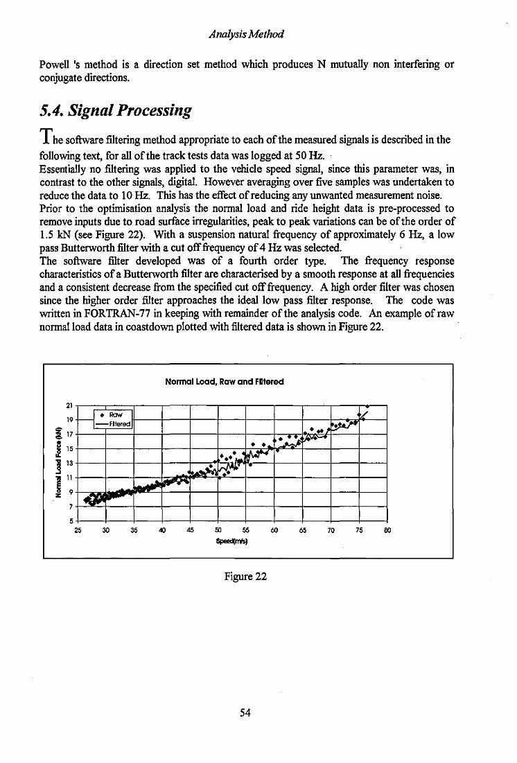
Analysis Method
Powell 's method is a direction set method which produces N mutually non interfering or conjugate directions.
5.4. Signal Processing
The software filtering method appropriate to each of the measured signals is described in the following text, for all of the track tests data was logged at 50 Hz. Essentially no filtering was applied to the vehicle speed signal, since this parameter was, in contrast to the other signals, digital. However averaging over five samples was undertaken to reduce the data to 10 Hz. This has the effect of reducing any unwanted measurement noise. Prior to the optimisation analysis the normal load and ride height data is pre-processed to remove inputs due to road surface irregularities, peak to peak variations can be of the order of 1.5 kN (see Figure 22). With a suspension natural frequency of approximately 6 Hz, a low pass Butterworth filter with a cut off frequency of 4 Hz was selected. The software filter developed was of a fourth order type. The frequency response characteristics of a Butterworth filter are characterised by a smooth response at all frequencies and a consistent decrease from the specified cut off frequency. A high order filter was chosen since the higher order filter approaches the ideal low pass filter response. The code was written in FORTRAN-77 in keeping with remainder of the analysis code. An example of raw normal load data in coastdown plotted with filtered data is shown in Figure 22.
21
19
~ 17
j 15
~ 13
111 z 9
7
5
H.- Row -FIltered
25 30 35
Normal Load, Raw and FIltered
•
40 45
- --.... -,..- ,-~<:.t.. rf!'-' •
50 55
Speed(m's)
Figure 22
54
-..;.J
60 65
~/. -.. , ~
70 75 eo

Analysis Method
5.5. Racing Car Coastdown Analysis Methods
In this part of the report the two methods of minimisation are considered in terms of their performance in analysing theoretical and practical coastdown data. Upon the finalisation of the analysis method, three different variations on the method were used, the first a four term analysis yielding An. Bo, Co and Ko (or a constant drag term D). Secondly a three term analysis yielding An, Bo, Co, and finally the third method used to find Co and D (a constant drag term) or simply just Co by accounting for the tyre losses via linear interpolated tyre data (the Goodyear data) from a given speed and normal load. The basic method used from raw logged data file to analysis and finally the resultant coefficients is detailed in the flowcharts in figures 23 and 24.
5.5.1. Minimisation Method
During the initial work on the development of the analysis method, two methods of optimisation, or minimisation were considered. Nelder and Mead's method had been used up to this point but was found to be processor intensive and therefore slow running on a P.C. Therefore a direction set method was required that would be less processor intensive and therefore quicker. Therefore in the development of the method the two different types of methods were applied to theoretical data. Initial verification of the method was undertaken by analysing coastdown data that was produced from the Matrixx simulation code (see Appendix II). Both optimisation methods were thus used to analyse the simulation generated speed time data. Both optimisation methods were successful when analysing theoretically generated coastdown data, the Powell method proving to be extremely quick. Additionally it required less initial information by way of start points. The method of Nelder and Mead requires a starting Simplex of N+ 1 sets of start points (N = number of undeterminates), Powell however only needed one start point and a direction. Existing actual coastdown data from normal road car tests that produced good results from using the method of Nelder and Mead was analysed using the Powell method in order to evaluate the performance of the method when analysing actual coastdown data. Unfortunately the Powell method did not yield exactly the same results as the Nelder and Mead method, in fact impossible values of the drag coefficients were converged to (Negative values of An). More work was needed to fully evaluate the method's potential, however only a finite amount of time was available for such purposes, so it was decided that the method of Nelder and Mead be used, the major reason being its dependability and that it was tried and trusted. This does not rule out the possibility of continued development of the Powell's method or indeed any other direction set method.
55

Analysis Method
- , " 7 11
! 1\ './ ~ /I " \,I. \ :j I I / \ I
70 .. . \: , I I ... I . ,) "'J V \ I
, -- I'" V - -20
" o _ _ ~ m m m ~ _ _
-~

Analysis Method cont ...
t
Contains:Test File Names Ambient Conditions Vehicle Set up Analysis n"""m, .. t""r", I
~_" ... _._~~ .. +_ ..... _ ...... + __ .............. + ... _ ........ _ .... l., , Ad Bd Cd Kd1 , ,
~
0.01' 9.2 0.02 9.0 0.025 9.5 0.02 9
0.8 4.0 j 0.9 5.0
·0.85 5.5 0.8 3.0
"\
'" I'--. " i'---........ r-
• •
Minimise COST function
Ad=,., Bd= ... Cd=,., Kd= ...
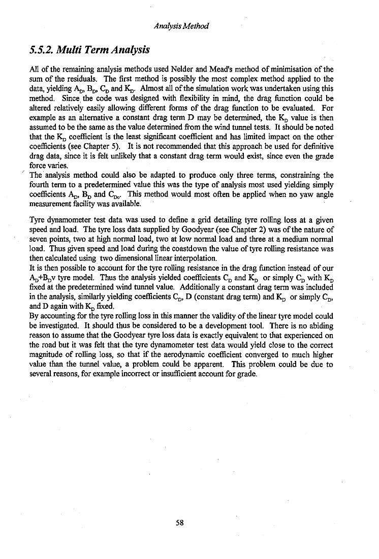
Analysis Method
5.5.2. Multi Term Analysis
All of the remaining analysis methods used Nelder and Mead's method of minimisation of the sum of the residuals. The first method is possibly the most complex method applied to the data, yielding An, BD, CD and Ko. Almost all of the simulation work was undertaken using this method. Since, the code was designed with flexibility in mind, the drag function could be altered relatively easily allowing different forms of the drag function to be evaluated. For example as an alternative a constant drag term D may be determined, the Ko value is then assumed to be the same as the value determined from the wind tunnel tests. It should be noted that the Ko coefficient is the least significant coefficient and has limited impact on the other coefficients (see Chapter 5). It is not recommended that this approach be used for definitive drag data, since it is felt unlikely that a constant drag term would exist, since even the grade force varies.
F The analysis method could also be adapted to produce only three terms, constraining the fourth term to a predetermined value this was the type of analysis most used yielding simply coefficients An, BD and COo' This method would most often be applied when no yaw angle measurement facility was available.
Tyre dynamometer test data was used to define a grid detailing tyre rolling loss at a given speed and load. The tyre loss data supplied by Goodyear (see Chapter 2) was of the nature of seven points, two at high normal load, two at low normal load and three at a medium normal load. Thus given speed and load during the coastdown the value of tyre rolling resistance was then calculated using two dimensional linear interpolation. It is then possible to account for the tyre rolling resistance in the drag function instead of our AD +Bo v tyre model. Thus the analysis yielded coefficients CD and Ko or simply Co with Ko fixed at the predetermined wind tunnel value. Additionally a constant drag term was included in the analysis, similarly yielding coefficients Co, D (constant drag term) and Ko or simply Co, and D again with Ko fixed. By accounting for the tyre rolling loss in this manner the validity of the linear tyre model could be investigated. It should thus be considered to be a development tool. There is no abiding reason to assume that the Goodyear tyre loss data is exactly equivalent to that experienced on the road but it was felt that the tyre dynamometer test data would yield close to the correct magnitude of rolling loss, so that if the aerodynamic coefficient converged to much higher value than the tunnel value, a problem could be apparent. This problem could be due to several reasons, for example incorrect or insufficient account for grade.
58

Analysis Method
5.6. Coefficient Sensitivities
In order to ascertain the sensitivity of a given coefficient, simulation tests were undertaken to determine the change in overall RMS. error associated with a 1 % change in the value of the particular coefficient. The process adhered to was to run a simulated coastdown, with known coefficients, one of which is changed by 1 % from the reference, and then comparing the velocity time profile with the unperturbed profile, producing an RMS. error in rn/s between reference and perturbed curves. The effect that this change has in RMS. terms dictates how easily the coefficient will be found via optimisation. When a sensitive coefficient is perturbed by a small amount a large change in RMS.error results. It is therefore easily determined during optimisation.
Tests were conducted with several steady state wind conditions, other than zero wind and the results showed that there was very little variation in the sensitivity of the coefficient with changing wind conditions. It can be concluded from this that coefficient sensitivity is independent of wind conditions. The results for the zero wind condition are detailed below.
Zero wind condition
Coefficient RMS. Error Normalised Coefficient Sensitivity (rn/s)
Ao 0.02 0.09
Bo 0.01 0.03
Co 0.17 1
Table 8
The fourth drag coefficient Ko modifies Co for aerodynamic yaw angle, therefore when there is zero wind Ko has no effect. Therefore the sensitivity of Ko is highly dependent on the value of the crosswind input.
Sensitivity of Ko
Cross Wind (rn/s) RMS.Error Normalised Coefficient Sensitivity (rn/s) (wrt Co)
0 0 -1 0.0003 0.0018
2 0.0013 0.0078
3 0.0027 0.0161
4 0.005 0.03
Table 9
59

Analysis Method
The results in table 8 show that KD is the least sensitive coefficient and therefore most difficult to ascertain for crosswinds of magnitude up to 4 m/s. For no wind input the results show quite clearly that BD is the least sensitive coefficient being thirty times less sensitive than the most sensitive coefficient, Co. AD is roughly three times more sensitive than BD' and is over 10 times less sensitive than CD' This underlines the dominant nature of the aerodynamic drag, compared with other forms of drag, for this vehicle. The implications of this are that the value of Co should be the easiest to determine in the analysis, followed by An and BD' The magnitude of the difference between each coefficients sensitivity and especially the magnitudes in comparison to Co are very high in comparison to the road car case", close to two and a half times greater. This is as expected due to the very high nature of the proportion of the drag attributed to aerodynamic drag. It can therefore be concluded that in practical coastdown testing the highest level of confidence will be achieved for CD followed by An, BD and lastly KD.
It should also be noted that a 1% error in An will produce a corresponding 0.1% error in CD' similarly a 1 % error in BD will yield a 0.03% error in Co.
Sensitivity to Ambient Wind
Following on from the pure coefficient sensitivity analysis, the following part of the work investigates the variation in RMS. error for different cases of head and cross wind. The effect of wind on RMS. error is represented in figure 25.
4
3.5
i 2.: -0 2 t:
" Cl) 1.5
i!! 1
0.5
0 0 0.5
___ HeodWlrd
___ Qos s Wlrd
1.5 2 2.5 3 3.5 4 4.5 5
Wind Speed (m/I)
Figure 25
It is thus concluded from the results that head wind causes the greatest RMS. error for a given magnitude of wind component when compared to crosswind. The headwind plot is notably, a straight line, in contrast to the curvature exhibited by the crosswind curve. The reason for this is due to the way in which CD is modified with aerodynamic yaw, i.e. it is approximately parabolic.
60

Analysis Method
5.7. Drivetrain And Undriven Wheel Coastdown Analysis
In contrast to the analysis methods discussed earlier in this section the driveline components
were determined 'off-line'. This means that individual coastdowns were performed on the drivetrain and an undriven wheel, yielding a velocity time profile, which is analysed to determine the drag force over a time period t, - t J, this process is described below.
Both types of test were analysed using fundamentally the same method. This method is detailed below.
From Newton's second law the equation of motion for a decelerating wheel is described below,
M=Ix(X
(X= dO) dt
F ,..R,.dt = Irw dO)
(37)
(38)
(39)
(40)
The deceleration of the wheel is found by simply differentiating between successive data points to yield the mean drag over the time period,
(41)
An optimisation method similar to one of those described before could have been used, however the mathematical model describing the drag force for each of these coastdowns was unknown for the most part, in contrast to the full scale coastdowns.
61
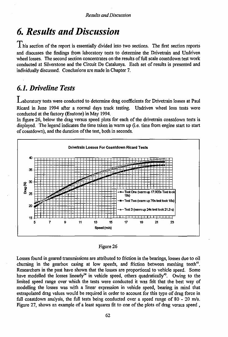
Results and Discussion
6. Results and Discussion This section of the report is essentially divided into two sections. The first section reports
and discusses the findings from laboratory tests to determine the Drivetrain and Undriven wheel losses. The second section concentrates on the results of full scale coastdown test work conducted at Silverstone and the Circuit De Catalunya. Each set of results is presented and individually discussed. Conclusions are made in Chapter 7.
6.1. Driveline Tests
Laboratory tests were conducted to determine drag coefficients for Drivetrain losses at Paul
Ricard in June 1994 after a normal days track testing. Undriven wheel loss tests were conducted at the factory (Enstone) in May 1994. In figure 26, below the drag versus speed plots for each of the drivetrain coastdown tests is displayed. The legend indicates the time taken in warm up (i.e. time from engine start to start of coastdown), and the duration of the test, both in seconds.
35
20
15 5 7 9
Drivetraln Losses For Coastdown Rlcard Tests
11 13 15
Speed (mls)
Figure 26
-+-Test One (warm up 17.905. 180)
....... Test Two (wa"" up 780 test took
.... ,. .. Test 3 (warm up 24s test took 21.3 s)
17 19 21 23
Losses found in geared transmissions are attributed to fiiction in the bearings, losses due to oil churning in the gearbox casing at low speeds, and fiiction between meshing teeth4S. Researchers in the past have shown that the losses are proportional to vehicle speed. Some have modelled the losses linearly'" in vehicle speed, others quadratically4S. Owing to the limited speed range over which the tests were conducted it was felt that the best way of modelling the losses was with a linear expression in vehicle speed, bearing in mind that extrapolated drag values would be required in order to account for this type of drag force in full coastdown analysis, the full tests being conducted over a speed range of 80 - 20 m/s. Figure 27, shows an example of a least squares fit to one of the plots of drag versus speed,
62

Results and Discussion
included on the plot is an expression describing the drivetrain drag in terms of vehicle speed, in addition to the R2 fit statistic.
40
38
38
34
~32
y= 1.0483x + 16.261 R2.0.9809
5 7 9
Drlvelr.ln Losses In Coasldown (Rlcard Tesl 1)
11 13 15 17 19 21 23
Vehicle speed (mls)
Figure 27
The coefficients determined for the drivetrain losses A, and B, are represented in the table 10,
Test Number A, B, 1 16.26 1.05
2 7.71 1.55
3 15.92 1.09
Average Values 13.3 1.23
Table 10
Linear and quadratic least square fits were made to the data, which showed that quite different calculated values would be found at higher speeds. Indeed the nature of the quadratic terms were in distinct contrast to those found for a normal road car. Linearly fitting to the data yielded similar coefficients for tests one and three. However for the second test the constant term was considerably (-50%) smaller. The term in vehicle speed was thus appreciably higher. Scrutiny of figure 26 shows that the drag versus speed plot for tests two and three are quite close (within 0.5 N) from a speed of 13 rn/s onwards, however at the lower speeds test two has a much lower drag (by as much as 5 N). Test two had the greatest amount of warm up time prior to testing and this is felt to be the reason why the curves are appreciably different, at the lower speeds test three, which had a longer warm up period than test one, is closer to test two. This may indicate that the drag is heavily related to the oil temperature at lower vehicle speeds, this was not monitored during the test. As the speed increases the differences are smaller showing that other drag mechanisms become more dominant, such as losses in the bearings. This is felt to be the reason why the curve described by tests one and two are more closely aligned from 13 rn/s onwards.
63
\

Results and Discussion
A simulation test (see Appendix 11) was run with known coefficients including the drivetrain loss modelled linearly with vehicle speed. This was analysed with and without drivetrain losses included. It was found that the converged aerodynamic drag coefficients were only slightly different (CD less than 0.25%, Ko 4%). The tyre loss coefficients were found to be most in error, AD being 33% in error, BD 17.5 % in error. Thus it can be seen that failure to account for the drivetrain drag appropriately can cause appreciable errors in the tyre loss coefficients. In comparison to the road car case46 Formula One car drivetrain losses are around two and a half times greater, this is due to the smaller bearing clearances, greater number of gears and high viscosity oil used.
6.2 Undriven Wheel
U ndriven wheel coastdown tests were undertaken for six hub operating temperatures, 23,50,75,100,107 and 110°C, reflecting the normal range of operating temperatures for the assembly. A plot of drag vs. vehicle speed for one of the tests is represented in figure 28, with linear and quadratic fits overlaid.
14
12
,.
!: a
• • 0 • 4
,
• • , . "
Undriven Wheel Coastdown
,. 25 30 35
Speed (m/e)
Figure 28
• Drag from data
-QuadratIC Model
- Uneor (Drag from data)
55
The quadratic fit offers the better solution, however it must be borne in mind that a higher· order fit offers the greatest scope for potential error, outside the vehicle speed range described by these tests. The evidence however pointed to a higher order term, so a quadratic in vehicle speed was deemed to be the best compromise, simulation data was used to assess the effect on the converged values of the drag coefficients.
64

Results and Discussion
Simulation tests were conducted in Matrix. with known vehicle drag coefficients, with the undriven wheel losses read in as actual drag data, in the analysis these were then modelled by a linear function in vehicle speed or a quadratic function, also in vehicle speed. The coastdown velocity time traces were then analysed to produce converged coefficients in Ao, BD., Co and Ko. In this way the effect of the choice of either model compared to the actual drag data on the converged drag coefficients could be determined, the results are displayed in table 11,
Model Effect on Converged Drag Coefficients c.f. actual drag
Ao BD Co Ko
Linear -2.2% 62.03% -2.016% 2.237%
Quadratic -0.741% 1.852% -0.1344% 1.585%
Table 11
It can be seen from the table that appreciable errors are apparent in the converged values of the drag coefficients when the linear model is chosen to represent the undriven wheel losses, these are outside· tolerable bands (nominally 2% in any coefficient). The quadratic model produces the least error in the converged coefficients and is therefore felt to be the most appropriate. The results of analysis of the other coastdowns at each of the other temperatures are represented in Figure 29. The results for a single wheel, are displayed in Table 12.
Uldrfven Wheel Loss .. for DHrerentT."peratu .... Quadra1lc Mode'
" " " " " " " so " V,hle" Speed (mll)
Figure 29
65

Results and Discussion
Test Number A. B. C. 1 5.626 0.001 0.002
2 5.86 0.025 0.002
3 6.64 -0.035 0.003
4 7.48 -0.018 0.002
5 6.81 -0.038 0.003
Average 6.48 -0.013 0.002
Standard Deviation 0.75 0.026 0.00055
Table 12
The results point towards a higher order model for the drag in contrast to a linear model that is usually applied to a normal road car4S
• Undriven wheel drag is the result of several different mechanisms'3• The largest form ofIoss is attributed to brake drag, where the pads rub on the brake disc, this form of loss is linear in vehicle speed. Due to the large surface area of the pads used on Formula One cars, this form ofIoss is much higher (typically 50%) than the road car case. The other type of losses encountered in undriven wheels freely coasting down are losses in the wheel bearings and aerodynamic losses. This is where it is felt that the second order terms come into the equation. The wheel bearings used in this type of vehicle are of the angular contact type, at higher speeds churning losses of the oil in the bearing account for an appreciable amount of the drag, this would infer temperate effects having an influence. The exact nature of this type of loss is of a marginally higher order type of effect43
• Hence the quadratic term in vehicle speed. The effect of temperature is notable. At ambient temperature the drag throughout the speed range is appreciably greater (2-3 N) than for the higher temperatures. Above ambient temperature the drag reduces as would be expected. It is apparent that a temperature range exists where the drag force changes only fractions of Newton's with temperature. Notably at 50°C the lowest drag over the speed range is noted, increasing the temperature increases the drag. However this is only by small amounts, indeed the 'working band' describes a maximum change in drag of one Newton. This suggests that there is a working band over which the undriven wheels operate at minimal loss. It should be noted at this point that no normal load was applied to the bearing to reflect the usual operating mode. This could mean that the coefficients are underestimates.
66

Results and Discussion
6.2 Full Coastdown Tests
Pilot coastdown tests were carried out on the Hangar straight at Silverstone. During these
tests the installation of onboard anemometry was impossible, therefore wind direction and speed were monitored throughout the coastdown on a site near the track side. The aim of these tests was to assess the potential of the method and the inherent problems inevitably encountered with real world testing. Therefore in terms of normal coastdown testing these tests were conducted in less than ideal conditions, the results are included for completeness. The main tests were subsequently conducted on the main straight at the Circuit De Catalunya. Records of the vehicle set-up for both of these sets of tests are located in Appendix I, internal codes are used to describe aerodynamic set-up.
6.2.1. Silverstone Tests
In all, five tests were conducted, at two separate test sessions, however one of these was undertaken in the rain. During the first test the car was in pre Hungarian G.P. configuration, this was a high downforcelhigh drag set-up. The second test was in pre Belgian G.P. configuration a lower downforceldrag set-up. It must be mentioned that none of the tests was conducted with the vehicle in exactly the same configuration. The results are presented in a tabulated form.
Pre Hungarian GP test .. Test AD BD CD KD Error Drag@ Comments No. (m/s) 150 mpb
1 0.030 0.893E-07 0.990 4.980 0.100 4356.19 Test had to be conducted with clutch engaged, gearbox in 5th
2§ 0.020 0.70lE-07 0.990 5.231 0.120 4287.410 Test Window 72-39 rn/s § Truncated test due to car being passed during coastdown
Table 12
For the unconstrained analysis the results (tables 12 and 13) show a high value of An compared to Goodyear rig test data (An=0.012), notably very high for the pre Spa tests. The values of BD are, for three of the tests, reasonable compared to the rig test data (Bo=ge-5). For both tests one and two, Co was lower than the wind tunnel value by 6.8%.
67
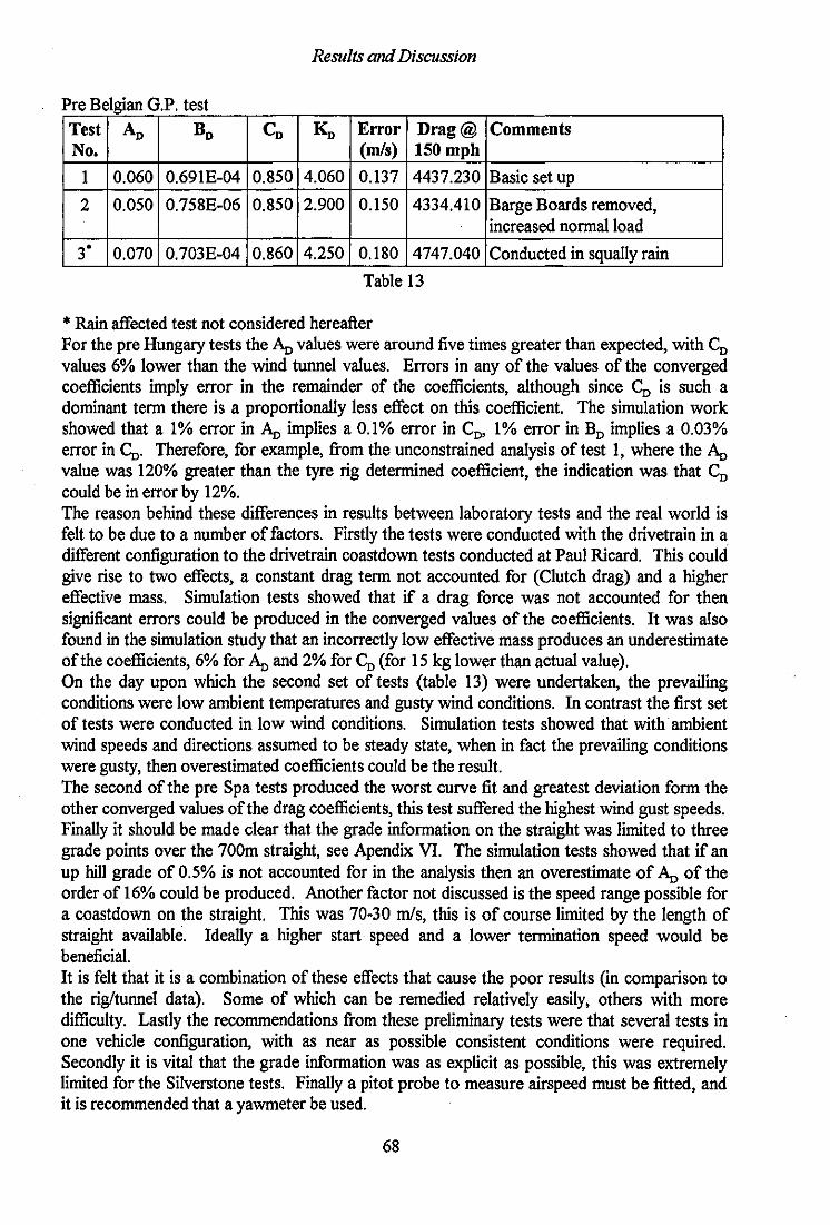
Results and Discussion
Pre Belgian GP test .. Test AD BD Co Ko Error Drag@ Comments No. (m/s) 150mph
1 0.060 0.691E-04 0.850 4.060 0.137 4437.230 Basic set up
2 0.050 0.758E-06 0.850 2.900 0.150 4334.410 Barge Boards removed, increased normal load
3' 0.070 0.703E-04 0.860 4.250 0.180 4747.040 Conducted in squally rain
Table 13
* Rain affected test not considered hereafter For the pre Hungary tests the An values were around five times greater than expected, with Co values 6% lower than the wind tunnel values. Errors in any of the values of the converged coefficients imply error in the remainder of the coefficients, although since Co is such a dominant term there is a proportionally less effect on this coefficient. The simulation work showed that a 1% error in An implies a 0.1% error in Co, 1% error in BD implies a 0.03% error in Co. Therefore, for example, from the unconstrained analysis oftest 1, where the An value was 120% greater than the tyre rig determined coefficient, the indication was that Co could be in error by 12%. The reason behind these differences in results between laboratory tests and the real world is felt to be due to a number of factors. Firstly the tests were conducted with the drivetrain in a different configuration to the drivetrain coastdown tests conducted at Paul Ricard. This could give rise to two effects, a constant drag term not accounted for (Clutch drag) and a higher effective mass. Simulation tests showed that if a drag force was not accounted for then significant errors could be produced in the converged values of the coefficients. It was also found in the simulation study that an incorrectly low effective mass produces an underestimate of the coefficients, 6% for An and 2% for CD (for 15 kg lower than actual value). On the day upon which the second set of tests (table 13) were undertaken, the prevailing conditions were low ambient temperatures and gusty wind conditions. In contrast the first set of tests were conducted in low wind conditions. Simulation tests showed that with ambient wind speeds and directions assumed to be steady state, when in fact the prevailing conditions were gusty, then overestimated coefficients could be the result. The second of the pre Spa tests produced the worst curve fit and greatest deviation form the other converged values of the drag coefficients, this test suffered the highest wind gust speeds. Finally it should be made clear that the grade information on the straight was limited to three grade points over the 700m straight, see Apendix VI. The simulation tests showed that if an up hill grade of 0.5% is not accounted for in the analysis then an overestimate of An of the order of 16% could be produced. Another factor not discussed is the speed range possible for a coastdown on the straight. This was 70-30 m/s, this is of course limited by the length of straight available. Ideally a higher start speed and a lower termination speed would be beneficial. It is felt that it is a combination of these effects that cause the poor results (in comparison to the rig/tunnel data). Some of which can be remedied relatively easily, others with more difficulty. Lastly the recommendations from these preliminary tests were that several tests in one vehicle configuration, with as near as possible consistent conditions were required. Secondly it is vital that the grade information was as explicit as possible, this was extremely limited for the Silverstone tests. Finally a pitot probe to measure airspeed must be fitted, and it is recommended that a yawmeter be used.
68

Results and Discussion
6.3.2. Circuit De Catalunya Tests
During the main coastdown tests the car was set up in exactly the same aerodynamic configuration for each test. This was felt to be important at this stage of the development of the method in order to establish the repeatability of the test, something not possible with the Silverstone test data and allow more meaningful comparisons to be made, test to test. Five test runs were made in total, the results of which are reported here.
Two analysis methods were used. The first determines Ao, Bo and Co the second simply Co, since the tyre losses are determined from linearly interpolated tyre dynamometer test data. For this test a pitot probe to measure airspeed was mounted on the vehicle and the track grade determined at 20m intervals. An example set of data is shown plotted in Figure 30, the five speed time histories for the tests are presented in Figure 31, and the residuals (errors) are displayed in Figure 32.
Example set of coastdown data 00
"" ~ ............ I: V.h~" Speed r -'-wIld ......... -Normollood
70
~ f'.-.......----- ----"'- --
o I I
·10 Tlmele)
Figure 30
The results found from Coastdown tests performed at Barcelona were encouraging, with the converged values of the drag coefficients produced matching the rig and wind tunnel test values, for the most part, very well in contrast to the Silverstone test results. The results found for one of the tests was distinctly different to the other four, this is discussed initially. The remainder of the discussion concentrates on the other more significant results. Turning initially to the plots, it can be seen from figure 31 that one of the curves (test 3) lies, for the most part, offset lower from the remainder. This is not with standing the similar start speed to the other coastdowns. Indeed the initial part of the coastdown (first 2 seconds) appears very much like a straight line on the plot, the test also terminates very much earlier than the other tests.
69
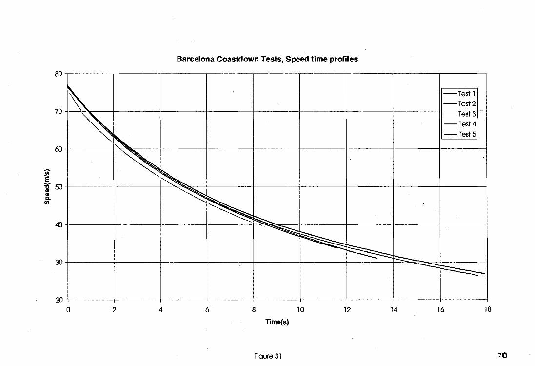
Barcelona Coastdown Tests, Speed time profiles
80
~ -Test 1 -Test 2
"\~ Test 3 r-
-Test 4 -Test 5
~ ~
70
60
~ ~ ~
>~ 40
-......;:-30
--20
o 2 4 6 8 10 12 14 16 18
Time(s)
Figure 31 70
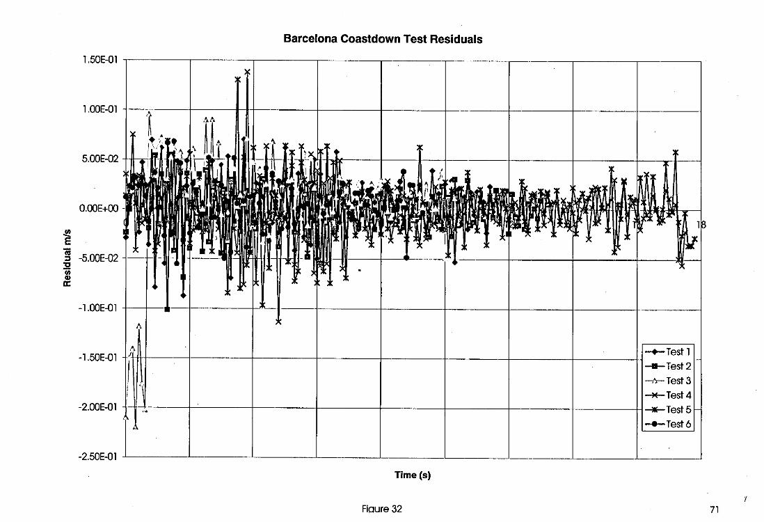
.!!.! E ftj :;, "0 u; .. a:
Barcelona Coastdown Test Residuals
1.50E-0l '---~'---'------'-----'------'-------r-'- .... -----,--.--.-----,,------,-----,
1.OOE-0l 4----;c---+-----I+I----+-----+----~-f_--·---_+_----__+----f_----_4
5.00E-02 -HI-r-fr-J
O.OOE+OO
-5.00E-02
-1.00E-0l
-1.50E-0l +~-\ttt-----+·----I----+_---_+-----t_---+_---_t----+i __ Test 1
--Test 2 ~'I-- Test 3 __ Test 4
-2.00E-0l -Hi-+.---t-'----+_----i-----i-----f_----+-----4-----t-l_llE_ Test 5
--Test 6
-2.50E-0l -'------L--------' ____ --'-___ --L_. ___ .L-______ L ___ . ___ -'-____ -'--___ ---'
Time (s)
Fiaure 32 71

Results and Discussion
Referring to figure 32, the residuals for tests 1,2 and tests 4,5 are largely distributed within ± 0.03 m/s indicating a very good fit of the model to the test data. The largest errors exist at the start of the tests (i.e. at high speed) and are considered to be largely due to track surface irregularities. The data also shows that test three is indeed exhibiting some very high errors from the theoretical values in the early part of the coastdown, further to this it appears to be generally producing higher errors from the theoretical. Inspection of the magnitude of the headwind or average ambient wind speed does not give any particular clues as to why this may be.
Test No, AD BD CD RMS. Drag@ Mean Distance Error (m!s) 150 mph Windspeed Travelled in
Coastdown
1 0.0142 8.85e-5 0.9690 0.1030 4,168.17 <0.2 m/s 587.1 m
2 0.0140 8.47e-5 0.9830 0.0710 4,217.39 1.1 m/s 641.0 m
3' 0.006 0.375e-7 1.12 0.34 4,450.17 1.0 m/s 559.9 m
4 0.0165 9.90e-5 0.966 0.145 4,220.62 1.7 m/s 750.2 m
5 0.0157 9.43e-5 1.007 0.185 4,359.67 3.32 m/s 757.8 m
Table 14
Considering the results displayed in table 14, the concerns mentioned above regarding test 3 are seen to be reflected in the results. A very high Co is apparent with the tyre terms converging to very small values. It is evident that this test did not go entirely to plan, the early part of the speed time plot indicates that the clutch may have been partially engaged due to driver error. This test is thus considered null and void and is not further considered. The remainder of the tests are fairly closely matched on the plots, tests 1 and 2 are almost direct overlays. The final two tests were both conducted over significantly longer distances, approximately 750 m. However for both these tests the magnitude of the ambient wind prevailing was significantly greater than that found for the other tests, potentially with a cross wind component. This is most notable on test 5, unaccounted for cross wind components could induce higher values of CD' with the absence of the Ko term. Again referring to Figure 32, on tests 4 and 5 there is a spike in the data around 3.5 seconds. This may be due to a sudden gust as the vehicle passed a bridge for example. Comparing the results test to test, the repeatability is good, in particular for CD which at the 95 per cent confidence level shows an error of less than two per cent. Test five yielded a slightly higher value of Co, which is felt to be due to the higher wind speed for this test, possibly including some cross wind. Since a yawmeter was not used, it was impossible to account for this in the analysis.
Coefficient Mean 95 percent Rig/Tunnel values Confidence
AD 0.0151 0.0151±0.0012 0.0117
BD 8.06e·s 8.06e-s±9.5e-O 8.85e-s
CD 0.981 0.981±0.018 0.983
Table 15
72
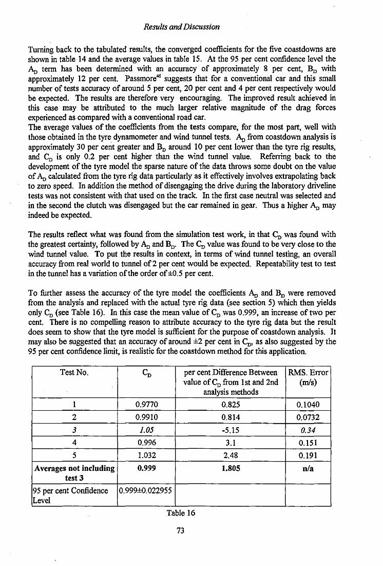
Results and Discussion
Turning back to the tabulated results, the converged coefficients for the five coastdowns are shown in table 14 and the average values in table 15. At the 95 per cent confidence level the An term has been determined with an accuracy of approximately 8 per cent, BD with approximately 12 per cent. Passmore46 suggests that for a conventional car and this small number of tests accuracy of around 5 per cent, 20 per cent and 4 per cent respectively would be expected. The results are therefore very encouraging. The improved result achieved in this case may be attributed to the much larger relative magnitude of the drag forces experienced as compared with a conventional road car. The average values of the coefficients from the tests compare, for the most part, well with those obtained in the tyre dynamometer and wind tunnel tests. An from coastdown analysis is approximately 30 per cent greater and BD around 10 per cent lower than the tyre rig results, and <;, is only 0.2 per cent higher than the wind tunnel value. Referring back to the development of the tyre model the sparse nature of the data throws some doubt on the value of An calculated from the tyre rig data particularly as it effectively involves extrapolating back to zero speed. In addition the method of disengaging the drive during the laboratory driveline tests was not consistent with that used on the track. In the first case neutral was selected and in the second the clutch was disengaged but the car remained in gear. Thus a higher An may indeed be expected.
The results reflect what was found from the simulation test work, in that <;, was found with the greatest certainty, followed by An and BD' The Co value was found to be very close to the wind tunnel value. To put the results in context, in terms of wind tunnel testing, an overall accuracy from real world to tunnel of 2 per cent would be expected. Repeatability test to test in the tunnel has a variation of the order of ±0.5 per cent.
To further assess the accuracy of the tyre model the coefficients An and BD were removed from the analysis and replaced with the actual tyre rig data (see section 5) which then yields only <;, (see Table 16). In this case the mean value of<;, was 0.999, an increase of two per cent. There is no compelling reason to attribute accuracy to the tyre rig data but the result does seem to show that the tyre model is sufficient for the purpose of coastdown analysis. It may also be suggested that an accuracy of around ±2 per cent in <;" as also suggested by the 95 per cent confidence limit, is realistic for the coastdown method for this application.
Test No. <;, per cent Difference Between RMS. Error value of CD from 1st and 2nd (m/s)
analysis methods
1 0.9770 0.825 0.1040
2 0.9910 0.814 0.0732
3 1.05 -5.15 0.34
4 0.996 3.1 0.151
5 1.032 2.48 0.191
Averages not including 0.999 1.805 nla test 3
95 per cent Confidence 0.999±0.022955 Level
Table 16
73

Results and Discussion
The results seem to be significantly better than those found from the Silverstone tests. There could be several reasons for this. Firstly the grade infonnation supplied by the Circuit De Catalunya was quite explicit. Previous data on the Silverstone Hangar straight was limited to three grades on the 675m straight. For the Barcelona straight the grade infonnation (see Appendix VI) was at 20m intervals. The additional infonnation provided also allowed the positioning of the car on the straight at the start of the Coastdown to be more accurately determined. Secondly the speed range described by the Coastdown tests at the Circuit De Catalunya (80-27 m1s) was greater than those at Silverstone (70-30 m1s). This implied that the higher order tenns were more easily determined due to the higher start speed, and that the determination of the lower order tenns was not compromised by a high termination speed. Another factor involved was that of the driver, although performing a coastdown test is not the most difficult test a Grand Prix driver has to undertake, the more familiar the driver is with the test and with the car the better the data is from the test. Undertaking several tests one after the other with the vehicle in a consistent configuration allowed the driver to become familiar with both test and vehicle, this is evidenced by the higher coastdown distances achieved for tests 4 and 5.
Another aspect that contributed to the better results was that the tests were conducted with much more stable ambient conditions than at Silverstone, where testing was hampered by rain at times. Finally ambient wind measurement on board the vehicle was carried out to some extent, with use of the airspeed pitot. This gave some idea of the fluctuation in the headwind during the coastdown.
An example plot of the theoretical speed time history and the actual is shown in figure 33, it can be seen that the plots overlay very closely, underlining the very promising nature of the results.
74

80
~ 75
70
65
60
50
45
40
35
30 o
Barcelona Coastdown Tests, Example of Plot of Theoretical vs. Actual Speed Time Profile, Test 1
~ ~ ~
~ ~
~
2 4
+--
.
~ ~
6 Time (s)
Figure 33
------- -
---
----- Actual
--------- Theoretical
-
~ ---~ r-----
------8 10
75
12

Conclusions
7. Conclusions
A mathematical model defining the dra:~ forces acting on aFormula One car in coastdown has been developed based on tunnel/rig data. A sophisticated test and analysis method has been developed and used to analyse real (i. e. on track) coastdown data. From coastdown tests performed at the Circuit De Catalunya, near Barcelona it has been possible to quantify drag coefficients that describe the drag force acting on a vehicle during a coastdown.
7.1. Mathematical Model
From tyre dynamometer tests, and wind tunnel tests it was possible to develop a comprehensive model for a Formula One car travelling in a straight line in coastdown. The aerodynamic model accounts for the effects of ambient wind and variation in the aerodynamic drag coefficient due to ride height changes in coastdown. The model includes tyre losses, as a function of vehicle speed and normal load, transmission and undriven wheel losses.
The tyre model was developed from data obtained during tyre dynamometer tests conducted at Goodyear racing Akron Ohio. The model consists of a constant plus a linear function of vehicle speed. The limited data available appeared to confirm this.
The aerodynamic model included the effects of changes in vehicle ride height in coastdown by varying a constant added to the aerodynamic drag coefficient with change in ride height. The form of this variation was determined from wind tunnel data. Ambient wind is accounted for by a term in aerodynamic yaw angle squared, multiplied by a constant determined from wind tunnel tests, or determined from coastdown tests with sufficient anemometry.
Drivetrain 'off line' tests were conducted in the laboratory to determine representative model for these facets of the vehicle drag force. Drivetrain losses were accounted for with a constant plus a linear term in vehicle speed. Undriven wheel losses were accounted for by a quadratic in vehicle speed. /'
76

Conclusions
7.2. Driveline Tests
7.2.1. Drivetrain Tests
• Drivetrain drag is not insignificant and the omission of the term can produce appreciable errors in the converged drag coefficients derived from coastdown testing.
• The values for the drivetrain loss coefficients for the vehicle were found to be,
A, = 13.3 (N) B, = 1.23 (Nm·ls)
• Unforeseen circumstances meant that it was not possible for the driver to select neutral during the track test, therefore the laboratory test conditions did not match the track test conditions.
7.2.2 .. Undriven Wheel Tests
• The values for the undriven wheel loss coefficients for the vehicle were found to be,
• There is an operating band of temperature over which the drag is at minimum, described by the 50 - 11 ooe temperature region.
• Undriven wheel drag is an appreciable effect and the omission of the term can cause appreciable errors in the converged values of the overall vehicle drag coefficients from coastdown analysis.
77

Conclusions
7.3. Full Coastdown Tests
• The SiIverstone tests showed that tests without sufficient instrumentation (i.e. airspeed and yaw probes) and explicit grade information caused the A" term tyre coefficient to be very high, more than twice tyre dynamometer rig test values. This additionally had effects on the other drag coefficients.
• For the car in the Pre European G.P. test set-up the values of the drag coefficients determined from uni directional coastdown testing are as follows,
95% Confidence =
=
=
0.0151 ± 0.0012 8.06e-5± 9.5e-6 0.981 ± O.oI8
(7.9%) (11.7%) (1.8%)
• The results show a good agreement with the theoretical coefficients determined from rig and tunnel testing, although AD is higher than expected.
• Accurate grade information is essential.
• If still wind conditions prevail (windspeed < Im1s) a pitot measuring airspeed must be considered the minimum in terms of ambient wind measurement instrumentation.
• A plot of the drag components acting on the vehicle during coastdown is shown in figure 34.
Vehicle drag components In eoastdown
7!XXl
~ ~ V
~Tyre Drag ./ ....... DrtvelIne lO$S8$
~ Y ~Aeroctvnomlc Drag ""*-Totol Drag
~ ~ V
" ~ y r
~
lOCO ....-o
25 35 45 ., 65 IIJ 70 7S '" SpHd~fs)
Figure 34
78
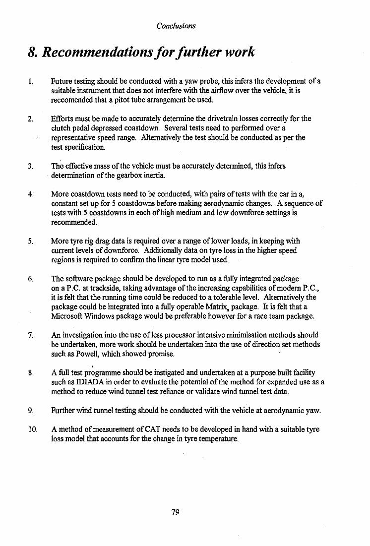
Conclusions
8. Recommendations for further work
1. Future testing should be conducted with a yaw probe, this infers the development of a suitable instrument that does not interfere with the airflow over the vehicle, it is reccomended that a pitot tube arrangement be used.
2. Efforts must be made to accurately determine the drivetrain losses correctly for the clutch pedal depressed coastdown. Several tests need to performed over a representative speed range. Alternatively the test should be conducted as per the test specification.
3. The effective mass ofthe vehicle must be accurately determined, this infers determination of the gearbox inertia.
4. More coastdown tests need to be conducted, with pairs of tests with the car in a, constant set up for 5 coastdowns before making aerodynamic changes. A sequence of tests with 5 coastdowns in each of high medium and low downforce settings is recommended.
5. More tyre rig drag data is required over a range oflower loads, in keeping with current levels of downforce. Additionally data on tyre loss in the higher speed regions is required to confirm the linear tyre model used.
6. The software package should be developed to run as a fully integrated package on a P.C. at trackside, taking advantage of the increasing capabilities of modern P.C., it is felt that the running time could be reduced to a tolerable level. Alternatively the package could be integrated into a fully operable Matrix,. package. It is felt that a Microsoft Windows package would be preferable however for a race team package.
7. An investigation into the use ofless processor intensive minimisation methods should be undertaken, more work should be undertaken into the use of direction set methods such as Powell, which showed promise .
. , 8. A full test programme should be instigated and undertaken at a purpose built facility
such as IDIADA in order to evaluate the potential of the method for expanded use as a method to reduce wind tunnel test reliance or validate wind tunnel test data.
9. Further wind tunnel testing should be conducted with the vehicle at aerodynamic yaw.
10. A method of measurement of CAT needs to be developed in hand with a suitable tyre loss model that accounts for the change in tyre temperature.
79

References
9. References
1. Bearman P.W., Mullarkey S.P. Aerodynamic forces on road vehicles due to steady side winds and gusts. RAeS Vehicle Aerodynamics conference, Loughborough University of Technology 1994.
2. Buckley F.T., Marks C.H., Walston W.H. Test procedures for the evaluation of aerodynamic drag on full scale vehicles in windy environments. Society of Automotive Engineers technical paper, SAE 760106(1976).
3. Buckley F.T., Marks C.H., Walston W.H. Analysis of coast down data to access aerodynamic drag reduction on full scale tractor-trailer trucks in a windy environment. Society of Automotive Engineers technical paper, SAE 760850(1976).
4. Carr G.W. A comparison of the ground plane suction and moving ground representation techniques. Society of Automotive Engineers technical paper, SAE 880249(1988).
5. Clark S.K. (ed), Mechanics of pneumatic tires. US Department of Transportation. National Highway Traffic Safety Administration. DOT HS 905 952 Aug. 1981.
6. Cogotti A. Aerodynamic characteristics of car wheels. International Journal of Vehicle Design. Technological advances in vehicle design series SP3, Impact of aerodynamics on vehicle design, pp 173-196. (1983).
7. Cooper RT. Aerodynamic atmospheric turbulence with respect to moving ground vehicles. Journal of wind engineering and industrial aerodynamics, Vo!. 17 p215-238 1984.
8. Cooper K.R The wind tunnel simulation of surface vehicles. Journal of wind engineering and industrial aerodynamics, Vo!. 171984.
9. Dayman B.(Jr), Tire rolling resistance measurements from coastdown tests. Society of Automotive Engineers technical paper, SAE 780258 (1978).
10. Dayman B.(Jr), Realistic effects of winds on the aerodynamic resistance of automobiles. Society of Automotive Engineers technical paper, SAE 780337(1978).
11. Dominy Dr. RG. Wind Tunnel testing techniques for high performance racing cars. RAeS Vehicle Aerodynamics conference, Loughborough University of Technology 1994.
80
References
12. Dominy, RG. Formula One racing car aerodynamics a teclmical review. Proceedings of the Institute of Mechanical Engineers, vol. 204. (1990).
13. Dominy, J.A., Dominy, RG. Aerodynamic influences on the performance of the Grand Prix racing cars. Proceedings of the Institute of Mechanical Engineers, vol. 198 D. (1984).
14. Dominy, RG. The influence of slip streaming on the performance ofa grand prix racing car. Proceedings of the Institute of Mechanical Engineers, vol. 204. (1990).
15. Dryden H.L., Schubauer G.B., Mock W.C. and Skramstad H.K. Measurements of intensity and scale of wind tunnel turbulence and their relationship to the critical number of spheres. NACAreportNo. 581, 1936
16. Emtage A.L. The vehicle coastdown test. MPhil thesis, Loughborough University of Technology, Department of Transport Technology, 1983.
17. ESDU. Characteristics of wind speed in lower layers of the atmosphere near the ground: Strong winds (Neutral atmosphere) 72026
18. ESDU. Characteristics of atmospheric turbulence near the ground. Part 1 74030; part 2 74031; Part 375001.
19. ESDU. Characteristics of atmospheric turbulence near the ground. part 2. 85020. 1985 (updates 74031).
20. ESDU. Blockage corrections for bluff bodies in confined flows. 80024
21. Goodyear Tyres racing Department. Private Facsimile J. Taube. 1994
22. Hilhorst R Giachi M. An experimental study on drag evaluation referred to the geometry of Formula One racing car tires. RAeS Vehicle Aerodynamics conference, Loughborough University of Technology 1994.
23. IDIADA (Institute for Applied Automotive research) Details of Spanish test site.
24. Ivens J., Lawser J.J. Experimental test track methods of estimating vehicle tractive resistance. FISITA paper 845105 Vienna 1984.
81
References
25. Jansen N.L., Hall G.L. Effect of ambient temperature on radial tyre rolling resistance. Society of Automotive Engineers technical paper, SAE 800090.(1980).
26. Katz 1. Calculation of the aerodynamic forces on automotive lifting surfaces. Journal of Fluids Engineering, vol. 107 number 4. (1985)
27. Katz J. Aerodynamic model for wing generated down force on open wheel racing car configurations. Society of Automotive Engineers technical paper, SAE 860218 (1986).
28. Katz J., Largman R., Effect of90 degree flap on the aerodynamics of a two element airfoil. Journal of fluids engineering March 1989 vol.lll/93
29. Katz J. Investigation of negative lifting surfaces attached to an open wheel configured racing car. Society of Automotive Engineers technical paper, SAE 850283 (1985).
30. Katz 1., Dykstra L. Effect ofwing/body interaction on the aerodynamics of two generic racing cars. Society of Automotive Engineers technical paper, SAE 920349(1992)
31. Knowles K, Donoghue D. T, Finnis M. V. A study of wings in ground effect. RAeS Vehicle Aerodynamics conference, Loughborough University of Technology 1994.
32. Kreyszig E. Advanced Engineering Mathematics. WHey science publishers.
33. Lippmann S.A., Oblizajek KL., Metters J.1. Sources of rolling resistance in radial ply tyres. Society of Automotive Engineers technical paper, SAE 70258 (1978).
34. L10yd S.E. Development of a flat tyre rolling resistance facility. Society of Automotive Engineers technical paper, SAE 780635(1978)
35. Lucas G.G., Britton 1.D. Drag data from deceleration tests and speed measurements during vehicle testing. Paper 2 in advances in road vehicle aerodynamics. BHRA, Fluid engineering, 1973.
36. Macabee F.G. Ground vehicle aerodynamics. Course notes. Loughborough University of Technology, Department of Transport Technology, 1988.
37. Macabee F.G. Basic fluid mechanics. Course notes. Loughborough University of Technology, Department of Transport Technology, 1988.
82

References
38. Massey K. Private communication with S.P. Tyres u.K. (23.03.93)
39. Mclean D. Gust alleviation study for aircraft. Transport Technology internal publication TT760617 1976.
40. McNay G., Southwick L. An approximate lap time minimisation based on Indy style racing car geometry. Society of Automotive Engineers technical paper, SAE 910011(1991)
41. Metz L.D. Emergency braking dynamics of ground effects open-wheeled racing cars. Society of Automotive Engineers technical paper, SAE 910012 (1991).
42. Metz L.D. Aerodynamic properties ofIndy cars. SAE 870726 (1987).
43. Newcombe Dr P. Private Conversation. June 1994.
44. Passmore M.A., Jenkins E.G. Measuring vehicle drag forces using an on board microcomputer. Proceedings of the Institute of Mechanical Engineers, vol. 204 part D pp 77-82. (1990).
45. Passmore M.A The measurement and analysis of road vehicle drag forces. PhD thesis, Loughborough University of Technology, 1990.
46. Passmore M.A., Le Good G.M. A detailed drag study using the coastdown method. SAE 940420 (1994).
47. Passmore M.A, Jenkins E.G. A comparison of the coastdown and steady state torque methods for estimating vehicle drag forces.
48. Remenda B.AP., Krause AE., Hertz P.B. Vehicle coastdown resistance analysis under windy and grade variable conditions. Society of Automotive Engineers technical paper, SAE 890371 (1989).
49. Rubbert P.E., Saaris G.R. A general 3-D potential flow method applied to v/STOL aerodynamics. Society of Automotive Engineers technical paper, SAE 680304. (1968).
83

References
50. SAE recommended practice. Road load measurement and dynamometer simulation using coastdown techniques. Society of Automotive Engineers technical Iournal, SAE 11263 (1984)
51. Schuring DJ., Siegfiied I.F., Hall G.L. Transient speed and temperature effects on rolling loss of passenger car tires. Society of Automotive Engineers technical paper, SAE 850463 (1985)
52. Seetharam H.C., Wentz W.H. Studies of flow separation and stalling on one and two element airfoils at low speeds. Society of Automotive Engineers technical paper, SAE 770442 (1977).
53. Silk C. Private communication with Benetton Formula 1 Racing team. (25.02.93).
54. Silk C. et al. Meeting with Benetton Formula 1 Racing team, private test Kemble Aerodrome (07.01.93).
55. Smith N.P. Wind gusts measured on high speed roads. Proc I Mech. E. Vol. 18730/73 1973.
56. Smith J.R., Tract I.C., Potter D.S. Tire rolling resistance - a speed dependent contribution. Society of Automotive Engineers technical paper, SAE 780255. (1978).
57. Stapleford W.R., Carr G.W. Aerodynamic characteristics of exposed rotating wheels. MIRA report number 1970/2 M.I.R.A (1970).
58. Symonds P.R., Toet W, Meeting at Enstone factory .. (13.01.94).
59. Symonds P.R. Private communication.
60. Toet W, Private communication. (12.07.94)
61. Toet W., Private communication. (10.10.94)
62. Toet W. Private communication.
84

References
63. Van Valkenburgh P. Race Car Engineering And Mechanics. Seal Beach, CA, 1986 ..
64. Watkins S. Wind tunnel modelling of vehicle aerodynamics: With emphasis on turbulent wind effects on commercial vehicle drag. PhD thesis Nov. 1990.
65. White RA., Korst HH. Coastdown tests: Determining Road Load Versus Drag Component Evaluation. Society of Automotive Engineers technical paper, SAE 901767 (1990).
66. White RA., Korst H.H. The determination of vehicle drag contributions from coastdown tests. Society of Automotive Engineers technical paper, SAE 720099. (1972).
67. Wildi Dr. J. Wind Tunnel testing of racing cars the importance of the road simulation technique. RAeS Vehicle Aerodynamics conference, Loughborough University of Technology 1994.
68. Wright P.G. The influence of aerodynamics on the design of Formula One racing cars. International Journal of vehicle design Vol. 3. Number 4 pp 383-397. (1982).
69. Yasin T.P. The analytical basis of automobile coastdown testing. Society of Automotive Engineers technical paper, SAE 780334 (1978).
85
10. Bibliography
a. Lucas G.G. Road Vehicle performance. Gordon and Breech science publishers. 1986.
b. Lumely J.L., Panofsky H.A., The structure of atmospheric turbulence. John Wiley and Sons, 1964.
c. Panofsky H.A. Atmospheric turbulence models and methods for engineering applications. J. Wiley and sons, New York, 1984.
d. Press W.H., Flannery B.P., Teukolsky S.A., Vettering W.T. Numerical Recipes. Cambridge University Press.
e. Neale MJ. Tribology Handbook. Butterworths 1973.
f. Homer J. High Performance Wheel And Tire Handbook. Motor books lnt.1988.
86
Appendices
Appendix I Coastdown Test Data Logging sheets. Silverstone and Barcelona tests.
Appendix IT Matrix. simulation
Appendix ill Wheel Inertia tests/calculations
Appendix IV Initial project proposal submitted to Benetton Formula One Racing Team in January 1994, outlines objectives and requirements.
Appendix V Optimisation method flow chart
Appendix VI Track Survey Circuit De Catalunya
87

Appendices
Appendix I
Vehicle data that is necessary for coastdown analysis is documented on the following sheets, this was collected during the course of general testing at the circuit. Internal codes are used to describe aerodynamic setups. Two sheets are shown, one for Silverstone and one for the Circuit De Catalunya tests.
88
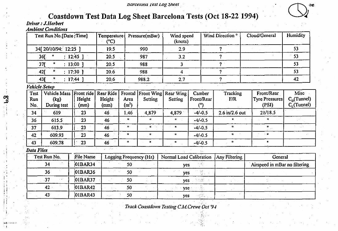
LJareelOna rest Log :Sheet
Coastdown Test Data Log Sheet Barcelona Tests (Qct 18-22 1994)
i ,
Driver: J.JIerbert Ambient Conditiolls
T/lst Run No.[Date ~Time]
34[20110/94: 12:25 ]
36[ 11 12:45 ] . 37[ 11 13:00 ] . 42( 11 17:30 ]
43( 11 17:44 ]
Vehicle Setup Test Vehicle Mass Front ride Run (kg) 1 Height No. During test i (mm)
34 619 11 23
36 615.5 I 23
37 613.9 1 23
42 609.93 1 23
43 609.78 I· 23
· : . Data Files
, • I
! ; · , : i I. , . · , i; ! I
I
~'l'''''''' · !
.
Test Run No. jFileName
34 iOIBAR34
36 iOIBAR36
37 iOIBAR37
42 !OIBAR42
43 iOIBAR43
Temperature Pressure(mBar) Wind speed Wind Dire.ction ° Cloud/General Humidity (OC) (knots)
19.5 990 2.9 ? 53
20.5 987 3.2 ? 53
20.5 988 3 ? 53
20.6 988 4 ? 53
20.6 988.2 2.7 ? . 42
Rear Ride Frontal Front Wing Rear Wing Camber Tracking FrontlRear Misc Height Area Setting Setting FrontlRear FIR Tyre Pressures Co(Tunnel) (mm) (ml) (0) (PSI) C,.(Tunnel)
46 1.46 4,879 4,879 -4/~0.5 2.6 inl2.6 out 21118.5
46 11 " 11 -4/-0.5 11 11
46 11 " " -4/-0.5 11 " 46 " " " -4/-0.5 "
. 11
46 " " " -4/-0.5 " "
Logging Frequency (Hz) Normal Load Calibration Any Filtering General
50 yes . Airspeed in mBar no filtering
50 yes ·.CC ., . 50 yes . ":
50 yse
50 yes
Traek Coastdown Testing C.M Crewe ·(Jet '9-/

J:)
9 , I , I
',' I I
; I : I I, • I
;:)IIl'I!rSIOIII! il!l'/ Log ;:Sllee/
Coastdown Test Data Log Sheet Silverstone Tests (Aug 1994) Driver: M.ScllUmacher Ambient COllditions
Tes~ Run No.[Date tme1 Temperature Pressure(mBar) Wind speed Wind Direction 0 Cloud/General Humidity ("C) (knots)
1[ 04/08/94: 16:1011 21.1 990.4 2.4 320 o/cast SO
2[ 11 : 16:2'5 1 20,7 990,3 3,5 310 o/cast 80
3[ 11 : 16:27 1 20.7 990.3 3.4 301 o/cast SO
4[ IS/0S/94: 16.19 1 19.6 986.2 7,7 3S 11 49
5[ 11 : 16.54 1 19.6 986.2 6 16 11 49
. Vehicle Setup Test Vehicle Mass Front ride Rear Ride Frontal Front Wing Rear Wing Camber Tracking FrontlRear Misc Run (kg) i Height Height Area Setting Setting FrontlRear F/R Tyre Pressures CD(Tunnel) No. During test ! (mm) . (mm) (ml) , (") (PSI) CL(Tunnel)
1 620.6 I 26 56 1.46 24 pS/6 -3.5/-0.5 2.6 inl2.6 out 20.5/18.5
2 620.6 I 26 56 11 I 24 pS/6 -3.5/-0.5 11 20.S/IS.5
3 620.6 I 26 56 11 24 pS/6 -3.5/-0.5 11 20.5/18.5
4 620.6 I 23 54 11 11 p3 -3.5/-0.5 11 20.5/18.3 I
5 620.6 I 23 54 11 11 p3 -3.5/-0.5 11 20.5/18.3
Data Files Test Run No. File Name Logging Frequency (Hz) Normal Load Calibration Any Filtering General
34 103SIL21 50 yes Airspeed in mBar no filtering
36 103SIL21 50 yes
37 103SIL21 50 yes •
42 jOlSIL2S 50 yse
43 iOlSIL28 50 yes
, , Track Coas/dolVlI Testillg C.M Crewe Qct '94

Appendices
AppendixII
Details of the Matrixx simulation method and data used are found in this appendix.
91

Appendices
Appendix 11. Simulation
1. Introduction
Prior to full scale coastdown testing, simulated coastdowns were undertaken using a simulation code developed in Integrated Systems Inc. (ISI) Matrix.. The simulated coastdowns with known characteristics allowed validation of the analysis software to be undertaken, to assess it's reliability, accuracy and indicate which aspects were the most significant. Coastdown data was produced by integrating the coastdown equation to yield a speed, yaw angle and airspeed versus time profile.
Investigations into the sensitivity of the coefficients were required to be made. The coefficient's sensitivity is an indication of the ease with which the coefficient will be extracted with respect to the other coefficients via analysis.
Due to the inevitable problems associated with real world testing, an appreciation of the robustness of the method to various conceivable situations had to be undertaken. Lastly steps were made to quantify the effect that neglection of ambient wind would have on the converged values of the drag coefficients. This had to be undertaken for a variety of wind conditions with particular attention being paid to higher wind cases.
2. Matrixx Simulation
The simulation software was developed using ISI Matrix. via the SystemBuild™ option. This is a commercial package developed to perform Computer Aided Engineering (CAB) for dynamic systems. The package allows the user to build up simulated systems using graphical, interactive block diagrams. Additionally included is the real time block diagram simulator program, which works closely with System Build to allow models to be evaluated before implementation.
• i The simulated system is composed of a number of Super blocks which include each modelled facet of the drag equation, and the imposition of noise to various signals or values. Ambient wind is simulated using a system based on a Dryden wind Gust generatorlS
• The Dryden filter network produces ambient wind spectrum with Power Spectral Density characteristic similar to the turbulent component of ambient wind when band limited white noise is input.
Analysis of the coastdown data was undertaken using code developed in FORTRAN 77. Both simulation and analysis were undertaken on DIGITAL DEC 5000 workstations.
87
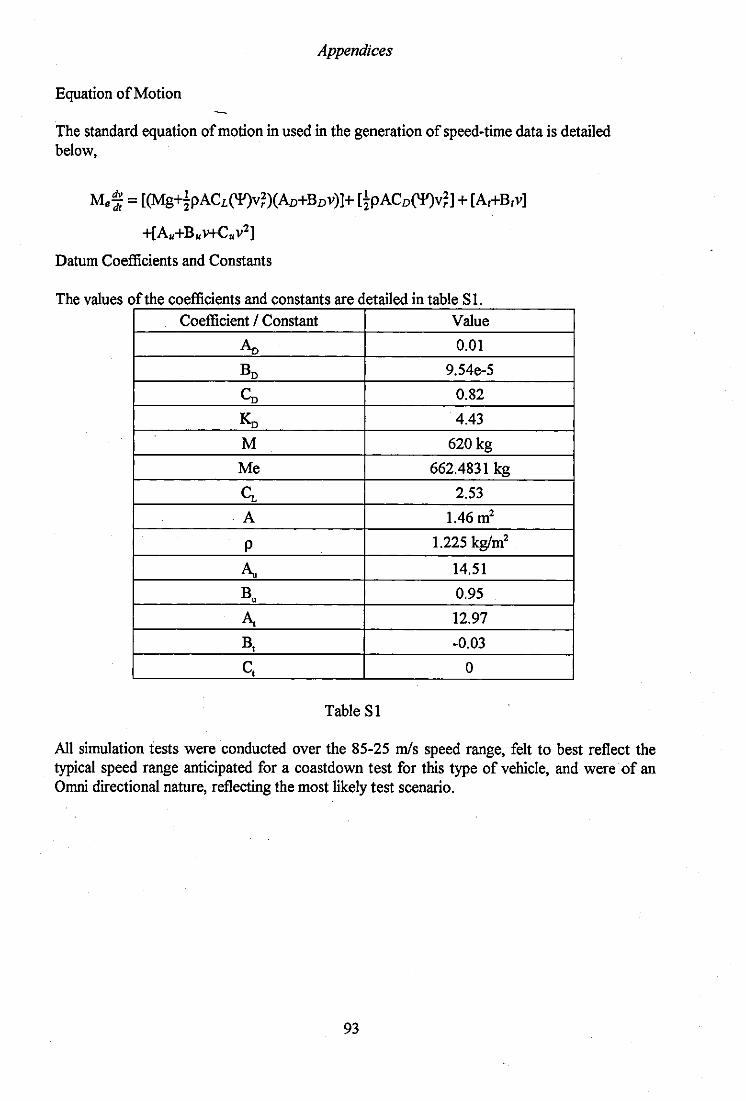
Appendices
Equation of Motion
The standard equation of motion in used in the generation of speed-time data is detailed below,
M.: = [(Mg+tpACL('¥)V~)(AD+BDV)]+ [tpACD('¥)V~] + [At+Btv]
+[Au+Bu v+Cu v2]
Datum Coefficients and Constants
The values of the coefficients and constants are detailed in table SI Coefficient / Constant Value
AD 0.01
BD 9.54e-5
Co 0.82
Ko 4.43
M 620 kg
Me 662.4831 kg
Cz. 2.53
A 1.46 m2
p 1.225 kg/m2
A" 14.51
Bu 0.95
A, 12.97
Bt -0.03
Ct 0 -:-
Table SI
AIl simulation tests were conducted over the 85-25 mls speed range, felt to best reflect the typical speed range anticipated for a coastdown test for this type of vehicle, and were of an Omni directional nature, reflecting the most likely test scenario.
93
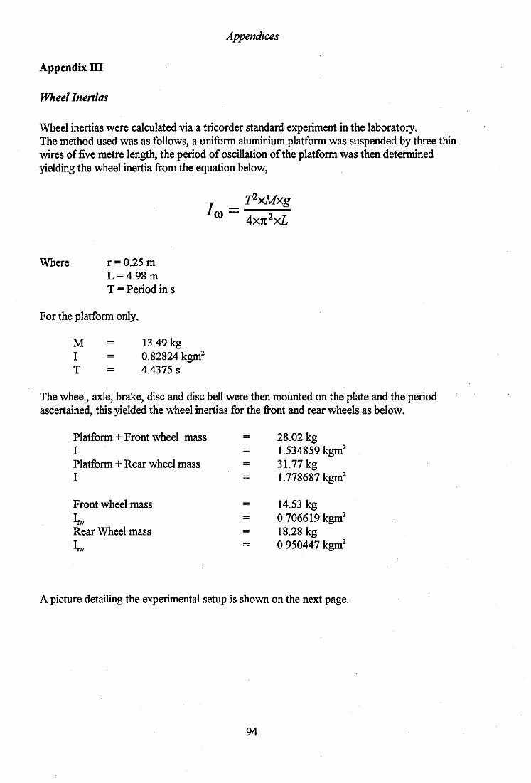
Appendices
Appendix m
Wheel Inertias
Wheel inertias were calculated via a tricorder standard experiment in the laboratory. The method used was as follows, a uniform aluminium platform was suspended by three thin wires offive metre length, the period of oscillation of the platform was then determined yielding the wheel inertia from the equation below,
Where r= 0.25 m L=4.98 m T = Period in s
For the platform only,
M I T
= = =
13.49 kg 0.82824 kgm2
4.4375 s
I _ 'f1xMxg ro - 4X1t2xL
The wheel, axle, brake, disc and disc bell were then mounted on the plate and the period ascertained, this yielded the wheel inertias for the front and rear wheels as below.
Platform + Front wheel mass = 28.02 kg I = 1.534859 kgm2
Platform + Rear wheel mass = 31.77 kg I = 1.778687 kgm2
Front wheel mass = 14.53 kg
In. = 0.706619 kgm2
Rear Wheel mass = 18.28 kg I.w = 0.950447 kgm2
A picture detailing the experimental setup is shown on the next page.
94

Appendices
Wheel Inertia Test Set-up
95
Appendices
Appendix IV
The following pages are a copy of the original project proposal made to the Benetton Formula One Racing team in January 1994. In this document the original objectives of the project are set out, the test method, the support required and the General requirements of the project from LVT's side.
96

Proposal
Formula One Racing Car Coastdown Analysis
Submitted to Benetton Formula One Racing Team, Enstone,
England
January 1994
The Department of Transport Technology
Loughborough University of Technology

1. Introduction
Coastdown testing is a proven method for the determination of vehicle drag for road cars whilst the vehicle is in it's normal operating environment. A method of achieving this has been developed at Loughborough University of Technology over the last few years. It is proposed that this method of determination of the vehicle drag forces is applied to the specific case of a Formula One racing car. Current methods, based on running the car at maximum horsepower and then deriving the aerodynamic drag coefficient, neglecting the other drag terms as small, are inaccurate. Thousands of hours are spent in the wind tunnel developing a modern Formula One car. A comparatively small amount of time is spent on environmental testing, validating the extensive wind tunnel test work. Additionally determination of the proportions and values of the different facets that go to make up the total vehicle drag would be extremely useful, providing data both of direct use, and allowing the simulation of the vehicle performance to be of a more accurate nature.
2. Objectives
The basic objective is to undertake the full development of a method of measuring vehicle drag of a Formula One car and separate it into it's constituent components. The work is largely split into three areas. These are:
l. To establish a Vehicle drag model pertinent to a Formula One racing car. 2. To develop a simulation of the coastdown to investigate parameters in the vehicle
drag model and evaluate the analysis technique, i.e. sensitivity of coefficients and the effect of neglecting terms in the analysis.
3. To produce an analysis technique to process real Formula One racing car coastdown data.
A summary of the data required, is included at the end of this document.
3. The Vehicle Drag Model
Unless a realistic model of the drag function is used in the analysis the components of vehicle drag cannot be separated or corrected for ambient conditions. Establishing a realistic drag function is dependent upon mathematically modelling each facet of the vehicle drag. The form of this model is usually a quadratic in vehicle speed, with mechanical losses composing the constant and velocity terms and aerodynamic composing the velocity squared term. Given the unusual nature ofa Formula One car, this is unlikely to be the case. The aim of this part of the work is to generate a model specific to the Formula One type of vehicle.
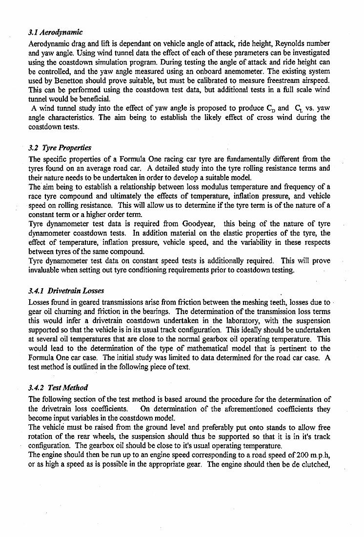
3.1 Aerodynamic
Aerodynamic drag and lift is dependant on vehicle angle of attack, ride height, Reynolds number and yaw angle. Using wind tunnel data the effect of each of these parameters can be investigated using the coastdown simulation program. During testing the angle of attack and ride height can be controlled, and the yaw angle measured using an onboard anemometer. The existing system used by Benetton should prove suitable, but must be calibrated to measure freestream airspeed. This can be performed using the coastdown test data, but additional tests in a full scale wind tunnel would be beneficial. A wind tunnel study into the effect of yaw angle is proposed to produce <;, and <;, vs. yaw
angle characteristics. The aim being to establish the likely effect of cross wind during the coastdown tests.
3.2 Tyre Properties
The specific properties of a Formula One racing car tyre are fundamentally different from the tyres found on an average road car. A detailed study into the tyre rolling resistance terms and their nature needs to be undertaken in order to develop a suitable model. The aim being to establish a relationship between loss modulus temperature and frequency of a race tyre compound and ultimately the effects of temperature, inflation pressure, and vehicle speed on rolling resistance. This will allow us to determine if the tyre term is of the nature of a constant term or a higher order term. Tyre dynamo meter test data is required from Goodyear, this being of the nature of tyre dynamometer coastdown tests. In addition material on the elastic properties of the tyre, the effect of temperature, inflation pressure, vehicle speed, and the variability in these respects between tyres of the same compound. Tyre dynamometer test data on constant speed tests is additionally required. This will prove invaluable when setting out tyre conditioning requirements prior to coastdown testing.
3.4.1 Drivetrain Losses
Losses found in geared transmissions arise from friction between the meshing teeth, losses due to gear oil churning and friction in the bearings. The determination of the transmission loss terms this would infer a drivetrain coastdown undertaken in the laboratory, with the suspension supported so that the vehicle is in its usual track configuration. This ideally should be undertaken at several oil temperatures that are close to the normal gearbox oil operating temperature. This would lead to the determination of the type of mathematical model that is pertinent to the Formula One car case. The initial study was limited to data determined for the road car case. A test method is outlined in the following piece of text.
3.4.2 Test Method
The following section of the test method is based around the procedure for the determination of the drivetrain loss coefficients. On determination of the aforementioned coefficients they become input variables in the coastdown model. The vehicle must be raised from the ground level and preferably put onto stands to allow free rotation of the rear wheels, the suspension should thus be supported so that it is in it's track configuration. The gearbox oil should be close to it's usual operating temperature. The engine should then be run up to an engine speed corresponding to a road speed of 200 m. p.h, or as high a speed as is possible in the appropriate gear. The engine should then be de clutched,

the gearbox set in neutral, and the wheels allowed to coastdown. Before the commencement of the test the following should be recorded if possible,
1. Ambient temperature ("C) 2. Gearbox oil temperature ("C) 3. Casing temperature ("C) 4. Quantity of oil in the gearbox (I)
At each time step (dependent on data logger) the following should be monitored, Wheel speed (in RP.M.) Gearbox Oil temperature ("C)
If it is impossible to measure the gearbox oil temperature on-line then a reading from temperature strips every five seconds should be taken. The gearbox oil temperature at the end of the test should also be measured. Ideally it would be beneficial to undertake this test at several gear oil temperatures, near the normal operating temperature.
3.5 Undriven Wheel Loses Undriven wheel losses usually arise from driven wheel brake drag and bearing friction. In a similar way to section 3.4, the undriven wheel loses need to be determined, for the relevant type of brake set up to be used by the team for coastdown tests. It would be necessary in this test to perform separate coastdown tests on each of the front wheels, with the front of the car jacked off the floor. It would then be necessary for the wheel to be motored up to the maximum wheel speed that would be encountered in a test, and then the speed should be allowed to steady, before being removed allowing the wheel to freely decelerate. A record of the angular velocity versus time should be retained.
4. Testing the Model
In the initial study a crude simulation code was developed in order to test the model for different steady inputs of ambient wind, and to establish coefficient sensitivities. The process needs to be extended to the generation of realistic wind conditions, including both time variations (turbulence) and spatial variations. It is proposed that a representation such as a Dryden spectral form be used, which closely matches power spectral density relationships found for ambient wind. The simulation will be used to determine the response to enforced noise, specifically system noise, such as and variations in the surface of the test track. The original coastdown simulation code was written in Fortran, this does not exactly lend itself to these rather more specific tasks, thus it is felt that a package that is.a more appropriate method of Engineering Analysis be used. Therefore the latest version of Matrix. is to be used for this purpose.

SAnalysis
This will be based on established methods successfully developed at LUT by Dr Passmore. A study into the type of analysis method to be used for this specific type of Coastdown test work, for instance the type of parameter optimisation method that is appropriate, must be established, i.e. be it of the nature ofa downhill simplex method, or a gradient type method. A study into the use of a constrained analysis method, i.e. constraining particular tenns, allowing a result to be determined with relatively few tests will be made. This is felt to be of particular relevance bearing in mind the extremely high cost implied with testing a modern Fonnula One Racing car.
6. Definition o/test method
The findings made from the full study into an applicable mathematical model will be reflected in the suitable test method chosen. The areas to which consideration must be given are summarised below. The length of track required. The simulation will allow us to determine the length of track required for a low drag configuration coastdown. The operating speed range of the vehicle must be reflected in the determination of the starting and finishing velocities for the coastdown. The higher speeds aiding the determination of aerodynamic tenns, the lower speeds the tyre tenns. The subject of tyre conditioning was discussed earlier in the tyre model part of this document. A study into the implications of nonnalload measurement on line, data from previous tests would be of particular interest. The topic of lift force implied by the wheels rotating in the flow, said to be of the order of 1 % of the magnitude of the total vehicle downforce, needs to be addressed. The method used in the measurement of ambient wind, if indeed it is felt necessary to measure ambient wind, must be considered. The use of the 'golf ball' type device was recommended in the recent meeting, data on the usage and properties of this type of device is required. The data logged by the teams weather station is also required. The study into the likely route for the test method is necessary in order to minimise the number of tests required. Determination of the various coefficients to a high degree of certainty requires the undertaking of a large number of tests. It is hoped that through the careful detailing of the test method that the number of test pairs needed will be kept to a minimum.
7 Support Required
Financial support for a research student, working in the field of Race Car Perfonnance and registered for a Research Masters Degree, has already been secured from The Department Of Transport Technology At Loughborough University Of Technology.
8 General Requirements
8.1 Access to Results Obtained
A condition of any contract is that results obtained directly from this work are always made available to Benetton Formula One racing team and LUT who would be equal partners in this project. However, each party, i.e. Benetton Formula One racing team and LUT, would agree not to disclose information resulting from this work to other parties without written agreement. This arrangement should be similar to procedures currently adopted between contractors in the motor industry. Benetton Formula One racing team will receive a summary of the final report containing the results and how they were achieved. The software will remain the property of LVT.
8.2 Publications
It is anticipated that the work carried out during this project will lead to a publication. In addition, it is hoped that this and other work will also culminate in the research student obtaining the award of MPhil. The wishes of all parties will be respected where possible and any highly confidential information would obviously not be published. On completion of the paper, the paper will be submitted to the Benetton Formula One racing team for approval. This paper will contain information on the method used and not detailed results. There will be a three year moratorium on University publication of the Research Masters thesis.
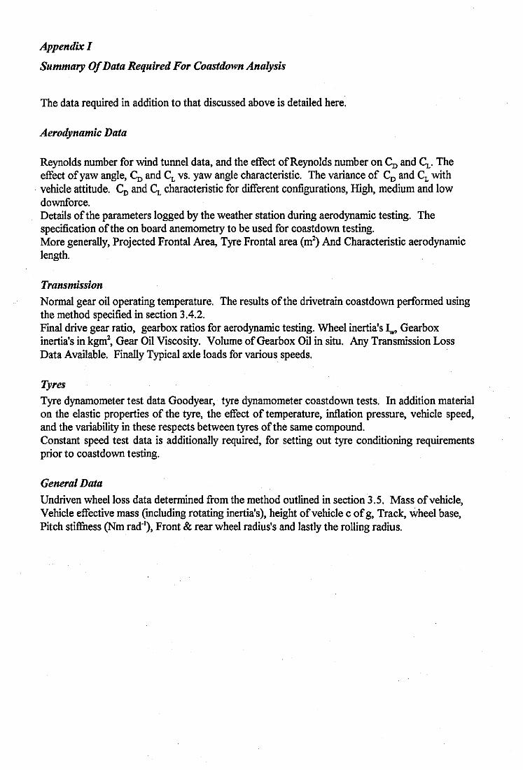
Appendix I
Summary Of Data Required For Coastdown Analysis
The data required in addition to that discussed above is detailed here.
Aerodynamic Data
Reynolds number for wind tunnel data, and the effect ofReynolds number on CD and c;,. The effect ofyaw angle, CD and CL vs. yaw angle characteristic. The variance of CD and CL with vehicle attitude. CD and c;, characteristic for different configurations, High, medium and low downforce. Details of the parameters logged by the weather station during aerodynamic testing. The specification of the on board anemometry to be used for coastdown testing. More generally, Projected Frontal Area, Tyre Frontal area (m~ And Characteristic aerodynamic length.
Transmission Normal gear oil operating temperature. The results of the drivetrain coastdown performed using the method specified in section 3.4.2. Final drive gear ratio, gearbox ratios for aerodynamic testing. Wheel inertia's I,., Gearbox inertia's in kgm2, Gear Oil Viscosity. Volume of Gearbox Oil in situ. Any Transmission Loss Data Available. Finally Typical axle loads for various speeds.
Tyres Tyre dynamometer test data Goodyear, tyre dynamometer coastdown tests. In addition material on the elastic properties of the tyre, the effect of temperature, inflation pressure, vehicle speed, and the variability in these respects between tyres of the same compound. Constant speed test data is additionally required, for setting out tyre conditioning requirements prior to coastdown testing.
General Data Undriven wheel loss data determined from the method outlined in section 3.5. Mass of vehicle, Vehicle effective mass (including rotating inertia's), height of vehicle c ofg, Track, wheel base, Pitch stiffuess (Nm rad'I), Front & rear wheel radius's and lastly the rolling radius.
Appendices
Appendix V
Track survey details from Silverstone and Circuit De CataIunya are detailed on the following pages. The Circuit De CataIunya grade information is as you can see very explicit in comparison to the Silverstone track survey, for which three elevations were made over a seven hundred metre straight.
103
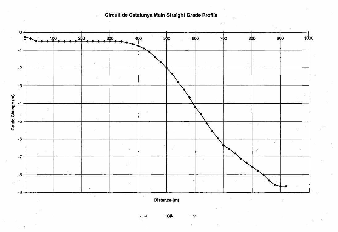
o
-1
-2
-3
g & -4 c ca fi CD -5 ~ ~
-6
-7
-8
-9
t-..... . 1 0 2 0
Circuit de Catalunya Main Straight Grade Profile
3 0 4 0 5 0 6 0 70 80 90 HO o .
-...., r--....
~ 1'\
\ 1\
" \ '" '" "-,
.....
Distance (m)

~
E ~
CD Cl C .. .c <)
CD 'tI f! Cl
Chapel
o
~1 -0.5
-1
-1.5
-2
-2.5
-3
-3.5
-4
-4.5
-5
0
~
Silverstone Hanger Straight Grade
20 30 40 5 0 6>0 7 0 8 0 9~
.........
~ c.c "
~ ~ ~
J !L ~ "-
~ ~ Stowe
" K / , V
Hanger ridge
Distance from start of straight (m)

Appendices
Appendix VI
Nelder and Mead's optimisation method flow chart.
105
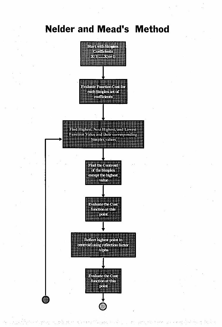
Nelder and Mead's Method

Yes
No

~------------~1
Ym

Related Documents