t e l 0 0 4 2 5 3 3 4 , v e r s i o n 1 2 0 O c t 2 0 0 9

Welcome message from author
This document is posted to help you gain knowledge. Please leave a comment to let me know what you think about it! Share it to your friends and learn new things together.
Transcript

7/13/2019 Rabaute Manuscrit de These
http://slidepdf.com/reader/full/rabaute-manuscrit-de-these 1/212
tel00425334,version1
20Oct2009

7/13/2019 Rabaute Manuscrit de These
http://slidepdf.com/reader/full/rabaute-manuscrit-de-these 2/212
™
tel00425334,version1
20Oct2009

7/13/2019 Rabaute Manuscrit de These
http://slidepdf.com/reader/full/rabaute-manuscrit-de-these 3/212
tel00425334,version1
20Oct2009

7/13/2019 Rabaute Manuscrit de These
http://slidepdf.com/reader/full/rabaute-manuscrit-de-these 4/212
tel00425334,version1
20Oct2009

7/13/2019 Rabaute Manuscrit de These
http://slidepdf.com/reader/full/rabaute-manuscrit-de-these 5/212
tel00425334,version1
20Oct2009

7/13/2019 Rabaute Manuscrit de These
http://slidepdf.com/reader/full/rabaute-manuscrit-de-these 6/212
Z/A
T 2
tel00425334,version1
20Oct2009

7/13/2019 Rabaute Manuscrit de These
http://slidepdf.com/reader/full/rabaute-manuscrit-de-these 7/212
tel00425334,version1
20Oct2009

7/13/2019 Rabaute Manuscrit de These
http://slidepdf.com/reader/full/rabaute-manuscrit-de-these 8/212
tel00425334,version1
20Oct2009

7/13/2019 Rabaute Manuscrit de These
http://slidepdf.com/reader/full/rabaute-manuscrit-de-these 9/212
tel00425334,version1
20Oct2009

7/13/2019 Rabaute Manuscrit de These
http://slidepdf.com/reader/full/rabaute-manuscrit-de-these 10/212
tel00425334,version1
20Oct2009

7/13/2019 Rabaute Manuscrit de These
http://slidepdf.com/reader/full/rabaute-manuscrit-de-these 11/212
−
™
tel00425334,version1
20Oct2009

7/13/2019 Rabaute Manuscrit de These
http://slidepdf.com/reader/full/rabaute-manuscrit-de-these 12/212
tel00425334,version1
20Oct2009

7/13/2019 Rabaute Manuscrit de These
http://slidepdf.com/reader/full/rabaute-manuscrit-de-these 13/212
tel00425334,version1
20Oct2009
7/13/2019 Rabaute Manuscrit de These
http://slidepdf.com/reader/full/rabaute-manuscrit-de-these 14/212
αβ γ
α β
α β α β
γ
103 106
α β
137
60Co
N 0
tel00425334,version1
20Oct2009
7/13/2019 Rabaute Manuscrit de These
http://slidepdf.com/reader/full/rabaute-manuscrit-de-these 15/212
dN dT
dN = −λ · N · dt
λ
N t = N 0e−λt
N t t N 0
N 0
t1/2 =0, 693
λ
P P x x z
zP
P x = µx e−µ
x!
P x xµ
σ =√
µ
40
1, 3 · 109 238 4, 4 · 109 232 1, 4 · 109
tel00425334,version1
20Oct2009
7/13/2019 Rabaute Manuscrit de These
http://slidepdf.com/reader/full/rabaute-manuscrit-de-these 16/212
+ ≈ ≈∗
+
∗
40
206 208
238 214232 208 228
tel00425334,version1
20Oct2009

7/13/2019 Rabaute Manuscrit de These
http://slidepdf.com/reader/full/rabaute-manuscrit-de-these 17/212
0
100
200
300
400
0 500 1000 1500 2000 2500 3000
P2 P3 P4 P5 P6 P9 P11 P14 15 16P12 1371 8 10P0
1 2 W3 W4 W5 W6 W108 9 W11 W12 W14 W15 16 17W0 W13W7
IAEA 1 IAEA 2 IAEA 3
SCHLUM 1 SCHLUM 2 SCHLUM 3 SCHLUM 4 SCHLUM 5
Energie (keV)
C o m p t e s / c a n a l
2 0 8 T l ( 5 8 4
k e V )
2 1 4 B i ( 6 1 0
k e V )
2 2 8 A c ( 9 1 2
e t 9 6 6
k e V )
2 1 4 B i ( 1 1 2 0
k e V )
2
1 4 B i ( 1 7 6 4
k e V )
4 0 K ( 1 4 6 0
k e V )
2 0
8 T l ( 2 6 1 5
k e V )
UO2+2
UO2
tel00425334,version1
20Oct2009

7/13/2019 Rabaute Manuscrit de These
http://slidepdf.com/reader/full/rabaute-manuscrit-de-these 18/212
ThSiO4
PO44 4
ZrSiO4
CaTiSiO4
Na Iµ
e
KCl
tel00425334,version1
20Oct2009

7/13/2019 Rabaute Manuscrit de These
http://slidepdf.com/reader/full/rabaute-manuscrit-de-these 19/212
Rayon gamma
Cristal NaI(Tl)
A)
Outil NGT
B)
Photomultiplicateur
Photocathode
J (r)
40K
tel00425334,version1
20Oct2009

7/13/2019 Rabaute Manuscrit de These
http://slidepdf.com/reader/full/rabaute-manuscrit-de-these 20/212
0 25 50 750
0.5
1.0
25 50 75
J(r)
r (cm) r (cm)
40
K232
Th
25 50 75
r (cm)
238
U
J(r)
J(r)
0
0.5
1.0
0
0.5
1.0
p u
i t s
p
u i t s
p u
i t s
J (r)
>
tel00425334,version1
20Oct2009

7/13/2019 Rabaute Manuscrit de These
http://slidepdf.com/reader/full/rabaute-manuscrit-de-these 21/212
P e
A
W i = AiT h + BiU + C iK + ri
T h U K ri
W i iAi Bi C i i
A
W 1W 2W 3W 4W 5
= A ×
Th
UK
ri
5
i=1
r2i =5
i=1
1
W i
(W i
−AiTh
−BiU
−C iK)2 = r2
tel00425334,version1
20Oct2009

7/13/2019 Rabaute Manuscrit de These
http://slidepdf.com/reader/full/rabaute-manuscrit-de-these 22/212
1/W ir2
Th
UK
= m ×
W 1W 2W 3W 4W 5
m A 1/W i
W i√W i W i
tel00425334,version1
20Oct2009

7/13/2019 Rabaute Manuscrit de These
http://slidepdf.com/reader/full/rabaute-manuscrit-de-these 23/212
tel00425334,version1
20Oct2009

7/13/2019 Rabaute Manuscrit de These
http://slidepdf.com/reader/full/rabaute-manuscrit-de-these 24/212
0
20
40
60
80
100
0.01 0.1 1 10 100
Numéroatomique,Z
Energie du rayon gamma (MeV)
Prédominance del’effet photoélectrique
Prédominance del’effet Compton
Prédominance del’effet de paire
ρe
ρb
P e
e− E 0
θ E
A Z
tel00425334,version1
20Oct2009

7/13/2019 Rabaute Manuscrit de These
http://slidepdf.com/reader/full/rabaute-manuscrit-de-these 25/212
ΣCo
ΣCo = σCoN Av
AρbZ
σCo AZ σ
−24 2
ρb Z/A
12
Φ = Φie−ρb
ZA
N AvσCoh = Φie−µρbh
Φi hh µ
2 −1
µ =Z
AN Avσ
σPe σCo σPe
Z
σPe = 12.1Z 4.6
E 3.15
σPe
Φ = Φie−ρb
ZA
N AvσPeh
137
tel00425334,version1
20Oct2009

7/13/2019 Rabaute Manuscrit de These
http://slidepdf.com/reader/full/rabaute-manuscrit-de-these 26/212
FORMATION FORMATIONPUITS
B r a
s m é c
a n i q
u e d u
d i a m
é t r e u r
( c a l i p
e r )
Détecteur F
Détecteur S
source radioactive
(137
Cs ou60Co)
mud-cake
Materiau absorbantles rayons gamma (W, Pb)
∆ρ
∆ρ∆ρ
tel00425334,version1
20Oct2009

7/13/2019 Rabaute Manuscrit de These
http://slidepdf.com/reader/full/rabaute-manuscrit-de-these 27/212
3
3
P eZ/A
P e
H B C O Na Mg A l Si P S Cl K Ca Ti Mn Fe
1
0,5
0
RapportZ/A
Elément
Z/A
Z/A 1/2
ρb
ρe = A − B ln N
N
ρlog
ρb
ρlog = 1, 07ρe − 0, 188 = ρb
tel00425334,version1
20Oct2009
7/13/2019 Rabaute Manuscrit de These
http://slidepdf.com/reader/full/rabaute-manuscrit-de-these 28/212
P e
P e =
Z 10
3.6
U 3 3
U = P eρe =
iV 1iP e,iρe,i
U =
i
V iU i
ρe,i i P e,i V iP eρe P eρb
σi3
Σi = N σi =N Avρb
Aσi
N Av ρb A Σi−1 cu Σi
tel00425334,version1
20Oct2009

7/13/2019 Rabaute Manuscrit de These
http://slidepdf.com/reader/full/rabaute-manuscrit-de-these 29/212
0.01 0.1 1 10 103
105
106
107 Energie (eV)
1 keV 1MeV
0.22
2.2
2200
V i t e s s e
( c m
/ µ s e c
)
Thermal
Epithermal
Rapide
Sourceschimiques
4 MeV
Minitron14 MeV
- Collision inélastique- Absorption totale- Activation rapide
- Collision élastique- Capture thermique- Activation par capture
thermique
REACTIONS
Ls
Σform
ΣBH
Ld
Ld
Σform
Lm L2m = L2s +L2d
tel00425334,version1
20Oct2009

7/13/2019 Rabaute Manuscrit de These
http://slidepdf.com/reader/full/rabaute-manuscrit-de-these 30/212
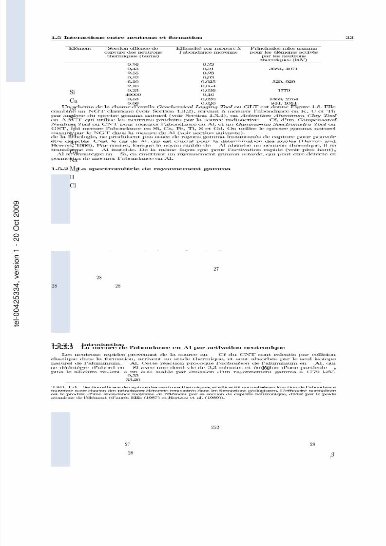
28Si28 28
σ = 33, 2barns
tel00425334,version1
20Oct2009
7/13/2019 Rabaute Manuscrit de These
http://slidepdf.com/reader/full/rabaute-manuscrit-de-these 31/212
SiCa
Fe
S
Ti
K
Al
Gd
Na
Mg
H
Cl
27
2828 28
252
252
27 28
28 β
tel00425334,version1
20Oct2009

7/13/2019 Rabaute Manuscrit de These
http://slidepdf.com/reader/full/rabaute-manuscrit-de-these 32/212
Grandeurs mesurées Configuration de l’outil
ΣBH
K, Th, U
Ls
Al
Si, Ca, FeS, Ti, Gd
Σformation
Auxiliary Measurement Sonde -- AMS
Natural Gamma Ray Tool -- NGT(détecteur à scintillation: cristal NaI)
Compensated Neutron Tool -- CNT
source radioactive au252
Cf(neutrons lents: 2,3 MeV)
Aluminum Activation Clay Tool -- AACT(détecteur à scintillation: cristal NaI)
Gamma Ray Spectrometry Tool -- GST(détecteur à scintillation: cristal NaI)
Gaine de bore
Minitron (neutrons rapides: 14 MeV)
Arc métallique plaquant l’outilcontre la formation
252
252
28
Na I
NaI
tel00425334,version1
20Oct2009

7/13/2019 Rabaute Manuscrit de These
http://slidepdf.com/reader/full/rabaute-manuscrit-de-these 33/212
Σform
ΣBH Σform Ls
Ls
Σform ΣBH
252
Na I
tel00425334,version1
20Oct2009

7/13/2019 Rabaute Manuscrit de These
http://slidepdf.com/reader/full/rabaute-manuscrit-de-these 34/212
Fe
Cl
Ca
Si
SH
Dû aucristal
1
10
100
1000
1 2 3 4 5 6 7
Energy gamma (MeV)
Tauxdecomptage
10
2
103
104
27 53 79 105 131 1 57 183 209Canal de mesure
CaH
CaCa
CaCa Ca
Fe
Fe
A) B)
16
tel00425334,version1
20Oct2009

7/13/2019 Rabaute Manuscrit de These
http://slidepdf.com/reader/full/rabaute-manuscrit-de-these 35/212
0 2 4 6 8 10 12 42 44 46 48 61
multiples de τ
Bruit de fond
Impulsions de neutrons
C a p t u r e
C a p t u r e
Mode de mesureCapture-Tau
τ
τ 62 ∗ τ µsec
τ
τ =1
vΣform
v = 0, 22 cm/µsec
τ =4550
Σform
τ τ
tel00425334,version1
20Oct2009

7/13/2019 Rabaute Manuscrit de These
http://slidepdf.com/reader/full/rabaute-manuscrit-de-these 36/212
252
p = sCaxCa + sSixSi + . . .
p sel
xel
p1 p2···
p200
=
sCa1 sSi1 . . . sS1sCa2 sSi2 . . . sS2· · . . . ·· · . . . ·· · . . . ·
sCa200 sSi200 . . . sS200
xCaxSi
xS
p = S · x
xT W
( p − S · x)T W ( p − S · x)
x = (S T W S )−1S T W · p
x E
ˆ p
tel00425334,version1
20Oct2009

7/13/2019 Rabaute Manuscrit de These
http://slidepdf.com/reader/full/rabaute-manuscrit-de-these 37/212
C/O
Cl/H
H/(Si + Ca)
Fe/(Si + Ca)
Si /(Si + Ca)
Y i S i
W i F
W i = F · Y iS i
F
F
F
F
i
X iY iS i
+ X KW K + X AlW Al = 1.0
X i i W KW Al
X i
X i =W SiO2
W Si= 2, 139
F
tel00425334,version1
20Oct2009

7/13/2019 Rabaute Manuscrit de These
http://slidepdf.com/reader/full/rabaute-manuscrit-de-these 38/212
σ
Si
Ca
FeTi
Gd
S
F
i X iY iS i
±
CaFe[CO3]2
i W ti
P e =
i
W ti
Z i10
3.6
P e,log = W fluideP e,fluide + (1 + W fluide)P e,matrice
W fluide = φ/ρb P e,fluide0/00
P e,matrice
P estime,matrice =
i
P e,iW i + P e,KW K + P e,AlW Al + P e,OW O
W OP loge,matrice = P estime,matrice
F P estime,matrice
F
F i
X iY i
S i+ X MgW Mg + X KW K + X AlW Al = 1.0
tel00425334,version1
20Oct2009

7/13/2019 Rabaute Manuscrit de These
http://slidepdf.com/reader/full/rabaute-manuscrit-de-these 39/212
P e
F i
P e,iY i
S i+ P e,MgW Mg + P e,KW K + P e,AlW Al + P e,OW O = P loge,matrice
W Mg
W Mg =
X i
P estime,matrice − P e,MgCO3
(P estime,matrice − P loge,matrice)
F /F
X NaNa2O
±
tel00425334,version1
20Oct2009
7/13/2019 Rabaute Manuscrit de These
http://slidepdf.com/reader/full/rabaute-manuscrit-de-these 40/212
D
D =1
3(Σt − µΣs)
Σt Σs
Σa µΣt = Σa + Σs
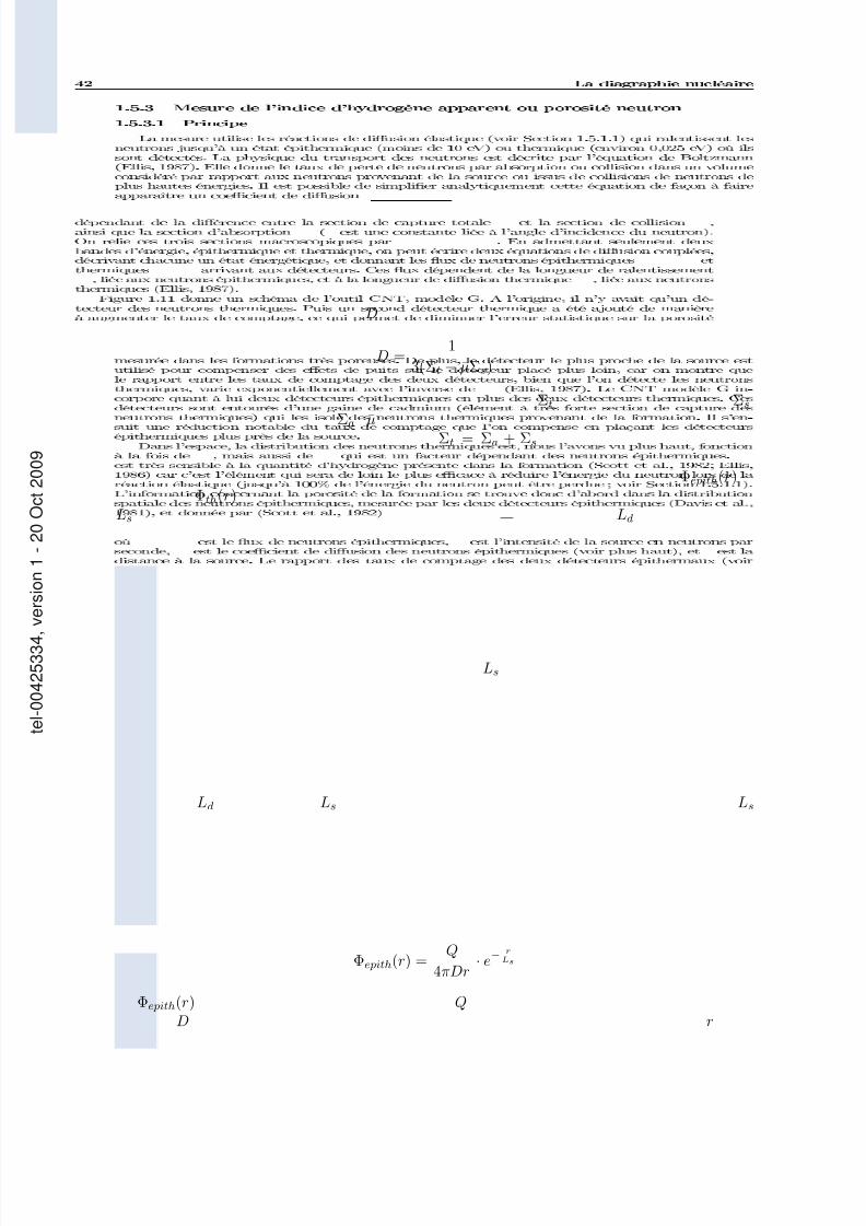
Φepith(r)Φth(r)
Ls Ld
Ls
Ld Ls Ls
Φepith(r) =Q
4πDr· e−
rLs
Φepith(r) QD r
tel00425334,version1
20Oct2009

7/13/2019 Rabaute Manuscrit de These
http://slidepdf.com/reader/full/rabaute-manuscrit-de-these 41/212
Détecteursthermiques
Source Am-Be(16 curie, E=4,5 MeV)
Détecteursépithermiques
Bras extensibleplaquant l’outil
contre la formation
r1 r2 Ls
Repith =Φepith(r1)
Φepith(r2)=
r1r2
e−(r1−r2)
Ls
Ld
Ld =1
3
Σa + Σs(1 − µ)
Lm
Lm
tel00425334,version1
20Oct2009
7/13/2019 Rabaute Manuscrit de These
http://slidepdf.com/reader/full/rabaute-manuscrit-de-these 42/212
10 α 3
tel00425334,version1
20Oct2009
7/13/2019 Rabaute Manuscrit de These
http://slidepdf.com/reader/full/rabaute-manuscrit-de-these 43/212
U = R · I J = σE J E σ
A l
R =U
I =
1
niµq2l
A
l/A1/(niµq2)
Ω Ω3
η
η = η0 · eCT
C
a q
R =6πηa
nq2l
A
σ
tel00425334,version1
20Oct2009

7/13/2019 Rabaute Manuscrit de These
http://slidepdf.com/reader/full/rabaute-manuscrit-de-these 44/212
R ≡ R0 = F F · Reau
F F ≈ 1φm
m
S w =
Rt
R0
− 1n
n
Rt φe S wRw
Rt =a · Rw
φme · S nw
a an
m = n = 2
F F ≈ 1φ2
S w =
RtR0
Rt = Rwφ2e · S 2w
E = −
V = R ·
i
tel00425334,version1
20Oct2009

7/13/2019 Rabaute Manuscrit de These
http://slidepdf.com/reader/full/rabaute-manuscrit-de-these 45/212
E V R iRt
Rxo
™
Rt
™
Rt
Rs
A0A1 A
1 A0
A1 A1
A0 A1 A1
M 1 − M 1M 2− M 2
A0A1 A
1
A™
tel00425334,version1
20Oct2009
7/13/2019 Rabaute Manuscrit de These
http://slidepdf.com/reader/full/rabaute-manuscrit-de-these 46/212
M2
M1
A1
M0
A0
M’2
M’1
A’1
Formation
mud-cake
M’0
A)
B)
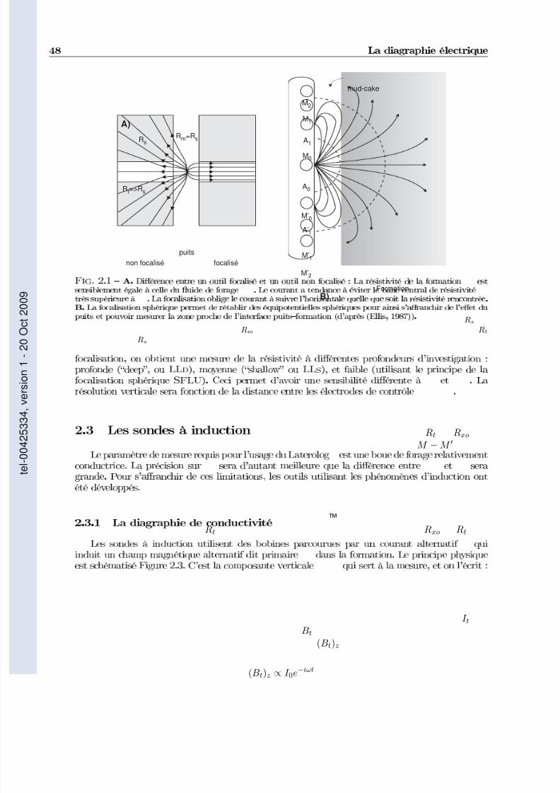
Rs
Rt>>Rs
Rm=Rs
non focalisé focalisé
puits
Rs
Rm Rt
Rs
Rt Rxo
M − M
™
Rt Rxo Rt
I tBt
(Bt)z
(Bt)z ∝ I 0e−iωt
tel00425334,version1
20Oct2009

7/13/2019 Rabaute Manuscrit de These
http://slidepdf.com/reader/full/rabaute-manuscrit-de-these 47/212
Configuration enmode profond
Configuration enmode peu profond
E
E ∝ −∂ (Bt)z
∂t∝ iωI 0e
−iωt
J
J ∝ σE ∝ iωσI 0e−iωt
B2
tel00425334,version1
20Oct2009
7/13/2019 Rabaute Manuscrit de These
http://slidepdf.com/reader/full/rabaute-manuscrit-de-these 48/212
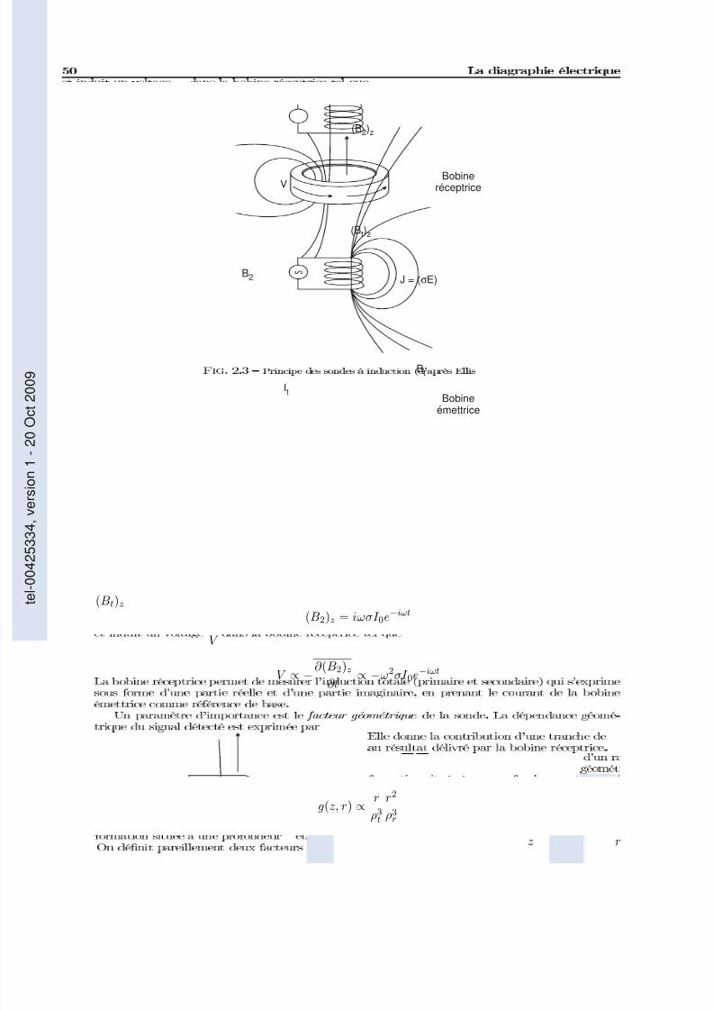
B2 J = (σE)
Bt
ItBobine
émettrice
(B2)z
BobineréceptriceV
(Bt)z
(Bt)z
(B2)z = iωσI 0e−iωt
V
V
∝ −
∂ (B2)z
∂t ∝ −ω2σI 0e
−iωt
g(z, r) ∝ r
ρ3t
r2
ρ3r
z r
tel00425334,version1
20Oct2009

7/13/2019 Rabaute Manuscrit de These
http://slidepdf.com/reader/full/rabaute-manuscrit-de-these 49/212
g(r) g(z) g(r)r
g(r) = ∞
−∞
g(r, z)dz
g(r)
g(z) z
g(z) =
∞0
g(r, z)dr
Rt
Rt
J B
J = χ
H
tel00425334,version1
20Oct2009
7/13/2019 Rabaute Manuscrit de These
http://slidepdf.com/reader/full/rabaute-manuscrit-de-these 50/212
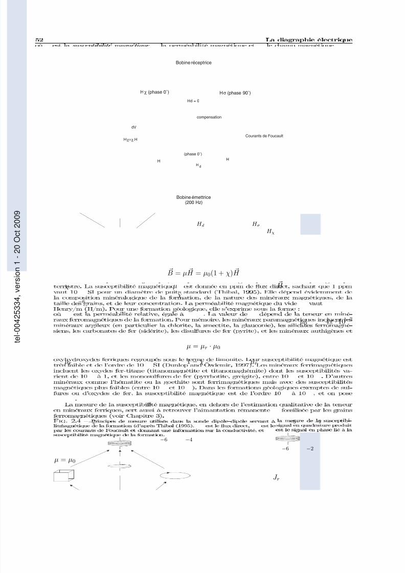
HHd
dV
Hχ=χ.HCourants de Foucault
Hσ (phase 90˚)Hχ (phase 0˚)
Bobine réceptrice
Bobine émettrice(200 Hz)
(phase 0˚)
compensation
Hd = 0
H
H d H σH χ
B = µ H = µ0(1 + χ) H
χ µ H
χ−6
µ0 4π · 10−7
µ = µr · µ0
µr 1 − χ µr
−8
−2 −5 −2
−6 −4
−6 −2
µ = µ0
J r
tel00425334,version1
20Oct2009

7/13/2019 Rabaute Manuscrit de These
http://slidepdf.com/reader/full/rabaute-manuscrit-de-these 51/212
Patin(électrodesémettrices)
c o u r
a n t
surfaceséquipotentielles
isolants
électroderéceptrice
lignes
d
e
courant
A) B)
électrode
C)
Rxo
tel00425334,version1
20Oct2009

7/13/2019 Rabaute Manuscrit de These
http://slidepdf.com/reader/full/rabaute-manuscrit-de-these 52/212
tel00425334,version1
20Oct2009

7/13/2019 Rabaute Manuscrit de These
http://slidepdf.com/reader/full/rabaute-manuscrit-de-these 53/212
tel00425334,version1
20Oct2009

7/13/2019 Rabaute Manuscrit de These
http://slidepdf.com/reader/full/rabaute-manuscrit-de-these 54/212
tel00425334,version1
20Oct2009
7/13/2019 Rabaute Manuscrit de These
http://slidepdf.com/reader/full/rabaute-manuscrit-de-these 55/212
J
µ
µ = γ · J
γ γ · 3 · 7 H t
µM
H 0
·10−4
tel00425334,version1
20Oct2009
7/13/2019 Rabaute Manuscrit de These
http://slidepdf.com/reader/full/rabaute-manuscrit-de-these 56/212
z
y
x
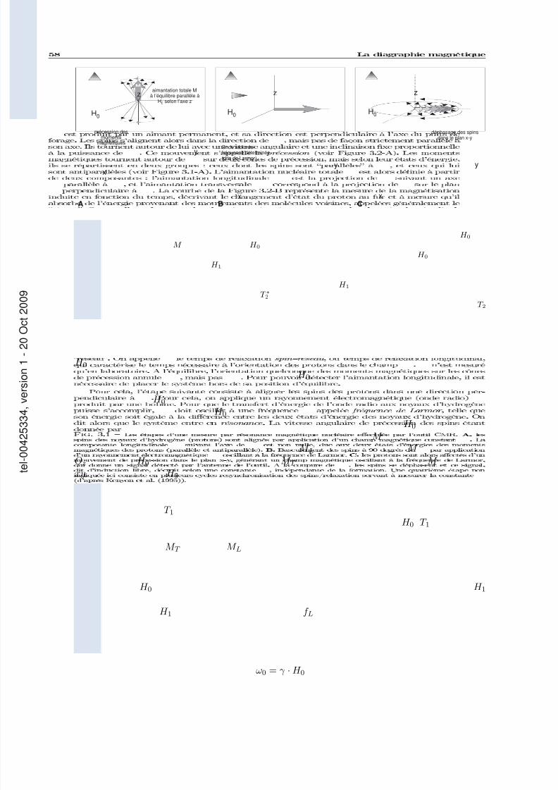
H0
z
y
x
H0
z
y
x
H0
précession desmoments
magnétiques
aimantation totale Mà l’équilibre parallèle à
H0 selon l’axe z
Onde radio defréquence déterminée(dite de Larmor)
déphasage des spinsdans le plan x-y
A B C
H 0M H 0
H 0H
1
H 1T ∗2
T 2
H 0H 0
H 0 H 0H 0
M M L M
Oz H 0 M T M xy H 0
T 1H 0 T 1
M T M L
H 0 H 1
H 1 f L
ω0 = γ · H 0
tel00425334,version1
20Oct2009
7/13/2019 Rabaute Manuscrit de These
http://slidepdf.com/reader/full/rabaute-manuscrit-de-these 57/212
H 1
f L
=ω0
2π= 0, 76gH
t
g gH 0 ≈ 550
H 1
H 0
H 1
T 2
T 2
H 0H 1
H 0
T 2
φf
φf
T 1 T 2H 0
φf
T 1 T 2
tel00425334,version1
20Oct2009

7/13/2019 Rabaute Manuscrit de These
http://slidepdf.com/reader/full/rabaute-manuscrit-de-these 58/212
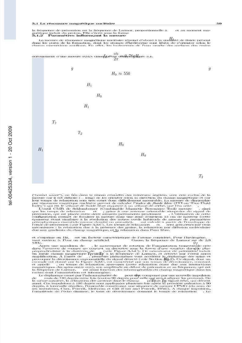
H0
α
précessionautour de H0
m a g n é
t i s a
t i o n
temps
ML=M0[1-exp(-t/T1)]
T1
T2
t e m p s d e d é c r o i s s a n c e
m a g n
é t i s a
t i o n
arrêt de lapolarisation
fréquence de Larmor
A)
B)
C)
H 0 H 0H 0
T 1T 1
T 2
H 0 T 1H 1
T 2T 1 T 2
ρ
ρ
tel00425334,version1
20Oct2009

7/13/2019 Rabaute Manuscrit de These
http://slidepdf.com/reader/full/rabaute-manuscrit-de-these 59/212
Amplitudedus
ignal
Temps (millisec)
0 4002000
1
Distribution
T2, millisec
0,03
0,000,1 1,0 10,0 100,0 1000,0
φf
T 21
T 2= ρ2 · S
V
T 1 ρ1
tel00425334,version1
20Oct2009

7/13/2019 Rabaute Manuscrit de These
http://slidepdf.com/reader/full/rabaute-manuscrit-de-these 60/212
T 2
T 2 T 2
T 2φf
T 2T 2
H 0
T 2
T ∗2 T 2 T ∗2T 2
H 0 T 1T ∗2 T 2
T 2 T 2
T 2φf
T 2
kRMN = C · φ4RMN · T 22,log
kRMN φ4RMN
T 22,log T 2 C
tel00425334,version1
20Oct2009

7/13/2019 Rabaute Manuscrit de These
http://slidepdf.com/reader/full/rabaute-manuscrit-de-these 61/212
BT (P, t)P t
BT (P, t) = B0(P ) + Ba(P ) + Bt(P, t) + Bf (P )
B0(P )Ba(P )
Bt(P, t)
Bf J f Bfi
J fi Bfr J fr
J fi χH t χH t
Ba(P ) B0(P ) Bt(P, t) Ba(P ) − Ba(0)
tel00425334,version1
20Oct2009

7/13/2019 Rabaute Manuscrit de These
http://slidepdf.com/reader/full/rabaute-manuscrit-de-these 62/212
tel00425334,version1
20Oct2009

7/13/2019 Rabaute Manuscrit de These
http://slidepdf.com/reader/full/rabaute-manuscrit-de-these 63/212
tel00425334,version1
20Oct2009

7/13/2019 Rabaute Manuscrit de These
http://slidepdf.com/reader/full/rabaute-manuscrit-de-these 64/212
tel00425334,version1
20Oct2009

7/13/2019 Rabaute Manuscrit de These
http://slidepdf.com/reader/full/rabaute-manuscrit-de-these 65/212
px z
z
tel00425334,version1
20Oct2009

7/13/2019 Rabaute Manuscrit de These
http://slidepdf.com/reader/full/rabaute-manuscrit-de-these 66/212
ΣBH
tel00425334,version1
20Oct2009

7/13/2019 Rabaute Manuscrit de These
http://slidepdf.com/reader/full/rabaute-manuscrit-de-these 67/212
FOR
MATION
ENVIRONNEMENT
DE
MESURE
Paramètres outils(accélération,configuration,
vitesse, ...)
TransmissiondesdonnéesParamètres
de mesure
Corrections
environnementales
Calibrations
Paramètresenvironnementaux supposés
Réponse de l’outil+
Effets de l ’environnement
Filtrage
Paramètres
corrigés
Résultats
Interprétation
NaI
λ
tel00425334,version1
20Oct2009

7/13/2019 Rabaute Manuscrit de These
http://slidepdf.com/reader/full/rabaute-manuscrit-de-these 68/212
w w
Rxo
Rm
a u g m
e n t a t i o n
résistivité mesurée
par l’électrode
Courant émispar l’outil
Excès de courant
R
Q
tel00425334,version1
20Oct2009
7/13/2019 Rabaute Manuscrit de These
http://slidepdf.com/reader/full/rabaute-manuscrit-de-these 69/212
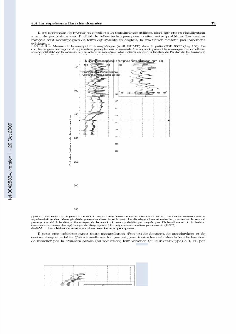
100 150 200 25050
100
150
200
250
300
350
Courbe en gras: Premier passageCourbe en continu: Second passage
Susceptibilité magnétique corrigée à partir du caliper (ppm uSI)
P r o f o n d e u r ( m è t r e s s o u s l e p l a n c h e r o c é a n i q u e )
80 100 120 140 160 180 200 220190
195
200
205
210
215
220
225
230
tel00425334,version1
20Oct2009

7/13/2019 Rabaute Manuscrit de These
http://slidepdf.com/reader/full/rabaute-manuscrit-de-these 70/212
xz
zi =xi − x
sx X s
xi zi
zi =xi − xmin
xmax − xmin
X n m
X X T X T ·X R m× mm
r jk =n
i=1
x jixik
j k
X · X T Qn × n
R
E f U f f (U ) = λU λ U
λ R RU = λU U Rλ R
R m D(λ) = 0det(R − λI ) = 0 R
D(λ) = 0 R
A U V U T ·U = V T ·V = I I V T AU
Λ A λiΛ A λ1 ≥ λ2 ≥ · · · ≥ λn
(u1, . . . , un) U Aλi
R R
SV D
A m × n A U ΣV T U m × m V n × n Σ
diag(σ1, σ2, . . . , σ p) p = minimum(m, n) σ1 ≥ σ2 ≥ · · · ≥ σ p ≥ 0 σi
i = 1, . . . , p A
tel00425334,version1
20Oct2009

7/13/2019 Rabaute Manuscrit de These
http://slidepdf.com/reader/full/rabaute-manuscrit-de-these 71/212
R X X T
m p p = m
U
u211 + u212 + u213 + u214 + . . . + u21m = 1
Y ij (x1,...,xm) X i = 1, n j = 1, m
(u j) U xi
yi1 =m
j=1
u1 j · xij
X · U = Y R
Y R X n × mU
x1,1 x1,2 · · · x1,mx2,1 x2,2 · · · x2,mx3,1 x3,2 · · · x3,m
xn,1 xn,2 · · · xn,m
·
u1,1 · · · u1,m
um,1 · · · um,m
=
y1,1 y1,2 · · · y1,my2,1 y2,2 · · · y2,my3,1 y3,2 · · · y3,m
yn,1 yn,2 · · · yn,m
R = X T ·X X X
λi R
tel00425334,version1
20Oct2009

7/13/2019 Rabaute Manuscrit de These
http://slidepdf.com/reader/full/rabaute-manuscrit-de-these 72/212
m m
x = ln(x/c) c
mm
p
p m p m p
tel00425334,version1
20Oct2009

7/13/2019 Rabaute Manuscrit de These
http://slidepdf.com/reader/full/rabaute-manuscrit-de-these 73/212
tel00425334,version1
20Oct2009
7/13/2019 Rabaute Manuscrit de These
http://slidepdf.com/reader/full/rabaute-manuscrit-de-these 74/212
1
2
3
4
5
6
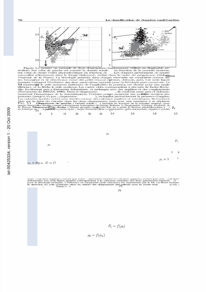
2,4
2,6
2,8
3,0
Pe
ρb
Grès
Dolomie
Calcaire
3,0
2,8
2,4
2,6
ρb
-5 5 15 25 35 45
Φn
C a l c a
i r e
D o l o
m i e
G r è
s
Pôlepyriteux
Pôlepyritique
ρb
P eρb
x y
ρb ≈ 5 3
φn ≈ 30 p.u. P e ≈ 17 −
ρb
ρb
P e = f (ρb)
ρb = f (φn)
tel00425334,version1
20Oct2009

7/13/2019 Rabaute Manuscrit de These
http://slidepdf.com/reader/full/rabaute-manuscrit-de-these 75/212
P e P e = 5.1Ca MgFe CO3 2
ρb = f (φn)P e = f (ρb)
P e
T h = f ( [Al2O3][Al2O3]+[SiO2])
Al2O3
2 × 2
tel00425334,version1
20Oct2009

7/13/2019 Rabaute Manuscrit de These
http://slidepdf.com/reader/full/rabaute-manuscrit-de-these 76/212
0.2 0.25 0.3 0.35 0.4
0
5
10
15
20
Smectite - Montmorillonite
Illite - Muscovite
Al2O3 / (Al2O3+SiO2)
Thorium
(ppm)
dAB
A B
dAB =
mi=1
(xiA − xiB)2
dAB =
mi=1(xiA − xiB)2
m
rAB
tel00425334,version1
20Oct2009
7/13/2019 Rabaute Manuscrit de These
http://slidepdf.com/reader/full/rabaute-manuscrit-de-these 77/212
8
4
31
32
33
17
16
1422
2434
11
10
25
1923
12
9
15
27
35
29
5
321
26
300
1
2
7
36
37
6
18
13
20
0 20 40 60 80
38
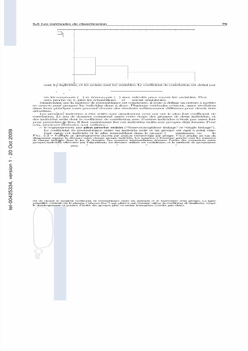
phénon
G1
G2
G3
G4
rAB =
mi=1(xiA − xA)(xiB − xB)
sAsB(n − 1)
xi si rAB
A B
dAB rAB
tel00425334,version1
20Oct2009

7/13/2019 Rabaute Manuscrit de These
http://slidepdf.com/reader/full/rabaute-manuscrit-de-these 78/212
1
n
n × n
k
k n
kk × n k
n
k × n n×n
tel00425334,version1
20Oct2009
7/13/2019 Rabaute Manuscrit de These
http://slidepdf.com/reader/full/rabaute-manuscrit-de-these 79/212
0
5000
1 104
1.5 104
2 104
2.5 104
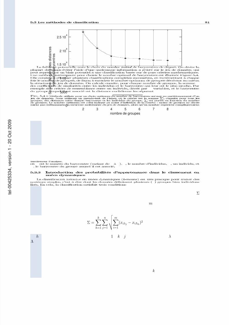
2 3 4 5 6 7 8
Sommeducarrédesdista
nces
individus-barycentres
nombre de groupes
Σ
m
Σ =
kh=1
n j=1
mi=1
(xiλj − xiΛh)2
h 1 k j λΛ
k
tel00425334,version1
20Oct2009
7/13/2019 Rabaute Manuscrit de These
http://slidepdf.com/reader/full/rabaute-manuscrit-de-these 80/212
i 2 ≤ i ≤ k X i = ∅ X i iX
i1 i2 X i1 X i2 = ∅
ki=1X i = X
< 1 >< 0 >
U k × nX i X
ui(x j) = uij =
1 si x j ∈ X i
0 sinon
U x j j = 1, n X kx j k ui
X
J w(U, Λ) =m
j=1
ki=1
(uij)w x j − Λi 2A
w Λi i ΛA
m Ax j Λi
d2ij =
x j
−Λi
2A= (x j
−Λi)
T A(x j
−Λi)
(uij)w d2
x j i uij w wJ w
U , Λ J w
U F kH k
F k(U ) =m
j=1
k
i=1
(uij)2
m
tel00425334,version1
20Oct2009
7/13/2019 Rabaute Manuscrit de These
http://slidepdf.com/reader/full/rabaute-manuscrit-de-these 81/212
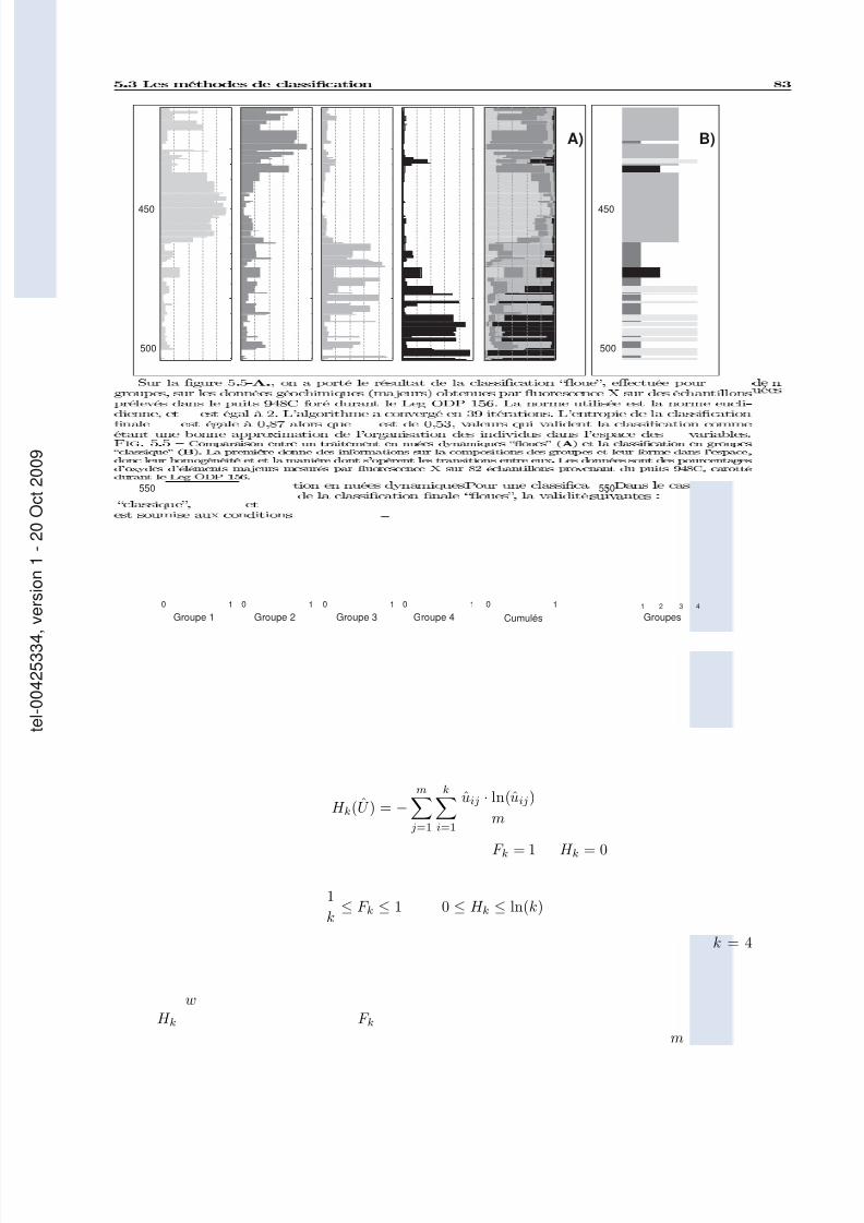
550
500
450
Groupe 1 Groupe 2 Groupe 3 Groupe 4 Cumulés
0 1 0 1 0 1 0 1 0 1
Groupes1 2 3 4
550
500
450
A) B)
H k(U ) = −m
j=1k
i=1uij · ln(uij)
m
F k = 1 H k = 0
1
k≤ F k ≤ 1 0 ≤ H k ≤ ln(k)
k = 4
wH k F k
m
tel00425334,version1
20Oct2009

7/13/2019 Rabaute Manuscrit de These
http://slidepdf.com/reader/full/rabaute-manuscrit-de-these 82/212
Gi Gi
G3G1 G2
G3G2
G4G2
Gi
G4
tel00425334,version1
20Oct2009

7/13/2019 Rabaute Manuscrit de These
http://slidepdf.com/reader/full/rabaute-manuscrit-de-these 83/212
P e ρb
G1P e ρb
G2
tel00425334,version1
20Oct2009

7/13/2019 Rabaute Manuscrit de These
http://slidepdf.com/reader/full/rabaute-manuscrit-de-these 84/212
Fe
Si
S
Peρ
b
Ca
Fe
Si
Ca
ρb
Pe
S
1.0
-1.0
0 -1.01.0
Facteur 1
Facteur2
Facteur 2
Facteur 1
G2
G1
G3
P e ρb
P e
ρb
tel00425334,version1
20Oct2009

7/13/2019 Rabaute Manuscrit de These
http://slidepdf.com/reader/full/rabaute-manuscrit-de-these 85/212
SiO2
Al2O3
Fe2O3
Mg O
Mn O
Ca O
Na2O
K2O
Ti O2
P2O5
Si Al
NaNa
FeMn Ca
Mn Fe MnCO3Ca
2 2 3 2 3 2 2
2
SiCa Fe Al S Ti Gd
tel00425334,version1
20Oct2009

7/13/2019 Rabaute Manuscrit de These
http://slidepdf.com/reader/full/rabaute-manuscrit-de-these 86/212
450
500
550
Groupes1 2 3 4
Unité riche en argiles(teneurs en Si et Al).
L’argile peut être illite ousmectite (teneurs en K et
Fe élevées)
niveau très riche enMn (oxide ou carbonate)
niveau très riche enMn (oxide ou carbonate)
limit e lit hologique
Unité riche en argiles(teneurs en Si et Al)
L’argile peut être illite ousmectite (teneurs en K et
Fe élevées)
Intercalations (groupe 4)de bancs riches en Ca
(calcite)
Informations provenant de lacomposition des barycentres
tel00425334,version1
20Oct2009

7/13/2019 Rabaute Manuscrit de These
http://slidepdf.com/reader/full/rabaute-manuscrit-de-these 87/212
x
x1 · c11 + x2 · c12 + x3 · c13 = y1
x1 · c21 + x2 · c22 + x3 · c23 = y2
x1 + x2 + x3 = 1
C · X = Y X
X = C −1 · Y
xi
j = 1, mi = 1, n
yi =
cijx j Y = CX
X Y Y
X Y Y X E = (Y − Y )T (Y − Y )
E Y Y
X = (C T C )−1C T Y
Y M
Y
X = (C T
M C )−1
C T
M Y
tel00425334,version1
20Oct2009

7/13/2019 Rabaute Manuscrit de These
http://slidepdf.com/reader/full/rabaute-manuscrit-de-these 88/212
M
M =
σ21 0
0 σ2n
σ2i yi
mi=1 xi = 1
xT J n = J T n x = 1 J n (1, 1, . . . , 1)T
f 2
f 2 = (y − C x)T (y − C x) − 2λ(xT J − 1)
xT J
−1
x
x = (C T C )−1C T y + λ(C T C )−1J = x0 + λ(C T C )−1J
x0 x0 = (C T C )−1C T y λ
wi =1
σ2yi −n j=1 x2 j σ2cij
X
xi
P V A R =m
m − 1·
1 −m
j=1
x2 j
tel00425334,version1
20Oct2009

7/13/2019 Rabaute Manuscrit de These
http://slidepdf.com/reader/full/rabaute-manuscrit-de-these 89/212
ASE = m
j=1|x j|− 1
E
SE =
ni=1 e2i
(n − m − 1)
χ2 n − m − 1χ2
M AD =
ni=1 |e j|
n
n+1
yi −m j=1 cijx j = 0 avec i = 1, nm
j=1 x j − 1 = 0
G(X ) = 0 X M
q2 = (X − X 0)T M −10 (X − X 0)
X 0 n + 1 G(X ) = 0q2
q2 = (X
−X 0)
T (X
−X 0)
−2
n+1
i=1
λigi(X )
tel00425334,version1
20Oct2009

7/13/2019 Rabaute Manuscrit de These
http://slidepdf.com/reader/full/rabaute-manuscrit-de-these 90/212
dq2 = dxT [X − X 0 −n+1i=1
λigrad(gi(X ))]
q2 X − X 0 = Hλ H G(X ) λ
λ = (H T H )−1H T (X − X 0)
M 0
X k+1 = X 0 + M 0 · H T k · (H k · M 0 · H T
k )−1 · [H k · (X − X 0) − G(X )]
M = M 0 − M 0 · H T · (H · M 0 · H T )−1 · H · M 0
tel00425334,version1
20Oct2009

7/13/2019 Rabaute Manuscrit de These
http://slidepdf.com/reader/full/rabaute-manuscrit-de-these 91/212
E = 12
o∈Sortie
(do − yo)2
do yo o
≡
wij i j
tel00425334,version1
20Oct2009

7/13/2019 Rabaute Manuscrit de These
http://slidepdf.com/reader/full/rabaute-manuscrit-de-these 92/212
-10
-5
5
10
-10 -5 5 1 0
-1
-0,5
0,5
-10 -5 5 1 0
1
0,5
1
-10 -5 5 1 0
-1
-0,5
0,5
1
-10 -5 5 1 0
0,5
1
-10 -5 5 1 0
0
0,5
1
-3 -2 -1 0 1 2 3
y = λ ·x
tanh
(1, 0)
tel00425334,version1
20Oct2009

7/13/2019 Rabaute Manuscrit de These
http://slidepdf.com/reader/full/rabaute-manuscrit-de-these 93/212
y = 11+e−xi
y = yi(1 − yi)
y = tanh(xi) dy = 1 − y2i
p(ai = 1) =1
1 + e(−1T
xi)
p(ai = 1) i T T ≥ 0
do
yo
E = −
o∈Sortie
do ln(yo) + (1 − do)ln(1 − yo)
∂E
∂yo=
yo − do
yo(1 − yo)
tel00425334,version1
20Oct2009
7/13/2019 Rabaute Manuscrit de These
http://slidepdf.com/reader/full/rabaute-manuscrit-de-these 94/212
yo
yo
γ γ
γ
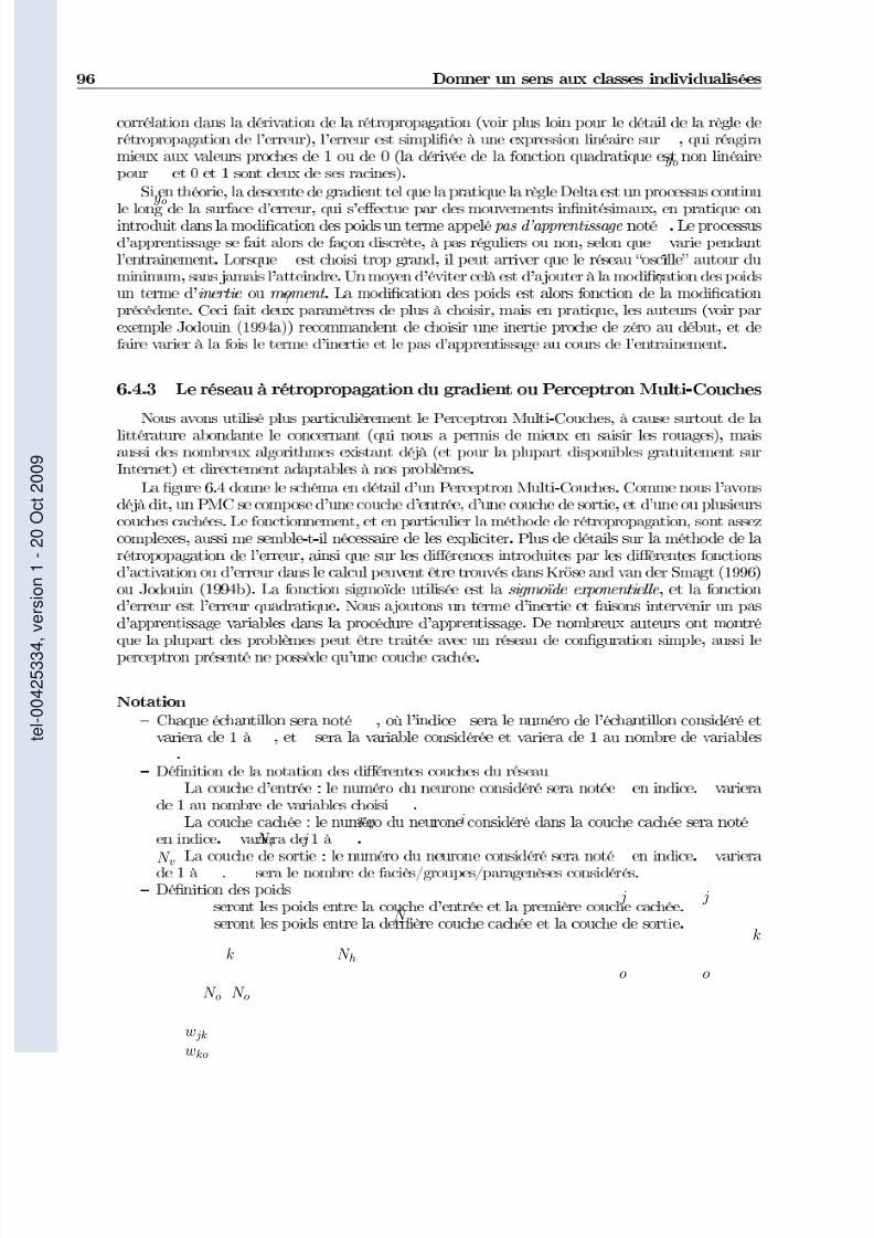
xij i
N i jN v
j jN v
kk N h
o oN o N o
w jk
wko
tel00425334,version1
20Oct2009
7/13/2019 Rabaute Manuscrit de These
http://slidepdf.com/reader/full/rabaute-manuscrit-de-these 95/212
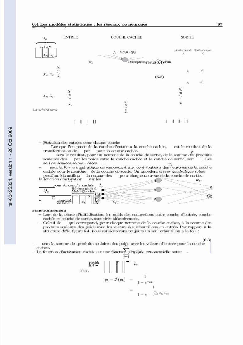
ENTREE COUCHE CACHEE SORTIE
j=1àNv
o=1àNo
xij
x11
x12
x13
x21
x22
x23
Un vecteur d’entrée
pk --> yk = F (pk )
d 1
d 2
i=1 à N i
j=1àNv
k=
1àNh
w jk
wko
Sortie attendue:
d o
Sortie calculée
yo
y1
y2
pk
F
yk
pk F yo
yk wko
do
Qo
o Qi
xi Qo
pk
pk =N v
j=1
xijw jk
F pk
yk = F ( pk) =1
1 − e− pk
=1
1 − e−N v
j=1 xijwjk
tel00425334,version1
20Oct2009

7/13/2019 Rabaute Manuscrit de These
http://slidepdf.com/reader/full/rabaute-manuscrit-de-these 96/212
yo
yo =
N h
k=1
wkoyk
Qo
Qo =1
2(do − yo)2
=1
2(do −
N hk=1
ykwko)2
=1
2
do −
N hk=1
wko
1 + e−N hk=1 pkwjk
2
xi Qi
Qi =N oo=1
Qo
=1
2
N oo=1
(do − yo)2
=1
2
N oo=1
do −
N hk=1
wko
1 + e−N hk=1 pkwkc
2
w jk wko Qi
γ xi
∆iw = −γ ∂Qi
∂w
γ
w jk
∂Qi
∂w jk=
∂Qi
∂pk
∂pk
∂w jk
wko
∂Qi
∂wko=
∂Qi
∂yo
∂yo
∂wko
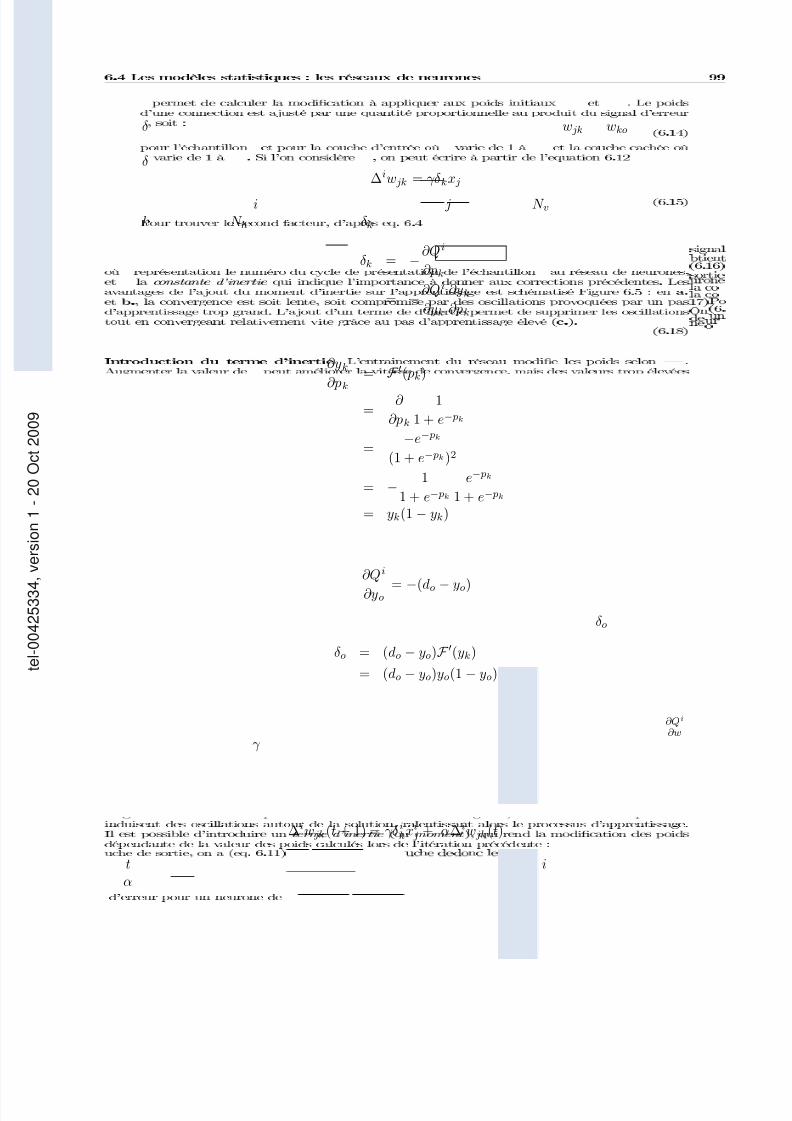
δk
δk = −∂Qi
∂pk
δo =−
∂Qi
∂yo
tel00425334,version1
20Oct2009
7/13/2019 Rabaute Manuscrit de These
http://slidepdf.com/reader/full/rabaute-manuscrit-de-these 97/212
δ w jk wko
δ∆iw jk = γδkx j
i j N vk N h δk
δk = −∂Qi
∂pk
= −∂Qi
∂yk
∂yk
∂pk
∂yk
∂pk=
F ( pk)
=∂
∂pk
1
1 + e− pk
=−e− pk
(1 + e− pk)2
= − 1
1 + e− pk
e− pk
1 + e− pk
= yk(1 − yk)
∂Qi
∂yo= −(do − yo)
δo
δo = (do − yo)F (yk)
= (do − yo)yo(1 − yo)
∂Qi
∂wγ
∆iw jk(t + 1) = γδ ikxi
j + α∆iw jk(t)
t iα
tel00425334,version1
20Oct2009

7/13/2019 Rabaute Manuscrit de These
http://slidepdf.com/reader/full/rabaute-manuscrit-de-these 98/212
a.
b.
c.
solutionminimumrelatif
départ
A.
B.
γ γ
γ
tel00425334,version1
20Oct2009
7/13/2019 Rabaute Manuscrit de These
http://slidepdf.com/reader/full/rabaute-manuscrit-de-these 99/212
x
y
x
1
00 1 0 1
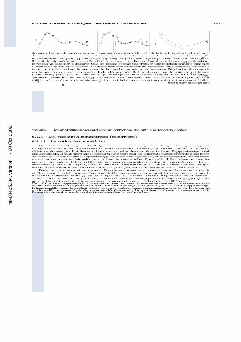
A B C e r r o r
nombre de neurones dans la couche cachée
j e u d e
t e s t
j eu d ’ ap p r ent i ssage
⇒
tel00425334,version1
20Oct2009
7/13/2019 Rabaute Manuscrit de These
http://slidepdf.com/reader/full/rabaute-manuscrit-de-these 100/212
x
yo = c∈
woyc = c∈
woxc
α x
yo =
i
wioxi = wT iox = |x|· wio · cos α
cos αx
x
wv(t + 1) = wv(t) + γ (x(t) − wv(t))
v t∆wo = 0 i
xdo =
n−1i=0 (xi(t) − wio(t))2 xi(t)
i
tel00425334,version1
20Oct2009

7/13/2019 Rabaute Manuscrit de These
http://slidepdf.com/reader/full/rabaute-manuscrit-de-these 101/212
Départ
x1
x2
x3
x4
w3
w 2
w 1
Présentation de x1
x1
x2
x3
x4
w 3
w 2
w1
w' 2
x1
x2
x3
x4
w 3
w' 2
w' 1
w' '2
Présentation de x3
x1
x2
x3
x4
w 3
w1
w' 2
w' 1
Présentation de x2
x1
x2
x3
x4
w 3
w' 1
w' '2
w' 3
Présentation de x4
x1
x2
x3
x4
w' 1
w' '2
w' 3
Après la présentation de4 vecteurs d’entrée:
l’espace des poids s’organise
(x1, . . . , x4) (w1, . . . , w3) x1
w2 x1
x2 x4 w1 w3
x3 w2
tel00425334,version1
20Oct2009

7/13/2019 Rabaute Manuscrit de These
http://slidepdf.com/reader/full/rabaute-manuscrit-de-these 102/212
voisinage carré voisinage hexagonal
V v,1V v,E n
∆wv = γ (v,o,t) · (xi − wv)
wv
γ (o,i,t) = γ (t) · e
−d(o,v)2
2σ(t)2
tel00425334,version1
20Oct2009

7/13/2019 Rabaute Manuscrit de These
http://slidepdf.com/reader/full/rabaute-manuscrit-de-these 103/212
fonction
"chapeau mexicain "
V v,1
σ(t)
tel00425334,version1
20Oct2009
7/13/2019 Rabaute Manuscrit de These
http://slidepdf.com/reader/full/rabaute-manuscrit-de-these 104/212
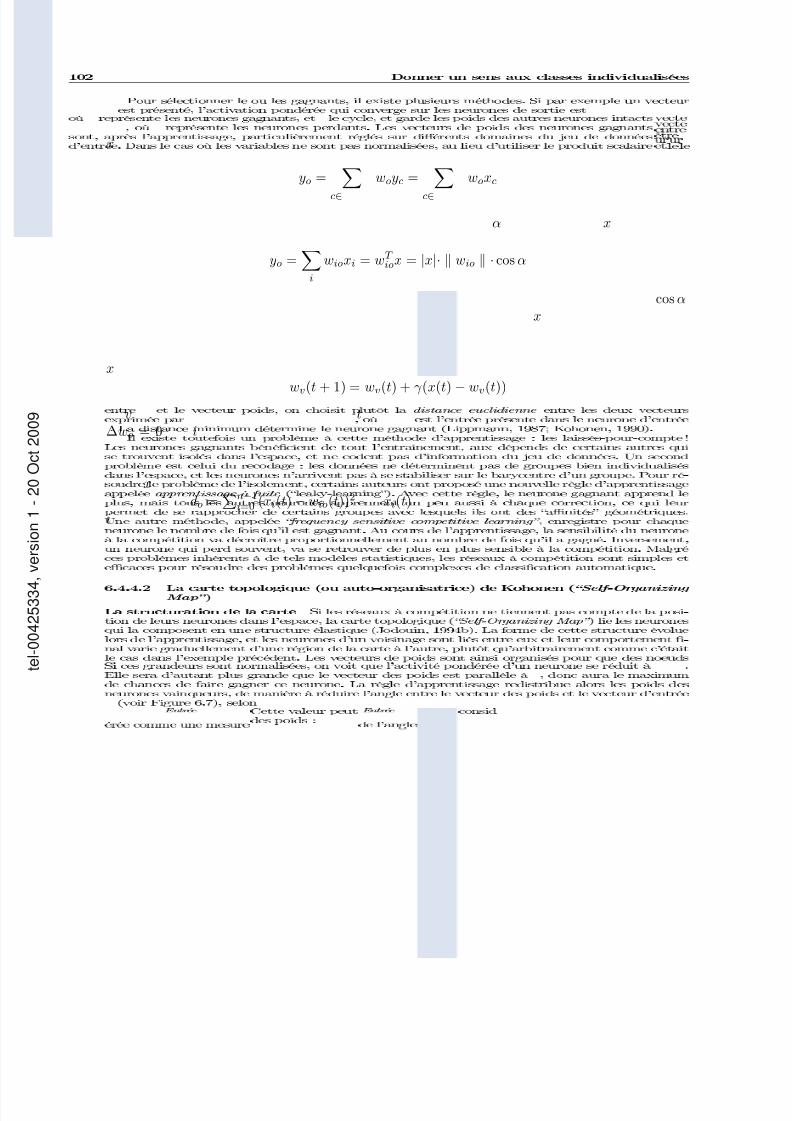
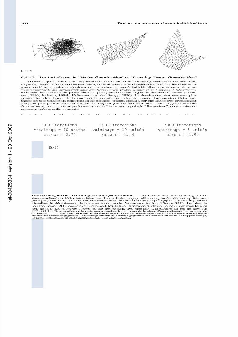
100 itérations
voisinage = 10 unités
erreur = 2,74
1000 itérations
voisinage = 10 unités
erreur = 2,54
5000 itérations
voisinage = 5 unités
erreur = 1,95
15×15
tel00425334,version1
20Oct2009

7/13/2019 Rabaute Manuscrit de These
http://slidepdf.com/reader/full/rabaute-manuscrit-de-these 105/212
yo o
xyo
w x
yk k x
wk(t + 1) = wk(t) − γ (x − wk(t))
yk k x
wk(t + 1) = wk(t) + γ (x − wk(t))
γ t
tel00425334,version1
20Oct2009

7/13/2019 Rabaute Manuscrit de These
http://slidepdf.com/reader/full/rabaute-manuscrit-de-these 106/212
tel00425334,version1
20Oct2009

7/13/2019 Rabaute Manuscrit de These
http://slidepdf.com/reader/full/rabaute-manuscrit-de-these 107/212
tel00425334,version1
20Oct2009

7/13/2019 Rabaute Manuscrit de These
http://slidepdf.com/reader/full/rabaute-manuscrit-de-these 108/212
tel00425334,version1
20Oct2009
7/13/2019 Rabaute Manuscrit de These
http://slidepdf.com/reader/full/rabaute-manuscrit-de-these 109/212
tel00425334,version1
20Oct2009

7/13/2019 Rabaute Manuscrit de These
http://slidepdf.com/reader/full/rabaute-manuscrit-de-these 110/212
tel00425334,version1
20Oct2009

7/13/2019 Rabaute Manuscrit de These
http://slidepdf.com/reader/full/rabaute-manuscrit-de-these 111/212
tel00425334,version1
20Oct2009
7/13/2019 Rabaute Manuscrit de These
http://slidepdf.com/reader/full/rabaute-manuscrit-de-these 112/212
1
To appear in the Geophysical Research Letters, 1998.
Combination of cluster analysis and total inversion of geochemical
data as a advantageous way of inferring mineralogy: Example fromthe North-Barbados accretionary prism, Leg ODP 156.
Alain Rabaute, Louis Briqueu, Mohamed Ramadan
Abstract
In order to infer mineralogy, the total inversion algorithm is used on major oxides weight percent
data measured on samples from cores taken in ODP Hole 948C, North-Barbados accretionary
prism. We show that using at first a simple cluster analysis on the data set helps the total
inversion algorithm to account for varying mineralogy. Each cluster’s centroid provides an
average geochemical composition which can drive the choice for an appropriate a priori mineral
assemblage. The advantages of the total inversion over a classical least-square fitting is the
taking into consideration of the original uncertainties on the input parameters and data. The
calculated error on the a posteriori solution is used to monitor the convergence process in order
to track down the source of potential error.
tel00425334,version1
20Oct2009

7/13/2019 Rabaute Manuscrit de These
http://slidepdf.com/reader/full/rabaute-manuscrit-de-these 113/212
2
Introduction
Laboratory and field devices are capable nowadaysto give precise major elements concentrations from
bulk rock samples. One way for these data to beof any use for the geologist is to be represented interms of an assemblage of mineral and fluid phasesusing various mineral inversion techniques. In case of sedimentary rocks, the problem becomes complex be-cause most encountered minerals have different habitsand origins, such as detrital or secondary authigenic,and can have very heterogeneous geochemical compo-sitions, a good example being clay minerals.
The principal objective of Ocean Drilling ProgramLeg 156 was to evaluate and monitor the effects, ratesand episodicity of fluid flow in an accretionary prismenvironment. Knowing precisely the mineralogy of the sediments is an important parameter to under-stand these effects on the formation. The classical X-ray diffraction method can give qualitative estimatesof mineral abundances, but semiquantitative analy-sis is known to be difficult. Fisher and Underwood
[1995] proposed a mathematical technique using ma-trix singular value decomposition that allows accu-rate conversion of XRD data to relative mineral abun-dances. Despite extremely good results, the authorsacknowledge some limitations to this approach. Thenormalization factors calculated are valid only for theranges of abundances used in the standard mixtures
chosen. Varying chemical compositions could createmismatches in the model. The system needs to befully-determined in order to be solved. In a tentativeto overcome these problems, we propose here to usethe total inversion algorithm [Tarantola and Valette
1982] as a way to calculate mineral abundances fromgeochemical data.
Core sampling and sediment
geochemistry
During Leg 156, 170 metres of marine sediments
were cored in Hole 948C across the decollement zoneof the North-Barbados accretionary prism. The coredsection could be divided into two distinct lithologicalunits, composed of sandy and silty claystones. Theclay minerals that form the background sediment aremostly smectite (Unit I) and illite (Unit II), with somekaolinite. 82 samples, 10 cc in volume, were carefullytaken from the cores, each from a single lithologicvariation. X-ray fluorescence analysis was performedto obtain the concentrations of the 10 common majoroxides CaO, SiO2, Al2O3, Fe2O3, K2O, TiO2, MgO,
MnO, Na2O, P2O5. The precision on these measure-ments are given for each element in Table 1.
Mineral transform
A lot of approaches to the calculation of an accu-rate mode have been investigated over the last thirtyyears, either in the field of algebra such as solvingfor sets of simultaneous equations by matrix inver-sion [Albarede and Provost, 1977]. All of the latterare based on the assumption that a linear relationshipexists between the bulk geochemical composition of asample and the mineral and fluid phases present inthat sample, that can be expressed by
yi =
cij · xj that is Y = C · X
where cij is the weigth percentage of the ith oxide inthe jth constituent phase, xj the proportion of the jth
phase present in the mode, and yi the weight percent-age of the ith oxide in the rock. i = 1, n, where n isthe number of oxides analysed and j = 1, m, where m
is the number of phases present. Moreover, the sumof minerals equals one, as do the sums of the oxideweight percentages in each mineral and in the rock.
The basic limitation becomes now the number of oxides (input responses) available for modelling. Har-
vey et al. [1990] have addressed the problem of under-, over- or fully-determined systems, the latter two
cases describing classical geological systems. Anotherrequirement is to take into account the uncertainties.Both systematic and random errors on the geochem-ical measurements have to be propagated through tothe modal analysis and final solution. The classicalleast squares solution can take into account the uncer-tainties on the measurements yi through a covariancematrix M . Assuming that these errors are indepen-dant and follow a normal law centered on zero, M
is diagonal and is composed of the variances on theinput parameters σ2
1, . . . , σ2n. The least squares solu-
tion, expressed as X = (C T M −1C )−1C T M −1Y , as-
sumes fixed chemical composition of the mineral ma-trix C , which is clearly over-simplifying the problemwhen confronted to clay minerals.
The total inversion algorithm
A different approach consists in solving for n + 1implicit equations using the total inversion algorithmproposed by Tarantola and Valette [1982]. The sys-
tel00425334,version1
20Oct2009
7/13/2019 Rabaute Manuscrit de These
http://slidepdf.com/reader/full/rabaute-manuscrit-de-these 114/212
3
tem can be written as
yi −
m;n
j=1;i=1
cijxj = 0 and
m
j=1
xj − 1 = 0
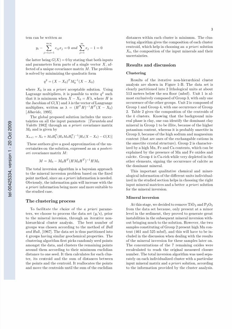
the latter being G(X ) = 0 by stating that both inputsand parameters form parts of a single vector X , af-fected of a unique covariance matrix M . The problemis solved by minimizing the quadratic form
q2 = (X − X 0)T M −10 (X − X 0)
where X 0 is an a priori acceptable solution. UsingLagrange multipliers, it is possible to write q2 suchthat it is minimum when X − X 0 = Hλ, where H isthe Jacobian of G(X ) and λ is the vector of Langrangemultipliers, written as λ = (H T H )−1H T (X − X 0)
[Albarede, 1995].The global proposed solution includes the uncer-
tainties on all the input parameters [Tarantola and Valette 1982] through an a priori covariance matrixM 0 and is given by
X k+1 = X 0 +M 0H T
k (H kM 0H T
k )−1[H k(X −X 0)−G(X )]
These authors give a good approximation of the un-certainties on the solution, expressed as an a posteri-
ori covariance matrix M :
M = M 0 − M 0H T (HM 0H T )−1HM 0
The total inversion algorithm is a bayesian approachto the mineral inversion problem based on the fixedpoint method, since an a priori information is needed.Obviously, the information gain will increase with thea priori information being more and more suitable tothe studied case.
The clustering process
To facilitate the choice of the a priori parame-ters, we choose to process the data set (yi’s), priorto the mineral inversion, through an iterative non-
hierarchical cluster analysis. The best number of groups was chosen according to the method of Ball
and Hall , [1967]. The data set is thus partitioned into4 groups having similar geochemical properties. Theclustering algorithm first picks randomly seed pointsamongst the data, and clusters the remaining pointsaround them according to their minimum euclidiandistance to one seed. It then calculates for each clus-ter, its centroid and the sum of distances betweenthe points and the centroid. It reallocates the pointsand move the centroids until the sum of the euclidian
distances within each cluster is minimum. The clus-tering algorithm gives the composition of each clustercentroid, which help in choosing an a priori solutionX 0, the composition of the input minerals and their
uncertainties.
Results and discussion
Clustering
Results of the iterative non-hierarchical clusteranalysis are shown in Figure 1-B. The data set isclearly partitioned into 2 lithological units at about513 meters below the sea floor (mbsf). Unit 1 is al-most exclusively composed of Group 3, with only oneoccurrence of the other groups. Unit 2 is composed of Group 1 and Group 4, with one occurrence of Group
2. Table 2 gives the composition of the centroids of the 4 clusters. Knowing that the background min-eral phase is clay, one can identify the dominant claymineral in Group 1 to be illite, because of the higherpotassium content, whereas it is probably smectite inGroup 3, because of the high sodium and magnesiumcontent (that are ones of the exchangable cations inthe smectite crystal structure). Group 2 is character-ized by a high Mn, Fe and Ca contents, which can beexplained by the presence of Mn and Fe oxides andcalcite. Group 4 is Ca-rich while very depleted in theother elements, signing the occurrence of calcite asthe dominant mineral.
This important qualitative chemical and miner-alogical information of the different units individual-ized in the studied section helps in choosing the rightinput mineral matrices and a better a priori solutionfor the mineral inversion.
Mineral inversion
At this stage, we decided to remove TiO2 and P2O5
from the data set because, only present at a minorlevel in the sediment, they proved to generate greatinstabilities in the subsequent mineral inversion with-
out bringing much to the solution. However, the twosamples constituting of Group 2 present high Mn con-tent (461 and 525 mbsf), and this will have to be in-cluded in the discussion when dealing with the resultsof the mineral inversion for these samples later on.The concentrations of the 7 remaining oxides wererecalculated to reach the original measured closurenumber. The total inversion algorithm was used sepa-rately on each individualized cluster with a particularinput mineral matrix and a priori solution, accordingto the information provided by the cluster analysis.
tel00425334,version1
20Oct2009

7/13/2019 Rabaute Manuscrit de These
http://slidepdf.com/reader/full/rabaute-manuscrit-de-these 115/212
4
To build the input mineral matrices, we averaged sev-eral compositions of smectites, illites, and kaolinites[Deer, Howie and Zussman, 1967], corresponding tothe environment studied here, and eventually sepa-
rated them into common, Fe-rich, or Mg-rich types.Table 3 shows the averaged mineral compositions usedin the mineral inversion of each cluster that give themost stable results. A slight percentage of Mg in theinput calcite was necessary to account for remainingMg. Despite the fact that the XRD showed no Fe-richphase such as magnetite, we introduced some in theanalysis to take into account the somewhat higher Fecontent of the top unit. This was supported by thehigher magnetic susceptibility measured on the cores[Shipley, Ogawa, Blum et al., 1995]. The plagioclaseis arbitrarily chosen closer to the albite composition(Na-rich).
All the input minerals have uncertainties on each of their oxide content. They are calculated as one stan-dard deviation of all the compositions for this typeof mineral found in the literature. The model needsan a priori solution X 0, which is estimated at first,for each sample, from the compositions of the corre-sponding cluster. An interval of uncertainty aroundeach a priori mineral proportion is also set accord-ing to the level of confidence of our prior knowledge.At last, the model integrate the uncertainties on theinput data, which can be taken from Table 1, or cal-culated over the studied interval.
Figure 1-D, 1-E and 1-G show the way to trackpossible sources of uncertainties and errors duringthe mineral inversion process. At each step of theconverging process, the cumulative difference, withineach cluster and for each input variable (here oxideweight percents), between X and X 0 is recorded (Fig-ure 1-G). If the a priori solution is inappropriate,it is easier to see which element induces the great-est uncertainty. After the algorithm has reached aminimum (step 10), it calculates the a posteriori co-variance matrix M giving the uncertainties on all theinput parameters. Figure 1-D gives an example of
the uncertainties on the final mineral abundances, forillite and smectite. Figure 1-E gives an example of the uncertainties on the elemental abundances (hereAl2O3, Fe2O3 and MgO) in the illite found to be thebest match of the input parameters, the darker theuncertainty, the farther the composition of this illiteis from the original illite as far as this particular el-ement is concerned. As an example, around 465 and530 mbsf, there is a rather large uncertainty on theestimate of MgO in the illite. These two particular
intervals are characterized by a high Mn and Fe con-tents (see Table 2). The analysis was performed againon these two discrete samples with a particular para-genesis that includes a Mn-oxide, needed to account
for the high Mn content (Table 2).Figure 1-C shows the results of the mineral inver-
sion, carried on with the parameters detailed above,on the left. The mineralogy inferred from X-ray dif-fraction [Fisher et al., 1995] is put on the right as areference basis (with keeping in mind that it is onlysemi-quantitative). The resolution is higher in XRDmineralogy column because of the number of sam-ples used, 183 for Fisher and Underwood [1995], and82 on our study. We can see immediately that thedynamics along the hole is preserved, a top homoge-neous unit, with the predominance of smectite, and
a bottom perturbated unit [Shipley, Ogawa, Blum et al., 1995], which is the result of the intercalationof several beds of different mineralogy. The bound-ary between the two lithologic units at 514 mbsf isclearly seen. The overall bulk mineralogy found byboth methods is also comparable. The total inver-sion algorithm sees the occurrence of calcite around450 mbsf and in the bottom unit (from 525 mbsf). Italso finds no more plagioclase in the bottom unit, asthe X-ray diffraction does. However, some discrepan-cies have to be noticed. The mineral inversion finds ahigher illite content in the top unit, while the quartzcontent is lower. We know that volcanogenic rocks
that compose the islands of the Lesser Antilles Arcproduce abundant smectite by weathering [Capet et
al., 1990], and the proximity of this volcanic arc isprobably the origin for the presence of plagioclase andmagnetite in the top unit.
Summary
Coupling statistics, through an Iterative Non-hier-archical Clustering, and probability, through the To-tal Inversion algorithm proved to be a good way todetermine mineral abundances, even in sedimentary
environments. Despite some discrepancies with theX-ray diffraction results, it is possible to have a goodestimate of the total clay content from total inversionof elemental abundances (Figure 1-F). This algorithmprovides uncertainties on all the input parameters,which makes it easier to monitor the behaviour of thelatter during the converging process. It becomes eas-ier to account for element varying concentrations byuse of the classification scheme before performing anymineral inversion. Furthermore, clustering the data
tel00425334,version1
20Oct2009
7/13/2019 Rabaute Manuscrit de These
http://slidepdf.com/reader/full/rabaute-manuscrit-de-these 116/212
5
set prior to the mineral inversion allow to deal witha large number of data, such as when using loggingtechniques. Logging can provide continuous measure-ment of a wide variety of parameters, from density
and porosity to elemental abundances. Being able tocalculate a mineralogy on a continuous basis can helpquantifying the effects of the fluid circulations in thedecollement zone of the North-Barbados accretionaryprism, materialized by the two negative density peaksin Figure 1-A.
Acknowledgments. We are thankful to J. Vernieresfor his useful advices and big help with the fundamentalsof the total inversion algorithm. Also acknowledged is thehelp and contribution of H. Mercadier, and Pierre Gaudonat Ecole des Mines d’Ales, for the X-ray fluorescence tech-nique.
References
Albarede, F., Introduction to Geochemical Modeling ,Cambridge University Press, 1995.
Albarede, F., and A. Provost, Petrological and geo chem-ical mass-balance equations: an algorithm for least-squares fitting and general error analysis, Computers
and Geosciences, 3, 309–326, 1977.
Ball, G.H., and D.J. Hall, A clustering technique for sum-marizing multivariate data, Behavioral Science, 12,153–155, 1967.
Capet, X., H. Chamley, C. Beck, and T. Holtzapffel, Clay
mineralogy of Sites 671 and 672, Barbados Ridge accre-tionary complex and atlantic abyssal plain: paleoenvi-ronmental and diagenetic implications, In Moore, J.C.,Mascle, A., et al., Proc. ODP, Sci. Results, 110, 85–96,1990.
Deer, W.A., R.A. Howie, and M.A. Zussman, Rock-
forming minerals, vol 1–5, Longmans, Green and Coltd(Eds.), 1967.
Fisher, A.T., M.B. Underwood, Calibration of an X-raydiffraction method to determine relative mineral abun-dances in bulk powders using matrix singular value de-composition: a test from the Barbados accretionarycomplex, In Shipley, T.H., Ogawa, Y., Blum, P. andJ.M. Bahr, Proc. ODP, Init. Repts, 156, 29–37, 1995.
Harvey, P.K., J.F. Bristow, and M.A. Lovell, Mineraltransforms and downhole geochemical measurements,Scientific Drilling, 1, 163–176, 1990.
Kohonen, T., Self-organising maps, Springer-Verlag, New-York, 1995.
Lofts, Jeremy C., Intergrated geochemical–geophysicalstudies of sedimentary reservoir rocks, PhD Thesis, 156pp., University of Leicester, UK, February 1993.
Shipboard Scientific Party, Site 948. In Shipley, T.H.,Ogawa, Y., Blum, P. and J.M. Bahr, Proc. ODP, Init.
Repts, 156, 87–192, 1995.
Tarantola, A., and B. Valette, Generalized nonlinear in-verse problems solved using the least squares criterion,Rev. Geophys. and Space Phys., 20, 2 , 219–232, 1982.
A. Rabaute, L. Briqueu, M. Ramadan, UMR
5567–CNRS, ISTEEM, cc 066, Universite Montpel-lier II, 34095 Montpellier Cedex 5, France. (e-mail:[email protected])
This preprint was prepared with AGU’s LATEX macros v4.
File TarVal formatted December 10, 2006.
tel00425334,version1
20Oct2009

7/13/2019 Rabaute Manuscrit de These
http://slidepdf.com/reader/full/rabaute-manuscrit-de-these 117/212
450
500
550
0 .5 1
Groups
1 2 3 4
illite smectite kaolinite quartz plagioclase calcite Fe-oxide
Calculated mineralogy
0 .5 1
XRD mineralogy
1.5 2.1
density (g/cm3)
LWD
12 .5 3 9.6 -6.99 24 .9 1 -0.87 1 0.97Al
2O
3Fe
2O
3MgO
Illite:
450
500
550
illite smectite0 1 0 1
Steps
2
0
-21 2 3 10
SiO2
Al2O
3
Fe2O
3
MgO
CaO
Na2O
K2O
|Sol XRD
-Sol TotalInversio
n|
20
40
60
80
20 40 60 80X-ray diffraction
Totalinversionalgorithm
Dé
collementzone
Mn-oxide
Figure 1: A. Example of Logg ing-While-Drilling (LWD) density measured downhole through the decollement zone o f the North-Barbados accretionary prism.The two negative peaks around 525 mbsf are related to fluid circulations. B. Results of the Iterative Non-hierarchical Cluster Analysis. C. Results of the mineralinversion using the Total Inversion algorithm (left). Mineralogy from quantitative X-ray diffraction performed during Leg 156 (right). D. Example of uncertaintiescalculated on the output mineral abundances. E. Example of uncertainties calculated on the output mineral compositions. F. Comparison of the total clay volumecalculated using mineral inversion and the one found by the quantitative X-ray diffraction method. G. Monitoring of the discrepancy between calculated and inputsolutions throughout the total inversion converging process.

7/13/2019 Rabaute Manuscrit de These
http://slidepdf.com/reader/full/rabaute-manuscrit-de-these 118/212
7
Table 1. Precision Obtained With X-ray FluorescenceAnalysis for the 10 Common Major Elements.
Oxide Precision Oxide Precision
SiO2 0.5% Al2O3 0.5%Fe2O3 0.5% MgO 1.0%MnO 1.0% CaO 0.6%Na2O 5.0% K2O 0.5%TiO2 1.0% P2O5 6.0%
tel00425334,version1
20Oct2009

7/13/2019 Rabaute Manuscrit de These
http://slidepdf.com/reader/full/rabaute-manuscrit-de-these 119/212
8
Table 2. Composition of the Clusters Centroids afterthe Iterative Non-hierarchical Cluster Analysis.
Centroid composition
Oxide Group 1 Group 2 Group 3 Group 4
SiO2 63.0 47.3 59.9 44.2Al2O3 21.2 17.6 20.7 16.4Fe2O3 7.7 9.9 9.4 6.3MgO 2.3 3.1 3.5 1.9MnO 0.1 7.5 0.3 0.6CaO 1.7 9.1 2.9 25.1Na2O 0.2 0.2 1.1 0.1K2O 2.7 1.7 2.1 1.0TiO2 0.9 0.7 0.9 0.6P2O5 0.1 0.3 0.2 0.3
# samples 26 2 38 16
tel00425334,version1
20Oct2009

7/13/2019 Rabaute Manuscrit de These
http://slidepdf.com/reader/full/rabaute-manuscrit-de-these 120/212
9
Table 3. Average mineral compositions chosen as input mineral matrices for total inversion algorithm. Numbersbetween parenthesis are the uncertainty on the element and are calculated as one standard deviation around theaverage composition of all the minerals found in the literature that belongs to the same type. Magnetite is 100%Fe2O3, and Mn-oxide is 100% Mn, both with the same uncertainties as quartz.
Elt Smectites Illites Kaolinite Quartz Plagio CalciteGroup 3 Groups 1,2,4 Group 1 Groups 2,3,4
SiO2 66.7(2.6) 65.4(2.5) 53.6(4.8) 53.2(4.5) 53.3(0.5) 100(0.001) 63.5(0.01) 0(0.001)
Al2O3 25.8(2.7) 23.2(2.7) 30.9(5.3) 27.1(9.6) 45.4(0.7) 0(0.001) 22.4(0.01) 0(0.001)
Fe2O3 1.1(0.5) 3.4(2.7) 4.7(2.2) 8.3(8.0) 0.4(0.4) 0(0.001) 0.5(0.01) 0(0.001)
MgO 4.2(1.1) 4.1(1.1) 1.8(1.1) 2.9(2.2) 0.1(0.1) 0(0.001) 0.1(0.001) 3.0(0.5)
CaO 2.1(0.9) 2.9(0.9) 0.7(0.7) 0.7(0.6) 0.2(0.1) 0(0.001) 3.3(0.5) 97.0(0.5)
Na2O 0.1(0.1) 0.3(0.3) 0.6(0.5) 0.5(0.5) 0.1(0.1) 0(0.001) 9.1(1) 0(0.001)
K2O 0.05(0.01) 0.7(0.7) 7.6(1.8) 7.1(1.9) 0.3(0.2) 0(0.001) 0.9(0.05) 0(0.001)
tel00425334,version1
20Oct2009

7/13/2019 Rabaute Manuscrit de These
http://slidepdf.com/reader/full/rabaute-manuscrit-de-these 121/212
tel00425334,version1
20Oct2009
7/13/2019 Rabaute Manuscrit de These
http://slidepdf.com/reader/full/rabaute-manuscrit-de-these 122/212
Inferring mineralogy with neural network classifier: Example
using Logging-While-Drilling data from Hole 948A, ODP Leg 156
Alain Rabaute∗
en preparation
Abstract
A neural network classifier was used on Logging-While-Drilling data obtained in Hole948A during Ocean Drilling Program Leg 156. This improved logging technique, used for thefirst time in ODP, gives better data because of better hole and measurements conditions. Thenetwork is a classical backpropagation neural network, with a exponential sigmoid activationfunction. The training was done separately on two data sets, made with correspondingLWD intervals chosen after fuzzy c-means classification of 1) X-ray diffraction data and 2)physical properties measurements (grain density, magnetic susceptibility and natural gammaradiation), in order to find the weights corresponding to a minimal quadratic error betweencalculated and desired outputs. These data were measured on the cores from Hole 948C,drilled at the same location as Hole 948A. Better results are obtained when the networkis trained after X-ray diffraction data. A continuous mineralogy is provided, showing agood agreement with the mineral concentrations calculated with a semi-quantitative x-raydiffraction method.
1 Introduction
Logging-While-Drilling technique ODP Leg 156 principal objective was to assess the ex-istence of pore-water overpressure in dcollement zone of the Northern Barbados accretionaryprism. In such an active environment, using wireline logging techniques is quite illusive, and forthe first time in ODP, the improved technique of Logging-While-Drilling was carried out. TheLWD logging string is composed of two logging tools:
• the CDR or Compensated Dual Resistivity tool, which is an electromagnetic propagationand spectral gamma-ray tool built into a drill collar. It is in many ways similar to dual in-
duction tools, responding to conductivity rather than resistivity, and providing two depthsof investigation. But whereas it has a better vertical resolution than dual induction tools,it has a shallower depth of investigation. A 2-MHz electromagnetic wave is sent into theformation, and the tool measures the phase shift (PSR) and the attenuation of the wave(ATR) between two receivers. These quantities are then converted into two independent
0cc066 UMR 5567-CNRS, GGP, ISTEEM, Universite Montpellier II, Place E. Bataillon, 34095 MontpellierCedex 5, France
1
tel0042
5334,version1
20Oct200
9
7/13/2019 Rabaute Manuscrit de These
http://slidepdf.com/reader/full/rabaute-manuscrit-de-these 123/212
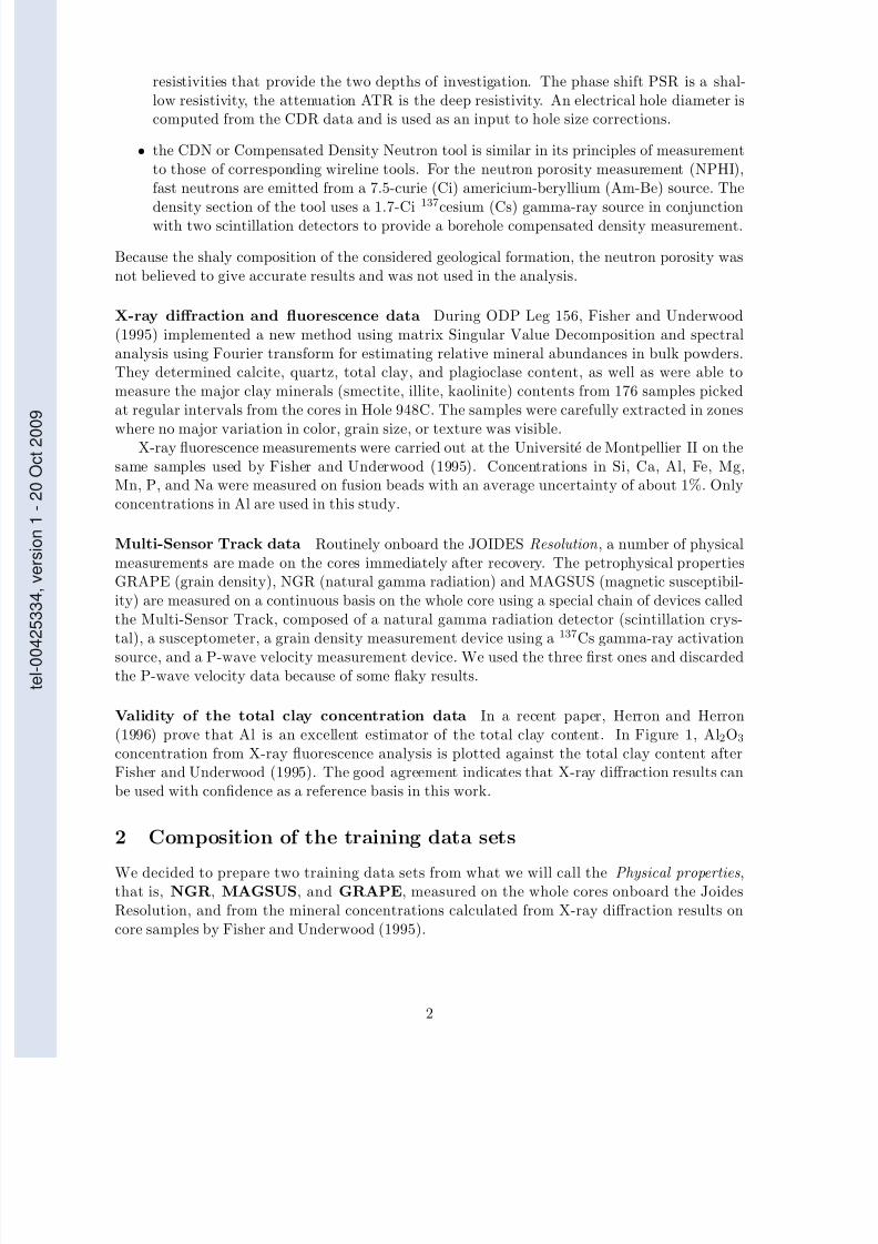
resistivities that provide the two depths of investigation. The phase shift PSR is a shal-low resistivity, the attenuation ATR is the deep resistivity. An electrical hole diameter iscomputed from the CDR data and is used as an input to hole size corrections.
• the CDN or Compensated Density Neutron tool is similar in its principles of measurementto those of corresponding wireline tools. For the neutron porosity measurement (NPHI),fast neutrons are emitted from a 7.5-curie (Ci) americium-beryllium (Am-Be) source. The
density section of the tool uses a 1.7-Ci137
cesium (Cs) gamma-ray source in conjunctionwith two scintillation detectors to provide a borehole compensated density measurement.
Because the shaly composition of the considered geological formation, the neutron porosity wasnot believed to give accurate results and was not used in the analysis.
X-ray diffraction and fluorescence data During ODP Leg 156, Fisher and Underwood(1995) implemented a new method using matrix Singular Value Decomposition and spectralanalysis using Fourier transform for estimating relative mineral abundances in bulk powders.They determined calcite, quartz, total clay, and plagioclase content, as well as were able tomeasure the major clay minerals (smectite, illite, kaolinite) contents from 176 samples pickedat regular intervals from the cores in Hole 948C. The samples were carefully extracted in zones
where no major variation in color, grain size, or texture was visible.X-ray fluorescence measurements were carried out at the Universite de Montpellier II on the
same samples used by Fisher and Underwood (1995). Concentrations in Si, Ca, Al, Fe, Mg,Mn, P, and Na were measured on fusion beads with an average uncertainty of about 1%. Onlyconcentrations in Al are used in this study.
Multi-Sensor Track data Routinely onboard the JOIDES Resolution , a number of physicalmeasurements are made on the cores immediately after recovery. The petrophysical propertiesGRAPE (grain density), NGR (natural gamma radiation) and MAGSUS (magnetic susceptibil-ity) are measured on a continuous basis on the whole core using a special chain of devices calledthe Multi-Sensor Track, composed of a natural gamma radiation detector (scintillation crys-
tal), a susceptometer, a grain density measurement device using a 137Cs gamma-ray activationsource, and a P-wave velocity measurement device. We used the three first ones and discardedthe P-wave velocity data because of some flaky results.
Validity of the total clay concentration data In a recent paper, Herron and Herron(1996) prove that Al is an excellent estimator of the total clay content. In Figure 1, Al2O3
concentration from X-ray fluorescence analysis is plotted against the total clay content afterFisher and Underwood (1995). The good agreement indicates that X-ray diffraction results canbe used with confidence as a reference basis in this work.
2 Composition of the training data sets
We decided to prepare two training data sets from what we will call the Physical properties,that is, NGR, MAGSUS, and GRAPE, measured on the whole cores onboard the JoidesResolution, and from the mineral concentrations calculated from X-ray diffraction results oncore samples by Fisher and Underwood (1995).
2
tel0042
5334,version1
20Oct200
9

7/13/2019 Rabaute Manuscrit de These
http://slidepdf.com/reader/full/rabaute-manuscrit-de-these 124/212
Total clay content (%; from X-ray diffraction)
Al 2O3content(%;from
X-ray
fluorescence)
5
10
15
20
25
20 30 40 50 60 70 80
422,2
433,39
444,72
455,4
464,56
475,77
485,36
493,49
504,27
513,87
526,94
536,52
545,21
552,45
560,97
570,93
578,65
588,27
Illite Smectite Kaol. Illite Smectite Kaol. Quartz Plagio Calcite
d é c o
l l e m e n
t U II
U III
Figure 1: Left: Clay mineralogy and total mineralogy of the cored section in Hole 948C. Right: Comparisonbetween total clay content and aluminium content around the dcollement zone.
5050
Plagioclase
Q u a r t z C
l a y
5050
CalciteCQP1
CQP2
CQP3CQP4
CQPC1CQPC2
CQPC3
CQPC4
CQ1CQ2
CQ3
CQC1CQC2
CQC3
QC1
5050
50
Smectite
KaoliniteIllite
Clay PlagioQuartz Ca lcite
5 8. 2 2 6. 3 5 .3 10 .1
53.8 25 5.6 15.6
40 26.5 2.2 31.4
3 9. 3 2 7. 8 2 .5 30 .4
5050
Plagioclase
Q u a r t z C
l a y
5050
Calcite
AP1
AP2
AP3
AP4
AP5
AP6AP7
AP8
AP9
US1
US2
US3
US4
US5
5050
50
Smectite
KaoliniteIllite
Clay PlagioQuartz Calcite
53.8 25 5.6 15.669.7 26.3 2. 2 1.7
62.8 29.2 7. 1 0.8
Figure 2: Compositions of the 15 groups made after the X-ray diffraction results and of the 14 groups madeafter the fuzzy clustering of LWD physical properties (resistivity, density, photoelectric effect, total gamma ray).
3
tel0042
5334,version1
20Oct200
9
7/13/2019 Rabaute Manuscrit de These
http://slidepdf.com/reader/full/rabaute-manuscrit-de-these 125/212
Code CQP1 CQP2 CQP3 CQP4 CQPC1 CQPC2 CQPC3 CQPC4
section 2X-6 2X-4 9X-1 12X-3 4X-4 5X-4 13X-6 15X-2
interval (cm) 52–54 116–118 94–96 107–109 12–14 47–49 19–21 104–106
depth (mbsf) 428.82 426.46 489.34 521.47 444.72 454.77 534.49 547.94
smectite 50.7 18.5 48.7 0.1 37.6 39.0 15.7 0.1
illite 10.0 54.6 0.0 29.7 13.8 9.2 8.2 18.0
kaolinite 4.0 2.3 6.5 17.1 6.7 5.6 16.0 21.3
total clay 64.7 75.4 55.2 46.8 58.2 53.8 40.0 39.3
quartz 28.9 23.1 28.1 47.7 26.3 25.0 26.5 27.8
plagio 6.4 1.5 16.7 5.5 5.3 5.6 2.2 2.5
calcite 0.0 0.0 0.0 0.0 10.1 15.6 31.4 30.4
Code CQ1 CQ2 CQ3 CQC1 CQC2 CQC3 QC1
section 11X-4 12X-1 16X-2 14X-1 14X-5 17X-4 16X-2
interval (cm) 68–70 79–81 24–26 146–148 61–63 21–23 91–93
depth (mbsf) 512.88 518.19 556.54 537.56 542.71 568.81 557.21
smectite 53.1 26.6 0.0 27.5 2.4 10.1 0.1
illite 9.6 40.3 69.5 0.0 55.0 23.9 0.0
kaolinite 4.2 7.8 13.1 27.0 14.1 8.9 0.0
total clay 66.9 74.6 82.6 54.5 71.5 43.0 0.0
quartz 33.1 25.4 7.4 21.0 20.9 22.2 5.9
plagio 0.1 0.1 0.1 0.0 0.1 0.0 0.0
calcite 0.0 0.0 0.0 24.5 7.4 34.9 94.1
Table 1: Mineral composition of the 15 groups chosen after the X-ray diffraction results.
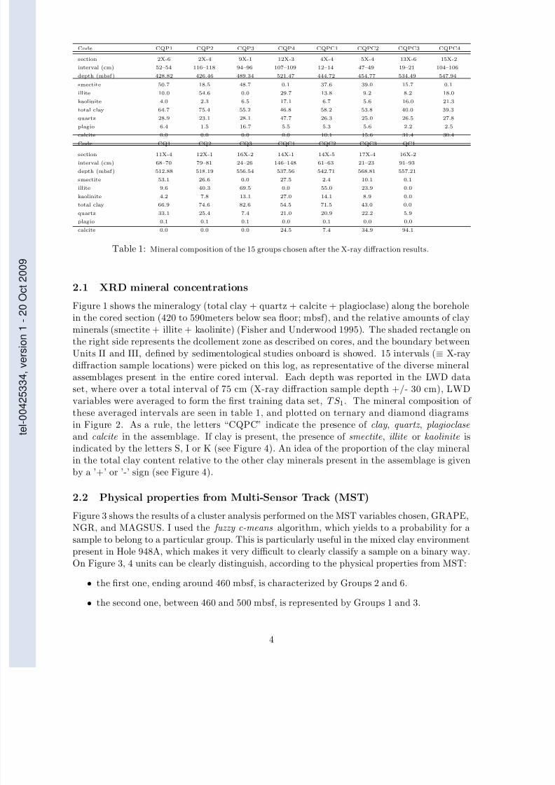
2.1 XRD mineral concentrations
Figure 1 shows the mineralogy (total clay + quartz + calcite + plagioclase) along the boreholein the cored section (420 to 590meters below sea floor; mbsf), and the relative amounts of clayminerals (smectite + illite + kaolinite) (Fisher and Underwood 1995). The shaded rectangle onthe right side represents the dcollement zone as described on cores, and the boundary betweenUnits II and III, defined by sedimentological studies onboard is showed. 15 intervals (≡ X-raydiffraction sample locations) were picked on this log, as representative of the diverse mineralassemblages present in the entire cored interval. Each depth was reported in the LWD dataset, where over a total interval of 75 cm (X-ray diffraction sample depth +/- 30 cm), LWD
variables were averaged to form the first training data set, TS 1. The mineral composition of these averaged intervals are seen in table 1, and plotted on ternary and diamond diagramsin Figure 2. As a rule, the letters “CQPC” indicate the presence of clay , quartz , plagioclase
and calcite in the assemblage. If clay is present, the presence of smectite, illite or kaolinite isindicated by the letters S, I or K (see Figure 4). An idea of the proportion of the clay mineralin the total clay content relative to the other clay minerals present in the assemblage is givenby a ’+’ or ’-’ sign (see Figure 4).
2.2 Physical properties from Multi-Sensor Track (MST)
Figure 3 shows the results of a cluster analysis performed on the MST variables chosen, GRAPE,NGR, and MAGSUS. I used the fuzzy c-means algorithm, which yields to a probability for a
sample to belong to a particular group. This is particularly useful in the mixed clay environmentpresent in Hole 948A, which makes it very difficult to clearly classify a sample on a binary way.On Figure 3, 4 units can be clearly distinguish, according to the physical properties from MST:
• the first one, ending around 460 mbsf, is characterized by Groups 2 and 6.
• the second one, between 460 and 500 mbsf, is represented by Groups 1 and 3.
4
tel0042
5334,version1
20Oct200
9

7/13/2019 Rabaute Manuscrit de These
http://slidepdf.com/reader/full/rabaute-manuscrit-de-these 126/212
Figure 3: Fuzzy clustering on the MST petrophysical properties, GRAPE, NGR and MAGSUS.
5
tel0042
5334,version1
20Oct200
9

7/13/2019 Rabaute Manuscrit de These
http://slidepdf.com/reader/full/rabaute-manuscrit-de-these 127/212
Code AP1 AP2 AP3 AP4 AP5 AP6 AP7
section 2X-1 3X-2 5X-1 5X-4 7X-4 8X-2 9X-4
interval (cm) 146–148 16–18 63–65 47–49 10–12 19–21 59–61
depth (mbsf) 422.26 432.16 450.43 454.77 473.6 480.39 493.49
smectite 32.0 52.8 47.1 39.0 48.0 48.0 48.7
illite 33.7 7.5 8.4 9.2 8.9 5.7 0
kaolinite 4.1 4.0 6.1 5.6 5.9 6.9 5.0
total clay 69.7 64.4 61.7 53.8 62.8 60.6 53.7
quartz 26.3 30.3 27.7 25.0 29.2 29.7 28.4
plagio 2.2 5.3 10.6 5.6 7.1 9.7 17.9
calcite 1.7 0.0 0.0 15.6 0.8 0.0 0.0
Code AP8 AP9 US1 US2 US3 US4 US5
section 10X-2 11X-1 11X-5 12X-3 14X-1 15X-4 16X-2
interval (cm) 51–53 70–72 17–19 27–29 146–148 121–123 91–93
depth (mbsf) 500.11 508.4 513.87 520.67 537.56 551.11 557.21
smectite 45.1 47.9 25.1 26.9 27.5 33.7 0.1
illite 5.2 10.7 39.0 33.5 0.0 20.1 0.0
kaolinite 4.1 4.3 7.5 10.3 27.0 8.2 0.0
total clay 54.3 62.9 71.6 70.7 54.5 72.0 0.0
quartz 27.2 29.4 28.4 29.3 21.0 28.0 5.9
plagio 18.2 7.7 0.1 0.1 0.0 0.1 0.0
calcite 0.0 0.0 0.0 0.0 24.5 0.0 94.1
Table 2: Mineral composition of the 14 groups chosen after the fuzzy clustering results based on MST data.
• the third one, between 500 and 510 mbsf, is mostly marked by Group 6, but with thepresence of all the other 5 groups. We can see this interval as a transition zone. The visualobservation of the cores placed the decollement zone between 498 and 529 mbsf (Shipleyet al. 1995). The upper boundary at about 500 mbsf is clearly seen by the physicalproperties. At 511 mbsf, begins the underthrust section. The “decollement portion” of the underthrust section, seen on the core from 511 to 529 mbsf, is not distinguished bythe physical properties, which suggests that this part his more homogeneous in terms of clay mineral nature (from NGR), layering and depositional texture (from MAGSUS andGRAPE).
• the fourth unit is thus the underthrust section of the prism, very homogeneous becauserepresented almost exclusively by Groups 4 and 5.
From this clustering, we picked by hand 9 locations in the accretionary prism portion (labeledAP1 to AP9) and 5 locations in the underthrust section (labeled US1 to US5). These 14locations are representative of the diversity of the entire interval in terms of group assemblages,and will be our training intervals. Again, as in Section 2.1, each depth was reported in theLWD data set, and the LWD variables were averaged over a 75 cm-interval (MST depth +/- 30cm) to compose the second training data set, TS 2. In table 2 are reported the correspondingmineralogical compositions for each location (according to the closest XRD analyzed sample,see Fisher and Underwood (1995)). In Figure 2, those compositions are plotted in ternary anddiamond diagrams. One can notice that the training intervals AP1 to US5 are far less scatteredthat the training set CQP1 . . . QC1 chosen from XRD results. The cored interval at Site 948 cantherefore be considered more complex in terms of mineralogy and chemistry than it is in termsof physical properties, because the various group assemblages distinguished after the clusteranalysis in Figure 3 show small differences in mineralogy (see Figure 2).
6
tel0042
5334,version1
20Oct200
9

7/13/2019 Rabaute Manuscrit de These
http://slidepdf.com/reader/full/rabaute-manuscrit-de-these 128/212
3 Neural Network analysis
We used a classical backpropagation neural network with a sigmoid transfert function. Beforeusing the network on the entire LWD data set, one has to train it on the corresponding trainingdata set (see Section 2). We took care of not over-training the network, thus 100% of thetraining data below the target error was not required for convergence. The learning rate was setto 0.4 and the momentum to 0.6, and be allowed to vary during the training process, in order to
avoid local minima. Convergence was attained when average error was below 0.05 (5% relativeuncertainty in attributing all training data samples to their corresponding group), and about85% of the training data fell below the target error. After the two training periods, the entireLWD data set was submitted to the net, using independantly the two sets of weights found whentrained with TS 1 and TS 2.
3.1 Results using TS 1
Figure 4 shows the clustering found by the neural net after being trained with the data setmade after mineral compositions. Only 10% of the samples are undetermined. The transitionbetween the accretionary prism and the underthrust section is clearly seen again, beginningat 490 mbsf and ending around 515 mbsf. The accretionary prism is mainly characterized by
CQP1, CQP3, CQPC2 (with also CQPC1, but those two groups are very close in terms of mineralogy), and CQ1. Those groups have in common (see Figure 3) a high clay content (54to 66%), mostly smectite. CQP2, which clay component is mostly illite, occurs throughoutthe accretionary prism but becomes more frequent around 340 mbsf indicating a change in claymineralogy, smectite becoming illite. The underthrust section is characterized by a high calcitecontent (groups CQPC3-4, CQC1-2-3). CQP4, which clay is half illite, half kaolinite, andwith a high quartz content, is appearing and indicates, together with CQ3 and CQPC4, thatsmectite becomes very rare in the underthrust section, being replaced by illite and kaolinite.QC1 indicates almost calcite-pure intervals.
According to the group(s) found by the neural net analysis, we infer the mineral contentsfor each sample. When a sample was found to belong to more than one group, a simple average
was performed between the corresponding mineral contents. Results of this processing for TS 1
is showed in Figures 5.
3.1.1 Whole borehole
• Figure 5-A show the resulting clay minerals, quartz, plagioclase and calcite percentagesfor the entire borehole. Four units can be isolated:
from 0 to 320 mbsf, Unit I is quite stable and is composed on average by 60% clay,25% quartz, 5% plagioclase and some calcite. Some alternance between smectite-rich unitsand illite-rich units can be noted.
then a increase in clay content and a decrease in plagioclase occur between 320 and 400
mbsf (Unit II ). Meanwhile, the quartz content shows higher fluctuations, as clay contentdoes also.
Unit III ends at 480 mbsf and is characterized by 60% total clay content, an increasein plagioclase and quartz contents.
Unit IV runs between 480 until the end of the log. It can be further subdivided inthree parts: subunit IV-1 from 480 to 510 mbsf, with no calcite and a slight increase in clayand quartz content. subunit IV-2 , which shows a lot of fluctuations in mineral contents, a
7
tel0042
5334,version1
20Oct200
9

7/13/2019 Rabaute Manuscrit de These
http://slidepdf.com/reader/full/rabaute-manuscrit-de-these 129/212
0
2
4
6
8
1 0
1 2
1 4
1 6
0
1 0 0
2 0 0
3 0 0
4 0 0
5 0 0
6 0 0
M i n e r a l o g i c a l G r o u p s
D e p t h ( m b s f )
C Q P 1
+ S - I K
C Q P 2
- S + I K
C Q P 3
S K
C Q P 4
I K
C Q P C 2
S I K
C Q P C 3
S I + K
C Q P C 1
S I K
C Q P C 4
I K
C Q 1
+ S I K
C Q 2
- S I K
C Q 3
+ I K
C Q C 1
S K
C Q C 3
S I K
Q C 1
n o c l a y m x
C Q C 2
- S + I K
U n d e t e r m i n e d i n t e r v a l s r e p r e s e n t c a . 1 0 % o f t h e d a t a
0
2
4
6
8
1 0
1 2
1 4
1 6
0
1 0 0
2 0 0
3 0 0
4 0 0
5 0 0
6 0 0
D e p t h ( m b s f )
A P 1
A P 2
A P 3
A P 4
A P 6
A P 7
A P 5
A P 8
A P 9
U S 1
U S 2
U S 3
U S 5
U S 4
P h y s i c a l P r o p e r t i e s G r o u p s
U n d e t e r m i n e d i n t e r v a l s r e p r e s e n t c a . 4 1 % o f t h e d a t a
Figure 4: Results given by the neural network for the two training data sets. The right-hand columns (purple)indicate the samples that the neural network was unable to allocate.
8
tel0042
5334,version1
20Oct200
9

7/13/2019 Rabaute Manuscrit de These
http://slidepdf.com/reader/full/rabaute-manuscrit-de-these 130/212
Figure 5: Mineralogy inferred from the neural network results for the first training data set TS 1. A. cumulativemineral contents. B. Clay minerals contents with respect to total clay content, for the whole borehole. C. Clayminerals contents with respect to total clay content, focused on the dcollement zone (cored section).
9
tel0042
5334,version1
20Oct200
9

7/13/2019 Rabaute Manuscrit de These
http://slidepdf.com/reader/full/rabaute-manuscrit-de-these 131/212
decrease in clay content and runs until 540 mbsf. subunit IV-3 , with almost no plagioclaseand an increase in calcite content.
• Figure 5-B brings some more information by displaying the relative amount of clay mineralswith respect to total clay. The data have been interpolated to give a curve easier tointerpret. The four units described above are easily seen on this figure, and one can evensay that the clay mineralogy variation is one of the major characteristics of the whole
sequence.Unit I clay mineral is mainly smectite, with some illite-rich intervals.
Unit II is an alternance of smectite-rich and illite-rich beds. We note a slight decreasein kaolinite content.
Unit III clay mineral is again essentially smectite. The illite content varies a lotthroughout the unit.
Unit IV shows also 3 different parts characterized by different smectite, illite, andkaolinite contents. The main feature is the sharp decrease in smectite content in subunitsIV-2 and -3, balanced by sharp increases in both kaolinite and illite contents. This wouldplace the actual decollement around 515 mbsf .
• On Figure 5-C, the decollement zone is expanded to show the variations in smectite, illiteand kaolinite content. The sharp boundary between a smectite-rich accretionary prismsection and an illite(kaolinite)-rich underthrust section around 515 mbsf is confirmed. Thevariations in clay mineral content below 515 mbsf seem to be larger above 540 mbsf thanbelow. 540 mbsf seem thus to be the lower limit for the decollement zone. The topof the decollement zone may be seen as the limit between Units III and IV.
3.1.2 Comparison between calculated mineral contents (from neural net analysis)and mineral contents inferred from XRD measurements
Figures 6 show the correlation between the measured mineral concentrations and the neural net
calculated ones. For quartz and clay minerals, the overall trend as well as the scattering of thedata after 515 mbsf is preserved in the calculated concentrations. The neural net confirms alsothat the plagioclase content tends to zero below 515 mbsf. The calcite content was a little bitmore difficult to infer for the algorithm, probably because this mineral is present locally in thinlayers. One observation is the contrast between the two units above and below the decollementzone at 515 mbsf. The neural network has been used on LWD physical properties like density,natural gamma-ray, resistivity, represented by only 15 groups for the whole cored interval, butthe calculated mineral concentrations show the same behaviour as the XRD measured mineralcontents (see Figure 7). This indicates that mineralogical and chemical variations influence suchphysical properties, that can of course be locally the result of tectonic features (thrust at 130mbsf, compaction trend visible on the resistivity profile).
3.2 Results using TS 2
The same analysis was carried out after the network has been trained with the second trainingdata set, composed with LWD intervals found after MST data cluster analysis (see Section 2.2).Figure 4 shows how the whole logged interval has been partitioned into the 14 facies. We noticea very high level of uncertainty as the neural net could not allocate 41% of the data. Anotherobservation is that two groups (AP8 and US1) have not been used at all. We can explain that
10
tel0042
5334,version1
20Oct200
9

7/13/2019 Rabaute Manuscrit de These
http://slidepdf.com/reader/full/rabaute-manuscrit-de-these 132/212
-10 0 10 20 30 40 50 60
400
450
500
550
600
Smectite
D e p t h ( m b s f )
-10 0 10 20 30 40 50 60 70
400
450
500
550
600
Illite
D e p t h ( m b s f )
-5 0 5 10 15 20 25 30
400
450
500
550
600
Kaolinite
D e p t h ( m b s f )
0 10 20 30 40 50
400
450
500
550
600Quartz
D e p t h ( m b s f )
-5 0 5 10 15 20 25
400
450
500
550
600Plagio
D e p t h ( m b s f )
-20 0 20 40 60 80 100
400
450
500
550
600Calcite
D e p t h ( m b s f )
Figure 6: Comparison between the mineral contents found by the neural network and the X-ray diffractiondata..
11
tel0042
5334,version1
20Oct200
9

7/13/2019 Rabaute Manuscrit de These
http://slidepdf.com/reader/full/rabaute-manuscrit-de-these 133/212
by the difference in groups mineralogical composition. The 14 facies individualized after theMST physical properties span a larger range than those found after the X-ray diffraction data(Figure 2). The variations in mineralogy that is visible on the XRD results does not show up inthe physical properties measured on the cores, at least around the decollement zone. Thus thegroups from TS 2 are not representative of the entire logged interval.
3.2.1 Whole borehole
Being made after physical properties, the training set has strongly influenced the mineralogyoutput: the compaction trend is visible, with a sharp decrease in clay content and increasesin plagioclase and calcite contents that mark the thrust at 130 mbsf. The limit at 400 mbsf is still visible, as well as the top of the decollement zone near 490 mbsf. Figure 7 shows thesame separation into different units as in Figure 5, simply the limits between those units arefuzzier, mostly because of high undetermination. Around the decollement zone, the clay mineralscontents show the same pattern as previously: sharp limit at 515 mbsf between the smectite-richaccretionary prism section above and the illite-rich underthrust section below. The decollementportion of this section ends at 540 mbsf with decreasing clay minerals variations.
4 Fuzzy Clustering of the entire LWD data setFigure 8 shows the results of a fuzzy clustering of the entire LWD data set for Hole 948A. Thelimit between the accretionary prism section and the underthrust section is very sharp at 515mbsf, marked by strong proportion of Group 1, and disapperance of Groups 3, 4 and 5. Group 1seems to characterize the tectonic events (thrust at 130 mbsf), so we can guess that something ishappening around 380 and 420 mbsf. The rest of the accretionary prism section shows repetitivealternance of the same units, presumably having the same physical properties.
References
Fisher, A. and M. Underwood (1995). Calibration of an x-ray diffraction method to determinerelative mineral abundances in bulk powders using matrix singular value decomposition: a testfrom the barbados accretionary complex. In Proc. of ODP, Initial Reports, Volume 156, pp.29–37.
Herron, S. and M. Herron (1996, 16-19 June). Quantitative lithology: an application foropen and cased hole spectroscopy. In Transactions of SPWLA Thirty-seventh Annual Logging
Symposium , Number Paper E, New Orleans.
Shipley, T., Y. Ogawa, and P. Blum (1995). Site 948, Hole 948C, Sedimentology chapter. InProc. ODP, Initial Reports, Volume 156.
12
tel0042
5334,version1
20Oct200
9
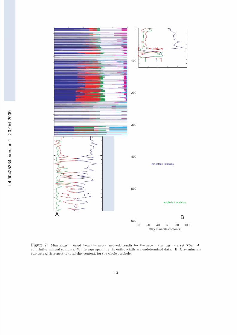
7/13/2019 Rabaute Manuscrit de These
http://slidepdf.com/reader/full/rabaute-manuscrit-de-these 134/212
0 20 40 60 80 100
0
100
200
300
400
500
600
Clay minerals contents
AB
smectite / total clay
kaolinite / total clay
illite / total clay
Figure 7: Mineralogy inferred from the neural network results for the second training data set TS 2. A.
cumulative mineral contents. White gaps spanning the entire width are undetermined data. B. Clay mineralscontents with respect to total clay content, for the whole borehole.
13
tel0042
5334,version1
20Oct200
9

7/13/2019 Rabaute Manuscrit de These
http://slidepdf.com/reader/full/rabaute-manuscrit-de-these 135/212
Figure 8: Fuzzy clustering on the LWD variables, for the whole borehole.
14
tel0042
5334,version1
20Oct200
9

7/13/2019 Rabaute Manuscrit de These
http://slidepdf.com/reader/full/rabaute-manuscrit-de-these 136/212
tel00425334,version1
20Oct2009

7/13/2019 Rabaute Manuscrit de These
http://slidepdf.com/reader/full/rabaute-manuscrit-de-these 137/212
Chypre
Cône du Nil
- 2 0 0
0
- 2 0 0 0
-1000
33°N
35°
34°
31°E 32° 33° 34°
- 2 0 0 0
Mont sous-marin Eratosthènes
Site 968
Site 965
Site 967
Site 966
tel00425334,version1
20Oct2009

7/13/2019 Rabaute Manuscrit de These
http://slidepdf.com/reader/full/rabaute-manuscrit-de-these 138/212
tel00425334,version1
20Oct2009
7/13/2019 Rabaute Manuscrit de These
http://slidepdf.com/reader/full/rabaute-manuscrit-de-these 139/212
tel00425334,version1
20Oct2009

7/13/2019 Rabaute Manuscrit de These
http://slidepdf.com/reader/full/rabaute-manuscrit-de-these 140/212
0 10 20 30 40 50
0
20
40
60
80
100
120
140
160
180
200
Pofondeur(mètres)
Effetperturbateurdutubage
11 13 15 17 19
100
150
200
250
300
350
400
450
500
550
600
Fe (%) Diamètre du puits (pouces)
tel00425334,version1
20Oct2009

7/13/2019 Rabaute Manuscrit de These
http://slidepdf.com/reader/full/rabaute-manuscrit-de-these 141/212
profondeur(mbsf)
110
120
130
140
150
caliper
S/Ca
Th (ppm)
11 19 0 3 0 14
0 10
PEF
K (comptes sur la fenêtrede mesure W3)
Fe (%)Al (%)
Ti (%)
0 5 0 10 0 6
profondeur(mbsf)
110
120
130
140
150
NPHI
30 65
GYPSE
GYPSE
GYPSE
GYPSE
Argiles (Fe-chlorite, illite)
Argiles (Fe-chlorite, illite)
shale ?
Intervalle riche en argilemais le mauvais état dupuits ne permet pas uneinterprétation précise
shale ?
Intervalle riche en argilemais le mauvais état dupuits ne permet pas uneinterprétation précise
Argiles (Fe-chlorite, illite)
Argiles (Fe-chlorite, illite)
tel00425334,version1
20Oct2009
7/13/2019 Rabaute Manuscrit de These
http://slidepdf.com/reader/full/rabaute-manuscrit-de-these 142/212
tel00425334,version1
20Oct2009

7/13/2019 Rabaute Manuscrit de These
http://slidepdf.com/reader/full/rabaute-manuscrit-de-these 143/212
0 40
200
300
400
500
600
Si
P r o f o n d e u r
Ca
0 4 8 12
Fe S
11 13 15 17 19
CALIPER
tel00425334,version1
20Oct2009

7/13/2019 Rabaute Manuscrit de These
http://slidepdf.com/reader/full/rabaute-manuscrit-de-these 144/212
PALEOSURFACE
Hettangien
Trias
?
CARBONIFERE ?
PROFONDEURS ALTITUDE
BA-1
Jurrassique supérieurcarbonaté
Bathonien
Toarcien
Oxfordien
Callovien
Hettangien
Trias
CARBONIFERE
F a i l l e
c o n j u
g u é e
a n t i t h
é t i q u
e
0 100 200 300 m
100
200
300
Echelle
W - NW E - SE
F
a i l l e n o r m
a l e d ’ U z e r
2 2 3 2 2 3 2 3 2
tel00425334,version1
20Oct2009

7/13/2019 Rabaute Manuscrit de These
http://slidepdf.com/reader/full/rabaute-manuscrit-de-these 145/212
Nuées
ILLITE
QUARTZ
FELDSPATH K
PLAGIOCLASE
PYRITE
HEMATITE
ANHYDRITE
CALCITE
DOLOMITE
Résultat de l ’inversion minérale Reconstruction dela lithologie
U. dolomitique
U. argilo-calcaire
dolomitisée
Ensemble
gréso-argileux
à passées
dolomitiques
Ensembleargilo-sulfaté
E. gréso-argileux
E. argilo-gréseux
U. dolomie gréseuse
1700
1560
1420
1280
1140
1000
Ensemble
argilo-calcaire
à passées
dolomitiques
niveaux non
résolus par
l'inversion
minérale
niveau non
résolu par
l'inversion
minérale
Ensemble
marno-calcaire
dolomitisé
q2 = (X − X 0)T M −10 (X − X 0)
X 0
tel00425334,version1
20Oct2009

7/13/2019 Rabaute Manuscrit de These
http://slidepdf.com/reader/full/rabaute-manuscrit-de-these 146/212
2 2 3 2 2 3 3 2
X M G(X ) = 0
tel00425334,version1
20Oct2009
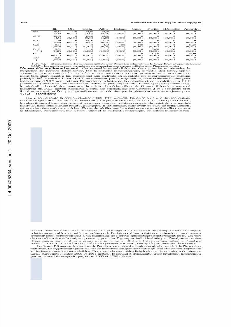
7/13/2019 Rabaute Manuscrit de These
http://slidepdf.com/reader/full/rabaute-manuscrit-de-these 147/212
2
2 3
2
2 3
3
2
tel00425334,version1
20Oct2009

7/13/2019 Rabaute Manuscrit de These
http://slidepdf.com/reader/full/rabaute-manuscrit-de-these 148/212
ILLITE
QUARTZ
FELDSPATH K
PLAGIOCLASE
PYRITE
HEMATITE
ANHYDRITE
CALCITE
DOLOMITE
1000
1100
1200
1300
1400
1500
1600
1700
Porosité neutron
Pe
−
tel00425334,version1
20Oct2009

7/13/2019 Rabaute Manuscrit de These
http://slidepdf.com/reader/full/rabaute-manuscrit-de-these 149/212
−
3 −
|ρcalc−ρb|ρb
tel00425334,version1
20Oct2009

7/13/2019 Rabaute Manuscrit de These
http://slidepdf.com/reader/full/rabaute-manuscrit-de-these 150/212
1350
P r o f o n d e u r ( m )
P r o f o n d e u r ( m )
densité (g/cm3) Feldspath K / Quartz
Z o n e à c i m e n t b a r y t i q u e
1400
1450
1500
1550
1600
1650
2.4 2.6 2.8 3.0 3.2 0 0.2 0.4 0.80.6 1.0 1.2 1.4 1.61700
1350
1400
1450
1500
1550
1600
1650
1700
tel00425334,version1
20Oct2009

7/13/2019 Rabaute Manuscrit de These
http://slidepdf.com/reader/full/rabaute-manuscrit-de-these 151/212
tel00425334,version1
20Oct2009

7/13/2019 Rabaute Manuscrit de These
http://slidepdf.com/reader/full/rabaute-manuscrit-de-these 152/212
tel00425334,version1
20Oct2009

7/13/2019 Rabaute Manuscrit de These
http://slidepdf.com/reader/full/rabaute-manuscrit-de-these 153/212
tel00425334,version1
20Oct2009

7/13/2019 Rabaute Manuscrit de These
http://slidepdf.com/reader/full/rabaute-manuscrit-de-these 154/212
tel00425334,version1
20Oct2009

7/13/2019 Rabaute Manuscrit de These
http://slidepdf.com/reader/full/rabaute-manuscrit-de-these 155/212
tel00425334,version1
20Oct2009

7/13/2019 Rabaute Manuscrit de These
http://slidepdf.com/reader/full/rabaute-manuscrit-de-these 156/212
Pore space components and their partitioning in carbonate rocks
Alain Rabaute, T.S. Ramakrishnan, Stefan Luthi, Marina Polyakov
December 12, 2006
Abstract
Pore space partitioning into different porosity types was carried out on numerous carbonatesamples selected from two wells with diverse sedimentological, petrophysical and petrographic
range. The vuggy fraction of porosity was evaluated from core and plug slabs using a novel butsimple method, while intergranular (“macro”) and intragranular (“micro”) fraction of porositywere estimated by judiciously combining optical microscope (OM) and environmental scanningelectron microscope (ESEM) views of thin sections. Total porosity estimates with the three poretypes compare reasonably well with the conventional He intrusion measurements. In additionto pore type partitioning, pore network characteristics in terms of lithofacies are also identified.The implication of classification to petrophysical data interpretation and transport calculationis briefly discussed.
To be submitted to Journal of Sedimentary Petrology
1
tel00425334,version1
20Oct2009

7/13/2019 Rabaute Manuscrit de These
http://slidepdf.com/reader/full/rabaute-manuscrit-de-these 157/212
Introduction
The petrophysical response and the flow characteristics of carbonate rocks is governed to a largeextent by their sedimentation and diagentic history. While the depositional environment is respon-sible for initial variations in texture, post depositional processes such as dissolution, cementation,and replacement add to the tremendous variability in the pore structure of carbonates (Choquetteand Pray 1970; Lucia 1983; Nurmi 1984; Lucia 1995). For this reason, Dunham (1962) classifiedcarbonates into two groups: (i) where the depositional texture is recognizable and (ii) where it isnot (see Figure 1).
Depositional features of carbonate rocks differ from sandstones since (i) many carbonate sedi-ments are characterized by a bimodal grain distribution (Folk 1959); (ii) organisms play an impor-tant role in producing the sediment both in terms of fossils and fecal pellets; and (iii) much of thecarbonate sediments deposit in shallow water.
Initially, a carbonate deposit may have void space ranging from 60 to 80% of the total volume,often as interparticle porosity (Choquette and Pray 1970; Lucia 1983). Unlike the siliciclastics,the physico-chemical processes following deposition have a tremendous influence in altering themineralogy and the texture, and in the formation of the carbonate rock. The shape and the sizeof the final open network is likely to be heterogeneous and difficult to predict. Pore sizes may varyfrom sub-microns to meters, sometimes only a few feet apart. Pore shapes may be altered due todissolution and/or recrystallization processes.
It is clear that a petrography study of carbonate rocks cannot cover all aspects and featuresthat are likely to be encountered. This is especially true with regards to quantitative partitioningof porosity and pore-types. Our attempt has therefore been to simplify the petrography classesto the essential features that are relevant to transport properties, be it electrical resistivity orpermeability.
1 Geological background
The petrography studies are based on two wells. The cores from the two wells were found to covera broad range of pore types, porosity and permeability.
1.1 Well 1
The lithology consists of mainly crystalline dolomite. The original deposit was as a shelf-margincarbonate, but extensively dolomitized, and mixed with nodules or intercalations of anhydrite. Wewere provided with 39 samples out of a cored interval of about 90 m. The depositional texture isno longer recognizable..
A tight arrangement of euhedral or semi-euhedral crystals of 30–100 µm is evident from the thinsection analysis. The pore space is dominated by intercrystalline and vuggy porosity with minoramounts of microporosity, present as microvugs. Much of the interval has a porosity less than 5%,and the permeability is mostly within 0.1 mD (100nm2). The lower limit of the permeameter thatwe used is 0.01mD (10nm2).
2
tel00425334,version1
20Oct2009

7/13/2019 Rabaute Manuscrit de These
http://slidepdf.com/reader/full/rabaute-manuscrit-de-these 158/212
Classification based on texture (Dunham, 1962)
- Depositional texture recognizable
mud supported grain supported
mudstone wackestone packstone grainstone
contains carbonate mud mud absent
boundstone crystalline carbonate
- Depositional texture non recognizable
Figure 1: The Dunham classification of carbonate rocks
1.2 Well 2
More than a hundred samples of 2 cm diameter from three depth interval groups were collected fromwhole cores. The samples were cut in vertical and horizontal directions at each depth to determineorientation effects if any. The samples spanned a shoaling-upward sequence of mudstones andwackestones to open-marine packstones and grainstones. The cores had suffered little diagenesis.1
The grains are either pellets or bioclasts (algae, foraminifera, globigerinidae), and range from50–200 µm in size. Recrystallisation occurs sporadically and is mostly inside the bioclasts, andoccasionally between the grains.
In this sequence, permeability generally decreases with depth while the porosity shows a slightincreases with depth, consistent with the observed trend in facies of grainstone to mudstone. Localsharp decreases in permeability correspond probably to sea-level fluctuations between the depositionof different sedimentary sub-units inside the sequence.
1In this article, the term diagenesis refers to the natural changes that occur after the deposition of a sedimentand are caused by changes in temperature, pressure, and/or weathering; see Murray and Pray (1965) for exhaustivedefinition.
3
tel00425334,version1
20Oct2009

7/13/2019 Rabaute Manuscrit de These
http://slidepdf.com/reader/full/rabaute-manuscrit-de-these 159/212
2 Pore space partitioning
Quantitative petrography was one of the steps in a sequence of several petrophysical measurements.To ensure that different types of data were obtained on samples of close proximity, we used amultistep sampling procedure. From the whole core, a 3 cm diameter plug was cut orthogonal tothe wellbore. The plug was then slabbed for petrography work, and the butt portion was used tocore a 2 cm cylinder, about 3.75 cm long. The remaining length was used to make thin sections andchips for mercury porosimetery (see Figure 2).
Given that carbonate rocks are extremely complex, any attempt at pore space partitioning islikely to be inexact. Our purpose here was to identify the main types of porosity contributors toenable us to compare them with our petrophysical interpretation and measurements. Since manyof the petrophysical data are sensitive only to gross features, the main emphasis in petrographywas to quantify the three main contributors to porosity. These were namely the intergranular ( f m),intragranular (f µ), and vuggy fractions (f v). The precise definitions of these quantities is elaboratedfurther below. Subtle variations from this gross picture were not taken into account. As illustratedin Figure 2, the three fractions of porosity (f v, f m, and f µ; see Section 2.2 for a definition of thesequantities) are from the slabs and the thin sections, while permeability, capillary pressures, NMRrelaxation, and He porosity are on the plugs. The 2 cm cylindrical core was used for measurementssuch as permeability, resistivity and NMR relaxation. For acoustic velocities, additional larger sizeplugs were cut, whenever it was feasible to do so .
Choquette and Pray (1970) stated the fact that the wide range of sedimentary carbonate par-ticles is one of the reason for the complexity of the carbonates pore space. They proposed a veryprecise classification by focusing on the concept of fabric selectivity , emphasizing the geologicaldifferences between carbonates and siliciclastic rocks porosity origin. They refers to the porosity as fabric selective when a dependent relation can be found between porosity and the fabric elements(i.e., the grains ) and as not fabric selective when such a relation cannot be established easily. Insidethese two broad classes, they distinguished 7 fabric selective pore types (interparticle, intraparti-cle, intercrystalline, moldic, fenestral, shelter, and growth-framework) and 4 not fabric selectivepore types (fracture, channel, vug, and cavern). On top of this classification, they also describedmodifications processes like solution, cementation, or vadose circulation , that can affect widelythe porosity and other petrophysical parameters of carbonates such as permeability or acousticproperties.
Lucia (1983) proposed a simpler classification based more on the petrophysical aspects of thecarbonate pore space components. Three classes of pore types were identified as mainly contribut-ing to the variations observed in the porosity, permeability, capillarity and Archie’s m values:interparticle porosity , defined as pore space between the particles—regardless of the nature of theparticle, pellets, bioclast, or crystal—and all other pore space, called vuggy porosity . He dividedthe latter into touching vugs, which tend to improve the overall connectivity of the pore space, andseparate vugs, which on the contrary, reduce the permeability while increasing the total porosity.
In this study, the pore space component classification is made in a slightly different way. Ourgoal is primarily to be able to account for the variations of such different measurements as acoustics,T2 distribution and permeability, without changing the petrological classification. Further on, wewill refer to ‘grain’ as the elementary particle in a carbonate rock, and will specify as necessary if it is a pellet, a bioclast or a crystal.
4
tel00425334,version1
20Oct2009

7/13/2019 Rabaute Manuscrit de These
http://slidepdf.com/reader/full/rabaute-manuscrit-de-these 160/212
f v
f m
f µ
Figure 2: Method of extraction of the three fraction of porosity — f v, f m, and f µ — from plugs, slabs and thinsections taken out from whole cores. For each sample, the thin section was made from the bottom or the top of theplug, thus allowing direct comparison between petrophysical measurements from plugs and quantities extracted fromimage analysis on thin section views.
5
tel00425334,version1
20Oct2009

7/13/2019 Rabaute Manuscrit de These
http://slidepdf.com/reader/full/rabaute-manuscrit-de-these 161/212
2.1 The concept of fraction of porosity
For simplication purpose, we have broken the total volume of the rock into three volume fractions :
• the vuggy fraction, noted f v, which is the volume occupied by the vugs. We are not yetdiscerning between touching or non-touching vugs, and we will call vug a pore that we caneasily see with the naked eye.
• the macro fraction, noted f m, which can be assimilated to the volume between the grains.
• the grain fraction, noted f g, which is the volume occupied by the grains.
These three quantities verify the simple relation:
f v + f m + f g = 1
Let φv and φm be the intrinsic porosities of respectively a vug and a macropore. We can writethat:
φv = φm = 1
A simple formula can link these three quantities to the total porosity φT :
φT = f v + f m + f gφµ
where φµ is the intrinsic porosity of the grain, or intrinsic microporosity . The fraction of microp-orosity f µ is then:
f µ = f gφµ
Further on, the raw fractions determined from Petrographic Image Analysis will be noted asf v, f m and f µ to emphasize that they are non corrected fractions. In Section 3.2.4, we explain howto correct the raw numbers in order to come back to the general notation defined above.
2.2 Definitions
As we are using Image Analysis to quantify the fractions of porosity, the critical parameter will bethe size of the pore. The following size thresholds are used:
• vuggy fraction: all pores larger than 200µm in size, that can easily be seen with the nakedeye.
• macro fraction: all pores between 200µm and 7µm in size, seen on thin section using anoptical microscope.
• micro fraction: all pores smaller than 7µm in size.
As the only criteria is the size, there is a need to define carefully the different pore types thatwe are using, not only on a geological aspect, but also on a petrophysical aspect.
6
tel00425334,version1
20Oct2009

7/13/2019 Rabaute Manuscrit de These
http://slidepdf.com/reader/full/rabaute-manuscrit-de-these 162/212
0
5
10
15
20
25
30
1 1.2 1.4 1.6 1.8 2
C o u n t
0
5
10
15
20
1 1.2 1.4 1.6 1.8 2
Figure 3: Example of different vug shape. Both samples are taken from the Well 1 core set. Sample 08 has roundedseparate vugs, most of them having a pore shape between 1.1 and 1.2 (dashed lines are 25% and 75% of the data).Sample 34 shows very connected vugs, most of them having a complicated shape of 1.1 to 1.35, but reaching almost1.9.
7
tel00425334,version1
20Oct2009

7/13/2019 Rabaute Manuscrit de These
http://slidepdf.com/reader/full/rabaute-manuscrit-de-these 163/212
2.2.1 Vuggy pore space
Choquette and Pray (1970) proposed a quite restrictive definition of a vug, as it is a pore “(1)
somewhat equant, or not markedly elongate, (2) large enough to be visible with the unaided eye,and (3) does not specifically conform in position, shape or boundaries to particular fabric elementsof the host rock (i.e., is not fabric selective)”. They distinguished it from a mold, which is theremoval of a former individual constituent from the host rock, and is thus considered as being fabricselective. In fact, a solution-enlarged mold, as long as its precursor’s identity is lost, may be calleda vug.
Lucia (1983) assimilated all “pore space larger than or within the particles of rock and commonlypresent as leached particles, fractures, and large irregular cavities” to a vug. These pore types,completely different in a geological sense, are indeed playing a similar role in terms of flow propertiesof the rock. Lucia (1983) then distinguished between touching vugs and separate vugs. He statedthat the effect of adding separate vugs to a non vuggy rock is to increase the porosity, with little or
no increase in permeability. On the other hand, adding touching vugs will give a higher permeabilitythan expected if all the porosity were interparticle.
Figure 3 shows two samples from Well 1. Sample 08 has a vuggy fraction f v equal to 5%, whilesample 34 vuggy fraction is 10%. The difference stands in the shape of the vugs. The pore shape
γ is a parameter defined by Anselmetti et al. (1996) as:
γ =Perimeter
2√
πArea
normalized to give a convenient value of 1 for a circle. It has a value of 1.9 for an interparticle porebetween spherical grains, and cracks or fractures may have values of γ > 5.
It is obvious in Figure 3 that most of the vugs in sample 08 areseparate
vugs, while they aremore connected in sample 34. This is confirmed by the distribution of the pore shape for the twosamples, showed below each slab picture. Most vugs in sample 08 have a shape between 1.1 and1.2, which is those of an elongated circle. The shape of most vugs from sample 34 is between 1.1and 1.4, but can be 1.8, which is those of an interparticle pore (see above). This difference in theshape of the pore will matter in acoustics because this petrophysical measurement is sensitive to the
shape, acoustics, and we will have to discuss the results qualitatively. In the case of T2 distributionhowever, the volume of the pore is the important criteria, and thus the way we measure the vuggyfraction of porosity will be valid.
2.2.2 Interparticle pore space
As the criteria in also the size, interparticle porosity will be the pore space between the grains. Thenature of the grain (pellet, bioclast, crystal) will not be taken into account although it can be of some importance in acoustics or NMR, and will then be considered as a qualitative variable. Inthe case where the grains are micritized, and the interparticle pore space is filled with micritizedmatrix, all the pore space will be accounted as microporosity (see below).
2.2.3 Intraparticle pore space
Intraparticle porosity will be the pore space inside the grains. Again, describing the shape andnature of these pores will result in a qualitative parameter. Samples from Well 1 presents isolated
8
tel00425334,version1
20Oct2009

7/13/2019 Rabaute Manuscrit de These
http://slidepdf.com/reader/full/rabaute-manuscrit-de-these 164/212
rounded solution-induced micropores that we can define as microvugs (see Choquette and Pray(1970) for a first use of this term), while in samples from Well 2, the microporosity forms a
complicated network due to the micritization of the grains. The microporous network is connectedthrough the interparticle pore space if present (in the case of a grainstone), or forms a one–scalenetwork if this space if filled with micritized matrix (case of mudstone).
3 Pore space component measurements
3.1 Data acquisition
We used the standard approach followed by Anselmetti et al. (1996), with some changes andimprovements, and introduced the determination of the vuggy fraction f v from rock slabs.
As explained in Figure 2, from the original 2” diameter plug drilled from the whole core, aslab face is cut and a 1” diameter plug sub-cored. The latter is devoted to the measurementsof petrophysical properties, while the slab is used to measure f v. 30 µm-thick thin sections wereprepared from the end pieces of the 1” diameter plugs, after impregnating them with blue-dyedepoxy (see also Ehrlich et al. (1991), Gerard et al. (1992)).
3.1.1 Determination of f v
Well 1 The slab face is polished on a grounding wheel in order to obtain a uniform color onits surface. Then we use red Play-Doh paste to fill the vugs. The filling is made in such a waythat we have at the end a flat surface with the vugs in red, and the polished rock in a contrasteduniform color. We will refer to this technique throughout this article as the “silly putty” technique.The crystalline dolomite from allows polishing and filling without modifying shape and size of the
vugs. We then digitize the surface in a 24 bits color image file using a regular flatbed scanner, ata resolution of 300 dpi.
Well 2 Vugs are present during a few feet at the top of the sequence. The loose texture of thesecarbonates make it very difficult to use the slab method because polishing and filling operationscan result in enlarging the vug, destroying together its original shape and size. We decided to useas a rough approximation the CT Scan images.
3.1.2 Determination of the interparticle and intraparticle fractions of porosity
Well 1 Interparticle and intraparticle pore networks are very well individualized both in size,
location and shape in samples from Well 1. We used the Optical Microscope (equipped with aToshiba CCD camera) to characterize the macroporosity. In order to avoid bias, we took 6 viewsrandomly distributed across each thin section, using a x5 magnification objective. In case of athin section presenting a big heterogeneity in the size and location of the macropores, we took 5additional views at lower magnification (x1). A good contrast between pore space and solid phaseis provided by the blue-dye epoxy filling the pore space.
We used the Environmental Scanning Electron Microscope (ESEM) to characterize the mi-croporosity, by taking 10 “pseudo-random” image views at a magnification of x2000 (the term“pseudo-random” means that the original locations of the views were randomly taken, but thenadjusted to avoid the presence of macropore in the views). The contrast between pore space and
9
tel00425334,version1
20Oct2009

7/13/2019 Rabaute Manuscrit de These
http://slidepdf.com/reader/full/rabaute-manuscrit-de-these 165/212
solid phase is mainly a density contrast between the two phases (the epoxy appearing black whilethe rock is grayish). The pore space present in the image is f µ.
Well 2 The two types of pore space seen in the thin section i.e., inter (macro) and intragran-ular (micro) are not easily distinguished, especially based on size alone. In a grainstone, thedistinction is made depending on whether the pores exist between grains or within grains. In awackestone/packstone, one has to clearly identify the grain first, and then make a judgement onwhether the pore is within the grain or outside. Normally when micrite particles partially fill the in-terparticle pore space, we assign the porosity among the micrite particles to be intragranular. Thismethod of partitioning was chosen not from a geological point, but from a petrophysical and trans-port calculation view. The quantification presented here maps easily to a simple, but consistentpore structure model that enables us to predict resistivity and permeability (see chapter xxx). Byno means is this a rigid and complete framework for predicting flow behavior of these rocks. Occa-
sionally deviations between predicted and observed petrophysical properties are explained throughqualitative description of features that are not quantifiable through the classification employed here.
Because of the micritization of the grains and of the matrix, the measurement of the macrofrac-tion of porosity from Optical Microscope views of thin sections will suffer a big uncertainty. In fact,the optical method uses transmitted light, thus penetrating the entire 30 µm of the thin section,and the small micrite particles (4 to 10 µm) are diffusing the incoming light, greatly lowering thecontrast between the blue-dye epoxy and the rest of the thin section. In order to avoid bias weacquired 6 randomly distributed views (24 bits RGB color) at x5 magnification.
The similarities in size and shape of the interparticle and the intraparticle pore networks preventto use the ESEM to simply count the microporous space. We chose to use the ESEM at a lowermagnification (x300) and to measure the total image porosity , which can be symbolized by φI . The
image view at that magnification is a square of 320x320 µm and thus includes both interparticleand intraparticle networks. 10 randomly distributed views were taken across the thin section, andtheir results averaged to give a value of φI .
In all cases, the final value for the fraction of porosity was obtained by averaging the resultsfrom the several views acquired across the thin section.
3.2 Petrographic Image Analysis
We used a standard image processing package (such as Adobe Photoshop + NIH Image). Theacquired digital images are then binarized into a pore space and a solid/matrix phase, using a
simple threshold . The fidelity of the thresholded image is verified by visual comparison with theoriginal image. Each particle (= pore) is individualized, and occasionally slight noise removal andsmoothing was applied. Several parameters are then computed for each particle, such as area ,perimeter , major and minor elongation axis. The sum of areas of all the particles in an imagerepresents an estimate of the pore space and is noted A pores.
3.2.1 Slab face scanning image processing
Red paste was chosen to fill the vug because this color is absent in the range of color of carbonaterocks. In a 24 bits RGB color image, each pixel has a value from 0 to 255 for Red, Green and Blue.
10
tel00425334,version1
20Oct2009
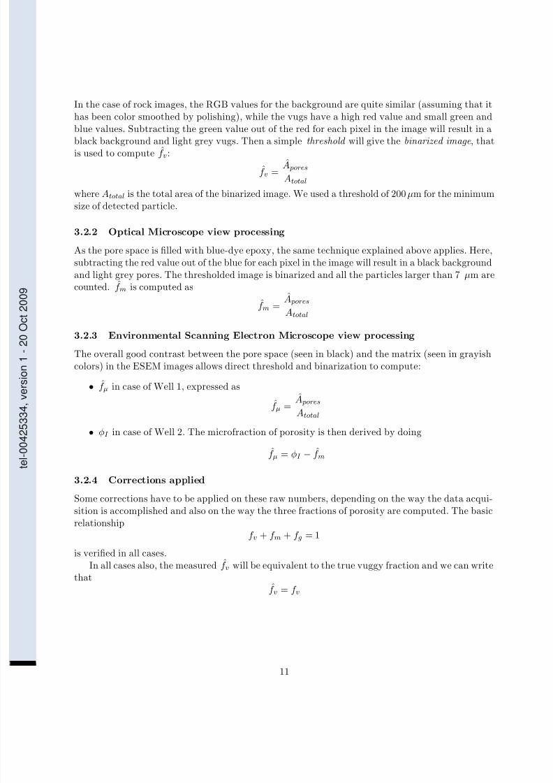
7/13/2019 Rabaute Manuscrit de These
http://slidepdf.com/reader/full/rabaute-manuscrit-de-these 166/212
In the case of rock images, the RGB values for the background are quite similar (assuming that ithas been color smoothed by polishing), while the vugs have a high red value and small green and
blue values. Subtracting the green value out of the red for each pixel in the image will result in ablack background and light grey vugs. Then a simple threshold will give the binarized image, thatis used to compute f v:
f v =A pores
Atotal
where Atotal is the total area of the binarized image. We used a threshold of 200µm for the minimumsize of detected particle.
3.2.2 Optical Microscope view processing
As the pore space is filled with blue-dye epoxy, the same technique explained above applies. Here,
subtracting the red value out of the blue for each pixel in the image will result in a black backgroundand light grey pores. The thresholded image is binarized and all the particles larger than 7 µm arecounted. f m is computed as
f m =A pores
Atotal
3.2.3 Environmental Scanning Electron Microscope view processing
The overall good contrast between the pore space (seen in black) and the matrix (seen in grayishcolors) in the ESEM images allows direct threshold and binarization to compute:
• f µ in case of Well 1, expressed as
f µ = A pores
Atotal
• φI in case of Well 2. The microfraction of porosity is then derived by doing
f µ = φI − f m
3.2.4 Corrections applied
Some corrections have to be applied on these raw numbers, depending on the way the data acqui-sition is accomplished and also on the way the three fractions of porosity are computed. The basicrelationship
f v + f m + f g = 1
is verified in all cases.In all cases also, the measured f v will be equivalent to the true vuggy fraction and we can write
thatf v = f v
11
tel00425334,version1
20Oct2009

7/13/2019 Rabaute Manuscrit de These
http://slidepdf.com/reader/full/rabaute-manuscrit-de-these 167/212
Well 1 We measure the interparticle porosity in the thin section, assuming that there is no vugpresent in the image. Thus the true value of the macrofraction of porosity is
f m = f m(1− f v)
In the same way, by avoiding interparticle porosity, the measure fraction f µ is the intrinsic
microporosity of the grain/crystal, noted φµ (see Section 2.1). Then, the true microporosity is:
f µ = f µ(1− f m − f v) = φµ(1− f m − f v)
The corrected total image porosity φT PIA , comparable to the total Helium porosity φHe measuredon plugs, will be
φT PIA = f v
f v
+ f m(1− f v)
f m
+ (1− f m(1− f v) − f v)
f g
f µ
Well 2 The interparticle fraction of porosity f m is measured on thin section, assuming that thereis no vugs present. As in the case of Well 1, f m will be
f m = f m(1− f v)
We measure the total image porosity noted φI , from the ESEM view at magnification x300. Wecan say that
φI = f m + f gφµ
The true microfraction of porosity noted f µ is then:
f µ = f gφµ = φI − f m(1− f v)
The corrected total image porosity φT PIA , directly comparable to the total Helium porosity φHe ,is
φT PIA = φI + f v
4 Results and discussion
4.1 Well 1
Comparison between φT PIA and φHe . φT PIA obtained from Petrographic Image Analysis
show a good agreement with the conventional method (Helium volumetry), which validates thepartitioning of the porosity into three volume fractions. Most of the samples where f v representsmore than 25% of φT PIA fall away from the 1:1 line, this discrepancy possibly being the result of bad statistics during the measurement of f v (we have only one measurement of f v from one slabface). Another source of error is the assumption of an isotropy in the third dimension by plottingthe fractions measured on 2D sections with volumes (Helium porosity).
12
tel00425334,version1
20Oct2009

7/13/2019 Rabaute Manuscrit de These
http://slidepdf.com/reader/full/rabaute-manuscrit-de-these 168/212
Correlation between total porosity and permeability. Solving the differential equationsallows to find the effective permeability of a medium with a specified f v, that is
k = km1− 3f v
As demonstrated in Chapter XXX, km can be expressed as follows:
km = K · φminterparticle · r2
Where K is a constant, m is the cementation exponent, and r is the average size of the interparticlepores. As φinterparticle = φm = φT He − f v, we can write
km = K · (φT He − f v)m · r2
In order to simplify, r is considered constant for a given lithotype, and m is roughly equal to 2. k
is plotted as
k(1− 3f v) = f (φT He − f v)2
The permeability k plotted against φHe correlate fairly well, showing idealy that estimating f vallows to consider the medium as a single pore type network, where the behaviour of the petro-physical properties is easier to model.
4.2 Well 2
Comparison between φT PIA and φHe . φT PIA is in good agreement with φHe . To evaluatef v, and because the results given by the “silly putty” technique were suffering from too muchuncertainty, we used CT Scan images that we analyzed exactly in the same way as our OpticalMicroscope images. However, these images were taken at a quite large interval (0.5 to 1 foot), and
at different depth than the samples’. Considering the common heterogeneity of this pore type,inferring a possible vuggy fraction for the depth locations of our samples is difficult and can revealitself inaccurate. That leads to the uncertainty affecting the samples which present vuggyness.
Considering the evolution of the three fractions of porosity according to depth in Well 2, themicrofraction of porosity f µ is increasing with depth, as the intergranular fraction f m is decreasing,as expected in a shoaling-upward sequence. f v is a rough estimate and only present in the grainstoneat the top of the sequence. The agreement between φHe and the sum of the three fractions of porosity is better at the bottom of the sequence (mud-supported lithotypes). This is due to theuncertainty on the measurement of f m, which is much larger than those of f µ (due to the techniqueof measurement; see Section 3.1.2). The grain-supported lithotypes having by definition a larger f m,the total uncertainty on the measurement of φT PIA is larger than for the mud-supported lithotypes.
Correlation between total porosity and permeability. Despite a larger scattering of the Petrographic Image Analysis data, it is obvious that there is strong textural dependence of
permeability . The porosity of the mud-supported lithotypes (wackestones and mudstones) is mainlysupported by a single pore-type network. Since all intergranular pore space has been filled bymicritic cement (with microporosity) or sparite cement (without microporosity), the resulting porenetwork is intergranular, where the grain is here a micrite particle, leading to a direct correlationbetween k and the total porosity. The grain-supported lithotypes (grainstones and packstones)have a two-pore types network, inter- and intra granular. k is then not directly dependent on thetotal porosity.
13
tel00425334,version1
20Oct2009

7/13/2019 Rabaute Manuscrit de These
http://slidepdf.com/reader/full/rabaute-manuscrit-de-these 169/212
Fractions of porosity and lithotypes Observation and description of the thin sections withboth the Optical and the Environmental Scanning Electron microscope lead to the classification of
the 53 samples into the 4 basic carbonates lithotypes defined by Dunham in 1962 (See Figure 1).The scattering of the data around the 1:1 line, illustrating the fact that the way we measure f mis quite inaccurate, is however less when going from the grainstone lithofacies, to the mudstonelithofacies, that is when the part of f m in the total porosity is decreasing.
4.3 Implications for NMR relaxation in carbonates
Two common assumptions are made in sandstones for interpretation of NMR relaxation. The firstis that magnetization relaxation in each pore is controlled by surface relaxivity (Sen et al. 1990;Kleinberg et al. 1994), i.e. V sρ
D 1, where D is the molecular diffusion coefficient, ρ the surface
relaxivity and V s the pore volume-to-surface ratio. The characteristic transverse relaxation constantfor the pore then becomes
1T 2
= 1T 2b
+ ρV s
where T 2b is the bulk relaxation of the fluid. Its effect is normally ignored, since it can be easilyaccounted for (Wilkinson et al. 1991). The second assumtion is that in multipore systems, eachpore act independently, and that the measured magnetization is an integral response of all thepores.
In carbonates, especially in grainstones and packstones, these assumptions fail due to significantdiffusion of magnetic moments between inter- and intra-granular pore space, whose we have seencan see their characteristic sizes may vary by an order of magnitude or more. Thus the directlink between T 2 and pore size is lost. In mudstones, only one pore type is present (intergranular,between the micrite crystals), and the problem can roughly be solved as for sandstones.
The petrography results in grainstones and mudstones, presented in the previous sections, areindicative of a bimodal pore size distribution, absent in the T − 2 spectra. This is explainedby the concept of enhanced relaxivity (Ramakrishnan et al. 1998). The diffusion of magneticmoments from a fraction f m into the intragranular pore space leads to an enhanced relaxation of magnetization than if two types of pores were isolated from each other. Solving for the quasisteadyequation gives an apparent relaxivity ρa for intergranular pores
ρa = ρ(1− φµ) +
φµD
F µT 2µcoth
φµDDT 2µ
R
− D
F µR
where F µ is the formation factor of the grain, T 2µ the relaxation time constant within the grain,and R the grain radius. Substituting typical numbers suggests for a typical grainstone an order of magnitude increase in relaxivity from intrinsic ρ values. Given the above equation, it is possible towrite an approximate expression for relaxation in carbonates with micro and macro porosity:
M (t) = (φ− f m) exp(− t
T 2µ) + f m exp(− ρat
V sm)
where V sm is the ratio of the volume of the macri pore to the external surface area of the grain in thecontinuum representation (Ramakrishnan et al. 1998). This is the basis of the two-exponential fitto the relaxation data in carbonates. However, because ρa is an order of magnitude larger than ρ,
14
tel00425334,version1
20Oct2009

7/13/2019 Rabaute Manuscrit de These
http://slidepdf.com/reader/full/rabaute-manuscrit-de-these 170/212
the time scale for macro pore relaxation is not significantly different from T 2µ. This approximationthen introduces errors. Furhermore, the boundary conditions are not satisfied and our estimates
based on the two exponential approximation to laboratory data are larger than the petrographydata, as confirmed by numerical simulations (“random walk”). These numerical simulations cancorrect for that by estimating an overlap volume to be subtracted from the measured value of f mto obtain the corrected one. Because the intergranular pore may have a complicated geometry, thequasistatic approximation may be extended to include transient terms within the grain.
In conclusion, once the facies identification step is carried out, whenever it is recognized that agrainstone/packstone is present, a model based inversion for f m, T 2µ and V sm may be implemented.These can be readily incorporated into transport calculation. If the lithotypes belongs to a wacke-stone or a mudstone, Ramakrishnan et al. (1998) find that a two exponential fit is sufficient todeduce the pore sizes. For a transport calculation, they use an average of the two sizes.
References
Anselmetti, F., S. Luthi, and G. Eberli (1996). A study of carbonate “end-member” rocks—Part1: Petrographic Image Analyses. Research Note ISD-001-96-05, SDR. Confidential.
Choquette, P. and L. Pray (1970). Geologic nomenclature and classification of porosity in sedi-mentary carbonates. AAPG Bulletin 54, 207–250.
Dunham, R. (1962). Classification of carbonate rocks according to depositional texture. In W. Ham(Ed.), Classification of carbonate rocks—a symposium , Volume 1, pp. 108–121. Am. Assoc. Petro-leum Geologists Mem.
Ehrlich, R., S. Crabtree, K. Horkowitz, and J. Horkowitz (1991). Petrography and ReservoirPhysics III: Objective classification of reservoir porosity. AAPG Bulletin 75 , 1547–1562.
Folk, R. (1959). Practical classification of limestones. AAPG Bulletin 43 , 1–38.
Gerard, R., C. Philipson, F. Manni, and D. Marshall (1992). Petrographic Image Analysis: Analternate method for determining petrophysical properties. In P. I. and S. S.K. (Eds.), Automated
pattern analysis in petroleum exploration , pp. 249–263. Springer-Verlag.
Kleinberg, R. L., W. E. Kenyon, and P. P. Mitra (1994). On the mechanism of NMR relaxationof fluids in rocks. Journal of Magnetic Resonance 108A(2), 206–214.
Lucia, F. (1983, March). Petrophysical parameters estimated from visual description of carbonaterocks: a field classification of carbonate pore space. Journal of Petroleum Technology 35 , 626–637.
Lucia, F. (1995). Rock-fabric/petrophysical classification of carbonate pore space for reservoircharacterization. AAPG Bulletin 79 (9), 1275–1300.
Murray, R. and L. Pray (1965). Dolomitization and limestone diagenesis, an introduction. InL. Pray and R. Murray (Eds.), Dolomitization and limestone diagenesis—a symposium , Volume 13,pp. 1–2. Soc. Econ. Paleontologists and Mineralogists Spec. Pub.
Nurmi, R. (1984). Pore structure in carbonate rocks. Schlumberger Technical Review 32 (1), 14–23.
15
tel00425334,version1
20Oct2009

7/13/2019 Rabaute Manuscrit de These
http://slidepdf.com/reader/full/rabaute-manuscrit-de-these 171/212
Ramakrishnan, T. S., L. M. Schwartz, E. Fordham, W. E. Kenyon, and D. J. Wilkinson (1998).Forward Models for Nuclear Magnetic Resonance in Carbonate Rocks. In Transactions of the
SPWLA Annual Meeting .Sen, P. N., C. Straley, W. E. Kenyon, and M. S. Whittingham (1990). Surface-to-volume ratio,charge density, nuclear magnetic relaxation and permeability in clay-bearing sandstones. Geo-
physics 55 (1), 61–69.
Wilkinson, D. J., D. L. Johnson, and L. M. Schwartz (1991). Nuclear magnetic relaxation inporous media: the role of the mean lifetime. Phys. Rev. B 44, 4960–4973.
16
tel00425334,version1
20Oct2009

7/13/2019 Rabaute Manuscrit de These
http://slidepdf.com/reader/full/rabaute-manuscrit-de-these 172/212
tel00425334,version1
20Oct2009

7/13/2019 Rabaute Manuscrit de These
http://slidepdf.com/reader/full/rabaute-manuscrit-de-these 173/212
tel00425334,version1
20Oct2009
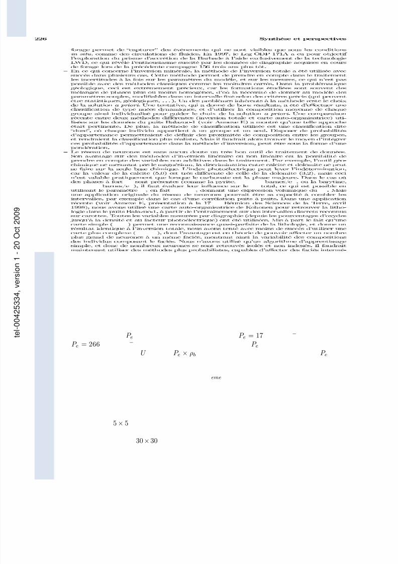
7/13/2019 Rabaute Manuscrit de These
http://slidepdf.com/reader/full/rabaute-manuscrit-de-these 174/212
P e P e = 17 −
P e = 266 − P eU P e × ρb P e
eme
5 × 5
30×30
tel00425334,version1
20Oct2009

7/13/2019 Rabaute Manuscrit de These
http://slidepdf.com/reader/full/rabaute-manuscrit-de-these 175/212
tel00425334,version1
20Oct2009

7/13/2019 Rabaute Manuscrit de These
http://slidepdf.com/reader/full/rabaute-manuscrit-de-these 176/212
tel00425334,version1
20Oct2009

7/13/2019 Rabaute Manuscrit de These
http://slidepdf.com/reader/full/rabaute-manuscrit-de-these 177/212
3
−
Ω
Ω
xo
Ω
tel00425334,version1
20Oct2009

7/13/2019 Rabaute Manuscrit de These
http://slidepdf.com/reader/full/rabaute-manuscrit-de-these 178/212
≤
P e
tel00425334,version1
20Oct2009

7/13/2019 Rabaute Manuscrit de These
http://slidepdf.com/reader/full/rabaute-manuscrit-de-these 179/212
1/200
1/1000
10−24 2
2
1.6 × 10⁻¹⁹
tel00425334,version1
20Oct2009

7/13/2019 Rabaute Manuscrit de These
http://slidepdf.com/reader/full/rabaute-manuscrit-de-these 180/212
−1
1 c.u. = 10−3cm−1tel00425334,version1
20Oct2009

7/13/2019 Rabaute Manuscrit de These
http://slidepdf.com/reader/full/rabaute-manuscrit-de-these 181/212
tel00425334,version1
20Oct2009

7/13/2019 Rabaute Manuscrit de These
http://slidepdf.com/reader/full/rabaute-manuscrit-de-these 182/212
1
Trace and major elements concentrations from ODP Leg 156 deep sea
cores: a data report.
Alain Rabaute1, Peter Blum
2, Pierre Gaudon
3, James F. Allan
2
1 ISTEEM, CC 066, Laboratoire de Géochimie Isotopique, UMR 5567, Université Montpellier II, Place E. Bataillon, 34095 Montpellier Cedex 5, France.2 Ocean Drilling Program, 1000 Discovery Drive, Texas A&M University, College Station, Texas, U.S.A.3 Ecole Nationale Supérieure des Techniques Industrielles et des Mines d'Alès, Laboratoire P3MG, 6 Avenue de Clavières, F-30319 Alès Cedex, France.
Abstract.
Geochemical trace and major elements concentrations measured on samples taken
from sediment cores are presented here from two holes (948C and 949B) drilled in the North-
Barbados accretionary prism during ODP Leg 156. These data include X-ray Fluorescence
(XRF), Inductively Coupled Plasma Mass Spectrometry (ICP-MS), and Instrumental Neutron
Activation (INA) analyses of the samples, providing accurate elemental concentrations in 10
major and 20 trace elements. The data set includes: 79 samples, each of them cut along a 20
cm interval in the section, in order to match corresponding gamma-ray spectra (see full study
in Blum et al., this volume); and 113 samples from physical properties measurements,
considered as representative of a particular lithology in the section. The sampling interval
spans the decollement zone with a very good resolution in Hole 948C (almost one sample per
meter), thus providing useful information on the effect of fluid flow on chemical and
mineralogical nature of the formation.
Introduction.
Leg 156 of the Ocean Drilling Program (ODP) cored two sites on the Northern Barbados
ridge accretionnary prism. At the opportunity of an investigation involving gamma-ray
measurements on sediments from ODP Leg 156 (See Blum at al., this volume), 79 samples were
taken from the cores recovered in Holes 948C and 949B. 113 discrete samples were also selected
from the physical properties measurements sample set. Various geochemical measurements werecarried out in order to obtain the elemental concentrations in K, U and Th, that were used as
calibration data set (See Blum at al., this volume). As a standard output of these analyses,
concentrations in 10 major elements, including K, and 20 trace elements, including U and Th are
obtained. This data report presents the results of this chemical analysis of bulk sediments. A
similar study was carried out during ODP Leg 110 (Wang et al., 1990) but we focused particularly
our interest in the decollement zone.
In Hole 948C, the sampling interval ranges from 421.55 meters below sea floor (mbsf) to
591.43 mbsf, which corresponds to cores 948C-2X-01 to 948C-19X-06. The average core
recovery was 94.9% and allowed encountered formations to be divided into two units. The first
one (cores 2X-01 through 11X-05, 17 cm) consists mainly in claystone and silty claystone of late
Miocene to middle Miocene age, occasionnaly crossed by local thin beds of altered tuffaceous
siltstone and altered volcanish ash, and is characterized by changes in color used to decribedlithologic variations. The second one (cores 11X-05, 17 cm, through 19X) consists in variegated
claystone of early to middle Miocene age at the top, and below 523.78 mbsf, appears as an
intercalation of carbonate-rich beds (nannofossil chalk with clay to silty claystone with
nannofossils), siliciclastic-rich beds (silty claystone to clayey siltstone), and claystone, which
forms the background sediment (see Shipboard Scientific Party, 1995; Site 948).
Cores 949B-2X-02 to 949B-25H-02 were sampled in Hole 949B, with a depth ranging from
255.48 mbsf to 460.53 mbsf. Despite the very low recovery (39.8%), the same two lithologic units
as in Hole 948C were recognized. The first unit (Cores 2X-02 to 22X-03, 52 cm) is characterized
by mottled nannofossil-bearing claystone, with thin layers of volcanic ash occuring sporadically.
When going deeper, the claystone becomes barren of nannofossils, and volcanic ash is rarer. The
second unit consists in a mottled variegated claystone, crossed by thin beds of sandy siltstone,
siltstone, clayey siltstone, nannofossil claystone, and micrite (see Shipboard Scientific Party, 1995;
Site 949).
tel00425334,version1
20Oct2009

7/13/2019 Rabaute Manuscrit de These
http://slidepdf.com/reader/full/rabaute-manuscrit-de-these 183/212
2
Sampling protocols.
All samples in this study were collected by P. Blum and A. Rabaute during ODP Leg 156,
using two different sampling protocols.
A first set of 79 samples were first taken from Holes 948C and 949B. Each of them consists
in a 20 cm long thin slice of material, centered at the core depth within the area of influence of the
MST-NGR apparatus, during the gamma-ray measurements carried out during ODP Leg 156 (seeBlum et al., this volume). Each sample weights about 250 g. This particular sampling mode was
used to prevent potential sampling error due to lithologic variations. These samples were freeze-
dried onboard the JOIDES Resolution, crushed in a Frysch mortar grinder Pulverisette, and
splitted 7 times at the Laboratoire de Geochimie Isotopique in order to obtain 2 g-splits that can be
considered as representative of the original sample. We will refer to this set of samples as ‘GR
(gamma-ray) samples’ in this report.
The second set of samples comprises 113 samples chosen from the physical properties
measurements residues. These samples were 10 cc in volume, and each of them was carrefully
taken out from a single lithologic variation, which reflects mostly a redox-associated change in
color. This second data set was intended as a calibration for the possible geochemical variations
that could happen along with the lithological changes, and therefore should represent geochemical
"end-members". These samples were freeze-dried and crushed onboard the JOIDES Resolution.We will refer to this set of samples as ‘Index Properties samples’ later in this report.
Methods of study.
X-ray fluorescence spectrometry was carried out at the Ecole Nationale Superieure des
Techniques Industrielles et des Mines d'Ales, France. The X-ray laboratory is equipped with a
Philips PW-1400 spectrometer with a Philips PW-1775 70 port automatic sample changer, driven
by a Philips X-40 software. Machine settings for all the samples analyzed were as follows:
generator=50 kV and 40 Ma; medium=vacuum; tube anode = Rh, with no beam filter; wavelength
= Cu-K . Table 1 gives the measuring conditions for each chemical element. Fusion beads were
prepared by mixing a sample split with lithium tetraborate + lanthanium oxide (LiBo4 + La2O5)
flux, with 1 for 8 relative respective proportions (0.750 g of sample per 6 g of flux). The method
depends on the quantitative measurements of specific X-rays emitted during electronic transitions
within atoms excited by irradiation with primary X-rays generated by a tube anode with a metal
target. X-ray fluorescence analysis gives the concentrations of the 10 common major oxides SiO 2,
Al2O3, Fe2O3, MgO, MnO, CaO, Na2O, K 2O, TiO2, and P2O5. Table 2 summarizes the results of a
repeat analysis carried out on 10 samples from Hole 948C and on 21 samples from Hole 949B. It
shows that the relative precision for silicon, calcium, iron, potassium, magnesium, titanium,
aluminium, and manganese data is within 0.5 to 1%. P2O5, due to low concentrations, and Na2O,
due to the masking effects of the lanthanium oxide on the Na peak, are considered precise within
respectively 7% and 9%. Replicate analysis of rock standards show excellent to very good
correlation for all elements except Na, which leads to an accuracy of 1 to 3 % for silica, calcium,
iron, manganese, titanium, aluminium and potassium, and about 11% for MgO and P2O5 (see
Table 3). Na is not considered accurate because of its huge uncertainty and is thus indicative here.
SiO2
Al2O
3Fe
2O
3MgO MnO CaO Na
2O K
2O TiO
2P
2O
5
Collimator coarse coarse fine coarse fine fine coarse fine fine coarse
Crystal PeT PeT LiF100 PX1 LiF100 LiF100 PX1 LiF100 LiF 100 PeT
Detector F F F+S F F+S F F F F F
Peak time 60 60 10 80 40 40 80 40 40 40
Table 1. X-ray fluorescence measuring conditions for each element. PeT = Pentaerytritol; LiF100 = lithium fluoride;
PX1 = artificial monodimensional crystal made with coating layers of Si and W; F = gas flow detector; S =
scintillation detector; coarse collimator = 550 mm; fine collimateur = 150 mm; Peak time is the counting time at the
element peak for each sample, in seconds. tel00425334,version1
20Oct2009

7/13/2019 Rabaute Manuscrit de These
http://slidepdf.com/reader/full/rabaute-manuscrit-de-these 184/212
3
The Inductively Coupled Plasma Mass Spectrometer analysis (ICP-MS) was carried out at
the Université de Montpellier II, France. The basic principle is to use a solution of the sample
which is passed, as an aerosol from a nebulizer, into an electrodeless argon plasma. The plasma is
sustained by inductive coupling to radio frequency magnetic fields, and is connected with a multi-
channel spectrometer. We determined only U and Th concentrations from the first set of 79
samples. The sample preparation involves the dissolution of 100 mg of powered sample in a 15 ml
screw-top Teflon® bomb (Savillex®) using HF 40% and HClO4 70%, at a temperature of 100°C.After evaporation of the HF-HClO4 mixture, this dissolution/evaporation operation is repeated in
order to get a complete dissolution of the sample. After evaporation to dryness, the sample is then
taken into solution in HNO3 65%, transferred in a 20.6 g bottle, and diluted with water until the
bottle is filled. For the analysis, 10 ml of this solution is taken, and, with the addition of 10 ppb of
a In-Bi internal calibration standard, flushed into the plasma field. We used routinely doubly
distilled reagents to minimize the blank. The use of screw-top bombs generally ensures more
complete dissolution of resistant silicate and oxide minerals. The presence of a known amount of
In-Bi standard in each sample preparation leads to the estimation of accuracy and precision. U is
precise within 4% and accurate within 3%, while Th has a precision of 3% but an accuracy of 7%.
Instrumental Neutron Activation (INA) analyses were conducted at the Center for Chemical
Characterization at Texas A&M University, using a TRIGA reactor. Fifty milligrams of samplewere irradiated for 14 hours and counted for six hours at 9 to 12 and 40 to 43 days using
germanium detectors. Spectral analysis was made using a Nuclear Data program and was followed
by manual U- and Th-series overlap and interference corrections. 12 samples of the international
AGV-1 standard were irradiated at multiple can levels during three runs and counted. Table 4
shows the results of error calculations from these repeated measurements of AGV-1 for all the
trace elements. All elements, except Cr, Ni, Zr, Yb and U, show an overall good precision ranging
from 1 to 8%, and an accuracy of 1 to 9%. Cr, Yb, and U are considered meaningful because of
their good accuracy, despite their common 11% of precision. Ni and Zr are not considered accurate
or precise and their values are thus only indicative here.
Results.
SiO2 Al2O3 Fe2O3 MgO MnO CaO Na2O K 2O TiO2 P2O5
Absolute
Average
Deviation
0.149 0.100 0.029 0.036 0.005 0.016 0.071 0.010 0.007 0.011
Relative
Average
Deviation
0.27% 0.49% 0.35% 1.00% 0.95% 0.61% 8.96% 0.48% 0.86% 6.89%
Table 2 . Evaluation of the precision of the X-ray fluorescence measurements given by absolute and relative average
deviations from duplicate XRF measurements of each of 30 samples taken from the Index Properties samples of
Holes 948C and 949B.
SiO2 Al2O3 Fe2O3 MgO MnO CaO Na2O K 2O TiO2 P2O5
Root Mean Square
~ absolute average
deviation (wt %)
0.705 0.266 0.216 0.305 0.007 0.111 1.482 0.062 0.025 0.016
Relative average
deviation 1.32% 1.39% 2.80% 10.74% 2.12% 3.23% N/A 3.07% 3.25% 11.43
%
Table 3 . Evaluation of the accuracy of the X-ray fluorescence measurements given by the square root of the sum of
the squares of the absolute deviations from the linear regression between 11 Geostandard concentrations and their
corresponding measured values. Input geostandard values during calibration were recommended values from
Govindaraju (1989).
tel00425334,version1
20Oct2009

7/13/2019 Rabaute Manuscrit de These
http://slidepdf.com/reader/full/rabaute-manuscrit-de-these 185/212
4
Tables 5 to 10 present the major and trace element concentrations obtained on the two sets
of samples from Holes 948C and 949B. In Hole 948C, because coring during Leg 156 was
concentrated around the decollement zone, our sampling covers a 170 meters-zone, between
421.35 and 591.4 mbsf. With a total of 135 samples taken from this hole, the resolution is 1.25
meters. In Hole 949B, the sampling was scarse due to poor and uncontinuous core recovery. The
57 samples range from 255.49 to 460.53 mbsf. The GR sample set is considered to be
representative of a global geochemical behaviour because of the technique of sampling used. It
should be usefully compared directly to the logging data that were acquired while drilling in Hole
948A (close to Hole 948C), or open-hole in Hole 948C after coring operations. The Index
Properties sample set can be used as discrete measurements of trace and major element
concentrations around the decollement zone, and as geochemical nature of particular sediment
layers, since each Index Properties sample was taken within a single-colored layer, which was
interpreted as lithologic variation. All trace and major elements concentrations were obtained for
the GR sample set. On the Index Properties sample set, only major elements concentrations were
measured using X-ray fluorescence spectrometry.
Figure 1 compares the Th and U values obtained with the two different methods - ICP-MS
and INAA. There is an overall good correlation, which is excellent for Hole 948C (plain circles),
although data from Hole 949B (open circles) show a scattering, especially for the Thorium. Data
from Hole 949B must be use with great care, in first hand because of these method-related
problems, and also because low recovery in this hole may have induced problems of depth
matching.
References.
Govindaraju, K. (1989) 1989 compilation of working values and sample description for 272
geostandards. Geostand. Newsl., 13: 1-114.
Shipboard Scientific Party, 1995. Site 948. In Shipley, T.H., Ogawa, Y., Blum, P., et al., Proc.
ODP, Init. Repts., 156: College Station, TX (Ocean Drilling Program), 87-192.
Shipboard Scientific Party, 1995. Site 949. In Shipley, T.H., Ogawa, Y., Blum, P., et al., Proc.
ODP, Init. Repts., 156: College Station, TX (Ocean Drilling Program), 193-296.
Wang, Y-C, Gieskes, J.M., and Musoke, L. (1990) Bulk chemical analysis of sediments - Hole
671B. In Moore, J.C., Mascle, A., et al., Proc. ODP, Sci. Results, 110: College Station, TX
(Ocean Drilling Program), 179-188.
Figure 1. Comparison between ICP-MS and INAA for U and Th. Plain circles are data from Hole 948C; open
circles are data from Hole 949B. The ellipse around each data point is the precision of the measurement (see
text and Table 4).
0
2
4
6
8
10
0 2 4 6 8 10
U I N A A
( p p m )
UICP-MS
(ppm )
0
5
10
15
20
25
0 5 10 15 20 25
T h
I N A A
( p p m )
ThICP-MS
(ppm )
tel00425334,version1
20Oct2009

7/13/2019 Rabaute Manuscrit de These
http://slidepdf.com/reader/full/rabaute-manuscrit-de-these 186/212
5
T a b l e 4 . P r e c i s i o n a n d a c c u r a c y o f I N A A m e a s u r e m e n t s f r o m A G V - 1 N I S T g e o s t a n d a r d ( A G V - 1
* v a l u e s a r e r e c o m m e n d e d v a l u e s f r o m G o v i n d a r a j u ( 1 9 8 9 ) )
A G
V - 1
S c
C r
C o
N i
Z n
R b
S r
Z r
B a
L a
C e
S m
E u
T b
Y b
L u
H f
T a
T h
U
R u
n 1
1 2 , 0 0
1 1 , 5 0
1 5 , 8 0
1 3 , 6 0
9 2 , 5 0
6 3 , 4 0
7 6 0 , 0
1 4 3 , 0
1 1 9 0
3 9 , 1 0
7 0 , 5 0
5 , 8 8
1 , 6 3
0 , 6 0 6
1 , 7 8
0 , 2 3 7
5 , 4 6
0 , 9 3 1
6 , 3 4
1 , 9 5
1 2 , 0 0
8 , 5 2
1 5 , 8 0
2 6 , 7 0
9 4 , 3 0
6 5 , 4 0
7 1 5 , 0
1 8 7 , 0
1 1 7 8
3 9 , 0 0
7 1 , 5 0
6 , 0 3
1 , 6 6
0 , 6 8 1
1 , 6 0
0 , 2 4 7
5 , 6 6
0 , 9 1 7
6 , 5 5
2 , 0 9
1 2 , 1 4
1 1 , 8 5
1 6 , 1 8 < 2 2 . 1 5
9 1 , 9 0
7 5 , 2 5
7 4 3 , 9
1 5 5 , 7
1 2 1 5
3 8 , 8 7
7 1 , 8 0
5 , 9 3
1 , 6 7
0 , 5 3 2
1 , 6 4
0 , 2 6 0
5 , 3 1
0 , 8 8 0
6 , 4 4
2 , 0 1
1 1 , 8 7
1 1 , 3 8
1 5 , 6 6 < 1 8 . 9 4
8 8 , 3 8
7 5 , 0 0
7 7 3 , 0
1 3 4 , 0
1 1 4 3
3 7 , 6 7
7 0 , 4 4
5 , 7 3
1 , 6 4
0 , 6 3 7
1 , 6 4
0 , 2 4 5
5 , 3 5
0 , 9 7 2
6 , 5 1
2 , 1 3
1 2 , 0 9
1 0 , 7 3
1 5 , 9 0 < 1 9 . 7 5
8 3 , 9 5
6 2 , 5 1
6 5 3 , 2
1 2 8 , 1
1 2 1 4
3 9 , 1 6
7 1 , 4 2
6 , 0 7
1 , 6 5
0 , 5 8 8
1 , 6 2
0 , 2 0 9
5 , 4 2
0 , 8 9 4
6 , 3 4
1 , 9 9
t
o
1 2 , 0 0
1 0 , 8 0
1 5 , 9 3
2 2 , 6 2
8 8 , 0 3
6 7 , 1 5
6 7 2 , 4
1 5 7 , 5
1 1 9 6
3 9 , 1 0
7 2 , 6 1
6 , 1 2
1 , 6 5
0 , 6 2 0
1 , 5 8
0 , 2 3 8
5 , 5 7
0 , 9 2 3
6 , 5 4
2 , 1 1
1 1 , 8 8
8 , 8 9
1 5 , 4 2 < 1 7 . 5 5
9 5 , 3 4
7 1 , 2 0
7 4 0 , 8
1 3 1 , 2
1 2 1 4
3 8 , 5 8
6 9 , 5 5
5 , 8 8
1 , 5 8
0 , 6 2 4
1 , 4 6
0 , 2 2 4
5 , 3 9
0 , 8 7 1
6 , 1 6
2 , 0 0
1 1 , 7 5
1 0 , 5 2
1 5 , 2 2 < 2 0 . 1 1
8 6 , 4 3
6 8 , 6 9
6 9 8 , 5
1 2 2 , 9
1 2 2 4
3 9 , 3 9
6 9 , 2 4
6 , 0 2
1 , 5 6
0 , 5 6 6
1 , 9 0
0 , 2 2 9
5 , 3 8
0 , 8 5 6
6 , 4 0
2 , 1 0
1 1 , 9 3
9 , 4 7
1 5 , 8 2 < 1 7 . 9 4
8 5 , 6 1
6 9 , 7 8
7 3 0 , 8
1 7 5 , 9
1 2 0 1
3 8 , 9 4
7 0 , 7 1
6 , 0 2
1 , 5 6
0 , 7 1 7
1 , 6 5
0 , 2 1 8
5 , 4 9
0 , 8 8 9
6 , 5 4
1 , 6 8
1 1 , 7 8
1 3 , 2 5
1 5 , 4 8 < 1 6 . 5 8
8 5 , 9 2
7 1 , 6 3
7 6 8 , 1
1 7 8 , 8
1 1 8 5
3 9 , 6 2
6 9 , 5 1
6 , 1 4
1 , 5 8
0 , 6 0 7
1 , 9 1
0 , 2 3 2
5 , 4 1
0 , 9 1 3
6 , 3 8
2 , 7 1
1 2 , 3 2
1 1 , 1 7
1 6 , 0 2 < 1 6 . 4 3
8 8 , 4 8
6 6 , 3 8
7 5 6 , 3
1 9 6 , 8
1 1 8 1
3 9 , 0 9
7 3 , 0 0
6 , 0 6
1 , 6 8
0 , 6 1 2
1 , 4 6
0 , 2 1 6
5 , 7 1
0 , 9 3 1
6 , 5 8
2 , 1 9
R u n 1 2
1 1 , 9 4
1 0 , 5 3
1 5 , 5 3 < 2 4 . 4 1
8 5 , 8 4
7 1 , 1 0
7 0 1 , 9
2 0 4 , 9
1 2 1 4
3 9 , 1 2
7 0 , 5 9
6 , 0 8
1 , 6 3
0 , 6 9 4
1 , 2 8
0 , 2 6 4
5 , 3 7
0 , 9 1 0
6 , 2 7
2 , 1 9
M e a n
1 1 , 9 8
1 0 , 7 2
1 5 , 7 3
2 0 , 9 7
8 8 , 8 9
6 8 , 9 6
7 2 6 , 2
1 5 9 , 6
1 1 9 6
3 8 , 9 7
7 0 , 9 1
6 , 0 0
1 , 6 2
0 , 6 2 4
1 , 6 3
0 , 2 3
5 , 4 6
0 , 9 1
6 , 4 2
2 , 1 0
S t a n d a r d
D e v i a t i o
n
0 , 1 5
1 , 2 5
0 , 2 6
5 , 4 7
3 , 5 8
3 , 9 6
3 6 , 8 0
2 7 , 2 6
2 1 , 5 8
0 , 4 6
1 , 1 5
0 , 1 1
0 , 0 4
0 , 0 5
0 , 1 7
0 , 0 2
0 , 1 2
0 , 0 3
0 , 1 2
0 , 2 3
P r e c i s i o
n ( % )
1 , 2 6
1 1 , 6 7
1 , 6 8
2 6 , 1 0
4 , 0 2
5 , 7 5
5 , 0 7
1 7 , 0 8
1 , 8 0
1 , 1 9
1 , 6 2
1 , 9 1
2 , 5 3
8 , 1 3
1 0 , 6 2
6 , 9 7
2 , 2 0
3 , 3 2
1 , 9 3
1 0 , 8 3
A G V - 1
*
1 2 , 2 0
1 0 , 1 0
1 5 , 3 0
1 6 , 0 0
8 8 , 0 0
6 7 , 3 0
6 6 7 , 0
2 2 7 , 0
1 2 2 6
3 8 , 0 0
6 7 , 0 0
5 , 9 0
1 , 6 4
0 , 7 0 0
1 , 7 2
0 , 2 2
5 , 1
0 , 9
6 , 5
1 , 9 2
A c c u r a c y ( % )
1 , 8 4
6 , 1 1
2 , 8 1
3 1 , 0 8
1 , 0 1
2 , 4 6
8 , 8 7
2 9 , 6 7
2 , 4 3
2 , 5 5
5 , 8 3
1 , 6 4
0 , 9 7
1 0 , 9 0
5 , 4 3
6 , 7 8
7 , 0 6
0 , 8 0
1 , 2 2
9 , 1 6
tel00425334,version1
20Oct2009
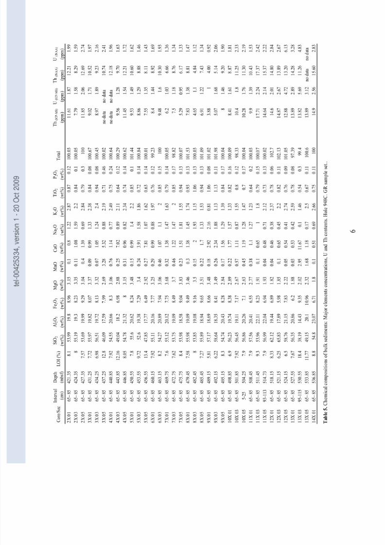
7/13/2019 Rabaute Manuscrit de These
http://slidepdf.com/reader/full/rabaute-manuscrit-de-these 187/212

7/13/2019 Rabaute Manuscrit de These
http://slidepdf.com/reader/full/rabaute-manuscrit-de-these 188/212
7
T a b l e 5
( c o n t i n u e d ) . C h e m i c a l c o m p o s i t i o n s o f b
u l k s e d i m e n t s : M a j o r e l e m e n t s c o n c e n t r a
t i o n s , U a n d T h c o n t e n t s . H o l e 9 4 8 C . G R
s a m p l e s e t .
C o r e / S e c
I n t e r v a l
( c m )
D e p t h
( m b s f )
L O I ( % )
S i O 2
( w t % )
A
l 2 O 3
( w
t % )
F e 2 O 3
( w t % )
M g O
( w t % )
M n O
( w t % )
C a O
( w t % )
N a 2 O
( w t % )
K 2 O
( w t % )
T i O 2
( w t % )
P 2 O 5
( w t % )
T o t a l
T h ( I C P - M S )
( p p m )
U ( I C P - M S )
( p p m )
T h
( I N A A )
( p
p m )
U ( I N A A )
( p p m )
1 4 X 0 3
6 5 - 8 5
5 3 9 , 8 5
8 , 9
5 2 , 9 8
2 3 , 5 7
7 , 9 7
1 , 7 9
0 , 0 2
0 , 3 8
0 , 6 1
2 , 8 8
0 , 7 9
0 , 1 1
1 0 0 , 0 4
1 6 , 6 2
2 , 1 2
1 7 , 6 2
2 , 4 7
1 4 X 0 5
6 5 - 8 5
5 4 2 , 8 5
1 0
5 4 , 1
2 1 , 7 3
6 , 4 7
1 , 8 1
0 , 0 8
1 , 9 3
0 , 5 8
2 , 4 6
0 , 7 3
0 , 1 1
1 0 0
1 4 , 2 8
3 , 4 3
1 5 , 1 0
3 , 8 4
1 5 X 0 1
6 5 - 8 5
5 4 6 , 1 5
1 0
5 2 , 8 8
2 3 , 2 8
7 , 0 4
2
0 , 4 9
1 , 2 1
0 , 4 7
1 , 6 6
0 , 7 8
0 , 1 9
1 0 0 , 0 6
1 4 , 6 3
1 , 7 9
1 5 , 4 8
2 , 0 6
1 5 X 0 3
6 5 - 8 5
5 4 9 , 1 5
1 2 , 9
4 9 , 4 5
2 1 , 7 7
5 , 7 7
1 , 6 9
0 , 0 3
5 , 3 1
0 , 3 7
1 , 9 3
0 , 6 8
0 , 1 1
1 0 0
1 5 , 7 8
3 , 3 5
1 4 , 0 4
3 , 4 2
1 5 X 0 5
6 5 - 8 5
5 5 2 , 1 5
7 , 5 6
5 6 , 3 8
1 9 , 2 7
7 , 1 8
1 , 8 5
0 , 0 4
1 , 5 1
0 , 3 8
2 , 5 4
0 , 7 7
0 , 0 8
9 7 , 5 6
1 4 , 2 9
1 , 4 7
1 4 , 7 6
1 , 7 1
1 6 X 0 1
6 5 - 8 5
5 5 5 , 5 5
8 , 9
5 5 , 7 4
2 1 , 6 1
6 , 7 9
1 , 8 6
0 , 0 3
1 , 4
0 , 4 7
2 , 3
0 , 7 6
0 , 1 2
1 0 0
1 5 , 2 3
2 , 1
1 6 , 7 0
2 , 2 2
1 6 X 0 3
6 5 - 8 5
5 5 8 , 5 5
1 0 , 6
5 1 , 8 5
2 2 , 7 8
7 , 1 5
1 , 9 3
0 , 0 3
2 , 3 8
0 , 4 6
1 , 8 8
0 , 7 8
0 , 1 6
1 0 0 , 0 9
1 6 , 3 4
1 , 5 9
1 6 , 1 3
1 , 8 1
1 6 X 0 5
6 5 - 8 5
5 6 1 , 5 5
2 2 , 4
3 4 , 2 2
1 1 , 6 2
4 , 3 5
1 , 5 7
0 , 3 5
2 2 , 9 5
0
1 , 1 7
0 , 4 6
0 , 2 6
9 9 , 3 5
9 , 3 9
3 , 2 7
9 , 8 9
3 , 7 0
1 7 X 0 1
6 5 - 8 5
5 6 4 , 8 5
6 , 9 5
5 9 , 1
2 0 , 0 1
7 , 4 3
1 , 8 9
0 , 0 3
0 , 4 6
0 , 6 4
3 , 2 4
0 , 9 1
0 , 0 7
1 0 0 , 7 4
1 6 , 9 1
2 , 3 3
1 8 , 0 1
2 , 4 6
1 7 X 0 3
6 5 - 8 5
5 6 7 , 8 5
8 , 2 4
5 6 , 5 1
1 9 , 8 4
8 , 2
1 , 9 7
0 , 0 4
2 , 5 4
0 , 4 1
2 , 9 8
0 , 8 4
0 , 0 9
1 0 1 , 6 7
1 4 , 8 5
2 , 1 1
1 5 , 6 0
2 , 3 5
1 7 X 0 5
6 5 - 8 5
5 7 0 , 8 5
1 1 , 8 5
5 2 , 2
1 6 , 5 1
5 , 7 1
1 , 6 2
0 , 0 7
8 , 8 4
0 , 1 1
2 , 4 9
0 , 7 6
0 , 1 1
1 0 0 , 2 8
1 5
3 , 0 6
1 3 , 6 7
3 , 3 1
1 8 X 0 1
6 5 - 8 5
5 7 4 , 0 5
1 5 , 0 3
4 6 , 1 3
1 8 , 5 7
5 , 4 8
1 , 4 9
0 , 1 1
1 0 , 7 8
0 , 8 1
1 , 9 4
0 , 7 4
0 , 2 3
1 0 1 , 3
1 8 , 6 3
4 , 6 9
1 5 , 2 0
4 , 3 5
1 8 X 0 3
6 5 - 8 5
5 7 7 , 0 5
1 6
4 3 , 0 5
2 0 , 6
5 , 4 6
1 , 5 6
0 , 0 8
1 0 , 6 6
0 , 3 8
1 , 4 9
0 , 5 6
0 , 1 5
1 0 0
1 2 , 3 1
2 , 1 2
1 2 , 3 8
2 , 0 3
1 8 X 0 5
6 5 - 8 5
5 8 0 , 0 5
8
5 5 , 9 6
2 2 , 7
6 , 7 8
1 , 7 2
0 , 0 3
0 , 7 2
0 , 4 7
2 , 7 1
0 , 8 3
0 , 1 1
1 0 0 , 0 1
1 6 , 4 5
2 , 4 5
1 7 , 3 6
2 , 8 6
1 9 X 0 1
6 5 - 8 5
5 8 3 , 5 5
1 3 , 8
4 6 , 0 6
2 0 , 7 4
4 , 8 7
1 , 6 5
0 , 1 4
8 , 0 3
0 , 3 9
1 , 9 6
0 , 6 4
0 , 1 4
9 8 , 4 1
1 4 , 0 1
1 , 6 3
1 4 , 8 8
1 , 8 0
1 9 X 0 3
6 5 - 8 5
5 8 6 , 5 5
7 , 7 5
5 8 , 7 8
2 1 , 0 3
7 , 6 2
1 , 8 9
0 , 0 8
0 , 8 2
0 , 2 6
3 , 0 2
0 , 9 2
0 , 0 8
1 0 2 , 2 6
1 7 , 1 9
2 , 8 1
1 6 , 0 1
3 , 3 4
1 9 X 0 5
6 5 - 8 5
5 8 9 , 5 5
1 0 , 6
5 3 , 0 4
2 0 , 4 7
7 , 4 9
1 , 8
0 , 1 7
3 , 1
0 , 4 5
2 , 0 3
0 , 7
0 , 1 5
1 0 0
1 3 , 6 2
2 , 3 6
1 4 , 1 7
2 , 5 0
tel00425334,version1
20Oct2009

7/13/2019 Rabaute Manuscrit de These
http://slidepdf.com/reader/full/rabaute-manuscrit-de-these 189/212
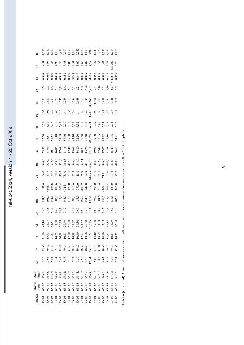
7/13/2019 Rabaute Manuscrit de These
http://slidepdf.com/reader/full/rabaute-manuscrit-de-these 190/212
9
T a b l e 6
( c o n t i n u e d ) . C h e m i c a l c o m p o s i t i o n s o f b
u l k s e d i m e n t s : T r a c e e l e m e n t s c o n c e n t r a t i o n s . H o l e 9 4 8 C . G R s a m p l e s e t .
C o r e / S e c
I n t e r v a l
( c m )
D e p t h
( m b s f )
S c
C r
C o
N i
Z n
R b
S r
Z r
B a
L a
C e
S m
E u
T b
Y b
L u
H f
T a
1 4 X 0 1
6 5 - 8 5
5 3 6 , 8 5
2 0 , 2 0
1 0 5 , 0 0
2 1 , 1
0
4 7 , 1 0
1 8 3 , 0
1 5 4 , 0
9 2 , 6
9 4 , 6
3 6 9 , 0
3 9 , 5 0
8 5 , 3 0
6 , 5 8
1 , 3 2
0 , 8 3 5
2 , 5 8
0 , 3 6 9
4 , 5 4
1 , 0 9 0
1 4 X 0 3
6 5 - 8 5
5 3 9 , 8 5
2 0 , 0 1
9 9 , 4 5
1 5 , 9
2
5 1 , 5 7
1 0 8 , 8
1 6 8 , 6
< 1 0 1 . 1
1 3 7 , 9
3 5 6 , 0
4 7 , 0 6
1 0 3 , 8 1
8 , 1 6
1 , 6 3
0 , 9 2 1
2 , 7 3
0 , 3 9 8
3 , 9 7
1 , 2 1 0
1 4 X 0 5
6 5 - 8 5
5 4 2 , 8 5
1 8 , 5 4
1 0 1 , 2 0
2 1 , 2
3
5 1 , 5 1
1 5 1 , 2
1 4 4 , 1
1 6 3 , 6
1 3 9 , 7
3 7 9 , 6
4 0 , 1 7
8 2 , 5 7
6 , 7 8
1 , 3 7
0 , 7 3 1
2 , 6 8
0 , 4 0 5
4 , 2 6
1 , 0 2 0
1 5 X 0 1
6 5 - 8 5
5 4 6 , 1 5
1 6 , 1 4
1 1 5 , 1 0
1 4 , 2
5
7 1 , 5 0
1 1 4 , 8
8 2 , 0
1 0 8 , 6
1 5
0 , 0
5 5 3 , 5
4 6 , 0 5
9 5 , 1 8
7 , 0 8
1 , 4 6
0 , 9 2 2
2 , 9 5
0 , 4 0 4
4 , 9 0
1 , 1 5 0
1 5 X 0 3
6 5 - 8 5
5 4 9 , 1 5
1 5 , 4 1
9 5 , 4 3
2 0 , 7
8
7 6 , 3 9
1 3 4 , 2
1 5 , 4
3 0 7 , 4
1 1
0 , 5
5 7 1 , 4
3 7 , 6 9
7 7 , 0 9
5 , 8 5
1 , 1 7
0 , 7 3 7
2 , 2 9
0 , 3 4 5
4 , 3 0
0 , 9 9 4
1 5 X 0 5
6 5 - 8 5
5 5 2 , 1 5
1 8 , 8 8
9 9 , 8 4
1 0 , 8
3
< 2 7 . 6 9
1 2 1 , 9
1 4 5 , 9
< 9 4 . 4 1
< 7 5
. 4 0
3 6 2 , 3
4 1 , 1 6
8 8 , 4 0
7 , 0 9
1 , 4 4
0 , 9 5 9
2 , 6 2
0 , 3 8 2
3 , 4 5
0 , 9 9 0
1 6 X 0 1
6 5 - 8 5
5 5 5 , 5 5
1 6 , 3 0
9 7 , 4 0
1 7 , 0
0
5 3 , 3 0
1 0 1 , 0
1 1 7 , 0
1 2 9 , 0
1 5 7 , 0
4 1 7 , 0
4 2 , 4 0
8 9 , 2 0
6 , 9 5
1 , 3 6
0 , 8 1 7
2 , 6 5
0 , 3 9 5
5 , 0 2
1 , 1 9 0
1 6 X 0 3
6 5 - 8 5
5 5 8 , 5 5
1 6 , 3 2
1 0 8 , 3 0
1 4 , 7
8
5 2 , 3 7
1 4 2 , 9
9 1 , 3
2 1 3 , 6
1 3
7 , 9
5 4 6 , 0
4 3 , 6 8
9 3 , 1 0
6 , 6 1
1 , 3 8
0 , 7 8 4
2 , 5 1
3 1 3 , 8
4 , 5 4
1 , 1 6 0
1 6 X 0 5
6 5 - 8 5
5 6 1 , 5 5
1 0 , 5 0
6 9 , 2 0
1 0 , 3
0
3 4 , 3 0
1 0 9 , 0
5 6 , 9
7 7 7 , 0
1 1
5 , 0
5 4 3 , 0
3 4 , 8 0
7 2 , 2 0
5 , 3 2
1 , 1 4
0 , 6 6 9
2 , 2 8
0 , 3 4 7
3 , 6 0
0 , 7 5 2
1 7 X 0 1
6 5 - 8 5
5 6 4 , 8 5
1 7 , 9 6
8 8 , 8 2
1 2 , 5
1
< 2 1 . 5 2
1 4 9 , 2
1 5 9 , 7
< 1 0 6 . 9
1 5
5 , 9
3 7 7 , 1
4 8 , 2 7
1 0 0 , 5 8
8 , 0 7
1 , 4 3
0 , 8 6 1
2 , 8 8
0 , 4 1 8
4 , 6 2
1 , 4 7 0
1 7 X 0 3
6 5 - 8 5
5 6 7 , 8 5
1 7 , 2 0
9 0 , 4 0
1 3 , 6
0
4 8 , 3 0
1 2 3 , 0
1 3 4 , 0
2 4 9 , 0
9
4 , 9
4 1 1 , 0
4 5 , 2 0
9 1 , 3 0
7 , 8 1
1 , 4 8
0 , 8 9 7
2 , 9 0
0 , 3 8 6
4 , 0 8
1 , 1 7 0
1 7 X 0 5
6 5 - 8 5
5 7 0 , 8 5
1 7 , 3 4
1 0 8 , 1 5
1 7 , 7
4
6 1 , 5 0 5
1 3 3
1 1 3 , 0 4
1 3 6 , 1
1 4 4
, 8 5
4 6 6 , 5 5
4 3 , 1 1
8 8 , 8 7 5
6 , 9 3
1 , 4 1 5
0 , 8 2 6 5
2 , 8 1 5
0 , 4 0 4 5
4 , 5 8
1 , 0 8 5
1 8 X 0 1
6 5 - 8 5
5 7 4 , 0 5
1 5 , 6 0
9 7 , 7 0
1 4 , 4
0
4 7 , 4 0
1 1 0 , 0
9 8 , 2
5 0 3 , 0
1 3
1 , 0
4 1 8 , 0
4 9 , 9 0
1 0 9 , 0 0
9 , 2 9
1 , 9 2
1 , 3 0 0
3 , 3 3
0 , 4 8 9
4 , 2 9
1 , 1 4 0
1 8 X 0 3
6 5 - 8 5
5 7 7 , 0 5
1 5 , 8 2
9 1 , 8 1
1 3 , 6
9
7 1 , 5 3
1 0 0 , 8
8 4 , 6
6 1 8 , 4
1 6
5 , 1
6 7 2 , 2
3 7 , 4 9
8 1 , 6 5
6 , 4 8
1 , 3 3
0 , 7 7 7
2 , 4 0
0 , 3 7 3
3 , 5 3
0 , 9 2 3
1 8 X 0 5
6 5 - 8 5
5 8 0 , 0 5
1 8 , 0 4
8 9 , 6 0
1 4 , 6
0
4 2 , 0 8
1 3 3 , 5
1 5 6 , 5
< 1 0 9 . 1
< 7 1 . 1 1
3 6 6 , 6
4 7 , 0 7
9 7 , 4 2
7 , 7 3
1 , 4 1
0 , 8 9 0
2 , 6 5
0 , 3 8 4
4 , 4 2
1 , 3 7 0
1 9 X 0 1
6 5 - 8 5
5 8 3 , 5 5
1 5 , 8 7
1 0 0 , 7 0
1 3 , 3
3
5 4 , 1 5
1 0 5 , 6
1 1 6 , 4
3 9 6 , 8
7 3 , 9
6 9 7 , 9
4 1 , 7 8
9 1 , 1 0
7 , 0 4
1 , 4 2
0 , 7 6 3
2 , 3 0
0 , 3 3 6
3 , 7 3
1 , 0 8 0
1 9 X 0 3
6 5 - 8 5
5 8 6 , 5 5
1 6 , 3 7
7 9 , 6 8
1 8 , 3
4
3 4 , 7 9
1 3 0 , 9
1 3 1 , 1
1 2 0 , 0
1 3 3 , 2
3 3 4 , 8
4 5 , 4 3
8 6 , 0 6
7 , 7 4
1 , 3 5
0 , 8 4 0
2 , 9 6
0 , 4 3 2 1 4
4 , 5 3 9 8 5
1 , 2 5 4
1 9 X 0 5
6 5 - 8 5
5 8 9 , 5 5
1 5 , 3 4
9 9 , 6 6
1 4 , 3
2
6 5 , 0 0
1 3 1 , 8
1 0 2 , 6
1 6 6 , 8
1 4 7 , 7
4 0 9 , 9
3 6 , 6 9
7 4 , 9 1
6 , 0 5
1 , 1 7
0 , 7 1 2
2 , 5 9
0 , 3 7 6
5 , 2 8
1 , 1 0 0
tel00425334,version1
20Oct2009

7/13/2019 Rabaute Manuscrit de These
http://slidepdf.com/reader/full/rabaute-manuscrit-de-these 191/212
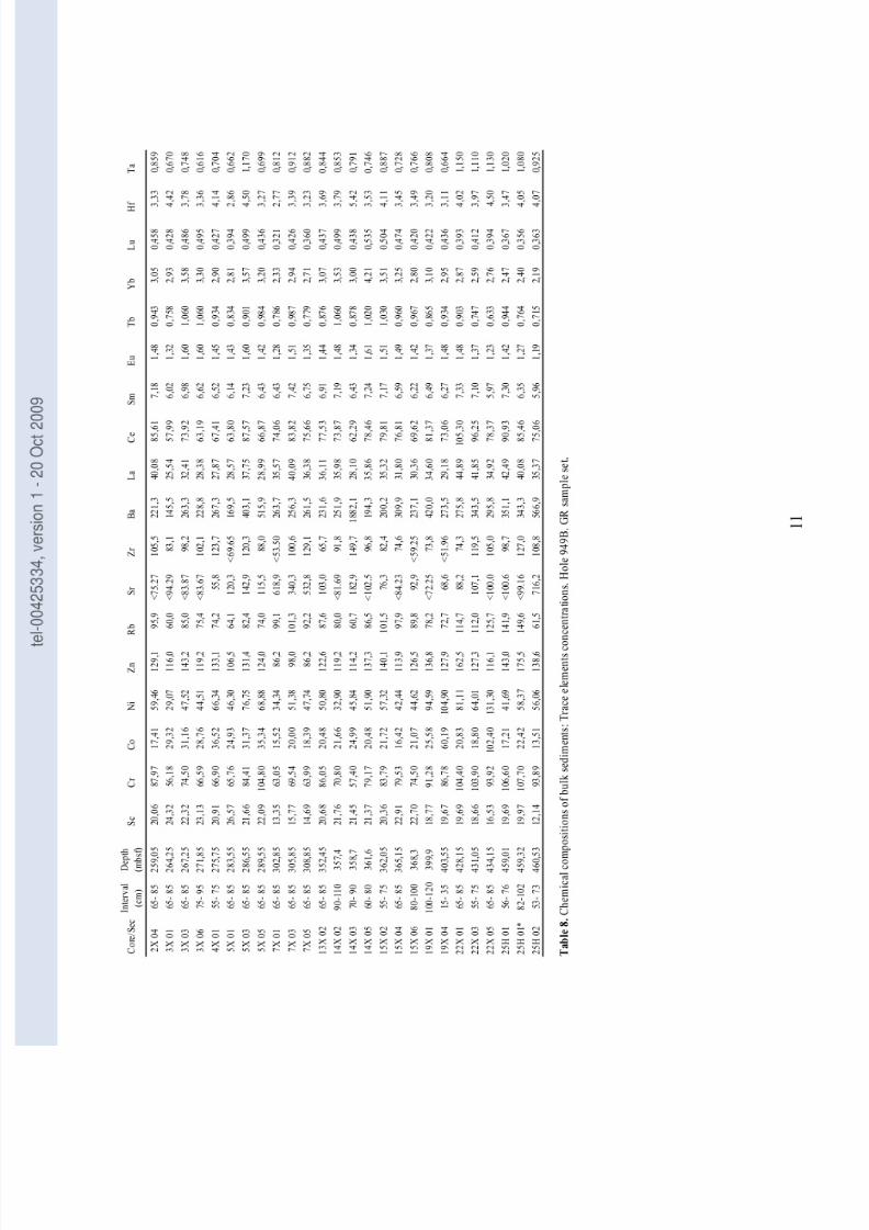
7/13/2019 Rabaute Manuscrit de These
http://slidepdf.com/reader/full/rabaute-manuscrit-de-these 192/212

7/13/2019 Rabaute Manuscrit de These
http://slidepdf.com/reader/full/rabaute-manuscrit-de-these 193/212
12
Table 9. Chemical compositions of bulk sediments: Major elements concentrations. Hole 948C. Index Properties sample set .
Core/SecInterval
(cm)
Depth
(mbsf)LOI (%)
SiO2
(wt%)
Al2O3
(wt%)
Fe2O3
(wt%)
MgO
(wt%)
MnO
(wt%)
CaO
(wt%)
Na2O
(wt%)
K 2O
(wt%)
TiO2
(wt%)
P2O5
(wt%)Total
2X 01 140-142 422,2 7,01 54,83 19,99 8,15 3,02 0,11 1,03 0,74 2,67 0,77 0,12 98,45
2X 01 146-148 422,3 6,99 55,61 20,26 8,39 3,11 0,12 1,04 0,75 2,63 0,79 0,14 99,84
2X 03 72- 74 424,5 8,55 54,94 18,84 8,35 3,4 0,12 1,15 1,07 2,31 0,86 0,08 99,68
2X 04 116-118 426,5 8,54 54,89 20,04 8 3,19 0,11 1,03 0,84 2,63 0,77 0,12 100,17
2X 05 95- 97 427,7 7,2 54,77 19,48 9,87 2,92 0,48 0,89 0,45 2,97 0,76 0,2 100
3X 01 55- 57 431 7,08 55,77 19,34 8,3 3,4 0,11 1,17 1,14 2,35 0,89 0,07 99,63
3X 02 139-141 433,4 6,6 57,21 20,82 6,91 3,7 0,09 1,27 1,86 1,84 0,64 0,09 101,03
3X 03 1- 3 433,5 7,03 56,49 19,81 7,49 3,49 0,09 1,31 1,29 2,05 0,73 0,09 99,88
3X 05 95- 97 437,5 11,69 48,96 17,73 8,49 2,78 0,34 5,03 0,58 2,38 0,87 0,11 98,98
4X 03 55-57 443,6 11,4 49,41 18,45 7,86 3,19 0,32 7,05 0,51 2,34 0,68 0,12 101,33
4X 03 142-144 444,5 10,69 50,53 19,21 6,89 2,86 0,31 5,24 0,5 2,27 0,66 0,15 99,31
4X 05 42- 44 446,5 10,54 49,99 18,82 8,24 2,83 0,31 5,11 0,54 2,33 0,69 0,13 99,55
5X 01 63- 65 450,4 7,62 54,82 19,91 8,58 3,44 0,14 1,07 0,88 2,09 0,88 0,13 99,55
5X 01 146-148 451,3 7,56 55,7 19,94 8,45 3,96 0,18 1,65 1,08 1,94 0,81 0,18 101,45
5X 02 43- 45 451,7 9,51 53,22 20,29 8,41 3,01 0,14 0,88 0,56 2,26 0,78 0,13 99,18
5X 03 127-129 454,1 13 47,93 18 7,84 3,03 0,3 7,01 0,84 1,97 0,71 0,15 100,79
5X 04 110-112 455,4 15,58 43,81 16,62 6,4 2,84 0,7 12,19 0,67 1,68 0,6 0,15 101,25
5X 05 63- 65 456,4 12,39 48,54 17,37 7,29 3,16 0,29 8,39 0,83 1,81 0,7 0,17 100,93
5X 05 99-101 456,8 16,79 41,27 15,4 5,76 2,62 0,57 14,17 0,25 1,54 0,5 0,12 98,995X CC 25- 27 459,5 17,32 41,57 14,41 5,22 2,8 0,58 15,38 0,56 1,17 0,52 0,16 99,68
6X 01 22-24 459,6 14,52 45,76 17,08 6,19 2,81 0,46 10,25 0,56 1,61 0,6 0,12 99,96
6X 02 6- 8 461 11,81 47,02 18,44 8,02 3,03 5,37 1,96 0,36 2,13 0,7 0,19 99,05
6X CC 15- 17 465,8 7,65 54,96 19,22 8,48 3,6 0,42 1,37 1 2,07 0,84 0,16 99,76
7X 02 123-125 471,7 7,47 55,29 19,01 8,59 3,5 0,24 1,18 0,99 1,97 0,81 0,15 99,21
8X 01 52- 54 479,2 7,26 55,44 18,43 9,44 3,59 0,25 1,44 1,08 1,71 0,86 0,15 99,65
8X 01 122-124 479,9 7,93 54,49 18,54 8,95 3,49 1,03 1,5 0,89 1,75 0,91 0,13 99,6
8X 03 9- 11 481,8 7,42 55,95 19,02 8,94 3,51 0,36 1,44 1 1,56 0,96 0,14 100,3
8X 04 141-143 484,6 7,71 54,93 18,31 9,59 3,51 0,33 1,33 0,86 1,78 0,92 0,15 99,43
8X 05 66- 68 485,4 6,85 55,47 17,95 9,97 3,6 0,17 1,99 1,41 1,4 0,98 0,13 99,9
8X 05 115-117 485,9 7,24 55,18 18,54 9,7 3,42 0,24 1,7 1,14 1,61 0,93 0,15 99,85
9X 01 52- 54 488,9 7,29 55,85 18,75 8,68 3,52 0,2 1,64 1,22 1,48 0,88 0,17 99,7
9X 01 94- 96 489,3 7,07 55,42 18,72 9,37 3,31 0,22 1,79 1,17 1,54 0,94 0,17 99,72
9X 04 59- 61 493,5 6,91 57,23 18 8,77 3,47 0,26 1,56 1,22 1,48 1 0,12 100,03
9X 05 7- 9 494,5 6,7 58,51 17,69 10,23 3,68 0,18 2,24 1,46 1,33 0,93 0,12 103,07
9X 05 81- 83 495,2 7,06 56,76 19,24 9,84 3,08 0,22 1,86 1,14 1,63 0,94 0,16 101,92
9X 06 43- 45 496,3 6,73 55,91 17,6 9,99 3,04 0,19 2,25 1,43 1,23 0,94 0,15 99,45
10X 01 124-126 499,3 6,88 57,95 17,47 7,38 3,61 0,63 1,8 1,42 1,14 0,72 0,11 99,11
10X 02 51- 53 500,1 7 57,06 18,51 7,95 2,81 0,32 1,85 1,23 1,55 0,79 0,16 99,22
10X 05 17- 19 504,3 7,84 58,3 19,42 8,39 2,86 0,23 1,39 0,92 1,62 0,73 0,17 101,87
10X 05 59- 61 504,7 7,16 58,34 17,41 8,13 3,02 0,29 1,56 1,01 1,42 0,77 0,13 99,24
11X 01 70- 72 508,4 7,75 59,78 16,97 7,55 3,12 0,54 1,22 1,05 1,31 0,66 0,15 100,1
11X 01 137-139 509,1 7,44 58,35 18,27 8,01 2,62 0,23 1,46 0,76 1,55 0,82 0,15 99,66
11X 04 37- 39 512,6 7,84 55,63 20,84 8,84 2,34 0,1 0,72 0,37 2,11 0,78 0,16 99,73
11X 05 17-19 513,4 6,92 57,97 21,52 6,74 2,33 0,04 0,55 0,26 2,67 0,76 0,07 99,83
12X 01 47- 49 517,9 4,54 69,96 15,32 4,69 1,64 0,04 0,47 0,52 2,15 0,76 0,07 100,15
12X 03 107-109 521,5 4,52 68,95 14,75 4,83 1,63 0,04 0,49 0,41 1,99 0,82 0,09 98,52
12X 04 83- 85 522,7 7,85 53,95 21,42 9,29 2,14 0,08 0,65 0,25 2,44 0,75 0,16 98,99
12X 05 45-47 523,8 6,17 64,79 17,61 5,45 1,87 0,04 0,6 0,27 2,33 0,85 0,08 100,06
12X 05 145-147 524,8 6,67 63,32 18,18 5,51 2,19 0,04 0,53 0,33 2,67 0,81 0,06 100,31
tel00425334,version1
20Oct2009

7/13/2019 Rabaute Manuscrit de These
http://slidepdf.com/reader/full/rabaute-manuscrit-de-these 194/212
13
Table 9 (continued). Chemical compositions of bulk sediments: Major elements concentrations. Hole 948C. Index Properties
sample set.
Core/SecInterval
(cm)
Depth
(mbsf)LOI (%)
SiO2
(wt%)
Al2O3
(wt%)
Fe2O3
(wt%)
MgO
(wt%)
MnO
(wt%)
CaO
(wt%)
Na2O
(wt%)
K 2O
(wt%)
TiO2
(wt%)
P2O5
(wt%)Total
12X 06 59- 61 525,5 7,68 58,97 20,49 6,46 2,2 0,18 0,58 0,25 2,66 0,82 0,09 100,39
13X 01 142-144 528,2 7,47 60,58 19,26 6,09 1,85 0,09 0,6 0,19 2,39 0,85 0,08 99,45
13X 02 101-103 529,3 22,05 31,53 11,91 9,78 2,6 6,77 12,68 0 0,85 0,54 0,28 98,97
13X 07 28- 30 536,1 7,08 62,35 18,85 6,02 1,64 0,08 0,47 0,17 2,46 0,83 0,07 100,04
14X 02 100-102 538,6 8 55,08 21,84 6,43 1,96 0,03 0,47 0 2,93 0,77 0,07 97,57
14X 04 116-118 541,8 18,51 39,2 19,32 4,92 1,34 0,08 13,94 0 0,98 0,69 0,1 99,09
15X 01 66- 68 546,1 8,49 55,02 22,14 7,81 2,33 0,03 0,68 0,17 2,18 0,89 0,18 99,93
15X 01 106-108 546,5 18,61 40,32 14,83 5,1 1,74 0,24 16,91 0,48 1,2 0,56 0,11 100,13
15X 02 51- 53 547,4 7,41 60,61 19,18 7,1 2,11 0,04 0,78 0,07 2,15 0,88 0,2 100,54
15X 05 28- 30 551,7 19,43 39,61 12,01 4,63 1,68 0,63 18,61 0 1,24 0,72 0,14 98,71
15X 06 42- 44 553,3 10,81 59 13,52 6,51 1,54 0,05 5,79 0 1,71 0,75 0,14 99,82
15X 07 44- 46 554,8 6,88 58,81 19,92 7,66 2 0,04 0,48 0,01 3,3 0,86 0,08 100,04
16X 01 106-108 555,9 6,21 61,5 18,23 7,42 2,38 0,06 0,67 0,36 2,8 0,77 0,11 100,5
16X 03 126-128 559,1 8,05 56,08 21,1 8,4 2,52 0,03 0,7 0,14 2,64 0,79 0,16 100,61
16X 04 109-111 560,4 8,18 56,02 21,59 7,36 2,59 0,03 0,73 0,12 2,41 0,96 0,17 100,14
16X 05 17- 19 561 17,93 42,97 14,74 5,32 1,29 0,07 14,85 0 1,2 0,62 0,11 99,1
17X 01 104-106 565,1 9,88 57,04 18,02 5,71 1,87 0,05 4,5 0,41 2,63 0,87 0,08 101,06
17X 02 33- 35 565,9 23,1 31,23 12,26 4,66 1,5 0,23 23,12 0 1,08 0,39 0,19 97,75
17X 04 21- 23 568,8 22,37 32,67 10,59 6,45 1,43 1,5 21,74 0 0,84 0,42 0,68 98,6917X 06 38- 40 572 23,02 32,62 16,39 3,93 1,28 0,18 20,51 0 0,55 0,55 0,13 99,16
17X 07 12- 14 573,2 21,98 33,68 15,98 4,05 1,1 0,12 20,19 0 0,58 0,54 0,19 98,42
18X 02 28- 30 575,1 14,6 46,99 18,95 5,9 1,66 0,06 8,49 0,09 2,07 0,7 0,09 99,6
18X 02 145-147 576,2 24,63 31,4 10,21 4,93 1,21 0,5 25,64 0 0,47 0,41 0,3 99,7
18X 04 85- 87 578,7 7,72 56,01 22,05 7,98 2,18 0,04 0,61 0,2 3,01 0,79 0,08 100,67
18X 06 11- 13 580,9 7,22 55,99 20,34 9,51 2,1 0,06 0,59 0,14 3,34 0,72 0,08 100,09
19X 01 43- 45 583,2 22,04 32,03 14,06 9,43 1,9 1,75 17,25 0 0,8 0,49 0,24 99,99
19X 01 134-136 584,1 29,48 19,3 7,65 9,06 1,73 1,28 29,64 0 0,11 0,25 0,47 98,97
19X 02 15- 17 584,5 20,79 35,96 14,91 4,85 1,52 0,1 20,2 0,06 0,85 0,48 0,14 99,86
19X 04 97- 99 588,3 9,24 56,25 19,11 7,05 1,84 0,22 2,81 0,15 2,73 0,8 0,11 100,32
19X 05 33- 35 589,1 7,79 60,52 19,05 6,52 1,79 0,17 1,43 0,17 2,65 0,85 0,1 101,03
19X 05 97- 99 589,8 21,37 34,95 16,59 4,57 1,39 0,44 19,04 0 0,6 0,56 0,13 99,63
19X 06 30- 32 590,6 20,5 37,79 12,31 5,56 1,19 0,09 19,18 0 0,9 0,49 0,14 98,15
19X 06 113-115 591,4 10,48 54,01 18,81 7,17 1,68 0,09 3,92 0,01 2,45 0,77 0,09 99,47
tel00425334,version1
20Oct2009
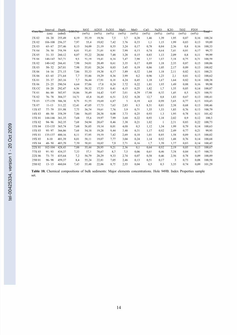
7/13/2019 Rabaute Manuscrit de These
http://slidepdf.com/reader/full/rabaute-manuscrit-de-these 195/212
14
Table 10. Chemical compositions of bulk sediments: Major elements concentrations. Hole 949B. Index Properties sampleset.
Core/SecInterval
(cm)
Depth
(mbsf)LOI (%)
SiO2
(wt%)
Al2O3
(wt%)
Fe2O3
(wt%)
MgO
(wt%)
MnO
(wt%)
CaO
(wt%)
Na2O
(wt%)
K2O
(wt%)
TiO2
(wt%)
P2O5
(wt%)Total
2X 02 18- 20 255,49 8,19 55,19 19,56 7,5 3,7 0,28 1,46 1,39 1,95 0,87 0,16 100,24
2X 02 106-108 256,37 7,97 55,4 19,82 7,42 3,76 0,33 1,1 1,15 1,99 0,83 0,13 99,89
2X 03 65- 67 257,46 8,15 54,09 21,19 8,55 3,24 0,17 0,78 0,84 2,36 0,8 0,16 100,33
2X 04 28- 30 258,59 8,01 53,41 21,01 8,91 2,99 0,13 0,74 0,64 2,41 0,81 0,17 99,22
2X 05 31- 33 260,12 8,07 55,22 20,84 7,48 3,28 0,15 0,83 1,13 2,09 0,8 0,11 99,99
2X 06 140-142 262,71 9,9 51,19 19,41 8,16 3,47 2,98 1,33 1,02 2,18 0,75 0,21 100,59
3X 02 140-142 266,41 7,98 54,01 20,49 8,61 3,35 0,17 0,89 1,18 2,35 0,87 0,15 100,06
3X 03 50- 52 267,01 7,98 55,01 20,24 8,03 3,45 0,19 0,86 1,05 2,17 0,89 0,13 100,02
3X 06 14- 16 271,15 7,86 55,33 19,38 8,17 3,89 0,32 1,04 1,18 2,11 0,82 0,11 100,21
3X 06 63- 65 271,64 7,7 55,86 19,29 8,36 3,99 0,2 0,96 1,23 2,1 0,81 0,12 100,62
5X 01 35- 37 283,16 7,7 56,44 17,91 8,18 4,24 0,45 1,18 1,67 1,64 0,82 0,14 100,38
5X 06 23- 25 290,54 6,64 57,06 17,8 8,24 3,72 0,22 1,81 1,95 1,49 0,88 0,16 99,98
5X CC 18- 20 292,47 6,56 58,32 17,33 8,41 4,15 0,25 1,82 1,7 1,35 0,85 0,14 100,87
7X 01 86- 88 302,97 18,86 38,49 14,42 5,97 2,01 0,29 17,98 0,32 1,45 0,5 0,21 100,51
7X 02 76- 78 304,37 14,71 43,8 16,45 6,51 2,52 0,28 12,7 0,8 1,83 0,67 0,13 100,41
7X 03 127-129 306,38 9,79 51,55 19,69 6,87 3 0,19 4,8 0,99 2,65 0,77 0,13 100,43
7X 07 11-13 311,22 12,41 47,05 17,73 7,63 2,83 0,3 8,51 0,81 2,38 0,68 0,13 100,46
13X 02 27- 29 351,98 7,75 56,24 19,61 7,26 3,9 0,21 1,55 1,53 1,85 0,76 0,13 100,79
14X 03 48- 50 358,39 7,86 56,05 20,38 8,08 3,73 0,25 0,93 1,3 1,95 0,78 0,11 101,4215X 01 144-146 361,35 7,68 55,6 19,97 7,99 3,68 0,22 0,93 1,18 2,02 0,9 0,12 100,3
15X 02 94- 96 362,35 7,68 54,94 20,67 8,46 3,38 0,21 1,02 1 2,31 0,83 0,22 100,73
15X 04 133-135 365,74 7,68 56,05 19,14 8,01 4,08 0,3 1,12 1,34 1,99 0,79 0,14 100,63
15X 05 95- 97 366,86 7,68 54,18 19,28 9,44 3,48 0,31 1,17 0,92 2,49 0,77 0,21 99,95
19X 01 135-137 400,16 8,11 57,95 19,19 7,42 2,69 0,18 1,01 0,85 1,58 0,89 0,15 100,02
19X 03 8-10 401,39 8,01 58,11 19,07 7,77 3,04 0,24 1,14 0,92 1,48 0,76 0,14 100,68
19X 04 48- 50 403,29 7,39 58,81 18,02 7,9 2,71 0,16 1,7 1,39 1,37 0,83 0,14 100,42
22X 01 102-104 428,43 7,88 55,44 20,95 9,21 2,36 0,1 0,64 0,92 2,19 0,85 0,13 100,67
22X 05 91- 93 434,32 7,33 57,1 20,62 8,2 2,5 0,06 0,61 0,46 2,38 0,84 0,12 100,23
22X 06 73- 75 435,64 7,2 56,79 20,29 9,33 2,74 0,07 0,58 0,46 2,56 0,78 0,09 100,89
25H 01 96- 98 459,37 8,4 55,24 22,81 7,05 2,46 0,13 0,51 0,17 3 0,73 0,08 100,58
25H 02 13- 15 460,04 7,43 55,48 22,06 8,75 2,55 0,04 0,5 0,3 3,35 0,74 0,09 101,29
tel00425334,version1
20Oct2009

7/13/2019 Rabaute Manuscrit de These
http://slidepdf.com/reader/full/rabaute-manuscrit-de-these 196/212
tel00425334,version1
20Oct2009

7/13/2019 Rabaute Manuscrit de These
http://slidepdf.com/reader/full/rabaute-manuscrit-de-these 197/212
tel00425334,version1
20Oct2009

7/13/2019 Rabaute Manuscrit de These
http://slidepdf.com/reader/full/rabaute-manuscrit-de-these 198/212
tel00425334,version1
20Oct2009
7/13/2019 Rabaute Manuscrit de These
http://slidepdf.com/reader/full/rabaute-manuscrit-de-these 199/212
tel00425334,version1
20Oct2009

7/13/2019 Rabaute Manuscrit de These
http://slidepdf.com/reader/full/rabaute-manuscrit-de-these 200/212
tel00425334,version1
20Oct2009

7/13/2019 Rabaute Manuscrit de These
http://slidepdf.com/reader/full/rabaute-manuscrit-de-these 201/212
2 2 3 2 3
2 2 2
tel00425334,version1
20Oct2009

7/13/2019 Rabaute Manuscrit de These
http://slidepdf.com/reader/full/rabaute-manuscrit-de-these 202/212
La Barbade
Martinique15°
14°
58°59°60°61°
T i b u r o n r i s e
Sites DSDP/ODPSismique 3D
UMR 5567
Alain RABAUTE, Louis BRIQUEU, Mohamed RAMADAN
Coordonnées : UMR 5567-CNRS, ISTEEM, Université de Montpellier II [email protected]
Structure minéralogique du prisme d’accrétion de la Barbade(Leg ODP 156): inversion linéaire de données géochimiques
560
540
520
500
480
460
440
1.5 1.7 1.9 2.1
densité (g/cm3)
5
7
0
6
Km1015 -5Ligne 688 - Migration 3D
W E
Profondeur(Km)
5ODP
671B - 948A/C
Décollement
Croûte océanique S e c t i o n s u b d
u i t e
450
500
550
La campagne 156 d’ODP s’est déroulé dans la partie frontale du prismenord-Barbade et avait pour but d’étudier divers paramètres (perméabilité, débit,épisodicité, surpression) liés à la dynamique des fluides qui circulent dans la zonede décollement. Une campagne de sismique réflexion 3D effectuée avant le leg 156montra que le décollement est caractérisé par une réflexion très intense de polaritésoit négative, due à la compaction, soit positive qui serait due à une forte porositéliée à une pression de l’eau interstitielle anormalement élevée à cet endroit.La méthode de diagraphie en cours de forage ou Logging-While-Drilling a étéutilisée dans le puits 948A car elle permet de minimiser les problèmes d’instabilitéde puits qui rendent la diagraphie en puits ouvert très difficile dans lesenvironnements instables comme un prisme d’accrétion actif. Des enregistrementsen continu de la résistivité, du rayonnement gamma naturel, de la densité totaleainsi que de la porosité neutron ont été obtenus jusqu’à 50 en dessous du
décollement dans le puits 948A. Au niveau de la zone de décollement, le log dedensité montre deux pics (flèches) à faible densité. Ces porosités anormalement
réflexion de polarité positive
Ecartsolutionmesurée/solutioncalculée
Itérations
2.0
1.0
0.0
-1.0
-2.01 2 3 10
SiO2
Al2O3
Fe2O
3
MgOCaONa
2O
K2OL’approche
L’approche
LWD
450
500
550
450
500
550
0 .5 10 1Groupes
1 2 3 4 0 10 10 10 10 10 1i l li te smectite kaolinite quartz plagioclase calcite magnétite
illite
smectite
kaolinite
quartz
plagioclase
calcite
magnétite
Minéralogie calculée
46.4 63.2 -0.51 1.13 4.1 10.61 2. 5 3 9 .6 - 6. 9 9 2 4. 91 - 0 .8 7 1 0. 9 7 - 0. 37 2 .2 3
SiO2 Al
2O
3Fe
2O
3MgO CaO Na
2O K
2O
Illite:
450
500
550
0 1 0 1 0 1 0 1 0 1 0 1illite smectite kaolinite quartz plagioclase calcite
ENTREE COUCHES CACHEES SORTIE
k=1àNh
j
=1àNv
o=1àNo
xij
x11
x12
x13
x21
x22
x23
Unvecteu r d’entrée
pk --> yk,c=F (pk )
d 1
d 2
Sortie attendue:
d o
yk,c --> yk,c=F (yk )i=1 à N i
j=1àNv
k=1àNh
c = 1 à N c
w jk
wkc
wko
Le principe du perceptron, ou réseau de neurone àrétropropagation du gradient, est illustré ci-dessus. Il secompose de plusieurs couches successives de neuronesdont chaque élément est le produit scalaire entre unetransformation de type y =F(x1, ..., xn; W) où la fonction F
est une fonction de transfert sigmoïde, et W la matrice
Il est possible d’enregistrer à chaque itérationl’écart cumulé pour chaque variable d’entrée (ici,des pourcentages d’oxydes) entre les mesures etles valeurs recalculées. Dans le cas où la solution
L’algorithme de l’inversion totale proposé par Tarantola et Valette (1982) a été utilisé sur lespourcentages d’oxydes mesurés par fluorescence X sur des échantillons du puits 948C. Cette méthodeconsidère données et paramètres du problème comme les composantes d’un vecteur unique X affectéd’une matrice de covariance M représentant les incertitudes. On cherche à minimiser la formequadratique entre X et une solution a priori acceptable X0.Une classification automatique partitionne au préalable le jeu de données (à gauche) en 4 groupes, ce
De la même façon, pour chaque phase minérale déterminée, ilest possible de déterminer l’écart entre les pourcentagesd’oxydes calculés et les paramètres de départ, en tenantcompte de leurs incertitudes et de l’erreur calculée sur lasolution a posteriori . Par exemple, pour l’illite (ci-dessus), lebleu foncé signale que la solution est dans l’intervalle de
Le réseau de neurones a été utilisé sur les paramètresphysiques mesurées par LWD dans le puits 948A, soitrésistivités à faible et moyenne profondeursd’investigation, densité totale, porosité neutron etrayonnement gamma naturel total. Le jeu d’entrainementfourni au perceptron pour son apprentissage a étécomposé à partir d’intervalles homogènes LWDindividualisés par classification automatique sur desdonnées densité, susceptibilité magnétique etrayonnement gamma naturel acquises sur carottes. Leperceptron donne pour chaque niveau de mesure LWDune probabilité d’appartenance à un ou plusieurs desgroupes de départ, donc une minéralogie (courbe noireci-contre). Les points rouges donnent la minéralogie
tel00425334,version1
20Oct2009

7/13/2019 Rabaute Manuscrit de These
http://slidepdf.com/reader/full/rabaute-manuscrit-de-these 203/212
x
[K 2O]Total =n
i=1
[K 2O]i · xi
yi = cijxj Y = CX
i j
2 2 2 3
2 2 3
X = (C T M −1C )−1C T M −1Y
M
M =
σ21 0
0 σ2
n
σ2i yi
wi =1
σ2yi−
n
j=1 x2jσ2
cij
X
n + 1
yi −m
j=1 cijxj = 0 avec i = 1, nm
j=1 xj − 1 = 0
G(X) = 0
XM
q2 = (X − X0)T M −10 (X − X0)
X0 n + 1G(X) = 0
q2
q2 = (X − X0)T (X − X0) − 2
n+1
i=1
λigi(X)
dq2 = dxT [X − X0 −
n+1
i=1
λigrad(gi(X))]
q2 X − X0 = Hλ H G(X) λ
λ = (H T H )−1H T (X − X0)
M 0
Xk+1 = X0 +M 0 ·HT k (Hk ·M 0 ·H
T k )−1
[Hk · (X −X0)−G(X)]
M = M 0 − M 0 · H T · (H ·M 0 ·H T )−1· H ·M 0
tel00425334,version1
20Oct2009

7/13/2019 Rabaute Manuscrit de These
http://slidepdf.com/reader/full/rabaute-manuscrit-de-these 204/212
87 86
tel00425334,version1
20Oct2009

7/13/2019 Rabaute Manuscrit de These
http://slidepdf.com/reader/full/rabaute-manuscrit-de-these 205/212
tel00425334,version1
20Oct2009

7/13/2019 Rabaute Manuscrit de These
http://slidepdf.com/reader/full/rabaute-manuscrit-de-these 206/212
tel00425334,version1
20Oct2009

7/13/2019 Rabaute Manuscrit de These
http://slidepdf.com/reader/full/rabaute-manuscrit-de-these 207/212
tel00425334,version1
20Oct2009

7/13/2019 Rabaute Manuscrit de These
http://slidepdf.com/reader/full/rabaute-manuscrit-de-these 208/212
γ
tel00425334,version1
20Oct2009

7/13/2019 Rabaute Manuscrit de These
http://slidepdf.com/reader/full/rabaute-manuscrit-de-these 209/212
tel00425334,version1
20Oct2009

7/13/2019 Rabaute Manuscrit de These
http://slidepdf.com/reader/full/rabaute-manuscrit-de-these 210/212
87 86
tel00425334,version1
20Oct2009

7/13/2019 Rabaute Manuscrit de These
http://slidepdf.com/reader/full/rabaute-manuscrit-de-these 211/212
tel00425334,version1
20Oct2009

7/13/2019 Rabaute Manuscrit de These
http://slidepdf.com/reader/full/rabaute-manuscrit-de-these 212/212
Related Documents