search.jsp?R=20020062997 2018-07-23T09:28:45… · Human Performance Monitoring 1 ... 45+00:00Z. Human Performance Monitoring ... human performance monitoring, signal detection, vision.

Human Performance Monitoring

1

Feature Extraction of Event-Related Potentials using Wavelets:

An Application to Human Performance Monitoring

Leonard J. Trejo

Human Information Processing Research Branch

Human Factors Research and Technology Division

NASA Ames Research Center

Moffett Field, CA

Mark J. Shensa

Naval Command, Control, and Ocean Surveillance Center, RDT&E

Division, San Diego, CA

Running head: PERFORMANCE MONITORING

https://ntrs.nasa.gov/search.jsp?R=20020062997 2018-08-05T04:29:07+00:00Z


Corresponding author:

Leonard J. Trejo, Chief

Human Information Processing Research Branch, MS 262-2

Human Factors Research and Technology Division

NASA Ames Research Center

Moffett Field, CA 94035-1000

[email protected]

Keywords:

wavelet, event-related potential, ERP, principal components,

feature extraction, linear regression, neural networks,

human performance monitoring, signal detection, vision.

Acknowledgements:

Supported by a grant from the US Navy, Office of Naval

Research (PE 60115N), monitored by Joel Davis and Harold

Hawkins, and by a grant from the Campus Research Board of

the University of Illinois at Urbana-Champaign.

Disclaimer:

The opinions of the authors do not necessarily reflect the

views of the Navy Department.


3

Abstract

This report describes the development and evaluation of

mathematical models for predicting human performance from discrete

wavelet transforms (DWT) of event-related potentials (ERP)

elicited by task-relevant stimuli. The DWTwas compared to

principal components analysis (PCA) for representation of ERPs in

linear regression and neural network models developed to predict a

composite measure of human signal detection performance. Linear

regression models based on coefficients of the decimated DWT

predicted signal detection performance with half as many free

parameters as comparable models based on PCA scores. In addition,

the DWT-based models were more resistant to model degradation due

to over-fitting than PCA-based models.

Feed-forward neural networks were trained using the

backpropagation> algorithm to predict signal detection performance

based on raw ERPs, PCA scores, or high-power coefficients of the

DWT. Neural networks based on high-power DWT coefficients trained

with fewer iterations, generalized to new data better, and were

more resistant to overfitting than networks based on raw ERPs.

Networks based on PCA scores did not generalize to new data as

well as either the DWTnetwork or the raw ERP network.

The results show that wavelet expansions represent the ERP

efficiently and extract behaviorally important features for use in

linear regression or neural network models of human performance.


4

The efficiency of the DWTis discussed in terms of its

decorrelation and energy compaction properties. In addition, the

DWTmodels provided evidence that a pattern of low-frequency

activity (I to 3.5 Hz) occurring at specific times and scalp

locations is a reliable correlate of human signal detection

performance.

Introduction

Studies have shown that linear regression models may

significantly explain and predict human performance from measures

of ERPs elicited by stimuli presented in the context of a task

(Trejo, Kramer, & Arnold, 1995). These models have used, as

predictors, measures such as the amplitude and latency of ERP

components (e.g., NI, P300). Other studies have used more

comprehensive measures such as factors derived from principal

components analysis and discriminant functions (Humphrey,

Sirevaag, Kramer, & Mecklinger, 1990). Such models work best when

they have been adapted to the individual subject, taking into

account the temporal and topographic uniqueness of the ERP. Even

then, the models often suffer from a limited ability to generalize

to new data. In addition, the cost of developing and adapting such

models for individuals is high, requiring many hours of expert

analysis and interpretation of ERP waveforms.

Neural-network models for ERPs may be an improvement over

linear regression models (DasGupta, Hohenberger, Trejo, & Mazzara,


5

1990; Ryan-Jones & Lewis, 1991). However, when neural network

models have been based on traditional ERP measures, such as the

sampled ERP time points or the amplitude of ERP components, the

improvement in correlation between ERP measures and human

performance has been small, typically about ten percent

(Venturini, Lytton, & Sejnowski, 1992). Transformations of ERPs

prior to neural network analysis, such as the fast Fourier

transform (FFT), may improve neural network models (DasGupta,

Hohenberger, Trejo, & Kaylani, 1990). However, the FFT is not

ideally suited for representing transient signals; it is more

appropriate for continuous signals, such as sine waves.

The wavelet transform is well suited for analysis of

transients with time-varying spectra (Tuteur, 1989; Daubechies,

1990, 1992) such as the ERP. Discrete wavelet transforms (DWT;

Shensa, 1991) represent signals as temporally ordered coefficients

in different scales of a time-frequency plane. More precisely, the

DWT represents signals in a time-scale plane, where scale is

related to -- but not identical with -- frequency. The concept of

scale comes from the dilation of a "mother wavelet" in the time

domain. Each dilation is a doubling of the wavelet length in the

time domain which results in a halving of the bandwidth in the

frequency domain.

Each scale of the transform corresponds to one octave of

signal bandwidth beginning with the smallest scale, i.e., the

scale that corresponds to the highest frequencies represented in

the signal. This scale, which is referred to as scale _, contains


6

frequencies ranging from the Nyquist frequency (half the sampling

rate) to one-half the Nyquist frequency. As scales increase, the

bandwidth decreases by a factor of two. For example, the bandwidth

of scale 1 extends from _ Nyquist to _ Nyquist, and so on. The

result of this successive halving of scale bandwidth is increasing

frequency resolution (narrower bands) at larger scales (lower

frequencies).

Because large scales represent low frequencies, fewer

coefficients are required to represent the signal at large scales

than at small scales. Since the bandwidth decreases by a factor of

two with each scale increase, the sampling rate or number of

coefficients can also be halved with each scale increase. This

process, called J_L_I___, leads to an economic but complete

representation of the signal in the time-scale plane. However, in

some cases decimation may be undesirable, for example, when the

temporal detail in a particular scale is of interest. In such/"

cases, the undecimated wavelet transform may be computed.

It is convenient to refer to the bandwidths of the scales in

units of Hz, and this familiar unit will be used to make the

following illustration. For a one-second long EEG signal with a

bandwidth of 32 Hz and 64 time points, the first and smallest

scale of the DWT would represent frequencies in the range from 16

to 32 Hz with 32 coefficients. The next larger scale would

represent frequencies of 8 to 16 Hz with 16 coefficients. Succes-

sively larger scales would have the bandwidths and numbers of

coefficients: 4-8 Hz/8, 2-4 Hz/4, 1-2 Hz/2, 0-i Hz/l. A single


7

additional coefficient would represent the DC level, for a total

of 64 coefficients. In practice, the scale boundaries may deviate

from this perfect halving of frequency and numbers of

coefficients, depending on the method of computation. In

particular, the undecimated DWTcomputations we will use here

(Shensa, 1991) lead to scale boundaries that differ slightly from

this example. However, the effects of these minor differences are

inconsequential.

As with the discrete Fourier transform, the DWT is

invertible, allowing for exact reconstruction of the original

signal. An important feature of the DWT, however, is that the

coefficients at any scale are a series that measures energy within

the bandwidth of that scale as a function of time. For this reason

it may be of interest to study signals within the DWT

representation and use the DWT coefficients of brain signals

directly in modeling cognitive or behavioral data.?.

In this Study, the effect of representing ERPs using the DWT

was compared with more traditional representations such as raw

ERPs, peak and latency measures, and factors derived using

principal components analysis (PCA). The comparisons determined

whether the DWT can efficiently extract valid features of ERPs for

use in linear regression models of human signal detection

performance. In addition, neural network models were tested to

determine whether the relative efficiency and validity of the DWT

and other ERP representations would be maintained with a non-

linear method. The signal detection task was chosen because ERP-


8

performance relationships in this task have been described and

analyzed with linear regression models based on peak and latency

measures of ERP components (Trejo et al., 1995).

Method

In an earlier study (Trejo eta!., 1995), ERPs were acquired

in a signal detection task from eight male Navy technicians

experienced in the operation of display systems. Each technician

was trained to a stable level of performance and tested in

multiple blocks of 50-72 trials each on two separate days. Blocks

were separated by 1-minute rest intervals. About I000 trials were

performed by each subject. Inter-trial intervals were of random

duration with a mean of 3s and a range of 2.5-3.5s. The entire

experiment was computer-controlled and performed with a 19-inch

color CRT display.

Triangular > symbols subtending 42 minutes of arc and of three

different luminance contrasts (.17, .43, or .53) were presented

parafoveally at a constant eccentricity of 2 degrees visual angle.

One symbol was designated as the target, the other as the non-

target. On some blocks, targets contained a central dot whereas

the non-targets did not. However, the association of symbols to

targets was alternated between blocks to prevent the development

of automatic processing. A single symbol was presented per trial,

at a randomly selected position on a 2-degree annulus. Fixation

was monitored with an infrared eye tracking device. Subjects were


9

required to classify the symbols as targets or nontargets using

button presses and then to indicate their subjective confidence on

a 3-point scale using a 3-button mouse. Performance was measured

as a linear composite of speed, accuracy, and confidence. A single

measure, PFI, was derived using factor analysis of the performance

data for all subjects, and validated within subjects. PFI varied

continuously, being high for fast, accurate, and confident

responses and low for slow, inaccurate, and unconfident responses.

The computational formula for PFI was

PF I = .33 Accuracy + .53 Confidence - .51 Reaction Time

using standard scores for accuracy, confidence, and reaction time

based on the mean and variance of their distributions across all

subjects.

ERPs were recorded from midline frontal, central, and

parietal electrodes (Fz, Cz, and Pz; Jasper, 1958), referred to

average mastoids, filtered digitally to a bandpass of .I to 25 Hz,

and decimatedto a final sampling rate of 50 Hz. The prestimulus

baseline (200 ms) was adjusted to zero to remove any DC offset.

Vertical and horizontal e!ectrooculograms (EOG) were also

recorded. Across subjects, a total of 8184 ERPs were recorded.

Epochs containing artifacts were rejected and EOG-contaminated

epochs were corrected (Gratton, Co!es, & Donchin, 1983).

Furthermore, any trial in which no detection response or

confidence rating was made by a subject was excluded along with

the corresponding ERP.


I0

Results

Data Sample Construction

Within each block of trials, a running-mean ERP was computed

for each trial. Each running-mean ERP was the average of the ERPs

over a window that included the current trial plus the 9 preceding

trials for a maximum of i0 trials per average. Within this 10-

trial window, a minimum of 7 artifact-free ERPs were required to

compute the running-mean ERP. If fewer than 7 were available, the

running mean for that trial was excluded. Thus each running mean

was based on at least 7 but no more than i0 artifact-free ERPs.

This 10tria! window corresponds to about 30s of task time. The PF I

scores for each trial were also averaged using the same running-

mean window applied to the ERPs, excluding PFI scores for trials in

which ERPs were rejected.

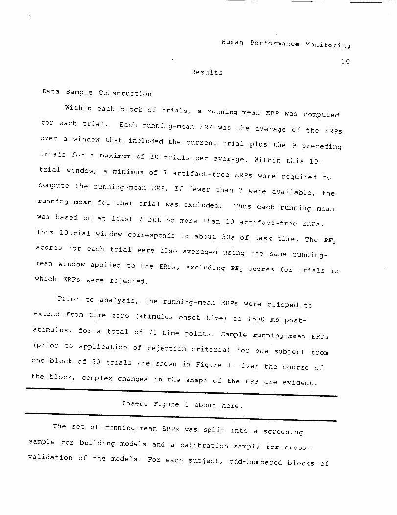
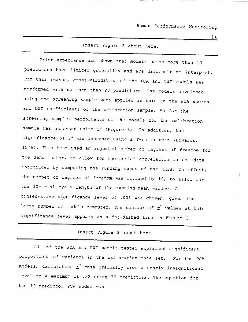
Prior to analysis, the running-mean ERPs were clipped to

extend from time zero (stimulus onset time) to 1500 ms post-

stimulus, for a total of 75 time points. Sample running-mean ERPs

(prior to application of rejection criteria) for one subject from

one block of 50 trials are shown in Figure i. Over the course of

the block, complex changes in the shape of the ERP are evident.

t.H J, t .

Insert Figure 1 about here.

The set of running-mean ERPs was split into a screening

sample for building models and a calibration sample for cross-

validation of the models. For each subject, odd-numbered blocks of


II

trials were assigned to the screening sample, and even blocks were

assigned to the calibration sample. After all trial-rejection

criteria were satisfied, 2765 running-mean ERPs remained in the

screening sample and 2829 remained in the calibration sample.

Linear Regression Models

A multiple-electrode (Fz, Cz, Pz) covariance-based PCA was

performed on the running-mean ERPs. Each observation consisted of

the 75 time points for each electrode for a total of 225 variables

per observation. Usually in PCAs applied to ERP data, the data

from different electrodes would be in different observations,

i.e., each observation representing an epoch x electrode

combination. The objective is to identify physiologically

meaningful components rather than to maximally decorrelate and

compress the data. However, to remain compatible with our DWT

computations (see below) we chose to consider each _ as an

observation rather than each epoch x electrode combination. This is

still a legitimate multivariate linear transform, where the

objective is to decorrelate and compress the variables rather than

to identify components. While this is unconventional, we have

other evidence that the conventional approach would not have made

a difference in this case. In another analysis (Trejo & Mullane,

1995), which compared DWT and PCA on the present data using a

bootstrap classification approach, a traditional PCA was required

more data to reach the same classification accuracy as a DWT

representation of the ERPs.


12

The BMDPprogram 4M (Dixon, 1988) was used for the

calculations, using no rotation and extracting all factors with an

eigenvalue greater than I. One hundred and thirty-six factors were

extracted, accounting for 99.45% of the variance in the data. The

decay of the eigenvalues was roughly exponential, with the first

I0 factors accounting for 70.96% of the variance in the data.

Factor scores were computed for each running-mean ERP and stored

for model development.

The DWT (Shensa, 1991) was computed using the same ERPs as in

the PCA. As for the PCA, each epoch served as an observation.

However, the DWT was computed separately for each electrode within

each observation. A Daubechies analyzing wavelet (Daubechies,

1990) was used to compute the DWT of the EEG data over four

scales. The length of the filters used for this wavelet was 20

points. This results in very smooth signal expansions in the

wavelet transform. The scale boundaries and center frequencies of

the scales are listed in Table i.

The transform was centered within the ERP epoch and decimated

by a factor of 2 at successive scales, yielding a total of 70

coefficients per transform (very low frequency scales and the DC

term were excluded). The number of coefficients was approximately

halved with each increasing scale after decimation. For scales 0-

3, the respective numbers of coefficients were 37, 19, 9, and 5.

The real values of the DWT were stored for model development. No

further transformations were performed.


13

Linear regression models for predicting performance (PFI) ,

from either the PCA factor scores or from the DWT coefficients of

the running-mean ERPs, were developed using a stepwise approach

(BMDPprogram 2R). A criterion F-ratio of 4.00 was used to control

the entry of predictor variables into a model. The F-ratio to

remove a variable from a model was 3.99, resulting in a forward-

stepping algorithm. The performance of each model was assessed by

examining the coefficient of determination, _2, as a function of

the number of predictors entered (_2 is the square of the multiple

correlation coefficient between the data and the model predictions

and also measures the proportion of variance accounted for by the

model when the sample size is adequate and distributional

assumptions are met).

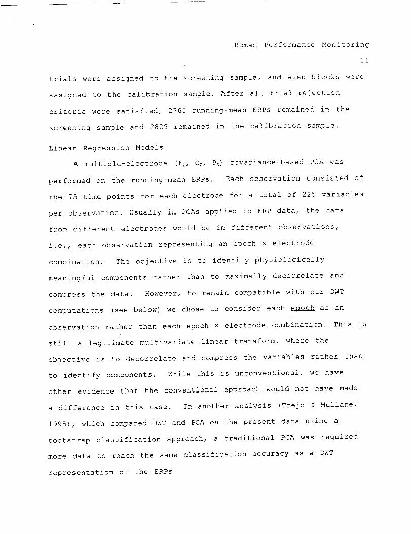
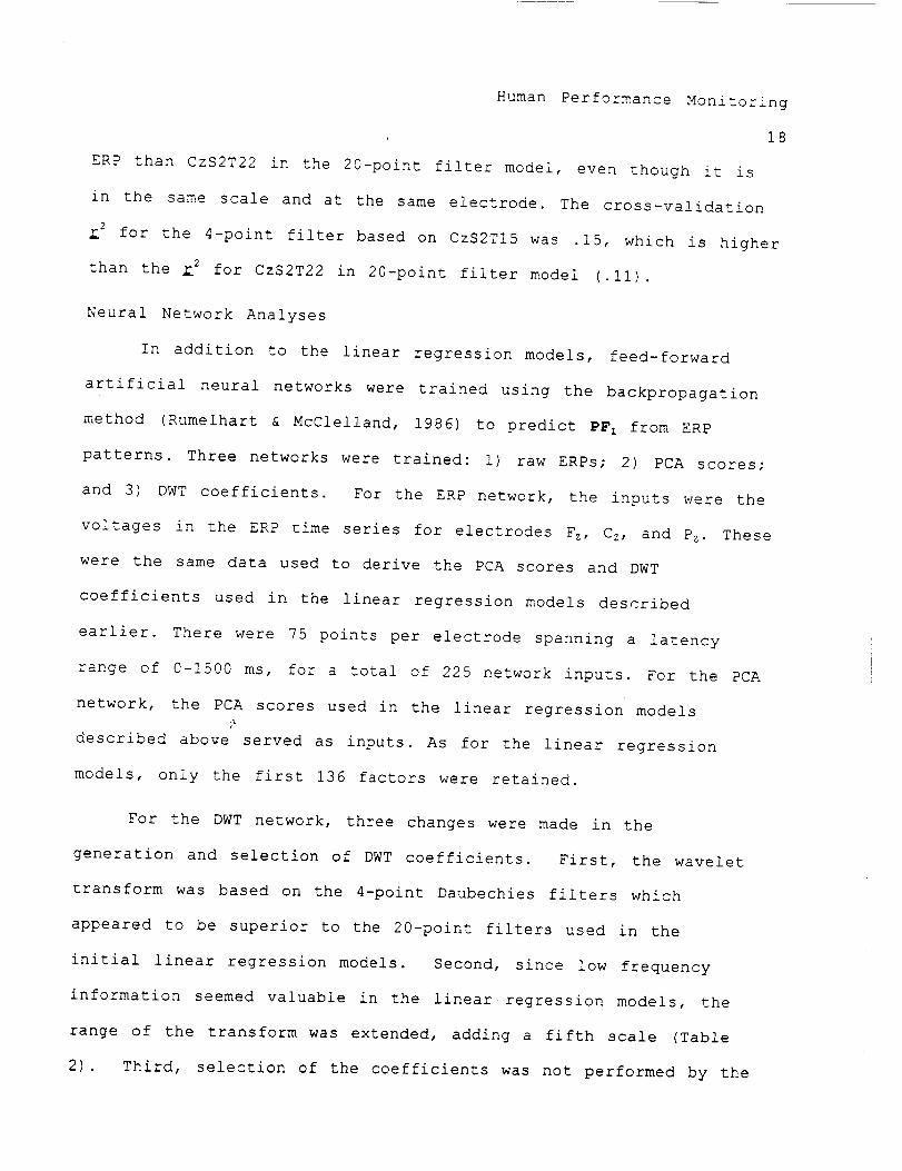
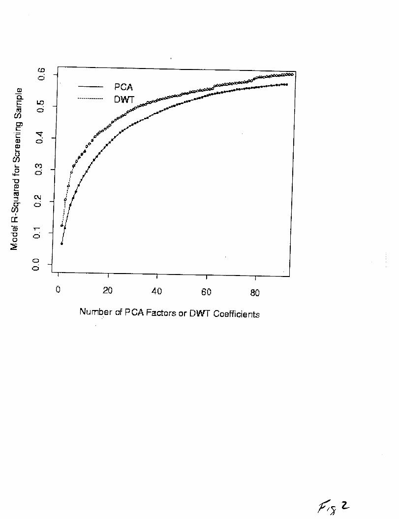
Using the criteria described above, 90 of the 136 PCA factors

entered into models predicting PFI, and 92 of the 210 DWTentered

into models predicting PFI (Figure 2). The _2 increased for the PCA

models in a fairly smooth, negatively accelerated fashion from a

minimum of .07 for a single factor model to a maximum of .58 using

90 factors as predictors. The _2 for the DWTmodel based on a

single coefficient was .12, nearly double that of the PCA model

based on a single factor. The increase in L2 for the DWTmodels was

almost linear for models using up to four coefficients as

predictors. Beyond that, further increases occurred in a piece-

wise linear fashion reaching a maximum of .62 using 92 predictors.

The greatest difference in _2 between the DWTand PCA models (.II)

also occurred with four predictors.


14i i i


Prior experience has shown that models using more than I0

predictors have limited generality and are difficult to interpret.

For this reason, cross-validation of the PCA and DWT models was

performed with no more than 20 predictors. The models developed

using the screening sample were applied in turn to the PCA scores

and DWT coefficients of the calibration sample. As for the

screening sample, performance of the models for the calibration

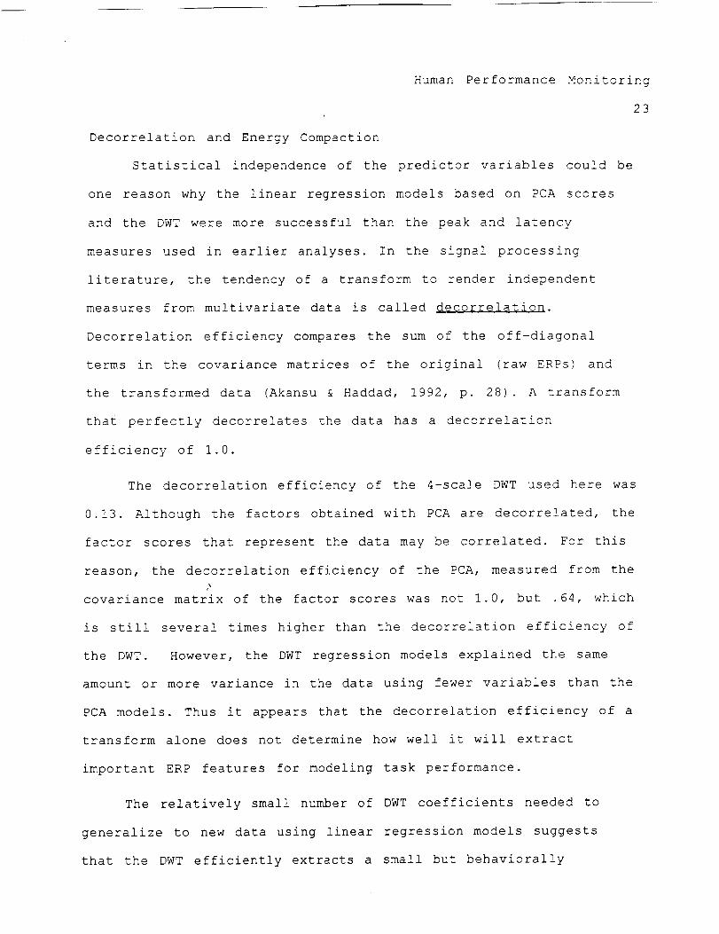
sample was assessed using _2 (Figure 3). In addition, the

significance of _2 was assessed using a F-ratio test (Edwards,

1976). This test used an adjusted number of degrees of freedom for

the denominator, to allow for the serial correlation in the data

introduced by computing the running means of the ERPs. In effect,

the number of degrees of freedom was divided by I0, to allow for

the 10-trial cycle length of the running-mean window. A

conservative significance level of .001 was chosen, given the

large number of models computed. The contour of _2 values at this

significance level appears as a dot-dashed line in Figure 3.

, i,., ii i,ll i ,i


i . i i

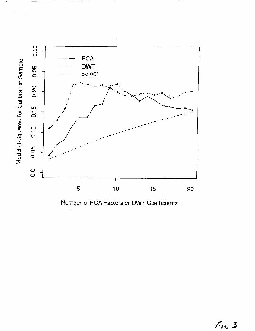
All of the PCA and DWT models tested explained significant

proportions of variance in the calibration data set. For the PCA

models, calibration _2 rose gradually from a nearly insignificant

level to a maximum of .22 using I0 predictors. The equation for

the 10-predictor PCA model was


15

PFI = .ii F2 - .I0 F4 + .13 F5 - .05 Fg - .09 F9 + .08 Fll

- .06 Fl5 - .08 F4_ + .07 F4_ - .07 F68 + .02,

where the factors are indexed according to the proportion of

variance accounted for in the running-mean ERPs. The factor

accounting for the greatest variance in the ERPs (Factor I) did

not enter the model. Five of the first i0 factors (Factors 2, 4,

5, 8, and 9) entered the model. Respectively, these factors

accounted for proportions of variance in the ERPs of .12, .031,

.0283, .0184, and .0169, or a total of .21 (21%). The entry of

some of the higher factors in the 10-predictor model is

surprising, given the small amount of variance in the ERPs that

they account for. For example, Factors II, 15, 43, 47, and 68

accounted for proportions of variance equal to .014, .01, .0022,

.0019, and .0011, respectively, or a total of .0292 (under 3%).

Among the DWT models, the calibration 2 for a single

predictor (.II) was well above that of the corresponding single-

factor PCA model (.04) and rose to a maximum of .22 using five DWT

coefficients as predictors. The DWT coefficients are coded by

electrode (Fz, Cz, Pz), scale (SO, SI, $2, S3) and time index (TO,

TI, .... TN). Actual latencies of the time points are obtained by

multiplying the time index by 20 ms, the sampling period.

The best single-predictor model was based on coefficient

CzS3T22, with a regression coefficient of -.03 and an intercept of

.02. Beyond five predictors, the _2 for the DWT models declined

slightly, and leveled off after about i0 predictors, showing no


16

further improvement. As for the screening sample data, the

greatest difference in _2 between the DWTand PCA models for the

calibration sample (.I0) occurred with four predictors.

The equation of the best five-predictor DWTmodel selected by

the stepwise regression algorithm was

PFI = - 0.03 * FzS2T6 + 0.04 * FzS2T22 + 0.06 * CzS2T 6

- 0.05 * CzS2T22 - 0.05 * PzS2T6 - 0.17.

From the five-predictor model, it is clear that a single scale,

number 2, is most important for predicting task performance. This

scale mainly reflects the time course of energy within the

bandwidth of .078 to 1.86 Hz, which overlaps the range of the

delta band of the EEG (I- 3.5 Hz) and will include some influence

from low-frequency ERP components such as the P300 and slow waves.

Two time intervals are indicated across electrodes: point 6 at Fz,

Cz, and Pz (120 ms), and point 22 and Fz and Pz (440 ms). Frontal

and parietal energy (Fz, Pz) in scale 2 at 120 ms is inversely

related to PF_ as shown by the negative regression coefficients,

whereas central activity (Cz) is positively related to PF_. Central

and parietal energy (Cz, Pz) in scale 2 is inversely related to PF I

at 440 ms.

One potential problem with the wavelet analysis performed

here stems from the length of Daubechies filters used (20 points).

These filters had lengths over one fourth the length of the

signals (75 points). While these filters produce smooth wavelet

transforms, they also increase the "support" of the transforms in


the time domain. This means that the transforms are extrapolated

in time before and after the interval of the signal. It also

means that, with respect to the filter length, the signal is short

in duration and appears to be a brief impulse at larger scales. A

possible complication from this is that time resolution for signal

features at the larger scales may be imprecise.

It is possible to decrease the support of the wavelet

transform at the expense of smoothness by using shorter filters.

To test the effects of shorter filters, the current data were

partially re-analyzed using Daubechies filters of 4 points in

length. With these filters, the support of the transform is

reasonable at all four of the scales analyzed and time resolution

of signal features at the larger scales is more precise than with

the 20-point filters.

The most important single predictor for the 4-point filter

DWTwas located at electrode Cz and scale 2, as for the best.<

sing!e-predictor model based on 20-point filters. However, the

wavelet coefficient in the 4-point filter model, CzS2TIS, was at

the 15 th time point or a latency of 300 ms. This lies 120 ms

earlier than the scale 2 coefficient in the best single-predictor

model based on the 20-point filters (CzS2T22). The regression

coefficient for CzS2TI5 in the 4-point filter model was .03, with

an intercept of -.16. This regression coefficient is negative,

whereas the regression coefficient for CzS2T22 in the 20-point

filter model was positive. The difference in sign suggests that

CzS2TI5 in the 4-point filter model is a different feature of the

17


18

ERP than CzS2T22 in the 20-point filter model, even though it is

in the same scale and at the same electrode. The cross-validation

_2 for the 4-point filter based on CzS2TI5 was .15, which is higher

than the _2 for CzS2T22 in 20-point filter model (.!I).

Neural Network Analyses

In addition to the linear regression models, feed-forward

artificial neural networks were trained using the backpropagation

method (Rumelhart & McClelland, 1986) to predict PF I from ERP

patterns. Three networks were trained: I) raw ERPs; 2) PCA scores;

and 3) DWT coefficients. For the ERP network, the inputs were the

voltages in the ERP time series for electrodes Fz, Cz, and Pz. These

were the same data used to derive the PCA scores and DWT

coefficients used in the linear regression models described

earlier. There were 75 points per electrode spanning a latency

range of 0-1500 ms, for a total of 225 network inputs. For the PCA

network, the PCA scores used in the linear regression models

described above served as inputs. As for the linear regression

models, only the first 136 factors were retained.

For the DWT network, three changes were made in the

generation and selection of DWT coefficients. First, the wavelet

transform was based on the 4-point Daubechies filters which

appeared to be superior to the 20-point filters used in the

initial linear regression models. Second, since low frequency

information seemed valuable in the linear regression models, the

range of the transform was extended, adding a fifth scale (Table

2). Third, selection of the coefficients was not performed by the


19

decimation approach taken for the linear regression models.

Instead, the undecimated transforms were computed (Shensa, 1991),

yielding 75 points for each scale. Then the mean power of each

coefficient was computed and the top 20% of the coefficients at

each scale were selected as inputs to the network (Figure 4). This

resulted in a set of 225 coefficients, or about the same number

that would be obtained by decimation. However, this scheme selects

coefficients that are high in power, and so account for large

proportions of the ERP signal variance at each scale.


Networks were trained and tested with a commercial software

package (Brainmaker, California Scientific Software, Inc. ) . All

three networks consisted of two layers. A single "hidden" layer

consisting of three neurons received connections from all the

inputs. These three neurons were fully connected to the output?"

layer, which consisted of a single neuron. The teaching signal for

this neuron was PFI. In addition to inputs from other neurons, each

neuron received a constant "bias" input, which was fixed at a

value of 1.0.

The output transfer function for all neurons was the logistic

function with a gain of 1.0 and a normalized output range of 0.0

to 1.0. The learning rate was 1.0 and the momentum was 0.9. All

inputs and the desired output (PF_) were independently and linearly

normalized to have a range of 0.0 to 1.0. As for the linear

regression models, the screening sample (half of runs) was used


2O

for training the networks and the calibration sample (the

remaining runs) was used for testing. Training proceeded by

adjusting the connection weights of the neurons for every input

vector. The training tolerance was 0.i, i.e., if the absolute

error between the network output (predicted PFI) and the actual PFI

value for a trial exceeded 10%, then the connection weights were

adjusted using the backpropagation algorithm.

Prior to training, the sequence of input vectors was

randomized. Training involved repeated passes (training epochs)

through the screening sample and was stopped after a maximum of

I000 training epochs. Testing was performed on the calibration

sample at intervals of I0 training epochs. The validity of a

trained network was measured in terms of the proportion of

calibration sample trials for which PFI was correctly predicted to

within the criterion 10% margin of error. The curve relating the

proportion of correctly predicted calibration sample trials to thei<

number of training epochs will be referred to as the

generaliz_%_on learning curve (Figure 5).

J ] J I I Ill I I I II I I I I I


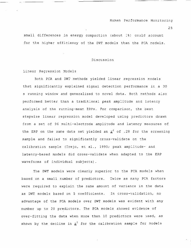
The probability of correctly guessing a uniform random

variable with a range of 0.0 to 1.0 with a 10% margin of error is

0.2. As shown in Figure 5, two of the three networks trained to

predict PFI in the calibration sample better than 0.2 with as few

as I0 training epochs. Beyond 50 training epochs, the


21

generalization learning curves of the three networks begin to

diverge.

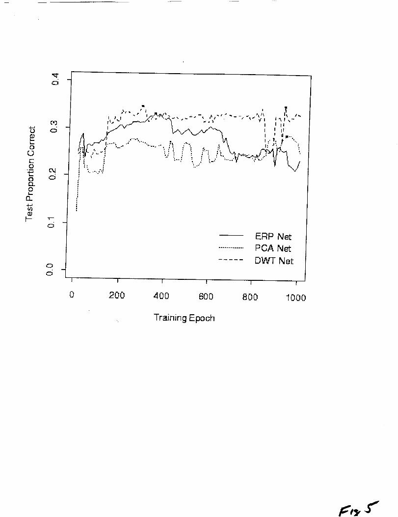
The DWTnetwork appears to "'learn" to generalize about as

well as it can by about 290 training epochs. For this network,

the proportion correct jumps from about 0.25 to over 0.3 near 200

epochs. From that point on, a rough plateau in the curve is held,

with a few dips between 800 and i000 epochs. The maximum

proportion correct of .348 occurs at epoch 930, but this is not

substantially (or significantly) greater than an earlier maximum

of .346 at epoch 290.

For the ERP network, a gradual rise in the proportion correct

occurs between I0 and 400 epochs, reaching a maximum of .331 at

training epoch 350. Beyond 400 epochs, the proportion correct for

the ERP network declines gradually to near chance levels of

performance.

The generalization learning curve of the PCA network exhibits

the most complex shape, rising and falling repeatedly over the

1000-epoch range. Interestingly, it also shows a large step near

200 epochs, as did the DWT network, and an early maximum of 0.279

at 250 epochs, after which the curve declines and oscillates up to

about 850 epochs. At that point the curve rises again, reaching a

new, higher maximum of 0.288 at 940 epochs.

Although the curves in Figure 5 are complex, two

generalizations seem possible. First, within the 1000-epoch scope

of the training, all three networks appear to achieve near-maximal


22

levels of generalization performance within the first 400 training

epochs. Beyond 400 training epochs, further training appears to

produce either declines or oscillations in generalization

performance, and only small increases above the earlier maximum

proportions of correctly predicted trials occur. Second, the DWT

network trained most rapidly and achieved the highest and most

stable level of generalization performance. The DWT network

"learned" to generalize to new data faster than the ERP network by

about 60 training epochs.

The raw ERP network achieved a proportion correct approaching

that of the DWT network (.331 versus .348) but was not as stable.

A z test of the significance of the difference between these

proportions based on the standard normal distribution [Fleiss,

1981, p. 23) yielded a R-value of .21. However, an F-test of the

ratio of variances of proportions correct for the ERP and DWT

networks between epochs 200 and I000 rejected the hypothesis that

the variances were equal, _F(79, 79) = 3.12, D < 0.000 (the

alternative hypothesis was that the true ratio of variances was

greater than 1.0_ .

Generalization performance of the PCA network was lower than

both the ERP and DWT networks. The _ tests of the differences

between the proportions correct of DWT and PCA networks and of ERP

and PCA networks yielded z-values of 0.0015 and 0.0162,

respectively.


23

Decorrelation and Energy Compaction

Statistical independence of the predictor variables could be

one reason why the linear regression models based on PCA scores

and the DWT were more successful than the peak and latency

measures used in earlier analyses. In the signal processing

literature, the tendency of a transform to render independent

measures from multivariate data is called _correlation.

Decorrelation efficiency compares the sum of the off-diagonal

terms in the covariance matrices of the original (raw ERPs) and

the transformed data (Akansu & Haddad, 1992, p. 28). A transform

that perfectly decorrelates the data has a decorrelation

efficiency of 1.0.

The decorrelation efficiency of the 4-scale DWT used here was

0.13. Although the factors obtained with PCA are decorrelated, the

factor scores that represent the data may be correlated. For this

reason, the decorrelation efficiency of the PCA, measured from the

covariance matrix of the factor scores was not 1.0, but 64 which

is still several times higher than the decorrelation efficiency of

the DWT. However, the DWT regression models explained the same

amount or more variance in the data using fewer variables than the

PCA models. Thus it appears that the decorrelation efficiency of a

transform alone does not determine how well it will extract

important ERP features for modeling task performance.

The relatively small number of DWT coefficients needed to

generalize to new data using linear regression models suggests

that the DWT efficiently extracts a small but behaviorally


24

important set of features from the ERP. The relative speed of

generalization learning by the DWTneural network may also be

consistent with this idea. If only a small proportion of the

inputs contains information related to the output then only the

weights corresponding to those inputs would require adjustment,

leading to faster generalization learning.

In signal processing, the property of a transform that

describes its tendency to concentrate information in a small

proportion of the variables is called 9nergy compact_Qn (Akansu &

Haddad, 1992, p. 28). Good energy compaction means having a small

number of large values on the diagonal of the covariance matrix of

the transform variables. It is measured as a function of the

number of variables retained to fit the data, sorted in order of

decreasing covariance. Energy compaction could also result in

more robust models, showing less overfitting. This could occur

when the variables that explain most of the variance enter first,

leaving only variables of low influence to adversely affect the

fits when added later.

For the data used in the linear regression models, energy

compaction measures of the raw ERPs, PCA scores, and DWT

coefficients for 5 variables was .06, .08, and .09. For I0

variables, energy compactions for ERP, PCA, and DWT were .Ii, .15,

and .16, and for 20 variables, energy compactions were .20, .25,

and .26, respectively. Thus over the range of models tested, the

DWT was only slightly more efficient in compacting the energy (or

variance) in the data than the PCA. It seems unlikely that such


25

small differences in energy compaction (about 1%) could account

for the higher efficiency of the DWTmodels than the PCA models.

Discussion

Linear Regression Models

Both PCA and DWTmethods yielded linear regression models

that significantly explained signal detection performance in a 30

s running window and generalized to novel data. Both methods also

performed better than a traditional peak amplitude and latency

analysis of the running-mean ERPs. For comparison, the best

stepwise linear regression model developed using predictors drawn

from a set of 96 multi-electrode amplitude and latency measures of

the ERP on the same data set yielded an _2 of .28 for the screening

sample and failed to significantly cross-validate on the

calibration sample (Trejo, et al., 1995; peak amplitude- and

latency-based models did cross-validate when adapted to the ERP

waveforms of individual subjects).

The DWTmodels were clearly superior to the PCA models when

based on a small number of predictors. Twice as many PCA factors

were required to explain the same amount of variance in the data

as DWT models based on 5 coefficients. In cross-validation, no

advantage of the PCA models over DWTmodels was evident with any

number up to 20 predictors. The PCA models showed evidence of

over-fitting the data when more than I0 predictors were used, as

shown by the decline in _2 for the calibration sample for models


26

using I0 to 20 predictors. In contrast, the DWTmodels suffered

relatively small decreases in r2 when using more than 5

coefficients.

Single-predictor models for the DWT based on 4-point filters

were compared to the 20-point filters used initially to determine

the sensitivity of the location estimates to filter length. The

net effects of using shorter filters to compute the wavelet

transform were to change the location estimate, but not the

electrode or scale estimates of the best single predictor model,

and increased cross-validation r 2. The higher cross-validation _2

for the 4-point filter model than the 20-point filter model was

unexpected. However, this result suggests that more precise

temporal localization of features in the wavelet transform may

provide more robust representation of the ERP or EEG features

associated with task performance.

PCA is known to produce factors that resemble the shape and

time course of ERP components. The information provided by the

DWT is somewhat different. For example, the 5predictor DWT model

indicated that a pattern of energy at specific latencies in the

ERP confined to the bandwidth associated with P300, slow waves,

and EEG delta band activity, was correlated with signal detection

performance across a sample of eight subjects. It is well known

that P300 and slow waves co-vary with the allocation of cognitive

resources during task performance. However, it is not clear

whether the wavelet coefficients included in the regression models

are simply better measures of P300 and slow wave or if they


27

represent new aspects of the ERP. Comparisons of ERPs

reconstructed from the DWTcoefficients and the average ERP

waveforms will be required to express the coefficients in terms of

familiar ERP peaks.

Neural Networks

As for the linear regression models, the best generalization

performance of neural networks -- measured in terms of predicting

PFI in the calibration sample -- was achieved with the DWT

representation of the ERPs. Somewhat surprisingly, neural networks

trained to predict PFl from raw ERPs generalized almost as well as

the DWT. Both ERP and DWT-based networks generalized to new data

significantly better than networks based on PCA scores.

The neural network based on the DWTrequired fewer training

epochs than the raw-ERP network to reach a maximal level of

generalization to new data. In addition, beyond the initial

training period of 200 epochs, generalization performance of thei<

DWT network was more stable than the ERP network. After about 400

training epochs, the generalization learning curve declined for

the ERP network, indicating overfitting of the data in the

screening sample. In contrast, the generalization learning curve

for the DWT exhibited a few dips, but remained surprisingly stable

over most of the training range, indicating a resistance to

overfitting. This result agrees with the resistance to overfitting

observed with more than the optimum number coefficients in the

linear regression models based on the DWT.


28

General Conclusions

The results described here show that the DWTcan provide an

efficient representation of ERPs suitable for performance-

prediction models using either linear regression or neural network

methods. Furthermore, the DWTmodels tested here needed the fewest

parameters, exhibited highest generalization and were relatively

insensitive to the detrimental effects of over-fitting as compared

to models based on PCA scores or raw ERPs. This result, together

with the initial rise in _2 for the linear regression DWTmodels

(Figure 3) suggest that the DWTcoefficients measure unique and

important sources of performance-related variance in the ERP.

The superiority of the DWTover PCA that we have seen in the

models tested here cannot be explained in terms of decorrelation

and energy compaction properties of these transforms.

Decorrelation was actually higher for PCA than for the DWT, and

energy compactions over the range of variables included in the

models were about equal for the two transforms. Instead, it

appears that the DWT simply provides more useful features than

PCA, when utility is measured by how efficiently task performance

can be predicted using ERPs.

For practical ERP-based models of human performance, ease of

model development and speed of computation are also important

factors. The cost of computing the DWT is trivial when compared to

deriving a PCA solution, which involves inverting and

diagonalizing a large covariance matrix. Even more time is


29

required for peak and latency analyses, which depend on expert

human interpretation of the waveforms.

The nature of the features extracted using the DWTmerits

further study. By identifying the time and scale of energy in the

ERP related to task performance, specific ERP or EEG components

may be indicated. For example, slow waves and delta-band activityr

appear in the 5-predictor linear regression DWT model of signal

detection performance. In this way, The DWT may provide new

insight into the physiological bases of cognitive states

associated with different performance levels in display monitoring

tasks.

Future work should examine the reconstructed time course and

scalp distribution of the patterns indicated by DWT or othe_

wavelet models and relate these to known physiological generators.

Through inversion of the DWT, it is possible to reconstruct the

time course of the energy indicated by a specific model. Ini<

addition, other wavelet transforms may provide a finer analysis of

the time-frequency distribution of the ERP. For example, wavelet

transforms using multiple "voices" per scale, such as the Morlet

wavelets or wavelet packets, provide much finer resolution than

that afforded by the DWT method used in this study. In addition,

data from other kinds of tasks should be analyzed and the

development of models for individual subjects should be also

explored.


30

References

Akansu, A. N., & Haddad, R. A. (1992). MultiresolutiQn

Decomposition. Transforms, Subbands, and Wavelets. San Diego:

Academic Press.

DasGupta, S., Hohenberger, M., Trejo, L. J., & Mazzara, M. (1990) .

Effect of using peak amplitudes of ERP signals for a class of

neural network Classification. Proceedinas of the First WorkshQp

on Neural Networks: Academic / Industrial / NASA / Defense, pp.

101-114, Auburn, AL: Space Power Institute.

DasGupta, S., Hohenberger, M., Trejo, L., & Kaylani, T. (1990,

April). Effect of data compression of ERP signals preprocessed

by FWT algorithm upon a neural network classifier. The

Annual Simulation _Q__, Nashville, TN.

Daubechies, I. (1990). The Wavelet Transform, Time-Frequency

Localization and Signal Analysis. IEEE Transactions on

_" Theory, 36 (5) .

Daubechies, I. (1992). Ten Lectures on Wavelets. Philadelphia:

Society for Industrial and Applied Mathematics.

Dixon, W. J., (1988). BMDP _ Software Manual. Berkeley:

University of California Press.

Edwards, A. L. (1976). An Introduction to Linear ReGression and

_. San Francisco: W. H. Freeman and Co.

Fleiss, J. L. (1981). _ m_thods for rates and

proportions. Second edition. New York: John Wiley and Sons.


31

Gratton, G., Coles, M. G., & Donchin, E. (1983). A new method for

off-line removal of ocular artifact. Electroencemhalogramhy and

Clinical Ng_roDhysioloav, 55, 468-484.

Humphrey, D., Sirevaag, E., Kramer, A. F., & Mecklinger, A.

(1990). Real-time measurement of mental wQrklQad 9__

psYChOphy$iological measures. (NPRDC Technical Note TN 90-18).

San Diego: Navy Personnel Research and Development Center.

Jasper, H. (1958). The ten-twenty electrode system of the

international federation. Electroencephalographv and Clinical

N_ur©physiology, 43, 397-403.

Kaylani, T., Mazzara, M., DasGupta, S., Hohenberger, M., & Trejo,

L. (1991, February). _lassification of ERP $_qnals _ n_ral

networks. PrQCe_dings of the Second Workshop on Neural Networks:

Acad@mi¢ / Industrial / NASA / Defen$@, pp 737-742. Madison,

WI: Omnipress.

Rumelhart, D. E., & McClel!and, J. L. (1986). Parallel

distributed processing: _Zplorations in the microstructure of

cognition. Vol. _. FQUndations. Cambridge, MA: MIT

Press/Bradford Books.

Ryan-Jones, D. L. & Lewis, G. W. (1991, February). Application of

neural network methods to prediction of job performance.

_rQ¢_edings of the __9__ Workshoo on Neura! Networks:

/ _ / NASA / Defense, pp. 731-735. Madison, W!:

Omnipress.

Shensa, M. J. (1991). The discrete wavelet transform (Technical

Report No. 1426). San Diego: Naval Ocean Systems Center.


32

Trejo, L. J., Kramer, A. F., & Arnold, J. (1995). Event-related

potentials as indices of display-monitoring performance.

Psycholoay, 40, 33-71.

Trejo, L. J., & Mul!ane, M. M. (1995). Event-related potentials

and signal detection performance: Classification functions based

on discrete wavelet transforms. Psychophysiology, 32, S77.

Tuteur, F. B. (1989). Wavelet transformations in signal detection.

In J. M. Combes, A. Grossman, & Ph. Tchamitchian, (Eds.),

Wavelets: Time-frequency methQ_$ and p_b_h__ space. New York:

Springer-Verlag, pp. 132-138.

Venturini, R., Lytton, W. W., & Sejnowski, T. J. (1992). Neural

network analysis of event related potentials and

electroencephalogram predicts vigilance. In J. E. Moody, S. J.

Hanson, & R. P. Lippmann (Eds.), Advances in Neural Information

Processing Systems _, pp. 651-658. San Mateo, CA: Morgan

Kaufmann Publishers.


33

Table I. Scales of the 20-point Daubechies Discrete Wavelet

Transform

Scale

i

Bandwidth (Hz)

ii i.i

Center Frequency (Hz)

0 I0 .50-25 .00 16.20

1 4.42-10.50 6. 82

2 1.86--4.42 2.87

3 0.78--1.86 1.20

Table 2.

Transform

Scales of the 4-point


34

Daubechies Discrete Wavelet

Scale Bandwidth (Hz) Center Frequency (Hz)

0

1

2

3

4

10.88-25.00 16.49

4.74-10.88 7.18

2.06-4.74 3.12

0.90--2.06 1.36

0.39--0.90 0.59


35

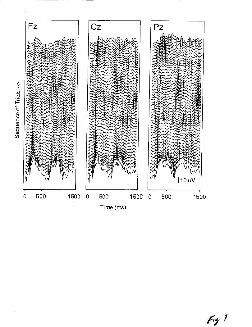
Figure i. Running-mean ERPs at sites Fz, Cz, and Pz for subject 2 in

the first block of 50 trials. Zero on the abscissa represents the

stimulus onset (appearance of the display symbol used for the

signal detection task). The ordinate represents scalp voltage at

each electrode site; positive is up. The running-mean ERPs for

successive trials of the block are stacked vertically from bottom

to top (lowest is first).

Figure 2. Coefficients of determination ( 2 or variance accounted

for) for PCA and DWTmodels developed to predict task performance

(PFI) for eight subjects in a signal detection task. Models were

based on a screening sample of running-mean ERP and PFI data, drawn

from odd-numbered blocks of trials. Models are assessed by the _2

as a function of the number of predictors entering into the model.

Only models in which predictors met a criterion F-ratio of 4.0 to

enter (3.99 to remove) are shown.

Figure 3. Coefficients of determination (_2 or variance accounted

for) for the first 20 PCA and DWT models of Figure 2, cross-

validated using running-mean ERP and PF_ data from a calibration

set of data drawn from even-numbered blocks of trials. The dot-

dashed line indicates the contour of _ values significant using an

F-ratio test at the p < .001 level where the numerator degree of

freedom depends on the number of predictors and the denominator

degrees of freedom is one-tenth of the sample size. Values above

this contour are significant.


36

Figure 4. Mean power of the undecimated 5-scale DWT coefficients

at electrodes Fz, Cz, and Pz, used for the neural network trained to

predict PFI. The DWT coefficients for each running-mean ERP were

squared, summed, averaged and plotted as a function of dime

relative to the stimulus. Each row of graphs represents one scale

of the transform beginning with the smallest scales at the top

(see Table 2) and proceeding to the largest scale at the bottom.

Each column of graphs corresponds to one electrode site in the

order Fz, Cz, Pz, from left to right. The 80% quantile was computed

across electrodes within each scale and is shown by the horizontal

line in each graph. Coefficients with mean power values greater

than the 80% quantile, i.e., the top 20%, were used as inputs to

the neural network.

Figure 5. Generalization learning curves of the three neural

networks trained to predict PFI from raw ERPs (solid line), PCA

scores (dotted line), or high-power DWT coefficients (dashed

line). The abscissa marks the number of training epochs (complete

passes through the screening sample) and the ordinate marks the

proportion of trials in the calibration sample for which PF I was

correctly predicted with a 10% margin of error. The solid circles

mark the highest proportion correct for each network.

Fz

A " ""- ^'_

' %_'f J_\_^".,-9.

g

0 500 1500 0

Cz

.-,%.

r',

,5,

,.,,.,

'%,",%,'v

V3

5OO

Time (ms)

"%1,

"-4.

-_. ,I.

.,-.-,

,,=,%-

4_

1500 0

Pz

,.,,%

.,-,-,,.,,,,,rJ', i,/,.'.69,,-,,_ - i ._;-..__

¢-_,a

,.+._. i .. +_i

@

i

5OO 1500

PCA

_3

g °

I I I I

0 20 40 60 80

Number of PCA Factors or DW-I Coefficients

E

t,,,0r"O

I,.-

I,--

O4.--

t,,'0

I

"OO

OCO

O

I,Do4,:5

O04O

'T--"

,:5

O',r"-

,:5

I.,9O

O

,:5

PCA

............. DW-I"

..... p<.001

/'... \•' / "_.. ""- c,-- -_'- -_ .":"'""_

I I I I

5 10 15 20

Number of P CA Factors or DWT Coefficients

,S C,31e 1

:s

_ Scale 3

ScaM 4

i.IlhllllJi,.!,,,,,:0

0 500 ]CO0 0 500 1000 0 _OO 11300

. Time (ms)

P0

L--0

0

0L

n.I-.,.I

(,¢

F--

0

0

ERP Net

PCA Net

DWT Net

I I I I I

200 400 600 800 1000

Training Epoch

search.jsp?R=20020062997 2018-07-23T09:28:45… · Human Performance Monitoring 1 ... 45+00:00Z. Human Performance Monitoring ... human performance monitoring, signal detection, vision.

Documents