r n a l - univie.ac.at · 2014-11-30 · class of important equations, including equations of nonlinear ltering, stochastic heat equation with nonlinear noise term, ... Of course

E l e c t r o n i c

Jo

ur n a l

of

Pr o b a b i l i t y

Vol. 6 (2001) Paper no. 12, pages 1–35.

Journal URLhttp://www.math.washington.edu/~ejpecp/

Paper URLhttp://www.math.washington.edu/~ejpecp/EjpVol6/paper12.abs.html

A NOTE ON KRYLOV’S Lp-THEORY FOR SYSTEMS OF SPDES

R. Mikulevicius1

Institute of Mathematics and Informatics, Akademijos 4, Vilnius, LithuaniaE-mail: [email protected]

B. Rozovskii2

Center for Applied Mathematical Sciences, USC, Los Angeles 90089-1113, [email protected]

Abstract We extend Krylov’s Lp-solvability theory to the Cauchy problem for systems ofparabolic stochastic partial differential equations (SPDEs). Some additional integrability andregularity properties are also presented.

Keywords Stochastic partial differential equations, Cauchy problem

AMS subject classification 60H15, 35R60.

Submitted to EJP on November 17, 2000. Final version accepted on March 14, 2001.

1Research supported in part by NSF Grant DMS-98-024232Research supported in part by NSF Grant DMS-98-02423, ONR Grant N00014-97-1-0229, and ARO Grant

DAAG55-98-1-0418

1 Introduction

A comprehensive theory of second order quasi-linear parabolic stochastic differential equationsin Bessel classes Hs

p(Rd) was developed by N. V. Krylov in [1], [2]. This theory applies to a largeclass of important equations, including equations of nonlinear filtering, stochastic heat equationwith nonlinear noise term, etc.. The main results of the theory are sharp in that they could notbe improved under the same assumptions.

In this paper we extend Krylov’s Lp−theory to parabolic systems of quasilinear stochastic PDEs.Specifically, we are considering the system of equations

∂tul = ∂i(aij(t, x)∂ju

l)+Dl(u, t, x)

+ [σk(t, x)∂kul +Ql(u, t, x)] · W , (1.1)

ul(0, x) = ul0(x), l = 1, . . . , d;x ∈ Rd

where W is a cylindrical Wiener process in a Hilbert space. In (1.1) and everywhere below thesummation with respect to the repeated indices is assumed.

Among other reasons this research was motivated by our interest in stochastic Fluid Mechanics(see e.g. [6], [7] ). While the results below do not apply directly to stochastic Navier-Stokesequations, they provide us with important estimates for solutions of suitable approximation tothe latter.

The structure of the paper is as follows.

In Section 2 we present a simple and straightforward construction of stochastic integrals forHs

p−valued integrands (for related results see [3], [4]). In this Section we also derive an Itoformula for Lp-norms of Hs

p−valued semimartingales.

In Section 3 we present some auxiliary results about pointwise multipliers in Hsp needed for

the derivation of apriori estimates for (1.1) (see Lemma 8). We give a more precise version ofKrylov’s Lemma 5.2 in [2] with an estimate that gives a positive answer to Krylov’s questionraised in Remark 6.5 (see [2]).

In Section 4, following Krylov’s ideas, we derive the main results about the existence and unique-ness of solutions to equation (1.1). The results of the last subsection, in particular those con-cerning the regularity of solutions (Proposition 1, Corollary 3, Corollary 4) are new not onlyfor systems but also for the scalar equations considered in [1], [2]. In addition, in Section 4, weobtain some new integrability properties of the solution (Proposition 2-3, Corollary 3-4).

To conclude the Introduction, we outline some notation which will be used throughout the paper.

Rd denotes d-dimensional Euclidean space with elements x = (x1, . . . , xd); if x, y ∈ Rd, we write

(x, y) =d∑

i=1

xiyi, |x| =√

(x, x).

Let us fix a separable Hilbert space Y . The scalar product of x, y ∈ Y will be denoted by x · y.

2

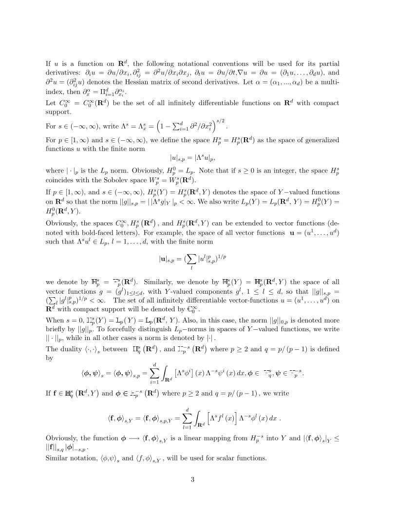
If u is a function on Rd, the following notational conventions will be used for its partialderivatives: ∂iu = ∂u/∂xi, ∂

2ij = ∂2u/∂xi∂xj , ∂tu = ∂u/∂t,∇u = ∂u = (∂1u, . . . , ∂du), and

∂2u = (∂2iju) denotes the Hessian matrix of second derivatives. Let α = (α1, ..., αd) be a multi-

index, then ∂αx = Πd

i=1∂αixi.

Let C∞0 = C∞

0 (Rd) be the set of all infinitely differentiable functions on Rd with compactsupport.

For s ∈ (−∞,∞), write Λs = Λsx =

(1 − ∑d

i=1 ∂2/∂x2

i

)s/2.

For p ∈ [1,∞) and s ∈ (−∞,∞), we define the space Hsp = Hs

p(Rd) as the space of generalizedfunctions u with the finite norm

|u|s,p = |Λsu|p,where | · |p is the Lp norm. Obviously, H0

p = Lp. Note that if s ≥ 0 is an integer, the space Hsp

coincides with the Sobolev space W sp = W s

p (Rd).

If p ∈ [1,∞), and s ∈ (−∞,∞), Hsp(Y ) = Hs

p(Rd, Y ) denotes the space of Y−valued functions

on Rd so that the norm ||g||s,p = | |Λsg|Y |p <∞. We also write Lp(Y ) = Lp(Rd, Y ) = H0p(Y ) =

H0p (Rd, Y ).

Obviously, the spaces C∞0 ,Hs

p

(Rd

), and Hs

p(Rd, Y ) can be extended to vector functions (de-noted with bold-faced letters). For example, the space of all vector functions u = (u1, . . . , ud)such that Λsul ∈ Lp, l = 1, . . . , d, with the finite norm

|u|s,p = (∑

l

|ul|ps,p)1/p

we denote by H sp = H s

p(Rd). Similarly, we denote by H sp(Y ) = H s

p(Rd, Y ) the space of allvector functions g = (gl)1≤l≤d, with Y -valued components gl, 1 ≤ l ≤ d, so that ||g||s,p =(∑

l |gl|ps,p)1/p < ∞. The set of all infinitely differentiable vector-functions u = (u1, . . . , ud) onRd with compact support will be denoted by C∞

0 .

When s = 0, H sp(Y ) = Lp(Y ) = Lp(Rd, Y ). Also, in this case, the norm ||g||0,p is denoted more

briefly by ||g||p. To forcefully distinguish Lp−norms in spaces of Y−valued functions, we write|| · ||p, while in all other cases a norm is denoted by |·| .The duality 〈·, ·〉s between H s

q

(Rd

), and H −s

p

(Rd

)where p ≥ 2 and q = p/ (p− 1) is defined

by

〈φ,ψ〉s = 〈φ, ψ〉s,p =d∑

i=1

∫Rd

[Λsφi

](x) Λ−sψi (x) dx,φ ∈ H

sq ,ψ ∈ H

−sp .

If f ∈ H sq

(Rd, Y

)and φ ∈ H −s

p

(Rd

)where p ≥ 2 and q = p/ (p− 1) , we write

〈f ,φ〉s,Y = 〈f ,φ〉s,p,Y =d∑

l=1

∫Rd

[Λsf l (x)

]Λ−sφl (x) dx .

Obviously, the function φ −→ 〈f ,φ〉s,Y is a linear mapping from H−sp into Y and |〈f ,φ〉s|Y ≤

||f ||s,q |φ|−s,p .

Similar notation, 〈φ,ψ〉s and 〈f, φ〉s,Y , will be used for scalar functions.

3

2 Stochastic integrals

Let (Ω,F ,P) be a probability space with a filtration F of right continuous σ-algebras (Ft)t≥0.All the σ−algebras are assumed to be P−completed. Let W (t) be an F-adapted cylindricalBrownian motion in Y . In this section we will construct a natural stochastic integral withrespect to W (t) for F-adapted Hs

p(Rd, Y )-valued integrands.Let p ≥ 2, s ∈ (−∞,∞) . Then Is,p denotes the set of all measurable F-adapted H s

p(Y )-valuedfunctions such that for every t, ∫ t

0||g(r)||ps,p dr <∞ P− a.s.

If g ∈Im,p then for every and φ ∈ H−mq where q = p/ (p− 1) , we can define a stochastic integral

Mt(φ) =∫ t

0〈g(r),φ〉s,Y · dW (r) .

Indeed, by Holder inequality,∫ t0

∣∣∣〈g (r) ,φ〉s,Y∣∣∣2Ydr ≤ ∫ t

0 ||g (r)||2s,p ||φ||2−s,q dr ≤

C(∫ t

0 ||g (r)||ps,p dr)(p−2)/p ||φ||2p/(p−2)

−s,q <∞ P − a.s.

(2.1)

Owing to (2.1), the stochastic integral∫ t0 〈g (r) ,φ〉s,Y ·dW (r) is well defined (see e.g. [9] or [5]).

Of course the integral above is defined as a linear functional on H −sq . In fact, it can be charac-

terized more precisely. Specifically, the following result holds.

Theorem 1 If g ∈ Is,p, p ≥ 2, then there is a unique H sp (Y )-valued continuous martingale

M(t) =∫ t0 g (r) · dW (r) such that for all φ ∈ H −s

q ,⟨∫ t

0g (r) · dW (r) ,φ

⟩s

=∫ t

0〈g(r),φ〉s,Y · dW (r) ∀t > 0,P − a.s. (2.2)

Moreover, for each T > 0 there exists a constant C so that for each stopping time τ ≤ T,

E supr≤τ

|M(r)|ps,p ≤ CE∫ τ

0||g(r)||ps,p dr.

To prove the Theorem we will need the following technical result.

Lemma 1 Assume g ∈Is,p. Then there is a sequence of F-adapted H sp(Rd)-valued processes

gn(r) = gn(r, x) such that P-a.s. gn(r, x) is smooth in x and for each n,

supx

|gn(s, x)|Y ≤ Cn||g(r)||s,p, ||gn(r)||s,p ≤ ||g(r)||s,p,

and ∫ t

0||gn(r) − g(r)||ps,p dr → 0, as n→ ∞.

P-a.s. for all t .

4

Proof If we have two Hsp (Y )-valued continuous martingales M1(t), M2(t) satisfying (2.2), then

P-a.s. for all t and φ ∈ H−sq ,

〈M1(t) − M2(t),φ〉s = 0,

and the uniqueness follows. Let ϕ be a nonnegative function so that ϕ ∈ C∞0 (Rd) and

∫ϕdx =

1. For ε > 0, write ϕε(x) = ε−dϕ(x/ε). Set

gn(r, x) =∫

Λ−sϕ1/n(x− y)Λsg(r,y) dy.

Note that gn is a smooth bounded Y -valued function. Moreover, by Holder inequality,

|∂αx gn(r, x)|Y ≤ C ′

1/n,α(∫

|Λsg(r, y)|pY dy)1/p

(∫|∂α

x Λ−sϕ1/n(x− y)|qdy)1/q

≤

≤ C1/n,α||g(r)||s,p,It is readily checked that for all r, ω, and p ≥ 2, we have the following:(a) ||gn(r, ·)||s,p ≤ ||g(r, ·)||s,p,(b) ||gn(r) − g(r)||s,p → 0 as n→ ∞ .

Indeed,||gn(r, ·)||s,p =

∣∣∣∣Λs∫

Λ−sϕ1/n(x− y)Λsg(r,y) dy∣∣∣∣

p=

∣∣∣∣∫ ϕ1/n(x− y)Λsg(r,y) dy∣∣∣∣

p≤ ||Λsg(r, ·)||p = ||g(r, ·)||s,p.

Analogously, one can prove (b) . Now, the statement follows by Lebesgue’s dominated conver-gence theorem.

Proof of Theorem 1 Let gn be a sequence from Lemma 1. Since for every x and t,∫ t0 |gn(r, x)|2Y dr <∞ P -a.s., the stochastic integral

Mn(t, x) =∫ t

0gn(r, x) · dW (r),

is well defined for each x (see e.g. [9] or [5]). It is not difficult to show that for every x,

ΛsMn(t, x) =∫ t

0Λsgn(r, x) · dWr (2.3)

P -a.s. By the Burkholder-Davis-Gundy and Minkowski’s inequality, for each stopping timeτ ≤ T

E supr≤τ

|Mn(r) |ps,p = E supr≤τ

|ΛsMn(r) |pp ≤ (2.4)

CE∫ τ

0||Λsgn(r)||pp dr = CE

∫ τ

0||gn(r)||ps,p dr

and

E supr≤τ

|Mn(r) − Mn′(r) |ps,p ≤ CE∫ τ

0||gn(r) − gn′(r)||ps,p dr.

5

Firstly, we prove the existence of a continuous in t H sp -valued modification of Mn(t, x). Let

gsn,k(r, x) = 1|x|≤k1‖g(r,·)‖s,p≤kgn(r, x)

Let τ ≤ T be a stopping time such that

E∫ τ

0||g(r, ·)||ps,p dr <∞.

Define

Mn,k(t, x) =∫ t∧τ

0gs

n,k(r, x) · dWr, Msn,k(t, x) =

∫ t∧τ

0Λsgs

n,k(r, x) · dWr.

Then, for all u ≤ t ≤ T,

E[(∫

|Msn,k(t, x) − Ms

n,k(u, x)|p dx)2]

≤ CkE∫

|Msn,k(t, x) − Ms

n,k(u, x)|2p dx

≤ Ck

∫E(

∫ t∧τ

u∧τ|Λsgs

n,k(r, x)|2Y dr)p dx ≤ Ck|t− u|p,

and by Kolmogorov’s criterion, Msn,k has a continuous Lp -valued modification. On the other

hand,

E supr≤τ |Mn,k(r, ·) − Mn(r, ·)|ps,p = E supr≤τ |Msn,k(r, ·) − ΛsMn(r, ·)|pp ≤

CE∫ τ0 ||Λs(gs

n,k(r, ·) − gn(r, ·))||pp dr → 0,

as k → ∞. So, ΛsMn has an Lp -valued continuous modification or, equivalently, Mn has anH s,p -valued continuous modification. By (2.3) we have that for all t > 0,φ ∈ H −s

q ,

〈Mn(t),φ〉s =∫ t

0〈gn(r),φ〉s,Y · dWr ∀t > 0,P − a.s.

for every t > 0, P-a.s.

Now, by (2.4), Mn is a Cauchy sequence. Making n ↑ ∞ on both sides of the equality wecomplete the proof.

Remark 1 For p ∈ [1, 2), the stochastic integral with the properties above does not exist (see[12]).

Lemma 2 Let p ≥ 2. Let g ∈I0,p and∫ t

0||g(r)||21 dr <∞ ∀t > 0, P − a.s.

6

Then for every t > 0, P-a.s. one has∫ ∫ t

0g(r, x) · dW (r) dx = lim

m→∞

∫φm(x)

(∫ t

0g(r, x) · dW (r)

)dx

=∫ t

0(∫

g(r, x) dx) · dW (r) ,

where φm ∈ C∞0 is any uniformly bounded sequence converging pointwise to 1.

Proof By Theorem 1,

Zm(t) =∫φm(x)

∫ t

0g(r, x) · dW (r) dx =

∫ t

0(∫

g(r, x)φm(x) dx) · dW (r)

for every t > 0, P-a.s.Let τ be a stopping time such that

E∫ τ

0||g(r)||21 dr <∞.

ThenE sup

r≤τ|Zn(r) − Zm(r)|2 ≤ CE

∫ τ

0||g(r)(φn − φm)||21 dr → 0,

as n,m→ ∞, and the statement follows.

Now we can prove the Ito formula for the Lp-norm of a semimartingale.

Lemma 3 Let p ≥ 2 . Set

u(t, x) = u0(x) +∫ t

0a(r, x) dr +

∫ t

0b(r, x) · dW (r) (2.5)

where b ∈ I0,p, u0 is an F0-measurable Lp -valued random variable, and a is an F-adaptedH n−1

p -valued process where n = 0 or 1. If u(t) is continuous Lp -valued process and∫ t

0(|a(r)|pn−1,p + |u(r)|p1−n,p) dr <∞

for all t > 0, P-a.s., then

|u(t)|pp = |u0|pp + p

∫ t

0〈|u(r)|p−2u(r),a(r)〉1−n dr

+ p

∫ t

0(∫

|u(r, x)|p−2(u(r, x),b(r, x)) dx dW (r) (2.6)

+p

2

∫ t

0(∫

[(p − 2)|u(r, x)|p−4ui(r, x)uj(r, x)

+ |u(r, x)|p−2δij ]bi(r, x) · bj(r, x) dx) dr

for all t > 0, P-a.s..

7

Proof We remark that all the integrals in (2.6) are well defined. For example, let us provethat the duality 〈|u(r)|p−2u(r),a(r)〉1−n makes sense if n = 0. Since a(r) ∈ H

−1p , there exist

functions ai(r) ∈ Lp so that a(r) =∑d

i=0 ∂iai (r) where ∂0 = 1. Now it is not difficult to seethat

〈|u(r)|p−2u(r),a(r)〉1 =∑d

i=0〈|u(r)|p−2u(r), ∂iai (r)〉1 =

−∑di=0〈∂i|u(r)|p−2u(r),ai (r)〉0.

(2.7)

The right hand side of the equality is finite owing to the obvious equality

∂i(|u|p−2ul) = (p − 2)|u|p−4um∂iumul + |u|p−2∂iu

l).

Let ϕ ∈ C∞0 be a non-negative function such that

∫ϕdx = 1. For ε > 0, write

ϕε(x) = ε−dϕ(x/ε), uε(t, x) =∫ϕε(x− y)u(t, y) dy = u(t) ∗ ϕε(x).

Similarly, we write bε(t) = b(t) ∗ ϕε(x), u0,ε = u0 ∗ ϕε(x). Let aε(t, x)

= 〈a(t), ϕε(x− ·)〉 . For all x and t, we have

uε(t, x) = u0,ε(x) +∫ t

0aε(r, x) ds +

∫ t

0bε(r, x) · dW (r) P− a.s.

Let φ ∈ C∞0 , φ = 1 on |x| ≤ 1, φ = 0 on |x| ≥ 2. Then φm(x) = φ(x/m) is a uniformly

bounded sequence converging pointwise to 1. By Ito formula, we have

|uε(t, x)|pφm(x) = |u0,ε(x)|pφm(x)+ (2.8)∫ t

0p|uε(r, x)|p−2(uε(r.x),aε(r, x))φm(x) dr

+∫ t

0pφm(x)|uε(r, x)|p−2(uε(r, x),bε(r, x)) · dW (r)

+p

2

∫ t

0φm(x)[(p − 2)|uε(r, x)|p−4ui

ε(r, x)ujε(r, x)

+ |uε(r, x)|p−2δij ]biε(r, x) · bjε(r, x) ds..Also,

supr≤t,x

|uε(r, x)| + suprst

|u(r)|p <∞ ∀t > 0, P − a.s.

and ∫ t

0(|aε(r) − a(r)|pn−1,p + |uε(r) − u(r)|p1−n,p + |bε(r) − b(r)|pp) dr → 0,

|u0,ε − u0|pp → 0,

8

as ε → 0. We complete the proof by taking integrals of both sides of (2.8) and passing to thelimit as ε→ 0, and then as m→ ∞ .

3 Pointwise multipliers in Hsp

If u ∈ Hsp(Y ) (resp. u ∈ H

sp(Y )), then

|u|s,p = |Λsu|p = |F−1[(1 + |ξ|2)s/2Fu]|p,(resp. |u|s,p = |Λsu|p = |F−1[(1 + |ξ|2)s/2Fu]|p) where F is the Fourier transform and F−1 isthe inverse Fourier transform:

Ff(ξ) = (2π)−d/2

∫e−iξ·xf(x) dx, F−1f(x) = (2π)−d/2

∫eiξ·xf(ξ) dξ.

Define the operators

Λsu = F−1[(1 + |ξ|s)Fu], if s ≥ 0,

F−1[(1 + |ξ||s|)−1Fu], if s < 0,

Λsu = F−1(|ξ|sFu), s ≥ 0.

Consider the norms on H sp(Y )

||u||ˆs,p = ||u||p + ||Λsu||p, if p ∈ [1,∞], s ≥ 0. ,

|u|˜s,p = |Λsu|p, p ∈ (1,∞), s ∈ (−∞,∞).

Now we prove the equivalence of the norms |f |s,p, |f |˜s,p.

Lemma 4 The norms ||u||s,p, and ||u||˜s,p are equivalent for p ∈ (1,∞), s ∈ (−∞,∞), and||u||s,p, and ||u||ˆs,p are equivalent for p ∈ [1,∞], s ≥ 0.

Proof For each multiindex µ and s ≥ 0, we have

|∂µξ

1 + |ξ|s(1 + |ξ|2)s/2

| ≤ Cµ|ξ|−|γ|,

(3.1)

|∂µξ

(1 + |ξ|2)s/2

1 + |ξ|s | ≤ Cµ|ξ|−|γ|.

Therefore, the equivalence of |u||s,p and ||u||˜s,p for p ∈ (1,∞) follows from Theorem 6.1.6 in[10].

The part of the statement regarding the case s > 0, p ∈ [1,∞] follows by Theorem 6.3.2 in [10].

9

Remark 2 For s ∈ (0, 2], f ∈ C∞0 (Y ), denote

∂sf(x) = −F−1[|ξ|sFf(ξ)](x).

It is well known (and easily seen) that there is a constant N = N(s) > 0 such that

∂sf(x) = N(s)∫

[f(x+ y) − f(x) − (∇f(x), y)(1|y|≤11s=1 + 11<s<2)]dy

|y|d+s,

∂2f(x) = ∆f(x),

i.e. ∂s is the generator of s-stable stochastic process.

Indeed, for w = ξ/|ξ|, we have

F [∫

[f(· + y) − f(·) − (∇f(·), y)(1|y|≤11s=1 + 11<s<2)]dy

|y|d+s]

= f(ξ)∫

[ei(ξ,y) − 1 − i(ξ, y)(1|y|≤11s=1 + 11<s<2)]dy

|y|d+s

= −|ξ|sf(ξ)∫

[1 − cos(w, y)]dy

|y|d+s= −c(s)|ξ|s f(ξ)

where c(s) is a positive constant depending on s.

Lemma 5 Let δ ∈ (0, 1). Then for each p ∈ [1,∞] there is a constant C so that for allu ∈ H s

p(Y ), z ∈ Rd

||u(· + z) − u(·)||s,p ≤ C||Λδu||s,p|z|δ ≤ C||u||s+δ,p|z|δ.

Proof Indeed, there is a constant N so that for any x, z ∈ Rd,u ∈ C∞b (Y )

u(x+ z) − u(x) = N

∫k(δ)(z, y)∂δu(x− y) dy (3.2)

where k(δ)(z, y) = |y + z|−d+δ − |y|−d+δ . One can easily see this by taking Fourier transform of(3.2) (see [11], Chapter II, section 2). Also, it can be easily seen, that for some constant C

∫|k(δ)(z, y)|dy = C|z|δ. (3.3)

Using Minkowsky’s inequality we obtain from (3.2), (3.3) the desired estimate.

Also, we will need some spaces of Y -valued continuous functions. For m = 1, 2, 3, . . . , we define

Cm(Y ) = u : ∂αu is uniformly continuous on Rd for all |α| ≤ m,

10

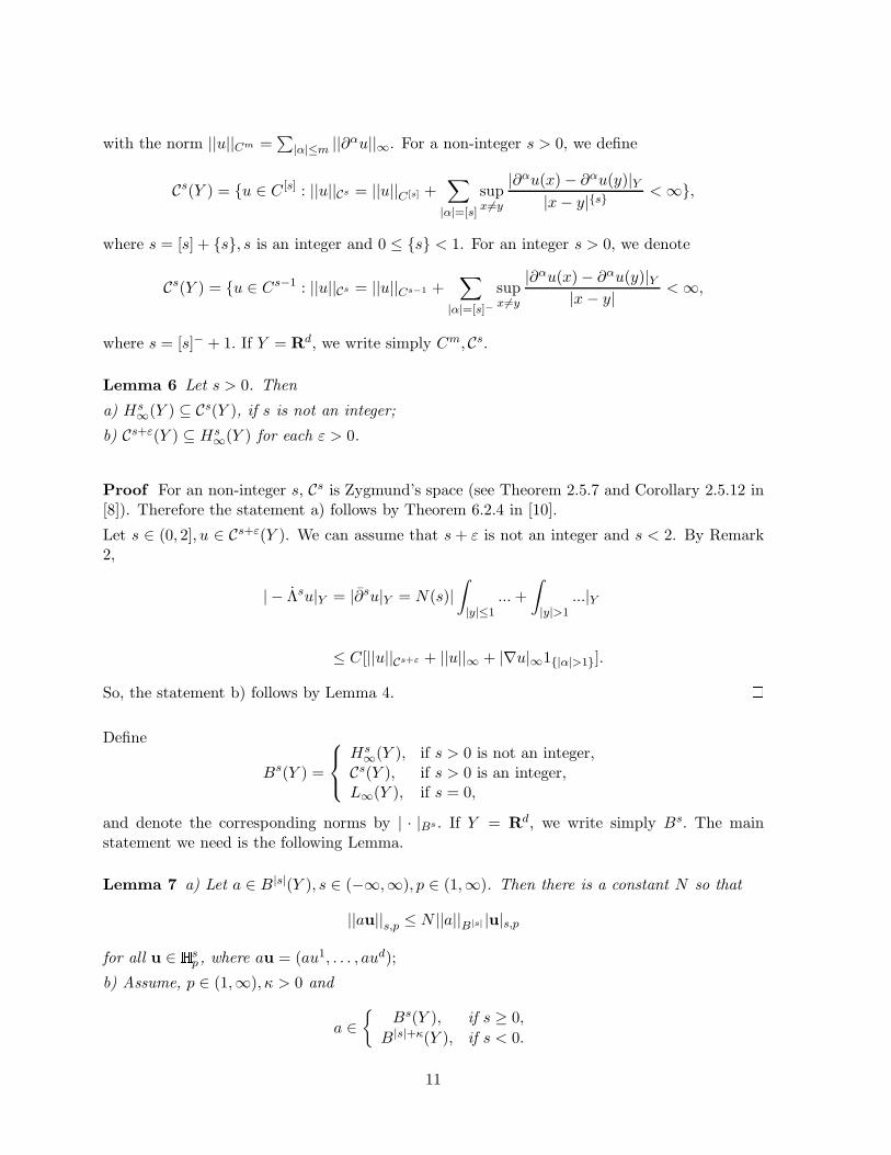
with the norm ||u||Cm =∑

|α|≤m ||∂αu||∞. For a non-integer s > 0, we define

Cs(Y ) = u ∈ C [s] : ||u||Cs = ||u||C[s] +∑

|α|=[s]

supx 6=y

|∂αu(x) − ∂αu(y)|Y|x− y|s <∞,

where s = [s] + s, s is an integer and 0 ≤ s < 1. For an integer s > 0, we denote

Cs(Y ) = u ∈ Cs−1 : ||u||Cs = ||u||Cs−1 +∑

|α|=[s]−supx 6=y

|∂αu(x) − ∂αu(y)|Y|x− y| <∞,

where s = [s]− + 1. If Y = Rd, we write simply Cm, Cs.

Lemma 6 Let s > 0. Then

a) Hs∞(Y ) ⊆ Cs(Y ), if s is not an integer;

b) Cs+ε(Y ) ⊆ Hs∞(Y ) for each ε > 0.

Proof For an non-integer s, Cs is Zygmund’s space (see Theorem 2.5.7 and Corollary 2.5.12 in[8]). Therefore the statement a) follows by Theorem 6.2.4 in [10].

Let s ∈ (0, 2], u ∈ Cs+ε(Y ). We can assume that s + ε is not an integer and s < 2. By Remark2,

| − Λsu|Y = |∂su|Y = N(s)|∫|y|≤1

...+∫|y|>1

...|Y

≤ C[||u||Cs+ε + ||u||∞ + |∇u|∞1|α|>1].

So, the statement b) follows by Lemma 4.

Define

Bs(Y ) =

Hs∞(Y ), if s > 0 is not an integer,Cs(Y ), if s > 0 is an integer,L∞(Y ), if s = 0,

and denote the corresponding norms by | · |Bs . If Y = Rd, we write simply Bs. The mainstatement we need is the following Lemma.

Lemma 7 a) Let a ∈ B|s|(Y ), s ∈ (−∞,∞), p ∈ (1,∞). Then there is a constant N so that

||au||s,p ≤ N ||a||B|s| |u|s,p

for all u ∈ H sp , where au = (au1, . . . , aud);

b) Assume, p ∈ (1,∞), κ > 0 and

a ∈

Bs(Y ), if s ≥ 0,B|s|+κ(Y ), if s < 0.

11

Let as = |a|Bs if s ≥ 0 and as = |a|B|s|+κ if s < 0.

Then for every s there exist constants s0 < s and N such that

||au||s,p ≤ N(||a||∞|u|s,p + as|u|s0,p)

for all u ∈ H sp .

Moreover,

Λs(au) = aΛsu + Hs(a,u), if s 6= 2m+ 1 (m = 0, 1, . . .),

∂iΛs−1(au) = a(∂iΛs−1u) + Hs(a,u), if s = 2m+ 1 (m = 0, 1, . . .)

where ||Hs(a,u)||p ≤ Cas|u|s0,p.

Proof Let s ∈ (0, 2), u ∈C∞0 , a ∈ C∞

b (Y ) (a and all its derivatives are bounded). Then, byRemark 2,

Λs(au) =aΛsu + uΛsa−∫

[u(x+ y) − u(x)](a(x+ y) − a(x))dy

|y|d+s. (3.4)

By Minkowski’s inequality,

||∫

[u( · +y) − u(·)](a(· + y) − a(·)) dy

|y|d+s||p

≤∫

|u( · +y) − u(·)|p||a(· + y) − a(·)||∞ dy

|y|d+s.

If s ∈ (0, 2) and s 6= 1, we have by Lemma 5 for each s0 ∈ ((s− 1)+, s)∫

|u( · +y) − u(·)|p||a(· + y) − a(·)||∞ dy

|y|d+s

≤ ||a||B|s|∧1 |Λs0u|p∫|y|≤1

dy

|y|d+s−(s∧1)−s0+ 4||a||∞|u|p

∫|y|>1

dy

|y|d+s.

In the case s = 1, we have ∂i(au) = a∂iu + u∂ia and

||∇(au)||p ≤ ||a||∞|∇u|p + ||∇a||∞|u|p.

In the case s = 2, we have ∆(au) = a∆u + u∆a+ 2(∇a)(∇u) and

||∆(au)||p ≤ ||a||∞|∆u|p + ||∆a||∞|∆u|p + 2||∇a||∞|∇u|p.Therefore both parts of our statement hold for s ∈ [0, 2]. For an arbitrary s > 2, we can find apositive integer m so that s = 2m+ r, r ∈ (0, 2]. If r 6= 1,

Λs(au) = ΛrΛ2m(au) = Λr(aΛ2mu) + Λrh

12

where h is a linear combinations of the products in the form (∂νu)(∂µa), where ν 6= 0, and|ν| + |µ| = 2m According to the previous estimates, there is s0 ∈ ((r − 1)+, r) so that

||Λrh||p ≤ C||a||B|s| |u|2m−1+s0 .

On the other hand, by (3.4)

Λr(aΛ2mu) = aΛsu+ΛraΛ2mu + h

where ||h||p ≤ C||a||Bs∧1 |Λs0+2mu|p. If s = 2m+ 1,m = 1, 2, . . . , then

∂iΛ2m(au) = a∂iΛ2mu + Hs

where ||Hs||p ≤ C||a||Bs |u|s−1,p.

So, we found that for each s > 0, there is a constant C so that

||au||s,p ≤ C||a||Bs |u|s,p.Since the multiplication by a is selfadjoint operation, by duality, obviously, follows that for eachs ∈ (−∞,∞) we have for some C

||au||s,p ≤ C||a||B|s| |u|s,p (3.5)

If s = −2m < 0,m = 1, 2, . . . ,u ∈ Hsp , then u = (1 − ∆)mh,h ∈ Lp . Then it is easy to check

thatau =(1 − ∆)m(ah) − H, (3.6)

and the function H is a linear combinations of the products in the form (∂νh)(∂µa), whereµ 6= 0, and |ν| + |µ| = 2m. Since ∂µa ∈ B|s|+κ−|µ|, using (3.5) we obtain

||(∂νh)(∂µa)||s,p ≤ ||(∂νh)(∂µa)||s−κ+|µ|,p ≤ C|(∂νh)|s−κ+|µ|||(∂µa)||B−s+κ−|µ|

≤ C||∂µa||B|s|+κ−|µ| |∂νh|s+|µ|−κ,p ≤

≤ C||a||B|s|+κ |h|−κ,p ≤ C||a||B|s|+κ |u|s−κ,p.

So, by (3.6)(1 − ∆)s(au) = a(1 − ∆)su− (1 − ∆)sH,

||(1 − ∆)sH||p = ||H||s,p ≤ C||a||B|s|+κ |u|s−κ,p, and

||au||s ≤ C(||a||∞|u|s + ||a||B|s|+κ |u|s−κ).

If s < 0 is not an integer, then there is a positive integer m so that s = −2m− r, r ∈ (0, 2). Letu ∈H s

p . Then u = h + ΛrΛ2mh, h ∈ Lp . Let h =Λ2mh. We have h ∈ H −2mp and

aΛrh = Λr(ah) − (Λra)h−∫

(h(x+ y) − h(x))(a(x + y) − a(x)) dy|y|d+r ,

ah = aΛ2mh =Λ2m(ah) − g,

(3.7)

13

where g is a linear combination of (∂νh)(∂µa), |µ| + |ν| = 2m,µ 6= 0. Since

||Λr(∂νh ∂µa)||s,p ≤ ||∂νh ∂µa||s+r,p ≤ ||∂νh ∂µa||s+r+|µ|−κ,p

≤ C||∂µa||B|s|−r−|µ|+κ |h|s+|µ|+|ν|+r−κ,p

= C||∂µa||B|s|−r−|µ|+κ |h|−κ,p ≤ C||a||B|s|−r+κ |h|−κ,p,

we have ||Λrg||s,p ≤ C||a||B|s|−r+κ |h|−κ.

Also by (3.5),

||(Λra)h||s ≤ C||(Λra)h||−2m−κ ≤ C||Λra||B2m+κ |h|−2m−κ ≤ C||Λra||B2m+κ |u|s−κ.

Fix κ′ ∈ (0, κ). Let δ1 = maxr− 1, 0 + κ, ε1 = δ1 − κ′, ε2 = min1, r. By Lemma 5 and (3.5)and using Minkowsky’s inequality, we have

||∫

(h(· + y) − h(·))(a(· + y) − a(·)) dy

|y|d+r||s,p

≤ C

∫||h(· + y) − h(·))(a(· + y) − a(·))||−2m−δ1 ,p

dy

|y|d+r

≤∫

|h(· + y) − h(·)|−2m−δ1 ||a(· + y) − a(·)||B2m+δ1

dy

|y|d+r

≤ C[∫|y|≤1

|h|−2m−δ1+ε1||a||B2m+δ1+ε2 |y|ε1+ε2−d−γ dy

+∫|y|>1

|h|−2m−δ1||a||B2m+δ1 ]

dy

|y|d+r].

So,

||∫

(h(x+ y) − h(x))(a(x + y) − a(x))dy

|y|d+r||s,p

≤ C|h|−2m−κ′ ||a||Bs+κ ≤ C|u|s−κ′ ||a||Bs+κ .

Thus, according to (3.7),au = aΛ−sh = Λ−s(ah) + G,

where ||G||s,p ≤ C||a||B|s|+κ |h|−κ,p ≤ C||a||B|s|+κ |u|s−κ,p. Therefore,

Λs(au) = ah + ΛsG = aΛsu+ΛsG,

and ||ΛsG||p ≤ C||G||s,p ≤ C||a||B|s|+κ |u|s−κ,p.

14

4 Systems of SPDEs in Sobolev spaces

As in the previous Section, let (Ω,F ,P) be a probability space with a filtration F of rightcontinuous σ-algebras (Ft)t≥0. All the σ−algebras are assumed to be P−completed. LetW (t) bean F-adapted cylindrical Brownian motion in Y . Let s ∈ (−∞,∞). For v ∈H s+1

p , let Q(v, t) =Q(v, t, x) be a predictable H

sp(Y )-valued function and D(v, t) = D(v, t, x) a predictable H

s−1p -

valued function. Let a = a(t) = (aij(t, x))1≤i,j≤d be a symmetric F-adapted matrix. Letσ = σ(t) = (σk(t, x))1≤k≤d be F-adapted vector function with Y -valued components σk, and letu0=

(ul

0

)1≤l≤d

be an F0−measurable Hs+1−2/pp −valued function so that E ||u0||ps+1−2/p,p < ∞.

Everywhere in this section it is assumed that p ≥ 2.

Consider the following nonlinear system of equations on [0,∞) :

∂tu(t, x) = ∂i(aij(t, x)∂ju) + D(u, t, x)+

[σk(t, x)∂ku(t, x) + Q(u, t, x)] · W , (4.1)

u(0, x) = u0(x)

where u(t) = u(t, x) = (uk(t, x))1≤k≤d.

The following assumptions will be used in the future:

A. For all t ≥ 0, x, λ ∈Rd,

K|λ|2 ≥ [aij(t, x) − 12σi(t, x) · σj(t, x)]λiλj ≥ δ|λ|2,

where K, δ are fixed strictly positive constants.

A1(s, p). For all t, x, y,P-a.s.

|aij(t, x) − aij(t, y)| + |σi(t, x) − σi(t, y)|Y ≤ K|x− y|

and

|aij(t)|Bs ≤ K, if s > 1,

|a(t, x)| ≤ K, if − 1 < s ≤ 1,

|aij(t)|B−s+ε ≤ K, if s ≤ −1,

where ε ∈ (0, 1).

The Y -valued function σ(t, x) is P-a.s. continuously differentiable in x and for all i, t

||σi(t)||Bs ≤ K, if s ≥ 1,|σi(t, x)|Y ≤ K, if s ∈ (−1, 1),||σi(t)||B−s+ε ≤ K, if s ≤ −1,

where ε ∈ (0, 1).

15

A2(s, p) For v ∈H s+1p , Q(v, t) = Q(v, t, x) is a predictable H s

p(Y )-valued function and D(v, t) =D(v, t, x) is a predictable H

s−1p -valued function, and P-a.s. for each t

∫ t

0(|D(0, r)|ps−1,p + ||Q(0, r)||ps,p) dr <∞ ∀t > 0,P − a.s.

where 0 = (0, . . . , 0).A3(s, p). For every ε > 0, there exists a constant Kε such that for any u,v ∈H s+1

p ,

|D(u, t, x) −D(v, t, x)|s−1,p + ||Q(u, t, x) − Q(v, t, x)||s,p ≤

ε|u − v|s+1,p +Kε|u− v|s−1,p P− a.s.

Given a stopping time τ , we consider a stochastic interval

[[0, τ ]] =

[0, τ(ω)], if τ(ω) <∞,[0,∞), otherwise.

Definition 1 Given a stopping time τ, an H sp(Rd)-valued F−adapted function u(t) on [0,∞) is

called an H sp -solution of equation (4.1) in [[0, τ ]] if it is strongly continuous in t with probability

1,

u(t ∧ τ) = u(t),∫ t∧τ

0|u(s)|ps+1,p ds <∞ ∀t > 0,P − a.s., (4.2)

and the equalityu(t ∧ τ) = u0 +

∫ t∧τ0

[∂i(aij(r)∂ju) + D(u, r)

]dr+

∫ t∧τ0 [σk(r)∂ku (r) + Q(u, r)] · dW (r)

(4.3)

holds in H s−1p (Rd) for every t > 0, P− a.s.

If τ = ∞, we simply say u is an H sp -solution of equation (4.1).

Sometimes, when the context is clear, instead of ”H sp -solution” we will simply say ”solution”.

It is readily checked that all the integrals in 4.3 are well defined. For example, let us considerthe stochastic integral. Since ∂i is a bounded operator from H s

p into H s−1p (see [8]), by Lemma

7 and Assumption A1(s, p), we have∣∣∣∣σk(r)∂ku (r)

∣∣∣∣s,p

≤ C ||u (r) ||s+1,p for r ≤ τ P-a.s. Byassumptions A2(s, p),A3(s, p),∫ t∧τ

0||Q(u, r)||ps,p dr ≤ C

∫ t∧τ

0(||Q(0, r)||ps,p + |u (r) |ps+1,p)dr.

Thus, [σk(r)∂ku + Q(u, r)]1r<τ ∈ Is,p, and the integral is defined by Theorem 1.

Remark 3 It is not difficult to show that (4.3) can be replaced by the equality⟨ul(t ∧ τ), φl

⟩s

=⟨ul

0, φl⟩s+

∫ t∧τ0 − ⟨

(aij(r)∂iul), ∂jφ

l⟩s+

〈Λ−1Dl(u, r),Λφl〉sdr +∫ t∧τ0 〈σk(r)∂ku

l +Ql(u, r), φl〉s,Y · dW (r)

∀t > 0,P − a.s.

(4.4)

which holds for all φ = (φl)1≤l≤d such that φl ∈ C∞0 , l = 1, . . . , d, .

16

Indeed, owing to (4.3), we have

⟨ul(t ∧ τ), φl

⟩s−1

=⟨ul

0, φl⟩s−1

+∫ t∧τ0

⟨∂j(aij(r)∂iu

l) +Dl(u, r), φl⟩s−1

dr

+∫ t∧τ0

⟨σk(r)∂ku

l +Ql(u, r), φl⟩s−1,Y

· dW (r) ∀t > 0,P − a.s.

(4.5)

On the other hand, since u ∈H sp ,u0 ∈H s+1−2/p

p , and P-a.s. for r ≤ τ, σk(r)∂ku+Ql(u, r)∈H sp ,we

have that⟨ul(t), φl

⟩s−1

=⟨ul(t), φl

⟩s,⟨ul

0, φl⟩s−1

=⟨ul

0, φl⟩s+1−2/p

, and,

⟨σk(r)∂ku

l +Ql(u, r), φl⟩

s−1,Y=

⟨σk(r)∂ku

l +Ql(u, r), φl⟩

s,Y.

It is readily checked that dr × dP-a.s.

⟨∂j(aij(r)∂iu

l), φl⟩s−1

= − ⟨aij(r)∂iu

l, ∂jφl⟩s−1

=

− ⟨Λs(aij(r)∂iu

l),Λ−s∂jφl⟩0

= − ⟨(aij(r)∂iu

l), ∂jφl⟩s

Note that to prove the first equality one should first establish it for smooth functions and thenprove it in the general case by approximations. Thus, (4.5) implies (4.4). Now by reversing theorder of our arguments one could easily show that (4.3) follows from (4.4).

The basic result of this Section is given in the following

Theorem 2 Let s ∈ (−∞,∞), p ≥ 2. Let A, A1(s, p)-A3(s, p) be satisfied and |u0|ps+1,p < ∞P-a.s. Then for each stopping time τ the Cauchy problem (1.1) has a unique H

sp -solution in

[[0, τ ]]. Moreover, for each T > 0, there is a constant C such that for each stopping timeτ ≤ T ∧ τ ,

E[supr≤τ

|u(r)|ps,p +∫ τ

0|∂2u(r)|ps−1,p ds] ≤ CE[|u0|ps+1−2/p,p

+∫ τ

0(|D(0, r)|ps−1,p + ||Q(0, r)||ps,p) dr].

The Theorem will be proved in several steps. We begin with a simple particular case.

Theorem 3 (cf Theorem 4.10 in [2]). Let s ∈ (−∞,∞), p ≥ 2. Assume A, A1(s, p)-A3(s, p).Suppose that D and Q are independent of u, aij and σk are independent of x, and u0= 0.

Then for each stopping time τ there is a unique H sp−solution u of equation (4.1) in [[0, τ ]].

Moreover,

(i) for each stopping time τ ≤ τ,

E∫ τ

0|∂2u(r)|ps−1,p dr ≤ NE

∫ τ

0(|D(r)|ps−1,p + ||Q(r)||ps,p) dr, (4.6)

where N = N(d, p, δ,K) does not depend on τ, τ ;

17

(ii) for each finite T and each stopping time τ ≤ T ∧ τ

E supr≤τ

|u(r)|ps,p ≤ eTCE∫ τ

0(|D(r)|ps−1,p + ||Q(r)||ps,p) dr], (4.7)

where C = C(d, p, δ,K) does not depend on T and τ , τ .

Proof The statement is a straightforward corollary of the results of [2]. Indeed, owing to ourassumptions one can treat each component ul of u separately. The the statement regardingthe existence follows directly by Theorem 4.10 in [2] considering D(r) = D(r)1[[0,τ ]](r), andQ(r) = Q(r)1[[0,τ ]](r). According to Lemma 4.7 in [2], the uniqueness is an obvious consequenceof the deterministic heat equation result. In particular, we obtain (4.7) by taking λ = 1/p in(4.26) in [2].

To prove Theorem 3 in the general case, we will rely on the two fundamental techniques: partitionof unity and the method of continuity. The same technology was used in [2] for scalar equations.

The next step is to derive a priori Lp-estimates for a solution of (4.1).

Lemma 8 Assume A, A1(s, p)-A3(s, p). Suppose that u is an Hsp− solution of equation (4.1)

in [[0, τ ]] with u0= 0.

Then for each T there is a constant C = C(d, p, δ,K, T ) such that for each stopping time τ ≤T ∧ τ,

E[ supr≤τ |u(r)|ps,p +∫ τ0 |∂2u(r)|ps−1,p dr] ≤

CE∫ τ0 (|D(0, r)|ps−1,p + ||Q(0, r)||ps,p) dr.

(4.8)

Proof In order to use Theorem 8 we start with a standard partition of unity. Let ψ ∈ C∞0 (R),

be [0, 1]-valued and such that ψ(s) = 1, if |s| ≤ 5/8, and ψ(s) = 0, if |s| > 6/8. For an arbitrarybut fixed κ > 0 there we choose m such that κ < 2−m. Consider a grid in Rd consisting ofxk = k2−m, k = (k1, . . . , kd) ∈ Zd, where Z is the set of all integers. Given k ∈ Zd, we define afunction on Rd :

ηk(x) =d∏

l=1

ψ((xl − xlk)2

m).

Notice that 0 ≤ ηk ≤ 1, ηk = 1 in the cube vk = x : |xl − xlk| ≤ (5/8)2−m, l = 1, . . . , d, and

ηk = 0 outside the cube Vk = x : |xl − xlk| ≤ (6/8)2−m, l = 1, . . . , d. Obviously,

1. ∪kvk = Rd and1 ≤

∑k

1Vk≤ 2d;

2. For all multiindices γ|∂γ ηk| ≤ N(d, |γ|)2m|γ| < N(d)κ−|γ|.

18

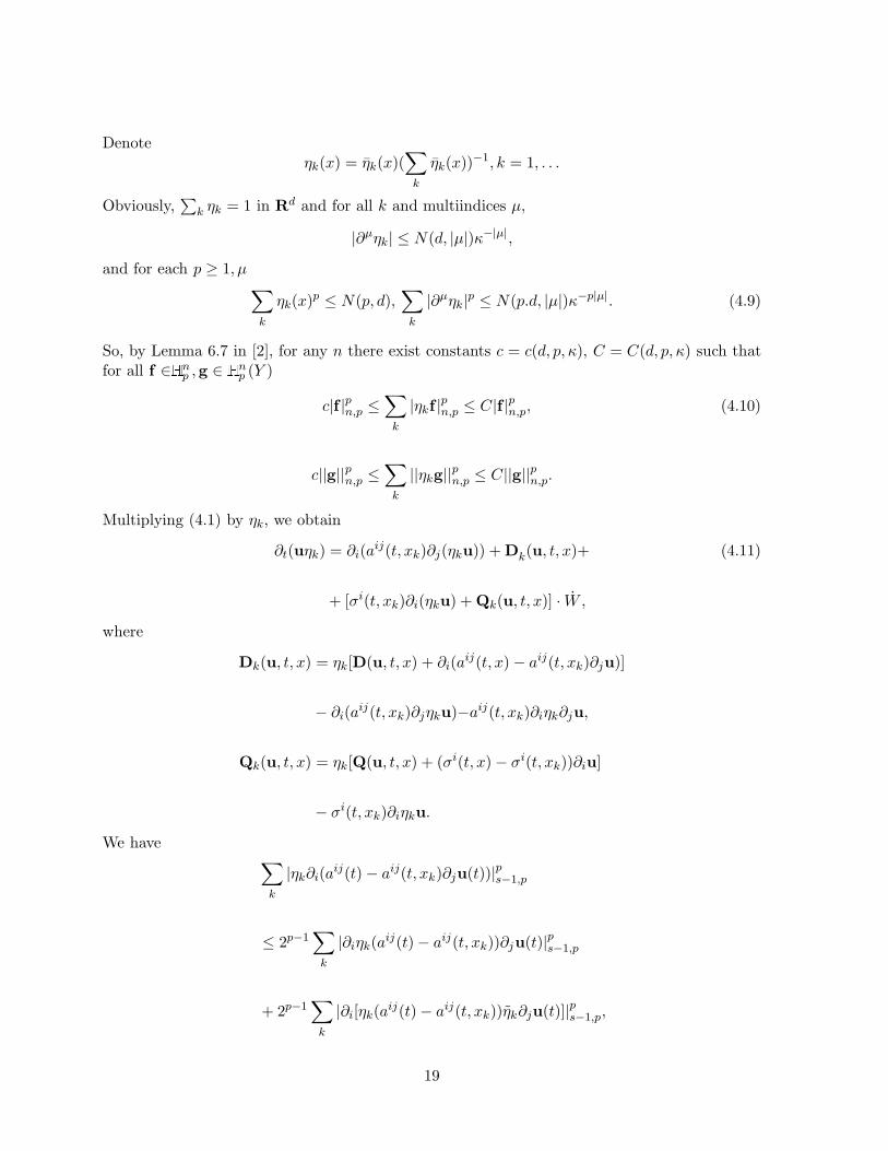
Denoteηk(x) = ηk(x)(

∑k

ηk(x))−1, k = 1, . . .

Obviously,∑

k ηk = 1 in Rd and for all k and multiindices µ,

|∂µηk| ≤ N(d, |µ|)κ−|µ|,

and for each p ≥ 1, µ ∑k

ηk(x)p ≤ N(p, d),∑

k

|∂µηk|p ≤ N(p.d, |µ|)κ−p|µ|. (4.9)

So, by Lemma 6.7 in [2], for any n there exist constants c = c(d, p, κ), C = C(d, p, κ) such thatfor all f ∈H n

p ,g ∈ H np (Y )

c|f |pn,p ≤∑

k

|ηkf |pn,p ≤ C|f |pn,p, (4.10)

c||g||pn,p ≤∑

k

||ηkg||pn,p ≤ C||g||pn,p.

Multiplying (4.1) by ηk, we obtain

∂t(uηk) = ∂i(aij(t, xk)∂j(ηku)) + Dk(u, t, x)+ (4.11)

+ [σi(t, xk)∂i(ηku) + Qk(u, t, x)] · W ,

where

Dk(u, t, x) = ηk[D(u, t, x) + ∂i(aij(t, x) − aij(t, xk)∂ju)]

− ∂i(aij(t, xk)∂jηku)−aij(t, xk)∂iηk∂ju,

Qk(u, t, x) = ηk[Q(u, t, x) + (σi(t, x) − σi(t, xk))∂iu]

− σi(t, xk)∂iηku.

We have ∑k

|ηk∂i(aij(t) − aij(t, xk)∂ju(t))|ps−1,p

≤ 2p−1∑

k

|∂iηk(aij(t) − aij(t, xk))∂ju(t)|ps−1,p

+ 2p−1∑

k

|∂i[ηk(aij(t) − aij(t, xk))ηk∂ju(t)]|ps−1,p,

19

where ηk(x) = ηk(5x/6) (notice ηk(x) = 1 in Vk and ηk(x) = 0 if there is l such that |xl − xlk| >

0.9 · 2−m). According to Lemma 7, there is a constant C and s0 < s such that∑

k

|∂i[ηk(aij(t) − aij(t, xk))ηk∂ju(t)]|ps−1,p

≤∑

k

|ηk(aij(t) − aij(t, xk))ηk∂ju(t)|ps,p

≤ C∑

k

[supx,k

|ηk(aij(t) − aij(t, xk))|p|∂u(t)|ps,p

+ |ηk∂ju(t)|ps0−1,p].

Similarly, by Lemma 7 there is s0 < s so that∑

k

||ηk(σi(t) − σi(t, xk))∂iu(t)||ps,p

=∑

k

||ηk(σi(t) − σi(t, xk))ηk∂iu(t)||ps,p

≤ C∑

k

[supx

||ηk(σi(t) − σi(t, xk))||p|ηk∂iu(t)|ps,p

+ |ηk∂iu(t)|ps0,p].

It follows by the assumptions, (4.10), Lemma 7 and interpolation theorem (see Lemma 6.7 in[2]) that for each ε there is κ > 0 and a constant C = C(ε, κ, d, p, δ,K) such that

∑k

|Dk(u, t)|ps−1,p ≤ ε|∂2u(t)|ps−1,p + C(|u(t, ·)|ps−1,p + |D(0, t)|ps−1,p),

∑k

||Qk(u, t, ·)||ps,p ≤ ε|∂2u(t)|ps−1,p + C(|u(t)|ps−1,p + ||Q(0, t)||ps,p).

Choosing ε sufficiently small, applying (4.10) and Theorem 3 to ηku (it is a solution to theequation (4.11), we obtain that

(i) for each stopping time τ ≤ τ

E∫ τ

0|∂2u(t)|ps−1,p dt ≤ NE

∫ τ

0(|u(t)|ps−1,p + |D(0, t)|ps−1,p + ||Q(0, t)||ps,p) dt

where N = N(p, d, δ,K) does not depend on τ .

20

(ii) for each T > 0 and each stopping time τ ≤ T ∧ τ

E supt≤τ

|u(t)|ps,p ≤ NeTE∫ τ

0(|u(t)|ps−1,p + |D(0, t)|ps−1,p + ||Q(0, t)||ps,p) dt

Fix an arbitrary τ ≤ T ∧ τ such that

E[ supt≤τ

|u(t)|ps,p +∫ τ

0(|u(t)|ps−1,p + |D(0, t)|ps−1,p + ||Q(0, t)||ps,p) dt] <∞.

Then for each t ≤ T

E supr≤t∧τ

|u(r)|ps,p ≤ NeTE∫ t

0sup

r≤r∧τ|u(r)|ps,p dr

+ E∫ τ

0|D(0, t)|ps−1,p + ||Q(0, t)||ps,p dt,

and the statement follows by Gronwall’s inequality.

Now we can prove the uniqueness of a solution to equation (4.1).

Corollary 1 Assume A, A1(s, p)-A3(s, p). Then for each stopping time τ there is at mostone H s

p−solution to (4.1) in [[0, τ ]].

Proof If u1,u2 are solutions to (4.1), then v = u2 − u1 satisfies on [[0, τ ]] the equation

∂tv(t, x) = ∂i(aij(t, x)∂jv) + D(v + u1, t, x) − D(u1, t, x)

+ [σk(t, x)∂kv(t, x) + Q(v + u1, t, x) − Q(u1, t, x)] · W ,

v(0, x) = 0.

Applying Lemma 8 to this equation we get v = 0 P-a.s.

Remark 4 In fact the uniqueness of the solution can be proved in a larger functional class,similar to the one of Theorem 5.1 in [2]. For the sake of simplicity we will not address thisproblem in the present paper.

To complete the proof of Theorem 2 we apply the standard method of continuity (cf. Theorem5.1 in [2]).

Proof of Theorem 2.

21

(Existence) Without any loss of generality we can assume u0 = 0 (see Proof of Theorem 5.1 in[2]) and τ = ∞. Now, let us take λ ∈ [0, 1] and consider the equation

∂tu(t, x) = ∂i[λδij + (1 − λ)aij∂ju] + (1− λ)D(u, t,x)+

+(1 − λ)[σk∂ku + Q(u, t, x)] · W(4.12)

with zero initial condition. By Lemma 8 the a priori estimate (4.8) holds with the same constantC for all λ. Assume that for λ = λ0 and any D,Q satisfying A3(n, p), equation (4.12) has aunique solution.

For other λ ∈ [0, 1] we rewrite (4.12) as follows:

∂tu(t, x) = ∂i[(λ0δij + (1 − λ0)aij)∂ju]+ (1 − λ0)D(u, t, x)

+(λ− λ0)(∂i[(δij − aij)∂ju] − D(u, t, x)

)

+(1 − λ0)[σk∂ku + Q(u, t, x)] · W

− (λ− λ0) [σk∂ku + Q(u, t, x)] · W

This equation can be solved by iterations. Specifically, take u0 = 0 and write

∂tuk+1(t, x) = ∂i[(λ0δij + (1 − λ0)aij)∂juk+1]+ (1 − λ0)D(uk+1, t, x)

+(λ− λ0)(∂i[(δij − aij)∂juk] − D(uk, t,x)

)

+(1 − λ0)[σi∂iuk+1 + Q(uk+1, t, x)] · W

− (λ− λ0) [σi∂iuk + Q(uk, t, x)] · W

(4.13)

So, for k ≥ 1, uk+1 = uk+1 − uk is a solution of the equation

∂tuk+1(t, x) = ∂i[(λ0δij + (1 − λ0)aij)∂juk+1]+ (1 − λ0) [D(uk + uk+1, t, x)−

D(uk, t, x)] + (λ− λ0)(∂i[(δij − aij)∂juk] − [D(uk, t, x) − D(uk−1, t, x)])

+(1 − λ0)[σi∂iuk+1 + Q(uk + uk+1, t, x) − Q(uk, t, x)] · W

− (λ− λ0) [σi∂iuk + Q(uk, t, x) − Q(uk−1, t, x)] · WBy Lemma 8, for each T > 0 there is a constant C = C(d, p, δ,K, T ) such that for all stopping

22

times τ ≤ T

E[ supr≤τ

|uk+1(r)|ps,p +∫ τ

0|∂2uk+1(r)|ps−1,p dr ]

≤ C ′|λ− λ0|pE∫ τ

0(|∂uk(r)|ps,p + |∂2uk(r)|ps−1,p) dr

≤ C|λ− λ0|pE[ supr≤τ

|uk(r)|ps,p +∫ τ

0|∂2uk(r)|ps−1,p dr].

Fix an arbitrary stopping time τ ≤ T such that

I(τ) = E[ supr≤τ

|u1(r)|ps,p +∫ τ

0|∂2u1(r)|ps−1,p dr] <∞,

Notice u1 and τ do not depend on λ (only on λ0). Let |λ− λ0| < C−1/p/2. Then

E[ supr≤τ

|uk+1(r)|ps,p +∫ τ

0|∂2uk+1(r)|ps−1,p dr]

1/p ≤ (1/2)kI(τ)1/p.

and (uk) is a Cauchy sequence on [0, τ ]. Therefore, there is a continuous in t and H sp -valued

process u such hat

E[ supr≤τ

|uk(r) − u(r)|ps,p +∫ τ

0|∂2(uk(r) − u(r))|ps−1,p dr] → 0,

as k → ∞. Obviously u is a solution to (4.12) on [0, τ ]. Since τ is any stopping time such thatI(τ) is finite, it follows that we have a solution for any |λ − λ0| < C−1/p/2 (assuming we haveone for λ0). For λ = 1 it does exist by Theorem 3. So, in finite number of steps starting withλ = 1, we get to λ = 0. This proves the statement.

Corollary 2 (cf. Corollary 5.11 in [2]) Assume A, A1(s, p)-A3(s, p). Assume furtherA1(s, q)-A3(s, q) for q ≥ 2, and suppose that |u0|s+1−2/p,p + |u0|s+1−2/q,q <∞ P-a.s. Then theH s

p−solution u of equation (4.1) is also an H sq−solution of the equation.

Moreover, for each T > 0, there is a constant C such that for each stopping time τ ≤ T ,

E[supr≤τ

|u(r)|ls,l +∫ τ

0|∂2u(r)|ls−1,l dr] (4.14)

≤ CE[|u0|ls+1−2/l,l +∫ τ

0(|D(0, r)|ls−1,l + ||Q(0, r)||ls,l) dr],

l = p, q.

23

Proof We follow the lines of the proof of the Theorem 2 by introducing the parameter λ ∈ [0, 1]and considering the equation (4.12). We can assume that u0 = 0. The statement holds truefor λ = 1 by Lemma 5.11 in [2] applied to each component of u. If it is true for λ0, then (4.13)defines a sequence uk of H s

p -valued continuous processes that are Hsq -valued and continuous as

well, and ∫ t

0(|∂2uk(r)|ls−1,l dr <∞, l = p, q

P-a.s. for all t.

For each T > 0, there are constants Cl = C(d, l, δ,K, T ), l = p, q such that for all stopping timesτ ≤ T,

E[ supr≤τ

|uk+1(r)|ls,l +∫ τ

0|∂2uk+1(r)|ls−1,l dr]

≤ C ′|λ− λ0|pE∫ τ

0((|uk(r)|ps,p + |∂2uk(r)|ps−1,p) dr

≤ Cl|λ− λ0|pE[ supr≤τ

|uk(r)|ls,l +∫ τ

0|∂2uk(r)|ls−1,l dr],

l = p.q. Fix an arbitrary stopping time τ ≤ T such that

I(τ) = E[ supr≤τ

(|u1(r)|ps,p + |u1(r)|qs,q +∫ τ

0(|∂2u1(r)|ps−1,p + |∂2u1(r)|qs−1,q) dr] <∞.

Let C = maxCp, Cq, |λ − λ0| < C−1/p/2. Then

E[ supr≤τ

|uk+1(r)|ls,l +∫ τ

0|∂2uk+1(r)|ls−1,l dr]

1/p ≤ (1/2)kI(τ)1/p,

l = p, q. Therefore, there is a continuous in t and Hsp ∩ H

sq -valued process u such hat

E[ supr≤τ

|uk(r) − u(r)|ls,l +∫ τ

0|∂2(uk(r) − u(r))|ls−1,l dr] → 0,

l = p, q, and the statement follows.

4.1 Some estimates

Unfortunately, if s is positive, Assumption A3(s, p) is rarely satisfied for equations of Mathe-matical Physics even in the scalar case (see Example 1 below). The following Proposition aswell Corollary 4 below help to circumvent this problem in many important cases.

24

Proposition 1 Assume that for each v ∈H s+1p , Q(v, t) is a predictable H

s+1p -valued process and

D(v, t) is a predictable Hsp -valued process. Let A, A1(s+1, p), A2(s+1, p), A3(s, p) be satisfied,

|u0|s+2,p <∞ with probability one, and for all t > 0,v ∈H s+1p ,

| |Q(v, t)| |s+1,p ≤ | |Q(0, t)| |s+1,p +C|v|s+1,p.

|D(v, t)|s,p ≤ |D(0, t)|s,p + C|v|s+1,p.

Suppose also that ∫ t

0(| |Q(0, r)| |ps+1,p + |D(0, r)|ps,p) dr <∞

P-a.s. for all t. Then (4.1) has a unique continuous Hr+1p - solution.

Moreover, for each T > 0 there is a constant C such that for each stopping time τ ≤ T ,

E1A[supr≤τ

|u(r)|ps+1,p +∫ τ

0|∂2u(r)|ps,p dr] ≤ CE1A[|u0|ps+2,p

+∫ τ

0(|D(0, r)|ps,p + | |Q(0, r)| |ps+1,p) dr].

Proof Since the assumptions A, A1(s, p)-A3(s, p) are satisfied, the existence and uniquenessof H s

p - solution is guaranteed by Theorem 2 By the same Theorem, the linear equation

∂tξ(t, x) = ∂i(aij(t, x)∂jξ(t, x)) + D(u, t, x)+

[σk(t, x)∂kξ(t, x) + Q(u, t, x)] · W ,

ξ(0, x) = u0(x),

has a unique H s+1p -solution. Thus, ξ = u P-a.s.. Moreover, for each T there is a constant C

such that for all stopping times τ ≤ T ,

E[ supr≤t∧τ

|u(r)|ps+1,p +∫ t∧τ

0|∂2u(r)|ps,p dr] ≤ CE[|u0|ps+2,p +

∫ t∧τ

0(|u(r)|pn+1,p

+ |D(0, r)|ps,p + ||Q (0,r)||ps+1,p) dr].

Now the estimate of the statement follows by Gronwall’s inequality.

Example 1 Let us consider the following scalar equation:

∂tu = ∆u+D(u) + u · W ,

u(0, x) = 0

25

where W (t) is a one-dimensional Wiener process, D(u) = ∂[f(u(x))](= ∂f(u(x))∂u(x)) and fis a scalar Lipschitz function on R1. Then A3(1,p) would require the following estimate:

|D(u) −D(v)|p = |∇f(u(x))∂u(x)) −∇f(v(x))∂v(x)|p

≤ ε|u− v|2,p +Kε|u− v|p,which is false in general even if ∇f is Lipschitz.

On the other hand, the assumptions of the Proposition are satisfied for n = 0. Indeed,

|D(u)|p = |∇f(u)∂u|p ≤ C|∂u|pwhere C is the Lipcshitz constant of f.

Now,since ∂ is a bounded operator from H sp into H s+1

p , we have

|D(u) −D(v)|−1,p = |∂[f(u)] − ∂[f(v)]|−1,p ≤

C|f(u) − f(v)|p ≤ C ′|u− v|p ≤

ε|u− v|1,p +Kε|u− v|−1,p.

(The latter inequality follows from Remark 5.5 in [2].) Thus assumption A3(0,p) is verified andwe are done.

Proposition 2 Let s ∈ (−∞,∞), p ≥ 2. Assume A, A1(s, 2)-A3(s, 2). Suppose |u0|s+1,2 <∞P-a.s. Assume further that∫ t

0(|D(0,r)|ps−1,2 + | |Q(0, r)| |ps,2) dr <∞

P-a.s. for all t.

Then for each T > 0, there is a constant C such that for each stopping time τ ≤ T,

E[ supr≤τ

|u(r)|ps,2 +∫ τ

0|u(r)|p−2

s,2 |∇u(r)|2s,2 dr ≤ CE[|u0|ps+1,2 +∫ τ

0(|D(0, r)|ps−1,2

+ | |Q(0, r)| |ps,2) dr].

Proof Since the assumptions of Theorem 2 are satisfied, there is a unique H s2 - solution u (t, x)

of equation (4.1). Let s 6= 2m + 1, m = 0, 1, . . .. Then u = Λsu is L2 -valued continuous andsatisfies the equation

∂tu(t, x) = Λs[∂i(aij(t, x)∂ju) + D(u, t, x)]+

Λs[σk(t, x)∂ku(t, x) + Q(u, t, x)] · W ,

u(0, x) = u0(x),

26

where u0 = Λsu0. On the other hand, by Lemma 7,

Λs∂i(aij(t, x)∂ju) = ∂iΛs(aij(t, x)∂ju)

= ∂i(aij(t, x)∂jΛsu) + ∂iHs(aij , ∂ju), (4.15)

Λs[σk(t, x)∂ku(t, x)] = σk(t, x)∂kΛsu(t, x) + H(σk, ∂ku),

and|Hs(aij , ∂ju)|2 + |H(σk, ∂ku)|2 ≤ C|∇u(t)|s0,2,

(s0 < s). By interpolation theorem, for each ε there is a constant Cε so that

|Hs(aij , ∂ju)|2 + |H(σk, ∂ku)|2 ≤ ε|∇u(t)|s,2 + Cε|∇u(t)|s−1,2. (4.16)

Applying Ito formula, we obtain

|u(t)|p2 = |u(0)|p2 + p

∫ t

0|u(r)|p−2

2 〈u(r), Λs(D(u(r), r)〉1,2 ds

− p

∫ t

0|u(r)|p−2

2

∫aij(r)∂iu

l(r))∂j ul(r) dx dr

− p

∫ t

0|u(r)|p−2

2

∫∂iu

l(r)H ls(a

ij(r), ∂ju(r)) dx dr

+ p

∫ t

0|u(r)|p−2

2 (∫ul(r)bl(r) dx) · dWr

+p

2

∫ t

0|u(r)|p−2

2

∫bi(r) · bi(r) dx ds

+p

2(p− 2)

∫ t

0|u(r)|p−4

2 |∫ul(r)bl(r) dx|2Y dr,

where bk(r) = σi(r)∂iuk(r) +H l

s(σk, ∂ku)+ΛsQk(u, r). Notice

Λs(D(u(r), r)) ∈ H−1q , ΛsQk(u, r) ∈ L2 ,

27

and, by A3(s, 2), for each ε there is a constant Cε so that

|Λs(D(u(r), r))|−1,2 ≤ C|D(u(r), r)|s−1,2

≤ ε|u(r)|s+1,2 +Cε(|u(r)|s−1,2 + |D(0,r)|s−1,2), (4.17)

||ΛsQk(u, r)||2 ≤ C||Qk(u, r)||s,2

≤ ε|u(r)|s+1,2 +Cε(|u(r)|s−1,2 + ||Q(0,r)||s,2),

|∫ul(r)bl(r) dx|Y ≤ ε|u(r)|s+1,2|u(r)|s.2 + Cε(|u(r)|2s,2 + |u(r)|s,2||Q(0,r)||s,2.

So, y(t) = |u(t)|p2 is a semimartingale:

y(t) = y(0) +∫ t

0h(r) dr +

∫ t

0g(r) · dW (r) ,

where h(r), g(r) are measurable F-adapted (g is Y -valued). Let c(r) = |u(r)|p−22

∫ |∇u(r)|2 dx.Since

N(u(r)) = −|u(r)|p−22

∫aij(r)∂iu

l(r)∂j ul(r) dx

+12|u(r)|p−2

2

∫σk(r) · σl(r)∂ku

i(r)∂lui(r)

≤ −δ|u(r)|p−22

∫|∇u(r)|2 dx = −δc(r),

using (4.15)-(4.17), we find easily that for each ε there is a constant Cε so that

h(r) ≤ (−δ + ε)c(r) + Cε(y(r) + f(r)), (4.18)

|g(r)|Y ≤ ε|u(r)|p−1s,2 |u|s+1,2 + Cε(y(r) + y(r)1−1/pl(r)1/p),

|g(r)|2Y ≤ ε2|u(r)|2p−2s,2 |u|2s+1,2 + Cε(y(r)2 + y(r)2−2/pl(r)2/p)

≤ ε2y(r)c(r) + Cε(y(r)2 + y(r)2−2/pl(r)2/p),

wheref(r) = |D(0, r)|ps−1,2, l(r) = | |Q(0, r)| |ps,2.

Let v < t ≤ T, t− v ≤ 1/4, and τ be a stopping time such that supr≤τ y(r) is bounded and

E∫ τ

0(f(r) + l(r)) dr <∞.

28

Fix an arbitrary stopping time τ . Let τ = τ ∧ τ . Then by Burkholder’s inequality and (4.18)

E supv≤r≤t

y(r ∧ τ) ≤ Ey(v ∧ τ) + CεE[ supv≤r≤t

y(r ∧ τ)(t− v)+

−∫ t∧τ

v∧τ(δ − ε)c(r) dr +

∫ t∧τ

v∧τf(r) dr

+ (∫ t∧τ

v∧τ[ε2y(r)c(r) + Cε(y(r)2 + y(r)2(1−1/p)l(r)2/p)] dr)1/2].

For each ε there is a constant Cε independent of T such that

(∫ t∧τ

v∧τy(r)2(1−1/p)l(r)2/p) dr)1/2 ≤ sup

v≤r≤ty(r ∧ τ)1−1/p(

∫ t∧τ

v∧τl(r)2/p dr)1/2

≤ ε supv≤r≤t

y(r ∧ τ) + Cε(∫ t∧τ

v∧τl(r)2/p dr)p/2

≤ ε supv≤r≤t

y(r ∧ τ) + Cε

∫ t∧τ

v∧τl(r) dr.

Also,

(∫ t∧τ

v∧τε2y(r)c(r) dr)1/2 ≤ ε sup

v≤r≤ty(r)1/2(

∫ t∧τ

v∧τc(r) dr)1/2

≤ 2ε[ supv≤r≤t

y(r) +∫ t∧τ

v∧τc(r) dr].

So, there is a constant C such that

E supv≤r≤t

y(r ∧ τ) ≤ CE[y(v ∧ τ) + supv≤r≤t

y(r ∧ τ)(t− v)1/2 +∫ t∧τ

v∧τ(f(r) + l(r)) dr],

and we can find ε0 such that for |t− v| ≤ ε0

E supv≤r≤t

y(r ∧ τ) ≤ CE[y(v ∧ τ) +∫ t∧τ

v∧τ(f(r) + l(r)) dr].

Now, the estimate easily follows.

Now we derive similar estimates for |u(t)|ps,q, q ≥ 2.

29

Proposition 3 Let s ∈ 0, 1, . . ., q ≥ 2, |u0|s+1−2/q,q < ∞ P-a.s., and A, A1(s, q)-A3(s, q)hold. Assume further that p ≥ q, aij ∈ Bs∨2, if s ≥ 1, and

| |Q(v, t)| |s,q ≤ | |Q(0, t)| |s,q + C|v|s,q.

|D(v, t)|s−1,q ≤ |D(0, t)|s−1,q + C|v|s,q,

∫ t

0(|D(0,r)|ps−1,q + | |Q(0, r)| |ps,q) dr <∞

P-a.s. for all t.

Then Theorem 2 holds. Moreover, for each T > 0, there is a constant C such that for eachstopping time τ ≤ T,

E supr≤τ

|u(r)|ps,q ≤ CE[|u0|ps,q +∫ τ

0(|D(0, r)|ps−1,q + | |Q(0, r)| |ps,q) dr]. (4.19)

Proof Since the assumptions of Theorem 2 are satisfied, there is a unique H sq - solution of

equation (4.1). Let α be a multiindex such that |α| ≤ s. Then uα = ∂αu is Lq -valued continuousand satisfies the equation

∂tuα(t, x) = ∂α[∂i(aij(t, x)∂ju) + D(u, t, x)]+

∂α[σk(t, x)∂ku(t, x) + Q(u, t, x)] · W ,

uα(0, x) = u0,α(x),

where u0,α = ∂αu0. Define

Gα =∑

ν+µ=α,|ν|≥1

∂νaij(t)∂j∂µu(t),

Gα =∑

ν+µ=α,|ν|≥1

∂νσk(t)∂k∂µu(t).

Differentiating the product, we obtain

∂α∂i(aij(t)∂ju(t)) = ∂i(aij(t)∂juα(t))+∂iGα(t) (4.20)

∂α[σk(t)∂ku(t)] = σk(t)∂kuα(t) + Gα(t).

and|Hα(t)|q + ||Hα(t)||q ≤ C|u(t)|s−1,q, (4.21)

30

Let bkα(r) = σi(r)∂iukα(r) + Gl

α(r)+∂α(Qk(u, r)), 1 ≤ k ≤ d. Applying Ito formula, we obtainthat yα(t) = |uα(t)|pq is a semimartingale:

yα(t) = yα(0) +∫ t

0hα(r) dr +

∫ t

0gα(r) · dW (r) ,

where

hα(r) = p|uα(r)|p−qq 〈|uα(r)|q−2uα(r), ∂α(D(u(r), r)〉0,q

−∫aij(r)uα(|uα(r)|q−2ul

α(r))∂julα(r) dx

−∫∂i(|uα(r)|q−2ul

α(r))Glα(r) dx

+12

∫[(q − 2)|uα(r)|q−4ui

α(r)ujα(r) + |uα(r)|q−2δij ]bi(r) · bj(r) dx

+p

2(p− q)|uα(r)|p−2q

q |∫

|uα(r)|q−2ulα(r)bl(r) dx|2Y ,

andgα(r) = p|uα(r)|p−q

q

∫|uα(r)|q−2ul

α(r)bl(r) dx.

Notice∂α(D(u(r), r)) ∈ H −1,q , ∂

α(Qk(u, r)) ∈ Lq ,

and, by our assumptions, there is a constant C so that

|∂α(D(u(r), r))|−1,q ≤ C|D(u(r), r)|s−1,q

≤ C(|u(r)|s,q + |D(0,r)|s−1,q),(4.22)

||∂αQk(u, r)||q ≤ C||Qk(u, r)||s,q ≤ C(|u(r)|s,q + ||Q(0,r)||s,q),

|∫

|uα(r)|q−2ulα(r)bl(r) dx|Y ≤ C(|u(r)|qs,q + |u(r)|q−1

s,q ||Q(0,r)||s,q.

We have hα(r) = p|uα(r)|p−qq h1

α(r) + h2α(r), where

h1α(r) = −

∫aij(r)∂i(|uα(r)|q−2ul

α(r))∂julα(r) dx+

12

∫[(q − 2)|uα(r)|q−4ui

α(r)uj

+ |uα(r)|q−2δij ]σk(r)∂kuiα(r) · σl(r)∂lu

jα(r) dx.

31

LetAij(r) = aij(r) − 1

2σi(r) · σj(r).

Then

h1α(r) = −

∫Aij(r)[∂iu

lα(r)∂ju

lα(r)|uα(r)|q−2

+4(q − 2)q2

∂i(|uα(r)|q/2)∂j(|uα(r)|q/2)] dx ≤ −δ∫

|uα(r)|q−2|∇u(r)|2 dx,

and for each ε > 0 there is a constant Cε such that

|h2α(r)| ≤ ε

∫|uα(r)|q−2|∇u(r)|2 dx+ Cε(|u(r)|qs,q + |D(0, r)|ps−1,q).

So, we obtain that

y(t) =∑|α|≤s

yα(t) = y(0) +∫ t

0h(r) dr +

∫ t

0g(r) · dWr

and

h(r) =∑|α|≤s

hα(r) ≤ C(y(r) + f(r)), (4.23)

|g(r)|Y ≤∑|α|≤s

|gα(r)|Y ≤ C(y(r) + y(r)1−1/pl(r)1/p),

wheref(r) = |D(0, r)|ps−1,q, l(r) = | |Q(0, r)| |ps,q.

Let v < t ≤ T, t− v ≤ 1/4, and τ be a stopping time such that supr≤τ y(r) is bounded and

E∫ τ

0(f(r) + l(r)) dr <∞.

Fix an arbitrary stopping time τ . Let τ = τ ∧ τ . Then by Burkholder’s inequality and (4.18)

E supv≤r≤t

y(r ∧ τ) ≤ Ey(v ∧ τ) +CE[ supv≤r≤t

y(r ∧ τ)(t− v) +∫ t∧τ

v∧τf(r) dr

+ (∫ t∧τ

v∧τ[y(r)2 + y(r)2(1−1/p)l(r)2/p)] dr)1/2].

32

For each ε there is a constant Cε independent of T such that

(∫ t∧τ

v∧τy(r)2(1−1/p)l(r)2/p) dr)1/2 ≤ sup

v≤r≤ty(r ∧ τ)1−1/p(

∫ t∧τ

v∧τl(r)2/p dr)1/2

≤ ε supv≤r≤t

y(r ∧ τ) + Cε(∫ t∧τ

v∧τl(r)2/p dr)p/2

≤ ε supv≤r≤t

y(r ∧ τ) + Cε

∫ t∧τ

v∧τl(r) dr.

So, there is a constant C such that

E supv≤r≤t

y(r ∧ τ) ≤ CE[y(v ∧ τ) + supv≤r≤t

y(r ∧ τ)(t− v)1/2 +∫ t∧τ

v∧τ(f(r) + l(r)) dr],

and we can find ε0 such that for |t− v| ≤ ε0

E supv≤r≤t

y(r ∧ τ) ≤ CE[y(v ∧ τ) +∫ t∧τ

v∧τ(f(r) + l(r)) dr].

Now, the estimate easily follows.

In the following two corollaries we combine Propositions 1 and 2, 3.

Corollary 3 Let s ∈ (−∞,∞), p ≥ 2. Assume that for each v ∈H s+12 , Q(v, t) is a predictable

Hs+12 -valued process and D(v, t) is a predictable H s

2-valued process. Let A, A1(s+1, 2), A2(s+1, 2), A3(s, 2) be satisfied, |u0|s+1,2 <∞ with probability one, and for all t > 0,v ∈H s+1

2 ,

| |Q(v, t)| |s+1,2 ≤ | |Q(0, t)| |s+1,2 + C|v|s+1,2.

|D(v, t)|s,2 ≤ |D(0, t)|s,2 + C|v|s+1,2.

Suppose also that, ∫ t

0(| |Q(0, r)| |ps+1,2 + |D(0, r)|ps,2) dr <∞

P-a.s. for all t. Then (4.1) has a unique continuous Hs+12 - solution. Moreover, for each T > 0,

there is a constant C such that for each stopping time τ ≤ T and set A ∈ F0,

E1A supr≤τ

|u(r)|ps+1,2 ≤ CE1A[|u0|ps+1,2 +∫ τ

0(|D(0, r)|ps,2 + | |Q(0, r)| |ps+1,2) dr].

33

Proof Since all the assumptions of Proposition 1are satisfied, there is a unique Hs+1p – solution

u for which the estimate of Proposition 1 holds. Then applying again Proposition 2 to s+1 andthe linear equation

∂tξ(t, x) = ∂i(aij(t, x)∂jξ) + D(u, t, x)+

[σk(t, x)∂kξ(t, x) + Q(u, t, x)] · W ,

ξ(0, x) = h(x),

and using the fact that ξ = u we obtain the statement.

Corollary 4 Let s ∈ 0, 1, . . ., p ≥ q ≥ 2. Assume that for each v ∈H s+1q , Q(v, t) is a pre-

dictable H s+1q -valued process and D(v, t) is a predictable H s

q -valued process. Let A, A1(s+1, q),A2(s + 1, q), A3(s, q) be satisfied, |u0|s+2−2/q,q < ∞ with probability one, and for all t >0,v ∈H s+1

q ,

| |Q(v, t)| |s+1,q ≤ |Q(0, t)| |s+1,q +C|v|s+1,q.

|D(v, t)|s,q ≤ |D(0, t)|s,q + C|v|s+1,q, .

Suppose also that, ∫ t

0(| |Q(0, r)| |ps+1,q + |D(0, r)|ps,q) dr <∞

P-a.s. for all t. Then (4.1) has a unique continuous H s+1q - solution. Moreover, for each T > 0,

there is a constant N such that for each stopping time τ ≤ T and set A ∈ F0,

E1A supr≤τ

|u(r)|ps+1,q ≤ NE1A[|u0|ps+1,q +∫ τ

0(|D(0, r)|ps,q + | |Q(0, r)| |ps+1,q) dr].

Proof Since all the assumptions of Proposition 1are satisfied, there is a unique H s+1q – solution

u for which the estimate of Proposition 1 holds. Then applying again Proposition 3 to s+1 andthe linear equation

∂tξ(t, x) = ∂i(aij(t, x)∂jξ) + D(u, t, x)+

[σk(t, x)∂kξ(t, x) + Q(u, t, x)] · W ,

ξ(0, x) = h(x),

and using the fact that ξ = u we obtain the statement.

34

References

[1] N. V. Krylov, On Lp-theory of stochastic partial differential equations, SIAM J. Math. Anal. 27(1996), 313-340.

[2] N. V. Krylov, An analytic approach to SPDEs, In: Stochastic Partial Differential Equations: SixPerspectives, AMS Mathematical Surveys and Monographs 64 (1999), 185-242.

[3] Z. Brzezniak, Stochastic partial differential equations in M -type 2 Banach spaces, Potential Anal. 4(1995), 1-45.

[4] A. L. Neihardt, Stochastic integrals in 2-uniformly smooth Banach spaces, Ph. D. Thesis, Universityof Wisconsin, 1978.

[5] R. Mikulevicius, B.L. Rozovskii, Martingale problems for SPDEs, In: Stochastic Partial DifferentialEquations: Six Perspectives (Editors: R. Carmona and B. L. Rozovskii), // AMS, MathematicalSurveys and Monographs 64 (1999), 243-325.

[6] R. Mikulevicius, B. L. Rozovskii, On Equations of Stochastic Fluid Mechanics In Stochastics in Finiteand Infinite Dimensions: In Honor of Gopinath Kallianpur” (Editors: T. Hida, R. Karandikar, H.Kunita, B. Rajput, S. Watanabe and J. Xiong ), Birkhauser (2001), 285-302.

[7] R. Mikulevicius, B. L. Rozovskii, Stochastic Navier-Stokes Equations. Propagation of Chaos andStatistical Moments, In A. Bensoussan Festschrift, IOS Press, Amsterdam, (2001), (to appear).

[8] H. Triebel, Theory of Function Spaces,Birkhauser, Basel,Boston, Stutgart, 1983.

[9] J. B. Walsh, An introduction to stochastic partial differential equations, in Ecole d’Ete de Proba-bilites de Saint-Flour XIV 1984, 265-439 Lecture Notes in Math. 1180 , Springer-Verlag, NewYork,1986.

[10] J. Bergh, J. Lofstrom, Interpolation Spaces, Springer-Verlag, Berlin, 1976.

[11] E. Stein, Singular Integrals and Differentiability Properties of Functions, Princeton University Press,Princeton, 1970.

[12] M. Yor, Sur les integrales stochastiques a valeurs dans un espace de Banach, Ann. Inst. HenriPoincare 10 (1) (1974), 31-36.

35