R & D Report 1998:6. On variance estimation for … och metod/R and D Report 1988-2004/RnD-Report... · R & D Report 1998:6. On variance estimation for measures of change when samples

R & D Report 1998:6. On variance estimation for measures of change when samples are coordinated by a permanent random numbers technique / Lennart Nordberg. Digitaliserad av Statistiska centralbyrån (SCB) 2016. urn:nbn:se:scb-1998-X101OP9806

INLEDNING

TILL

R & D report : research, methods, development / Statistics Sweden. – Stockholm :

Statistiska centralbyrån, 1988-2004. – Nr. 1988:1-2004:2.

Häri ingår Abstracts : sammanfattningar av metodrapporter från SCB med egen

numrering.

Föregångare:

Metodinformation : preliminär rapport från Statistiska centralbyrån. – Stockholm :

Statistiska centralbyrån. – 1984-1986. – Nr 1984:1-1986:8.

U/ADB / Statistics Sweden. – Stockholm : Statistiska centralbyrån, 1986-1987. – Nr E24-

E26

R & D report : research, methods, development, U/STM / Statistics Sweden. – Stockholm :

Statistiska centralbyrån, 1987. – Nr 29-41.

Efterföljare:

Research and development : methodology reports from Statistics Sweden. – Stockholm :

Statistiska centralbyrån. – 2006-. – Nr 2006:1-.

R&D Report 1998:6 Research - Methods - Development

On variance estimation for measures of change when samples are coordinated by a

permanent random numbers technique

by

Lennart Nordberg

R&D Report 1998:6 Research - Methods - Development

On variance estimation for measures of change when samples are coordinated by a permanent random numbers technique

Från trycket Januari 1999 Producent Statistiska centralbyrån, Statistics Sweden, metodenheten

Box 24300, SE-104 51 STOCKHOLM Utgivare Lars Lyberg

Förfrågningar Lennart Nordberg [email protected] telefon 019-17 60 12

© 1999, Statistiska centralbyrån ISSN 0283-8680

Printed in Sweden SCB-Tryck, Örebro 1999

December 1998

Abstract

A common objective in business surveys is to compare two estimates 00 and 0, of the same characteristic taken on two occasions, e.g. the level of production the same month in two subsequent years, and to judge whether the observed change is statistically significant or merely subject to random variation.

Business surveys often use samples at subsequent occasions that are positively coordinated, i.e. overlapping, in order to increase precision in estimates of change over time. Such sample coordination will make d0 and 0, become correlated.

Under common rotating panel designs this correlation can often be estimated in a straightforward way. However, some systems used for sample coordination are designed not only to generate samples that are positively coordinated between subsequent occasions but also to obtain negative coordination between different surveys in order to spread the response burden. One way of simultanously creating positive and negative coordination is to use permanent random number techniques. In some of these systems the rotation pattern becomes random which makes the estimation of the correlation more difficult than under common rotating panels.

The so called SAMU system for sample coordination of business surveys at Statistics Sweden is such a system. The purpose of the present paper is to show how to estimate the variance for measures of change such as

are estimated from two separate SAMU samples.

Note: This manuscript is an extended version, translated into English, of Nordberg (1994), see reference list.

Acknowledgements: I am indepted to Dr. Tiina Orusild for letting me use a result from her forthcoming paper Orusild (1999), see reference list. I also want to thank Dr. Sixten Lundström for helpful comments on an earlier version of this manuscript.

Key words: Survey Sampling, Variance Estimation, Estimates of Change, Panel Designs, Permanent Random Numbers.

Contents Page

1 Introduction 1

2 Estimator for the covariance 5

3 A procedure for estimation of the covariance and the

measures of change 9

4 Extension to GREG estimation 13

5 References 15

Appendix A: Proof of the relation (2.7) 16

Appendix B: On SAS-implementation of Procedure 3.1 18

1. Introduction

Often in business surveys one wants to compare two estimates 60 and 0, of the same characteristic taken on two occasions 0 and 1, e.g. the level of production the same month in two subsequent years, and to judge whether the observed change is statistically significant or merely subject to random variation.

Business surveys often use samples at subsequent occasions that are positively coordinated, i.e. overlapping, in order to increase precision in estimates of change over time. Such sample coordination will make 60 and 0, become correlated.

Under common rotating panel designs this correlation can often be estimated in a straightforward way. However, some systems used for sample coordination are designed not only to generate samples that are positively coordinated between subsequent occasions but also to obtain negative coordination between different surveys in order to spread the response burden. One way of simultanously creating positive and negative coordination is to use permanent random number techniques. In some of these systems the rotation pattern becomes random which makes the estimation of the correlation more difficult than under common rotating panels.

The so called SAMU system for sample coordination of business surveys at Statistics Sweden is such a system. The word SAMU ('SAMordnade Urval') is an abbreviation in Swedish for co-ordinated samples.

The purpose of the present paper is to show how to estimate the variances for

measures of chanse such as when Q» and ft are

estimated from two separate SAMU samples. Although SAMU applies also to other types of designs we will confine the discussion here to the simple and common case of stratified sampling of elements (businesses) with simple random sampling without replacement within strata. Next we give a brief presentation of SAMU. For more complete descriptions, see Ohlsson (1992), (1995).

Every sample in the SAMU system is drawn from an up-to-date version of the Business Register. The co-ordination of samples is obtained by the so called JALES technique, the basic idea being to associate a random number to every element (enterprise or local unit) as soon as it enters the Business Register and to keep it as long as the element remains in the register. All generated random numbers are to be independent. Suppose that we want to sample 10 elements in a particular stratum. All the frame elements in the current stratum are ordered by the size of their random numbers. An arbitrary starting point is chosen and the first 10 elements 'to the right' (say) of this starting point are included in the sample. It can be shown, see Ohlsson (1992), that this sampling mechanism is equivalent to simple random sampling.

1

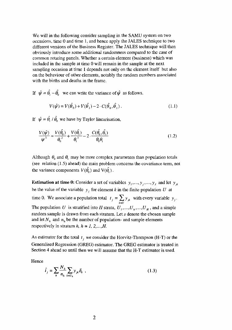
We will in the following consider sampling in the SAMU system on two occasions, time 0 and time 1, and hence apply the JALES technique to two different versions of the Business Register. The JALES technique will then obviously introduce some additional randomness compared to the case of common rotating panels. Whether a certain element (business) which was included in the sample at time 0 will remain in the sample at the next sampling occasion at time 1 depends not only on the element itself but also on the behaviour of other elements, notably the random numbers associated with the births and deaths in the frame.

, we can write the variance of \j/ as follows.

(1.1)

we have by Taylor linearisation,

(1.2)

Although 60 and 0, may be more complex parameters than population totals (see relation (1.5) ahead) the main problem concerns the covariance term, not the variance components V(60) and V(0,).

Estimation at time 0: Consider a set of variables y,,...,y.,...,yy and let yjk

be the value of the variable yy for element k in the finite population U at

time 0. We associate a population total with every variable y..

The population U is stratified into H strata, £/,,..., Uh,..., UH , and a simple random sample is drawn from each stratum. Let s denote the chosen sample and let Nh and nh be the number of population- and sample elements respectively in stratum h, h = 1, 2,...,H.

As estimator for the total t j we consider the Horvitz-Thompson (H-T) or the

Generalised Regression (GREG) estimator. The GREG estimator is treated in Section 4 ahead so until then we will assume that the H-T estimator is used.

Hence

(1-3)

2

where

(1.4)

We will assume that the estimator d0 can be expressed on the following form:

(1.5)

where/is an arbitrary rational function. A common estimator for a population mean or a difference between two domain totals, a ratio estimator or a poststratified ratio estimator for a population total are examples of such functions.

Estimation at time 1: The population U' at time 1 consisting of N' elements is stratified into L strata, U[,...,U'l,...,U'L . The stratification at time 1 does not have to be the same as the one at time 0. Let s' be the sample and let N', and ri, be the population- and sample size in stratum /, 1=1, 2,...,L.

The population totals at time 1 are estimated in analogy with (1.3).

(1.6)

where

(1.7)

We assume that the estimator 0, can be written on the form

(1.8)

Notice that the same function / is assumed in (1.5) and (1.8). This should be the most common case in practice. Generalisation to the case of different functions /„ and / , is straight forward.

3

The covariance: By standard Taylor linearisation we can now write the covariance in (1.1) and (1.2) as follows.

(1.9)

/ / being the partial derivative the covariance for the pair

Next we will study the term Cit^tj) with its estimator C(tntj) and

C(0O,0, ) with its estimator C(0O,0, ) in detail.

4

2. Estimator for the covariance

By combination of (1.3) and (1.6) we can write the covariances as follows.

(2.1)

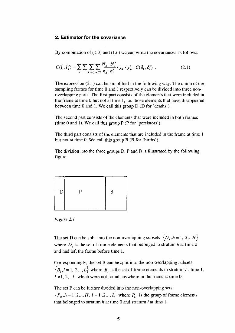
The expression (2.1) can be simplified in the following way. The union of the sampling frames for time 0 and 1 respectively can be divided into three non-overlapping parts. The first part consists of the elements that were included in the frame at time 0 but not at time 1, i.e. those elements that have disappeared between time 0 and 1. We call this group D (D for 'deaths').

The second part consists of the elements that were included in both frames (time 0 and 1). We call this group P (P for 'persistors').

The third part consists of the elements that are included in the frame at time 1 but not at time 0. We call this group B (B for 'births').

The division into the three groups D, P and B is illustrated by the following figure.

Figure 2.1

The set D can be split into the non-overlapping subsets \Dh ,h = 1, 2,..H\

where Dh is the set of frame elements that belonged to stratum h at time 0

and had left the frame before time 1.

Correspondingly, the set B can be split into the non-overlapping subsets

{B,,1 = 1, 2,..,L\ where B, is the set of frame elements in stratum / , time 1,

/ =1, 2,..,L which were not found anywhere in the frame at time 0.

The set P can be further divided into the non-overlapping sets

{Phl,h = 1 ,2,..,H, 1 = 1 ,2,..,L\ where Phl is the group of frame elements

that belonged to stratum h at time 0 and stratum / at time 1.

5

Among the nh elements sampled from stratum h at time 0 we assume that dhbelong to Dh, h=l, 2,...,H and that ahl belong to the stratum combination

Among the n\ elements sampled from stratum / at time 1 we assume that b[ belong to B,, 1=1, 2,...,L and that a'hl belong to the stratum combination Phl.

Let Gu be the number of frame elements in PM. Furthermore, let ghl be the number of elements that belong to Phl and are included in both samples (time 0 and 1). We illustrate this by the following figure.

Figure 2.2 (Number of elements)

The quantity could

be considered as random (Sjölinder (1971), Bäcklund (1972) and Garås (1989). However, we will in the following make the analysis conditional on Q. since Q can be considered as an ancillary quantity for the present analysis.

6

Hence in the general expression

(2.2)

we will estimate the conditional variance V(y/]Q), and ignore the second

component of (2.2). We can then rewrite (2.1) as a conditional covariance:

(2.3)

It follows from the use of independent random numbers under the JALES -technique that we only have to consider the covariance of (2.3) for those pairs of frame elements k and r that both come from the same stratum (h) at time 0 and the same stratum (/ ) at time 1, i.e only those pairs of elements k and r where both elements belong to Phl. (Sjölinder (1971) and Bäcklund (1972).

Hence the relation (2.3) can be written on the following form.

(2.4)

or, equivalently

(2.5)

The following quantity is unbiased for

(2.6)

7

Orusild (1999) computes the three expectations included in (2.6) and shows that the estimator (2.6) can be put on the following form (see Appendix A for an alternative proof).

where

and

Comment: The quantities aM, a'hl, gM och Ghl were defined in connection with figure 2.2 above.

The complete covariance, conditional on Q,,

(2.8)

is obtained by inserting the expressions (1.3), (1.6) and (2.7) into (1.9).

8

3. A procedure for estimation of the covariance and the measures of change

We will first show how the covariance formula (2.7) can be transformed so that it can be written on the 'usual' form under stratified SRS.

Then (2.7) can be written on the following form, i.e. the 'usual' formula for the estimator of the covariance between two n-weighted totals under stratified SRS where strata comprise every combination of (h, I) in Phl, the population size "Capital N" equals GM and the sample size "small n" equals äM.

(3.1)

In order to get the whole covariance term (2.8) right we must also compute

the point estimates ti and t. according to (1.3) and (1.6) respectively. This

means that also the observations that are not included in PM must be

accounted for. These observations contribute to the partial derivatives in (2.8)

but not to Cit^tjQ.). We will now introduce a data transformation which

will enable us to write (2.8) on a "standard form" which can be handled by a 'normal' variance algorithm.

Procedure 3.1

1) Distribute every sample element (which appeared in either one of the time 0 and time 1 samples) to the following groups :

where

- Dh includes the elements in stratum h at time 0 which disappeared from the frame before time 1, i.e. the deaths in stratum h.

- Phl includes the elements which belonged to stratum h at time 0 and stratum I at time 1. Notice that elements that are included in just one of the two samples must be included, not only the ones included in both samples.

- B, includes the elements that are not found in the frame at time 0 but that

belong to stratum I at time 1, i.e the births in stratum I.

9

2) For every group q, compute the following quantities N och n :

(3.2)

(3.3)

3) Transform

(3.4)

b)

(3.5)

c)

(3.6)

(3.7)

End of Procedure 3.1

10

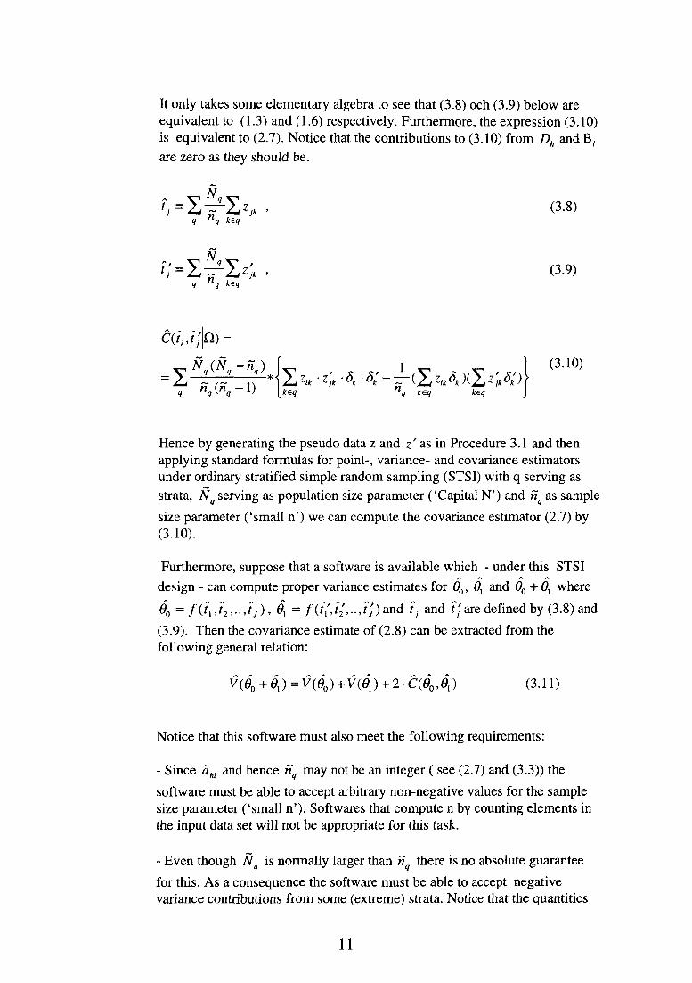
It only takes some elementary algebra to see that (3.8) och (3.9) below are equivalent to (1.3) and (1.6) respectively. Furthermore, the expression (3.10) is equivalent to (2.7). Notice that the contributions to (3.10) from Dh and B;

are zero as they should be.

(3.8)

(3.9)

(3.10)

Hence by generating the pseudo data z and z as in Procedure 3.1 and then applying standard formulas for point-, variance- and covariance estimators under ordinary stratified simple random sampling (STSI) with q serving as strata, N serving as population size parameter ('Capital N') and nq as sample

size parameter ('small n') we can compute the covariance estimator (2.7) by (3.10).

Furthermore, suppose that a software is available which - under this STSI

design - can compute proper variance estimates for 00, 6i and 60 + 0, where

% = / 0 \ Â > • •.h)> 0) = /(n4">->tj) a n d tj a n d tj we defined by (3.8) and (3.9). Then the covariance estimate of (2.8) can be extracted from the following general relation:

(3.11)

Notice that this software must also meet the following requirements:

- Since ahl and hence nq may not be an integer ( see (2.7) and (3.3)) the

software must be able to accept arbitrary non-negative values for the sample size parameter ('small n'). Softwares that compute n by counting elements in the input data set will not be appropriate for this task.

- Even though N is normally larger than n there is no absolute guarantee

for this. As a consequence the software must be able to accept negative variance contributions from some (extreme) strata. Notice that the quantities

11

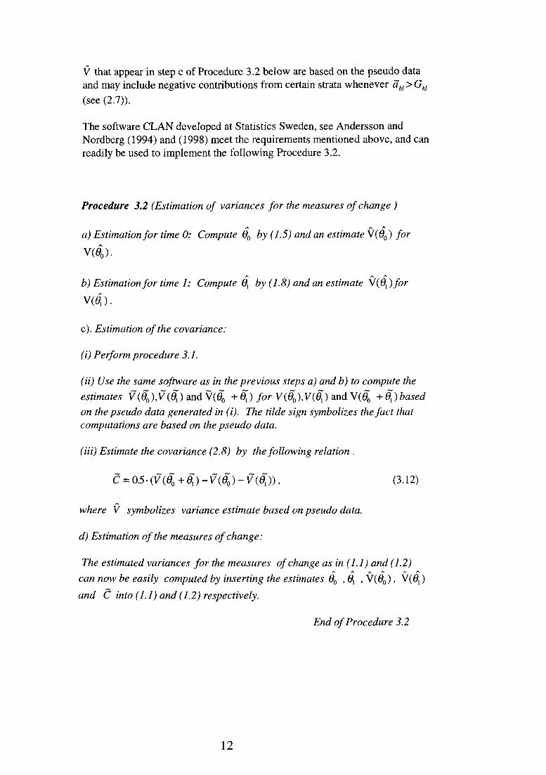
V that appear in step c of Procedure 3.2 below are based on the pseudo data and may include negative contributions from certain strata whenever ahl > Ghl

(see (2.7)).

The software CLAN developed at Statistics Sweden, see Andersson and Nordberg (1994) and (1998) meet the requirements mentioned above, and can readily be used to implement the following Procedure 3.2.

Procedure 3.2 (Estimation of variances for the measures of change )

a) Estimation for time 0: Compute 60 by (1.5) and an estimate V(0O) for

v(4).

b) Estimation for time 1: Compute 0, by (1.8) and an estimate V(0,)/or

V(3).

c). Estimation of the covariance:

(i) Perform procedure 3.1.

(ii) Use the same software as in the previous steps a) and b) to compute the estimates V(0o),V(^) and V(d0 +%) for V(0o),V(0^) and W(60 +6{)based on the pseudo data generated in (i). The tilde sign symbolizes the fact that computations are based on the pseudo data.

(Hi) Estimate the covariance (2.8) by the following relation .

(3.12)

where V symbolizes variance estimate based on pseudo data,

d) Estimation of the measures of change:

The estimated variances for the measures of change as in (1.1) and (1.2) ys yv /\ .A. ^ ./v

can now be easily computed by inserting the estimates 60 ,0, , V(0O), V(0,)

and C into (1.1) and (1.2) respectively.

End of Procedure 3.2

12

4. Extension to GREG estimation

We will now show how the procedure presented above can be modified to incorporate the case when the H-T estimators of (1.3) and (1.6) respectively replaced by GREG estimators. Before proceeding we need some notation and results concerning GREG -estimation. See Särndal, Swensson and Wretman (1992) for a comprehensive presentation of the theory.

Let y be a variable of interest and let yk be the y-value for element k in a

finite population. Also available is a value xk = (xlk ,...,xmk,..., xm )T of the

vector x of length M.

The GREG-estimator can be motivated in terms of regression theory along the following lines. Suppose that the scatter of the N points (yk ,x]k,...,xmk,...,xMk) : k= 1, ...,N looks as if it had been generated by a linear regression model with y as the response and the x:s as covariates. The values, yl,...,yk,...,yN are assumed to be realised values of independent

random variables, Y\, ..., Yk, ..., YN. Moreover it is assumed that,

(4.1)

where E^ and Vç denote expected value and variance with respect to the model £, while p and a\ are usually unknown model parameters and T (>0) is

a known scale parameter. Suppose that the values of y are only known for the elements in the sample while x is known for every element in the population.

The GREG-estimator of the population total t for y can now be expressed

on the form

(4.2)

where t J is the (transposed) vector of totals for x , teHT is the H-T

estimator for the residual:

(4.3)

and

(4.4)

13

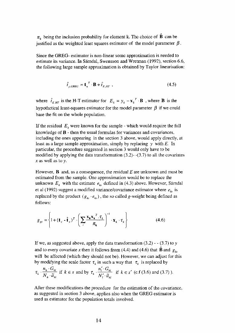
Kk being the inclusion probability for element k. The choice of B can be justified as the weighted least squares estimator of the model parameter j8.

Since the GREG- estimator is non-linear some approximation is needed to estimate its variance. In Särndal, Swensson and Wretman (1992), section 6.6, the following large sample approximation is obtained by Taylor linearisation:

(4.5)

where tEHT is the H-T estimator for Ek = yk -xkT B , where B is the

hypothetical least-squares estimator for the model parameter f5 if we could

base the fit on the whole population.

If the residual Ek were known for the sample - which would require the full knowledge of B - then the usual formulas for variances and covariances, including the ones appearing in the section 3 above, would apply directly, at least as a large sample approximation, simply by replacing y with E. In particular, the procedure suggested in section 3 would only have to be modified by applying the data transformation (3.2)- -(3.7) to all the covariates x as well as to y.

However, B and, as a consequence, the residual E are unknown and must be estimated from the sample. One approximation would be to replace the unknown Ek with the estimate e^ defined in (4.3) above. However, Särndal et al (1992) suggest a modified variance/covariance estimator where e^ is replaced by the product (gfa • eh), the so called g-weight being defined as follows:

(4.6)

If we, as suggested above, apply the data transformation (3.2) - - (3.7) to y and to every covariate x then it follows from (4.4) and (4.6) that B and g^ will be affected (which they should not be). However, we can adjust for this by modifying the scale factor Tk in such a way that zk is replaced by

After these modifications the procedure for the estimation of the covariance, as suggested in section 3 above, applies also when the GREG estimator is used as estimator for the population totals involved.

14

5. References

Andersson, C. and Nordberg, L. (1994): A Method for Variance Estimation of Non-Linear Functions of Totals in Surveys - Theory and a Software Implementation. Journal of Official Statistics, 10, 395-405.

Andersson, C. and Nordberg, L. (1998): A User's Guide to CLAN 91 - a SAS Program for Computation of Point- and Standard Error Estimates in Sample Surveys. Statistics Sweden.

Bäcklund, S. (1972): Tillämpning av JALES metod vid stratifierade urval. Skattning av en förändringsparameter. Bestämning av variansen i denna skattning när enheter byter stratum mellan två tidpunkter. Memo, Statistics Sweden. (In Swedish).

Garås, T. (1989): Förändringsestimatorer vid dynamiska populationer. Memo, Statistics Sweden. (In Swedish).

Nordberg, L. (1994): En Procedur för att Skatta Varianser för Förändringstal Baserade på Två Separate SAMU-Urval. Technical Report, Dept. for Economic Statistics, Statistics Sweden. (In Swedish).

Ohlsson, E. (1992): S AMU - The System for Co-Ordination of Samples from the Business Register at Statistics Sweden. R&D Report 1992:18, Statistics Sweden.

Ohlsson, E. (1995): Coordination of Samples Using Permanent Random Numbers. In Business Survey Methods. Ed. Cox, B. et al Wiley 1995.

Orusild, T. (1999): Confidence Intervals for Functions of Quantiles under Finite Population Sampling . Forthcoming Technical Report at Dept. of Mathematical Statistics, University of Stockholm.

Sjölinder, K. (1971): Beräkning av kovarianstermen vid urvalsdragning enligt JALES-metoden. Memo, Statistics Sweden. (In Swedish).

Särndal, CE., Swensson, B. and Wretman, J. (1992): Model Assisted Survey Sampling. New York: Springer-Verlag.

15

Appendix A: Proof of the relation (2.7)

The point of departure will be the following expression - (2.6) in Section 2.

(Al)

The three expectations must be computed in order to make the estimator (Al) operational. The following result - where all the quantities involved have been defined earlier in the main text - is shown, under a different notation, by Orusild (1999). An alternative proof follows here:

Lemma:

a)

b)

c)

d)

Proof: a) By symmetry E(ôk \Q) must be a constant for all ke Phl. Set

this constant to

b) proved analogously.

c)

16

d) since this expectation due to symmetry must

But the left hand side is

Hence with assistance of c) above: which proves

point d of the lemma.

End of proof of lemma.

By the lemma and some algebra we have,

(A2)

(A3)

where

(A4)

By inserting (A2)~(A4) into (Al), finally, we arrive at the expression for the covariance estimator conditional on Q., i.e. formula (2.7) in the main text.

17

Appendix B: On SAS-implementation of Procedure 3.1

To implement Procedure 3.1 it is necessary to merge information that is likely to be found in different computer files. We will here give an outline of a SAS program that may be useful for this implementation.

Suppose that the sample at time 0 is found in the SAS dataset SampO:

Data SampO; length stratO $ 5;

respO-1; keep id stratO npopO nrespO respO yO; proc sort; by id;

Comment: The variables in the keep-list are the identity of current element (e.g. enterprise), the stratum identity for the stratum to which'id' belongs (we assume here that this stratum identity is a character of (say) five 'positions', hence the 'length' statement above), the number of population elements in current stratum, the number of responding elements in current stratum, a response indicator (to be used below) for current element and finally the observational value y for current element at time 0.

Analogously for sample at time 1 :

Data Sampl; length strati $ 5;

respl=l; keep id strati npopl nrespl respl yl; proc sort; by id;

Next consider the frames for time 0 and 1 :

Data FrameO; length stratO $ 5;.

keep id stratO; proc sort; by id;

Data Framel; length strati $ 5;.

keep id strati; proc sort; by id;

18

/ Generating data sets D('death'), B ('birth') and P ('persistors'j /

Data D; merge SampO (in=a) Framel (in=b); by id; if a and not b ;

Data B; merge Sampl (in=a) FrameO (in=b); by id; if a and not b ;

Data sOsl; / elements included in both samples / merge SampO (in=a) Sampl (in=b); by id; if a and b;

Data sOFl_sl; / elements included in sample 0 and Framel but not in sample 1 / merge SampO (in=a) Framel (in=b) Sampl (in=c); by id; if a and b and not c;

Data slFO_sO; /* elements included in samplel and FrameO but not in sample 0 */ merge Sampl (in=a) FrameO (in=b) SampO (in=c); by id; if a and b and not c;

Data P; set sOsl sOFl_sl slFO_sO; ifrespO=l and respl=l then resp01=l; else resp01-0; ifrespO ne 1 then respO=0; if resp 1 ne 1 then resp1=0; proc sort; by stratO strati;

/* Computation of GM, here denoted 'glarge' */

data tempo; merge FrameO (in=a) Framel(in=b); by id; if a and b; proc sort; by stratO strati; proc summary data=tempo; by stratO strati; output out=gdata; data gdata; set gdata; rename _freq_=glarge;

19

/* Computation of ïïM here denoted 'atilde', */

proc summary data=P; by stratO strati; var respO respl respOl; output out=adata sum=ahl aprhl gsmall; run; data adata; set adata; if gsmall-0 then atilde=l; if gsmall>0 then atilde=ahl*aprhl/gsmall; run;

I* Transformations (3.2)—(3.7) in Procedure 3.1 */

data P; merge P gdata adata; by stratO strati; strat=stratO II strati; nlarge=glarge; nsmall=atilde; ifrespO=l then zO=yO(npopO*atilde) /(nrespOglarge); else z0=0; if respl=1 then zl =yl (npopl atilde) / (nrespl glarge); else zl=0; run;

data D; set D; strat=stratOWOOOOO'; nlarge-npopO; nsmall=nrespO; zO=yO;zl=0; run;

data B; set B; strat='00000'\\ strati; nlarge-npopl; nsmall=nrespl; zO=0;zl=yl; run;

data indat; set D B P; proc sort; by strat; run;

20