Quintic B-spline collocation method for numerical solution of the Kuramoto–Sivashinsky equation

ANZIAM J. 49(2008), 389–410doi:10.1017/S1446181108000072

QUINTIC B-SPLINE COLLOCATION METHOD FORNUMERICAL SOLUTION OF THE RLW EQUATION

BULENT SAKA ˛ 1, IDRIS DAG1 and DURSUN IRK1

(Received 10 March, 2007; revised 5 March, 2008)

Abstract

Quintic B-spline collocation schemes for numerical solution of the regularized longwave (RLW) equation have been proposed. The schemes are based on the Crank–Nicolson formulation for time integration and quintic B-spline functions for spaceintegration. The quintic B-spline collocation method over finite intervals is also appliedto the time-split RLW equation and space-split RLW equation. After stability analysisis applied to all the schemes, the results of the three algorithms are compared bystudying the propagation of the solitary wave, interaction of two solitary waves andwave undulation.

2000 Mathematics subject classification: 65D07, 65N30, 65N35, 76B25.

Keywords and phrases: RLW equation, collocation, solitary waves, quintic B-splines,undular bore.

1. Introduction

The present study is concerned with numerical solution of the regularized longwave (RLW) equation, which was first derived by Peregrine to define undular boredevelopment [15]. Since then, this equation has been used to model a large number ofproblems arising in various areas of applied science. The analytical solutions of theRLW equation together with some initial and boundary conditions are shown in [3, 5].Thus numerical solutions of this equation are of interest for various boundary andinitial conditions. Well-known numerical techniques, including finite difference, finiteelement and Fourier pseudospectral methods, are applied to obtain numerical solutionsof the RLW equation.

The B-spline functions are the basis for piecewise polynomials and are used toconstruct approximate solutions in the finite element techniques. So approximationsolutions of the differential equations with B-splines can be obtained by the method ofweighted residuals, of which the Galerkin and collocation methods are particular cases.

1Mathematics Department, Eskisehir Osmangazi University, 26480 Eskisehir, Turkey;e-mail: [email protected]© Australian Mathematical Society 2008, Serial-fee code 0334-2700/08

389

390 B. Saka, I. Dag and D. Irk [2]

The Galerkin method is a widely used method for B-spline approximation. Thismethod provides very smooth solutions for numerical solutions of partial differentialequations. For example, Gardner et al. [11] proposed a Petrov–Galerkin quintic B-spline finite element method to obtain the numerical solution of the RLW equation.Burgers’ equation is also numerically solved by the Galerkin method using quinticB-splines as both shape and weight functions over the finite elements [7]. The finiteelement solution using quadratic B-splines as the element and the weight functionsfor the space split EW equation is set up in [19]. But application of the Galerkinmethod accompanied by higher-degree polynomials results in a higher-degree matrixsystem. That brings a burden for numerical analysis, and the computational cost ofthe matrix system increases in the evaluation of both linear and nonlinear systems.On the other hand, the collocation method together with B-spline approximationsrepresents an economical alternative since it only requires the evaluation of theunknown parameters at the grid points. A variant of this method has been successfullyapplied to solve differential equations [6, 8, 9, 12, 17, 20, 21, 23]. As is known,the success of the B-spline collocation method is dependent on the choice of B-spline basis. Quintic B-splines bases have been used to build up the approximationsolutions for some nonlinear differential equations. For instance, a numerical solutionof the Korteweg–de Vries (KdV) equation was obtained using collocation of quinticB-spline interpolation functions over finite elements in [10]. An algorithm based onthe collocation method with quintic B-spline finite elements was set up to simulate thesolutions of the KdV, Burgers’ and KdVB equations [23].

The RLW equation has been used as a test equation for numerical methods sincethis equation can be solved analytically for some boundary and initial conditions. Soa comparison between analytical and numerical solutions of the RLW equation can becarried out. Various forms of both B-spline collocation and B-spline Galerkin methodshave been constructed in obtaining the numerical solutions of the RLW equation[2, 4, 6, 8, 9, 12, 13, 17, 20, 21]. A numerical solution of the RLW equation has alsobeen found by applying a splitting-up scheme, which is used to be able to constructthe approximating solution with lower-degree piecewise polynomials, and both theapplicability and the efficiency of the splitting of the differential equations are soughtfor numerical methods [6].

The organization of this paper is as follows. In Section 2.1, a quintic B-splinefinite element algorithm is designed for the numerical solution of the RLW equation.In Section 2.2, the same method is applied to the time-split RLW equation. Lastly,in Section 2.3 the RLW equation is split into the first-order coupled matrix systemby letting V (x, t) = −Ux (x, t). The results of the three algorithms are compared inSection 3 using three test problems. The efficiencies of both time and space splittingtechniques together with quintic B-splines are sought. In addition, some of the earlierresults are also compared with those of the present algorithms.

The RLW equation is given by

Ut + Ux + εUUx − µUxxt = 0, (1.1)

[3] Quintic B-spline collocation method for solution of RLW equation 391

where ε and µ are positive parameters, and x and t denote differentiation. Boundaryconditions are chosen from

U (a, t) = β1,

Ux (a, t) = 0,

U (b, t) = β2,

Ux (b, t) = 0,(1.2)

and the initial condition is

U (x, 0) = f (x), a ≤ x ≤ b, (1.3)

where f (x) will be defined in the later sections depending on the test problems.The existence and uniqueness properties of the problem given by (1.1)–(1.3) werediscussed by Bona and Bryant [5].

We consider a uniformly spatially distributed set of nodes

a = x0 < x1 < · · · < xN = b

over the solution domain a ≤ x ≤ b with h = xm − xm−1, m = 1, . . . , N .

2. Numerical method

2.1. Quintic B-spline collocation method I (QBCM1) At the nodes xm the quinticB-splines Qm, m = −2, . . . , N + 2, are defined by

Qm(x)

=1

h5

(x − xm−3)5, [xm−3, xm−2],

(x − xm−3)5− 6(x − xm−2)

5, [xm−2, xm−1],

(x − xm−3)5− 6(x − xm−2)

5+ 15(x − xm−1)

5, [xm−1, xm],

(x − xm−3)5− 6(x − xm−2)

5+ 15(x − xm−1)

5

− 20(x − xm)5, [xm, xm+1],

(x − xm−3)5− 6(x − xm−2)

5+ 15(x − xm−1)

5

− 20(x − xm)5+ 15(x − xm+1)

5, [xm+1, xm+2],

(x − xm−3)5− 6(x − xm−2)

5+ 15(x − xm−1)

5

− 20(x − xm)5+ 15(x − xm+1)

5

− 6(x − xm+2)5, [xm+2, xm+3],

0, otherwise,

(2.1)

and the set of those B-splines defines the form of a basis over the interval [a, b]

(see [16]). A numerical solution of (1.1) will be derived by using the collocationmethod based on quintic B-splines. So a global approximation solution UN (x, t) tothe analytical solution U (x, t) will be sought in the form of an expansion of B-splines,

UN (x, t) =

N+2∑m=−2

δm(t)Qm(x), (2.2)

392 B. Saka, I. Dag and D. Irk [4]

where Qm are the quintic B-splines and δm are time-dependent parameters to bedetermined from the quintic B-spline collocation form of the RLW equation.

By using the approximation (2.2) and quintic B-splines (2.1), the nodal value U andits first and second derivatives U ′ and U ′′ at the nodes xi are obtained in terms of theelement parameters as

Um = U (xm) = δm−2 + 26δm−1 + 66δm + 26δm+1 + δm+2,

U ′m = U ′(xm) =

5h

(δm+2 + 10δm+1 − 10δm−1 − δm−2),

U ′′m = U ′′(xm) =

20

h2 (δm+2 + 2δm+1 − 6δm + 2δm−1 + δm−2),

(2.3)

where ′ and ′′ denote first and second differentiation with respect to x respectively.

Collocation points are selected to coincide with nodes. Substituting (2.3) into (1.1)leads to the set of the coupled first-order ordinary differential equations

δm−2 + 26δm−1 + 66δm + 26δm+1 + δm+2

+5(1 + εzm)

h(δm+2 + 10δm+1 − 10δm−1 − δm−2)

−20µ

h2 (δm+2 + 2δm+1 − 6δm + 2δm−1 + δm−2) = 0, (2.4)

where ◦ denotes derivative with respect to time and

zm = δm−2 + 26δm−1 + 66δm + 26δm+1 + δm+2.

Time discretization of (2.4) is carried out by interpolating time parameters δmand their time derivatives δm by using the Crank–Nicolson rule for δm and the usualforward difference rule for δm respectively between two time levels n and n + 1:

δm =δn+1

m + δnm

2, δm =

δn+1m − δn

m

1t. (2.5)

Thus a recurrence relationship is obtained between two successive time levels nand n + 1 which relates two successive unknown parameters δn+1

i and δni (where

i = m − 2, . . . , m + 2) as

αm1δn+1m−2 + αm2δ

n+1m−1 + αm3δ

n+1m + αm4δ

n+1m+1 + αm5δ

n+1m+2

= αm5δnm−2 + αm4δ

nm−1 + αm3δ

nm + αm2δ

nm+1 + αm1δ

nm+2, (2.6)

[5] Quintic B-spline collocation method for solution of RLW equation 393

where

αm1 = 2h2− 5h1t (1 + εzm) − 40µ,

αm2 = 52h2− 50h1t (1 + εzm) − 80µ,

αm3 = 132h2+ 240µ,

αm4 = 52h2+ 50h1t (1 + εzm) − 80µ,

αm5 = 2h2+ 5h1t (1 + εzm) − 40µ, m = 0, 1, . . . , N .

(2.7)

The above system consists of the N + 1 equations in the N + 5 unknownparameters. The elimination of parameters δn+1

−2 , δn+1−1 , δn+1

N+1, δn+1N+2 from

the system (2.6) using the boundary conditions U (a, t) = β1, U (b, t) = β2 andUx (a, t) = Ux (b, t) = 0 enables one to get a solvable (N + 1) × (N + 1) matrixsystem. The resulting pentadiagonal matrix system is easily and efficiently solvedwith a variant of the Thomas algorithms [18].

To initiate element parameters δnm , we must find the initial unknown parameters δ0

mby means of the following requirements:

(UN )x (a, 0) = δ0−2 + 10δ0

−1 − 10δ01 − δ0

2 = 0,

(UN )xx (a, 0) = δ0−2 + 2δ0

−1 − 6δ00 + 2δ0

1 + δ02 = 0,

UN (x, 0) = δ0m−2 + 26δ0

m−1 + 66δ0m + 26δ0

m+1 + δ0m+2 = U (xm, 0),

(UN )x (b, 0) = δ0N+2 + 10δ0

N+1 − 10δ0N−1 − δ0

N−2 = 0,

(UN )xx (b, 0) = δ0N+2 + 2δ0

N+1 − 6δ0N + 2δ0

N−1 + δ0N−2 = 0.

(2.8)

This also allows us to determine the solution of the pentadiagonal matrix equation withthe parameters δ0

m , m = −2, . . . , N + 2.To deal with nonlinearity in (2.6), the time parameters δm in zm are replaced by δn

mfor the time level, so the linearized algebraic system (2.6) is used together with thefollowing iteration process to get a better result:

(1) calculate δn+1 using iteration procedure (2.6) by employing the Thomasalgorithms; and

(2) obtain a new approximation to (δ∗)n+1 by the procedure

(δ∗)n+1= δn

+12 (δn+1

− δn). (2.9)

Before moving the calculation of the next time step approximation for the timeparameters, iteration should be repeated two or three times.

To investigate the stability of the difference scheme (2.6), we apply von Neumannstability analysis. We assume that the quantity U in the nonlinear term UUx islocally constant p for the RLW equation. This selection is the same as assumingthat the corresponding values of zm are also constant and equal to p. Let usconsider a particular solution, δn

m = qneimϕ , where i is an imaginary unit, ϕ is anarbitrary real number, and q = q(ϕ) is a complex number whose value must be found.

394 B. Saka, I. Dag and D. Irk [6]

After substituting the Fourier mode δnm = qneimϕ into the linearized form of the

difference equation, we have the growth factor

q =a + ib

a − ib,

where

a = (αm1 + αm5) cos 2ϕ + (αm2 + αm4) cos ϕ + αm3,

b = (αm1 − αm5) sin 2ϕ + (αm2 − αm4) sin ϕ.

Since the magnitude of the growth factor is |q| = 1, the difference scheme (2.6) isunconditionally stable.

2.2. Quintic B-spline collocation method II (QBCM2) The time-split RLWequation is

(U − µUxx )t + 2εUUx = 0, (2.10)

(U − µUxx )t + 2Ux = 0. (2.11)

If we identify the collocation points with nodes xm and substitute the nodalvalues Um and their first two successive derivatives U ′

m and U ′′m into (2.10) and (2.11),

we have the following coupled matrix system of first-order ordinary differentialequations:

δm−2 + 26δm−1 + 66δm + 26δm+1 + δm+2

−20µ

h2 (δm+2 + 2δm+1 − 6δm + 2δm−1 + δm−2)

+10εzm

h(δm+2 + 10δm+1 − 10δm−1 − δm−2) = 0, (2.12)

δm−2 + 26δm−1 + 66δm + 26δm+1 + δm+2

−20µ

h2 (δm+2 + 2δm+1 − 6δm + 2δm−1 + δm−2)

+10h

(δm+2 + 10δm+1 − 10δm−1 − δm−2) = 0, (2.13)

where again ◦ denotes derivative with respect to time and

zm = δm−2 + 26δm−1 + 66δm + 26δm+1 + δm+2.

With a Crank–Nicolson formulation in time for the unknown parameters δm and theusual finite difference scheme for their time derivatives δm ,

δm =δn

m + δn+1/2m

2, δm =

δn+1/2m − δn

m

1t, (2.14)

[7] Quintic B-spline collocation method for solution of RLW equation 395

we obtain an equation between two time levels, for the unknown parameters of (2.12)relating time levels n and n + 1/2, δn

i to δn+1/2i (i = m − 2, . . . , m + 2),

α1δn+1/2m−2 + α2δ

n+1/2m−1 + α3δ

n+1/2m + α4δ

n+1/2m+1 + α5δ

n+1/2m+2

= α5δnm−2 + α4δ

nm−1 + α3δ

nm + α2δ

nm+1 + α1δ

nm+2, (2.15)

where

α1 = 2h2− 5h1tεzm − 40µ,

α2 = 52h2− 50h1tεzm − 80µ,

α3 = 132h2+ 240µ,

α4 = 52h2+ 50h1tεzm − 80µ,

α5 = 2h2+ 5h1tεzm − 40µ.

Similarly, using the Crank–Nicolson approach for parameters δm and the finitedifference scheme for their time derivatives δm respectively between two time levelsn + 1/2 and n + 1 in (2.13),

δm =δn+1

m + δn+1/2m

2, δm =

δn+1m − δ

n+1/2m

1t, (2.16)

we have an equation relating δn+1/2i to δn+1

i (i = m − 2, . . . , m + 2),

α6δn+1m−2 + α7δ

n+1m−1 + α8δ

n+1m + α9δ

n+1m+1 + α10δ

n+1m+2

= α10δn+1/2m−2 + α9δ

n+1/2m−1 + α8δ

n+1/2m + α7δ

n+1/2m+1 + α6δ

n+1/2m+2 , (2.17)

where

α6 = 2h2− 5h1t − 40µ,

α7 = 52h2− 50h1t − 80µ,

α8 = 132h2+ 240µ,

α9 = 52h2+ 50h1t − 80µ,

α10 = 2h2+ 5h1t − 40µ.

Equations (2.15) and (2.17) constitute a multistep finite difference scheme, forsolving the RLW equation, having N + 1 equations containing N + 5 unknownparameters. We obtain a unique solution by eliminating the parameters δi

−2,δi−1, δi

N+1, δiN+2 (i = n + 1/2, n + 1) from (2.15) and (2.17) after imposition of

the boundary conditions U (a, t) = β1, U (b, t) = β2 and Ux (a, t) = Ux (b, t) = 0.Boundary conditions U (a, t) = β1 and Ux (a, t) = 0 are used to eliminate δi

−2 andδi−1, while the conditions U (b, t) = β1 and Ux (b, t) = 0 are used to eliminate δi

N+1

396 B. Saka, I. Dag and D. Irk [8]

and δiN+2, so that this solvable five-banded pentadiagonal matrix system is solved

by way of the Thomas algorithms. Once we find an approximation δ0m , the next

time solution parameters δn+1m having been found, parameters δ

n+1/2m from (2.15) are

computed using (2.17).To handle the nonlinearity in (2.15), the corrector procedure

(δ∗)n+1/2= δn

+12 (δn+1/2

− δn) (2.18)

is used. To start the iteration for calculating the unknown parameters, the initialunknown parameters δ0

m must be determined from the initial and boundary conditionsto satisfy the requirements given in (2.8).

To investigate the stability of the difference equation (2.15), we apply the vonNeumann stability method after linearizing by taking U in the nonlinear term UUxas a local constant p. Thus the term zm in the difference equation corresponds toconstant p. Substitute δn

m = qneimϕ in (2.15), then

q =a + ib

a − ib,

where the quantities q , ϕ have the same meaning as in previous considerations and

a = (α1 + α5) cos 2ϕ + (α2 + α4) cos ϕ + α3,

b = (α1 − α5) sin 2ϕ + (α2 − α4) sin ϕ.

Von Neumann’s condition |q| ≤ 1 is satisfied so that the difference scheme isunconditionally stable. With the similar calculation the difference equation (2.17) isalso unconditionally stable.

2.3. Quintic B-spline collocation method III (QBCM3) In this section, the quinticB-spline collocation method discussed above is employed to obtain the numericalsolution of the space-split RLW equation. If we set V (x, t) = −Ux (x, t) in the RLWequation, it becomes

Ut − (1 + εU )V + µVxt = 0,

V + Ux = 0.(2.19)

The boundary and initial conditions can be rewritten as

U (a, t) = β1, U (b, t) = β2, V (a, t) = 0, V (b, t) = 0,

Ux (a, t) = 0, Ux (b, t) = 0, Vx (a, t) = 0, Vx (b, t) = 0,(2.20)

U (x, 0) = f (x), V (x, 0) = − f ′(x), a ≤ x ≤ b. (2.21)

Expressing U (x, t) and V (x, t) by using quintic B-splines, Qm(x) and the time-dependent parameters δm and σm are given as

UN (x, t) =

N+2∑m=−2

δm(t)Qm(x), VN (x, t) =

N+2∑m=−2

σm(t)Qm(x). (2.22)

[9] Quintic B-spline collocation method for solution of RLW equation 397

The nodal variables Um , Vm and their space derivatives U ′m , V ′

m can be calculatedby using expressions (2.22) and the quintic B-splines (2.1) as

Um = U (xm) = δm−2 + 26δm−1 + 66δm + 26δm+1 + δm+2,

U ′m = U ′(xm) =

5h

(δm+2 + 10δm+1 − 10δm−1 − δm−2),

Vm = V (xm) = σm−2 + 26σm−1 + 66σm + 26σm+1 + σm+2,

V ′m = V ′(xm) =

5h

(σm+2 + 10σm+1 − 10σm−1 − σm−2).

(2.23)

Substituting (2.23) into (2.19) yields

δm−2 + 26δm−1 + 66δm + 26δm+1 + δm+2

− (1 + εzm)(σm−2 + 26σm−1 + 66σm + 26σm+1 + σm+2)

+5µ

h(σm+2 + 10σm+1 − 10σm−1 − σm−2)

= 0,

σm−2 + 26σm−1 + 66σm + 26σm+1 + σm+2

+5h

(δm+2 + 10δm+1 − 10δm−1 − δm−2)

= 0,

(2.24)

where ◦ denotes differentiation with respect to time and

zm = δm−2 + 26δm−1 + 66δm + 26δm+1 + δm+2.

To derive the fully discretized difference equation, we use the following Crank–Nicolson approximation in time for the unknown parameters δm , σm and the usualfinite difference scheme for the time derivative of the parameters δm, σm :

δm =δn+1

m + δnm

2,

σm =σ n+1

m + σ nm

2,

δm =δn+1

m − δnm

1t,

σm =σ n+1

m − σ nm

1t.

(2.25)

These lead to a system of 2N + 2 algebraic equations in 2N + 10 unknowns:

2hδn+1m−2 + βm1σ

n+1m−2 + 52hδn+1

m−1 + βm2σn+1m−1 + 132hδn+1

m

+ βm3σn+1m + 52hδn+1

m+1 + βm4σn+1m+1 + 2hδn+1

m+2 + βm5σn+1m+2

= 2hδnm−2 − βm5σ

nm−2 + 52hδn

m−1 − βm4σnm−1 + 132hδn

m − βm3σnm

+ 52hδnm+1 − βm2σ

nm+1 + 2hδn

m+2 − βm1σnm+2, (2.26)

398 B. Saka, I. Dag and D. Irk [10]

−5δn+1m−2 + hσ n+1

m−2 − 50δn+1m−1 + 26hσ n+1

m−1 + 66hσ n+1m

+ 50δn+1m+1 + 26hσ n+1

m+1 + 5δn+1m+2 + hσ n+1

m+2

= 5δnm−2 − hσ n

m−2 + 50δnm−1 − 26hσ n

m−1 − 66hσ nm

− 50δnm+1 − 26hσ n

m+1 − 5δnm+2 − hσ n

m+2, m = 0, . . . , N ,

where

βm1 = −dh1t − 10µ,

βm4 = −26 dh1t + 100µ,

βm2 = −26 dh1t − 100µ,

βm5 = −dh1t + 10µ,

βm3 = −66 dh1t,d = 1 + εzm .

Application of the boundary conditions

U (a, t) = β1, Ux (a, t) = 0, V (a, t) = 0, Vx (a, t) = 0,

U (b, t) = β2, Ux (b, t) = 0, V (b, t) = 0 and Vx (b, t) = 0

enables us to eliminate the parameters δn+1−2 , σ n+1

−2 , δn+1−1 , σ n+1

−1 , δn+1N+1, σ n+1

N+1, δn+1N+2

and σ n+1N+2 from the system (2.26) so that we have a solvable 11-banded matrix system

of dimension (2N + 2) × (2N + 2). This system is solved by employing the Gausselimination procedure.

Time evolution of the parameters δn+1m , σ n+1

m is computed once the initialparameters δ0

m , σ 0m are obtained with the help of the following boundary and initial

conditions:

(UN )x (a, 0) = δ0−2 + 10δ0

−1 − 10δ01 − δ0

2 = 0,

(UN )xx (a, 0) = δ0−2 + 2δ0

−1 − 6δ00 + 2δ0

1 + δ02 = 0,

UN (x, 0) = δ0m−2 + 26δ0

m−1 + 66δ0m + 26δ0

m+1 + δ0m+2 = U (xm, 0),

(UN )x (b, 0) = δ0N+2 + 10δ0

N+1 − 10δ0N−1 − δ0

N−2 = 0,

(UN )xx (b, 0) = δ0N+2 + 2δ0

N+1 − 6δ0N + 2δ0

N−1 + δ0N−2 = 0,

(VN )x (a, 0) = σ 0−2 + 10σ 0

−1 − 10σ 01 − σ 0

2 = 0,

(VN )xx (a, 0) = σ 0−2 + 2σ 0

−1 − 6σ 00 + 2σ 0

1 + σ 02 = 0,

VN (x, 0) = σ 0m−2 + 26σ 0

m−1 + 66σ 0m + 26σ 0

m+1 + σ 0m+2 = V (xm, 0),

(VN )x (b, 0) = σ 0N+2 + 10σ 0

N+1 − 10σ 0N−1 − σ 0

N−2 = 0,

(VN )xx (b, 0) = σ 0N+2 + 2σ 0

N+1 − 6σ 0N + 2σ 0

N−1 + σ 0N−2 = 0.

(2.27)

The system above is also solved by a variant of the Thomas algorithms.The procedure defined in (2.9) is applied two or three times at every time step to

accomplish better results.To investigate the stability of the difference scheme (2.26), we apply the method

of harmonics [22] after linearizing by taking U in the nonlinear term U V as a local

[11] Quintic B-spline collocation method for solution of RLW equation 399

constant p. Thus the term zm in the difference equation corresponds to a constant p.In this case, we will try to find the solution in the form

δnm = Pqneimϕ,

σ nm = Wqneimϕ,

where the quantities q and ϕ have the same meaning as in the previous twoconsiderations and P , W are the amplitudes of harmonics. Substituting δn

m = Pqneimϕ

and σ nm = Wqneimϕ into the difference scheme (2.26) gives

a1 P + (b1 + ic1)W = 0,

ia2 P + b2W = 0,(2.28)

where

a1 = (2h cos 2ϕ + 52h cos ϕ + 132h + 52h cos ϕ + 2h cos 2ϕ)(q − 1),

b1 = (β1 cos 2ϕ + β2 cos ϕ + β3 + β4 cos ϕ + β5 cos 2ϕ)(q + 1),

c1 = (−β1 sin 2ϕ − β2 sin ϕ + β4 sin ϕ + β5 sin 2ϕ)(q − 1),

a2 = (10 sin 2ϕ + 100 sin ϕ)(q + 1),

b2 = (h cos 2ϕ + 26h cos ϕ + 66h + 26h cos ϕ + h cos 2ϕ)(q + 1).

The system (2.28), with respect to P and W , will have a nontrivial solution if thedeterminant of the coefficient matrix is equal to zero. After some mathematicalmanipulation, the roots of the determinant of the coefficient matrix can be found as

q1 =z1

z2, q2 = −1,

where

z1 = −90 dh1t sin3 ϕ + 490 dh1t sin ϕ + 410 dh1t cos ϕ sin ϕ

− 5 dh1t cos ϕ sin3 ϕ + i(−406h2 sin2 ϕ + 1300µ sin2 ϕ + 916h2

+ 500µ sin2 ϕ cos ϕ − 50µ sin4 ϕ + 2h2 sin4 ϕ + 884h2 cos ϕ

− 52h2 sin2 ϕ cos ϕ),

z2 = 90 dh1t sin3 ϕ − 490 dh1t sin ϕ − 410 dh1t cos ϕ sin ϕ

+ 5 dh1t cos ϕ sin3 ϕ + i(−406h2 sin2 ϕ + 1300µ sin2 ϕ + 916h2

+ 500µ sin2 ϕ cos ϕ − 50µ sin4 ϕ + 2h2 sin4 ϕ + 884h2 cos ϕ

− 52h2 sin2 ϕ cos ϕ).

Since |q1| ≤ 1 and |q2| ≤ 1 are satisfied, the difference scheme is unconditionallystable.

400 B. Saka, I. Dag and D. Irk [12]

3. Numerical calculations

The only three conservation quantities of the RLW equation are [14]

C1 =

∫ b

aU dx ' h

N∑j=1

U nj ,

C2 =

∫ b

a(U 2

+ µ(Ux )2) dx ' h

N∑j=1

{(U nj )

2+ µ((Ux )

nj )

2},

C3 =

∫ b

a(U 3

+ 3U 2) dx ' hN∑

j=1

{(U nj )

3+ 3(U n

j )2}.

(3.1)

The integrals above are approximated by the rectangle rule for quadrature. Thus U nj

and its first derivative are calculated from (2.3). Conservation quantities, the L2 errornorm

L2 =

√h

∑N

j=0|U exact

j − (UN ) j |2 (3.2)

and the L∞ error norm

L∞ = ‖U exact− UN ‖∞ = max

j|U exact

j − (UN ) j | (3.3)

will be computed to show how well the behaviour of the numerical schemes modelsthe test problems in terms of accuracy.

3.1. Single solitary wave The exact solution of (1.1) is given by

U (x, t) = 3c sech2(k[x − x0 − vt]), (3.4)

which represents a single solitary wave of amplitude 3c, velocity v = 1 + εc andk =

12 (εc/µν)1/2 (see [15]). This solution travels across the interval −40 ≤ x ≤ 60

in the time period 0 ≤ t ≤ 20 with parameters ε = µ = 1, x0 = 0 and boundaryconditions β1 = 0, β2 = 0.

The numerical experiment of this single solitary wave motion is performed for thethree schemes. The experiment is carried out using the initial condition

U (x, 0) = 3c sech2(k[x − x0]). (3.5)

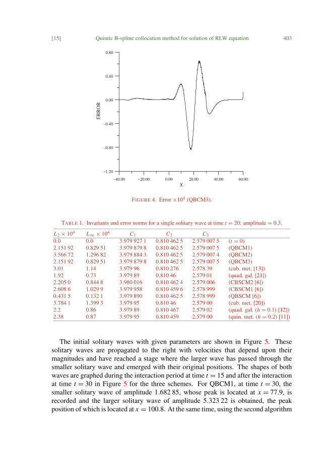
First, the program is run up to time t = 20 with parameters c = 0.1, 1t = 0.1 andh = 0.125, which are chosen to be the same as in some earlier papers [6, 11, 12,20, 21]. The results of the error norms and conservation invariants are documented inTable 1 at times t = 0 and 20 for the three schemes. During the program run, numericalinvariants C2 and C3 remain constant and C1 remains almost constant. Although thethree schemes produce the same order accuracy, QBCM1 and QBCM3 give a slightlysmaller error than QBCM2. The initial function and numerical solution are drawn for

[13] Quintic B-spline collocation method for solution of RLW equation 401

–40.00 –20.00 0.00 20.00 40.00 60.00

X

0.00

0.10

0.20

0.30

U

t=0 t=20

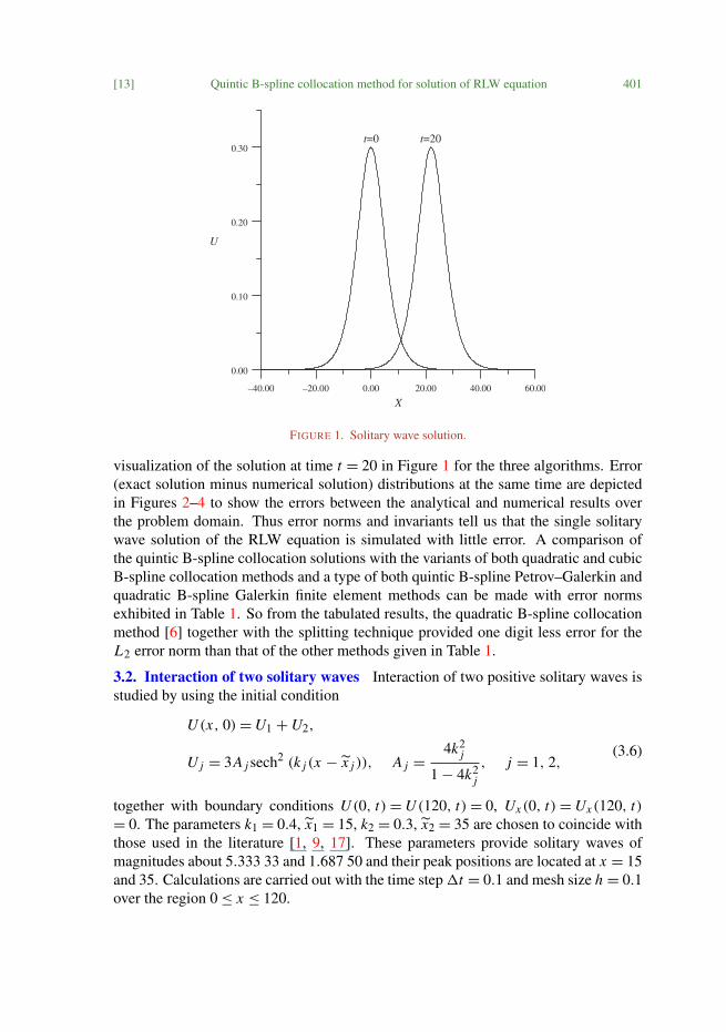
FIGURE 1. Solitary wave solution.

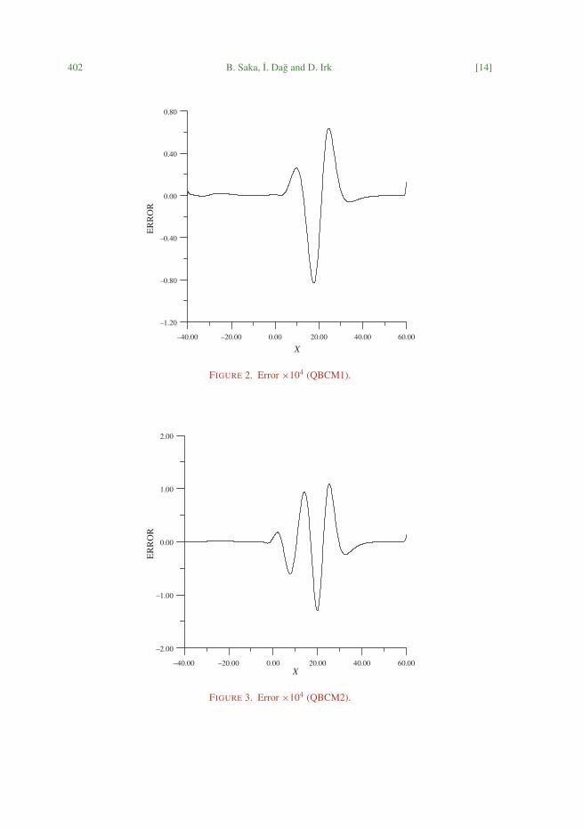
visualization of the solution at time t = 20 in Figure 1 for the three algorithms. Error(exact solution minus numerical solution) distributions at the same time are depictedin Figures 2–4 to show the errors between the analytical and numerical results overthe problem domain. Thus error norms and invariants tell us that the single solitarywave solution of the RLW equation is simulated with little error. A comparison ofthe quintic B-spline collocation solutions with the variants of both quadratic and cubicB-spline collocation methods and a type of both quintic B-spline Petrov–Galerkin andquadratic B-spline Galerkin finite element methods can be made with error normsexhibited in Table 1. So from the tabulated results, the quadratic B-spline collocationmethod [6] together with the splitting technique provided one digit less error for theL2 error norm than that of the other methods given in Table 1.

3.2. Interaction of two solitary waves Interaction of two positive solitary waves isstudied by using the initial condition

U (x, 0) = U1 + U2,

U j = 3A j sech2 (k j (x − x j )), A j =4k2

j

1 − 4k2j

, j = 1, 2,(3.6)

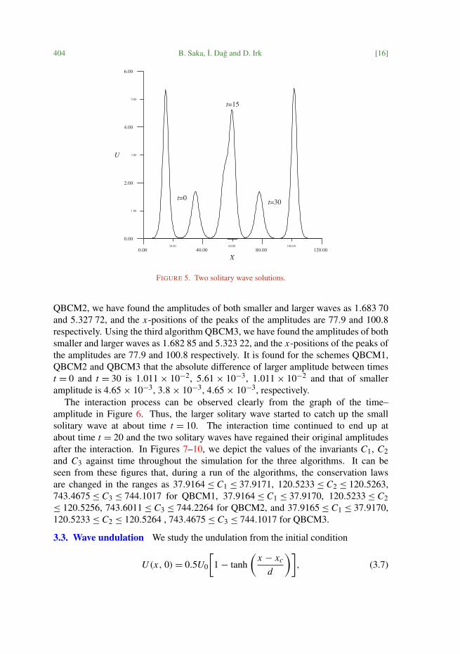
together with boundary conditions U (0, t) = U (120, t) = 0, Ux (0, t) = Ux (120, t)= 0. The parameters k1 = 0.4, x1 = 15, k2 = 0.3, x2 = 35 are chosen to coincide withthose used in the literature [1, 9, 17]. These parameters provide solitary waves ofmagnitudes about 5.333 33 and 1.687 50 and their peak positions are located at x = 15and 35. Calculations are carried out with the time step 1t = 0.1 and mesh size h = 0.1over the region 0 ≤ x ≤ 120.

402 B. Saka, I. Dag and D. Irk [14]

–40.00 –20.00 0.00 20.00 40.00 60.00

X

0.

0.40

800.

ER

RO

R

–0.80

–0.40

00

–1.20

FIGURE 2. Error ×104 (QBCM1).

–40.00 –20.00 0.00 20.00 40.00 60.00X

0.

1.00

002.

ER

RO

R

–1.00

00

–2.00

FIGURE 3. Error ×104 (QBCM2).

[15] Quintic B-spline collocation method for solution of RLW equation 403

–40.00 –20.00 0.00 20.00 40.00 60.00X

0.

0.40

0.80

ER

RO

R00

–1.20

–0.80

–0.40

FIGURE 4. Error ×104 (QBCM3).

TABLE 1. Invariants and error norms for a single solitary wave at time t = 20: amplitude = 0.3.

L2 × 104 L∞ × 104 C1 C2 C3

0.0 0.0 3.979 927 1 0.810 462 5 2.579 007 5 (t = 0)2.151 92 0.829 51 3.979 879 8 0.810 462 5 2.579 007 5 (QBCM1)3.566 72 1.296 82 3.979 884 3 0.810 462 5 2.579 007 4 (QBCM2)2.151 92 0.829 51 3.979 879 8 0.810 462 5 2.579 007 5 (QBCM3)3.01 1.14 3.979 96 0.810 276 2.578 39 (cub. met. [13])1.92 0.73 3.979 89 0.810 46 2.579 01 (quad. gal. [21])2.205 0 0.844 8 3.980 016 0.810 462 4 2.579 006 (CBSCM2 [6])2.608 6 1.029 9 3.979 958 0.810 459 6 2.578 999 (CBSCM1 [6])0.431 5 0.132 1 3.979 890 0.810 462 5 2.578 999 (QBSCM [6])3.784 1 1.399 3 3.979 95 0.810 46 2.579 00 (cub. met. [20])2.2 0.86 3.979 89 0.810 467 2.579 02 (quad. gal. (h = 0.1) [12])2.38 0.87 3.979 95 0.810 459 2.579 00 (quin. met. (h = 0.2) [11])

The initial solitary waves with given parameters are shown in Figure 5. Thesesolitary waves are propagated to the right with velocities that depend upon theirmagnitudes and have reached a stage where the larger wave has passed through thesmaller solitary wave and emerged with their original positions. The shapes of bothwaves are graphed during the interaction period at time t = 15 and after the interactionat time t = 30 in Figure 5 for the three schemes. For QBCM1, at time t = 30, thesmaller solitary wave of amplitude 1.682 85, whose peak is located at x = 77.9, isrecorded and the larger solitary wave of amplitude 5.323 22 is obtained, the peakposition of which is located at x = 100.8. At the same time, using the second algorithm

404 B. Saka, I. Dag and D. Irk [16]

U

X

t=15

t=0t=30

FIGURE 5. Two solitary wave solutions.

QBCM2, we have found the amplitudes of both smaller and larger waves as 1.683 70and 5.327 72, and the x-positions of the peaks of the amplitudes are 77.9 and 100.8respectively. Using the third algorithm QBCM3, we have found the amplitudes of bothsmaller and larger waves as 1.682 85 and 5.323 22, and the x-positions of the peaks ofthe amplitudes are 77.9 and 100.8 respectively. It is found for the schemes QBCM1,QBCM2 and QBCM3 that the absolute difference of larger amplitude between timest = 0 and t = 30 is 1.011 × 10−2, 5.61 × 10−3, 1.011 × 10−2 and that of smalleramplitude is 4.65 × 10−3, 3.8 × 10−3, 4.65 × 10−3, respectively.

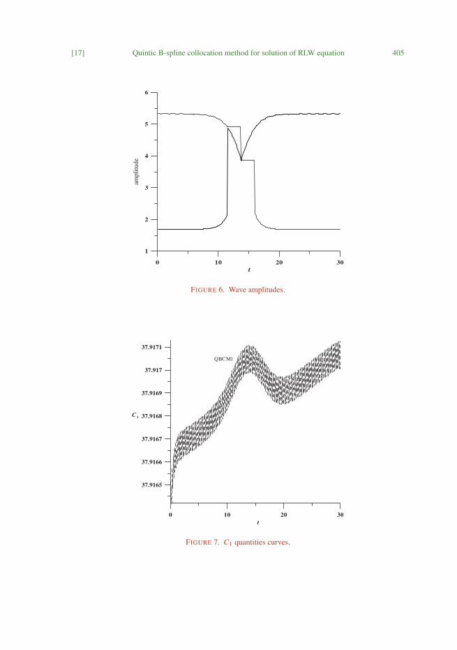
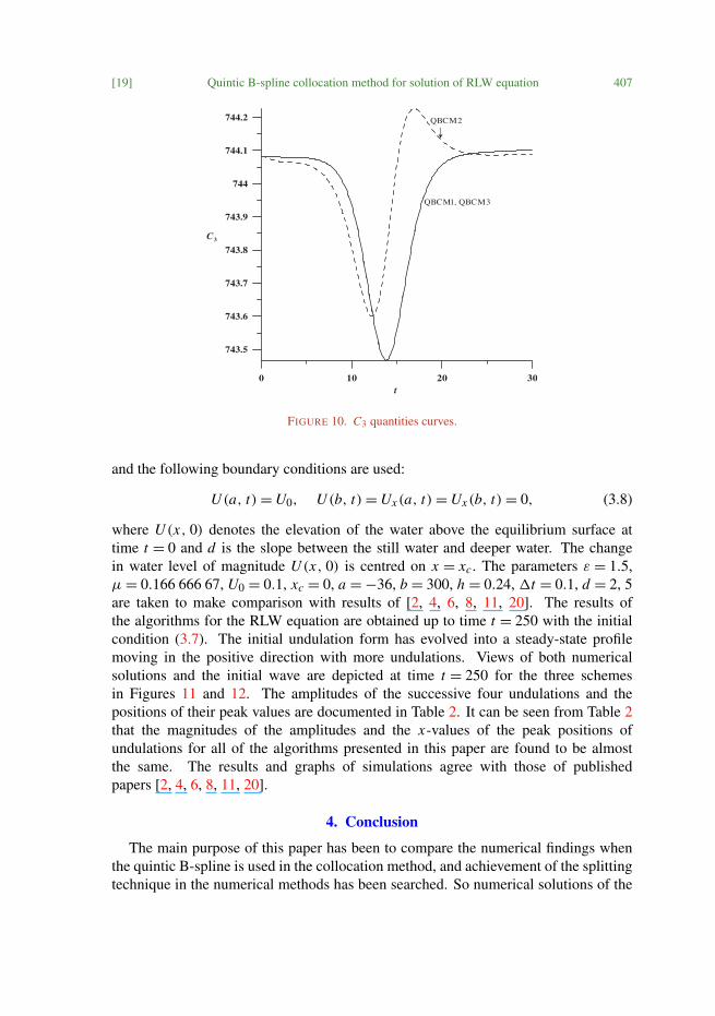
The interaction process can be observed clearly from the graph of the time–amplitude in Figure 6. Thus, the larger solitary wave started to catch up the smallsolitary wave at about time t = 10. The interaction time continued to end up atabout time t = 20 and the two solitary waves have regained their original amplitudesafter the interaction. In Figures 7–10, we depict the values of the invariants C1, C2and C3 against time throughout the simulation for the three algorithms. It can beseen from these figures that, during a run of the algorithms, the conservation lawsare changed in the ranges as 37.9164 ≤ C1 ≤ 37.9171, 120.5233 ≤ C2 ≤ 120.5263,743.4675 ≤ C3 ≤ 744.1017 for QBCM1, 37.9164 ≤ C1 ≤ 37.9170, 120.5233 ≤ C2≤ 120.5256, 743.6011 ≤ C3 ≤ 744.2264 for QBCM2, and 37.9165 ≤ C1 ≤ 37.9170,120.5233 ≤ C2 ≤ 120.5264 , 743.4675 ≤ C3 ≤ 744.1017 for QBCM3.

3.3. Wave undulation We study the undulation from the initial condition

U (x, 0) = 0.5U0

[1 − tanh

(x − xc

d

)], (3.7)

[17] Quintic B-spline collocation method for solution of RLW equation 405

0 10 20 30

2

3

4

5

t

1

6

ampl

itude

FIGURE 6. Wave amplitudes.

0 10 20 30

37.9165

37.9166

37.9167

37.9168

37.9169

37.917

37.9171

t

C1

QBCM1

FIGURE 7. C1 quantities curves.

406 B. Saka, I. Dag and D. Irk [18]

0 10 20 30

37.9165

37.9166

37.9167

37.9168

37.9169

37.917

37.9171

t

C1

QBCM2

QBCM3

FIGURE 8. C1 quantities curves.

0 10 20 30

120.5235

120.524

120.5245

120.525

120.5255

120.526

t

C2

QBCM2

QBCM1, QBCM3

FIGURE 9. C2 quantities curves.

[19] Quintic B-spline collocation method for solution of RLW equation 407

0 10 20 30

743.5

743.6

743.7

743.8

743.9

744

744.1

744.2

t

C3

QBCM1, QBCM3

QBCM2

FIGURE 10. C3 quantities curves.

and the following boundary conditions are used:

U (a, t) = U0, U (b, t) = Ux (a, t) = Ux (b, t) = 0, (3.8)

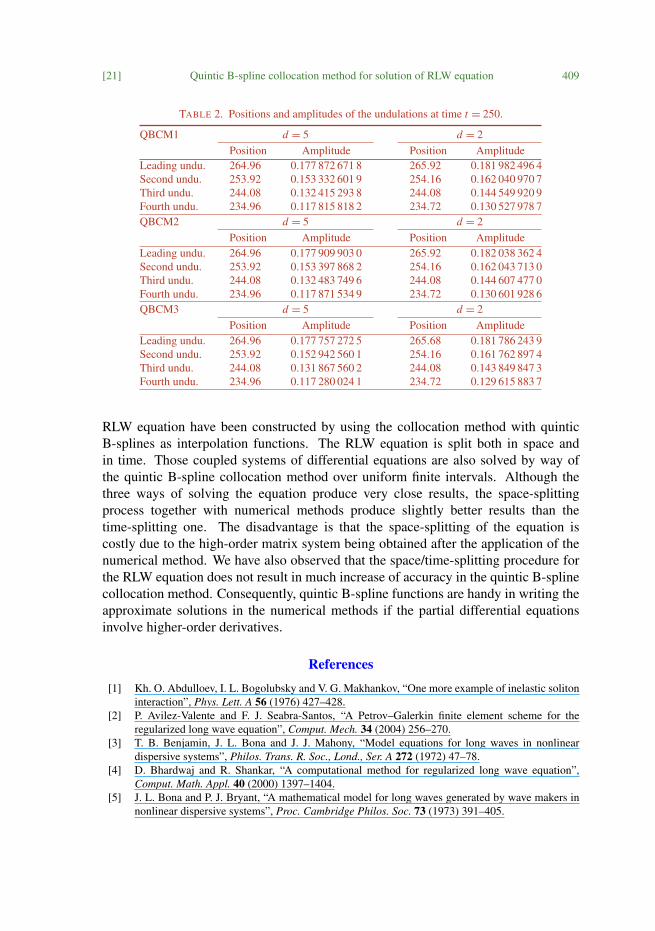
where U (x, 0) denotes the elevation of the water above the equilibrium surface attime t = 0 and d is the slope between the still water and deeper water. The changein water level of magnitude U (x, 0) is centred on x = xc. The parameters ε = 1.5,µ = 0.166 666 67, U0 = 0.1, xc = 0, a = −36, b = 300, h = 0.24, 1t = 0.1, d = 2, 5are taken to make comparison with results of [2, 4, 6, 8, 11, 20]. The results ofthe algorithms for the RLW equation are obtained up to time t = 250 with the initialcondition (3.7). The initial undulation form has evolved into a steady-state profilemoving in the positive direction with more undulations. Views of both numericalsolutions and the initial wave are depicted at time t = 250 for the three schemesin Figures 11 and 12. The amplitudes of the successive four undulations and thepositions of their peak values are documented in Table 2. It can be seen from Table 2that the magnitudes of the amplitudes and the x-values of the peak positions ofundulations for all of the algorithms presented in this paper are found to be almostthe same. The results and graphs of simulations agree with those of publishedpapers [2, 4, 6, 8, 11, 20].

4. Conclusion

The main purpose of this paper has been to compare the numerical findings whenthe quintic B-spline is used in the collocation method, and achievement of the splittingtechnique in the numerical methods has been searched. So numerical solutions of the

408 B. Saka, I. Dag and D. Irk [20]

U

X

t=0 t=250

FIGURE 11. Results for d = 5.

U

X

t=0 t=250

FIGURE 12. Results for d = 2.

[21] Quintic B-spline collocation method for solution of RLW equation 409

TABLE 2. Positions and amplitudes of the undulations at time t = 250.

QBCM1 d = 5 d = 2Position Amplitude Position Amplitude

Leading undu. 264.96 0.177 872 671 8 265.92 0.181 982 496 4Second undu. 253.92 0.153 332 601 9 254.16 0.162 040 970 7Third undu. 244.08 0.132 415 293 8 244.08 0.144 549 920 9Fourth undu. 234.96 0.117 815 818 2 234.72 0.130 527 978 7QBCM2 d = 5 d = 2

Position Amplitude Position AmplitudeLeading undu. 264.96 0.177 909 903 0 265.92 0.182 038 362 4Second undu. 253.92 0.153 397 868 2 254.16 0.162 043 713 0Third undu. 244.08 0.132 483 749 6 244.08 0.144 607 477 0Fourth undu. 234.96 0.117 871 534 9 234.72 0.130 601 928 6QBCM3 d = 5 d = 2

Position Amplitude Position AmplitudeLeading undu. 264.96 0.177 757 272 5 265.68 0.181 786 243 9Second undu. 253.92 0.152 942 560 1 254.16 0.161 762 897 4Third undu. 244.08 0.131 867 560 2 244.08 0.143 849 847 3Fourth undu. 234.96 0.117 280 024 1 234.72 0.129 615 883 7

RLW equation have been constructed by using the collocation method with quinticB-splines as interpolation functions. The RLW equation is split both in space andin time. Those coupled systems of differential equations are also solved by way ofthe quintic B-spline collocation method over uniform finite intervals. Although thethree ways of solving the equation produce very close results, the space-splittingprocess together with numerical methods produce slightly better results than thetime-splitting one. The disadvantage is that the space-splitting of the equation iscostly due to the high-order matrix system being obtained after the application of thenumerical method. We have also observed that the space/time-splitting procedure forthe RLW equation does not result in much increase of accuracy in the quintic B-splinecollocation method. Consequently, quintic B-spline functions are handy in writing theapproximate solutions in the numerical methods if the partial differential equationsinvolve higher-order derivatives.

References

[1] Kh. O. Abdulloev, I. L. Bogolubsky and V. G. Makhankov, “One more example of inelastic solitoninteraction”, Phys. Lett. A 56 (1976) 427–428.

[2] P. Avilez-Valente and F. J. Seabra-Santos, “A Petrov–Galerkin finite element scheme for theregularized long wave equation”, Comput. Mech. 34 (2004) 256–270.

[3] T. B. Benjamin, J. L. Bona and J. J. Mahony, “Model equations for long waves in nonlineardispersive systems”, Philos. Trans. R. Soc., Lond., Ser. A 272 (1972) 47–78.

[4] D. Bhardwaj and R. Shankar, “A computational method for regularized long wave equation”,Comput. Math. Appl. 40 (2000) 1397–1404.

[5] J. L. Bona and P. J. Bryant, “A mathematical model for long waves generated by wave makers innonlinear dispersive systems”, Proc. Cambridge Philos. Soc. 73 (1973) 391–405.

410 B. Saka, I. Dag and D. Irk [22]

[6] I. Dag, A. Dogan and B. Saka, “B-spline collocation methods for numerical solutions of the RLWequation”, Int. J. Comput. Math. 80 (2003) 743–757.

[7] I. Dag, B. Saka and A. Boz, “Quintic B-spline Galerkin methods for numerical solutions of theBurgers’ equation”, in Proc. Int. Conf. Dynamical Systems and Applications, Antalya, Turkey,5–10 July 2004 (Altas Conferences Inc.), 295–309.

[8] A. Esen and S. Kutluay, “Application of a lumped Galerkin method to the regularized long waveequation”, Appl. Math. Comput. 174 (2006) 833–845.

[9] L. R. T. Gardner and G. A. Gardner, “Solitary wave of the regularized long wave equation”,J. Comput. Phys. 91 (1990) 441–459.

[10] G. A. Gardner, L. R. T. Gardner and A. H. A. Ali, “Modelling solitons of the Korteweg–de Vriesequation with quintic B-splines”, U.C.N.W. Math., Preprint, 1990.

[11] L. R. T. Gardner, G. A. Gardner, F. A. Ayoub and N. K. Amein, “Modelling an undular bore withB-splines”, Comput. Methods Appl. Mech. Engrg. 147 (1997) 147–152.

[12] L. R. T. Gardner, G. A. Gardner and I. Dag, “A B-spline finite element method for the regularizedlong wave equation”, Comm. Numer. Methods Engrg. 11 (1995) 59–68.

[13] D. Irk, I. Dag and A. Dogan, “Numerical integration of the RLW equation using cubic splines”,ANZIAM J. 47 (2005) 131–142.

[14] P. J. Olver, “Euler operators and conservation laws of the BBM equation”, Math. Proc. CambridgePhilos. Soc. 85 (1979) 143–159.

[15] D. H. Peregrine, “Calculations of the development of an undular bore”, J. Fluid. Mech. 25 (1966)321–330.

[16] P. M. Prenter, Splines and variational methods (John Wiley & Sons, New York, 1975).[17] K. R. Raslan, “A computational method for the regularized long wave (RLW) equation”, Appl.

Math. Comput. 167 (2005) 1101–1118.[18] V. Rosenberg, Methods for solution of partial differential equations, Vol. 113 (Elsevier, New York,

1969).[19] B. Saka, “A finite element method for equal width equation”, Appl. Math. Comput. 175 (2006)

730–747.[20] B. Saka and I. Dag, “A collocation method for the numerical solution of the RLW equation using

cubic B-spline basis”, Arab. J. Sci. Eng. 30 (2005) 39–50.[21] B. Saka, I. Dag and A. Dogan, “Galerkin method for the numerical solution of the RLW equation

using quadratic B-splines”, Int. J. Comput. Math. 81 (2004) 727–739.[22] M. Shashkov, Conservative finite-difference methods on general grids (CRC Press, Boca Raton,

FL, 1996).[23] S. I. Zaki, “A quintic B-spline finite elements scheme for the KdVB equation”, Comput. Methods

Appl. Mech. Engrg. 188 (2000) 121–134.