Quickest Path Queries on Transportation Network

Quickest Path Queries on Transportation Network

Radwa El Shawi1, Joachim Gudmundsson1, and Christos Levcopoulos2

1 NICTA?, Sydney, Australia. radwa.elshawi,[email protected] Department of Computer Science, Lund University. [email protected]

Abstract. This paper considers the problem of finding a quickest path between two pointsin the Euclidean plane in the presence of a transportation network. A transportation networkconsists of a planar network where each road (edge) has an individual speed. A traveller mayenter and exit the network at any point on the roads. Along any road the traveller moves witha fixed speed depending on the road, and outside the network the traveller moves at unit speedin any direction.We give an exact algorithm for the basic version of the problem: given a transportation networkof total complexity n in the Euclidean plane, a source point s and a destination point t, find aquickest path between s and t. We also show how the transportation network can be preprocessedin time O(n2 logn) into a data structure of size O(n2) such that a (1 + ε)-approximate quickestpath cost queries between any two points in the plane can be answered in time O(1/ε4 logn).

1 Introduction

Transportation networks are a natural part of our infrastructure. We use bus or train in ourdaily commute, and often walk to connect between networks or to our final destination.

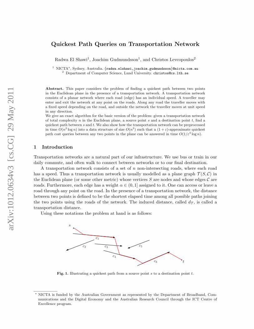
A transportation network consists of a set of n non-intersecting roads, where each roadhas a speed. Thus a transportation network is usually modelled as a plane graph T (S, C) inthe Euclidean plane (or some other metric) whose vertices S are nodes and whose edges C areroads. Furthermore, each edge has a weight α ∈ (0, 1] assigned to it. One can access or leave aroad through any point on the road. In the presence of a transportation network, the distancebetween two points is defined to be the shortest elapsed time among all possible paths joiningthe two points using the roads of the network. The induced distance, called dT , is called atransportation distance.

Using these notations the problem at hand is as follows:

s

t

c1

c2 c3

c4

c5

c6

Fig. 1. Illustrating a quickest path from a source point s to a destination point t.

? NICTA is funded by the Australian Government as represented by the Department of Broadband, Com-munications and the Digital Economy and the Australian Research Council through the ICT Centre ofExcellence program.

arX

iv:1

012.

0634

v3 [

cs.C

G]

29

May

201

1

Problem 1. Given two points s and t in R2 and a transportation network T (S, C) in theEuclidean plane. The problem is to find a path with the smallest transportation distancefrom s to t, as shown in Fig. 1.

Most of the previous research has focussed on shortest paths and Voroni diagrams. Abel-lanas et al. [1, 2] started work in this area considering the Voronoi diagram of a point setand shortest paths given a horizontal highway under the L1-metric and the Euclidean metric.Aichholzer et al. [4] introduced the city metric induced by the L1-metric and a highway net-work that consists of a number of axis-parallel line segments. They gave an efficient algorithmfor constructing the Voronoi diagram and a quickest path map for a set of points given thecity metric. Gorke et al. [14] and Bae et al. [5] improved and generalised these results.

In the case when the edges can have arbitrary orientation and speed, Bae et al. [6] presentedalgorithms that compute the Voronoi diagram and shortest paths. They gave an algorithmfor Problem 1 that uses O(n3) time and O(n2) space. This result was recently extended tomore general metrics including asymmetric convex distance functions [7].

In this paper we improve on the results by Bae et al. [6] and give an O(n2 log n) timealgorithm using O(n2) space. Furthermore, we introduce the (approximate) query version.That is, a transportation network with n roads in the Euclidean plane can be preprocessedin O(n2 log n) time into a data structure of size O(n2/ε2) such that given any two points sand t in the plane a (1 + ε)-approximate quickest path between s and t can be answered inO(1/ε4 · log n) time. For the query structure we assume that the minimum and maximumweights, αmin and αmax, are constants in the interval (0, 1] independent of n, the exact boundis stated in Theorem 8.

This paper is organized as follows. Next we prove three fundamental properties about anoptimal path among a set of roads. Then, in Section 3, we show how we can use these propertiesto build a graph of size O(n2) that models the transportation network, a source point s, adestination point t and, contains a quickest path between s and t. In Section 4 we considerthe query version of the problem. That is, preprocess the input such that an approximatequickest path query between two query points s and t can be answered efficiently. Finally, weconclude with some remarks and open problems.

2 Three Properties of an Optimal Path

In this section we are going to prove three important properties of an optimal path. Theproperties will be used repeatedly in the construction of the algorithms in Sections 3 and 4.Consider an optimal path P and let CP = 〈c1, c2, . . . , ck〉 be the sequence of roads that areencountered and followed in order along P, that is, the sequence of roads on which the pathchanges direction. For example, in Fig. 1 that sequence would be 〈c1, c4, c6〉 but not includec3 since the path does not follow c3. For any path P1, let wt(P1) denote the cost of the pathP1. Note that a road can be encountered, and followed, several times by a path. For eachroad ci ∈ CP let si and ti be the first and last point on ci encountered for each occasion by P.Without loss of generality, we assume that ti+1 lies below si when studying two consecutiveroads in CP . We have:

Property 1. For any two consecutive roads ci and ci+1 in CP the subpath of P between ti andsi+1 is the straight line segment (ti, si+1).

The endpoints of a road cj = (uj , vj) are denoted start point (uj) and end point (vj), asthey appear along the road direction.

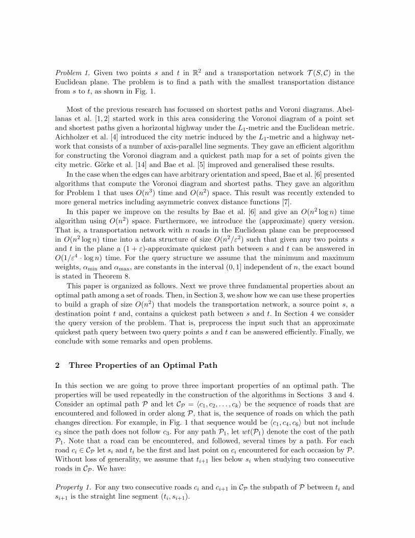
Consider a segment (ti, si+1) connecting two consecutive roads ci and ci+1 along CP . Letφi+1 denote the angle ∠(ti, si+1, ui+1), as illustrated in Fig. 2(a).

Property 2. If si+1 lies in the interior of ci+1 then φi+1 = arccos(αi+1).

Proof. For simplicity rotate C such that ci+1 is horizontal and lies below ti, as shown inFig. 2(a). Let r denote the orthogonal projection of ti onto the ray containing ci+1 (notnecessarily on ci+1 and let h = |tir|. We have:

|tisi+1| =h

sinφi+1and |rsi+1| = h · cosφi+1

sinφi+1.

Thus, the cost of the path from ti to ti+1 along CP as a function of φi+1 is:

f(φi+1) = |tisi+1|+ αi+1 · |si+1ti+1| =h

sinφi+1+ αi+1 · (|rti+1| − h ·

cosφi+1

sinφi+1).

Differentiating the above function with respect to φi+1 gives:

f ′(φi+1) =h(cosφi+1 − αi+1)

cos2 φi+1 − 1.

Setting f ′(φi+1) = 0 the resulting function gives that the minimum weight path between tiand ti+1 along C(P) is obtained when

φi+1 = arccos(αi+1).

Property 3. There exists an optimal path P ′ of total cost wt(P) with CP ′ = CP that fulfillsProperties 1-2 such that for any two consecutive roads ci and ci+1 in CP ′ the straight-linesegment (ti, si+1) of P ′ must have an endpoint at an endpoint of ci or ci+1, respectively.

Proof. Assume the opposite, i.e., (ti, si+1) does not coincide with any of the endpoints of ci orci+1. Consider the three segment path from si to ti+1, that is, (si, ti), (ti, si+1) and (si+1, ti+1).The length of this path is:

αi · |si, ti|+ |ti, si+1|+ αi+1 · |si+1, ti+1|.

According to Lemma 2 the orientation of (ti, si+1) is fixed, which implies that the weight ofthe path is a linear function only depending on the position of ti (or si+1). Hence, moving ti inone direction will monotonically increase the weight of the path until one of two cases occur:(1) either ti or si+1 encounters an endpoint of ci or ci+1, or (2) ti = si or si+1 = ti+1. If (1)then we have a contradiction since we assumed (ti, si+1) did not coincide with any endpoint.And if (2) then we have a contradiction since P must follow both ci and ci+1 (again from thedefinition of CP).

r

ti

si+1

h

φi+1

θ

ti+1

(a) (b) (c)

φi

p

ci

p

ci φi

PRf (p, ci) PRb(p, ci)ui

viui+1

Fig. 2. (a) Illustrating Property 2. (b) Defining PRf (s, ci) and (c) PRb(t, ci).

3 The basic case

In this section we consider Problem 1, that is, as input we are given a source point s, adestination point t and a transportation network T (S, C) and the aim is to find a path withminimum transportation distance from s to t. Our algorithm will construct a graph G thatmodels the set C of roads and quickest paths between the roads. Using the three propertiesshown in the previous section we will show that if a shortest path in G between s and t hascost W then an optimal path between s and t has cost W . The optimal path can then befound by running Dijkstra’s algorithm [13] on G.

Fix an optimal path P that fulfills Properties 1-3 (we know such a path exists). If Pfollows ci and ci+1 then the path between ci and ci+1 (a) is a straight line segment, (b) thesegment (ti, si+1) forms a fixed angle with ci+1, and (c) at least one of its endpoints coincideswith an endpoint of ci or ci+1. These three properties suggest that P has a very restrictedstructure which we will try to take advantage of.

Let PRf (p, ci) be the projection of a point p onto a road ci, if it exists, such that the angle∠(p, PRf (p, ci), ui) is φi, as shown in Fig. 2(b). Furthermore, let PRb(p, ci) be the projectionof point p on a road ci, if it exists, such that the angle ∠(p, PRb(p, ci), vi) is φi, as shown inFig. 2(c).

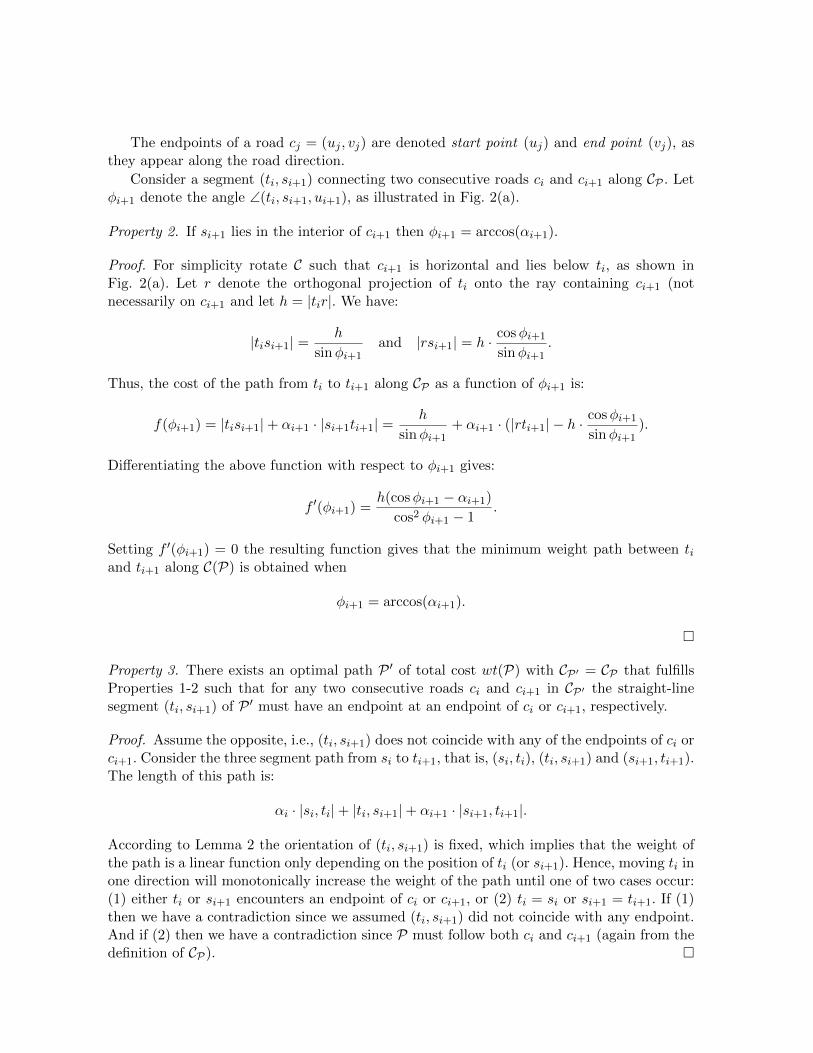
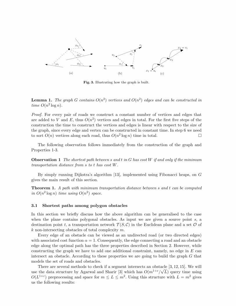
Consider the graph G(V,E) with vertex set V and edge set E. Initially V and E areempty. The graph G is defined as follows:

1. Add s and t as vertices to V .2. Add the nodes in S as vertices to V .3. For every road ci ∈ C add the point PRf (s, ci) (if it exists) as a vertex to V and add the

directed edge (s, PRf (s, ci)) (if it exists) with weight |sPRf (s, ci)| to E, see Fig. 3(a).4. For every road ci ∈ C add the point PRb(t, ci) (if it exists) as a vertex to V and add the

directed edge (PRb(s, ci), t) (if it exists) with weight |PRb(s, ci)t| to E.5. For every pair of roads ci, cj ∈ C add the following points (if they exist) as vertices toV : PRf (vi, cj), PRf (ui, cj), PRf (uj , ci) and PRf (vj , ci). Add the following four directededges to E (if their endpoints exist): (vi, PRf (vi, cj)), (ui, PRf (ui, cj)), (vj , PRf (vj , ci))and (uj , PRf (uj , ci)). The weight of an edge is equal to the Euclidean distance betweenits endpoints, see Fig. 3(b).

6. For every pair of roads ci, cj ∈ C add the directed edges (vi, uj) with weight |viuj | and(vj , ui) with weight |vjui| to E.

7. For every road ci consider the vertices of V that correspond to points on ci in order fromui to vi. For every consecutive pair of vertices xj , xj+1 along ci add a directed edge fromxj to xj+1 of weight αi · |xjxj+1|, as shown in Fig. 3(c).

φ1φ2

φ3

φ4

(a) (b) (c)

ui

uj

vj

vi

φi

φj

x1 = ui

x2

x3

x4 = vi

Fig. 3. Illustrating how the graph is built.

Lemma 1. The graph G contains O(n2) vertices and O(n2) edges and can be constructed intime O(n2 log n).

Proof. For every pair of roads we construct a constant number of vertices and edges thatare added to V and E, thus O(n2) vertices and edges in total. For the first five steps of theconstruction the time to construct the vertices and edges is linear with respect to the size ofthe graph, since every edge and vertex can be constructed in constant time. In step 6 we needto sort O(n) vertices along each road, thus O(n2 log n) time in total.

The following observation follows immediately from the construction of the graph andProperties 1-3.

Observation 1 The shortest path between s and t in G has cost W if and only if the minimumtransportation distance from s to t has cost W .

By simply running Dijkstra’s algorithm [13], implemented using Fibonacci heaps, on Ggives the main result of this section.

Theorem 1. A path with minimum transportation distance between s and t can be computedin O(n2 log n) time using O(n2) space.

3.1 Shortest paths among polygon obstacles

In this section we briefly discuss how the above algorithm can be generalised to the casewhen the plane contains polygonal obstacles. As input we are given a source point s, adestination point t, a transportation network T (S, C) in the Euclidean plane and a set O ofk non-intersecting obstacles of total complexity m.

Every edge of an obstacle can be viewed as an undirected road (or two directed edges)with associated cost function α = 1. Consequently, the edge connecting a road and an obstacleedge along the optimal path has the three properties described in Section 2. However, whileconstructing the graph we have to add one additional constraint, namely, no edge in E canintersect an obstacle. According to these properties we are going to build the graph G thatmodels the set of roads and obstacles.

There are several methods to check if a segment intersects an obstacle [3, 12, 15]. We willuse the data structure by Agarwal and Sharir [3] which has O(m1+ε/

√L) query time using

O(L1+ε) preprocessing and space for m ≤ L ≤ m2. Using this structure with L = m2 givesus the following results:

Lemma 2. The graph G has size O(N2+ε) and can be constructed in time O(N2+ε), whereN = n+m.

By simply running Dijkstra’s algorithm, implemented using Fibonacci heaps, on G gives:

Theorem 2. A collision-free path with minimum transportation distance between s and tamong O can be computed in O(N2 logN) time using O(N2) space, where N = n+m.

4 Shortest Path Queries

In this section we turn our attention to the query version. That is, preprocess C such thatgiven any two points s and t in R2 find a quickest path between s and t among C effectively.We will present a data structure D that returns an approximate quickest path. That is, giventwo query points s and t, and a positive real value ε, the data structure returns a pathbetween s and t having transportation distance at most (1 + ε) times the cost of an optimalpath between s and t.

To simplify the description we will start (Sections 4.1-4.2) with the case when t is alreadyknown in advance and we are only given the start point s as a query. Then in Section 4.4 wegeneralize this to the case when both s and t are given as a query, and in Section 4.5 we showhow one can improve the preprocessing time and space requirement using the well-separatedpair decomposition.

Fix an optimal path P that fulfills Properties 1-3 (we know such a path exists), andconsider the first segment ` = (s, s1) of P. Obviously s1 must be either a start/endpoint ofa road (type 1) or an interior point of a road ci ∈ C (type 2) such that ` and ci form anangle of φi (ignoring the trivial case when s1 = t). We will use this observation to develop anapproximation algorithm. The idea is simple. Build a graph G(V,E), as described in Section 3,with T and t as input. Compute the cost of the quickest path between t and every vertex inV . Now, given a query point s, find a good vertex s1 in V to connect s (either directly or viaa 2-link path) to and then lookup the cost of the quickest path from s1 to t in G. Obviouslythe problem is how to find a “good” vertex. In the next subsection we will select a constantnumber of candidate vertices such that we can guarantee that at least one of the vertices willbe a “good” candidate, i.e., there exists a path, that fulfills Properties 1-3, from s to t viathis vertex that has cost at most (1 + ε) times the cost of an optimal path.

4.1 Finding good candidates: Type 1 and Type 2

Let SC denote the set of the endpoints (both start and end) of the roads in C and let s be thequery point. As described above we will have two types to consider, and we will construct aset D1 for the type 1 cases and a set D2 for the type 2 cases. The first set, D1, is a subset of SCand the second set, D2, is a set of 3-tuples that will be used by the query process (describedin Section 4.2) to calculate the quickest path.

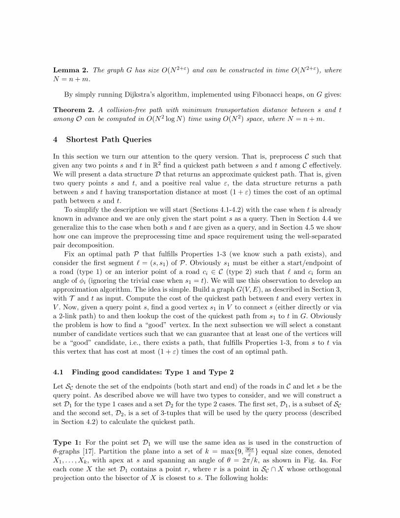
Type 1: For the point set D1 we will use the same idea as is used in the construction ofθ-graphs [17]. Partition the plane into a set of k = max9, 36πε equal size cones, denotedX1, . . . , Xk, with apex at s and spanning an angle of θ = 2π/k, as shown in Fig. 4a. Foreach cone X the set D1 contains a point r, where r is a point in SC ∩ X whose orthogonalprojection onto the bisector of X is closest to s. The following holds:

Lemma 3. Given a point set SC and a positive constant ε one can preprocess SC into a datastructure of size O(n/ε) in O(1/ε · n log n) time such that given a query point s the point setD1, of size at most 36π/ε, can be reported in O(1/ε · log n) time.

Proof. Given a direction d and a point s let `d(s) denote the infinite ray originating at swith direction d, see Fig. 4b. Let C(s, d, θ) be the cone with apex at s, bisector `d(s) andangle θ. It has been shown (see for example Section 4.1.2 in [17] or Lemma 2 in [10]) that SCcan be preprocessed in O(n log n) time into a data structure of size O(n) such that given aquery point s in the plane the data structure returns the point in C(s, d, θ) whose orthogonalprojection onto `d(s) is closest to s in O(log n) time. We have 36π/ε directions, thus thelemma follows.

sθ

p

pi

`d(s)s p′i

p′

C(s, d, θ)

Fig. 4. (a) Partitioning the plane into k cones. (b) Selecting the point whose orthogonal projection onto thebisector of X.

Type 2: It remains to construct the set D2 of 3-tuples. Unfortunately the constructionmight look unnecessarily complicated but hopefully it will become clear, when we prove theapproximation bound (Section 4.3) why we need this construction. Before constructing D2 weneed some basic definitions.

Let αmax and αmin be the maximum and minimum weight of the roads in C. Partition theset C of roads into a minimum number of sets, C1, . . . , Cm, such that the orientation of a roadin Ci is in [(i− 1)θ · αmin, iθ · αmin), where θ = ε/18. Partition each set Ci, 1 ≤ i ≤ m, into bsets Ci,1, . . . , Ci,b such that the weight of a road in Ci,j is in [αmin · (1 + ε)j−1, αmin · (1 + ε)j).

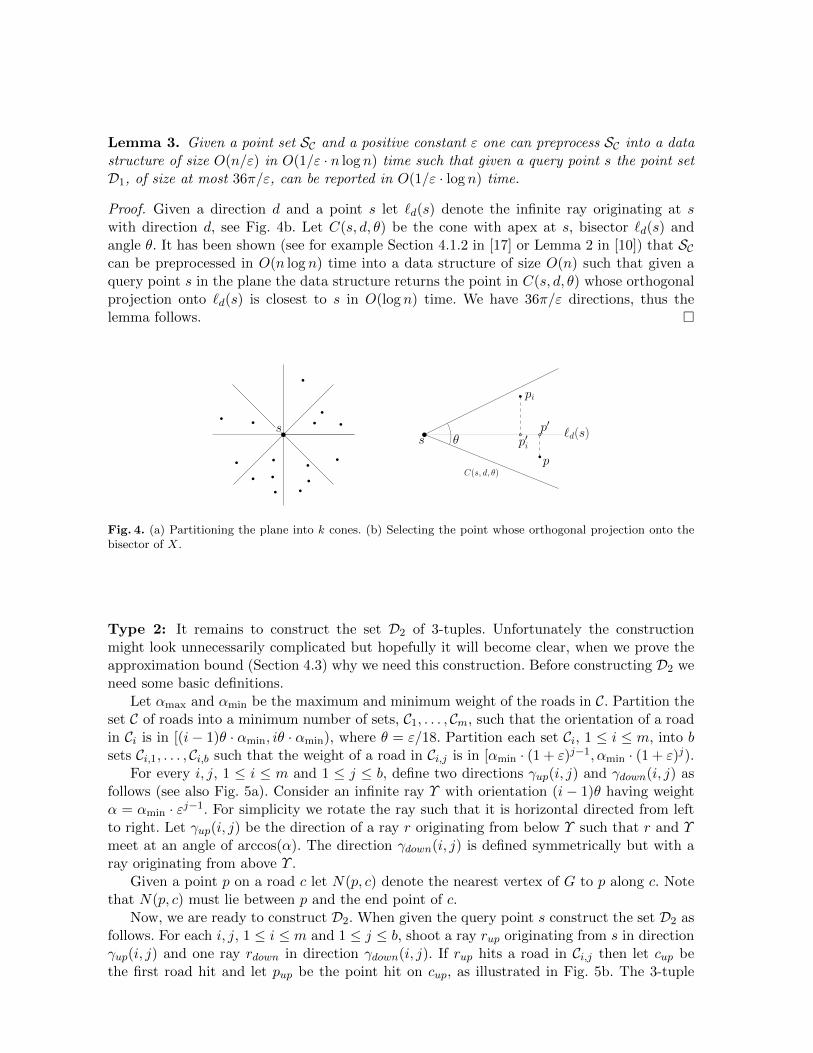
For every i, j, 1 ≤ i ≤ m and 1 ≤ j ≤ b, define two directions γup(i, j) and γdown(i, j) asfollows (see also Fig. 5a). Consider an infinite ray Υ with orientation (i − 1)θ having weightα = αmin · εj−1. For simplicity we rotate the ray such that it is horizontal directed from leftto right. Let γup(i, j) be the direction of a ray r originating from below Υ such that r and Υmeet at an angle of arccos(α). The direction γdown(i, j) is defined symmetrically but with aray originating from above Υ .

Given a point p on a road c let N(p, c) denote the nearest vertex of G to p along c. Notethat N(p, c) must lie between p and the end point of c.

Now, we are ready to construct D2. When given the query point s construct the set D2 asfollows. For each i, j, 1 ≤ i ≤ m and 1 ≤ j ≤ b, shoot a ray rup originating from s in directionγup(i, j) and one ray rdown in direction γdown(i, j). If rup hits a road in Ci,j then let cup bethe first road hit and let pup be the point hit on cup, as illustrated in Fig. 5b. The 3-tuple

[cup, pup, N(pup, cup)] is added to D2. If rdown hits a road in Ci,j then let cdown be the firstroad hit and let pdown be the point hit on cdown. The 3-tuple [cdown, pdown, N(pdown, cdown)] isadded to D2.

Lemma 4. Given a transportation network T (S, C) with n roads in the Euclidean plane anda positive constant ε one can preprocess T in O(n log n) time into a data structure of sizeO(n) such that given a query point s the set D2 can be reported in O( 1

αmin·ε2 · log n log1+εαmaxαmin

)

time. The number of 3-tuples in D2 is O( 1αminε2

· log1+εαmaxαmin

).

Proof. The preprocessing consists of two steps: (1) partitioning C into the sets Ci,j , 1 ≤ i ≤ mand 1 ≤ j ≤ b, and (2) preprocessing each set Ci,j into a data structure that answers rayshooting queries efficiently.

The first part is easily done in O(n log n) time by sorting the roads first with respect totheir orientation and then with respect to their weight.

The second step of the preprocessing can be done by building two trapezoidal mapsTup(Ci,j) and Tdown(Ci,j) (also know as a vertical decomposition) of each set Ci,j as follows(see Fig. 5c). Rotate Ci,j such that γup(i, j) is vertical and upward. Build a trapezoidal mapTup(Ci,j) of Ci,j as described in Chapter 6.1 in [8]. Then preprocess Tup(Ci,j) to allow for planarpoint location. Note that every face in T (C) either is a triangle or a trapezoid, and the leftand right edges of each face (if they exists) are vertical. The trapezoidal map Tdown(Ci,j) canbe computed in the same way by rotating Ci,j such that γdown(i, j) is vertical and upward.The total time needed for this step is O(n log n) and it requires O(n) space.

When a query point s is given, two ray shooting queries are performed for each set Ci,j .However, instead we perform a point location in the trapezoidal maps Tup(Ci,j) and Tdown(Ci,j).Consider Tup(Ci,j) and let f be the face in the map containing s. The top edge of f correspondsto the first road cup hit by a ray emanating from s in direction γup(i, j). When cup is found wejust add to D2 the first vertex on cup in G to the right of s. The same process is repeated forTdown(Ci,j). Performing the point location requires O(log n) time per trapezoidal map, thusthe total query time is O(mb log n) = O( 1

αmin·ε2 · log n log1+ε(αmax/αmin)).

(a) (c)

Υ

arccosα

arccosα

γup(i, j)

γdown(i, j)

γup(i, j)

s

(b)

s

cuppup

N(cup, pup)

Fig. 5. (a) Illustrating the definition of γup(i, j) and γdown(i, j). (b) pup is the first point hit by the ray andN(cup, pup) is the nearest neighbour of pup along cup. (c) The trapezoidal map of a set Ci,j and the querypoint s.

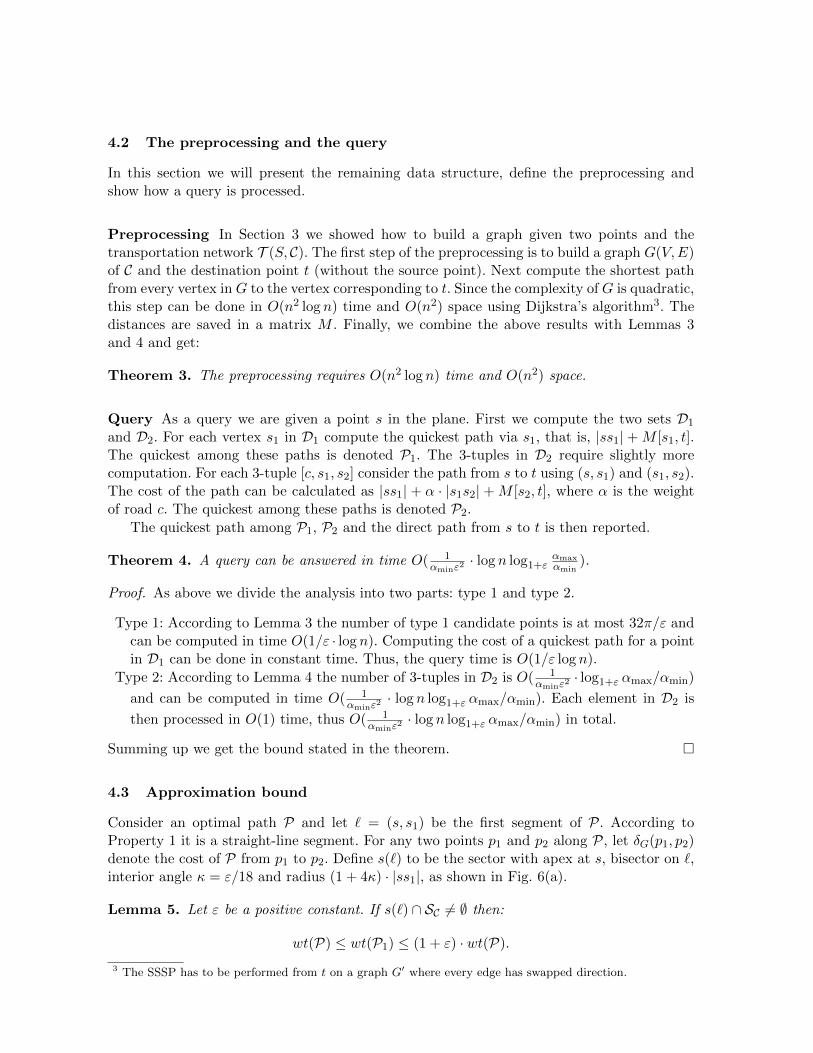
4.2 The preprocessing and the query

In this section we will present the remaining data structure, define the preprocessing andshow how a query is processed.

Preprocessing In Section 3 we showed how to build a graph given two points and thetransportation network T (S, C). The first step of the preprocessing is to build a graph G(V,E)of C and the destination point t (without the source point). Next compute the shortest pathfrom every vertex in G to the vertex corresponding to t. Since the complexity of G is quadratic,this step can be done in O(n2 log n) time and O(n2) space using Dijkstra’s algorithm3. Thedistances are saved in a matrix M . Finally, we combine the above results with Lemmas 3and 4 and get:

Theorem 3. The preprocessing requires O(n2 log n) time and O(n2) space.

Query As a query we are given a point s in the plane. First we compute the two sets D1

and D2. For each vertex s1 in D1 compute the quickest path via s1, that is, |ss1| + M [s1, t].The quickest among these paths is denoted P1. The 3-tuples in D2 require slightly morecomputation. For each 3-tuple [c, s1, s2] consider the path from s to t using (s, s1) and (s1, s2).The cost of the path can be calculated as |ss1| + α · |s1s2| + M [s2, t], where α is the weightof road c. The quickest among these paths is denoted P2.

The quickest path among P1, P2 and the direct path from s to t is then reported.

Theorem 4. A query can be answered in time O( 1αminε2

· log n log1+εαmaxαmin

).

Proof. As above we divide the analysis into two parts: type 1 and type 2.

Type 1: According to Lemma 3 the number of type 1 candidate points is at most 32π/ε andcan be computed in time O(1/ε · log n). Computing the cost of a quickest path for a pointin D1 can be done in constant time. Thus, the query time is O(1/ε log n).

Type 2: According to Lemma 4 the number of 3-tuples in D2 is O( 1αminε2

· log1+ε αmax/αmin)

and can be computed in time O( 1αminε2

· log n log1+ε αmax/αmin). Each element in D2 is

then processed in O(1) time, thus O( 1αminε2

· log n log1+ε αmax/αmin) in total.

Summing up we get the bound stated in the theorem.

4.3 Approximation bound

Consider an optimal path P and let ` = (s, s1) be the first segment of P. According toProperty 1 it is a straight-line segment. For any two points p1 and p2 along P, let δG(p1, p2)denote the cost of P from p1 to p2. Define s(`) to be the sector with apex at s, bisector on `,interior angle κ = ε/18 and radius (1 + 4κ) · |ss1|, as shown in Fig. 6(a).

Lemma 5. Let ε be a positive constant. If s(`) ∩ SC 6= ∅ then:

wt(P) ≤ wt(P1) ≤ (1 + ε) · wt(P).

3 The SSSP has to be performed from t on a graph G′ where every edge has swapped direction.

Proof. The proof will be shown in two steps: (1) first we prove that for every endpoint pwithin s(`) the quickest path, denoted P(p), from s to t using the segment (s, p) has cost atmost (1+12κ) ·wt(P), and then (2) we prove that wt(P1) has cost at most (1+3κ) ·wt(P(p)).Combining the two parts proves the lemma.

Part 1: Consider any point p within s(`), and let P(p) denote the quickest path from s tot using the segment (s, p). We have:

wt(P(p)) = |sp|+ δG(p, t)

≤ |sp|+ |ps1|+ δG(s1, t)

≤ (1 + 4κ) · |ss1|+√

(cosκ

2− 1− 4κ)2 + sin2 κ

2· |ss1|+ δG(s1, t)

< (1 + 12κ) · |ss1|+ δG(s1, t)

≤ (1 + 12κ) · δG(s, t)

Part 2: As above let p be any endpoint of C within s(`), and let P(p) be the quickest pathfrom s to t using the segment |sp|.

Consider the set D1 as described in Section 4.1 and assume without loss of generality thatp lies in a cone X. If there exists a point q in D1 such that q = p then we are done since|sq|+ δG(q, t) = wt(P(p)).

Otherwise, there must exist another point q in D1 such that q ∈ X and whose orthogonalprojection q′ onto the bisector of X is closer to s than the orthogonal projection p′ of p ontothe bisector of X.

wt(P(q)) ≤ |sq|+ |qp|+ δG(p, t)

≤ |sq|+ |qq′|+ |q′p′|+ |p′p|+ δG(p, t)

≤ |sq′|( 1

cosκ+

sinκ

cosκ) + |q′p′|+ |sp| · sinκ+ δG(p, t)

< (|sq′|+ |q′p′|)( 1

cosκ+

sinκ

cosκ) + |sp| · sinκ+ δG(p, t)

≤ |sp|( 1

cosκ+

sinκ

cosκ+ sinκ) + δG(p, t)

<|sp|cosκ

(1 + 2 sinκ) + δG(p, t)

< |sp| · (1 + 3 cotκ) + δG(p, t)

< (1 + 3κ) · wt(P(p))

In the last step we used that κ = ε/18 < 2π/9.

Now we can combine the two results as follows.

wt(P1) ≤ wt(P(q))

≤ (1 + 12κ) · δG(p, t) (from Part 1)

≤ (1 + 3κ) · (1 + 12κ) · δG(s, t) (from Part 2)

< (1 + ε) · δG(s, t) (since κ = ε/18 and ε < 1)

This completes the proof of the lemma.

`

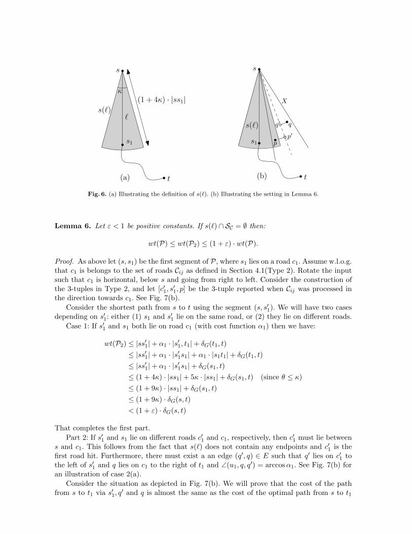
s

s1

t

s(`)

κ(1 + 4κ) · |ss1|

(a)

s

s1

t

s(`)

(b)

p

q

p′

q′

X

Fig. 6. (a) Illustrating the definition of s(`). (b) Illustrating the setting in Lemma 6.

Lemma 6. Let ε < 1 be positive constants. If s(`) ∩ SC = ∅ then:

wt(P) ≤ wt(P2) ≤ (1 + ε) · wt(P).

Proof. As above let (s, s1) be the first segment of P, where s1 lies on a road c1. Assume w.l.o.g.that c1 is belongs to the set of roads Cij as defined in Section 4.1(Type 2). Rotate the inputsuch that c1 is horizontal, below s and going from right to left. Consider the construction ofthe 3-tuples in Type 2, and let [c′1, s

′1, p] be the 3-tuple reported when Cij was processed in

the direction towards c1. See Fig. 7(b).

Consider the shortest path from s to t using the segment (s, s′1). We will have two casesdepending on s′1: either (1) s1 and s′1 lie on the same road, or (2) they lie on different roads.

Case 1: If s′1 and s1 both lie on road c1 (with cost function α1) then we have:

wt(P2) ≤ |ss′1|+ α1 · |s′1, t1|+ δG(t1, t)

≤ |ss′1|+ α1 · |s′1s1|+ α1 · |s1t1|+ δG(t1, t)

≤ |ss′1|+ α1 · |s′1s1|+ δG(s1, t)

≤ (1 + 4κ) · |ss1|+ 5κ · |ss1|+ δG(s1, t) (since θ ≤ κ)

≤ (1 + 9κ) · |ss1|+ δG(s1, t)

≤ (1 + 9κ) · δG(s, t)

< (1 + ε) · δG(s, t)

That completes the first part.

Part 2: If s′1 and s1 lie on different roads c′1 and c1, respectively, then c′1 must lie betweens and c1. This follows from the fact that s(`) does not contain any endpoints and c′1 is thefirst road hit. Furthermore, there must exist a an edge (q′, q) ∈ E such that q′ lies on c′1 tothe left of s′1 and q lies on c1 to the right of t1 and ∠(u1, q, q

′) = arccosα1. See Fig. 7(b) foran illustration of case 2(a).

Consider the situation as depicted in Fig. 7(b). We will prove that the cost of the pathfrom s to t1 via s′1, q

′ and q is almost the same as the cost of the optimal path from s to t1

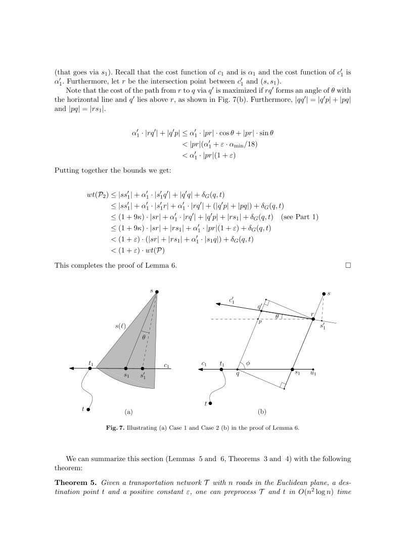
(that goes via s1). Recall that the cost function of c1 and is α1 and the cost function of c′1 isα′1. Furthermore, let r be the intersection point between c′1 and (s, s1).

Note that the cost of the path from r to q via q′ is maximized if rq′ forms an angle of θ withthe horizontal line and q′ lies above r, as shown in Fig. 7(b). Furthermore, |qq′| = |q′p|+ |pq|and |pq| = |rs1|.

α′1 · |rq′|+ |q′p| ≤ α′1 · |pr| · cos θ + |pr| · sin θ< |pr|(α′1 + ε · αmin/18)

< α′1 · |pr|(1 + ε)

Putting together the bounds we get:

wt(P2) ≤ |ss′1|+ α′1 · |s′1q′|+ |q′q|+ δG(q, t)

≤ |ss′1|+ α′1 · |s′1r|+ α′1 · |rq′|+ (|q′p|+ |pq|) + δG(q, t)

≤ (1 + 9κ) · |sr|+ α′1 · |rq′|+ |q′p|+ |rs1|+ δG(q, t) (see Part 1)

≤ (1 + 9κ) · |sr|+ |rs1|+ α′1 · |pr|(1 + ε) + δG(q, t)

< (1 + ε) · (|sr|+ |rs1|+ α′1 · |s1q|) + δG(q, t)

< (1 + ε) · wt(P)

This completes the proof of Lemma 6.

(a) (b)

s

s′1s1

t1

θ

s(`)

t

c1

s

s1

t1

t

c1

c′1

s′1

θ

q

q′

u1

φ

rp

Fig. 7. Illustrating (a) Case 1 and Case 2 (b) in the proof of Lemma 6.

We can summarize this section (Lemmas 5 and 6, Theorems 3 and 4) with the followingtheorem:

Theorem 5. Given a transportation network T with n roads in the Euclidean plane, a des-tination point t and a positive constant ε, one can preprocess T and t in O(n2 log n) time

and O(n2) space such that given a query point s, a (1 + ε)-approximate quickest path can becalculated in O( 1

αminε2· log n log1+ε

αmaxαmin

) time.

4.4 General case

In this section we turn our attention to the query version when we are given two querypoints s and t in R2 and our goal is to find a quickest path between s and t among C. Theidea is the same as in the previous section. That is we perform the exact same preprocessingsteps as in the previous section (omitting the destination point t), but with the exception thatM contains all-pair shortest distances. Using Johnson’s algorithm [16] the all-pairs shortestpaths can be computed in O(n4 log n) using O(n4) space.

Given a query we compute the two candidate sets of type 1 and type 2 for both s and t.For each pair of elements p ∈ D1(s)∪D2(s) and q ∈ D1(t)∪D2(t) compute a path between sand t as follows:

if p ∈ D1 and q ∈ D1 then |sp|+M [p, q] + |qt|if p ∈ D1 and q = [c, s1, s2] ∈ D2 then |sp|+M [p, s2] + α(c) · |s2s1|+ |s1s|if p = [c, s1, s2] ∈ D2 and q ∈ D1 then |ss1|+ α(c) · |s1s2|+M [s2, q] + |qt|if p = [c1, s1, s2] ∈ D2 and q = [c2, t1, t2] ∈ D2 then |ss1|+ α(c1) · |s1s2|+M [s2, t2] + α(c2) ·|t2t1|+ |t1t|

Note that for a specific pair p, q the calculated distance might not be a good approximationof the actual distance. However, for the shortest path there exists a pair p, q such that thedistance is a good approximation.

By putting together the results, we obtain the following theorem:

Theorem 6. Given a transportation network T with n roads in the Euclidean plane and apositive constant ε, one can preprocess T in O(n4 log n) time using O(n4) space such thatgiven two query points s and t a (1 + ε)-approximate quickest path between s and t can becalculated in O(( 1

αmin·ε2 · log1+εαmaxαmin

)2 · log n) time.

4.5 Improving the complexity using the well-separated pair decomposition

The bottleneck of the preprocessing algorithm is the fact that n4 shortest paths are computedin a graph of quadratic complexity. Is there a way to get around this? Since it suffices toapproximate the shortest paths we can reduce the number of shortest path queries from O(n4)to O(n2), that is, linear in the number of vertices, using the well-separated pair-decomposition(WSPD).

Definition 1 ([11]). Let s > 0 be a real number, and let A and B be two finite sets of pointsin Rd. We say that A and B are well-separated with respect to s, if there are two disjoint d-dimensional balls CA and CB, having the same radius, such that (i) CA contains the boundingbox R(A) of A, (i) CB contains the bounding box R(B) of B, and (ii) the minimum distancebetween CA and CB is at least s times the radius of CA.

The parameter s will be referred to as the separation constant. The next lemma followseasily from Definition 1.

Lemma 7 ([11]). Let A and B be two finite sets of points that are well-separated w.r.t. s,let x and p be points of A, and let y and q be points of B. Then (i) |xy| ≤ (1 + 4/s) · |pq|, and(ii) |px| ≤ (2/s) · |pq|.Definition 2 ([11]). Let S be a set of n points in Rd, and let s > 0 be a real number. Awell-separated pair decomposition (WSPD) for S with respect to s is a sequence of pairs ofnon-empty subsets of S, (A1, B1), . . . , (Am, Bm), such that

1. Ai ∩Bi = ∅, for all i = 1, . . . ,m,2. for any two distinct points p and q of S, there is exactly one pair (Ai, Bi) in the sequence,

such that (i) p ∈ Ai and q ∈ Bi, or (ii) q ∈ Ai and p ∈ Bi,3. Ai and Bi are well-separated w.r.t. s, for 1 ≤ i ≤ m.

The integer m is called the size of the WSPD.

Callahan and Kosaraju showed that a WSPD of size m = O(sdn) can be computed inO(sdn+ n log n) time.

Construct the graph G(V,E) of T , as defined in Section 3. Compute a WSPD (Ai, Bi)ki=1

of V with respect to a separation constant s = 8τ ·αmin

, where τ < 1 is a positive constantgiven as input. Then for each well-separated pair (Ai, Bi) pick two arbitrary points a ∈ Aiand b ∈ Bi as representative points, and calculate the shortest path in G between a and b.All paths are stored in a matrix M ′. According to Definition 2, we have O(n2) well separatedpairs. It follows that the number of the shortest path queries in M is O(n2).

The queries are performed in almost the same way as above. The only difference is howthe cost of the path between two points is calculated. Assume that we want the minimumtransportation distance between two query points p and q. According to Definition 2 thereexists a well-separated pair A,B such that p ∈ A and q ∈ B, or vice versa. Furthermore, letrA and rB be the representative points of A and B, respectively. Instead of using the valuein M [p, q] we approximate the cost by |prA|+M ′[rA, rB] + |rBq|.Theorem 7.

δG(p, q) ≤ |prA|+M ′[rA, rB] + |rBq| ≤ (1 + τ) · δG(p, q).

Proof. The left inequality is immediate, thus we will focus on the right inequality.

|prA|+M ′[rA, rB] + |rBq| = |prA|+ δG(rA, rB) + |rBq|≤ 2|prA|+ 2|rBq|+ δG(p, q)

≤ 4 · 2/s · |pq|+ δG(p, q)

≤ τ · αmin · |pq|+ δG(p, q)

≤ (1 + τ) · δG(p, q)

Where the last step follows by using |pq| ≤ δG(p, q)/αmin.

Given a positive constant σ < 1 we can obtain the claimed bounds by setting the constantsappropriately (for example τ = σ/3 and ε = σ/3). We get:

Theorem 8. Given a transportation network T (S, C) with n roads and a positive constant ε,one can preprocess C in O(( n

αmin·ε)2 log n) time using O(( n

αmin·ε)2) space such that given two

query points s and t a (1 + ε)-approximate quickest path between s and t can be calculated inO(( 1

αmin·ε2 · log1+εαmaxαmin

)2 · log n) time.

Assuming αmin and αmax being constants the bounds can be rewritten as: preprocessingis O(n2 log n), space is O(n2/ε2) and the query time is O(1/ε4 · log n).

5 Concluding Remarks

We considered the problem of computing a quickest path in a transportation network. In thestatic case our algorithm has a running time of O(n2 log n) which is a linear factor betterthan the best algorithm known so far. We also introduce the query version of the problem.

There are many open problems remaining. For example, can one develop a more efficientdata structure that has a smaller dependency on αmin and ε? Also, is there a subquadratictime algorithm for the static case? If not, can we prove that the problem is 3sum-hard? Baeand Chwa [6] proved that the shortest path map for a transportation metric can have Ω(n2)size, which indicates that the problem may indeed be 3sum-hard.

References

1. M. Abellanas, F. Hurtado, C. Icking, R. Klein, E. Langetepe, L. Ma, B. Palop del Rıo and V. Sacristan.Proximity problems for time metrics induced by the L1 metric and isothetic networks. In Actas de los IXEncuentros de Geometra Computacional, pages 175182, Girona, 2001.

2. M. Abellanas, F. Hurtado, C. Icking, R. Klein, E. Langetepe, L. Ma, B. Palop del Rıo and V. Sacristan.Voronoi diagram for services neighboring a highway. Information Processessing Letters, 86:283-288, 2003.

3. P. K. Agarwal and M. Sharir. Applications of a new space partitioning technique. Discrete & Computa-tional Geometry, 9:11–38, 1993.

4. O. Aichholzer, F. Aurenhammer and B. Palop del Rıo. Quickest paths, straight skeletons, and the cityVoronoi diagram. Discrete & Computatational Geometry, 31:17-35, 2004.

5. S. W. Bae, J.-H. Kim and K.-Y. Chwa. Optimal construction of the city Voronoi diagram. InternationalJournal on Computational Geometry & Applications, 19(2):95–117, 2009.

6. S. W. Bae and K.-Y. Chwa. Voronoi Diagrams for a Transportation Network on the Euclidean Plane.International Journal on Computational Geometry & Applications, 16:117–144, 2006.

7. S. W. Bae and K.-Y. Chwa. Shortest Paths and Voronoi Diagrams with Transportation Networks UnderGeneral Distances. ISAAC, pages 1007–1018, 2005.

8. M. de Berg, O. Cheong, M. van Kreveld and M. Overmars. Computational Geometry: Algorithms andApplications. (3rd edition). Springer-Verlag, Heidelberg, 2008.

9. J. L. Bentley. Multidimensional divide-and-conquer. Communications of the ACM, 23(5):214–228, 1978.10. P. Bose, J. Gudmundsson and P. Morin. Ordered theta graphs. Computational geometry – Theory &

Applications, 28(1):11–18, 2004.11. P. B. Callahan and S. R. Kosaraju. A decomposition of multidimensional point sets with applications to

k-nearest-neighbors and n-body potential fields. Journal of the ACM, 42:67–90, 1995.12. S. W. Cheng and R. Janardan. Algorithms for ray-shooting and intersection searching. Journal of Algo-

rithms 13:670–692, 1992.13. E. W. Dijkstra. A note on two problems in connexion with graphs. Numerische Mathematik, 1:269-271,

1959.14. R. Gorke, C.-C. Shin and A. Wolff. Constructing the City Voronoi Diagram Faster. International Journal

of Computational Geometry and Applications 18(4):275–294, 2008.15. J. Hershberger and S. Suri. A pedestrian approach to ray shooting: Shoot a ray, take a walk. Journal of

Algorithms 18:403–431, 1995.16. D. B. Johnson Efficient algorithms for shortest paths in sparse networks. Journal of the ACM, 24(1):1-13,

1977.17. G. Narasimhan and M. Smid Geometric Spanner Networks. Cambridge University Press, 2007.