Queues with waiting time dependent service

Queues with waiting time dependent service

R. Bekker†, G.M. Koole†, B.F. Nielsen�, T.B. Nielsen�

†Dept. MathematicsVU University Amsterdam

De Boelelaan 1081, 1081 HV, the Netherlands.

�Dept. Informatics and Mathematical ModellingTechnical University of Denmark

Richard Petersens Plads, 2800 Kgs. Lyngby, Denmark.

Abstract

Motivated by service levels in terms of the waiting-time distribution seen in e.g. callcenters, we consider two models for systems with a service discipline that depends onthe waiting time. The first model deals with a single server that continuously adaptsits service rate based on the waiting time of the first customer in line. In the secondmodel, one queue is served by a primary server which is supplemented by a secondaryserver when the waiting of the first customer in line exceeds a threshold. Using levelcrossings for the waiting-time process of the first customer in line, we derive steady-state waiting-time distributions for both models. The results are illustrated withnumerical examples.

Keywords: Waiting-time distribution; Adaptive service rate; Call centers; Contactcenters; Queues; Deterministic threshold; Overflow; Level crossing.

1 Introduction

In service systems, the tail probability (or distribution function) of the waiting time ofcustomers is one of the main service-level indicators. For example, in call centers theservice level is generally characterized by the telephone service factor (TSF), i.e., thefraction of calls whose delay fall below a prespecified target. Typically, call centers use a80-20 TSF meaning that 80% of the calls should be taken into service within 20 seconds,see [12]. Motivated by performance measures in terms of tail probabilities of waiting times,we consider queueing systems where the service mechanism is based on waiting times ofcustomers. This type of control policy is commonly used in call centers [21], and indeedthe authors have often encountered it in various forms when working with call centers.However, the literature on it is limited. In the traditional queueing literature, routing andcontrol are commonly based on the number of customers present.The main goal of this paper is to find the steady-state waiting-time distribution for queue-ing systems where the service characteristics depend on the waiting time of the first cus-tomer in line. This type of service control seems to be new in the queueing literature,despite its widespread use in the industry. The aim of this paper is to show ways toanalyse queueing models where the service mechanism depends on the waiting time. Inthe sequel we use FIL as an abbreviation of first customer in line.

1

We consider two Markovian queueing models: (i) single-server queues with FIL waiting-time dependent service speed and (ii) a queue with two heterogeneous servers, where thesecondary server is only activated as soon as the FIL waiting time exceeds some targetlevel. For both models, the analysis is based on the waiting process of the first customerin line (FIL-process). Using level crossings, we find the steady-state distribution of theFIL-process and derive the waiting-time distribution as a corollary.First, in Section 2, we study the single-server model, where the service speed can becontinuously adapted based on the waiting time of the first customer in line. This modelis related to the study of dams and queueing systems with workload-dependent servicerates, see e.g. [4], [5], [16] or [25]. The difference is that the service speed here dependson the waiting time instead of the amount of work present.Second, in Section 3, we consider a system with a single queue and two heterogeneousservers, where the secondary server takes the first customer in line into service as soon ashis waiting time exceeds some threshold. The primary motivation for this model stemsfrom routing mechanisms in call centers with operators in front and back offices. Typically,the only task of operators in the front office would be to answer calls whereas operatorsin the back office would have other assignments and only answer calls under high load.A common problem is then how to meet the service level agreements while keeping thedisturbance of the back office operators to a minimum, see [12] and references therein.Overflow problems are in general difficult to analyze, see [11], because the overflow trafficis not Poisson; the deterministic threshold of this model only adds to this. We believethough that the model is of independent interest and has its applications in other areaswhere the service level involves the (tail) distribution of the waiting time, as in, e.g.,telecommunication and production systems, or in supply chains with lead time decisions[20].Related to the heterogeneous-servers model above is the slow-server problem, see [18],[19], [24] and [26]. In the slow-server model, a single queue is served by two heterogeneousservers with service rates μ1 and μ2, where μ1 > μ2. In [24], the author gives qualitativeand explicit quantitative results on when to maintain or discard the slow server. In themodels of [18] and [19], customers can be assigned to one of the servers depending on thenumber of customers present. There it was shown that the fast server should always beused and that the slow server should only be used if the number of customers exceeds somethreshold. This result was derived for an infinite waiting space. We note that in case of afinite queue length, the optimal policy is not necessarily of a threshold type, see [26].The literature on queueing models where the service time process depends on the waitingtime is limited. In [3], a system with time dependent overflow is approximated by aqueue-length dependent overflow. Prioritization based on adding different constants to thewaiting times of customers is introduced in [17] and referred to as dynamic prioritization.There are some studies of single-server queues where the service time depends on thewaiting time experienced by the customer in service (instead of the first customer in line),see [6], [23] and [27]. Furthermore, in [7] the authors consider an M/M/2 queue wherenon-waiting customers receive a different rate of service than customers who first wait inline. Their analysis is based on the “system point method” [8], which is closely related tothe level crossing equations [10] of Section 3.Some numerical results are presented in Section 4. Conclusions and topics for furtherresearch can be found in Section 5.

2

2 Single-server queue

In this section we consider a single-server queue where the service speed depends on thewaiting time of the first customer in line. In particular, we assume that customers arriveaccording to a Poisson process with rate λ and have exponentially distributed servicerequirements with mean 1/μ. The service discipline is assumed to be FIFO. Denote byWt the waiting time of the first customer in the queue at time t, with the convention thatWt = 0 if the queue is empty. Also, let Yt denote the number of customers in serviceat time t (thus Yt ∈ {0, 1}). The service speed depends on the waiting time of the firstcustomer in line and the service speed function is denoted by r(·). Let r(0) be the servicespeed for state (Wt, Yt) = (0, 1) and 0 be the speed for state (0, 0). For convenience, defineρ0 = λ/(μr(0)). We assume that r(·) is strictly positive, left-continuous, and has a strictlypositive right limit on (0,∞).The process {(Wt, Yt), t ≥ 0} can now be described as follows. Given that Wt0 = w > 0and the next service completion is at time t1 > t0, the waiting-time process of the firstcustomer in line during (t0, t1) behaves as Wt0+t = w+ t and Yt0+t = 1. If Sw denotes thetime until the next service completion, conditioned on the initial waiting time w > 0, then

P(Sw > t) = exp(−μ

∫ w+tw r(y)dy

). At the moment of a service completion, the second

customer in line (if there is any) becomes the first customer in line. Since the interarrivaltimes between customers are exponentially distributed, we have

Wt+1=

(Wt−1

−Aλ

)+, (1)

where (x)+ = max{x, 0} and Aλ denotes an exponential random variable of rate λ.It remains to specify the boundary cases of an empty queue. For (0, Yt0), the time untilthe next state transition has an exponential distribution with rate λ+μr(0)Yt0 . For (0, 1)the next state is (0, 0) with probability μr(0)/(λ+μr(0)), or Wt starts to increase linearlyas described above with probability λ/(λ+ μr(0)). For (0, 0), the next state is (0, 1) withprobability one.Since the service requirements and interarrival times are exponentially distributed, theprocess {(Wt, Yt), t ≥ 0} is a Markov process. Assuming that the system is stable (see [9,Corollary 4.2] for stability conditions), the process is regenerative and thus has a stationarydistribution, see e.g. [2, Chapter VII]. Below, we determine the steady-state distributionof this process and derive from it the waiting-time distribution of an arbitrary customer.For this, we introduce the steady-state distribution of the FIL-process as WFIL(x) =limt→∞ P(Wt ≤ x) and the corresponding density as wFIL(x) = dWFIL(x)/dx. For theatom in zero, Yt is included in the notation as WFIL(0, y) = limt→∞ P(Wt = 0, Yt = y).

Theorem 2.1 We have WFIL(0, 1) = ρ0WFIL(0, 0). The density of the FIL-process is

wFIL(x) = λρ0WFIL(0, 0) exp

{∫ x

0(λ− μr(y))dy

},

where

WFIL(0, 0) =

[1 + ρ0 + λρ0

∫ ∞

0exp

{∫ x

0(λ− μr(y))dy

}dx

]−1

.

It is instructive to derive the distribution of the FIL-process based on level crossing argu-ments. We refer to Remark 2.1 below for an alternative proof based on results in [5].

3

Proof For x > 0, using (1), the level crossing equations read

wFIL(x) =

∫ ∞

y=xe−λ(y−x)μr(y)wFIL(y)dy. (2)

The left-hand side corresponds to upcrossings of level x and the right-hand side correspondsto the long-run average number of downcrossings through level x. Observe that we havecontinuous upcrossings of waiting-time levels and downcrossings by jumps, where thejump sizes correspond to interarrival times between successive customers (in contrast toworkloads in single-server queues). Taking derivatives on both sides of Equation (2) yields

d

dxwFIL(x) = λ

[∫ ∞

y=xe−λ(y−x)μr(y)wFIL(y)dy

]− μr(x)wFIL(x)

= (λ− μr(x))wFIL(x),

where the second step follows from (2). The solution of this first-order differential equationcan be readily obtained as

wFIL(x) = Cexp

{∫ x

0(λ− μr(y))dy

}. (3)

Balancing the transitions between the interior part of the state space and the boundarypart, we have

λWFIL(0, 1) =

∫ ∞

0e−λyμr(y)wFIL(y)dy.

Using the above and letting x ↓ 0 in (2) yields limx↓0 wFIL(x) = λWFIL(0, 1). Also, lettingx ↓ 0 in (3) determines the constant C = limx↓0wFIL(x) = λWFIL(0, 1).Now, balancing the transitions between the two boundary states gives

λWFIL(0, 0) = μr(0)WFIL(0, 1),

which enables us to determine the three constants in terms of WFIL(0, 0). Finally, usingnormalization, we have

WFIL(0, 0) +WFIL(0, 1) + λWFIL(0, 1)

∫ ∞

0exp

{∫ x

0(λ− μr(y))dy

}dx = 1.

Expressing WFIL(0, 1) in WFIL(0, 0) and solving for WFIL(0, 0) completes the proof.

To determine the waiting time, we only need to consider the FIL-process at specific pointsin time. We introduce the waiting time an arbitrary customer experiences as W and thedistribution of this as W (x) = P(W ≤ x). Using PASTA, it is easy to see that the atom inzero of the waiting time is given by P(W = 0) = WFIL(0, 0). In case of non-zero waitingtimes, the waiting times are given by the FIL-process embedded at epochs just beforedownward jumps.Let Ns(u, v) denote the number of customers taken into service during the interval (u, v].Consider an infinitesimal interval (t, t + h], h > 0. Then, P(Wt > x;Ns(t, t + h) = 1) =∫∞x μr(y)hwFIL(y)dy + o(h). Note that P(Ns(t, t + h) = 1)/h (for h → 0) is the rate at

4

which customers are taken into service and, since every customer leaves the queue throughthe server and the system is stable, equals λ. Combining the above, we have

P(W > x) = limh→0

P(Wt > x | Ns(t, t+ h) = 1)

= limh→0

P(Wt > x;Ns(t, t+ h) = 1)

P(Ns(t, t+ h) = 1)

=1

λ

∫ ∞

xμr(y)wFIL(y)dy.

The density of the steady-state waiting time, w(x), can be obtained by differentiating theabove:

Corollary 2.1 For the steady-state waiting time, we have P(W = 0) = WFIL(0, 0) anddensity

w(x) =μr(x)wFIL(x)

λ,

where WFIL(0, 0) and wFIL(·) are given in Theorem 2.1.

Remark 2.1 We note that the steady-state waiting time and FIL distributions take asimilar form as the steady-state workload distribution of an M/M/1 queue with workload-dependent arrival and/or service rate, see e.g. [4], [16] or [2], p. 388. Also related is theelapsed waiting time process in the M/G/1 queue [22].For positive values, the FIL-process is a special case of the model considered in [5], i.e.,an on/off storage system with state-dependent rates restricted to up intervals. Applying[5, Theorem 1] combined with [5, Section 6] and taking (in the notation of [5]) r0(x) ≡ 1,λ0(x) = μr(x) and λ1(x)/r1(x) ≡ λ with λ1(x) and r1(x) tending to infinity, directly yieldsthe FIL-density represented in (3). Furthermore, combining results on expected excursiontimes [5, Theorem 2] with standard renewal arguments provides the remaining constants.Remark 2.2 For a renewal arrival process, the interior part of the state space can bestraightforwardly adapted. In particular, Wt is still a Markov process for positive waitingtimes and the level crossing equation (2) then reads

wFIL(x) =

∫ ∞

y=xμr(y)wFIL(y)(1−A(y − x))dy,

where A(·) is the interarrival-time distribution. Note that the above equation can bewritten as a Volterra integral equation of the second kind, see e.g. [28]. For the FILprocess to be a Markov process, a supplementary variable is required to describe theelapsed interarrival time at the boundary of the state space, i.e., in case there is nocustomer in line. We note that Corollary 2.1 remains valid for a renewal arrival process.Example 2.1 The results become even more tractable in various special cases. Here, weconsider the case of two service speeds determined by a threshold value of the waitingtime of the first customer in the queue. Specifically, we assume that

r(x) =

{r1, for 0 ≤ x ≤ K,r2, for x > K.

5

This example may serve as an approximation for the case of two heterogeneous servers inSection 3, where the secondary server is only activated as soon as the FIL-process exceedsK.Using Theorem 2.1 and Corollary 2.1, we may easily obtain the steady-state distribution ofthe FIL-process and the waiting time. Here, we present the atom in zero and the density ofthe waiting time. Let ρi = λ/(μri), for i = 1, 2. After some straightforward calculations,we obtain

w(x) =

⎧⎨⎩

r1μρ1W (0)e−r1μ(1−ρ1)x, for 0 < x ≤ K,

r2μρ1W (0)e(r2−r1)μKe−r2μ(1−ρ2)x, for x > K,

where

W (0) =

[1

1− ρ1+ ρ1e

−r1μ(1−ρ1)K

(1

1− ρ2− 1

1− ρ1

)]−1

.

3 Two-server queue

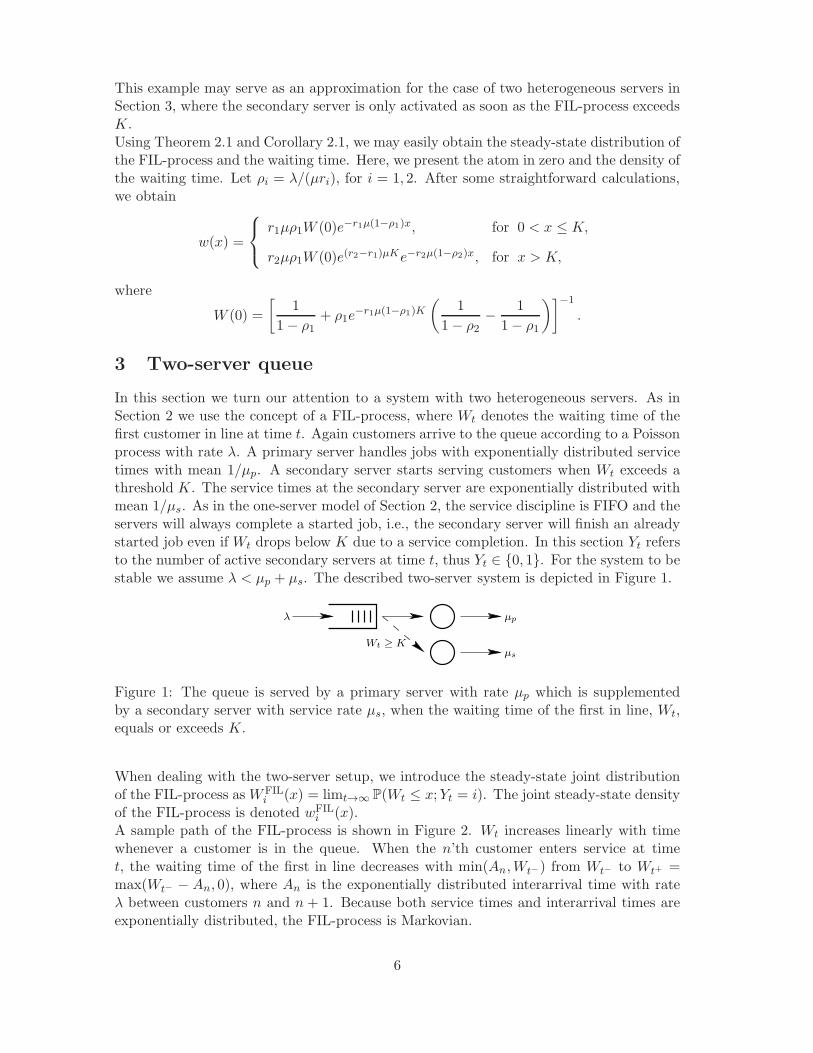
In this section we turn our attention to a system with two heterogeneous servers. As inSection 2 we use the concept of a FIL-process, where Wt denotes the waiting time of thefirst customer in line at time t. Again customers arrive to the queue according to a Poissonprocess with rate λ. A primary server handles jobs with exponentially distributed servicetimes with mean 1/μp. A secondary server starts serving customers when Wt exceeds athreshold K. The service times at the secondary server are exponentially distributed withmean 1/μs. As in the one-server model of Section 2, the service discipline is FIFO and theservers will always complete a started job, i.e., the secondary server will finish an alreadystarted job even if Wt drops below K due to a service completion. In this section Yt refersto the number of active secondary servers at time t, thus Yt ∈ {0, 1}. For the system to bestable we assume λ < μp + μs. The described two-server system is depicted in Figure 1.

Wt ≥ K

λ μp

μs

Figure 1: The queue is served by a primary server with rate μp which is supplementedby a secondary server with service rate μs, when the waiting time of the first in line, Wt,equals or exceeds K.

When dealing with the two-server setup, we introduce the steady-state joint distributionof the FIL-process as WFIL

i (x) = limt→∞ P(Wt ≤ x;Yt = i). The joint steady-state densityof the FIL-process is denoted wFIL

i (x).A sample path of the FIL-process is shown in Figure 2. Wt increases linearly with timewhenever a customer is in the queue. When the n’th customer enters service at timet, the waiting time of the first in line decreases with min(An,Wt−) from Wt− to Wt+ =max(Wt− − An, 0), where An is the exponentially distributed interarrival time with rateλ between customers n and n + 1. Because both service times and interarrival times areexponentially distributed, the FIL-process is Markovian.

6

Arrivals

5

A6

A3

A2

tW

1 2 4 7 8

3 5 6

75 643 81

t

2

Primary server

Secondary server

A4

A

K

Figure 2: Elapsed waiting time of the first customer in line, Wt. The occupation of theservers are shown beneath the graph. Notice how Wt keeps increasing after customer #3finishes service as the secondary server is not allowed to start a new service until the levelK is reached.

The analysis of the system is based on the level crossing equations for the FIL-process.These are more involved, compared to those in Section 2, and are thus presented inLemma 3.1. From this, the steady state distribution of the FIL-process is determined andgiven in Theorem 3.1.

Lemma 3.1 We consider the level crossing equations for three different cases.

(i) For x < K and an active secondary server we have

wFIL1 (x) + μsW

FIL1 (x) = μp

∫ ∞

y=xe−λ(y−x)wFIL

1 (y)dy

+ μs

∫ ∞

y=Ke−λ(y−x)wFIL

1 (y)dy

+ wFIL0 (K−)e−λ(K−x).

(ii) For x < K and an inactive secondary server

wFIL0 (x) = μp

∫ K

y=xe−λ(y−x)wFIL

0 (y)dy + μsWFIL1 (x).

(iii) For x > K the secondary server will always be active

wFIL1 (x) = (μp + μs)

∫ ∞

y=xe−λ(y−x)wFIL

1 (y)dy.

Proof Only case (i) is dealt with in detail as it is the most complicated. The levelcrossing equations are obtained from setting up forward Kolmogorov equations. For case

7

(i) this becomes

P(Wt+h ≤ x+ h;Yt+h = 1)

= (1− μph− μsh)P(Wt ≤ x;Yt = 1)

+ μphP(Wt ≤ x+An;Yt = 1)

+ μshP(K < Wt ≤ x+An;Yt = 1)

+ (1− μph)P(Wt ∈ [K − h,K];Wt ≤ x+An;Yt = 0) + o(h).

Subtracting P(Wt ≤ x+h;Yt = 1) from both sides, dividing by h and letting h → 0 allowsus to rewrite the term on the left side and the first term on the right side as derivativeswith regard to t and x respectively. Moreover h cancels from the rest of the terms exceptthe last. Note that μpP(Wt ∈ [K − h,K];Wt ≤ x+An;Yt = 0) → 0 for h → 0. Hence,

d

dtP(Wt ≤ x;Yt = 1)

=− d

dxP(Wt ≤ x;Yt = 1)− (μp + μs)P(Wt ≤ x;Yt = 1)

+ μpP(Wt ≤ x+An;Yt = 1) + μsP(K < Wt ≤ x+An;Yt = 1)

+ limh→0

P(Wt ≤ K;Yt = 0)− P(Wt ≤ K − h;Yt = 0)

h· P(An > K − x).

By letting t → ∞, the left side of the expression tends to zero. The probabilities can bewritten in form of density and distribution functions, using convolution for the probabilitiesinvolving An; e.g. P(Wt ≤ x + An;Yt = 1) = WFIL

1 (x) + P(x < Wt ≤ x + An, Yt = 1) =

WFIL1 (x) +

∫∞y=x e

−λ(y−x)wFIL1 (y)dy. Using limh→0,t→∞

(P(Wt≤K;Yt=0)−P(Wt≤K−h;Yt=0)

h

)=

wFIL0 (K−), then leads to:

0 = − wFIL1 (x)− (μp + μs)W

FIL1 (x)

+ μp

(WFIL

1 (x) +

∫ ∞

y=xe−λ(y−x)wFIL

1 (y)dy

)+ μs

∫ ∞

y=Ke−λ(y−x)wFIL

1 (y)dy

+ wFIL0 (K−)e−λ(K−x).

Finally, the level crossing equation for case (i) can be obtained by simply rearranging theabove terms.We now turn to case (ii). Following an approach similar to the one for case (i), the levelcrossing equation can be found from the initial Kolmogorov equation

P (Wt+h ≤ x+ h;Yt+h = 0) = (1− μph)P(Wt ≤ x;Yt = 0)

+ μphP(Wt ≤ x+An;Yt = 0)

+ μshP(Wt ≤ x;Yt = 1) + o(h).

In case (iii) the Kolmogorov equation is of the following form

P(Wt+h ≤ x+ h;Yt+h = 1) = (1− μph− μsh)P(Wt ≤ x;Yt = 1)

+ (μp + μs)hP(Wt ≤ x+An;Yt = 1) + o(h).

Again, using the same approach as for case (i), the level crossing equation of Lemma 3.1,case (iii), can be obtained.

8

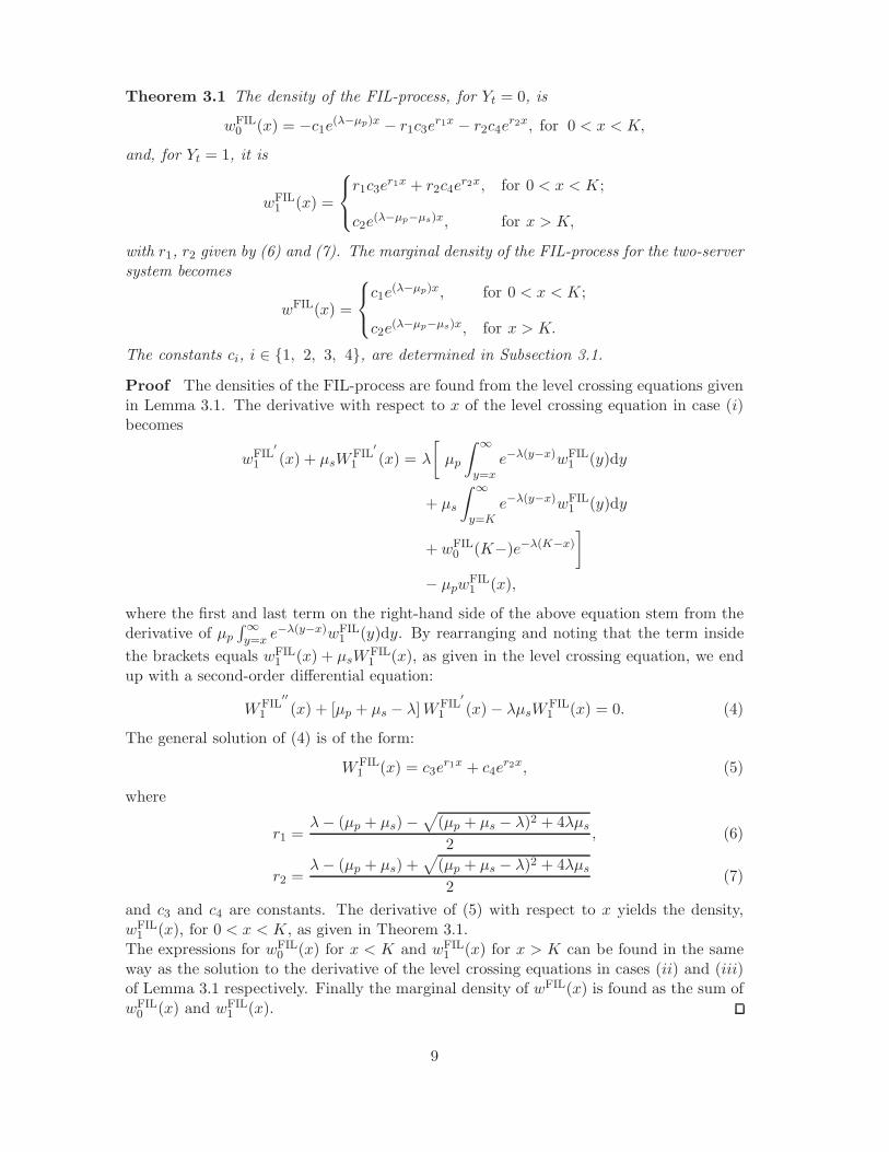
Theorem 3.1 The density of the FIL-process, for Yt = 0, is

wFIL0 (x) = −c1e

(λ−μp)x − r1c3er1x − r2c4e

r2x, for 0 < x < K,

and, for Yt = 1, it is

wFIL1 (x) =

⎧⎨⎩r1c3e

r1x + r2c4er2x, for 0 < x < K;

c2e(λ−μp−μs)x, for x > K,

with r1, r2 given by (6) and (7). The marginal density of the FIL-process for the two-serversystem becomes

wFIL(x) =

⎧⎨⎩c1e

(λ−μp)x, for 0 < x < K;

c2e(λ−μp−μs)x, for x > K.

The constants ci, i ∈ {1, 2, 3, 4}, are determined in Subsection 3.1.

Proof The densities of the FIL-process are found from the level crossing equations givenin Lemma 3.1. The derivative with respect to x of the level crossing equation in case (i)becomes

wFIL′

1 (x) + μsWFIL

′1 (x) = λ

[μp

∫ ∞

y=xe−λ(y−x)wFIL

1 (y)dy

+ μs

∫ ∞

y=Ke−λ(y−x)wFIL

1 (y)dy

+ wFIL0 (K−)e−λ(K−x)

]

− μpwFIL1 (x),

where the first and last term on the right-hand side of the above equation stem from thederivative of μp

∫∞y=x e

−λ(y−x)wFIL1 (y)dy. By rearranging and noting that the term inside

the brackets equals wFIL1 (x) + μsW

FIL1 (x), as given in the level crossing equation, we end

up with a second-order differential equation:

WFIL′′

1 (x) + [μp + μs − λ]WFIL′

1 (x)− λμsWFIL1 (x) = 0. (4)

The general solution of (4) is of the form:

WFIL1 (x) = c3e

r1x + c4er2x, (5)

where

r1 =λ− (μp + μs)−

√(μp + μs − λ)2 + 4λμs

2, (6)

r2 =λ− (μp + μs) +

√(μp + μs − λ)2 + 4λμs

2(7)

and c3 and c4 are constants. The derivative of (5) with respect to x yields the density,wFIL1 (x), for 0 < x < K, as given in Theorem 3.1.

The expressions for wFIL0 (x) for x < K and wFIL

1 (x) for x > K can be found in the sameway as the solution to the derivative of the level crossing equations in cases (ii) and (iii)of Lemma 3.1 respectively. Finally the marginal density of wFIL(x) is found as the sum ofwFIL0 (x) and wFIL

1 (x).

9

3.1 Constants and atoms

To fully describe the distribution of the FIL-process, the atoms in zero must be determinedtogether with the constants in Theorem 3.1. The atoms, corresponding to the queue beingempty, can be divided into four different boundary states; both servers are unoccupied(N), only the primary server is occupied (P), only the secondary server is occupied (S),and both servers are occupied (PS). The probabilities of being in these states are referredto as WFIL

N (0), WFILP (0), WFIL

S (0) and WFILPS (0), respectively.

Eight independent equations are needed to determine the eight constants; the probabilityof being in the four boundary states and the ci’s, i ∈ {1, 2, 3, 4}. Two equations followdirectly from the boundary states in 0, as N and S can only be entered and left from otherboundary states. Writing the rate out of the states on the left-hand side and the rate intothe states on the right-hand side gives

λWFILN (0) = μpW

FILP (0) + μsW

FILS (0) (8)

and

(λ+ μs)WFILS (0) = μpW

FILPS (0). (9)

The rate out of P is λ + μp as this state can only be left by an arrival or a departurefrom the primary server. The state can be entered by an arrival in state N or a departurefrom the secondary server in state PS. P can also be entered from the FIL-process fornon-zero Wt given that Yt = 0 and Wt < An. This is represented by the second term onthe right-hand side in (10).

(λ+ μp)WFILP (0) = λWFIL

N (0) + μp

∫ K

0+e−λywFIL

0 (y)dy + μsWFILPS (0). (10)

The balance equation for WFILPS (0) is found in the same way:

(λ+ μp + μs)WFILPS (0) = λWFIL

S (0) + μp

∫ ∞

0+e−λywFIL

1 (y)dy

+ μs

∫ ∞

Ke−λywFIL

1 (y)dy + wFIL0 (K−)e−λK . (11)

Three more equations can be obtained by considering boundary conditions. By lettingx ↓ 0 in (5) we have

WFILS (0) +WFIL

PS (0) = c3 + c4. (12)

Letting x ↑ K in the level crossing equation of case (ii) in Lemma 3.1 gives

wFIL0 (K−) = μsW

FIL1 (K)

= μs

[WFIL

S (0) +WFILPS (0) +

∫ K

0wFIL1 (y)dy

], (13)

and the same limit in the level crossing equation of case (i) gives

wFIL1 (K−) + μsW

FIL1 (K) = wFIL

0 (K−) + (μp + μs)

∫ ∞

y=Ke−λ(y−K)wFIL

1 (y)dy

= wFIL0 (K−) + c2e

(λ−μp−μs)K . (14)

10

The final equation is obtained by normalization of the FIL-process:

1 =

∫ K

0wFIL0 (y)dy +

∫ ∞

0wFIL1 (y)dy +WFIL

N (0) +WFILS (0) +WFIL

P (0) +WFILPS (0). (15)

The analytical expressions for the constants do not seem to give any additional insight intothe problem. Solving the equations numerically is straightforward. We have shown that atmost two of the equations can be mutually dependent and all numerical investigations pointtoward them being independent. Furthermore we argue that as long as the requirementsfor stability of the system are fulfilled, a unique solution to the equation array must existand thus the equations must indeed be independent.

3.2 Waiting-time distribution

We now turn to the waiting-time distribution and use the same definition of this as inSection 2; W (x) = P(W ≤ x), where W is the waiting time an arbitrary customer expe-riences. Observe that arriving customers are directly taken into service in case the queueis empty and the primary server is available. Using PASTA, it is easy to obtain the atomin zero of the waiting time:

P(W = 0) = WFILN (0) +WFIL

S (0).

In case the waiting time is non-zero, the waiting time corresponds to the FIL-process atepochs right before downward jumps. Here, we again consider an infinitesimal interval(t, t+ h) and apply similar arguments as in Section 2. In particular, for x ≥ K, we have

P(Wt > x;Ns(t, t+ h) = 1) = (μp + μs)h

∫ ∞

xwFIL1 (y)dy + o(h).

For 0 < x < K, we have

P(Wt > x;Ns(t, t+ h) = 1) = μph

∫ K−h

xwFIL0 (y)dy + μph

∫ K

xwFIL1 (y)dy

+

∫ K

K−hwFIL0 (y)dy + (μp + μs)h

∫ ∞

KwFIL1 (y)dy + o(h).

Note that∫KK−hw

FIL0 (y)dy/h → wFIL

0 (K−), as h → 0. Also, observe that P(Ns(t, t+ h) =1)/h (for h → 0) is the rate at which customers are taken into service and, since everycustomer leaves the queue through the server and the system is stable, equals λ. Combiningthe above and using a similar conditioning as in Section 2, we obtain

P(W > x) =

⎧⎪⎪⎪⎨⎪⎪⎪⎩

1λ

[μp

∫Kx (wFIL

0 (y) + wFIL1 (y))dy

+wFIL0 (K−) + (μp + μs)

∫∞K wFIL

1 (y)dy], for 0 ≤ x < K,

μp+μs

λ

∫∞x wFIL

1 (y)dy, for x ≥ K.

(16)

From this, we obtain the density of the steady-state waiting time and the atom at K:

11

Corollary 3.1 For the steady-state waiting time, we have two atoms

P(W = 0) = WFILN (0) +WFIL

S (0),

P(W = K) =wFIL0 (K−)

λ,

and density

w(x) =

⎧⎨⎩

μp

λ c1e(λ−μp)x, for 0 < x < K,

μp+μs

λ c2e(λ−μp−μs)x, for x > K.

Remark 3.1 Note that the form of the steady-state waiting time density (and distribu-tion) is closely related to the density in Example 2.1, i.e., the single-server model with twoservice speeds determined by a threshold on the FIL-process. In particular, the parame-ters ri, i = 1, 2, and μ should be taken such that r1μ = μp and r2μ = μp+μs (for instance,let μ = μp, r1 = 1, and r2 = 1 + μs/μp). The main difference between the waiting-timedistributions concerns the atom at K.

4 Numerical results

To illustrate the difference in behavior of the waiting-time distribution for the one serversystem of Example 2.1 and the two-server system treated in Section 3, a few numericalresults are shown in Figure 3. The parameters have been chosen such that the two casesare comparable.The waiting-time distributions in Figure 4 are found from Corollary 3.1 and the corre-sponding eight constants, found with Maple, are given in Table 1. It is seen how therelation between λ and μp governs the shape of the distribution for x < K; it is convexfor λ < μp, concave for λ > μp and a straight line for λ = μp. Notable are also the atomsat K which are absent in the two-speed single server case of Figure 4.The somewhat better performance of the two-server model can be explained by the sec-ondary server finishing an already started service when Wt drops below K, whereas thesingle server system of Example 2.1 will change the service speed to r1 immediately.

Table 1: Numerical results for common parameters λ = 2, μs = 3.

(μp = 1, K = 1.5) (μp = 2, K = 1.0) (μp = 4, K = 0.5)

WN 0.0470 0.2298 0.5318WP 0.0860 0.2181 0.2559WS 0.0027 0.0078 0.0133WPS 0.0135 0.0195 0.0166c1 0.1990 0.4751 0.5451c2 6.3453 2.9956 0.6123c3 -0.6401·10−4 -0.2673·10−3 -0.4749·10−3

c4 0.01626 0.0276 0.0304

In Figure 4 we compared the performance of the service mechism based on waiting times tothe control based on queue lengths, since the latter is common in the queueing literature.For the model with queue-length based control, the secondary server is only allowed to

12

0 1 2 3 40

0.2

0.4

0.6

0.8

1

x

P(W

>x)

r1=1, r

2=4, K=1.5

r1=2, r

2=5, K=1

r1=4, r

2=7, K=0.5

0 1 2 3 40

0.2

0.4

0.6

0.8

1

x

P(W

>x)

μ

p=1, K=1.5

μp=2, K=1

μp=4, K=0.5

Figure 3: Numerical comparison of the one and two-server models.

take customers into service when more than 30 and 3 customers, in Figures 4 and 4,respectively, are waiting in the queue. These parameters have been chosen such that theresulting average waiting times are nearly identical for the two policies. The waiting-timedistribution for the queue-length based threshold is found by taking the average of 50simulations of 100.000 calls each. In this way the 95% confidence intervals become toonarrow to display in the figure. It is seen that the waiting-time based threshold results inless variation of waiting times which is preferable as the objective is to have more controlover the system. This reduction in variability of waiting times is accentuated for largerthreshold value as displayed in Figure 4. The figure illustrates the interesting, but notsurprising, phenomenon of how the probability mass gathers around K for λ > μp, Klarge and waiting-time based control.

0 5 10 15 20 250

0.2

0.4

0.6

0.8

1

x

P(W

>x)

Waiting timethresholdQueue lengththreshold

0 1 2 3 40

0.2

0.4

0.6

0.8

1

x

P(W

>x)

Waiting timethresholdQueue lengththreshold

Figure 4: Waiting-time thresholds compared to queue-length thresholds.

13

Given the distribution of the waiting-time and FIL-process, most of the commonly usedperformance measures such as TSF are easily found. Other performance measures suchas the utilization of the servers can be found as

ap = 1−WN(0)−WS(0),

as = 1−WN(0)−WP(0) −∫ K

0wFIL0 (y)dy,

where ap and as are the utilization of the primary and secondary server, respectively.

5 Conclusions and topics for further research

We have studied queueing systems where the provided service depends on the waiting timeof the first customer in line. This type of control is commonly used in call centers and hasmainly been motivated by a frequently used setup referred to as an “inverted V”, see [1].The main contribution is that we have shown ways to deal with systems where the servicechanges depending on the waiting time, which can be inherently difficult to deal with inparticular in the case of fixed thresholds.The first model of this paper deals with a single server that operates with a service speeddepending on the waiting time of the first customer in line. We derived the waiting-timedistribution of an arbitrary customer entering the system and showed how the model canbe used for the threshold case.The second model of this paper deals with a two-server setup where a secondary serversupplements a primary server when the waiting time of the first in line exceeds a threshold.Again the waiting distribution of an arbitrary customer has been derived and numericalexamples have been given. It was illustrated that a waiting-time based threshold is prefer-able to a queue-length based, when a high degree of control of the waiting times is desired.Also, The simplicity of the form of the solution for the waiting time given in Corollary 3.1provides some useful insight.In the model presented in Section 3, only one primary and one secondary server wasconsidered. This is easily extended to a more general setup with multiple primary serversby introducing additional states for WFIL(0) along with the four already used. The extraboundary states should describe the number of unoccupied servers. Analyzing a setupwith multiple secondary servers would be much more difficult as the joint distribution ofwFILi (x) must be extended to include i ∈ {0, 1, ..., n}, where n is the number of secondary

servers.A related routing setup, often seen in call centers and used as a way to prioritize a group ofcustomers over another, is the “N” design, see [12]. Also related are [13], [14] and [15]. The“N” design is basically an extension to the model of Section 3 where the secondary serveralso has a queue of its own, from which it receives jobs. Extending the model presented inthis paper to the “N” design, necessitates the use of a 2-dimensional FIL-process in orderto keep track of the waiting time of the first customer in line in both queues.There is still much to be done in relation to analysis of complex queueing systems suchas those seen in call centers. Even though simulation may remain the dominant way ofmodelling these systems, it is indeed worth pursuing analytical approaches to gain insightnot obtainable through simulation such as the result in Corollary 3.1.

14

References

[1] Armony, M. (2005). Dynamic routing in large-scale service systems with heterogeneous servers.Queueing Systems 51, 287–329.

[2] Asmussen, S. (2003). Applied Probability and Queues, Second Edition. Springer, New York.

[3] Barth, W., M. Manitz, R. Stolletz (2009). Analysis of Two-Level Support Systems with Time-Dependent Overflow - A Banking Application. Forthcoming in Production and Operations Man-agement.

[4] Bekker, R., S.C. Borst, O.J. Boxma, O. Kella (2004). Queues with workload-dependent arrivaland service rates. Queueing Systems 46, 537–556.

[5] Boxma, O., H. Kaspi, O. Kella, D. Perry (2005). On/off storage systems with state dependentinput, output and switching rates. Probability in the Engineering and Informational Sciences19, 1–14.

[6] Boxma, O.J., M. Vlasiou (2007). On queues with service and interarrival times depending onwaiting times. Queueing Systems 56, 121–132.

[7] Brill, P.H., M.J.M. Posner (1981). A two server queue with nonwaiting customers receivingspecialized service. Management Science 27, 914–925.

[8] Brill, P.H., M.J.M. Posner (1981). The system point method in exponential queues: a levelcrossing approach. Mathematics of Operations Research 6, 31–49.

[9] Browne, S., K. Sigman (1992). Work-modulated queues with applications to storage processes.Journal of Applied Probability 29, 699–712.

[10] Cohen, J.W., M. Rubinovitch (1977). On level crossings and cycles in dam processes. Mathe-matics of Operations Research 2, 297–310.

[11] Franx, G.J., G.M. Koole, S.A. Pot (2006). Approximating multi-skill blocking systems byhyperexponential decomposition. Performance Evaluation 63, 799–824.

[12] Gans, N., G.M. Koole, A. Mandelbaum (2003). Telephone call centers: tutorial, review, andresearch prospects. Manufacturing and Service Operations Management 5, 79–141.

[13] Gans, N., Y.-P. Zhou (2003). A call-routing problem with service-level constraints. OperationsResearch 51, 255–271.

[14] Gans, N., Y.-P. Zhou (2007). Call-routing schemes for call-center outsourcing. Manufacturingand Service Operations Management 9, 33–50.

[15] Gurvich, I., M. Armony, A. Mandelbaum (2008). Service-level differentiation in call centerswith fully flexible servers. Management Science 54, 279–294.

[16] Harrison, J.M., S.I. Resnick (1976). The stationary distribution and first exit probabilities ofa storage process with general release rule. Mathematics of Operations Research 1, 347–358.

[17] Jackson, J.R. (1960). Some problems in queueing with dynamic priorities. Naval ResearchLogistics Quarterly 7, 235–249.

[18] Koole, G.M. (1995). A simple proof of the optimality of a threshold policy in a two-serverqueueing system. Systems & Control Letters 26, 301–303.

[19] Lin, W., P.R. Kumar (1984). Optimal control of a queueing system with two heterogeneousservers. IEEE Trans. Automat. Control 29, 696–703.

[20] Liu, L., M. Parlar, S. Zhu (2007). Pricing and lead time decisions in decentralized supplychains. Management Science 53, 713–725.

15

[21] Lucent Technologies (1999). CentreVu Release 8 Advocate User Guide. P.O. Box 4100, Craw-fordsville, IN 47933, U.S.A.: Lucent Technologies.

[22] Perry, D., L. Benny (1989). Continuous Production/Inventory Model with Analogy to CertainQueueing and Dam Models. Advances in Applied Probability 21, 123–141.

[23] Posner, M.J.M (1973). Single-server queues with service time dependent on waiting time.Operations Research 21, 610–616.

[24] Rubinovitch, M. (1985). The slow server problem. Journal of Applied Probability 22, 205–213.

[25] Scheinhardt, W.R.W., N. van Foreest, M. Mandjes (2005). Continuous feedback fluid queues.Operations Research Letters 33, 551–559.

[26] Stockbridge, R.H. (1991). A martingale approach to the slow server problem. Journal ofApplied Probability 28, 480–486.

[27] Whitt, W. (1990). Queues with service times and interarrival times depending linearly andrandomly upon waiting times. Queueing Systems 6, 335–351.

[28] Zabreiko, P.P, A.I. Koshelev, M.A. Krasnosel’skii; transl. and ed. by T.O. Shaposhnikova,R.S. Anderssen and S.G. Mikhlin (1975). Integral Equations: a Reference Text. Monographsand textbooks on pure and applied mathematics. Noordhoff, Leiden.

16