Queueing Networks and Markov Chains...Queueing Networks and Markov Chains Modeling and Performance Evaluation with Computer Science Applications Second Edition Gunter Bolch Stefan

Queueing Networks and Markov Chains Modeling and Performance Evaluation with Computer Science Applications

Second Edition

Gunter Bolch Stefan Greiner Hermann de Meer Kishor S. Trivedi

WILEY- INTERSCIENCE

A JOHN WILEY & SONS, INC., PUBLICATION

This Page Intentionally Left Blank

Queueing Networks and Markov Chains

This Page Intentionally Left Blank

Queueing Networks and Markov Chains Modeling and Performance Evaluation with Computer Science Applications

Second Edition

Gunter Bolch Stefan Greiner Hermann de Meer Kishor S. Trivedi

WILEY- INTERSCIENCE

A JOHN WILEY & SONS, INC., PUBLICATION

Copyright 0 2006 by John Wiley & Sons, Inc. All rights reserved.

Published by John Wiley & Sons, Inc., Hoboken, New Jersey Published simultaneously in Canada.

No part of this publication may be reproduced, stored in a retrieval system, or transmitted in any form or by any means, electronic, mechanical, photocopying, recording, scanning, or otherwise, except as permitted under Section 107 or 108 ofthe 1976 United States Copyright Act, without either the prior written permission of the Publisher, or authorization through payment o f the appropriate per-copy fee to the Copyright Clearance Center, Inc., 222 Rosewood Drive, Danvers, MA 01923, (978) 750-8400, fax (978) 750-4470, or on the web at www.copyright.com. Requests to the Publisher for permission should be addressed to the Permissions Department, John Wiley & Sons, Inc., 1 1 1 River Street, Hoboken, N J 07030, (201) 748-601 I , fax (201) 748-6008, or online at http://www.wiley.com/go/permission.

Limit of Liability/Disclaimer of Warranty: While the publisher and author have used their best efforts in preparing this book, they make no representations or warranties with respect to the accuracy or completeness of the contents of this book and spccifically disclaim any implied warranties of merchantability or fitness for a particular purpose. No warranty may be created or extended by sales representatives or written sales materials. The advice and strategies contained herein may not be suitable for your situation. You should consult with a professional where appropriate. Neither the publisher nor author shall be liable for any loss of profit or any other commercial damages, including but not limited to special, incidental, consequential, or other damages.

For general information on our other products and services or for technical support, please contact our Customer Care Department within the United States at (800) 762-2974, outside the United States at (317) 572-3993 or fax (317) 572-4002.

Wiley also publishes its books in a variety of electronic formats. Some content that appears in print may not be available in electronic format. For information about Wiley products, visit our web site at www.wiley.com.

Library of Congress Cataloging-in-Publication Data:

Queueing networks and Markov chains : modeling and performance evaluation with computer science applications / Gunter Bolch . , . [et al.].-2nd rcv. and enlarged ed.

“A Wiley-lnterscience publication.” Includes bibliographical references and index. ISBN- I3 978-0-47 1-56525-3 (acid-free paper) ISBN- I0 0-47 1-56525-3 (acid-free paper) I . Markov processes. 2. Queuing theory. I. Bolch, Gunter

p. cm.

QA76.9E94Q48 2006 004.2’4015 19233-dc22 200506965

Printed in the United States of America.

1 0 9 8 7 6 5 4 3 2 1

Contents

... Preface to the Second Edition Xlll

Preface to the First Edition xv

1 Introduction 1

1.1 Motivation . . . . . . . . . . . . . . . . . . . . . . . . . . . . . 1

1.2 Methodological Background . . . . . . . . . . . . . . . . . . . 5

1.2.1 Problem Formulation . . . . . . . . . . . . . . . . . . . 6

1.2.2 The Modeling Process . . . . . . . . . . . . . . . . . . . 8 1.2.3 Evaluation . . . . . . . . . . . . . . . . . . . . . . . . . 10 1.2.4 Summary . . . . . . . . . . . . . . . . . . . . . . . . . . 12

1.3 Basics of Probability and Statistics . . . . . . . . . . . . . . . 15 1.3.1 Random Variables . . . . . . . . . . . . . . . . . . . . . 15

1.3.2 Multiple Random Variables . . . . . . . . . . . . . . . . 30 1.3.3 Transforms . . . . . . . . . . . . . . . . . . . . . . . . . 36 1.3.4 Parameter Estimation . . . . . . . . . . . . . . . . . . . 38

1.3.5 Order Statistics . . . . . . . . . . . . . . . . . . . . . . 46 1.3.6 Distribution of Sums . . . . . . . . . . . . . . . . . . . 46

V

vi CONTENTS

2 Markov Chains 51

2.1 Markov Processes . . . . . . . . . . . . . . . . . . . . . . . . . 51

2.1.1 Stochastic and Markov Processes . . . . . . . . . . . . 51 2.1.2 Markov Chains . . . . . . . . . . . . . . . . . . . . . . . 53

2.2.1 A Simple Example . . . . . . . . . . . . . . . . . . . . . 71 2.2.2 Markov Reward Models . . . . . . . . . . . . . . . . . . 75

2.2.3 A Casestudy . . . . . . . . . . . . . . . . . . . . . . . 80

2.3 Generation Methods . . . . . . . . . . . . . . . . . . . . . . . 90

2.3.1 Petri Nets . . . . . . . . . . . . . . . . . . . . . . . . . 94

2.3.2 Generalized Stochastic Petri Nets . . . . . . . . . . . . 96 2.3.3 Stochastic Reward Nets . . . . . . . . . . . . . . . . . . 97

2.3.4 GSPN/SRN Analysis . . . . . . . . . . . . . . . . . . . 101

A Larger Exanlple . . . . . . . . . . . . . . . . . . . . . 108 2.3.6 Stochastic Petri Net Extensions . . . . . . . . . . . . . 113

2.3.7 Non-Markoviarl Models . . . . . . . . . . . . . . . . . . 115

2.3.8 Symbolic State Space Storage Techniques . . . . . . . . 120

2.2 Performance Measures . . . . . . . . . . . . . . . . . . . . . . 71

2.3.5

3 Steady-State Solutions of Markov Chains 123

3.1 Solution for a Birth Death Process . . . . . . . . . . . . . . . 125

3.2 Matrix-Geometric Method: Quasi-Birth-Death Process . . . . 127

3.2.1 The Concept . . . . . . . . . . . . . . . . . . . . . . . . 127

3.2.2 Example: The QBD Process . . . . . . . . . . . . . . . 128

3.3 Hessenberg Matrix: Non-Markovian Queues . . . . . . . . . . 140

3.3.1 Nonexporlential Servicc Times . . . . . . . . . . . . . . 141

3.3.2 Server with Vacations . . . . . . . . . . . . . . . . . . . 146 3.4 Numerical Solution: Direct Methods . . . . . . . . . . . . . . 151

3.4.1 Gaussian Elimination . . . . . . . . . . . . . . . . . . . 152

3.4.2 The Grassmanrl Algorithm . . . . . . . . . . . . . . . . 158 3.5 Numerical Solution: Iterative Methods . . . . . . . . . . . . . 165

3.5.1 Convergence of Iterative Methods . . . . . . . . . . . . 165

3.5.2 Power Method . . . . . . . . . . . . . . . . . . . . . . . 166

3.5.3 Jacobi's Method . . . . . . . . . . . . . . . . . . . . . . 169

3.5.4 Gauss-Seidel Method . . . . . . . . . . . . . . . . . . . 172

3.5.5 The Method of Successive Over-Relaxation . . . . . . . 173 3.6 Comparison of Numerical Solution Methods . . . . . . . . . . 177

3.6.1 Case Studies . . . . . . . . . . . . . . . . . . . . . . . . 179

4 Steady-S tate Aggregation/Disaggregation Methods 185

4.1 Courtois’ Approximate Method . . . . . . . . . . . . . . . . . 185

4.1.1 Decomposition . . . . . . . . . . . . . . . . . . . . . . . 186 4.1.2 Applicability . . . . . . . . . . . . . . . . . . . . . . . . 192

4.1.3 Analysis of the Substructures . . . . . . . . . . . . . . 194 4.1.4 Aggregation and Unconditioning . . . . . . . . . . . . . 195

4.1.5 The Algorithm . . . . . . . . . . . . . . . . . . . . . . . 197 4.2 Takahashi’s Iterative Method . . . . . . . . . . . . . . . . . . 198

4.2.1 The Fundamental Equations . . . . . . . . . . . . . . . 199 4.2.2 Applicability . . . . . . . . . . . . . . . . . . . . . . . . 201

4.2.3 The Algorithm . . . . . . . . . . . . . . . . . . . . . . . 202 4.2.4 Application . . . . . . . . . . . . . . . . . . . . . . . . . 202 4.2.5 Final Remarks . . . . . . . . . . . . . . . . . . . . . . . 206

5 Transient Solution of Markov Chains 209

5.1 Transient Analysis Using Exact Methods . . . . . . . . . . . . 210

5.1.1 A Pure Birth Process . . . . . . . . . . . . . . . . . . . 210 5.1.2 A Two-State CTMC . . . . . . . . . . . . . . . . . . . 213

5.1.3 Solution Using Laplace Transforms . . . . . . . . . . . 216

5.1.4 Numerical Solution Using Uniformization . . . . . . . . 216 5.1.5 Other Numerical Methods . . . . . . . . . . . . . . . . 221

5 .2 Aggregation of Stiff Markov Chains . . . . . . . . . . . . . . . 222

5.2.1 Outline arid Basic Definitions . . . . . . . . . . . . . . 223

5.2.2 Aggregation of Fast Recurretit Subset. s . . . . . . . . . 224 5.2.3 Aggregation of Fast Transient Subsets . . . . . . . . . . 227 5.2.4 Aggregation of Initial State Probabilities . . . . . . . . 228 5.2.5 Disaggregations . . . . . . . . . . . . . . . . . . . . . . 229 5.2.6 The Algorithm . . . . . . . . . . . . . . . . . . . . . . . 230 5.2.7 An Example: Server Breakdown arid Repair . . . . . . 232

6 Single Station Queueing Systems 241

6.1 Notation . . . . . . . . . . . . . . . . . . . . . . . . . . . . . . 242

6.1.1 Kendall’s Notation . . . . . . . . . . . . . . . . . . . . 242 6.1.2 Performance Measures . . . . . . . . . . . . . . . . . . 244

6.2 Markovian Queues . . . . . . . . . . . . . . . . . . . . . . . . 246

6.2.1 The M/M/l Queue . . . . . . . . . . . . . . . . . . . . 246

viii CONTENTS

6.2.2 The M/M/ca Queue . . . . . . . . . . . . . . . . . . . 249 6.2.3 The M/M/m Queue . . . . . . . . . . . . . . . . . . . . 250 6.2.4 The M/M/ l /K Finite Capacity Queue . . . . . . . . . 251 6.2.5 Machine Repairman Model . . . . . . . . . . . . . . . . 252

6.2.6 Closed Tandem Network . . . . . . . . . . . . . . . . . 253 6.3 Non-Markovian Queues . . . . . . . . . . . . . . . . . . . . . . 255

6.3.1 The M/G/1 Queue . . . . . . . . . . . . . . . . . . . . 255

6.3.2 The GI/M/l Queue . . . . . . . . . . . . . . . . . . . . 261 6.3.3 The GI/M/m Queue . . . . . . . . . . . . . . . . . . . 265 6.3.4 The GI/G/1 Queue . . . . . . . . . . . . . . . . . . . . 265 6.3.5 The M/G/m Queue . . . . . . . . . . . . . . . . . . . . 267

The GI/G/m Queue . . . . . . . . . . . . . . . . . . . . 269 6.4 Priority Queues . . . . . . . . . . . . . . . . . . . . . . . . . . 272

6.4.1 Queue without Preemption . . . . . . . . . . . . . . . . 272 6.4.2 Conservation Laws . . . . . . . . . . . . . . . . . . . . 278 6.4.3 Queur: with Preemption . . . . . . . . . . . . . . . . . . 279 6.4.4 Queue with Time-Dependent Priorities . . . . . . . . . 280

6.5 Asymmetric Queues . . . . . . . . . . . . . . . . . . . . . . . . 283 6.5.1 Approximate Analysis . . . . . . . . . . . . . . . . . . . 284

6.5.2 Exact Analysis . . . . . . . . . . . . . . . . . . . . . . . 286 6.6 Queues with Batch Service and Batch Arrivals . . . . . . . . . 295

6.6.1 Batch Service . . . . . . . . . . . . . . . . . . . . . . . 295 6.6.2 Batch Arrivals . . . . . . . . . . . . . . . . . . . . . . . 296

6.7 Retrial Queues . . . . . . . . . . . . . . . . . . . . . . . . . . . 299 6.7.1 M/M/1 Ret. rial Queue . . . . . . . . . . . . . . . . . . 300

6.7.2 M / G / l Retrial Queue . . . . . . . . . . . . . . . . . . . 301 Special Classes of' Point Arrival Processes . . . . . . . . . . . . 302 6.8.1 Point, Renewal, and Markov Renewal Processes . . . . 303 6.8.2 MMPP . . . . . . . . . . . . . . . . . . . . . . . . . . . 303 6.8.3 MAP . . . . . . . . . . . . . . . . . . . . . . . . . . . . 306 6.8.4 BMAP . . . . . . . . . . . . . . . . . . . . . . . . . . . 309

6.3.6

6.8

7 Queueing Networks 321

7.1 Definit. ions and Notation . . . . . . . . . . . . . . . . . . . . . 323 7.1.1 Single Class Networks . . . . . . . . . . . . . . . . . . . 323 7.1.2 Multiclass Networks . . . . . . . . . . . . . . . . . . . . 325

7.2 Performance Measures . . . . . . . . . . . . . . . . . . . . . . 326 7.2.1 Single Class Networks . . . . . . . . . . . . . . . . . . . 326

CONTENTS ix

7.2.2 Multiclass Networks . . . . . . . . . . . . . . . . . . . . 330 7.3 Product-Form Queueing Networks . . . . . . . . . . . . . . . . 331

7.3.1 Global Balance . . . . . . . . . . . . . . . . . . . . . . . 332 7.3.2 Local Balance . . . . . . . . . . . . . . . . . . . . . . . 335 7.3.3 Product-Form . . . . . . . . . . . . . . . . . . . . . . . 340 7.3.4 Jackson Networks . . . . . . . . . . . . . . . . . . . . . 341 7.3.5 Gordon-Newel1 Networks . . . . . . . . . . . . . . . . . 346 7.3.6 BCMP Networks . . . . . . . . . . . . . . . . . . . . . . 353

8 Algorithms for Product-Form Networks 369

8.1 The Convolution Algorithm . . . . . . . . . . . . . . . . . . . 371 8.1.1 Single Class Closed Networks . . . . . . . . . . . . . . . 371 8.1.2 Multiclass Closed Networks . . . . . . . . . . . . . . . . 378

8.2 The Mean Value Analysis . . . . . . . . . . . . . . . . . . . . 384 8.2.1 Single Class Closed Networks . . . . . . . . . . . . . . . 385 8.2.2 Multiclass Closed Networks . . . . . . . . . . . . . . . . 393 8.2.3 Mixed Networks . . . . . . . . . . . . . . . . . . . . . . 400

8.2.4 Networks with Load-Dependent Service . . . . . . . . . 405 8.3 Flow Equivalent Server Method . . . . . . . . . . . . . . . . . 410

8.3.1 FES Method for a Single Node . . . . . . . . . . . . . . 410 8.3.2 FES Method for Multiple Nodes . . . . . . . . . . . . . 414

8.4 Summary . . . . . . . . . . . . . . . . . . . . . . . . . . . . . . 417

9 Approximation Algorithms for Product-Form Networks 421

9.1 Approximations Based on the MVA . . . . . . . . . . . . . . . 422 9.1.1 Bard Schweitzer Approximation . . . . . . . . . . . . . 422 9.1.2 Self-correcting Approximation Technique . . . . . . . . 427

9.2 Summation Method . . . . . . . . . . . . . . . . . . . . . . . . 440 9.2.1 Single Class Networks . . . . . . . . . . . . . . . . . . . 442 9.2.2 Multiclass Networks . . . . . . . . . . . . . . . . . . . . 445

9.3 Bottapprox Method . . . . . . . . . . . . . . . . . . . . . . . . 447 9.3.1 Initial Value of X . . . . . . . . . . . . . . . . . . . . . 447 9.3.2 Single Class Networks . . . . . . . . . . . . . . . . . . . 447 9.3.3 Multiclass Networks . . . . . . . . . . . . . . . . . . . . 450

9.4 Bounds Analysis . . . . . . . . . . . . . . . . . . . . . . . . . . 452 9.4.1 Asymptotic Bounds Analysis . . . . . . . . . . . . . . . 453

x CONTENTS

9.4.2 Balanced Job Bounds Analysis . . . . . . . . . . . . . . 456 9.5 Summary . . . . . . . . . . . . . . . . . . . . . . . . . . . . . . 459

10 Algorithms for Non-Product-Form Networks 461

10.1 Nonexponential Distributions . . . . . . . . . . . . . . . . . . 463

10.1.1 Diffusion Approximation . . . . . . . . . . . . . . . . . 463

10.1.2 Maximum Entropy Method . . . . . . . . . . . . . . . . 470

10.1.3 Decomposition for Open Networks . . . . . . . . . . . . 479 10.1.4 Methods for Closed Networks . . . . . . . . . . . . . . 488

10.1.5 Closing Method for Open and Mixed Networks . . . . . 507 10.2 Different Service Times at FCFS Nodes . . . . . . . . . . . . . 512

10.3 Priority Networks . . . . . . . . . . . . . . . . . . . . . . . . . 514

10.3.1 PRIOMVA . . . . . . . . . . . . . . . . . . . . . . . . . 514

10.3.2 The Method of Shadow Server . . . . . . . . . . . . . . 522

10.3.3 PRIOSUM . . . . . . . . . . . . . . . . . . . . . . . . . 537

10.4 Simultaneous Resource Possession . . . . . . . . . . . . . . . . 541 10.4.1 Memory Constraints . . . . . . . . . . . . . . . . . . . . 541

10.4.2 1/0 Subsystems . . . . . . . . . . . . . . . . . . . . . . 544

10.4.3 Method of Surrogate Delays . . . . . . . . . . . . . . . 547 10.4.4 Serialization . . . . . . . . . . . . . . . . . . . . . . . . 548

10.5 Programs with Internal Concurrency . . . . . . . . . . . . . . 549

10.6 Parallel Processing . . . . . . . . . . . . . . . . . . . . . . . . 550

10.6.1 Asynchronous Tasks . . . . . . . . . . . . . . . . . . . . 551

10.6.2 Fork-Join Systems . . . . . . . . . . . . . . . . . . . . . 558

10.7 Networks with Asymmetric Nodes . . . . . . . . . . . . . . . . 577

10.7.1 Closed Networks . . . . . . . . . . . . . . . . . . . . . . 577

10.7.2 Open Networks . . . . . . . . . . . . . . . . . . . . . . 581 10.8 Networks with Blocking . . . . . . . . . . . . . . . . . . . . . 591

10.8.1 Different Blocking Types . . . . . . . . . . . . . . . . . 592

10.9 Networks with Batch Service . . . . . . . . . . . . . . . . . . . 600 10.9.1 Open Networks with Batch Service . . . . . . . . . . . 600

10.9.2 Closed Networks with Batch Service . . . . . . . . . . . 602

10.8.2 Product-Form Solution for Networks with Two Nodes . 593

11 Discrete-Event Simulation 607

11.1 Introduction to Simulat. ion . . . . . . . . . . . . . . . . . . . . 607 11.2 Simulative or Analytic Solution? . . . . . . . . . . . . . . . . 608

CONTENTS xi

11.3 Classification of Simulatiori Models . . . . . . . . . . . . . . . 610 11.4 Classification of Tools in DES . . . . . . . . . . . . . . . . . . 612 11.5 The Role of Probability and Statistics in Simulation . . . . . . 613

11.5.1 Random Variate Generation . . . . . . . . . . . . . . . 614 11.5.2 Generating Events from an Arrival Process . . . . . . . 624

11.5.3 Output Analysis . . . . . . . . . . . . . . . . . . . . . . 629

11.5.4 Speedup Techniques . . . . . . . . . . . . . . . . . . . . 636 11.5.5 Summary of Output Analysis . . . . . . . . . . . . . . 639

11.6 Applications . . . . . . . . . . . . . . . . . . . . . . . . . . . . 639 11.6.1 CSIM-19 . . . . . . . . . . . . . . . . . . . . . . . . . . 640 11.6.2 Web Cache Example in CSIM-19 . . . . . . . . . . . . 641

11.6.3 OPNET Modeler . . . . . . . . . . . . . . . . . . . . . 647 11.6.4 ns-2 . . . . . . . . . . . . . . . . . . . . . . . . . . . . . 651

11.6.5 Model Construction in ns-2 . . . . . . . . . . . . . . . . 652

12 Performance Analysis Tools 657

12.1 PEPSY . . . . . . . . . . . . . . . . . . . . . . . . . . . . . . . 658 12.1.1 Structure of PEPSY . . . . . . . . . . . . . . . . . . . . 659

12.1.2 Different Programs in PEPSY . . . . . . . . . . . . . . 660 12.1.3 Example of Using PEPSY . . . . . . . . . . . . . . . . 661

12.1.4 Graphical User Interface XPEPSY . . . . . . . . . . . . 663 12.1.5 WinPEPSY . . . . . . . . . . . . . . . . . . . . . . . . 665

12.2 SPNP . . . . . . . . . . . . . . . . . . . . . . . . . . . . . . . 666 12.2.1 SPNP Features . . . . . . . . . . . . . . . . . . . . . . 668

12.2.2 The CSPL Language . . . . . . . . . . . . . . . . . . . 669

12.2.3 iSPN . . . . . . . . . . . . . . . . . . . . . . . . . . . . 673 12.3 MOSEL-2 . . . . . . . . . . . . . . . . . . . . . . . . . . . . . 676

12.3.1 Introduction . . . . . . . . . . . . . . . . . . . . . . . . 676

12.3.2 The MOSEL-2 Formal Description Technique . . . . . 679 12.3.3 Tandem Network with Blocking after Service . . . . . . 683 12.3.4 A Retrial Queue . . . . . . . . . . . . . . . . . . . . . . 685

12.3.5 Conclusions . . . . . . . . . . . . . . . . . . . . . . . . 687 12.4 SHARPE . . . . . . . . . . . . . . . . . . . . . . . . . . . . . . 688

12.4.1 Central-Server Queueing Network . . . . . . . . . . . . 689

12.4.2 M/M/m/K System . . . . . . . . . . . . . . . . . . . . 691 12.4.3 M/M/I /K System with Server Failure and Repair . . . 693

12.4.4 GSPN Model of a Polling System . . . . . . . . . . . . 695

12.5 Characteristics of Some Tools . . . . . . . . . . . . . . . . . . 701

xii CONTENTS

13 Applications 703

13.1 Case Studies of Queueing Networks . . . . . . . . . . . . . . . 703 13.1.1 Multiprocessor Systems . . . . . . . . . . . . . . . . . . 704 13.1.2 Client-Server Systems . . . . . . . . . . . . . . . . . . . 707

13.1.3 Communication Systems . . . . . . . . . . . . . . . . . 709 13.1.4 Proportional Differentiated Services . . . . . . . . . . . 720 13.1.5 UNIX Kernel . . . . . . . . . . . . . . . . . . . . . . . . 724 13.1.6 J2EE Applications . . . . . . . . . . . . . . . . . . . . . 733

13.1.7 Flexible Production Systems . . . . . . . . . . . . . . . 745 13.1.8 Kanban Control . . . . . . . . . . . . . . . . . . . . . . 753

13.2 Case Studies of Markov Chains . . . . . . . . . . . . . . . . . 756

13.2.1 Wafer Production System . . . . . . . . . . . . . . . . . 756 13.2.2 Polling Systems . . . . . . . . . . . . . . . . . . . . . . 759

13.2.3 Client-Server Systems . . . . . . . . . . . . . . . . . . . 762 13.2.4 ISDN Channel . . . . . . . . . . . . . . . . . . . . . . . 767 13.2.5 ATM Network IJnder Overload . . . . . . . . . . . . . . 775 13.2.6 UMTS Cell with Virtual Zones . . . . . . . . . . . . . . 782 13.2.7 Handoff Schemes in Cellular Mobile Networks . . . . . 786

13.3 Case Studies of Hierarchical R4odels . . . . . . . . . . . . . . . 793

13.3.1 A Multiprocessor with Different Cache Strategies . . . 793

13.3.2 Performability of a Multiprocessor System . . . . . . . 803

Glossary 807

Bibliography 82 1

Index 869

Preface to the Second Edition

Nearly eight years have passed since the publication of the first edition of this book. In this second edition, we have thoroughly revised all the chapters. Many examples and problems are updated, and many new examples and problems have been added. A significant. addition is a new chapter on simulation methods arid applications. Application to current topics such as wireless system performance, Internet performance, J2EE applications, and Kanban systems performance are added. New material on non-Markovian and fluid stochastic Petri nets, along with solution techniques for Markov regenerative processes, is added. Topics that are covered briefly include self-similarity, large deviation theory, and diffusion approximation. The topic of hierarchical and fixed-point iterative models is also covered briefly. Our collective research experience and the application of these methods in practice for the past 30 years (at the time of writing) have been distilled in these chapters as much as possible. We hope that the book will be of use as a classroom textbook as well as of use for practicing engineers. Researchers will also find valuable information here.

We wish to thank many of our current students and former postdoctoral associates:

0 Dr. Jorg Barner, for his contribution of the methodological background section in Chapter 1. He again supported us a lot in laying out the chapters and producing and improving figures and plots and with intensive proofreading.

... X I / /

xiv PREFACE TO THE SECOND EDITION

0 Pawan Choudhary, who helped considerably with the simulation chapter, Dr. Dharmaraja Selvamuthu helped with the section on SHARPE, and Dr. Hairong Sun helped in reading several chapters.

0 Felix Engelhard, who was responsible for the new or extended sections on distributions, parameter estimation, Petri nets, and non-Markovian systems. He also did a thorough proofreading.

0 Patrick Wuchner, for preparing the sections on matrix-analytic and matrix-geometric methods as well as the MMPP and MAP sections, and also for intensive proofreading.

0 Dr. Michael Frank, who wrote and extended several sections: batch system and networks, summation method, and Kanban systems.

0 Lassaad Essafi, who wrote the application section on differentiated services in the Internet.

Thanks are also due to Dr. Samuel Kounev and Prof. Alejandro Buchmann for allowing us to use their paper "Performance Modelling and Evaluation of Large Scale J2EE Applications" to produce the J2EE section, which is a shortened and adapted version of their paper.

Our special thanks are due to Prof. Helena Szczerbicka for her invaluable contribution to Chapter 11 on simulation and to modeling methodology section of Chapter 1. Her overall help with the second edition is also appreciated.

We also thank Val Moliere, George Telecki, Emily Simmons, and Whitney A. Lesch from John Wiley & Sons for their patience and encouragement.

The support from the Euro-NGI (Design and Engineering of the Next Gen- eration Internet) Network of Excellence, European Commission grant IST- 507613: is acknowledged.

Finally, a Web page has been set up for further information regarding the second edition. The URL is h t t p : //www . net. fmi . uni-passau. de/QNMC2/

Gunter Bolch, Stefan Greiner, Hermarin de Meer, Kishor S. Trivedi

Erlangen, Passau, Durham, August 2005

Preface to the First Edition

Queueing networks and Markov chains are commonly used for the performance and reliability evaluation of computer, communication, and manu- facturing systems. Although there are quite a few books on the individual topics of queueing networks and Markov chains, we have found none that covers both of these topics. The purpose of this book, therefore, is to offer a detailed treatment of queueing systems, queueing networks, and continuous and discrete-time Markov chains.

In addition to introducing the basics of these subjects, we have endeav- ored to:

0 Provide some in-depth numerical solution algorithms.

0 Incorporate a rich set of examples that demonstrate the application of the different paradigms and corresponding algorithms.

0 Discuss stochastic Petri nets as a high-level description language, there- by facilitating automatic generation and solution of voluminous Markov chains.

0 Treat in some detail approximation methods that will handle large models.

0 Describe and apply four software packages throughout the text.

0 Provide problems as exercises.

This book easily lends itself to a course on performance evaluation in the computer science and computer engineering curricula. It can also be used for a course 011 stochastic models in mathematics, operations research and industri- al engineering departments. Because it incorporates a rich and comprehensive set of numerical solution methods comparatively presented, the text may also

xv

xvi PREFACE TO THE FlRST EDlTlON

well serve practitioners in various fields of applications as a reference book for algorithms.

With sincere appreciation to our friends, colleagues, and students who so ably and patiently supported our manuscript project, we wish to publicly acknowledge:

0 Jorg Barner and Stepban Kosters, for their painstaking work in keying the text and in laying out the figures and plots.

0 Peter Bazan, who assisted both with the programming of many examples and comprehensive proofreading.

0 Hana SevEikovg, who lent a hand in solving many of the examples and contributed with proofreading.

0 Jdnos Sztrik, for his comprehensive proofreading.

0 Doris Ehrenreich, who wrote the first version of the section on communication systems.

0 Markus Decker, who prepared the first draft of the mixed queueing networks sect ion.

0 Those who read parts of the manuscript and provided many useful com- ments, including: Khalid Begain, Oliver Dusterhoft, Ricardo Fricks, Swapna Gokhale, Thomas Hahn. Christophe Hirel, Graham Horton, Steve Hunter, Demetres Kouvatsos, Yue Ma, Raymond Marie, Var- sha Mainkar, Victor Nicola, Cheul Woo Ro, Helena Szczerbicka, Lorrie Tomek, Bernd Wolfinger, Katinka Wolter, Martin Zaddach, and Henry Zang.

Gunter Bolch and Stefan Greiner are grateful to Fridolin Hofmann, and Hermann de Meer is grateful to Bernd Wolfinger, for their support in providing the necessary freedom from distracting obligations.

Thanks are also due to Teubner B.G. Publishing House for allowing us to borrow sections from the book entitled Leistungsbewertung von Rechen- systemen (originally in German) by one of the coauthors, Gunter Bolch. In the present book, these sections are integrated in Chapters 1 and 7 through 10.

We also thank Andrew Smith, Lisa Van Horn, and Mary Lynn of John Wiley & Sons for their patience and encouragement.

The financial support from the SFB (Collaborative Research Centre) 182 (“Multiprocessor and Network Configurations”) of the DFG (Deutsche For- schungsgemeinschaft) is acknowledged.

Finally, a Web page has been set up for further information regarding the book. The URL is h t t p : //www4. cs . f au. de/QNMC/

GUNTER BOLCH, STEFAN GREINER, HERMANN DE MEER, KISHOR s. TRIVEDI

Erlangen, June 1998

Introduction

1.1 MOTIVATION

Information processing system designers need methods for the quantification of system design factors such as performance and reliability. Modern computer, communication, and production line systems process complex workloads with random service demands. Probabilistic and statistical methods are commonly employed for the purpose of performance and reliability evaluation. The purpose of-this book is to explore major probabilistic modeling techniques for the performance analysis of information processing systems. Statistical methods are also of great importance but we refer the reader to other sources [Jaingl, TrivOl] for this topic. Although we concentrate on performance analysis, we occasionally consider reliability, availability, and combined performance and reliability analysis. Performance measures that are commonly of interest include throughput, resource utilization, loss probability, and delay (or response time).

The most direct method for performance evaluation is based on actual measurement of the system under study. However, during the design phase, the system is not available for such experiments, and yet performance of a given design needs to be predicted to verify that it meets design requirements and to carry out necessary trade-offs. Hence, abstract models are necessary for performance prediction of designs. The most popular models are based on discrete-event simulation (DES). DES can be applied to almost all problems of interest, and system details to the desired degree can be captured in such

1

simulation models. Furthermore, many software packages are available that facilitate the construction and execution of DES models.

The principal drawback of DES models, however, is the time taken to run such models for large, realistic systems, particularly when results with high accuracy (i.e., narrow confidence intervals) are desired. A cost-effective alternative to DES models, analytic models can provide relatively quick answers to “what if” questions and can provide more insight into the system being studied. However, analytic models are often plagued by unrealistic assumptions that need to be made in order to make them tractable. Recent advances in stochastic models and numerical solution techniques, availability of software packages, and easy access to workstations with large computational capabilities have extended the capabilities of analytic models to more complex systems.

Analytical models can be broadly classified into state-space models and non-state-space models. Most commonly used state-space models are Markov chains. First introduced by A. A. Markov in 1907, Markov chains have been in use in performance analysis since around 1950. In the past decade, consider- able advances have been made in the numerical solution techniques, methods of automated state-space generation, and the availability of software packages. These advances have resulted in extensive use of Markov chains in performance and reliability analysis. A Markov chain consists of a set of states and a set of labeled transitions between the states. A state of the Markov chain can model various conditions of interest in the system being studied. These could be the number of jobs of various types waiting to use each resource. the number of resources of each type that have failed, the number of concurrent tasks of a given job being executed, and so on. After a sojourn in a state, the Markov chain will make a transition to another state. Such transitions are labeled with either probabilities of transition (in case of discrete-time Markov chains) or rates of transition (in case of continuous-time Markov chains).

Long run (steady-state) dynamics of Markov chains can be studied using a system of linear equations with one equation for each state. Transient (or time dependent) behavior of a continuous-time Markov chain gives rise to a system of first-order, linear, ordinary differential equations. Solution of these equations results in state probabilities of the Markov chain from which desired performance measures can be easily obtained. The number of states in a Markov chain of a complex system can become very large, and, hence, automated generation and efficient numerical solution methods for underlying equations are desired. A number of concise notations (based on queueing networks and stochastic Petri nets) have evolved, and software packages that automatically generate the underlying state space of the Markov chain are now available. These packages also carry out efficient solution of steady-state and transient behavior of Markov chains. In spite of these advances, there is a continuing need to be able to deal with larger Markov chains and much research is being devoted to this topic.

MOTIVATION 3

If the Markov chain has nice structure, it is often possible to avoid the generation and solution of the underlying (large) state space. For a class of queueing networks, known as product-form queueing networks (PFQN), it is possible to derive steady-state performance measures without resorting to the underlying state space. Such models are therefore called non-state- space models. Other examples of non-state-space models are directed acyclic task precedence graphs [SaTr87] and fault-trees [STP96]. Other examples of methods exploiting Markov chains with “nice” structure are matrix-geometric methods [Neut81] (see Section 3.2).

Relatively large PFQN can be solved by means of a small number of sinipler equations. However, practical queueing networks can often get so large that approximate methods are needed to solve such PFQN. Furthermore, many practical queueing networks (so-called non-product-form queueing networks, NPFQN) do not satisfy restrictions implied by product form. In such cases, it is often possible to obtain accurate approximations using variations of algorithms used for PFQNs. Other approximation techniques using hierarchical and fixed-point iterative methods are also used.

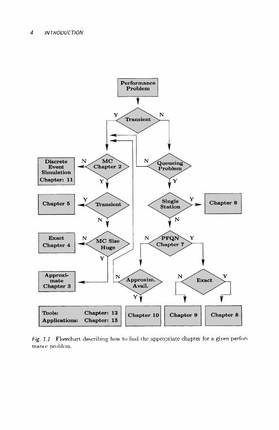
The flowchart shown in Fig. 1.1 gives the organization of this book. After a brief treatment on methodological background (Section 1.2), Section 1.3 covers the basics of probability and statistics. In Chapter 2, Markov chains basics are presented together with generation methods for them. Exact steady- state solution techniques for Markov chains are given in Chapter 3 and their aggregation/disaggregation counterpart in Chapter 4. These aggregation/disaggregation solution techniques are useful for practical Markov chain models with very large state spaces. Transient solution techniques for Markov chains are introduced in Chapter 5.

Chapter 6 deals with the description and coniputation of performance niea- sures for single-station queueing systems in steady state. A general description of queueing networks is given in Chapter 7. Exact solution methods for PFQN are described in detail in Chapter 8 while approximate solution techniques for PFQN are described in Chapter 9. Solution algorithms for different types of NPFQN (such as networks with priorities, nonexponential service times, blocking, or parallel processing) are presented in Chapter 10.

Since there are many practical problems that may not be analytically tractable, discrete-event simulation is commonly used in this situations. We introduce the basics of DES in Chapter 11. For the practical use of modeling techniques described in this book, software packages (tools) are needed. Chap- ter 12 is devoted to the introduction of a queueing network tool, a stochastic Petri net tool, a tool based on Markov chains and a toolkit with many model types, and the facility for hierarchical modeling is also introduced. Each tool is described in some detail together with a simple example. Throughout the book we have provided many example applications of different algorithms introduced in the book. Finally, Chapter 13 is devoted to several large real-life applications of the modeling techniques presented in the book.

4 INTRODUCTION

Fig. 1.1 mance problem.

Flowchart describing how to find the appropriate chapter for a given perfor-

METHODOLOGICAL BACKGROUND 5

1.2 METHODOLOGICAL BACKGROUND

The focus of this book is the application of stochastic and probabilistic methods to obtain conclusions about performance and reliability properties of a wide range of systems. In general, a system can be regarded as a collection of components which are organized and interact in order to fulfill a common task [IEEESO].

Reactive systems and nondeterminism: The real-world systems treated in this book usually contain at least one digital component which controls the operation of other analog or digital components, and the whole system reacts to stimuli triggered by its environment. As an example, consider a computer communication network in which components like routers, switches, hubs, and communication lines fulfill the common task of transferring data packets between the various computers connected to the network. If the system of interest is the communication network only, the connected computers can be regarded as its environment which triggers the network by sending and receiv- ing data packets. The behavior of the systems studied in this book can be characterized as nondeterministic since the stimulation by the environment is usually unpredictable. In case of a communication system like the Internet, the workload depends largely on the number of active users. When exactly a specific user will start to access information on the WWW via a browser is usually riot known in advance. Another source of nondeterminism is the potential failure of one or several system components, which in most cases leads to an altered behavior of the complete system.

Modeling vs. Measurement: In contrast to the empirical methods of measurement, i.e., the collection of output data during the observation of an executing system, the deductive methods of model-based performance evaluation have the advantage to be applicable in situations when the system of interest is not yet existing. Deductive methods can thus be applied during the early design phases of the system developnient process in order to ensure that the final product meets its performance and reliability requirements. Although the material presented in this book is restricted to modeling approaches, it should be noticed that measurement as a supplementary technique can be employed to validate that the conclusions obtained by model-based performance evaluation can be translated into useful statements about the real-world system.

Another possible scenario for the application of modeling is the situation in which measurements on an existing system would either be too dangerous or too expensive. New policies, decision rules, or information flows can be explored without disrupting the ongoing operation of the real system. More- over, new hardware architectures, scheduling algorithms, routing protocols, or reconfiguration strategies can be tested without committing resources for their acquisition/implementation. Also, the behavior of an existing system

6 INTRODUCTION

under a variety of anticipated workloads and environments can be evaluated very cost-effectively in advance by model-based approaches.

1.2.1 Problem Formulation

Before a meaningful model-based evaluation can commence, one should care- fully consider what performance metric is of interest besides the nature of the system. This initial step is indispensable since it determines what is the appropriate formalism to be used. Most of the formalisms presented in the following chapters are suitable for the evaluation of specific metrics but inap- propriate for the derivation of others. In general, it is important to consider the crucial aspects of the application domain with respect to the metrics to be evaluated before starting with the formalization process. Here, the application context strongly determines the kind of information that is meaningful in a concrete modeling exercise.

As an illustrative example, consider the power outage problem of computer systems. For a given hardware configuration, there is no ideal way to represent it without taking into consideration the software applications which run on the hardware and which of course have to be reflected in the model. In a real-time context, such as flight control, even the shortest power failure might have catastrophic implications for the system being controlled. Therefore, an appropriate reliability model of the flight control computer system has to be very sensitive to such a (hopefully) rare event of short duration. In contrast, the total number of jobs processed or the work accomplished by the computer hardware during the duration of a flight is probably a less important performance measure for such a safety-critical system. If the same hardware configuration is used in a transaction processing system, however, short out- ages are less significant for the proper system operation but the throughput is of predominant importance. As a consequence thereof, it is not useful to represent effects of short interruptions in the model, since they are of less importance in this application context.

Another important aspect to consider at the beginning of a model-based evaluation is how a reactive real-world system - as the core object of the study - is triggered by its environment. The stimulation of the system by its environment has to be captured in such a way during formalization so it reflects the conditions given in the real world as accurately as possible. Otherwise, the measures obtained during the evaluation process cannot be meaningfully retrarisformed into statements about the specific scenario in the application domain. In t,he context of stochastic modeling, the expression of the environment’s influence on the system in the model is usually referred to as workload modeling. A frequently applied technique is the characterization of the arriving workload, e.g., the parts which enter a production line or the arriving data packets in a communication system, as a stochastic arrival process. Various arrival processes which are suitable in specific real-world scenarios can be defined (see Section 6.8).


The following four categories of system properties which are within the scope of the methods presented in this book can be identified:

Performance Properties: They are the oldest targets of performance evaluation and have been calculated already for non-compiiting systems like tele- phone switching centers [Erlal7] or patient flows in hospitals [Jack541 using closed-form descriptions from applied probability theory. Typical properties to be evaluated are the mean throughput of served customers, the mean waiting, or response time and the utilization of the various system resources. The IEEE standard glossary of software engineering terminology [IEEESO] contains the following definition:

Definition 1.1 Performance: The degree to which a system or component accomplishes its designated functions within given constraints, such as speed, accuracy, or memory usage.

Reliability and Availability: Requirements of these types can be evaluated quantitatively if the system description contains information about the failure and repair behavior of the system components. In some cases it is also necessary to specify the conditions under which a new user cannot get access to the service offered by the operational system. The information about the failure behavior of system components is usually based on heuristics which are reflected in the parameters of probability distributions. In [IEEESO], software reliability is defined as:

Definition 1.2 Reliability: The probability that the software will not cause the failure of the system for a specified time under specified conditions.

System reliability is a measure for the continuity of correct service, whereas availatdity measures for a system refer to its readiness for correct service, as stated by the following definition from [IEEESO]:

Definition 1.3 Availability: The ability of a system to perform its required function at a stated instant or over a stated period of time. It is usually expressed as the availability ratio, i.e., the proportion of time that the service is actually available for use by the Customers within the agreed service hours.

Note that reliability and availability are related yet distinct system properties: a system which - during a mission time of 100 days -~ fails on average every two minutes but becomes operational again after a few milliseconds is not very reliable but nevertheless highly available.

Dependability and Performability: These terms and the definitions for them originated from the area of dependable and faul t tolerant computing. The following definition for dependability is taken from [ALRL04]:

Definition 1.4 Dependability: The dependability of a computer system is the ability to deliver a service that can justifiably be trusted. The service

delivered by a system is its behavior as it is perceived by its user(s); a user is another system (physical, human) that interacts with the former at the service interface.

This is a rather general definition which comprises the five attributes availability, reliability, maintainabi l i ty - the systems ability to undergo modifications or repairs, integrity - the absence of improper system alterations and safety as a measure for the continuous delivery of service free from occurrences of catastrophic failures. The term performabili ty was coined by J.F. MEYER [Meye781 as a measure to assess a system’s ability to perform when performance degrades as a consequence of faults:

Definition 1.5 Performability: The probability that the system reaches an accomplishment level y over a utilization interval (0, t ) . That is, the probability that the system does a certain amount of useful work over a mission time t .

Subsequently, many other measures are included under performance as we shall see in Section 2.2. Informally, the performability refers to performance in the presence of failures/repair/recovery of components and the system. Performability is of special interest for gracefully degrading s y s t e m s [Beau77]. In Section 2.2, a framework based on Markov reward models (MRMs) is presented which provides recipes for a selection of the right model type and the definition of an appropriate performance measure.

1.2.2 The Modeling Process

The first step of a model-based performance evaluation consists of the formalization process, during which the modeler generates a f o r m a l description of the real-world system. Figure 1.2 illustrates the basic idea: Starting from an informal system description, e.g. in natural language, which includes struc- tural and functional information as well as the desired performance and reliability requirements, the modeler creates a formal model of the real-world system using a specific conceptualization. A conceptualization is an abstract, simplzfied view of the reference reality which is represented for some purpose. Two kinds of conceptualizations for the purpose of performance evaluation are presented in detail in this book: If the system is to be represented as a queueing network, the modeler applies a ?outed job flow” modeling paradigm in which the real-world system is conceptualized as a set of service stations which are connected by edges through which independent entities “ f l o ~ ” through the network and sojourn in the queues and servers of the service stations (see Chapter 7). In an alternative Markov chain conceptualization a “state- transition” modeling paradigm is applied in which the possible trajectories through the system’s global state space are represented as a graph whose directed arcs represent the transitions between subsequent system states (see Chapter 2). The main difference between the two conceptualizations is that


the queueing network formalism is oriented more towards the structure of the real-world system, whereas in the Markov chain formalization the emphasis is put on the description of the system behavior on the underlying state- space level. A Markov chain can be regarded to “mimic” the behavior of the executing real-world system, whereas the service stations and jobs of a queueing network establish a one-to-one correspondence to the components of the real-world system. As indicated in Fig. 1.2, a Markov chain serves as the underlying semantic model of the high-level queueing network model.

Fig. 1.2 Formalization of a real-world system.

During the formalization process the following abstractions with respect to the real-world system are applied:

0 In both conceptualizations the behavior of the real-world system is regarded to evolve in a discrete-event fashion, even if the real-world system contains components which exhibit continuous behavior, such as the movements of a conveyor belt of a production line.

0 The application of the queueing network formalism abstracts away from all synchronization mechanisms which may be present in the real-world system. If the representation of these synchronization mechanisms is crucial in order to obtain useful results from the evaluation, the niodeler can resort to variants of stochastic Petri nets as an alternative description t,echnique (see Section 2.3 and Section 2.3.6) in which almost arbi- trary synchronization pattcrns can be captured.

0 The corc abstractions applied during the formalization process are the association of system activity durations with random variables and the inclusion of branching probabilities to represent alternative system evo- lutions. Both abstractions resolve the nondeterminisrn inherent in the

10 lNTRODUCTlON

real-world system and turn the formal queueing network or Markov chain prototype into an “executable” specification [WingOl]. For these, at any moment during their operation each possible future evolution has a well-defined probability to oc(w. Depending on which kind of random variables are used to represent the durations of the system activities either a discrete-time interpretation using a DTMC or a continuous-time interpretation of the system behavior based on a CTMC is achieved. It should be noted that for systems with asynchronously evolving components the continuous-time interpretation is more appropriate since changes of the global system state may occur at any moment in continuous time. Systems with components that evolve in a lock-step fashion triggered by a global clock are usually interpreted in discrete-time.

1.2.3 Evaluation

The second step in the model-based system evaluation is the deduction of performance measures by the application of appropriate solution methods. Depending on the conceptualization chosen during the formalization process the following solution methods are available:

Analytical Solutions: The core principle of the analytic: solution methods is to represent the formal system description either as a single equation from which the interesting measures can be obtained as closed-form solutions, or as a set of system equations from which exact or approximate measures can be calculated by appropriate algorithms from numerical mathematics.

1. Closed-form solutions are available if the system can be described as a simple queucing system (see Chapter 6) or for simple product-form queueing networks (PFQN) [Chhla83] (see Section 7.3) or for structured small CTMCs. For these kind of formalizations equations can be derived from which the mean number of jobs in the service stations can be calculated as a closed-form solution, i.e., the solutions can be expressed analytically in terms of a bounded number of well-known operations. Also from certain types of Markov chains with regular structure (see Section 3. 1), closed-form representations like the well-known Erlang- B and Erlang-C formulae [Erlal7] can be derived. The measures can either be computed by ad-hoc programming or with the help of computer algebra packages such as Mathernatica [Mat05]. A big advantage of‘the closed-form solutions is their moderate computational complexity which enables a fast calculation of performance measures even for larger system descriptions.

2. Numerical solutions: Many types of equations which can be derived from a formal system description do not possess a closed-form solution, e.g., in the case of complex systems of integro-differential equations. In these cases, approximate solutions can be obtained by the appli-


cation of algorithms from numerical mathematics, many of which are implemented in computer algebra packages [Mat051 or are integrated in performance analysis tools such as SHARPE [HSZTOO], SPNP [HTTOO], or TimeNET [ZFGHOO] (see Chapter 12). The formal system descriptions can be either given as a queueing network, stochastic Petri net or another high-level modeling formalism, from which a state-space representation is generated manually or by the application of state-space generation algorithms. Depending on the stochastic information present in the high-level description, various types of system state equations which mimic the dynaniics of the modeled system can be derived and solved by appropriate algorithms. The numerical solution of Markov models is discussed in Chapters 3 ~ 5, numerical solution methods for queueing networks can be found in Chapters 7 - 10. In comparison to closed-form solution approaches, numerical solution met hods usually have a higher computational complexity.

Simulation Solutions: For many types of models no analytic solution method is feasible, because either a theory for the derivation of proper system equations is not known, or the computational complexity of an applicable numerical solution algorithm is too high. In this situation, solutions can be obtained by the application of discrete-event simulation (DES), which is described in detail in Chapter 11. Instead of solving system equations which have been derived from the formal model, the DES algorithm “executes” the model and collects the information about the observed behavior for the subsequent derivation of performance measures. In order to increase the quality of the results, the simulation outputs collected during multiple “executions” of the model are collected and from which the interesting measures are calculated by statistical methods. All the formalizations presented in this book, i.e., queueing networks, stochastic Petri nets, or Markov chains can serve as input for a DES, which is the most flexible and generally applicable solution method. Since the underlying state space does not have to be generated, simulation is not affected by the state-space explosion problem. Thus, simulation can also be employed for the analysis of complex models for which the numerical approaches would fail because of an exuberant number of system states.

Hybrid solutions: There exists a number of approaches in which different modeling formalisms and solution methods are combined in oder to exploit their coniplementing strengths. Examples of hybrid solution methods are mixed simulation and analytical/numerical approaches, or the combination of fault trees, reliability block diagrams, or reliability graphs, and Markov models [STP96]. Also product-form queueing networks and stochastic Petri nets or non-product-form networks and their solution methods can be combined. More generally, this approach can be characterized as intermingling of state- space-based and non-state-space-based methods [STP96]. A combination of analytic and simulative solutions of connected sub-models may be employed

to combine the benefits of both solution methods [Sarg94, ShSa831. More cri- teria for a choice between simulation and analytical/numerical solutions are discussed in Chapter 11.

Largeness Tolerance: Many high-level specification techniques, queueing systems, generalized stochastic Petri nets (GSPNs), and stochastic reward nets (SRNs), as the most prominent representatives, have been suggested in the literature to automate the model generation [HaTr93]. GSPNs/SRNs that are covered in more detail in Section 2.3, can be characterized as tolerating largeness of the underlying computational models and providing effective means for generating large state spaces.

Largeness Avoidance: Another way to deal with large models is to avoid the creation of such models from the beginning. The major largeness-avoidance technique we discuss in this book is that of product-form queueing networks. The main idea is, the structure of the underlying CTMC allows for an efficient solution that obviates the need for generation, storage, and solution of the large state space. The second method of avoiding largeness is to separate the originally single large problem into several smaller problems and to combine sub-model results into an overall solution. Both approximate and exact techniques are known for dealing with such multilevel models. The flow of information needed among sub-models may be acyclic, in which case a hierarchical model [STP96] results. If the flow of needed information is non-acyclic, a fixed-point iteration may be necessary [CiTr93]. Other well-known techniques applicable for limiting model sizes are state truncation [BVDT88, GCS+86] and state lumping [NicoSO].

1.2.4 Summary

Figure 1.3 summarizes the different phases and activities of the model-based performance evaluation process. Two main scenarios are considered: In the first one, model-based performance evaluation is applied during the early phases of the system development process to predict the performance or reliability properties of the final product. If the predicted properties do not fulfill the given requirements, the proposed design has to be changed in order to avoid the expected performance problems. In the second scenario, the final product is already available and model-based performance evaluation is applied to derive optimal system configuration parameters, to solve capacity planning problems, or to check whether the existing system would still operate satis- factorily after a modification of its environment. In both scenarios the first activity in the evaluation process is to collect information about the structure and functional behavior of an existing or planned system. The participation of a domain expert in this initial step is very helpful and rather indispensable for complex applications. Usually, the collected information is stated informally and stored in a document using either a textual or a combined textu-

Queueing Networks and Markov Chains...Queueing Networks and Markov Chains Modeling and Performance Evaluation with Computer Science Applications Second Edition Gunter Bolch Stefan

Documents