Queueing Models with Multiple Waiting Lines

Queueing models with multiple waiting lines

I.J.B.F. Adan, O.J. Boxma1, J.A.C. Resing

Department of Mathematics and Computing Science,Eindhoven University of Technology,

P.O. Box 513, 5600 MB Eindhoven, The Netherlands

Abstract

This paper discusses analytic solution methods for queueing models with multiple wait-ing lines. The methods are briefly illustrated, using key models like the 2 × 2 switch, theshortest queue and the cyclic polling system.

AMS subject classification: 60K25, 90B22.Keywords and phrases: multiple waiting lines, analytic methods.

1 Introduction

This paper reviews analytic solution methods for queueing models with multiple waiting lines.The models under consideration represent isolated service centers; we do not consider networksof queues. We basically distinguish between two classes of models.Class I: Customers arrive at a service center with several queues, each with one server. Thecustomers choose a server according to some mechanism (e.g., shortest queue or shortest work-load) or divide their work among several servers (e.g., fork-join).Class II: Customers of several types arrive at a service center with one or more servers. Theserver or servers choose a customer for service according to some static (e.g., preemptive re-sume) or dynamic (e.g., polling) priority rule.While not all queueing models with multiple waiting lines are naturally classified as belongingto Class I (passive servers; customers choose a queue) or Class II (active servers; servers choosea customer), this classification does help to bring some structure in the large family of queueingmodels with multiple waiting lines.

Our aim in this paper is to give the reader insight into which methods are available for theanalysis of queueing models with multiple waiting lines. These queueing models often giverise to Markov processes with an N -dimensional state space that is the set of lattice points withinteger-valued, nonnegative coordinates. The methods for solving the equilibrium equations ofsuch Markov processes may also be divided into two groups.Complex-function methods: These methods aim at solving the functional equation for the gen-erating function of the equilibrium distribution.

1also: CWI, P.O. Box 94079, 1090 GB Amsterdam, The Netherlands.

1

Direct methods: Their aim is to solve directly (i.e., without resorting to transforms) the equilib-rium equations.We emphasize the main ideas behind the methods, and their strengths and limitations. We alsopoint out some relations between the various methods. While our orientation is methodological,we do pay much attention to a few particular queueing models. These are relatively simple butimportant models, that are used as vehicle to illustrate and compare various methods.

We already mentioned that not all queueing models with multiple waiting lines will fit intoour classification. One of these are the interesting queueing models with simultaneous resourcepossession. For these models an important new product-form result has been established byBerezner et al. [16] which shows that at least in some simple situations they have an exactexplicit solution.

The paper is organized in the following way. In Section 2 we discuss three direct methods(the compensation method, the precedence-relation method and the power-series algorithm) andtwo methods from complex-function theory (the boundary value method and the uniformizationmethod). They are discussed for two basic models of Class I: the 2 × 2 switch and the short-est queue. In Section 3 we consider models of Class II. Some of the above-mentioned meth-ods also apply to those models; we also discuss some other methods from complex-functiontheory. Most analytically tractable queueing models are special examples of particular, oftentwo-dimensional, Markov processes or random walks. Section 4 considers a few classes oftwo-dimensional random walks that allow an exact analysis.

2 Customers choose a queue

2.1 Introduction

In this section we consider two basic queueing models where arriving customers choose a wait-ing line, viz. the 2 × 2 switch and the shortest queue model. We expose and compare severaltechniques that have been used to analyse these models. We end the section with a brief dis-cussion of the fork-join queue, a queueing model in which each job consists of various subjobswho each choose a different queue.

2.2 The 2 × 2 switch

Among the queueing models with multiple waiting lines, the 2 × 2 switch may be the simplestnon-trivial model. It is therefore most suitable for exposing and comparing various analyticsolution techniques. In the present subsection we shall discuss three such techniques, viz.:(i) the compensation method, (i i) the boundary value method, and (i i i) the uniformizationmethod. But first we describe the model.

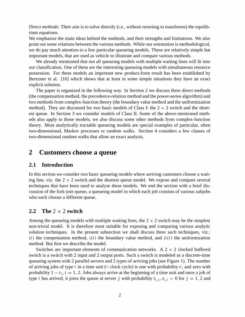
Switches are important elements of communication networks. A 2 × 2 clocked bufferedswitch is a switch with 2 input and 2 output ports. Such a switch is modeled as a discrete-timequeueing system with 2 parallel servers and 2 types of arriving jobs (see Figure 1). The numberof arriving jobs of type i in a time unit (= clock cycle) is one with probability ri and zero withprobability 1 − ri , i = 1, 2. Jobs always arrive at the beginning of a time unit and once a job oftype i has arrived, it joins the queue at server j with probability ti, j , ti, j > 0 for j = 1, 2 and

2

ti,1 + ti,2 = 1. Jobs that have arrived at the beginning of a time unit are immediately candidatesfor service. A server serves exactly one job per time unit, if at least one is present. For eachserver, the average number of arriving jobs per time unit is assumed to be less than one, i.e.

r1t1, j + r2t2, j < 1, j = 1, 2. (2.1)

This assumption guarantees the ergodicity of the system. By (2.1), the case r1 = r2 = 1 mustbe excluded.

�r2

��

t2;2

�r1

��

t1;1 �t1;2

�

t2;1

2

1

�

�

Figure 1: The 2 × 2 switch.

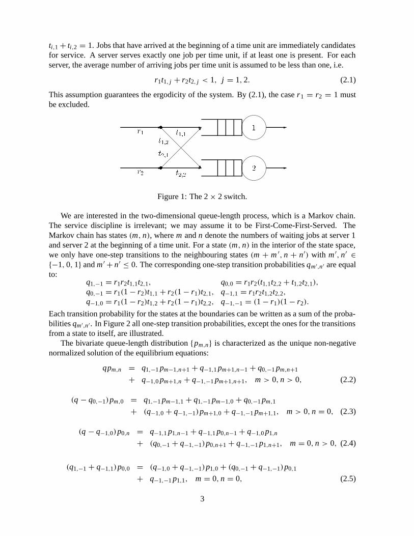
We are interested in the two-dimensional queue-length process, which is a Markov chain.The service discipline is irrelevant; we may assume it to be First-Come-First-Served. TheMarkov chain has states (m, n), where m and n denote the numbers of waiting jobs at server 1and server 2 at the beginning of a time unit. For a state (m, n) in the interior of the state space,we only have one-step transitions to the neighbouring states (m + m ′, n + n′) with m ′, n′ ∈{−1, 0, 1} and m ′ + n′ ≤ 0. The corresponding one-step transition probabilities qm′,n′ are equalto:

q1,−1 = r1r2t1,1t2,1, q0,0 = r1r2(t1,1t2,2 + t1,2t2,1),q0,−1 = r1(1 − r2)t1,1 + r2(1 − r1)t2,1, q−1,1 = r1r2t1,2t2,2,q−1,0 = r1(1 − r2)t1,2 + r2(1 − r1)t2,2, q−1,−1 = (1 − r1)(1 − r2).

Each transition probability for the states at the boundaries can be written as a sum of the proba-bilities qm′,n′. In Figure 2 all one-step transition probabilities, except the ones for the transitionsfrom a state to itself, are illustrated.

The bivariate queue-length distribution {pm,n} is characterized as the unique non-negativenormalized solution of the equilibrium equations:

qpm,n = q1,−1 pm−1,n+1 + q−1,1 pm+1,n−1 + q0,−1 pm,n+1

+ q−1,0 pm+1,n + q−1,−1 pm+1,n+1, m > 0, n > 0, (2.2)

(q − q0,−1)pm,0 = q1,−1 pm−1,1 + q1,−1 pm−1,0 + q0,−1 pm,1

+ (q−1,0 + q−1,−1)pm+1,0 + q−1,−1 pm+1,1, m > 0, n = 0, (2.3)

(q − q−1,0)p0,n = q−1,1 p1,n−1 + q−1,1 p0,n−1 + q−1,0 p1,n

+ (q0,−1 + q−1,−1)p0,n+1 + q−1,−1 p1,n+1, m = 0, n > 0, (2.4)

(q1,−1 + q−1,1)p0,0 = (q−1,0 + q−1,−1)p1,0 + (q0,−1 + q−1,−1)p0,1

+ q−1,−1 p1,1, m = 0, n = 0, (2.5)

3

�

m �

n

�

�q1;�1

�q�1;1

�q�1;0 + q

�1;�1

�q1;�1

�q�1;1

�

�q0;�1 + q�1;�1

�q�1;1

�q1;�1

�

�q1;�1

�q0;�1

�q�1;�1

�q�1;0

�q�1;1

�

Figure 2: The one-step transition probabilities.

whereq := q1,−1 + q−1,1 + q0,−1 + q−1,0 + q−1,−1. (2.6)

We now describe three methods to solve these equations.

Method 1: The compensation methodThis method yields an explicit expression, without transforms, for the equilibrium distribution.It is not only successful for this model, but in [9] it has been shown to work for the classof two-dimensional nearest-neighbor random walks (i.e., with unit steps only) for which inthe interior of the state space no one-step transitions are allowed to the North, North-Eastand East, and also for some special cases not contained in this class (see [8, 6]). Clearly, thepresent random walk is an element in this class (see Figure 2). It is a special one, because thetransition probabilities on the boundaries are ‘projections’ of the transition probabilities in theinterior states. This property leads to several simplifications in the analysis. But the essentialcharacteristics in the analysis are still maintained and therefore the problem is most suitable todemonstrate the compensation method.

The compensation method attempts to solve the equilibrium equations by a linear combi-nation of product forms. This is achieved by first characterizing a sufficiently rich basis ofproduct-form solutions satisfying the equilibrium equations in the interior of the state space.Subsequently this basis is used to construct a linear combination that also satisfies the equa-tions for the boundary states. A similar method is of course well known in the theory of dif-ferential and difference equations (cf. the separation of variables method [73]) where the basisusually contains countably many elements, all of which are used to construct the solution. Inthe present model, however, the basis contains uncountably many elements. Therefore a proce-dure is needed to select the appropriate elements. This procedure is based on a compensationargument (which explains the name of the method): after introducing the first term, countablymany terms are subsequently added so as to alternatingly compensate for the error on one ofthe two boundaries. The main steps in the analysis will be briefly outlined below (see [28] for

4

more details on the 2 × 2 switch case).

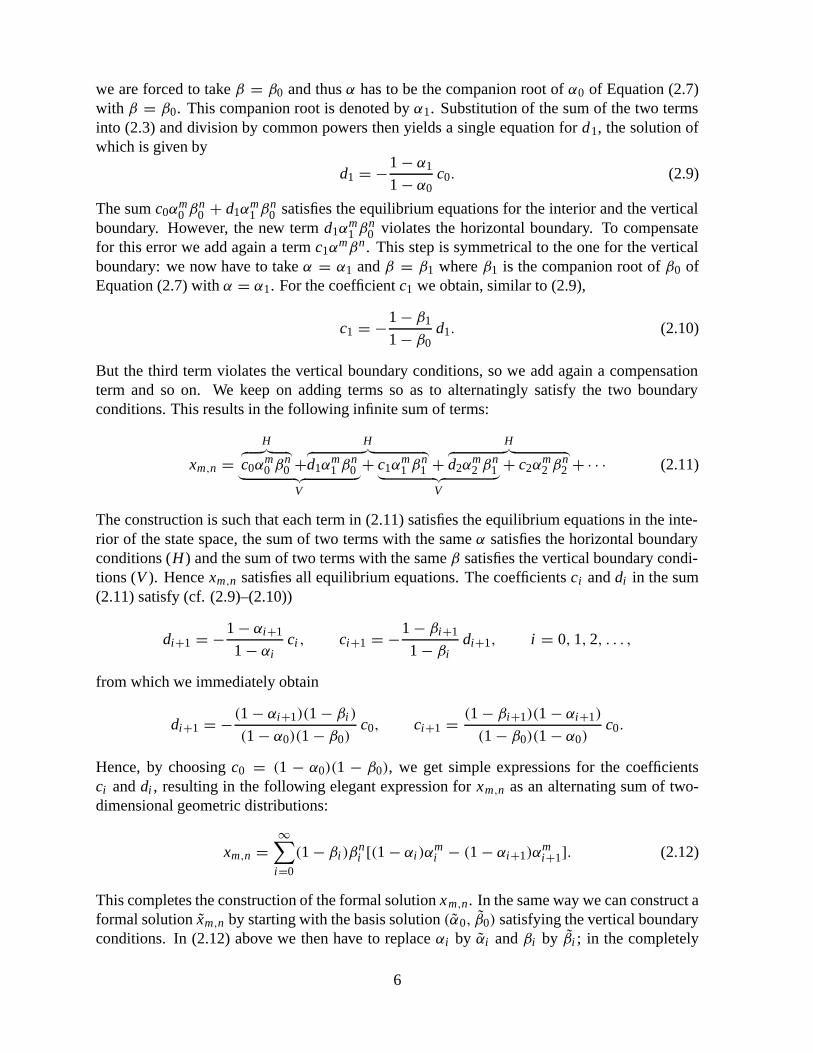
Step 1: Characterize the set of product forms αmβn satisfying the equilibrium equations in theinterior of the state space, i.e., the equations (2.2). Substitution of the product form into (2.2)and division by common powers yields a quadratic equation in α and β:

qαβ = q1,−1β2 + q−1,1α

2 + q0,−1αβ2 + q−1,0α

2β + q−1,−1α2β2 . (2.7)

Because later in the analysis the solution has to be normalized, the factors α and β are requiredto satisfy 0 < |α| < 1 and 0 < |β| < 1. The points on the curve (2.7) inside this regioncharacterize a continuum of product forms satisfying the inner equations (see Figure 3).

1 α

1

β

••

•

α 0α 1

β0

β1

Figure 3: Curve (2.7) in the positive quadrant, generating the sequence α0, β0, α1, β1, . . .

Step 2: Construct a linear combination of elements in this rich basis, which is a formal solutionto the equilibrium equations. Here the word formal is used to indicate that (at this stage) wedo not bother about the convergence of the solution. This aspect will be taken care of later.The construction of a linear combination starts with a suitable initial term. This is a basissolution αm

0 βn0 that also satisfies the equilibrium equations on one of the two boundaries, i.e.,

the equations (2.3) or (2.4). Later we will explain why a special starting solution is needed. Inthe general case in [9] one finds at least one and at most four initial terms. Here there exist twoinitial terms: one for the horizontal boundary and another for the vertical boundary. Both termscan be explicitly calculated. The first one is given by

(α0, β0) = (q1,−1

q−1,1 + q−1,0 + q−1,−1,

q−1,1α20

q1,−1 + q0,−1α0 + q−1,−1α20

) ; (2.8)

the term (α0, β0) for the vertical boundary is symmetrical. Let us consider the initial termc0α

m0 β

n0 for the horizontal boundary, where c0 is a (arbitrary) nonnull constant. This term

violates the equilibrium equations (2.4) on the vertical boundary. To compensate for this errorwe add a term d1α

mβn with α and β satisfying (2.7) such that the sum of the two terms satisfiesthe equilibrium equations in all states on the vertical boundary. This immediately implies that

5

we are forced to take β = β0 and thus α has to be the companion root of α0 of Equation (2.7)with β = β0. This companion root is denoted by α1. Substitution of the sum of the two termsinto (2.3) and division by common powers then yields a single equation for d1, the solution ofwhich is given by

d1 = −1 − α1

1 − α0c0. (2.9)

The sum c0αm0 β

n0 + d1α

m1 β

n0 satisfies the equilibrium equations for the interior and the vertical

boundary. However, the new term d1αm1 β

n0 violates the horizontal boundary. To compensate

for this error we add again a term c1αmβn . This step is symmetrical to the one for the vertical

boundary: we now have to take α = α1 and β = β1 where β1 is the companion root of β0 ofEquation (2.7) with α = α1. For the coefficient c1 we obtain, similar to (2.9),

c1 = −1 − β1

1 − β0d1. (2.10)

But the third term violates the vertical boundary conditions, so we add again a compensationterm and so on. We keep on adding terms so as to alternatingly satisfy the two boundaryconditions. This results in the following infinite sum of terms:

xm,n = ︸ ︷︷ ︸V

H︷ ︸︸ ︷c0α

m0 β

n0 +

H︷ ︸︸ ︷d1α

m1 β

n0 + ︸ ︷︷ ︸

V

c1αm1 β

n1 +

H︷ ︸︸ ︷d2α

m2 β

n1 + c2α

m2 β

n2 + · · · (2.11)

The construction is such that each term in (2.11) satisfies the equilibrium equations in the inte-rior of the state space, the sum of two terms with the same α satisfies the horizontal boundaryconditions (H ) and the sum of two terms with the same β satisfies the vertical boundary condi-tions (V ). Hence xm,n satisfies all equilibrium equations. The coefficients ci and di in the sum(2.11) satisfy (cf. (2.9)–(2.10))

di+1 = −1 − αi+1

1 − αici , ci+1 = −1 − βi+1

1 − βidi+1, i = 0, 1, 2, . . . ,

from which we immediately obtain

di+1 = −(1 − αi+1)(1 − βi )

(1 − α0)(1 − β0)c0, ci+1 = (1 − βi+1)(1 − αi+1)

(1 − β0)(1 − α0)c0.

Hence, by choosing c0 = (1 − α0)(1 − β0), we get simple expressions for the coefficientsci and di , resulting in the following elegant expression for xm,n as an alternating sum of two-dimensional geometric distributions:

xm,n =∞∑

i=0

(1 − βi )βni [(1 − αi )α

mi − (1 − αi+1)α

mi+1]. (2.12)

This completes the construction of the formal solution xm,n. In the same way we can construct aformal solution xm,n by starting with the basis solution (α0, β0) satisfying the vertical boundaryconditions. In (2.12) above we then have to replace αi by αi and βi by βi ; in the completely

6

symmetric case these equal βi and αi , respectively.

Step 3: Prove that the two formal solutions converge. In the general case in [9] it is shown thatthe formal solutions absolutely converge in all states, except in a (possibly empty) neighbor-hood of the origin. It is important to note that the requirement of convergence of the formalsolutions is responsible for the exclusion of one-step transitions to the North, North-East andEast and the need of suitable initial terms. In the present model x(m, n) and x(m, n) convergeeverywhere, except in (0, 0). Hence they satisfy the equilibrium equations in all states, exceptin (0, 0), (1, 0) and (0, 1).

Step 4: Determine the equilibrium probabilities by taking the linear combination p(m, n) =cx(m, n)+ cx(m, n) in all states, except in the origin. The unknowns p(0, 0), c and c are thendetermined from the normalization equation and the equilibrium equations in (1, 0) and (0, 1).Here we may omit the one in (0, 0), because the equilibrium equations are dependent. In thepresent model the coefficients can be solved explicitly, namely c = c = 1. So the equilibriumprobabilities can be simply expressed as:

pm,n = xm,n + xm,n, m ≥ 0, n ≥ 0,m + n > 0. (2.13)

Clearly, from this result we can derive similar expressions for performance characteristics suchas, e.g., the mean queue lengths and the correlation between the queue lengths.

The compensation method clearly has its limitations. The most important one is that tran-sitions to the North, North-East and East are forbidden in the case of two-dimensional nearest-neighbor random walks. The conditions become even more severe for the extension to higherdimensional random walks (see [81]). The strong feature of the method, however, is that ithelps in finding such conditions for getting explicit solutions and that it provides constructivemethods for obtaining the explicit solutions in case the conditions are satisfied.

Method 2: The boundary value methodComplex-function methods aim at solving the equilibrium equations by introducing the gen-erating function of the equilibrium distribution and studying the functional equations that itshould satisfy. Usually, those functional equations present formidable difficulties. For a classof two-dimensional random walks and queueing problems, however, techniques have been de-veloped which reduce those functional equations to standard Riemann(-Hilbert) boundary valueproblems and to singular integral equations for complex-valued functions. The general theory isexposed in the monograph [47] and surveyed in [38]. Jaffe [87] has applied this ‘boundary valuemethod’ to the (symmetric) 2×2 clocked buffered switch. Below we outline his approach; laterin this section we point out some differences and similarities with the compensation method. Inthe symmetric case we write r1 = r2 = p, 0 < p < 1, while t1,1 = t1,2 = t2,1 = t2,2 = 1

2 .Step 1: The set-up. We introduce the generating function

f (x, y) :=∞∑

m=0

∞∑n=0

pm,nxm yn, |x | ≤ 1, |y| ≤ 1. (2.14)

It follows from (2.2)-(2.5) that f (x, y) satisfies the following functional equation: For |x | ≤ 1,

7

|y| ≤ 1,

(xy − r(x, y)) f (x, y) = (y − 1)r(x, 0) f (x, 0)+ (x − 1)r(0, y) f (0, y)

+ (x − 1)(y − 1)r(0, 0) f (0, 0), (2.15)

wherer(x, y) := (1 − p + p

2(x + y))2. (2.16)

The distribution {pm,n} is completely determined by (2.15), the normalizing condition f (1, 1) =1, and the fact that the probability generating function f (x, y) should be regular for |x | < 1,continuous for |x | ≤ 1 for all |y| ≤ 1, and similarly with x and y interchanged. In the sequel,we denote the interior of these unit circles by D, and their closure by D.

Step 2: Analysis of ‘the kernel’. The boundedness of f (x, y) implies that the right-hand side of(2.15) should be zero for all those (x, y) on the complex curve S = {(x, y) : xy − r(x, y) = 0},that lie in D2. These zeros of the kernel xy − r(x, y) offer a large choice. It suffices to choosean appropriate set; by analytic continuation, other zero-tuples of the kernel may be constructed.In this symmetric case, it is natural to consider those (x, y) on S with y = x . This is an ellipseE = {x : |x |2 = r(x, x), x ∈ D}.

Step 3: Formulation of a boundary value problem. For the present example this proceeds asfollows. Introduce for |x | ≤ 1, |x | �= 1,

g(x) := r(x, 0) f (x, 0)

x − 1+ 1

2r(0, 0) f (0, 0) = r(0, x) f (0, x)

x − 1+ 1

2r(0, 0) f (0, 0). (2.17)

Then the boundedness of f (x, y) in D2, combined with the fact that g(·) has a simple pole at1, implies that

g(x)+ g(x) = 2Re g(x) = 0, x ∈ E\{1}, (2.18)

limx→1

(x − 1)g(x) = 1 − p. (2.19)

We now have a boundary value problem: Determine a function g(x) that is analytic inside theellipse E , that has a simple pole at 1, and that satisfies (2.18) on the ellipse (on the boundary).Let φ, with inverse ψ , be the conformal mapping of the unit disk onto the region bounded by E ,with normalization conditions φ(0) = p/(1+ p), φ(1) = 1. Define h(w) := g(φ(w)). We thenobtain a relatively simple ‘Riemann-Hilbert boundary value problem with a pole’, cf. SectionI.3.3 of [47], for h(.) on the unit circle D (actually, it is a Dirichlet problem with a pole):

Re h(w) = 0, w ∈ D\{1}, (2.20)

limw→1

(w − 1)h(w) = 1 − p

φ′(1), (2.21)

with h(.) analytic on D, continuous on D\{1}. The solution of this boundary value problem is

h(w) = 1

2

1 − p

φ′(1)w + 1

w − 1, w ∈ D, (2.22)

8

which determines g(x) = h(ψ(x))= 12

1−pφ′(1)

ψ(x)+1ψ(x)−1 inside the ellipse E ; the conformal mapping

ψ(x) is explicitly expressed in the Jacobi elliptic (sin am or sn) function. Substitution in (2.15)and analytic continuation finally yields f (x, y), for |x | ≤ 1, |y| ≤ 1:

f (x, y) = (1 − p)ψ ′(1) (x − 1)(y − 1)

(ψ(x)− 1)(ψ(y)− 1)

ψ(x)ψ(y)− 1

xy − r(x, y). (2.23)

Remark 2.1 The boundary value method may also be applied to the asymmetric 2 × 2 clockedbuffered switch. In fact, it can even be applied to a much more general class of two-dimensionalrandom walks and queueing models; see Subsection 4.3.

Method 3: The uniformization methodThe ‘uniformization method’ is a complex-function method that has been applied by Kingman[91] and Flatto and McKean [68] to the symmetric shortest queue, and by Jaffe [87] to thesymmetric 2 × 2 clocked buffered switch. It has been applied by Cohen to both the symmet-ric [43] and asymmetric [44] 2 × 2 clocked buffered switch and for the symmetric [42] andasymmetric [45] shortest queue. The global idea of the uniformization method is as follows.Firstly, as in the above-described boundary value method, the generating function f (x, y) ofthe two-dimensional equilibrium distribution is introduced, and the equilibrium equations forthe distribution lead to a functional equation for f (x, y). The relatively simple form of thekernel K (x, y) (=xy − r(x, y) in the case of the 2 × 2 switch) allows the following approach.K (x, y) = 0 defines an algebraic curve, which can be uniformized in a convenient way. In-troduce a uniformizing variable p, writing x = x(p) and y = y(p). Consider f (x(p), 0) andf (0, y(p)). They are shown to be analytic functions of p in certain p-regions; in addition,for all p with |x(p)| ≤ 1, |y(p)| ≤ 1, for which K (x(p), y(p)) = 0, the boundedness off (x(p), y(p)) results in a relation between f (x(p), 0) and f (0, y(p)). This relation is usedto continue f (x(p), 0) and f (0, y(p)) meromorphically into the plane 0 < |p| < ∞. For the2×2 switch as well as the shortest queue, the generating functions f (x, 0) and f (0, y) turn outto be meromorphic, i.e., all their singularities are isolated poles. Starting with a certain pole,one may find another pole that is linked to it via the fact that together they make the kernel zero,etc., ad infinitum (in much the same way as, in the compensation method, each boundary con-dition gives rise to yet another product-form term in an infinite sum; the reader will realize thattaking generating functions of xm,n in (2.12) results in terms 1

1−αi x1

1−βi y , with poles x = 1/αi ,y = 1/βi ).

We discuss the determination of the poles, and also the zeros, in some more detail for thecase of the symmetric 2 × 2 clocked buffered switch.

Step 1: The poles. As observed above, for all those zero-tuples (x, y) of the kernel xy − r(x, y)that lie inside D2, we should have

g(x)+ g(y) = r(x, 0) f (x, 0)

x − 1+ r(0, y) f (0, y)

1 − y+ r(0, 0) f (0, 0) = 0. (2.24)

Since xy − r(x, y) is a biquadratic form in x and y, it is easily seen that it has, for each fixedx , two zeros y1(x) and y2(x) with the property that |y1(x)| < |x | < |y2(x)| for |x | ≥ 1,x �= 1; analogously for x1(y) and x2(y). Cohen [43] equates −r(x, 0) f (x, 0)/(x − 1) to

9

r(0, y2(x)) f (0, y2(x))/(1−y2(x))+r(0, 0) f (0, 0), via (2.24), and uses this to continue f (x, 0)analytically outside the unit circle; similarly for f (0, y). The only points where these functionsare not analytic are the simple poles y+

n respectively x+n , n = 1, 2, . . . . With x+

0 = y+0 := 1

(remember that g(x) has a simple pole in x = 1!), we have y+1 := y2(x

+0 ) = (2 − p)2/p2,

y+n := y2(x

+n−1) = x+

n = x2(y+n−1), n = 1, 2, . . . . Note that y+

n = x+n due to the complete

symmetry of the model under consideration.

Step 2: The zeros. After having thus shown that f (x, 0) has a unique analytic continuation in|x | ≥ 1, except for x = x+

n , n = 1, 2, . . . , where it has simple poles, Cohen [43] also determinesall zeros of f (x, 0) (this is a rare case in which all zeros can be determined explicitly). Heobserves that r(x, 0) has only one zero x = x−

0 = 2 − 2/a, and this zero has multiplicitytwo. Introducing y−

1 := y2(x−0 ), x−

n = x2(y−n−1) = y−

n = y2(x−n−1), n = 1, 2, . . . , it follows

from g(x) = −g(y2(x)) and g(y) = −g(x2(y)) that f (x, 0) (and, symmetrically, f (0, x)) haszeros of multiplicity two at x = x−

2n, n = 1, 2, . . . (and r(x,0) f (x,0)1−x + r(0, 0) f (0, 0) has zeros

of multiplicity two at x = x−2n−1, n = 1, 2, . . . ). The zeros and poles do not have a finite

accumulation point. It is shown that f (x, 0) is a meromorphic function, that is given by:

f (x, 0) = 1 − p

(1 − p/2)2

∏∞n=1(1 − 1

x+n)

∏∞n=1(1 − x

x+n)

∏∞n=1(1 − x

x−2n)2

∏∞n=1(1 − 1

x−2n)2. (2.25)

Finally, an expression for f (x, y) follows from (2.15). Cohen [43] shows that it is the uniquesolution.

Some relations between the above-mentioned methods are indicated in [28]. Below we sum-marize them. From an analytic point of view, both function-theoretic methods are for thepresent model of similar complexity (compared with the shortest queue problem and similartwo-dimensional problems, one might say: of similar simplicity). They lead to different repre-sentations of the two-dimensional queue-length generating function. From a numerical point ofview these representations can be exploited to obtain, e.g., queue length moments; the explicitrepresentations in (2.25) and the one obtained by the compensation method are very suitable fornumerical calculations.

It is interesting to compare the compact expression (2.23) for f (x, y) at y = 0, as suppliedby the boundary value method, with the infinite-product expression in (2.25). In the boundaryvalue method, g(x) has poles at the zeros of ψ(x) − 1 = 0. The normalization conditionφ(1) = 1 for the conformal mapping implies ψ(1) = 1, so that x +

0 = 1 is again found to bea pole of g(·). The periodic nature of the Jacobian elliptic function ψ(.) subsequently leads to(again) the sequence of poles x+

1 , x+2 , . . . .

Let us also compare (2.25) with the expressions (2.12) and (2.13) as obtained by the compen-sation method. In the completely symmetric case, xm,n is obtained from xm,n by interchangingαi and βi . Taking its generating function yields

f (x, y) = p0,0 +∞∑

i=0

1 − βi

1 − βi y[(1 − αi )αi x

1 − αi x− (1 − αi+1)αi+1x

1 − αi+1x− (αi − αi+1)βi y]

+∞∑

i=0

1 − βi

1 − βi x[(1 − αi )αi y

1 − αi y− (1 − αi+1)αi+1y

1 − αi+1y− (αi − αi+1)βi x]. (2.26)

10

Observe that this generating function is a meromorphic function in x for all y and also iny for all x , with simple poles at 1/αi and at 1/βi , i = 0, 1, .... It can be verified that thesequence {1/α0, 1/β0, 1/α1, 1/β1, ...} corresponds to the sequence {x+

1 , x+2 , . . . }. Finding, in

the compensation method, pairs (αi , βi ) that satisfy (2.2) (i.e., finding terms αmi β

ni that satisfy

the equilibrium equations in the interior of the state space) corresponds to finding pairs (x, y)that satisfy xy − r(x, y) = 0; and for such pairs, we have (x, y) = ( 1

αi, 1βi). Similarly, trying

to satisfy the relation g(x)+ g(y(x)) = 0 for zero-tuples of the kernel corresponds to trying tosatisfy equilibrium equations on the boundaries as well as in the interior. In the compensationmethod each time a new term is added, to compensate an error on one of the boundaries; in thefunction-theoretic method based on meromorphic functions, this is translated into adding a newpole x+

n to compensate a pole x+n−1 in g(x)+ g(y(x)) (or g(x(y))+ g(y)).

2.3 The shortest queue

One of the most important multiserver models is the shortest queue. In this model there are twoor more parallel servers, each with their own queue. Customers arrive according to a Poissonprocess. An arriving customer chooses the shortest queue. The service times are exponentiallydistributed. Many solution techniques have been developed and applied to this problem. In fact,the three methods discussed in the previous subsection also work for the shortest queue withtwo servers. For an application of the first method we refer to [7, 8]; for the second method toFayolle and Iasnogorodski [62, 86] (who, in their respective PhD theses, reduce the problem toa generalized Riemann-Hilbert problem) and to [47]; and for the third one to [91, 68, 42, 45]. Inthe last two papers it is shown that the bivariate queue-length generating function is meromor-phic in each of its variables, and the zeros and poles of the bivariate queue-length generatingfunction (GF) are determined, yielding a relatively simple expression for this GF. But thesemethods only work for two queues. In this section we discuss two other methods, viz.: (i) theprecedence relation method and (i i) the power-series algorithm (PSA). The strength of thesemethods is that they are not restricted to two queues, but apply equally well to more than twoqueues. A weak point, however, is that method (i) produces no exact results, but bounds, andthat the theoretical foundation of method (i i) is still incomplete.

Method 1: The precedence relation methodThis method has been developed in [82, 83]. It is a systematic approach to the construction ofbounds for the average cost in Markov chains. In particular, the method is useful for generatingbounds for relevant performance characteristics in Markovian systems. Usually, these char-acteristics can be expressed as the average cost for some appropriately chosen cost function.Below we explain how the method leads to bounds for the mean sojourn time in the shortestqueue problem. To keep the presentation simple we consider the case of two identical servers.

The shortest queue model can be represented by a continuous-time Markov process withstates m = (m1,m2) where m1 and m2 are the length of the shortest and longest queue, respec-tively (so m1 ≤ m2). If we take as cost function the total number of customers in the system, soc(m) = m1 + m2, then the average cost g yields the mean number of customers in the system,and by Little’s law, the mean sojourn time.

Step 1: Convert the continuous-time Markov process into a discrete-time Markov chain.

11

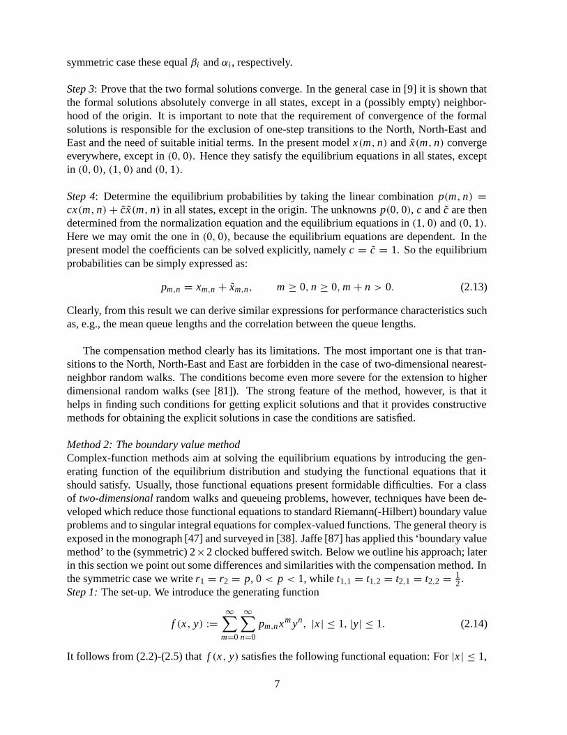
This proceeds straight-forwardly by uniformizing the transition rates. Let λ and µ denote thearrival rate and service rate, respectively. In the states (0,m2) with m2 > 0 and (0, 0) weintroduce fictitious one-step transitions from the state to itself with rate µ and 2µ, respectively(see Figure 4). This implies that in each state the transition rates add up to λ + 2µ, wherewithout loss of generality we may take λ + 2µ = 1. Hence we can interpret λ and µ astransition probabilities and the corresponding Markov chain has the same distribution as theoriginal Markov process. If we take c(m) as cost per period, then it also has the same averagecost. From here on we consider the Markov chain.

m 2

m 1

g

g g

g g g

g g g g

g g g g g

g g g g g g

g g g g g g g

λ2µ

λ

µ

µ

λµ

µ 2µλ

Figure 4: One-step transition rate diagram for the shortest queue system.

Step 2: Identify precedence relations. The precedence relation method systematically constructsmodifications of the Markov chain, which produce bounds for the average cost. First one shouldtry to identify precedences between states. We say that m has precedence over n, or is moreattractive than n, if vt(m) ≤ vt(n) for all t ≥ 0. Here vt (m) denotes the expected cost in the firstt periods when starting in state m. Based on these precedences it appears to be easy to constructmodifications yielding bounds. Of course one should aim for bounds that are easy to compute.

For the present model it is intuitively clear that state m = (m 1,m2) is more attractive thanits neighbours (m1 + 1,m2), (m1,m2 + 1) and (m1 − 1,m2 + 1), provided these neighboursare in the state space. This means that it is preferable to have less customers in the system andto have more balance in queue lengths. The precedences are shown in Figure 5. They can beproved by induction over t . It is important to note that (i) the proof of the induction step can betranslated to a standard transportation problem (which may be useful in more complex models),and (i i) the precedences depend on the choice of the cost function c.Step 3: Construction of bounds. We now consider a modification of the original Markov chainby redirecting in some states m = (m1,m2) one or more transitions. Redirecting a transitionfrom (m1,m2) to (n1, n2) to another state (n1, n2), say, means that the new transition probabilityto (n1, n2) is zero and the one to (n1, n2) is increased by the original transition probability from(m1,m2) to (n1, n2). We assume that the modified chain has only one recurrent subchain andthat its equilibrium distribution exists. The cost per period is not altered and the average costis denoted by g. The following result is crucial for the construction of bounds. If the modified

12

m 2

m 1

g

g g

g g g

g g g g

g g g g g

g g g g g g

g g g g g g g

Figure 5: Precedence relations for the shortest queue model with one-period cost c(m) = m1 +m2. Each arrow points to a more attractive state.

chain is obtained by redirecting to more (less) attractive states, then it holds for all t that theexpected t-period cost vector in the modified chain is less (greater) than the one in the originalchain. This can be proved by induction and it directly implies that g ≤ (≥) g.

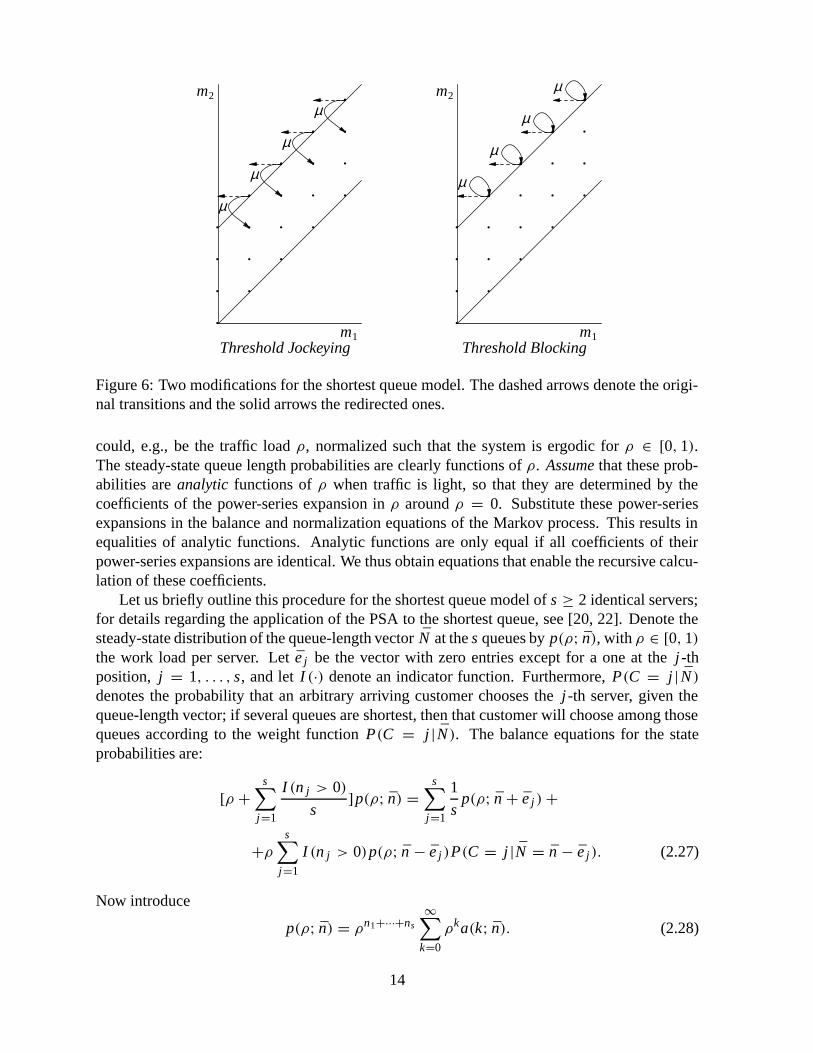
Hence, from the precedences in Figure 5 it is easy to construct models producing upper orlower bounds for g. Two such modifications are shown in Figure 6. In model (a) transitions areredirected to more attractive states, so this model gives a lower bound for g. The interpretationof the redirections is that one customer is allowed to jockey from the longest to the shortestqueue as soon as the difference between the queue lengths exceeds a threshold T . Figure 6shows model (a) for T = 3. In model (b) transitions are redirected to less attractive states, sothis model yields an upper bound. Its interpretation is that when the departure of a customerwould lead to a difference in queue lengths greater than T , then its departure is blocked and thecustomer is taken into service once more. In both models the state space is a semi-infinite strip,the size of which is controlled by a threshold parameter T . They can be solved very efficientlyby using the matrix geometric method of Neuts [115], see also Section 4.2. In fact, the ratematrix can be obtained explicitly in the two models (cf. [118]). It will be clear that the larger Tthe more accurate the bounds will be, but also the more effort it takes to compute them. Notethat the two models exploit the property that most of the probability mass in the shortest queuemodel is concentrated around the diagonal of the state space. So the bounds will already betight for small values of T . Based on the precedences it is possible to construct a number ofother models producing bounds. They cover the ones studied in [10, 48, 74, 119, 134].

The idea to construct bounds on the basis of precedences has been used for a number ofspecific models, see e.g. [3, 84, 2, 55, 56, 57, 58, 59]. The precedence relation method can beseen as an attempt to unify the approaches in these references.

Method 2: The power series algorithmThe power-series algorithm (PSA) is a numerical-analytic method for analyzing certain Markovprocesses. The main idea of the PSA is to consider the steady-state distribution of the Markovprocess as a function of a system parameter. In the shortest queue model, this system parameter

13

m2

m1Threshold Jockeying

•

•

•

•

•

•

•

•

•

•

•

•

•

•

•

•

•

•

•

•

µ

µ

µ

µm2

m1Threshold Blocking

•

•

•

•

•

•

•

•

•

•

•

•

•

•

•

•

•

•

•

•

µ

µ

µ

µ

Figure 6: Two modifications for the shortest queue model. The dashed arrows denote the origi-nal transitions and the solid arrows the redirected ones.

could, e.g., be the traffic load ρ, normalized such that the system is ergodic for ρ ∈ [0, 1).The steady-state queue length probabilities are clearly functions of ρ. Assume that these prob-abilities are analytic functions of ρ when traffic is light, so that they are determined by thecoefficients of the power-series expansion in ρ around ρ = 0. Substitute these power-seriesexpansions in the balance and normalization equations of the Markov process. This results inequalities of analytic functions. Analytic functions are only equal if all coefficients of theirpower-series expansions are identical. We thus obtain equations that enable the recursive calcu-lation of these coefficients.

Let us briefly outline this procedure for the shortest queue model of s ≥ 2 identical servers;for details regarding the application of the PSA to the shortest queue, see [20, 22]. Denote thesteady-state distribution of the queue-length vector N at the s queues by p(ρ; n), with ρ ∈ [0, 1)the work load per server. Let e j be the vector with zero entries except for a one at the j -thposition, j = 1, . . . , s, and let I (·) denote an indicator function. Furthermore, P(C = j | N)denotes the probability that an arbitrary arriving customer chooses the j -th server, given thequeue-length vector; if several queues are shortest, then that customer will choose among thosequeues according to the weight function P(C = j |N). The balance equations for the stateprobabilities are:

[ρ +s∑

j=1

I (n j > 0)

s]p(ρ; n) =

s∑j=1

1

sp(ρ; n + e j )+

+ρs∑

j=1

I (n j > 0)p(ρ; n − e j )P(C = j |N = n − e j ). (2.27)

Now introduce

p(ρ; n) = ρn1+···+ns

∞∑k=0

ρka(k; n). (2.28)

14

The idea is, that the p(ρ; n) are analytic functions of the traffic load ρ for small values of ρ, andthat in fact the limit for ρ ↓ 0 of ρ−(n1+···+ns) p(ρ; n) will exist. Substituting (2.28) into (2.27)and equating the coefficients of corresponding powers of ρ in the resulting equations yields thefollowing equations: For k = 0, 1, . . . ,

s∑j=1

I (n j > 0)

sa(k; n) = −

s∑j=1

I (n j > 0)

sI (k > 0)a(k − 1; n)

+s∑

j=1

1

sI (k > 0)a(k − 1; n + e j )

+s∑

j=1

I (n j > 0)a(k; n − e j )P(C = j |N = n − e j ). (2.29)

The left-hand side of (2.29) vanishes when n = 0. In addition we have from the normalizationequation:

a(k; 0) = −∑

· · ·∑

0<n1+···+ns≤ka(k − n1 − · · · − ns; n), k = 1, 2, . . . . (2.30)

To obtain the coefficients of p(ρ; n) up to ρM , proceed from k = 0 to M: Start from a(0; 0) =1; determine a(k; 0) from (2.30), and then calculate a(k; n) recursively from (2.29) for increas-ing values of

∑ni up to

∑ni = M − k (cf. [20]).

However, the power-series expansion of p(ρ; n) as functions of ρ is not convergent on thewhole interval 0 < ρ < 1 for this model. To enlarge the convergence radius of the power-seriesexpansion we can use the conformal mapping θ = 1+G

1+Gρ ρ (with G ≥ 0) that maps (0, 1) ontoitself and introduce

p(ρ(θ); n) = θn1+···+ns

∞∑k=0

θ kb(k; n). (2.31)

Substitution of (2.31) into (2.27) and equating the coefficients of corresponding powers of θagain yields a set of equations from which the coefficients can be solved recursively. The powerseries (2.31) now has a larger radius of convergence than the original one (2.28), i.e., it con-verges for values of ρ(θ) for which (2.28) diverges.

The principal idea of the PSA is originally due to Benes [15], p. 295 ff. It was independentlyrediscovered by Hooghiemstra, Keane and Van de Ree [78], who applied it to the model of cou-pled processors with exponential service times (see also Section 3.5). In [14], the coefficientsof the expansion are obtained explicitly for the symmetric two-queue coupled processor case.In a series of papers, Blanc and his colleagues greatly extended the applicability of the PSA(see the survey [23]). One of the key contributions of Blanc [21] was the introduction of theepsilon algorithm which strongly improved the convergence properties of the PSA. Koole [98]showed that the PSA can be applied to any Markov process with a single recurrent class. Vanden Hout and Blanc [80, 79] extended the applicability of the PSA to networks of queues with amulti-queue Markovian arrival process, Markovian service process and Markovian routing. Inhis PhD thesis, Van den Hout [79] takes the viewpoint that the PSA not only can be viewed asa light-traffic method, but also as a homotopy method: He transforms particular, well-chosen,

15

transition rates of the original Markov process with a parameter γ , such that for γ = 1 the orig-inal process reappears and the transformed process for γ near 0 is easy to analyze. Knowledgeabout the transformed process near 0 may then be used to solve the problem at γ = 1. He alsostrengthened the theoretical foundation of the PSA by proving for a wide class of models thatthe steady-state probabilities of the transformed process are, indeed, analytic functions of thetransformation parameter γ at γ = 0. Furthermore, he developed some ideas on using the PSAto calculate the transient distribution of a continuous-time Markov process.

The major advantage of the PSA is its flexibility: apart from the Markovian assumption,it does not require much structure. It also does not require sophisticated numerical methods,apart from extrapolation methods like the epsilon algorithm to make the PSA applicable forintermediate and even heavy traffic. Disadvantages of the PSA are: (i) it suffers from the curseof dimensionality (because it directly depends on the balance equations); (i i) no useful errorbounds exist sofar; (i i i) it is sensitive to extreme parameter values.

Remark 2.2 The MacLaurin approach of Gong and Hu [75] for the G I/G/1 queue and of Zhuand Li [135] for the Markov-modulated G/G/1 queue is another light-traffic approach, that issomewhat similar to the PSA. These authors derive power-series expansions of the moments ofthe sojourn and waiting time from the Lindley recursion equation. In this respect, a useful re-sult of Hu [85] should be mentioned; he has proven certain performance measures of G I/G/1queues to be analytic at zero as a function of the arrival rate, when the interarrival time distribu-tion can be expanded as a MacLaurin series over [0,∞). Blaszczyszyn, Frey and Schmidt [24]and Baccelli and Schmidt [13] also use a light-traffic approach to analyze Markov-modulatedmultiserver queues and Poisson-driven (max,+)-linear structures, respectively. The latter sys-tems can model non-Markovian stochastic Petri nets in the class of event graphs. Examplesinclude fork-join networks and synchronized queueing networks, and Kanban manufacturingnetworks.

Other approaches to the shortest-queue problemKnessl et al. [95] develop a scheme to obtain approximations for the joint queue length dis-tribution, valid when one of the queue lengths is large. Foschini and Salz [69] use a heavytraffic diffusion approximation. Gertsbakh [74] and Rao and Posner [119] apply the matrix-geometric method, and Zhao and Grassmann [133] propose an algorithm based on the resultsof [68]. Halfin [77] obtains bounds by using linear programming techniques, and Nelson andPhilips [112] present mean response time approximations for the case of K queues and gen-eral interarrival and service time distributions, assuming in their approximation method that thevarious queue lengths can differ by at most one (see also [111]). Lui et al. [103, 104] developapproximations for a generalization of the shortest queue model, viz. shortest expected delayrouting of customers to servers with different working speeds.

Remark 2.3 The ordinary M/G/2 queue basically is a 2-queue model where the customers areassigned to the queue with the smallest workload instead of the shortest queue. Using a Wiener-Hopf decomposition, Cohen [33] presents an exact analysis of the two-dimensional workloadprocess of this M/G/2 queue, for the case in which the service times have a rational LST. Knesslet al. [96] present an asymptotic analysis for general service times. Formal asymptotic ap-proximations are constructed for the two-dimensional workload process, treating separately theasymptotic limits of heavy traffic, light traffic and large buffer contents.

16

2.4 The fork-join queue

The fork-join queue is a simple model for a parallel processing system. It consists of c parallelservers, each with their own queue. Each arriving job consists of c subjobs, who each joina different queue (the fork node). A job is completed when all its subjobs have completedservice (the join node). Clearly the queues in this model are dependent due to the coupledarrivals. This model frequently arises in the context of computer systems, production systemsand maintenance systems.

An exact analysis is possible for c = 2 and Poisson arrivals. The model with heterogeneousexponential servers has been studied by Flatto and Hahn [67]. The generating function for thequeue lengths is found by using a uniformization technique (expressing two complex variablesas analytic functions of one and the same variable) and from this asymptotic expressions for theequilibrium probabilities are obtained. Their generating function is shown to be a meromorphicfunction on a 2-sheeted Riemann surface. Wright [130] generalizes the result of [67] by alsoallowing jobs consisting of one subjob to join the system. A completely different approach toobtain asymptotic results has been used by Shwartz and Weiss [122] (see also the afterword in[130]). It is based on large deviations and time reversibility. Baccelli [11] solves the modelwith general, but exchangeable, service times by using complex-function theory methods. Inhis PhD thesis, De Klein [92] analyses the model with general service times. He applies andcompares two methods, viz. the boundary value method (see Subsection 2.2) and the singularintegral equation technique. The latter technique has been initiated by Eisenberg [60] and itconcerns the reduction of the functional equation for the generating function to a Fredholmintegral equation. For the model with more than two servers no exact analytical results areavailable in the literature. In this case, bounds and approximations have been developed, seee.g. [12, 113, 114].

3 Servers choose a customer

3.1 Introduction

In this section we consider queues with multiple waiting lines, where the server or serverschoose a customer for service according to some priority rule. In polling systems the prior-ity is changing dynamically; these systems are considered in Subsection 3.2. Systems withfixed (static) priority are studied in Subsection 3.3. The ‘priority for the longer queue’ disci-pline is briefly considered in Subsection 3.4. An important mechanism to introduce prioritiesin integrated-services networks with heterogeneous Quality-of-Service requirements is Gener-alized Processor Sharing; it is the topic of Subsection 3.5.

While some of these models may, in particular cases, be analyzed by direct methods like thepower-series algorithm, the methodological emphasis in this chapter is on complex-functionmethods.

3.2 Polling systems

The performance analysis of computer-communication and production systems often gives riseto single-server multi-queue models. The characteristic feature of these so-called polling mod-

17

els is that a single server is moving between a number of queues (which possibly requiressome switchover time), implying that the priority of the queues is dynamically (e.g., cyclically)changing. Many applications of polling models can be found in [76, 102, 127]. In [126, 128]extensive and updated bibliographies of polling studies are given.

In a cyclic polling model, the joint queue length process at polling instants (i.e. time pointsat which the server starts a visit at a queue) can under some conditions on the service disciplinesat the queues be represented by a multi-type branching process with immigration [120]. In thecase of polling models with switchover times, it turns out that we are dealing with a multi-typebranching process with immigration in each state, whereas in the case of polling models withoutswitchover times we are dealing with a multi-type branching process with immigration onlyin state zero. The theory of such branching processes then provides necessary and sufficientergodicity conditions, and, using an iterative method, it gives an explicit expression for thegenerating function of the joint queue length process at polling instants.

Let us describe the polling model, the required conditions on the service disciplines at thequeues and the iterative method in some more detail. A single server S visits n infinite-bufferqueues Q1, . . . , Qn in cyclic order. When S moves from Qi to Qi+1 this requires a switchovertime with distribution function Si (·) with mean σi and Laplace-Stieltjes transform σi (·). Cus-tomers arrive at Qi according to a Poisson process with rate λi . The service times of customersat Qi have distribution function Bi (·) with mean βi and Laplace-Stieltjes transform βi (·). Theservice discipline at each queue should satisfy the following ‘branching’ property:

Property 1 If S arrives at Qi to find ki customers there, then during the course of the server’svisit, each of these ki customers will effectively be replaced in an i.i.d. manner by a random pop-ulation having probability generating function h i (z1, . . . , zn), which can be any n-dimensionalprobability generating function.

For example, in the case of the well-known gated and exhaustive service disciplines, Prop-erty 1 is satisfied with hi (z1, . . . , zn) = βi (

∑nj=1 λ j (1−z j)) and hi (z1, . . . , zn) = ηi (

∑j �=i λ j (1−

z j )), respectively, where ηi (·) is the Laplace-Stieltjes transform of the length of the busy periodof the ’corresponding’ isolated M/G/1 queue of Qi . Unfortunately, the branching propertydoes not hold for several important service disciplines, like those that put a limit on the time ofa server visit or the number of services during a server visit.

From now on we use the notation z = (z1, . . . , zn) and we denote by V (z) the generatingfunction of the joint queue length vector at polling instants of a fixed queue, say Q 1. Under thebranching property we can prove that

V (z) = V ( f (z))g(z). (3.1)

Here, the function f (z), defined by

f (z) := ( f1(z), . . . , fn(z))

withfi (z) := hi (z1, . . . , zi , fi+1(z), . . . , fn(z)),

represents the offspring generating function. The function g(z), defined by

g(z) =n∏

i=1

σi (

i∑j=1

λ j (1 − z j )+N∑

j=i+1

λ j (1 − f j (z))),

18

represents the immigration generating function in the branching process.Iteration of equation (3.1) yields

V (z) =∞∏

k=0

g( f (k)(z)), (3.2)

where the iterates f (k)(z) are defined by

f (0)(z) = z,

f (k)(z) = f ( f (k−1)(z)).

The infinite product in (3.2) is convergent when the ergodicity condition is fulfilled.In the case of zero switchover times we have, instead of Equation (3.1), that

V (z) = V ( f (z))− π0(1 − g(z)). (3.3)

Here the offspring generating function f (·) is defined as before, π0 is the probability of anempty system and the immigration generating function g(·) is now given by

g(z) =N∑

j=1

λ j

λz j , or g(z) =

N∑j=1

λ j

λf j (z),

depending on the behaviour of the server when the system becomes empty. The first expressioncorresponds to the situation where, when the system becomes empty, the server makes a fullcycle and subsequently stops right before Q1 (see [25]). The second one corresponds to thesituation where in an empty system the server immediately stops right behind Q 1 (see [120]).Iteration of Equation (3.3) yields

V (z) = 1 − π0

∞∑k=0

[1 − g( f (k)(z))]. (3.4)

The infinite sum in (3.4) is convergent when the ergodicity condition is fulfilled.As mentioned before, the branching property does not hold for several important service

disciplines, like those that put a limit on the time of a server visit or the number of servicesduring one server visit. In exceptional two-queue cases of the latter class, the joint queue lengthdistribution can be determined by using the theory of Riemann-Hilbert boundary value problems[27, 46, 47, 100]. A pioneering paper in this area was that of Eisenberg [60], transforming atwo-queue polling problem into a Fredholm integral equation.

Numerical approachesLeung [101] has developed a numerical procedure, based on the fast Fourier transform, thatenables one in principle to determine polling performance measures with any required accu-racy. The power series algorithm is also applicable to a large class of polling models (see Blanc[21]). An essential difficulty of both numerical techniques is their large computational com-plexity. Choudhury and Whitt [30] have shown that probability distributions and moments ofperformance measures for many polling models can be effectively computed by numericallyinverting generating functions and Laplace-Stieltjes transforms. The computational complexity

19

of their approach is much lower than that of the approaches of Leung and Blanc. However,the method of Choudhury and Whitt does not readily extend to models that do not satisfy thebranching property.

If switchover times are zero, work conservation leads to a conservation law, an exact ex-pression for a particular weighted sum of mean waiting times [93]. If switchover times arenon-zero, a principle of work decomposition [26, 27] gives rise to a pseudo-conservation lawwhich is again an exact expression for a particular weighted sum of mean waiting times. Thiscan provide a useful check for the accuracy of simulations, numerical calculations and approx-imations, as well as providing the basis for further approximations.

3.3 Fixed priorities

An important queueing model is the single server queue with k classes of customers, that arriveaccording to independent Poisson processes and have fixed priorities. The non-preemptive andpreemptive-resume priority disciplines have in particular been analyzed in considerable detail.A classical reference is the book of Jaiswal [89]; see also the discussions in [34, 94, 129].Jaiswal discusses, a.o., generating functions of joint queue length distributions. He heavily usesthe concept of completion time, viz., the time from the start of a service of a particular classuntil the server is available to serve the next customer of that same class. The completion timeconcept allows a unified study of several priority disciplines. Another important observationin single server priority queues is that it often suffices to study k = 2 classes, temporarilyaggregating all lower (higher) classes into a single class.In the present study we focus on the challenging problem of multiserver priority queues. Bothinterarrival and service times are now assumed to be exponentially distributed. In most studiesthat have considered multiserver queues with nonpreemptive priority, the restrictive assumptionhas been made that all mean service times are equal. Cohen [32] derived the joint queue lengthdistribution under this assumption, for the case k = 2. Cobham [31] derived the mean waitingtimes under the same assumption, for general k, while Davis [52] and Kella and Yechiali [90]obtained the waiting time transform of each class. Gail et al. [70] discarded the assumption ofequal service means. They obtained, for k = 2 classes and an arbitrary number m of servers,the steady-state bivariate generating function of a convenient two-dimensional Markov processthat is immediately related to the queue length process. We sketch their approach and refer to[70] for the (very involved) analytic details. The generating function equations correspondingto the equilibrium equations take the form

A(z, w)G(z, w) = B(z, w)F(w)+ C(z, w)K . (3.5)

G, F are unknown vector valued analytic functions, K is a vector of unknown constants, andA, B,C are known (m +1)×(m +1) matrices with polynomial entries. Gail et al. then identifythe m + 1 zeros zi (w) of det A(z, w) for given |w| ≤ 1, with the property |zi (w)| ≤ 1. Sincethe GF G(z, w) should be bounded in |z| ≤ 1, |w| ≤ 1, this yields a matrix equation

M(w)F(w) = N (w)K , (3.6)

where M(w) is known. This is a set of (m + 1)2 equations, at most m + 1 of which are in-dependent. A careful study of the zeros of det M(w) inside the unit circle, instigated by the

20

boundedness of the GF F(w) inside the unit circle, yields a set of equations from which K canbe determined. F(w) then follows from (3.6) and finally G(z, w) from (3.5).Gail et al. [71] have used a similar approach, with a similar state-space representation, to de-termine the bivariate queue-length GF in the preemptive resume case (again there are m serversand 2 classes).

3.4 Priority for the longest queue

The queueing model with priority for the longest queue is in a sense dual to the shortest queuemodel. It is also similar, in the sense that both systems employ a mechanism that tends to equal-ize the queue lengths. Cohen [37] solves the 2-queue model with server priority for the longestqueue. He uses a translation into a Riemann boundary value problem of a type that was notstudied earlier in a queueing context. In Van Houtum et al. [84] the precedence relation method(see Subsection 2.3) is used to obtain lower and upper bounds for the model with exponentialservice times and an arbitrary number of queues. The exponential longest queue model withtwo queues has also been studied by Flatto [66] in the case that the longest queue policy is ap-plied preemptively (i.e. service to a customer in a given queue is interrupted whenever the otherqueue becomes larger). He uses a generating-function approach. He argues that the longestqueue model is easier than the shortest queue model, in the sense that in the former one f (0, y)does not appear in the basic functional equation, and that it is a rational function of y.

3.5 Generalized Processor Sharing

In the design of high-speed networks, an increasingly important issue is the provision of Quality-of-Service (QoS) guarantees. A key problem is the study of scheduling disciplines to be em-ployed at network switches. Ideally, these scheduling disciplines should protect sessions fromthe possibly bad behavior of other sessions, but also exploit statistical multiplexing gain. Onedesign paradigm for such scheduling disciplines is the Generalized Processor Sharing (GPS)discipline. GPS-based scheduling algorithms like Weighted Fair Queueing have emerged asan important mechanism for accommodating heterogeneous QoS requirements in integrated-services networks.GPS operates as follows. Consider N sources (sessions) sharing a link of unit rate. Thereare weights φ1, . . . , φN associated with each of these sources, with

∑Ni=1 φi = 1. If all the

sources are backlogged at time t , i.e., the buffer content of each source is positive at time t , thensource i is served at rate φi , i = 1, . . . , N . But if some of the sources are not backlogged, thenthe excess capacity is redistributed among the backlogged sources according to their respectiveweights. GPS has the following two properties: (i) it is work-conserving, serving at the full linkrate whenever at least one source is backlogged; (i i) it guarantees minimum rate φi to source iwhenever it is backlogged.Generally speaking, the stochastic analysis of the GPS discipline is prohibitively difficult. How-ever, the case N = 2 allows, for several variants, a quite detailed analysis. Konheim, Meilijsonand Melkman [97] determine the joint queue length distribution in the completely symmetriccase of independent Poisson arrival processes and exponential service times (with the samerates at each queue) and φ1 = φ2 = 1/2. They employ a uniformization technique. The cou-pled processor model, as it was called by the above-mentioned authors, has been a most fruitful

21

model from the viewpoint of methodology. In a pioneering paper, Fayolle and Iasnogorodski[63] have shown that the functional equation for the two-dimensional generating function of thejoint queue length distribution in the asymmetrical coupled processors may be transformed intoa Riemann-Hilbert boundary value problem. This allowed the application of powerful resultsfrom the theory of boundary value problems. Cohen and Boxma [47] have presented a system-atic and detailed study of that new technique. In many cases, their approach allowed generalservice time distributions. One of these cases is the coupled processor model; in [47] it is ex-actly analyzed for the case of generally distributed service times. The service speed of server iis ri when the other server is also busy, and r ∗

i when the other server is idle (r∗1 = r∗

2 = r1 + r2

gives GPS). The topic of interest in Chapter III.3 of [47] is the LST φ(s1, s2) of the joint work-load distribution at both servers. A parametrisation technique yields a suitable set of zeros(s1, s2) = (δ1(w), δ2(w)) of the kernel, leading to a Wiener-Hopf problem with boundary(line of discontinuity) Re w = 0.The question naturally arises whether the boundary value technique can be extended to queueingmodels with a higher-dimensional state space. Cohen [35, 36] obtains partial results for 3 cou-pled processors, while he also derives a large collection of interesting results for entrance timesand entrance points of homogeneous N -dimensional random walks [39]. We are not aware ofother such higher-dimensional results. For the same coupled-processor model (not necessarilycompletely symmetric, and with an arbitrary number N ≥ 2 of queues), Hooghiemstra, Keaneand Van de Ree [78] have developed the Power Series Algorithm (PSA; see Section 2.3).For the general GPS scheduling discipline with an arbitrary number of sources, there seems tobe little hope of obtaining explicit expressions for queue length or workload distributions. Itis already quite an accomplishment to derive useful bounds on backlog (workload) and delay.Parekh and Gallager [116, 117] study GPS in which the arriving traffic conforms to Cruz’s lin-ear bounded arrival processes [49, 50]. They obtain worst-case deterministic upper bounds onbacklog and delay for each session. Thus hard guarantees can be given for networks employingGPS scheduling. Zhang et al. [132] model the source session traffic as an exponentially boundedburstiness process (a notion introduced in [131]), and derive statistical bounds on backlog anddelay for each session. Other important contributions to the performance analysis of GPS arebased on a large deviations approach: see Bertsimas et al. [18], Dupuis and Ramanan [54], andMassoulie [106].

4 Various two-dimensional random walks

4.1 Introduction

In this section we discuss two classes of Markov processes that naturally arise in queueingmodels with multiple waiting lines, and for which a detailed analysis is possible. Subsec-tion 4.2 considers Markov processes on a semi-infinite strip. Three methods for determiningthe equilibrium probabilities are briefly described. Subsection 4.3 is concerned with tractabletwo-dimensional random walks on the lattice in the first quadrant. Some methods that werediscussed in the previous sections also apply to these Markov processes. As indicated before,the power-series algorithm can be applied to any Markov process with a single recurrent classbut has some restrictions regarding its theoretical foundation and suffers from the curse of di-

22

mensionality; the compensation method applies under restrictions on the one-step transitionrates.

4.2 Markov processes on a semi-infinite strip

Many queueing systems can be modelled by a Markov process, the state space of which is givenby a semi-infinite strip of states (m, n) where m ranges from 0 to s and n from 0 to ∞. In thesesystems, typically m denotes the state of the service facility or of the arrival process, and ndenotes the number of jobs waiting in the system. m and n could also denote the number oftype-1 and type-2 customers, the waiting room for type-1 customers being finite. Often, there isa threshold N , such that the transition rates out of state (m, n) do not depend on n when n ≥ N .

The equilibrium probabilities pm,n can be determined using three alternative methods. Theyare briefly described below. A comparison of the three methods can be found in the survey pa-per by Mitrani [107].

Method 1: The matrix-geometric methodIn this approach the row vectors of equilibrium probabilities pn = (p0,n, p1,n, . . . , ps,n) areexpressed as

pn = pN Rn−N , n ≥ N , (4.1)

where the so-called rate matrix R is the minimal nonnegative solution of a nonlinear matrixequation; see Neuts’ book [115]. For the special class of quasi-birth-and-death processes, i.e.,processes where for each state (m, n) outgoing transtions are restricted to states (k, l) with|l −n| ≤ 1, Ramaswami and Latouche [99] have developed a highly efficient algorithm to solvethe matrix equation for the rate matrix R.

Method 2: The generating function methodThis approach uses generating functions to solve the set of equilibrium equations. By introduc-ing the vector generating function g(z) = (g0(z), g1(z), . . . , gs(z)) where

gm(z) =∞∑

n=N

p(m, n)zn,

the equilibrium equations can be transformed to a matrix equation for g(z) of the form

g(z)A(z) = b(z).

The vector b(z) involves a number of unknown boundary probabilities. These probabilities aredetermined by exploiting the zeros of the determinant of the matrix A(z) inside or on the unitcircle. The generating function approach is, for example, used by Mitrani and Avi-Itzhak [108]to analyse the M/M/s queue with service interruptions.

Method 3: The spectral expansion methodThis method is based on reducing the equilibrium equations to a vector difference equationwith constant coefficients, the solution of which can be expressed in terms of eigenvalues and

23

eigenvectors of the associated characteristic polynomial; see Mitrani and Mitra [109]. Thisgives

pn =s∑

i=0

Ci yi xn−Ni , n ≥ N , (4.2)

where the geometric factors xi are the s + 1 eigenvalues inside the unit circle, the vectors yi

are the corresponding eigenvectors and the coefficients Ci follow from the boundary equationsand the normalization equation. The difficult step in this approach is the computation of theeigenvalues, which are the s + 1 roots inside the unit circle of a determinantal equation. Adirect approach of finding these roots is inefficient for large s and therefore not recommended.However, in special cases, particular properties may be exploited to simplify the eigenvalueproblem, see e.g. Elwalid et al. [61]. For a class of systems with rates linear in m or s − m,Adan and Resing [5] showed that the roots can be determined very efficiently. They use agenerating function technique to reduce the single equation for the s + 1 roots inside the unitcircle to s + 1 equations for a single root in the interval (−1, 1). This considerably simplifiesthe determination of the roots, also because the computations can now be restricted to the realdomain. Queueing models included in this class of systems are, e.g., the multi-server queuewith Poisson arrivals and E2, H2 or C2 distributed service times (see [121, 123, 124, 17]), theM/M/s queue with service interruptions (see [108]), the

∑I P P/M/1 queue (see [61]) and a

multi-server queue with locking (see [4]).

Remark 4.1 Result (4.2) may be linked to the (modified) matrix-geometric representation (4.1)of the equilibrium distribution. Clearly, when R is diagonalizable, the factors xm in the form(4.2) are the eigenvalues of R and the row vectors ym are the associated row eigenvectors (cf.Daigle and Lucantoni [51]).

Remark 4.2 De Smit [125] surveys the application of matrix Wiener-Hopf factorizations to theanalysis of waiting times in multidimensional queues. The class of models that this methodcan handle shows considerable overlap with the class which can be solved by matrix-geometricmethods. One of De Smit’s key examples is a semi-Markov queue. Dukhovny [53] also consid-ers semi-Markov queues. He surveys the application of vector Riemann-Hilbert boundary valueproblems to the analysis of queue lengths in multidimensional queues.

4.3 Markov processes on the lattice in the first quadrant

An interesting class of two-dimensional random walks on the lattice in the first quadrant hasbeen studied by Fayolle, King and Mitrani [65]. They assume that there exist positive integersN1 and N2, such that the transition rates out of state (n1, n2) do not depend on n1 for n1 ≥ N1

and not on n2 for n2 ≥ N2. One example is an M/M/1 queue with two classes of customersand a restricted processor sharing discipline: Up to N1 jobs of class 1 and up to N2 jobs of class2 are allowed to share the processor at any time, and the remaining jobs must wait. Fayolle etal. [65] reduce the determination of the bivariate generating function to the problem of solvinga Riemann-Hilbert boundary value problem on a circle.

A quite general class of two-dimensional random walks on the lattice in the first quadranthas been analysed in [47], where the solution is again obtained via transformation to a bound-

24

ary value problem. One-step transitions to the West, South-West and South can only go to thenearest neighbour, but one-step transitions in other directions may be more general. The func-tional equation for the unknown generating function f (x, y) of its equilibrium solution is of thefollowing type: For |x | ≤ 1, |y| ≤ 1,

K (x, y) f (x, y) = A10(x, y) f (x, 0)+ A01(x, y) f (0, y)+ A00(x, y) f (0, 0)+ B(x, y). (4.3)

The kernel K (x, y) contains all the information concerning the structure of the random walk inthe interior of its state space. The boundedness of the probability generating function f (x, y)for |x | ≤ 1, |y| ≤ 1 again leads to an inspection of the zeros of the kernel, K (x, y), in thisproduct of unit circles. For each of those zeros, the righthand side of (4.3) should be zero. Fur-thermore, f (x, 0) should be analytic in x for |x | < 1 and continuous in x for |x | ≤ 1, similarlyfor f (0, y). The structure of the problem of determining f (x, 0) and f (0, y) that satisfy theseconditions resembles that of a Riemann-type boundary value problem: The determination ofanalytic functions in prescribed domains, these functions moreover satisfying a linear relation.In [47] the above problem is indeed transformed into a Riemann-type boundary value problem.Using the extensive theory of Riemann-type boundary value problems [72, 110], the above-described two-dimensional random walk is in principle solved. The solution does involve thedetermination of some conformal mappings, that can be accomplished via the solution of sin-gular integral equations. In most cases, this requires numerical analysis. The above-sketchedapproach is surveyed in much more detail in [38]. From a numerical point of view, an inter-esting approach is also the transformation of the functional equation into a Fredholm integralequation [38]; standard techniques are available to solve such an integral equation numerically(cf. [92]).

Various matters simplify when one restricts oneself, within the class of random walks on thelattice in the first quadrant, to the subclass of nearest-neighbour random walks (only transitionsto immediate neighbours may occur). In that case, the kernel K (x, y) is a biquadratic functionof x and y. A pioneering study of such random walks is the one of Malyshev [105]. Togetherwith Fayolle and Iasnogorodski, [64], he has recently developed a new analytic approach fornearest-neighbour random walks in the quarter plane. Like in the above approach, they considerthe (elliptic) curve K (x, y) = 0. A key idea of them is to use Galois automorphisms on this al-gebraic curve. They prove that the unknown functions f (x, 0) and f (0, y), while in general notbeing meromorphic functions, can be ‘lifted’ as meromorphic functions onto the ‘universal cov-ering’ of some Riemann surface that corresponds to the algebraic curve K (x, y) = 0 (see also[67, 130]). Cohen has made several important contributions to the theory of nearest-neighbourrandom walks. In the monograph [39], he extensively discusses ergodicity conditions, entrancetimes into the boundaries, and entrance points. He relates the zero-tuples of the kernel to thedistributions of the entrance times into the boundary points of the state space, by a very elegantidentity. When only a few one-step transitions are allowed in a nearest-neighbour random walk,further simplifications may occur.

Cohen [40] considers the semi-homogeneous nearest-neighbour random walk without tran-sitions to the East, North-East and East. This is the class of random walks studied in [1] viathe compensation method. Cohen proves that the bivariate generating function of the station-ary distribution of such two-dimensional random walks in the first quadrant can be representedby meromorphic functions. Subsequently he exposes the construction of those meromorphicfunctions; this construction is based on the iterative calculation of poles and their residues.

25

Examples are discussed in [42, 43, 44, 45], cf. Subsection 2.2. Cohen [40] observes that thebivariate generating function for this class of random walks may also be obtained using theboundary value method, even when one-step transitions to the North, East and North-East areallowed; but he remarks that when such transitions are excluded, then the construction of themeromorphic function via the iterative calculation of poles and residues is simpler because itavoids the explicit calculation of a conformal mapping.

In [41] Cohen considers a nearest-neighbour random walk with transitions to the South-West, North and East. The generating functions f (x, 0) and f (0, y) are here not meromorphicfunctions. However, the bivariate generating function f (x, y) is shown to be a fairly simplealgebraic function that can be explicitly determined. Cohen uses the uniformization techniqueof Flatto and Hahn [67] and Wright [130], who study a fork-join queue, cf. Subsection 2.4. Theunderlying model of this random walk study actually is a queueing model with one server, twoPoisson classes of customers and ‘paired services’: As soon as a service has been completed, anew service is started if there are customers present. In general, a couple of customers of dif-ferent type is simultaneously served (after which they leave simultaneously). If only customersof one type are present after a service completion, then one customer of that type is served. If aservice leaves the system empty, then the server starts serving as soon as a customer has arrived.Cohen [41] assumed exponential service time distributions. Blanc [19] allows a general servicetime distribution, that is the same in each of the above cases. He obtains several performancemeasures, including the joint queue-length distribution at service completion epochs and at anarbitrary time. He accomplishes this by formulating the problem as a Riemann-Hilbert or aHilbert boundary value problem. Its solution requires a conformal mapping that in general can-not be obtained explicitly and must be determined numerically.

Acknowledgment. The authors are indebted to Professor J.W. Cohen for some very interestingdiscussions. The survey paper [29] has provided some useful input for the present paper. Itfocuses less on the analytic methods, but it considers a broader range of models that are rele-vant for the performance analysis of parallel and distributed systems; in addition, it discussesoptimization aspects.

References

[1] I.J.B.F. Adan. A Compensation Approach for Queueing Problems. PhD thesis, EindhovenUniversity of Technology, 1991.

[2] I.J.B.F. Adan and G. Hooghiemstra. The M/M/c with critical jobs. Mathematics ofOperations Research, 47:341–353, 1998.

[3] I.J.B.F. Adan, G.J.J.A.N. van Houtum and J. van der Wal. Upper and lower bounds forthe waiting time in the symmetric shortest queue system. Annals of Operations Research,48:197–217, 1994.

[4] I.J.B.F. Adan, A.G. de Kok and J.A.C. Resing. A multi-server queueing model withlocking. European Journal of Operational Research, 116:16–26, 1999.

26

[5] I.J.B.F. Adan and J.A.C. Resing. A class of Markov processes on a semi-infinite strip.In B. Plateau, W.J. Stewart and M. Silva, editors, Numerical Solution of Markov Chains(NSMC ’99), Prensas Universitarias de Zaragoza, Zaragoza, 1999, pages 41–57.

[6] I.J.B.F. Adan and J. Wessels. Shortest expected delay routing for Erlang servers. Queue-ing Systems, 23:77–105, 1996.

[7] I.J.B.F. Adan, J. Wessels and W.H.M. Zijm. Analysis of the symmetric shortest queueproblem. Stochastic Models, 6:691–713, 1990.

[8] I.J.B.F. Adan, J. Wessels, and W.H.M. Zijm. Analysis of the asymmetric shortest queueproblem. Queueing Systems, 8:1–58, 1991.

[9] I.J.B.F. Adan, J. Wessels, and W.H.M. Zijm. A compensation approach for two-dimensional Markov processes. Advances in Applied Probability, 25:783–817, 1993.

[10] I.J.B.F. Adan, J. Wessels and W.H.M. Zijm. Matrix-geometric analysis of the symmetricshortest queue problem with threshold jockeying, Operations Research Letters, 13:107–112, 1993.

[11] F. Baccelli. Two parallel queues created by arrivals with two demands: The M/G/2symmetrical case. Technical report 426, INRIA-Rocquencourt, 1985.

[12] F. Baccelli, A.M. Makowski, and A. Shwartz. The fork-join queue and related systemswith synchronization constraints: Stochastic ordering and computable bounds. Advancesin Applied Probability, 21:629–660, 1989.

[13] F. Baccelli and V. Schmidt. Taylor series expansions for Poisson driven (max,+)-linearsystems. Annals of Applied Probability, 6:138–185, 1996.

[14] H. Bavinck, G. Hooghiemstra and E. de Waard. An application of Gegenbauer polyno-mials in queueing theory. J. Comput. Appl. Math., 49:1-10, 1993.

[15] V.E. Benes. Mathematical Theory of Connecting Networks and Telephone Traffic. Aca-demic Press, New York, 1965.

[16] S.A. Berezner, C.F. Kriel and A.E. Krzesinski. Quasi-reversible multiclass queues withorder independent departure rates. Queueing Systems, 19:345–359, 1995.

[17] D. Bertsimas and X.A. Papaconstantinou. Analysis of the stationary Ek/C2/s queueingsystem. European Journal of Operational Research, 37:272–287, 1988.

[18] D. Bertsimas, I.Ch. Paschalidis and J.N. Tsitsiklis. Large deviations analysis of the gen-eralized processor sharing policy. Report Boston University, 1997.

[19] J.P.C. Blanc. Application of the Theory of Boundary Value Problems in the Analysis of aQueueing Model with Paired Services. PhD Thesis, University of Utrecht, 1982.

[20] J.P.C. Blanc. A note on waiting times in systems with queues in parallel. Journal ofApplied Probability, 24:540–546, 1987.

27

[21] J.P.C. Blanc. A numerical approach to cyclic-service queueing models. Queueing Sys-tems, 6:173–188, 1990.

[22] J.P.C. Blanc. The power-series algorithm applied to the shortest-queue model. Opera-tions Research, 40:157–167, 1992.

[23] J.P.C. Blanc. Performance analysis and optimization with the power-series algorithm.In L. Donatiello and R.D. Nelson, editors, Performance Evaluation of Computer andCommunication Systems, North-Holland, Amsterdam, 1993, pages 53–80.

[24] B. Blaszczyszyn, A. Frey and V. Schmidt. Light traffic aproximations for Markov-modulated multi-server queues. Stochastic Models 11:423–445, 1995.

[25] S.C. Borst and O.J. Boxma. Polling systems with and without switchover times. Opera-tions Research, 45:536–543, 1997.

[26] O.J. Boxma. Workloads and waiting times in single-server systems with multiple cus-tomer classes. Queueing Systems, 5:185–214, 1989.

[27] O.J. Boxma and W.P. Groenendijk. Two queues with alternating service and switchingtimes. In O.J. Boxma and R. Syski, editors, Queueing Theory and its Applications,North-Holland, Amsterdam, 1988, pages 261–288.

[28] O.J. Boxma and G.J. van Houtum. The compensation approach applied to a 2 × 2 switch.Probability in the Engineering and Informational Sciences, 7:171–193, 1993.

[29] O.J. Boxma, G.M. Koole and Z. Liu. Queueing-theoretic solution methods for models ofparallel and distributed systems. In O.J. Boxma and G.M. Koole, editors, PerformanceEvaluation of Parallel and Distributed Systems – Solution Methods, CWI Tract 105,CWI, Amsterdam, 1994, pages 1–24.

[30] G.L. Choudhury and W. Whitt. Computing distributions and moments in polling modelsby numerical transform inversion. Performance Evaluation, 25:267–292, 1996.

[31] A. Cobham. Priority assignment in waiting line problems. Operations Research, 2:70–76, 1954.

[32] J.W. Cohen. Certain delay problems for a full availability trunk group loaded by twotraffic sources. Communication News, 16:105–113, 1956.

[33] J.W. Cohen. On the M/G/2 queueing model. Stochastic Processes and their Applications,12:231–248, 1982.

[34] J.W. Cohen. The Single Server Queue. North-Holland, Amsterdam, 1982.

[35] J.W. Cohen. On a functional relation in three complex variables; three coupled proces-sors. Report 359, Mathematical Institute, University of Utrecht, 1984.

[36] J.W. Cohen. On the analysis of parallel, independent processors. Report 374, Mathemat-ical Institute, University of Utrecht, 1985.

28

[37] J.W. Cohen. A two-queue, one-server model with priority for the longer queue. QueueingSystems, 2:261–283, 1987.

[38] J.W. Cohen. Boundary value problems in queueing theory. Queueing Systems, 3:97–128,1988.

[39] J.W. Cohen. Analysis of Random Walks. IOS Press, Amsterdam, 1992.

[40] J.W. Cohen. On a class of two-dimensional nearest neighbouring random walks. In J.Gani and J. Galambos, editors, Studies in Applied Probability Theory, Special Volume ofJournal of Applied Probability, 31A:207–237, 1994.

[41] J.W. Cohen. Analysis of a two-dimensional algebraic nearest-neighbour random walk(queue with paired services). Technical report BS-R9437, CWI, Amsterdam, 1994.

[42] J.W. Cohen. Two-dimensional nearest-neighbour queueing models, a review and an ex-ample. In F. Baccelli, A. Jean-Marie and I. Mitrani, editors, Quantitative Methods inParallel Systems, Springer, Berlin, 1995, pages 141–152.

[43] J.W. Cohen. On the determination of the stationary distribution of a symmetric clockedbuffered switch. In V. Ramaswami and P.E. Wirth, editors, Teletraffic Contributions forthe Information Age, Proc. ITC-15, North-Holland, Amsterdam, 1997, pages 297–307.

[44] J.W. Cohen. On the asymmetric clocked buffered switch. Queueing Systems, 30:385–404, 1998.

[45] J.W. Cohen. Analysis of the asymmetrical shortest two-server queueing model. J. AppliedMath. and Stoch. Analysis, 11:115–162, 1998.

[46] J.W. Cohen and O.J. Boxma. The M/G/1 queue with alternating service formulated asa Riemann-Hilbert problem. In F.J. Kylstra, editor, Performance ’81, North-Holland,Amsterdam, 1981, pages 181–199.

[47] J.W. Cohen and O.J. Boxma. Boundary Value Problems in Queueing System Analysis.North-Holland, Amsterdam, 1983.

[48] B.W. Conolly. The autostrada queueing problem. J. Appl. Prob., 21:394–403, 1984.

[49] R.L. Cruz. A calculus for network delay, Part I: Network elements in isolation. IEEETransactions on Information Theory, 37:114–131, 1991.

[50] R.L. Cruz. A calculus for network delay, Part II: Network analysis. IEEE Transactionson Information Theory, 37:132–141, 1991.

[51] J.N. Daigle and D.M. Lucantoni. Queueing systems having phase-dependent arrivaland service rates. In W.J. Stewart, editor, Numerical Solution of Markov Chains, Mar-cel Dekker, New York, 1991, pages 161–202.

[52] R.H. Davis. Waiting-time distribution of a multi-server, priority queuing system. Oper-ations Research, 14:133–136, 1966.

29

[53] A. Dukhovny. Applications of vector Riemann boundary value problems to analysis ofqueueing systems. In J.H. Dshalalow, editor, Advances in Queueing: Theory, Methodsand Open Problems, CRC Press, Boca Raton, 1995, pages 353–376.

[54] P. Dupuis and K. Ramanan. A Skorokhod problem formulation and large deviation anal-ysis of a processor sharing model. Queueing Systems, 28:109–124, 1998.

[55] N.M. van Dijk. A formal proof for the insensitivity of simple bounds for finite multi-server non-exponential tandem queues. Stochastic Processes, 27:261–277, 1988.

[56] N.M. van Dijk. Simple bounds for queueing systems with breakdowns. PerformanceEvaluation, 8:117–128, 1988.

[57] N.M. van Dijk. Queueing Networks and Product Forms: A Systems Approach. Wiley,Chichester, 1993.

[58] N.M. van Dijk and B.F. Lamond. Simple bounds for finite single-server exponentialtandem queues. Operations Research, 36:470–477, 1988.

[59] N.M. van Dijk and J. van der Wal. Simple bounds and monotonicity results for finitemulti-server exponential tandem queues. Queueing Systems, 4:1–16, 1989.

[60] M. Eisenberg. Two queues with alternating service. SIAM Journal on Applied Mathe-matics, 36:287–303, 1979.

[61] A.I. Elwalid, D. Mitra and T.E. Stern. A theory of statistical multiplexing of Markoviansources: spectral expansions and algorithms. In W.J. Stewart, editor, Numerical Solutionof Markov Chains, Marcel Dekker, New York, 1991, pages 223–238.

[62] G. Fayolle. Methodes Analytiques pour les Files d’Attente Couplees. PhD thesis, Uni-versite de Paris VI, Paris, 1979.

[63] G. Fayolle and R. Iasnogorodski. Two coupled processors: The reduction to a Riemann-Hilbert problem. Z. Wahrsch. Verw. Gebiete, 47:325–351, 1979.

[64] G. Fayolle, R. Iasnogorodski and V. Malyshev. Random Walks in the Quarter-Plane.Springer, Berlin, 1999.

[65] G. Fayolle, P.J. King and I. Mitrani. The solution of certain two-dimensional Markovmodels. Advances in Applied Probability, 14:295–308, 1982.

[66] L. Flatto. The longer queue model. Prob. Engineer. Inform. Sci., 3:537–559, 1989.

[67] L. Flatto and S. Hahn. Two parallel queues created by arrivals with two demands. SIAMJournal on Applied Mathematics, 44:1041–1053, 1984.

[68] L. Flatto and H.P. McKean. Two queues in parallel. Comm. Pure Appl. Math., 30:255–263, 1977.

[69] G.J. Foschini and J. Salz. A basic dynamic routing problem and diffusion. IEEE Trans-actions on Communications, 26:320–327, 1978.

30

[70] H.R. Gail, S.L. Hantler, and B.A. Taylor. Analysis of a non-preemptive priority multi-server queue. Advances in Applied Probability, 20:852–879, 1988.

[71] H.R. Gail, S.L. Hantler, and B.A. Taylor. On a preemptive Markovian queue with multi-ple servers and two priority classes. Mathematics of Operations Research, 17:365–391,1992.

[72] F.D. Gakhov. Boundary Value Problems. Pergamon Press, Oxford, 1966.

[73] P.R. Garabedian. Partial Differential Equations. Wiley, Chichester, UK, 1967.

[74] I. Gertsbakh. The shorter queue problem: A numerical study using the matrix geometricsolution. European Journal of Operational Research, 15:374–381, 1984.

[75] W.B. Gong and J.Q. Hu. The MacLaurin series for the G I/G/1 queue. Journal ofApplied Probability, 29:176–184, 1992.

[76] D. Grillo. Polling mechanism models in communication systems – some applicationexamples. In H. Takagi, editor, Stochastic Analysis of Computer and CommunicationSystems, North-Holland, Amsterdam, 1990, pages 659–698.

[77] S. Halfin. The shortest queue problem. Journal of Applied Probability, 22:865–878,1985.

[78] G. Hooghiemstra, M. Keane, and S. van de Ree. Power series for stationary distributionsof coupled processor models. SIAM Journal on Applied Mathematics, 48:1159–1166,1988.

[79] W.B. van den Hout. The Power-series Algorithm. Ph.D. Thesis, Tilburg University, 1996.

[80] W.B. van den Hout and J.P.C. Blanc. The power-series algorithm for Markovian queueingnetworks. In W.J. Stewart, editor, Computations with Markov Chains, Kluwer AcademicPublishers, Boston, 1995, pages 321–338.

[81] G.J.J.A.N. van Houtum, I.J.B.F. Adan, J. Wessels, and W.H.M. Zijm. The compensationapproach for three and more dimensional random walks. Technical Report COSOR 92-39, Eindhoven University of Technology, Eindhoven, 1992.

[82] G.J.J.A.N. van Houtum. New approaches for multi-dimensional queueing systems. Ph.D.Thesis, Eindhoven University of Technology, 1995.

[83] G.J.J.A.N. van Houtum, W.H.M. Zijm, I.J.B.F. Adan and J. Wessels. Bounds for per-formance characteristics: a systematic approach via cost structures. Stochastic Models,14:205–224, 1998.

[84] G.J.J.A.N. van Houtum, I.J.B.F. Adan and J. van der Wal. The symmetric longest queuesystem. Stochastic Models, 13:105–120, 1997.

[85] J.Q. Hu. Analyticity of single-server queues in light traffic. Queueing Systems, 19:63–80,1995.

31

[86] R. Iasnogorodski. Problemes-Frontieres dans les Files d’Attente. PhD thesis, Universitede Paris VI, Paris, 1979.

[87] S. Jaffe. The equilibrium distribution for a clocked buffered switch. Probability in theEngineering and Informational Sciences, 6:425–438, 1992.

[88] S. Jaffe. Equilibrium results for a pair of coupled discrete-time queues. UltracomputerNote, NYA Ultracomputer Research Lab, Courant Institute of Mathematical Sciences,New York, 1989.

[89] N.K. Jaiswal. Priority Queues. Academic Press, New York, 1968.

[90] O. Kella and U. Yechiali. Waiting times in the non-preemptive priority M/M/c queue.Stochastic Models, 1:257–262, 1985.

[91] J.F.C. Kingman. Two similar queues in parallel. Annals of Mathematical Statistics,32:1314–1323, 1961.

[92] S.J. de Klein. Fredholm Integral Equations in Queueing Analysis. PhD thesis, Universityof Utrecht, 1988.

[93] L. Kleinrock. Communication Nets; Stochastic Message Flow and Delay. McGraw-Hill,London, 1964.

[94] L. Kleinrock. Queueing Systems, Vol. 2: Computer Applications. Wiley, New York,1976.

[95] C. Knessl, B.J. Matkowsky, Z. Schuss, and C. Tier. Two parallel queues with dynamicrouting. IEEE Transactions on Communications, 34:1170–1176, 1986.

[96] C. Knessl, B.J. Matkowsky, Z. Schuss, and C. Tier. Two parallel M/G/1 queues wherearrivals join the system with the smaller buffer content. IEEE Transactions on Commu-nications, 35:1153–1158, 1987.

[97] A.G. Konheim, I. Meilijson, A. Melkman. Processor-sharing of two parallel lines. Jour-nal of Applied Probability, 18:952–956, 1981.

[98] G.M. Koole. On the power series algorithm. In O.J. Boxma and G.M. Koole, editors,Performance Evaluation of Parallel and Distributed Systems — Solution Methods. CWI,Amsterdam, 1994, pages 139–155. CWI Tract 105 & 106.

[99] G. Latouche and V. Ramaswami. A logarithmic reduction algorithm for quasi-birth-and-deatch processes. Journal of Applied Probability, 30:650–674, 1993.

[100] D.-S. Lee. Analysis of a two-queue model with Bernoulli schedules. Journal of AppliedProbability, 34:176–191, 1997.

[101] K.K. Leung. Waiting time distributions for token-passing systems with limited-k ser-vice via discrete Fourier transforms. In P.J.B. King, I. Mitrani, and R.J. Pooley, editors,Performance ’90, North-Holland, Amsterdam, 1990, pages 333–347.

32

[102] H. Levy and M. Sidi. Polling systems: Applications, modeling and optimization. IEEETransactions on Communications, 38:1750–1760, 1990.

[103] J.C.S. Lui, R.R. Muntz and R. Richard. Algorithmic approach to bounding the meanresponse time of a minimum expected delay routing system. Performance EvaluationReview, 20:140–151, 1992.

[104] J.C.S. Lui, R.R. Muntz and D. Towsley. Bounding the mean response time of a minimumexpected delay routing system: an algorithmic approach. CMPSCI Technical report 93-68, University of Massachusetts, 1993.

[105] V. Malyshev. An analytic method in the theory of two-dimensional random walks.Sibirski Math. Zh., 13:1314–1329, 1972.

[106] L. Massoulie. Large deviations for polling and weighted fair queueing service systems.Report France Telecom-CNET, 1998.

[107] I. Mitrani. The spectral expansion solution method for Markov processes on lattice strips.In J.H. Dshalalow, editor, Advances in Queueing: Theory, Methods and Open Problems,CRC Press, Boca Raton, 1995, pages 337–352.

[108] I. Mitrani and B. Avi-Itzhak. A many server queue with service interruptions. OperationsResearch, 16:628–638, 1968.

[109] I. Mitrani and D. Mitra. A spectral expansion method for random walks on semi-infinitestrips. In R. Beauwens and P. de Groen, editors, Iterative Methods in Linear Algebra.North-Holland, Amsterdam, 1992, pages 141–149.

[110] N.I. Mushkelishvili. Singular Integral Equations. Noordhoff, Groningen, 1953.

[111] R.D. Nelson and T.K. Philips. An approximation to the mean response time for shortestqueue routing. Performance Evaluation Review, 7:181–189, 1989.

[112] R.D. Nelson and T.K. Philips. An approximation for the mean response time for short-est queue routing with general interarrival and service times. Performance Evaluation,17:123–139, 1993.

[113] R. Nelson and A.N. Tantawi. Approximate analysis of fork/join synchronization in par-allel queues. IEEE Transactions on Computers, 37:739–743, 1988.

[114] R. Nelson and A.N. Tantawi. Approximating task response times in fork/join queues.In E. Gelenbe, editor, High Performance Computer Systems, Elsevier Science PublishersB.V., Amsterdam, 1988, pages 157–167.

[115] M.F. Neuts. Matrix-Geometric Solutions in Stochastic Models. Johns Hopkins, Balti-more, 1981.

[116] A.K. Parekh and R.G. Gallager. A generalized processor sharing approach to flow con-trol in integrated services networks: The single node case. IEEE/ACM Transactions onNetworking, 1:344–357, 1993.

33

[117] A.K. Parekh and R.G. Gallager. A generalized processor sharing approach to flow controlin integrated services networks: The multiple node case. IEEE/ACM Transactions onNetworking, 2:137–150, 1994.

[118] V. Ramaswami and G. Latouche. A general class of Markov processes with explicitmatrix-geometric solutions. OR Spektrum, 8:209–218, 1986.

[119] B.M. Rao and M.J.M. Posner. Algorithmic and approximation analysis of the shorterqueue model. Naval Res. Log., 34:381–398, 1987.

[120] J.A.C. Resing. Polling systems and multitype branching processes. Queueing Systems,13:409–426, 1993.

[121] S. Shapiro. The M-server queue with Poisson input and Gamma-distributed service oforder two. Operations Research, 14:685–694, 1966.

[122] A. Shwartz and A. Weiss. Induced rare events: Analysis via large deviations and timereversal. Advances in Applied Probability, 25:667–689, 1993.

[123] J.H.A. De Smit. The queue G I/M/s with customers of different types or the queueG I/Hm/s. Advances in Applied Probability, 15:392–419, 1983.

[124] J.H.A. De Smit. A numerical solution for the multi-server queue with hyper-exponentialservice times. Operations Research Letters, 2:217–224, 1983.

[125] J.H.A. de Smit. Explicit Wiener-Hopf factorizations for the analysis of multidimensionalqueues. In J.H. Dshalalow, editor, Advances in Queueing: Theory, Methods and OpenProblems, CRC Press, Boca Raton, 1995, pages 293–311.

[126] H. Takagi. Queueing analysis of polling models: An update. In H. Takagi, editor,Stochastic Analysis of Computer and Communication Systems, North-Holland, Amster-dam, 1990, pages 267–318.

[127] H. Takagi. Applications of polling models to computer networks. Computer Networksand ISDN Systems, 22:193–211, 1991.

[128] H. Takagi. Queueing analysis of polling models: progress in 1990-1994. In J.H. Dsha-lalow, editor, Frontiers in Queueing : Models and Applications in Science and Engineer-ing, CRC-Press, Boca Raton, 1997, pages 119–146.

[129] R.W. Wolff. Stochastic Modeling and the Theory of Queues. Prentice Hall, EnglewoodCliffs, 1989.

[130] P.E. Wright. Two parallel processors with coupled inputs. Advances in Applied Proba-bility, 24:986–1007, 1992.

[131] O. Yaron and M. Sidi. Performance and stability of communication networks via robustexponential bounds. IEEE/ACM Transactions on Networking, 1:372–385, 1993.

34

[132] Z.-L. Zhang, D. Towsley and J. Kurose. Statistical analysis of the generalized processorsharing scheduling discipline. IEEE J. Sel. Areas Comm., 13:1071–1080, 1995.

[133] Y. Zhao and W.K. Grassmann. A numerically stable algorithm for two server queuemodels. Queueing Systems, 8:59–79, 1991.

[134] Y. Zhao and W.K. Grassmann. Queueing analysis of a jockeying model. OperationsResearch, 43:520–529, 1995.

[135] Y. Zhu and H. Li. The MacLaurin expansion for a G/G/1 queue with Markov-modulatedarrivals and services. Queueing Systems, 14:125–134, 1993.

35