Query Processing in Spatial-Query-by-Sketch

Journal of Visual Languages and Computing, Vol. 8, No. 4, pp. 403-424, 1997.

Query Processing in Spatial-Query-by-Sketch*

Max J. EgenhoferDepartment of Spatial Information Science and Engineering

Department of Computer Scienceand

National Center for Geographic Information and AnalysisUniversity of Maine

Orono, ME 04469-5711, [email protected]

http://www.spatial.maine.edu/~max/max.html

AbstractSpatial-Query-by-Sketch is the design of a query language for geographic information systems. Itallows a user to formulate a spatial query by drawing the desired configuration with a pen on atouch-sensitive computer screen and translates this sketch into a symbolic representation that canthe processed against a geographic database. Since the configurations queried usually do not matchexactly the sketch, it is necessary to relax the spatial constraints drawn. This paper describes therepresentation of a sketch and outlines the design of the constraint relaxation methods used duringquery processing.

1 . IntroductionTraditional methods for spatial querying are tedious [17]. The difficulties of communicating auser’s request to a spatial database through conventional spatial query languages becomes mostapparent when several users have to work together. Fundamental to this problem is the fact thatverbal descriptions of spatial situations are frequently ambiguous and may easily lead tomisinterpretations, particularly in multi-language groups. The use of traditional spatial querylanguages has serious limitations, because geographic concepts are often vague, imprecise, littleunderstood, or not standardized. As an example, take the notion of the spatial predicate crosswhose semantics may vary depending on the context in which it is used, the meaning of the objectsto which the predicate relates, and the topology and the metric of the particular configuration [39].These drawbacks make most current spatial query languages error-prone and difficult to use.Graphical user interfaces provide only little improvement for such query languages, because theyuse the same type of syntax and grammar as the typed languages, and their primary advantage isthat they release users from remembering the particular syntax.

We attempt to overcome the limitations of conventional spatial query languages by consideringalternative interaction methods between users and geographic data in a geographic informationsystem. With the advent of pen-based user interfaces, a more intuitive style of interaction withspatial data is made possible than typing a query or composing it from menus. Pen-based userinterfaces are expected to become more important in the future with an increasing demand formulti-media systems in most any application domain [31]. Particularly for the interaction withgeographic data, pen-based user interfaces provide a series of advantages over current interaction

* This work was partially supported by the National Science Foundation under grant numbers SBR-8810917 (for theNational Center for Geographic Information and Analysis), IRI-9309230, IRI-9613646, and SBR-9600465; by RomeLaboratory under grant number F30602-95-1-0042; and by a Massive Digital Data Systems contract sponsored bythe Advanced Research and Development Committee of the Community Management Staff and administered by theOffice of Research and Development.

Journal of Visual Languages and Computing, Vol. 8, No. 4, pp. 403-424, 1997.

techniques. By their very nature, geographic data are spatial and it is most appealing to refer tothem in terms of explicit spatial concepts. Rather than expressing a spatial query in lexical terms,users may prefer to sketch a spatial query. Sketching is an interaction mode that more directlysupports human spatial thinking than interactions through a verbal spatial query language alone,because users frequently have an image-like representation in their minds when they query aboutspatial configurations. It also provides immediate graphical feedback and, therefore, is aninherently more natural process to formulate many spatial constraints than a textual language. Inlieu of forcing users to express a spatial configuration in some (semi)-formal or natural language, itis a major step towards the successful use of spatial information systems if users are allowed todraw a picture of the image they have in their minds, in order to retrieve the spatial data of interest.Such a spatial query language is Spatial-Query-by-Sketch [10], which will allow users to expressspatial queries closer to the way they think about many spatial problems and incorporates powerfulreasoning mechanisms to infer geometric variations in the sketch. Spatial-Query-by-Sketch is adesign and a prototype implementation is currently under development. An area of particularinterest is the access to digital image libraries [22, 42] through a language like Spatial-Query-by-Sketch, where users may want to retrieve, for instance, remotely-sensed images on which featuresmatch a particular geometric configuration drawn.

Besides many interesting considerations about interaction by sketching, Spatial-Query-by-Sketch poses challenging questions with respect to the processing of sketched queries. If thedatabase were to retrieve only those configurations that provide an exact match with the geometryof the drawing, standard methods used in image matching and image retrieval could be applied. Ina geographic context, however, it may be necessary to relax some of the constraints of the sketch,because trying to retrieve a situation that fits exactly the geometry of the sketch would only rarelyresult in a match. There is an important conceptual difference, however, between finding a picturethat matches a sketch vs. finding a geographic configuration that matches a sketched query. Inpictorial queries, the shape of the objects, their relative sizes, and their proportions are consideredto be known [26]. The match between the picture and the sketch—the outline of some features thatmust appear on the image of interest—could be established through modest variations of themetric. The processing task is then to match the outlines with the boundaries on the pictures.Deviations between the image and the sketch occur due to inevitable inaccuracies in the user’sdrawing. To compensate for them, methods like epsilon bands around the boundaries, withinwhich valid matches would be found, are acceptable solutions. In queries about geographic data,however, this is not the case, because such spatial properties as the orientation of the objects maybe immaterial for the query or relative distances among the objects may be highly distorted.

To decide which constraints might be relaxed and which constraints should be maintained, it isnecessary to base the query processing on a computational model for similarity of spatial relations.For this goal, we use a powerful computational model to represent spatial relations and extend thismodel where necessary to account for various degrees of similarity. This approach enables us toretrieve not only those situations that provide a perfect match with the sketch, but also those thatcapture the essence of the sketch; therefore, Spatial-Query-by-Sketch enables spatial similarityretrieval [26]. Experiments in psychology and cartography showed that topology is among themost critical information people refer to when they assess spatial relationships in geographic space[38, 49, 52], while metrical changes are frequently considered to be of lesser importance. Toreflect such human behavior, Spatial-Query-by-Sketch is based on the premise topology matters,metrical refines [19].

The remainder of this paper first reviews previous approaches to spatial querying, focusing ontraditional spatial query languages, visual spatial query languages, and sketching. Section 3introduces the principles of Spatial-Query-by-Sketch and gives a guided tour through somefundamental interactions in Spatial-Query-by-Sketch. Section 4 focuses on the internalrepresentation of a sketched query in the form of a semantic network with spatial objects and theirspatial relationships. Query processing of spatial relations, relaxation of spatial constraints,

Journal of Visual Languages and Computing, Vol. 8, No. 4, pp. 403-424, 1997.

prioritization of query results are described in Sections 5, 6, and 7, respectively. Conclusions andfuture work are discussed in section 8.

2 . Spatial QueryingSpatial-Query-by-Sketch builds on state-of-the-art knowledge in spatial query languages,particularly visual spatial query languages, and extends the sketching paradigm. This sectionreviews relevant approaches in these fields.

2 .1 . Spatial Query LanguagesQuery languages for geographic databases and geographic information systems are either complexmacro languages or extensions of SQL. There exists a large variety of Spatial SQL dialects [7, 28,32, 47]. Such SQL extensions are relevant to Spatial-Query-by-Sketch, because they provide themeans for accessing geographic databases and retrieving data from a database. Most critical is thesupport for spatial relations. Many SQL dialects include some notions of spatial relations,however, the semantics of the operations provide varying levels of detail and differ quitedramatically. Spatial extensions to SQL are currently being addressed by the SQL3 Multimediaworking group.

Similar to SQL extensions, there are several spatial query languages that are derivatives ofQuery-by-Example. Query-by-Pictorial-Example [5] and Picquery [33] are examples for theQuery-by-Example approach of inserting example values in tables, without exploiting the 2-dimensional characteristics of the language for spatial (2-dimensional) querying.

2 .2 . Visual Spatial Query LanguagesMore advanced user interfaces and spatial query languages include concepts similar to Spatial-Query-by-Sketch. The query language Cigales, for example, allows users to draw a query [4].Unlike Spatial-Query-by-Sketch, Cigales requires the users, prior to drawing the sketch, to selectthe type of spatial relation they are addressing [37]. For instance, to specify that the road enters thepark, the user would have to select the “intersect” operation, and then draw the particularconfiguration [1]. This leads to moded interfaces, which are tedious to use.

In a similar attempt, Lee and Chin [36] designed an iconic query language in which userscompose a query by selecting spatial relations from a predefined set represented as icons. Theyonly consider a small subset of topological relations, so that a user can select them from a set oficons.

A visual spatial query language that is based on a comprehensive algebra is Query-by-Visual-Example [43], an extension of Query-by-Example. Users of Query-by-Visual-Example constructtemplates of scenes in an array-like framework, describing primarily cardinal directions. While thisapproach comes closer to the way people think about space and its objects, it has its limitationsthrough the equal resolution of the space. The grid also favors the specification of directionrelations, but makes it more difficult to state approximate distances and topological relationsindependent of directions.

All of these visual spatial query languages lack a method to cope with the fact that an acceptableanswer—even the best fit—may actually differ from the geometry in the query configuration.

2 .3 . SketchingSketching was used in the past primarily in CAD for design. Sketchpad [51] and ThingLab [2]were initial approaches to formulate constraints graphically. Pizano et al. [46] used spatialconstraints for describing consistency in spatial databases; however, unlike describing situationsthat should match the configuration of interest, they focused on constructing those situations thatwould establish unacceptable database states. Although their language was iconic rather thansketch-based, it shares much similarity with the principles of sketching.

Sketching for querying was used in Query by Visual Example [29, 30, 34, 35] and Query byImage Content [22], which are targeted for content-based image retrieval. While the interaction

Journal of Visual Languages and Computing, Vol. 8, No. 4, pp. 403-424, 1997.

mode of these query languages is similar to the basics of Spatial-Query-by-Sketch [10]—in bothcases users draw an approximate spatial configuration of what to retrieve—scope and sketchinterpretation are considerably different. Sketches for content-based image retrieval assume that theuser draws something that matches quite closely the target and that all relations are intended asdrawn. Their query processors accommodate primarily metrical variations and they are verysensitive to variations in sizes, orientations, and shapes. On the other hand, Spatial-Query-by-Sketch assumes that the user’s sketch and the targets may vary considerably, as long as they matchin the most important criteria.

Spatial relations have been considered as a secondary criterion in an image retrieval system thatfocuses on shape similarity [6]. The measures for shape are quantitative and thus expensive toprocess in a spatial database, and the spatial relations considered use rough approximations basedon minimum-bounding rectangles. In contrast, Spatial-Query-by-Sketch prefers qualitativemeasures, starting with the spatial relations among the objects drawn, and resorts to quantitativemethods only to prioritize hits.

The concepts of Spatial-Query-by-Sketch come closest to the Electronic Cocktail Napkin [25],which uses free-hand drawings to interact with architectural images, and a query language forsketch-based querying of geographic databases [40]. While their interactions modes and intentionfor similarity retrieval closely match with Spatial-Query-by-Sketch, their models used forrepresenting sketches and processing them use an ad-hoc collection of spatial relations, whichdistinguishes Spatial-Query-by-Sketch as it is founded on a solid mathematical model of spatialrelations and their relaxations.

3 . Spatial-Query-by-SketchSpatial-Query-by-Sketch is designed to use a touch-sensitive input device—ideally a touch screenwith a pen, such as Apple’s Newton. Simulations may be obtained with a mouse or a trackball, butsketching with these devices is more cumbersome and therefore less effective. Users draw with apen a geometric configuration that matches closely the spatial situation(s) they expect to retrievefrom the geographic database. While composing the sketch, they may annotate the sketch todescribe desired properties of the sketched objects. Spatial-Query-by-Sketch parses the sketch andtranslates it into a topological vector data model [27]. Subsequently, Spatial-Query-by-Sketchdevelops a query processing plan and executes the query against the spatial database. If severalscenes match the query, the results are prioritized such that scenes with the best match to the queryare presented first.

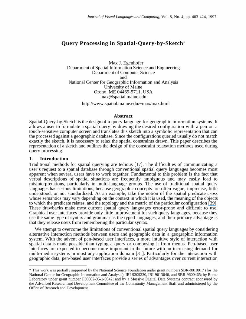
The following scenario provides a cursory outline of the envisioned interaction a user mayperform when sketching a query. This user interface is organized into three major interaction areas:the sketch region in which the user draws the configuration of interest; the overview area whichdisplays the sketch in its entirety and allows users to pan and zoom; and the control panel fromwhich the user selects database commands, the type of feature he or she is drawing, and theconfidence level for the placement of a feature. Users employ a pen to sketch an example of whatthey want to find in the database. In this particular case, the user is interested in all land parcels thathave a wooded area and a river crossing the parcel. The user first sketches the parcel by selectingthe class of the object (in this case a Parcel), and drawing its boundary (Figure 1a). Then shedescribes the location of the forest by drawing part of the forest’s boundary (Figure 1b). Since it isunclear on which side of the line the forest is located, the user fills the interior of the forest (Figure1c). Finally the user draws a river such that it crosses the land parcel (Figure 1d). Since the user issatisfied with the drawing, she requests that all configurations that match the sketch be retrievedfrom the database by pressing the Go! button on the control panel.

Journal of Visual Languages and Computing, Vol. 8, No. 4, pp. 403-424, 1997.

Figure 1: (a) The user draws the geometry of a land parcel; (b) the user adds the boundary ofa forest; (c) to determine the location of the forest, the user fills the forest’s interior;and (d) the user adds the location of a stream such that it crosses the land parcel, butdoes not intersect with the forest.

4 . Symbolic Representation of a SketchWhile a bitmap representation would provide an accurate snapshot of such a sketch, it would bedifficult to interpret it and match it against elements in other datasets whose relations, sizes, andshapes are distorted or not to scale with the sketch or whose orientations among elements differ tosome degree. Instead, we select an object representation for the sketch, which allows us to abstractaway some details of the sketch while it emphasizes its salient parts. This representation stressesobjects, their spatial and non-spatial properties, and the spatial relations among the objects drawn.The latter are of particular importance for processing a query in Spatial-Query-by-Sketch as theycapture the essence of a spatial scene.

We represent the sketch internally as a semantic network of spatial objects and their binaryspatial relations. In this network, each object drawn corresponds to a node whose values are givenby the semantics assigned in the sketch. They may include the class of an object, a name, otherattribute values, or such metrical constraints as the size of the area or length of an object. Directed

Journal of Visual Languages and Computing, Vol. 8, No. 4, pp. 403-424, 1997.

edges between nodes stand for binary spatial relations between the spatial objects. For thispurpose, we distinguish five different types of spatial relations: coarse binary topological relations,detailed binary topological relations, metrical refinements, coarse cardinal directions, and detailedcardinal directions. With these five types of binary spatial relations, a qualitative model of a sketchis built in the form of a multi-resolution semantic network, called a scene network. Such a networkserves as a symbolic, qualitative representation of the sketch. Its elements translate into predicatesin spatial queries. See [44] for a discussion about the completeness of the approach of using binaryrelations for spatial queries. The scene network may be constructed at different levels of detail, forinstance only at a coarse level of detail with topological and direction relations, or only as atopological representation with coarse and detailed topological relations. For the most detailedanalysis, a complete scene network would be derived with all five types of spatial relations. Such arepresentation translates easily into database queries in the form of first-order predicates orextended-SQL statements. Depending on the configuration, fewer binary relations may besufficient to describe the scene completely if they allow to drive uniquely the eliminated relationsthrough compositions of elementary or inferred relations [20]. There are additional dependenciesamong the different types of binary relations that could further reduce the smallest number ofrelations required to fully specify a scene. For example, detailed cardinal directions imply theircorresponding coarse cardinal directions. The actual number of spatial relations to be consideredfor processing a particular query is an issue of spatial query optimization [8]. In the following, wediscuss the models used for the five types of spatial relations.4.1 Coarse Topological RelationsWe base the analysis of topological relations on the 9-intersection, a comprehensive model forbinary topological relations that applies to objects of type area, line, and point [13, 15]. Itcharacterizes the topological relation between two point sets, A and B , by the set intersections ofA ’s interior, boundary, and exterior with the interior, boundary, and exterior of B , called the 9-intersection. With each of these nine intersections being empty or non-empty, the model has 512possible topological relations between two point sets, some of which cannot be realized. For twosimple regions without holes embedded in R2, the categorization shows eight distinct topologicalrelations. They have been called disjoint, meet, equal, overlap, inside, contains, covers, andcoveredBy (Figure 2). For two simple lines (non-branching, no self-intersections) embedded inR2, 33 different topological relations can be realized with the 9-intersection, and for a line and aregion, 19 different situations are found [16].

meet

B

A

covers

B

A

coveredBy

BA

overlap

B

A

disjoint

A

B

contains

BA

inside

AB

equal

A=B

Figure 2: The eight topological relations that can be realized between two spatial regionsembedded in R2.

4.2 Detailed Topological RelationsMore detailed distinctions about topological relations are possible if further criteria are employed toevaluate the non-empty intersections. In order to establish topological-relation equivalence betweentwo regions (i.e., to decide whether or not two pairs of objects have the same topologicalrelations), it is sufficient to describe topological invariants for the components (or separations) ofthe boundary-boundary intersection [14] and the approach generalizes to line-line and line-regionrelations. The necessary invariants to consider for region-region relations are:

Journal of Visual Languages and Computing, Vol. 8, No. 4, pp. 403-424, 1997.

• the sequence of components counted in a consistent orientation of the plane along the boundariesof the regions (Figure 3a);

• the dimension of each component—0-dimensional for boundary-boundary intersections in asingle point and 1-dimensional for boundary-boundary intersections that form a common line(Figure 3b);

• the type of boundary-boundary component intersection—touching if the boundary enters andleaves the component intersection from the same part, or crossing if the boundary enters from adifferent part than it leaves (Figure 3c);

• the crossing direction of boundary-boundary components—into and out of the interior (Figure3d);

• the boundedness, i.e., whether a 1-dimensional boundary-boundary component is inside oralong the border of the union of the two objects (Figure 3e); and

• the complement relationship, i.e., whether a component is a next to an open or closed exterior(Figure 3f).

Journal of Visual Languages and Computing, Vol. 8, No. 4, pp. 403-424, 1997.

(a) (b) (c)

(d)

0

(f)(e)

Figure 3: Six pairs of relations each of which distinguishes by different detailed topologicalrelations: (a) component sequences, (b) component dimensions, (c) types ofboundary-boundary component intersections, (d) crossing directions, (e)boundedness, and (f) complement relationships.

Detailed topological relations between two regions are expressed by the component invarianttable for non-empty boundary-boundary sequences, which lists the sequence of boundary-boundary components and each component’s dimension, type, crossing direction, boundedness,and complement relationship [12, 14].

Journal of Visual Languages and Computing, Vol. 8, No. 4, pp. 403-424, 1997.

4.3 Metrical RefinementsOccasionally, topology per se is insufficient to characterize the essence of spatial relations. Forinstance, in order to capture the semantics of the spatial relation between Interstate I-95 and thestate of New Hampshire requires the consideration of some metrical properties in addition totopological concerns—I-95 divides New Hampshire into a very small area on one side of I-95 anda larger piece on the other side. To describe metrical details, we apply measures about areas andlengths as refinements of the topological properties [48]. These measures are normalized valueswith respect to the areas or lengths of interiors and boundaries and, therefore, scale-independent.These measures are defined as refinements of the 9-intersection, adding length and area measuresto quantify non-empty intersections. The same concepts apply to the 9-intersections of line-regionand line-line relations, although the number of measures that are applicable may vary with thegeometric types of the objects involved. Figure 4 shows the eight measures that apply to region-region relations—six splitting ratios that capture how object A’s parts separate object B, and twocloseness measures that describe relative distances from A’s boundary to B’s boundary. The sametypes of measures apply as ratios of A’s metrical properties over B’s.

Inner Area Splitting Outer Area Splitting Exterior Splitting

A

B

A

B

A

B

IAS =area(A°∩ B° )

area( A)OAS =

area(A°∩ B−)

area(A)ES =

area(bouded( A− ∩ B− ))

area(A)

Inner Traversal Splitting Outer Traversal Splitting Alongness Splitting

A

B

A

B

A

B

ITS =length(∂A ∩ B° )

length(∂A)OTS =

length(∂A ∩ B−)

length(∂A)AS =

length(∂A ∩ ∂B)

length(∂A)

Inner Closeness Outer Closeness

BA∆ BA ∆

IC =area(∆(A))

area(A)OC =

area(∆(A)) + area(A)

area(A)

Figure 4: Metrical refinements of topological relations.

Journal of Visual Languages and Computing, Vol. 8, No. 4, pp. 403-424, 1997.

4.4 Cardinal DirectionsAnalogous to the role metrical properties may play in the interpretation of a scene, directionrelations may provide a basis for certain decisions about matching and similarity. Directionrelations are well understood for point objects; however, for extended spatial objects, such aslinear or areal features, no generally accepted models exist and a variety of semantically differentapproaches have been proposed [45]. In this case, we adapt the projection-based method [23, 43]around a the minimum bounding rectangle of an object, partitioning space into nine regions for anareal object. These partitions are named north (N), northeast (NE), east (E), southeast (SE), south(S), southwest (SW), west (W), northwest (NW), and at the same location (0). The cardinaldirection from an object to a target direction is described by recording the partitions into which atleast some parts of the target object fall (Figure 5). Further refinements would be possible todescribe if a target’s outline coincides with the boundaries between partitions [24].

N

S

W E

NW

SW

NE

SE

0

Figure 5: Projection-based cardinal directions for extended spatial objects.

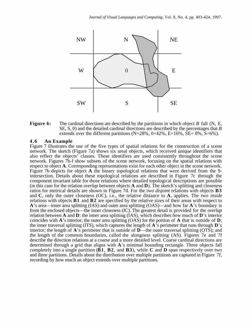
4.5 Detailed Cardinal DirectionsCardinal directions are often a coarse approximation such that an interpretation of the mere fact thatan object falls within some direction partition(s) of another object may be misleading orinappropriate. To provide more detail about directions among objects, we extend the cardinal-direction method, recording for each object that falls into more than one direction partition thepercentage of the common intersection between a partition and the object (Figure 6). The range ofeach detailed cardinal direction x is 0 < x <1.0 . The sum of all percentages for an object withrespect to the partitions of another object must be 1.0. The refinement measure does not apply toempty partitions nor would it provide any additional information if the entire object falls into asingle partition.

Journal of Visual Languages and Computing, Vol. 8, No. 4, pp. 403-424, 1997.

N

S

W E

NW

SW

NE

SE

0

Figure 6: The cardinal directions are described by the partitions in which object B fall (N, E,SE, S, 0) and the detailed cardinal directions are described by the percentages that Bextends over the different partitions (N=28%, 0=42%, E=16%, SE= 8%, S=6%).

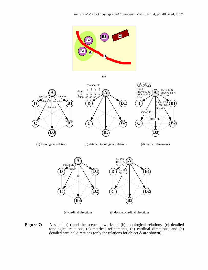
4.6 An ExampleFigure 7 illustrates the use of the five types of spatial relations for the construction of a scenenetwork. The sketch (Figure 7a) shows six areal objects, which received unique identifiers thatalso reflect the objects’ classes. These identifiers are used consistently throughout the scenenetwork. Figures 7b-f show subsets of the scene network, focusing on the spatial relations withrespect to object A. Corresponding representations exist for each other object in the scene network.Figure 7b depicts for object A the binary topological relations that were derived from the 9-intersection. Details about these topological relations are described in Figure 7c through thecomponent invariant table for those relations where detailed topological descriptions are possible(in this case for the relation overlap between objects A and D). The sketch’s splitting and closenessratios for metrical details are shown in Figure 7d. For the two disjoint relations with objects B3and C, only the outer closeness (OC), i.e., the relative distance to A, applies. The two insiderelations with objects B1 and B2 are specified by the relative sizes of their areas with respect toA’s area—inner area splitting (IAS) and outer area splitting (OAS)—and how far A’s boundary isfrom the enclosed objects—the inner closeness (IC). The greatest detail is provided for the overlaprelation between A and D: the inner area splitting (IAS), which describes how much of D’s interiorcoincides with A’s interior; the outer area splitting (OAS) for the portion of A that is outside of D;the inner traversal splitting (ITS), which captures the length of A’s perimeter that runs through D’sinterior; the length of A’s perimeter that is outside of D—the outer traversal splitting (OTS); andthe length of the common boundaries, called the alongness splitting (AS). Figures 7e and 7fdescribe the direction relations at a coarse and a more detailed level. Coarse cardinal directions aredetermined through a grid that aligns with A’s minimal bounding rectangle. Three objects fallcompletely into a single partition (B1 , B2 , and B3), while C and D span respectively over twoand three partitions. Details about the distribution over multiple partitions are captured in Figure 7f,recording by how much an object extends over multiple partitions.

Journal of Visual Languages and Computing, Vol. 8, No. 4, pp. 403-424, 1997.

IAS=0.14 &OAS=0.86 &ES=0 &ITS=0.07 &OTS=0.93 &AS=0

IAS=.12 &OAS=0.88 &IC=.40

IAS=.12 &OAS=.88 &IC=.46

OC=1.92

OC=6.12

A

B3

D

B2C

B1

(d) metric refinements

A

B3

D

B2C

B1

contains

contains

disjoint

disjoint

overlap

(b) topological relations

B3

D

B2C

B1

A

components

dim.typecomp.

00

crop

10

crop

20

crop

30

crop

(c) detailed topological relations

E=.98&NE=.02

0=.47&E=.31&SE=.22

A

B3

D

B2C

B1

(f) detailed cardinal directions

00

E

E&NE

0&E&SEA

B3

D

B2C

B1

(e) cardinal directions

B1

B3B2

A

C

D

(a)

Figure 7: A sketch (a) and the scene networks of (b) topological relations, (c) detailedtopological relations, (c) metrical refinements, (d) cardinal directions, and (e)detailed cardinal directions (only the relations for object A are shown).

Journal of Visual Languages and Computing, Vol. 8, No. 4, pp. 403-424, 1997.

5 . Processing Sketched QueriesThe scene network forms the basis for processing a sketched query and for presenting the queryresults in a prioritized order to the user. The spatial relations captured in the scene network relate todifferent query processing stages, because the relations are of different levels of importance forcapturing the semantics of a spatial scene; therefore, different strategies may be pursued, such asmultiple querying of a geographic database using each time a different part of the scene description.

We use the 9-intersection relations as the key for pre-processing spatial relations sketched andquerying, because they describe topological relations at a coarse level and, therefore, groupsketches into classes of similar relations. By mapping the sketched relations onto 9-intersectionrelations, we capture the most salient features of a sketch in a form that is independent oforientations and sizes. This abstraction is critical for the translation of a sketched configuration intoa database query.

The component invariants are the key for analyzing the intentional complexity of the spatialrelations sketched, because the component invariants capture complexity of topological relations. Agreater number of component intersections indicates more complexity [12]. If a user draws asketch with a high level of complexity, then we assume that this complexity was intended and thatit provides the lower bound of what should be retrieved; therefore, a configuration in a spatialdatabase with the same 9-intersection relation, but lower-rated component invariants, would notqualify as a match. On the other hand, a sketch of a low-complexity spatial relation may indicatethat more complex configurations under the same 9-intersection category should be considered aswell.

With the metrical refinements of the 9-intersection relations we formalize detailed geometricconstraints about sketched spatial relations. In Spatial-Query-by-Sketch, metrical details play tworoles. First, they are critical to decide whether the query processor should also search forconfigurations that deviate from the topology sketched. For instance, a particularly short closenessmeasure for two disjoint regions may indicate that the user also would accept as an answer aconfiguration in which the two objects meet topologically. Second, the metrical properties are thekey to prioritizing query results that have the same topology as the sketch, but differ in relativesizes of the objects, common lengths and areas, and distances between boundaries.

We exploit the cardinal directions for those queries in which the user explicitly states theimportance of orientation relations, for instance, if the user drew a north arrow to give a globalorientation to the sketch. Cardinal directions are also used to prioritize query results, i.e., as a tie-breaker among configurations with the same topology.

Finally, detailed cardinal directions are used to rank the query results such that the situation thatmatches most closely the sketch is presented first. Unlike the use of topological and detailedtopological relations, the transition from coarse to detailed cardinal directions is used as a mererefinement and no intended complexity of the configuration is derived from the detailed directionrelations.

A strategy that makes use of the dependencies among the different types of spatial relations isoutlined below. Since the five types of spatial relations play different roles in the interpretation of asketch, we employ a multi-step query processing strategy.• First, the topological scene description is used to formulate a spatial database query. A

topological relation is relaxed if its metrical refinements have small values indicating thatalternative topological configurations may be considered as well. In addition, if the userspecifies explicitly an orientation of the sketch, the cardinal directions are incorporated into thequery.

• Second, for a non-empty result set of such a spatial query, each configuration is analyzedaccording to topological details, metrical details, and detailed cardinal directions, eliminatingfalse hits and prioritizing the remaining configurations.

• If the query result is an empty set (i.e., no configuration was found that matches the relationsspecified), the initial constraints may be relaxed, from which a revised spatial query getsformulated.

Journal of Visual Languages and Computing, Vol. 8, No. 4, pp. 403-424, 1997.

6 . Relaxing Spatial RelationsThe comparison of the sketched spatial relations with the spatial relations recorded in a geographicdatabase may not necessarily provide an exact match. The sketch may, for instance, be distortedleading to different relations than intended or the user may be satisfied with a configuration that isan approximation of what he or she drew. For this purpose it is necessary to consider not onlyexact matches, but also similar matches [3, 41]. The challenging aspect of determining similarconfigurations is that spatial relations represent discrete concepts that are usually thought of asbeing on a nominal scale. In order to assess similarity among elements, however, it is necessary tointroduce some non-arbitrary order over the elements. Spatial-Query-by-Sketch establishessimilarity over different types of spatial relations through a formal model, including a metric, thatassesses deviations of a spatial relation from a target relation.

An important basis for the similarity assessment is Stevens’s categorization of scales ofmeasurements, which distinguishes nominal, ordinal, interval, and ratio type data [50].Topological relations are discrete values on a nominal scale, therefore, no linear order can beestablished among them. Similarity among topological relations is described in terms of theconceptual neighborhood graph, which links most similar relations to each other. It is based on thecomputational model of determining for each relation those relations with the least number ofdifferences in the 9-intersection matrices. For instance, disjoint and meet are conceptually closer toeach other than disjoint and overlap, because disjoint and meet differ in one entry in their 9-intersections—they have different boundary-boundary intersections—while disjoint and overlapdiffer in four entries. Conceptual neighborhood graphs have been derived for the eight region-region relations [11] (Figure 8), line-line relations [21], and line-region relations [18].

inside

overlap

coveredBy

contains equal

covers

meet

disjoint

Figure 8: Conceptual neighborhood graph of the eight region-region relations.Relaxing a topological relation corresponds to changing a constraint from a topological relation

to include its conceptual neighbors. For example, if a user drew a scenario in which a region wasfully included in the interior of another region, then a relaxation would consider not only thoseconfigurations that match exactly its topological relation, but also those that match the relation’sconceptual neighbors [3]. Figure 9 shows the relaxation of all topological constraints for the sketch

Journal of Visual Languages and Computing, Vol. 8, No. 4, pp. 403-424, 1997.

in Figure 7a. Higher degrees of dissimilarity can be achieved by recursively moving from theconceptual neighbors to their conceptual neighbors (without moving back). The more thetopological relation gets relaxed, the less similar a relation becomes to its target.

B1 B2 B3 C D

A

B1

B2

B3

C

Figure 9: First-degree relaxation of all topological relations for the objects in figure 7a.A more controlled way of relaxing topological relations exploits the metrical details as well.

Metrical details are refinements of topological relations and a small value for a particular metricaldetail indicates that an alternative topological relation may be considered as well. For example, theconfiguration in Figure 7a shows objects A and B3 being disjoint, but close together (the outercloseness from A to B3 is 1.92), whereas A and C are disjoint as well, but further apart from eachother (the outer closeness from A to C is 6.12). If a threshold for the outer closeness was set to2.0, A disjoint B3 may be relaxed into A disjoint or meet B3 . This type of relaxation implies adirection on the conceptual neighborhood graph, i.e., not all conceptual neighbors are used. Forexample, an overlap with a small value for inner area splitting, but large value for outer areasplitting, gets relaxed from overlap to overlap or meet, but not covers or coveredBy.

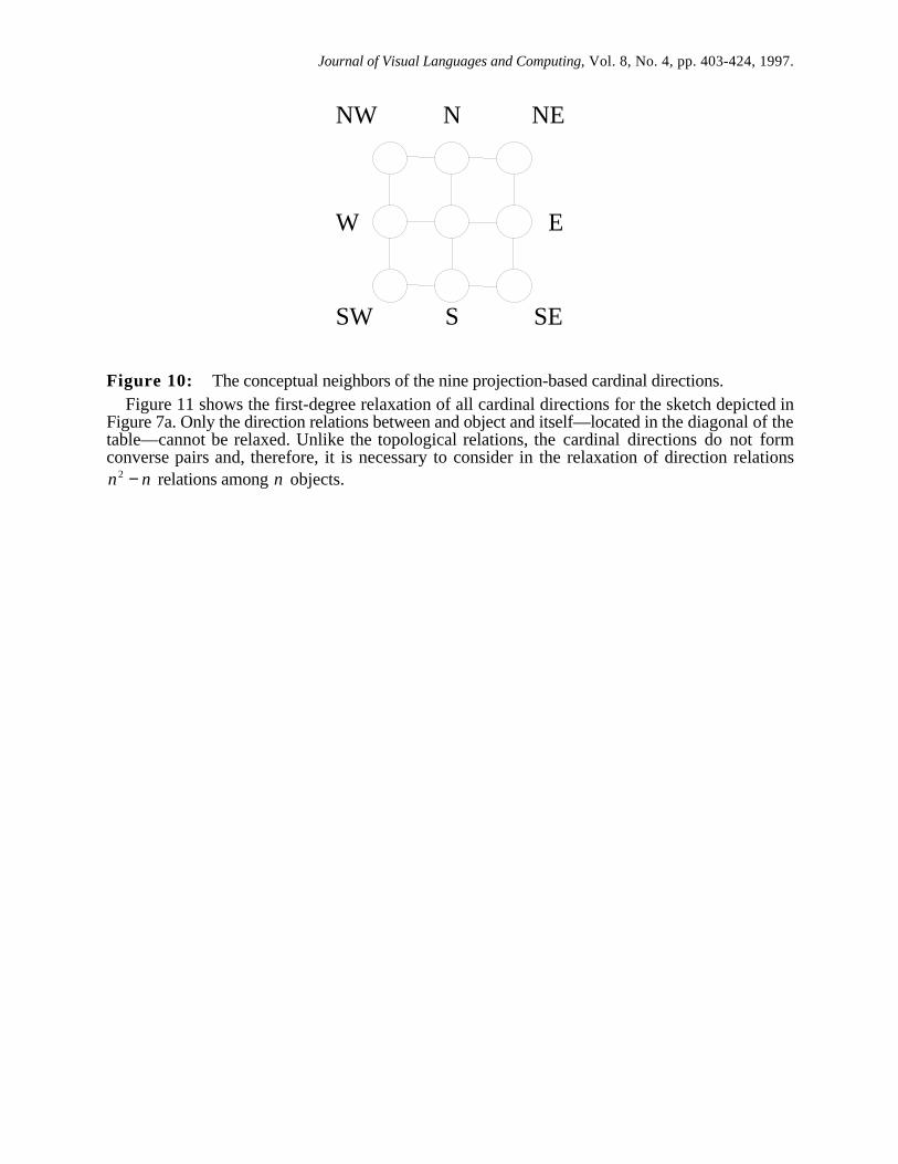
If cardinal directions are an explicit part of a sketch, they may be subject to relaxation duringquery processing in the same way topological relations are. For this purpose, it is necessary tomodel the conceptual neighborhoods of cardinal directions such that the most similar direction canbe determined. For the projection-based model with nine direction values, a simple model arrangesthe relations in a 3 × 3 grid, reflecting the nine partitions such that conceptual neighborhoods areestablished both in horizontal and vertical directions (Figure 10). The conceptual neighbor of adirection relation are then its immediate horizontal and vertical neighbors in the graph. If an objectextends through more than one partition, the conceptual neighbors of its cardinal directioncomprise the union of the neighbors of each relation in the set.

Journal of Visual Languages and Computing, Vol. 8, No. 4, pp. 403-424, 1997.

N

S

NW

W

SW

NE

E

SE

Figure 10: The conceptual neighbors of the nine projection-based cardinal directions.Figure 11 shows the first-degree relaxation of all cardinal directions for the sketch depicted in

Figure 7a. Only the direction relations between and object and itself—located in the diagonal of thetable—cannot be relaxed. Unlike the topological relations, the cardinal directions do not formconverse pairs and, therefore, it is necessary to consider in the relaxation of direction relationsn2 − n relations among n objects.

Journal of Visual Languages and Computing, Vol. 8, No. 4, pp. 403-424, 1997.

A B1 B2 B3 C D

A

B1

B2

B3

C

D

Figure 11: First-degree relaxation of all cardinal directions among the objects in Figure 7a.

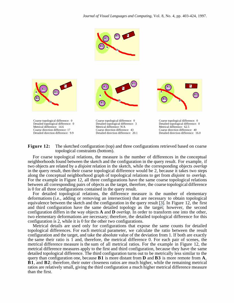
7 . Prioritizing Query ResultsIndependent of whether the query is relaxed or not, the result that is returned from a spatialdatabase may contain multiple configurations, all of which fulfill the constraints of the query(Figure 12); however, in such a set of configurations there will be some that fit the original sketchbetter than others. Since the query acts as a filter, it is necessary to sort through the query resultduring the subsequent phase of query result prioritization and to rank the configurations retrievedaccording to their similarity with the sketch. This assessment requires difference measures for allfive types of spatial relations. All measures introduced are such that lower difference valuesrepresent more similar configurations, while larger values indicate more differences. A value of 0indicates no difference according to the type of spatial relation.

Journal of Visual Languages and Computing, Vol. 8, No. 4, pp. 403-424, 1997.

B1

B3B2

A

C

D

B1

B3B2

A

C

DB1

B3

B2

A

C

B1

B3

A

CB2

DD

Coarse topological difference: 0Detailed topological difference: 0Metrical difference: 14.6Coarse direction difference: 17Detailed direction difference: 9.9

Coarse topological difference: 0Detailed topological difference: 3Metrical difference: N/ACoarse direction difference: 43Detailed direction difference: 20.1

Coarse topological difference: 0Detailed topological difference: 0Metrical difference: 62.5Coarse direction difference: 40Detailed direction difference: 16.0

Figure 12: The sketched configuration (top) and three configurations retrieved based on coarsetopological constraints (bottom).

For coarse topological relations, the measure is the number of differences in the conceptualneighborhoods found between the sketch and the configuration in the query result. For example, iftwo objects are related by a disjoint relation in the sketch, while the corresponding objects overlapin the query result, then their coarse topological difference would be 2, because it takes two stepsalong the conceptual neighborhood graph of topological relations to get from disjoint to overlap.For the example in Figure 12, all three configurations have the same coarse topological relationsbetween all corresponding pairs of objects as the target, therefore, the coarse topological differenceis 0 for all three configurations contained in the query result.

For detailed topological relations, the difference measure is the number of elementarydeformations (i.e., adding or removing an intersection) that are necessary to obtain topologicalequivalence between the sketch and the configuration in the query result [3]. In Figure 12, the firstand third configuration have the same detailed topology as the target; however, the secondconfiguration differs in the way objects A and D overlap. In order to transform one into the other,two elementary deformations are necessary; therefore, the detailed topological difference for thisconfiguration is 2, while it is 0 for the other two configurations.

Metrical details are used only for configurations that expose the same counts for detailedtopological differences. For each metrical parameter, we calculate the ratio between the resultconfiguration and the target, and take the absolute value of the deviation from 1. If both are exactlythe same their ratio is 1 and, therefore, the metrical difference 0. For each pair of scenes, themetrical difference measure is the sum of all metrical ratios. For the example in Figure 12, themetrical difference measures apply to the first and third configuration, because they have the samedetailed topological difference. The third configuration turns out to be metrically less similar to thequery than configuration one, because B1 is more distant from D and B3 is more remote from A,B1 , and B2; therefore, their outer closeness ratios are much higher, while the remaining metricalratios are relatively small, giving the third configuration a much higher metrical difference measurethan the first.

Journal of Visual Languages and Computing, Vol. 8, No. 4, pp. 403-424, 1997.

As the measure for coarse direction differences we determine for each corresponding pair ofobjects the shortest path between their cardinal directions along their conceptual neighborhoods.For example, the shortest path from N to SW is 3; from NW to SE it is 4; from N to N it is 0, fromNW and W to SW and S it is 4; and from NW and W to SW it is 3. The direction differencemeasure between two configurations is the sum of all shortest paths along the conceptualneighborhoods. For the example in Figure 12, the first configuration in the query result has thebest match with respect to the target. The other two configurations differ more strongly from thesketch primarily due to the significantly different locations of objects B3 and C, which leads tohigh scores for the direction differences of the relations between B3 and C, but also between B3and B2 .

The difference measure for detailed cardinal directions gives weights to the counts of the stepsof the coarse direction differences according to the percentages of changes. For example, from thedetailed direction relations E (0.98) and NE (0.02) to E (1.00), the weighted count is 0.02, whilefrom E (0.98) and NE (0.02) to NE (1.00) would be 0.98; the count from E (0.10) and SE (0.70)and S (0.20) to S (1.00) is 2 * 0.10 + 1 * 0.70 = 0.90. The difference measure for detaileddirections also applies if both directions span the same partitions, but are differently distributed.For example, the weighted count from E (0.98) and NE (0.02) to E (0.04) and NE (0.96) is 0.98 –0.04 = 0.94. For the example in Figure 12, the detailed direction differences confirm the similarityrankings of the query results obtained from the coarse direction differences. Comparisons with thedetailed direction differences, however, may lead to different results than the coarse directiondifferences if the individual counts are primarily small values.8 . ConclusionsThis paper presented the design principles of Spatial-Query-by-Sketch, a visual spatial querylanguage for geographic information systems. Users interact through Spatial-Query-by-Sketch byusing a pen to draw an example of the configuration they are interested in. Spatial-Query-by-Sketch parses this graphical input, analyzes it, and translates it into a database query. We base itsquery processing mechanisms on a powerful computational model for spatial relations that allowsus to emphasize cognitively important criteria of the sketch, and to suppress aspects that may be oflesser importance. Spatial-Query-by-Sketch uses five types of spatial relations: coarse topologicalrelations, detailed topological relations, metrical details, coarse cardinal directions, and detailedcardinal directions. This approach is tailored for geographic similarity retrieval, where frequentlythe orientation, size, and shape of an object may not matter, but the relationship with respect toother objects is critical. Each set of spatial relations is formally defined, including computationalmethods to address similarity among pairs of relations of the same type. These models of spatialrelations are used when translating the sketch into a database query, when relaxing spatialconstraints, and when sorting query results according to highest similarity with the sketch.

A prototype of Spatial-Query-by-Sketch is under development with methods implemented forthe assessment and relaxation of topological and direction relations. From experiments with theprototype we expect to gain new insights into the match between different querying strategies andpeople’s intuition about similarity retrieval. Such future experiments also will provide us withguidance as to whether and how a single similarity measure as a weighted combination of the fiveindividual measures would useful. To work efficiently with a spatial database system, indexingand access methods for spatial relations are required that would support the query execution in adatabase system. Current spatial access methods are limited to the location of spatial objects and,therefore, only support fast retrieval based on coordinate values, such as point-in-polygon orwindow queries. Since Spatial-Query-by-Sketch is based on a different paradigm—spatial relationsrather than location in space—either a mapping onto existing methods or the development of newmethods will be necessary.

Spatial-Query-by-Sketch is on the opposite scale of a verbal spatial query language. Whiledrawing spatial configurations is an intuitive interaction with geographic data, there are somespatial concepts, such as intentional orientation, distance, or shape, that may be difficult to express

Journal of Visual Languages and Computing, Vol. 8, No. 4, pp. 403-424, 1997.

through a sketch alone. A sketch-based spatial query language may benefit from an embedding intoa multi-modal interaction, where sketching may be augmented by verbal instructions [9].

9 . AcknowledgmentsDiscussions with Doug Flewelling, Bob Franzosa, Dimitris Papadias, and Jayant Sharma helped inthe development of the concepts in Spatial-Query-by-Sketch. Thanks also to the Spatial-Query-by-Sketch team, which includes Peggy Agouris, Andreas Blaser, Tom Bruns, James Craswell, YvesDennebouy, Roop Goyal, João Paiva, Dieter Pfoser, Uwe Rupp, Rashid Shariff, and TonyStefanidis.

10. References[1] M.-A. Aufaure-Portier, “Definition of a Visual Language for GIS,” Cognitive Aspects of

Human-Computer Interaction for Geographic Information Systems, T. Nyerges, D. Mark,R. Laurini, and M. Egenhofer, eds., vol. Kluwer, Dordrecht, 1995, pp. 163-178.

[2] A. Borning, “Defining Constraints Graphically,” Human Factors in Computing Systems,CHI `86, Boston, MA, 1986, pp. 137-143.

[3] T. Bruns and M. Egenhofer, “Similarity of Spatial Scenes,” Seventh InternationalSymposium on Spatial Data Handling, M.-J. Kraak and M. Molenaar, eds., Delft, TheNetherlands, 1996, pp. 4A.31-42.

[4] D. Calcinelli and M. Mainguenaud, “Cigales, a Visual Query Language for a GeographicalInformation System: the User Interface,” Journal of Visual Languages and Computing, vol.5, no. 2, pp. 113-132, 1994.

[5] N.S. Chang and K.S. Fu, “Query-by-Pictorial-Example,” IEEE Transactions on SoftwareEngineering, vol. SE-6, no. 6, pp. 519-524, 1980.

[6] A. Del Bimbo, P. Pala, and S. Santini, “Visual Image Retrieval by Elastic Deformation ofObject Sketches,” IEEE Symposium on Visual Languages, IEEE Computer Society Press,St. Louis, MO, 1994, pp. 216-223.

[7] M. Egenhofer, “Why not SQL!,” International Journal of Geographical InformationSystems, vol. 6, no. 2, pp. 71-85, 1992.

[8] M. Egenhofer, “Pre-Processing Queries with Spatial Constraints,” PhotogrammetricEngineering & Remote Sensing, vol. 60, no. 6, pp. 783-790, 1994.

[9] M. Egenhofer, “Multi-Modal Spatial Querying,” Seventh International Symposium on SpatialData Handling, M.-J. Kraak and M. Molenaar, eds., Delft, The Netherlands, 1996, pp.12B.11-15.

[10] M. Egenhofer, “Spatial-Query-by-Sketch,” VL ‘96: IEEE Symposium on Visual Languages,IEEE Computer Society, Boulder, CO, 1996, pp. 60-67.

[11] M. Egenhofer and K. Al-Taha, “Reasoning About Gradual Changes of TopologicalRelationships,” Theories and Methods of Spatio-Temporal Reasoning in Geographic Space,Pisa, Italy, A. Frank, I. Campari, and U. Formentini, eds., Lecture Notes in ComputerScience, vol. 639, Springer-Verlag, Berlin, 1992, pp. 196-219.

[12] M. Egenhofer, E. Clementini, and P. Di Felice, “Evaluating Inconsistencies Among MultipleRepresentations,” Sixth International Symposium on Spatial Data Handling, T. Waugh andR. Healey, eds., Edinburgh, Scotland, 1994, pp. 901-920.

[13] M. Egenhofer and R. Franzosa, “Point-Set Topological Spatial Relations,” InternationalJournal of Geographical Information Systems, vol. 5, no. 2, pp. 161-174, 1991.

[14] M. Egenhofer and R. Franzosa, “On the Equivalence of Topological Relations,” InternationalJournal of Geographical Information Systems, vol. 9, no. 2, pp. 133-152, 1995.

[15] M. Egenhofer and J. Herring, “A Mathematical Framework for the Definition of TopologicalRelationships,” Fourth International Symposium on Spatial Data Handling, K. Brassel andH. Kishimoto, eds., Zurich, Switzerland, 1990, pp. 803-813.

Journal of Visual Languages and Computing, Vol. 8, No. 4, pp. 403-424, 1997.

[16] M. Egenhofer and J. Herring, Categorizing Binary Topological Relationships BetweenRegions, Lines, and Points in Geographic Databases, Department of Surveying Engineering,University of Maine, Orono, ME, 1991.

[17] M. Egenhofer and J. Herring, “Querying a Geographical Information System,” HumanFactors in Geographical Information Systems, D. Medyckyj-Scott and H. Hearnshaw, eds.,vol. Belhaven Press, London, 1993, pp. 124-136.

[18] M. Egenhofer and D. Mark, “Modeling Conceptual Neighbourhoods of Topological Line-Region Relations,” International Journal of Geographical Information Systems, vol. 9, no.5, pp. 555-565, 1995.

[19] M. Egenhofer and D. Mark, “Naive Geography,” Spatial Information Theory—A TheoreticalBasis for GIS, International Conference COSIT ‘95, Semmering, Austria, A. Frank and W.Kuhn, eds., Lecture Notes in Computer Science, vol. 988, Springer-Verlag, Berlin, 1995,pp. 1-15.

[20] M. Egenhofer and J. Sharma, “Assessing the Consistency of Complete and IncompleteTopological Information,” Geographical Systems, vol. 1, no. 1, pp. 47-68, 1993.

[21] M. Egenhofer, J. Sharma, and D. Mark, “A Critical Comparison of the 4-Intersection and 9-Intersection Models for Spatial Relations: Formal Analysis,” Autocarto 11, R. McMaster andM. Armstrong, eds., Minneapolis, MN, 1993, pp. 1-11.

[22] C. Faloutsos, R. Barber, M. Flickner, J. Hafner, W. Niblack, D. Petrovic, and W. Equitz,“Efficient and Effective Querying by Image Content,” Journal of Intelligent InformationSystems, vol. 3, no. pp. 231-262, 1994.

[23] A. Frank, “Qualitative Spatial Reasoning about Cardinal Directions,” Autocarto 10, D. Markand D. White, eds., Baltimore, MD, 1991, pp. 148-167.

[24] C. Freksa, “Using Orientation Information for Qualitative Spatial Reasoning,” Theories andMethods of Spatio-Temporal Reasoning in Geographic Space, A. Frank, I. Campari, and U.Formentini, eds., Lecture Notes in Computer Science, vol. 639, Springer-Verlag, NewYork, NY, 1992, pp. 162-178.

[25] M. Gross, “Recognizing and Interpreting Diagrams in Design,” Advanced Visual Interfaces‘94, T. Catarci, M. Costabile, S. Levialdi, and G. Santucci, eds., ACM Press, New York,NY, 1994, pp. 88-94.

[26] V. Gudivada and V. Raghavan, “Design and Evaluation of Algorithms for Image Retrievalby Spatial Similarity,” ACM Transactions on Information Systems, vol. 13, no. 2, pp. 115-144, 1995.

[27] J. Herring, “The Mathematical Modeling of Spatial and Non-Spatial Information inGeographic Information Systems,” Cognitive and Linguistic Aspects of Geographic Space,D. Mark and A. Frank, eds., vol. Kluwer Academic Publishers, Dordrecht, 1991, pp. 313-350.

[28] J. Herring, R. Larsen, and J. Shivakumar, “Extensions to the SQL Language to SupportSpatial Analysis in a Topological Data Base,” GIS/LIS ‘88, San Antonio, TX, 1988, pp.741-750.

[29] K. Hirata and T. Kato, “Query by Visual Example—Content-Based Image Retrieval,”Advances in Database Technology—EDBT ‘92, 3rd International Conference on ExtendingDatabase Technology, Vienna, Austria, A. Pirotte, C. Delobel, and G. Gottlob, eds., LectureNotes in Computer Science, vol. 580, Springer-Verlag, Berlin, 1992, pp. 56-71.

[30] K. Hirata and T. Kato, “Rough Sketch-Based Image Information Retrieval,” NEC Researchand Development, vol. 34, no. 2, pp. 263-273, 1993.

[31] T. Imielinski and H. Korth, “MOBIDATA Workshop Report,” MOBIDATA: An InteractiveJournal of Mobile Computing, vol. 1, no. 2, pp.http://www.cs.rutgers.edu/~badri/journal/contents12.html, 1995.

Journal of Visual Languages and Computing, Vol. 8, No. 4, pp. 403-424, 1997.

[32] K. Ingram and W. Phillips, “Geographic Information Processing Using a SQL-Based QueryLanguage,” AUTO-CARTO 8, Eighth International Symposium on Computer-AssistedCartography, N.R. Chrisman, eds., Baltimore, MD, 1987, pp. 326-335.

[33] T. Joseph and A. Cardenas, “PICQUERY: A High Level Query Language for PictorialDatabase Management,” IEEE Transactions on Software Engineering, vol. 14, no. 5, pp.630-638, 1988.

[34] T. Kato, T. Kurita, N. Otsu, and K. Hirata, “A Sketch Retrieval Method for Full ColorImage Database—Query by Visual Example,” 11th IAPA International Conference on PatternRecognition, IEEE Computer Society Press, The Hague, The Netherlands, 1992, pp. 530-533.

[35] T. Kato, T. Kurita, and H. Shimogaki, “Multimedia Interaction with Image DatabaseSystems,” Advanced Database System Symposium ‘89, Kyoto, Japan, 1989, pp. 271-278.

[36] Y.C. Lee and F.L. Chin, “An Iconic Query Language for Topological Relationships in GIS,”International Journal of Geographical Information Systems, vol. 9, no. 1, pp. 25-46, 1995.

[37] M. Mainguenaud and M.-A. Portier, “Cigales: A Graphical Query Language forGeographical Information Systems,” Fourth International Symposium on Spatial DataHandling, K. Brassel and H. Kishimoto, eds., Zurich, Switzerland, 1990, pp. 393-404.

[38] D. Mark, “Counter-Intuitive Geographic “Facts:” Clues for Spatial Reasoning at GeographicScales,” Theories and Methods of Spatio-Temporal Reasoning in Geographic Space, Pisa,Italy, A. Frank, I. Campari, and U. Formentini, eds., Lecture Notes in Computer Science,vol. 639, Springer-Verlag, Berlin, 1992, pp. 305-317.

[39] D. Mark, D. Comas, M. Egenhofer, S. Freundschuh, M. Gould, and J. Nunes, “Evaluatingand Refining Computational Models of Spatial Relations Through Cross-Linguistic Human-Subject Testing,” Spatial Information Theory—A Theoretical Basis for GIS, InternationalConference COSIT ‘95, Semmering, Austria, A. Frank and W. Kuhn, eds., Lecture Notesin Computer Science, vol. 988, Springer-Verlag, Berlin, 1995, pp. 553-568.

[40] B. Meyer, “Pictorial Deduction in Spatial Information Systems,” IEEE Symposium on VisualLanguages, A. Ambler and T. Kimura, eds., IEEE Computer Society Press, St. Louis, MO,1994, pp. 23-39.

[41] N. Nabil, A. Ngu, and J. Shepherd, “Picture Similarity Retrieval Using the 2D ProjectionInterval Representation,” IEEE Transactions on Knowledge and Data Engineering, vol. 8,no. 4, pp. 533-539, 1996.

[42] V. Ogle and M. Stonebraker, “Chabot: Retrieval from a Relational Database of Images,”IEEE Computer, vol. 28, no. 9, pp. 40-48, 1995.

[43] D. Papadias and T. Sellis, “A Pictorial Query-by-Example Language,” Journal of VisualLanguages and Computing, vol. 6, no. 1, pp. 53-72, 1995.

[44] C. Papadimitriou, D. Suciu, and V. Vianu, “Topological Queries in Spatial Databases,”Fifteenth ACM SIGACT-SIGMOD-SIGART Symposium on Principles of Database Systems(PODS), ACM Press, Montreal, Canada, 1995,

[45] D. Peuquet and C.-X. Zhan, “An Algorithm to Determine the Directional RelationshipBetween Arbitrarily-Shaped Polygons in the Plane,” Pattern Recognition, vol. 20, no. 1, pp.65-74, 1987.

[46] A. Pizano, A. Klinger, and A. Cardenas, “Specification of Spatial Integrity Constraints inPictorial Databases,” Computer, vol. 22, no. 12, pp. 59-71, 1989.

[47] N. Roussopoulos, C. Faloutsos, and T. Sellis, “An Efficient Pictorial Database System forPSQL,” IEEE Transactions on Software Engineering, vol. 14, no. 5, pp. 630-638, 1988.

[48] R. Shariff, Natural Language Spatial Relations: Metric Refinements of TopologicalProperties, Department of Spatial Information Science and Engineering, University of Maine,Orono, ME, 1996.

[49] A. Stevens and P. Coupe, “Distortions in Judged Spatial Relations,” Cognitive Psychology,vol. 10, no. pp. 422-437, 1978.

Journal of Visual Languages and Computing, Vol. 8, No. 4, pp. 403-424, 1997.

[50] S. Stevens, “On the Theory of Scales of Measurement,” Science Magazine, vol. 103, no.2684, pp. 677-680, 1946.

[51] I. Sutherland, “SketchPad: A Man-Machine Graphical Communication System,” AFIPSSpring Joint Computer Conference, 1963, pp. 329-346.

[52] B. Tversky, “Distortions in Memory for Maps,” Cognitive Psychology, vol. 13, no. pp.407-433, 1981.