Query Processing - DI.UBI

Query Processing

Chapter 9

Database System Concepts, Cap. 13

A. Silberschatz, H. Korth, and S. Sudarshan

Database Management Systems, Cap. 13 & 14

R. Ramakrishnan and J. Gehrke

Overview

Basic Steps of Query ProcessingMeasures of Query CostSelection OperationExternal Sorting Join OperationOther OperationsEvaluation of Expressions

Basic Stepsin Query Processing Parsing and translation Optimization Evaluation

Basic Stepsin Query Processing Parsing and translation

Translate a SQL query into its internal form. This is then translatedinto relational algebra.

Parser checks syntax, verifies relations

Optimization The query optimizer translates a relational algebra expression into an

execution plan.A relational algebra expression may have many equivalent

expressions, each of which gives rise to a different evaluation plan.Amongst all equivalent evaluation plans choose the one with lowest

cost.

Evaluation The query-execution engine takes a query-evaluation plan, executes

that plan, and returns the answers to the query.

Query Processing: Optimization A relational algebra expression may have many equivalent

expressions e.g., σbalance<2500(∏balance(account)) is equivalent to ∏balance(σbalance<2500(account))

Each relational algebra operation can be evaluated using one ofseveral different algorithms Correspondingly, a relational algebra expression can be evaluated in many

ways.

Annotated expression specifying detailed evaluation strategy iscalled an evaluation-plan. e.g., can use an index on balance to find accounts with balance< 2500, or can perform complete relation scan and discard accounts with balance ≥

2500

Query Optimization: Amongst all equivalent evaluation planschoose the one with lowest cost. Cost is estimated using statistical information from the

database catalog e.g. number of tuples in each relation, size of tuples, etc.

Query Processing vs.Optimization In this chapter (Query Processing) we

studyHow to measure query costsAlgorithms for evaluating relational

algebra operationsHow to combine algorithms for

individual operations in order to evaluatea complete expression

In the next chapter (QueryOptimization)We study how to optimize queries, that

is, how to find an evaluation plan withlowest estimated cost

Query Optimizationand Execution

Relational Operators

Files and Access Methods

Buffer Management

Disk Space Management

DB

SQL Query

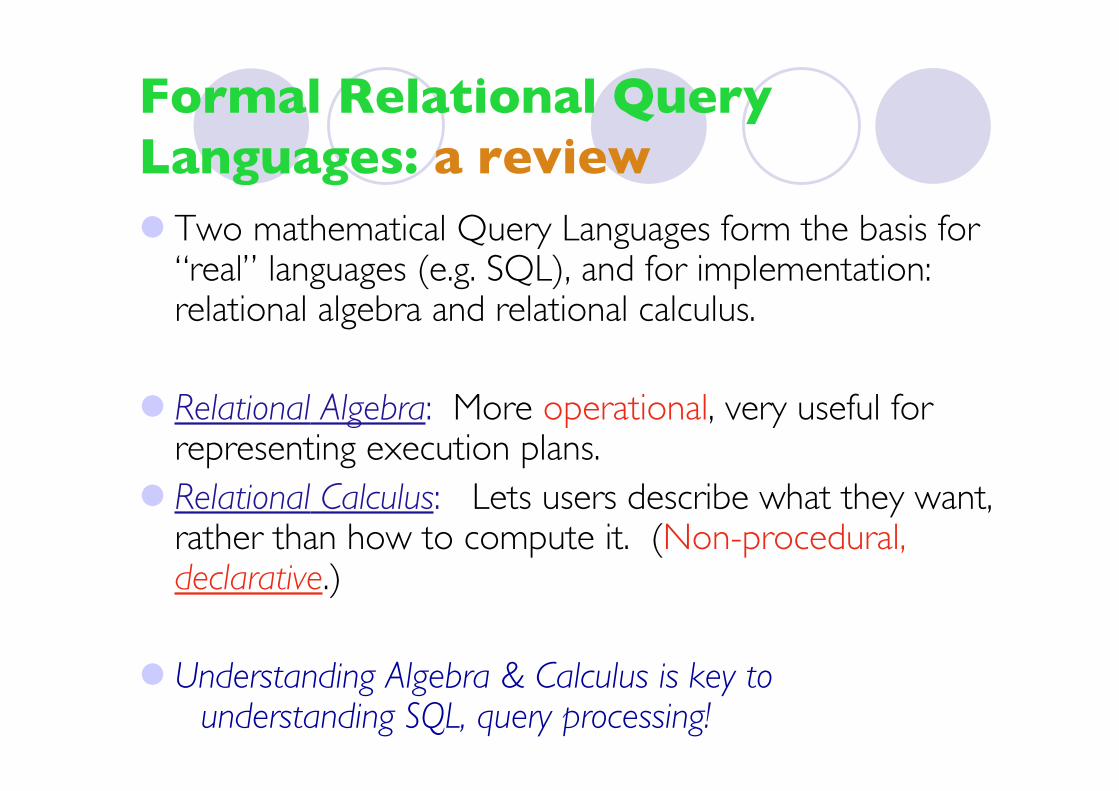
Formal Relational QueryLanguages: a review Two mathematical Query Languages form the basis for

“real” languages (e.g. SQL), and for implementation:relational algebra and relational calculus.

Relational Algebra: More operational, very useful forrepresenting execution plans.

Relational Calculus: Lets users describe what they want,rather than how to compute it. (Non-procedural,declarative.)

Understanding Algebra & Calculus is key to understanding SQL, query processing!

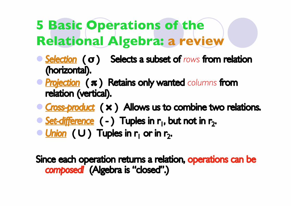
5 Basic Operations of theRelational Algebra: a review Selection ( σ ) Selects a subset of rows from relation

(horizontal). Projection ( π ) Retains only wanted columns from

relation (vertical). Cross-product ( × ) Allows us to combine two relations. Set-difference ( - ) Tuples in r1, but not in r2. Union ( ∪ ) Tuples in r1 or in r2.

Since each operation returns a relation, operations can becomposed! (Algebra is “closed”.)

Overview


Measures of Query Cost

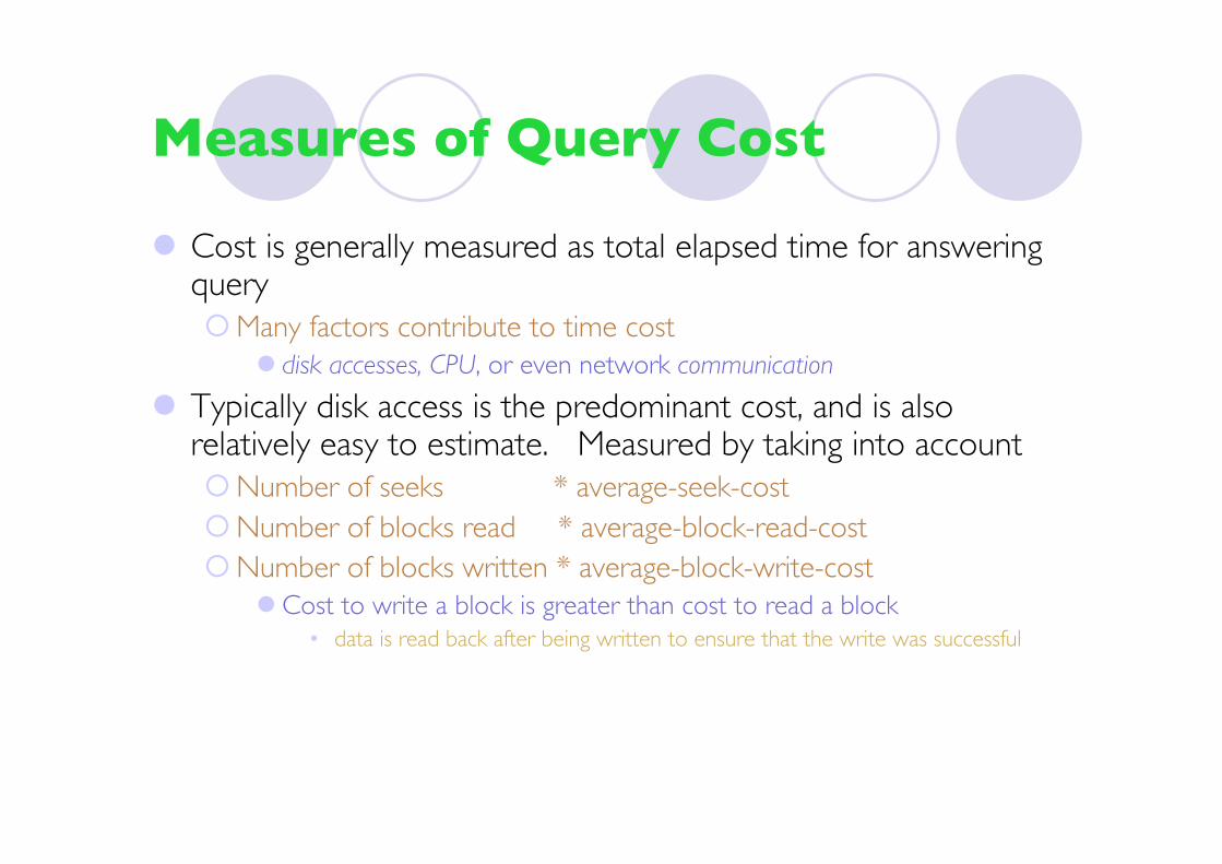
Cost is generally measured as total elapsed time for answeringqueryMany factors contribute to time cost

disk accesses, CPU, or even network communication

Typically disk access is the predominant cost, and is alsorelatively easy to estimate. Measured by taking into accountNumber of seeks * average-seek-costNumber of blocks read * average-block-read-costNumber of blocks written * average-block-write-cost

Cost to write a block is greater than cost to read a block• data is read back after being written to ensure that the write was successful

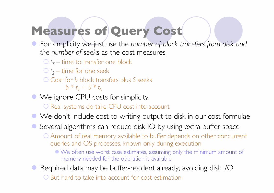
Measures of Query Cost For simplicity we just use the number of block transfers from disk and

the number of seeks as the cost measures tT – time to transfer one block tS – time for one seekCost for b block transfers plus S seeks

b * tT + S * tS We ignore CPU costs for simplicity

Real systems do take CPU cost into account

We don’t include cost to writing output to disk in our cost formulae Several algorithms can reduce disk IO by using extra buffer space

Amount of real memory available to buffer depends on other concurrentqueries and OS processes, known only during execution We often use worst case estimates, assuming only the minimum amount of

memory needed for the operation is available

Required data may be buffer-resident already, avoiding disk I/O But hard to take into account for cost estimation

Overview


Selection Operation ( σ ):using basic scan algorithms File scan – search algorithms that locate and retrieve records

that fulfill a selection condition.

Algorithm A1 (linear search). Scan each file block and test allrecords to see whether they satisfy the selection condition.Cost estimate = br block transfers + 1 seek

br denotes number of blocks containing records from relation r

If selection is on a key attribute, can stop on finding record cost = (br /2) block transfers + 1 seek

Linear search is slow, but it is general because it can be appliedregardless of selection condition or ordering of records in the file, or availability of indices

Selection Operation ( σ ):using basic scan algorithms A2 (binary search). Applicable if selection is an equality

comparison on the attribute on which file is ordered.Assume that the blocks of a relation are stored contiguouslyCost estimate (number of disk blocks to be scanned):

cost of locating the first tuple by a binary search on the blocks• log2(br) * (tT + tS)

If there are multiple records satisfying selection• Add transfer cost of the number of blocks containing records that satisfy

selection condition• Will see how to estimate this cost in the next chapter

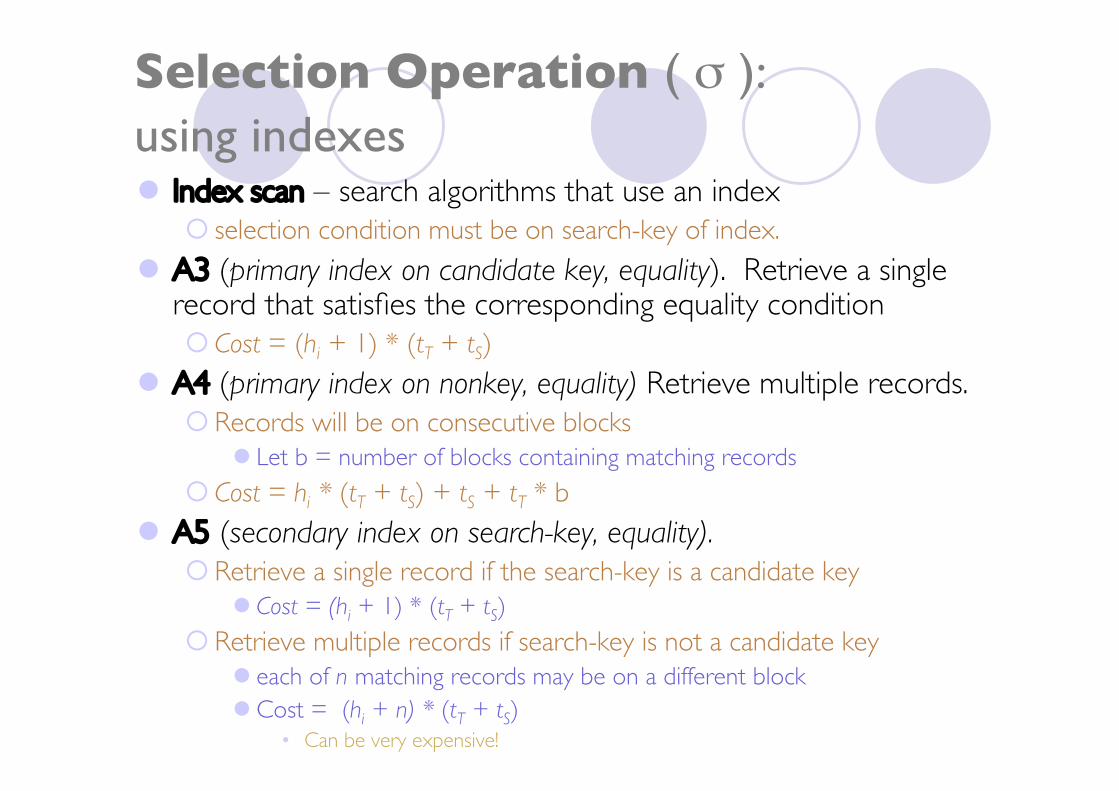
Selection Operation ( σ ):using indexes Index scan – search algorithms that use an index

selection condition must be on search-key of index.

A3 (primary index on candidate key, equality). Retrieve a singlerecord that satisfies the corresponding equality condition Cost = (hi + 1) * (tT + tS)

A4 (primary index on nonkey, equality) Retrieve multiple records. Records will be on consecutive blocks

Let b = number of blocks containing matching records Cost = hi * (tT + tS) + tS + tT * b

A5 (secondary index on search-key, equality). Retrieve a single record if the search-key is a candidate key

Cost = (hi + 1) * (tT + tS) Retrieve multiple records if search-key is not a candidate key

each of n matching records may be on a different block Cost = (hi + n) * (tT + tS)

• Can be very expensive!

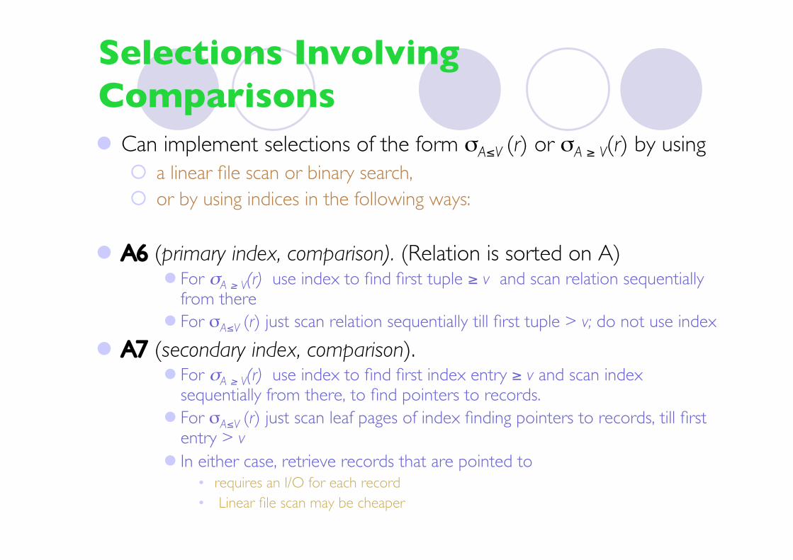
Selections InvolvingComparisons Can implement selections of the form σA≤V (r) or σA ≥ V(r) by using

a linear file scan or binary search, or by using indices in the following ways:

A6 (primary index, comparison). (Relation is sorted on A) For σA ≥ V(r) use index to find first tuple ≥ v and scan relation sequentially

from there For σA≤V (r) just scan relation sequentially till first tuple > v; do not use index

A7 (secondary index, comparison). For σA ≥ V(r) use index to find first index entry ≥ v and scan index

sequentially from there, to find pointers to records. For σA≤V (r) just scan leaf pages of index finding pointers to records, till first

entry > v In either case, retrieve records that are pointed to

• requires an I/O for each record• Linear file scan may be cheaper

Complex Selections

Conjunction: σθ1∧ θ2∧. . . θn(r)

A8 (conjunctive selection using one index). Select a combination of θi and algorithms A1 through A7 that results in

the least cost for σθi (r). Test other conditions on tuple after fetching it into memory buffer.

A9 (conjunctive selection using multiple-key index).Use appropriate composite (multiple-key) index if available.

A10 (conjunctive selection by intersection of identifiers). Requires indices with record pointers.Use corresponding index for each condition, and take intersection of all

the obtained sets of record pointers. Then fetch records from file If some conditions do not have appropriate indices, apply test in

memory.

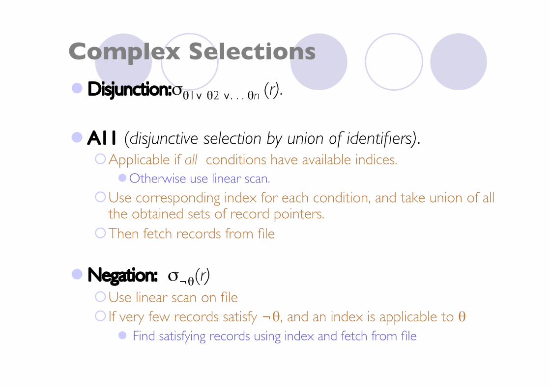
Complex Selections Disjunction:σθ1∨ θ2 ∨. . . θn (r).

A11 (disjunctive selection by union of identifiers).Applicable if all conditions have available indices.

Otherwise use linear scan.Use corresponding index for each condition, and take union of all

the obtained sets of record pointers.Then fetch records from file

Negation: σ¬θ(r)Use linear scan on file If very few records satisfy ¬θ, and an index is applicable to θ

Find satisfying records using index and fetch from file

Overview


External Sorting

We may build an index on the relation, and thenuse the index to read the relation in sorted order.May lead to one disk block access for each tuple.

For relations that fit in memory, techniques likequicksort can be used. For relations that don’t fitin memory, external sort-merge is a good choice.

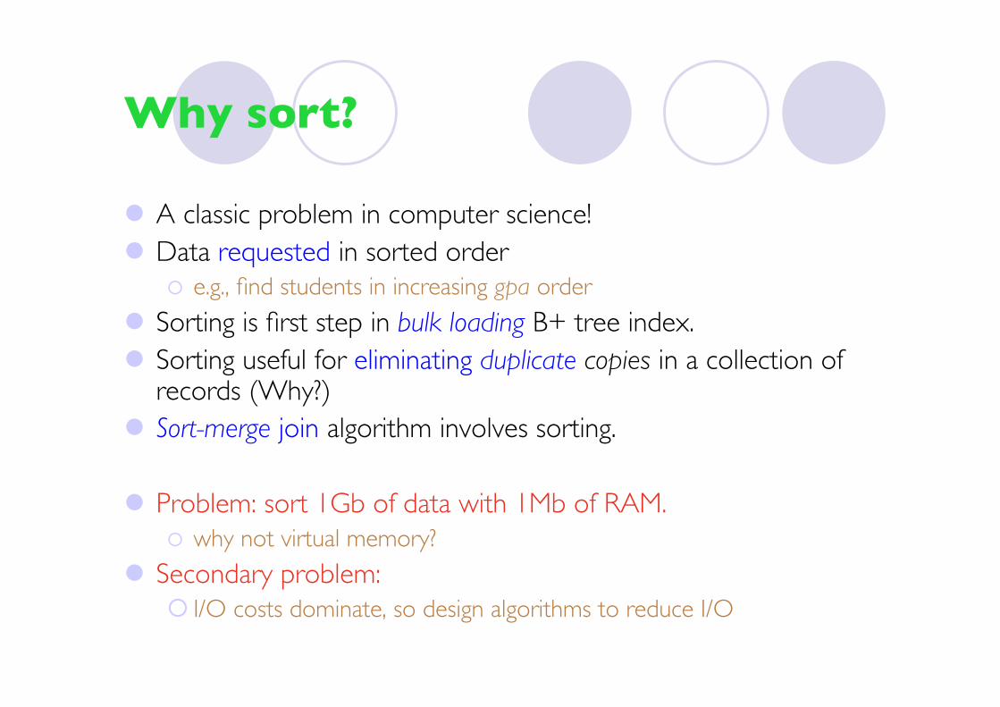
Why sort?

A classic problem in computer science! Data requested in sorted order

e.g., find students in increasing gpa order

Sorting is first step in bulk loading B+ tree index. Sorting useful for eliminating duplicate copies in a collection of

records (Why?) Sort-merge join algorithm involves sorting.

Problem: sort 1Gb of data with 1Mb of RAM. why not virtual memory?

Secondary problem: I/O costs dominate, so design algorithms to reduce I/O

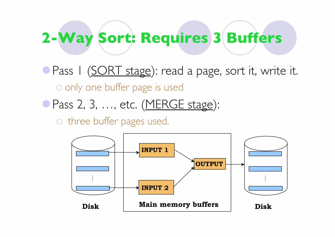
2-Way Sort: Requires 3 Buffers

Pass 1 (SORT stage): read a page, sort it, write it. only one buffer page is used

Pass 2, 3, …, etc. (MERGE stage): three buffer pages used.

Main memory buffers

INPUT 1

INPUT 2

OUTPUT

Disk Disk

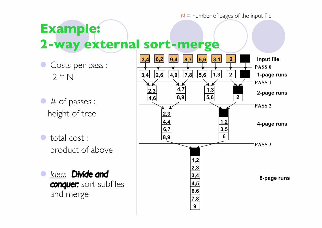
Example:2-way external sort-merge

Costs per pass : 2 * N

# of passes : height of tree

total cost : product of above

Idea: Divide andconquer: sort subfilesand merge

Input file

1-page runs

2-page runs

4-page runs

8-page runs

PASS 0

PASS 1

PASS 2

PASS 3

9

3,4 6,2 9,4 8,7 5,6 3,1 2

3,4 5,62,6 4,9 7,8 1,3 2

2,34,6

4,78,9

1,35,6 2

2,34,46,78,9

1,23,56

1,22,33,44,56,67,8

N = number of pages of the input file

Cost of the 2-way sort-mergealgorithm Number of pages N=2k (k=0,1,...P-1), where P is # of passes.

Pass 0 produces 2k sorted runs of one page each; Pass 1 produces 2k-1 sorted runs of two pages each; Pass 2 produces 2k-2 sorted runs of four page each; ... Pass k produces 20 sorted runs of 2k pages.

Costs per pass: 2 . N each page we read + each page we write into file

P=(log2N)+1 Total cost (I/Os) : 2 . N . P = 2N(log2N+1)

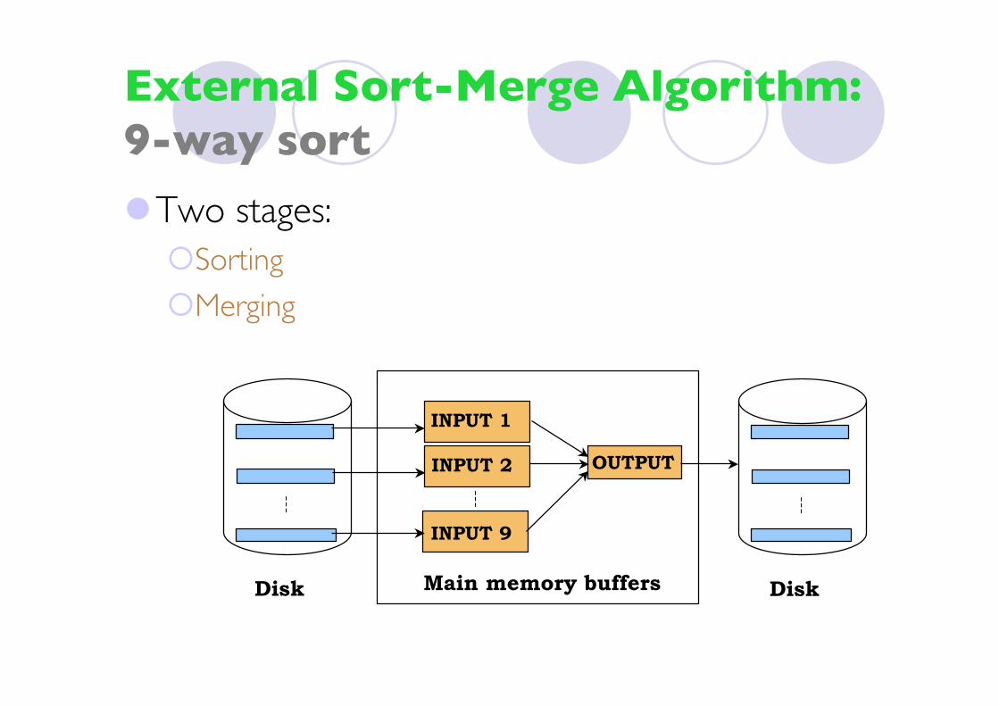
External Sort-Merge Algorithm:9-way sort

Two stages:SortingMerging

Main memory buffers

INPUT 1

INPUT 9

OUTPUT

Disk

INPUT 2

Disk

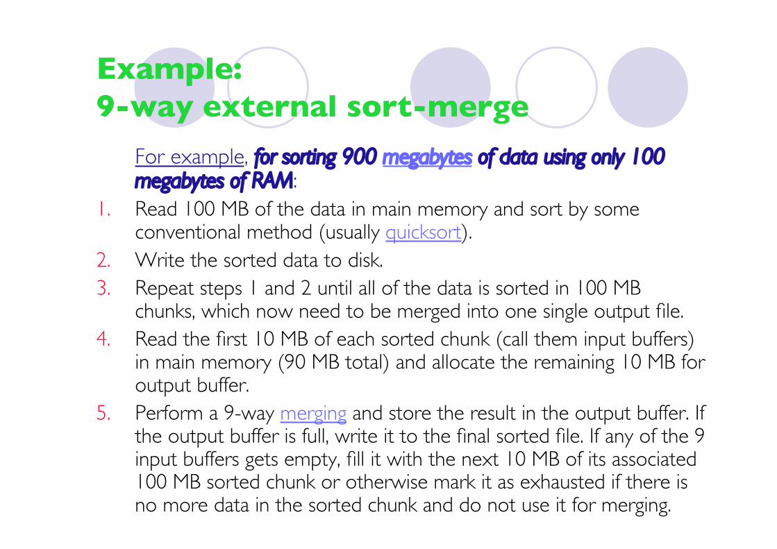
Example:9-way external sort-merge

For example, for sorting 900 megabytes of data using only 100megabytes of RAM:

1. Read 100 MB of the data in main memory and sort by someconventional method (usually quicksort).

2. Write the sorted data to disk.3. Repeat steps 1 and 2 until all of the data is sorted in 100 MB

chunks, which now need to be merged into one single output file.4. Read the first 10 MB of each sorted chunk (call them input buffers)

in main memory (90 MB total) and allocate the remaining 10 MB foroutput buffer.

5. Perform a 9-way merging and store the result in the output buffer. Ifthe output buffer is full, write it to the final sorted file. If any of the 9input buffers gets empty, fill it with the next 10 MB of its associated100 MB sorted chunk or otherwise mark it as exhausted if there isno more data in the sorted chunk and do not use it for merging.

General External Merge Sort

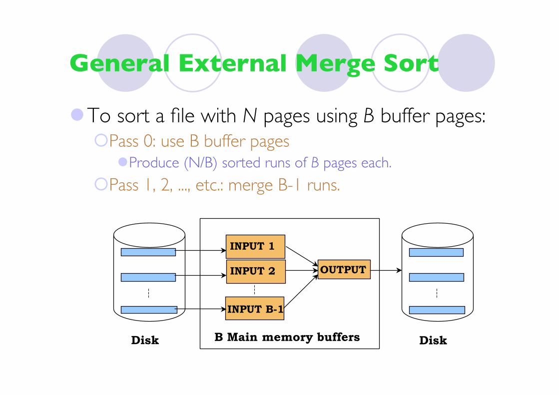
To sort a file with N pages using B buffer pages:Pass 0: use B buffer pages

Produce (N/B) sorted runs of B pages each.

Pass 1, 2, ..., etc.: merge B-1 runs.

B Main memory buffers

INPUT 1

INPUT B-1

OUTPUT

Disk

INPUT 2

Disk

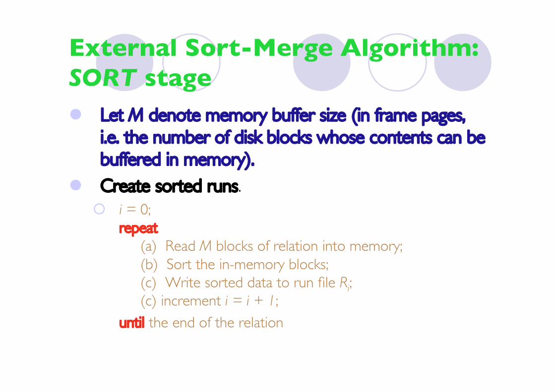
External Sort-Merge Algorithm:SORT stage Let M denote memory buffer size (in frame pages,

i.e. the number of disk blocks whose contents can bebuffered in memory).

Create sorted runs. i = 0;

repeat (a) Read M blocks of relation into memory; (b) Sort the in-memory blocks; (c) Write sorted data to run file Ri; (c) increment i = i + 1;until the end of the relation

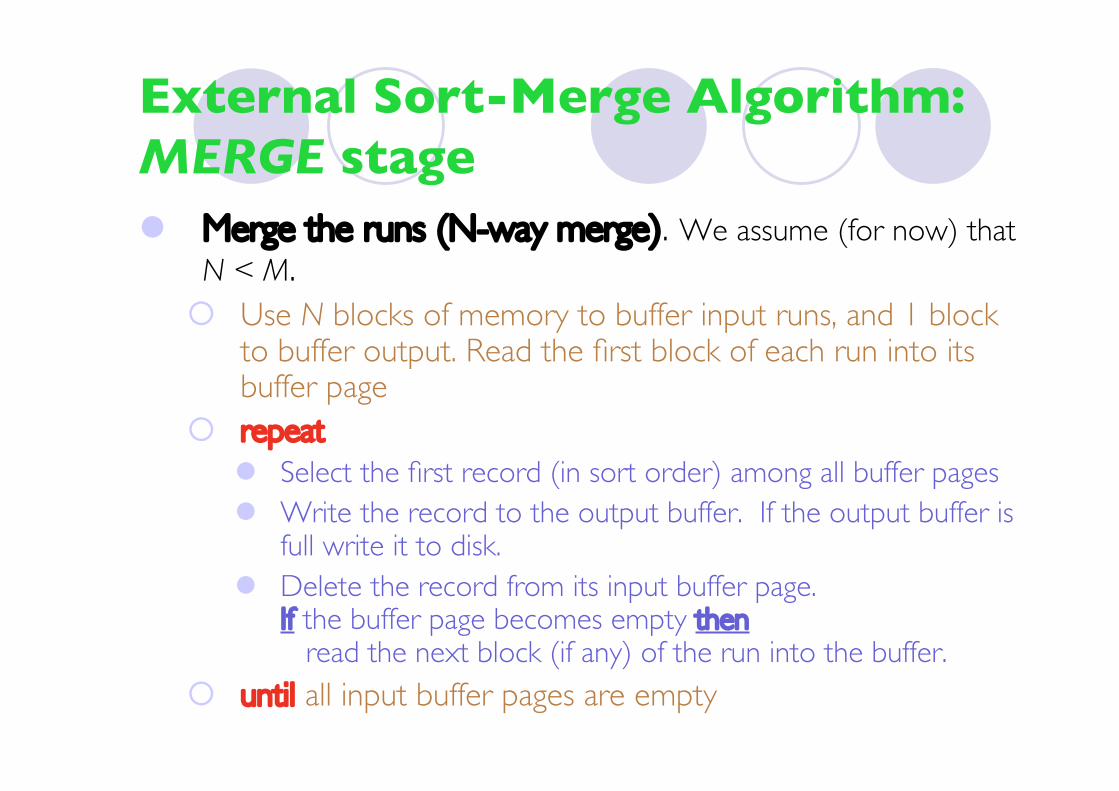
External Sort-Merge Algorithm:MERGE stage Merge the runs (N-way merge). We assume (for now) that

N < M. Use N blocks of memory to buffer input runs, and 1 block

to buffer output. Read the first block of each run into itsbuffer page

repeat Select the first record (in sort order) among all buffer pages Write the record to the output buffer. If the output buffer is

full write it to disk. Delete the record from its input buffer page.

If the buffer page becomes empty then read the next block (if any) of the run into the buffer.

until all input buffer pages are empty

External Sort-Merge Algorithm:MERGE stage If N ≥ M, several merge passes are required.

In each pass, contiguous groups of M - 1 runs are merged.A pass reduces the number of runs by a factor of M -1, and

creates runs longer by the same factor.E.g. If M=11, and there are 90 runs, one pass reduces the

number of runs to 9, each 10 times the size of the initial runs

Repeated passes are performed till all runs have beenmerged into one.

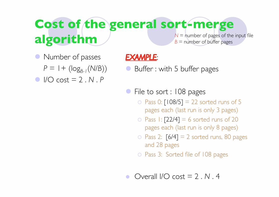
Cost of the general sort-mergealgorithm Number of passes

P = 1+ (logB-1(N/B)) I/O cost = 2 . N . P

EXAMPLE: Buffer : with 5 buffer pages

File to sort : 108 pages Pass 0: [108/5] = 22 sorted runs of 5

pages each (last run is only 3 pages)

Pass 1: [22/4] = 6 sorted runs of 20pages each (last run is only 8 pages)

Pass 2: [6/4] = 2 sorted runs, 80 pagesand 28 pages

Pass 3: Sorted file of 108 pages

Overall I/O cost = 2 . N . 4

N = number of pages of the input fileB = number of buffer pages

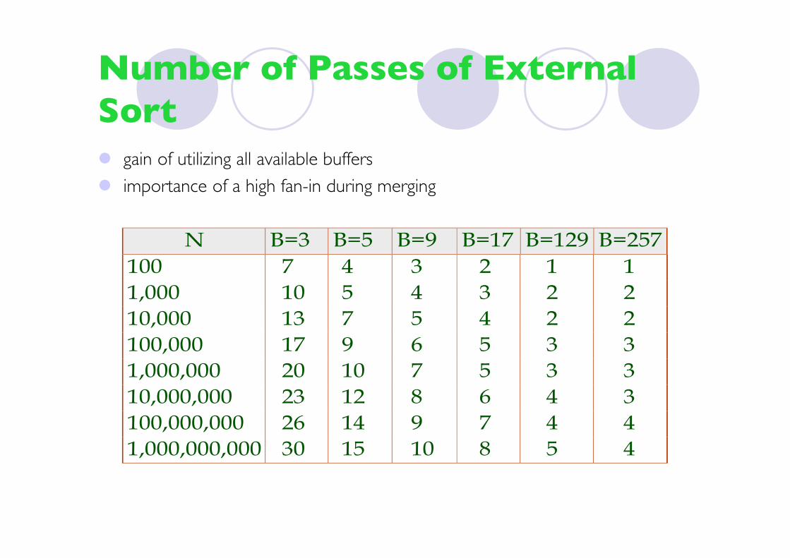
Number of Passes of ExternalSort gain of utilizing all available buffers

importance of a high fan-in during merging

N B=3 B=5 B=9 B=17 B=129 B=257

100 7 4 3 2 1 1

1,000 10 5 4 3 2 2

10,000 13 7 5 4 2 2

100,000 17 9 6 5 3 3

1,000,000 20 10 7 5 3 3

10,000,000 23 12 8 6 4 3

100,000,000 26 14 9 7 4 4

1,000,000,000 30 15 10 8 5 4

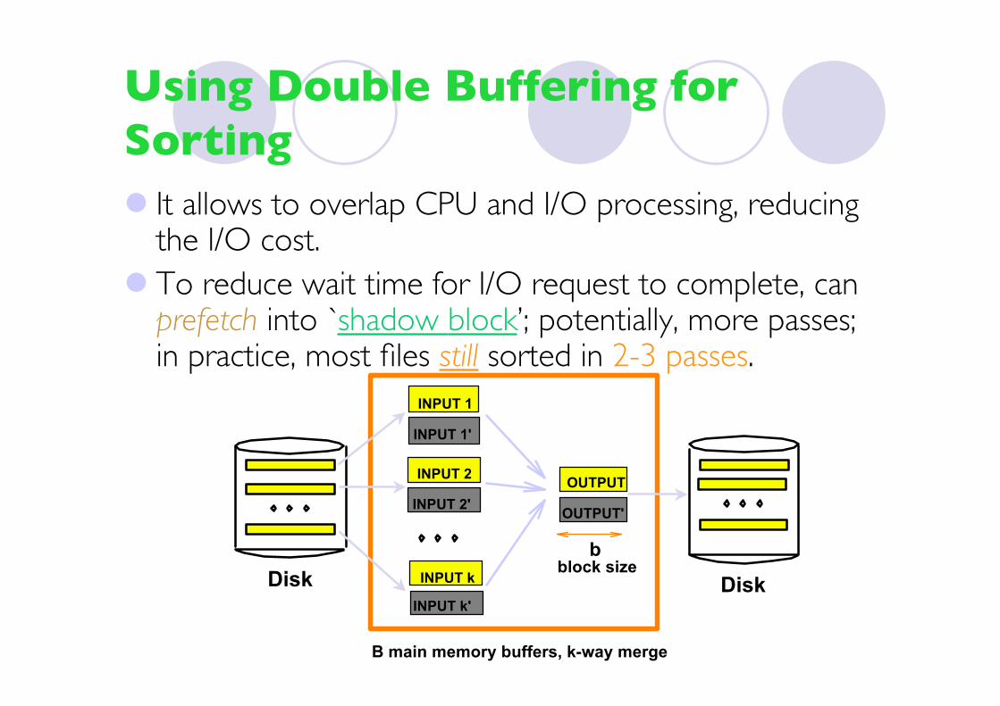
Using Double Buffering forSorting It allows to overlap CPU and I/O processing, reducing

the I/O cost. To reduce wait time for I/O request to complete, can

prefetch into `shadow block’; potentially, more passes;in practice, most files still sorted in 2-3 passes.

OUTPUT

OUTPUT'

Disk Disk

INPUT 1

INPUT k

INPUT 2

INPUT 1'

INPUT 2'

INPUT k'

block sizeb

B main memory buffers, k-way merge

Sorting Records!

Sorting has become a blood sport! Parallel sorting is the name of the game ...

Datamation: Sort 1M records of size 100 bytes Typical DBMS: 15 minutes World record: 3.5 seconds

12-CPU SGI machine, 96 disks, 2GB of RAM

New benchmarks proposed: Minute Sort: How many can you sort in 1 minute? Dollar Sort: How many can you sort for $1.00?

Using B+ Trees for Sorting

Scenario: Table to be sorted has B+ tree indexon sorting column(s).

Idea: Can retrieve records in order by traversingleaf pages.

Is this a good idea?Cases to consider:

B+ tree is clustered Good idea! B+ tree is not clustered Could be a very bad idea!

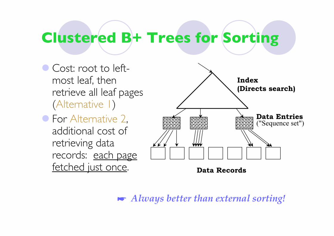
Clustered B+ Trees for Sorting

Cost: root to left-most leaf, thenretrieve all leaf pages(Alternative 1)

For Alternative 2,additional cost ofretrieving datarecords: each pagefetched just once.

(Directs search)

Data Records

Index

Data Entries("Sequence set")

Always better than external sorting!

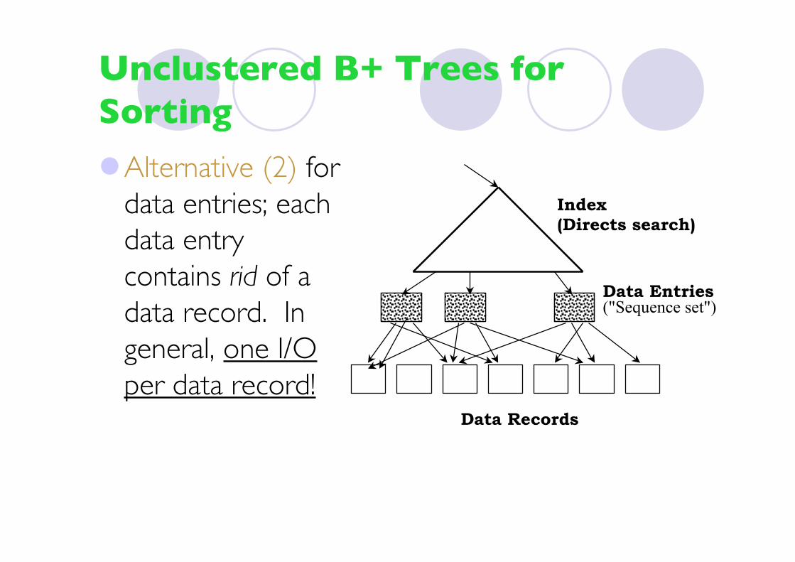
Unclustered B+ Trees forSorting

Alternative (2) fordata entries; eachdata entrycontains rid of adata record. Ingeneral, one I/Oper data record!

(Directs search)

Data Records

Index

Data Entries("Sequence set")

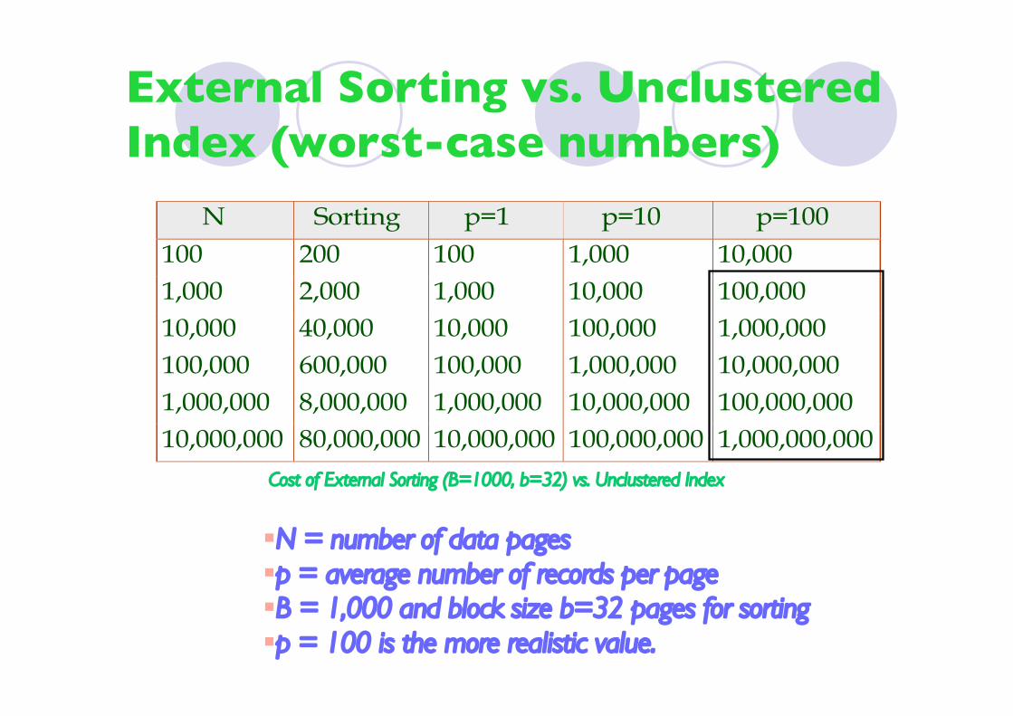
External Sorting vs. UnclusteredIndex (worst-case numbers)

N Sorting p=1 p=10 p=100

100 200 100 1,000 10,000

1,000 2,000 1,000 10,000 100,000

10,000 40,000 10,000 100,000 1,000,000

100,000 600,000 100,000 1,000,000 10,000,000

1,000,000 8,000,000 1,000,000 10,000,000 100,000,000

10,000,000 80,000,000 10,000,000 100,000,000 1,000,000,000

N = number of data pagesp = average number of records per pageB = 1,000 and block size b=32 pages for sortingp = 100 is the more realistic value.

Cost of External Sorting (B=1000, b=32) vs. Unclustered Index

Summary External sorting is important; DBMS may dedicate part of

buffer pool for sorting! External merge sort minimizes disk I/O cost:

Pass 0: Produces sorted runs of size B (# buffer pages). Laterpasses: merge runs.

# of runs merged at a time depends on B, and block size. Larger block size means less I/O cost per page. Larger block size means smaller # runs merged. In practice, # of runs rarely more than 2 or 3.

Choice of internal sort algorithm may matter. The best sorts are wildly fast:

Despite 40+ years of research, we’re still improving!

Clustered B+ tree is good for sorting; unclustered tree isusually very bad.

Overview


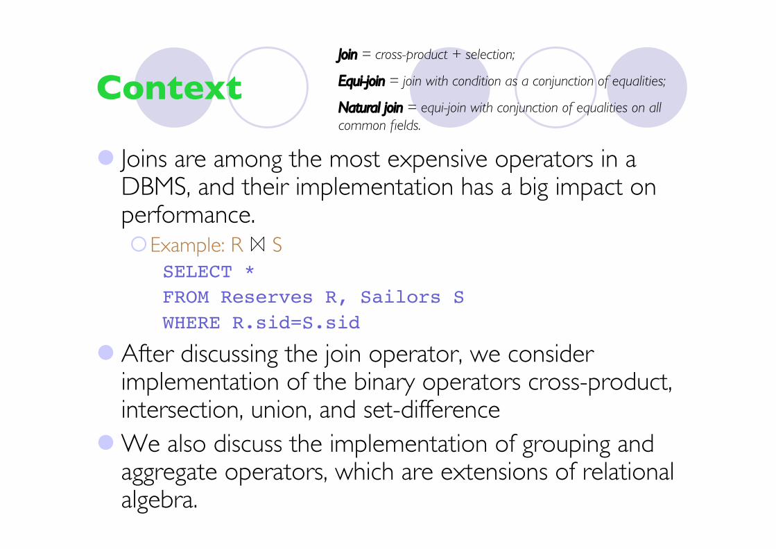
Context

Joins are among the most expensive operators in aDBMS, and their implementation has a big impact onperformance.Example: R S

SELECT *FROM Reserves R, Sailors SWHERE R.sid=S.sid

After discussing the join operator, we considerimplementation of the binary operators cross-product,intersection, union, and set-difference

We also discuss the implementation of grouping andaggregate operators, which are extensions of relationalalgebra.

Join = cross-product + selection;

Equi-join = join with condition as a conjunction of equalities;

Natural join = equi-join with conjunction of equalities on allcommon fields.

Join Operation

Several different algorithms to implement joinsNested-loop join Block nested-loop join Indexed nested-loop joinMerge-joinHash-join

Choice based on cost estimate Examples use the following information

Number of records of customer: 10,000Number of blocks of customer: 400Number of records of depositor: 5000Number of blocks of depositor: 100

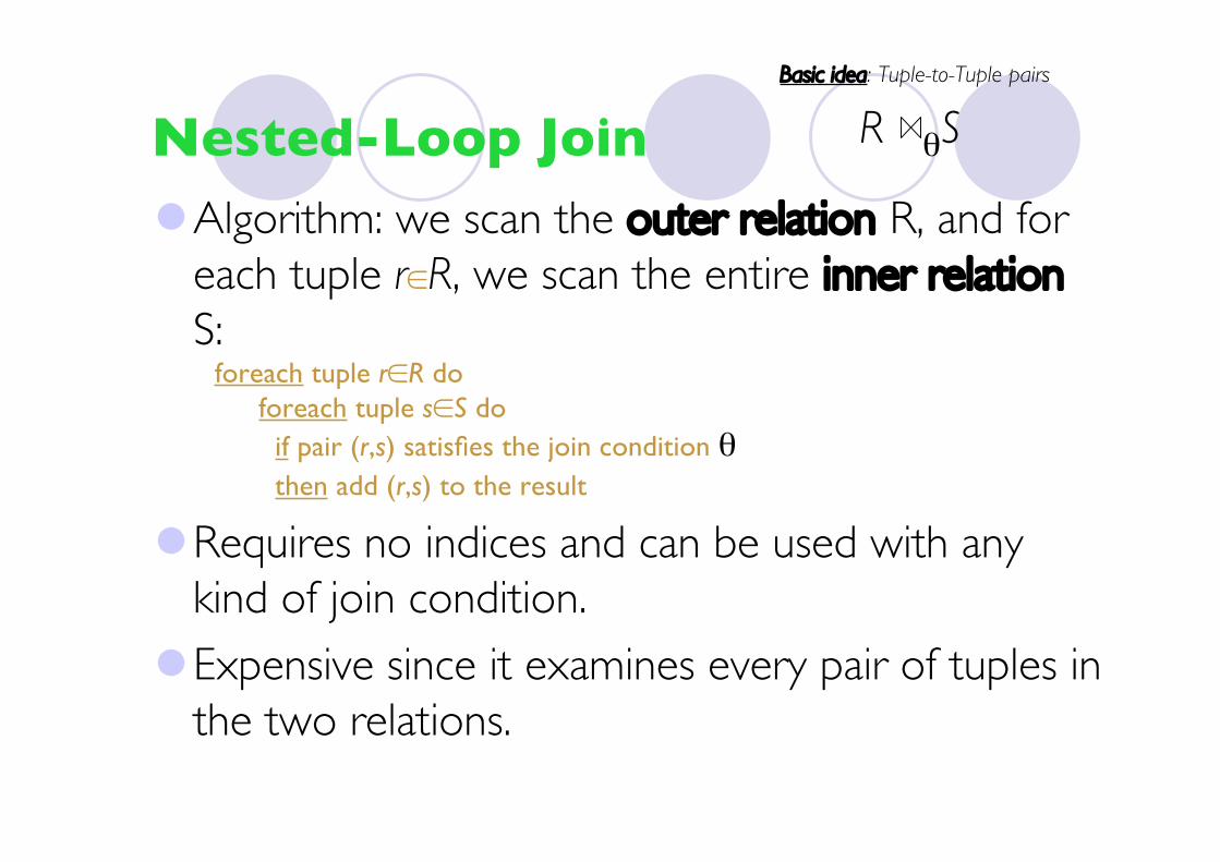
Nested-Loop JoinAlgorithm: we scan the outer relation R, and for

each tuple r∈R, we scan the entire inner relationS: foreach tuple r∈R do

foreach tuple s∈S do if pair (r,s) satisfies the join condition θ then add (r,s) to the result

Requires no indices and can be used with anykind of join condition.

Expensive since it examines every pair of tuples inthe two relations.

Basic idea: Tuple-to-Tuple pairs

R θS

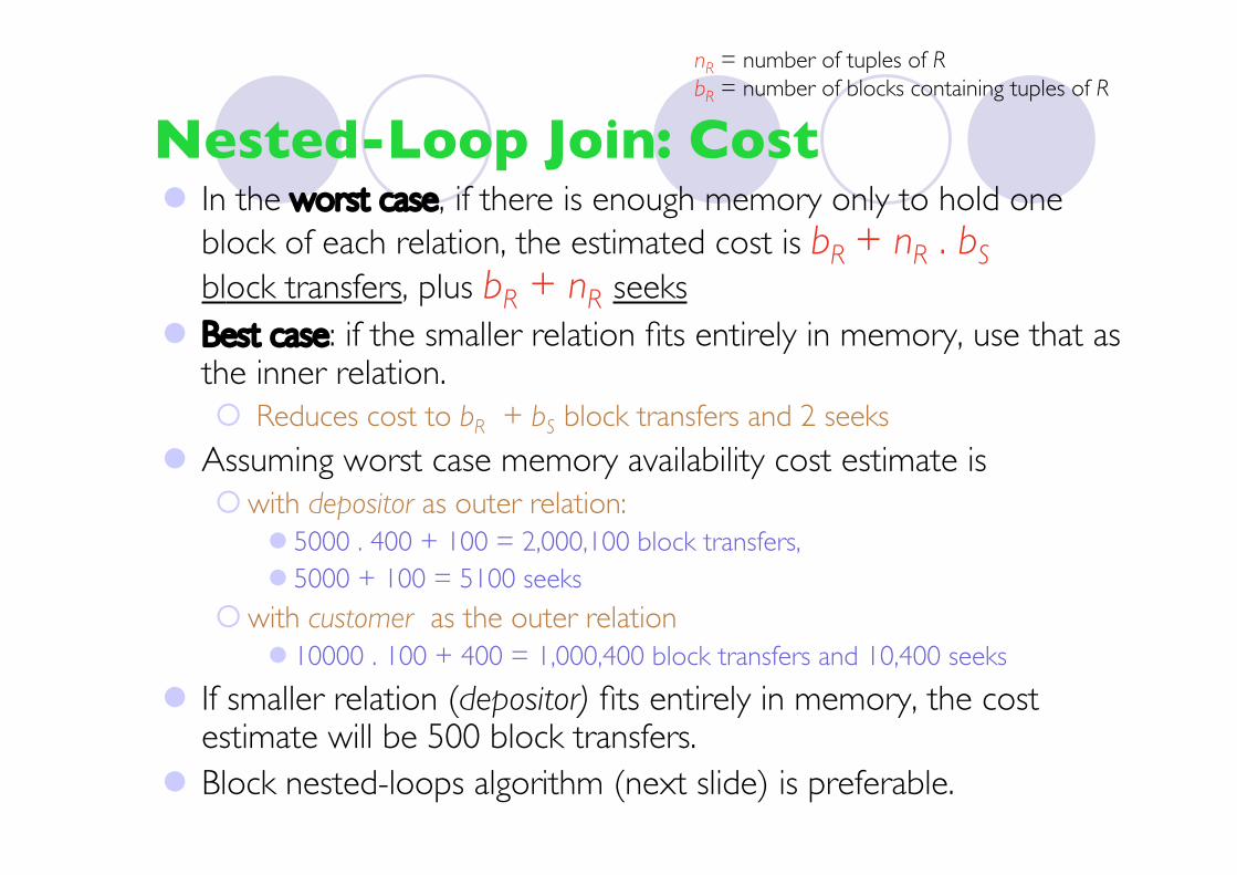
Nested-Loop Join: Cost In the worst case, if there is enough memory only to hold one

block of each relation, the estimated cost is bR + nR . bSblock transfers, plus bR + nR seeks

Best case: if the smaller relation fits entirely in memory, use that asthe inner relation. Reduces cost to bR + bS block transfers and 2 seeks

Assuming worst case memory availability cost estimate iswith depositor as outer relation:

5000 . 400 + 100 = 2,000,100 block transfers, 5000 + 100 = 5100 seeks

with customer as the outer relation 10000 . 100 + 400 = 1,000,400 block transfers and 10,400 seeks

If smaller relation (depositor) fits entirely in memory, the costestimate will be 500 block transfers.

Block nested-loops algorithm (next slide) is preferable.

nR = number of tuples of RbR = number of blocks containing tuples of R

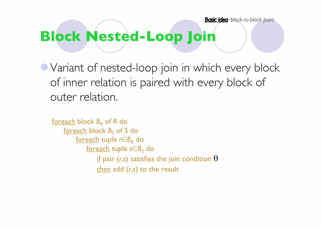
Block Nested-Loop Join

Variant of nested-loop join in which every blockof inner relation is paired with every block ofouter relation.

foreach block BR of R doforeach block BS of S do

foreach tuple r∈BR doforeach tuple s∈BS do

if pair (r,s) satisfies the join condition θ then add (r,s) to the result

Basic idea: block-to-block pairs

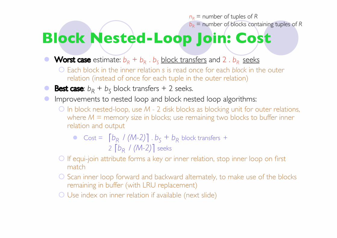
Block Nested-Loop Join: Cost Worst case estimate: bR + bR . bS block transfers and 2 . bR seeks

Each block in the inner relation s is read once for each block in the outerrelation (instead of once for each tuple in the outer relation)

Best case: bR + bS block transfers + 2 seeks. Improvements to nested loop and block nested loop algorithms:

In block nested-loop, use M - 2 disk blocks as blocking unit for outer relations,where M = memory size in blocks; use remaining two blocks to buffer innerrelation and output

Cost = bR / (M-2) . bS + bR block transfers + 2 bR / (M-2) seeks

If equi-join attribute forms a key or inner relation, stop inner loop on firstmatch

Scan inner loop forward and backward alternately, to make use of the blocksremaining in buffer (with LRU replacement)

Use index on inner relation if available (next slide)


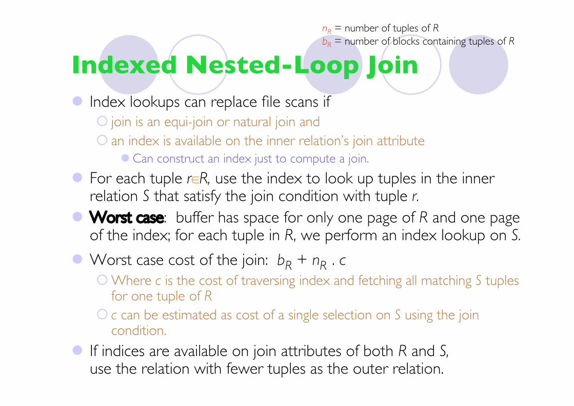
Indexed Nested-Loop Join Index lookups can replace file scans if

join is an equi-join or natural join and an index is available on the inner relation’s join attribute

Can construct an index just to compute a join.

For each tuple r∈R, use the index to look up tuples in the innerrelation S that satisfy the join condition with tuple r.

Worst case: buffer has space for only one page of R and one pageof the index; for each tuple in R, we perform an index lookup on S.

Worst case cost of the join: bR + nR . cWhere c is the cost of traversing index and fetching all matching S tuples

for one tuple of R c can be estimated as cost of a single selection on S using the join

condition.

If indices are available on join attributes of both R and S,use the relation with fewer tuples as the outer relation.


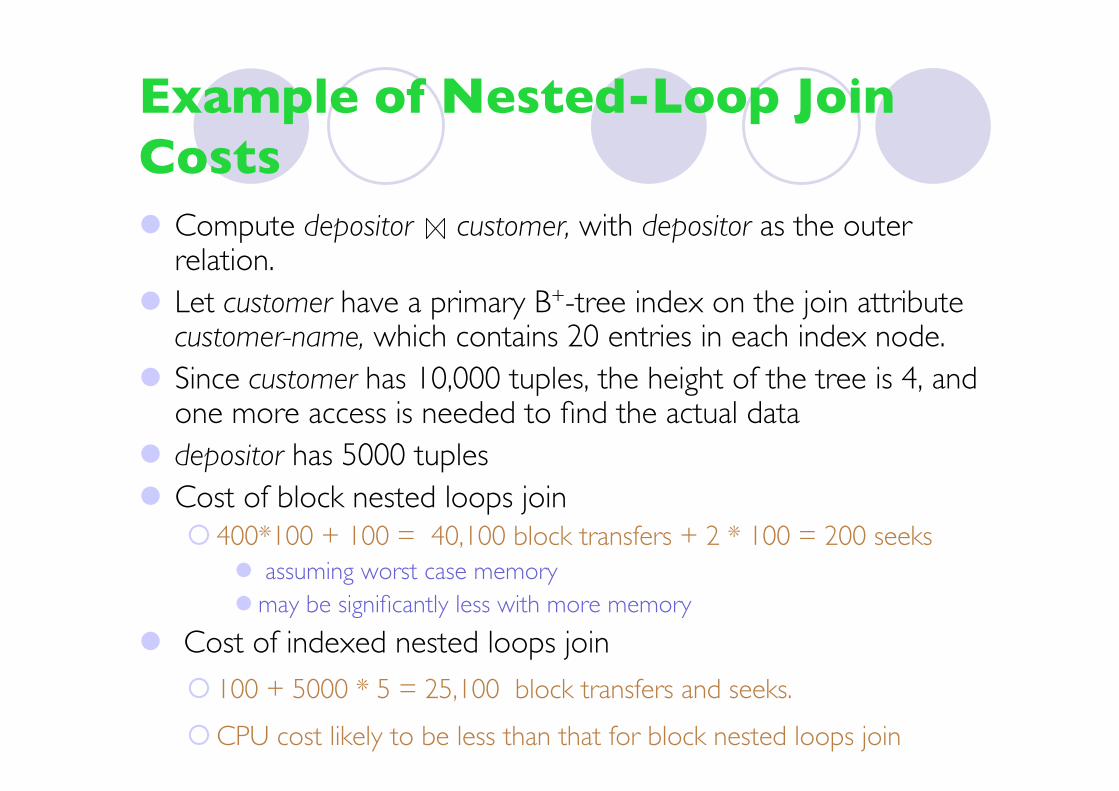
Example of Nested-Loop JoinCosts Compute depositor customer, with depositor as the outer

relation. Let customer have a primary B+-tree index on the join attribute

customer-name, which contains 20 entries in each index node. Since customer has 10,000 tuples, the height of the tree is 4, and

one more access is needed to find the actual data depositor has 5000 tuples Cost of block nested loops join

400*100 + 100 = 40,100 block transfers + 2 * 100 = 200 seeks assuming worst case memory may be significantly less with more memory

Cost of indexed nested loops join 100 + 5000 * 5 = 25,100 block transfers and seeks.

CPU cost likely to be less than that for block nested loops join

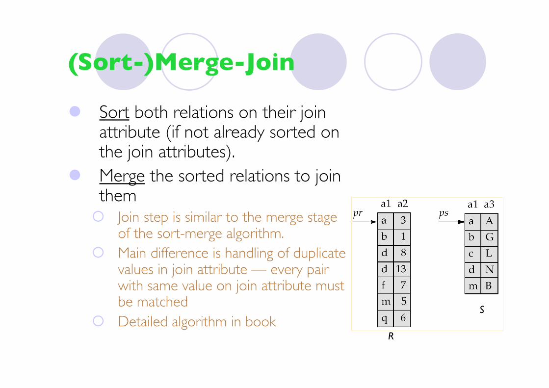
(Sort-)Merge-Join

Sort both relations on their joinattribute (if not already sorted onthe join attributes).

Merge the sorted relations to jointhem

Join step is similar to the merge stageof the sort-merge algorithm.

Main difference is handling of duplicatevalues in join attribute — every pairwith same value on join attribute mustbe matched

Detailed algorithm in bookR

S

Merge-Join: Cost Can be used only for equi-joins and natural joins Each block needs to be read only once (assuming all tuples for

any given value of the join attributes fit in memory Thus the cost of merge join is:

bR + bS block transfers + [(bR / bb)+ (bS / bb)] seeks+ the cost of sorting if relations are unsorted.

hybrid merge-join: If one relation is sorted, and the other has asecondary B+-tree index on the join attributeMerge the sorted relation with the leaf entries of the B+-tree. Sort the result on the addresses of the unsorted relation’s tuples Scan the unsorted relation in physical address order and merge with

previous result, to replace addresses by the actual tuples Sequential scan more efficient than random lookup

nR = number of tuples of RbR = number of blocks containing tuples of Rbb = number of buffer blocks allocated for each relation

Hash-Join

Applicable for equi-joins and natural joins. A hash function h is used to partition tuples of both relations h maps JoinAttrs values to {0, 1, ..., n}, where JoinAttrs denotes the

common attributes of r and s used in the natural join. r0, r1, . . ., rn denote partitions of r tuples

Each tuple tr ∈ r is put in partition ri where i = h(tr [JoinAttrs]).

r0,, r1. . ., rn denotes partitions of s tuples Each tuple ts ∈s is put in partition si, where i = h(ts [JoinAttrs]).

Note: In book, ri is denoted as Hri, si is denoted as Hsi and n is denoted as nh.

Não abordado!

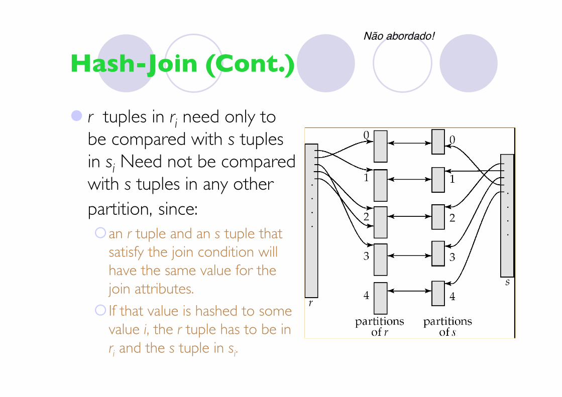
Hash-Join (Cont.)

r tuples in ri need only tobe compared with s tuplesin si Need not be comparedwith s tuples in any otherpartition, since:an r tuple and an s tuple that

satisfy the join condition willhave the same value for thejoin attributes.

If that value is hashed to somevalue i, the r tuple has to be inri and the s tuple in si.

Não abordado!

Hash-Join Algorithm

The hash-join of r and s is computed as follows:1. Partition the relation s using hashing function h. When

partitioning a relation, one block of memory is reserved asthe output buffer for each partition.

2. Partition r similarly.3. For each i:

(a) Load si into memory and build an in-memory hash index on itusing the join attribute. This hash index uses a different hashfunction than the earlier one h.

(b) Read the tuples in ri from the disk one by one. For each tuple trlocate each matching tuple ts in si using the in-memory hashindex. Output the concatenation of their attributes.

Relation s is called the build input and r is called the probe input.

Não abordado!

Hash-Join algorithm (Cont.)

The value n and the hash function h is chosen such that each sishould fit in memory. Typically n is chosen as bs/M * f where f is a “fudge factor”, typically

around 1.2 The probe relation partitions si need not fit in memory

Recursive partitioning required if number of partitions n is greaterthan number of pages M of memory. instead of partitioning n ways, use M – 1 partitions for s Further partition the M – 1 partitions using a different hash functionUse same partitioning method on r Rarely required: e.g., recursive partitioning not needed for relations of

1GB or less with memory size of 2MB, with block size of 4KB.

Não abordado!

Handling of Overflows Partitioning is said to be skewed if some partitions have

significantly more tuples than some others Hash-table overflow occurs in partition si if si does not fit in

memory. Reasons could beMany tuples in s with same value for join attributes Bad hash function

Overflow resolution can be done in build phase Partition si is further partitioned using different hash function. Partition ri must be similarly partitioned.

Overflow avoidance performs partitioning carefully to avoidoverflows during build phase E.g. partition build relation into many partitions, then combine them

Both approaches fail with large numbers of duplicates Fallback option: use block nested loops join on overflowed partitions

Não abordado!

Cost of Hash-Join If recursive partitioning is not required: cost of hash join is

3(br + bs) +4 ∗ nh block transfers + 2( br / bb + bs / bb) seeks

If recursive partitioning required: number of passes required for partitioning build relation

s is logM–1(bs) – 1 best to choose the smaller relation as the build relation. Total cost estimate is:

2(br + bs logM–1(bs) – 1 + br + bs block transfers + 2(br / bb + bs / bb) logM–1(bs) – 1 seeks

If the entire build input can be kept in main memory nopartitioning is requiredCost estimate goes down to br + bs.

Não abordado!

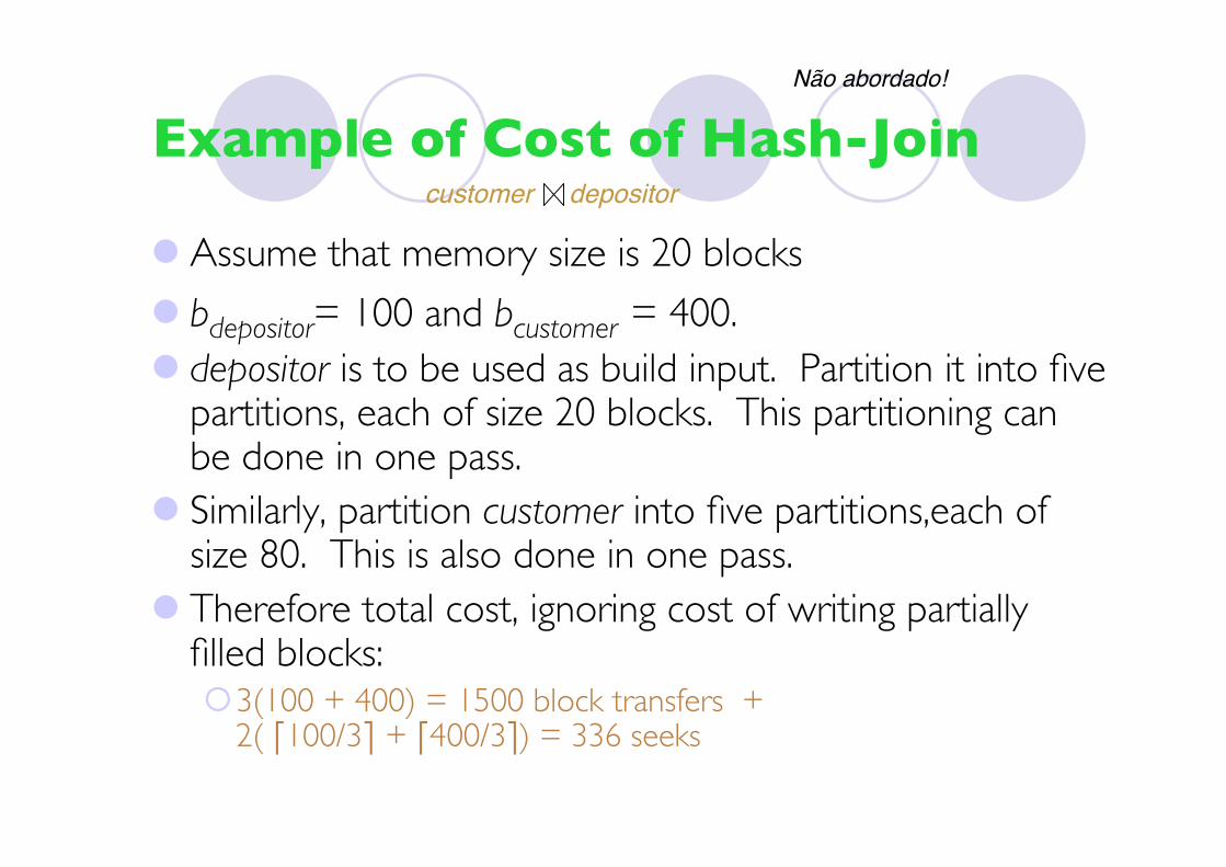
Example of Cost of Hash-Join

Assume that memory size is 20 blocks

bdepositor= 100 and bcustomer = 400. depositor is to be used as build input. Partition it into five

partitions, each of size 20 blocks. This partitioning canbe done in one pass.

Similarly, partition customer into five partitions,each ofsize 80. This is also done in one pass.

Therefore total cost, ignoring cost of writing partiallyfilled blocks:3(100 + 400) = 1500 block transfers +

2( 100/3 + 400/3) = 336 seeks

customer depositor

Não abordado!

Hybrid Hash–Join Useful when memory sized are relatively large, and the build input

is bigger than memory. Main feature of hybrid hash join: Keep the first partition of the build relation in memory. E.g. With memory size of 25 blocks, depositor can be partitioned

into five partitions, each of size 20 blocks. Division of memory:

The first partition occupies 20 blocks of memory 1 block is used for input, and 1 block each for buffering the other 4

partitions.

customer is similarly partitioned into five partitions each of size 80 the first is used right away for probing, instead of being written out

Cost of 3(80 + 320) + 20 +80 = 1300 block transfers for hybrid hash join, instead of 1500 with plain hash-join.

Hybrid hash-join most useful if M >> sb

Não abordado!

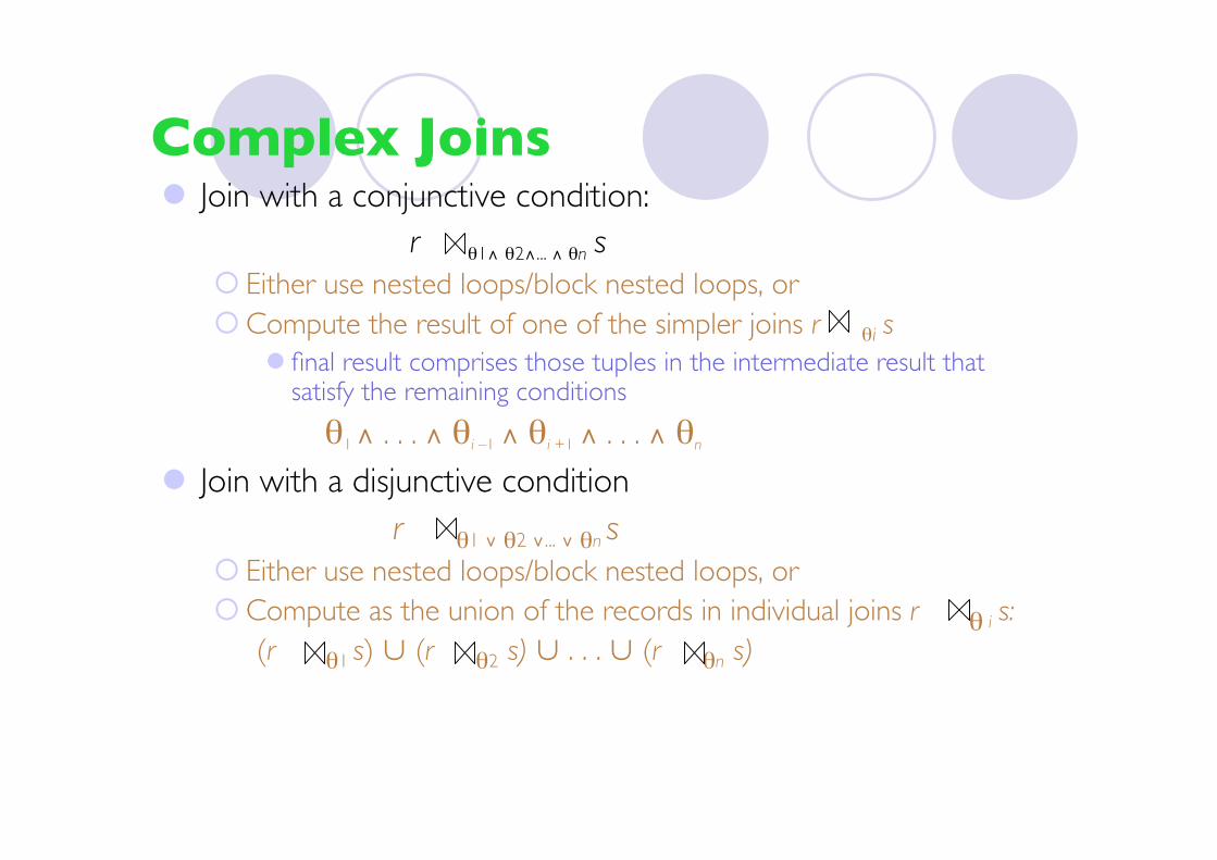
Complex Joins Join with a conjunctive condition:

r θ1∧ θ2∧... ∧ θn s Either use nested loops/block nested loops, orCompute the result of one of the simpler joins r θi s

final result comprises those tuples in the intermediate result thatsatisfy the remaining conditions

θ1 ∧ . . . ∧ θi –1 ∧ θi +1 ∧ . . . ∧ θn

Join with a disjunctive condition

r θ1 ∨ θ2 ∨... ∨ θn s Either use nested loops/block nested loops, orCompute as the union of the records in individual joins r θ i s:

(r θ1 s) ∪ (r θ2 s) ∪ . . . ∪ (r θn s)

Overview


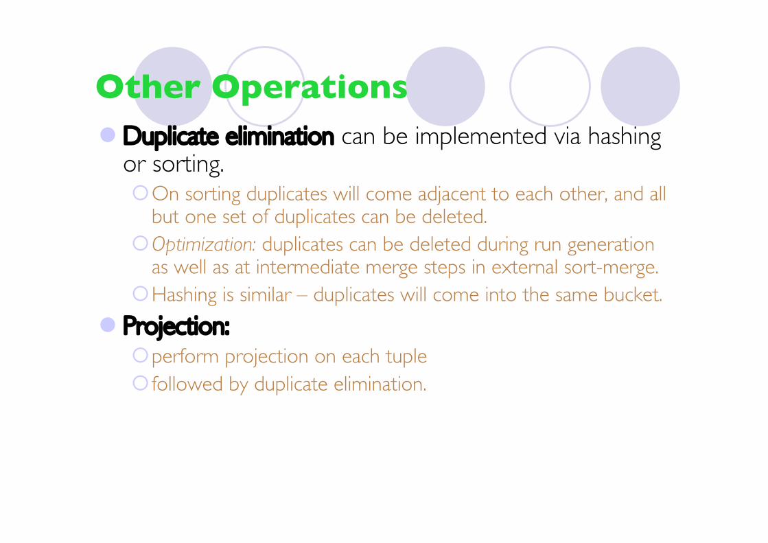
Other Operations Duplicate elimination can be implemented via hashing

or sorting.On sorting duplicates will come adjacent to each other, and all

but one set of duplicates can be deleted.Optimization: duplicates can be deleted during run generation

as well as at intermediate merge steps in external sort-merge.Hashing is similar – duplicates will come into the same bucket.

Projection:perform projection on each tuple followed by duplicate elimination.

Other Operations : Aggregation

Aggregation can be implemented in a manner similarto duplicate elimination.Sorting or hashing can be used to bring tuples in the same

group together, and then the aggregate functions can beapplied on each group.

Optimization: combine tuples in the same group during rungeneration and intermediate merges, by computing partialaggregate valuesFor count, min, max, sum: keep aggregate values on tuples found

so far in the group.• When combining partial aggregate for count, add up the aggregates

For avg, keep sum and count, and divide sum by count at the end

Other Operations : SetOperations Set operations (∪, ∩ and ): can either use variant of

merge-join after sorting, or variant of hash-join. E.g., Set operations using hashing:

Partition both relations using the same hash function Process each partition i as follows.

Using a different hashing function, build an in-memory hash indexon ri.

Process si as follows• r ∪ s:

Add tuples in si to the hash index if they are not already in it.At end of si add the tuples in the hash index to the result.

• r ∩ s:Output tuples in si to the result if they are already there in the hashindex

• r – s:for each tuple in si, if it is there in the hash index, delete it from theindex.At end of si add remaining tuples in the hash index to the result.

Other Operations : Outer Join Outer join can be computed either as

A join followed by addition of null-padded non-participating tuples. by modifying the join algorithms.

Modifying merge join to compute r s In r s, non participating tuples are those in r – ΠR(r s)Modify merge-join to compute r s: During merging, for every

tuple tr from r that do not match any tuple in s, output tr padded withnulls.

Right outer-join and full outer-join can be computed similarly.

Modifying hash join to compute r s If r is probe relation, output non-matching r tuples padded with nulls If r is build relation, when probing keep track of which

r tuples matched s tuples. At end of si outputnon-matched r tuples padded with nulls

Overview


Evaluation of Expressions

So far: we have seen algorithms for individualoperations

Alternatives for evaluating an entire expression treeMaterialization: generate results of an expression whose inputs

are relations or are already computed, materialize (store) it ondisk. Repeat.

Pipelining: pass on tuples to parent operations even as anoperation is being executed

We study above alternatives in more detail

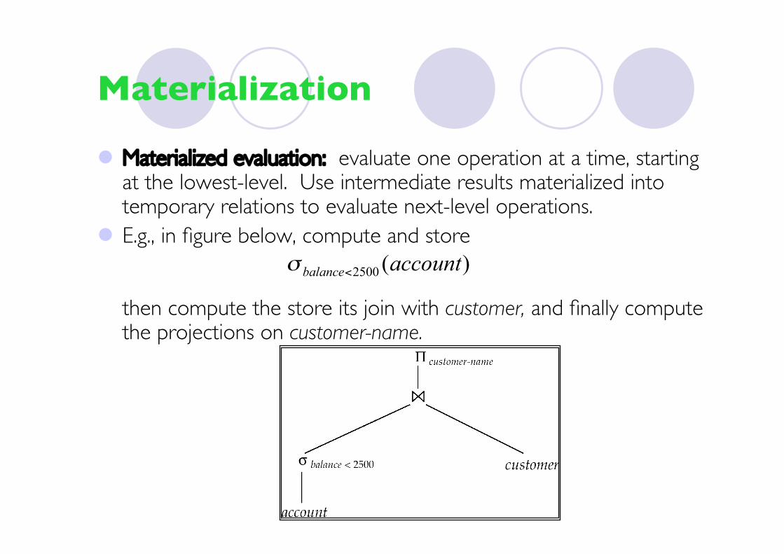
Materialization

Materialized evaluation: evaluate one operation at a time, startingat the lowest-level. Use intermediate results materialized intotemporary relations to evaluate next-level operations.

E.g., in figure below, compute and store

then compute the store its join with customer, and finally computethe projections on customer-name.

)(2500 accountbalance<!

Materialization (Cont.)

Materialized evaluation is always applicable Cost of writing results to disk and reading them back

can be quite highOur cost formulas for operations ignore cost of writing results

to disk, soOverall cost = Sum of costs of individual operations +

cost of writing intermediate results to disk

Double buffering: use two output buffers for eachoperation, when one is full write it to disk while theother is getting filledAllows overlap of disk writes with computation and reduces

execution time

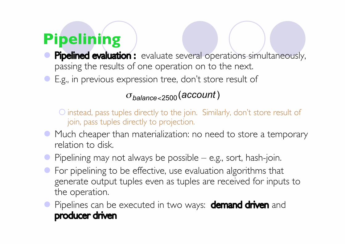
Pipelining Pipelined evaluation : evaluate several operations simultaneously,

passing the results of one operation on to the next. E.g., in previous expression tree, don’t store result of

instead, pass tuples directly to the join. Similarly, don’t store result ofjoin, pass tuples directly to projection.

Much cheaper than materialization: no need to store a temporaryrelation to disk.

Pipelining may not always be possible – e.g., sort, hash-join. For pipelining to be effective, use evaluation algorithms that

generate output tuples even as tuples are received for inputs tothe operation.

Pipelines can be executed in two ways: demand driven andproducer driven

)(2500 accountbalance<!

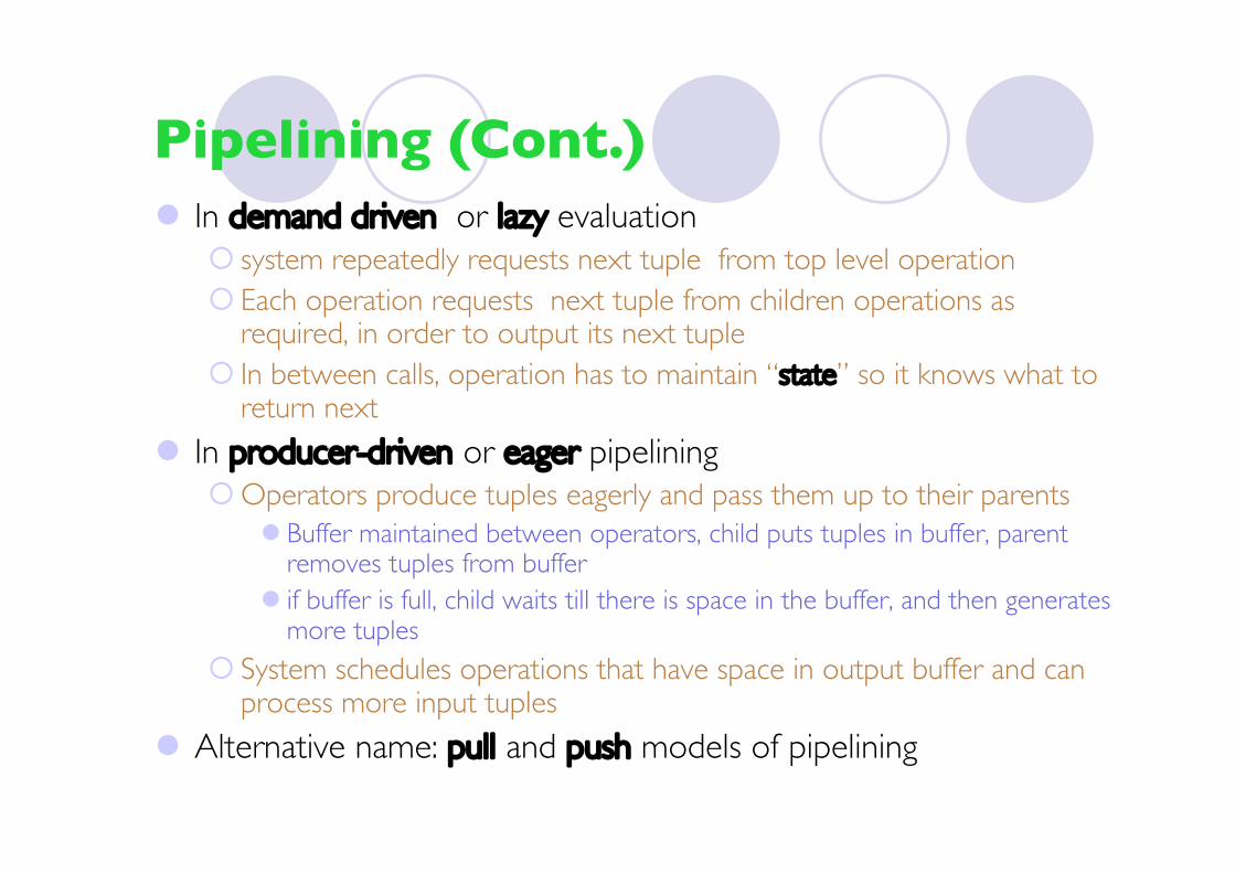
Pipelining (Cont.) In demand driven or lazy evaluation

system repeatedly requests next tuple from top level operation Each operation requests next tuple from children operations as

required, in order to output its next tuple In between calls, operation has to maintain “state” so it knows what to

return next

In producer-driven or eager pipeliningOperators produce tuples eagerly and pass them up to their parents

Buffer maintained between operators, child puts tuples in buffer, parentremoves tuples from buffer

if buffer is full, child waits till there is space in the buffer, and then generatesmore tuples

System schedules operations that have space in output buffer and canprocess more input tuples

Alternative name: pull and push models of pipelining

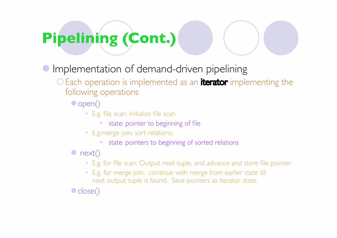
Pipelining (Cont.)

Implementation of demand-driven pipeliningEach operation is implemented as an iterator implementing the

following operationsopen()

• E.g. file scan: initialize file scan state: pointer to beginning of file

• E.g.merge join: sort relations; state: pointers to beginning of sorted relations

next()• E.g. for file scan: Output next tuple, and advance and store file pointer• E.g. for merge join: continue with merge from earlier state till

next output tuple is found. Save pointers as iterator state.

close()

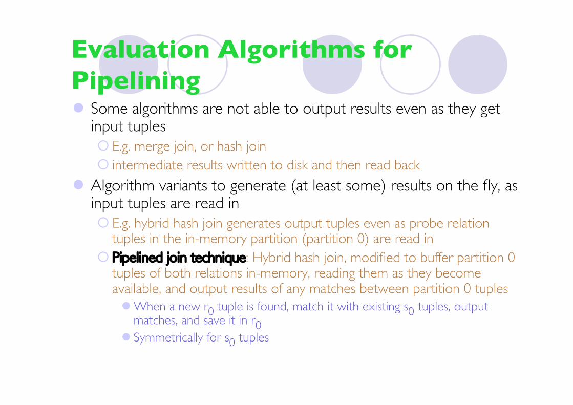
Evaluation Algorithms forPipelining Some algorithms are not able to output results even as they get

input tuples E.g. merge join, or hash join intermediate results written to disk and then read back

Algorithm variants to generate (at least some) results on the fly, asinput tuples are read in E.g. hybrid hash join generates output tuples even as probe relation

tuples in the in-memory partition (partition 0) are read in Pipelined join technique: Hybrid hash join, modified to buffer partition 0

tuples of both relations in-memory, reading them as they becomeavailable, and output results of any matches between partition 0 tuples When a new r0 tuple is found, match it with existing s0 tuples, output

matches, and save it in r0 Symmetrically for s0 tuples

Summary

OverviewMeasures of Query CostSelection OperationSorting Join OperationOther OperationsEvaluation of Expressions

Query Processing - DI.UBI

Documents