Queries and materialized views on probabilistic databases

Queries and Materialized Views on Probabilistic

Databases∗

Nilesh Dalvi Christopher Re Dan Suciu

September 11, 2008

Abstract

We review in this paper some recent yet fundamental resultson evaluating queries over probabilistic databases. While one cansee this problem as a special instance of general purpose probabilis-tic inference, we describe in this paper two key database specifictechniques that significantly reduce the complexity of query evalu-ation on probabilistic databases. The first is the separation of thequery and the data: we show here that by doing so, one can identifyqueries whose data complexity is #P-hard, and queries whose datacomplexity is in PTIME. The second is the aggressive use of pre-viously computed query results (materialized views): in particular,by rewriting a query in terms of views, one can reduce its complex-ity from #P-complete to PTIME. We describe a notion of a partialrepresentation for views, show how to validated it based on the viewdefinition, then show how to use it during query evaluation.

1 Introduction

Probabilistic database are databases where the presence of a tuple, or the valueof an attribute is a probabilistic event. The major difficulty in probabilisticdatabase is query evaluation: the result of a SQL query over a probabilisticdatabase is a set of tuples together with the probability that those tuples be-long to the output, and those probabilities turn out to be hard to compute. Infact, computing those output probabilities is a special instance of probabilisticinference, which is a problem that has been studied extensively by the Knowl-edge Representation community. Unlike general purpose probabilistic inference,in query evaluation we have a few specific techniques that we can deploy to speedup the evaluation considerably.

∗This work was partially supported by NSF Grants IIS-0454425, IIS-0513877, IIS-0713576,and a Gift from Microsoft.

1

The first is the separation between the query and the data: the query issmall, the data is large. Following Vardi [29], define the data complexity to thebe complexity of query evaluation where the query is fixed, and the complexityis measured only in the size of the database. A number of results in queryprocessing over probabilistic databases have shown that for some queries thedata complexity is PTIME, while for others it is #P-hard: we review thoseresults in Sec. 3, following mostly [11].

The second is the ability to use materialized views. These are queries thathave been previously computed and whose results have been stored. Computingthe views could have been hard, and the system has spent considerable resourcesto materialize them. However, once computed, the views can be used to answerqueries, if these queries can be answered in terms of the views [18]. Today’sdatabase systems routinely use materialized views on conventional databases:indexes are a special case of materialized views, and so are join-indexes [26], andtoday’s system can use arbitrary views during query processing [2]. However, inprobabilistic databases, views cannot always be materialized efficiently, becauseit is difficult to represent the correlations between the tuples in the view. Oneapproach to represent those correlations is to use lineage [6]. However, usinga view with explicit lineage for each tuple during query evaluation does notmake the probabilistic inference problem any easier than expanding the viewdefinition in the query body, and then evaluating the query. The approach wepropose is to store only the marginal probabilities in the materialized view, andcompute, by static analysis of the view definition, a partial representation ofthe probabilistic table defined by the view. This partial representation is at theschema level, not at the data level, and captures sufficient information about thecorrelations in the view to allow some queries to be answered from the view. Wedescribe this approach in Section 4. The main results in this part are from [25],but the presentation has been changed, and some new results have been addedthat shed further light on the view representation problem.

2 Definition: the Possible Worlds Data Model

We review here the definition of a probabilistic database based on possibleworlds, and of a disjoint-independent database. We restrict our discussion torelational data over a finite domain: extensions to continuous domains [14] andto XML [19, 1, 28] have also been considered.

We fix a relational schema R = (R1, . . . , Rk), where Ri is a relation name,has a set of attributes Attr(Ri), and a key Key(Ri) ⊆ Attr(Ri). Denote Da finite domain of atomic values. And denote Tup the set of all typed tuplesof the form t = Ri(a1, . . . , ak), for some i = 1, k and a1, . . . , ak ∈ D. Wedenote Key(t) the tuple consisting of the key attributes in t (hence its arity is|Key(Ri)|). A database instance is any subset I ⊆ Tup that satisfies all keyconstraints.

In a probabilistic database the state of the database, i.e. the instance I isnot known. Instead the database can be in any one of a finite number of possible

2

states I1, I2, . . ., called possible worlds, each with some probability.

Definition 2.1 A probabilistic database is a probability space PDB = (W,P)where the set of outcomes is a set of possible worlds W = {I1, . . . , In}, and Pis a function P : W → (0, 1] s.t.

∑I∈W P(I) = 1.

Fig. 1 illustrates three possible worlds of a probabilistic database. The prob-abilistic database has more worlds, and the probabilities of all worlds must sumup to 1; the figure illustrates only three worlds. The intuition is that we have adatabase with schema R(A,B,C,D), but we are not sure about the content ofthe database: there are several possible contents, each with a probability.

A possible tuple for a probabilistic database PDB is a tuple that occurs inat least one possible world; we typically denote T the set of possible tuples.

2.1 Query Semantics

Consider a query q of output arity k, expressed over the relational schema R.Recall that, when evaluated over a standard database instance I, a query returnsa relation of arity k, q(I) ⊆ Dk. If k = 0, then we call the query a Booleanquery.

Definition 2.2 Let q be a query of arity k and PDB = (W,P) a probabilisticdatabase. Then q(PDB) is the following probability distribution on the query’soutputs: q(PDB) = (W ′,P′) where:

W ′ = {q(I) | I ∈W}P′(J) =

∑I∈W :q(I)=J

P(I)

That is, when applied to a probabilistic database PDB the query returnsanother probabilistic database obtained by applying the query separately oneach world. The probability space q(PDB) is called an image probability spacein [16].

A particular case of great importance to us is when q is a Boolean query.Then q defines the event {I | I |= q} over a probabilistic database, and itsmarginal probability is P(q) =

∑I∈W |I|=q P(I): note that the image probability

space in this case has only two possible worlds: q(PDB) = ({I0, I1},P′), whereI0 = ∅, I1 = {()}, and P′(I0) = 1−P(q), P′(I1) = P(q). Thus, for all practicalpurposes q(PDB) and P(q) are the same, and we will refer only to P(q) whenthe query q is boolean. A special case of a boolean query is a single tuple t,and its marginal probability is P(t) =

∑I∈W |t∈I P(I). Note that t 6= t′ and

Key(t) = Key(t′) implies P(t, t′) = 0, i.e. t, t′ are disjoint events.

2.2 Block-Independent-Disjoint Databases

In order to study query complexity on probabilistic databases we need to choosea way to represent the input database. We could enumerate all possible worlds

3

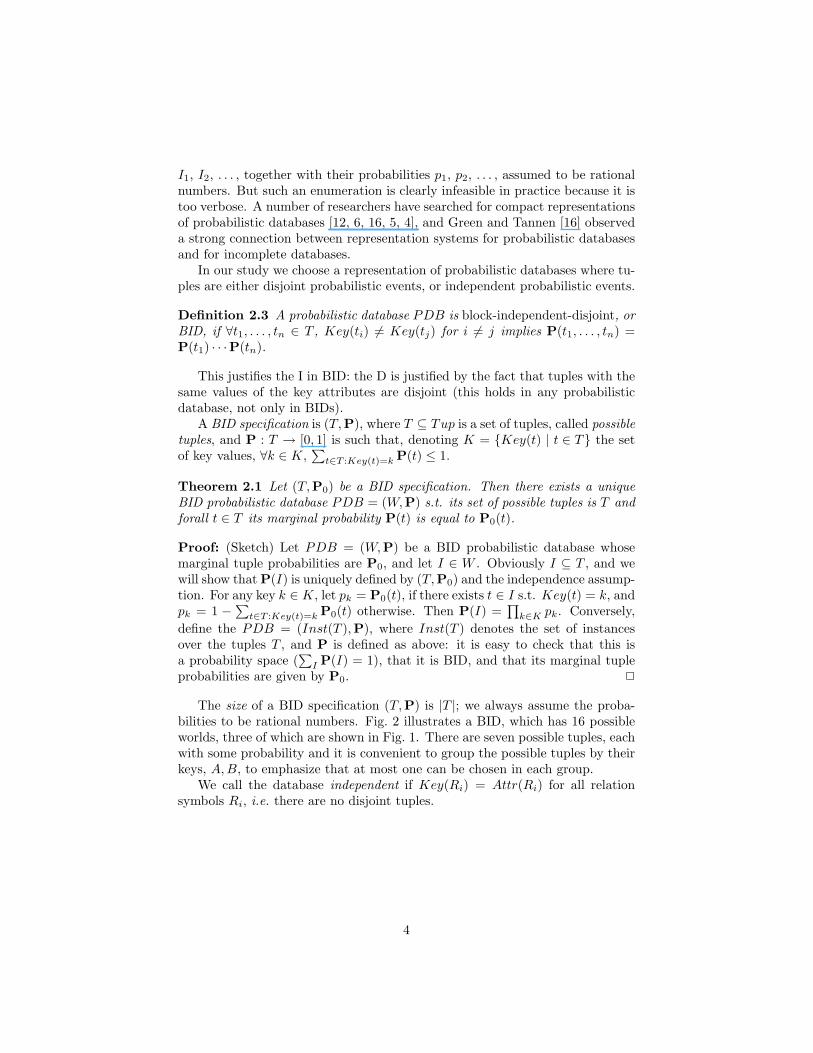
I1, I2, . . . , together with their probabilities p1, p2, . . . , assumed to be rationalnumbers. But such an enumeration is clearly infeasible in practice because it istoo verbose. A number of researchers have searched for compact representationsof probabilistic databases [12, 6, 16, 5, 4], and Green and Tannen [16] observeda strong connection between representation systems for probabilistic databasesand for incomplete databases.

In our study we choose a representation of probabilistic databases where tu-ples are either disjoint probabilistic events, or independent probabilistic events.

Definition 2.3 A probabilistic database PDB is block-independent-disjoint, orBID, if ∀t1, . . . , tn ∈ T , Key(ti) 6= Key(tj) for i 6= j implies P(t1, . . . , tn) =P(t1) · · ·P(tn).

This justifies the I in BID: the D is justified by the fact that tuples with thesame values of the key attributes are disjoint (this holds in any probabilisticdatabase, not only in BIDs).

A BID specification is (T,P), where T ⊆ Tup is a set of tuples, called possibletuples, and P : T → [0, 1] is such that, denoting K = {Key(t) | t ∈ T} the setof key values, ∀k ∈ K,

∑t∈T :Key(t)=k P(t) ≤ 1.

Theorem 2.1 Let (T,P0) be a BID specification. Then there exists a uniqueBID probabilistic database PDB = (W,P) s.t. its set of possible tuples is T andforall t ∈ T its marginal probability P(t) is equal to P0(t).

Proof: (Sketch) Let PDB = (W,P) be a BID probabilistic database whosemarginal tuple probabilities are P0, and let I ∈ W . Obviously I ⊆ T , and wewill show that P(I) is uniquely defined by (T,P0) and the independence assump-tion. For any key k ∈ K, let pk = P0(t), if there exists t ∈ I s.t. Key(t) = k, andpk = 1 −

∑t∈T :Key(t)=k P0(t) otherwise. Then P(I) =

∏k∈K pk. Conversely,

define the PDB = (Inst(T ),P), where Inst(T ) denotes the set of instancesover the tuples T , and P is defined as above: it is easy to check that this isa probability space (

∑I P(I) = 1), that it is BID, and that its marginal tuple

probabilities are given by P0. 2

The size of a BID specification (T,P) is |T |; we always assume the proba-bilities to be rational numbers. Fig. 2 illustrates a BID, which has 16 possibleworlds, three of which are shown in Fig. 1. There are seven possible tuples, eachwith some probability and it is convenient to group the possible tuples by theirkeys, A,B, to emphasize that at most one can be chosen in each group.

We call the database independent if Key(Ri) = Attr(Ri) for all relationsymbols Ri, i.e. there are no disjoint tuples.

4

2.3 pc-Tables and Lineage

BID’s are known to be an incomplete representation system1. Several, essen-tially equivalent, complete representation systems have been discussed in theliterature [12, 16, 6]. Here we follow the representation system described byGreen and Tannen [16] and called pc-tables, which extends the c-tables of [20].

Fix a set of variables X = {X1, . . . , Xm}, and for each variable Xi fix a finitedomain Dom(Xj) = {0, 1, . . . , dj}. We consider Boolean formulas ϕ consistingof Boolean combinations of atomic predicates of the form Xj = v, where v ∈Dom(Xj). Define a constant c-table to be conventional relation R, where eachtuple ti is annotated with a Boolean formula ϕi, called the lineage of t. Notethat our definition is a restriction of the standard definition of c-tables [20] inthat no variables are allowed in the tuples, hence the term “constant”: we willdrop this term and refer to a constant c-table simply as a c-table in the rest ofthis paper.

A valuation θ assigns each variable Xj to a value θ(Xj) ∈ Dom(Xj), andwe write θ(R) = {ti | θ(ϕi) = true}.

A pc-table [16] PR is a pair (R,P), consisting of a c-table R and a setof probability spaces (Dom(Xj),Pj), one for each j = 1, . . . ,m. We denoteP the product space, i.e. where the variables Xj are independent: P(θ) =∏

j Pj(θ(Xj)), for every valuation θ.A BID database PDB = (T,P) can be expressed as pc-tables as follows.

Denote K = {k1, k2, . . . , km} the set of all key values in T , and define a set ofvariables X = {X1, . . . , Xm} (one variable for each key value). Suppose that thekey value kj occurs in dj distinct tuples in T , call them tj1, tj2, . . . , tjdj : thendefine Dom(Xj) = {0, 1, . . . , dj} and annotate the tuple tji with the Boolean ex-pression Xj = i. Finally, for each j define the probability space (Dom(Xj),Pj)by setting Pj(i) = P(tji) for i > 0 and Pj(0) = 1−

∑i P(tji).

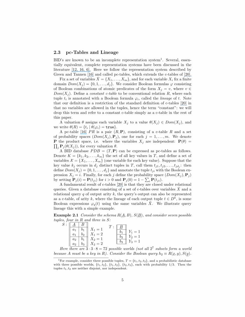
A fundamental result of c-tables [20] is that they are closed under relationalqueries. Given a database consisting of a set of c-tables over variables X and arelational query q of output arity k, the query’s output can also be representedas a c-table, of arity k, where the lineage of each output tuple t ∈ Dk, is someBoolean expressions ϕq(t) using the same variables X. We illustrate querylineage this with a simple example.

Example 2.1 Consider the schema R(A,B), S(B), and consider seven possibletuples, four in R and three in S:

S : A Ba1 b1 X1 = 1a1 b2 X1 = 2a2 b1 X2 = 1a2 b3 X2 = 2

T : Bb1 Y1 = 1b2 Y2 = 1b3 Y3 = 1

Here there are 3 · 3 · 8 = 72 possible worlds (not all 27 subsets form a worldbecause A must be a key in R). Consider the Boolean query h2 ≡ R(x, y), S(y).

1For example, consider three possible tuples, T = {t1, t2, t3}, and a probabilistic databasewith three possible worlds, {t1, t2}, {t1, t2}, {t2, t3}, each with probability 1/3. Then thetuples t1, t2 are neither disjoint, nor independent.

5

I1A B C D

a1 b1 c1 d1

a2 b1 c3 d1

a2 b2 c4 d2

P(I1) = 0.06(= p1p3p6)

I2A B C D

a1 b1 c2 c2a2 b1 c2 c1a2 b2 c4 c2

P(I2) = 0.12(= p2p5p6)

I3A B C D

a1 b1 c1 d1

a2 b2 c4 d2

P(I3) = 0.04(= p1(1-p3-p4-p5)p6)

Figure 1: A probabilistic database PDB = ({I1, I2, I3, . . .},P) with schemaR(A,B,C,D); we show only three possible worlds.

A B C D Pa1 b1 c1 d1 p1 = 0.25

c2 d2 p2 = 0.75a2 b1 c3 d1 p3 = 0.3

c1 d3 p4 = 0.3c2 d1 p5 = 0.2

a2 b2 c4 d2 p6 = 0.8c5 d2 p7 = 0.2

Figure 2: Representation of a BID. The seven possible tuples are grouped bytheir keys, for readability. There are 16 possible worlds; three are shown inFig. 1.

Then ϕq is:

ϕq = (X1 = 1)∧(Y1 = 1)∨(X1 = 2)∧(Y2 = 1)∨(X2 = 1)∧(Y1 = 1)∨(X2 = 2)∧(Y3 = 1)

3 Query Evaluation on Probabilistic Databases

In this section we summarize the results on query evaluation from [11]. We omitthe proofs, since they are already given in [11].

We study here the following problem. Given a Boolean query q and a BIDPDB = (T,P), compute q(PDB). In general the query is expressed in FO,and we will study extensively the case when q is a conjunctive query. We areinterested in the data complexity [29]: fix q, and study the complexity of P(q)as a function of the input PDB. The probabilities are assumed to be rationalnumbers.

When q is expressed in FO, then its lineage ϕq is a Boolean formula whosesize is polynomial in the size of the set of possible tuples T . Moreover, if q is aconjunctive query, then ϕq is a DNF formula of polynomial size in T , therefore,

6

any upper bounds for computing the probability of a boolean formula P(ϕq)become upper bounds for computing a query probability P(q). Thus:

Theorem 3.1 (1) Computing P(ϕ) for a Boolean expression ϕ is in #P [27].It follows that for any query q in FO, the problem “given a BID, compute P(q)”is in #P. (2) Computing P(ϕ) for a DNF formula ϕ has a FPTRAS 2 [21].It follows that for any conjunctive query q the problem “given a BID, computeP(q)” has an FPTRAS.

The complexity class #P consists of problems of the following form: givenan NP machine, compute the number of accepting computations [23]. For aBoolean expression ϕ, let #ϕ denote the number of satisfying assignments for ϕ.Valiant [27] has shown that the problem: given ϕ, compute #ϕ, is #P-complete.The statement above “computing P(ϕ) is in #P” means the following: thereexists a function F over the input probabilities P(X1), . . . ,P(Xn) (which arerational numbers) s.t. (a) F can be computed in PTIME in n, and (b) theproblem “compute F · P(ϕ)” is in #P. For example, in the case of a uniformdistribution where P(Xi) = 1/2 and all variables are independent, then we takeF = 2n, and 2nP(ϕ) = #ϕ, hence computing F ·P(ϕ) is in #P.

A Dichotomy for Queries without Self-joins

We now establish the following dichotomy for conjunctive queries without self-joins: computing P(q) is either #P-hard or is in PTIME in the size of thedatabase PDB = (T,P). A query q is said to be without self-joins if eachrelational symbol occurs at most once in the query body [9, 8]. For exampleR(x, y), R(y, z) has self-joins, R(x, y), S(y, z) has not.

Theorem 3.2 For each of the queries below (where k,m ≥ 1), computing P(q)is #P-hard in the size of the database:

h1 = R(x), S(x, y), T (y)

h+2 = R1(x, y), . . . , Rk(x, y), S(y)

h+3 = R1(x, y), . . . , Rk(x, y), S1(x, y), . . . , Sm(x, y)

The underlined positions represent the key attributes (see Sec. 2), thus, in h1

the database is tuple independent, while in h+2 , h

+3 it is a BID. When k = m = 1

then we omit the + superscript and write:

h2 = R(x, y), S(y)h3 = R(x, y), S(x, y)

2FPTRAS stands for fully poly-time randomized approximation scheme. More precisely:there exists a randomized algorithm A with inputs ϕ, ε, δ, which runs in polynomial timein |ϕ|, 1/ε, and 1/δ, and returns a value p s.t. PA(|p/p − 1| > ε) < δ. Here PA denotesthe probability over the random choices of the algorithm. Gradel et al.show how to extendthis to independent probabilities, and we show in the Appendix how to extend it to disjoint-independent probabilities

7

The significance of these three (classes of) queries is that the hardness ofany other conjunctive query without self-joins follows from a simple reductionfrom one of these three (Lemma 3.1). By contrast, the hardness of these threequeries is shown directly (by reducing Positive Partitioned 2DNF [24] to h1, andPERMANENT [27] to h+

2 , h+3 ) and these proofs are more involved.

Previously, the complexity has been studied only for independent probabilis-tic databases. De Rougemont [13] claimed that it is is in PTIME. Gradel atal. [13, 15] corrected this and proved that the query R(x), R(y), S1(x, z), S2(y, z)is #P-hard, by reduction from regular (non-partitioned) 2DNF: note that thisquery has a self-join (R occurs twice); h1 does not have a self-join, and was firstshown to be #P-hard in [9]; h+

2 and h+3 were first shown to be #P-hard in [11].

A PTIME Algorithm We describe here an algorithm that evaluates P(q)in polynomial time in the size of the database, which works for some queries,and fails for others. We need some notations. V ars(q) and Sg(q) are the setof variables, and the set of subgoals respectively. If g ∈ Sg(q) then V ars(g)and KV ars(g) denote all variables in g, and all variables in the key positionsin g: e.g. for g = R(x, a, y, x, z), V ars(g) = {x, y, z}, KV ars(g) = {x, y}. Forx ∈ V ars(q), let sg(x) = {g | g ∈ Sg(q), x ∈ KV ars(g)}. Given a databasePDB = (T,P), D is its active domain.

Algorithm 3.1 computes P(q) by recursion on the structure of q. If q con-sists of connected components q1, q2, then it returns P(q1)P(q2): this is correctsince q has no self-joins, e.g P(R(x), S(y, z), T (y)) = P(R(x))P(S(y, z), T (y)).If some variable x occurs in a key position in all subgoals, then it applies theindependent-project rule: e.g. P(R(x)) = 1 −

∏a∈D(1−P(R(a))) is the prob-

ability that R is nonempty. For another example, we apply an independentproject on x in q = R(x, y), S(x, y): this is correct because q[a/x] and q[b/x]are independent events whenever a 6= b. If there exists a subgoal g whose keypositions are constants, then it applies a disjoint project on any variable in g:e.g. x is such a variable in q = R(x, y), S(c, d, x), and any two events q[a/x],q[b/x] are disjoint because of the S subgoal.

We illustrate the algorithm on the query below, where a is a constant, andx, y, u are variables:

8

Algorithm 3.1 Safe-EvalInput: query q and database PDB = (T,P)Output: P(q)1: Base Case: if q = R(a)

return if R(a) ∈ T then P(R(a)) else 02: Join: if q = q1, q2 and V ars(q1) ∩ V ars(q2) = ∅

return P(q1)P(q2)3: Independent project: if sg(x) = Sg(q)

return 1−∏

a∈D(1−P(q[a/x]))4: Disjoint project: if ∃g(x ∈ V ars(g),KV ars(g) = ∅)

return∑

a∈D P(q[a/x])5: Otherwise: FAIL

q = R(x), S(x, y), T (y), U(u, y), V (a, u)

P(q) =∑b∈D

P(R(x), S(x, y), T (y), U(b, y), V (a, b))

=∑b∈D

P(R(x), S(x, y), T (y), U(b, y))P(V (a, b))

=∑b∈D

∑c∈D

P(R(x), S(x, c), T (c), U(b, c))P(V (a, b))

=∑b∈D

∑c∈D

P(R(x), S(x, c))P(T (c))P(U(b, c))P(V (a, b))

=∑b∈D

∑c∈D

(1−∏d∈D

(1−P(R(d))P(S(d, c)))) ·P(T (c))P(U(b, c))P(V (a, b))

We call a query safe if algorithm Safe-Eval terminates successfully; other-wise we call it unsafe. Safety is a property that depends only on the query q,not on the database PDB, and it can be checked in PTIME in the size of q bysimply running the algorithm over an active domain of size 1, D = {a}. Basedon our previous discussion, if the query is safe then the algorithm computes theprobability correctly:

Proposition 3.1 For any safe query q, the algorithm computes correctly P(q)and runs in time O(|q| · |D||V ars(q)|).

We first described Safe-Eval in [8], in a format more suitable for an im-plementation, by translating q into an algebra plan using joins, independentprojects, and disjoint projects, and stated without proof the dichotomy prop-erty. Andritsos et al. [3] describe a query evaluation algorithm for a morerestricted class of queries.

The Dichotomy Property We define below a rewrite rule q ⇒ q′ betweentwo queries. Here q is a conjunctive query without self-joins over a schema R,

9

while q′ is a conjunctive query without self-joins over a possibly different schemaR′. The symbols g, g′ denote subgoals below:

q ⇒ q[a/x] if x ∈ V ars(q), a ∈ Dq ⇒ q1 if q = q1, q2, V ars(q1) ∩ V ars(q2) = ∅q ⇒ q[y/x] if ∃g ∈ Sg(q), x, y ∈ V ars(g)

q, g ⇒ q if KV ars(g) = V ars(g)q, g ⇒ q, g′ if KV ars(g′) = KV ars(g),

V ars(g′) = V ars(g), arity(g′) < arity(g)

The intuition is that if q ⇒ q′ then evaluating P(q′) can be reduced inpolynomial time to evaluating P(q). The reduction is quite easy to prove ineach case. For example consider an instance of the first reduction: if q[a/x] is ahard query, then obviously q (which has no self-joins) is hard too: otherwise, wecan compute q[a/x] on a BID instance by simply removing all possible tuplesthat do not have an a in the positions where x occurs. All other cases can bechecked similarly. This implies:

Lemma 3.1 If q ⇒∗ q′ and q′ is #P-hard, then q is #P-hard.

Thus, ⇒ gives us a convenient tool for checking if a query is hard, by tryingto rewrite it to one of the known hard queries. For example, consider the queriesq and q′ below: Safe-Eval fails immediately on both queries, i.e. none of itscases apply. We show that both are hard by rewriting them to h1 and h+

3

respectively. By abuse of notations we reuse the same relation name during therewriting. Strictly speaking, the relation schema in the third line should containnew relation symbols S′, T ′, different from those in the second line, but we reusethe same symbols for readability:

q = R(x), R′(x), S(x, y, y), T (y, z, b)⇒ R(x), S(x, y, y), T (y, z, b)⇒∗ R(x), S(x, y), T (y) = h1

q′ = R(x, y), S(y, z), T (z, x), U(y, x)⇒ R(x, y), S(y, x), T (x, x), U(y, x)

⇒∗ R(x, y), S(y, x), U(y, x) = h+3

Call a query q final if it is unsafe, and ∀q′, if q ⇒ q′ then q′ is safe. Clearlyevery unsafe query rewrites to a final query: simply apply ⇒ repeatedly untilall rewritings are to safe queries. We prove in [11]:

Lemma 3.2 h1, h+2 , h

+3 are the only final queries.

This implies immediately the dichotomy property:

Theorem 3.3 Let q be a query without self-joins. Then one of the followingholds:

10

• q is unsafe and q rewrites to one of h1, h+2 , h

+3 . In particular, q is #P-hard.

• q is safe. In particular, it is in PTIME.

How restrictive is the assumption that the query has no self-joins ? It is usedboth in Join and in Independent project. We illustrate on q = R(x, y), R(y, z)how, by dropping the assumption, independent projects become incorrect. Al-though y occurs in all subgoals, we cannot apply an independent project becausethe two queries q[a/y] = R(x, a), R(a, z) and q[b/y] = R(x, b), R(b, z) are notindependent: both ϕq[a/y] and ϕq[b/y] depend on the tuple R(a, b) (and also onR(b, a)). In fact q is #P-hard [10]. The restriction to queries without self-joins isthus significant, see. We have extended the dichotomy property to unrestrictedconjunctive queries , but only over independent probabilistic databases [10]; thecomplexity of unrestricted conjunctive queries over BID probabilistic databasesis open.

The Complexity of the Complexity We complete our analysis by study-ing the following problem: given a relational schema R and conjunctive queryq without self-joins over R, decide whether q is safe3. We have seen that thisproblem is in PTIME (simply run the algorithm on a PDB with one tuple perrelation and see if it gets stuck); here we establish tighter bounds.

In the case of independent databases, the key in each relation R consistsof all the attributes, Key(R) = Attr(R), hence sg(x) becomes: sg(x) = {g |x ∈ V ars(g)}.

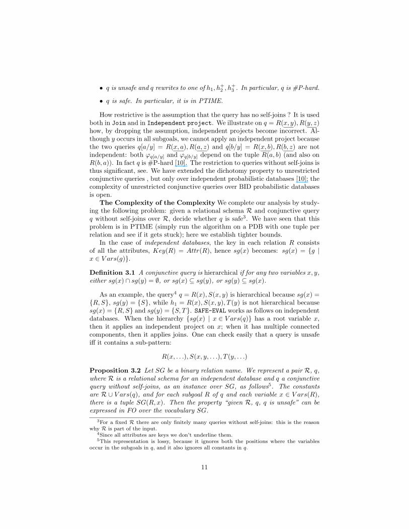
Definition 3.1 A conjunctive query is hierarchical if for any two variables x, y,either sg(x) ∩ sg(y) = ∅, or sg(x) ⊆ sg(y), or sg(y) ⊆ sg(x).

As an example, the query4 q = R(x), S(x, y) is hierarchical because sg(x) ={R,S}, sg(y) = {S}, while h1 = R(x), S(x, y), T (y) is not hierarchical becausesg(x) = {R,S} and sg(y) = {S, T}. SAFE-EVAL works as follows on independentdatabases. When the hierarchy {sg(x) | x ∈ V ars(q)} has a root variable x,then it applies an independent project on x; when it has multiple connectedcomponents, then it applies joins. One can check easily that a query is unsafeiff it contains a sub-pattern:

R(x, . . .), S(x, y, . . .), T (y, . . .)

Proposition 3.2 Let SG be a binary relation name. We represent a pair R, q,where R is a relational schema for an independent database and q a conjunctivequery without self-joins, as an instance over SG, as follows5. The constantsare R ∪ V ars(q), and for each subgoal R of q and each variable x ∈ V ars(R),there is a tuple SG(R, x). Then the property “given R, q, q is unsafe” can beexpressed in FO over the vocabulary SG.

3For a fixed R there are only finitely many queries without self-joins: this is the reasonwhy R is part of the input.

4Since all attributes are keys we don’t underline them.5This representation is lossy, because it ignores both the positions where the variables

occur in the subgoals in q, and it also ignores all constants in q.

11

In fact, it is expressed by the following conjunctive query with negations,with variables R,S, T, x, y:

SG(R, x),¬SG(R, y), SG(S, x), SG(S, y), SG(T, y),¬SG(T, x)

In the case of BIDs, checking safety is PTIME complete. Recall the Alter-nating Graph Accessibility Problem (AGAP): given a directed graph where thenodes are partitioned into two sets called AND-nodes and OR-nodes, decide ifall nodes are accessible. An AND-node is accessible if all its parents are; an ORnode is accessible if at least one of its parents is. AGAP is PTIME-complete [17].We prove in the Appendix:

Proposition 3.3 AGAP is reducible in LOGSPACE to the following problem:given a schema R and a query q without self-joins, check if q is safe. In partic-ular, the latter is PTIME-hard.

4 Materialized Views on Probabilistic Databases

The main results in this section are from [25], but the presentation is quite dif-ferent, and we have added several new results to shed more light on materializedviews. In this section we include most of the proofs.

Materialized views are a widely used today to speedup query evaluation.Early query optimizers used materialized views that were restricted to indexes(which are simple projections on the attributes being indexed) and join in-dexes [26]; modern query optimizers can use arbitrary materialized views [2].

Materialized views on probabilistic databases can make dramatic impact.Suppose we need to evaluate a Boolean query q on a BID probabilistic database,and assume q is unsafe. Normally, the only available technique is Luby andKarp’s FPTRAS, and its performance is two orders of magnitudes or moreworse than a safe plan. However, by rewriting q in terms of a view it may bepossible to transform it into a safe query, which can be evaluated very efficiently.There is no magic here: we simply pay the #P cost when we materialize theview, then evaluate the query in PTIME at runtime.

The major challenge is how to represent the view. In general the tuples inthe view may be correlated in complex ways. One possibility is to store thelineage for each tuple t (this is the approach in Trio [7]), but this makes queryevaluation on the view no more efficient than expanding the view definition inthe query.

We propose an alternative approach:

• When we materialize the view we store only the set of possible tuples andtheir marginal probabilities. We do not need to store their lineage.

• We compute a partial representation for the view. This is a schema-level(i.e. data independent) information about the independence/disjointness/correlationsof the tuples in the view, obtained from static analysis on the view defi-nition.

12

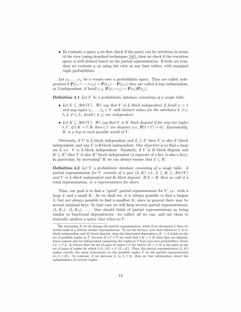
• To evaluate a query q we first check if the query can be rewritten in termsof the view (using standard techniques [18]), then we check if the rewrittenquery is well defined based on the partial representation. If both are true,then we evaluate q on using the view as any base tables, with marginaltuple probabilities.

Let e1, . . . , en be n events over a probabilistic space. They are called inde-pendent if P(e1∧· · ·∧en) = P(e1) · · ·P(en); they are called 2-way independent,or 2-independent, if forall i, j, P(ei ∧ ej) = P(ei)P(ej).

Definition 4.1 Let V be a probabilistic database consisting of a single table.

• Let L ⊆ Attr(V ). We say that V is L-block independent if forall n > 1and any tuples t1, . . . , tn ∈ V with distinct values for the attributes L (i.e.ti.L 6= tj .L, forall i 6= j) are independent.

• Let K ⊆ Attr(V ). We say that V is K block disjoint if for any two tuplest, t′, if t.K = t′.K then t, t′ are disjoint (i.e. P(t ∧ t′) = 0). Equivalently,K is a key in each possible world of V .

Obviously, if V is L-block independent and L ⊇ L′ then V is also L′-blockindependent, and any V is ∅-block independent. Our objective is to find a largeset L s.t. V is L-block independent. Similarly, if V is K-block disjoint andK ⊆ K ′ then V is also K ′-block independent (a superset of a key is also a key).In particular, by increasing6 K we can always ensure that L ⊆ K.

Definition 4.2 Let V a probabilistic database consisting of a single table. Apartial representation for V consists of a pair (L,K) s.t. L ⊆ K ⊆ Attr(V )and V is L-block independent and K-block disjoint. If L = K then we call it atotal representation, or a representation for short.

Thus, our goal is to find a “good” partial representation for V , i.e. with alarge L and a small K. As we shall see, it is always possible to find a largestL, but not always possible to find a smallest K, since in general there may beseveral minimal keys. In that case we will keep several partial representations,(L,K1), (L,K2), . . . . One should think of partial representations as beingsimilar to functional dependencies: we collect all we can, and use them tostatically analyze a query that refers to V .

6By increasing K we do change the partial representation, while if we decreased L then wewould make it a strictly weaker representation. To see the former, note that whenever V is L-block independent and K-block disjoint, then the functional dependency K → L holds on theset of possible tuples in T , because if t, t′ ∈ T are such that t.K = t′.K then they are disjoint,hence cannot also be independent (assuming the tuples in T have non-zero probability), hencet.L = t′.L. It follows that the set of pairs of tuples t, t′ for which t.K = t′.K is the same as theset of pairs of tuples for which t.(L∪K) = t′.(L∪K). Thus, the partial representation (L, K)makes exactly the same statements on the possible tuples T as the partial representation(L, L ∪ K). In contrast, if we decrease L to L ∩ K, then we lose information about theindependence of certain tuples.

13

Note that V is a BID table iff it has a total representation: in this caseKey(V ) = L = K.

We start with a negative result: with our current definition, there is nolargest L. This can be shown from the following example.

Example 4.1 Consider a probabilistic table V (A,B,C) with four possible tu-ples:

T : A B Ca b c t1a b′ c t2a b′ c′ t3

and four possible worlds: I1 = ∅, I1 = {t1, t2}, I2 = {t2, t3}, I3 = {t1, t3},each with probability 1/4. Any two tuples are independent: indeed P(t1) =P(t2) = P(t3) = 1/2 and P(t1t2) = P(t1t3) = P(t2t3) = 1/4. V is AB-block independent: this is because the only sets of tuples that differ on AB are{t1, t2} and {t1, t3}, and they are independent. Similarly, V is also AC-blockindependent. But V is not ABC-block independent, because any two tuples in set{t1, t2, t3} differ on ABC, yet the entire set is not independent: P(t1t2t3) = 0.This shows that there is no largest set L: both AB and AC are maximal.

Thus, for a general probabilistic databases we cannot hope to have a bestpartial representation. However, we can prove the following weaker result, whichwe will use later:

Lemma 4.1 For a set L ⊆ Attr(V ) we say that V is L-block 2-independent ifany two tuples t1, t2 s.t. t1.L 6= t2.L are independent. Then, any probabilistictable V has a largest set L s.t. V is L-block 2-independent.

Proof: It suffices to prove the following. Let L1, L2 ⊆ Attr(V ) be s.t. V isLi-block 2-independent for each i = 1, 2: then, denoting L = L1 ∪ L2, V isL-block 2-independent. Indeed, let t1, t2 be two tuples s.t. t1.L 6= t2.L. Theneither t1.L1 6= t2.L1 or t1.L2 6= t2.L2, hence t1, t2 are independent tuples. 2

Continuing Example 4.1 we note that V is ABC-block 2-independent, sinceany two of the tuples t1, t2, t3 are independent.

4.1 Materialized Views Expressed by c-Tables

Despite Example 4.1, it turns out that c-tables do admit a largest set L, foran appropriate definition of L-block independence. Recall that a pc-table Vconsists of two parts: V = (CV,P), where CV is a c-table and P a productprobability space on the set of variables X.

Definition 4.3 Let CV be a c-table of arity k.

• Let L ⊆ Attr(CV ). We say that CV is L-block independent if for anypc-table V = (CV,P), V is L-block independent.

14

• Let K ⊆ Attr(CV ). We say that CV is K block disjoint if for any pc-tableV = (CV,P), V is K-block disjoint.

In general there is no smallest set K s.t. V is K-block disjoint: see Exam-ple 4.4 below. On the other hand, we prove the following in this section:

Theorem 4.1 For any c-table CV there exists a largest set of attributes L ⊆Attr(CV ) s.t. CV is L-block independent.

It is easy to see that every c-table CV has a largest set of attributes L s.t.CV is L-block 2-independent: the proof is similar to that of Lemma 4.1. Weneed to prove, however, that CV is also L-block independent.

To prove this, we establish a few simple results. First, consider a Booleanformula ϕ over variables X = {X1, . . . , Xm}: the atomic formulas in ϕ areexpressions Xi = v, where v ∈ Dom(Xi). A valuation is a function θ : X →∏Dom(Xi), and we denote with ϕ[θ] the truth value of the formula ϕ under

the valuation θ.Let ϕ1, . . . , ϕn be n formulas over the same sets of variables X. We say

that they are independent if for any product probability space P the eventsϕ1, . . . , ϕn are independent. Similarly, we say that they are 2-way independentif for any probability spaces for its variables, they are 2-way independent events.Theorem 4.1 obviously follows from the following:

Proposition 4.1 A set of formulas ϕ1, . . . , ϕn is independent iff it is 2-wayindependent.

Let’s see first how this implies Theorem 4.1: if L is the largest set of at-tributes s.t. V is L-block 2-independent: then the proposition implies that V isalso L-block independent, and L is obviously the largest such set.

To prove the proposition we give an alternative characterization of indepen-dence in terms of critical variables.

Definition 4.4 A variable Xj is called a critical variable for ϕ if there existsa valuation θ for the variables X − {Xj} and two values v′, v′′ ∈ Dom(Xj) s.t.ϕ[θ ∪ {(Xj , v

′)}] 6= ϕ[θ ∪ {(Xj , v′′)}].

In other words Xj is a critical variable if there is a choice of values for theother variables for which Xj makes a difference: when Xj changes v′ to v′′, thenϕ changes from false to true. If the expression ϕ does not mention the variableXj at all, then it is obviously not a critical variable. Conversely, if Xj is nota critical variable for ϕ then one can rewrite ϕ as an expression that does notmention Xj . For example, consider ϕ = X1 ∨ (X1 ∧ X2) (where the variablesare assumed to be Boolean). Here X1 is a critical variable, but X2 is not: infact ϕ can be rewritten as ϕ = X1. In general:

Proposition 4.2 Deciding whether Xj is a critical variable for ϕ is NP-complete.

15

Membership in NP follows by definition, while hardness follows from the factthat if ψ is a Boolean expression that does not mention Xj , then Xj is criticalfor ψ ∧Xj iff ψ is satisfiable.

The connection between independence and critical variables is the following:

Theorem 4.2 Let ϕ, ψ be two Boolean formulas over the same set of variablesX. Then ϕ,ψ are independent iff they have no common critical variables.

The “if” direction is trivial: if ϕ,ψ use disjoint sets of variables, then theyare clearly independent. Before we prove the “only if” direction, we note thatthe theorem immediately implies Proposition 4.1: if the formulas are 2-wayindependent, then each ϕi uses a set of variables that is disjoint for the variablesused by any other ϕj , hence they are independent.

Proof: (“Only if” of Theorem 4.2). The “only if” direction was shown in [22]for the case when all variables Xj are Boolean, i.e. |Dom(Xj)| = 2. We brieflyreview the proof here. Given a probability spaces (Dom(Xj),Pj), denote xj =Pj(Xj = 1), hence P(Xj = 0) = 1 − xj . Then P(ϕ) is a polynomial in thevariables x1, . . . , xm where each variable has degree ≤ 1. (For example, if ϕ =¬(X1 ⊗ X2 ⊗ X3) (exclusive or) then P(ϕ) = x1x2(1 − x3) + x1(1 − x2)x3 +(1 − x1)x2x3 + (1 − x1)(1 − x2)(1 − x3), which is a polynomial of degree 1 inx1, x2, x3.) The identity P(ϕ)P(ψ) = P(ϕ ∧ ψ) must hold for any values ofx1, . . . , xm. If Xj is a common critical variable for ϕ and ψ then the left handside is a polynomial of degree 2 in xj , while the right hand side has degree 1,which is a contradiction.

We now extend this proof to non-Boolean domains. In this case a variableXj may take values 0, 1, . . . , dj , for dj ≥ 1. Define the variables xij to bexij = P(Xj = i), for i = 1, . . . , dj , thus P(Xj = 0) = 1− x1j − x2j − · · · − xdjj .As before P(ϕ) is a polynomial of degree 1 in the variables xij with the additionalproperty that if i1 6= i2 then xi1j and xi2j cannot appear in the same monomial.We still have the identity P(ϕψ) = P(ϕ)P(ψ), for all values of the variables xij

(since the identity holds on the open set xij ≥ 0 forall i, j, and∑

i xij ≤ 1, forallj). If Xj is a critical variable for ϕ then P(ϕ) must have a monomial containingsome xi1j ; if it is also critical for ψ, then P(ψ) has a monomial containing xi2j .Hence their product contains xi1j · xi2j , contradiction. 2

4.2 Materialized Views Expressed by Conjunctive Queries

The conjunctive queries that we consider in this section may have self-joins,unless we explicitly say that they don’t have self-joins. We fix the schema Rof a BID database, and consider the case when V is defined by a conjunctivequery over R. That is, V : −v, where V is the name of the view, and v is theconjunctive query defining it.

Definition 4.5 • Let L ⊆ Attr(V ): V is L-block independent if for anyinput BID database PDB, the probabilistic table v(PDB) is L-block inde-pendent.

16

• Let K ⊆ Attr(V ): V is K-block independent if for any input BID databasePDB, the the probabilistic table v(PDB) is K-block disjoint.

We illustrate with three examples.

Example 4.2 Consider the relational schema R(C,A), S(C,A,B), T (C,B),and the following view:

v(z) : − R(z, x), S(z, x, y), T (z, y)

Denote V (Z) the schema of the materialized view. Then V is Z-block indepen-dent: in other words all tuples in V are independent. Note that this query is ahard query, since it reduces to h1 from Theorem 3.2, but it is fully representableas a table where all tuples are independent. That means that we need to pay ahigh price to materialize the view V : the result is the set of all possible tuples inV , together with their marginal probabilities. But later we can use V freely inqueries, and we know that all tuples are independent. Importantly, we can useV in queries that have RST as a subquery. For example consider the Booleanquery q : −R(z, x), S(z, x, y), T (z, y), U(z, v), where U(C,D) is another relation.Then q is #P-hard, but after rewriting it as q : −V (z), U(z, v) it becomes a safequery, i.e. it is in PTIME. Thus, by using V to evaluate q we obtain a dramaticreduction in complexity.

Example 4.3 For a second example, consider the schema R(A), S(A,B,C).,and the query:

v(x, y, z) : − R(x), S(x, y, z)

This query is safe (there are no projections), but is not fully representable.Denoting V (X,Y, Z) the output schema, the best we can say is that V is X-blockindependent, and XY -block disjoint. Thus, we know that the tuples V (a, b, c)and V (a′, b, c) are independent, and the tuples V (a, b, c), V (a, b, c′) are disjoint.But we do not know the correlation between the tuples V (a, b, c) and V (a, b′, c).In fact, we cannot answer the Boolean query q = V (a, b, c), V (a, b′, c) by exam-ining only the view V : to answer q we need to expand it and answer it from thebase relations.

Example 4.4 Finally, consider the schema R(A,B,C), S(A,C,B) and theview:

v(x, y, z) : − R(x, y, z), S(x, z, y)

Here V is X-block independent. In addition, V is both XY -block disjoint andXZ-block disjoint: but it is not X-block disjoint. In practice, in this case wewill keep both partial representations (X,XY ) and (X,XZ).

17

Recall that a BID instance PDB is a special case of a (set of) pc-tables.Thus, we can expressed it as PDB = (CDB,P) separating the c-tables fromthe probability P. This implies that the view V = v(PDB) can be expressedas follows: it has a c-table v(CDB), which can be computed by computingseparately the lineage of each output tuple, and it has a probability space Pon the variables X. Both the variables X and the product probability P arethe same as for PDB. From this it follows that V is L-block independent iffor any input c-tables CDB, the c-table v(CDB) is L-block independent, andis K-block disjoint if for any input c-tables CDB, v(CDB) is K-block disjoint.The following are immediate:

Proposition 4.3 (a) V is L-block 2-independent iff it is L-block independent.(b) There exists a largest set L s.t. V is L-block independent.

Proof: (a) follows immediately from the corresponding fact for c-tables. (b)for each c-table CDB, there exists a largest set LCDB s.t. v(CDB) is LCDB-block independent. Then the largest set L s.t. V is L-block independent is⋂

CDB LCDB (the intersection ranges over infinitely many CDBs). 2

Thus, there exists a “best” (largest) choice for the attributes L. On the otherhand, we know that there is no “best” (smallest) choice for the K attributes,as shown in Example 4.4.

The proof above gives no clue how to actually search for the largest set L.To find L we can iterate over all subsets L ⊆ Attr(V ), but we still need a criteriato check if for a given set L, the view V is L-block independent. For that weuse the notion of critical tuples, introduced in [22].

Given a Boolean query q, a critical tuple is a ground tuple t for one of therelations Ri occurring in q s.t. there exists a (conventional) database instanceI s.t. q(I) 6= q(I ∪ {t}). For a simple illustration, consider the Boolean queryq : −R(x, x), S(a, x, y), where a is a constant. Then R(b, b) (for some constantb) is a critical tuple because q is false on the instance I = {S(a, b, c)} but trueon the instance {R(b, b), S(a, b, c)}. On the other hand R(b, c) is not a criticaltuple. In general, if the query q is a conjunctive query, then any critical tuplemust be the ground instantiation of a subgoal. The converse is not true asthe following example from [22] shows: q : −R(x, y, z, z, u), R(x, x, x, y, y). Thetuple t = R(a, a, b, b, c), which is a ground instantiation of the first subgoal, isnot a critical tuple. Indeed, if q is true on I ∪ {t}, then only the first subgoalcan be mapped to t, and therefore the second subgoal is mapped to the groundtuple R(a, a, a, a, a), which must be in I: but then q is also true on I, hence tis not critical. In general:

Theorem 4.3 [22] The problem: given q, t, check whether t is a critical tuplefor q, is Σp

2-complete.The problem: given two Boolean queries q, q′, check whether they have no

common critical tuples is Πp2 complete.

For the first statement, membership in Σp2 follows from the observation that

the size of I can be bounded by the number of variables occurring in q plus the

18

constants occurring in q and t. The second statement follows immediately fromthe first (hardness follows by taking q′ = t).

There is a strong connection between critical variables of a Boolean formulaand critical tuples of a Boolean query. Let CDB be a c-table database, and letϕ be the lineage formula for q(CDB). Then if Xj is a critical variable for ϕ,then at least one of the tuples in CDB that is annotated with an expressionXj = v is a critical tuple for q. Conversely, if t is a critical tuple for q then onecan find a c-table database CDB containing t s.t. the variable Xj annotating tis a critical variable for the lineage formula for q(CDB).

This implies:

Proposition 4.4 Let q, q′ be two Boolean queries over a common BID schemaR. Then the following are equivalent:

• For any input probabilistic database q and q′ are independent.

• q and q′ do not have any common critical tuples.

Corollary 4.4 Checking whether q, q′ are independent forall BID databases isΠp

2-complete.

We use this to derive a necessary and sufficient condition for V to be L-block 2-independent, which, as we have shown, implies that V is also L-blockindependent. Recall that k is the arity of V (k = |Attr(V )|).

Proposition 4.5 Let V be a view defined by a conjunctive query over a BIDschema. For any L ⊆ Attr(V ), the following two conditions are equivalent:

• V is L-block independent.

• V is L-block 2-independent.

• For any two ground tuples t, t′ ∈ Dk s.t. t.L 6= t′.L, the two Booleanqueries v(t) and v(t′) have no common critical tuples. Here v(t) denotesthe Boolean query obtained by substituting the head variables in v with thetuple t, and similarly v(t′).

Thus, an upper bound on the complexity is Πp2. It turns out that the problem

is also hard for this class, as shown in the full version of [25].

Theorem 4.5 Checking whether V is L-block independent is Πp2-complete.

We can now better understand the set of attributes L for which V is L-blockindependent. Any such set consists only of all attributes A s.t. V is A-blockindependent; and the maximal set L is precisely the set of all such attributesA. Moreover, given an attribute A, checking whether V is A-block independentis precisely the safety test for an independent project on A. We have shown inSec. 3 that in the case of queries without self joins, this happens iff A appears

19

in a key position in each subgoal of v. On the other hand, if v is allowed to haveself-joins, then checking if a safe project on A is possible is Πp

2-complete.Finally, we briefly comment on how to compute the set K that describes

disjoint tuples. This is simply a key K ⊆ Attr(V ), in the conventional sense,where the relations mentioned in the query v have explicit keys. There arestandard procedures for computing the set of keys in a conjunctive query.

4.3 Querying Partially Represented Views

We now turn to an interesting question: given a partial representation (L,K)for a materialized view V , and a query q that uses the view, check whether q canbe answered from V . Notice that this is orthogonal to the query answering usingviews problem [18]: there we are given a query q over a conventional databaseand a set of views, and we want to check if q can be rewritten into an equivalentquery q′ that uses the views. Here we assume that the rewriting has alreadybeen done, thus q already mentions the view(s). The problem is whether q iswell-defined: we saw in Example 4.4 a case when the query is not well-defined,because the partial representation (L,K) and the marginal tuple probabilitiesdo not uniquely define a probabilistic database for the view.

In this section we restrict the query q to be over a single view V , andmention no other relations. Thus, q can perform selections and self-joins over Vonly. Our discussion of well-definedness extends immediately to the case whenq is written over multiple views, each with its own partial representation, andeven over input BID tables (which for this purpose are views with a completerepresentation), provided that all views and base tables are independent.

Definition 4.6 Let PV be a probabilistic relation of schema V . We writePV |= (L,K) if PV is L-block independent and K-block disjoint.

Definition 4.7 Let q be a Boolean query over the single relation name V . Wesay that q is well-defined given the partial representation (L,K), if forall PV ,PV ′ s.t. PV |= (L,K), PV ′ |= (L, k), and ∀t P(t) = P′(t), P(q) = P′(q).

Thus, q is well defined iff P(q) depends only on the marginal tuple probabil-ities P(t) (which we know), and not on the entire distribution (which we don’tknow). We will give now a necessary and sufficient condition for q to be welldefined. For that we first need some background on numerical functions.

4.3.1 Numerical Functions and Differentials

Recall that we have a fixed domain D and denote Tup the set of tuples (overa given relational schema R) that can be constructed with constants from D.Let Inst = P(Tup) be the set of instances. A numerical function is a functionof the form f : Inst → R, where R is the set of reals. A Boolean query is aparticular numerical function: q(I) = 0 if the query is false at I, and q(I) = 1when the query is true.

20

Definition 4.8 Let s ∈ Tup be a ground tuple. The differential of f w.r.t. sis:

∆sf(I) = f(I)− f(I − {s})

Iterating this definition gives us the differential ∆S for a set of tuples S: fors 6∈ S define ∆{s}∪Sf = ∆s(∆Sf). Note that the differential of a monotoneBoolean query is also a Boolean query, but it is not necessarily monotone;furthermore, the differential of a non-monotone query may take the value −1.

Definition 4.9 A set of tuples C is critical for f if ∃I s.t. ∆Cf(I) 6= 0.

This generalizes the previous definition of a critical tuple. Indeed, a tuplet is critical for a query q iff the set {t} is critical for the numerical functionassociated to q.

The following identities can easily be derived:

f(I) = f(I − {s}) + ∆sf(I)f(I) = f(I − {s1, s2}) + ∆s1f(I − {s2}) + ∆s2f(I − {s1}) + ∆s1s2f(I)

In order to generalize the latter formula, we introduce another definition:

Definition 4.10 Let T ⊆ Tup be a set of tuples. The restriction of f to T is:fT (I) = f(I ∩ T ).

In particular f = fTup, where Tup is the set of all tuples over the domain. Ifq is a Boolean query then qT is also a Boolean query; if moreover q is monotone,then qT is also monotone.

Proposition 4.6 For any set of tuples T :

f =∑S⊆T

∆SfTup−(T−S)

In particular, by taking T = Tup we obtain f =∑

S⊆Tup ∆SfS.

For any set of tuples S:

∆Sf =∑T⊆S

(−1)|T |fTup−T

The proofs are immediate: the first equation generalizes the two identitiesabove, while the second equation generalizes identies like:

∆sf(I) = f(I)− f(I − {s})∆s1,s2f(I) = f(I)− f(I − {s1})− f(I − {s2}) + f(I − {s1, s2})

Finally, we state the following (which is easy to check):

Proposition 4.7 (1) If C is critical for ∆Sf , then C is critical for f . (2) IfC is critical for fT , then C is critical for f .

21

4.3.2 The Well-definedness Condition

We call two tuples t,t′ intertwined if t.L = t′.L and t.K 6= t′.K. If two tuples arenot intertwined, then they are either independent (when t.L 6= t′.L), or disjoint(when t.K = t′.K). Thus, intertwined tuples are correlated in ways that wecannot determine.

Theorem 4.6 Let q be a monotone Boolean query over V . Then q is welldefined iff for any two intertwined tuples t, t′ the set {t, t′} is not critical for q(in other words, ∆t,t′q = 0).

Before proving the theorem we illustrate with an example:

Example 4.5 Let V (A,B,C) have the following partial representation: L = A,K = AB. Consider the following queries:

q1 : − V (a,−,−)q2 : − V (−, b,−)q3 : − V (−,−, c)

Of the three, q2 is the only query that is well-defined. We first explain intuitivelywhy q2 is well-defined. Its value depends only on the tuples of the form (ai, b, cj):these can be partitioned by ai into independent sets, while the tuples in each setare disjoint. In other words, q2 depends only on a subset of tuples that form aBID table. One can also see that q2 has no two intertwined, critical tuples: ift1, t2 is a critical set then each of t1, t2 must be critical, hence they must be of theform (ai, b, bj): but then they are not intertwined (they are either independent(t1.A 6= t2.A) or disjoint (t1.AB = t2.AB, but t1.C 6= t2.C).

In contrast, neither q1 nor q2 are well-defined. To see this, consider a viewV with two tuples: t1 = (a, b1, c) and t2 = (a, b2, c); these tuples are intertwined,i.e. the correlation of t1 and t2 is unknown. Further, P[q1] = P[q3] = P[t1 ∨ t2]and so neither q1 nor q3 is well-defined. They also form a set of critical tuples:denoting I = {t1, t2}, q1(I) = q1(I−{t1}) = q1(I−{t2}) = 1, q1(I−{t1, t2}) = 0,hence ∆t1,t2q1(I) = −1; similarly for q3.

We now prove the theorem.

Proof: We start with the “only if” direction. Let t, t′ be a critical set of twointertwined tuples. By definition there exists an instance I s.t. q(I) − q(I −{t}) − q(I − {t′}) + q(I − {t, t′}) 6= 0. Since q is monotone we have q(I) = 1,q(I − {t, t′}) = 0, and either q(I − {t}) = q(I − {t′}) = 0 or q(I − {t}) =q(I − {t′}) = 1. Without loss, we assume that q(I − {t}) = q(I − {t′}) = 0.Then we define two probabilistic databases PV = (W,P) and PV ′ = (W,P′)as follows. Each has four possible worlds: I, I − {t}, I − {t′}, I − {t, t′}. In PVthese worlds are assigned probability P = (0.5, 0, 0, 0.5), respectively; here, t1and t2 are positively correlated. In PV ′, all worlds are assigned probability 0.25

22

i.e. tuple independence. Observe that in both cases, the marginal probabilityof any tuple is the same, P[t] = P[t′] = 0.5 and all other tuples probability 1,then P[q] = 0.5 while P′[q] = 0.25, so the value of q is not well-defined.

Next we prove the “if” part. The basic plan is this. Suppose an instanceI contains two intertwined tuples t, t′ (hence we don’t know their correlations).Write q(I) = q(I − {t, t′}) + ∆tq(I − {t′}) + ∆t′q(I − {t}) (because ∆t,t′q = 0).Thus, we can “remove” t or t′ or both from I and get a definition of q on asmaller instance, and by repeating this process we can eliminate all intertwinedtuples from I. We need to make this intution formal, and we start with a lemma.We say that a set of tuples T is non-intertwined, or NIT, if ∀t, t′ ∈ T , t and t′

are not intertwined.

Lemma 4.2 Let q be a monotone, Boolean query without critical pairs of in-tertwined tuples, and let T be a NIT set of tuples. Then the Boolean query qT

is well defined.

Proof: A minterm for qT is a minimal instance J s.t. qT (J) is true (that isif J ′ ⊆ J and qT (J ′) is true then J = J ′). Obviously, each minterm for qT

is a subset of T . Since qT is monotone (because q is monotone), it is uniquelydetermined by the set M of all its minterms: qT (I) =

∨J∈M(J ⊆ I). Denoting rJ

the boolean query rJ(I) = (J ⊆ I), we apply the inclusion-exclusion formula toderive P(qT ) = P(

∨J∈M r

J) =∑

N⊆M,N 6=∅(−1)|N |P(rS

N ). Finally, we observethat for each N ⊆ M, the expression P(r

SN ) is well defined. Indeed, the set

J =⋃N is the union of minterms in N , thus it is a subset of T , hence it is a NIT

set. If J = {t1, t2, . . .}, the query rJ simply checks for the presence of all tuplest1, t2, . . .; in more familiar notation P(rJ) = P(t1t2 · · · ). If the set J containstwo disjoint tuples (ti.K = tj .K) then P(t1t2 · · · ) = 0. Otherwise, it containsonly independent tuples (ti.L 6= tj .L), hence P(t1t2 · · · ) = P(t1)P(t2) · · · Ineither cases it is well-defined and, hence, so is P(qT ). 2

Thus, we know that, for every NIT T , qT is well defined: we need to provethat q is well defined, and for that we use the expansions above. Let PV bea probabilistic database s.t. PV |= (L,K), and let Tup be the set of possibletuples in PV . Then:

q =∑

T⊆Tup

∆T qT

=∑

T is NIT∆T q

T

=∑

T is NIT

∑S⊆T

(−1)|S|qT−S

Here we used the fact that if T contains any two intertwined tuples, then∆T q

T = 0: indeed, suppose t, t′ ∈ T are two intertwined tuples, and denoteS = T − {t, t′}. Then there exists I s.t. ∆T q

T (I) = ∆t,t′∆SqT (I) 6= ∅, hence

23

t, t′ are critical for ∆SqT : therefore they are critical for qT , and therefore they

are critical for q, contradicting our assumption. Hence if T is not NIT, then∆T q

T = 0. Therefore in the second line above it suffices to iterate over NITsets T . The last line is just a further expansion of ∆T .

Next we apply the expectation on both sides, and use the linearity of expec-tation plus P(q) = E[q]:

P(q) = E[q] =∑

T is NIT

∑S⊆T

(−1)|S|E[qT−S ]

=∑

T is NIT

∑S⊆T

(−1)|S|P(qT−S)

Finally, we use the lemma to argue that each expression P(qT−S) is welldefined. 2

Finally, we mention without proof the complexity (the proof can be foundin the full version of [25]):

Theorem 4.7 Checking whether q is well defined w.r.t. (L,K) is Πp2-complete.

As a final comment, we remark that once we have determined that a queryq is well defined for a given partial representation (L,K), of a view V it iseasy to evaluate it, using e.g. the techniques from Sec. 3: for that it suffices topretend that V is a BID, either with Key(V ) = L or with Key(V ) = K: bothassumptions will lead to the same value for q because q is well-defined.

5 Conclusions

At a superficial look, query evaluation on probabilistic databases seems just aspecial instance of probabilistic inference, e.g. in probabilistic networks. How-ever, there are specific concepts and techniques that have been used on con-ventional databases for many years, and that can be depolyed to probabilisticdatabases as well, to scale up query processing to large data instances. We havepresented two such techniques in this paper. The first is the separation of thequery and the data: we have shown here that by doing so, one can identifyqueries whose data complexity is #P-hard, and queries whose data complexityis in PTIME. The second is the aggressive use of materialized views (or anypreviously computed query results): we have shown that by using a materizliedview the query complexity can decrease from #P-hard to PTIME, and havedescribed static analysis techniques to derive a partial representation for theview, and to further use it in query evaluation.

References

[1] S. Abiteboul and P. Senellart. Querying and updating probabilistic infor-mation in XML. In EDBT, pages 1059–1068, 2006.

24

[2] Sanjay Agrawal, Surajit Chaudhuri, and Vivek R. Narasayya. Automatedselection of materialized views and indexes in sql databases. In VLDB 2000,Proceedings of 26th International Conference on Very Large Data Bases,September 10-14, 2000, Cairo, Egypt, pages 496–505. Morgan Kaufmann,2000.

[3] P. Andritsos, A. Fuxman, and R. J. Miller. Clean answers over dirtydatabases. In ICDE, 2006.

[4] L. Antova, C. Koch, and D. Olteanu. 10^(10^6) worlds and beyond: Ef-ficient representation and processing of incomplete information. In ICDE,2007.

[5] L. Antova, C. Koch, and D. Olteanu. World-set decompositions: Expres-siveness and efficient algorithms. In ICDT, pages 194–208, 2007.

[6] O. Benjelloun, A. Das Sarma, A. Halevy, and J. Widom. ULDBs:Databases with uncertainty and lineage. In VLDB, pages 953–964, 2006.

[7] O. Benjelloun, A. Das Sarma, C. Hayworth, and J. Widom. An introductionto ULDBs and the Trio system. IEEE Data Eng. Bull, 29(1):5–16, 2006.

[8] N. Dalvi, Chris Re, and D. Suciu. Query evaluation on probabilisticdatabases. IEEE Data Engineering Bulletin, 29(1):25–31, 2006.

[9] N. Dalvi and D. Suciu. Efficient query evaluation on probabilistic databases.In VLDB, Toronto, Canada, 2004.

[10] N. Dalvi and D. Suciu. The dichotomy of conjunctive queries on proba-bilistic structures. In PODS, pages 293–302, 2007.

[11] N. Dalvi and D. Suciu. Management of probabilistic data: Foundationsand challenges. In PODS, pages 1–12, Beijing, China, 2007. (invited talk).

[12] A. Das Sarma, O. Benjelloun, A. Halevy, and J. Widom. Working modelsfor uncertain data. In ICDE, 2006.

[13] Michel de Rougemont. The reliability of queries. In PODS, pages 286–291,1995.

[14] A. Deshpande, C. Guestrin, S. Madden, J. M. Hellerstein, and W. Hong.Model-driven data acquisition in sensor networks. In VLDB, pages 588–599,2004.

[15] E. Gradel, Y. Gurevich, and C. Hirsch. The complexity of query reliability.In PODS, pages 227–234, 1998.

[16] T. Green and V. Tannen. Models for incomplete and probabilistic infor-mation. IEEE Data Engineering Bulletin, 29(1):17–24, March 2006.

25

[17] R. Greenlaw, J. Hoover, and W. Ruzzo. Limits to Parallel Computation.P-Completeness Theory. Oxford University Press, New York, Oxford, 1995.

[18] Alon Halevy. Answering queries using views: A survey. VLDB Journal,10(4):270–294, 2001.

[19] E. Hung, L. Getoor, and V.S. Subrahmanian. PXML: A probabilisticsemistructured data model and algebra. In ICDE, 2003.

[20] T. Imielinski and W. Lipski. Incomplete information in relationaldatabases. Journal of the ACM, 31:761–791, October 1984.

[21] R. Karp and M. Luby. Monte-Carlo algorithms for enumeration and relia-bility problems. In Proceedings of the annual ACM symposium on Theoryof computing, 1983.

[22] G. Miklau and D. Suciu. A formal analysis of information disclosure indata exchange. J. Comput. System Sci., 73(3):507–534, 2007.

[23] Christos Papadimitriou. Computational Complexity. Addison Wesley Pub-lishing Company, 1994.

[24] J. S. Provan and M. O. Ball. The complexity of counting cuts and ofcomputing the probability that a graph is connected. SIAM J. Comput.,12(4):777–788, 1983.

[25] C. Re and D.Suciu. Materialized views in probabilistic databases for infor-mation exchange and query optimization. In Proceedings of VLDB, 2007.

[26] Patrick Valduriez. Join indices. ACM Transactions on Database Systems,12(2):218–246, 1987.

[27] L. Valiant. The complexity of enumeration and reliability problems. SIAMJ. Comput., 8:410–421, 1979.

[28] M. van Keulen, A. de Keijzer, and W. Alink. A probabilistic XML approachto data integration. In ICDE, pages 459–470, 2005.

[29] M. Y. Vardi. The complexity of relational query languages. In Proceedingsof 14th ACM SIGACT Symposium on the Theory of Computing, pages137–146, San Francisco, California, 1982.

26