Quasi-independence, homology and the unity of type: A topological theory of characters

J. theor. Biol. (2003) 220, 505–527doi:10.1006/jtbi.2003.3150, available online at http://www.idealibrary.com on

InL14

00

Quasi-Independence, Homology and the Unity of Type:A Topological Theory of Characters

Guº nter P.Wagnerw and Peter F. Stadlernzy

wDepartment of Ecology and Evolutionary Biology, Yale University, New Haven, CT, U.S.A.zBioinformatik, Institut fur Informatik, Universitat Leipzig, Kreustraße 7b, D-04103 Leipzig,Germany and yThe Santa Fe Institute, 1399 Hyde Park Road, Santa Fe, NM 87501, U.S.A.

(Received on 1 April 2002, Accepted in revised form on 5 August 2002)

In this paper Lewontin’s notion of ‘‘quasi-independence’’ of characters is formalized as theassumption that a region of the phenotype space can be represented by a product space oforthogonal factors. In this picture each character corresponds to a factor of a region of thephenotype space. We consider any region of the phenotype space that has a givenfactorization as a ‘‘type’’, i.e. as a set of phenotypes that share the same set of phenotypiccharacters. Using the notion of local factorizations we develop a theory of character identitybased on the continuation of common factors among different regions of the phenotypespace. We also consider the topological constraints on evolutionary transitions amongregions with different regional factorizations, i.e. for the evolution of new types or bodyplans. It is shown that direct transition between different ‘‘types’’ is only possible if thetransitional forms have all the characters that the ancestral and the derived types have andare thus compatible with the factorization of both types. Transitional forms thus have to goover a ‘‘complexity hump’’ where they have more quasi-independent characters than eitherthe ancestral as well as the derived type. The only logical, but biologically unlikely,alternative is a ‘‘hopeful monster’’ that transforms in a single step from the ancestral type tothe derived type. Topological considerations also suggest a new factor that may contribute tothe evolutionary stability of ‘‘types’’. It is shown that if the type is decomposable into factorswhich are vertex irregular (i.e. have states that are more or less preferred in a random walk),the region of phenotypes representing the type contains islands of strongly preferred states. Inother words types have a statistical tendency of retaining evolutionary trajectories withintheir interior and thus add to the evolutionary persistence of types.

r 2003 Elsevier Science Ltd. All rights reserved.

1. Introduction

Evolutionary change results from the sponta-neous generation of genetic variation and thefixation of variants in the population through

nCorresponding author. Bioinformatik, Institut furformatik, Universitat Leipzig, Kreustraße 7b, D-04103,eipzig, Germany. Tel.: +49-341-149-5120; fax: +49-341-9-5119.E-mail address: [email protected] (P. F. Stadler).

22-5193/03/$35.00

natural selection and genetic drift. This basicassumption of the Neo-Darwinian model impliespopulation genetics as a natural framework forstudying the evolution of phenotypic adaptation,the evolution of gene sequences, and the processof speciation, (see e.g. Futuyma, 1998; Graur& Li, 2000).Patterns of phenotypic evolution (Schlichting

& Pigliucci, 1998), on the other hand, such as thepunctuated mode (the partially discontinuous

r 2003 Elsevier Science Ltd. All rights reserved.

G. P. WAGNER AND P. F. STADLER506

nature) of evolutionary change (Eldredge &Gould, 1972), developmental constraints orconstraints to variation (Maynard-Smith et al.,1985; Schwenk, 1995), innovation (Muller &Wagner, 1991), directionality in evolution, andphenotypic stability or homology are not ade-quately described by population genetics models.The reason is that before selection can determinethe fate of a new phenotype, the phenotype mustfirst be produced or ‘‘accessed’’ by means ofvariational mechanisms (Fontana & Buss, 1994).Phenotypes are not varied directly in a heritablefashion, but through genetic mutation and itsconsequences on development. The accessibilityof a phenotype is therefore determined by thegenotype–phenotype map which determines howphenotypes vary with genotypes (Lewontin,1974; Wagner & Altenberg, 1996; Fontana &Schuster, 1998a). In previous contributions ithas been demonstrated that many of therecalcitrant phenomena in evolutionary biology,like punctuated innovation, developmental con-straints, homology, and irreversibility, can beunderstood as statements about the accessibilitystructure of the phenotype space (Fontana &Schuster, 1998a; Cupal et al., 2000; Stadler et al.,2001).The motivation for emphasizing the central

role of the genotype–phenotype map arose fromstudies in which RNA folding from sequences tosecondary structures is used as a biophysicallyrealistic, yet extremely simplified, toy model ofa genotype–phenotype map. Simulated popula-tions of replicating and mutating sequencesunder selection exhibit many phenomena knownfrom organismal evolution: neutral drift, punc-tuated change, plasticity, environmental andgenetic canalization, and the emergence ofmodularity (see e.g. Fontana et al., 1989;Schuster et al., 1994; Huynen et al., 1996;Fontana & Schuster, 1998a,b; Ancel & Fontana,2000). Laboratory experiments have also gener-ated phenomena consistent with these patterns(Spiegelman, 1971; Lenski & Travisano, 1994;Szostak & Ellington, 1993).The accessibility structure at the genotypic

level is defined by the genetic operators such asmutation, homologous as well as non-homolo-gous cross-over, gene duplication and gene-loss,and genomic rearrangements. In the simplest

case of point-mutations only, accessibility ar-ranges the sequences as Hamming graph. Thevertices of this graph are the sequences; twosequences are connected by an edge, if and onlyif, they differ by a single point mutation. In thecase of recombination a more complicatedstructure arises (Gitchoff & Wagner, 1996;Stadler & Stadler, 2002). The genotype–pheno-type map translates genotypic accessibility intoaccessibility among phenotypes and thereforedefines the structure of phenotype space (Fonta-na & Schuster, 1998a,b; Cupal et al., 2000). Theimportant observation, as we shall see in thefollowing, is that this translation is biased andhence is a source of asymmetries even ifmutational mechanisms generate genetic varia-tion without biases. This is caused by the factthat the genotype–phenotype relation is stronglymany-to-one and far from random. In the caseof RNA secondary structures there is a closerelationship between accessibility and the inter-sections of the sets of sequences that arecompatible w.r.t. the base pairing rule with thetwo structures in question (Forst et al., 1995;Weber, 1997).Accessibility is an inherently topological no-

tion. It does not come as a surprise, therefore,that the mathematical description of phenotypespace proposed by Stadler et al., (2001) is ageneralized version of point set topology. It hasbeen pointed out by Stadler & Stadler (2002)that accessibility in a natural way implies a weaknotion of closure that turns out to be aconvenient starting point for the formal treat-ment which is outlined in Section 4. The abstractdescription of phenotype spaces as objects thathave even less a priori structure than topologicalspaces requires us to investigate the properties ofeach individual phenotype space before predic-tions are even conceivable. We may ask, forinstance, whether there is a notion akin to‘‘dimension’’ that can be related to the notionof character or module. This issue was partiallyexplored by Stadler et al., (2001) in terms of afactorization of the space.The motivation for the theory developed in

this contribution is to obtain a mathematicallanguage in which the origin of evolutionarynovelties can be described and modeled. Afterthe conceptual preliminaries that are discussed

MATHEMATICAL THEORY OF CHARACTERS 507

in the following section, we provide an intuitivesummary of the mathematical results as a guideto read the two mathematical Sections 4 and 5.In Section 6, we return to an intuitive inter-pretation of the mathematical framework devel-oped in this paper.

2. Conceptual Preliminaries

Population genetic theory is the basis for allmajor branches of evolutionary biology explain-ing the origin of adaptations, social behavior,and the origin of species (Futuyma 1998). Forone class of evolutionary processes, however,population genetics has been surprisingly unin-formative, namely the origin of evolutionarynovelties (Wagner et al., 2000). Novelties areparts of a body plan that are neither homologousto an ancestral character nor serially homolo-gous to another part of the body (Muller &Wagner, 1991). Various explanations have beengiven for this apparent limitation (Fontana &Buss, 1994; Gilbert, 2000; Wagner et al., 2000).One line of argumentation holds that the limitedsuccess of population genetic theory in dealingwith evolutionary novelties is not due to aninherent conceptual limitation of the Neo-Darwinian theory of evolution. Rather it hasbeen argued that these limitations are condi-tional on the mathematical structure of popula-tion genetic theory (Shpak & Wagner, 2000).The variables of population genetic theory aregenotype frequencies and derived quantities, likehaplotype frequencies, allele frequencies andlinkage disequilibria. The parameters of thetheory are fitness values of genotypes and theirderived variables, such as additive effects andparameters describing the transmission process:mutation and recombination rates, inbreedingcoefficients and so on. In this mathematicalpicture the phenotype is excluded from consid-eration. For that simple reason, questions aboutthe evolution of phenotypic organization (no-velties) cannot even be stated as problems. Anyinformation about the organization of thephenotype is implicitly given by the parametersand the structure of the equations describingchanges in genotype frequencies.Quantitative genetic theory is a branch of

population genetics which does have a represen-

tation of the phenotype as a model variable,namely the state of quantitative attributes of thephenotype such as body weight or clutch size.The objective of quantitative genetic theory is topredict the changes of the distribution of thesequantitative attributes caused by mutation,recombination, inbreeding, and selection Burger,2000). This approach assumes that the processesmodeled by the equations do not change the setof relevant attributes of the phenotype. In otherwords, it is assumed that the set of characters ofa phenotype does not change. This assumptionexcludes any meaningful discussion of evolu-tionary novelties, which per definitionem are theaddition of phenotypic characters to the bodyplan of the organism. Quantitative genetictheory predicts changes given an unchangingbody plan, because the set of descriptors of thephenotype is not a variable in the mathematicallanguage used.This limitation of mathematical evolutionary

theory can only be overcome if one finds amathematical language in which the number andkind of phenotypic characters is not assumeda priori, but is a result of an analysis of themodel (Wagner & Laubichler, 2000; Shpak &Wagner, 2000; Stadler et al., 2001). We thinkthat the theory of configuration spaces based onaccessibility structures is such a language. Wewill use this language to achieve two goals: (1) todevelop a mathematical character concept thatallows the description of the origin and the lossof characters in evolutionary change, and (2) toclarify some elusive concepts like homology (i.e.character identity), body plans and innovation.Configuration spaces are defined in terms of

the genetic operators which transform genotypesand phenotypes (Reidys & Stadler, 2002). Assuch they are rooted in the Neo-Darwinianinsight that evolution results from the fixation ofheritable variation produced by mutation and/orrecombination. For this reason we think that thetheory of configuration spaces is particularlywell suited for our purposes. The geneticoperators directly define the configuration spaceof genotypes, i.e. the genotype space. It isimportant to note that this space is conditionalon the kind of genetic operators acting ongenotypes, such that with and without recombi-nation the genotype space of the same set of


genotypes might be different. In this picture thenotion of a phenotype space is derived from thatof the genotype space with some qualifications.Unlike genotypes, for which a canonical descrip-tion exists on the molecular level, namely thesequence of the DNA, phenotypes come indifferent flavors, depending on the technologyused to describe them. All that is assumed inthe following model is that phenotypes can bedistinguished in one way or the other, dependingon the available investigative technology (e.g.anatomy, histology, in situ hybridization, orbiochemistry, etc.) and the kind of phenotypicproperties that are the focus of the investigation.Typically, each phenotypic state will be realiz-able with more than one genotype. This followstrivially at least from the redundancy ofthe genetic code, but higher level redundanciesin the developmental process have beendiscovered recently, namely the existence ofalternative developmental pathways for the samecharacter (Carroll et al., 2001). Each phenotypicstate can therefore be thought of as an equiva-lence class of genotypes. The topological struc-ture of the phenotype space is then induced bythe accessibility structure of the underlyinggenotypes representing the same phenotypicstate.The theory of configuration spaces does not

make any a priori assumptions about thetopological properties of the abstract spacesinduced by mutation or other genetic operators.In contrast, quantitative genetic theory assumesthat phenotypic evolution can adequately bedescribed in a multidimensional Euclidian space,with all its strong topological properties. Nojustification is usually given for that assumption.Furthermore, configuration spaces do not implyany assumptions about which parts of theorganism are relevant characters. In fact, thereis not even a vocabulary in this theory thatdescribes what a character is in a physical sense.All that is assumed is that there are organismsand that there are genetic processes that cantransform the phenotypes of organism in someknown fashion. Hence configuration spaces donot require us to make any ontic commitmentson whether cells, genes, or organs are therelevant units. All we assume is that organismsare transformed and that the rules of these

transformation can be described in an abstract(pre-)topological space (Stadler et al., 2001).A natural question to ask is how the proposed

approach to the problems of novelties andphenotypic evolution relates to the role ofdevelopment in evolution. The recent re-synth-esis of developmental biology with evolutionarybiology suggests that development might be anessential part in the explanation of phenotypicevolution (Gilbert et al., 1996; Raff et al., 1996;Wagner et al., 2000). The present approach issimilar to classical quantitative genetics, as itdoes not explicitly consider developmental me-chanisms as part of the model and, we think, iscomplementary to that of developmental evolu-tion. The main goal of this and the previouspaper (Stadler et al., 2001) is to overcomeunwarranted assumptions implicit in the math-ematical structure of quantitative genetic theory.The structure of the genotype–phenotype mapthat is not accounted for in quantitative genetictheory is due to biases and constraints on thegenotype–phenotype map caused by develop-mental mechanisms (Maynard-Smith et al.,1985; Raff, 1996). Hence the approach proposedhere does not attempt to explain the fact ofdevelopmental constraints and the origin ofnovelties at a mechanistic level but captures theinfluence of developmental mechanisms on thedynamics of evolution within the model of agenotype–phenotype map. Thus our formalismdescribes the interface between developmentaland population genetic mechanisms. In contrast,developmental evolution explores the mechan-isms that cause the structure of the genotype–phenotype map. The theory of genotype–pheno-type maps and the associated configurationspaces is therefore complementary to the projectof developmental evolution rather than analternative or competing enterprise.The central question addressed in this con-

tribution is how one can use the informationabout the evolutionary process represented in aconfiguration space to define a biologicallymeaningful character concept. We propose thatthe most promising avenue is to start withLewontin’s notion of ‘‘quasi-independence’’.This concept was introduced by Lewontin(1978) to clarify the mechanistic assumptionsunderlying the adaptationist research program.


Explaining a character state as an adaptationcaused by natural selection requires the assump-tion that the character state can be producedby mutation without significantly affecting thefunctionality and/or structure of the rest of thebody. This notion does not assume that geneticand mutational variation among characters isstochastically independent (and in particular notcorrelated). All that is assumed is that geneticvariation can be produced at not too low ratethat natural selection can adjust one characterwithout permanently altering other attributes ofthe phenotype. Hence we interpret the notion ofquasi-independence as a statement about thetopological properties of phenotypic configura-tion spaces. In Stadler et al. (2001) we arguedthat quasi-independence is equivalent to localfactorizability of the phenotypic configurationspace. Local factorization means that the varia-tional neighborhood of a phenotype can bedescribed by the combination of character states,i.e. the coordinates of ‘‘dimensions’’ or factors.Characters which correspond to local factorshave been called ‘‘structurally independent’’(Stadler et al. 2001) to emphasize that thisnotion is our interpretation of Lewontin’sconcept rather than his original definition. Thebiological meaning of ‘‘locally factorizable’’ isthat there are no variational limitations onrealizing all possible combinations of adjacentcharacter states. The range of phenotypes thatcan be described as a combination of states ofa given set of character is of course limited. Forinstance it may be possible to describe allsquirrel species by a combination of a characterstates of the set of ‘‘squirrel characters’’, butthere is no such set of characters which woulddescribe the phenotypic disparity of all metazo-ans. Therefore it was important to develop themathematical concept of local factorization inStadler et al. (2001).In this paper the theory of local factorization

is developed further and applied to the questionof how character identity can be defined andhow the evolution of novelties can be describedwithin this framework. We then ask what onecan say about the identity of characters in twospecies, also known as homology, making noother assumption than the existence of quasi-independence. These considerations will also

reveal several topological constraints on theacquisition of new characters, i.e. constraintson the origin of evolutionary novelties. Finally,we will discuss two properties of factorizableconfiguration spaces which may contribute tothe stability of body plans.

3. Factorization of Phenotype Space:Non-technical Summary

In this section, we give an intuitive preview ofthe results described in the mathematical part ofthis paper. Here we avoid many of the technicalfine points that will be covered below and whichwill also be important for the biological inter-pretation of the results after the next section.The notion of factorizability as a way to define

characters and character identity can only beuseful if it can be applied locally, i.e. restricted toparts of the configuration space. It is unlikelythat there are any identifiable phenotypic char-acters that apply to all living beings or even toreasonably large taxa, such a vertebrates orinsects. There is no set of characters that wouldallow describing the organismal diversity asa combination of character states of this setof characters. Only within a limited range ofphenotypic variation will we be able to identifyquasi-independent characters that will provide areasonable framework for describing the varia-tional tendencies of these characters. Hencecritical for the present paper is the introductionof the notion of a local factorization.The first step is to recognize that it is possible

to restrict our attention to a smaller region Ywithin the whole phenotype space X ; YCX andthen may be find a factorizable part that embedsthis subspace Y : Such a factorization can becalled regional since it applies to a more limitedregion of the whole phenotype space. Thesmallest meaningful region to factorize is theneighborhood of a particular phenotype xAX ;also called the vicinity of x, NðxÞ: See Fig. 1. If itexists, we call the factorization of the vicinity ofx the local factorization at (around) x: The localfactorization at x summarizes the variationaldegrees of freedom of the type x and is thus evenexperimentally operational.The notion of local factorization is the basis

for our topological approach to character

x x x

N(x) N(x) N(x)

Y YX XX

Fig. 1. Global, regional, and local factors. If the entire phenotype space admits a factorization (l.h.s.) then each‘‘rectangular’’ region, as well as the vicinities of all its points are factorizable. The existence of a factorizable region (middle)implies that the vicinities of all interior points of this region decompose accordingly. Finally, a factorization might bepossible only locally (r.h.s).

Xx

y

N(x)

N(y)

H

Fig. 2. A regional factorization of H implies localfactorizations at the interior points x and y that have allfactors of H in common.


definition, since it can be understood as anintrinsic dispositional (variational) property ofthe type x; say a certain phenotype. This notionalso provides a connection between the localproperties of phenotypes and the more globalproperties of the phenotype space. An importanttechnical result is that any factorization of afinite space into parts that cannot be factorizedfurther is unique. This means that the identifica-tion of characters based on the variationaldegrees of freedom is entirely non-arbitrary.The next step is to clarify what it means, in the

topological language, to say that two types x andy have the same characters, or in other words,have consistent local factorizations. Note thatthe vicinities of x and y do not need to overlap.Here we propose that the local factorizations ofx and y are consistent if x and y can beembedded in a subspace H that has a regionalfactorization H1 � H2 �y� Hn; (Fig. 2). Fac-tors of NðxÞ and NðyÞ are then comparable orequivalent if they project onto the same factorsHi of the regional factorization of H: In otherwords, embedding x and y into a regionalfactorization that encompasses both NðxÞ andNðyÞ allows one to use the regional factorsto establish correspondences between the localfactors, say NkðxÞ and NlðyÞ:This method of establishing correspondence

between local factors (characters) requires thatthere is a region containing the two types whichis in itself factorizable. Hence the reach of thismethod can be limited, if the phenotype space iscomplex and irregular. It is, however, possible toidentify corresponding factors even betweentypes which are not embedded in a factorizableregion. To do this we have to introduce thenotion of common factors of two overlapping

but distinct factorizable regions, say A and B:Let us assume that the overlap A-B of A and Bcontains a type y and its vicinity NðyÞ: Of courseNðyÞ is factorizable in this situation. Commonfactors of A and B are then those whichcorrespond to the same factors or combinationof factors of Nð yÞ: Note that the two regionsdiscussed in the previous paragraph do not needto be embedded into a larger region which isfactorizable. This affords us with the opportu-nity to establish the correspondence between twotypes, say x and z; which are not embedded in aregional factorization. All we need is a type ywhich shares common factors with x and z

through regional factorizations that embedx and y; say A; and y and z; say B; (Fig. 3). IfA and B overlap and have common factors, thesecommon factors can be used to establish acorrespondence between some factors of x and z:This approach is similar to the method of localcontinuations through overlapping neighbor-hoods in functional analysis (Fig. 4).

X

x

N(x)

A

By

N(y)

z

N(z)

Fig. 3. Suppose the factorizations in the regions A andB are such that the two resulting factorizations of thevicinity NðzÞ have common factors. The correspondingfactors also appear in the local factorizations aroundNðxÞCA and NðyÞCB and hence establish as (partial)correspondences between the factors of NðxÞ and NðyÞ eventhough x and y are not contained a common factorizableregion.

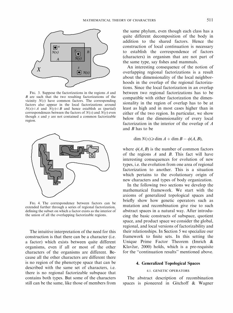
Fig. 4. The correspondence between factors can beextended further through a series of regional factorization,defining the subset on which a factor exists as the interior ofthe union of all the overlapping factorizable regions.


The intuitive interpretation of the need for thisconstruction is that there can be a character (i.e.a factor) which exists between quite differentorganisms, even if all or most of the othercharacters of the organisms are different. Be-cause all the other characters are different thereis no region of the phenotype space that can bedescribed with the same set of characters, i.e.there is no regional factorizable subspace thatcontains both types. But some of the charactersstill can be the same, like those of members from

the same phylum, even though each class has aquite different decomposition of the body inaddition to the shared factors. Hence theconstruction of local continuation is necessaryto establish the correspondence of factors(characters) in organism that are not part ofthe same type, say fishes and mammals.An interesting consequence of the notion of

overlapping regional factorizations is a resultabout the dimensionality of the local neighbor-hoods in the overlap of the regional factoriza-tions. Since the local factorization in an overlapbetween two regional factorizations has to becompatible with either factorization the dimen-sionality in the region of overlap has to be atleast as high and in most cases higher than ineither of the two region. In particular, we showbelow that the dimensionality of every localfactorization in the interior of the overlap of Aand B has to be

dimNðxÞXdimA þ dimB � fðA;BÞ;

where fðA;BÞ is the number of common factorsof the regions A and B: This fact will haveinteresting consequences for evolution of newtypes, i.e. the evolution from one area of regionalfactorization to another. This is a situationwhich pertains to the evolutionary origin ofnew characters and types of body organization.In the following two sections we develop the

mathematical framework. We start with theaxioms of generalized topological spaces andbriefly show how genetic operators such asmutation and recombination give rise to suchabstract spaces in a natural way. After introdu-cing the basic constructs of subspace, quotientspace, and product space we consider the global,regional, and local versions of factorizability andtheir relationships. In Section 5 we specialize ourframework to finite sets. In this setting theUnique Prime Factor Theorem (Imrich &Klavzar, 2000) holds, which is a pre-requisitefor the ‘‘continuation results’’ mentioned above.

4. Generalized Topological Spaces

4.1. GENETIC OPERATORS

The abstract description of recombinationspaces is pioneered in Gitchoff & Wagner


(1996); Stadler & Wagner (1998) and Stadleret al. (2000). It is based on the notion of therecombination function R : X � X-PðX Þ as-signing to each pair of parents x and y therecombination set Rðx; yÞ introduced by Gitchoff& Wagner (1996) as the set of all their potentialoffsprings. Recombination in general satisfiestwo axioms:

(X1) fx; ygARðx; yÞ;(X2) Rðx; yÞ ¼ Rðy; xÞ:

Condition (X1) states that replication may occurwithout recombination, and (X2) means that therole of the parents is exchangeable. Often a thirdcondition

(X3) Rðx;xÞ ¼ fxg

is assumed. Note that (X3) is not satisfied bymodels of unequal cross-over (Shpak & Wagner,2000; Stadler et al., 2002b). Functions R : X �X-PðX Þ satisfying (X1), (X2), and (X3) wereconsidered recently as so-called transit functions

(Changat et al., 2001) and as P-structures, witha focus on algebraic properties, in (Stadler &Wagner, 1998 and Stadler et al., 2000). A closureoperator associated with a recombination func-tion was introduced by Gitchoff & Wagner(1996) as

clðAÞ ¼[

x;yAA

Rðx; yÞ: ð1Þ

The situation is much simpler in the case ofmutation. Following the spirit of the Gitchoff–Wagner closure function we define clðAÞ as theset of all mutations that can be obtained from aset A in a single step.The abstract notion of assigning a ‘‘closure’’

clðAÞ to every subset A of the set of types X is

Tabl

Axioms for Generali

Closure

(K0) clð|Þ ¼ |ADB ) clðAÞDclðBÞ

(K1) isotone clðA-BÞDclðAÞ-clðBclðAÞ,clðBÞDclðA,B

(K2) expansive ADclðAÞ(K3) sub-linear clðA,BÞDclðAÞ,clðB(K4) idempotent clðclðAÞÞ ¼ clðAÞ

the starting point of our formal development. Ingeneral, we may think of clðAÞ as the set of alltypes that can be produced from a ‘‘population’’in a single step.

4.2. CLOSURE AND NEIGHBORHOOD

Let cl : PðX Þ-PðX Þ be a set-valued setfunction which we call the closure function. Itsconjugate is the interior function int : X-X

defined by

intðAÞ ¼ X \clðX \AÞ: ð2Þ

The neighborhood function N : X-PðPðX ÞÞ isdefined by

NðxÞ ¼ fNDX jxAintðNÞg: ð3Þ

It is not hard to show that closure, interior, andneighborhood can be used to define each other.For example, given the neighborhood functionN; the closure function is obtained as

xAclðAÞ3ðX \AÞeNðxÞ: ð4Þ

The most commonly assumed properties ofclosure function, or (equivalently) neighborhoodfunctions, are summarized in Table 1. Theequivalence of closure and neighborhood ver-sions of these conditions is well known, (see e.g.Gastl & Hammer, 1967). We say that ðX ; clÞ isan isotone space if (K0) and (K1) is satisfied. If inaddition (K2) holds then ðX ; clÞ is a neighbor-hood space. Neighborhood spaces satisfying (K3)are the pre-topological spaces studied in detail byCech (1966). Finally, a pre-topological spacewith idempotent closure is a topological spacein the usual sense. If (K1) holds then eqn (4) isequivalent to the more common expression

e 1zed Closure Spaces

Neighborhood

XANðxÞ

Þ NANðxÞ ;NDN 0 ) N 0ANðxÞÞ

NANðxÞ ) xANÞ N 0;N 00ANðxÞ ) N 0-N 00ANðxÞ

NANðxÞ3intðNÞANðxÞ


(Day, 1944, Theorem 3.1, Corollary 3.2)

clðAÞ ¼ fxAX j8NANðxÞ : A-Na|g: ð5Þ

Since the mutants of each parent are indepen-dent of the rest of the population we have

clðAÞ ¼[xAA

clðfxgÞ ð6Þ

in the case of mutation. This condition isequivalent to (K1) and (K3) in finite sets. Weassume that replication without mutation ispossible, thus xAclðfxgÞ and hence AAclðAÞ;i.e. (K2) holds. The validity of (K0) is assumedby definition. It follows that mutation defines apretopology on the genotype space (see Stadleret al., 2002).The case of recombination is dealt with in

some more detail in Stadler & Stadler (2002). Wehave

Theorem 1. The closure space ðX ; clÞ arisingfrom any recombination function R for which

(X1) and (X2) hold, satisfies (K0), (K1), and(K2).

Condition (X3) is then equivalent toclðfxgÞ ¼ fxg; i.e., the well-known (T1)-separa-tion axiom.Consider a genotype–phenotype map F :

ðV ; clÞ-X from the genotype space ðV ; clÞ;which we describe as a generalized closure spacewith closure function cl, into a set of pheno-types X : The GP-map F defines a closurefunction on X such that yAcðBÞ means ‘‘pheno-type y is accessible from the collection B ofphenotypes’’. It is argued at length by Fontana& Schuster (1998a) and Stadler et al. (2001) thatthis construction is meaningful because the pre-images F�1ðyÞ ¼ fvAV jFðvÞ ¼ yg form extensiveneutral networks. If we assume that b0 isaccessible from b iff there is a pair of genotypesv and v0 with b ¼ FðvÞ and b0 ¼ FðvÞ thatare accessible in genotype space, we obtain theso-called induced closure or accessibility closure

cnðBÞ ¼ FðclðF�1ðBÞÞÞ ð7Þ

on the phenotype space X : The other extreme isknown as the shadow topology (Stadler et al.,

2001). Here c is accessible from f only if everysequence x that folds into f has a mutant thatfolds into c: We cannot expect the existence ofsuch mutants (apart from the trivial case c ¼ f),i.e. the shadow topology might be close todiscrete topology. Thus a useful closure structureon the phenotype space will in general be finerthan the accessibility closure and coarserthan the shadow closure. We emphasize thatthe entire discussion in this contribution isindependent of the details of the definition ofthe closure function on the phenotype space. Itis sufficient to assume that a closure functionexists that reflects the mutual accessibilities ofphenotypes.

4.3. NEIGHBORHOOD SPACES

In this section we collect some basic facts onneighborhood spaces that will be used through-out the mathematical parts of this contribution.The theory of neighborhood spaces directlygeneralizes the theory of topological spaces.Additional information of neighborhood spacescan be found in the work of Day (1944),Hammer (1962), Gastl & Hammer (1967)and Gni"ka (1994). For a detailed account ofseparation axioms in neighborhood spaces werefer to Stadler & Stadler (2001).

4.3.1. Subspaces

The notion of a subspace in the topologicalcontext should not be confused with subspacesof vector spaces. In the topological context, asubspace of X is simply an arbitrary subset thatinherits its structure from X :

Definition 2. Let ðX ; clÞ be a neighborhoodspace and let YDX : We say that ðY ; cY Þ is asubspace of ðX ; clÞ if cY ðAÞ ¼ clðAÞ-Y for allADY :

We will sometimes use the notation Y !X : Itfollows directly from the definition that therestriction map ðY ; cY Þ-ðX ; clÞ : x/x is con-tinuous. Furthermore, the relative interior is

intY ðAÞ ¼ Y-intðA,ðX \Y ÞÞ ð8Þ


and the neighborhood systems in ðY ; cY Þ aregiven by

NY ðxÞ ¼ fN-Y jNANðxÞg ð9Þ

for each xAY : This can be seen as e.g. followingthe lines of Cech (1966, 17.A).

4.3.2. Product Spaces

Products of neighborhood spaces will play acrucial role in our discussion.

Definition 3. Let ðX1; c1Þ and ðX2; c2Þ be twoisotonic closure spaces. Then the product spaceðX1 � X2; c1 � c2Þ is defined by means of theneighborhood system Nðx1; x2Þ; where

NANðx1;x2Þ3

(N1AN1ðx1Þ and N2AN2ðx2Þ

such that N1 � N2DN ð10Þ

For sets of the form A1 � A2 this translates toa simple formula for the product closure inisotonic spaces (see also Gni"ka, 1994, Theorem8.1):

clðA1 � A2Þ ¼ c1ðA1Þ � c2ðA2Þ: ð11Þ

If ðX1; c1Þ and ðX2; c2Þ satisfy (K2), (K3), or (K4),respectively, then so does their product.

4.3.3. Quotient Spaces

Let P be a partition of X and denote by ½x� theclass of P to which x belongs. The function wP :X-X=P; x/½x� is called the canonical mapfrom X to X=P: We use the abbreviation ½A� ¼wPðAÞ:

Definition 4. Let ðX ; clÞ be an isotone spaceand P be a partition of X : Then the quotientspace X=P is the isotone space on the set X=Pthat has

Bð½x�Þ ¼ ½N�jNANðx0Þ for all x0A½x��

ð12Þ

as a basis of the neighborhood system of ½x�:

It follows that eqn (12) defines the fineststructure on X=P such that wP is continuous.(For all ½x� and all MAMð½x�Þ we need that foreach x0A½x� there is Nx0ANðx0Þ such that½N�DM; i.e.

Sx0A½x�½Nx0 � ¼ ½

Sx0A½x� Nx0 �DM: The

argument is then essentially the same as inFischer (1959)).

4.4. THE FACTORIZATION THEOREM

Throughout this contribution we will beconcerned with criteria under which a givenisotonic space can be represented as a product ofother non-trivial neighborhood spaces.

Definition 5. An isotone space ðX ; clÞ is factor-izable if there are non-trivial spaces ðX1; c1Þ andðX2; c2Þ such that ðX ; clÞCðX1; c1Þ � ðX2; c2Þ:

Before we derive a characterization of factor-izability we need a few more definitions:A pair of partitions P1 and P2; with canonical

maps wP1ðxÞ ¼ ½x�1 and wP2ðxÞ ¼ ½x�2; is ortho-gonally complementary (Wagner & Laubichler,2000) if for all xAX holds ½x�1-½x�2 ¼ fxg:Furthermore, given X and a pair of partitions P1and P2 of X we introduce the map

i :X-X=P1 � X=P2;

x/iðxÞ ¼ ð½x�1; ½x�2Þ ð13Þ

which defines the coordinate representation ofxAX for the product of the quotient space.By construction i is continuous. It is not hard

to verify that i is invertible, if and only if, P1 andP2 are orthogonally complementary, (see Stadleret al., 2001) for a more detailed discussion. Itfollows that X is factorizable if i�1 is continuous(in which case i is an isomorphism between X

and X=P1 � X=P2Þ; and neither P1 nor P2 is thediscrete partition (in which case neither X=P1nor X=P2 consists of a single point).The product of the quotient spaces has a basis

of its neighborhood system that is of the form½N 0�1 � ½N 00�2 with N 0ANð½x�1Þ and N 00ANð½x�2Þ:Furthermore, we have iðAÞD½A�1 � ½A�2 forall sets ADX : Factorizability thus requires inparticular that iðNÞ is a neighborhood in theproduct space for all NANðxÞ: This condition


can be rewritten as a condition on neighbor-hoods in ðX ; clÞ and we obtain

Theorem 6. An isotone space ðX ; clÞ is factoriz-able, if and only if, there is a pair of non-trivial

orthogonally complementary partitions P1 and P2such that the neighborhood systems satisfy the

following ‘‘rectangle condition’’:

8NANðxÞ (N 0;N 00ANðxÞ :

½N 0�1 � ½N 00�2DiðNÞ : ð14Þ

In pre-topological spaces the rectangle condi-tion simplifies because of the ‘‘filter property’’(K3) of neighborhoods: For any two neighbor-hoods N 0 and N 00 of x; their intersectionN 0-N 00 ¼ N 000 is again a neighborhood. Thuswe can replace N 0 and N 00 by the sameneighborhood N 000 in eqn (14) and find thefollowing stronger version of the rectanglecondition:

8NANðxÞ (N 0ANðxÞ :

½N 0�1 � ½N 0�2DiðNÞ : ð15Þ

4.5. LOCAL FACTORIZATION

It was argued already by Stadler et al. (2001)that it may be unlikely that the space of allpossible phenotypes will be factorizable as awhole. A local theory of factorization is thusdesirable. We start with a simple but usefultechnical result:

Lemma 7. Suppose ðX ; clÞ has a factorization

ðX ; clÞCðX1; c1Þ � ðX2; c2Þ; let Y1DX1; Y2DX2;and Y ¼ Y1 � Y2: Then ðY1; c1Y1Þ � ðY2; c2Y 2ÞCðY ; cY Þ is a subspace of ðX ; clÞ:

Proof. The neighborhoods of y ¼ ðy1; y2ÞAY arethe sets N-ðY1 � Y2Þ for all NANðyÞ: This set-system has a basis of the form ðN1 � N2Þ-ðY1 �Y2Þ ¼ ðN1-Y1Þ � ðN2-Y2Þ where N1ANðy1Þand N2ANðy2Þ: On the other hand, Ni-Yi; i ¼1; 2 are (by construction) a basis of the neighbor-hood systems on the subspaces ðYi; ci

YiÞ: &

Lemma 7 allows us to transfer a factorizationdown to all its ‘‘rectangular’’ subspaces. Inparticular, we already know that the neighbor-

hood system of each point has a basis ofrectangular neighborhoods by eqn (14). Thissuggests to consider a local version of factoriz-ability (Stadler et al., 2001):

Definition 8. ðX ; clÞ is locally factorizable inxAX provided for each neighborhood N 0ANðxÞthere is a neighborhood NDN 0 such that thesubspace ðN; cNÞ is factorizable.

Suppose Y !X has a factorization intosubspaces Y1 and Y2: Of course such a regionalfactorization does not imply that the entirespace X is factorizable. However, we have thefollowing

Lemma 9. Let ðY ; cY Þ be a subspace of ðX ; clÞthat is factorizable with the two factors Y1 and Y2:Suppose xAintðY Þ and such that fxigeNYi

ðxiÞfor i ¼ 1; 2; where ðx1; x2Þ is the coordinaterepresentation of x: Then ðX ; clÞ is locally

factorizable at x:

Proof. By construction the subspace ðY ; cY Þ isfactorizable at x: Since xAintðY Þ there is aneighborhood NANðxÞ (w.r.t. X ) that is con-tained in Y and that is of the form N 0 � N 00 withN 0afx1g and N 00afx2g: &

We can summarize the results of this section asfollows: If X ¼ X1 � X2 is a global factorization,then every rectangular subspace Y ¼ Y1 � Y2has a regional factorization. The existence of aregional factorization of some subspace Y !Xin turn implies a local factorization for allxAintðY Þ (subject to the technical conditionthat factors must not be sets consisting of asingle point).It is important to note that we cannot expect

to obtain useful information about the localfactors of a boundary point yA@Y ¼clðY Þ \intðY Þ from a factorization of a subspaceðY ; cY Þ! ðX ; clÞ:

4.6. PRIME FACTORS AND COMMON REFINEMENT

All the above results can be generalizedby induction to a finite number of factors.


We write

ðX ; clÞCYn

k¼1

ðXk; ckÞ: ð16Þ

Now consider a set QDX and the canonicalprojections wPk

: X-Xk; x-xk ¼ ½x�Pk: Clearly

we have

ðQ; cQÞ !Yn

k¼1

wPkðQÞ;

Yn

k¼1

ckwPk

ðQÞ

!

!Yn

k¼1

Xk;Yn

k¼1

ck

!CðX ; clÞ; ð17Þ

where ! means subspace. By abuse of notationwe write x ¼ ðx1;x2;y; xnÞ and call this acoordinate representation of x (w.r.t. a givenfactorization).In the following we will use the abbreviation

Q + Xk ¼ wPkðQÞ ð18Þ

for the projection of a subset (subspace) Q!X

onto the factor space Xk: The most importantproperties of the projection operator can besummarized as follows. Suppose A ¼

Qk Ak

with AkDXk and QDA: Then Ak ¼ A + Xk

and Q + Ak ¼ Q + Xk: If Q0DQ then Q0 +AkDQ + Ak: Finally, Q + Ak ¼ ½

QjðQ + AjÞ�

+ Ak:

Definition 10. A factorization ðX ; clÞCQkðXk; ckÞ is a prime factor decomposition if

none of the factors ðXk; ckÞ is factorizable.

In general, the prime factor decomposition isnot unique as the following example by Imrich &Klavzar (2000) shows. We will see below that theso-called strong product of graphs correspondsto the product of finite pre-topological spaces.We denote by Kn the complete graph withn vertices (and edges connecting each vertexpair). The symbol ’, stands for the disjointunion of graphs. Using the well-known formulaKp2Kq ¼ Kpq and the validity of the distri-butive law A2ðB ’,CÞ ¼ ðA2BÞ ’,ðA2CÞ we

may write

K1 ’,K2 ’,K4 ’,K8 ’,K16 ’,K32

¼ ðK1 ’,K2 ’,K22 Þ ’,ðK3

2 ’,K42 ’,K5

2 Þ

¼ K1 ’,K2 ’,K22

2 K1 ’,K3

2

¼ ðK1 ’,K2

2 ’,K42 Þ ’,ðK2 ’,K3

2 ’,K52 Þ

¼ K1 ’,K22 ’,K4

2

2 K1 ’,K2ð Þ

None of the graphs G1 ¼ K1 ’,K2 ’,K22 ; G2 ¼

K1 ’,K32 ; G3 ¼ K1 ’,K2

2 ’,K42 ; and G4 ¼ K1 ’,K2 is

factorizable. Since G12G2 ¼ G32G4; we seethat non-connected graphs in general do nothave a unique prime factor decomposition.We say that the factorizations of X have the

common refinement property if the followingholds. If X ¼ X1 � X2 ¼ Y1 � Y2 then there arespaces Z11; Z12; Z21; and Z22 such that X1 ¼Z11 � Z12; X2 ¼ Z21 � Z22; Y1 ¼ Z11 � Z21 andY2 ¼ Z12 � Z22:Of course, if a space has a unique prime factor

decomposition then it also has the commonrefinement property. The converse is not true ingeneral. In the finite case, which we will considernext, however, the existence of unique primefactor decomposition and the common refine-ment property are equivalent.

5. Finite Sets

5.1. VICINITIES

In the applications parts of this contributionwe will be interested mostly in the case of finitesets. In this case the neighborhood systemsNðxÞhave a finite basis, i.e. there is a collectionBðxÞCNðX Þ such that:

(1) If NANðxÞ then there is BABðxÞ such thatBDN:(2) If B0;B00ABðxÞ and B0DB00 then B0 ¼ B00:

Clearly, BðxÞ is uniquely defined. Condition(2) guarantees that BðxÞ is minimal. Note thatexistence of BðxÞ is guaranteed only in the finitecase.In particular, ifBðxÞ contains only a single set,

NðxÞ; thenNðxÞ ¼ fN jNðxÞDNg is the ‘‘discretefilter’’ of NðxÞ:We call NðxÞ the vicinity (smallest


neighborhood) of x: It follows immediately thata finite neighborhood space is a pre-topology ifand only if, BðxÞ ¼ fNðxÞg for all xAX : Inparticular, the product of two finite pre-topolo-gical spaces ðX1; c1Þ and ðX2; c2Þ with vicinitiesN1ðx1Þ and N2ðx2Þ; resp., is again a finite pre-topological space ðX1 � X2; c12Þ with vicinities

N12ðx1;x2Þ ¼ N1ðx1Þ � N2ðx2Þ ð19Þ

Furthermore, we have

clðfðx1; x2ÞgÞ ¼ c1ðfx1gÞ � c2ðfx2gÞ ð20Þ

as an immediate consequence of eqn (11).For finite neighborhood spaces we have the

following generalization:

Lemma 11. Let BiðxiÞ ¼ fBjiðxiÞj1pjpciðxÞg be

the bases of neighborhood spaces on Xi; i ¼ 1; 2:Then

B12ðx1;x2Þ ¼ fBj11 ðx1ÞB

j22 ðx2Þj

1pj1pc1ðx1Þ; 1pj2pc2ðx2Þg

ð21Þ

is the (uniquely defined) vicinity basis of their

product. Furthermore, all products of vicinities aredistinct vicinities in the product space.

Proof. Equation (21) follows directly fromthe definition of the product in eqn (10). To see

that Bj11 ðx1Þ � B

j22 ðx2ÞDB k1

1 ðx1Þ � B k22 ðx2Þ im-

plies i1 ¼ k1 and i2 ¼ k2 we observe that this

implies Bjii ðxiÞDB ki

i ðxiÞ; i ¼ 1; 2: Equality nowfollows from item (2) in the definitionabove. &

5.2. DIGRAPHS

Finite pre-topological spaces are equivalentto directed graphs with vertex set X : Beforeintroducing this correspondence we proof thefollowing simple

Lemma 12. Let ðX ; clÞ be a finite pre-topological

space. Then yANðxÞ if and only if, xAclðyÞ:

Proof. xAclðyÞ iff yAN for all NANðxÞ; i.e. iffyANð yÞ: &

At the level of individual points N and cl aretherefore ‘‘dual’’ in the same sense as the in-neighbors and the out-neighbors of a directedgraph.

Definition 13. Let ðX ; clÞ be a finite pre-topolo-gical space. The graph GðX ; clÞ is the directedgraph with vertex set X and an edge xy if andonly if, xay and yAclðxÞ; i.e. xANðyÞ: We callclðxÞ the out-neighbors of x and NðyÞ thein-neighbors of y:

This definition establishes a one-to-one corre-spondence between finite directed graphs andfinite pre-topological spaces (see Stadler et al.,2001). In the following we briefly recall thecorrespondences between graph-theoretical andtopological language.A graph H is a subgraph of G; HDG; if

VHDVG and EHDEG: A graph H is an induced

subgraph, in symbols H !G; if VHDVG and forall x; yAVH ; xyAEH if and only if, xyAEG: Theinduced subgraphs are exactly the pretopologicalsubspaces on a given point set. The subgraph ofG induced by the vertex set NðxÞ thus representsthe pretopological vicinity in the graph-theo-retical context. By abuse of notation we shalluse the same symbol for a vertex set and acorresponding induced subgraph (subspace).A directed graph is symmetric if the sets of in-

neighbors and out-neighbors agree at each vertex,i.e. if NðxÞ ¼ clðxÞ for all xAX : This is the finitecase of the following two symmetry axioms,which are equivalent in neighborhood spaces.

(R0) xAclðyÞ ¼ yAclðxÞ:(S) xAN 0 for all N 0ANðyÞ implies yAN 00 for

all N 00ANðxÞ:

The symmetric digraphs are equivalent to theundirected graphs.Let H !G: Then xAVH is an interior vertex of

H !G if NðxÞDVH ; i.e. NðxÞ!H: Again thismatches the definition in pre-topological spaces:‘‘x is an interior point of H if H contains aneighborhood of x’’. Consequently, we see thatintðHÞ is the set of all interior points of H:Conveniently, we will regard intðHÞ also as aninduced subgraph of H: This allows us to speake.g. of the connectedness of intðHÞ: In thefollowing we will regard a vertex set always as


an induced subgraph of G unless explicitly statedotherwise.

Remark. We have re-interpreted here the direc-tionality of the arcs of the graph G compared tothe discussion in Stadler et al., (2001). In thiscontribution we regard clðxÞ as the out-neigh-bors because we interpret the closure clðAÞinstead of the vicinity of A as the set of potentialoffspring of A: This is the natural interpretationfor the recombination case and matches theusage of the recombination closure operator inGitchoff & Wagner (1996), Stadler & Stadler(2002). The vicinities, which took a central rolein the interpretation of the pretopological frame-work in our previous paper (Stadler et al., 2001)are here represented as the in-neighbors. Weargue that representing the ‘‘immediate neigh-bors’’ of a population A by its closure clðAÞ ismore natural than using vicinities because theclosure-based formalism extends without mod-ifications to all genetic operators and to the caseof infinite spaces while a vicinity-based formal-ism does not. The reason is that vicinities are ingeneral not neigborhoods in the infinite case.Fortunately, there is a duality between closures

and vicinities of individual points in finite pre-topological spaces. This guarantees that the changeof the arrow directions does not affect any of theconclusions in our previous paper. Only thegraphical representation is modified. To illustratethis fact we briefly outline here one simpleexample: Let f : ðX ; clÞ-ðY ; clÞ be a functionbetween two pre-topological spaces. Then f iscontinuous iff for each x and each neighborhoodM of f ðxÞ there is neighborhood N of x such thatf ðNÞDM: Reformulating this argument usingvicinities we immediately obtain: ‘‘f is continuousat x iff f ðNðxÞÞDMð f ðxÞÞ’’. On the otherhand, closure preservation, f ðclðxÞÞDclð f ðxÞÞ; isequivalent to continuity in all isotone closurespaces. Hence it does not matter whether we usethe in-neighbors or the out-neighbors to determinewhether f is continuous.

5.3. THE STRONG PRODUCT OF GRAPHS

The product of pre-topological spaces trans-lates, in the finite case, into the strong product ofgraphs (see Stadler et al., 2001), Fig. 5.

Definition 14. Let G ¼ ðVG;EGÞ and H ¼ðVH ;EHÞ be finite simple graphs (directed orundirected). The strong product G2H has thevertex set VG2H ¼ VG � VH and (x1,x2)(y1,y2)AG2H if either (i) x1 ¼ y1 and x2y2AEH ; or (ii)x1y1AEG and x2 ¼ y2; or (iii) x1y1AEG andx2y2AEH : The edges of type (i) and (ii) are calledCartesian edges, edges of type (iii) are non-Cartesian.

A graph G is prime or non-factorizable if it isnot isomorphic to a 2-product of at least twonon-trivial (i.e. empty or one-vertex) graphs.Note that the graph G is locally factorizable at avertex x if and only if, the vicinity NðxÞ (viewedas induced subgraph) is a factorizable.We denote the degree, in-degree and out-

degree of a vertex x in a graph G by dGðxÞ; diGðxÞ;

and doGðxÞ; respectively. For later reference we

note the following simple fact:

dzG�Hðx1; x2Þ ¼ dz

Gðx1Þ þ dzHðx2Þ þ dz

Gðx1ÞdzHðx2Þ

ð22Þ

for z denoting the superscript for in-degree, out-degree, or undirected degree, respectively. Forthe case of multiple factors eqn (22) generalizesto

dzQiHi

ðx1;x2;yxnÞ

¼Xn

i¼1

dzHiðxiÞ þ

Xn

ioj

dzHiðxiÞd

zHjðxjÞ

þXn

iojok

dzHiðxiÞd

zHjðxjÞd

zHkðxkÞ þ?

þYn

l¼1

dzHlðxlÞ: ð23Þ

Probably the most important property of thestrong product is

Proposition 15 (Imrich & Klavzar, 2000, Chap-ter 5). Every connected graph G has a unique

prime factor decomposition

G ¼2Yn

k¼1

Gk ð24Þ

up to the ordering of the factors.

3

2

1

33

1 1

1

1

22

Fig. 6. This graph (the non-Cartesian edges in each cube are omitted for clarity) is locally factorizable at each vertex butnot globally factorizable.

Fig. 7. Proof of Theorem 19. The black boxes represent the prime factors of NðxÞ: The factorizations of A and B eachintroduce a partition of the prime factors of NðxÞ; shown here by red and blue boxes. The common factors correspond to thefinest partition that is refined by both A and B partition, which is indicated by the dashed green boxes.

Fig. 8. L.h.s.: The induced subgraph highlighted by thick edges is factorizeable (H ¼ P12P2). Its interior vertices areindicated by green squares. In these four points the local factors (P12P1) are induced subgraphs of the factors of H : Hencetheir local factorizations are mutually consistent. However, G is not locally factorizable in the two points shown as blackcircles (because of the spikes attached to them). R.h.s.: The vertex in red has consistent factorizations in common with boththe green vertices (mediated by the vertical rectangle) and the yellow and violet vertices (mediated by the horizontalrectangle). The green and yellow vertices are factorization-consistent (via the red vertex as an intermediate) even though theyare not directly related by the factorization of any subgraph.

doi: 10.1006/jtbi.2003.3150G. P. WAGNER ET AL.


Hence the dimension of a graph G, defined asthe number of dimG ¼ n of prime factors is welldefined. By definition dimG ¼ 1 if and only if, Gis prime.It is well known that the strong product of two

graphs is connected if and only if, each factor isconnected. A related result for directed graphs isthe following simple

Lemma 16. A directed graph G ¼2Qn

k¼1 Gk isstrongly connected if and only if, each factor is

strongly connected.

Proof. It is clear that the product of twostrongly connected graphs is strongly connected.Conversely, suppose G is strongly connected.Consider xk; ykAVGk

and let x; y be two arbitraryvertices that have coordinates xk and yk in thek-th factor. By assumption there is a directedpath from x to y: The projection of this path ontoGk is necessarily a connected directed path fromxk to yk: Thus Gk is strongly connected. &

Not surprisingly, factorization at a global levelis not necessary for local factorizability. Figure 6gives an example of a graph that is prime butallows for local factorizations at every vertex.

Conjecture 17. Any connected finite neighborhood

space has a unique prime factor decomposition.

This generalization of the Unique PrimeFactor Theorem is suggested by the discussionof combinatorial structures in Lovasz(1967,1971) that are very similar in the finiteneighborhood spaces considered here. The un-ique prime factor decomposition of finite neigh-borhood spaces will be considered elsewhere inmore detail.

Fig. 5. Example of a strong graph product.

5.4. OVERLAPPING LOCAL FACTORIZATIONS

For the sake of clarity we will restrict ourdiscussion in this subsection to the case of finitegraphs although the results remain valid whenever

we work in a situation in which the unique primefactor theorem holds.

The most important observation here con-cerns the intersection of two factorizable inducedsubgraphs A;B!G: The following lemma sim-ply rephrases the Unique Prime Factor Theoremfor the special case of neighborhoods of a singlepoint.

Lemma 18. Suppose A;B!G are factorizablesuch that A ¼2

Qmk¼1 Ak and B ¼2

Qnl¼1 Bl

and let xAintðAÞ-intðBÞ; i.e. NðxÞ!A andNðxÞ!B: Then for each of the factors Ak and Bl

there is a collection of prime factors ofNðxÞ ¼2

Qqj¼1 NjðxjÞ such that

NðxÞ + Ak ¼2YjAIk

NjðxjÞ

and

NðxÞ + Bl ¼2YjAJl

NjðxjÞ: ð25Þ

Furthermore, the index sets fIkj1pkpmg and

fJl j1plpng each form a partition of f1yqg:

In simpler words, the q prime factors of NðxÞare combined in different ‘‘packages’’ to yieldthe restrictions of the given factorizations on Aand B to NðxÞ: (In the general case, correspond-ing expressions hold for all vicinitiesNiðxÞABðxÞ).We say that A and B have the factor AkBBl in

common if there is xAintðAÞ-intðBÞ such thatNðxÞ + Ak ¼ NðxÞ + Bl : Since the factorizations


of A and B; respectively, each define a partition onthe set of prime factors of NðxÞ we see that thenumber of common factors is the number ofclasses in the join of these two partitions (seeFig. 6). We define fðA;BÞ as the number of factorsthat the prime factor decompositions of A and B

have in common. The number fðA;BÞ is welldefined as a consequence of the uniqueness of theprime factor decomposition. Of course, we have

1pfðA;BÞpminfdimA;dim Bg: ð26Þ

Recall that intðA-BÞ ¼ intðAÞ-intðBÞ holdsin pre-topological spaces but not in generalneighborhood spaces.We can use this observation to derive a lower

bound on the number of factors into which NðxÞmust decompose:

Theorem 19. Let A;B!G be factorizable and letxAintðAÞ-intB: Then

dimNðxÞXdimA þ dimB � fðA;BÞ; ð27Þ

where fðA;BÞ is the number of factors that A andB have in common at x:

Proof. As a consequence of the discussion abovewe have to solve the following combinatorialproblem (Fig. 7). Let A and B be two partitionsof a finite set X : What is the minimum cardinality

of X given the number of classes of A; B; andA3B? (Recall that A3B is the partition of X

defined as the transitive closure of the relation ‘‘xand y belong to the same class of A or B’’.Similarly, the classes of A4B are defined by ‘‘xand y belong to the same class of both A and B’’,i.e. they are the non-empty intersections of theform A-B with AAA and BAB:)Of course, dimNðxÞXjA4Bj; because each

class must contain at least one factor of NðxÞ:The result follows directly from the inequality

jA4BjXjAj þ jBj � jA3Bj ð28Þ

which is easily proved by induction in thenumber of classes of B: &

5.5. CONTINUATION OF A LOCAL FACTORIZATION

Definition 20. Let ðX ; clÞ be a neighborhoodspace. Two points x; yAX have consistent local

factorizations if there is a subset YDX such thatx; yAintðY Þ and the subspace Y !X has afactorization YC

Qj Yk:

Under these assumptions we see that NðxÞhas a basis consisting of sets of form

Qk N 0

k;where N 0

kDNðxkÞ and N 0kDYk: Analogously,

NðyÞ has a basis of the formQ

k N 00k with

N 00kDNðykÞ and N 00

kDYk: This establishes acorrespondence between the neighborhoods N 0

k

and N 00k ; even though the sets N 0

k and N 00k will in

general be disjoint. In fact, the set of points withconsistent factorizations is not necessarily con-nected in G: A simple counterexample is given onthe l.h.s. of Fig. 8.

Definition 21. Two points x and y are directly

prime-factorization consistent, x #By; if there issubspace Y ¼

Qk Yk of X such that x; yAintðY Þ

and the factors Yk are not locally factorizable atx and y:

In this case Yk is also prime provided xk andyk do not both have a neighborhood consistingof a single point.Definition 20 can be recast in graph-theore-

tical language:

Lemma 22. Let G be a graph x; yAVG with local

(not necessarily prime) factorizations NðxÞ ¼2Q

Nxk and NðyÞ ¼2

QN

yk ; respectively. Then

these local factorizations are consistent if there isan induced subgraph H !G that has a (notnecessarily prime) factorization H ¼2

QHk

such that

(1) x and y are interior points of H;(2) for all k holds Nx

k ¼ NðxÞ + Hk and Nyk ¼

Nð yÞ + Hk (with a suitable numbering of the localfactors at x and y).

We write Nxk# N

yk# Hk for the corresponding

factors.

Furthermore, x and y are factorizationconsistent if Nx

k and Nyk are prime for

all k:The relations # and #B are obviously reflexive

(x #Bx for all x) and symmetric. They are nottransitive however, as the r.h.s. example in Fig. 8


shows. Their transitive closures B and ^ aretherefore equivalence relations.We will say that two vertices are prime

factorization-consistent if xBy; i.e. if there is asequence of vertices x ¼ x0;x1;y;xk�1; xk ¼ ysuch that xj�1 and xj have consistent factoriza-tions for all 1pjpk: By definition, the factoriza-tion-consistent points form an equivalencerelation. If there are locally non-factorizablepoints in G; these will form a separate class ofthis equivalence relation (only a single factor,trivially mediated through the graph G itself ). Anecessary condition for a class of factorization-consistent vertices with non-trivial factorizationto be connected is that the induced subgraphs H

in definition of the relation #B has a connectedset of interior points.Similarly, local factors Nx

k and Nzl are

equivalent, Nxk^Nz

l if there is a sequence ofpoints x ¼ y0; y1;y; ym ¼ z with local factors

Nyi

jisuch that N

yi�1ji�1

# Nyi

ji: Note that if Nx

k^Nzk

for k ¼ 1;y;m then 2Q

jAJ Nxj ^

2Q

jAJ Nzj for

all index sets JDf1;y;mg: In other words, ifx and z have some consistent factors, than anyproduct of a number of these factors is alsoconsistent.Now consider a factor F of a local factoriza-

tion of the space at some point xAX : Let H½F �be the collection of induced subgraphs of X thathave a factor F 0^F consistent with F : Clearly,H½F � is a partial covering of G: The set GF ¼SH½F � of points covered can be interpreted as

the maximal subset of G on which we can speakof the identity of the factor F : Clearly, there is alocal factor Nz^F consistent with F at a point z

if and only if, zAintðGF Þ: Hence intðGF Þ is theset of all phenotypes for which the character F isdefined.

6. Interpretations

The starting point of the current study isLewontin’s idea of quasi-independence (Lewon-tin, 1978) as a bases for the development of acharacter concept. A mathematical interpreta-tion of this idea was given before (Stadler, et al.2001) with the notion of structural decomposa-bility of the phenotype space. Characters areidentified with factors or dimensions of a regionof the phenotype space. We will call the so

identified characters ‘‘variational characters’’.Then we asked what one can say about theidentity of characters in two species or organ-isms, also known as homology, making no otherassumption than the existence of quasi-indepen-dence. An intuitive summary of the main resultshas been given in Section 3. Here we discuss thebiological interpretation and some of the con-ceptual implications of these results. In particu-lar, we will focus on homology, evolutionarynovelties, and the stability of body plans.

6.1. IDENTITY OF QUASI-INDEPENDENT

CHARACTERS AND HOMOLOGY

The original definition of homology by Owenidentified two characters as homologous if theyare ‘‘the same’’ in some unspecified way. Themeaning of ‘‘sameness’’ was implicitly definedthrough the morphological criteria used todistinguish between superficial and essentialsimilarity, i.e. between analogy and homology.This notion was re-interpreted by Darwin withreference to a common ancestor. In the Darwi-nian tradition homologues are two characters indifferent species that correspond to the samecharacter in a common ancestor of these species.Homology is thus identified with continuity ofdescent of an entity, which does not tend tochange its identity during the process of descentwith modifications. This homology concept canbe called ‘‘historical’’ since it is defined solely onthe basis of historical, genealogical relationships,but it does not clarify what character identitymeans (Wagner, 1994).In fact, the historical homology concept also

pre-supposes a notion of sameness, just asOwen’s does, otherwise the phrase ‘‘the samecharacter in a common ancestor’’ would not bedefined. An attempt to clarify the notion ofsameness that underlies, both Owen’s as well asDarwin’s notions of homology, is the so-calledbiological homology concept (Wagner, 1989a,b).It is based on the idea that homologues areclusters of observable attributes that remainstable during adaptive evolution by naturalselection. They are thus thought of as causallyhomeostatic parts of the body which thus retaintheir identity during (most) evolutionary trans-formations (Wagner, 1999). This notion is, in its


definition, independent of continuity of descentand thus has an unclear relationship to thehistorical homology concept. Here we argue thatboth homology concepts and their relationshipcan be accommodated in a theory of characteridentity based on quasi-independence. In Section5.5 it is shown that identity of variationalcharacters is well defined and determines a classof (in most cases) variationally connectedphenotypes sharing this factor. This means thatphenotypes which share a certain factor/char-acter can evolve into each other without goingthrough states where the character is not defined.The notion of character identity based on quasi-independence is thus fully consistent with thehistorical homology concept.The consistence between the historic homology

concept and the identity of variational characters,however, takes an interesting form. It shows thatcontinuity of descent is sufficient to establishcharacter identity. Hence descent from a commonancestor is sufficient to establish characteridentity, as implied in the historical homologyconcept. But continuity of descent is not neces-sary for character identity. There is no intrinsicreason, although it may be unlikely, why twolineages could not independently evolve pheno-types which have the same variational character.Nothing in the theory of phenotype spaces wouldforbid that. One can thus say that the historicalhomology concept is an appropriate criterion ofhomology but may be deficient as a definition ofhomology. This potential deficiency is the samethat causes the ambiguity with respect to themeaning of parallel evolution. Parallel evolutionis the independent derivation of the samecharacter from an ancestral phenotype (Futuyma,1998). Can a character which is physically andgenetically the same but arose independently besomething different? This is a matter of definition,but a strict adherence to the definition of thehistorical homology concept may lead to biolo-gically meaningless distinctions among differentinstances of the same biological character.The relationship between variational charac-

ters and the biological homology concept is lessobvious. The biological homology concept di-rectly refers to the physical realization of thecharacter and its variational properties, i.e.common developmental constraints. In contrast,

the variational character concept is entirelyabstract from what phenotypes and charactersphysically are. It is only based on the topologicalrelationships of phenotypes defined by thevariational mechanisms that transform pheno-types (say the underlying genotypes) by mutationand recombination. Variational characters arethus defined as statements about the symmetriesof phenotype space and make no explicitreference to a description of the phenotypesthemselves. The connection between variationalcharacters and biological homologues, however,is provided through the fact that every set oforthogonal factors implies a set of orthogonalpartitions, as shown in Stadler et al., (2001).A partition P of a set A is a set of equivalence

classes PAP; PDA; which collectively contain allthe elements in this set. This means that eachcharacter state of a variational character can beunderstood as an equivalence class consisting ofall the phenotypes which have the same state ofthe variational character but which may bedifferent in other respects. In that way anabstract factor can be translated into a clusterof phenotypic and genotypic attributes, which iswhat we usually think of when we speak of anorganismal character, for instance a bone with acertain shape and location in the body. Regard-less of whether a character is defined as anattribute cluster in the sense of the biologicalhomology concept, or as a variational characterbased on quasi-independence, these two notionsare translatable into each other, due to theconnection between factors and partitions. Ineither way a character can be understood as ahypothesis about the existence of homeostaticmechanisms that maintain the identity of a partof the phenotype and which makes them thuscombinable with different contexts of othercharacters. We conclude that quasi-indepen-dence is a strong enough concept to explainand accommodate both the historical as well asthe biological homology concept. Nothing else isneeded but quasi-independence to clarify theseconcepts.

6.2. EVOLUTIONARY NOVELTIES

The novelty concept is about as elusive as thehomology concept, and closely connected to the


notion of character identity (Nitecky, 1990). Anovelty can be defined as any character thatarises in evolution which is neither homologousto a character in an ancestor or serially homo-logous to any other part of the organism (Muller& Wagner, 1991). In the language of phenotypespace topology as developed in Stadler et al.,2001) and this paper, the evolution of a noveltyis equivalent to evolution from one part of thephenotype space into another part that has adifferent regional factorization. In other words,the origin of a novelty is the appearance of avariational character that is not defined in theancestral lineage. Formal phenotype spaces andtheir factorizations provides a mathematicallanguage in which the process of the evolution-ary innovation can be described. This is a majoradvantage over other, established mathematicaltheories of phenotypic evolution, like quantita-tive genetics, where the set of characters isassumed to be fixed. In these models the originof novelties is structurally impossible to model.In fact the search for a language that canaccommodate evolutionary novelties was amajor motivation for developing the presenttheory. The result most relevant to the evolutionof novelties is Theorem 19, which determines theminimal dimensionality of phenotypes thatbelong to the overlap between two areas ofregional factorization, say A and B:Any maximal part of the phenotype space,

which has its own regional factorization, can bethought of as a particular type or body plan.They consist of all the mutationally connectedphenotypes that can be decomposed onto thesame set of variational characters. One implicitresults of Theorem 19 is that types can overlapand that overlap among body plans is in factnatural in the way factorization works. Types orbody plans defined on the basis of variationalcharacters are thus not mutually exclusive classesbut can to various degrees be connected to eachother. In this context there can be transitionalforms that connect two different body plans.Hence a variational body plan concept is, incontrast to a typological body plan concept,fully compatible with evolutionary theory. Nohopeful monsters are necessary (although logi-cally possible, see below) to evolve a new bodyplan and no logical contradictions exist between

evolution and body plans as those suggested byMedawar & Medawar (1983, pp. 281–282).There are, however, some topological restric-tions that arise in the transition betweendifferent body plans. We will explore thosebelow.Theorem 19 tells us that if there is a phenotype

x which belongs to the overlap of types A and Bits dimensionality has to be larger than the sumof the dimensionalities of A and B; minus thenumber of factors that A and B share, fðA;BÞ

dimNðxÞXdimA þ dimB � fðA;BÞ:

The reason simply is that any phenotype thatbelongs both to A as well as B has to becompatible with both regional factorizations.Any factor of A and any factor of B has tocorrespond to one or a combination of localfactors of NðxÞ: Now let us consider a fewscenarios to see whether this result makesintuitive sense.Let us consider cases where evolution pro-

ceeds from A to B and B is the same as A exceptthat it has one factor more that is not present inA; i.e. a single novelty. Then fðA;BÞ ¼ dimAand the local dimensionality of x only has to beat least as high as B: dimNðxÞXdim B: This isa simple accretion of a novelty. An analogousargument can be made for the loss of acharacter, dimB ¼ dimA � 1 and dimB ¼fðA;BÞ:More interesting is the case where the two

types differ by more than one variationalcharacter and do not simply differ by accretionof characters on top of those of A;fðA;BÞominfdimA; dimBg: Two situationsneed to be distinguished: (1) the two types donot directly overlap, and (2) the two typesoverlap and thus share transitional phenotypesthat belong to either. In the first case the theorymakes no prediction except that there have to beother types D; E; F ; etc., that form a chain ofoverlapping types, or some arbitrary non-decomposable forms. In the second case, how-ever, topological constraints mandate that thetransitional form is strictly more complex (hasmore variational characters) than either of thetwo types. This is easily seen by rewritingdimA ¼ fðA;BÞ þ nA; where nA is the number


of unique variational characters of A not sharedwith B; and dim B ¼ fðA;BÞ þ nB; analogously.From this it immediately follows that

dimNðxÞXdimB þ nA ð29Þ

or dimNðxÞ4maxfdimA;dim Bg by assump-tion. If there are transitional forms between Aand B (phenotypes which belong to both A andB) have to represent a complexity hump sincethey need to have all the variational charactersof either type. Of course these new charactersdo not need to appear all at once, since anyphenotype that has acquired some of thecharacters of B but not all of them does notstrictly belong to B and thus is not in the overlapof A and B (both of them sets with non-emptyinterior).Although not strictly necessary, from a

mathematical point of view, transitional formswhich possess a combination of plesiomorphicand apomorphic characters is a natural conse-quence of topological constraints on local factordecompositions. The only constraint is that therehas to be at least one form that has all thecharacters of the ancestal and the derived bodyplan. Otherwise the evolution has to go throughforms that belong neither to type A nor totype B:Next we want to ask whether it is mathema-

tically possible to have a direct evolutionarytransition between two types but avoids thecomplexity hump, i.e. are there cases not coveredby Theorem 19. We will proceed by asking whatfollows from a violation of the dimensionalityequation for NðxÞ: It is easy to show thatdimNðxÞodimA þ dimB � fðA;BÞ implies thatx will not be an element of intðAÞ or not anelement of intðBÞ; or both. This condition canbe satisfied if x is neither internal to A nor to B;but then there would be no direct transitionbetween them either. The other possibility tosatisfy this condition amounts to the definitionof a hopeful monster. We translate the notion ofa hopeful monster as a phenotype that can bereached from the ancestor A by a single step butis not part of A; xeintðAÞ; but belongs to B;xAintðBÞ: Whether this is possible depends onthe kind of space the phenotype space represents.If A and B are open sets in a topological space,

this is not possible, because it is true that ifintðAÞ-intðBÞ ¼ |; then also intðAÞ-clðBÞ ¼|: In pre-topological spaces and neighborhoodspaces, however, a hopeful monster is possible inprinciple, though it may not be likely from abiological point of view. If one wants to avoidthe complexity hump in a direct transitionbetween two types then (1) the transition hasto occur in a pre-topological space or aneighborhood space and (2) has to involve ahopeful monster, i.e. a descendant of A but nota representative of the type A and already a fullyfledged member of type B: Hopeful monsters are(pre-)topologically possible but this theory can-not speak to the biological likelihood of such atransition.

6.3. THE STABILITY OF BODY PLANS

In the previous section a body plan or typewas conceptualized as a part of the phenotypespace with its own regional factorization, or setof variational characters. Types, however, arenot only characterized by their own set ofcharacters but often, if not always, displayremarkable evolutionary stability. This stabilitycan have multiple causes, from developmentalconstraints to functional integration. Here wepropose two additional factors that may con-tribute to the stability of body plans. The firsthas to do with the topological properties offactorizable spaces, the second with the evolva-bility of modular body plans.In Section 5.3, eqns (22) and (23) give an

equation about the vertex degree of factorizablegraphs. Recall that graphs are a model of finitepre-topological spaces, where each vertex repre-sents a phenotype and each edge a possiblegenetic transformation of the phenotype. Thevertex degree is the number of edges that end ororiginate at a particular vertex. A graph is calledvertex regular, if each vertex has the samenumber of edges, and irregular if they do not.The vertex degree is an interesting property of

graphs for the following reason. If one considersa graph as a ‘‘map’’ of possible paths to go, aswe do with phenotype spaces, then the vertexdegree tells us how often a vertex is visitedduring a random walk on the graph. In otherwords, the vertex degree is proportional (in


undirected graphs) to the probability that arandom walk will be at the given vertex. Ofcourse the probability will also depend on thedegree of the other vertices in the graph, butthe vertices with the higher degree will bevisited more often than those with lower vertexdegrees.If a graph that represents a configuration

space for a genetic operator, has vertices with amuch higher degree than others there will be an‘‘intrinsic (entropic) pull’’ towards the statesrepresented with higher vertex degree. This pullis independent and can be opposed to anyevolutionary force caused by natural selection.In contrast, in configuration spaces that arevertex regular, no such preferred directions exist.Examples are the Hamming graph representingnucleotide sequences with constant length andbase substitutions as variational operator. On avertex regular configuration space any direction-ality has to come from natural selection ratherthan from intrinsic tendencies. With this in mindlet us now consider product spaces.Equation (22) tells us that if each factor is

vertex regular, so will be the product spaceobtained from these factors. If, however, thefactors are vertex irregular, this irregularity willbe transmitted to the product space and evenamplified. If each factor has mildly preferredstates, i.e. vertices with somewhat higher vertexdegree, these preferences translate into a clusterof highly preferred states in the product space.This is because the vertex degree of the vertex inthe product space is a multilinear function of thevertex degrees of all of the vertices in the factors.In other words, a product space generically willcontain one or more clusters of highly preferredstates. Furthermore, in particular in undirectedgraphs, these island of preferred states will be inthe interior of the factorizable region. Thismeans that the preferred states in a productspace will be the ones that are not poised to leavethe factorizable region. In other words, thepreferred states make it less likely to realize amutation that leaves the type. Hence there is ageneric tendency for types to evolve states withinthe same type and thus to preserve the type. Thiseffect is entirely statistical and adds to the othermechanistic reasons for the stability of types, likefunctional and developmental integration.

Note that this suggestion implies that irregularproduct spaces are predicted to be both, highlyevolvable among states within the type as well asstable against transformations that affect thetype itself. Factorizability can also be seen as acondition of modularity, i.e. the existence ofindependently changeable parts of the organism.It is widely thought that if modularity matchesthe different functions the organism has toperform, it can increase evolvability. Henceevolution within a type is likely to be facilitated,while phenotypes outside factorizable regionsare likely to be less evolvable. Hence there aretwo reasons why adapative evolution is pre-dicted to occur preferentially within the confinesof a given type than leading to another type orany other state outside the focal type. There is anentropic pull to the interior of the part of thephenotype space representing the type. In addi-tion there is a higher chance to increase fitness byevolution within a type (due to modularity) thanwith mutational steps leaving regions of highmodularity. Both of these factors make it morelikely that adaptive challenges will be met byphenotypic states within a given type thanleading to the evolution of a new type.

Stimulating discussions with Wilfried Imrich,Barbel M. R. Stadler, and the members of the WagnerLab are gratefully acknowledged.

REFERENCES

Ancel, L. & Fontana, W. (2000). Plasticity, evolvabilityand modularity in RNA. J. Exp. Zool. (Mol. Dev. Evol.)288, 242–283.

Buº rger, R. 2000. The Mathematical Theory of Selection,Recombination, and Mutation. Chichester, UK: Wiley.

Carroll, S. B., Grenier, J. K. & Weatherbee, S. D.2001. From DNA to Diversity. Malden, MA: BlackwellScience.

C ech, E. (1966). Topological Spaces. London: Wiley.Changat, M. Klavz ar, S. & Mulder, H. M. (2001). Theall-path transit function of a graph. Czech. Math. J. 51,

439–448.Cupal, J., Kopp, S. & Stadler, P. F. (2000). RNA shapespace topology. Artif. Life 6, 3–23.

Day, M. M. (1944). Convergence, closure, and neighbor-hoods. Duke Math. J. 11, 181–199.

Eldredge, N. & Gould, S. J. (1972). In: Modelsin Paleobiology, (Schopf, T. J. M., ed.), pp. 82–115.San Francisco: Freeman.

Fischer, H. R. 1959. Limesraume. Math. Ann. 137,

269–303.


Fontana, W. & Buss, L. W. (1994). The arrival of thefittest: towards a theory of biological organisation. Bull.Math. Biol. 56, 1–64.

Fontana, W., Schnabl, W. & Schuster, P. (1989).Physical aspects of evolutionary optimization & adap-tion. Phys. Rev. A 40, 3301–3321.

Fontana, W. & Schuster, P. (1998). Continuity inevolution: on the nature of transitions. Science 280,

1451–1455.Fontana, W. & Schuster, P. (1998). Shaping space: thepossible and the attainable in RNA genotype-phenotypemapping. J. theor. Biol. 194, 491–515.

Forst, C.V., Reidys, C. &Weber, J. (1995). Evolutionarydynamics and optimization: neutral networks as model-landscape for RNA secondary structure folding land-scapes. In: Advances in Artificial Life, (Moran, F.,Moreno, A., Merelo, J. J. & Chacon, P., eds), LectureNotes in Artificial Intelligence Vol. 929, pp. 128–147.Berlin: Springer.

Futuyma, D. J. (1998). Evolutionary Biology. Sunderland,MA: Sinauer Associates.

Gastl, G. C. &Hammer, P. C. (1967). Extended topology.Neighborhoods and convergents. In: Proceedings of theColloquium on Convexity 1965 (Fenchel, W. ed.), pp. 104–116, Copenhagen, DK, K�benhavns Univ. Matematiske.Inst.

Gilbert, S. F. (2000). Genes classical and genes develop-mental: the difference uses of genes in evolutionary theory.In: The Concept of the Gene in Development and Evolution,(Beurton, P., Falk, R. & Rheinberger, H.-J., eds), pp. 178–192. New York: Cambridge University Press.

Gilbert, S. F., Opitz, J. M. & Raff, R. A. (1996).Resynthesizing evolutionary and developmental biology.Dev. Biol. 173, 357–372.

Gitchoff, P. & Wagner, G. P. (1996). Recombinationinduced hypergraphs: a new approach to mutation-recombination isomorphism. Complexity 2, 37–43.

GniŁka, S. (1994). On extended topologies. I: Closureoperators. Ann. Soc. Math. Pol., Ser. I, Commentat.Math. 34, 81–94.

Graur, D. & Li, W.-H. (2000). Fundamentals of MolecularEvolution. Sunderland, MA: Sinauer Associates.

Hammer, P. C. (1962). Extended topology: set-valued setfunctions. Nieuw Arch. Wisk. III 10, 55–77.

Huynen, M. A., Stadler, P. F. & Fontana, W.(1996). Smoothness within ruggedness: the role ofneutrality in adaptation. Proc. Natl. Acad. Sci. U.S.A.93, 397–401.

Imrich, W. & Klavz ar, S. (2000). Product Graphs:Structure & Recognition. New York: Wiley.

Lenski, R. E. & Travisano, M. (1994). Dynamics ofadaptation and diversification: a 10,000-generation ex-periment with bacterial populations. Proc. Natl. Acad.Sci. U.S.A. 91, 6808–6814.

Lewontin, R. C. (1974). The Genetic Basis of EvolutionaryChange. NY: Columbia University Press.

Lewontin, R. C. (1978). Adaptation. Sci. Am. 239, 156–169.LovaŁ sz, L. (1967). Operations with structures. Acta Math.

Acad. Sci. Hung. 18, 321–328.LovaŁ sz, L. (1971). Unique factorization in certain classes ofstructures. In: Mini-Conf. Univers. Algebra, Szeged 1971,pp. 24–25. Bolyai Janos Mathematical Society.

Maynard-Smith, J., Burian, R., Kauffman, S. A., Al-

berch, P., Campbell, J., Goodwin, B., Lande, R.,

Raup, D. & Wolpert, L. (1985). Developmental con-straints and evolution. Quart. Rev. Biol. 60, 265–287.

Medawar, P. B. & Medawar, J. S. (1983). Aristotle toZoos. A philosophical Dictionary of Biology, Cambridge,MA: Harvard University Press.

Muº ller, G. B. & Wagner G. P. (1991). Novelty inevolution: restructuring the concept. Annu. Rev. Ecol.Syst. 22, 229–256.

Nitecky, M. H. (1990). Evolutionary Innovations. Chicago:University of Chicago Press.

Raff, R. (1996). The Shape of Life. Chicago, IL: ChicagoUniversity Press.

Reidys, C. M. & Stadler, P. F. (2002). Combinatoriallandscapes. SIAM Rev. 44, 3–54.

Schlichting, C. D. & Pigliucci, M. (1998). PhenotypicEvolution: A Reaction Norm Perspective. Sunderland,MA.: Sinauer Associates, Inc.

Schuster, P., Fontana,W., Stadler, P. F. & Hofacker,I. L. (1994). From sequences to shapes & back: a casestudy in RNA secondary structures. Proc. R. Soc. LondonB 255, 279–284.

Schwenk, K. (1995). A utilitarian approach to evolu-tionary constraint. Zoology 98, 251–262.

Shpak, M. & Wagner, G. P. (2000). Asymmetry ofconfiguration space induced by unequal crossover:implications for a mathematical theory of evolutionaryinnovation. Artif. Life 6, 25–43.

Spiegelman, S. (1971). An approach to experimentalanalysis of precellular evolution. Quart. Rev. Biophys. 4,213–253.

Stadler, B. M. R. & Stadler, P. F. (2001). Higherseparation axioms in generalized closure spaces. Techni-cal Report, Institute for Theoretical Chemistry andStructural Biology, University of Vienna, Vienna,Austria. www.tbi.univie.ac.at/papers/.

Stadler, B. M. R., Stadler, P. F., Shpak, M. &Wagner,G. P. (2002). Recombination spaces, metrics, & pre-topologies. Z. Phys. Chem. 216, 217–234.

Stadler, B. M. R., Stadler, P. F.,Wagner, G. P. & Fon-

tana, W. (2001). The topology of the possible: formalspaces underlying patterns of evolutionary change.J. theor. Biol. 213, 241–274.

Stadler, B. M. R. & Stadler, P. F. (2002). Generalizedtopological spaces in evolutionary theory and combina-torial chemistry. J. Chem. Inf. Comput. Sci. 42, 577–585.

Stadler, P. F., Seitz, R. & Wagner, G. P. (2000).Evolvability of complex characters: population depen-dent Fourier decomposition of fitness landscapes overrecombination spaces. Bull. Math. Biol. 62, 399–428.

Stadler, P. F. & Wagner, G. P. (1998). The algebraictheory of recombination spaces. Evol. Comp. 5, 241–275.

Szostak, J. W. & Ellington, A. D. (1993). In vitroselection of functional RNA sequences. In The RNAWorld, Gesteland, R. F. & Atkins, J. F., eds), pp. 511–533.Plainview, NY: Cold Spring Harbor Laboratory Press.

Wagner, G. P. (1989). The biological homology concept.Ann. Rev. Ecol. Syst. 20, 51–69.

Wagner, G. P. (1989). The origin of morphologicalcharacters and the biological basis of homology. Evolu-tion 43, 1157–1171.

Wagner, G. P. (1994). Homology and the mechanisms ofdevelopment. In: Homology: The Hierarchical Basisof Comparative Biology, (Hall, B. K., ed.), pp. 273–299.San Diego, CA: Academic Press.


Wagner, G. P. (1999). A research programme for testing thebiological homology concept. In: Homology, (Bock, G. R.& Cardew, G., eds), pp. 125–134. New York: John Wiley.

Wagner, G. P. & Altenberg, L. (1996). Complexadaptations and the evolution of evolvability. Evolution50, 967–976.

Wagner, G. P., Chiu, C.-H. & Laubichler, M. D. (2000).Developmental evolution as a mechanistic science: The

inference from developmental mechanisms to evolution-ary processes. Am. Zool. 40, 108–120.

Wagner, G. P. & Laubichler, M. D. (2000). Characteridentification in evolutionary biology: The role of theorganism. Theory Biosci. 119, 20–40.

Weber, J. (1997). Dynamics of neutral evolution.Ph.D. Dissertation, Friedrich-Schiller-Universitat Jena,Germany. http://www.tbi.univie.ac.at.

Quasi-independence, homology and the unity of type: A topological theory of characters

Documents