Quasi-Empirical Likelihood : Exponential Bounds

INSTITUT NATIONAL DE LA STATISTIQUE ET DES ETUDES ECONOMIQUES Série des Documents de Travail du CREST

(Centre de Recherche en Economie et Statistique)

n° 2005-34 Empirical *ϕ -Discrepancies and

Quasi-Empirical Likelihood : Exponential Bounds

P. BERTAIL* – E. GAUTHERAT*

H. HARARI-KERMADEC* Les documents de travail ne reflètent pas la position de l'INSEE et n'engagent que leurs auteurs. Working papers do not reflect the position of INSEE but only the views of the authors.

* CREST-LS, Timbre J340, 3 avenue Pierre Larousse, 92245 Malakoff Cedex. France.

Empirical ϕ∗-Discrepancies and quasi-empirical

likelihood : exponential bounds.

BERTAIL Patrice, GAUTHERAT Emmanuelle

& HARARI-KERMADEC HugoCREST-LS, Timbre J340, Malakoff

17th January 2006

Abstract

We study some extensions of the empirical likelihood method, when the

Kullback distance is replaced by some general convex divergence or Iϕ∗ dis-

crepancy. We propose to use, instead of empirical likelihood, some regularized

form or quasi-empirical likelihood method, corresponding to a convex combina-

tion of Kullback and χ2 discrepancies. We show that for some adequate choice

of the weight in this combination, the corresponding quasi-empirical likelihood

is Bartlett-correctable. We also establish some non-asymptotic, explicit and ex-

ponential bounds for the confidence intervals that may be deduced by using this

method. These bounds are derived via the study of self-normalized sums in the

multivariate case. The results on self-normalized sums are of interest by them-

selves.

1 Introduction

Empirical likelihood is now a useful and classical method for testing or constructing con-

fidence regions for the value of some parameters in non-parametric or semi-parametric

models. It has been introduced and studied by Owen (1988, 1990), see Owen (2001)

for a complete overview and exhaustive references. The now well-known idea of empir-

ical likelihood consists in maximizing a profile likelihood supported by the data, under

some model constraints. It can be seen as an extension of “model based likelihood”

used in survey sampling when some marginal constraints are available (see Hartley &

Rao, 1968, Deville & Sarndal, 1992). Owen and many followers have shown that one

can get a useful and automatic non-parametric version of Wilks’ theorem (stating the

convergence of the log-likelihood ratio to a χ2 distribution). Generalizations of em-

pirical likelihood methods are available for many statistical and econometric models

as soon as the parameter of interest is defined by some moment constraints (see Qin

& Lawless, 1994, Newey & Smith, 2003). It can now be considered as an alternative

to the generalized method of moments (GMM, see Smith, 1997). Moreover just like

in the parametric case, this log-likelihood ratio is Bartlett-correctable. This means

that an explicit correction leads to confidence regions with third order properties. The

asymptotic error on the level is then of order O(n−2) instead of O(n−1) under some

regularity assumptions (see DiCiccio et al., 1991).

A possible interpretation of empirical log-likelihood ratio is to see it as the mini-

mization of the Kullback divergence, say K, between the empirical distribution of the

data Pn and a measure (or a probability measure) Q dominated by Pn, under linear

or non-linear constraints imposed on Q by the model (see Bertail, 2005). The use

of other pseudo-metrics instead of the Kullback divergence K has been suggested by

Owen (1990) and many other authors. For example, the choice of relative entropy

has been investigated by DiCiccio & Romano (1990), Jing & Wood (1995) and led

to “Entropy econometrics” in the econometric field (see Golan et al., 1996). Related

results may be found in the probabilistic literature about divergence or the method of

entropy in mean (see Csiszar, 1967, Liese & Vajda, 1987, Gamboa & Gassiat, 1997,

Leonard, 2001, Broniatowski & Keziou, 2005). More recently, some generalizations of

the empirical likelihood method have also been obtained by using Cressie-Read discrep-

ancies (Baggerly 1998, Corcoran 1998 and led to some econometric extensions known

as “generalized empirical likelihood” (Newey & Smith, 2003), even if the “likelihood”

properties and in particular the Bartlett-correctability in these cases are lost (Jing

1

& Wood, 1995). Bertail, Harari & Ravaille (2005) have recently shown that Owen’s

(1988) original method in the case of the mean can be extended to any regular convex

statistical divergence or ϕ∗−discrepancy (where ϕ∗ is a regular convex function) under

weak assumptions. We call this method “empirical energy minimizers” by reference to

the theoretical probabilistic literature on the subject (see Leonard, 2001 and references

therein).

However, the previous results (including Bartlett-correction) are all asymptotic re-

sults. A natural statistical issue is how the choice of ϕ∗ influences the corresponding

confidence regions and their coverage probability, for finite sample size n, in a multi-

variate setting.

Figure 1: Coverage probability for different discrepancies

To illustrate this fact, we use different discrepancies to build confidence intervals for

the mean of the product of a uniform r.v. with an independent standard gaussian r.v.

(a scale mixture) on R6. The figure (1) represents the coverage probability obtained by

Monte-Carlo simulations (100 000 repetitions) for different divergences and different

sample sizes n. Asymptotically, all these empirical energy minimizers are theoretically

2

equivalent in the case of the mean (Bertail, Harari & Ravaille, 2005). However, this

simulation clearly stresses their distinct behavior for small sample sizes. Empirical

likelihood corresponding to K performs very badly for small sample size, even with a

Bartlett-correction. However, the χ2 divergence (leading to GMM type of estimators)

tends to be too conservative. These problems tend to increase with the dimension of

the parameter of interest. For very small sample size, Tsao (2004) obtained an exact

upper bounds for the coverage probability of empirical likelihood for q, the parameter

size, less than 2, which confirms our simulation results. It also sheds some doubt on

the relevance of empirical likelihood when n is small compared to q.

One goal of this paper is to introduce and study a family of discrepancies for which

we have a non-asymptotic control of the level of the confidence regions -a lower bound

for the coverage probability- for any parameter size. The basic idea is to consider a

family of barycenters of the Kullback divergence and the χ2 divergence, called quasi-

Kullback, defined by (1− ε)K + εχ2 for ε ∈ [0, 1] and to minimize the dual expression

of this divergence on the constraints. It can be seen as a quasi-empirical likelihood or

a penalized empirical likelihood. The domain of the corresponding divergence is the

whole real line making the algorithmic aspects of the problem much more tractable

than for empirical likelihood. Moreover, this approach allows us to keep the interesting

properties of both discrepancies. On the one hand, from an asymptotic point of view,

we show that this method is still Bartlett-correctable for an adequate choice of ε,

typically depending on n. Regions are still automatically shaped by the sample, as in

the empirical likelihood case without the limitation stressed by Tsao (2004). On the

other hand, for any fixed value of ε, it is possible to use the self-normalizing properties

of the χ2 divergence to obtain non-asymptotic exponential bounds for the error of the

confidence intervals.

Exponential bounds for self-normalized sums have been obtained by several authors

in the unidimensional case or can be derived from non-uniform Berry-Esseen or Cramer

type bounds (see Shao, 1997, Wang & Jing, 1999, Christiakov & Gotze, 1999, Jing,

Shao & Wang, 2003). However, to our knowledge, non-asymptotic exponential bounds

with explicit constants are only available in the unidimensional framework with

symmetric distribution (Hoeffding, 1963 and Efron, 1969). In this paper, we obtain a

generalization of this kind of bounds by using the symmetrization method developed

by Panchenko (2003) as well as arguments taken from the literature on self-normalized

process (see Bercu, Gassiat & Rio, 2002). Our bounds hold for any value of the

3

parameter size q: one technical difficulty in this case is to obtain an explicit exponential

bound for the smallest eigenvalue of the empirical variance. For this, we use chaining

arguments from Barbe & Bertail (2004). These bounds are of interest in our quasi-

empirical likelihood framework but also for self-normalized sums.

The layout of this paper is the following. In Part 2, we first recall some basic facts

about convex integral functionals and their dual representation. As a consequence, we

briefly state the asymptotic validity of the corresponding “empirical energy minimizers”

in the case of M-estimators. We then focus in part 3 on a specific family of discrep-

ancies, that we call quasi-Kullback divergences. These pseudo-distances enjoy several

interesting convex duality and Lipschitz properties. This makes them an alternative

method to empirical likelihood, easier to handle in practical situations. Moreover, for

adequate choices of the weight ε, the corresponding empirical energy minimizers are

shown to be Bartlett-correctable. In part 4, our main result claims that, for these

discrepancies, it is possible to obtain exact asymptotic exponential bounds in a multi-

variate framework. A data-driven method for choosing the weight ε is also proposed.

Part 5 gives some small sample simulation results and compares the confidence regions

and their level for different discrepancies. The proofs of the main theorems are post-

poned to the appendix. There, some lemmas are also of interest for self-normalized

sums.

2 Empirical ϕ∗-discrepancy minimizers

In this part, we extend the empirical likelihood method to a large class of ϕ∗-discrepancies,

including Kullback and Cressie-Read discrepancies. We show that Owen’s results

(1990), stating a generalized version of Wilk’s theorem and recent results of the econo-

metric literature, are essentially linked to the convexity of the ϕ∗-discrepancies say

Iϕ∗ .

2.1 Notations : ϕ∗-discrepancies and convex duality

We recall here a few notions on ϕ∗-discrepancies or divergences (Csiszar 1967). For

more details on these metrics and some historical comments, see Rockafellar (1968,

1970 and 1971), Liese & Vajda (1987), Leonard (2001).

We consider a measured space (X ,A,M) where M is a space of signed measures.

4

For simplicity, X is a finite dimensional space endowed with A the Borel σ-algebra

but general spaces may be considered at the price of additional technical measurability

assumptions. It will be essential for applications to work with signed measures. Let f

be a measurable function defined from X to Rr, r ≥ 1. For any measure µ ∈ M, we

write µf =∫

fdµ.

In the following, we consider ϕ, a convex function whose support d(ϕ), defined as

x ∈ R, ϕ(x) < ∞, is assumed to be non-void (ϕ is said to be proper).

We denote respectively inf d(ϕ) and sup d(ϕ), the extremes of this support. For

every convex function ϕ, its convex dual or Fenchel-Legendre transform is given by

ϕ∗(y) = supx∈R

xy − ϕ(x), ∀ y ∈ R.

Recall that ϕ∗ is then a semi-continuous inferiorly (s.c.i.) convex function. We define

by ϕ(i) the derivative of order i of ϕ when it exists. From now on, we will assume the

following assumptions for the function ϕ.

H1 ϕ is strictly convex and d(ϕ) contains a neighborhood of 0 ;

H2 ϕ is twice differentiable on a neighborhood of 0 ;

H3 ϕ(0) = 0 and ϕ(1)(0) = 0, ϕ(2)(0) > 0, which implies that ϕ has an unique

minimum at zero ;

H4 ϕ is differentiable on d(ϕ), that is to say differentiable on intd(ϕ), with right

and left limits on the respective endpoints of the support of d(ϕ), where int.is the topological interior.

H5 ϕ is twice differentiable on d(ϕ) ∩ R+ and, on this domain, the second order

derivative of ϕ is bounded from below by m > 0.

The assumptions in H3 on the value of ϕ and ϕ(1) at 0 are simply normalization

properties. Notice that the boundedness in H5 hold as soon as ϕ(1) is itself convex

(then ϕ(2)(x) is increasing and then on R+ by hypothesis, ϕ(2)(x) ≥ ϕ(2)(0) > 0 ).

Let ϕ satisfies the hypotheses H1, H2, H3. Then, the Fenchel dual transform ϕ∗

of ϕ also satisfies these hypotheses. The ϕ∗-discrepancy Iϕ∗ between Q and P, where

Q is a signed measure and P a signed positive measure, is defined as follows :

Iϕ∗(Q, P) =

∫Ω

ϕ∗ (dQ

dP− 1)dP if Q ≪ P

+∞ else.(1)

5

Under H1-H3, Iϕ∗(., .) is a pseudo-metric (it is not symmetric in general).

It is easy to check that Cressie-Read discrepancies (Cressie & Read, 1988) fulfill

these assumptions with, for κ ∈ R,

ϕ∗κ(x) =

(1 + x)κ − κx − 1

κ(κ − 1), ϕκ(x) =

[(κ − 1)x + 1]κ

κ−1 − κx − 1

κ

This family contains all the usual discrepancies, such as Relative Entropy (κ → 1),

Hellinger distance (κ = 1/2), the χ2 (κ = 2) and the Kullback distance (κ → 0). The

use of Cressie-Read in the framework of empirical likelihood goes back to Baggerly

(1998) (see also Newey & Smith, 2003)

For us, the main interest of ϕ∗-discrepancies lies on the following duality repre-

sentation, which follows from results of Borwein & Lewis (1991) on convex functional

integrals (see also Leonard, 2001).

Theorem 1 Let P ∈M be a probability with a finite support and f be a measurable

function on (X ,A,M). Let ϕ be a convex function satisfying assumptions H1-H3. If

the following qualification constraint holds,

Qual(P) :

∃T ∈ M, Tf = b0 and

inf d(ϕ∗) < infΩdT

dP≤ supΩ

dT

dP< sup d(ϕ∗) P − a.s.,

then, we have the dual equality :

infQ∈M

(Iϕ∗(Q, P)| (Q − P)f = b0) = supλ∈Rr

(λ′b0 −

∫

Xϕ(λ′f)dP

). (2)

If ϕ satisfies H4, then the supremum on the right hand side of (2) is achieved at a

point λ∗ and the infimum on the left hand side at Q∗ is given by

Q∗ = (1 + ϕ(1)(λ∗′f))P.

Remark 1 We obtain the results for a probability with a finite support for our applica-

tions. This clearly simplifies the statement of the dual equality but a similar result holds

for general P under additional assumptions. It may be trivially (or easily) checked, pro-

vided that we work with signed measures. If ϕ is finite everywhere (that is d(ϕ) = R)

then (2) holds without Qual(P) for general P, see Borwein & Lewis (1991), Bertail

(2004) or Broniatowski & Keziou (2005).

6

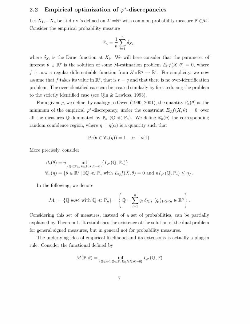
2.2 Empirical optimization of ϕ∗-discrepancies

Let X1, ...Xn be i.i.d r.v.’s defined on X =Rp with common probability measure P ∈M.

Consider the empirical probability measure

Pn =1

n

n∑

i=1

δXi,

where δXiis the Dirac function at Xi. We will here consider that the parameter of

interest θ ∈ Rq is the solution of some M-estimation problem EPf(X, θ) = 0, where

f is now a regular differentiable function from X×Rq → Rr. For simplicity, we now

assume that f takes its value in Rq, that is r = q and that there is no over-identification

problem. The over-identified case can be treated similarly by first reducing the problem

to the strictly identified case (see Qin & Lawless, 1993).

For a given ϕ, we define, by analogy to Owen (1990, 2001), the quantity βn(θ) as the

minimum of the empirical ϕ∗-discrepancy, under the constraint EQf(X, θ) = 0, over

all the measures Q dominated by Pn (Q ≪ Pn). We define Cn(η) the corresponding

random confidence region, where η = η(α) is a quantity such that

Pr(θ ∈ Cn(η)) = 1 − α + o(1).

More precisely, consider

βn(θ) = n infQ≪Pn, EQf(X,θ)=0

Iϕ∗(Q, Pn)

Cn(η) = θ ∈ Rq |∃Q ≪ Pn with EQf(X, θ) = 0 and nIϕ∗(Q, Pn) ≤ η .

In the following, we denote

Mn = Q ∈M with Q ≪ Pn =

Q =

n∑

i=1

qi δXi, (qi)1≤i≤n ∈ Rn

.

Considering this set of measures, instead of a set of probabilities, can be partially

explained by Theorem 1. It establishes the existence of the solution of the dual problem

for general signed measures, but in general not for probability measures.

The underlying idea of empirical likelihood and its extensions is actually a plug-in

rule. Consider the functional defined by

M(P, θ) = infQ∈M, Q≪P, EQf(X,θ)=0

Iϕ∗(Q, P)

7

that is, the minimization of a contrast under the constraints imposed by the model.

This can be seen as a projection of P on the model of interest for the given pseudo-

metric Iϕ∗ . If the model is true at P, that is, if EPf(X, θ) = 0 at the true underlying

probability P, then clearly M(P, θ) = 0. A natural estimator of M(P, θ) for fixed θ is

given by the plug-in estimator M(Pn, θ), which is βn(θ)/n. This estimator can then

be used to test M(P, θ) = 0 or, in a dual approach, to build confidence region for θ by

inverting the test.

For Q in Mn, the constraints can be rewritten as

(Q − Pn)f(., θ) = −Pnf(., θ).

Using Theorem 1, we get the dual representation

βn(θ) := n infQ∈Mn

Iϕ∗(Q, Pn), (Q − Pn)f(., θ) = −Pnf(., θ)

= n supλ∈Rq

−λ′Pnf(., θ) −

∫

Ω

ϕ(λ′f(X, θ))dPn

= n supλ∈Rq

Pn

(− λ′f(., θ) − ϕ(λ′f(., θ))

). (3)

Notice that −x − ϕ(x) is a strictly concave function and that the function λ → λ′f

is also concave. The parameter λ can be simply interpreted as the Kuhn & Tucker

coefficient associated to the original optimization problem. From this representation

of βn(θ), we can now derive the usual properties of the empirical likelihood and its

generalization. In the following, we will also use the notations

fn = n−1n∑

i=1

f(Xi, θ), S2n = n−1

n∑

i=1

f(Xi, θ)f(Xi, θ)′ and S−2

n = (S2n)−1.

The following theorem states that generalized empirical likelihood essentially be-

haves asymptotically like a self-normalized sum. Links to self-normalized sum for finite

n will be investigated in paragraph 4.

Theorem 2 Let X, X1, ..., Xn be in Rp, i.i.d. with probability P and θ ∈ Rq such that

EPf(X, θ) = 0. Assume that S = EPf(X, θ)f(X, θ)′ is of rank q and that ϕ satisfies

the hypotheses H1-H4. Assume that the qualification constraints Qual(Pn) hold. For

any α in ]0, 1[, set η =ϕ(2)(0)χ2

q(1−α)

2, where χ2

q(.) is the χ2 distribution quantile. Then

8

Cn(η) is a convex asymptotic confidence region with

limn→∞

Pr(θ /∈ Cn(η)) = limn→∞

Pr(βn(θ) ≥ η)

= limn→∞

Pr(nf

′nS−2

n fn ≥ χ2q(1 − α)

)

= 1 − α.

The proof of this theorem starts from the convex dual-representation and follows

the main arguments of Bertail, Harari-Kermadec & Ravaille (2005) and Owen (2001)

for the case of the mean. It is left to the reader.

Remark 2 As noticed earlier, if ϕ is finite everywhere then the qualification con-

straints are not needed (this is for instance the case for the χ2 divergence). However,

in the case of empirical likelihood or the generalized empirical method introduced below,

this actually simply puts some restriction on the θ which are of interest as noticed in

the following examples.

2.3 Two basic examples

We illustrate Theorem 1 by reexamiming the case of the Kullback and χ2 discrepancies,

which lead respectively to the empirical likelihood method and the Generalized Method

of Moments (GMM).

2.3.1 Empirical likelihood and the Kullback discrepancy

In the particular case ϕ0(x) = −x− log(1−x) and ϕ∗0(x) = x− log(1+x) corresponding

to the Kullback divergence K(Q, P) = −∫

log(dQ

dP)dP, the dual program obtained in

(3) becomes, for the admissible θ,

βn(θ) = supλ∈Rq

(n∑

i=1

log(1 + λ′f(Xi, θ))

).

As Bertail (2003, 2004) points out, this quantity is itself a parametric log-likelihood

ratio indexed by the parameter λ (to test λ = 0). It can also be seen as a dual likelihood

in the sense of Mykland (1995). It is then easy to show that 2βn(θ) is asymptotically

χ2(q) when n → ∞, if the variance of f(X, θ) is definite. As a parametric likelihood

indexed by λ, it is also Bartlett-correctable (DiCiccio et al., 1991). Using a duality

9

point of view, the proof of the Bartlett-correctability is almost immediate, see Mykland

(1995) and Bertail (2004). For a general discrepancy, the dual form is not a likelihood

and may not be Bartlett-correctable, see DiCiccio et al. (1991) and Jing & Wood

(1995). We will latter propose a family of discrepancies, the Quasi-Kullback indexed

by some smoothing parameter ε, which still have this property for some specific choice

of ε.

Moreover, we necessarily have the q′is > 0 and∑n

i=1 qi = 1, so that the qualification

constraint essentially means that 0 belongs to the convex hull of the f(Xi, θ). Only

the θ’s which satisfy this constraint are of interest to us ; asymptotically, this is by

no mean a restriction, unless we have for some specific configuration of the realization

intθ\ 0 ∈ conv(f(X1, θ), ..., f(Xn, θ)) = ∅, where conv(., ., .) is the convex hull of the

points.

2.3.2 GMM and χ2 discrepancy

The particular case of the χ2 corresponds to ϕ2(x) = ϕ∗2(x) = x2

2. The Kuhn & Tucker

multiplier λ, and consequently the value of βn(θ) at any point θ, can be explicitly

calculated. Indeed, we get easily that λn = S−2n fn so that, by Theorem 1, the minimum

is attained at Q∗n =

∑ni=1 qi,nδXi

with

qi,n =1

n(1 + f

′nS−2

n f(Xi, θ))

and

Iϕ∗2(Q∗

n, Pn) =n∑

i=1

(nqi,n − 1)2

2n=

1

2f′nS−2

n fn,

which is exactly the square of a self-normalized sum which typically appears in the

Generalized Method of Moments (GMM). Notice that Q∗n is a signed measure, not a

probability.

This short calculus also shows that if we want to force our measure Q ∈ Mn to be a

probability measure, then the qualification constraints Qual(Pn) of Theorem 1 can not

be fulfilled. Indeed, imposing the additional constraints qi ≥ 0,∑n

i=1 qi = 1, implies

that the dual problem has no solution. This explains why, for some discrepancies, we

have to work with signed measure and not probability measure. The drawback is that,

in opposition to the Kullback discrepancy, we may charge positively some region outside

of the convex hull of the points, yielding bigger (that is too conservative) confidence

region. See the simulation results of Bertail et al. (2004). However, as noticed in the

10

introduction, the results of Tsao (2004) shows that taking the convex hull of the points

(the largest confidence region for empirical likelihood) may yield too narrow confidence

regions, when n is small compared to q.

Remark 3 If S2n is of rank l < q, notice that we still have the duality relationship :

βn(θ) = n supλ∈q

−λ′ 1

n

n∑

i=1

f(Xi, θ) −1

2nλ′S2

nλ

.

Write S2n = R′

0 ∆n 0

0 0

1AR, where ∆n is inversible of rank l, R =

0 Ra

Rb

1A is an orthog-

onal matrix with Ra ∈ Ml,q(R) and Rb ∈ Mq−l,q(R). We denote fn = (fn,1, · · · , fn,q)′.

Since for all j = 1, · · · , q − l, we can write

0 ≤ (Rbfn)2j ≤

1

n

n∑

i=1

(q∑

k=1

Rbj,kfk(Xi, θ)

)2

≤(RbS

2nRb

)l+j,l+j

= 0.

We deduce that Rbfn = 0. Then, the duality relationship becomes

βn(θ) = n supλ∈Rl

−λ′Rafn − 1

2λ′∆nλ

=

(Rafn)′

∆−1n (Rafn)

2.

Notice that (Rafn)(Rafn)′

= ∆n. This means that if S2n has rank l < q we can always

reduce the problem to the study of a self-normalized sum in Rl and that, from an

algorithmic point of view this reduction is carried out internally by the optimization

program. From now on, we will assume that S2n is of rank l = q.

3 Quasi-Kullbacks and Bartlett-correctability

The main underlying idea for considering these functions is that we want to keep the

good properties of Kullback discrepancy and to avoid some algorithmic problems linked

with the behavior of the log of Kullback discrepancy in the neighborhood of 0. This

kind of discrepancies is actually currently used in the convex optimization literature

(see for instance Auslender et al., 1999) because the resulting optimization algorithm

leads to efficient tractable interior point solutions.

11

3.1 Quasi-Kullback: definitions

For ε ∈]0; 1] and x ∈] −∞; 1[ let,

Kε(x) = ε x2/2 + (1 − ε)(−x − log(1 − x)).

We call the corresponding K∗ε -discrepancy, the quasi-Kullback discrepancy. The pa-

rameter ε > 0 may be interpreted as a regularization parameter (proximal in term of

convex optimization). This family fulfills our hypotheses H1-H5. Its Fenchel-Legendre

transform K∗ε has the following explicit expression, for all x in R :

K∗ε (x) = −1

2+

(2ε − x − 1)√

1 + x(x + 2 − 4ε) + (x + 1)2

4ε

− (ε − 1) log2ε − x − 1 +

√1 + x(x + 2 − 4ε)

2ε.

The second order derivative of Kε is bounded from below : K(2)ε (x) ≥ ε. More-

over, the second order derivative of K∗ε is bounded both from below and above :

0 ≤ K∗(2)ε (x) ≤ 1/ε. These controls ensure a quick and regular convergence of the

algorithms based on such discrepancies.

In addition, another algorithmic improvement is obtained in comparison with em-

pirical likelihood. The Kullback must be approached for practical optimization, for

instance by replacing the log by a pseudo log, see section 12.3 in Owen (2001). Since

the domain of K∗ε is R, the quasi-Kullback discrepancy can be used exactly. Thus,

the use of quasi-Kullback discrepancy in the empirical likelihood method, the “quasi-

empirical likelihood” may be seen as a “regularized” empirical likelihood.

12

Figure 2: Cover probabilities and Quasi-Kullback

Figure 2 illustrates the improvements coming from the use of Quasi-Kullbacks. It

presents the coverage probabilities of the usual discrepancies given in the introduction,

as well as the ones for Quasi-Kullback discrepancy (for a given value of ε = 0.5) on the

same data. As expected, the Quasi-Kullback discrepancy leads to a confidence region

with a coverage probability much closer to the targeted one, especially with a Bartlett

adjustment.

3.2 Bartlett-correctability

The following theorem establishes sufficient conditions on the regularization parameter

ε to obtain the Bartlett-correctability of quasi-empirical likelihood.

Theorem 3 Under the assumptions of Theorem 2, assume that f(X, θ) satisfies the

Cramer condition : lim||t||→∞|EP exp(it′f(X, θ))| < 1, as well as the moment condition

EP||f(X, θ)||s < ∞, for s > 8.

If ε ⊜ εn = O(n−3/2/ log(n)

)then the quasi-empirical likelihood is Bartlett-correctable

up to O(n−3/2).

This choice of ε is probably not optimal but considerably simplifies the proof. An

attentive reading of Corcoran (2001) shows that, if ε is small enough, the statistic

13

is Bartlett-correctable. Unfortunately, as our discrepancy depend on n, Corcoran’s

result cannot be applied directly and does not allow ε to be precisely calibrated . We

conjecture that, at the cost of tedious calculations, the rate of εn in o(n−1) is enough,

at least to get Bartlett-correctability up to o(n−1).

4 Exponential bounds for self-normalized sums and

quasi-empirical likelihood

Another interesting feature of quasi-Kullback discrepancies is that the control of

the second order derivatives allows the behavior of βn(θ) to be linked to that of self-

normalized sums. We thus can get exponential bounds for the quantities of interest.

Some of the bounds that we propose here for self-normalized sums are new and of

interest by themselves. These bounds may be quite easily obtained in the symmetric

case (that is for random variables having a symmetric distribution) and are well-known

in the unidimensional case.

Self-normalized sums have recently given rise to an important literature : see for

instance Jing & Wang (1999), Gotze & Chistyakov (2003) or Bercu, Gassiat & Rio

(2002) for self-normalized processes. Unfortunately, except in the unidimensional sym-

metric case, these bounds are not universal and depend on higher order moments,

γ3 = EP|S−1f(Xi, θ)|3 or even an higher moment condition : γ10/3 = EP|S−1f(Xi, θ)|10/3.

Actually, uniform bounds in P are impossible to obtain, otherwise this would contradict

Bahadur & Savage (1956)’s result on the non-existence of uniform confidence region

over large class of probabilities, see Romano & Wolf (2000) for related results.

In the general non-symmetric case, for q = 1, if γ10/3 < ∞, for some A ∈ R and

some a ∈]0, 1[, the result of Jing & Wang (1999) lead to

Pr(n

2f

2

n/S2n ≥ εη

)= χ2

1(εη) + Aγ10/3n−1/2e−aεη. (4)

However the constants A and a are not explicit and the bound is of no practical use.

In the non-symmetric case our bounds are worse than (4) as far as the power in the

exponential and the control of the approximation by a χ2 distribution are concerned,

but entirely explicit.

14

Theorem 4 Let (Zi)i=1,··· ,n be i.i.d. sample in Rq with probability P. Note that

Zn = 1n

∑ni=1 Zi, S2

n = 1n

∑ni=1 ZiZ

′i and S2 = EPZ1Z

′1 is of rank q. Then the

following inequalities hold, for finite n > q and for u ≤ nq,

a) if Z1 has a symmetric distribution, without any moment assumption,

Pr(nZnS−2

n Zn ≥ u)≤ 2qe−

u2q ; (5)

b) for general distribution of Z1 with kurtosis γ4 < ∞,

Pr(nZnS−2

n Zn ≥ u)≤ inf

a>1

2qe1− u

2q(1+a) + C(q) n3eqγ−eq4 e

− nγ4(q+1)(1− 1

a)2

(6)

≤ infa>1

2qe

1− u2q(1+a) + C(q) n3eqe− n

γ4(q+1)(1− 1a)

2

with q = q−1q+1

, γ4 = EP(‖S−1Z1‖42) and C(q) = (2eπ)2eq(q+1)

22/(q+1)(q−1)3eq ≤ (2eπ)2(q+1)(q−1)3eq ≤ 18.

Moreover for nq ≤ u, we have

Pr(nZnS−2

n Zn ≥ u)

= 0.

The proof is postponed to Appendix A.3. The exponential inequality (5) is classical

in the unidimensional case. This bound is universal for symmetric laws. We generalize

it to the multidimensional case by using simple diagonalization arguments leading to

a sum of q self-normalized sums. In the general multidimensional framework, the

main difficulty is actually to keep the self-normalized structure when symmetrizing the

original sum. For this we use a multidimensional extension of a symmetrization lemma

by Panchenko (2003). Another difficulty is to have a precise control of the behavior of

the smallest eigenvalue of the normalizing empirical variance. The second term in the

right hand side of inequality (6) is essentially due to this control.

Remark 4 In the best case, past studies give some bounds for n sufficiently large,

without an exact value for “sufficiently large”. Here, the bounds are valid for any n.

All the constants are also explicit. This bound may also be used to give some ideas on

the sample size needed to reach a given confidence level (as a function of q and γ4).

15

The following corollary implies that, for the whole class of quasi-Kullback discrep-

ancies, the finite sample behavior of the corresponding empirical energy minimizers is

reduced to the study of a self-normalized sum.

Corollary 1 Under the hypotheses of Theorem 2, the following inequalities hold, for

finite n > q, for any η > 0, for any n ≥ 2εηq

,

Pr(θ /∈ Cn(η)) = Pr(βn(θ) ≥ η) ≤ Pr(nfnS−2

n fn ≥ 2εη). (7)

Else if n > 2εηq

, Pr(θ /∈ Cn(η)) = 0.

Then bounds (5) and (6) may be used with u = 2εη and Zi = f(Xi, θ).

Proof. Following the arguments of the remark of Theorem 2, we use the dual form

and expand Kε near 0. Then we get

βn(θ) = supλ∈Rq

−nλ′fn − 1

2

n∑

i=1

(λ′f(Xi, θ))2K(2)

ε (ti,n)

≤ supλ∈Rq

−nλ′fn − 1

2

n∑

i=1

(λ′f(Xi, θ))2ε

. (8)

Indeed, by construction of the quasi-Kullback, we have K(2)ε ≥ ε. If we write l = −ελ,

the right hand side of inequality (8) becomes

n

εsupl∈Rq

l′fn − 1

2l′S2

nl

=

n

2εf′nS−2

n fn.

Thus we immediately get

Pr(θ /∈ Cn(η)) ≤ Pr(n

2f′nS−2

n fn ≥ ηε)

.

♦

Remark 5 In Hjort, McKeague, and Van Keilegom (2004), convergence of empirical

likelihood is investigated when q is allowed to increase with n. They show that conver-

gence to a Chi-square distribution still holds when q = O(n13 ) as n tends to infinity.

Our bounds shows that even if q = o (n/log(n)), it is still possible to get asymptoti-

cally valid confidence intervals with our bounds. Notice that the constant C(q) does not

increase with q as can be seen on the following graph.

16

0 20 40 60 80 100

05

1015

q

C(q

)

Figure 3: Value of C(q) as a function of q

A close examination of the bounds shows that essentially qγ4 has to be small com-

pared to n for practical use of these bounds. Of course practically γ4 is not known,

however one may use an estimator or an upper bound for this quantity to get some

insight on a given estimation problem.

Notice that the bounds are non-informative when ε → 0, which corresponds to

empirical likelihood. Actually, it is not possible to establish an exponential bound

for this case. If we were able to do so, for a sufficiently large η, we could control

the confidence region built with empirical likelihood for any level 1 − α. This would

contradict the statements of Tsao (2004), which gives a lower bound for the attainable

levels.

5 Discussion and simulation results

5.1 Non-asymptotic comparisons

For ε = 1, that is for the χ2 discrepancy, the inequality (7) becomes an equality. In

the following table 1, we tabulate some values of η corresponding to a given confidence

level 1 − α, for different γ4 and n for a unidimensional model (q = 1). The values of

η corresponding to Kε with ε 6= 1 are easily obtained by multiplying the values in the

table by 1/ǫ.

• The column “Asymptotic” corresponds to η equal to the (1 − α)-quantile of the

χ21 distribution.

17

• The column “Symmetric bound” corresponds to η obtained by inverting the ex-

ponential inequality in the symmetric case, that is η = −q ln( α2q

).

• The next column NS, for “Non-symmetric”, is obtained by inverting the general

exponential bound for γ4 = 3 (that corresponds to the kurtosis of standard

gaussian distribution) and for two values of n, 50 and 200.

• The last column is similar to the third, but for γ4 = 5.4 (that corresponds to our

gaussian scale mixture).

Asymptotic Symmetric NS γ4 = 3 NS γ4 = 5.4

Confidence χ2 bound n = 50 n = 200 n = 50 n = 200

50% 0.46 1.4 7.99 6.05 9.86 6.62

90% 2.71 3.0 16.3 10.6 26.7 12.0

95% 3.84 3.7 21.5 12.7 44.1 14.7

99% 6.64 5.3 40.4 18.0 104 21.7

Table 1: Values of η for q = 1.

We notice that, for small values of n, the values of η are quite high, leading to

confidence regions that may be too conservative but that are very robust.

In the following graphics, we build confidence intervals for the mean of unidimen-

sional data. We simulated 50 i.i.d. centered gaussian scale mixture r.v.’s : that is

realizations of U ∗ N , where U and N are respectively independent uniform r.v.’s on

[0,1] and standard gaussian r.v.’s. The figure shows the profile quasi-likelihood βn(θ)

for different values of ε, the bottom right graphic correspond to ε = 1. In addition to

the profile quasi-likelihood, we indicate the bounds corresponding to 90% confidence

intervals (1 − α = 0.9) using respectively the asymptotic approximation, the symmet-

ric bound and the general bound (NS) with the true kurtosis (5.4) and an estimated

kurtosis.

18

Figure 4: Discrepancy profile and 90% confidence levels

For a given sample size n and confidence 1 − α, the profile quasi-likelihood gets

wider as ε increases. As a consequence, the asymptotic confidence intervals become

wider. With the non-asymptotic bounds, the behavior of the corresponding confidence

interval as ε increases is more delicate to understand. The profile likelihood gets wider

but the η’s corresponding to the symmetric and NS bounds decrease like 1/ε. These

two behaviors have contradictory effects on the confidence intervals Cn(η). On the

figure 4, for α = 0.1, q = 1 and our simulated data, the effect of the decrease of η

dominates : the confidence intervals get smaller when ε increases. In higher dimension

or for a smaller α, the two contradictory effects could be balanced.

In figure 5, we build confidence regions for the mean of multi-dimensional (R2) data,

for 2 sizes (500 and 2000) and 2 distributions : a couple of independent gaussian scale

mixtures and the distribution 0.01 · δ(10,10) + 0.814

·(δ(−1,−1) + δ(−1,1) + δ(1,−1) + δ(1,1)

)+

19

0.092

·(δ(−1,10) + δ(1,10) + δ(10,−1) + δ(10,1)

), that will be referred as discrete distribution.

We give in figure 5 the corresponding 90% confidence regions, using respectively the

asymptotic approximation, the symmetric bound and the general bound (NS) with the

true kurtosis.

scale mixture : 500 data

scale mixture : 2000 data

discrete distribution : 500 data

discrete distribution : 2000 data

Figure 5: Confidence regions, for 2 distributions and 2 data sizes.

For small sample size, as expected, the confidence region obtained with NS bound is

quite large (for our discrete data and n = 500, the region is too large to be represented

on the figure) with a coverage probability close to 1. On the contrary, the asymptotic

confidence regions are small but when the distribution has a large γ4, the coverage

probability can be significantly smaller than the targeted level 1 − α.

We conclude from these simulations that, on the one hand, if the asymptotic and

NS confidence regions are not too far from each other then we may trust the asymptotic

20

behavior for a coverage point of view. On the other hand, to protect oneself against

exotic distributions, the use of NS bound is justified.

5.2 Adaptative asymptotic confidence regions

Corollary 1 does not allow for a precise calibration of ε for finite sample size. Indeed,

the finite exponential bounds essentially say that the bigger ε is (close to 1), the better

the bound. This clearly advocates that, in term of our bound sizes, the χ2 discrepancy

leads to the best results. This is partially true in the sense that the χ2 leads immediately

to a self-normalized sum which has quite robust properties. However, it can be argued

that, for regular enough distributions, the χ2 discrepancy leads to confidence regions

that are too conservative. The result on Bartlett-correctability suggests that the bias

of the empirical minimizer for quasi-Kullback is smaller for very small values of ε (see

also Newey & Smith (2002) for argument in that direction). Choosing adequately ε

could result in a better equilibrium and a compromise between coverage probability

and the adaptation to the data.

From a practical point of view, several choices are possible for calibrating ε. A

simple solution is simply to use cross-validation (either bootstrap, leave one-out or

K-fold methods). Of course, this is very computationally-expensive but the use of

a quasi-Kullback distance eases the convergence of the algorithms. Moreover, it is

not clear how the use of cross-validation and thus the use of an ε depending on the

data will deteriorate the finite sample bounds. The figure 6 allows us to compare the

asymptotic confidence regions built with the Kullback discrepancy (K0), the χ2 (K1)

and the Quasi-Kullback (Kε) with ε chosen by cross-validation, for a parameter in R2.

21

scale mixture : 15 data exponential distribution : 25 data

Figure 6: Asymptotic confidence regions for data driven Kε.

The figure 7 represents the coverage probability obtained by Monte-Carlo simula-

tions (10 000 repetitions) for Kε with data driven ε and different sample sizes n. Some

curves from figure 1 giving the coverage probability of previously available methods

are recalled for comparison.

22

Figure 7: Coverage probability for different data sizes n for data-driven ε.

The adaptative value of ε decreases with n : over our 25 000 Monte-Carlo rep-

etitions, the mean value of ε is 1 for n = 15 and n = 20. It decreases to 0.7 for

n = 100.

For smooth distributions like our scale mixture, the coverage probability of the con-

fidence region constructed with the calibrated Kε is close to the targeted one. Moreover,

the region is small and adapts to the data.

Note that when, for all values of ε, the cross-validation estimate of the coverage

probability is smaller than the targeted confidence, the distribution may be “exotic”.

In such a case, the NS bound should be considered.

The simulations and graphics have been computed with Matlab : algorithms are

available from the authors on request . The Monte-Carlo simulations of figure 7 have

been carried out simulatively on 18 computers with 2.5 GHz processors and took

23

18*200 hours of computation time.

A Proofs of the main results

A.1 Proof of theorem 3

Write βεn(θ) for the the value of n times the sup in the dual program (3) when ϕ = Kε.

β0n(θ) corresponds to the log likelihood ratio for Kullback discrepancy ϕ = K0 and β1

n(θ)

corresponds to the minimization of the χ2-divergence ϕ = K1. Let En be either the

true value of E[β0n(θ)]/q or an estimator of this quantity such that empirical likelihood

is Bartlett-correctable when standardized by this quantity. We denote

T εn =

2βεn(θ)

En

.

Then, using DiCiccio, Hall & Romano [16] (see also Bertail, 2005), under the Cramer

condition and assuming EP||f(X, θ)||8 < ∞, the Bartlett-correctability of T 0n implies

that

Pr

(2β0

n(µ)

En

≥ x

)= Fχ2(x) + O(n−2),

where we denote FZ(.) = P(Z > .), when Z ∼ P. This equality implies in particular

that

FT 0n(η − n− 3

2 ) = Fχ2(q)(η) + O(n− 32 ). (9)

Now, we can write

T εn =

2

Ensupλ∈Rq

n∑

i=1

λ′f(Xi, θ) −n∑

i=1

Kε(λ′f(Xi, θ))

≤ 2

En

εβ1

n(θ) + (1 − ε)β0n(θ)

.

In other words

T εn ≤ T 0

n + ε[T 1

n − T 0n

].

This implies

FT εn(η) ≤ FT 0

n+ε[T 1n−T 0

n](η).

We also have with (9)

FT 0n+ε[T 1

n−T 0n](η) ≤ Pr(T 0

n + n− 32 ≥ η) + Pr(|T 1

n − T 0n | ≥ ε−1n− 3

2 )

= FT 0n(η − n− 3

2 ) + Pr(|T 1n − T 0

n | ≥ ε−1n− 32 )

= Fχ2(η) + O(n− 32 ) + Pr(|T 1

n − T 0n | ≥ ε−1n− 3

2 ).

24

If we take ε of order n−3/2 log(n)−1, the last term in the right hand side of this inequality

is of order O(n−3/2). This can be shown by using for example the moderate deviation

inequality (4) for T 1n and the fact that T 0

n is already Bartlett-correctable. It follows

that the corresponding discrepancy is still Bartlett-correctable, at least up to the order

O(n−3/2).

A.2 Some bounds for self-normalized sums

Lemma 1 (Extension of Panchenko, 2003 Corollary 1) Let Γ be the unit circle

of Rq, Γ = λ ∈ Rq, ‖λ‖2,q = 1. Let (Zi)1≤i≤n and (Yi)1≤i≤n be i.i.d. centered random

vectors in Rq with (Zi)1≤i≤n independent of (Yi)1≤i≤n. We denote for all random vector

W with probability P : S2n(W ) = 1

n

∑ni WiW

′i and S2 = EP(WW ′).

If there exists D > 0 and d > 0 such that, for all u ≥ 0,

Pr

(supλ∈Γ

(√nλ′(Zn − Y n)√λ′S2

n(Z − Y )λ

)≥

√u

)≤ De−du,

then, for all u ≥ 0,

Pr

(supλ∈Γ

√nλ′Zn√

λ′S2n(Z)λ + λ′S2λ

≥√

u

)≤ De1−du. (10)

Proof. In the unidimensional case, this result reduces to Corollary 1 of Panchenko

(2003) [32]. In the multidimensional case, this is an extension of Panchenko (2003)’s

Lemma 1[32]. Denote

An(Z) = supλ∈Γ

supb>0

EZY

4b(λ′(Zn − Y n) − bλ′S2

n(Z − Y )λ)

Cn(Z, Y ) = supλ∈Γ

supb>0

4b(λ′(Zn − Y n) − bλ′S2

n(Z − Y )λ)

.

By Jensen inequality, we have Pr-almost surely

An(Z) ≤ EY [Cn(Z, Y )|Z]

and, for any convex function Φ, by Jensen inequality, we also get

Φ(An(Z)) ≤ EY [Φ(Cn(Z, Y ))|Z].

25

We obtain

EZ(Φ(An(Z))) ≤ E(Φ(Cn(Z, Y ))). (11)

Now remark that

An(Z) = supλ∈Γ

supb>0

4b(λ′Zn − bλ′S2

n(Z)λ − bλ′S2λ)

= supλ∈Γ

λ′Zn√λ′S2

n(Z)λ + λ′S2λ

and

Cn(Z, Y ) = supλ∈Γ

λ′(Zn − Y n)√λ′S2

n(Z − Y )λ.

Now, notice that supλ∈Γλ′Zn√λ′S2

nλ> 0 and apply the same arguments as Corollary 1’s

proof of Panchenko [32] applied to inequality (11) to obtain the result.

♦

We now extend a result of [5], which controls the behaviour of the smallest eigen-

value of the empirical variance. In the following, for a given symmetric matrix A, we

denote µ1(A) its smallest eigenvalue.

Lemma 2 Let (Zi)i=1,···n be i.i.d. random vectors in Rq with common mean 0. Denote

S2 = E(Z1Z′1), 0 < γ4 = E(‖Z1‖4

2) < +∞ and q = q−1q+1

. Then, for any 1 ≤ q < n and

0 < u ≤ µ1(S2),

Pr(µ1(S

2n) ≤ u

)≤ C(q)

n3eqµ1(S2)2eq

γeq4 e−n(µ1(S2)−u)2

γ4(q+1) ∧ 1,

with

C(q) = π2eq(q + 1)e2eq(q − 1)−3eq22eq− 2q+1 (12)

≤ 4π2(q + 1)e2(q − 1)−3eq. (13)

Remark 6 The value of C(q) could certainly be improved. The term π2eq essentially

comes from a basic bound for the number of caps of diameter ε needed to cover a

half unit-sphere Sq−1, say N(Sq−1, ε). We use the bound N(Sq−1, ε) ≤ πq−1ε−(q−1).

There is a huge bibliography in convex geometry about covering numbers of the sphere.

For instance Boroczky & Wintsche (2003) give a bound on the number of sphere (for

the euclidian geometry on the sphere) needed to cover the sphere. We can deduce from

26

Boroczky & Wintsche (2003) the following bound for N(Sq−1, ε) : when ε ≤ Arcos( 1√q),

for q ≥ 2, there exists c an universal constant such that

ε−(q−1) ≤ N(Sq−1, ε) ≤ c cos(ε) sin(ε)−(q−1)(q − 1)3/2 log(1 + (q − 1) cos(ε)2)

Using the fact that for x > 0, 2πx ≤ sin(x) ≤ x and cos(ε)2 ≤ 1

q, we get the more

friendly bound

ε−(q−1) ≤ N(Sq−1, ε) ≤ c( π

2ε

)q−1

(q − 1)3/2 log

(1 +

q − 1

q

).

However, an explicit value for c is not clear to us.

Proof. This proof is adapted from the proof of [5] and makes use of some idea of

Bercu-Gassiat-Rio [3]. In the following, we denote by Sq−1 the northern hemisphere of

the sphere.

We first have by a truncation argument and applying Markov’s inequality on the

last term in the inequality (see the proof of Barbe and Bertail [5], lemma 4), for every

M > 0, Pr (µ1(∑n

i=1 ZiZ′i) ≤ t) is less than

Pr

(inf

v∈Sq−1

n∑

i=1

(v′Zi)2 ≤ t, sup

i=1,...,n||Zi||2 ≤ M

)+ n

γ4

M4(14)

We call the first term on right side I.

Notice that by symmetry of the sphere, we can always work with the northern hemi-

sphere of the sphere rather than the sphere. Notice first, that, if supi=1,...,n ||Zi||2 ≤ M ,

then for u, v in Sq−1, we have

|n∑

i=1

(v′Zi)2 −

n∑

i=1

(u′Zi)2| ≤ 2n||u − v||M2.

Thus if u and v are apart of tη/(2nM2) then |∑ni=1(v

′Zi)2 −∑n

i=1(u′Zi)

2| ≤ ηt. Now

let N(Sq−1, ε) be the smallest number of caps of radius ε centered at some points on

Sq−1 (for the ||.||2 norm) needed to cover Sq−1 (the half sphere). Following the same

arguments as [5], we have, for any η > 0,

I ≤ N(Sq−1,tη

2nM2) max

u∈Sq−1

Pr

(n∑

i=1

(u′Zi)2 ≤ (1 + η)t

).

The proof is now divided in three steps, i) control of N(Sq−1,tη

2nM2 ) ii) control of

the maximum over Sq−1 of the last expression in I, iii) optimization over all the free

27

parameters.

i) On the one hand, we have

N(Sq−1, ε) ≤ b(q)ε−(q−1) ∨ 1, (15)

with, for instance, b(q) ≤ πq−1. Indeed, following [5], the northern hemisphere can be

parameterized in polar coordinates, realizing a diffeomorphism with Sq−2 × [0, π]. Now

proceed by induction, notice that for q = 2, Sq−1, the half circle can be covered by

[π/2ε]∨ 1 + 1 ≤ 2([π/2ε]∨ 1) ≤ π/ε∨ 1 caps of diameter 2ε, that is, we can choose the

caps with their center on a ε−grid on the circle. Note that this is not a good bound

for q=2 since in that case the overlapping of the caps is ε. Now, by induction we can

cover the cylinder Sq−2× [0, π] with [π/2ε (π)q−2/εq−2]∨1+1 ≤ πq−1/εq−1 intersecting

cylinders which in turn can be mapped to region belonging to caps of radius ε, covering

the whole sphere (this is still a covering because the mapping from the cylinder to the

sphere is contractive).

ii) On the other hand, for all t > 0, we have by exponentiation and Markov’s inequality,

and independence of (Zi), for any λ > 0

maxu∈Sq−1

Pr

(n∑

i=1

u′ZiZ′iu ≤ t

)≤ eλt max

u∈Sq−1

(E(e−λu′Z1Z′1u))n.

Now, using the classical inequalities, log(x) ≤ x − 1 and e−x − 1 ≤ −x + x2/2, both

valid for x > 0, we have

maxu∈Sq−1

(E(e−λu′Z1Z′1u))n ≤ max

u∈Sq−1

exp n(E(e−λu′Z1Z′1u − 1))

≤ maxu∈Sq−1

exp n

(E(−λu′Z1Z

′1u) +

λ2

2E(u′Z1Z

′1u)2

))

≤ maxu∈Sq−1

exp n

(−λu′S2u +

λ2

2γ4

)

≤ eλ2

2nγ4e−λn minu∈Sq−1

u′S2u

= eλ2

2nγ4−λnµ1(S2). (16)

iii) From (16) and (15), we deduce that, for any t > 0, λ > 0, η > 0,

I ≤ b(q)(2nM2

tη)q−1eλ(1+η)t+ λ2

2nγ4−λnµ1(S2).

Optimizing the expression exp(−(q − 1)log(η)+ ληt) in η > 0, yields immediately , for

any t > 0, any M > 0, any λ > 0

I ≤ b(q)

(2enM2λ

q − 1

)q−1

eλ(t−nµ1(S2))+nλ2γ4/2.

28

The infimum in λ in the exponential term is attained at λ =µ1(S2)− t

n

γ4, provided that

0 < t < n µ1(S2). Therefore, for these t and all M > 0, we get Pr(µ1(

∑ni=1 ZiZ

′i) ≤ t)

is less than

b(q)

(2enM2µ1(S

2)

γ4(q − 1)

)q−1

exp

(− n

2γ4

(µ1(S

2) − t

n

)2)

+ nγ4

M4.

We now optimize in M2 > 0 and the optimum is attained at

M2∗ =

(2nγ4

(q − 1)b(q)

) 1q+1(

2en

q − 1

µ1(S2)

γ4

)− (q−1)q+1

exp

(n(µ1(S

2) − tn)2

2γ4(q + 1)

),

yielding the bound

Pr

(µ1

(n∑

i=1

ZiZ′i

)≤ t

)≤ C(q) n3 q−1

q+1 µ1(S2)

2(q−1)q+1 γ

− q−1q+1

4 exp

(−n

(µ1(S

2) − tn

)2

γ4(q + 1)

),

with

C(q) = b(q)2

q+1 (q + 1)e2(q−1)

q+1 (q − 1)−3 q−1q+1 2

2q−4q+1 .

Using b(q) ≤ πq−1 we obtained C(q), which is majorized by the simpler bound (for large

q this bound will be sufficient) 4π2(q + 1)e2(q − 1)−3 q−1q+1 , using the fact that γ4 ≥ 1.

The result of the Lemma follows by applying this inequality on inequation 14 with

t = nu.

♦

A.3 Proof of Theorem 4

Notice that we have always Z ′nS−2

n Zn ≤ q. Indeed, there exists an orthogonal transfor-

mation On and a diagonal matrix Λ2n := diag[µj]1≤j≤q with µj > 0 being the eigenvalues

of S2n, such that S2

n = O′

nΛ2nOn. Now put Yi,n := [Yi,j,n]1≤j≤q = OnZi. It is easy to see

that by construction the empirical variance of the Yi,n is

1

n

n∑

i=1

Yi,nY′i,n =

1

n

n∑

i=1

OnZiZ′iO

′n = OnS2

nO′

n = Λ2n.

It also follows from this equality that, for all j = 1, · · · , q, 1n

∑ni=1 Y 2

i,j,n = µj , and

Z ′nS−2

n Zn = Y ′nΛ−2

n Yn =

q∑

j=1

(1

n

n∑

i=1

Yi,j,n

)2

/µj ≤ q.

29

by Cauchy-Schwartz. So, for all u > qn

P (Z ′nS

−2n Zn ≥ u

n) = 0.

a) In the symmetric and unidimensional framework (q = 1), this bound easily follows

from Hoeffding inequality (see Efron, 1969). For completeness and to fix the notations,

we recall the following simple proof. First of all

Pr(nZ

2

n

S2n

≥ u) = 2 Pr(

∑ni=1 Zi∑ni=1 Z2

i

≥√

u).

With q = 1 inequality Pr(√

nZn ≥ √uSn) becomes

Pr

( ∑ni=1 Zi

(∑n

i=1 Z2i )

12

>√

u

)≤ e−

u2 . (17)

Let σi, 1 ≤ i ≤ n be Rademacher random variables, independent from (Zi)1≤i≤n,

P(σi = −1) = P(σi = 1) = 1/2. We denote σn(Z) =(

1√n

∑ni=1 σiZi

)and remark

that S2n = 1

n

∑ni=1 σiZiZ

′iσi.

Then we have by independence and symmetry of the Zi’s

Pr

(Zn

Sn

≥ √u

)=

∫Pr

(σn(Z)

Sn

≥ √u

∣∣∣∣n⋂

i=1

Zi = zi

)Πn

i=1P(dzi).

But by Hoeffding inequality, we have

Pr

(σn(Z)

Sn

≥ √u

∣∣∣∣n⋂

i=1

Zi = zi

)≤ e−u/2 (18)

and the result follows by integration.

In the symmetric multidimensional framework (q > 1), the result is based on the

inequality (18). Since the Zi’s have a symmetric distribution meaning, −Zi has the

same distribution as Zi. Then using a first symmetrization step we have,

Pr(nZ

′nS−2

n Zn ≥ u)

= Pr(σn(Z)′

S−2n σn(Z) ≥ u).

Now,

σn(Z)′

S−2n σn(Z) = σn(Y )

′

Λ−2n σn(Y )

=

q∑

j=1

(1√n

n∑

i=1

σiYi,j,n

)2

/µj

=

q∑

j=1

(n∑

i=1

σiYi,j,n

)2

/

n∑

i=1

Y 2i,j,n.

30

It follows that

Pr(σn(Z)′

S−2n σn(Z) ≥ u) ≤

q∑

j=1

Pr

|∑n

i=1 σiYi,j,n|√∑ni=1 Y 2

i,j,n

≥√

u/q

≤ 2

q∑

j=1

E Pr

∑n

i=1 σiYi,j,n√∑ni=1 Y 2

i,j,n

≥√

u/q

∣∣∣∣∣∣(Zi)1≤i≤n

.

Apply now (18) to each self-normalized term in this sum to conclude.

b) The non-symmetric framework requires further investigations.

Our goal is to control Pr(nZ ′nS−2

n Zn ≥ t). Define

Bn = sup‖λ‖2,q=1

λ′Zn≥0

λ′Zn√λ′S2

nλ

and Dn = sup

‖λ‖2,q=1

λ′Zn≥0

√1 +

λ′S2λ

λ′S2nλ

.

First of all, remark that the following events are equivalent

nZ

′nS−2

n Zn ≥ t

=

Bn ≥

√t

n

.

The final control is obtain by the control of two terms since

Pr

(Bn ≥

√t

n

)≤ inf

a>−1

Pr

(BnD−1

n ≥√

t

n(1 + a)

)+ Pr(Dn ≥

√1 + a)

.

The control of the first term on the right side is obtained by applying part a) of Theo-

rem 2 to n1/2 sup‖λ‖2,q=1λ′∈Γ

λ′Zn−Y n√λ′S2

n(Z−Y )λto obtain the control 2qe−

t2q . Then, by application

of the Lemma 1 and the previous remark, we get√

nBnD−1n ≤ n1/2 sup‖λ‖2,q=1

λ′Zn≥0

λ′Zn√λ′S2

nλ+λ′S2λ, we have for all t > 0,

Pr

(BnD−1

n ≥√

t

n

)≤ 2qe1− t

2q .

The control of the second term is trivial and useless for a ≤ 0. Whereas, for all a > 0,

and all t > 0 we have

Dn ≥

√a + 1

=

sup‖λ‖2,q=1

λ′Zn≥0

(1 +

λ′S2λ

λ′S2nλ

)≥ 1 + a

=

inf‖λ‖2,q=1

λ′Zn≥0

(λ′S−1S2

nS−1λ)≤ 1

a

=

µ1(S

−1S2nS−1) ≤ 1

a

.

31

We now use Lemma 2 applied to the r.v.’s (S−1Zi)i=1,··· ,n. Note that here we have

γ4 = E‖S−1Z1‖42, S2 = Idq, µ1(S

2) = 1 and u = 1a. For all 1 < a, we have,

Pr(Dn >√

1 + a) ≤ C(q)

(n3

γ4

)q

e− n

(q+1)γ4(1− 1

a)2

.

Since infa>−1 ≤ infa>1, we conclude that, for any t > n,

Pr

(Bn >

√t

n

)≤ inf

a>1

2qe e−

t2q(1+a) + C(q)

(n3

γ4

)q

e− n

(q+1)γ4(1− 1

a)2

.

References

[1] Ausslender, A., Teboulle, M., and Ben-Tiba, S. Logarithm-quadratic

proximal method for variational inequalities. Computational Optimization and

Applications 12 (1999), 31–40.

[2] Baggerly, K. A. Empirical likelihood as a goodness of fit measure. Biometrika

85 (1998), 535–547.

[3] Bercu, B., Gassiat, E., and Rio, E. Concentration inequalities, large and

moderate deviations for self-normalized empirical processes. Annals of Probability

30 (2002), 1576–1604.

[4] Bertail, P. Empirical likelihood in non and semi-parametric models. M. Nikulin,

2003. to appear in Semi-parametric models and applications.

[5] Bertail, P., and Barbe, P. Testing the global stability of a linear model.

Working Paper at CREST, 2004.

[6] Bertail, P., Harari-Kermadec, H., and Ravaille, D. γ−Divergence em-

pirique et vraisemblance empirique generalisee. Submitted, 2005.

[7] Borwein, J. M., and Lewis, A. S. Duality relationships for entropy like

minimization problem. SIAM Journal on Computation and Optimization 29, 2

(1991), 325–338.

[8] Broniatowski, M., and Keziou, A. Parametric estimation and tests through

divergences. PhD thesis, L.S.T.A., 2003.

32

[9] Broniatowski, M., and Keziou, A. Optimization of phi-divergences on sets

of signed measures. to appear in Studia Mathematicarum Huncaricarum, 2005.

[10] Chen, S., and Cui, H. On the second order properties of empirical likelihood

with moment restrictions. preprint at Iowa State University, 2005.

[11] Chistyakov, G. P., and Gtze, F. Moderate deviations for Student’s statistic.

Theory of Probability & Its Applications 47, 3 (2003), 415–428.

[12] Corcoran, S. A. Bartlett adjustment of empirical discrepancy statistics. Bio-

metrika 85, 4 (1998), 967–972.

[13] Cressie, N., and Read, T. R. C. Multinomial goodness-of-fit tests. Journal

of the Royal Statistical Society, Series B 46, 3 (1984), 440–464.

[14] Csiszar, I. Information type measures of difference of probability distribu-

tions and indirect observations. Studia Scientiarum Mathematicarum Hungarica

2 (1967), 299–318.

[15] Deville, J. C., and Srndal, C. E. Calibration estimators in survey sampling.

Journal of the American Statistical Association 87 (1992), 376–382.

[16] DiCiccio, T., Hall, P., and Romano, J. Empirical likelihood is bartlett-

correctable. Annals of statistics 19, 2 (1991), 1053–1061.

[17] DiCiccio, T., and Romano, J. Nonparametric confidence limits by resampling

methods and least favorable families. International Statistical Review 58 (1990),

59–76.

[18] Efron, B. Student’s t-test under symmetry conditions. Journal of american

statistical society 64 (1969), 1278–1302.

[19] Embrechts, P., Lindskog, F., and McNeil, A. J. Handbook of heavy tailed

distributions in finance. Elsevier, 2003, ch. Modelling dependence with copulas

and applications to risk management. edited by Rachev ST.

[20] Golan, A., Judge, G., and Miller, D. Maximum Entropy Econometrics.

Wiley, New York, 1996.

[21] Hartley, H. O., and Rao, J. N. K. A new estimation theory for sample

surveys. Biometrika 55 (1968), 547–557.

33

[22] Jing, B.-Y., and Wang, Q. An exponential nonuniform Berry-Esseen bound

for self-normalized sums. Annals of Probability 27, 4 (1999), 2068–2088.

[23] Jing, B. Y., and Wood, A. T. A. Exponential empirical likelihood is not

bartlett correctable. Annals of Statistics 24 (1996), 365–369.

[24] Liese, F., and Vajda, I. Convex Statistical distance. Teubner, Leipzig, 1987.

[25] Lonard, C. Minimization of energy functionals applied to some inverse problems.

Applied mathematics and optimization 44, 3 (2001), 273–297.

[26] Mykland, P. A. Bartlett type of identities. Annals of Statistics 22 (1994),

21–38.

[27] Mykland, P. A. Dual likelihood. Annals of Statistics 23 (1995), 396–421.

[28] Newey, W. K., and Smith, R. J. Higher order properties of GMM and

generalized empirical likelihood estimators. Econometrica 72, 1 (2004), 219–255.

[29] Owen, A. B. Empirical likelihood ratio confidence intervals for a single func-

tional. Biometrika 75, 2 (1988), 237–249.

[30] Owen, A. B. Empirical likelihood ratio confidence regions. Annals of Statistics

18 (1990), 90–120.

[31] Owen, A. B. Empirical Likelihood. Chapman and Hall/CRC, Boca Raton, 2001.

[32] Panchenko, D. Symmetrization approach to concentration inequalities for em-

pirical processes. Annals of Probability 31, 4 (2003), 2068–2081.

[33] Qin, J., and Lawless, J. Empirical likelihood and general estimating equations.

Annals of Statistics 22, 1 (1994), 300–325.

[34] Rao, M. M., and Ren, Z. D. Theory of Orlicz Spaces. Marcel Dekker, New

York, 1991.

[35] Rockafellar, R. T. Integrals which are convex functionals. Pacific Journal of

Mathematics 24 (1968), 525–539.

[36] Rockafellar, R. T. Convex Analysis. Princeton University Press, Princeton,

NJ, 1970.

34

[37] Rockafellar, R. T. Integrals which are convex functionals (II). Pacific Journal

of Mathematics 39 (1971), 439–469.

35