Quantum Quantum Trajectory Method Trajectory Method in in Quantum Optics Quantum Optics Tarek Ahmed Mokhiemer Tarek Ahmed Mokhiemer Graduate Student Graduate Student King Fahd University of Petroleum King Fahd University of Petroleum and Minerals and Minerals

Quantum Trajectory Method in Quantum Optics Tarek Ahmed Mokhiemer Graduate Student King Fahd University of Petroleum and Minerals Graduate Student King.
Dec 22, 2015
Welcome message from author
This document is posted to help you gain knowledge. Please leave a comment to let me know what you think about it! Share it to your friends and learn new things together.
Transcript
Quantum Quantum Trajectory Method Trajectory Method
in in Quantum OpticsQuantum Optics
Tarek Ahmed MokhiemerTarek Ahmed Mokhiemer
Graduate StudentGraduate Student
King Fahd University of Petroleum King Fahd University of Petroleum and Mineralsand Minerals
OutlineOutline
• General overview
• QTM applied to a Two level atom interacting with a classical field
• A more formal approach to QTM
• QTM applied to micromaser
• References
The beginningThe beginning……• J. Dalibard, Y. Castin and K. Mølmer,
Phys. Rev. Lett. 68, 580 (1992)
• R. Dum, A. S. Parkins, P. Zoller and C. W. Gardiner, Phys. Rev. A 46, 4382 (1992)
• H. J. Carmichael, “An Open Systems Approach to Quantum Optics”, Lecture Notes in Physics (Springer, Berlin , 1993)
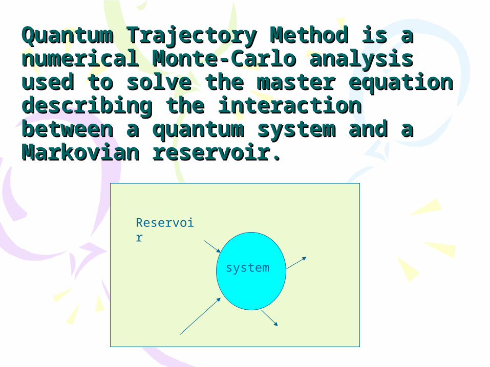
Quantum Trajectory Method is a Quantum Trajectory Method is a numerical Monte-Carlo analysis numerical Monte-Carlo analysis used to solve the master equation used to solve the master equation describing the interaction between describing the interaction between a quantum system and a Markovian a quantum system and a Markovian reservoir.reservoir.
system
Reservoir
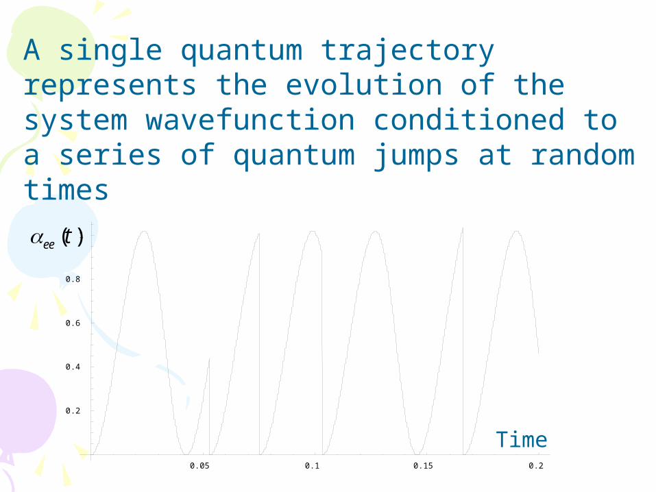
A single quantum trajectory represents the evolution of the system wavefunction conditioned to a series of quantum jumps at random times
0.05 0.1 0.15 0.2
0.2
0.4
0.6
0.8
1
Time
( )ee t
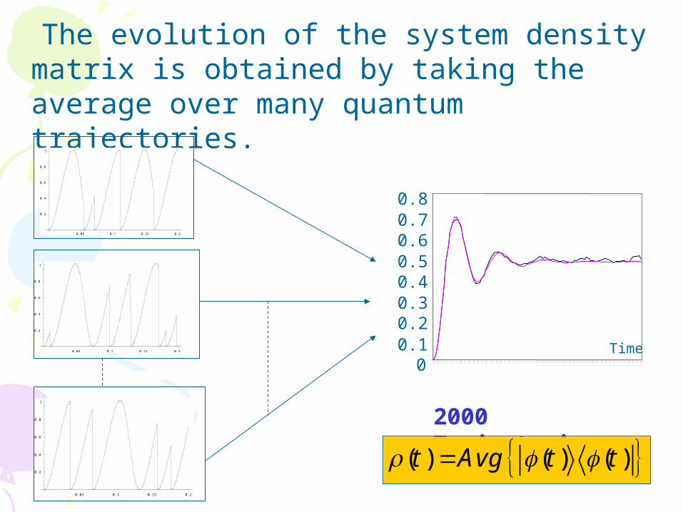
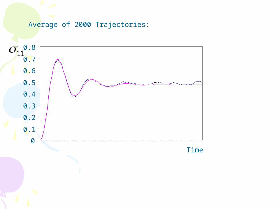
The evolution of the system density matrix is obtained by taking the average over many quantum trajectories.
0.05 0.1 0.15 0.2
0.2
0.4
0.6
0.8
1
0.05 0.1 0.15 0.2
0.2
0.4
0.6
0.8
1
0.05 0.1 0.15 0.2
0.2
0.4
0.6
0.8
1
2000 Trajectories
00.10.20.30.40.50.60.70.8
Time
( ) ( ) ( )t Avg t t
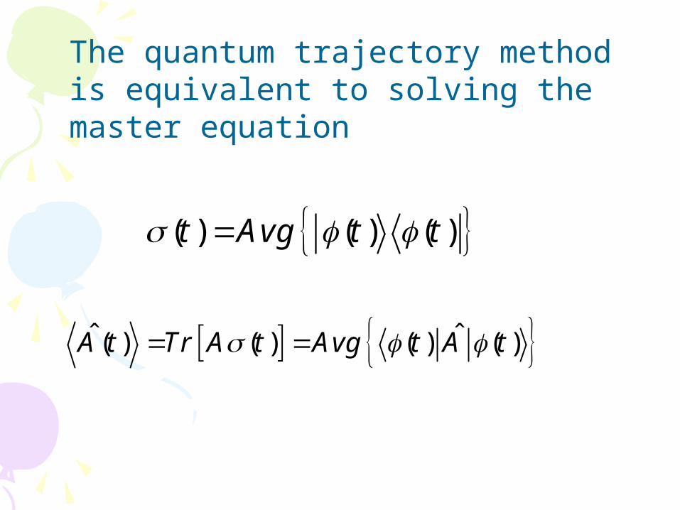
( ) ( ) ( )t Avg t t
ˆ ˆ( ) ( ) ( ) ( )A t Tr A t Avg t A t
The quantum trajectory method is equivalent to solving the master equation
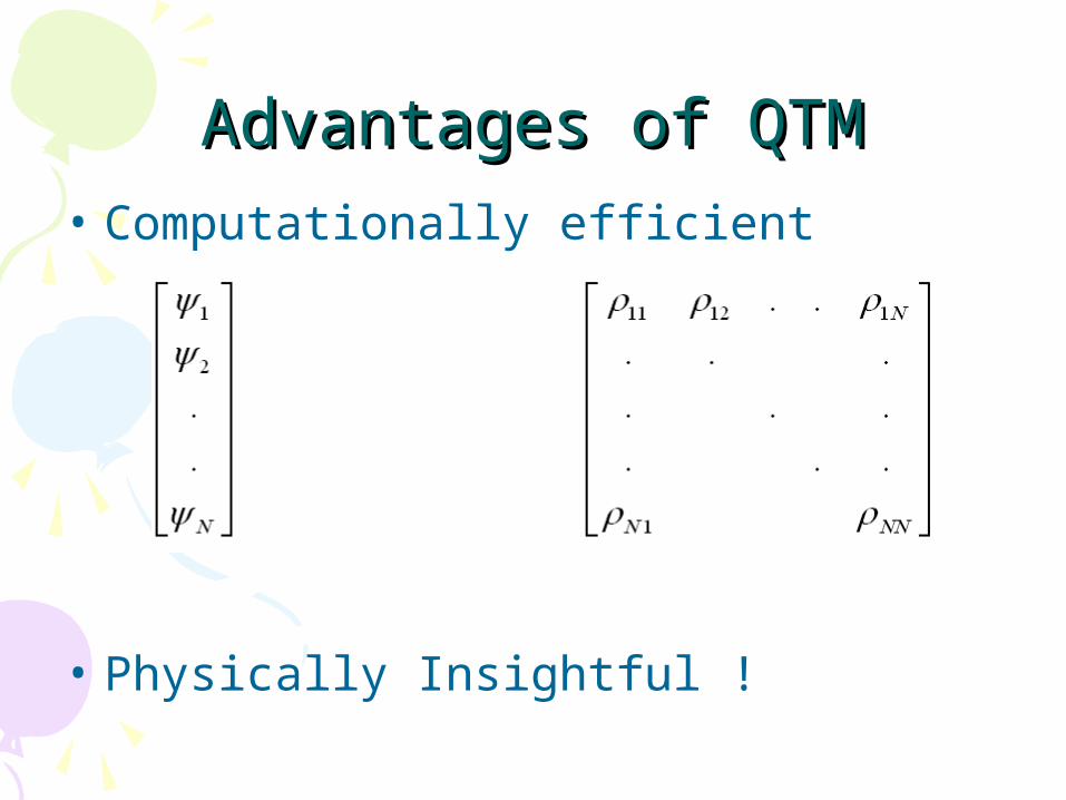
Advantages of QTMAdvantages of QTM• Computationally efficient
• Physically Insightful !
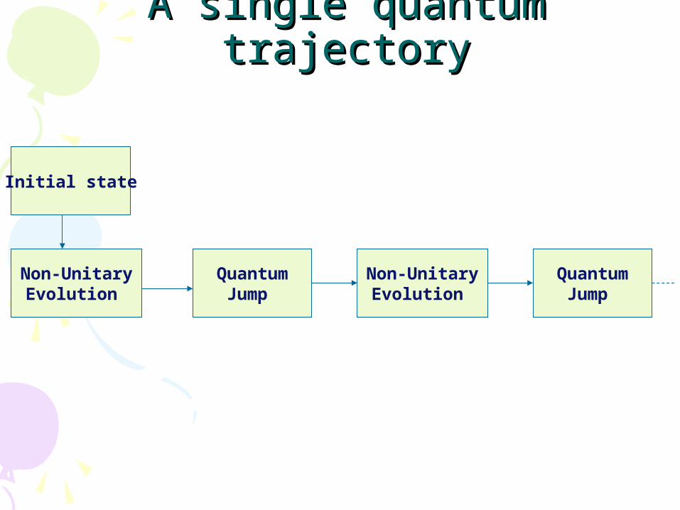
A single quantum trajectoryA single quantum trajectory
Initial state
Non-Unitary Evolution
Quantum Jump
Non-Unitary Evolution
Quantum Jump
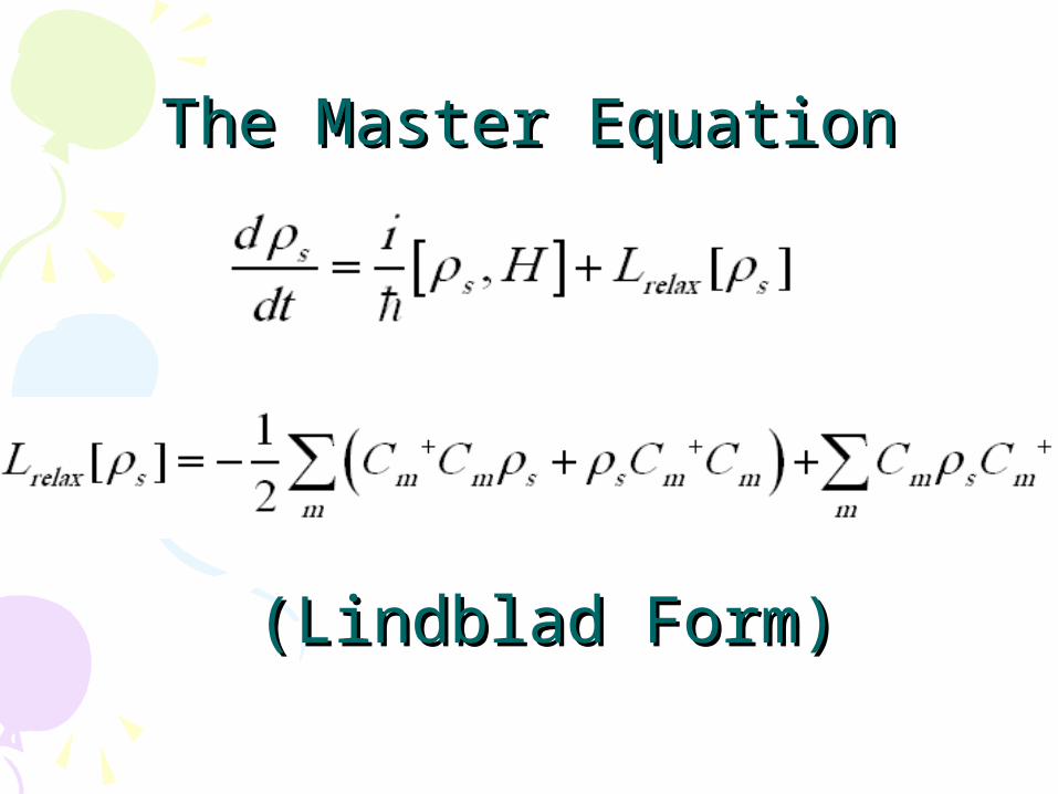
The Master EquationThe Master Equation
((Lindblad FormLindblad Form))
Two level atom Two level atom interacting with a interacting with a
classical field classical field
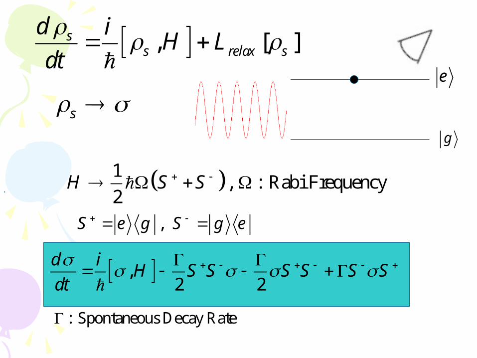
s
, [ ]ss relax s
d iH L
dt
,2 2
d iH S S S S S S
dt
. 1, : Rabi Frequency
2H S S
e
g
: Spontaneous Decay Rate
, S e g S g e
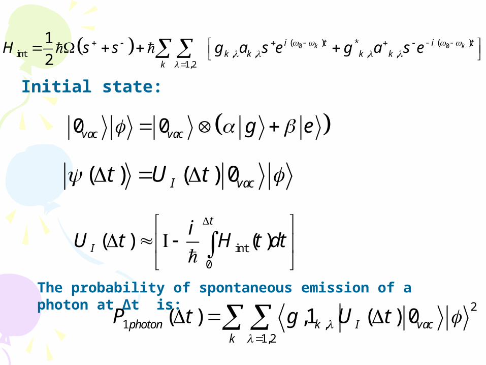
0 0( ) ( )*int , , , ,
1,2
1
2k ki t i t
k k k kk
H s s g a s e g a s e
0 0vac vac g e
( ) ( ) 0I vact U t
int
0
( ) ( )t
I
iU t H t dt
The probability of spontaneous emission of a photon at Δt is: 2
1 ,1,2
( ) ,1 ( ) 0photon k I vack
P t g U t
Initial state:
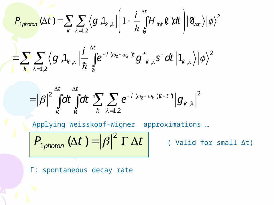
2
1 , int1,2 0
( ) ,1 ( ) 0t
photon k vack
iP t g H t dt
02( ) *
, , ,1,2 0
,1 1k
ti t
k k kk
ig e g s dt
022 ( )( ')
,1,20 0
' k
t ti t t
kk
dt dt e g
2
1 ( ) . .photonP t t
Г: spontaneous decay rate
Applying Weisskopf-Wigner approximations …
( Valid for small Δt)
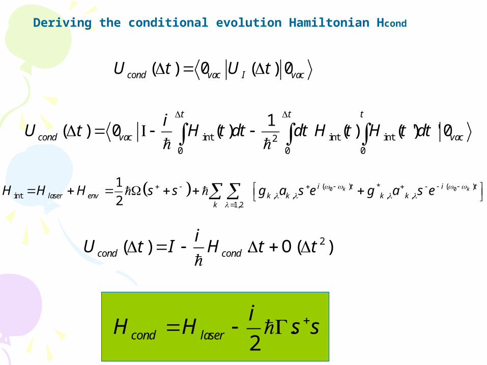
Deriving the conditional evolution Hamiltonian Hcond
( ) 0 ( ) 0cond vac I vacU t U t
int int int20 0 0
1( ) 0 ( ) ( ) ( ') ' 0
t t t
cond vac vac
iU t H t dt dt H t H t dt
0 0( ) ( )*int , , , ,
1,2
1
2k ki t i t
laser env k k k kk
H H H s s g a s e g a s e
2( ) . ( )cond cond
iU t I H t t
O
.2cond laser
iH H s s
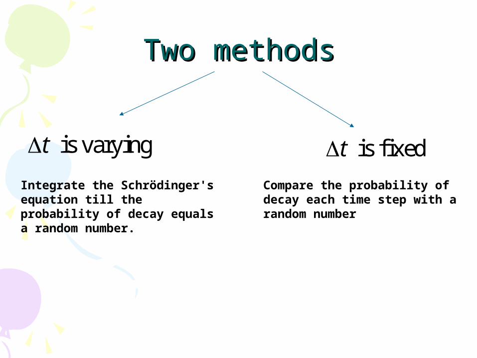
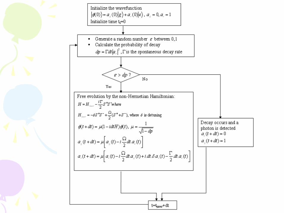
Two methodsTwo methods
is fixedtCompare the probability of decay each time step with a random number
is varyingt
Integrate the Schrödinger's equation till the probability of decay equals a random number.
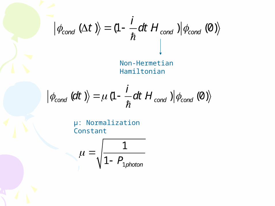
( ) (1 . ) (0)cond cond cond
it dt H
Non-Hermetian Hamiltonian
( ) (1 . ) (0)cond cond cond
idt dt H
μ: Normalization Constant
1
1
1 photonP
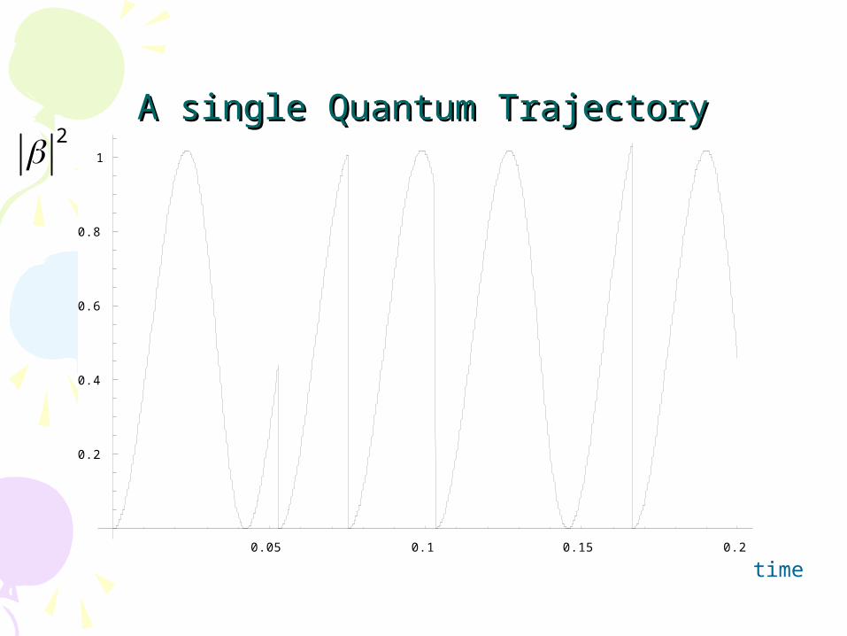
A single Quantum TrajectoryA single Quantum Trajectory
0.05 0.1 0.15 0.2
0.2
0.4
0.6
0.8
1
time
2
0
0.1
0.2
0.3
0.4
0.5
0.6
0.7
0.8
Average of 2000 Trajectories:
Time
11

Spontaneous decay in the absence of the driving field
time
11
0.05 0.1 0.15 0.2
0.2
0.4
0.6
0.8
1
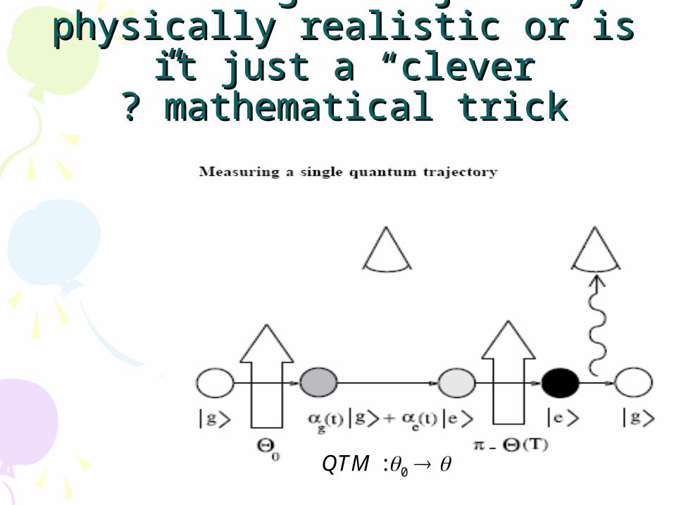
Is a single trajectory physically Is a single trajectory physically realistic or is it just a “clever realistic or is it just a “clever
mathematical trickmathematical trick?”?”
0: QTM
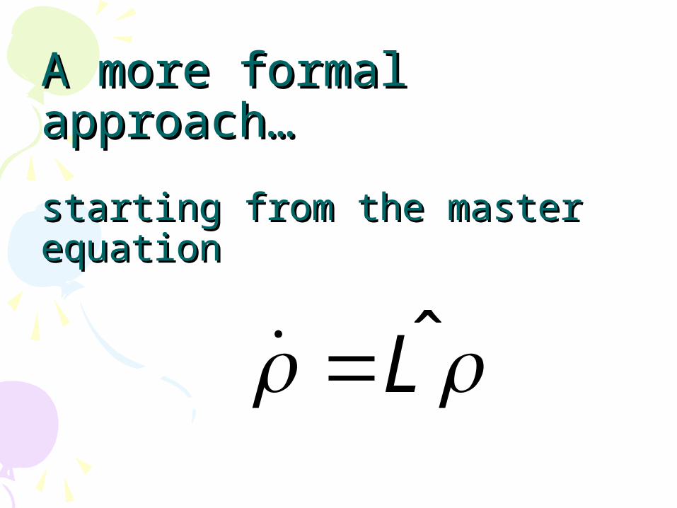
A more formal A more formal approach…approach…
starting from the master starting from the master equationequation
L̂
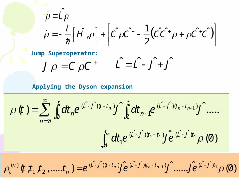
1ˆ ˆ ˆ ˆ ˆ ˆˆ ,2
iH C C CC C C
J C C Jump Superoperator:
Applying the Dyson expansion
1
22 1 1
ˆ ˆ ˆ ˆ( )( ) ( )( )10 0
0
ˆ ˆ ˆ ˆ( )( ) ( )10
ˆ ˆ( ) .....
ˆ (0)
n n nt tL J t t L J t t
n nn
t L J t t L J t
t dt e J dt e J
dt e Je
L̂
1 1ˆ ˆ ˆ ˆ ˆ ˆ( )( ) ( )( ) ( )( )
1 2ˆ ˆ ˆ( ; , ,...... ) ....... (0)n n nL J t t L J t t L J tn
c nt t t t e Je J Je
ˆ ˆ ˆ ˆL L J J
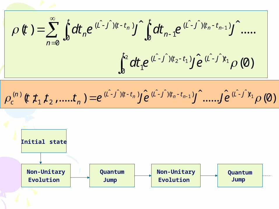
Initial state
Non-Unitary Evolution
Quantum Jump
Non-Unitary Evolution
Quantum Jump
1
22 1 1
ˆ ˆ ˆ ˆ( )( ) ( )( )10 0
0
ˆ ˆ ˆ ˆ( )( ) ( )10
ˆ ˆ( ) .....
ˆ (0)
n n nt tL J t t L J t t
n nn
t L J t t L J t
t dt e J dt e J
dt e Je
1 1
ˆ ˆ ˆ ˆ ˆ ˆ( )( ) ( )( ) ( )( )1 2
ˆ ˆ ˆ( ; , ,...... ) ....... (0)n n nL J t t L J t t L J tnc nt t t t e Je J Je
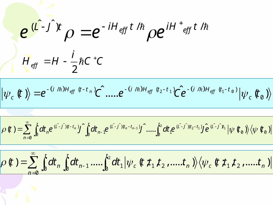
ˆ ˆ / /( ) eff effiH t iH tL J te e e
2eff
iH H C C
2 1 1 0/ ( ) / ( ) / ( )0
ˆ ˆ( ) ...... ( )eff n eff effi H t t i H t t i H t tc ct e C e Ce t
21 2 1 1
ˆ ˆ ˆ ˆ ˆ ˆ ˆ ˆ( )( ) ( )( ) ( )( ) ( )1 1 0 00 0 0
0
ˆ ˆ ˆ( ) ..... ( ) ( )n n nt t tL J t t L J t t L J t t L J t
n nn
t dt e J dt e J dt e Je t t
2
1 1 1 2 1 20 0 00
( ) ..... ( ; , ,...... ) ( ; , ,...... )t t t
n n c n c nn
t dt dt dt t t t t t t t t
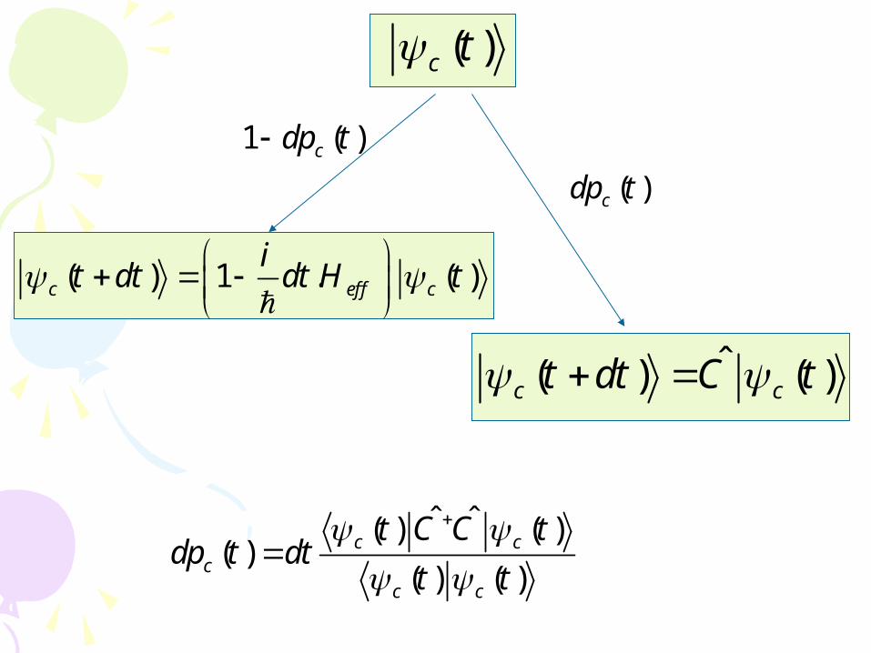
( )c t
ˆ( ) ( )c ct dt C t
( ) 1 . ( )c eff c
it dt dt H t
ˆ ˆ( ) ( )( )
( ) ( )c c
cc c
t C C tdp t dt
t t
( )cdp t
1 ( )cdp t
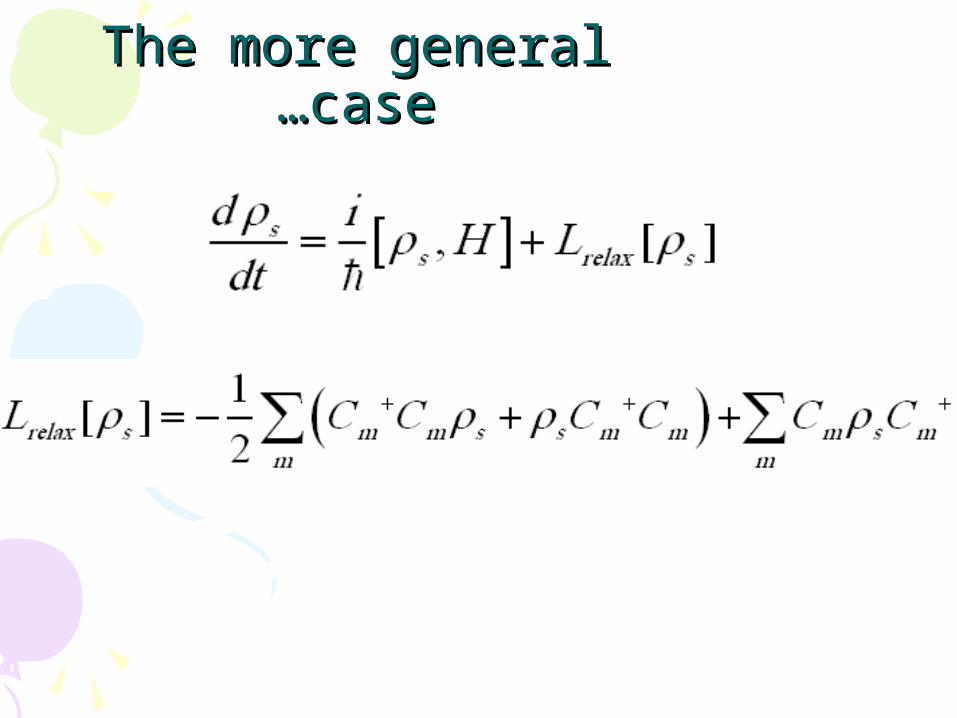
The more general caseThe more general case……
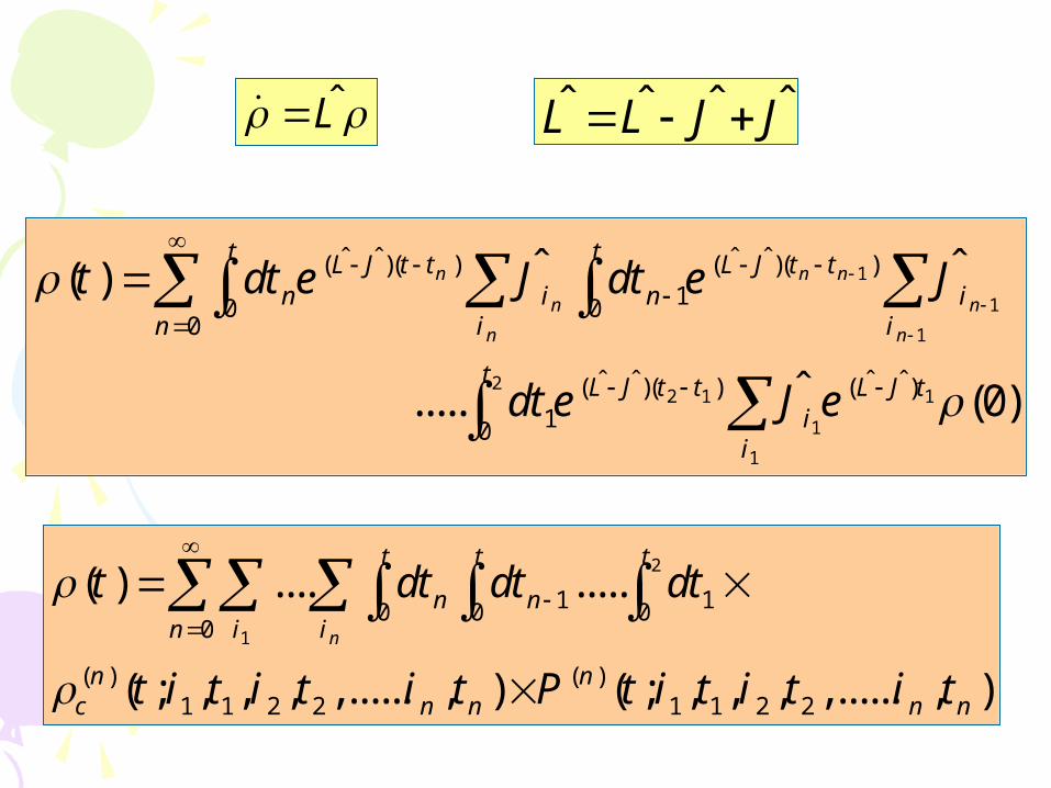
1
1
1
22 1 1
1
1
ˆ ˆ ˆ ˆ( )( ) ( )( )10 0
0
ˆ ˆ ˆ ˆ( )( ) ( )10
ˆ ˆ( )
ˆ ..... (0)
n n n
n n
n n
t tL J t t L J t tn i n i
n i i
t L J t t L J ti
i
t dt e J dt e J
dt e J e
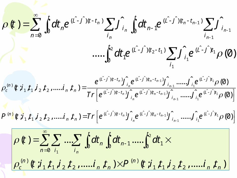
2
1
1 10 0 00
( ) ( )1 1 2 2 1 1 2 2
( ) .... .....
( ; , , , ,...... , ) ( ; , , , ,...... , )
n
t t t
n nn i i
n nc n n n n
t dt dt dt
t i t i t i t P t i t i t i t
L̂ ˆ ˆ ˆ ˆL L J J
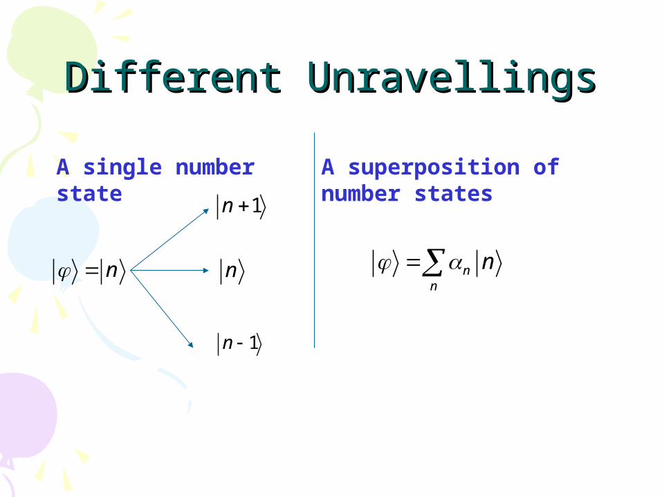
Different UnravellingsDifferent Unravellings
n
1n
1n
A single number state
n nn
n
A superposition of number states
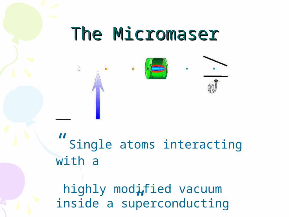
The MicromaserThe Micromaser
“Single atoms interacting with a
highly modified vacuum inside
a superconducting resonator”
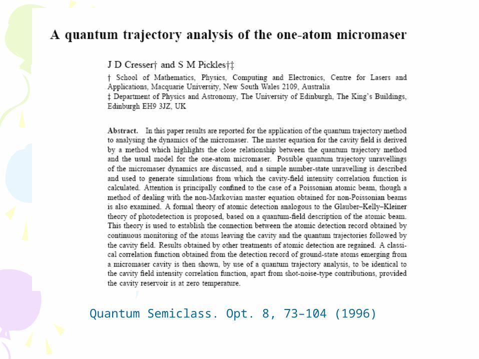
Quantum Semiclass. Opt. 8, 73–104 (1996)
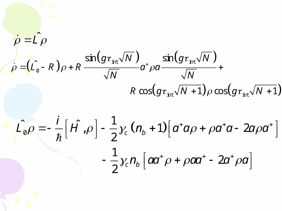
L̂
int int
0
int int
sin sinˆ
cos 1 cos 1
g N g NL R R a a
N N
R g N g N
0
1ˆ ˆ , 1 221
22
c b
c b
iL H n a a a a a a
n aa aa a a
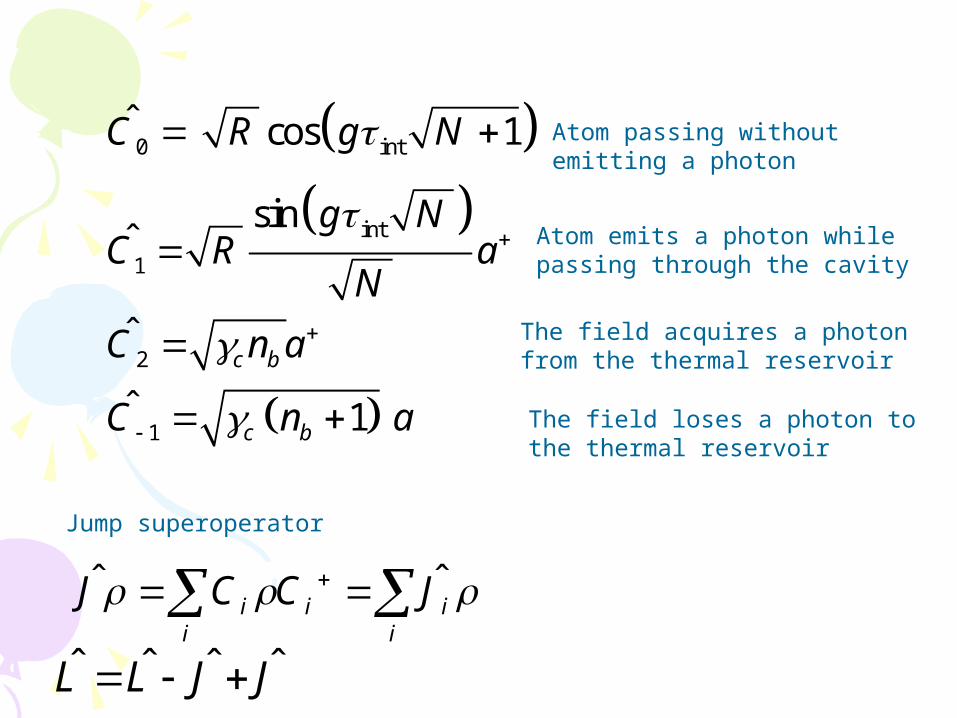
0 int
int
1
2
1
ˆ cos 1
sinˆ
ˆ
ˆ 1
c b
c b
C R g N
g NC R a
N
C n a
C n a
Atom passing without emitting a photon
Atom emits a photon while passing through the cavity
The field acquires a photon from the thermal reservoir
The field loses a photon to the thermal reservoir
ˆ ˆi i i
i i
J C C J Jump superoperator
ˆ ˆ ˆ ˆL L J J
1
1
1
22 1 1
1
1
ˆ ˆ ˆ ˆ( )( ) ( )( )10 0
0
ˆ ˆ ˆ ˆ( )( ) ( )10
ˆ ˆ( )
ˆ ..... (0)
n n n
n n
n n
t tL J t t L J t tn i n i
n i i
t L J t t L J ti
i
t dt e J dt e J
dt e J e
1 1
1 1
1 1
1 1
ˆ ˆ ˆ ˆ ˆ ˆ( )( ) ( )( ) ( )( )
1 1 2 2 ˆ ˆ ˆ ˆ ˆ ˆ( )( ) ( )( ) ( )
ˆ ˆ ˆ....... (0)( ; , , , ,...... , )
ˆ ˆ ˆ....... (0)
n n n
n n
n n n
n n
L J t t L J t t L J ti i in
c n n L J t t L J t t L J ti i i
e J e J J et i t i t i t
Tr e J e J J e
1 1
1 1
ˆ ˆ ˆ ˆ ˆ ˆ( )( ) ( )( ) ( )( )1 1 2 2
ˆ ˆ ˆ( ; , , , ,...... , ) ....... (0)n n n
n n
L J t t L J t t L J tnn n i i iP t i t i t i t Tr e J e J J e
2
1
1 10 0 00
( ) ( )1 1 2 2 1 1 2 2
( ) .... .....
( ; , , , ,...... , ) ( ; , , , ,...... , )
n
t t t
n nn i i
n nc n n n n
t dt dt dt
t i t i t i t P t i t i t i t
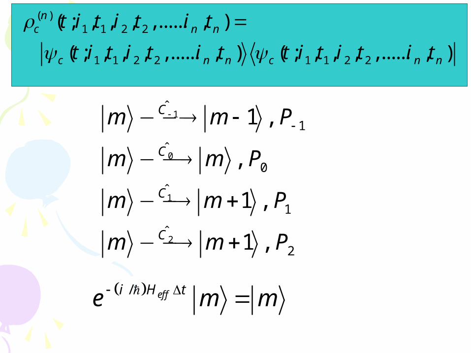
( )1 1 2 2
1 1 2 2 1 1 2 2
( ; , , , ,...... , )
( ; , , , ,...... , ) ( ; , , , ,...... , )
nc n n
c n n c n n
t i t i t i t
t i t i t i t t i t i t i t
1
0
1
2
ˆ
1
ˆ
0
ˆ
1
ˆ
2
1 ,
,
1 ,
1 ,
C
C
C
C
m m P
m m P
m m P
m m P
/ effi H te m m
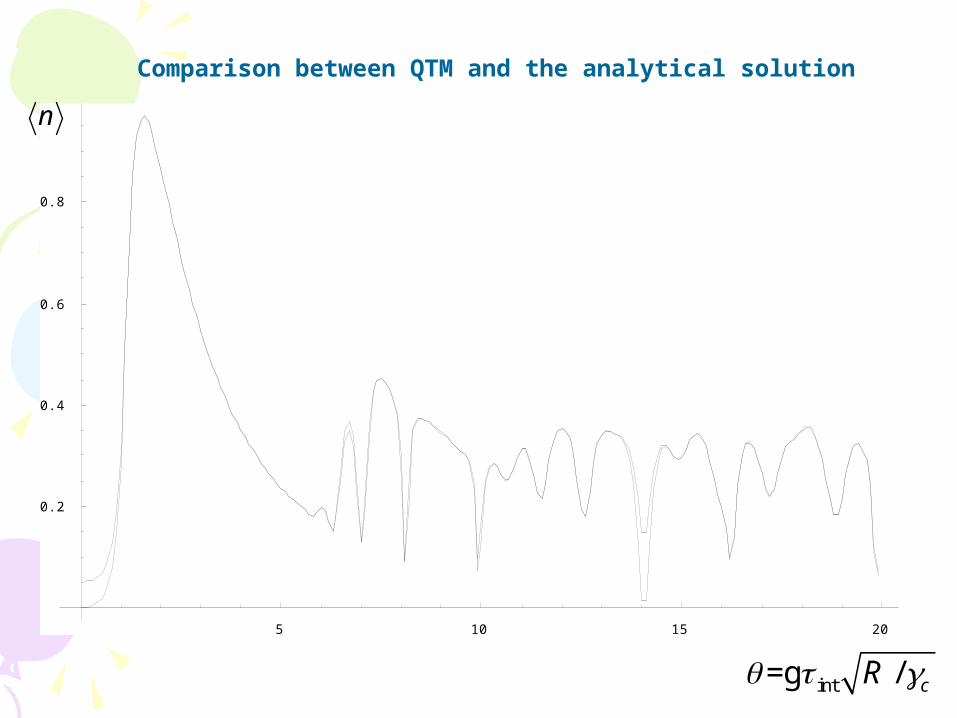
5 10 15 20
0.2
0.4
0.6
0.8
n
Comparison between QTM and the analytical solution
int=g / cR
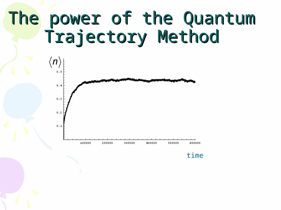
The power of the Quantum The power of the Quantum Trajectory MethodTrajectory Method
time
n
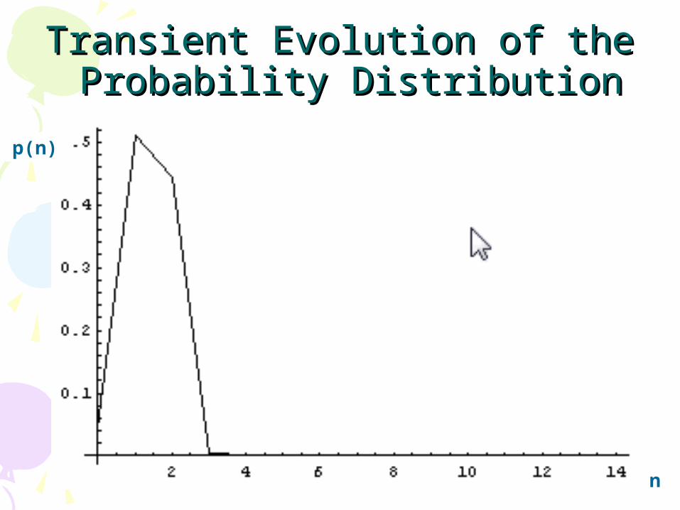
Transient Evolution of the Transient Evolution of the Probability DistributionProbability Distribution
p(n)
n
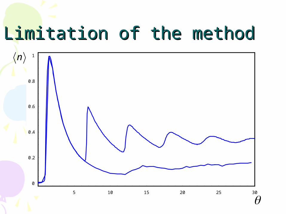
Limitation of the methodLimitation of the method
5 10 15 20 25 30
0
0.2
0.4
0.6
0.8
1n
ConclusionConclusion• Quantum Trajectory Method can be
used efficiently to simulate transient and steady state behavior of quantum systems interacting with a markovian reservoir.
• They are most useful when no simple analytic solution exists or the dimensions of the density matrix are very large.
ReferencesReferences• A quantum trajectory analysis of the one-atom micromaser, J D
Cressery and S M Pickles, Quantum Semiclass. Opt. 8, 73–104 (1996)
• Wave-function approach to dissipative processes in quantum optics,Phys. Rev. Lett., 68, 580 (1992)
• Quantum Trajectory Method in Quantum Optics, Young-Tak Chough
• Measuring a single quantum trajectory, D Bouwmeester and G Nienhuis, Quantum Semiclass. Opt. 8 (1996) 277–282

QuestionsQuestions……


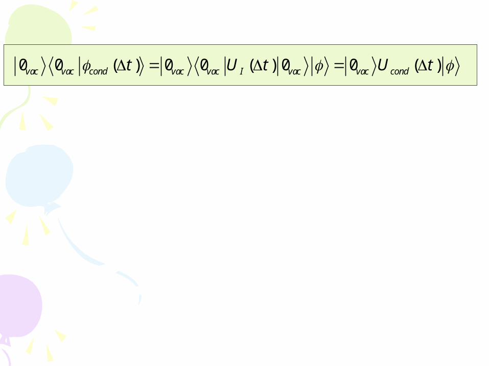
0 0 ( ) 0 0 ( ) 0 0 ( )vac vac cond vac vac I vac vac condt U t U t
Related Documents


![HOLOGRAPHY, QUANTUM GEOMETRY, AND QUANTUM INFORMATION THEORY · The emerging fields of quantum computation [22], quantum communication and quantum cryptography [23], quantum dense](https://static.cupdf.com/doc/110x72/5ec76f6b603b2e345706bd5a/holography-quantum-geometry-and-quantum-information-theory-the-emerging-fields.jpg)