Quantum Theory in Accelerated Frames of Reference

arX

iv:h

ep-t

h/05

0715

7v1

15

Jul 2

005

Quantum Theory in Accelerated Frames of Reference

Bahram Mashhoon

Department of Physics and Astronomy

University of Missouri-Columbia

Columbia, Missouri 65211, USA

Abstract

The observational basis of quantum theory in accelerated systems is studied. The

extension of Lorentz invariance to accelerated systems via the hypothesis of locality

is discussed and the limitations of this hypothesis are pointed out. The nonlocal

theory of accelerated observers is briefly described. Moreover, the main observa-

tional aspects of Dirac’s equation in noninertial frames of reference are presented.

The Galilean invariance of nonrelativistic quantum mechanics and the mass super-

selection rule are examined in the light of the invariance of physical laws under

inhomogeneous Lorentz transformations.

1. INTRODUCTION

Soon after Dirac discovered the relativistic wave equation for a spin 12

particle [1], the

generally covariant Dirac equation was introduced by Fock and Ivanenko [2] and was studied

in great detail by a number of authors [3]. Dirac’s equation

(i~γα∂α −mc)ψ = 0 (1)

transforms under a Lorentz transformation x′α = Lαβ x

β as

ψ′(x′) = S(L)ψ(x), (2)

where S(L) is connected with the spin of the particle and is given by

S−1γαS = Lαβγ

β. (3)

The generally covariant Dirac equation can be written as

(i~γµ∇µ −mc)ψ = 0, (4)

2

where ∇µ = ∂µ + Γµ and Γµ is the spin connection. Let us consider a class of observers in

spacetime with an orthonormal tetrad frame λµ

(α), i.e.

gµνλµ

(α)λν(β) = η(α)(β), (5)

where η(α)(β) is the Minkowski metric tensor. Then in equation (4), γµ is given by γµ =

λµ

(α)γ(α) and

Γµ = −i

4λν(α)[λ

ν(β)];µ σ

(α)(β), (6)

where

σ(α)(β) =i

2[γ(α), γ(β)]. (7)

In this way, the generally covariant Dirac equation is minimally coupled to inertia and

gravitation.

The standard quantum measurement theory involves ideal inertial observers. However,

all actual observers are more or less accelerated. Indeed, the whole observational basis of

Lorentz invariance as well as quantum mechanics rests upon measurements performed by ac-

celerated observers. It is therefore necessary to discuss how the measurements of noninertial

observers are connected with those of ideal inertial observers. This paper is thus organized

into two parts. In the first part, sections 2-4, we consider the basic physical assumptions

that underlie the covariant generalization of Dirac’s equation. The second part, sections 5-

9, are devoted to the physical consequences of this generalization for noninertial frames of

reference. In particular, the connection between the relativistic theory and nonrelativistic

quantum mechanics in accelerated systems is examined in detail. Section 10 contains a brief

discussion.

2. HYPOTHESIS OF LOCALITY

The extension of Lorentz invariance to noninertial systems necessarily involves an as-

sumption regarding what accelerated observers actually measure. What is assumed in the

standard theory of relativity is the hypothesis of locality, which states that an accelerated

observer is pointwise equivalent to an otherwise identical momentarily comoving inertial ob-

server. It appears that Lorentz first introduced such an assumption in his theory of electrons

to ensure that an electron—conceived as a small ball of charge—is always Lorentz contracted

along its direction of motion [4]. He clearly recognized that this is simply an approximation

3

based on the assumption that the time in which the electron velocity changes is very long

compared to the period of the internal oscillations of the electron (see section 183 on page

216 of [4]).

The hypothesis of locality was later adopted by Einstein in the course of the develop-

ment of the theory of relativity (see the footnote on page 60 of [5]). In retrospect, the

locality assumption fits perfectly together with Einstein’s local principle of equivalence to

guarantee that every observer in a gravitational field is locally (i.e. pointwise) inertial. That

is, Einstein’s heuristic principle of equivalence, namely, the presumed local equivalence of

an observer in a gravitational field with an accelerated observer in Minkowski spacetime,

would lose its operational significance if one did not know what accelerated observers mea-

sure. However, combined with the hypothesis of locality, Einstein’s principle of equivalence

provides a basis for a theory of gravitation that is consistent with (local) Lorentz invariance.

Early in the development of the theory of relativity, the hypothesis of locality was usually

stated in terms of the direct acceleration independence of the behavior of rods and clocks.

The clock hypothesis, for instance, states that “standard” clocks measure proper time. Thus

measuring devices that conform to the hypothesis of locality are usually called “standard”.

It is clear that inertial effects exist in any accelerated measuring device; however, in a

standard device these effects are usually expected to integrate to a negligible influence over

the duration of each elementary measurement. Thus a standard measuring device is locally

inertial [6].

Following the development of the general theory of relativity, the hypothesis of locality

was discussed by Weyl [7]. Specifically, Weyl [7] noted that the locality hypothesis was an

adiabaticity assumption in analogy with slow processes in thermodynamics.

The hypothesis of locality originates from Newtonian mechanics: the accelerated observer

and the otherwise identical momentarily comoving inertial observer have the same position

and velocity; therefore, they share the same state and are thus pointwise identical in clas-

sical mechanics. The evident validity of this assertion for Newtonian point particles means

that no new assumption is required in the treatment of accelerated systems of reference in

Newtonian mechanics. It should also hold equally well in the classical relativistic mechanics

of point particles, as originally recognized by Minkowski (see page 80 of [8]). If all phys-

ical phenomena could be reduced to pointlike coincidences of particles and rays, then the

hypothesis of locality would be exactly valid.

4

The hypothesis of locality is not in general valid, however, in the case of classical wave

phenomena. Consider, for instance, the determination of the frequency of an incident elec-

tromagnetic wave by a linearly accelerated observer. Clearly, the frequency cannot be de-

termined instantaneously; in fact, the observer needs to measure a few oscillations of the

electromagnetic field before a reasonable determination of the frequency becomes opera-

tionally possible. Let λ be the characteristic wavelength of the incident radiation and L

be the acceleration length of the observer; then, the hypothesis of locality is approximately

valid for λ≪ L. Here L is a length scale that involves the speed of light c and certain scalars

formed from the acceleration of the observer such that the acceleration time L/c character-

izes the time in which the velocity of the observer varies appreciably. In an Earth-based

laboratory, for instance, the main translational and rotational acceleration lengths would

be c2/g⊕ ≈ 1 lt-yr and c/Ω⊕ ≈ 28 AU, respectively. Thus in most experimental situations

λ/L is negligibly small and any possible deviations from the locality hypothesis are therefore

below the current levels of detectability. Indeed, in the ray limit, λ/L → 0, the hypothesis

of locality would be valid; therefore, λ/L is a measure of possible deviation from the locality

postulate.

Consider a classical particle of mass m and charge q under the influence of an external

force fext. The accelerated charge radiates electromagnetic radiation with a typical wave-

length λ ∼ L, where L is the acceleration length of the particle.We would expect that a

significant breakdown of the locality hypothesis occurs in this case, since λ/L ∼ 1 in the

interaction of the particle with the electromagnetic field. The violation of the hypothesis

of locality implies that the state of the particle cannot be characterized by its position and

velocity. This is indeed the case, since the equation of motion of the radiating particle in

the nonrelativistic approximation is given by the Abraham-Lorentz equation

mdv

dt−

2

3

q2

c3d2v

dt2+ · · · = fext (8)

which implies that position and velocity are not sufficient to specify the state of the radiating

charged particle [9].

To discuss quantum mechanics in an accelerated system of reference, it is therefore useful

to investigate the status of the hypothesis of locality vis-a-vis the basic principles of quantum

theory. The physical interpretation of wave functions is based on the notion of wave-particle

duality. On the other hand, the locality hypothesis is valid for classical particles and is in

5

general violated for classical waves. This circumstance provides the motivation to develop a

nonlocal theory of accelerated systems that would go beyond the hypothesis of locality and

would be consistent with wave-particle duality. Such a theory has been developed [10] and

can be employed, in principle, to describe a nonlocal Dirac equation in accelerated systems

of reference. Some of the main aspects of the nonlocal theory are described in section 4.

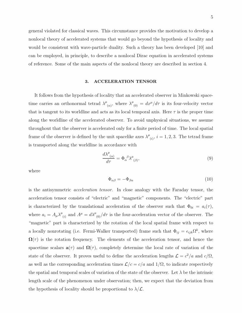
3. ACCELERATION TENSOR

It follows from the hypothesis of locality that an accelerated observer in Minkowski space-

time carries an orthonormal tetrad λµ

(α), where λµ

(0) = dxµ/dτ is its four-velocity vector

that is tangent to its worldline and acts as its local temporal axis. Here τ is the proper time

along the worldline of the accelerated observer. To avoid unphysical situations, we assume

throughout that the observer is accelerated only for a finite period of time. The local spatial

frame of the observer is defined by the unit spacelike axes λµ

(i), i = 1, 2, 3. The tetrad frame

is transported along the worldline in accordance with

dλµ

(α)

dτ= Φ β

α λµ

(β), (9)

where

Φαβ = −Φβα (10)

is the antisymmetric acceleration tensor. In close analogy with the Faraday tensor, the

acceleration tensor consists of “electric” and “magnetic” components. The “electric” part

is characterized by the translational acceleration of the observer such that Φ0i = ai(τ),

where ai = Aµλµ

(i) and Aµ = dλµ

(0)/dτ is the four-acceleration vector of the observer. The

“magnetic” part is characterized by the rotation of the local spatial frame with respect to

a locally nonrotating (i.e. Fermi-Walker transported) frame such that Φij = ǫijkΩk, where

Ω(τ) is the rotation frequency. The elements of the acceleration tensor, and hence the

spacetime scalars a(τ) and Ω(τ), completely determine the local rate of variation of the

state of the observer. It proves useful to define the acceleration lengths L = c2/a and c/Ω,

as well as the corresponding acceleration times L/c = c/a and 1/Ω, to indicate respectively

the spatial and temporal scales of variation of the state of the observer. Let λ be the intrinsic

length scale of the phenomenon under observation; then, we expect that the deviation from

the hypothesis of locality should be proportional to λ/L.

6

It follows from a detailed analysis that if D is the spatial dimension of a standard mea-

suring device, then D ≪ L [6]. Such devices are necessary for the determination of the local

frame of the accelerated observer. In fact, this circumstance is analogous to the correspon-

dence principle: while we are interested in the deviations from the hypothesis of locality,

such nonlocal effects are expected to be measured with standard measuring devices.

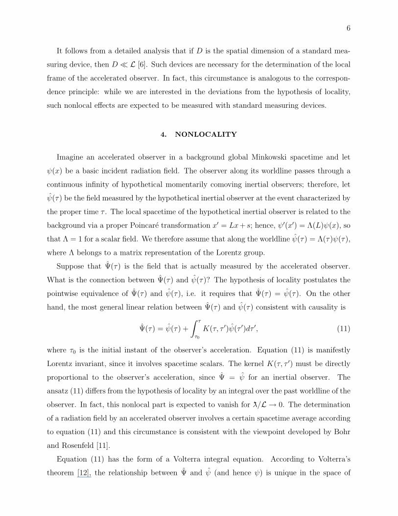
4. NONLOCALITY

Imagine an accelerated observer in a background global Minkowski spacetime and let

ψ(x) be a basic incident radiation field. The observer along its worldline passes through a

continuous infinity of hypothetical momentarily comoving inertial observers; therefore, let

ψ(τ) be the field measured by the hypothetical inertial observer at the event characterized by

the proper time τ . The local spacetime of the hypothetical inertial observer is related to the

background via a proper Poincare transformation x′ = Lx+ s; hence, ψ′(x′) = Λ(L)ψ(x), so

that Λ = 1 for a scalar field. We therefore assume that along the worldline ψ(τ) = Λ(τ)ψ(τ),

where Λ belongs to a matrix representation of the Lorentz group.

Suppose that Ψ(τ) is the field that is actually measured by the accelerated observer.

What is the connection between Ψ(τ) and ψ(τ)? The hypothesis of locality postulates the

pointwise equivalence of Ψ(τ) and ψ(τ), i.e. it requires that Ψ(τ) = ψ(τ). On the other

hand, the most general linear relation between Ψ(τ) and ψ(τ) consistent with causality is

Ψ(τ) = ψ(τ) +

∫ τ

τ0

K(τ, τ ′)ψ(τ ′)dτ ′, (11)

where τ0 is the initial instant of the observer’s acceleration. Equation (11) is manifestly

Lorentz invariant, since it involves spacetime scalars. The kernel K(τ, τ ′) must be directly

proportional to the observer’s acceleration, since Ψ = ψ for an inertial observer. The

ansatz (11) differs from the hypothesis of locality by an integral over the past worldline of the

observer. In fact, this nonlocal part is expected to vanish for λ/L → 0. The determination

of a radiation field by an accelerated observer involves a certain spacetime average according

to equation (11) and this circumstance is consistent with the viewpoint developed by Bohr

and Rosenfeld [11].

Equation (11) has the form of a Volterra integral equation. According to Volterra’s

theorem [12], the relationship between Ψ and ψ (and hence ψ) is unique in the space of

7

continuous functions. Volterra’s theorem has been extended to the Hilbert space of square-

integrable functions by Tricomi [13].

To determine the kernel K, we postulate that a basic radiation field can never stand

completely still with respect to an accelerated observer. This physical requirement is a

generalization of a well-known consequence of Lorentz invariance to all observers. That

is, the invariance of Maxwell’s equations under the Lorentz transformations implies that

electromagnetic radiation propagates with speed c with respect to all inertial observers.

That this is the case for any basic radiation field is reflected in the Doppler formula, ω′ =

γ(ω − v · k), where ω = c|k|. An inertial observer moving uniformly with speed v that

approaches c measures a frequency ω′ that approaches zero, but the wave will never stand

completely still (ω′ 6= 0) since v < c; hence, ω′ = 0 implies that ω = 0. Generalizing this

situation to arbitrary accelerated observers, we demand that if Ψ turns out to be a constant,

then ψ must have been constant in the first place. The Volterra-Tricomi uniqueness result

then implies that for any true radiation field ψ in the inertial frame, the field Ψ measured

by the accelerated observer will vary in time. Writing equation (11) as

Ψ(τ) = Λ(τ)ψ(τ) +

∫ τ

τ0

K(τ, τ ′)Λ(τ ′)ψ(τ ′)dτ ′, (12)

we note that our basic postulate that a constant Ψ be associated with a constant ψ implies

Λ(τ0) = Λ(τ) +

∫ τ

τ0

K(τ, τ ′)Λ(τ ′)dτ ′, (13)

where we have used the fact that Ψ(τ0) = Λ(τ0)ψ(τ0). Given Λ(τ), equation (13) can be

used to determine K(τ, τ ′); however, it turns out that K(τ, τ ′) cannot be uniquely specified

in this way. To go forward, it originally appeared most natural from the standpoint of

phenomenological nonlocal theories to postulate that K(τ, τ ′) is only a function of τ−τ ′ [10];

however, detailed investigations later revealed that such a convolution kernel can lead to

divergences in the case of nonuniform acceleration [14]. It turns out that the only physically

acceptable solution of equation (13) is of the form [15, 16]

K(τ, τ ′) = k(τ ′) = −dΛ(τ ′)

dτ ′Λ−1(τ ′). (14)

In the case of uniform acceleration, equation (14) and the convolution kernel both lead to

the same constant kernel. The kernel (14) is directly proportional to the acceleration of the

observer and is a simple solution of equation (13), as can be verified by direct substitution.

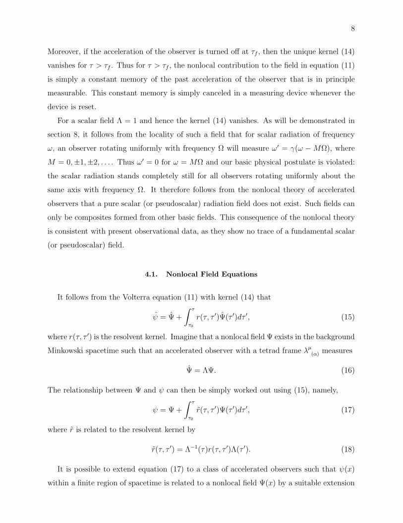
8

Moreover, if the acceleration of the observer is turned off at τf , then the unique kernel (14)

vanishes for τ > τf . Thus for τ > τf , the nonlocal contribution to the field in equation (11)

is simply a constant memory of the past acceleration of the observer that is in principle

measurable. This constant memory is simply canceled in a measuring device whenever the

device is reset.

For a scalar field Λ = 1 and hence the kernel (14) vanishes. As will be demonstrated in

section 8, it follows from the locality of such a field that for scalar radiation of frequency

ω, an observer rotating uniformly with frequency Ω will measure ω′ = γ(ω −MΩ), where

M = 0,±1,±2, . . . . Thus ω′ = 0 for ω = MΩ and our basic physical postulate is violated:

the scalar radiation stands completely still for all observers rotating uniformly about the

same axis with frequency Ω. It therefore follows from the nonlocal theory of accelerated

observers that a pure scalar (or pseudoscalar) radiation field does not exist. Such fields can

only be composites formed from other basic fields. This consequence of the nonlocal theory

is consistent with present observational data, as they show no trace of a fundamental scalar

(or pseudoscalar) field.

4.1. Nonlocal Field Equations

It follows from the Volterra equation (11) with kernel (14) that

ψ = Ψ +

∫ τ

τ0

r(τ, τ ′)Ψ(τ ′)dτ ′, (15)

where r(τ, τ ′) is the resolvent kernel. Imagine that a nonlocal field Ψ exists in the background

Minkowski spacetime such that an accelerated observer with a tetrad frame λµ

(α) measures

Ψ = ΛΨ. (16)

The relationship between Ψ and ψ can then be simply worked out using (15), namely,

ψ = Ψ +

∫ τ

τ0

r(τ, τ ′)Ψ(τ ′)dτ ′, (17)

where r is related to the resolvent kernel by

r(τ, τ ′) = Λ−1(τ)r(τ, τ ′)Λ(τ ′). (18)

It is possible to extend equation (17) to a class of accelerated observers such that ψ(x)

within a finite region of spacetime is related to a nonlocal field Ψ(x) by a suitable extension

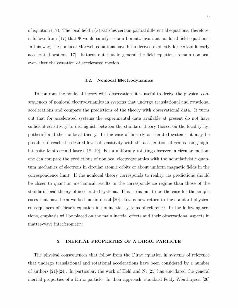
9

of equation (17). The local field ψ(x) satisfies certain partial differential equations; therefore,

it follows from (17) that Ψ would satisfy certain Lorentz-invariant nonlocal field equations.

In this way, the nonlocal Maxwell equations have been derived explicitly for certain linearly

accelerated systems [17]. It turns out that in general the field equations remain nonlocal

even after the cessation of accelerated motion.

4.2. Nonlocal Electrodynamics

To confront the nonlocal theory with observation, it is useful to derive the physical con-

sequences of nonlocal electrodynamics in systems that undergo translational and rotational

accelerations and compare the predictions of the theory with observational data. It turns

out that for accelerated systems the experimental data available at present do not have

sufficient sensitivity to distinguish between the standard theory (based on the locality hy-

pothesis) and the nonlocal theory. In the case of linearly accelerated systems, it may be

possible to reach the desired level of sensitivity with the acceleration of grains using high-

intensity femtosecond lasers [18, 19]. For a uniformly rotating observer in circular motion,

one can compare the predictions of nonlocal electrodynamics with the nonrelativistic quan-

tum mechanics of electrons in circular atomic orbits or about uniform magnetic fields in the

correspondence limit. If the nonlocal theory corresponds to reality, its predictions should

be closer to quantum mechanical results in the correspondence regime than those of the

standard local theory of accelerated systems. This turns out to be the case for the simple

cases that have been worked out in detail [20]. Let us now return to the standard physical

consequences of Dirac’s equation in noninertial systems of reference. In the following sec-

tions, emphasis will be placed on the main inertial effects and their observational aspects in

matter-wave interferometry.

5. INERTIAL PROPERTIES OF A DIRAC PARTICLE

The physical consequences that follow from the Dirac equation in systems of reference

that undergo translational and rotational accelerations have been considered by a number

of authors [21]-[24]. In particular, the work of Hehl and Ni [25] has elucidated the general

inertial properties of a Dirac particle. In their approach, standard Foldy-Wouthuysen [26]

10

transformations are employed to decouple the positive and negative energy states such that

the Hamiltonian for the Dirac particle may be written as

H = β

(

mc2 +p2

2m

)

+ βma · x −Ω · (L + S) (19)

plus higher-order terms. Here βma·x is an inertial term due to the translational acceleration

of the reference frame, while the inertial effects due to the rotation of the reference frame

are reflected in −Ω · (L + S).

Before proceeding to a detailed discussion of these inertial terms in sections 6-9, it

is important to observe that Obukhov [27] has recently introduced certain exact “Foldy-

Wouthuysen” (FW) transformations to decouple the positive and negative energy states of

the Dirac particle. Such a FW transformation is defined up to a unitary transformation,

which introduces a certain level of ambiguity in the physical interpretation. That is, it is

not clear from [27] what one could predict to be the observable consequences of Dirac’s

theory in noninertial systems and gravitational fields. For instance, in Obukhov’s exact FW

transformation, an inertial term of the form −12S ·a appears in the Hamiltonian [27]; on the

other hand, it is possible to remove this term by a unitary transformation [27]. The analog

of this term in a gravitational context would be 12S · g. Thus the energy difference between

the states of a Dirac particle with spin polarized up and down in a laboratory on the Earth

would be 12~g⊕ ≈ 10−23eV, which is a factor of five larger than what can be detected at

present [28]. A detailed examination of spin-acceleration coupling together with theoretical

arguments for its absence is contained in [29].

The general question raised in [27] has been treated in [30]. It appears that with a proper

choice of the unitary transformation such that physical quantities would correspond to simple

operators, the standard FW transformations of Hehl and Ni [25] can be recovered [30].

Nevertheless, a certain phase ambiguity can still exist in the wave function corresponding

to the fact that the unitary transformation may not be unique. This phase problem exists

even in the nonrelativistic treatment of quantum mechanics in translationally accelerated

systems as discussed in detail in section 9.

11

6. ROTATION

It is possible to provide a simple justification for the rotational inertial term in the

Hamiltonian (19). Let us start with the classical nonrelativistic Lagrangian of a particle

L = 12mv2 −W , where W is a potential energy. Under a transformation to a rotating frame

of reference, v = v′ + Ω × r, the Lagrangian takes the form

L′ =1

2m(v′ + Ω × r)2 −W, (20)

where W is assumed to be invariant under the transformation to the rotating frame. The

canonical momentum of the particle p′ = ∂L′/∂v′ = p is an invariant and we find that

H ′ = H − Ω · L, where L = r × p is the invariant angular momentum of the particle. Let

us note that this result of Newtonian mechanics [31] has a simple relativistic generalization:

the rotating observer measures the energy of the particle to be E ′ = γ(E − v · p), where

v = Ω × r; therefore, E ′ = γ(E −Ω · L).

This local approach may be simply extended to nonrelativistic quantum mechanics, where

the hypothesis of locality would imply that [32]

ψ′(x′, t) = ψ(x, t), (21)

since the rotating measuring devices are assumed to be locally inertial. Thus ψ′(x′, t) =

Rψ(x′, t), where

R = T ei

~

∫

t

0Ω(t′)·Jdt′ . (22)

Here T is the time-ordering operator and we have replaced L by J = L + S, since the total

angular momentum is the generator of rotations [32]. It follows that from the standpoint of

rotating observers, Hψ = i~∂ψ/∂t takes the form H ′ψ′ = i~∂ψ′/∂t, where

H ′ = RHR−1 −Ω · J . (23)

For the case of the single particle viewed by uniformly rotating observers, H ′ can be written

as

H ′ =1

2m(p′ −mΩ × r)2 −

1

2m(Ω × r)2 − Ω · S +W, (24)

where −12m(Ω × r)2 is the standard centrifugal potential and −Ω · S is the spin-rotation

coupling term [32]. The Hamiltonian (24) is analogous to that of a charged particle in a uni-

form magnetic field; this situation is a reflection of the Larmor theorem. The corresponding

12

analog of the Aharonov-Bohm effect is the Sagnac effect for matter waves [33]. This effect

is discussed in the next section.

7. SAGNAC EFFECT

The term −Ω · L in the Hamiltonian (19) signifies the coupling of the orbital angular

momentum of the particle with the rotation of the reference frame and is responsible for the

Sagnac effect exhibited by the Dirac particle. The corresponding Sagnac phase shift is given

by

∆ΦSagnac =2m

~

∫

Ω · dA, (25)

where A is the area of the interferometer. Equation (25) can be expressed as

∆ΦSagnac =2ω

c2

∫

Ω · dA, (26)

where mc2 ≈ ~ω and ω is the de Broglie frequency of the particle. Equation (26) is equally

valid for electromagnetic radiation of frequency ω.

For matter waves, the Sagnac effect was first experimentally measured for Cooper pairs

in a rotating superconducting Josephson-junction interferometer [34]. Using slow neutrons,

Werner et al. [35] measured the Sagnac effect with Ω as the rotation frequency of the

Earth. The result was subsequently confirmed with a rotating neutron interferometer in the

laboratory [36]. Significant advances in atom interferometry have led to the measurement of

the Sagnac effect for neutral atoms as well. This was first achieved by Riehle et al. [37] and

has been subsequently developed with a view towards achieving high sensitivity for atom

interferometers as inertial sensors [38]. In connection with charged particle interferometry,

the Sagnac effect has been observed for electrons by Hasselbach and Nicklaus [39].

The Sagnac effect has significant and wide-ranging applications and has been reviewed

in [40].

8. SPIN-ROTATION COUPLING

The transformation of the wave function to a uniformly rotating system of coordinates

involves (t, r, θ, φ) → (t, r, θ, φ + Ωt) in spherical coordinates, where Ω is the frequency of

rotation about the z axis. If the dependence of the wave function on φ and t is of the

13

form exp(iMφ − iEt/~), then in the rotating system the temporal dependence of the wave

function is given by exp[−i(E − ~MΩ)t/~]. The energy of the particle measured by an

observer at rest in the rotating frame is

E ′ = γ(E − ~MΩ), (27)

where γ = t/τ is the Lorentz factor due to time dilation. Here ~M is the total angular

momentum of the particle along the axis of rotation; in fact, M = 0,±1,±2, . . . , for a scalar

or a vector particle, while M ∓ 12

= 0,±1,±2, . . . , for a Dirac particle.

In the JWKB approximation, equation (27) may be expressed as E ′ = γ(E −Ω · J) and

hence

E ′ = γ(E − Ω · L) − γΩ · S. (28)

It follows that the energy measured by the observer is the result of an instantaneous Lorentz

transformation together with an additional term

δH = −γΩ · S, (29)

which is due to the coupling of the intrinsic spin of the particle with the frequncy of rotation

of the observer [32]. The dynamical origin of this term can be simply understood on the

basis of the following consideration: The intrinsic spin of a free particle remains fixed with

respect to the underlying global inertial frame; therefore, from the standpoint of observers

at rest in the rotating system, the spin precesses in the opposite sense as the rotation of the

observers. The Hamiltonian responsible for this inertial motion is given by equation (29).

The relativistic nature of spin-rotation coupling has been demonstrated by Ryder [41]. Let

us illustrate these ideas by a thought experiment involving the reception of electromagnetic

radiation of frequency ω by an observer that rotates uniformly with frequency Ω. We

assume for the sake of simplicity that the plane circularly polarized radiation is normally

incident on the path of the observer, i.e. the wave propagates along the axis of rotation.

We are interested in the frequency of the wave ω′ as measured by the rotating observer. A

simple application of the hypothesis of locality leads to the conclusion that the measured

frequency is related to ω by the transverse Doppler effect, ω′D = γω, since the instantaneous

rest frame of the observer is related to the background global inertial frame by a Lorentz

transformation. On the other hand, a different answer emerges when we focus attention on

14

the measured electromagnetic field rather than the propagation vector of the radiation,

F(α)(β)(τ) = Fµνλµ

(α)λν(β), (30)

where Fµν is the Faraday tensor of the incident radiation and λµ

(α) is the orthonormal tetrad

of the rotating observer. The nonlocal process of Fourier analysis of F(α)(β) results in [42]

ω′ = γ(ω ∓ Ω), (31)

where the upper (lower) sign refers to positive (negative) helicity radiation. We note that in

the eikonal limit Ω/ω → 0 and the instantaneous Doppler result is recovered. The general

problem of electromagnetic waves in a (uniformly) rotating frame of reference has been

treated in [43].

It is possible to understand equation (31) in terms of the relative motion of the observer

with respect to the field. In a positive (negative) helicity wave, the electric and magnetic

fields rotate with the wave frequency ω (−ω) about its direction of propagation. Thus

the rotating observer perceives that the electric and magnetic fields rotate with frequency

ω−Ω (−ω−Ω) about the direction of wave propagation. Taking due account of time dilation,

the observed frequency of the wave is thus γ(ω−Ω) in the positive helicity case and γ(ω+Ω)

in the negative helicity case. These results illustrate the phenomenon of helicity-rotation

coupling for the photon, since (31) can be written as E ′ = γ(E − S · Ω), where E = ~ω,

S = ~H and H = ±ck/ω is the unit helicity vector.

It follows from (31) that for a slowly moving detector γ ≈ 1 and

ω′ ≈ ω ∓ Ω, (32)

which corresponds to the phenomenon of phase wrap-up in the Global Positioning System

(GPS) [44]. In fact, equation (32) has been verified for ω/(2π) ≈ 1 GHz and Ω/(2π) ≈ 8 Hz

by means of the GPS [44]. For ω ≫ Ω, the modified Doppler and aberration formulas due

to the helicity-rotation coupling are [45]

ω′ = γ[(ω − H · Ω) − v · k], (33)

k′ = k +1

v2(γ − 1)(v · k)v −

1

c2γ(ω − H · Ω)v, (34)

and similar formulas can be derived for any spinning particle. Circularly polarized radiation

is routinely employed for radio communication with artificial satellites as well as Doppler

15

tracking of spacecraft. In general, the rotation of the emitter as well as the receiver should

be taken into account. It follows from (33) that ignoring helicity-rotation coupling would

lead to a systematic Doppler bias of magnitude cΩ/ω. In the case of the Pioneer spacecraft,

the anomalous acceleration resulting from the helicity-rotation coupling has been shown to

be negligibly small [46].

A half-wave plate flips the helicity of a photon that passes through it. Imagine a half-

wave plate that rotates uniformly with frequency Ω and an incident positive helicity plane

wave of frequency ωin that propagates along the axis of rotation. It follows from (32) that

ω′ ≈ ωin − Ω. The spacetime of a uniformly rotating system is stationary; therefore, ω′

remains fixed inside the plate. The radiation that emerges from the plate has frequency

ωout and negative helicity; hence, equation (32) implies that ω′ ≈ ωout + Ω. Thus the

rotating half-wave plate is a frequency shifter: ωout − ωin ≈ −2Ω. In general, any rotating

spin flipper can cause an up/down energy shift given by −2S · Ω as a consequence of the

spin-rotation coupling. The frequency-shift phenomenon was first discovered in microwave

experiments [47] and has subsequently been used in many optical experiments (see [45] for

a list of references).

Regarding the spin-rotation coupling for fermions, let us note that for experiments in a

laboratory fixed on the Earth, we must add to every Hamiltonian the spin-rotation-gravity

term

δH ≈ −S · Ω + S · ΩP , (35)

where the second term is due to the gravitomagnetic field of the Earth. That is, the rotation

of the Earth causes a dipolar gravitomagnetic field (due to mass current), which is locally

equivalent to a rotation by the gravitational Larmor theorem. In fact, ΩP is the frequency

of precession of an ideal fixed test gyro and is given by

ΩP ≈G

c2r5[3(J · r)r − Jr2], (36)

where J is the proper angular momentum of the central source. It follows from (35) that for

a spin 12

particle, the difference between the energy of the particle with spin up and down

in the laboratory is characterized by ~Ω⊕ ∼ 10−19eV and ~ΩP ∼ 10−29eV, while the present

experimental capabilities are in the 10−24eV range [28]. In fact, indirect observational evi-

dence for the spin-rotation coupling has been obtained [48] from the analysis of experiments

16

that have searched for anomalous spin-gravity interactions [49]. Further evidence for spin-

rotation coupling exists based on the analysis of muon g − 2 experiment [51].

An experiment to measure directly the spin-rotation coupling for a spin 12

particle was

originally proposed in [32]. This involved a large-scale neutron interferometry experiment

with polarized neutrons on a rotating platform [52]. A more recent proposal [53] employs

a rotating neutron spin flipper and hence is much more manageable as it avoids a large-

scale interferometer. The slow neutrons from a source are longitudinally polarized and the

beam is coherently split into two paths that contain neutron spin flippers, one of which

rotates with frequency Ω about the direction of motion of the neutrons. In this leg of the

interferometer, an energy shift δH = −2S ·Ω is thus introduced. The two beams are brought

back together and the interference beat frequency Ω is then measured. It is interesting to

note that a beat frequency in neutron interferometry has already been measured in another

context [54]; therefore, similar techniques can be used in the proposed experiment [53].

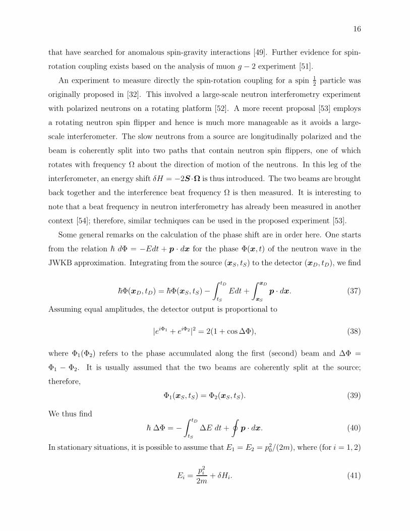
Some general remarks on the calculation of the phase shift are in order here. One starts

from the relation ~ dΦ = −Edt + p · dx for the phase Φ(x, t) of the neutron wave in the

JWKB approximation. Integrating from the source (xS, tS) to the detector (xD, tD), we find

~Φ(xD, tD) = ~Φ(xS, tS) −

∫ tD

tS

Edt+

∫ xD

xS

p · dx. (37)

Assuming equal amplitudes, the detector output is proportional to

|eiΦ1 + eiΦ2 |2 = 2(1 + cos ∆Φ), (38)

where Φ1(Φ2) refers to the phase accumulated along the first (second) beam and ∆Φ =

Φ1 − Φ2. It is usually assumed that the two beams are coherently split at the source;

therefore,

Φ1(xS, tS) = Φ2(xS, tS). (39)

We thus find

~ ∆Φ = −

∫ tD

tS

∆E dt+

∮

p · dx. (40)

In stationary situations, it is possible to assume that E1 = E2 = p20/(2m), where (for i = 1, 2)

Ei =p2

i

2m+ δHi. (41)

17

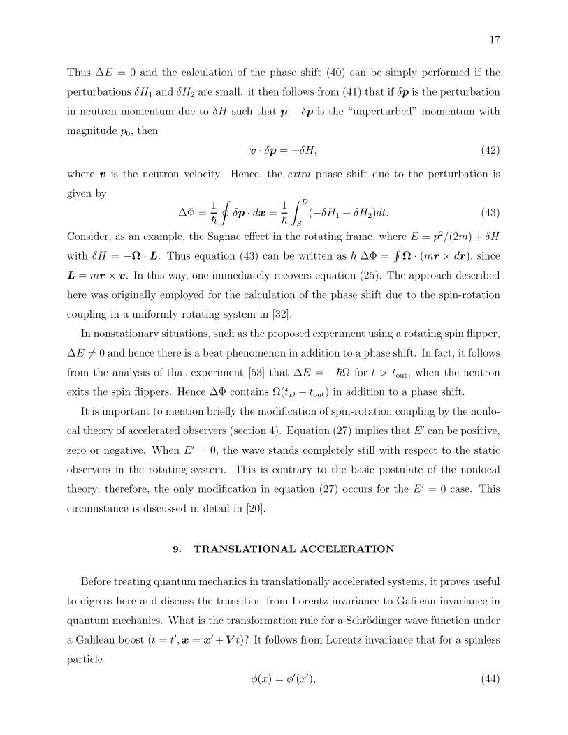
Thus ∆E = 0 and the calculation of the phase shift (40) can be simply performed if the

perturbations δH1 and δH2 are small. it then follows from (41) that if δp is the perturbation

in neutron momentum due to δH such that p − δp is the “unperturbed” momentum with

magnitude p0, then

v · δp = −δH, (42)

where v is the neutron velocity. Hence, the extra phase shift due to the perturbation is

given by

∆Φ =1

~

∮

δp · dx =1

~

∫ D

S

(−δH1 + δH2)dt. (43)

Consider, as an example, the Sagnac effect in the rotating frame, where E = p2/(2m) + δH

with δH = −Ω · L. Thus equation (43) can be written as ~ ∆Φ =∮

Ω · (mr × dr), since

L = mr × v. In this way, one immediately recovers equation (25). The approach described

here was originally employed for the calculation of the phase shift due to the spin-rotation

coupling in a uniformly rotating system in [32].

In nonstationary situations, such as the proposed experiment using a rotating spin flipper,

∆E 6= 0 and hence there is a beat phenomenon in addition to a phase shift. In fact, it follows

from the analysis of that experiment [53] that ∆E = −~Ω for t > tout, when the neutron

exits the spin flippers. Hence ∆Φ contains Ω(tD − tout) in addition to a phase shift.

It is important to mention briefly the modification of spin-rotation coupling by the nonlo-

cal theory of accelerated observers (section 4). Equation (27) implies that E ′ can be positive,

zero or negative. When E ′ = 0, the wave stands completely still with respect to the static

observers in the rotating system. This is contrary to the basic postulate of the nonlocal

theory; therefore, the only modification in equation (27) occurs for the E ′ = 0 case. This

circumstance is discussed in detail in [20].

9. TRANSLATIONAL ACCELERATION

Before treating quantum mechanics in translationally accelerated systems, it proves useful

to digress here and discuss the transition from Lorentz invariance to Galilean invariance in

quantum mechanics. What is the transformation rule for a Schrodinger wave function under

a Galilean boost (t = t′,x = x′ +V t)? It follows from Lorentz invariance that for a spinless

particle

φ(x) = φ′(x′), (44)

18

where φ is a scalar wave function that satisfies the Klein-Gordon equation(

+m2c2

~2

)

φ(x) = 0. (45)

To obtain the Schrodinger equation from (45) in the nonrelativistic limit, we set

φ(x) = ϕ(x, t)e−i mc2

~t. (46)

Then, (45) reduces to

−~

2

2m∇2ϕ = i~

∂ϕ

∂t−

~2

2mc2∂2ϕ

∂t2. (47)

Neglecting the term proportional to the second temporal derivative of ϕ in the nonrelativistic

limit (c→ ∞), we recover the Schrodinger equation for the wave function ϕ.

Under a Lorentz boost, (44) and (46) imply that

ϕ(x, t)e−i mc2

~t = ϕ′(x′, t′)e−i mc

2

~t′ , (48)

where

t = γ

(

t′ +1

c2V · x′

)

. (49)

It follows from

t− t′ =1

c2

(

V · x′ +1

2V 2t′

)

+O

(

1

c4

)

(50)

that in the nonrelativistic limit (c→ ∞),

ϕ(x, t) = ei m

~(V ·x′+ 1

2V 2t)ϕ′(x′, t). (51)

This is the standard transformation formula for the Schrodinger wave function under a

Galilean boost.

On the other hand, we expect from equations (2) and (44) that in the absence of spin,

the wave function should turn out to be an invariant. Writing equation (48) in the form

ϕ(x, t)e−i mc2

~t = [ϕ′(x′, t′)ei mc

2

~(t−t′)]e−i mc

2

~t, (52)

we note that the nonrelativisitic wave function may be assumed to be an invariant under a

Galilean transformation

ψ(x, t) = ψ′(x′, t), (53)

where

ψ(x, t) = ϕ(x, t), ψ′(x′, t) = ei m

~(V ·x′+ 1

2V 2t)ϕ′(x′, t). (54)

19

That is, in this approach the phase factor in (51) that is due to the relativity of simultaneity

belongs to the wave function itself.

The form invariance of the Schrodinger equation under Galilean transformations was used

by Bargmann [55] to show that under the Galilei group, the wave function transforms as

in (51). Bargmann used this result in a thought experiment involving the behavior of a wave

function under the following four operations: a translation (s) and then a boost (V ) followed

by a translation (−s) and finally a boost (−V ) to return to the original inertial system. It

is straightforward to see from equation (51) that the original wave function ϕ(x, t) is related

to the final one ϕ′(x, t) by

ϕ(x, t) = e−i m

~s·V ϕ′(x, t). (55)

The phase factor in (55) leads to the mass superselection rule, namely, one cannot coherently

superpose states of particles of different inertial masses [55, 56]. This rule guarantees strict

conservation of mass in nonrelativistic quantum mechanics. The physical significance of

this superselection rule has been critically discussed by Giulini [57] and more recently by

Greenberger [58]. The main point here is that only Lorentz invariance is fundamental, since

the nonrelativistic limit (c→ ∞) is never actually realized.

It should be clear from the preceding discussion that no mass superselection rule is

encountered in the second approach based on the invariance of the wave function (53).

It follows from the hypothesis of locality that the two distinct methods under discussion

here carry over to the quantum mechanics of accelerated systems [59].

Let us therefore consider the transformation to an accelerated system

x = x′ +

∫ t

0

V (t′)dt′, (56)

where a = dV /dt is the translational acceleration vector. Starting from the Schrodinger

equation Hψ = i~∂ψ/∂t and assuming the invariance of the wave function, ψ(x, t) =

ψ′(x′, t), as in the second approach, we find that ψ′(x′, t) = Uψ(x′, t), where

U = ei

~

∫

t

0V (t′)·p dt′ . (57)

If follows that ψ′ satisfies the Schrodinger equation H ′ψ′ = i~∂ψ′/∂t with the Hamiltonian

H ′ = UHU−1 − V (t) · p, (58)

20

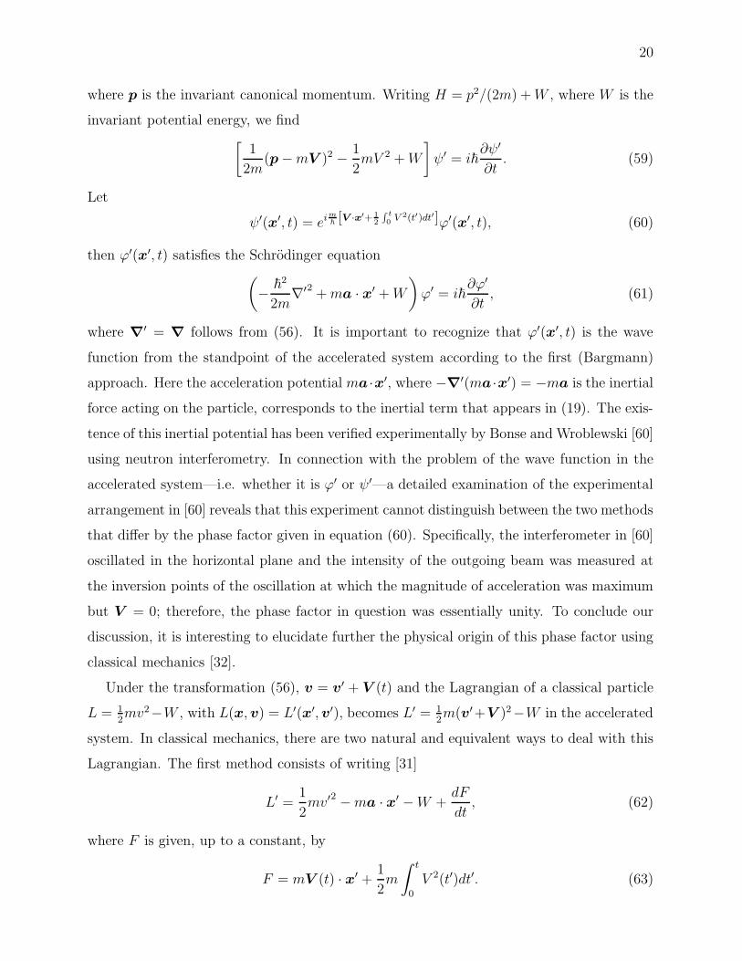
where p is the invariant canonical momentum. Writing H = p2/(2m) +W , where W is the

invariant potential energy, we find[

1

2m(p −mV )2 −

1

2mV 2 +W

]

ψ′ = i~∂ψ′

∂t. (59)

Let

ψ′(x′, t) = ei m

~[V ·x′+ 1

2

∫

t

0V 2(t′)dt′]ϕ′(x′, t), (60)

then ϕ′(x′, t) satisfies the Schrodinger equation(

−~

2

2m∇′2 +ma · x′ +W

)

ϕ′ = i~∂ϕ′

∂t, (61)

where ∇′ = ∇ follows from (56). It is important to recognize that ϕ′(x′, t) is the wave

function from the standpoint of the accelerated system according to the first (Bargmann)

approach. Here the acceleration potential ma ·x′, where −∇′(ma ·x′) = −ma is the inertial

force acting on the particle, corresponds to the inertial term that appears in (19). The exis-

tence of this inertial potential has been verified experimentally by Bonse and Wroblewski [60]

using neutron interferometry. In connection with the problem of the wave function in the

accelerated system—i.e. whether it is ϕ′ or ψ′—a detailed examination of the experimental

arrangement in [60] reveals that this experiment cannot distinguish between the two methods

that differ by the phase factor given in equation (60). Specifically, the interferometer in [60]

oscillated in the horizontal plane and the intensity of the outgoing beam was measured at

the inversion points of the oscillation at which the magnitude of acceleration was maximum

but V = 0; therefore, the phase factor in question was essentially unity. To conclude our

discussion, it is interesting to elucidate further the physical origin of this phase factor using

classical mechanics [32].

Under the transformation (56), v = v′ + V (t) and the Lagrangian of a classical particle

L = 12mv2−W , with L(x,v) = L′(x′,v′), becomes L′ = 1

2m(v′+V )2−W in the accelerated

system. In classical mechanics, there are two natural and equivalent ways to deal with this

Lagrangian. The first method consists of writing [31]

L′ =1

2mv′

2−ma · x′ −W +

dF

dt, (62)

where F is given, up to a constant, by

F = mV (t) · x′ +1

2m

∫ t

0

V 2(t′)dt′. (63)

21

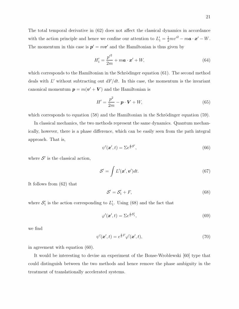
The total temporal derivative in (62) does not affect the classical dynamics in accordance

with the action principle and hence we confine our attention to L′1 = 1

2mv′2 −ma · x′ −W .

The momentum in this case is p′ = mv′ and the Hamiltonian is thus given by

H ′1 =

p′2

2m+ma · x′ +W, (64)

which corresponds to the Hamiltonian in the Schrodinger equation (61). The second method

deals with L′ without subtracting out dF/dt. In this case, the momentum is the invariant

canonical momentum p = m(v′ + V ) and the Hamiltonian is

H ′ =p2

2m− p · V +W, (65)

which corresponds to equation (58) and the Hamiltonian in the Schrodinger equation (59).

In classical mechanics, the two methods represent the same dynamics. Quantum mechan-

ically, however, there is a phase difference, which can be easily seen from the path integral

approach. That is,

ψ′(x′, t) = Σei

~S′

, (66)

where S ′ is the classical action,

S ′ =

∫

L′(x′,v′)dt. (67)

It follows from (62) that

S ′ = S ′1 + F, (68)

where S ′1 is the action corresponding to L′

1. Using (68) and the fact that

ϕ′(x′, t) = Σei

~S′

1 , (69)

we find

ψ′(x′, t) = ei

~Fϕ′(x′, t), (70)

in agreement with equation (60).

It would be interesting to devise an experiment of the Bonse-Wroblewski [60] type that

could distinguish between the two methods and hence remove the phase ambiguity in the

treatment of translationally accelerated systems.

22

10. DISCUSSION

The main observational consequences of Dirac’s equation in noninertial frames of reference

are related to the Sagnac effect, the spin-rotation coupling and the Bonse-Wroblewski effect.

These inertial effects can be further elucidated by interferometry experiments involving

matter waves. In particular, a neutron interferometry experiment has been proposed for

the direct measurement of inertial effect of intrinsic spin. Moreover, neutron interferometry

experiments involving translationally accelerated interferometers may help resolve the phase

ambiguity in the description of the wave function from the standpoint of a translationally

accelerated system.

[1] P.A.M. Dirac, Proc. Roy. Soc. (London) A117, 610 (1928); 118, 351 (1928).

[2] V.A. Fock and D.D. Ivanenko, C.R. Acad. Sci. 188, 1470 (1929); Z. Phys. 54, 798 (1929).

[3] H. Tetrode, Z. Phys. 50, 336 (1928); V. Bargmann, Sitzber., Preuss. Akad. Wiss. Phys.-Math.

Kl. 346 (1932); E. Schrodinger, Sitzber., Preuss. Akad. Wiss. Phys.-Math. Kl. 105 (1932); L.

Infeld and B.L. van der Waerden, Sitzber., Preuss. Akad. Wiss. Phys.-Math. Kl. 380 (1933);

474 (1933); D.R. Brill and J.A. Wheeler, Rev. Mod. Phys. 29, 465 (1957); 33, 623E (1961).

[4] H.A. Lorentz, The Theory of Electrons (Dover, New York, 1952).

[5] A. Einstein, The Meaning of Relativity (Princeton University Press, Princeton, 1950).

[6] B. Mashhoon, Phys. Lett. A 143, 176 (1990); 145, 147 (1990).

[7] H. Weyl, Space-Time-Matter (Dover, New York, 1952), pp. 176-177.

[8] H. Minkowski, in The Principle of Relativity, by H.A. Lorentz, A. Einstein, H. Minkowski and

H. Weyl (Dover, New York, 1952).

[9] B. Mashhoon, in Relativity in Rotating Frames, edited by G. Rizzi and M.L. Ruggiero (Kluwer,

Dordrecht, 2004), pp. 43-55.

[10] B. Mashhoon, Phys. Rev. A 47, 4498 (1993); in Cosmology and Gravitation, edited by M.

Novello (Editions Frontieres, Gif-sur-Yvette, 1994), pp. 245-295; U. Muench, F.W. Hehl and

B. Mashhoon, Phys. Lett. A 271, 8 (2000).

[11] N. Bohr and L. Rosenfeld, K. Dan. Vindensk. Selsk. Mat. Fys. Medd. 12, No. 8, (1993);

translated in Quantum Theory and Measurement, edited by J.A. Wheeler and W.H. Zurek

23

(Princeton University Press, Princeton, 1983); Phys. Rev. 78, 794 (1950).

[12] V. Volterra, Theory of Functionals and of Integral and Integro-Differential Equations (Dover,

New York, 1959).

[13] F.G. Tricomi, Integral Equations (Interscience, New York, 1957).

[14] C. Chicone and B. Mashhoon, Ann. Phys. (Leipzig) 11, 309 (2002).

[15] C. Chicone and B. Mashhoon, Phys. Lett. A 298, 229 (2002).

[16] F.W. Hehl and Y.N. Obukhov, Foundations of Classical Electrodynamics (Birkhauser, Boston,

2003).

[17] B. Mashhoon, Ann. Phys. (Leipzig) 12, 586 (2005); Int. J. Mod. Phys. D 14, 171 (2005).

[18] R. Sauerbrey, Phys. Plasmas 3, 4712 (1996); G. Schafer and R. Sauerbrey, astro-ph/9805106.

[19] B. Mashhoon, Phys. Rev. A 70, 062103 (2004).

[20] B. Mashhoon, hep-th/0503205.

[21] C.G. de Oliveira and J. Tiomno, Nuovo Cimento 24, 672 (1962); J. Audretsch and G. Schafer,

Gen. Relativ. Gravit. 9, 243 (1978); E. Fischbach, B.S. Freeman and W.-K. Cheng, Phys. Rev.

D 23, 2157 (1981); F.W. Hehl and W.-T. Ni, Phys. Rev. D 42, 2045 (1990); Y.Q. Cai and G.

Papini, Phys. Rev. Lett. 66, 1259 (1991); 68, 3811 (1992); J.C. Huang, Ann. Phys. (Leipzig)

3, 53 (1994); K. Konno and M. Kasai, Prog. Theor. Phys. 100, 1145 (1998); K. Varju and

L.H. Ryder, Phys. Lett. A 250, 263 (1998); L. Ryder, J. Phys. A 31, 2465 (1998); K. Varju

and L.H. Ryder, Phys. Rev. D 62, 024016 (2000).

[22] N.V. Mitskievich, Physical Fields in General Relativity Theory, in Russian (Nauka, Moscow,

1969); E. Schmutzer, Ann. Phys. (Leipzig) 29, 75 (1973); B.M. Barker and R.F. O’Connell,

Phys. Rev. D 12, 329 (1975); T.C. Chapman and D.J. Leiter, Am. J. Phys. 44, 858 (1976);

E. Schmutzer and J. Plebanski, Fortschr. Phys. 25, 37 (1977).

[23] J. Audretsch and C. Lammerzahl, Appl. Phys. B 54, 351 (1992); J. Audretsch, F.W. Hehl

and C. Lammerzahl, Lect. Notes Phys. 410, 368 (1992); C. Lammerzahl, Gen. Rel. Grav. 28,

1043 (1996); Class. Quantum Grav. 15, 13 (1998).

[24] J. Anandan, Phys. Rev. Lett. 68, 3809 (1992); J. Anandan and J. Suzuki, in Relativity in

Rotating Frames, edited by G. Rizzi and M.L. Ruggiero (Kluwer, Dordrecht, 2004), pp. 361-

370; Y.Q. Cai, D.G. Lloyd and G. Papini, Phys. Lett. A 178, 225 (1993); D. Singh and G.

Papini, Nuovo Cimento B 115, 223 (2000); G. Papini, in Relativity in Rotating Frames, edited

by G. Rizzi and M.L. Ruggiero (Kluwer, Dordrecht, 2004), pp. 335-359; Z. Lalak, S. Pokorski

24

and J. Wess, Phys. Lett. B 355, 453 (1995); I. Damiao Soares and J. Tiomno, Phys. Rev. D

54, 2808 (1996); C.J. Borde, J.-C. Houard and A. Karasiewicz, Lect. Notes Phys. 562, 403

(2001); C. Kiefer and C. Weber, Ann. Phys. (Leipzig) 14, 253 (2005).

[25] F.W. Hehl and W.-T. Ni, Phys. Rev. D 42, 2045 (1990).

[26] L.L. Foldy and S.A. Wouthuysen, Phys. Rev. 78, 29 (1950).

[27] Y.N. Obukhov, Phys. Rev. Lett. 86, 192 (2001); Fortschr. Phys. 50, 711 (2002); N. Nicolaevici,

Phys. Rev. Lett. 89, 068902 (2002); Y.N. Obukhov, Phys. Rev. Lett. 89, 068903 (2002).

[28] M.V. Romalis, W.C. Griffith, J.P. Jacobs and E.N. Fortson, Phys. Rev. Lett. 86, 2505 (2001).

[29] D. Bini, C. Cherubini and B. Mashhoon, Class. Quantum Grav. 21, 3893 (2004).

[30] A.J. Silenko and O.V. Teryaev, Phys. Rev. D 71, 064016 (2005).

[31] L.D. Landau and E.M. Lifshitz, Mechanics (Pergamon, Oxford, 1966).

[32] B. Mashhoon, Phys. Rev. Lett. 61, 2639 (1988); 68, 3812 (1992).

[33] J.J. Sakurai, Phys. Rev. D 21, 2993 (1980).

[34] J.E. Zimmerman and J.E. Mercereau, Phys. Rev. Lett. 14, 887 (1965).

[35] S.A. Werner, J.-L. Staudenmann and R. Colella, Phys. Rev. Lett. 42, 1103 (1979).

[36] D.K. Atwood, M.A. Horne, C.G. Shull and J. Arthur, Phys. Rev. Lett. 52, 1673 (1984).

[37] F. Riehle, T. Kisters, A. Witte, J. Helmcke and C.J. Borde, Phys. Rev. Lett. 67, 177 (1991).

[38] A. Lenef et al., Phys. Rev. Lett. 78, 760 (1997); T.L. Gustavson, P. Bouyer and M.A. Kasevich,

Phys. Rev. Lett. 78, 2046 (1997); T.L. Gustavson, A. Landragin and M.A. Kasevich, Class.

Quantum Grav. 17, 2385 (2000).

[39] F. Hasselbach and M. Nicklaus, Phys. Rev. A 48, 143 (1993).

[40] E.J. Post, Rev. Mod. Phys. 39, 475 (1967); G.E. Stedman, Rep. Prog. Phys. 60, 615 (1997).

[41] L. Ryder, J. Phys. A 31, 2465 (1998); L.H. Ryder and B. Mashhoon, in Proc. Ninth Marcel

Grossmann Meeting, edited by V.G. Gurzadyan, R.T. Jantzen and R. Ruffini (World Scientific,

Singapore, 2002), pp. 486-497.

[42] B. Mashhoon, Found. Phys. 16 (Wheeler Festschrift), 619 (1986).

[43] B. Mashhoon, Phys. Lett. A 173, 347 (1993); J.C. Hauck and B. Mashhoon, Ann. Phys.

(Leipzig) 12, 275 (2003).

[44] N. Ashby, Living Rev. Relativity 6, 1 (2003).

[45] B. Mashhoon, Phys. Lett. A 306, 66 (2002).

[46] J.D. Anderson and B. Mashhoon, Phys. Lett. A 315, 199 (2003).

25

[47] P.J. Allen, Am. J. Phys. 34, 1185 (1966).

[48] B. Mashhoon, Phys. Lett. A 198, 9 (1995).

[49] B.J. Venema et al., Phys. Rev. Lett. 68, 135 (1992); D.J. Wineland et al., Phys. Rev. Lett.

67, 1735 (1991).

[50] B. Mashhoon, Gen. Rel. Grav. 31, 681 (1999); Class. Quantum Grav. 17, 2399 (2000).

[51] G. Papini, Phys. Rev. D 65, 077901 (2002); G. Papini and G. Lambiase, Phys. Lett. A 294,

175 (2002); G. Lambiase and G. Papini, Phys. Rev. D 70, 097901 (2004); D. Singh, N. Mobed

and G. Papini, J. Phys. A 37, 8329 (2004).

[52] H. Rauch and S.A. Werner, Neutron Interferometry (Oxford University Press, New York,

2000).

[53] B. Mashhoon, R. Neutze, M. Hannam and G.E. Stedman, Phys. Lett. A 249, 161 (1998).

[54] G. Badurek, H. Rauch and D. Tuppinger, Phys. Rev. A 34, 2600 (1986).

[55] V. Bargmann, Ann. Math. 59, 1 (1954).

[56] F.A. Kaempffer, Concepts in Quantum Mechanics (Academic Press, New York, 1965).

[57] D. Giulini, Ann. Phys. (NY) 249, 222 (1996).

[58] D.M. Greenberger, Phys. Rev. Lett. 87, 100405 (2001).

[59] S. Takagi, Prog. Theor. Phys. 86, 783 (1991); W.H. Klink, Ann. Phys. (NY) 260, 27 (1997);

I. Bialynicki-Birula and Z. Bialynicka-Birula, Phys. Rev. Lett. 78, 2539 (1997).

[60] U. Bonse and T. Wroblewski, Phys. Rev. Lett. 51, 1401 (1983); Phys. Rev. D 30, 1214 (1984).