Quantum reduced loop gravity: Semiclassical limit

arX

iv:1

402.

3155

v1 [

gr-q

c] 1

3 Fe

b 20

14

Quantum Reduced Loop Gravity: Semiclassical limit

Emanuele Alesci∗

Instytut Fizyki Teoretycznej, Uniwersytet Warszawski, ul. Hoza 69, 00-681 Warszawa, Poland, EU

Francesco Cianfrani†

Institute for Theoretical Physics, University of Wroc law,

Pl. Maksa Borna 9, Pl–50-204 Wroc law, Poland.

We discuss the semiclassical limit of Quantum Reduced Loop Gravity, a recently proposed modelto address the quantum dynamics of the early Universe. We apply the techniques developed infull Loop Quantum Gravity to define the semiclassical states in the kinematical Hilbert space andevaluating the expectation value of the euclidean scalar constraint we demonstrate that it coincideswith the classical expression, i.e. the one of a local Bianchi I dynamics. The result holds asa leading order expansion in the scale factors of the Universe and opens the way to study thesubleading corrections to the semiclassical dynamics. We outline how by retaining a suitable finitecoordinate length for holonomies our effective Hamiltonian at the leading order coincides with theone expected from LQC. This result is an important step in fixing the correspondence between LQGand LQC.

I. INTRODUCTION

A viable Quantum Gravity model must reduce to General Relativity (GR) in the proper semiclassical limit. Al-though this is a quite natural requirement, nevertheless it can be a far-from-trivial issue. This is the case also for theapproaches as Loop Quantum Gravity (LQG) in its canonical [1, 2] or covariant formulation (Spinfoam Models) [3, 4].In fact, while going from the classical to the quantum realm is a well-settled procedure, going back is much morecomplicated since it involves the construction of a proper semiclassical limit. The definition of semiclassical statesfor a quantum theory of the geometry has been given in [5, 6] in the kinematical Hilbert space via the applicationof the complexifier technique. At the end one can define states peaked around a given set of classical holonomiesand fluxes, but these have to be tested against the dynamics. This can be done looking at the graviton propagatorin the Spinfoam setting [7–10] or looking at the expectation value of the Hamiltonian [11] or the Master Constraint[12, 13] in canonical LQG. The difficulties with finding an analytic expression for the scalar constraint matrix elements[14–16] in the spin network basis forbids a direct computation of the dynamic behavior of semiclassical states. Onlythe Master Constraint operator in the context of Algebraic Quantum Gravity [17] has been shown to convergenceto the right classical expression in the semiclassical limit [18, 19] under the simplifying replacing of the gauge groupSU(2) with U(1)3.The situation is quite different in Loop Quantum Cosmology (LQC) [20, 21], the standard cosmological imple-

mentation of LQG (other cosmological models related with LQG are given in [22, 23], [24] and [25]). In LQC, thequantization is performed in minisuperspace, i.e. after reducing the phase space according with the homogeneityrequirement for Bianchi models. All the kinematical symmetries (SU(2) gauge symmetry and background indepen-dence) are fixed on a classical level, such that quantum states are described by quasi periodic functions of the threeindependent connection components ca. The semiclassical states are naturally defined by peaking around classicaltrajectories. The dynamic issue is greatly simplified and an analytic expression for the scalar constraint is obtained.A crucial point is the regularization, which is realized by fixing non vanishing polymeric parameters µa, such that themomenta operators have a discrete spectrum, whose eigenvalues ∝ µa. The expectation value of the scalar constraintin the presence of a clock like scalar field reproduces the classical expression as soon as the energy density of the fieldρ >> ρcr, ρcr being a critical energy density related with µa. For ρ ∼ ρcr quantum effects are not negligible and theyinduce a bouncing scenario replacing the inital singularity [26].In [27] we proposed a new loop quantum model, namely Quantum Reduced Loop Gravity (QRLG), in which the

dynamic issue is simplified with respect to the full theory thanks to the restriction to a diagonal metric tensor (see also[28, 29] for a local Bianchi I space). The idea of QRLG is to implement such a restriction directly in the kinematicalHilbert space of LQG. This allows to retain the basic structure of the full theory, such as graphs and intertwiner

∗Electronic address: [email protected]†Electronic address: [email protected]

2

structures, but in a simplified framework. As a consequence, the (reduced) graphs have only a cuboidal structure,while intertwiners are only complex numbers. In the limit of the Belinski Lipschitz Kalatnikov (BKL) conjecture[30, 31], the dynamics preserves the metric to be diagonal and it locally coincides with those of the Bianchi I model.The associated scalar constraint can be defined along the lines developed in the full theory. The volume operatorturns out to be diagonal in the (reduced) spin network basis and the matrix elements of the scalar constraint can beanalytically evaluated. The possibility to apply LQG techniques in a computable model makes QRLG a tantalizingsubject of investigation.In this work we investigate the semiclassical limit of QRLG. We will outline how the construction of semiclassical

states can be done as in [5, 6, 32–35], the only difference being that the sum over spin quantum numbers is replacedby the one over the maximun/minimum magnetic indexes. Then, we will evaluate explicitly the expectation value ofthe non-graph changing euclidean scalar constraint on such states. We will carry on in details all the calculations. Byusing the asymptotic expansion of the Clebsch-Gordan coefficients entering the final expression we will compute theleading order contribution in the limit of high spin quantum numbers. This way, we demonstrate how at each nodethe expectation of the euclidean scalar constraint reproduces the analogous expression for the Bianchi I model and,in the continuum limit, the corresponding classical expression, i.e. a local Bianchi I dynamics.Hence, the semiclassical dynamics in QRLG coincides with the one a local Bianchi I model. This means that the

quantum restriction we performed to simplify the dynamic problem is well-grounded, since the resulting quantumsystem approaches in the classical limit GR within the proper approximation scheme.QRLG can thus be used to realize a viable quantum description for the Universe, in which all the prediction of the

Standard Cosmological Model are safe, while we can get some hints on the fate of the initial singularity in LQG.At the same time, even if in this work we investigate only the leading order term in the semiclassical expansion, we

will set up all the techniques to evaluate the corrections, which can provide non trivial modification with respect tothe classical behavior. We want to stress how among such corrections there are the ones related with the fundamentalSU(2) structure, which have no counterpart in LQC and come from the next-to-leading order expansion of the 3j, 6jand 9j symbols entering the euclidean scalar constraints.The expectation value of the Hamiltonian equals the anologous expression for the quantum Hamiltonian used in

LQC [36, 37], the relevant difference being due to subleading corrections (to be computed in upcoming works) and theexplicit presence of the coordinate length in the semiclassical expression, which plays the role of µa. In our analysisthis parameter is not entering at all in the quantum theory, it’s only an artifact of the semiclassical construction therequires the use of kinematical states; it can be removed with the same considerations that allow to remove it inthe full theory. The final expression we find open the way to properly relate LQC and LQG (see also [38, 39]) andeventually address the role of the holonomic and triad corrections to LQC [40, 41].The article is organized as follows: in section II, LQG is reviewed, focusing our attention on the construction of

semiclassical states. In section III, the framework of QRLG is introduced, while semiclassical states are defined insection IV along the lines of the full theory. The action of the Euclidean scalar constraint is evaluated on basis statesbased at dressed nodes in section V, such that we can compute the expectation value of the scalar constraint onsemiclassical states in section VI. Concluding remarks follow in section VII.

II. LOOP QUANTUM GRAVITY

Gravity phase space in LQG is described by the holonomies of Ashtekar-Barbero connections Aia along curves and

the fluxes of inverse densitized triads Eia across surfaces. The corresponding kinematical Hilbert space H is the direct

sum over all graph Γ of the single Hilbert spaces HΓ associated with each graph. The elements of GHΓ are gauge-invariant functions of L copies of the SU(2) group, L being the total number of links in Γ. Basis vectors are given byinvariant spin networks

< h|Γ, {jl}, {xn} >=∏

n∈Γ

xn ·∏

l

Djl(hl), (1)

Djl(hl) and xn being Wigner matrices in the representation jl and invariant intertwiners, respectively, while theproducts extend over all the nodes n in Γ and all the links l emanating from n. The symbol · means the contractionbetween the indexes of intertwiners and Wigner matrices.Fluxes Ei(S) across a surface S realize a faithful representation of the holonomy-flux algebra and they act as left

(right)-invariant vector fields of the SU(2) group. In particular, given a surface S having a single intersection with Γ

in a point P ∈ l, such that l = l1⋃

l2 and l1 ∩ l2 = P , the operator Ei(S) is given by

Ei(S)D(jl)(hl) = 8πγl2P o(l, S) Djl(hl1) τiD

jl(hl2), (2)

3

γ and lP being the Immirzi parameter and the Planck length, respectively, while o(l, S) is equal to 0, 1,−1 accordingwith the relative sign of l and the normal to S, and τi denotes the SU(2) generator in jl-dimensional representation.Indeed, one still has to impose background independence and this can be done in the dual space H∗ via s-knots,

which are equivalence class of spin networks under diffeomorphisms.Finally, the last constraint to implement is the scalar one H , for which a regularized expression can be given in [11]

by a graph-dependent triangulation of the spatial manifold. This triangulation T contains the tetrahedra ∆ obtainedby considering all the incident links at a given node and all the possible nodes of the graph Γ on which the operatoracts. For each pair of links li and lj incident at a node n of Γ we choose a semi-analytic arcs aij whose end pointssli , slj are interior points of li and lj , respectively, and aij ∩ Γ = {sli , slj}. The arc si (sj) is the segment of li (lj)

from n to sli (slj ), while si, sj and aij generate a triangle αij := si ◦ aij ◦ s−1j . The Euclidean and Lorentian parts

of the scalar constraint can then be promoted to operators replacing the classical holonomies and fluxes entering theregularized expression with their quantum expression. In this process one can fix an arbitrary representation (m) forthe holonomies contained in the regularized constraint. The final expression for the Euclidean part is then

HE =∑

∆∈T

Hm∆ [N ] :=

∑

∆∈T

N(n)C(m) ǫijk Tr[

h(m)αij

h(m)−1sk

[

h(m)sk

, V]

]

. (3)

V being the volume operator and C(m) = −i8πγl2PN2

mdenotes a normalization constant depending on the representation

(m) chosen for the holonomy operators where N2m = −dmm(m+ 1).

The lattice spacing ǫ of the triangulation T (which here acts as a regulator) can be removed in a suitable operatortopology in the space of s-knots.Even though one can write formal solutions to the constraint in terms of graphs based at “dressed” nodes [2, 11],

these solutions are only formal since an analytical expression for the matrix elements of the volume V , thus of thewhole scalar constraint, is missing.The same strategy can be adopted to build regularizations using different decompositions, for example in terms of

cubulations and can be extended to be graph changing or not using loops to regularize the curvature that belong ornot to the underlying spin networks [2, 18].

A. Semiclassical limit of LQG

The development of semiclassical states in LQG is based on the application of the complexifier technique to aHilbert space made of functions of copies of the SU(2) group. Let us consider a single link l and a dual surface Sand let us suppose that we want to peak around the classical configuration, i.e. an holonomy h′ along l and a flux E′

i

across S. These two quantities can be combined to form the complexifier H ′

H ′ = h′ exp

(

α

8πγl2PE′

iτi

)

, (4)

α being a parameter, which is an element of SL(2, C), the complexification of the original SU(2) group. Following[33], a state ψα

H′(hl) peaked around such a classical configuration can be constructed from the heat-kernel of theLaplace-Beltrami operator ∆hl

applied to the δ-function over the group elements hl, i.e.

Kα(hl, h′) = e−

α2 ∆hl δ(hl, h

′), (5)

and the explicit form reads

Kα(hl, h′) =

∑

jl

(2jl + 1)e−jl(jl+1)α2 Tr(Djl(h−1

l h′)). (6)

The semiclassical state is obtained via analytic continuation from h′ ∈ SU(2) to H ′ ∈ SL(2, C) as follows

ψαH′(hl) = Kα(hl, H

′). (7)

These states are eigenfunctions of the operator Hl = hl exp(

α8πγl2

P

Ei(S)τi

)

with eigenvalue H ′ and, just like the

usual coherent states in quantum mechanics, they are peaked around hl = h′ and Ei(S) = E′i, while fluctuations are

controlled by the parameter α.

4

By repeating this construction for several copies of the SU(2) group one can define coherent states for a genericgraph, so finding

ΨH′,Γ({hl}) =∏

l∈Γ

ψαH′ (hl). (8)

The main difficulty is to reconcile such a construction with SU(2) gauge-invariance. In fact the expression abovebehavess as follows under a SU(2) transformation

Ψ′H′,Γ({hl}) =

∏

l∈Γ

ψαH′ (gtl hl g

−1sl ), (9)

sl and tl being the source and target points of l. In order to define gauge-invariant coherent states one must averageΨ′

H′,Γ({hl}) over gsl and gtl for the links of the graph. The resulting expression can be expanded in terms of invariantspin networks. However, while by construction the gauge variant coherent state exibiths the right peakness properties,this is not necessary the case for gauge-invariant ones. In fact, it has been verified only by explicit calculation thatgauge invariant coherent states are proper semiclassical states in GH [33].

III. QUANTUM REDUCED LOOP GRAVITY

QRLG realizes the quantum reduction of the full LQG kinematical Hilbert space down to a proper reduced spaceHR capturing the relevant degrees of freedom of a system with a diagonal metric tensor [27] (see also [28, 29] for earlyattempts restricted to the Bianchi I model). Such a projection has been perfomed by

1. the implementation of the partial gauge fixing condition of diffeomorphisms invariance restricting to a diagonalmetric tensor: this implies a truncation of the admissible graphs to reduced graphs, which are the union of somelinks which are parallel to one of the three fiducial vectors ωi (we denote these links as being of the kind li forsome i),

2. the implementation of a SU(2) gauge-fixing condition: this is realized via the restriction to those functions ofSU(2) group elements based at li which are entirely determined by their restriction to some functions of U(1)igroup elements. Such U(1)i are the U(1) subgroup obtained by stabilizing the SU(2) group around the internaldirection ~ui

~u1 = (1, 0, 0), ~u2 = (0, 1, 0), ~u3 = (0, 0, 1). (10)

.

These two steps affect the kind of symmetries we have on a kinematical level. The former implies that not fullbackground independence is realized. In fact, the only kind of diffeomorphisms which survives after the truncationto reduced graphs are those mapping reduced graphs among themeselves (and on a classical level preserving thediagonal form of the metric). We call these transformations reduced diffeomorphisms. As for the SU(2) gauge-fixing,it makes SU(2) gauge invariance not manifest anymore. Nevertheless, since the U(1)i groups are not independent,some reduced intertwiners arise as a relic of the original SU(2) gauge invariance.Finally, the kinematical Hilbert space HR is the direct sum over all reduced graphs Γ of the ones based on a single

reduced graph HRΓ ,

HR = ⊕ΓHRΓ . (11)

A generic element ψΓ ∈ HRΓ is a proper function of L1 + L2 + L3 copies of SU(2) group elements hl, Li being the

total number of the links of the kind li in Γ. Given a link l, let us denote by ul the internal direction correspondingto it (if l is the kind li then ~ul = ~ui), the functions of hl group elements can be expandend in terms of the followingprojected Wigner matrices

lDjljljl

(hl) = 〈jl, ~ul|Dj(g)|jl, ~ul〉, lDjl−jl−jl

(hl) = 〈jl,−~ul|Dj(g)|jl,−~ul〉 (12)

|j, ~ul〉 and |j,−~ul〉 being the basis of SU(2) irreducible representations with spin number j and magnetic componentsalong the direction ~ul equal to j and −j, respectively. We will denote them by lDjl

mlml(hl) with ml = ±jl. Here for

the first time we will consider also reduced states with minimum magnetic numbers. The projected Wigner matricesare entirely determined by their restriction the the U(1)i subgroup.

5

The whole basis state in the gauge-invariant reduced space GHR is obtained by inserting at each node n the reducedintertwiners 〈jl,xn|ml, ~ul〉, which are constructed from the SU(2) intertwiner basis xn. At the end, one gets

〈h|Γ,ml,xn〉 =∏

n∈Γ

〈jl,xn|ml, ~ul〉∏

l

lDjlmlml

(hl), (13)

where∏

n∈Γ and∏

l extend over all the nodes n ∈ Γ and over all the links l emanating from n, respectively. Henceforth,each basis element is labeled by the reduced graph Γ, the spin quantum numbers ml associated with each link andthe SU(2) intertwiners xn used to construct the reduced ones (jl = |ml|).These basis states are not orthogonal with respect to xn, since the scalar product is given by

< Γ,ml,xn|Γ′,m′l,x′

n>= δΓ,Γ′

∏

n∈Γ

∏

l∈Γ

δml,m′

l<ml, ~ul|jl,xn >< jl,x

′n|ml, ~ul > . (14)

The reduced fluxes REi are defined only across the surfaces Si dual to ωi and their action is non-vanishing only onthose states based at links li, in which case it reads

REi(Si)lDjl

mlml(hl) = 8πγl2P ml

lDjlmlml

(hl) li ∩ Si 6= ⊘. (15)

As a consequence the reduced volume operator is diagonal in the basis (13). For instance the volume of a region ωcontaining the node n acts as follows on basis vectors based at the links li emanating from n

RV (ω)∏

l

〈jl,xn|ml, ~ul〉 · lDjlmlml

(hl) = (8πγl2P )3/2Vml

∏

l

〈jl,xn|ml, ~ul〉 · lDjlmlml

(hl). (16)

where

Vml=

√

∏

i

|∑

li

mli | (17)

The sum inside the square root extends over the links of the kind li emanating from n, thus generically it is the sumof two terms (based at the links incoming and outcoming in n).The invariance under reduced diffeomorphisms can be implemented on a quantum level according with standard

LQG techniques, i.e. by defining reduced s-knots

< s, jl,xn|h >=∑

Γ∈s

< Γ, jl,xn|h >, (18)

where the sum is over all the reduced graphs related by a reduced diffeomorphism.The scalar constraint can be implemented in GHR by taking the expression of the full theory and substituting

the elements of the reduced Hilbert space as in [28]. This procedure provides a quantum operator acting in thereduced Hilbert space describing a diagonal metric tensor. Hence, it is well-grounded only if the classical action ofthe scalar constraint preserves the gauge condition on the metric tensor. This is not generically the case, since aftera finite transformation generated by H the metric is diagonal only modulo a diffeomorphism (which is not a reducedone). The definition of the modified constraint preserving the diagonal form of the metric and its quantization willbe discussed elsewhere. Here we return back to the first application to QRLG, the inhomogeneous extension of theBianchi I model, in which case the dynamics is entirely determined by the reduced Euclidean scalar constraint, whichpreserves the diagonal form of the metric.

A. Inhomogeneous extension Bianchi I model

The Bianchi I model is the anisotropic extension of the flat FRW space-time. The spatial sections are still flat andthe fiducial one forms, whose dual ωi are Killing vectors, can be taken as ωi = δiadx

a, xa being Cartesian coordinates.The line element reads

ds2I = N2(t)dt2 − a21(t)dx1 ⊗ dx1 − a22(t)dx

2 ⊗ dx2 − a23(t)dx3 ⊗ dx3, (19)

N = N(t) being the lapse function, while ai (i = 1, 2, 3) denote the three scale factors, all depending on the timevariable only.

6

We considers the following inhomogeneous extension of the line element (19)

ds2I = N2(x, t)dt2 − a21(t, x)dx1 ⊗ dx1 − a22(t, x)dx

2 ⊗ dx2 − a23(t, x)dx3 ⊗ dx3, (20)

in which each scale factor ai is a function of time and of the spatial coordinates. By fixing the group of internalrotations [42, 43] the densitized inverse 3-bein vectors can be taken as

Eai = pi(t, x)δai , pi =

a1a2a3ai

, (21)

where the index i is not summed. In the following, repeated indexes will not be summed. As for Ashtekar connections,we get a similar expression, i.e.

Aia(t, x) = ci(t, x)δ

ia, ci(t, x) =

γ

Nai. (22)

in the two relevant cases of i) reparametrized Bianchi I model (in which each scale factor ai is a function of thecorresponding Cartesian coordinate xi = δiax

a only) and ii) the generalized Kasner solution within a fixed Kasnerepoch (in which spatial gradients are negligible with respect to time derivatives). It is worth noting how the expressionfor Aa

i (22) is exact in the former case, which is equivalent to the homogeneous Bianchi I model, while it holds onlyapproximatively in the latter by assuming the BKL conjecture [31]. In which case, the inhomogeneous model is madeof a collection of homogeneous patches, one for each point.In reduced phase space the SU(2) Gauss constraint and the vector constraint do not vanish but they generate U(1)i

gauge transformations and reduced diffeomorphisms. The Lorentzian part of the scalar constraint is proportional tothe Euclidean one, such the sum is 1/γ2 times the latter and the explicit expression reads

H [N ] =1

γ2HE [N ] =

1

γ2

∫

d3xN

[√

p1p2

p3c1c2 +

√

p2p3

p1c2c3 +

√

p3p1

p2c3c1

]

, (23)

which can be seen as the sum of local Bianchi I patches, i.e.

H [N ] =1

γ2

∑

x

V (x)N(x)

[√

p1p2

p3c1c2 +

√

p2p3

p1c2c3 +

√

p3p1

p2c3c1

]

(x), (24)

Vx being the volume of the homogeneous patch based at the point x, where all the ci and pi variables are evaluated.

This the kind of classical dynamics we are going to compare with the semiclassical limit of QRLG, since it preservesthe diagonal form of the metric.

IV. SEMICLASSICAL STATES IN QRLG

Let us define semiclassical states in QRLG by projecting the expression (7) down to redH. Hence, let us first definethe semiclassical states along a given link l. The analogous of the expression (6) now reads

Kα(hl, h′) =

+∞∑

ml=−∞(2jl + 1)e−jl(jl+1)α

2 lDjlmlml

(h−1l h′), (25)

where jl = |ml| and h′ is an element of the SU(2) subgroup generated by τi (U(1)i), i being the internal directionassociated with the link l (l is of the kind li), i.e.

h′ = eiθlτi , (26)

θl being the parameter along the group, which can be determined from the explicit expression of the holonomy alongthe links l. In the limit in which ci is constant along l, there is the direct identification θl = ±ǫl ci, ǫl being the lengthof l and the +(-) signs is for positive(negative)- oriented l.The complexification of h′ is given by

H ′ = h′eα

8πγl2P

E′

iτi, (27)

7

which differs from the expression (4) because the indexes i in the exponent are not summed and h′ is a U(1)i groupelement. We can rewrite the expression (27) as follows

H ′ = R(~ul)eiθlτ3+

α

8πγl2P

E′

iτ3R−1(~ul), (28)

R(~ul) being the rotation sending the direction ~ul into the direction ~u3. A clear interpretation of the classical datawe are peaking on can now be given in terms of a cellar decomposition. In fact, we can compare Eq.(28) with theexpression of the coherent states for a homogeneous model defined in [34, 35]. These coherent states are defined via ageometrical parametrization of the phase space in terms of twisted geometries [44],[46], in which two SU(2) rotationsare inserted at the target and source points. By comparing Eq.(28) with Eq.(52) in [35], one sees how in our case,in which the intrinsic curvature of the spatial section vanishes, these two rotations coincides and they are given byR(~ul).The semiclassical state for QRLG takes the following expression

ψαH′(hl) = Kα(hl, H

′), (29)

Kα(hl, H′) and H ′ given by Eq.(25) and (27), respectively. We can write an explicit expression for ψα

H′(hl) in termsof basis vectors (12), thanks to the fact that the SU(2) representation lDjl

mn(hl) of U(1)i group elements is diagonal,i.e.

lDjlmlml

(h−1l H ′) =

jl∑

n=−jl

lDjlmln

(h−1l ) lDjl

nml(H ′) = lDjl

mlml(h−1

l ) lDjlmlml

(H ′). (30)

The last factor on the right-hand side of the equation above can be easily evaluated, so getting

lDjlmlml

(H ′) = eiθlmleα

8πγl2P

E′

iml

. (31)

By collecting together all the equations of this section one finds the following expression for the semiclassical statesin QRLG

ψαH′(hl) =

∞∑

ml=−∞ψαH′(ml)

lDjlmlml

(h−1l ), (32)

with

ψαH′ (ml) = (2jl + 1)e−jl(jl+1)α

2 eiθlmleα

8πγl2P

E′

iml

. (33)

where jl = |ml|. It is worth noting how in the limit E′

8πγl2P

>> 1 one has

− j(j + 1)α

2+m

αE′

8πγl2P= −m(m± 1)

α

2+m

αE′

8πγl2P∼ −α

2

(

m− E′

8πγl2P

)2

+ α

(

E′

8πγl2P

)2

. (34)

Hence the coefficients ψαH′ (ml) modulo a factor not depending on ml become Gaussian weights and ψα

H′

l(hl) can be

written as

ψαH′(hl) ∼

∞∑

ml=−∞(2jl + 1)e

−α2

(

ml−E′

i

8πγl2P

)2

eiθlml lDjlmlml

(h−1l ) =

∞∑

ml=−∞ψαH′ (ml)

iDjlmlml

(h−1l ), (35)

which outlines that the state is peaked around ml =E′

l

8πγl2P

. Such a value corresponds to the following momenta pl

plδ2l = 8πγl2P ml , (36)

δ2l being the area of the surface across which E′l is smeared in the fiducial metric. Similarly it can be shown that the

state is also peaked around the classical holonomy h′.For multi-link states, one simply has to consider the direct product of states of the kind (32) and to insert invariant

intertwiners at nodes. We remember that in QRLG the invariant intertwiners are merely coefficients, so the extensionof the expression (35) to the gauge invariant Hilbert space GHR can be done straightforwardly by inserting reducedintertwiners both in basis elements and in the coefficients, so finding

ψαΓH′ =

∑

ml

∏

n∈Γ

〈jl,xn|ml, ~ul〉∗∏

l∈Γ

ψαH′

l(ml) 〈h|Γ,ml,xn〉 , (37)

where∑

ml=∏

l∈Γ

∑

ml.

8

V. THE HAMILTONIAN ON BASIS STATES

We are now interested in implementing the action of the Hamiltonian RH as

RH =1

γ2RHE , (38)

via an operator RHE defined on GHR: a convenient way of constructing it is to replace in the expression (3), regularizedvia a cubulation C adapted to the reduced spinnetwork graph, as explained in [28], quantum holonomies and fluxeswith the ones acting on the reduced space as follows

RHE [N ] =∑

RHm

E[N ] (39)

where

RHm

E[N ] := N(n)C(m) ǫijk Tr

[

Rh(m)αij

Rh(m)−1sk

[

Rh(m)sk

,RV]

]

. (40)

The reduced holonomy operators Rh are obtained by projecting the SU(2) ones on the projected Wigner matrices(12), while the reduced volume operator is the one given in (16).The action of this operator has already been computed in [28], however there we allowed only states of the kind

jDjjj(h) for the holonomies contained in the expresssion (40), but here we consider general states in GHR of the

form jDjnn(h) with n = ±j . This implies that in the regularized Hamiltonian the intertwiners between two different

directions will have the possibility to connect holonomies projected on maximum and minimum magnetic numberrunning on different segments si. The practical rule is then to connect in the Hamiltonian (40) objects of the kind:

RDjmn(hl) =

∑

λ=±1

< j,m|j, λ~ul >< j, λ~ul|Dj(hl)|j, λ~ul >< j, λ~ul|j, n > . (41)

to the standard intertwiners.In view of the application of the non graph changing version of the hamiltonian we consider the simplest state on

which the action is non trivial, namely[49]:

|nz〉R =

jx

hx

Rx

R−1x

Rx

R−1x

jx

jzhz

jz

jy

hy

Ry

R−1y

Ry

R−1y

jy

jl

jl

jz

jl

hly

Ry

R−1y

Ry

R−1y

jl jl

h−1lx

Rx

R−1x

Rx

R−1x

jx jy

j′yj′x

(42)

Note that here and in the following in the graphical formulas the 3-valent nodes represent Clebsh-Gordan coefficients,while in the previous papers [28, 29] instead, we were using the same symbol for 3-j symbols. This is just toavoid the presence of dimension factors that would appear in subsequent recouplings, and if one keeps track of the

9

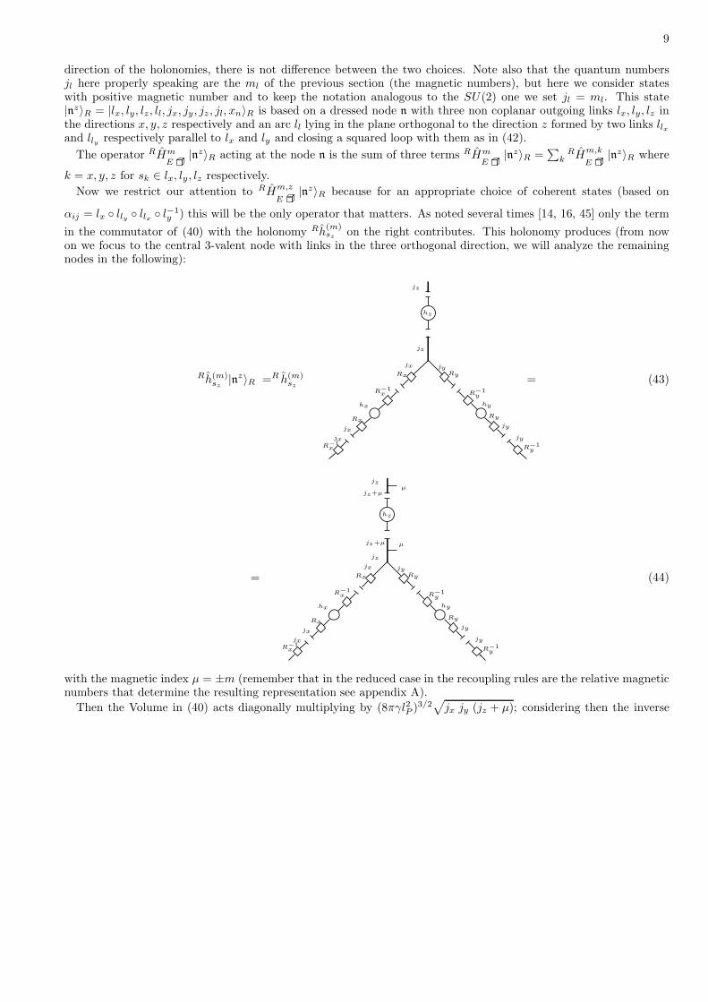
direction of the holonomies, there is not difference between the two choices. Note also that the quantum numbersjl here properly speaking are the ml of the previous section (the magnetic numbers), but here we consider stateswith positive magnetic number and to keep the notation analogous to the SU(2) one we set jl = ml. This state|nz〉R = |lx, ly, lz, ll, jx, jy, jz , jl, xn〉R is based on a dressed node n with three non coplanar outgoing links lx, ly, lz inthe directions x, y, z respectively and an arc ll lying in the plane orthogonal to the direction z formed by two links llxand lly respectively parallel to lx and ly and closing a squared loop with them as in (42).

The operator RHm

E|nz〉R acting at the node n is the sum of three terms RHm

E|nz〉R =

∑

kRHm,k

E|nz〉R where

k = x, y, z for sk ∈ lx, ly, lz respectively.

Now we restrict our attention to RHm,z

E|nz〉R because for an appropriate choice of coherent states (based on

αij = lx ◦ lly ◦ llx ◦ l−1y ) this will be the only operator that matters. As noted several times [14, 16, 45] only the term

in the commutator of (40) with the holonomy Rh(m)sz on the right contributes. This holonomy produces (from now

on we focus to the central 3-valent node with links in the three orthogonal direction, we will analyze the remainingnodes in the following):

Rh(m)sz |nz〉R =R h(m)

sz

jx

hx

Rx

R−1x

Rx

R−1x

jx

jx

hz

jz

jy

hy

Ry

R−1y

Ry

R−1y

jy

jy

jz

= (43)

=

jx

hx

Rx

R−1x

Rx

R−1x

jx

jx

hz

jz

jy

hy

Ry

R−1y

Ry

R−1y

jy

jy

jz

jz+µ µ

µjz+µ

.

(44)

with the magnetic index µ = ±m (remember that in the reduced case in the recoupling rules are the relative magneticnumbers that determine the resulting representation see appendix A).

Then the Volume in (40) acts diagonally multiplying by (8πγl2P )3/2√

jx jy (jz + µ); considering then the inverse

10

holonomy along z we have:

Rh(m)−1sz

RV Rh(m)sz |nz〉R = (8πγl2P )

3/2√

jx jy (jz + µ)

jy

hy

Ry

R−1x

Ry

R−1y

jy

jx

hx

Rx

R−1x

Rx

R−1x

jx

jx

jz+µ hz

jz+µ

jz+µ

h−1z

µ′

. (45)

Before attaching the last part of the action of RHm,3

Eit’s convenient so simplify the U(1)z group elements and

separate the projected lines obtaining:

Rh(m) −1sz

RV Rh(m)sz |nz〉R = (8πγl2P )

3/2√

jx jy (jz + µ)

jy

hy

Ry

R−1x

Ry

R−1y

jy

jx

hx

Rx

R−1x

Rx

R−1x

jx

jx

jzhz

jz

jz

µ′µ

µ µ′

(46)

The next step is to compute the action of hαij−hαji

contained in (40); to this aim we can use a recoupling identity(the loop trick, see [16]) namely:

hα[ij]= (hαij

− hαji) =

∑

m∈(2N+1)

(−)2m (47)

where all the lines are SU(2) objects with the arrows in the upper part of the diagram representing a recoupling ofthe free indexes while the arrows in the loop represent the group element hαij

, and the sum extends over all the oddvalue for m compatible with recoupling theory. Applying this identity, using the reduced recoupling and summing

11

over µ and µ′ we get

Tr[ (

Rh(m)αxy

− Rh(m)αyx

)

Rh(m)−1sz

RV Rh(m)sz

]

|nz〉R =

= (8πγl2P )3/2∑

m

∑

µ,µ′

√

jx jy (jz + µ)

jx

hx

Rx

R−1x

Rx

R−1x

jx

jx

jzhz

jz

jy

hy

Ry

R−1y

Ry

R−1y

jy

jym

hx

R−1x

Rx

R−1x

Rx

m

m

m

h−1y

Ry

R−1y

Ry

R−1y

jy

mjz

jz µ′µ

m

µ µ′

mm

(48)

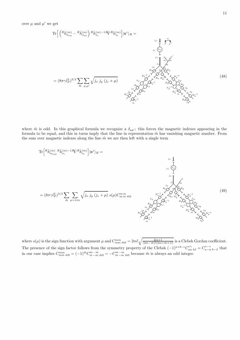
where m is odd. In this graphical formula we recognize a δµµ′ ; this forces the magnetic indexes appearing in theformula to be equal, and this in turns imply that the line in representation m has vanishing magnetic number. Fromthe sum over magnetic indexes along the line m we are then left with a single term

Tr[

Rh(m)α[xy]

Rh(m)−1sz

RV Rh(m)sz

]

|nz〉R =

= (8πγl2P )3/2∑

m

∑

µ=±m

√

jx jy (jz + µ) s(µ)Cmmmm m0

jx

hx

Rx

R−1x

Rx

R−1x

jx

jx

jzhz

jz

jy

hy

Ry

R−1y

Ry

R−1y

jy

jym

hx

R−1x

Rx

R−1x

Rx

m

m

m

h−1y

Ry

R−1y

Ry

R−1y

jy

mjz

jz

0

(49)

where s(µ) is the sign function with argument µ and Cmmmm m0 = 2m!

√

2m+1(2m−m)!(2m+m+1)! is a Clebsh Gordan coefficient.

The presence of the sign factor follows from the symmetry property of the Clebsh (−1)a+b−cCcγaα bβ = Cc−γ

a−α b−β that

in our case implies Cmmmm m0 = (−1)mCm−m

m−m m0 = −Cm−mm−m m0 because m is always an odd integer.

12

Recoupling the rotation matrices R around the central node and multipling the U(1) elements we get :

Tr[

Rh(m)α[xy]

Rh(m)−1sz

RV Rh(m)sz

]

|nz〉R =

= (8πγl2P )3/2

∑

µx,µy=±m

∑

k

∑

m

∑

µ=±m

√

jx jy (jz + µ) s(µ)Cmmmm m0

jx+µx

hx

Rx

R−1x

Rx

R−1x

jx

jx

jzhz

k

jz

jy−µy

hy

Ry

R−1y

Ry

R−1y

jy

jy

Rx

m

mjz

jz

jx+µxjy−µy

jyjx

R−1y

m

0

R−1x

m m

Ry

(50)

with k running from |jk − m| to |jk + m| and with µx = ±m,µy = ±m being the magnetic numbers of the reducedholonomy in representation m attached by the hamiltonian in direction lx and ly, respectively. The central node canthen be simplified obtaining a 9j symbol as showed in [16], thus we get

Tr[

Rh(m)α[xy]

Rh(m)−1sz

RV Rh(m)sz

]

|nz〉R = (8πγl2P )3/2

∑

µx,µy=±m

∑

k

∑

m

∑

µ=±m

√

jx jy (jz + µ) s(µ)Cmmmm m0

{

k m jzjy−µy m jyjx+µx m jx

}

jx+µx

hx

Rx

R−1x

Rx

R−1x

jx+µx

jx

jzhz

k

jz

jy−µy

hy

Ry

R−1y

Ry

R−1y

jy−µy

jy

jz

jx+µxjy−µy

jyjx

m

0

R−1x

m m

Ry

µx µy

(51)

We can now turn our attention to the remaining nodes, where the loop attached by the Hamiltonian constraintoverlaps the existing loop in the state and we have to evaluate the following diagram:

13

∑

µ′

x,µ′

y

jx+µx

hx

Rx

R−1x

Rx

R−1x

jx+µx

jzhz

jz

jy−µy

hy

Ry

R−1y

Ry

R−1y

jy

jl

jl

jz

jl

hly

Ry

R−1y

Ry

R−1y

jl

jl

h−1lx

Rx

R−1x

Rx

R−1x

jx+µx jy−µy

j′yj′x

R−1x

µx

Ry

µy

µ′

yµ′

x

µ′

y

hly

Ry

R−1y

Ry

R−1y

µ′

x

h−1lx

Rx

R−1x

Rx

R−1x

m

0k

(52)

Recoupling at the nodes produces just a 6j symbol per node and we finally find

Tr[

Rh(m)α[xy]

Rh(m)−1sz

RV Rh(m)sz

]

|nz〉R =∑

µ′

xµ′

yµx,µy=±m

Hm jxj

′

xjyj′

y

µxµ′

xµyµ′

y(jz , jl)

jx+µx

hx

Rx

R−1x

Rx

R−1x

jzhz

jz

hy

Ry

R−1y

Ry

R−1y

jy−µy

jl+µ′

y

jz

jl+µ′

y

hly

Ry

R−1y

Ry

R−1y

jl+µ′

x

h−1lx

Rx

R−1x

Rx

R−1x

jx+µx jy−µy

j′yj′x

jl+µ′

x

m

0k

(53)

14

with

Hm jxj

′

xjyj′

y

µxµ′

xµyµ′

y(jz , jl) = (8πγl2P )

3/2∑

k

∑

m

∑

µ=±m

√

jx jy (jz + µ) s(µ)Cmmmm m0

{

k m jzjy−µy m jyjx+µx m jx

}

{ j′x jl+µ′

y jx+µx

m jx jl}{ jl+µ′

x j′y jy−µy

jy m jl}

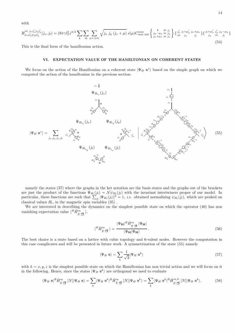
(54)This is the final form of the hamiltonian action.

VI. EXPECTATION VALUE OF THE HAMILTONIAN ON COHERENT STATES

We focus on the action of the Hamiltonian on a coherent state |ΨH nz〉 based on the simple graph on which we

computed the action of the hamiltonian in the previous section:

|ΨH nz〉 =

∑

jx,jy ,jz,jl

ΨHlx(jx)

Rx

R−1x

jx

jz

Ry

R−1y

jy

jl

jl

jz

Ry

R−1y

jl

Rx

jx jy

j′yj′x

ΨHly(jy)

ΨHlly(jl) ΨHllx

(jl)

ΨHlz(jz)

*

**

*

∣

∣

∣

∣

∣

jx

hx

Rx

R−1x

Rx

R−1x

jx

jzhz

jz

jy

hy

Ry

R−1y

Ry

R−1y

jy

jl

jl

jz

jl

hly

Ry

R−1y

Ry

R−1y

jl jl

h−1lx

Rx

R−1x

Rx

R−1x

jx jy

j′yj′x

⟩

(55)

namely the states (37) where the graphs in the ket notation are the basis states and the graphs out of the bracketsare just the product of the functions ΨHl

(jl) = NψHl(jl) with the invariant intertwiners proper of our model. In

particular, these functions are such that∑

jl|ΨHl

(jl)|2 = 1, i.e. obtained normalizing ψHl(jl), which are peaked on

classical values Hl, in the magnetic spin variables (35) .We are interested in describing the dynamics on the simplest possible state on which the operator (40) has non

vanishing expectation value 〈RHm

E〉,

〈RHm

E〉 =

〈ΨH|RHm

E|ΨH〉

〈ΨH|ΨH〉 . (56)

The best choice is a state based on a lattice with cubic topology and 6-valent nodes. However the computation inthis case complicates and will be presented in future work. A symmetrization of the state (55) namely

|ΨH n〉 =∑

k

1√3|ΨH n

k〉 (57)

with k = x, y, z is the simplest possible state on which the Hamiltonian has non trivial action and we will focus on itin the following. Hence, since the states |ΨH n

k〉 are orthogonal we need to evaluate

〈ΨH n|RHm

E[N ]|ΨH n〉 =

∑

k

〈ΨH nk|RHm

E[N ]|ΨH n

k〉 =∑

k

〈ΨH nk|RHm,k

E[N ]|ΨH n

k〉. (58)

15

It is enough to understand the behavior of a single term in the sum. Restricting to k = z we have

RHm,z

E[N ]|ΨH n

z〉 = −N(n)C(m)

∑

jx,jy,jz ,jl

ΨHlx(jx)

Rx

R−1x

jx

jz

Ry

R−1y

jy

jl

jl

jz

Ry

R−1y

jl

Rx

jx jy

j′yj′x

ΨHly(jy)

ΨHlly(jl) ΨHllx

(jl)

ΨHlz(jz)

*

**

*

∑

µ′

xµ′

yµx,µy

Hm jxj

′

xjyj′

y

µxµ′

xµyµ′

y(jz , jl)

∣

∣

∣

∣

∣

jx+µx

hx

Rx

R−1x

Rx

R−1x

jzhz

jz

hy

Ry

R−1y

Ry

R−1y

jy−µy

jl+µ′

y

jz

jl+µ′

y

hly

Ry

R−1y

Ry

R−1y

jl+µ′

x

h−1lx

Rx

R−1x

Rx

R−1x

jx+µx jy−µy

j′yj′x

jl+µ′

x

m0k

⟩

(59)

To proceed note that the state (42) is not normalized in the SU(2) scalar product as shown in (14); to normalizeit, it’s enough to divide each three valent node by

√

| < jl,xn3|nl, ~ul > |2 =

√

√

√

√

√

√

√

√

R1 R2

j3

j1 j2

R3

∗

R1 R2

j3

j1 j2

R3

(60)

In the coherent states (55), this normalization must be done twice: for both the intertwiners in the basis elementsand the intertwiners in the coefficients (since the latter are dual to the former). This corresponds to use a normalizedintertwiners basis for which each intertwiner is just a phase and the expression above is equal to 1. Having normalizedintertwiners, the full state |ΨH n〉 is normalized too, i.e.

〈ΨH n |ΨH n 〉 = 1 . (61)

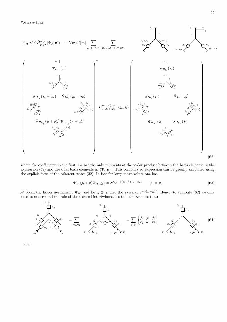
16

We have then

〈ΨH nz|RHm,z

E|ΨH n

z〉 = −N(n)C(m)∑

jx,jy,jz ,jl

∑

µ′

xµ′

yµx,µy=±mRx Ry

jz

jx+µx jy−µy

*

Rx

k

Ry

jz

jx+µxjy−µy

m

0

ΨHlx(jx + µx)

Rx

R−1x

jx+µx

jz

Ry

R−1y

jy−µy

jl+µ′

y

jl+µ′

x

jz

Ry

R−1y

jl+µ′

y jl+µ′

x

Rx

jx+µx jy−µy

j′yj′x

ΨHly(jy − µy)

ΨHlly(jl + µ′

y) ΨHllx(jl + µ′

x)

ΨHlz(jz)

*

**

*

∗

Hm jxj

′

xjyj′

y

µxµ′

xµyµ′

y(jz, jl)

ΨHlx(jx)

Rx

R−1x

jx

jz

Ry

R−1y

jy

jl

jl

jz

Ry

R−1y

jl

Rx

jx jy

j′yj′x

ΨHly(jy)

ΨHlly(jl) ΨHllx

(jl)

ΨHlz(jz)

*

**

*

(62)

where the coefficients in the first line are the only remnants of the scalar product between the basis elements in theexpression (59) and the dual basis elements in 〈ΨHn

z|. This complicated expression can be greatly simplified usingthe explicit form of the coherent states (32). In fact for large mean values one has

Ψ∗Hl(jl + µ)ΨHl

(jl) ≈ N 2e−α(jl−jl)2

e−iθlµ jl ≫ µ, (63)

N being the factor normalizing ΨHland for jl ≫ µ also the gaussian e−α(jl−jl)

2

. Hence, to compute (62) we onlyneed to understand the role of the reduced intertwiners. To this aim we note that:

R1 R2

j3

j1 j2

R3

R1 R2

µ1 µ2

m=∑

k1,k2 R1 R2

j3

j1 j2

R3

µ1 µ2j1 j2

k2k1

m

=∑

k1k2

{

j1 j2 j3k2 k1 m

}

R1 R2

j3

R3

µ1 µ2j1 j2

k2k1 (64)

and

17

Rx

jx

Ry

jy

Rx

m

R−1y

mjz

jz

0

m m

µx µy

=∑

i,l,k

Rx

jx

k

Ry

jy

Rx

m

m

jz

jz

l i

R−1y

m

0

µx µyjx jy

=∑

i,l,k

{

k m jzl m jyi m jx

}

Rx

k

Ry

jz

l i

m

0

µx µyj1 j2

(65)We can thus proceed observing that the gaussians peak the jl around large values jl’s and this allow us to use a

fundamental approximation for the Clebsh Gordan coefficients viable when a, c >> b [47]:

Cccaαbβ ≈ δβ,c−αδβ,c−a . (66)

The coefficients appearing in the previous formula (64) and (65) are of the form:

Ckκjjmµ = (−1)j+m−kCkκ

mµjj = (−1)j+m−k

√

dkdj

(−1)m−µCjjkκm−µ, (67)

and using (66) we have:

Ckκjjmµ ≈ (−1)j+m−k(−1)m−µ

√

dkdjδ−µ,j−κδ−µ,j−k = (−1)j+m−k(−1)m−µ

√

dkdjδκ,j+µδk,j+µ . (68)

Hence, equation (64) can be approximated as

R1 R2

j3

j1 j2

R3

R1 R2

µ1 µ2

m=∑

k1,k2

∑

κ1κ2

{

j1 j2 j3k2 k1 m

}

R1 R2

j3

R3

µ1 µ2j1 j2

k2k1

κ1 κ2

≈√

dj1+µ1

dj1

√

dj1+µ2

dj2

{

j1 j2 j3j2 + µ2 j1 + µ1 m

}

R1 R2

j3

R3

j2+µ2j1+µ1

j1+µ1 j2+µ2

+O

(

1√j1

)

+O(1√j2)

(69)

where in the first line we have explicitly reintroduced the magnetic indexes in the inferior legs and we used (68) toevaluate the two inferior Clebsh coefficients. Proceeding in the same way for (65) we find

Rx

jx

Ry

jy

Rx

m

R−1y

mjz

jz

0

m m

µx µy

≈∑

k

√

djx+µx

djx

{

k m jzjx+µx m jyjy−µy m jx

}

Rx

k

Ry

jz

jx+µxjy−µy

m

0

+O

(

1√jx

)

+O

(

1√

jy

)

(70)

18

Up to subleading corrections we can use (69) and (70) to simplify (62). We note that the expression (62) is made bythe product of the following four kind of terms:

1. two factors in the first line, namely the remnant of the scalar product between the basis elements,

2. the coefficients in the big conjugate parenthesis ()∗ left from the coherent state coefficients of 〈ΨHnz|,

3. the coefficients in the big () parenthesis left from the coherent state coefficients of |ΨHnz〉,

4. the matrix elements of the Hamiltonian operator RHm

E.

The terms of the kind 2) and 3) are disposed according to their original position with respect to the state, i.e. node,

left corner, corner opposite to the node and right corner. The matrix elements of RHm

Etoo consist of a 9j and two

6j-s associated respectively to the node and the two corners. We illustrate the simplification looking at the coefficientinvolving the node.The first coefficient in the first line of (62) times the node coefficient in the complex conjugate parenthesis ()∗

simplifies due to the normalization. The node contribution left is then the node coefficient in (), the second factor inthe first line of the (62) and the 9j in Hm...

... . The product of the latter two terms is the left hand side of (70) at theleading order. This expression is in turn made of two factors: a 3-valent reduced intertwiner in the j-s representationsand a second in the m and 1 representation. The first is just the dual of the one appearing in () and their productgives 1 according to the normalization. Proceeding in the same way for the corners we obtain the leading ordercontribution:

〈ΨH nz|RHm

E|ΨH n

z〉 ≈ −N(n)C(m)(8πγl2P )3/2

≈∑

m

∑

µ=±m

∑

µx,µy=±m

∑

µ′

x,µ′

y=±m

∑

jx,jy,jz ,jl

√

jx jy (jz + µ) s(µ)Cmmmm m0

Ψ∗Hlx

(jx + µx)ΨHlx(jx)

Rx

R−1x

µx

Ry

R−1y

µy

m

µ′

y

m

µ′

x

0

Ry

R−1y

m

µ′

y µ′

x

Rx

Rx−1

m

m

µx

m

µy

Ψ∗Hly

(jy − µy)ΨHly(jy)

Ψ∗Hlly

(jl + µ′y)ΨHlly

(jl) Ψ∗Hllx

(jl + µ′x)ΨHllx

(jl)

Ψ∗Hlz

(jz)ΨHlz(jz)

(71)

We see how each link of the plaquette provides a contribution Ψ∗Hl(jl +µ)ΨHl

(jl) for µ = ±m, which gives a phaseterms and the product of two gaussian centered around different values, i.e.

Ψ∗Hl(jl + µ)ΨHl

(jl) ∝ N 2 e−αl2 (jl−jl+µ)2e−

αl2 (jl−jl)

2

e−iθµ, (72)

which can be rewritten as

Ψ∗Hl(jl + µ)ΨHl

(jl) ∝ N 2 e−αlµ(jl−jl)−αl2 µ2

e−αl2 (jl−jl)

2

e−iθµ, (73)

19

The sum over the spin numbers jx, jy, jz and jl can be approximated with an integral over continuous variables asthey go to infinity, such that the expression (71) can be evaluated via a saddle point expansion around jl, so finding

〈ΨH nz|RHm

E|ΨH n

z〉 ≈ −N(n)C(m)(8πγl2P )3/2

∑

m

∑

µ=±m

∑

µx,µy=±m

∑

µ′

x,µ′

y=±m

√

jx jy (jz + µ) s(µ)Cmmmm m0

e−iθlxµx

Rx

R−1x

µx

Ry

R−1y

µy

m

µ′

y

m

µ′

x

0

Ry

R−1y

m

µ′

y µ′

x

Rx

Rx−1

m

m

µx

m

µy

eiθlyµy

e−iθlly

µ′

y e−iθllxµ′

x

(74)

whose leading order corrections are O(αl) and since, as discussed in [34], αl = 1/(jl)k with k > 1, they are negligible

in the limit jl → ∞.

Let us now fix m = 1/2, which implies m = 1 and Cmmmm m0 = C

12

12

12

12 10

= 1√3. The sums over µ’s in the plaquette are

now actually sums over all the components of the SU(2) fundamental representations m = 1/2 and we have∑

µ=±1/2

Riµ′µe−iθµR−1

iµµ′′ = (e−i2 θσi)µ′µ′′ ≡ hµ′µ′′(θli), i = x, y, z , (75)

σi being Pauli matrices. Hence, we can represent the expression (74) as follows

〈ΨH nz|RH1/2

E|ΨH n

z〉 ≈ −N(n)(8πγl2P )1/2 2i

3√3

∑

µ=±1/2

√

jx jy (jz + µ) s(µ)

h(θlx)

1

0

12

h−1(θly)

h(θllx)

12 1

2

12

12

h(θlly)

.

(76)We can reverse the orientation of h−1(θy) such that the 3-valent intertwiner projected on 0 coincides with the Pauli

matrix σ3 (modulo a factor 1/√3) and we can rewrite Eq.(76) as

〈ΨH nz|RH1/2

E|ΨH n

z〉 ≈ −2i

9N(n)(8πγl2P )

1/2∑

µ=±1/2

√

jx jy (jz + µ) s(µ)Tr{σ3h(θlx)h(θlly )h(θllx )h(θ−ly )} (77)

20

We have seen how θ(li) = ±ciǫl, ǫl being the length of the link l and the sign depends on the orientation, while cidenote locally constant connections around which the semiclassical state is peaked. The expression above becomes

〈ΨH nz|RH1/2

E|ΨH n

z〉 ≈ 2

9N(n)(8πγl2P )

1/2∑

µ=±1/2

√

jx jy (jz + µ) s(µ) sin (ǫlx cx) sin (ǫly cy), (78)

and by expanding√

jz + µ and making the sum we get

〈ΨH nz|RH1/2

E|ΨH n

z〉 ≈ 2

9N(n)(8πγl2P )

1/2

√

jx jyjz

sin (ǫlx cx) sin (ǫly cy). (79)

The full semiclassical state is the sum over the directions x, y, z (57) and remembering the relations (36) and (38), wecan write the expectation value of the scalar constraint as

〈RH1/2 〉n ≈ 2

9

1

γ2N(n)δ

(√

px py

pzsin (ǫlx cx) sin (ǫly cy)+

√

py pz

pxsin (ǫly cy) sin (ǫlz cz)+

√

pz px

pysin (ǫlz cz) sin (ǫlx cx)

)

,

(80)where we assumed δx = δy = δz = δ. In the continuum limit ǫ, δ → 0, the scalar constraint describing a local BianchiI dynamics comes out (the term within square brackets into equation (23)) if we also assume ǫlx = ǫly = ǫlz = ǫ:

〈RH1/2 〉n → 2

9

1

γ2N(n)δǫ2

(√

px py

pzcxcy +

√

py pz

pxcy cz +

√

pz px

pycz cx

)

, (81)

which means that the model has the proper semiclassical limit (24), 29δǫ

2 playing the role of the volume element V (n)of the homogeneous patch around the node n (this result has been foreseen in [48]). Generically, we have arbitraryvalues for δ’s and ǫ’s, in which case the proper semiclassical limit is achieved in the continuum limit for

δx =9V (n)

2ǫlx√ǫlyǫlz

, δy =9V (n)

2ǫly√ǫlzǫlx

, δz =9V (n)

2ǫlz√ǫlxǫly

. (82)

If instead we fix non vanishing values for ǫ, δ, the expectation value of the scalar constraint is given by the expression(80). By using Eqs. (82) this expression becomes

〈RH1/2 〉n ≈ 1

γ2N(n)V (n)

(√

px py

pzsin (ǫlx cx)

ǫlx

sin (ǫly cy)

ǫly+

√

py pz

pxsin (ǫly cy)

ǫly

sin (ǫlz cz)

ǫlz+

+

√

pz px

pysin (ǫlz cz)

ǫlz

sin (ǫlx cx)

ǫlx

)

, (83)

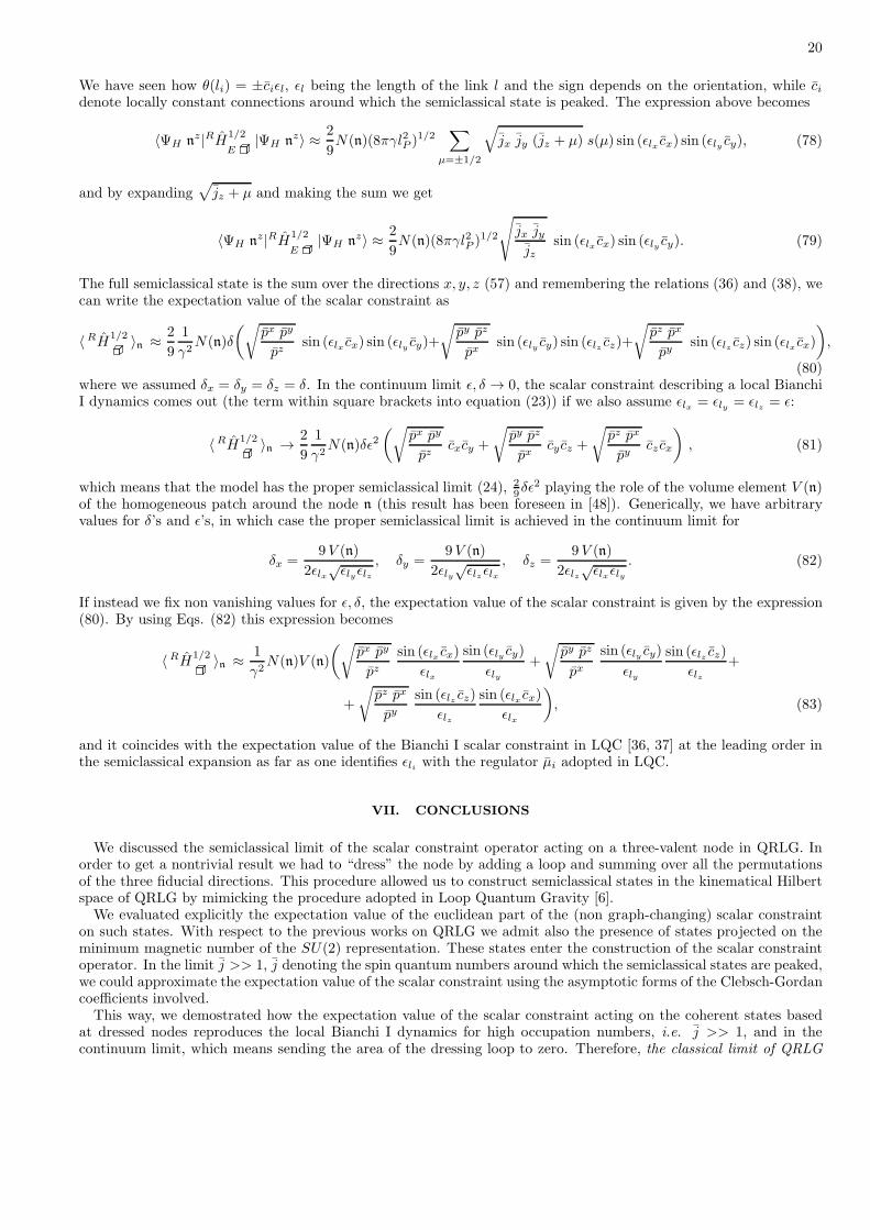
and it coincides with the expectation value of the Bianchi I scalar constraint in LQC [36, 37] at the leading order inthe semiclassical expansion as far as one identifies ǫli with the regulator µi adopted in LQC.

VII. CONCLUSIONS

We discussed the semiclassical limit of the scalar constraint operator acting on a three-valent node in QRLG. Inorder to get a nontrivial result we had to “dress” the node by adding a loop and summing over all the permutationsof the three fiducial directions. This procedure allowed us to construct semiclassical states in the kinematical Hilbertspace of QRLG by mimicking the procedure adopted in Loop Quantum Gravity [6].We evaluated explicitly the expectation value of the euclidean part of the (non graph-changing) scalar constraint

on such states. With respect to the previous works on QRLG we admit also the presence of states projected on theminimum magnetic number of the SU(2) representation. These states enter the construction of the scalar constraintoperator. In the limit j >> 1, j denoting the spin quantum numbers around which the semiclassical states are peaked,we could approximate the expectation value of the scalar constraint using the asymptotic forms of the Clebsch-Gordancoefficients involved.This way, we demostrated how the expectation value of the scalar constraint acting on the coherent states based

at dressed nodes reproduces the local Bianchi I dynamics for high occupation numbers, i.e. j >> 1, and in thecontinuum limit, which means sending the area of the dressing loop to zero. Therefore, the classical limit of QRLG

21

coincides with a local Bianchi I dynamics, i.e. it reproduces General Relativity in the proper (BKL) approximationscheme. This result makes the whole QRLG a viable scenario to investigate the quantum corrections to the earlyUniverse dynamics.Furthermore, by taking only the limit of high occupation numbers for spins, while retaining a nonvanishing loop,

then we reproduced the leading order term of the scalar constraint in LQC. The length of the edges into the loop

plays the role of the regulator in LQC. Therefore, we can trace back the origin of the LQC regulator as entering thedefinition of semiclassical states in QRLG. However, from this analysis we get no indication on how to fix such aparameter or on its dependence from the spins (as in the µ scheme).The next step is to investigate the semiclassical corrections to the classical dynamics. These are of two kinds: the

corrections coming from the expansion in ǫ and those due to the expansion around j. While the latter are expectedto provides (at least qualitatively) the same corrections as in LQC, the former will provides new contributions whichsurvive in the continuous limit. These will be determined by considering the next-to-leading order expansion of the3j, 6j and 9j symbols entering the expression (62). The order of magnitude of these corrections will tell us whetherthey can be discussed in the QRLG paradigm or if the full LQG theory is needed. Moreover, it remains to investigatethe Lorentzian part of the constraint, which in the classical limit is proportional to the Euclidean one. It will bediscussed elsewhere. However, we gave in this work all the necessary tools to make such an analysis and we expect itto be pursued straightforwardly.Furthermore, we discussed only the case of a three-valent node. In order to realize a realistic description of a

quantum Universe we must consider a generic three-dimensional reduced graph, whose nodes are up to six-valent. Weexpect that the approximation scheme adopted here is still suitable to provide a proper semiclassical limit, the onlydifficulty being that more complicated n-j symbols appears in calculations.Finally, the semiclassical techniques we developed are expected to be useful also with respect to the quantization of

a generic metric in the diagonal form, in which case a combination of the scalar and the vector constraints generatesthe dynamics.

Appendix A: Reduced Recoupling

The standard multiplication of SU(2) holonomies and their recoupling, i.e.

Dj1m1n1

(g)Dj2m2n2

(g) =∑

k

Ckmj1m1j2m2

Dkmn(g) C

knj1n1j2n2

(A1)

using the graphical calculus, introduced in [15] and based on 3j-symbols related to Clebsch-Gordan coefficients by

Cj3m3

j1m1j2m2= (−1)j1−j2+m3

√

dj3( j1 j2 j3m1 m2 −m3

)

, (A2)

can be written as

j1

j2=∑

k

dkj1

j2 j2

j1k (A3)

where the triangle denotes a generic SU(2) group element and the notation with the two kind of arrows is usedto distinguish indexes belonging to the vector space Hj or the dual vector space Hj∗. The expression (A1) in thequantum reduced case [28] becomes

D|n1|n1n1

(g)D|n2|n2n2

(g) = C|n1+n2|n1+n2

j1n1j2n2D

|n1+n2|n1+n2 n1+n2

(g) C|n1+n2|n1+n2

j1n1j2n2(A4)

If in the graphical notation we use 3-valent nodes to represent Clebsh-Gordan coefficients instead of 3-j symbols,the graphical transposition of the previous formula, using the label n to denote the magnetic number of a link inrepresentation |n|, is just:

j1

j2

j1

j2 j2

j1

=n1+n2

n1

n2

n1+n2

n2

n1n1+n2

(A5)

22

where the projection on the reduced Hilbert space forces the magnetic number n1+n2 of the recoupled group elementto be equal to the spin admitting only the channel K = |n1 + n2|.

Acknowledgments

The authors wish to thank T. Thiemann, K. Giesel, T. Pawlowski for useful discussions. This work of FC wassupported by funds provided by the National Science Center under the agreement DEC12 2011/02/A/ST2/00294.The work of E.A. was supported by the grant of Polish Narodowe Centrum Nauki nr 2011/02/A/ST2/00300.

[1] C. Rovelli, Cambridge, UK: Univ. Pr. (2004) 455 p[2] T. Thiemann, Cambridge, UK: Cambridge Univ. Pr. (2007) 819 p [gr-qc/0110034].[3] A. Perez, Class. Quant. Grav. 20, R43 (2003) [gr-qc/0301113].[4] C. Rovelli, PoS QGQGS 2011, 003 (2011) [arXiv:1102.3660 [gr-qc]].[5] T. Thiemann, Class. Quant. Grav. 18, 2025 (2001) [hep-th/0005233][6] T. Thiemann, Class. Quant. Grav. 23, 2063 (2006) [gr-qc/0206037].[7] E. Bianchi, L. Modesto, C. Rovelli and S. Speziale, Class. Quant. Grav. 23, 6989 (2006)[8] E. Alesci and C. Rovelli, Phys. Rev. D 76, 104012 (2007)[9] E. Alesci, E. Bianchi and C. Rovelli, Class. Quant. Grav. 26, 215001 (2009)

[10] E. Bianchi and Y. Ding, Phys. Rev. D 86, 104040 (2012)[11] T. Thiemann, Class. Quant. Grav. 15, 839 (1998) [gr-qc/9606089].[12] T. Thiemann, Class. Quant. Grav. 23, 2211 (2006)[13] T. Thiemann, Class. Quant. Grav. 23, 2249 (2006)[14] M. Gaul and C. Rovelli, Class. Quant. Grav. 18, 1593 (2001) [gr-qc/0011106].[15] E. Alesci, T. Thiemann and A. Zipfel, Phys. Rev. D 86, 024017 (2012) [arXiv:1109.1290 [gr-qc]].[16] E. Alesci, K. Liegener and A. Zipfel, Phys. Rev. D 88, 084043 (2013) [arXiv:1306.0861 [gr-qc]].[17] K. Giesel and T. Thiemann, Class. Quant. Grav. 24, 2465 (2007) [gr-qc/0607099].[18] K. Giesel and T. Thiemann, Class. Quant. Grav. 24, 2499 (2007) [gr-qc/0607100].[19] K. Giesel and T. Thiemann, Class. Quant. Grav. 24, 2565 (2007) [gr-qc/0607101].[20] M. Bojowald, Lect. Notes Phys. 835, pp.1 (2011).[21] A. Ashtekar and P. Singh, Class. Quant. Grav. 28, 213001 (2011) [arXiv:1108.0893 [gr-qc]].[22] C. Rovelli and F. Vidotto, Class. Quant. Grav. 25, 225024 (2008) [arXiv:0805.4585 [gr-qc]].[23] E. Bianchi, C. Rovelli and F. Vidotto, Phys. Rev. D 82, 084035 (2010) [arXiv:1003.3483 [gr-qc]].[24] E. F. Borja, J. Diaz-Polo, I. Garay and E. R. Livine, Class. Quant. Grav. 27, 235010 (2010) [arXiv:1006.2451 [gr-qc]].[25] S. Gielen, D. Oriti and L. Sindoni, Phys. Rev. Lett. 111, 031301 (2013) [arXiv:1303.3576 [gr-qc]].[26] A. Ashtekar, T. Pawlowski and P. Singh, Phys. Rev. D 74, 084003 (2006) [gr-qc/0607039].[27] E. Alesci, F. Cianfrani and C. Rovelli, Phys. Rev. D 88, 104001 (2013) [arXiv:1309.6304 [gr-qc]].[28] E. Alesci and F. Cianfrani, Phys. Rev. D 87, no. 8, 083521 (2013) [arXiv:1301.2245 [gr-qc]].[29] E. Alesci and F. Cianfrani, Europhys. Lett. 104, 10001 (2013) [arXiv:1210.4504 [gr-qc]].[30] V. A. Belinsky, I. M. Khalatnikov and E. M. Lifshitz, Adv. Phys. 19, 525 (1970).[31] V. A. Belinsky, I. M. Khalatnikov and E. M. Lifshitz, Adv. Phys. 31, 639 (1982).[32] B. Bahr and T. Thiemann, Class. Quant. Grav. 26, 045012 (2009) [arXiv:0709.4636 [gr-qc]].[33] T. Thiemann and O. Winkler, Class. Quant. Grav. 18, 2561 (2001) [hep-th/0005237].[34] E. Bianchi, E. Magliaro and C. Perini, Phys. Rev. D 82, 024012 (2010) [arXiv:0912.4054 [gr-qc]].[35] E. Magliaro, A. Marciano and C. Perini, Phys. Rev. D 83, 044029 (2011) [arXiv:1011.5676 [gr-qc]].[36] M. Martin-Benito, G. A. Mena Marugan and T. Pawlowski, Phys. Rev. D 78, 064008 (2008) [arXiv:0804.3157 [gr-qc]].[37] A. Ashtekar and E. Wilson-Ewing, Phys. Rev. D 79, 083535 (2009) [arXiv:0903.3397 [gr-qc]].[38] J. Brunnemann and T. A. Koslowski, Class. Quant. Grav. 28, 245014 (2011)[39] J. Engle, Class. Quant. Grav. 30, 085001 (2013) [arXiv:1301.6210 [gr-qc]].[40] M. Bojowald and G. M. Paily, Phys. Rev. D 86, 104018 (2012) [arXiv:1112.1899 [gr-qc]].[41] M. Bojowald and G. M. Paily, Class. Quant. Grav. 29, 242002 (2012) [arXiv:1206.5765 [gr-qc]].[42] F. Cianfrani and G. Montani, Phys. Rev. D 85, 024027 (2012) [arXiv:1104.4546 [gr-qc]].[43] F. Cianfrani, A. Marchini and G. Montani, Europhys. Lett. 99, 10003 (2012) [arXiv:1201.2588 [gr-qc]].[44] L. Freidel and S. Speziale, “Twisted geometries: A geometric parametrisation of SU(2) phase space,” Phys. Rev. D 82,

084040 (2010) [arXiv:1001.2748 [gr-qc]][45] R. Borissov, R. De Pietri and C. Rovelli, Class. Quant. Grav. 14, 2793 (1997) [gr-qc/9703090].[46] C. Rovelli and S. Speziale, “On the geometry of loop quantum gravity on a graph,” Phys. Rev. D 82, 044018 (2010)[47] Brussaard PJ, Tolhoek HA “Classical limits of Clebsch-Gordan coefficients, Racah coefficients and Dl

mn(φ, θ, ψ)-functions”,Physica 23 (10): 955-971 1957

23

[48] F. Cianfrani and G. Montani, Phys. Rev. D 82, 021501 (2010) [arXiv:1006.1814 [gr-qc]].[49] We take the coordinates x, y, z along the fiducial directions i = 1, 2, 3