Welcome message from author
This document is posted to help you gain knowledge. Please leave a comment to let me know what you think about it! Share it to your friends and learn new things together.
Transcript


Quantum Optics Experiments in aMicrostructured Ion Trap
Dissertation
zur Erlangung des Doktorgrades Dr. rer. nat.
der Fakultat fur Naturwissenschaften der Universitat Ulm
vorgelegt von
Ulrich Georg Poschinger
aus Berlin
2010

Amtierender Dekan: Prof. Dr. Axel Groß
Erstgutachter: Prof. Dr. Ferdinand Schmidt-Kaler
Zweitgutachter: Prof. Dr. Johannes Hecker Denschlag
Hiermit erklare ich, Ulrich Poschinger, dass ich die vorliegende Dissertation QuantumOptics Experiments in a Microstructured Ion Trap selbststandig angefertigt und keine an-deren als die angegebenen Quellen und Hilfsmittel benutzt sowie die wortlich und inhaltlichubernommenen Stellen als solche kenntlich gemacht und die Satzung der Universitat Ulm zurSicherung guter wissenschaftlicher Praxis beachtet habe.
Ulrich PoschingerUlm, den 12. November 2010
The work described in this thesis was carried out at the
Universitat UlmInstitut fur QuanteninformationsverarbeitungAlbert-Einstein-Allee 11D-89069 Ulm
Funding from the EU within the research programsMICROTRAP, SCALA, AQUTE and the MRTN EMALI,and from the DFG within the framework SFB/TRR21is gratefully acknowledged.
Tag der mündlichen Prüfung: 15.2.2011


Extraordinary rains pretty generally fall after great battles.-Plutarch

Abstract
This dissertation describes a prototype experiment aiming at the realization of scalable quan-tum information. The essential feature is the usage of a novel microstructured ion trap de-rived from the Paul trap. It allows for storing and manipulating a large number of ions,as compared to conventional linear Paul traps. This thesis describes how the way is pavedtowards the realization of quantum information experiments in this ion trap. An analysisof the electrostatic properties of the ion trap is presented, which is laying the foundationfor understanding the limits of confinement stability and effects beyond standard Paul trapbehavior. The focus of this work lies on the realization and characterization of single anddual qubit operations, which are achieved by means of (semiclassical) atom-light interaction.In our experiment, the qubit is implemented in the Zeeman sublevels of the ion’s groundstate, i.e. in the spin of the bright electron of a 40Ca+ ion. The main body of this the-sis then describes the realization of the necessary steps of preparation, manipulation andreadout of this qubit. The preparation includes optical pumping and cooling close to themotional quantum ground state by means of sideband cooling. Several possible techniquesfor these steps are tested and analyzed. Coherent manipulations are carried out by meansof stimulated Raman transitions. Here, a strong emphasis is put on the characterization ofthe various decoherence mechanisms, which are dominated by the motional excitation of theion due to thermalization of the ion with the trap electrodes, and by imperfections in theion-laser interactions. As by-product of the latter investigation, a new measurement schemefor the experimental determination of atomic dipole matrix elements is presented. Finally,experimental results on the preparation of Schrodinger Cat states and on the tomography ofa single ion’s motional state are presented. It is also described how Schrodinger Cat statescan be used as a measurement tool for the ultraprecise monitoring of a single ion’s phasespace trajectory, where deviations from the Lamb-Dicke limit dynamics are seen.
i

Zusammenfassung
Diese Dissertation behandelt die grundlegenden Schritte eines Prototyp-Experiments welchesauf die Realisierung skalierbarer Quanteninformation abzielt. Das entscheidende Merkmalliegt in der Verwendung einer neuartigen mikrostrukturierten Ionenfalle, welche auf derbekannten Paulfalle basiert. Verglichen mit konventionellen Paulfallen erlaubt diese die Spe-icherung und Manipulation einer grosseren Anzahl von Ionen. Diese Arbeit beschreibt wieder Weg zur Realisierung von Quanteninformationsexperimenten in dieser Ionenfalle geebnetwird. Zuerst wird eine detaillierte Analyse der elektrostatischen Eigenschaften der verwen-deten Ionenfalle prasentiert, was ein grundlegendes Verstandnis der Einschlusseigenschaftenund moglicher Effekte jenseites des idealen Verhaltens ermoglicht. Der Fokus dieser Ar-beit liegt bei der Realisierung und Charakterisierung von Operationen mit einem und zweiQubits, welche mit Hilfe der (semiklassischen) Atom-Licht Wechselwirkung ausgefhrt wer-den. In unserem Experiment wird das Qubit in den Zeeman-Unterzustanden des elek-tronischen Grundzustands des Ions kodiert, also im Spin des Leuchtelektrons eines 40Ca+
Ions. Der Hauptteil dieser Arbeit umfasst die Realisierung der notigen VerfahrensschrittePraparation, Manipulation und Auslese dieser Art von Qubit. Die Praparation umfasst op-tisches Pumpen und Kuhlen nahe an den quantenmechanischen Grundzustand der Bewegung.Mehrere mogliche Techniken dafur werden getestet und analysiert. Koharente Manipulatio-nen werden mithilfe stimulierter Ramanubergange ausgefuhrt. Hier wird eine starke Beto-nung auf die Charakterisierung der verschiedenen Dekoharenzprozesse gelegt, die von derAnregung der Ionenbewegung durch Thermalisierung mit der Umgebung und Imperfektio-nen bei der Ionen-Licht-Wechselwirkung dominiert werden. Als Nebenprodukt des letzterenwird ein neues Messverfahren zur Bestimmung atomarer Dipolmatrixelemente prasentiert.Zuletzt werden experimentelle Ergebnisse zur Praparation eines Schrodinger-Katzenzustandsund zur Tomographie des Bewegungszustandes eines einzelnen Ions gezeigt. Es wird ebenfallsdemonstriert, wie Schrodinger-Katzenzustande benutzt werden konnen um die Phasenraum-trajektorie eines einzelnen ions mit hoher Genauigkeit zu verfolgen, wobei auch Abweichungenvom Lamb-Dicke Regime beobachtet werden.
iii

Contents
1. Introduction 1
2. Theoretical Foundations 92.1. Laser-Ion Interactions . . . . . . . . . . . . . . . . . . . . . . . . . . . . . . . 9
2.1.1. The Two-Level System: Dynamics . . . . . . . . . . . . . . . . . . . . 92.1.2. The Two-Level System: Coupling Matrix Elements . . . . . . . . . . . 132.1.3. Including the Motional Degrees of Freedom: Laser Cooling . . . . . . 152.1.4. Including the Motional Degrees of Freedom: The Resolved Sideband
Regime . . . . . . . . . . . . . . . . . . . . . . . . . . . . . . . . . . . 192.1.5. Multilevel Systems Interacting with Multiple Laser Fields: Optical
Pumping . . . . . . . . . . . . . . . . . . . . . . . . . . . . . . . . . . 232.1.6. Multilevel Systems Interacting with Off-Resonant Laser Fields: Stim-
ulated Raman Transitions and Decoherence Effects . . . . . . . . . . . 292.2. Linear Segmented Paul Traps . . . . . . . . . . . . . . . . . . . . . . . . . . . 33
2.2.1. Confinement Mechanism . . . . . . . . . . . . . . . . . . . . . . . . . . 332.2.2. Vibrational Modes of Ion Crystals . . . . . . . . . . . . . . . . . . . . 37
3. Experimental Setup 413.1. The Trap, Vacuum Vessel and the Ovens . . . . . . . . . . . . . . . . . . . . . 413.2. Laser Systems . . . . . . . . . . . . . . . . . . . . . . . . . . . . . . . . . . . . 42
3.2.1. 423 nm and 375 nm for Photoionization . . . . . . . . . . . . . . . . . 433.2.2. 397 nm for Doppler Cooling, Ion Detection and Optical Pumping . . . 443.2.3. 854 nm and 866 nm for Repumping and Quenching . . . . . . . . . . . 463.2.4. 729 nm for Electron Shelving . . . . . . . . . . . . . . . . . . . . . . . 473.2.5. 397 nm for Stimulated Raman Transitions . . . . . . . . . . . . . . . . 50
3.3. Imaging and Detection . . . . . . . . . . . . . . . . . . . . . . . . . . . . . . . 543.4. Trap Voltage Supplies . . . . . . . . . . . . . . . . . . . . . . . . . . . . . . . 543.5. Quantizing Magnetic Field . . . . . . . . . . . . . . . . . . . . . . . . . . . . . 563.6. Experimental Control System . . . . . . . . . . . . . . . . . . . . . . . . . . . 56
4. Implementation of the Spin Qubit 594.1. A Brief Survey of Trapped Ion Qubit Types . . . . . . . . . . . . . . . . . . . 594.2. Basic Qubit Operations . . . . . . . . . . . . . . . . . . . . . . . . . . . . . . 61
4.2.1. State Discrimination by Fluorescence Counting . . . . . . . . . . . . . 614.2.2. Spectroscopy on the Quadrupole Transition . . . . . . . . . . . . . . . 664.2.3. Coherent Dynamics on the Quadrupole Transition . . . . . . . . . . . 68
v
Contents
4.2.4. Qubit Preparation . . . . . . . . . . . . . . . . . . . . . . . . . . . . . 734.2.5. Qubit Reset . . . . . . . . . . . . . . . . . . . . . . . . . . . . . . . . . 77
4.3. 3D Heating Rate Measurement by Fluorescence Observation . . . . . . . . . . 804.4. Qubit Readout via Electron Shelving . . . . . . . . . . . . . . . . . . . . . . . 824.5. Stimulated Raman Transitions . . . . . . . . . . . . . . . . . . . . . . . . . . 88
4.5.1. Raman Spectroscopy and Single Qubit Rotations . . . . . . . . . . . . 884.6. Sideband Cooling and Phonon Distribution Measurements . . . . . . . . . . . 944.7. Coherence and Decoherence of the Spin Qubit . . . . . . . . . . . . . . . . . . 102
5. Trap Characteristics 1135.1. Electrostatic Potentials . . . . . . . . . . . . . . . . . . . . . . . . . . . . . . 1135.2. Micromotion Compensation . . . . . . . . . . . . . . . . . . . . . . . . . . . . 119
6. Determination of Atomic Matrix Elements with Off-Resonant Radiation 1276.1. Motivation . . . . . . . . . . . . . . . . . . . . . . . . . . . . . . . . . . . . . 1276.2. Basic Idea of the Measurement Procedure . . . . . . . . . . . . . . . . . . . . 1276.3. Measurement of the Scattering Rates . . . . . . . . . . . . . . . . . . . . . . . 1306.4. Measurement of the Raman Detuning . . . . . . . . . . . . . . . . . . . . . . 1316.5. Measurement of the AC Stark Shift . . . . . . . . . . . . . . . . . . . . . . . . 1316.6. Robustness against Experimental Imperfections . . . . . . . . . . . . . . . . . 1346.7. Extraction of the Scattering Parameters and Error Analysis . . . . . . . . . . 1366.8. Final Results . . . . . . . . . . . . . . . . . . . . . . . . . . . . . . . . . . . . 1386.9. Additional Error Sources . . . . . . . . . . . . . . . . . . . . . . . . . . . . . . 1396.10. Complete Measurement by Measuring Absolute Stark Shifts . . . . . . . . . . 140
7. Motional State Tomography 1457.1. The Method . . . . . . . . . . . . . . . . . . . . . . . . . . . . . . . . . . . . . 1457.2. The Measurement Scheme . . . . . . . . . . . . . . . . . . . . . . . . . . . . . 147
8. Preparation and Characterization of Schrodinger Cat States 1538.1. Preparation of a Schrodinger Cat State of a Single Ion . . . . . . . . . . . . . 1538.2. Temperature Dependence and Quantum Effects . . . . . . . . . . . . . . . . . 1618.3. Phonon Distribution Dynamics . . . . . . . . . . . . . . . . . . . . . . . . . . 1638.4. The Wavepacket Beating Scheme . . . . . . . . . . . . . . . . . . . . . . . . . 169
9. Measurements with Two-Ion Crystals 1779.1. Stability and Read-out . . . . . . . . . . . . . . . . . . . . . . . . . . . . . . . 1779.2. Localization and Alignment in a Standing Wave . . . . . . . . . . . . . . . . . 1809.3. Spectroscopy and Cooling . . . . . . . . . . . . . . . . . . . . . . . . . . . . . 1869.4. Coherent Manipulations . . . . . . . . . . . . . . . . . . . . . . . . . . . . . . 1909.5. A Two-Ion Schrodinger Cat . . . . . . . . . . . . . . . . . . . . . . . . . . . . 195
10.Conclusion and Outlook 20310.1. Conclusion . . . . . . . . . . . . . . . . . . . . . . . . . . . . . . . . . . . . . 203
vi

Contents
10.2. Open Questions . . . . . . . . . . . . . . . . . . . . . . . . . . . . . . . . . . . 20410.3. Outlook . . . . . . . . . . . . . . . . . . . . . . . . . . . . . . . . . . . . . . . 205
A. Adiabatic Elimination on the Master Equation 207
B. Trap Voltage Supply Electronics 211
C. Advanced Reconstruction Technique for Phonon Number Distributions 219
D. Tomography Method for States with Entanglement of Spin and Motion 223
E. Coherently Driven Ion Crystals 227E.1. Driving the Internal State . . . . . . . . . . . . . . . . . . . . . . . . . . . . . 227E.2. Driving the Motion . . . . . . . . . . . . . . . . . . . . . . . . . . . . . . . . . 228
F. Atomic Properties of Calcium 231
G. Publications 233G.1. Journal Publications . . . . . . . . . . . . . . . . . . . . . . . . . . . . . . . . 233G.2. Talks . . . . . . . . . . . . . . . . . . . . . . . . . . . . . . . . . . . . . . . . . 234G.3. Posters . . . . . . . . . . . . . . . . . . . . . . . . . . . . . . . . . . . . . . . . 234
vii


List of Figures
1.1. Progress in ion-trap quantum computing . . . . . . . . . . . . . . . . . . . . . 21.2. Illustration of the limited scalability in linear Paul traps . . . . . . . . . . . . 4
2.1. Doppler cooling . . . . . . . . . . . . . . . . . . . . . . . . . . . . . . . . . . . 162.2. Product Hilbert space for a two-level system and a harmonic oscillator . . . . 202.3. Motional matrix elements . . . . . . . . . . . . . . . . . . . . . . . . . . . . . 212.4. Simulated Rabi oscillations on carrier and first order sideband for different
temperatures and Lamb-Dicke factors . . . . . . . . . . . . . . . . . . . . . . 242.5. Sideband cooling scheme . . . . . . . . . . . . . . . . . . . . . . . . . . . . . . 252.6. Dephasing of Rabi oscillations . . . . . . . . . . . . . . . . . . . . . . . . . . . 262.7. Level scheme for the pumping problem . . . . . . . . . . . . . . . . . . . . . . 272.8. Continuous pumping rates in a four-level system . . . . . . . . . . . . . . . . 282.9. Optimum depump Rabi frequency versus excitation Rabi frequency . . . . . . 292.10. Excitation suppression and broadening in a three- and four-level system . . . 302.11. Level scheme for off-resonant interactions . . . . . . . . . . . . . . . . . . . . 312.12. Basic types of Paul traps . . . . . . . . . . . . . . . . . . . . . . . . . . . . . 332.13. Mechanism for confinement in a quadrupolar rf potential . . . . . . . . . . . . 352.14. Regions of stability for different trap geometries . . . . . . . . . . . . . . . . . 36
3.1. Trap layout and picture . . . . . . . . . . . . . . . . . . . . . . . . . . . . . . 423.2. General beam geometry . . . . . . . . . . . . . . . . . . . . . . . . . . . . . . 433.3. Optical setup for the laser at 397 nm for Doppler cooling . . . . . . . . . . . 443.4. Optical setup of the laser at 866 nm and 854 nm . . . . . . . . . . . . . . . . 463.5. Optical setup of the 729 nm laser . . . . . . . . . . . . . . . . . . . . . . . . . 473.6. 729 nm AOM characterization . . . . . . . . . . . . . . . . . . . . . . . . . . . 483.7. Optical setup for the laser at 397 nm for off-resonant coherent manipulations 503.8. Characterization of the switching EOM . . . . . . . . . . . . . . . . . . . . . 513.9. rf network for the supply of the AOMs in the Raman beamline . . . . . . . . 523.10. Setup for imaging and fluorescence detection . . . . . . . . . . . . . . . . . . 553.11. Experimental control system . . . . . . . . . . . . . . . . . . . . . . . . . . . 57
4.1. Complete level scheme of 40Ca+ . . . . . . . . . . . . . . . . . . . . . . . . . . 604.2. Fluorescence histogram . . . . . . . . . . . . . . . . . . . . . . . . . . . . . . 624.3. Fluorescence discrimination errors for different count rates . . . . . . . . . . . 634.4. Spectroscopy on the S1/2 to P1/2 transition . . . . . . . . . . . . . . . . . . . 654.5. Detailed level scheme of the quadrupole transition . . . . . . . . . . . . . . . 66
ix

List of Figures
4.6. Accessible quadrupole transitions . . . . . . . . . . . . . . . . . . . . . . . . . 67
4.7. Spectroscopy on the quadrupole transition . . . . . . . . . . . . . . . . . . . . 68
4.8. Coherent dynamics on the quadrupole transition . . . . . . . . . . . . . . . . 69
4.9. Effective Rabi frequency distribution . . . . . . . . . . . . . . . . . . . . . . . 70
4.10. Gauge of the Rabi frequency on the quadrupole transition . . . . . . . . . . . 71
4.11. Two different schemes for optical pumping . . . . . . . . . . . . . . . . . . . . 73
4.12. Optical pumping on the quadrupole transition . . . . . . . . . . . . . . . . . . 74
4.13. Measurement of spurious polarization components . . . . . . . . . . . . . . . 75
4.14. Quenching of the D5/2 state . . . . . . . . . . . . . . . . . . . . . . . . . . . . 78
4.15. Quenching of the D3/2 state . . . . . . . . . . . . . . . . . . . . . . . . . . . . 79
4.16. Fluorescence heating rate measurement . . . . . . . . . . . . . . . . . . . . . 80
4.17. Scheme of the RAP process . . . . . . . . . . . . . . . . . . . . . . . . . . . . 82
4.18. Rapid adiabatic passage pulse . . . . . . . . . . . . . . . . . . . . . . . . . . . 83
4.19. RAP efficiency versus peak Rabi frequency for different chirp ranges . . . . . 84
4.20. Robustness of the shelving process with respect to frequency errors . . . . . . 85
4.21. Parasitic shelving . . . . . . . . . . . . . . . . . . . . . . . . . . . . . . . . . . 86
4.22. Spectroscopy on the orthogonal Raman transition . . . . . . . . . . . . . . . . 89
4.23. Spectroscopy on the collinear Raman transition . . . . . . . . . . . . . . . . . 90
4.24. Coherent dynamics on the collinear Raman transition . . . . . . . . . . . . . 92
4.25. Coherent versus incoherent effects on the Raman transition . . . . . . . . . . 93
4.26. Two different schemes for sideband cooling . . . . . . . . . . . . . . . . . . . 94
4.27. Raman spectra with and without sideband cooling . . . . . . . . . . . . . . . 95
4.28. Coherent dynamics on the blue sideband after sideband cooling . . . . . . . . 96
4.29. Cosine transform of blue sideband Rabi oscillations . . . . . . . . . . . . . . . 97
4.30. Coherent dynamics on the orthogonal Raman transition after sideband cooling 98
4.31. Results of the heating rate measurement . . . . . . . . . . . . . . . . . . . . . 99
4.32. Calculated phonon removal times for different red sideband transitions . . . . 100
4.33. T∗2 measurement on various transitions . . . . . . . . . . . . . . . . . . . . . . 102
4.34. T2 measurement on various transitions . . . . . . . . . . . . . . . . . . . . . . 103
4.35. Sample results from the spin echo contrast measurement . . . . . . . . . . . . 105
4.36. Laser induced dephasing mechanisms . . . . . . . . . . . . . . . . . . . . . . . 106
4.37. Spin-echo contrast versus decohering pulse time . . . . . . . . . . . . . . . . . 107
4.38. Resulting decoherence rate coefficients . . . . . . . . . . . . . . . . . . . . . . 108
4.39. Investigation of the intensity-fluctuation induced decoherence process . . . . . 110
5.1. Trap layout for electrostatic field simulation . . . . . . . . . . . . . . . . . . . 113
5.2. Electrostatic axial confinement potentials . . . . . . . . . . . . . . . . . . . . 115
5.3. Radial potential cuts . . . . . . . . . . . . . . . . . . . . . . . . . . . . . . . . 116
5.4. Radial confinement strength along the trap axis . . . . . . . . . . . . . . . . . 118
5.5. Off-site spectroscopy . . . . . . . . . . . . . . . . . . . . . . . . . . . . . . . . 119
5.6. Micromotion compensation by fluorescence measurement . . . . . . . . . . . . 122
5.7. Modulation index along the trap axis . . . . . . . . . . . . . . . . . . . . . . . 124
5.8. Micromotion induced phonon lasing effect . . . . . . . . . . . . . . . . . . . . 125
x
List of Figures
6.1. Relevant levels and transitions for the lifetime measurement scheme . . . . . 128
6.2. Raw data from the scattering rate measurement . . . . . . . . . . . . . . . . . 131
6.3. Comparison of theoretical and experimental error bars . . . . . . . . . . . . . 132
6.4. Spin flip curves . . . . . . . . . . . . . . . . . . . . . . . . . . . . . . . . . . . 133
6.5. Fluorescence calibration of the wavemeter . . . . . . . . . . . . . . . . . . . . 134
6.6. Example Stark shift measurement . . . . . . . . . . . . . . . . . . . . . . . . . 135
6.7. Stark shift measurement accuracy . . . . . . . . . . . . . . . . . . . . . . . . . 136
6.8. Calibration by means of the Stark shift . . . . . . . . . . . . . . . . . . . . . 137
6.9. Error ellipsoid for the scattering rates . . . . . . . . . . . . . . . . . . . . . . 138
6.10. Level scheme for absolute Stark shift measurement . . . . . . . . . . . . . . . 141
6.11. Measurement scheme for the absolute Stark shift . . . . . . . . . . . . . . . . 142
6.12. Measurement scheme for the absolute Stark shift . . . . . . . . . . . . . . . . 143
7.1. The complete tomography measurement . . . . . . . . . . . . . . . . . . . . . 148
7.2. Resulting phonon distributions . . . . . . . . . . . . . . . . . . . . . . . . . . 149
7.3. Resulting density matrix . . . . . . . . . . . . . . . . . . . . . . . . . . . . . . 150
8.1. Illustration of the spin-dependent light force . . . . . . . . . . . . . . . . . . . 154
8.2. Analogy between the Schrodinger cat experiment and a Mach-Zehnder inter-ferometer . . . . . . . . . . . . . . . . . . . . . . . . . . . . . . . . . . . . . . 158
8.3. Entanglement-induced contrast loss for the Schrodinger cat state . . . . . . . 159
8.4. Groundstate versus thermal signals . . . . . . . . . . . . . . . . . . . . . . . . 161
8.5. Classical and quantum mechanical trajectories . . . . . . . . . . . . . . . . . 163
8.6. Reconstructed phonon distributions . . . . . . . . . . . . . . . . . . . . . . . 164
8.7. Reconstructed phonon distributions with fits to coherent state distributions . 165
8.8. Results from the phonon distribution measurements . . . . . . . . . . . . . . 166
8.9. Decoherence rate versus displacement . . . . . . . . . . . . . . . . . . . . . . 167
8.10. Quantum jumps during sideband Rabi oscillations . . . . . . . . . . . . . . . 168
8.11. Schematic of the wavepacket beating experiment . . . . . . . . . . . . . . . . 169
8.12. Measurement results for the wavepacket beating scheme . . . . . . . . . . . . 170
8.13. Measured signals from the wavepacket beating scheme . . . . . . . . . . . . . 171
8.14. Contrast and carrier off-resonance . . . . . . . . . . . . . . . . . . . . . . . . 172
8.15. Measured particle trajectory . . . . . . . . . . . . . . . . . . . . . . . . . . . . 173
8.16. Cat states with varying parity . . . . . . . . . . . . . . . . . . . . . . . . . . . 174
9.1. Fluorescence histogram of two ions . . . . . . . . . . . . . . . . . . . . . . . . 178
9.2. Shelving of two ions . . . . . . . . . . . . . . . . . . . . . . . . . . . . . . . . 179
9.3. Localization measurement samples . . . . . . . . . . . . . . . . . . . . . . . . 181
9.4. Localization measurement result . . . . . . . . . . . . . . . . . . . . . . . . . 182
9.5. Fluorescence autocorrelation . . . . . . . . . . . . . . . . . . . . . . . . . . . . 183
9.6. Raman spectrum of two ions . . . . . . . . . . . . . . . . . . . . . . . . . . . 186
9.7. Sideband cooling of two ions . . . . . . . . . . . . . . . . . . . . . . . . . . . . 189
9.8. Rabi oscillations of two ions . . . . . . . . . . . . . . . . . . . . . . . . . . . . 190
xi
List of Figures
9.9. Balanced Rabi oscillations of two ions . . . . . . . . . . . . . . . . . . . . . . 1919.10. Camera-based read-out of a two ion crystal . . . . . . . . . . . . . . . . . . . 1929.11. Histograms resulting from the two-ion readout . . . . . . . . . . . . . . . . . 1929.12. Independent readout of two-ion Rabi oscillations . . . . . . . . . . . . . . . . 1939.13. PMT data of two-ion Rabi oscillations . . . . . . . . . . . . . . . . . . . . . . 1949.14. Schrodinger cat state schematic with two ions . . . . . . . . . . . . . . . . . . 1959.15. Schrodinger cat state creation with two ions . . . . . . . . . . . . . . . . . . . 1969.16. Parameters describing the quantum dynamics of two ions . . . . . . . . . . . 1999.17. Beat between displacement and squeezing . . . . . . . . . . . . . . . . . . . . 201
B.1. Voltage generation stage . . . . . . . . . . . . . . . . . . . . . . . . . . . . . . 212B.2. Buffer and adding stage . . . . . . . . . . . . . . . . . . . . . . . . . . . . . . 213B.3. Transistor buffer stage . . . . . . . . . . . . . . . . . . . . . . . . . . . . . . . 213B.4. Heating rate measurements for different buffer stages . . . . . . . . . . . . . . 214B.5. Design of the scalable trap voltage supply . . . . . . . . . . . . . . . . . . . . 215B.6. Data flow within the FPGA subsystem . . . . . . . . . . . . . . . . . . . . . . 216
C.1. Determination of confidence interval for an occupation probability . . . . . . 220
xii
1. Introduction
The reason for the late discovery of quantum mechanics is that genuine quantum phenom-ena are hardly observed in our everyday life. Even though the stability of atoms, nucleiand condensed matter objects - without which we would not even exist - originates fromquantum mechanics, essential quantum concepts like superposition states and entanglementappear to be counterintuitive. They still lead to philosophical objections against the theory.Because of this, quantum mechanics was not even fully accepted by some of its inventors,like Albert Einstein or Erwin Schrodinger. However, it is up to now the only theory whichcould withstand every experimental test with tremendous success. The last decades haveseen a paradigm shift from the pure investigation of quantum phenomena and tests of thetheory to the usage of quantum mechanics for technological applications. There are alreadydevices which play crucial roles in the modern world which heavily rely on quantum me-chanics, e.g. semiconductor microelectronics or the laser. Applications of the pure quantumeffects mentioned above, however, remain scarce. Nevertheless, a large number of promisingproposals, an impressive number of stunning experimental demonstrations and even somecommercial products show that the application of fundamental quantum mechanics is cur-rently one the most exciting fields of research. This field can be roughly subdivided into theareas of quantum information, quantum simulation, quantum communication and quantummetrology. Quantum information is based on the idea of using entanglement as a computa-tional resource, which promises a tremendous increase in computational efficiency for certainproblems. The idea behind quantum simulation is to use the ability to control tailoredquantum systems to model real-life systems which are still not completely understood, likee.g. high-temperature superconductors. Quantum communication makes use of fundamentalideas like the no-cloning theorem to provide absolutely safe information transfer. Finally,quantum metrology attempts to increase the measurement accuracy for natural constantsby means of entanglement enhancement are even to construct more accurate sensors, likeSQUIDS for magnetic fields.Both the late discovery of these effects and the difficulty of their usage can be explainedby the fact that they are obscured by the complexity of systems consisting of many degreesof freedom. If we consider a small system of interest, superposition states within this sys-tem are destroyed by the interaction with many degrees of freedom from the surroundingenvironment, a process which is called decoherence. This transfer of information from thesmall system to the outside world, which is a model for the measurement process, provides atleast a partial explanation for the projection postulate. Ironically, entanglement is difficultto observe because of - entanglement: Coherences within the system of interest effectivelydecay because the interaction with the environmental degrees of freedom lead to mutual en-tanglement. This in turn reduces the quantum coherence within the system, such that the
1

1. Introduction
fundamental concepts of classical physics, i.e. causality, locality and reality are restored onthe macroscopic scale.
1975: Proposals for laser cooling (HS75, WD75)
1978: Demonstration of laser cooling (HS75, WD75)
1953: Quadrupole mass filter (HS75,)
1958: Paul trap (HS75,)
1978: Observation of ion crystals (Diedrich87, Wineland87)
1986: Observation of quantum jumps (Bergquist86,Nagourney86, Sauter86)
1995: 3D groundstate cooling (MMK+95)
1998: Entanglement of two ions (TWK+98)
1995: Cirac-Zoller gate proposal (CZ95)
2000: Entanglement of four ions (SKK+00)
1999: Individual laser addressing (Nägerl1999)
2001: Decoherence free quantum memory (KMR+01)
2002: Proposal of segmented ion traps (KMW02) 2002: Demonstration of a CNOT gate (DBKL+02)
2003: Demonstration of a geomtric phase gate (LBMW03) 2003: Realization of the Cirac Zoller gate (SKHR+03)
2003: Deutsch-Josza algorithm (GRL+03)
2004: Quantum teleportation (RHR+04, BCS+04) 2004: Heisenberg spectroscopy (LBS+04)
2005: Quantum Fourier Transform (CBL+05) 2005: Entaglement of eight ions (HHR+05)
2008: Fault-tolerant gates (BKRB08)
2009: Demonstration of scalability (Home 2009)
2007: Entanglement of distant ions (MMO+07)
2008: Cryogenic surface ion trap (LGA+08)
2004: Single photon generation (KLH+04)
Figure 1.1.: Milestones in ion-trap quantum computing..
The ability to investigate, control and utilize quantum systems thus relies on the abilityto isolate small systems sufficiently from the outside world and to provide techniques forcontrolled quantum state manipulations and measurements. Today, the best possible tech-nical realizations of this are traps for charged atomic particles, i.e. ion traps. These comebasically in two flavors, namely Paul traps, where a combination of static and rapidly alter-nating electric fields is used to provide confinement in free space, or Penning traps, whichuse static electric and magnetic fields to accomplish this task. Despite the very successfulhistory of Penning traps, Paul traps have shown to be a better suited tool to realize someof the ideas mentioned above. An overview of the milestones of quantum physics with Paultraps is shown in Fig. 1.1, where the selection reflects the personal opinion of the author.The basic physical idea of the Paul trap, namely to provide stable confinement in two spa-
2
tial dimensions by means of ponderomotive forces, initially led to its original use as a massspectrometer, for which it is actually still employed for today. However, it was recognizedthat also stable confinement in three spatial directions is possible, which allowed for studieson isolated single atomic particles. With the advent of laser-cooling, it became possible tobring these particles completely to rest, enabling a large number of fundamental experiments,which even the founding fathers of quantum mechanics would have never dreamed of. Asthe trapped ions are isolated from massive objects, the suitable means to exert control andobtain information is light. As lasers are monochromatic and coherent, they provide the idealtool for cooling, manipulation and read-out of the ions. If the atomic species which is usedhas at least two (meta)stable energy levels, between which population can be transferredby means of laser light, it represents a carrier of binary quantum information, a qubit. Thefigures define the value of any quantum information register: The number of qubits that canbe stored and manipulated, the timescales on which decoherence occurs and the speed of theinformation processing steps, i.e. the quantum gates. In particular, the latter has to beatthe decoherence timescale. Despite the successful demonstration of all necessary steps torealize a quantum information processor based on a Paul trap, the limiting issue for actualapplication is the scalability to a large enough number of qubits. The current state of the artis the demonstration of complete control over a number of eight ion qubits, which is unlikelyto be overtrumped on the basis of conventional technology. A number of problems arise ifone attempts to store a large number of ions in a single linear Paul trap: First, the requiredstrength of radial confinement to maintain the ions aligned along a string increases with thenumber of ions. Second, the decrease of the minimum distance between two qubits for largernumbers of ions makes the ion addressing more and more difficult. Third, the addressing ofmotional modes in frequency space also becomes a challenge for many ions, as the numberof motional modes increases linearly, leading to spectral crowding. To make this point clear,these statements are illustrated in Fig. 1.2.
Several ways to circumvent these scalability problems have been proposed and partiallyrealized:
Atom-photon networkingIt has been successfully demonstrated that groups of up to eight ions can be fullycontrolled in a single linear Paul trap. Thus, one could simply operate several ofsuch traps. This brings up the necessity to transfer quantum information betweenthe different sub-processors, i.e. the nodes of the quantum network. The naturalcandidate as information carrier is of course the photon, which has a long traditionas a carrier of quantum information. This scheme has been originally proposed in[Cir97]. The scheme only works if a deterministic mapping of quantum informationfrom atomic to photonic qubits can be performed, for which cavity QED delivers themost suitable physical realization. A successful demonstration of this mapping withneutral atoms has been performed in [Wil07]. The combination of ion traps and high-finesse cavities has already led to a deterministic single photon generation from ions[Kel04], the combination of these techniques however still remains an experimentalchallenge. An alternative method to provide the desired coupling between photons and
3
1. Introduction
0 2 4 6 8 10 12 14 16 18 200
1
2
3
4
5
6
7
8
9
Min
imum
sta
bilit
y as
pect
ratio
Number of ions
2 4 6 80
1
2
3
4
5
6
7
N=10Im ω
rad
Aspect ratio
N=15
0 2 4 6 8 10 12 14 16 18 20
2
3
4
5
6
Min
imum
dis
tanc
e [µ
m]
Number of ions
2 4 6 8 10 12 14 16 18 20
-20
-15
-10
-5
0
5
10
15
20
Equ
ilibr
ium
pos
ition
[µm
]
Number of ions
a) b)
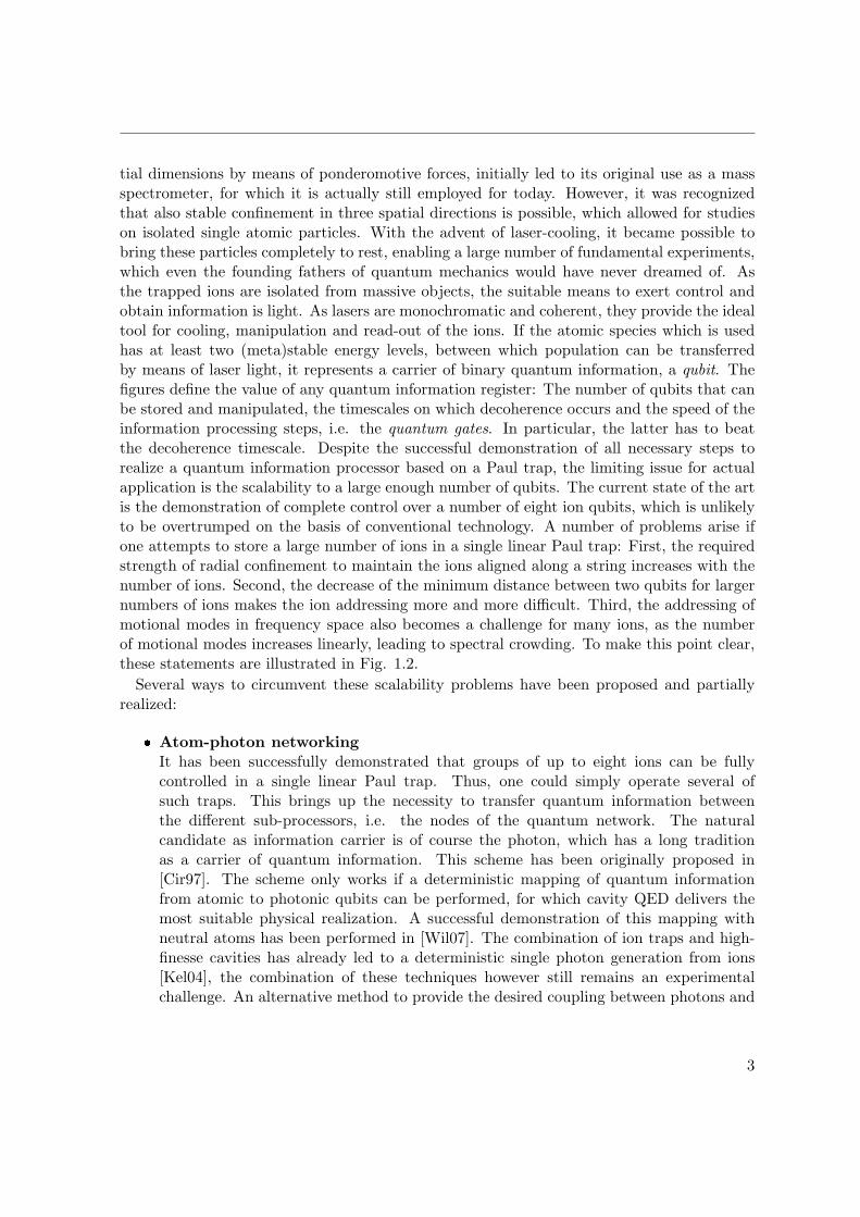
Figure 1.2.: Illustration of the limited scalability in linear Paul traps: a) shows how the min-imum ion distance decreases as more and more ions are stored in a trap (example parametersassumed here are a trap frequency of 1 MHz and the mass of 40Ca+ ions). The inset showsthe equilibrium positions of the ions, also demonstrating the increasing inhomogeneity of thestring for larger ions numbers. The scaling behavior is found to be ∆zmin ∝ N−0.56 [Jam98].b) shows how the radial confinement has to be increased for stable operation with largernumbers of ions. The minimum trap aspect ratio is ωrad/ωax yielding a linear ion string isplotted against the ion number. The inset shows how the instability occurs for decreasedradial confinement, see Sec. 2.2.
atoms is a free-space configuration with strong focusing [Tey09]. Another alternative isnot to use light, but charge excitations in metal wires to transfer the qubit informationover distances [Dan09].
Probabilistic entanglementA tremendous experimental simplification is achieved if the requirement of determinis-tic coupling in the previously mentioned scheme, i.e. unit efficiency of qubit conversion,is dropped. The price to be paid is that the computation scheme becomes probabilis-tic. A possible realization was proposed in [Dua04b], with the key idea of making useof emitted photons as heralds for entanglement. After a certain number of attempts,one would therefore know that ions at remote locations are in a given entangled state.This state can then be used as a resource for quantum computation without the ne-cessity of further quantum information transfer, e.g. in the spirit of the cluster statecomputation scheme proposed in [Rau01]. The scheme has recently been realized fortwo ions [Moe07], but the future prospects remain questionable because of the low suc-
4
cess rates for entanglement and the unfavorable scaling behavior for more than twoqubits. However, a hybrid approach where cavities are used to enhance the photoncollection efficiencies might still be a very promising candidate for large-scale quantumcomputation.
Laserless quantum computingThe necessity of ultra-stable laser sources in unfavorable wavelength ranges, with highdemands on power and stability, represents one of the greatest obstacles for the com-mercial use of quantum computation. Also, some of the scalability limits listed abovearise due to the requirement of well-defined interactions between ions and laser light.Furthermore, frequency and intensity fluctuations and scattering represent unavoidabledecoherence sources, which is carefully investigated in this thesis. A partial relief fromthese difficulties would be to place an ion string in a strong magnetic field gradient,which breaks translational symmetry such that the conservation of momentum does nothold anymore. Thus, a coupling between qubit state and external degrees of freedomcan be achieved without short wavelength laser radiation, and thereby enables the cou-pling of the internal states of distant ions. This was originally proposed in [Min01], andthe selective addressing of different ions in a magnetic field gradient has been demon-strated in [Joh09], along with the observation of a signature of magnetic-field inducedcoupling between radio-frequency and motion.
Fast gates on large ion arraysAccording to a gate proposal from 2003 [GR03], ultrafast laser pulses with durationsmuch shorter than the radiative lifetime of an excited state pertaining to a dipole tran-sition can be used for coherent population transfer. The momentum kick accompanyingthe photon absorption can then be used to mediate the gate by conditional pick-up ofgeometric phases as in the conventional geometric phase gate [Lei03b]. It was realizedin Ref. [Dua04a] that due to the fact that the total gate time can be shorter thanthe vibrational period of the ions, only local oscillations are excited and the errors thatoccur from parasitic coupling to spectator ions is strongly reduced. It was found in Ref.[Zhu06a] that the experimental effort can be reduced with the application of quantumcontrol techniques, and it is shown in Ref. [Zhu06b] that the usage of radial vibrationalmodes instead of the axial ones yields major experimental advantages. Radial modeentangling gates based on conventional cw-laser radiation have been demonstrated inRef. [Kim09], and entangling gates with pulse trains comprised of ultrashort laser pulseswere accomplished in Ref. [Hay10].
Multiplexed trap architecturesA way to overcome the limits for the manipulation of large ion crystals is the usageof multiplexed trap structures. The idea is to use more complicated electrode geome-tries making up an array of miniature Paul traps, where smaller groups of ions canbe stored and manipulated easily. In order to make use of the full number of ions asqubits, ions must be shuttled between the different trap sites. This approach was firstpresented in [Kie02], and in the following years several groups have made attempts to
5
1. Introduction
fabricate and use microstructured segmented Paul traps. Shuttling and splitting oper-ations have been successfully demonstrated [Row02]. Variations in the geometry suchas surface traps [Sei06], T-junction traps with three layers [Hen06] and semiconductortraps [Sti06] have been successfully used. Two main issues determine the usability ofthese segmented traps for a future quantum computer: The first is the feasibility andscalability of the fabrication process, which led to the strong interest in surface andsemiconductor traps, as one hopes that it is possible to adapt well-established fabri-cation techniques from the semiconductor industry for the production of arbitrarilycomplicated structures. Second, as the trap structures become smaller and more com-plex, the behavior of trapped ions will deviate more from ideal harmonically confinedparticles. Especially the heating rate from the motional ground state increases andmicromotion compensation and optical access become more difficult. Because of this,up to date more conventional microchip trap made out of gold-coated ceramic arrangedin a 3D geometry have been more successful, although they are more difficult to fab-ricate. However, several experiments utilizing surface traps are catching up [Lab08].Another advantage of surface traps is their dimensionality: Structures which allow forrearranging the order of ion crystals can be fabricated more easily. Recently, high-fidelity shuttling over an X-junction in a 3D geometry has been demonstrated [Bla09].The most tremendous challenge for microstructured traps certainly is the largely en-hanced heating rate, which scales as r−4 with respect to the minimum distance r ofan ion to the most nearby surface [Des06]. A possible solution to this is to utilizeother ion species for sympathetic cooling [Hom09], which however largely increases theexperimental overhead.
In this thesis, we employ the last of the presented approaches. We describe the effort to-wards utilizing a microstructured trap with a linear 3D geometry for scalable quantum logic.The manuscript is organized as follows: In chapter 2, we lay the theoretical foundations ina way such that the thesis is mostly self-contained. We introduce the basics of atom-lightinteractions, which are extended step by step to include motional degrees of freedom, dissi-pation and far-off-resonant laser beams. We also give a theoretical account on the operationprinciples of Paul traps, which is generalized for the treatment of arbitrary trap structures.In chapter 3, we present the experimental setup which was partially created, enhanced andoptimized throughout the course of this dissertation. Technicalities are avoided as much aspossible, emphasis is put on the experimental limitations arising from technological issues,and on the usability as a reference manual for future work on the experiment. In chapter 4,we describe how the experimental apparatus is used to establish a qubit based on a trappedion. Basic qubit operations such as initialization, readout and coherent manipulation aredescribed in detail, along with measurement results on cooling and heating of trapped ionsand an exhaustive study of decoherence effects. The next chapter 5 describes how elaboratenumerical tools are used to shed light on the properties of our microtrap. It presents a precisecalculation of the trap potentials, which are used to infer secular frequencies. Measured trapfrequencies are then compared to experimental values. Furthermore, the compensation ofmicromotion in our trap is explained. Chapter 6 presents a novel measurement method for
6
atomic dipole matrix elements, i.e. transition lifetimes. This method is based on the methodsdeveloped for handling the spin qubit. First results indicate that the method might be usedfor attaining a comparable or even better accuracy than conventional methods. In chapter 7,we perform a tomographic measurement of the quantum state of a motional mode of a singletrapped ion, which lays the foundation for envisaged experiments in the field of quantumthermodynamics. Chapter 8 gives a detailed account on the experimental preparation andmanipulation of Schrodinger cat states of a single ion, i.e. on the entanglement between spinand motional degrees of freedom. These measurements represent a crucial step for the real-ization of two-qubit gates for quantum computation. Chapter 9 shows various measurementresults on two-ion crystals, providing an essential step towards quantum computation andscalability. In chapter 10, we conclude the thesis and give an outlook on future perspectives.Some rather detailed matter is presented in appendices: Appendix A shows a method toobtain a dissipative quantum mechanical equation of motion for an effective two-level systemexposed to off-resonant laser fields. Appendix C describes how phonon number distributionscan be reconstructed from the coherent dynamics of a laser-driven ion. In appendix B, wegive an account on the trap voltage supply electronics, which represents a key technology forthe realization of scalable quantum information with segmented microchip ion traps. Finally,appendix D deals with theoretical considerations on quantum state tomography schemessuperior and more powerful than the one used in chapter 7.
7

2. Theoretical Foundations
In this chapter, we intend to provide the theoretical foundation for the classical and quantumdynamics of trapped ion in a mostly self-contained way. After starting from the dynamics ofa laser-driven two-level system including dissipation in Sec. 2.1.1, we establish a necessarylink to fundamental atomic physics to explain how laser beam parameters have to set tocontrol the interaction with the ion in Sec. 2.1.2. We then include motional effects to thelaser-driven dynamics both semiclassically in Sec. 2.1.3 and on the quantum level in Sec.2.1.4. Sec. 2.1.5 treats dissipative effects in multilevel systems, while Sec. 2.1.6 gives ageneralized framework for coherent and incoherent effects in multilevel systems interactingwith multiple off-resonant lasers. Finally, Sec. 2.2 gives a basic account on Paul-trap theorywhich is present with an emphasis on applicability for general trap geometries.
2.1. Laser-Ion Interactions
This section treats some general and specific aspects of the interaction between light andatoms. As a starting point, the dynamics of a two-level system is treated, with an emphasison how it can be used for basic single qubit operations and the observation of resonancefluorescence. For understanding how the laser polarization affects the couplings in a multilevelsystem, we give expressions for the coupling matrix elements for the cases of electric dipoleand quadrupole transitions. We then include the motional degree of freedom in order toexplain how laser cooling in both the regimes of unresolved and resolved sidebands works.Finally, we give a framework for the treatment of multilevel atoms in multiple laser fieldsin the presence of spontaneous emission. This enables a rigorous derivation of the relevantparameters for driving stimulated Raman transitions, which is of crucial importance in thefollowing chapters.
2.1.1. The Two-Level System: Dynamics
We consider two electronic levels of an atom, referred to as ground state |g〉 and excited state|e〉. The atom is placed in a laser beam, which is described as a monochromatic electric fieldpropagating in direction x:
E(t) = E0 cos(kx− ωlt+ φ). (2.1)
The prefactor E0 = E0ε gives the amplitude and polarization of the laser beam. Due to thefact that the atom is localized within a small fraction of the optical wavelength, we set thespatial phase kx of the wave to be constant which can be absorbed in the optical phase φ.This approximation is to be dropped in Sec. 2.1.4. The Schodinger picture Hamiltonian is
9
2. Theoretical Foundations
written as the sum of the atomic Hamiltonian H0 setting the energies of the two states, andthe interaction Hamiltonian Hi(t) coupling the states via the light field:
H = H0 + Hi
H0 = EgPg + EePe = ωgeσz
Hi(t) = Vge(t)σ+ + h.c. , (2.2)
where
Pg = |g〉 〈g|Pe = |e〉 〈e|σ+ = |g〉 〈e|σz = −Pg + Pe (2.3)
and Eg and Ee are the energies of the atomic levels and ωge = (Ee − Eg)/. Differentmechanisms for the coupling between the light wave and the atom exist, see Sec. 2.1.2below. For the moment, we just assume a given coupling matrix element Vge(t) containing
the electric field E(t) between ground and excited state, which allows us to write down thetime dependent Schrodinger equation in matrix notation:
|Ψ〉 = cg |g〉+ ce |e〉i
d
dt|Ψ〉 = H |Ψ〉
⇒ id
dt
(cgce
)=
(Eg Vge(t)
V ∗ge(t) Ee
)(cgce
). (2.4)
The off-diagonal coupling matrix element
Vge(t) = E0 cos(ωlt+ φ)Mge(ε) (2.5)
is comprised of the electric field amplitude, the oscillation at the laser frequency ωl and apolarization dependent matrix element. With the definitions
ωeg = (Ee − Eg)/
δ = ωl − ωeg
Ω = E0Mge/, (2.6)
where Ω is called the Rabi frequency and δ is the detuning from resonance, we can transformthe Hamiltonian in a frame rotating at ωeg according to
H ′ = U †HU − i˙U †U (2.7)
withU = eiEgt/|g〉〈g|+ eiEet/|e〉〈e|. (2.8)
10
2.1. Laser-Ion Interactions
and cos(ωlt+ φ) = (ei(ωlt+φ) + e−i(ωlt+φ))/2, we obtain a new representation of Eq. 2.4:
⇒ id
dt
(cgce
)=
(0 Ωeiδt
Ω∗e−iδt 0
)(cgce
), (2.9)
where terms oscillating at the sum of laser frequency and the atomic transition frequency,ωl + ωeg were omitted. This is the rotating wave approximation (RWA), which is justifiedby the fact that the sum frequency is in the 1015 Hz range for optical transitions, whereasthe timescales of interest are on the order of microseconds, such that the fast oscillationsaverage out upon integration of the Schrodinger equation. Note that the laser phase φ hasbeen absorbed in the Rabi frequency in Eq. 2.9. Another unitary transformation of the typedefined by Eqs. 2.8 and 2.8 with respect to the frame rotating at the detuning δ leads to thefollowing convenient representation of the Schrodinger equation:
⇒ id
dt
(cgce
)=
1
2
(−δ ΩΩ∗ δ
)(cgce
), (2.10)
which has a time-independent Hamiltonian for constant Ω and δ. Hence, it can be straight-forwardly integrated to give the propagator
U(t) =
(cos(Ωt/2)− i δ
Ωsin(Ωt/2) iΩ
Ωsin(Ωt/2)
iΩ∗Ω
sin(Ωt/2) cos(Ωt/2) + i δΩsin(Ωt/2)
), (2.11)
where Ω =√Ω2 + δ2 is the off-resonant Rabi frequency, at which population is transferred
back and forth between ground and excited state. Note that the coefficients cg, ce still pickup a phase of ±δt/2 during time t which is not contained in Eq. 2.11 because we transformedinto the frame rotating at δ. At resonance, δ = 0, Eq. 2.11 reduces to
U(t) =
(cos(Ωt/2) −ieiφ sin(Ωt/2)
−ie−iφ sin(Ωt/2) cos(Ωt/2)
). (2.12)
In the resonant case, after initially starting in the ground state, the population in the excitedstate is found to be
pe(t) = |ce(t)|2 = sin2(Ωt/2), (2.13)
which results in the well-known Rabi oscillations. If we now define the pulse area to beθ = Ωt, it can be seen that a pulse with θ = π, termed π-pulse, can transfer the populationcompletely from the ground state to the excited state and vice versa. A pulse with θ = π/2,termed π/2-pulse, creates a balanced superposition of ground and excited state upon startingfrom either ground or excited state. Both types of pulses are elementary building blocks ofquantum algorithms.Note the laser phase φ explicitly reappears in Eq. 2.12. Of course, the laser phase cannotbe controlled globally, but becomes both controllable and relevant when several propagatorsof the form Eq. 2.12 are concatenated, corresponding to a sequence of laser pulses withdifferent phases. Another useful picture of this is to see the laser as a stopwatch which is
11
2. Theoretical Foundations
always running. The first laser pulse then starts another stopwatch, namely the atom. Theexperimentalist can change the pace of the laser stopwatch and give it sudden kicks, theformer corresponding to changing the detuning, the latter to changing the phase directly.Furthermore, the pace of the atomic stopwatch can also be controlled by changing the energydifference between ground and excited state by external control fields, exploiting either Stark-or Zeeman shifts. At every laser pulse following the first one, the relative position of thestopwatch pointers will decide on how the atom reacts on the field. Any uncontrolled externalinfluence on either the laser or the atomic stopwatch will lead to a loss of control over thesystem, which is called dephasing. It is interesting to note that controlling the phase ofthe atom is only possible if the laser phase is well defined during the whole pulse sequence,therefore the coherence of the laser field is of crucial importance. The coherence time τc ischaracterized by the autocorrelation function of the laser field, which is related to the laserbandwidth ∆f by the Wiener-Khintchine theorem:
τc∆f = 1 (2.14)
Generally, the laser bandwidth has to be much smaller than the maximum duration of thecontrol pulse sequence.Vacuum fluctations drive spontaneous decay processes, where the excited state is depletedunder emission of a photon. This depletion takes place a rate of
Γ =1
τ=
M2geω
3ge
3πε0c3. (2.15)
In order to include this disspipative process which gives rise to depletion of the excited stateand loss of phase coherence of superposition states, we generalize the treatment by describingthe system by a density matrix ρ:
ρ =
(ρgg ρgeρeg ρee
)=
(|cg|2 cgc∗e
c∗gce |ce|2). (2.16)
The Schrdinger equation of motion of the states is straightforwardly extended to the Heisen-berg equation of motion for the density matrix:
i ˙ρ = [H, ρ]. (2.17)
Now the decay from |e〉 to |g〉 at rate Γ and the decay of the off-diagonal elements at rateΓ/2 is empirically included which yields the famous Bloch equations:
ρgg = Γρee +i2Ω (ρeg − ρge)
ρee = −Γρee +i2Ω (ρge − ρeg)
˙ρge = − ((Γ/2 + iδ) ρge +i2Ω (ρee − ρgg)
˙ρeg = − (Γ/2 +−iδ) ρeg +i2Ω (ρgg − ρee)
(2.18)
12
2.1. Laser-Ion Interactions
Here ρge = e−iδtρge and ρeg = eiδtρeg are the off-diagonal elements the a frame rotating at thedetuning. From the steady-state solution ρij = 0 , one obtains the rate at which the two-levelatom will emit photons under laser exposure. It is given by the time-averaged population inthe excited state times the decay rate:
R = Γρee(t) =Γ
2
Ω2
Γ2 + 2Ω2 + 4δ2, (2.19)
which gives the familiar Lorentzian lineshape of atomic emission. A generalized version ofthe Bloch equations is given below in Sec. 2.1.6. One can see that the natural linewidth Γ isbroadened if Ω becomes comparable in magnitude, which is called saturation broadening. Itis convenient to express Eq. 2.19 as
R =Γ
2S
1
1 + S + 4δ2/Γ2(2.20)
with the saturation parameter
S =2Ω2
Γ2. (2.21)
Due to the quadratic dependence on Ω, S can be given in terms of the laser intensity I:
S =12πc2
ω3geΓ
I. (2.22)
ωge and Γ can be found in atomic data tables [NIS06]. This relation can be directly usedto read off the laser power required to saturate a given transition. For laser cooling andfluorescence observation in ion traps, saturation parameters of S =1..10 are typically used.
2.1.2. The Two-Level System: Coupling Matrix Elements
As will be explained in detail in Chapter 4, electric dipole (E1) and electric quadrupoletransitions (E2) are of particular interest for the work with Ca+. The coupling matrixelements for these transitions read
ME1ge = e 〈g|ε · r|e〉
ME2ge = e 〈g|ε · (r r) · k(0)|e〉, (2.23)
where ε is the amplitude vector of the electric field, i.e. its polarization, and k(0) is thenormalized propagation vector of the light wave. A quantizing magnetic field defines thecoordinate system up to an arbitrary rotation around the field axis.
By invoking the Wigner-Eckart theorem, one obtains for these matrix elements:
ME1ge = 〈g||e rC(1)||e〉
∑i=x,y,z
+1∑q=−1
(Jg 1 Je
−mg q me
)c(q)i εi
ME2ge = 〈g||e r2C(2)||e〉
∑i,j=x,y,z
+2∑q=−2
(Jg 2 Je
−mg q me
)c(q)ij εik
(0)j , (2.24)
13
2. Theoretical Foundations
where c(q)i , c
(q)ij are the Racah tensors [Jam98] and 〈g||·||e〉 denote the reduced matrix elements,
respectively. These are unique properties of the electronic transition under consideration andcan be inferred from the lifetime of excited states, i.e. the corresponding Einstein coefficients.The matrix elements in round brackets, giving the relative coupling strengths between specificmJ sublevels by a specific polarization component are the Wigner three-j symbols. Theimportant result is that even without the exact knowledge of the electric field strength at theposition of the ion and the Einstein coefficients, one is able to calculate the relative drivingstrength of the transitions between the different sublevels within the ground and excitedstate manifolds. This is of crucial importance for setting up the beam geometry for drivingthe quadrupole transition , see Sec. 4.2.2, and for driving Raman transitions and exertingspin-dependent forces, see Sec. 4.5 and 8.1. The value of the reduced matrix element,together with the energy difference between ground and excited state, ultimately sets thelifetime of the excited state by Eq. 2.15 when all decay channels to lower lying states areconsidered. Dipole transitions lead lifetimes on the order of nanoseconds, thus excited stateswhich possess dipolar couplings to lower lying states are not suitable for storing quantuminformation. By contrast, an excited state which is only connected to lower lying state bya quadrupole transition has a lifetime on the order of seconds and can therefore be used asinformation carrier.The polarization vector ε determines the transition between the specific Zeeman sublevelswhich are driven by the laser field. With the quantizing magnetic field along the z-axis, isconveniently expressed in the basis
ε(0)− =
1√2
⎛⎝1i0
⎞⎠ ε
(0)0 =
⎛⎝001
⎞⎠ ε
(0)+ =
1√2
⎛⎝−1
i0
⎞⎠ . (2.25)
In the electric dipole case, the ε− component drives ∆mJ = −1/2, the ε0 component drives∆mJ = 0 and the ε+ component drives ∆mJ = +1/2 transitions. If we consider a beampropagating at angle θ to the quantizing magnetic field with its polarization at angle φ tothe k − B plane, i.e. φ = 0 if k ⊥ B ‖ ε, the polarization components can be expressed as
ε− = ε(0)− · ε = 1√
2(i sinφ− cos θ cosφ)
ε0 = ε(0)0 · ε = sin θ cosφ
ε+ = ε(0)+ · ε = 1√
2(i sinφ+ cos θ cosφ). (2.26)
In general, if we consider a beam with propagating in the direction k with polarization
components ε(k)− , ε
(k)0 , ε
(k)+ , and if we assume the magnetic field to be aligned in the y-direction,
the polarization vector is transformed by the rotation matrix
R =
(cos θ sinψ sin θ − sin θ cosψ0 cosψ − sinψ
sin θ sinψ cos θ cosψ cos θ
), (2.27)
14
2.1. Laser-Ion Interactions
where θ is the azimuth and ψ is the inclination of the k-vector with respect to the coordinatesystem defined by the magnetic field and the trap axis. The effective polarization componentsacting on the atomic system can then be obtained by the scalar product
εp = ε(0)∗p ·Rε(k). (2.28)
2.1.3. Including the Motional Degrees of Freedom: Laser Cooling
In this section, we consider the effect of the spatial phase eikx which we omitted in theprevious section. Due to the fact that quantum mechanically, the ion has to be described bya wavefunction with a finite spatial extension, it ’samples’ a portion of the light wave withvarying optical phase. Then, a varying phase is imprinted onto the wavefunction, leading tomomentum transfer due to the correspondence principle. This coupling between light andmotion is important in ion trap experiments for the following reasons:
The ion has to be strongly localized in phase space. This is achieved by laser cooling,where the coupling between light and motion is used for transferring energy from theion’s motion to the vacuum modes of the electromagnetic field.
According to the DiVincenzo criteria, one needs to realize quantum gates between atleast two ions. Because of the strong localization, the wavefunctions of the ion do notoverlap, such that the coupling is only provided by the mutual (classical) Coulombinteraction. The way to realize two-ion quantum gates is then to couple the motion ofone ion to the internal degree of the other one, which can be achieved by means of amotion dependent light-matter interaction.
Due to the different physics and the distinct relevance, we treat the cases where the motionis semiclassical and the case when it is quantized separately.
The trajectory of an atom with mass m moving a harmonic potential is simply given by
x(t) =
√2E
mω2sinωt
v(t) =
√2E
mcosωt, (2.29)
where E is the total energy. If we irradiate a laser beam onto the atom, it will fluoresce ata rate given by Eq. 2.20, but in order to incorporate the Doppler effect, we have to replacethe detuning as δ → δ − kxv(t):
R(v) =Γ
2S
1
1 + S + 4(δ − kxv)2/Γ2. (2.30)
If the laser is now red-detuned from the transition, i.e. δ < 0, the absorption rate will increaseif the ion moves antiparallel to the laser beam direction. Shortly after the absorption of aphoton, an emission process will take the atom back into the ground state. According tomomentum conservation, each absorbed photon will change the momentum along the laser
15
2. Theoretical Foundations
-100 -80 -60 -40 -20 0 20 400,0
0,1
0,2
0,3
0,4
0,5
Sca
tterin
g ra
te / Γ
velocity [m/s]0 0.5 1 1.5 2
0
k v
[arb
. uni
ts]
time [1/ωvib]
b)a) c)
S=10
S=1
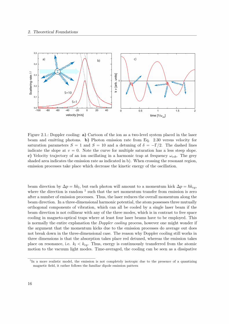
Figure 2.1.: Doppler cooling: a) Cartoon of the ion as a two-level system placed in the laserbeam and emitting photons. b) Photon emission rate from Eq. 2.30 versus velocity forsaturation parameters S = 1 and S = 10 and a detuning of δ = −Γ/2. The dashed linesindicate the slope at v = 0. Note the curve for multiple saturation has a less steep slope.c) Velocity trajectory of an ion oscillating in a harmonic trap at frequency ωvib. The greyshaded area indicates the emission rate as indicated in b). When crossing the resonant region,emission processes take place which decrease the kinetic energy of the oscillation.
beam direction by ∆p = kl, but each photon will amount to a momentum kick ∆p = keg,where the direction is random 1 such that the net momentum transfer from emission is zeroafter a number of emission processes. Thus, the laser reduces the overall momentum along thebeam direction. In a three-dimensional harmonic potential, the atom possesses three mutuallyorthogonal components of vibration, which can all be cooled by a single laser beam if thebeam direction is not collinear with any of the three modes, which is in contrast to free spacecooling in magneto-optical traps where at least four laser beams have to be employed. Thisis normally the entire explanation the Doppler cooling process, however one might wonder ifthe argument that the momentum kicks due to the emission processes do average out doesnot break down in the three-dimensional case. The reason why Doppler cooling still works inthree dimensions is that the absorption takes place red detuned, whereas the emission takesplace on resonance, i.e. kl < keg. Thus, energy is continuously transferred from the atomicmotion to the vacuum light modes. Time-averaged, the cooling can be seen as a dissipative
1In a more realistic model, the emission is not completely isotropic due to the presence of a quantizingmagnetic field, it rather follows the familiar dipole emission pattern
16
2.1. Laser-Ion Interactions
forceFcool(v) = keqR(v), (2.31)
leading to an energy dissipation rate of
Edrift = Fcool(v) · v (2.32)
This is a drift process, which is counteracted by a diffusion process in momentum spacedue to the random emission processes. A detailed analysis reveals that optimum Dopplercooling takes place if the detuning just amount half the linewidth δ = −Γ/2 and at unitysaturation S = 1. However, a completely realistic treatment would have to involve the factthat one is dealing with a multilevel system, leakage to other electronic states, the anisotropyof the trap and of the emission pattern, the discrete nature of the emission processes and themicromotion in ion traps, see Sec. 5.2. Quite generally, one finds that the limit for Dopplercooling in ion traps is given by an average number of typically 10..30 motional quanta permode, depending mostly on the ion species and on the trap secular frequencies. Dopplercooling can be seen as driving the atom to a thermal equilibrium with a reservoir given bythe laser, and the equilibrium temperature is given by the transition linewidth. Hence, onewill find the atom with a thermal distribution of phonon number after Doppler cooling:
pn =nn
(n+ 1)n+1with n =
kBT
ωv(2.33)
Fig. 2.1 shows the photon emission rate versus atomic velocity for different saturation pa-rameters. It can be seen that a finite probability exists that emission processes can take placefor kv > 0, leading to energy transfer to the atom. For low energies, i.e. small velocities,the slope of the emission rate at zero velocity determines the relative weight of cooling andheating processes and therefore sets the final temperature. Thus, narrow atomic lines andsmall intensities lead to lower final temperatures, but smaller fluorescence rates and coolingrates. This tradeoff is circumvented in ion trap experiments by using small laser power forcooling, but larger power for trapping and fluorescence detection.
In the following, we explain how information about the motional state of a single harmoni-cally confined ion can be extracted from fluorescence rate measurements. We assume a singleion to undergoes classical oscillatory motion along the directions of the motional modes:
ri(t) = Ai sin(ωit+ φi) i = x, y, z, (2.34)
with the amplitudes Ai, frequencies ωi and relative phases φi for the three normal modes. Inprinciple one has to average any resulting quantity about the undefined φi, however as theobservation time is much longer than the oscillation periods this is not necessary. The energystored in the motional modes is given by
Ei = A2imω2
i . (2.35)
It should be mentioned here that the equipartition theorem from thermodynamics does notnecessarily hold for a single trapped ion, therefore we also do not make use of the notion
17
2. Theoretical Foundations
of a temperature here. Because we obtain only information about the total energy, we stillhave to make to approximation that the energy is shared equally among the three motionalmodes:
Etot =∑i
Ei ≈ 3E (2.36)
For deriving an expression for the fluorescence rate, we take into account that the oscillatorymotion acts as to effectively modulate the frequency of the Doppler cooling beam, wherethe modulation frequency is given by the oscillation frequency and the frequency deviationδFM = k · vmax
i is given by
δ(i)FM = Aiωi
cosαi
λ=
√2Etot
3m
2π cosαi
λ, (2.37)
where αi is the angle that the cooling beam makes with the oscillation vector pertaining tomode i and λ is the cooling beam’s wavelength. With the modulation index Mi given by theratio of frequency deviation and modulation frequency, the relative power of the frequencycomponent which is seen by the ion to have an effective detuning of δeffi = δ0 ± nωi is givenby the Bessel coefficient
Pn = J2n(Mi) with Mi =
√2Etot
3m
2π cosαi
ωiλ. (2.38)
For motional frequencies in the MHz range and large thermal excitations of hundreds ofphonons, modulation indices Mi ≥ 1 occur, such that the following approximation for theBessel coefficient is justified:
P (i)n =
1
2Min ≤ Mi
0 n > Mi
(2.39)
If the condition holds that the fluorescence observation time is shorter than the timescale atwhich cooling takes place, we can now use these results together with Eq. 2.30 for the finalfluorescence rate:
R =∑ni
(∏i
P (i)ni
)Γ
2S
1
1 + S + 4 (∑
i niωi)2 /Γ2
≈ 1
8
intMi∑ni=0
(∏i
1
2Mi
)ΓS
2(1 + S)
(1− 1
1 + S
∑i
c2in2i
)
≈ R0 −intMi∑ni=0
(∏i
1
2Mi
)ΓS
2(1 + S)2
∑i
c2in2i , (2.40)
where we additionally assumed δ0 = 0 for simplicity. Thus the n-summations have beentruncated to positive values for symmetry reasons and a second-order Taylor expansion withrespect to c2in
2i has also been performed in the second line. R0 as the fluorescence level a
18

2.1. Laser-Ion Interactions
zero motional energy and ci = 2ωi/Γ have been introduced. As c2i is assumes values in the10−4 range, the Taylor expansion is clearly justified. Rearranging the correction term yieldsthe fluorescence rate defect
RH = R0 −R =
(∏i
1
Mi
)ΓS
2(1 + S)2
∑i
intMi∑ni=0
c2in2i
≈(∏
i
1
Mi
)ΓS
2(1 + S)21
3
(∏i
Mi
)∑i
c2iM2i . (2.41)
In order to obtain a useful expression, we consider that the individual properties of the dif-ferent motional modes are blurred out in the summation, assume a single effective oscillationfrequency ω, angle α and modulation index M . The final result for the fluorescence defectrate then reads
RH ≈ ΓS
2(1 + S)2c2M2
=S
Γ(1 + S)2Etot
3m
4π2 cos2 α
λ2. (2.42)
For a number d motional modes carrying kinetic energy, which might occur for varying ionnumbers or very different heating rates for different modes, the defect rate does not dependon d, because the lower energy per mode in Eq. 2.36 is balanced by the number of modescontributing to the frequency modulation in the first line of Eq. 2.42. Furthermore, note theremarkable fact that the final result Eq. 2.42 is independent of the average trap frequency ω.
2.1.4. Including the Motional Degrees of Freedom: The ResolvedSideband Regime
We now treat the case that the linewidth of the atomic transition under consideration Γ issmaller than the vibrational frequency of the trapped ion ωv. In this case, the quantizationof the motion plays an essential role. The ion is confined by a harmonic potential, its motionis therefore the vibration of a harmonic oscillator. Restricting ourselves to one spatial di-mension, the Hilbert space of the system is given by the product Hilbert space of the atomictwo-level system and the Fock-space of the harmonic oscillator, comprised of equidistantlevels separated by the vibrational frequency ωv. A sketch of the system is shown in Fig.2.2. We include the Hamiltonian pertaining the harmonic motion of the ion Hm. In secondquantization, we have
Hm = ωv
(a†a+
1
2
)
x =
√
2mωv(a† + a), (2.43)
19
2. Theoretical Foundations
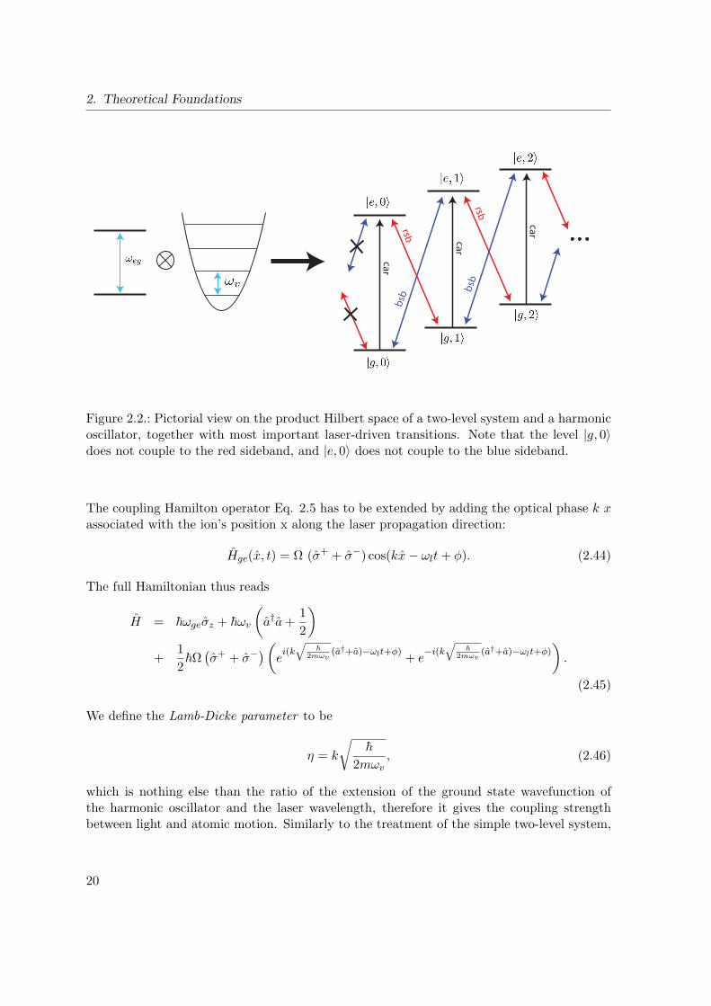
bsb
bsb
rsb
rsb
ca
r
ca
r
ca
r
Figure 2.2.: Pictorial view on the product Hilbert space of a two-level system and a harmonicoscillator, together with most important laser-driven transitions. Note that the level |g, 0〉does not couple to the red sideband, and |e, 0〉 does not couple to the blue sideband.
The coupling Hamilton operator Eq. 2.5 has to be extended by adding the optical phase k xassociated with the ion’s position x along the laser propagation direction:
Hge(x, t) = Ω (σ+ + σ−) cos(kx− ωlt+ φ). (2.44)
The full Hamiltonian thus reads
H = ωgeσz + ωv
(a†a+
1
2
)
+1
2Ω(σ+ + σ−)(ei(k√
2mωv(a†+a)−ωlt+φ)
+ e−i(k
√
2mωv(a†+a)−ωlt+φ)
).
(2.45)
We define the Lamb-Dicke parameter to be
η = k
√
2mωv, (2.46)
which is nothing else than the ratio of the extension of the ground state wavefunction ofthe harmonic oscillator and the laser wavelength, therefore it gives the coupling strengthbetween light and atomic motion. Similarly to the treatment of the simple two-level system,
20
2.1. Laser-Ion Interactions
we transform into the interaction picture with respect to H0 + Hm:
HI =1
2Ω(σ+ei(η(a
†e−iωvt+aeiωvt)−δt+φ) + σ−e−i(η(a†e−iωvt+aeiωvt)−δt+φ)). (2.47)
Here we employed the RWA similar to above and made use of the Campbell-Baker-Haussdorffformula e−iωv a†ataeiωv a†at = aeiωvt. Eq. 2.47 is the famous Cirac-Zoller Hamiltonian,[Cir95]. The occurring exponential can be expanded in terms of η:
HI =1
2Ωσ+e−iδt+iφ
(1 + iη(a†e−iωvt + aeiωvt)− 1
2η2(a†e−iωvt + aeiωvt)2 + ...
)+ h.c.
(2.48)If η 1 and for low vibrational quantum numbers, which defines the Lamb-Dicke regime oflaser-ion interactions, we can write
HI ≈ 1
2Ωσ+e−iδt+iφ
(1 + iηa†e−iωvt + iηaeiωvt
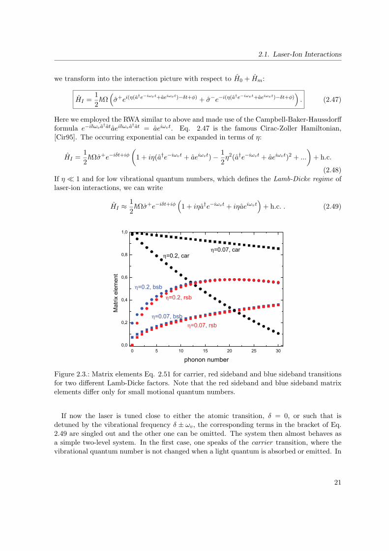
)+ h.c. . (2.49)
0 5 10 15 20 25 300,0
0,2
0,4
0,6
0,8
1,0
η=0.2, bsb
η=0.2, rsb
η=0.07, bsbη=0.07, rsb
η=0.2, car
Mat
rix e
lem
ent
phonon number
η=0.07, car
Figure 2.3.: Matrix elements Eq. 2.51 for carrier, red sideband and blue sideband transitionsfor two different Lamb-Dicke factors. Note that the red sideband and blue sideband matrixelements differ only for small motional quantum numbers.
If now the laser is tuned close to either the atomic transition, δ = 0, or such that isdetuned by the vibrational frequency δ ± ωv, the corresponding terms in the bracket of Eq.2.49 are singled out and the other one can be omitted. The system then almost behaves asa simple two-level system. In the first case, one speaks of the carrier transition, where thevibrational quantum number is not changed when a light quantum is absorbed or emitted. In
21

2. Theoretical Foundations
the second case, we deal with a sideband transition, where one vibrational quantum is created(δ = +ωv, blue sideband, bsb) or annihilated (δ = −ωv, red sideband, rsb) upon absorptionof a photon. Thus, if the Lamb-Dicke regime is attained, the atomic motion can be controlledat the single quantum level. The difference to the simple two-level system is however thatthe coupling strength, i.e. the Rabi frequency, depends on the vibrational quantum numbern. In the carrier case, all transitions |g, n〉 ↔ |e, n〉, and in the sideband case, all transitions|g, n〉 ↔ |e, n±1〉 are driven. The specific Rabi frequencies for a particular n can then be readoff Eq. 2.49 by taking the matrix element of the ladder operators with the levels involved inthe transition:
Ωcar ≈ Ω
Ωrsb ≈ η√nΩ
Ωbsb ≈ η√n+ 1Ω. (2.50)
Inspection of Eq. 2.50 reveals that the blue sideband can be driven for n = 0, whereas thered sideband vanishes, which is of crucial importance for temperature diagnostics. Beyondthe Lamb-Dicke regime, one has to consider all higher order sidebands ∆n ± m, includingthe fact that an arbitrary number virtual phonons can be exchanged during a transition, i.e.terms such as aa† for the carrier transition. The effective Rabi frequencies are then obtainedfrom the matrix element [Cah69]
Mn,n+m = 〈n+m|eikx|n〉 = e−η2/2(iη)|m|L|m|n (η2)
(n!
(n+m)!
)sign(m)/2
, (2.51)
where L|m|n are the associated Laguerre polynomials. The Rabi frequencies are then simply
given by
Ωn,n+m = Mn,n+mΩ. (2.52)
Matrix elements for the car, rsb and bsb transitions for experimentally relevant Lamb-Dickefactors are depicted in Fig. 2.3. The solution of the time-dependent Schrodinger equation forthe two-level system given by the propagator Eq. 2.11 can straightforwardly be extended inthe case that the detuning is close to a sideband of any order and if η and Ω are sufficientlysmall to ignore off-resonant excitation on other transitions. The propagator can be cast intoblock diagonal form by appropriate ordering of the coefficients when the m-th order sidebandis resonantly driven:
|Ψ〉 =∑n
cg,n|g, n〉+∑n
ce,n|e, n〉
|Ψ〉 →
⎛⎜⎜⎜⎜⎜⎝
cg,0ce,mcg,1
ce,1+m...
⎞⎟⎟⎟⎟⎟⎠ (2.53)
22

2.1. Laser-Ion Interactions
We then obtain for the propagator:
U(t) =
⎛⎜⎜⎜⎜⎜⎝
x0,m y0,m 0 0 · · ·y0,m x0,m 0 0 · · ·0 0 x1,m+1 y1,m+1 · · ·0 0 y1,m+1 x1,m+1 · · ·...
......
.... . .
⎞⎟⎟⎟⎟⎟⎠ , (2.54)
with
xn,m = cos(Ωn,mt/2) and yn,m = ieiφ sin(Ωn,mt/2) (2.55)
Analogously to Eq. 2.13, we obtain for the total population in the excited state upon drivingRabi oscillations starting from the ground state:
pe(t) =∑n
|ce,n(t)|2 =∑n
pn sin2(Ωn,n+mt/2), (2.56)
where pn is the initial phonon probability distribution, which can for example be given byEq. 2.33.
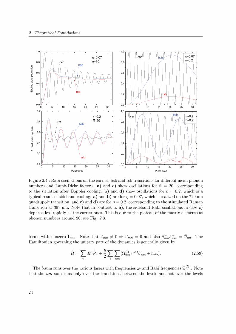
Fig. 2.4 depicts Rabi oscillations for different thermal states with different mean phononnumbers, where the average over many experiments is plotted. The data is also shown for thesame two Lamb-Dicke factors as in Fig. 2.3. One can see that a narrow phonon distribution,i.e. a low temperature, is crucial for driving high-fidelity single qubit rotations if the drivingtransition is sensitive to the motion.
2.1.5. Multilevel Systems Interacting with Multiple Laser Fields: OpticalPumping
We now extend the treatment of a laser-driven two-level system to an arbitrary number ofstates, which can be different electronic states or harmonic oscillator levels pertaining to anelectronic state due to quantized motion, see Sec. 2.1.4. We also will include spontaneousemission processes in a more rigorous way than in Sec. 2.1.1. The suitable framework forthis is a description of the system by a density matrix and utilization of the quantum opticalMaster equation as the equation of motion:
˙ρ = −i[H, ρ]+∑n,m
Dnm(ρ). (2.57)
where n,m run over the various levels and the dissipator D
Dnm(ρ) = Γnm
(σ+nmρσ−
nm − (ρσ−nmσ+
nm + σ−nmσ+
nmρ)/2), (2.58)
where Γnm is the spontaneous decay rate associated with the decay channel n → m andσ+nm = |m〉〈n| is the corresponding jump operator. The sum in Eq. 2.57 runs only over
23
2. Theoretical Foundations
0 5 10 15 20 25 300,0
0,2
0,4
0,6
0,8
1,0
rsb
bsbcar
Exc
ited
stat
e po
pula
tion
η=0.07n=20
0 5 10 15 20 25 300,0
0,2
0,4
0,6
0,8
1,0
rsb
bsbcar
Exc
ited
stat
e po
pula
tion
η=0.07n=0.2
0 5 10 15 20 25 300,0
0,2
0,4
0,6
0,8
1,0
rsb
bsbcar
Exc
ited
stat
e po
pula
tion
Pulse area
η=0.2n=20
0 5 10 15 20 25 300,0
0,2
0,4
0,6
0,8
1,0
rsb
bsbcarE
xcite
d st
ate
popu
latio
n
Pulse area
η=0.2n=0.2
Figure 2.4.: Rabi oscillations on the carrier, bsb and rsb transitions for different mean phononnumbers and Lamb-Dicke factors. a) and c) show oscillations for n = 20, correspondingto the situation after Doppler cooling. b) and d) show oscillations for n = 0.2, which is atypical result of sideband cooling. a) and b) are for η = 0.07, which is realized on the 729 nmquadrupole transition, and c) and d) are for η = 0.2, corresponding to the stimulated Ramantransition at 397 nm. Note that in contrast to a), the sideband Rabi oscillations in case c)dephase less rapidly as the carrier ones. This is due to the plateau of the matrix elements atphonon numbers around 20, see Fig. 2.3.
terms with nonzero Γnm. Note that Γnm = 0 ⇒ Γmn = 0 and also σ−nmσ+
nm = Pnn. TheHamiltonian governing the unitary part of the dynamics is generally given by
H =∑n
EnPn +
2
∑l
∑nm
(Ω(l)nmeiωltσ+
nm + h.c.). (2.59)
The l-sum runs over the various lasers with frequencies ωl and Rabi frequencies Ω(l)nm. Note
that the nm sum runs only over the transitions between the levels and not over the levels
24
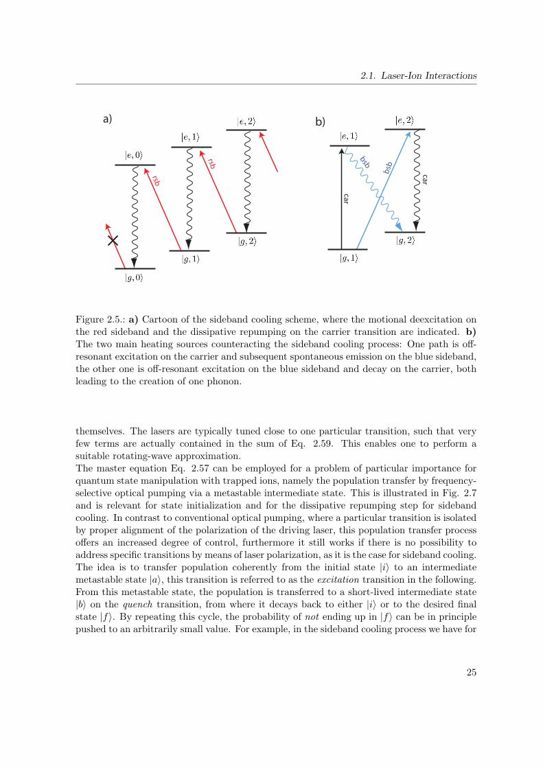
2.1. Laser-Ion Interactions
rsb
rsb
ca
r
bsb
ca
r
bsb
a) b)
Figure 2.5.: a) Cartoon of the sideband cooling scheme, where the motional deexcitation onthe red sideband and the dissipative repumping on the carrier transition are indicated. b)The two main heating sources counteracting the sideband cooling process: One path is off-resonant excitation on the carrier and subsequent spontaneous emission on the blue sideband,the other one is off-resonant excitation on the blue sideband and decay on the carrier, bothleading to the creation of one phonon.
themselves. The lasers are typically tuned close to one particular transition, such that veryfew terms are actually contained in the sum of Eq. 2.59. This enables one to perform asuitable rotating-wave approximation.The master equation Eq. 2.57 can be employed for a problem of particular importance forquantum state manipulation with trapped ions, namely the population transfer by frequency-selective optical pumping via a metastable intermediate state. This is illustrated in Fig. 2.7and is relevant for state initialization and for the dissipative repumping step for sidebandcooling. In contrast to conventional optical pumping, where a particular transition is isolatedby proper alignment of the polarization of the driving laser, this population transfer processoffers an increased degree of control, furthermore it still works if there is no possibility toaddress specific transitions by means of laser polarization, as it is the case for sideband cooling.The idea is to transfer population coherently from the initial state |i〉 to an intermediatemetastable state |a〉, this transition is referred to as the excitation transition in the following.From this metastable state, the population is transferred to a short-lived intermediate state|b〉 on the quench transition, from where it decays back to either |i〉 or to the desired finalstate |f〉. By repeating this cycle, the probability of not ending up in |f〉 can be in principlepushed to an arbitrarily small value. For example, in the sideband cooling process we have for
25

2. Theoretical Foundations
0 500 1000 1500 20000,0
0,1
0,2
0,3
0,4
0,5
0,6
0,7
0,8
0,9
1,0
Rec
ycle
d po
pula
tion
Rabi cycles0 2 4 6 8 10
0
20
40
60
80
100
120
140
Tim
e in
Rab
i cyc
les
Tim
e in
Rab
i cyc
les
Trap frequency [MHz]
0
500
1000
1500
2000
= 1
.6 M
Hz
= 3
.6 M
Hz
Dephasing
Revival
Figure 2.6.: Dephasing study of Rabi oscillations in thermal ensembles. For this examplecase, the driving wavelength is chosen to 729 nm and the angle of the beam to the oscillationmode is 45o, corresponding to a typical situation in experiments. For the trap frequencyvarying between 100 kHz and 10 MHz and a 40Ca+ ion, the Lamb-Dicke factor is varyingbetween 0.22 and 0.022. For each trap frequency, a thermal phonon number distributionaccording to Eqs. 2.33 is assumed. a) shows the population in the excited state after driving2n + 1 π-pulses. The decrease from unity is due to the dephasing occurring at timescaletdeph, which is reverted after the revival time trev. Curves for two different trap frequenciesare shown, such that it can be immediately seen that both timescales increase for a tightertrap. b) shows tdeph and trev versus trap frequency. tdeph increases quadratically with ωv,whereas trev grows linearly.
a single phonon removal step |i〉 = |g, n〉 and |f〉 = |g, n− 1〉. The process can be performedeither continuously, i.e. the lasers driving the excitation and quench transitions are alwaysswitched on, or in a pulsed way, such that the population is first transferred from |i〉 to |a〉by the first laser, and then dumped back to the ground state via |b〉 by the second laser.
The first scheme acts as to effectively decrease the lifetime of the metastable state |i〉[Mar94], increasing the total population transfer rate. However, one is confronted with atradeoff situation because the lifetime of |a〉 leads to a less efficient coherent drive of the|i〉 → |a〉 transition, which requires careful adjustment of Ωab. This problem is circumventedin the pulsed scheme, which in turn suffers from the drawback that off-resonant excitations|f〉 → |a〉 might occur for short excitation pulses on |i〉 → |a〉.
Figs. 2.8,2.9 and 2.10 show a detailed investigation of the continuous pumping processby means of full numerical solution of the master equation Eq. 2.57, revealing some impor-
26
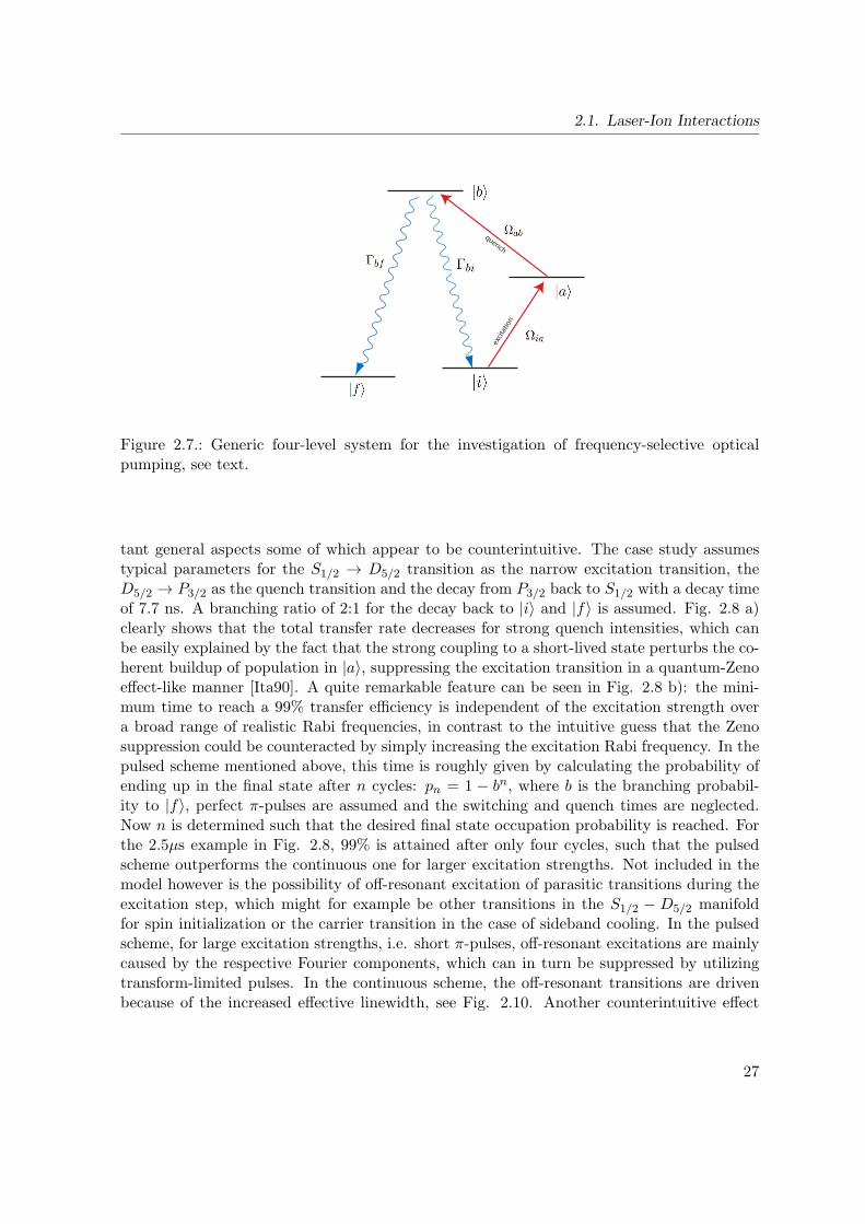
2.1. Laser-Ion Interactions
exc
itat
ion
quench
Figure 2.7.: Generic four-level system for the investigation of frequency-selective opticalpumping, see text.
tant general aspects some of which appear to be counterintuitive. The case study assumestypical parameters for the S1/2 → D5/2 transition as the narrow excitation transition, theD5/2 → P3/2 as the quench transition and the decay from P3/2 back to S1/2 with a decay timeof 7.7 ns. A branching ratio of 2:1 for the decay back to |i〉 and |f〉 is assumed. Fig. 2.8 a)clearly shows that the total transfer rate decreases for strong quench intensities, which canbe easily explained by the fact that the strong coupling to a short-lived state perturbs the co-herent buildup of population in |a〉, suppressing the excitation transition in a quantum-Zenoeffect-like manner [Ita90]. A quite remarkable feature can be seen in Fig. 2.8 b): the mini-mum time to reach a 99% transfer efficiency is independent of the excitation strength overa broad range of realistic Rabi frequencies, in contrast to the intuitive guess that the Zenosuppression could be counteracted by simply increasing the excitation Rabi frequency. In thepulsed scheme mentioned above, this time is roughly given by calculating the probability ofending up in the final state after n cycles: pn = 1 − bn, where b is the branching probabil-ity to |f〉, perfect π-pulses are assumed and the switching and quench times are neglected.Now n is determined such that the desired final state occupation probability is reached. Forthe 2.5µs example in Fig. 2.8, 99% is attained after only four cycles, such that the pulsedscheme outperforms the continuous one for larger excitation strengths. Not included in themodel however is the possibility of off-resonant excitation of parasitic transitions during theexcitation step, which might for example be other transitions in the S1/2 − D5/2 manifoldfor spin initialization or the carrier transition in the case of sideband cooling. In the pulsedscheme, for large excitation strengths, i.e. short π-pulses, off-resonant excitations are mainlycaused by the respective Fourier components, which can in turn be suppressed by utilizingtransform-limited pulses. In the continuous scheme, the off-resonant transitions are drivenbecause of the increased effective linewidth, see Fig. 2.10. Another counterintuitive effect
27
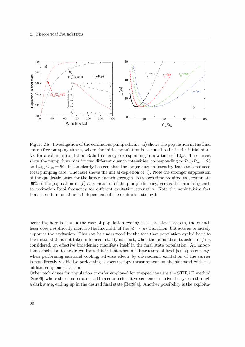
2. Theoretical Foundations
0 50 100 150 200 250 3000,0
0,2
0,4
0,6
0,8
1,0
Ωab
/Ωia=50
Ωab
/Ωia=25
Pop
ulat
ion
in fi
nal s
tate
Pump time [µs]
τπ=10µs
0 2 4 6 8 100,5
0,6
0,7
0,8
0,9
1,0
Pop
ulat
ion
in in
itial
sta
te
20 40 60 800
20
40
60
τπ=15µs
τπ=10µsτ
π=5µs
τ 99 [µ
s]Ω
ab/Ω
ia
τπ=2.5µs
a)
b)
Figure 2.8.: Investigation of the continuous pump scheme: a) shows the population in the finalstate after pumping time t, where the initial population is assumed to be in the initial state|i〉, for a coherent excitation Rabi frequency corresponding to a π-time of 10µs. The curvesshow the pump dynamics for two different quench intensities, corresponding to Ωab/Ωia = 25and Ωab/Ωia = 50. It can clearly be seen that the larger quench intensity leads to a reducedtotal pumping rate. The inset shows the initial depletion of |i〉. Note the stronger suppressionof the quadratic onset for the larger quench strength. b) shows time required to accumulate99% of the population in |f〉 as a measure of the pump efficiency, versus the ratio of quenchto excitation Rabi frequency for different excitation strengths. Note the nonintuitive factthat the minimum time is independent of the excitation strength.
occurring here is that in the case of population cycling in a three-level system, the quenchlaser does not directly increase the linewidth of the |i〉 → |a〉 transition, but acts as to merelysuppress the excitation. This can be understood by the fact that population cycled back tothe initial state is not taken into account. By contrast, when the population transfer to |f〉 isconsidered, an effective broadening manifests itself in the final state population. An impor-tant conclusion to be drawn from this is that when a substructure of level |a〉 is present, e.g.when performing sideband cooling, adverse effects by off-resonant excitation of the carrieris not directly visible by performing a spectroscopy measurement on the sideband with theadditional quench laser on.Other techniques for population transfer employed for trapped ions are the STIRAP method[Sor06], where short pulses are used in a counterintuitive sequence to drive the system througha dark state, ending up in the desired final state [Ber98a]. Another possibility is the exploita-
28
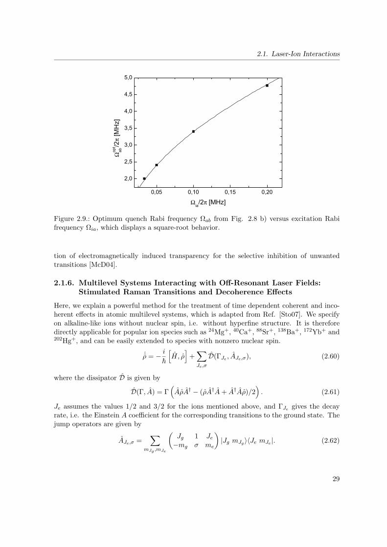
2.1. Laser-Ion Interactions
0,05 0,10 0,15 0,20
2,0
2,5
3,0
3,5
4,0
4,5
5,0
Ωop
tab
/2π [M
Hz]
Ωia/2π [MHz]
Figure 2.9.: Optimum quench Rabi frequency Ωab from Fig. 2.8 b) versus excitation Rabifrequency Ωia, which displays a square-root behavior.
tion of electromagnetically induced transparency for the selective inhibition of unwantedtransitions [McD04].
2.1.6. Multilevel Systems Interacting with Off-Resonant Laser Fields:Stimulated Raman Transitions and Decoherence Effects
Here, we explain a powerful method for the treatment of time dependent coherent and inco-herent effects in atomic multilevel systems, which is adapted from Ref. [Sto07]. We specifyon alkaline-like ions without nuclear spin, i.e. without hyperfine structure. It is thereforedirectly applicable for popular ion species such as 24Mg+, 40Ca+, 88Sr+, 138Ba+, 172Yb+ and202Hg+, and can be easily extended to species with nonzero nuclear spin.
˙ρ = − i
[H, ρ]+∑Je,σ
D(ΓJe , AJe,σ), (2.60)
where the dissipator D is given by
D(Γ, A) = Γ(AρA† − (ρA†A+ A†Aρ)/2
). (2.61)
Je assumes the values 1/2 and 3/2 for the ions mentioned above, and ΓJe gives the decayrate, i.e. the Einstein A coefficient for the corresponding transitions to the ground state. Thejump operators are given by
AJe,σ =∑
mJg ,mJe
(Jg 1 Je
−mg σ me
)|Jg mJg〉〈Je mJe |. (2.62)
29

2. Theoretical Foundations
-300 -200 -100 0 100 200 3000,0
0,2
0,4
0,6
0,8
1,0
δia/2π [kHz]
Pop
ulat
ion
in f
afte
r t=1
0 τ π
Ωab/Ω
ia=25τ
π=10µs
Ωab/Ω
ia=50
-300 -200 -100 0 100 200 3000,0
0,1
0,2
0,3
0,4
0,5
Ωab/Ω
ia=25
Ωab/Ω
ia=10
Mea
n po
pula
tion
in a
δia/2π [kHz]
τπ=10µs
Figure 2.10.: Illustration of the effective line-broadening of the quench laser. a) shows thesteady-state population in |b〉 in a three-level system with missing |f〉 versus detuning of theexcitation laser frequency, for two different quench intensities. Note that for the three-levelsystem, increased quench strength merely leads to a suppression of the excitation. b) showsthe population of 10 µs pumping in the |f〉 state of the four-level system. Here, the quenchindeed effectively increases the linewidth of the excitation transition.
The Hamiltonian consists of three parts:
H = HB + He + Hi. (2.63)
The Zeeman Hamiltonian HB simply describes the energy splitting of the mJ sublevels inthe presence of the quantizing magnetic field B:
HB = µBgJ∑mJ
mJB|J mJ〉〈J mJ |, (2.64)
with the Bohr magneton µB and the Lande factors gJ . He simply sets the energies of theexcited states:
He =∑Je
ωJe |Je〉〈Je|. (2.65)
Finally, the light-atom interaction Hamiltonian is given by
Hi =∑l
Ωl
2√2eiωlt∑Je,σ
εl,−σAJe,σ + h.c., (2.66)
30

2.1. Laser-Ion Interactions
P1/2
mj=+1/2mj=-1/2
mj=-1/2mj=+1/2
S1/2
P1/2
mj=+1/2
mj=-1/2
mj=-1/2
mj=+1/2
S1/2
mj=-1/2
mj=+1/2
mj=+3/2
mj=-3/2
P3/2
a) b)
Figure 2.11.: Level scheme for off-resonant interactions: a) illustrates the general situationof a 40Ca+ ion in two off-resonant laser fields, along with the relevant energy scales. b)shows in detail the various excitation and decay pathways for one laser beam with arbitrarypolarization components within the S1/2-P1/2 manifold.
where l runs over the different laser beams, which each have ’bare’ Rabi frequencies Ωl,angular frequencies ωl and are comprised of the polarization components εl,σ. Due to shortlifetime of the excited states, the detailed quantum dynamics is not really of interest, we arerather interested in the dynamics of the ground state levels only. In Schrodinger equationframework, one performs an adiabatic elimination of the exited state levels to obtain aneffective Schrodinger equation for the ground state manifold. This does of course not includedecoherence effects. An analogous adiabatic elimination procedure on the master equation isdone as follows [Sto07]: Considering the projection on the ground state manifold,
Pgg = |S1/2,mJ = +1/2〉〈S1/2,mJ = +1/2|+ |S1/2,mJ = −1/2〉〈S1/2,mJ = −1/2|ρgg = PggρPgg, (2.67)
31
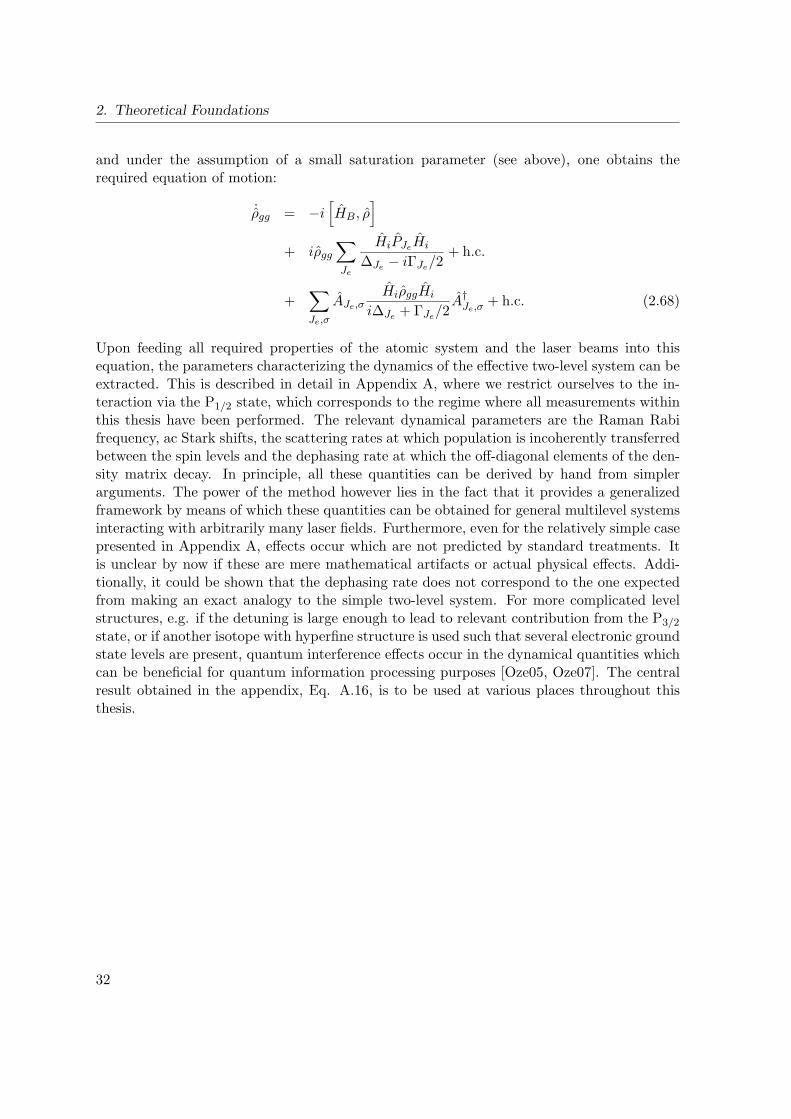
2. Theoretical Foundations
and under the assumption of a small saturation parameter (see above), one obtains therequired equation of motion:
˙ρgg = −i[HB, ρ
]+ iρgg
∑Je
HiPJeHi
∆Je − iΓJe/2+ h.c.
+∑Je,σ
AJe,σHiρggHi
i∆Je + ΓJe/2A†
Je,σ+ h.c. (2.68)
Upon feeding all required properties of the atomic system and the laser beams into thisequation, the parameters characterizing the dynamics of the effective two-level system can beextracted. This is described in detail in Appendix A, where we restrict ourselves to the in-teraction via the P1/2 state, which corresponds to the regime where all measurements withinthis thesis have been performed. The relevant dynamical parameters are the Raman Rabifrequency, ac Stark shifts, the scattering rates at which population is incoherently transferredbetween the spin levels and the dephasing rate at which the off-diagonal elements of the den-sity matrix decay. In principle, all these quantities can be derived by hand from simplerarguments. The power of the method however lies in the fact that it provides a generalizedframework by means of which these quantities can be obtained for general multilevel systemsinteracting with arbitrarily many laser fields. Furthermore, even for the relatively simple casepresented in Appendix A, effects occur which are not predicted by standard treatments. Itis unclear by now if these are mere mathematical artifacts or actual physical effects. Addi-tionally, it could be shown that the dephasing rate does not correspond to the one expectedfrom making an exact analogy to the simple two-level system. For more complicated levelstructures, e.g. if the detuning is large enough to lead to relevant contribution from the P3/2
state, or if another isotope with hyperfine structure is used such that several electronic groundstate levels are present, quantum interference effects occur in the dynamical quantities whichcan be beneficial for quantum information processing purposes [Oze05, Oze07]. The centralresult obtained in the appendix, Eq. A.16, is to be used at various places throughout thisthesis.
32
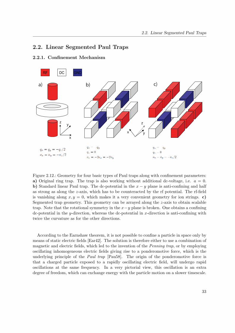
2.2. Linear Segmented Paul Traps
2.2. Linear Segmented Paul Traps
2.2.1. Confinement Mechanism
RF DC GND
a) b) c)
zy
x
z
x y
Figure 2.12.: Geometry for four basic types of Paul traps along with confinement parameters:a) Original ring trap. The trap is also working without additional dc-voltage, i.e. a = 0.b) Standard linear Paul trap. The dc-potential in the x− y plane is anti-confining and halfas strong as along the z-axis, which has to be counteracted by the rf potential. The rf-fieldis vanishing along x, y = 0, which makes it a very convenient geometry for ion strings. c)Segmented trap geometry. This geometry can be arrayed along the z-axis to obtain scalabletrap. Note that the rotational symmetry in the x−y plane is broken. One obtains a confiningdc-potential in the y-direction, whereas the dc-potential in x-direction is anti-confining withtwice the curvature as for the other directions.
According to the Earnshaw theorem, it is not possible to confine a particle in space only bymeans of static electric fields [Ear42]. The solution is therefore either to use a combination ofmagnetic and electric fields, which led to the invention of the Penning trap, or by employingoscillating inhomogeneous electric fields giving rise to a ponderomotive force, which is theunderlying principle of the Paul trap [Pau58]. The origin of the ponderomotive force isthat a charged particle exposed to a rapidly oscillating electric field, will undergo rapidoscillations at the same frequency. In a very pictorial view, this oscillation is an extradegree of freedom, which can exchange energy with the particle motion on a slower timescale.
33
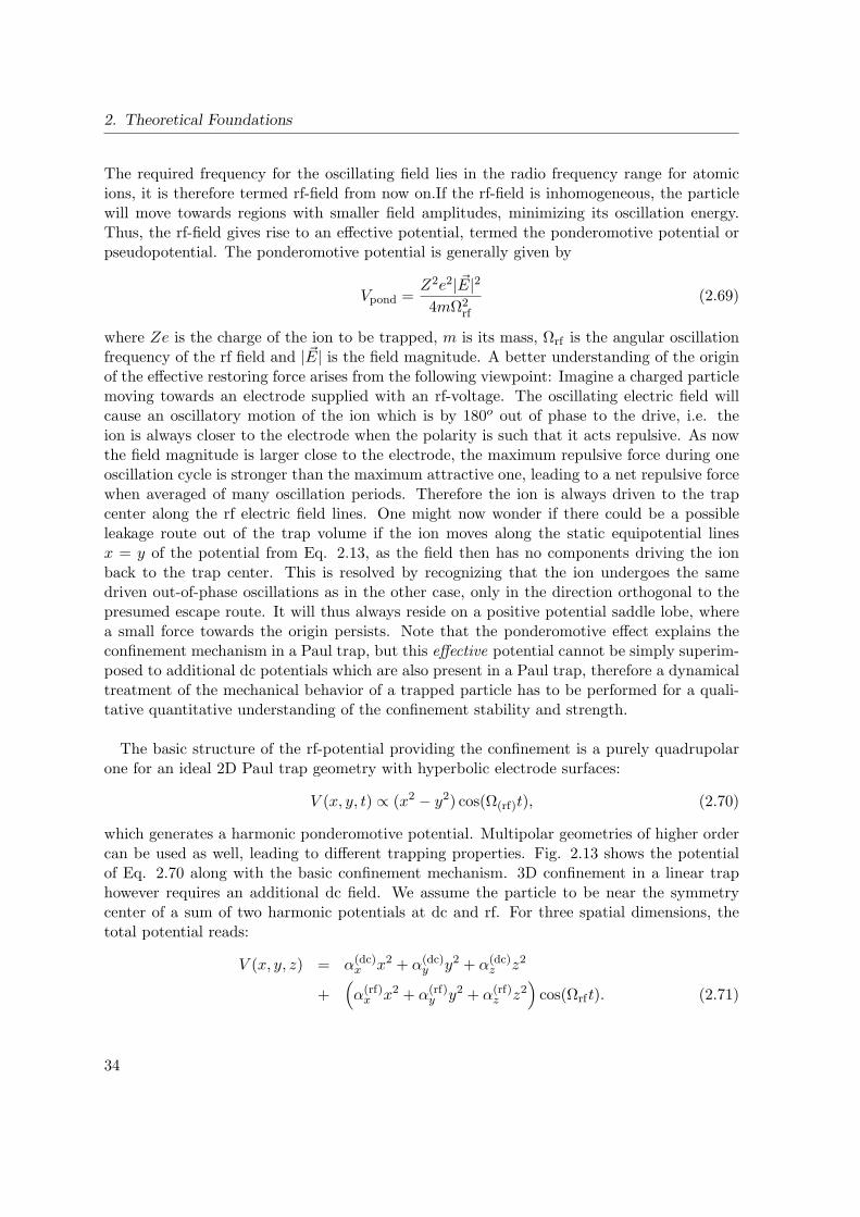
2. Theoretical Foundations
The required frequency for the oscillating field lies in the radio frequency range for atomicions, it is therefore termed rf-field from now on.If the rf-field is inhomogeneous, the particlewill move towards regions with smaller field amplitudes, minimizing its oscillation energy.Thus, the rf-field gives rise to an effective potential, termed the ponderomotive potential orpseudopotential. The ponderomotive potential is generally given by
Vpond =Z2e2| E|24mΩ2
rf
(2.69)
where Ze is the charge of the ion to be trapped, m is its mass, Ωrf is the angular oscillationfrequency of the rf field and | E| is the field magnitude. A better understanding of the originof the effective restoring force arises from the following viewpoint: Imagine a charged particlemoving towards an electrode supplied with an rf-voltage. The oscillating electric field willcause an oscillatory motion of the ion which is by 180o out of phase to the drive, i.e. theion is always closer to the electrode when the polarity is such that it acts repulsive. As nowthe field magnitude is larger close to the electrode, the maximum repulsive force during oneoscillation cycle is stronger than the maximum attractive one, leading to a net repulsive forcewhen averaged of many oscillation periods. Therefore the ion is always driven to the trapcenter along the rf electric field lines. One might now wonder if there could be a possibleleakage route out of the trap volume if the ion moves along the static equipotential linesx = y of the potential from Eq. 2.13, as the field then has no components driving the ionback to the trap center. This is resolved by recognizing that the ion undergoes the samedriven out-of-phase oscillations as in the other case, only in the direction orthogonal to thepresumed escape route. It will thus always reside on a positive potential saddle lobe, wherea small force towards the origin persists. Note that the ponderomotive effect explains theconfinement mechanism in a Paul trap, but this effective potential cannot be simply superim-posed to additional dc potentials which are also present in a Paul trap, therefore a dynamicaltreatment of the mechanical behavior of a trapped particle has to be performed for a quali-tative quantitative understanding of the confinement stability and strength.
The basic structure of the rf-potential providing the confinement is a purely quadrupolarone for an ideal 2D Paul trap geometry with hyperbolic electrode surfaces:
V (x, y, t) ∝ (x2 − y2) cos(Ω(rf)t), (2.70)
which generates a harmonic ponderomotive potential. Multipolar geometries of higher ordercan be used as well, leading to different trapping properties. Fig. 2.13 shows the potentialof Eq. 2.70 along with the basic confinement mechanism. 3D confinement in a linear traphowever requires an additional dc field. We assume the particle to be near the symmetrycenter of a sum of two harmonic potentials at dc and rf. For three spatial dimensions, thetotal potential reads:
V (x, y, z) = α(dc)x x2 + α(dc)
y y2 + α(dc)z z2
+(α(rf)x x2 + α(rf)
y y2 + α(rf)z z2
)cos(Ωrft). (2.71)
34
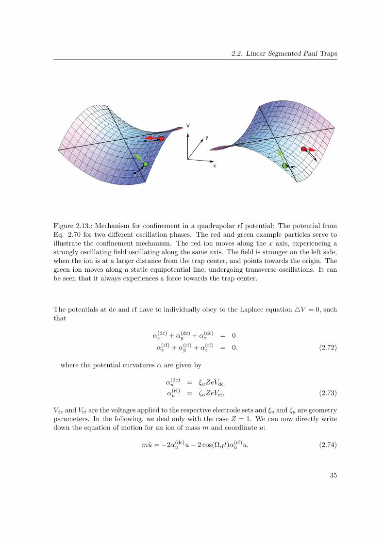
2.2. Linear Segmented Paul Traps
x
y
V
Figure 2.13.: Mechanism for confinement in a quadrupolar rf potential: The potential fromEq. 2.70 for two different oscillation phases. The red and green example particles serve toillustrate the confinement mechanism. The red ion moves along the x axis, experiencing astrongly oscillating field oscillating along the same axis. The field is stronger on the left side,when the ion is at a larger distance from the trap center, and points towards the origin. Thegreen ion moves along a static equipotential line, undergoing transverse oscillations. It canbe seen that it always experiences a force towards the trap center.
The potentials at dc and rf have to individually obey to the Laplace equation V = 0, suchthat
α(dc)x + α(dc)
y + α(dc)z = 0
α(rf)x + α(rf)
y + α(rf)z = 0. (2.72)
where the potential curvatures α are given by
α(dc)u = ξuZeVdc
α(rf)u = ζuZeVrf , (2.73)
Vdc and Vrf are the voltages applied to the respective electrode sets and ξu and ζu are geometryparameters. In the following, we deal only with the case Z = 1. We can now directly writedown the equation of motion for an ion of mass m and coordinate u:
mu = −2α(dc)u u− 2 cos(Ωrft)α
(rf)u u, (2.74)
35
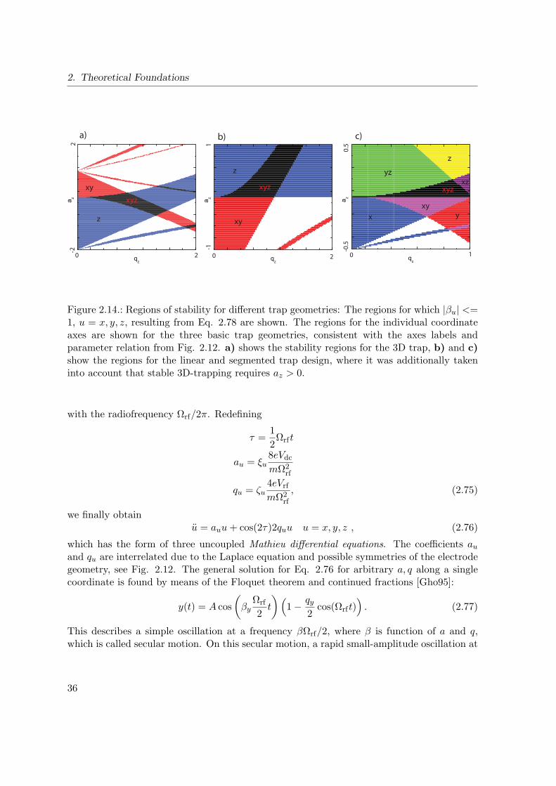
2. Theoretical Foundations
qz
a z
qz
a z
qz
a z
z
xy
y
xyz xyz
xyz
z xy
yz
x
z
xy
xz
2
-1
2
1
10 0 0
2-2 -0
.50
.5
a) b) c)
Figure 2.14.: Regions of stability for different trap geometries: The regions for which |βu| <=1, u = x, y, z, resulting from Eq. 2.78 are shown. The regions for the individual coordinateaxes are shown for the three basic trap geometries, consistent with the axes labels andparameter relation from Fig. 2.12. a) shows the stability regions for the 3D trap, b) and c)show the regions for the linear and segmented trap design, where it was additionally takeninto account that stable 3D-trapping requires az > 0.
with the radiofrequency Ωrf/2π. Redefining
τ =1
2Ωrft
au = ξu8eVdc
mΩ2rf
qu = ζu4eVrf
mΩ2rf
, (2.75)
we finally obtainu = auu+ cos(2τ)2quu u = x, y, z , (2.76)
which has the form of three uncoupled Mathieu differential equations. The coefficients auand qu are interrelated due to the Laplace equation and possible symmetries of the electrodegeometry, see Fig. 2.12. The general solution for Eq. 2.76 for arbitrary a, q along a singlecoordinate is found by means of the Floquet theorem and continued fractions [Gho95]:
y(t) = A cos
(βy
Ωrf
2t
)(1− qy
2cos(Ωrft)
). (2.77)
This describes a simple oscillation at a frequency βΩrf/2, where β is function of a and q,which is called secular motion. On this secular motion, a rapid small-amplitude oscillation at
36
2.2. Linear Segmented Paul Traps
Ωrf is superimposed, which is called micromotion. The stability of the motion is determinedby the value of β:
β2 ≈ a− (a− 1)q2
2(a− 1)2 − q2− (5a+ 7)q4
32(a− 1)3(a− 4)− (9a2 + 58a+ 29)q6
64(a− 1)5(a− 4)(a− 9)(2.78)
Stable trajectories are only obtained if |β| < 1, which is intuitively clear as the secular motionmust be slower than its ponderomotive drive. The regions of stability in the space of theparameters a and q are universal properties of the Mathieu equation, only the scaling of theaxes depends on a given set of physical trapping parameters. Considering stable trappingin three dimensions, the global region of stability is the intersection of the stability regionsfor the individual spatial directions. This is illustrated in Fig. 2.14 for the three basic Paultrap geometries. Due to the dependence of the trap parameters on the ion mass m, the trapcan be made very mass selective when the parameters are set to an outer tip in the regionof stability. This is exactly what the geometry was initially conceived for, namely as a massfilter for mass spectrometry [Pau53].
2.2.2. Vibrational Modes of Ion Crystals
The linear and segmented traps now offer the possibility to store an entire string of ions alongthe node of the rf-field, which coincides with z-axis, such that none of the ions is exposedto the rf electric field under ideal conditions. This leads to the fact that an ion string in alinear Paul trap represents a physical realization of a quantum register whose controllabilityproperties have so far not been beaten by any other experimental approach. The ion string ischaracterized by its static and dynamic properties, namely by its equilibrium ion positions,the frequencies and the structure of the vibrational modes. These are found by writing downthe potential energies for a set of N ions aligned along the z-axis, where the x, y and zcoordinates of the n-th ion are denoted as rn = (uxn, uyn,uzn)
T :
V =1
2m
N∑n
(ω2xu
2xn + ω2
yu2ynω
2z + u2zn
)+
e2
4πε0
N∑n,m,n =m
1√(rn − rm)2
. (2.79)
The trap frequency ω2z along the trap axis has to be smaller than the transverse frequency
ωr, for simplicity we assume a cylindrical symmetry here. Setting the elongations along thex, y directions to zero, the equilibrium positions along the trap axis are found by balancingthe external trap force with the repulsive Coulomb force:
N∑n
dV
duzn
∣∣∣u(0)zn
≡ 0 = mω2z
N∑n
u(0)zn − e2
4πε0
N∑m,n =m
u(0)zn − u
(0)zm
|u(0)zn − u(0)zm|3
, (2.80)
which can be solved analytically only for up tp N = 3. Now expand V around the equilibriumpositions to the second order in the coordinates:
V ≈∑
a,b=x,y,z
N∑i,j
d2V
duaidubj
∣∣∣u(0)ai ,u
(0)bj
δuaiδuaj ≡ V(ab)ij δuaiδubj . (2.81)
37
2. Theoretical Foundations
The δuai are small elongations from the equilibrium positions: δuai = uai − u(0)ai . As mixed
derivatives vanish if the ions are aligned in a linear string, e.g.
d2V
duaidubj
∣∣∣u(0)zi ,u
(0)xj
= 0 for a = b, (2.82)
we can separately write down the matrix elements V(aa)ij :
V(zz)ij =
⎧⎨⎩mω2
z +e2
4πε0
∑k =i
2
|u(0)zi −u
(0)zk |3 i = j
− e2
4πε02
|u(0)zi −u
(0)zj |3 i = j
(2.83)
V(xx)ij =
⎧⎨⎩mω2
x − e2
4πε0
∑k =i
1
|u(0)zi −u
(0)zk |3 i = j
+ e2
4πε01
|u(0)zi −u
(0)zj |3 i = j,
(2.84)
and correspondingly for V(yy)ij . These matrices can be diagonalized:
V (aa) = MTa ΛaMa (2.85)
with the diagonal matrix
Λa =
⎛⎜⎝µ(a)1 0 · · ·0 µ
(a)2 · · ·
......
. . .
⎞⎟⎠ , (2.86)
and the orthogonal matrices
Ma =
⎛⎜⎝M
(a)11 M
(a)12 · · ·
M(a)21 M
(a)22 · · ·
......
. . .
⎞⎟⎠ . (2.87)
The oscillation frequency of the n-th vibrational mode in a direction is given by the diagonalentries of Λa:
ν(a)n =
õ(a)n . (2.88)
The structure of the motional modes can be inferred from the orthogonal matrices Ma. Therelative amplitude and phase of the i-ion of an ion string oscillating at the n-th mode in
a direction is directly given by the matrix entry M(a)jn . We introduce a set of generalized
coordinates q(a)n :
q(a)n =∑j
M(a)nj δuaj and δuaj =
∑j
M(a)Tjn q(a)n (2.89)
Therefore the coupling strength of a motional mode to a given laser field, i.e. the correspond-ing Lamb-Dicke factor, can be calculated from the eigenvector components, which is of crucial
38
2.2. Linear Segmented Paul Traps
importance for entangling gates with single ion addressing [Jam98] or by means of a runningstanding wave [Iva09]. The eigenvalues of the radial modes of vibration from Eq. 2.84 yieldinformation about the stability of ion crystals: negative eigenvalues indicate instabilities, i.e.it occurs that for a too weak radial confinement and too many ions, the string assumes azig-zag configuration instead of a linear one. Results for the equilibrium ion positions andthe radial stability are shown in Fig. 1.2. The eigenvectors and eigenvalues of the matricesV (aa) are used in appendix for a generalized framework for the coherent interaction of ioncrystals with laser beams.
39

3. Experimental Setup
This chapter is devoted to a description of our experimental setup. Sec. 3.1 describes theinstallation of the trap in its UHV chamber, and Sec. 3.2 gives a detailed account on thesetup of the laser systems. Sec. 3.3 shows how the imaging and fluorescence detection isperformed, and sections 3.4 and 3.5 briefly explain how suitable electric and magnetic fieldare supplied to the trap site. Finally, Sec. 3.6 describes how simultaneous computer controlof the lasers, rf-sources, trap voltages and readout is accomplished.
3.1. The Trap, Vacuum Vessel and the Ovens
The fabrication, assembly and mounting of the trap is described in detail in [Sch09, Sch06,Sch08] and shall be only briefly outlined here. The microchip Paul trap is basically a sand-wich design of three alumina wafers, where the trap structure is created by a laser cuttingprocedure. The top and bottom layers making up the trap electrodes are gold coated. Thethree layers are glued and mounted in a commercial chip carrier. The rf and dc voltagesare supplied to the electrodes via bond wires. The chip carrier in turn is mounted on aPCB board from which the voltage wires run to four 25 pin Sub-D connectors of the topflange of the ultra high vacuum (UHV) chamber. Additional electric feedthroughs are forthe rf-supply and for the current for the two Ca ovens. The UHV is maintained by an ionpump 1 and an additional titanium sublimation pump 2, such that after bakeout at 120C apressure of typically 4·10−10 mbar is achieved, which is monitored by a UHV gauge 3. Theeffusive Ca ovens are built according to ref. [Rot03]. They consist of a stainless steel tubefilled with Calcium granules, connected to a stainless steel rod by a sheet of Tantalum. Theresistive heating is provided by a current of typically 3.4 Ampere flowing from the rod viathe Tantalum sheet through the tube, where heat is generated due to the thin tube walls.According to [Rot03], a temperature of roughly 200C is attained, corresponding to a vaporpressure of less than 10−12 mbar, such that the background pressure is not affected. Theoven is operated continuously, because its heating takes place on a timescale of 10 minutes,as compared to a trap loss on a similar time scale. After three years of continuous operationduring experiments, no adverse effects from possible coating of the trap electrodes have everbeen observed. Neither did we observe any visible changes on the trap surface when thetrap is monitored by an extra CCD camera with macro objective (which is used for beamalignment), nor did we observe any effects on the heating rate or trapping behavior, as is
1DN63CF StarCell, Varian Inc., Palo Alto, USA2tectra GmbH, Frankfurt am Main, Germany3Varian Inc., Palo Alto, USA
41
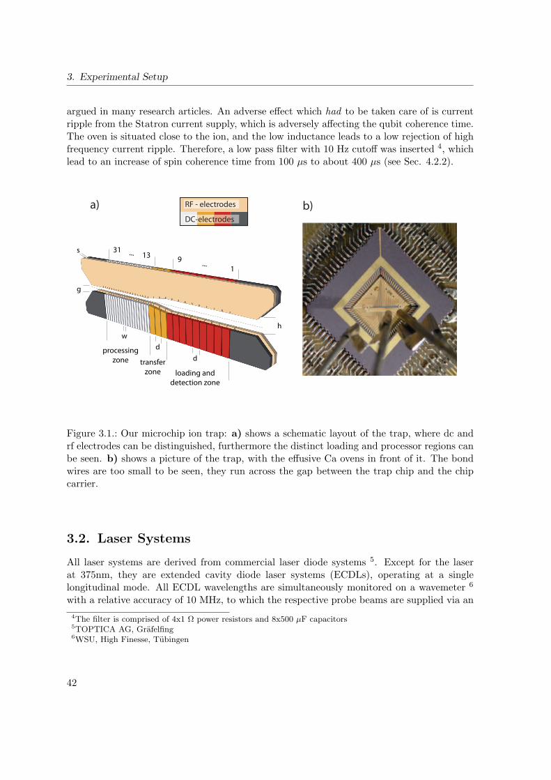
3. Experimental Setup
argued in many research articles. An adverse effect which had to be taken care of is currentripple from the Statron current supply, which is adversely affecting the qubit coherence time.The oven is situated close to the ion, and the low inductance leads to a low rejection of highfrequency current ripple. Therefore, a low pass filter with 10 Hz cutoff was inserted 4, whichlead to an increase of spin coherence time from 100 µs to about 400 µs (see Sec. 4.2.2).
1
913...31
...
loading and
detection zone
transfer
zone
processing
zone d
d
w
h
g
s
DC-electrodes
RF - electrodesa) b)
Figure 3.1.: Our microchip ion trap: a) shows a schematic layout of the trap, where dc andrf electrodes can be distinguished, furthermore the distinct loading and processor regions canbe seen. b) shows a picture of the trap, with the effusive Ca ovens in front of it. The bondwires are too small to be seen, they run across the gap between the trap chip and the chipcarrier.
3.2. Laser Systems
All laser systems are derived from commercial laser diode systems 5. Except for the laserat 375nm, they are extended cavity diode laser systems (ECDLs), operating at a singlelongitudinal mode. All ECDL wavelengths are simultaneously monitored on a wavemeter 6
with a relative accuracy of 10 MHz, to which the respective probe beams are supplied via an
4The filter is comprised of 4x1 Ω power resistors and 8x500 µF capacitors5TOPTICA AG, Grafelfing6WSU, High Finesse, Tubingen
42
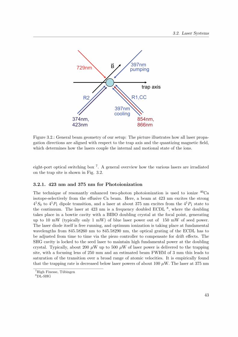
3.2. Laser Systems
729nm
R1,CCR2
854nm,866nm
374nm,423nm
B 397nmpumping
397nmcooling
trap axis
Figure 3.2.: General beam geometry of our setup: The picture illustrates how all laser propa-gation directions are aligned with respect to the trap axis and the quantizing magnetic field,which determines how the lasers couple the internal and motional state of the ions.
eight-port optical switching box 7. A general overview how the various lasers are irradiatedon the trap site is shown in Fig. 3.2.
3.2.1. 423 nm and 375 nm for Photoionization
The technique of resonantly enhanced two-photon photoionization is used to ionize 40Caisotope-selectively from the effusive Ca beam. Here, a beam at 423 nm excites the strong41S0 to 41P1 dipole transition, and a laser at about 375 nm excites from the 41P1 state tothe continuum. The laser at 423 nm is a frequency doubled ECDL 8, where the doublingtakes place in a bowtie cavity with a BIBO doubling crystal at the focal point, generatingup to 10 mW (typically only 1 mW) of blue laser power out of 150 mW of seed power.The laser diode itself is free running, and optimum ionization is taking place at fundamentalwavelengths from 845.58260 nm to 845.58290 nm, the optical grating of the ECDL has tobe adjusted from time to time via the piezo controller to compensate for drift effects. TheSHG cavity is locked to the seed laser to maintain high fundamental power at the doublingcrystal. Typically, about 200 µW up to 500 µW of laser power is delivered to the trappingsite, with a focusing lens of 250 mm and an estimated beam FWHM of 3 mm this leads tosaturation of the transition over a broad range of atomic velocities. It is empirically foundthat the trapping rate is decreased below laser powers of about 100 µW. The laser at 375 nm
7High Finesse, Tubingen8DL-SHG
43
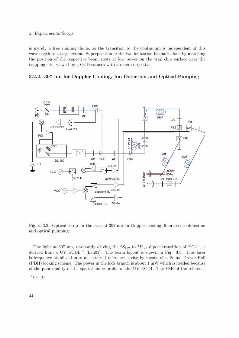
3. Experimental Setup
is merely a free running diode, as the transition to the continuum is independent of thiswavelength to a large extent. Superposition of the two ionization beams is done by matchingthe position of the respective beam spots at low power on the trap chip surface near thetrapping site, viewed by a CCD camera with a macro objective.
3.2.2. 397 nm for Doppler Cooling, Ion Detection and Optical Pumping
866nm
ZFL-500HLN
ZHL-3A
ZHL-3A
ZHL-3A-10dB
Figure 3.3.: Optical setup for the laser at 397 nm for Doppler cooling, fluorescence detectionand optical pumping.
The light at 397 nm, resonantly driving the 2S1/2 to 2P1/2 dipole transition of 40Ca+, isderived from a UV ECDL 9 [Lan03]. The beam layout is shown in Fig. 3.3. This laseris frequency stabilized onto an external reference cavity by means of a Pound-Drever-Hall(PDH) locking scheme. The power in the lock branch is about 1 mW which is needed becauseof the poor quality of the spatial mode profile of the UV ECDL. The FSR of the reference
9DL 100
44
3.2. Laser Systems
cavity is 1.5 GHz, and its Finesse ranges at about 100. The transition is located at about397.95920 nm. The cavity is mounted on an ultralow thermal extension ceramic block 10, itsdrift is slow enough to be ignored. One of the cavity mirrors is mounted on a ring piezo, suchthat one electrode can be supplied with a static high voltage 11 in order to obtain a resonancefor a Gaussian transversal mode within the wavelength range of interest, whereas the otherelectrode is supplied by an HV amplifier 12 in order to perform controlled spectroscopy onthe corresponding transition. The largest portion of the laser output (about 12 mW, 10 mWremaining after an external Faraday isolator) is supplied to the experiment via a polarizationmaintaining single mode fiber 13. The low fiber output of only up to 1.4 mW is due to thebad quality of the transversal mode profile of the UV diode. The input into the fiber iscontrolled by an acousto-optical modulator (AOM) running at 80 MHz and up to 2 W inputpower 14. The AOM supply can be switched between no power, full power or attenuatedpower, such that the laser power at the ion can either be a multiple saturation of slightlybelow saturation, see Figs. 4.4 and 3.3. The beam is then supplied near the vacuum chamber,where it is split into two branches serving different purposes: one branch with typically about130 µW is used for Doppler cooling and fluorescence detection, and the remaining power isused for initializing the spin state by optical pumping. The respective beams are switchedby individual AOMs, where the first orders are coupled into short single optical fibers forspatial filtering. This was found to be of crucial importance for the fidelity of the opticalpumping process, especially in connection with Raman sideband cooling, see Sec. 4.6. Thereason for this is that a substantial amount of stray light is still irradiated onto the ion ifthe AOM in the corresponding branch is switched off. This stray light is due to solarizationin the UV fiber and diffraction at the AOM apertures and in the AOM crystal. Only withSM fibers in both beams, good results for optical pumping and Raman sideband coolingcould be obtained. The Doppler cooling beam is π-polarized, such that mainly vertical (mJ
conserving) transitions are driven. The advantage is then that the Zeeman splitting betweenthese two transitions is smaller than it is the case for the ∆mJ=±1 transitions driven byσ± polarized light, yielding higher fluorescence rates and better Doppler cooling. The NIRbeams at 866 nm and 854 nm are superimposed onto the Doppler cooling beam on a UVreflective/NIR transmissive dielectric mirror. The optical pumping beam is directed alongthe quantizing magnetic field. A λ/2 and PBS are used to control the power, and a λ/4 isused to control the polarization. It was initially tried to use additional compensation coilsto align the magnetic field better along the beam propagation axis, such that the observedfluorescence is minimized upon irradiation with a circularly polarized beam with the Dopplercooling light switched off. However, fluorescence rates already close to the detection thresholdcan be observed, and as the trap lifetime is substantially shortened without Doppler cooling,this method was found to be not useful for further improvements of the pumping fidelity.
10Hellma Optics GmbH, Jena11EHQ-8010p, iseg Spezialelektronik GmbH, Radeberg12miniPiA 103, TEM Messtechnik GmbH, Hannover13PMC-400Si-2,9-NA011-3-APC-50-P, SUK Hamburg14QZF-80-20, Brimrose Corporation of America, USA
45
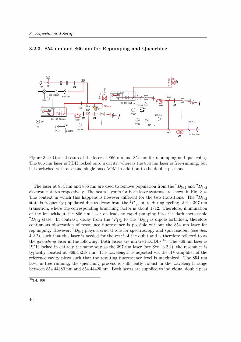
3. Experimental Setup
3.2.3. 854 nm and 866 nm for Repumping and Quenching
ZHL-3A
ZHL-3A
ZHL-3A
ZFL-1000LN+
Figure 3.4.: Optical setup of the laser at 866 nm and 854 nm for repumping and quenching.The 866 nm laser is PDH locked onto a cavity, whereas the 854 nm laser is free-running, butit is switched with a second single-pass AOM in addition to the double-pass one.
The laser at 854 nm and 866 nm are used to remove population from the 2D5/2 and 2D3/2
electronic states respectively. The beam layouts for both laser systems are shown in Fig. 3.4.The context in which this happens is however different for the two transitions: The 2D3/2
state is frequently populated due to decay from the 2P1/2 state during cycling of the 397 nmtransition, where the corresponding branching factor is about 1/12. Therefore, illuminationof the ion without the 866 nm laser on leads to rapid pumping into the dark metastable2D3/2 state. In contrast, decay from the 2P1/2 to the 2D5/2 is dipole forbidden, thereforecontinuous observation of resonance fluorescence is possible without the 854 nm laser forrepumping. However, 2D5/2 plays a crucial role for spectroscopy and spin readout (see Sec.4.2.2), such that this laser is needed for the reset of the qubit and is therefore referred to asthe quenching laser in the following. Both lasers are infrared ECDLs 15. The 866 nm laser isPDH locked in entirely the same way as the 397 nm laser (see Sec. 3.2.2), the resonance istypically located at 866.45218 nm. The wavelength is adjusted via the HV-amplifier of thereference cavity piezo such that the resulting fluorescence level is maximized. The 854 nmlaser is free running, the quenching process is sufficiently robust in the wavelength rangebetween 854.44380 nm and 854.44420 nm. Both lasers are supplied to individual double pass
15DL 100
46
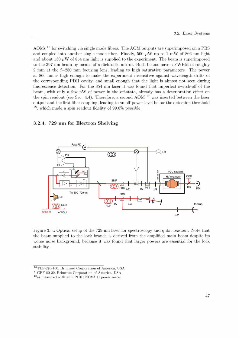
3.2. Laser Systems
AOMs 16 for switching via single mode fibers. The AOM outputs are superimposed on a PBSand coupled into another single mode fiber. Finally, 500 µW up to 1 mW of 866 nm lightand about 130 µW of 854 nm light is supplied to the experiment. The beam is superimposedto the 397 nm beam by means of a dichroitic mirror. Both beams have a FWHM of roughly2 mm at the f=250 mm focusing lens, leading to high saturation parameters. The powerat 866 nm is high enough to make the experiment insensitive against wavelength drifts ofthe corresponding PDH cavity, and small enough that the light is almost not seen duringfluorescence detection. For the 854 nm laser it was found that imperfect switch-off of thebeam, with only a few nW of power in the off-state, already has a deterioration effect onthe spin readout (see Sec. 4.4). Therefore, a second AOM 17 was inserted between the laseroutput and the first fiber coupling, leading to an off-power level below the detection threshold18, which made a spin readout fidelity of 99.6% possible.
3.2.4. 729 nm for Electron Shelving
~
Figure 3.5.: Optical setup of the 729 nm laser for spectroscopy and qubit readout. Note thatthe beam supplied to the lock branch is derived from the amplified main beam despite itsworse noise background, because it was found that larger powers are essential for the lockstability.
16TEF-270-100, Brimrose Corporation of America, USA17GEF-80-20, Brimrose Corporation of America, USA18as measured with an OPHIR NOVA II power meter
47
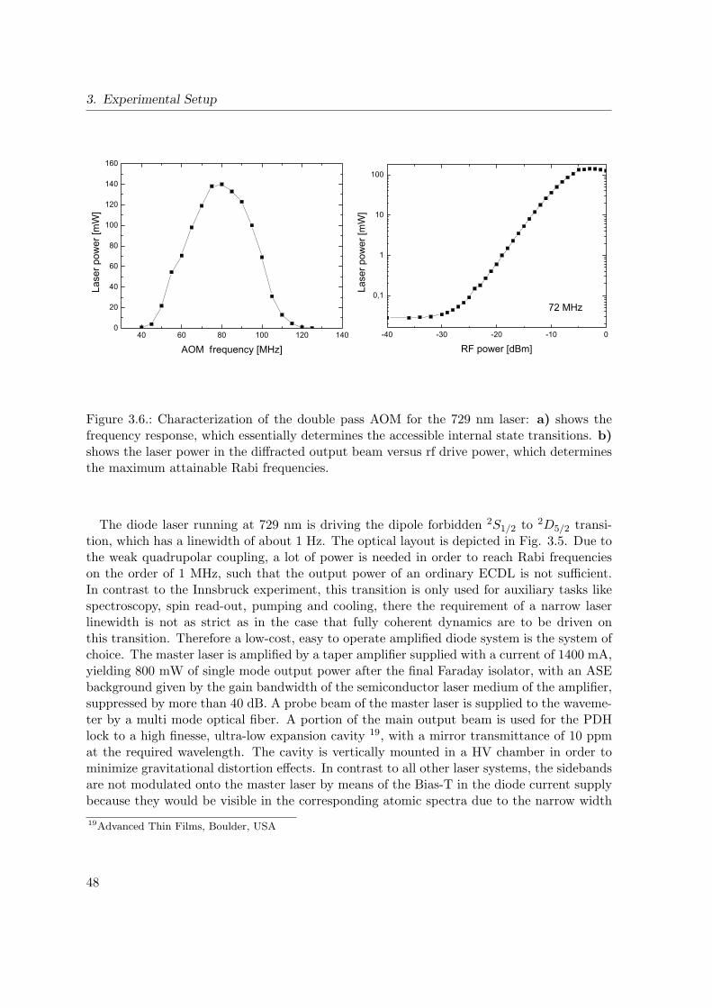
3. Experimental Setup
40 60 80 100 120 1400
20
40
60
80
100
120
140
160
Lase
r pow
er [m
W]
AOM frequency [MHz]-40 -30 -20 -10 0
0,1
1
10
100
Lase
r pow
er [m
W]
RF power [dBm]
72 MHz
Figure 3.6.: Characterization of the double pass AOM for the 729 nm laser: a) shows thefrequency response, which essentially determines the accessible internal state transitions. b)shows the laser power in the diffracted output beam versus rf drive power, which determinesthe maximum attainable Rabi frequencies.
The diode laser running at 729 nm is driving the dipole forbidden 2S1/2 to 2D5/2 transi-tion, which has a linewidth of about 1 Hz. The optical layout is depicted in Fig. 3.5. Due tothe weak quadrupolar coupling, a lot of power is needed in order to reach Rabi frequencieson the order of 1 MHz, such that the output power of an ordinary ECDL is not sufficient.In contrast to the Innsbruck experiment, this transition is only used for auxiliary tasks likespectroscopy, spin read-out, pumping and cooling, there the requirement of a narrow laserlinewidth is not as strict as in the case that fully coherent dynamics are to be driven onthis transition. Therefore a low-cost, easy to operate amplified diode system is the system ofchoice. The master laser is amplified by a taper amplifier supplied with a current of 1400 mA,yielding 800 mW of single mode output power after the final Faraday isolator, with an ASEbackground given by the gain bandwidth of the semiconductor laser medium of the amplifier,suppressed by more than 40 dB. A probe beam of the master laser is supplied to the waveme-ter by a multi mode optical fiber. A portion of the main output beam is used for the PDHlock to a high finesse, ultra-low expansion cavity 19, with a mirror transmittance of 10 ppmat the required wavelength. The cavity is vertically mounted in a HV chamber in order tominimize gravitational distortion effects. In contrast to all other laser systems, the sidebandsare not modulated onto the master laser by means of the Bias-T in the diode current supplybecause they would be visible in the corresponding atomic spectra due to the narrow width
19Advanced Thin Films, Boulder, USA
48
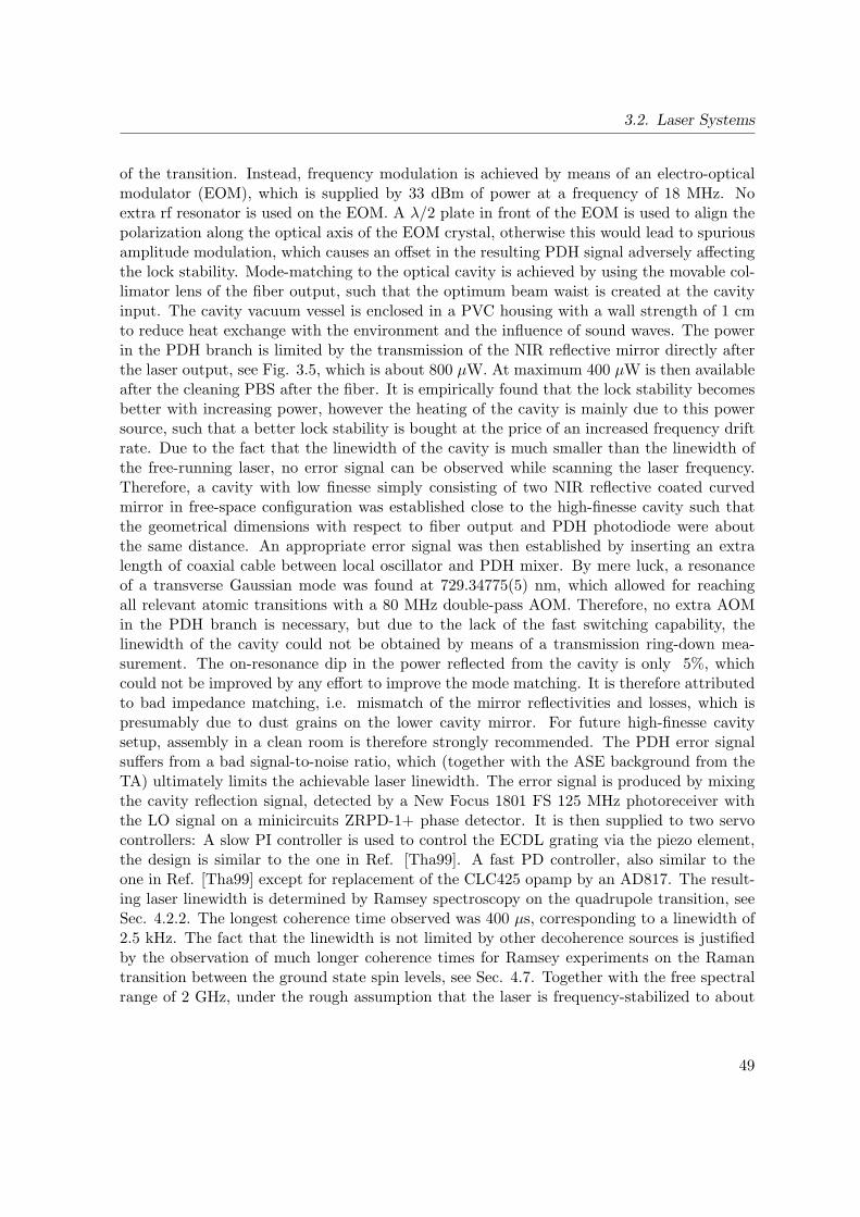
3.2. Laser Systems
of the transition. Instead, frequency modulation is achieved by means of an electro-opticalmodulator (EOM), which is supplied by 33 dBm of power at a frequency of 18 MHz. Noextra rf resonator is used on the EOM. A λ/2 plate in front of the EOM is used to align thepolarization along the optical axis of the EOM crystal, otherwise this would lead to spuriousamplitude modulation, which causes an offset in the resulting PDH signal adversely affectingthe lock stability. Mode-matching to the optical cavity is achieved by using the movable col-limator lens of the fiber output, such that the optimum beam waist is created at the cavityinput. The cavity vacuum vessel is enclosed in a PVC housing with a wall strength of 1 cmto reduce heat exchange with the environment and the influence of sound waves. The powerin the PDH branch is limited by the transmission of the NIR reflective mirror directly afterthe laser output, see Fig. 3.5, which is about 800 µW. At maximum 400 µW is then availableafter the cleaning PBS after the fiber. It is empirically found that the lock stability becomesbetter with increasing power, however the heating of the cavity is mainly due to this powersource, such that a better lock stability is bought at the price of an increased frequency driftrate. Due to the fact that the linewidth of the cavity is much smaller than the linewidth ofthe free-running laser, no error signal can be observed while scanning the laser frequency.Therefore, a cavity with low finesse simply consisting of two NIR reflective coated curvedmirror in free-space configuration was established close to the high-finesse cavity such thatthe geometrical dimensions with respect to fiber output and PDH photodiode were aboutthe same distance. An appropriate error signal was then established by inserting an extralength of coaxial cable between local oscillator and PDH mixer. By mere luck, a resonanceof a transverse Gaussian mode was found at 729.34775(5) nm, which allowed for reachingall relevant atomic transitions with a 80 MHz double-pass AOM. Therefore, no extra AOMin the PDH branch is necessary, but due to the lack of the fast switching capability, thelinewidth of the cavity could not be obtained by means of a transmission ring-down mea-surement. The on-resonance dip in the power reflected from the cavity is only 5%, whichcould not be improved by any effort to improve the mode matching. It is therefore attributedto bad impedance matching, i.e. mismatch of the mirror reflectivities and losses, which ispresumably due to dust grains on the lower cavity mirror. For future high-finesse cavitysetup, assembly in a clean room is therefore strongly recommended. The PDH error signalsuffers from a bad signal-to-noise ratio, which (together with the ASE background from theTA) ultimately limits the achievable laser linewidth. The error signal is produced by mixingthe cavity reflection signal, detected by a New Focus 1801 FS 125 MHz photoreceiver withthe LO signal on a minicircuits ZRPD-1+ phase detector. It is then supplied to two servocontrollers: A slow PI controller is used to control the ECDL grating via the piezo element,the design is similar to the one in Ref. [Tha99]. A fast PD controller, also similar to theone in Ref. [Tha99] except for replacement of the CLC425 opamp by an AD817. The result-ing laser linewidth is determined by Ramsey spectroscopy on the quadrupole transition, seeSec. 4.2.2. The longest coherence time observed was 400 µs, corresponding to a linewidth of2.5 kHz. The fact that the linewidth is not limited by other decoherence sources is justifiedby the observation of much longer coherence times for Ramsey experiments on the Ramantransition between the ground state spin levels, see Sec. 4.7. Together with the free spectralrange of 2 GHz, under the rough assumption that the laser is frequency-stabilized to about
49

3. Experimental Setup
1% of the cavity linewidth, this is giving a finesse of only 8000, compared to the finesse of300000 inferred from the mirror manufacturer data.The main laser output is delivered to the experiment via a single mode fiber, where roundabout 300 mW of power is available. The light is switched and modulated by a double-pass AOM 20, which allows better switch-off and scanning of the frequency for spectroscopypurposes without changing the beam alignment. The characterization of the diffraction per-formance of this AOM with respect to input frequency and amplitude is crucial for exertingcontrol over the atomic system, the corresponding measurement results are shown in Fig.3.6. For details of the rf supply of this AOM, see Fig. 3.9. The beam is directed orthogonallyto the magnetic field, and a λ/2 plate is used to align the polarization at roughly 45withrespect to the magnetic field, such that all quadrupole allowed transition between the vari-ous sublevels can in principle be addressed, see Sec. 4.2.2. In front of the vacuum window,150 mW of laser power at a beam FWHM of roughly 8 mm is focused onto the ion witha f=250 mm lens, such that high enough Rabi frequencies of up to 2π·500 kHz are readilyobtained.
3.2.5. 397 nm for Stimulated Raman Transitions
EOM
Figure 3.7.: Optical setup for the laser at 397 nm for off-resonant coherent manipulations.The EOM is superior to an AOM for the task of lossless fast switching.
A single mode laser close to the 2S1/2 to 2P1/2 dipole transition is used for driving stim-ulated Raman transitions between the ground state spin levels, which is supposed to be the
20GEF-80-20, Brimrose Corporation of America, USA
50
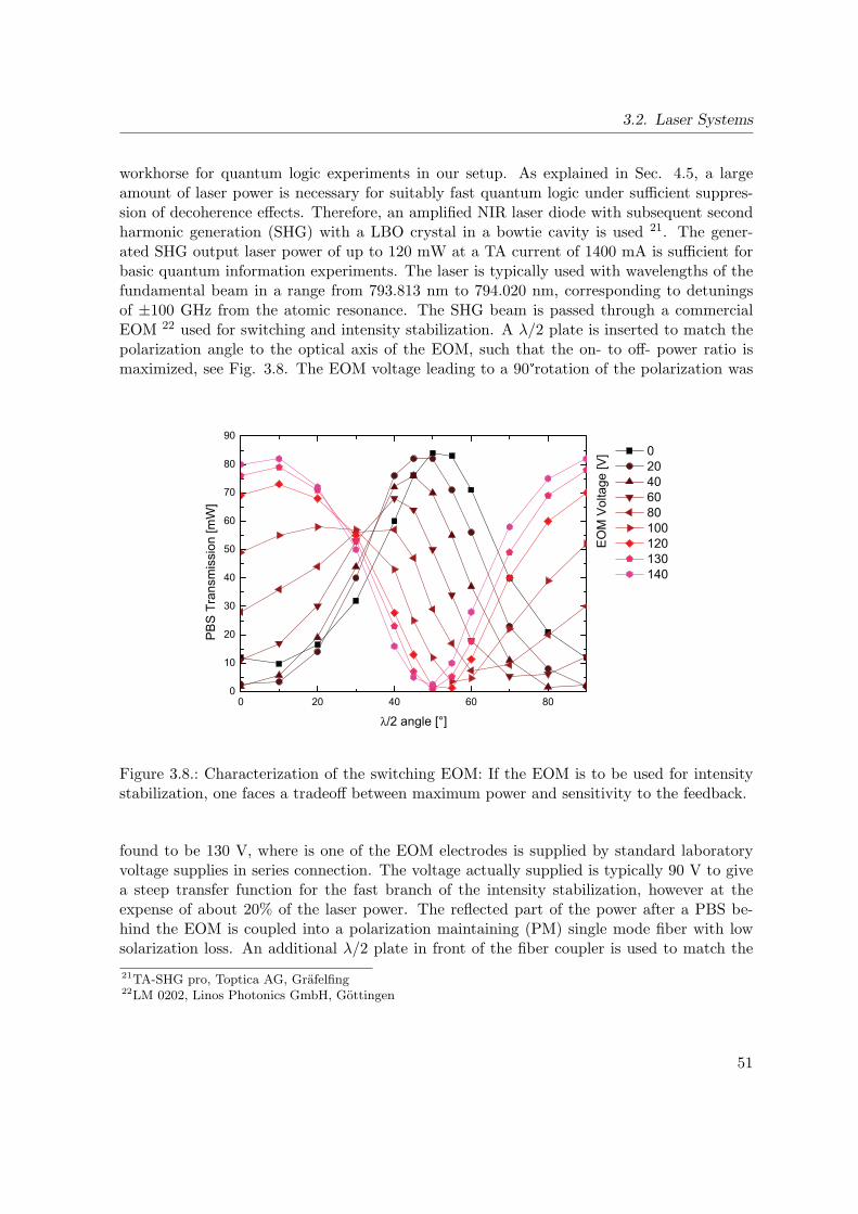
3.2. Laser Systems
workhorse for quantum logic experiments in our setup. As explained in Sec. 4.5, a largeamount of laser power is necessary for suitably fast quantum logic under sufficient suppres-sion of decoherence effects. Therefore, an amplified NIR laser diode with subsequent secondharmonic generation (SHG) with a LBO crystal in a bowtie cavity is used 21. The gener-ated SHG output laser power of up to 120 mW at a TA current of 1400 mA is sufficient forbasic quantum information experiments. The laser is typically used with wavelengths of thefundamental beam in a range from 793.813 nm to 794.020 nm, corresponding to detuningsof ±100 GHz from the atomic resonance. The SHG beam is passed through a commercialEOM 22 used for switching and intensity stabilization. A λ/2 plate is inserted to match thepolarization angle to the optical axis of the EOM, such that the on- to off- power ratio ismaximized, see Fig. 3.8. The EOM voltage leading to a 90rotation of the polarization was
0 20 40 60 800
10
20
30
40
50
60
70
80
90
PB
S T
rans
mis
sion
[mW
]
λ
EO
M V
olta
ge [V
]
Figure 3.8.: Characterization of the switching EOM: If the EOM is to be used for intensitystabilization, one faces a tradeoff between maximum power and sensitivity to the feedback.
found to be 130 V, where is one of the EOM electrodes is supplied by standard laboratoryvoltage supplies in series connection. The voltage actually supplied is typically 90 V to givea steep transfer function for the fast branch of the intensity stabilization, however at theexpense of about 20% of the laser power. The reflected part of the power after a PBS be-hind the EOM is coupled into a polarization maintaining (PM) single mode fiber with lowsolarization loss. An additional λ/2 plate in front of the fiber coupler is used to match the
21TA-SHG pro, Toptica AG, Grafelfing22LM 0202, Linos Photonics GmbH, Gottingen
51
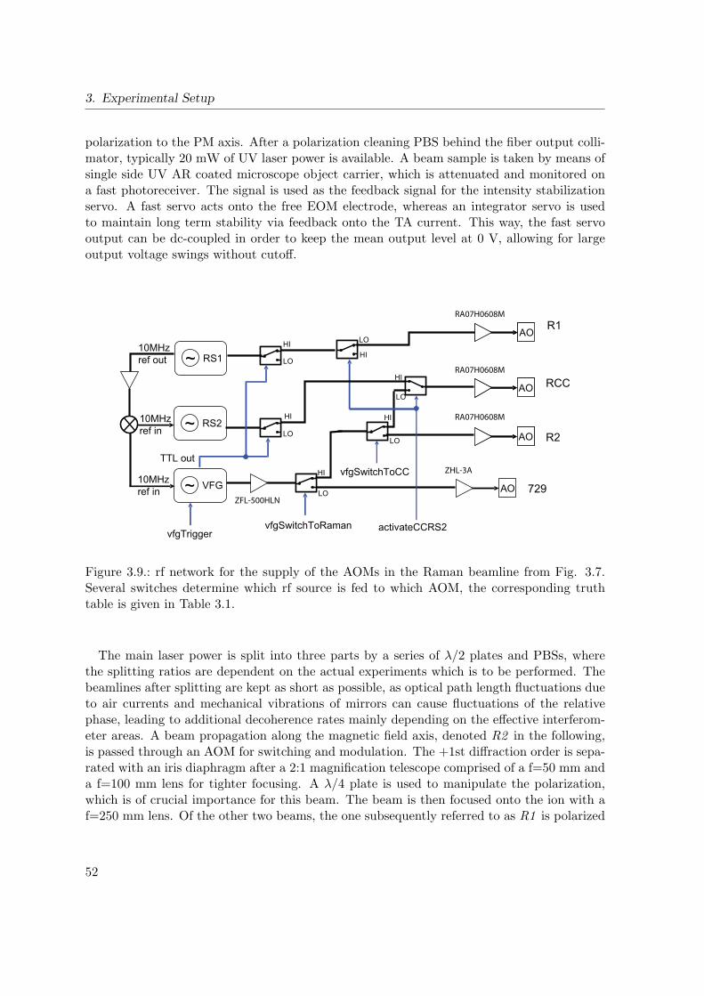
3. Experimental Setup
polarization to the PM axis. After a polarization cleaning PBS behind the fiber output colli-mator, typically 20 mW of UV laser power is available. A beam sample is taken by means ofsingle side UV AR coated microscope object carrier, which is attenuated and monitored ona fast photoreceiver. The signal is used as the feedback signal for the intensity stabilizationservo. A fast servo acts onto the free EOM electrode, whereas an integrator servo is usedto maintain long term stability via feedback onto the TA current. This way, the fast servooutput can be dc-coupled in order to keep the mean output level at 0 V, allowing for largeoutput voltage swings without cutoff.
HI
HIHI
HI
HIHI RA07H0608M
RA07H0608M
RA07H0608M
ZFL-500HLN
ZHL-3A
Figure 3.9.: rf network for the supply of the AOMs in the Raman beamline from Fig. 3.7.Several switches determine which rf source is fed to which AOM, the corresponding truthtable is given in Table 3.1.
The main laser power is split into three parts by a series of λ/2 plates and PBSs, wherethe splitting ratios are dependent on the actual experiments which is to be performed. Thebeamlines after splitting are kept as short as possible, as optical path length fluctuations dueto air currents and mechanical vibrations of mirrors can cause fluctuations of the relativephase, leading to additional decoherence rates mainly depending on the effective interferom-eter areas. A beam propagation along the magnetic field axis, denoted R2 in the following,is passed through an AOM for switching and modulation. The +1st diffraction order is sepa-rated with an iris diaphragm after a 2:1 magnification telescope comprised of a f=50 mm anda f=100 mm lens for tighter focusing. A λ/4 plate is used to manipulate the polarization,which is of crucial importance for this beam. The beam is then focused onto the ion with af=250 mm lens. Of the other two beams, the one subsequently referred to as R1 is polarized
52

3.2. Laser Systems
1 2 3 R1 R2 CC Purpose
0 0 X - VFG - Scattering and Stark shift measurements
0 1 X - - VFG Stark shift measurements
1 0 0 RS1 VFG - Raman transitions with η = 0
1 0 1 - VFG RS2 Spin dependent forces
1 1 1 - - RS2 CC beam alignment
1 1 0 RS1 - VFG Raman transitions with η = 0
Table 3.1.: Truth table for the required TTL settings of the Raman beams. The first threecolumns show the logic states of the relevant TTL channels of the experiment control systemand the next three columns indicate which rf source is connected to the AOMs R1, R2and CC, see Fig. 3.7. The last columns describes the purpose of each configuration. TheTTL channels are referred to Fig. 3.9 as follows: TTL 1 → VFG TTL channel 1, 2 →vfgSwitchToCC, 3 → activateCCRS2. An X in the TTL setting columns means that thelogical state of the corresponding line is irrelevant for this setting.
horizontally with respect to the optical table, whereas the other one, called RCC is verti-cally polarized. Both beams are passed through individual AOMs and are re-superimposedon a PBS. The beam pair is directed orthogonally to the magnetic field, such that R1 isπ polarized, driving ∆mJ = 0 transitions, and RCC has balanced σ+ and σ− components,driving the ∆mJ = ±1 transitions equally strong. The respective +1st diffraction ordersare selected by means of an iris diaphragm and focused onto the ion with a f=250 mm lens.In contrast to the R2 beamline, no additional telescope is necessary because of the shorterpropagation distance. All AOMs are QZF-80-20. The rf supply network is shown in Fig. 3.9,its sophistication arises from the fact that the beams are to be used in different combinations.All AOMs are oriented such that the propagation direction of the sound wave in the crystal isperpendicular to the beam polarization, which drastically affects the diffraction performanceof the QZF-80-20, in contrast to AOMs working in the IR. All three AOMs are situated atapproximately the same distance from the delivery fiber output, such that the beam diameterinside the crystals can be adjusted to be the same value for all modulators by means of thefiber collimator focusing screw. This way, high diffraction efficiencies of up of 65% to 75%are achieved for all the AOMs.In principle, much tighter focusing of the Raman beams is feasible, with illumination ofthe complete 1” diameter of the focusing lenses spot sizes in the µm range are achieved.This would provide much stronger Raman couplings, such that reduced decoherence can beachieved by choosing larger Raman detunings. However, for small spot sizes strong decoher-ence effects set in that are not fully understood but that can only be caused by an unstableillumination strength of the ion, see Sec. 4.7. Possible physical effects are therefore pointinginstabilities of the beams or radial position drifts of the ion on the second scale.
53
3. Experimental Setup
3.3. Imaging and Detection
The imaging system allows for simultaneous detection of ion fluorescence near 397 nm onan electron multiplier CCD (EMCCD) camera system 23 or on a photomultiplier (PMT) 24.While the camera mainly serves for asserting that the right number of ions is loaded and thatthe ions are properly cooled and localized, the fluorescence data from which the experimentalresults are obtained is collected with the PMT. This is because the PMT readout is moreeasily accomplished than the readout of the EMCCD camera images. Simultaneous readoutof several ions however can only be accomplished with the spatially resolving camera, whichis already demonstrated in chapter 9 and will serve as the standard readout method in thefuture. The spatial resolution also enables an improved filtering of the stray light backgroundas the image of the ion is directly at hand, in the PMT case this can be only accomplishedby adjusting a 2D aperture consisting of 4 independently movable blades 25.The fluorescence is collected by a specially designed objective 26 with a focal length of 48 mm.The inverted viewport allows for placing the objective at an approximate distance of 50 mmfrom the ion, resulting in a covered solid angle of dΩ/4π ≈6% and a magnification factor of28 at an image distance of about 1400 mm, which allows for the distinction of ions aligned ina string at a typical ion distance of 3 µm and a pixel size of 24 µm. As the PMT photon countrate sets the minimum time in which the bright and dark states of an ion can be reliablydistinguished, see Sec. 4.2.1, most of the fluorescence light is directed in the PMT branch ofthe detection optics using a 80:20 beam splitter 27. Both in the PMT and EMCCD branches,the light is spectrally filtered with a 397 nm band-pass filter 28. Considering the photoncollection solid angle, 96% transmission through the objective, 88% filter transmission andthe PMT quantum efficiency of 20% at 397 nm, a photon count rate in the range of 500 s−1 isexpected. By contrast, only count rates of 30 s−1 are actually attained, the huge discrepancybetween these rates is still unclear.
3.4. Trap Voltage Supplies
As the trap confinement mechanism relies on the application of suitable electric fields bothat dc and rf, individual supply systems for each of these components are needed. As thedc supply electronics is of crucial importance especially in conjunction with the scalabilityscheme based on the segmented trap, Appendix B is entirely devoted to this issue. Impor-tant experimental findings for the characterization of the voltage supply are found in Secs.2.1.3,4.2.3 and 4.3. It shall be briefly mentioned here that two main types of dc supplies wereused throughout this thesis: Most experiments were carried out with a purely static voltagesupply providing only voltages for a single segment pair, and all the other segments were
23iXon DV860DCS-BV, Andor, Belfast, Northern Ireland, 128x128 pixels24P25PC, ET Enterprises, Uxbridge, United Kingdom25SP60, OWIS GmbH, Staufen26Sill Optics GmbH, Wendelstein27CVI Melles Griot, Bensheim28FF01-377/50-23.7-D, Semrock, Rochester, USA
54
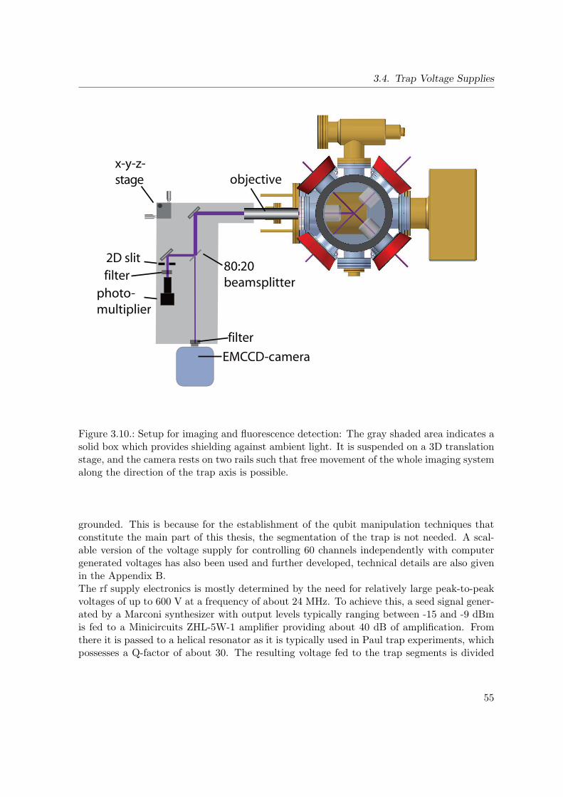
3.4. Trap Voltage Supplies
photo-
multiplier
EMCCD-camera
80:20
beamsplitter
objective
x-y-z-
stage
2D slit
filter
filter
Figure 3.10.: Setup for imaging and fluorescence detection: The gray shaded area indicates asolid box which provides shielding against ambient light. It is suspended on a 3D translationstage, and the camera rests on two rails such that free movement of the whole imaging systemalong the direction of the trap axis is possible.
grounded. This is because for the establishment of the qubit manipulation techniques thatconstitute the main part of this thesis, the segmentation of the trap is not needed. A scal-able version of the voltage supply for controlling 60 channels independently with computergenerated voltages has also been used and further developed, technical details are also givenin the Appendix B.The rf supply electronics is mostly determined by the need for relatively large peak-to-peakvoltages of up to 600 V at a frequency of about 24 MHz. To achieve this, a seed signal gener-ated by a Marconi synthesizer with output levels typically ranging between -15 and -9 dBmis fed to a Minicircuits ZHL-5W-1 amplifier providing about 40 dB of amplification. Fromthere it is passed to a helical resonator as it is typically used in Paul trap experiments, whichpossesses a Q-factor of about 30. The resulting voltage fed to the trap segments is divided
55
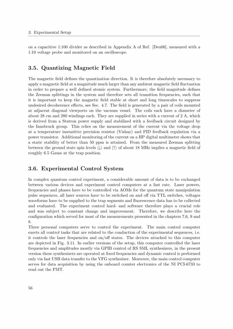
3. Experimental Setup
on a capacitive 1:100 divider as described in Appendix A of Ref. [Deu00], measured with a1:10 voltage probe and monitored on an oscilloscope.
3.5. Quantizing Magnetic Field
The magnetic field defines the quantization direction. It is therefore absolutely necessary toapply a magnetic field at a magnitude much larger than any ambient magnetic field fluctuationin order to prepare a well defined atomic system. Furthermore, the field magnitude definesthe Zeeman splittings in the system and therefore sets all transition frequencies, such thatit is important to keep the magnetic field stable at short and long timescales to suppressundesired decoherence effects, see Sec. 4.7. The field is generated by a pair of coils mountedat adjacent diagonal viewports on the vacuum vessel. The coils each have a diameter ofabout 28 cm and 280 windings each. They are supplied in series with a current of 2 A, whichis derived from a Statron power supply and stabilized with a feedback circuit designed bythe Innsbruck group. This relies on the measurement of the current via the voltage dropat a temperature insensitive precision resistor (Vishay) and PID feedback regulation via apower transistor. Additional monitoring of the current on a HP digital multimeter shows thata static stability of better than 50 ppm is attained. From the measured Zeeman splittingbetween the ground state spin levels |↓〉 and |↑〉 of about 18 MHz implies a magnetic field ofroughly 6.5 Gauss at the trap position.
3.6. Experimental Control System
In complex quantum control experiment, a considerable amount of data is to be exchangedbetween various devices and experiment control computers at a fast rate. Laser powers,frequencies and phases have to be controlled via AOMs for the quantum state manipulationpulse sequences, all laser sources have to be switched on and off via TTL switches, voltageswaveforms have to be supplied to the trap segments and fluorescence data has to be collectedand evaluated. The experiment control hard- and software therefore plays a crucial roleand was subject to constant change and improvement. Therefore, we describe here theconfiguration which served for most of the measurements presented in the chapters 7,6, 9 and8.Three personal computers serve to control the experiment. The main control computerexerts all control tasks that are related to the conduction of the experimental sequences, i.e.it controls the laser frequencies and on/off states. The devices attached to this computerare depicted in Fig. 3.11. In earlier versions of the setup, this computer controlled the laserfrequencies and amplitudes mostly via GPIB control of RS SML synthesizers, in the presentversion these synthesizers are operated at fixed frequencies and dynamic control is performedonly via fast USB data transfer to the VFG synthesizer. Moreover, the main control computerserves for data acquisition by using the onboard counter electronics of the NI PCI-6733 toread out the PMT.
56
3.6. Experimental Control System
Expe
rimen
t con
trol c
ompu
ter NI PCI 6733
NI PCI 6733
NI PCI 6713
VFG-150
Trap voltagesupply
Gig
abit
Ethe
rnet
USB
64x trap voltages
attenuator voltageTrap RF att.
RF for 729 & Raman AOMs
Up to 15 TTL channelsto RF switches
Photoion shutter TTL
2x analog voltage Mini PIA HV amplifiersfor 397 and 866 PDH cavities
Counter TTL
Photon count signal
VFG trigger
Figure 3.11.: Experimental control system: The main control computer controls the exper-iment mainly via digital output channels of NI PCI-6733 cards and the USB-driven VFGsynthesizer. The 64 channel voltage control box has actually been used on another computerfor historical reasons, but will be attached to the main control computer in the future setup.
Another computer involved in the experiment control is the camera computer which exclu-sively serves for the readout of the EMCCD camera, see Sec. 3.3. The remaining computermainly serves for the readout of the wavemeter and is also assigned to some less criticalcontrol tasks. As the wavemeter provides laser frequency measurements with an accuracyof below 10 MHz, it can be used to regulate laser frequencies by feedback if the frequencystability is not crucial, which is exactly the case for the laser at 397 nm driving the Ramantransitions. The feedback signal obtained from a discrete software PI controller is fed backto the master grating by means of a digital to analog converter circuit to which the digitalinformation is supplied via a standard serial interface. To assure proper laser operation, agalvanic separation between the systems was found to be necessary, which was achieved byutilizing an IL300 analog optocoupler. Furthermore, the computer is connected via a CAN-bus interface to the iseg high voltage generator that coarse-controls the PDH cavity piezovoltage for the 866 nm and 397 nm lasers.
57

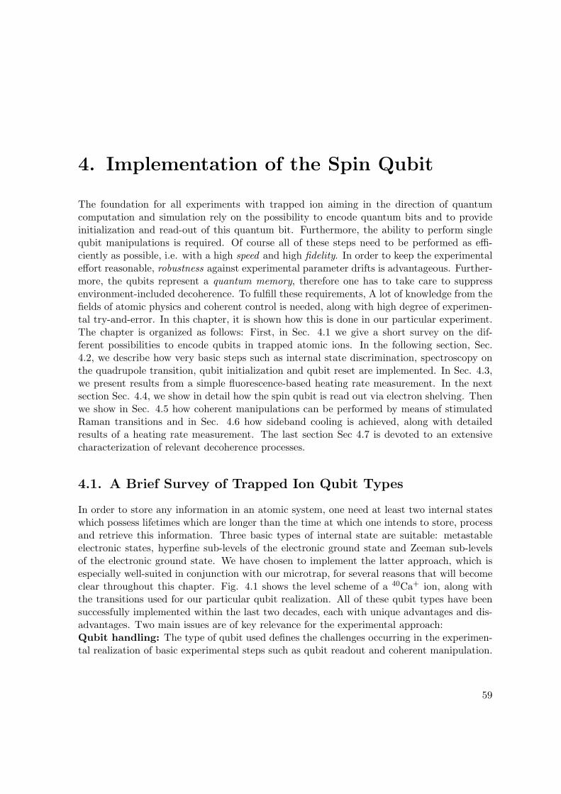
4. Implementation of the Spin Qubit
The foundation for all experiments with trapped ion aiming in the direction of quantumcomputation and simulation rely on the possibility to encode quantum bits and to provideinitialization and read-out of this quantum bit. Furthermore, the ability to perform singlequbit manipulations is required. Of course all of these steps need to be performed as effi-ciently as possible, i.e. with a high speed and high fidelity. In order to keep the experimentaleffort reasonable, robustness against experimental parameter drifts is advantageous. Further-more, the qubits represent a quantum memory, therefore one has to take care to suppressenvironment-included decoherence. To fulfill these requirements, A lot of knowledge from thefields of atomic physics and coherent control is needed, along with high degree of experimen-tal try-and-error. In this chapter, it is shown how this is done in our particular experiment.The chapter is organized as follows: First, in Sec. 4.1 we give a short survey on the dif-ferent possibilities to encode qubits in trapped atomic ions. In the following section, Sec.4.2, we describe how very basic steps such as internal state discrimination, spectroscopy onthe quadrupole transition, qubit initialization and qubit reset are implemented. In Sec. 4.3,we present results from a simple fluorescence-based heating rate measurement. In the nextsection Sec. 4.4, we show in detail how the spin qubit is read out via electron shelving. Thenwe show in Sec. 4.5 how coherent manipulations can be performed by means of stimulatedRaman transitions and in Sec. 4.6 how sideband cooling is achieved, along with detailedresults of a heating rate measurement. The last section Sec 4.7 is devoted to an extensivecharacterization of relevant decoherence processes.
4.1. A Brief Survey of Trapped Ion Qubit Types
In order to store any information in an atomic system, one need at least two internal stateswhich possess lifetimes which are longer than the time at which one intends to store, processand retrieve this information. Three basic types of internal state are suitable: metastableelectronic states, hyperfine sub-levels of the electronic ground state and Zeeman sub-levelsof the electronic ground state. We have chosen to implement the latter approach, which isespecially well-suited in conjunction with our microtrap, for several reasons that will becomeclear throughout this chapter. Fig. 4.1 shows the level scheme of a 40Ca+ ion, along withthe transitions used for our particular qubit realization. All of these qubit types have beensuccessfully implemented within the last two decades, each with unique advantages and dis-advantages. Two main issues are of key relevance for the experimental approach:Qubit handling: The type of qubit used defines the challenges occurring in the experimen-tal realization of basic experimental steps such as qubit readout and coherent manipulation.
59
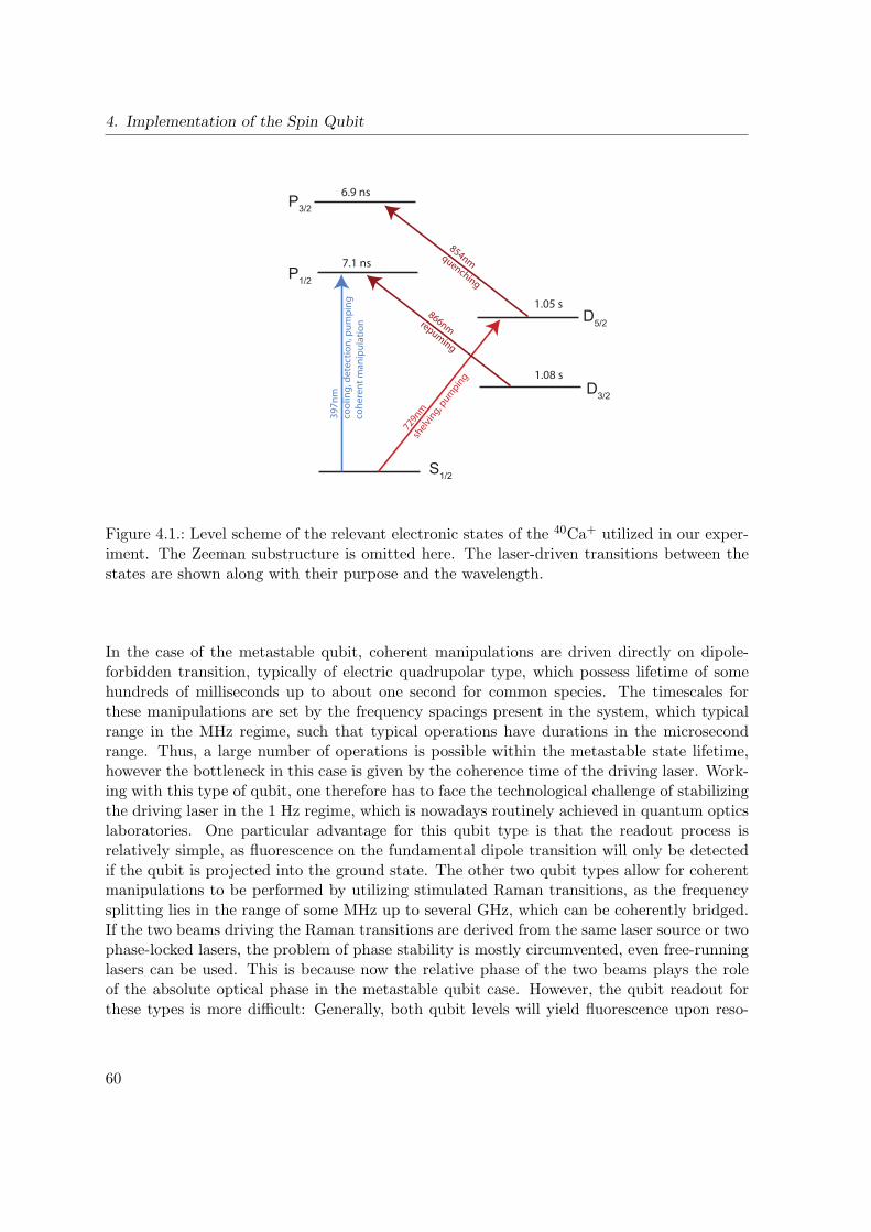
4. Implementation of the Spin Qubit
729nm
shel
vin
g, p
um
pin
g
39
7n
m
co
oli
ng
, d
ete
cti
on
, p
um
pin
g
co
he
ren
t m
an
ipu
lati
on
866nmrepuming
854nmquenching
S1/2
D3/2
D5/2
P1/2
P3/26.9 ns
7.1 ns
1.05 s
1.08 s
Figure 4.1.: Level scheme of the relevant electronic states of the 40Ca+ utilized in our exper-iment. The Zeeman substructure is omitted here. The laser-driven transitions between thestates are shown along with their purpose and the wavelength.
In the case of the metastable qubit, coherent manipulations are driven directly on dipole-forbidden transition, typically of electric quadrupolar type, which possess lifetime of somehundreds of milliseconds up to about one second for common species. The timescales forthese manipulations are set by the frequency spacings present in the system, which typicalrange in the MHz regime, such that typical operations have durations in the microsecondrange. Thus, a large number of operations is possible within the metastable state lifetime,however the bottleneck in this case is given by the coherence time of the driving laser. Work-ing with this type of qubit, one therefore has to face the technological challenge of stabilizingthe driving laser in the 1 Hz regime, which is nowadays routinely achieved in quantum opticslaboratories. One particular advantage for this qubit type is that the readout process isrelatively simple, as fluorescence on the fundamental dipole transition will only be detectedif the qubit is projected into the ground state. The other two qubit types allow for coherentmanipulations to be performed by utilizing stimulated Raman transitions, as the frequencysplitting lies in the range of some MHz up to several GHz, which can be coherently bridged.If the two beams driving the Raman transitions are derived from the same laser source or twophase-locked lasers, the problem of phase stability is mostly circumvented, even free-runninglasers can be used. This is because now the relative phase of the two beams plays the roleof the absolute optical phase in the metastable qubit case. However, the qubit readout forthese types is more difficult: Generally, both qubit levels will yield fluorescence upon reso-
60
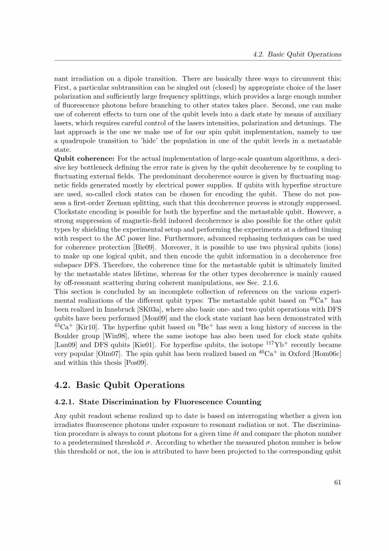
4.2. Basic Qubit Operations
nant irradiation on a dipole transition. There are basically three ways to circumvent this:First, a particular subtransition can be singled out (closed) by appropriate choice of the laserpolarization and sufficiently large frequency splittings, which provides a large enough numberof fluorescence photons before branching to other states takes place. Second, one can makeuse of coherent effects to turn one of the qubit levels into a dark state by means of auxiliarylasers, which requires careful control of the lasers intensities, polarization and detunings. Thelast approach is the one we make use of for our spin qubit implementation, namely to usea quadrupole transition to ’hide’ the population in one of the qubit levels in a metastablestate.Qubit coherence: For the actual implementation of large-scale quantum algorithms, a deci-sive key bottleneck defining the error rate is given by the qubit decoherence by te coupling tofluctuating external fields. The predominant decoherence source is given by fluctuating mag-netic fields generated mostly by electrical power supplies. If qubits with hyperfine structureare used, so-called clock states can be chosen for encoding the qubit. These do not pos-sess a first-order Zeeman splitting, such that this decoherence process is strongly suppressed.Clockstate encoding is possible for both the hyperfine and the metastable qubit. However, astrong suppression of magnetic-field induced decoherence is also possible for the other qubittypes by shielding the experimental setup and performing the experiments at a defined timingwith respect to the AC power line. Furthermore, advanced rephasing techniques can be usedfor coherence protection [Bie09]. Moreover, it is possible to use two physical qubits (ions)to make up one logical qubit, and then encode the qubit information in a decoherence freesubspace DFS. Therefore, the coherence time for the metastable qubit is ultimately limitedby the metastable states lifetime, whereas for the other types decoherence is mainly causedby off-resonant scattering during coherent manipulations, see Sec. 2.1.6.This section is concluded by an incomplete collection of references on the various experi-mental realizations of the different qubit types: The metastable qubit based on 40Ca+ hasbeen realized in Innsbruck [SK03a], where also basic one- and two qubit operations with DFSqubits have been performed [Mon09] and the clock state variant has been demonstrated with43Ca+ [Kir10]. The hyperfine qubit based on 9Be+ has seen a long history of success in theBoulder group [Win98], where the same isotope has also been used for clock state qubits[Lan09] and DFS qubits [Kie01]. For hyperfine qubits, the isotope 117Yb+ recently becamevery popular [Olm07]. The spin qubit has been realized based on 40Ca+ in Oxford [Hom06c]and within this thesis [Pos09].
4.2. Basic Qubit Operations
4.2.1. State Discrimination by Fluorescence Counting
Any qubit readout scheme realized up to date is based on interrogating whether a given ionirradiates fluorescence photons under exposure to resonant radiation or not. The discrimina-tion procedure is always to count photons for a given time δt and compare the photon numberto a predetermined threshold σ. According to whether the measured photon number is belowthis threshold or not, the ion is attributed to have been projected to the corresponding qubit
61
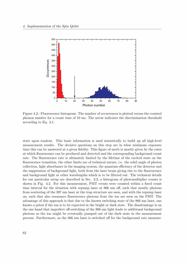
4. Implementation of the Spin Qubit
0 10 20 30 40 50 60 70 80 900
50
100
150
200
250
300
350
400
450
500
550
Photon number
Occ
urr
ence
s
Figure 4.2.: Fluorescence histogram: The number of occurrences is plotted versus the countedphonon number for a count time of 10 ms. The arrow indicates the discrimination thresholdaccording to Eq. 4.1.
state upon readout. This basic information is used statistically to build up all high-levelmeasurement results. The decisive questions on this step are in what minimum exposuretime this can be answered at a given fidelity. This figure of merit is mostly given by the ratesat which fluorescence can be produced and detected and the corresponding background countrate. The fluorescence rate is ultimately limited by the lifetime of the excited state on thefluorescence transition, the other limits are of technical nature, i.e. the solid angle of photoncollection, light absorbance in the imaging system, the quantum efficiency of the detector andthe suppression of background light, both from the laser beam giving rise to the fluorescenceand background light at other wavelengths which is to be filtered out. The technical detailsfor our particular setup are described in Sec. 3.3, a histogram of photomultiplier counts isshown in Fig. 4.2. For this measurement, PMT events were counted within a fixed counttime interval for the situation with repump laser at 866 nm off, such that mostly photonsfrom scattering of the 397 nm laser at the trap structure are seen, and with the repump laseron, such that also resonance fluorescence photons from the ion are seen on the PMT. Theadvantage of this approach is that due to the known switching state of the 866 nm laser, oneknows a priori if the ion is to be expected in the bright or dark state. The disadvantage is onthe one hand that imperfect off-switching of the 866 nm light leads to additional backgroundphotons as the ion might be eventually pumped out of the dark state in the measurementprocess. Furthermore, as the 866 nm laser is switched off for the background rate measure-
62
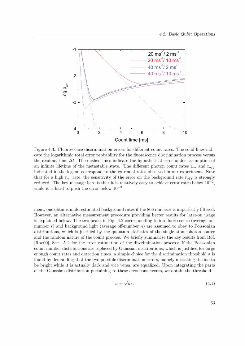
4.2. Basic Qubit Operations
0 2 4 6 8 10-4
-3
-2
-1
Log
p err
Count time [ms]
20 ms-1/ 2 ms-1
20 ms-1/ 10 ms-1
40 ms-1/ 2 ms-1
40 ms-1/ 10 ms-1
Figure 4.3.: Fluorescence discrimination errors for different count rates: The solid lines indi-cate the logarithmic total error probability for the fluorescence discrimination process versusthe readout time ∆t. The dashed lines indicate the hypothetical error under assumption ofan infinite lifetime of the metastable state. The different photon count rates ron and roffindicated in the legend correspond to the extremal rates observed in our experiment. Notethat for a high ron rate, the sensitivity of the error on the background rate roff is stronglyreduced. The key message here is that it is relatively easy to achieve error rates below 10−2,while it is hard to push the error below 10−3.
ment, one obtains underestimated background rates if the 866 nm laser is imperfectly filtered.However, an alternative measurement procedure providing better results for later-on usageis explained below. The two peaks in Fig. 4.2 corresponding to ion fluorescence (average on-number s) and background light (average off-number n) are assumed to obey to Poissoniandistributions, which is justified by the quantum statistics of the single-atom photon sourceand the random nature of the count process. We briefly summarize the key results from Ref.[Roo00], Sec. A.2 for the error estimation of the discrimination process: If the Poissoniancount number distributions are replaced by Gaussian distributions, which is justified for largeenough count rates and detection times, a simple choice for the discrimination threshold σ isfound by demanding that the two possible discrimination errors, namely mistaking the ion tobe bright while it is actually dark and vice versa, are equalized. Upon integrating the partsof the Gaussian distribution pertaining to these erroneous events, we obtain the threshold
σ =√ns. (4.1)
63
4. Implementation of the Spin Qubit
Most of the results presented in this thesis have been obtained by using this threshold type,however it was found that it leads to problems if the background count rate is very low andthe Gaussian approximation breaks down, i.e. the threshold is chosen to small. An advancedscheme for measuring n and s is to make use of the quadrupole transition at 729 nm toturn the ion bright or dark, which is more adapted to actual experiments where it is tobe measured if the ion is in |↑〉 or |↓〉. Another advantage of this scheme is that the finitelifetime of the metastable state is included in the measurement. If the lifetime of this statewas infinitely long, one could press the error probability below any given threshold by simplyincreasing the count interval in order to separate the Poissonians further from each other.For example, with a D5/2 lifetime τ5/2 of about 1s, one would face an error probability inthe 1% range for a count interval of 10ms. Thus, an optimal count time ∆t along with andoptimal threshold σ can be found by correcting the probability for wrong bright counts byprobability for detecting above-threshold fluorescence from a spontaneous decay event. ∆tis found by minimizing this probability, while σ can still be determined by the requirementthat the other error type, which is not affected by the finite metastable state lifetime, isto occur equally often. The dependence of the discrimination fidelity on the count rates isvisualize in Fig. 4.3. However, as the fidelity bottleneck for the spin readout is given by theoptical pumping and shelving steps, see Sec. 4.2.4 and 4.4, we do not elaborate further onthis. It shall be mentioned that the fidelity of the fluorescence discrimination can even beincreased by time-resolved measurements, which was demonstrated in Ref. [Mye08]. In sucha time-resolved measurement, spontaneous decay events are likely to be discerned because ofthe abrupt onset of fluorescence, furthermore error from cosmic ray events can be detected.In general, fluorescence readout with a PMT is limited by the fact that for several ions, onlythe total number of bright ions can be determined. For simultaneous readout of increasinglylarge numbers of qubits, this represents a drastic information loss. It was shown in Ref.[Hom06b] that an almost-complete internal state tomography of two ions is still possible if thislimited information is available. Other ways to circumvent this are single-ion laser addressing,which has so far only been realized by the Innsbruck group [Nag99], or to use a segmentedtrap and conduct a procedure of splitting and individual fluorescence measurement. Anotherapproach which was realized in Ref. [Bur10] and in this thesis, see Sec. 9.1, is to make useof the EMCCD camera as an imaging device which provides spatial resolution in contrast tothe PMT.The fluorescence state readout provides only binary information: the ion is always foundeither bright or dark. In order to infer a dark state occupation probability as a measurementresult, each measurement has to be performed repeatedly under exactly the same conditionssuch that the dark state probability can be inferred from the relative number of dark countevents. Even if perfect fluorescence discrimination was possible, this inferred probability willstatistically deviate from the physical occupation probability because of the finite number ofexperimental runs. The process leading to the final outcome can be seen as the realizationof an unbalanced Galton board, where the decision probability at each stage is given by thephysical occupation probability. After N stages, the probability distribution to find ND dark
64
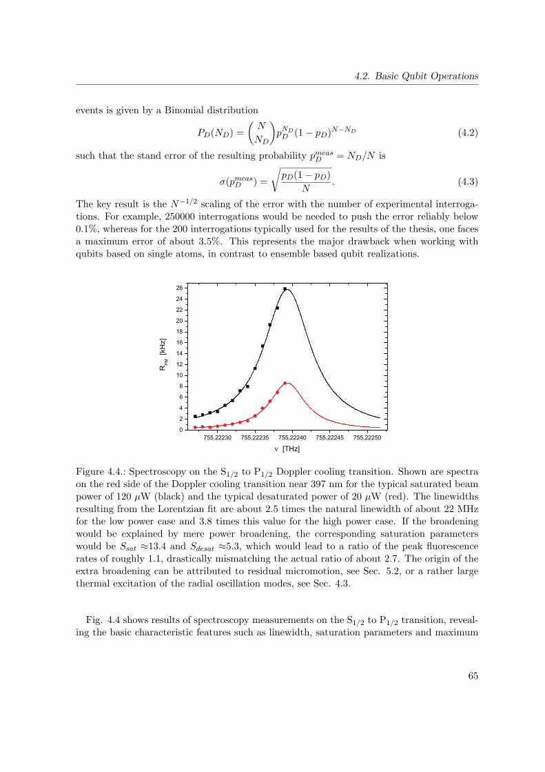
4.2. Basic Qubit Operations
events is given by a Binomial distribution
PD(ND) =
(N
ND
)pNDD (1− pD)
N−ND (4.2)
such that the stand error of the resulting probability pmeasD = ND/N is
σ(pmeasD ) =
√pD(1− pD)
N. (4.3)
The key result is the N−1/2 scaling of the error with the number of experimental interroga-tions. For example, 250000 interrogations would be needed to push the error reliably below0.1%, whereas for the 200 interrogations typically used for the results of the thesis, one facesa maximum error of about 3.5%. This represents the major drawback when working withqubits based on single atoms, in contrast to ensemble based qubit realizations.
755,22230 755,22235 755,22240 755,22245 755,222500
2
4
6
8
10
12
14
16
18
20
22
24
26
RP
M [
kHz]
[THz]ν
Figure 4.4.: Spectroscopy on the S1/2 to P1/2 Doppler cooling transition. Shown are spectraon the red side of the Doppler cooling transition near 397 nm for the typical saturated beampower of 120 µW (black) and the typical desaturated power of 20 µW (red). The linewidthsresulting from the Lorentzian fit are about 2.5 times the natural linewidth of about 22 MHzfor the low power case and 3.8 times this value for the high power case. If the broadeningwould be explained by mere power broadening, the corresponding saturation parameterswould be Ssat ≈13.4 and Sdesat ≈5.3, which would lead to a ratio of the peak fluorescencerates of roughly 1.1, drastically mismatching the actual ratio of about 2.7. The origin of theextra broadening can be attributed to residual micromotion, see Sec. 5.2, or a rather largethermal excitation of the radial oscillation modes, see Sec. 4.3.
Fig. 4.4 shows results of spectroscopy measurements on the S1/2 to P1/2 transition, reveal-ing the basic characteristic features such as linewidth, saturation parameters and maximum
65

4. Implementation of the Spin Qubit
fluorescence rate. All following experimental results in the remainder of this thesis, unlessnoted otherwise, have been obtained using the same essential experimental sequence: Theion is first Doppler cooled for typically 2 ms and then prepared in either |↑〉 or |↓〉 by opticalpumping, see Sec. 4.2.4. If required, it is sideband cooled to the ground state of the axialmode of vibration, see Sec. 4.6. Then, the coherent manipulations constituting the partic-ular measurement take place, see Sec. 4.5.1. If the spin is to be read out, one of the spinpopulations is shelved to the metastable state as explained in Sec. 4.4, before finally thefluorescence is counted (Sec. 4.2.1) for 1..10 ms and the qubit is reset, see Sec. 4.2.5. Thebottleneck steps taking most of the time are the Doppler and sideband cooling steps and thefluorescence readout, each taking up to several milliseconds. These durations can be reducedto the 100 µs range upon technological improvements.
4.2.2. Spectroscopy on the Quadrupole Transition
P1/2-1/2
+1/2
D5/2 +5/2 b)a)
+3/2+1/2
-1/2-3/2
-5/2a
b
c
D5/2
+5/2+3/2
P1/2-1/2
+1/2
P3/2 +3/2+1/2
-1/2-3/2
D3/2+3/2
+1/2-1/2
+1/2-1/2
P1/2
Figure 4.5.: a) Complete level scheme of the quadrupole transition between the S1/2 andthe D5/2 state with the full Zeeman substructure. The transitions marked as a,b and c areactually used in the experiment.b) shows the decay channels for quenching the D5/2 stateon the dipole transition to the P3/2 on 854 nm. One can see that the 854 nm needs to havecircular polarization components for reliable quenching, furthermore the 866 nm repumpbeam has to be switched on to deplete the D3/2 state.
With the fluorescence state discrimination explained in the previous section at hand, weare in the position to make use of the quadrupole transition S1/2 →D5/2 to perform resolved-sideband spectroscopy for a precise determination of the motional frequencies and a charac-terization of the trapped ion’s motional state by investigating its coherent dynamics. A level
66
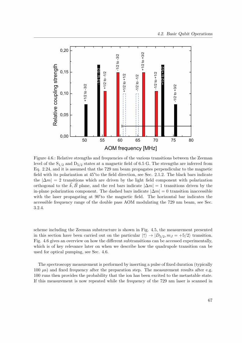
4.2. Basic Qubit Operations
50 55 60 65 70 75 800,00
0,05
0,10
0,15
0,20
+1/2
to +
1/2
-1/2
to -1
/2
+1/2
to -1
/2
-1/2
to -3
/2
+1/2
to +
3/2
-1/2
to +
1/2
-1/2
to -5
/2
+1/2
to -3
/2
-1/2
to +
3/2
Rel
ativ
e co
uplin
g st
reng
th
AOM frequency [MHz]
+1/2
to +
5/2
Figure 4.6.: Relative strengths and frequencies of the various transitions between the Zeemanlevel of the S1/2 and D5/2 states at a magnetic field of 6.5 G. The strengths are inferred fromEq. 2.24, and it is assumed that the 729 nm beam propagates perpendicular to the magneticfield with its polarization at 45to the field direction, see Sec. 2.1.2. The black bars indicatethe |∆m| = 2 transitions which are driven by the light field component with polarizationorthogonal to the k, B plane, and the red bars indicate |∆m| = 1 transitions driven by thein-plane polarization component. The dashed bars indicate |∆m| = 0 transition inaccessiblewith the laser propagating at 90to the magnetic field. The horizontal bar indicates theaccessible frequency range of the double pass AOM modulating the 729 nm beam, see Sec.3.2.4.
scheme including the Zeeman substructure is shown in Fig. 4.5, the measurement presentedin this section have been carried out on the particular |↑〉 → |D5/2,mJ = +5/2〉 transition.Fig. 4.6 gives an overview on how the different subtransitions can be accessed experimentally,which is of key relevance later on when we describe how the quadrupole transition can beused for optical pumping, see Sec. 4.6.
The spectroscopy measurement is performed by inserting a pulse of fixed duration (typically100 µs) and fixed frequency after the preparation step. The measurement results after e.g.100 runs then provides the probability that the ion has been excited to the metastable state.If this measurement is now repeated while the frequency of the 729 nm laser is scanned in
67

4. Implementation of the Spin Qubit
-3 -2 -1 0 1 2 3
0
0.1
0.2
0.3
0.4
0.5D
5/2
sta
te p
op
ula
tio
n
Car
rier
1st
axi
al r
sb
2n
d a
xial
rsb
1st
axi
al b
sb
2n
d a
xial
bsb
1st
rad
ial b
sb 1
1st
rad
ial r
sb 1
Detuning [MHz]
1st
rad
ial r
sb 2
1st
rad
ial b
sb 2
Figure 4.7.: Spectroscopy on the quadrupole transition: Data for a spectroscopy measurementon the S1/2,mJ=+1/2 to D5/2,mJ=+5/2 is shown. The axial and radial sidebands are well-resolved. The data was taken with the 729 nm locked to a on ordinary cavity with a resultinglinewidth of about 100 kHz limiting the spectroscopic resolution.
discrete steps, a spectrum such as shown in Fig. 4.7 is obtained. This spectroscopy methodis the most simple way for accurate measurements of the motional frequencies in our trap.On the other hand, it is the prerequisite for using the 729 nm transition as a tool for qubitpreparation (Sec. 4.2.4), sideband cooling (Sec. 4.6) and readout (Sec. 4.4).
4.2.3. Coherent Dynamics on the Quadrupole Transition
We now turn to the coherent evolution of an the internal state of a single trapped ion underexposure to a laser beam driving the quadrupole transition. This is important for mainlytwo reasons: First, it reveals information about the motional state of the ion and second, itis a decisive foundation for the spin readout procedure explained in Sec. 4.4. As the beamis impinging horizontally at an angle of 45 with respect to the trap axis, it couples to themotion along all three oscillation directions of the vibrational modes. Fig. 4.8 shows theoscillatory behavior of he population in the metastable state upon exposure to a resonant729 nm pulse of variable duration and fixed frequency. Information about the motional stateafter Doppler cooling can be inferred from the decay of the envelope.
68
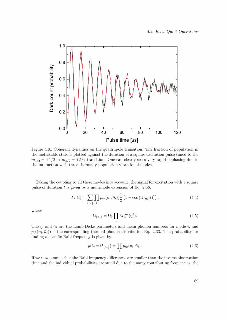
4.2. Basic Qubit Operations
0 20 40 60 80 100 1200,0
0,2
0,4
0,6
0,8
1,0D
ark
coun
t pro
babi
lity
Pulse time [µs]
Figure 4.8.: Coherent dynamics on the quadrupole transition: The fraction of population inthe metastable state is plotted against the duration of a square excitation pulse tuned to them1/2 = +1/2 → m5/2 = +5/2 transition. One can clearly see a very rapid dephasing due tothe interaction with three thermally population vibrational modes.
Taking the coupling to all these modes into account, the signal for excitation with a squarepulse of duration t is given by a multimode extension of Eq. 2.56:
PD(t) =∑ni
∏i
pth(ni, ni))1
2
(1− cos
(Ωnit)
)), (4.4)
whereΩni = Ω0
∏i
M carni
(η2i ). (4.5)
The ηi and ni are the Lamb-Dicke parameters and mean phonon numbers for mode i, andpth(ni, ni)) is the corresponding thermal phonon distribution Eq. 2.33. The probability forfinding a specific Rabi frequency is given by
p(Ω = Ωni) =∏i
pth(ni, ni). (4.6)
If we now assume that the Rabi frequency differences are smaller than the inverse observationtime and the individual probabilities are small due to the many contributing frequencies, the
69
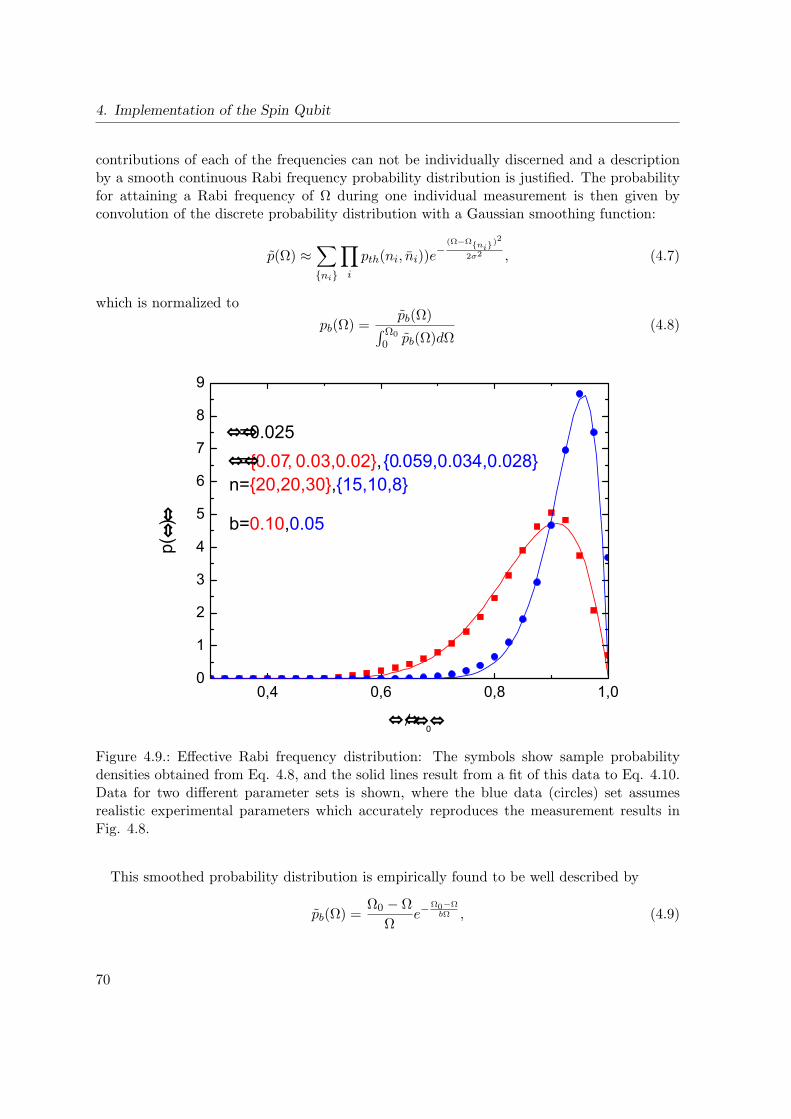
4. Implementation of the Spin Qubit
contributions of each of the frequencies can not be individually discerned and a descriptionby a smooth continuous Rabi frequency probability distribution is justified. The probabilityfor attaining a Rabi frequency of Ω during one individual measurement is then given byconvolution of the discrete probability distribution with a Gaussian smoothing function:
p(Ω) ≈∑ni
∏i
pth(ni, ni))e− (Ω−Ωni)
2
2σ2 , (4.7)
which is normalized to
pb(Ω) =pb(Ω)∫ Ω0
0 pb(Ω)dΩ(4.8)
0,4 0,6 0,8 1,00
1
2
3
4
5
6
7
8
9
p()
/0
=0.025=0.07, 0.03,0.02,0.059,0.034,0.028n=20,20,30,15,10,8
b=0.10,0.05
Figure 4.9.: Effective Rabi frequency distribution: The symbols show sample probabilitydensities obtained from Eq. 4.8, and the solid lines result from a fit of this data to Eq. 4.10.Data for two different parameter sets is shown, where the blue data (circles) set assumesrealistic experimental parameters which accurately reproduces the measurement results inFig. 4.8.
This smoothed probability distribution is empirically found to be well described by
pb(Ω) =Ω0 − Ω
Ωe−
Ω0−ΩbΩ , (4.9)
70
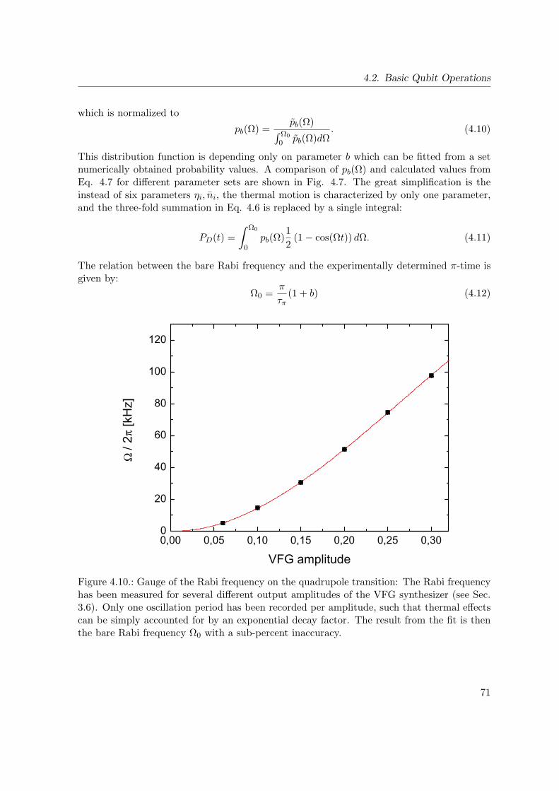
4.2. Basic Qubit Operations
which is normalized to
pb(Ω) =pb(Ω)∫ Ω0
0 pb(Ω)dΩ. (4.10)
This distribution function is depending only on parameter b which can be fitted from a setnumerically obtained probability values. A comparison of pb(Ω) and calculated values fromEq. 4.7 for different parameter sets are shown in Fig. 4.7. The great simplification is theinstead of six parameters ηi, ni, the thermal motion is characterized by only one parameter,and the three-fold summation in Eq. 4.6 is replaced by a single integral:
PD(t) =
∫ Ω0
0pb(Ω)
1
2(1− cos(Ωt)) dΩ. (4.11)
The relation between the bare Rabi frequency and the experimentally determined π-time isgiven by:
Ω0 =π
τπ(1 + b) (4.12)
0,00 0,05 0,10 0,15 0,20 0,25 0,300
20
40
60
80
100
120
Ω /
2π [k
Hz]
VFG amplitude
Figure 4.10.: Gauge of the Rabi frequency on the quadrupole transition: The Rabi frequencyhas been measured for several different output amplitudes of the VFG synthesizer (see Sec.3.6). Only one oscillation period has been recorded per amplitude, such that thermal effectscan be simply accounted for by an exponential decay factor. The result from the fit is thenthe bare Rabi frequency Ω0 with a sub-percent inaccuracy.
71
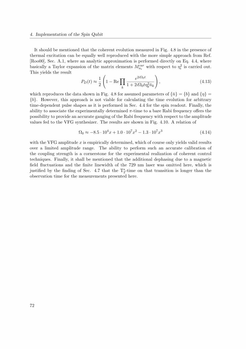
4. Implementation of the Spin Qubit
It should be mentioned that the coherent evolution measured in Fig. 4.8 in the presence ofthermal excitation can be equally well reproduced with the more simple approach from Ref.[Roo00], Sec. A.1, where an analytic approximation is performed directly on Eq. 4.4, wherebasically a Taylor expansion of the matrix elements M car
niwith respect to η2i is carried out.
This yields the result
PD(t) ≈ 1
2
(1− Re
∏k
e2iΩ0t
1 + 2iΩ0tη2knk
), (4.13)
which reproduces the data shown in Fig. 4.8 for assumed parameters of n = b and η =b. However, this approach is not viable for calculating the time evolution for arbitrarytime-dependent pulse shapes as it is performed in Sec. 4.4 for the spin readout. Finally, theability to associate the experimentally determined π-time to a bare Rabi frequency offers thepossibility to provide an accurate gauging of the Rabi frequency with respect to the amplitudevalues fed to the VFG synthesizer. The results are shown in Fig. 4.10. A relation of
Ω0 ≈ −8.5 · 104x+ 1.0 · 107x2 − 1.3 · 107x3 (4.14)
with the VFG amplitude x is empirically determined, which of course only yields valid resultsover a limited amplitude range. The ability to perform such an accurate calibration ofthe coupling strength is a cornerstone for the experimental realization of coherent controltechniques. Finally, it shall be mentioned that the additional dephasing due to a magneticfield fluctuations and the finite linewidth of the 729 nm laser was omitted here, which isjustified by the finding of Sec. 4.7 that the T∗
2-time on that transition is longer than theobservation time for the measurements presented here.
72
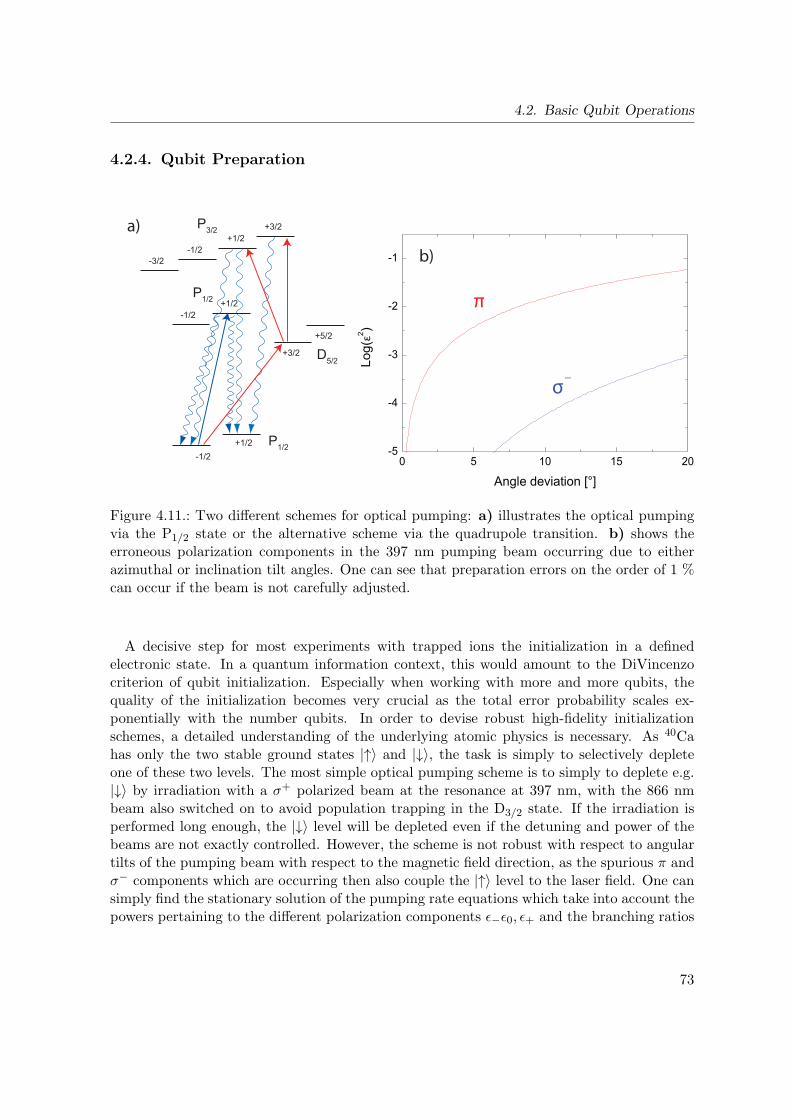
4.2. Basic Qubit Operations
4.2.4. Qubit Preparation
a)
D5/2
+5/2
+3/2
P1/2-1/2
+1/2
P3/2 +3/2+1/2
-1/2-3/2
+1/2-1/2
P1/2
0 5 10 15 20-5
-4
-3
-2
-1
Log(
ε2 )
π
σ−
b)
Figure 4.11.: Two different schemes for optical pumping: a) illustrates the optical pumpingvia the P1/2 state or the alternative scheme via the quadrupole transition. b) shows theerroneous polarization components in the 397 nm pumping beam occurring due to eitherazimuthal or inclination tilt angles. One can see that preparation errors on the order of 1 %can occur if the beam is not carefully adjusted.
A decisive step for most experiments with trapped ions the initialization in a definedelectronic state. In a quantum information context, this would amount to the DiVincenzocriterion of qubit initialization. Especially when working with more and more qubits, thequality of the initialization becomes very crucial as the total error probability scales ex-ponentially with the number qubits. In order to devise robust high-fidelity initializationschemes, a detailed understanding of the underlying atomic physics is necessary. As 40Cahas only the two stable ground states |↑〉 and |↓〉, the task is simply to selectively depleteone of these two levels. The most simple optical pumping scheme is to simply to deplete e.g.|↓〉 by irradiation with a σ+ polarized beam at the resonance at 397 nm, with the 866 nmbeam also switched on to avoid population trapping in the D3/2 state. If the irradiation isperformed long enough, the |↓〉 level will be depleted even if the detuning and power of thebeams are not exactly controlled. However, the scheme is not robust with respect to angulartilts of the pumping beam with respect to the magnetic field direction, as the spurious π andσ− components which are occurring then also couple the |↑〉 level to the laser field. One cansimply find the stationary solution of the pumping rate equations which take into account thepowers pertaining to the different polarization components ε−ε0, ε+ and the branching ratios
73
4. Implementation of the Spin Qubit
given by the Clebsch-Gordan factors, which leads to the stationary remaining population
P↓P↑
≈ P↓ =ε2− + ε20ε2+ + ε20
(4.15)
The Zeeman splitting leading to different pump rates on the sub-transitions and the branchingto the D3/2 state have been neglected here for the sake of simplicity. In order to obtainan estimation of the experimental accuracy requirements, the magnitude of the spuriouspolarization components has been plotted versus the tilt angle in Fig. 4.11 b), where thedata was obtained by invoking Eqs. 2.28.
0 5 10 15 20 25 300,0
0,2
0,4
0,6
0,8
1,0
0 100 200 300 400 5000,0
0,2
0,4
0,6
0,8
1,0
Single pulse duration [ s] Total pulse duration [ s]
Pum
p fi
del
ity
Pum
p fi
del
ity
(a) (b)
Figure 4.12.: Optical pumping on the quadrupole transition: a) shows results for the robustpulsed pumping scheme. The shelving probability is plotted against the duration of theindividual square pulses on the quadrupole transition. Results are shown for various numbersof pulses in the pumping sequence. For increasing pulse numbers, one obtains a broad plateau,such that the scheme is robustified against drifts in the Rabi frequency, the detuning andthe quench rate. b) shows results for continuous pumping with the 854 nm and the 729 nmbeams switched on simultaneously, for the same beam powers as in a). One can see that theconvergence behavior is very poor. Better results could however be obtained if the 854 nmpower is optimized.
A more robust pumping scheme which can be realized for 40Ca relies on the frequencyselectivity on the narrow quadrupole transition instead of polarization selectivity. The laserat 729 nm is used to transfer population only from the level which is to be depleted to themetastable D5/2 state, from which it transferred back to both ground state levels by quenchingat 854 nm. After a large enough number of cycles, the unwanted initial level is sufficientlydepleted. As can be seen from Fig. 4.11 a), the efficiency can be optimized if a purely πpolarized quench laser is used, however this would require an additional quenching beam for
74
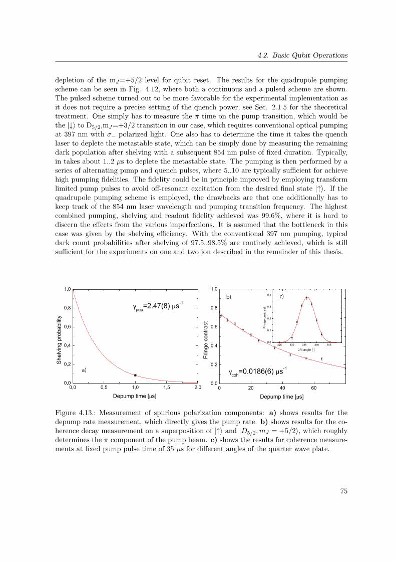
4.2. Basic Qubit Operations
depletion of the mJ=+5/2 level for qubit reset. The results for the quadrupole pumpingscheme can be seen in Fig. 4.12, where both a continuous and a pulsed scheme are shown.The pulsed scheme turned out to be more favorable for the experimental implementation asit does not require a precise setting of the quench power, see Sec. 2.1.5 for the theoreticaltreatment. One simply has to measure the π time on the pump transition, which would bethe |↓〉 to D5/2,mJ=+3/2 transition in our case, which requires conventional optical pumpingat 397 nm with σ− polarized light. One also has to determine the time it takes the quenchlaser to deplete the metastable state, which can be simply done by measuring the remainingdark population after shelving with a subsequent 854 nm pulse of fixed duration. Typically,in takes about 1..2 µs to deplete the metastable state. The pumping is then performed by aseries of alternating pump and quench pulses, where 5..10 are typically sufficient for achievehigh pumping fidelities. The fidelity could be in principle improved by employing transformlimited pump pulses to avoid off-resonant excitation from the desired final state |↑〉. If thequadrupole pumping scheme is employed, the drawbacks are that one additionally has tokeep track of the 854 nm laser wavelength and pumping transition frequency. The highestcombined pumping, shelving and readout fidelity achieved was 99.6%, where it is hard todiscern the effects from the various imperfections. It is assumed that the bottleneck in thiscase was given by the shelving efficiency. With the conventional 397 nm pumping, typicaldark count probabilities after shelving of 97.5..98.5% are routinely achieved, which is stillsufficient for the experiments on one and two ion described in the remainder of this thesis.
0,0 0,5 1,0 1,5 2,00,0
0,2
0,4
0,6
0,8
1,0
She
lvin
g pr
obab
ility
Depump time [µs]
γpop=2.47(8) µs-1
0 20 40 600,0
0,2
0,4
0,6
0,8
1,0
γcoh=0.0186(6) µs-1
Frin
ge c
ontra
st
Depump time [µs]
325 330 335 340 3450,0
0,1
0,2
0,3
0,4
Frin
ge c
ontra
st
λ/4 angle [°]
a)
b) c)
Figure 4.13.: Measurement of spurious polarization components: a) shows results for thedepump rate measurement, which directly gives the pump rate. b) shows results for the co-herence decay measurement on a superposition of |↑〉 and |D5/2,mJ = +5/2〉, which roughlydetermines the π component of the pump beam. c) shows the results for coherence measure-ments at fixed pump pulse time of 35 µs for different angles of the quarter wave plate.
75
4. Implementation of the Spin Qubit
It is difficult to measure the wrong polarization components because it is difficult to dis-cern imperfect pumping from other experimental imperfections, however we show here howquantum coherence can be utilized as a measurement tool to achieve this. The idea is tocompare the rate which the pump beam can transfer population to the rate at which it de-stroys a coherence between its ’dark’ state and the metastable D5/2 state, see Sec. 4.7 for adetailed explanation of coherence measurements. For the population measurement, the ionis pumped to |↑〉 with the quadrupole pumping technique described above, and before theshelving a depump pulse of σ− polarized light at 397 nm is applied. The remaining pop-ulation in |↑〉 vesus the depump pulse duration is shown in Fig. 4.13, and a depump rateof γpop=2.47(8) µs−1 is obtained. For the coherence measurement a coherent superpositionis prepared on the |↑〉 to |D5/2,mJ = +5/2〉 transition by a π/2 pulse at 729 nm. Beforeprobing, the superposition is decohered by pulses of σ+ polarized light at 397 nm. If no σ−
or π components were present in the beam, it would not couple to the levels present in thesuperposition state such that it would remain unaffected. The coherence loss rate, which isfound to be 0.0186(6) µs−1, is therefore a direct measure of the spurious polarization com-ponents. Two assumptions are made to find the amount of wrong polarization: First, weassume that the driving strengths for σ+ and σ− light are the same, i.e. the Zeeman splittingis neglected. Second we assume that the π component is much stronger, which is justifiedwhen looking at Fig. 4.11 b). Taking the Clebsch-Gordan factors into account, we find
γpop =1
9ε2+γ0 ≈
1
9γ0
γcoh =1
9
1
2ε20γ0, (4.16)
where the appearance of ε2+ instead of the ε2− actually used in the measurement is due to thefirst assumption above and the additional factor 1/2 in the second line is due to the fact thatonly half the population resides in |↑〉 in the decoherence measurement. γ0 is the raw pumprate defined by the Rabi frequency in the 397 nm, the detuning and the lifetime of the P1/2
state. We then findε20 = 2
γcohγpop
≈ 1.5%, (4.17)
which is completely consistent with the comparison of the efficiencies for the 397 nm andquadrupole pumping schemes. Fig. 4.13 shows measurement results revealing the requiredprecision of the setting of the quarter wave plate for the pump beam: The coherence mea-surement was performed for a fixed decoherence pulse time of 25 µs at varying angle of thewaveplate, such that a σ− component is added to the beam, along with a fit to
C(α) = C0e−A sin(α+α0)2 . (4.18)
It can be inferred that at the needed adjustment precision of the waveplate is about 1, whichshould be independent of the power in the pump beam as only the ratio of the σ+ and σ−components determine the pumping fidelity. The power of the pump beam throughout allthe measurements shown in Fig. 4.13 has been 52 µW.
76
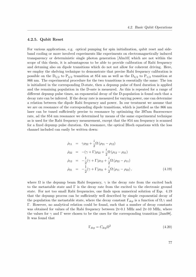
4.2. Basic Qubit Operations
4.2.5. Qubit Reset
For various applications, e.g. optical pumping for spin initialization, qubit reset and side-band cooling or more involved experiments like experiments on electromagnetically inducedtransparency or deterministic single photon generation [Alm10] which are not within thescope of this thesis, it is advantageous to be able to provide calibration of Rabi frequencyand detuning also on dipole transitions which do not not allow for coherent driving. Here,we employ the shelving technique to demonstrate that precise Rabi frequency calibration ispossible on the D5/2 to P3/2 transition at 854 nm as well as the D3/2 to P1/2 transition at866 nm. The experimental procedure for the two transitions is essentially the same: The ionis initialized in the corresponding D-state, then a depump pulse of fixed duration is appliedand the remaining population in the D-sate is measured. As this is repeated for a range ofdifferent depump pulse times, an exponential decay of the D-population is found such that adecay rate can be inferred. If the decay rate is measured for varying power, one can determinea relation between the dipole Rabi frequency and power. In our treatment we assume thatwe are on resonance of the corresponding dipole transitions, which is justified as the 866 nmlaser can be tuned sufficiently precise to resonance by optimizing the 397nm fluorescencerate, ad the 854 nm resonance we determined by means of the same experimental techniqueas is used for the Rabi frequency measurement, except that the 854 nm frequency is scannedfor a fixed depump pulse duration. On resonance, the optical Bloch equations with the losschannel included can easily be written down:
ρ11 = γρ22 +i
2Ω (ρ21 − ρ12)
ρ22 = −(γ + Γ)ρ22 +i
2Ω (ρ12 − ρ21)
ρ12 = −1
2(γ + Γ)ρ12 +
i
2Ω (ρ22 − ρ11)
ρ21 = −1
2(γ + Γ)ρ21 +
i
2Ω (ρ11 − ρ22) , (4.19)
where Ω is the depump beam Rabi frequency, γ is the decay rate from the excited backto the metastable state and Γ is the decay rate from the excited to the electronic groundstate. For not too small Rabi frequencies, one finds upon numerical solution of Eqs. 4.19that the depump process can be sufficiently well described by simple exponential decay ofthe population the metastable state, where the decay constant Γdep is a function of Ω,γ andΓ. However, no analytical relation could be found, such that a number of decay constantswas obtained for values of the Rabi frequency between 2π·0.1 MHz and 2π·10 MHz, wherethe values for γ and Γ were chosen to be the ones for the corresponding transition [Jam98].It was found that
Γdep = CdepΩ2 (4.20)
77

4. Implementation of the Spin Qubit
matches the behavior very well over the entire range of Rabi frequencies, such that theproportionality constants
CD3/2→P1/2
dep = 0.00332MHz−1
CD5/2→P3/2
dep = 0.00315MHz−1 (4.21)
could be determined.For the first transition, the ion is initialized in |↑〉 by optical pumping and shelved to theD5/2, mJ=+5/2 state. Quenching pulses at 854 nm at variable duration are used to removepopulation from the metastable state, finally the remaining population measured. The resultsare shown in Fig. 4.14. For each specific depump power, a depump rate Γdep can be inferred,such that Eq. 4.21 can be invoked to yield the desired relation between power and Rabifrequency:
Ω2 = 1.0(1)MHz2µW−1 (4.22)
frequency at 854nm [MHz]
D5/
2 st
ate
popu
latio
n
D5/
2 st
ate
popu
latio
n
0-50 100500
0.1
0.2
0.3
0.4
depump pulse duration [µs]
quen
ch ra
te [M
Hz]
power [µW]0 20 40 600 0.3 0.6 0.9
0.2
0.4
0.6
0.81.0
0
0.5
1.0
1.5
2.0
a) b) c)
Figure 4.14.: Quenching of the D5/2 state: a) illustrates spectroscopy on the 854 nm transitionby depumping the D5/2 state with a pulse of fixed duration and variable laser frequency. b)shows the dynamics of the depopulation of the D5/2 state on resonance for varying pulseduration and different power levels. c) shows the quench rates versus power inferred fromthese measurements.
The measurement on the D3/2 to P1/2 transition at 866 nm had to be performed in aslightly different way, as no laser at 710 nm for coherent population transfer to the D3/2 statewas at hand. Here, population is simply pumped to the D3/2 state with the 397 nm laser andthe 866 nm switched off. The shelving from |↑〉 is then performed after the 866 nm depumppulse, such that the remaining population in D3/2 and in the |↓〉 level is measured as bright.
78
4.2. Basic Qubit Operations
Thus, only a limited fraction is counted dark after complete depump of the D3/2, howeverthe desired decay constant can still be measured with sufficient precision. The results areshown in Fig. 4.15, and the relation between power and Rabi frequency reads
Ω2 = 5.0(1)MHz2µW−1 (4.23)
The striking dissimilarity between the constants in Eqs. 4.22 and 4.23 is explained by thefact the data for the 854 nm depumping was taken at a much earlier time when the 854 nmand 866 nm beams were freely propagating over a large distance and the focus was muchlarger than necessary. One should expect to see very similar values for the present situationwith the fiber output collimator for the 854 nm and 866 nm beams close the ion trap, seeFig. 3.4.
0 2 4 6 8 100,1
0,2
0,3
0,4
0,5
She
lvin
g pr
obab
ility
Depump time [us]0 1 2 3 4 5 6 7 8 9 10
0,0
0,2
0,4
0,6
0,8
1,0
1,2
1,4
1,6
Dep
ump
rate
[MH
z]
866 power [µW]
a)
b)
Figure 4.15.: Quenching of the D3/2 state: a) shows the population transferred to the D5/2
state after depumping the D3/2 state with the resonant 866 nm laser with variable pulseduration for different depump powers, see text. b) shows the depump rates inferred fromthese curves.
79
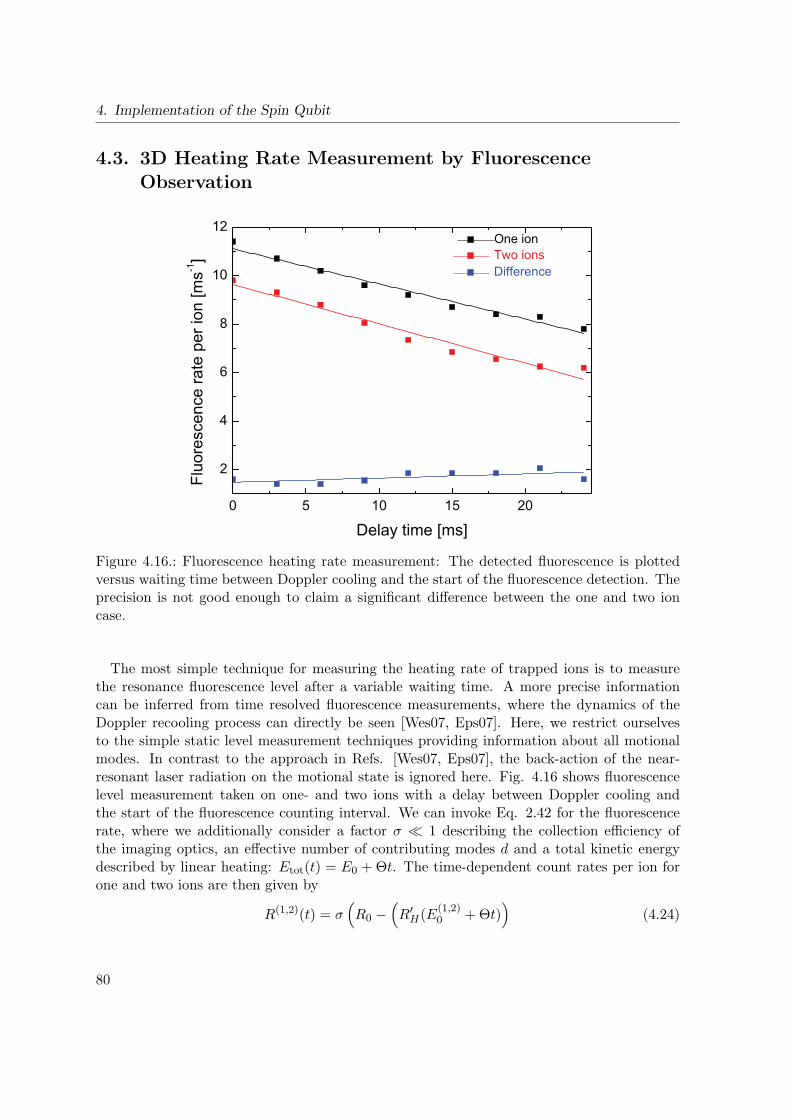
4. Implementation of the Spin Qubit
4.3. 3D Heating Rate Measurement by FluorescenceObservation
0 5 10 15 20
2
4
6
8
10
12
Fluo
resc
ence
rate
per
ion
[ms-1
]
Delay time [ms]
One ionTwo ionsDifference
Figure 4.16.: Fluorescence heating rate measurement: The detected fluorescence is plottedversus waiting time between Doppler cooling and the start of the fluorescence detection. Theprecision is not good enough to claim a significant difference between the one and two ioncase.
The most simple technique for measuring the heating rate of trapped ions is to measurethe resonance fluorescence level after a variable waiting time. A more precise informationcan be inferred from time resolved fluorescence measurements, where the dynamics of theDoppler recooling process can directly be seen [Wes07, Eps07]. Here, we restrict ourselvesto the simple static level measurement techniques providing information about all motionalmodes. In contrast to the approach in Refs. [Wes07, Eps07], the back-action of the near-resonant laser radiation on the motional state is ignored here. Fig. 4.16 shows fluorescencelevel measurement taken on one- and two ions with a delay between Doppler cooling andthe start of the fluorescence counting interval. We can invoke Eq. 2.42 for the fluorescencerate, where we additionally consider a factor σ 1 describing the collection efficiency ofthe imaging optics, an effective number of contributing modes d and a total kinetic energydescribed by linear heating: Etot(t) = E0 +Θt. The time-dependent count rates per ion forone and two ions are then given by
R(1,2)(t) = σ(R0 −
(R′
H(E(1,2)0 +Θt)
)(4.24)
80

4.3. 3D Heating Rate Measurement by Fluorescence Observation
The measurement results are fitted to a linear behavior R(1,2)(t) = a(1,2)−b(1,2)t, yielding theresults a(1)=11.1(1)ms−1, a(2)=9.6(2)ms−1, b(1)=0.145(9)ms−2 and b(2)=0.16(1)ms−2. Dueto the (expected) non-significant difference between b(1) and b(2), we used their mean value b
in the following. If we neglect E(1)0 , which is justified for about 20 initial phonons per mode
after Doppler cooling of a single ion, we can solve for σ,Θ and E(2)0 :
σ =a(1)
R0≈ (4.25)
Θ =bR0
a(1)R′H
E(2)0 =
(a(1) − a(2))R0
a(1)R′H
. (4.26)
All assumed parameters and resulting quantities are compiled in Table 4.1.
Parameter Symbol Value Estimated uncertainty
Saturation parameter S 5.1 ±1.1
Mean oscillation frequency [MHz] ω 2π·2.0 ±0.5
Mean oscillation angle factor cos2 α 0.5 ±0.05
Initial energy for single ion [phonons] E(1)0 0.0 +20.0
Photon collection efficiency [%] σ 0.02 ±0.001
Heating rate [phonons/ms] Θ 2.1·105 ± 3·10−4
Two-ion initial energy [phonons] E(2)0 2100.0 ± 300.0
Table 4.1.: Final results fluorescence heating rate measurement.
The validity of the results is justified as follows: The most critical approximation for deriv-ing Eq. 2.42 is the Taylor expansion made in Eq. 2.40, which clearly holds as a linear decreaseof the fluorescence is observed. As a conclusion, we find a 3D heating rate which is fully con-sistent with the more precise finding to be presented below. However, the astonishingly largenumber of initial quanta in the two-ion case could not be explained yet.
81

4. Implementation of the Spin Qubit
4.4. Qubit Readout via Electron Shelving
Rabi frequency
Ex
cit
ed
sta
te
po
pu
lati
on
Detu
ning
0
0
1
Figure 4.17.: Scheme of the RAP process: The portion of the excited (target) state in theeigenstate Eq. 4.27 is plotted versus laser detuning and coupling strength. Adiabatic switch-ing of the coupling strength together with sweeping of the detuning across resonance guar-antees a smooth transition into the target state.
As mentioned in the introduction of this chapter, an additional complication for the spinqubit is the requirement of an additional step for the discrimination of the qubit levels |↑〉and |↓〉. Upon irradiation at 397 nm or 393 nm, both levels will give rise to fluorescence.Frequency selectivity at these dipole transitions would require Zeeman splittings much largerthan the linewidth of about 24 MHz, which would lead to other experimental complications.Therefore, the only feasible solution is the mapping of the spin qubit to the metastable one.As only information about the occupation probabilities can be obtained anyway when themetastable qubit is read out by means of the fluorescence discrimination method, the mappingprocedure does not have to be coherent, i.e. the phase information can be discarded. A phasecoherent mapping would be realized by performing π-pulses on the quadrupole transition,which brings up the necessity of a careful experimental calibration and stabilization of thecoupling strength and optical frequency for that transition. Even if this is realized, the Rabifrequency is subject to intrinsic statistics of the ions are not ground-state cooled on all modesto which the laser beam driving the quadrupole transition couples, see Sec. 4.2.2. Thus, atechnique for fast, efficient and robust transfer of population is needed. One possibility is toperform optical pumping to the metastable state via the S1/2 →P3/2 transition at 393 nm,where the spin selectivity can be achieved by using another laser beam driving the D3/2 →P3/2
82
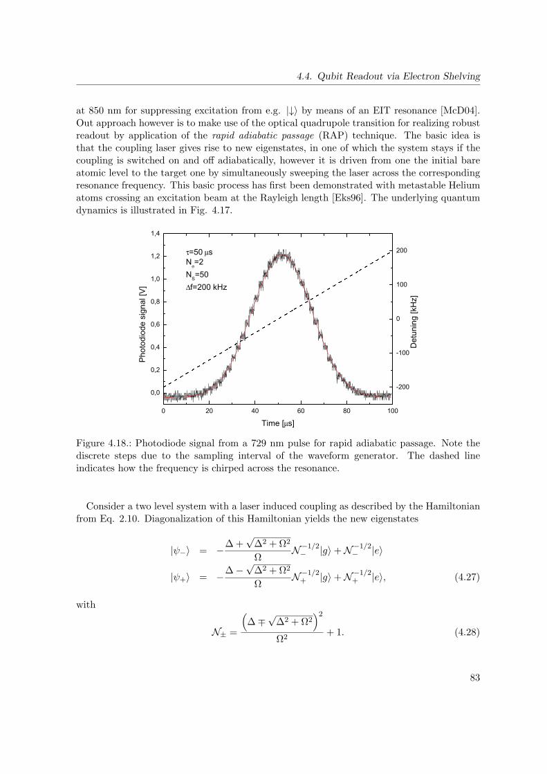
4.4. Qubit Readout via Electron Shelving
at 850 nm for suppressing excitation from e.g. |↓〉 by means of an EIT resonance [McD04].Out approach however is to make use of the optical quadrupole transition for realizing robustreadout by application of the rapid adiabatic passage (RAP) technique. The basic idea isthat the coupling laser gives rise to new eigenstates, in one of which the system stays if thecoupling is switched on and off adiabatically, however it is driven from one the initial bareatomic level to the target one by simultaneously sweeping the laser across the correspondingresonance frequency. This basic process has first been demonstrated with metastable Heliumatoms crossing an excitation beam at the Rayleigh length [Eks96]. The underlying quantumdynamics is illustrated in Fig. 4.17.
0 20 40 60 80 100
0,0
0,2
0,4
0,6
0,8
1,0
1,2
1,4
Det
unin
g [k
Hz]
Pho
todi
ode
sign
al [V
]
Time [µs]
τ=50 µsN
σ=2
NS=50
∆f=200 kHz
-200
-100
0
100
200
Figure 4.18.: Photodiode signal from a 729 nm pulse for rapid adiabatic passage. Note thediscrete steps due to the sampling interval of the waveform generator. The dashed lineindicates how the frequency is chirped across the resonance.
Consider a two level system with a laser induced coupling as described by the Hamiltonianfrom Eq. 2.10. Diagonalization of this Hamiltonian yields the new eigenstates
|ψ−〉 = −∆+√∆2 +Ω2
ΩN−1/2
− |g〉+N−1/2− |e〉
|ψ+〉 = −∆−√∆2 +Ω2
ΩN−1/2
+ |g〉+N−1/2+ |e〉, (4.27)
with
N± =
(∆∓√
∆2 +Ω2)2
Ω2+ 1. (4.28)
83
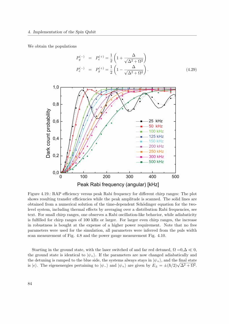
4. Implementation of the Spin Qubit
We obtain the populations
P (−)g = P (+)
e =1
2
(1 +
∆√∆2 +Ω2
)
P (−)e = P (+)
g =1
2
(1− ∆√
∆2 +Ω2
). (4.29)
0 100 200 300 400 5000,0
0,2
0,4
0,6
0,8
1,0
Dar
k co
unt p
roba
bilit
y
Peak Rabi frequency (angular) [kHz]
250 kHz300 kHz
150 kHz200 kHz
100 kHz125 kHz
25 kHz50 kHz
500 kHz
Figure 4.19.: RAP efficiency versus peak Rabi frequency for different chirp ranges: The plotshows resulting transfer efficiencies while the peak amplitude is scanned. The solid lines areobtained from a numerical solution of the time-dependent Schodinger equation for the two-level system, including thermal effects by averaging over a distribution Rabi frequencies, seetext. For small chirp ranges, one observes a Rabi oscillation-like behavior, while adiabaticityis fulfilled for chirp ranges of 100 kHz or larger. For larger even chirp ranges, the increasein robustness is bought at the expense of a higher power requirement. Note that no freeparameters were used for the simulation, all parameters were inferred from the puls widthscan measurement of Fig. 4.8 and the power gauge measurement Fig. 4.10.
Starting in the ground state, with the laser switched of and far red detuned, Ω =0,∆ 0,the ground state is identical to |ψ+〉. If the parameters are now changed adiabatically andthe detuning is ramped to the blue side, the systems always stays in |ψ+〉, and the final stateis |e〉. The eigenenergies pertaining to |ψ−〉 and |ψ+〉 are given by E± = ±(/2)
√∆2 +Ω2.
84
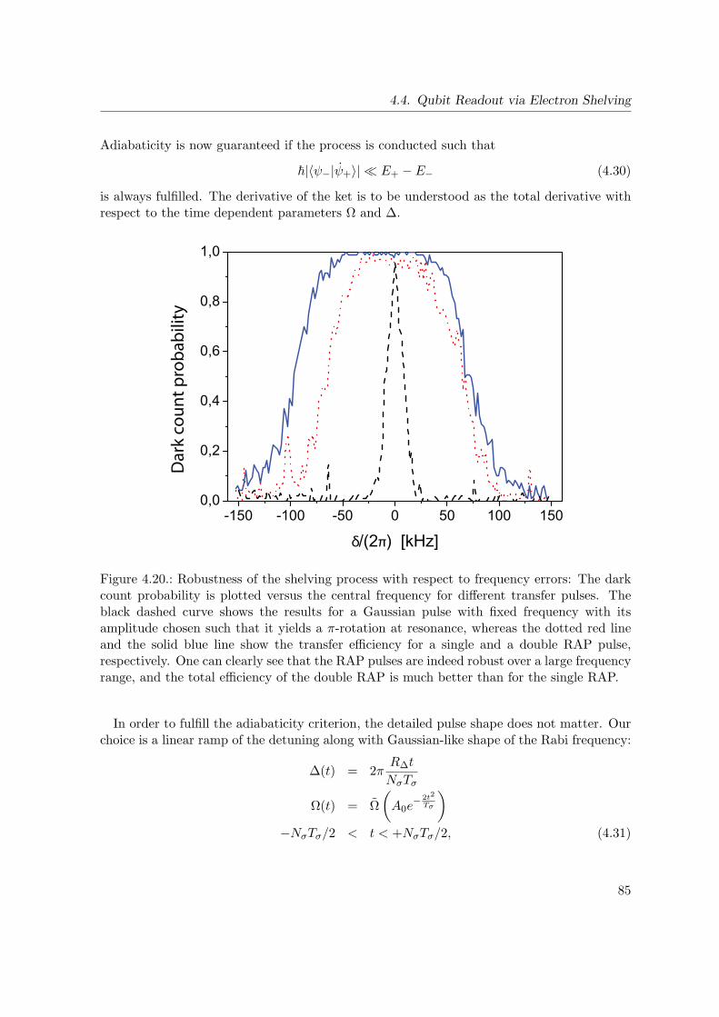
4.4. Qubit Readout via Electron Shelving
Adiabaticity is now guaranteed if the process is conducted such that
|〈ψ−|ψ+〉| E+ − E− (4.30)
is always fulfilled. The derivative of the ket is to be understood as the total derivative withrespect to the time dependent parameters Ω and ∆.
-150 -100 -50 0 50 100 1500,0
0,2
0,4
0,6
0,8
1,0
δ/(2π) [kHz]
Dar
k co
un
t p
rob
abili
ty
Figure 4.20.: Robustness of the shelving process with respect to frequency errors: The darkcount probability is plotted versus the central frequency for different transfer pulses. Theblack dashed curve shows the results for a Gaussian pulse with fixed frequency with itsamplitude chosen such that it yields a π-rotation at resonance, whereas the dotted red lineand the solid blue line show the transfer efficiency for a single and a double RAP pulse,respectively. One can clearly see that the RAP pulses are indeed robust over a large frequencyrange, and the total efficiency of the double RAP is much better than for the single RAP.
In order to fulfill the adiabaticity criterion, the detailed pulse shape does not matter. Ourchoice is a linear ramp of the detuning along with Gaussian-like shape of the Rabi frequency:
∆(t) = 2πR∆t
NσTσ
Ω(t) = Ω
(A0e
− 2t2
Tσ
)−NσTσ/2 < t < +NσTσ/2, (4.31)
85
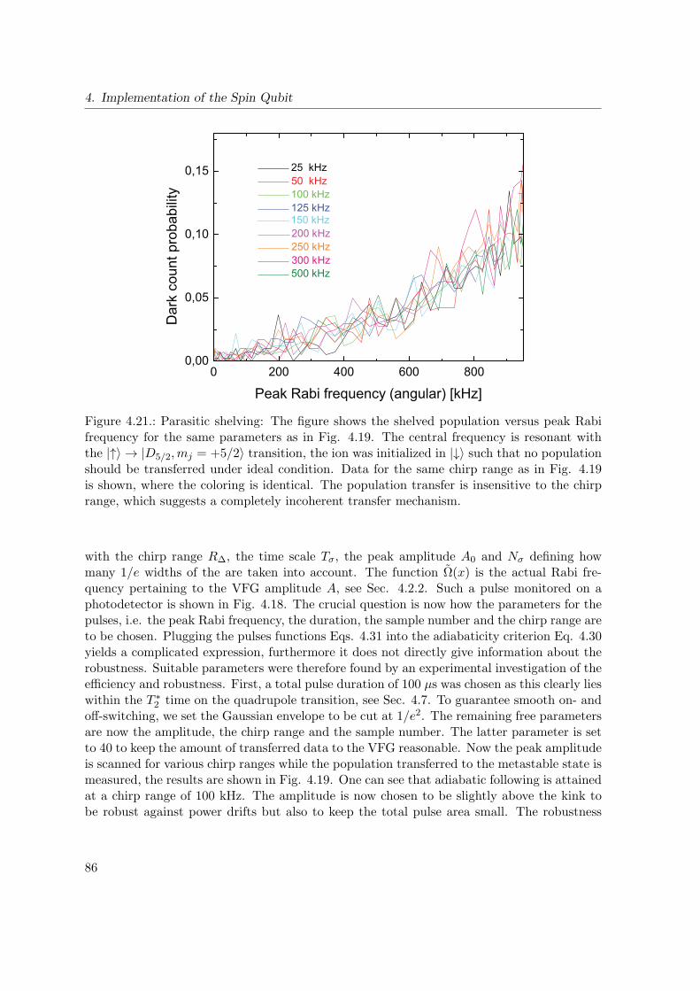
4. Implementation of the Spin Qubit
0 200 400 600 8000,00
0,05
0,10
0,15D
ark
coun
t pro
babi
lity
Peak Rabi frequency (angular) [kHz]
250 kHz300 kHz
150 kHz200 kHz
100 kHz125 kHz
25 kHz50 kHz
500 kHz
Figure 4.21.: Parasitic shelving: The figure shows the shelved population versus peak Rabifrequency for the same parameters as in Fig. 4.19. The central frequency is resonant withthe |↑〉 → |D5/2,mj = +5/2〉 transition, the ion was initialized in |↓〉 such that no populationshould be transferred under ideal condition. Data for the same chirp range as in Fig. 4.19is shown, where the coloring is identical. The population transfer is insensitive to the chirprange, which suggests a completely incoherent transfer mechanism.
with the chirp range R∆, the time scale Tσ, the peak amplitude A0 and Nσ defining howmany 1/e widths of the are taken into account. The function Ω(x) is the actual Rabi fre-quency pertaining to the VFG amplitude A, see Sec. 4.2.2. Such a pulse monitored on aphotodetector is shown in Fig. 4.18. The crucial question is now how the parameters for thepulses, i.e. the peak Rabi frequency, the duration, the sample number and the chirp range areto be chosen. Plugging the pulses functions Eqs. 4.31 into the adiabaticity criterion Eq. 4.30yields a complicated expression, furthermore it does not directly give information about therobustness. Suitable parameters were therefore found by an experimental investigation of theefficiency and robustness. First, a total pulse duration of 100 µs was chosen as this clearly lieswithin the T ∗
2 time on the quadrupole transition, see Sec. 4.7. To guarantee smooth on- andoff-switching, we set the Gaussian envelope to be cut at 1/e2. The remaining free parametersare now the amplitude, the chirp range and the sample number. The latter parameter is setto 40 to keep the amount of transferred data to the VFG reasonable. Now the peak amplitudeis scanned for various chirp ranges while the population transferred to the metastable state ismeasured, the results are shown in Fig. 4.19. One can see that adiabatic following is attainedat a chirp range of 100 kHz. The amplitude is now chosen to be slightly above the kink tobe robust against power drifts but also to keep the total pulse area small. The robustness
86
4.4. Qubit Readout via Electron Shelving
is now assessed by performing the transfer efficiency measurement at these parameters, butwith varying center frequency. The results are shown in Fig. 4.20, where one can see thata broad plateau of a width roughly corresponding to the chirp range is given, indicatingstability of the shelving rate despite the drift of the 729 nm laser frequency. The stabilityis even enhanced if the shelving on an additional backup transition is performed, which isthe |↑〉 → |D5/2,mJ = +3/2〉 transition in this case. By contrast, population transfer witha transform limited Gaussian pulse leads to a strong dependence on the center frequency,such that no robustness is given and the transition frequencies would have to be recalibratedfrequently.A second important criterion for the fidelity of the shelving process is the amount of pop-ulation transferred on the wrong transition, i.e. the excitation from |↓〉 to the D5/2 state.Fig. 4.21 shows the population transferred from |↓〉 versus RAP amplitude under the sameconditions as in Fig. 4.19. Four possible mechanisms could be responsible for this unwantedbehavior: i) direct off-resonant excitation, ii) off-resonant excitation from the discrete ampli-tude and frequency steps in the pulse and iii) resonant background light from the laser andiv) (near-)resonant excitation on higher order motional sidebands. Simulation results indi-cate that the first two mechanisms lead to negligibly small population transfer for reasonableRAP parameters. The fact that the population transfer is does not depend on the chirprange excludes a resonant excitation mechanism such as iv). Therefore we conclude thatthe unwanted excitation is caused by incoherent background light. For optimum shelvingfidelity, it is therefore necessary to chose the lowest RAP amplitude at which the shelvingprobability from |↑〉 saturates, and one has to trade the robustness increase from larger chirpranges against infidelity as larger saturation amplitudes are required for larger chirp ranges.A possible technological solution to this is to employ a filtering cavity with a linewidth inthe MHz range for the amplified 729 nm beam.
87
4. Implementation of the Spin Qubit
4.5. Stimulated Raman Transitions
The possibilities to perform coherent manipulations by means of the 729 nm laser drivingthe quadrupole transition are quite limited. This is on the one hand due to the linewidthof the 729 nm, where a stabilization to the 1 Hz range is technologically possible but rathertedious. Furthermore, as will be worked out in Sec. 4.3, the radial motion of ions in ourmicrotrap represents an even more limiting constraint. As a second possibility for laser-driven coherent manipulations, we utilize stimulated Raman transitions driven by a pairof laser beams detuned by some tens of GHz from the S1/2 to P1/2 state, which can beseen as a resonantly enhanced two-photon transition. Stimulated Raman transitions canbe used for separate or joint manipulation of the internal and external degrees of freedomof trapped ions, such that they provide a versatile tool for quantum optics and quantuminformation experiments. The characterization of the various types of interactions alongwith the associated decoherence effects is the main focus of this thesis.
4.5.1. Raman Spectroscopy and Single Qubit Rotations
In order to perform single qubit rotations, one needs to provide a controllable coherentcoupling between the qubit levels |↑〉 and |↓〉. This can be realized by simultaneous irradiationof two laser beams split by a frequency difference which is given by the Zeeman splitting ofthe qubit levels. It is intuitively clear that one of the beams has to include a π polarizationcomponent and the other one has to include a circular polarization component, such thatone of the Zeeman levels of the excited P1/2 state can serve as the intermediate level for theresonant population transfer. If we assume the blue beam to be completely π polarized andthe red beam to consist only of circular components, we can invoke Eq. A.12 to obtain theRaman Rabi frequency upon neglecting off-resonant terms and usage of Eq. A.10:
Ω =1
2∆
1
3√2εb0ε
∗r−e
i(∆k−δ′t), (4.32)
where δ′ = δ − ωL is the detuning of the frequency difference from the ground state Larmorfrequency. Irradiating both beams simultaneously for a constant duration at fixed intensitiestherefore realizes the unitary transform Eq. 2.12. Two main advantages arise from theusage of stimulated Raman transitions: First, the optical frequency and phase of the drivinglaser does not occur in the expression for the Rabi frequency, only the relative frequencyand phase play a role. The frequency difference can be controlled to arbitrary accuracy byusage of phase-locked rf sources driving the switching acousto-optical frequency shifters, andthe relative phase is limited by the mechanical interferometer stability of the optical setup.Second, the coupling to the ionic motion can be controlled via the difference wavevector ∆k.
As already mentioned in the description of the experimental setup in Sec. 3.2.5, we utilizetwo different beam geometries for driving Raman transitions: a collinear geometry withoutany coupling to the ionic motion (beam pair R1/CC) and an orthogonal geometry with acoupling only to the axial motion (beam pair R1/R2) described by a Lamb-Dicke factor inthe range between 0.25 and 0.3, depending on the axial trap frequency. Fig. 4.22 shows a
88
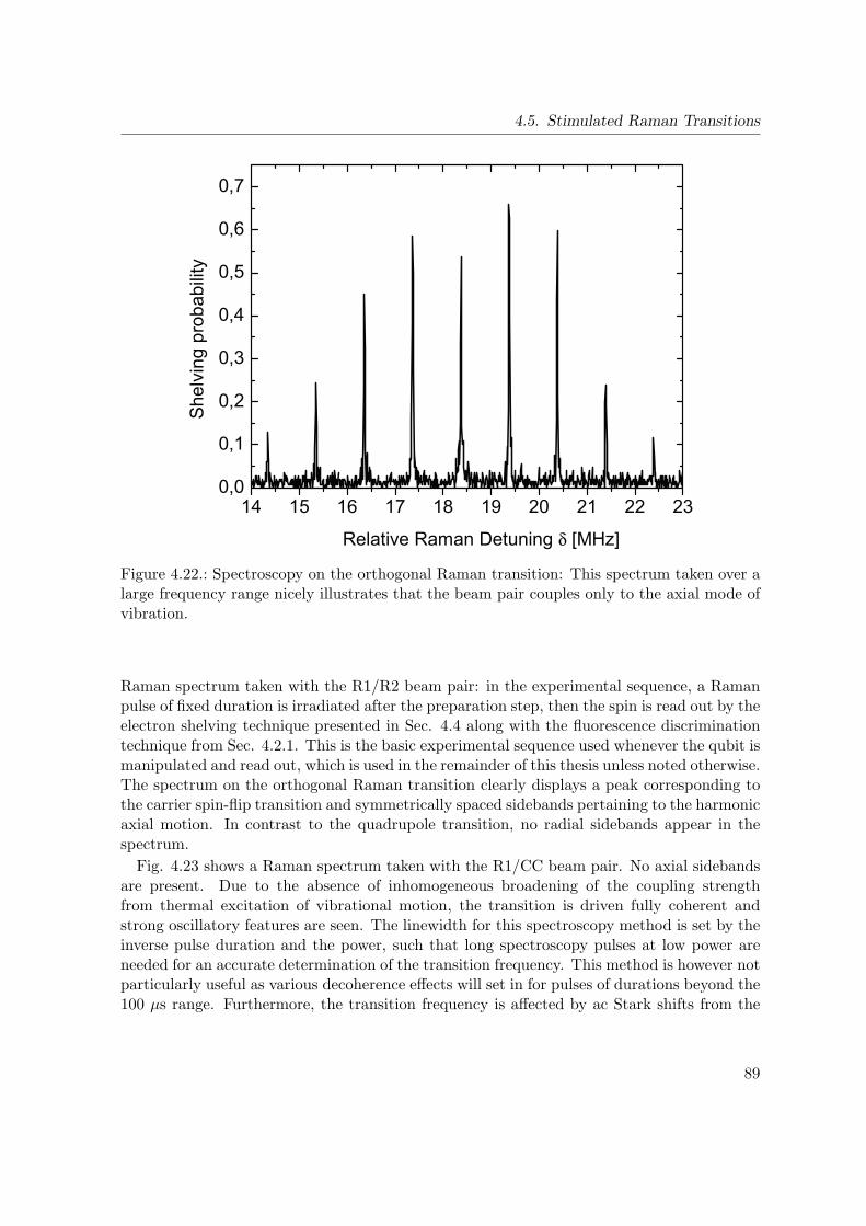
4.5. Stimulated Raman Transitions
14 15 16 17 18 19 20 21 22 230,0
0,1
0,2
0,3
0,4
0,5
0,6
0,7S
helv
ing
prob
abilit
y
Relative Raman Detuning δ [MHz]
Figure 4.22.: Spectroscopy on the orthogonal Raman transition: This spectrum taken over alarge frequency range nicely illustrates that the beam pair couples only to the axial mode ofvibration.
Raman spectrum taken with the R1/R2 beam pair: in the experimental sequence, a Ramanpulse of fixed duration is irradiated after the preparation step, then the spin is read out by theelectron shelving technique presented in Sec. 4.4 along with the fluorescence discriminationtechnique from Sec. 4.2.1. This is the basic experimental sequence used whenever the qubit ismanipulated and read out, which is used in the remainder of this thesis unless noted otherwise.The spectrum on the orthogonal Raman transition clearly displays a peak corresponding tothe carrier spin-flip transition and symmetrically spaced sidebands pertaining to the harmonicaxial motion. In contrast to the quadrupole transition, no radial sidebands appear in thespectrum.
Fig. 4.23 shows a Raman spectrum taken with the R1/CC beam pair. No axial sidebandsare present. Due to the absence of inhomogeneous broadening of the coupling strengthfrom thermal excitation of vibrational motion, the transition is driven fully coherent andstrong oscillatory features are seen. The linewidth for this spectroscopy method is set by theinverse pulse duration and the power, such that long spectroscopy pulses at low power areneeded for an accurate determination of the transition frequency. This method is however notparticularly useful as various decoherence effects will set in for pulses of durations beyond the100 µs range. Furthermore, the transition frequency is affected by ac Stark shifts from the
89
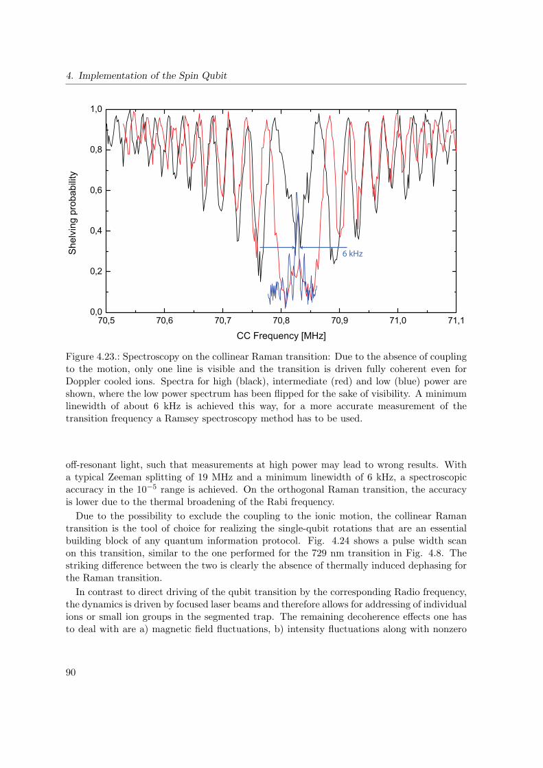
4. Implementation of the Spin Qubit
70,5 70,6 70,7 70,8 70,9 71,0 71,10,0
0,2
0,4
0,6
0,8
1,0
She
lvin
g pr
obab
ility
CC Frequency [MHz]
6 kHz
Figure 4.23.: Spectroscopy on the collinear Raman transition: Due to the absence of couplingto the motion, only one line is visible and the transition is driven fully coherent even forDoppler cooled ions. Spectra for high (black), intermediate (red) and low (blue) power areshown, where the low power spectrum has been flipped for the sake of visibility. A minimumlinewidth of about 6 kHz is achieved this way, for a more accurate measurement of thetransition frequency a Ramsey spectroscopy method has to be used.
off-resonant light, such that measurements at high power may lead to wrong results. Witha typical Zeeman splitting of 19 MHz and a minimum linewidth of 6 kHz, a spectroscopicaccuracy in the 10−5 range is achieved. On the orthogonal Raman transition, the accuracyis lower due to the thermal broadening of the Rabi frequency.
Due to the possibility to exclude the coupling to the ionic motion, the collinear Ramantransition is the tool of choice for realizing the single-qubit rotations that are an essentialbuilding block of any quantum information protocol. Fig. 4.24 shows a pulse width scanon this transition, similar to the one performed for the 729 nm transition in Fig. 4.8. Thestriking difference between the two is clearly the absence of thermally induced dephasing forthe Raman transition.
In contrast to direct driving of the qubit transition by the corresponding Radio frequency,the dynamics is driven by focused laser beams and therefore allows for addressing of individualions or small ion groups in the segmented trap. The remaining decoherence effects one hasto deal with are a) magnetic field fluctuations, b) intensity fluctuations along with nonzero
90

4.5. Stimulated Raman Transitions
AC Stark shifts, c) off-resonant scattering and d) intensity fluctuations leading to pulse areafluctuations. The first three decoherence mechanisms are discussed extensively in Sec. 4.7.The mechanisms b) and d) stem from the same technical origin, but the mechanisms aresill fundamentally different, especially in that effect b) can be avoided in most cases. Theoff-resonant scattering can be suppressed by detuning the lasers further from resonance, onetherefore faces a tradeoff between Rabi frequency and coherence time. Considering the resultsfrom Sec. 2.1.6, one recognizes that the Rabi frequency divided by the geometric mean isproportional to the detuning:
ΩRabi√RbRr
=3√2∆
Γ. (4.33)
where Rb and Rr denote the scattering rates from the blue and red Raman beams respectively.This is confirmed for the collinear transition as can be seen in Fig. 4.25. The figure of meriton the left-hand side of Eq. 4.33 which is plotted on the ordinate of Fig. 4.25 is essentiallythe number of π-rotations that could be driven within the timescale at which decoherence byscattering occurs, if other decoherence sources are neglected. Similar data was taken on theorthogonal Raman transition, where it can be seen that the data is not described by Eq. 4.33.The Rabi frequency was measured for Doppler cooled ion, such that it is decreased by thermaleffects. This decrease however is much smaller than the measured one, which can only beexplained by a strong effective frequency modulation due to a residual RF component alongthe trap axis. This strong component has indeed been confirmed by a long range spectroscopymeasurement in a much older version of the setup where 270 MHz long-range AOMs havebeen used. RF-echoes at the one- and twofold trap drive frequency have been found in thespectrum which were not significantly weaker than than the carrier peak. This indicates alarge modulation index, consistent with the data in Fig. 4.25. The RF field expected to occurat the ions position due to the taper electrodes is by far too small to account for that effect,see Sec. 5.7. It is therefore concluded that unbalanced RF-pickup on the DC-electrodes isresponsible for the strong modulation. However, it will be shown that the basic suitability ofthe trap for quantum logic is still given, see especially the measurement results in chapter 8.
91
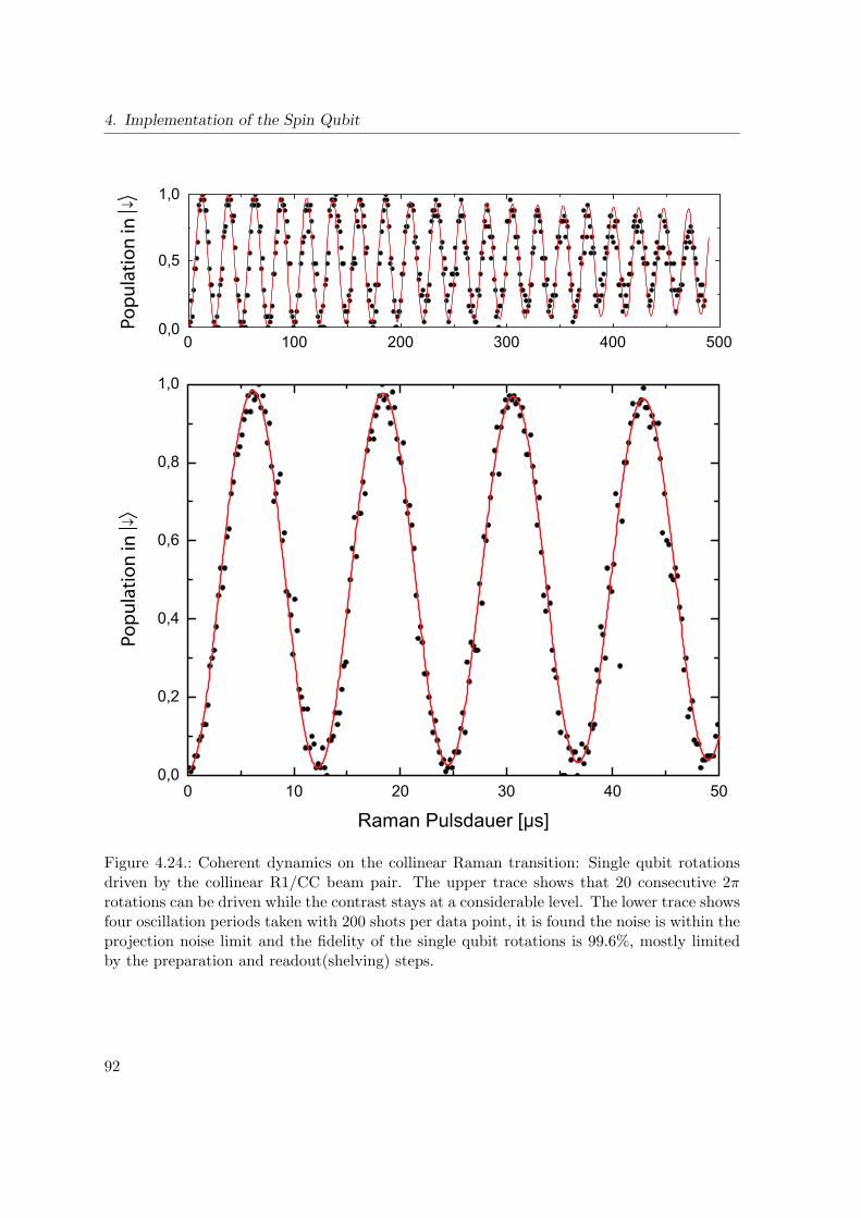
4. Implementation of the Spin Qubit
0 100 200 300 400 5000,0
0,5
1,0
0 10 20 30 40 500,0
0,2
0,4
0,6
0,8
1,0
Pop
ula
tio
n in
↓Po
pu
lati
on
in ↓
Figure 4.24.: Coherent dynamics on the collinear Raman transition: Single qubit rotationsdriven by the collinear R1/CC beam pair. The upper trace shows that 20 consecutive 2πrotations can be driven while the contrast stays at a considerable level. The lower trace showsfour oscillation periods taken with 200 shots per data point, it is found the noise is within theprojection noise limit and the fidelity of the single qubit rotations is 99.6%, mostly limitedby the preparation and readout(shelving) steps.
92
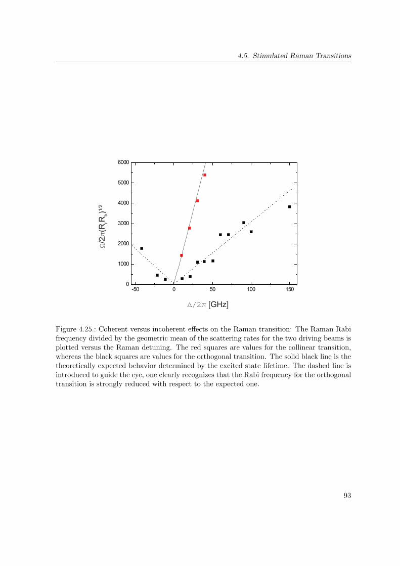
4.5. Stimulated Raman Transitions
-50 0 50 100 1500
1000
2000
3000
4000
5000
6000
[GHz]
/2(R
rRb)1
/2
Figure 4.25.: Coherent versus incoherent effects on the Raman transition: The Raman Rabifrequency divided by the geometric mean of the scattering rates for the two driving beams isplotted versus the Raman detuning. The red squares are values for the collinear transition,whereas the black squares are values for the orthogonal transition. The solid black line is thetheoretically expected behavior determined by the excited state lifetime. The dashed line isintroduced to guide the eye, one clearly recognizes that the Rabi frequency for the orthogonaltransition is strongly reduced with respect to the expected one.
93
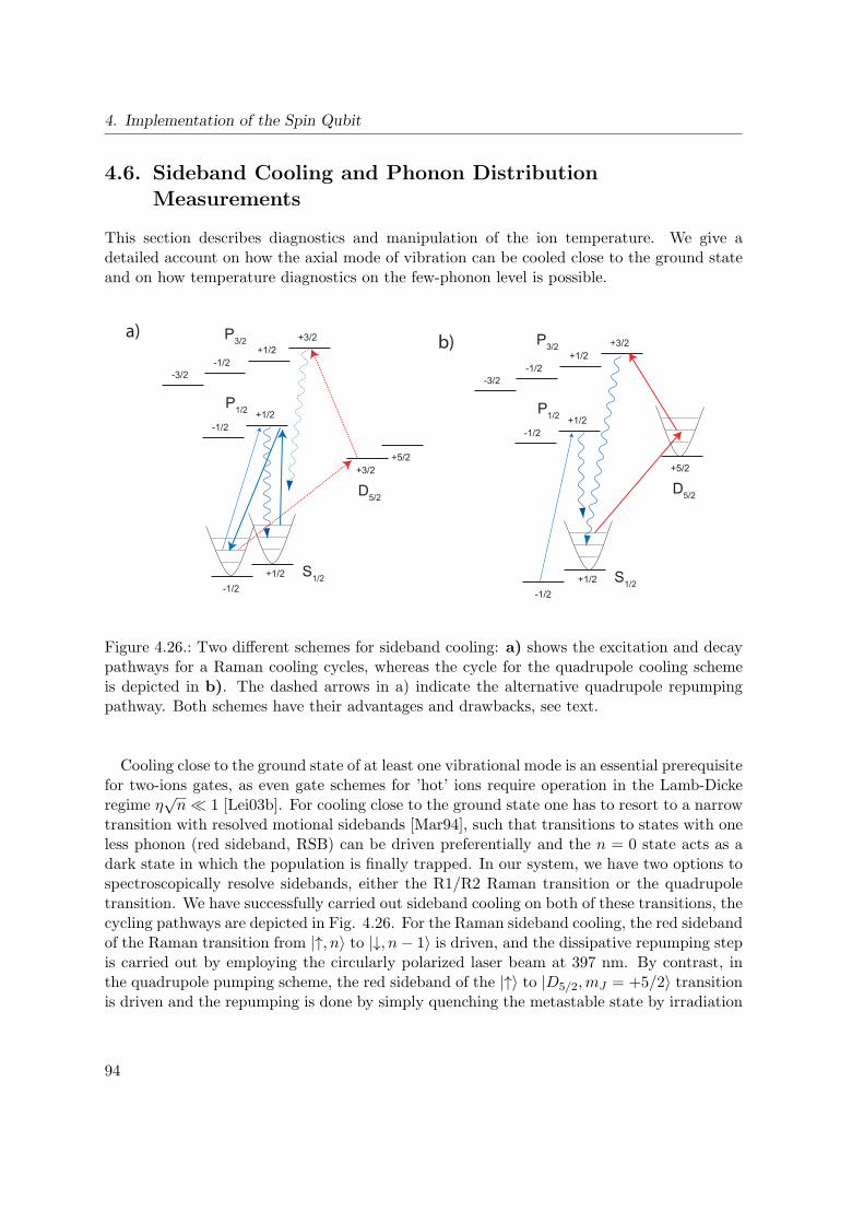
4. Implementation of the Spin Qubit
4.6. Sideband Cooling and Phonon DistributionMeasurements
This section describes diagnostics and manipulation of the ion temperature. We give adetailed account on how the axial mode of vibration can be cooled close to the ground stateand on how temperature diagnostics on the few-phonon level is possible.
b)a)
D5/2
+5/2
S1/2-1/2
+1/2
P3/2 +3/2+1/2
-1/2-3/2
+1/2-1/2
P1/2
S1/2-1/2
+1/2
P3/2 +3/2+1/2
-1/2-3/2
+1/2-1/2
P1/2
D5/2
+3/2+5/2
Figure 4.26.: Two different schemes for sideband cooling: a) shows the excitation and decaypathways for a Raman cooling cycles, whereas the cycle for the quadrupole cooling schemeis depicted in b). The dashed arrows in a) indicate the alternative quadrupole repumpingpathway. Both schemes have their advantages and drawbacks, see text.
Cooling close to the ground state of at least one vibrational mode is an essential prerequisitefor two-ions gates, as even gate schemes for ’hot’ ions require operation in the Lamb-Dickeregime η
√n 1 [Lei03b]. For cooling close to the ground state one has to resort to a narrow
transition with resolved motional sidebands [Mar94], such that transitions to states with oneless phonon (red sideband, RSB) can be driven preferentially and the n = 0 state acts as adark state in which the population is finally trapped. In our system, we have two options tospectroscopically resolve sidebands, either the R1/R2 Raman transition or the quadrupoletransition. We have successfully carried out sideband cooling on both of these transitions, thecycling pathways are depicted in Fig. 4.26. For the Raman sideband cooling, the red sidebandof the Raman transition from |↑, n〉 to |↓, n− 1〉 is driven, and the dissipative repumping stepis carried out by employing the circularly polarized laser beam at 397 nm. By contrast, inthe quadrupole pumping scheme, the red sideband of the |↑〉 to |D5/2,mJ = +5/2〉 transitionis driven and the repumping is done by simply quenching the metastable state by irradiation
94
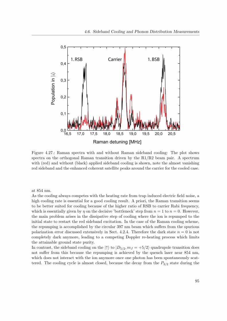
4.6. Sideband Cooling and Phonon Distribution Measurements
16,5 17,0 17,5 18,0 18,5 19,0 19,5 20,0 20,50,0
0,1
0,2
0,3
0,4
0,5
Raman detuning [MHz]
Pop
ulat
ion
in
Carrier1. RSB 1. BSB
Figure 4.27.: Raman spectra with and without Raman sideband cooling: The plot showsspectra on the orthogonal Raman transition driven by the R1/R2 beam pair. A spectrumwith (red) and without (black) applied sideband cooling is shown, note the almost vanishingred sideband and the enhanced coherent satellite peaks around the carrier for the cooled case.
at 854 nm.As the cooling always competes with the heating rate from trap induced electric field noise, ahigh cooling rate is essential for a good cooling result. A priori, the Raman transition seemsto be better suited for cooling because of the higher ratio of RSB to carrier Rabi frequency,which is essentially given by η on the decisive ’bottleneck’ step from n = 1 to n = 0. However,the main problem arises in the dissipative step of cooling where the ion is repumped to theinitial state to restart the red sideband excitation. In the case of the Raman cooling scheme,the repumping is accomplished by the circular 397 nm beam which suffers from the spuriouspolarization error discussed extensively in Sect. 4.2.4. Therefore the dark state n = 0 is notcompletely dark anymore, leading to a competing Doppler re-heating process which limitsthe attainable ground state purity.In contrast, the sideband cooling on the |↑〉 to |D5/2,mJ = +5/2〉 quadrupole transition doesnot suffer from this because the repumping is achieved by the quench laser near 854 nm,which does not interact with the ion anymore once one photon has been spontaneously scat-tered. The cooling cycle is almost closed, because the decay from the P3/2 state during the
95
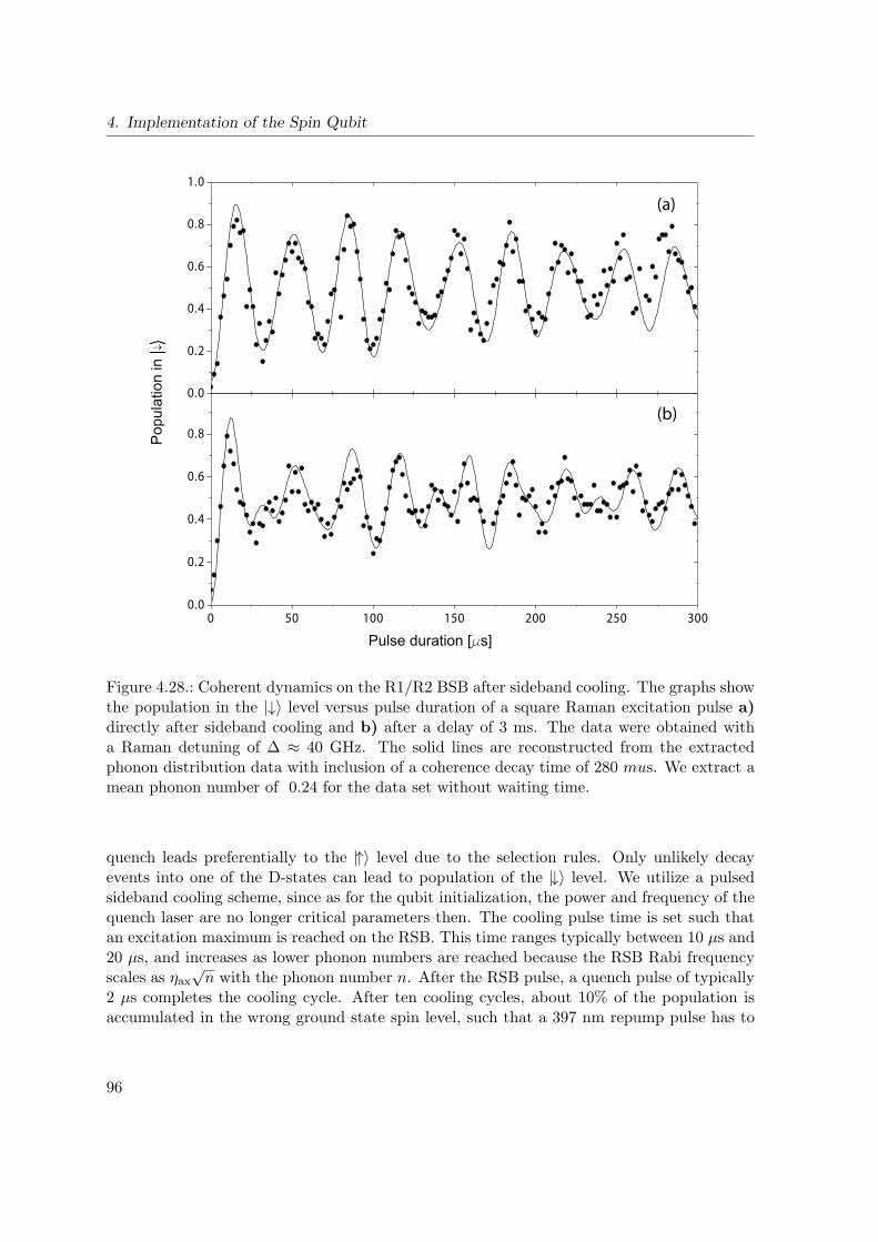
4. Implementation of the Spin Qubit
0 50 100 150 200 250 300
0.0
0.2
0.4
0.6
0.8
0.0
0.2
0.4
0.6
0.8
1.0
Pop
ulat
ion
in
(a)
(b)
Pulse duration [ s]
Figure 4.28.: Coherent dynamics on the R1/R2 BSB after sideband cooling. The graphs showthe population in the |↓〉 level versus pulse duration of a square Raman excitation pulse a)directly after sideband cooling and b) after a delay of 3 ms. The data were obtained witha Raman detuning of ∆ ≈ 40 GHz. The solid lines are reconstructed from the extractedphonon distribution data with inclusion of a coherence decay time of 280 mus. We extract amean phonon number of 0.24 for the data set without waiting time.
quench leads preferentially to the |↑〉 level due to the selection rules. Only unlikely decayevents into one of the D-states can lead to population of the |↓〉 level. We utilize a pulsedsideband cooling scheme, since as for the qubit initialization, the power and frequency of thequench laser are no longer critical parameters then. The cooling pulse time is set such thatan excitation maximum is reached on the RSB. This time ranges typically between 10 µs and20 µs, and increases as lower phonon numbers are reached because the RSB Rabi frequencyscales as ηax
√n with the phonon number n. After the RSB pulse, a quench pulse of typically
2 µs completes the cooling cycle. After ten cooling cycles, about 10% of the population isaccumulated in the wrong ground state spin level, such that a 397 nm repump pulse has to
96
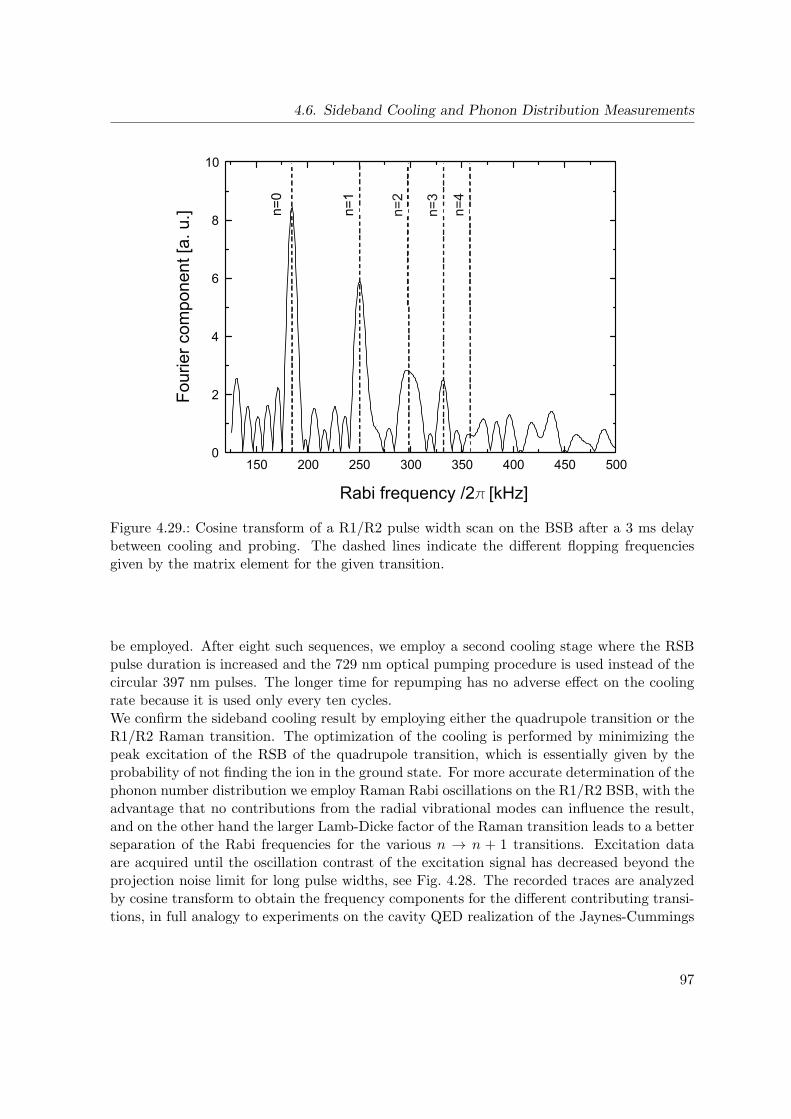
4.6. Sideband Cooling and Phonon Distribution Measurements
150 200 250 300 350 400 450 5000
2
4
6
8
10
n=4
n=3
n=2
n=1
n=0
Rabi frequency /2 [kHz]
Four
ier c
ompo
nent
[a. u
.]
Figure 4.29.: Cosine transform of a R1/R2 pulse width scan on the BSB after a 3 ms delaybetween cooling and probing. The dashed lines indicate the different flopping frequenciesgiven by the matrix element for the given transition.
be employed. After eight such sequences, we employ a second cooling stage where the RSBpulse duration is increased and the 729 nm optical pumping procedure is used instead of thecircular 397 nm pulses. The longer time for repumping has no adverse effect on the coolingrate because it is used only every ten cycles.We confirm the sideband cooling result by employing either the quadrupole transition or theR1/R2 Raman transition. The optimization of the cooling is performed by minimizing thepeak excitation of the RSB of the quadrupole transition, which is essentially given by theprobability of not finding the ion in the ground state. For more accurate determination of thephonon number distribution we employ Raman Rabi oscillations on the R1/R2 BSB, with theadvantage that no contributions from the radial vibrational modes can influence the result,and on the other hand the larger Lamb-Dicke factor of the Raman transition leads to a betterseparation of the Rabi frequencies for the various n → n + 1 transitions. Excitation dataare acquired until the oscillation contrast of the excitation signal has decreased beyond theprojection noise limit for long pulse widths, see Fig. 4.28. The recorded traces are analyzedby cosine transform to obtain the frequency components for the different contributing transi-tions, in full analogy to experiments on the cavity QED realization of the Jaynes-Cummings
97
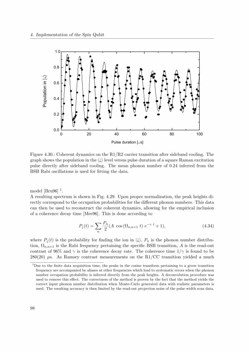
4. Implementation of the Spin Qubit
0 20 40 60 80 1000.0
0.2
0.4
0.6
0.8
1.0
Pop
ulat
ion
in
Pulse duration [ s]
Figure 4.30.: Coherent dynamics on the R1/R2 carrier transition after sideband cooling. Thegraph shows the population in the |↓〉 level versus pulse duration of a square Raman excitationpulse directly after sideband cooling. The mean phonon number of 0.24 inferred from theBSB Rabi oscillations is used for fitting the data.
model [Bru96] 1.A resulting spectrum is shown in Fig. 4.29. Upon proper normalization, the peak heights di-rectly correspond to the occupation probabilities for the different phonon numbers. This datacan then be used to reconstruct the coherent dynamics, allowing for the empirical inclusionof a coherence decay time [Mee96]. This is done according to
P↓(t) =∑n
Pn
2(A cos (Ωn,n+1 t) e−γ t + 1), (4.34)
where P↓(t) is the probability for finding the ion in |↓〉, Pn is the phonon number distribu-tion, Ωn,n+1 is the Rabi frequency pertaining the specific BSB transition, A is the read-outcontrast of 96% and γ is the coherence decay rate. The coherence time 1/γ is found to be280(20) µs. As Ramsey contrast measurements on the R1/CC transition yielded a much
1Due to the finite data acquisition time, the peaks in the cosine transform pertaining to a given transitionfrequency are accompanied by aliases at other frequencies which lead to systematic errors when the phononnumber occupation probability is inferred directly from the peak heights. A deconvolution procedure wasused to remove this effect. The correctness of the method is proven by the fact that the method yields thecorrect input phonon number distribution when Monte-Carlo generated data with realistic parameters isused. The resulting accuracy is then limited by the read-out projection noise of the pulse width scan data.
98

4.6. Sideband Cooling and Phonon Distribution Measurements
0 1 2 3 4 50,0
0,2
0,4
0,6
0,8
1,0
1,2
1,4
1,6
1,8
2,0
2,2
0 1 2 3 4 50,0
0,1
0,2
0,3
0,4
0,5
0,6
0,7
0,8
0,9
1,0
n=0 n=1 n=2
(a) (b)
Occ
up
atio
n p
rob
abili
ty
Mea
n p
ho
no
n n
um
ber
Waiting time [ms] Waiting time [ms]
Figure 4.31.: Results of the heating rate measurement: a) Occupation probabilities Pn forthe lowest vibrational levels n ≤ 2, extracted from frequency spectra of the BSB pulse widthscans (see Fig. 4.29) after different waiting times. For comparison, the solid lines show theoccupation probabilities given by a thermal distribution p(n) = nn/(n + 1)n+1, where n(t)is given by a linear fit through the mean phonon numbers calculated from the data. b)Mean occupation number n calculated from Pn at different times after cooling. The linearfit indicates a constant heating rate of n = (0.3± 0.1)/ms.
longer coherence time, the additional decoherence either stems from pulse area fluctuationsor a reduced interferometric stability in the R1/R2 beam setup with respect to the R1/CCgeometry. The phonon distribution is reconstructed for various waiting times after sidebandcooling in order to reveal the trap induced heating dynamics. The time dependent phononnumber distribution is shown in Fig. 4.31, along with the resulting mean phonon number.This directly gives the heating rate to be 0.3(1) phonons/ms2.The corresponding Rabi oscillations on the carrier of the R1/R2 Raman transition are shownin Fig. 4.30. Taking the phonon numbers after sideband cooling inferred from the BSBRabi oscillations, we find excellent agreement with the measurements made on the carriertransition.
The cooling results presented in this chapter were obtained with the quadrupole coolingscheme, however at a later evolution state of the setup we have also successfully implementedRaman cooling with comparable and even better final temperatures. The results presentedin chapter 8 were obtained based on Raman sideband cooling. The final temperature couldbe reduced such that the ground state purity does not deviate from 100% within the mea-surement accuracy, any effect of remaining population in e.g. n=1 would be overshadowedby decoherence effects in the interaction with the lasers driving the blue sideband Rabi os-cillations when the motional state is read out. The improvement was mainly achieved by
2This is about one order of magnitude better than earlier findings of 2.13 phonons/ms [Sch08], which isattributed to an improved trap voltage supply.
99
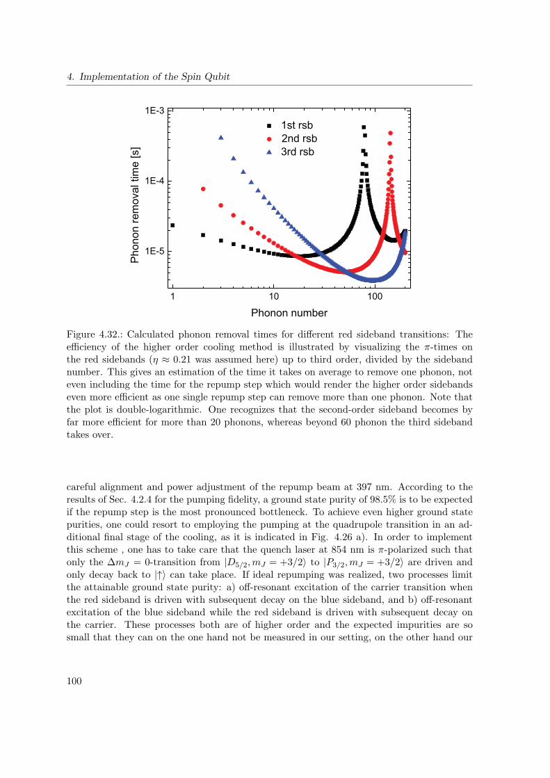
4. Implementation of the Spin Qubit
1 10 100
1E-5
1E-4
1E-31st rsb 2nd rsb3rd rsb
Pho
non
rem
oval
tim
e [s
]
Phonon number
Figure 4.32.: Calculated phonon removal times for different red sideband transitions: Theefficiency of the higher order cooling method is illustrated by visualizing the π-times onthe red sidebands (η ≈ 0.21 was assumed here) up to third order, divided by the sidebandnumber. This gives an estimation of the time it takes on average to remove one phonon, noteven including the time for the repump step which would render the higher order sidebandseven more efficient as one single repump step can remove more than one phonon. Note thatthe plot is double-logarithmic. One recognizes that the second-order sideband becomes byfar more efficient for more than 20 phonons, whereas beyond 60 phonon the third sidebandtakes over.
careful alignment and power adjustment of the repump beam at 397 nm. According to theresults of Sec. 4.2.4 for the pumping fidelity, a ground state purity of 98.5% is to be expectedif the repump step is the most pronounced bottleneck. To achieve even higher ground statepurities, one could resort to employing the pumping at the quadrupole transition in an ad-ditional final stage of the cooling, as it is indicated in Fig. 4.26 a). In order to implementthis scheme , one has to take care that the quench laser at 854 nm is π-polarized such thatonly the ∆mJ = 0-transition from |D5/2,mJ = +3/2〉 to |P3/2,mJ = +3/2〉 are driven andonly decay back to |↑〉 can take place. If ideal repumping was realized, two processes limitthe attainable ground state purity: a) off-resonant excitation of the carrier transition whenthe red sideband is driven with subsequent decay on the blue sideband, and b) off-resonantexcitation of the blue sideband while the red sideband is driven with subsequent decay onthe carrier. These processes both are of higher order and the expected impurities are sosmall that they can on the one hand not be measured in our setting, on the other hand our
100
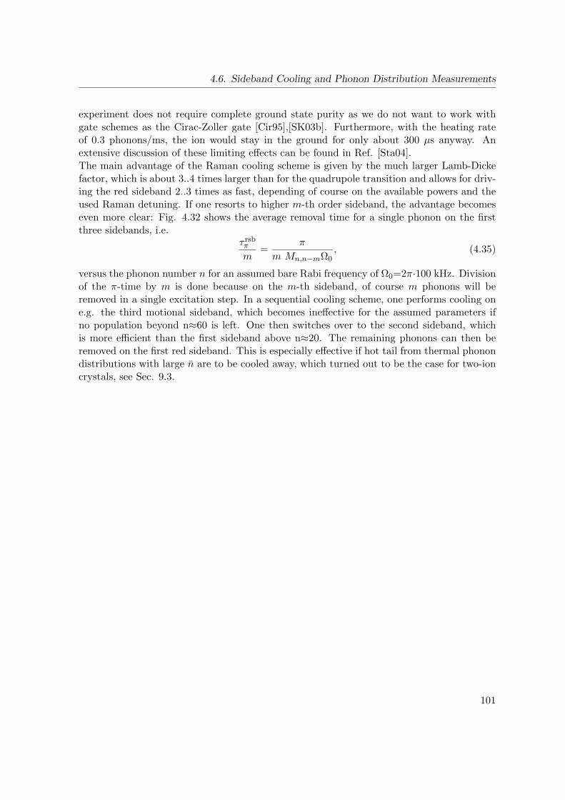
4.6. Sideband Cooling and Phonon Distribution Measurements
experiment does not require complete ground state purity as we do not want to work withgate schemes as the Cirac-Zoller gate [Cir95],[SK03b]. Furthermore, with the heating rateof 0.3 phonons/ms, the ion would stay in the ground for only about 300 µs anyway. Anextensive discussion of these limiting effects can be found in Ref. [Sta04].The main advantage of the Raman cooling scheme is given by the much larger Lamb-Dickefactor, which is about 3..4 times larger than for the quadrupole transition and allows for driv-ing the red sideband 2..3 times as fast, depending of course on the available powers and theused Raman detuning. If one resorts to higher m-th order sideband, the advantage becomeseven more clear: Fig. 4.32 shows the average removal time for a single phonon on the firstthree sidebands, i.e.
τ rsbπ
m=
π
m Mn,n−mΩ0, (4.35)
versus the phonon number n for an assumed bare Rabi frequency of Ω0=2π·100 kHz. Divisionof the π-time by m is done because on the m-th sideband, of course m phonons will beremoved in a single excitation step. In a sequential cooling scheme, one performs cooling one.g. the third motional sideband, which becomes ineffective for the assumed parameters ifno population beyond n≈60 is left. One then switches over to the second sideband, whichis more efficient than the first sideband above n≈20. The remaining phonons can then beremoved on the first red sideband. This is especially effective if hot tail from thermal phonondistributions with large n are to be cooled away, which turned out to be the case for two-ioncrystals, see Sec. 9.3.
101
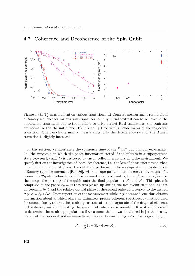
4. Implementation of the Spin Qubit
4.7. Coherence and Decoherence of the Spin Qubit
0,0 0,2 0,4 0,6 0,8 1,0 1,20,0
0,2
0,4
0,6
0,8
1,0
Nor
mal
ized
frin
ge c
ontra
st
Delay time [ms]
Raman
729 +1/2 to +3/2729 +1/2 to +5/2
729 +1/2 to +1/2
0
1
2
3
4
5
6
7
Con
trast
dec
ay ra
te [m
s-1]
24/52/5
a)
b)
Figure 4.33.: T∗2 measurement on various transitions: a) Contrast measurement results from
a Ramsey sequence for various transitions. As no unity initial contrast can be achieved in thequadrupole transitions due to the inability to drive perfect Rabi oscillations, the contrastsare normalized to the initial one. b) Inverse T∗
2 time versus Lande factor of the respectivetransition. One can clearly infer a linear scaling, only the decoherence rate for the Ramantransition is slightly increased.
In this section, we investigate the coherence time of the 40Ca+ qubit in our experiment,i.e. the timescale on which the phase information stored if the qubit is in a superpositionstate between |↓〉 and |↑〉 is destroyed by uncontrolled interactions with the environment. Wespecify first on the investigation of ’bare’ decoherence, i.e. the loss of phase information whenno additional manipulations on the qubit are performed. The appropriate tool to do this isa Ramsey-type measurement [Ram86], where a superposition state is created by means of aresonant π/2-pulse before the qubit is exposed to a fixed waiting time. A second π/2-pulsethen maps the phase φ of the qubit onto the final populations P↓ and P↑. This phase iscomprised of the phase φ0 = δt that was picked up during the free evolution if one is slightoff-resonant by δ and the relative optical phase of the second pulse with respect to the first on∆φ: φ = φ0+∆φ. Upon repetition of the measurement while ∆φ is scanned, one thus obtainsinformation about δ, which offers an ultimately precise coherent spectroscopy method usedfor atomic clocks, and via the resulting contrast also the magnitude of the diagonal elementsof the density matrix indicating the amount of coherence is revealed. It is straightforwardto determine the resulting populations if we assume the ion was initialized in |↑〉 the densitymatrix of the two-level system immediately before the concluding π/2-pulse is given by ρ:
P↑ =1
2(1 + 2|ρ12| cos(φ)) , (4.36)
102
4.7. Coherence and Decoherence of the Spin Qubit
with |ρ12| ≤ 1/2, the resulting contrast of the measurement directly yields the coherence loss.If now the coherence loss is measured versus the free evolution time, the decoherence processis made visible. A compilation of such measurement results is shown in Fig. 4.33, where themeasurement was performed on the orthogonal Raman transition and three subtransitionsof the quadrupole transition. The coherence decays with a Gaussian behavior, where thetimescale is called T∗
2 time in contrast to the T1 time at which population decay wouldoccur. As the decoherence rate scales linearly with the Lande factor describing the linearcoefficient of the Zeeman shift for the corresponding transition, it can be concluded thatambient magnetic field fluctuations are the main decoherence source in this regime.
0 1 2 3 4 5 6 7 80,0
0,2
0,4
0,6
0,8
1,0
AC line triggered
Nor
mal
ized
Ram
sey
cont
rast
Delay time [ms]
Raman parallel carrier
Raman orthogonal carrier
Raman orthogonal bsb
729 +1/2 to +5/2
Figure 4.34.: T2 measurement on various transitions: Results for spin-echo contrast measure-ment on various transitions. Note the strong increase of the coherence times if triggering onthe AC-line is used.
The most tremendous source of the coherence loss is given by the low-frequency componentsof the magnetic field fluctuations. This can be understood by the fact that if we consideran additional magnetic field fluctuating at a period much shorter than the delay time ofthe Ramsey experiment, its effect will mostly average out, analogous to phase modulationwhere the modulation index scales with the inverse modulation frequency. By contrast, ifthe oscillation period is longer than the delay time, the effect can be reverted by meansof the famous spin-echo technique originally conceived for NMR experiments. One simply
103
4. Implementation of the Spin Qubit
utilizes a π-pulse to swap the spin components in the middle of the delay time, such thatany phase offset due to a static energy shift is simply reverted. This leads to much longereffective coherence times, corresponding measurement results are shown in Fig. 4.34. Thetimescale T2 ≥T∗
2 obtained this way is of the key parameter describing the quality of aquantum memory, of course it is only meaningful in relation to the timescale at which coherentmanipulations can be carried out. We performed this measurement also on different Ramantransitions, namely the collinear, the orthogonal carrier and the orthogonal blue sidebandtransitions. The contrast decay on the orthogonal Raman transitions is additionally increasedby the heating rate. Furthermore, data sets were taken where AC-line triggering was usedin addition the spin-echo technique, which leads to an even more pronounced increase incoherence time. This is due to the fact that upon carrying out the experiment at a definitephase to the AC mains, the most part of the offset magnetic field behaves in the same wayfor each experimental run, leading to a more defined phase pick-up.Now that the timescales and mechanisms for the bare decoherence have been investigated indetail, we shall focus our attention to laser induced decoherence processes. If we restrict thetreatment to the interaction with a single off-resonant laser beam, the two processes occurringare dephasing due to intensity fluctuations in the presence of an unbalanced Stark shift andoff-resonant scattering. The relevant physical parameters thus are the detuning of the laserfrom resonance, its polarization and its intensity noise spectrum.
We briefly derive how the spin decoherence due to intensity fluctuations is related to thepower spectrum of the fluctuations. The Hamiltonian for the dispersive interaction of theeffective two-level system with the off-resonant beam is simply given by HAC(t) = ∆AC(t)σz.The corresponding unitary evolution operator is
UAC(t, 0) = eiΦAC(t)σz/2 (4.37)
with the accumulated Stark phase
ΦAC(t) =
∫ t
0dt′∆AC(t
′). (4.38)
The noisy character of ∆ACS(t) is modeled by expanding it in a Fourier series:
∆AC(t) =+∞∑
n=−∞∆n
AC(t) =+∞∑
n=−∞pn cos(2πnt/T + φn) (4.39)
where T is much larger than the experimental time scale considered and every measurementresult is to be averaged over all randomly distributed phases φn. The quantity of interest isthe spin coherence
C(t) = 〈eiΦAC(t)〉av
=+∞∏
n=−∞
(1
2π
∫ 2π
0dφn
)exp
(i
+∞∑m=−∞
Φ(m)AC (t)
)
=
+∞∏n=−∞
(1
2π
∫ 2π
0dφn
) +∞∏m=−∞
exp(iΦ
(m)AC (t)
)(4.40)
104
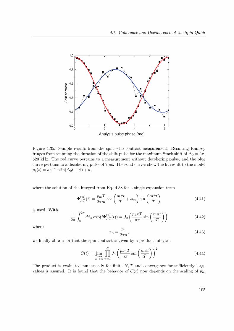
4.7. Coherence and Decoherence of the Spin Qubit
0 2 4 60,0
0,2
0,4
0,6
0,8
1,0
Spi
n co
ntra
st
Analysis pulse phase [rad]
Figure 4.35.: Sample results from the spin echo contrast measurement: Resulting Ramseyfringes from scanning the duration of the shift pulse for the maximum Stark shift of ∆0 ≈ 2π·620 kHz. The red curve pertains to a measurement without decohering pulse, and the bluecurve pertains to a decohering pulse of 7 µs. The solid curves show the fit result to the modelp↑(t) = ae−γ t sin(∆0t+ φ) + b.
where the solution of the integral from Eq. 4.38 for a single expansion term
Φ(m)AC (t) =
pmT
2πmcos
(mπt
T+ φm
)sin
(mπt
T
)(4.41)
is used. With1
2π
∫ 2π
0dφn exp(iΦ
(n)AC(t)) = J0
(pnπT
nπsin
(mπt
T
))(4.42)
wherexn =
pn2πn
, (4.43)
we finally obtain for that the spin contrast is given by a product integral:
C(t) = limT→∞N→∞
N∏n=1
J0
(pnπT
nπsin
(mπt
T
))2
(4.44)
The product is evaluated numerically for finite N,T and convergence for sufficiently largevalues is assured. It is found that the behavior of C(t) now depends on the scaling of pn.
105

4. Implementation of the Spin Qubit
1/6
S1/2
D5/2
P1/2DR
mJ=+5/2
mJ=+1/2
mJ=-1/2mJ=+1/2
Shel
ving
1/6 1/3
1/3
S1/2 mJ=+1/2
a) b)
1
mJ=-1/2
2
3
S1/2 mJ=-1/2
Figure 4.36.: a) Illustration of spin diffusion on the equator of the two-level system’s Blochsphere. Note that one is not dealing with shot-to-shot fluctuations on slow timescales whichcould be undone by employing spin echo techniques. b)Relevant energy levels and transitionsof 40Ca+. All relevant excitation and spontaneous decay pathways are shown for the S1/2- P1/2 transition. The squared Clebsch-Gordan coefficients are indicated on the differenttransitions. The shelving to the metastable D5/2 state is indicated to the right.
Under the assumption of white noise, pn = const., the noise correlation time vanishes andC(t) displays an exponential coherence decay. Under the more realistic assumption of 1/fnoise, pn = ∆0 p0/n
1/2, the nonvanishing autocorrelation can by modeled by a Gaussiandecay:
C(t) = exp
(− t2
2τ2
)(4.45)
with
τ ∝ 1
∆0(4.46)
This scaling relationship is empirically tested to be invariant against the detailed structureof the noise spectrum, the only necessary condition for it to hold is that the noise is bandlimited.Additionally to the Gaussian decay caused by the intensity fluctuations, spontaneous photonscattering from the off-resonant beam also leads to exponential decoherence, see Eq. A.16.The total coherence decay can then be modeled by
C(t) = exp
(− t
τ1(∆0)− t2
2τ22 (∆0)
)(4.47)
106
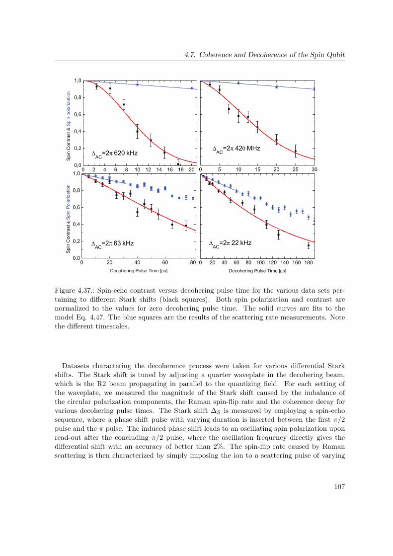
4.7. Coherence and Decoherence of the Spin Qubit
0 20 40 60 80 100 120 140 160 180
∆AC
=2π 22 kHz
Decohering Pulse Time [µs]
0 20 40 60 800,0
0,2
0,4
0,6
0,8
1,0
∆AC
=2π 63 kHz
Spi
n C
ontra
st &
Spi
n P
olar
izat
ion
Decohering Pulse Time [µs]
0 5 10 15 20 25 30
∆AC
=2π 420 MHz
0 2 4 6 8 10 12 14 16 18 200,0
0,2
0,4
0,6
0,8
1,0
Spi
n C
ontra
st &
Spi
n po
lariz
atio
n
∆AC
=2π 620 kHz
Figure 4.37.: Spin-echo contrast versus decohering pulse time for the various data sets per-taining to different Stark shifts (black squares). Both spin polarization and contrast arenormalized to the values for zero decohering pulse time. The solid curves are fits to themodel Eq. 4.47. The blue squares are the results of the scattering rate measurements. Notethe different timescales.
Datasets charactering the decoherence process were taken for various differential Starkshifts. The Stark shift is tuned by adjusting a quarter waveplate in the decohering beam,which is the R2 beam propagating in parallel to the quantizing field. For each setting ofthe waveplate, we measured the magnitude of the Stark shift caused by the imbalance ofthe circular polarization components, the Raman spin-flip rate and the coherence decay forvarious decohering pulse times. The Stark shift ∆S is measured by employing a spin-echosequence, where a phase shift pulse with varying duration is inserted between the first π/2pulse and the π pulse. The induced phase shift leads to an oscillating spin polarization uponread-out after the concluding π/2 pulse, where the oscillation frequency directly gives thedifferential shift with an accuracy of better than 2%. The spin-flip rate caused by Ramanscattering is then characterized by simply imposing the ion to a scattering pulse of varying
107
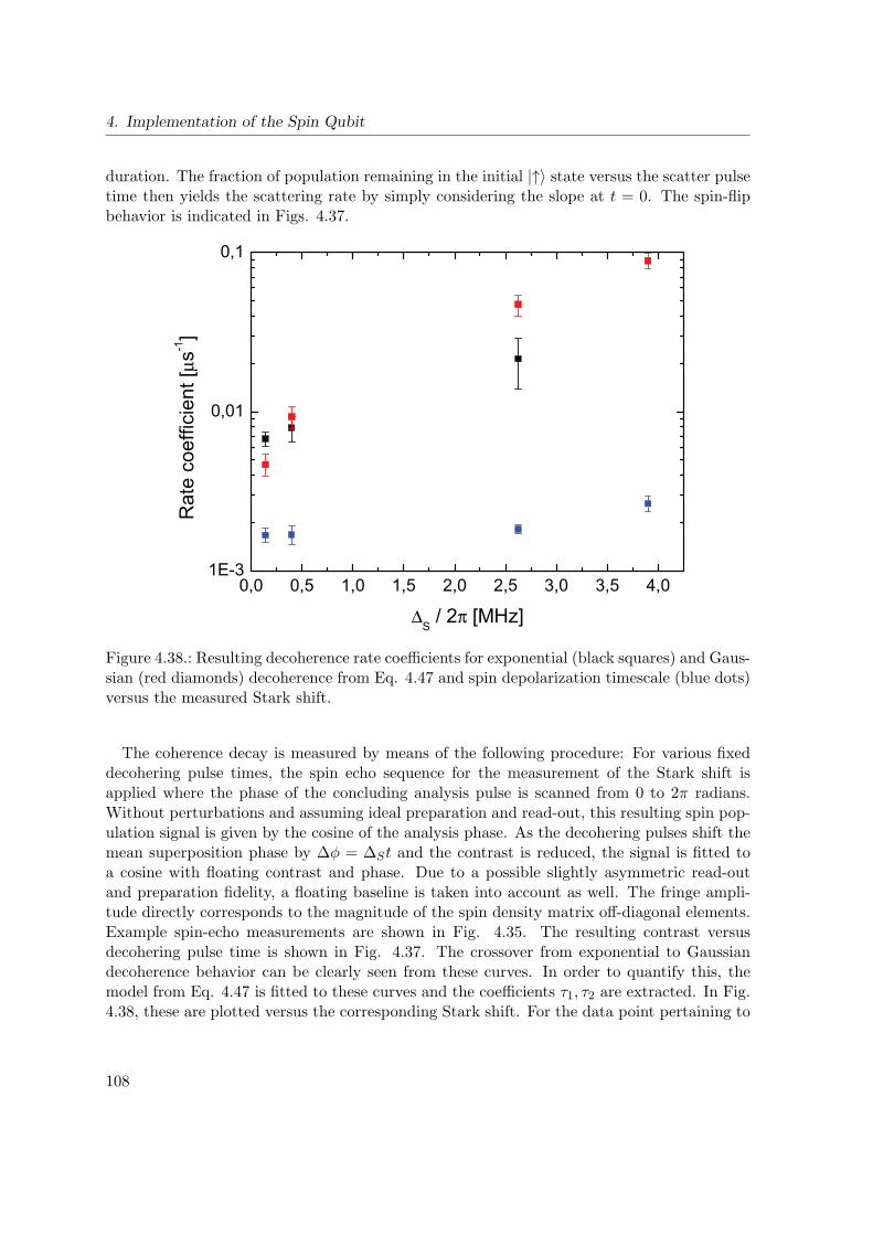
4. Implementation of the Spin Qubit
duration. The fraction of population remaining in the initial |↑〉 state versus the scatter pulsetime then yields the scattering rate by simply considering the slope at t = 0. The spin-flipbehavior is indicated in Figs. 4.37.
0,0 0,5 1,0 1,5 2,0 2,5 3,0 3,5 4,01E-3
0,01
0,1
Rat
e co
effic
ient
[µs-1
]
∆S / 2π [MHz]
Figure 4.38.: Resulting decoherence rate coefficients for exponential (black squares) and Gaus-sian (red diamonds) decoherence from Eq. 4.47 and spin depolarization timescale (blue dots)versus the measured Stark shift.
The coherence decay is measured by means of the following procedure: For various fixeddecohering pulse times, the spin echo sequence for the measurement of the Stark shift isapplied where the phase of the concluding analysis pulse is scanned from 0 to 2π radians.Without perturbations and assuming ideal preparation and read-out, this resulting spin pop-ulation signal is given by the cosine of the analysis phase. As the decohering pulses shift themean superposition phase by ∆φ = ∆St and the contrast is reduced, the signal is fitted toa cosine with floating contrast and phase. Due to a possible slightly asymmetric read-outand preparation fidelity, a floating baseline is taken into account as well. The fringe ampli-tude directly corresponds to the magnitude of the spin density matrix off-diagonal elements.Example spin-echo measurements are shown in Fig. 4.35. The resulting contrast versusdecohering pulse time is shown in Fig. 4.37. The crossover from exponential to Gaussiandecoherence behavior can be clearly seen from these curves. In order to quantify this, themodel from Eq. 4.47 is fitted to these curves and the coefficients τ1, τ2 are extracted. In Fig.4.38, these are plotted versus the corresponding Stark shift. For the data point pertaining to
108

4.7. Coherence and Decoherence of the Spin Qubit
the maximum Stark shift, the Gaussian coherence decay is completely dominating such thatno valid linear coefficient could be fitted from the data. As the exponential decoherence iscaused by Raman scattering, it does not vanish at zero Stark shift, as can be seen clearlyfrom the data. Note the different scaling behavior of the spin depolarization rate and theexponential decay coefficient. Upon increasing the Raman detuning ∆R and cranking upthe laser power to leave ∆S unaffected, the crossover point between exponential and Gaus-sian decoherence would be shifted towards smaller Stark shifts, rendering the spin diffusionmechanism more dominant. It is interesting to compare the exponential decoherence rateat vanishing Stark shift to the scattering rate: From the data at the lowest Stark shift, thefigure Rdeph/R1→2 = 4.0 ± 0.58 is obtained. Comparing this to Eqs. A.14 and A.16, underthe consideration that |ε+|2 = |ε−|2 = 1/2, the scattering rate
R1→2 =1
2 · 3ΓΩ2
4∆2(4.48)
and the decoherence rate
Rdeph =1
2 · 3ΓΩ2
4∆2(4.49)
are obtained, such that the decoherence rate should the threefold scattering rate. If the ad-ditional term L23 from Eq. A.19 is additionally considered and the phase shift between thecircular components is such that ε+ε
∗− = +1/2, the decoherence rate would be exactly thefourfold scattering rate, which is clearly supported by the experimental data. This would rep-resent an additional, yet unknown decoherence mechanism which is dependent on the phaserelation between the + and - circular polarization components. For a linearly polarized beampropagating along the magnetic field axis, this corresponds to a breaking of the cylindricalsymmetry of the physical system. Furthermore, the source of the increase of the exponentialdecoherence rate coefficient with the Stark shift is yet unknown: Rdeph from Eq. A.16 isindependent of the balance of the circular components, and the extra term L23 should be ofmaximum magnitude for balanced components. A possible explanation is a white noise floorin the power spectrum of the intensity fluctuations, but as the effect is only manifested in asingle data point, no thorough claim on this can be supported.
Attempts were made to reduce the decoherence due to intensity fluctuations in the presenceof a nonzero Stark shift. This was done by establishing an intensity stabilization by means ofthe fast switching EOM, which allows for regulation bandwidths of up to 1 MHz and larger.However, no effect on the coherence time could be seen between measurements where theintensity stabilization was switched on or off. Furthermore, a common observation whilemeasuring either Stark shifts or Rabi oscillations (even with nulled Stark shift) is that forlonger pulse times the oscillatory patterns become distorted and even spiky. This raised thesuspect that not direct laser intensity noise is responsible for the observed strong decoherence,but rather the localization of the ion in the Raman beams is subject to drifts at a secondtimescale. It was therefore checked if the readout values indeed obey to the statistical errorgiven by Eq. 4.3. This was done by means of a repeated ac stark shift measurement withonly the R2 beam involved to exclude other error sources. The results are shown in Fig. 4.39,where the measurement was performed for two different ac stark shifts, and each curve was
109

4. Implementation of the Spin Qubit
0 5 10 15 20 25 30 35 40 45 500,0
0,2
0,4
0,6
0,8
She
lvin
g pr
obab
ility
σz Pulse time [µs]
,0,2
0,4
0,6
0,8
1,0S
helv
ing
prob
abili
ty
Figure 4.39.: Investigation of the intensity-fluctuation induced decoherence process: The factthat the error bars increase for longer pulse times clearly indicates that the error is due topulse area fluctuations. As the error results from the statistics over several runs of the samemeasurement, it can be concluded that these fluctuations take place on slow timescales, i.e.beyond the time for the acquisition of a single data point, which is about 1 s.
measured ten times repeatedly. The error bars from the statistics over these measurementsclearly reveal that the error increases in time, and that it becomes indeed much larger thanthe expected projection noise error. The conclusion is that the error arises due to effectivepulse area fluctuations, which occur on longer time scales than the acquisition of a singledata point, otherwise the exponential envelope would be seen in a single measurement runand the error bars would obey to the statistical limit. If the ac stark shift is divided by thedecay time scale for each setting, similar figures of 60.6(2.5) and 64.0(2.4) result, provingthat the decoherence is indeed given by pulse area fluctuations. The underlying reasoning isthat the ideal signal for the ac stark measurement is given by
P↑(t) = cos2(∆St/2), (4.50)
110

4.7. Coherence and Decoherence of the Spin Qubit
the signal deviation due to a small Stark shift offset δS is given by
〈P↑(t)〉 =
∫dδS
1√2πσ2
S
e− δ2S
2σ2S cos2((∆S(1 + δS)t/2)
=1
2
(1 + e−
12σ2S∆
2St
2cos(∆St/2)
)(4.51)
In conclusion, there are only two possible mechanisms giving rise to these observations: Eitherthe ion moves in the beam on a second timescale, or the beam has pointing instabilities. Thelatter possibility could be excluded by focusing the beam on a remotely placed CCD chip,where no drift could be observed. The first possibility in the strict sense is also unlikelyas a movement in the µm range over longer timescales should be visible on the EMCCDcamera. Therefore, a likely mechanism is the delocalization of the ion in the radial planeon the trap due to the strong radial heating measured in Sec. 4.3. If the heating wasmediated by micromotion, the delocalization would be influenced by random charging of thetrap electrodes. The suggested mechanism is further supported by the fact that stronglyenhanced decoherence was observed for tightly focused Raman beams.
111

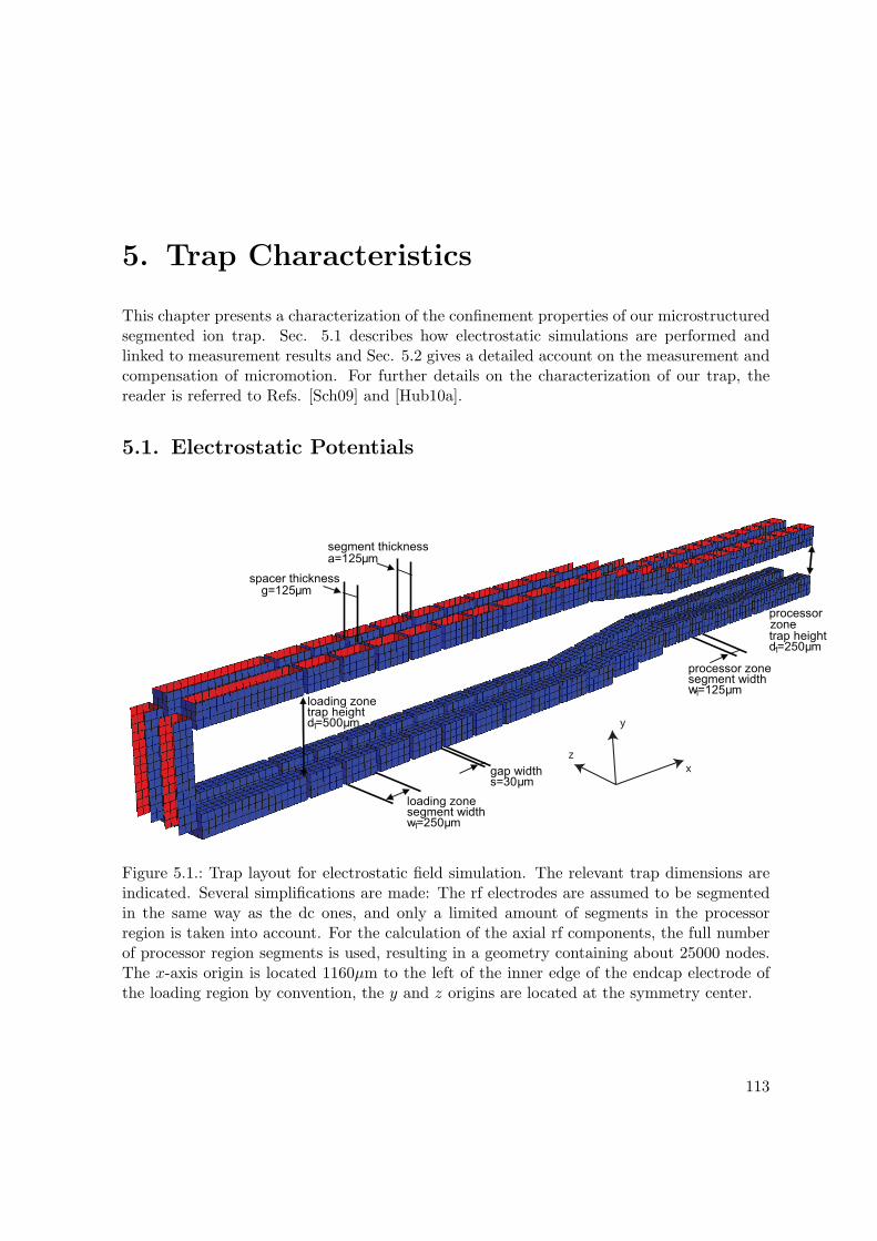
5. Trap Characteristics
This chapter presents a characterization of the confinement properties of our microstructuredsegmented ion trap. Sec. 5.1 describes how electrostatic simulations are performed andlinked to measurement results and Sec. 5.2 gives a detailed account on the measurement andcompensation of micromotion. For further details on the characterization of our trap, thereader is referred to Refs. [Sch09] and [Hub10a].
5.1. Electrostatic Potentials
loading zone segment widthw1=250 m
processor zone segment widthw1=125 m
gap widths=30 m
loading zone trap heightd1=500 m
spacer thicknessg=125 m
segment thicknessa=125 m
processor
trap heightd1=250 m
zone
x
y
z
Figure 5.1.: Trap layout for electrostatic field simulation. The relevant trap dimensions areindicated. Several simplifications are made: The rf electrodes are assumed to be segmentedin the same way as the dc ones, and only a limited amount of segments in the processorregion is taken into account. For the calculation of the axial rf components, the full numberof processor region segments is used, resulting in a geometry containing about 25000 nodes.The x-axis origin is located 1160µm to the left of the inner edge of the endcap electrode ofthe loading region by convention, the y and z origins are located at the symmetry center.
113
5. Trap Characteristics
The key feature of our experimental approach towards scalable quantum logic is the factthat our trap possesses multiple segments in order to store and control a quite large number ofqubits. Furthermore, the electrode structures are small compared to macroscopic standard-type Paul traps. This has the consequence that the structure of the confining potentials ismore complicated than in a macroscopic setting, where the basic properties of electrostatictheory guarantee very harmonic potentials. For microstructured ion traps in general, it isvery advantageous to know the electrostatic potentials with a high degree of precision, be itin the design process to obtain structures that provide the desired confinement properties, beit for the determination of possible operating voltages at the first attempts to trap with a newdevice or be it for the optimization of transport operations in segmented traps. This chapteris structured as follows: In Sec. 5.1, we briefly explain how we calculate the potentials forcomplicated trap structures and then analyze the properties of our trap based on the resultsof these simulations. Sec. 5.2 gives a detailed account on residual micromotion, its adverseeffects on our experiments and how it is compensated in our setup.
The calculation of the electrostatic fields and potentials in an arbitrary electrode geom-etry, i.e. the solution of the Laplace equation for complicated boundary conditions is aninteresting but rather complicated matter on its own, and it was found that a homebuiltcustomized software was needed to calculate the potentials with sufficient accuracy and ef-ficiency. Conventional tools employ the finite-element method (FEM), which was found toproduce resulting potential with additional spurious irregularities, furthermore commercialtools were found to be difficult to adapt to our custom geometries and calculation require-ments, e.g. the feature to calculate trajectories can not easily be implemented. We thereforeuse a program written by Kilian Singer which employs the boundary element method (BEM)instead of FEM, which does not not require a 3D collocation of the volume of interest butrather a 2D one of the electrode surfaces. The basic idea is that each surface in the geometryis subdivided into small basic elements. The surface charge on each element is then givenby the voltages applied to the electrodes and analytic relations for the mutual capacitancebetween each two segments. The surface charges are obtained from the inversion of a inversecapacitance matrix which has the dimension of the number of surface elements, which canrange in the 105 regime. As the computational effort for matrix inversion scales to the thirdpower of the number of surface elements N , a simplification which renders the calculationmore effective is needed. The fast multipole method was found to be extremely useful for this,as it reduces the scaling law to N logN . The underlying idea is that surface elements faraway from the element of interest are bundled in a group, for which a multipolar expansionof the potential is performed. If the surface charges are known, the potential at a given pointr is obtained by summing the potential arising from each surface element, which are in turncalculated by employing Greens functions. A more extensive discussion of all these methodsis found in Ref. [Sin10]. Fig. 5.1 shows the geometry model of our trap used for the calcula-tion of the electrostatic potentials. For this model, the inverse capacitance matrix inversiontakes only about 20 minutes on a conventional personal computer. Potentials can be directlycomputed by application of the appropriate Greens functions, electric fields are obtained byfinite differencing. The resulting potentials and fields are free of numerical artifacts, which
114

5.1. Electrostatic Potentials
1 2 3 4 5 6 70,00
0,05
0,10
0,15
0,20
0,25
0,30
0,35
0,40
0,45
0,50E
lect
rost
atic
pot
entia
l [V
]
Position along trap axis [mm]
Figure 5.2.: Electrostatic axial confinement potentials: The potentials along the trap axis(y, z = 0) arising if dc electrode n is set to +1 V and the other ones are grounded. Thepotentials for the loading region electrodes are shown in blue, the taper region ones in magentaand the processor region ones in red. It can be seen that the potential wells overlap each othersuch that a strong linear potential, i.e. a force, can be generated at a given trapping stateby setting a neighboring electrode to nonzero voltage, which enables fast and efficient iontransport in the throughout the trap structure. Furthermore, considerable potential depthsin the 2 V range are readily attained.
allows for a very precise calculation of the potential curvatures which are needed to predictsecular frequencies of trapped ions.
Resulting axial confinement potentials for the individual segments are shown in Fig. 5.2. Aquantitative characterization of the confinement strengths is given in table 5.1, from which theaxial secular frequency and the a and q parameters can be directly inferred by multiplicationwith the respective voltages. In contrast to the axial confinement, the radial confinementis influenced by both dc and rf potentials and is therefore more complicated to analyzequantitatively. Calculated radial cuts at the trapping site of segment 5 for the rf and dcpotentials are shown in Fig. 5.3. An important result is that the potential ellipsoids aroundthe origin are aligned differently for the dc and rf fields. The deviation of the dc axes from therf ones originates from the fact the rf voltage is applied along the whole trap length, whereasthe neighboring segments of segment 5 are set to ground, which breaks the symmetry between
115
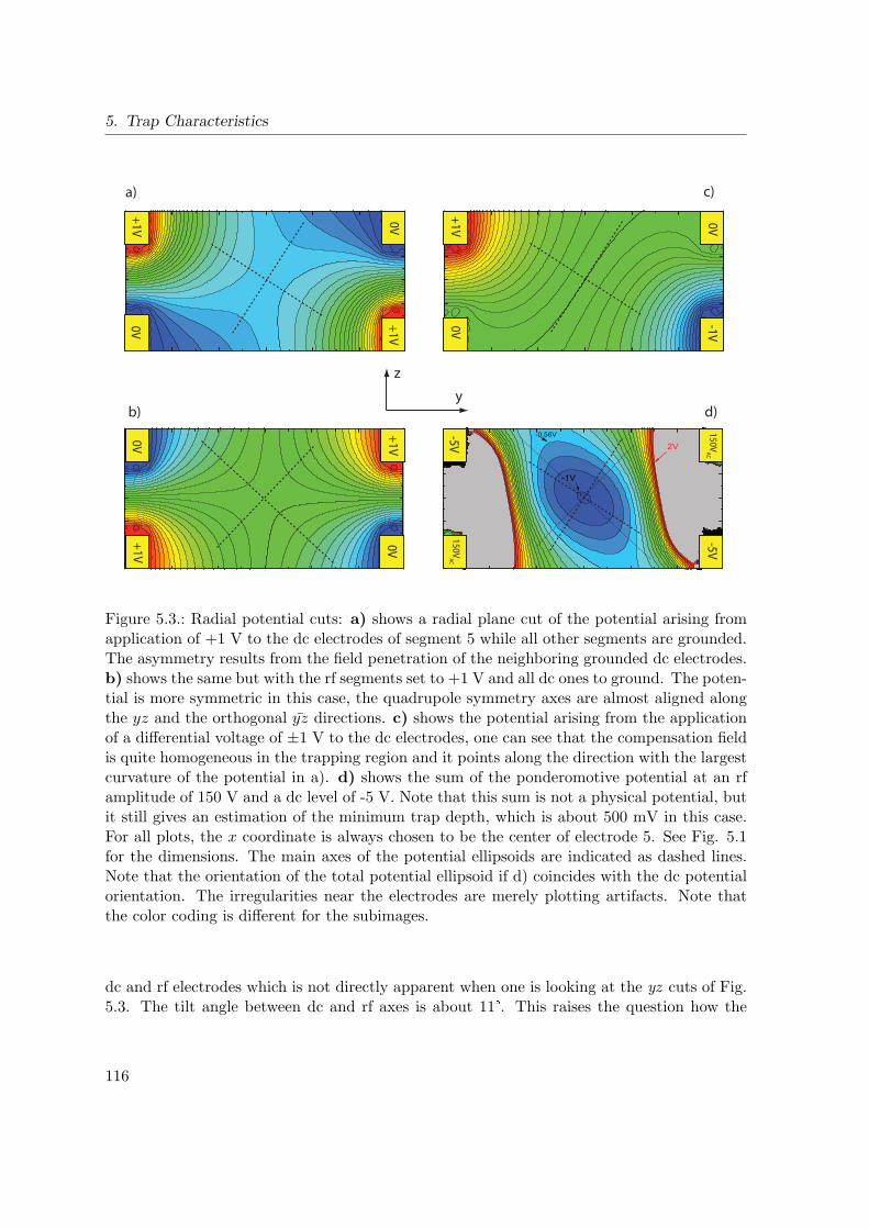
5. Trap Characteristics
2V
-1V
-0.56V
+1
V
+1
V
+1
V
-1V
0V
0V
0V
0V
0V
0V
+1
V
+1
V
-5V
-5V
15
0V
AC
15
0V
AC
a) c)
b) d)
z
y
Figure 5.3.: Radial potential cuts: a) shows a radial plane cut of the potential arising fromapplication of +1 V to the dc electrodes of segment 5 while all other segments are grounded.The asymmetry results from the field penetration of the neighboring grounded dc electrodes.b) shows the same but with the rf segments set to +1 V and all dc ones to ground. The poten-tial is more symmetric in this case, the quadrupole symmetry axes are almost aligned alongthe yz and the orthogonal yz directions. c) shows the potential arising from the applicationof a differential voltage of ±1 V to the dc electrodes, one can see that the compensation fieldis quite homogeneous in the trapping region and it points along the direction with the largestcurvature of the potential in a). d) shows the sum of the ponderomotive potential at an rfamplitude of 150 V and a dc level of -5 V. Note that this sum is not a physical potential, butit still gives an estimation of the minimum trap depth, which is about 500 mV in this case.For all plots, the x coordinate is always chosen to be the center of electrode 5. See Fig. 5.1for the dimensions. The main axes of the potential ellipsoids are indicated as dashed lines.Note that the orientation of the total potential ellipsoid if d) coincides with the dc potentialorientation. The irregularities near the electrodes are merely plotting artifacts. Note thatthe color coding is different for the subimages.
dc and rf electrodes which is not directly apparent when one is looking at the yz cuts of Fig.5.3. The tilt angle between dc and rf axes is about 11. This raises the question how the
116
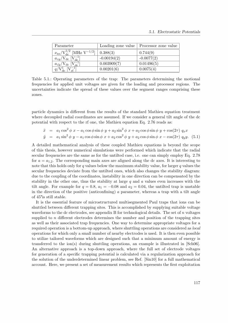
5.1. Electrostatic Potentials
Parameter Loading zone value Processor zone value
νax/V1/2dc [MHz V−1/2] 0.388(3) 0.744(9)
azy/Vdc [V−1dc ] -0.00194(2) -0.0077(2)
azy/Vdc [V−1dc ] 0.003909(7) 0.01496(5)
q/V1dc [V−1
rf ] 0.00201(6) 0.0075(4)
Table 5.1.: Operating parameters of the trap: The parameters determining the motionalfrequencies for applied unit voltages are given for the loading and processor regions. Theuncertainties indicate the spread of these values over the segment ranges comprising thesezones.
particle dynamics is different from the results of the standard Mathieu equation treatmentwhere decoupled radial coordinates are assumed. If we consider a general tilt angle of the dcpotential with respect to the rf one, the Mathieu equation Eq. 2.76 reads as:
x = a1 cos2 φ x− a1 cosφ sinφ y + a2 sin
2 φ x+ a2 cosφ sinφ y + cos(2τ) qxx
y = a1 sin2 φ y − a1 cosφ sinφ x+ a2 cos
2 φ y + a2 cosφ sinφ x− cos(2τ) qyy. (5.1)
A detailed mathematical analysis of these coupled Mathieu equations is beyond the scopeof this thesis, however numerical simulations were performed which indicate that the radialsecular frequencies are the same as for the untilted case, i.e. one can simply employ Eq. 2.78for a = a1,2. The corresponding main axes are aligned along the dc axes. It is interesting tonote that this holds only for q values below the maximum stability value, for larger q values thesecular frequencies deviate from the untilted ones, which also changes the stability diagram:due to the coupling of the coordinates, instability in one direction can be compensated by thestability in the other one, thus the stability at large q and a values even increases with thetilt angle. For example for q = 0.8, a1 = −0.08 and a2 = 0.04, the untilted trap is unstablein the direction of the positive (anticonfining) a parameter, whereas a trap with a tilt angleof 45is still stable.
It is the essential feature of microstructured multisegmented Paul traps that ions can beshuttled between different trapping sites. This is accomplished by supplying suitable voltagewaveforms to the dc electrodes, see appendix B for technological details. The set of n voltagessupplied to n different electrodes determines the number and position of the trapping sitesas well as their associated trap frequencies. One way to determine appropriate voltages for arequired operation is a bottom-up approach, where shuttling operations are considered as localoperations for which only a small number of nearby electrodes is used. It is then even possibleto utilize tailored waveforms which are designed such that a minimum amount of energy istransferred to the ion(s) during shuttling operations, an example is illustrated in [Sch06].An alternative approach is a top-down approach, where the full set of electrode voltagesfor generation of a specific trapping potential is calculated via a regularization approach forthe solution of the underdetermined linear problem, see Ref. [Sin10] for a full mathematicalaccount. Here, we present a set of measurement results which represents the first exploitation
117
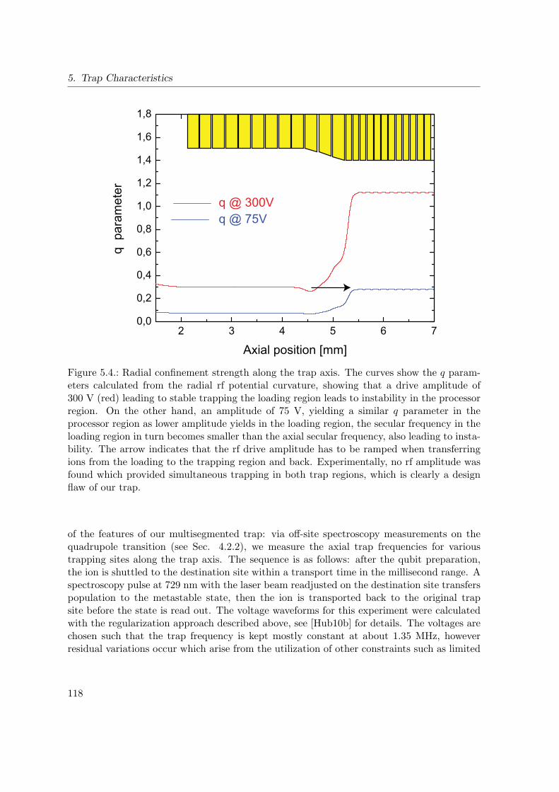
5. Trap Characteristics
2 3 4 5 6 70,0
0,2
0,4
0,6
0,8
1,0
1,2
1,4
1,6
1,8q
par
amet
er
Axial position [mm]
q @ 300Vq @ 75V
Figure 5.4.: Radial confinement strength along the trap axis. The curves show the q param-eters calculated from the radial rf potential curvature, showing that a drive amplitude of300 V (red) leading to stable trapping the loading region leads to instability in the processorregion. On the other hand, an amplitude of 75 V, yielding a similar q parameter in theprocessor region as lower amplitude yields in the loading region, the secular frequency in theloading region in turn becomes smaller than the axial secular frequency, also leading to insta-bility. The arrow indicates that the rf drive amplitude has to be ramped when transferringions from the loading to the trapping region and back. Experimentally, no rf amplitude wasfound which provided simultaneous trapping in both trap regions, which is clearly a designflaw of our trap.
of the features of our multisegmented trap: via off-site spectroscopy measurements on thequadrupole transition (see Sec. 4.2.2), we measure the axial trap frequencies for varioustrapping sites along the trap axis. The sequence is as follows: after the qubit preparation,the ion is shuttled to the destination site within a transport time in the millisecond range. Aspectroscopy pulse at 729 nm with the laser beam readjusted on the destination site transferspopulation to the metastable state, then the ion is transported back to the original trapsite before the state is read out. The voltage waveforms for this experiment were calculatedwith the regularization approach described above, see [Hub10b] for details. The voltages arechosen such that the trap frequency is kept mostly constant at about 1.35 MHz, howeverresidual variations occur which arise from the utilization of other constraints such as limited
118
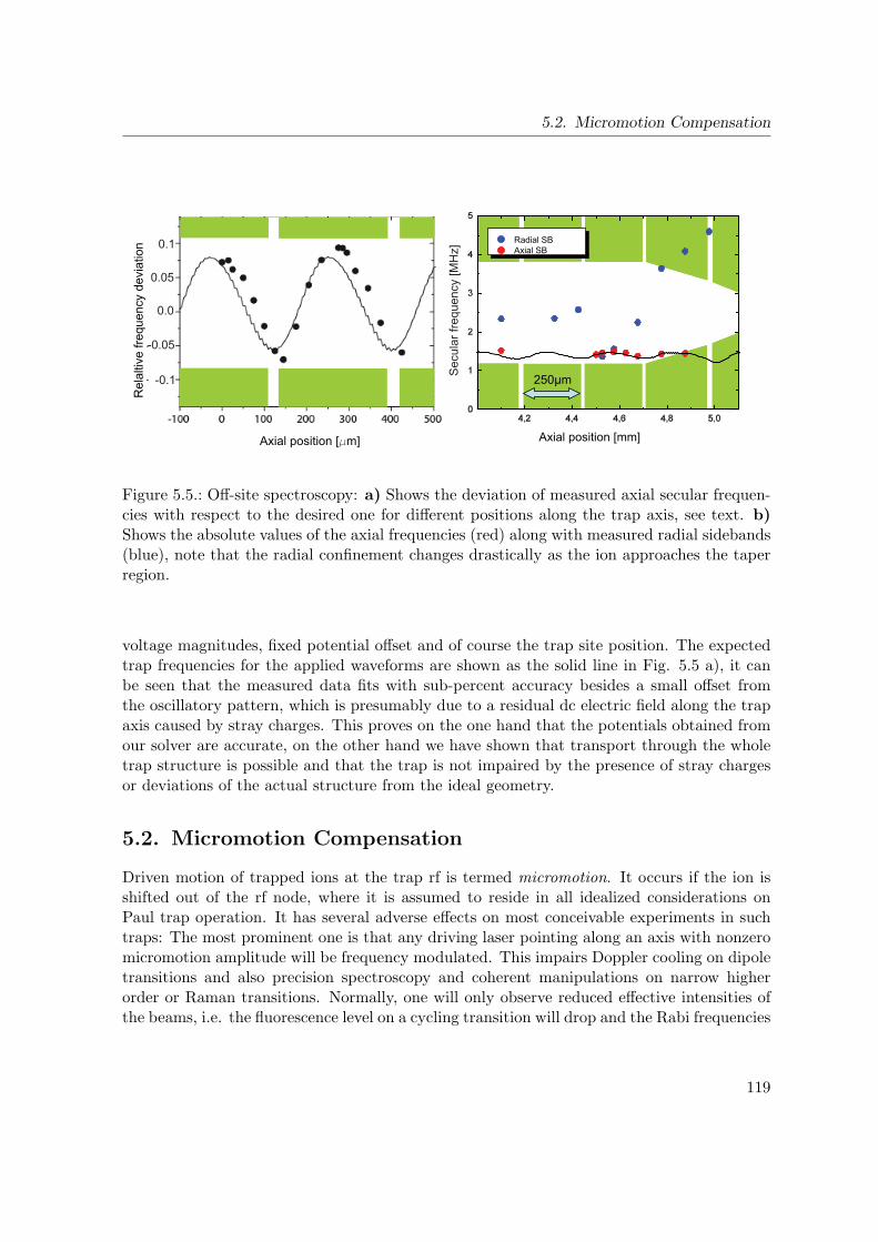
5.2. Micromotion Compensation
Axial position [ m]
Rel
altiv
e fre
quen
cy d
evia
tion Radial SB
Axial SB
250 m
Axial position [mm]
0.1
-0.1
0.0
0.05
-0.05
Sec
ular
freq
uenc
y [M
Hz]
Figure 5.5.: Off-site spectroscopy: a) Shows the deviation of measured axial secular frequen-cies with respect to the desired one for different positions along the trap axis, see text. b)Shows the absolute values of the axial frequencies (red) along with measured radial sidebands(blue), note that the radial confinement changes drastically as the ion approaches the taperregion.
voltage magnitudes, fixed potential offset and of course the trap site position. The expectedtrap frequencies for the applied waveforms are shown as the solid line in Fig. 5.5 a), it canbe seen that the measured data fits with sub-percent accuracy besides a small offset fromthe oscillatory pattern, which is presumably due to a residual dc electric field along the trapaxis caused by stray charges. This proves on the one hand that the potentials obtained fromour solver are accurate, on the other hand we have shown that transport through the wholetrap structure is possible and that the trap is not impaired by the presence of stray chargesor deviations of the actual structure from the ideal geometry.
5.2. Micromotion Compensation
Driven motion of trapped ions at the trap rf is termed micromotion. It occurs if the ion isshifted out of the rf node, where it is assumed to reside in all idealized considerations onPaul trap operation. It has several adverse effects on most conceivable experiments in suchtraps: The most prominent one is that any driving laser pointing along an axis with nonzeromicromotion amplitude will be frequency modulated. This impairs Doppler cooling on dipoletransitions and also precision spectroscopy and coherent manipulations on narrow higherorder or Raman transitions. Normally, one will only observe reduced effective intensities ofthe beams, i.e. the fluorescence level on a cycling transition will drop and the Rabi frequencies
119
5. Trap Characteristics
for coherently driving a quadrupole or stimulated Raman transition will be reduced. Moresevere effects might also be present: the Doppler cooling will be less efficient if the coolingtransition line is effectively broadened by the micromotion echoes, and if these are on theblue side of the transition they will even counteract the cooling. Furthermore, the powerin the FM sidebands acts as to increase laser-driven decoherence mechanisms when drivingRaman transition, see Sec. 4.7. In the worst case, echo components might even hit otherresonance, e.g. higher order motional sideband or different Zeeman transitions in the case ofa quadrupole transition. It should be also noted that for precision spectroscopy, especially fordesigning optical atomic clocks based on trapped ions, the ac Stark shift from uncompensatedmicromotion will be the predominant error source. Micromotion can be compensated byapplying dc voltages to a set of compensation electrodes to shift the ion into the node of therf field. The difficulty lies in precise measurement of the micromotion amplitude. Throughoutthe last decades, several methods for this have been conceived:
Ion position shift: This technique does not directly measure effects of the micromo-tion, it rather monitors the change of the ion position upon change of the rf level whichcan only occur of dc and ac potential minima are offset with respect to each other, suchthat a residual dc field drives the ion out of the rf node. The accuracy of the methodis very limited by the spatial resolution of the imaging optics.
Coherent echo strength measurement: If a narrow transition is at hand whichcan be coherently driven, the strength of micromotion echoes can be directly measuredand minimized.
Phonon correlations: The fluorescence counting electronics can be set up such thattime resolved measurements of the photon arrival times can be correlated with thetrap rf. Nonvanishing correlation will be found in the presence of micromotion. Theadvantage of this method is that its implementation is possible without coherentlydriven optical transitions or even without imaging, however it requires a considerableamount of data acquisition.
Fluorescence heterodyning: The fluorescence can be heterodyned with a phase-locked laser offset by about the drive rf. The signal then directly provides informationabout the oscillation amplitude [Raa00].
Coherent Raman effects: Phase coherent modulation of a repump laser with the traprf can be used to obtain a modulation of the fluorescence level [All10]. The advantageof this technique is essentially that the vertical direction, which is inaccessible for thecooling laser due to stray light issues in surface traps, can be accessed.
rf modulation: If the rf voltage is fed onto the different electrodes via distinct path-ways, it is possible to modulate one of these by a secular frequency. It the ion senses therf field, its secular motion will be driven by the resulting beat, which strongly affectsthe fluorescence level. This method is also especially suited for planar traps [Dan09].
120
5.2. Micromotion Compensation
Fluorescence measurement: The primary effect of micromotion is the alteration ofthe line shape on a cooling transition. Due to the broadening, the fluorescence levelwill increase due to micromotion for sufficient detunings and appropriate range of rffrequencies and modulation amplitudes. As this is the technique of our choice due toits simplicity, it will be discussed in detail below.
The first three techniques are discussed in detail in Ref. [Ber98b]. We have realized boththe echo strength measurement and the correlation measurement, however the first techniqueyields high accuracy but accounts only spatial direction, while the latter was found to berather impractical. We have found that for the every-day lab routine, it is most useful tored-detune the Doppler cooling laser at 397 nm by more than one linewidth and to minimizethe fluorescence level at that detuning. The compensation is performed by applying a voltagedifference between the adjacent dc trapping electrodes. The accuracy of this method is to beassessed in the following. If we assume the ion to be a free particle, which is justified by thetimescale separation ωrad Ωrf , its motion in a homogeneous rf field is given by
x(t) =qE
(rf)x
mΩ2rf
cos(Ωrft)
v(t) =qE
(rf)x
mΩrfsin(Ωrft), (5.2)
where we consider the motion along a laser beam direction x with wavenumber k and the
corresponding component of the rf electric field E(rf)x . The maximum first-order Doppler shift
during one motional cycle is then
δmax = k vmax = kqE
(rf)x
mΩrf. (5.3)
The oscillatory motion then leads to frequency modulation of the laser with a modulationindex of
β =δmax
Ωrf= k
qE(rf)x
mΩ2rf
= 2πxmax
λ(5.4)
If the beam is detuned from the atomic resonance by δ0, one obtains effective saturation Sn
parameters for the frequency components δn = δ0 + nΩrf with n = −∞..+∞:
Sn = S0J2n(β). (5.5)
The total fluorescence level upon neglecting the motional effects due to a changed Dopplercooling efficiency then is
R =
+∞∑n=−∞
Γ
2
Sn
1 + S0 + 4 (δ + nΩrf)2 /Γ2
, (5.6)
where a reasonable parameter regime is of course only given for small enough modulationindices, such that the summation will include only a few nonvanishing terms around n = 0.
121
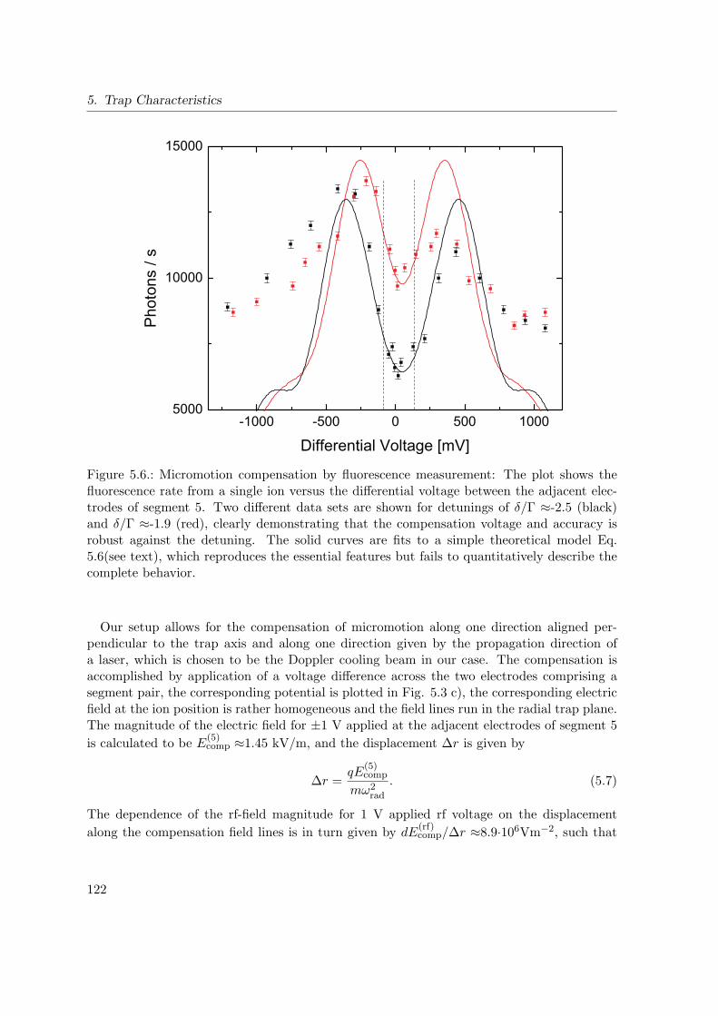
5. Trap Characteristics
-1000 -500 0 500 10005000
10000
15000P
hoto
ns /
s
Differential Voltage [mV]
Figure 5.6.: Micromotion compensation by fluorescence measurement: The plot shows thefluorescence rate from a single ion versus the differential voltage between the adjacent elec-trodes of segment 5. Two different data sets are shown for detunings of δ/Γ ≈-2.5 (black)and δ/Γ ≈-1.9 (red), clearly demonstrating that the compensation voltage and accuracy isrobust against the detuning. The solid curves are fits to a simple theoretical model Eq.5.6(see text), which reproduces the essential features but fails to quantitatively describe thecomplete behavior.
Our setup allows for the compensation of micromotion along one direction aligned per-pendicular to the trap axis and along one direction given by the propagation direction ofa laser, which is chosen to be the Doppler cooling beam in our case. The compensation isaccomplished by application of a voltage difference across the two electrodes comprising asegment pair, the corresponding potential is plotted in Fig. 5.3 c), the corresponding electricfield at the ion position is rather homogeneous and the field lines run in the radial trap plane.The magnitude of the electric field for ±1 V applied at the adjacent electrodes of segment 5
is calculated to be E(5)comp ≈1.45 kV/m, and the displacement ∆r is given by
∆r =qE
(5)comp
mω2rad
. (5.7)
The dependence of the rf-field magnitude for 1 V applied rf voltage on the displacement
along the compensation field lines is in turn given by dE(rf)comp/∆r ≈8.9·106Vm−2, such that
122

5.2. Micromotion Compensation
we obtain dE(rf)comp/dV
(5)comp. Inserting this into Eq. 5.4 yields
β ≈ keffq
mΩrf
dE(rf)comp
dV(5)comp
V (5)compVrf , (5.8)
which can be inserted into Eq. 5.6 to predict the behavior of the fluorescence on the com-pensation voltage. A comparison between the model and measured data is shown in Fig. 5.6.The detunings are inferred from a measurement of the fluorescence rate versus 397 nm wave-length, and a saturation parameter of S0=5 is assumed. The applied rf voltage amplitude isVrf=200 V at Ωrf ≈ 2π·24.8 MHz, resulting in ωrad ≈ 2π·3.5 MHz. A compensation offsetvoltage of 50 mV is inferred and a factor for scaling the absolute photon collection rate is in-troduced. As can be seen, the width and depth of the fluorescence dip is correctly reproducedby the model for both detunings, however the decrease for large compensation voltage mag-nitudes is much less pronounced for the measured data. Furthermore, the asymmetry of thedip is not at all explained by the model. The reason for the first discrepancy might be thatthe Zeeman splitting of the two driven transitions |S1/2,mJ = ±1/2〉 → |P1/2,mJ = ±1/2〉of about 12 MHz is not included, as is the effect of the photon scattering on the motionalstate of the ion. The asymmetry might arise from a displacement giving rise to additionalmicromotion in the y-direction, which is not directly visible in the 397 nm fluorescence butmight be responsible for an inhomogeneous compensation field. The precision attained by thiscompensation method is indicated by the dashed lines in Fig. 5.6, from the voltage windowof about 80 mV, a maximum residual modulation index of |βres| 0.56, equivalent to 85% ofthe laser power acting on the carrier transition. As can be seen from simulations for variousparameter sets, the width of the dip is rather independent of the laser and trap parameters,however the attainable micromotion suppression is quite poor. However, all methods used forqubit preparation, manipulation and readout are designed to be resilient against the presenceof a tolerable amount of micromotion, as is explained in detail in chapter 4.
Micromotion aligned along the trap axis can not be directly compensated by means of adifferential voltage. The origin of axial micromotion is on the one hand given by the transla-tional asymmetry along the trap axis. To make this more clear, we consider an ion placed atany given site in the loading region. It has a direct line of sight on the rf-electrode surfaces inthe taper region, which is not present in the other direction along the trap axis. The modula-tion index inferred from the simulation axial rf field strength by the same reasoning as aboveis plotted for standard operating parameters in Fig. 5.7. It can be seen that the expectedmodulation might be sufficiently small in the processor region. An additional increase ofthe modulation will occur if rf pickup is present on the confining dc electrode and the ion isshifted into a nonzero electric field arising from this electrode by stray charges acting in theaxial direction. An estimation along the same lines of thought as above is readily obtainedby considering the axial potential from the confining electrode can be written as
V (x) =1
2mω2
axx2 = q Vdccdcx
2, (5.9)
123
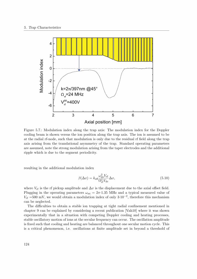
5. Trap Characteristics
2 3 4 5 6 7
-6
-4
-2
0
2
4M
odul
atio
n in
dex
π
Ω
Figure 5.7.: Modulation index along the trap axis: The modulation index for the Dopplercooling beam is shown versus the ion position along the trap axis. The ion is assumed to beat the radial rf-node, such that modulation is only due to the residual rf field along the trapaxis arising from the translational asymmetry of the trap. Standard operating parametersare assumed, note the strong modulation arising from the taper electrodes and the additionalripple which is due to the segment periodicity.
resulting in the additional modulation index
β(∆x) = keffω2axVrf
Ω2rfVdc
∆x, (5.10)
where Vrf is the rf pickup amplitude and ∆x is the displacement due to the axial offset field.Plugging in the operating parameters ωax = 2π·1.35 MHz and a typical measured value ofVrf =500 mV, we would obtain a modulation index of only 3·10−2, therefore this mechanismcan be neglected.
The difficulties to obtain a stable ion trapping at tight radial confinement mentioned inchapter 9 can be explained by considering a recent publication [Vah10] where it was shownexperimentally that in a situation with competing Doppler cooling and heating processes,stable oscillatory motion of ions at the secular frequency can occur. The oscillation amplitudeis fixed such that cooling and heating are balanced throughout one secular motion cycle. Thisis a critical phenomenon, i.e. oscillations at finite amplitude set in beyond a threshold of
124
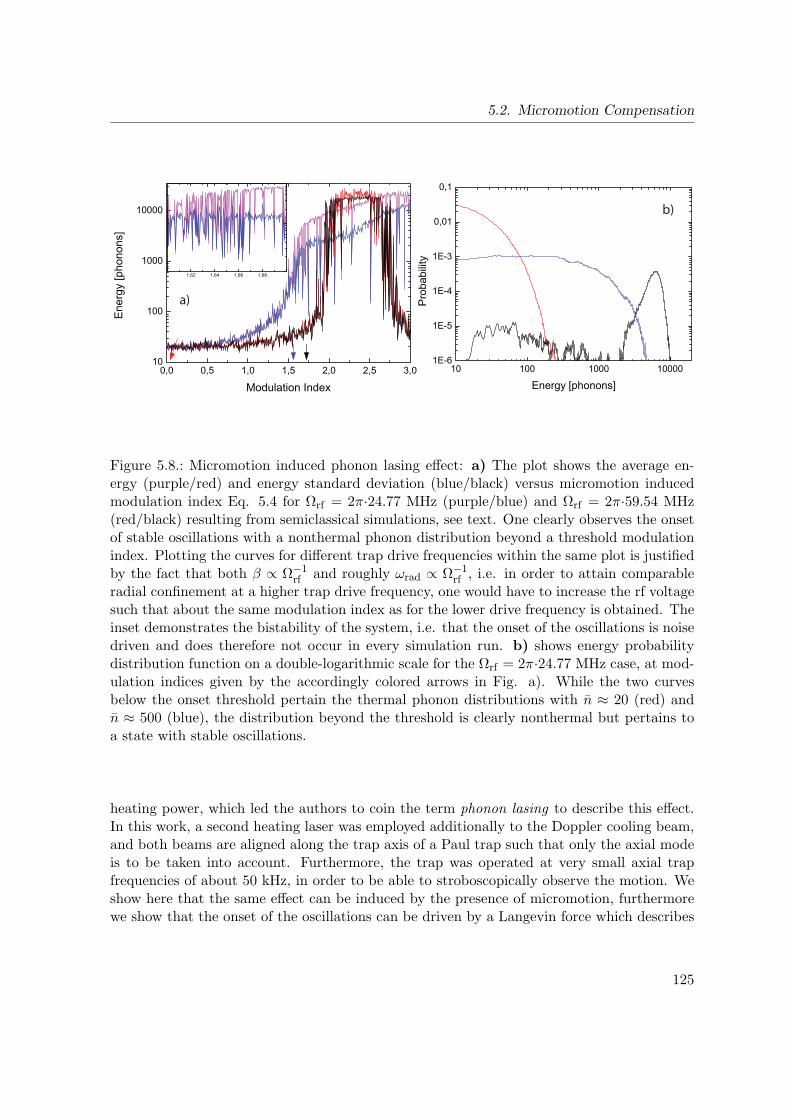
5.2. Micromotion Compensation
10 100 1000 100001E-6
1E-5
1E-4
1E-3
0,01
0,1
Pro
babi
lity
Energy [phonons]0,0 0,5 1,0 1,5 2,0 2,5 3,0
10
100
1000
10000
Ene
rgy
[pho
nons
]
Modulation Index
1,62 1,64 1,66 1,68
a)
b)
Figure 5.8.: Micromotion induced phonon lasing effect: a) The plot shows the average en-ergy (purple/red) and energy standard deviation (blue/black) versus micromotion inducedmodulation index Eq. 5.4 for Ωrf = 2π·24.77 MHz (purple/blue) and Ωrf = 2π·59.54 MHz(red/black) resulting from semiclassical simulations, see text. One clearly observes the onsetof stable oscillations with a nonthermal phonon distribution beyond a threshold modulationindex. Plotting the curves for different trap drive frequencies within the same plot is justifiedby the fact that both β ∝ Ω−1
rf and roughly ωrad ∝ Ω−1rf , i.e. in order to attain comparable
radial confinement at a higher trap drive frequency, one would have to increase the rf voltagesuch that about the same modulation index as for the lower drive frequency is obtained. Theinset demonstrates the bistability of the system, i.e. that the onset of the oscillations is noisedriven and does therefore not occur in every simulation run. b) shows energy probabilitydistribution function on a double-logarithmic scale for the Ωrf = 2π·24.77 MHz case, at mod-ulation indices given by the accordingly colored arrows in Fig. a). While the two curvesbelow the onset threshold pertain the thermal phonon distributions with n ≈ 20 (red) andn ≈ 500 (blue), the distribution beyond the threshold is clearly nonthermal but pertains toa state with stable oscillations.
heating power, which led the authors to coin the term phonon lasing to describe this effect.In this work, a second heating laser was employed additionally to the Doppler cooling beam,and both beams are aligned along the trap axis of a Paul trap such that only the axial modeis to be taken into account. Furthermore, the trap was operated at very small axial trapfrequencies of about 50 kHz, in order to be able to stroboscopically observe the motion. Weshow here that the same effect can be induced by the presence of micromotion, furthermorewe show that the onset of the oscillations can be driven by a Langevin force which describes
125

5. Trap Characteristics
the random recoil kicks from emitted photons during Doppler cooling. Finally, we commenton the impact of these effects on micro ion trap based quantum information experiments andpoint out possible technological improvements.In the presence of a Doppler cooling laser, the position coordinate xi in direction i withharmonic confinement ωi obeys to the equation of motion
xi +kim
R(x) + ω2i xi = χi(t, R(x)), (5.11)
where the second (cooling) term is comprised of the photon recoil ki and the photon scat-tering rate R(v) given by Eq. 2.30. The term on the right-hand side is a Langevin forcearising from photon emission in random direction. In contrast to Ref. [Vah10], this is amore general approach which does not require small saturation parameters and allows forthe consideration of three spatial dimensions. For the solution of this differential equationby numerical integration with time step dt, Nph = R(x) · dt photons are scattered within dt(which is assumed to be smaller than the trap periods). This results in a momentum kickin direction i which is a random variable with Gaussian distribution with zero mean and astandard deviation of σ =
√Nph/3. Micromotion is included by employing Eq. 5.6 for the
scattering rate, where the modulation index β is given by the projection of the micromotionamplitude vector on the normalized laser wavevector: β = β ·k0. The effect of the micromo-tion thus is to add ’extra laser beams’ at frequencies ±nΩrf with integer n. Frequencies onthe blue side of the atomic resonance contribute to heating instead of cooling. The net effectdepends on the total saturation, the carrier detuning and the secular and rf frequencies aswell as the beam and micromotion alignment. Due to this rather complex parameter space,the situation is not easily accessed. To start with, we illustrate the effect by calculating anatomic trajectory over a long time interval (several ms) for typical trap operating parameters(S0=2, ∆ = −Γ/2, Ωrf = 2π·24.77 MHz, ωz,y,x = 2π·1.4,3.1,3.6 MHz), but varying micromo-tion amplitude β. The beam is assumed to be at 45 with the z direction and at 60 withthe y and x directions. The resulting energy statistics are shown in Fig. 5.8. One can clearlyobserve how the Doppler cooling is adversely affected at increasing micromotion amplitudes,however the energy distribution is still thermal until at the critical micromotion amplitudethe mean energy exceeds the energy variance and classical oscillations set in.
126

6. Determination of Atomic MatrixElements with Off-Resonant Radiation
This chapter describes a new measurement method for atomic matrix elements for dipoletransitions, i.e. Einstein A coefficients or lifetimes developed as a side-product during theestablishment of the methods for the spin qubit. The basic measurement idea is to com-pare absorptive and dispersive effects occurring in the interaction of a trapped ion with anoff-resonant laser beam. The chapter is organized as follows: Sec. 6.1 gives a scientific mo-tivation, while Sec. 6.2 introduces the particular measurement scheme. Sec. 6.3 explainsin detail how the absorptive effect is measured, whereas Sec. 6.5 explains the measurementprocedure for the dispersive effects and 6.4 describes how a calibration of the laser detuningis carried out. Sec. 6.6 treats the robustness of the method against dominant experimentalimperfections, while Sec. 6.7 describes in detail how the error estimates are obtained. Sec.6.8 then presents the final results. Sec. 6.9 discusses the relevance of additional error sources,and Sec. 6.10 concludes with the presentation of an alternative measurement scheme for thedispersive effects.
6.1. Motivation
6.2. Basic Idea of the Measurement Procedure
Exposure to an off-resonant light beam can cause two different effects in an atomic system:Spontaneous Raman transitions between atomic levels by off-resonant inelastic scattering andAC Stark energy shifts of the levels, i.e. absorptive and dispersive effects. Both effects can bequantitatively measured, and both depend on the intensity and detuning of the off-resonantbeam, whereas only the Raman transition rates depend on the lifetime of the intermediateexcited state. The idea is therefore to measure the AC Stark shift as a calibration of laserintensity, such that the lifetime can then be inferred from the Raman transition rates.
The inelastic spontaneous Raman transition rates, from now on referred to as spin-flipscattering rates between the ground state Zeeman sublevels upon exposure to the off-resonantbeam are inferred from Eq. A.14 and Eq. A.15
R↑ = ΓPSΩ2
4∆2R
1
9
(ε2− + ε20
)R↓ = ΓPS
Ω2
4∆2R
1
9
(ε2+ + ε20
), (6.1)
127
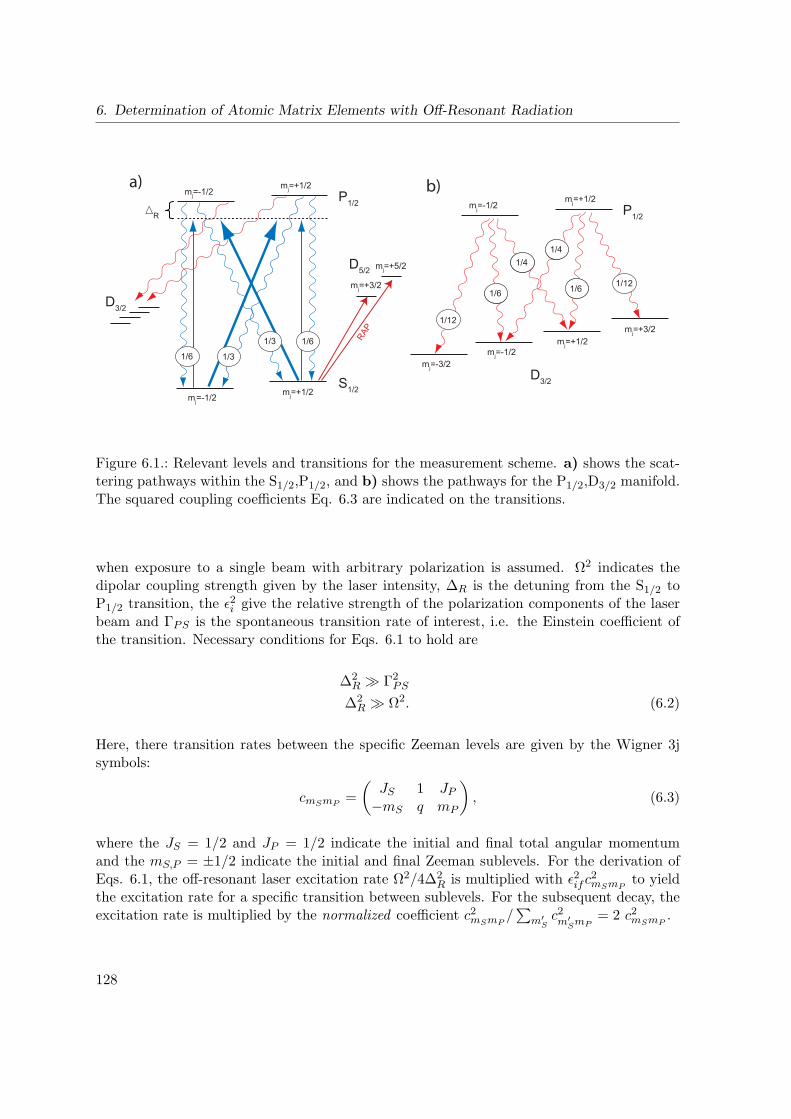
6. Determination of Atomic Matrix Elements with Off-Resonant Radiation
1/6
S1/2
D5/2
P1/2
D3/2
R
mj=+5/2
mj=+1/2mj=-1/2
mj=-1/2mj=+1/2
RAP
1/6 1/3
1/3
mj=+3/2
P1/2mj=-1/2
mj=+1/2
D3/2
mj=+1/2mj=-1/2
mj=+3/2
mj=-3/2
1/12
1/121/61/61/61/6
1/61/41/61/4
a) b)
Figure 6.1.: Relevant levels and transitions for the measurement scheme. a) shows the scat-tering pathways within the S1/2,P1/2, and b) shows the pathways for the P1/2,D3/2 manifold.The squared coupling coefficients Eq. 6.3 are indicated on the transitions.
when exposure to a single beam with arbitrary polarization is assumed. Ω2 indicates thedipolar coupling strength given by the laser intensity, ∆R is the detuning from the S1/2 toP1/2 transition, the ε2i give the relative strength of the polarization components of the laserbeam and ΓPS is the spontaneous transition rate of interest, i.e. the Einstein coefficient ofthe transition. Necessary conditions for Eqs. 6.1 to hold are
∆2R Γ2
PS
∆2R Ω2. (6.2)
Here, there transition rates between the specific Zeeman levels are given by the Wigner 3jsymbols:
cmSmP =
(JS 1 JP
−mS q mP
), (6.3)
where the JS = 1/2 and JP = 1/2 indicate the initial and final total angular momentumand the mS,P = ±1/2 indicate the initial and final Zeeman sublevels. For the derivation ofEqs. 6.1, the off-resonant laser excitation rate Ω2/4∆2
R is multiplied with ε2ifc2mSmP
to yieldthe excitation rate for a specific transition between sublevels. For the subsequent decay, theexcitation rate is multiplied by the normalized coefficient c2mSmP
/∑
m′Sc2m′
SmP= 2 c2mSmP
.
128
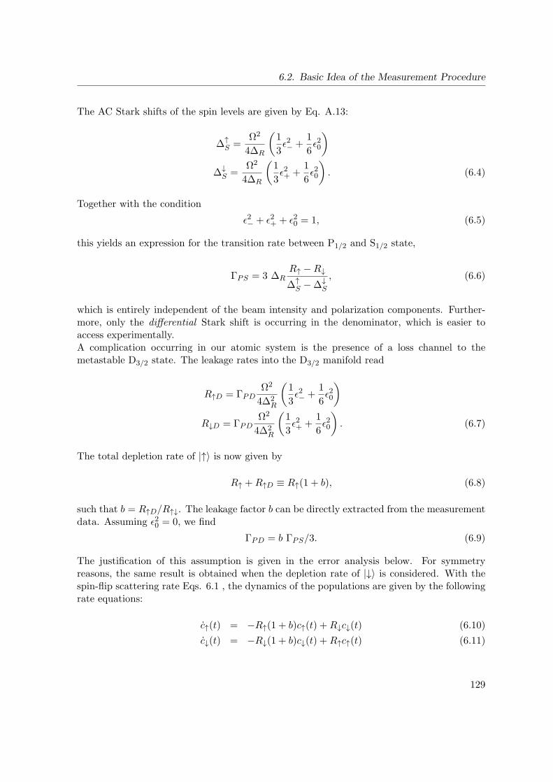
6.2. Basic Idea of the Measurement Procedure
The AC Stark shifts of the spin levels are given by Eq. A.13:
∆↑S =
Ω2
4∆R
(1
3ε2− +
1
6ε20
)
∆↓S =
Ω2
4∆R
(1
3ε2+ +
1
6ε20
). (6.4)
Together with the condition
ε2− + ε2+ + ε20 = 1, (6.5)
this yields an expression for the transition rate between P1/2 and S1/2 state,
ΓPS = 3 ∆RR↑ −R↓∆↑
S −∆↓S
, (6.6)
which is entirely independent of the beam intensity and polarization components. Further-more, only the differential Stark shift is occurring in the denominator, which is easier toaccess experimentally.A complication occurring in our atomic system is the presence of a loss channel to themetastable D3/2 state. The leakage rates into the D3/2 manifold read
R↑D = ΓPDΩ2
4∆2R
(1
3ε2− +
1
6ε20
)
R↓D = ΓPDΩ2
4∆2R
(1
3ε2+ +
1
6ε20
). (6.7)
The total depletion rate of |↑〉 is now given by
R↑ +R↑D ≡ R↑(1 + b), (6.8)
such that b = R↑D/R↑↓. The leakage factor b can be directly extracted from the measurementdata. Assuming ε20 = 0, we find
ΓPD = b ΓPS/3. (6.9)
The justification of this assumption is given in the error analysis below. For symmetryreasons, the same result is obtained when the depletion rate of |↓〉 is considered. With thespin-flip scattering rate Eqs. 6.1 , the dynamics of the populations are given by the followingrate equations:
c↑(t) = −R↑(1 + b)c↑(t) +R↓c↓(t) (6.10)
c↓(t) = −R↓(1 + b)c↓(t) +R↑c↑(t) (6.11)
129
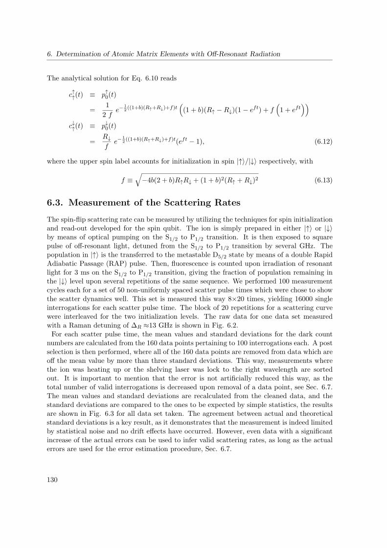
6. Determination of Atomic Matrix Elements with Off-Resonant Radiation
The analytical solution for Eq. 6.10 reads
c↑↑(t) ≡ p↑0(t)
=1
2 fe−
12((1+b)(R↑+R↓)+f)t
((1 + b)(R↑ −R↓)(1− eft) + f
(1 + eft
))c↓↑(t) ≡ p↓0(t)
=R↓f
e−12((1+b)(R↑+R↓)+f)t(eft − 1), (6.12)
where the upper spin label accounts for initialization in spin |↑〉/|↓〉 respectively, with
f ≡√
−4b(2 + b)R↑R↓ + (1 + b)2(R↑ +R↓)2 (6.13)
6.3. Measurement of the Scattering Rates
The spin-flip scattering rate can be measured by utilizing the techniques for spin initializationand read-out developed for the spin qubit. The ion is simply prepared in either |↑〉 or |↓〉by means of optical pumping on the S1/2 to P1/2 transition. It is then exposed to squarepulse of off-resonant light, detuned from the S1/2 to P1/2 transition by several GHz. Thepopulation in |↑〉 is the transferred to the metastable D5/2 state by means of a double RapidAdiabatic Passage (RAP) pulse. Then, fluorescence is counted upon irradiation of resonantlight for 3 ms on the S1/2 to P1/2 transition, giving the fraction of population remaining inthe |↓〉 level upon several repetitions of the same sequence. We performed 100 measurementcycles each for a set of 50 non-uniformly spaced scatter pulse times which were chose to showthe scatter dynamics well. This set is measured this way 8×20 times, yielding 16000 singleinterrogations for each scatter pulse time. The block of 20 repetitions for a scattering curvewere interleaved for the two initialization levels. The raw data for one data set measuredwith a Raman detuning of ∆R ≈13 GHz is shown in Fig. 6.2.For each scatter pulse time, the mean values and standard deviations for the dark count
numbers are calculated from the 160 data points pertaining to 100 interrogations each. A postselection is then performed, where all of the 160 data points are removed from data which areoff the mean value by more than three standard deviations. This way, measurements wherethe ion was heating up or the shelving laser was lock to the right wavelength are sortedout. It is important to mention that the error is not artificially reduced this way, as thetotal number of valid interrogations is decreased upon removal of a data point, see Sec. 6.7.The mean values and standard deviations are recalculated from the cleaned data, and thestandard deviations are compared to the ones to be expected by simple statistics, the resultsare shown in Fig. 6.3 for all data set taken. The agreement between actual and theoreticalstandard deviations is a key result, as it demonstrates that the measurement is indeed limitedby statistical noise and no drift effects have occurred. However, even data with a significantincrease of the actual errors can be used to infer valid scattering rates, as long as the actualerrors are used for the error estimation procedure, Sec. 6.7.
130
6.4. Measurement of the Raman Detuning
0,0 0,5 1,0 1,5 2,00,0
0,2
0,4
b)
Dar
k C
ount
Fra
ctio
n
Scatter Pulse time [ms]0,0 0,5 1,0 1,5 2,0
0,0
0,2
0,4
0,6
0,8
1,0
Dar
k C
ount
Fra
ctio
n
Scatter Pulse time [ms]
a)
Figure 6.2.: Raw data from the scattering rate measurement. Each point corresponds to 100interrogations. Curve a) results from initialization in |↑〉, b) is for initialization in |↓〉. Notethe different vertical scales.
6.4. Measurement of the Raman Detuning
The remaining quantity to be measured is the Raman detuning ∆R occurring in Eq. 6.6. Thelaser frequency is simply read off an High Finesse WSU wavemeter which has 10 MHz relativeaccuracy. As the detuning is relative to the atomic resonance, its position has to be measuredas well. This can be done in two ways: First, the scattering laser can be simply tuned toresonance as the laser frequency for which the maximum fluorescence occurs is identified asthe atomic resonance. The results are shown in Fig. 6.5.
The second method is to perform additional Stark shift measurements for different detun-ings. According to Eq. 6.4, 1/∆S should depend linearly on the detuning, such that thezero of a line fitted through several measured Stark shifts also gives the resonance frequency.However, it is found that the deviation of the measured data from the fit exceeds the expectederror. This is attributed to optical elements in the beam which might change the intensityand polarization of the laser at the location of the ion depending on the frequency. Further-more, for small detunings the Stark shift deviates from Eq. 6.4, and for large detunings theStark shift arising from the P3/2 also plays a role.
6.5. Measurement of the AC Stark Shift
The differential Stark shift measurement is accomplished in entirely the same way as alreadydescribed in Sec. 4.7: A pulse from the off-resonant laser beam at variable duration is insertedbetween two Ramsey pulses, the resulting oscillatory pattern with respect to the shift pulseduration reveals the Stark shift ∆S according to
S(t) = a e−γ t sin(∆S t+ φ) + b, (6.14)
131
6. Determination of Atomic Matrix Elements with Off-Resonant Radiation
0 10 20 30 40 500,015
0,020
0,025
0,030
0,035
0,040
0,045
d)
index
0 10 20 30 40 50
0,02
0,03
0,04
0,05 c)
10 20 30 40 500,01
0,02
0,03
0,04
0,05
0,06
Rel
ativ
e Er
ror
a)
10 20 30 40 500,015
0,020
0,025
0,030
0,035
0,040
0,045
b)
Rel
ativ
e Er
ror
index
Figure 6.3.: Comparison between the actual spreads of the raw data point (red dots) and thestatistical expectation (solid curve). Curves a) and b) pertain to the 15 GHz datasets, c) andd) to the 14 GHz ones. a) and c) are for initialization in |↑〉, b) and d) for initialization in|↓〉. The horizontal axis gives the data index instead of the scatter pulse time.
where amplitude a, baseline b, dephasing rate γ and offset phase φ are floating. Due to thefact that the oscillation frequency can be extracted from the data with high precision, thismeasurement takes much less effort in data acquisition and evaluation as the scattering ratemeasurement. Furthermore, as only the frequency of the oscillation pattern is relevant, theprecision does not rely on stable readout and preparation, such that the stability of the laserintensity and polarization can also be evaluated. An example data set is shown in Fig. 6.6.
Measurements of the Stark shift were performed several times for each data set pertainingto a fixed Raman detuning. From the spread of the obtained values, the long-term stabilitylimiting the total accuracy is calculated, which is used in the final evaluation to determine thetotal accuracy. The measured values for the shift are shown in Fig. 6.7, note that the totalspread in the 0.25% range is much larger the uncertainty of a single measurement, which isin the sub-per mil range.
132
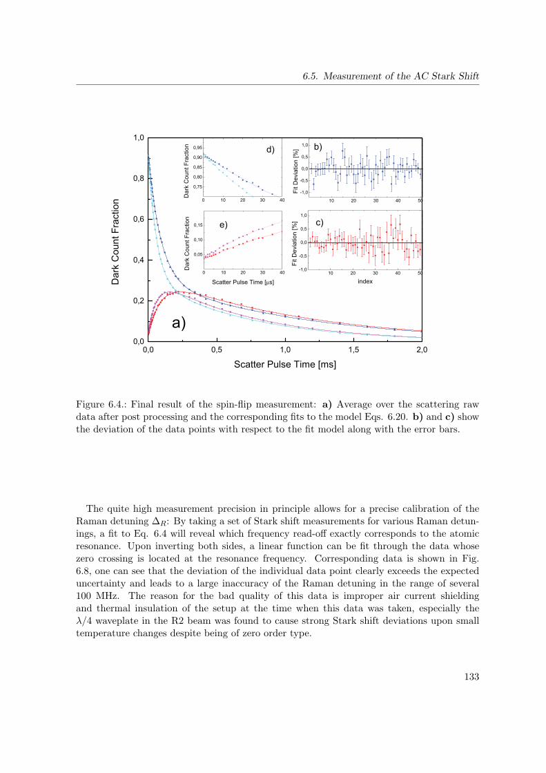
6.5. Measurement of the AC Stark Shift
0 10 20 30 40
0,05
0,10
0,15
Dar
k C
ount
Fra
ctio
n
Scatter Pulse Time [µs]
e)
0 10 20 30 40
0,75
0,80
0,85
0,90
0,95
Dar
k C
ount
Fra
ctio
n d)
10 20 30 40 50-1,0
-0,5
0,0
0,5
1,0
Fit D
evia
tion
[%]
index
c)
10 20 30 40 50
-1,0
-0,5
0,0
0,5
1,0 b)
Fit D
evia
tion
[%]
0,0 0,5 1,0 1,5 2,00,0
0,2
0,4
0,6
0,8
1,0
Dar
k C
ount
Fra
ctio
n
Scatter Pulse Time [ms]
a)
Figure 6.4.: Final result of the spin-flip measurement: a) Average over the scattering rawdata after post processing and the corresponding fits to the model Eqs. 6.20. b) and c) showthe deviation of the data points with respect to the fit model along with the error bars.
The quite high measurement precision in principle allows for a precise calibration of theRaman detuning ∆R: By taking a set of Stark shift measurements for various Raman detun-ings, a fit to Eq. 6.4 will reveal which frequency read-off exactly corresponds to the atomicresonance. Upon inverting both sides, a linear function can be fit through the data whosezero crossing is located at the resonance frequency. Corresponding data is shown in Fig.6.8, one can see that the deviation of the individual data point clearly exceeds the expecteduncertainty and leads to a large inaccuracy of the Raman detuning in the range of several100 MHz. The reason for the bad quality of this data is improper air current shieldingand thermal insulation of the setup at the time when this data was taken, especially theλ/4 waveplate in the R2 beam was found to cause strong Stark shift deviations upon smalltemperature changes despite being of zero order type.
133
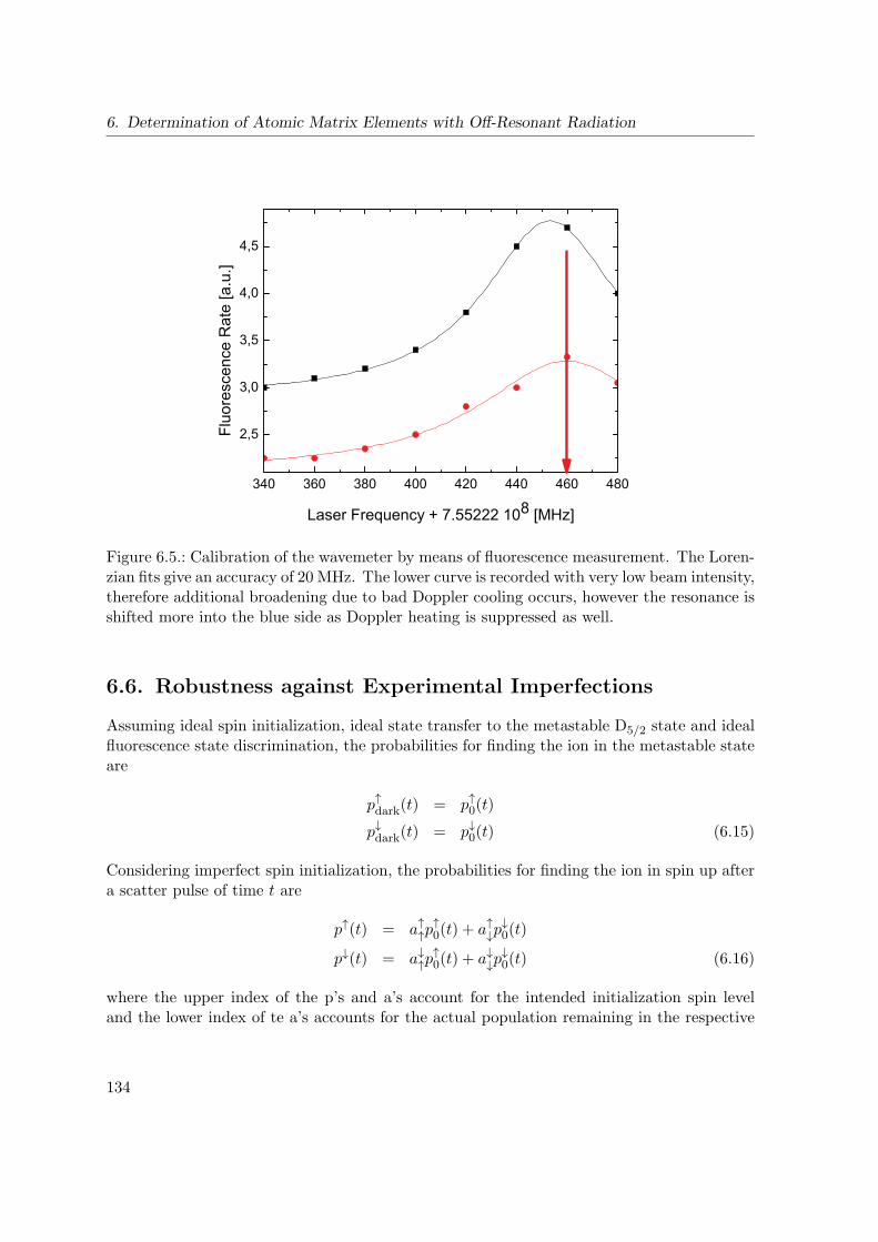
6. Determination of Atomic Matrix Elements with Off-Resonant Radiation
340 360 380 400 420 440 460 480
2,5
3,0
3,5
4,0
4,5Fl
uore
scen
ce R
ate
[a.u
.]
Laser Frequency + 7.55222 108 [MHz]
Figure 6.5.: Calibration of the wavemeter by means of fluorescence measurement. The Loren-zian fits give an accuracy of 20 MHz. The lower curve is recorded with very low beam intensity,therefore additional broadening due to bad Doppler cooling occurs, however the resonance isshifted more into the blue side as Doppler heating is suppressed as well.
6.6. Robustness against Experimental Imperfections
Assuming ideal spin initialization, ideal state transfer to the metastable D5/2 state and idealfluorescence state discrimination, the probabilities for finding the ion in the metastable stateare
p↑dark(t) = p↑0(t)
p↓dark(t) = p↓0(t) (6.15)
Considering imperfect spin initialization, the probabilities for finding the ion in spin up aftera scatter pulse of time t are
p↑(t) = a↑↑p↑0(t) + a↑↓p
↓0(t)
p↓(t) = a↓↑p↑0(t) + a↓↓p
↓0(t) (6.16)
where the upper index of the p’s and a’s account for the intended initialization spin leveland the lower index of te a’s accounts for the actual population remaining in the respective
134
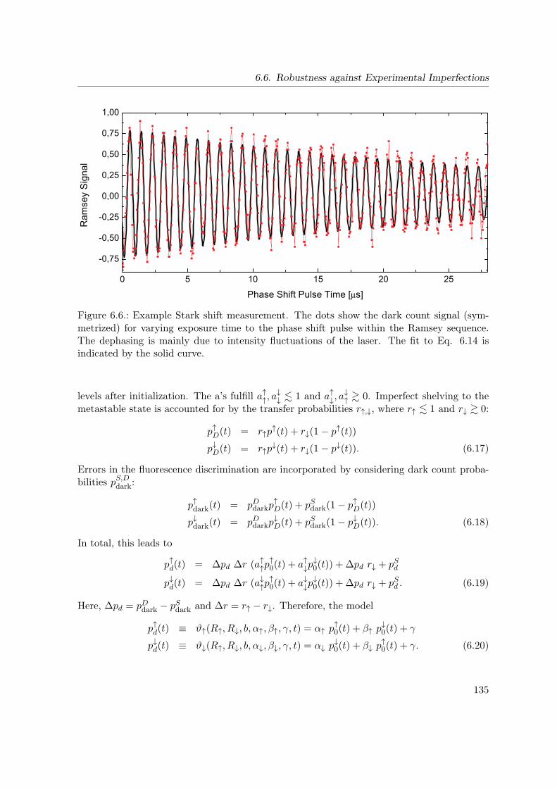
6.6. Robustness against Experimental Imperfections
0 5 10 15 20 25
-0,75
-0,50
-0,25
0,00
0,25
0,50
0,75
1,00
Ram
sey
Sig
nal
Phase Shift Pulse Time [µs]
Figure 6.6.: Example Stark shift measurement. The dots show the dark count signal (sym-metrized) for varying exposure time to the phase shift pulse within the Ramsey sequence.The dephasing is mainly due to intensity fluctuations of the laser. The fit to Eq. 6.14 isindicated by the solid curve.
levels after initialization. The a’s fulfill a↑↑, a↓↓ 1 and a↑↓, a
↓↑ 0. Imperfect shelving to the
metastable state is accounted for by the transfer probabilities r↑,↓, where r↑ 1 and r↓ 0:
p↑D(t) = r↑p↑(t) + r↓(1− p↑(t))
p↓D(t) = r↑p↓(t) + r↓(1− p↓(t)). (6.17)
Errors in the fluorescence discrimination are incorporated by considering dark count proba-bilities pS,Ddark:
p↑dark(t) = pDdarkp↑D(t) + pSdark(1− p↑D(t))
p↓dark(t) = pDdarkp↓D(t) + pSdark(1− p↓D(t)). (6.18)
In total, this leads to
p↑d(t) = ∆pd ∆r (a↑↑p↑0(t) + a↑↓p
↓0(t)) + ∆pd r↓ + pSd
p↓d(t) = ∆pd ∆r (a↓↑p↑0(t) + a↓↓p
↓0(t)) + ∆pd r↓ + pSd . (6.19)
Here, ∆pd = pDdark − pSdark and ∆r = r↑ − r↓. Therefore, the model
p↑d(t) ≡ ϑ↑(R↑, R↓, b, α↑, β↑, γ, t) = α↑ p↑0(t) + β↑ p↓0(t) + γ
p↓d(t) ≡ ϑ↓(R↑, R↓, b, α↓, β↓, γ, t) = α↓ p↓0(t) + β↓ p↑0(t) + γ. (6.20)
135
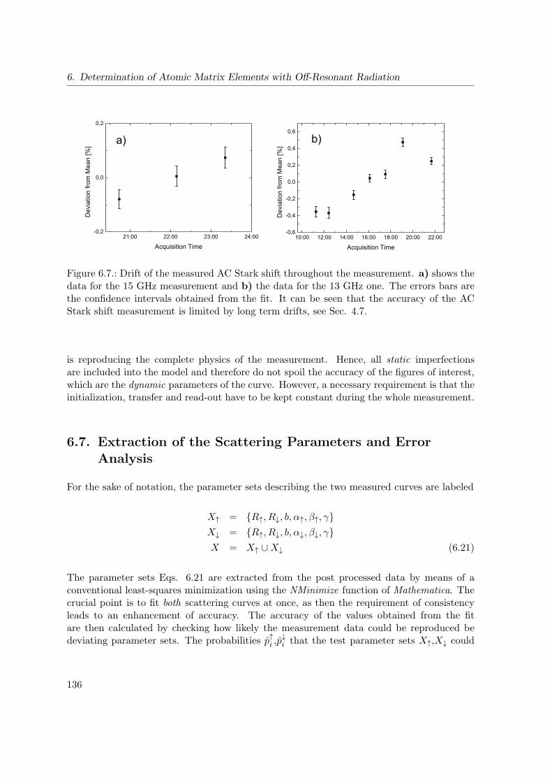
6. Determination of Atomic Matrix Elements with Off-Resonant Radiation
21:00 22:00 23:00 24:00-0,2
0,0
0,2
Dev
iatio
n fro
m M
ean
[%]
Acquisition Time
a)
10:00 12:00 14:00 16:00 18:00 20:00 22:00-0,6
-0,4
-0,2
0,0
0,2
0,4
0,6b)
Dev
iatio
n fro
m M
ean
[%]
Acquisition Time
Figure 6.7.: Drift of the measured AC Stark shift throughout the measurement. a) shows thedata for the 15 GHz measurement and b) the data for the 13 GHz one. The errors bars arethe confidence intervals obtained from the fit. It can be seen that the accuracy of the ACStark shift measurement is limited by long term drifts, see Sec. 4.7.
is reproducing the complete physics of the measurement. Hence, all static imperfectionsare included into the model and therefore do not spoil the accuracy of the figures of interest,which are the dynamic parameters of the curve. However, a necessary requirement is that theinitialization, transfer and read-out have to be kept constant during the whole measurement.
6.7. Extraction of the Scattering Parameters and ErrorAnalysis
For the sake of notation, the parameter sets describing the two measured curves are labeled
X↑ = R↑, R↓, b, α↑, β↑, γX↓ = R↑, R↓, b, α↓, β↓, γX = X↑ ∪X↓ (6.21)
The parameter sets Eqs. 6.21 are extracted from the post processed data by means of aconventional least-squares minimization using the NMinimize function of Mathematica. Thecrucial point is to fit both scattering curves at once, as then the requirement of consistencyleads to an enhancement of accuracy. The accuracy of the values obtained from the fitare then calculated by checking how likely the measurement data could be reproduced bedeviating parameter sets. The probabilities p↑i ,p
↓i that the test parameter sets X↑,X↓ could
136
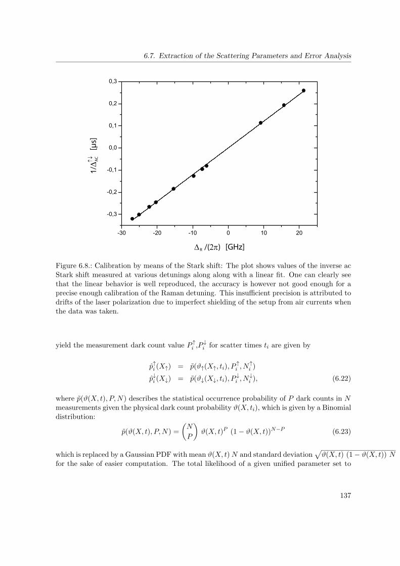
6.7. Extraction of the Scattering Parameters and Error Analysis
-30 -20 -10 0 10 20
-0,3
-0,2
-0,1
0,0
0,1
0,2
0,3
[GHz]R∆ /(2π)
↑↓ ∆A
C1/
[µs]
Figure 6.8.: Calibration by means of the Stark shift: The plot shows values of the inverse acStark shift measured at various detunings along along with a linear fit. One can clearly seethat the linear behavior is well reproduced, the accuracy is however not good enough for aprecise enough calibration of the Raman detuning. This insufficient precision is attributed todrifts of the laser polarization due to imperfect shielding of the setup from air currents whenthe data was taken.
yield the measurement dark count value P ↑i ,P
↓i for scatter times ti are given by
p↑i (X↑) = p(ϑ↑(X↑, ti), P↑i , N
↑i )
p↓i (X↓) = p(ϑ↓(X↓, ti), P↓i , N
↓i ), (6.22)
where p(ϑ(X, t), P,N) describes the statistical occurrence probability of P dark counts in Nmeasurements given the physical dark count probability ϑ(X, ti), which is given by a Binomialdistribution:
p(ϑ(X, t), P,N) =
(N
P
)ϑ(X, t)P (1− ϑ(X, t))N−P (6.23)
which is replaced by a Gaussian PDF with mean ϑ(X, t)N and standard deviation√
ϑ(X, t) (1− ϑ(X, t)) Nfor the sake of easier computation. The total likelihood of a given unified parameter set to
137
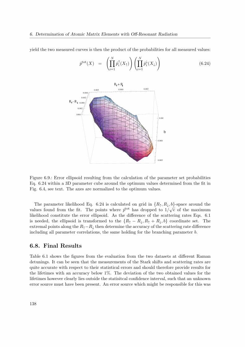
6. Determination of Atomic Matrix Elements with Off-Resonant Radiation
yield the two measured curves is then the product of the probabilities for all measured values:
ptot(X) =
(N∏i=1
p↑i (X↑)
)(N∏i=1
p↓i (X↓)
)(6.24)
0.004
0.002
0.000
0.002
0.004
0.005 0.000 0.005
0.005
0.000
0.005
R + R
R - R
b
Figure 6.9.: Error ellipsoid resulting from the calculation of the parameter set probabilitiesEq. 6.24 within a 3D parameter cube around the optimum values determined from the fit inFig. 6.4, see text. The axes are normalized to the optimum values.
The parameter likelihood Eq. 6.24 is calculated on grid in R↑, R↓, b-space around thevalues found from the fit. The points where ptot has dropped to 1/
√e of the maximum
likelihood constitute the error ellipsoid. As the difference of the scattering rates Eqs. 6.1is needed, the ellipsoid is transformed to the R↑ − R↓, R↑ + R↓, b coordinate set. Theextremal points along the R↑−R↓ then determine the accuracy of the scattering rate differenceincluding all parameter correlations, the same holding for the branching parameter b.
6.8. Final Results
Table 6.1 shows the figures from the evaluation from the two datasets at different Ramandetunings. It can be seen that the measurements of the Stark shifts and scattering rates arequite accurate with respect to their statistical errors and should therefore provide results forthe lifetimes with an accuracy below 1%. The deviation of the two obtained values for thelifetimes however clearly lies outside the statisitcal confidence interval, such that an unknownerror source must have been present. An error source which might be responsible for this was
138
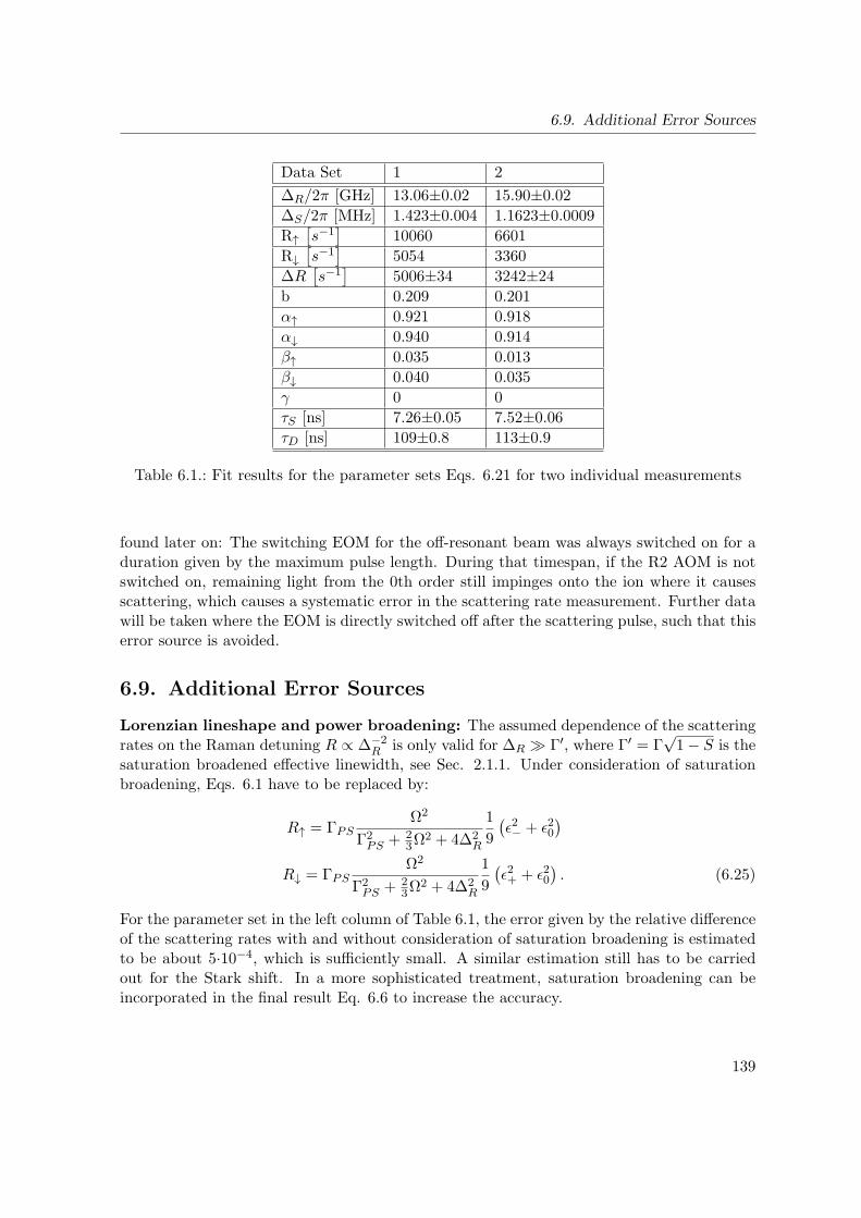
6.9. Additional Error Sources
Data Set 1 2
∆R/2π [GHz] 13.06±0.02 15.90±0.02
∆S/2π [MHz] 1.423±0.004 1.1623±0.0009
R↑[s−1]
10060 6601
R↓[s−1]
5054 3360
∆R[s−1]
5006±34 3242±24
b 0.209 0.201
α↑ 0.921 0.918
α↓ 0.940 0.914
β↑ 0.035 0.013
β↓ 0.040 0.035
γ 0 0
τS [ns] 7.26±0.05 7.52±0.06
τD [ns] 109±0.8 113±0.9
Table 6.1.: Fit results for the parameter sets Eqs. 6.21 for two individual measurements
found later on: The switching EOM for the off-resonant beam was always switched on for aduration given by the maximum pulse length. During that timespan, if the R2 AOM is notswitched on, remaining light from the 0th order still impinges onto the ion where it causesscattering, which causes a systematic error in the scattering rate measurement. Further datawill be taken where the EOM is directly switched off after the scattering pulse, such that thiserror source is avoided.
6.9. Additional Error Sources
Lorenzian lineshape and power broadening: The assumed dependence of the scatteringrates on the Raman detuning R ∝ ∆−2
R is only valid for ∆R Γ′, where Γ′ = Γ√1− S is the
saturation broadened effective linewidth, see Sec. 2.1.1. Under consideration of saturationbroadening, Eqs. 6.1 have to be replaced by:
R↑ = ΓPSΩ2
Γ2PS + 2
3Ω2 + 4∆2
R
1
9
(ε2− + ε20
)
R↓ = ΓPSΩ2
Γ2PS + 2
3Ω2 + 4∆2
R
1
9
(ε2+ + ε20
). (6.25)
For the parameter set in the left column of Table 6.1, the error given by the relative differenceof the scattering rates with and without consideration of saturation broadening is estimatedto be about 5·10−4, which is sufficiently small. A similar estimation still has to be carriedout for the Stark shift. In a more sophisticated treatment, saturation broadening can beincorporated in the final result Eq. 6.6 to increase the accuracy.
139
6. Determination of Atomic Matrix Elements with Off-Resonant Radiation
Scattering curve offset: One might be surprised by the fact that the values for γ in thescattering parameters Eq. 6.21 are found to be zero, however an analysis of the underlyingphysics leads to a justification the γ is indeed negligible. According to Eq. 6.20, the definingquantities for γ are the false transfer probability from |↓〉, r↓, and the probability the fluo-rescence below discrimination threshold is detected albeit the ion is in the bright S1/2,D3/2
manifold, pSd . The false transfer probability is below 1%, which is shown in Fig. 4.21. Thistranslates into a much smaller error in the scattering parameters, because the offset is only astatic parameter. pSd can be calculated from the fluorescence rates, which were 25 kHz brightcounts and 4 kHz dark counts for 3 ms detection time. The result is pSd 10−7,see Ref.[Roo00], pp. 119.Resonant beam components: The laser source for the off-resonant beam is derived froman amplified system with an ASE background spanning several nm, such that sum frequencygeneration (SFG) with a laser photon and an ASE photon could in principle lead to nearresonant components in the doubled beam which might strongly enhance the scattering rate.The conditions for this process would be that the Raman detuning is an integer multipleof two times the SHG cavity FSR of about 500 MHz, furthermore phase matching condi-tions for SFG have to be fulfilled. To assert that this effect plays no role, a measurementwas performed where a scattering pulse of fixed power and duration such that roughly 20%of population of the initially populated |↑〉 level is removed, while the laser wavelength isscanned sufficiently slow over four SHG cavity FSRs. No resonant features were observed,such we can claim that the SFG effect does not contribute to scattering.Presence of the P3/2 state: The P3/2 state also contributes to the Stark shift and scat-tering rates, however the fine-structure splitting of about 6.8 THz is large compared to thetypical Raman detuning, leading to errors in the per mil range for the Stark shift and in the10−6 range for the scattering rates. However, the P3/2 contributions can be included in thetreatment leading to the result Eq. 6.6.Zeeman splitting: The Zeeman splitting of roughly 18 MHz within the S1/2 manifold androughly 6 MHz in the P1/2 manifold is small compared to the Raman detuning, the errorsare of similar magnitudes as for the reasoning for the P3/2 state above. Also in this case, themodel can be extended to include the Zeeman splitting.
6.10. Complete Measurement by Measuring Absolute StarkShifts
In this section we briefly present an extension of the measurement scheme which allows for acomplete determination of the parameters characterizing the interaction between an atomicsystem and a classical laser beam. In the final result for the lifetime of the excited state,Eq. 6.6, the Rabi frequency Ω and the polarization components εi drop out. However, ifthe Stark shifts of the levels |↑〉 and |↓〉 can be measured individually, one obtains sufficient
140

6.10. Complete Measurement by Measuring Absolute Stark Shifts
1/6
S1/2
D5/2
P1/2R
mj=+5/2
mj=+1/2mj=-1/2
mj=-1/2mj=+1/2
1/6
1/31/3
mj=+3/2
Figure 6.10.: Level scheme for absolute Stark shift measurement: The two red arrows indicatethe transitions on which the absolute Stark shifts of the |↑〉 and |↓〉 are probed.
information to determine all unknown parameters. We obtain the Rabi frequency
Ω2 = 12 ∆R
(∆↑
S +∆↓S
), (6.26)
and the polarization components:
ε2+ =R↓∆
↓S +R↓∆
↑S − 2 R↑∆
↓S(
∆↑S +∆↓
S
)(R↑ −R↓)
ε2− =2 R↓∆
↑S −R↑∆
↓S −R↑∆
↑S(
∆↑S +∆↓
S
)(R↑ −R↓)
ε20 = −2R↓∆
↑S −R↑∆
↓S(
∆↑S +∆↓
S
)(R↑ −R↓)
. (6.27)
In the case of the 40Ca+ ion, the quadrupole transition at 729 nm can be utilized to measurethe absolute Stark shifts. Fig. 6.10 shows the relevant transitions: The Stark shift of the|↑〉 levels is probed on the |↑〉 → |D5/2,mJ = +5/2〉 transition and the shift of the |↓〉 levelsis probed on the |↓〉 → |D5/2,mJ = +3/2〉 transition. The same basic Ramsey sequenceas in Sec. 6.5 is used, only that the 729 nm laser is employed for the Ramsey pulses, themeasurement sequences are depicted in Fig. 6.11 d). The precision of these measurementsis mostly impaired by the drift of the PDH cavity of the 729 nm laser stabilization. For aRamsey delay time of 20 µs and an absolute shift 2π·2 MHz, a resonance drift of 25 kHz wouldlead to an additional phase slip by π throughout the data acquisition, leading to a differenceof one fringe compared 40 expected ones, which amounts to an error of 2.5%. At typical drift
141

6. Determination of Atomic Matrix Elements with Off-Resonant Radiation
70,70 70,75 70,80 70,85 70,90 70,95 71,00 71,05 71,100,0
0,2
0,4
0,6
0,8
1,0
70,70 70,75 70,80 70,85 70,90 70,95 71,00 71,05 71,100,0
0,2
0,4
0,6
0,8
1,0
AOM-Frequency [MHz]
70,70 70,75 70,80 70,85 70,90 70,95 71,00 71,05 71,10-1,00
-0,75
-0,50
-0,25
0,00
0,25
0,50
0,75
1,00
Pop
ulat
ion
in
Diff
eren
ce s
igna
l
Pop
ulat
ion
in
(a) (b)
(c)(d)
(e)
AOM-Frequency [MHz]
AOM-Frequency [MHz]
Figure 6.11.: Measurement scheme for the absolute Stark shift: a) and b) show resultingRamsey fringes for the two measurement sequences indicated in e). The difference signal isshown in c) along with the capture range of the resonance tracking (dashed box). d) showsthe measurement sequence for the absolute Stark shift measurement.
rates of about 10 kHz per hour and data acquisition times of up to 20 minutes, this can leadto considerable measurement errors. The solution for this problem is an automatic tracking ofthe resonance performed during the actual measurement. To keep the measurement effort forthis at a minimum, a single measurement providing a value (instead of a curve from whichthe resonance locations can be derived as a fit parameter) from which the location of theresonance can be inferred is required. Such a measurement scheme was demonstrated in Ref.[Let04]: Two Ramsey measurements (without shift pulse) are performed where in one case theconcluding pulse has a +π/4 phase shift with respect to the first pulse, and the in the othercase the phase shift is −π/4. The sequences are depicted in Fig. 6.11 e). Measurement resultsfor the two sequences are shown in a) and b), and the difference between the two signals isshown in c). The signal within the dashed box has a zero crossing at resonance, this representsthe capture range for which a correction frequency can be calculated to calculate the newresonance frequency. The extra phase shift from an off-resonance of δ for a Ramsey delay τ
142
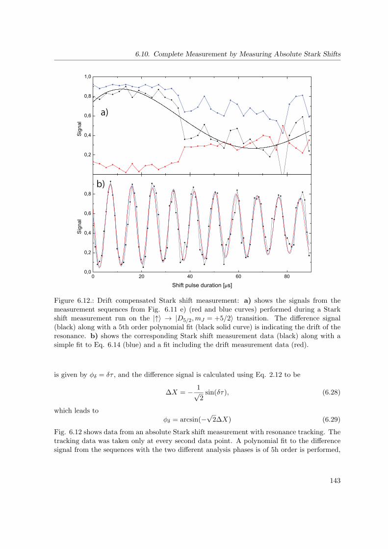
6.10. Complete Measurement by Measuring Absolute Stark Shifts
0 20 40 60 800,0
0,2
0,4
0,6
0,8
Sig
nal
Shift pulse duration [µs]
0,2
0,4
0,6
0,8
1,0S
igna
l
a)
b)
Figure 6.12.: Drift compensated Stark shift measurement: a) shows the signals from themeasurement sequences from Fig. 6.11 e) (red and blue curves) performed during a Starkshift measurement run on the |↑〉 → |D5/2,mJ = +5/2〉 transition. The difference signal(black) along with a 5th order polynomial fit (black solid curve) is indicating the drift of theresonance. b) shows the corresponding Stark shift measurement data (black) along with asimple fit to Eq. 6.14 (blue) and a fit including the drift measurement data (red).
is given by φδ = δτ , and the difference signal is calculated using Eq. 2.12 to be
∆X = − 1√2sin(δτ), (6.28)
which leads toφδ = arcsin(−
√2∆X) (6.29)
Fig. 6.12 shows data from an absolute Stark shift measurement with resonance tracking. Thetracking data was taken only at every second data point. A polynomial fit to the differencesignal from the sequences with the two different analysis phases is of 5h order is performed,
143

6. Determination of Atomic Matrix Elements with Off-Resonant Radiation
giving a smooth approximate time-dependent extra phase shift ∆X(t), which is incorporatedinto Eq. 6.14:
S(t) = a e−γ t sin(∆S t− φδ(t) + φ) + b. (6.30)
Fits to the simple model and the corrected model are shown in Fig. 6.12 b), where on cansee a considerable difference between the results. In this specific case, the relative differenceof the resulting shift is about 1.8%, which is clearly beyond the accuracy of the fit resultof 0.18%. We therefore conclude that the accuracy of the measurement can be increased byabout one order of magnitude by utilizing the resonance tracking method, which only doublesthe data acquisition effort.
144

7. Motional State Tomography
This chapter deals with the experimental reconstruction of the density matrix describingthe quantum state of the axial mode of vibration of a single trapped atom. The techniquesestablished for coherent qubit manipulation are now extended by Raman sideband cooling,which represents a necessary ingredient for the investigation of the quantized harmonic motionof the ion. The measurement presented in this chapter is to be seen as a demonstration ofquantum state tomography. The precise control and measurement of the ion’s motionalstate which is accomplished serves as a basis for many experiments, some of which havebeen performed within the scope of this thesis such as the ones presented in Sec. 8.3, whileenvisaged experiments in the field of quantum thermodynamics heavily rely on the techniquesdemonstrated here, see [Hub08],[Hub10a]. Rabi oscillations on the blue motional sidebandof the stimulated Raman transition between the qubit levels |↑〉 and |↓〉 provide informationabout the motional state, as it was demonstrated in Sec. 4.6. As can be seen from Eq.2.56, only the phonon occupation probabilities, i.e. the diagonal elements of the densitymatrix can be extracted from a single scan, no information about the off-diagonal elements isobtained. Thus, one has to resort to a measurement protocol where phonon distributions areacquired for various conditions, and from this data the density matrix can be reconstructed.Because of the analogy to experiments utilizing photons, where integrals of phase spacedistribution functions are measured from which these distribution can be obtained by meansof the inverse Radon transform, these measurement methods are summarized as quantum statetomography. A pioneering experiment on the generation and characterization of nonclassicalstates has been performed in [Mee96], which was extended to a tomographic reconstructionof the density matrix characterizing the quantum state of the system in [Lei96].
7.1. The Method
The tomography method of our choice consists in the acquisition of blue sideband Rabioscillations after an arbitrary additional displacement of the motional mode. The generalexpression for the probability Qk(α, ρ) the find k phonons after a displacement operationU(α) on the initial state described by the density matrix ρ is
Qk(α, ρ) = 〈k|U †(α) ρ U(α)|k〉. (7.1)
145
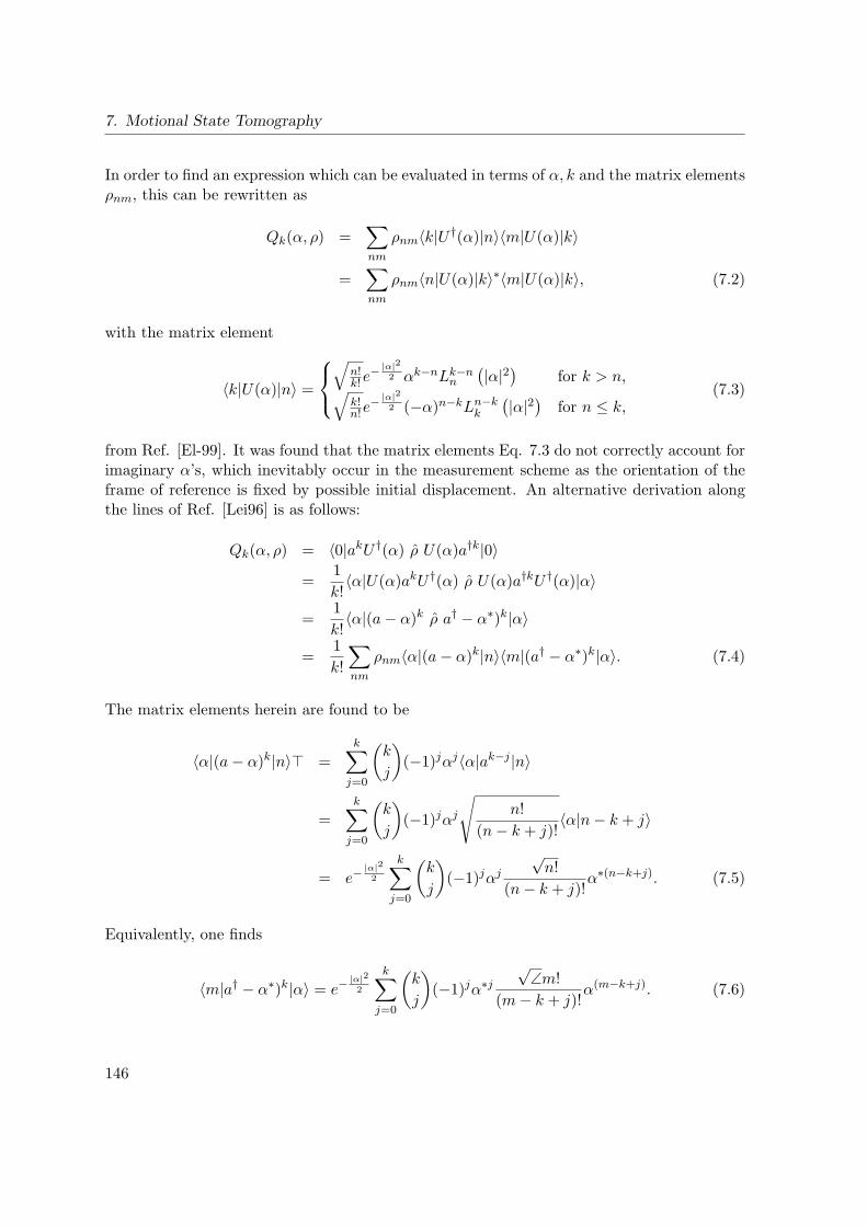
7. Motional State Tomography
In order to find an expression which can be evaluated in terms of α, k and the matrix elementsρnm, this can be rewritten as
Qk(α, ρ) =∑nm
ρnm〈k|U †(α)|n〉〈m|U(α)|k〉
=∑nm
ρnm〈n|U(α)|k〉∗〈m|U(α)|k〉, (7.2)
with the matrix element
〈k|U(α)|n〉 =⎧⎨⎩√
n!k!e
− |α|22 αk−nLk−n
n
(|α|2) for k > n,√k!n!e
− |α|22 (−α)n−kLn−k
k
(|α|2) for n ≤ k,(7.3)
from Ref. [El-99]. It was found that the matrix elements Eq. 7.3 do not correctly account forimaginary α’s, which inevitably occur in the measurement scheme as the orientation of theframe of reference is fixed by possible initial displacement. An alternative derivation alongthe lines of Ref. [Lei96] is as follows:
Qk(α, ρ) = 〈0|akU †(α) ρ U(α)a†k|0〉=
1
k!〈α|U(α)akU †(α) ρ U(α)a†kU †(α)|α〉
=1
k!〈α|(a− α)k ρ a† − α∗)k|α〉
=1
k!
∑nm
ρnm〈α|(a− α)k|n〉〈m|(a† − α∗)k|α〉. (7.4)
The matrix elements herein are found to be
〈α|(a− α)k|n〉 =
k∑j=0
(k
j
)(−1)jαj〈α|ak−j |n〉
=
k∑j=0
(k
j
)(−1)jαj
√n!
(n− k + j)!〈α|n− k + j〉
= e−|α|22
k∑j=0
(k
j
)(−1)jαj
√n!
(n− k + j)!α∗(n−k+j). (7.5)
Equivalently, one finds
〈m|a† − α∗)k|α〉 = e−|α|22
k∑j=0
(k
j
)(−1)jα∗j
√∠m!
(m− k + j)!α(m−k+j). (7.6)
146
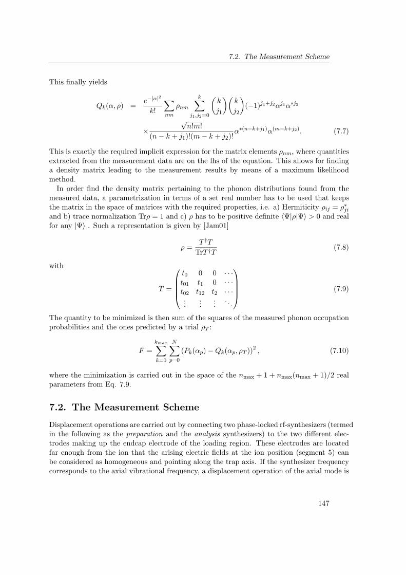
7.2. The Measurement Scheme
This finally yields
Qk(α, ρ) =e−|α|2
k!
∑nm
ρnm
k∑j1,j2=0
(k
j1
)(k
j2
)(−1)j1+j2αj1α∗j2
×√n!m!
(n− k + j1)!(m− k + j2)!α∗(n−k+j1)α(m−k+j2). (7.7)
This is exactly the required implicit expression for the matrix elements ρnm, where quantitiesextracted from the measurement data are on the lhs of the equation. This allows for findinga density matrix leading to the measurement results by means of a maximum likelihoodmethod.
In order find the density matrix pertaining to the phonon distributions found from themeasured data, a parametrization in terms of a set real number has to be used that keepsthe matrix in the space of matrices with the required properties, i.e. a) Hermiticity ρij = ρ∗jiand b) trace normalization Trρ = 1 and c) ρ has to be positive definite 〈Ψ|ρ|Ψ〉 > 0 and realfor any |Ψ〉 . Such a representation is given by [Jam01]
ρ =T †T
TrT †T(7.8)
with
T =
⎛⎜⎜⎜⎝
t0 0 0 · · ·t01 t1 0 · · ·t02 t12 t2 · · ·...
......
. . .
⎞⎟⎟⎟⎠ (7.9)
The quantity to be minimized is then sum of the squares of the measured phonon occupationprobabilities and the ones predicted by a trial ρT :
F =
kmax∑k=0
N∑p=0
(Pk(αp)−Qk(αp, ρT ))2 , (7.10)
where the minimization is carried out in the space of the nmax + 1 + nmax(nmax + 1)/2 realparameters from Eq. 7.9.
7.2. The Measurement Scheme
Displacement operations are carried out by connecting two phase-locked rf-synthesizers (termedin the following as the preparation and the analysis synthesizers) to the two different elec-trodes making up the endcap electrode of the loading region. These electrodes are locatedfar enough from the ion that the arising electric fields at the ion position (segment 5) canbe considered as homogeneous and pointing along the trap axis. If the synthesizer frequencycorresponds to the axial vibrational frequency, a displacement operation of the axial mode is
147
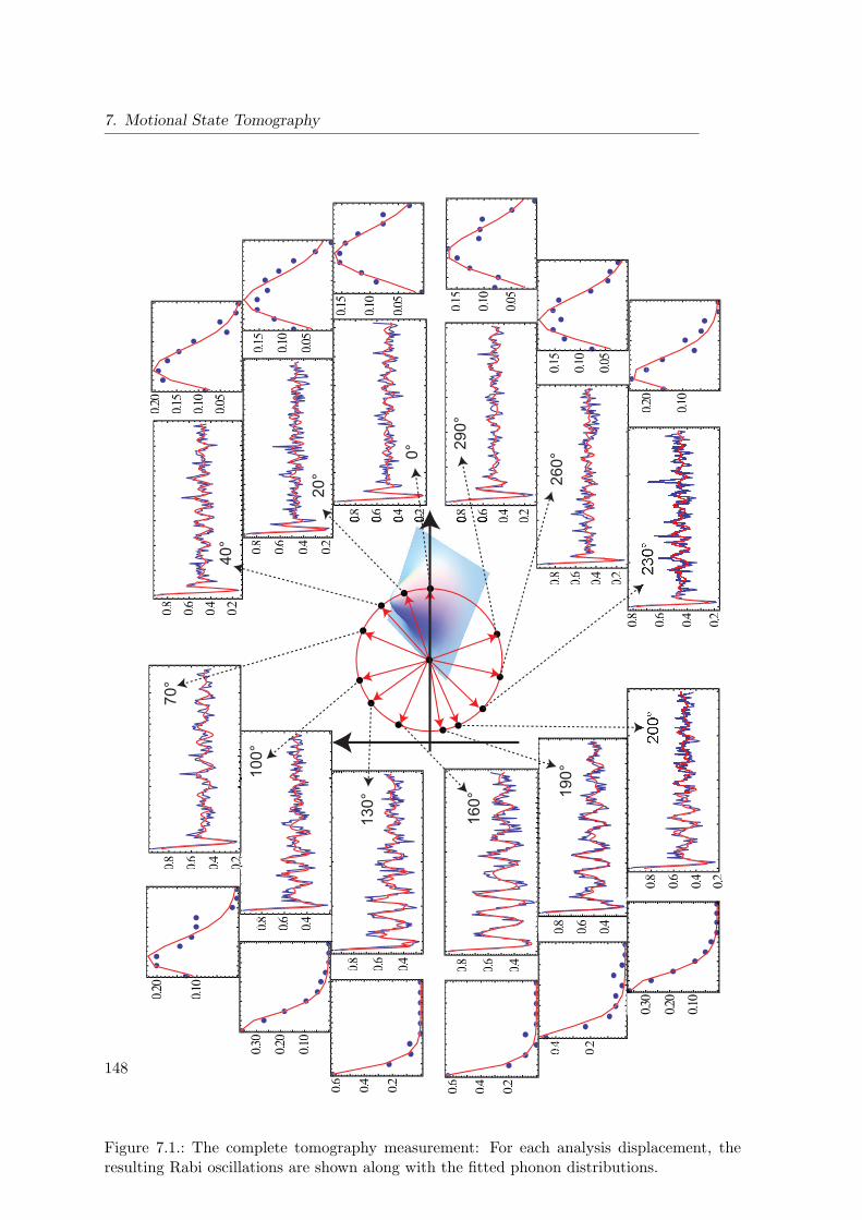
7. Motional State Tomography
0.20.40.60.808
0.20.40.60.8
0.20.40.60.8
0.20.40.60.8 0.2
0.40.60.8
02
0.40.60.8 0.40.60.8
0.40.60.8
0.20.40.600.88
0.20.40.60.80.20.40.60.8
0.20.40.60.8
0°
20°
40°
70°
100°
130°
160° 19
0°
200°
230°
260°
290°
0.05
0.10
0.15
00.05
00.10
00.15
0015
000.05
000.10
000.15
0000.2022
08
0.10
0.2022
08
0.10
0.20220.30
0.20.40.6 0.20.40.6
0.200.44
0.10
0.20
0.30
0.10
00.22002222
0.05
0.10
00.1155
0.05
0.10
0.15
Figure 7.1.: The complete tomography measurement: For each analysis displacement, theresulting Rabi oscillations are shown along with the fitted phonon distributions.
148
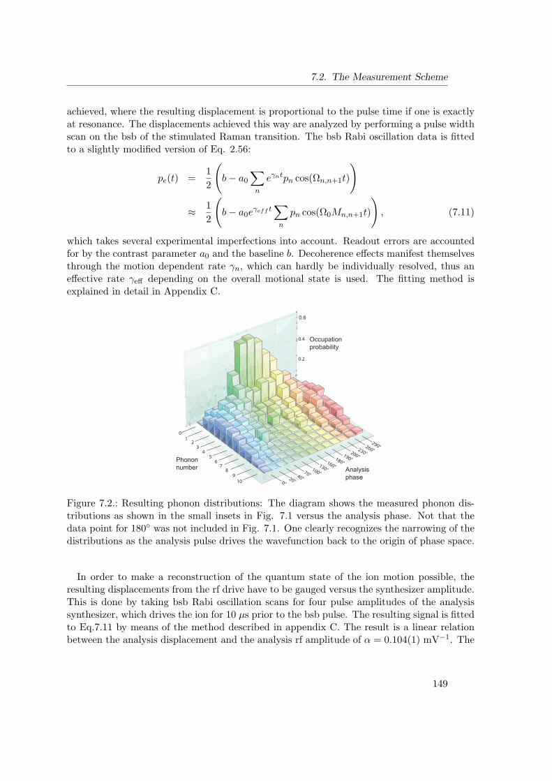
7.2. The Measurement Scheme
achieved, where the resulting displacement is proportional to the pulse time if one is exactlyat resonance. The displacements achieved this way are analyzed by performing a pulse widthscan on the bsb of the stimulated Raman transition. The bsb Rabi oscillation data is fittedto a slightly modified version of Eq. 2.56:
pe(t) =1
2
(b− a0
∑n
eγntpn cos(Ωn,n+1t)
)
≈ 1
2
(b− a0e
γeff t∑n
pn cos(Ω0Mn,n+1t)
), (7.11)
which takes several experimental imperfections into account. Readout errors are accountedfor by the contrast parameter a0 and the baseline b. Decoherence effects manifest themselvesthrough the motion dependent rate γn, which can hardly be individually resolved, thus aneffective rate γeff depending on the overall motional state is used. The fitting method isexplained in detail in Appendix C.
0.0
0.2
0.4
0.6
130°100°70°40°20°0°
160°
200°
230°
260°
290°
190°180°
Analysisphase
0
12
34
56
78
9
10
Phononnumber
Occupationprobability
Figure 7.2.: Resulting phonon distributions: The diagram shows the measured phonon dis-tributions as shown in the small insets in Fig. 7.1 versus the analysis phase. Not that thedata point for 180 was not included in Fig. 7.1. One clearly recognizes the narrowing of thedistributions as the analysis pulse drives the wavefunction back to the origin of phase space.
In order to make a reconstruction of the quantum state of the ion motion possible, theresulting displacements from the rf drive have to be gauged versus the synthesizer amplitude.This is done by taking bsb Rabi oscillation scans for four pulse amplitudes of the analysissynthesizer, which drives the ion for 10 µs prior to the bsb pulse. The resulting signal is fittedto Eq.7.11 by means of the method described in appendix C. The result is a linear relationbetween the analysis displacement and the analysis rf amplitude of α = 0.104(1) mV−1. The
149

7. Motional State Tomography
n=0
n=1
n=2
n=3
n=4
n=5
n=0n=1n=2n=3n=4n=5
n=0n=1
n=2n=3
n=4n=5
n=0n=1
n=2n=3
n=4n=5
a) b)
0.0
0.1
0.2
0.3
-0.05
0.0
+0.05
Figure 7.3.: Resulting density matrix: The density matrix obtained from the measurementdata shown in Fig. 7.1 by means of a maximum-likelihood reconstruction is shown. The leftdiagram shows the real parts and the right diagram shows the imaginary parts. The densitymatrix pertains to a coherent state with a displacement of α ≈ 0.295 + i 0.195, where theimaginary part is presumably due to slight off-resonance of the displacement drive from thevibrational frequency.
tomography itself is then carried out by preparing a coherent state by displacing the motionby means of a pulse of fixed amplitude, duration and phase from the preparation synthesizer,and then exerting a second displacement pulse with fixed duration and amplitude but varyingphase with the analysis synthesizer. The preparation amplitude is 70 mV, and the analysisamplitude is chosen to be 100 mV. The resulting signal then depends on the difference vectorof the two displacement operations. Fig. 7.1 shows the resulting data for the differentanalysis displacement phases in detail. For the resulting phonon distributions establish thelhs of Eq. 7.7, while the calibration data determines the rhs. The data is then fed into agenetic algorithm which builds test density matrices out of initially random number accordingto the recipe given by Eq. 7.9. The fitness of each each test density matrix is then evaluatedby comparing the expected phonon distributions from the test matrix to the measured dataaccording to the fidelity function Eq. 7.10. After several iterations of the algorithm, a validdensity matrix optimally reproducing the measurement data is found. The real and imaginary
150

7.2. The Measurement Scheme
parts of the retrieved matrix are shown in Fig. 7.3. This matrix pertains to a coherent statewith a displacement of α ≈ 0.295 + i 0.195. The nonvanishing imaginary part is presumablydue to a detuning of the drive rf from the motional mode. This is due to the fact that thespectroscopic determination of the motional frequency is always obscured by Stark shifts fromthe off-resonant light and from the off-resonant driving of carrier Rabi oscillations.
151

8. Preparation and Characterization ofSchrodinger Cat States
This chapter gives a detailed account on the preparation and characterization of states withentanglement between spin and motion. The basic mechanism for the generation of thesestates is the usage of spin-dependent light forces, which is explained in detail in Sec. 8.1. Insec. 8.2, the influence of the preparation of the initial state on the evolution under these forcesis investigated, and in Sec. 8.3, the dynamics of the phonon distribution during this kind ofdynamics is presented. Finally, in Sec. 8.4, results from measurements where spin-dependentforces are used to establish a general, precise and efficient state tomography scheme areshown.
8.1. Preparation of a Schrodinger Cat State of a Single Ion
In order to express his objections against quantum theory, Erwin Schrodinger devised afamous Gedankenexperiment where a quantum superposition state of a microscopic object ismapped to a superposition state of a macroscopic object, which was exemplified by a cat beingdead and alive at the same time. It is known today that quantum interference phenomenaof macroscopic objects are not observed in every day life because unavoidable interaction ofsuch objects with their surroundings leads to a loss of their quantum coherence on extremelyfast timescales determined by the distinguishability. This process is termed decoherence, andit is the reason why most experiments demonstrating pure quantum behavior are carriedout on either microscopic objects which are isolated from other objects with a tremendousexperimental effort, or on particles that are interacting weakly with the environment, e.g.photons. It is however still an open question how far the transfer of quantum coherence fromsmaller to larger scale, which is termed the von-Neumann chain, can be principally pushed,i.e. if there is a yet unknown fundamental limit leading to the impossibility of observingquantum superpositions in the macroscopic world. This is one of the main motivations forcreating large-scale entanglement of many qubits in devices like our segmented ion trap.
Schrodinger cat states could be successfully prepared in ion traps by utilizing state depen-dent light forces [Mon96]. Their decoherence behavior in engineered reservoirs was exten-sively studied in [Mya00]. In these experiments, the state of an internal (electronic) degreeof freedom determines the motional behavior upon exposure to a tailored laser field. There-fore, an internal state superposition leads to a nonclassical superposition of motional states,which could in principle be made arbitrarily large under perfect conditions. The resultingjoint quantum states exhibit entanglement between internal and external degrees of freedom,which suggests the usage of spin dependent forces for two-qubit entangling gates. How two-
153
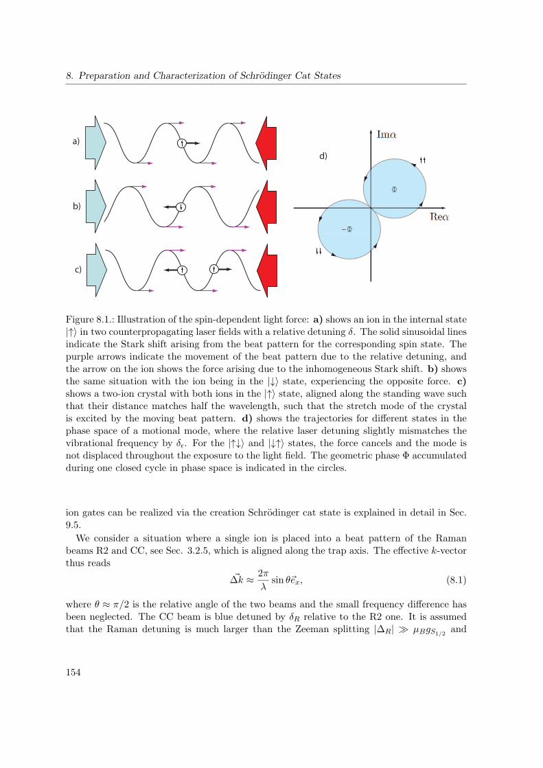
8. Preparation and Characterization of Schrodinger Cat States
a)
b)
c)
d)
Figure 8.1.: Illustration of the spin-dependent light force: a) shows an ion in the internal state|↑〉 in two counterpropagating laser fields with a relative detuning δ. The solid sinusoidal linesindicate the Stark shift arising from the beat pattern for the corresponding spin state. Thepurple arrows indicate the movement of the beat pattern due to the relative detuning, andthe arrow on the ion shows the force arising due to the inhomogeneous Stark shift. b) showsthe same situation with the ion being in the |↓〉 state, experiencing the opposite force. c)shows a two-ion crystal with both ions in the |↑〉 state, aligned along the standing wave suchthat their distance matches half the wavelength, such that the stretch mode of the crystalis excited by the moving beat pattern. d) shows the trajectories for different states in thephase space of a motional mode, where the relative laser detuning slightly mismatches thevibrational frequency by δε. For the |↑↓〉 and |↓↑〉 states, the force cancels and the mode isnot displaced throughout the exposure to the light field. The geometric phase Φ accumulatedduring one closed cycle in phase space is indicated in the circles.
ion gates can be realized via the creation Schrodinger cat state is explained in detail in Sec.9.5.
We consider a situation where a single ion is placed into a beat pattern of the Ramanbeams R2 and CC, see Sec. 3.2.5, which is aligned along the trap axis. The effective k-vectorthus reads
∆k ≈ 2π
λsin θex, (8.1)
where θ ≈ π/2 is the relative angle of the two beams and the small frequency difference hasbeen neglected. The CC beam is blue detuned by δR relative to the R2 one. It is assumedthat the Raman detuning is much larger than the Zeeman splitting |∆R| µBgS1/2
and
154
8.1. Preparation of a Schrodinger Cat State of a Single Ion
the atomic linewidth |∆R| Γ. As we do not want to drive stimulated Raman processesbetween |↑〉 and |↓〉 but rather to give rise to Stark shifts, we chose the beam geometry suchthat only circular components are present. We can now invoke Eq. A.16 to obtain the Starkshift exerted by the two beams:
∆S =1
12∆R
(Ω2b
(ε2b− − ε2b+
)+Ω2
r
(ε2r− − ε2r+
))+ ΩrΩb
(εr−ε∗b−e
i(∆kx−δRt+∆φ) − εr+ε∗b+e
i(∆kx−δRt+∆φ) + c.c.). (8.2)
Considering that the − components act only on the |↑〉 state and the + components act onlyon the |↓〉 state, we can write down a corresponding Hamiltonian operator
HS =
12∆R
(Ω2bε
2b− +Ω2
rε2r− +ΩrΩbεr−ε∗b−e
i(∆kx−δRt+∆φ))|↑〉 〈↑|
+
12∆R
(Ω2bε
2b+ +Ω2
rε2r+ +ΩrΩbεr+ε
∗b+e
i(∆kx−δRt+∆φ))|↓〉 〈↓| . (8.3)
The CC beam is vertically polarized, such that Eqs. 2.26 yield εb− = εb+ = i/√2. R2 is
assumed to propagate exactly in parallel to the quantizing magnetic field, only the rotationangle φr can be freely adjusted, which leads to εr± = (i sinφr ± cosφr)/
√2. Inserting these
polarizations into Eq. 8.3 yields
HS =ΩrΩb
12∆R(sinφr cos(∆kx− δRt+∆φ)− cosφr sin(∆kx− δRt+∆φ)) |↑〉 〈↑|
+ΩrΩb
12∆R(sinφr cos(∆kx− δRt+∆φ) + cosφr sin(∆kx− δRt+∆φ)) |↓〉 〈↓| .
(8.4)
From the cosφr factor, it can be seen that a pure differential shift only arises for φr = 0, i.e.if the R2 beam polarization is horizontally aligned. We then obtain
HS = ∆S sin(∆kx− δRt+∆φ)σz. (8.5)
with the dynamical Stark shift amplitude
∆S =ΩrΩb
12∆R, (8.6)
which is not to be confused with the static Stark shift
H(0)S =
1
12∆R
((ε2r+ − ε2r−)Ω
2r + (ε2b+ − ε2b−)Ω
2b
)σz, (8.7)
which is set to zero by appropriate choice of the polarizations. The Hamiltonian containsproducts of the position and spin operators, it therefore becomes immediately clear that itcan be used to entangle spin and motion. Eq. 8.5 can be rearranged to
HS = ∆S(sin(∆kx) cos(δRt−∆φ)− cos(∆kx) sin(δRt−∆φ))σz. (8.8)
155
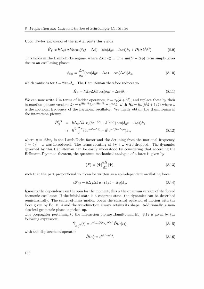
8. Preparation and Characterization of Schrodinger Cat States
Upon Taylor expansion of the spatial parts this yields
HS ≈ ∆S(∆kx cos(δRt−∆φ)− sin(δRt−∆φ))σz +O(∆k2x2). (8.9)
This holds in the Lamb-Dicke regime, where ∆kx 1. The sin(δt−∆φ) term simply givesrise to an oscillating phase:
φosc =∆S
δR(cos(δRt−∆φ)− cos(∆φ))σz, (8.10)
which vanishes for t = 2πn/δR. The Hamiltonian therefore reduces to
HS = ∆S∆kx cos(δRt−∆φ)σz. (8.11)
We can now write x in terms of ladder operators, x = x0(a+ a†), and replace these by theirinteraction picture versions aI = eiH0t/ae−iH0t/ = eiωta, with H0 = ω(a†a+ 1/2) where ωis the motional frequency of the harmonic oscillator. We finally obtain the Hamiltonian inthe interaction picture:
H(I)S = ∆S∆k x0(ae
−iωt + a†eiωt) cos(δRt−∆φ))σz
≈ η ∆S
2(aei(δt+∆φ) + a†e−i(δt−∆φ))σz, (8.12)
where η = ∆kx0 is the Lamb-Dicke factor and the detuning from the motional frequency,δ = δR − ω was introduced. The terms rotating at δR + ω were dropped. The dynamicsgoverned by this Hamiltonian can be easily understood by considering that according theHellmann-Feynman theorem, the quantum mechanical analogue of a force is given by
〈F〉 = 〈Ψ|dHdx
|Ψ〉, (8.13)
such that the part proportional to x can be written as a spin-dependent oscillating force:
〈F〉S = ∆S∆k cos(δRt−∆φ)σz. (8.14)
Ignoring the dependence on the spin for the moment, this is the quantum version of the forcedharmonic oscillator: If the initial state is a coherent state, the dynamics can be describedsemiclassically. The center-of-mass motion obeys the classical equation of motion with theforce given by Eq. 8.14 and the wavefunction always retains its shape. Additionally, a non-classical geometric phase is picked up.The propagator pertaining to the interaction picture Hamiltonian Eq. 8.12 is given by thefollowing expression:
UH
(I)S
(t) = eiφosc(t)σzeiΦ(t)D(α(t)), (8.15)
with the displacement operator
D(α) = eαa†−α∗a. (8.16)
156

8.1. Preparation of a Schrodinger Cat State of a Single Ion
The parameters α(t) and Φ(t) can by analytically found by writing down the general solutionof the time-dependent Schrodinger equation as a Magnus expansion up to second order:
UH
(I)S
(t) = exp
(− i
(∫ t
0H
(I)S (t′)dt′ − i
2
∫ t
0
∫ t′
0[H
(I)S (t′), H(I)
S (t′′)]dt′dt′′ + ...
)). (8.17)
Keeping only the first term of the Magnus expansion, inserting Eq. 8.12 and comparing withEq. 8.16, we obtain the time-dependent displacement α(t)
α(t) = −iη∆S
2
∫ t
0e−i(δt′−∆φ)dt′
=η∆S
2δei∆φ(e−iδt − 1)
= −iη∆S
δei∆φe−i δt
2 sinδt
2. (8.18)
The geometric phase results from the second order contribution from the Magnus expansionEq. 8.17. With the commutator evaluated to be
[HS(t′), HS(t
′′)] = i2η2∆2
S
2sin(δ(t′ − t′′)), (8.19)
we can evaluate the double integral,∫ t
0
∫ t′
0[HS(t
′), HS(t′′)]dt′dt′′ = −i
2η2∆2
S
2
sin δt− δt
δ2(8.20)
such that we finally obtain for the geometric phase
Φ(t) =η2∆2
S
4
sin δt− δt
δ2. (8.21)
As can be directly seen in the derivation, the geometric phase is a consequence of the non-commutativity of the Hamiltonian at different intermediate times, i.e. the final state of thesystem depends on intermediate steps in the time evolution, such that different classicaltrajectories ending up at the same displacement can still yield different geometric phases.The geometric phase can also be expressed by the area encircled by the trajectory, which isgiven by
Φ(t) =1
∫ t
0〈x(t′)〉d〈p(t′)〉 − 〈p(t′)〉d〈x(t′)〉
=
∫ t
0α(t′)dα∗(t′)− α∗(t′)dα(t′)
=
∫ t
0(α(t′)α∗(t′)− α∗(t′)α(t′))dt
= −η2∆2S
4δ
∫ t
0sin2(δt
2
)dt
=η2∆2
S
4δ2(sin(δt)− δt) (8.22)
157
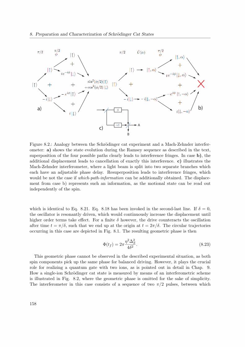
8. Preparation and Characterization of Schrodinger Cat States
a) b)
c)A
B
Figure 8.2.: Analogy between the Schrodinger cat experiment and a Mach-Zehnder interfer-ometer: a) shows the state evolution during the Ramsey sequence as described in the text,superposition of the four possible paths clearly leads to interference fringes. In case b), theadditional displacement leads to cancellation of exactly this interference. c) illustrates theMach-Zehnder interferometer, where a light beam is split into two separate branches whicheach have an adjustable phase delay. Resuperposition leads to interference fringes, whichwould be not the case if which-path-information can be additionally obtained. The displace-ment from case b) represents such an information, as the motional state can be read outindependently of the spin.
which is identical to Eq. 8.21. Eq. 8.18 has been invoked in the second-last line. If δ = 0,the oscillator is resonantly driven, which would continuously increase the displacement untilhigher order terms take effect. For a finite δ however, the drive counteracts the oscillationafter time t = π/δ, such that we end up at the origin at t = 2π/δ. The circular trajectoriesoccurring in this case are depicted in Fig. 8.1. The resulting geometric phase is then
Φ(tf ) = 2πη2∆2
S
4δ2. (8.23)
This geometric phase cannot be observed in the described experimental situation, as bothspin components pick up the same phase for balanced driving. However, it plays the crucialrole for realizing a quantum gate with two ions, as is pointed out in detail in Chap. 9.How a single-ion Schrodinger cat state is measured by means of an interferometric schemeis illustrated in Fig. 8.2, where the geometric phase is omitted for the sake of simplicity.The interferometer in this case consists of a sequence of two π/2 pulses, between which
158

8.1. Preparation of a Schrodinger Cat State of a Single Ion
0 20 40 60 80 1000,0
0,2
0,4
0,6
0,8
1,0Fr
inge
Con
trast
Displacement pulse length [µs]
Figure 8.3.: Entanglement-induced contrast loss for the Schrodinger cat state: The curveshows the measured Ramsey contrast versus displacement pulse time, along with a fit to themodel Eq. 8.26. After a rapid initial decay due to the displacement, the curve displays acontrast revival after t = 2π/δ when the trajectory goes back to the starting point, such thatspin and motion are disentangled again. The maximum size of the cat is reached after halfthis time, and is found to be 2|α|max ≈ 1.55.
the displacement force is applied. The final spin state depends on the phase of the secondπ/2 pulse, similar to the decoherence measurements of Sec. 4.7. In analogy to a Mach-Zehnder interferometer, the displacement caused by the light force, which is conditional onthe spin state, gives a which-path information which leads to the collapse of the Ramseyfringe contrast. As the motional state after application of the force depends on the spin,which is in a coherent superposition of |↑〉 and |↓〉 after the first π/2 pulse, the force leads toentanglement between the spin and motional degree of freedom. This beautifully illustrateshow entanglement between a small initial system under observation (the spin) and degrees offreedom of a larger Hilbert space (the motion) obscures the observation of coherence of theinitial system.For the displaced ion, the probabilities to find the ion in either |↑〉 or |↓〉 after the analysis
159

8. Preparation and Characterization of Schrodinger Cat States
π/2-pulse are given by
P↑ =1
2(1− cosφ〈−α|α〉) = 1
2(1− cosφ e−2|α|2)
P↓ =1
2(1 + cosφ〈−α|α〉) = 1
2(1 + cosφ e−2|α|2). (8.24)
The fringe contrast obtained when measuring P↑ while scanning the phase φ, C = Pmax↑ −Pmin
↑ ,is then given by
C = e−2|α|2 . (8.25)
If we now perform the contrast measurement for varying duration t of the displacement pulse,we can insert the time-dependent displacement from Eq. 8.18 into Eq. 8.25:
C(t) = e−η2∆2
Sδ2
sin2(δt/2) (8.26)
Measurement results are shown in Fig. 8.3, where a spin-echo sequence was used instead ofthe simple Ramsey sequence in order to reduce decoherence effects, which does not change theresult Eq. 8.26. For each data point corresponding to a fixed displacement pulse duration,the phase of the analysis pulse was scanned from 0 to 2π in steps of π/10. The resultingsignal is fitted to a single sine period with floating phase shift, offset and amplitude, and theamplitude gives the Ramsey contrast C(t). Eq. 8.26 is then fitted to the measured contrastcurve, where the detuning from the vibrational frequency, δ, and the displacement amplitude|α|max = η∆S/2δ are floating and an additional decoherence induced contrast decay factore−γt with floating γ is included.
160
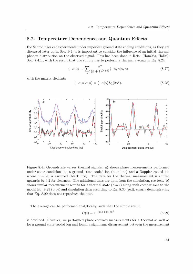
8.2. Temperature Dependence and Quantum Effects
8.2. Temperature Dependence and Quantum Effects
For Schrodinger cat experiments under imperfect ground state cooling conditions, as they arediscussed later on in Sec. 9.4, it is important to consider the influence of an initial thermalphonon distribution on the observed signal. This has been done in Refs. [Hom06a, Hal05],Sec. 7.4.1., with the result that one simply has to perform a thermal average in Eq. 8.24:
〈−α|α〉 →∑n
nn
(n+ 1)(n+1)〈−α, n|α, n〉 (8.27)
with the matrix elements〈−α, n|α, n〉 = 〈−α|α〉L0
n(2α2). (8.28)
0 20 40 60 80 1000,3
0,4
0,5
0,6
0,7
0,8
0,9
1,0
She
lvin
g pr
obab
ility
Displacement pulse time [µs]0 20 40 60
0,3
0,4
0,5
0,6
0,7
0,8
0,9
1,0S
helv
ing
prob
abili
ty
Displacement pulse time [µs]
a) b)
Figure 8.4.: Groundstate versus thermal signals: a) shows phase measurements performedunder same conditions on a ground state cooled ion (blue line) and a Doppler cooled ionwhere n = 20 is assumed (black line). The data for the thermal measurement is shiftedupwards by 0.2 for clearness. The additional lines are data from the simulation, see text. b)shows similar measurement results for a thermal state (black) along with comparisons to themodel Eq. 8.29 (blue) and simulation data according to Eq. 8.30 (red), clearly demonstratingthat Eq. 8.29 does not reproduce the data.
The average can be performed analytically, such that the simple result
C(t) = e−(2n+1)|α(t)|2 (8.29)
is obtained. However, we performed phase contrast measurements for a thermal as well asfor a ground state cooled ion and found a significant disagreement between the measurement
161
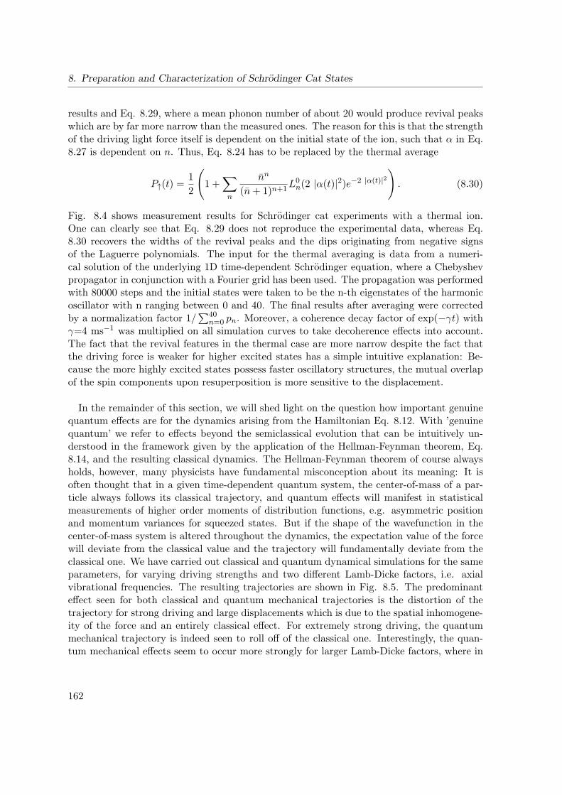
8. Preparation and Characterization of Schrodinger Cat States
results and Eq. 8.29, where a mean phonon number of about 20 would produce revival peakswhich are by far more narrow than the measured ones. The reason for this is that the strengthof the driving light force itself is dependent on the initial state of the ion, such that α in Eq.8.27 is dependent on n. Thus, Eq. 8.24 has to be replaced by the thermal average
P↑(t) =1
2
(1 +∑n
nn
(n+ 1)n+1L0n(2 |α(t)|2)e−2 |α(t)|2
). (8.30)
Fig. 8.4 shows measurement results for Schrodinger cat experiments with a thermal ion.One can clearly see that Eq. 8.29 does not reproduce the experimental data, whereas Eq.8.30 recovers the widths of the revival peaks and the dips originating from negative signsof the Laguerre polynomials. The input for the thermal averaging is data from a numeri-cal solution of the underlying 1D time-dependent Schrodinger equation, where a Chebyshevpropagator in conjunction with a Fourier grid has been used. The propagation was performedwith 80000 steps and the initial states were taken to be the n-th eigenstates of the harmonicoscillator with n ranging between 0 and 40. The final results after averaging were correctedby a normalization factor 1/
∑40n=0 pn. Moreover, a coherence decay factor of exp(−γt) with
γ=4 ms−1 was multiplied on all simulation curves to take decoherence effects into account.The fact that the revival features in the thermal case are more narrow despite the fact thatthe driving force is weaker for higher excited states has a simple intuitive explanation: Be-cause the more highly excited states possess faster oscillatory structures, the mutual overlapof the spin components upon resuperposition is more sensitive to the displacement.
In the remainder of this section, we will shed light on the question how important genuinequantum effects are for the dynamics arising from the Hamiltonian Eq. 8.12. With ’genuinequantum’ we refer to effects beyond the semiclassical evolution that can be intuitively un-derstood in the framework given by the application of the Hellman-Feynman theorem, Eq.8.14, and the resulting classical dynamics. The Hellman-Feynman theorem of course alwaysholds, however, many physicists have fundamental misconception about its meaning: It isoften thought that in a given time-dependent quantum system, the center-of-mass of a par-ticle always follows its classical trajectory, and quantum effects will manifest in statisticalmeasurements of higher order moments of distribution functions, e.g. asymmetric positionand momentum variances for squeezed states. But if the shape of the wavefunction in thecenter-of-mass system is altered throughout the dynamics, the expectation value of the forcewill deviate from the classical value and the trajectory will fundamentally deviate from theclassical one. We have carried out classical and quantum dynamical simulations for the sameparameters, for varying driving strengths and two different Lamb-Dicke factors, i.e. axialvibrational frequencies. The resulting trajectories are shown in Fig. 8.5. The predominanteffect seen for both classical and quantum mechanical trajectories is the distortion of thetrajectory for strong driving and large displacements which is due to the spatial inhomogene-ity of the force and an entirely classical effect. For extremely strong driving, the quantummechanical trajectory is indeed seen to roll off of the classical one. Interestingly, the quan-tum mechanical effects seem to occur more strongly for larger Lamb-Dicke factors, where in
162

8.3. Phonon Distribution Dynamics
0 2 4 6 8 10
-1
0
1
2
3
4
5
Im(α)
Re(α)
∆S
classicalq.m.
0 2 4 6 80
1
2
3
4
5
6
Im(α)
Re(α)
∆S
q.m.classicala) b)
Figure 8.5.: Classical and quantum mechanical trajectories: a) Classical (red) and quantummechanical (blue) trajectories resulting from the displacement drive at a motional frequencyof ωax=2π·1 MHz. b) the same for ωax=2π·1.4 MHz. The black arrow indicates that theouter trajectories result from driving with larger Stark shift ∆S , see Eq. 8.12. The maximumStark shift for the outermost trajectories is ∆S=2π·200 kHz, changed in steps of π·10 kHz.The detuning from the motional mode is δ=2π·5 kHz. Note the additional microoscillationsresulting from the mismatch between drive and oscillation frequency.
turn the anharmonic distortion effect is less pronounced. It can be concluded that genuinequantum effects are not significant in the regime where quantum gates are usually driven,but one might have to take them into account. If a strong enough driving can be realized,it might be of interest to perform a proof-of-principle experiment where the occurrence ofnonclassical trajectories of a single ion is unambiguously demonstrated.
8.3. Phonon Distribution Dynamics
A detailed analysis of the effect of the light force on the motional state is performed by recon-struction of the phonon distributions on the axial vibrational mode, with a method similar tothe one presented in Chap. 7. Instead of a phase coherence measurement as it was performedin the Schrodinger cat experiment described above, we recorded Rabi oscillations on the bluemotional sideband and used this information for a maximum-likelihood reconstruction of thephonon distribution function p(n). For preceding displacement pulses of times of up to 64 µs,changed in steps of 4 µs, Rabi oscillations of a duration of 200 µs, including approximately5.5 oscillation periods were recorded. The reconstruction of the phonon distribution is per-formed in entirely the same way as in Chap. 7, where the phonon distributions are obtained
163
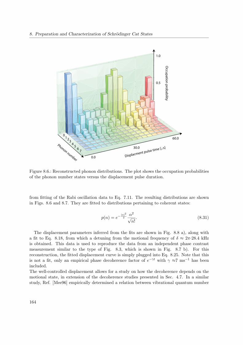
8. Preparation and Characterization of Schrodinger Cat States
Occu
patio
n p
rob
ability
Displacment pulse time [ s]Phonon number
0.0
60.0
30.0
012
34
56
7
1.0
0.5
Figure 8.6.: Reconstructed phonon distributions. The plot shows the occupation probabilitiesof the phonon number states versus the displacement pulse duration.
from fitting of the Rabi oscillation data to Eq. 7.11. The resulting distributions are shownin Figs. 8.6 and 8.7. They are fitted to distributions pertaining to coherent states:
p(n) = e−|α|22
α2
√n!. (8.31)
The displacement parameters inferred from the fits are shown in Fig. 8.8 a), along witha fit to Eq. 8.18, from which a detuning from the motional frequency of δ ≈ 2π·28.4 kHzis obtained. This data is used to reproduce the data from an independent phase contrastmeasurement similar to the type of Fig. 8.3, which is shown in Fig. 8.7 b). For thisreconstruction, the fitted displacement curve is simply plugged into Eq. 8.25. Note that thisis not a fit, only an empirical phase decoherence factor of e−γt with γ ≈7 ms−1 has beenincluded.The well-controlled displacement allows for a study on how the decoherence depends on themotional state, in extension of the decoherence studies presented in Sec. 4.7. In a similarstudy, Ref. [Mee96] empirically determined a relation between vibrational quantum number
164

8.3. Phonon Distribution Dynamics
0 1 2 3 4 5 6 70,0
0,2
0,4
0,6
0,8
1,0
t = 0us
0 1 2 3 4 5 6 70,0
0,2
0,4
0,6
0,8
1,0
t = 4us
0 1 2 3 4 5 6 70,0
0,2
0,4
0,6
0,8
1,0
t = 8us
0 1 2 3 4 5 6 70,0
0,2
0,4
0,6
0,8
1,0
t = 12us
0 1 2 3 4 5 6 70,0
0,2
0,4
0,6
0,8
1,0
t = 16us
0 1 2 3 4 5 6 70,0
0,2
0,4
0,6
0,8
1,0
t = 20us
0 1 2 3 4 5 6 70,0
0,2
0,4
0,6
0,8
1,0
t = 24us
0 1 2 3 4 5 6 70,0
0,2
0,4
0,6
0,8
1,0
t = 28us
0 1 2 3 4 5 6 70,0
0,2
0,4
0,6
0,8
1,0
t = 32us
0 1 2 3 4 5 6 70,0
0,2
0,4
0,6
0,8
1,0
t = 36us
0 1 2 3 4 5 6 70,0
0,2
0,4
0,6
0,8
1,0
t = 40us
0 1 2 3 4 5 6 70,0
0,2
0,4
0,6
0,8
1,0
t = 44us
0 1 2 3 4 5 6 70,0
0,2
0,4
0,6
0,8
1,0
t = 48us
0 1 2 3 4 5 6 70,0
0,2
0,4
0,6
0,8
1,0
t = 52us
0 1 2 3 4 5 6 70,0
0,2
0,4
0,6
0,8
1,0
t = 56us
0 1 2 3 4 5 6 70,0
0,2
0,4
0,6
0,8
1,0
t = 60us
Figure 8.7.: Reconstructed phonon distributions with fits to coherent state distributions (redsolid lines). Note the close to perfect agreement between the theoretical and the reconstructedprobability distributions.
and decoherence rate of
γn ≈ γ0(n+ 1)χ, (8.32)
with χ ≈0.7. The motion-dependent decoherence was attributed to technical imperfectionslike fluctuating trap parameters. Theoretical investigations were performed in Ref. [Fid00]and [Bud02], where quantum jumps due to off-resonant light scattering were found to beresponsible for the effect. However, in Ref. [Fid00], no dependence of the dephasing rateon the initial motional state was found. Ref. [Bud02] partially recovers this dependence byadditionally considering the heating rate caused by fluctuating electric fields, but the heatingrate required to cause a noticeable contribution to the dephasing would be way larger thanthe one found in our experiments, where it takes place on a slower timescale (about 3 ms perphonon in contrast to the 200 µs maximum BSB pulse time). Fig. 8.10 shows the differenttypes of quantum jumps which contribute to the dephasing. The scattering within the |↑, n〉and |↓, n〉 manifolds is not contained in Eqs. A.14 and A.15 as the scattering from and tothe states is a balance of the last two terms in Eq. 2.68, where the motion is not taken
165
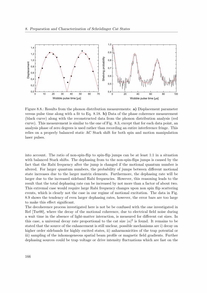
8. Preparation and Characterization of Schrodinger Cat States
0 10 20 30 40 50 60 700,0
0,2
0,4
0,6
0,8
1,0
1,2
1,4
Dis
plac
emen
t
Wobble pulse time [µs]0 20 40 60 80 100
0,4
0,5
0,6
0,7
0,8
0,9
1,0
Shel
ving
pro
babi
lity
Wobble pulse time [µs]
Figure 8.8.: Results from the phonon distribution measurements: a) Displacement parameterversus pulse time along with a fit to Eq. 8.18. b) Data of the phase coherence measurement(black curve) along with the reconstructed data from the phonon distribution analysis (redcurve). This measurement is similar to the one of Fig. 8.3, except that for each data point, ananalysis phase of zero degrees is used rather than recording an entire interference fringe. Thisrelies on a properly balanced static AC Stark shift for both spin and motion manipulationlaser pulses.
into account. The ratio of non-spin-flip to spin-flip jumps can be at least 1:1 in a situationwith balanced Stark shifts. The dephasing from to the non-spin-flips jumps is caused by thefact that the Rabi frequency after the jump is changed if the motional quantum number isaltered. For larger quantum numbers, the probability of jumps between different motionalstate increases due to the larger matrix elements. Furthermore, the dephasing rate will belarger due to the increased sideband Rabi frequencies. However, this reasoning leads to theresult that the total dephasing rate can be increased by not more than a factor of about two.This extremal case would require large Rabi frequency changes upon non spin flip scatteringevents, which is clearly not the case in our regime of motional excitation. The data in Fig.8.9 shows the tendency of even larger dephasing rates, however, the error bars are too largeto make this effect significant.The decoherence process investigated here is not be be confused with the one investigated inRef [Tur00], where the decay of the motional coherence, due to electrical field noise duringa wait time in the absence of light-matter interaction, is measured for different cat sizes. Inthis case, a universal decay rate proportional to the cat size |α|2 is found. It remains to bestated that the source of the enhancement is still unclear, possible mechanisms are i) decay onhigher order sidebands for highly excited states, ii) anharmonicities of the trap potential oriii) sampling of the inhomogeneous spatial beam profile or magnetic field gradients. Furtherdephasing sources could be trap voltage or drive intensity fluctuations which are fast on the
166
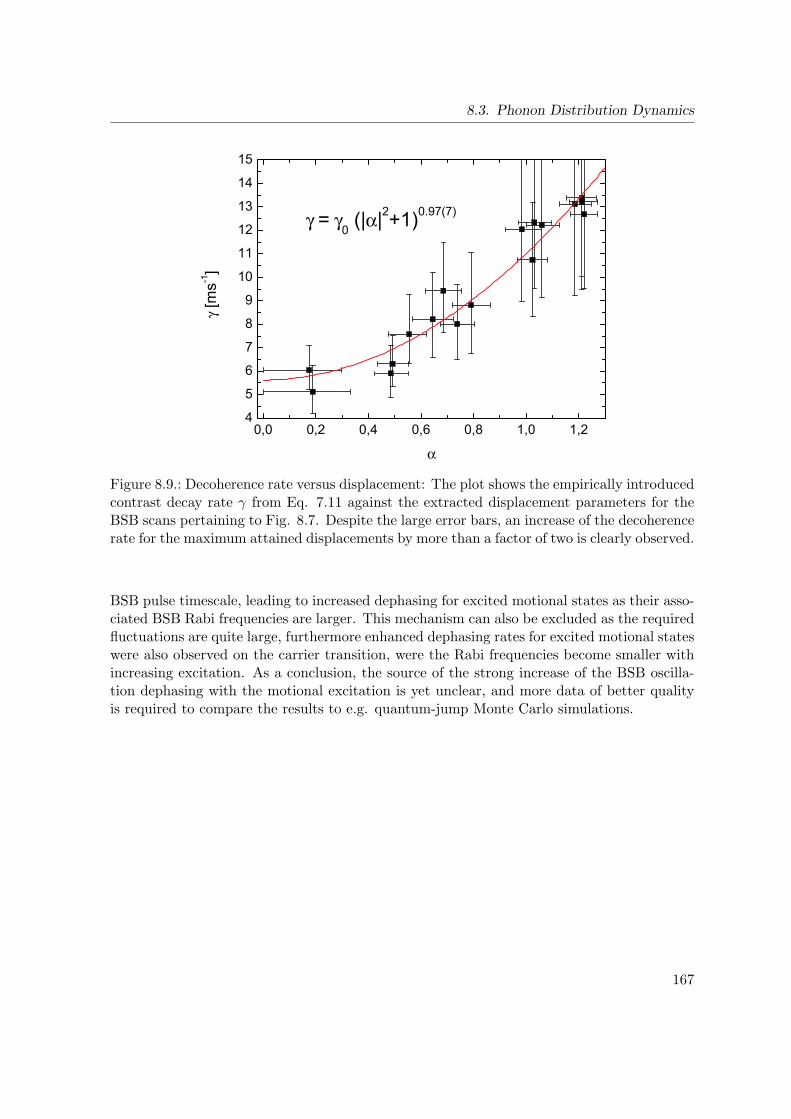
8.3. Phonon Distribution Dynamics
0,0 0,2 0,4 0,6 0,8 1,0 1,24
5
6
7
8
9
10
11
12
13
14
15
γ [m
s-1]
α
γ = γ0 (|α|2+1)0.97(7)
Figure 8.9.: Decoherence rate versus displacement: The plot shows the empirically introducedcontrast decay rate γ from Eq. 7.11 against the extracted displacement parameters for theBSB scans pertaining to Fig. 8.7. Despite the large error bars, an increase of the decoherencerate for the maximum attained displacements by more than a factor of two is clearly observed.
BSB pulse timescale, leading to increased dephasing for excited motional states as their asso-ciated BSB Rabi frequencies are larger. This mechanism can also be excluded as the requiredfluctuations are quite large, furthermore enhanced dephasing rates for excited motional stateswere also observed on the carrier transition, were the Rabi frequencies become smaller withincreasing excitation. As a conclusion, the source of the strong increase of the BSB oscilla-tion dephasing with the motional excitation is yet unclear, and more data of better qualityis required to compare the results to e.g. quantum-jump Monte Carlo simulations.
167
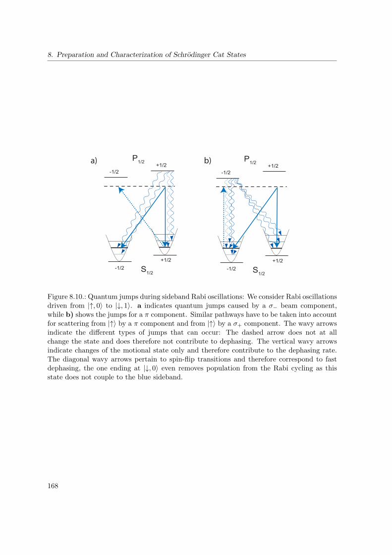
8. Preparation and Characterization of Schrodinger Cat States
S1/2-1/2+1/2
+1/2-1/2
P1/2
S1/2-1/2+1/2
+1/2-1/2
P1/2a) b)
Figure 8.10.: Quantum jumps during sideband Rabi oscillations: We consider Rabi oscillationsdriven from |↑, 0〉 to |↓, 1〉. a indicates quantum jumps caused by a σ− beam component,while b) shows the jumps for a π component. Similar pathways have to be taken into accountfor scattering from |↑〉 by a π component and from |↑〉 by a σ+ component. The wavy arrowsindicate the different types of jumps that can occur: The dashed arrow does not at allchange the state and does therefore not contribute to dephasing. The vertical wavy arrowsindicate changes of the motional state only and therefore contribute to the dephasing rate.The diagonal wavy arrows pertain to spin-flip transitions and therefore correspond to fastdephasing, the one ending at |↓, 0〉 even removes population from the Rabi cycling as thisstate does not couple to the blue sideband.
168

8.4. The Wavepacket Beating Scheme
8.4. The Wavepacket Beating Scheme
x
p
x
pa)
x
p
x
pb)
x
p
x
pc)
x
p
x
pd)
x
p
x
pe)
Figure 8.11.: Schematic of the wavepacket beating experiment: a) A resonant π/2 pulsecreates an initial spin superposition (resonant driving of the spin transition is indicated bydashed arrows). b) The displacement force acting only on |↓〉 gives rise to a displacement αof only the |↓〉-part of the wavefunction. c) A π pulse is used to swap the populations. d) Asecond displacement pulse now displaces the part of the wavefunction which was previouslynot affected by the force. e) A concluding π/2 pulse gives rise to the final populations in |↑〉and |↓〉 which are to be measured.
Two modifications of the measurement scheme presented above can be used to measure thetrajectory of the ion in phase space: First, the R2 beam has to be circularly polarized suchthat the light force acts on one spin component only. Furthermore, a second displacementpulse of the same strength and duration but with variable phase is employed in the secondbranch of the spin echo sequence. Physically, one is now subsequentially displacing twodifferent portions of the wavepacket, which yields interference if the parts are displaced suchthat they have a substantial overlap in the end. The scheme is illustrated in Fig. 8.11and described in detail in the following. It has been used in Ref. [Mon96] for the firstdemonstration of the generation of Schrodinger cat states, however it has not been realizedthere that the scheme is capable of ultraprecise trajectory measurements. In contrast to Ref.[Mon96], we assume resonant driving of the spin-flip transition, such that no extra phasesare accumulated during the π/2 and π pulses, but we account for off-resonant driving of themotion. The frequency difference of the driving beams during the displacement pulses is
169
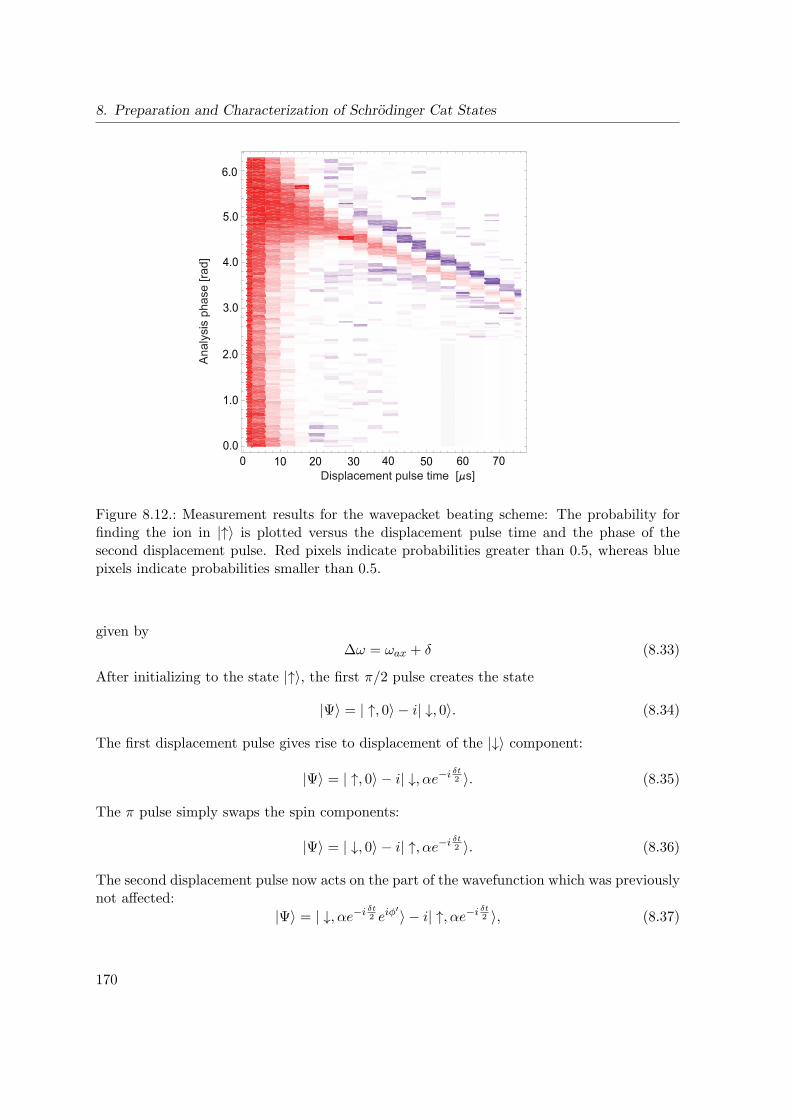
8. Preparation and Characterization of Schrodinger Cat States
6.0
5.0
4.0
3.0
2.0
1.0
0.0
Ana
lysi
s ph
ase
[rad]
0 10 20 30 40 50 60 70Displacement pulse time [ s]
Figure 8.12.: Measurement results for the wavepacket beating scheme: The probability forfinding the ion in |↑〉 is plotted versus the displacement pulse time and the phase of thesecond displacement pulse. Red pixels indicate probabilities greater than 0.5, whereas bluepixels indicate probabilities smaller than 0.5.
given by
∆ω = ωax + δ (8.33)
After initializing to the state |↑〉, the first π/2 pulse creates the state
|Ψ〉 = | ↑, 0〉 − i| ↓, 0〉. (8.34)
The first displacement pulse gives rise to displacement of the |↓〉 component:
|Ψ〉 = | ↑, 0〉 − i| ↓, αe−i δt2 〉. (8.35)
The π pulse simply swaps the spin components:
|Ψ〉 = | ↓, 0〉 − i| ↑, αe−i δt2 〉. (8.36)
The second displacement pulse now acts on the part of the wavefunction which was previouslynot affected:
|Ψ〉 = | ↓, αe−i δt2 eiφ
′〉 − i| ↑, αe−i δt2 〉, (8.37)
170
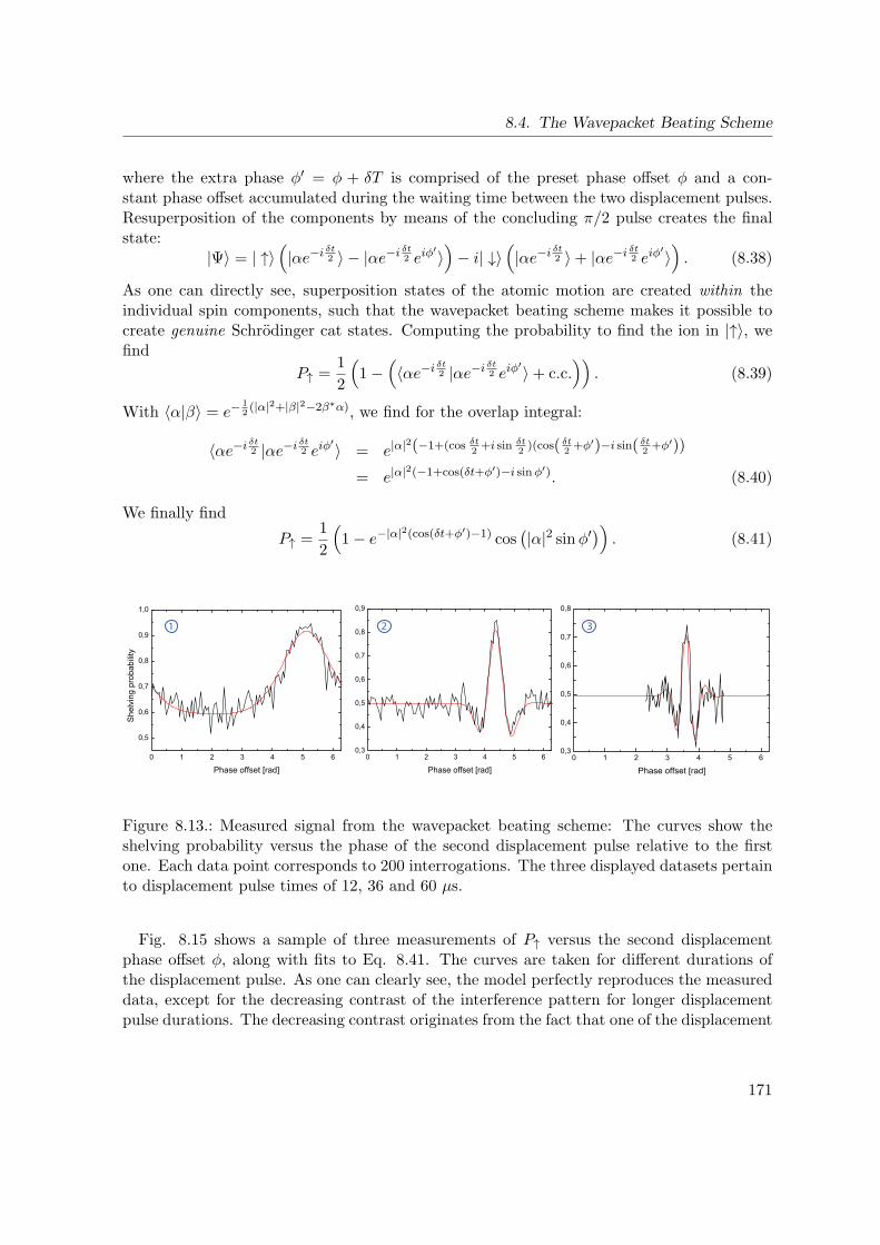
8.4. The Wavepacket Beating Scheme
where the extra phase φ′ = φ + δT is comprised of the preset phase offset φ and a con-stant phase offset accumulated during the waiting time between the two displacement pulses.Resuperposition of the components by means of the concluding π/2 pulse creates the finalstate:
|Ψ〉 = | ↑〉(|αe−i δt
2 〉 − |αe−i δt2 eiφ
′〉)− i| ↓〉
(|αe−i δt
2 〉+ |αe−i δt2 eiφ
′〉). (8.38)
As one can directly see, superposition states of the atomic motion are created within theindividual spin components, such that the wavepacket beating scheme makes it possible tocreate genuine Schrodinger cat states. Computing the probability to find the ion in |↑〉, wefind
P↑ =1
2
(1−(〈αe−i δt
2 |αe−i δt2 eiφ
′〉+ c.c.))
. (8.39)
With 〈α|β〉 = e−12(|α|2+|β|2−2β∗α), we find for the overlap integral:
〈αe−i δt2 |αe−i δt
2 eiφ′〉 = e|α|
2(−1+(cos δt2+i sin δt
2)(cos( δt
2+φ′)−i sin( δt
2+φ′))
= e|α|2(−1+cos(δt+φ′)−i sinφ′). (8.40)
We finally find
P↑ =1
2
(1− e−|α|2(cos(δt+φ′)−1) cos
(|α|2 sinφ′)) . (8.41)
0 1 2 3 4 5 6
0,5
0,6
0,7
0,8
0,9
1,0
She
lvin
g pr
obab
ility
Phase offset [rad]0 1 2 3 4 5 6
0,3
0,4
0,5
0,6
0,7
0,8
0,9
Phase offset [rad]0 1 2 3 4 5 6
0,3
0,4
0,5
0,6
0,7
0,8
Phase offset [rad]
1 2 3
Figure 8.13.: Measured signal from the wavepacket beating scheme: The curves show theshelving probability versus the phase of the second displacement pulse relative to the firstone. Each data point corresponds to 200 interrogations. The three displayed datasets pertainto displacement pulse times of 12, 36 and 60 µs.
Fig. 8.15 shows a sample of three measurements of P↑ versus the second displacementphase offset φ, along with fits to Eq. 8.41. The curves are taken for different durations ofthe displacement pulse. As one can clearly see, the model perfectly reproduces the measureddata, except for the decreasing contrast of the interference pattern for longer displacementpulse durations. The decreasing contrast originates from the fact that one of the displacement
171

8. Preparation and Characterization of Schrodinger Cat States
beams is circularly polarized and therefore exerts a strong AC Stark shift, which leads to theloss of spin coherence by intensity fluctuations, see Sec. 4.7. The contrast versus displacementtime is shown in Fig. 8.14. It is also found that the accuracy of the fits to the measureddata could be improved by considering a slight detuning from the spin-flip carrier transition.According to Ref. [Mon96], Eq. 8.41 only has to be modified to
P↑ =1
2
(1− e−γte−|α|2(cos(δt+φ′)−1) cos
(ψ + |α|2 sinφ′)) , (8.42)
where γ describes the contrast decay and ψ = δcart describes the detuning from the carrier.The phase ψ is picked up because the experimental sequence is set up such that gaps of thespin echo sequence become longer for increasing displacement pulse durations. The AC Starkshift does not lead to an extra phase pick-up as both components of the wavefunction aresubjected to same displacement pulse area. The results for the determination of δcar are alsoshown in Fig. 8.14.
0 20 40 60 800,0
0,1
0,2
0,3
0,4
0,5
0,6
0,7
0,8
0,9
1,0
Sig
nal c
ontra
st
t in µs
0 10 20 30 40 50 60 70 802,6
2,8
3,0
3,2
3,4
3,6
3,8
4,0
4,2
4,4
ψ in
rad
t in µs
a) b)
Figure 8.14.: a) Contrast decay due to intensity fluctuations. The 1/e time is found to be73.2 µs.b) Correction for a slight carrier off-resonance. The detuning is determined to beδcar ≈2.3 kHz.
The maximum displacement values around α ≈ 3 are already large enough for the finiteLamb-Dicke factor, i.e. the spatial inhomogeneity, to be seen in the dynamics. According toRef. [Hom06a], this can be accounted for by replacing Eq. 8.18 by
α(t) = −η∆S
2δ
δ
δeffei∆φei
δt2 sin
δefft
2. (8.43)
where δeff > δ, i.e. the particle returns to the origin in phase space before the phase of theforce is back to its original value. As the phase of the driving force has not completed a fullcycle then, further driving will lead to a cycloid-shaped trajectory, as is indicated in Fig.
172

8.4. The Wavepacket Beating Scheme
8.15. Furthermore, the maximum displacement attained is reduced by a factor δ/δeff , whichmeans that when attempting to drive ultrafast gates within a few cycles of the trap motion,the efficiency of the light force will be seriously impaired. δeff depends on δ, the Lamb-Dickefactor and the strength of the driving field. Empirical formulae are given in Ref. [Hom06a].
0 10 20 30 40 50 60 70 800,0
0,5
1,0
1,5
2,0
2,5
3,0ψ
t in µs
a)
c)
b)
1
2
3
0 10 20 30 40 50 60 70 800,0
0,5
1,0
1,5
2,0
2,5
3,0
3,5
4,0
abs(
α)
t in µs
-0,5 0,0 0,5 1,0 1,5 2,0-0,5
0,0
0,5
1,0
1,5
2,0
2,5
3,0
3,5
Im α
Re α
=2 5.24(27) kHz
eff=2 6.6(1) kHz
Figure 8.15.: Measured particle trajectory: a) The real and imaginary parts of the displace-ments inferred from the measured curves are shown along with the theoretical curve Eq. 8.18.For comparison with the error bars, the 1/e radius of the harmonic oscillator ground statewavefunction is also indicated. The red dashed line indicates how the trajectory would pro-cess beyond the measured data range. The blue curve indicates the trajectory which wouldbe observed in the case of a spatially homogeneous force.b) shows a fit of the absolute valuesof the displacements as the are extracted from the experimental data to Eq. 8.43, from whichδeff is inferred. The dashed curve shows the values that would be expected in the case of ahomogeneous force. c) shows the motional phase φ where the constant phase offset δT wasalready removed.
As a result, the wavepacket beating scheme allows for an extremely precise measurementof the motion of the ion, where the error bars along both quadrature directions are muchsmaller than the corresponding scale of the ground state wavefunction. Of course this doesnot mean that the uncertainty principle is violated; the nature of the measurement is sta-
173
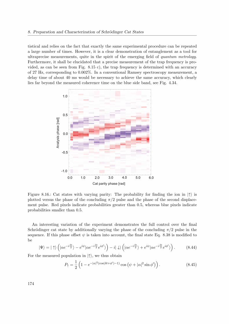
8. Preparation and Characterization of Schrodinger Cat States
tistical and relies on the fact that exactly the same experimental procedure can be repeateda large number of times. However, it is a clear demonstration of entanglement as a tool forultraprecise measurements, quite in the spirit of the emerging field of quantum metrology.Furthermore, it shall be elucidated that a precise measurement of the trap frequency is pro-vided, as can be seen from Fig. 8.15 c), the trap frequency is determined with an accuracyof 27 Hz, corresponding to 0.002%. In a conventional Ramsey spectroscopy measurement, adelay time of about 40 ms would be necessary to achieve the same accuracy, which clearlylies far beyond the measured coherence time on the blue side band, see Fig. 4.34.
1.0
0.5
0.0
-0.5
-1.0
0.0 1.0 2.0 3.0 4.0 5.0 6.0
Cat parity phase [rad]
Ana
lysi
s ph
ase
[rad]
Figure 8.16.: Cat states with varying parity: The probability for finding the ion in |↑〉 isplotted versus the phase of the concluding π/2 pulse and the phase of the second displace-ment pulse. Red pixels indicate probabilities greater than 0.5, whereas blue pixels indicateprobabilities smaller than 0.5.
An interesting variation of the experiment demonstrates the full control over the finalSchrodinger cat state by additionally varying the phase of the concluding π/2 pulse in thesequence. If this phase offset ψ is taken into account, the final state Eq. 8.38 is modified tobe
|Ψ〉 = | ↑〉(|αe−i δt
2 〉 − eiψ|αe−i δt2 eiφ
′〉)− i| ↓〉
(|αe−i δt
2 〉+ eiψ|αe−i δt2 eiφ
′〉). (8.44)
For the measured population in |↑〉, we thus obtain
P↑ =1
2
(1− e−|α|2(cos(δt+φ′)−1) cos
(ψ + |α|2 sinφ′)) . (8.45)
174

8.4. The Wavepacket Beating Scheme
The results of a corresponding measurement at a fixed displacement pulse time of 65µs areshown in Fig. 8.16. It is interesting to note that the measurement principle is quite analogousto 2D spectroscopy methods in molecular science. This offers the possibility to make use ofthis scheme for exploring nonlinear cross-couplings between distinct vibrational modes. Thebasic idea would be to perform the experiment on a two ion crystal, where the ions areplaced such that the COM as well as the STR mode can be excited. The modes will then beexcited in a sandwich-like manner, such that the influence of an initial COM excitation onthe STR mode dynamics can be investigated and vice versa. This would be analogous to theexperiment performed in Ref. [Roo08], only the controlled excitation of single vibrationalquanta is replaced by the controlled excitation of semiclassical vibrations. It is important tonote that the wavepacket beating scheme represents a very simple method for quantum statetomography of a vibrational mode, see chapter 7. The mathematical details and possiblefuture extensions are worked out in appendix D.
175

9. Measurements with Two-Ion Crystals
This chapter deals with the extension of the techniques for qubit handling developed through-out the chapters 4 and 8 to two-ion crystals, which represent the fundamental building blockfor our envisaged scheme for scalable quantum computing. Sec. 9.1 explains general issueson the crystal stability and shows how the read-out of two ions is performed. Measurementresults on the precise alignment of crystals in the driving Raman laser field are presentedin Sec. 9.2. Results from spectroscopy measurements and sideband cooling of crystals areshown in Sec. 9.3. Sec 9.4 treats the coherent manipulation of two ions and demonstrates anadvanced technique for simultaneous readout, while the concluding Sec. 9.5 presents resultson the generation of Schrodinger cat states with two ions, which is a crucial step towardsentangling quantum gates.
9.1. Stability and Read-out
Two ion crystals represent the intended basic building block for scalable quantum informa-tion experiments in our microtrap. Two-ion crystals are only loaded in the loading region ofour trap for rf-levels below 300 V peak-to-peak, corresponding to radial modes in the rangebetween 2 MHz and 3 MHz. Sufficient stability is attained at 250 V peak-to-peak and below.This behavior is counterintuitive as normally a high aspect ratio of the trap potential is favor-able for loading crystals, see Sec. 2.2. The reasons for this behavior are not entirely clear, butthe following facts are known: First, parametric instabilities can occur in Paul traps if secularfrequencies correspond to fractions of the rf frequency with small integer numbers in nomi-nator and denominator, which is a well known phenomenon in classical nonlinear dynamicsand is related to the Komolgoroff-Arnold-Moser (KAM) theorem. ’Canyons’ of instabilityfor such values β = n/m, n,m ∈ N were measured with high resolution in Ref. [Alh96]. Thereason for these instabilities, which are not predicted by the (harmonic) Mathieu equationsare anharmonicities, i.e. higher-order terms in the equations of motion Eqs. 2.76. These caneither arise because of the trap potentials themselves or from the highly nonlinear Coulombinteraction in the case of several ions, i.e. effects beyond the linearization in Eq. 2.81. Thiseffect was treated theoretically in [Mar03] and measurements of the energy transfer rate be-tween different motional modes were carried out in [Roo08]. The fact that the instability ofthe crystal increases for higher rf-levels despite the trap parameters are still deep inside theregion of stability suggests that micromotion also contributes to the instability.
However, it was found that at an rf-level of 250 Vpp and an axial trap frequency of2π·950 kHz, a sufficient stability to perform measurements on a two-ion crystal was at-tained. The stability substantially decreased at axial trap frequencies below 2π·900 kHz andabove 2π·1000 kHz. A fluorescence histogram of a two-ion crystal is shown in Fig. 9.1. In
177
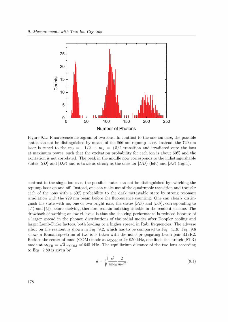
9. Measurements with Two-Ion Crystals
0 50 100 150 200 2500
5
10
15
20
25C
ount
s
Number of Photons
Figure 9.1.: Fluorescence histogram of two ions. In contrast to the one-ion case, the possiblestates can not be distinguished by means of the 866 nm repump laser. Instead, the 729 nmlaser is tuned to the mJ = +1/2 → mJ = +5/2 transition and irradiated onto the ionsat maximum power, such that the excitation probability for each ion is about 50% and theexcitation is not correlated. The peak in the middle now corresponds to the indistinguishablestates |SD〉 and |DS〉 and is twice as strong as the ones for |DD〉 (left) and |SS〉 (right).
contrast to the single ion case, the possible states can not be distinguished by switching therepump laser on and off. Instead, one can make use of the quadrupole transition and transfereach of the ions with a 50% probability to the dark metastable state by strong resonantirradiation with the 729 nm beam before the fluorescence counting. One can clearly distin-guish the state with no, one or two bright ions, the states |SD〉 and |DS〉, corresponding to|↓↑〉 and |↑↓〉 before shelving, therefore remain indistinguishable in the readout scheme. Thedrawback of working at low rf-levels is that the shelving performance is reduced because ofa larger spread in the phonon distributions of the radial modes after Doppler cooling andlarger Lamb-Dicke factors, both leading to a higher spread in Rabi frequencies. The adverseeffect on the readout is shown in Fig. 9.2, which has to be compared to Fig. 4.19. Fig. 9.6shows a Raman spectrum of two ions taken with the noncopropagating beam pair R1/R2.Besides the center-of-mass (COM) mode at ωCOM ≈ 2π·950 kHz, one finds the stretch (STR)mode at ωSTR =
√3 ωCOM ≈1645 kHz. The equilibrium distance of the two ions according
to Eqs. 2.80 is given by
d = 3
√e2
4πε0
2
mω2, (9.1)
178
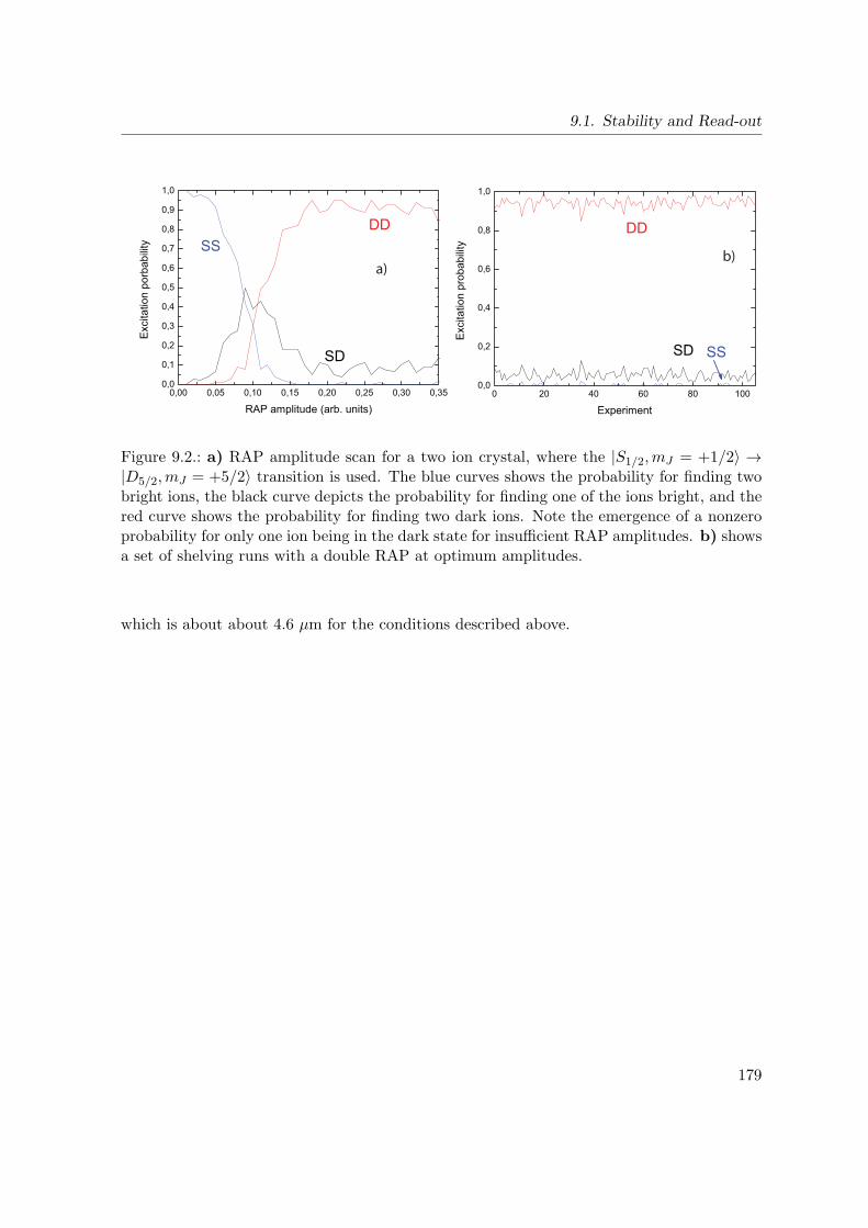
9.1. Stability and Read-out
0,00 0,05 0,10 0,15 0,20 0,25 0,30 0,350,0
0,1
0,2
0,3
0,4
0,5
0,6
0,7
0,8
0,9
1,0
SD
SSDD
Exc
itatio
n po
rbab
ility
RAP amplitude (arb. units)0 20 40 60 80 100
0,0
0,2
0,4
0,6
0,8
1,0
SD SS
Exc
itatio
n pr
obab
ility
Experiment
DD
a)b)
Figure 9.2.: a) RAP amplitude scan for a two ion crystal, where the |S1/2,mJ = +1/2〉 →|D5/2,mJ = +5/2〉 transition is used. The blue curves shows the probability for finding twobright ions, the black curve depicts the probability for finding one of the ions bright, and thered curve shows the probability for finding two dark ions. Note the emergence of a nonzeroprobability for only one ion being in the dark state for insufficient RAP amplitudes. b) showsa set of shelving runs with a double RAP at optimum amplitudes.
which is about about 4.6 µm for the conditions described above.
179
9. Measurements with Two-Ion Crystals
9.2. Localization and Alignment in a Standing Wave
The two-ion crystal is intended to be the basic building block in our future scalable quantuminformation processor, and one of the most advanced ingredients for its realization is theability to perform quantum logic gates between two spin qubits comprising such a crystal.The essential prerequisites for conducting the most suitable gate for our setting, which is thegeometric phase gate as is was realized in Rf. [Lei03b], are on the one hand that the spatiallocalization of the ions on a scale much below the wavelength of the driving laser field, whichis nothing else than the statement that the ions have to be in the Lamb-Dicke regime. Effectsoccurring if the ions are outside this regime are discussed in Sec. 8.2 for a single ion. Onthe other hand, the crystal has to be aligned to the running standing wave in such a waythat the relative phase of the driving field at the two different ion locations is such that the’gate’ mode on which the operation is driven couples to the field whereas the other does not.This requirement is not a strict one, however the performance of the gate deteriorates as thecoupling to the gate mode becomes weaker and the off-resonant excitation of the spectatormode increases when the alignment deviates from the optimum one.
In principle, if the Lamb-Dicke factor was known with sufficient precision, the alignmentof the crystal could be adjusted simply via the trap frequency. However, the angles atwhich the Raman beams intersect the trap axis cannot be precisely determined, and alsothe measurement of the Lamb-Dicke factor from the Fourier decomposition of sideband Rabioscillations, see Sec. 4.6, is subject to a relatively high uncertainty. A measurement schemeused in Ref. [Hom06a] for the alignment quantifies the coupling strengths to the COM andSTR modes with respect to the trap frequency by exerting a displacement pulse and probingthe motional state. This approach is rather tedious and requires ground state cooling ofboth modes. We have devised a method for measuring both localization and alignment byfluorescence observation, where the alignment can be performed in real-time. The underlyingidea is simple: If the frequency of the running standing wave from the R1 and R2 beams(which are necessarily vertically polarized for this measurement) is tuned close to the cyclingresonance and the normal Doppler cooling laser is turned off, both cooling and fluorescenceemission will be provided by the running standing wave. Therefore, the frequency componentpertaining to the relative detuning δ of the beams will be visible in each ion’s fluorescencelevel. The relative phase between these fluorescence oscillations of the two ions will bedetermined by the ion distance set by the trap frequency, Eq. 9.1, and information aboutthe localization of the ions is contained in the total signal levels.
180

9.2. Localization and Alignment in a Standing Wave
0 10 20 30 40 50
2200
2300
2400
2500
2600
2700
2800
2900
Fluo
resc
ence
[cou
nts/
50m
s]
Time [s]10 20 30 40 50
Time [s]
0 1 2 3 40
200
400
600
800
1000
1200
1400
1600
Four
ier c
ompo
nent
[a.u
.]
Frequency [Hz]1 2 3 4
Frequency [Hz]
0
50
100
150
200
250
300
Sig
nal a
mpl
itude
[a.u
.]
0 10 20 30 40 50-3
-2
-1
0
1
2
3
Sig
nal p
hase
[rad
]
Time [s]0 10 20 30 40 50
Time [s]
a)
b)
c)
d)
Figure 9.3.: Localization measurement samples: a)Measured two-ion fluorescence traces afterpreprocessing. b) Fast Fourier transform results with the Gaussian filter functions for σ=2 Hz(red), 4 Hz (blue) and 6 Hz (green). c) and d) show the resulting amplitude and phase curvesafter frequency shift and backward transform for the three different filter widths. The datain the left column is taken at an axial trap frequency of 1.36(1) MHz, whereas the data inthe right column pertains to a trap frequency of 1.22(1) MHz
181

9. Measurements with Two-Ion Crystals
4,4 4,6 4,8 5,0 5,2 5,4 5,6 5,80,0
0,5
1,0
1,5
Sig
nal a
mpl
itude
[a.u
.]
Ion distance [µm]
Figure 9.4.: Result of the localization measurement: The integrated signal amplitude is plot-ted versus the ion distance inferred from the spectroscopically measured trap frequency, alongwith a fit to Eq. 9.8.
The probability to find a thermal ion at position x is given by the thermal average
p(x) =∑n
pn|ψn(x)|2, (9.2)
which is a Gaussian distribution if the pn from Eq. 2.33 are used:
p(x) =1√2πσ2
e−x2
2σ2 , (9.3)
with
σ =
√2n+ 1
2σ0, (9.4)
where σ0 is the spatial extension of the ground state wavefunction σ0 =√
/2mω. If thetrap frequency is lowered, the localization is decreased not only due to a larger σ0, but alsothat n increases if a constant Doppler cooling temperature is assumed:
n =kBT
ω. (9.5)
182

9.2. Localization and Alignment in a Standing Wave
0 5 10 15 20 25-1,0
-0,5
0,0
0,5
1,0A
utoc
orre
latio
n am
plitu
de [a
.u.]
Time [s]
Figure 9.5.: Fluorescence autocorrelation: The autocorrelation function for the data set inthe left column of Fig. 9.3 is shown. From the correlation decay it can be inferred that thetimescale on which the R1/R2 interferometer drifts by a relative phase of π is in the rangeof 10 s.
For small saturation, the fluorescence rate of a single ion located at position x in the inter-ference pattern will be
R =Γ
2(1 + 4∆2/Γ2)
(S21 + S2
2 + 2√
S1S2 cos(δkx− δt+∆φ)), (9.6)
where S1,2 are the saturation parameters of the R1 and R2 beams, δk is the difference wavevec-tor pointing along the trap axis, ∆φ is the relative optical phase and ∆ δ is the commonred-detuning from resonance. If the saturation parameters are not exactly matched or thepolarization if imperfectly aligned, a fluorescence baseline occurs in the interference whichdecreases the signal-to-noise ratio. As we are interested only in the frequency component atδ, the baseline will be ignored in the following. For two ions, we thus obtain
R(x) ∝ (cos (δk(x0 − l/2)− δt) + cos (δk(x0 + l/2)− δt)) . (9.7)
We now consider the case of two ions located at the sites x0 + x′ ± (l0 + l′)/2. x0 = 0 and l0are the center positions of the COM and STR wavefunctions, and x′ and l′ are the quantum
183
9. Measurements with Two-Ion Crystals
statistical deviations, which are to be averaged over. This yields
Rtot ∝∫
dx′p(x′)∫
dl′p(l′)(ei∆k(x′−(l0+l′/2)) + ei∆k(x′+(l0+l′)/2)
)∝ cos (δkl0/2) e
−δk2(σ2x/2+σ2
l /2), (9.8)
where already only the frequency component at δ is considered and the thermal delocalizationwidths σx and σl for the COM and STR motion from Eq. 9.4 are used.The experiment is carried out as follows: A two ion crystal is trapped at various axialconfinement frequencies, i.e. the trapping voltage at segment #5 is changed. For eachtrapping voltage, spectroscopy on the quadrupole transition is performed to determine theposition of the carrier and the red axial sideband. The crystal is then placed in the verticallypolarized standing wave of the R1 and R2 beams, where the R2 beam is detuned from the R1beam by exactly 2 Hz. Fluorescence is then recorded on the PMT for 50 seconds, with 50 msbinning. The resulting fluorescence displays 2 Hz oscillation if the ions are spaced exactly byan integer number of nodal distances. This 2 Hz signal component is strongly affected by shotnoise, interferometer drift and spontaneous melting of the ion crystal, thus great care mustbe taken to obtain a valid figure of the signal strength. Two sample data sets are shown inFig. 9.3. The data set is preprocessed to remove melting effects which would spuriously affectthe resulting signal amplitude, also very large fluorescence values are present which possiblystem from cosmic ray events. The data is cleaned in such a way that fluorescence values lyingoutside the interval given by ±3 standard deviations from the mean fluorescence are set tozero, the resulting corrected mean of the cleaned data then provides a valid normalizationreference for the final result. The values set to zero are then set to this mean value in orderto avoid artifacts in the frequency spectrum. The processed data set is Fourier transformed,the spectrum is the filtered by applying a Gaussian filer function of fixed width around 2 Hz.The filtered spectrum is then shifted such that the 2 Hz component becomes the dc one, thenthe backward transform is carried out, giving a smoothed information of signal amplitudeand phase versus time. The amplitude is then integrated to give the final value, which isnormalized on the mean of the valid fluorescence counts. For each trap voltage, 5 individualtraces are taken to obtain an error estimation. Fig. 9.3 shows sample measurement resultsfor two different trap frequencies, where also the dependence of the result on the width of theGaussian filter function is demonstrated. For broader filter widths, the integral amplitude,which is the final quantity of interest, seems to be quite independent of this parameter.Fig. 9.4 shows the final result, together with a fit to the model Eq. 9.8, where the datafor the 6 Hz filter window was used. The floating parameters are the effective wavenumberalong the trap axis, the temperature T and an amplitude scaling factor A. The effectivewavelength of the beat pattern can be accurately determined due to the oscillatory structure,its value is found to be λeff=267.8(2) nm. The temperature can not be accurately determinedas it is mainly given by the slope of the maxima, which is strongly correlated to A. Valuesaround 1.5 mK, equivalent to nCOM ≈23 and nSTR ≈13 at ωax = 2π · 1.35 MHz are found,which is entirely consistent with the expected Doppler cooling result, which is also foundin the thermal Schrodinger cat measurement in Sec. 8.2. In conclusion, this method is to
184

9.2. Localization and Alignment in a Standing Wave
our knowledge to only method the determine the Lamb-Dicke factor with permil accuracyin a setting where no two-mode ground state purity of a two ion crystal, nor long enoughcoherence times for observing Rabi oscillations on a blue motional sideband can be attained.It provides an easy method for alignment of a two ion crystal in a standing wave and mighttherefore be part of the every-day routine in the future operation of the setup after beamrealignment. Furthermore, it provides an easy verification that the Doppler cooling performsas expected for future traps, and is also a benchmark for the interferometic stability. Fig.9.5 shows the autocorrelation function as it is calculated by employing the Wiener-Khinchinetheorem: The power spectrum of the signal is calculated by taking the absolute squaredvalues of an FFT of the fluorescence data, followed by the inverse transform. The resultingautocorrelation function
C(τ) = 〈S(t)S(t+ τ)〉t (9.9)
is of course only an approximation as the Wiener-Khinchine theorem holds only strictly foran infinitely long acquisition period, however the correlation decay timescale is still clearlyvisible. 1
1The finding of a 10 s timescale is consistent with a measurement where a ’mixed’ Ramsey experiment isperformed, where the R1/CC beam pair is used for the first π/2 pulse, and the R1/R2 beam pair forthe second one. If the interferometers were perfectly stable, the fringe pattern would reveal the relativeoptical phase of the R2 beam with respect to the CC one. Upon scanning the concluding π/2 pulse phase,data points deviating significantly from 0.5 were measured, indicating nonvanishing correlation during theacquisition time of one data point, but no clear and reproducible fringe pattern could be observed.
185
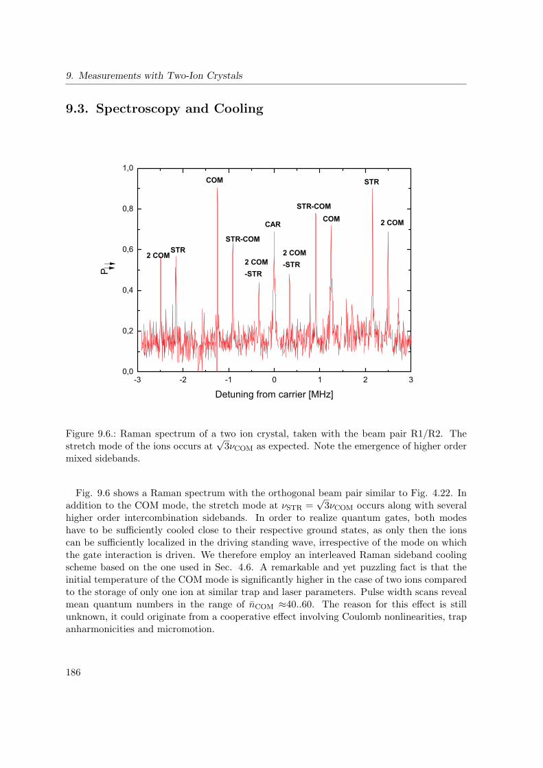
9. Measurements with Two-Ion Crystals
9.3. Spectroscopy and Cooling
-3 -2 -1 0 1 2 30,0
0,2
0,4
0,6
0,8
1,0
2 COM-STR
P
Detuning from carrier [MHz]
CAR
COM
COM
STR
STR
2 COM
2 COM
STR-COM
STR-COM
2 COM-STR
Figure 9.6.: Raman spectrum of a two ion crystal, taken with the beam pair R1/R2. Thestretch mode of the ions occurs at
√3νCOM as expected. Note the emergence of higher order
mixed sidebands.
Fig. 9.6 shows a Raman spectrum with the orthogonal beam pair similar to Fig. 4.22. Inaddition to the COM mode, the stretch mode at νSTR =
√3νCOM occurs along with several
higher order intercombination sidebands. In order to realize quantum gates, both modeshave to be sufficiently cooled close to their respective ground states, as only then the ionscan be sufficiently localized in the driving standing wave, irrespective of the mode on whichthe gate interaction is driven. We therefore employ an interleaved Raman sideband coolingscheme based on the one used in Sec. 4.6. A remarkable and yet puzzling fact is that theinitial temperature of the COM mode is significantly higher in the case of two ions comparedto the storage of only one ion at similar trap and laser parameters. Pulse width scans revealmean quantum numbers in the range of nCOM ≈40..60. The reason for this effect is stillunknown, it could originate from a cooperative effect involving Coulomb nonlinearities, trapanharmonicities and micromotion.
186

9.3. Spectroscopy and Cooling
Removal of these large phonon numbers requires a sequential cooling scheme involvinghigher order sidebands making use of the fact that the average Rabi frequencies on higherorder sidebands is larger for higher initial temperatures and excitation on higher order side-bands leads to simultaneous removal of multiple phonons, see Fig. 4.32. The cooling sequenceused in our experiments is indicated in table 9.1. From the pulse times, the cycles numbersand the repump time of 2 µs, a total cooling time of 1.66 ms results. During this time,significant radial heating of the ions takes place and also the stability of the crystal duringthe measurement is adversely affected.
No. Sideband Cooling cycles π-time
1 3rd COM 20 6.0
2 2nd COM 30 10.0
3 1st STR 50 7.0
4 1st COM 50 11.0
5 1st STR 5 7.0
Table 9.1.: Sideband cooling sequence for two ions.
The radial temperature degrades the efficiency of both the RAP pulses and the fluorescencereadout, therefore the state discrimination of |↑↑〉 , |↑↓〉 and |↓↓〉 deviates strongly from theideal one. The readout has to be described by the conditional probabilities to find theions dark or bright (d/b) depending on their actual state before the readout. The followingconditional probabilities were found when fitting the pulse width scans in Fig. 9.7:
p(dd| ↑↑) ≈ 0.885 p(dd| ↑↓) ≈ 0.100 p(dd| ↓↓) ≈ 0.015
p(db| ↑↑) ≈ 0.250 p(db| ↑↓) ≈ 0.525 p(db| ↓↓) ≈ 0.050
p(bb| ↑↑) ≈ 0.015 p(bb| ↑↓) ≈ 0.225 p(bb| ↓↓) ≈ 0.800 (9.10)
(9.11)
Note the low probability p(db| |↑↓〉) that one ion in |↑〉 actually leads to measurement of adb event. This indicates that the fluorescence rates are subject to additional fluctuations,i.e. the count statistics is strongly affected by the probabilistic heating of the ions. Weextend the model for a coherently driven ion with coupling to one motional mode Eq. 4.34 tosimultaneous coupling to two motional modes. The probability to find a single ion initializedin |↑〉 in the |↓〉 state after irradiation of a pulse of duration t is given by:
P(∆nC ,∆nS)↓ (t) = 1
2
∑nC
∑nS
P (C)nC
P (S)nS
(cos (M(C)n,n+∆nC
M(S)n,n+∆nS
Ω0 t) e−γ t + 1), (9.12)
describing Rabi oscillations on the ∆nC-th, ∆nS-th sideband obtained by summation over
the COM (C) and STR (S) modes with the respective phonon distributions P(C)nC ,P
(S)nS in-
cluding the matrix elements M(C)n,n+∆nC
and M(S)n,n+∆nS
. From this, the probabilities for two
187
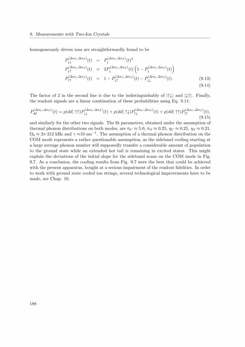
9. Measurements with Two-Ion Crystals
homogeneously driven ions are straightforwardly found to be
P(∆nC ,∆nS)↓↓ (t) = P
(∆nC ,∆nS)↓ (t)2
P(∆nC ,∆nS)↓↑ (t) = 2P
(∆nC ,∆nS)↓ (t)
(1− P
(∆nC ,∆nS)↓ (t)
)P
(∆nC ,∆nS)↑↑ (t) = 1− P
(∆nC ,∆nS)↓↑ (t)− P
(∆nC ,∆nS)↓↓ (t). (9.13)
(9.14)
The factor of 2 in the second line is due to the indistinguishably of |↑↓〉 and |↓↑〉. Finally,the readout signals are a linear combination of these probabilities using Eq. 9.11:
P(∆nC ,∆nS)dd (t) = p(dd| ↑↑)P (∆nC ,∆nS)
↓↓ (t) + p(dd| ↑↓)P (∆nC ,∆nS)↑↓ (t) + p(dd| ↑↑)P (∆nC ,∆nS)
↑↑ (t),(9.15)
and similarly for the other two signals. The fit parameters, obtained under the assumption ofthermal phonon distributions on both modes, are nC ≈ 5.0, nS ≈ 0.25, ηC ≈ 0.25, ηS ≈ 0.21,Ω0 ≈ 2π·212 kHz and γ ≈10 ms−1. The assumption of a thermal phonon distribution on theCOM mode represents a rather questionable assumption, as the sideband cooling starting ata large average phonon number will supposedly transfer a considerable amount of populationto the ground state while an extended hot tail is remaining in excited states. This mightexplain the deviations of the initial slope for the sideband scans on the COM mode in Fig.9.7. As a conclusion, the cooling results from Fig. 9.7 were the best that could be achievedwith the present apparatus, bought at a serious impairment of the readout fidelities. In orderto work with ground state cooled ion strings, several technological improvements have to bemade, see Chap. 10.
188
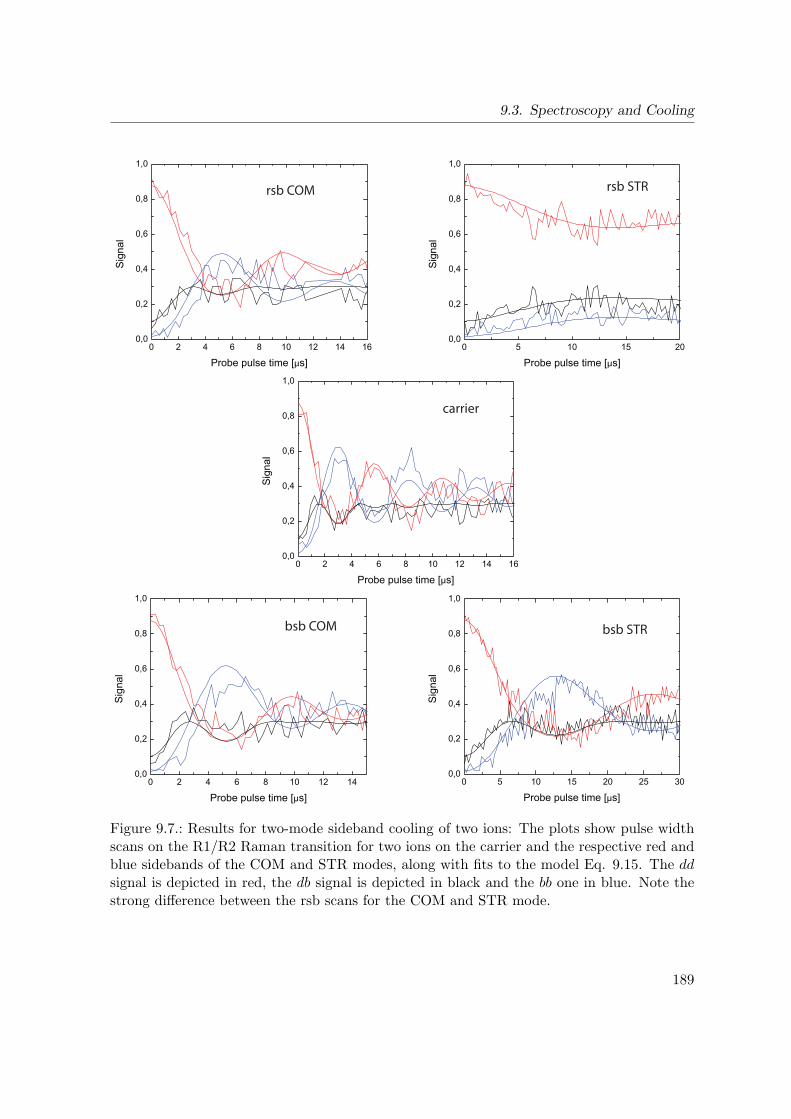
9.3. Spectroscopy and Cooling
0 2 4 6 8 10 12 14 160,0
0,2
0,4
0,6
0,8
1,0
Sig
nal
Probe pulse time [µs]
0 5 10 15 200,0
0,2
0,4
0,6
0,8
1,0
Sig
nal
Probe pulse time [µs]0 2 4 6 8 10 12 14 16
0,0
0,2
0,4
0,6
0,8
1,0
Sig
nal
Probe pulse time [µs]
0 5 10 15 20 25 300,0
0,2
0,4
0,6
0,8
1,0
Sig
nal
Probe pulse time [µs]0 2 4 6 8 10 12 14
0,0
0,2
0,4
0,6
0,8
1,0
Sig
nal
Probe pulse time [µs]
rsb COM rsb STR
carrier
bsb COM bsb STR
Figure 9.7.: Results for two-mode sideband cooling of two ions: The plots show pulse widthscans on the R1/R2 Raman transition for two ions on the carrier and the respective red andblue sidebands of the COM and STR modes, along with fits to the model Eq. 9.15. The ddsignal is depicted in red, the db signal is depicted in black and the bb one in blue. Note thestrong difference between the rsb scans for the COM and STR mode.
189
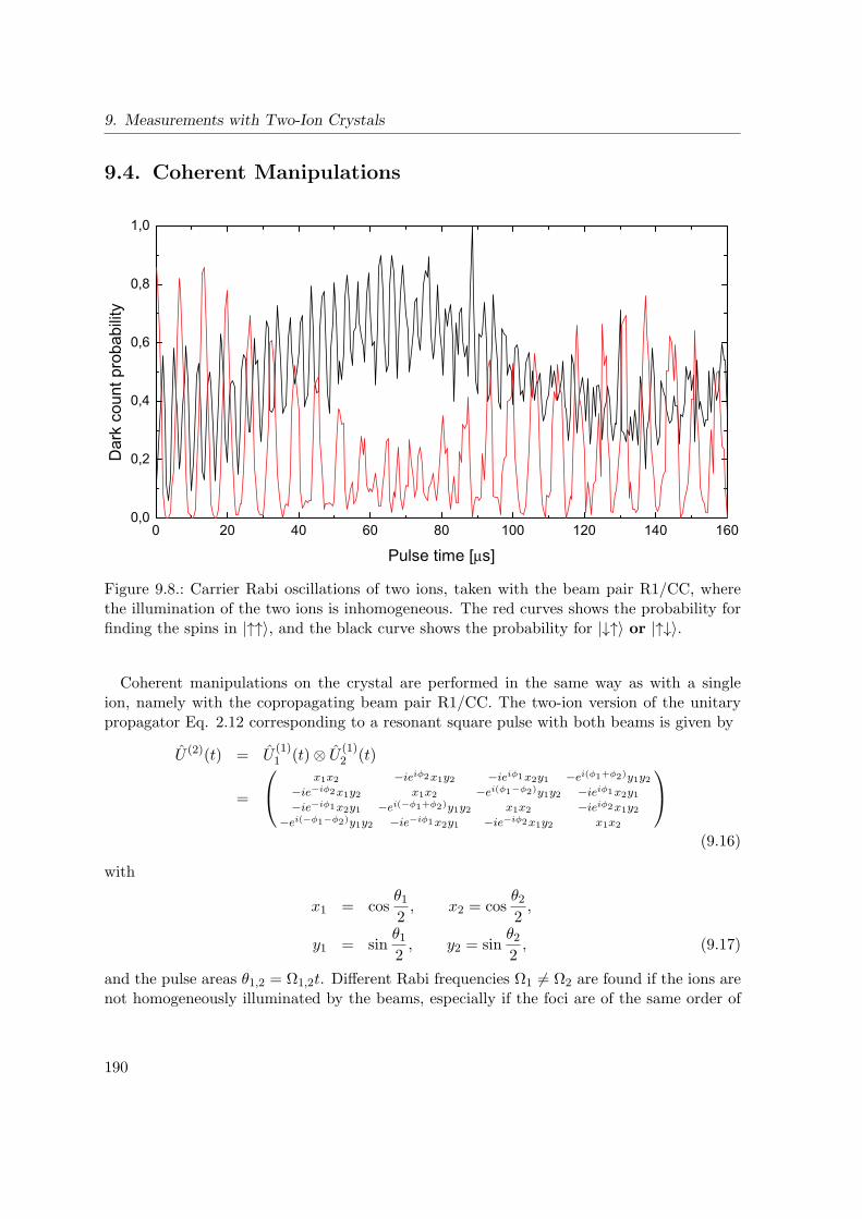
9. Measurements with Two-Ion Crystals
9.4. Coherent Manipulations
0 20 40 60 80 100 120 140 1600,0
0,2
0,4
0,6
0,8
1,0
Dar
k co
unt p
roba
bilit
y
Pulse time [µs]
Figure 9.8.: Carrier Rabi oscillations of two ions, taken with the beam pair R1/CC, wherethe illumination of the two ions is inhomogeneous. The red curves shows the probability forfinding the spins in |↑↑〉, and the black curve shows the probability for |↓↑〉 or |↑↓〉.
Coherent manipulations on the crystal are performed in the same way as with a singleion, namely with the copropagating beam pair R1/CC. The two-ion version of the unitarypropagator Eq. 2.12 corresponding to a resonant square pulse with both beams is given by
U (2)(t) = U(1)1 (t)⊗ U
(1)2 (t)
=
⎛⎝ x1x2 −ieiφ2x1y2 −ieiφ1x2y1 −ei(φ1+φ2)y1y2
−ie−iφ2x1y2 x1x2 −ei(φ1−φ2)y1y2 −ieiφ1x2y1−ie−iφ1x2y1 −ei(−φ1+φ2)y1y2 x1x2 −ieiφ2x1y2
−ei(−φ1−φ2)y1y2 −ie−iφ1x2y1 −ie−iφ2x1y2 x1x2
⎞⎠
(9.16)
with
x1 = cosθ12, x2 = cos
θ22,
y1 = sinθ12, y2 = sin
θ22, (9.17)
and the pulse areas θ1,2 = Ω1,2t. Different Rabi frequencies Ω1 = Ω2 are found if the ions arenot homogeneously illuminated by the beams, especially if the foci are of the same order of
190
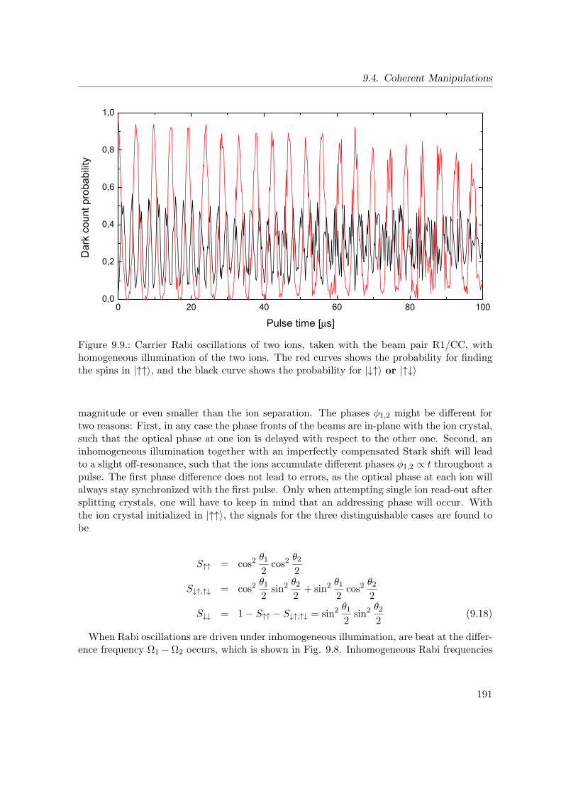
9.4. Coherent Manipulations
0 20 40 60 80 1000,0
0,2
0,4
0,6
0,8
1,0
Dar
k co
unt p
roba
bilit
y
Pulse time [µs]
Figure 9.9.: Carrier Rabi oscillations of two ions, taken with the beam pair R1/CC, withhomogeneous illumination of the two ions. The red curves shows the probability for findingthe spins in |↑↑〉, and the black curve shows the probability for |↓↑〉 or |↑↓〉
magnitude or even smaller than the ion separation. The phases φ1,2 might be different fortwo reasons: First, in any case the phase fronts of the beams are in-plane with the ion crystal,such that the optical phase at one ion is delayed with respect to the other one. Second, aninhomogeneous illumination together with an imperfectly compensated Stark shift will leadto a slight off-resonance, such that the ions accumulate different phases φ1,2 ∝ t throughout apulse. The first phase difference does not lead to errors, as the optical phase at each ion willalways stay synchronized with the first pulse. Only when attempting single ion read-out aftersplitting crystals, one will have to keep in mind that an addressing phase will occur. Withthe ion crystal initialized in |↑↑〉, the signals for the three distinguishable cases are found tobe
S↑↑ = cos2θ12cos2
θ22
S↓↑,↑↓ = cos2θ12sin2
θ22
+ sin2θ12cos2
θ22
S↓↓ = 1− S↑↑ − S↓↑,↑↓ = sin2θ12sin2
θ22
(9.18)
When Rabi oscillations are driven under inhomogeneous illumination, are beat at the differ-ence frequency Ω1 −Ω2 occurs, which is shown in Fig. 9.8. Inhomogeneous Rabi frequencies
191
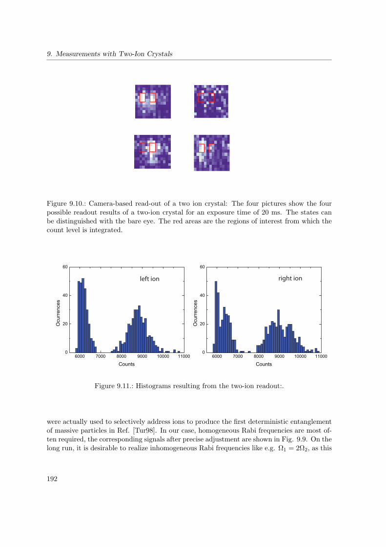
9. Measurements with Two-Ion Crystals
Figure 9.10.: Camera-based read-out of a two ion crystal: The four pictures show the fourpossible readout results of a two-ion crystal for an exposure time of 20 ms. The states canbe distinguished with the bare eye. The red areas are the regions of interest from which thecount level is integrated.
6000 7000 8000 9000 10000 110000
20
40
60
Ocurrences
Counts6000 7000 8000 9000 10000 11000
0
20
40
60
Ocurrences
Counts
left ion right ion
Figure 9.11.: Histograms resulting from the two-ion readout:.
were actually used to selectively address ions to produce the first deterministic entanglementof massive particles in Ref. [Tur98]. In our case, homogeneous Rabi frequencies are most of-ten required, the corresponding signals after precise adjustment are shown in Fig. 9.9. On thelong run, it is desirable to realize inhomogeneous Rabi frequencies like e.g. Ω1 = 2Ω2, as this
192
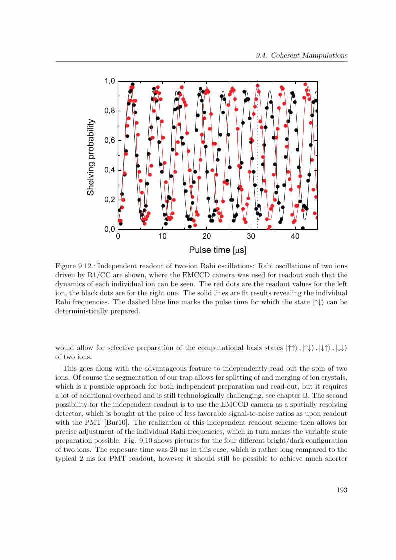
9.4. Coherent Manipulations
0 10 20 30 400,0
0,2
0,4
0,6
0,8
1,0S
helv
ing
prob
abili
ty
Pulse time [µs]
Figure 9.12.: Independent readout of two-ion Rabi oscillations: Rabi oscillations of two ionsdriven by R1/CC are shown, where the EMCCD camera was used for readout such that thedynamics of each individual ion can be seen. The red dots are the readout values for the leftion, the black dots are for the right one. The solid lines are fit results revealing the individualRabi frequencies. The dashed blue line marks the pulse time for which the state |↑↓〉 can bedeterministically prepared.
would allow for selective preparation of the computational basis states |↑↑〉 , |↑↓〉 , |↓↑〉 , |↓↓〉of two ions.
This goes along with the advantageous feature to independently read out the spin of twoions. Of course the segmentation of our trap allows for splitting of and merging of ion crystals,which is a possible approach for both independent preparation and read-out, but it requiresa lot of additional overhead and is still technologically challenging, see chapter B. The secondpossibility for the independent readout is to use the EMCCD camera as a spatially resolvingdetector, which is bought at the price of less favorable signal-to-noise ratios as upon readoutwith the PMT [Bur10]. The realization of this independent readout scheme then allows forprecise adjustment of the individual Rabi frequencies, which in turn makes the variable statepreparation possible. Fig. 9.10 shows pictures for the four different bright/dark configurationof two ions. The exposure time was 20 ms in this case, which is rather long compared to thetypical 2 ms for PMT readout, however it should still be possible to achieve much shorter
193
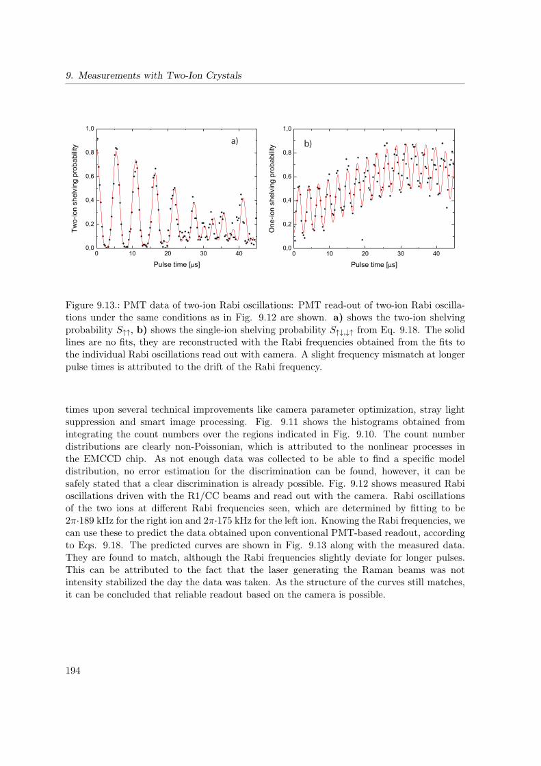
9. Measurements with Two-Ion Crystals
0 10 20 30 400,0
0,2
0,4
0,6
0,8
1,0
Two-
ion
shel
ving
pro
babi
lity
Pulse time [µs]0 10 20 30 40
0,0
0,2
0,4
0,6
0,8
1,0
One
-ion
shel
ving
pro
babi
lity
Pulse time [µs]
a) b)
Figure 9.13.: PMT data of two-ion Rabi oscillations: PMT read-out of two-ion Rabi oscilla-tions under the same conditions as in Fig. 9.12 are shown. a) shows the two-ion shelvingprobability S↑↑, b) shows the single-ion shelving probability S↑↓,↓↑ from Eq. 9.18. The solidlines are no fits, they are reconstructed with the Rabi frequencies obtained from the fits tothe individual Rabi oscillations read out with camera. A slight frequency mismatch at longerpulse times is attributed to the drift of the Rabi frequency.
times upon several technical improvements like camera parameter optimization, stray lightsuppression and smart image processing. Fig. 9.11 shows the histograms obtained fromintegrating the count numbers over the regions indicated in Fig. 9.10. The count numberdistributions are clearly non-Poissonian, which is attributed to the nonlinear processes inthe EMCCD chip. As not enough data was collected to be able to find a specific modeldistribution, no error estimation for the discrimination can be found, however, it can besafely stated that a clear discrimination is already possible. Fig. 9.12 shows measured Rabioscillations driven with the R1/CC beams and read out with the camera. Rabi oscillationsof the two ions at different Rabi frequencies seen, which are determined by fitting to be2π·189 kHz for the right ion and 2π·175 kHz for the left ion. Knowing the Rabi frequencies, wecan use these to predict the data obtained upon conventional PMT-based readout, accordingto Eqs. 9.18. The predicted curves are shown in Fig. 9.13 along with the measured data.They are found to match, although the Rabi frequencies slightly deviate for longer pulses.This can be attributed to the fact that the laser generating the Raman beams was notintensity stabilized the day the data was taken. As the structure of the curves still matches,it can be concluded that reliable readout based on the camera is possible.
194
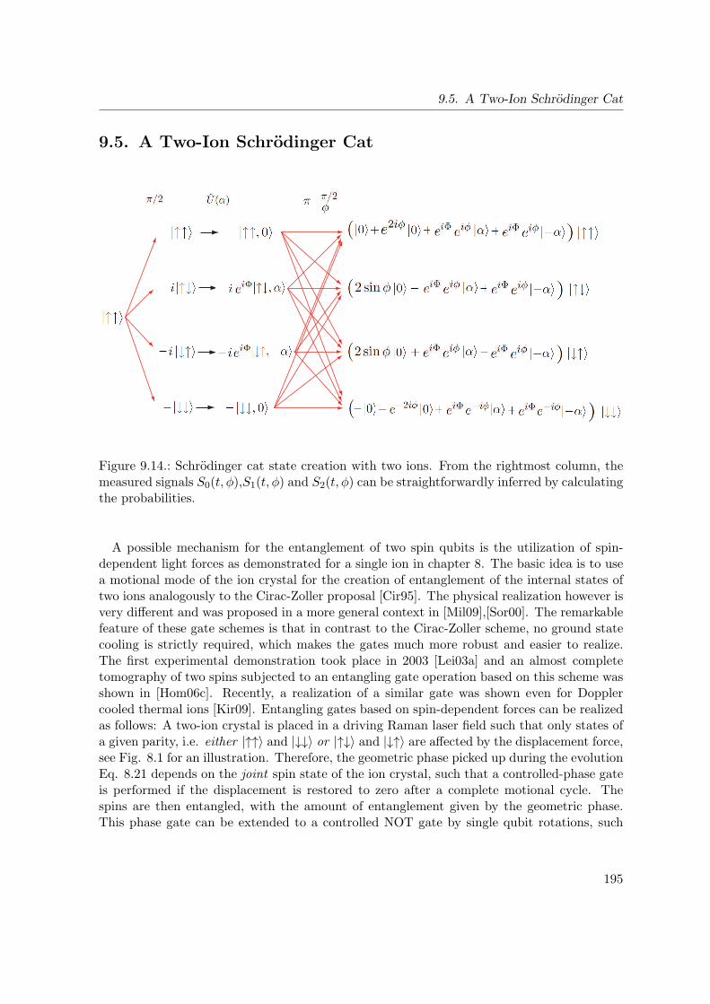
9.5. A Two-Ion Schrodinger Cat
9.5. A Two-Ion Schrodinger Cat
Figure 9.14.: Schrodinger cat state creation with two ions. From the rightmost column, themeasured signals S0(t, φ),S1(t, φ) and S2(t, φ) can be straightforwardly inferred by calculatingthe probabilities.
A possible mechanism for the entanglement of two spin qubits is the utilization of spin-dependent light forces as demonstrated for a single ion in chapter 8. The basic idea is to usea motional mode of the ion crystal for the creation of entanglement of the internal states oftwo ions analogously to the Cirac-Zoller proposal [Cir95]. The physical realization however isvery different and was proposed in a more general context in [Mil09],[Sor00]. The remarkablefeature of these gate schemes is that in contrast to the Cirac-Zoller scheme, no ground statecooling is strictly required, which makes the gates much more robust and easier to realize.The first experimental demonstration took place in 2003 [Lei03a] and an almost completetomography of two spins subjected to an entangling gate operation based on this scheme wasshown in [Hom06c]. Recently, a realization of a similar gate was shown even for Dopplercooled thermal ions [Kir09]. Entangling gates based on spin-dependent forces can be realizedas follows: A two-ion crystal is placed in a driving Raman laser field such that only states ofa given parity, i.e. either |↑↑〉 and |↓↓〉 or |↑↓〉 and |↓↑〉 are affected by the displacement force,see Fig. 8.1 for an illustration. Therefore, the geometric phase picked up during the evolutionEq. 8.21 depends on the joint spin state of the ion crystal, such that a controlled-phase gateis performed if the displacement is restored to zero after a complete motional cycle. Thespins are then entangled, with the amount of entanglement given by the geometric phase.This phase gate can be extended to a controlled NOT gate by single qubit rotations, such
195
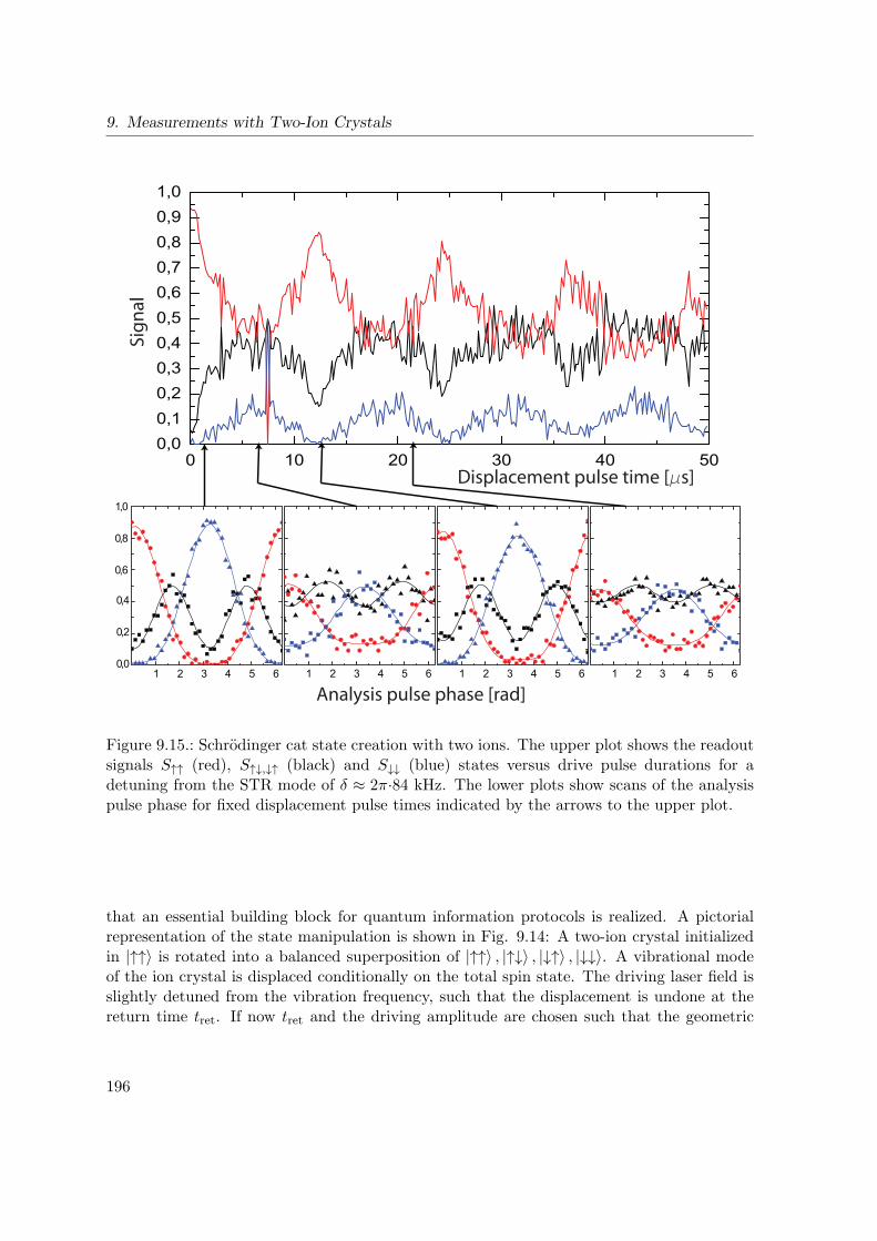
9. Measurements with Two-Ion Crystals
0 10 20 30 40 500,00,10,20,30,40,50,60,70,80,91,0
1 2 3 4 5 61 2 3 4 5 61 2 3 4 5 61 2 3 4 5 60,0
0,2
0,4
0,6
0,8
1,0
Displacement pulse time [ s]
Analysis pulse phase [rad]
Sig
na
l
Figure 9.15.: Schrodinger cat state creation with two ions. The upper plot shows the readoutsignals S↑↑ (red), S↑↓,↓↑ (black) and S↓↓ (blue) states versus drive pulse durations for adetuning from the STR mode of δ ≈ 2π·84 kHz. The lower plots show scans of the analysispulse phase for fixed displacement pulse times indicated by the arrows to the upper plot.
that an essential building block for quantum information protocols is realized. A pictorialrepresentation of the state manipulation is shown in Fig. 9.14: A two-ion crystal initializedin |↑↑〉 is rotated into a balanced superposition of |↑↑〉 , |↑↓〉 , |↓↑〉 , |↓↓〉. A vibrational modeof the ion crystal is displaced conditionally on the total spin state. The driving laser field isslightly detuned from the vibration frequency, such that the displacement is undone at thereturn time tret. If now tret and the driving amplitude are chosen such that the geometric
196
9.5. A Two-Ion Schrodinger Cat
phase Φ = π/2, the resulting state is can be unitarily rotated to
|Ψ〉 = 2−1/2 (| ↑↑〉+ i| ↓↓〉) , (9.19)
which is a maximally entangled state. The creation of entanglement can be easily deducedfrom the suppression of the signals pertaining to the |↑↓〉 , |↓↑〉 signals. The ultimate proofof entanglement and measurement of the fidelity of the operation is performed by a parityoscillation measurement, see Ref. [Lei03b]. The constraint that only the spin states pertainingto a given parity are to be displaced can be relaxed to the requirement that the displacementfor the different parities has to be substantially different, such that a differential geometricphase is picked up. Imperfect alignment will only degrade the efficiency of the gate withrespect to the exploitation of the driving laser power. The important implication of this isthat the gate scheme can be straightforwardly extended to a larger number of ions, mostimportantly to the case of four ions comprising a pair of a pair of logical qubits, encoded in adecoherence free subspace (DFS). Such a gate would have the advantage that the logical qubitswould never leave the DFS at any point during the gate operation, as we have investigatedin [Iva09].The choice of the right drive amplitude is performed simply by minimizing the S↑↓,↓↑ signalat a drive time of tret, and the placement of the ions by choice of the trap frequency isnot crucial, i.e. a spin-dependent geometric phase can be picked up as long as the couplingstrength to the laser field is substantially different for |↑↓〉 , |↓↑〉 and |↓↓〉 , |↓↓〉. However,near-perfect ground state cooling of both motional modes of the two-ion crystal is a criticalprerequisite, as a finite temperature has several detrimental effects on the gate performance:i) Due to the temperature-induced delocalization, the coupling strength difference between|↑↓〉 , |↓↑〉 and |↓↓〉 , |↓↓〉 is diminished, ii) the overall coupling strength is diminished and iii)the geometric phase picked up is fluctuating, leading to a loss of phase coherence.We have created Schrodinger cat states of two Doppler cooled ions by near resonant excitationof the STR mode. The results are shown in Fig. 9.15, where the results of a scan of thedisplacement pulse time at fixed analysis pulse phase are shown, along with scans of theanalysis pulse phase for a set of fixed displacement pulse times. As can be seen, no signatureof a geometric phase, i.e. a nonzero S↓↓ signal and suppression of the S↑↓,↓↑ signal at thereturn times is visible, despite the fact that a clear decay and revival of the contrast is present.The reason is the increased sensitivity of motionally excited states to displacement, see themeasurements for a thermal single ion shown in Fig. 8.4 for comparison. The data from thescans of the analysis pulse phase can be used for a detailed characterization of the quantumdynamics of the two ions. We first need to generalize the simplified dynamics illustrated inFig. 9.14 to account for imperfections: First, we include a possible displacement of the evenstates |↑↑〉 and |↓↓〉 by the value β, and therefore include a geometric phase Φ for these states.Furthermore, we include a possible residual Stark shift, leading to an additional spin phase
197
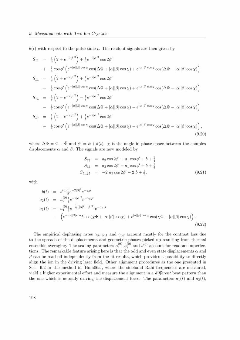
9. Measurements with Two-Ion Crystals
θ(t) with respect to the pulse time t. The readout signals are then given by
S↑↑ = 18
(2 + e−2|β|2
)+ 1
8e−2|α|2 cos 2φ′
+ 14 cosφ
′(e−|α||β| cosχ cos(∆Φ + |α||β| cosχ) + e|α||β| cosχ cos(∆Φ− |α||β| cosχ)
)S↓↓ = 1
8
(2 + e−2|β|2
)+ 1
8e−2|α|2 cos 2φ′
− 14 cosφ
′(e−|α||β| cosχ cos(∆Φ + |α||β| cosχ) + e|α||β| cosχ cos(∆Φ− |α||β| cosχ)
)S↑↓ = 1
8
(2− e−2|β|2
)− 1
8e−2|α|2 cos 2φ′
− 14 cosφ
′(e−|α||β| cosχ cos(∆Φ + |α||β| cosχ)− e|α||β| cosχ cos(∆Φ− |α||β| cosχ)
)S↓↑ = 1
8
(2− e−2|β|2
)+ 1
8e−2|α|2 cos 2φ′
− 14 cosφ
′(e−|α||β| cosχ cos(∆Φ + |α||β| cosχ)− e|α||β| cosχ cos(∆Φ− |α||β| cosχ)
),
(9.20)
where ∆Φ = Φ − Φ and φ′ = φ + θ(t). χ is the angle in phase space between the complexdisplacements α and β. The signals are now modeled by
S↑↑ = a2 cos 2φ′ + a1 cosφ
′ + b+ 14
S↓↓ = a2 cos 2φ′ − a1 cosφ
′ + b+ 14
S↑↓,↓↑ = −2 a2 cos 2φ′ − 2 b+ 1
2 , (9.21)
with
b(t) = b(0) 18e−2|β|2e−γβt
a2(t) = a(0)2
18e
−2|α|2e−γα2t
a1(t) = a(0)1
14e
−12(|α|2+|β|2)e−γα1t
·(e−|α||β| cosχ cos(χΦ+ |α||β| cosχ) + e|α||β| cosχ cos(χΦ− |α||β| cosχ)
).
(9.22)
The empirical dephasing rates γβ , γα1 and γα2 account mostly for the contrast loss dueto the spreads of the displacements and geometric phases picked up resulting from thermal
ensemble averaging. The scaling parameters a(0)1 , a
(0)2 and b(0) account for readout imperfec-
tions. The remarkable feature arising here is that the odd and even state displacements α andβ can be read off independently from the fit results, which provides a possibility to directlyalign the ion in the driving laser field. Other alignment procedures as the one presented inSec. 9.2 or the method in [Hom06a], where the sideband Rabi frequencies are measured,yield a higher experimental effort and measure the alignment in a different beat pattern thanthe one which is actually driving the displacement force. The parameters a1(t) and a2(t),
198
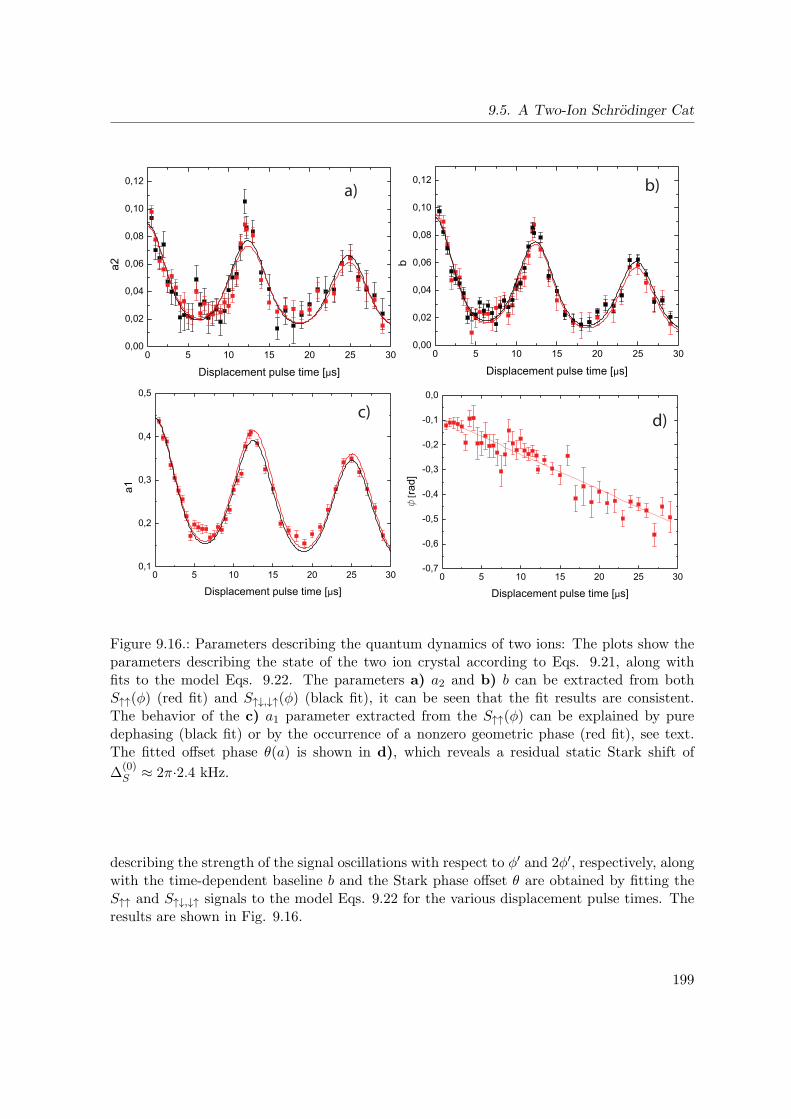
9.5. A Two-Ion Schrodinger Cat
0 5 10 15 20 25 30-0,7
-0,6
-0,5
-0,4
-0,3
-0,2
-0,1
0,0[ra
d]
Displacement pulse time [µs]
0 5 10 15 20 25 300,00
0,02
0,04
0,06
0,08
0,10
0,12
b
Displacement pulse time [µs]0 5 10 15 20 25 30
0,00
0,02
0,04
0,06
0,08
0,10
0,12
a2
Displacement pulse time [µs]
0 5 10 15 20 25 300,1
0,2
0,3
0,4
0,5
a1
Displacement pulse time [µs]
a) b)
c)d)
Figure 9.16.: Parameters describing the quantum dynamics of two ions: The plots show theparameters describing the state of the two ion crystal according to Eqs. 9.21, along withfits to the model Eqs. 9.22. The parameters a) a2 and b) b can be extracted from bothS↑↑(φ) (red fit) and S↑↓,↓↑(φ) (black fit), it can be seen that the fit results are consistent.The behavior of the c) a1 parameter extracted from the S↑↑(φ) can be explained by puredephasing (black fit) or by the occurrence of a nonzero geometric phase (red fit), see text.The fitted offset phase θ(a) is shown in d), which reveals a residual static Stark shift of
∆(0)S ≈ 2π·2.4 kHz.
describing the strength of the signal oscillations with respect to φ′ and 2φ′, respectively, alongwith the time-dependent baseline b and the Stark phase offset θ are obtained by fitting theS↑↑ and S↑↓,↓↑ signals to the model Eqs. 9.22 for the various displacement pulse times. Theresults are shown in Fig. 9.16.
199
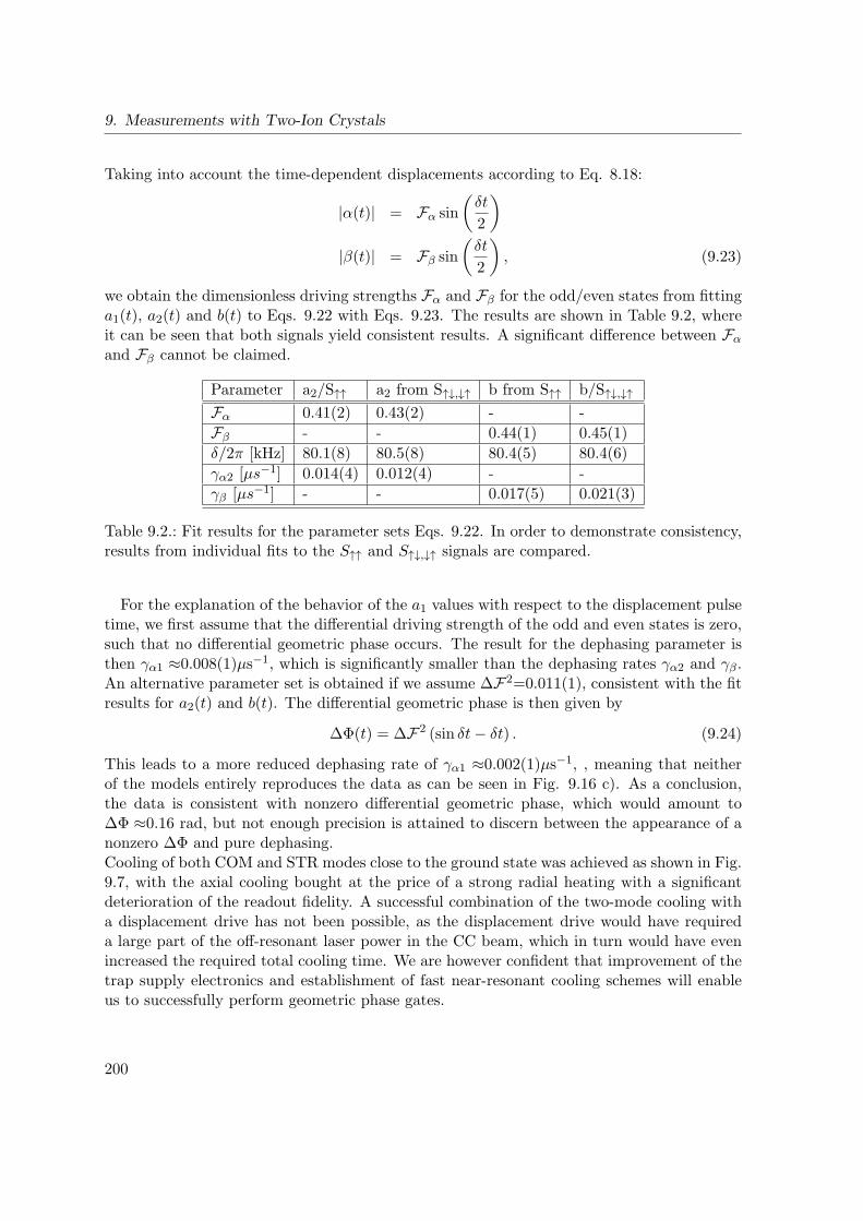
9. Measurements with Two-Ion Crystals
Taking into account the time-dependent displacements according to Eq. 8.18:
|α(t)| = Fα sin
(δt
2
)
|β(t)| = Fβ sin
(δt
2
), (9.23)
we obtain the dimensionless driving strengths Fα and Fβ for the odd/even states from fittinga1(t), a2(t) and b(t) to Eqs. 9.22 with Eqs. 9.23. The results are shown in Table 9.2, whereit can be seen that both signals yield consistent results. A significant difference between Fα
and Fβ cannot be claimed.
Parameter a2/S↑↑ a2 from S↑↓,↓↑ b from S↑↑ b/S↑↓,↓↑Fα 0.41(2) 0.43(2) - -
Fβ - - 0.44(1) 0.45(1)
δ/2π [kHz] 80.1(8) 80.5(8) 80.4(5) 80.4(6)
γα2 [µs−1] 0.014(4) 0.012(4) - -
γβ [µs−1] - - 0.017(5) 0.021(3)
Table 9.2.: Fit results for the parameter sets Eqs. 9.22. In order to demonstrate consistency,results from individual fits to the S↑↑ and S↑↓,↓↑ signals are compared.
For the explanation of the behavior of the a1 values with respect to the displacement pulsetime, we first assume that the differential driving strength of the odd and even states is zero,such that no differential geometric phase occurs. The result for the dephasing parameter isthen γα1 ≈0.008(1)µs−1, which is significantly smaller than the dephasing rates γα2 and γβ .An alternative parameter set is obtained if we assume ∆F2=0.011(1), consistent with the fitresults for a2(t) and b(t). The differential geometric phase is then given by
∆Φ(t) = ∆F2 (sin δt− δt) . (9.24)
This leads to a more reduced dephasing rate of γα1 ≈0.002(1)µs−1, , meaning that neitherof the models entirely reproduces the data as can be seen in Fig. 9.16 c). As a conclusion,the data is consistent with nonzero differential geometric phase, which would amount to∆Φ ≈0.16 rad, but not enough precision is attained to discern between the appearance of anonzero ∆Φ and pure dephasing.Cooling of both COM and STR modes close to the ground state was achieved as shown in Fig.9.7, with the axial cooling bought at the price of a strong radial heating with a significantdeterioration of the readout fidelity. A successful combination of the two-mode cooling witha displacement drive has not been possible, as the displacement drive would have requireda large part of the off-resonant laser power in the CC beam, which in turn would have evenincreased the required total cooling time. We are however confident that improvement of thetrap supply electronics and establishment of fast near-resonant cooling schemes will enableus to successfully perform geometric phase gates.
200
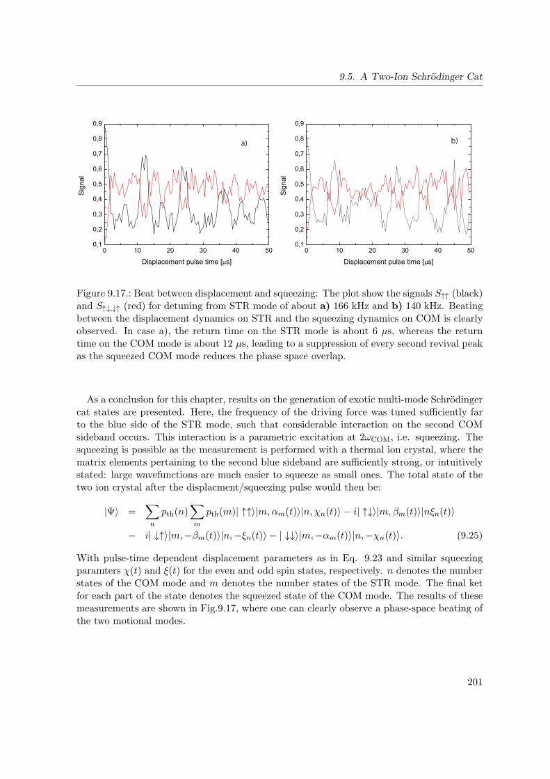
9.5. A Two-Ion Schrodinger Cat
0 10 20 30 40 500,1
0,2
0,3
0,4
0,5
0,6
0,7
0,8
0,9
Sig
nal
Displacement pulse time [µs]0 10 20 30 40 50
0,1
0,2
0,3
0,4
0,5
0,6
0,7
0,8
0,9
Sig
nal
Displacement pulse time [µs]
a) b)
Figure 9.17.: Beat between displacement and squeezing: The plot show the signals S↑↑ (black)and S↑↓,↓↑ (red) for detuning from STR mode of about a) 166 kHz and b) 140 kHz. Beatingbetween the displacement dynamics on STR and the squeezing dynamics on COM is clearlyobserved. In case a), the return time on the STR mode is about 6 µs, whereas the returntime on the COM mode is about 12 µs, leading to a suppression of every second revival peakas the squeezed COM mode reduces the phase space overlap.
As a conclusion for this chapter, results on the generation of exotic multi-mode Schrodingercat states are presented. Here, the frequency of the driving force was tuned sufficiently farto the blue side of the STR mode, such that considerable interaction on the second COMsideband occurs. This interaction is a parametric excitation at 2ωCOM, i.e. squeezing. Thesqueezing is possible as the measurement is performed with a thermal ion crystal, where thematrix elements pertaining to the second blue sideband are sufficiently strong, or intuitivelystated: large wavefunctions are much easier to squeeze as small ones. The total state of thetwo ion crystal after the displacment/squeezing pulse would then be:
|Ψ〉 =∑n
pth(n)∑m
pth(m)| ↑↑〉|m,αm(t)〉|n, χn(t)〉 − i| ↑↓〉|m,βm(t)〉|nξn(t)〉
− i| ↓↑〉|m,−βm(t)〉|n,−ξn(t)〉 − | ↓↓〉|m,−αm(t)〉|n,−χn(t)〉. (9.25)
With pulse-time dependent displacement parameters as in Eq. 9.23 and similar squeezingparamters χ(t) and ξ(t) for the even and odd spin states, respectively. n denotes the numberstates of the COM mode and m denotes the number states of the STR mode. The final ketfor each part of the state denotes the squeezed state of the COM mode. The results of thesemeasurements are shown in Fig.9.17, where one can clearly observe a phase-space beating ofthe two motional modes.
201

10. Conclusion and Outlook
10.1. Conclusion
The introduction of this thesis stated that robustness and fidelity of all required qubit op-erations are essential foundations of any approach to achieve an experimental realizationof scalable quantum information. The high fidelity is needed to attain the quantum errorcorrection threshold and robustness is needed because the scalability inevitably implies atechnological approach which will offer a less favorable environment for individual qubits. Inthe course of this thesis, every required operation for single qubits could be successfully real-ized at high fidelities, and the bottleneck limiting the fidelity could be identified in every casesuch that future technological improvements can be devised in order to achieve even higherfidelities. It also became clear that the robust implementations of the individual operatingsteps is indeed necessary, as can be seen from the measurements of the extremely high radialand intermediately high axial heating rates, see sections 4.3 and 4.6. Detailed studies of thequbit coherence were performed both in the absence and under the influence of external laserfields, with the results that the decoherence rates at the present stage allow for quantuminformation experiments from basic up to intermediate complexity, see Sec. 4.7. The tech-nical and physical sources of the decoherence processes were almost completely understood,such that it is clear what the required technological improvements are. An extensive char-acterization and testing of the trap was performed, with the main results that ion transportthroughout the whole trap structure is possible and that the actual electrostatic potentialmatch the predicted ones with great accuracy. For the latter achievement, the microchiptrap provided the testbed for our potential calculation software and for potential shapingtechniques.The methods established for single qubit operation were used for various demonstrationsthat complex experiments at the quantum level are indeed possible in microstructured iontraps. These experiments were of course not just carried out for demonstration purposes:The successful reconstruction of a density matrix of the state of the axial vibrational modeis the basis for future experiments on the emerging field of quantum thermodynamics. Thecoherent measurement method developed for the determination of atomic matrix elements isside product of the decoherence studies. It addresses a contemporary problem from atomicphysics. The extensive experiments carried out on the action of spin-dependent light forces ona single ion provide the basis for future robust entangling gate operations. Furthermore, thetwo-ion crystal as the more complex basic building block of our experimental scheme was in-vestigated, where individual readout and manipulation were successfully demonstrated. Thestability and initial temperature of the two-ion crystal however remains to be improved.
203
10. Conclusion and Outlook
10.2. Open Questions
This section briefly addresses the questions arising from measurement data acquired through-out this thesis which could not be entirely understood, which is done for the sake of docu-mentation and completeness.Stability of ion crystals: The predominant questions are associated with the rather badstability of two-ion crystals, which is also of fundamental importance because it representsa crucial bottleneck for future progress. The bistable behavior of the crystals implies thatnonlinearities are involved. In Sec. 5.2, a bistability originating from the nonlinear natureof Doppler cooling was explained, which can also be mediated by micromotion and wouldtherefore explain the decreased stability at large trap drive rf amplitudes. However, it is notclear why two ions should be unstable at parameters where a single ion is completely stable.Furthermore, the drastically impaired Doppler cooling result of the COM mode of a two ioncrystal cannot be straightforwardly explained by this mechanism. If the additional Coulombnonlinearity present for the crystal would give rise to these effects, one would intuitivelyexpect that the STR mode should be affected instead of the COM one.Parasitic shelving: The incoherent excitation of population from the |↓〉 level occurringduring the shelving pulses could not be explained by off-resonant excitation or laser phasefluctuations. It therefore must be associated with an incoherent spectral background of the729 nm laser. The width, strength and origin of this background remain unclear.Enhanced laser-driven decoherence: The ratio of photon-scattering induced spin qubitdecoherence and scattering rate determined experimentally in Sec. 4.7 is supported by thetheoretical derivation given in Appendix A, which also predicts a set of counterintuitive ef-fects. Future measurements are supposed to yield more precise figures for the decoherencerate and will test more sophisticated theoretical predictions.Laser coupling fluctuations: The measurements of the Stark-shift induced decoherencerates presented at the end of Sec. 4.7 show that slow but large fluctuations of the atom-lasercoupling strength are present in our system, which are not consistent with the expected beampointing fluctuations or intensity fluctuations. A possible source of this effect might be anunstable radial behavior of the ions, which could be improved by better voltage supply elec-tronics and better Doppler cooling.Radial heating rates: Measurements of the fluorescence rate decrease after waiting timesin the millisecond range presented in Sec. 4.3 show that the heating rates in the radial direc-tions are tremendously larger than the one measured for the axial direction. The source ofthis behavior is still unknown, it can hopefully be counteracted with improved trap supplyelectronics.Lower bound of the heating rates: Axial heating rate measurement have shown that theheating rate is strongly dependent on the voltage supply electronics (see Fig. B.4), it is yetunclear how low the heating can be suppressed by improvement of the circuitry.Line broadening: Measurements of the fluorescence rates at 397 nm are inconsistent withthe linewidth of about 22 MHz of that transition, see Figs. 4.4 and 5.6. Possible sources ofthis additional broadening are residual micromotion along the 397 nm beam or broadening
204
10.3. Outlook
due to a large radial temperature.
10.3. Outlook
The future tasks to be solved for the demonstration of our scalable quantum informationconcept break down into two basic fields: First, entangling gate operations between two ionshave to be accomplished, which requires a better stability of these crystals at larger trap fre-quencies. One therefore has to find ways to suppress noise on the DC electrodes even furtherand investigate the stability and noise characteristics of the trap drive RF. It might also be ofgreat interest to investigate theoretically why the stability and initial temperature of the twoion crystal is so much different compared to the single ion case, despite the trap operation pa-rameters are deep in the stability region. The other basic direction is the further developmentof the scalable voltage supply that will allow for shuttling operations much faster than qubitcoherence time. This development is currently underway, however, due to the technologicalcomplexity, it might require a certain number of development iterations before the requiredspecifications are met. If these two hurdles are taken, the methods can be combined to realizebasic quantum computing tasks based on shuttling qubits in a segmented trap. For example,locally created entanglement between two qubits can be distributed by splitting the crystaland moving the ions far apart, which would allow for the realization of the largest distanceever achieved between deterministically entangled massive particles. The ability to handlethree or more qubits would open the door to a rich plethora of quantum physics, addressingquestions such as quantum state estimation and the characterization of higher dimensionalHilbert spaces, along with the decoherence properties of complex quantum states. In fact,the number of apparatuses worldwide which allow for deterministic operations with three ormore ion-based qubits is to our knowledge limited to two at the time this thesis is written,indicating the vast unknown territory which is still open to explore.It remains to be stated that up to now no fundamentally unsolvable problem with our ex-perimental approach has been found, we therefore conclude with the statement that the waytowards scalable quantum information still seems to be an adventurous path full of expectedand unexpected obstacles, but also with many beautiful treasures at its sides and a mysteriousend(?) that is yet not known.
205

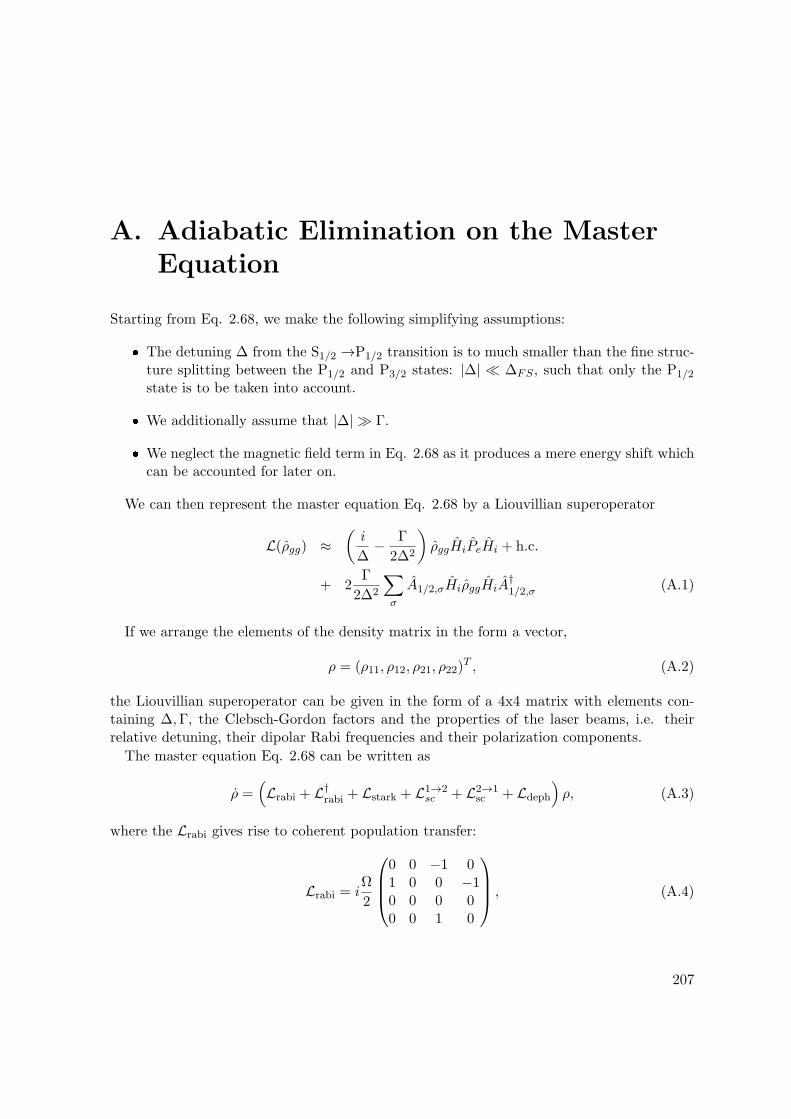
A. Adiabatic Elimination on the MasterEquation
Starting from Eq. 2.68, we make the following simplifying assumptions:
The detuning ∆ from the S1/2 →P1/2 transition is to much smaller than the fine struc-ture splitting between the P1/2 and P3/2 states: |∆| ∆FS , such that only the P1/2
state is to be taken into account.
We additionally assume that |∆| Γ.
We neglect the magnetic field term in Eq. 2.68 as it produces a mere energy shift whichcan be accounted for later on.
We can then represent the master equation Eq. 2.68 by a Liouvillian superoperator
L(ρgg) ≈(
i
∆− Γ
2∆2
)ρggHiPeHi + h.c.
+ 2Γ
2∆2
∑σ
A1/2,σHiρggHiA†1/2,σ (A.1)
If we arrange the elements of the density matrix in the form a vector,
ρ = (ρ11, ρ12, ρ21, ρ22)T , (A.2)
the Liouvillian superoperator can be given in the form of a 4x4 matrix with elements con-taining ∆,Γ, the Clebsch-Gordon factors and the properties of the laser beams, i.e. theirrelative detuning, their dipolar Rabi frequencies and their polarization components.
The master equation Eq. 2.68 can be written as
ρ =(Lrabi + L†
rabi + Lstark + L1→2sc + L2→1
sc + Ldeph
)ρ, (A.3)
where the Lrabi gives rise to coherent population transfer:
Lrabi = iΩ
2
⎛⎜⎜⎝0 0 −1 01 0 0 −10 0 0 00 0 1 0
⎞⎟⎟⎠ , (A.4)
207
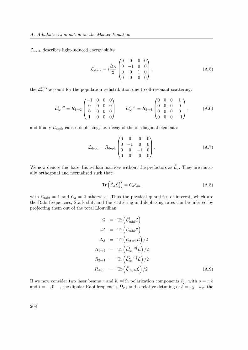
A. Adiabatic Elimination on the Master Equation
Lstark describes light-induced energy shifts:
Lstark = i∆S
2
⎛⎜⎜⎝0 0 0 00 −1 0 00 0 1 00 0 0 0
⎞⎟⎟⎠ , (A.5)
the Li→jsc account for the population redistribution due to off-resonant scattering:
L1→2sc = R1→2
⎛⎜⎜⎝−1 0 0 00 0 0 00 0 0 01 0 0 0
⎞⎟⎟⎠ L2→1
sc = R2→1
⎛⎜⎜⎝0 0 0 10 0 0 00 0 0 00 0 0 −1
⎞⎟⎟⎠ , (A.6)
and finally Ldeph causes dephasing, i.e. decay of the off-diagonal elements:
Ldeph = Rdeph
⎛⎜⎜⎝0 0 0 00 −1 0 00 0 −1 00 0 0 0
⎞⎟⎟⎠ . (A.7)
We now denote the ’bare’ Liouvillian matrices without the prefactors as La. They are mutu-ally orthogonal and normalized such that:
Tr(LaL†
b
)= Caδab, (A.8)
with Crabi = 1 and Ca = 2 otherwise. Thus the physical quantities of interest, which arethe Rabi frequencies, Stark shift and the scattering and dephasing rates can be inferred byprojecting them out of the total Liouvillian:
Ω = Tr(L†rabiL
)Ω∗ = Tr
(LrabiL
)∆S = Tr
(LstarkL
)/2
R1→2 = Tr(L1→2†sc L
)/2
R2→1 = Tr(L2→1†sc L
)/2
Rdeph = Tr(LdephL
)/2 (A.9)
If we now consider two laser beams r and b, with polarization components εq,i with q = r, band i = +, 0,−, the dipolar Rabi frequencies Ωr,b and a relative detuning of δ = ωb − ωr, the
208
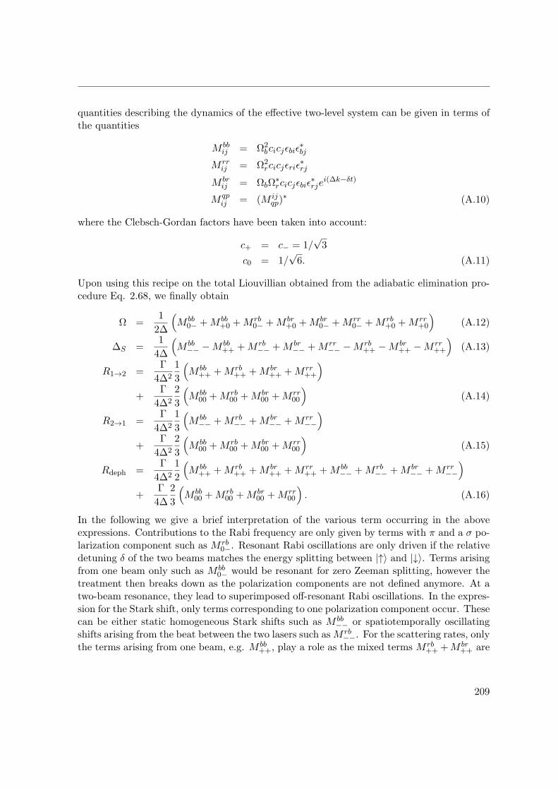
quantities describing the dynamics of the effective two-level system can be given in terms ofthe quantities
M bbij = Ω2
bcicjεbiε∗bj
M rrij = Ω2
rcicjεriε∗rj
M brij = ΩbΩ
∗rcicjεbiε
∗rje
i(∆k−δt)
M qpij = (M ij
qp)∗ (A.10)
where the Clebsch-Gordan factors have been taken into account:
c+ = c− = 1/√3
c0 = 1/√6. (A.11)
Upon using this recipe on the total Liouvillian obtained from the adiabatic elimination pro-cedure Eq. 2.68, we finally obtain
Ω =1
2∆
(M bb
0− +M bb+0 +M rb
0− +M br+0 +M br
0− +M rr0− +M rb
+0 +M rr+0
)(A.12)
∆S =1
4∆
(M bb
−− −M bb++ +M rb
−− +M br−− +M rr
−− −M rb++ −M br
++ −M rr++
)(A.13)
R1→2 =Γ
4∆2
1
3
(M bb
++ +M rb++ +M br
++ +M rr++
)+
Γ
4∆2
2
3
(M bb
00 +M rb00 +M br
00 +M rr00
)(A.14)
R2→1 =Γ
4∆2
1
3
(M bb
−− +M rb−− +M br
−− +M rr−−)
+Γ
4∆2
2
3
(M bb
00 +M rb00 +M br
00 +M rr00
)(A.15)
Rdeph =Γ
4∆2
1
2
(M bb
++ +M rb++ +M br
++ +M rr++ +M bb
−− +M rb−− +M br
−− +M rr−−)
+Γ
4∆
2
3
(M bb
00 +M rb00 +M br
00 +M rr00
). (A.16)
In the following we give a brief interpretation of the various term occurring in the aboveexpressions. Contributions to the Rabi frequency are only given by terms with π and a σ po-larization component such as M rb
0−. Resonant Rabi oscillations are only driven if the relativedetuning δ of the two beams matches the energy splitting between |↑〉 and |↓〉. Terms arisingfrom one beam only such as M bb
0− would be resonant for zero Zeeman splitting, however thetreatment then breaks down as the polarization components are not defined anymore. At atwo-beam resonance, they lead to superimposed off-resonant Rabi oscillations. In the expres-sion for the Stark shift, only terms corresponding to one polarization component occur. Thesecan be either static homogeneous Stark shifts such as M bb−− or spatiotemporally oscillatingshifts arising from the beat between the two lasers such asM rb−−. For the scattering rates, onlythe terms arising from one beam, e.g. M bb
++, play a role as the mixed terms M rb++ +M br
++ are
209
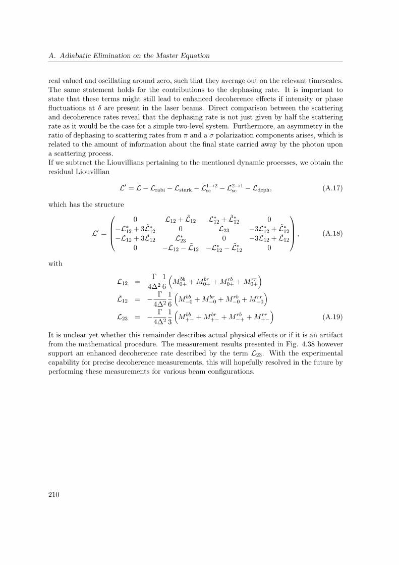
A. Adiabatic Elimination on the Master Equation
real valued and oscillating around zero, such that they average out on the relevant timescales.The same statement holds for the contributions to the dephasing rate. It is important tostate that these terms might still lead to enhanced decoherence effects if intensity or phasefluctuations at δ are present in the laser beams. Direct comparison between the scatteringand decoherence rates reveal that the dephasing rate is not just given by half the scatteringrate as it would be the case for a simple two-level system. Furthermore, an asymmetry in theratio of dephasing to scattering rates from π and a σ polarization components arises, which isrelated to the amount of information about the final state carried away by the photon upona scattering process.If we subtract the Liouvillians pertaining to the mentioned dynamic processes, we obtain theresidual Liouvillian
L′ = L − Lrabi − Lstark − L1→2sc − L2→1
sc − Ldeph, (A.17)
which has the structure
L′ =
⎛⎜⎜⎝
0 L12 + L12 L∗12 + L∗
12 0
−L∗12 + 3L∗
12 0 L23 −3L∗12 + L∗
12
−L12 + 3L12 L∗23 0 −3L12 + L12
0 −L12 − L12 −L∗12 − L∗
12 0
⎞⎟⎟⎠ , (A.18)
with
L12 =Γ
4∆2
1
6
(M bb
0+ +M br0+ +M rb
0+ +M rr0+
)L12 = − Γ
4∆2
1
6
(M bb
−0 +M br−0 +M rb
−0 +M rr−0
)L23 = − Γ
4∆2
1
3
(M bb
+− +M br+− +M rb
−+ +M rr+−)
(A.19)
It is unclear yet whether this remainder describes actual physical effects or if it is an artifactfrom the mathematical procedure. The measurement results presented in Fig. 4.38 howeversupport an enhanced decoherence rate described by the term L23. With the experimentalcapability for precise decoherence measurements, this will hopefully resolved in the future byperforming these measurements for various beam configurations.
210
B. Trap Voltage Supply Electronics
The supply electronics for dc trap voltages represents the crucial technological cornerstonefor scalable quantum information experiments in segmented ion traps. In conventional iontrap experiments, noise reduction is accomplished by massive low-pass filtering of the supplyvoltages, this approach is not viable for our scheme as the ions are supposed to be movedwithin the trap structure on short timescales, such that voltages in the frequency range of upto 1 MHz or even more need to be admitted. Instead of relying on filtering, the developmentof suitable low-noise electronics is necessary. The voltage noise present on the electrodesis responsible for the heating of the ions, while the heating rate determines the suitabilityof a given trap for quantum information experiments. This heating process is investigatedtheoretically in Ref. [Lam97]. A detailed experimental study where the heating rate wasinvestigated with respect to the ion-trap surface distance and the surface temperature resultedin heating rates that were y orders of magnitude larger than the theoretically expected ones[Des06], the reason for which remains unclear as of today. It is argued the insulting ’dirt’patches on the trap surfaces with thermally fluctuating charges give rise to the observedstrong noise components, another possibility would be that residual uncompensated RF-fields lead to energy transfer to secular modes of vibrations via anharmonicities. However,that heating rate will be even larger if additional noise from the supply electronics is present.We summarize the required specifications for the required supply electronics:
Individual supply for 64 channels.
Voltages in the range between +10 V and -10 V.
Extremely low noise.
Possibility to supply individual arbitrary voltage waveforms containing frequencies inthe MHz range.
Suppression of rf pickup fed back to the output stage, or even the possibility to regulaterf-pickup on the electrodes away.
The required low noise level can only be accomplished with the use of well-shielded, battery-powered equipment. In an early stage of the experiment, we have seen tremendous improve-ments in the observation of coherent dynamics on the quadrupole transition upon changingthe voltage supply from computer controlled analog output boards via a 9 V battery block,a battery driven buffer based on an operational amplifier to a transistor-based output stagethat was finally used. This hand-made supply electronics provides only voltage supply fora single electrode pair, for this reason most experiments were conducted at a single site.
211
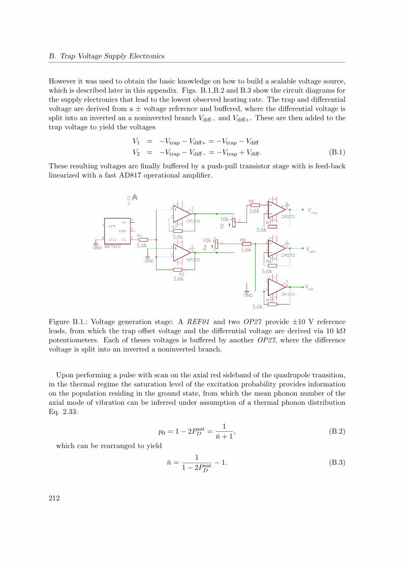
B. Trap Voltage Supply Electronics
However it was used to obtain the basic knowledge on how to build a scalable voltage source,which is described later in this appendix. Figs. B.1,B.2 and B.3 show the circuit diagrams forthe supply electronics that lead to the lowest observed heating rate. The trap and differentialvoltage are derived from a ± voltage reference and buffered, where the differential voltage issplit into an inverted an a noninverted branch Vdiff− and Vdiff+. These are then added to thetrap voltage to yield the voltages
V1 = −Vtrap − Vdiff+ = −Vtrap − Vdiff
V2 = −Vtrap − Vdiff− = −Vtrap + Vdiff . (B.1)
These resulting voltages are finally buffered by a push-pull transistor stage with is feed-backlinearized with a fast AD817 operational amplifier.
5,6k
5,6k
5,6k
10k
10k
Vtrap
Vdiff+
Vdiff-
5,6k
5,6k
5,6k
5,6k
5,6k
Figure B.1.: Voltage generation stage: A REF01 and two OP27 provide ±10 V referenceleads, from which the trap offset voltage and the differential voltage are derived via 10 kΩpotentiometers. Each of theses voltages is buffered by another OP27, where the differencevoltage is split into an inverted a noninverted branch.
Upon performing a pulse with scan on the axial red sideband of the quadrupole transition,in the thermal regime the saturation level of the excitation probability provides informationon the population residing in the ground state, from which the mean phonon number of theaxial mode of vibration can be inferred under assumption of a thermal phonon distributionEq. 2.33:
p0 = 1− 2P satD =
1
n+ 1, (B.2)
which can be rearranged to yield
n =1
1− 2P satD
− 1. (B.3)
212
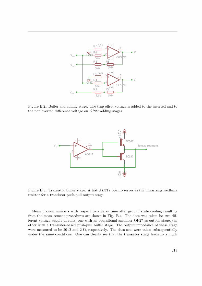
5,6k
5,6k
5,6k
5,6k
5,6k
5,6k 5,6k
5,6k
Vtrap
Vdiff+
Vdiff-
V1
V2
Figure B.2.: Buffer and adding stage: The trap offset voltage is added to the inverted and tothe noninverted difference voltage on OP27 adding stages.
BC557
BC547
To trap segmentVin
AD817
Figure B.3.: Transistor buffer stage: A fast AD817 opamp serves as the linearizing feedbackresistor for a transistor push-pull output stage.
Mean phonon numbers with respect to a delay time after ground state cooling resultingfrom the measurement procedures are shown in Fig. B.4. The data was taken for two dif-ferent voltage supply circuits, one with an operational amplifier OP27 as output stage, theother with a transistor-based push-pull buffer stage. The output impedance of these stagewere measured to be 20 Ω and 2 Ω, respectively. The data sets were taken subsequentiallyunder the same conditions. One can clearly see that the transistor stage leads to a much
213
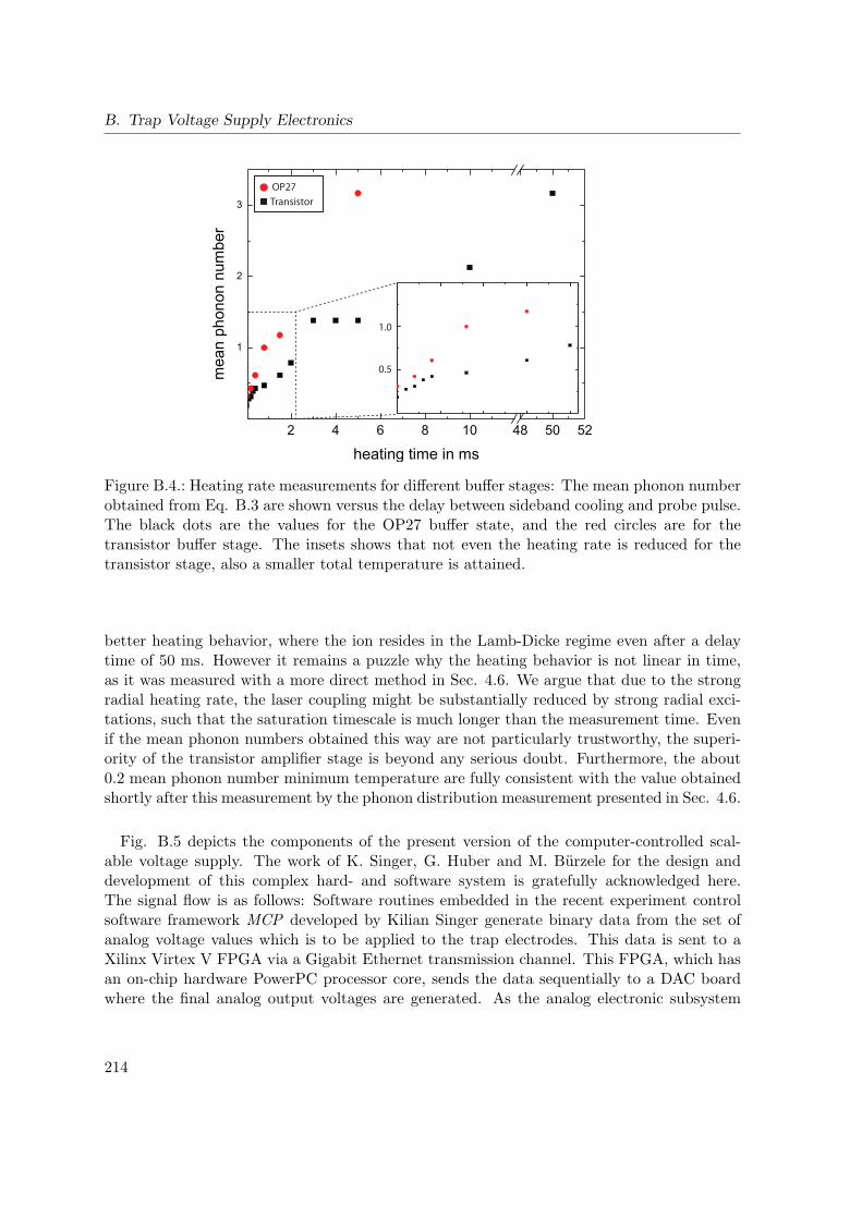
B. Trap Voltage Supply Electronics
2 4 6 8 10 48 50 52
1
2
3
Transistor buffer OP27 buffer
mea
n ph
onon
num
ber
heating time in ms
1.0
0.5
Transistor
OP27
Figure B.4.: Heating rate measurements for different buffer stages: The mean phonon numberobtained from Eq. B.3 are shown versus the delay between sideband cooling and probe pulse.The black dots are the values for the OP27 buffer state, and the red circles are for thetransistor buffer stage. The insets shows that not even the heating rate is reduced for thetransistor stage, also a smaller total temperature is attained.
better heating behavior, where the ion resides in the Lamb-Dicke regime even after a delaytime of 50 ms. However it remains a puzzle why the heating behavior is not linear in time,as it was measured with a more direct method in Sec. 4.6. We argue that due to the strongradial heating rate, the laser coupling might be substantially reduced by strong radial exci-tations, such that the saturation timescale is much longer than the measurement time. Evenif the mean phonon numbers obtained this way are not particularly trustworthy, the superi-ority of the transistor amplifier stage is beyond any serious doubt. Furthermore, the about0.2 mean phonon number minimum temperature are fully consistent with the value obtainedshortly after this measurement by the phonon distribution measurement presented in Sec. 4.6.
Fig. B.5 depicts the components of the present version of the computer-controlled scal-able voltage supply. The work of K. Singer, G. Huber and M. Burzele for the design anddevelopment of this complex hard- and software system is gratefully acknowledged here.The signal flow is as follows: Software routines embedded in the recent experiment controlsoftware framework MCP developed by Kilian Singer generate binary data from the set ofanalog voltage values which is to be applied to the trap electrodes. This data is sent to aXilinx Virtex V FPGA via a Gigabit Ethernet transmission channel. This FPGA, which hasan on-chip hardware PowerPC processor core, sends the data sequentially to a DAC boardwhere the final analog output voltages are generated. As the analog electronic subsystem
214

+12V Accu
+12V Accu
7805+5V
+12V
-12V
GND
DAC8814
OP4277
1x clock1x ldac16x chipselect
Optocouplers
FPGA Board
FPGAPowersupply
Gigabit ethernet
DAC8814
To trap
AGND
DG
ND
VREF
Battery box
FPGA & DAC box
OP4277 OP4277
data
#1
data
#2
data
#n
Control computer
linedriversNI
Digital out
Trigger
Figure B.5.: Design of the scalable trap voltage supply: The FPGA is supplied with thewaveform data via Gigabit Ethernet from the control computer. The FPGA output is bufferedand supplied to the DAC board via optocouplers to achieve galvanic separation. The outputof the DACs is buffered by OP4277 opamps.
is to be isolated galvanically from FPGA digital electronics to suppress digital clock noiseand power line frequencies, all digital signals supplied to the DAC board are buffered byoptocouplers. The quad-channel DACs 8814 are addressed by chip-select lines and seriallyobtain their 4x16-bit samples via a single serial data line connected to all DACs. One datasample consists of a 2-bit information selecting one of the four DACs on the chip, and theactual 16 bit voltage sample. When all DACs are supplied with their samples, an enableline (LDAC) causes them to update their output voltages simultaneously. The analog outputsignals are in the range between 0 V and +10 V, with respect to a +10 V precision referencesupplied to all DACs. This range is mapped onto the required -10 V to +10 V range by meansof two operational amplifiers, which also serve as output buffers. These OP4277 operationalamplifiers come in quad packages, such that one chip can drive two analog output lines andtwo OP4277 chips per DAC chip are needed. The signals run via individual SMA cablesto an additional output printed circuit board where they are bundled on four 25-pin Sub-Dconnectors. From there the voltages are supplied to the vacuum flange via shielded printercables 1. The power supply for the DAC board is realized with a shielded battery system
1LEUNIG GmbH, Sigburg, Germany
215
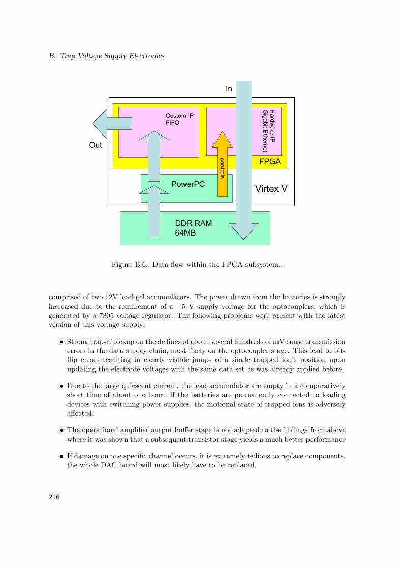
B. Trap Voltage Supply Electronics
Virtex V
FPGA
PowerPC
DDR RAM64MB
controls
Hardw
are IPG
igabit Ethernet
Custom IPFIFO
In
Out
Figure B.6.: Data flow within the FPGA subsystem:.
comprised of two 12V lead-gel accumulators. The power drawn from the batteries is stronglyincreased due to the requirement of a +5 V supply voltage for the optocouplers, which isgenerated by a 7805 voltage regulator. The following problems were present with the latestversion of this voltage supply:
Strong trap-rf pickup on the dc lines of about several hundreds of mV cause transmissionerrors in the data supply chain, most likely on the optocoupler stage. This lead to bit-flip errors resulting in clearly visible jumps of a single trapped ion’s position uponupdating the electrode voltages with the same data set as was already applied before.
Due to the large quiescent current, the lead accumulator are empty in a comparativelyshort time of about one hour. If the batteries are permanently connected to loadingdevices with switching power supplies, the motional state of trapped ions is adverselyaffected.
The operational amplifier output buffer stage is not adapted to the findings from abovewhere it was shown that a subsequent transistor stage yields a much better performance
If damage on one specific channel occurs, it is extremely tedious to replace components,the whole DAC board will most likely have to be replaced.
216
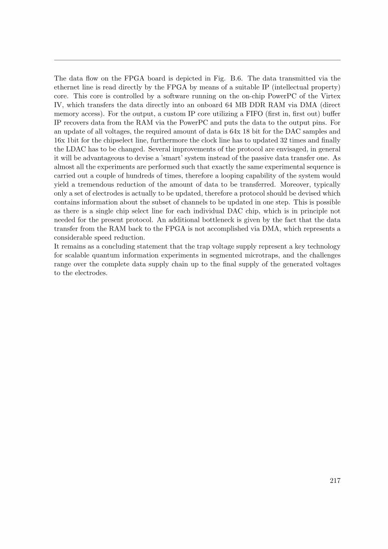
The data flow on the FPGA board is depicted in Fig. B.6. The data transmitted via theethernet line is read directly by the FPGA by means of a suitable IP (intellectual property)core. This core is controlled by a software running on the on-chip PowerPC of the VirtexIV, which transfers the data directly into an onboard 64 MB DDR RAM via DMA (directmemory access). For the output, a custom IP core utilizing a FIFO (first in, first out) bufferIP recovers data from the RAM via the PowerPC and puts the data to the output pins. Foran update of all voltages, the required amount of data is 64x 18 bit for the DAC samples and16x 1bit for the chipselect line, furthermore the clock line has to updated 32 times and finallythe LDAC has to be changed. Several improvements of the protocol are envisaged, in generalit will be advantageous to devise a ’smart’ system instead of the passive data transfer one. Asalmost all the experiments are performed such that exactly the same experimental sequence iscarried out a couple of hundreds of times, therefore a looping capability of the system wouldyield a tremendous reduction of the amount of data to be transferred. Moreover, typicallyonly a set of electrodes is actually to be updated, therefore a protocol should be devised whichcontains information about the subset of channels to be updated in one step. This is possibleas there is a single chip select line for each individual DAC chip, which is in principle notneeded for the present protocol. An additional bottleneck is given by the fact that the datatransfer from the RAM back to the FPGA is not accomplished via DMA, which represents aconsiderable speed reduction.It remains as a concluding statement that the trap voltage supply represent a key technologyfor scalable quantum information experiments in segmented microtraps, and the challengesrange over the complete data supply chain up to the final supply of the generated voltagesto the electrodes.
217


C. Advanced Reconstruction Techniquefor Phonon Number Distributions
Rabi oscillations on a blue sideband are an important measurement tool to determine phononnumber distributions, i.e. to characterize the (quantum) state of a given vibrational mode oftrapped ions. This technique is employed in Sec. 4.6 for a precise heating rate measurement,in chapter 7 for a complete quantum state tomography and in Sec. 8.3 for monitoring theaction of a light-induced displacement force. As the reconstructed occupation probabilities pnrepresent physical quantities characterizing the quantum state, it is of fundamental interestto find the most accurate way to extract them from the bsb Rabi oscillation data. This taskis hindered by experimental imperfections, i.e. shot noise on the data and drifting parametersas the Rabi frequency and the spin and motional preparation imperfections. The startingpoint is the bsb oscillation signal
P↓(t) =1
2
∑n
pn(a e−γ t cos (Ωn,n+1 t) + b), (C.1)
with the Rabi frequency Ωn,n+1 = Ω0Mn,n+1(η), the contrast a, baseline b and the decoher-ence rate γ. The base Rabi frequency Ω0 is not exactly known and might be subject to drifts,the Lamb-Dicke factor η depends on the beam angles which are also not exactly known, thebaseline and contrast factors depend on the spin preparation and readout, which are alsosubject to drifts. The decoherence rate γ depends on the impinging light intensity and alsoon the motional state itself, see Sec. 8.3. We also have to take into account the normalizationof the pn, thus if we consider the reconstruction as a nonlinear regression problem, we facea situation with a large number of heavily correlated and partially constrained parameters,which might also have very different ranges of values. Any standard nonlinear regressionroutine will therefore be condemned to fail on this problem. Two different points of viewon Eq. C.1 seem to offer ways to solve this problem: First, the bsb signal can be seen as aFourier synthesis of oscillations at different frequencies Ωn,n+1, the relative strength of whichare directly given by the pn. When looking at the spectrum of bsb Rabi oscillations as inFig. 4.29, we immediately recognize two problems, namely that alias peaks appear due tothe finite data acquisition time and that the peaks are rather broad and distorted, such thatit is difficult to reliably read off the pn and give figures for their accuracy. Furthermore,components beyond n = 4 cannot be resolved under the experimental conditions in this case.Another way would be to consider the pn as a vector, which is multiplied by a rectangular ma-trix to yield the measurement values. Therefore, singular value decomposition (SVD) of thismatrix can be applied to find the pseudo-inverse, which reveals the pn when multiplied on thevector of measured data points. This was used in Ref. [Mee96], with the result that negative
219
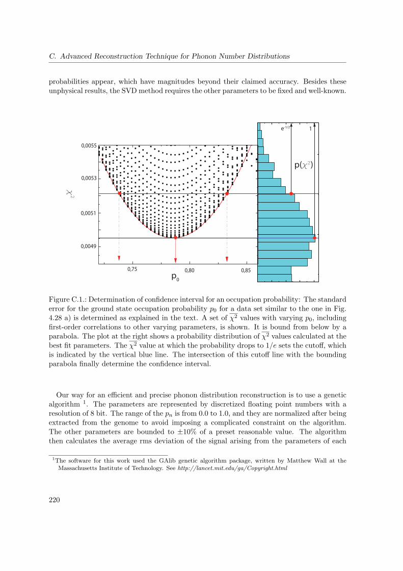
C. Advanced Reconstruction Technique for Phonon Number Distributions
probabilities appear, which have magnitudes beyond their claimed accuracy. Besides theseunphysical results, the SVD method requires the other parameters to be fixed and well-known.
1e-1/2
p0
2
0,0055
0,0053
0,0051
0,0049
0,850,800,75
p( 2)
Figure C.1.: Determination of confidence interval for an occupation probability: The standarderror for the ground state occupation probability p0 for a data set similar to the one in Fig.4.28 a) is determined as explained in the text. A set of χ2 values with varying p0, includingfirst-order correlations to other varying parameters, is shown. It is bound from below by aparabola. The plot at the right shows a probability distribution of χ2 values calculated at thebest fit parameters. The χ2 value at which the probability drops to 1/e sets the cutoff, whichis indicated by the vertical blue line. The intersection of this cutoff line with the boundingparabola finally determine the confidence interval.
Our way for an efficient and precise phonon distribution reconstruction is to use a geneticalgorithm 1. The parameters are represented by discretized floating point numbers with aresolution of 8 bit. The range of the pn is from 0.0 to 1.0, and they are normalized after beingextracted from the genome to avoid imposing a complicated constraint on the algorithm.The other parameters are bounded to ±10% of a preset reasonable value. The algorithmthen calculates the average rms deviation of the signal arising from the parameters of each
1The software for this work used the GAlib genetic algorithm package, written by Matthew Wall at theMassachusetts Institute of Technology. See http://lancet.mit.edu/ga/Copyright.html
220
individual in the population from the measured data:
χ2 =1
N
N∑i=1
(P
(meas)↓ (ti)− P
(calc)↓ (ti)
)2. (C.2)
Additional quantities are calculated to provide a guidance for the algorithm to physicallyreasonable phonon distributions, namely the variance of the phonon distribution
V = 〈(n− n)2〉pn (C.3)
and the curvature of the distribution
C =
nmax−1∑n=1
(pn−1 + pn+1 − 2pn)2 (C.4)
The final quantity to be maximized is then
Q = (αχχ+ αV V + αCC)−1, (C.5)
where the α are positive values to be chosen such that the algorithm finds reasonable results.In other words, the algorithm is set to find parameters such that the measurement datais reproduced, and the phonon distribution should favor low n and be smooth. The lastcondition is related to a general aspect of tomographic maximum likelihood reconstructionof probabilistic quantities describing physical systems, where one maximizes the entropyadditionally to the fitting in order to find the most reasonable physical state. Generally, theprobability distributions with a large curvature correspond to a low entropy, as the containmore information, therefore the usage of the curvature term in Eq. C.5 is physically justified.The question is now how to obtain reliable error estimations for the resulting pn, includingtheir mutual correlations and correlations to the other parameters. For this, we calculatelarge sets of χ2 values, where always two of the variables are slightly changed, e.g.:
χ2(Ω0 + dΩ0, a, b, γ, p0, ..., pnmax)
χ2(Ω0, a, b, γ + dγ, p0, ..., pi + dpi..., pnmax)
χ2(Ω0, a, b, γ, p0, ..., pi + dpi, ..., pj + dpj , pnmax)
... (C.6)
where the deviations are scanned across a range of 10% of the resulting value for the extraparameters and a fixed value 0.1 for the pn. The pn are of course to be renormalized. Theset of resulting χ2 values is plotted versus one parameter of interest, e.g. p0, an examplefor which is shown in Fig. C.1. The structure of the set is always that a minimum χ2
min
occurs, from which the best fit parameter p(best)0 can be read off. The set is then bounded
from below by a curve which is parabolic around p(best)0 . The parabolic curve is obtained
by reducing the set of χ values to the minimum values in a set of bins along the parameter
axis. A parabolic fit can then be performed in a narrow range around p(best)0 , which is also
221
C. Advanced Reconstruction Technique for Phonon Number Distributions
shown in Fig. C.1. From this parabola, the desired confidence interval can then be obtainedby elementary statistical reasoning. For this, we assume that for the measurement data, theprojection noise error amounts to the theoretical maximum one, i.e.
√0.52/M for M shots,
corresponding to a constant readout value of P↓ = 0.5. For large enough M , it is then allowedto consider the shot-to-shot distribution of the P↓ to be Gaussian, with a standard error ofσ2 = 0.52/M . If a given measurement of a curve P↓ with N data points and M shots perpoint was to be repeated several times, the statistical expectation value for the shot noisedeviation is given by
〈χ2〉 = σ2. (C.7)
χ2 is to be considered as a random variable as well, such that we can determine what thestatistical spread of the χ2 is. This allows to infer the confidence interval of the fit parametersfrom the calculated χ2 sets by the assumption that if χ2 deviates by more than its own
statistical spread σ(χ2)
from the optimum value, the fit parameter can be considered as
erroneous. The standard deviation of χ2 is found to be:
σ(χ2)=
√2
N〈χ2〉 =
√1
2 N M. (C.8)
Fig. C.1 illustrates this procedure for determination of the confidence interval for theextracted ground state population p0 from a bsb Rabi oscillation data set similar to the oneshown in Fig. 4.28 a). A probability distribution for χ2 is calculated by drawing randommeasurement values according to Poissonian distributions with the calculated readout valuesas mean value for each probe pulse time of the data set. The χ2 at which the probability dropsto 1/e of the maximum value serves as a cutoff value for the determination of the confidenceinterval. As a general result, it can be stated that this method for the characterization ofthe quantum state is rather imprecise and also bounded to the Lamb-Dicke regime, thereforeeither the decoherence timescales have to be much improved or one has to resort to beatingtomography schemes such as the one presented in Sec. 8.4 and Appendix D.
222
D. Tomography Method for States withEntanglement of Spin and Motion
It is of great interest to investigate the decoherence of nonclassical Schrodinger cat states bydirectly observing the coherent features in phase space, as it was performed on a cavity fieldin Ref. [Gle07]. The question arises if similar experiments could be performed with a trappedion, as both the preparation of Schrodinger cat states (see chapter 8) and the tomography ofthe quantum state of a motional mode (see chapter 7) is readily achieved. It turns out thatthese two experiments cannot be easily combined, as the entanglement of spin and motionobscures the direct observation of the desired interference features. The Schrodinger cat statee.g. |↑, α〉+ |↓,−α〉 cannot be unitarily transformed to |↑, α〉+ |↑,−α〉 which would allow forthe application of tomography methods such as the one presented in chapter 7. A dissipativetransfer would destroy the quantum coherence of the state. A possible way to perform suchan experiment is the application of the wavepacket beating scheme presented in chapter 8.If a similar experiment as in Ref. [Gle07] could be performed with a single trapped ion, theway would be paved for investigations in higher-dimensional spin Hilbert spaces, i.e. thedecoherence properties of Schrodinger cat states with several ions can be measured, which isnot directly possible for the cavity QED system.First, we briefly discuss what quantity the wavepacket beating scheme measures at all andestablish the connection to quantum state tomography, see chapter 7. Let us assume wecould perform an arbitrary manipulation of the motional state for a single spin componentonly. We then generalize the scheme above such that the displacement operation in the firstgap of the spin-echo sequence is replaced by a general operation leading to the quantum stateof the vibrational mode |χ〉. The reasoning leading to the measurement signal Eq. 8.41 nowyields
P↑ =1
2(1 + 〈α|χ〉) . (D.1)
One realizes that besides the trivial offset and scaling factor, this partially gives the Husimi-Kano Q-function:
Q(α) =1
π〈α|χ〉〈χ|α〉, (D.2)
which contains the complete information about the quantum state |χ〉. If the phase of thesecond π/2 pulse in the sequence is changed to φ = π/2, the obtained signal is
P↑ =1
2(1−〈α|χ〉) . (D.3)
We therefore find that(2P↑ − 1)2 + (2P↑ − 1)2 =
π
4Q(α), (D.4)
223
D. Tomography Method for States with Entanglement of Spin and Motion
which states that the value of the Q-function at a particular point in phase space can bedirectly measured by running two different sequences. The restriction of this tomographyscheme lies in the fact that no given input state can be used, one rather has to employspin-dependent mechanisms for the state preparation. If a general input state |χ〉 which wascreated before the measurement sequence was to be analyzed, the resulting signal would be
P↑ =1
2
(1 + 〈χ|D†(α)|χ〉
). (D.5)
This signal can also be used to fully determine the quantum state. The preparation stepis not part of the sequence anymore, the spin-echo scheme is therefore replaced by a singledisplacement pulse sandwiched between the π/2 pulses. The resulting signals then read
P↑ =1
2
(1−〈χ|D(α)|χ〉
)P↑ =
1
2
(1−〈χ|D(α)|χ〉
). (D.6)
As pointed out in [Bar98], this provides a direct measurement of the characteristic functionof the Wigner function:
fW (α) = 〈χ|D(α)|χ〉, (D.7)
which can straightforwardly be extended to mixed states. The Wigner function is simplyobtained by a Fourier transform:
W (β) =1
π2
∫fW (α)eβα
∗−β∗αd2α. (D.8)
We now proceed towards the generalization to input states with possible entanglement be-tween spin and motion, i.e.
|Ψ〉 = | ↑, χ↑〉+ eiψ| ↓, χ↓〉. (D.9)
Normalization factors are omitted in the following and the relative phase ψ of the spinsuperposition is also dropped as it can be safely assumed that it can be measured and modifiedseparately. We now consider a simple analysis sequence where a displacement drive actingonly on |↓〉 creates the state:
|Ψ〉 = | ↑, χ↑〉+ D(α)| ↓, χ↓〉. (D.10)
A concluding π/2 pulse with analysis phase φ gives rise to
|Ψ〉 = | ↑, χ↑〉 − ie−iφ| ↑, χ↓〉+ D(α)| ↓, χ↓〉 − ieiφD(α)| ↑, χ↓〉. (D.11)
The resulting measured population is
P↑(α, φ) = N(1 + cosφ 〈χ↑|D(α)|χ↓〉+ sinφ 〈χ↑|D(α)|χ↓〉
)(D.12)
It can be seen that this leads towards the desired result: a component of the characteristicfunction pertaining to the motional wavefunctions associated with the adjacent spin compo-nents. More information can be extracted with a more complex scheme. Starting again fromthe input state Eq. D.9, we follow the sequence:
224
1. Shift the superposition phase by means of a Stark shift laser beam by θ1.
2. Employ a first π/2 pulse with phase φ1.
3. Drive the displacement of |↓〉 by α.
4. Employ a second phase shift of θ2.
5. Exert the concluding π/2 pulse with phase φ2.
The resulting signal is then given by
P↑(α, φ) ∝ 2 + (cos(θ1 + φ1)− cos(θ1 + φ1 − 2φ2)) M↑↓(0)+ (sin(θ1 + φ1)− sin(θ1 + φ1 − 2φ2)) M↑↓(0)+ cos(θ1 + θ2 − φ2)M↑↓(α) + sin(θ1 + θ2 − φ2)M↑↓(α)+ cos(θ1 − θ2 + 2φ1 − φ2)M↓↑(α)− sin(θ1 − θ2 + 2φ1 − φ2)M↓↑(α)− sin(θ2 − φ1 − φ2)M↓↓(α) + cos(θ2 − φ1 − φ2)M↓↓(α)+ sin(θ2 − φ1 + φ2)M↑↑(α)− cos(θ2 − φ1 + φ2)M↑↑(α), (D.13)
withMij(0) = 〈χi|χj〉 and Mij(α) = 〈χi|D(α)|χj〉 (D.14)
Thus, by performing different measurements with appropriate choice of the phase angles
φ1, φ2, θ1, θ2, a maximum amount of information can be obtained about the M(α)ij for a point
in phase space given by α. The overlap integrals be be separately measured with a simplemeasurement as for the simple Schrodinger cat measurement leading to the result Eq. 8.24,the overlap integral pertaining to adjacent spin states can be measured with the simplifiedsequence presented above and the symmetry relation
Mij(α) = Mji(−α)∗ (D.15)
can be used for additional simplification. It is beyond the scope of this thesis the answerthe question of the complete information about the quantum state can be obtained with thismeasurement scheme, but it can be stated the desired coherence measurement can alreadybe performed with the simplified scheme.
225


E. Coherently Driven Ion Crystals
In this appendix, we derive a general frame work for the coherent interaction of laser beamswith ion crystals aligned along the z-axis. The coupling strength for i-th ion is given by
Ωi = Ω(z(0)i ) with the equilibrium position z
(0)i derived from Eq. 2.80. This admits both
single ion addressing of the k-th ion Ωi = Ω0δik and homogeneous illumination as the limitingcases. In order to not overburden the notation, we restrict ourselves to a beam propagationalong the z-axis, such that the (scalar) laser field is given by
E(z, t) = E0 cos(kzz − ωlt+ φ). (E.1)
This leads to exclusive coupling to the axial vibrational case, however, the most general casecan be straightforwardly retrieved by replacing kzz with k · r. For direct applicability toan experimental situation, we discern the cases for coherent driving of internal states (spin)corresponding to the situations in Secs. 2.1.4 and 9.3, and the direct driving of motionalmodes as in Secs. 8.1 and 9.5.
E.1. Driving the Internal State
We extend the interaction part of the Cirac-Zoller-Hamiltonian Eq. 2.45 to the case of Nions:
HI =
N∑j
12Ωj(σ
+j + σ−
j )(exp[i(kz(z
(0)j + δuzj)− ωlt+ φ
)]+ h.c.
). (E.2)
Employing the generalized coordinates Eq. 2.89 leads to
HI =
N∑j
12Ωj(σ
+j + σ−
j )
(exp
[i
(kz(z
(0)j +
∑n
M(z)Tjn q(z)n )− ωlt+ φ
)]+ h.c.
). (E.3)
Writing the q(z)n in second quantization
q(z)n =
√
2mωn(an + a†n) (E.4)
and replacing the ladder operators by their interaction picture versions
an → eiωntan , a†n → e−iωnta†n,σ+i → eiωegtσ+
i , σ−i → e−iωegtσ−
i , (E.5)
227
E. Coherently Driven Ion Crystals
we obtain the interaction picture Hamiltonian:
H(I)I =
N∑j
12Ωj(e
iωegtσ+j + e−iωegtσ−
j )
·(exp
[i
(kzz
(0)j +
∑n
M(z)Tjn ηn(e
iωntan + e−iωnta†n)− ωlt+ φ
)]+ h.c.
),
(E.6)
where ηn = kk
√
2mωnis the Lamb-Dicke factor for the n-th mode. Invoking the rotating
wave approximation yields
H(I)I =
N∑j
12Ωj σ
−j exp
[i
(kzz
(0)j +
∑n
M(z)Tjn ηn(e
iωntan + e−iωnta†n)− δt+ φ
)]+ h.c. ,
(E.7)which constitutes the most general result. We now perform the Lamb-Dicke approximationassuming all δuzj are much smaller than the driving wavelength and expand the exponentialcontaining the spatial phases up to first order:
H(I)I =
N∑j
12Ωj σ
−j
(1 + i
∑n
M(z)Tjn ηn(e
iωntan + e−iωnta†n)
)e−i
(δt−kzz
(0)j −φ
)+ h.c. , (E.8)
from which we can perform a second rotating-wave-approximation under the assumption thatthe laser is tuned to the rsb or bsb of a specific motional mode n, δ = +(−)ωn:
H(I)I =
N∑j
12Ωj σ
−j
(i M
(z)Tjn ηna
(†)n
)ei(kzz
(0)j +φ
)+ h.c.. (E.9)
The key difference between the driving of an ion crystal and a single ion is the occurrenceof the phase factors depending on the equilibrium positions. This means that the phases ofthe unitary transform that is realized by the coupling to a given mode jointly depend on thetotal internal state, the trap frequency and the structure of the motional mode.
E.2. Driving the Motion
We start from the generalization of the coupling Hamiltonian Eq. 8.5 to N ions:
HI =N∑j
12∆S,j σ
(j)z exp [i (∆kzj − δRt+∆φ)] + h.c. . (E.10)
This is equivalent to the case of the internal state driving besides the replacement of the
internal state operator σ−j and σ+
j with the self-adjoint operator σ(j)z . We can therefore
228

E.2. Driving the Motion
proceed along the same lines of thought as in the previous section to arrive at
H(I)I =
N∑j
i2∆S,j σ
(j)z ηnM
(z)Tjn
(ane
i(∆k z
(0)j −δt+∆φ
)+ h.c.
)(E.11)
Where we admit a detuning from the motional frequency of the n-th mode of δ = δR − ωn.The equation can be rearranged to
H(I)I = −
N∑j
∆S,j σ(j)z M
(z)Tjn
(∆kqn sin
(∆kz
(0)j − δt+∆φ
)+
∆k
mωnpn cos
(∆kz
(0)j − δt+∆φ
)).
(E.12)Assuming all motional modes to be in the ground state and denoting a total unentangled
spin state with the set of spin variables s(j)z = ±1/2, we can calculate the driving force onresonance acting onto the mode using Eq. 8.14 to be
Fn = −N∑j
∆S,js(j)z M
(z)Tjn ∆k sin
(∆kz
(0)j +∆φ
)(E.13)
As in the case of the internal state driving, the effect of the interaction depends on the totalspin state and on the oscillation mode properties. Here, even the strength of the displacementforce depends on these parameters. On the one hand, this is provides a cornerstone of thegeometric phase gate described in Sec. 9.5 as specific spin configurations can be selectivelydisplaced, on the other hand this adds extra complexity especially when gates on larger,unevenly spaced ion crystals are to be performed as we investigated in detail in [Iva09].
229


F. Atomic Properties of Calcium
40Ca ionization energy [eV] 6.11
Atomic weight [u] 40.07840Ca+ P-state finestructure splitting [GHz] 6682.22
Table F.1.: General properties of 40Ca.
S1/2 2
P1/2 2/3
P3/2 4/3
D3/2 4/5
D5/2 6/5
Table F.2.: Lande factors of the 40Ca+ states [Roo00].
Transition Physical wavelength [nm] Lab wavelength [nm] Lifetime
S1/2 →P1/2 396.847 396.95916(2) 7.7(2) ns
S1/2 →P3/2 393.366 - 7.4(3) ns
S1/2 →D3/2 732.389 - 1.080 s
S1/2 →D5/2 729.147 729.34770(5) 1.045 s
D3/2 →P1/2 866.214 866.45220(5) 94.3 ns
D5/2 →P3/2 854.209 854.444(1) 101 ns
D3/2 →P3/2 849.802 - 901 ns
Table F.3.: Properties of the 40Ca+ transitions [Roo00]. The laboratory wavelength denotesthe readout value of our wavemeter at resonance.
231

G. Publications
G.1. Journal Publications
U. Poschinger, M. Hettrich, A. Walther, F. Ziesel, M. Deiss, K. Singer and F. Schmidt-Kaler, High precision atomic decay rate measurement using a single trapped ion, manuscriptin preparation
Andreas Walther, U. Poschinger, F. Ziesel, M. Hettrich, A. Wiens and F. Schmidt-Kaler,Using a single ion as a shot-noise limited magnetic field gradient probe, manuscript in prepa-ration
U. Poschinger, Andreas Walther, Kilian Singer and Ferdinand Schmidt-Kaler, Observingthe phase space trajectory of an entangled ion wave packet, Phys. Rev. Lett. 105, 263602(2010)
Gerhard Huber, Frank Ziesel, U. Poschinger, Kilian Singer and Ferdinand Schmidt-Kaler,A trapped-ion local field probe, Applied Physics B 100, 725 (2010)
K. Singer, U. Poschinger, M. Murphy, P. Ivanov, F. Ziesel, T. Calarco, F. Schmidt-Kaler,Experiments with atomic quantum bits - essential numerical tools, Rev. Mod. Phys. 82,2609 (2010)
P. Ivanov, U. Poschinger, K. Singer, F. Schmidt-Kaler, Quantum gate between logicalqubits in decoherence-free subspace implemented with trapped ions, Eur. Phys. Lett. 92,30006 (2010)
U. Poschinger, G. Huber, F. Ziesel, M. Deiss, M. Hettrich, S. A. Schulz, G. Poulsen,M. Drewsen, R. J. Hendricks, K. Singer and F. Schmidt-Kaler, Coherent manipulation of a40Ca+ spin qubit in a micro ion trap, J. Phys. B: At. Mol. Opt. Phys. 42, 154013 (2009)
S. Schulz, U. Poschinger, F. Ziesel and F. Schmidt-Kaler, Sideband cooling and coherentdynamics in a microchip multi-segmented ion trap, New Journal of Physics 10, 045007 (2008)
Stephan Schulz, U. Poschinger, Kilian Singer, and Ferdinand Schmidt-Kaler, Optimiza-tion of segmented linear Paul traps and transport of stored particles, Progress of Physics,Wiley 54, 648 (2006)
233
G. Publications
G.2. Talks
Quantum optics experiments in a micro ion trap-towards scalable quantum logic, DPG Fruhjahrstagung,Hannover 2010
A spin qubit in a segmented micro ion trap - towards scalable quantum logic under roughconditions, QIon 09, Tel Aviv, Israel 2009
A spin qubit in a segmented micro ion trap - towards scalable quantum logic under roughconditions, EMALI YR Meeting, Oxford UK 2009
A spin qubit in a segmented micro ion trap - towards scalable quantum logic under roughconditions, CCM Group Seminar, Imperial College London, UK 2009
A spin qubit in a segmented micro ion trap, DPG Fruhjahrstagung, Hamburg 2009
Raman ground state cooling and coherent manipulations in the segmented micro ion trap,STR TR21 Meeting, Reisensburg, 2008
Quantenzustandsmanipulation in segmentierten Ionenfallen, DPG Fruhjahrstagung, Dusseldorf2007
Quantum state engineering in segmented ion traps, EMALI Kickoff Meeting, Zrich, CH, 2006
Optimization of transport and splitting of linear ion strings, SFB TR21 Workshop, Freuden-stadt, 2006
G.3. Posters
Spin-dependent forces on trapped Ions: Entangled matter wave dynamics and decoherence,International Conference Quantum Engineering of Matter and Light, Barcelona, ES, 2010
Spin-dependent forces on trapped Ions: Entangled matter wave dynamics and decoherence,ICAP, Cairns, AUS, 2010
A spin qubit in a segmented micro-ion trap, SCALA conference, Cortina dAmpezzo, IT,2009
234
G.3. Posters
Application of optimal control techniques in scalable ion trap quantum logic, Batsheva deRothschild Seminar on Ultracold-Ultrafast Processes, Ein Gedi, Israel 2008
Application of optimal control techniques in scalable ion trap quantum logic, DPG Fruhjahrstagung,Darmstadt 2008
Application of optimal control techniques in scalable ion trap quantum logic, EMALI an-nual meeting, Heraklion, GR, 2007
Application of optimal control techniques in scalable ion trap quantum logic, Gordon ResearchConference on Quantum Control of Light and Matter, Newport, RI, USA 2007
235

Bibliography
[Alh96] R. Alheit, T. Gudjons, S. Kleineidam, and G. Werth, Some observations on higher-order non-linear resonances in a Paul trap, Rapid Commun. Mass Spectrom. 10,583 (1996).
[All10] D. T. C. Allcock, J. A. Sherman, D. N. Stacey, A. H. Burrell, M. J. Curtis,G.Imreh, N. M. Linke, D. J. Szwer, S. C. Webster, A. M. Steane, and D. M. Lucas,Implementation of a symmetric surface electrode ion trap with field compensationusing a modulated Raman effect, N. J. Phys. 12 (2010).
[Alm10] M. Almendros, J. Huwer, N. Piro, F. Rohde, C. Schuck, M. Hennrich, F. Dubin,and J. Eschner, Bandwidth-tunable single-photon source in an ion-trap quantumnetwork, Phys. Rev. Lett. 103, 213601 (2010).
[Bar98] P. J. Bardroff, M. T. Fontenelle, and S. Stenholm, Simple scheme for state mea-surement, Phys. Rev. A 59, R950 (1998).
[Bar04] M. D. Barrett, J. Chiaverini, T. Schaetz, J. Britton, W. M. Itano, J. D. Jost,E. Knill, C. Langer, D. Leibfried, R. Ozeri, and D. J. Wineland, Deterministicquantum teleportation of atomic qubits, Nature 429, 737 (2004).
[Ben08] J. Benhelm, G. Kirchmair, C. F. Roos, and R. Blatt, Experimental quantum in-formation processing with 43Ca+ ions, Phys. Rev. A 77, 062306 (2008).
[Ber98a] K. Bergmann, H. Theuer, and B. W. Shore, Coherent population transfer amongquantum states of atoms and molecules, Rev. Mod. Phys. 70, 1003 (1998).
[Ber98b] D. Berkeland, J. Miller, J. Bergquist, W. Itano, and D. Wineland, Minimizationof ion micromotion in a Paul trap, J. Appl. Phys. 83, 5025 (1998).
[Bie09] M. J. Biercuk, H. Uys, A. P. VanDevender, N. Shiga, W. M. Itano, and J. J.Bollinger, Optimized dynamical decoupling in a model quantum memory, Nature458, 996 (2009).
[Bla09] R. B. Blakestad, C. Ospelkaus, A. P. VanDevender, J. M. Amini, J. Britton,D. Leibfried, and D. J. Wineland, High fidelity transport of trapped-ion qubitsthrough an X-junction trap array, Phys. Rev. Lett. 102, 153002 (2009).
[Bru96] M. Brune, F. Schmidt-Kaler, A. Maali, J. Dreyer, E. Hagley, J. M. Raimond,and S. Haroche, Quantum Rabi oscillation: A direct test of field quantization in acavity, Phys. Rev. Lett. 76, 1800 (1996).
237
Bibliography
[Bud02] A. A. Budini, R. L. de Matos Filho, and N. Zagury, Localization and dispersivelikedecoherence in vibronic states of a trapped ion, Phys. Rev. A 65, 041402 (2002).
[Bur10] A. H. Burrell, D. J. Szwer, S. C. Webster, and D. M. Lucas, Scalable simultaneousmulti-qubit readout with 99.99% single-shot fidelity (2010).
[Cah69] K. E. Cahill and R. J. Glauber, Ordered expansions in boson operators, Phys. Rev.177, 1857 (1969).
[Chi05] J. Chiaverini, J. Britton, D. Leibfried, E. Knill, M. D. Barrett, R. B. Blakestad,W. M. Itano, J. D. Jost, C. Langer, R. Ozeri, T. Schaetz, and D. J. Wineland, Im-plementation of the semiclassical quantum Fourier transform in a scalable system,Science 308, 997 (2005).
[Cir95] I. Cirac and P. Zoller, Quantum computations with cold trapped ions, Phys. Rev.Lett. 74, 4714 (1995).
[Cir97] J. I. Cirac, P. Zoller, H. J. Kimble, and H. Mabuchi, Quantum state transfer andentanglement distribution among distant nodes in a quantum network, Phys. Rev.Lett. 78, 3221 (1997).
[Dan09] N. Daniilidis, T. Lee, R. Clark, S. Narayanan, and H. Haffner, Wiring up trappedions to study aspects of quantum information, J. Phys. B 42, 154012 (2009).
[DeM02] B. DeMarco, A. Ben-Kish, D. Leibfried, V. Meyer, M. Rowe, B. Jelenkovic,W. Itano, J. Britton, C. Langer, T. Rosenband, and D. J.Wineland, Experimentaldemonstration of a controlled-NOT wave-packet gate, Phys. Rev. Lett. 89, 267901(2002).
[Des06] L. Deslauriers, S. Olmschenk, D. Stick, W. Hensinger, and C. Monroe, Scaling andsupressions of anomalous heating in ion traps, Phys. Rev. Lett. 97, 103007 (2006).
[Deu00] T. W. Deuschle, Kalte Ionenkristalle in einer segmentierten Paul-Falle, Ph.D.thesis, Universitat Ulm (2000).
[Dua04a] L.-M. Duan, Scaling ion trap quantum computation through fast quantum gates,Phys. Rev. Lett. 93, 100502 (2004).
[Dua04b] L.-M. Duan, B. B. Blinov, D. L. Moehring, and C. Monroe, Scalable trapped ionquantum computation with a probabilistic ion-photon mapping, Quant. Inf. Comp.4, 165 (2004).
[Ear42] S. Earnshaw, On the nature of the molecular forces which regulate the constitutionof the luminiferous ether, Trans. Camb. Phil. Soc. 7, 97 (1842).
[Eks96] C. R. Ekstrom, C. Kurtsiefer, D. Voigt, O. Dross, T. Pfau, and J. Mlynek, Co-herent excitation of a He* beam observed in atomic momentum distributions, Opt.Commun. 123, 505 (1996).
238

Bibliography
[El-99] F. El-Orany, Quantum statistical properties of superposition of squeezed and dis-placed number states, Czech. J. Phys. (1999).
[Eps07] R. J. Epstein, S. Seidelin, D. Leibfried, J. H. Wesenberg, J. J. Bollinger, J. M.Amini, R. B. Blakestad, J. Britton, J. P. Home, W. M. Itano, J. D. Jost, E. Knill,C. Langer, R. Ozeri, N. Shiga, and D. J. Wineland, Simplified motional heatingrate measurements of trapped ions, Phys. Rev. A 76, 033411 (2007).
[Fid00] C. D. Fidio and W. Vogel, Damped Rabi oscillations of a cold trapped ion, Phys.Rev. A 62, 031802 (2000).
[Gho95] P. Ghosh, Ion Traps, Clarendon Press, Oxford, 1995.
[Gle07] S. Gleyzes, S. Kuhr, C. Guerlin, J. Bernu, S. Delglise, U. B. Hoff, M. Brune, J.-M.Raimond, and S. Haroche, Quantum jumps of light recording the birth and deathof a photon in a cavity, Nature 446, 297 (2007).
[GR03] J. J. Garcia-Ripoll, P. Zoller, and J. I. Cirac, Speed optimized two-qubit gates withlaser coherent control techniques for ion trap quantum computing, Phys. Rev. Lett.91, 157901 (2003).
[Gul03] S. Gulde, M. Riebe, G. Lancaster, C. Becher, J. Eschner, H. Haffner, F. Schmidt-Kaler, I. Chuang, and R. Blatt, Implementing the Deutsch-Josza algorithm on anion trap quantum computer, Nature 421, 48 (2003).
[Haf05] H. Haffner, W. Hansel, C. Roos, J. Benhelm, D. C. al kar, M. Chwalla, T. Korber,U. Rapol, M. Riebe, P. Schmidt, C. Becher, O. Guhne, W. Dur, and R. Blatt,Scalable multiparticle entanglement of trapped ions, Nature 438, 643 (2005).
[Hal05] P. C. Haljan, K.-A. Brickman, L. Deslauriers, P. J. Lee, and C. Monroe, Spin-dependent forces on trapped ions for phase-stable quantum gates and entangledstates of spin and motion, Phys. Rev. Lett. 94, 153602 (2005).
[Hay10] D. Hayes, D. N. Matsukevich, P. Maunz, D. Hucul, Q. Quraishi, S. Olmschenk,W. Campbell, and J. Mizrahi, Entanglement of atomic qubits using an opticalfrequency comb, Phys. Rev. Lett. 104, 140501 (2010).
[Hen06] W. Hensinger, S. Olmschenk, D. Stick, D. Hucul, M. Yeo, M. Acton, L. Deslauriers,J. Rabchuk, and C. Monroe, T-junction ion trap array for two-dimensional ionshuttling, storage and manipulation, App. Phys. Lett. 88, 034101 (2006).
[Hom06a] J. Home, Entanglement of Two Trapped-Ion Spin Qubits, Dissertation, LinacreCollege Oxford (2006).
[Hom06b] J. Home and A. Steane, Electrode configuration for fast seperation of trapped ions,Quantum Inf. and Comput. 6, 289 (2006).
239
Bibliography
[Hom06c] J. P. Home, M. J. McDonnell, D. M. Lucas, G. Imreh, B. C. Keitch, D. J. Szwer,N. R. Thomas, S. C. Webster, D. N. Stacey, and A. M. Steane, Deterministicentanglement and tomography of ionspin qubits, New J. Phys. 8, 188 (2006).
[Hom09] J. P. Home, D. Hanneke, J. D. Jost, J. M. Amini, D. Leibfried, and D. J. Wineland,Complete Methods Set for Scalable Ion Trap Quantum Information Processing,Science 325, 1227 (2009).
[Hub08] G. Huber, F. Schmidt-Kaler, S. Deffner, and E. Lutz, Employing trapped cold ionsto verify the quantum Jarzynski equality, Phys. Rev. Lett. 101, 070403 (2008).
[Hub10a] G. Huber, Quantum thermodynamics with trapped ions, Ph.D. thesis, UniversitatUlm (2010).
[Hub10b] G. Huber, F. Ziesel, U. G. Poschinger, K. Singer, and F. Schmidt-Kaler, A trapped-ion local field probe, Applied Physics B: Lasers and Optics 100, 725 (2010).
[Ita90] W. M. Itano, D. J. Heinzen, J. J. Bollinger, and D. J. Wineland, Quantum Zenoeffect, Phys. Rev. A 41, 2295 (1990).
[Iva09] P. Ivanov, U. Poschinger, K. Singer, and F. Schmidt-Kaler, Quantum gate betweenlogical qubits in decoherence-free subspace implemented with trapped ions, arXiv:0909.5397 (2009).
[Jam98] D. James, Quantum dynamics of cold trapped ions with application to quantumcomputation, Appl. Phys. B 66, 181 (1998).
[Jam01] D. F. V. James, P. G. Kwiat, W. J. Munro, and A. G. White, Measurement ofqubits, Phys. Rev. A 64, 052312 (2001).
[Joh09] M. Johanning, A. Braun, N. Timoney, V. Elman, W. Neuhauser, and C. Wunder-lich, Individual addressing of trapped ions and coupling of motional and spin statesusing rf radiation, Phys. Rev. Lett. 102, 073004 (2009).
[Kel04] M. Keller, B. Lange, K. Hayasaka, W. Lange, and H. Walther, Continuous gen-eration of single photons with controlled waveform in an ion-trap cavity system,Nature 431, 1075 (2004).
[Kie01] D. Kielpinski, V. Meyer, M. A. Rowe, C. A. Sackett, W. M. Itano, C. Monroe, andD. J. Wineland, A decoherence-free quantum memory using trapped ions, Science291, 1013 (2001).
[Kie02] D. Kielpinski, C. Monroe, and D. Wineland, Architecture for a large-scale ion-trapquantum computer, Nature 417, 709 (2002).
[Kim09] K. Kim, M.-S. Chang, R. Islam, S. Korenblit, L.-M. Duan, and C. Monroe, En-tanglement and tunable spin-spin couplings between trapped ions using multipletransverse modes, Phys. Rev. Lett. 103, 120502 (2009).
240
Bibliography
[Kir09] G. Kirchmair, J. Benhelm, F. Zahringer, R. Gerritsma, C. F. Roos, and R. Blatt,Deterministic entanglement of ions in thermal states of motion, New. J. Phys. 11,023002 (2009).
[Kir10] G. Kirchmair, J. Benhelm, F. Zahringer, R. Gerritsma, C. F. Roos, and R. Blatt,High-fidelity entanglement of ions of 43Ca+ hyperfine clock states, Phys. Rev. A79, 020304 (2010).
[Lab08] J. Labaziewicz, Y. Ge, P. Antohi, D. Leibrandt, K. R. Brown, and I. L. Chuang,Suppression of heating rates in cryogenic surface-electrode ion traps, Phys. Rev.Lett. 100, 013001 (2008).
[Lam97] S. K. Lamoreaux, Thermalization of trapped ions: A quantum perturbation ap-proach, Phys. Rev. A 56, 4970 (1997).
[Lan03] G. Lancaster, H. Haffner, M. Wilson, C. Becher, J. Eschner, F. Schmidt-Kaler,and R. Blatt, Doppler cooling a single Ca+ ion with a violet extended-cavity diodelaser, Appl. Phys. B 76, 805 (2003).
[Lan09] C. Langer, R. Ozeri, J. D. Jost, J. Chiaverini, B. Demarco, A. Ben-Kish, R. B.Blakestad, J. Britton, D. B. Hume, W. M. Itano, D. Leibfried, R. Reichle,T. Rosenband, T. Schaetz, P. Schmidt, and D. J. Wineland, Long-lived qubit mem-ory using atomic ions, Phys. Rev. Lett. 95, 060502 (2009).
[Lei96] D. Leibfried, D. M. Meekhof, B. E. King, C. Monroe, W. M. Itano, and D. J.Wineland, Experimental determination of the motional quantum state of a trappedatom, Phys. Rev. Lett. 77, 4281 (1996).
[Lei03a] D. Leibfried, R. Blatt, C. Monroe, and D. Wineland, Quantum dynamics of singletrapped ions, Rev. Mod. Phys. 75, 281 (2003).
[Lei03b] D. Leibfried, B. DeMarco, V. Meyer, D. Lucas, M. Barrett, J. Britton, W. M.Itano, B. Jelenkovic, C. Langer, T. Rosenband, and D. J. Wineland, Experimentaldemonstration of a robust, high-fidelity geometric two ion-qubit phase gate, Nature422, 412 (2003).
[Lei04] D. Leibfried, M. D. Barrett, T. Schaetz, J. Britton, J. Chiaverini, W. M. Itano,J. D. Jost, C. Langer, and D. J. Wineland, Toward Heisenberg-limited spectroscopywith multiparticle entangled states, Science 304, 1476 (2004).
[Let04] V. Letchuman, P. Gill, E. Riis, and A. G. Sinclair, Optical Ramsey spectroscopyof a single trapped 88Sr+ ion, Phys. Rev. A 70, 033419 (2004).
[Mar94] I. Marzoli, J. I. Cirac, R. Blatt, and P. Zoller, Laser cooling of trapped three-levelions: Designing two-level systems for sideband cooling, Phys. Rev. A 49, 2771(1994).
241

Bibliography
[Mar03] C. Marquet, F. Schmidt-Kaler, and D. F. V. James, Phonon-phonon interactionsdue to non-linear effects in a linear ion trap, Appl. Phys. B 76, 199 (2003).
[McD04] M. J. McDonnell, J.-P. Stacey, S. C. Webster, J. P. Home, A. Ramos, D. M. Lucas,D. N. Stacey, and A. M. Steane, High-efficiency detection of a single quantum ofangular momentum by suppression of optical pumping, Phys. Rev. Lett. 93, 153601(2004).
[Mee96] D. M. Meekhof, C. Monroe, B. E. King, W. M. Itano, and D. J. Wineland, Gener-ation of nonclassical motional states of a trapped atom, Phys. Rev. Lett. 76, 1796(1996).
[Mil09] G. J. Milburn, S. Schnieder, and D. F. James, Ion trap quantum computing withwarm ions, Fortschr. d. Physik 48, 801 (2009).
[Min01] F. Mintert and C. . Wunderlich, Ion-Trap Quantum Logic Using Long-WavelengthRadiation, Phys. Rev. Lett. 87, 257904 (2001).
[Moe07] D. L. Moehring, P. Maunz, S. Olmschenk, K. C. Younge, D. N. Matsukevich, L.-M. Duan, and C. Monroe, Entanglement of single-atom quantum bits at adistance,Nature 449, 68 (2007).
[Mon95] C. Monroe, D. M. Meekhof, B. E. King, W. M. Itano, and D. J. Wineland, Demon-stration of a fundamental quantum logic gate, Phys. Rev. Lett. 75, 4714 (1995).
[Mon96] C. Monroe, D. M. Meekhof, B. E. King, and D. J. Wineland, A Schrodinger catsuperposition state of an atom, Science 272, 1131 (1996).
[Mon09] T. Monz, K. Kim, A. Villar, P. Schindler, M. Chwalla, M. Riebe, C. F. Roos,H. Haffner, W. Hansel, M. Hennrich, and R. Blatt, Realization of universal ion-trapquantum computation with decoherence-free qubits, Phys. Rev. Lett. 103, 200503(2009).
[Mya00] C. J. Myatt, B. E. King, Q. A. Turchette, C. A. Sackett, D. Kielpinski, W. M.Itano, C. Monroe, and D. J. Wineland, Decoherence of quantum superpositionsthrough coupling to engineered reservoirs, Nature 403, 269 (2000).
[Mye08] A. H. Myerson, D. J. Szwer, S. C. Webster, D. T. Allcock, M. J. Curtis, G. Imreh,J. A. Sherman, D. N. Stacey, A. M. Steane, and D. M. Lucas, High-fidelity readoutof trapped-ion qubits, Phys. Rev. Lett. 100, 200502 (2008).
[Nag99] H. C. Nagerl, D. Leibfried, H. Rohde, G. Thalhammer, J. Eschner, F. Schmidt-Kaler, and R. Blatt, Laser addressing of individual ions in a linear ion trap, Phys.Rev. A 60, 145 (1999).
[NIS06] National Institute of Standards and Technology (NIST) Atomic Spectra Database(ASD), http://physics.nist.gov/PhysRefData/ASD/index.html (2006).
242
Bibliography
[Olm07] S. Olmschenk, K. C. Younge, D. L. Moehring, D. N. Matsukevich, P. Maunz, andC. Monroe, Manipulation and detection of a trapped Yb+ hyperfine qubit, Phys.Rev. A 76, 052314 (2007).
[Oze05] R. Ozeri, C. Langer, J. D. Jost, B. DeMarco, A. Ben-Kish, B. R. Blakestad, J. Brit-ton, J. Chiaverini, W. M. Itano, D. B. Hume, D. Leibfried, T. Rosenband, P. O.Schmidt, and D. J. Wineland, Hyperfine coherence in the presence of spontaneousphoton scattering, Phys. Rev. Lett. 95, 030403 (2005).
[Oze07] R. Ozeri, W. Itano, R. Blakestad, J. Britton, J. Chiaverini, J. Jost, C. Langer,D. Leibfried, R. Reichle, S. Seidelin, J. Wesenberg, , and D. Wineland, Errors intrapped-ion quantum gates due to spontaneous photon scattering, Phys. Rev. A.75, 042329 (2007).
[Pau53] W. Paul and H. Steinwedel, Quadrupole mass filter, Z. Naturforsch. A8, 448(1953).
[Pau58] W. Paul, Q. Osberghaus, and E. Fischer, Ein Ionenkafig, Forschungsberichte desWirtschafts- und Verkehrsministeriums Nordrhein-Westfalen 415 (1958).
[Pos09] U. G. Poschinger, G. Huber, F. Ziesel, M. Deiss, M. Hettrich, S. A. Schulz,G. Poulsen, M. Drewsen, R. J. Hendricks, K. Singer, and F. Schmidt-Kaler, Co-herent Manipulation of a 40Ca+ Spin Qubit in a Micro Ion Trap, J. Phys. B: At.Mol. Opt. Phys. 42, 154013 (2009).
[Raa00] C. Raab, J. Eschner, J. Bolle, H. Oberst, F. Schmidt-Kaler, and R. Blatt, Motionalsidebands and direct measurement of the cooling rate in the resonance fluorescenceof a single trapped ion, Phys. Rev. Lett. 85, 538 (2000).
[Ram86] N. F. Ramsey, Molecular Beams, Clarendon Press, 1986.
[Rau01] R. Raussendorf and H. J. Briegel, A one-way quantum computer, Phys. Rev. Lett.86, 5188 (2001).
[Rie04] M. Riebe, H. Haffner, C. Roos, W. Hansel, J. Benhelm, G. Lancaster, T. Korber,C. Becher, F. Schmidt-Kaler, D. James, and R. Blatt, Deterministic quantumteleportation of atomic qubits, Nature 429, 734 (2004).
[Roo00] C. Roos, Controlling the quantum state of trapped ions, Ph.D. thesis, UniversitatInnsbruck (2000).
[Roo08] C. F. Roos, T. Monz, K. Kim, M. Riebe, H. Haffner, D. F. V. James, and R. Blatt,Nonlinear coupling of continuous variables at the single quantum level, Phys. Rev.A 77, 040302 (2008).
[Rot03] D. Rotter, Photoionisation von Kalzium, Diplomarbeit, Universitat Innsbruck(2003).
243
Bibliography
[Row02] M. Rowe, A. Ben-Kish, B. DeMarco, D. Leibfried, V. Meyer, J. Beall, J. Britton,J. Hughes, W. Itano, B. Jelenkovic, C. Langer, T. Rosenband, and D. Wineland,Transport of quantum states and seperation of ions in a dual rf ion trap, QuantumInf. and Comput. 2, 257 (2002).
[Sac00] C. A. Sackett, D. Kielpinski, B. E. King, C. Langer, V. Meyer, C. J. Myatt,M. Rowe, Q. A. Turchette, W. M. Itano, D. J. Wineland, and C. Monroe, Exper-imental entanglement of four particles, Nature 404, 256 (2000).
[Sch06] S. Schulz, U. Poschinger, K. Singer, and F. Schmidt-Kaler, Optimization of seg-mented linear Paul traps and transport of stored particles, Fortschr. Phys. 54, 648(2006).
[Sch08] S. Schulz, U. Poschinger, F. Ziesel, and F. Schmidt-Kaler, Sideband cooling andcoherent dynamics in a microchip multi-segmented ion trap, New J. Phys. 10,045007 (2008).
[Sch09] S. Schulz, Scalable microchip ion traps for quantum computation, Ph.D. thesis,Universitat Ulm (2009).
[Sei06] S. Seidelin, J. Chiaverini, R. Reichle, J. Bollinger, D. Leibfried, J. Britton, J. We-senberg, R. Blakestad, R. Epstein, D. Hume, W. Itano, J. Jost, C. Langer, R. Ozeri,N. Shiga, and D. Wineland, Microfabricated surface-electrode ion trap for scalablequantum information processing, Phys. Rev. Lett. 96, 253003 (2006).
[Sin10] K. Singer, U. Poschinger, M. Murphy, P. Ivanov, F. Ziesel, T. Calarco, andF. Schmidt-Kaler, Colloquium: Experiments with atomic quantum bits - essen-tial numerical tools, Rev. Mod. Phys. 82, 2609 (2010).
[SK03a] F. Schmidt-Kaler, S. Gulde, M. Riebe, T. Deuschle, A. Kreuter, G. Lancaster,C. Becher, J. Eschner, H. Haffner, and R. Blatt, The coherence of qubits based onsingle Ca+ ions, J. Phys. B: At. Mol. Opt. Phys. 36, 623 (2003).
[SK03b] F. Schmidt-Kaler, H. Haffner, M. Riebe, S. Gulde, G. Lancaster, T. Deuschle,C. Becher, C. Roos, J. Eschner, and R. Blatt, Realization of the Cirac-Zollercontrolled-NOT quantum gate, Nature 422, 408 (2003).
[Sor00] A. Sorensen and K. Molmer, Entanglement and quantum computation with ionsin thermal motion, Phys. Rev. A 62, 022311 (2000).
[Sor06] J. Sorensen, D. Moller, T. Iversen, J. Thomsen, F. Jensen, P. Staanum, D. Voigt,and M. Drewsen, Efficient coherent internal state transfer in trapped ions usingstimulated Raman adiabatic passage, N. J. Phys. 8, 261 (2006).
[Sta04] P. Staanum, Quantum optics with trapped calcium ions, Ph.D. thesis, Aarhus Uni-versitet (2004).
244
Bibliography
[Sti06] D. Stick, W. Hensinger, S. Olmschenk, M. Madsen, K. Schwab, and C. Monroe,Ion trap in a semiconductor chip, Nature Physics 2, 36 (2006).
[Sto07] J. K. Stockton, Continuous quantum measurement of cold alkali-atom spins, Ph.D.thesis, California Institute of Technology, Pasadena, California (2007).
[Tey09] M. Tey, G. Maslennikov, T. Liew, S. Aljunid, F. Huber, B. Chng, Z. Chen,V. Scarani, and C. Kurtsiefer, Interfacing light and single atoms with a lens, NewJ. Phys. 11, 043011 (2009).
[Tha99] G. Thalhammer, Frequenzstabilisierung von Diodenlasern bei 850, 854 und 866nmmit Linienbreiten im Kilohertz-Bereich, Master’s thesis, Leopold-Franzens Uni-verstat Innsbruck (1999).
[Tur98] Q. A. Turchette, C. S. Wood, B. E. King, C. J. Myatt, D. Leibfried, W. M. Itano,C. Monroe, and D. J. Wineland, Deterministic entanglement of two trapped ions,Phys. Rev. Lett. 81, 3631 (1998).
[Tur00] Q. A. Turchette, C. J. Myatt, B. E. King, C. A. Sackett, D. Kielpinski, W. M.Itano, C. Monroe, and D. J. Wineland, Decoherence and decay of motional quan-tum states of a trapped atom coupled to engineered reservoirs, Phys. Rev. A 62,053807 (2000).
[Vah10] K. Vahala, M. Herrmann, S. Knunz, V. B. G. Saathoff, T. W. Hansch, andT. Udem, A phonon laser, Nature Physics 5, 682 (2010).
[Wes07] J. Wesenberg, R. Epstein, D. Leibfried, R. Blakestad, J. Britton, J. Home,W. Itano, J. Jost, E. Knill, C. Langer, R. Ozeri, S. Seidelin, and D. Wineland, Fluo-rescence during Doppler cooling of a single trapped ion, arXiv:quant-ph/0707.1314(2007).
[Wil07] T. Wilk, S. C. Webster, A. Kuhn, and G. Rempe, Single-atom single-photon quan-tum interface, Science 317, 488 (2007).
[Win98] D. Wineland, C. Monroe, W. Itano, D. Leibfried, B. King, and D. Meekhof, Ex-perimental issues in coherent quantum-state manipulation of trapped atomic ions,J. Res. Natl. Inst. Stand. Technol. 103, 259 (1998).
[Zhu06a] S.-L. Zhu, C. Monroe, and L.-M. Duan, Arbitrary-speed quantum gates withinlarge ion crystals through minimum control of laser beams, Eur. Phys. Lett. 73,485 (2006).
[Zhu06b] S.-L. Zhu, C. Monroe, and L.-M. Duan, Trapped ion quantum computation withtransverse phonon modes, Phys. Rev. Lett. 97, 050505 (2006).
245
Related Documents