Quantum Nonequilibrium Physics with Rydberg Atoms

Quantum Nonequilibrium Physics

with Rydberg Atoms

Thesis by

Tony E. Lee

In Partial Fulfillment of the Requirements

for the Degree of

Doctor of Philosophy

California Institute of Technology

Pasadena, California

2012

(Defended May 2, 2012)

c© 2012

Tony E. Lee

All Rights Reserved

ii

Acknowledgements

I would like to thank my advisor, Michael Cross, for his mentorship. I learned from

him how to ask basic questions when doing research, as well as how to articulate the

results in a paper or talk. I appreciate that I could always drop by to ask questions

about any kind of physics. I also appreciate the freedom I had to work on some

admittedly random problems. Next, I would like to thank Gil Refael for teaching

me a lot of new physics and broadening my horizons. In addition, I want to thank

Hartmut Haffner, to whom I owe my knowledge of quantum optics. Thanks also to

Harvey Newman for his support during college.

I would also like to acknowledge the people that I have had the pleasure of dis-

cussing physics with: Oleg Kogan, Milo Lin, Heywood Tam, Olexei Motrunich, De-

banjan Chowdhury, Hsin-Hua Lai, Kun Woo Kim, Liyan Qiao, Shankar Iyer, Chang-

Yu Hou, Ron Lifshitz, Alexey Gorshkov, Jens Honer, Mark Rudner, Rob Clark, Nikos

Daniilidis, and Sankar Narayanan. Thanks to Loly Ekmekjian for her help. Thanks

also to Kevin Park, whom I hold responsible for introducing me to Caltech.

I am grateful to my parents and brother for encouraging and supporting my ed-

ucation. Finally, I want to thank Patty for her support over the past few years.

Without her, graduate school would have been much less enjoyable.

iii

Abstract

A Rydberg atom is an atom excited to a high energy level, and there is a strong

dipole-dipole interaction between nearby Rydberg atoms. While there has been much

interest in closed systems of Rydberg atoms, less is known about open systems of

Rydberg atoms with spontaneous emission. This thesis explores the latter.

We consider a lattice of atoms, laser-excited from the ground state to a Rydberg

state and spontaneously decaying back to the ground state. Using mean-field theory,

we study the how the steady-state Rydberg population varies across the lattice. There

are three phases: uniform, antiferromagnetic, and oscillatory.

Then we consider the dynamics of the quantum model when mean-field theory

predicts bistability. Over time, the system occasionally jumps between a state of low

Rydberg population and a state of high Rydberg population. We explain how entan-

glement and quantum measurement enable the jumps, which are otherwise classically

forbidden.

Finally, we let each atom be laser-excited to a short-lived excited state in addi-

tion to a Rydberg state. This three-level configuration leads to rich spatiotemporal

dynamics that are visible in the fluorescence from the short-lived excited state. The

atoms develop strong spatial correlations that change on a long time scale.

iv

Contents

Acknowledgements iii

Abstract iv

List of Figures ix

List of Tables xi

1 Introduction 1

1.1 Nonequilibrium physics . . . . . . . . . . . . . . . . . . . . . . . . . . 1

1.2 Examples of nonequilibrium systems . . . . . . . . . . . . . . . . . . 3

1.3 Quantum nonequilibrium systems . . . . . . . . . . . . . . . . . . . . 4

1.4 Cold atoms . . . . . . . . . . . . . . . . . . . . . . . . . . . . . . . . 5

1.5 Overview of the thesis . . . . . . . . . . . . . . . . . . . . . . . . . . 6

2 Quantum trajectory method 8

2.1 Thought experiment . . . . . . . . . . . . . . . . . . . . . . . . . . . 8

2.2 Quantum trajectory method . . . . . . . . . . . . . . . . . . . . . . . 11

2.3 Two-level atom with laser excitation . . . . . . . . . . . . . . . . . . 13

2.4 Quantum jumps of a three-level atom . . . . . . . . . . . . . . . . . . 15

v

2.5 Derivation of jump rates for one atom . . . . . . . . . . . . . . . . . . 18

2.6 Interpretation of quantum jumps . . . . . . . . . . . . . . . . . . . . 22

3 Rydberg atoms 24

3.1 Energy levels . . . . . . . . . . . . . . . . . . . . . . . . . . . . . . . 24

3.2 Lifetimes . . . . . . . . . . . . . . . . . . . . . . . . . . . . . . . . . . 26

3.2.1 Spontaneous emission . . . . . . . . . . . . . . . . . . . . . . . 26

3.2.2 Black-body radiation . . . . . . . . . . . . . . . . . . . . . . . 27

3.3 Interaction in absence of a static electric field . . . . . . . . . . . . . 29

3.3.1 Simplified example . . . . . . . . . . . . . . . . . . . . . . . . 30

3.3.2 More-realistic situation . . . . . . . . . . . . . . . . . . . . . . 32

3.4 Interaction in presence of a static electric field . . . . . . . . . . . . . 34

3.4.1 Single hydrogen atom . . . . . . . . . . . . . . . . . . . . . . . 34

3.4.2 Interaction of two hydrogen atoms . . . . . . . . . . . . . . . 36

3.4.3 Nonhydrogenic atoms . . . . . . . . . . . . . . . . . . . . . . . 36

3.5 Rydberg blockade . . . . . . . . . . . . . . . . . . . . . . . . . . . . . 37

4 Antiferromagnetic phase transition in a nonequilibrium lattice of

Rydberg atoms 40

4.1 Model . . . . . . . . . . . . . . . . . . . . . . . . . . . . . . . . . . . 40

4.2 Mean-field theory . . . . . . . . . . . . . . . . . . . . . . . . . . . . . 43

4.3 Mean-field results . . . . . . . . . . . . . . . . . . . . . . . . . . . . . 45

4.4 Original quantum model . . . . . . . . . . . . . . . . . . . . . . . . . 49

4.5 Experimental considerations . . . . . . . . . . . . . . . . . . . . . . . 50

vi

4.6 Conclusion . . . . . . . . . . . . . . . . . . . . . . . . . . . . . . . . . 51

4.A Mean-field solutions for sublattices . . . . . . . . . . . . . . . . . . . 52

4.A.1 Number of uniform fixed points . . . . . . . . . . . . . . . . . 54

4.A.2 Stability of uniform fixed points . . . . . . . . . . . . . . . . . 55

4.A.2.1 Stability to symmetric perturbations . . . . . . . . . 56

4.A.2.2 Stability to antisymmetric perturbations . . . . . . . 58

4.A.3 Nonuniform fixed points . . . . . . . . . . . . . . . . . . . . . 59

4.A.4 Connection between uniform and nonuniform fixed points . . . 61

4.B Mean-field solutions for the complete lattice . . . . . . . . . . . . . . 62

5 Collective quantum jumps of Rydberg atoms 67

5.1 Model . . . . . . . . . . . . . . . . . . . . . . . . . . . . . . . . . . . 67

5.2 Case of N = 2 atoms . . . . . . . . . . . . . . . . . . . . . . . . . . . 70

5.3 Case of N = 16 atoms . . . . . . . . . . . . . . . . . . . . . . . . . . 72

5.4 Experimental considerations . . . . . . . . . . . . . . . . . . . . . . . 76

5.5 Conclusion . . . . . . . . . . . . . . . . . . . . . . . . . . . . . . . . . 76

6 Spatiotemporal dynamics of quantum jumps with Rydberg atoms 78

6.1 Many-atom model . . . . . . . . . . . . . . . . . . . . . . . . . . . . . 79

6.2 Case of Ωr Ω2e/γe . . . . . . . . . . . . . . . . . . . . . . . . . . . . 83

6.3 Case of Ωr = Ωe, ∆r = 0 . . . . . . . . . . . . . . . . . . . . . . . . . 87

6.4 Experimental considerations . . . . . . . . . . . . . . . . . . . . . . . 88

6.5 Conclusion . . . . . . . . . . . . . . . . . . . . . . . . . . . . . . . . . 89

6.A Jump rates for two atoms, Ωr Ω2e/γe . . . . . . . . . . . . . . . . . 90

vii

6.B Jump rates for two atoms, Ωr = Ωe, ∆r = 0 . . . . . . . . . . . . . . 94

7 Conclusion 98

Bibliography 100

viii

List of Figures

1.1 An open system with driving and dissipation . . . . . . . . . . . . . . 2

1.2 Rayleigh-Benard convection . . . . . . . . . . . . . . . . . . . . . . . . 4

2.1 Excited-state population over time for a two-level atom that starts in

(|g〉+ |e〉)/√

2 . . . . . . . . . . . . . . . . . . . . . . . . . . . . . . . . 10

2.2 Level diagram of an atom with laser excitation and spontaneous emission 13

2.3 Quantum trajectory for single atom with laser excitation and sponta-

neous emission . . . . . . . . . . . . . . . . . . . . . . . . . . . . . . . 14

2.4 Level diagram of an atom with three levels . . . . . . . . . . . . . . . . 16

2.5 Quantum trajectory of an atom undergoing quantum jumps . . . . . . 17

2.6 Probability that the atom has not emitted a photon by time t, given

that it emitted at time 0 . . . . . . . . . . . . . . . . . . . . . . . . . . 19

3.1 Two views of Rydberg blockade . . . . . . . . . . . . . . . . . . . . . . 38

4.1 Two sublattices . . . . . . . . . . . . . . . . . . . . . . . . . . . . . . . 44

4.2 Bifurcation diagram showing fixed-point solutions as function of ∆ . . 47

4.3 Oscillatory steady-state solution and phase diagram . . . . . . . . . . . 48

4.4 Numerical solution of master equation for a 1D chain of length N = 10 50

ix

5.1 Level diagram and quantum trajectory for N = 2 atoms . . . . . . . . 71

5.2 Photon correlation for two atoms . . . . . . . . . . . . . . . . . . . . . 71

5.3 Mean-field bistability and photon correlation for N = 16 atoms . . . . 73

5.4 Quantum trajectory of N = 16 atoms showing collective quantum jumps 74

5.5 Statistics comparing N = 4, 8, 16 . . . . . . . . . . . . . . . . . . . . . 76

6.1 Level diagrams for one and two atoms . . . . . . . . . . . . . . . . . . 80

6.2 Quantum trajectory simulations of a chain of N = 8 atoms . . . . . . . 82

6.3 Quantum trajectory simulations of N = 2 atoms . . . . . . . . . . . . 83

6.4 Ratio of ΓBD→DD to ΓBD→BB . . . . . . . . . . . . . . . . . . . . . . . 84

6.5 Dynamics of dark regions . . . . . . . . . . . . . . . . . . . . . . . . . 86

6.6 Comparison of analytical and numerical values of the jump rates . . . 88

x

List of Tables

3.1 Properties of Rydberg states . . . . . . . . . . . . . . . . . . . . . . . . 26

xi

Chapter 1

Introduction

1.1 Nonequilibrium physics

This thesis is about nonequilibrium many-body systems. To clarify what a nonequi-

librium system is, it is useful to review what an equilibrium system is. An equilibrium

system has certain conserved quantities, such as energy or particle number, which are

constant in time [43]. The system explores all the states that are allowed by the values

of the conserved quantities. One writes down a thermodynamic potential, from which

one calculates properties of the system, like specific heat or susceptibility. There are

many powerful tools in statistical mechanics to deal with equilibrium systems.

For example, one type of equilibrium system is the canonical ensemble, which has

conserved temperature and particle number. Suppose the system has many possible

states that it can be in, each labelled by i and with energy Ei. The system ergodically

explores all the possible states in time, but the probability that it is in state i at a

given moment is proportional to the Boltzmann factor, exp(−kbEi/T ). One writes

down a partition function, Z =∑

i exp(−kbEi/T ), and then calculates the free energy,

F = −kb logZ, which is the thermodynamic potential for the canonical ensemble. By

1

minimizing the free energy, one determines the phase of the system.

In contrast, a nonequilibrium system does not have conserved quantities and hence

has no partition function or free energy. This is because it is coupled to its environ-

ment through driving and dissipation (Fig. 1.1) [16]. An open system like this is often

called a driven-dissipative system.1 The driving and dissipation are such that there

are no conserved quantities like energy or temperature. Thus, one cannot use the

tools of statistical mechanics that were developed to deal with equilibrium systems.

Instead, one needs to look at the underlying dynamical equations of motion.

systemsystemdriving dissipation

environment

Figure 1.1: An open system with driving and dissipation

People have been interested in nonequilibrium systems for a long time, because

there are many phenomena that occur in nonequilibrium that are not possible in

equilibrium. The phenomena arise due to the balance of driving and dissipation.

Below, we give some examples.

1“Nonequilibrium” can also mean something different: the system is not in equilibrium at first,but approaches it as time progresses. An example is a structural glass: the system is stuck ina local minimum of the free energy and takes a very long time to relax to the global minimum[9]. Another example is a system that starts in equilibrium but then undergoes a quench, i.e., aparameter is suddenly changed [67]. After the quench, the system is not in the minimum of the freeenergy anymore but gradually approaches it. In contrast, a driven-dissipative system never reachesequilibrium.

2

1.2 Examples of nonequilibrium systems

A good example is the weather. In the absence of any driving, the dissipative processes

of heat diffusion and air diffusion would eventually equilibrate the Earth, so that it

would have a uniform temperature and hence be described by equilibrium statistical

mechanics.

However, the atmosphere is driven by sunlight and the rotation of the Earth. The

combination of driving and dissipation leads to gradients of temperature, e.g., the

temperature in Los Angeles is different from that in San Diego. There are always

temperature gradients, so air is constantly moving around and the atmosphere is

permanently nonequilibrium. The fact that it is nonequilibrium leads to fascinating

phenomena, like clouds, snow, and thunderstorms, which are not possible in equilib-

rium.

Another example is Rayleigh-Benard convection [17]. Suppose there is a thin layer

of fluid, and the temperature of the lower surface is set to be permanently higher than

the upper surface by an amount ∆T (Fig. 1.2). There are two competing processes:

buoyancy causes warmer fluid to rise and cooler fluid to fall, while viscosity inhibits

fluid movement. When ∆T is below a threshold, there is no flow. But when ∆T

is above the threshold, buoyancy is strong enough to cause the fluid to flow. The

interesting thing is that the flow exhibits a spatial pattern: in one region, the flow

is clockwise, while in a neighboring region, the flow is counter-clockwise. The fluid

spontaneously divides into alternating regions of clockwise and counter-clockwise flow.

For even larger ∆T , complicated behaviors such as spatiotemporal chaos appear.

3

T2T2

T1T1

Figure 1.2: Rayleigh-Benard convection

Rayleigh-Benard convection is nonequilibrium due to the permanent temperature

gradient. Buoyancy acts as driving, since it causes the fluid to move. Dissipation

comes from viscosity and heat diffusion. Mathematically, the dynamics of the system

are described by the Navier-Stokes equations, which are nonlinear differential equa-

tions. The state of the system is determined by the steady state of these equations,

as opposed to the minimum of a free energy, as in the canonical ensemble.

1.3 Quantum nonequilibrium systems

The above examples were classical systems. This thesis is about quantum nonequi-

librium systems. An important difference between quantum and classical systems

is quantum measurement, i.e., whenever one measures a quantum system, the wave-

function changes. Quantum measurement is especially important in a nonequilibrium

setting: since the system is coupled to the environment, the environment constantly

measures the system, causing the wavefunction to decohere.

There has been much work on quantum nonequilibrium physics of single objects,

and Chapter 2 reviews some examples for a single atom. In contrast, the bulk of this

thesis is about systems of many atoms. A notable feature of quantum many-body

systems is entanglement, which is not possible in classical systems.

4

The general question I am interested in is: What interesting nonequilibrium phe-

nomena occur in quantum many-body systems, when quantum measurement and en-

tanglement play important roles? Note that there is no guarantee that anything

interesting will happen. If there is too much decoherence, the system will simply end

up in a decohered state. However, sometimes the balance of coherence and decoher-

ence leads to interesting effects.

This motivation is different from quantum computing and quantum phase tran-

sitions. A quantum computer should be very isolated from the environment, since

decoherence destroys quantum information. A quantum phase transition happens in

a closed quantum system at zero temperature; the system is in equilibrium and in the

ground state. In contrast, this thesis is about what happens when the environmental

effects play a central role.

1.4 Cold atoms

A convenient setting to study quantum nonequilibrium physics is cold atoms. Ex-

perimentally, one can form a regular lattice of atoms by trapping them in an optical

lattice [11]. The lattice can have up to three dimensions and be in various shapes.

The atoms are laser-cooled so that they are fixed in position. To make the system

nonequilibrium, one shines lasers at the atoms to excite them, and the atoms even-

tually spontaneously emit photons. Here, driving comes from laser excitation, and

dissipation comes from spontaneous emission. Spontaneous emission is convenient

because one can detect the photons on a camera or photomultiplier tube and thus

5

see what is happening in the system. There are many ways to get the atoms to in-

teract and hence become entangled. The bulk of this thesis is based on the Rydberg

interaction, which will be introduced in Chapter 3.

Recently, others have also been interested in using cold atoms to study quantum

nonequilibrium physics using different approaches. One idea is to immerse an optical

lattice of atoms into a Bose-Einstein condensate [20, 21, 83]. The atoms hop between

sites of the lattice, and the condensate acts as a phonon bath, leading to dissipation.

Another idea is to form an array of optical cavities, each with an atom inside [27,

12, 32, 84]. The cavities are laser-driven, and photons can hop between neighboring

cavities. Dissipation is due to the leakage of photons out of the cavities.

1.5 Overview of the thesis

This thesis discusses nonequilibrium physics of Rydberg atoms. Chapter 2 provides

background on quantum measurement in the context of spontaneous emission, and

Chapter 3 provides background on Rydberg atoms and the interaction between them.

Then Chapters 4, 5, and 6 describe three works, which are the main results of the

thesis. Chapter 4 describes a nonequilibrium phase transition of Rydberg atoms

using mean-field theory [47]. Chapter 5 compares mean-field theory with the actual

quantum dynamics, leading to collective quantum jumps [48]. Chapter 6 shows how

the Rydberg interaction leads to spatiotemporal dynamics of atomic fluorescence [45].

In the first part of graduate school, I worked on classical nonequilibrium systems.

Since those projects are quite different, I have not included them in this thesis. But,

6

for the record, I worked on synchronization of nonlinear oscillators in one and two

dimensions [49, 50], and pattern formation with trapped ions [46].

7

Chapter 2

Quantum trajectory method

This chapter provides background on quantum measurement in the context of spon-

taneous emission. It introduces the quantum trajectory method and applies it to a

few examples.

2.1 Thought experiment

Suppose there is an atom with two levels: ground state |g〉 and excited state |e〉. The

atom is coupled to the environment, and that coupling manifests itself as spontaneous

emission: with rate γ, the excited state decays to the ground state and emits a

photon at the same time. Suppose the environment also detects the emitted photon

with 100% efficiency. (Any experiment will inevitably be surrounded by walls which

absorb the photon. Or one can imagine surrounding the atom with photomultiplier

tubes.)

Let the wave function of the atom start in a superposition:

|ψ(t)〉 = α|g〉+ β|e〉. (2.1)

8

The question is: after a short time interval dt, what is the wave function, |ψ(t+dt)〉?

In that time interval, two things can happen: either a photon is detected or not. If a

photon is detected, the wave function is projected into the ground state: |ψ(t+dt)〉 =

|g〉. But if a photon is not detected, it is not obvious what to do. One might think

that since nothing happened, the wave function is still in the original state, Eq. (2.1).

But that turns out to be incorrect, because even the non-detection of a photon is a

measurement, and the wave function must be updated accordingly.

Let us examine this problem more carefully. In addition to the atomic wave

function, we keep track of an electromagnetic mode near the atom. In reality, there

is an infinite number of modes around the atom, but for simplicity we lump them all

into one mode. The state of this mode is |n〉, where n is the number of photons in it.

Suppose there are no photons at the beginning:

|ψ(t)〉 = (α|g〉+ β|e〉)|0〉. (2.2)

In the time interval dt, the probability that the atom decays is p = γ|β|2dt. Note

that p 1. The wave function then evolves to

|ψ(t+ dt)〉 = α|g〉|0〉+ β

(1− γ dt

2

)|e〉|0〉+

√p|g〉|1〉. (2.3)

In other words, with probability p, the excited state decays to the ground state,

emitting a photon in the process. Equation (2.3) makes intuitive sense, but it can

be derived rigorously with the Weisskopf-Wigner approximation [76]. (To derive this

9

rigorously, one needs to keep track of all the electromagnetic modes instead of just

one.)

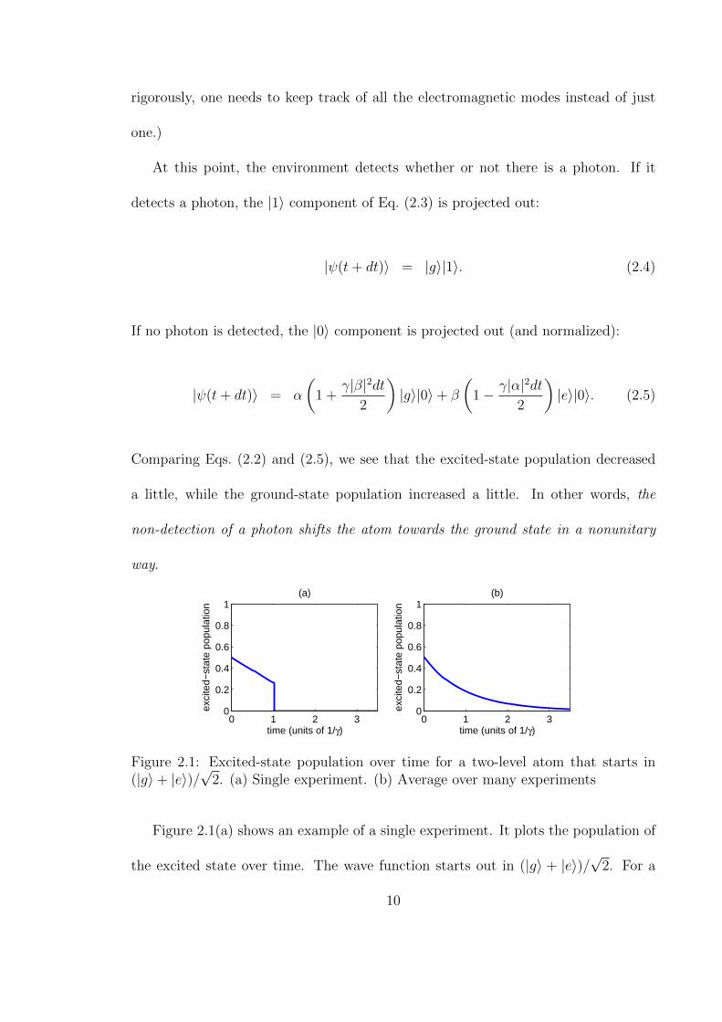
At this point, the environment detects whether or not there is a photon. If it

detects a photon, the |1〉 component of Eq. (2.3) is projected out:

|ψ(t+ dt)〉 = |g〉|1〉. (2.4)

If no photon is detected, the |0〉 component is projected out (and normalized):

|ψ(t+ dt)〉 = α

(1 +

γ|β|2dt2

)|g〉|0〉+ β

(1− γ|α|2dt

2

)|e〉|0〉. (2.5)

Comparing Eqs. (2.2) and (2.5), we see that the excited-state population decreased

a little, while the ground-state population increased a little. In other words, the

non-detection of a photon shifts the atom towards the ground state in a nonunitary

way.

0 1 2 30

0.2

0.4

0.6

0.8

1

time (units of 1/γ)

exci

ted−

stat

e po

pula

tion

(a)

0 1 2 30

0.2

0.4

0.6

0.8

1

time (units of 1/γ)

exci

ted−

stat

e po

pula

tion

(b)

Figure 2.1: Excited-state population over time for a two-level atom that starts in(|g〉+ |e〉)/

√2. (a) Single experiment. (b) Average over many experiments

Figure 2.1(a) shows an example of a single experiment. It plots the population of

the excited state over time. The wave function starts out in (|g〉 + |e〉)/√

2. For a

10

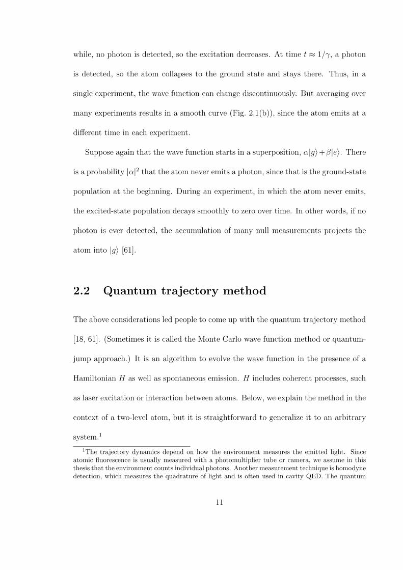
while, no photon is detected, so the excitation decreases. At time t ≈ 1/γ, a photon

is detected, so the atom collapses to the ground state and stays there. Thus, in a

single experiment, the wave function can change discontinuously. But averaging over

many experiments results in a smooth curve (Fig. 2.1(b)), since the atom emits at a

different time in each experiment.

Suppose again that the wave function starts in a superposition, α|g〉+β|e〉. There

is a probability |α|2 that the atom never emits a photon, since that is the ground-state

population at the beginning. During an experiment, in which the atom never emits,

the excited-state population decays smoothly to zero over time. In other words, if no

photon is ever detected, the accumulation of many null measurements projects the

atom into |g〉 [61].

2.2 Quantum trajectory method

The above considerations led people to come up with the quantum trajectory method

[18, 61]. (Sometimes it is called the Monte Carlo wave function method or quantum-

jump approach.) It is an algorithm to evolve the wave function in the presence of a

Hamiltonian H as well as spontaneous emission. H includes coherent processes, such

as laser excitation or interaction between atoms. Below, we explain the method in the

context of a two-level atom, but it is straightforward to generalize it to an arbitrary

system.1

1The trajectory dynamics depend on how the environment measures the emitted light. Sinceatomic fluorescence is usually measured with a photomultiplier tube or camera, we assume in thisthesis that the environment counts individual photons. Another measurement technique is homodynedetection, which measures the quadrature of light and is often used in cavity QED. The quantum

11

One starts with the atomic wave function at time t, |ψ(t)〉 = α|g〉 + β|e〉 and

calculates the probability of an emission in time interval dt, p = γ|β|2dt. With

probability p, one decides that the atom emits, in which case |ψ(t+ dt)〉 = |g〉. With

probability 1− p, the atom does not emit, in which case one evolves |ψ(t)〉 using an

effective Hamiltonian: |ψ(t + dt)〉 = (1 − iHeff dt)|ψ(t)〉, where Heff = H − iγ2|e〉〈e|.

The non-Hermitian part of Heff is a shortcut to account for the fact that the non-

detection of a photon decreases the excited-state population. At this point, one

normalizes |ψ(t + dt)〉 to 1 and repeats the process for the next time step, and this

cycle repeats over and over.

The quantum trajectory method simulates what happens in a single experiment.

It is a Monte Carlo approach, since each trajectory is different. The method can

be shown to be equivalent to the Lindblad master equation for the density matrix ρ

[18, 61]:

d

dtρ = −i[H, ρ] +

γ

2(−|e〉〈e|ρ− ρ|e〉〈e|+ 2|g〉〈e|ρ|g〉〈e|). (2.6)

The difference is that the quantum trajectory method describes how a single wave

function evolves in a single experiment, while the master equation describes how an

ensemble of wave functions evolves. Although they are equivalent, quantum trajec-

tories sometimes provide a lot of insight into what is happening in the system, which

might not be obvious from the master equation. In particular, quantum trajectories

provide examples of photon signals that an experimentalist would measure. This

trajectory method for homodyne detection is quite different from that of photon counting, eventhough they are described by the same master equation [65].

12

thesis will show many quantum trajectories.

The quantum trajectory method can even be used to solve the master equation,

since the two are equivalent. Sometimes, it is computationally faster to average over

many quantum trajectories than to directly integrate the master equation [18, 61].

2.3 Two-level atom with laser excitation

Here, we apply the quantum trajectory method to a two-level atom in the presence of

laser excitation and spontaneous emission. This is the simplest quantum nonequilib-

rium system. Driving comes from the laser, while dissipation comes from spontaneous

emission. This textbook problem is usually solved using the master equation [60], but

it is interesting to view it from a quantum-trajectory point of view.

|e Ú

|e Ú

|g Ú

Figure 2.2: Level diagram of an atom with laser excitation and spontaneous emission

The Hamiltonian is2

H = −∆|e〉〈e|+ Ω

2(|g〉〈e|+ |e〉〈g|), (2.7)

2Throughout this thesis, we use the interaction picture, rotating-wave approximation, and let~ = 1.

13

where ∆ is the laser detuning and Ω is the Rabi frequency, which depends on the laser

intensity (Fig. 2.2). The linewidth γ accounts for spontaneous emission. An example

trajectory is shown in Fig. 2.3, which plots the excited-state population vs. time. The

atom starts in the ground state and emits photons at various times. Interestingly,

after a long period without a photon emission, the wave function approaches a steady

state and the excitation levels off. Physically, this is due to the balance of two

processes: laser driving increases the excitation, while the non-detection of photons

decreases the excitation.

0 10 20 30 400

0.2

0.4

0.6

0.8

1

time (units of 1/γ)

exci

ted−

stat

e po

pula

tion

steady state

Figure 2.3: Quantum trajectory for single atom with laser excitation and spontaneousemission. The parameters are Ω = ∆ = γ. Photons are emitted at t/γ = 18.8, 33.5,35.2, and 36.6.

Mathematically, the steady state is because of the following. In the absence of a

photon emission, the wave function evolves with Heff = H − iγ2|e〉〈e|:

id

dt|ψ(t)〉 = Heff|ψ(t)〉. (2.8)

The general solution to this differential equation is given by the eigenvalues λi and

14

eigenvectors |ui〉 of Heff:

|ψ(t)〉 = c1e−iλ1t|u1〉+ c2e

−iλ2t|u2〉, (2.9)

where c1 and c2 are determined by the initial condition, |ψ(0)〉 = |g〉. Since Heff is

non-Hermitian, λ1 and λ2 are complex, so both terms in Eq. (2.9) decay. In general,

one of the eigenvalues has a less negative imaginary part, so that term decays more

slowly than the other. Thus, after a long time without a photon detection, only that

term remains, and it corresponds to the steady-state wave function seen in Fig. 2.3.

This effect will be important in Chapters 5 and 6.

2.4 Quantum jumps of a three-level atom

A good application of quantum trajectories is to quantum jumps of a three-level atom

[15, 13, 65]. This section summarizes the main results, while Section 2.5 reviews the

derivation of the jump rates, and Section 2.6 provides a physical interpretation of

quantum jumps in terms of quantum measurement.

Consider an atom with three levels: ground state |g〉, short-lived excited state |e〉,

and metastable state |r〉 (Fig. 2.4). A laser drives the strong transition |g〉 → |e〉,

while another drives the weak transition |g〉 → |r〉. The strong transition acts as a

measurement of whether or not the atom is in |r〉. When the atom is not in |r〉, the

atom is repeatedly excited to |e〉 and spontaneously emits photons. Occasionally the

atom is excited to |r〉 and stays there, and the fluorescence from the strong transition

15

|r Úr

|e Ú r

|g Ú

e e

Figure 2.4: Level diagram of an atom with three levels

turns off. Eventually, the atom returns to |g〉, and the fluoresence turns back on.

Thus, the fluorescence signal of the strong transition exhibits bright and dark periods,

and the occurrence of a dark period implies that the atom is in |r〉. The transitions

between the bright and dark periods are quite sudden and reflect quantum jumps to

and from |r〉. Quantum jumps are a good example of how a quantum nonequilibrium

system can have nontrivial dynamics.

The Hamiltonian for the system is

H =Ωe

2(|g〉〈e|+ |e〉〈g|) +

Ωr

2(|g〉〈r|+ |r〉〈g|)−∆e|e〉〈e| −∆r|r〉〈r|, (2.10)

where ∆e and Ωe are the laser detuning and Rabi frequency of the strong transition,

while ∆r and Ωr are the corresponding quantities for the weak transition. In the

absence of spontaneous emission, Eq. (2.10) would completely describe the system.

However, the excited states have lifetimes given by their linewidths, γe and γr.

For simplicity, we make the following assumptions on the parameters. We set

16

∆e = 0, so the strong transition is on resonance. We also set γr = 0, so the metastable

state has an infinite lifetime. It is straightforward to extend the analysis to nonzero

∆e = 0 and γr = 0.

Figure 2.5 shows an example quantum trajectory. The population of the Rydberg

state jumps between a low value and a high value.

0 2000 4000 6000 8000 100000

0.2

0.4

0.6

0.8

1

time (units of 1/γe)

Ryd

berg

pop

ulat

ion

Figure 2.5: Quantum trajectory of an atom undergoing quantum jumps. Ωe = 0.2γe,Ωr = 0.005γe, ∆e = ∆r = γr = 0.

Well-defined jumps appear in the fluorescence signal when a bright period consists

of many emitted photons while a dark period consists of the absence of many photons.

For a single atom, this happens when Ωr Ω2e/γe in the case of ∆r = 0 [13]. The

transition rate from a dark period to a bright period is [65]

ΓD→B(∆r) =γeΩ

2eΩ

2r

16∆4r + 4∆2

r(γ2e − 2Ω2

e) + Ω4e

, (2.11)

and the rate from a bright period to a dark period is

ΓB→D(∆r) =γ2e + 4∆2

r

γ2e + 2Ω2

e

ΓD→B(∆r), (2.12)

17

where B and D denote bright and dark periods. An important feature of these

equations is that both rates are maximum when ∆r = 0 since the strength of the weak

transition is maximum there. When ∆r = 0, both rates are approximately γeΩ2r/Ω

2e.

This depends inversely on Ωe, because increasing Ωe is equivalent to measuring the

atomic state more frequently; this inhibits transitions to and from |r〉, similar to the

quantum Zeno effect [36].

Quantum jumps have been observed in many settings, such as trapped ions [62, 74,

8], photons [28], electrons [85], and superconducting qubits [87]. In these experiments,

the object being observed is a single particle or can be described by a single degree of

freedom. In Chapters 5 and 6, we discuss quantum jumps involving many Rydberg

atoms.

2.5 Derivation of jump rates for one atom

This section reviews the derivation of jump rates for one atom. We essentially repro-

duce the derivation in Refs. [13, 68, 65], because we need to refer back to it in Chapter

6, and it is convenient to see it in our notation. We use the quantum-trajectory ap-

proach, which is based on the wave function, to account for spontaneous emission,

but it is also possible to base the calculation on the density matrix [42].

When an atom exhibits quantum jumps, the fluorescence signal has bright periods,

in which the photons are closely spaced in time, and dark periods, in which no photons

are emitted for a while. The goal is to calculate the transition rate from a bright period

to a dark period and vice versa. The important quantity is the time interval between

18

successive emissions [13]. During a bright period, the intervals are short, but a dark

period is an exceptionally long interval. Suppose one has the function P0(t), which

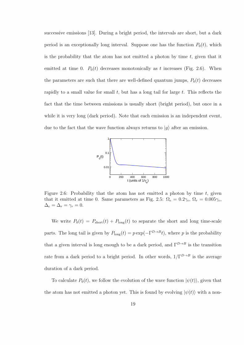
is the probability that the atom has not emitted a photon by time t, given that it

emitted at time 0. P0(t) decreases monotonically as t increases (Fig. 2.6). When

the parameters are such that there are well-defined quantum jumps, P0(t) decreases

rapidly to a small value for small t, but has a long tail for large t. This reflects the

fact that the time between emissions is usually short (bright period), but once in a

while it is very long (dark period). Note that each emission is an independent event,

due to the fact that the wave function always returns to |g〉 after an emission.

0 200 400 600 800 1000

0.01

0.1

1

t (units of 1/γe)

P0(t)

Figure 2.6: Probability that the atom has not emitted a photon by time t, giventhat it emitted at time 0. Same parameters as Fig. 2.5: Ωe = 0.2γe, Ωr = 0.005γe,∆e = ∆r = γr = 0.

We write P0(t) = Pshort(t) + Plong(t) to separate the short and long time-scale

parts. The long tail is given by Plong(t) = p exp(−ΓD→Bt), where p is the probability

that a given interval is long enough to be a dark period, and ΓD→B is the transition

rate from a dark period to a bright period. In other words, 1/ΓD→B is the average

duration of a dark period.

To calculate P0(t), we follow the evolution of the wave function |ψ(t)〉, given that

the atom has not emitted a photon yet. This is found by evolving |ψ(t)〉 with a non-

19

Hermitian Hamiltonian Heff = H − iγe2|e〉〈e|. The non-Hermitian term accounts for

the population that emits a photon, hence dropping out of consideration [13]. Thus,

P0(t) = 〈ψ(t)|ψ(t)〉.

In the basis |g〉, |e〉, |r〉, the matrix form of Heff is

Heff =

0 Ωe

2Ωr

2

Ωe

2− iγe

20

Ωr

20 −∆r

. (2.13)

As stated in Section 2.4, we assume ∆e = γr = 0. We want to solve the differential

equation i ddt|ψ(t)〉 = Heff|ψ(t)〉 given the initial condition |ψ(0)〉 = |g〉. The gen-

eral solution is |ψ(t)〉 =∑

n cne−iλnt|un〉, where λn and |un〉 are the eigenvalues and

eigenvectors of Heff, and cn is determined from the initial condition |g〉 =∑

n cn|un〉.

We calculate the eigenvalues and eigenvectors pertubatively in Ωr, which is as-

sumed to be small. (Note that since Heff is non-Hermitian, perturbation theory is

different from the usual Hermitian case [81].) All three eigenvalues have negative

imaginary parts, which leads to the nonunitary decay. It turns out that the imag-

inary part of one of the eigenvalues, which we call λ3, is much less negative than

the other two. This means that the |u1〉 and |u2〉 components in |ψ(t)〉 decay much

faster than the |u3〉 component. After a long time without a photon emission, |ψ(t)〉

contains only |u3〉. Thus, λ3 corresponds to the long tail of P0(t).

20

To second order in Ωr [13, 68],

λ3 = −∆r +Ω2r(−2∆r + iγe)

8∆2r − 2Ω2

e − 4iγe∆r

. (2.14)

To first order in Ωr,

|u3〉 =Ωr(−2∆r + iγe)

4∆2r − Ω2

e − 2iγe∆r

|g〉+ΩeΩr

4∆2r − Ω2

e − 2iγe∆r

|e〉+ |r〉 (2.15)

c3 =Ωr(−2∆r + iγe)

4∆2r − Ω2

e − 2iγe∆r

. (2.16)

Since |u3〉 consists mainly of |r〉, the occurrence of a dark period implies, as expected,

that the atom is in |r〉. (However, note that the atom is not completely in |r〉. In

fact, the dark period ends when the small |e〉 component in |u3〉 decays and emits a

photon [65].)

We can now construct Plong(t):

p = |c3|2 =Ω2r(γ

2e + 4∆2

r)

16∆4r + 4∆2

r(γ2e − 2Ω2

e) + Ω4e

(2.17)

ΓD→B = −2 Im λ3 =γeΩ

2eΩ

2r

16∆4r + 4∆2

r(γ2e − 2Ω2

e) + Ω4e

. (2.18)

Then, instead of finding Pshort(t) explicity, we use a shortcut [65]. During a bright

period, there is negligible population in |r〉, so the atom is basically a two-level atom

driven by a laser with Rabi frequency Ωe. Thus, to lowest order in Ωr, the emission

21

rate Γshort during a bright period is the same as a two-level atom [60]:

Γshort =γeΩ

2e

γ2e + 2Ω2

e

. (2.19)

However, each emission in a bright period has a small probability p of taking a long

time, in which case the bright period ends. Thus, the transition rate from a bright

period to a dark period is

ΓB→D = p Γshort =γ2e + 4∆2

r

γ2e + 2Ω2

e

ΓD→B. (2.20)

The jumps are well-defined when a bright or dark period is much longer than the

typical emission time during a bright period: ΓB→D,ΓD→B Γshort. When ∆r = 0

and Ωe γe, this condition becomes Ωr Ω2e/γe [13].

2.6 Interpretation of quantum jumps

The previous section contained a lot of math, so it is worthwhile to clarify the physics

of what is happening. Suppose the atom starts out bright, so it cycles back and forth

between |g〉 and |e〉. The transition to a dark period occurs when the atom happens

to not emit a photon for a while. The non-detection of photons projects the atom

into |r〉. In other words, the accumulation of many null measurements means that

the atom must be in the state that does not emit, which is |r〉. To be precise, the

atom is projected into |u3〉 (Eq. (2.15)), which is the slowest-decaying eigenstate of

Heff. This is similar to the steady-state wave function discussed in Section 2.3.

22

However, |u3〉 does not consist completely of |r〉, because there are small compo-

nents of |g〉 and |e〉. The dark period ends when the |e〉 component in |u3〉 happens

to finally emit, projecting the atom into |g〉. At this point, the atom is repeatedly

excited to |e〉, emits photons, and is bright again.

Note that during the transition to a dark period, the wave function evolves con-

tinuously towards the metastable state [65]. In contrast, during the transition to a

bright period, the wave function suddenly collapses to |g〉.

23

Chapter 3

Rydberg atoms

A Rydberg atom is an atom with an electron excited to a high principal quantum

number n. The high n leads to exaggerated atomic properties, including a strong

interaction between two nearby Rydberg atoms. This chapter describes Rydberg

atoms and the interaction between them.

3.1 Energy levels

Rydberg atoms are usually studied in the context of alkali atoms, which have a single

valence electron and hence relatively simple level diagrams. Consider, for example,

rubidium, which has a single valence electron and a core, which consists of 36 electrons

in filled bands and 37 protons. When the valence electron is far from the core, the

core appears as a point charge of +1. Thus, if the electron’s orbit stays far from the

core, the energy levels are the same as in hydrogen.

On the other hand, when the electron is near the core, it sees how the charge

is distributed in space. For example, when the electron is inside the core, it sees

the +37 charge of the nucleus, which increases the binding energy and decreases the

24

total energy. In addition, the electron polarizes the core, which also decreases the

energy. Thus, when the electron’s orbit is close to the core, the energy levels differ

significantly from those of hydrogen.

The energy of a Rydberg state nl is [26]:

Enl = − Ry

(n− δl)2(3.1)

where Ry is the Rydberg constant. δl is a quantum defect that depends on the orbital

angular momentum l, and it accounts for deviations due to the finite core size. When

δl = 0, Eq. (3.1) is the usual formula for hydrogen. The quantum defect is usually

determined empirically. For rubidium, δ0 = 3.13, δ1 = 2.64, δ2 = 1.35, and δ3 = 0.016

[54, 31]. As l increases, the electron spends less time near the core, and hence the

atom behaves more like hydrogen. Note that the Rydberg levels are also shifted by

fine structure [78], which is not included in Eq. (3.1). Hyperfine splitting is relatively

small for Rydberg states, so it is usually ignored [73].

Using quantum defect theory, one can construct the wavefunctions of the Ryd-

berg states [26]. An important application of the wavefunctions is to calculate the

dipole matrix elements between different atomic states. Instead of going through the

calculation, we summarize the results in Table 3.1.

25

Property Expression n dependence

Binding energy En n−2

Level spacing En − En−1 n−3

Orbital radius 〈nl|r|nl〉 n2

Dipole matrix element between e.g. 〈5P |r|nS〉 n−3/2

low-lying state and Rydberg state

Dipole matrix element between e.g. 〈nP |r|nS〉 n2

two Rydberg states

Radiative lifetime τ0nl n3

Table 3.1: Properties of Rydberg states

3.2 Lifetimes

The lifetime τnl of a Rydberg state is limited by two factors: spontaneous emission

and black-body radiation. The two contributions can be written as

1

τnl=

1

τ 0nl

+1

τ bbnl, (3.2)

where τ 0nl is the lifetime due to spontaneous emission only and τ bbnl is the lifetime due

to black-body radiation only. At 0 K, there is no black-body radiation, so τnl = τ 0nl.

3.2.1 Spontaneous emission

In a spontaneous emission event, the atom decays to a state of lower energy and emits

a photon that carries away the energy difference. The rate of spontaneous decay from

nl to n′l′ is given by the Einstein A coefficient [26],

An′l′,nl =e2ω3

n′l′,nl

3πε0~c3

lmax

2l + 1|〈n′l′|r|nl〉|2, (3.3)

26

where ωn′l′,nl is the frequency difference of the two states, and lmax is the larger of

l and l′. We are only interested in dipole-allowed transitions (l′ = l ± 1). The

dipole-forbidden transitions have much smaller rates. The lifetime of a nl state is the

reciprocal of the sum of decay rates to all possible n′l′ states:

τ 0nl =

1∑n′l′ An′l′,nl

. (3.4)

Note that each An′l′,nl is proportional to ω3n′l′,nl. It turns out that the decay from

nl is dominated by transitions to the lowest possible values of n′, because ωn′l′,nl is

maximum for those n′ [26]. The ω3n′l′,nl factor outweighs the fact that the matrix

element 〈n′l′|r|nl〉 is small for low n′. For example, the ground state of rubidium is

5S, so nS decays mostly to 5P and 6P , while nP decays mostly to 5S, 6S, and 4D

[19].

For the transitions from nl to low-lying n′l′, as n increases, ωn′l′,nl approaches a

constant due to the form of the energy equation (Eq. (3.1)). Thus, for large n, An′l′,nl

depends only on the matrix elements from nl to low-lying n′l′. As shown in Table

3.1, the dipole matrix elements scale as n−3/2. Thus for large n,

τ 0nl ∼ n3. (3.5)

3.2.2 Black-body radiation

Rydberg states are much more sensitive to black-body radiation than normal states.

This is because the energy spacing between Rydberg states is small, so at room

27

temperature, there are many black-body photons resonant with transitions between

Rydberg states. In addition, the matrix elements between Rydberg states are large.

The effect of black-body radiation is to transfer the atom from a Rydberg state to

nearby Rydberg states.

Recall that in equilibrium at temperature T , an electromagnetic mode of frequency

ω contains N(ω) photons [43]:

N(ω) =1

e~ω/kbT − 1. (3.6)

When ~ω kbT , N(ω) ≈ kbT/~ω. Thus, as T increases, the mode is more populated.

The effect of black-body radiation on an atom in state nl is twofold: (i) a black-body

photon can induce stimulated emission to a lower state n′l′; (ii) the atom can absorb

a photon to go to a higher state n′l′. Both rates are given by [26]:

Kn′l′,nl = An′l′,nlN(ωn′l′,nl), (3.7)

where An′l′,nl is given by Eq. (3.3). The frequency dependence of Kn′l′,nl differs from

that of An′l′,nl due to the additional N(ω) factor. As a result, black-body radia-

tion tends to cause transitions to nearby Rydberg states (n′ ≈ n), in contrast to

spontaneous emission, which causes transitions to low-lying states.

By summing over all possible n′l′, one finds the approximate relation [26]

τ bbnl =3~n2

4α3kbT. (3.8)

28

Note that τ 0nl scales as n3 while τ bbnl scales as n2. This means that as n increases, the

overall lifetime τ increases, but the contribution from black-body radiation increas-

ingly dominates over that of spontaneous emission.

More precise estimates for τnl are tabulated in Ref. [10]. In general, black-body

radiation interferes with experiments people want to do, since it transfers the atom

to Rydberg states that are not coupled to laser light. Black-body effects can be

minimized by working at cryogenic temperatures, as is done in some experiments

[69].

3.3 Interaction in absence of a static electric field

The interaction between Rydberg atoms can be a confusing subject because it can

take different forms, depending on the experimental setup. In this section, we discuss

the interaction when there is no external static electric field. In Section 3.4, we discuss

the interaction in the presence of a static electric field.

Suppose there are two atoms, each with one valence electron, and let the atoms

be separated by a distance R. The dipole-dipole interaction between them is [37]

Vdd =e2

4πε0R3[~r1 · ~r2 − 3(~r1 · R)(~r2 · R)], (3.9)

where ~r1 and ~r2 are the positions of the two valence electrons relative to their nuclei,

and R is a unit vector that points from one to the other. In the absence of an electric

field, an atom in a parity eigenstate does not have a permanent dipole moment, so

29

classically there would be no interaction between the two atoms. However, there is

a quantum mechanical interaction, because quantum fluctuations induce momentary

dipole moments in the atoms that interact with each other.

In the absence of the dipole-dipole interaction, the eigenstates of the system are

product states of the two atoms, denoted by |n′l′, n′′l′′〉. However, the operator Vdd

couples each two-atom state to all other two-atom states allowed by the dipole selec-

tion rules. Thus, in the presence of the interaction, the eigenstates of the two-atom

system are mixtures of the original |n′l′, n′′l′′〉 states.

3.3.1 Simplified example

We illustrate the interaction with a simple example, while Section 3.3.2 describes the

more-realistic situation. Due to spin-orbit coupling, a Rydberg state is specified by

four quantum numbers: n, l, j,mj. But for simplicity, we only keep track of n and

l. Consider the state |nl, nl〉, which has both atoms in the same Rydberg state. We

describe the effect of the interaction for the case when |nl, nl〉 couples to only one

state, denoted by |n′l′, n′′l′′〉. Let δ = En′l′ + En′′l′′ − 2Enl be the energy difference

between the two two-atom states. In the |nl, nl〉, |n′l′, n′′l′′〉 basis, the Hamiltonian

is

H =

0 〈nl, nl|Vdd|n′l′, n′′l′′〉

〈n′l′, n′′l′′|Vdd|nl, nl〉 δ

. (3.10)

30

The eigenstates of H are mixtures of |nl, nl〉 and |n′l′, n′′l′′〉, but in the limit of small

|〈n′l′, n′′l′′|Vdd|nl, nl〉|, one eigenstate corresponds asymptotically to |nl, nl〉, while the

other to |n′l′, n′′l′′〉. We are interested in the one that corresponds to |nl, nl〉 since

that is the experimentally relevant one (Section 3.5). The energy of that eigenstate

is given by its eigenvalue:

V =δ − sgn(δ)

√δ2 + 4|〈n′l′, n′′l′′|Vdd|nl, nl〉|2

2. (3.11)

Since |nl, nl〉 originally had zero energy, V is the level shift that it experiences due to

the interaction.

Recall that Vdd ∼ R−3. Consider first the limit |〈n′l′, n′′l′′|Vdd|nl, nl〉| δ, which

corresponds to large R. The level shift becomes

V ≈ −|〈n′l′, n′′l′′|Vdd|nl, nl〉|2

δ. (3.12)

For large n, the dipole matrix element between nearby Rydberg levels, such as

〈nP |r|nS〉, scales as n2. Thus, |〈n′l′, n′′l′′|Vdd|nl, nl〉| contains two factors of n2, one

for each atom. Also, δ scales as n−3, since that is how the characteristic level spacing

scales. For large n,

|V | ∼ n11

R6. (3.13)

31

Then consider the limit |〈n′l′, n′′l′′|Vdd|nl, nl〉| δ, which corresponds to small R:

V ≈ −sgn(δ)|〈n′l′, n′′l′′|Vdd|nl, nl〉|

R3, (3.14)

which scales for large n as

|V | ∼ n4

R3. (3.15)

One can define a crossover distance Rc given by when |〈n′l′, n′′l′′|Vdd|nl, nl〉| ≈ δ.

When R > Rc, the interaction has the van der Waals form in Eq. (3.13). When

R < Rc, the interaction has the dipolar form in Eq. (3.15). The scaling with n shows

that the interaction between Rydberg atoms can be very strong.

3.3.2 More-realistic situation

The above example was simplified to bring out the main points. In reality, due to spin-

orbit coupling, one must also specify a state’s total angular momentum j and magnetic

quantum number mj. Another simplification we made above was that |nl, nl〉 couples

to only one state. To accurately calculate the level shift, one needs to include the

contribution from all possible states1, which is most conveniently done with second-

order perturbation theory. Thus, the level shift that |nljmj, nljmj〉 experiences is

1But the level shift is often dominated by only a few two-atom states that are close in energy.For instance, |60p3/2, 60p3/2〉 couples most strongly to |60s1/2, 61s1/2〉 [73].

32

actually

V ≈ −∑

n′,l′,j′,m′j

n′′,l′′,j′′,m′′j

|〈n′l′j′m′j, n′′l′′j′′m′′j |Vdd|nljmj, nljmj〉|2

En′l′j′m′j

+ En′′l′′j′′m′′j− 2Enljmj

. (3.16)

Equation (3.16) is the revised version of Eq. (3.12). When one of the energy denomi-

nators is small compared to the matrix element, one needs to use degenerate pertur-

bation theory to find the level shift; this produces the revised version of Eq. (3.14).

The level shifts for many different |nljmj, nljmj〉 have been calculated in Ref. [71].

Note that V can be positive or negative, depending on the state.

Even with all contributions included, the scaling forms in Eqs. (3.13) and (3.15)

still hold [73]. For typical distances R in current experimental setups, the interaction

is usually in the van der Waals regime. However, for special |nljmj, nljmj〉 states,

an energy denominator in Eq. (3.16) almost vanishes, leading to the dipolar type of

interaction. This is known as a Forster resonance, and the level shift is especially

large. One can also apply a weak electric field to make an energy denominator vanish

and thus obtain a Forster resonance.

In general, the level shifts are anisotropic. More precisely, the level shift depends

on the angle between R and the quantization axis, where R points from one atom to

the other. However, it turns out that the nS states are almost perfectly isotropic,

due to the spherical symmetry of the S wavefunction [71]. As a result, the nS states

are particularly useful in experiments.

33

3.4 Interaction in presence of a static electric field

In this section, we consider what happens when a static electric field is applied. We

first describe how the energy levels of hydrogen are affected. Then we describe the

dipole-dipole interaction between two hydrogen atoms. Finally, we discuss modifica-

tions when the atom is not hydrogen.

3.4.1 Single hydrogen atom

The Hamiltonian for the hydrogen atom in the absence of fine structure is

H0 =p2

2m− 1

4πε0r. (3.17)

A state is described by three quantum numbers, |nlm〉. Let the quantization axis

be along z, so m is the projection of l along z. For a given n, all the lm states are

degenerate. Now we turn on a weak electric field in the z direction with amplitude

ε, which adds a perturbation to the Hamiltonian,

H = H0 + eεz. (3.18)

The perturbation lifts the degeneracy among the lm states of a given n, leading

to a first-order Stark shift. To see this, consider matrix elements between the original

eigenstates: 〈nl′m′|z|nlm〉. Due to the dipole selection rules, the matrix element is

nonzero only if l′ = l ± 1 and m′ = m [78]. Thus for a given n and m, multiple

values of l are coupled together. The eigenstates of H are mixtures of lm states that

34

are coupled by the perturbation. Since the degeneracy is lifted in first order, the

eigenvalues are linear in ε.

For example, consider n = 3. The groups of coupled states are: |300〉, |310〉, |320〉,

|31 −1〉, |32 −1〉, |311〉, |321〉, |32 −2〉, and |322〉. The states within each

group mix to form the new eigenstates.

Since different values of l mix together, l is no longer a good quantum num-

ber. Instead, we use the parabolic quantum number q, which can take the values:

n− 1− |m|, n− 3− |m|, . . ., −(n− 1− |m|) [26]. A Stark state is specified by |nqm〉.

Note that m is still a good quantum number. The energy levels are [38]

Enqm =3nqea0ε

2, (3.19)

where a0 is the Bohr radius. As ε increases, the energy levels of a given n manifold

increase and decrease linearly, since q can take on different values. This is called a

first-order Stark shift. Since the Stark states are not parity eigenstates, they have

permanent dipole moments,

~µnqm =3nqea0z

2, (3.20)

which are independent of the field strength ε.

35

3.4.2 Interaction of two hydrogen atoms

Now we consider the dipole-dipole interaction between two atoms in the presence of

a static field. Suppose the atoms are in the two-atom state |nqm, nqm〉, where both

atoms are in the same Stark state. Since Stark states have permanent dipole moments

~µ, the interaction is the same as between two classical dipoles. Equation (3.9) can be

rewritten as

Vdd =1

4πε0R3[~µ1 · ~µ2 − 3(~µ1 · R)(~µ2 · R)]. (3.21)

The interaction is anisotropic, since it depends on the relative orientation between

R and the electric field. Suppose R is perpendicular to the electric field. Then the

two-atom state experiences a level shift,

V = 〈nqm, nqm|Vdd|nqm, nqm〉 (3.22)

=9(nqea0)2

16πε0R3. (3.23)

For example, consider the state with q = n− 1 and m = 0. This state has the largest

Stark shift within a given n manifold. For large n, V ∼ n4/R3.

3.4.3 Nonhydrogenic atoms

As discussed in Section 3.1, the nonhydrogenic atoms have a finite core size, and

their energy levels are shifted by an amount that depends on l. Thus, for a given

n, the lm states are not degenerate like they are in hydrogen. The l ≥ 3 states can

36

still be considered degenerate, since their quantum defects are small. However, the

l = 0, 1, 2 states are especially affected, since their quantum defects are large. The

lack of degeneracy means that the l = 0, 1, 2 states have second-order Stark shifts,

which are smaller than the usual first-order Stark shifts. But when the electric field

is large enough to mix those states with others, the Stark shift becomes first-order

[26]. Since it is complicated to accurately determine the energies and wavefunctions

of nonhydrogenic atoms, it is common to use the hydrogen case as a rough estimate.

3.5 Rydberg blockade

Sections 3.3 and 3.4 showed that when two atoms are both in a Rydberg state, the

dipole-dipole interaction leads to a level shift of the two-atom state. Here, we describe

how the level shift affects the dynamics when the atoms are excited by a laser.

Let the ground state and a Rydberg state be denoted by |g〉i and |r〉i, where

i denotes which atom. |r〉 is shorthand for a particular Rydberg state (|nljmj〉 or

|nqm〉). The interaction term in the Hamiltonian is V |r〉〈r|1 ⊗ |r〉〈r|2, which reflects

the fact that when both atoms are in the Rydberg state, there is a level shift V . In

principle, there is also a dipole-dipole interaction between the ground states, but it

is much weaker than the Rydberg interaction, so we ignore it.

Suppose a laser shines on both atoms. The Hamiltonian is:

H =∑i

[−∆|r〉〈r|i +

Ω

2(|g〉〈r|i + |r〉〈g|i)

]+ V |r〉〈r|1 ⊗ |r〉〈r|2, (3.24)

37

where ∆ is the laser detuning and Ω is the Rabi frequency. Suppose the laser is on

resonance (∆ = 0). The system gets excited from |gg〉 to |gr〉 and |rg〉. However, due

to the level shift, |rr〉 is shifted off resonance, so that it is effectively uncoupled from

the other levels (Fig. 3.1(a)). Thus, the system stays within the space spanned by

|gg〉, |gr〉, |rg〉. This is called Rydberg blockade, since the dipole-dipole interaction

prevents the atoms from both being in the Rydberg state at the same time [57].

V|rrÚ

(a) (b)

V

|grÚ |rgÚ

|rÚV

|ggÚ

|grÚ, |rgÚ

|gÚatom 1 atom 2

Figure 3.1: Two views of Rydberg blockade

In general, the dipole-dipole interaction leads to entanglement between the atoms.

In fact, the blockade effect can be used to prepare entangled states, as seen in

the following argument [57]. Let us work in the basis |gg〉, |s〉, |a〉, |rr〉, where

|s〉 = (|gr〉 + |rg〉)/√

2 and |a〉 = (|gr〉 − |rg〉)/√

2. Due to the symmetry of H, the

antisymmetric state |a〉 is uncoupled from the other states. Consider how the state

|ψ(t)〉 = c1(t)|gg〉+ c2(t)|s〉+ c3(t)|rr〉 evolves under the Hamiltonian in Eq. (3.24):

ic1 =Ω√2c2 (3.25)

ic2 =Ω√2c1 +

Ω√2c3 (3.26)

ic3 =Ω√2c2 + V c3. (3.27)

38

Suppose both atoms start in the ground state: c1(0) = 1, c2(0) = 0, c3(0) = 0. If V is

very large, then c3(t) ≈ 0 for all times due to the blockade effect. Then Eqs. (3.25)

and (3.26) become

ic1 =Ω√2c2 (3.28)

ic2 =Ω√2c1. (3.29)

At time t = π/(√

2Ω), c1(t) = 0 and c2(t) = 1, which means that the atoms are in the

entangled state |s〉. This scheme can be extended to entangle N atoms. Note that if

V = 0, the atoms would never be entangled.

Here is another way of viewing the blockade effect. Again set ∆ = 0. Let atom 2

start in |g〉, and suppose the laser shines only on atom 2. If atom 1 is in |g〉, atom 2

gets excited to |r〉. However, if atom 1 is in |r〉, atom 2’s Rydberg level is effectively

shifted by V , so atom 2 is no longer on resonance with the laser and it stays in |g〉

(Fig. 3.1(b)). Thus, whether or not atom 2 gets excited to the Rydberg state depends

on whether atom 1 is in the ground or Rydberg state.

Rydberg atoms have drawn much interest in the past decade because the blockade

effect can be used for quantum information processing [57, 73] and many-body physics

[66, 52, 33]. The rest of this thesis will be about how the Rydberg interaction can be

used to study nonequilibrium physics.

39

Chapter 4

Antiferromagnetic phase transitionin a nonequilibrium lattice ofRydberg atoms

In this chapter, we study a driven-dissipative system of atoms in the presence of laser

excitation to a Rydberg state and spontaneous emission back to the ground state.

The atoms interact via the blockade effect, whereby an atom in the Rydberg state

shifts the Rydberg level of neighboring atoms. We use mean-field theory to study

how the Rydberg population varies in space. As the laser frequency changes, there

is a continuous transition between the uniform and antiferromagnetic phases. The

nonequilibrium nature also leads to a novel oscillatory phase and bistability between

the uniform and antiferromagnetic phases. The results of this chapter were published

in Ref. [47].

4.1 Model

We briefly review the Rydberg interaction, which was described in Chapter 3. Suppose

two atoms are in the same Rydberg state nlj. There is a dipole-dipole matrix element

40

between |nlj, nlj〉 and nearby energy levels, and this interaction shifts the energy of

|nlj, nlj〉 by an amount V . When the atoms are separated by a small distance R,

the dipolar interaction dominates (V ≈ −C3/R3), but for large distances, the van

der Waals interaction dominates (V ≈ −C6/R6). For mathematical convenience, we

use the van der Waals interaction and a |ns1/2, ns1/2〉 state, so that the interaction

is short range and isotropic. However, it is straightforward to extend the analysis to

long-range and anisotropic interactions.

Consider a lattice of atoms that is uniformly excited by a laser from the ground

state to a Rydberg state. The atoms are assumed to be fixed in space. Since the van

der Waals interaction decreases rapidly with distance, we assume nearest-neighbor

interactions. Let |g〉j and |e〉j denote the ground and Rydberg states of atom j. The

Hamiltonian in the interaction picture and rotating-wave approximation is (~ = 1)

H =∑j

Hj + V∑〈jk〉

|e〉〈e|j ⊗ |e〉〈e|k, (4.1)

Hj = −∆ |e〉〈e|j +Ω

2(|e〉〈g|j + |g〉〈e|j). (4.2)

The second term in Eq. (4.1) is the Rydberg interaction, and Hj is the Hamiltonian

for a two-level atom interacting with a laser. ∆ = ω` − ωo is the detuning between

the laser and transition frequencies. Ω is the Rabi frequency, which depends on the

laser intensity.

The lifetime of the Rydberg state is limited by several processes: spontaneous

emission, blackbody radiation, and superradiance. We account for spontaneous emis-

41

sion from the Rydberg level using the linewidth γ. When a Rydberg atom sponta-

neously decays, it usually goes directly into the ground state or, first, to a low-lying

state [19]; the low-lying states are relatively short-lived, so we ignore them. We also

ignore blackbody radiation and superradiance1, both of which transfer atoms in a

Rydberg level to nearby levels. Blackbody radiation can be minimized by working at

cryogenic temperatures [10], and it is not clear if superradiance is important when

the interaction V is large [89, 19]. Future treatments could account for them by

considering several Rydberg levels instead of just one.

Thus, each atom has two possible states, and the system is equivalent to a dissi-

pative spin model. Previous works have added dissipation to other spin models by

coupling each spin to a heat bath; in those works, there is global thermal equilibrium,

and the spins are described by an effective partition function [91, 80]. However, in

quantum optics, dissipation from spontaneous emission leads to a nonequilibrium sit-

uation, since the coupling to the heat bath is weak and Markovian [14]. The density

matrix for the atoms, ρ, is described by a master equation that is local in time:

ρ = −i[H, ρ] + γ∑j

(−1

2|e〉〈e|j, ρ+ |g〉〈e|j ρ |e〉〈g|j

). (4.3)

The nonequilibrium nature is exhibited in the interplay between unitary and dissi-

pative dynamics [21, 83], and we are interested in the properties of the steady-state

1Superradiance is a cooperative phenomenon that affects the radiative decay of a group of atoms[29]. When the distance between atoms is smaller than the wavelength of the atomic transition, theatoms are coupled to the same electromagnetic modes. Due to quantum effects, the spontaneousemission rate is enhanced compared to a single atom. For Rydberg atoms, superradiance can beimportant, since transitions between Rydberg states have long wavelengths. In fact, superradiancewas observed with Rydberg atoms in Ref. [70].

42

solution of Eq. (4.3).

4.2 Mean-field theory

Due to the complexity of the full quantum problem, we use mean-field theory. For

equilibrium spin models, mean-field theory is useful for determining the existence of

different phases [4]. Its predictions are accurate in high dimensions but not in low

dimensions. For the current nonequilibrium case, we use the approach of Refs. [21, 83]:

factorize the density matrix by site, ρ =⊗

j ρj, and work with the reduced density

matrices, ρj = Tr6=jρ. This accounts for on-site quantum fluctuations but not inter-

site fluctuations: for atom j, the interaction, |e〉〈e|j⊗∑

k |e〉〈e|k, is replaced with the

mean field, |e〉〈e|j∑

k ρk,ee. In high dimensions, this is a good approximation, since

fluctuations of the neighbors average out.

Then the evolution of each ρj is given by

wj = −2Ω Im qj − γ(wj + 1), (4.4)

qj = i

∆− V

2

∑〈jk〉

(wk + 1)

qj − γ

2qj + i

Ω

2wj, (4.5)

where we have defined the inversion wj ≡ ρj,ee − ρj,gg and off-diagonal element qj ≡

ρj,eg. The Rydberg population ρj,ee = (wj + 1)/2 is the observable measured in the

experiment by measuring the photon scattering rate of each atom. wj = −1 and 1

mean that the atom is in the ground and Rydberg states, respectively. Equations

(4.4) and (4.5) are the optical Bloch equations, except that the Rydberg interaction

43

V

(a) (b)

|e>

|g>

Figure 4.1: (a) When one atom is excited to the Rydberg state, it shifts the transitionfrequency of a neighboring atom by V . (b) The lattice is divided into two sublattices.

introduces nonlinearity: the detuning for an atom is renormalized by the excitation

of its neighbors (Fig. 4.1(a)).

Since the system is dissipative, it will end up at an attracting solution, which can

be a fixed point, limit cycle, quasiperiodic orbit, or strange attractor [82]. (We have

not observed the latter two.) We want to know: for given parameter values, how

many steady-state solutions are there and are they stable? A solution is stable or

unstable if a perturbation to it decays or grows, respectively; the system will end up

only in a stable solution.

Equations (4.4) and (4.5) always have a steady-state solution, in which the Ryd-

berg population is uniform across the lattice (wj = w, qj = q). For some parameter

values, this uniform solution is stable, but for others, it is unstable to perturbations

of wavelength 2. In the latter case, the lattice divides into two alternating sublat-

tices, and the atoms on one sublattice have higher Rydberg population than the other

(Fig. 4.1(b)). Hence an antiferromagnetic pattern emerges from the uniform solution

through a dynamical instability. To simplify the discussion here, we keep track of

only the two sublattices instead of every site. We stress that the antiferromagnetic

transition is not an artifact of dividing the lattice into two sublattices, as shown

44

explicitly in Appendix 4.B.

To simplify the equations, we rescale time by γ and also rescale the Rabi frequency

Ω = Ω/γ, detuning ∆ = ∆/γ, and interaction c = dV/γ = −dC6/γR6, where d is the

lattice dimension. Labeling the sublattices 1 and 2,

w1 = −2Ω Im q1 − w1 − 1, (4.6)

w2 = −2Ω Im q2 − w2 − 1, (4.7)

q1 = i [∆− c(w2 + 1)] q1 −q1

2+ i

Ω

2w1, (4.8)

q2 = i [∆− c(w1 + 1)] q2 −q2

2+ i

Ω

2w2. (4.9)

There are six nonlinear differential equations (since q1 and q2 are complex) and three

parameters (Ω, ∆, c). The uniform version of these equations (w1 = w2, q1 = q2)

has been studied before in the context of a medium that interacts with its own

electromagnetic field; it is known that there is bistability [34]. We are considering

the more general case by letting the sublattices differ.

4.3 Mean-field results

In Appendix 4.A, we determine the solutions and stabilities for Eqs. (4.6)–(4.9).

Here, we summarize the main results. Consider first the fixed points, i.e., when

w1 = w2 = q1 = q2 = 0. There are two types of fixed points: the uniform fixed

points (w1 = w2) correspond to spatially homogeneous Rydberg excitation, while the

nonuniform fixed points (w1 6= w2) correspond to the antiferromagnetic phase, i.e.,

45

when one sublattice has higher excitation than the other.

There are either one or three uniform fixed points, corresponding to the real roots

of a cubic polynomial,

f(w) = c2w3 − c(2∆− 3c)w2 +

[Ω2

2+

1

4+ (∆− 3c)(∆− c)

]w + (∆− c)2 +

1

4.

(4.10)

As the parameters change, pairs of uniform fixed points appear and disappear via

saddle-node bifurcations. The uniform fixed points never undergo Hopf bifurcations,

so we do not expect limit cycles emerging from them [82].

There are up to two nonuniform fixed points, given by the real roots of a quadratic

polynomial,

g(w) = c2(1 + 4∆2 + 2Ω2)w2 − 2c[(∆− c)(1 + 4∆2) + (2∆− c)Ω2]w

+c2(1 + 4∆2)− 2c∆(1 + 4∆2 + 2Ω2) +1

4(1 + 4∆2 + 2Ω2)2. (4.11)

The two roots correspond to w1 and w2. As the parameters change, the two nonuni-

form fixed points appear and disappear together.

Since the laser detuning ∆ is the easiest parameter to vary experimentally, we

describe what happens as a function of it (Fig. 4.2). Suppose ∆ starts out large

and negative. There is one stable uniform fixed point and no other fixed points. As

∆ increases, the uniform fixed point may undergo a pitchfork bifurcation, in which

it becomes unstable and the nonuniform fixed points appear. The bifurcation is

46

−1 0 1 2 3 4−1

−0.8

−0.6

−0.4

−0.2

0

Δ

w

−1 0 1 2 3 4−1

−0.8

−0.6

−0.4

−0.2

0

Δ

(a) (b)

Figure 4.2: Bifurcation diagram showing fixed-point solutions as function of ∆, withc = 5 and (a) Ω = 0.5 and (b) Ω = 1.5. The inversion w is -1 (1) when the atomis in the ground (Rydberg) state. Solid (dashed) lines denote stable (unstable) fixedpoints. Black (red) lines denote uniform (nonuniform) fixed points. Green pointsdenote bifurcations. In (b), the nonuniform fixed points undergo Hopf bifurcationsat ∆ = 3.48 and 1.33, and there is a stable limit cycle in that interval [shown inFig. 4.3(a)].

supercritical, which means that when the nonuniform fixed points appear, they are

stable and coincide with the uniform fixed point [82]. Thus, this is a continuous

phase transition between the uniform and antiferromagnetic phases. As ∆ increases

further, there is another supercritical pitchfork bifurcation, in which the same uniform

fixed point becomes stable again and the nonuniform fixed points disappear. As ∆

increases further towards ∞, there is again one stable uniform fixed point and no

other fixed points.

Although the nonuniform fixed points are stable when they appear and disap-

pear, they could become unstable in between via a Hopf bifurcation [82]. We find

numerically that sometimes the nonuniform fixed points do have Hopf bifurcations

(Fig. 4.2(b)) and give rise to a stable limit cycle, in which w1 and w2 oscillate pe-

riodically in time (Fig. 4.3(a)). This oscillatory phase is due to the nonequilibrium

nature of the system.

47

Δ

Ω

0 1 2 3 4 5

4

3

2

1

0100 102 104 106

−1

−0.8

−0.6

−0.4

−0.2

0

time (1/γ)

w

w1

w2

osc

uniform

uni/AFuni/osc

AF

(b)(a)

Figure 4.3: (a) Oscillatory steady-state solution (limit cycle) for c = 5, Ω = 1.5, and∆ = 1.5. (b) Phase diagram for mean-field theory in Ω,∆ space for c = 5. The systemis either in the uniform, antiferromagnetic, or oscillatory phase. It can be bistablebetween uniform and antiferromagnetic phases or between uniform and oscillatoryphases.

Thus, in mean-field theory, there are three phases: uniform, antiferromagnetic,

and oscillatory. Figure 4.3(b) shows a phase diagram in ∆,Ω space. For some pa-

rameters, the system is bistable between uniform and antiferromagnetic or between

uniform and oscillatory (Fig. 4.2(b)); the final state depends on the initial conditions.

The existence of the antiferromagnetic phase can be intuitively understood from

the fact that the effective detunings for sublattices 1 and 2 are ∆1 = ∆ − c(w2 + 1)

and ∆2 = ∆ − c(w1 + 1), respectively (Eqs. (4.8)–(4.9)). Suppose the atoms are

originally on resonance (∆ ≈ 0) and sublattice 1 is excited (w1 ≈ 0). This shifts

sublattice 2 off resonance (∆2 ≈ −c), so it is in the ground state (w2 ≈ −1). Then

sublattice 1 remains on resonance (∆1 ≈ 0), so it remains excited (w1 ≈ 0). Thus

the antiferromagnetic phase arises from the nonequilibrium properties of the system,

in contrast to equilibrium systems, where it is due to the balance of energy and

entropy [4]. However, the critical exponent β is the same as the equilibrium mean-

field value. Near the pitchfork bifurcation (∆ ≈ ∆c), the nonuniform fixed points

48

satisfy w(∆−∆c)− w(∆c) ∼ ±|∆−∆c|1/2, so β = 1/2.

4.4 Original quantum model

Since mean-field theory is an approximation, we also numerically solve the origi-

nal master equation, Eq. (4.3), in 1D, where mean-field theory is least accurate.

We use fourth-order Runge-Kutta integration to find the steady state ρ for a chain

of length N = 10. Figure 4.4(a) shows the correlation as a function of distance,

〈EiEi+j〉 − 〈Ei〉〈Ei+j〉, where Ei = |e〉〈e|i. The rapid decay suggests that there is no

long-range order in 1D, but the fact that it alternates sign means that there is an

antiferromagnetic tendency. We also calculate the order parameter, [〈(Ee−Eo)2〉]1/2,

where the operator Ee = 2N

∑i even Ei measures the average Rydberg population on

the even sublattice, and Eo does likewise for the odd sublattice. The order parameter

measures the difference between the two sublattices: it is 0 when they are iden-

tical (uniform phase), but positive when they are different (antiferromagnetic and

oscillatory phases). The order parameter is largest for roughly the same parameter

space, for which mean-field theory predicts the uniform phase to be unstable (com-

pare Fig. 4.4(b) with Fig. 4.2(b)). Thus, mean-field theory captures some qualitative

aspects of the full quantum model in 1D, but it remains to be seen whether there

is long-range order in higher dimensions, where mean-field theory is more accurate.

Chapter 5 investigates the original quantum model in the regime where mean-field

theory predicts bistability of uniform fixed points.

49

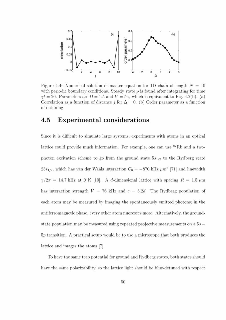
0 2 4 6 8 10−0.05

0

0.05

0.1

0.15

0.2

j

corr

elat

ion

−4 −2 0 2 4 60

0.1

0.2

0.3

0.4

Δ

orde

r pa

ram

eter

(a) (b)

Figure 4.4: Numerical solution of master equation for 1D chain of length N = 10with periodic boundary conditions. Steady state ρ is found after integrating for timeγt = 20. Parameters are Ω = 1.5 and V = 5γ, which is equivalent to Fig. 4.2(b). (a)Correlation as a function of distance j for ∆ = 0. (b) Order parameter as a functionof detuning

4.5 Experimental considerations

Since it is difficult to simulate large systems, experiments with atoms in an optical

lattice could provide much information. For example, one can use 87Rb and a two-

photon excitation scheme to go from the ground state 5s1/2 to the Rydberg state

23s1/2, which has van der Waals interaction C6 = −870 kHz µm6 [71] and linewidth

γ/2π = 14.7 kHz at 0 K [10]. A d-dimensional lattice with spacing R = 1.5 µm

has interaction strength V = 76 kHz and c = 5.2d. The Rydberg population of

each atom may be measured by imaging the spontaneously emitted photons; in the

antiferromagnetic phase, every other atom fluoresces more. Alternatively, the ground-

state population may be measured using repeated projective measurements on a 5s−

5p transition. A practical setup would be to use a microscope that both produces the

lattice and images the atoms [7].

To have the same trap potential for ground and Rydberg states, both states should

have the same polarizability, so the lattice light should be blue-detuned with respect

50

to the 5s− 5p transitions [73]. This would also minimize the photoionization induced

by lattice light, since the atoms would sit at the minimum of the light intensity. A

practical setup would be to use a microscope that both produces the lattice and images

the atoms [7]; this allows the lattice spacing to be independent of the wavelength of

the lattice light.

4.6 Conclusion

Thus, a driven-dissipative system of Rydberg atoms has a unique type of antifer-

romagnetism. The next step is to investigate in more detail how the full quantum

model behaves in low dimensions. The existence of limit cycles in the mean-field

limit is particularly surprising, and it would be interesting to see what happens to

them in low dimensions. Limit cycles occur in the mean-field limit of other models,

such as cavity QED [3], second-harmonic generation [22], and optomechanics [58]. In

those models, a limit cycle means that the number of photons in an optical cavity

oscillates in time. As the system becomes more quantum, the limit cycles still exist,

but quantum fluctuations cause the oscillations to become noisy.

Our work can be extended to Rydberg states with anisotropic and long-range

interactions. Such interactions usually give rise to very rich physics [44], so the

nonequilibrium version should be interesting. One can also see what happens when

the atoms are not fixed on a lattice but free to move; this is reminiscent of classical

reaction-diffusion systems [17, 16]. Finally, we note that a system of interacting

Rydberg atoms is similar to a system of spins interacting with each other’s magnetic

51

dipolar field [39, 55]. Thus, when an NMR system is made nonequilibrium with

continuous driving and spin relaxation, the spins may form a stable pattern in space.

4.A Mean-field solutions for sublattices

This appendix provides details on the steady-state solutions of the mean-field model,

where we only keep track of the two sublattices. One might wonder whether the

antiferromagnetic phase is an artifact of dividing up the lattice into two sublattices.

Appendix 4.B discusses the mean-field solutions without assuming sublattices and

shows that the antiferromagnetic phase is not an artifact.

Let the two sublattices be labelled 1 and 2. The system is described by

w1 = −2Ω Im q1 − w1 − 1, (4.12)

w2 = −2Ω Im q2 − w2 − 1, (4.13)

q1 = i [∆− c(w2 + 1)] q1 −q1

2+ i

Ω

2w1, (4.14)

q2 = i [∆− c(w1 + 1)] q2 −q2

2+ i

Ω

2w2. (4.15)

Remember that w1, w2 are real while q1, q2 are complex. There are six differen-

tial equations and three parameters (Ω,∆, c). The equations are symmetric un-

der the transformations w1, q1 ↔ w2, q2, ∆, c, q1, q2 → −∆,−c,−q∗1,−q∗2, and

Ω, q1, q2 → −Ω,−q1,−q2.

We focus on the fixed points of the system, i.e., when w1 = w2 = q1 = q2 = 0.

52

The fixed points are given by the simultaneous roots of two cubic polynomials:

f1(w1, w2) = (w1 + 1)

1

4+ [∆− c(w2 + 1)]2

+

Ω2

2w1, (4.16)

f2(w1, w2) = (w2 + 1)

1

4+ [∆− c(w1 + 1)]2

+

Ω2

2w2. (4.17)

Once w1 and w2 are found, q1 and q2 can be calculated,

q1(w1, w2) =−Ω

2w1[∆− c(w2 + 1)] + iΩ

4w1

14

+ [∆− c(w2 + 1)]2, (4.18)

q2(w1, w2) =−Ω

2w2[∆− c(w1 + 1)] + iΩ

4w2

14

+ [∆− c(w1 + 1)]2. (4.19)

Since f1(w1 ≤ −1, w2) is negative and f1(w1 ≥ 0, w2) is positive (and similarly for f2

and w2), we know that the fixed points lie in the range w1, w2 ∈ [−1, 0].

By combining f1 and f2, we find that the fixed points correspond to the real roots

of a fifth-order polynomial h(w), which is too complicated to show here. Fortunately,

one can factor it. Note that there are two kinds of fixed points: a uniform fixed

point (w1 = w2 and q1 = q2) means that the two sublattices are identical, and a

nonuniform fixed point (w1 6= w2 and q1 6= q2) means that the system is in the

antiferromagnetic phase. The uniform fixed points are given by real roots of a cubic

polynomial, f(w) = f1(w,w),

f(w) = c2w3 − c(2∆− 3c)w2 +

[Ω2

2+

1

4+ (∆− 3c)(∆− c)

]w + (∆− c)2 +

1

4.

(4.20)

53

Since the roots of f are also roots of h, we know that f is a factor of h. Thus,

h(w) = 4f(w)g(w) and the real roots of the quadratic polynomial g(w) correspond

to nonuniform fixed points,

g(w) = c2(1 + 4∆2 + 2Ω2)w2 − 2c[(∆− c)(1 + 4∆2) + (2∆− c)Ω2]w

+c2(1 + 4∆2)− 2c∆(1 + 4∆2 + 2Ω2) +1

4(1 + 4∆2 + 2Ω2)2. (4.21)

Hence, there are at most three uniform fixed points and two nonuniform fixed points.

One should think of the two nonuniform fixed points as being a joint pair, since they

correspond to w1 and w2.

At this point, the uniform and nonuniform fixed points can be found by numer-

ically solving for the roots of f and g, and their stabilities can be determined by

calculating the eigenvalues of the Jacobian for each fixed point. However, to obtain

general results, we derive as much information as possible analytically without ex-

plicitly solving for the fixed points. In particular, we care about the number of each

kind of fixed point and their stabilities as a function of the parameters.

4.A.1 Number of uniform fixed points

Here, we examine the number of uniform fixed points, i.e., the number of real roots of

f(w). Since f is cubic, it has one or three real roots (two in special cases). Suppose

c and ∆ have opposite signs. The polynomial f(w) ≡ f(w = w − 1) has coefficients

with signs + + +−. By Descartes’ rule of signs [6], f(w) has exactly one positive

root, which means that f(w) has exactly one root with w > −1. Since we know that

54

all roots of f(w) are in the interval [−1, 0], this shows that if c and ∆ have opposite

signs, there is only one root.

Now we check when f has three roots. Since f is cubic, it has three roots when

the local maximum and minimum exist and are positive and negative, respectively.

Thus, there are three roots if and only if

4∆2 > 6Ω2 + 3 and (4.22)

c ∈

(2∆(18Ω2 + 4∆2 + 9)− (4∆2 − 6Ω2 − 3)

32

54Ω2,

2∆(18Ω2 + 4∆2 + 9) + (4∆2 − 6Ω2 − 3)32

54Ω2

). (4.23)

According to this condition, for large |∆|, there is exactly one root, i.e., one uniform

fixed point, regardless of the sign of c.

4.A.2 Stability of uniform fixed points

We check the linear stability of the uniform fixed points to perturbations. Since

Eqs. (4.12)–(4.15) are symmetric between 1 and 2, the eigenvectors of the Jacobian

for uniform fixed points are either symmetric or antisymmetric between 1 and 2.

(The symmetric eigenvectors correspond to perturbations that affect 1 and 2 identi-

cally, while the antisymmetric eigenvectors represent perturbations that affect 1 and

2 in opposite directions.) This is convenient, because we can check the stability to

symmetric and antisymmetric perturbations separately, and the characteristic poly-

nomials are cubic instead of sixth degree. A uniform fixed point is stable overall if it

55

is stable to both kinds of perturbations.

The Routh-Hurwitz criterion is very useful here because it can provide stability

information without explicitly knowing the fixed point [56]. Suppose the characteristic

polynomial for a fixed point is cubic: λ3 + a2λ2 + a1λ+ a0. All the eigenvalues have

a negative real part if and only if a2, a0, a1a2 − a0 > 0; this means the fixed point

is stable. All the eigenvalues have a negative real part, except for a pair of purely

imaginary roots, if and only if a2, a0 > 0 and a2a1 − a0 = 0; this indicates a Hopf

bifurcation [82].

4.A.2.1 Stability to symmetric perturbations

First we consider the stability of a uniform fixed point to symmetric perturbations.

In this case, we can consider a simpler system by letting w ≡ w1 = w2, q ≡ q1 = q2,

and

w = −2Ω Im q − w − 1, (4.24)

q = i [∆− c(w + 1)] q − q

2+ i

Ω

2w, (4.25)

whose fixed points are given by the roots of f(w) in Eq. (4.20). Once w is found, q is

given by

q =−Ω

2w[∆− c(w + 1)] + iΩ

4w

14

+ [∆− c(w + 1)]2. (4.26)

56

The characteristic polynomial for a fixed point w, q is

α(λ) = λ3 + 2λ2 +

[∆− c(w + 1)]2 + Ω2 +

5

4− 2ΩcRe q

λ

+[∆− c(w + 1)]2 +Ω2

2+

1

4− 2ΩcRe q. (4.27)

For α(λ), we see that a2 > 0 and a2a1 − a0 = a0 + Ω2 + 2. According to the Routh-

Hurwitz criterion given above, the fixed point is stable to symmetric perturbations if

and only if a0 > 0. Also, since a2a1 − a0 > a0, there is never a Hopf bifurcation from

symmetric perturbations for any uniform fixed point.

Now suppose c and ∆ have opposite signs. We showed in Section 4.A.1 that in

this case, there is one uniform fixed point. We also see that 2ΩcRe q ≤ 0 in this

case and hence a0 > 0. Thus the single uniform fixed point is stable to symmetric

perturbations.

Since f is cubic, fixed points of Eqs. (4.24)–(4.25) appear and disappear through

saddle-node bifurcations as the parameters change [82]. In a saddle-node bifurcation,

two fixed points with opposite stabilities appear or disappear together. Also, since

there is never a Hopf bifurcation, a given fixed point has the same stability as the

parameters change.

These statements allow us to deduce the stabilities of all the uniform fixed points.

Suppose we start with c and ∆ having opposite signs. There is a single uniform fixed

point and it is stable as shown above. As we change the parameters, eventually it

collides with another uniform fixed point via a saddle-node bifurcation, so the second

fixed point must be unstable. Furthermore, that unstable fixed point undergoes a

57

saddle-node bifurcation with a third fixed point, so the third fixed point must be

stable, even when it is the only fixed point. (Remember that these stabilities are

with respect to symmetric perturbations.)

To summarize, when there is one uniform fixed point, it is stable to symmetric

perturbations. When there are three uniform fixed points, the outer two (highest and

lowest values of w) are stable to symmetric perturbations, while the inner one (middle

value of w) is unstable to symmetric perturbations. Of course, the outer fixed points

could be unstable to antisymmetric perturbations, which is what we check in the next

section.

4.A.2.2 Stability to antisymmetric perturbations

We now check when the uniform fixed points become unstable to antisymmetric per-

turbations. Let the fixed point be w, q. We consider antisymmetric perturbations

around it: w1 = w + δw, w2 = w − δw, q1 = q + δq, and q2 = q − δq. By plug-

ging into Eqs. (4.12)–(4.15) and linearizing for small δw, δq, we find the characteristic

polynomial,

β(λ) = λ3 + 2λ2 +

[∆− c(w + 1)]2 + Ω2 +

5

4+ 2ΩcRe q

λ

+[∆− c(w + 1)]2 +Ω2

2+

1

4+ 2ΩcRe q, (4.28)

which is similar to Eq. (4.27). For β(λ), we see that a2 > 0 and a2a1−a0 = a0+Ω2+2.

According to the Routh-Hurwitz criterion given above, the fixed point is stable to

58

antisymmetric perturbations if and only if a0 > 0, i.e.,

[∆− c(w + 1)]2 +Ω2

2+

1

4+ 2ΩcRe q > 0. (4.29)

We can simplify this using the fact that the fixed point satisfies f(w) = 0: the uniform

fixed point is stable to antisymmetric perturbations if and only if

φ(w) ≡ c2w2 + 2c2w + c2 −∆2 − Ω2

2− 1

4< 0. (4.30)

So when a uniform fixed point is on the verge of instability, it satisfies

w = −1 +

√1 + 4∆2 + 2Ω2

2|c|. (4.31)

For large |∆|, φ < 0, so the one uniform fixed point that exists is stable to both

symmetric and antisymmetric perturbations.

Note that since a2a1 − a0 > a0, there is never a Hopf bifurcation from antisym-

metric perturbations. Since we already ruled out Hopf bifurcations from symmetric

perturbations, we conclude that uniform fixed points never have Hopf bifurcations.

4.A.3 Nonuniform fixed points

The nonuniform fixed points are given by the roots of the quadratic polynomial g(w)

in Eq. (4.21). The two nonuniform fixed points appear and disappear together as

the parameters change. The symmetry in Eqs. (4.12)–(4.15) between 1 and 2 means

59

that the two nonuniform fixed points have the same stability. Thus, the nonuniform

fixed points must appear via a pitchfork bifurcation from a uniform fixed point as the

parameters change [82]. In other words, the nonuniform fixed points intersect with

a uniform fixed point, which changes stability at the intersection. (In Section 4.A.4,

we will determine whether the bifurcation is supercritical or subcritical and which

uniform fixed point is involved.)

The intersection of the nonuniform fixed points with a uniform fixed point can

be shown explicitly. From g(w), the nonuniform fixed points exist if and only if

ζ(Ω,∆, c) < 0, where

ζ(Ω,∆, c) = 16(1 + 2Ω2)∆4 − 32cΩ2∆3 + 8(1 + 2Ω2)2∆2

−8cΩ2(1 + 2Ω2)∆ + (1 + 2Ω2)3 − 4c2Ω4. (4.32)

On the verge of the appearance of the nonuniform fixed points, ζ = 0 and the root of

g(w) is

w = −1 +∆

c+

Ω2

1 + 4∆2 + 2Ω2. (4.33)

One can show that Eqs. (4.31) and (4.33) are equal using f(w) = 0. Thus, the change

in stability of a uniform fixed point coincides with the appearance of the nonuniform

fixed points.

In the case when |∆| is large, ζ ∼ ∆4, so nonuniform fixed points do not exist.

There is a convenient sufficient condition for the existence of the nonuniform fixed

60

points. If ζ(∆ = 0) = (1 + 2Ω2)3 − 4c2Ω4 < 0, there is a range of ∆ around ∆ = 0,

for which the nonuniform fixed points exist. In other words, if

|c| >(2Ω2 + 1)

32

2Ω2, (4.34)

there is a range of ∆ around ∆ = 0, for which nonuniform fixed points exist.

4.A.4 Connection between uniform and nonuniform fixed points

We describe what happens as ∆ changes. Without loss of generality (due to symme-

try), assume c > 0. Suppose ∆ starts out large and negative. There is one uniform

fixed point and it is stable. Nonuniform fixed points do not exist. Then let ∆ in-

crease. At some point, a uniform fixed point may undergo a pitchfork bifurcation:

it becomes unstable to antisymmetric perturbations and the nonuniform fixed points

appear. The fact that the nonuniform fixed points exist when the uniform fixed point

is unstable indicates that the bifurcation is supercritical [82].

When the pitchfork bifurcation happens, there may be three uniform fixed points.

Which one undergoes the bifurcation? Since φ(w) ∼ w2 in Eq. (4.30), as ∆ decreases,

the first uniform fixed point to go unstable must be the upper one (the one with the

highest w). Furthermore, since there can be at most two nonuniform fixed points,

only the upper uniform fixed point may be unstable to antisymmetric perturbations.

We conclude that when there are three uniform fixed points, only the upper one may

undergo a pitchfork bifurcation, and the lower one is stable. According to Section

4.A.2.1, the middle uniform fixed point is always unstable.

61

It is possible that the pitchfork bifurcation happens when there is only one uniform

fixed point. Then obviously that fixed point must undergo the pitchfork bifurcation.

Since the pitchfork bifurcation is supercritical, the nonuniform fixed points are

stable when they appear.

Then let ∆ increase towards ∞. Eventually ζ > 0 and φ < 0 again. This

indicates that there was another pitchfork bifurcation in which the nonuniform fixed

points disappeared and the uniform fixed point became stable again.

Note that we have not determined here whether the nonuniform fixed points ever

have Hopf bifurcations. As stated in Section 4.3, we found numerically that they do

sometimes have Hopf bifurcations.

4.B Mean-field solutions for the complete lattice

In this appendix, we study the solutions for the complete lattice, keeping track of

every site instead of lumping them into sublattices. We show that there is a dynamical

instability, in which the uniform steady state becomes unstable to perturbations of

wavelength 2. The solutions of the complete lattice are the same as the solutions

using sublattices, so the antiferromagnetic transition is not an artifact of dividing the

lattice into two sublattices.

The approach is to find the uniform steady state and see when it becomes unstable

to perturbations. Consider a d-dimensional lattice with N sites in each direction. Let

62

~n be a d-dimensional position vector. The system is described by

w~n = −2Ω Im q~n − w~n − 1, (4.35)

q~n = i

∆− b∑〈~m~n〉

(w~m + 1)

q~n − q~n2

+ iΩ

2w~n, (4.36)

where b = V/2γ = c/2d is the nearest-neighbor interaction.

The uniform steady state (w~n = w, q~n = q) is given by the fixed points of the

system,

w = −2Ω Im q − w − 1, (4.37)

q = i [∆− 2db(w + 1)] q − q

2+ i

Ω

2w. (4.38)

These equations are the same as Eqs. (4.24)–(4.25) but with c = 2db. Thus, we can use

the results of Section 4.A.2.1. The uniform steady state is given by the real roots of

f(w) in Eq. (4.20), and there are one or three solutions. The Jacobian of Eqs. (4.37)–

(4.38) determines the stability of a uniform solution to uniform perturbations, i.e.,

an identical offset to every site.

Now we consider perturbations δw~n, δq~n around the uniform steady state:

w~n = w + δw~n, (4.39)

q~n = q + δq~n. (4.40)

63

We write them in terms of Fourier components δw~k, δq~k:

δw~n =1

N

∑~k

ei~k·~nδw~k, (4.41)

δq~n =1

N

∑~k

ei~k·~nδq~k, (4.42)

~k = (k1, k2, . . . , kd), (4.43)

k` =2π

Nj, j = 0, . . . , N − 1. (4.44)

We write Eqs. (4.35)–(4.36) in terms of δw~k, δq~k and linearize. The Fourier compo-

nents are uncoupled from each other and each component ~k is described by three

differential equations:

δ ˙w~k = iΩ(δq~k − δq∗−~k)− δw~k, (4.45)

δ ˙q~k = −2ibq

(d∑`=1

cos k`

)δw~k + i

Ω

2δw~k +

i[∆− 2db(w + 1)]− 1

2

δq~k,

(4.46)

δ ˙q∗−~k = 2ibq∗

(d∑`=1

cos k`

)δw~k − i

Ω

2δw~k +

−i[∆− 2db(w + 1)]− 1

2

δq∗−~k.

(4.47)

The characteristic polynomial for component ~k is

η(λ) = λ3 + 2λ2 +

[∆− 2db(w + 1)]2 + Ω2 +

5

4− 4ΩbRe q

d∑`=1

cos k`

λ

+[∆− 2db(w + 1)]2 +Ω2

2+

1

4− 4ΩbRe q

d∑`=1

cos k`. (4.48)

64

Note the similarity to Eqs. (4.27) and (4.28). Now we use the Routh-Hurwitz criterion

given in Section 4.A.2. For η(λ), a2 > 0 and a2a1 − a0 = a0 + Ω2 + 2. Thus, the

uniform steady state is stable to a perturbation with wave vector ~k if and only if

[∆− 2db(w + 1)]2 +Ω2

2+

1

4− 4ΩbRe q

d∑`=1

cos k` > 0. (4.49)

Suppose the uniform steady state satisfies 4ΩbRe q > 0. As the parameters

change, the first mode to go unstable is the one with all k` = 0. This corresponds to

uniform perturbations that simply offset the uniform solution. Thus we identify this

uniform steady state as the unstable fixed point of Eqs. (4.37)–(4.38). Based on the

discussion in Section 4.A.2.1, this uniform solution is actually always unstable when

it exists.

Now suppose the uniform steady state satisfies 4ΩbRe q < 0. As the parameters

change, the first mode to go unstable is the one with all k` = π. This corresponds

to perturbations of wavelength 2, i.e., antiferromagnetic perturbations. The uniform

steady state is unstable to this mode when

[∆− 2db(w + 1)]2 +Ω2

2+

1

4+ 4ΩdbRe q > 0. (4.50)

This is the same as Eq. (4.29) with c = 2db. Thus, the discussion in Section 4.A.4

applies here: as the parameters change, the uniform solution becomes unstable to the

antiferromagnetic solution. One can find the antiferromagnetic solution, but that is

equivalent to the nonuniform fixed points of Eqs. (4.12)–(4.15), i.e., the real roots of

65

g(w) in Eq. (4.21).

Thus, the complete lattice has the same antiferromagnetic transition as the bipar-

tite lattice.

66

Chapter 5

Collective quantum jumps ofRydberg atoms

In this chapter, we consider the same setup as in Chapter 4: a group of atoms laser-

driven to the Rydberg state and spontaneously decaying back to the ground state.

But this time, we study the dynamics using the method of quantum trajectories. In

particular, we are interested in what happens in the original quantum model when

mean-field theory predicts bistability of uniform fixed points. It turns out that the

system jumps between the two stable fixed points of mean-field theory. The jumps are

inherently collective and in fact exist only for a large number of atoms. We explain

how entanglement and quantum measurement enable the jumps, which are otherwise

classically forbidden. The results of this chapter were published in Ref. [48].

5.1 Model

The model is the same as in Chapter 4, except that we are now interested in the long-

range type of coupling (V ∼ 1/R3). This way, we can ignore the nonuniform fixed

67

points, which would otherwise complicate the dynamics.1 The long-range type of

coupling can be obtained by a Forster resonance or by applying a static electric field.

However, to be able to simulate large systems, we approximate the long-range coupling

as a constant all-to-all coupling with suitable normalization; this approximation is

appropriate for a two- or three-dimensional lattice for the system sizes used here. In

Section 5.5, we discuss what happens with a more-realistic type of coupling.

Consider a system of N atoms continuously excited by a laser from the ground

state |g〉 to a Rydberg state |e〉. The Hamiltonian in Eq. (4.1) is modified to be

H =∑j

[−∆ |e〉〈e|j +

Ω

2(|e〉〈g|j + |g〉〈e|j)

]+

V

N − 1

∑j<k

|e〉〈e|j ⊗ |e〉〈e|k, (5.1)

where ∆ = ω` − ωo is the detuning between the laser and transition frequencies and

Ω is the Rabi frequency, which depends on the laser intensity. As in Chapter 4,

each atom is approximated as a two-level system, and we account for spontaneous

emission from the Rydberg state using the linewidth γ. Note that each atom emits

into different electromagnetic modes due to the large inter-particle distance; this is

an important difference with the Dicke model [70].

The environment absorbs all the spontaneously emitted photons, so the atoms

are continuously monitored by the environment. We are interested in the temporal

properties of the emitted photons. As discussed in Chapter 2, there are two equivalent

ways to study such an open quantum system. The first is the master equation, which

1But it would be interesting to do a similar study of the nonuniform fixed points.

68

describes how the density matrix of the atoms, ρ, evolves in time:

ρ = −i[H, ρ] + γ∑j

(−1

2|e〉〈e|j, ρ+ |g〉〈e|j ρ |e〉〈g|j

).

A master equation of this form has a unique steady-state solution [75], ρss, which

can be found numerically by Runge-Kutta integration. The integration can be vastly

sped up by utilizing the fact that the atoms are symmetric under interchange due to

all-to-all coupling; the complexity is then O(N3) instead of O(4N). Using ρss, one can

calculate the statistics of the emitted light. In particular, the correlation of photons

emitted by two different atoms is [76]

g(2)ij =

〈EiEj〉〈Ei〉〈Ej〉

, (5.2)

where Ei ≡ |e〉〈e|i. If g(2)ij > 1, the atoms tend to emit in unison (bunching); if

g(2)ij < 1, they avoid emitting in unison (antibunching).

The second approach is the method of quantum trajectories, which simulates

how the wave function evolves in a single experiment [18, 61, 23]. We describe the

quantum-trajectory algorithm in the context of the Rydberg model. Given the wave

function |ψ(t)〉, one randomly decides whether an atom emits a photon in the time

interval [t, t+ δt] based on its current Rydberg population. If atom j emits a photon,

the wave function is collapsed: |ψ(t+ δt)〉 = |g〉〈e|j|ψ(t)〉. If no atoms emit a photon,

|ψ(t+δt)〉 = (1−iHeffδt)|ψ(t)〉, where Heff = H−(iγ/2)∑

j |e〉〈e|j. After normalizing

the wave function, the process is repeated for the next time step. The non-Hermitian

69

part of Heff is a shortcut to account for the fact that the non-detection of a photon

shifts the atoms toward the ground state, as discussed in Section 2.1.

These two approaches are related: the master equation describes an ensemble of

many individual trajectories [18, 61]. Also, ρss can be viewed as the ensemble of wave

functions that a single trajectory explores over time. We use both approaches below,

although quantum jumps are most clearly seen using quantum trajectories.

5.2 Case of N = 2 atoms

We first consider the case of N = 2 atoms since it is instructive for larger N . Laser

excitation and spontaneous emission distribute population throughout the Hilbert

space, |gg〉, |ge〉, |eg〉, |ee〉. When ∆ = 0, |ee〉 is uncoupled from the other states

due to its energy shift, so there is little population in it (Fig. 5.1(a)); this is the well-

known blockade effect [57, 73]. But when ∆ ≈ V/2, there is a resonant two-photon

transition between |gg〉 and |ee〉, so |ee〉 becomes populated (Fig. 5.1(b)). Using the

master equation, one can calculate the photon correlation between the two atoms

(Fig. 5.2). There is strong antibunching for ∆ ≈ 0 and strong bunching for ∆ ≈ V/2,

because a joint emission requires population in |ee〉. In the limit of small Ω, the

correlation is

g(2)12 =

γ2 + 4∆2

γ2 + (V − 2∆)2+

4V (V − 4∆)Ω2

[γ2 + (V − 2∆)2]2+O(Ω4/γ4). (5.3)

70

14 16 18 200

0.2

0.4

0.6

0.8

time (units of 1/γ)

⟨Ei⟩

⟨E1⟩

⟨E2⟩

(a) (b)

|ee⟩

|ge⟩, |eg⟩

|gg⟩

(c)

Figure 5.1: Two atoms. (a) When ∆ = 0, |ee〉 is uncoupled from the other states.(b) When ∆ = V/2, there is a resonant two-photon transition between |gg〉 and |ee〉.(c) Quantum trajectory simulation with Ω = 1.5γ, ∆ = V/2 = 5γ, showing Rydbergpopulation of each atom over time. Atom 1 (solid blue line) emits at t = 14.4/γ,which causes 〈E2〉 (dashed red line) to suddenly increase. Atom 2 then emits att = 14.7/γ. When no photons have been emitted for a while, the wave functionapproaches a steady state.

Δ/γ

Ω/γ

0 2 4 6

1

0.8

0.6

0.4

0.2

0 0

20

40

60

80

100

0 2 4 60.01

0.1

1

10

100

Δ/γ

g(2)12

(a) (b)

Figure 5.2: Photon correlation for N = 2 atoms with V = 10γ. (a) Correlation vs ∆for Ω = 0.5γ. (b) Correlation as a function of Ω and ∆ using color scheme on right

Note that the correlation can be made arbitrarily large by setting Ω ≈ 0, ∆ = V/2,

and V large; this may be useful as a heralded single-photon source [25].

Further insight is provided by quantum trajectories. An example trajectory for

∆ = V/2 is shown in Fig. 5.1(c). The atoms emit photons at various times. When no

photons have been emitted for a while, the wave function approaches an entangled

steady state due to the balance of laser excitation and nonunitary decay from the

71

non-detection of photons:

|ψ〉ss = c1|gg〉+ c2|ge〉+ c3|eg〉+ c4|ee〉, (5.4)

where the coefficients have constant magnitudes and their phases evolve with the

same frequency. A similar thing happens with a single atom, as discussed in Section

2.3. Mathematically, the steady-state wave function is the eigenvector of Heff corre-

sponding to the eigenvalue with least negative part. Because of the laser detuning,

|c1|2 is much larger than |c2|2, |c3|2, |c4|2, which are comparable to each other. Thus

〈E1〉, 〈E2〉 ≈ 0 and the atoms are unlikely to emit. But when atom 1 happens to

emit, the wave function becomes

|ψ〉 =c3|gg〉+ c4|ge〉|c3|2 + |c4|2

. (5.5)

Now, 〈E2〉 is large and atom 2 is likely to emit, which leads to photon bunching

(Fig. 5.1(c)).

5.3 Case of N = 16 atoms

Now we consider the case of large N . We first review mean-field theory, which was

discussed in Chapter 4, but here we adapt it to use Eq. (5.1). Mean-field theory

is a classical approximation to the quantum model: correlations between atoms are

ignored, and the density matrix factorizes by atom, ρ =⊗N

j=1 ρ, where ρ evolves

72

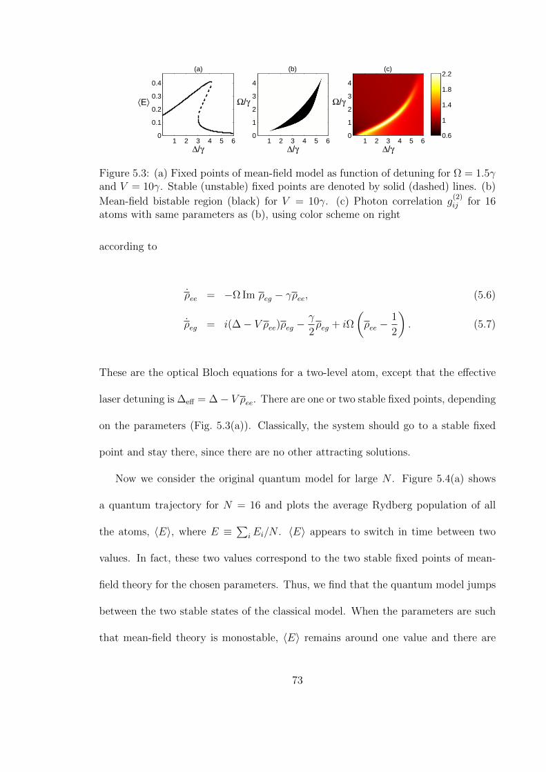
Δ/γ

Ω/γ

1 2 3 4 5 6

4

3

2

1

01 2 3 4 5 6

0

0.1

0.2

0.3

0.4

Δ/γ

⟨E⟩

Δ/γ

Ω/γ

1 2 3 4 5 6

4

3

2

1

0 0.6

1

1.4

1.8

2.2(a) (b) (c)

Figure 5.3: (a) Fixed points of mean-field model as function of detuning for Ω = 1.5γand V = 10γ. Stable (unstable) fixed points are denoted by solid (dashed) lines. (b)

Mean-field bistable region (black) for V = 10γ. (c) Photon correlation g(2)ij for 16

atoms with same parameters as (b), using color scheme on right

according to

ρee = −Ω Im ρeg − γρee, (5.6)

ρeg = i(∆− V ρee)ρeg −γ

2ρeg + iΩ

(ρee −

1

2

). (5.7)

These are the optical Bloch equations for a two-level atom, except that the effective

laser detuning is ∆eff = ∆− V ρee. There are one or two stable fixed points, depending

on the parameters (Fig. 5.3(a)). Classically, the system should go to a stable fixed

point and stay there, since there are no other attracting solutions.

Now we consider the original quantum model for large N . Figure 5.4(a) shows

a quantum trajectory for N = 16 and plots the average Rydberg population of all

the atoms, 〈E〉, where E ≡∑

iEi/N . 〈E〉 appears to switch in time between two

values. In fact, these two values correspond to the two stable fixed points of mean-

field theory for the chosen parameters. Thus, we find that the quantum model jumps

between the two stable states of the classical model. When the parameters are such

that mean-field theory is monostable, 〈E〉 remains around one value and there are

73

200 300 400 500 600 700 800 9000

0.1

0.2

0.3

0.4

time (units of 1/γ)

⟨E⟩

228 230 232 234 2360

0.1

0.2

0.3

0.4

time (units of 1/γ)

⟨E⟩

310 312 314 316 318time (units of 1/γ)

(a)

(b) (c)

Figure 5.4: Quantum trajectory of 16 atoms showing average Rydberg populationover time with Ω = 1.5γ, V = 10γ, ∆ = 3.4γ. (a) Quantum jumps between twometastable collective states. Red arrows point at the stable fixed points of mean-fieldtheory. (b) and (c) are zoomed-in views, and red lines mark photon emissions. (b)Rapid succession of emissions around t = 232/γ causes a jump up. (c) Absence ofemissions around t = 313/γ causes a jump down.

no jumps. Hence, the photons are bunched when mean-field theory is bistable but

are uncorrelated otherwise. This correspondence is evident in Fig. 5.3(b)–(c), with

better agreement for larger N .

We call the two states in Fig. 5.4(a) the dark and bright states, since the one with

lower 〈E〉 has a lower emission rate. In the dark state, the wave function approaches

a steady state, |ψ〉ss, in between the sporadic emissions. This is due to the balance of

laser excitation and non-unitary decay from the non-detection of photons, similar to

the case of two atoms. In the bright state, the large Rydberg population brings the

system effectively on resonance (∆eff ≈ 0). The bright state sustains itself because

an atom is quickly reexcited after emitting a photon.

Suppose the system is in the dark state. The steady-state wavefunction |ψ〉ss is

74

an entangled state of all the atoms with most population in |gg . . . g〉. Although 〈E〉

is small, when an atom happens to emit a photon, 〈E〉 increases due to the entangled

form of |ψ〉ss. In fact, if more atoms emit within a short amount of time, 〈E〉 increases

further (Fig. 5.5(a)). When enough atoms have emitted such that 〈E〉 is high, the

system is in the bright state and sustains itself there (Fig. 5.4(b)). If too few atoms

emitted, the system quickly returns to |ψ〉ss.

Then suppose the system is in the bright state. There are two ways to jump to

the dark state: most of the atoms emit simultaneously or most of the atoms do not

emit for a while (the non-detection of photons projects the atoms toward the ground

state). For our parameters, simulations indicate that the latter is usually responsible

for the jumps down (Fig. 5.4(c)).

The jumps are inherently collective, since they result from joint emissions or joint

non-emissions. As N increases, the dark and bright periods become longer and more

distinct (Fig. 5.5(b)–(c)). This can be understood intuitively as follows. Suppose

the system is in |ψ〉ss. As N increases, the increment of 〈E〉 per emission decreases

(Fig. 5.5(a)). Thus, for large N , a rapid succession of many emissions is necessary to

jump to the bright state. Although the emission rate in the dark state increases with

N , the rate of nonunitary decay in Heff also increases with N . The result is that the

probability rate of a jump up decreases. Then suppose the system is in the bright

state. As N increases, a jump down requires more atoms to not emit in some time

interval, so the probability rate of a jump down decreases.

75

0 20 40

10−4

10−2

100

length of bright period

rela

tive

num

ber

0 0.1 0.2 0.3 0.40

0.1

0.2

0.3

0.4

⟨E⟩

rela

tive

num

ber

0 5 10 150

0.05

0.1

0.15

0.2

0.25

number of emissions

⟨E⟩

N = 4N = 8N = 16

(a) (b) (c)

Figure 5.5: Statistics for Ω = 1.5γ, V = 10γ, ∆ = 3.4γ comparing N = 4, 8, 16. (a)Rydberg population 〈E〉 after a number of simultaneous emissions from the steady-state wave function |ψ〉ss. (b) Length distribution of bright periods (in units of 1/γ),using arbitrary threshold of 〈E〉 = 0.2 and sampling rate of 10γ. (c) Distribution of〈E〉. Red arrows point at stable fixed points of mean-field theory.

5.4 Experimental considerations

Experimentally, the jumps may be observed in a 2D optical lattice of atoms with

a static electric field normal to the plane for long-range Rydberg interaction. For

example, two 87Rb atoms in the |n = 15, q = 14,m = 0〉 Rydberg state have a coupling

of about 44 kHz at a distance of 13 µm [38], and the linewidth is γ/2π ≈ 68 kHz at

0 K [10]. This corresponds to V ≈ 10γ with N = 16 atoms for the all-to-all model

in Eq. (5.1), which are the parameters used in our discussion. One could observe

the jumps directly by monitoring the fluorescence from the atoms. Alternatively, one

could make repeated projective measurements and thereby infer the existence of two

metastable states from the distribution of 〈E〉.

5.5 Conclusion

These collective jumps are reminiscent of a familiar classical effect. It is well known

that adding thermal noise to a bistable classical system induces transitions between

76

the two stable fixed points [24, 1]. In contrast, the jumps here are induced by quantum

noise due to entanglement and quantum measurement. We note that the jumps may

be the many-body version of quantum activation, in which quantum fluctuations drive

transitions over a classical barrier [59, 40].

In Eq. (5.1), we assumed an infinite-range coupling for simplicity. One might won-

der whether the collective jumps still occur when the coupling is more realistic. A re-

cent work studied the quantum dynamics of the Rydberg model on a one-dimensional

chain with nearest-neighbor interactions [5]. They also observed well-defined jumps

of the Rydberg population in a chain of N = 12 atoms. Thus, for a small system, the

existence of jumps does not seem to depend critically on the coupling range. On the

other hand, a large system of, say, N = 1000 atoms with nearest-neighbor interac-

tions would exhibit more complicated dynamics: the system would probably divide

into small domains, and the Rydberg population of a domain would correspond to a

mean-field fixed point. The collective jumps would occur on a local scale as domains

grow and shrink. The domain-wall dynamics are worth future study.

It would be interesting to see whether similar jumps appear in other settings,

such as coupled optical cavities [27, 12, 32, 84] and quantum-reservoir engineering

[20, 21, 83, 86]. In particular, since mean-field bistability seems to predict collective

jumps in the underlying quantum model, one should look for bistability in the mean-

field models of other systems [21, 83, 84]. It is known that a single cavity coupled to an

atom is bistable [3]; in fact, jumps between the stable fixed points have been observed

recently [41]. It is worth looking at the jump dynamics in an array of cavities.

77

Chapter 6

Spatiotemporal dynamics ofquantum jumps with Rydbergatoms

Chapter 5 showed the Rydberg interaction greatly affects how a group of atoms

fluoresce when the atoms are laser-excited from the ground state to a Rydberg state

and spontaneously decay back to the ground state. In this chapter, we study what

happens when the atoms are laser-excited to a low-lying excited state as well as a

Rydberg state. This three-level scheme leads to qualitatively different behavior: the

atoms develop strong spatial correlations that change on a long time scale.

Our idea is based on quantum jumps of a three-level atom. As discussed in Section

2.4, an atom driven strongly to a short-lived state and weakly to a metastable state

occasionally jumps to and from the metastable state. The jumps are visible in the

fluorescence of the strong transition, which exhibits distinct bright and dark periods.

Here, we consider a one-dimensional chain of many three-level atoms, and we let the

metastable state be a Rydberg state, so that a jump of one atom affects its neighbors’

jumps via the Rydberg interaction. This leads to rich spatiotemporal dynamics, which

78

are observable by imaging the fluorescence of the strong transition. The results of

this chapter were published in Ref. [45]

Previous works studied correlated quantum jumps of atoms in the context of the

Dicke model [53, 79]. They concluded that cooperative effects are very difficult to

see experimentally, because the interatomic distance must be much smaller than a

wavelength. In contrast, the strong Rydberg interaction here allows the interatomic

distance to be much longer than a wavelength. Thus, the atoms develop strong

correlations while being individually resolvable.

6.1 Many-atom model

As discussed in Section 2.4, an atom is assumed to have three states: ground state |g〉,

short-lived excited state |e〉, and metastable state |r〉 (Fig. 6.1(a)). In this chapter,

we choose the metastable state to be a Rydberg state since Rydberg states have long

lifetimes [26]. A laser drives the strong transition |g〉 → |e〉, while another drives the

weak transition |g〉 → |r〉. Alternatively, one could use a cascade configuration with

|e〉 → |r〉 as the weak transition (see Section 6.4).

We make the following assumptions on the parameters. To avoid power-broadening

on the strong transition, we choose to work in the low-intensity limit, Ωe γe; this

choice is clarified in Section 6.4. As in Section 2.4, for convenience, we set ∆e = 0,

although it may be experimentally useful to set ∆e < 0 for continuous laser cooling

[60]. We also set γr = 0, since the lifetime of the Rydberg state scales as n3 and hence

can be chosen to be arbitrarily long [26]. It is straightforward to extend the analysis

79

(b)V (d)

(a) V|rrÚ

|eÚ|rÚ

(c)|grÚ |rgÚ

|gÚ(c)

V|ggÚ

Figure 6.1: (a) An atom has a ground state |g〉, short-lived excited state |e〉, andmetastable state |r〉, which is chosen to be a Rydberg state. One observes the spon-taneous emission from |e〉. (b) The |g〉 → |r〉 transition is originally on resonance(∆r = 0), but when one atom is in |r〉, the other atom is off resonance. (c) The|g〉 → |r〉 transition is originally off resonance (∆r = V ), but when one atom is in|r〉, the other atom is on resonance. (d) When ∆r = 0, |rr〉 is weakly coupled to theother states. Note that (b) and (d) are equivalent.

to nonzero ∆e and γr.

We consider a one-dimensional chain of N three-level atoms, which are all uni-

formly excited on the same two transitions. The interatomic distance is assumed to

be large enough so that the fluorescence from each atom is resolvable in situ on a

camera [7]. The atoms are coupled via the dipole-dipole interaction between their

Rydberg states. As discussed in Chapter 3, in the absence of a static electric field,

the interaction decreases with the third power of distance for short distances and

with the sixth power of distance for long distances. We focus on the latter case, since

the example numbers given in Sec. 6.4 are for relatively long distances, although the

80

former case would also be interesting to study. The Hamiltonian is

H =∑i

[Ωe

2(|g〉〈e|i + |e〉〈g|i) +

Ωr

2(|g〉〈r|i + |r〉〈g|i)−∆r|r〉〈r|i

]+∑i<j

V

|i− j|6|r〉〈r|i ⊗ |r〉〈r|j, (6.1)

where V is the nearest-neighbor interaction. We have included interactions beyond

nearest neighbors in case the long-distance interactions are important; it is known

that they affect the many-body ground state of Eq. (6.1) when Ωe = 0 [77].

To demonstrate the rich spatiotemporal dynamics of the many-body system,

Fig. 6.2 shows simulations of a chain of N = 8 atoms, generated using the method of

quantum trajectories [18, 61]. Each trajectory simulates a single experimental run.

The simulations use periodic boundary conditions and include interactions up to the

third neighbor. Figure 6.2 plots the time evolution of the Rydberg population of each

atom, i.e., the expectation value of Ri ≡ |r〉〈r|i. The atoms undergo quantum jumps,

and the Rydberg interaction clearly leads to spatial correlations in the fluorescence.

There are different types of collective dynamics depending on the parameters. In

Fig. 6.2(a)–(b), Ωr Ω2e/γe, so an atom by itself would exhibit quantum jumps. In

Fig. 6.2(a) (∆r = 0), a dark period usually does not spread to the neighboring atoms.

But once in a while, a dark period does spread to the neighbors, so that there are two

or three dark atoms in a row (e.g., BDDB). When there are multiple dark atoms

in a row, they stay dark for a relatively long time. In Fig. 6.2(b) (∆r = V ), once a

dark spot is created, it spreads quickly to the neighboring atoms. The dark region

expands and contracts in size and appears to diffuse along the chain. Interestingly,

81

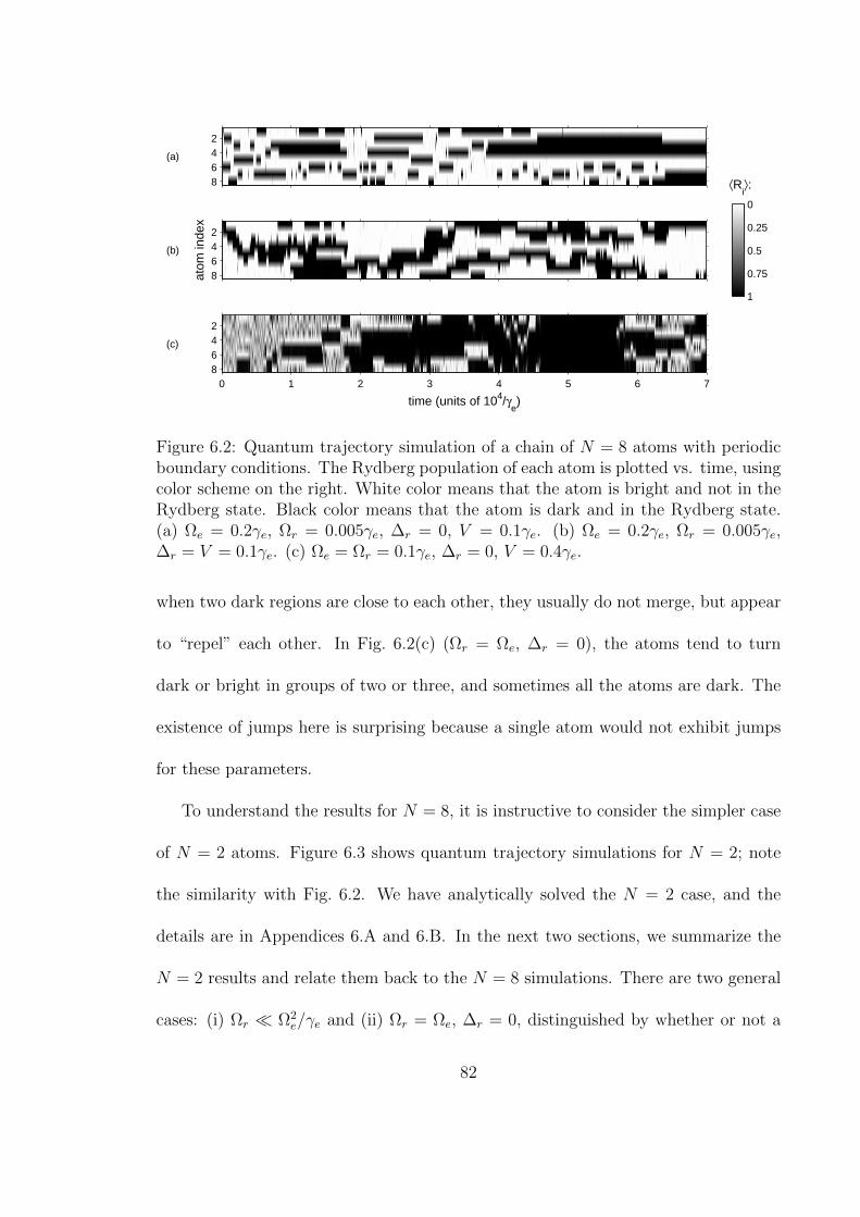
(a)

2468

atom

inde

x

(b)

2468

(c)

time (units of 104/γe)

0 1 2 3 4 5 6 7

2468

1

0.75

0.5

0.25

0

⟨Ri⟩:

Figure 6.2: Quantum trajectory simulation of a chain of N = 8 atoms with periodicboundary conditions. The Rydberg population of each atom is plotted vs. time, usingcolor scheme on the right. White color means that the atom is bright and not in theRydberg state. Black color means that the atom is dark and in the Rydberg state.(a) Ωe = 0.2γe, Ωr = 0.005γe, ∆r = 0, V = 0.1γe. (b) Ωe = 0.2γe, Ωr = 0.005γe,∆r = V = 0.1γe. (c) Ωe = Ωr = 0.1γe, ∆r = 0, V = 0.4γe.

when two dark regions are close to each other, they usually do not merge, but appear

to “repel” each other. In Fig. 6.2(c) (Ωr = Ωe, ∆r = 0), the atoms tend to turn

dark or bright in groups of two or three, and sometimes all the atoms are dark. The

existence of jumps here is surprising because a single atom would not exhibit jumps

for these parameters.

To understand the results for N = 8, it is instructive to consider the simpler case

of N = 2 atoms. Figure 6.3 shows quantum trajectory simulations for N = 2; note

the similarity with Fig. 6.2. We have analytically solved the N = 2 case, and the

details are in Appendices 6.A and 6.B. In the next two sections, we summarize the

N = 2 results and relate them back to the N = 8 simulations. There are two general

cases: (i) Ωr Ω2e/γe and (ii) Ωr = Ωe, ∆r = 0, distinguished by whether or not a

82

(a)1

2

atom

inde

x

(b)1

2

(c)

time (units of 104/γe)

0 1 2 3 4 5 6 7

1

2

1

0.75

0.5

0.25

0

⟨Ri⟩:

Figure 6.3: Quantum trajectory simulation of N = 2 atoms. The Rydberg populationof each atom is plotted vs. time, using color scheme on the right. Parameters are thesame as in Fig. 6.2: (a) Ωe = 0.2γe, Ωr = 0.005γe, ∆r = 0, V = 0.1γe. (b) Ωe = 0.2γe,Ωr = 0.005γe, ∆r = V = 0.1γe. (c) Ωe = Ωr = 0.1γe, ∆r = 0, V = 0.4γe.

single atom would exhibit jumps.

6.2 Case of Ωr Ω2e/γe

For these parameters, an atom by itself would exhibit jumps. Let the two atoms be

labelled 1 and 2. If atom 1 is in |r〉, then according to Eq. (6.1), atom 2 effectively

sees a laser detuning of ∆r − V . But if atom 1 is not in |r〉, then atom 2 sees the

original detuning ∆r. Whether atom 1 is in |r〉 depends on whether it is in a dark

period. This suggests that the jump rates for atom 2 are the same as for a single

atom (Eqs. (2.11)–(2.12)), except with an effective detuning that depends on whether

atom 1 is in a bright or dark period at the moment. In Appendix 6.A, we use a more

careful analysis to show that this is indeed correct in the limit of small Ωr. Thus, the

83

transition rates for two atoms are

ΓBB→BD(∆r) = ΓBB→DB(∆r) = ΓB→D(∆r) (6.2)

ΓBD→BB(∆r) = ΓDB→BB(∆r) = ΓD→B(∆r) (6.3)

ΓBD→DD(∆r) = ΓDB→DD(∆r) = ΓB→D(∆r − V ) (6.4)

ΓDD→BD(∆r) = ΓDD→DB(∆r) = ΓD→B(∆r − V ). (6.5)

An insightful quantity is the ratio ΓBD→DD/ΓBD→BB, which indicates how often DD

periods occur relative to BB periods. As shown in Fig. 6.4, the ratio is minimum at

∆r = 0 and maximum at ∆r = V .

The minimum at ∆r = 0 is due to the blockade effect: although the laser is

originally on resonance, when atom 1 is in |r〉, it shifts the Rydberg level of atom 2

off resonance so that atom 2 is prevented from jumping to |r〉 (Fig. 6.1(b)). Thus,

the atoms switch between BB, BD, and DB; they are almost never in DD. In other

words, there is at most one dark atom at a time (Fig. 6.3(a)).

The maximum at ∆r = V is due to the opposite effect: the laser is originally off

−0.2 −0.1 0 0.1 0.210

−2

10−1

100

101

102

Δr / γ

e

Γ (B

D to

DD

)Γ

(BD

to B

B)

Figure 6.4: Ratio of ΓBD→DD to ΓBD→BB for Ωe = 0.2γe, Ωr = 0.005γe, V = 0.1γe

84

resonance, but when atom 1 happens to jump to |r〉, it brings the Rydberg level of

atom 2 on resonance, encouraging atom 2 to jump to |r〉 (Fig. 6.1(c)). Thus, the

atoms switch between DD, BD, and DB; they are almost never in BB, except for

the initial transient. Since

ΓDD→BD + ΓDD→DB

ΓBD→BB + ΓBD→DD≈ 2, (6.6)

a DD period is shorter than a BD or DB period by about a factor of two. When the

atoms are in DD, there is an equal chance to go to BD or DB. Thus, the dark spot

appears to do a random walk between the two atoms (Fig. 6.3(b)).

The above considerations can be generalized to larger N . The transition rates

for atom i are given by Eqs. (2.11)–(2.12) but with an effective detuning that de-

pends on the number of nearest neighbors that are currently dark: ∆eff = ∆r − V ×

number of dark neighbors. This analytical prediction agrees with quantum trajec-

tory simulations of N = 8 atoms: Fig. 6.5 plots the rates of expansion (ΓDBB→DDB),

contraction (ΓDDB→DBB), and merging (ΓDBD→DDD) of dark regions. The agree-

ment implies that interactions beyond nearest neighbors in Eq. (6.1) do not play an

important role in the dynamics.

When ∆r = 0, the blockade effect prevents dark periods from spreading (Fig. 6.2(a)).

But once in a while, a dark period does spread to a neighbor and there are two dark

atoms in a row (BDDB); when this happens, the dark atoms are effectively off res-

onance, so they stay dark for a long time. In other words, dark regions expand and

contract on a long time scale. Note that the expansion and contraction rates decrease

85

0 0.05 0.1 0.15 0.2 0.25

10−5

10−4

10−3

Δr / γ

era

te (

units

of γ

e)

Figure 6.5: Dynamics of dark regions in a chain of N = 8 atoms with Ωe = 0.2γe, Ωr =0.005γe, V = 0.1γe. The rates of expansion (black squares), contraction (red circles),and merging (blue triangles) were determined from quantum trajectory simulations.The simulation for each value of ∆r was run for a time of 106/γe, and the rates werecalculated by sampling at a rate of γe and defining an atom to be dark if 〈Ri〉 > 0.98.The scatter of data points with low rates is due to statistical uncertainty. Analyticalpredictions are shown for the rates of expansion (black, solid line), contraction (red,dashed line), and merging (blue, dash-dotted line).

as V increases.

On the other hand, when ∆r = V , the anti-blockade effect encourages dark periods

to spread to the neighbors, causing a dark region to expand (Fig. 6.2(b)). But a dark

region usually does not expand enough to encompass the entire chain, because an atom

at the edge of a dark region can turn bright, causing the dark region to contract. The

expansion and contraction processes have similar rates (ΓDBB→DDB ≈ ΓDDB→DBB).

As a result, the dark region appears to diffuse randomly along the chain. Also, two

dark regions usually do not merge with each other, i.e., ΓDBD→DDD is relatively small.

This is because a bright atom with two dark neighbors is effectively off resonance and

is unlikely to turn dark. Hence, the dark regions appear to repel each other.

86

6.3 Case of Ωr = Ωe, ∆r = 0

For these parameters, an atom by itself would not exhibit jumps because of the

absence of a weak transition. The existence of jumps for two atoms is solely due to

the dipole-dipole interaction, which causes |gr〉 → |rr〉 and |rg〉 → |rr〉 to become

off-resonant and thus weak transitions (Fig. 6.1(d)). Since |rr〉 is metastable, the

system occasionally jumps to and from |rr〉. When the system is in |rr〉, the atoms

do not fluoresce. When the system is not in |rr〉, it turns out that the wavefunction

rapidly oscillates among the other eigenstates so that both atoms fluoresce from |e〉.

Thus, the system switches between BB and DD (Fig. 6.3(c)). In Appendix 6.B, we

derive the rates,

ΓDD→BB =γeΩ

4

2V 2(γ2e + 4V 2)

(6.7)

ΓBB→DD ≤ Ω4

2γeV 2, (6.8)

where Ω ≡ Ωr = Ωe. The inequality for ΓBB→DD is due to incomplete knowledge

of the wave function after a photon emission. Equations (6.7)–(6.8) agree well with

quantum trajectory simulations (Fig. 6.6). Both rates are inversely related to V , since

the weak transitions become weaker as V increases. The condition for well-defined

jumps is roughly Ω 2V .

A larger chain has similar behavior (Fig. 6.2(c)). The atoms tend to turn dark or

bright simultaneously with their neighbors. However, the dynamics are more complex

due to the presence of two neighbors.

87

0.1 110

−6

10−5

10−4

10−3

10−2

V / γe

rate

(un

its o

f γe)

Figure 6.6: Comparison of analytical and numerical values of the jump rates for Ωr =Ωe = 0.1γe, ∆r = 0. ΓDD→BB: analytical result (black, solid line) and numerical data(black circles). ΓBB→DD: analytical upper bound (blue, dashed line) and numericaldata (blue triangles)

6.4 Experimental considerations

These results can be observed experimentally by using atoms trapped in an optical

lattice. For example, one can use 87Rb, which has a strong 5S − 5P transition with

linewidth γe/2π = 6 MHz [60]. Suppose one chooses the 60S Rydberg state, which

can be reached via a two-photon transition. For a lattice spacing of 7 µm, the dipole-

dipole interaction decreases with the sixth power of distance [73], and the nearest-

neighbor interaction is V = 0.2γe [71]. The lifetime of that Rydberg state is 250 µs at

0 K [10]; in other words, γr ≈ γe/104. Transitions due to blackbody radiation can be

minimized by working at cryogenic temperatures. Also, the nS states have negligible

losses from trap-induced photoionization [72, 2]. The trapping of Rydberg atoms in

optical lattices was recently demonstrated in Refs. [88, 2].

There is an important constraint on the experimental parameters: the interaction

V should be much less than the trap depth, or else the repulsive interaction between

two Rydberg atoms will push them out of the lattice. Since a trap depth of 10 MHz

88

is possible [2], we require V γe. Then to avoid broadening the strong transition

[13] and smearing out the effect of V , we choose Ωe γe, as stated in Section 6.1.

Instead of using the V configuration in Fig. 6.1(a), one can use a cascade con-

figuration by driving the atom on the |g〉 → |e〉 and |e〉 → |r〉 transitions. It is

known that quantum jumps occur in this configuration when the upper transition is

weak and |r〉 is metastable [64]. In fact, this is probably the most convenient setup,

since experiments often use a two-photon scheme to reach the Rydberg state [92, 35].

To see quantum jumps in a cascade configuration, both transitions should be near

resonance instead of far detuned.

6.5 Conclusion

Thus, quantum jumps of Rydberg atoms lead to interesting spatiotemporal dynamics

of fluorescence. The next step is to see what happens in larger systems, especially in

higher dimensions: what collective behaviors emerge in a large system? It would also

be interesting to see what happens when the Rydberg interaction is longer range,

i.e., decreasing with the third instead of sixth power of distance; this may lead to

significant frustration effects like in equilibrium [77]. Finally, one should study what

happens when the atoms are free to move instead of being fixed on a lattice; the

combination of electronic and motional degrees of freedom will likely result in rich

nonequilibrium behavior.

A potential application of our work is to prepare Rydberg crystals. These are

many-body states, in which Rydberg excitations are distributed periodically among

89

ground-state atoms, e.g., |grgrgr〉. Rydberg crystals are important for quantum

phase transitions, because they are the ground states of the Hamiltonian in Eq. (6.1)

with Ωe = 0 [90, 66, 51, 77]. In addition, they are useful for generating non-classical

light [66]. However, they are nontrivial to make, because it is experimentally difficult

to address individual atoms to excite them one at a time to the Rydberg state. On

the other hand, uniformly exciting all the atoms on the |g〉 → |r〉 transition leads

to complicated collective dynamics [63, 52]. One way to circumvent these difficulties

is to uniformly excite all the atoms but adiabatically change the laser detuning to

transfer the system to a crystalline state [66]. An alternative approach may be to use

quantum jumps by exciting both the |g〉 → |e〉 and |g〉 → |r〉 transitions. One would

let the atoms jump to and from the Rydberg state while monitoring the fluorescence

until the desired crystal is obtained. For example, in Fig. 6.2(a), there is sometimes

a BDBDBD pattern. This is in the spirit of recent works that use dissipation to

prepare nontrivial quantum states [20]. It is left for future work to study how to

optimize the parameters for crystal preparation.

6.A Jump rates for two atoms, Ωr Ω2e/γe

In this appendix, we derive the jump rates for N = 2 atoms and Ωr Ω2e/γe. For

these parameters, a single atom would exhibit quantum jumps. In the case of two

interacting atoms, each one still undergoes quantum jumps, but the jump rates of

each depend on the current state of the other atom. The goal is to calculate, to lowest

order in Ωr, the transition rates among the possible states: BB, BD, DB, and DD.

90

Suppose for a moment that the interaction strength V = 0. Then each atom jumps

independently, and the jump rates are the same as the single-atom case (Eqs. (2.11)–

(2.12)).

Then let V 6= 0. Due to its form, the Rydberg interaction only affects the state

|rr〉. When the atoms are in BB, BD, and DB, there is negligible population in |rr〉,

so the interaction has negligible effect on the transitions among BB, BD, and DB.

So to lowest order in Ωr, those transition rates are the same as when V = 0. Thus,

we can immediately write down:

ΓBB→BD = ΓBB→DB = ΓB→D (6.9)

ΓBD→BB = ΓDB→BB = ΓD→B. (6.10)

The remaining task is to calculate the transition rates that involve DD: ΓBD→DD,

ΓDB→DD, ΓDD→BD, and ΓDD→DB.

To calculate these rates, we use an approach similar to Section 2.5. Suppose

the atoms are initially in BD, i.e., atom 1 is fluorescing while atom 2 is not. We

are interested in the time interval between an emission by atom 1 and a subsequent

emission by either atom 1 or 2. Usually the intervals are short since atom 1 is in a

bright period. But once in a while, there is a very long interval, which means that

atom 1 has become dark and the atoms are in DD. If the long interval ends due to

an emission by atom 1, the atoms end up in BD; if it is due to an emission by atom

2, the atoms end up in DB. We want to calculate P0(t), which is the probability that

neither atom has emitted a photon by time t, given that atom 1 emitted at time 0

91

and also given that atom 2 started dark. P0(t) has a long tail corresponding to time

spent in DD.

We write P0(t) = Pshort(t)+Plong(t) to separate the short and long time-scale parts.

The long tail is given by Plong(t) = p exp(−2ΓDD→BDt), where p is the probability that

a given interval is long enough to be a DD period. 2ΓDD→BD is the total transition

rate out of DD since ΓDD→BD = ΓDD→DB.

To evolve the wave function in the absence of an emission, we use the non-

Hermitian Hamiltonian Heff = H − iγe2

(|e〉〈e|1 + |e〉〈e|2), where H is the two-atom

Hamiltonian. We want to solve the differential equation i ddt|ψ(t)〉 = Heff|ψ(t)〉 in

order to find P0(t) = 〈ψ(t)|ψ(t)〉.

The question now is what initial condition to use. Since atom 1 is assumed to

emit at time 0, it is in |g〉. Also, as discussed above, during a BD period, there is

very little population in |rr〉, so the interaction has negligible effect on the dynamics.

To first order in Ωr, atom 2’s wave function is the same as that of a single atom in a

dark period (Eq. (2.15)). So the initial condition of the two-atom system is:

|ψ(0)〉 =Ωr(−2∆r + iγe)

4∆2r − Ω2

e − 2iγe∆r

|gg〉+ΩrΩe

4∆2r − Ω2

e − 2iγe∆r

|ge〉+ |gr〉. (6.11)

The general solution to the differential equation is |ψ(t)〉 =∑

n cne−iλnt|un〉, where

λn and |un〉 are the eigenvalues and eigenvectors of Heff, which is a 9× 9 matrix. cn

is determined from the initial condition |ψ(0)〉 =∑

n cn|un〉.

We calculate the eigenvalues and eigenvectors perturbatively in Ωr. All nine eigen-

values have negative imaginary parts, which leads to the nonunitary decay. It turns

92

out that the imaginary part of one of the eigenvalues, which we call λ9, is much less

negative than the other eight. This means that the other eight components of |ψ(t)〉

decay much faster than the |u9〉 component. After a long time without a photon

emission, |ψ(t)〉 contains only |u9〉. Thus, λ9 corresponds to the long tail of P0(t).

To second order in Ωr,

λ9 = −2∆r + V +Ω2r(−2∆′r + iγe)

4∆′r2 − Ω2

e − 2iγe∆′r, (6.12)

where ∆′r = ∆r − V . To first order in Ωr,

|u9〉 =Ωr(−2∆′r + iγe)

4∆′r2 − Ω2

e − 2iγe∆′r|gr〉+

ΩeΩr

4∆′r2 − Ω2

e − 2iγe∆′r|er〉

+Ωr(−2∆′r + iγe)

4∆′r2 − Ω2

e − 2iγe∆′r|rg〉+

ΩeΩr

4∆′r2 − Ω2

e − 2iγe∆′r|re〉+ |rr〉

c9 =Ωr(−2∆′r + iγe)

4∆′r2 − Ω2

e − 2iγe∆′r. (6.13)

Note that |u9〉 consists mainly of |rr〉, since it corresponds to a DD period.

We can now construct Plong(t):

p = |c9|2 (6.14)

=Ω2r(γ

2e + 4∆′r

2)

16∆′r4 + 4∆′r

2(γ2e − 2Ω2

e) + Ω4e

(6.15)

ΓDD→BD = ΓDD→DB = − Im λ9 (6.16)

=γeΩ

2eΩ

2r

16∆′r4 + 4∆′r

2(γ2e − 2Ω2

e) + Ω4e

. (6.17)

To calculate ΓBD→DD, we use the shortcut from Section 2.5. Since atom 1 is bright,

93

it has negligible population in |r〉, so its emission rate Γshort is the same as a two-level

atom (Eq. (2.19)). Each emission has probability p of being long enough to be a dark

period.

ΓBD→DD = ΓDB→DD = p Γshort (6.18)

=γ2e + 4∆′r

2

γ2e + 2Ω2

e

ΓDD→BD. (6.19)

Note the similarity between Eqs. (6.17) and (2.11) and between Eqs. (6.19) and (2.12)

6.B Jump rates for two atoms, Ωr = Ωe, ∆r = 0

In this appendix, we derive the jump rates for N = 2 atoms and Ωr = Ωe, ∆r = 0.

For these parameters, a single atom would not exhibit quantum jumps. The existence

of jumps for two atoms is solely due to the interaction. To calculate the jump rates,

we use an approach similar to Section 2.5 and Appendix 6.A, but there are some

important differences.

We are interested in the time intervals between photon emissions of either atom.

We want to calculate P0(t), which is the probability that neither atom has emitted a

photon by time t, given that atom 1 emitted at time 0. (Alternatively, one could let

atom 2 emit at time 0.) We write P0(t) = Pshort(t)+Plong(t) to separate the short and

long time-scale parts. As in Appendix 6.A, we want to solve the differential equation

i ddt|ψ(t)〉 = Heff|ψ(t)〉 in order to find P0(t) = 〈ψ(t)|ψ(t)〉.

Before discussing what initial condition to use, we first calculate the eigenvalues

94

λn and eigenvectors |un〉 of Heff. We define Ω ≡ Ωr = Ωe and do perturbation theory

in Ω, which is assumed to be small. As in Appendix 6.A, all nine eigenvalues have

negative imaginary parts, which leads to the nonunitary decay. The imaginary part

of one of the eigenvalues, which we call λ9, is much less negative than the other eight.

This means that the other eight components of |ψ〉 decay much faster than the |u9〉

component. Thus, λ9 corresponds to the long tail of P0(t). To fourth order in Ω,

λ9 = V +Ω2

2V+

Ω4(2V − iγe)4V 2(γ2

e + 4V 2). (6.20)

To first order in Ω,

|u9〉 =Ω

2V|gr〉+

Ω

2V|rg〉+ |rr〉, (6.21)

which consists mainly of |rr〉, reflecting the fact that if both atoms have not emitted

for a while, they are in a DD period.

Now it turns out that the real parts of the other eight eigenvalues have very

different values, which causes the wave function to oscillate rapidly among the eight

eigenvectors. Thus, after atom 1 emits a photon, the short time scale behavior consists

of rapid oscillation among the eight eigenvectors, and each atom’s |e〉 population

fluctuates a lot. The time scale of the oscillation is faster than the typical photon

emission rate, so both atoms are equally likely to emit next. Thus, the atoms can

either be in BB or DD. When in BB, both atoms emit, and the time interval between

emissions is relatively short. But once in a while, it takes a very long time for the

95

next photon to be emitted, which means that the atoms are in DD. Once the long

interval ends, the atoms go back to BB.

The rapid oscillation during BB makes it impossible to choose a unique initial

condition |ψ(0)〉, because each time atom 1 emits, atom 2’s wave function is different.

To account for this ignorance, we let atom 2’s wave function be completely arbitrary:

|ψ(0)〉 = a1|gg〉+ a2|ge〉+ a3|gr〉. (6.22)

Normalization requires |a1|2 + |a2|2 + |a3|2 = 1, but a1, a2, a3 are otherwise unknown.

Despite the incomplete knowledge, we can still obtain a useful bound on ΓBB→DD.

The general solution to the differential equation i ddt|ψ(t)〉 = Heff|ψ(t)〉 is |ψ(t)〉 =∑

n cne−iλnt|un〉, where cn is determined from the initial condition |ψ(0)〉 =

∑n cn|un〉.

To first order in Ω,

c9 = a3Ω

2V. (6.23)

Given the above results, we can now construct Plong(t) = p exp(−ΓDD→BBt), where

p is the probability that a given interval is long enough to be a DD period, and

ΓDD→BB is the transition rate from DD to BB:

p = |c9|2 ≤Ω2

4V 2(6.24)

ΓDD→BB = −2 Im λ9 (6.25)

=γeΩ

4

2V 2(γ2e + 4V 2)

. (6.26)

96

The inequality for p reflects the incomplete knowledge of the initial wave function.

To calculate ΓBB→DD, we have to first calculate Γshort, which is the total emission

rate of both atoms during a BB period. We approximate Γshort using the emission

rate in the absence of the |g〉 → |r〉 transition, like in Eq. (2.19):

Γshort ≈2γeΩ

2

γ2e + 2Ω2

. (6.27)

However, since the |g〉 → |r〉 transition is not weak, the above approximation to Γshort

is usually an upper bound. Now we can calculate:

ΓBB→DD = p Γshort ≤Ω4

2γeV 2. (6.28)

The jumps are well-defined when a BB period consists of many emissions while

a DD period consists of the absence of many emissions: ΓBB→DD,ΓDD→BB Γshort.

Roughly speaking, this happens when

Ω 2V. (6.29)

97

Chapter 7

Conclusion

We have shown that Rydberg atoms are a promising setting to study quantum

nonequilibrium physics. An important avenue for future research is the nonequi-

librium critical phenomena of this system. In Chapter 4, we used mean-field theory

to identify different phases and the transitions between them. The question now is

whether long-range order occurs in finite dimensions. Since it is difficult to simulate

large systems, one probably needs to develop new analytical techniques to deal with

this problem. In addition, experiments could provide much information.

Throughout the thesis, we assumed that the atoms are fixed on a lattice. It would

be interesting to study what happens when the atoms are free to move. Experi-

mentally, this is easier to implement than an optical lattice, and many experiments

already produce large clouds of cold atoms. The dipole-dipole interaction would lead

to an attractive or repulsive force, and there would also be momentum kicks due to

spontaneous emission. Thus, the interaction between two atoms would constantly

change as the distance between them changes. It is not obvious what collective be-

havior would emerge when the atoms are not fixed on a lattice. This is reminiscent of

classical reaction-diffusion systems that are often studied in the context of chemical

98

reactions [16].

While we have focused on Rydberg atoms, one should explore nonequilibrium

physics in other cold-atom systems. A promising candidate is trapped ions. One

can trap several ions in a radio-frequency trap and manipulate their quantum states

with lasers. The ions interact via Coulomb repulsion. There has been much interest

in using trapped ions for quantum information processing [30]. On the other hand,

they can also be used for nonequilibrium physics, since dissipation can come from

spontaneous emission or sideband cooling. The question then is how to arrange

driving and dissipation in a way so that something interesting happens.

In any case, the field of quantum nonequilibrium physics promises to be very rich.

99

Bibliography

[1] J. S. Aldridge and A. N. Cleland. Phys. Rev. Lett., 94:156403, Apr 2005.

[2] S. E. Anderson, K. C. Younge, and G. Raithel. Phys. Rev. Lett., 107:263001,

Dec 2011.

[3] M. A. Armen and H. Mabuchi. Phys. Rev. A, 73:063801, Jun 2006.

[4] N. W. Ashcroft and N. D. Mermin. Solid State Physics. Brooks/Cole, 1976.

[5] C. Ates, B. Olmos, J. P. Garrahan, and I. Lesanovsky. Phys. Rev. A, 85:043620,

Apr 2012.

[6] J. J. B. Anderson and M. Sitharam. Amer. Math. Monthly, 105:447, 1998.

[7] W. S. Bakr, J. I. Gillen, A. Peng, S. Foelling, and M. Greiner. Nature, 462:74,

2009.

[8] J. C. Bergquist, R. G. Hulet, W. M. Itano, and D. J. Wineland. Phys. Rev. Lett.,

57:1699–1702, Oct 1986.

[9] L. Berthier and G. Biroli. Rev. Mod. Phys., 83:587–645, Jun 2011.

[10] I. I. Beterov, I. I. Ryabtsev, D. B. Tretyakov, and V. M. Entin. Phys. Rev. A,

79:052504, May 2009.

100

[11] I. Bloch, J. Dalibard, and W. Zwerger. Rev. Mod. Phys., 80:885–964, Jul 2008.

[12] I. Carusotto, D. Gerace, H. E. Tureci, S. De Liberato, C. Ciuti, and A. Imamoglu.

Phys. Rev. Lett., 103:033601, Jul 2009.

[13] C. Cohen-Tannoudji and J. Dalibard. Europhys. Lett., 1:441, 1986.

[14] C. Cohen-Tannoudji, J. Dupont-Roc, and G. Grynberg. Atom-Photon Interac-

tions. Wiley, New York, 1992.

[15] R. J. Cook and H. J. Kimble. Phys. Rev. Lett., 54:1023–1026, Mar 1985.

[16] M. C. Cross and H. Greenside. Pattern Formation and Dynamics in Nonequilib-

rium Systems. Cambridge University Press, Cambridge, 2009.

[17] M. C. Cross and P. C. Hohenberg. Rev. Mod. Phys., 65:851–1112, Jul 1993.

[18] J. Dalibard, Y. Castin, and K. Mølmer. Phys. Rev. Lett., 68:580–583, Feb 1992.

[19] J. O. Day, E. Brekke, and T. G. Walker. Phys. Rev. A, 77:052712, May 2008.

[20] S. Diehl, A. Micheli, A. Kantian, B. Kraus, H. P. Buchler, and P. Zoller. Nature

Phys., 4:878, 2008.

[21] S. Diehl, A. Tomadin, A. Micheli, R. Fazio, and P. Zoller. Phys. Rev. Lett.,

105:015702, Jul 2010.

[22] P. D. Drummond, K. J. McNeil, and D. F. Walls. Opt. Acta, 28:211, 1981.

[23] R. Dum, P. Zoller, and H. Ritsch. Phys. Rev. A, 45:4879–4887, Apr 1992.

101

[24] M. I. Dykman and M. A. Krivoglaz. Sov. Phys. JETP, 50:30, 1979.

[25] M. D. Eisaman, J. Fan, A. Migdall, and S. V. Polyakov. Rev. Sci. Instrum.,

82:071101, 2011.

[26] T. Gallagher. Rydberg Atoms. Cambridge University Press, Cambridge, 1994.

[27] D. Gerace, H. E. Tureci, A. Imamoglu, V. Giovannetti, and R. Fazio. Nature

Phys., 5:281, 2009.

[28] S. Gleyzes, S. Kuhr, C. Guerlin, J. Bernu, S. Deleglise, U. B. Hoff, M. Brune,

J.-M. Raimond, and S. Haroche. Nature, 446:297, 2007.

[29] M. Gross and S. Haroche. Phys. Rep., 93:301–396, 1982.

[30] H. Haffner, C. Roos, and R. Blatt. Phys. Rep., 469:155–203, 2008.

[31] J. Han, Y. Jamil, D. V. L. Norum, P. J. Tanner, and T. F. Gallagher. Phys.

Rev. A, 74:054502, Nov 2006.

[32] M. J. Hartmann. Phys. Rev. Lett., 104:113601, Mar 2010.

[33] J. Honer, H. Weimer, T. Pfau, and H. P. Buchler. Phys. Rev. Lett., 105:160404,

Oct 2010.

[34] F. A. Hopf, C. M. Bowden, and W. H. Louisell. Phys. Rev. A, 29:2591–2596,

May 1984.

[35] L. Isenhower, E. Urban, X. L. Zhang, A. T. Gill, T. Henage, T. A. Johnson,

T. G. Walker, and M. Saffman. Phys. Rev. Lett., 104:010503, Jan 2010.

102

[36] W. M. Itano, D. J. Heinzen, J. J. Bollinger, and D. J. Wineland. Phys. Rev. A,

41:2295–2300, Mar 1990.

[37] J. D. Jackson. Classical Electrodynamics. Wiley, 1999.

[38] D. Jaksch, J. I. Cirac, P. Zoller, S. L. Rolston, R. Cote, and M. D. Lukin. Phys.

Rev. Lett., 85:2208–2211, Sep 2000.

[39] J. Jeener. Phys. Rev. Lett., 82:1772–1775, Feb 1999.

[40] I. Katz, A. Retzker, R. Straub, and R. Lifshitz. Phys. Rev. Lett., 99:040404, Jul

2007.

[41] J. Kerckhoff, M. A. Armen, and H. Mabuchi. Opt. Express, 19:24468, 2011.

[42] H. J. Kimble, R. J. Cook, and A. L. Wells. Phys. Rev. A, 34:3190–3195, Oct

1986.

[43] C. Kittel and H. Kroemer. Thermal Physics. Freeman, New York, 1980.

[44] T. Lahaye, C. Menotti, L. Santos, M. Lewenstein, and T. Pfau. Rep. Prog. Phys.,

72:126401, 2009.

[45] T. E. Lee and M. C. Cross. arXiv:1202.1508.

[46] T. E. Lee and M. C. Cross. Phys. Rev. Lett., 106:143001, Apr 2011.

[47] T. E. Lee, H. Haffner, and M. C. Cross. Phys. Rev. A, 84:031402(R), Sep 2011.

[48] T. E. Lee, H. Haffner, and M. C. Cross. Phys. Rev. Lett., 108:023602, Jan 2012.

103

[49] T. E. Lee, G. Refael, M. C. Cross, O. Kogan, and J. L. Rogers. Phys. Rev. E,

80:046210, Oct 2009.

[50] T. E. Lee, H. Tam, G. Refael, J. L. Rogers, and M. C. Cross. Phys. Rev. E,

82:036202, Sep 2010.

[51] I. Lesanovsky. Phys. Rev. Lett., 106:025301, Jan 2011.

[52] I. Lesanovsky, B. Olmos, and J. P. Garrahan. Phys. Rev. Lett., 105:100603, Sep

2010.

[53] M. Lewenstein and J. Javanainen. Phys. Rev. Lett., 59:1289–1292, Sep 1987.

[54] W. Li, I. Mourachko, M. W. Noel, and T. F. Gallagher. Phys. Rev. A, 67:052502,

May 2003.

[55] Y.-Y. Lin, N. Lisitza, S. Ahn, and W. S. Warren. Science, 290:118, 2000.

[56] W.-M. Liu. J. Math. Anal. Appl., 182:250, 1994.

[57] M. D. Lukin, M. Fleischhauer, R. Cote, L. M. Duan, D. Jaksch, J. I. Cirac, and

P. Zoller. Phys. Rev. Lett., 87:037901, Jun 2001.

[58] F. Marquardt, J. G. E. Harris, and S. M. Girvin. Phys. Rev. Lett., 96:103901,

Mar 2006.

[59] M. Marthaler and M. I. Dykman. Phys. Rev. A, 73:042108, Apr 2006.

[60] H. J. Metcalf and P. van der Straten. Laser Cooling and Trapping. Springer,

New York, 1999.

104

[61] K. Mølmer, Y. Castin, and J. Dalibard. J. Opt. Soc. Am. B, 10:524–538, Mar

1993.

[62] W. Nagourney, J. Sandberg, and H. Dehmelt. Phys. Rev. Lett., 56:2797–2799,

Jun 1986.

[63] B. Olmos, R. Gonzalez-Ferez, and I. Lesanovsky. Phys. Rev. A, 79:043419, Apr

2009.

[64] D. T. Pegg, R. Loudon, and P. L. Knight. Phys. Rev. A, 33:4085–4091, Jun 1986.

[65] M. B. Plenio and P. L. Knight. Rev. Mod. Phys., 70:101–144, Jan 1998.

[66] T. Pohl, E. Demler, and M. D. Lukin. Phys. Rev. Lett., 104:043002, Jan 2010.

[67] A. Polkovnikov, K. Sengupta, A. Silva, and M. Vengalattore. Rev. Mod. Phys.,

83:863–883, Aug 2011.

[68] M. Porrati and S. Putterman. Phys. Rev. A, 39:3010–3030, Mar 1989.

[69] J. M. Raimond, M. Brune, and S. Haroche. Rev. Mod. Phys., 73:565–582, Aug

2001.

[70] J. M. Raimond, P. Goy, M. Gross, C. Fabre, and S. Haroche. Phys. Rev. Lett.,

49:1924–1927, Dec 1982.

[71] A. Reinhard, T. C. Liebisch, B. Knuffman, and G. Raithel. Phys. Rev. A,

75:032712, Mar 2007.

[72] M. Saffman and T. G. Walker. Phys. Rev. A, 72:022347, Aug 2005.

105

[73] M. Saffman, T. G. Walker, and K. Mølmer. Rev. Mod. Phys., 82:2313–2363, Aug

2010.

[74] T. Sauter, W. Neuhauser, R. Blatt, and P. E. Toschek. Phys. Rev. Lett., 57:1696–

1698, Oct 1986.

[75] S. G. Schirmer and X. Wang. Phys. Rev. A, 81:062306, Jun 2010.

[76] M. O. Scully and M. S. Zubairy. Quantum Optics. Cambridge University Press,

Cambridge, 1997.

[77] E. Sela, M. Punk, and M. Garst. Phys. Rev. B, 84:085434, Aug 2011.

[78] R. Shankar. Principles of Quantum Mechanics. Springer, New York, 1994.

[79] C. Skornia, J. von Zanthier, G. S. Agarwal, E. Werner, and H. Walther. Europhys.

Lett., 56:665, 2001.

[80] I. B. Sperstad, E. B. Stiansen, and A. Sudbø. Phys. Rev. B, 81:104302, Mar

2010.

[81] M. M. Sternheim and J. F. Walker. Phys. Rev. C, 6:114–121, Jul 1972.

[82] S. H. Strogatz. Nonlinear Dynamics and Chaos. Perseus Books, Cambridge,

1994.

[83] A. Tomadin, S. Diehl, and P. Zoller. Phys. Rev. A, 83:013611, Jan 2011.

[84] A. Tomadin, V. Giovannetti, R. Fazio, D. Gerace, I. Carusotto, H. E. Tureci,

and A. Imamoglu. Phys. Rev. A, 81:061801, Jun 2010.

106

[85] A. N. Vamivakas, C.-Y. Lu, C. Matthiesen, Y. Zhao, S. Falt, A. Badolato, and

M. Atatre. Nature, 467:297, 2010.

[86] F. Verstraete, M. M. Wolf, and J. I. Cirac. Nature Phys., 5:633, 2009.

[87] R. Vijay, D. H. Slichter, and I. Siddiqi. Phys. Rev. Lett., 106:110502, Mar 2011.

[88] M. Viteau, M. G. Bason, J. Radogostowicz, N. Malossi, D. Ciampini, O. Morsch,

and E. Arimondo. Phys. Rev. Lett., 107:060402, Aug 2011.

[89] T. Wang, S. F. Yelin, R. Cote, E. E. Eyler, S. M. Farooqi, P. L. Gould,

M. Kostrun, D. Tong, and D. Vrinceanu. Phys. Rev. A, 75:033802, Mar 2007.

[90] H. Weimer and H. P. Buchler. Phys. Rev. Lett., 105:230403, Nov 2010.

[91] P. Werner, K. Volker, M. Troyer, and S. Chakravarty. Phys. Rev. Lett.,

94:047201, Jan 2005.

[92] T. Wilk, A. Gaetan, C. Evellin, J. Wolters, Y. Miroshnychenko, P. Grangier, and

A. Browaeys. Phys. Rev. Lett., 104:010502, Jan 2010.

107