Quantum Monte Carlo methods for electronic structure ...

HAL Id: tel-03045954https://tel.archives-ouvertes.fr/tel-03045954

Submitted on 8 Dec 2020

HAL is a multi-disciplinary open accessarchive for the deposit and dissemination of sci-entific research documents, whether they are pub-lished or not. The documents may come fromteaching and research institutions in France orabroad, or from public or private research centers.

L’archive ouverte pluridisciplinaire HAL, estdestinée au dépôt et à la diffusion de documentsscientifiques de niveau recherche, publiés ou non,émanant des établissements d’enseignement et derecherche français ou étrangers, des laboratoirespublics ou privés.

Quantum Monte Carlo methods for electronic structurecalculations : application to hydrogen at extreme

conditionsVitaly Gorelov

To cite this version:Vitaly Gorelov. Quantum Monte Carlo methods for electronic structure calculations : application tohydrogen at extreme conditions. Materials Science [cond-mat.mtrl-sci]. Université Paris-Saclay, 2020.English. NNT : 2020UPASF002. tel-03045954

Thès

e de

doc

tora

tNNT:2020UPA

SF0

02

Quantum Monte Carlo methodsfor electronic structure

calculations: application tohydrogen at extreme conditions

Thèse de doctorat de l’Université Paris-Saclay

École doctorale n 571, sciences chimiques : molécules,matériaux, instrumentation et biosystèmes (2MIB)

Spécialité de doctorat: physiqueUnité de recherche: Université Paris-Saclay, UVSQ, Inria, CNRS, CEA,

Maison de la Simulation, 91191, Gif-sur-Yvette, FranceRéférent: Faculté des sciences d’Orsay

Thèse présentée et soutenue à Gif-sur-Yvette,le 23 septembre 2020, par

Vitaly GORELOV

Composition du jury:

Rodolphe VUILLEUMIER PrésidentProfesseur des Universités, Sorbonne UniversitéLucia REINING Rapportrice & examinatriceDirectrice de recherche, CNRS, École PolytechniqueMichele CASULA Rapporteur & examinateurChargé de recherche, HDR, CNRSFederica AGOSTINI ExaminatriceMaîtresse de conférence, Université Paris-SaclayPaul LOUBEYRE ExaminateurDirecteur de recherche, CEAChris PICKARD ExaminateurProfesseur, University of Cambridge

Daniel BORGIS Directeur de thèseDirecteur de recherche, Université Paris-SaclayCarlo PIERLEONI Co-directeur de thèseProfesseur, University of L’AquilaMarkus HOLZMANN InvitéDirecteur de recherche, CNRS

SynthèseLe problème de la métallisation de l’hydrogène, posé il y a près de 80 ans, a été désigné

comme la troisième question ouverte en physique du XXIe siècle. En effet, en raison de salégèreté et de sa réactivité, les informations expérimentales sur l’hydrogène à haute pressionsont limitées et extrêmement difficiles à obtenir. Il est donc essentiel de mettre au point desméthodes précises pour guider les expériences.

Au début de la thèse, nous présentons la théorie générale des méthodes électroniques del’état fondamental utilisées dans cette thèse, qui sont principalement la théorie fonctionnellede la densité (DFT) et la méthode de Monte Carlo quantique (QMC). Une attentionparticulière est portée à la méthode quantique de Monte Carlo.

Ensuite, dans le Chapitre 2, nous nous concentrons sur l’étude de la structure électronique,y compris les phénomènes d’état excité, en utilisant les techniques de QMC. En particulier,nous développons une nouvelle méthode de calcul pour le gap accompagnée d’un traitementprécis de l’erreur induit par la taille finie de la cellule de simulation. Nous établissons unlien formel entre l’erreur de la taille finie et la constante diélectrique du matériau. Avantd’étudier l’hydrogène, la nouvelle méthode est testée sur le silicium cristallin et le carbonede diamant, pour lesquels des informations expérimentales sur le gap sont disponibles. Nosrésultats montrent que le biais dû à la supercellule de taille finie peut être corrigé, de sorteque des valeurs précises dans la limite thermodynamique peuvent être obtenues pour lespetites supercellules sans avoir besoin d’une extrapolation numérique.

Comme l’hydrogène est un matériau très léger, les effets quantiques nucléaires sontimportants. Une description précise des effets nucléaires peut être réalisée par la méthode deMonte Carlo à ions et électrons couplés (CEIMC), une méthode de simulation des premiersprincipes basée sur le QMC. Dans le Chapitre 4 nous utilisons les résultats de la méthodeCEIMC pour discuter des effets quantiques et thermiques des noyaux sur les propriétésélectroniques. Nous introduisons une méthode formelle de traitement du gap électronique etde la structure des bandes à température finie dans l’approximation adiabatique et discutonsdes approximations qui doivent être faites. Nous proposons également une nouvelle méthodepour calculer des propriétés optiques à basse température, qui constituera une améliorationpar rapport à l’approximation semi-classique couramment utilisée.

Enfin, nous appliquons l’ensemble du développement méthodologique de cette thèse pourétudier la métallisation de l’hydrogène solide et liquide dans les Chapitres 5 et 6. Nousconstatons que pour l’hydrogène moléculaire dans sa structure cristalline parfaite, le gapQMC est en accord avec les calculs précédents de GW. Le traitement des effets quantiquesnucléaires entraîne une forte réduction du gap ( 2 eV). Selon la structure, le gap indirectfondamental se ferme entre 380 et 530 GPa pour les cristaux idéaux et 330-380 GPa pourles cristaux quantiques, ce qui dépend moins de la symétrie cristalline. Au-delà de cettepression, le système entre dans une phase de mauvais métal où la densité des états au niveaude Fermi augmente avec la pression jusqu’à 450-500 GPa lorsque le gap direct se ferme.Notre travail confirme partiellement l’interprétation des récentes expériences sur l’hydrogèneà haute pression.

Pour l’hydrogène liquide, la principale conclusion est que la fermeture du gap estcontinue et coïncide avec la transition de dissociation moléculaire. Nous avons été en mesured’étalonner les fonctions de la théorie fonctionnelle de la densité (DFT) en nous basant surla densité QMC des états. En utilisant les valeurs propres des calculs Kohn-Sham corrigé parQMC pour calculer les propriétés optiques dans le cadre de la théorie de Kubo-Greenwood ,nous avons constaté que l’absorption optique théorique calculée précédemment s’est déplacéevers des énergies plus faibles.

Nous explorons également la possibilité d’utiliser une représentation multidéterminantedes états excités pour modéliser les excitations neutres et calculer la conductivité via laformule de Kubo. Nous avons appliqué cette méthodologie à l’hydrogène cristallin idéal etlimité au niveau de Monte Carlo variationnel de la théorie, les résultats peuvent être trouvésdans le Chapitre 3. Le développement théorique présenté dans cette thèse n’est pas limitéà l’hydrogène et peut être appliqué à différents matériaux, ce qui donne une perspectivepotentielle pour des travaux futurs.

Quantum Monte Carlo methods for

electronic structure calculations:

application to hydrogen at extreme

conditions

Vitaly GORELOV

This dissertation is submitted for the degree of Doctor of Philosophy

Abstract

The hydrogen metallization problem, posed almost 80 years ago [1], was named as the

third open question in physics of the XXI century [2]. Indeed, due to its lightness and

reactivity, experimental information on high pressure hydrogen is limited and extremely

difficult to obtain. Therefore, the development of accurate methods to guide experiments

is essential.

In this thesis, we focus on studying the electronic structure, including excited state

phenomena, using quantum Monte Carlo (QMC) techniques. In particular, we develop a

new method of computing energy gaps accompanied by an accurate treatment of the finite

simulation cell error. We formally relate finite size error to the dielectric constant of the

material. Before studying hydrogen, the new method is tested on crystalline silicon and

carbon diamond, for which experimental information on the gap are available. Although

finite-size corrected gap values for carbon and silicon are larger than the experimental

ones, our results demonstrate that the bias due to the finite size supercell can be corrected

for, so precise values in the thermodynamic limit can be obtained for small supercells

without need for numerical extrapolation.

As hydrogen is a very light material, the nuclear quantum effects are important.

An accurate capturing of nuclear effects can be done within the Coupled Electron Ion

Monte Carlo (CEIMC) method, a QMC-based first-principles simulation method. We

use the results of CEIMC to discuss the thermal renormalization of electronic properties.

We introduce a formal way of treating the electronic gap and band structure at finite

temperature within the adiabatic approximation and discuss the approximations that have

to be made. We propose as well a novel way of renormalizing the optical properties at

low temperature, which will be an improvement upon the commonly used semiclassical

approximation.

Finally, we apply all the methodological development of this thesis to study the

metallization of solid and liquid hydrogen. We find that for ideal crystalline molecular

hydrogen the QMC gap is in agreement with previous GW calculations [3]. Treating nuclear

zero point effects cause a large reduction in the gap (∼2 eV). Determining the crystalline

structure of solid hydrogen is still an open problem. Depending on the structure, the

fundamental indirect gap closes between 380 and 530 GPa for ideal crystals and 330–380

GPa for quantum crystals, which depends less on the crystalline symmetry. Beyond this

pressure the system enters into a bad metal phase where the density of states at the Fermi

level increases with pressure up to ∼450–500 GPa when the direct gap closes. Our work

partially supports the interpretation of recent experiments in high pressure hydrogen.

However, the scenario where solid hydrogen metallization is accompanied by the structural

change, for example a molecular dissociation, can not be disproved.

We also explore the possibility to use a multideterminant representation of excited

states to model neutral excitations and compute the conductivity via the Kubo formula[4].

We applied this methodology to ideal crystalline hydrogen and limited to the variational

Monte Carlo level of the theory.

For liquid hydrogen the main finding is that the gap closure is continuous and coincides

with the molecular dissociation transition. We were able to benchmark density functional

theory (DFT) functionals based on QMC density of states. When using the QMC

renormalized Kohn-Sham eigenvalues to compute optical properties within the Kubo-

Greenwood theory [4, 5], we found that previously calculated theoretical optical absorption

[6] have a shift towards lower energies.

Acknowledgements

Firstly, I want to express my gratitude to my advisor Dr. Carlo Pierleoni for his advice,

support, and patience during the years of the doctoral school. I owe him greatly for the

privilege I have had to be his student and for his availability to discuss and to help at

any time. I also want to thank my second advisor, Dr. Markus Holzmann, from CNRS

in Grenoble for the enumerate insightful conversations that contributed so much to my

research and my understanding of condensed matter physics. I am very grateful to Dr.

David Ceperley for his scientific advice. Moreover, I would like to thank my colleagues,

Dominik Domin, and Michele Ruggeri, for interesting scientific discussions during coffee

breaks and to all the members of Maison de la Simulation for creating a positive working

atmosphere. Lastly, I want to thank my beautiful fiancee Irina, for her infinite support

and patience during these years.

Contents

List of abbreviations 14

List of publications related with the thesis 15

Introduction 17

0.1 Hydrogen under extreme conditions . . . . . . . . . . . . . . . . . . . . . . 17

0.2 Structure of the thesis . . . . . . . . . . . . . . . . . . . . . . . . . . . . . 20

1 Electronic Ground State Methods 21

1.1 Many body problem . . . . . . . . . . . . . . . . . . . . . . . . . . . . . . 21

1.2 Hartree-Fock . . . . . . . . . . . . . . . . . . . . . . . . . . . . . . . . . . 22

1.3 Density functional theory (DFT) . . . . . . . . . . . . . . . . . . . . . . . 24

1.3.1 Generalized Kohn-Sham theory (GKS) . . . . . . . . . . . . . . . . 27

1.3.2 Bloch theorem and pseudopotentials . . . . . . . . . . . . . . . . . 27

1.4 Quantum Monte Carlo (QMC) . . . . . . . . . . . . . . . . . . . . . . . . . 28

1.4.1 Variational Monte Carlo (VMC) . . . . . . . . . . . . . . . . . . . . 29

1.4.2 Reptation Quantum Monte Carlo (RQMC) . . . . . . . . . . . . . . 31

1.4.2.1 Importance sampling . . . . . . . . . . . . . . . . . . . . . 35

1.4.2.2 Fermion sign problem . . . . . . . . . . . . . . . . . . . . 38

1.4.3 Trial wave function . . . . . . . . . . . . . . . . . . . . . . . . . . . 39

1.4.3.1 Slater Jastrow . . . . . . . . . . . . . . . . . . . . . . . . 39

1.4.3.2 Backflow transformation . . . . . . . . . . . . . . . . . . . 40

1.4.4 Size effects . . . . . . . . . . . . . . . . . . . . . . . . . . . . . . . . 41

1.4.4.1 Twist averaged boundary conditions . . . . . . . . . . . . 42

1.4.4.2 Corrections arising from two-particle correlations . . . . . 42

1.5 Summary . . . . . . . . . . . . . . . . . . . . . . . . . . . . . . . . . . . . 44

2 Excited States 47

2.1 Electron addition/removal . . . . . . . . . . . . . . . . . . . . . . . . . . . 48

2.1.1 Single electron fundamental gap . . . . . . . . . . . . . . . . . . . . 48

2.1.2 Quasiparticles . . . . . . . . . . . . . . . . . . . . . . . . . . . . . . 50

2.1.3 Quasiparticle excitations in QMC . . . . . . . . . . . . . . . . . . . 50

2.1.4 Band structure . . . . . . . . . . . . . . . . . . . . . . . . . . . . . 51

2.1.5 Finite size effects in electron addition/removal calculations . . . . . 52

2.1.5.1 Potential energy . . . . . . . . . . . . . . . . . . . . . . . 52

2.1.5.2 Kinetic energy . . . . . . . . . . . . . . . . . . . . . . . . 54

2.1.5.3 Total gap corrections from Coulomb singularity . . . . . . 55

2.1.5.4 Twist correction of two particle correlations . . . . . . . . 58

2.1.6 Grand-Canonical twist averaged boundary condition (GCTABC) . . 60

2.1.7 Results: silicon and carbon diamond . . . . . . . . . . . . . . . . . 62

2.1.8 Results: hydrogen . . . . . . . . . . . . . . . . . . . . . . . . . . . . 66

2.2 Neutral excitations . . . . . . . . . . . . . . . . . . . . . . . . . . . . . . . 67

2.2.1 Single particle excitations . . . . . . . . . . . . . . . . . . . . . . . 68

2.2.2 QMC excitations . . . . . . . . . . . . . . . . . . . . . . . . . . . . 68

2.2.3 Excited states expansion in VMC . . . . . . . . . . . . . . . . . . . 69

2.2.4 Results: hydrogen . . . . . . . . . . . . . . . . . . . . . . . . . . . . 71

2.2.5 Size effects . . . . . . . . . . . . . . . . . . . . . . . . . . . . . . . . 72

2.3 Conclusion . . . . . . . . . . . . . . . . . . . . . . . . . . . . . . . . . . . . 72

3 Optical properties 75

3.1 Dielectric response functions . . . . . . . . . . . . . . . . . . . . . . . . . . 75

3.2 Linear response theory . . . . . . . . . . . . . . . . . . . . . . . . . . . . . 79

3.3 Independent particle polarisability . . . . . . . . . . . . . . . . . . . . . . . 80

3.4 Kubo-Greenwood electrical conductivity . . . . . . . . . . . . . . . . . . . 81

3.4.1 Optical spectra of hydrogen . . . . . . . . . . . . . . . . . . . . . . 82

3.5 Kubo electrical conductivity . . . . . . . . . . . . . . . . . . . . . . . . . . 84

3.5.1 Momentum matrix elements within VMC . . . . . . . . . . . . . . . 86

3.5.2 Results: solid hydrogen . . . . . . . . . . . . . . . . . . . . . . . . . 87

3.6 Conclusion . . . . . . . . . . . . . . . . . . . . . . . . . . . . . . . . . . . . 88

4 Thermal crystals: renormalization of electronic properties 89

4.1 Born-Oppenheimer approximation . . . . . . . . . . . . . . . . . . . . . . . 90

4.2 Ab initio path integrals . . . . . . . . . . . . . . . . . . . . . . . . . . . . . 92

4.3 Quasiparticle energy gap in a canonical ensemble at finite temperature . . 97

4.4 Quasiparticle energy gap in a semigrand canonical ensemble at finite tem-

perature . . . . . . . . . . . . . . . . . . . . . . . . . . . . . . . . . . . . . 99

4.5 Quasi-momentum of the electronic wave function of quantum crystals . . . 101

4.6 Band structure at finite temperature . . . . . . . . . . . . . . . . . . . . . 104

4.7 Optical properties renormalization . . . . . . . . . . . . . . . . . . . . . . . 105

4.7.1 Semiclassical averaging . . . . . . . . . . . . . . . . . . . . . . . . . 105

4.7.2 Quantum averaging . . . . . . . . . . . . . . . . . . . . . . . . . . . 106

4.8 Conclusion . . . . . . . . . . . . . . . . . . . . . . . . . . . . . . . . . . . . 109

5 Metallization of crystalline molecular hydrogen 111

5.1 Introduction . . . . . . . . . . . . . . . . . . . . . . . . . . . . . . . . . . . 111

5.1.1 Phase diagram . . . . . . . . . . . . . . . . . . . . . . . . . . . . . 112

5.1.2 High pressure hydrogen crystal structures . . . . . . . . . . . . . . 113

5.2 Fundamental energy gap . . . . . . . . . . . . . . . . . . . . . . . . . . . . 115

5.3 Optical properties . . . . . . . . . . . . . . . . . . . . . . . . . . . . . . . . 119

5.3.1 QMC benchmark of XC functionals . . . . . . . . . . . . . . . . . . 121

5.3.2 Tauc analysis of absorption profiles . . . . . . . . . . . . . . . . . . 122

5.3.3 Optical properties: details . . . . . . . . . . . . . . . . . . . . . . . 123

5.4 Conclusions . . . . . . . . . . . . . . . . . . . . . . . . . . . . . . . . . . . 125

6 Metal insulator transition in dense liquid hydrogen 127

6.1 Introduction . . . . . . . . . . . . . . . . . . . . . . . . . . . . . . . . . . . 127

6.1.1 Discussion of previous experimental and theoretical works . . . . . 127

6.2 Theoretical method . . . . . . . . . . . . . . . . . . . . . . . . . . . . . . . 131

6.3 Results . . . . . . . . . . . . . . . . . . . . . . . . . . . . . . . . . . . . . . 133

6.3.1 Fundamental gap . . . . . . . . . . . . . . . . . . . . . . . . . . . . 133

6.3.2 Benchmark of XC approximations . . . . . . . . . . . . . . . . . . . 136

6.3.3 Optical properties . . . . . . . . . . . . . . . . . . . . . . . . . . . . 137

6.4 Conclusion . . . . . . . . . . . . . . . . . . . . . . . . . . . . . . . . . . . . 138

7 Conclusions 139

A Monte Carlo methods and the Metropolis algorithm 143

B Optimising the wave function 145

C Unfolding the band structure 147

D Coupled electron-ion Monte Carlo 149

D.1 The Penalty method . . . . . . . . . . . . . . . . . . . . . . . . . . . . . . 151

Bibliography 153

13

List of abbreviations

QMC quantum Monte Carlo

(PI)MC (path integral) Monte Carlo

(PI)MD (path integral) molecular dynamics

CEIMC coupled electron-ion Monte Carlo

DAC diamond-anvil-cell

DFT density functional theory

KS Kohn-Sham

KG Kubo-Greenwood

VMC variational Monte Carlo

HF Hartree-Fock

RQMC reptation quantum Monte Carlo

DMC diffusion Monte Carlo

LDA local density approximation

GGA generalized-gradient approximation

HEG homogeneous electron gas

GKS generalized Kohn-Sham

FN fixed node

RPA random-phase approximation

QP quasiparticle

XC exchange correlation

BZ Brillouin zone

(GC)TABC (Grand-Canonical) twist averaged boundary conditions

SJ Slater-Jastrow

BF backflow

BOA Born-Oppenheimer approximation

PES potential energy surface

WL Williams-Lax

DOS density of states

ZPM zero point motion

IM insulator-metal

LLPT liquid-liquid phase transition

14

List of publications related with the

thesis

• V. Gorelov, M. Holzmann, D. M. Ceperley and C. Pierleoni, Energy gap closure of

crystalline molecular hydrogen with pressure, Phys. Rev. Lett. 124, 116401, (March

2020)

• Y. Yang, V. Gorelov, C. Pierleoni, D. M. Ceperley and M. Holzmann Electronic

band gaps from Quantum Monte Carlo methods, Phys.Rev.B 101, 085115, (February

2020)

• V. Gorelov, C. Pierleoni and D. M. Ceperley Benchmarking vdW-DF first-principles

predictions against Coupled Electron–Ion Monte Carlo for high-pressure liquid hy-

drogen, Contributions to Plasma Physics, DOI: 10.1002/ctpp.201800185 (February

2019)

• V. Gorelov, M. Holzmann, D. M. Ceperley and C. Pierleoni, Electronic energy

gap closure and metal-insulator transition in dense liquid hydrogen., accepted to

Phys.Rev.B, arXiv:2009.00652, (october 2020)

• V. Gorelov, M. Holzmann, D. M. Ceperley and C. Pierleoni, Electronic struc-

ture and optical properties of quantum crystals from first principles calculations in

the Born-Oppenheimer approximation, accepted to Journal of Chemical Physics,

arXiv:2010.01988 (october 2020)

15

16

Introduction

It has been now almost a hundred years since according to the own words of Paul Dirac,

”the general theory of quantum mechanics is now almost complete...” [7]. Certainly, thanks

to quantum mechanics we know the laws of how electrons and nuclei, building blocks of

matter, interact with each other. The main problem is that the equations that need to

be solved to explain the main properties of matter are too complicated to be solvable

and approximations have to be made. However, since that time many important physical

phenomena have been discovered that have pushed fundamental science and technological

progress towards up to these days.

Year after year in the past few decades we see a dramatic improvement in modern

computers. With this, our ability to simulate more and more complex physical systems

with better and better accuracy is increasing. Particularly, in quantum mechanics, where

the use of analytical methods is limited to only a few simplest cases and, the numerical

methods must be used in order to study realistic systems. Nowadays, modern ab-initio

methods can be used to accurately model systems comprising a few thousand atoms [8].

Despite all the impressive progress in this field, we are still very far from the ultimate goal,

being able to accurately reproduce experimental information based only on the knowledge

of atom types.

Nowadays, due to technological progress and algorithmic advances, it is possible

to combine electronic and nuclear problems and to accurately obtain the ground-state

properties of the full electron-nuclear system from first-principles [9, 10]. The troubles,

however, arise when considering the excited states of the joint system. The treatment of

electronic structure properties in the presence of nuclei at finite temperature is among the

problems addressed in this work.

0.1 Hydrogen under extreme conditions

It is for a single hydrogen atom that the equations of quantum mechanics can be solved

exactly. Thus, from the first sight, it seems like bulk hydrogen can be a simple enough

material and can be used in testing new theoretical methods. However, being partially

true, this assumption also leads to discover that the physics behind bulk hydrogen is much

17

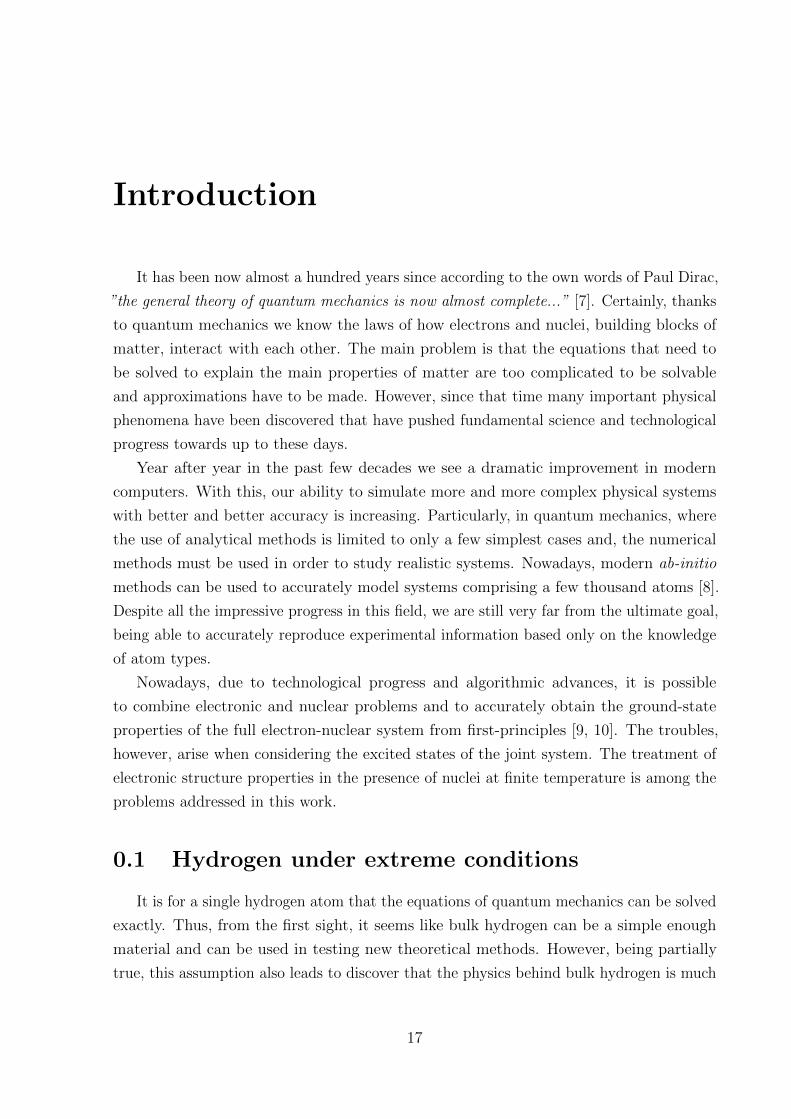
100 200 300 400 500Pressure (GPa)

0

250

500

750

1000

1250

1500

Tem

pera

ture

(K)

Fluid H2

Solid H2

I

II

IV IV - V

H2(PRE)Metallic H2

Metallic H

Fluid H

III

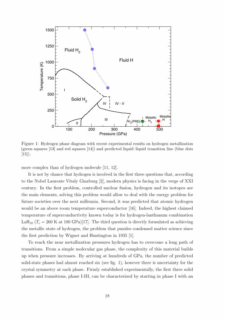
Figure 1: Hydrogen phase diagram with recent experimental results on hydrogen metallization(green squares [13] and red squares [14]) and predicted liquid–liquid transition line (blue dots[15]).

more complex than of hydrogen molecule [11, 12].

It is not by chance that hydrogen is involved in the first three questions that, according

to the Nobel Laureate Vitaly Ginzburg [2], modern physics is facing in the verge of XXI

century. In the first problem, controlled nuclear fusion, hydrogen and its isotopes are

the main elements, solving this problem would allow to deal with the energy problem for

future societies over the next millennia. Second, it was predicted that atomic hydrogen

would be an above room temperature superconductor [16]. Indeed, the highest claimed

temperature of superconductivity known today is for hydrogen-lanthanum combination

LaH10 (Tc = 260 K at 180 GPa)[17]. The third question is directly formulated as achieving

the metallic state of hydrogen, the problem that puzzles condensed matter science since

the first prediction by Wigner and Huntington in 1935 [1].

To reach the near metallization pressures hydrogen has to overcome a long path of

transitions. From a simple molecular gas phase, the complexity of this material builds

up when pressure increases. By arriving at hundreds of GPa, the number of predicted

solid-state phases had almost reached six (see fig. 1), however there is uncertainty for the

crystal symmetry at each phase. Firmly established experimentally, the first three solid

phases and transitions, phase I-III, can be characterized by starting in phase I with an

18

initial rotational symmetry of spherically disordered molecules arranged in a hexagonal

close packed (hcp) structure [11]. The rotational symmetry then breaks when compressing

hydrogen further to phase II, the molecules are now ordered or at least partially ordered,

but their exact arrangement and their shape are unknown [18]. The transition to phase II,

also known as the broken symmetry phase (BSP), depends substantially on isotope, which

implies an important role of nuclear quantum effects [19]. The transition to phase III is

characterized by the changes in infrared (IR) and Raman spectra [20, 21]. Also called

hydrogen-A, phase III spans from ∼155 GPa at 100 K, over more than 200 GPa at low

temperature [20]. It is from this phase that hydrogen is predicted to transform into a

metallic phase, and in this thesis, the main focus will be on phase III. By the spectroscopic

measurements, recent experimental investigations predict metallization pressure being

between 425 GPa [13] and 495 GPa [14]

The main difficulty with achieving high pressures for solid hydrogen, especially above

room temperature, is associated with the diffusive and reactive nature of the material

in a dense state. Experimentally solid hydrogen is obtained by static compression in a

diamond-anvil-cell (DAC), and very often, hydrogen can penetrate inside the diamond,

breaking it and interrupting the experiment [22].

Going up in the phase diagram by increasing the temperature in the solid phase, the

crystal will melt forming a melting line, which was studied extensively over the past 30

years [23]. Interestingly, that having a negative slope (see fig. 1 [24]) the line can be

extrapolated to zero temperature, meaning that hydrogen might be a liquid at the ground

state. The liquid phase makes up a major fraction of hydrogen in the Universe. Studying

this phase can answer many questions in planetary science, regarding the composition

of the planets. The predicted first order phase transition [25] should occur in hydrogen

at temperatures below some critical temperature and should be accompanied by the

dissociation of the molecules and metallization. In this regime, besides static compression

in DAC with pulse laser heating, hydrogen can be compressed by a dynamic shock wave,

which results in higher pressure, however, the pay-off is the uncertainty in temperature

[26–28]. There is still an open question whether dissociation and metallization occur at

the same time. We will try to shed more light on it in chapter 6.

The fact that hydrogen can behave as a metal can be easily demonstrated by considering

the general Hamiltonian (see eq. 1.2 for example). Its potential energy scales as r−1s while

the kinetic energy goes as r−2s , where rs is the Wigner–Seitz radius [29]. Therefore, as

pressure increases (rs → 0), the kinetic part will dominate and electrons will favor the free

particle regime (simple metal). A simple theoretical description of this transition can be

given in terms of band theory. Change of density causes molecular bands to shift which

can lead to band-gap closure. The transition to the metallic state does not necessarily

involve the dissociation from molecular to atomic hydrogen. We discuss the gap closure of

19

hydrogen in Chapters 5 and 6.

0.2 Structure of the thesis

In this thesis, a methodological development to study electronic gaps and excitations

within quantum Monte Carlo (QMC) is discussed. The necessary treatment of electronic

properties at finite temperature is presented within QMC and density functional theory

(DFT) in combination with path integrals used for nuclei. The methodology is then used

to discuss the gap closure and the optical properties of liquid and solid hydrogen around

the metallization transition.

Chapter 1 presents the general theory of the electronic ground state methods used in

this thesis, which are mostly DFT and QMC. Particular attention is drawn to quantum

Monte Carlo. In chapter 2 the main methodology for computing energy gaps and excited

states within QMC is presented. There we introduce a novel method to compute gaps and

an important treatment of finite size effects for electron addition and removal energies,

the main problem of QMC simulations of extended systems. The methodology is tested

on silicon, carbon, and ideal crystalline hydrogen. A small overview of optical properties

calculations within Kubo-Greenwood [4, 5] formalism with application to ideal solid

hydrogen is given in chapter 3. In this chapter, within variational Monte Carlo (VMC), the

Kubo formula [4] for computing electronic conductivity of solid hydrogen was used. Next,

in chapter 4 finite temperature renormalization of electronic properties is discussed. All

these new theoretical developments are applied to compute the fundamental gap closure

and the optical properties of liquid (chapter 6) and solid (chapter 5) hydrogen at extreme

conditions.

Note that the theoretical development presented in this thesis is not limited to hydrogen

and can be applied to different materials, which gives a potential perspective for future

work. At the end of the thesis, the conclusions, with a summary of the main topics

addressed in this work are provided.

20

Chapter 1

Electronic Ground State Methods

In this chapter, we will lay the foundations of the quantum mechanical simulation

techniques used to obtain the electronic ground state properties of systems of interest,

which will serve as basis methods throughout the thesis. Firstly, the tremendous problem

of electrons in the presence of nuclei as an external field is introduced. Then we discuss

the independent particle Hartree-Fock (HF) approximation and the density functional

theory (DFT). The major part of the chapter is devoted to the central method of this

work: quantum Monte Carlo (QMC). In particular, we introduce variational Monte Carlo

(VMC) and reptation quantum Monte Carlo (RQMC) and discuss its advantages and

disadvantages. The most important part of any QMC simulation - the wave function, is

discussed here in details including its different terms and approximations. Finally, we

introduce a technique of treating the finite simulation cell size effects - an important

problem of all QMC simulations.

Besides a standard textbook of Martin [30] which covers the single electron theory,

a more recent book by Martin, Reining and Ceperley [31] gives a whole overview on all

methods used in treating systems with interacting electrons, including QMC. Moreover,

there is a fundamental review on QMC methods by Foulkes et al. [32], which was followed

by a more recent review by Kolorenc and Mitas [33]. Detailed information on RQMC

method can be found in lecture notes of Pierleoni and Ceperley [9].

1.1 Many body problem

Knowing that the matter is a collection of electrons and nuclei interacting via the

Coulomb potential, the equation for the stationary states δE/δΨ = 0, with E representing

21

the eigenenergies and Ψ are the eigenfunctions or wave functions,

[N∑i=1

(−1

2∇2i + vext(ri)

)+

1

2

N∑i 6=j

1

|ri − rj|

]Ψ(r1, .., rN) = EΨ(r1, .., rN), (1.1)

is the time-independent Schrodinger equation in atomic units (~ = 1, electron mass and

charge e = me = 1) for N electrons moving in a static potential vext created by the

presence of Np nuclei, which describes the behavior of electrons in atoms, molecules, and

condensed matter. Spin and relativistic effects have been neglected, as they will not be

discussed in this thesis. In eq. 1.1, it was assumed that the nuclei are static and placed at

their equilibrium positions, the external potential vext, therefore, depends on particular

nuclear geometry R = R1, ..,RNp . What happens if the nuclear effects are included will

be discussed in detail in chapter 4.

The eigenvalues of the Schrodinger equation 1.1 are the energies of the electronic

system. However, even when the nuclear motion is neglected, solving this equation remains

a complex problem. In fact, if the Hamiltonian

H = Te + Vep + Vee (1.2)

is split into three parts, it is clear that the complexity comes from the last term, which

is the Coulomb interaction between electrons. The presence of the Coulomb interaction

is the cause of high-dimensionality, indeed, the many-body wave function Ψ(r1, .., rN) is

a function of 3N variables. In real systems N is on the order of 1023, the Avogadro’s

number. However, even restricting the number of electrons to a few makes it impossible

to solve the Schrodinger equation directly and approximations have to be made. By

neglecting the last term in eq. 1.2, one can decouple the Schrodinger equation 1.1 into

many one-particle problems of independent electrons. However, despite the success of the

independent electron picture, there are many systems, some of them are considered in

this work, where this picture is not valid and more correlation has to be incorporated,

introducing higher-order approximations, for example as GW [34], Bethe-Salpeter equation

[35] or quantum Monte Carlo [36]. We will nevertheless start by discussing single electron

approximations to compute the electronic ground state.

1.2 Hartree-Fock

Starting from the wave function factorized into the single particle states, the first

approximation to include electronic correlation is simply based on Pauli exclusion principle

[37]. Working directly with electrons one has to take into account its fermionic nature,

22

e.g., the many-body wave function is restricted to be antisymmetric under the particle

exchange. It was firstly proposed by Slater in 1929 [38] that for single particle orbitals

this constrain is automatically satisfied when the product wave function is written as a

determinant:

ΨHF =1

(N !)1/2det(ψσi (rj)), (1.3)

where ψσi (rj) denotes a normalized single-particle orbital with the spin, σ quantised along

z. The energy,

EHF =

∫dr1..drNΨ∗HF HΨHF , (1.4)

can be calculated exactly and obeys the variational principle, e.g., for any wave function,

Ψ, the energy, E, obtained with eq. 1.1, is always an upper bound for a true ground state

energy E0. The total HF energy for Hamiltonian in eq. 1.1 is

EHF = −∫dr∑i,σ

ψσ∗i (r)∇2

2ψσi (r) +

∫drvext(r)n(r) + EH + Ex, (1.5)

where

n(r) =∑i,σ

ψσ∗i (r)ψσi (r) (1.6)

the first and the second terms are the kinetic energy and the energy due to the external

potential vext for independent particles,

EH =1

2

∫drdr′

n(r)n(r′)

|r− r′| (1.7)

is the Hartree contribution, which is the interaction energy if electrons were classical

particles,

Ex = −1

2

∑σ

occ∑i,j

∫drdr′ψσ∗j (r′)ψσi (r′)

1

|r− r′|ψσj (r)ψσ∗i (r) (1.8)

is the Fock term and is the result of Pauli exclusion principle. Further minimisation of

the HF total energy with respect to the orthonormal single-body orbitals ψσi leads to the

Hartree-Fock equations for single-body orbitals [39][−1

2∇2 + vext(r) + vH(r)

]ψσi (r) +

∫dr′Σx,σ(r, r′)ψσi (r′) = εσi ψ

σi (r), (1.9)

23

where vH(r) is the Hartree potential that acts locally on a wave function at each point r.

It arises from the charge of all the electrons, including each electron acting on itself,

vH(r) =

∫dr′

n(r′)

|r− r′| . (1.10)

The Σxσ(r, r′) is the non-local Fock operator, contains only like spins

Σx,σ(r, r′) = −occ∑j

ψσ∗j (r′)1

|r− r′|ψσj (r). (1.11)

Equation 1.9 can be solved exactly only in some cases: for spherically symmetric atoms

and the homogeneous electron gas. Usually, these equations are written in a finite basis

and are solved for the coefficients of the expansion.

The HF ground state wave function is the determinant built from the N lowest-energy

single-particle states. Koopmans’ theorem [40] shows that the eigenvalues of the HF

equations correspond to the total energy differences, namely, to the energies to add or

subtract electrons,

±εN±1 = EN±1 − EN , (1.12)

that would result from increasing the size of the matrix by adding an empty orbital or

decreasing the size by removing an orbital if all other orbitals are frozen. Excited states

can be represented by choosing other combinations of single-particle spin orbitals ψσi to

build the determinant. However, note that in the absence of relaxation the addition,

removal, and excitation energies are often overestimated. Though, performing the separate

calculations of N and N ± 1-particle states would include some aspect of correlation, for

an infinite system this will be negligible and would merely reproduce the eigenvalues. In

general, assuming a single-determinant form for the wave function neglects correlation

between electrons, which makes the Hartree-Fock theory insufficient to make accurate

quantitative predictions.

1.3 Density functional theory (DFT)

In the attempts to solve the many-body problem one can try to reduce the dimensionality

of the problem. For example, by working with the electronic density one can go from the

3N dimensional space of the wave function to a function of only 3 coordinates. Indeed, it

seems very appealing to be able to solve the quantum mechanical problem just relying on

the knowledge of the electronic density. To see how it can be possible, let us first note that

the ground state total energy and wave function of an interacting many-electron system

can be considered as a functional of the external potential vext, i.e., it depends on the

entire function vext(r). This potential can be due to the nuclei and other sources (see eq.

24

1.1). By the use of Legendre transformation, it was shown by Hohenberg and Kohn in

1964 [41] that the energy can be also written as a functional of the density, which is the

main idea of density functional theory (DFT).

EHK [n] = 〈Ψ|T + Vee|Ψ〉+

∫drvext(r)n(r)

= FHK [n] +

∫drvext(r)n(r), (1.13)

where FHK [n] is the universal functional of the density. The ground state is determined

by minimizing the energy. This functional is unknown and very difficult to approximate

in general. However due to the ingenious work by Kohn and Sham in 1965 [42] practical

use of DFT became possible. In their work, they were able to reformulate the original

many body problem and represent it with a set of independent particle problems having

an effective potential. Which have led to the set of equations representing an auxiliary

system of independent-particles having the same density as the original, interacting one.

The properties of this system can be derived from the single-particle equation with an

effective potential veff (r), (−1

2∇2 + veff (r)

)ψi(r) = εiψi(r), (1.14)

where all the interactions are placed into an effective potential veff (r) which every particle

feels independently. The ground state density,

n(r) =occ∑i

ψ∗i (r)ψi(r), (1.15)

then corresponds to the interacting one by construction, ψi now denote the Kohn-Sham

eigenfunctions.

Making the connection to eq. 1.13 the energy functional for the Kohn-Sham system

can be rewritten as

EKS[n] =N∑i=1

−1

2|∇ψi(r)|2 +

∫drvext(r)n(r) + EH [n] + Exc[n], (1.16)

where Exc[n] = 〈Ψ|T + Vee|Ψ〉 −∑N

i=1−12|∇ψi(r)|2 − EH [n] includes all the contributions

of exchange and correlation to the ground state energy. It accounts also for many body

corrections to the kinetic energy. The effective potential veff (r) is defined by the condition

25

for the minimum energy:

δEKS[n]

δn(r)= −veff ([n], r) + vext(r) +

δEH [n]

δn(r)+δExc[n]

δn(r)= 0 (1.17)

veff ([n], r) = vext(r) + vH([n], r) + vxc([n], r). (1.18)

The set of eqs. 1.14, 1.15 and 1.17 (the famous Kohn-Sham equations) must be

solved self-consistently, as the effective potential, veff([n], r), is itself a functional of the

density. Since Exc[n] is a small fraction of the total energy, it is much easier to create

approximate expressions for it, than approximate the full energy functional FHK [n]. A

first reasonable approximation for Exc[n], called local density approximation (LDA) was

originally proposed by Kohn and Sham, is taken from results for the homogeneous electron

gas (HEG) and is a local functional of the density:

ELDAxc [n] =

∫dr n(r) εHEGxc ([n(r)], r). (1.19)

The exchange energy density εHEGxc ([n(r)], r) = −34

(3πn)(1/3)

is the energy per electron

of the HEG at point r that depends only upon the density n(r) at r. The correlation

energy density has been calculated numerically for a set of densities by Ceperley and

Alder (1980) using quantum Monte Carlo [43] and parametrized by Perdew and Zunger

(1981) [44]. It is expected that it will be best for solids close to a homogeneous gas (like a

nearly-free-electron metal) and worst for very inhomogeneous cases like atoms where the

density must go continuously to zero outside the atom.

Due to the success of LDA there were developed functionals which include dependence

on gradients and higher derivatives of the density. However, the straightforward expansion

has not solved the problem and lead to worse results as the gradients in real materials are so

large that the expansion breaks down. Thus, the term generalized-gradient approximation

(GGA) denotes a variety of parametrization proposed for functions that modify the behavior

at large gradients in such a way as to preserve desired properties. For spin unpolarised

system the generalization of eq. 1.19 will take the form of:

EGGAxc [n] =

∫dr n(r) εxc([n], |∇n|, .., r). (1.20)

The parametrization proposed by Perdew, Burke, and Enzerhof (PBE) [45] is used in this

thesis most frequently, for example, to generate the starting Slater determinant for QMC

calculations.

26

1.3.1 Generalized Kohn-Sham theory (GKS)

One can obtain a large improvement in accuracy by considering a non-local effective KS

potential instead of a local one. This approach is regarded as a generalisation of the original

Kohn-Sham idea. Recently, it was shown by Perdew et al. [46] that in generalized KS theory

(GKS), the band gap of an extended system equals to the fundamental gap. One of the

ways to include non-locality is to mix the orbital-dependent Hartree-Fock and an explicit

density functional, introducing a mixing parameter a. Functionals constructed in this way

are called ”hybrids”. One of the ”hybrid” functionals used throughout this manuscript is

named after Heyd-Scuseria-Ernzerhof (HSE) and based on a screened Coulomb potential

for the exchange interaction [47]. This form of functional was shown to accurately describe

energy band gaps and lattice parameters of many semiconductors [48].

1.3.2 Bloch theorem and pseudopotentials

When dealing with periodic structures, it is possible to use relatively small cells and

employ periodic boundary conditions. In fact, for crystal structures, the simulation cell

can be as small as the primitive cell. Indeed, in the case of single particle orbitals, the

translational symmetries of the system result in Bloch’s theorem [29]. The KS orbitals

can be then written as,

ψki(r) = eik · ruki(r), (1.21)

uki(r + Lα) = uki(r),

with uki(r) having periodicity of the crystal cell with lattice vectors (L1,L2,L3). By

introducing further the reciprocal lattice vectors, Gm,

Gm = m1B1 +m2B2 +m3B3, m = (m1,m2,m3) ∈ N3, (1.22)

B1 = 2πL2 × L3

L1 · (L2 × L3),

B2 = 2πL3 × L1

L2 · (L3 × L1), (1.23)

B3 = 2πL1 × L2

L3 · (L1 × L2),

the periodic part can then be expanded as

uki(r) =∑m

CkimeiGm · r (1.24)

27

where the summation over integers is possible thanks to the periodicity of uki(r). Moreover,

for any vector Gn,

ψ(k+Gn)i(r) = eik · r∑m

C(k+Gn)imei(Gm+Gn) · r (1.25)

= eik · r∑m

CkimeiGm · (r+Ln) = ψki(r),

meaning that the vector k can be confined to the primitive cell of the reciprocal lattice,

conventionally called the first Brillouin zone. This plane-wave expansion is used in codes

written to deal with periodic systems including those used throughout this work.

The main drawback of plane waves is the fact that they require highly dense grids

to be able to represent the core atomic states. Due to orthogonality requirements, these

functions are very oscillatory and localized in the core region. In the majority of cases, these

states are chemically inert, so it should be possible to remove them from the calculation

without major changes to the properties of the system. Pseudopotentials are renormalized

electron-nuclei potentials for the valence states of an atom that include both the Coulomb

attraction of the nuclei and the screening effects resulting from the presence of core

electrons. By employing pseudopotentials, not only do we remove core states from the

calculation, but we also obtain valence states which are smooth in the core region, which

greatly reduces the computational demands of the method. For the additional details see

ref. [30].

In the DFT calculations presented in this work, pseudopotentials are used for hydrogen,

even though it does not possess a core. That is necessary because the Coulomb potential,

1/r, requires a large number of plane waves Gm to achieve the convergence, which greatly

increases the computational demands of the calculations. The pseudopotentials are built

to reproduce the scattering properties of the atom, therefore, valence states should not be

significantly affected outside the core region.

1.4 Quantum Monte Carlo (QMC)

All the methods discussed above can be classified as deterministic, which boils down

to numerically solving an approximate equation to determine the properties of a quantum

system. As we have seen they usually have a trade-off problem of correctly describing

correlations while keeping numerical simplicity of equations. Alternatively one can try to

solve the Schrodinger equation 1.1 directly by designing an appropriate stochastic method

and putting correlations directly into the wave function. Such methods, named quantum

Monte Carlo (QMC), provide results more accurate than DFT or HF with just an order of

28

magnitude increase in computational cost (for both methods computational effort grows

with the third power of system size, but the prefactor can differ by an order of magnitude).

Being an exact method for bosons, in many cases for fermionic systems QMC provides the

energies and other properties very close to the exact results.

In this section, the discussion will be limited to zero temperature or ground state QMC

methods. Giving a proper description of the ground state methods is necessary, as it serves

as the starting point for the development of excited states and finite temperature QMC.

For a more complete description of the ground state QMC see refs. [31, 32, 49]

1.4.1 Variational Monte Carlo (VMC)

The variational Monte Carlo method (VMC) was first introduced by McMillan in 1965

[36], who observed that the calculation of a quantum system using a correlated wave

function can be seen as the evaluation of a classical many-body system of atoms interacting

with a pair potential and can be calculated with Monte Carlo techniques. The VMC

method is based on the variational principle, which tells us that by choosing an arbitrary

trial wave function ΨT (R) for the electronic configuration R = r1, .., rN, the expectation

value of H evaluated with the trial wave function ΨT is always greater or equal, than the

exact ground state energy

EV =

∫Ψ∗T (R)HΨT (R)dR∫Ψ∗T (R)ΨT (R)dR

> E0. (1.26)

One can rewrite equation (1.26) in the form

EV =

∫|ΨT (R)|2[Ψ−1

T (R)HΨT (R)]dR∫|ΨT (R)|2dR > E0, (1.27)

from which it is easy to separate the integral into the probability distribution P(R) and

the observable EL(R)

P(R) =|ΨT (R)|2∫|ΨT (R)|2dR ,

EL(R) = Ψ−1T (R)HΨT (R).

(1.28)

Now the variational energy EV will take the form of an average, that can be evaluated

by the Monte Carlo technique

EV =

∫P(R)EL(R)dR. (1.29)

29

0 500 1000 1500 2000 2500 3000 3500NR

51.64

51.62

51.60

51.58

51.56

E, H

artre

e

EL(a1)< EL(a1) > 2

EL(a2)< EL(a2) > 2

E0

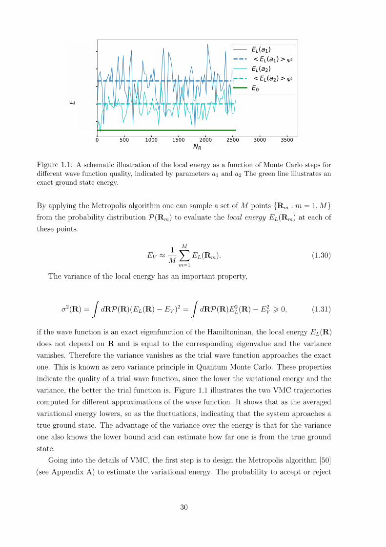
Figure 1.1: A schematic illustration of the local energy as a function of Monte Carlo steps fordifferent wave function quality, indicated by parameters a1 and a2 The green line illustrates anexact ground state energy.

By applying the Metropolis algorithm one can sample a set of M points Rm : m = 1,Mfrom the probability distribution P(Rm) to evaluate the local energy EL(Rm) at each of

these points.

EV ≈1

M

M∑m=1

EL(Rm). (1.30)

The variance of the local energy has an important property,

σ2(R) =

∫dRP(R)(EL(R)− EV )2 =

∫dRP(R)E2

L(R)− E2V > 0, (1.31)

if the wave function is an exact eigenfunction of the Hamiltoninan, the local energy EL(R)

does not depend on R and is equal to the corresponding eigenvalue and the variance

vanishes. Therefore the variance vanishes as the trial wave function approaches the exact

one. This is known as zero variance principle in Quantum Monte Carlo. These properties

indicate the quality of a trial wave function, since the lower the variational energy and the

variance, the better the trial function is. Figure 1.1 illustrates the two VMC trajectories

computed for different approximations of the wave function. It shows that as the averaged

variational energy lowers, so as the fluctuations, indicating that the system aproaches a

true ground state. The advantage of the variance over the energy is that for the variance

one also knows the lower bound and can estimate how far one is from the true ground

state.

Going into the details of VMC, the first step is to design the Metropolis algorithm [50]

(see Appendix A) to estimate the variational energy. The probability to accept or reject

30

the trial move of electron positions from R to R′, according to Metropolis, is proportional

to the ratio of the probability distributions P(R′)/P(R), more specifically,

A(R→ R′) = min

[1,T (R→ R′)

T (R′ → R)

∣∣∣∣Ψ(R′)

Ψ(R)

∣∣∣∣2], (1.32)

where T (R → R′) is the transition probability of proposing the trial configuration R′

given the actual configuration R. In case of uniform displacement of one electron within

a volume Ω it becomes T (ri → r′i) = T (r′i → ri) = Ω−1. The algorithm for performing

Variational Monte Carlo simulation is the following:

• Pick the trial wave function. The most common form is Slater-Jastrow wave function,

which includes pair correlations. The choice of the trial wave function will be

discussed in detail in section 1.4.3.

• Initialise electron positions R(0) ≡ r(0)1 , r

(0)2 , ..., r

(0)N

• Iterate the loop over electrons i, M times:

– Propose the move ri → r′i of electron i in a uniform way within the volume Ω

– Determine the acceptance probability:

A = min[1, |Ψ(R′)/Ψ(R(n))|2

](1.33)

– If A > u with u ∈ (0, 1) a uniform random number, accept the move and update

the coordinates (R(n+1) = R′). Otherwise, reject the move and keep the old

coordinates (R(n+1) = R(n)).

– Compute and average the local energy EL(R(n+1)) and other properties.

• Adjust the trial wave function parameters to minimise the average local energy.

The variational method is very powerful and intuitively understandable. The only

assumption is the form of the trial wave function and no further uncontrolled approxima-

tions. But this fact can also bring problems to the method, for example, the construction

and optimization of trial functions for many-body systems can be time-consuming and can

bring an element of human bias (see Appendix B for more information). Moreover, the

result of VMC calculation is strongly influenced by the form of the trial wave function.

1.4.2 Reptation Quantum Monte Carlo (RQMC)

Despite all the advantages of VMC, it is still desirable to have a method that will be

less dependent on the input trial wave function. That can be achieved based on the idea

31

that starting from a trial wave function and applying a suitable projection operator one

can project onto the ground state.

Suppose the exact eigenfunctions and eigenvalues of the Hamiltonian H in 1.2 are φi

and Ei. It is true that any trial state can be decomposed in the eigenstate basis,

|ΨT 〉 =∑i

ci|φi〉, (1.34)

where ci is the overlap of the trial state with the ith eigenstate. Let us consider the

application of the operator e−βH onto this state,

|Ψ(β)〉 = e−βH |Ψ(0)〉 =∑i

cie−βEi |φi〉 ∝

β→∞c0e−βE0|φ0〉, (1.35)

with the initial state |Ψ(0)〉 = |ΨT 〉. All excited states will be suppressed exponentially

fast with increasing β, the imaginary projection time. The rate of convergence to the

ground state depends on the energy gap between the ground state and the first excited

state, non-orthogonal to the trial function. The total energy as a function of the imaginary

time is defined as follows,

E(β) =〈ΨT |e−

β2HHe−

β2H |ΨT 〉

〈ΨT |e−βH |ΨT 〉. (1.36)

The reason for splitting the projector operator and putting it on two sides is to get a pure

(unmixed) estimator. In other words, to make the same wave function appear on both

sides. That is the main difference of the method described below and used throughout

this thesis, called reptation quantum Monte Carlo (RQMC) [51], from the conventional

diffusion Monte Carlo (DMC) [52] that was developed first and is more widespread.

Similarly to the thermal partition function, one can define the generating function of

the moments of H as

Z(β) = 〈ΨT |e−βH |ΨT 〉. (1.37)

The total energy at β can be simply expressed as the derivative of the logarithm of Z(β)

E(β) = − ∂

∂βln(Z(β)). (1.38)

Now, we will prove that the energy as a function of β decreases and converges to the

ground state E0 at β → ∞. To do so it is convenient to define the variance of energy

σ2E(β), which is by definition positive,

σ2E(β) = 〈H2〉 − 〈H〉2 =

∂2

∂2βln(Z(β)) = − ∂

∂βE(β) > 0, (1.39)

the derivative of the energy with respect to β should then be negative, meaning that it

32

monotonically decreases as β increases and therefore the following relations must hold,

limβ→∞

E(β)→ E0, (1.40)

limβ→∞

σ2E(β)→ 0, (1.41)

the last relation is also known as zero variance principle Eq. (1.31).

Now it is useful to define the operator e−βH as the density matrix.

ρ(R,R′, β) = 〈R|e−βH |R′〉, (1.42)

where R again represents a set of electronic coordinates. For exact eigenstates φi(R) the

density matrix writes,

ρ(R,R′, β) =∑i

φ∗i (R)e−βEiφi(R′). (1.43)

The partition function Z can be then expressed as,

Z(β) =

∫dRdR′〈ΨT |R〉ρ(R,R′, β)〈R′|ΨT 〉, (1.44)

which allows us to write the average of an observable A, not commuting with Hamiltonian

H, as follows,

〈A〉(β) =1

Z(β)

∫d R1...d R4〈ΦT |R1〉ρ(R1,R2;

β

2)〈R2|A|R3〉ρ(R3,R4;

β

2)〈R4|ΦT 〉.

(1.45)

To get the best estimate to the ground state average it is necessary to put the observable

at β/2, as this is where the left and right trial functions have been projected equally.

Putting observable at any other β will provide a mixed estimator since the observable

sandwiches with different wave functions.

To compute an average over the ground state one needs to know the density matrix at

large β. For that it is necessary to factorize β at small imaginary time steps τ = β/M with

M being the number of steps. If the time step τ is short enough the system approaches

its classical limit and one can do approximations. Consider factorizing the density matrix,

ρ(R,R′, β) = 〈R|e(−τH)M |R′〉 =

∫dR1...dRM−1

M∏k=1

〈Rk−1|e−τH |Rk〉, (1.46)

with the boundary conditions: R0 = R and RM = R′. Now, one has to evaluate the short

33

time propagator. Applying the Trotter [53] split-up one gets,

〈Rk−1| exp[−τ(T + V )]|Rk〉 ≈ e−τV (Rk−1)/2〈Rk−1|e−τT |Rk〉e−τV (Rk)/2, (1.47)

where it has been used the fact that the potential energy operator is diagonal in the

position representation and its matrix elements are trivial,

〈R| exp(−τ V )|R′〉 = e−τV (R)δ(R′ −R). (1.48)

For the kinetic propagator the solution is the Green’s function of the free particle

diffusion equation, which in configurational space is,

∂tΦ(R, t) =1

2

N∑i=1

∇2iΦ(R, t), (1.49)

which in the integral form becomes,

Φ(R, t+ τ) =

∫G(R← R′, τ)Φ(R′, t)dR′, (1.50)

where

G(R← R′, τ) = 〈R| exp[−τ T ]|R′〉. (1.51)

The solution is well known and has a form of a gaussian with variance τ ,

〈Rk−1|e−τT |Rk〉 = (2πτ)−3N/2 exp

[−(Rk −Rk−1)2

2τ

]. (1.52)

Putting everything back together to obtain density matrix ρ(R,R′, t) one gets,

ρ(R,R′, β) =

∫dR1...dRM−1

M∏k=1

e−

(Rk −Rk−1)2

2τ

(2πτ)3N/2

e−τ[V (R0)

2+∑M−1k=1 V (Rk)+

V (RM)

2

].

(1.53)

In the continuous limit (M → ∞, τ → 0, β = Mτ = const.) it becomes the

Feynman-Kac formula [54]:

ρ(R,R′, β) =

⟨exp

(−∫ β

0

dτV (R(τ))

)⟩RW

, (1.54)

where 〈...〉RW indicate a path average over gaussian random walks R(τ) starting at

R(0) = R and ending at R(β) = R′ at time β.

34

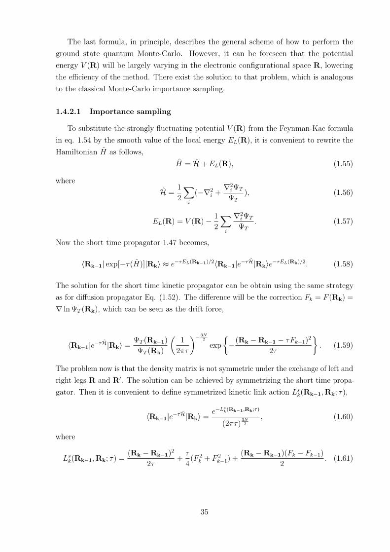
The last formula, in principle, describes the general scheme of how to perform the

ground state quantum Monte-Carlo. However, it can be foreseen that the potential

energy V (R) will be largely varying in the electronic configurational space R, lowering

the efficiency of the method. There exist the solution to that problem, which is analogous

to the classical Monte-Carlo importance sampling.

1.4.2.1 Importance sampling

To substitute the strongly fluctuating potential V (R) from the Feynman-Kac formula

in eq. 1.54 by the smooth value of the local energy EL(R), it is convenient to rewrite the

Hamiltonian H as follows,

H = H + EL(R), (1.55)

where

H =1

2

∑i

(−∇2i +∇2iΨT

ΨT

), (1.56)

EL(R) = V (R)− 1

2

∑i

∇2iΨT

ΨT

. (1.57)

Now the short time propagator 1.47 becomes,

〈Rk−1| exp[−τ(H)]|Rk〉 ≈ e−τEL(Rk−1)/2〈Rk−1|e−τH|Rk〉e−τEL(Rk)/2. (1.58)

The solution for the short time kinetic propagator can be obtain using the same strategy

as for diffusion propagator Eq. (1.52). The difference will be the correction Fk = F (Rk) =

∇ ln ΨT (Rk), which can be seen as the drift force,

〈Rk−1|e−τH|Rk〉 =ΨT (Rk−1)

ΨT (Rk)

(1

2πτ

)− 3N2

exp

−(Rk −Rk−1 − τFk−1)2

2τ

. (1.59)

The problem now is that the density matrix is not symmetric under the exchange of left and

right legs R and R′. The solution can be achieved by symmetrizing the short time propa-

gator. Then it is convenient to define symmetrized kinetic link action Lsk(Rk−1,Rk; τ),

〈Rk−1|e−τH|Rk〉 =e−L

sk(Rk−1,Rk;τ)

(2πτ)3N2

, (1.60)

where

Lsk(Rk−1,Rk; τ) =(Rk −Rk−1)2

2τ+τ

4(F 2

k + F 2k−1) +

(Rk −Rk−1)(Fk − Fk−1)

2. (1.61)

35

Putting eqs. 1.58, 1.60 and 1.46 together, the density matrix, ρ(R,R′, β), becomes,

ρ(R,R′, β) =

∫dR1...dRM−1

[M∏k=1

e−Lsk(Rk−1,Rk;τ)

(2πτ)3N/2

]e−τ

[EL(R0)

2+∑M−1k=1 EL(Rk)+

EL(RM)

2

].

(1.62)

The final result in the continuum limit is called the generalised Feynman-Kac formula

[9, 55, 56]:

ρ(R,R′, β) =

⟨exp

(−∫ β

0

dτEL(R(τ))

)⟩DRW

, (1.63)

where 〈...〉DRW indicates a path averaged over drifted random walk starting at R(0) = R

and ending at R(β) = R′.

It is important to define the estimator for the total energy. However, to compute

the total energy one can put the local energy operator either on the left or on the right,

meaning,

E(β) =1

Z(β)

∫dRdR′EL(R)ΨT (R)ρ(R,R′, β)ΨT (R′)

=1

Z(β)

∫dRdR′ΨT (R)ρ(R,R′, β)ΨT (R′)EL(R′)

=1

2〈EL(R) + EL(R′)〉.

(1.64)

For the variance calculation it make sense to split the local energy operator in two and

insert it on both sides of the density matrix, leading to

σ2(β) =

∫dRdR′EL(R)ΨT (R)ρ(R,R′, β)ΨT (R′)EL(R′)− E2(β). (1.65)

Now we will sketch the algorithm of the importance sampling reptation QMC [51]. Let’s

define a discretised path X = R0,R1, ...,RM, consisting of M electronic configurations,

then the probability of this path π(X) will be,

π(X) =Ψ(R0)ρ(R0,R1, τ)...ρ(RM−1,RM, τ)Ψ(RM)

Z(t). (1.66)

The transition probability to grow the path either left or right can be defined as,

T+1 = e−(R′−RM−τFM )2/2τ ,

T−1 = e−(R′−R0−τF0)2/2τ .(1.67)

36

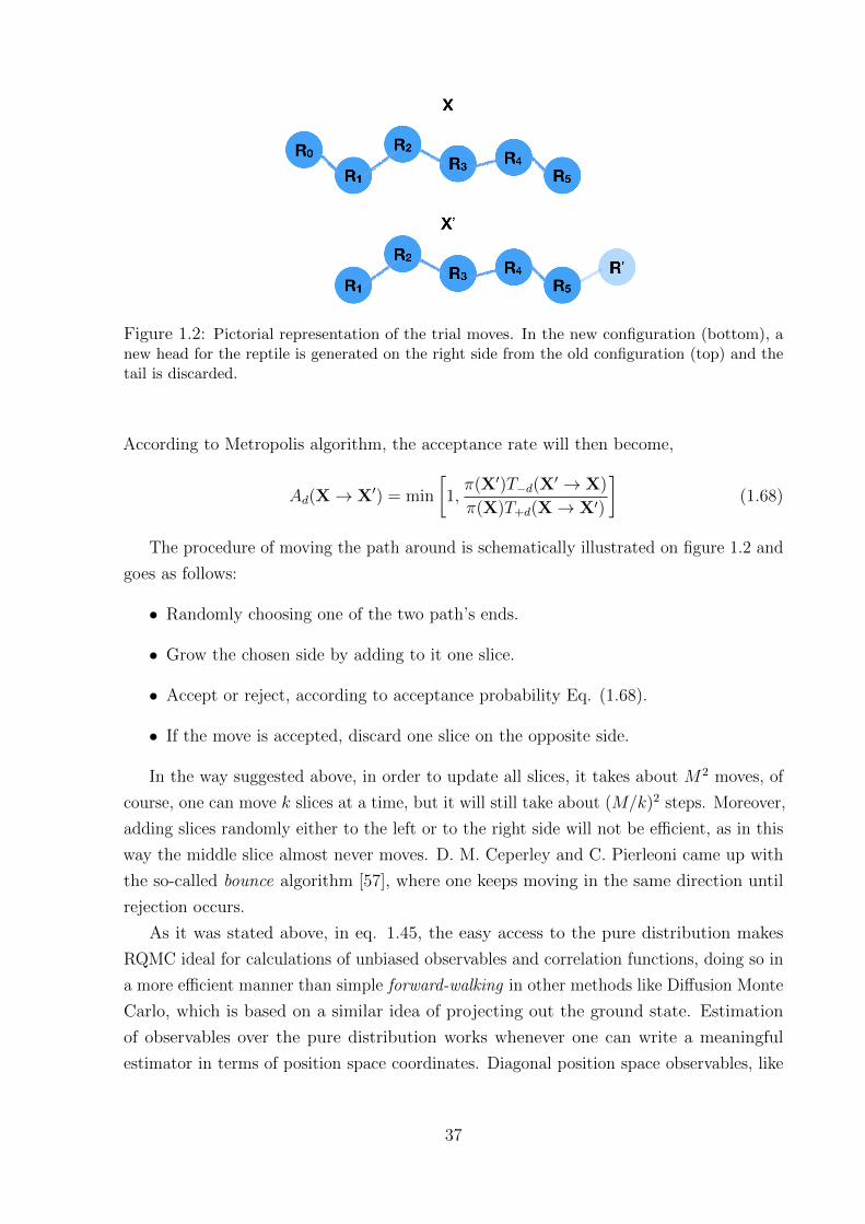
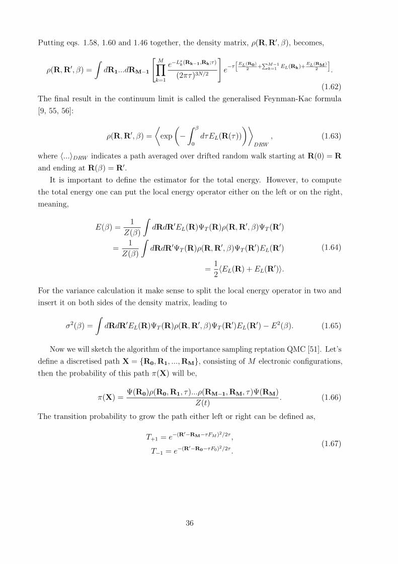
Figure 1.2: Pictorial representation of the trial moves. In the new configuration (bottom), anew head for the reptile is generated on the right side from the old configuration (top) and thetail is discarded.

According to Metropolis algorithm, the acceptance rate will then become,

Ad(X→ X′) = min

[1,π(X′)T−d(X

′ → X)

π(X)T+d(X→ X′)

](1.68)

The procedure of moving the path around is schematically illustrated on figure 1.2 and

goes as follows:

• Randomly choosing one of the two path’s ends.

• Grow the chosen side by adding to it one slice.

• Accept or reject, according to acceptance probability Eq. (1.68).

• If the move is accepted, discard one slice on the opposite side.

In the way suggested above, in order to update all slices, it takes about M2 moves, of

course, one can move k slices at a time, but it will still take about (M/k)2 steps. Moreover,

adding slices randomly either to the left or to the right side will not be efficient, as in this

way the middle slice almost never moves. D. M. Ceperley and C. Pierleoni came up with

the so-called bounce algorithm [57], where one keeps moving in the same direction until

rejection occurs.

As it was stated above, in eq. 1.45, the easy access to the pure distribution makes

RQMC ideal for calculations of unbiased observables and correlation functions, doing so in

a more efficient manner than simple forward-walking in other methods like Diffusion Monte

Carlo, which is based on a similar idea of projecting out the ground state. Estimation

of observables over the pure distribution works whenever one can write a meaningful

estimator in terms of position space coordinates. Diagonal position space observables, like

37

the average potential energy and pair-correlation function, can be measured directly from

the sampled pure distribution. Observables that are not diagonal in position space, like

off-diagonal density matrix elements and the momentum distribution, can be estimated

from the pure distribution with some suitable additions to the basic algorithm [58].

Even though, the projection result guarantees a closer answer to the ground state that

the VMC, there is still some dependency on having a good trial wave function. Firstly, for

the reasons of convergence efficiency. Secondly, and more importantly, when dealing with

Fermi statistics the density matrix between configurations R and R′ is no longer positive

everywhere since the permutation of the final configuration PR′, multiplied by the sign of

the permutation has to be taken care of. In this form the fermionic density matrix can not

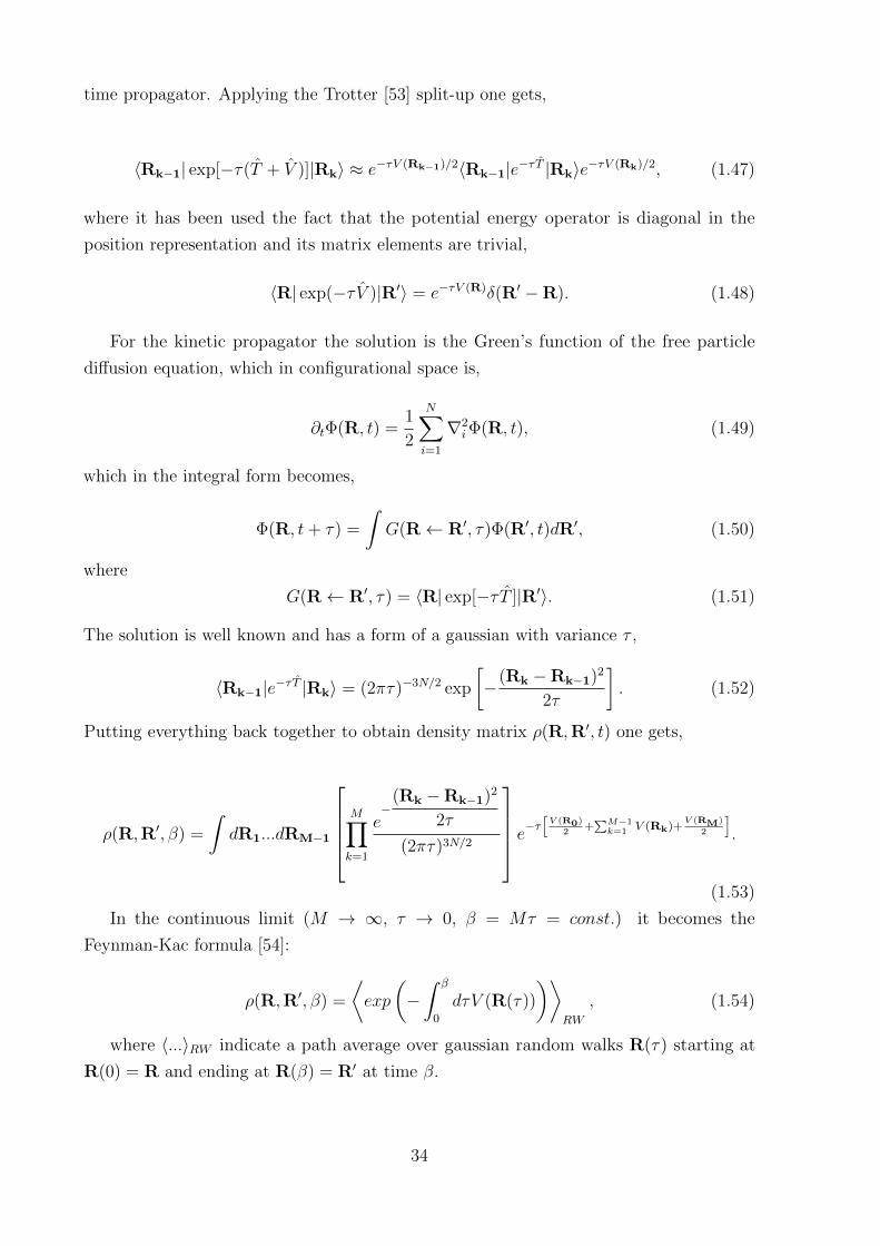
serve as the probability distribution. Information on the regions where the wave function

changes sign should be then taken from the trial wave function, which introduces a crucial

approximation to the projection methods for fermions.

1.4.2.2 Fermion sign problem

So far, there was only defined the general Boltzmann density matrix 1.46, which serves

us as a probability distribution in the MC run. No information concerning the bosonic or

fermionic nature of the particles was provided up to this point. In order to generalize the

density matrix for bosons and fermions one has to take into account permutations and

antisymmetry:

ρB/F (R,R′, t) =1

N !

∑P

(±1)Pρ(R,PR′, t) (1.69)

where P is one of the N ! permutations of particle labels. One can, therefore, think of a

path in the configurational space of distinguishable particles as an object carrying not

only a weight (given by the exponential of minus the integral of the local energy along

the path eq. 1.63), but also a sign fixed by its boundary conditions in time. Hence, as

far as this sign is positive (ρ(R,R′, t) ≥ 0 for any R′ and t at given R, i. e. as far as one

is dealing with bosons, the sum over permutations can be easily carried out. However,

for fermions the density matrix ρF can be negative, which gives rise to the fermion sign

problem [59]. The origin of the problem is the fact that the sign has to be left in the

estimator for the averages in order to have a density matrix as a sampling probability.

Therefore, for such alternating series, the signal to noise ratio will decay exponentially

and it will be very inefficient to use the direct method to sample fermions. The fermion

sing problem is the most challenging problem in QMC, which many scientists are trying

to solve. However, nowadays pretty robust approximations are available. The most widely

used is the so-called restricted path or fixed node method [60].

Within the fixed node method, one needs to consider the nodal surfaces of the fermion

38

density matrix. For any given configuration R, these are defined by the implicit equation

ρF (R,R′, t) = 0, as the set of locations R′ at which the density matrix at time t vanishes.

The nodal surfaces of the initial configuration R divide the configurational space of R′

in regions of positive ρF and regions of negative ρF . One can define Υ(R, t) as the set of

points that can be reached from R in time t without having crossed the nodal surfaces at

previous times. Formally it can be written as the restricted path identity by restricting

the functional integral to paths inside Υ(R, t) in such a way that Ψ(R)Ψ(R′) ≥ 0,

ρF (R,R′, t) =1

N !

∑P

(−1)P(∫Y(0)=R,Y(t)=PR′

DYe−S[Y]

)Υ(R,t)

, (1.70)

where S[Y ] represents the action over generic path Y . Therefore, using the restricted path

identity it can be shown [9] that the generating function is a positive function at any

time t and can be computed considering only positive paths which do not cross the nodal

surfaces. A further very important property of the fixed node method is the existence of a

variational theorem: the FN-RQMC energy is an upper bound of the true ground state

energy ET (∞) ≥ E0, and the equality holds if the trial nodes coincide with the nodes of

the exact ground state [61]. Therefore even for fermions, the projection methods such as

RQMC are variational with respect to the nodal positions.

In principle, if one knows the exact nodal surface, then the solution will be exact.

However, knowing the exact nodes means knowing the density matrix itself, which is

the final goal of the simulations. Thus, nodal surface has to be approximated by the

nodes of the trial wave function and usually is defined by the Slater determinant. In a

real simulation of many-body, the nodal surface can be extremely complex, despite that,

comparing to VMC, the fixed node approximation dramatically improves energies, however

other properties such as the momentum distribution may not be improved to the same

order.

1.4.3 Trial wave function

The choice of trial wave function is critical, especially in VMC calculations. The power

of Quantum Monte Carlo methods lies in the flexibility of the form of the trial wave

function.

1.4.3.1 Slater Jastrow

The trial wave function in most of quantum Monte Carlo simulations is based on the

Slater determinant of single particle orbitals, det(ψσk (ri)), first introduced in eq. 1.3. The

next step will be to add the pair correlation by simply multiplying the Slater determinant

by symmetric pair function∏

i<j f(rij), such that f(rij) > 0 everywhere. For mathematical

39

convenience one can use the logarithm u(r) = − ln(f(r)). Therefore, the pair product trial

wave function can be written as:

ΨSJ(R) =∏σ

det(ψσk (ri)) exp[−∑i<j

u(rij)], (1.71)

where u(rij) can be understood as a ”pseudopotential” acting between particles i and j

at a distance r apart. Pair-product trial functions are employed because they are quite

accurate in studies of solid hydrogen [62]. The trial function of Eq. (1.71) contains two

pseudopotentials, which act between pairs of electrons, and between electrons and nuclei

and depend parametrically on nuclei coordinates, RI = R1, ...,RNp,

ΨSJ(R; RI) =∏σ

det(ψσk (ri)) exp

(−

Ne∑i=1

[1

2

Ne∑j 6=i

uee(rij)−Np∑I=1

uep(|ri −RI |)])

. (1.72)

In order to reduce the number of variational parameters to a minimum, the random-

phase approximation (RPA) for pseudopotentials [63] was employed. Derived for the

electron gas, this approximation assumes that the Hamiltonian of the system is a sum of

a short-range interaction among electrons and a long range part described by collective

oscillations (plasmons). As it was shown in [62], to provide lower energies for solid hydrogen,

the two body pseudopotential can be supplemented by gaussian functions:

uα(r) = uRPAα (r) + λα2b exp[−(r/wα2b)2], (1.73)

with variational parameters λα2b, wα2b and α = (ee, ep), which makes it four variational

parameters to be optimised.

1.4.3.2 Backflow transformation

The same two body correction can be derived iteratively, using the Feynman-Kac

formula. Starting from a determinant of single electron orbitals which will be assumed

as an initial ansatz, ΨT (R), the projection in eq. 1.35 can be expressed via the density

matrix in eq. 1.63

Ψ0(R) ∝ CΨT (R)

⟨exp

(−∫ β

0

dτEL(R(τ))

)⟩DRW

. (1.74)

Consider that for any stochastic process, one can write the average of the exponent as

the exponential of the cumulant expansion. Then, the first iteration generates a bosonic

(symmetric) two body correlation function (Jastrow) while the next iteration naturally

provides the backflow transformation of the orbitals and a three-body bosonic correlation

40

term [64–66]. The second iteration suggests the backflow transformation of the orbitals:

xi = ri +∑j

νij(|rij|)rij, (1.75)

where νij are the electron-electron and electron-proton backflow functions that must be

parameterized. When the single body-orbitals in the determinant det(ψσk (xi)) are expressed

in terms of the quasiparticle (QP) coordinates xi, the nodal surfaces of the trial wave

function become explicitly dependent on the backflow functions ν, a crucial characteristic

for electron systems which will provide more accurate energy. Similar to the two body

term Eq. (1.73), the RPA was employed to get an analytical expression for backflow

function plus gaussian parametrization,

xi = ri +Ne∑j 6=i

[yRPAee (rij) + νee(rij)(ri − rj)]

+

Np∑I=1

[yRPAee (|ri −RI |) + νep(|ri −RI |)(ri −RI)],

(1.76)

where να(r) = λαb exp[−((r − rαb )/wαb )2] and again α = (ee, ep).

Besides the backflow correction, the second iteration also gives the three body correlation

factor. However, it was shown [66] that the inclusion of three-body terms does not

noticeably affect the energies when using projector methods like RQMC or DMC.

For high pressure hydrogen, the described above trial wave function with the Slater

orbitals coming from different exchange-correlation functionals was extensively tested

and compared with each other in ref. [67]. It has been shown by the authors that for all

different parts of the wave function described in this section, combined with the Slater

determinant obtained from the DFT-PBE functional, the QMC ground state energy is the

lowest.

1.4.4 Size effects

The goal of computational physics is to calculate the properties of the real systems,

which can contain on the order of 1023 electrons. From first sight, it seems impossible

to simulate such large systems. Indeed, typical QMC calculations are limited to fewer

than several thousand electrons. Nonetheless, as discussed in [68–70], there are different

methods that one can use to extract properties in thermodynamic limit from the small

simulation cell size.

41

1.4.4.1 Twist averaged boundary conditions

By analogy with the single-particle theory, where each single-particle orbital can be

taken of the Bloch form ψk(r) = exp[ik · r]uk(r) (see section 1.3.2), one can write the

generalization of the Bloch theorem for a many-body wave function.

Ψ(r1 + Lx, r2, ..., r3) = eiθ(x)Ψ(r1, r2, ..., r3), (1.77)

if θ = 0 one restore the PBC, if θ = π the boundary conditions are called anti-periodic

boundary conditions (ABC) and the general θ 6= 0 are twisted boundary conditions (TBC).

The ”twist”, or the phase can be written as a product of supercell momentum and the

cell vector θ(x) = K ·Lx. θ(x) is a 3D vector, so it has components θi, i = 1, 2, 3. It is

straightforward that most observables are (triply) periodic in twist A(θi + 2π) = A(θi)

(does not hold in the presence of magnetic field), from where it follows that each component

of the twist can be restricted to the range:

−π < θi 6 π. (1.78)

It has been shown [68], that finite-size effects are much reduced if the twist angle is

averaged over, which is called twist averaged boundary conditions (TABC).

〈A〉TABC ≡1

(2π)3

∫ π

−πd3θ(x)〈Ψθ|A|Ψθ〉. (1.79)

As can be seen, TABC is equivalent to integrating over the Brillouin zone in single particle

representation, thus removing only independent particles finite size effects. Therefore,

by doing TABC in QMC one cannot completely eliminate finite size effects, as further

corrections are arising from many particle correlations.

1.4.4.2 Corrections arising from two-particle correlations

In the following we will discuss finite size error and correction schemes for electronic

energies arising from the two-particle correlations [69, 70], we will restrict our discussion

to a single component system to simplify the notation. One can understand the potential

energy finite size effects writing the electron-electron interaction energy:

〈VN〉 =1

2Ω

∑k 6=0

vk[SN(k)− 1], (1.80)

42

where vk = 4πk2 is the Fourier transform of the Coulomb potential, S(k) is the charged

structure factor,

S(k) = 〈 1

N|∑j

eirj ·k|2〉 = 〈 1

Nρkρ−k〉, (1.81)

where the sum j is over all particles and ρk =∑

i eikri are the collective density fluctuations.

The dominant finite-size error of the potential energy comes from the fact that the smallest

k in eq. 1.80 is limited by the simulation cell size, which can be written as:

[ limN→∞

〈VN〉]− 〈VN〉 =1

2

∫dk

(2π)3vk[S∞(k)− 1]− 1

2Ω

∑k 6=0

vk[SN(k)− 1]. (1.82)

The leading order size correction, assuming S(k → 0) = 0, which holds for any charge-

neutral system, is given by the Madelung constant, vM ,

vM2

= −[∫

dk

(2π)3− 1

Ω

∑k 6=0

]vk2

(1.83)

with the remaining subleading term of the potential energy corrections being

∆VN =1

2

∫dk

(2π)3vkS∞(k)− 1

2Ω

∑k 6=0

vkSN(k). (1.84)

Practically, subleading corrections from eq. 1.84 may be evaluated by integrating

asymptotic expansions of the structure factor around k = 0, effectively taking into account

the contributions only from the volume element around the origin.

The kinetic energy expressed as a function of the momentum distribution writes as

TN =1

N

∑k

k2

2nk, (1.85)

where the momentum distribution,

nk =1

Ω

∫dr

∫dr′eik · (r−r′)ρ(r, r′), (1.86)

is written in terms of the single particle density matrix, ρ(r, r′). Again, the finite-size error

is due to the discrete underlying mesh in Fourier space

∆TN = T∞ − TN =1

2ρ

[∫dk

(2π)3k2n∞k −

1

Ω

∑k

k2nNk

](1.87)

Note that, since the direct interpolation to the continuum for the momentum distribu-

tion is nontrivial. However, as long as one is only interested in the kinetic energy, it is

43

easier to express it in terms of a different purely local estimators and discuss size effects

using them.

Considering that the electronic ground state can be described with the Slater-Jastrow

form, ΨT = De−U , where D is a Slater determinant and ensures the antisymmetry of

fermions and U is a many-body symmetric function (for electrons). The kinetic energy

contribution involving only the Jastrow factor, U = 12Ω

∑k ukρkρ−k, with uk being the

Fourier transform of Jastrow potential, can be expressed as,

TU =1

N

⟨∑i

1

2[∇iU ]2

⟩(1.88)

=1

2NΩ2〈∑i

∑k 6=0

(ik)ukeikriρ−k

∑k′ 6=0

(ik′)uk′eik′riρ−k′〉

= − 1

2NΩ2

∑k6=0,k′ 6=0

(k ·k′)ukuk′〈ρk+k′ρ−kρ−k′〉

' 1

Ω

∑k 6=0

k2

2ρuku−kSN(k),

where the singular contributions involving ρk=0 ≡ Ne were isolated and all the terms with

k 6= −k′ have been neglected, which correspond to the RPA [63] approximation. The

integration error then, by analogy to the potential energy, becomes,

∆TU =ρ

2

[∫dk

(2π)3k2uku−kS∞(k)− 1

Ω

∑k 6=0

k2uk.u−kSN(k)

](1.89)

Again, in practice to analyze the finite size corrections one can interpolate the Jastrow

potential, uk, from its values at discrete k points to all values of k, which allows applying

the same procedure as for the potential energy correction via the integration of the

asymptotic expansion of the structure factor around k = 0.

The remaining part of the finite size correction scheme comes from backflow. Signifi-

cantly improving the accuracy of QMC calculations, backflow is an important part of the

QMC wave function. The corrections coming from backflow coordinates can be derived in

the same fashion as the corrections presented above. However, being quite lengthy, will

not be discussed here. Detailed derivation and discussion of the correction schemes can be

found in ref. [70].

1.5 Summary

The foundations of the quantum mechanical simulation techniques for the electronic

ground state properties were established. We discussed independent particle approxima-

44

tions: Hartree-Fock (HF) and density functional theory (DFT). The main problem of

the Hartree-Fock and DFT methods is the treatment of electron correlation. In the HF

method, electron correlations beyond a mean-field picture are entirely neglected. In DFT

they are included via a functional of the density Exc[n]. DFT methods require careful

calibration to establish their accuracy on a case by case basis.

The major part of the chapter was devoted to the quantum Monte Carlo (QMC).

We introduced the variational Monte Carlo (VMC) and reptation quantum Monte Carlo

(RQMC). A very practical feature of Quantum Monte Carlo methods is that they provide

a direct measure of the accuracy obtained via the variance of the local energy of the

wave function. The VMC method provides a way to statistically evaluate observables

for electronic systems using a given many-body trial wave function. Although, the wave

functions must be designed using physical insight, as the VMC method does not provide

direct insight into the parameterization of a wave function.

The fixed-node RQMC method is a variational method for finding the fermionic ground

state of a Hamiltonian, with the approximation being the use of an approximate nodal

surface from a trial wave function. In practice, the optimized VMC wave function is

sufficient to obtain a good quality trial wave function for RQMC calculations.

We have presented different pieces of the trial wave function, with the most important

being Slater-Jastrow plus backflow. In our simulation, the wave function is to the large

extend analytical with only a few optimization parameters. Finally, we have introduced a

technique of treating the finite simulation cell size effects for potential and kinetic energy,

which is based on extrapolating the structure factor.

The presented methods are used extensively throughout the thesis.

45

46

Chapter 2

Excited States

For an interacting many electron system, besides the ground state properties, it

is important to know the electronic excited state related to spectroscopic properties.

Properties that can be measured in photoemission, transport, and tunneling experiments

involve creating an excited particle (electron or hole) above the ground state. It is as an

N + 1 particle problem that requires a different theoretical treatment from those of the

ground-state approaches [71]. Theoretical understanding of the optical properties, such as

absorption, from first principles is yet a further challenge because it is an N + 2 particle

problem [72]: when an electron is promoted to the conduction state it leaves the hole

in the valence band and an electron-hole pair is created. In this case, the electron–hole

interaction needs to be involved, which can be quite important in many systems [73].

In the present chapter, the different ways to calculate excitation energies will be

discussed. We will limit ourselves to two types of excitations: (charged) quasiparticle and

neutral. First, we will focus on the fundamental quasiparticle gap, which is defined as

the energy difference required to add and subtract an electron. We start by discussing

the fundamental gap within the single electron theory, further switching to many body,

where we provide a new method to obtain a gap within QMC. A very important result

of this chapter is the treatment of finite size effects on addition and removal energies,

which we formally demonstrate to be related to the dielectric constant of the material.

We apply the new methodology to determine gaps of silicon, carbon diamond, and ideal

crystalline hydrogen. In the second part of this chapter, we discuss the neutral or optical

excitations. Within the QMC, we construct a wave function to model the excited states,

which are orthogonal to the lower lying states. Applying it to compute optical excitations

of solid crystalline hydrogen, shows that by using such wave function we can capture an

electron-hole correlation and lower the gap.

Having a lot of reviews (such e.g. [74]) and books (such e.g [75]) written on determining

excited states within the perturbation theory, in QMC this field is still in the stage of

development with some information on the excited state provided in the general QMC

47

reviews [32, 33].

2.1 Electron addition/removal

The first kind of excitations discussed in this chapter will be the excitations by adding

or removing an electron. The process can be illustrated as follows: consider, for example,

a missing electron. Positive charge that is left behind will induce other electrons to

oscillate, effectively creating an electron-hole pair. The induced oscillations will change

the kinetic energy of the outgoing electron. An experiment that measures the kinetic

energy and angle (momentum) of an electron emitted by the photon irradiation is called

angle-resolved photoemission spectroscopy [76]. Combination with an inverse process of

electron irradiation and photon emission, inverse photoemission (IPES), makes these two

methods to be the most direct measurements for determining N ± 1 excitations.

In insulators and semiconductors, it is energetically more favorable to remove an

electron than to add one, the resulting difference is a fundamental gap defined as [31],

Eg = [E0(N + 1)− E0(N)]− [E0(N)− E0(N − 1)], (2.1)

the lowest possible energy to add and electron minus the lowest possible energy to remove

one. The energies involved are all at ground states without the possibility of decay. Correct

determination of the gap became like some sort of a test for the theoretical methods aiming

to correctly describe the excited states. We will see further that for some theories it is by

definition not possible to correctly predict the fundamental gap.

2.1.1 Single electron fundamental gap

Within the Hartree-Fock theory there exist the Koopmans’ theorem [40], introduced in

section 1.2, which states that the HF eigenvalues correspond to the total energy differences

when an electron is added or subtracted (eq. 1.12) assuming that the orbitals do not relax

when an electron is added or removed.

In turn, when the Kohn-Sham system is considered, the Koopmans’ theorem holds

only for the highest occupied eigenvalue εN in a finite system. Generalizing the DFT to

fractional particle number [77], the concept of fractional particle number with occupations

fi can be introduced. The Kohn-Sham eigenvalues can be then written according to

Janak’s theorem [78] as,

εKSi =∂E

∂fi. (2.2)

48

Thus the ionization energy EN − EN−1 is then,

−I = EN − EN−1 =

∫ N

N−1

dfN∂E

∂fN=

∫ N

N−1

dfNεN = εN , (2.3)

which is true if εN does not depend on fN . For the exact functional, E(N) is linear within

the integration region, with the slope discontinuity at integer N [77].

This reasoning, however, does not apply to the electron addition energy, εN+1 6=EN+1 − EN as εN+1 and εN are not eigenvalues of the same KS hamiltonian. The

fundamental gap, expressed in terms of Kohn-Sham eigenvalues, therefore is,

Eg = εN+1(N + 1)− εN(N), (2.4)

where the number of electrons is indicated in parenthesis. However, the KS gap, εKSg =

εN+1(N) − εN(N), calculated for N -electron KS hamiltonian, is just a part of the gap

defined in eq. 2.4,

Eg = εKSg + εN+1(N + 1)− εN+1(N), (2.5)

where the correction ∆ = εN+1(N + 1) − εN+1(N) is called the derivative discontinuity.

Knowing that the density changes by an infinitesimal amount when adding an electron, the

discontinuity should be directly related to the rigid shift in the KS potential. To illustrate

this consider the exchange correlation (XC) potential vxc([n], r) within LDA, which is the

functional derivative of Exc with respect to density n(r) (see eq. 1.19 and eq. 1.18),

vxc([n], r) = εHEGxc ([n], r) + n(r)δεHEGxc ([n(r)], r)

δn(r). (2.6)

In an insulator, the functional derivative in the second term of eq. 2.6 should be dis-

continuous at a band gap, where the nature of the states changes discontinuously as a

function of n. This is a “derivative discontinuity” where the Kohn–Sham potential for all

the electrons changes by a constant amount when a single electron is added.

Therefore, if one thinks of using directly eq. 2.4 to determine the gap, then when

computing the total energy of the system with an extra electron there should be a derivative

discontinuity artificially incorporated into the XC potential [79]. Standard functionals like

LDA do not have this property, thus, even within exact KS, the electron addition-removal

gap will differ from the experimental one.

Therefore, it is strictly speaking inadequate to use KS eigenvalues as electron addition

and removal energies. Nonetheless, KS eigenvalues and eigenstates are well defined within

the theory and can be used to construct physically meaningful quantities, which is done in

quantum Monte Carlo and many-body perturbation approaches, where KS eigenstates are

used as an input.

49

Although, hybrid functionals, which form a so-called generalized Kohn-Sham (GKS)

theory, involve a part of non-local HF potential and obey the Koopmans’ theorem and

can cure the derivative discontinuity problem.

2.1.2 Quasiparticles

Returning to the HF theory, where the eigenvalues have a physical meaning and the

gap can be computed straightforwardly with eq. 2.1, in reality, it is found that the gap is

always much larger than the experimental gap. For example, for carbon diamond, the HF

gap is predicted to be twice the experimental value (12 eV and 5.5 eV [80]). Indeed, in HF

an extra electron feels the bare Coulomb interaction, which tends to localize it excessively.

Although, in reality, the interaction should be screened by the relaxation of the other

electrons. In this picture, we can define the quasiparticles (QP), that interact through

the screened Coulomb interaction, which is weaker and more short-ranged, than the bare

one. Each quasiparticle can be seen as an electron plus its screening cloud, which moves

around when an electron is added into the system.

2.1.3 Quasiparticle excitations in QMC

Within QMC the quasiparticle gap in eq. 2.1 is immediately accessible because electrons

are treated explicitly contrary to mean field methods like DFT and HF. One of the first

applications of QMC to compute a fundamental gap was by Ceperley and Alder (1987)

[62] who calculated the energy gap closure with pressure of Pa3 solid molecular hydrogen

crystal. In this pioneering work, the authors observed significant size effects, however,

even considering all the approximations, i.e. small systems, zero momentum excitations,

and fixed node approximation, the resulting value was not very far from the present GW

calculations [81]. Although, in the literature, the prevailing number of QMC calculations is

addressing charge neutral excitations, where faster convergence with respect to the size of

the supercell is expected [82–90], in the following sections we will focus mainly on the QP

excitations within the QMC and will introduce the scheme to correct for the size effects.

Being a good quantum number, the twist θ (introduced in section 1.4.4.1) can be used

to resolve the QP energies into the momentum space. We can define the energy differences,

∆N(θ) = EN(θ)− EN−1(θ), (2.7)

the quasiparticle gap is then,

EQP (θ,θ′) = ∆N+1(θ)−∆N(θ′), (2.8)

50

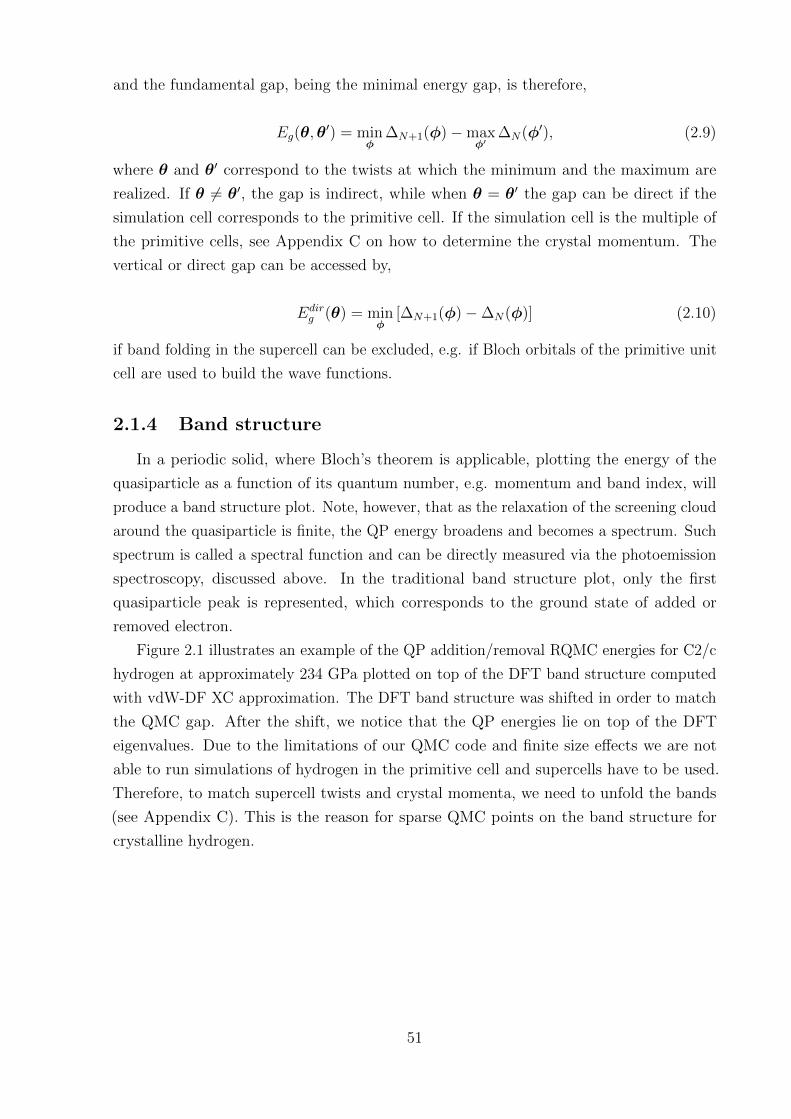
and the fundamental gap, being the minimal energy gap, is therefore,

Eg(θ,θ′) = min

φ∆N+1(φ)−max

φ′∆N(φ′), (2.9)

where θ and θ′ correspond to the twists at which the minimum and the maximum are

realized. If θ 6= θ′, the gap is indirect, while when θ = θ′ the gap can be direct if the

simulation cell corresponds to the primitive cell. If the simulation cell is the multiple of

the primitive cells, see Appendix C on how to determine the crystal momentum. The

vertical or direct gap can be accessed by,

Edirg (θ) = min

φ[∆N+1(φ)−∆N(φ)] (2.10)

if band folding in the supercell can be excluded, e.g. if Bloch orbitals of the primitive unit

cell are used to build the wave functions.

2.1.4 Band structure

In a periodic solid, where Bloch’s theorem is applicable, plotting the energy of the

quasiparticle as a function of its quantum number, e.g. momentum and band index, will

produce a band structure plot. Note, however, that as the relaxation of the screening cloud

around the quasiparticle is finite, the QP energy broadens and becomes a spectrum. Such

spectrum is called a spectral function and can be directly measured via the photoemission

spectroscopy, discussed above. In the traditional band structure plot, only the first

quasiparticle peak is represented, which corresponds to the ground state of added or

removed electron.

Figure 2.1 illustrates an example of the QP addition/removal RQMC energies for C2/c

hydrogen at approximately 234 GPa plotted on top of the DFT band structure computed

with vdW-DF XC approximation. The DFT band structure was shifted in order to match

the QMC gap. After the shift, we notice that the QP energies lie on top of the DFT

eigenvalues. Due to the limitations of our QMC code and finite size effects we are not

able to run simulations of hydrogen in the primitive cell and supercells have to be used.

Therefore, to match supercell twists and crystal momenta, we need to unfold the bands

(see Appendix C). This is the reason for sparse QMC points on the band structure for

crystalline hydrogen.

51

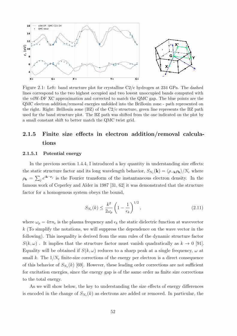
X+ G+ X′+ Y+ G+

4

6

8

10

12

14

16, (

eV)

vdW-DF - QMC C2/c-24QMC Ideal

Figure 2.1: Left: band structure plot for crystalline C2/c hydrogen at 234 GPa. The dashedlines correspond to the two highest occupied and two lowest unoccupied bands computed withthe vdW-DF XC approximation and corrected to match the QMC gap. The blue points are theQMC electron addition/removal energies unfolded into the Brillouin zone - path represented onthe right. Right: Brillouin zone (BZ) of the C2/c structure, green line represents the BZ pathused for the band structure plot. The BZ path was shifted from the one indicated on the plot bya small constant shift to better match the QMC twist grid.

2.1.5 Finite size effects in electron addition/removal calcula-

tions

2.1.5.1 Potential energy

In the previous section 1.4.4, I introduced a key quantity in understanding size effects:

the static structure factor and its long wavelength behavior, SNe(k) = 〈ρ−kρk〉/Ne where

ρk =∑

j eik · rj is the Fourier transform of the instantaneous electron density. In the

famous work of Ceperley and Alder in 1987 [31, 62] it was demonstrated that the structure

factor for a homogenous system obeys the bound,

SNe(k) ≤ k2

2ωp

(1− 1

εk

)1/2

, (2.11)

where ωp = 4πne is the plasma frequency and εk the static dielectric function at wavevector

k (To simplify the notations, we will suppress the dependence on the wave vector in the

following). This inequality is derived from the sum rules of the dynamic structure factor

S(k, ω) . It implies that the structure factor must vanish quadratically as k → 0 [91].

Equality will be obtained if S(k, ω) reduces to a sharp peak at a single frequency, ω at

small k. The 1/Ne finite-size corrections of the energy per electron is a direct consequence

of this behavior of SNe(k) [69]. However, these leading order corrections are not sufficient

for excitation energies, since the energy gap is of the same order as finite size corrections

to the total energy.

As we will show below, the key to understanding the size effects of energy differences

is encoded in the change of SNe(k) as electrons are added or removed. In particular, the

52

limiting behavior of SNe±1(k) as k → 0 will provide the dominant finite size correction.

For concreteness, we will assume a Slater-Jastrow form (see eq. 1.71) for the ground

state wave function Ψ0 ∝ D exp[−U ]. The determinant, D, is built out of Bloch orbitals,

ψqn(r) with q inside the first Brillouin zone, n is the band index, and U is, as defined in

eq. 1.72, a general symmetric n-body correlation factor [70]. For simplicity we assume it

is pairwise additive: U =∑

i<j u(ri, rj). Let us consider the action of eik · rj on a single

particle orbital ψqn(rj) in the Slater determinant of the ground state. In the limit of small

k, this can be approximately written as ψ(q+k)n(rj). According to Jacobi’s formula, the

determinant can be expanded in terms of its cofactors δDδψqn(rj)

as,

D =∑q,n

δD

δψqn(rj)ψqn(rj) (2.12)

Formally making the excitation means,

ρkΨ0 ∝∑j

eik · rj∑q,n

δD

δψqn(rj)ψqn(rj)e

−U (2.13)

=∑j

∑q,n

δD

δψqn(rj)eik · rjψqn(rj)e

−U ,

where the determinant was expanded for each j in the first summation. Notice that after

the summation over j the resulting determinant vanishes for small k if the Bloch orbital

(q+k, n) is already occupied in the ground state determinant. Considering Ne±1 electron

wave functions, Ψ0(Ne ± 1;±q,m) where Ne corresponds to the insulating state with fully

occupied bands in the Slater determinant, and qm denotes the additional particle/hole

orbital, based on equation 2.13 we get,

limk→0

ρkΨ0(Ne ± 1; q,m) = limk→0

∑j

∑q,n

δD

δψqn(rj)eik · rjψqn(rj)e

−U

= limk→0

∑j

δD

δψqn(rj)ψq+kn(rj)e

−U

∼ ±Ψ0(Ne ± 1; q + k,m), (2.14)

for k 6= 0 where different sign for particle or hole excitations on the r.h.s. is chosen to

match the most common sign convention, e.g. of ref. [92]. The limit k → 0 is discontinuous

since ρk=0Ψ0(Ne ± 1; q,m) ≡ (Ne ± 1)Ψ0(Ne ± 1; q,m).

Kohn [92, 93] has pointed out that in the insulating state the matrix elements,

limq′→q〈Ψ0(Ne ± 1; q,m)|ρq−q′ |Ψ0(Ne ± 1; q′,m)〉 = ±1

ε, (2.15)

53

approach the inverse dielectric constant, ε−1, up to a sign.

Substituting eq. 2.14 into eq. 2.15, suggests the following,

±1

ε∼ lim

q′→q〈Ψ0(Ne ± 1; q,m)|ρq−q′ lim

k→0ρk|Ψ0(Ne ± 1; q,m)〉 (2.16)

= limk→0〈Ψ0(Ne ± 1; q,m)|ρ−kρk|Ψ0(Ne ± 1; q,m)〉

= limk→0

(Ne ± 1)SNe±1(k),

where we put q′ = q + k. Permitting us to define a finite size behavior of the static

structure factor of insulators,

limk→0

S±k = α± +O(k2), S±k ≡ (Ne ± 1)SNe±1(k)−NeSNe(k), (2.17)

where the NeSNe(k) term was added to get the size correction for the addition/removal

energies and α± is proportional to ε−1. However, α± in general differs from ε−1 unless

eq. (2.14) is an exact equality.

Figure 2.2 shows the behavior of S±k for carbon and silicon crystals. Note that these

functions extrapolate to a nonzero value as k → 0.

The long wavelength behavior of the structure factor, eq. (2.17), similarly to the total

energy correction (see eq. 1.84), then gives rise to size corrections to excitation energies

through the potential energy term,[∫d3k

(2π)3− 1

Ω

∑k 6=0

]vk2S±k ' α±

|vM |2, (2.18)

where we have defined the Madelung constant as in eq. 1.83,

vM =

[1

Ω

∑k 6=0

−∫

d3k

(2π)3

]vk ∼ L−1 ∼ N−1/3

e . (2.19)

For the Coulomb potential, vM is proportional to L−1, the inverse linear extension of the

simulation cell. The negative proportionality constant depends on the boundary conditions,

e.g. cell geometry, and can be calculated by the Ewald image technique [94].

2.1.5.2 Kinetic energy

Following ref. [70] and section 1.4.4, we now discuss the kinetic energy contribu-

tion [∇U ]2/2 which arises from electron correlation. For a two-body Jastrow U =∑k ukρkρ−k/2Ω, and we are only interested in the long-wave length limit, k → 0, of

the electron-electron correlation, with wave vectors smaller than the reciprocal lattice

54

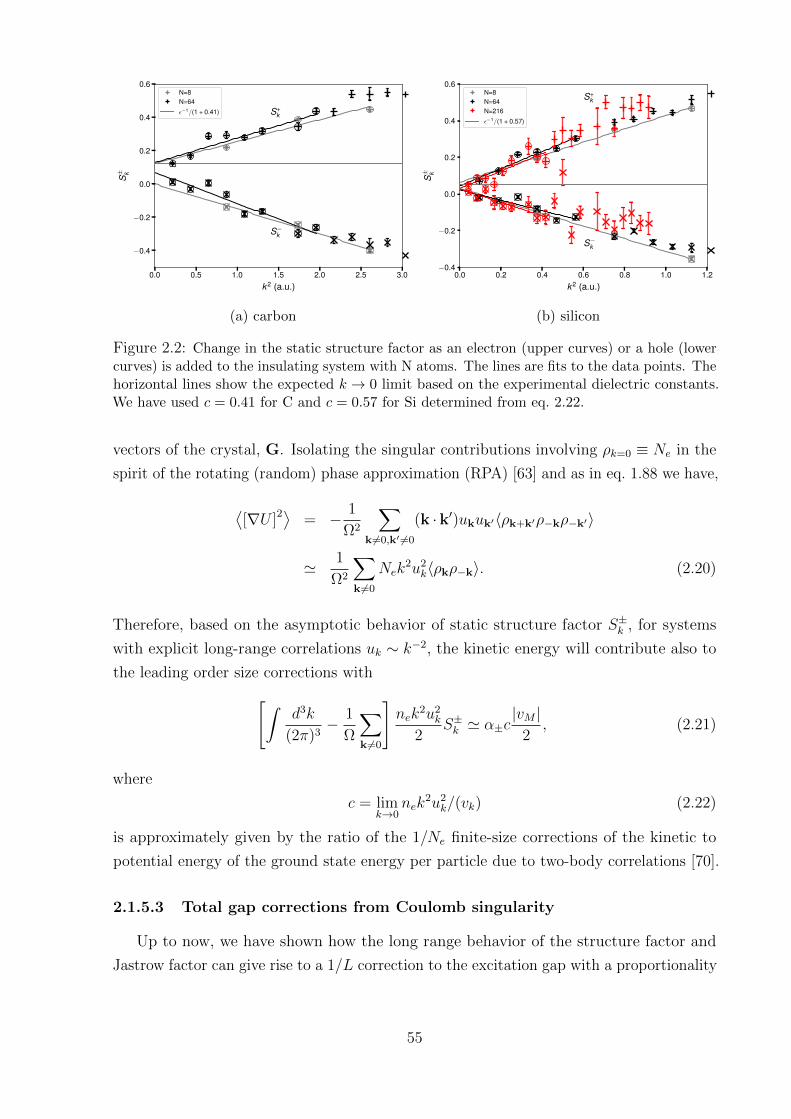
0.0 0.5 1.0 1.5 2.0 2.5 3.0

k2 (a.u.)

−0.4

−0.2

0.0

0.2

0.4

0.6

S± k

S+k

S−k

N=8N=64

ε−1/(1 + 0.41)

(a) carbon

0.0 0.2 0.4 0.6 0.8 1.0 1.2

k2 (a.u.)

−0.4

−0.2

0.0

0.2

0.4

0.6

S± k

S+k

S−k

N=8N=64N=216

ε−1/(1 + 0.57)

(b) silicon

Figure 2.2: Change in the static structure factor as an electron (upper curves) or a hole (lowercurves) is added to the insulating system with N atoms. The lines are fits to the data points. Thehorizontal lines show the expected k → 0 limit based on the experimental dielectric constants.We have used c = 0.41 for C and c = 0.57 for Si determined from eq. 2.22.

vectors of the crystal, G. Isolating the singular contributions involving ρk=0 ≡ Ne in the

spirit of the rotating (random) phase approximation (RPA) [63] and as in eq. 1.88 we have,

⟨[∇U ]2

⟩= − 1

Ω2

∑k 6=0,k′ 6=0

(k ·k′)ukuk′〈ρk+k′ρ−kρ−k′〉

' 1

Ω2

∑k 6=0

Nek2u2

k〈ρkρ−k〉. (2.20)

Therefore, based on the asymptotic behavior of static structure factor S±k , for systems

with explicit long-range correlations uk ∼ k−2, the kinetic energy will contribute also to

the leading order size corrections with[∫d3k

(2π)3− 1

Ω

∑k 6=0

]nek

2u2k

2S±k ' α±c

|vM |2, (2.21)

where

c = limk→0

nek2u2

k/(vk) (2.22)

is approximately given by the ratio of the 1/Ne finite-size corrections of the kinetic to

potential energy of the ground state energy per particle due to two-body correlations [70].

2.1.5.3 Total gap corrections from Coulomb singularity

Up to now, we have shown how the long range behavior of the structure factor and

Jastrow factor can give rise to a 1/L correction to the excitation gap with a proportionality

55

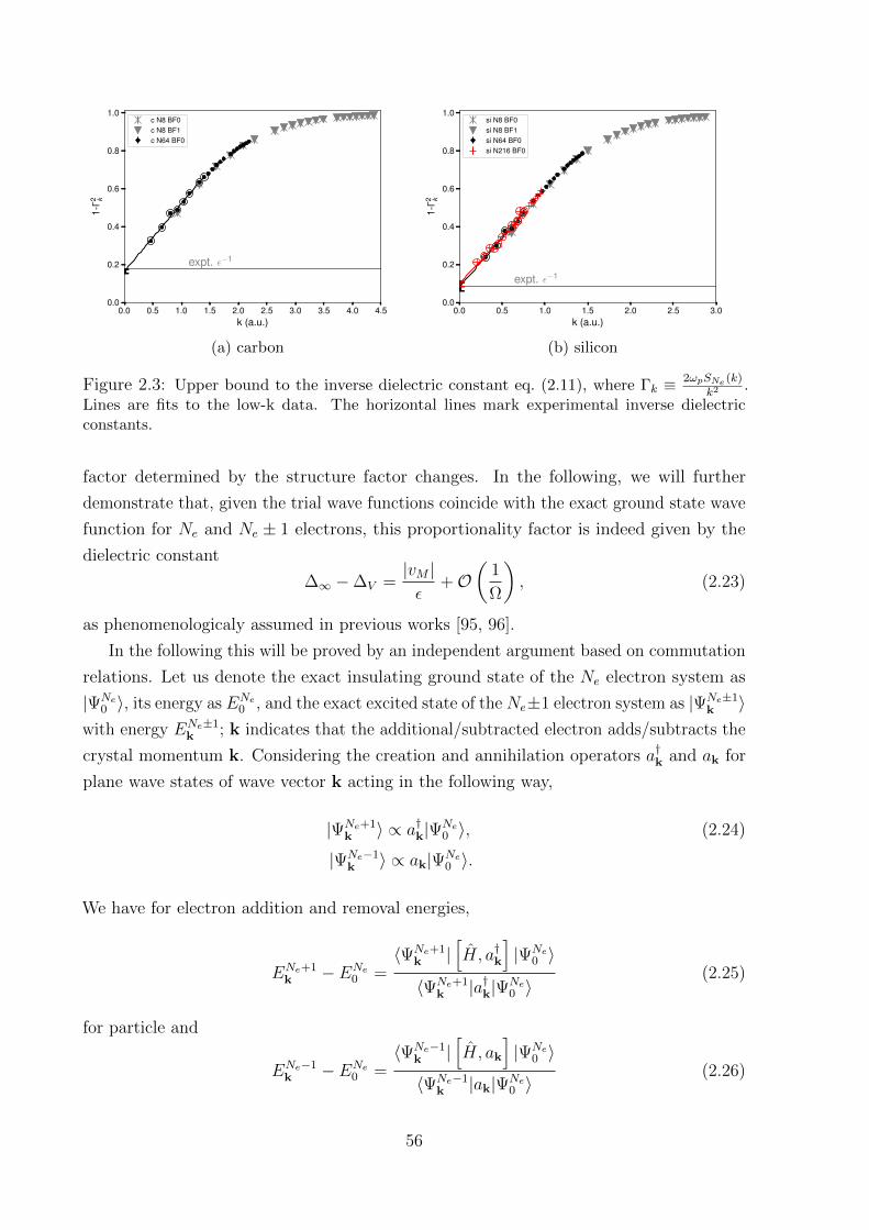
0.0 0.5 1.0 1.5 2.0 2.5 3.0 3.5 4.0 4.5k (a.u.)

0.0

0.2

0.4

0.6

0.8

1.0

1-Γ

2 k

expt. ε−1

c N8 BF0c N8 BF1c N64 BF0

(a) carbon

0.0 0.5 1.0 1.5 2.0 2.5 3.0k (a.u.)

0.0

0.2

0.4

0.6

0.8

1.0

1-Γ

2 k

expt. ε−1

si N8 BF0si N8 BF1si N64 BF0si N216 BF0

(b) silicon

Figure 2.3: Upper bound to the inverse dielectric constant eq. (2.11), where Γk ≡ 2ωpSNe (k)k2 .

Lines are fits to the low-k data. The horizontal lines mark experimental inverse dielectricconstants.

factor determined by the structure factor changes. In the following, we will further

demonstrate that, given the trial wave functions coincide with the exact ground state wave

function for Ne and Ne ± 1 electrons, this proportionality factor is indeed given by the

dielectric constant

∆∞ −∆V =|vM |ε

+O(

1

Ω

), (2.23)

as phenomenologicaly assumed in previous works [95, 96].

In the following this will be proved by an independent argument based on commutation

relations. Let us denote the exact insulating ground state of the Ne electron system as

|ΨNe0 〉, its energy as ENe

0 , and the exact excited state of the Ne±1 electron system as |ΨNe±1k 〉

with energy ENe±1k ; k indicates that the additional/subtracted electron adds/subtracts the

crystal momentum k. Considering the creation and annihilation operators a†k and ak for

plane wave states of wave vector k acting in the following way,

|ΨNe+1k 〉 ∝ a†k|ΨNe

0 〉, (2.24)

|ΨNe−1k 〉 ∝ ak|ΨNe

0 〉.

We have for electron addition and removal energies,

ENe+1k − ENe

0 =〈ΨNe+1

k |[H, a†k

]|ΨNe

0 〉〈ΨNe+1

k |a†k|ΨNe0 〉

(2.25)

for particle and

ENe−1k − ENe

0 =〈ΨNe−1

k |[H, ak

]|ΨNe

0 〉〈ΨNe−1

k |ak|ΨNe0 〉

(2.26)

56

for hole excitations.

In second quantization , the Hamiltonian, H = Te + Vee, is given by

Te =∑k

[k2

2a†kak +

∑G

u(G)a†k+Gak

], (2.27)

Vee =1

2V

∑q 6=0

vq [ρqρ−q −Ne] , (2.28)

u(G) the periodic crystal potential, and vq is the Coulomb potential between electrons,

ρq =∑

k a†k+qak, and Ne =

∑k a†kak.

Considering the commutator relations for fermions,

ai, a†j ≡ aia†j + a†jai = δij, (2.29)

a†i , a†j = ai, aj = 0,

the commutator involving the single-particle energy term becomes

[Te, a

†k

]=k2

2a†k +

∑G

u(G)a†G+k. (2.30)

There are corresponding terms for hole excitations, but none of these terms involve singular

contributions responsible for anomalous size effects, so that these terms do not contribute

at leading order. However, [Vee, a

†k

]=

1

V

∑q 6=0

vq

[ρqa

†k−q − 1

](2.31)

and

[Vee, ak] = − 1

V

∑q 6=0

vqρqak+q (2.32)

involve terms approaching the Coulomb singularity, vq ∼ q−2 →∞ for q → 0.

From these terms we get the leading order size corrections by noting that

limk,q→0

〈ΨNe+1k |ρqa†k−q|ΨNe

0 〉〈ΨNe+1

k |a†k|ΨNe0 〉

=1

2

[1

ε+ 1

](2.33)

and

limk,q→0

〈ΨNe−1k |ρqak+q|ΨNe

0 〉〈ΨNe−1

k |ak|ΨNe0 〉

= −1

2

[1 +

1

ε

]. (2.34)

Both relations can be obtained by extending Kohn’s diagrammatic approach [92] (see

supplementary information of [97]). Integrating around the vq singularity for small q in

57

eq. (2.31), we obtain the leading order finite size corrections. As before, this involves the

Madelung constant, Eq (2.19). In the particle channel we get |vM |2

(1ε− 1)

and in the hole

channel, |vM |2

(1ε

+ 1). The corrections independent of ε correspond to the change in the

background charge which cancel for the fundamental gap and we obtain eq. (2.23).

Previous, heuristic approaches [96] have suggested that one can use experimental or

DFT values of the dielectric constant for finite-size extrapolation. Our approach further

suggests that this value can be determined from the QMC structure factor extrapolated

to zero wave vector2

ε≡ (1 + c) lim

Ne→∞limk→0

[S+k + S−k

], (2.35)

with the singular behavior of the Jastrow factor determining c. We emphasize that the

order of the limits involved above is crucial.

An independent estimate of the dielectric constant is based on the inequality of eq. 2.11.

We can bound and estimate the value of dielectric constant using the structure factor of

the insulating ground state. By extrapolating 1− Γ2k vs. k to k = 0 we obtain an upper

bound to the inverse dielectric constant, where Γk ≡ 2ωpSNe(k)/k2. This involves only

the extensive part of the density-density correlations, thus, it is less sensitive to noise

and has much smaller statistical uncertainty. In fig. 2.3, we show that for C and Si, this

upper bound gives accurate values of the dielectric constant (see section 2.1.7 for a more

quantitative comparison).

2.1.5.4 Twist correction of two particle correlations

The above size effects explain the leading order 1/L correction to the single particle

gap. However, as we will see in our results, the asymptotic region, where this law can

be reliably applied, may still be difficult to reach for currently used system sizes and

next-to-leading order effects are important. Here, we show that an important part can be

corrected for, by further restoring the full symmetry properties in the contribution of the

direct Coulomb interaction.

For non homogeneous systems, it is convenient to separate the mean density from its

fluctuating components in the static structure factor [66], i.e.

SNe(k) =1

Ne

〈ρk〉〈ρ−k〉+ δSNe(k) (2.36)

δSNe(k) =1

Ne

〈(ρk − 〈ρk〉) (ρ−k − 〈ρ−k〉)〉 (2.37)

For crystals with periodic density distributions, the Fourier components of the mean

density, 〈ρk〉, only contribute for reciprocal lattice vectors, k ∈ G. The long wavelength

behavior of the structure factor is entirely due to the fluctuating part δSNe(k), which

therefore contains the leading order size effects [70]. However, the mean single particle

58

density, 〈ρ(r)〉 = V −1∑

k〈ρk〉eik · r, of the finite system may significantly differ from the

infinite one, particularly in cases where the supercell is not compatible with the full

symmetry group of the crystal.

Averaging over twisted boundary conditions is designed to restore the symmetry of the

crystal and thus accelerate the convergence of single particle densities to the thermodynamic

limit. In the following, we denote the twist averaged expectation value by

O ≡ 1

Mθ

∑θ

〈O〉Ne,θ (2.38)

where we have explicitly indicated the Ne and θ dependence on the expectation value

on the r.h.s. For any single particle theory, ρ(r) approaches its thermodynamic limit for

calculations at fixed Ne by averaging over a dense grid of twist angles (Mθ →∞). Within

many-body calculations, twist-averaging [68] takes over a large part of the size effects to

any observable linear in the density. Here, we extend this approach to correct also the

quadratic expression entering the two-body contributions of the total energy.

For the potential energy, this correction to the twist converged QMC calculation is

δV sNe =

1

2V

∑k

vkδC(k)

δC(k) = ρk ρ−k − ρkρ−k. (2.39)

For the ground state energies, this correction provides only a small improvement over our

previous correction [69, 70].

For the gap, many terms entering eq. (2.39) cancel, and the expression can be simplified.

Let us consider the case of adding/removing one electron at twist ψ to the insulating

ground state, denoting Π±k the difference of the respective densities

Π±k ≡ 〈ρk〉Ne±1,ψ − 〈ρk〉Ne,ψ (2.40)

In the thermodynamic limit, the density of the ground state system with Ne electrons

coincides with the twist averaged ground state density ρk, whereas we obtain ρk + Π±kfor the density of the Ne ± 1 electron system. Inserting into eq. (2.39), we obtain the

correction for the δV sNe±1,ψ,

δV sNe±1,ψ =

1

2V

∑kθ

vk[(ρk + Π±k )(ρ−k + Π±−k)− (〈ρk〉Ne,θ + Π±k δψθ)(〈ρ−k〉Ne,θ + Π±−kδψθ)

]=

1

2V

∑k

vk[Π±k(ρ−k − 〈ρ−k〉Ne,ψ

)+ (ρk − 〈ρk〉Ne,ψ) Π±−k + δC(k)

], (2.41)

59

which results into the difference between the two states,

δV sNe±1,ψ − δV s

Ne =1

V

∑k∈G

vkRe[(ρk − 〈ρk〉Ne,ψ) Π±−k

](2.42)

where only wave vectors of the reciprocal crystal lattice contribute to the sum. The

corresponding finite size correction for the gap, denoted by δ∆s in the following, is order

1/Ne or smaller, mainly determined by the changes of the ground state densities at the

first Bragg-peaks due to twist averaging.

Equation (2.42) can be understood as follows: it corrects the direct Coulomb interaction

between the electron/hole in the excited state (Π±) with the unexcited electrons. The

density of those electrons is expected to change by ρk − 〈ρk〉Ne,ψ in the thermodynamic

limit.

Converged ground state densities are naturally calculated within Grand-Canonical twist

averaged boundary conditions. It is straightforward to apply the correction eq. (2.42) to

all excitation energies. Alternatively, the corresponding DFT densities may be used. This

removes the stochastic error at the cost of introducing a small bias in the next-to-leading

order size correction.

2.1.6 Grand-Canonical twist averaged boundary condition (GCTABC)

In the following, we consider Ne electrons in a perfect crystal, neglecting both, zero

point motion of the ions and temperature effects. A uniform background charge (depending

on Ne) is added to assure global charge neutrality when adding or substracting electrons,

without introducing defects in the ionic crystal. The fundamental gap, eq. 2.1, is unaffected

by the background energy, because the background charge needed when adding an electron

cancels against the one needed when removing an electron. Periodic boundary conditions

of the charge densities are used to eliminate surface effects.

The energetic cost of adding an electron to the system at a fixed volume, V = L3,

defines the chemical potential

µ+Ne

= E0(Ne + 1)− E0(Ne). (2.43)

A non-vanishing gap implies a discontinuity in the chemical potential from eq. 2.1.

It is convenient to work in the grand-canonical (GC) ensemble. There, the chemical

potential µ is treated as an independent variable. At the ground state and fixed volume

in the GC ensemble, the number of electrons assumes the value Ne(µ) that minimize the

grand potential,

Ω(µ) = minNe

[E0(Ne)− µNe] . (2.44)

60

Insulators then represent an incompressible electronic state within the gap where ∂Ne/∂µ =

0 in the thermodynamic limit, i.e. when V →∞.

Periodic boundary conditions of theNe-body density are guaranteed by imposing twisted

boundary conditions on many-body wave function where the twist angle θ is applied to

the phase of the many body wave function as an electron is moved across the supercell,

as defined in eq. 1.77 Different twist angles modify the ground state energy E0(Ne,θ)

and twist averaging can significantly accelerate the convergence to the thermodynamic

limit [68].

Within the grand-canonical ensemble [69, 70], the number of electrons Ne(µ,θ) will

depend on θ for given chemical potential µ. Single particle finite size effects are reduced

by averaging over the twists. For the total number of independent twist angles Mθ, the

following quantities can be defined,

ω(µ) =1

MθV

∑θ

e0(ne(µ))− µne(µ), (2.45)

ne(µ) = (MθV )−1∑θ

Ne(µ,θ), (2.46)

e0(ne(µ)) = (MθV )−1∑θ

E0(Ne(µ),θ), (2.47)

where ω(µ) is the free energy density, e0(µ) the energy density and ne(µ) the electron

density. By eliminating µ from the last two equations we obtain the discontinuity in the

energy derivative at ne corresponding to the energy gap

∆gc = µ+ − µ− =de

dne

∣∣∣n+p

− de

dne

∣∣∣n−p, (2.48)

where the derivatives are computed at ne = np = Np/V . For any single electron theory the

electronic density, ne(µ), as well as the ground state energy density, e0(ne(µ)), coincide

exactly with the corresponding thermodynamic limit values, where the sum over twists

becomes an integral over the Brillouin zone. Size effects remaining after twist averaging

are due to electron-electron correlations.

Figure 2.4 illustrates e0(µ) and ne(µ) with result for solid hydrogen, computed from

HSE functional and from QMC (see section 2.1.8 for details). The value of the band

gap can be directly extracted from the width of the incompressible region. Alternatively,

eliminating µ in favor of ne, and plotting e0 as a function of ne, the fundamental gap is

obtained by the discontinuity of the derivative, according to eq. (2.48). It is straightforward

to generalize the fundamental gap for different symmetry sectors. For a perfect ionic

crystal, the total momentum of the electrons modulo reciprocal lattice vectors is conserved.

Imposing the total momentum of the electrons e.g. using Bloch type orbitals in the

Slater-determinant, the full band structure in the Brillouin zone can be mapped out. For

61

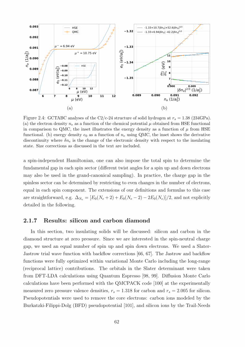
6 7 8 9 10 11 12 (eV)

0.087

0.088

0.089

0.090

0.091

0.092

0.093n e

(1/a

3 0)

= 6.94 eV+ = 10.75 eV

HSEQMC

6 8 10 12 (eV)

0.12

0.11

0.10

0.09

0.08

e 0 (e

V/a3 0) HSE

(a)

0.089 0.090 0.091 0.092ne (1/a3

0)

1.35

1.34

1.33

1.32

e 0 (e

V/a3 0)

-1.33+10.7| ne|+52.6| ne|5/3

-1.33+6.94| ne| -42.2| ne|5/3

0.000 0.009| ne|2/3 (1/a2

0)6

7

8

9

10

11

de0

dne (e

V)

(b)

Figure 2.4: GCTABC analyses of the C2/c-24 structure of solid hydrogen at rs = 1.38 (234GPa).(a) the electron density ne as a function of the chemical potential µ obtained from HSE functionalin comparison to QMC, the inset illustrates the energy density as a function of µ from HSEfunctional. (b) energy density e0 as a function of ne using QMC, the inset shows the derivativediscontinuity where δne is the change of the electronic density with respect to the insulatingstate. Size corrections as discussed in the text are included.

a spin-independent Hamiltonian, one can also impose the total spin to determine the

fundamental gap in each spin sector (different twist angles for a spin up and down electrons

may also be used in the grand-canonical sampling). In practice, the charge gap in the

spinless sector can be determined by restricting to even changes in the number of electrons,

equal in each spin component. The extensions of our definitions and formulas to this case

are straightforward, e.g. ∆Ne = [E0(Ne + 2) +E0(Ne− 2)− 2E0(Ne)]/2, and not explicitly

detailed in the following.

2.1.7 Results: silicon and carbon diamond

In this section, two insulating solids will be discussed: silicon and carbon in the

diamond structure at zero pressure. Since we are interested in the spin-neutral charge

gap, we used an equal number of spin up and spin down electrons. We used a Slater-

Jastrow trial wave function with backflow corrections [66, 67]. The Jastrow and backflow

functions were fully optimized within variational Monte Carlo including the long-range

(reciprocal lattice) contributions. The orbitals in the Slater determinant were taken

from DFT-LDA calculations using Quantum Espresso [98, 99]. Diffusion Monte Carlo

calculations have been performed with the QMCPACK code [100] at the experimentally

measured zero pressure valence densities, rs = 1.318 for carbon and rs = 2.005 for silicon.

Pseudopotentials were used to remove the core electrons: carbon ions modeled by the

Burkatzki-Filippi-Dolg (BFD) pseudopotential [101], and silicon ions by the Trail-Needs

62

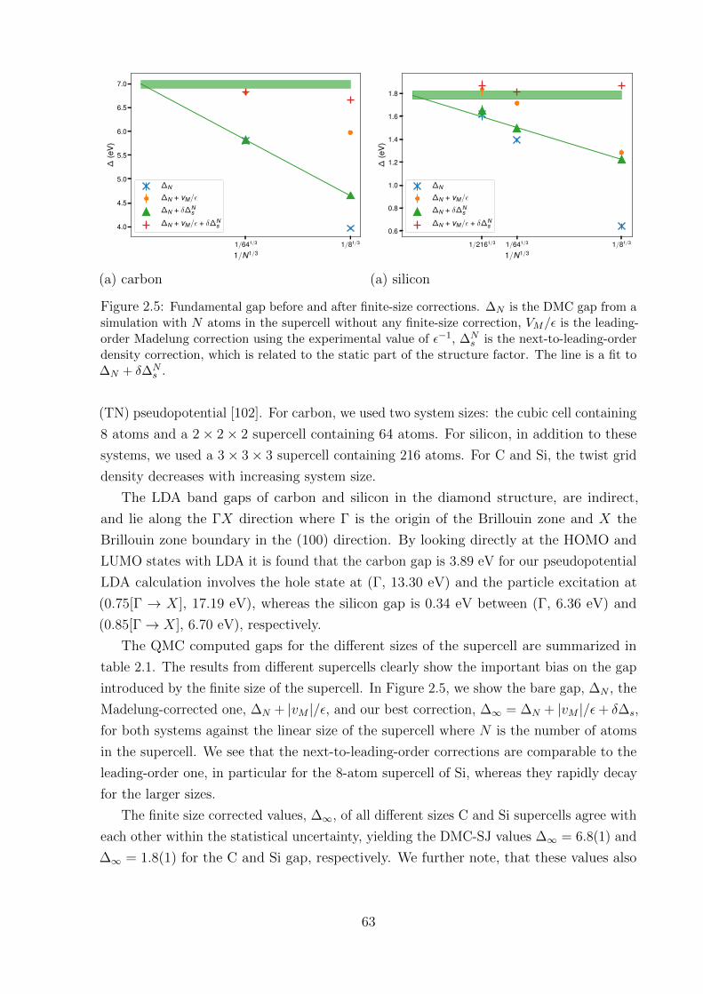
1/81/31/641/3

1/N1/3

4.0

4.5

5.0

5.5

6.0

6.5

7.0

∆(e

V)

∆N

∆N + vM/ε

∆N + δ∆Ns

∆N + vM/ε + δ∆Ns

(a) carbon

1/81/31/641/31/2161/3

1/N1/3

0.6

0.8

1.0

1.2

1.4

1.6

1.8

∆(e

V)

∆N

∆N + vM/ε

∆N + δ∆Ns

∆N + vM/ε + δ∆Ns

(a) silicon

Figure 2.5: Fundamental gap before and after finite-size corrections. ∆N is the DMC gap from asimulation with N atoms in the supercell without any finite-size correction, VM/ε is the leading-order Madelung correction using the experimental value of ε−1, ∆N

s is the next-to-leading-orderdensity correction, which is related to the static part of the structure factor. The line is a fit to∆N + δ∆N

s .

(TN) pseudopotential [102]. For carbon, we used two system sizes: the cubic cell containing

8 atoms and a 2× 2× 2 supercell containing 64 atoms. For silicon, in addition to these

systems, we used a 3× 3× 3 supercell containing 216 atoms. For C and Si, the twist grid

density decreases with increasing system size.

The LDA band gaps of carbon and silicon in the diamond structure, are indirect,

and lie along the ΓX direction where Γ is the origin of the Brillouin zone and X the

Brillouin zone boundary in the (100) direction. By looking directly at the HOMO and

LUMO states with LDA it is found that the carbon gap is 3.89 eV for our pseudopotential

LDA calculation involves the hole state at (Γ, 13.30 eV) and the particle excitation at

(0.75[Γ → X], 17.19 eV), whereas the silicon gap is 0.34 eV between (Γ, 6.36 eV) and

(0.85[Γ→ X], 6.70 eV), respectively.

The QMC computed gaps for the different sizes of the supercell are summarized in

table 2.1. The results from different supercells clearly show the important bias on the gap

introduced by the finite size of the supercell. In Figure 2.5, we show the bare gap, ∆N , the

Madelung-corrected one, ∆N + |vM |/ε, and our best correction, ∆∞ = ∆N + |vM |/ε+ δ∆s,

for both systems against the linear size of the supercell where N is the number of atoms

in the supercell. We see that the next-to-leading-order corrections are comparable to the

leading-order one, in particular for the 8-atom supercell of Si, whereas they rapidly decay

for the larger sizes.

The finite size corrected values, ∆∞, of all different sizes C and Si supercells agree with

each other within the statistical uncertainty, yielding the DMC-SJ values ∆∞ = 6.8(1) and

∆∞ = 1.8(1) for the C and Si gap, respectively. We further note, that these values also

63

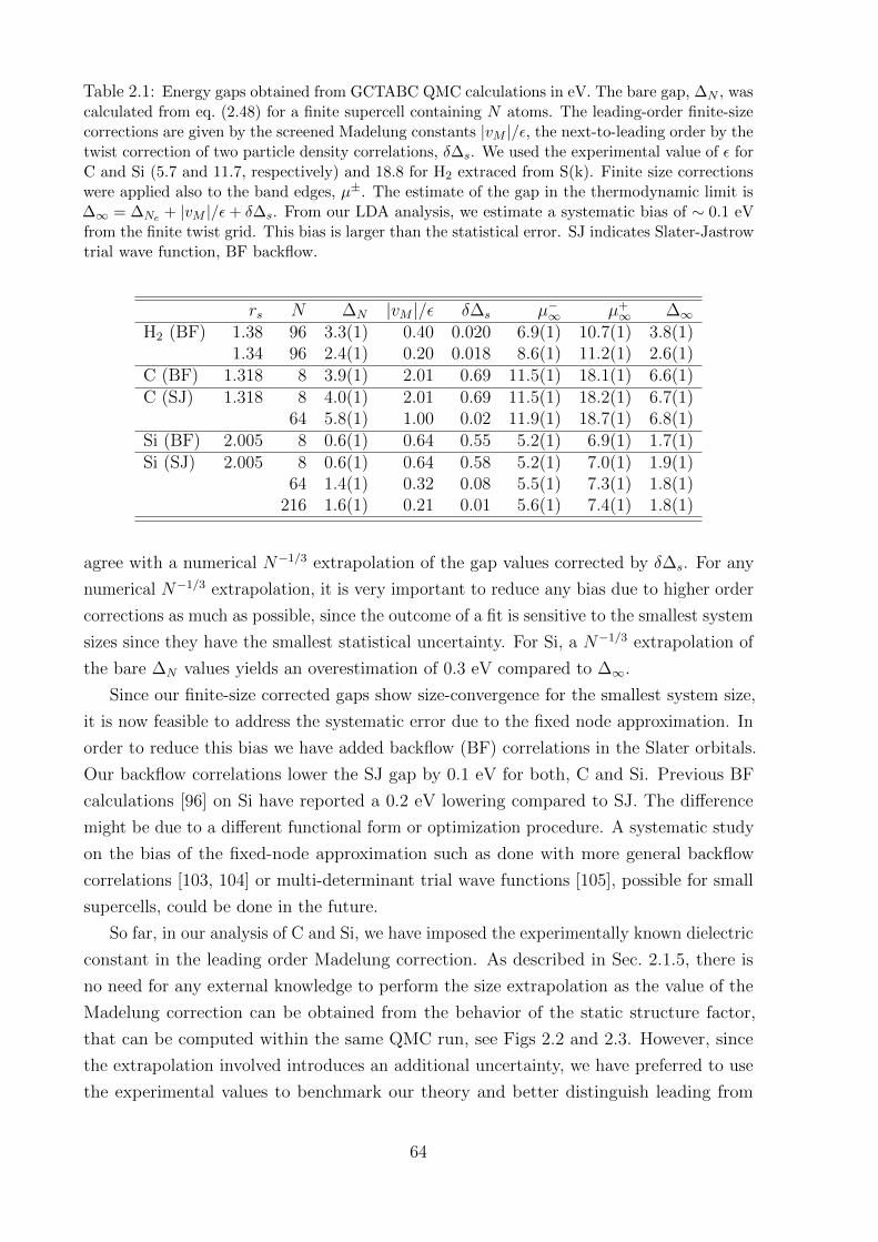
Table 2.1: Energy gaps obtained from GCTABC QMC calculations in eV. The bare gap, ∆N , wascalculated from eq. (2.48) for a finite supercell containing N atoms. The leading-order finite-sizecorrections are given by the screened Madelung constants |vM |/ε, the next-to-leading order by thetwist correction of two particle density correlations, δ∆s. We used the experimental value of ε forC and Si (5.7 and 11.7, respectively) and 18.8 for H2 extraced from S(k). Finite size correctionswere applied also to the band edges, µ±. The estimate of the gap in the thermodynamic limit is∆∞ = ∆Ne + |vM |/ε+ δ∆s. From our LDA analysis, we estimate a systematic bias of ∼ 0.1 eVfrom the finite twist grid. This bias is larger than the statistical error. SJ indicates Slater-Jastrowtrial wave function, BF backflow.

rs N ∆N |vM |/ε δ∆s µ−∞ µ+∞ ∆∞

H2 (BF) 1.38 96 3.3(1) 0.40 0.020 6.9(1) 10.7(1) 3.8(1)1.34 96 2.4(1) 0.20 0.018 8.6(1) 11.2(1) 2.6(1)

C (BF) 1.318 8 3.9(1) 2.01 0.69 11.5(1) 18.1(1) 6.6(1)C (SJ) 1.318 8 4.0(1) 2.01 0.69 11.5(1) 18.2(1) 6.7(1)

64 5.8(1) 1.00 0.02 11.9(1) 18.7(1) 6.8(1)Si (BF) 2.005 8 0.6(1) 0.64 0.55 5.2(1) 6.9(1) 1.7(1)Si (SJ) 2.005 8 0.6(1) 0.64 0.58 5.2(1) 7.0(1) 1.9(1)

64 1.4(1) 0.32 0.08 5.5(1) 7.3(1) 1.8(1)216 1.6(1) 0.21 0.01 5.6(1) 7.4(1) 1.8(1)

agree with a numerical N−1/3 extrapolation of the gap values corrected by δ∆s. For any

numerical N−1/3 extrapolation, it is very important to reduce any bias due to higher order

corrections as much as possible, since the outcome of a fit is sensitive to the smallest system

sizes since they have the smallest statistical uncertainty. For Si, a N−1/3 extrapolation of

the bare ∆N values yields an overestimation of 0.3 eV compared to ∆∞.

Since our finite-size corrected gaps show size-convergence for the smallest system size,

it is now feasible to address the systematic error due to the fixed node approximation. In

order to reduce this bias we have added backflow (BF) correlations in the Slater orbitals.

Our backflow correlations lower the SJ gap by 0.1 eV for both, C and Si. Previous BF

calculations [96] on Si have reported a 0.2 eV lowering compared to SJ. The difference

might be due to a different functional form or optimization procedure. A systematic study

on the bias of the fixed-node approximation such as done with more general backflow

correlations [103, 104] or multi-determinant trial wave functions [105], possible for small

supercells, could be done in the future.

So far, in our analysis of C and Si, we have imposed the experimentally known dielectric

constant in the leading order Madelung correction. As described in Sec. 2.1.5, there is

no need for any external knowledge to perform the size extrapolation as the value of the

Madelung correction can be obtained from the behavior of the static structure factor,

that can be computed within the same QMC run, see Figs 2.2 and 2.3. However, since

the extrapolation involved introduces an additional uncertainty, we have preferred to use

the experimental values to benchmark our theory and better distinguish leading from

64

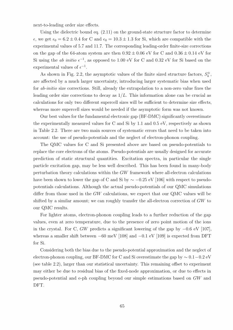
next-to-leading order size effects.

Using the dielectric bound eq. (2.11) on the ground-state structure factor to determine

ε, we get ε0 = 6.2± 0.4 for C and ε0 = 10.3± 1.3 for Si, which are compatible with the

experimental values of 5.7 and 11.7. The corresponding leading-order finite-size corrections

on the gap of the 64-atom system are then 0.92± 0.06 eV for C and 0.36± 0.14 eV for

Si using the ab initio ε−1, as opposed to 1.00 eV for C and 0.32 eV for Si based on the

experimental values of ε−1.

As shown in Fig. 2.2, the asymptotic values of the finite sized structure factors, S±k ,

are affected by a much larger uncertainty, introducing larger systematic bias when used

for ab-initio size corrections. Still, already the extrapolation to a non-zero value fixes the

leading order size corrections to decay as 1/L. This information alone can be crucial as

calculations for only two different supercell sizes will be sufficient to determine size effects,

whereas more supercell sizes would be needed if the asymptotic form was not known.

Our best values for the fundamental electronic gap (BF-DMC) significantly overestimate

the experimentally measured values for C and Si by 1.1 and 0.5 eV, respectively as shown

in Table 2.2. There are two main sources of systematic errors that need to be taken into

account: the use of pseudo-potentials and the neglect of electron-phonon coupling.

The QMC values for C and Si presented above are based on pseudo-potentials to

replace the core electrons of the atoms. Pseudo-potentials are usually designed for accurate

prediction of static structural quantities. Excitation spectra, in particular the single

particle excitation gap, may be less well described. This has been found in many-body

perturbation theory calculations within the GW framework where all-electron calculations

have been shown to lower the gap of C and Si by ∼ −0.25 eV [106] with respect to pseudo-

potentials calculations. Although the actual pseudo-potentials of our QMC simulations

differ from those used in the GW calculations, we expect that our QMC values will be

shifted by a similar amount; we can roughly transfer the all-electron correction of GW to

our QMC results.

For lighter atoms, electron-phonon coupling leads to a further reduction of the gap

values, even at zero temperature, due to the presence of zero point motion of the ions

in the crystal. For C, GW predicts a significant lowering of the gap by −0.6 eV [107],

whereas a smaller shift between −60 meV [108] and −0.1 eV [109] is expected from DFT

for Si.

Considering both the bias due to the pseudo-potential approximation and the neglect of

electron-phonon coupling, our BF-DMC for C and Si overestimate the gap by ∼ 0.1−0.2 eV

(see table 2.2), larger than our statistical uncertainty. This remaining offset to experiment

may either be due to residual bias of the fixed-node approximation, or due to effects in

pseudo-potential and e-ph coupling beyond our simple estimations based on GW and

DFT.

65

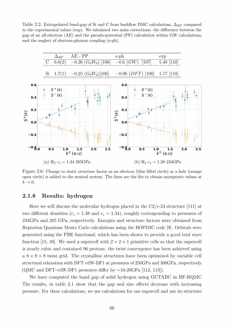
Table 2.2: Extrapolated band-gap of Si and C from backflow DMC calculations, ∆BF comparedto the experimental values (exp). We tabulated two main corrections: the difference between thegap of an all-electron (AE) and the pseudo-potential (PP) calculation within GW calculations,and the neglect of electron-phonon coupling (e-ph).

∆BF AE - PP e-ph expC 6.6(2) −0.26 (G0W0) [106] −0.6 (GW ) [107] 5.48 [110]

Si 1.7(1) −0.25 (G0W0)[106] −0.06 (DFT ) [108] 1.17 [110]

0.0 0.5 1.0 1.5 2.0 2.5k2 (a.u)

0.4

0.2

0.0

0.2

0.4

0.6

S±(k

)

S + (k)S (k)

(a) H2 rs = 1.34 285GPa

0.0 0.5 1.0 1.5 2.0 2.5k2 (a.u)

0.4

0.2

0.0

0.2

0.4

0.6

S±(k

)

S + (k)S (k)

(b) H2 rs = 1.38 234GPa

Figure 2.6: Change to static structure factor as an electron (blue filled circle) or a hole (orangeopen circle) is added to the neutral system. The lines are the fits to obtain asymptotic values atk → 0.

2.1.8 Results: hydrogen

Here we will discuss the molecular hydrogen placed in the C2/c-24 structure [111] at

two different densities (rs = 1.38 and rs = 1.34), roughly corresponding to pressures of

234GPa and 285 GPa, respectively. Energies and structure factors were obtained from

Reptation Quantum Monte Carlo calculations using the BOPIMC code [9]. Orbitals were

generated using the PBE functional, which has been shown to provide a good trial wave

function [15, 49]. We used a supercell with 2× 2× 1 primitive cells so that the supercell

is nearly cubic and contained 96 protons. the twist convergence has been achieved using

a 8 × 8 × 8 twist grid. The crystalline structures have been optimized by variable cell

structural relaxation with DFT vdW-DF1 at pressures of 250GPa and 300GPa, respectively.

(QMC and DFT-vdW-DF1 pressures differ by ∼10-20GPa [112, 113]).

We have computed the band gap of solid hydrogen using GCTABC in BF-RQMC

The results, in table 2.1 show that the gap and size effects decrease with increasing

pressure. For these calculations, we use calculations for one supercell and use its structure

66

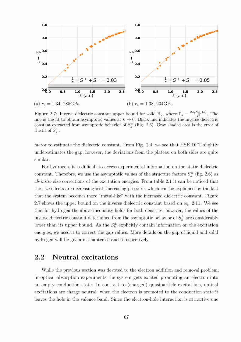
0.0 0.5 1.0 1.5 2.0 2.5k (a.u)

0.0

0.2

0.4

0.6

0.8

1.0

12 k

1 = S + + S = 0.03

(a) rs = 1.34, 285GPa

0.0 0.5 1.0 1.5 2.0 2.5k (a.u)

0.0

0.2

0.4

0.6

0.8

1.0

12 k

1 = S + + S = 0.05

(b) rs = 1.38, 234GPa

Figure 2.7: Inverse dielectric constant upper bound for solid H2, where Γk ≡ 2ωpSNe (k)k2 . The

line is the fit to obtain asymptotic values at k → 0. Black line indicates the inverse dielectricconstant extracted from asymptotic behavior of S±k (Fig. 2.6). Gray shaded area is the error ofthe fit of S±k .

factor to estimate the dielectric constant. From Fig. 2.4, we see that HSE DFT slightly

underestimates the gap, however, the deviations from the plateau on both sides are quite

similar.

For hydrogen, it is difficult to access experimental information on the static dielectric

constant. Therefore, we use the asymptotic values of the structure factors S±k (fig. 2.6) as

ab-initio size corrections of the excitation energies. From table 2.1 it can be noticed that

the size effects are decreasing with increasing pressure, which can be explained by the fact

that the system becomes more ”metal-like” with the increased dielectric constant. Figure

2.7 shows the upper bound on the inverse dielectric constant based on eq. 2.11. We see

that for hydrogen the above inequality holds for both densities, however, the values of the

inverse dielectric constant determined from the asymptotic behavior of S±k are considerably

lower than its upper bound. As the S±k explicitly contain information on the excitation

energies, we used it to correct the gap values. More details on the gap of liquid and solid

hydrogen will be given in chapters 5 and 6 respectively.

2.2 Neutral excitations

While the previous section was devoted to the electron addition and removal problem,

in optical absorption experiments the system gets excited promoting an electron into

an empty conduction state. In contrast to (charged) quasiparticle excitations, optical

excitations are charge neutral: when the electron is promoted to the conduction state it

leaves the hole in the valence band. Since the electron-hole interaction is attractive one

67

may expect a lowering of the excitation energy. The resulting energy gap to the ground

state is usually called excitonic or optical gap. Electron-hole interaction effect can also

play an important role when calculating the absorption spectrum, because the localization

of the electron-hole pair also affects the oscillator strength of the corresponding transitions.

Possible bound state are called excitons. Note that usually in solids, the electron-hole pair

is delocalized and the exciton is weakly bound, however there are many exceptions [73].

2.2.1 Single particle excitations

To zeroth order one might use the KS eigenvalues to describe neutral excitations.

Indeed, the unoccupied KS orbitals are one-electron states resulting from exactly the same

(local) potential as the occupied orbitals. The excited electron ”sees” the same Coulomb

field of N − 1 electrons as do the ground state electrons. However, excitations from an

independent particle picture, like Hartree-Fock, typically overestimate excitation energies,

as we have already discussed in section 2.1.1.

2.2.2 QMC excitations

Within the QMC, the trial wave function for neutral excitations is formed by replacing

an occupied orbital by an unoccupied in the ground-state determinant of the Slater-Jastrow

wave function. However, note that the variational principle only provides an energy which

is greater or equal to the lowest eigenstate within the given symmetry class. Therefore one

has to construct an excited state trial wave function that will be orthogonal by symmetry

to the lower-lying states. Even if the different determinants are orthogonal within the

DFT, the Jastrow factor in general causes the wave functions not to be any more strictly

orthogonal to the ground state. Running projector Monte Carlo for such states will only

guarantee an upper bound of the ground state, not the desired excited one. In practice, one

of the ways to achieve orthogonality is by substituting an orbital in the Slater determinant

by an unoccupied orbital which has a different crystal momentum k. Note that here we

refer to the crystal momentum, which coincides with k-points of the primitive cell, when

working in a supercell, to determine the crystal momentum it is necessary to unfold k-point

to the Brillouin zone of the primitive cell (see Appendix C).

Assuming that the wave function that models an excited state is appropriately con-

structed, i.e. is orthogonal to the lower lying excitations, the excitonic/optical gap will,

therefore, be the difference of total energies between the system with an electron promoted

to the excited state and the ground state,

Eex(ki,kf ) = E+N(ki,kf )− EN , (2.49)

where E+N(ki,kf ) is the lowest energy of the system with an electron promoted from the

68

initial occupied valence-band orbital at crystal momentum ki to the final unoccupied

conduction-band orbital at kf . Since momentum transfer can be negletced in photon

absorption, only vertical transitions are possible with ki = kf as long as nuclear motion is

not considered. The wave function of an excited state describes a correlated state of an

excited electron and a remaining hole, which creates an exciton. The excitonic effect is

defined as the difference between the quasiparticle gap, defined in eq. 2.8 and an excitonic

gap from eq. 2.49,

∆ex(ki,kf ) = EQP (ki,kf )− Eex(ki,kf ) (2.50)

= EN+1(kf ) + EN−1(ki)− E+N(ki,kf )− EN ,

the QMC total energies entering the equation above are statistically independent and can

be calculated in parallel.

2.2.3 Excited states expansion in VMC

In order to construct an excited state wave function orthogonal to the lower lying

excitations, we will use the generalized variational principle (i.e., the variational principle

for the energies of a set of orthogonal trial functions). In QMC this method was first

used by Ceperley and Bernu in 1988 [114]. Using the DMC algorithm, authors derived a

method for calculating the eigenvalues of several different excited states simultaneously.

In the following, we will construct a basis, consisting of M linearly independent excited

states Slater-Jastrow wave functions using different orbitals in the Slater determinant as

excitations,

Φi(R) = Di(R)e−U(R), (2.51)

where R represents electronic coordinate, Di is a Slater determinant with an excitation

i and e−U is a Jastrow pair correlation. An approximation to the eigenstates I of the

hamiltonian H can be constructed as a linear combinations of the basis functions,

|ΨI〉 =M∑i

cIi |Φi〉. (2.52)

Upper bound to the exact eigenvalues is then found by minimizing the Rayleigh quotient

with respect to cIi [114],

ΛI =

∑Mi,j c

I∗i c

Ij〈Φi|H|Φj〉∑M

i,j cI∗i c

Ij〈Φi|Φj〉

≥ EI . (2.53)

69

Minimizing ΛI with respect to cIi , one obtains the many-body generalized eigenvalue

equation,∂ΛI

∂cIi=∑j

cI∗j (Hij − ΛISij) = 0, (2.54)

which in matrix notation will become,

HcI − ΛIScI = 0. (2.55)

There will be M independent solutions (cI ,ΛI) to the equation above, unless S and H are

not singular. Due to MacDonald’s theorem [115], the eigenvalues ΛI are upper bounds to

the exact excited-state energies of the many-body Schrodinger equation,

ΛI ≥ EI for all 0 ≤ I ≤M − 1. (2.56)

Looking closely into the H matrix, its components can be rewritten in a way that they

can be sampled within the VMC run,

Hi,j =

∫dRφ∗i Hφj|ΦT |2 (2.57)

=

∫dRφ∗iφjELj|ΦT |2

= 〈φ∗iφjELj〉ΦT ≡ Hri,j,

where φi = Φi/ΦT and 〈...〉ΦT means the VMC sampling is over |ΦT |2. In practice, we

choose the ΦT to be the ground state trial wave function. As we work with extended

systems, we are sure that the trial wave function does not have zeroes and that there is

always an overlap between the ground and the first excited states. Of course, by choosing

ΨT as a combination between the ground and excited states will result in a smaller variance.

Index r indicates that we applied the Hamiltonian to the right. One can also apply the

Hamiltonian to the left getting,

H li,j ≡ 〈E∗Liφ∗iφj〉ΦT , (2.58)

taking the conjugate transpose of H li,j we get,

Hl† ≡ 〈ELjφjφ∗i 〉ΦT (2.59)

= 〈φ∗iφjELj〉ΦT ≡ Hr.

The property of Hl† = Hr is satisfied by construction, so the H matrix should be self-

adjoint. However, note that due to fluctuations, H will not be symmetric and one should

not symmetrize it, because, according to [116] that will destroy the zero-variance property.

70

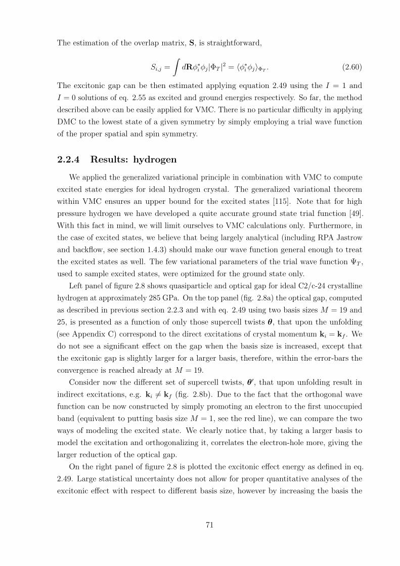
The estimation of the overlap matrix, S, is straightforward,

Si,j =

∫dRφ∗iφj|ΦT |2 = 〈φ∗iφj〉ΦT . (2.60)

The excitonic gap can be then estimated applying equation 2.49 using the I = 1 and

I = 0 solutions of eq. 2.55 as excited and ground energies respectively. So far, the method

described above can be easily applied for VMC. There is no particular difficulty in applying

DMC to the lowest state of a given symmetry by simply employing a trial wave function

of the proper spatial and spin symmetry.

2.2.4 Results: hydrogen

We applied the generalized variational principle in combination with VMC to compute

excited state energies for ideal hydrogen crystal. The generalized variational theorem

within VMC ensures an upper bound for the excited states [115]. Note that for high

pressure hydrogen we have developed a quite accurate ground state trial function [49].

With this fact in mind, we will limit ourselves to VMC calculations only. Furthermore, in

the case of excited states, we believe that being largely analytical (including RPA Jastrow

and backflow, see section 1.4.3) should make our wave function general enough to treat

the excited states as well. The few variational parameters of the trial wave function ΨT ,

used to sample excited states, were optimized for the ground state only.

Left panel of figure 2.8 shows quasiparticle and optical gap for ideal C2/c-24 crystalline

hydrogen at approximately 285 GPa. On the top panel (fig. 2.8a) the optical gap, computed

as described in previous section 2.2.3 and with eq. 2.49 using two basis sizes M = 19 and

25, is presented as a function of only those supercell twists θ, that upon the unfolding

(see Appendix C) correspond to the direct excitations of crystal momentum ki = kf . We

do not see a significant effect on the gap when the basis size is increased, except that

the excitonic gap is slightly larger for a larger basis, therefore, within the error-bars the

convergence is reached already at M = 19.

Consider now the different set of supercell twists, θ′, that upon unfolding result in

indirect excitations, e.g. ki 6= kf (fig. 2.8b). Due to the fact that the orthogonal wave

function can be now constructed by simply promoting an electron to the first unoccupied

band (equivalent to putting basis size M = 1, see the red line), we can compare the two

ways of modeling the excited state. We clearly notice that, by taking a larger basis to

model the excitation and orthogonalizing it, correlates the electron-hole more, giving the

larger reduction of the optical gap.

On the right panel of figure 2.8 is plotted the excitonic effect energy as defined in eq.

2.49. Large statistical uncertainty does not allow for proper quantitative analyses of the

excitonic effect with respect to different basis size, however by increasing the basis the

71

excitonic effect energy decreases. The difference between the direct and indirect excitations

is also minor, with the excitonic effect for indirect excitations being lower. Averaged over

all twists, the values for the excitonic effect energy are 0.37(0.21) eV for M = 19 and

0.30(0.21) eV for M = 25.

2.2.5 Size effects

Unfortunately, within this work we could not afford to consider systems with differ-

ent sizes in order to properly evaluate the finite size effect on the neutral excitations.

Nevertheless, we will still present general ideas on the origin of the size effects.

In the case of neutral excitations, an effective size of the electron hole interaction plays

an important role in determining the size effects. For the simulation cell of the linear size

exceeding the effective size of an exciton, the bound state can be formed and the FS error

should be dominated by the interaction of excitons with its periodic images and should

scale as 1/L3, with L being the linear cell size [96]. However, when the cell size is smaller

than the exciton effective size, the exciton consists of weakly interacting electron and hole

and the FS error dominated by the Madelung energies of the free electron and hole and

should scale as 1/L. Usually, in solids, an electron-hole interaction is delocalized resulting

in a single FS scaling similar to the quasiparticle one (see section 2.1.5) with the error

being 1/L.

An estimation of an effective exciton size can be obtained considering a hydrogen-like

model of an exciton and a hole interacting with each other. An effective length, Lex,

associated to the electron hole interaction can be estimated from the kinetic energy as,

∆ex =~2

2µL2ex

, (2.61)

where µ = memh/(me + mh) is the reduced mass of an electron me and a hole mh. If

assuming the mass of a hole mh = me and considering the ∆ex = 0.4 eV of solid C2/c-24

crystalline hydrogen discussed above, then the Lex ≈ 8.3 bohr, which is on the order of

the simulation cell size. This indicates that the excitonic effect is indeed delocalized and

the FS scaling of the optical gap would potentially be as in quasiparticle excitation of

the order of 1/L. However, all this is just a model and extensive studies of size effects of

neutral excitation should be performed before making any conclusion.

2.3 Conclusion

In this chapter, we have focused on computing the excited states with QMC. The first

major part of the discussion is on electron addition and removal energies. We have discussed

the fundamental gap, which is the difference between electron addition and removal energy,

72

and have defined its meaning within single electron theories and experiments. We have

proposed a new way of computing the fundamental gap using QMC only, which relies

on grand canonical twist averaging. Most importantly, we have proposed a scheme for

correcting finite simulation cell size effects when computing the fundamental gap. We have

shown that for charged systems, finite size supercell calculations are necessarily biased

by a finite size error decaying as 1/L, where the prefactor is determined by the absolute

value of the Madelung constant and the inverse dielectric constant. We have pointed out

that the 1/L functional form is encoded in the long wavelength behavior of the finite size

structure factor extrapolating to a nonvanishing value at the origin. We have applied this

procedure to determine the fundamental gap of molecular hydrogen at high pressure and

carbon and silicon in the diamond structure at zero pressure. Our finite-size corrected

gap values for carbon and silicon are larger than the experimental ones. Our results for C

and Si demonstrate that the bias due to the finite size supercell can be corrected for, so

precise values in the thermodynamic limit can be obtained for small supercells without

the need for numerical extrapolation.

In the second part of the chapter, we have discussed the neutral excitations, which are

made by promoting an electron from the valence to conduction band and characterized by

the coupling between the promoted electron and the hole that was left behind. Within

the QMC, we have constructed a wave function to model the excited states by considering

a basis of excited states Slater determinants multiplied by Jastrow factor. Applying the

generalized variational principle, we can assure that the new excited stated are orthogonal

to the lower lying states. Using this procedure, we have computed optical excitations

of solid crystalline hydrogen with variational Monte Carlo and have found that we can

capture an electron-hole correlation and lower the gap.

73

0 5 10 15 20

3.5

4.0

4.5

5.0

5.5

6.0

E g, e

V

QP RQMCOptical VMC M = 19Optical VMC M = 25

0 5 10 15 200.2

0.0

0.2

0.4

0.6

0.8

1.0

ex, e

V

M = 19, 0.44(0.21) eVM = 25, 0.35(0.20) eV

(a) Direct kf = ki

0 5 10 15 20′

3.0

3.5

4.0

4.5

5.0

5.5

E g, e

V

QP RQMCOptical VMC M = 19Optical VMC M = 1

0 5 10 15 20′

0.0

0.2

0.4

0.6

0.8

1.0ex

, eV

M = 19, 0.37(0.21) eVM = 25, 0.30(0.21) eV

(b) Indirect kf 6= ki

Figure 2.8: Left: Comparison of the optical VMC gap and quasiparticle (QP) RQMC gap,computed with QMC for C2/c-24 crystalline hydrogen at approximately 285 GPa at differentvalues of twist angle. Two different basis sizes are considered for the neutral excitations: M = 19(orange) and 25 (green). The values without size corrections are present for the quasiparticle gap(blue line). (a) Direct/vertical excitations with crystal momentum kf = ki and supercell twistθ. (b) Indirect excitations with crystal momentum kf 6= ki and supercell twist θ′ that uponunfolding gives indirect excitations, red line is done by considering only one neutral excitation(M=1) by substituting orbital in Slater determinant by the lowest unoccupied one. Right:excitonic effect energy as defined in eq. 2.50 for different basis sizes.

74

Chapter 3

Optical properties

We shall discuss in this chapter how the previously introduced electronic excited states

are closely related to the optical spectra of materials. By the spectra, we refer to an

object’s response to a probe, for example, light as a function of probe’s energy. Different

kinds of responses correspond to different ways of probing the material and measuring

the outcome. Here we will limit our focus to a linear response and its formalism within

the Kubo theory [4]. With all generality, we will start by defining the response functions

from Maxwell’s equations. Then, within independent particle theory, we will provide the

derivations of the Kubo-Greenwood formula for the conductivity [5] and will compare the

single particle optical spectra of ideal crystalline hydrogen with the results provided in

the literature. Finally, we will show the conductivity spectra, computed with many-body

Kubo theory within VMC for ideal crystalline hydrogen.

An introduction to the optical properties of solids can be found in the book of Wooten

[117]. An in-depth theoretical description of the linear response theory is provided in

the book of Mahan [118]. Moreover, detailed derivations of Kubo and Kubo-Greenwood

formalism is provided in the book chapter on electron transport by Allen [119].

3.1 Dielectric response functions

Propagation of electromagnetic waves in materials is described by Maxwell’s equations

[117, 120]. We shall write these as follows,

∇×H =1

c

∂D

∂t+

4π

cj,

∇× E = −1

c

∂B

∂t, (3.1)

∇ ·D = 0,

∇ ·B = 0,

75

where E and D are the electric field strength and displacement, H and B are the magnetic

field strength and induction and j is the current density. We have assumed that there

are no external sources, therefore the external current and electron density are zero. The

electric and magnetic fields E and H are related to their derived fields D and B via the

polarisation P and magnetisation M,

D = E + 4πP,

H = B− 4πM. (3.2)

However, when non-linear effects are neglected we can simplify this relations introducing

the coefficients,

D(r, t) =

∫dr′dt′ε(r, r′, t− t′)E(r, t),

B(r, t) =

∫dr′dt′µ(r, r′, t− t′)H(r, t),

j(r, t) =

∫dr′dt′σ(r, r′, t− t′)E(r, t), (3.3)

P(r, t) =

∫dr′dt′χe(r, r

′, t− t′)E(r, t),

M(r, t) =

∫dr′dt′χm(r, r′, t− t′)H(r, t),

where ε, µ, σ, χe and χm are complex dielectric tensor, permeability tensor, conductivity

tensor, (electric) susceptibility and (magnetic) permeability. From eqs. 3.2 and 3.3 we

have,

ε = 1 + 4πχe, (3.4)

µ = 1 + 4πχm.

In the following, we will consider a non-magnetic media by setting µ = 1 and χm = 0.

Eliminating the magnetic field by substituting the first equation into the second in eqs.

3.2 and using relations in eqs. 3.3, one obtains a wave equation for the electric field E,

∇2E =ε

c2

∂2E

∂t2+

4πσ

c2

∂E

∂t. (3.5)

For optical fields, we must look for a sinusoidal wave propagated with dissipation, K, at

76

frequency, ω,

E = E0 expi(K · r− ωt), (3.6)

the real part of K can be identified as a wave vector, while the imaginary part accounts

for attenuation of the wave inside the material. Then our wave equation requires,

−K2 = −εω2

c2− 4πiσω

c2. (3.7)

We can define a complex refractive index N such that,

K =ω

cN =

ω

c(n + ik), (3.8)

where n is the refractive index and k is the extinction coefficient. Rewriting the eq. 3.6 as,

E = E0 exp−(ωc

k · r)

expi(ωc

n · r− ωt)

, (3.9)

we get the equation describing the attenuation of wave amplitude with distance. The

fractional decrease in intensity with distance refers to the absorption coefficient, defined

as,

α = −1

I

dI

dr, (3.10)

where I is the intensity that is proportional to the square of the wave amplitude, from eqs.

3.9 and 3.10 we find,

α = 2ωk/c, (3.11)

here and in the following we will consider that the wave propagation vector is just in one

direction (plane waves). Combining eqs. 3.7 and 3.8 we obtain expressions for ε and σ,

ε = n2 − k2, (3.12)

4πσ/ω = 2nk, (3.13)

together they can be identified as a complex dielectric function,

ε = ε1 + iε2 = N2, (3.14)

ε1 = n2 − k2,

ε2 = 4πσ/ω = 2nk.

77

All these quantities are, in the most general case, frequency dependent. From eqs. 3.14 we

can see that the ε1 and ε2 are related, together with n and k. These quantities depend

on each other in a quite fundamental way by means of the Kramers-Kronig dispersion

relations [121, 122], which for any complex function χ(ω), which is analytic in the closed

upper half-plane of ω give,

Reχ(ω) =1

πP∫ ∞−∞

dω′Imχ(ω′)

ω′ − ω , (3.15)

Imχ(ω) = − 1

πP∫ ∞−∞

dω′Reχ(ω′)

ω′ − ω ,

where where P denotes the Cauchy principal value.

When concering the optical properties of solids, often the normal incidence reflectivity

is involved. In this case we want to construct a solution to Maxwell’s equations 3.2 matched

to an incident and reflected wave outside. Restricting the wave propagation to x direction

we have for the wave outside in the vacuum,

Ez = Eiei(ωxc −ωt) + Ere

−i(ωxc +ωt), (3.16)

where the Er < Ei. Inside the material we have the transmitted part,

Ez = Etei(kx−ωt), (3.17)

with the amplitude conservation boundary condition Ei + Er = Et. There is as well a

magnetic field Hy associated with these waves,

−∂xEz =iω

cHy, (3.18)

resulting in the condition Ei − Er = NEt. Normal incidence reflectivity is defined as,

R =

∣∣∣∣ErEi∣∣∣∣2 =

∣∣∣∣1−N1 +N

∣∣∣∣2 =(n− 1)2 + k2

(n+ 1)2 + k2< 1. (3.19)

Therefore, by measuring the reflectivity and absorption coefficient, all the optical constant

can be determined, which will help to infer many properties of the material. In our interest

is to compare measured optical constants to the theoretical predictions. We will only

consider here the linear response functions. Theoretically, they can be determined by

considering the response of the system to an external perturbation.

78

3.2 Linear response theory

A linear response of an expectation value of an operator O to an external field Eext

can be written via the coefficient χ,

〈O(r, t)〉ext = 〈O(r, t)〉+

∫dr′dt′χ(r, r′, t− t′)Eext(r′, t′), (3.20)

which resembles to the macroscopic response coefficients in eqs. 3.3. It was shown by

Kubo in 1957 [4] that the linear response to a time dependent perturbation Hext(t) writes

as

δ〈O(t)〉 = i

∫ t

t0

dt′〈Ψ0|[HextH (t′), OH(t)

]|Ψ0〉, (3.21)

where subscript H denotes the Heisenberg picture and |Ψ0〉 is the many-body ground state.

Now, consider the external perturbation to a scalar field Hext(t) =∫drn(r, t)V ext(r, t),

where n(r, t) is the electron density operator. Such perturbation would induce a charge

density nind in the system and the response can be written according to eq. 3.21 as

〈nind(r, t)〉 = i

∫ t

t0

dt′∫dr′V ext(r′, t′)〈Ψ0| [n(r′, t′), n(r, t)] |Ψ0〉. (3.22)

The response function χ now can be written, by combining eq. 3.20 and eq. 3.22,

χ(r, r′, t− t′) = −iΘ(t− t′)〈Ψ0| [n(r, t), n(r′, t′)] |Ψ0〉, (3.23)

where Θ(t− t′) has been introduced to meet the causality conditions to be able to write

the response in the form of eq. 3.20. Elaborating further by opening the commutator,

inserting the completeness relation for the N-particle basis states∑

i |Ψi〉〈Ψi| = 1 and

putting τ = t− t′ we get

χ(r, r′, τ) = −iΘ(τ)∑i

〈Ψ0|n(r, τ)|Ψi〉〈Ψi|n(r′, 0)|Ψ0〉+ c.c. (3.24)

Now, recalling from eq. 3.22 that n(r, τ) = eiH0τn(r, 0)e−iH0τ and denoting the matrix

element ρi(r) = 〈Ψ0|n(r, 0)|Ψi〉, eq. 3.24 transforms to

χ(r, r′, τ) = −iΘ(τ)∑i

[ρi(r)ρ∗i (r

′)ei(E0−Ei)τ − c.c], (3.25)

79

where Ei is the energy of the ith state. The Fourier transform (FT) to a frequency domain

brings us to the final expression for χ,

χ(r, r′, ω) =∑i

[ρi(r)ρ∗i (r

′)

ω − (E0 − Ei) + iη+

ρi(r′)ρ∗i (r)

ω + (E0 − Ei) + iη

], (3.26)

where infinitesimal η was introduced to have the time integral in FT converge. In the end

one should consider η → 0.

3.3 Independent particle polarisability

Considering the independent particle electronic system and writing χ in single particle

orbitals, φn(r), we get

χ0(r, r′, ω) =∑nn′

2(fn − fn′)φ∗n(r)φn′(r)φ∗n′(r′)φn(r′)

ω − (εn − εn′) + iη, (3.27)

where χ0 states for the independent particle polarizability and fn is the occupation number.

All the quantum numbers are contained in the label n. Independent particle irreducible

polarizability, χ0, is often called the random phase approximation (RPA), the name that

is related historically to the RPA used in section 1.4.4. When Fourier transformed, going

from r to q space, and considering the single particles orbitals as Bloch functions with

n = (i,k), with k being in the first Brillouin zone, the independent particle polarisability

obtains the usual form

χ0G,G′(q, ω) =

2

Ω

∑k,k′,i,j

(fk,i − fk′,j)〈φk,i|ei(q+G)r|φk′,j〉〈φk′,j|e−i(q+G′)r|φk,i〉ω − (εk,i − εk′,j) + iη

, (3.28)

where Ω is the cell volume, which comes from performing the Fourier transform and

〈φk,i|ei(q+G)r|φk′,j〉 ≡∫

Ω

dru∗k,ie−ikriei(q+G)ruk′,je

−ik′rj (3.29)

is calculated as an integral over the cell with volume Ω. Vector q is lying within the first

Brillouin zone and vectors G and G′ are the reciprocal lattice vectors. It can be shown

that in order to obtain a macroscopic polarisability it is necessary to take G = G′ = 0,

considering only the first Brillouin zone. Therefore, in the following we omit indexes G

and G′, considering only zero’s components. Note further that due to the momentum

conservation k′ = k + q, the sum over k′ can be omitted,

χ0(q, ω) =2

Ω

∑k,i,j

(fk,i − fk+q,j)|〈φk,i|eiqr|φk+q,j〉|2ω − (εk,i − εk+q,j) + iη

, (3.30)

80

the dielectric function in Fourier space, ε(q, ω) = 1− 4πe2

q2 χ(q, ω), becomes

ε0(q, ω) = 1− 8πe2

Ωq2

∑k,i,j

(fk,i − fk+q,j)|〈φk,i|eiqr|φk+q,j〉|2ω − (εk,i − εk+q,j) + iη

, (3.31)

in the following we will consider only the long-wavelength dielectric function, i.e. q→ 0

limit. The exponent can by then expanded, eiqr ' 1 + iqr, and the dielectric function for

insulators writes as a tensor,

ε0;α,β(ω) = 1− 8πe2

Ω

∑k,i,j

(fk,i − fk,j)〈φk,i|rα|φk,j〉〈φk,j|rβ|φk,i〉ω − (εk,i − εk,j) + iη

, (3.32)

For small η the imaginary part of denominator in eq. 3.32 behaves like the Dirac delta

function,

limη→0

Im

(1

ω − (εk,i − εk,j) + iη

)= lim

η→0

−η[ω − (εk,i − εk,j)]2 − η2

(3.33)

= −πδ(ω − (εk,i − εk,j)).

The imaginary part of the dielectric function is then,

ε0;α,β2 (ω) =

8π2e2

Ω

∑k,i,j

(fk,i − fk,j)〈φk,i|rα|φk,j〉〈φk,j|rβ|φk,i〉 (3.34)

×δ(ω − (εk,i − εk,j)).

3.4 Kubo-Greenwood electrical conductivity

For systems with periodic boundary conditions it is useful to transform the matrix

elements in eq. 3.35 from rα to ∇α. Using the commutator relation (in SI units, for

comparison to the literature and for local pseudopotentials),

i

~[H, rα] = −i~∇α

m, (3.35)

the matrix elements of rα can be expressed in terms of ∇α as follows,

〈φk,i|rα|φk,j〉 =~2

m

〈φk,i|∇α|φk,j〉εk,i − εk,j

. (3.36)

81

The real part of the independent particle conductivity σ1(ω), according to eq. 3.14, can

be expressed as,

σ1(ω) =ωε24π

. (3.37)

Explicitly including the directionality dependence, the conductivity then fully described

by the Cartesian tensor,

σα,β1 (ω) =2πe2~2

m2Ωω

∑k,i,j

(fk,i − fk,j)〈φk,i|∇α|φk,j〉〈φk,j|∇β|φk,i〉δ(ω − (εk,i − εk,j)) (3.38)

the imaginary part is easily accessible via the Kramers-Kronig relations defined in eq. 3.15.

3.4.1 Optical spectra of hydrogen

In the following section, we will discuss the optical spectra of ideal crystalline hydrogen

computed with the Kubo-Greenwood (KG) formula. We considered C2/c-24 and Cmca-

12 crystalline symmetry at approximately 300 GPa. Calculations of the eigenstates

and eigenvalues were done using HSE [48] and vdW-DF2 [123] XC approximation using

Quantum Espresso [98, 99], Kubo-Greenwood conductivity was then evaluated with the

KGEC code [124]. Note that, as in section 2.1.8, the crystalline structures have been

optimized by variable cell structural relaxation with DFT vdW-DF1 at pressures of 300

GPa. From the real and imaginary parts of the conductivity, all the other optical properties

can be inferred using relations in eqs. 3.14 and 3.19.

First, we discuss the convergence of the spectra with respect to the simulation parame-

ters. Figure 3.1 shows the real and imaginary part of the Kubo-Greenwood conductivity

of C2/c-24 hydrogen crystal at 300 GPa, computed for a 2× 2× 1 supercell of 96 nuclei.

The convergence is tested for three parameters: number of k-points, the total number of

bands included in DFT calculations, and smearing used to represent the delta function in

the equation for the KG conductivity. For all the KG calculations within this thesis, we

used Gaussians to represent the delta function. Changing the number of bands results in

the largest changes in the spectrum, middle panel of fig. 3.1. In order to reach the full

convergence, we will have to include much more than 70 bands in our DFT calculation with

96 electrons. However, sometimes one is just interested in the beginning of the spectrum

(up to ∼8 eV, sometimes called the edge or profile ), for that region, the convergence

can be achieved already with 56 bands. On the top panel of fig. 3.1 conductivity with

the different number of k-points is presented, the convergence is reached already with

8× 8× 8 grid. Finally, the test of the smearing factor in the lower panel of fig. 3.1 done at

8× 8× 8 k-point grid shows that the spectra are best represented at 0.2 eV. The top and

the bottom panels are connected, indeed, the dependency is that by increasing the size of

k-grid, the smearing needed for a smooth representation of the spectra should decrease.

82

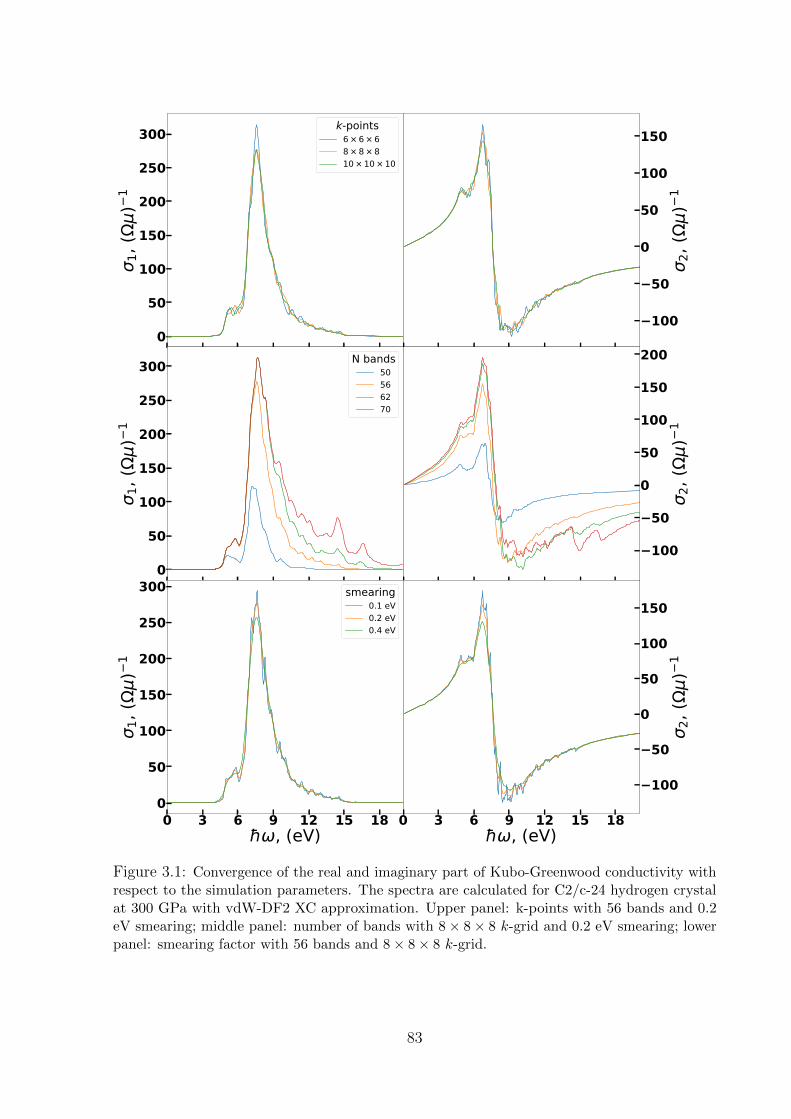
0 3 6 9 12 15 18

0

50

100

150

200

250

3001,

()

1k-points

6 × 6 × 68 × 8 × 810 × 10 × 10

0 3 6 9 12 15 18

100

50

0

50

100

150

2, (

)1

0 3 6 9 12 15 18E , eV0

50

100

150

200

250

300

1, (

)1

N bands50566270

0 3 6 9 12 15 18

100

50

0

50

100

150

200

2, (

)1

0 3 6 9 12 15 18, (eV)

0

50

100

150

200

250

300

1, (

)1

smearing0.1 eV0.2 eV0.4 eV

0 3 6 9 12 15 18, (eV)

100

50

0

50

100

150

2, (

)1

Figure 3.1: Convergence of the real and imaginary part of Kubo-Greenwood conductivity withrespect to the simulation parameters. The spectra are calculated for C2/c-24 hydrogen crystalat 300 GPa with vdW-DF2 XC approximation. Upper panel: k-points with 56 bands and 0.2eV smearing; middle panel: number of bands with 8× 8× 8 k-grid and 0.2 eV smearing; lowerpanel: smearing factor with 56 bands and 8× 8× 8 k-grid.

83

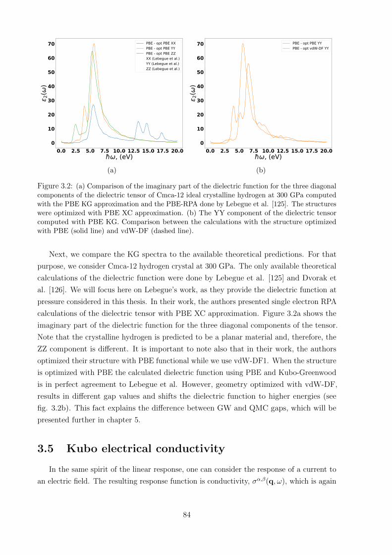
0.0 2.5 5.0 7.5 10.0 12.5 15.0 17.5 20.0, (eV)

0

10

20

30

40

50

60

702(

)PBE - opt PBE XXPBE - opt PBE YYPBE - opt PBE ZZXX (Lebegue et al.)YY (Lebegue et al.)ZZ (Lebegue et al.)

(a)

0.0 2.5 5.0 7.5 10.0 12.5 15.0 17.5 20.0, (eV)

0

10

20

30

40

50

60

70

2()

PBE - opt PBE YYPBE - opt vdW-DF YY

(b)

Figure 3.2: (a) Comparison of the imaginary part of the dielectric function for the three diagonalcomponents of the dielectric tensor of Cmca-12 ideal crystalline hydrogen at 300 GPa computedwith the PBE KG approximation and the PBE-RPA done by Lebegue et al. [125]. The structureswere optimized with PBE XC approximation. (b) The YY component of the dielectric tensorcomputed with PBE KG. Comparison between the calculations with the structure optimizedwith PBE (solid line) and vdW-DF (dashed line).

Next, we compare the KG spectra to the available theoretical predictions. For that

purpose, we consider Cmca-12 hydrogen crystal at 300 GPa. The only available theoretical

calculations of the dielectric function were done by Lebegue et al. [125] and Dvorak et

al. [126]. We will focus here on Lebegue’s work, as they provide the dielectric function at

pressure considered in this thesis. In their work, the authors presented single electron RPA

calculations of the dielectric tensor with PBE XC approximation. Figure 3.2a shows the

imaginary part of the dielectric function for the three diagonal components of the tensor.

Note that the crystalline hydrogen is predicted to be a planar material and, therefore, the

ZZ component is different. It is important to note also that in their work, the authors

optimized their structure with PBE functional while we use vdW-DF1. When the structure

is optimized with PBE the calculated dielectric function using PBE and Kubo-Greenwood

is in perfect agreement to Lebegue et al. However, geometry optimized with vdW-DF,

results in different gap values and shifts the dielectric function to higher energies (see

fig. 3.2b). This fact explains the difference between GW and QMC gaps, which will be

presented further in chapter 5.

3.5 Kubo electrical conductivity

In the same spirit of the linear response, one can consider the response of a current to

an electric field. The resulting response function is conductivity, σα,β(q, ω), which is again

84

given by the Kubo formula [4, 118] (in SI units, for future comparison to the literature),

σα,β(q, ω) =1

Ω~ω

∫ ∞0

dteiωt〈[j†α(q, t), jβ(q, 0)

]〉 (3.39)

the angular brackets

〈O〉 ≡ 1

Z

∑I

e−βEI 〈I|O|I〉 (3.40)

mean a canonical ensemble average using the equilibrium density matrix, Z =∑

I e−βEI is

the partition function and |I〉 is a complete set of many-body eigenstates of the system

before the external field is applied, H|I〉 = EI |I〉. Considering Heisenberg time-dependence

for the current ,

jα(q, t) = exp(iHt/~)jα(q, 0) exp(−iHt/~), (3.41)

with the time independent Fourier transform of the current operator being,

jα(q) = − 1

2m

∑n

ei[pn,αe

iq · rn + eiq · rnpn,α]. (3.42)

The time integral can be solved by assigning to a frequency a small positive imaginary part,

ω → ω + iη. In the further we will as well work in q→ 0 limit in the current operator. If

we know the complete set of many-body eigenstates |I〉, then eq. 3.39 reads,

σα,β(ω) =i

Ωω

∑IJ

e−βEI − e−βEJZ

〈I|j†α|J〉〈J |jβ|I〉~ω − (EJ − EI) + iη

. (3.43)

When considering just the real part of the conductivity, the denominator can be transformed

to a delta function as in eq. 3.34

σα,β1 (ω) =π

Ωω

∑IJ

e−βEI − e−βEJZ

〈I|j†α|J〉〈J |jβ|I〉δ(~ω − (EJ − EI)). (3.44)

Consider now low temperature limit, so only the ground state will contribute to the density

matrix. Regrouping the temperature factors, e−βEI (1− e−β(EJ−EI)), we get,

σα,β1 (ω) =π(1− e−β~ω

)ΩωZ

∑IJ

e−βEI 〈I|j†α|J〉〈J |jβ|I〉δ(~ω − (EJ − EI)) (3.45)

→β→∞

π

Ωω

∑J

〈0|j†α|J〉〈J |jβ|0〉δ(~ω − (EJ − E0)).

85

Rewriting the current operator in the q→ 0 limit,

jα = − e

m

∑n

pn,α =ie~m

∑n

∇n,α, (3.46)

where pn,α is the momentum of nth electron, e is electronic charge and m electronic mass.

The final expression for the real part of the conductivity tensor at zero temperature writes,

σα,β1 (ω) =πe2~2

Ωωm2

∑J

〈0|∑n

∇n,α|J〉〈J |∑n

∇n,β|0〉δ(~ω − (EJ − E0)). (3.47)

In this final form, the Kubo formula for conductivity can be used within the VMC to

obtain the optical properties of the systems at ground state and zero temperature.

3.5.1 Momentum matrix elements within VMC

The momentum matrix elements in the basis introduced in eq. 2.52,

−iPαij = 〈Φi|

∑n

∇n,α|Φj〉, (3.48)

where∑

n indicates the sum over the electrons, can be obtained within VMC in the same

fashion as described in section 2.2.3. Indeed, the quantity

−iPαij =

∫dRφ∗iφj

∑n

∇n,α log(Φj)|ΦT |2 = 〈φ∗iφj∑n

∇n,α log(Φj)〉ΦT , (3.49)

with φi = Φi/ΦT , can be accumulated during the VMC run. However, in eq. 3.47 the

momentum matrix element is between the ground state Ψ0 and excited state ΨJ . In terms

of the basis functions, Φi, it can be written as,

−iP ′α0J =∑i,j,n

c0∗i 〈φi|∇n,α|φj〉cJj =

∑i,j

c0∗i P

αijc

Jj = c0†PαcJ , (3.50)

where vectors cJ are the solutions of the many-body generalized eigenvalue equation

2.55 normalized by√∑M

i,j cJ∗i c

Jj 〈Φi|Φj〉. With this, the real part of the Kubo electrical

conductivity tensor can be obtained within VMC as

σα,β1 (ω) =πe2~2

Ωωm2

∑J

P′α0JP

′β∗J0 δ(~ω − (Ej − E0)). (3.51)

86

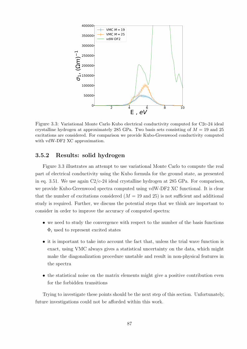
2 4 6 8 10E , eV

0

50000

100000

150000

200000

250000

300000

350000

400000

1, (

m)

1

VMC M = 19VMC M = 25vdW-DF2

Figure 3.3: Variational Monte Carlo Kubo electrical conductivity computed for C2c-24 idealcrystalline hydrogen at approximately 285 GPa. Two basis sets consisting of M = 19 and 25excitations are considered. For comparison we provide Kubo-Greenwood conductivity computedwith vdW-DF2 XC approximation.

3.5.2 Results: solid hydrogen

Figure 3.3 illustrates an attempt to use variational Monte Carlo to compute the real

part of electrical conductivity using the Kubo formula for the ground state, as presented

in eq. 3.51. We use again C2/c-24 ideal crystalline hydrogen at 285 GPa. For comparison,

we provide Kubo-Greenwood spectra computed using vdW-DF2 XC functional. It is clear

that the number of excitations considered (M = 19 and 25) is not sufficient and additional

study is required. Further, we discuss the potential steps that we think are important to

consider in order to improve the accuracy of computed spectra:

• we need to study the convergence with respect to the number of the basis functions

Φi used to represent excited states

• it is important to take into account the fact that, unless the trial wave function is

exact, using VMC always gives a statistical uncertainty on the data, which might

make the diagonalization procedure unstable and result in non-physical features in

the spectra

• the statistical noise on the matrix elements might give a positive contribution even

for the forbidden transitions

Trying to investigate these points should be the next step of this section. Unfortunately,

future investigations could not be afforded within this work.

87

3.6 Conclusion

We have introduced in this chapter the theoretical background for computing the

optical properties of materials. In particular, we have presented the introduction into the

linear response theory, discussing different optical response coefficients such as dielectric

function, conductivity, and reflectivity and have established the relations between them.

We have made the derivations necessary to establish the single particle Kubo-Greenwood

formula for conductivity, and have applied it to the ideal solid crystalline hydrogen.

Moreover, we have attempted to compute the Kubo many-body conductivity with

variational Monte Carlo. Our preliminary results for the C2c-24 ideal solid crystalline

hydrogen indicate that further investigations of the convergence of the spectra are necessary.

88

Chapter 4

Thermal crystals: renormalization of

electronic properties

In the previous chapters, we have assumed that the nuclear lattice is immobile and the

protons were point particles, fixed at their equilibrium positions. This assumption can

only be valid for some materials with the nuclear mass large enough such that the energy

contribution due to the lattice vibration is small compared to the electronic excitation

energies (such e.g. eq. 2.49) computed for a static lattice,

Estaticex << Evib. (4.1)

Moreover, the above assumption makes sense only if the property of interest is the electronic

energy. However, when dealing with light materials such as hydrogen, the vibrational

energy is no longer small and has to be taken into account when computing the electronic

structure properties.

The focus of this chapter, therefore, will be on the renormalization of energy gaps,

excited states, and optical spectra of materials at finite temperature. We first define the

full electron nuclear hamiltonian and will explain the adiabatic splitting and path integral

formulation of the problem. Then, we introduce the formal treatment of electron addition

energies and gaps in the canonical and semi-grand canonical ensemble at finite temperature

and will discuss the approximations to be made. Further, we proceed with an issue of

determining crystal momentum in the presence of finite temperature nuclei. At the end of

the chapter, we provide a new way of treating the optical spectra of finite temperature

materials, an alternative to the common semiclassical method.

A general introduction to the nuclear dynamics and the adiabatic approximation can

be found in the book of Marx [10]. An introduction to the finite temperature methods

used for finite temperature nuclei to study matter at extreme conditions can be found in

the review of MaMahon [11]. There is as well an instructive review of path integral Monte

89

Carlo [127], together with the lecture notes by Pierleoni and Ceperley [9].

To properly treat electrons and nuclei as a quantum mechanical system, one has to

consider the full Hamiltonian (non relativistic, in atomic units):

H =

TR︷ ︸︸ ︷−

Np∑I=1

∇2RI

2MI

+

V Rpp︷ ︸︸ ︷

Np∑I

Np∑J>I

ZIZJ|RI −RJ |

+Te + Vee + V Rep︸ ︷︷ ︸

HRe

, (4.2)

where for convenience, HRe , is the electronic Hamiltonian, defined in eq. 1.2, plus the

nuclear-nuclear interaction potential:

HRe = V R

pp + Te + Vee + V Rep , (4.3)

which now depends parametrically on the nuclear coordinates. This Hamiltonian can be

viewed as coupled nuclear and electronic problems. In fact, if the nuclei were fixed in

space, the full Hamiltonian in eq. 4.2 would become just the electronic one, HRe . The

eigenstates, Φn(r,R), of the full Hamiltonian will depend on the positions of the electrons

and of the nuclei. In the following, unless the index is specifically given, r and R denote

the set of all electronic and nuclear positions,

r = r1, .., ri, .., rNe (4.4)

R =R1, ..,RI , ..,RNp

,

being a 3Ne and 3Np dimensional vector respectively. Solving the Schrodinger equation

analytically with the Hamiltonian defined in eq. 4.2 for all particles together is essentially

an impossible task for most systems except a few extremely simple cases such as the

H+2 . Therefore, when dealing with nuclear motion, one has to decouple electrons and

nuclei. In the following, we will consider a non-degenerate case, when the eigenvalues of

the electronic hamiltonian are well separated from each other.

4.1 Born-Oppenheimer approximation

The mass of the electrons is much smaller than that of the nuclei, therefore the ratio of

kinetic to potential energy for nuclei is much smaller than in the case of electrons. As long

as the temperature is not too high, the time scale of electronic motion is much smaller

than the corresponding time scale for nuclei. As a consequence, one can assume that

electrons relax infinitely fast to their equilibrium state as the ions move, neglecting any

90

coupling between different electronic states and also retardation effects in the electron-ion

interaction. In these conditions the electrons do not exchange energy with the nuclei;

therefore their evolution is adiabatic. If further considering that the electronic ground

state contribution will be dominant, then this approximation goes under the name of the

Born-Oppenheimer approximation (BOA) [128, 129] To be more concrete let us expand

the total electron nuclei wave function in the eigenstates of the electronic Hamiltonian,

Φn(r,R) =∑α

Ψα(r|R)χαn(R), (4.5)

where the electronic wave function Ψα(r|R) depends parametrically on the nuclear coordi-

nates, R. Plugging it into the Schrodinger equation with the full Hamiltonian defined in

eq. 4.2,

∑α

TRΨα(r|R)χαn(R) +∑α

HRe Ψα(r|R)χαn(R) =

∑α

EαnΨα(r|R)χαn(R), (4.6)

one can see that the electronic Hamiltonian operates only on the electronic wave function,

Ψα(r|R), and not on the coefficients χαn(R),

∑α

HRe Ψα(r|R)χαn(R) =

∑α

ERα Ψα(r|R)χαn(R). (4.7)

Whereas the nuclear kinetic operator acts on both wave functions,

∇2I

2MI

Ψα(r|R)χαn(R) = − 1

2MI

Ψα(r|R)(∇2RIχαn(R)) (4.8)

− 1

MI

(∇RIΨα(r|R))(∇RI

χαn(R))

− 1

2MI

(∇2RI

Ψα(r|R))χαn(R).

Plugging eq. 4.8 and eq. 4.7 into the eq. 4.6, one can integrate out the electronic degrees

of freedom by multiplying Ψ∗β(r|R)) on the left,

[TR + ER

α − Eαn]χαn(R) =

Np∑I=1

[ 1

MI

∑α

〈Ψβ|∇RI|Ψα〉(∇RI

χαn(R))

+1

2MI

∑α

〈Ψβ|∇2RI|Ψα〉χαn(R)

]. (4.9)

91

The adiabatic approximation relies on neglecting the r.h.s of the previous equation, which

would lead to an eigenvalue problem for nuclei with potential given by the electronic

eigenvalue, ERβ , evaluated at fixed nuclei, R. This approximation assumes that the

electrons react instantaneously on the change of the nuclear positions. To understand its

validity lets use the following notation for the terms on the r.h.s of eq. 4.9:

AIαβ =1

MI

〈Ψβ|∇RI|Ψα〉∇RI

,

BIαβ =

1

2MI

〈Ψβ.|∇2RI|Ψα〉 (4.10)

The off-diagonal terms AIαβ and BIαβ are usually regarded as non-adiabatic corrections and

are neglected such that the electrons stay in a given state as the ions move. Note that,

for normalized wave functions the diagonal part of AIαα is identically zero, which can be

shown by integration by parts. Neglecting further the BIαα term, the Schrodinger equation

for the nuclei writes:

[TR + ER

α

]χαn(R) = Eαnχαn(R), (4.11)

where the potential energy surface (PES) felt by the nuclei is defined as the eigenvalue

of electronic Hamiltonian in the clamped nuclei approximation, ERβ , which includes as

well the nuclei-nuclei potential energy contribution, V Rpp . As in this work, the typical

temperatures of the interest are T TF , where TF is the Fermi energy for the electrons,

it can be assumed that electrons remain in their ground state, arriving at the modern

version of the BOA,

[TR + ER

BO

]χαn(R) = E0nχ0n(R), (4.12)

where we define the BO potential energy surface as the ground state energy of the electronic

Hamiltonian, HRe .

4.2 Ab initio path integrals

Alternatively, one can derive the BOA using the path integral (PI) formulation [130]. In

analogy to [10], we will work in a mixed basis combining the position representation for the

nuclear degrees of freedom with the energy representation for the electrons. In particular,

the product basis, |Ψα(R),R〉 = |Ψα(R)〉|R〉, involving the complete and orthonormal

92

basis set of the eigenstates of the electronic Hamiltonian. The completeness relation,∫ ∑α

|Ψα(R),R〉〈R,Ψα(R)|dR = 1, (4.13)

if necessary, has to be extended over the full available space in the integration over the

nuclear positions, and the summation over the electronic states α must also include all

continuum states.

We will be interested in computing the expectation value of an operator O, that can

be then expressed according to Statistical mechanics,

〈O〉 =1

ZTrO exp

[−βH

]. (4.14)

The exact partition function, Z, of the quantum-statistical canonical ensemble reads,

Z = Tr exp[−βH

]=

∫dR∑α

〈R,Ψα(R)|e−β[TR+HRe ]|Ψα(R),R〉 (4.15)

=

∫dR∑α

ρ(R,Ψα; R,Ψα; β),

where ρ(R,Ψα; R,Ψα; β) is the density matrix at inverse temperature β = 1/kBT with

kB being the Boltzmann constant. Since the nuclear kinetic energy operator does not

commute with the rest of the full Hamiltonian, the lowest-order Trotter factorization [53],

e−β[TR+HR

e ] = limP→∞

(e−

βPTR

e−βPHRe

)P, (4.16)

can be invoked in order to decouple nuclear kinetic energy from the rest of the Hamiltonian.

Inserting P − 1 times completeness relation, this will allow us to rewrite the partition

function as the product,

Z = limP→∞

∫ P∏s=1

[∑α(s)

〈R(s+1),Ψα(s+1)(R(s+1))|e− βPTR

e−βPHRe |Ψα(s)(R(s)),R(s)〉dR(s)

],

(4.17)

where the trace condition imposes periodic boundary conditions, R(P+1) = R1 and

Ψα(P+1) = Ψα1 , on the Trotter discretization parameters s = 1, .., P . It remains to evaluate

the following matrix element:

93

〈R(s+1)|〈Ψα(s+1)(R(s+1))|e− βPTR

e−βPHRe |Ψα(s)(R(s))〉|R(s)〉 = (4.18)

〈R(s+1)|〈Ψα(s+1)(R(s+1))|e− βPTR |Ψα(s)(R(s))〉|R(s)〉e− β

PEα(s) (R(s)),

where the effect of the electronic Hamiltonian is expressed by the adiabatic energy,

Eα(s)(R(s)), in electronic state Ψα(s) evaluated at the fixed nuclear configuration R(s) at

time slice s and can be pulled out of the integral.

At this stage the adiabatic approximation can be applied, which amounts to assuming

that the nuclear kinetic energy operator, TR, does not act on the electronic wave functions,

Ψα(s) . This means that the variation of the electronic wave functions as the result of

changes in the nuclear coordinates is negligible. In the same spirit, the overlap between

the two electronic wave functions at time slice s and s + 1 will yield the orthogonality

relation:

〈Ψα(s+1)(R(s+1))|Ψα(s)(R(s))〉 = 〈Ψα(s+1)(R(s+1))||Ψα(s)(R(s+1))〉 (4.19)

+∑I

∇I |Ψα(s)(R(s+1))〉(R(s+1) −R(s))

+O[(R(s+1) −R(s))2

] ≈ 〈Ψα(s+1)(R(s+1))|Ψα(s)(R(s+1))〉 = δα(s+1)α(s) .

The final expression of the partition function in the adiabatic approximation writes:

Zadia = limP→∞

∫ P∏s=1

[dR(s)

∑α(s)

δα(s+1)δα(s)〈R(s+1)|e− βPTR |R(s)〉e− β

P [Eα(s) (R(s))]

]

=∑α

limP→∞

∫ P∏s=1

[dR(s)〈R(s+1)|e− β

PTR |R(s)〉e− β

P [Eα(R(s))]], (4.20)

where as a result of the product of Kronecker deltas, each of them connecting two adiabatic

states Ψ(s)α and Ψ

(s+1)α under periodic boundary conditions in imaginary time s = P +1 = 1,

only one sum,∑

α(1) =∑

α, survives. More compactly the eq. 4.20 can be written as the

trace,

Zadia =∑α

Tre−β(TR+Eα(R)). (4.21)

The remaining sum over all electronic eigenstates, Ψα, means that the nuclear fluctuations

are sampled according to Boltzmann’s thermal distribution with the weight given by the

electronic eigenvalue ∝ exp [−βEα]. Thus, the contribution of excited states (α > 1) to

94

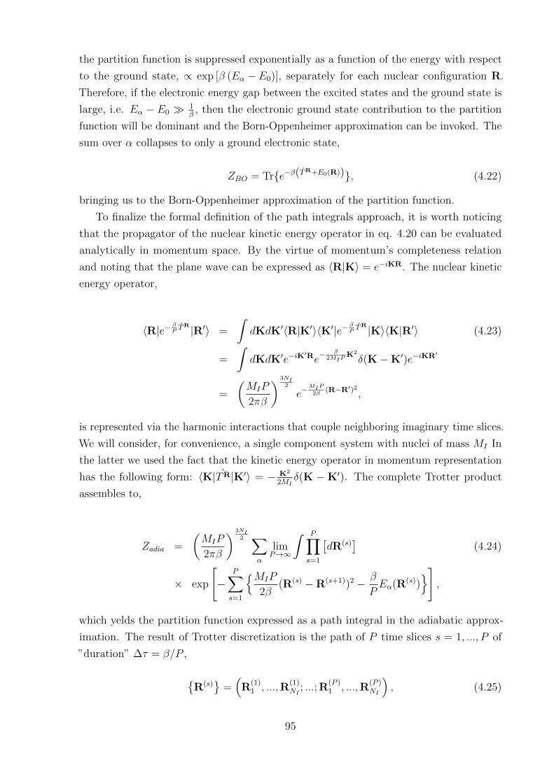
the partition function is suppressed exponentially as a function of the energy with respect

to the ground state, ∝ exp [β (Eα − E0)], separately for each nuclear configuration R.

Therefore, if the electronic energy gap between the excited states and the ground state is

large, i.e. Eα − E0 1β, then the electronic ground state contribution to the partition

function will be dominant and the Born-Oppenheimer approximation can be invoked. The

sum over α collapses to only a ground electronic state,

ZBO = Tre−β(TR+E0(R)), (4.22)

bringing us to the Born-Oppenheimer approximation of the partition function.

To finalize the formal definition of the path integrals approach, it is worth noticing

that the propagator of the nuclear kinetic energy operator in eq. 4.20 can be evaluated

analytically in momentum space. By the virtue of momentum’s completeness relation

and noting that the plane wave can be expressed as 〈R|K〉 = e−iKR. The nuclear kinetic

energy operator,

〈R|e− βPTR |R′〉 =

∫dKdK′〈R|K′〉〈K′|e− β

PTR |K〉〈K|R′〉 (4.23)

=

∫dKdK′e−iK

′Re− β

2MIPK2

δ(K−K′)e−iKR′

=

(MIP

2πβ

) 3NI2

e−MIP

2β(R−R′)2

,

is represented via the harmonic interactions that couple neighboring imaginary time slices.

We will consider, for convenience, a single component system with nuclei of mass MI In

the latter we used the fact that the kinetic energy operator in momentum representation

has the following form: 〈K|TR|K′〉 = − K2

2MIδ(K −K′). The complete Trotter product

assembles to,

Zadia =

(MIP

2πβ

) 3NI2 ∑

α

limP→∞

∫ P∏s=1

[dR(s)

](4.24)

× exp

[−

P∑s=1

MIP

2β(R(s) −R(s+1))2 − β

PEα(R(s))

],

which yelds the partition function expressed as a path integral in the adiabatic approx-

imation. The result of Trotter discretization is the path of P time slices s = 1, ..., P of

”duration” ∆τ = β/P ,

R(s)

=(R

(1)1 , ...,R

(1)NI

; ...; R(P )1 , ...,R

(P )NI

), (4.25)

95

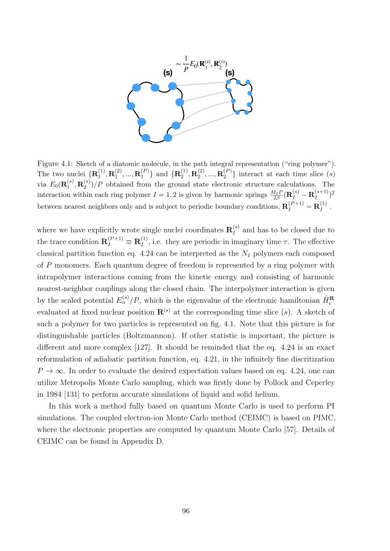
Figure 4.1: Sketch of a diatomic molecule, in the path integral representation (“ring polymer”).

The two nuclei R(1)1 ,R

(2)1 , ...,R

(P )1 and R(1)

2 ,R(2)2 , ...,R

(P )2 interact at each time slice (s)

via E0(R(s)1 ,R

(s)2 )/P obtained from the ground state electronic structure calculations. The

interaction within each ring polymer I = 1, 2 is given by harmonic springs MIP2β (R

(s)I −R

(s+1)I )2

between nearest neighbors only and is subject to periodic boundary conditions, R(P+1)I = R

(1)I .

where we have explicitly wrote single nuclei coordinates R(s)I and has to be closed due to

the trace condition R(P+1)I ≡ R

(1)I , i.e. they are periodic in imaginary time τ . The effective

classical partition function eq. 4.24 can be interpreted as the NI polymers each composed

of P monomers. Each quantum degree of freedom is represented by a ring polymer with

intrapolymer interactions coming from the kinetic energy and consisting of harmonic

nearest-neighbor couplings along the closed chain. The interpolymer interaction is given

by the scaled potential E(s)α /P , which is the eigenvalue of the electronic hamiltonian HR

e

evaluated at fixed nuclear position R(s) at the corresponding time slice (s). A sketch of

such a polymer for two particles is represented on fig. 4.1. Note that this picture is for

distinguishable particles (Boltzmannon). If other statistic is important, the picture is

different and more complex [127]. It should be reminded that the eq. 4.24 is an exact

reformulation of adiabatic partition function, eq. 4.21, in the infinitely fine discritization

P →∞. In order to evaluate the desired expectation values based on eq. 4.24, one can

utilize Metropolis Monte Carlo sampling, which was firstly done by Pollock and Ceperley

in 1984 [131] to perform accurate simulations of liquid and solid helium.

In this work a method fully based on quantum Monte Carlo is used to perform PI

simulations. The coupled electron-ion Monte Carlo method (CEIMC) is based on PIMC,

where the electronic properties are computed by quantum Monte Carlo [57]. Details of

CEIMC can be found in Appendix D.

96

4.3 Quasiparticle energy gap in a canonical ensemble

at finite temperature

In this section, we will discuss the thermal renormalization of the quasiparticle energy

gap, defined in section 2.1.3. We will consider the system of Np nuclei and Ne = Np + n

electrons. The canonical partition function in the Born-Oppenheimer approximation,

ZBO(Ne, Np) = Tre−β(TR(Np)+E0(R;Ne,Np)) (4.26)

= e−βF (Ne,Np)

now is written in terms of the Helmholtz free energy and the dependency on the number

of nuclei and electrons has been indicated explicitly. For convenience, the free energy, F ,

corresponding to the PES E0(R) has been introduced. In the further, we will remove the

subscript BO from the partition function and will explicitly state when it is otherwise.

We will try now to reformulate the partition function, Z(Ne, Np), of Ne = Np + n

electrons in terms of Ne = Np electrons times some correction. Multiplying and dividing

eq. 4.26 by the e−βF (Np,Np),

Z(Ne, Np) =e−βF (Np,Np)

e−βF (Np,Np)e−βF (Ne,Np) (4.27)

= e−βF (Np,Np) Tre−β(TR(Np)+E0(R;Np,Np)+∆E0(R;n,Np))e−βF (Np,Np)

= e−βF (Np,Np)〈e−β∆E0(R;n,Np)〉Np ,

one can argue that the correction, which is defined via the average over the system with

the Ne = Np, is given by the increment of the PES, when n electrons are added to the

system, ∆E0(R;n,Np) = E0(R;Ne, Np)−E0(R;Np, Np). Notice that as long as n << Np,

∆E0(R;n,Np) E0(R;Np, Np), because the energy is extensive property. We assume that

the ∆E0(R;n,Np) is normally distributed over the nuclear fluctuations (the verification of

the distribution is given on fig. 4.2). The average of the exponent can be expanded in

cumulants, for normally distributed variable being,

log[〈e−β∆E0(R;n,Np)〉Np

]= −β〈∆E0(R;n,Np)〉Np + σ2β

2

2+O(β3), (4.28)

σ2 = 〈∆E0(R;n,Np)2〉Np − 〈∆E0(R;n,Np)〉2Np

where σ is the variance of normally distributed ∆Eα(R;n,Np). Figure 4.2 illustrates that

97

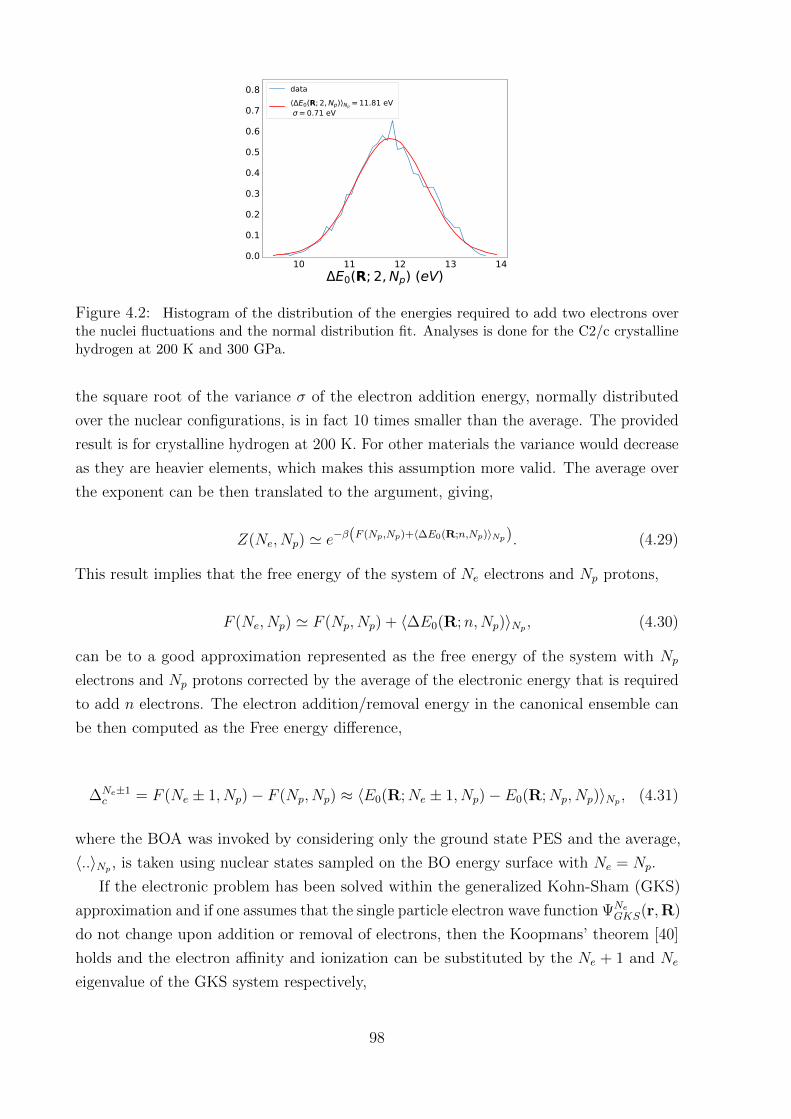
10 11 12 13 14E0(R; 2, Np) (eV)

0.0

0.1

0.2

0.3

0.4

0.5

0.6

0.7

0.8 dataE0(R; 2, Np) Np = 11.81 eV

= 0.71 eV

Figure 4.2: Histogram of the distribution of the energies required to add two electrons overthe nuclei fluctuations and the normal distribution fit. Analyses is done for the C2/c crystallinehydrogen at 200 K and 300 GPa.

the square root of the variance σ of the electron addition energy, normally distributed

over the nuclear configurations, is in fact 10 times smaller than the average. The provided

result is for crystalline hydrogen at 200 K. For other materials the variance would decrease

as they are heavier elements, which makes this assumption more valid. The average over

the exponent can be then translated to the argument, giving,

Z(Ne, Np) ' e−β(F (Np,Np)+〈∆E0(R;n,Np)〉Np). (4.29)

This result implies that the free energy of the system of Ne electrons and Np protons,

F (Ne, Np) ' F (Np, Np) + 〈∆E0(R;n,Np)〉Np , (4.30)

can be to a good approximation represented as the free energy of the system with Np

electrons and Np protons corrected by the average of the electronic energy that is required

to add n electrons. The electron addition/removal energy in the canonical ensemble can

be then computed as the Free energy difference,

∆Ne±1c = F (Ne ± 1, Np)− F (Np, Np) ≈ 〈E0(R;Ne ± 1, Np)− E0(R;Np, Np)〉Np , (4.31)

where the BOA was invoked by considering only the ground state PES and the average,

〈..〉Np , is taken using nuclear states sampled on the BO energy surface with Ne = Np.

If the electronic problem has been solved within the generalized Kohn-Sham (GKS)

approximation and if one assumes that the single particle electron wave function ΨNeGKS(r,R)

do not change upon addition or removal of electrons, then the Koopmans’ theorem [40]

holds and the electron affinity and ionization can be substituted by the Ne + 1 and Ne

eigenvalue of the GKS system respectively,

98

∆Ne+1c (θ) = 〈ε(Ne+1)R

GKS (θ)〉Np , (4.32)

∆Ne−1c (θ) = 〈ε(Ne)RGKS (θ)〉Np ,

where the translation symmetries of the supercell are invoked via the k-point or twist θ,

Bloch’s vectors of the supercell. Quasiparticle energy gap in the canonical ensemble is

then given by,

∆c(θ,θ′) = ∆Ne+1

c (θ)−∆Ne−1c (θ′). (4.33)

In analogy with section 2.1.3, the fundamental energy gap is then,

∆c(θ,θ′) = min

φ

[∆Ne+1c (φ)

]−max

φ′

[∆Ne−1c (φ′)

], (4.34)

where θ and θ′ correspond to the Bloch’s vectors at which the min and max are realized.

If θ 6= θ′ the gap is indirect, while when θ = θ′ the gap can be direct. The connection

of the supercell twist angle θ to the crystal momentum k and therefore to the vertical

(direct) energy gap will be discussed in section 4.5.

4.4 Quasiparticle energy gap in a semigrand canoni-

cal ensemble at finite temperature

We can extend the previously defined in section 2.1.6 formalism to compute the gap for

quantum crystals at finite temperature in the grand canonical ensemble. Note that only

electrons are treated in the grand canonical ensemble, that is why we call it semigrand

canonical ensemble.

Consider again the system of Np nuclei and Ne = Np + n electrons for a given twist

angle θ. In the semigrand-ensemble the partition function is

Z(µ, θ) =∞∑

Ne=0

eβµNee−βF (Ne,θ) = e−βΩ(µ,θ) (4.35)

where the dependence on temperature, volume, and the number of nuclei has been kept

implicit and F and Ω are respectively the Helmholtz free energy and the grand-potential.

For kBT much smaller than the energies of electronic excitations (either at fixed Ne or

different Ne), electrons can be assumed to be in the ground state and the sum over Ne

99

reduces to the values Ne(µ, θ) that minimizes the exponent

Ω(µ, θ) = minNe

[F (Ne, θ)− µNe] = F (Ne, θ)− µNe. (4.36)

The Helmholtz free energy includes the average nuclear kinetic energy, the average potential

energy over the ground state Born-Oppenheimer (BO) surface of the Ne electron system,

and the nuclear entropy. To reduce finite size effects we can average over the twists, as in

section 2.1.6, obtaining the free energy and electron densities,

ω(µ) = f(ne(µe))− µene(µ) (4.37)

f(ne(µ)) =1

MθV

∑θ

F (N , θ) (4.38)

ne(µ) =1

MθV

∑θ

N(µ, θ) (4.39)

As in the ideal crystal case, the fundamental energy gap is

∆gc = µ+ − µ− =df

dne

∣∣∣∣n+p

− df

dne

∣∣∣∣n−p

. (4.40)

In this work, we analyze nuclear configurations generated during CEIMC calculations

performed in the canonical ensemble at Ne = Np with twist averaged energies. As we don’t

have access to free energies, it is tempting to replace them with total energies in eq. 4.40.

We assume that both the average nuclear kinetic energy and the nuclear entropy are nearly

independent of the specific number of electrons and can be replaced by their values at

Ne = Np. To justify this we write the partition function in the canonical ensemble as in

eq. 4.29

Z(Ne, θ) ' e−β[F (Np,θ)+〈∆E(n,θ)〉Np ] (4.41)

which implies

F (Ne, θ) ' F (Np, θ) + 〈∆E(n, θ)〉Np . (4.42)

Using this expression in eq. 4.36 we obtain

Ω(µ, θ) ' F (Np, θ) +minNe

[〈∆E(n, θ)〉Np − µNe

]= F (Np, θ) + 〈∆E(n, θ)〉Np − µ(Np + n), (4.43)

with n = n(µ) depending on the chemical potential. The free energy density is now,

f(ne(µ)) ' 1

θV

∑θ

[F (Np, θ) + 〈∆E(n(µ), θ)〉Np

](4.44)

= f(np) + 〈e(ne(µ))− e(np)〉Np ,

100

where e(ne(µ)) = 1θV

∑θ E(n(µ) +Np, θ). Following the same reasoning as in eqs. 4.36-4.40

we arrive at our final expression of the fundamental gap

∆gc = µ+ − µ− =df(ne(µ))

dne

∣∣∣∣n+p

− df(ne(µ))

dne

∣∣∣∣n−p

(4.45)

' d〈e(ne(µ))〉Npdne

∣∣∣∣n+p

− d〈e(ne(µ))〉Npdne

∣∣∣∣n−p

As before 〈..〉Np means that the averages are taken using nuclear states sampled on the

BO energy surface with Ne = Np. To ensure the convergence of the averages we consider

40 statistically independent nuclear configurations from the CEIMC trajectory.

Note that putting the average over nuclear configurations outside the derivatives in

eq. 4.45 gives a different value for the fundamental gap. This is the usual procedure to

compute electronic properties from nuclear trajectories. Further, we call it the ”semiclas-

sical approximation”. The application of these results can be found in chapters 5 and

6.

4.5 Quasi-momentum of the electronic wave function

of quantum crystals

We will focus here on a single adiabatic PES, which is the Nth eigenstate ΨN(r,R) of

the electrons for the corresponding ground state wave function χN0(R) of the nuclei and

we neglect for a moment any other adiabatic surface entering the wave function expansion

in eq. 4.5. Note that it has in general lost any symmetry properties of the perfect crystal.

To restore them, the electronic wave function ΨN(r,R) can be expanded around the

eigenstate of the ideal crystal ΨR0kn (r) in the spirit of the Allen-Heine expansion [132].

Considering U(R) = HRe − HR0

e as a small perturbation it can then be Taylor-expanded

around the ideal nuclear configuration R0,

U ′(R) =

NI∑l=1

∆Rl [∇RlU(R)]

∣∣∣R0l

+O(∆R2), (4.46)

where ∆Rl = Rl − R0,l and the expansion was truncated after the first order for the

reasons that will be apparent later. Perturbation theory can then be used to expand the

wave function ΨN(r,R) up to first order in the nuclear displacements,

101

ΨN(r,R) = ΨR0kn (r) +

∑l

∑qm

′ ΨR0qm(r)

ER0qm − ER0

kn

∆Rl∇Rl〈qm|U(R)|kn〉

∣∣∣R0l

(4.47)

= ΨR0kn (r) +

∑qm

′ ΨR0qm(r)

ER0qm − ER0

kn

∆RAqmkn ,

with Aqmkn,l = ∇Rl

〈qm|U(R)|kn〉∣∣∣R0

being the electron-nuclei coupling matrix element, and

the sum over the nuclei is inside the scalar product ∆RAqmkn . The electronic eigenvalues,

ER0kn , and eigenfunctions, ΨR0

kn (r), of the ideal crystal are characterized by the crystal

momentum k and the Band index n. By integrating the electronic wave function in eq. 4.47

over the nuclei density distribution |χN0(R)|2, one can restore the symmetry properties of

the perfect crystal,

ΨN(r) ≡∫dR|χN0(R)|2ΨN(r,R) (4.48)

≈∫dR|χN0(R)|2

[ΨR0

kn (r) +∑qm

′ ΨR0qm(r)

ER0qm − ER0

kn

(R−R0)Aqmkn

]= ΨR0

kn (r).

Note that, if the higher order terms had been included in the expansion in eq. 4.46,

then the symmetry properties of the perfect crystal would not be restored. Therefore,

within the harmonic approximation, the wave function of the perfect crystal is restored

when integrating over the nuclear ground state density. In particular, the translational

symmetries of the integrated wave function ΨN(r) are the same as of the ideal crystal

wave function ΨR0kn (r), so that the crystal wave vector k of ΨR0

kn (r) carries over to ΨN(r).

However, note that the BO electronic wave function ΦN (r,R) that depends parametri-

cally on R is defined up to an arbitrary phase φ(R) which depends on the nuclear position

R, this arbitrariness in the choice of phases is called gauge arbitrariness [133]

ΦN(r,R) ' ΨN(r,R)eiφ(R). (4.49)

Therefore if the phase φ(R) was known one could determine the crystal momentum k by

calculating,

ΨN(r) ≡∫dR|χN0(R)|2ΦN(r,R)e−iφ(R) ≈ ΨR0

kn (r). (4.50)

A numerical determination of φ(R) could be possible by adiabatic changes of the nuclear

positions, R, unfortunately that will be out of the scope of this thesis.

Alternatively, the crystal momentum of ΨN(r) can be determined by designing an

102

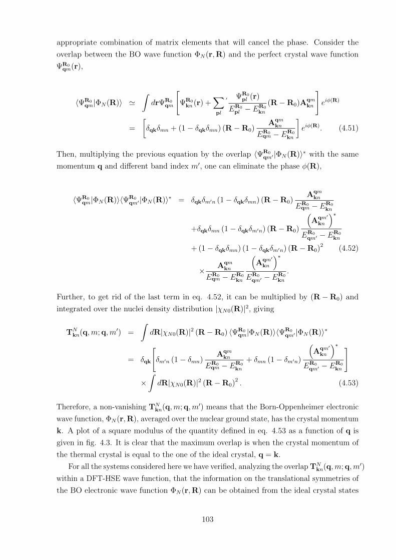
appropriate combination of matrix elements that will cancel the phase. Consider the

overlap between the BO wave function ΦN(r,R) and the perfect crystal wave function

ΨR0qm(r),

〈ΨR0qm|ΦN(R)〉 '

∫drΨR0

qm

[ΨR0

kn (r) +∑pl

′ ΨR0pl (r)

ER0pl − ER0

kn

(R−R0)Aqmkn

]eiφ(R)

=

[δqkδmn + (1− δqkδmn) (R−R0)

Aqmkn

ER0qm − ER0

kn

]eiφ(R). (4.51)

Then, multiplying the previous equation by the overlap 〈ΨR0

qm′ |ΦN(R)〉∗ with the same

momentum q and different band index m′, one can eliminate the phase φ(R),

〈ΨR0qm|ΦN(R)〉〈ΨR0

qm′ |ΦN(R)〉∗ = δqkδm′n (1− δqkδmn) (R−R0)Aqm

kn

ER0qm − ER0

kn

+δqkδmn (1− δqkδm′n) (R−R0)

(Aqm′

kn

)∗ER0

qm′ − ER0kn

+ (1− δqkδmn) (1− δqkδm′n) (R−R0)2 (4.52)

× Aqmkn

ER0qm − ER0

kn

(Aqm′

kn

)∗ER0

qm′ − ER0kn

.

Further, to get rid of the last term in eq. 4.52, it can be multiplied by (R−R0) and

integrated over the nuclei density distribution |χN0(R)|2, giving

TNkn(q,m; q,m′) =

∫dR|χN0(R)|2 (R−R0) 〈ΨR0

qm|ΦN(R)〉〈ΨR0

qm′|ΦN(R)〉∗

= δqk

[δm′n (1− δmn)

Aqmkn

ER0qm − ER0

kn

+ δmn (1− δm′n)

(Aqm′

kn

)∗ER0

qm′ − ER0kn

]×∫dR|χN0(R)|2 (R−R0)2 . (4.53)

Therefore, a non-vanishing TNkn(q,m; q,m′) means that the Born-Oppenheimer electronic

wave function, ΦN (r,R), averaged over the nuclear ground state, has the crystal momentum

k. A plot of a square modulus of the quantity defined in eq. 4.53 as a function of q is

given in fig. 4.3. It is clear that the maximum overlap is when the crystal momentum of

the thermal crystal is equal to the one of the ideal crystal, q = k.

For all the systems considered here we have verified, analyzing the overlap TNkn(q,m; q,m′)

within a DFT-HSE wave function, that the information on the translational symmetries of

the BO electronic wave function ΦN(r,R) can be obtained from the ideal crystal states

103

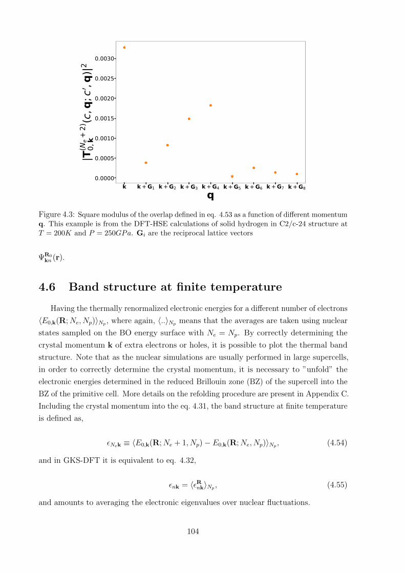
k k + G1 k + G2 k + G3 k + G4 k + G5 k + G6 k + G7 k + G8

q0.0000

0.0005

0.0010

0.0015

0.0020

0.0025

0.0030

|T(N

e+

2)0,

k(c

,q;c

′ ,q)|2

Figure 4.3: Square modulus of the overlap defined in eq. 4.53 as a function of different momentumq. This example is from the DFT-HSE calculations of solid hydrogen in C2/c-24 structure atT = 200K and P = 250GPa. Gi are the reciprocal lattice vectors

ΨR0kn (r).

4.6 Band structure at finite temperature

Having the thermally renormalized electronic energies for a different number of electrons

〈E0,k(R;Ne, Np)〉Np , where again, 〈..〉Np means that the averages are taken using nuclear

states sampled on the BO energy surface with Ne = Np. By correctly determining the

crystal momentum k of extra electrons or holes, it is possible to plot the thermal band

structure. Note that as the nuclear simulations are usually performed in large supercells,

in order to correctly determine the crystal momentum, it is necessary to ”unfold” the

electronic energies determined in the reduced Brillouin zone (BZ) of the supercell into the

BZ of the primitive cell. More details on the refolding procedure are present in Appendix C.

Including the crystal momentum into the eq. 4.31, the band structure at finite temperature

is defined as,

εNek ≡ 〈E0,k(R;Ne + 1, Np)− E0,k(R;Ne, Np)〉Np , (4.54)

and in GKS-DFT it is equivalent to eq. 4.32,

εnk = 〈εRnk〉Np , (4.55)

and amounts to averaging the electronic eigenvalues over nuclear fluctuations.

104

X+ G+ X′+ Y+ G+

4

6

8

10

12

14

16

, (eV

)

vdW-DF C2/c-24QMC IdealQMC T200

Figure 4.4: Band structure at finite temperature from QMC-CEIMC calculations (orange points)and for perfect crystal QMC (blue points) of 96 hydrogen atoms compared to the band structurefrom vdW-DF density functional for a unitary cell of C2/c-24 hydrogen crystal at approximately250 GPa. Horizontal lines are the corresponding valence band maximum and conduction bandminimum. The Brillouin zone path is equivalent to the one in fig. 2.1 and the vdW-DF bandsare shifted to match the QMC ideal bands.

Figure 4.4 illustrates the QMC highest occupied and lowest unoccupied bands at 200 K

and for ideal structure plotted on top of the vdW-DF DFT band structure of the unitary

cell of C2/c-24 hydrogen crystal at approximately 250 GPa. The Brillouin zone path and

ideal crystal QMC and DFT bands are identical to fig. 2.1. The reduction of the gap due

to the nuclear effects is of the order of 2 eV, we believe that such a strong reduction is

mainly caused by the nuclear quantum effects, which are large in hydrogen. More details

on the electronic gaps of thermal hydrogen crystals will be given in the next chapter.

4.7 Optical properties renormalization

In the section to come, we will discuss how to account for the nuclear motion when

computing the optical properties of solids. For practical reasons we only focus on the

single particle optical properties, namely computed with the Kubo-Greenwood formula as

in eq. 3.38.

4.7.1 Semiclassical averaging

Let us assume the product approximation to the exact electron-nuclear wave function

|αn〉 ' |ΨRα 〉 |χαn〉, where ΨR

α , ERα is the solution of electronic problem depending

parametrically on the nuclear configuration R and |χαn〉 is the nuclear wave-function

on the Born-Oppenheimer energy surface ERα . Assuming the electrons are initially in

105

the ground state, one can write the real part of KG conductivity (and similarly for the

imaginary part) as a thermal average over nuclear states,

σ1(ω, T ) =1

Z

∑n

e− E0nkBT σ1(ω, n), (4.56)

where E0n are the eigenvalues of the nuclear motion in the BO ground electronic states,

Z =∑

n e−E0n/kBT is the partition function and kB is Boltzmann constant. In the single

electron representation - the Kubo-Greenwood theory, σ1(ω, n) takes the form (in SI units),

σ1(ω, n) ∝ 1

ω

occ.∑α

unocc.∑β,m

〈χαn|PRαβ |χβm〉

× 〈χβm|PRβα |χαn〉 δ(εαn − εβm − ~ω), (4.57)

where the constant prefactor was omitted for convenience, α indicate Kohn-Sham initial

states in the valence band |φRα 〉, β and m indicate, respectively, final electronic and nuclear

states in the conduction band, PRαβ = 〈φR

α | ∇ |φRβ 〉 is the matrix element of the single

electron momentum operator at fixed nuclear configuration R, and εαn = 〈χαn|εRα |χαn〉are the joint electron-nuclear eigenvalues. The conventional quasiclassical procedure

introduced by Williams [134] and Lax [135] (WL) substitutes the final nuclear states with

a continuum. In practice it replaces the eigenvalues εαn in Eq. (4.57) by the eigenvalues

evaluated at fixed nuclear configuration εRα , a procedure that can be justified as discussed

in refs. [135, 136].

σWL1 (ω, n) =

1

ω

occ.∑α

unocc.∑β

〈χαn| |PRαβ|2δ(∆εRα,β − ~ω) |χαn〉

(4.58)

Using second order perturbation theory, it can be shown that this expression considers

in an effective way the phonon-assisted indirect transitions[136, 137]. However, for light

nuclei as in the case of hydrogen, replacing the nuclear spectrum by a classical continuum

might not be accurate enough.

4.7.2 Quantum averaging

An alternative method is to consider only direct transitions between pairs of electronic

states of thermally averaged bands. This procedure will include temperature renormal-

ization of the bands but, assuming momentum conservation does not include indirect

transitions. In practice, we replace the eigenvalues in eq. 4.57 by its thermal average.

To justify this approximation, consider, in analogy with Lax [135], the integral repre-

106

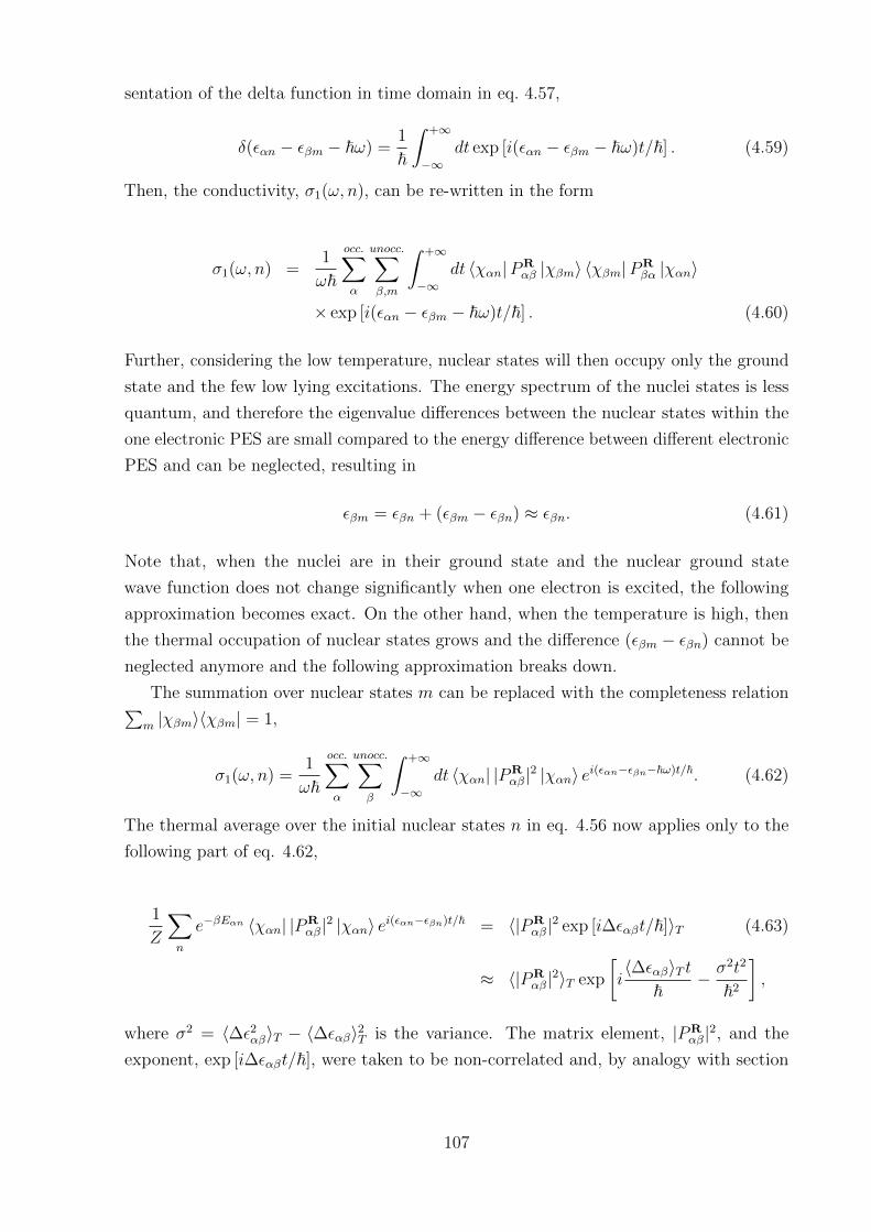
sentation of the delta function in time domain in eq. 4.57,

δ(εαn − εβm − ~ω) =1

~

∫ +∞

−∞dt exp [i(εαn − εβm − ~ω)t/~] . (4.59)

Then, the conductivity, σ1(ω, n), can be re-written in the form

σ1(ω, n) =1

ω~

occ.∑α

unocc.∑β,m

∫ +∞

−∞dt 〈χαn|PR

αβ |χβm〉 〈χβm|PRβα |χαn〉

× exp [i(εαn − εβm − ~ω)t/~] . (4.60)

Further, considering the low temperature, nuclear states will then occupy only the ground

state and the few low lying excitations. The energy spectrum of the nuclei states is less

quantum, and therefore the eigenvalue differences between the nuclear states within the

one electronic PES are small compared to the energy difference between different electronic

PES and can be neglected, resulting in

εβm = εβn + (εβm − εβn) ≈ εβn. (4.61)

Note that, when the nuclei are in their ground state and the nuclear ground state

wave function does not change significantly when one electron is excited, the following

approximation becomes exact. On the other hand, when the temperature is high, then

the thermal occupation of nuclear states grows and the difference (εβm − εβn) cannot be

neglected anymore and the following approximation breaks down.

The summation over nuclear states m can be replaced with the completeness relation∑m |χβm〉〈χβm| = 1,

σ1(ω, n) =1

ω~

occ.∑α

unocc.∑β

∫ +∞

−∞dt 〈χαn| |PR

αβ|2 |χαn〉 ei(εαn−εβn−~ω)t/~. (4.62)

The thermal average over the initial nuclear states n in eq. 4.56 now applies only to the

following part of eq. 4.62,

1

Z

∑n

e−βEαn 〈χαn| |PRαβ|2 |χαn〉 ei(εαn−εβn)t/~ = 〈|PR

αβ|2 exp [i∆εαβt/~]〉T (4.63)

≈ 〈|PRαβ|2〉T exp

[i〈∆εαβ〉T t

~− σ2t2

~2

],

where σ2 = 〈∆ε2αβ〉T − 〈∆εαβ〉2T is the variance. The matrix element, |PRαβ|2, and the

exponent, exp [i∆εαβt/~], were taken to be non-correlated and, by analogy with section

107

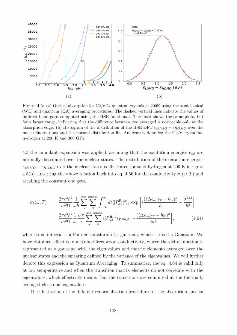
0.0 0.5 1.0 1.5 2.0 2.5 3.0 3.5 4.0 (eV)

0

5000

10000

15000

20000

25000

30000

35000

40000 (c

m1 )

248 GPa QA248 GPa WL290 GPa QA290 GPa WL

0 1 2 3 4 5 60

106

(a)

0.0 0.5 1.0 1.5 2.0 2.5LUMO HOMO (eV)

0.0

0.2

0.4

0.6

0.8

1.0data

LUMO HOMO T = 1.21 eV = 0.44 eV

(b)

Figure 4.5: (a) Optical absorption for C2/c-24 quantum crystals at 200K using the semiclassical(WL) and quantum (QA) averaging procedures. The dashed vertical lines indicate the values ofindirect band-gaps computed using the HSE functional. The inset shows the same plots, butfor a larger range, indicating that the difference between two averaged is noticeable only at theabsorption edge. (b) Histogram of the distribution of the HSE-DFT εLUMO − εHOMO over thenuclei fluctuations and the normal distribution fit. Analyses is done for the C2/c crystallinehydrogen at 200 K and 300 GPa.

4.3 the cumulant expansion was applied, assuming that the excitation energies εαβ are

normally distributed over the nuclear states. The distribution of the excitation energies

εLUMO − εHOMO over the nuclear states is illustrated for solid hydrogen at 200 K in figure

4.5(b). Inserting the above relation back into eq. 4.56 for the conductivity σ1(ω, T ) and

recalling the constant one gets,

σ1(ω, T ) =2πe2~2

m2Ω

1

ω~

occ.∑α

unocc.∑β

∫ ∞−∞

dt〈|PRαβ|2〉T exp

[i(〈∆εαβ〉T − ~ω)t

~− σ2t2

~2

]

=2πe2~2

m2Ω

1

ω

√π

σ

occ.∑α

unocc.∑β

〈|PRαβ|2〉T exp

[−(〈∆εαβ〉T − ~ω)2

4σ2

], (4.64)

where time integral is a Fourier transform of a gaussian, which is itself a Gaussian. We

have obtained effectively a Kubo-Greenwood conductivity, where the delta function is

represented as a gaussian with the eigenvalues and matrix elements averaged over the

nuclear states and the smearing defined by the variance of the eigenvalues. We will further

denote this expression as Quantum Averaging. To summarize, the eq. 4.64 is valid only

at low temperature and when the transition matrix elements do not correlate with the

eigenvalues, which effectively means that the transitions are computed at the thermally

averaged electronic eigenvalues.

The illustration of the different renormalization procedures of the absorption spectra

108

of solid C2c-24 hydrogen at 200 K is presented in fig. 4.5(a). When looking at the large

absorption (inset of fig. 4.5(a)), the difference is negligible, however, looking at absorption

onset (below 40000 cm−1) we clearly see the difference between the two procedures.

Especially at 290 GPa, the semiclassical way predicts the closed gap, i.e. finite absorption

at zero frequency, when in reality the gap is ∼ 0.4 eV. Moreover, the quantum procedure

brings the absorption onset closer to the experimental values, which is discussed in chapter

5.

4.8 Conclusion

In this chapter, we have developed the necessary formalism to treat the excitations and

optical properties in the presence of finite temperature nuclei. We have first considered

the path integral formalism, defining the partition function in the Born-Oppenheimer and

adiabatic approximation. Further, we have discussed the electron addition and removal

energies in the canonical and semi–grandcanonical ensemble at finite temperature. We

have argued that the correct quasiparticle and fundamental gap can only be obtained if

the addition and removal energies are first averaged over the nuclear fluctuations.

To extract the band structure from the supercell calculations at finite temperature,

the crystal momentum has to be determined first. We have provided a general formalism

of determining the crystal momentum of thermal crystals, which we further use to plot

the band structure of solid crystalline hydrogen at 200 K.

Finally, we have introduced an alternative to the semiclassical procedure of renormaliz-

ing optical properties obtained with single electron theory. We have argued that the new

procedure is more suitable for systems at low temperatures with large zero-point nuclear

effects. We call the new procedure quantum averaging. We illustrate the effect of quantum

averaging by computing the absorption coefficient of solid crystalline hydrogen at 200 K

using single electron Kubo-Greenwood theory.

109

110

Chapter 5

Metallization of crystalline molecular

hydrogen

The theoretical framework developed in chapters 2, 3 and 4 is applied to study optical

properties and gap closure with pressure of crystalline molecular hydrogen. We start

by discussing the solid hydrogen phase diagram and possible metallization picture. The

temperature range considered in this work is between 100 K and 430 K. Depending on the

structure, we find that the fundamental indirect gap closes between 380 and 530 GPa for

ideal crystals and 330–380 GPa for quantum crystals. Beyond this pressure, the system

enters into a bad metal phase where the density of states at the Fermi level increases with

pressure up to ∼450–500 GPa when the direct gap closes. To draw a connection between

theoretical and experimental work, we compute optical properties using Kubo-Greenwood

formalism. Furthermore, a procedure of benchmarking DFT functionals, which is based

on mapping DFT and QMC densities of states, is introduced.

For an extensive review of hydrogen, its experimental and theoretical ways of studying,

consider the review paper of McMahon [11], which is accompanied by the recent update

by Goncharov [12].

5.1 Introduction

The metallization of crystalline hydrogen under pressure has attracted considerable

attention over the last century. Predicted to be stable in an atomic bcc lattice around

25GPa, the mechanism for molecular dissociation was first discussed by Wigner and

Huntington [1]. The search for its metallization has driven high pressure research until

the recent [14], still debated [138–141], observation of reflective samples at 495GPa in a

Diamond Anvil Cell (DAC) apparatus. Even though it is the simplest element and H2 the

simplest homonuclear molecule in nature, the study of hydrogen under extreme conditions

has uncovered rich and unexpected physics [11, 142, 143].

111

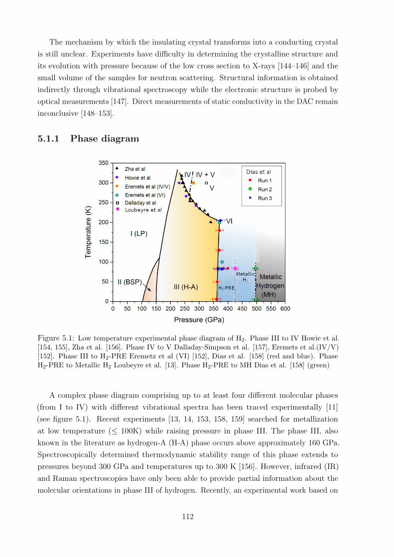
The mechanism by which the insulating crystal transforms into a conducting crystal

is still unclear. Experiments have difficulty in determining the crystalline structure and

its evolution with pressure because of the low cross section to X-rays [144–146] and the

small volume of the samples for neutron scattering. Structural information is obtained

indirectly through vibrational spectroscopy while the electronic structure is probed by

optical measurements [147]. Direct measurements of static conductivity in the DAC remain

inconclusive [148–153].

5.1.1 Phase diagram

Figure 5.1: Low temperature experimental phase diagram of H2. Phase III to IV Howie et al.[154, 155], Zha et al. [156]. Phase IV to V Dalladay-Simpson et al. [157], Eremets et al.(IV/V)[152]. Phase III to H2-PRE Eremetz et al (VI) [152], Dias et al. [158] (red and blue). PhaseH2-PRE to Metallic H2 Loubeyre et al. [13]. Phase H2-PRE to MH Dias et al. [158] (green)

A complex phase diagram comprising up to at least four different molecular phases

(from I to IV) with different vibrational spectra has been traced experimentally [11]

(see figure 5.1). Recent experiments [13, 14, 153, 158, 159] searched for metallization

at low temperature (≤ 100K) while raising pressure in phase III. The phase III, also

known in the literature as hydrogen-A (H-A) phase occurs above approximately 160 GPa.

Spectroscopically determined thermodynamic stability range of this phase extends to

pressures beyond 300 GPa and temperatures up to 300 K [156]. However, infrared (IR)

and Raman spectroscopies have only been able to provide partial information about the

molecular orientations in phase III of hydrogen. Recently, an experimental work based on

112

the new high-quality single-crystal x-ray diffraction (XRD) technique was performed [145].

The authors have predicted that in phase III crystalline hydrogen has a lattice of molecular

centers, which is close to hexagonal close packed (hcp). However, the critics show that the

data remains very limited and insufficient for the complete structural determination [146].

The fact that the II→III transition pressure is relatively insensitive to the isotope (H2

and D2) suggests that phase III is mainly determined by the Born-Oppenheimer energy of

interacting static molecules (i.e. obeys the classical ordering). This allows the use of DFT

as the first approximation to search for the structure of phase III. Indeed, the study of

Pickard and Needs [111] revealed that a monoclinic structure C2/c-24 with 12 molecules

per unit cell provides a good match to the experimental vibrational data for phase III and

is the lowest-enthalpy phase over the pressure range, where phase III is observed (160–300

GPa). However, by including the nuclear quantum effects a new structure, hexagonal

P6122 closer related to the hcp, has emerged and was shown to be more stable than

C2/c-24 below 200 GPa [160].

Considerable attention has also been paid to the higher temperature phase IV since its

discovery [148, 154–156, 161, 162]. Predicted above 220 GPa at room temperature [148, 154]

with the Raman spectra suggesting the existence of two distinct local environments, phase

IV could be a mixture of graphene like layers and unbound hydrogen molecules (see fig.

5.2(c)), which is thought to be a precursor of molecular dissociation. Indeed, repeating

the study of Pickard and Needs [111], but using larger unit cells, several consistent mixed

phases were found with space groups Pc [163, 164], with the best prediction being Pc-48

structure. Further increasing pressure it was shown by Dalladay-Simpson et al. [157],

based on the changes in vibrational spectra, that the new phase (V) will appear, which

should coexist with phase IV in some P-T range [158, 159], because no first order phase

transition was observed [152] but a gradual phase change from IV to V.

At higher pressure, the emerging metallization picture is that the transparent insulating

molecular phase III transforms into a strongly absorbing (in the visible) molecular phase at

∼ 350-360GPa with different IR frequencies, first named phase V [152] and later H2-PRE

or phase VI [147, 158], with semiconducting characteristics [165]. Hydrogen finally reaches

a metallic phase with the observation of reflective samples at ∼495GPa[14], although

disagreement concerning the pressure scale still remains [139, 147, 166]. New synchrotron

infrared spectroscopy measurements [13] report a reversible collapse of the IR transmission

spectrum at 427GPa, interpreted as a first order transition to the metallic state.

5.1.2 High pressure hydrogen crystal structures

The primary information for theoretical investigations of solids is the crystalline

structure. Candidate structures for high pressure phases have been obtained by ab initio

Random Structural Search methods [111, 163, 164, 168], most of them are formed by

113

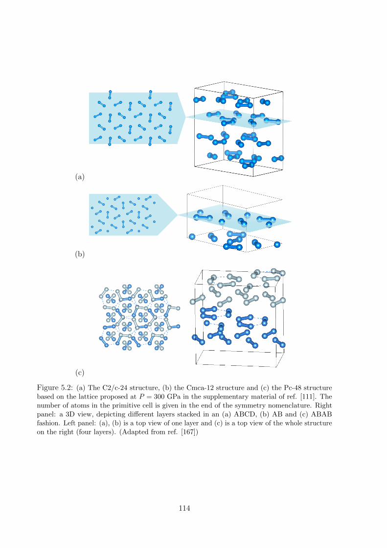
(a)

(b)

(c)

Figure 5.2: (a) The C2/c-24 structure, (b) the Cmca-12 structure and (c) the Pc-48 structurebased on the lattice proposed at P = 300 GPa in the supplementary material of ref. [111]. Thenumber of atoms in the primitive cell is given in the end of the symmetry nomenclature. Rightpanel: a 3D view, depicting different layers stacked in an (a) ABCD, (b) AB and (c) ABABfashion. Left panel: (a), (b) is a top view of one layer and (c) is a top view of the whole structureon the right (four layers). (Adapted from ref. [167])

114

bidimensional layers stacked in various ways.

One of the most probable candidate structures for phase III is the layered C2/c-24

structure with 24 atoms in the primitive cell. Indeed, it gives the lowest free energy in

ground state QMC calculations assuming harmonic phonons corrections (with DFT-PBE)

[3, 169]. The four layers are depicted in figure 5.2(a). Stacked in ABCDA fashion, each

layer consists of molecules almost parallel to the respective planes. Such arrangement of

the molecules creates a non vanishing electric dipole moment, leading to a strong infrared

signal [111], which is qualitatively compatible with experimental results [154].

A structure that is competitive at higher pressures (P > 250 GPa) is the Cmca-12

[3, 169] (fig. 5.2(b)). The structure is similar to C2/c-24, with slightly different stacking

of the layers in ABAB fashion and with the molecules being completely parallel to the

planes.

For Phase IV we consider only Pc-48, since the recently proposed Pca21 structure

[168] is found to be rather similar to Pc48 after geometry relaxation with the vdW-DF

functional. Depicted in fig. 5.2(c), Pc-48 structure which has 48 atoms in the primitive cell.

The structure is layered in ABAB fashion. While the A layers are formed by molecules, the

atoms in the B layers form a distorted hexagonal network. The distortion of the hexagonal

lattice results in different distances among the first neighbours.

We first consider ideal crystal structures (protons fixed at lattice sites) relaxed at

constant pressure with the DFT-vdW-DF functional. Quantum crystals, with protons

represented by path integrals at finite temperature, are addressed with CEIMC at constant

volume1. All systems considered have 96 protons in nearly cubic supercells. Optimized

Slater-Jastrow-Backflow trial wave functions have been used for the CEIMC calculations

[15]; details of the CEIMC simulations are reported in ref.[170]. Averages over ionic

positions for gaps are obtained using 40 statistically independent configurations from the

CEIMC trajectories.

5.2 Fundamental energy gap

In this section we investigate the closure of the electronic gap of candidate structures

for phase III (Cmca-12 and C2/c-24) and phase IV (Pc48)[111, 163] within a Quantum

Monte Carlo (QMC) framework introduced in section 2.1.6. For ideal structures, the

fundamental gap decreases with pressure from ∼ 3-3.5 eV at ∼250GPa to a vanishing value

∼380GPa in the Cmca12 structure and ∼530GPa in the C2/c-24 structure. Using Coupled

Electron-Ion Monte Carlo (CEIMC) calculations, we then include Zero Point Motion

(ZPM) and finite temperature effects of the nuclei within a first principle, non-perturbative

1We have checked that the stress tensor in the constant volume CEIMC run remains diagonal withsame diagonal elements within our statistical noise.

115

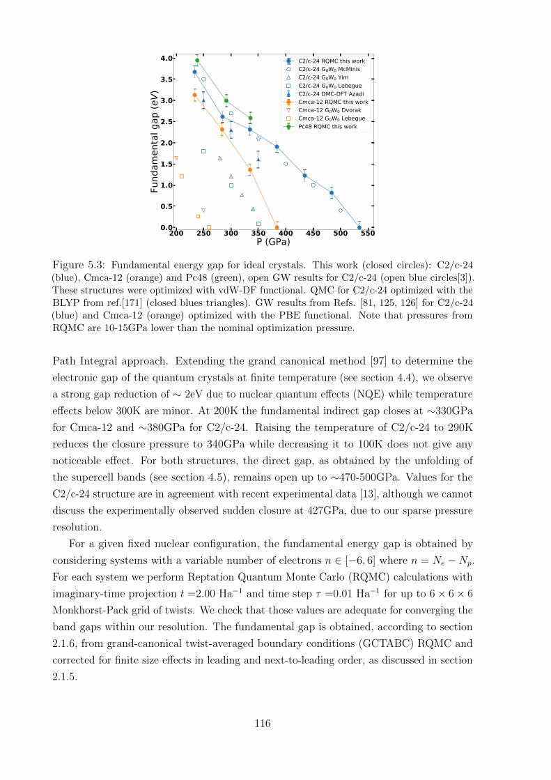
200 250 300 350 400 450 500 550P (GPa)

0.0

0.5

1.0

1.5

2.0

2.5

3.0

3.5

4.0

Fund

amen

tal g

ap (e

V)

C2/c-24 RQMC this workC2/c-24 G0W0 McMinisC2/c-24 G0W0 YimC2/c-24 G0W0 LebegueC2/c-24 DMC-DFT AzadiCmca-12 RQMC this workCmca-12 G0W0 DvorakCmca-12 G0W0 LebeguePc48 RQMC this work

Figure 5.3: Fundamental energy gap for ideal crystals. This work (closed circles): C2/c-24(blue), Cmca-12 (orange) and Pc48 (green), open GW results for C2/c-24 (open blue circles[3]).These structures were optimized with vdW-DF functional. QMC for C2/c-24 optimized with theBLYP from ref.[171] (closed blues triangles). GW results from Refs. [81, 125, 126] for C2/c-24(blue) and Cmca-12 (orange) optimized with the PBE functional. Note that pressures fromRQMC are 10-15GPa lower than the nominal optimization pressure.

Path Integral approach. Extending the grand canonical method [97] to determine the

electronic gap of the quantum crystals at finite temperature (see section 4.4), we observe

a strong gap reduction of ∼ 2eV due to nuclear quantum effects (NQE) while temperature

effects below 300K are minor. At 200K the fundamental indirect gap closes at ∼330GPa

for Cmca-12 and ∼380GPa for C2/c-24. Raising the temperature of C2/c-24 to 290K

reduces the closure pressure to 340GPa while decreasing it to 100K does not give any

noticeable effect. For both structures, the direct gap, as obtained by the unfolding of

the supercell bands (see section 4.5), remains open up to ∼470-500GPa. Values for the

C2/c-24 structure are in agreement with recent experimental data [13], although we cannot

discuss the experimentally observed sudden closure at 427GPa, due to our sparse pressure

resolution.

For a given fixed nuclear configuration, the fundamental energy gap is obtained by

considering systems with a variable number of electrons n ∈ [−6, 6] where n = Ne −Np.

For each system we perform Reptation Quantum Monte Carlo (RQMC) calculations with

imaginary-time projection t =2.00 Ha−1 and time step τ =0.01 Ha−1 for up to 6× 6× 6

Monkhorst-Pack grid of twists. We check that those values are adequate for converging the

band gaps within our resolution. The fundamental gap is obtained, according to section

2.1.6, from grand-canonical twist-averaged boundary conditions (GCTABC) RQMC and

corrected for finite size effects in leading and next-to-leading order, as discussed in section

2.1.5.

116

Extending calculations of the fundamental gaps to quantum crystals, the trace over

nuclear degrees of freedom must be taken with care. In the semiclassical approximation

(see section 4.3), the fundamental gap is the smallest electronic excitation energy that

occurs from quantum or thermal fluctuations of the lattice. Strictly speaking this gap is

always closed, since the probability of a proton configuration with a metallic character

is never exactly zero. For dense molecular hydrogen phonon energies are ∼ 0.1− 0.5 eV

[163]. ZPM dominates for T ≤ 1000K, so the semi-classical approach is not appropriate.

Electronic energies should be averaged over the nuclear configurations according to their

thermal distribution. The gap will be given by the minimum of the average excitation

energies, always larger than the semiclassical gap. Figure 5.5a illustrates typical results

for the integrated density of states as a function of (electronic) chemical potential. The

gap of the quantum crystal can be directly read off from the width of the incompressible

region. More details are given in section 4.4.

Figure 5.3 shows estimates of the fundamental gap for ideal crystals versus pressure.

The gap decreases with pressure in a similar fashion for all structures: Cmca-12 has the

smallest gap, followed by C2/c-24 and by Pc48. We find reasonable agreement with the

QMC estimates of ref. [171] 2. References [81, 125, 126] report smaller values of the gap

based on GW. We believe this disagreement is primarily due to the lattice geometry that

has been optimized at constant pressure with PBE in refs. [81, 125, 126] and with vdW-DF

in the present work. It has been previously observed that PBE optimized geometries has

longer H2 bonds and smaller gap values at DFT level [49, 112] (see fig. 3.2b for illustration).

This propagates into G0W0. Indeed, GW results from structures optimized with vdW-DF

[3] are in excellent agreement with our predictions.

Values of the fundamental gap from GCTABC for quantum crystals at various temper-

atures and pressures are shown in Fig. 5.4a: they are smaller by ∼2eV with respect to the

ideal crystal. ZPM is almost entirely responsible for this reduction. Note that the gap

hardly changes from 300K to 200K within our estimated errors. Similar to ideal crystals,

Cmca-12 gap is smaller than C2/c-24 gap at T=200K, the former closing at ∼340GPa

while the latter at higher pressures ∼380GPa. As for the Pc-48 structure at T=430K

(phase IV) the gap is slightly below values for C2/c-24 at 200K. Our results show that the

electronic gap is fairly independent of the specific crystalline structure of the molecular

quantum crystals. We also report gap values for C2/c-24 at T=200K from Path Integral

Molecular Dynamics (PIMD)[49] with two different DFT functionals, namely HSE [48]

and vdW-DF2 [123]. As vdW-DF2 underestimates the molecular bond lengths of the ideal

crystalline structure [112], its PIMD configurations are expected to bias the electronic

gap towards larger values. Our results do not agree with predictions of ref. [173] (not

2The observed small difference, in particular at the higher pressure, is probably due to the differentXC approximation used for geometry optimization, vdW-DF in our case, BLYP in ref. [171] and differentsize extrapolation.

117

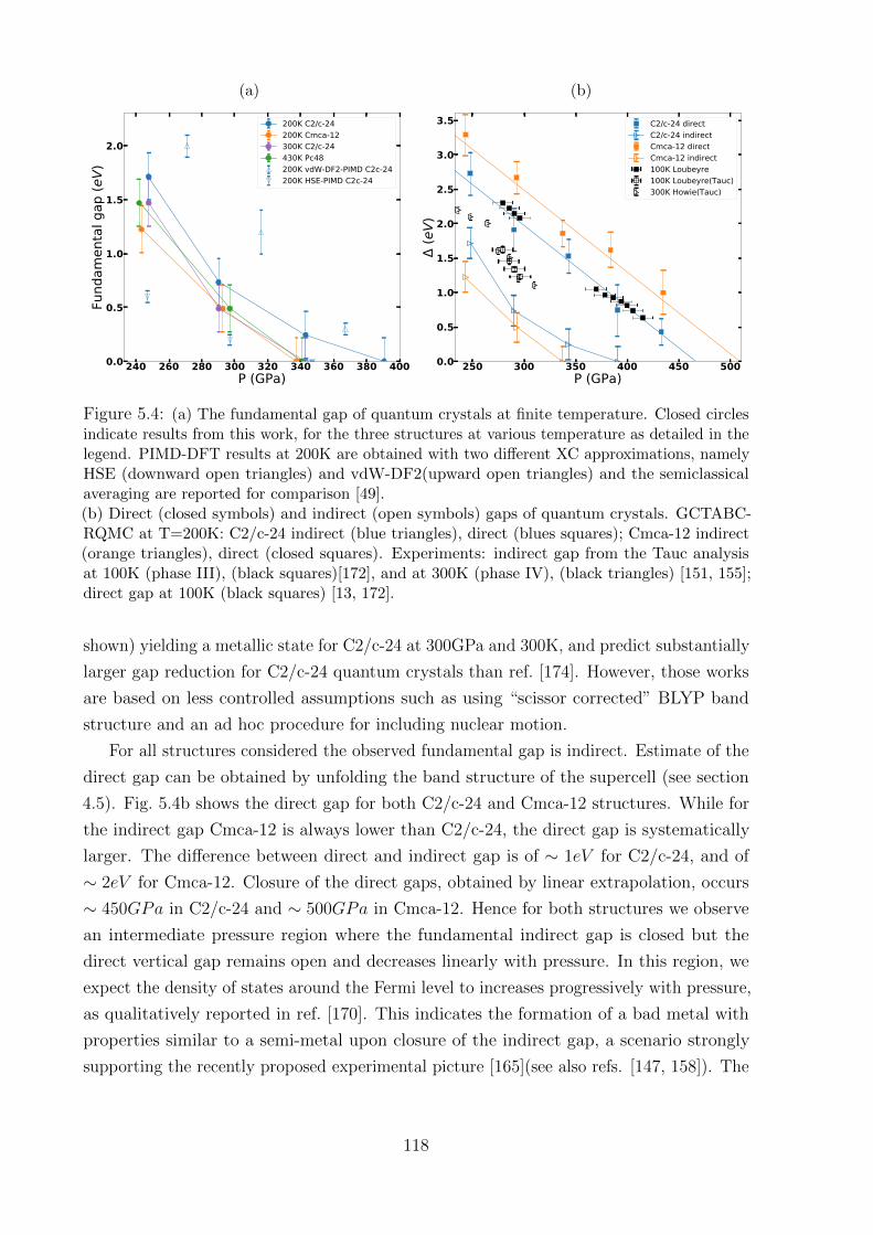
(a)

240 260 280 300 320 340 360 380 400P (GPa)

0.0

0.5

1.0

1.5

2.0

Fund

amen

tal g

ap (e

V)200K C2/c-24200K Cmca-12300K C2/c-24430K Pc48200K vdW-DF2-PIMD C2c-24200K HSE-PIMD C2c-24

(b)

250 300 350 400 450 500P (GPa)

0.0

0.5

1.0

1.5

2.0

2.5

3.0

3.5

(eV)

C2/c-24 directC2/c-24 indirectCmca-12 directCmca-12 indirect100K Loubeyre100K Loubeyre(Tauc)300K Howie(Tauc)

Figure 5.4: (a) The fundamental gap of quantum crystals at finite temperature. Closed circlesindicate results from this work, for the three structures at various temperature as detailed in thelegend. PIMD-DFT results at 200K are obtained with two different XC approximations, namelyHSE (downward open triangles) and vdW-DF2(upward open triangles) and the semiclassicalaveraging are reported for comparison [49].(b) Direct (closed symbols) and indirect (open symbols) gaps of quantum crystals. GCTABC-RQMC at T=200K: C2/c-24 indirect (blue triangles), direct (blues squares); Cmca-12 indirect(orange triangles), direct (closed squares). Experiments: indirect gap from the Tauc analysisat 100K (phase III), (black squares)[172], and at 300K (phase IV), (black triangles) [151, 155];direct gap at 100K (black squares) [13, 172].

shown) yielding a metallic state for C2/c-24 at 300GPa and 300K, and predict substantially

larger gap reduction for C2/c-24 quantum crystals than ref. [174]. However, those works

are based on less controlled assumptions such as using “scissor corrected” BLYP band

structure and an ad hoc procedure for including nuclear motion.

For all structures considered the observed fundamental gap is indirect. Estimate of the

direct gap can be obtained by unfolding the band structure of the supercell (see section

4.5). Fig. 5.4b shows the direct gap for both C2/c-24 and Cmca-12 structures. While for

the indirect gap Cmca-12 is always lower than C2/c-24, the direct gap is systematically

larger. The difference between direct and indirect gap is of ∼ 1eV for C2/c-24, and of

∼ 2eV for Cmca-12. Closure of the direct gaps, obtained by linear extrapolation, occurs

∼ 450GPa in C2/c-24 and ∼ 500GPa in Cmca-12. Hence for both structures we observe

an intermediate pressure region where the fundamental indirect gap is closed but the

direct vertical gap remains open and decreases linearly with pressure. In this region, we

expect the density of states around the Fermi level to increases progressively with pressure,

as qualitatively reported in ref. [170]. This indicates the formation of a bad metal with

properties similar to a semi-metal upon closure of the indirect gap, a scenario strongly

supporting the recently proposed experimental picture [165](see also refs. [147, 158]). The

118

non-vanishing direct gap naturally explains the reported observation of absorbing (black)

hydrogen around 320-360 GPa (depending on the experimental pressure scale) [172].

Fig. 5.4b also shows the experimental estimates of both indirect and direct gaps

from optical absorption. Measuring indirect gaps is difficult in hydrogen since samples

are very thin and the optical signal from phonon-assisted absorption is too low to be

detected [150, 153]. The indirect gap value has been extracted from a Tauc analysis of

the absorption profiles at 300K (Phase IV) [151, 155] and 100K (Phase III) [156, 172]

assuming the low energy absorption spectrum can be reliably extrapolated to zero energy.

We have re-analyzed the spectra of ref. [172] to extract the value of the indirect gap from

a Tauc plot [175], as was performed in ref. [151] for the data from ref. [155]. Details are

further given in section 5.3.2. Conversely the direct gap at 100K (phase III) has been

associated with the absorption edge at lower pressure [172] or with full absorption at higher

pressure [13] and corresponds roughly to the energy where the absorption coefficient equals

30000cm−1. The direct gap of C2/c-24 structure is in agreement with the experimental

data up to 425GPa, where experiments report a collapse of the gap value ascribed to

the metallization transition[13]. Our results do not allow to predict this transition, but

rule out C2/c-24 and Cmca-12 for this new metallic phase 3. For the indirect gap we

predict ∼ 0.3 − 0.5eV smaller values than in experiments. However, the Tauc analysis

of refs. [151, 155, 172] does not consider the energy of the emitted or absorbed phonons,

which should be comparable to the observed discrepancy. However, excitonic effects and

exciton-phonon coupling, neglected within the present approach, need to be addressed

for this level of precision. In agreement with our findings, the experimental indirect gap

depends little on both temperature and structure 4.

5.3 Optical properties

Next we explore optical properties computed using the Kubo-Greenwood (KG) frame-

work with Kohn-Sham (KS) orbitals. To reduce the bias of the underlying DFT functional,

we have benchmarked several XC approximations to reproduce the behavior of the QMC

density of states close to the gap. In fig. 5.5a for C2/c-24 at 200K, we compare the

electronic excess density, ne − np, as a function of electronic chemical potential, µ, from

QMC and from DFT-HSE 5. The observed plateau at ne − np = 0 is the signature of the

indirect gap. Deviations from the plateau on both sides characterize the density of states

of the valence and conduction band close to the band edges. As shown in Fig. 5.5a the

HSE approximation provides slightly smaller values of the fundamental gap and reproduces

3Our estimates of the direct gap could be biased by ∼ 0.3eV due to the discreteness of our twist grid.Correcting for this bias will place the experimental data in between the C2/c-24 and Cmca-12 predictions.

4Note that the pressure values of ref. [172] have been recently corrected [13]5This quantity is closely related to the integrated density of states.

119

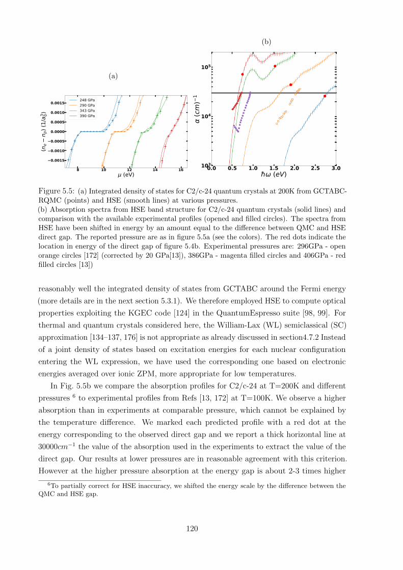
(a)

8 10 12 14 16 (eV)

0.0015

0.0010

0.0005

0.0000

0.0005

0.0010

0.0015

(ne

n p) (

1/a3 0)

248 GPa290 GPa343 GPa390 GPa

(b)

0.0 0.5 1.0 1.5 2.0 2.5 3.0 (eV)

103

104

105

(cm

)1

Figure 5.5: (a) Integrated density of states for C2/c-24 quantum crystals at 200K from GCTABC-RQMC (points) and HSE (smooth lines) at various pressures.(b) Absorption spectra from HSE band structure for C2/c-24 quantum crystals (solid lines) andcomparison with the available experimental profiles (opened and filled circles). The spectra fromHSE have been shifted in energy by an amount equal to the difference between QMC and HSEdirect gap. The reported pressure are as in figure 5.5a (see the colors). The red dots indicate thelocation in energy of the direct gap of figure 5.4b. Experimental pressures are: 296GPa - openorange circles [172] (corrected by 20 GPa[13]), 386GPa - magenta filled circles and 406GPa - redfilled circles [13])

reasonably well the integrated density of states from GCTABC around the Fermi energy

(more details are in the next section 5.3.1). We therefore employed HSE to compute optical

properties exploiting the KGEC code [124] in the QuantumEspresso suite [98, 99]. For

thermal and quantum crystals considered here, the William-Lax (WL) semiclassical (SC)

approximation [134–137, 176] is not appropriate as already discussed in section4.7.2 Instead

of a joint density of states based on excitation energies for each nuclear configuration

entering the WL expression, we have used the corresponding one based on electronic

energies averaged over ionic ZPM, more appropriate for low temperatures.

In Fig. 5.5b we compare the absorption profiles for C2/c-24 at T=200K and different

pressures 6 to experimental profiles from Refs [13, 172] at T=100K. We observe a higher

absorption than in experiments at comparable pressure, which cannot be explained by

the temperature difference. We marked each predicted profile with a red dot at the

energy corresponding to the observed direct gap and we report a thick horizontal line at

30000cm−1 the value of the absorption used in the experiments to extract the value of the

direct gap. Our results at lower pressures are in reasonable agreement with this criterion.

However at the higher pressure absorption at the energy gap is about 2-3 times higher

6To partially correct for HSE inaccuracy, we shifted the energy scale by the difference between theQMC and HSE gap.

120

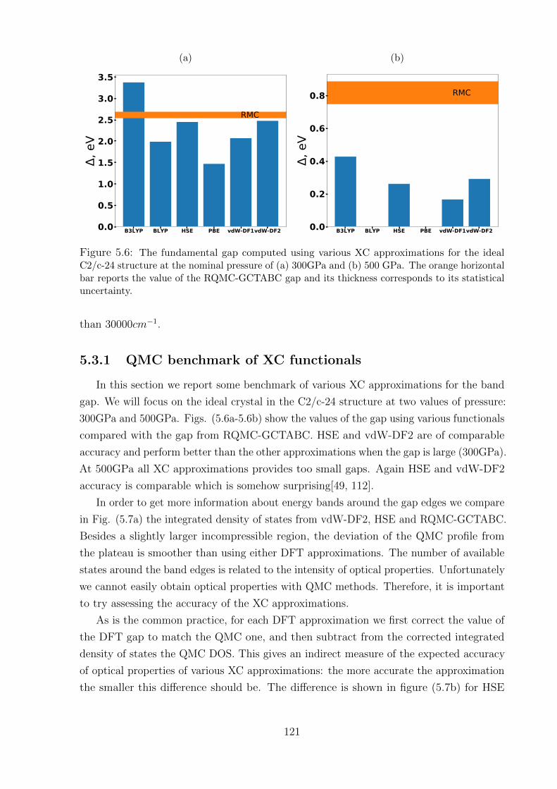
(a)

B3LYP BLYP HSE PBE vdW-DF1vdW-DF20.0

0.5

1.0

1.5

2.0

2.5

3.0

3.5, e

V

RMC

(b)

B3LYP BLYP HSE PBE vdW-DF1vdW-DF20.0

0.2

0.4

0.6

0.8

, eV

RMC

Figure 5.6: The fundamental gap computed using various XC approximations for the idealC2/c-24 structure at the nominal pressure of (a) 300GPa and (b) 500 GPa. The orange horizontalbar reports the value of the RQMC-GCTABC gap and its thickness corresponds to its statisticaluncertainty.

than 30000cm−1.

5.3.1 QMC benchmark of XC functionals

In this section we report some benchmark of various XC approximations for the band

gap. We will focus on the ideal crystal in the C2/c-24 structure at two values of pressure:

300GPa and 500GPa. Figs. (5.6a-5.6b) show the values of the gap using various functionals

compared with the gap from RQMC-GCTABC. HSE and vdW-DF2 are of comparable

accuracy and perform better than the other approximations when the gap is large (300GPa).

At 500GPa all XC approximations provides too small gaps. Again HSE and vdW-DF2

accuracy is comparable which is somehow surprising[49, 112].

In order to get more information about energy bands around the gap edges we compare

in Fig. (5.7a) the integrated density of states from vdW-DF2, HSE and RQMC-GCTABC.

Besides a slightly larger incompressible region, the deviation of the QMC profile from

the plateau is smoother than using either DFT approximations. The number of available

states around the band edges is related to the intensity of optical properties. Unfortunately

we cannot easily obtain optical properties with QMC methods. Therefore, it is important

to try assessing the accuracy of the XC approximations.

As is the common practice, for each DFT approximation we first correct the value of

the DFT gap to match the QMC one, and then subtract from the corrected integrated

density of states the QMC DOS. This gives an indirect measure of the expected accuracy

of optical properties of various XC approximations: the more accurate the approximation

the smaller this difference should be. The difference is shown in figure (5.7b) for HSE

121

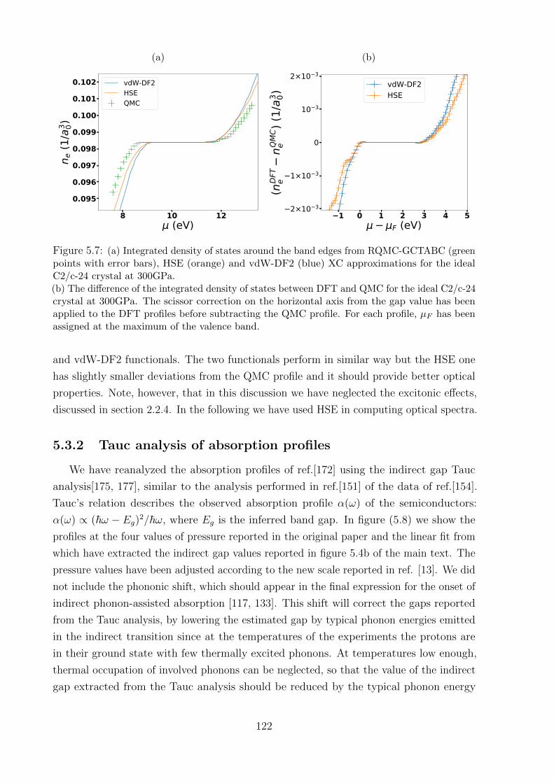
(a)

8 10 12 (eV)

0.095

0.096

0.097

0.098

0.099

0.100

0.101

0.102

n e (1

/a3 0)

vdW-DF2HSEQMC

(b)

1 0 1 2 3 4 5F (eV)

2×10 3

1×10 3

0

10 3

2×10 3

(nD

FTe

nQM

Ce

) (1/

a3 0)

vdW-DF2HSE

Figure 5.7: (a) Integrated density of states around the band edges from RQMC-GCTABC (greenpoints with error bars), HSE (orange) and vdW-DF2 (blue) XC approximations for the idealC2/c-24 crystal at 300GPa.(b) The difference of the integrated density of states between DFT and QMC for the ideal C2/c-24crystal at 300GPa. The scissor correction on the horizontal axis from the gap value has beenapplied to the DFT profiles before subtracting the QMC profile. For each profile, µF has beenassigned at the maximum of the valence band.

and vdW-DF2 functionals. The two functionals perform in similar way but the HSE one

has slightly smaller deviations from the QMC profile and it should provide better optical

properties. Note, however, that in this discussion we have neglected the excitonic effects,

discussed in section 2.2.4. In the following we have used HSE in computing optical spectra.

5.3.2 Tauc analysis of absorption profiles

We have reanalyzed the absorption profiles of ref.[172] using the indirect gap Tauc

analysis[175, 177], similar to the analysis performed in ref.[151] of the data of ref.[154].

Tauc’s relation describes the observed absorption profile α(ω) of the semiconductors:

α(ω) ∝ (~ω − Eg)2/~ω, where Eg is the inferred band gap. In figure (5.8) we show the

profiles at the four values of pressure reported in the original paper and the linear fit from

which have extracted the indirect gap values reported in figure 5.4b of the main text. The

pressure values have been adjusted according to the new scale reported in ref. [13]. We did

not include the phononic shift, which should appear in the final expression for the onset of

indirect phonon-assisted absorption [117, 133]. This shift will correct the gaps reported

from the Tauc analysis, by lowering the estimated gap by typical phonon energies emitted

in the indirect transition since at the temperatures of the experiments the protons are

in their ground state with few thermally excited phonons. At temperatures low enough,

thermal occupation of involved phonons can be neglected, so that the value of the indirect

gap extracted from the Tauc analysis should be reduced by the typical phonon energy

122

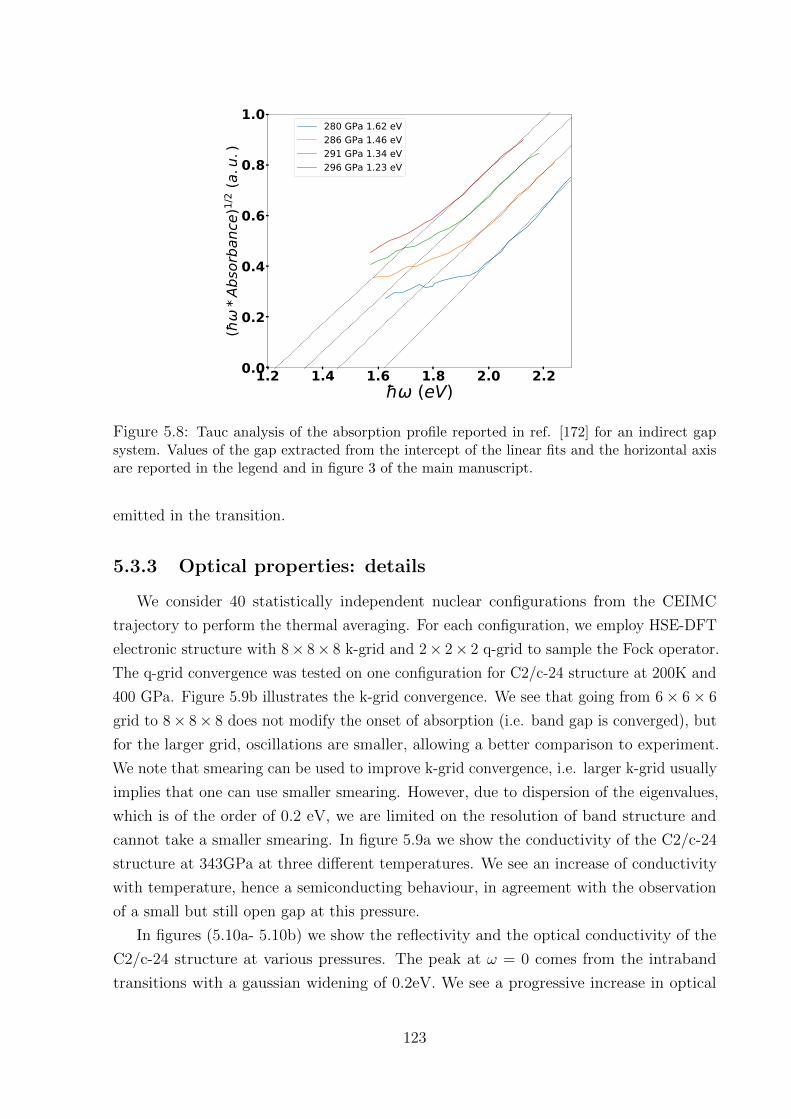
1.2 1.4 1.6 1.8 2.0 2.2 (eV)

0.0

0.2

0.4

0.6

0.8

1.0

(*A

bsor

banc

e)1/

2 (a.

u.)

280 GPa 1.62 eV286 GPa 1.46 eV291 GPa 1.34 eV296 GPa 1.23 eV

Figure 5.8: Tauc analysis of the absorption profile reported in ref. [172] for an indirect gapsystem. Values of the gap extracted from the intercept of the linear fits and the horizontal axisare reported in the legend and in figure 3 of the main manuscript.

emitted in the transition.

5.3.3 Optical properties: details

We consider 40 statistically independent nuclear configurations from the CEIMC

trajectory to perform the thermal averaging. For each configuration, we employ HSE-DFT

electronic structure with 8× 8× 8 k-grid and 2× 2× 2 q-grid to sample the Fock operator.

The q-grid convergence was tested on one configuration for C2/c-24 structure at 200K and

400 GPa. Figure 5.9b illustrates the k-grid convergence. We see that going from 6× 6× 6

grid to 8× 8× 8 does not modify the onset of absorption (i.e. band gap is converged), but

for the larger grid, oscillations are smaller, allowing a better comparison to experiment.

We note that smearing can be used to improve k-grid convergence, i.e. larger k-grid usually

implies that one can use smaller smearing. However, due to dispersion of the eigenvalues,

which is of the order of 0.2 eV, we are limited on the resolution of band structure and

cannot take a smaller smearing. In figure 5.9a we show the conductivity of the C2/c-24

structure at 343GPa at three different temperatures. We see an increase of conductivity

with temperature, hence a semiconducting behaviour, in agreement with the observation

of a small but still open gap at this pressure.

In figures (5.10a- 5.10b) we show the reflectivity and the optical conductivity of the

C2/c-24 structure at various pressures. The peak at ω = 0 comes from the intraband

transitions with a gaussian widening of 0.2eV. We see a progressive increase in optical

123

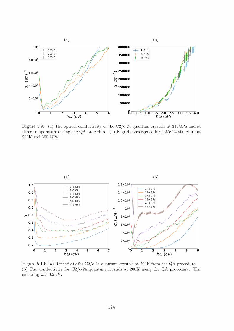
(a)

0 1 2 3 4 5 6 (eV)

0

2×105

4×105

6×105

8×105

106

, (m

)1

100 K200 K300 K

(b)

0.0 0.5 1.0 1.5 2.0 2.5 3.0 3.5 4.0 (eV)

0

50000

100000

150000

200000

250000

300000

350000

400000

(cm

1 )

4x4x46x6x68x8x8

Figure 5.9: (a) The optical conductivity of the C2/c-24 quantum crystals at 343GPa and atthree temperatures using the QA procedure. (b) K-grid convergence for C2/c-24 structure at200K and 300 GPa

(a)

0 1 2 3 4 5 6 7 (eV)

0.2

0.3

0.4

0.5

0.6

0.7

0.8

0.9

1.0

R

248 GPa290 GPa343 GPa390 GPa433 GPa475 GPa

(b)

0 1 2 3 4 5 6 (eV)

0

2×105

4×105

6×105

8×105

106

1.2×106

1.4×106

1.6×106

, (m

)1

248 GPa290 GPa343 GPa390 GPa433 GPa475 GPa

Figure 5.10: (a) Reflectivity for C2/c-24 quantum crystals at 200K from the QA procedure.(b) The conductivity for C2/c-24 quantum crystals at 200K using the QA procedure. Thesmearing was 0.2 eV.

124

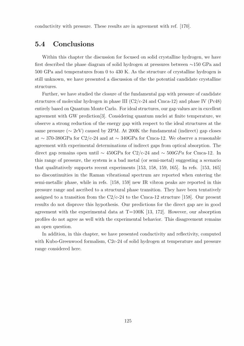
conductivity with pressure. These results are in agreement with ref. [170].

5.4 Conclusions

Within this chapter the discussion for focused on solid crystalline hydrogen, we have

first described the phase diagram of solid hydrogen at pressures between ∼150 GPa and

500 GPa and temperatures from 0 to 430 K. As the structure of crystalline hydrogen is

still unknown, we have presented a discussion of the the potential candidate crystalline

structures.

Further, we have studied the closure of the fundamental gap with pressure of candidate

structures of molecular hydrogen in phase III (C2/c-24 and Cmca-12) and phase IV (Pc48)

entirely based on Quantum Monte Carlo. For ideal structures, our gap values are in excellent

agreement with GW prediction[3]. Considering quantum nuclei at finite temperature, we

observe a strong reduction of the energy gap with respect to the ideal structures at the

same pressure (∼ 2eV) caused by ZPM. At 200K the fundamental (indirect) gap closes

at ∼ 370-380GPa for C2/c-24 and at ∼ 340GPa for Cmca-12. We observe a reasonable

agreement with experimental determinations of indirect gaps from optical absorption. The

direct gap remains open until ∼ 450GPa for C2/c-24 and ∼ 500GPa for Cmca-12. In

this range of pressure, the system is a bad metal (or semi-metal) suggesting a scenario

that qualitatively supports recent experiments [153, 158, 159, 165]. In refs. [153, 165]

no discontinuities in the Raman vibrational spectrum are reported when entering the

semi-metallic phase, while in refs. [158, 159] new IR vibron peaks are reported in this

pressure range and ascribed to a structural phase transition. They have been tentatively

assigned to a transition from the C2/c-24 to the Cmca-12 structure [158]. Our present

results do not disprove this hypothesis. Our predictions for the direct gap are in good

agreement with the experimental data at T=100K [13, 172]. However, our absorption

profiles do not agree as well with the experimental behavior. This disagreement remains

an open question.

In addition, in this chapter, we have presented conductivity and reflectivity, computed

with Kubo-Greenwood formalism, C2c-24 of solid hydrogen at temperature and pressure

range considered here.

125

126

Chapter 6

Metal insulator transition in dense

liquid hydrogen

Liquid hydrogen at temperatures between 900 K and 3000 K and pressures from 70

GPa to 220 GPa, the area where the molecular dissociation occurs, is the focus of this

chapter. In particular, here we address the fundamental gap closure across the liquid-liquid

phase transition in hydrogen. The main finding is that the gap closure coincides with the

molecular dissociation transition of liquid hydrogen. The chapter begins with a review

of the experimental and theoretical works focusing on studying liquid hydrogen and its

metallization. Besides the fundamental gap results, obtained with QMC, we provide a

benchmark of some DFT functionals based on the QMC density of states. Finally, using

the benchmarked HSE functional, we reanalyze optical absorption results provided in Rillo

et al. [6].

For a discussion of the physics of liquid hydrogen, I again refer to a review by McMahon

[11] with an additional discussion of the recent advances by Goncharov [12] and Gregoryanz

[178].

6.1 Introduction

6.1.1 Discussion of previous experimental and theoretical works

The insulator-metal (IM) transition in liquid hydrogen has been a longstanding focus

in physics. Initially, the first order transition from the insulating molecular to metallic

monoatomic fluid, called plasma-phase transition (PPT), was predicted theoretically

based on chemical models [25, 185–187]. Besides, there was proposed that above some

critical temperature dielectric liquid should continuously transform to a metal [25, 186].

Experimentally high P-T conditions necessary to observe the PPT can be achieved in two

ways: using dynamic or static compression. Dynamically, hydrogen can be compressed

127

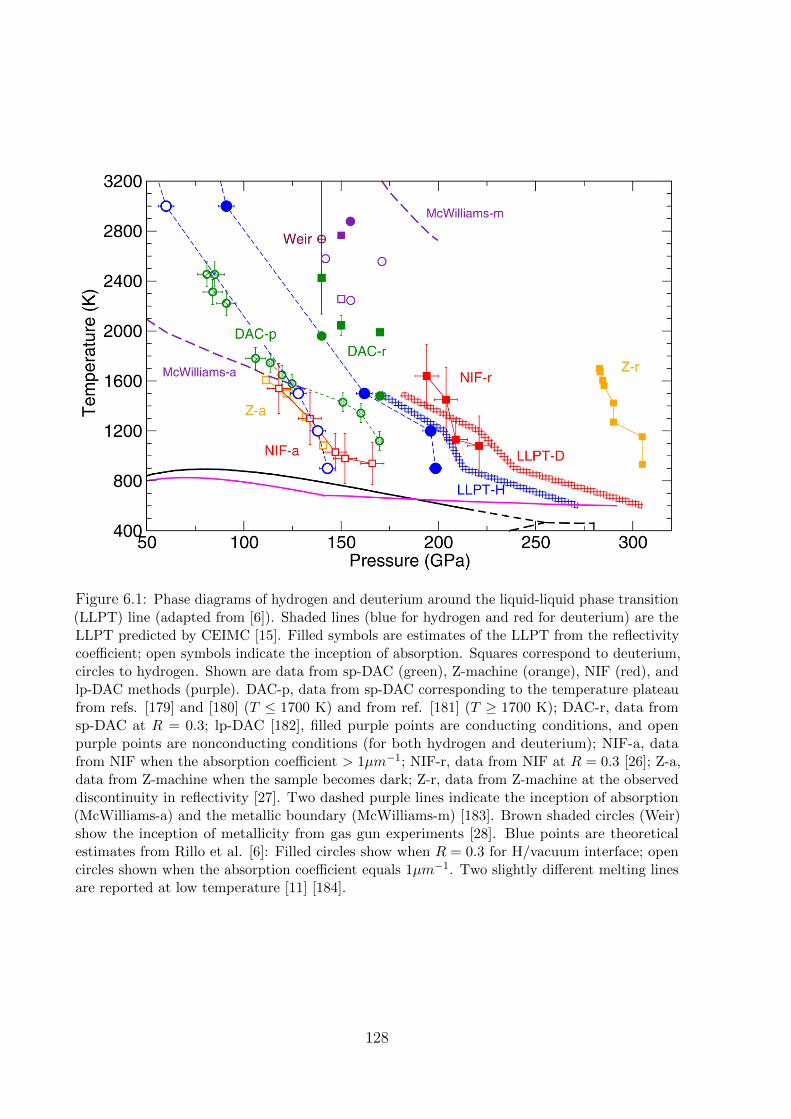
Figure 6.1: Phase diagrams of hydrogen and deuterium around the liquid-liquid phase transition(LLPT) line (adapted from [6]). Shaded lines (blue for hydrogen and red for deuterium) are theLLPT predicted by CEIMC [15]. Filled symbols are estimates of the LLPT from the reflectivitycoefficient; open symbols indicate the inception of absorption. Squares correspond to deuterium,circles to hydrogen. Shown are data from sp-DAC (green), Z-machine (orange), NIF (red), andlp-DAC methods (purple). DAC-p, data from sp-DAC corresponding to the temperature plateaufrom refs. [179] and [180] (T ≤ 1700 K) and from ref. [181] (T ≥ 1700 K); DAC-r, data fromsp-DAC at R = 0.3; lp-DAC [182], filled purple points are conducting conditions, and openpurple points are nonconducting conditions (for both hydrogen and deuterium); NIF-a, datafrom NIF when the absorption coefficient > 1µm−1; NIF-r, data from NIF at R = 0.3 [26]; Z-a,data from Z-machine when the sample becomes dark; Z-r, data from Z-machine at the observeddiscontinuity in reflectivity [27]. Two dashed purple lines indicate the inception of absorption(McWilliams-a) and the metallic boundary (McWilliams-m) [183]. Brown shaded circles (Weir)show the inception of metallicity from gas gun experiments [28]. Blue points are theoreticalestimates from Rillo et al. [6]: Filled circles show when R = 0.3 for H/vacuum interface; opencircles shown when the absorption coefficient equals 1µm−1. Two slightly different melting linesare reported at low temperature [11] [184].

128

with shock waves, following the time-varying changes in pressure, the metallic states can

be detected via electrical, optical and density measurements [26–28, 188–193]. Meanwhile,

statically metallic liquid hydrogen can be reached in diamond anvil cell (DAC), following

the controlled laser heating at constant pressure [179–183, 194].

The detailed experimental and theoretical phase diagrams of hydrogen and deuterium

around the PPT, which is usually called liquid-liquid phase transition (LLPT), is presented

on figure 6.1.

The most direct information on the IM transition can be achieved via the conductivity

measurements. The first experimental work that directly determined conductivity via

the resistance measurements in the liquid hydrogen was carried out using a shock wave

compression in the gas-gun experiment [28, 188, 189]. To achieve high pressures, the

initial shock is split into multiple, relatively weak shocks reverberating in hydrogen

between two sapphire anvils. The resistance was measured by putting the electrodes to the

hydrogen/anvil interface, the electrodes, in turn, were connected to the oscilloscope through

a battery-charged isolated capacitor. When a shock wave transits the liquid hydrogen

between the electrodes, the liquid becomes conducting and the capacitors discharge through

hydrogen allowing the resistance measurements. Pressure was determined via the measured

mass velocity of the initial shock and the Hugoniot equation of state (EOS) of the sapphire

anvil. The other thermodynamic parameters such as density and temperature were

determined from different EOS of hydrogen [195, 196] which result in a large temperature

uncertainty. Based on the minimum conductivity of 2000 (Ωcm)−1 the IM transition

was placed at 140 GPa and 2600 K. To determine the energy gap the authors fitted the

conductivities in the range 93− 120 GPa to the equation for a liquid semiconductor with

the thermally activated conductivity that depends on the mobility gap and the limiting

value of conductivity.

Shock compression can as well be a laser-driven process [26, 190] (NIF). The setup

is almost identical to the one in gas-gun experiment, except that now the shock wave is

created by laser irradiation of the pusher (Al or Be or Cu) and then being transmitted to

the liquid hydrogen/deuterium. The shock velocity and the reflectance are measured with

another lasers. Thermodynamic parameters are inferred from the velocity data based on

the known EOSs. Different EOSs result again in the large uncertainty on temperature.

The latest results on IM transition in liquid deuterium in this experimental setup predict

it to be the first order with the critical temperature in the range of 1100 K< TC <3000 K

with the metallization pressure around 200 GPa [26]. Based on optical measurements, two

transition boundaries were identified: first, sample becomes opaque, which corresponds to

the onset of absorption, then follows by the increase of the reflectivity to 30%, which is

attributed to the IM transition. The reported band gap is based on the empirical relations

to the refractive index of semiconductor materials.

129

In a similar experiment, the shock wave in deuterium was created using the electro-

magnetic current pulse [27] (Z-machine). The authors see the absorption increase at the

same P-T range as Cellier et al. [26], however their reflectivity increases abruptly at higher

pressure, between 280 and 305 GPa. The temperature range (again inferred via the EOS)

is between 1000 K and 1800 K. The band gap is not measured directly but based on the

energy of absorption onset (∼ 2.3 eV) and qualitatively compared to the reanalyzed data

of Weir et al. [189] and to first-principle density functional theory (DFT) predictions.

Hydrogen is a very diffusive material, therefore it is difficult to achieve high tempera-

tures, required to observe the IM transition, during static compression. However, using

short pulsed-laser heating it was possible to reach up to 3000 K in a DAC with compressed

liquid hydrogen [179–181, 194, 197] (sp-DAC). By increasing the laser power, a plateau in

temperature between 1100-2200 K and 90-160 GPa [137, 179, 181] accompanied by the

increase of reflectivity and decrease in optical transmission [180] was interpreted as being

due to the latent heat, a signature of the first order phase transition. Although, a finite

element analysis (FEA) of the pulsed-laser heated DAC predicts the latent heat necessary

to reach the plateau to be rather large (∼ 2eV/atom), in contrast to the theoretical predic-

tions for the latent heat at the PPT (∼ 0.035 eV) [198]. The plateaus were alternatively

interpreted by other authors as the onset of hydrogen absorption [26, 27, 199]. Measured

reflectivity reaches saturation at higher temperatures than the plateau [194]. Based on

the Drude fit, at the saturation hydrogen is predicted to be largely atomic and degenerate,

in contrast to the semiconductor model. However, below the saturation, the nature of the

liquid is non-free-electron like [200].

Using long pulsed-laser heating, another experimental group observed similar two-stage

transition: anomalous temperature behavior and the onset of absorption followed by the

rapid increase of the reflectivity [182, 183] (lp-DAC). However, the P-T conditions ascribed

to these transitions are somewhat in disagreement with the previous DAC experiments

[179–181, 194, 197]. The authors used Tauc’s relation [177] to describe the observed

absorption profile of the semiconducting liquid hydrogen: α ∝ (~ω − Eg)2/~ω, where Eg

is the inferred band gap.

Overall, most of the experimental works conclude that the metallization of liquid

hydrogen occurs in two steps: entering first into the absorbing semiconductor regime which

follows by the rapid increase of reflectivity and IM transition. However, it remains uncertain

the behavior of the fundamental gap: whether the transition is Mott-like temperature

activated and accompanied by the continuous band overlap, or gap closure is discontinuous

and coincides with the PPT.

To shine more light on the problem of the IM transition in liquid hydrogen a considerable

number of theoretical studies were made in the past. Recent various theoretical investi-

gations [15, 27, 113, 198, 201–207] based on the Born-Oppenheimer molecular dynamics

130

(BOMD) and path integral Monte-Carlo (PIMC) predict the presence of the first order

transition between insulating molecular and conductive monoatomic fluid. The location of

the transition in P-T space is strongly influenced by the choice of the exchange-correlation

(XC) approximation in the DFT driven BOMD or PIMC [204, 206–210]. More reliable

QMC-based methods (CEIMC and QMC-based molecular dynamics [15, 201]) predict the

transition line that is in agreement with the experimental observation of the reflective

sample in most of the experiments except by Knudson et al. [208].

Electronic properties necessary to identify the IM transition, such as optical conductivity,

reflectivity and absorption can be computed within DFT [6, 15, 198, 202, 203, 206, 207]

by the Kubo-Greenwood formula [4, 5]. Based on the HSE density functional and nuclear

trajectory from CEIMC [6], the DC conductivity and reflectivity jump coincide with the

dissociation transition, which together with the onset of absorption agrees with most

experiments [26, 183, 197]. However, changing the XC approximation gives rather different

results on optical properties and shifts the IM transition line, which can be mostly explained

by the incorrect band gaps. Therefore, considering a correlated many-body theory, such

as QMC, can give an accurate prediction of optical properties and might further serve as

a benchmark for single electron theories.

In the past, within the QMC and using the many-body Kubo formula [4, 211] electrical

conductivity, computed for liquid hydrogen at temperatures above the critical, showed a

good agreement with the experimental results available at the time [28, 189]. However, to

address the IM transition it is needed to have the information on the large temperature

scale below and above the critical point. With the recently available method to accurately

compute energy gaps within the QMC for ideal [97] and thermal crystals [212], we perform

the next step to the fully consistent characterization of the IM transition in liquid hydrogen

within this theory.

6.2 Theoretical method

Here we report results of an extensive study of the band gap closure of hydrogen

near the LLTP using a recently developed QMC based method (see section 2.1.6 and

4.4) [97, 212]. We have studied the systems along three isotherms: T = 900, 1500, and

3000 K. Quantum effects are addressed with path integrals at finite temperature using

CEIMC at constant volume. All systems considered have 54 protons. Optimized Slater-

Jastrow-Backflow trial wave functions have been used for the CEIMC calculations; details

of the CEIMC simulations are reported in Ref. [15]. Averages over ionic positions for

band gaps are obtained using 40 statistically independent configurations from the CEIMC

trajectories.

For a given configuration we perform several reptation quantum Monte Carlo (RQMC)

131

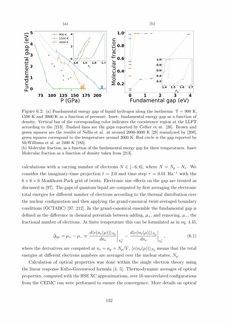
(a) (b)

0 1 2 3 4Fundamental gap (eV)

0.2

0.4

0.6

0.8

1.0

Mol

ecul

ar fr

actio

n

1.4 1.5 1.6 1.7rs

0.2

0.4

0.6

0.8

1.0

Figure 6.2: (a) Fundamental energy gap of liquid hydrogen along the isotherms: T = 900 K,1500 K and 3000 K as a function of pressure. Inset: fundamental energy gap as a function ofdensity. Vertical bar of the corresponding color indicates the coexistence region at the LLPTaccording to the [213]. Dashed lines are the gaps reported by Cellier et at. [26]. Brown andgreen squares are the results of Nellis et al. at around 2000-3000 K [28] reanalyzed by [208],green squares correspond to the temperature around 3000 K. Red circle is the gap reported byMcWilliams et al. at 2400 K [183].(b) Molecular fraction, as a function of the fundamental energy gap for three temperatures. Inset:Molecular fraction as a function of density taken from [213].

calculations with a varying number of electrons N ∈ [−6, 6], where N = Np − Ne. We

consider the imaginary-time projection t = 2.0 and time step τ = 0.01 Ha−1 with the

6× 6× 6 Monkhorst-Pack grid of twists. Electronic size effects on the gap are treated as

discussed in [97]. The gaps of quantum liquid are computed by first averaging the electronic

total energies for different number of electrons according to the thermal distribution over

the nuclear configuration and then applying the grand-canonical twist-averaged boundary

conditions (GCTABC) [97, 212]. In the grand-canonical ensemble the fundamental gap is

defined as the difference in chemical potentials between adding, µ+, and removing, µ−, the

fractional number of electrons. At finite temperature this can be formulated as in eq. 4.45,

∆gc = µ+ − µ− 'd〈e(ne(µ))〉Np

dne

∣∣∣∣N+p

− d〈e(ne(µ))〉Npdne

∣∣∣∣n−p

, (6.1)

where the derivatives are computed at ne = np = Np/V , 〈e(ne(µ))〉Np means that the total

energies at different electrons numbers are averaged over the nuclear states, Np.

Calculation of optical properties was done within the single electron theory using

the linear response Kubo-Greenwood formula [4, 5]. Thermodynamic averages of optical

properties, computed with the HSE XC approximations, over 16 uncorrelated configurations

from the CEIMC run were performed to ensure the convergence. More details on optical

132

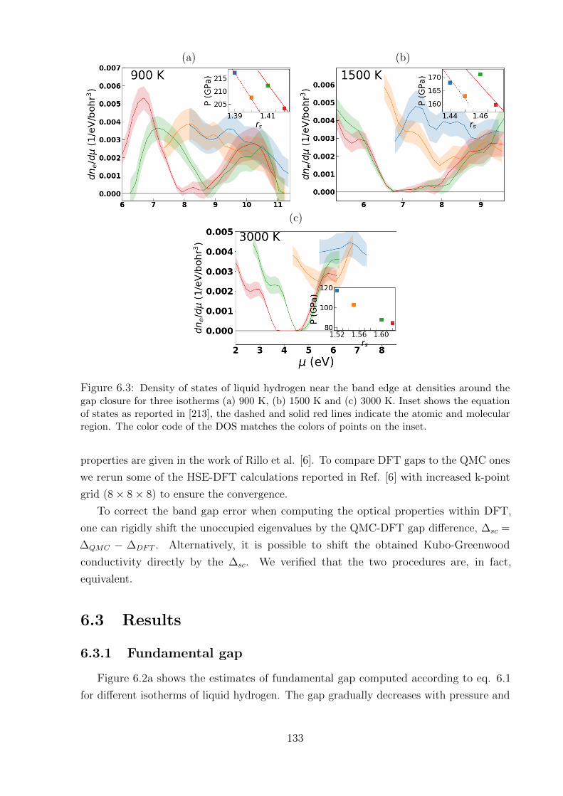
(a) (b)

(c)

Figure 6.3: Density of states of liquid hydrogen near the band edge at densities around thegap closure for three isotherms (a) 900 K, (b) 1500 K and (c) 3000 K. Inset shows the equationof states as reported in [213], the dashed and solid red lines indicate the atomic and molecularregion. The color code of the DOS matches the colors of points on the inset.

properties are given in the work of Rillo et al. [6]. To compare DFT gaps to the QMC ones

we rerun some of the HSE-DFT calculations reported in Ref. [6] with increased k-point

grid (8× 8× 8) to ensure the convergence.

To correct the band gap error when computing the optical properties within DFT,

one can rigidly shift the unoccupied eigenvalues by the QMC-DFT gap difference, ∆sc =

∆QMC − ∆DFT . Alternatively, it is possible to shift the obtained Kubo-Greenwood

conductivity directly by the ∆sc. We verified that the two procedures are, in fact,

equivalent.

6.3 Results

6.3.1 Fundamental gap

Figure 6.2a shows the estimates of fundamental gap computed according to eq. 6.1

for different isotherms of liquid hydrogen. The gap gradually decreases with pressure and

133

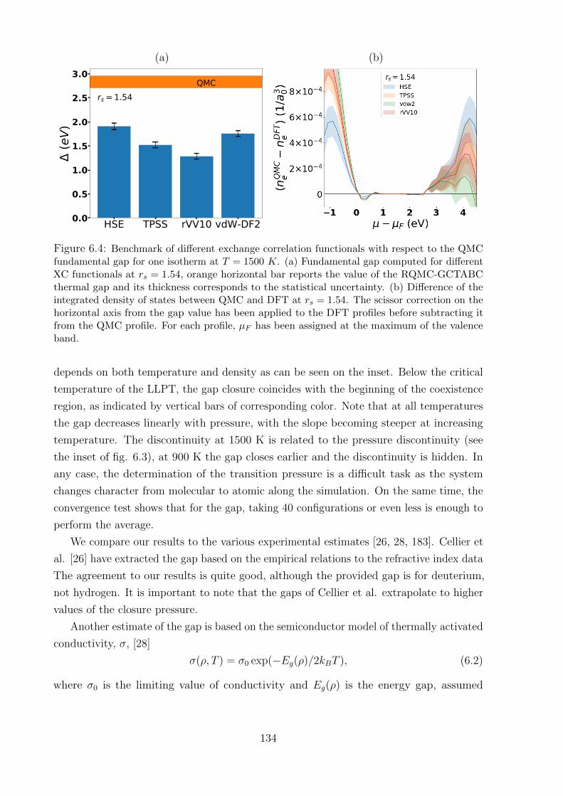
(a)

HSE TPSS rVV10 vdW-DF20.0

0.5

1.0

1.5

2.0

2.5

3.0 (e

V)QMC

rs = 1.54

(b)

Figure 6.4: Benchmark of different exchange correlation functionals with respect to the QMCfundamental gap for one isotherm at T = 1500 K. (a) Fundamental gap computed for differentXC functionals at rs = 1.54, orange horizontal bar reports the value of the RQMC-GCTABCthermal gap and its thickness corresponds to the statistical uncertainty. (b) Difference of theintegrated density of states between QMC and DFT at rs = 1.54. The scissor correction on thehorizontal axis from the gap value has been applied to the DFT profiles before subtracting itfrom the QMC profile. For each profile, µF has been assigned at the maximum of the valenceband.

depends on both temperature and density as can be seen on the inset. Below the critical

temperature of the LLPT, the gap closure coincides with the beginning of the coexistence

region, as indicated by vertical bars of corresponding color. Note that at all temperatures

the gap decreases linearly with pressure, with the slope becoming steeper at increasing

temperature. The discontinuity at 1500 K is related to the pressure discontinuity (see

the inset of fig. 6.3), at 900 K the gap closes earlier and the discontinuity is hidden. In

any case, the determination of the transition pressure is a difficult task as the system

changes character from molecular to atomic along the simulation. On the same time, the

convergence test shows that for the gap, taking 40 configurations or even less is enough to

perform the average.

We compare our results to the various experimental estimates [26, 28, 183]. Cellier et

al. [26] have extracted the gap based on the empirical relations to the refractive index data

The agreement to our results is quite good, although the provided gap is for deuterium,

not hydrogen. It is important to note that the gaps of Cellier et al. extrapolate to higher

values of the closure pressure.

Another estimate of the gap is based on the semiconductor model of thermally activated

conductivity, σ, [28]

σ(ρ, T ) = σ0 exp(−Eg(ρ)/2kBT ), (6.2)

where σ0 is the limiting value of conductivity and Eg(ρ) is the energy gap, assumed

134

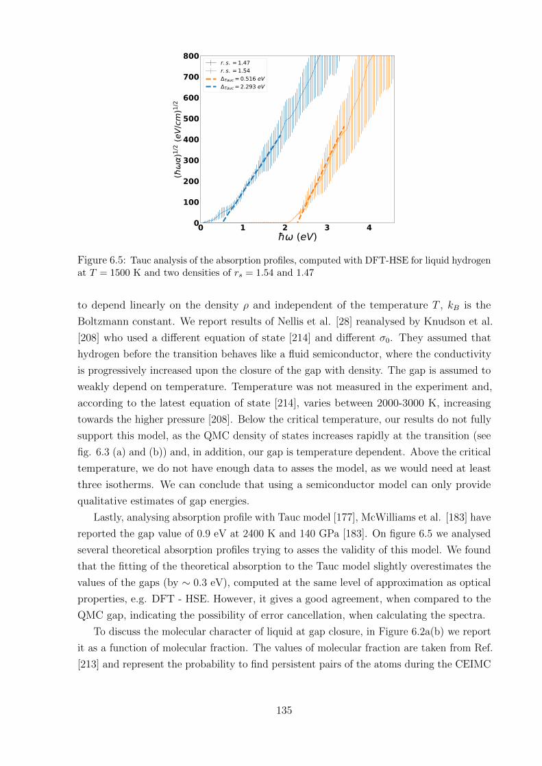
0 1 2 3 4 (eV)

0

100

200

300

400

500

600

700

800

()1/

2 (eV

/cm

)1/2

r. s. = 1.47r. s. = 1.54

Tauc = 0.516 eVTauc = 2.293 eV

Figure 6.5: Tauc analysis of the absorption profiles, computed with DFT-HSE for liquid hydrogenat T = 1500 K and two densities of rs = 1.54 and 1.47

to depend linearly on the density ρ and independent of the temperature T , kB is the

Boltzmann constant. We report results of Nellis et al. [28] reanalysed by Knudson et al.

[208] who used a different equation of state [214] and different σ0. They assumed that

hydrogen before the transition behaves like a fluid semiconductor, where the conductivity

is progressively increased upon the closure of the gap with density. The gap is assumed to

weakly depend on temperature. Temperature was not measured in the experiment and,

according to the latest equation of state [214], varies between 2000-3000 K, increasing

towards the higher pressure [208]. Below the critical temperature, our results do not fully

support this model, as the QMC density of states increases rapidly at the transition (see

fig. 6.3 (a) and (b)) and, in addition, our gap is temperature dependent. Above the critical

temperature, we do not have enough data to asses the model, as we would need at least

three isotherms. We can conclude that using a semiconductor model can only provide

qualitative estimates of gap energies.

Lastly, analysing absorption profile with Tauc model [177], McWilliams et al. [183] have

reported the gap value of 0.9 eV at 2400 K and 140 GPa [183]. On figure 6.5 we analysed

several theoretical absorption profiles trying to asses the validity of this model. We found

that the fitting of the theoretical absorption to the Tauc model slightly overestimates the

values of the gaps (by ∼ 0.3 eV), computed at the same level of approximation as optical

properties, e.g. DFT - HSE. However, it gives a good agreement, when compared to the

QMC gap, indicating the possibility of error cancellation, when calculating the spectra.

To discuss the molecular character of liquid at gap closure, in Figure 6.2a(b) we report

it as a function of molecular fraction. The values of molecular fraction are taken from Ref.

[213] and represent the probability to find persistent pairs of the atoms during the CEIMC

135

sampling. Noticeably, below the critical temperature, the gap is closed immediately

after the molecules start to dissociate. At higher temperatures, on the contrary, the

gap progressively closes with the dissociation. In Ref. [58], analyzing the momentum

distribution of liquid hydrogen with QMC, authors pointed out to the localized nature

of electrons at temperatures above critical for all densities, consistently with our results

of open gap at low molecular fraction. On the contrary, below the critical temperature,

it was shown that the electronic properties of liquid change its nature, becoming more

delocalized and Fermi-like, in accordance with the closed gap.

Our GCTABC method allows us to have an access to the density of states (DOS) near

the conduction-valence band edges. Figure 6.3 shows the DOS at three isotherms for

densities around the gap closure. Below the critical temperature, at 1500 K and 900 K, we

show the DOS at four densities around the LLPT, the equation of state is plotted on the

inset as reported in ref. [213]. Remarkably, when the LLPT transition occurs, the DOS

changes rapidly from semiconductor shape with just a few states around the Fermi energy

to metal like almost straight line shape, which clearly indicates the metal to insulator

transition. At high temperature, where the IM transition is continuous we do not see such

behaviour, on the contrary, the DOS indicates that when gap closes the deep at Fermi

energy will be progressively filled with states. Note that at 3000 K we cannot precisely

locate the gap closure density, more calculations will be needed between rs = 1.6, where

the gap is 0.8 eV and rs = 1.55, where the gap is closed.

6.3.2 Benchmark of XC approximations

Further, we provide a benchmark for the various XC approximations for the band gap.

We will focus only on one isotherm of 1500 K and one density rs = 1.54. Four functionals

are considered: non-local and semi-local van-der-Waals density functionals rVV10 [215] and

vdW-DF2 [123], semi-local meta-GGA TPSS functional [216], and non-local hybrid HSE

[48]. Figure 6.4(a) shows the value of the gap using different DFT functionals compared

to the thermal gap from RQMC-GCTABS. The discrepancy is on the order of ∼ 1 eV

with HSE and vdW-DF2 being the closest to the QMC prediction, scenario similar to

solid hydrogen [212]. We try to asses the accuracy of the intensity of optical properties

computed with different XC functionals. With QMC we do not have a direct access to

the optical properties, however, note that to the large extend they are defined by the

density of states. For each DFT approximation we correct the value of the gap to match

the QMC one and then we plot the difference in the integrated density of states between

QMC and gap-corrected DFT. The results for single density, rs = 1.54, and temperature

1500 K are shown in Figure 6.4(b). Similarly to the gap comparison, HSE and vdW-DF2

perform better than the others with HSE being the best. At the same time note that

the vdW-DF2 performs almost as good as HSE at higher and better at lower density at

136

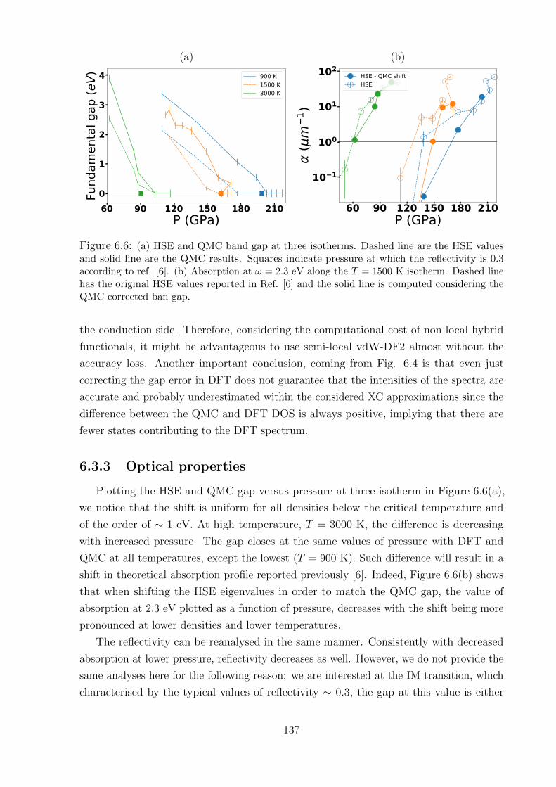
(a)

60 90 120 150 180 210P (GPa)

0

1

2

3

4Fu

ndam

enta

l gap

(eV) 900 K

1500 K3000 K

(b)

60 90 120 150 180 210P (GPa)

10 1

100

101

102

(m

1 )

HSE - QMC shiftHSE

Figure 6.6: (a) HSE and QMC band gap at three isotherms. Dashed line are the HSE valuesand solid line are the QMC results. Squares indicate pressure at which the reflectivity is 0.3according to ref. [6]. (b) Absorption at ω = 2.3 eV along the T = 1500 K isotherm. Dashed linehas the original HSE values reported in Ref. [6] and the solid line is computed considering theQMC corrected ban gap.

the conduction side. Therefore, considering the computational cost of non-local hybrid

functionals, it might be advantageous to use semi-local vdW-DF2 almost without the

accuracy loss. Another important conclusion, coming from Fig. 6.4 is that even just

correcting the gap error in DFT does not guarantee that the intensities of the spectra are

accurate and probably underestimated within the considered XC approximations since the

difference between the QMC and DFT DOS is always positive, implying that there are

fewer states contributing to the DFT spectrum.

6.3.3 Optical properties

Plotting the HSE and QMC gap versus pressure at three isotherm in Figure 6.6(a),

we notice that the shift is uniform for all densities below the critical temperature and

of the order of ∼ 1 eV. At high temperature, T = 3000 K, the difference is decreasing

with increased pressure. The gap closes at the same values of pressure with DFT and

QMC at all temperatures, except the lowest (T = 900 K). Such difference will result in a

shift in theoretical absorption profile reported previously [6]. Indeed, Figure 6.6(b) shows

that when shifting the HSE eigenvalues in order to match the QMC gap, the value of

absorption at 2.3 eV plotted as a function of pressure, decreases with the shift being more

pronounced at lower densities and lower temperatures.

The reflectivity can be reanalysed in the same manner. Consistently with decreased

absorption at lower pressure, reflectivity decreases as well. However, we do not provide the

same analyses here for the following reason: we are interested at the IM transition, which

characterised by the typical values of reflectivity ∼ 0.3, the gap at this value is either

137

small or already closed. Pressure at which reflectivity is 0.3, according to [6] is reported

on Fig. 6.6(a) as squares of the corresponding colors. Therefore, correcting the gap for

the reflectivity will not give a meaningful result, because of the incorrect determination of

the intensity of optical properties within HSE-DFT. As it has been seen in fig. 6.4(b), the

DFT optical intensities might be underestimated.

Pressure at which hydrogen turns opaque was attributed by several experimental works

to correspond to the absorption of ∼ 1 (µm)−1 [26, 27, 183]. Based on our QMC shifted

HSE absorption, we predict that the onset of absorption line on phase diagram will shift to

higher pressure, with respect to the previously reported line [6]. This fact again indicates

that the absorption intensities might be underestimated within the HSE XC approximation

and that there might be an error cancellation between the underestimated band gap and

underestimated intensities.

On the other side, closure of the gap, being an indicator of IM transition, perfectly

underlines experimentally observed increase of reflectivity and coincides with the previously

reported [15] structural phase transition. This fact concludes the assumption that the

liquid-liquid phase transition is as also an IM transition accompanied as well by the

increase of the reflectivity and conductivity.

6.4 Conclusion

In this final chapter, we have addressed the fundamental gap closure across the liquid-

liquid phase transition (LLPT) in hydrogen using the newly developed (see section 4.4)

formalism purely within QMC. The main finding was that gap closure is continuous and

coincides with the the beginning of the molecular dissociation transition. The gap has

been found to depend on temperature. Comparing to the previous work [58], we find

that below the critical temperature the closing is accompanied by the change of electron

localization. We have benchmarked some DFT functional on the basis of the QMC inferred

density of states and have found that all considered functionals underestimate the gap and

underestimate the optical transition intensities (see fig. 6.4(b)). Finally, we have found

that by shifting the HSE gap values to the ones of QMC, the absorption curves also shift,

and therefore, a better description of the optical intensities is required.

138

Chapter 7

Conclusions

It is true that even having access to a ”complete set of information” for a theoretical

understanding of all real materials, the amount of those understood is finite. The reason

essentially is that some materials, for example, hydrogen, require more accurate approx-

imations to the solution of Schrodinger equation 1.1. However, there are methods, like

QMC, that are potentially able to reach better accuracy. Nowadays, however, QMC can

only reliably predict some ground state properties. The goal of this thesis, therefore, was

to extend the QMC to make it as accurate in computing the excited state properties, in

particular charged quasiparticle excitations.

The starting point of most of the QMC calculations is the single electron methods.

Therefore, before switching to QMC, in chapter 1, the two methods, Hartree-Fock and DFT,

were first discussed. Within the QMC we have introduced the variational Monte Carlo and

the reptation quantum Monte Carlo. The former provides a way to statistically evaluate

most observables for electronic systems using given many-body trial wave function. The

latter is an almost exact method for finding the fermionic ground state of a Hamiltonian,

with the main approximation being the use of an approximate nodal surface from a trial

wave function.

We have extended the ground state QMC to compute the excited states. Firstly, in

chapter 2 we have proposed a new way of computing the fundamental gap using QMC

only, which relies on grand canonical twist averaging. Most importantly we have shown

that for charged systems, finite size supercell calculations are necessarily biased by a finite

size error decaying as 1/L, with L being the linear size of the system, where the prefactor

is determined by the absolute value of the Madelung constant and the inverse dielectric

constant. We have applied this procedure to determine the fundamental gap of molecular

hydrogen at high pressure and carbon and silicon in the diamond structure at zero pressure.

Secondly, we have discussed the neutral excitations, which are made by promoting an

electron from the valence to conduction band and characterized by the coupling between

the promoted electron and the hole that was left behind. Within the QMC, we have

139

constructed a wave function to model the excited states, with the generalized variational

principle, we can assure that the new excited stated are orthogonal to the lower lying states.

Thirdly, in chapter 3 we have made an attempt to compute many-body conductivity with

variational Monte Carlo using Kubo [4] formula. Our preliminary results for the C2c-24

ideal solid crystalline hydrogen indicate that the electron-hole interaction energy is about

∼0.4 eV, and concerning the conductivity, further investigations of the convergence of the

spectra are necessary.

Bearing in mind the fact that the system of our interest is hydrogen at extreme

conditions, we have had to consider the nuclear degrees of freedom and its effects on the

electronic structure. In chapter 4 we have introduced the concept of Path Integrals, which

is the basis of the coupled electron ion Monte Carlo (CEIMC), the method of preference

in this work. We have formally argued the way of treating electron addition and removal

energies in canonical and semigrand canonical ensemble at finite temperature. We have

provided a general formalism of determining the crystal momentum of thermal crystals,

which we further use to plot the band structure of solid crystalline hydrogen having the

C2c-24 symmetry at 200 K and 250 GPa. An important extension of the traditional

semiclassical way of temperature renormalization of the optical properties was introduced

in the end of chapter 4 and named quantum averaging. We illustrate the effect of quantum

averaging by computing the absorption coefficient of solid crystalline hydrogen at 200 K

using single electron Kubo-Greenwood theory.

Most of the methodological developments done in this work has been driven by the

practical goal to study the metallization of liquid and solid hydrogen. In chapter 5, we

have studied the closure of the fundamental gap with pressure of candidate structures of

solid molecular hydrogen in phase III (C2/c-24 and Cmca-12) and phase IV (Pc48) entirely

based on Quantum Monte Carlo. For ideal structures, our gap values are in excellent

agreement with GW prediction[3]. Considering quantum nuclei at finite temperature, we

observe a strong reduction of the energy gap with respect to the ideal structures at the

same pressure (∼ 2eV) caused by ZPM. At 200K the fundamental (indirect) gap closes

at ∼ 370-380GPa for C2/c-24 and at ∼ 340GPa for Cmca-12. We observe a reasonable

agreement with experimental determinations of indirect gaps from optical absorption.

The direct gap remains open until ∼ 450GPa for C2/c-24 and ∼ 500GPa for Cmca-12.

We have found that in this range of pressure, the system is a bad metal (or semi-metal)

suggesting a scenario that qualitatively supports recent experiments [153, 158, 159, 165].

In refs. [153, 165] no discontinuities in the Raman vibrational spectrum are reported

when entering the semi-metallic phase, while in refs. [158, 159] new IR vibron peaks are

reported in this pressure range and ascribed to a structural phase transition. They have

been tentatively assigned to a transition from the C2/c-24 to the Cmca-12 structure [158].

Our present results do not disprove this hypothesis. Our predictions for the direct gap

140

are in good agreement with the experimental data at T=100K [13, 172]. However, our

absorption profiles do not agree as well with the experimental behavior. This disagreement

remains an open question.

In the case of liquid hydrogen, in chapter 6, we have found that the gap closure

is continuous and coincides with the beginning of the molecular dissociation transition

meaning that the metallization and the molecular breaking occur at the same time. Our

method of computing the gaps with QMC allows to benchmark some DFT functional

basing on the QMC inferred density of states. We have found that for liquid and solid

hydrogen almost all considered functionals underestimate the gap and underestimate the

optical transition intensities.

Certainly, the goal to have the QMC methods to be as reliable to predict excited state

properties as the ground state is a formidable goal and can not be fully reached within a

thesis. Therefore, it is important to continue to push the QMC methods for excited states

to make it both affordable computationally and accurate at the same time.

141

142

Appendix A

Monte Carlo methods and the

Metropolis algorithm

Monte Carlo integration is a general purpose algorithm used to calculate averages of

arbitrary functions. Consider the one dimensional integral

A =

∫ b

a

dxf(x)g(x), (A.1)

where g(x) is any positive definite function such that∫ badxg(x) = 1, which can be

interpreted as a distribution. The integral can be approximated by an average over a

discrete set of points distributed according to g(x). Using the Central Limit Theorem, it

is easy to show that the error in the resulting estimate is given by [63]

A =

∫ b

a

dxf(x)g(x) =1

N

N∑i=1

f(x) +O

√σ2f

N

, (A.2)

where xi is distributed according to g(x) and σ2f is the variance of f(x) over g(x).

Traditional quadrature methods, which would work better in this case, have a very

bad scaling with the number of dimensions. Note that because the error in eq. A.2

is independent of the number of dimensions, Monte Carlo integration is able to handle

integrals in an arbitrary number of dimensions and is very efficient if the integrand is

peaked in a localized region of space.

Extending this simple idea one could calculate the integral in eq. A.1 by sampling any

arbitrary distribution, π(x) being any positive definite function that satisfies∫ baπ(x)dx = 1,

A =

∫ b

a

dxπ(x)f(x)g(x)

π(x), (A.3)

This idea is typically called importance sampling. In fact, any definite integral in dx over

143

[a, b] can be simultaneously calculated from a sample of π(x) by “reweighting” the averages

according to:

A =

∫ b

a

f(x)dx =

∫ b

a

π(x)f(x)

π(x)dx = lim

N→∞

1

N

N∑i=1

f(xi)

π(xi), (A.4)

where xi is distributed according to π(x). To sample arbitrary distributions, π(x), the

Metropolis algorithm [90] is used. It consists on the following three steps:

• Starting from a state x, choose a trial state x′ with probability T (x→ x′), where T

is a simple distribution function that can be sampled directly.

• Evaluate the acceptance probability:

A(x→ x′) = min

[1,T (x′ → x)π(x′)

T (x→ x′)π(x)

](A.5)

• Accept the step x′ with probability A. For this generate a random number, η,

uniformly distributed in [0, 1] and accept the step if η < A.

The algorithm is both general and very simple, the only knowledge needed is of the

limiting distribution and the only with requirement for the transition probability, T , to be

ergodic. The main drawback of the method is that the steps along the random walk are

highly correlated, meaning that it takes a certain number of steps to produce statistically

uncorrelated data. This, in turn, implies that longer simulations are needed to reduce

error bars in the resulting averages. Nonetheless, the simplicity of the method allows us to

apply it to very complicated problems like the Schrodinger equation.

144

Appendix B

Optimising the wave function

The simplest way to find the best trial function is to perform independent VMC runs

(possibly in parallel) with different values for the variational parameters. Then one fits

the energies as a function of parameters to a simple analytic form, does more calculations

around the predicted minimum, and continues until convergence in parameter space is

attained. However this is not the most efficient method as close to the minimum the

independent statistical errors will mask the variation with respect to the trial function

parameters. And what is more important, doing optimisation by hand is limited to a few

parameters. There exist several other techniques, for example the reweighting method,

that allow efficient wave function optimisation.

Also called correlated sampling method, the reweighting method uses the output of a

single random walk to estimate the energy as the function of variational parameters. One

has to store the set of configurations R(1), R(2), ..., R(M), sampled from initial distribution

Π0(R) = |ΨT (R; a0)|2. Then the energy for a given set of variational parameters a is

written as:

EV (a) =

∫Ψ∗(R; a)HΨ∗(R; a)∫|Ψ(R; a)|2 7→ EV (a) =

∑nwn(a)EL(R(n); a)∑

nwn(a), (B.1)

where the weight of the nth configuration is wn(a) = |ΨT (R(n); a)/ΨT (R(n); a0)|2. One

then can use a minimiser to find the lowest variational energy or variance (zero variance

principle Eq. 1.31) or, as it is usually done, their linear combination as a function of a.

The problem of this method is that if the overlap between current and initial distri-

butions |ΨT (R(n); a)|2 and |ΨT (R(n); a0)|2 gets too small, the error of EV (a) will become

large and optimisation becomes unstable. For that reason it is useful to monitor the

effective number of configurations Neff = (∑

nwn(a))2/∑

nw2n(a) and when it gets too

small one can reset Π0(R) = |ΨT (R(n); a∗)|2, where a∗ is the current best estimate of the

parameters, regenerate the set of configurations, and proceed.

It is worth mentioning that the optimisation of trial functions for many-body systems is

145

time consuming, particularly for complex trial functions. The dimension of the parameter

space increases rapidly with the complexity of the system and the optimisation can become

very cumbersome since it is, in general, a nonlinear optimisation problem.

146

Appendix C

Unfolding the band structure

If in the simulation we are using the supercell, in order to determine the Bloch crystal

momentum ideal structure in the primitive cell we will have to first unfold the bands of

the supercell. Single electron wave function can be written using plane waves and a Bloch

representation as the following:

φn,θ(r) = un,θ(r)eiθr =∑G

Cn(G + θ)ei(G+θ)r, (C.1)

where n = 1..N/2 and un,θ is the periodic function, which has the periodicity of the

simulation supercell. In order to unfold the bands of a supercell we can displace the

electrons by the primitive cell vectors (Rijk = ia1 + ja2 + ka3), the resulting phase will

be the crystal momentum, k

φn,θ(0) =∑G

Cn(G + θ) =∑G

Cn(G + θ)ei(G+θ+k)Rijk = φn,θ(Rijk)eikRijk . (C.2)

In practice to determine the phase one can compute the ratio of the two wave functions

respectively displaced by the vector of the unit cell:

p =

∑GCn(G + θ)eiG2Rijk∑GCn(G + θ)eiGRijk

, (C.3)

then the phase k could be determined from p = |p|eikRijk . One should use at least three

independent displacements.

147

148

Appendix D

Coupled electron-ion Monte Carlo

The Coupled Electron-Ion Monte Carlo (CEIMC) [9] is based entirely on the Monte

Carlo method, both for solving the electronic problem, and for sampling the ionic config-

uration space. In treating finite temperature ions which are coupled with ground state

electrons this method relies on the Born-Oppenheimer approximation. The essence of this

method is the following: at finite temperature the ionic degrees of freedom (either classical

point particles or path integrals) are sampled using a Metropolis Monte Carlo based on

the electronic energies computed during independent ground state quantum Monte Carlo

calculations.

As discussed in section 4.2, in order to compute the expectation value of an operator

O,

〈O〉 =Tr[ρ(R,R; β)O

]Tr [ρ(R,R; β)]

, (D.1)

where β is inverse temperature, R denotes the set of all nuclear positions and ρ(R,R; β)

is density matrix. We can then write the density matrix as a chain of P density matrices

at τ = β/P with each element being,

ρ(R,R′; τ) = 〈R|e−τ(TR+E0(R))|R′〉. (D.2)

In CEIMC, however, to reach the convergence for smaller number of slices, an effective pair

potential, Vpair(R), called pair action is introduced. The lowest-order Trotter factorisation

[53] for the difference E0(R)− Vpair(R) can be then written as,

ρ(R,R′; τ) = 〈R|e−τ[TR+Vpair(R)]|R′〉e− τ2 [E0(R)−Vpair(R)+E0(R′)−Vpair(R′)]. (D.3)

With the pair potential, the matrix element in eq. D.3 can be evaluated analytically,

〈R|e−τ[TR+Vpair(R)]|R′〉 = exp

[−MI(R−R′)2

2τ−∑ij

u(Rij,R′ij)

]. (D.4)

149

The density matrix ρ(R,R; β) then becomes,

ρ(R,R; β) =P∏s=1

exp

[−MI(R

(s) −R(s+1))2

2τ−∑ij

u(R(s)ij ,R

(s+1)ij )

]e−τ

∑Ps=1[E0(R(s))−Vpair(R(s))]

= Ppair(R)e−τ∑Ps=1[E0(R(s))−Vpair(R(s))], (D.5)

where u(R(s)ij ,R

(s+1)ij ) is the interpotential action for a single pair of particles. The intro-

duction of the potential Vpair is meant to serve two purposes. First, better approximating

the density matrix allows us to use a smaller number of beads to converge to the infinite

limit. Second, the first product of exponents, indicated as Ppair(R) in D.5, is rather cheap

to evaluate, leaving the expensive part of evaluating electronic Born Oppenheimer energy

to the second exponent, which suggests to use a multilevel Metropolis algorithm to sample

the distribution [9]:

• a move in the P×3Np configurational space is proposed from point R to R′according

to a priori transition probability T (R,R′)

• the acceptance probability for this move is

A1 = min

[1,T (R,R

′)Ppair(R

′)

T (R′ ,R)Ppair(R)

](D.6)

• if accepted, then a second test is performed with acceptance

A2 = min

[1, e−τ

∑Ps=1

[E0(R

′(s))−E0(R(s))−Vpair(R′(s)+Vpair(R(s))

]](D.7)

The consequence of separating the acceptance test in two phases is that the first phase

(called the ”pre-rejection step“) is computationally cheap, as it prevents the expensive

evaluation of the electronic energy for moves that are not likely to be accepted. Of course,

an important role is played by the effective potential Vpair: the more it resembles the

true energy landscape, the more efficient this process becomes. There is an important

issue, however associated with the algorithm, in the CEIMC method, variational Monte

Carlo is used to compute the electronic energy differences E0(R′(s))− E0(R(s)), which is

evaluated with a statistical error that can bias the outcome of the acceptance test. The

simplest solution would be to make this error negligible with respect to the difference

E0(R′(s))−E0(R(s)), however this would require sampling a lot of electronic configurations

and would be highly inefficient. Instead a different approach can be used called: the

penalty method.

150

D.1 The Penalty method

Consider ∆ and σ2∆ being an average value and a variance of ∆ = −τ∑P

s=1E0(R′(s))−

E0(R(s)). Since ∆ is a random variable with the probability distribution Pnoise(∆), the

acceptance a(∆) is also a random variable, with average

A(R,R′) =

∫ ∞−∞

d∆a(∆)Pnoise(∆). (D.8)

We assume that Pnoise(∆) is a gaussian

Pnoise(∆) =1√

2πσ2e−

(∆−∆)2

2σ2 , (D.9)

which can be justified by using the central limit theorem if the energy difference is averaged

over many samples and has a finite variance. Choosing as the acceptance probability

a(∆) = min

[1,T (R′,R)

T (R,R′)e−∆−σ

2

2

](D.10)

and defining Γ(R,R′) = ln T (R′,R)T (R,R′)

, the average acceptance A has the form,

A(R,R′) = 1

2√

2σerfc

[σ2

2+ ∆(R,R′) + Γ(R,R′)

](D.11)

+1

2√

2σerfc

[σ2

2− ∆(R,R′)− Γ(R,R′)

]×e−∆(R,R′)−Γ(R,R′),

which solves the averaged detailed balance condition, as ∆(R,R′) = −∆(R′,R) and

Γ(R,R′) = −Γ(R′,R). The effect of the statistical noise is increasing the rejection by a

factor e−σ2

2 , as we can see from eq. D.10. However, the variance σ is not known a priori,

but is estimated during the run to compute the energy as well. Given n independent

samples yi, one has for the estimators of ∆ and σ2

∆ =1

n

n∑i=1

yi (D.12)

χ2 =1

n(n− 1)

n∑i=1

(yi −∆)2. (D.13)

The average acceptance in eq. D.8 is then

A(R,R′) =

∫ ∞−∞

d∆

∫ ∞0

dχ2a(∆, χ2)Pnoise(∆, χ2), (D.14)

151

with the new acceptance formula being

a(∆, χ2) = min

[1,T (R′,R)

T (R,R′)e∆−ub

](D.15)

ub =χ2

2+

χ2

4(n+ 1)..., (D.16)

where ub is the penalty term obtained using an asymptotic expansion that converges as

long as χ2/n < 1/4. This procedure is known as penalty method [97]. For large n the

first term is dominating, since χ2 is a good enough estimator of σ2.On the other hand the

purpose of the penalty method is to get consistent results even when n is not too large: in

this case the additional terms in eq. D.15 provides an extra rejection factor motivated by

our ignorance of σ.

152

Bibliography

[1] E. Wigner and H. B. Huntington. On the Possibility of a Metallic Modification of

Hydrogen. J. Chem. Phys., 3:764–770, 1935. Cited on pages 3, 18, and 111.

[2] Vitaly L. Ginzburg. Nobel Lecture: On superconductivity and superfluidity (what

I have and have not managed to do) as well as on the ”physical minimum” at the

beginning of the XXI century. Reviews of Modern Physics, 76(3):981–998, dec 2004.

Cited on pages 3 and 18.

[3] Jeremy McMinis, Raymond C. Clay, Donghwa Lee, and Miguel A. Morales. Molecular

to Atomic Phase Transition in Hydrogen under High Pressure. Phys. Rev. Letts.,

114(10):105305, 2015. Cited on pages 3, 115, 116, 117, 125, and 140.

[4] Ryogo Kubo. Statistical-mechanical theory of irreversible processes. i. general theory

and simple applications to magnetic and conduction problems. Journal of the

Physical Society of Japan, 12(6):570–586, 1957. Cited on pages 4, 20, 75, 79, 85, 131, 132,

and 140.

[5] D A Greenwood. The Boltzmann Equation in the Theory of Electrical Conduction

in Metals. Proc. Phys. Soc., 71(4):585–596, 1958. Cited on pages 4, 20, 75, 131, and 132.

[6] Giovanni Rillo, Miguel A. Morales, David M. Ceperley, and Carlo Pierleoni. Optical

properties of high-pressure fluid hydrogen across molecular dissociation. Proceedings

of the National Academy of Sciences of the United States of America, 116(20):9770–

9774, 2019. Cited on pages 4, 127, 128, 131, 133, 137, and 138.

[7] P. A. M. Dirac. Quantum mechanics of many-electron systems. Proceedings of

the Royal Society of London. Series A, Containing Papers of a Mathematical and

Physical Character, 123(792):714–733, 1929. Cited on page 17.

[8] M. O. Steinhauser. Computational Methods on Electronic/Atomistic Scale. In

Computational Multiscale Modeling of Fluids and Solids, pages 225–267. Springer

Berlin Heidelberg, Berlin, Heidelberg, oct 2008. Cited on page 17.

153

[9] Carlo Pierleoni and D.M. Ceperley. The Coupled Electron-Ion Monte Carlo Method.

In Mauro Ferrario, Giovanni Ciccotti, and Kurt Binder, editors, Computer Simula-

tions in Condensed Matter Systems: From Materials to Chemical Biology Volume 1,

volume 703 of Lecture Notes in Physics, pages 641–683. Springer Berlin Heidelberg,

Berlin, Heidelberg, 2006. Cited on pages 17, 21, 36, 39, 66, 90, 149, and 150.

[10] Dominik Marx and Jurg Hutter. Ab Initio Molecular Dynamics. Cambridge University

Press, Cambridge, 2009. Cited on pages 17, 89, and 92.

[11] Jeffrey M. McMahon, Miguel A. Morales, Carlo Pierleoni, and David M. Ceperley.

The properties of hydrogen and helium under extreme conditions. Rev. Mod. Phys.,

84:1607–1653, 2012. Cited on pages 18, 19, 89, 111, 112, 127, and 128.

[12] Alexander Goncharov. Phase diagram of hydrogen at extreme pressures and temper-

atures; Updated through 2019 (Review article). Low Temperature Physics, 46(2),

2020. Cited on pages 18, 111, and 127.

[13] Paul Loubeyre, Florent Occelli, and Paul Dumas. Synchrotron infrared spectroscopic

evidence of the probable transition to metal hydrogen. Nature, 577:631, 2020. Cited

on pages 18, 19, 112, 113, 116, 118, 119, 120, 122, 125, and 141.

[14] Ranga P Dias and Isaac F Silvera. Observation of the Wigner-Huntington transition

to metallic hydrogen. Science, 355:715–718, 2017. Cited on pages 18, 19, 111, 112, and 113.

[15] Carlo Pierleoni, Miguel a Morales, Giovanni Rillo, Markus Holzmann, and David M

Ceperley. Liquid–liquid phase transition in hydrogen by coupled electron–ion Monte

Carlo simulations. Proceedings of the National Academy of Sciences, 113(18):4954–

4957, 2016. Cited on pages 18, 66, 115, 128, 130, 131, and 138.

[16] N W Ashcroft. Metallic hydrogen: A high-temperature superconductor? Phys. Rev.

Letts., 21(26):1748–1749, 1968. Cited on page 18.

[17] Maddury Somayazulu, Muhtar Ahart, Ajay K. Mishra, Zachary M. Geballe, Maria

Baldini, Yue Meng, Viktor V. Struzhkin, and Russell J. Hemley. Evidence for

superconductivity above 260 k in lanthanum superhydride at megabar pressures.

Phys. Rev. Lett., 122:027001, Jan 2019. Cited on page 18.

[18] Igor Goncharenko and Paul Loubeyre. Neutron and X-ray diffraction study of the

broken symmetry phase transition in solid deuterium. Nature, 435(7046):1206–1209,

2005. Cited on page 19.

[19] Isaac F. Silvera. The solid molecular hydrogens in the condensed phase: Fundamentals

and static properties. Reviews of Modern Physics, 52(2):393–452, 1980. Cited on page

19.

154

[20] R J Hemley and H K Mao. Phase transition in solid molecular hydrogen at ultrahigh

pressures. Phys. Rev. Letts., 61(7):857–860, 1988. Cited on page 19.

[21] Hector E. Lorenzana, Isaac F. Silvera, and Kenneth A. Goettel. Evidence for a

structural phase transition in solid hydrogen at megabar pressures. Phys. Rev. Lett.,

63:2080–2083, Nov 1989. Cited on page 19.

[22] Alexander F. Goncharov and Russell J. Hemley. Probing hydrogen-rich molecular

systems at high pressures and temperatures. Chem. Soc. Rev., 35:899–907, 2006.

Cited on page 19.

[23] I. F. Silvera and S. Deemyad. Pathways to metallic hydrogen. Low Temperature

Physics, 35(4):318–325, 2009. Cited on page 19.

[24] Shanti Deemyad and Isaac F. Silvera. Melting line of hydrogen at high pressures.

Phys. Rev. Lett., 100:155701, Apr 2008. Cited on page 19.

[25] LD Landau and Ya B Zeldovich. On the relation between the liquid and the gaseous

states of metals. Acta Physicochim. USSR, 18(2–3):194–196, 1943. Cited on pages 19

and 127.

[26] Peter M Celliers, Marius Millot, Stephanie Brygoo, R. Stewart McWilliams, Dayne E

Fratanduono, J Ryan Rygg, Alexander F Goncharov, Paul Loubeyre, Jon H Eggert,

J Luc Peterson, Nathan B Meezan, Sebastien Le Pape, Gilbert W Collins, Raymond

Jeanloz, and Russell J Hemley. Insulator-metal transition in dense fluid deuterium.

Science, 361(6403):677–682, aug 2018. Cited on pages 19, 128, 129, 130, 131, 132, 134,

and 138.

[27] M. D. Knudson, M. P. Desjarlais, A. Becker, R. W. Lemke, K. R. Cochrane, M. E.

Savage, D. E. Bliss, T. R. Mattsson, and R. Redmer. Direct observation of an abrupt

insulator-to-metal transition in dense liquid deuterium. Science, 348(6242):1455–1460,

2015. Cited on pages 128, 130, and 138.

[28] W. J. Nellis, S. T. Weir, and A. C. Mitchell. Minimum metallic conductivity of

fluid hydrogen at 140 gpa (1.4 mbar). Physical Review B - Condensed Matter and

Materials Physics, 59(5):3434–3449, feb 1999. Cited on pages 19, 128, 129, 131, 132, 134,

and 135.

[29] Neil W. Ashcroft and N. David. Mermin. Solid state physics. Holt, Rinehart and

Winston, New York, 1976. Cited on pages 19 and 27.

[30] Richard M. Martin. Electronic Structure: Basic Theory and Practical Methods.

Cambridge University Press, 2004. Cited on pages 21 and 28.

155

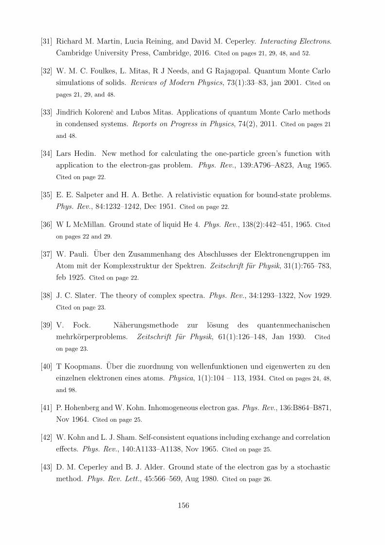
[31] Richard M. Martin, Lucia Reining, and David M. Ceperley. Interacting Electrons.

Cambridge University Press, Cambridge, 2016. Cited on pages 21, 29, 48, and 52.

[32] W. M. C. Foulkes, L. Mitas, R J Needs, and G Rajagopal. Quantum Monte Carlo

simulations of solids. Reviews of Modern Physics, 73(1):33–83, jan 2001. Cited on

pages 21, 29, and 48.

[33] Jindrich Kolorenc and Lubos Mitas. Applications of quantum Monte Carlo methods

in condensed systems. Reports on Progress in Physics, 74(2), 2011. Cited on pages 21

and 48.

[34] Lars Hedin. New method for calculating the one-particle green’s function with

application to the electron-gas problem. Phys. Rev., 139:A796–A823, Aug 1965.

Cited on page 22.

[35] E. E. Salpeter and H. A. Bethe. A relativistic equation for bound-state problems.

Phys. Rev., 84:1232–1242, Dec 1951. Cited on page 22.

[36] W L McMillan. Ground state of liquid He 4. Phys. Rev., 138(2):442–451, 1965. Cited

on pages 22 and 29.

[37] W. Pauli. Uber den Zusammenhang des Abschlusses der Elektronengruppen im

Atom mit der Komplexstruktur der Spektren. Zeitschrift fur Physik, 31(1):765–783,

feb 1925. Cited on page 22.

[38] J. C. Slater. The theory of complex spectra. Phys. Rev., 34:1293–1322, Nov 1929.

Cited on page 23.

[39] V. Fock. Naherungsmethode zur losung des quantenmechanischen

mehrkorperproblems. Zeitschrift fur Physik, 61(1):126–148, Jan 1930. Cited

on page 23.

[40] T Koopmans. Uber die zuordnung von wellenfunktionen und eigenwerten zu den

einzelnen elektronen eines atoms. Physica, 1(1):104 – 113, 1934. Cited on pages 24, 48,

and 98.

[41] P. Hohenberg and W. Kohn. Inhomogeneous electron gas. Phys. Rev., 136:B864–B871,

Nov 1964. Cited on page 25.

[42] W. Kohn and L. J. Sham. Self-consistent equations including exchange and correlation

effects. Phys. Rev., 140:A1133–A1138, Nov 1965. Cited on page 25.

[43] D. M. Ceperley and B. J. Alder. Ground state of the electron gas by a stochastic

method. Phys. Rev. Lett., 45:566–569, Aug 1980. Cited on page 26.

156

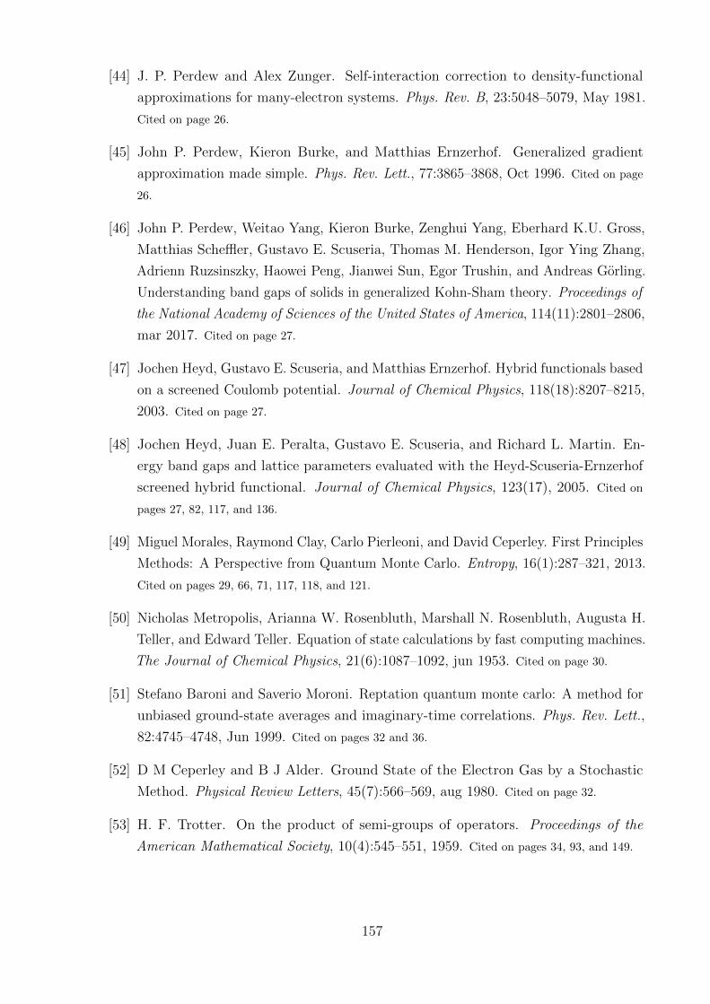
[44] J. P. Perdew and Alex Zunger. Self-interaction correction to density-functional

approximations for many-electron systems. Phys. Rev. B, 23:5048–5079, May 1981.

Cited on page 26.

[45] John P. Perdew, Kieron Burke, and Matthias Ernzerhof. Generalized gradient

approximation made simple. Phys. Rev. Lett., 77:3865–3868, Oct 1996. Cited on page

26.

[46] John P. Perdew, Weitao Yang, Kieron Burke, Zenghui Yang, Eberhard K.U. Gross,

Matthias Scheffler, Gustavo E. Scuseria, Thomas M. Henderson, Igor Ying Zhang,

Adrienn Ruzsinszky, Haowei Peng, Jianwei Sun, Egor Trushin, and Andreas Gorling.

Understanding band gaps of solids in generalized Kohn-Sham theory. Proceedings of

the National Academy of Sciences of the United States of America, 114(11):2801–2806,

mar 2017. Cited on page 27.

[47] Jochen Heyd, Gustavo E. Scuseria, and Matthias Ernzerhof. Hybrid functionals based

on a screened Coulomb potential. Journal of Chemical Physics, 118(18):8207–8215,

2003. Cited on page 27.

[48] Jochen Heyd, Juan E. Peralta, Gustavo E. Scuseria, and Richard L. Martin. En-

ergy band gaps and lattice parameters evaluated with the Heyd-Scuseria-Ernzerhof

screened hybrid functional. Journal of Chemical Physics, 123(17), 2005. Cited on

pages 27, 82, 117, and 136.

[49] Miguel Morales, Raymond Clay, Carlo Pierleoni, and David Ceperley. First Principles

Methods: A Perspective from Quantum Monte Carlo. Entropy, 16(1):287–321, 2013.

Cited on pages 29, 66, 71, 117, 118, and 121.

[50] Nicholas Metropolis, Arianna W. Rosenbluth, Marshall N. Rosenbluth, Augusta H.

Teller, and Edward Teller. Equation of state calculations by fast computing machines.

The Journal of Chemical Physics, 21(6):1087–1092, jun 1953. Cited on page 30.

[51] Stefano Baroni and Saverio Moroni. Reptation quantum monte carlo: A method for

unbiased ground-state averages and imaginary-time correlations. Phys. Rev. Lett.,

82:4745–4748, Jun 1999. Cited on pages 32 and 36.

[52] D M Ceperley and B J Alder. Ground State of the Electron Gas by a Stochastic

Method. Physical Review Letters, 45(7):566–569, aug 1980. Cited on page 32.

[53] H. F. Trotter. On the product of semi-groups of operators. Proceedings of the

American Mathematical Society, 10(4):545–551, 1959. Cited on pages 34, 93, and 149.

157

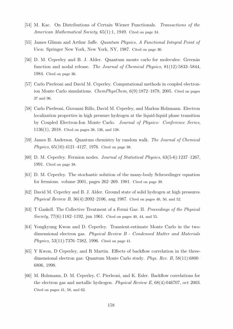
[54] M. Kac. On Distributions of Certain Wiener Functionals. Transactions of the

American Mathematical Society, 65(1):1, 1949. Cited on page 34.

[55] James Glimm and Arthur Jaffe. Quantum Physics, A Functional Integral Point of

View. Springer New York, New York, NY, 1987. Cited on page 36.

[56] D. M. Ceperley and B. J. Alder. Quantum monte carlo for molecules: Greenas

function and nodal release. The Journal of Chemical Physics, 81(12):5833–5844,

1984. Cited on page 36.

[57] Carlo Pierleoni and David M. Ceperley. Computational methods in coupled electron-

ion Monte Carlo simulations. ChemPhysChem, 6(9):1872–1878, 2005. Cited on pages

37 and 96.

[58] Carlo Pierleoni, Giovanni Rillo, David M. Ceperley, and Markus Holzmann. Electron

localization properties in high pressure hydrogen at the liquid-liquid phase transition

by Coupled Electron-Ion Monte Carlo. Journal of Physics: Conference Series,

1136(1), 2018. Cited on pages 38, 136, and 138.

[59] James B. Anderson. Quantum chemistry by random walk. The Journal of Chemical

Physics, 65(10):4121–4127, 1976. Cited on page 38.

[60] D. M. Ceperley. Fermion nodes. Journal of Statistical Physics, 63(5-6):1237–1267,

1991. Cited on page 38.

[61] D. M. Ceperley. The stochastic solution of the many-body Schroedinger equation

for fermions. volume 2001, pages 262–269. 1981. Cited on page 39.

[62] David M. Ceperley and B. J. Alder. Ground state of solid hydrogen at high pressures.

Physical Review B, 36(4):2092–2106, aug 1987. Cited on pages 40, 50, and 52.

[63] T Gaskell. The Collective Treatment of a Fermi Gas: II. Proceedings of the Physical

Society, 77(6):1182–1192, jun 1961. Cited on pages 40, 44, and 55.

[64] Yongkyung Kwon and D. Ceperley. Transient-estimate Monte Carlo in the two-

dimensional electron gas. Physical Review B - Condensed Matter and Materials

Physics, 53(11):7376–7382, 1996. Cited on page 41.

[65] Y Kwon, D Ceperley, and R Martin. Effects of backflow correlation in the three-

dimensional electron gas: Quantum Monte Carlo study. Phys. Rev. B, 58(11):6800–

6806, 1998.

[66] M. Holzmann, D. M. Ceperley, C. Pierleoni, and K. Esler. Backflow correlations for

the electron gas and metallic hydrogen. Physical Review E, 68(4):046707, oct 2003.

Cited on pages 41, 58, and 62.

158

[67] Carlo Pierleoni, Kris T. Delaney, Miguel A. Morales, David M. Ceperley, and Markus

Holzmann. Trial wave functions for high-pressure metallic hydrogen. Computer

Physics Communications, 179(1-3):89–97, 2008. Cited on pages 41 and 62.

[68] C. Lin, F. H. Zong, and D. M. Ceperley. Twist-averaged boundary conditions in

continuum quantum Monte Carlo algorithms. Physical Review E, 64(1):016702, jun

2001. Cited on pages 41, 42, 59, and 61.

[69] Simone Chiesa, David M. Ceperley, Richard M. Martin, and Markus Holzmann.

Finite-size error in many-body simulations with long-range interactions. Physical

Review Letters, 97(7):6–9, 2006. Cited on pages 42, 52, 59, and 61.

[70] Markus Holzmann, Raymond C. Clay, Miguel A. Morales, Norm M. Tubman,

David M. Ceperley, and Carlo Pierleoni. Theory of finite size effects for elec-

tronic quantum Monte Carlo calculations of liquids and solids. Physical Review B,

94(3):035126, jul 2016. Cited on pages 41, 42, 44, 53, 54, 55, 58, 59, and 61.

[71] Mark S. Hybertsen and Steven G. Louie. First-principles theory of quasiparticles:

Calculation of band gaps in semiconductors and insulators. Physical Review Letters,

55(13):1418–1421, 1985. Cited on page 47.

[72] Stefan Albrecht, Lucia Reining, Rodolfo Del Sole, and Giovanni Onida. Ab initio

calculation of excitonic effects in the optical spectra of semiconductors. Phys. Rev.

Lett., 80:4510–4513, May 1998. Cited on page 47.

[73] Michael Rohlfing and Steven G. Louie. Electron-hole excitations in semiconductors

and insulators. Phys. Rev. Lett., 81:2312–2315, Sep 1998. Cited on pages 47 and 68.

[74] Giovanni Onida, Lucia Reining, and Angel Rubio. Electronic excitations: density-

functional versus many-body Green’s-function approaches. Reviews of Modern

Physics, 74(2):601–659, jun 2002. Cited on page 47.

[75] Louie, Steven G. and Marvin L. Cohen. Conceptual Foundations of materials.

Elsevier Science, 2007. Cited on page 47.

[76] Stefan Hufner. Photoelectron Spectroscopy. Advanced Texts in Physics. Springer

Berlin Heidelberg, Berlin, Heidelberg, 2003. Cited on page 48.

[77] John P. Perdew, Robert G. Parr, Mel Levy, and Jose L. Balduz. Density-functional

theory for fractional particle number: Derivative discontinuities of the energy. Phys.

Rev. Lett., 49:1691–1694, Dec 1982. Cited on pages 48 and 49.

[78] J. F. Janak. Proof that ∂e∂ni

= ε in density-functional theory. Phys. Rev. B, 18:7165–

7168, Dec 1978. Cited on page 48.

159

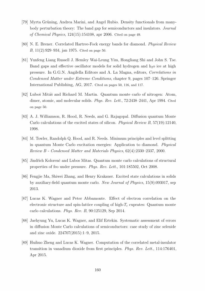
[79] Myrta Gruning, Andrea Marini, and Angel Rubio. Density functionals from many-

body perturbation theory: The band gap for semiconductors and insulators. Journal

of Chemical Physics, 124(15):154108, apr 2006. Cited on page 49.

[80] N. E. Brener. Correlated Hartree-Fock energy bands for diamond. Physical Review

B, 11(2):929–934, jan 1975. Cited on page 50.

[81] Yunfeng Liang Russell J. Hemley Wai-Leung Yim, Hongliang Shi and John S. Tse.

Band gaps and effective oscillator models for solid hydrogen and h2o ice at high

pressure. In G.G.N. Angilella Editors and A. La Magna, editors, Correlations in

Condensed Matter under Extreme Conditions, chapter 9, pages 107–126. Springer

International Publishing, AG, 2017. Cited on pages 50, 116, and 117.

[82] Lubos Mitas and Richard M. Martin. Quantum monte carlo of nitrogen: Atom,

dimer, atomic, and molecular solids. Phys. Rev. Lett., 72:2438–2441, Apr 1994. Cited

on page 50.

[83] A. J. Williamson, R. Hood, R. Needs, and G. Rajagopal. Diffusion quantum Monte

Carlo calculations of the excited states of silicon. Physical Review B, 57(19):12140,

1998.

[84] M. Towler, Randolph Q. Hood, and R. Needs. Minimum principles and level splitting

in quantum Monte Carlo excitation energies: Application to diamond. Physical

Review B - Condensed Matter and Materials Physics, 62(4):2330–2337, 2000.

[85] Jindrich Kolorenc and Lubos Mitas. Quantum monte carlo calculations of structural

properties of feo under pressure. Phys. Rev. Lett., 101:185502, Oct 2008.

[86] Fengjie Ma, Shiwei Zhang, and Henry Krakauer. Excited state calculations in solids

by auxiliary-field quantum monte carlo. New Journal of Physics, 15(9):093017, sep

2013.

[87] Lucas K. Wagner and Peter Abbamonte. Effect of electron correlation on the

electronic structure and spin-lattice coupling of high-Tc cuprates: Quantum monte

carlo calculations. Phys. Rev. B, 90:125129, Sep 2014.

[88] Jaehyung Yu, Lucas K. Wagner, and Elif Ertekin. Systematic assessment of errors

in diffusion Monte Carlo calculations of semiconductors: case study of zinc selenide

and zinc oxide. 224707(2015):1–9, 2015.

[89] Huihuo Zheng and Lucas K. Wagner. Computation of the correlated metal-insulator

transition in vanadium dioxide from first principles. Phys. Rev. Lett., 114:176401,

Apr 2015.

160

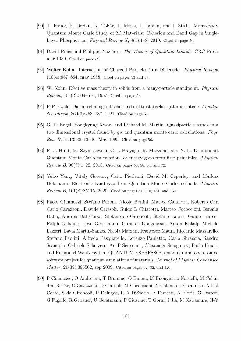
[90] T. Frank, R. Derian, K. Tokar, L. Mitas, J. Fabian, and I. Stich. Many-Body

Quantum Monte Carlo Study of 2D Materials: Cohesion and Band Gap in Single-

Layer Phosphorene. Physical Review X, 9(1):1–8, 2019. Cited on page 50.

[91] David Pines and Philippe Nozieres. The Theory of Quantum Liquids. CRC Press,

mar 1989. Cited on page 52.

[92] Walter Kohn. Interaction of Charged Particles in a Dielectric. Physical Review,

110(4):857–864, may 1958. Cited on pages 53 and 57.

[93] W. Kohn. Efective mass theory in solids from a many-particle standpoint. Physical

Review, 105(2):509–516, 1957. Cited on page 53.

[94] P. P. Ewald. Die berechnung optischer und elektrostatischer gitterpotentiale. Annalen

der Physik, 369(3):253–287, 1921. Cited on page 54.

[95] G. E. Engel, Yongkyung Kwon, and Richard M. Martin. Quasiparticle bands in a

two-dimensional crystal found by gw and quantum monte carlo calculations. Phys.

Rev. B, 51:13538–13546, May 1995. Cited on page 56.

[96] R. J. Hunt, M. Szyniszewski, G. I. Prayogo, R. Maezono, and N. D. Drummond.

Quantum Monte Carlo calculations of energy gaps from first principles. Physical

Review B, 98(7):1–22, 2018. Cited on pages 56, 58, 64, and 72.

[97] Yubo Yang, Vitaly Gorelov, Carlo Pierleoni, David M. Ceperley, and Markus

Holzmann. Electronic band gaps from Quantum Monte Carlo methods. Physical

Review B, 101(8):85115, 2020. Cited on pages 57, 116, 131, and 132.

[98] Paolo Giannozzi, Stefano Baroni, Nicola Bonini, Matteo Calandra, Roberto Car,

Carlo Cavazzoni, Davide Ceresoli, Guido L Chiarotti, Matteo Cococcioni, Ismaila

Dabo, Andrea Dal Corso, Stefano de Gironcoli, Stefano Fabris, Guido Fratesi,

Ralph Gebauer, Uwe Gerstmann, Christos Gougoussis, Anton Kokalj, Michele

Lazzeri, Layla Martin-Samos, Nicola Marzari, Francesco Mauri, Riccardo Mazzarello,

Stefano Paolini, Alfredo Pasquarello, Lorenzo Paulatto, Carlo Sbraccia, Sandro

Scandolo, Gabriele Sclauzero, Ari P Seitsonen, Alexander Smogunov, Paolo Umari,

and Renata M Wentzcovitch. QUANTUM ESPRESSO: a modular and open-source

software project for quantum simulations of materials. Journal of Physics: Condensed

Matter, 21(39):395502, sep 2009. Cited on pages 62, 82, and 120.

[99] P Giannozzi, O Andreussi, T Brumme, O Bunau, M Buongiorno Nardelli, M Calan-

dra, R Car, C Cavazzoni, D Ceresoli, M Cococcioni, N Colonna, I Carnimeo, A Dal

Corso, S de Gironcoli, P Delugas, R A DiStasio, A Ferretti, A Floris, G Fratesi,

G Fugallo, R Gebauer, U Gerstmann, F Giustino, T Gorni, J Jia, M Kawamura, H-Y

161

Ko, A Kokalj, E KAŒcAŒkbenli, M Lazzeri, M Marsili, N Marzari, F Mauri, N L

Nguyen, H-V Nguyen, A Otero de-la Roza, L Paulatto, S Ponce, D Rocca, R Sabatini,

B Santra, M Schlipf, A P Seitsonen, A Smogunov, I Timrov, T Thonhauser, P Umari,

N Vast, X Wu, and S Baroni. Advanced capabilities for materials modelling with

quantum ESPRESSO. Journal of Physics: Condensed Matter, 29(46):465901, oct

2017. Cited on pages 62, 82, and 120.

[100] P. R. C. Kent, Abdulgani Annaberdiyev, Anouar Benali, M. Chandler Bennett,

Edgar Josue Landinez Borda, Peter Doak, Hongxia Hao, Kenneth D. Jordan, Jaron T.

Krogel, Ilkka Kylanpaa, Joonho Lee, Ye Luo, Fionn D. Malone, Cody A. Melton,

Lubos Mitas, Miguel A. Morales, Eric Neuscamman, Fernando A. Reboredo, Brenda

Rubenstein, Kayahan Saritas, Shiv Upadhyay, Guangming Wang, Shuai Zhang, and

Luning Zhao. Qmcpack: Advances in the development, efficiency, and application of

auxiliary field and real-space variational and diffusion quantum monte carlo. The

Journal of Chemical Physics, 152(17):174105, 2020. Cited on page 62.

[101] M. Burkatzki, C. Filippi, and M. Dolg. Energy-consistent pseudopotentials for

quantum monte carlo calculations. The Journal of Chemical Physics, 126(23):234105,

2007. Cited on page 62.

[102] J. R. Trail and R. J. Needs. Smooth relativistic hartreeafock pseudopotentials for h

to ba and lu to hg. The Journal of Chemical Physics, 122(17):174109, 2005. Cited on

page 63.

[103] Michele Ruggeri, Saverio Moroni, and Markus Holzmann. Nonlinear network de-

scription for many-body quantum systems in continuous space. Phys. Rev. Lett.,

120:205302, May 2018. Cited on page 64.

[104] Markus Holzmann and Saverio Moroni. Orbital-dependent backflow wave functions

for real-space quantum monte carlo. Phys. Rev. B, 99:085121, Feb 2019. Cited on

page 64.

[105] Luning Zhao and Eric Neuscamman. Variational Excitations in Real Solids: Optical

Gaps and Insights into Many-Body Perturbation Theory. Physical Review Letters,

123(3):36402, 2019. Cited on page 64.

[106] Ricardo Gomez-Abal, Xinzheng Li, Matthias Scheffler, and Claudia Ambrosch-Draxl.

Influence of the core-valence interaction and of the pseudopotential approximation

on the electron self-energy in semiconductors. Phys. Rev. Lett., 101:106404, Sep

2008. Cited on pages 65 and 66.

162

[107] Feliciano Giustino, Steven G. Louie, and Marvin L. Cohen. Electron-phonon renor-

malization of the direct band gap of diamond. Phys. Rev. Lett., 105:265501, Dec

2010. Cited on pages 65 and 66.

[108] Bartomeu Monserrat and R. J. Needs. Comparing electron-phonon coupling strength

in diamond, silicon, and silicon carbide: First-principles study. Phys. Rev. B,

89:214304, Jun 2014. Cited on pages 65 and 66.

[109] P. Lautenschlager, P. B. Allen, and M. Cardona. Temperature dependence of band

gaps in si and ge. Phys. Rev. B, 31:2163–2171, Feb 1985. Cited on page 65.

[110] O. Madelung., Osten. W.Von der, and U. Rossler. Intrinsic Properties of Group IV

Elements and III-V, II-VI and I-VII Compounds. Springer-Verlag Berlin Heidelberg,

1 edition, 1987. Cited on page 66.

[111] Chris J Pickard and Richard J Needs. Structure of phase III of solid hydrogen.

Nature Physics, 3(7):473–476, may 2007. Cited on pages 66, 113, 114, and 115.

[112] Raymond C Clay, Jeremy McMinis, Jeffrey M McMahon, Carlo Pierleoni, David M

Ceperley, and Miguel A Morales. Benchmarking exchange-correlation functionals for

hydrogen at high pressures using quantum Monte Carlo. Phys. Rev. B, 89(18):184106,

2014. Cited on pages 66, 117, and 121.

[113] Vitaly Gorelov, Carlo Pierleoni, and David M. Ceperley. Benchmarking vdW-DF first-

principles predictions against Coupled Electron–Ion Monte Carlo for high-pressure

liquid hydrogen. Contributions to Plasma Physics, 59(4-5):1–8, 2019. Cited on pages

66 and 130.

[114] D. M. Ceperley and B. Bernu. The calculation of excited state properties with

quantum Monte Carlo. The Journal of Chemical Physics, 89(10):6316–6328, 1988.

Cited on page 69.

[115] J. K. L. MacDonald. Successive Approximations by the Rayleigh-Ritz Variation

Method. Physical Review, 43(10):830–833, may 1933. Cited on pages 70 and 71.

[116] M. P. Nightingale and Vilen Melik-Alaverdian. Optimization of ground- and excited-

state wave functions and van der waals clusters. Physical Review Letters, 87(4):43401–

1–43401–4, 2001. Cited on page 70.

[117] Frederick Wooten. Optical properties of Solids. Academic Press, NY, 1972. Cited on

pages 75 and 122.

[118] Gerald D. Mahan. Many-Particle Physics. Springer US, Boston, MA, 2000. Cited on

pages 75 and 85.

163

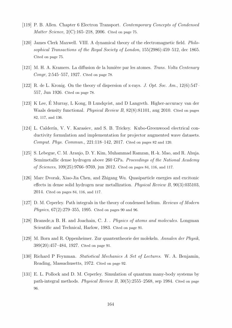
[119] P. B. Allen. Chapter 6 Electron Transport. Contemporary Concepts of Condensed

Matter Science, 2(C):165–218, 2006. Cited on page 75.

[120] James Clerk Maxwell. VIII. A dynamical theory of the electromagnetic field. Philo-

sophical Transactions of the Royal Society of London, 155(2986):459–512, dec 1865.

Cited on page 75.

[121] M. H. A. Kramers. La diffusion de la lumiere par les atomes. Trans. Volta Centenary

Congr, 2:545–557, 1927. Cited on page 78.

[122] R. de L. Kronig. On the theory of dispersion of x-rays. J. Opt. Soc. Am., 12(6):547–

557, Jun 1926. Cited on page 78.

[123] K Lee, E Murray, L Kong, B Lundqvist, and D Langreth. Higher-accuracy van der

Waals density functional. Physical Review B, 82(8):81101, aug 2010. Cited on pages

82, 117, and 136.

[124] L. Calderın, V. V. Karasiev, and S. B. Trickey. Kubo-Greenwood electrical con-

ductivity formulation and implementation for projector augmented wave datasets.

Comput. Phys. Commun., 221:118–142, 2017. Cited on pages 82 and 120.

[125] S. Lebegue, C. M. Araujo, D. Y. Kim, Muhammad Ramzan, H.-k. Mao, and R. Ahuja.

Semimetallic dense hydrogen above 260 GPa. Proceedings of the National Academy

of Sciences, 109(25):9766–9769, jun 2012. Cited on pages 84, 116, and 117.

[126] Marc Dvorak, Xiao-Jia Chen, and Zhigang Wu. Quasiparticle energies and excitonic

effects in dense solid hydrogen near metallization. Physical Review B, 90(3):035103,

2014. Cited on pages 84, 116, and 117.

[127] D. M. Ceperley. Path integrals in the theory of condensed helium. Reviews of Modern

Physics, 67(2):279–355, 1995. Cited on pages 90 and 96.

[128] Bransde,n B. H. and Joachain, C. J. . Physics of atoms and molecules. Longman

Scientific and Technical, Harlow, 1983. Cited on page 91.

[129] M. Born and R. Oppenheimer. Zur quantentheorie der molekeln. Annalen der Physik,

389(20):457–484, 1927. Cited on page 91.

[130] Richard P Feynman. Statistical Mechanics A Set of Lectures. W. A. Benjamin,

Reading, Massachusetts, 1972. Cited on page 92.

[131] E. L. Pollock and D. M. Ceperley. Simulation of quantum many-body systems by

path-integral methods. Physical Review B, 30(5):2555–2568, sep 1984. Cited on page

96.

164

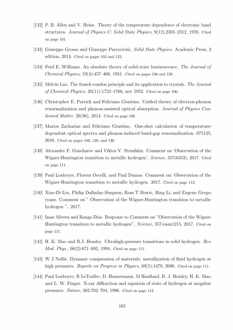
[132] P. B. Allen and V. Heine. Theory of the temperature dependence of electronic band

structures. Journal of Physics C: Solid State Physics, 9(12):2305–2312, 1976. Cited

on page 101.

[133] Giuseppe Grosso and Giuseppe Parravicini. Solid State Physics. Academic Press, 2

edition, 2014. Cited on pages 102 and 122.

[134] Ferd E. Williams. An absolute theory of solid-state luminescence. The Journal of

Chemical Physics, 19(4):457–466, 1951. Cited on pages 106 and 120.

[135] Melvin Lax. The franck-condon principle and its application to crystals. The Journal

of Chemical Physics, 20(11):1752–1760, nov 1952. Cited on page 106.

[136] Christopher E. Patrick and Feliciano Giustino. Unified theory of electron-phonon

renormalization and phonon-assisted optical absorption. Journal of Physics Con-

densed Matter, 26(36), 2014. Cited on page 106.

[137] Marios Zacharias and Feliciano Giustino. One-shot calculation of temperature-

dependent optical spectra and phonon-induced band-gap renormalization. 075125,

2016. Cited on pages 106, 120, and 130.

[138] Alexander F. Goncharov and Viktor V. Struzhkin. Comment on ’Observation of the

Wigner-Huntington transition to metallic hydrogen’. Science, 357(6353), 2017. Cited

on page 111.

[139] Paul Loubeyre, Florent Occelli, and Paul Dumas. Comment on: Observation of the

Wigner-Huntington transition to metallic hydrogen. 2017. Cited on page 113.

[140] Xiao-Di Liu, Philip Dalladay-Simpson, Ross T Howie, Bing Li, and Eugene Grego-

ryanz. Comment on ” Observation of the Wigner-Huntington transition to metallic

hydrogen ”. 2017.

[141] Isaac Silvera and Ranga Dias. Response to Comment on ”Observation of the Wigner-

Huntington transition to metallic hydrogen”. Science, 357:eaan1215, 2017. Cited on

page 111.

[142] H. K. Mao and R.J. Hemley. Ultrahigh-pressure transitions in solid hydrogen. Rev.

Mod. Phys., 66(2):671–692, 1994. Cited on page 111.

[143] W J Nellis. Dynamic compression of materials: metallization of fluid hydrogen at

high pressures. Reports on Progress in Physics, 69(5):1479, 2006. Cited on page 111.

[144] Paul Loubeyre, R LeToullec, D. Hausermann, M Hanfland, R. J. Hemley, H. K. Mao,

and L. W. Finger. X-ray diffraction and equation of state of hydrogen at megabar

pressures. Nature, 383:702–704, 1996. Cited on page 112.

165

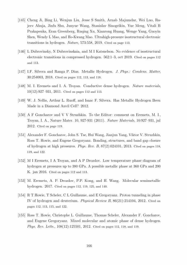
[145] Cheng Ji, Bing Li, Wenjun Liu, Jesse S Smith, Arnab Majumdar, Wei Luo, Ra-

jeev Ahuja, Jinfu Shu, Junyue Wang, Stanislav Sinogeikin, Yue Meng, Vitali B

Prakapenka, Eran Greenberg, Ruqing Xu, Xianrong Huang, Wenge Yang, Guoyin

Shen, Wendy L Mao, and Ho-Kwang Mao. Ultrahigh-pressure isostructural electronic

transitions in hydrogen. Nature, 573:558, 2019. Cited on page 113.

[146] L Dubrovinsky, N Dubrovinskaia, and M I Katsnelson. No evidence of isostructural

electronic transitions in compressed hydrogen. 562:1–3, oct 2019. Cited on pages 112

and 113.

[147] I.F. Silvera and Ranga P. Dias. Metallic Hydrogen. J. Phys.: Condens. Matter,

30:254003, 2018. Cited on pages 112, 113, and 118.

[148] M. I. Eremets and I. A. Troyan. Conductive dense hydrogen. Nature materials,

10(12):927–931, 2011. Cited on pages 112 and 113.

[149] W. J. Nellis, Arthur L. Ruoff, and Isaac F. Silvera. Has Metallic Hydrogen Been

Made in a Diamond Anvil Cell? 2012.

[150] A F Goncharov and V V Struzhkin. To the Editor: comment on Eremets, M. I.,

Troyan, I. A., Nature Mater. 10, 927-931 (2011). Nature Materials, 10:927–931, jul

2012. Cited on page 119.

[151] Alexander F. Goncharov, John S. Tse, Hui Wang, Jianjun Yang, Viktor V. Struzhkin,

Ross T. Howie, and Eugene Gregoryanz. Bonding, structures, and band gap closure

of hydrogen at high pressures. Phys. Rev. B, 87(2):024101, 2013. Cited on pages 118,

119, and 122.

[152] M I Eremets, I A Troyan, and A P Drozdov. Low temperature phase diagram of

hydrogen at pressures up to 380 GPa. A possible metallic phase at 360 GPa and 200

K. jan 2016. Cited on pages 112 and 113.

[153] M. Eremets, A. P. Drozdov, P.P. Kong, and H. Wang. Molecular semimetallic

hydrogen. 2017. Cited on pages 112, 119, 125, and 140.

[154] R T Howie, T Scheler, C L Guillaume, and E Gregoryanz. Proton tunneling in phase

IV of hydrogen and deuterium. Physical Review B, 86(21):214104, 2012. Cited on

pages 112, 113, 115, and 122.

[155] Ross T. Howie, Christophe L. Guillaume, Thomas Scheler, Alexander F. Goncharov,

and Eugene Gregoryanz. Mixed molecular and atomic phase of dense hydrogen.

Phys. Rev. Letts., 108(12):125501, 2012. Cited on pages 112, 118, and 119.

166

[156] Chang Sheng Zha, Zhenxian Liu, and Russell J. Hemley. Synchrotron infrared

measurements of dense hydrogen to 360 GPa. Physical Review Letters, 108(14):1–5,

2012. Cited on pages 112, 113, and 119.

[157] Philip Dalladay-Simpson, Ross T Howie, and Eugene Gregoryanz. Evidence for a

new phase of dense hydrogen above 325 gigapascals. Nature, 529(7584):63–67, jan

2016. Cited on pages 112 and 113.

[158] R P Dias, O Noked, and I F Silvera. Quantum phase transition in solid hydrogen at

high pressure. Physical Review B, 100:184112, 2019. Cited on pages 112, 113, 118, 125,

and 140.

[159] Ranga P Dias, Ori Noked, and Isaac F Silvera. New insulating low temperature

phase in dense hydrogen: The phase diagram to 421 GPa. 2016. Cited on pages 112,

113, 125, and 140.

[160] Bartomeu Monserrat, Richard J Needs, Eugene Gregoryanz, Chris J Pickard, T C M

Group, J J Thomson Avenue, Cambridge Cb, and United Kingdom. Hexagonal

structure of phase III of solid hydrogen. 134101:1–7, 2016. Cited on page 113.

[161] Paul Loubeyre, Florent Occelli, and Paul Dumas. Hydrogen phase IV revisited via

synchrotron infrared measurements in H 2 and D 2 up to 290 GPa at 296 K. Phys.

Rev. B, 87(13):134101, apr 2013. Cited on page 113.

[162] Ross T Howie, Philip Dalladay-Simpson, and Eugene Gregoryanz. Raman spec-

troscopy of hot hydrogen above 200 GPa. Nature Materials, 14(February):1–5, 2015.

Cited on page 113.

[163] Chris J Pickard, Miguel Martinez-Canales, and Richard J Needs. Density functional

theory study of phase IV of solid hydrogen. Phys. Rev. B, 85(21):214114, jun 2012.

Cited on pages 113, 115, and 117.

[164] Chris Pickard, Miguel Martinez-Canales, and Richard Needs. Erratum: Density

functional theory study of phase IV of solid hydrogen [Phys. Rev. B 85, 214114

(2012)]. Phys. Rev. B, 86(5):214114, 2012. Cited on page 113.

[165] M I Eremets, A P Drozdov, P P Kong, and H Wang. Semimetallic molecular

hydrogen at pressure above 350 GPa. Nat. Phys., 2019. Cited on pages 113, 118, 125,

and 140.

[166] M. I. Eremets and A. P. Drozdov. Comments on the claimed observation of the

Wigner-Huntington Transition to Metallic Hydrogen. (Akahama 2007), 2016. Cited

on page 113.

167

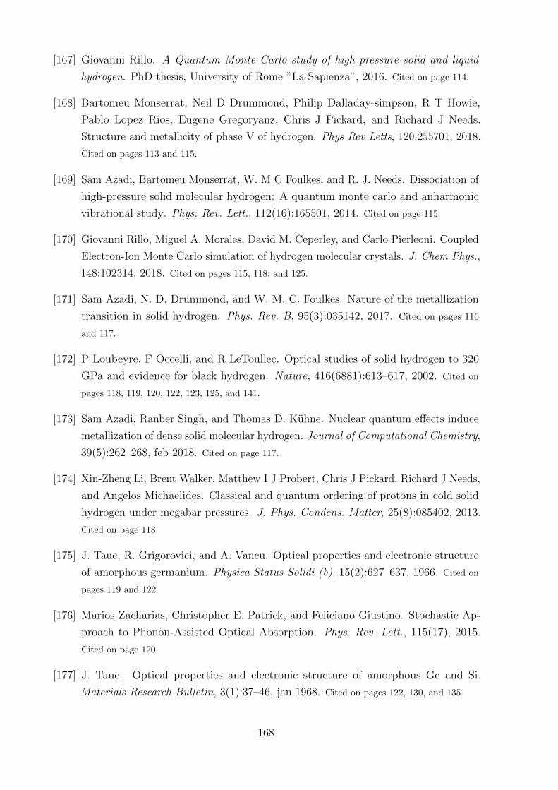
[167] Giovanni Rillo. A Quantum Monte Carlo study of high pressure solid and liquid

hydrogen. PhD thesis, University of Rome ”La Sapienza”, 2016. Cited on page 114.

[168] Bartomeu Monserrat, Neil D Drummond, Philip Dalladay-simpson, R T Howie,

Pablo Lopez Rios, Eugene Gregoryanz, Chris J Pickard, and Richard J Needs.

Structure and metallicity of phase V of hydrogen. Phys Rev Letts, 120:255701, 2018.

Cited on pages 113 and 115.

[169] Sam Azadi, Bartomeu Monserrat, W. M C Foulkes, and R. J. Needs. Dissociation of

high-pressure solid molecular hydrogen: A quantum monte carlo and anharmonic

vibrational study. Phys. Rev. Lett., 112(16):165501, 2014. Cited on page 115.

[170] Giovanni Rillo, Miguel A. Morales, David M. Ceperley, and Carlo Pierleoni. Coupled

Electron-Ion Monte Carlo simulation of hydrogen molecular crystals. J. Chem Phys.,

148:102314, 2018. Cited on pages 115, 118, and 125.

[171] Sam Azadi, N. D. Drummond, and W. M. C. Foulkes. Nature of the metallization

transition in solid hydrogen. Phys. Rev. B, 95(3):035142, 2017. Cited on pages 116

and 117.

[172] P Loubeyre, F Occelli, and R LeToullec. Optical studies of solid hydrogen to 320

GPa and evidence for black hydrogen. Nature, 416(6881):613–617, 2002. Cited on

pages 118, 119, 120, 122, 123, 125, and 141.

[173] Sam Azadi, Ranber Singh, and Thomas D. Kuhne. Nuclear quantum effects induce

metallization of dense solid molecular hydrogen. Journal of Computational Chemistry,

39(5):262–268, feb 2018. Cited on page 117.

[174] Xin-Zheng Li, Brent Walker, Matthew I J Probert, Chris J Pickard, Richard J Needs,

and Angelos Michaelides. Classical and quantum ordering of protons in cold solid

hydrogen under megabar pressures. J. Phys. Condens. Matter, 25(8):085402, 2013.

Cited on page 118.

[175] J. Tauc, R. Grigorovici, and A. Vancu. Optical properties and electronic structure

of amorphous germanium. Physica Status Solidi (b), 15(2):627–637, 1966. Cited on

pages 119 and 122.

[176] Marios Zacharias, Christopher E. Patrick, and Feliciano Giustino. Stochastic Ap-

proach to Phonon-Assisted Optical Absorption. Phys. Rev. Lett., 115(17), 2015.

Cited on page 120.

[177] J. Tauc. Optical properties and electronic structure of amorphous Ge and Si.

Materials Research Bulletin, 3(1):37–46, jan 1968. Cited on pages 122, 130, and 135.

168

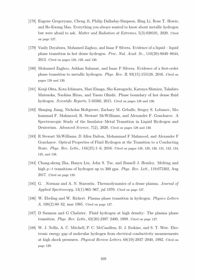
[178] Eugene Gregoryanz, Cheng Ji, Philip Dalladay-Simpson, Bing Li, Ross T. Howie,

and Ho-Kwang Mao. Everything you always wanted to know about metallic hydrogen

but were afraid to ask. Matter and Radiation at Extremes, 5(3):038101, 2020. Cited

on page 127.

[179] Vasily Dzyabura, Mohamed Zaghoo, and Isaac F Silvera. Evidence of a liquid – liquid

phase transition in hot dense hydrogen. Proc. Nat. Acad. Sc., 110(20):8040–8044,

2013. Cited on pages 128, 129, and 130.

[180] Mohamed Zaghoo, Ashkan Salamat, and Isaac F Silvera. Evidence of a first-order

phase transition to metallic hydrogen. Phys. Rev. B, 93(15):155128, 2016. Cited on

pages 128 and 130.

[181] Kenji Ohta, Kota Ichimaru, Mari Einaga, Sho Kawaguchi, Katsuya Shimizu, Takahiro

Matsuoka, Naohisa Hirao, and Yasuo Ohishi. Phase boundary of hot dense fluid

hydrogen. Scientific Reports, 5:16560, 2015. Cited on pages 128 and 130.

[182] Shuqing Jiang, Nicholas Holtgrewe, Zachary M. Geballe, Sergey S. Lobanov, Mo-

hammad F. Mahmood, R. Stewart McWilliams, and Alexander F. Goncharov. A

Spectroscopic Study of the Insulator–Metal Transition in Liquid Hydrogen and

Deuterium. Advanced Science, 7(2), 2020. Cited on pages 128 and 130.

[183] R Stewart McWilliams, D Allen Dalton, Mohammad F Mahmood, and Alexander F

Goncharov. Optical Properties of Fluid Hydrogen at the Transition to a Conducting

State. Phys. Rev. Letts., 116(25):1–6, 2016. Cited on pages 128, 129, 130, 131, 132, 134,

135, and 138.

[184] Chang-sheng Zha, Hanyu Liu, John S. Tse, and Russell J. Hemley. Melting and

high p−t transitions of hydrogen up to 300 gpa. Phys. Rev. Lett., 119:075302, Aug

2017. Cited on page 128.

[185] G. . Norman and A. N. Starostin. Thermodynamics of a dense plasma. Journal of

Applied Spectroscopy, 13(1):965–967, jul 1970. Cited on page 127.

[186] W. Ebeling and W. Richert. Plasma phase transition in hydrogen. Physics Letters

A, 108(2):80–82, mar 1985. Cited on page 127.

[187] D Saumon and G Chabrier. Fluid hydrogen at high density: The plasma phase

transition. Phys. Rev. Letts., 62(20):2397–2400, 1989. Cited on page 127.

[188] W. J. Nellis, A. C. Mitchell, P. C. McCandless, D. J. Erskine, and S. T. Weir. Elec-

tronic energy gap of molecular hydrogen from electrical conductivity measurements

at high shock pressures. Physical Review Letters, 68(19):2937–2940, 1992. Cited on

page 129.

169

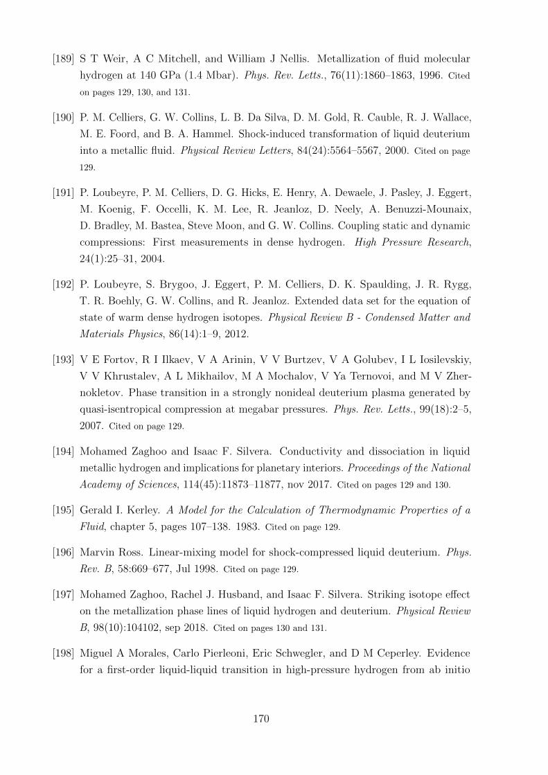
[189] S T Weir, A C Mitchell, and William J Nellis. Metallization of fluid molecular

hydrogen at 140 GPa (1.4 Mbar). Phys. Rev. Letts., 76(11):1860–1863, 1996. Cited

on pages 129, 130, and 131.

[190] P. M. Celliers, G. W. Collins, L. B. Da Silva, D. M. Gold, R. Cauble, R. J. Wallace,

M. E. Foord, and B. A. Hammel. Shock-induced transformation of liquid deuterium

into a metallic fluid. Physical Review Letters, 84(24):5564–5567, 2000. Cited on page

129.

[191] P. Loubeyre, P. M. Celliers, D. G. Hicks, E. Henry, A. Dewaele, J. Pasley, J. Eggert,

M. Koenig, F. Occelli, K. M. Lee, R. Jeanloz, D. Neely, A. Benuzzi-Mounaix,

D. Bradley, M. Bastea, Steve Moon, and G. W. Collins. Coupling static and dynamic

compressions: First measurements in dense hydrogen. High Pressure Research,

24(1):25–31, 2004.

[192] P. Loubeyre, S. Brygoo, J. Eggert, P. M. Celliers, D. K. Spaulding, J. R. Rygg,

T. R. Boehly, G. W. Collins, and R. Jeanloz. Extended data set for the equation of

state of warm dense hydrogen isotopes. Physical Review B - Condensed Matter and

Materials Physics, 86(14):1–9, 2012.

[193] V E Fortov, R I Ilkaev, V A Arinin, V V Burtzev, V A Golubev, I L Iosilevskiy,

V V Khrustalev, A L Mikhailov, M A Mochalov, V Ya Ternovoi, and M V Zher-

nokletov. Phase transition in a strongly nonideal deuterium plasma generated by

quasi-isentropical compression at megabar pressures. Phys. Rev. Letts., 99(18):2–5,

2007. Cited on page 129.

[194] Mohamed Zaghoo and Isaac F. Silvera. Conductivity and dissociation in liquid

metallic hydrogen and implications for planetary interiors. Proceedings of the National

Academy of Sciences, 114(45):11873–11877, nov 2017. Cited on pages 129 and 130.

[195] Gerald I. Kerley. A Model for the Calculation of Thermodynamic Properties of a

Fluid, chapter 5, pages 107–138. 1983. Cited on page 129.

[196] Marvin Ross. Linear-mixing model for shock-compressed liquid deuterium. Phys.

Rev. B, 58:669–677, Jul 1998. Cited on page 129.

[197] Mohamed Zaghoo, Rachel J. Husband, and Isaac F. Silvera. Striking isotope effect

on the metallization phase lines of liquid hydrogen and deuterium. Physical Review

B, 98(10):104102, sep 2018. Cited on pages 130 and 131.

[198] Miguel A Morales, Carlo Pierleoni, Eric Schwegler, and D M Ceperley. Evidence

for a first-order liquid-liquid transition in high-pressure hydrogen from ab initio

170

simulations. Proc. Nat. Acad. Sc., 107(29):12799–12803, 2010. Cited on pages 130

and 131.

[199] Alexander F. Goncharov and Zachary M. Geballe. Comment on “evidence of a

first-order phase transition to metallic hydrogen”. Phys. Rev. B, 96:157101, Oct

2017. Cited on page 130.

[200] Mohamed Zaghoo. Dynamic conductivity and partial ionization in dense fluid

hydrogen. Physical Review E, 97(4):043205, apr 2018. Cited on page 130.

[201] Guglielmo Mazzola, Ravit Helled, and Sandro Sorella. Phase Diagram of Hydrogen

and a Hydrogen-Helium Mixture at Planetary Conditions by Quantum Monte Carlo

Simulations. Physical Review Letters, 120:25701, 2018. Cited on pages 130 and 131.

[202] W Lorenzen, B Holst, and R Redmer. First-order liquid-liquid phase transition in

dense hydrogen. Phys. Rev. B, 82(19):195107, 2010. Cited on page 131.

[203] Bastian Holst, Martin French, and Ronald Redmer. Electronic transport coefficients

from ab initio simulations and application to dense liquid hydrogen. Phys. Rev. B,

83(23):235120, 2011. Cited on page 131.

[204] Miguel A Morales, Jeffrey M McMahon, Carlo Pierleoni, and David M Ceperley.

Nuclear quantum effects and nonlocal exchange-correlation functionals applied to

liquid hydrogen at high pressure. Phys. Rev. Letts., 110(6):65702, 2013. Cited on page

131.

[205] G. E. Norman and I. M. Saitov. Plasma phase transition in warm dense hydrogen.

Contributions to Plasma Physics, 58(2-3):122–127, 2018.

[206] Binbin Lu, Dongdong Kang, Dan Wang, Tianyu Gao, and Jiayu Dai. Towards

the Same Line of Liquid-Liquid Phase Transition of Dense Hydrogen from Various

Theoretical Predictions. Chinese Physics Letters, 36(10), 2019. Cited on page 131.

[207] Joshua Hinz, Valentin V. Karasiev, S. X. Hu, Mohamed Zaghoo, Daniel Mejıa-

Rodrıguez, S. B. Trickey, and L. Calderın. Fully Consistent Density Functional

Theory Determination of the Insulator-Metal Transition Boundary in Warm Dense

Hydrogen. 2011(2865):1–9, feb 2020. Cited on pages 130 and 131.

[208] M. D. Knudson, M. P. Desjarlais, M. Preising, and R. Redmer. Evaluation of

exchange-correlation functionals with multiple-shock conductivity measurements in

hydrogen and deuterium at the molecular-to-atomic transition. Physical Review B,

98(17):174110, nov 2018. Cited on pages 131, 132, and 135.

171

[209] Kushal Ramakrishna, Tobias Dornheim, and Jan Vorberger. Influence of finite

temperature Exchange-Correlation effects in Hydrogen. 49, 2020.

[210] Hua Y. Geng, Q. Wu, Miriam Marques, and Graeme J. Ackland. Thermodynamic

anomalies and three distinct liquid-liquid transitions in warm dense liquid hydrogen.

Physical Review B, 100(13):134109, oct 2019. Cited on page 131.

[211] Fei Lin, Miguel A. Morales, Kris T. Delaney, Carlo Pierleoni, Richard M. Martin,

and D. M. Ceperley. Electrical conductivity of high-pressure liquid hydrogen by

quantum Monte Carlo methods. Physical Review Letters, 103(25):1–4, 2009. Cited on

page 131.

[212] Vitaly Gorelov, Markus Holzmann, David M. Ceperley, and Carlo Pierleoni. Energy

Gap Closure of Crystalline Molecular Hydrogen with Pressure. Physical Review

Letters, 124(11):116401, mar 2020. Cited on pages 131, 132, and 136.

[213] Carlo Pierleoni, Markus Holzmann, and David M Ceperley. Local structure in dense

hydrogen at the liquid-liquid phase transition by coupled electron-ion Monte Carlo.

Contributions to Plasma Physics, 58(2-3):99–106, feb 2018. Cited on pages 132, 133, 135,

and 136.

[214] Gerald Irwin Kerley. Equations of state for hydrogen and deuterium. 12 2003. Cited

on page 135.

[215] Riccardo Sabatini, Tommaso Gorni, and Stefano de Gironcoli. Nonlocal van der

waals density functional made simple and efficient. Phys. Rev. B, 87:041108, Jan

2013. Cited on page 136.

[216] Jianmin Tao, John P. Perdew, Viktor N. Staroverov, and Gustavo E. Scuseria.

Climbing the density functional ladder: Nonempirical meta–generalized gradient

approximation designed for molecules and solids. Phys. Rev. Lett., 91:146401, Sep

2003. Cited on page 136.

172

Titre: Méthodes de monte carlo quantique pour le calcul des structures électroniques:application à l’hydrogène dans des conditions extrêmes

Mots clés: Monte Carlo quantique, structure électronique, méthode CEIMC, conditions ex-trêmes, hydrogène solide

Résumé: Le problème de la métallisation del’hydrogène, posé il y a près de 80 ans, a étédésigné comme la troisième question ouverte enphysique du XXIe siècle. En effet, en raison desa légèreté et de sa réactivité, les informationsexpérimentales sur l’hydrogène à haute pressionsont limitées et extrêmement difficiles à obtenir.Il est donc essentiel de mettre au point des méth-odes précises pour guider les expériences.

Dans cette thèse, nous nous concentrons surl’étude de la structure électronique, y comprisles phénomènes d’état excité, en utilisant lestechniques de Monte Carlo quantique (QMC).En particulier, nous développons une nouvelleméthode de calcul pour le gap accompagnéed’un traitement précis de l’erreur induit par lataille finie de la cellule de simulation. Nous étab-lissons un lien formel entre l’erreur de la taillefinie et la constante diélectrique du matériau.Avant d’étudier l’hydrogène, la nouvelle méth-ode est testée sur le silicium cristallin et le car-bone de diamant, pour lesquels des informationsexpérimentales sur le gap sont disponibles. Nosrésultats montrent que le biais dû à la super-cellule de taille finie peut être corrigé, de sorteque des valeurs précises dans la limite thermody-namique peuvent être obtenues pour les petitessupercellules sans avoir besoin d’une extrapola-tion numérique.

Comme l’hydrogène est un matériau trèsléger, les effets quantiques nucléaires sont im-portants. Une description précise des ef-fets nucléaires peut être réalisée par la méth-ode de Monte Carlo à ions et électrons cou-plés (CEIMC), une méthode de simulation despremiers principes basée sur le QMC. Nousutilisons les résultats de la méthode CEIMCpour discuter des effets quantiques et ther-miques des noyaux sur les propriétés électron-iques. Nous introduisons une méthode formellede traitement du gap électronique et de lastructure des bandes à température finie dansl’approximation adiabatique et discutons desapproximations qui doivent être faites. Nousproposons également une nouvelle méthode pour

calculer les propriétés optiques à basse tempéra-ture, qui constituera une amélioration par rap-port à l’approximation semi-classique couram-ment utilisée.

Enfin, nous appliquons l’ensemble dudéveloppement méthodologique de cette thèsepour étudier la métallisation de l’hydrogènesolide et liquide. Nous constatons quepour l’hydrogène moléculaire dans sa structurecristalline parfaite, le gap QMC est en accordavec les calculs précédents de GW. Le traite-ment des effets quantiques nucléaires entraîneune forte réduction du gap ( 2 eV). Selon lastructure, le gap indirect fondamental se fermeentre 380 et 530 GPa pour les cristaux idéauxet 330-380 GPa pour les cristaux quantiques, cequi dépend moins de la symétrie cristalline. Au-delà de cette pression, le système entre dans unephase de mauvais métal où la densité des étatsau niveau de Fermi augmente avec la pressionjusqu’à 450-500 GPa lorsque le gap direct seferme. Notre travail confirme partiellement par-tie l’interprétation des récentes expériences surl’hydrogène à haute pression.

Nous explorons également la possibilitéd’utiliser une représentation multidéterminantedes états excités pour modéliser les excitationsneutres et calculer la conductivité via la for-mule de Kubo. Nous avons appliqué cetteméthodologie à l’hydrogène cristallin idéal etlimité au niveau de Monte Carlo variationnel dela théorie.

Pour l’hydrogène liquide, la principale con-clusion est que la fermeture du gap est con-tinue et coïncide avec la transition de dissoci-ation moléculaire. Nous avons été en mesured’étalonner les fonctions de la théorie fonction-nelle de la densité (DFT) en nous basant surla densité QMC des états. En utilisant lesvaleurs propres des calculs Kohn-Sham corrigépar QMC pour calculer les propriétés optiquesdans le cadre de la théorie de Kubo-Greenwood, nous avons constaté que l’absorption optiquethéorique calculée précédemment s’est déplacéevers des énergies plus faibles.

3

Title: Quantum Monte Carlo methods for electronic structure calculations: applicationto hydrogen at extreme conditions

Keywords: Quantum Monte Carlo, electronic structure, Ferrite, CEIMC method, extremeconditions, solid hydrogen

Abstract: The hydrogen metallization prob-lem posed almost 80 years ago, was named asthe third open question in physics of the XXIcentury. Indeed, due to its lightness and reac-tivity, experimental information on high pres-sure hydrogen is limited and extremely difficultto obtain. Therefore, the development of accu-rate methods to guide experiments is essential.

In this thesis, we focus on studying the elec-tronic structure, including excited state phe-nomena, using quantum Monte Carlo (QMC)techniques. In particular, we develop a newmethod of computing energy gaps accompaniedby an accurate treatment of the finite simulationcell error. We formally relate finite size error tothe dielectric constant of the material. Beforestudying hydrogen, the new method is tested oncrystalline silicon and carbon diamond, systemsfor which experimental information on the gapis available. Although finite-size corrected gapvalues for carbon and silicon are larger than theexperimental ones, our results demonstrate thatthe bias due to the finite size supercell can becorrected for, so precise values in the thermody-namic limit can be obtained for small supercellswithout need for numerical extrapolation.

As hydrogen is a very light material, thenuclear quantum effects are important. Anaccurate capturing of nuclear effects can bedone within the Coupled Electron Ion MonteCarlo (CEIMC) method, a QMC-based first-principles simulation method. We use the re-sults of CEIMC to discuss the thermal renormal-ization of electronic properties. We introduce aformal way of treating the electronic gap andband structure at a finite temperature withinthe adiabatic approximation and discuss the ap-proximations that have to be made. We proposeas well a novel way of renormalizing the opticalproperties at low temperature, which will be animprovement upon the commonly used semiclas-

sical approximation.Finally, we apply all the methodological de-

velopment of this thesis to study the metal-lization of solid and liquid hydrogen. We findthat for ideal crystalline molecular hydrogen theQMC gap is in agreement with previous GWcalculations. Treating nuclear zero point effectscause a large reduction in the gap ( 2 eV). Deter-mining the crystalline structure of solid hydro-gen is still an open problem. Depending on thestructure, the fundamental indirect gap closesbetween 380 and 530 GPa for ideal crystals and330–380 GPa for quantum crystals, which de-pends less on the crystalline symmetry. Beyondthis pressure, the system enters into a bad metalphase where the density of states at the Fermilevel increases with pressure up to 450–500GPa when the direct gap closes. Our work par-tially supports the interpretation of recent ex-periments in high pressure hydrogen. However,the scenario where solid hydrogen metallizationis accompanied by the structural change, for ex-ample, a molecular dissociation, can not be dis-proved.

We also explore the possibility to use a mul-tideterminant representation of excited states tomodel neutral excitations and compute the con-ductivity via the Kubo formula. We applied thismethodology to ideal crystalline hydrogen andlimited to the variational Monte Carlo level ofthe theory.

For liquid hydrogen, the main finding is thatthe gap closure is continuous and coincides withthe molecular dissociation transition. We wereable to benchmark different density functionaltheory (DFT) functionals based on the QMCelectronic density of states. When using theQMC renormalized Kohn-Sham eigenvalues tocompute optical properties within the Kubo-Greenwood theory, we found that previously cal-culated theoretical optical absorption has a shifttowards lower energies.

Université Paris-SaclayEspace Technologique / Immeuble DiscoveryRoute de l’Orme aux Merisiers RD 128 / 91190 Saint-Aubin, France