Quantum Machine Learning for Radio Astronomy

Quantum Machine Learning for Radio Astronomy

Mohammad KordzanganehDepartment of Physics & Astronomy

University of Manchester, [email protected]

Aydin UttingDepartment of Physics & Astronomy

University of Manchester, [email protected]

Anna Scaife∗Department of Physics & Astronomy

University of Manchester, [email protected]

Abstract

In this work we introduce a novel approach to the pulsar classification problemin time-domain radio astronomy using a Born machine, often referred to as aquantum neural network. Using a single-qubit architecture, we show that thepulsar classification problem maps well to the Bloch sphere and that comparableaccuracies to more classical machine learning approaches are achievable. Weintroduce a novel single-qubit encoding for the pulsar data used in this work andshow that this performs comparably to a multi-qubit QAOA encoding.

1 Introduction

Pulsars are rapidly rotating neutron stars that emit very precisely timed repeating radio pulses withperiods of milli-seconds to seconds. These objects are formed through the death of massive stars(> 8 M�), which have collapsed masses that are insufficient to undergo complete gravitationalcollapse and form a black hole but are sufficiently massive that collapse causes their electrons tocombine with protons and form neutrons, a process which continues until neutron degeneracy pressureis high enough to prevent further gravitational collapse. By the time this happens such stars are almostexclusively comprised of neutrons, compressed into a sphere of approximately 20 km in diameter [8].

Finding and observing pulsars is a core science aim of the Square Kilometre Array (SKA) observatory,a global project to build the world’s largest radio telescope [7]. The SKA intends to conduct a cosmiccensus of the pulsar population with the aim of addressing a number of key questions in modernphysics, including the detection and mapping of gravitational waves as they pass through our Galaxy.By timing the arrival of radio pulses produced by numerous pulsars with milli-second spin periods,the presence of gravitational waves can be detected as a disturbance in the regularity of these pulsearrival times on Earth [4, 5, 6], opening up a new gravitational wave regime to that detected by (e.g.)the LIGO experiment on Earth [e.g. 2]. To conduct such an experiment the SKA must identify andmap the location of thousands of previously unknown pulsars by separating their periodic signals fromthose of other radio frequency interference sources. Consequently the development of classificationalgorithms for this purpose has become a subject of significant interest over the past few years [9].

This work In this work we introduce a novel approach to pulsar classification using a Born machine,often referred to as a quantum neural network. Using a single qubit architecture, we show that thepulsar classification problem maps well to the Bloch sphere and that comparable accuracies to moreclassical machine learning approaches are achievable. We introduce a novel single-qubit quantum

∗The Alan Turing Institute, 96 Euston Rd, London, UK [email protected]

Fourth Workshop on Machine Learning and the Physical Sciences (NeurIPS 2021).

· · ·|0〉 H W (0) Rz(x1) W (1) W (n−1) Rz(xn) W (n)

Figure 1: One encoding repetition of the single qubit network used in this work. To add morerepetitions the series of gates (excluding the initial Hadamard gate) need to be repeated with newtrainable parameters.

encoding for the pulsar data used in this work and compare this encoding with the more standardQAOA encoding [3]. The former shows great promise in trainability and expressivity compared tothe QAOA ansatz.

2 Quantum Model

The quantum model introduced in this work is an extension of the single-qubit models explored in[10]. These extensions are: (i) a model for a general single-qubit trainable layer, and (ii) the extensionof the single feature Fourier series to a multi-dimensional Fourier series. The architecture of themodel consists of generalised trainable layers interlaced with a single-gate rotations encoding thefeatures, see Figure 1.

Trainable layers The trainable layers play an important role in determining the expressivity of aquantum model [10]. A trainable layer needs to be complex enough to provide sufficient access tothe Fourier coefficient space, but also simple enough to be efficient for gradient calculations. Thetrainable layer chosen in this work consists of three consecutive rotations, about Z, then X , and thenY . This gives the most general SU(2) rotation, and in a single-qubit case it can convert any initialstate, |ψ〉, to any final state, |φ〉. This ensures that we can fully access the group space and maximallyaccess the Fourier space in the most efficient way possible2.

Multi-feature encoding The data features are encoded usingZ-rotations placed between the trainablelayers. This means that for the 8 features in the HTRU 2 dataset, there are 9 trainable layers enclosing8 Z-rotation encoding gates. We show here that this architecture is able to express the first degreemulti-dimensional Fourier series of the dataset. We refer to this as a quantum asymptotically universalmulti-feature (QAUM) encoding.

We follow the analytical derivation of [10] by encoding using

S(x) = eiGx, (1)

where G is an SU(2) generator, i.e. one of the Pauli matrices. These encoding layers are surroundedby trainable layers with weights, W . In tensor notation, we can express a circuit with a singleencoding:

|ψ〉 = W (2)S(x)W (1)|0〉 −→W(2)ki e

iGijxW(1)j1 , (2)

where |0〉 −→ [1, 0]T is absorbed in the second index ofW (1) and the Einstein summation conventionis assumed. Choosing G to be the Pauli-Z matrix, we can re-write Eqn 2 with the eigenvalues ofPauli-Z λ ∈ {−1, 1}:

|ψ〉k −→W(2)ki e

iλixW(1)i1 =

(W

(2)ki W

(1)i1

)eiλix. (3)

This encoding can be extended to a more general case with N features and L encoding repetitions:

|ψ〉k →W(L1)kiL1

eiλi

L1x1W

(L2)iL1 iL2

· · ·W (LN )iLN−1 iLN

eiλLN xNW((L−1)N )iLN i(L−1)1

· · ·W (0)i1N 1. (4)

Measuring this qubit in some basis defined by a measurement operator, M̂ , gives us the expectationvalue of this operator in the |ψ〉 basis3,

〈ψ|M̂ |ψ〉 = W†(0)1j1N· · ·W †(L

1)jL1k′

Mk′kW(L1)kiL1· · ·W (0)

i1N 1ei∑N

l=1 xl

(∑Lm=1 λi

ml−∑L

p=1 λjpl

). (5)

2Given a particular use case, these trainable layers may be pruned to increase efficiency.3In this work, M̂ is taken to be the fundamental measurement basis of {|0〉, |1〉}

2

In this equation, it is possible to think of λiml

as a matrix whose dimensions are indexed by m and l.The values in this matrix are 1 and −1 with uniform probability and all the possible combinations ofthese values, create a matrix ensemble. Each member of the ensemble has an associated coefficientthat is calculated by multiplying the trainable layers with indices iml - a vector of 1s and 2s. All ofthese possibilities are included in the calculation of the expectation value in Equation 5. With this inmind, we can re-write the exponent of this equation

β =

N∑l=1

xl

(L∑

m=1

λiml−

L∑p=1

λjpl

)= [1, 1, · · · , 1]([λi

ml]− [λj

pl])[x1, x2, · · · , xN ]T , (6)

where the sum over m and p are replaced with a matrix multiplication of the member ensemblesby a vector of ones, and the sum over l by a multiplication with the vector of features. Making thesubstitution 2α = λi

ml− λi

plshows that members of α are {−1, 0, 1}, where the number of terms

contributing to each value is distributed as (1, 2, 1). Multiplication of α with the vector of ones yields

γ = [1, 1, · · · , 1]α = [γ1, γ2, · · · , γN ], (7)where γq ∈ {−L,−(L − 1), · · · ,−1, 0, 1, · · · , L − 1, L}, and subsequently the number of termscontributing to each is given by {

(2L2L

),(

2L2L−1

),(

2L2L−2

), · · · ,

(2L0

)}. This means that the higher

frequency terms are less accessible than those with lower frequencies, and consequently

β = 2γ [x1, x2, · · · , xN ]T. (8)

We get a superposition of all the frequencies of the features up to L, the number of encodingrepetitions. This means that by increasing the number of repetitions, we approximate the problemwith a truncated Fourier series of higher frequency. We therefore expect the training loss to decreaseas the number of repetitions increase. This means that an architecture that can access the entireFourier space is expected to model any function to approach a training loss of zero as the encodingrepetitions approach infinity. The term asymptotically universal is used in Ref [10] to describe suchmodels.

2.1 Training

For this work we use the HTRU 2 pulsar dataset4 [9], which contains 16,259 spurious examplescaused by RFI/noise and 1,639 real pulsar examples. Each example is described by 8 continuousfeature variables and a single class label. We scale the original HTRU 2 feature values individually tolie in the range (0, π) to produce the full Fourier series5.

The circuits were simulated using the PennyLane default.qubit [1] device and the gradients werecalculated using the simulator’s backprop method. The Adam Optimiser with a learning rate of 0.1was utilised to update the trainable parameters and the cross entropy loss function was used. The fulldataset was randomly sampled 5 times, to obtain five training data sets with 100 data points each anda balanced class ratio. The model was trained for 150 epochs on Kaggle using Intel Xeon CPU. Eachtraining run took approximately ∆t = 760± 20 seconds67.

Two types of uncertainty were evaluated: (i) weight initialisation error, and (ii) sampling error.The former was measured by running the training on a set sample of data 5 times using uniformlyrandomised weights in the range w = [0, 2π], and the latter was measured by changing the trainingsample 5 times. In each case, the mean and standard deviation of the performance was calculated.

The QAOA ansatz using Y rotations was directly imported from the PennyLane templates for trainingthe network. This model was implemented on 9 qubits and had 18 trainable parameters per repetition.

3 Results

The trained QAUM L = 2 model achieves a training accuracy of 95.8± 2.3% and a test accuracy of91.6± 3.6%, approaching the accuracies achieved using more classical machine learning approaches

4Data are publicly available at https://archive.ics.uci.edu/ml/datasets/HTRU2.5The reason π was chosen over 2π was to account for the factor of 2 in Eqn 8.6Time shown is for the QAUM L = 2 model, which is the main subject of comparison in Section 3. The

training time is highly dependent on the number of trainable parameters.7Full code to recreate the results is available at https://github.com/kordham/qaum.

3

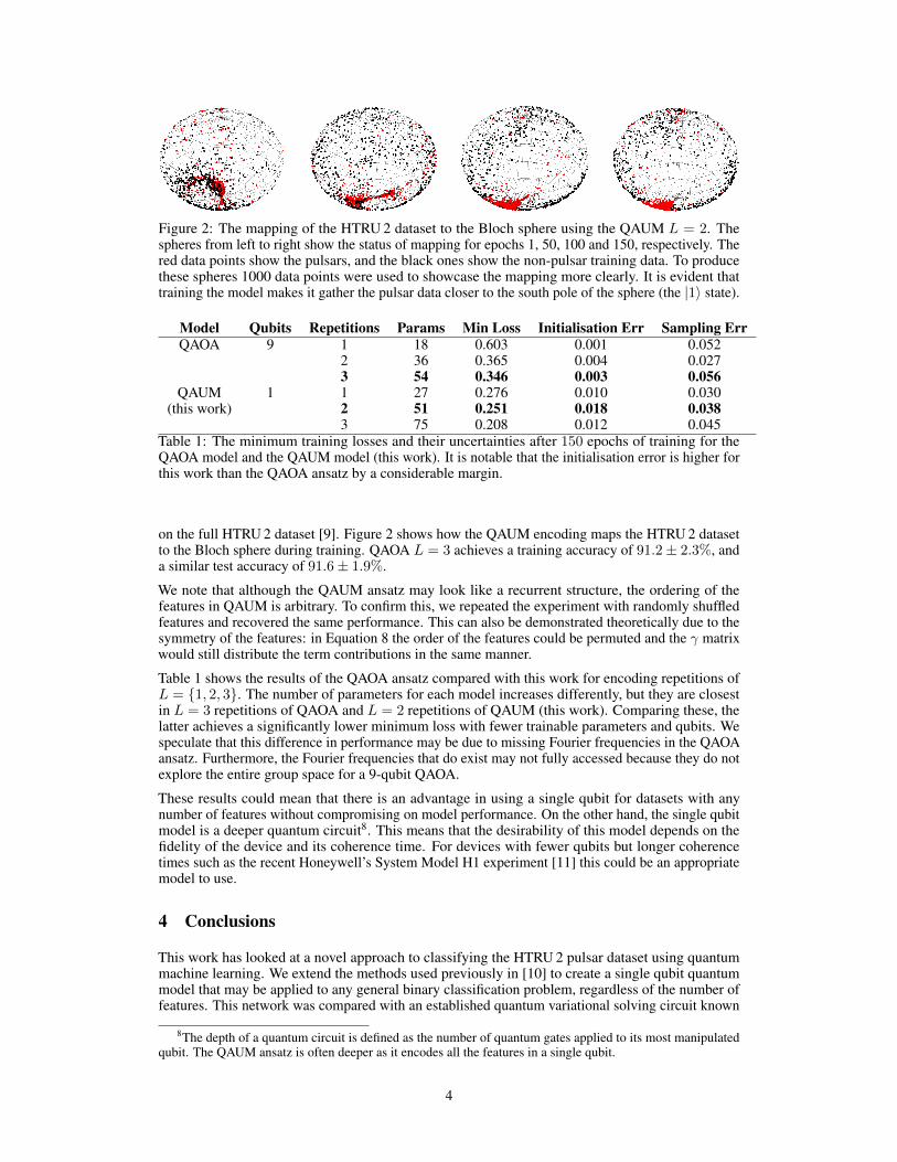
Figure 2: The mapping of the HTRU 2 dataset to the Bloch sphere using the QAUM L = 2. Thespheres from left to right show the status of mapping for epochs 1, 50, 100 and 150, respectively. Thered data points show the pulsars, and the black ones show the non-pulsar training data. To producethese spheres 1000 data points were used to showcase the mapping more clearly. It is evident thattraining the model makes it gather the pulsar data closer to the south pole of the sphere (the |1〉 state).

Model Qubits Repetitions Params Min Loss Initialisation Err Sampling ErrQAOA 9 1 18 0.603 0.001 0.052

2 36 0.365 0.004 0.0273 54 0.346 0.003 0.056

QAUM 1 1 27 0.276 0.010 0.030(this work) 2 51 0.251 0.018 0.038

3 75 0.208 0.012 0.045Table 1: The minimum training losses and their uncertainties after 150 epochs of training for theQAOA model and the QAUM model (this work). It is notable that the initialisation error is higher forthis work than the QAOA ansatz by a considerable margin.

on the full HTRU 2 dataset [9]. Figure 2 shows how the QAUM encoding maps the HTRU 2 datasetto the Bloch sphere during training. QAOA L = 3 achieves a training accuracy of 91.2± 2.3%, anda similar test accuracy of 91.6± 1.9%.

We note that although the QAUM ansatz may look like a recurrent structure, the ordering of thefeatures in QAUM is arbitrary. To confirm this, we repeated the experiment with randomly shuffledfeatures and recovered the same performance. This can also be demonstrated theoretically due to thesymmetry of the features: in Equation 8 the order of the features could be permuted and the γ matrixwould still distribute the term contributions in the same manner.

Table 1 shows the results of the QAOA ansatz compared with this work for encoding repetitions ofL = {1, 2, 3}. The number of parameters for each model increases differently, but they are closestin L = 3 repetitions of QAOA and L = 2 repetitions of QAUM (this work). Comparing these, thelatter achieves a significantly lower minimum loss with fewer trainable parameters and qubits. Wespeculate that this difference in performance may be due to missing Fourier frequencies in the QAOAansatz. Furthermore, the Fourier frequencies that do exist may not fully accessed because they do notexplore the entire group space for a 9-qubit QAOA.

These results could mean that there is an advantage in using a single qubit for datasets with anynumber of features without compromising on model performance. On the other hand, the single qubitmodel is a deeper quantum circuit8. This means that the desirability of this model depends on thefidelity of the device and its coherence time. For devices with fewer qubits but longer coherencetimes such as the recent Honeywell’s System Model H1 experiment [11] this could be an appropriatemodel to use.

4 Conclusions

This work has looked at a novel approach to classifying the HTRU 2 pulsar dataset using quantummachine learning. We extend the methods used previously in [10] to create a single qubit quantummodel that may be applied to any general binary classification problem, regardless of the number offeatures. This network was compared with an established quantum variational solving circuit known

8The depth of a quantum circuit is defined as the number of quantum gates applied to its most manipulatedqubit. The QAUM ansatz is often deeper as it encodes all the features in a single qubit.

4

as the QAOA ansatz on this dataset. The single qubit network trained to a lower loss than the QAOAdespite the large difference in the number of qubits.

We show that the single-qubit encoding creates a multi-dimensional Fourier series whose highestfrequency is determined by the number of repetitions. To access the maximum potential of the Fouriercoefficients, this work suggests the use of the most general state of a qubit as the trainable layers.

We note that although the pulsar classification application considered here is not a high-dimensionalproblem, this does not necessarily mean that this architecture is limited by the Bloch sphere. Indeed,by adding additional repetitions we generate more Fourier terms which should assist in separatingclasses in a given classification task. The limitation of this, however, is the accessibility to the Fourierspace. The performance of a single-qubit QAUM, as demonstrated here, compared with a 2-qubitQAUM is not immediately clear, and is the subject of future research. Furthermore, while the singlequbit encoding demonstrated here can be efficiently run on a classical computer - there are currentlyfew arguments that make it appealing to run on a quantum computer - this would no longer be thecase when extending the QAUM ansatz to the multi-qubit case.

Acknowledgments and Disclosure of Funding

The authors gratefully acknowledge support from the UK Alan Turing Institute under grant referenceEP/V030302/1.

References[1] Source code for pennylane.devices.default_qubit https://pennylane.readthedocs.io/

en/stable/_modules/pennylane/devices/default_qubit.html#DefaultQubit.

[2] B. P. Abbott and the LIGO Consortium. Observation of gravitational waves from a binary blackhole merger. Phys. Rev. Lett., 116:061102, Feb 2016.

[3] E. Farhi, J. Goldstone, S. Gutmann, and M. Sipser. Quantum computation by adiabatic evolution,2000.

[4] R. S. Foster and D. C. Backer. Constructing a Pulsar Timing Array. , 361:300, Sept. 1990.

[5] G. Hobbs, A. G. Lyne, and M. Kramer. An analysis of the timing irregularities for 366 pulsars.Notices of the Royal Astronomical Society, 402(2):1027–1048, Feb. 2010.

[6] G. Janssen, G. Hobbs, M. McLaughlin, C. Bassa, A. Deller, M. Kramer, K. Lee, C. Mingarelli,P. Rosado, S. Sanidas, A. Sesana, L. Shao, I. Stairs, B. Stappers, and J. P. W. Verbiest. Gravita-tional Wave Astronomy with the SKA. In Advancing Astrophysics with the Square KilometreArray (AASKA14), page 37, Apr. 2015.

[7] E. Keane, B. Bhattacharyya, M. Kramer, B. Stappers, E. F. Keane, B. Bhattacharyya, M. Kramer,B. W. Stappers, S. D. Bates, M. Burgay, S. Chatterjee, D. J. Champion, R. P. Eatough, J. W. T.Hessels, G. Janssen, K. J. Lee, J. van Leeuwen, J. Margueron, M. Oertel, A. Possenti, S. Ransom,G. Theureau, and P. Torne. A Cosmic Census of Radio Pulsars with the SKA. In AdvancingAstrophysics with the Square Kilometre Array (AASKA14), page 40, Apr. 2015.

[8] A. Lyne and F. Graham-Smith. Pulsar Astronomy. Cambridge University Press, 2012.

[9] R. J. Lyon, B. W. Stappers, S. Cooper, J. M. Brooke, and J. D. Knowles. Fifty Years of PulsarCandidate Selection: From simple filters to a new principled real-time classification approach.Notices of the Royal Astronomical Society, 459:1104, June 2016.

[10] M. Schuld, R. Sweke, and J. J. Meyer. Effect of data encoding on the expressive power ofvariational quantum-machine-learning models. Physics Reviews A, 103(3):032430, Mar. 2021.

[11] T. Uttley. Honeywell sets new record for quantum comput-ing performance https://www.honeywell.com/us/en/news/2021/03/honeywell-sets-new-record-for-quantum-computing-performance.

5

Checklist

1. For all authors...(a) Do the main claims made in the abstract and introduction accurately reflect the paper’s

contributions and scope? [Yes](b) Did you describe the limitations of your work? [Yes] The limitations were discussed in

Section 3 where the depth of the network could be problematic for the devices it is runon.

(c) Did you discuss any potential negative societal impacts of your work? [N/A](d) Have you read the ethics review guidelines and ensured that your paper conforms to

them? [Yes]2. If you are including theoretical results...

(a) Did you state the full set of assumptions of all theoretical results? [Yes] See Section2.1.

(b) Did you include complete proofs of all theoretical results? [Yes] In Section 2 see themulti-feature encoding proof.

3. If you ran experiments...(a) Did you include the code, data, and instructions needed to reproduce the main experi-

mental results (either in the supplemental material or as a URL)? [Yes] Code includedin GitHub link provided in Section 3.

(b) Did you specify all the training details (e.g., data splits, hyperparameters, how theywere chosen)? [Yes] See Section 2.1.

(c) Did you report error bars (e.g., with respect to the random seed after running experi-ments multiple times)? [Yes] See Section 3 and specifically Table 1.

(d) Did you include the total amount of compute and the type of resources used (e.g.,type of GPUs, internal cluster, or cloud provider)? [Yes] The full specification of thetraining resources were discussed in 2.1

4. If you are using existing assets (e.g., code, data, models) or curating/releasing new assets...(a) If your work uses existing assets, did you cite the creators? [Yes] This work uses the

HTRU 2 dataset as mentioned in full in the introduction section and linked to in Section2.1

(b) Did you mention the license of the assets? [Yes] The full URL to the dataset is givenand no license is specified on the weblink. Just a request for citation, which we havefulfilled.

(c) Did you include any new assets either in the supplemental material or as a URL? [Yes]A GitHub repository with the code in this work is included in Section 2.1

(d) Did you discuss whether and how consent was obtained from people whose data you’reusing/curating? [N/A]

(e) Did you discuss whether the data you are using/curating contains personally identifiableinformation or offensive content? [N/A]

5. If you used crowdsourcing or conducted research with human subjects...(a) Did you include the full text of instructions given to participants and screenshots, if

applicable? [N/A](b) Did you describe any potential participant risks, with links to Institutional Review

Board (IRB) approvals, if applicable? [N/A](c) Did you include the estimated hourly wage paid to participants and the total amount

spent on participant compensation? [N/A]

6