Quantum Groups - University of California, Berkeley

Quantum Groups

Prof. Nicolai Reshetikhinnotes by Theo Johnson-Freyd

UC-Berkeley Mathematics DepartmentSpring Semester 2009

Contents

Contents 1

Introduction 40.1 Conventions and numbering . . . . . . . . . . . . . . . . . . . . . . . . . . . . . . . . 5

Lecture 1 January 21, 2009 51.1 Introduction . . . . . . . . . . . . . . . . . . . . . . . . . . . . . . . . . . . . . . . . . 51.2 Let us start . . . . . . . . . . . . . . . . . . . . . . . . . . . . . . . . . . . . . . . . . 5

Lecture 2 January 23, 2009 82.1 Poisson algebras . . . . . . . . . . . . . . . . . . . . . . . . . . . . . . . . . . . . . . 82.2 Symplectic leaves . . . . . . . . . . . . . . . . . . . . . . . . . . . . . . . . . . . . . . 10

Lecture 3 January 26, 2009 123.1 More symplectic geometry . . . . . . . . . . . . . . . . . . . . . . . . . . . . . . . . . 123.2 Poisson Lie groups . . . . . . . . . . . . . . . . . . . . . . . . . . . . . . . . . . . . . 14

Lecture 4 January 28, 2009 154.1 Braid groups . . . . . . . . . . . . . . . . . . . . . . . . . . . . . . . . . . . . . . . . 17

Lecture 5 January 30, 2009 195.1 More on the Braid Group . . . . . . . . . . . . . . . . . . . . . . . . . . . . . . . . . 19

Lecture 6 January 26, 2009 22

Lecture 7 February 4, 2009 25


1

Lecture 9 February 9, 2009 319.1 The double construction of Drinfeld . . . . . . . . . . . . . . . . . . . . . . . . . . . 32


Lecture 11 February 13, 2009 3711.1 Kac-Moody algebras . . . . . . . . . . . . . . . . . . . . . . . . . . . . . . . . . . . . 3711.2 Real forms of Lie bialgebras . . . . . . . . . . . . . . . . . . . . . . . . . . . . . . . . 39

Lecture 12 February 18, 2009 4012.1 Bruhat decomposition . . . . . . . . . . . . . . . . . . . . . . . . . . . . . . . . . . . 42

Lecture 13 February 20, 2009 4313.1 Bruhat Decomposition . . . . . . . . . . . . . . . . . . . . . . . . . . . . . . . . . . . 43

Lecture 14 February 23, 2009 4614.1 Shubert Cells . . . . . . . . . . . . . . . . . . . . . . . . . . . . . . . . . . . . . . . . 4614.2 Kac-Moody algebras — mini-presentation by Chul-hee Lee . . . . . . . . . . . . . . . 48

Lecture 15 February 25, 2009 4915.1 Symplectic leaves of Poisson Lie groups . . . . . . . . . . . . . . . . . . . . . . . . . 49


Lecture 17 March 2, 2009 5517.1 Matt presents a proof from last time . . . . . . . . . . . . . . . . . . . . . . . . . . . 5517.2 Symplectic leaves of compact groups . . . . . . . . . . . . . . . . . . . . . . . . . . . 5617.3 Symplectic Leaves of G∗C? . . . . . . . . . . . . . . . . . . . . . . . . . . . . . . . . . 57

Lecture 18 March 4, 2009 5818.1 Symplectic Leaves in G∗ . . . . . . . . . . . . . . . . . . . . . . . . . . . . . . . . . . 59

Lecture 19 March 6, 2009 6119.1 Theo presents a proof of Weinstein’s theorem . . . . . . . . . . . . . . . . . . . . . . 63

Lecture 20 March 9, 2009 66

Lecture 21 March 11, 2009 6821.1 Geometry review . . . . . . . . . . . . . . . . . . . . . . . . . . . . . . . . . . . . . . 6821.2 Algebra review . . . . . . . . . . . . . . . . . . . . . . . . . . . . . . . . . . . . . . . 6921.3 Looking forward . . . . . . . . . . . . . . . . . . . . . . . . . . . . . . . . . . . . . . 70

Lecture 22 March 13, 2009 7222.1 Drinfeld Double of a Hopf Algebra . . . . . . . . . . . . . . . . . . . . . . . . . . . . 72

2

Lecture 23 March 16, 2009. Guest Lecture by Noah Snyder 7423.1 Quasitriangular Hopf Algebras and Braided Tensor Categories . . . . . . . . . . . . . 7423.2 The quantum double . . . . . . . . . . . . . . . . . . . . . . . . . . . . . . . . . . . . 77

Lecture 24 March 13, 2009 7724.1 Matt describes a particular quantum group. . . . . . . . . . . . . . . . . . . . . . . . 77

Lecture 25 March 30, 2009 79

Lecture 26 April 1, 2009 8226.1 Schur-Weyl duality . . . . . . . . . . . . . . . . . . . . . . . . . . . . . . . . . . . . . 8226.2 Deformations of Hopf algebras . . . . . . . . . . . . . . . . . . . . . . . . . . . . . . 82

Lecture 27 April 3, 2009 85




Lecture 31 April 15, 2009 9731.1 Ch[SL2] . . . . . . . . . . . . . . . . . . . . . . . . . . . . . . . . . . . . . . . . . . . 9731.2 q-Schur-Weyl duality . . . . . . . . . . . . . . . . . . . . . . . . . . . . . . . . . . . . 100

Lecture 32 April 17, 2009 10032.1 Hecke-Iwakori algebra . . . . . . . . . . . . . . . . . . . . . . . . . . . . . . . . . . . 100



Lecture 35 April 24, 2009 10935.1 Harold: The Belavin-Drinfeld Classification . . . . . . . . . . . . . . . . . . . . . . . 109

Lecture 36 April 27, 2009 11136.1 Manny: Quantum GL2 . . . . . . . . . . . . . . . . . . . . . . . . . . . . . . . . . . . 11136.2 NR: We give a short by useful definition . . . . . . . . . . . . . . . . . . . . . . . . . 114

Lecture 37 April 29, 2009 11537.1 Framed ribbon tangled graphs . . . . . . . . . . . . . . . . . . . . . . . . . . . . . . . 116

Lecture 38 April 29, 2009, extra session 4:00–6:00pm 117

Lecture 39 May 1, 2009 12239.1 Uqsl2 . . . . . . . . . . . . . . . . . . . . . . . . . . . . . . . . . . . . . . . . . . . . . 122

3

Lecture 40 May 4, 2009 125

Lecture 41 May 6, 2009 12841.1 Multiplicative formula for R . . . . . . . . . . . . . . . . . . . . . . . . . . . . . . . . 128

Lecture 42 May 8, 2009 13142.1 Dan HL: Quantum sl2 at Roots of Unity . . . . . . . . . . . . . . . . . . . . . . . . . 131

List of Homework Exercises 133

Index 136

Introduction

In the Spring of 2009, Nicolai Reshetikhin taught Math 261B: Quantum Groups. These are thenotes from that class. The class met three times a week — Mondays, Wednesdays, and Fridays —from 10am to 11am. NR’s website for the course is at http://math.berkeley.edu/~reshetik/math261B.html. In particular, on NR’s website are links to his hand-written lecture notes.

This course was a continuation of the Fall 2008 course Math 261A: Lie Groups, taught by Prof.Mark Haiman. My notes from that course are available at http://math.berkeley.edu/~theojf/LieGroups.pdf, and Anton Geraschenko’s notes from Reshetikhin et al.’s similar course in 2006are at http://math.berkeley.edu/~anton/written/LieGroups/LieGroups.pdf. This course as-sumes 261A as a prerequisite; in particular, many definitions used in the class are supplied in thosenotes.

As with my other course notes, I typed these mostly for my own benefit, although I do hope thatthey will be of use to other readers. (It was Anton’s excellent notes from a variety of classes— in addition to the Lie groups notes mentioned above, he has other notes on his website —that inspired me to type my own notes, and I have borrowed from his preamble.) I apologizein advance for any errors or omissions. Places where I did not understand what was writtenor think that I in fact have an error will be marked **like this**. Please e-mail me (mailto:[email protected]) with corrections. For the foreseeable future, these notes are availableat http://math.berkeley.edu/~theojf/QuantumGroups.pdf.

These notes are typeset using TEXShop Pro on a MacBook running OS 10.5; the backend ispdfLATEX. Pictures are drawn using pgf/TikZ, a graphics language far-superior to XY-pic. The rawLATEX sources are available at http://math.berkeley.edu/~theojf/LieQuantumGroups.tar.gz.These notes were last updated May 8, 2009.

4

http://math.berkeley.edu/~reshetik/math261B.html

http://math.berkeley.edu/~reshetik/math261B.html

http://math.berkeley.edu/~theojf/LieGroups.pdf

http://math.berkeley.edu/~theojf/LieGroups.pdf

http://math.berkeley.edu/~anton/written/LieGroups/LieGroups.pdf

mailto:[email protected]

mailto:[email protected]

http://math.berkeley.edu/~theojf/QuantumGroups.pdf

http://math.berkeley.edu/~theojf/LieQuantumGroups.tar.gz

0.1 Conventions and numbering

Each lecture begins a new “section”, and if a lecture breaks naturally into multiple topics, I try toreflect that with subsections. Equations, theorems, lemmas, etc., are numbered by their lecture.Theorems, lemmas, and propositions are counted the same, but corollaries are assumed to followfrom the most recent theorem/lemma/proposition. Definitions are not marked qua definitions, butitalics always mean that the word is being defined by that sentence. All definitions are indexedin the index. Homework exercises are numbered consecutively throughout the course. Sometimesexercises are set off as their own “theorem”, but just as often they are mentioned in the text. A listof all homework exercises is at the end of the document, with page numbers. A list of all theorems,propositions, etc., is also at the end of the document. To generate these lists and to format theorems,etc., I have used the package ntheorem. Better referencing is done by cleveref.

Lecture 1 January 21, 2009

1.1 Introduction

In this class, we will study Quantum Groups, which are neither quantum nor groups. They arenon-commucative non-cocommutative Hopf algebras, deformations of Ug and C(G). Unless we sayotherwise, G will always be an affine algebraic group over C. But this is too general. Any G has realforms. Did you go over the classification of real forms? No. Well, we all know that there is SLn(C),but an important but only one of the real forms is SUn, e.g. SLn(R) is also important.

So that’s sort of the main subject. Fortunately, Mark laid down the foundations in 261A, focusingon algebraic groups and defining the universal enveloping algebra.

Well, formalities. It depends on how many people survive to the end of the class. NR won’t tryto make it difficult to survive, but it is a matter of taste. Depending on how many people makeit to the end, NR will have a take-home final so that you feel like you get something out of theclass. There will be homeworks, which NR will grade each month, but this is a graduate course, sogrades don’t matter that much. Only the homework will matter towards the grade.

NR will post hand-written lecture notes on the website, some links past http://math.berkeley.edu/~reshetik. Office hours will be Monday 4-5:30.

1.2 Let us start

Let g be a Lie algebra. If there is a complex algebraic group G with g = Lie(G), then to g we canassociate two Hopf algebras Ug and C(G), and these are dual.

If g is a Lie algebra, then let g∗ be the dual vector space, and let’s fix a Lie algebra structure on g∗.So we have a pair of algebras, and subject to certain compatibility restrictions, this pair (g, g∗) willbe called a Lie bialgebra. Before we give the definition, we draw a map of quantum groups.

5

http://math.berkeley.edu/~reshetik

http://math.berkeley.edu/~reshetik

To the bialgebra (g, g∗), then g gives us a connected simply-connected Lie group G, and g∗ givesus another (connected simply-connected) group G∗. So we get a dual pair of Lie groups G andG∗, and out of this we can construct, assuming everything is algebraic, the pair of Hopf algras Ug

and C(G), and also the pair Ug∗ and C(G∗). Each is a pair of dual Hopf algebras, and the pairsare dual to each other in this other sense. Then we will have corresponding quantum groups Uq(g)and Cq(G∗), deformations in the category of Hopf algebras of U(g) and C(G), and also Uq(g∗) andCq(G). In fact, the algebras Uq(g) and Cq(G∗) are more or less the same — they are the samealgebraically, but the topology is different. So the slang is that “after quantization, there is nodifference between Universal Enveloping Algebra and Algebra of Functions.”

The story will continue with Poisson geometry. Who knows what is a Poisson manifold? **veryfew** Well, the deformations above are essentially a reformulation of what you already know. Butthe general notion of quantization first appeared in physics, and then filtered to mathematics andeventually representation theory. The general idea is that to a symplectic manifold (M, ω), andmaybe using extra data, you can construct a family of associative algebras A~, but the center of A~is usually trivial (C ·1). But to a Poisson manifold (P, p), the family, which at least exists formally,can be very interesting. And there is a notion of symplectic leaves, and a general philosophywhich is hard to formulate precisely, that to symplectic leaves we should associate irreduciblerepresentations.

So, we now start from the beginning: a definition of Lie bialgebra, and then a digression intoPoisson geometry whence we will understand that G will have a natural Poisson structure, andwhence the notion of Poisson Lie group. Why “Poisson Lie” and not “Lie Poisson” you’ll have toask Drinfeld. Probably because “Lie group” sounds like one word.

In Lie theory, we normally introduce the more natural notion of Lie group, then define Lie algebraby noticing that the tangent space at the identity has some natural structure. But we will go inthe opposite direction, so to avoid having to know what a Poisson manifold is.

For now, we consider only finite-dimensional algebras over C. A pair (g, δ : g → ∧2g) is a Liebialgebra if g is a Lie algebra and δ satisfies:

1. δ is a Lie cobracket. We can understand this condition in two ways: either that δ∗ :∧2g∗ → g∗

is a Lie bracket, and also by the co-Jacobi identity:

Alt(δ ⊗ id) δ = 0 (1.1)

2. a compatibility condition:δ([x, y]) = [x, δ(y)] + [δ(x), y] (1.2)

This is a cocycle property of δ. We define [x, y ∧ z] def= [x, y] ∧ z + y ∧ [x, z].

Example 1.1 Let b+ = CH ⊕ CX with [H,X] = 2X. Then you can check (this is Exercise 1)that δ(H) = 0, δ(X) = H ∧X makes b+ into a Lie bialgebra. ♦

6

Question from the audience: I don’t understand how to bracket an element of g with a wedgeproduct. Answer: It’s the diagonal action on the exterior square: write δ(x) =

∑i x

i ∧ xi, andthen define [y, δ(x)] =

∑i[y, xi] ∧ xi +

∑i x

i ∧ [y, xi].

We mentioned that the definition provides a “cocycle condition”. Did Mark discuss Lie cohomology?**audience says no**. Who knows BRST? Chevalley complex? **one student each**.

Our problem is that we misspell the names. We define the Chevalley complex for a Lie algebra as thecomplex C•(g,M) = Linear Maps(

∧•g→M), where M is a g-module. Let Cn = Hom(∧n →M);

then the differential d : Cn → Cn+1 is given by

df(x1, . . . , xn+1) =∑i<j

(−1)i+j−1f([xi, xj ], x1, . . . , xi, . . . , xj , . . . , xn+1)

+∑i

(−1)ixi · f(x1, . . . , xi, . . . , xn+1). (1.3)

Here · is the action of g on M .

Exercise 2 Show that d2 = 0.

Who knows the notion of Grassman algebra? Exterior algebra of a vector space? There is a verysimple description of the Chevalley complex in terms of Grassman algebra

∧•g. Let ci be abasis of g; then

∧•g is the associative algebra generated by the ci subject to cicj + cjci = 0. Forsimplicity, let M = C. Let fkij be the structure constants. Then d =

∑ijk f

kijc

icj ∂∂ck

.

Exercise 3 Make sense of this. You need to be careful about upper and lower indices.

See, when M = C, then C∗ =∧∗g∗. A mathematician (Chevalley) invented this, and the physicists

reinvented it and called it BRST.

Now, let’s consider M = g with the adjoint action x · f = [x, f ]. Consider (∧•(g⊕ g∗))∗ =∧•(g ⊕ g∗) ∼=

∧•g ⊗ ∧•g∗. This is a bigraded vector space. The nth row is dual to the Chevalleycomplex: M =

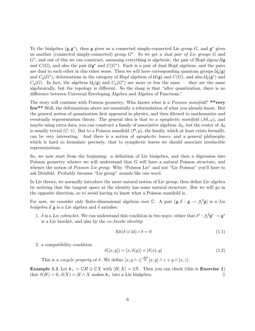
∧ng. Probably we shouldn’t have dualized earlier. So each row has differentcoefficients. But now let’s say we had a bialgebra structure. Then we also have vertical maps fromthe cohomology of g∗.

7

C g∗∧2g∗

∧3g∗ · · · M = C

g g⊗ g∗ g⊗∧2g∗ g⊗∧3g∗ · · · M = g

∧2g∧2g⊗ g∗

∧2g⊗∧2g∗∧2g⊗∧3g∗ · · · M =

∧2g

∧3g∧3g⊗ g∗

∧3g⊗∧2g∗∧3g⊗∧3g∗ · · · M =

∧3g

......

......

dg dg dg dg

dg dg dg dg

dg dg dg dg

dg dg dg dg

dg∗

dg∗

dg∗

dg∗

dg∗

dg∗

dg∗

dg∗

dg∗

dg∗

dg∗

dg∗

dg∗

dg∗

dg∗

dg∗

Question from the audience: So we have a bunch of Chevalley complexes, and if g∗ also has aLie algebra structure, then this is a complex of complexes? Answer: Well, the map [, ] :

∧2g→ g

gives the differential dg, and Jacobi gives d2 = 0. If we also have a cobracket with coJacobi, thenwe get the vertical maps dg∗ . It’s a neat way of saying the bracket satisfies Jacobi: it’s equivalentto saying that d2 = 0. And what’s the meaning of the compatibility? Well, we have a bicomplex,and the key question is when two differentials commute? Well, they never actually commute; whendo they anticommute? I.e. when is dgdg∗ + dg∗dg = 0? The answer is that this happens exactly ifδ dual to the cobracket gives a Lie bialgebra structure for g.

So this is the algebraical notion of a Lie bialgebra. Any questions? So this finishes the Lie bialgebradiscussion, and next time we will have examples and the definition of Poisson structure.

Question from the audience: So δ gives the Lie algebra structure on g∗? Answer: Yes. Itmust both be a cobracket, and also be compatible.

Next time, we will see the following: If g is a Lie algebra, it’s a well-known fact that g∗ is a Poissonmanifold. But in fact we will get a non-linear version of this on G, and many notions like theadjoint and coadjoint actions will all have nonlinear counterparts.


2.1 Poisson algebras

We continue with the Lie bialgebras and Poisson Lie groups. Last time we gave the definitionof a Lie bialgebra. We explained that to g a Lie algebra we associate the Chevalley complexC•(g) ∼= (

∧•g)∗ with differential dg. If we have a Lie bialgebra, we can construct C•(g⊕ g∗) with

8

two differentials dg and dg∗ , which anti-commute. But this doesn’t explain the terminology: inwhat sense is δ : g→ ∧2g a 1-cocycle? Well, δ gives a map

∧•g→ ∧2g, and δ gives a 1-cocycle inthe complex C•(g;

∧2g).

But these notions make more sense within the language of Poisson Lie groups. We begin with thedefinition of a Poisson algebra: this is a pair (A, , ) such that

• A is a commutative algebra. **unital?**

• The vector space A with , : A⊗2 → A is a Lie algebra.

• , is a biderivation: a, bc = a, bc+ ba, c.

So it is a mixture of Lie algebra and commutative algebra.

There are several reasons why this structure is very natural.

Example 2.1 Consider a family of associative multiplications ∗h : A⊗2 → A such that

• a ∗0 b = ab is commutatiive.

• Let’s assume that the multiplication is given by an analytic function in h: a ∗h b = ab +hm1(a, b) + h2m2(a, b) +O(h3) as h→ 0. Of course, to say this precisely we must introducesome topology on A.

Proposition 2.1 a, b def= m1(a, b)−m1(b, a) is a Poisson structure on a commutative algebra A.

This is probably the reason Poisson algebra is so important: they describe the infinitesimal jets ofdeformations of commutative algebra.

Proof: It’s a very nice and very easy Exercise 4. All you have to check is that the Jacobi identityon the commutator induces the Jacobi on , , and then you have to check the Leibniz rule.

(Again, homeworks mostly will not be graded, but eventually NR will give homework that isgraded. Question from the audience: Will there be pdfs with the homework? Answer: Yes,the handwritten notes are already there — don’t skip lecture — and Theo is typing the notes.)

Since this is a deformation, it is in a sense “quantum”, and it is in this sense that Quantum Groupsare quantum. ♦

Example 2.2 A Poisson manifold is a pair (M,p) where p ∈ Γ(∧2TM). We let M be a manifold

(C∞, affine algebraic variety, etc.; and whatever M is, we take the appropriate type of section p).So this p is a bivector field, and in local coordinates p(x) =

∑ij p

ij ∂∂xi∧ ∂∂xj

. Any time we chooselocal coordinates xi on M , then we let dxi be the corresponding basis of T ∗xM and ∂

∂xithe basis

in TxM . Then we define f, g def= 〈p, df ∧ dg〉 =∑ij p

ij(x) ∂f∂xi∧ ∂g∂xj

, and we demand that , is aPoisson bracket on C(M) (the space of C∞ or polynomial or whatever functions). That , is abiderivation is trivial, since everything is a first-order operator. That it satisfies the Jacobi identityrequires p to satisfy a non-trivial condition. **I missed the equation it must satisfy.** ♦

9

Example 2.3 Let g be a Lie algebra, g∗ its dual vector space. Since these are vector spaces,we have a canonical isomorphism T ∗xg∗ ∼= g for each x ∈ g∗. **finite-dimensional** (If it issomething more complicated, you may have to make a choice of isomorphism.) Thus, for anyf ∈ C(g∗) and x ∈ g∗, then df(x) ∈ g. So if f, g ∈ C(g∗), we can define [f(x), g(x)], and we definethe Poisson bracket

f, g(x) def= 〈x, [df(x), dg(x)]〉 (2.1)

This is the Lie-Kirollov-Kostant bracket. It was discovered by Lie, and used to study the represen-tation of Lie algebras.

It’s probably more instructive to see this is local coordinates. Let ei be a basis in g, and xithe coresponding coordinate functions on g∗. Then

xi, xj =∑k

fkijxk (2.2)

where fkij are the structure constants: [ei, ej ] =∑k f

kijek. ♦

If (M1, p1) and (M2, p2) are Poisson manifolds, we can define their product as (M1×M2, p12) wherep12 is the sum of p1 and p2. More explicitly, T(x,y)(M1×M2) = TxM1⊕TyM2, so

∧2T(x,y)(M1×M2) =∧2TxM1 ⊕ TxM1 ⊗ TyM2 ⊕∧2TyM2, and we define p12(x, y) def= p1(x)⊕ 0⊕ p2(y).

Now, let’s assume M1,M2 are affine algebraic, so that C(M1×M2) = C(M1)⊗C(M2). Then

f1 ⊗ f2, g1 ⊗ g2 = f1, g1 ⊗ f2g2 + f1g1 ⊗ f2, g2 (2.3)

If A1, A2 is a pair of Poisson manifolds, we define their tensor product A1 ⊗C A2 to be the Poissonalgebra with the bracket defined by 2.3.

Question from the audience: Even if Mi are not algebraic, this still works for functions thatare a product. Answer: Yes, but you won’t get all functions.

If A1 and A2 are two Poisson algebra, then φ : A1 → A2 is a morphism of Poisson algebras ifφ(ab) = φ(a)φ(b) and φ(a, b) = φ(a), φ(b). We define a map φ : (P1, p1) → (P2, p2) to bea morphism of Poisson manifolds if ψ is a manifold map and the pullback ψ∗ is a morphism ofPoisson algebras.

So Poisson algebra is the Lie-algebraic enhancement of commutative algebra. We can ask what isthe analogue of representations. One can argue that the correct analogue is the very importantnotion in Poisson geometry called symplectic leaves

2.2 Symplectic leaves

Who knows the definition of a “symplectic manifold”? **Four or five hands.** A symplecticmanifold is a pair (M,ω) where M is a manifold (in your favorite category) and ω is a nondegenerateclosed 2-form. More precisely:

10

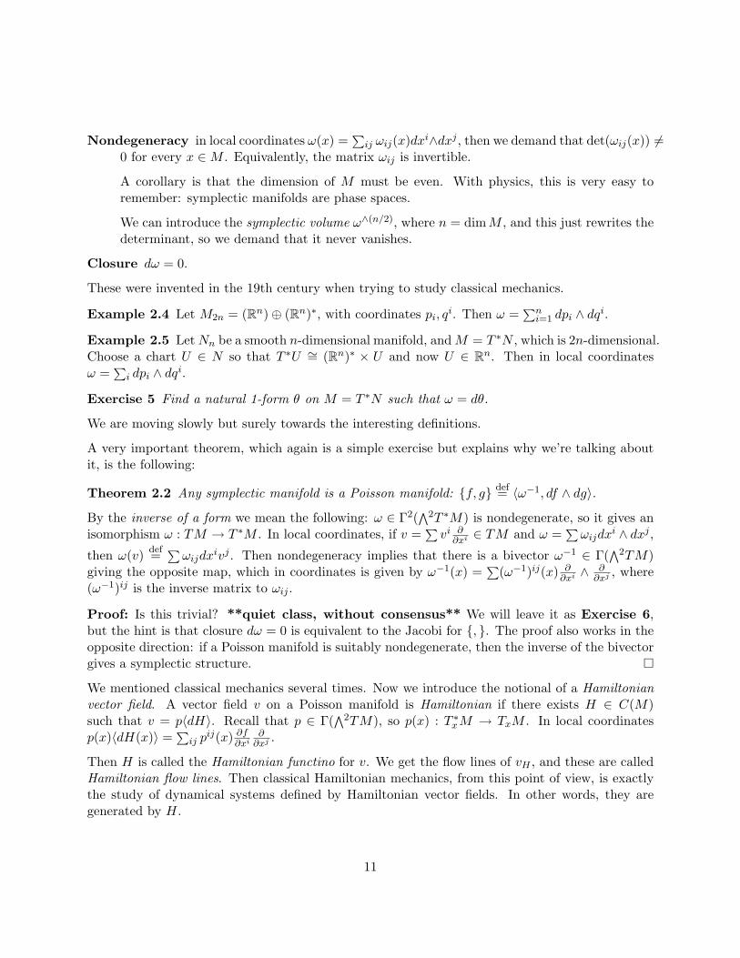
Nondegeneracy in local coordinates ω(x) =∑ij ωij(x)dxi∧dxj , then we demand that det(ωij(x)) 6=

0 for every x ∈M . Equivalently, the matrix ωij is invertible.

A corollary is that the dimension of M must be even. With physics, this is very easy toremember: symplectic manifolds are phase spaces.

We can introduce the symplectic volume ω∧(n/2), where n = dimM , and this just rewrites thedeterminant, so we demand that it never vanishes.

Closure dω = 0.

These were invented in the 19th century when trying to study classical mechanics.

Example 2.4 Let M2n = (Rn)⊕ (Rn)∗, with coordinates pi, qi. Then ω =∑ni=1 dpi ∧ dqi.

Example 2.5 LetNn be a smooth n-dimensional manifold, andM = T ∗N , which is 2n-dimensional.Choose a chart U ∈ N so that T ∗U ∼= (Rn)∗ × U and now U ∈ Rn. Then in local coordinatesω =

∑i dpi ∧ dqi.

Exercise 5 Find a natural 1-form θ on M = T ∗N such that ω = dθ.

We are moving slowly but surely towards the interesting definitions.

A very important theorem, which again is a simple exercise but explains why we’re talking aboutit, is the following:

Theorem 2.2 Any symplectic manifold is a Poisson manifold: f, g def= 〈ω−1, df ∧ dg〉.

By the inverse of a form we mean the following: ω ∈ Γ2(∧2T ∗M) is nondegenerate, so it gives an

isomorphism ω : TM → T ∗M . In local coordinates, if v =∑vi ∂∂xi∈ TM and ω =

∑ωijdx

i ∧ dxj ,then ω(v) def=

∑ωijdx

ivj . Then nondegeneracy implies that there is a bivector ω−1 ∈ Γ(∧2TM)

giving the opposite map, which in coordinates is given by ω−1(x) =∑

(ω−1)ij(x) ∂∂xi∧ ∂

∂xj, where

(ω−1)ij is the inverse matrix to ωij .

Proof: Is this trivial? **quiet class, without consensus** We will leave it as Exercise 6,but the hint is that closure dω = 0 is equivalent to the Jacobi for , . The proof also works in theopposite direction: if a Poisson manifold is suitably nondegenerate, then the inverse of the bivectorgives a symplectic structure.

We mentioned classical mechanics several times. Now we introduce the notional of a Hamiltonianvector field. A vector field v on a Poisson manifold is Hamiltonian if there exists H ∈ C(M)such that v = p〈dH〉. Recall that p ∈ Γ(

∧2TM), so p(x) : T ∗xM → TxM . In local coordinatesp(x)〈dH(x)〉 =

∑ij p

ij(x) ∂f∂xi

∂∂xj

.

Then H is called the Hamiltonian functino for v. We get the flow lines of vH , and these are calledHamiltonian flow lines. Then classical Hamiltonian mechanics, from this point of view, is exactlythe study of dynamical systems defined by Hamiltonian vector fields. In other words, they aregenerated by H.

11

Just one last word. A symplectic leaf on (P, p) through x is the space of points on the manifoldthat you can reach by piecewise Hamiltonian flow starting at x. We will see that symplectic leavesare identical to co-adjoint orbits of **missed**. Then we will study Poisson Lie groups, whichare an enhancement of the geometry of Lie groups, and then we will deform everything.

Question from the audience: It’s not obvious that you get a manifold doing this. Answer:Not at all. It is a theorem.


3.1 More symplectic geometry

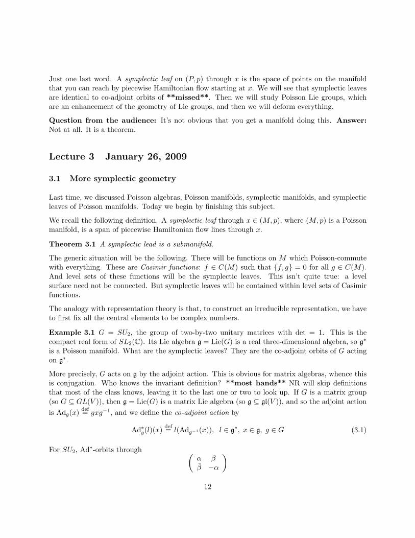
Last time, we discussed Poisson algebras, Poisson manifolds, symplectic manifolds, and symplecticleaves of Poisson manifolds. Today we begin by finishing this subject.

We recall the following definition. A symplectic leaf through x ∈ (M,p), where (M,p) is a Poissonmanifold, is a span of piecewise Hamiltonian flow lines through x.

Theorem 3.1 A symplectic lead is a submanifold.

The generic situation will be the following. There will be functions on M which Poisson-commutewith everything. These are Casimir functions: f ∈ C(M) such that f, g = 0 for all g ∈ C(M).And level sets of these functions will be the symplectic leaves. This isn’t quite true: a levelsurface need not be connected. But symplectic leaves will be contained within level sets of Casimirfunctions.

The analogy with representation theory is that, to construct an irreducible representation, we haveto first fix all the central elements to be complex numbers.

Example 3.1 G = SU2, the group of two-by-two unitary matrices with det = 1. This is thecompact real form of SL2(C). Its Lie algebra g = Lie(G) is a real three-dimensional algebra, so g∗

is a Poisson manifold. What are the symplectic leaves? They are the co-adjoint orbits of G actingon g∗.

More precisely, G acts on g by the adjoint action. This is obvious for matrix algebras, whence thisis conjugation. Who knows the invariant definition? **most hands** NR will skip definitionsthat most of the class knows, leaving it to the last one or two to look up. If G is a matrix group(so G ⊆ GL(V )), then g = Lie(G) is a matrix Lie algebra (so g ⊆ gl(V )), and so the adjoint actionis Adg(x) def= gxg−1, and we define the co-adjoint action by

Ad∗g(l)(x) def= l(Adg−1(x)), l ∈ g∗, x ∈ g, g ∈ G (3.1)

For SU2, Ad∗-orbits through Çα ββ −α

å12

where α ∈ R and β ∈ C. So this is a generic traceless Hermitian 2× 2 matrix. The co-adjoint orbitof this is

Ad∗G

Çα ββ −α

å=®u

Çα ββ −α

åu−1 : u ∈ SU2

´(3.2)

Question from the audience: That’s the adoint orbit. Answer: Well, g has a killing form〈x, y〉 = tr(xy), which is nondegenerate for su2, so g ∼= g∗ as an isomorphism of G-modules.

Now, what is the moduli space of conjugacy classes? Eigenvalues, module permutation. So

Ad∗G ∼=®Ç

λ 00 −λ

å´/

®Çλ 00 −λ

å∼Ç−λ 00 λ

å´(3.3)

Question from the audience: Hermitian or anti-Hermitian? Answer: Doesn’t matter, becauseyou can multiply by i.

Is this clear? The conjugation by the matrixÇ0 1−1 0

å∈ SU2

In any case, equation 3.3 gives just the ray R≥0.

Let’s let H have eigenvalues ±λ. Then tr(H2) = 2λ2 is an invariant of the conjugation. Let’s writein terms of the basis of Pauli matrices:Ç

1 00 −1

å,

Ç0 −ii 0

å,

Ç0 11 −0

å(3.4)

with coordinates x1, x2, x3, then tr(H2) = 2(x21 +x2

2 +x23). So the Ad∗-orbits are the spheres, which

are two-dimensional, and the special leaf at the origin. ♦

Question from the audience: Does this generalize to SUn? Answer: We will later prove, forevery Lie group:

Theorem 3.2 Sumplectic leaves of g∗ are Ad∗-orbits of G acting on g∗.

Example 3.2 What about SUn? We identify sun ∼= su∗n as vector spaces via 〈x, y〉 = tr(xy). Theco-adjoint orbits are classified by the set of eigenvalues, so this is Rn−1/Sn. It’s Rn−1 embeddedas the hyperplane ∑i λi = 0. These are the level surfaces of ci = tr(xi), i = 2, . . . , n. (Becausec1 = 0 on this hyperplane.) ♦

These two examples are of real Poisson manifolds. What if everything is complex-homolmorphic?

Example 3.3 G = SL2(C), g = sl2(C), which is non-canonically isomorphic to C3. But theKilling form gives a canonical isomorphism g∗ ∼= g = sl2(C). The theorem that symplectic leavesare Ad∗-orbits still holds, and we identify these with adjoint orbits. Let’s understand the orbit:

C

Ça bc −a

å=®g

Ça bc −a

åg−1 : g ∈ SL2(C)

´These come in various forms.

13

1. If the matrix is diagonalizable and non-zero, then the matrix is classified by its eigenvalues±λ. So the set of orbits through diagonalizable matrices is (C r 0)/Z2. Each orbit is2-dimensional over C.

2. If the matrix is not diagonalizable, it must have 0s on diagonal to be traceless. So, there’s

only one orbit, the one through x =Ç

0 10 0

å. What is it’s dimension? How do you compute

the dimension of an orbit? You subtract the dimension of the stabilizer. And the stabilizerof x is the unipotent matrices

exp(ax) =®Ç

1 a0 1

å´3. There is the 0-dimensional orbit through 0. ♦

You can do GLn at home.

Exercise 7 List all possible dimensions of conjugation orbits for sl3, and describe the set of suchorbits.

In the complex-analytic case, symplectic leaves are complex homomorphic symplectic manifolds,and are algebraic. You can treat them like the real manifolds you’re used to.

Exercise 8 Consider the group of triangular matricesÖa a1 b10 b c1

0 0 c

èAny questions?

3.2 Poisson Lie groups

You should specify a category in which you want to work, and then be consistent within thiscategory. For example, real smooth, affine algebraic, etc.

A pair (G, p) where G is a Lie group and p ∈ Γ(∧2TG) is a Poisson structure on G is a Poisson

Lie group if

1. Multiplication µ : G×G→ G is a Poisson map.

2. g 7→ g−1 is also a Poisson map.

Exercise 9 Check if g 7→ g−1 follows from the first condition. We will give the answer later.

How does this relate to Lie bialgebras? We consider the tangent space at the identity.

14

We have two special geometric structures. The multiplication, and the Poisson structure, andthese are compatible. Before we start further discussion, let’s say a few words about tangentbundles.

If G is a group, then the tangent bundle TG is trivial: TG ∼= g×G, and we will always in this coursechoose the trivialization by left-translation. I.e. `g : G → G is x 7→ gx. Then d`g : TG ∼→ TG.It takes ThG → TghG, and in particular d`h−1 : Th

∼→ TeG = g. So d` : TG ∼→ g × G by(ξ, h) 7→ (d`h−1(ξ), h).

So, the Poisson structure is a section p ∈ Γ(∧2TG), which consists of section maps G → ∧2TG,

but we can identify this with maps G→ ∧2g. So if x ∈ G, then p(x) ∈ ∧2g.

Exercise 10 p(0) = 0. **Feb 9: certainly this should be p(e) = 0?**

Corollary 3.2.1 dp(e) : TeG→∧2T0g; in other words this is a map g→ ∧2g.

We will choose this as our Lie bialgebra structure.


We pick up where we left off last time. We stated the definition of the tangent Lie bialgebra to aPoisson Lie group. Recall, a Poisson Lie group is a Lie group G along with a compatible Poissonstructure p. We take g = Lie(G) = TeG, and we want to use the Poisson structure p to constructa bialgebra structure on g. As we did last time, we trivialize TG ∼= g×G by left translations, andthen p ∈ Γ(

∧2TG) — which is a section map, i.e. a map p : G → ∧2TG such that the naturalprojection π :

∧2TG → G composes to that π p = idG — after trivialization, p becomes a mapp : G → ∧2g. So a Poisson structure on a Lie group is a map p : G → ∧2g with the followingcompatibility condition (equivalent to the earlier condition):

p(xy) = (Adx⊗Ady)p(y) + p(x) (4.1)

Exercise 11 Verify this.

**I think the equation should read p(xy) = (Adx⊗Adx)p(y) + p(x). The RHS of equa-tion 4.1 is not obviously antisymmetric, and I don’t believe it it internally consis-tent.**

**Actually, the formula is totally wrong. If you use left-translations to trivialize, theformula should read:

pl(xy) = pl(y) + (Ady−1 ⊗Ady−1)pl(x) (4.2)

and if you use right-translations, then you get

pr(xy) = pr(x) + (Adx⊗Adx)pr(y) (4.3)

15

where each of pl and pr are functions G→ ∧2g. Very precisely, pl(g) = (dlg−1 ⊗ dlg−1)p(g)and pr(g) = (drg−1 ⊗ drg−1)p(g), where lg and rg are the left- and right-translations of Gby g ∈ G.**

Another name for this is to say that p is a 1-cocycle in the standard cohomology complex for Gwith coefficients in

∧2g.

In any case, dp : TG→ T (∧2g) ∼=

∧2Tg. At the identity e ∈ G, equation 4.1 becomes

p(ee) = p(e) + p(e) (4.4)

and hence p(e) = 0. So dp(e) is a map TeG → Tp(e)(∧2g) = T0(

∧2g) =∧2g since g is a vector

space. So we define δ = dp(e) : g→ ∧2g.

Theorem 4.1 (g, δ) is a Lie bialgebra.

Proof: 1. The Jacobi identity: Something must satisfy Jacobi, since p did; we need to checkthat the dual map [, ]g∗

def= δ∗ : g∗ ∧ g∗ → g∗ is this something. Well, g∗ is the space oflinear functions on g. How do we get these? Let’s fix f1, f2 ∈ C(G), and their differentialsdf1(e), df2(e) ∈ T ∗eG = g∗. Let’s denote dfi(e) by ξi. Then, letting X ∈ g, we have

[ξ1, ξ2]g∗(X) = 〈dp(e)(X), df1(e) ∧ df2(e)〉 (4.5)

=d

dt

∣∣∣∣t=0f1, f2(etX) (4.6)

Here , is our Poisson bracket on G, and etX is the exponential map g→ G.

Exercise 12 Prove equation 4.6. Try to do it invariantly, but if you cannot, do it in localcoordinates. On the one hand, local coordinates are very messy, and on the other hand, bymaking your hands dirty, you can really see what you’re doing.

On the other hand, f1, f2(e) = 0. The Jacobi for , says that f1, f2, f3(etX)+cyclic =0. So take d2

dt2

îf1, f2, f3(etX) + cyclic

ó∣∣∣t=0

and conclue the Jacobi for [, ]g∗ .

2. The cocycle property: The two-line proof says “p is a 1-cocycle for G, and so automaticallyinduces a 1-cocycle for TG.” We proceed to prove this:

We apply equation 4.1 twice, on a commutator:

p(y−1zy) =ÄAdy−1z ⊗Ady−1z

äp(y) +

ÄAdy−1 ⊗Ady−1

äp(z) + p(y−1) (4.7)

All proofs in Lie algebras/groups feel like the first part. We apply equation 4.7 to z = etX ,as t→ 0. The order-1 elements in t give

δÄAdy−1(X)

ä=ÄAdy−1 ⊗Ady−1

ä[X, p(y)] +

ÄAdy−1 ⊗Ady−1

äδ(X) (4.8)

We’ve used that δ = dp(e). Now we take y = etY and differentiate in t at t = 0:

δ ([X,Y ]) = [X, δ(Y )]− [Y, δ(X)] (4.9)

Here we used that [X,Y ∧ Z] = [X,Y ] ∧ Z + Y ∧ [X,Z].

16

Did we ever supply examples of Poisson Lie groups?

Example 4.1 Suppose there is an element r ∈ g⊗ g satisfying the classical Yang-Baxter equation:

[r12, r13] + [r12, r23] + [r13, r23] = 0 (4.10)

This equation lives in U(g)⊗3. r12def= r ⊗ 1, where we have embedded g ⊗ g → Ug ⊗ Ug, and

r23def= 1⊗ r. We leave it as an exercise to guess r13.

Well, r =∑ij r

ijei ⊗ ej , where ei is a basis of g. So r has (dim g)2 variables, and equation 4.10 is(dim g)3 equations, so it’s entirely nonobvious why there would be any solutions to this equation.But, indeed, the “Drinfeld douple construction” says there are some.

For example, if g = sl2, then r = 14H ⊗ H + X ⊗ Y , where we have the basis X,Y,H with

[H,X] = 2X, [H,Y ] = −2Y , and [X,Y ] = H. We will later see scientifically why this works.

We assume we have such an r. We define δr(x) def= [r, x⊗1+1⊗x]. This would be a natural candidateif it were obvious that the image is in the exterior square. Question from the audience: Whatis this commutator, and above? Answer: For example, [A ⊗ B,C ⊗ 1] def= [A,C] ⊗ B. **So weextend [, ] to tensors by the Leibniz rule?**

Proposition 4.2 δr(x) ∈ ∧2g ⊆ g⊗ g

Proof: Exercise 13. Compare with notes when they appear online.

Theorem 4.3 (g, δr) is a Lie bialgebra.

It has a special name: Drinfeld calls it quasitriangular, because there is a triangle in the Braidrelation.

Now, let G be a Lie group such that g = Lie(G). Define pr(x) def= (Adx⊗Adx) (r)− r, which givesa map p : G→ ∧2g.

Theorem 4.4 This is a Poisson Lie structure on G such that (g, δr) is the tangent Lie bialgebra.

See, it’s obvious that pr is a 1-cocycle for G with coefficients in∧2g, but is’t also a 1-coboundary.

We don’t want to go into group cohomology, but for example Fuchs’ book Cohomologies of Infinite-Dimensional Lie Algebras, or any textbook with cohomology of groups and Lie groups, will explainthis.

Question from the audience: Does it go the other way? If I have a 1-coboundary... Answer:No, a coboundary will not necessarily satisfy the Yang-Baxter equation. ♦

4.1 Braid groups

Let us see why we used the Yang-Baxter equation rather than something else. Let

Xndef=¶

(x1, . . . , xn) : xi 6= xj , xi ∈ R2©.

17

Then Sn acts on Xn, and we define Xndef= Xn/Sn. The braid group is the fundamental group of

this space Bndef= π1(Xn). So what should happen is that you start with points, and they move

around and end up where they started, up to a permutation. **we let time be the downwarddirection, and draw the worldlines of the particles**

The more standard drawing: you pick the points on line, and project to the plane, with overcrossingsand undercrossings. **I don’t guarantee that this is the same picture as above.**

•1

•2

•3

•4

•1

•2

•3

•4

In any case, in π1, we should take paths, but only up to isotopy. We have two Reidemeister moves**and their mirror versions**:

= =

Question from the audience: What about Reidemeister 1? Answer: They are braids: pathsonly go down.

We define si, for i = 1, . . . , n− 1, to be the braid that is trivial on all strands except for i and i+ 1,and there is a single crossing between i and i+ 1.

Theorem 4.5 The braid group has presentation:

Bn ∼= 〈si, i = 1, . . . , n− 1 s.t. sisj = sjsi if |i− j| > 1, and sisi+1si = si+1sisi+1〉 (4.11)

18

Well, any group has many representations. The relations are very local, so it’s natural to look forrepresentations of Bn on V ⊗n, where

si = 1⊗ · · · ⊗ S ⊗ · · · ⊗ 1

where S ∈ Aut(V ⊗ V ), and it’s acting in the i and i+ 1 spots.

Proposition 4.6 π : Bn → Aut(V ⊗n) is a representation if (S ⊗ 1)(1⊗ S)(S ⊗ 1) = (1⊗ S)(S ⊗1)(1⊗ S).

The whole reason for developing quantum groups, Poisson Lie groups, etc., was to study theseequations. Except that this didn’t evolve in Topology, but rather in Statistical Mechanics.


The handwritten lecture notes are now online. These notes are also available, usually a few hoursafter class — they go up as soon as Theo has a chance to say “upload”.

5.1 More on the Braid Group

Last time, we stopped at the Yang-Baxter equation. We have the braid group

Bndef= 〈si s.t. sisj = sjsi if |i− j| ≥ 2, and sisi+1si = si+1sisi+1〉 (5.1)

There are tensor-product representations π : Bn → Aut(V ⊗n) where si 7→ 1 ⊗ · · · ⊗ S ⊗ · · · ⊗ 1,where S ∈ Aut(V ⊗V ) is acting in the i, i+1th spots. This satisfies the first condition, and satisfiesthe second iff S satisfies the Yang-Baxter equation:

(S ⊗ 1)(1⊗ S)(S ⊗ 1) = (1⊗ S)(S ⊗ 1)(1⊗ S) (5.2)

This is a hugely over-determined system: there are (dimV )6 equations for (dimV )4 unknowns.

Example 5.1 S = P : x⊗y 7→ y⊗x. This is a boring solution: the map factors through Bn → Sn,hence ignores under- versus over-crossings. ♦

We should try to construct a family S(h) = P (1 + hr +O(h2)) of solutions.

Proposition 5.1 S satisfies the Yang-Baxter equation only if r satisfies:

[r12, r13] + [r12, r23] + [r13, r23] = 0. (5.3)

Proof: Expand equation 5.2 to order h2; the order-h stuff cancels.

This is an equation that involves only commutators. We should consider it as an equation ingl(V )⊗3 for r ∈ gl(V )⊗2.

Recall from 261A:

19

Theorem 5.2 (Ado) Any finite-dimensional Lie algebra is a subalgebra of gl(V ) for some finite-dimensional V .

So finding solutions to equation 5.3 is the same as classifying all solutions in g⊗3 in arbitrary finite-dimensional g a Lie algebra. This is why we are interested in Lie bialgebras if we are interested inknot theory.

So the philosophy is: we want to construct S satisfying equation 5.2, and we have one solution; weshould perturb that solution in the direction r. So the general questions are

1. How to construct solutions to equation 5.3? I.e. how to construct Lie bialgebras.

2. “Quantization”: How to construct S for a given r? The answer is in the construction of aspecial class of quantum groups.

This second question is the historical motivation for our subject. Similarly, the main motivationfor Lie was to study the solutions of differential equations. This history is almost completelyforgotten.

We gave an example last time of a solution to equation 5.3 for g = sl2.

Let g be a Lie algebra. Suppose that r ∈ g ⊗ g satisfies equation 5.3. We consider r± : g∗ → g

given by

r+(l) def= (l ⊗ id)r (5.4)

r−(l) def= −(id⊗ l)r (5.5)

The minus sign, we will see, is for later convenience.

Lemma 5.3 Im(r±) def= g± ⊆ g are Lie subalgebras of g.

Proof: We just look in g ⊗ g ⊗ g. By the definition, r ∈ g− ⊗ g+ ⊆ g⊗2: if r =∑i ri ⊗ ri, then

r+(l) =∑i l(ri)ri and r−(l) = −∑i r

il(ri), and by definition ri ∈ g+ span g+ and ri ∈ g−span g−. **there is some unhappiness** This is general linear algebra. If x ∈ V ∗ ⊗W , thenwe get x+ : V →W and x− : W ∗ → V ∗.

Example 5.2 Let’s do a small example. g = C3 with the basis H,X, Y , and g∗ = C3 with thedual bases H∨, X∨, Y ∨. We choose r = 1

4H ⊗H +X ⊗ Y . Then r+(l) = l(H)H4 + l(X)Y . Sincel can vary over all of g∗, then Im(r+) = CH ⊕ CY . ♦

Question from the audience: What about the following:

Example 5.3 r = H⊗X+X⊗X = (H+X)⊗X. Then Im(r+) = CX, and Im(r−) = C(H+X),not the span CH + CX. ♦

Then we get different answers depending on how we write it. Do we need it to span? Answer:Ah, we were sloppy. By definition, g+ =

∑i l(ri)ri s.t. l ∈ g∗

. This is contained in the span of

the ri, but it’s not equal.

20

Ok, so the earlier claim was wrong, but it’s certainly the case that r ∈ g− ⊗ g+ ⊆ g⊗2. Questionfrom the audience: Ok, but now I don’t know why r ∈ g− ⊗ g+? Answer: We will answer thisnext time, to save ourselves from thinking at the board. Maybe we have to impose more: in therelevant examples, it is true, and we thought it was obvious in all cases, but we may have to havemore conditions. We will assume that r ∈ g− ⊗ g+.

We continue with the proof. We look at equation 5.3:

[r12, r13]3

[g−,g−]⊗g+⊗g+

+ [r12, r23]

3

g−⊗[g+,g−]⊗g+

+ [r13, r23]

3

g−⊗g−⊗[g+,g+]

= 0 (5.6)

So this is only possible if [g−, g−] ⊆ g−, [g+, g−] ⊆ g+ + g−, and [g+, g+] ∈ g+.

We will clarify this next time.

We can also see, form the above proof, that there is a subspace gdef= g+ + g− ⊆ g. So we have

another statement:

Lemma 5.4 g is a Lie subalgebra of g.

And then we consider t = r+σ(r), where σ is the permutation x⊗ y 7→ y⊗x. So t is symmetrized:t ∈ S2(g). But since the only elements involved in the definition, in fact t ∈ S2g.

Proposition 5.5 t ∈ S2(g)g — i.e. t is in the g-invariant part.

Proof: We act by (σ ⊗ id) on equation 5.3, which just switches the indices 1 and 2, and add. Sothe last term cancels:

σ ⊗ id : [r21, r13] + [r21, r23] + [r23, r13] = 0 (5.7)[r12, r13] + [r12, r23] + [r13, r23] = 0 (5.8)

+ : [r12 + r21, r13 + r23] = 0 (5.9)

But the first is t12. So [t⊗ 1, ri ⊗ 1⊗ ri + 1⊗ ri ⊗ ri] = 0. This is equivalent to saying that for alll, [t,

∑i(ri ⊗ 1 + 1⊗ ri)l(ri)] = 0. And similarly for g+.

Theorem 5.6 (g, δr(x) def= [r, x⊗ 1 + 1⊗ x]) is a Lie bialgebra.

Proof: We did this last time. We have to prove two prove two facts.

0. σ δr(x) = [σ(r), x⊗ 1 + 1⊗ x] = [t− r, x⊗ 1 + 1⊗ x] = 0− δ(x), so δr lands in the exteriorsquare.

1. cocycle: δr[x, y] = [r, [x, y] ⊗ 1 + 1 ⊗ [x, y]] = [x, δry] + [deltarx, y] by Jacobi for g. Recall,[x, y ∧ z] def= [x, y] ∧ z + y ∧ [x, z].

2. co-Jacobi: AltÄ(δr ⊗ id) δr

ä= 0. This is equivalent to equation 5.3.

21

We say that a Lie bialgebra g is factorizable if there is a nondegenerate t ∈ S2(g) ⊆ g ⊗ g (i.e.t : g∗ → g is a linear isomorphism), and such that for any x ∈ g, there are unique x± ∈ g± suchthat x = x+ + x−.

Example 5.4 Linear Gaussian factoraizationÇa bc d

å=Ça+ b0 d+

å+Ça− 0c d−

å. ♦

**I wouldn’t put a lot of faith, gentle reader, in this definition; I may have misheardit.**


Recall from last time, we have r ∈ g⊗ g satisfying

[r12, r13] + [r12, r23] + [r13, r23] = 0 (6.1)

Then we define r+(l) = (id⊗ l)r, and r−(l) = −(l ⊗ id)r.

Proposition 6.1 1. r ∈ g+ ⊗ g−

2. g+, g−, and gdef= g+ + g− are Lie subalgebras in g.

Proof: See notes.

Lemma 6.2 Let t = r+σ(r) ∈ S2(g) ⊆ g⊗ g. Then t ∈ §2(g)g, i.e. [t, x⊗ 1 + 1⊗x] = 0 for x ∈ g.

We assume that everything is in U(g), and the bracket is a commutator **extended to tensorproducts by the Leibniz rule**.

So, define δr : g → g ∧ g ⊆ g⊗2 by δr(x) = [r, x ⊗ 1 + 1 ⊗ x]. It’s easy to check that this has thecorrect codomain, using the pervious lemma.

Proposition 6.3 (g, δr) is a Lie bialgebra.

Proof: 1. δr([x, y] = [r, [x, y]⊗ 1 + 1⊗ [x, y]] = [x, δr(r)] + [δr(x), y] by the Jacobi identity.

2. Jacobi for δ∗r follows from the classical Yang-Baxter equation.

From now on, we will forget about tildes. The pair (g, δr) is a quasitriangular Lie bialgebra assum-ing

• r + σ(r) ∈ S2(g)g

• Classical Yang-Baxter equation for r.

We say that (g, δr) is factorizable if t ∈ g ⊗ g defines a nondegenerate bilinear form on g∗ (where〈l,m〉t

def= (l ⊗m)(t)). If (g, δr) is factorizable, then we have x = x+ + x− uniquely, where x± ∈Im(r±) and x± = r±(l) for some l ∈ g∗.

22

Any questions? It is better to move to semi-meaningless discussion — semi-meaningless on NR’spart, because we asserted something wrong — than to leave something out.

Example 6.1 Let g = sl2(C) with standard basis H,X, Y (H is the Cartan, X,Y are the rootelements): [H,X] = 2X, [H,Y ] = −2Y , [X,Y ] = H. Then r = 1

4H ⊗H + X ⊗ Y is a solution toequation 6.1, and t = r + σ(r) = 1

2H ⊗H + X ⊗ Y + Y ⊗X ∈ S2(sl2)sl2 . This gives the Casimir

element c def= H2

2 + XY + Y X ∈ Usl2. I.e. c ∈ Z(Usl2), which is in fact freely generated by c:Z(Usl2) = C[c].

Then t = 12∆(c)− c⊗ 1− 1⊗ c, where ∆ : Usl2 → Usl⊗2

2 is a coassociative algebra homomorphismsuch that ∆x = x ⊗ 1 + 1 ⊗ x for x ∈ sl2 ⊆ Usl2. Anyway, so ∆ is a homomorphism, and sincec ∈ Z(Usl2), we have [t,∆x] = 0 for each x ∈ sl2. t is called a mixed Casimir, and r then is not sostrange, being like half of the mixed Casimir.

Let’s look at sl∗2. We have our special basis of sl2, so let’s choose the dual basis: sl∗2 = CH∨ ⊕CX∨ ⊕ CY ∨, where we define K∨ (for K = H,X, Y ) to be the linear functional that is 1 onK and 0 on the other two basis elements. Then r+(l) = H

4 l(H) + X l(Y ), where l ∈ sl∗2, soIm(r+) = CH ⊕ CX = b+ ⊆ sl2 and Im(r−) = b−. We will see counterparts of this for all simpleLie algebras.

What about the kernels? ker(r+) = CX∨ and ker(r−) = CY ∨, so ker(r+)⊥, which is the collectionof all elements of sl2 on which X∨ vanishes, is just b−. See, the definition we were trying to selllast time and the correct definition from today coincide.

A little claim: (sl2, δr) is a factorizable Lie bialgebra: t is given by the Killing form, which isnondegenerate for sl2(C).

Question from the audience: Can you say a bit more? It seems we don’t have unique factor-ization. Answer: We’re coming to it.

The cobracket δr : a 7→ [r, a⊗ 1 + 1⊗ a]. In particular:

δr(H) = [r,H ⊗ 1 + 1⊗H] = 0

δr(X) =14

[H,X]⊗H +14H ⊗ [H,X] +X ⊗ [Y,X]

=12X ⊗H +

12H ⊗X −X ⊗H

=12H ∧X

δr(Y ) =12H ∧ Y

**check the signs** ♦

The factorization: We have t = r + σ(r) ∈ S2(g)g, defining a nondegenerate bilinear form on g∗,

23

and so the linear map t : g∗ → g defined by l 7→ (id⊗ l)(t) is a linear isomorphism. Now,

t(l) = (id⊗ l)(r) + (id⊗ l)(σ(r))= (id⊗ l)(r) + (l ⊗ id)(r)= r+(l)− r−(l)

Thus we had a sign error earlier with the definition of the factorization.

Proposition 6.4 Because t is a linear isomorphism, any x ∈ g has a unique presentation asx = x+ − x− where x± = r±(l) for some l.

Now we check how this works for sl2: x = αH + βX + γY , then x+ = α2H + βX and x− =

−α2H − γY .

We finish with the Lie algebra structure on sl∗2. By definition:

[H∨, X∨](a) = H∨ ∧X∨(δr(a)) (6.2)

Well, δr(a) had better be in CH ∧X, otherwise equation 6.2 is 0. So equation 6.2 is non-zero onlyif a = cX.

[H∨, X∨](X) = (H∨ ∧X∨)Å1

2H ∧X

ã(6.3)

=12〈H∨ ∧X∨, H ∧X〉 (6.4)

=12〈H∨ ⊗X∨ −X∨ ⊗X∨, H ⊗X −X ⊗H〉 (6.5)

=12

(2) (6.6)

= 1 (6.7)

So [H∨, X∨] = X∨ and [H∨, Y ∨] = Y ∨, and [X∨, Y ∨] = 0. So this is a very different Lie algebra:it’s not semisimple. This is the standard Lie bialgebra structure on sl2. There is a classification ofLie bialgebra structures, and for sl2 there is only one factorizable one.

Question from the audience: So there can be bialgebras that don’t come from an r-matrix?Answer: Yes. Question from the audience: Then the notion of factorizability doesn’t makesense? Answer: That’s correct.

We say that g− ⊆ g2 is a Lie sub-bialgebra if δ(g1) ⊆ g1 ∧ g1.

Example 6.2 b± ⊆ (sl2, δr) is a Lie sub-bialgebra, because δH = 0 and δX = 12H ∧X, etc. These

are not quasitriangular. ♦

Exercise 14 Formulate the notion of Lie bialgebra ideal. You must decide on the correct conditionon the cobracket.

Next time we will begin the discussion of groups. For example, there are three real forms of SL2(C):SL2(R), U(2), and the less-well-known one U(1, 1).

24

Lecture 7 February 4, 2009

Recall, if G is a Lie group, we can trivialize TG by right-translation: dR : TG ∼= g × G, wheredRh−1 : ThG

∼→ TeG ∼= g. Then pr(x) = −Adx⊗Adx(r) + r ∈ Γ(∧2TG) ∼= C(G → ∧2g) is

a Poisson Lie structure on G if the tangent Lie bialgebra (g, δr) has δr = dp(e) : g → ∧2g,δr(x) = [e, x⊗ 1 + 1⊗ x].

Then let’s compute the Poisson bracket on SL2(C). We have coordinates:

SL2(C) =®Ç

a bc d

ås.t. ad− bc = 1

´(7.1)

And so C(SL2) = C[a, b, c, d]/ ∼ is a commutative hops algebra. We compute the Poisson pracketsbetween a, b, c, d: ∆a = a⊗a+b⊗x, ∆b = a⊗b+b⊗d, etc., from the multiplication of matrices.

Then the Poisson bracket is f1, f2(g) = 〈p(q), df1(g) ∧ df2(g)〉, and

p(g) =∑α,β

pαβ(g)eα ⊗ eβ (7.2)

〈eα, df(g)〉 =d

dtf(eteαg)

∣∣∣t=0

(7.3)

=∑ij

d

dt(eteαg)ij

∣∣∣t=0

∂f

∂gij(g) (7.4)

=∑ij

(eαg)ij∂f

∂gij(7.5)

To define the last line “eαg”, we use the fact that SL2 is a matrix group. We will always assumethat all our groups are matrix groups, whence the exponential map really is matrix exponential.We did this with right-trivialization. If we had used left trivialization, then the formula would haveincluded f(geteα).

Hence:

f1, f2(g) = 〈p(q), df1(g) ∧ df2(g)〉 = 2∑

α,β,i,j,k,l

pαβ(g)(eαg)ij(eβg)kl∂f1

gij

∂f2

gkl(7.6)

The 2 comes because from the wedge bracket, whence we should have subtracted ij ↔ kl, buteverything is skew symmetric.

Well,

pαβ(g)eαg ⊗ eβg = p(g)(g ⊗ g) (7.7)

=Ä−(g ⊗ g)(r)(g−1 ⊗ g−1) + r

ä(g ⊗ g) (7.8)

= −(g ⊗ g)r + r(g ⊗ g) (7.9)

25

and so, up to an unfortunate factor of 2, we have

f1, f2 = 2∑ijkl

[r, g ⊗ g]ij,kl∂f1

∂gij

∂f2

∂gkl(7.10)

Let us find gij , gkl in SL2; and we will organize this as a matrix in End(V ⊗2), where V = C2.Using the formula, the derivatives are 1 (really δ functions), and so

gij , gkl = 2[r, g ⊗ g]ij,kl (7.11)

and so, assuming that our group is a matrix group, so that the formula makes sense:

g⊗g = 2[rV , g ⊗ g] (7.12)

Everywhere r should be rV , which is the image of r ∈ g⊗ g in End(V )⊗2.

**NR used the symbol ·⊗· for the matrix of brackets. I couldn’t tell quite whatsymbol he was using, and replaced ⊗ with either ⊗ or ,. So some of the formulas fromtoday are not what was on the board.**

Ok, so we introduce a particularly useful notation: g1def= g⊗1, g2 = 1⊗g, and r12 = r ∈ End(V )⊗2.

**NR writes “I” for the identity matrix, but says “one”.** Then r12 ∈ End(V )⊗n isr ⊗ 1⊗ · · · ⊗ 1 where the 1s are in positions 3, . . . , n.

Ok, so g1, g2 = 2[r, g1g2] = 2[r12, g1g2]. Eventually, we may kill this 2. We can do this: we canrescale the Poisson bracket. The problem is the pairing of elements of the wedge product. **arethose the same 1 and 2 on either side of the equation?**

Ok, so let’s prove the Jacobi identity:

g1, g2, g3 = g1, [r23, g2g3] (7.13)= [r23, g1, g2g3] (7.14)

g1, g2g3 = g1, g2g3 + g2g1, g3 (7.15)= [r12, g1g2]g3 + g2[r13, g1g3] (7.16)

**I don’t understand these indices.**

One more computation. Let rV = 14H ⊗H +X ⊗ Y , considered as a matrix in End(C2)⊗2, where

H,X, Y is the standard basis of sl2. Let’s choose a basis e1, e2 of C2, and so eij = ei⊗ ej is a basis

of C4 = C2 ⊗ C2. Then if g =Ça bc d

å, we have

g ⊗ g =

Öaa ab ba bbac ad bc bd

ca . . .

è, rV =

á1/4 0 0 00 −1/4 1 00 0 −1/4 00 0 0 1/4

ë(7.17)

26

Hence,

[rV , g ⊗ g] =

á0 1

2ab . .12ac bd 0 .

−12ac 0 . .. . 1

2cd .

ë(7.18)

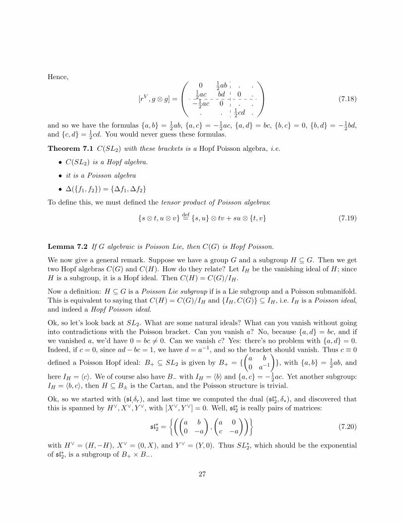
and so we have the formulas a, b = 12ab, a, c = −1

2ac, a, d = bc, b, c = 0, b, d = −12bd,

and c, d = 12cd. You would never guess these formulas.

Theorem 7.1 C(SL2) with these brackets is a Hopf Poisson algebra, i.e.

• C(SL2) is a Hopf algebra.

• it is a Poisson algebra

• ∆(f1, f2) = ∆f1,∆f2

To define this, we must defined the tensor product of Poisson algebras:

s⊗ t, u⊗ v def= s, u ⊗ tv + su⊗ t, v (7.19)

Lemma 7.2 If G algebraic is Poisson Lie, then C(G) is Hopf Poisson.

We now give a general remark. Suppose we have a group G and a subgroup H ⊆ G. Then we gettwo Hopf algebras C(G) and C(H). How do they relate? Let IH be the vanishing ideal of H; sinceH is a subgroup, it is a Hopf ideal. Then C(H) = C(G)/IH .

Now a definition: H ⊆ G is a Poisson Lie subgroup if is a Lie subgroup and a Poisson submanifold.This is equivalent to saying that C(H) = C(G)/IH and IH , C(G) ⊆ IH , i.e. IH is a Poisson ideal,and indeed a Hopf Poisson ideal.

Ok, so let’s look back at SL2. What are some natural ideals? What can you vanish without goinginto contradictions with the Poisson bracket. Can you vanish a? No, because a, d = bc, and ifwe vanished a, we’d have 0 = bc 6= 0. Can we vanish c? Yes: there’s no problem with a, d = 0.Indeed, if c = 0, since ad− bc = 1, we have d = a−1, and so the bracket should vanish. Thus c ≡ 0

defined a Poisson Hopf ideal: B+ ⊆ SL2 is given by B+ = Ça b0 a−1

å, with a, b = 1

2ab, and

here IH = 〈c〉. We of course also have B− with IH = 〈b〉 and a, c = −12ac. Yet another subgroup:

IH = 〈b, c〉, then H ⊆ B± is the Cartan, and the Poisson structure is trivial.

Ok, so we started with (sl,δr), and last time we computed the dual (sl∗2, δ∗), and discovered thatthis is spanned by H∨, X∨, Y ∨, with [X∨, Y ∨] = 0. Well, sl∗2 is really pairs of matrices:

sl∗2 =®ÇÇ

a b0 −a

å,

Ça 0c −a

åå´(7.20)

with H∨ = (H,−H), X∨ = (0, X), and Y ∨ = (Y, 0). Thus SL∗2, which should be the exponentialof sl∗2, is a subgroup of B+ ×B−.

27

Question from the audience: How do those pairs pair with the matrices in sl2? Answer:**missed**

Next time we will repeat this, and then finish with SL∗2, and then explain the Double construc-tion and see how to obtain Poisson structures on all complex simple Lie groups, and bialgebrastructures on complex simple Lie algebras, and also the story of symplectic leaves, which willgive us a wonderful excuse to study the geometry of Lie groups. And after this we will quantizeeverything.


Today we continue with the basic example of SL2. We now try to understand the dual Poisson Liegroup SL∗2, the Poisson Lie group with TeSL∗2 = (sl∗2, [, ]

∗sl2

). Question from the audience: Thesimply-connected one? Answer: Let’s demand it being connected, but chose any Lie group; thechoice is parameterized by π1.

We know the Lie bialgebra: sl∗2 is spanned by H∨, X∨, Y ∨, with [H∨, X∨] = X∨, [H∨, Y ∨] = Y ∨,and [X∨, Y ∨] = 0. We understand best how to exponentiate matrix algebras, so we first try to finda faithful representations. sl∗2 cannot be written as 2× 2 matrices, as is easy to see, but there is a4-dimensional representation. Let I be the 2× 2 identity matrix. Then

H∨ =12

(H ⊗ I − I ⊗H) , X∨ = X ⊗ I, Y ∨ = I ⊗ Y (8.1)

where H,X, Y are the 2× 2 matrices giving the usual action of sl2. Another way of writing this isas pairs, so

SL∗2 =®ÇÇ

a b0 a−1

å,

Ça−1 0c a

åå´(8.2)

Let us find the Poisson Lie structure on SL∗2 with [, ]∗sl2 = dp(e).

Theorem 8.1 Let b+ =Ça b0 a−1

åand b− =

Ça−1 0c a

å. Then

b+⊗b+ def= [r, b+ ⊗ b+]

b+⊗b− def= [r, b+ ⊗ b−]

b−⊗b− def= [r, b− ⊗ b−]

where r = 14H ⊗ H + X ⊗ Y ∈ End(C2)⊗2 in C2 ⊗ C2, and if M is any Poisson manifold and

A,B : M → End(V ), we define A⊗B to be the matrix Aij , Bkl where i, j, k, l range from 1 todimV .

28

Well, this is so far an ad hoc definition with elusive meaning. But in fact it’s a calculation that theabove brackets give the correct Poisson Lie structure, or equivalently a Poisson Hopf structure onC(SL∗2). By “functions” C(·) we mean (possibly Laurant) polynomials.

So far we have simply taken the linear-algebraic duality (sl∗2, δ∗) ↔ (sl2, δr), and integrated to geta duality (SL∗2, p∗)↔ (SL2, pr).

Proof: We have to prove that ∆(A,B) = ∆A,∆B, where by definition A ⊗ B,C ⊗ D def=A,C⊗BD+AC⊗B,D. Since the Poisson bracket acts by derivations, we need only check thison generators, which for us are the coordinate functions. This is a straightforward computation:

∆bε1 ⊗ bε2 = ∆ ([r, bε1 ⊗ bεe ])

where εi is + or −. Ok, so we have two tensor products: the tensor product of Hopf algebras, andthe tensor product of matrices, and we’re using both of them. We adopt the following notation:b1 = b⊗ I and b2 = I ⊗ b. So we have:

∆bε11 ⊗ bε22 = ∆ ([r, bε11 b

εe2 ])

= [r,∆(bε11 )∆(bε22 )]= [r, (bε11 ⊗ b

ε11 )(bε22 ⊗ b

ε22 )]

= [r, b⊗11 bε22 ⊗ b

ε11 b

ε22 ]

where this is not the ⊗ of Hopf algebras. Question from the audience: What is the co-product?Answer: On generators, ∆(b±) = b± ⊗ b±. More precisely, ∆(bij) =

∑k bik ⊗ bkj . It’s the matrix

multiplication along with the tensor product of Hopf algebras.

∆bε11 ,∆bε22 = bε11 ⊗ b

ε11 , b

ε22 ⊗ b

ε22

= bε11 , bε22 ⊗ b

ε11 b

ε22 +ε1

1 bε22 ⊗ bε11 , b

ε22

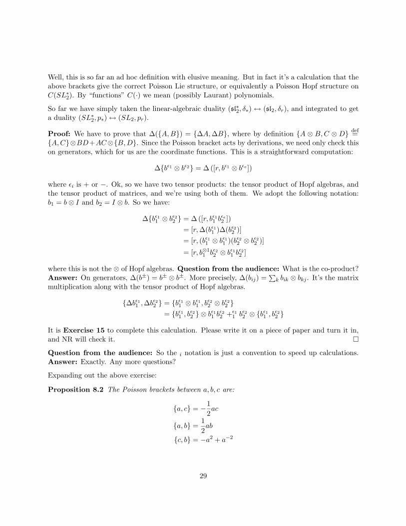
It is Exercise 15 to complete this calculation. Please write it on a piece of paper and turn it in,and NR will check it.

Question from the audience: So the i notation is just a convention to speed up calculations.Answer: Exactly. Any more questions?

Expanding out the above exercise:

Proposition 8.2 The Poisson brackets between a, b, c are:

a, c = −12ac

a, b =12ab

c, b = −a2 + a−2

29

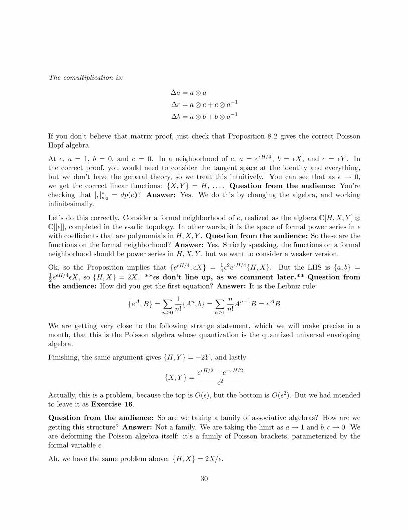
The comultiplication is:

∆a = a⊗ a∆c = a⊗ c+ c⊗ a−1

∆b = a⊗ b+ b⊗ a−1

If you don’t believe that matrix proof, just check that Proposition 8.2 gives the correct PoissonHopf algebra.

At e, a = 1, b = 0, and c = 0. In a neighborhood of e, a = eεH/4, b = εX, and c = εY . Inthe correct proof, you would need to consider the tangent space at the identity and everything,but we don’t have the general theory, so we treat this intuitively. You can see that as ε → 0,we get the correct linear functions: X,Y = H, . . . . Question from the audience: You’rechecking that [, ]∗sl2 = dp(e)? Answer: Yes. We do this by changing the algebra, and workinginfinitesimally.

Let’s do this correctly. Consider a formal neighborhood of e, realized as the algbera C[H,X, Y ]⊗C[[ε]], completed in the ε-adic topology. In other words, it is the space of formal power series in εwith coefficients that are polynomials in H,X, Y . Question from the audience: So these are thefunctions on the formal neighborhood? Answer: Yes. Strictly speaking, the functions on a formalneighborhood should be power series in H,X, Y , but we want to consider a weaker version.

Ok, so the Proposition implies that eεH/4, εX = 14ε

2eεH/4H,X. But the LHS is a, b =12eεH/4εX, so H,X = 2X. **εs don’t line up, as we comment later.** Question from

the audience: How did you get the first equation? Answer: It is the Leibniz rule:

eA, B =∑n≥0

1n!An, b =

∑n≥1

n

n!An−1B = eAB

We are getting very close to the following strange statement, which we will make precise in amonth, that this is the Poisson algebra whose quantization is the quantized universal envelopingalgebra.

Finishing, the same argument gives H,Y = −2Y , and lastly

X,Y =eεH/2 − e−εH/2

ε2

Actually, this is a problem, because the top is O(ε), but the bottom is O(ε2). But we had intendedto leave it as Exercise 16.

Question from the audience: So are we taking a family of associative algebras? How are wegetting this structure? Answer: Not a family. We are taking the limit as a→ 1 and b, c→ 0. Weare deforming the Poisson algebra itself: it’s a family of Poisson brackets, parameterized by theformal variable ε.

Ah, we have the same problem above: H,X = 2X/ε.

30

So the summary is we have a family of Poisson algebras parameterized by ε:

H,Xε =2εX

H,Y ε = −2εY

X,Y ε =eεH/2 − e−εH/2

ε2

And we define, 0

def= limε→0

ε, (8.3)

See, nobody said we had to take this Poisson structure. Well, we did.

Correction: Let p : G → ∧2g be a Poisson Lie structure on G. Then for any α, αp is also aPoisson-Lie strucuter, and this defined a family of Lie bialgebras δ = αdp(e). So, anyway, we dothe rescaling, and we see that

H,X0 = 2XH,Y 0 = −2YX,Y 0 = H

Exercise 17 Show that δ∗ = dp(e) in the usual way.

Oh, before you all leave: if you have particular questions about Poisson Lie groups and quantumgroups, send NR an e-mail: the syllabus is fluid.


**We begin class with: I arrive a minute or two late, NR passes out a name-and-emailsheet, and then NR’s cell-phone rings.**

We have a Lie bialgebra (sl2, δr), with r = 14H ⊗ H + X ⊗ Y , and its dual (sl∗2, δ = [, ]∗sl2). We

exponentiate sl2 to (SL2, pr) with pr = −Adx⊗Adx(r) + r, wheer we assume TG ∼= g×G by righttranslations. We exponentiate sl∗2 to (SL∗2, p∗), which we described last time in coordinates. Thisexample provides a definition of the ideal of a dual pair of Poisson Lie groups. Given a (dual pairof) Lie bialgebras, there is a unique dual pair of connected simply-connected Poisson Lie groups,but in fact we should think of the pair as parameterized by the π1s.

Where did the formula r = 14H ⊗H +X ⊗ Y come from?

31

9.1 The double construction of Drinfeld

We begin by constructing the bicross-product of Lie bialgebra. We let g1, g2 be finite-dimensionalLie algebras over C.

**NR pauses to quiz people about what they are doing.** We have a specific group withspecific interests, and Quantum Groups is a huge subject. We could take a month to talk aboutUq(n+), but no one is interested in this. We suggest the following agenda:

• Poisson Hopf algebras, and then quantum-deform these into associative noncommutativealgebras. We will do this by taking a family of ideals Iq in the free algebra F , and then formAq = F/Iq, which we will identify as vector spaces. In this way we will form Uq(g) and Cq(G).

• We will spend some time on the real forms of these.

• Closer to NR’s interest, we will end by studying affine **missed** algebras. For example,we have the diagonal action SLn y (Cn)⊗N with centralizer SN . The quantum version of thisis that ◊Uq(sln) y (Cn)⊗N , with centralizer the affine Hecke algebra ◊HN (q). There are manyreasons to be interested in this construction, including reasons from mathematical physics.

Anyway, the Drinfeld construction is well-known, and we describe it now.

Assume that g1 acts by derivations on g2, meaning that g2 is a g1-module, and also that x · [l,m] =[x · l,m] + [l, x ·m], where x ∈ g1, l,m ∈ g2, · is the action, and [, ] is the bracket in g2.

Then g1 n g2def= g1 ⊕ g2 as a vector space, with [(x, l), (y,m)] = ([x, y], [l,m] + x ·m− y · l) is a Lie

algebra. It is the infinitesimal version of the semi-direct product of groups.

Oh, who knows the rule for which way to write the n? The open end points towards the thingbeing acted on: it’s a pair of hands, twisting things around.

Example 9.1 Let g be a Lie algebra, g∗ a dual vector space with [, ]g∗ = 0 trivial. Then g y g∗ withthe ad∗-action, and so we form g n g∗. For example, g = so(3), g∗ = R∗, then g n g∗ = so(3) n R3

is the affine transformations. ♦

We now explain Drinfeld’s construction, at least in the case when g2 = g∗1. So let (g, δ) be a Liebialgerba, (g∗, δ∗) its dual. Then g y g∗ be ad∗g, and g∗ y g by ad∗g∗ . We should look for a versionof n that is more symmetrical. We formulate the construction as a theorem:

Theorem 9.1 There exists a unique Lie algebra structure on D(g) def= g⊕ g∗ such that

• g, g∗ → g⊕ g∗ are Lie subalgebras.

• the natural bilinear form ((x, l), (y,m)) = 〈x,m〉+ 〈y, l〉 is D(g)-invariant. I.e.

([η, ξ1], ξ2) + (ξ1, [η, ξ2]) = 0 ∀η, ξ1, ξ2 ∈ D(g) (9.1)

In other words, we have a pairing D(g)⊗D(g)→ C, with and D(g) y D(g)⊗D(g) diagonally,and trivially on C, and we require that the pairing is a D(g)-module homomorphism.

32

We outline the proof, essentially computing the structure.

Proof (Outline): 1. Let ei be a basis in g, with structure constants [ei, ej ] =∑k C

kijek and

δei =∑jk f

jki ei ∧ ek.

2. Let ei be the dual basis in g∗, so 〈ei, ej〉 = δji . Then the brackets are [ei, ej ] =∑k f

ijk e

k

and δ∗ei =

∑jk c

ijke

j ∧ ek.

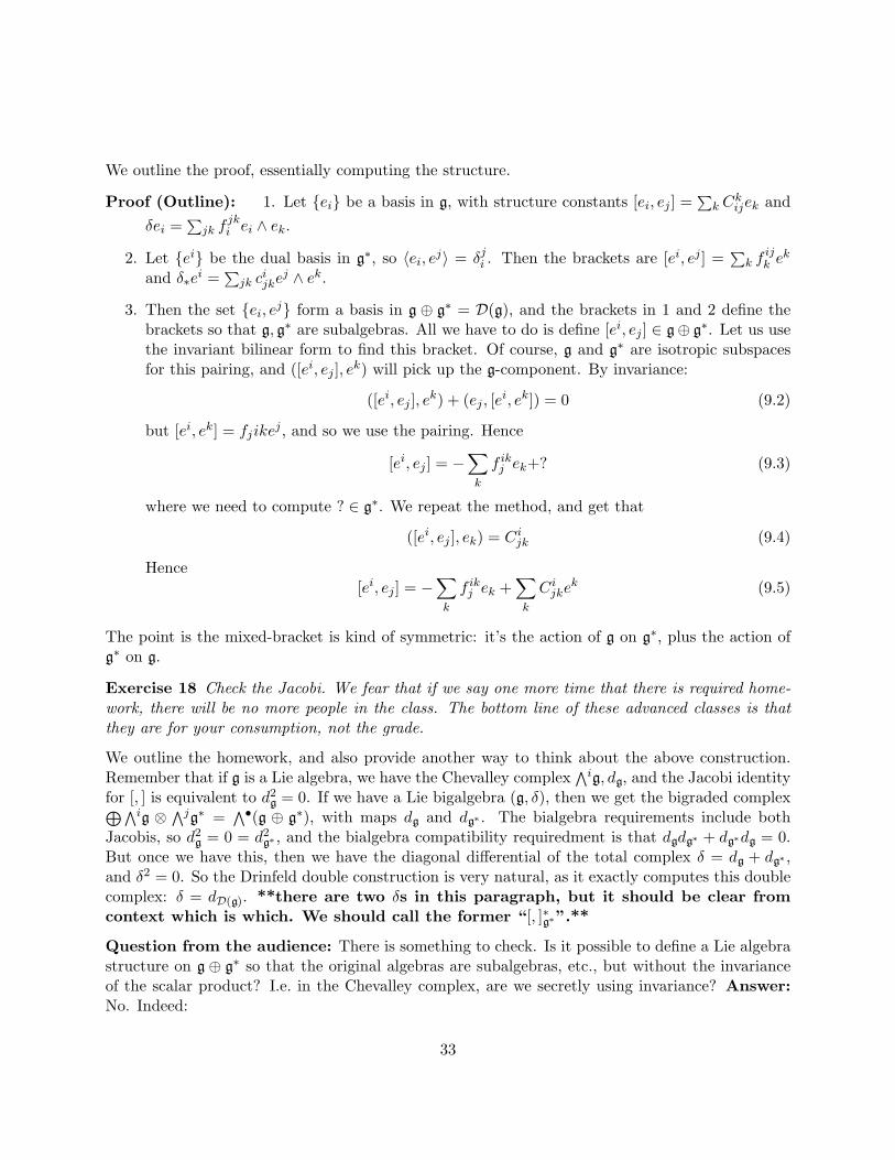
3. Then the set ei, ej form a basis in g ⊕ g∗ = D(g), and the brackets in 1 and 2 define thebrackets so that g, g∗ are subalgebras. All we have to do is define [ei, ej ] ∈ g⊕ g∗. Let us usethe invariant bilinear form to find this bracket. Of course, g and g∗ are isotropic subspacesfor this pairing, and ([ei, ej ], ek) will pick up the g-component. By invariance:

([ei, ej ], ek) + (ej , [ei, ek]) = 0 (9.2)

but [ei, ek] = fjikej , and so we use the pairing. Hence

[ei, ej ] = −∑k

f ikj ek+? (9.3)

where we need to compute ? ∈ g∗. We repeat the method, and get that

([ei, ej ], ek) = Cijk (9.4)

Hence[ei, ej ] = −

∑k

f ikj ek +∑k

Cijkek (9.5)

The point is the mixed-bracket is kind of symmetric: it’s the action of g on g∗, plus the action ofg∗ on g.

Exercise 18 Check the Jacobi. We fear that if we say one more time that there is required home-work, there will be no more people in the class. The bottom line of these advanced classes is thatthey are for your consumption, not the grade.

We outline the homework, and also provide another way to think about the above construction.Remember that if g is a Lie algebra, we have the Chevalley complex

∧ig, dg, and the Jacobi identityfor [, ] is equivalent to d2

g = 0. If we have a Lie bigalgebra (g, δ), then we get the bigraded complex⊕∧ig ⊗ ∧jg∗ =∧•(g ⊕ g∗), with maps dg and dg∗ . The bialgebra requirements include both

Jacobis, so d2g = 0 = d2

g∗ , and the bialgebra compatibility requiredment is that dgdg∗ + dg∗dg = 0.But once we have this, then we have the diagonal differential of the total complex δ = dg + dg∗ ,and δ2 = 0. So the Drinfeld double construction is very natural, as it exactly computes this doublecomplex: δ = dD(g). **there are two δs in this paragraph, but it should be clear fromcontext which is which. We should call the former “[, ]∗g∗”.**

Question from the audience: There is something to check. Is it possible to define a Lie algebrastructure on g ⊕ g∗ so that the original algebras are subalgebras, etc., but without the invarianceof the scalar product? I.e. in the Chevalley complex, are we secretly using invariance? Answer:No. Indeed:

33

Theorem 9.2 δ as defined in the previous paragraph defines a Lie algebra structure on g ⊕ g∗,which is isomorphic to D(g) from the previous theorem.

Both constructions are useful: Jacobi comes for free from the Chevalley construction, but youdon’t see the scalar product, whereas it’s central to the other construction (where Jacobi is ob-scured).

Theorem 9.3 There is a natural Lie bialgebra structure on D(g) = g on g∗ defined by requiringthat the embeddings g, g∗ → D(g) are Lie bialgebra embeddings.

Exercise 19 Prove this.

Corollary 9.3.1 D(g)∗ = g∗ ⊕ g is the direct sum of Lie algebras.


Lecture notes up through today are on the website. These are shorter than the actual lecture: Theohas a complete **only mildly paraphrased, and occasionally annotated** transcript.

Today we finish the Double construction, and then consider some examples.

Recall, g is a Lie bialgebra. The double D(g) of g is the direct sum of two vector spaces g ⊕ g∗

as a vector space. It is D(g) = g ⊕ g∗op as a Lie coalgebra. **I missed the word op, whichcontrols the sign of the cobracket, last time.** The Lie brackets are such that g, g∗ → D(g)as Lie subalgebras, but D(g) is not a direct sum. In terms of a basis:

[ei, ej ] =∑k

Cijkek −

∑k

f ikj ek (10.1)

Another word for the Double is the bicross-product D(g) = g on g∗.

Theorem 10.1 D(g) is a quasitriangular Lie bialgebra with r =∑i ei⊗ei ∈ g∗⊗g → D(g)⊗D(g).

(Hence r does not depend on the basis: it is simply the identity map id : g → g thought of as anelement of g⊗ g∗.)

Proof: There is probably a basis-independent proof. We work in a basis.

δr(ei) = [r, ei ⊗ 1 + 1⊗ ei] (10.2)

=∑j

[ej , ei]⊗ ej +∑j

ej ⊗ [ej , ei] (10.3)

=∑jk

Ckjiek ⊗ ej +∑j

ej ⊗(∑

k

Cijkek −

∑k

f ikj ek

)(10.4)

=∑k

f jki ej ⊗ ek (10.5)

34

In equation 10.5 we have reindexed and used the skew-symmetry to cancel two terms. **Equa-tion 10.4 is wrong: we realized a sign error, and have gone back and fixed it mostly.**

Question from the audience: You need also to check that r satisfies the Yang-Baxter equation.Answer: Yes. We need to prove that. Of course, the best way to prove the Yang-Baxter equationis to leave it as an exercise. How should you prove this? We are working in a basis, because this isuseful when you compute examples.

In a basis, the first term [r12, r13] of the Yang-Baxter equation is really

[r12, r13] = [ei ⊗ ei ⊗ 1, ej ⊗ 1⊗ ej ] = [ei, ej ]⊗ ei ⊗ ej (10.6)

The second term is ei ⊗ ej ⊗ [ei, ej ], and the last is ei ⊗ [ei, ej ]⊗ ej . So we should have

[ei, ej ]⊗ ei ⊗ ej + ei ⊗ ej ⊗ [ei, ej ] + ei ⊗ [ei, ej ]⊗ ej?= 0 (10.7)

Sure enough, we have

f ijk ek ⊗ ei ⊗ ej + Ckije

i ⊗ ej ⊗ ej + ei ⊗ (−Cjikek + f jki ek)⊗ ej = 0 (10.8)

because everything cancels.

So, given enough supply of Lie bialgebras, we can take their doubles to get a number of examplesof quasitriangular.

Question from the audience: Is there a more invariant way to express the bracket? Answer:Yes. It should be something like [(x, l), )y,m)] = ([x, y]g + Ad∗xm, [l,m]g∗ + Ad∗ . . . ). Well, this isa good question, and we didn’t prepare this, so we will make it Exercise 20. Here’s a way to getparticipation: each time we suggest a problem, someone will explain it the next time. Let’s vote.**7 to 2 in favor.**

In fact, it’s better than quasitriangular:

Proposition 10.2 D(g) is facotrizable, and r+σ(r) =∑i(ei⊗ei+ei⊗ei) defines a nondegenerate

invariant scalar product ((x, l), (y,m)) = l(y) + m(x). Hence the map t : D(g)∗ → D(g) by l 7→r+(l)− r−(l) is a linear isomorphism, and so ∀x there is a unique factorization x = x+⊕x− wherex± ∈ g±.

Proof: In fact, in this form is is a tautology, since as a vector space D(g) is defined as a directsum.

Example 10.1 We saw already there is a Lie algebra b+ ⊆ sl2 given by [H,X] = 2X, δH = 0,δX = 1

2H ∧X.

Let us describe D(b+). We choose a dual basis H∨, X∨, so that b∨+ = CH∨⊕CX∨ with [H∨, X∨] =X∨, δH∨ = 0, and δX∨ = H∨ ∧X∨. Then D(b+) = b+ ⊕ b∨+ = CH ⊕ CX ⊕ CH∨ ⊕ CX∨.

Question from the audience: Confused by notation, what is this δ on b∨+? Answer: We wouldwrite b∨ = b∗, and δ should be δ∗, dual to [, ]b.

35

If we think about Lie algebras alebraically, rather than geometrically, we can present it with abasis, hopefully.

Ok, so we want to compute the cross brackets, using the above formulas. We have, e.g. CXHX = 2,and fHXX is the only other non-zero structural constant.

[X∨, H] =∑a

CXHaa∨ −

∑b

fXbH b = 2X∨ (10.9)

[X∨, X] =∑a

CXXaa∨ −

∑b

fXbX b = −2H∨ +H (10.10)

[H∨, H] = 0 (10.11)[H∨, X] = −X (10.12)

We should also write out the coalgebra. Remember that as a coalgebra D(g) = g ⊕ g∗op, soδH∨ = 0 = δH, δX = 1

2H ∧X, and δX∨ = −H∨ ∧X∨. Also, we have:

r = H∨ ⊗H +X∨ ⊗X (10.13)

So, let’s define H ′ = 12H − H

∨, H ′′ = 12H + H ′, X ′ = X, and Y ′ = −1

2X∨. Then H ′′ is in the

center of the Lie algebra D(b+), and in fact spans the center. Moreover, δH ′′ = 0, and so CH ′′ isa Lie bialgebra ideal.

Also, H ′, X ′, Y ′ generate sl2 → D(b+), and so D(b+) = CH ′′ ⊕ sl2 as a Lie algebra. And CH ′′ is aLie bialgebra ideal, so the quotient D(b+)/CH ′′ is a Lie bialgebra, whose algebra part is sl2. Butin fact the coalgebra part is our old friend: D(b+)/CH ′′ = (sl2, δ) is the standard Lie bialgebrastructure on sl2.

This also explains why our example is quasitriangular:

r =12H ′′ ⊗H ′′ + 1

2(H ′ ⊗H ′′ −H ′′ ⊗H ′

)− 1

2

Å14H ′ ⊗H ′ − Y ′ ⊗X ′

ã(10.14)

We will have to clean up signs and 12s. The signs are always wrong, and the 1

2s come from theproblem of pairing exterior squares.

Anyway, that last term if the sl2 r-matrix.

Question from the audience: Is that a general fact, that the quotient of a quasitriangular Liebialgebra by a Lie bialgebra ideal is quasitriangular? Answer: Yes. ♦

Ok, so we didn’t explain where b+ with [H,X] = 2X, δH = 0, and δX = 12H ∧ X — we didn’t

explain where this Lie bialgebra comes from. But this algebra is vecy natural: on C[x], we let Xact as x, and H by 2x ∂

∂x . So b+ is the linear part of the derivations.

In fact, there is a generalization of this algebra to b+ ⊆ ga for any symmetrizable Kac-Moodyalgebra. In particular, this works for

36

• simple Lie algebras

• central extensions of loop algebras S1 → g.

• other examples.

We said the words “Kac-Moody algebras”. Who knows this word? **two or so hands** Theusual suspects. We will explain this construction for simple algebras, and later explain what a KMalgebra is.

Ok, so let g be simple, and define b+ in terms of generators and relations. For each i ∈ Γ theDynkin diagram, we have two basis elements Hi and Xi, and we let

[Hi, Hj ] = 0, [Hi, Xi] = aijXj , and (adXi)1−aij (Xj) = 0 if i 6= j (10.15)

The dimension is r + |∆+|, and Xi = Xαi are the corresponding simply roots. Then δHi = 0,δXi = di

2 Hi ∧Xi, where di is the length of the root di = (αi, αi)/2.

Exercise 21 D(b+) ∼= g ⊕ h, where h is a central copy of the Cartan, as a Lia algebra. Thebialgebra you know.

In particular, as before, D(b+) ∼= sl2 ⊕ h.


We begin with Matt presenting a basis-free description of the bracket on the Drinfeld Double D(g)of a Lie bialgebra g. **I was caught in this morning’s hailstorm, rather than catchingthe bus. I will later include an invariant discussion of the Drinfeld Double and theChevalley Complex in terms of Penrose et al.’s “birdtrack” stringy notation.**

We now turn to a few examples.

11.1 Kac-Moody algebras

Last time we gave an example of a canonical Lie bialgebra structure for any simple Lie algebra.

We now explain this in full generality. (Ten years ago, NR wrote a paper, never published, workinga number of nice examples in Kac-Moody algebras.)

Let h be a finite-dimensional vector space, h∗ its dual, and a collection h1, . . . , hn ∈ h of “co-roots”and α1, . . . , αn ∈ h of “roots”. We define the generalized Cartan matrix to be aij = 〈αi, hj. Wedemand the following conditions:

• aii = 2,

• aij ∈ Z≤0 for i 6= j

37

• If aij 6= 0, then aji 6= 0.

• There exists d1, . . . , dn ∈ Z>0 diagonalizing the matrix, i.e. diaij = ajidi (no sum).

• dim h = n+ dim(ker a).

Then we define the Kac-Moody algebra g(a) to be the Lie algebra generated by h (the Cartan), andei, fi for i = 1, . . . , n, with defining relations

[h, h′] = 0, [h, ei] = 〈αi, h〉ei, [h, fi] = −〈αi, h〉fi, and [ei, fj ] = δijhi (11.1)

and also the Serre relations:

(adei)1−aij (ej) = 0 and (adfi)

1−aij (fj) = 0 (11.2)

It is clear that g(a) is Z-graded with deg(h) = 0, deg(ei) = 1, and deg(fi) = −1.

Example 11.1 Assume a is nondegenerate, so that n = dim h, and g(a) is a simple finite-dimensional Lie algebra. ♦

Example 11.2 Assume that dim ker a = 1. Then dim h = 1 + n, and we have

Theorem 11.1 (Galber, Kac) Then the a has block form of an (n− 1)× (n− 1) nondegeneratething, in columns 1, . . . , n− 1, and a last column number 0, and the nondegenerate part generatesa simple Lie algbera g. Then

g(a) ∼= g[t, t−1]⊕ CK ⊕ Ctd

dt(11.3)

and the Cartan is hg ⊕ CK ⊕ Ct ddt .

In particular, for i = 1, . . . , n − 1, then ei 7→ ei ∈ g, and fi 7→ fi ∈ g. Also, e0 7→ tfθ, where θ isthe longest root for g, and f0 7→ t−1eθ.

These are the most studied infinite-dimensional Lie algebras. On the one hand, they have a simplepresentation, and the representation theory of simple Lie algebras transfers directly. On the otherhand, they have a simply geometrical interpretation as a central extension to the loop algebra,along with derivatives. Connections to physics: two-dimensional gauge theories, CFTs.

**missed something about the grading** ♦

In the 80s, people asked about whether there were interesting examples when dim ker a ≥ 2. Theredon’t seem to be.

NR learned from Richard Borcherds that you should think of the simple Lie algebras as spheres,and the affine ones **when dim ker a = 1?** as cylinders. The higher examples grow exponen-tially. There are difficult questions, because e.g. the Weyl groups of these generalized algebras areinteresting. For example, SL2(Z) shows up. You think that it’s a difficult problem, so there shouldbe geniuses working on it, but no: geniuses look for difficult problems with easy solutions. So thisis an open field of research.

38

Ok, so why are we doing this? Every Kac-Moody algebra has a Lie bialgebra question, and moreovera quantum counterpart. But in the generalized case, it’s strange to ask these questions, becausewe know so little about the Lie algebra: why make it more complicated?

Proposition 11.2 If g(a) is a Kac-Moody algebra, then

δh = 0, δei =di2hi ∧ ei, δfi =

di2hi ∧ fi (11.4)

is a Lie bialgebra structure, and moreover it is quasitriangular.

We will not explain the quasitriangular structure, although there is a formula for it, because it isa good presentation. See, the dimension of the Cartan is larger than the rank of the algebra. Sothere are extra elements, and always they act as derivations, as in the example.

11.2 Real forms of Lie bialgebras

A real Lie bialgebra is a real vector space, real [, ] : g ⊗ g → g, and real δ : g → g ∧ g, i.e. it is aLie bialgebra over R. When we have such a thing gR, we can define as always the complexificationgC = gR ⊗R C. Then gR ⊆ gC is invariant with respect to complex conjugation.

What we can do is complement the conjugation with an automorphism. Let σ : g → g be a realautomorphism of gC, so that σ[a, b] = [σa, σb], and we demand that it be a C-antilinear involution:σ(λa) = λσa, and σ2 = id.

A real form of gC is a real Lie algebra gR such that gC = gR⊗R C. Then the real form correspondingto σ is gσ = the set of fixed points of σ.

Exercise 22 Real forms of gC are classified by equivalence classes (modulo inner automorphism)of such σ. (C.f. Fulton and Harris)

We can make all the same definitions for Lie bialgebras, additionally demanding that σ preservesthe coalgebra: (σ ⊗ σ)δ = δσ. Then again gσ is a real Lie bialgebra with complexification gC, andthis gives the classification of real forms.

Example 11.3 We start with sl2(C) and the standard Lie bialgebra structure. If we have x =aH + bX + cY , then we define the Killing form (x, x) = tr(Adx Adx) = 2a2 + bc. So this is aquadratic form on C3, and it’s natural to ask what it looks like on the real three-dimensionalsubspace.

Compact real form Let σ = (−1) (Hermetian conjugation), i.e. σ(H) = −H, σ(X) = −Y ,σ(Y ) = −X. It’s important that this is minus conjugation. If you think of UgC, it has a∗-operation from Hermetian conjugation, and this is not that. It’s a combination of that withthe antipode. We say this for those who know to much. Then iH, X − Y , and i(X + Y ) arethe invariant elements, and the real form is su2 = R(iH)⊕ R(X − Y )⊕ Ri(X + Y ), and weadopt coordinates s, t, u.

39

The Killing form is is −2(s2 +t2 +u2). There is a problem for the Lie coalgebra structure. Wehave δX = 1

2H ∧X. So (σ⊗σ)δX = 12σH ∧σX = −1

2H ∧Y , but δσX = δ(−Y ) = −12H ∧Y .

So it’s fine, but it’s not supposed to be.

For Lie algebras, we have two real forms: su2, sl2(R) ∼= su1,1, but for bialgebras these will split. ♦


Last time we began discussing real forms of complex Lie algebras. We gave the most naturaldefinition for Lie bialgebras. Recall, a real Lie bialgebra is simple a Lie bialgebra over R, so thatthe bracket and cobracket are real linear maps. Such an algebra has a complexification, and thenwe have:

Theorem 12.1 (Fulton, Harris) Equivalence classes of real forms of Lie bialgebras are in bijec-tion with outer automorphisms σ such that σ2 = id, σ(λa) = λσ(a), and σ is an automorphism ofthe Lie bialgebra **over Z**: σ([a, b]) = [σa, σb] and (σ ⊗ σ)δ(a) = δ(σa).

If we just said “automorphism of the Lie algebra”, we’d get that classification, and there’s the dec-orated Dynkin diagrams with which to compute these. The classification of real forms of bialgebras— we don’t know where it is.

Example 12.1 sl2(C), and there are two nonequivalent real forms. See, there’s the bilinear non-degenerate form (, ), the Killing form, on sl2(C). If g is a real form of sl2(C), then (, )g is a realKilling form, quadratic on R3, and so it is classified by the signature: (+ + +) or (+ +−). So wehave su2 (+ + + or −−−) and su1,1

∼= sl2 (+−− or −+ +). It is a matter of taste the sign of theKilling form.

su2: Then σ(H) = −H, σ(X) = −Y , and σ(Y ) = −X. This is a bialgebra automorphism of thestandard Lie bialgebra structure (δH = 0, δX = 1

2H ∧X, and δY = 12H ∧ Y ).

We make an aside: the 12s are a mess, because of the confusion about how to define the bracket of

exterior products. If you embed in the tensor product, you get (l∧m,x∧y) = 2(l(x)m(y)−m(x)l(y)).We will fix the notes.

Oh, and there’s another error. If you just have a solution to CYB, the arguments we gave don’twork to give a quasitriangular structure.

So back to su2. We have su2 = slσ2 = RiH ⊕Ri(X + Y )⊕R(X − Y ). Let’s look at the cobracket.We’d have δ(iH) = 0, δ(i(X + Y )) = iH2 ∧ (X + Y ) = −i iH2 ∧ i(X + Y ). This i is a bigproblem, but not really: λδ is a Lie cobracket for sl2(C) for any complex λ. So we takeδ = iδ, whence (su2, δ) is a real Lie bialgebra, with complexification (sl2(C), δ). **Jacobiand compatibility are both homogeneous, so for any bialgebra, you can scale thebracket and cobracket independently**

sl2(R): σ(H) = H, σ(X) = X, and σ(Y ) = Y . Then sl(2C)σ = RH ⊕ RX ⊕ RY = sl2(R). So

(sl2(R), δ) is a real Lie bialgebra.

40

su1,1: Lastly, we consider su1,1, which happens to be isomorphic to sl2; for sln, there will be a familyof real forms sup,q, which are not isomorphic to sln. In any case, σ(H) = −H, σ(X) = Y , andσ(Y ) = X. You can see that the Cartan is imaginary as for su2, but there is no minus signon X,Y , which will change the signature. We have su1,1 = RiH ⊕ Ri(X − Y )⊕ R(X + Y ).

Let’s check the signature, looking at the value of the Killing form with respect to this ba-sis, which is special, since this basis is orthonormal. Rather than working over the adjointrepresentation, let’s work over C2, and we’ll get a multiply of the basis. Then

iH =Çi 00 −i

å, i(X − Y ) =

Ç0 i−i 0

å, iH =

Ç0 11 0

å(12.1)

and the signature of the Killing form is

trC2

(ÄαiH + βi(X − Y ) + γ(X + Y )

ä2)= −2α2 + 2β2 + 2γ2 (12.2)

Looking at the cobracket, we see that δ(iH) = 0, but we have the same problems as with su2 :δ(i(X − Y )) = iH2 ∧ (X − Y ) = −i iH2 ∧ i(X − Y ), and δ(X + Y ) = −i iH2 ∧ (X + Y ). So we take δ,and then (su1,1, δ) is a real Lie bialgebra, and its complexification is not (sl2, δ) but rather (sl2, δ).♦

In general in this class sl2 will be our main hero, and you can try sln based on the literature outthere. But we make some general remarks.

If g is simple, we let it be generated by (Hi, Xi, Yi) for roots i = 1, . . . , r = rank(g), and there’s theChevalley-Serre relations. Then we have the “standard Lie bialgebra structure” — there are otherchoices —

δHi = 0, δXi =di2Hi ∧Xi, δYu =

di2Hi ∧ Yi (12.3)

Then we have compact real forms: σ(Hi) = −Hi, σ(Xi) = −Yi, and σ(Yi) = −Xi. Then we get

gcompactR =

r⊕j=1

RiHj ⊕⊕α∈∆+

ÄRi(Xα +X−α)⊕ R(Xα −X−α)

ä(12.4)

For g = sln, this is sun. We take the notation that j = αj for the (enumerated) simple roots.Anyway, (gcompact

R , δ = iδ) is a real compact Lie bialgebra.

For sln, ∆+ = εi − εji<j , where ε1, . . . , εn is a basis in Rn, and Xεi−εj = eij , X−εi+εj = eji, andHi = eii − ei+1,i+1 for i = 1, . . . , n− 1.

Ok, so we have the Lie bialgebra (gcompactR , δ). Let’s try to recognize the dual as a known Lie

algebra, so that perhaps we can recognize the double.

Let’s start with su2, with basis iH, i(X+Y ), (X−Y ). Then su∗2 has the dual basis h, e, f , with thebracket [h, e] = e, [h, f ] = f , and [e, f ] = 0, a real Lie algebra. The easiest faithful representationof this algebra is . . . . Can we do this real algebra as 2× 2 matrices? Yes:

h =12

Ç1 00 −1

å, e =

Ç0 10 0

å, f =

Ç0 i0 0

å(12.5)

41

So we can write this as triangular traceless 2 × 2 matrices with real diagonal but complex upperpart:

su∗2∼=®Ç

λ c0 −λ

ås.t. λ ∈ R, c ∈ C

´(12.6)

We write it in this way so that we can exponentiate:

We have the pairing (su2, δ) with (su∗2, δ∗), and we can recognize su∗2∼= hR⊕nC

+. We can exponentiatethis pairing: (SU2, p) versus (SU∗2 , p∗), where

SU∗2 =®Ç

a c0 a−1

ås.t. a > 0, c ∈ C

´(12.7)

Now we turn to SUn. The most amazing thing is that it seems different, but is ultimately the same.Did we ask this exercises last time?

Exercise 23 The Lie bialgebra structure is given by equation 12.3, and so we have sl∗n generatedby H∨i , X∨i , and Y ∨i , and the bracket

[H∨i , H∨j ] = 0, [H∨i , X

∨j ] = δij

di2Xj , [H∨i , Y

∨j = δij

di2Y ∨j (12.8)

and Serre’s relations for X∨i and Y ∨i .

Then sl∗n ⊆ b+ ⊕ b− as (h⊕ x,−h⊕ y) where h ∈ h, x ∈ n+, and y ∈ n−.

You know, there are two levels. The first level is when a name appears in a subject, and the secondlevel is where “gaussian” is written with a small “g”. We were tempted to write “serre”.

Ok, so let’s take σ(Hi) = −Hi, σ(Xi) = −Yi, and σ(Yi) = −Xi.

Theorem 12.2 su∗n = sl∗nσ is isomorphic as a Lie algebra to the space of traceless triangular

matrices with complex upper part but pure-real diagonal.

Proof: Exercise 24. The proof is almost the same as for su2.

And so we have

SU∗n =

Öa1 ∗

. . .0 an

ès.t. ai > 0, a1 . . . an = 1, ∗ ∈ C

(12.9)

Next time we will start looking at symplectic leaves

12.1 Bruhat decomposition

We assume that everyone knows that if W is the Weyl group of g (of the root system of g), thenit acts naturally on h. In particular, for g = sln(C), we have h = Cn−1 embedded in Cn as the

42

hyperplane perpendicular to (1, . . . , 1). Then W is the symmetric group Sn acting naturally on Cn

and fixing (1, . . . , 1).

Well, G acts on g be the Adjoint action, e.g. SLn y sln by conjugation of matrices. The questionis: do we have a natural embedding of W → SLn? The answer is no: rather, N(H), the normalizerof the Cartan as a subgroup H ≤ G, and then N(H) ∼= H o W . So N(H) acts naturally on sln,and that’s how W acts on the whole algebra.

The goal: find symplectic leaves of SUn, which will be the Shubert cells of SUn/T .


13.1 Bruhat Decomposition

Last time we began to discuss Bruhat Decomposition. We will see that this provides a cell decom-position of a Poisson Lie group into symplectic leaves.

First we recollect the Weyl group. Suppose we have a root system ∆ = α ∈ Rn. We will be dealingonly with semisimple finite-dimensional Lie algebras. We pick Γ ⊆ ∆ the simple roots, so that∆ = ∆+ ∪∆− and Γ ⊆ ∆+. It will be convenient to enumerate the simple roots: Γ = α1, . . . , αrwhere r is the rank of ∆ (i.e. the rank of g).

To each root α ∈ ∆+, we associate a reflection sα : x 7→ x − 2(α, x)/(α, α), which is reflectionwith respect to the hyperplane α⊥. We define the Wely group to be the group generated by thesereflections, and it is a property of root systems that this is a finite group.

We let si = sαi . Then we have a well-known result (c.f. Fulton and Harris):

Theorem 13.1 W ∼= 〈si, i = 1, . . . , r s.t. s2i = 1, (sisj)mij = 1〉, where mij is related to the

Cartan matrix.

Example 13.1 For SLn, ∆ = An−1, and so (sisj)2 = 1 if i 6= j ± 1, and (sisi+1)3 = 1. ThusWAn−1 = Sn. If ∆+ = εi − εji<j , then Γ = εi − εi+1n−1

i=1 , and W acts by permutations on εi. ♦

If ∆ is the root system of g, we let h ⊆ g be the Cartan subalgebra, and so h =⊕r

i=1 Rα∗i (rootsare in h∗). Then g = h⊕ n+ ⊕ n−, where n± are nilpotent and correspond to ∆±.

W acts naturally on h. Does it act naturally on g? Not quite. Strictly speaking, the answer is No.But anytime the answer is No, you can ask “if not this, then what?”

I’m making all these pseudo jokes, and you are putting them online. You can skip most ofthem.

So, let G be the Lie group with g = Lie(G). Then G acts on G by conjugation, and thus G acts ong = TeG by the Adjoint action. Can W naturally embed into G? If it can, then it has a naturalaction on g.

43

Let H ⊆ G by the Cartan subgroup. Question from the audience: Is G connected? Or doesit matter? Answer: It probably doesn’t matter, but let’s always assume that G is connected, andmost of the time that G is simply connected.

So H ⊆ G, and we can construct N(H) ⊆ G the normalizer of H in G. In other words, N(H) =g ∈ G s.t. gHg−1 ⊆ H.

Theorem 13.2 N(H) ∼= W nH.

Proof: For all G, see Fulton and Harris. For SLn, it is obvious: Suppose d is diagonal, and so isgdg−1 = d′. So gd = d′g, and if gij 6= 0, then di = d′j . So d′i = dσ(i), where σ is a permutationon the indices 1, . . . , n. When gij = 0, no conditions, but of course det g = 1. Thus g must be amonomial matrix (one non-zero entry in each row and each column).

Question from the audience: How does this give us the semidirect product? Answer: N(H)is the monomial matrices. For example,Ö

ab

c

è=

Ö1

11

èÖb

ca

è∈ Sn n diagonal = W nH (13.1)

Corollary 13.2.1 1. N(H) acts naturally by conjugation on G.

2. N(H) acts naturally by Ad on g.

Corollary 13.2.2 If we choose representations of W in N(H), i.e. we chose a section W →N(H) : w 7→ w, when w acts on g.

This is not canonical, but it is up to the action of the Cartan. We will have the same story forquantum Weyl group.

Exercise 25 Find the action of

si =

1. . .

10 1−1 0

1. . .

1

(13.2)

on sln. On generators: Tidef= Adsi, and find Ti(Hj = ejj−ej+1,j+1), Tj(ei,i+1 = ei), and Tj(ei+1,i =

fi).

If you can do this, then quantizing is easy: you judiciously add qs.

44

Ok, so We have G a complex Lie group, and a fix a Borel subgroup B ⊆ G. A priori there are manyBorel subgroups, but for simple groups we can list all of them, and they are related by conjugation.

Theorem 13.3 G =⊔w∈W

BwB.

BwB = BwB = bwb′ s.t. b, b′ ∈ B, where w is any representative of w in N(H). We remarkthat BwB does not depend on the choice of w ∈ N(H). If w and w are two representatives, thenw = wh for h ∈ H.

Ok, so for SLn, we take B the upper triangular matrices. Then

Theorem 13.4 G =⊔w∈W

B−wB− =⊔w∈W

B−wB+ =⊔w∈W

B+wB+

Hence, we can define double Bruhat cells Gu,v = BuB ∩ B−vB−. These are very important in theanalysis of totally positive subsets of SLn.

Proof: For all G, look in textbooks, c.f. Cherry **?** and Preston. We will do SLn.

1. Let us fix g ∈ SLn. We want to put it in one cell. We chose b ∈ B such that bg−1 has maximalnumber of zeros in the left side of each row. For example, any matrix can be multiplied by

a triangular from the left to get into the form

Ö0 0 ∗0 ∗ ∗∗ ∗ ∗

è. This is backwards row-eschelon

reduction: if at any time two rows have the same number of 0s, then we can multiply by anupper triangular to create another 0.

So each row will have different number of zeros, we can find σ ∈ Sn such that σbg−1 is uppertriangular.

So for any g there is σ, b so that σbg−1 = b′ ∈ B, and so g = (b′)−1σb ∈ BσB.

2. We now must show that these cells do not intersect. So assume that bσb′ = bτ b′ for somebs∈ B, σ, τ ∈ Sn. Letting β = b−1b and β′ = b′(b′)−1, we have βσ = τβ′. But σ, τ aremonomial matrices, and so the only possibility is that σ = τ and β, β′ ∈ H.

Exercise 26 Do it by hand for SL2.

Exercise 27 Describe the closure BwB.

Then you will see why it’s called “Bruhat cells”: there’s something called Bruhat **?** for per-mutations.

A few remarks:

• SLn/B is naturally isomorphic to the flag variety, in other words the collection of chains ofsubspaces 0 ⊆ V1 ⊆ · · · ⊆ Vn−1 ⊆ Cn, where dimVi = i. See, SLn includes all changes ofbases, and the Borel changes the basis in each flag.

45

• Theorem 13.5 Consider G/B as a real manifold. Then G/B ∼= K/T , where K is thecompact real form of G and T ⊆ K is the maximal torus, i.e. the Cartan in K.

• G/B is called the generalized flag variety. It is (⊔BwB) bwb′B = bwB s.t. b ∈ B. But

often w conjugates b to another upper-triangular, so in fact bwB s.t. b ∈ B = uwB s.t. u ∈B and w−1uw ∈ U−, where U− are the unipotent lower-triangular matrices.

The remarkable fact is that dimC(U−w ) = `(w) is the length of the permutation.

dimC(BwB/B) = `(w). Hence the corresponding cell of K/T has real dimension twice thecomplex dimension, hence 2`(w). And any time the dimension is even, you should expect anatural symplectic structure. This will happen.


**I was ten minutes late. I pick up when I arrived.**

14.1 Shubert Cells

We have K/T =⊔w∈W Cw, where Cw = Uw is regarded as a real manifold. We have “almost

coordinates” on Uw, for which everything is algebraic over C, meaning we have coordinates on aZariski open subset of Uw.

See, U = exp(n+) and n+ =⊕α∈∆+

Ceα. Let ei = eαi are generators corresponding to simpleroots, whence n+ is the Lie algebra generated by ei with standard relations.

Example 14.1 n+ ⊆ sl3, generated by e1, e2 with [e1, [e1, e2]] = [e2, [e1, e2]] = 0. This is equivalentto [e1, e2] = e12 ∈center. ♦

How do you get the coordinates? We formulate as a theorem, and skip the proof. It is not difficult,but involves involved computations.

Theorem 14.1 The mapping φw : C`(w) → Uw gives an almost coordinate system on Uw (meaninga coordinate system on a Zariski open subset). Here:

1. w is a reduced decomposition si1 . . . sil of w. I.e. it is a factorization of w into simple re-flections which is minimal in length. E.g. s1s2s1 is reduced in S3, but s1s2s1s2s1s2 is not (itequals 1). Reduced decompositions are not unique, but do all have the same length l = `(w).

2. Fix such a decomposition w of w. Define φw : C`(w) → Uw by

(t1, . . . , tl) 7→ exp(t1ei1) . . . exp(tleil) (14.1)

46

Example 14.2 sl3, and w = w0. So Uw is the subset of all upper triangular matrices so that when

you conjugate, you get a lower-triangular matrix. But we can take w0 to be

Ö0 0 10 1 0−1 0 0

è, whence

the conjugation of any upper-triangular is lower-triangular. So Uw0 = U .

There are two reduced recompositions of w0: w′0 = s1s2s1, and w′′0 = s2s1s2. Then:

φw′0(t1, t2, t3) =

Ö1 t1 00 1 00 0 1

èÖ1 0 00 1 t20 0 1

èÖ1 t3 00 1 00 0 1

è(14.2)

When you multiply these matrices, you will get some Zariski open subset of U . For the other one:

φw′′0 (t1, t2, t3) =

Ö1 0 00 1 t10 0 1

èÖ1 t2 00 1 00 0 1

èÖ1 0 00 1 t30 0 1

è(14.3)♦

One can ask: do these different coordinate systems fit together to form a chart? This is a very deepsubject, and quickly gets you into the topic of Cluster algebras.

One can now ask: Does there exist a similar coordinate system on G? Answer: yes, on each BwBthere exists a similar system.

In fact, these become not just almost-coordinate systems, but coordinate systems on G(R)≥0, thespace on non-negative elements in the split real form.

We will make a detour advertising the split real form. Everyone knows the compact real form; thenonnegative part of the split real form is important too.

Example 14.3 G = SLn. Then SLn(R)≥0 is the space of matrices g ∈ SLn(R) such that allminors are non-negative. ♦

This has been studied since the nineteenth century, and interesting results were discovered in the50s and then forgotten, and the subject has come back again in representation theory with theresults of Lusztig and **?**.

Ok, so let’s look at the above example from a more theoretical point of view. What is a minor?

Let V = Cn. This is the first fundamental representation of sln, and it is the representation Vω1 ofthe fundamental weight ω1. There are other representations: Vωi =

∧iV , where g acts diagonally:g(x1 ∧ · · · ∧ xi) = gx1 ∧ · · · ∧ gxi **for g ∈ G; for g ∈ g, it acts as a derivation?**. Ok, leteini=1 be a basis in Cn. Then ei1 ∧ · · · ∧ eiki1<···<ik is a basis of

∧kCn. There is not a naturaldot product, but there is an SLn-invariant pairing

∧n−kCn ⊗∧kCn → C.

g(ei1 ∧ eik) = gei1 ∧ · · · ∧ geik=

∑j1<···<jk

gj1...jki1...ikej1 ∧ ejk

47

Then gj1...jki1...ikis (the determinant of the) k × k minor of g.

So g ∈ SLn is nonnegative exactly if it has nonnegative matrix elements in the monomial basis forthe fundamental representation **meaning the full

∧•V ?**.

Ok, but in representation-theory, we should not talk about the basis ei as we have, but rather asthe weight basis. And there is a unique weight basis up to rescaling:

Theorem 14.2 (Lusztig) In each finite-dimensional representation Vλ, there exists a unique basisin which ll matrix elements of non-negative g ∈ SLn are non-negative. This is called the canonicalbasis or the Crystal basis, and was originally discovered in Uqg. The theorem is true for any G,although we didn’t define what it means.

The non-negative matrices are not a subgroup: if you take inverses, you do not remain nonnegative.But it is a subsemigroup. In terms of Hopf algebras, it is not a sub-Hopf algebra, but it is asubbialgebra over R≥0.

We now make the definition of nonnegative element for any group. Question from the audience:What is the split real form? Answer: Given gC, we define gR the split real form to be the real formcorresponding to σ = id on generators are σ(λa) = λσ(a). So it is the real span of the generators,and G(R) = exp(gR). In any case, we define G(R)≥0 to be the subset of G(R) where “matrixelements” in fundamental representation are non-negative. C.f. Fomin and Zelevinsky.

We will see soon that as we pass to quantization, we will deform the Poisson algebra to an associativealgebra. If it is over R, we will deform the real algebra to a complex ∗-algebra. The natural question:what exactly gives the quantization of this positive part? There are some works on this, but thisdirection is still largely open. It’s some kind of non-compact quantum groups with this positivitycondition: Not Hopf algebras, but some well-structured bialgebras.

Next time we start the description of symplectic leaves.

14.2 Kac-Moody algebras — mini-presentation by Chul-hee Lee

We show the quasi-triangularity of Kac-Moody algebras. For simplicity, we restrict to affine KMalgebras. The idea: we learned the double construction of Lie bialgebras, and Kac-Moody algebrashave Borel subalgebras, and if we apply the double construction to the Borel subalgebra, we willget back the KM algebra. We halve and then double.

Review: If we have a Lie bialgebra (g, δ), then as we did in class, we have [ei, ej ] =∑k C

kijek and

δ(ei) =∑jk f

jki ej ∧ ek. Then on g∗ we have [ei, ej ]∗ =

∑f ijk e

k and δ∗(ei) =∑Cijke

j ∧ ek. So onD(g) = g⊕ g∗op we have [ej , ei] =

∑k C

ijke

k −∑k fiki ek.

Ok, so let A be a generalized Cartain matrix. It is n×n, and on an index-set i, j ∈ I = 0, . . . , n−1we have A = (aij). We are in the affine case if rank(A) = n − 1. We also assume that (aij) isalready symmetric: we are in the A,D, or E cases.

48

Ok, so the Borel subalgebra is b+(A) = h⊕ n+(A), where h is generated by hi for i ∈ I and also anew symbol d, and n+ by ei for i ∈ I, with relations [hi, hj ] = [hi, d] = 0, and [hi, ej ] = aijej , and[d, ej ] = δ0, jej , and also (adei)

1−aij (ej) = 0.

So the Lie bialgebra structure on b+(A) is given by δhi = δd = 0 and δei = 12hi ∧ ei. So D(b+(A))

is generated by hi, d, ei, h∗i , d∗, e∗i .

Theorem 14.3 D(b+) ∼= g(A)⊕H is the direct sum of Lie algebras. Where g(A) is generated byHi =

∑n−1j=0 h

∗jaij + hi + d∗, and also by ei, fi = e∗i , and D = d + h∗0. The H part is generated

by Hi = −∑n−1j=0 h

∗jaij + hi − d∗ and by D = d − h∗0. Then Hi/2 and D/2 satisfy the relations

above. The H and D are central. Moreover, the quotient map D(b+) → g(A) lets us push thequasitriangular element from the double to the Kac-Moody algebra.

Notes on this last part will be online.


Recall, we have G/B ∼= K/T as a real space, and a decomposition as the disjoint union⊔w∈W Uw,

where Uw = u ∈ U s.t. w−1uw ∈ U−, where U = exp(n+) are the upper-triangular unipotentmatrices. Then dimC Uw = `(w). A better name of Uw is Cw, and K =

⊔w∈W Kw with the fibration

Cw → Kw → T . We will see that G/B has a natural Poisson structure, and these are the symplecticleaves.

15.1 Symplectic leaves of Poisson Lie groups

Let P be a Poisson manifold, G×P → R an action of the Lie group G on P . If G is a Poisson Liegroup, the action is called a Poisson Lie action if G× P → P is a Poisson map.

Example 15.1 G : P → P , so that the Poisson-structure is G-invariant. Then if G is given thetrivial Poisson structure, then G× P → P is Poisson. ♦

Example 15.2 G × G → G the group multiplication, if G is Poisson Lie. Both left- and right-actions are Poisson Lie. ♦

When we have a Poisson Lie action G y P , we can look at the quotient manifold P/G, which willbe a Poisson manifold, but we will say this again later — we don’t need it yet.

General fact: If P is a Poisson manifold with Poisson tensor π; i.e. f, g = π(df ∧ dg). Let’s saythat ω, ω′, ω′′ are one-forms. We can define the usual pairing π(ω ∧ ω′). If we have a triple, wedefine

π(ω, (ω′ ∧ ω′′)) def= π(ω ∧ ω′) ∧ ω′′ − π(ω ∧ ω′′) ∧ ω′ (15.1)

Theorem 15.1 (Koszul) If π is a Poisson tensor, then

[ω1, ω2] = dπ(ω1, ω2) + dπ(ω1, dω2)− π(dω1, ω2) (15.2)

49

if a Lie bracket on Ω1(P ).

Proof: Exercise 28.

Ok, so we will use this in the following way. We have G y g∗ by the coadjoint action Ad∗. Wewill look for a nonlinear version of this. More precisely, if we have a pair of Poisson Lie groups,G∗ y g = Lie(G) by Ad∗G∗ , and we want at least a local action of G∗ y G. It is unrealistic to lookfor a global action.

A local action of G∗ on G is a Lie algebra homomorphism g∗ → Vect(G). If this distribution isintegrable, then we will have a global map.

Theorem 15.2 (Weinstein) If G is a Poisson Lie group, then:

1. The space of left-invariant one-forms on G is a Lie subalgebra in Ω1(G) with the bracket asin equation 15.2.

2. We trivialize the cotangent bundle T ∗G ∼= G × g∗ by right-translations. This gives a naturalembedding g∗ → Ω1(G), with image exactly the left-invariant forms, which is a homomorphismof Lie algebras. With the Poisson tensor p, we take p : Ω1(G) → Vect(G). Then g∗ →Ω1(G)

p→ Vect(G) is a Lie algebra homomorphism.

Question from the audience: Which partial maps are Lie algebra homomorphisms? Answer:g∗ → Ω1(G) is, and picks out the space of left-invariant forms. The map p : Ω1(G) → Vect(G) isnot a Lie algebre homomorphism, but its restriction to g∗ is.

This gives the action of g∗ y G by vector fields. The map g∗ → Vect(G) is the (local) dressingaction of G∗ on G. You may ask “Why is it called Dressing? What does it dress?” The namecame from the theory of solitons, which are waves that propagate without loosing shape. Thetheory from the 70s is that waves are an infinite-dimensional completely integrable system, and thesolitons really matter. Examples: KdV, nonlinear Schrodinger, and other examples from nonlinearphysics.

In order to talk more about integrable systems, let’s review very quickly Hamiltonian mechanics.You have a symplectic manifold (M,ω), and H ∈ C∞(M). You invert ω to get the Poissonstructure, and then define vH = ω−1(dH). Then we have a Lagrangian fibration Ln →M2n → Bn,and this reduces the dimension of the action. Anyway, the language is that there are subgroups ofthe group that create solitons — they dress soliton solutions into multiple solitons. So that’s werethe terminology comes from: from the action of Poisson Lie groups on phase space of integrablesystems.

In any case, if the dressing action is integrable, then it gives the global dressing action. **I thinkthat “integrable” only depends on the Lie algebra homomorphism. To integrate to aLie group action, we should assume that G∗ is connected and simply-connected.**

So, we have g∗ → Im(p) ⊆ TG, by α 7→ αl 7→ p(αl), where α ∈ g∗, αl is a left-invariant one-form,and p(αl) ∈ Vect(G).

50

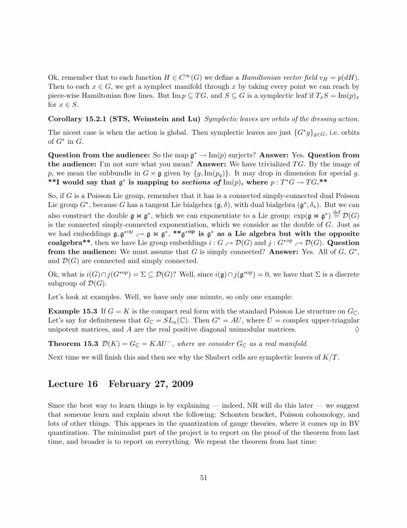
Ok, remember that to each function H ∈ C∞(G) we define a Hamiltonian vector field vH = p(dH).Then to each x ∈ G, we get a symplect manifold through x by taking every point we can reach bypiece-wise Hamiltonian flow lines. But Im p ⊆ TG, and S ⊆ G is a symplectic leaf if TxS = Im(p)xfor x ∈ S.

Corollary 15.2.1 (STS, Weinstein and Lu) Symplectic leaves are orbits of the dressing action.

The nicest case is when the action is global. Then symplectic leaves are just G∗gg∈G, i.e. orbitsof G∗ in G.

Question from the audience: So the map g∗ → Im(p) surjects? Answer: Yes. Question fromthe audience: I’m not sure what you mean? Answer: We have trivialized TG. By the image ofp, we mean the subbundle in G × g given by g, Im(pq). It may drop in dimension for special g.**I would say that g∗ is mapping to sections of Im(p), where p : T ∗G→ TG.**

So, if G is a Poisson Lie group, remember that it has is a connected simply-connected dual PoissonLie group G∗, because G has a tangent Lie bialgebra (g, δ), with dual bialgebra (g∗, δ∗). But we canalso construct the double g on g∗, which we can exponentiate to a Lie group: exp(g on g∗) def= D(G)is the connected simply-connected exponentiation, which we consider as the double of G. Just aswe had embeddings g, g∗op → g on g∗, **g∗op is g∗ as a Lie algebra but with the oppositecoalgebra**, then we have Lie group embeddings i : G → D(G) and j : G∗op → D(G). Questionfrom the audience: We must assume that G is simply connected? Answer: Yes. All of G, G∗,and D(G) are connected and simply connected.

Ok, what is i(G)∩ j(G∗op) = Σ ⊆ D(G)? Well, since i(g)∩ j(g∗op) = 0, we have that Σ is a discretesubgroup of D(G).

Let’s look at examples. Well, we have only one minute, so only one example:

Example 15.3 If G = K is the compact real form with the standard Poisson Lie structure on GC.Let’s say for definiteness that GC = SLn(C). Then G∗ = AU , where U = complex upper-triagularunipotent matrices, and A are the real positive diagonal unimodular matrices. ♦

Theorem 15.3 D(K) = GC = KAU−, where we consider GC as a real manifold.

Next time we will finish this and then see why the Shubert cells are symplectic leaves of K/T .


Since the best way to learn things is by explaining — indeed, NR will do this later — we suggestthat someone learn and explain about the following: Schonten bracket, Poisson cohomology, andlots of other things. This appears in the quantization of gauge theories, where it comes up in BVquantization. The minimalist part of the project is to report on the proof of the theorem from lasttime, and broader is to report on everything. We repeat the theorem from last time:

51

Theorem 16.1 (K) 1. The bracket on Ω1(M) defined by:

[ω, ω′] def= dπ(ω ∧ ω′) + πω(dω′)− πω′(dω) (16.1)

where π is the Poisson bivector field on M , and πω(ω′ ∧ ω′′) def= π(ω, ω′)ω′′ − π(ω, ω′′)ω′, is aLie bracket.

2. The mappting π : Ω1(M)→ Vect(M) is a Lie algebra homomorphism.

Proof: Matt will present this next week.

It’s not clear how the bracket in 1. came up, but if you try to pull back the bracket from vectorfields, you will see that it is what it must be. But perhaps its source is also from the more generaltechnology.

Theorem 16.2 (W) The natural mapping g∗ → Ω1(G)left induced by the trivialization of T ∗G byright translations is a Lie algebra isomorphism.

Proof: Theo will present this next week.

Corollary 16.2.1 We have g∗ → Vect(G), a local action G∗ y G.

Question from the audience: So we have that TG is foliated by the image of g∗. The factthat these are the symplectic leaves follows from that the image of g∗ is in Hamiltonian vectorfields? And these are all of them? Answer: Yes, well the Hamiltonian vector fields are exactly theimage under π of the exact forms, so you have to prove that this is the image of the left-invariantthings.

Corollary 16.2.2 The symplectic leaf through x ∈ G is the orbit of the above action through x.

Ok, so let’s now give an algebraic description of these orbits. First, some preliminaries. Let M bea Poisson manifold, and G and Poisson Lie group acting via a Poisson Lie action: the action mapG ×M → M is a Poisson map. An example is whenever M is Poisson, G preserves the Poissonstructure on M , and G has the trivial Poisson structure. Another example is that if H ⊆ G is asubgroup, the left and right actions H ×G→ G and G×H → G are Poisson-Lie.

Proposition 16.3 The functions preserved by G — C(M)G ⊆ C(M) — make a Poisson subalge-bra.

Proof: Let α : G×M →M , then α∗f(g,m) def= f(α(g,m)). Well, α∗(f, gM ) = α∗f, α∗gG×M ,and G-invariance means α∗f = 1 ⊗ f . Let’s make the assumption that everything is algebraic, sothat C(G ×M) = C(G) ⊗ C(M). Then if f ∈ C(M)G, then α∗f, gM = 1 ⊗ f, gM , and sof, gM is G-invariant.

Ok, so one more thing, which is an obvious corollary, but indeed isn’t even: it’s just what we said.If M/G is a manifold — this is non-trivial, it may be quite singular, but suppose that it is or thatit can naturally be made so — then the projection M →M/G is a Poisson map. This is just whatwe said above, but not in terms of Poisson algebras but in terms of their spectra.

52

Corollary 16.3.1 If H ⊆ G is a Poisson Lie subgroup, then both H\G and G/H are Poissonmanifolds with Poisson maps G→ G/H and G→ H\G.

Question from the audience: Why is the action of G on G/H Poisson? Answer: G y G isPoisson, and you push it down.

Ok, so consider the double D(G), the connected simply-connected Lie group with algebra g on g∗.Then we have natural embeddings G →

iD(G) ←

jG∗op. Because i(g) ∩ j(g∗op) = 0, we see that

Σ def= i(G) ∩ j(G∗op) is a discrete subgroup of D(G).

We have already proven:

Proposition 16.4 i and j are inclusions of Poisson Lie groups.

Corollary 16.4.1 D(G) → D(G)/j(G∗op) is Poisson and commutes with the left D(G)-action.Ditto for D(G)→ D(G)/i(G).

So, we have a sequence of Poisson maps:

G D(G) D(G)/G∗opi

and G∗op acts on the double by left multiplication (as a subgroup of D(G)), and so also acts on theright term, and the diagram commutes:

G D(G) D(G)/G∗opi

G∗op G∗op

Then G→ D(G)/G∗op x G∗op. In particular, this gives g∗ → Vect(D(G)/G∗op).

Theorem 16.5 f commutes with g∗ action (dressing on G, and natural on D(G)/G∗op).

Corollary 16.5.1 Symplectic leaves of G are connected components of G∗op orbits on D(G)/G∗op.I.e. they are double cosets G∗opxG∗op for x ∈ D(G).

This is a general fact, and of course it is the same for G∗, because there is this symmetry. We haveto use G∗ → D(G)/G.

Example 16.1 Let K be the compact real form of GC simple. Think of K = SU(n). Let’s assumethe standard Poisson Lie structure on GC. We already had the discussion that K∗ = AU ⊆ B ⊆ G,the subgroup of the Borel subgroup of G, where U is the subgroup of complex unipotent matricesin B, and A is the real positive diagonal matrices. If you want: A is the split real form of theCartan H ⊆ B; it is the one for this particular Borel. ♦

The Iwasawa decomposition of GC is G = KAU .

53

Theorem 16.6 D(K) ∼= G as a real manifold, and the Iwasawa decomposition agrees with naturalembeddings i : K → G and j : K∗op → G.

We are not that careful about K∗ and K∗op, but it doesn’t matter: it’s upper- versus lower-triangular matrices.

In this particular case, i(K) ∩ j(K∗op) = 1.

So the Double of a complex simple Lie group has a natural description: you just have to complexify**missed**.

Corollary 16.6.1 D(K)/K∗op ∼= K, and so we have a global action of K∗op on K.

Thus, symplectic leaves of K are preimages of the double cosets K∗opxK∗op ⊆ G with respect tothe natural embedding K → G = KAU .

So what we have to do now is to describe the double cosets. What do we know about G? We mustdescribe AUxAU .

Well, we know that G =⊔w∈W BwB, the Bruhat decomposition. So let’s choose x ∈ BwB.

Ok, so let’s consider AUbwb′AU . How many parameters are left? Can we absorb b into AU?Obviously not. But we can write b = auk, where k ∈compact part of H, so it is in (S1)r, wherer is the rank. Ok, so we have AUkwk′AU — we have also used b′ = k′a′u′ —, and we move k′

past w to get k′ww. Ok, so what is kk′ww? It is an element where? We claim that it is naturally inN(T ) ⊆ K. Because anything else can be absorbed.

So we have proved: The space of double cosets K∗op\D(K)/K∗op is naturally isomorphic toN(T ).

So let’s take the subset Nw(T ) ⊆ N(T ) ∼= T oW corresponding the w ∈W . Then:

Theorem 16.7 K ∼=⊔w∈W Kw, where each Kw is homogeneous Poisson submanifold, fibered over

the torus T ⊆ K, such that fibers are symplectic leaves isomorphic to Shubert cells of K/T .

The idea is you take a point in the symplectic leaf, and the statement is that you can assemblethese into a homogeneous Poisson submanifold: i.e. it is the union of leaves of the same size. Weknow that K/T ∼= G/B ∼=

⊔w Cw, where G/B is the generalized flag variety, and Cw ⊆ Uw, the

elements mapped to the negative **something** when conjugated by w.

The point is that because D(K) ∼= G ∼= KAU , the space of double cosets really parameterizessymplectic leaves, because it is the space of dressing orbits K∗op\K. But some symplectic leaveshave the same dimension, and the wonderful thing is that you can assemble leaves of the samedimension into these subvarieties.

Example 16.2 In particular, you take SU(2). How many cells are there in SU(2)/T? It is Cw0tC1,of dimensions 2 and 0. (How many even numbers are there less than 3? dimR(Cw) = 2`(w).) Andthis is Bw0B/B t pt. So it is easy to show that Cw0

∼= S2, and so the result is a symplecticmanifold (S2, ωSU(2)).

54

Do we have any Poisson forms on the sphere? Well, there’s the area form, (S2, ω), coming fromthe coadjoint orbit of SU(2) on SU(2)∗. But this is a different one. ♦

Anyway, all the C2 have symplectic structure.

Lecture 17 March 2, 2009

17.1 Matt presents a proof from last time

We will show that the bracket defined last time on Ω1(P ) is a Lie bracket, and that we get ahomomorphism into vector fields. Precisely: we have a Poisson manifold (P, π), and from this wedefine: π : Ω1(P ) → Vect(P ) defined by 〈η, π〉 = π(η, ω). This may be the negative of last time:we keep the one-forms in the same order. From this we define a bracket on Ω1(P ), by:

[ω1, ω2]Ω1(P ) = dÄπ(ω1, ω2)

ä− iπω1(dω2) + iπω2(dω1) (17.1)

We remark that if ω1, ω2 are closed, then [ω1, ω2] is exact. We will show that −π is a Lie algebrahomomorphism.

Lemma 17.1 π(df) = Xf : the image of an exact one-form is a Hamiltonian vector field.

Proof: 〈dg, π(df)〉 def= π(dg, df) def= g, f def= 〈dg,Xf 〉.

We remark that we have chosen to define Hamiltonian vector fields by putting in the secondcoordinate. This is a sign choice, and with this convention [Xf , Xh] = −Xf,h. Otherwise, we’dhave a sign somewhere else.

Lemma 17.2 [fω1, ω2] = f [ω1, ω2] + π(df, ω2) · ω1, where · is the action **?**

Proof: Exercise 29.

Proposition 17.3 [, ] is a Lie bracket on Ω1(P ).

Proof: Antisymmetry is clear. We check Jacobi, by checking it on exact forms and then using thederivation property lemma 17.2.

[df, dg] = dÄπ(df, dg)

ä= df, g (17.2)

[[df, dg], dh] + c.p. = [df, g, dh] + c.p. = df, g, h+ c.p. = 0 (17.3)

Proposition 17.4 −π : Ω1(P )→ Vect(P ) is a Lie algebra homomorphism.

Proof: Again we check on exact things, and then show that everything performs well under mul-tiplication by functions.

−π([df, dg]) = −π(df, g) = −Xf,g = [−Xf ,−Xg] = [−π(df),−π(dg)] (17.4)

55

For the general case, observe that [fV,W ] = f [V,W ]− (Wf) · V .

17.2 Symplectic leaves of compact groups

Last time, we discussed: we have K ⊆ GC the compact real form of G, with standard PoissonLie structure. Last time we came to the conclusion that K =

⊔wKw, each of which is a Poisson

homogeneous space. And each Kw is fibered over the torus, with fibers Cw the Shubert cells.

Last time we gave an example of SU2, with a small mistake. We have SU2∼= S3, and we were

talking about SU2/T . Of course, K/T =⊔w Cw. In our case, SU2/T = S3/T = Cw0 t C1. The

first is two-dimensional and the latter zero-dimensional.

Question from the audience: How do you build the Cws? Answer: The way we did before,we took K/T ∼= G/B ∼=

⊔w BwB/B ∼=

⊔w Uw, and Cw = Uw = u ∈ U s.t. w−1uw ∈ U−. So

in the case of SU2, Uw0 = Ç

1 a0 1

ås.t. a 6= 0 = U r e, and U1 = e. Question from the

audience: So it’s the sphere without two points, and then another point. How is this compact?Answer: We will return to it.

Moving on, we had two facts:

1. D(K) = GC = KAU , and AU = K∗op.

2. K → D(K) → D(K)/K∗op, and the actions of right-multiplication compute. So: Sym-plectic leaves are connected components of pre-images of K∗op-orbits, where K∗op acts byleft-multiplicaiton.

Now we can also ask about symplectic leaves of K∗op. Think about the analogy. When we have Liealgebras, it looks like we have two inputs of symplectic geometry: structures on K and K∗. Whenwe quantize, and get a bialgebra, we will have two representation theories: one of “representations”and one of “corepresentations”.

So the counterpart will be dual pairs of Lie bialgebras. So far we have worked finite-dimensionally,except for a short aside on KM algebra. Infinite-dimensional spaces have canonical duals only inthe presence of topology. Algebraically, we will talk not about a space and its dual, but rather adual pair, which is a pair of spaces and a nondegenerate pairing.

Anyway, so we have:K∗op → D(K)→ D(K)/K (17.5)

and symplectic leaves of K∗op are preimages of K-orbits in D(K)/K, where K acts by left multi-plication.

Exercise 30 Provide an explicit description of the symplectic leaves. We will return to this afterstudying symplectic leaves of GC and G∗C. Hint: G = KAU = UAK and G = KH are twodecompositions. In the latter, this is “compact” times “hermitian”. In SLn, this is SUn ·H, whereH really is the space of Hermitian matrices. In this language the symplectic leaves will be simply

56

Hermitian orbits. There is a natural identification H with AU . Question from the audience:This is the polar decomposition? Answer: Yes.

17.3 Symplectic Leaves of G∗C?

Let’s investigate the following question. Suppose we have (g, δr) a factorizable Lie bialgebra. Forexample: 1. g simple with the standard r-matrix; 2. D(b) for any b a Lie bialgebra is factorizable.We haven’t really talked about what happens if you take the double of the double, but you don’tget anything new.

So, t = r + σ(r0 ∈ S2(g)g is a nondegenerate invariant bilinear form on g∗. If g is simple, t is thedual to the Killing form.

Then we defined r± : g∗ → g by r+ : l 7→ (id⊗ l)r and r− : l 7→ −(l⊗ id)r. So we define t : g∗∼→ g,

and then t(l) = (id⊗ l)t = r+(l)− r−(l). So we have the factorization property: for all x ∈ g, thereis a unique decomposition x = x+ − x− such that for some l ∈ g∗, x± = r±(l).

Now, let’s consider the map i : D(g) = g⊕ g∗ → g⊕ g by (x, l) 7→ (x+ r+(l), x− r−(l)).

Theorem 17.5 This map is a Lie algebra isomorphism.

Proof: First we show that this is a Linear isomorphism. Well, (x1, x2) 7→? ∈ g ⊕ g∗. We havex = (x1 + x2)/2, and we want to extract l. But x1 − x2 = r+(l)− r−(l) = t(l), so l = t−1(x1 − x2).By the definition of factorizability, this defines l uniquely, and so we have the inverse to the abovemap.

Second, it’s clear that i is a Lie algebra homomorphism. Indeed, the diagonal map g→ g⊕ g is aLie homomorphism, and so are r±.

Corollary 17.5.1 When g is factorizable, we have:

• D(G) ∼= g⊕ g as a Lie algebra.

• D(G) ∼= g⊕ g∗ as a coalgebra.

and so D(D(b)) has no new data for any bialgebra b.

Now we take G corresponding to our factorizable g, and by the corollary we can take D(G) ∼= G×Gand D(G)∗ ∼= G×G∗.

Exercise 31 Let g be factorizable. Take rD to be the r-matrix for the double of g. This is canonical:

rD =∑i

ei ⊗ ei ∈ g⊗ g∗ → D(g)⊗2 (17.6)

Ok, so let’s take (i⊗ i)(rD) ∈ (g⊕ g)2. Compute the image in terms of i.

57

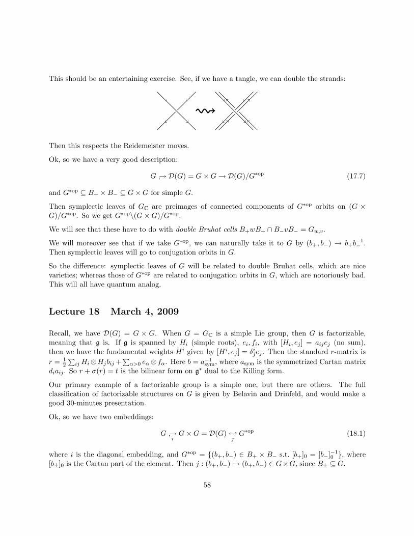
This should be an entertaining exercise. See, if we have a tangle, we can double the strands:

Then this respects the Reidemeister moves.

Ok, so we have a very good description:

G → D(G) = G×G→ D(G)/G∗op (17.7)

and G∗op ⊆ B+ ×B− ⊆ G×G for simple G.

Then symplectic leaves of GC are preimages of connected components of G∗op orbits on (G ×G)/G∗op. So we get G∗op\(G×G)/G∗op.

We will see that these have to do with double Bruhat cells B+wB+ ∩B−vB− = Gw,v.

We will moreover see that if we take G∗op, we can naturally take it to G by (b+, b−) → b+b−1− .

Then symplectic leaves will go to conjugation orbits in G.

So the difference: symplectic leaves of G will be related to double Bruhat cells, which are nicevarieties; whereas those of G∗op are related to conjugation orbits in G, which are notoriously bad.This will all have quantum analog.


Recall, we have D(G) = G × G. When G = GC is a simple Lie group, then G is factorizable,meaning that g is. If g is spanned by Hi (simple roots), ei, fi, with [Hi, ej ] = aijej (no sum),then we have the fundamental weights H i given by [H i, ej ] = δijej . Then the standard r-matrix isr = 1

2

∑ij Hi⊗Hjbij +

∑α>0 eα⊗fα. Here b = a−1

sym, where asym is the symmetrized Cartan matrixdiaij . So r + σ(r) = t is the bilinear form on g∗ dual to the Killing form.

Our primary example of a factorizable group is a simple one, but there are others. The fullclassification of factorizable structures on G is given by Belavin and Drinfeld, and would make agood 30-minutes presentation.

Ok, so we have two embeddings:

G →iG×G = D(G)←

jG∗op (18.1)

where i is the diagonal embedding, and G∗op = (b+, b−) ∈ B+ × B− s.t. [b+]0 = [b−]−10 , where

[b±]0 is the Cartan part of the element. Then j : (b+, b−) 7→ (b+, b−) ∈ G×G, since B± ⊆ G.

58

18.1 Symplectic Leaves in G∗

G∗op is G∗ with the opposite Poisson structure. But we will for a while talk only about the groupstructure, keeping the Poisson structure only up to non-zero constant multiple. So we will writeG∗.

So, we have G∗ →jG × G → (G × G)/G, and symplectic leaves in G∗ are exactly connected

components of preimages of left-G-orbits in (G×G)/G.

So, first of all, what is (G × G)/G? As a set, it is the set of cosets (g1, g2)G s.t. gi ∈ G. So(g1, g2)G = (g1g, g2g) s.t. g ∈ G. When we have a set with orbits, a good way to parameterizethem is to take a cross section. One way to do this is make one of them the identity: g = g−1

2 ,whence (G×G)/G is in bijection with G× e.

Here’s another way to understand this set. Let’s consider G-invariant functions. I.e., we look atthe function π : (G×G)→ G by (g1, g2) 7→ g1g

−12 . Then G y (G×G) diagonally, and this pushes

forward to the trivial action G y G. So, G acts transitively on fibers π : (G×G)→ G, and so wecan identify the set of cosets with the base: π : (G×G)/G ∼= G.

Ok, so what about the left action? We have h(g1, g2)G = (hg1, hg2)G π→ h(g1g−12 )h−1. Ok, so

the left action of G on (G × G)/G corresponds under π to the conjugation action of G on G. Inparticular, π : left G orbits on (G×G)/G ∼= conjugation orbits of G.

Theorem 18.1 Symplectic leaves of G∗ are connected components of preimages of conjugation

orbits in G with respect to the map G∗j→ G×G π→ G. This map is (b+, b−) 7→ (b+, b−)→ b+(b−)−1.

Now look at what happens to diagonal elements. If both b± are in the Cartan, well [b+]0 = [b−]−10 ,

so elements in the Cartan are mapped to their square. We mentioned the group Σ = i(B+)∩j(B−),and we have shown that |Σ| = 2r, because Σ is the kernel of the map, which is also the diagonalthings with only ±1s.

We did the symplectic leaves of K, the compact real form of G. We will now try to do K∗. SinceG is Poisson-Lie, k = Lie(K) is the compact real form of g, and inherits the Poisson bialgebrastructure. So K∗ is the real form of the corresponding dual algebra, and is a real form of G∗. **Itis not necessarily compact.** Indeed, we say that k is spanned by iHj , eα− fα, i(eα + fα). AndK∗ ∼= AU where A is the real positive form of HC ⊆ GC.

Proposition 18.2 AU ∼= H as real varieties, where H is the Hermetian unimodular matriceswith positive eigenvalues.

Proof: We map b 7→ b∗b. This is obvious on the diagonal matrices, and the rest is Exercise 32.

Here b∗ is the Hermetian conjugation of b.

Proposition 18.3 K∗ ∼= (b, (b∗)−1) ⊆ G∗C. This is a real form of G∗C dual to K ⊆ GC.

Proof: Exercise 33.

59

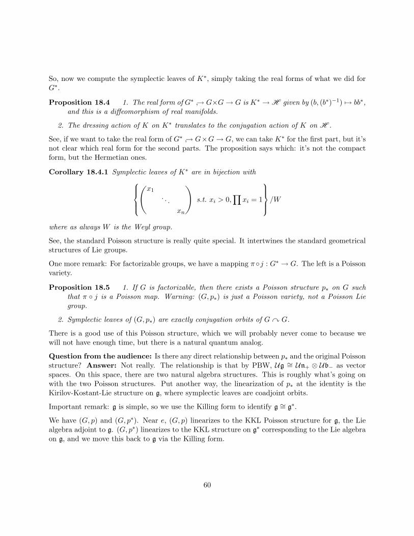
So, now we compute the symplectic leaves of K∗, simply taking the real forms of what we did forG∗.

Proposition 18.4 1. The real form of G∗ → G×G→ G is K∗ →H given by (b, (b∗)−1) 7→ bb∗,and this is a diffeomorphism of real manifolds.

2. The dressing action of K on K∗ translates to the conjugation action of K on H .

See, if we want to take the real form of G∗ → G×G→ G, we can take K∗ for the first part, but it’snot clear which real form for the second parts. The proposition says which: it’s not the compactform, but the Hermetian ones.

Corollary 18.4.1 Symplectic leaves of K∗ are in bijection withÖx1

. . .xn

ès.t. xi > 0,

∏xi = 1

/Wwhere as always W is the Weyl group.

See, the standard Poisson structure is really quite special. It intertwines the standard geometricalstructures of Lie groups.

One more remark: For factorizable groups, we have a mapping πj : G∗ → G. The left is a Poissonvariety.

Proposition 18.5 1. If G is factorizable, then there exists a Poisson structure p∗ on G suchthat π j is a Poisson map. Warning: (G, p∗) is just a Poisson variety, not a Poisson Liegroup.

2. Symplectic leaves of (G, p∗) are exactly conjugation orbits of G y G.

There is a good use of this Poisson structure, which we will probably never come to because wewill not have enough time, but there is a natural quantum analog.

Question from the audience: Is there any direct relationship between p∗ and the original Poissonstructure? Answer: Not really. The relationship is that by PBW, Ug ∼= Un+ ⊗ Ub− as vectorspaces. On this space, there are two natural algebra structures. This is roughly what’s going onwith the two Poisson structures. Put another way, the linearization of p∗ at the identity is theKirilov-Kostant-Lie structure on g, where symplectic leaves are coadjoint orbits.

Important remark: g is simple, so we use the Killing form to identify g ∼= g∗.

We have (G, p) and (G, p∗). Near e, (G, p) linearizes to the KKL Poisson structure for g, the Liealgebra adjoint to g. (G, p∗) linearizes to the KKL structure on g∗ corresponding to the Lie algebraon g, and we move this back to g via the Killing form.

60

(g, δr) Lie bialgebra

g g∗

g∗ g

(g, p(0)∗ ) (g, p(0))

dual dual


Last time we classified symplectic leaves of G∗ and K∗, corresponding to G and K — K is thecompact real form of G, and K∗ is its dual group. Today we will classify symplectic leaves of G,and this will conclude our classical-geometry discussion of Poisson Lie groups.

We use the same strategy. We embed G → D(G) → D(G)/G∗ as a Poisson Lie group, where asalways G is simple and complex. We want to understand connected components of preimages ofleft G∗-orbits on D(G)/G∗, which are orbits of the dressing action on G∗, which will be symplecticleaves. As before, but the groups are different.

As we saw before, G is factorizable if it has the standard PL structure, and so as D(G) = G ×G.

Ok, so we have the diagonal embeddingG → G×G, and we mod out byG×G→ (G×G)/G∗. **Wewrite G∗ rather than G∗op because we are only interested in the group structure.**And G∗ = (b+, b−) s.t. b± ∈ B±, [b+]0 = [b−]−1

0 → G × G. What are the G∗ orbits on (G ×G)/G∗?

Recall, we have the Bruhat decomposions G =⊔w BwB, but we actually have four different ones:

each B can be a B+ or a B−. So let’s take G =⊔w B−wB−. So, we have:

(G×G) x G∗ → B+ ×B− (19.1)

And it’s natural to take different decompositions. Indeed, if (g, h) ∈ G × G, we should takeg ∈ B+uB+ and h ∈ B−vB−. Then this is designed for studying the action of B+ ×B−.

Oh, let’s take a correction. We don’t want to study G∗-orbits on G×G, but rather on the diagonalembedding mod G∗. I.e. we want to understand:

G∗\diag(G)/G∗

Ok, so we have (g, g) ∈ G × G, with g ∈ B+uB+ ∩ B−vB−def= Guv, a double Bruhat cell. Then

G∗(g, g)G∗ =? G∗ = (u+h, u−h−1) s.t. u± ∈ U±B±, h ∈ H. We remark that by the Bruhat

61

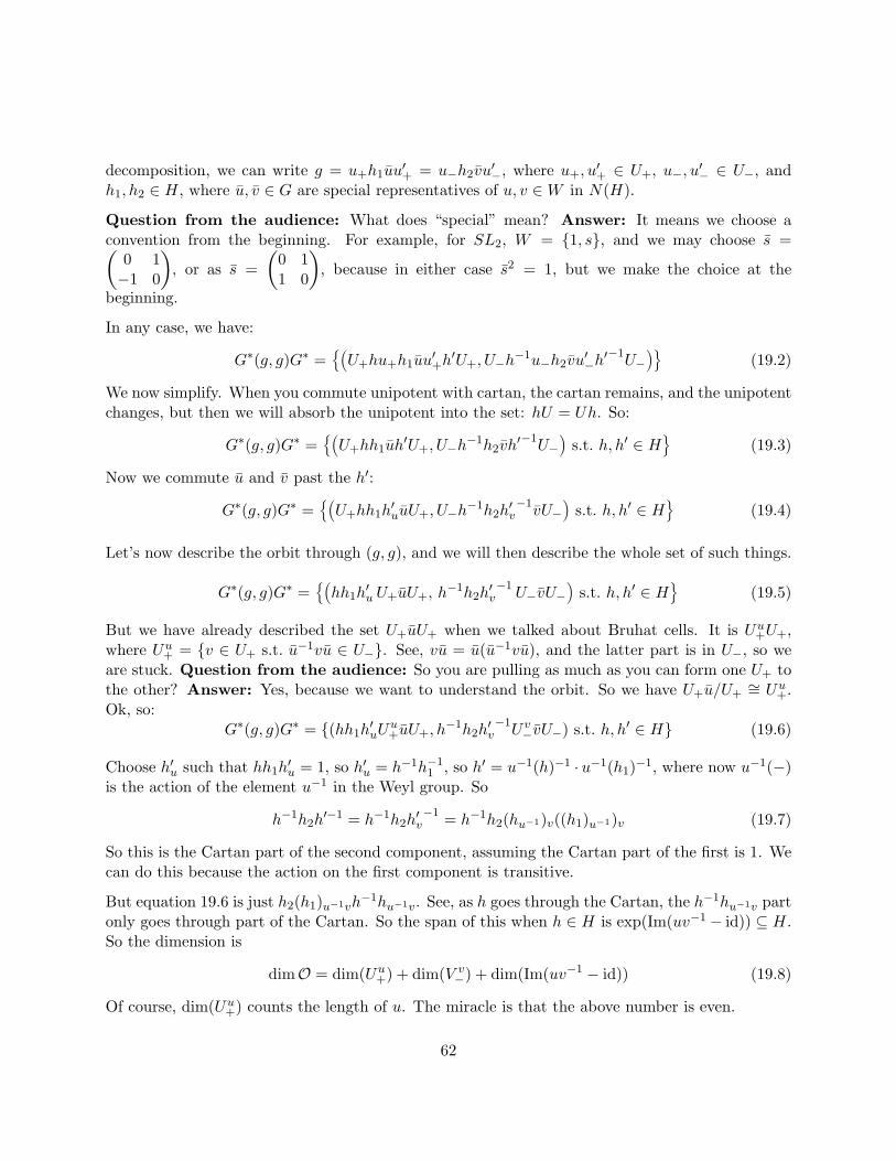
decomposition, we can write g = u+h1uu′+ = u−h2vu

′−, where u+, u

′+ ∈ U+, u−, u′− ∈ U−, and

h1, h2 ∈ H, where u, v ∈ G are special representatives of u, v ∈W in N(H).

Question from the audience: What does “special” mean? Answer: It means we choose aconvention from the beginning. For example, for SL2, W = 1, s, and we may choose s =Ç

0 1−1 0

å, or as s =

Ç0 11 0

å, because in either case s2 = 1, but we make the choice at the

beginning.

In any case, we have:

G∗(g, g)G∗ =¶ÄU+hu+h1uu

′+h′U+, U−h

−1u−h2vu′−h′−1U−ä©

(19.2)

We now simplify. When you commute unipotent with cartan, the cartan remains, and the unipotentchanges, but then we will absorb the unipotent into the set: hU = Uh. So:

G∗(g, g)G∗ =¶ÄU+hh1uh

′U+, U−h−1h2vh

′−1U−ä

s.t. h, h′ ∈ H©

(19.3)

Now we commute u and v past the h′:

G∗(g, g)G∗ =¶ÄU+hh1h

′uuU+, U−h

−1h2h′v−1vU−

äs.t. h, h′ ∈ H

©(19.4)

Let’s now describe the orbit through (g, g), and we will then describe the whole set of such things.

G∗(g, g)G∗ =¶Ähh1h

′u U+uU+, h

−1h2h′v−1U−vU−

äs.t. h, h′ ∈ H

©(19.5)

But we have already described the set U+uU+ when we talked about Bruhat cells. It is Uu+U+,where Uu+ = v ∈ U+ s.t. u−1vu ∈ U−. See, vu = u(u−1vu), and the latter part is in U−, so weare stuck. Question from the audience: So you are pulling as much as you can form one U+ tothe other? Answer: Yes, because we want to understand the orbit. So we have U+u/U+

∼= Uu+.Ok, so:

G∗(g, g)G∗ = (hh1h′uU

u+uU+, h

−1h2h′v−1Uv−vU−) s.t. h, h′ ∈ H (19.6)

Choose h′u such that hh1h′u = 1, so h′u = h−1h−1

1 , so h′ = u−1(h)−1 · u−1(h1)−1, where now u−1(−)is the action of the element u−1 in the Weyl group. So

h−1h2h′−1 = h−1h2h

′v−1 = h−1h2(hu−1)v((h1)u−1)v (19.7)

So this is the Cartan part of the second component, assuming the Cartan part of the first is 1. Wecan do this because the action on the first component is transitive.

But equation 19.6 is just h2(h1)u−1vh−1hu−1v. See, as h goes through the Cartan, the h−1hu−1v part

only goes through part of the Cartan. So the span of this when h ∈ H is exp(Im(uv−1 − id)) ⊆ H.So the dimension is

dimO = dim(Uu+) + dim(V v−) + dim(Im(uv−1 − id)) (19.8)

Of course, dim(Uu+) counts the length of u. The miracle is that the above number is even.

62

19.1 Theo presents a proof of Weinstein’s theorem

**Naturally, I could not take notes and speak at the board. Here are my preparedremarks:**

This section consists of a proof of Theorem 16.2 stated in the February 27th lecture of NicolaiReshetikhin’s seminar on Quantum Groups. We first restate the theorem, and then proceed withthe proof. The proof is largely the same as Weinstein’s original, available in:

A. Weinstein. Some remarks on dressing transformations. J. Fac. Sci. Univ. Tokyo.Sect. 1A, Math. 35 (1988), 163-167.

Theorem 19.1 (Alan Weinstein) Let G be a Poisson Lie group, with Poisson bivector field π.Define a Lie bracket on Ω1(G) by

[ω, ω′]Ω1(G)def= dÄπ(ω ∧ ω′)

ä+ πÄω(dω′)

ä− πÄω′(dω)

ä(19.9)

where πÄω(ω′∧ω′′)

ä def= π(ω, ω′)ω′′−π(ω, ω′′)ω′. Then the natural mapping g∗ → Ω1(G)left inducedby the trivialization of T ∗G by right translations is a Lie algebra isomorphism.

Proof: We have seen already (Theorem 16.1) that [, ]Ω1(G) is a valid Lie bracket, and that g∗ →Ω1(G)left is an isomorphism of vector spaces. Let w1, w2 ∈ g∗, and choose functions any one-formsω1, ω2 ∈ Ω1(G) so that ωi(e) = wi. Then [ω1, ω2]Ω = d

Äπ(ω1, ω2)

ä(e), since π(e) = 0. But this is

just dπ(e)Äω1(e), ω2(e)

ä= [w1, w2]g∗ , since π(e) = 0. So it suffices to show that the bracket of two

left-invariant forms is left-invariant.

We now make an aside about sign conventions and notation. The “insert” contraction c used bythe mathematicians is horrendous: do you insert into the first spot, the last, ??? The physicists’indices are better, as long as you’re not taking derivatives: when you do, you have to rememberthat it’s not all tensorial. For our purposes, we adopt the following conventions. We will alwayswrite sections of wedge products of the tangent bundle before sections of wedge products of thecotangent bundle, and we will work in terms of the pairing 〈, 〉 : Vect(G) ⊗ Ω1(G) → C(G). Thenπ is our Poisson field, and we will define π : Ω1(G)→ Vect(G) by:

〈πω1, ω2〉 = 〈π, (ω1, ω2)〉 = π(ω1, ω2) (19.10)

The philosophy is always to keep all the symbols in the same order.

Moreover, given a vector field X, we have the Lie derivative LX acting on tensor fields (andpreserving their type), defined by LXf = 〈X, df〉 = X[f ], LXY = [X,Y ] the bracket of vectorfields, and on one-forms:

〈Y,LXω〉 = 〈(Y,X), dω〉+ 〈Y, d(〈X,ω〉)〉 (19.11)

In general, LX is a derivation across any tensor contraction.

63

In this notation, the bracket [, ]Ω defined in equation 19.9 is determined by:

〈Y, [ω1, ω2]Ω〉 = 〈Y, d(π(ω1, ω2)) + 〈(Y, πω1), dω2〉 − 〈(Y, πω2), dω1〉 (19.12)

In light of equation 19.11, we now perform a long sequence of manipulations, simplifying the aboveexpression.

〈(Y, πω1), dω2〉 = 〈Y,Lπω1ω2〉 − 〈Y, d(〈πω1, ω2〉= 〈Y,Lπω1ω2〉 − 〈Y, d(π(ω1, ω2)〉 (19.13)

−〈(Y, πω2), dω1〉 = −〈Y,Lπω2ω1〉+ 〈Y, d(〈πω2, ω1〉= −〈Y,Lπω2ω1〉 − 〈Y, d(π(ω1, ω2)〉 (19.14)

Therefore, making heavy use of cut-and-paste:

〈Y, [ω1, ω2]Ω〉 = −〈Y, d(π(ω1, ω2)〉+ 〈Y,Lπω1ω2〉 − 〈Y,Lπω2ω1〉 (19.15)

= −LY

Äπ(ω1, ω2)

ä+ 〈Y,Lπω1ω2〉 − 〈Y,Lπω2ω1〉 (19.16)

= −(LY π)(ω1, ω2)− π(LY ω1, ω2)− π(ω1,LY ω2)+ 〈Y,Lπω1ω2〉 − 〈Y,Lπω2ω1〉 (19.17)

= −(LY π)(ω1, ω2)− π(LY ω1, ω2)− π(ω1,LY ω2)+ Lπω1〈Y, ω2〉 − 〈Lπω1Y, ω2〉 −Lπω2〈Y, ω1〉+ 〈Lπω2Y, ω1〉 (19.18)

= −(LY π)(ω1, ω2)− π(LY ω1, ω2)− π(ω1,LY ω2)− 〈[πω1, Y ], ω2〉+ 〈[πω2, Y ], ω1〉+ Lπω1〈Y, ω2〉 −Lπω2〈Y, ω1〉 (19.19)

= −(LY π)(ω1, ω2)− π(LY ω1, ω2)− π(ω1,LY ω2)+ 〈[Y, πω1], ω2〉 − 〈[Y, πω2], ω1〉+ Lπω1〈Y, ω2〉 −Lπω2〈Y, ω1〉 (19.20)

= −(LY π)(ω1, ω2)− π(LY ω1, ω2)− π(ω1,LY ω2)+ 〈LY (πω1), ω2〉 − 〈LY (πω2), ω1〉+ Lπω1〈Y, ω2〉 −Lπω2〈Y, ω1〉 (19.21)

= −(LY π)(ω1, ω2)− π(LY ω1, ω2)− π(ω1,LY ω2)+ 〈(LY π)ω1 + πLY ω2, ω2〉 − 〈(LY π)ω2 + πLY ω2, ω1〉+ Lπω1〈Y, ω2〉 −Lπω2〈Y, ω1〉 (19.22)

= (LY π)(ω1, ω2) + Lπω1〈Y, ω2〉 −Lπω2〈Y, ω1〉 (19.23)

Now let ω1, ω2, and Y be left-invariant. Then 〈Y, ωi〉 is a constant, and so the correspondingderivatives vanish. We win if we can show that 〈Y, [ω1, ω2]Ω〉, or equivalently that (LY π)(ω1, ω2)is a constant, or that LY π is left-invariant whenever Y is.

But this is almost immediate. The condition that G be Poisson-Lie is that π satisfy the followingcocycle identity:

π(gh) = dl⊗2g π(h) + dr⊗2

h π(g) (19.24)

We have used the left- and right-actions lg, rg : G → G given by lgh = gh and rgh = hg. Thenfor any g, h ∈ G, lg and rh commute, l· is a homomorphism, and r· an antihomomorphism. Thedifferentials dlg, drg : TG→ TG, and so the tensor square of a differential acts on a bivector.

64

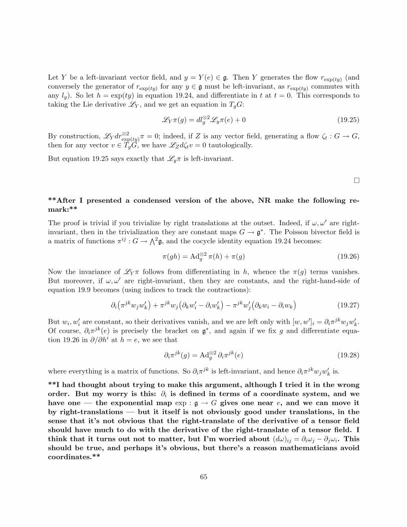
Let Y be a left-invariant vector field, and y = Y (e) ∈ g. Then Y generates the flow rexp(ty) (andconversely the generator of rexp(ty) for any y ∈ g must be left-invariant, as rexp(ty) commutes withany lg). So let h = exp(ty) in equation 19.24, and differentiate in t at t = 0. This corresponds totaking the Lie derivative LY , and we get an equation in TgG:

LY π(g) = dl⊗2g Lyπ(e) + 0 (19.25)

By construction, LY dr⊗2exp(ty)π = 0; indeed, if Z is any vector field, generating a flow ζt : G → G,

then for any vector v ∈ TgG, we have LZdζtv = 0 tautologically.

But equation 19.25 says exactly that Lyπ is left-invariant.

**After I presented a condensed version of the above, NR make the following re-mark:**

The proof is trivial if you trivialize by right translations at the outset. Indeed, if ω, ω′ are right-invariant, then in the trivialization they are constant maps G → g∗. The Poisson bivector field isa matrix of functions πij : G→ ∧2g, and the cocycle identity equation 19.24 becomes:

π(gh) = Ad⊗2g π(h) + π(g) (19.26)

Now the invariance of LY π follows from differentiating in h, whence the π(g) terms vanishes.But moreover, if ω, ω′ are right-invariant, then they are constants, and the right-hand-side ofequation 19.9 becomes (using indices to track the contractions):

∂iÄπjkwjw

′k

ä+ πjkwj

Ä∂kw

′i − ∂iw′k

ä− πjkw′j

Ä∂kwi − ∂iwk

ä(19.27)

But wi, w′i are constant, so their derivatives vanish, and we are left only with [w,w′]i = ∂iπjkwjw

′k.

Of course, ∂iπjk(e) is precisely the bracket on g∗, and again if we fix g and differentiate equa-tion 19.26 in ∂/∂hi at h = e, we see that

∂iπjk(g) = Ad⊗2

g ∂iπjk(e) (19.28)

where everything is a matrix of functions. So ∂iπjk is left-invariant, and hence ∂iπjkwjw′k is.

**I had thought about trying to make this argument, although I tried it in the wrongorder. But my worry is this: ∂i is defined in terms of a coordinate system, and wehave one — the exponential map exp : g → G gives one near e, and we can move itby right-translations — but it itself is not obviously good under translations, in thesense that it’s not obvious that the right-translate of the derivative of a tensor fieldshould have much to do with the derivative of the right-translate of a tensor field. Ithink that it turns out not to matter, but I’m worried about (dω)ij = ∂iωj − ∂jωi. Thisshould be true, and perhaps it’s obvious, but there’s a reason mathematicians avoidcoordinates.**

65


We begin by repeating some material from last time.

We let G be a simple complex Poisson Lie group with the standard structure. Recall that thesymplectic leaves of G are given by the map G → D(G) = G×G → D(G)/G∗, and G∗ → G×Gas (b+, b−) s.t. b± ∈ B±, [b+]0 = [b−]−1

0 . In this language, the symplectic leaves are connectedcomponents of preimages of left G∗ orbits in D(G)/G∗.

We have two related Bruhat decompositions: G =⊔u∈W B+uB+ =

⊔u∈W B−uB− and we define

the double Bruhat cells Gu,v = B+uB+ ∩ B−vB−. Let g ∈ Gu,v; we want to study the G∗ orbitthrough (g, g)G∗.

Well, B± = HU±. We fix u and v representing u and v; then g ∈ B+uB+ so g = u+h1uu′+, and

by the same token g = u−h2vu′− **shame we’re using “u” in two different ways**. Then he

orbit through (g, g)G∗ is

O(g,g)G∗ = U+hu+h1uu′+︸︷︷︸

g

h′U+, U−h−1u−h2vu

′−︸︷︷︸

g

h′−1U− (20.1)

So, we now want to commute things past each other, so as to understand what part of G is thestabilizer, and what part is transitive on the orbit. We explained last time that U+uU+ = Uu+uU+,

where Uu+def= x ∈ Y s.t. u−1xu ∈ U−; this is the limit of our ability to commute an upper-

triangular past u. For SLn, u and v are monomimal n × n matrices, i.e. exactly one nonzeroelement in each row and each column. I.e. these are permutation matrices up to a diagonal matrix.Similarly, U−vU− = Uv−vU−, where Uv−

def= x ∈ U− s.t. v−1xv ∈ U+.

So,O =

¶Uu+hh1h

′uuU+, U

v−h−1h2(h′v)

−1vU− s.t. h, h′ ∈ H©

(20.2)

We make a change of variables: h′u = h′′uh−11 h−1, whence (h′v)

−1 =Äh′′v(h1)−1

vu−1h−1vu−1

ä−1. (H is

commutative.) Hence the orbit is:

O =¶Uu+h′′uuU+, U

v−h−1h2(h1)vu−1hvu−1h′′v

−1vV− s.t. h′′, h ∈ H

©(20.3)

We can always move elements of the Cartan past U+, because it acts by conjugation. Then weget:

O =¶¶Uu+uU+h

′′, Uv−Äh−1hvu−1

ä[h2(h1)vu−1 ] vU−h′′

−1©

s.t. h, h′′ ∈ H©

(20.4)

=¶ÄUu+u, U

v−Äh−1hvu−1

ä[h2(h1)vu−1 ] v

äs.t. h ∈ H

©G∗ (20.5)

Now, as we vary the Cartan h, the part(h−1hvu−1

)is not the full Cartan H. Indeed, we define

Hw = h−1hw = exp(Im(w−id)), where (w−id) : h→ h naturally. This is often smaller dimensionthan all of H. For example, when w = id, Hw = e. But also, w2

0 = e, where w0 is the longest

66

element, and so the matrix is filled with ±1; thus even for w = w0 this dimension may be less thanr, the rank. So this dimension doesn’t correspond to length.

Anyway, so in equation 20.5 we can easily see the dimension:

dimC(O(g,g)) = dimC(Uu+) + dimC(Uv−) + dimC(Imh(vu−1 − id)) = `(u) + `(v) + something (20.6)

Corollary 20.0.1 This number is even.

Because the preimage is a symplectic leaf. One can show that there is no loss of dimension movingfrom the symplectic leaf to the orbit — the symplectic leaf may be complicated, some cover withdifferent components, but it has finite fiber. That the number is even is absolutely clear whenu = v.

We make a claim, which we will not prove, but someone might make into a presentation. It is relatedto “cluster algebras” and other things in modern research that people are doing now.

Proposition 20.1 Uw+ has an almost coordinate system, meaning it’s a coordinate system on aZariski-open subset. (That’s the idea of “cluster variety”: you have almost-coordinates on twoZariski subsets, and you play a while and discover that the transition functions are simple niceLaurent polynomials, and with this you can cover the whole manifold.) The description is: letw = si1 . . . sil be a reduced decomposition. Then Uw+ ⊇ exp(t1ei1) . . . exp(tleil) s.t. ti ∈ C.

See,exp(t1ei1) . . . exp(tleil)si1 . . . sil = si1 . . . silu

− (20.7)

for some u− ∈ U−, by the definition of Uw+ . Think about it for SLn, where exp(tei) is a mostly-zeromatrix with 1s on the diagonal and t in the ith row, (i+ 1)th column.

Ok, so what have we proved?

Theorem 20.2 1. Gu,v is fibered over Hvu−1, where Hw = exp(ker(w− id)). The fibers are the

orbits Ou,v, which are isomorphic to Uu+ × Uv− ×Hvu−1.

2. Gu,v is a homogeneous Poisson subvariety, i.e. a fiber bundle whose fibers are symplecticleaves.

Proof: Exercise 34

Using finite-dimensional representation theory, its very easy to describe exactly this fibering, alongwith coordinates, etc. We won’t do it, but if anyone wants to learn it, there is good literature.

Rather, we make a short return to the discussion of the compact real form of G. Let G be acomplex algebraic Poisson manifold, and K ⊆ G is the compact real form of the Lie group and ofthe Poisson manifold. Then K = Gσ, the set of fixed points with respect to the involution σ on G.When G = SLn, σ(g) = g∗−1, the complex conjugation. Then the symplectic leaves of K shouldbe the fixed points of the symplectic leaves.

You can see that (Uu+)∗ = Uu−. Hence, we leave as Exercise 35:

67

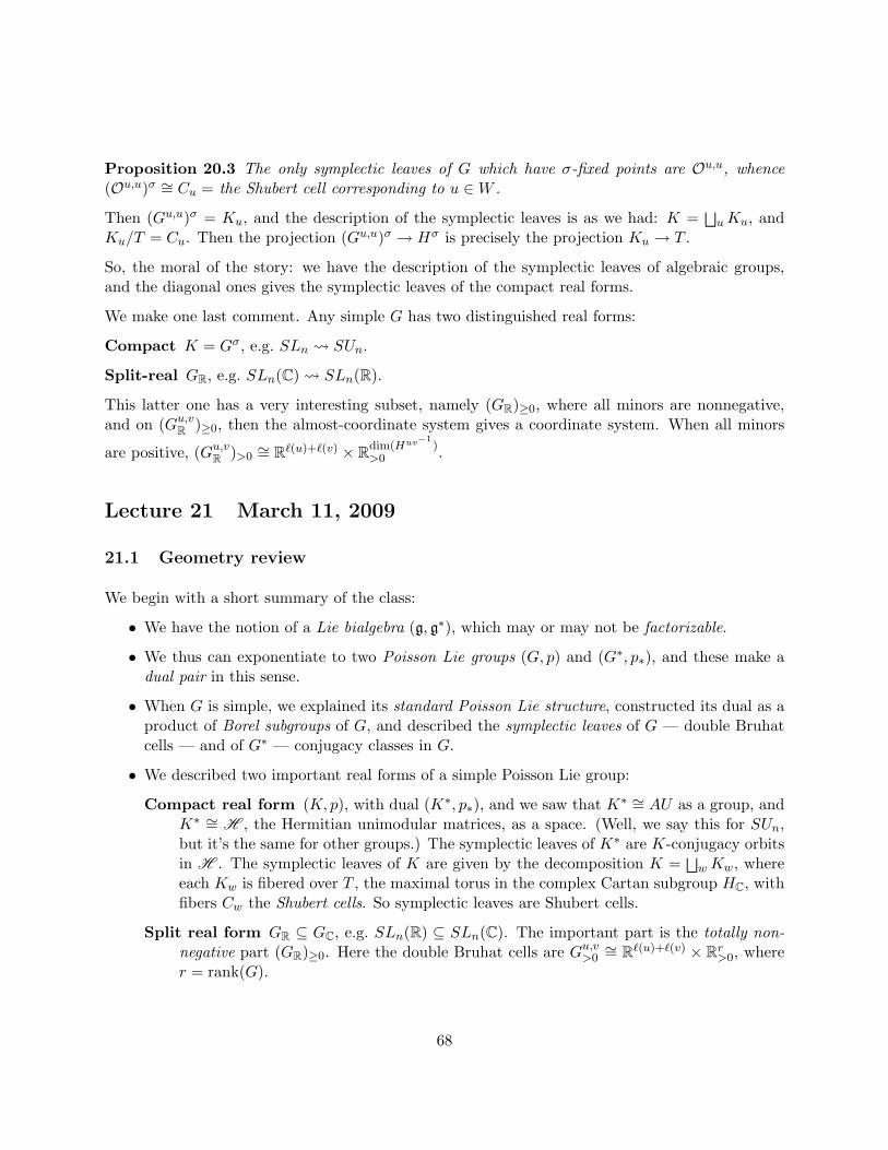
Proposition 20.3 The only symplectic leaves of G which have σ-fixed points are Ou,u, whence(Ou,u)σ ∼= Cu = the Shubert cell corresponding to u ∈W .

Then (Gu,u)σ = Ku, and the description of the symplectic leaves is as we had: K =⊔uKu, and

Ku/T = Cu. Then the projection (Gu,u)σ → Hσ is precisely the projection Ku → T .

So, the moral of the story: we have the description of the symplectic leaves of algebraic groups,and the diagonal ones gives the symplectic leaves of the compact real forms.

We make one last comment. Any simple G has two distinguished real forms:

Compact K = Gσ, e.g. SLn SUn.

Split-real GR, e.g. SLn(C) SLn(R).

This latter one has a very interesting subset, namely (GR)≥0, where all minors are nonnegative,and on (Gu,vR )≥0, then the almost-coordinate system gives a coordinate system. When all minors

are positive, (Gu,vR )>0∼= R`(u)+`(v) × Rdim(Huv−1

)>0 .


21.1 Geometry review

We begin with a short summary of the class:

• We have the notion of a Lie bialgebra (g, g∗), which may or may not be factorizable.

• We thus can exponentiate to two Poisson Lie groups (G, p) and (G∗, p∗), and these make adual pair in this sense.

• When G is simple, we explained its standard Poisson Lie structure, constructed its dual as aproduct of Borel subgroups of G, and described the symplectic leaves of G — double Bruhatcells — and of G∗ — conjugacy classes in G.

• We described two important real forms of a simple Poisson Lie group:

Compact real form (K, p), with dual (K∗, p∗), and we saw that K∗ ∼= AU as a group, andK∗ ∼= H , the Hermitian unimodular matrices, as a space. (Well, we say this for SUn,but it’s the same for other groups.) The symplectic leaves of K∗ are K-conjugacy orbitsin H . The symplectic leaves of K are given by the decomposition K =

⊔wKw, where

each Kw is fibered over T , the maximal torus in the complex Cartan subgroup HC, withfibers Cw the Shubert cells. So symplectic leaves are Shubert cells.

Split real form GR ⊆ GC, e.g. SLn(R) ⊆ SLn(C). The important part is the totally non-negative part (GR)≥0. Here the double Bruhat cells are Gu,v>0

∼= R`(u)+`(v) × Rr>0, where

r = rank(G).

68

These two compact forms are in an important sense opposite.

What’s amazing is that the geometry given by the standard Poisson Lie structure matches thesepurely algebraic structure. We remark that there is a classification of factorizable Poisson Liestructures, on which there will be a presentation after the break.

There are other interesting geometries, coming from other groups. E.g. the Borel group in SLn isthe upper-triangular matrices; we could take a parabolic subgroup of SLn, which sits between these,and study the geometry relative to it. But going in this direction will lead to a class on PoissonLie geometry, and that’s not our overall topic.

21.2 Algebra review

Recall that if P is a Poisson manifold, then C(P ) is a Poisson algebra: it is a commutative algebraalong with a Lie bracket , which satisfies the Leibniz rule a, bc = a, bc+ ba, c.

On the other hand, if G is a group, then C(G) is a Hopf algebra: it is an associative unital algebra(commutative in the case of C(G), but not part of the definition) along with a comultiplication∆ : A → A⊗2, which is a homomorphism of unital algebras. ∆ should be coassociative — (∆ ⊗id) ∆ = (id ⊗∆) ∆ — and there should be a counit — a linear functional ε : A → C that is ahomomorphism of algebras satisfying (id⊗ ε) ∆ = id = (ε⊗ id) ∆. For a A = C(G), where G isfinite or algebraic, we have (∆f)(x, y) = f(xy), and ε(f) = f(1). So far we have defined a bialgebra.A Hopf algebra is a bialgebra along with a map S : A → A that is a bialgebra antiautomorphism— S(ab) = S(b)S(a) and (S⊗S) ∆ = ∆op S, where ∆op = σ ∆, where σ is the canonical “flip”map X ⊗ Y → Y ⊗X. Moreover, S must satisfy the following commutative diagram:

**pentagon**

In the case of a group, S(f)(x) = f(x−1), and the diagram is the statement that f(xx−1) =f(x−1x) = f(1). So a Hopf algebra is an algebraic description of a group.

Ok, so now let’s assume that G is algebraic. We make this assumption because there are all sortsof completions one has to make to deal with functions that are not polynomials. This is possible,but one needs to go deep into functional analysis.

Ok, so if G is an algebraic Poisson Lie group, then A = C(G) is a Poisson algebra and also a Hopfalgebra, and moreover the comultiplication is a homomoprhism of Poisson algebras. Questionfrom the audience: You have to prove that the bracket of polynomials is polynomails? An-swer: Yes, well, that’s part of the word “algebraic Poisson Lie group”. Also S is an anti-Poissonmap.

If g is a Lie algebra, there is another natural Hopf algebra associated to g: the universal envelopingalgebra Ug.

Proposition 21.1 We saw that (g, δ) is a Lie bialgebra if and only if δ : g→ ∧2g is a one-cocyclefor the Chevalley complex with coefficients in

∧2g. The proposition is that this induces a one-cocycle

69

in the Hochschild cohomology of Ug with coefficients in Ug⊗2.

Recall, the Hochschild complex: Let A be an associative algebra, and M a module over A. Thenwe define

C•(A,M) def=⊕n≥0

HomC(A⊗n,M) (21.1)

So all linear maps over the field; if A is infinite-dimensional, we should talk about topology on it,but we will obscure this. Anyway, suppose that c ∈ Cn; we must produce a cochain in Cn+1. Wedo it thus:

dc(x1, . . . , xn+1) = c(x1x2, x3, . . . , xn)− · · ·+ (−1)n−1c(x1, . . . , xn−1xn) + next time (21.2)

We will do this next time; we don’t want to get confused by pluses and minuses at the board. **Itshould be almost that, but also with some reference to the module structure on M , Ithink.**

21.3 Looking forward

A dual pair of Hopf algebras is a pair A,B of Hopf algebras along with a nondegenerate pairing〈, 〉 : A⊗B → C that gets along with the Hopf algebra structure:

〈ab, l〉 = 〈a⊗ b,∆B(l)〉 (21.3)〈∆A(a), l ⊗m〉 = 〈a, lm〉 (21.4)

〈1A, l〉 = εB(l) (21.5)〈a, 1B〉 = εA(a) (21.6)

〈SA(a), l〉 = 〈a, SB(l)〉 (21.7)

We will use the not-ideal but at least historical notation that 〈a⊗b, l⊗m〉 = 〈a, l〉〈b,m〉. In general,we say that a pairing is nondegenerate if 〈a, l〉 = 0∀l implies a = 0, and also on the other side.

Example 21.1 If A is finite-dimensional, then there is a unique Hopf algebra B = A∗. ♦

Example 21.2 If g is a Lie algebra, and G the corresponding algebraic Lie group, then Ug andC(G) are not dual vector spaces — the dual to an infinite-dimensional vector space is a hairy thing— but they are a dual pair of Hopf algebras. We define the pairing by 〈1, f〉 def= f(e), 〈x, f〉 def=ddt

∣∣∣t=0

f(etX) when x ∈ g → Ug, and for a product, 〈x1 . . . xn, f〉 = dn

dt1...dtn

∣∣∣ti=0

f(etX1 . . . etXn).

**The opposite pairing convention above might lead to different order here.** ♦

Now, if (g, g∗) is a Lie bialgebra, then we get two Hopf Poisson algebras C(G) and C(G∗), and infact four Hopf algebras producible naturally form this data:

Ug, C(G), G(G∗), Ug∗

Question from the audience: If G is algebraic, is G∗ also? Answer: We assume that theyall are: this is the case for the standard Poisson Lie structure. It is also the case in all standard

70

interesting applications. The standard examples are (1) topological (knot) invariants, and (2)quantum integrable systems. A small detour to mathematical physics: The initial motivation for Lieto invent Lie groups and Lie algebras were the symmetries of differential equations, because ClassicalMechanics was the primary game. About one hundred years later, Hopf algebras arose in the samecontext, to understand the symmetries in quantum field theories. This will be the 21st centurychallenge — constructing a mathematical theory of QFT — just like the 20th century success wasthe mathematics of Quantum Mathematics. There is currently only bits and pieces of a consistentmathematical theory of quantum fields. Certain models can be constructed mathematically withthe above algebraic tools, whence they become representation theory of certain affine algebras.Point being, everything is algebraic in all examples.

g g∗

Ug C(G) C(G∗) Ug∗

Hopf duality Hopf dualityPoisson duality

Lie bialgebra duality

Lie bialgebra duality

These last dualities are δ : C(G)∗ → ∧2C(G)∗ and δ : Ug→ ∧2Ug⊗2 → Ug⊗2.

We will begin a program of quantization. We will deform all these Hopf algebras to non-commutative,non-cocummutative Hopf algebras. When we do, we will find that algebraically (but not topologi-cally), Uqg ∼= CqG

∗, and this will make a dual pairing with Cq(G) ∼= Uqg∗.

There are two ways to do this: either to deform the multiplication of the algebra, or to writethe algebras in generators and relations, deform the ideals, and identify the vector spaces. In theinterest of time, we will only do the second, quoting:

Theorem 21.2 (Kontsevich) Every Poisson algebra has a formal quantization.

There is a description of the classification of these. There is a QFT that explains these.

Next week NR will be away at a conference. Noah Snyder will substitute.

71


22.1 Drinfeld Double of a Hopf Algebra

Let (H,H∗, 〈〉) be a dual pair of Hopf algebras. We let Ho be the Hopf algebra H∗ with the oppositecomultilication: ∆Ho = σ ∆H∗ .

Then we define the multiplication on the vector space H ⊗H∗ by:

(a⊗ l) · (b⊗m) =∑b,l

ab(2) ⊗ l(2)m 〈b(1), S−1(l(1))〉〈b(3), l(3)〉 (22.1)

where S is the antipode for H∗, and we introduce the notation: ∆H(a) =∑a a(1) ⊗ a(2), and

∆(3)H (a) =

∑a a(1)⊗a(2)⊗a(3). This is well-defined by the coassociativity. Similarly for l(i), defined

in terms of ∆Ho .

Theorem 22.1 This multiplication defines an associative unital algebra structure on D(H,H∗) def=H ⊗ H∗ with unit 1D = 1H ⊗ 1H∗, such that it is also a Hopf algebra with H → D(H,H∗) andHo → D(H,H∗) Hopf algebra emberrings. (So D(H,H∗) ∼= H ⊗Ho as a coalgebra.)

D(H,H∗) is called the Drinfeld double of a Hopf algebra.

Exercise 36 Prove this. You will need the coassciativity, and that S is an antiautomorphism.

Question from the audience: This has a natural symmetric bilinear form. Is there a notion inwhich this is invariant, like the double of a Lie bialgebra? Answer: You have to formulate what“invariance” means. Yes, we will do this.

A pair (H,R ∈ H⊗2), where H is a Hopf algebra, and it’s OK if R is in some natural completionof H⊗2 — such a pair is a quasitriangular Hopf algebra if the comultipliation acts on R by:

(∆⊗ id)R = R12R23 (22.2)(id⊗∆)R = R13R23 (22.3)

σ∆a = R∆(a)R−1 (22.4)

So R intertwines the two multiplications. The right hand side for the first two conditions iscomponentwise multiplication: R =

∑αi ⊗ βi, then R13 =

∑αi ⊗ 1 ⊗ βi, etc., and R13R12 =∑

ij αiαj ⊗ βj ⊗ βi.

If g is a Lie algebra, then Ug the universal enveloping algebra is a Hopf algebra. Then the co-multiplication is symmetric: ∆x = x ⊗ 1 + 1 ⊗ x for x ∈ g → Ug. Then the category Ug-mod offinite-dimensional modules over Ug has morphisms maps f : V → W linear and intertwining theaction, and it is naturally an abelian category. But moreover if H = Ug, then the comultiplicationlets use define the tensor product of modules.

We will be more careful now about notation. An object is a pair (πV , V ), where V is a finite-dimensional vector space, and πV : H → End(V ). Then hom

Ä(πV , V ), (πW ,W )

ä= f : V →

72

W linear s.t. fπV (a) = πW (a) f for any a ∈ H. Now we can define:

(πV , V )⊗ (πW ,W ) def=Ä(πV ⊗ πW ) ∆, V ⊗W

ä(22.5)

A short digression. If H = K (e.g. K = C), then H-mod = VectC. Then the tensor product notstrict: (V1⊗V2)⊗V3 is not the same object as V1⊗(V2⊗V3). But there are canonical isomorphisms:

(V1 ⊗ V2)⊗ V3∼= V1 ⊗ V2 ⊗ V3

∼= V1 ⊗ (V2 ⊗ V3) (22.6)

So Vect is not a strict monoidal category, which is when (V1 ⊗ V2) ⊗ V3 = V1 ⊗ (V2 ⊗ V3) on thenose. Vect is almost this: there is a canonical object V1⊗V2⊗V3, etc. In other monoidal categoriesin which there is no canonical object for the tensor of n objects.

Anyway, H-mod is like Vect in this way.

Proposition 22.2 If H is a Hopf algebra, then H-mod is an almost strict monoidal category,meaning that it is not strict, but for any n objects, there is a canonical unbracketed tensor productof those objects.

Now, if H = Ug, then σ∆ = ∆, so the products are isomorphic (πV⊗W , V ⊗W ) ∼→ (πW⊗V ,W ⊗V )by SV,W : v ⊗ w 7→ w ⊗ v.

Proposition 22.3 Ug-mod is a symmetric category. (There exist maps SV,W : V ⊗W ∼→ W ⊗ Vsatisfying axioms.)

The idea is that the R in a quasitriangular Hopf algebra (H,R) will make H-mod into a braidedcategory.

Let’s recall some definitions:

• The category C is monoidal if there is a functor ⊗ : C × C → C such that :

C × C × C

C × C

C × C

C

⊗× id

id×⊗ ⊗

⊗

a

(22.7)

where the diagram need not commute on the nose, but up to a particular natural isomorphisma.

Moreover, where should also be a choice of object 1 ∈ C with natural isomorphisms V ⊗1 ∼→rV

V∼←lV1⊗ V .

73

Example 22.1 If H is a bialgebra, i.e. like a Hopf algebra except without the antipode,then H-mod is monoidal. We have to choose a unit object: pick a one-dimensional space L,whence φ : EndC(L) ∼= C, and use the comultiplication ε : H → C to define the action ofH → End(L). ♦

• A monoidal category C is rigid if for any object V ∈ C there exists V ∗ (unique up to uniqueisomorphism) and maps iV : 1 → V ⊗ V ∗ and eV : V ∗ ⊗ V → 1, satisfying natural axioms.So V 7→ V ∗ is not yet a (contravariant) functor — it is once we choose V ∗ for each V , anddifferent choices give isomorphic functors. **Once we chose a functor, I expect that iand e should be dinatural transformations.** Some references: Bakalov and Kirillov,and there are some notes (not yet a book) by Kevin Walker.

Example 22.2 If H is a Hopf algebra, then H-mod is rigid, with (πV , V )∗ def=Ä(πV S)∗, V ∗

ä,

where on the right-hand side we mean that linear-algebraic dual (V is finite-dimensional). Ifyou didn’t have S, then you wouldn’t be able to construct this homomorphism. A simpleproperty:

Ä(πV , V )⊗ (πW ,W )

ä∗ ∼= (πW ,W )∗ ⊗ (πV , V )∗. ♦

Next time, we will see that if (H,R) is quasitriangular, then there will be a natural braidingcV,W : V ⊗W ∼→W ⊗ V , given by cV,W = SV,W (πV ⊗ πW )R. This will be a tensor category.

Moreover, we will see that the Double of any Hopf algebra is quasitriangular.

Lecture 23 March 16, 2009. Guest Lecture by Noah Snyder

23.1 Quasitriangular Hopf Algebras and Braided Tensor Categories

Often when Hopf algebras are first introduced, they’re seen as generalizations of “functions on agroup”: ∆ comes from ·, ε from e, S from g 7→ g−1, and the algebra structure understands thegeometry of the group.

But then there’s a switcheroo: we will think about H-modules, which make a category with extrastructure. We will have the following dictionary:

• ∆ ⊗

• S ∗

• ε 1

• and the algebra structure makes H-mod into an abelian category.

One can ask whether H-mod includes a natural map σV,W : V ⊗W →W ⊗V . For H = C(G), yes:the vector-space trivial “swap” map does the job. But there may be others.

Example 23.1 The category of supervector spaces has objects Z/2-graded vector spaces, andbraiding is v ⊗ w 7→ (−1)|v|·|w|w ⊗ v, where |v| is the degree of v (either 0 or 1). ♦

74

How would one construct a map σV,W in general? Well, we should define v ⊗ w 7→ swapR(v ⊗ w),where R ∈ H⊗H. This should be a map of modules, and so we need to demand that it intertwinesthe action of any x ∈ H. For this to happen, we’d need to demand:

R∆x = ∆opxR (23.1)

where ∆op = swap ∆.

What properties do we demand of σV,W ? The old fashioned answer is to satisfy the relations onthe symmetric group.

We will explain this in pictures. The yoga is to draw objects as labeled strands. For example, V

is an object, V is its dual, and is the pairing V ⊗ V ∗ → C.

Anyway, so if g ∈ Sn the symmetric group, we could demand that there is a unique and well-definedσg : V1⊗ · · · ⊗ Vn → Vg(1)⊗ Vg(n). I.e. any two ways to build g out of transpositions, we should getthe same map. In pictures, this is equivalent to the requirement that:

= =

There is also another thing we might want. For example, σA⊗B,C : ABC → CAB is well-defined;

we should demand that it matches ABC1⊗σB,C−→ ACB

σA,C⊗1−→ CAB.

If any element of the symmetric group has a well-defined action on a long string of tensor products,we say the category is symmetric. For example, the category of supervector spaces is symmet-ric.

Exercise 37 Consider the category of supervector spaces, and think of it has H-mod where H =Z/2. Doing this is tricky: you need to consider the odd or even parts in terms of the action of thegenerator x. Anyway, find R. It should be something like R = 1

2(1⊗ 1 + 1⊗ x+ x⊗ 1− x⊗ x).

But we now introduce new hotness:

Rather than demanding that the symmetric group act on tensor products, let’s only demand thebraid group. This has overcrossings and undercrossings.

Then we will have infinitely many maps between tensor products, which will generally be different.For example, just on two elements, we have Z many maps. A result of Artin: the braid groupcan be presented by two versions, one with all overcrossings and one with all undercrossings, ofReidemeister Three.

75

But using naturality, there’s a better description.

=

By the way, you read diagrams bottom to top, because then when reading diagrams top to bottom,you get the words left to right.

Ah, but naturality says exactly that you can pull things across the crossing. So for example we canprove the Braid relation:

= = =

where the first and third equalities are the relation above, and the second is naturality.

Clearly this can be made into an algebraic proof, but that would take a lot longer to write.

So, a braiding is a natural transformation σV,W : V ⊗W 7→W ⊗ V such that

σA⊗B,C = (σA,B ⊗ 1)(1⊗ σB,C) (23.2)

and σA,B⊗C = Exercise 38.

Let’s translate this into a condition on R. The LHS of equation 23.2 mean swap12,3(∆⊗ 1)(R) andthe RHS means swap1,2(R ⊗ 1)swap2,3(1 ⊗ R). This is a bit awkward because of the swap in themiddle. Let’s move the middle swap past R ⊗ 1, which leaves the first part of R fixed and movesthe other part past. So we have R =

∑R(1) ⊗R(2), and we define R13 =

∑R(1) ⊗ 1⊗R(2). Thus,

the final condition, after canceling some swaps, is:

(∆⊗ 1)(R) = R13R23 (23.3)

There’s also another condition; you can run the argument backwards to show that if R satisfiesboth, then it gives a braiding.

Exercise 39 Work out the braid relation in terms of R. You will get the Yang Baxter Relation.

76

23.2 The quantum double

In a braiding, it’s easy to satisfy the desire to make σ : V ⊗W →W ⊗ V a module map, and hardto make it satisfy the relation. But in the Double, the second part is easy, and the first hard.

You start with a Hopf algebra H, and we want to build a Hopf algebra of the form H ⊗H∗. I.e.we know the products on each component, and the coproduct is defined by its components, andthe only thing to define is how to write x∗y as a sum of things of the form ab∗, where a, y ∈ H andx∗, b∗ ∈ H∗. Then the relation is obvious **?**

Then we have a miracle. We can get V ⊗W → W ⊗ V and that H ⊗ H∗ is a Hopf algebra inexactly one way. It’s a long calculation.


**I was late, but that’s OK: VS has not shown up.**

24.1 Matt describes a particular quantum group.

We pick q ∈ C r 0, such that q2 6= 1.

We define the quantum plane C2q to be the algebra 〈x, y s.t. xy = qyx〉. Then normal classical

matrix multiplication Ça bc d

åÇxy

å=Çax+ bycx+ dy

åis actually a coaction of algebras: C(C2) → C(M(2)) ⊗ C(C2). What should act on the quantumplane? “Quantum matrices”. So we decorate the equation with qs — C(C2

q)→ C(Mq(2))⊗C(C2q)

— and now we want to know the relations on C(Mq(2)) to make everything consistent. Well, ifx′ = a⊗x+b⊗y and y′ = c⊗x+d⊗y, then we want x′y′ = qy′x′. This requires that the coefficientsafter expanding x′y′ = qy′x′ into xs and ys (and q-muting the ys past the xs) match:

ac = qca (24.1)bd = qdb (24.2)

qad+ bc = q(qcb+ da) (24.3)

By looking at the right action, we get more relationships. Question from the audience: Theright action is on the dual space C(C2

q∗). Is it obvious that this should be the same algebra, when

you go crazy with the qs? Are you imposing the Euclidean bilinear form on C2q? Answer: Good

question. We will not answer it. We have:

ab = qba (24.4)cd = qdc (24.5)

qad+ cb = q(qbc+ da) (24.6)

77

We can rearrange equation 24.3 to q(ad− da) = q2cb− bc, and equation 24.6 becomes q(ad− da) =q2bc− cb. Subtracting and dividing gives:

bc = cb (24.7)

ad− da = (q − q−1)bc (24.8)

This approach is in Klimyk and Schmudgen, Quantum Groups and their Representations. Thewhole approach is due to Yuri Manin.

All of this is thinking of C(Mq(2)) as a bialgebra; there’s nothing invertible yet.

Anyway, the algebra C(Mq(2)) we define as being the algebra generated by a, b, c, d such thatequations 24.1, 24.2, 24.4, 24.5, 24.7, and 24.8 hold. The nemonic: adjacent generators in thematrix q-mute with the alphabetical order. Antidiagonal commute, and diagonal have the weirdone.

One can check, moreover, that the coalgebra structure from C(M(2)) given by:Ça bc d

å7→Ça bc d

å⊗Ça bc d

å(24.9)

is an algebra homomorphism for C(Mq(2)) as well. The counit a, d 7→ 1, c, b 7→ 0 also works.

We want inverses. Thinking hard about exterior powers, one can decide that the correct “quantumdeterminant” is Dq = ad− qbc. Some facts:

• Dq is central.

• Dq is grouplike: ∆(Dq) = Dq ⊗Dq.

These imply that the ideal I generated by Dq − 1 is a bialgebra ideal. We define C(SLq(2)) =C(Mq(2))/I. Then on this we can define an antipode:

S

Ça bc d

å=Ç

d −b−qc a

å(24.10)

One now has to check the antipode axiom:

A A⊗A

A⊗AA

C

∆

id⊗ S

m

ε

1

(24.11)

which is an exercise in multiplying matrices.

This Hopf algebra deserves to be called C(SLq(2)).

**Then we left ten minutes early.**

78


Before the break, Noah said the words “quasi-triangular Hopf algebra”, and Matt introduced “quan-tum SL(2)”. VS was teaching at the same time, and so was unavailable.

By the way, on NR’s website, there is a reference to TQFT lectures from last year. On that website,there are notes on tensor categories, so there is some overlap. Everything related to the fact thatthe category of modules over a quasitriangular Hopf algebra is braided monoidal — this part isexplained well there.

Let’s recall NR’s discussion from two weeks ago. If H is a Hopf algebra, we define its double tobe the coalgebra D(H) def= H ⊗ H, where H is H∗ with the opposite comultiplication. If H isinfinite-dimensional, we must supply H with a dual pairing H∗, 〈, 〉. The multiplication on D(H)is given by:

(a⊗ l)(b⊗m) =∑b,l

ab(2) ⊗ l(2)m〈b(1), S−1H∗(l(1))〉〈b(3), l(3)〉 (25.1)

The notation is that a, b ∈ H, l,m ∈ H, and S−1H∗ = SH . We also use the notation that

δ(3)H (b) =

∑b b(1) ⊗ b(2) ⊗ b(3), and δ

(3)H(l) =

∑l l(1) ⊗ l(2) ⊗ l(3). We also write D(H) = H on H; it

is a Hopf algebra.

Let A be a Hopf algebra and R ∈ A⊗2, possibly completed to A⊗2 in some way. For example, ifA = C(M) for a space M , then perhaps we want to complete A ⊗ A to C(M ×M). We will alsohave an example from formal power series. Anyway, the pair (A,R ∈ A⊗2) is a quasitriangularHopf algebra if

(∆⊗ id)(R) = R13R23 (25.2)(id⊗∆)(R) = R13R12 (25.3)

whence R is invertible, and we also demand that

∆op(a) = R∆(a)R−1 (25.4)

This definition is totally natural, given the following:

Proposition 25.1 If (A,R) is a quasitriangular Hopf algebra, then the category A−mod of finite-dimensional A-modules is a tensor category. I.e. it is rigid (dual objects), monoidal (⊗), Abelian(a category of modules), and braided (this follows from the quasitriangular structure).

Let us define these words better. A category C is monoidal if it is endowed with a (covariant) functor⊗ : C × C → C. Recall, a morphism (A,B) → (C,D) ∈ C × C is a pair (f : A → C, g : B → D). If(C,⊗) is monoidal, then we can also construct ⊗op : C × C → C by (A,B) 7→ B ⊗A. **Really weare using the canonical flip map C × C → C × C.**

So we have two functors ⊗,⊗op : C × C → C. When we have two functors, we can ask whetherthey are the same — well, not the same, because “the same” does not exist in categories, but

79

isomorphic.

C × C C

⊗

⊗op

c∼

That c is an isomorphism means that for every pair of objects, there is an isomorphism cA,B :A⊗B ∼→ B ⊗A, and this system commutes with all morphisms.

So, the data C,⊗,1, a, c, where a is the associativity (included in the word “monoidal”) and c isan isomorphism ⊗ ∼→ ⊗op, is braided monoidal if c is compatible with the associativity constrain.This condition consists of two hexagon diagrams:

(A⊗B)⊗ C

A⊗ (B ⊗ C)

C ⊗ (A⊗B)

A⊗ (C ⊗B)

(C ⊗A)⊗B

(A⊗ C)⊗B

aA,B,Cid⊗ cB,C a−1

A,C,B

cA,C ⊗ id

cA⊗B,C aC,A,B

(25.5)

The other hexagon is the same, with cA,B replaced by c−1B,A. Question from the audience: So

those are not always the same? Answer: No. For G-mod when G is a group, they are, but we willhave examples where it is not, and Noah gave one: the category of tangles.

So, for example, C = A-mod, a is trivial (well, as trivial as for Vect; so it is not completely trivial,but for any ordered collection of objects, there is a canonical tensor of the whole collection, andany bracketing is naturally isomorphic to this object), the tensor is given by

(πV , V )⊗ (πW ,W ) = ((πV ⊗ πW ) ∆, V ⊗W ), (25.6)

the unit 1 is the one-dimensional representation given by ε : A→ C, and the braiding is:

cV,W = PV,W (πV ⊗ πW )(R) (25.7)

where R is the quasitriangular structure and P is the permutation map of vector spaces.

One can check that this is an isomorphism of modules; it is equivalent to equation 25.4.

Exercise 40 The hexagons (equation 25.5) are equivalent to equations 25.2 and 25.3.

This continues the correspondence:

If A is . . . then A-mod is . . .an algebra Abeliana bialgebra monoidalHopf rigidquasitriangular braided

80

One of the main applications of all of this is the construction of topological invariants. And wecertainly want a braiding, so that we can study knots.

Well, it’s very nice to have a definition, but we should also have an example.

Theorem 25.2 The double D(H) of any Hopf algebra with the canonical element R =∑i(ei⊗1)⊗

(1⊗ei) is quasitriangular. We have picked any basis ei of H, and its dual basis ei of H∗ defined viathe pairing 〈, 〉 : H ⊗H∗ → C. But if H is infinite-dimensional, then we have written down only aformal sum; the topology needed to define the correct completion D(H)⊗2 is a sensitive question.

We now make a logical jump, and study the double of quantized Borel in sl2. Let us definethis. Uhb+ is the algebra generated by H,E and completed over C[[h]] with the defining relations[H,E] = 2E. In other words, Uhb+

∼= Ub+[[h]].

Theorem 25.3 1. The map ∆ : Uhb+ → Uhb⊗2+ defined on generators as

∆(H) = H ⊗ 1 + 1⊗H (25.8)

∆(E) = E ⊗ ehH/2 + 1⊗ E (25.9)

is a comultiplication for Uhb+.

2. ε(1) = 0, ε(H) = ε(E) = 0 extends to a counit ε : Uh : b+ → C[[h]].

So Uhb+ is a bialgebra over the commutative ring C[[h]]. In particular, we demand that both mapsbe continuous.

Exercise 41 Find S.

Let us know describe a dual to Uhb+. We define the symbol Uhb+ to be generated over C[[h]] by

H∨ and F with the defining relation [H∨, F ] = −h2F . The bialgebra part is:

∆H∨ = H∨ ⊗ 1 + 1⊗H∨ (25.10)

∆F = F ⊗ 1 + e−2H∨ ⊗ F (25.11)

Well, the second term in equation 25.11 is a problem; it is an infinite series. So we need to define atopology in which eH

∨can be written. We do this via a filtration on Uhb+

given by deg(H∨) ≤ 1and deg(F ) ≤ 1, and deg(ab) ≤ deg(a) deg(b). If this were commutative, then we this would be thegrading of the polynomial algebra, but it is noncommutative. So we define a topology in terms ofthe filtration, and complete to the “formal power series” ring.

Proposition 25.4 There is a unique Hopf pairing 〈, 〉 : Uhb+⊗Uhb+ → C[[h]] such that 〈H,H∨〉 =

1 = 〈E,F 〉 and 〈H,F 〉 = 0 = 〈E,H∨〉. We comment that if these were commutative rings, thenthis would be the pairing of polynomial functions on V with polynomial functions **formal powerseries?** on the dual vector space.

Next time we will construct the double, build quantized universal enveloping algebras, and connectit up with what we learned about Lie bialgebras and Poisson Lie groups.

81

Lecture 26 April 1, 2009

26.1 Schur-Weyl duality

Do you know about Schur-Weyl duality? No? Well, we will certainly discuss it, but we shoulddeviate from the story of quantum groups to describe it.

Let us consider the action of GLn on Cn. Then GLn acts on (Cn)⊗N , and the symmetric groupSN also acts on (Cn)⊗N , by permutations.

Theorem 26.1 (Schur-Weyl duality) These actions centralize each other.

I.e. everything that commutes with the entire GLn action is in Sn, and vice versa.

Corollary 26.1.1 (Cn)⊗N decomposes as⊕

λaN VGLnλ ⊗WSN

λ , where λ is a partition of N : λ =(λ1, λ2, . . . , λk) with λi ≥ 0 and λ1 + · · ·+ λk = N . The sum is over partitions with k ≤ n.

We hope that everyone knows the representation theory of SN , but of course it is never the case.MH described the representation of simple Lie groups.

More generally, consider the action Γ y W when it is multiplicity-free. Then there are **?**dualities, GLn ×GLm on the polynomials on an n×m array of variables.

Theorem 26.2 This action is multiplicity free.

There are names that are completely misleading. For example, “quantum groups”, which arevaguely quantum but definitely not groups. Similarly, “Lie supergroups” are not groups but Hopfalgebras in the category of Lie supervector spaces. Since you do not know Lie superalgebra, we willnot go in this direction right now.

There is an object called the Hecke algebra, given by:

Hn(q) def= 〈si, i = 1, . . . , N − 1 s.t. (si − q)(si + 1) = 0, sisi±1si = si±1sisi±1, sisj = sjsi, |i− j| > 1〉(26.1)

It is a deformation of the symmetric group. Then there is a natural action of HN (q) on (Cn)⊗N

and also of Uq(gln) on (Cn)⊗n, and then we have:

Theorem 26.3 (q-Schur-Weyl duality) Hn(q) centralizes Uq(gln) in (Cn)⊗N , and vice versa.

More precisely, if π : A y W , then we define the cetralizer of A in W to be **NR uses “C” butI’d prefer “Z”** C(A;W ) = a : W →W s.t. [a, π(x)] = 0∀x ∈ A.

26.2 Deformations of Hopf algebras

Last time we discussed Uhb+ and its dual Uhb+ We briefly mentioned the words “formal deforma-

tion” last time, but now we make some definitions.

82

Let (A,m, 1) be an associative unital algebra over C (or anything else); we list the algebra as atriple: a vector space, an associative multiplication, and a unit. Then B = A[[h]] is a formal(torsion free) deformation of A if (B, m, 1) is an associative unital algebra such that:

m(a, b) = m(a, b) +∞∑n=1

hnm(n)(a, b) (26.2)

where m(n) : A ⊗ A → A are extended to B ⊗ B → B by h-linearity **and continuity**; and:

1 = 1 +∞∑n=1

hn1(n) (26.3)

where 1 is the unit in A and 1(n) ∈ A.

Now let (B, m, 1) and (B, m, 1) be two formal deformations of (A,m, 1). Then we say that theseare equivalent and write (B, m, 1) ∼ (B, m, 1) if there is a φ : B → B that is C[[h]]-linear withφ = id +

∑∞n=1 h

nφ(n) (whence φ is invertible) such that φ m = m (φ⊗ φ) and φ(1) = 1.

Then there is a natural question: Given A, describe the equivalence classes of formal deformationsof A. There is always, of course, the trivial deformation; there may not be any others.

So these are formal deformations, but what we really want is a family of algebras. We say that afamily of algebras Ah where h ranges over h ∈ X, where X is some set with a limit point 0, is adeformation of A if:

• We have linear isomorphisms φh : Ah∼→ A. This can be slightly problematic: if A is an

infinite-dimensional vector space, then these isomorphisms should also be continuous, in somenatural topology. One way to do this is to choose bases and identify them.

• limh→0

φh mh (φ−1h ⊗ φ−1

h ) = m. For each h, the inside is an associative multiplication

A⊗A→ A.

• limh→0

φ1(1h) = 1.

The isomorphisms φh are part of the data; the other two conditions are properties. The meaningof limh→0 is a bit sloppy.

But all these questions have a trivial answer. The only way we know how to construct algebras —well, there are algebras of functions, but other than that — is to take quotients of free algebras.This is how we will proceed. We will take a free algebra F (x1, . . . , xn), and we will constructa family of ideals Ih ⊆ F , such that A0 = A. Then we will try to define Ah = F/Ih, and thebiggest problem is to construct the linear isomorphisms Ah

∼→ A0. The usual way we will do thisis to construct algebras of PBW-type. For example, we may know that Ah ∼= S(x1, . . . , xn) thesymmetric algebra.

This is really what we want: to have families of algebras. Not just formal deformations, which arelike the formal Taylor expansions of the formal algebras. But formal deformations are easier todescribe; this is the difference between micro-local analysis and global analysis.

83

Question from the audience: Why do we really want families of algebras Answer: It is ageneral philosophy of life. If you want to study some structures, look for stable structures thatcome in families. When you try to classify stable structures, you hope that there is a discretecollection of them, e.g. for simple Lie algebras, even though simplicity is an open condition. Youcan stratify branches of mathematics by the strength of the equivalence relations. In many branches,the goal is to classify something. If you try to classify all vector spaces, this is tedious. But up toisomorphism? Then they are classified by dimension. Similarly, if you are classifying a structure,and you are sitting at a singular point, it can be quite hard, but classifying families is easy.

Here’s another reason. Well, it’s another reason for someone indoctrinated by physics. The world,it turns out, is not commutative. It is at least quantum-mechanical. What we see — the commu-tativity of classical mechanics — is a limit of quantum mechanics as the parameter goes to 0. Sothe problem of quantization is that it’s the wrong direction. The natural direction is the other one:to specialize to h→ 0. Then we get various degeneracies.

Having said this, let’s forget about the real world and return to formal deformations of associativealgebras.

Suppose that A is commutative, and that B is a formal deformation of A. Then the multiplicationis given by:

m = m+ hm(1) +O(h2) (26.4)

We are following the previous outline, that the natural direction is not quantization by degeneration.Anyway, we define a, b def= m(1)(a, b)−m(1)(b, a).

Theorem 26.4 (A, m, , ) is a Poisson algebra.

**NR: “We have a small theorem...” Theo: “I don’t have a symbol for ‘small theo-rem’.” NR: “The definition of ‘small theorem’ is that the proof is a homework.” Matt:“There are many small theorems in this class.” NR: “Well, let’s make this into a bigtheorem.”**

Proof: a, b = 1h [a, b] mod h, and A = B mod h. So the Jacobi and Leibniz for , follow from

those for [, ].

So, if at a special point a family of associative algebras becomes commutative, then it induces aPoisson structure. Question from the audience: We don’t have a family. Answer: No, wehave a formal family.

Exercise 42 Let B be a formal deformation of A; A may not be commutative. Prove:

1. It induces a Poisson structure on Z(A), the center of A.

2. This Poisson structure extends to , : Z(A) ⊗ A → A, which is the action of the Poissonalgebra Z(A) by derivations on A. In other words, z, ab = z, ab+ az, b.

The theorem is a specialization of the homework, when the whole algebra is commutative.

84

B is a formal deformation quantization of the Poisson algebra (A, m, , ) if the Poisson bracketon A agrees with the one given by the deformation. The natural question: What is the set ofequivalence classes of (formal) deformation quantizations of a given Poisson algebra?

It is a complicated question. There is a complete answer in the case of algebras on a Poissonmanifold. Consider A = C∞(M) and

• m = m+∑∞n=1 h

nm(n) is special in the sense that it is symmetric: m(n)(a, b) = (−1)nm(n)(b, a).

• m(n) are bidifferential operators on M of degree (n, n).

Theorem 26.5 (Kontesevich) Equivalence classes of such formal deformations quantizationsare in bijection with formal deformations of the Poisson structure, i.e. p = p+

∑∞n=1 h

np(n) wherep(n) are bivector fields and p satisfies Jacobi.

Next time we give a few more definitions, and then we will proceed with examples.


Last time we define deformations of Hopf algebras. We make a quick summary: if (A,m,∆, ε, 1, S)is a Hopf algebra, then (B, m, . . . ) is a formal deformation of A if B = A[[h]] as a vector space,and m = m+

∑∞n=1 h

nm(n), etc. The elements of the formal power series are, for example, m(n) :A⊗A→ A extended to B ⊗B → B by h-linearity **and continuity**.

Example 27.1 If A is a commutative Hopf algebra and a Poisson Hopf algebra. In other words,there is a Poisson bracket , : A ⊗ A → A such that ∆ : A → A ⊗ A is a morphism of Poissonalgebras. Then we say that B is a formal deformation of A if in addition to the above we have:m(1) −m(1)op

= , . From the previous lecture, we saw that m(1) −m(1)op: A⊗A→ A is always

a Poisson map; now we are demanding that it be the given Poisson structure on A.

For example, let A = C(G) where G is a Poisson Lie group, then any formal deformation B ofC(G) we will call Ch(G), and call it the “quantum group” of G.

Question from the audience: There are some choices involved in constructing Ch(G), so this isan imprecise notation. Answer: Yes, but it is the usual notation in the literature. ♦

Example 27.2 Consider now the case when A is cocommutative, i.e. ∆op = ∆. For example,A = Ug. Well, if g is a Lie bialgebra, the Lie coalgebra lifts to a 1-cocycle on Ug. Let’s describethis. We have a linear map δ : g→ g∧ g, which is a 1-cocycle for the Chevalley complex for g withcoefficients M = g ∧ g. In other words, δ([x, y]) = [x, δ(y)] + [δ(x), y], in other words dChδ = 0.

Let us recall the Hoschild Complex of an algebra. Let A be an associative algebra, M a moduleover A. We define CHoschild(A,M) as follows. (By the way, G. Hoschild is emeritus here, but isnever around: he is very shy.) The nth part is

C(n)(A,M) def= HomC(A⊗n,M) (27.1)

85

and of course C(A,M) =⊕n≥0C

(n)(A,M). The differential is: if αn ∈ C(n)(A,M), then

dαn(a1, . . . , an+1) def= αn(a1a2, a3, . . . , an+1)− αn(a1, a2a3, . . . , an+1) + . . .

±Äa1αn(a2, a3, . . . , an+1)− a2αn(a1, a3, . . . , an+1) + . . .

ä(27.2)

The principle is that this is exactly the what you get if you try to lift the Chevalley Complex toUg.

So for exampledα1(a, b) = α1(ab)− aα1(b) + bα1(a) (27.3)

And α1 is a one-cocycle if dα1 = 0, i.e.:

α1(ab) = aα1(b)− bα1(a) (27.4)

Ok, so let’s let A = Ug, and by the PBW theorem we can identify this as a vector space with S(g).Let a, b ∈ g → Ug. Let’s let M = A, and α1 : A → A. So we can think of α1 : S(g) → S(g). Andthese are graded vector spaces — the multiplication respects only the filtration.

Let’s change our mind now about the set-up. In particular, let’s demand that M be a bimoduleover A, and at least understand the one-cocycle condition to be:

α1(ab) = aα1(b) + α1(a)b (27.5)

Then if α1 is a cocycle A→ A, then the conditions are:

α1(ab+ ba) = α1(ab) + α1(ba) = aα1(b) + α1(a)b+ bα1(a) + . . . (27.6)

α1(ab− ba) = . . . (27.7)

Actually, this is not the story we meant to tell. It’s a very nice story, but we want something else.

Let us consider a map α1 : A → A ⊗ A, such that A is a bialgebra, and let’s ask what happenswhen

α1(ab) = ∆aα1(b) + α1(a) ∆b (27.8)

Then we see thatα1(ab− ba) = [∆a, α1(b)] + [α1(a),∆b] (27.9)

so α1 restricts to a one-cocycle on g→ g⊗ g.

Conversely, any such one-cocycle δ, which is really just a Lie bialgebra structure, lifts to a mapα1 : Ug→ Ug⊗ Ug by α1(ab) = ∆aα1(b) + α1(a)∆b.

If A is a cocommutative Hopf algebra with α : A→ A⊗A such that:

αop = −α (27.10)α(ab) = ∆aα(b) + α(a) ∆(b) (27.11)

86

and also the coJacobi identity, then we say that A is a co-Poisson Hopf algebra. Question fromthe audience: Shouldn’t there also be some compatibility between α and the multiplication?Answer: **? Some sort of “co-Leibniz identity”, and also that α is a morphism of thecorrect structures**

Proposition 27.1 If A and B are a dual pair (via 〈, 〉) of Hopf algebras,and , : B ∧ B → B isa Poisson structure on B, then we define α : A→ A⊗A by:

〈α(a), l ⊗m〉 = 〈a, l,m〉 (27.12)

Then this is a co-Poisson Hopf structure.

Proof: Antisymmetry is obvious.

〈α(ab), l ⊗m〉 = 〈ab, l,m〉 (27.13)= 〈a⊗ b,∆l,m〉 (27.14)= 〈a⊗ b, ∆l,∆m〉 (27.15)

= 〈a⊗ b,∑l,m

l(1),m(1)〉 ⊗ l(2)m(2) +∑l,m

l(1)m(1) ⊗ l(2),m(2)〉 (27.16)

=∑l,m

Ä〈a, l(1),m(1)〉〈b, l(2)m(2)〉+ 〈a, l(1)m(1)〉〈b, l(2),m(2)〉

ä(27.17)

=∑l,m

Ä〈α(a), l(1) ⊗m(1)〉〈∆b, l(2) ⊗m(2)〉+ 〈∆(a), l(1) ⊗m(1)〉〈αb, l(2) ⊗m(2)〉

ä(27.18)

=∑l,m

Ä〈α13(a)∆24(b), l(1) ⊗ l(2) ⊗m(1) ⊗m(2)〉+ 〈∆13(a)α24(b), l(1) ⊗ l(2) ⊗m(1) ⊗m(2)〉

ä(27.19)

= 〈α13(a)∆24(b) + ∆13(a)α24(b),∆(l)⊗∆(m)〉 (27.20)= 〈m12m34(α13(a)∆24(b)) +m12m34(∆13(a)α24(b)), l ⊗m〉 (27.21)= 〈α(a)∆(b) + ∆(a)α(b), l ⊗m〉 (27.22)

and so we have the cocycle condition.

Ok, let’s formulate the theorem:

Theorem 27.2 Let (A,B, 〈, 〉) be a dual Hopf pairing, and let B be a Poisson Hopf algebra. Defineα : A → A⊗ A by 〈α(a), l ⊗m〉 def= 〈a, l,m〉. Then α is skew-symmetric, a cocycle, and satisfiesco-Jacobi. Such an algebra is a co-Poisson Hopf algebra.

Theorem 27.3 If g is a Lie bialgebra, with δ : g→ g ∧ g → g⊗ g the one-cocycle, then δ definesa a unique co-Poisson structure α : Ug→ Ug⊗ Ug such that α|g = δ.

Suppose that A is co-Poisson with α the structure. Then B is its formal deformation quantizationif ∆ = ∆ + hα+O(h2), and other conditions.

87

So we have two notions: the deformation of a Poisson Hopf algebra, and of a co-Poisson Hopfalgebra.

Example 27.3 If g is a Lie bialgerba, Ug is co-Poisson, and Uhg is a formal deformation of Ug asa co-Poisson Hopf algebra is a quantized universal enveloping algebra of g. ♦

At the classical level we have dual pairs of Poisson and co-Poisson Hopf algebras, and these deforminto dual pairs.

Next time, we will study examples: Uhb+ and Uhb+ = Ch(B−).


A general question is whether, given Ug, does there exist a formal deformation Uhg such that themultiplication and comultiplication deform:

∆ha = ∆a+ h∆(1)a+ . . . (28.1)

s.t. ∆(1) −∆(1)op= δ (28.2)

where δ is a one-cocycle for Ug.

Theorem 28.1 (Etingof, Kazhdan) For any g a finite-dimensional Lie bialgebra (or Kac-Moody,etc.), there exists such a Uhg.

Just as Ug is dual as a Hopf algebra to C(G), Uhg will be dual to Ch(G) in the appropriatetopologies.

For each simple Lie algebra g with the standard Lie bialgebra structure, we can give an explicitdescription of Uhg in terms of generators and relations. We will describe this construction.

Let us begin with g = sl2. Then we defined Uhb+ = 〈H,E s.t. [H,E] = 2E〉 as an algebra overC[[h]], with the coalgebra structure

∆H = H ⊗ 1 + 1⊗H (28.3)

∆E = E ⊗ ehH/2 + 1⊗ E (28.4)

Exercise 43 Check that this defines a Hopf algebra.

Let us check also that this in fact deforms Ub+. We have presented the algebra in terms of generatorsand relations, and it’s clear that in terms of the basis HnEmn,m≥0, we have:

Uhb+ = Ub+[[h]] (28.5)

88

as a linear space, and in fact as an algebra. Let’s compute the comultiplication in terms of thebasis:

∆h(HnEm) = (∆hH)n(∆hE)m (28.6)

= (∆H)n(∆E + h∆(1)E + . . . )m (28.7)

= (∆H)nÄ∆Em + h

Ä(∆E)m−1∆(1)E + (∆E)m−2(∆(1)E)(∆E) + . . .

ä+O(h2)

ä(28.8)

where ∆(1)E = E⊗H/2 is the linear term in the expansion of E⊗ehH/2. Thus, we compute:

δ = ∆(1) −∆(1)op(28.9)

∆(1)(HnEm) = ∆HnÄ∆Em−1∆(1)E + · · ·+ ∆(1)E∆Em−1

ä(28.10)

Hence δ(HnEm) = ∆HnÄ∆Em−1δE + · · ·+ δE∆Em−1

ä(28.11)

which is exactly the standard Lie bialgebra structure on b+.

Anyway, recall that sl2 = D(b+)/I, where D(b+) is the double of the Lie bialgebra. So our strategyto compute Uhsl2 will be to describe it as:

Uhsl2 = D(Uhb+)/I = Uhb+ on Uhb+/I (28.12)

The full dual opposite is too big. We will define Uhb+ in terms of a dual pair (Uhb+,Uhb+

, 〈, 〉),and see that it is a natural definition. We use:

Uhb+ def= 〈H∨, F s.t. [H∨, F ] = −h

2F 〉 (28.13)

as a complete algebra over C[[h]], with the coproducts

∆H∨ = H∨ ⊗ 1 + 1⊗H∨ (28.14)

∆F = F ⊗ 1 + e−2H∨ ⊗ F (28.15)

As an algebra Uhb+ is a formal deformation of the commutative algebra F (B−), the formal func-

tions on B−, generated by H∨ and F with H∨, F = −F . We work with this to make sense ofthe exponent in 28.15; the algebra F (B−) is an algebra of formal power series. I.e. it is C[[H∨, F ]]as an algebra, with a non-cocommutative coalgebra structure.

Indeed, we can recognize F (B−) as the algebra of matrices with coordinatesÇ1 0F e−2H∨

å(28.16)

Thus F (B−) is the algebra of functions on the formal neighborhood of the identity in B−. Well,B− should be all lower-triangular matrices with unit determinant. Fixing this is straightforward;we can use the coordinates: Ç

eH∨

0eH∨F e−H

∨

å(28.17)

89

Question from the audience: What is a formal neighborhood of the identity? Answer: Youtake all analytic functions near the origin, and complete with the formal-power-series topology.This way, we don’t need to worry about convergence issues and we can still do just algebra.

When we say that these coordinates explain the algebra, we mean that the comultiplication of“coordinate functions” is precisely the corresponding multiplication of matrices:Ç

eH∨1 0

eH∨1 F1 e−H

∨1

åÇeH∨2 0

eH∨2 F2 e−H

∨2

å=Ç

eH∨1 +H∨2 0

eH∨1 +H∨2 (F11 + e−2H∨1 F2) e−H

∨1 +H∨2

å(28.18)

Theorem 28.2 F (B−) with the Poisson bracket H∨, F = −F is a Hopf Poisson algebra offunctions on the formal neighborhood of e in the Poisson Lie group B−.

In particular, then, Uhb+ def= Fh(B−) is a formal deformation of F (B−). Incidentally, we can now

choose Uhb+∗ = Fh(B−)coop = Fh(B+), which deforms F (B+) which is dual to Ub+.

Theorem 28.3 There exists a unique Hopf pairing 〈, 〉 : Uhb+⊗Uhb+ → C[[h]] such that 〈H,H∨〉 =

1 = 〈E,F 〉, 〈E,H∨〉 = 0 = 〈H,F 〉, and such that:

〈HnEm, (H∨)n′Fm

′〉 = δn,n′δm,m′n!(m)! (28.19)

where (m)! def= (m)(m− 1) . . . (1), and (m) def= sinh(hm/2)sinh(h/2) . **I would prefer writing this as [m]

rather than (m).**

Question from the audience: The first part is a theorem, and the second part is a corollary,right? Answer: Well, but they are proved simultaneously. But yes, logically it’s better to say thatthere is a unique Hopf pairing, and that the formula on monomials follows.

Proof: Exercise 44.

Actually, strictly speaking this is not a dual pairing, but one with the opposite comultiplica-tion:

〈ab, l〉 = 〈a⊗ b,∆co op(l)〉 (28.20)

〈S(a), l〉 = 〈a, S−1(l)〉 (28.21)

and the rest is the same. **So it’s the correct pairing without any crossings.**

Theorem 28.4 D(Uhb+) def= Uhb+ on Uhb+ (which is just Uhb+ ⊗ Uhb+

as coalgebras, and thenatural embeddings of Uhb+ and Uhb+

are Hopf subalgebras) is generated by H,E,H∨, F , withdefining relations:

[H,H∨] = 0, [H,E] = 2E, [E,F ] = −2F, (28.22)

[H∨, E] =h

2E, [H∨, F ] = −h

2F, [E,F ] = ehH/2 − e−2H∨ (28.23)

and the coalgebra from equations 28.3, 28.4, 28.14, and 28.15.

90

Theorem 28.5 D(Uhb+) is a quasitriangular Hope algbera with R =∑ei⊗ ei ∈ Uhb+⊗Uhb+

→D ⊗D given by:

R =∑

n,m≥0

HnEm ⊗H∨nFm

n!(m)!= eH⊗H

∨ ∑m≥0

Em ⊗ Fm

(m)!(28.24)

where (m)! is as above.

The formal series∑∞n=0

xn

(n)! was first introduced by Euler.

We will define I = 〈h4H −H∨〉. And then we will claim that I is a Hopf ideal, and we will define

Uhsl2 = D(Uhb+)/I.


Question from the audience: Before we begin, can you say something about the motivationfor the double? Answer: First there were groups. If G y H by automorphisms, then we canconstruct G n H. If each acts on the other, then there is G n H and G o H, so there must beG on H. This is generalized to Hopf algebras. If G acts on H, then C(G) co-acts on C(H). If Gacts by automorphisms, then the co-action agrees with the coalgebra structure on C(H). So saythat A coacts on B, now Hopf algebras, by coalgebra endomorphisms.

It is a coaction, so we also want the commutativity of:

B A⊗B

A⊗B A⊗A⊗B

α

α ∆A ⊗ id

id⊗ α

(29.1)

But also we want another diagram, which we make as a homework. Also, there is a version thatcomes from the group algebra.

Exercise 45 Find the Hopf algebra version of GnH for C[G] and C(H).

This gives the smash product A#B. There is the more complicated construction A on H. The bestsource for these is the book Hopf Algebras by S. Montgomery.

We now return to the quantum double construction.

Theorem 29.1 1. There exists a unique algebra structure on the space D(A) = A ⊗ A suchthat

• A,A → D(A) are Hopf algebra embeddings.

• If R =∑i ei ⊗ ei ∈ A⊗ A → D ⊗D, where A embeds in the first copy and A embeds

in the second, then R∆D(a) = ∆opD (a)R

91

2. Then R satisfies:

(∆⊗ id)(R) = R13R23 (29.2)(id⊗∆)(R) = R13R12 (29.3)

Drinfeld came up with the D(A) to generalize the double of a Lie bialgebra.

Question from the audience: To define R, are you assuming that A is finite-dimensional?Answer: No, but we are completing with some topology. Usually, A will not be finite-dimensional,but it will be filtered A = A0 ⊇ A1 ⊇ A2 ⊇ . . . such that AiAj ⊆ Ai+j , and the quotients Ai/Ai+1

are finite-dimensional. Then the associated graded space Agr def=⊕i≥0Ai/Ai+1

∼= A as a filteredvector space. Question from the audience: The idea of R is to give a braiding on the categoryof finite-dimensional representations. So we need a way to make it act? Answer: Yes. Well, inmany topological examples, R does not exist, but the category is braided anyway, because there isanother algebra in which R exists.

Anyway, so we saw last time that D(Uhb+) contains an ideal I def= 〈H∨ − h4H〉, and I is a Hopf

ideal. Then we defined D(Uhb+)/I def= Uhsl2.

So Uhsl2 is generated by H,E, F , complete over C[[h]], with defining relations

[H,E] = 2E, [H,F ] = −2F, [E,F ] =sinh(h2H)sinh(h2 )

(29.4)

It is a Hopf algebra with:

∆H = H ⊗ 1 + 1⊗H (29.5)

∆E = E ⊗ ehH/2 + 1⊗ E (29.6)

∆F = F ⊗ 1 + e−hH/2 ⊗ F (29.7)

Actually, it is not quite what we just said. Last time, we saw that in D(Uhb+), we have

[E,F ] = ehH/2 − e−2H∨ (29.8)

Then we specialize H∨ to hH/4, so that the commutator becomes the hyperbolic sine:

[E,F ] = ehH/2 − e−hH/2 (29.9)

But this begins in degree h, and we should like the h → 0 limit to give [E,F ] = H. Why is therethis problem? Well, we started with E,H ∈ Ub+ and deformed it; then F,H∨ ∈ F(B−), the formalfunctions on B−, and so F,H∨ are both infinitesimal. So what we really want to do is work withE,H in D, but the generator F ∈ D we declare divisible by h, and the corresponding generatorof Uhsl2 will be F ′ def= F/ sinh(h/2). Thus, let’s add ′s everywhere, so that Uhsl2 is generated byE′, F ′, H ′ with:

[H ′, E′] = 2E′, [H ′, F ′] = −2F ′, [E′, F ′] =sinh(h2H

′)sinh(h2 )

(29.10)

92

∆H ′ = H ′ ⊗ 1 + 1⊗H ′ (29.11)

∆E′ = E′ ⊗ ehH′/2 + 1⊗ E′ (29.12)

∆F ′ = F ′ ⊗ 1 + e−hH′/2 ⊗ F ′ (29.13)

Then Uhsl2 is quasitriangular with

R = expÅh

4H ⊗H

ã ∞∑n=0

sinh(h/2)n

(n)!(E′)n ⊗ (F ′)n (29.14)

Exercise 46 Clean up the F F ′ by thinking about filtrations on D(Uhb+) so that F is divisibleby h.

Now it is clear where R lives. It does not live in the algebraic tensor product, but in Uhsl2⊗Uhsl2,where ⊗ completes with the h-adic topology, i.e. Uhsl2⊗Uhsl2 is the collection of infinite sums∑∞n=1 anh

n, where an ∈ (Uhsl2)⊗2

Theorem 29.2 There exists an algebra isomorphism φ : Uhsl2 ∼= Usl2[[h]] such that φ|C[H′][[h]] = id.

Proof: We forget about ′s. Then we set φ(H) = H, φ(E) = E f(hH), and φ(F ) = g(hH)F .

Exercise 47 Find at least one such function — i.e. find f, g — such that φ(E)φ(F )−φ(F )φ(E) =H, recalling that EF − FE = sinh(hH/2)/ sinh(h/2).

So, to find finite-dimensional representations is very easy: you represent Usl2, and then pull back.So finite-dimensional irreps of Uhsl2 are parameterized by l ∈ Z≥0, the highest weights, with

Vl = Cv(l)0 ⊕ Cv(l)

1 ⊕ · · · ⊕ Cv(l)l (29.15)

and E moves to the left, F to the right, and H diagonally. **draw with arrows**. In particular,

Hv(l)m = (l − 2m)v(l)

m , Ev(l)m = v

(l)m−1, Fv

(l)m = f(m, l)v(l)

m+1 (29.16)

So a representation (π(l), Vl) gives linear functions π(l)m,m′ on Uhsl2. Then we can look at the space

of special linear functionals on Uhsl2 as

L(Uhsl2) =⊕l≥0

⊕m,m′=0,1,...,l

Cπ(l)m,m′ (29.17)

Question from the audience: What does π(l)m,m′ mean? Answer: π(l) is a map Uhsl2 → End(V (l).

And we have chosen a basis v(l)m of V (l), and so π

(l)m,m′ is the matrix element: π(l)(a)v(l)

mdef=∑

m′ π(l)m,m′(a)v′(l)m .

Ok, so we can ask whether L is an algebra. We should define:

〈π(l1)m1,m′1

π(l2)m2,m′2

, a〉 def= 〈π(l1)m1,m′1

⊗ π(l2)m2,m′2

,∆a〉 (29.18)

93

Then the question is whether the tensor product of irreps decomposes as a direct sum of irreps.We know that it does, by understanding the representation theory of sl2:

V (l1) ⊗ V (l2) ∼= V (l1+l2) ⊕ · · · ⊕ V (|l1−l2|) (29.19)

but the isomorphism of Uhsl2-modules depends as a formal power series in h. See, we only havean isomorphism of algebras, not of Hopf algebras, so we know there is a splitting but not what itis. We will develop the Clebsch-Gordon coefficients with which to understand the product of thesematrix elements.

We also have the multiplication π(l)(ab) = π(l)(a)π(l)(b), and this will give the coalgebra structureon L. There is also an antipode, so that L is a Hopf algebra, and we will see next time that Lis generated by π

(1)00 , π(1)

01 , π(1)10 , and π

(1)11 . Matt discussed UqSL2, where q = eh, and these will be

a, b, c, d.


Last time we had a discussion of all sorts of special representations of Uhsl2. We have W (λ, c) =⊕n∈Z Cv(λ)

n , infinite in both directions. The Verma module M (λ)+ =

⊕n≥0 Cv(λ)

n , and its graded dual

M∗+ =⊕n≥0 Cv(λ)

n∗, the lowest-weight Verma module. Also the finite-dimensional representation

V (l) =⊕ln=0 Cv(l)

n . Here λ ∈ C, c ∈ C[[h]], and l ∈ Z≥0, and for special cλ we have an exactsequence 0 ← M ← W (λ, cλ) ← M∗ ← 0, and for λ = l ∈ Z+, we have 0 ← V (l) ← M (l) ←M (−l−2) ← 0.

We now restrict our attention to finite-dimensional representations; the category is called Uhsl2-mod.

Theorem 30.1 1. All finite-dimensional Uhsl2 modules are reducible.

2. V (l) ⊗ V (m) ∼= V (l+m) ⊕ · · · ⊕ V (|l−m|).

Proof: Uhsl2 ∼= Usl2[[h]] as an algebra.

Thus we define L(Uhsl2) =⊕l≥0⊕

0≤m,m′≤l Cπ(l)m,m′ . To define this, we chose a weight basis

v(l)n ln=0 in V (l), and then for a ∈ Uhsl2 we have π(l)(a)v(l)

n =∑ln′=0 π

(l)n,n′(a)v(l)

n′ , and then π(l)n,n′ are

linear forms on Uhsl2.

Theorem 30.2 L(Uhsl2) is a Hopf algebra with

π(l1)m1,m′1

π(l)m2,m′2

=l1+l2∑

m=|l1−l2|(. . . )π(l)

n,n′ (30.1)

C.f. Kassel.

We remark that to define this multiplication we have to choose bases in HomUhsl2(V (l), V (l1)⊗V (l2))and in HomUhsl2(V (l1)⊗V (l2), V (l)). These are all 0- or 1-dimensional, so different bases correspond

94

to choices of nonzero complex numbers. Hence different bases correspond to different but equivalent(by a linear transformation) multiplication on L(Uhsl2). Then (. . . ) above is a coefficient in thisbasis.

The coalgebra is

∆π(l)n,n′ =

l∑n′′=0

π(l)n,n′′ ⊗ π

(l)n′′,n′ (30.2)

We then can define Ch[SL2] def= L(Uhsl2), which is the quantized algebra of polynomial functionson SL2. We remark that Ch[SL2] =

⊕∞l=0 EndC[[h]](V (l)) as a vector space. Also End(V (l)) ∼=

V (l)∗ ⊗ V (l), where the right multiplicand is the C-linear dual.

Theorem 30.3 (Peter-Weyl) Consider C[SL2] as a module over SL2×SL2, where these are themultiplication on the left and on the right. Then C[SL2] ∼=

⊕∞l=0 V

(l)∗ ⊗ V (l) as a module.

(This is an interesting theorem because “Peter” and “Weyl” are two different names, not somebodynamed “Peter Weyl”.)

Recall that if (π, V ) is a representation of a Hopf algebra, we define the left dual representation to be(π∗ S, V ∗). This is good, because a 7→ π∗ is an antihomomorphism of algebras, so a 7→ π∗(S(a)) isa representation. Question from the audience: S isn’t always invertible? Answer: It is alwaysinvertible. It is not always an involution.

Well, anyway, so we are going in the backwards direction pedagogically. We of course have C[SL2] =C[a, b, c, d]/〈ad − bc − 1〉, and Matt told us how to quantize this. We will see how to derive thequantized presentation.

Theorem 30.4 Any irreducible representation occurs as a submodule of (V (1))⊗N for sufficientlylarge N .

Corollary 30.4.1 π(1)n,n′ generate Ch[SL2].

So, we record some facts.

The category Uhsl2-mod is braided. Indeed, for any V,W ,

cV,Wdef= PV,W (πv ⊗ πw)(R) : V ⊗W →W ⊗ V (30.3)

where PV,W is the C-linear flip map, is an isomorphism of Uhsl2-modules.

In particular, with R(1,1) def= (π(1) ⊗ π(1))(R), we see that PR(1,1) : V (1) ⊗ V (1) ∼→ V (1) ⊗ V (1)

commutes with Uhsl2. Thus:

PR(1,1)(π(1) ⊗ π(1))∆(a) = (π(1) ⊗ π(1))∆(a)PR(1,1) (30.4)

Then equation 30.4 is a collection of relations in Ch[SL2]. Because the left-hand side is just∑n′1,n

′2

(PR(1,1))n′1,n′2

n1,n2〈π(1)n′1,n

′′1π

(1)n′2,n

′′2, a〉 =

∑n′1,n

′2

〈π(1)n1,n′1

π(1)n2,n′2

, a〉(PR(1,1))n′1,n′2

n′′1 ,n′′2

(30.5)

95

since 〈l⊗m,∆a〉 = 〈lm, a〉. Then we define ⊗ to be the tensor product of matrices with the productof matrix elements in the algebra. Thus we have:

PR(1,1)(π(1,1)⊗π(1,1)) = (π(1,1)⊗π(1,1))PR(1,1) (30.6)

an identity in End(C2)⊗ End(C2)⊗ Ch[SL2].

Ok, so what have we done. We have π(1) =Ça bc d

å, where a = π

(1)0,0, etc., and a, b, c, d ∈ Ch[SL2].

This is what happens with ⊗. Then all the ns in the calculations are either 0 or 1, and we havewritten out the matrix products. This gives 16 identities. So (PR(1,1))n

′1,n′2

n1,n2 ∈ C[[h]] are matrixcoefficients. And we did the calculation with a arbitrary, and since the pairing is nondegenerate,we can drop a, getting equation 30.6.

Let’s do an example. In V (1) ⊗ V (1) we choose an ordered basis v(1)0 ⊗ v

(1)0 , v(1)

0 ⊗ v(1)1 , v(1)

1 ⊗ v(1)0 ,

v(1)1 ⊗ v

(1)1 . Then in this basis let us write out ⊗:Ç

a bc d

å⊗Ça bc d

å=

aa ab ba bbac ad bc bd

ca cb da dbcc cd dc dd

(30.7)

Question from the audience: Where is this living? Answer: It is a matrix, with coefficientsin Ch[SL2], so it is in End(C2 ⊗ C2)⊗ Ch[SL2].

**There is still some unhappiness.** Let us make this absolutely clear. Let us act byÇa bc d

å⊗Ça bc d

åon e1 = v

(1)0 ⊗ v

(1)0 . Then we haveÇ

a bc d

å⊗Ça bc d

åe1 =

Ça bc d

åÇ10

å⊗Ça bc d

åÇ10

å=Çac

å⊗Çac

å=

áa2

accac2

ë(30.8)

This is exactly the first column. It’s better when things are trivial, which is why we are overdoingit.

Ok, so in this basis, let’s understand the permutation matrix P . How does it act on e1? It isv0 ⊗ v0, so it acts trivially. Whereas it takes e2 7→ e3 Continuing, if you think about it, you get

P =

á1 0 0 00 0 1 00 1 0 00 0 0 1

ë(30.9)

What about (π(1) ⊗ π(1))(R)? Well,

R = expÅh

4H ⊗H

ã ∞∑n≥0

En ⊗ Fn

[n]!

Äeh/2 − e−h/2

än(30.10)

96

π(1)(H) =Ç

1 00 −1

å, π(1)(E) =

Ç0 10 0

å, π(1)(F ) =

Ç0 01 0

å(30.11)

(π(1) ⊗ π(1))(R) = (π(1) ⊗ π(1))(eh2H⊗H)

Ä1 +Äeh/2 − e−h/2

äπ(1)(E)⊗ π(1)(F )

ä(30.12)

Exercise 48 Show this is eh/2 0 0 0

0 e−h/2 e−h/2(eh/2 − e−h/2) 00 0 e−h/2 00 0 0 eh/2

(30.13)

Then equation 30.6 is just an identity of matrices. These give 16 indentities between a, b, c, d. Theygive all the relations in Ch[SL2] that Matt gave, except that ad − e−h/2bc = 1. We will see nexttime that this comes from the embedding V (0) → V (1) ⊗ V (1).


31.1 Ch[SL2]

**We write C[X] for the polynomial functions on X, and Ch[X] for a formal quantiza-tion.**

Through the natural isomorphism PR(1,1) : V (1) ⊗ V (1) ∼→ V (1) ⊗ V (1) of Uhsl2-modules, andusing the embedding V (0) → V (1) ⊗ V (1), we want to describe the generators and relations forCh[SL2].

Last time we introduced the matrix π(1) =Ça bc d

å, where if x ∈ Uhsl2, we defined π(1)(x) =Ç

〈a, x〉〈b, x〉〈c, x〉〈d, x〉

å— this defined the linear functionals a, b, c, d.

Theorem 31.1 Ch[SL2] is generated by a, b, c, d.

We introduce the letter q = eh. Then

R(1,1) =

q1/2

q−1/2 q−1/2(q − q−1)q−1/2

q1/2

(31.1)

97

where we have picked a basis V (1) = Cv(1)0 ⊕ Cv(1)

1 , so that v0 =Ç

10

åand v1 =

Ç01

å. We have

e1 = v0 ⊗ v0, e2 = v0 ⊗ v1, e3 = v1 ⊗ v0, and e4 = v1 ⊗ v1. Then π(1) ⊗ π(1) is a 4× 4 matrix withcoefficients in Ch[SL2]. The isomorphism PR(1,1) : V (1) ⊗ V (1) ∼→ V (1) ⊗ V (1) then becomes theequation

PR(1,1)π(1) ⊗ π(1) = π(1) ⊗ π(1)PR(1,1) (31.2)

Expanding these out give six relations:

qab = ba, db = qbd, ca = acq, dc = q?cd, [a, d] = −(q − q−1)cb, cb = bd (31.3)

When q = 1 these are just the commutativity relations. These relations do not define quantum SL2,but rather the quantum 2×2 matrices, because there is no invertibility/determinant condition.

So we now consider the map φ : V (0 → V (1) ⊗ V (1), which is Uhsl2-linear. To define Ch[SL2] as⊕n≥0 V

(n)∗⊗V (n), we should choose a basis in each V (n) and in each Hom(V (n) V (n1)⊗V (n2)).Then we can get the basis π(n)

m,m′ ∈ V (n)∗ ⊗ V (n).

So let’s pick the basis v(0)0 for V (0), such that Hφ(v(0)

0 ) = 0, Eφ(v(0)0 ) = 0, and F (v(0)

0 ) = 0. Fromthe first equation, we see that

φ(v(0)0 ) = αv

(1)0 ⊗ v

(1)1 + βv

(1)1 ⊗ v

(1)0 (31.4)

since Hv(1)0 = v

(1)0 and Hv

(1)1 = −v(1)

1 . From the second equation, and recalling that E acts onV (1) ⊗ V (1) as E ⊗ ehH/2 + 1⊗ E, we get

α+ βeh/2 = 0 (31.5)

The F action gives the same equation. Thus, we choose

φ(v(0)0 ) = eh/4v

(1)0 ⊗ v

(1)1 + e−h/4v

(1)1 ⊗ v

(1)0 (31.6)

What kind of relations do these give for a, b, c, d? We demand:Ça bc d

å⊗Ça bc d

åφ(v(0)

0 ) = φ(v(0)0 ) (31.7)

which we write out in matrices: a2 abac ad

0eh/4

e−h/4

0

=

0eh/4

e−h/4

0

(31.8)

When you expand this out, you get two relations that are redundant with equation 31.3, and twowhich are the same:

ad− e−h/2bc = 1 (31.9)

98

Theorem 31.2 The relations equations 31.3 and 31.9 are defining in Ch[SL2].

Proof: By the definition and the Peter-Weyl theorem, Ch[SL2] ∼= C[SL2][[h]] as a vector space,where C[SL2] is the algebra of polynomial functions on SL2. **I lost some of what NRsaid about this** When G is compact, L2(G) ∼=

⊕i End(Vi), but you need some completions.

Horrible things happen in the non-compact C∞ case. For example, C∞(SL2[C]) does not have theabove decomposition, because the representation theory of SL2 includes irreducible representationsinfinite in both directions, and these contribute. C.f. “SL2(R)” by S. Lang, or the yellow book byWolfe **?**.

So one should probe that the algebra generated by a, b, c, d with equations 31.3 and 31.9 is stillisomorphic to C[SL2][[h]] as a vector space. This follows from a version of the PBW theorem.

Exercise 49 Complete this proof. Hint: cnakdlbm is a convenient basis.

So this completes the following square, where by h→ 0 we mean the definition limh→0

adef= a mod h:

Uhsl2 Ch[SL2]

Usl2 C[SL2]

dual

dual

h→ 0 h→ 0 (31.10)

Let us fix a linear isomorphism C[SL2][[h]] ∼= Ch[SL2], for example one can identify alphabetizedmonomials. Then let us understand the identity

R(1,1)π(1)1 π

(1)2 = π

(1)2 π

(1)1 R(1,1) (31.11)

where π1 = π ⊗ 1, π2 = 1⊗ π. Then we see in End(C2 ⊗ C2)⊗ Ch[SL2], we have

R(1,1) = 1 + 2h

ÜH ⊗H

4+ E ⊗ F︸︷︷︸r

ê+O(h2) (31.12)

where r is the classical R-matrix. Recall that H =Ç

1 00 −1

å, E =

Ç0 10 0

å, and F =

Ç0 01 0

å. We

see that:[π(1)

1 , π(1)2 ]Å− 1

2h

ã= [r, π(1)

1 π(1)2 ] +O(h) (31.13)

In this way,

limh→0

Å− 1

2h

ã(ab− ba) def= a, b (31.14)

whenceπ(1)

1 , π(1)2 = [r, π(1)

1 π(1)2 ] (31.15)

99

Question from the audience: In the classical case, we saw that each of these objects has twodifferent duals: the dual Hopf algebra, and the dual arising from the bialgebra/Poisson structure.But your square only has one dual? Answer: Well, yes, and we already have some of this, sinceCh[SL2] has some form of PBW theorem, so it should be considered as a universal envelopingalgebra. In fact, it will be the same as quantized universal enveloping algebra for sl2-dual, but witha different topology.

31.2 q-Schur-Weyl duality

Let us considerHN = V (1)⊗· · ·⊗V (1), where there areN copies. There are two natural algebras thatact on this: Uhsl2 with the diagonal action, and the braid group BN = 〈si, 1 ≤ i ≤ N−1 s.t. sisj =sjsi for |i− j| > 1, si±1sisi±1 = sisi±1si〉.

We recall the relation for the universal R-matrix:

R12R13R23 = R23R13R12 (31.16)

where R12 = R⊗ 1, etc. So we consider S = PR(1,1)e−h/2, and this then satisfies

(S ⊗ 1)(1⊗ S)(S ⊗ 1) = (1⊗ S)(S ⊗ 1)(1⊗ S) (31.17)

So C[BN ] acts on Hn by si 7→ 1⊗ · · · ⊗ S ⊗ · · · ⊗ 1, where S is in the (i, i+ 1)th spots. Let q = eh,then

S =

q

11 q − q−1

q

(31.18)

so the eigenvalues are q with multiplicity 2 and −q−1 with multiplicity 1, and (S − q)(S + q−1) =0.

Next time we will discuss this more fully, and introduce Temperly-Lieb.


**I arrived five minutes late, in the middle of an historical discussion: Euler, Bernouli,et al. The question was the introduction of the letter q.**

32.1 Hecke-Iwakori algebra

We return to the discussion of the Braid group and the Hecke algebra.

100

The Hecke-Iwakori algebra is a quotient of the braid group:

Hn(q) def= C(q)[Bn]/〈(si − q)(si + q−1)〉 (32.1)

It is an algebra over C(q), the rational functions in q, where q is a formal variable. There isan isomorphism of vector spaces: Hn(q) ∼= C(q)[Sn]. One can study irreducible representationsof Hn(q), which are enumerated by the same data as the representations of Sn; this is a specialtopic.

Consider Hn = (V (1))⊗n. Then we defined

S = e−h/2PR(1,1) =

eh 0 0 00 0 1 00 1 eh − e−h 00 0 0 1

(32.2)

This has block form:

S =

eh

0 11 eh − e−h

1

(32.3)

So the eigenvalues of S are q def= eh with multiplicity 2 from the top and bottom blocks, and themiddle one is 2×2, and we can check that q and −q−1. So the eigenvalues of S are q with multiplicity3 and −q−1 with multiplicity 1. We see that St = S, so we can write it in spectral decomposition:SqP (3)(q)− q−1P (1)(q), where P (3) and P (1) are orthogonal projections.

Therefore (S − q)(S + q−1) = 0, and so C[Bn] y Hn by si 7→ 1⊗ · · · ⊗ S ⊗ · · · ⊗ 1, where the S isin the (i, i+ 1) spot. Then this representation C[Bn]→ End(Hn) factors through Hn(q).

Proposition 32.1 Irreducible representations of Hn(q) are parameterized by partitions of n: Hn(q) ∼=⊕λan End(Wλ).

Thus we can build the Temperley-Lieb quotient or Temperley-Lieb algebra, by TLn(q) = Hn(q)/In,where TLn(q)|Wλ = 0 if λ has more than two rows. Thus In is the sum

⊕End(Wλ) where λ has

more than two rows.

In is generated by elements p−i,i+1,i+2 = 1− q−1(si + si+1) + q−2(sisi+1 + si+1si)− q3sisi+1si.

Question from the audience: When q is a root of unity, the isomorphism is not true. Answer:That’s correct. For us, q is a formal variable. When q is an lth root of unity, Hn(q) behaves likethe representation theory of Sn in characteristic l.

Another describtion:

TLn(q) = 〈ei s.t. e2i = ei, eiei±1ei = (q + q−1)ei±1〉 (32.4)

Then the homomorphism Hn(q) → TLn(q) is si 7→ q(1 − ei) − q−1ei. The proof is purely alge-braic.

101

So we have three important algebras. C[Bn] → Hn(q) → TLn(q), and we know that Hn(q) →End(Hn).

Theorem 32.2 In fact, TLn(q)→ End(Hn).

Question from the audience: We defined Hn over formal power series in h. But now we areworking with rational functions in q. Answer: What we do is that among the rational functions inq, some of them are regular at q = 1, and these can be expanded as formal power series. Conversely,we can extend the h action to a q action.

Question from the audience: We are just aiming to understand Uqsl2. Answer: Yes. ForUqsln, there will not be Temperley-Lieb. Question from the audience: The “2” in TL is the 2in sl2? Answer: Yes.

Proof: We have Hn(q) → End(Hn) by si 7→ 1 ⊗ · · · ⊗ S ⊗ · · · ⊗ 1 = Si, and we know that(Si − q)(Si + q−1) = 0, so Si = q(1− P (1)

i,i+1 − q−1P(1)i,i+1, so this P (1)

i,i+1 is a natural candidate for ei.This just comes from S = qP (3) − q−1P (1) and 1 = P (3) + P (1).

From last time, we saw φ : V (0) → V (1) ⊗ V (1) sends v(0)0 7→

á0eh/4

−e−h/40

ë.

Now we do some linear algebra. The orthogonal projector onto φ(v(0)0 ) is P (1):

P (1) =1

q1/2 + q−1/2

á0eh/4

−e−h/40

ë⊗Ä0 eh/4 −e−h/4 0

ä=

q1/2 −1−1 q−1/2

1q1/2 + q−1/2

(32.5)

**There is general concern about q versus q1/2.** We check that v(0)0 is the eigenvector of

S. In fact, the formula should be v(0)0 =

á0eh/2

−e−h/20

ë=

á0q1/2

−q−1/2

0

ë. So we need to make a

correction in the last lecture. Then:

P (1) ==

q −1−1 q−1

1q + q−1

(32.6)

Lemma 32.3 P(1)i,i+1P

(1)i+2,i+3P

(1)i,i+1 = (q + q−1)−2P

(1)i,i+1

102

To understand this, we write

P (1) =1

q + q−1(32.7)

Look at the lectures on TQFT from Amsterdam on NR’s website.

The correct way to say this. Consider the category where objects are points on a line upto isotopy, and morphisms are diagrams that you can use to connect such points:

D(32.8)

And the point is that there is a functor from diagrams to vector spaces.

So the way to understand the above statement is:

= (q + q−1) (32.9)

where the value of a loop is q + q−1. The lemma is another diagram:

= (32.10)

**I need to write some code to draw these diagrams quickly.**

**NR said this quickly, but I didn’t catch it live. To clarify, we have = φ(v(0)0 ) and

= φ(v(0)0 )T its transpose, or perhaps the other order depending on whether you read

diagrams up or down.**


Last time we introduced the Temperley-Lieb algebra. Today we develop this further, including thegraphical language for this algebra.

We first defined the category of self-avoiding diagrams. We need to describe: objects, morphisms,composition.

103

objects These are parameterized by non-negative integers. You should think of these as equiv-alence classes of points on a line, equivalence up to homotopy, which lets you move pointsaround but not past each other. **draw**

morphisms Morphisms Mor(m,n) are equivalence classes of self-avoiding diagrams, up to regularisotopy. There can be no intersections, and “regular isotopy” means no cusps, etc. **draw**

composition We explain by picture: **convention is that D2 over D1 is called D2D1**.We take a geometric representative of each morphism, glue them together, and then take theequivalence class.

This is a category with many nice properties. We will actually take the Z-linear envelop: morphismsare Z-linear combinations of equivalence classes.

The Temperley-Lieb quotient TL(τ), where τ is a formal variable, by doing nothing with objectsbut we assign a simple closed loop to have the value τ (multiplication), and then we remove the loop.So now the morphisms are Z[τ ]-linear combinations of self-avoiding diagrams with no loops.

Question from the audience: So we can have nested loops, and these are the same as disjointloops? Answer: Yes, in the quotient. Not in the the original. Question from the audience:And that has value τ2 or 2τ? Answer: τ2.

Theorem 33.1 Mor(n, n) in TL(τ) is isomorphic to TLn(τ).

Proof: We give a correct definition of the Temperley-Lieb algebra:

TLn(τ) def= 〈ei s.t. e2i = τei, eiei±iei = ei〉 (33.1)

Then the morphism from Mor(n, n) → TLn(τ) is Ei 7→ ei, where Ei is the diagram with verticalstrands for each spot 1, . . . , n except i, i+1, and a cap-cup conbination at spot i, i+1. **draw**

Exercise 50 Finish the proof. You check that the two algebras have the same dimension. It isa nice combinatorial exercise to compute the number of such diagrams in Mor(n, n). The word“Catalan numbers” is everywhere here. So the exercise is:

Construct a basis of diagrams.

The category of ribbon tangles is a generalization of knots and braids. We really should talk aboutn-categories here, which are becoming very popular in every area. But we will just talk about the1-category for now. But there are more or less one or two steps from what we are doing now tovery modern results in the theory of knot invariants, the so-called “Categorification” business. See,you think of these diagrams as slices of soap bubbles in three dimensions. Imagine a movie of aplane passing through bubbles. Then at most times you get a self-avoiding diagram, and the two-morphisms are the soap bubbles. We will derive Jones’ Polynomial today, and in this two-categoryviewpoint you can refine this, and find out that Jones is a q-Euler characteristic of the dimensionsof the homologies of the Khovanov categorified story. On the representation-theory side, one cantry to categorify representations. If you have an algebra over the integers and a basis in which allmorphisms are integer matrices, then you can ask for a category where instead of linear maps you

104

have functors, and the integers in the matrices are dimensions of certain spaces of morphisms. Sowe replace the algebra by a category and the category of modules by a two-category. We will nothave time to do this.

Anyway, the category of ribbon tangles:

objects collections of signs (ε1, . . . , εk) where εi = ±.

morphism You put a diagram in the middle, where now the components are oriented, and agreewith the signs on the boundary given by the rule **+ =↓, − =↑.** We mod out by thefollowing equivalences:

• Regular homotopies just as before.

• Reidemeisters 2 and 3. **draw** We allow all possible orientations.

So these are oriented planar diagrams with an extra crossing symbol. **draw**

Why is this the category of ribbon tangles? We image a plane R2 with a chosen line, and pointspositioned irregularly with respect to the line, so that the orthogonal projects do not align. Thenmorphisms live in R2 × I, and a geometrical braid is when m = n and it is a map φ : Itn → R2Iwhere all 0s go to the bottom and all 1s go to the top, and a braid is an isotopy class of such anembedding. So we are taking braids, but also allowing strings to go back to the top, and to haveloops.

The word “ribbon” is also called framed. This means that connected components are very thinribbons. In R3, we can always choose the framing to be orthogonal to the ribbon. Here’s a betterdescription of a component of a framed tangle. You choose an embedding of I, and afterwords youpick a section of the normal bundle, or rather of the unit-normal sphere-bundle.

Proposition 33.2 For any geometrical tangle, there exists a blackboard framing.

We chose the two lines, and we assume that they are parallel. Then we have a projection to theplane that includes these lines. We take any tangle, deform it slightly so that its projection isregular, and then we pick the framing to be orthogonal to the plane.

Proposition 33.3 Any framing of a tangle corresponds to a blackboard framing of some diagramof the tangle.

Theorem 33.4 Equivalence classes of diagrams with respect to the Reidemeister moves are inbijection with equivalence classes of framed geometrical tangles.

Actually, let’s say this this way: Let us write D for the category of ribbon tangles defined above,and T for the category with objects sequences, and morphisms homeomorphism classes of framedgeometrical tangles such that the signs agree. The framing is required to be blackboard near theboundary. The composition is gluing of representatives, and then taking equivalence classes of theresult.

Theorem 33.5 D and T are equivalent.

105

Question from the audience: Do we lose the information of twists? Answer: No. Because wedo not have Reidemeister 1.

Question from the audience: I’m confused by signs. Do the signs say whether the framing istowards the viewer or away? Answer: No. The tangles also have a long direction, and the signsof the endpoints determine that direction.

We recall the correct definition of equivalence of categories. We want functors DFGT , so that

F G is isomorphic as a functor to idD, and G F ∼= idT .

Exercise 51 Construct these functors.

Let’s make D very precise. In addition to self-avoiding diagrams, we have two types of vertices:overcrossings and undercrossings. So a diagram is a self-avoiding four-valent directed graph withtwo types of vertices. **draw**

When studying T , the two lines are essential; without them you get much more complicatedobjects.

Now if you want to construct invariants of tangles, you sort of know what to do. You constructa functor. An invariant of ribbon (framed) tangles is a functor D → C, where C is known. Whatis the most known category? It’s the category of vector spaces. So we could do that. Next time,we can construct Jones polynomials, which is essentially a functor from D to TL(τ). We will useprevious results about TL algebras to construct TL(τ)→ Vect/Z(τ).


**We begin with some discussion of scheduling, voting for whether to hold a separateclass.** Next Wednesday (April 29) we will have an extra class, 4-6pm, in 939 Evans. The followingweek (May 6) the Representations Theory seminar will be a discussion of Uqg.

We begin by formulating an open problem in Schur-Weyl duality. This is a duality between Uhslnand TLn(eh + e−h). Last time we discussed diagrams and framed tangles. If T is the category offramed tangles, we described the functor T → TL(τ). We did not discuss the functor TL(τ)→ Vect.An outline:

• We will do this.

• We will construct the category Γ of framed tangled graphs.

• We will then define the notion of a ribbon category C and of a ribbon Hopf algebra.

• We will define Γ(C) the category of C-colored graphs.

• We will define the functor Γ(C)→ C.

106

• We will pose a conjecture, with input data Uhg and Vλ1 ⊗ · · · ⊗ VλN which will be reduce toSchur-Weyl when g = sln and Vλi = Cn.

First, the functor. On objects, we define F ( • • • • • ) = (C2)n. On morphisms:

F

Ö•

•è

= idC2 (34.1)

F

Ö• •

••è

=Ä0 q1/2 q−1/2 0

ä⊗

á0q1/2

q−1/2

0

ë: C2 ⊗ C2 → C→ C2 ⊗ C2 (34.2)

There aren’t really 1/2s in the last equation: the matrix is just qs.

Theorem 34.1 There exists a unique covariant monoidal functor F : TL(τ)→ Vect/Z[q, q−1] thatextends F above. Here the monoidal structure on TL(τ) is given by disjoint (left-to-right) union.

Exercise 52 Prove the theorem. You will need to show that the above morphisms generate all

morphisms, modulo = τ and ••

= ••

= ••

.

So, we now take any framed knot K : S1 → R3; this then defines a morphism ∅ → ∅ in T , andhence in TLn(q + q−1) and thus a number in Z[q, q−1]. This number will be, up to a scalar, theJones polynomial of framed K.

**I then missed some discussion, because I was fixing the above pictures.**

Ah, we never defined the functor from framed tangles to TL(τ).

We have T the category of framed tangles. Objects are sequences (ε1, . . . , εn) of signs, and mor-phisms are regular homotopy classes of diagrams of tangles, and module the two Reidemeistermoves R2 and R3 **draw**. We want to define a functor to TL, and we will define it, but thedefinition will probably be wrong.

So, objects in TL(τ) are integers (no signs), and morphisms are regular homotopy classes of non-self-intersecting diagrams with no loops. Composition is gluing and then evaluating all loops toτ .

So, we propose the functor that on objects simply forgets about the signs: FÄ(ε1, . . . , εn)

ä= n. On

107

the crossings, we take:

F

Ñ é= q

•

• •

•−• •

••(34.3)

F

Ñ é= q−1

•

• •

•−• •

••(34.4)

(34.5)

On everything else (cups, caps, lines), we just forget the arrows and framings. **the picturesneed improvement**

Theorem 34.2 The mapping F defines a unique covariant monoidal functor T → TL(q + q−1).

Proof: The strategy is twofold: 1. Prove that T is generated by the diagrams above. 2. Provethat the functor respects the relations.

Question from the audience: In TL(q+ q−1), it seems that you can only multiply by q+ q−1; itis Z[q + q−1]-linear. But we want it to be Z[q, q−1]-linear. Answer: Ok, so now we have extendedTL, and we set τ = q + q−1.

Ok, so let’s prove the Reidemeister moves. **I’m not going to keep up with the drawingslive. Do it yourself. Be sure to check both the down-down R2 and the down-up R2.How do we define F in a down-up crossing? We rotate the crossing by 90 degrees, anduse cups and caps.** We did R2; do R3 as Exercise 53.

Thus the functor produces invariants of **framed** knots, and moreover given a **framed**tangle it produces a linear map that depends only on the topology of the tangle.

This construction depended only on the tangle. Next time, we will extend the story to framedgraphs: graphs embedded in R2 × I, but with a framing. So the edges are ribbons, and at anyvertex the framings are all parallel. We will then construct invariants, but we will need slightlymore than quasitriangularity: we will need a “ribbon” structure.

Then we will need examples. Hopf algebras were invented in the late 60s, early 70s, but therewere no examples, except for Sweedler’s prototype of Uqb+. So the subject became dormant formany years until Uqg was invented. Luckilly, our framed graph construction will extend to manyexamples.

108


35.1 Harold: The Belavin-Drinfeld Classification

Although the classification can be extended, we restrict to the case when g is a simple finite-dimensional complex Lie algebra. Then:

Theorem 35.1 Any bialgebra structure δ on g is quasitriangular.

We will outline the proof of this. First we state two facts:

1. H1(g, V ) = 0 for all V .

2.(∧3g

)g is one-dimensional, generated by [Ω12,Ω23], where Ω is the Casimir.

By the first statement, δ must be a one-coboundary, as by definition it is a one-cocycle. Recallingthe Chevalley complex:

HomC(C,∧2g) d→ HomC(g,∧2g)→ . . . (35.1)

So there is some r ∈ ∧2g so that δ = dr : x 7→ [x⊗ 1 + 1⊗x, r]. Then it is a general statement thatδ satisfies co-Jacobi if and only if CY B(r) ∈ (

∧3g)g, where CY B(−) is the classical Yang Baxterfunction. We want CY B(r) = 0.

Let us use the second statement to write CY B(r). Then CY B(r) = c[Ω12,Ω23]. Then we definer

def= r +√cΩ. Since Ω is central, it’s clear that r and r define the same δ.

Moveover, r + r21 = 2√cΩ, so if c 6= 0, then (g, δ) is factorizable. Recall, this means that r + r21

defines a nondegenerate form on g∗, i.e. an isomorphism j : g→ g∗.

Thus, we see that classifying factorizable structures on g reduces to classifying r-matrices withr + r21 = Ω up to a rescaling.

Ok, so let Γ be a set of simple roots. Let Γ1,Γ2 ⊆ Γ and τ : Γ1 → Γ2. Then (Γ1,Γ2, τ) is aBelavin-Drinfeld triple (BD triple) if:

1. τ is an orthogonal bijection.

2. ∀α ∈ Γ1, there exists n such that τn(α) ∈ Γ2 r Γ1.

Example 35.1 In sln+1 (n roots), let Γ1 be the leftmost n − 1 roots and Γ2 the rightmost n − 1roots, and let τ be the shift map once to the right. ♦

We remark that τ extends to ZΓ1 → ZΓ2, and we get a partial order on ∆+ where α ≤ β if τnα = βfor some n.

Theorem 35.2 If (Γ1,Γ2, τ) is a BD triple, and if r0 ∈ h⊗ h satisfies:

1. r0 + r210 = Ω0 (the “h-part” of Ω)

2. (τα⊗ id)r0 + (id⊗ α)r0 = 0 for all α ∈ Γ1.

109

Thenr

def= r0 +∑α∈∆+

fα ⊗ eα +∑

α,β∈∆+

α<β

fα ∧ eβ (35.2)

is an r-matrix with r + r21 = Ω.

Conversely, all r matrices with r + r21 = Ω are of this form for some choice of h,Γ, (Γ1,Γ2, τ).

The strategy: study r by studying the induced map f def= r−j : g→ g (whence r = (f⊗id)Ω).

For example, r + r21 = Ω iff f + f∗ = id. Then CY B(r) = 0 iff for all x, y ∈ g we have:

(f − id)[f(x), f(y)] = f [(f − id)(x), (f − id)(y)] (35.3)

We write 1 = id. Let’s say that both f and f − 1 were invertible — this can never happen. Thenwe write x = (f − 1)−1x, and the same for y, and we drop the hats. Then equation 35.3 would say:

f(f − 1)−1[x, y] = [f(f − 1)−1x, f(f − 1)−1y] (35.4)

Of course, this is nonsense. What we can define is a map θ which we will think of as f/(f − 1),where θ : Im(f − 1)/ ker f → Im f/ ker(f − 1). To make clear that this makes sense, if x ∈ ker f ,then (f − 1)(−x) = x, so the quotient makes sense.

We has another condition: f + f∗ = 1. Then ker f = Im(f − 1)⊥, and ker(f − 1) = (Im f)⊥.Because f(x) = 0 iff (f(x), y) = 0∀y iff (x, f∗(y)) = 0∀y iff (x, (1− f)(y)) = 0 ∀y iff x ⊥ Im(f − 1).We continue to play with the formula, discovering:

Lemma 35.3 If f + f∗ = 1, then equation 35.3 holds iff c1def= Im(f − 1) and c2

def= Im(f) aresubalgebras and θ is an isomorphism.

So we started out being interested in r-matrices that symmetrize to the Casimir, and now we’reinterested in subalgebras. We say that c1, c2 are the Cayley transform of f .

How does all this connect with BD triples? We remark that if gi, i = 1, 2 is the subalgebrahα, eα, fα ∈ ZΓi, then τ induces an isomorphism g1 → g2 by τ(hα) = hτα, etc. So both BDtriples and r-matrices give isomorphisms of subalgebras.

Goal: construct (c1, c2, θ) corresponding to (Γ1,Γ2, τ), and figure out what r we get. Let’s fixnotation: each gi = n−i ⊕h⊕n+

i . Then we write n+r1

def= 〈Ceα s.t. α 6∈ ZΓ1〉 and n−r2def= 〈Cfα s.t. α 6∈

ZΓ2〉. We mean these to be subalgebras.

Well, so we saw a rather strong condition: ci ⊇ c⊥i . And we also want ci ⊇ gi. So, we chosec1 = g1 ⊕ n+

r1 ⊕ V1, where V1 ⊆ h⊥1 satisfies V ⊥1 ⊆ (h⊥1 ∩ V1). Then c⊥1 = n+r1 ⊕ V ⊥1 ⊆ c1, and

c1/c⊥1 = g1 ⊕ V1/(V ⊥1 ∩ h⊥1 ). Likewise, we define c2 = g2 ⊕ n−r2 ⊕ V2.

We want f such that θ|g1 = τ . Since θ respects the decomposition g = n−⊕h⊕n+, we should hopethat f does this as well: f = f+ + f0 + f−, where f+ : n+ → n+, etc.

110

For this to work, we had better have: Im(f − 1) = c1 = g1⊕ n+r1⊕ V1, Im f = c2, and ker f = c⊥1 =

n+r1 ⊕ V1/(V ⊥1 ∩ g⊥1 ) and ker(f − 1) = c⊥2 .

In particular, ker(f − 1) lives only in the negative nilpotents and the Cartan. In particular, (f+ −1+) : n+ → n+ is invertible, and ψ

def= f+/(f+ − 1+) should be:

ψ(x) =®

0 x ∈ n+r1

τ(x) x ∈ n+1

(35.5)

We remark that since we want ψ − 1+ = (f+ − 1+)−1, then ψ+ − 1+ is invertible if and only if(f+ − 1+) is invertible. This gives the second condition in the definition of BD triple:

Lemma 35.4 ψ − 1+ is invertible iff ∀α ∈ Γ1, there exists n such that τn(α) ∈ Γ2 r Γ1.

Proof: If the latter condition folds, then ψ is nilpotent and (ψ − 1+)−1 = −∑n≥0 ψn.

Conversely, suppose that for some α ∈ Γ1, τn(α) ∈ Γ1 for all n. Since τ is a bijection and Γ1 isfinite, then eventually α = τn(α) for some n. So ψ has 1 as an eigenvalue, and so the map is notinvertible.

So one we know f+, using f+f∗ = 1, we can figure out f−. Figuring out what everything is, we seethat f = f0 −

∑n≥1 ψ

n + id− +∑n≥1(ψ∗)n, where ψ∗ undoes ψ on the negative nilpotents.

Moreover, we know how to get an r-matrix from f , and using this gives equation 35.2. Most of thetools for the converse are here.


36.1 Manny: Quantum GL2

Most of this lecture is from Brown and Goodearl, Lectures on Algebraic Quantum Groups.

Recall that for a field k, GL2(k) is an algebraic group. This means that it’s an algebraic variety, andthat the group structure is compatible. In particular, it’s a variety with coordinate ring — well, thecoordinate ring for 2×2 matrices is the four-dimensional polynomials k[a, b, c, d], and to make all ourmatrices invertible, we localize at D = ad−bc — so the coordinate ring of GL2(k) is k[a, b, c, d][D−1].NR: So it’s polynomials in five variables, with the added condition that D = ad − bc. M: Sure,that’s another way to say it.

Let us recall the notation from Matt’s lecture a while back. We define Oq(M2(k)), the quantizedcoordinate ring of 2×2 matrices, to be the noncommutative ring generated by a, b, c, d with relationsab = qba, ac = qca, bd = qdb, cd = qdc, bc = cb, ad− da = (q − q−1)bc. Here we either take q ∈ k×a non-zero element of the field, or we take q a formal variable and replace k with k(q) the field ofrational functions.

We define the quantum determinant to be Dq = ad− qbc.

111

Proposition 36.1 Dq is a central element of Oq(M2(k)).

Proof: It’s enough to check that Dq commutes with the generators. **Manny does this fora.**

NR: This fact follows from the structure of the category of modules. It follows from the functorialisomorphisms 1⊗V ∼= V ⊗1. In particular, the chain (V ⊗V ∗)⊗V → 1⊗V ∼→ V ⊗1→ V ⊗(V ∗⊗V )should give the fact that Dq is central. Let us leave this as Exercise 54. It’s a nice way to doit, because the same thing holds in GLn, where you can also check it by hand but it becomestedious.

M: Great. So we have a central element, and we now move to defining the coordinate ringOq(GL2(k)). In noncommutative land, the noncommutative localization is doable but difficultand technical. However, localization at a central multiplicative subset is as easy as it gets. Take myword for it: writing things as fractions all works. So, we define Oq(GL2(k)) def= Oq(Mq(k))[D−1

q ],the localization of Oq(Mq(k)) at Dq

n∞n=0.

B and G present a motto: “Quantized coordinate rings should be noetherian affine domains.”“noetherian” should mean left- and right-noetherian, and “domain” should mean no zero divisors.“affine” means finitely generated algebraic.

Then Oq(Mq(k))[D−1q ] is clearly affine. Let’s check that it’s noetherian. This requires that we talk

about “skew polynomial rings”. Let R be a ring with an endomorphism σ : R → R. A (left)σ-derivation δ : R→ R is an abelian group endomorphism satisfying:

δ(xy) = δ(x) y + σ(x) δ(y) (36.1)

If you take σ = id, you get the usual notion of derivation.

Given such σ, δ, the skew polynomial ring T = R[x;σ, δ] is defined by:

1. T is an overring of R, with x ∈ T .

2. T =⊕∞

n=0R · xn is a free left R-module (i.e. any f ∈ T can be written uniquely as∑anx

n)

3. ∀r ∈ R, we have:xr = σ(r)x+ δ(r) (36.2)

So, if you take σ = id and δ = 0, then you get the usual polynomial ring. This is some twist-ing.

Today we only care when σ is an automorphism.

Multiplication is determined by xnr, which is a complicated formula. But an induction argumentshows that xnr = σn(r)xn+lower degree in x. More generally,(

m∑i=0

rixi

)Ñn∑j=0

sjxj

é= rmσ

m(sn)xm+n + lower degree (36.3)

112

From this we can prove:

Proposition 36.2 Let R be a ring. Then R[x;σ, δ] is a domain iff: R is a domain and σ isone-to-one.

Similarly, there is a noncommutative version of the Hilbert Basis Theorem, which says in thecommutative case that if R is commutative noetherian, then so is R[x].

Theorem 36.3 (Hilbert Basis) Suppose that σ is an automorphism. Then if R is left- (right-)noetherian, then so is R[x;σ, δ].

There are lots of examples showing that this fails if σ is not an automorphism.

So, if we can realize quantized coordinate rings as iterated skew polynomial rings over some noethe-rian domain, then we win: the quantized coordinate rings will be noetherian domains.

NR: Conceptually, the skew polynomial ring construction defines a ring structure on the tensorproduct. You take two algebras, R and k[x], and you build a ring structure on the tensor product.We have seen this construction already in the case of Hopf algebras: the Double, the Smash Product.Then the polynomiality is asking for a filtered version of this. Are there other generalizations? M:Yes. There are skew group algebras. Normally in a group algebra the scalers commute with thegroup elements, but you can do a skew version. Also when R = k[x], σ = id, and δ = ∂x, thenR[y;σ, δ] is the differential operators in one variable. But I don’t know of any presentation thatputs all of these together.

Example 36.1 What about Oq(M2(k))? Well, we build B = k[x][y;σ2][z;σ3] by σ2 : x 7→ q−1xand σ3 : x 7→ q−1x, y 7→ y. The derivations are all 0.

Now we define σ4 : B → B by x 7→ x, y 7→ q−1y, and z 7→ q−1z.

At this point, we haven’t used any derivations, but now we build δ4 : B → B by x 7→ (q − q−1)yz,y, z 7→ 0. Then the claim is that:

Oq(M2(k)) ∼= B[w;σ4, δ4] (36.4)♦

Proposition 36.4 Oq(M2(k)) is a noetherian domain by Hilbert Basis, etc. Oq(GL2(k)) is qualocalization of Oq(M2(k)).

Lastly, we suggest how this related to quantum SL2. In the commutative case, there is an iso-morphism O(GL2(k)) ∼= O(SL2(k))[z±1]. It turns out that this extends to the quantum case:Oq(GL2(k)) ∼= Oq(SL2(k))[z±1]. Then in fact it turns out that

Oq(M2) Oq(SL2) → Oq(GL2) (36.5)

NR: There are connections to this and symplectic leaves. There are papers by the same authors.Take Mn×n(C), with the standard Poisson structure — it’s the structure on GLn, but this isalgebraic, so it extends, and there there is a rather explicit coorespondence between this and that**missed**.

113

36.2 NR: We give a short by useful definition

This Wednesday 4-6, everyone can make it? We’re also thinking about a barbecue with the RTGseminar. This would be next Friday, at then end of next week, which is the last week of classes.There will be one more student lecture, which will concern the zoo of these algebras at roots ofunity, where the representation theory is almost completely different.

A ribbon Hopf algebra is a refinement of the notion of a quasitriangular Hopf algebra. It is a triple(A,R, τ), where A is a Hopf algebra, R ∈ A⊗2 invertible defining a quasitriangular structure on A,and τ ∈ A central and invertible satisfying:

• ε(τ) = 1

• S(τ) = τ

• ∆(τ) = (τ ⊗ τ)(σ(R)R) **σ now is the flip map?**

So τ is almost a “grouplike” element. A grouplike element in a bialgebra is g s.t. ∆g = g ⊗ g. It iscalled this because of the bialgebra structure on C[G].

Another definition: A ribbon braided monoidal rigid category. We have:

rigid existence of duals

monoidal V ⊗W functorial

braided cVW : V ⊗W ∼→W ⊗ V functorial with conditions.

ribbon There exist functorial isomorphisms τV : V ∼→ V such that:

• τ1 = id1

• τA∗ = (τA)∗

• τA⊗B = τA ⊗ τB(cBAcAB)

We will say ribbon category for a category with everything above.

For example, if (A,R, τ) is a ribbon Hopf algebra, then its category of modules is ribbon. It’s rigidbecause A is a Hopf algebra, braided with cAB = PAB(πA ⊗ πB)R, where P is the flip map. Andwe now set τA = πA(τ).

Next time we will see that the ribbon structure corresponds to the twist, and so ribbon categoriesallow us to represent the category of framed tangles. We will see that Uhsl2 has such a τ , and soits category provides invariants of framed graphs.

After this, we will study Uqsl2 over k(q), and the culmination will be the structure of such algebraswhen q is a root of unity.

About this barbecue: May 7th starting around 4, ish?

114


We begin by correcting the signs in the definition from last time.

A triple (A,R, τ), where A is a Hopf algebra and R is a quasitriangular structure and τ ∈ Z(A),is ribbon if: ε(τ) = 1, S(τ) = τ , and ∆(τ) = (τ ⊗ τ)

Äσ(R)R

ä−1. **Later in the lecture we add

the axiom that τ be invertible.** Then a rigid (existence of duals) braided (a crossing cAB)monoidal (⊗) category is ribbon if there is a system of functorial isomorphisms φA : A ∼→ A suchthat: θ1 = id1, θA∗ = (θA)∗, and θA⊗B = (θA ⊗ θB)(cBAcAB).

Proposition 37.1 (A,R, τ)-mod is ribbon with θA = πA(τ).

Theorem 37.2 Let (A,R) be a quasitriangular Hopf algebra. Let R =∑i αi ⊗ βi, and define

u =∑i S(βi)αi = mop

Ä(id⊗ S)(R)

ä. Then:

• ε(u) = 1

• S2(a) = uau−1

• S(u)u = uS(u) ∈ Z(A)

• ∆u = u⊗ uÄσ(R)R

ä−1

Proof: See the paper by Drinfeld “On central elements in quasitriangular Hopf algebras”, or seeNR’s TQFT notes.

Let use assume that there exists b ∈ A invertible such that ∆b = b⊗ b and S2(a) = bab−1 for everya ∈ A. Then ε(b) = 1 and S(b) = b−1. For example, let A = Uhsl2, and choose b = ehH/2.

Proposition 37.3 If such b exists, then (A,R, τ) is ribbon with τ = b−1u.

Incidentally, in any ribbon Hopf algebra, we can choose b = uτ−1. Question from the audience:Is it obvious that τ is invertible from the axioms? Answer: Let’s add this property.

Example 37.1 In Uhsl2, we have u =∑i S(βi)αi and τ = e−hH/2u ∈ Uhsl2. Now, τ is central, so

it must act as a scalar on any irreducible representation. So let Vλ be an irreducible Uhsl2-modulewith highest weight λ and highest-weight vector vλ, whence Evλ = 0 and Hvλ = λvλ.

Then R = exp(h4H ⊗H)∑n≥0 an(h)En ⊗ Fn. Then we compute

mopÄid⊗ S)(R)

ä= mop

Ñ ∑n,m≥0

(−h/2)n

n!am(h)HnEm ⊗ S(F )mHn

é(37.1)

=∑

n,m≥0

(−h/2)n

n!am(h) S(F )mH2nEm (37.2)

Then uvλ has only terms with m = 0, since Evλ = 0, and so

uvλ =∑n≥0

(−h/2)n

n!λ2n = e−hλ

2/2vλ (37.3)

115

But this is not the action of the central element. The central element is τ = e−hH/2u, which actsas

τvλ = e−h4λ(λ+2)vλ (37.4)

and this is c2(λ) = λ(λ+ 2) is the value of the second casimir for Usl2 on vλ. Since τ is central, itacts by this scalar on the entire irreducible representation.

We define:τλ

def= e−h4λ(λ+2) (37.5)

♦

Corollary 37.3.1 Let us compute

(πλ ⊗ πµ)Äσ(R)R

ä=Äπλ(τ)⊗ πµ(τ)

ä(πλ ⊗ πµ)

Ä∆(τ−1)

ä(37.6)

= τλτµ(πλ ⊗ πµ)Ä∆(τ−1)

ä(37.7)

But we also have:

(πλ ⊗ πµ)(∆a) =λ+µ∑

ν=|λ−µ|πν(a)Pν (37.8)

if a is central. Therefore once we know the decomposition Vλ ⊗ Vµ ∼=⊕ν Vν , then we have

(πλ ⊗ πµ)Äσ(R)R

ä=

λ+µ∑ν=|λ−µ|

τλτµτ−1ν Pν (37.9)

The story for general simple Lie algebra is just the same as for sl2, except that there can bymultiplicity in the tensor product: Vλ ⊗ Vµ =

⊕ν(Vν ⊗Wν). Then the formula remains the same

except that Pλ is not multiplicity-free.

We are moving slowly towards the generalization of Schur-Weyl duality. In the classical case it isa duality between the action of SL2 and the symmetric group, and in the quantum case betweenquantum SL2 and the Hecke algebra.

37.1 Framed ribbon tangled graphs

A geometric standard framed tangled graph is: a pair (Γ, φ), where Γ is a graph with specialproperties, and φ : Γ → R2 × [0, 1] is an embedding of the graph. **There is a third bit ofdata, mentioned later: a framing. From a previous time, this is a choice of section ofthe unit normal bundle of the edges.** We demand:

• Write ∂Γ for the set of 1-valent vertices. Then φ(∂Γ) ⊆ (L × 0 ∪ (L × 1) ⊆ R2 × [0, 1],where L is a chosen line in R2. **There is a picture**

• Γ should have oriented edges.

116

• For each vertex, the set of adjacent edges is totally ordered. **another picture**

• φ(Γ) is transversal to R2 × 0 and R2 × 1 at the boundary, and at every vertex.

• The framing is perpendicular to L at the boundary points and is pointing to the positivedirection.

• The framing is parallel at each vertex. **a complicated picture**

A standard framed tangled graph is the isotopy class of a geometric tangled graph. In other words,we take a geometric graph up to continuous deformations which are constant at the boundary.There are several versions: either constant at the boundary, or you could allow isotopies at theboundary, but the points and framings should not collapse.

These tangles form a natural category. The category of blah blah tangled graphs: Objects aresequences of signs (ε1, . . . , εn), and morphisms form ε to σ are blah tangled graphs such that theorientation at the boundary agrees with the +s and −s as in previous days. Composition is bystacking: you can always choose representatives that agree at the boundary, and then you takeisotopy class. This is a standard construction in topology. It’s very hard to compose geometricobjects, because you need smoothness, but gluing topological objects is easy: you take a geometricrepresentative, chosen to be smooth, glue, and then take isotopy classes.

So, let us simplify this. We have already done so in the pictures **that I haven’t drawn yet**:we replace three-dimensional objects with two-dimensional pictures of objects.

Thus, we introduce another category, the category of diagrams, and we choose it in such a waythat it is equivalent to the category of tangles.

A geometric diagram is a regular projection of a geometric tangled graph to the plane L × [0, 1].Here “regular” means that the only singularities are double points — the crossings.

So essentially it is a graph with oriented edges with two types of vertices: special four-valent verticescalled undercrossings and overcrossings, and also the inner vertices of the graph.

A diagram is an equivalence class of geometric diagrams with respect to regular homotopies, plusReidemeister moves R2 and R3, and an extra move that allows you to pull vertices past cross-ings.

Theorem 37.4 To be continued 4pm-6pm in 939.

Lecture 38 April 29, 2009, extra session 4:00–6:00pm

This morning, we introduces the notion of a framed tangled graphs. It is a category T : objects aresequences of +s and −s, and morphisms are geometric trangled graphs that look like **picture**,with a rule how the orientation agrees with the signs at the boundary **and rules about theframing that we described this morning**.

117

There is another category D, of diagrams of framed tangled graphs. It has the same objects asabove, and you should think of the morphisms as regular projections of geometric tangled graphs,with morphisms given by equivalence classes of regular isotopy and the framed Reidemeister moves:**pictures. R2 and R3 are well-known. What I would call R1

2 is a strand with twoopposite-oriented R1s that pulls through to the identity string.**

**We need also the rule that we can pull graph-vertices past crossings.**

Theorem 38.1 The categories T and D defined above are equivalent, meaning that there are func-tors F : T ↔ D : G with F G ∼= idD and G F ∼= idT .

These functors are trivial on objects. On morphism, F finds a representative of an isomorphismclass of embedded graphs such that the projection to the plane is regular and such that the framingis always perpendicular to the plane — i.e. the representative has “blackboard framing” — and weproject to get a geometric diagram, and then we take its diagram equivalence class. In the otherdirection, G picks out a geometric diagram from the equivalence class, and lifts it to a geometrictangle, and then takes the isotopy class of the lifting.

Let us now define colored tangled graphs, colored by a ribbon category C. This is a category withobjects being sequences of pairs (A1, ε1), . . . , (An, εn), where εi is a sign and Ai ∈ C. The morphismsare framed tangled graphs, colored as follows: we assign an object of C to each edge **agreeingwith the objects on the boundary** and we assign a morphism to each vertex. The assignmenton the vertices is as follows. Remember we had a total ordering of the incoming edges for eachvertex. Then we pick a morphism g : 1→⊗

iBi, where Bi = Ai if the edge is incoming, and A∗i ifthe edge is outgoing.

One more remark: the framing at each vertex should be compatible with the total ordering. Hereis what we mean by this. Let’s take R2 with the standard orientation e1 ∧ e2. It you have a totalordering, then there is a unique embedding of the vertex into R2 such that the total ordering iscounterclockwise. Then this orientation plus the framing at the vertex should be the orientation ofR3.

Once we pick a framing, then at each vertex infinitesimally the vertex lies in a plane perpendicularto the framing. We are now demanding that the edges arrive in counterclockwise order.

We can now also define colored diagrams. Objects are (ε1, Ai), . . . , (εn, An), morphisms are diagramswith edges assigned to objects. For diagrams, we require that at each vertex the edges are totallyordered, and that this total ordering agrees with the cyclic ordering in R2. Then we assign amorphism g : 1→ A1 ⊗A∗2 . . . , where as before incoming means the object that labels the strand,and outgoing means the dual.

So we have two categories. One is the three-dimensional category T (C) with colored framed tangles,and the other is a combinatoreal two-dimensional category D(C) of colored diagrams, where C isthe ribbon category of coloring. As before, we have an equivalence of categories, and this is a smallgeneralization of what we had before: T (C) ∼= D(C).

We make a side remark, which is important to CFT and **missed**. We defined these categories

118

by saying that the endpoints of the T (C) morphisms are on special lines. There is an equivalentcategory — another version of T (C) — where the objects are simply enumerated points in R2, andthe morphisms are “the same” as above, i.e. isotopy classes of tangles, where we demand that theisotopies are constant at the boundary. This is a very geometric category: it is topological in R3

but geometric in R2. Then we can generalize this category to the one where the morphisms arethree-manifolds with tangles inside them, and the objects are two-manifolds with marked points.When you glue, the geometric information of the intermediate plane disappears, because you takeisotopy class.

Well, now if you try to find a representation of this category, you have to ask: morphisms gowhere? objects go where? If you move the points around, you will need to represent π1(R2 rthe marked points). In any case, the mapping from this topological/geometric category to thetopological one by putting the points along the line in order.

**the last two paragraphs should have the word “framed” sprinkled about**

Theorem 38.2 D(C) is a ribbon category.

Proof: Arnold first said: “I am more an expert in posing problems than in solving problems.”

monoidal (ε1, . . . , εn)⊗ (σ1, . . . , σm) = (ε1, . . . , εn, σ1, . . . , σm) and 1 = ∅

braiding cε,σ =**crossing with top line from NE to SW**

ribbon The twist **again NE-SW is on top, and the loop is in the east with the openends in the NW and SW**

rigid We need to define the duals. We useÄ(ε1, A1), . . . , (εn, An)

ä∗=Ä(−εn, A∗n), . . . , (−ε1, A∗1)

ä.

Then e : (A, ε)∗ ⊗ (A, ε)→ 1 is the cap, and i is the cup.

Theorem 38.3 There is a functor F : D(C)→ C. It acts on objects as F : (ε1, A1), . . . , (εn, An)ä→

Aε11 ⊗· · ·⊗Aεnn , where A+ def= A and A− def= A∗. We define F (↓A) = idA, F (yA) = eA : A∗⊗A→ 1,F () = i1 : 1 → A ⊗ A∗, and we define the other cups and caps using the ribbon structure. Forexample, F (xA) = e∗A (id ⊗ b−1

∗A). Here ∗A is the left dual of A, and A∗ is the right dual. Thebraiding is cAB **all these should be re-drawn. We let cAB be the crossing with A ontop from NE to SW, and B on bottom from NW to SE.**

The last part of the definition says how to act on morphisms from the emptyset. To the diagramwith one vertex labeled by f and all the strands going straight up to the top of the page, we assignf : 1→ A1 ⊗A∗2 → . . . .

The theorem is that the F given above extends uniquely to a monoidal functor D(C)→ C.

By the way, if the category C is H-mod, where H is a Hopf algebra, then (π,A)∗ = (π(S(a))∗, A∗),and ∗(π,A) = (π(S−1(a))∗, A∗), the right- and left- duals.

Proof: Look in the book by Turaev, Quantum Topological Invariants.

So now we have a tool. We have a tool how to produce morphisms in the category C. We have

119

T (C)→ D(C)→ C, and so if we take any colored tangle, it will go to some morphism in C, and thisis an invariant of such tangles.

So this is one application. If you think about it, it produces some interesting spaces of morphismsfor C. Let’s consider morphisms of T (C) that near the boundary all the strands point down, andhave the same objects (A1, . . . , An). Then for any such tangle, F (t) ∈ HomC(A1 ⊗ · · · ⊗ An, A1 ⊗· · · ⊗An).

Problem: Describe the image of all F (t) in the algebra of endomorphisms End(A1 ⊗ · · · ⊗ An).We said “algebra”: we assume that C is abelian, whence this is really an algebra, and the imageunder F is a special subalgebra. Question from the audience: These are tangled graphs? Thenof course it’s onto. Answer: Yes. We don’t want graphs. Just tangles. Let’s call the image ofnon-graph tangles under F by the name tEnd(A1 ⊗ · · · ⊗An).

Example 38.1 Let C = Uhsl2-mod, and let A1, . . . , An be finite-dimensional Uhsl2-mod.

Theorem 38.4 tEnd(A1 ⊗ · · · ⊗An) is the centralizer of Uhsl2.

In particular, if Ai = V = C2, then tEnd(V ⊗n) = TLn(eh). ♦

Question from the audience: So what is the statement of the problem? Answer: For simpleg a Lie algebra, and C = Uhg-mod, then tEnd(A1 ⊗An) is the centralizer of the Uhg y A1 ⊗An. Ithink it has not been proven, but it must be true.

Let g be a simple Lie algebra, and fix a borel b ⊆ g, and so simple roots Γ ⊆ ∆+ ⊆ ∆. Forconvenience, let’s enumerate simple roots. Then we define Uhg is an associative algebra over C[[h]]generated by Hi, Ei, Fi as i runs through Γ, with defining relations:

[Hi, Hj ] = 0 (38.1)[Hi, Ej ] = aijEj (38.2)[Hi, Fj ] = −aijFj (38.3)

[Ei, Fj ] =sinh(hdiHi/2)

sinh(hdi/2)δij (38.4)

and also the q-deformed Serre relations: if i 6= j and aij 6= 0, then

[[Ei, Ej ]ehaij/2 , Ej ]ehaij/2 · · · = 0 (38.5)

and similarly for h. This should be the usual Serre relations (adEj )1−aijEi = 0. The symbol [, ]q is

the “q-commutator; we will take

[A,B]qdef= qAB − q−1BA (38.6)

Next time we will give the correct definition.

The interesting and important fact about such algebras is that Uhg is a Hopf algebra with the

120

comultiplication acting on generators by:

∆Hi = Hi ⊗ 1 + 1⊗Hi (38.7)

∆Ei = Ei ⊗ ehdiHi/2 + 1⊗ Ei (38.8)

∆Fi = Fi ⊗ 1 + e−hdiHi/2 ⊗ Fi (38.9)

Question from the audience: Can you say more about the q-commutators? Answer: We willgive an example. Above are the q-Serre relations. Before Serre, one would describe g by the entireroot system. Chevalley noticed the Serre relations, and Serre noticed that they are enough.

Example 38.2 For Uhsln, the q-Serre relations are:

E2i Ei±1 − (eh + e−hEiEi±1Ei + Ei±1E

2i = 0 (38.10)

which rearranges to

eh/2EiÄe−h/2EiEi+1 − eh/2Ei+1Ei

ä− e−h/2

Äe−h/2EiEi+1 − eh/2Ei+1Ei

äEi = 0 (38.11)

♦

So what is important about this algebra? Well, there are many important things. But one is thatthere is an important analogue of the Weyl group. And another is:

Theorem 38.5 Uhg is quasitriangular with

R = exp

Ñh

2

r∑i,j=1

bijHi ⊗Hj

é(1 +

r∑i=1

sinhÅhdi2

ãEi ⊗ Fi + . . .

)(38.12)

where r is the rank of g and aij is the Cartan matrix, and b = (da)−1, where (da)ij = diaij is thesymmetrized Cartan matrix. And . . . are the higher terms in E,F .

Another important fact:

Exercise 55 S2(a) = eh2Hρae−

h2Hρ, where Hρ is the element of the Cartan corresponding to ρ =

12

∑α∈∆+

α.

Corollary 38.5.1 Let τ =∑i S(βi)αie−

h2Hρ. Then (Uhg, R, τ) is a ribbon Hopf algebra.

Question from the audience: We motivated ribbon categories so as to compute invariants oftangles. Is there a computer somewhere that actually does this? Answer: I can imaging twoquestions in the direction you’re asking. One: are these actually computable? Two: are theyuseful? As to One: See the homepage of D. Bar-Natan. Two: we can ask how precise are theseinvariants? And the answer is that they are still not very precise, that they cannot distinguishcertain tangles. But an important part of these tangle invariants is that they are not just tangleinvariants, but they have a long history with physics and quantum field theory.

**NR tells a story, but has declared it off the record.**

121

Lecture 39 May 1, 2009

Last time we started talking about Uhg for arbitrary simple g. At this case, it is better to do aslightly different version, called Uqg. We first explain this for sl2:

39.1 Uqsl2

This is an algebra over rational functions C(q), generated by K±1, E, F with defining relations

KE = e2EK, KF = q−2FK, [E,F ] =K −K−1

q − q−1(39.1)

Then the mapping Uqsl2 → Uhsl2[h−1] given by φ(q) = eh/2, φ(K) = ehH/2, φ(E) = E, andφ(F ) = F , induces an algebra homomorphism. Then we can easily guess that Uqsl2 is a Hopfalgebra with

∆K = K ⊗K, ∆E = E ⊗K + 1⊗ E, ∆F = F ⊗ 1 +K−1 ⊗ F (39.2)

However, they are different algebras. In particular, Uqsl2 is not a quasitriangular Hopf algebra.The R-matrix for Uhsl2 does not pull back to an element in the completion of (Uqsl2)⊗2. Questionfrom the audience: What is the completion? Answer: We localize near q: add formal powerseries in (q − 1). But then K − 1 is not close to 0. See, the element R = exp(h4H ⊗H)(1 + . . . )does not come from any natural construction in Uqsl2. You could complete Uqsl2 to power series inK − 1, but then you really would get back Uhsl2, and in particular you would lose representationsif you do this.

There are two types of finite-dimensional representations of Uqsl2, called V ελ , where ε = ±, and

λ ∈ Z≥0. Then Cελ = Cvλ0 (ε) ⊕ · · · ⊕ Cvλλ(ε). So the dimension is just the dimension of Vλ the

representation of sl2. The action is:

Kvλn(ε) = εqλ−2nvλn(ε) (39.3)

Evλn(ε) = ε[λ+ 1− n]qvλn−1(ε) (39.4)

Fvλn(ε) = [n+ 1]qvλn+1(ε) (39.5)

Proposition 39.1 Finite-dimensional Uqsl2 modules are completely reducible.

In particular, one can show that V ελ ⊗ V ε′

µ∼=⊕λ+µ

ν=|λ−µ| Vεε′ν .

In particular, contained within the category of Uqsl2 modules is the category Uqsl2 −mod+, ofobjects with ε = +. It is a monoidal subcategory.

122

Moreover, Uqsl2 −mod+ is braided. This is trivial because we can use the braiding from Uhsl2evaluated at q. The following is a simple exercise:

R = exp(h

4H ⊗H)

∑n≥0

(q − q−1)n

[n]q!En ⊗ Fn (39.6)

where q = eh/2. Then let’s understand the action of R on a product of irreducibles:

(πλ ⊗ πµ)(R) = exp(h

4πλ(H)⊗ πµ(H))f(q) (39.7)

The E,F part is fine, because they act by Laurant polynomials in q. THe only problem is theother part, and it’s only a problem because of the h/4, so we really ought to extend by scalarsUqsl2 −mod+ ⊗C[q,q−1] C[q±1/2].

A diagram commutes:Uqsl2Uhsl2[h−1]

End(V +λ )/C(q)End(Vλ)/C[h−1, h]]

φπ+λ

πλq 7→eh/2

Proposition 39.2 Uqsl2 −mod+ is braided monoidal.

Proof: Exercise 56

Theorem 39.3 Z(Uqsl2) = C[c], where c = EF +Kq−1 +K−1q

(q − q−1)2.

Proof: Similar to Uhsl2.

Let us now describe the integral forms of Uqsl2.

We will tautologically get rid of the denominators. We introduce the following notations:

A = Z[q, q−1][m]qdef= (qm − q−m)/(q − q−1) ∈ A (39.8)

[m]q!def= [m]q · · · [1]q ∈ A (39.9)ñ

nm

ôq

=[n]q!

[m]q![n−m]q!∈ A (39.10)

[K;m]qdef=

Kqm −K−1q−m

q − q−1(39.11)ñ

K; cr

ôq

def=r∏s=1

[K; c+ 1− s]q[s]q

(39.12)

(39.13)

123

Lemma 39.4

[K;m]q = [K; 0]qq−m + [m]qK (39.14)

∆[K; 0]q = [K; 0]q ⊗K +K−1 ⊗ [K; 0]q (39.15)

SÄ[K; 0]q

ä= −[K; 0]q (39.16)

εÄ[K; 0]q

ä= 0 (39.17)

Then we define UAsl2 the subalgebra of Uqsl2 generated over A by E(n) def=En

[n]q!, F (n) def=

Fn

[n]q!,ñ

K; cr

ô, and K±1.

Proposition 39.5 UAsl2 is a Hopf algebra over A.

Proof: We only outline the proof. You can find the details in **?**

We have ñK; rc

ôE(n) = E(n)

ñKq2n; r

c

ô(39.18)ñ

K; rc

ôF (n) = . . . (39.19)

Moverover, []s commute between themselves and K. Also, there is a long inductive proof that:

E(n)F (m) = F (m)E(n) + ()F (m−1)E(n−1) + ()F (m−2)E(n−2) + . . . (39.20)

where () are counits **?** of [].

Exercise 57 Find this relation.

For example,EF (m) = F (m)E + ()F (m−1) (39.21)

Now for the coalgebra structure. We check that ∆[] =∑

(coeff in A)[] ⊗ []. Moreover, it is acomputation exercise to prove that

∆E(n) =n∑k=0

q−k(n−k)E(k) ⊗KkE(k) (39.22)

∆F (n) =n∑k=0

qk(n−k)F (k)K−(n−k) ⊗ F (k) (39.23)

Did MH mention the notion of Chevalley groups last semester? **I don’t remember them, butit seems that the answer is “briefly”.**

These are important when working over positive characteristic.

124

q = 1 We define UZsl2 the subalgebra of |Uusl2 generated by:ñHn

ô=H(H − 1) · · · (H − n+ 1)

n(n− 1) · · · 2 · 1, E(n) =

En

n!, Fn =

Fn

n!(39.24)

Then UZsl2 is a Hopf algebra over Z. See, the universal enveloping algebra is bad mod p:[H,E] = 2E, and so [H,Ep] = 2pEp. In particular, Ep is central over Fp. But in thisdivided-polynomial ring, it’s not too bad: the center is still reasonable.

We will see that the same happens at roots of unity. You can either do divided powers, which iswhat we did above, or you can work with the universal enveloping algebra, which is another integralversion with completely different properties at roots of unity.


Last time we described integral versions of Uqsl2 over Z[q, q−1]. One of these had divided powers,

generated by E(n), F (n),

ñK; cr

ôq

,K±1. The other does not have divided powers, and is generated

by E = (q − q−1), F = (q − q−1)F,K±1.

Let us call A = Z[q, q−1], and let us call the divided-power version UAsl2. Then the other is UAsl2,a subring of Uqsl2/C(q). The only problematic relationship is [E,F ], and after multiplying by(q − q−1) we have [E, F ] = (q − q−1)(K −K−1), so UAsl2 really is defined over A.

Let us turn our attention now to Uqg for g simple. Let Γ be the set of simple roots, which weidentity with the noes of the Dynkin diagram. We have a Borel subalgebra b ⊆ g, and let us writeaij for the Cartan matrix (i, j ∈ Γ), di = (αi, αi)/2, and qi = qdi , so that qaiji = q

ajij .

Then we define Uqg to be generated by K±1i , Ei, Fi subject to

KiEj = qaiji EjKi, KiFj = q

aiji FjKi, [Ei, Fj ] =

Ki −K−1i

qi − q−1i

, KiKj = KjKi (40.1)

We also have the q-Serre relations:1−aij∑r=0

(−1)rñ1− aijr

ôqi

E1−aij−ri EjE

r = 0, i 6= j (40.2)

and the same for F . In particular, when q = 1, we have:1−aij∑k=0

(−1)kÇ

1− aijk

åE

1−aij−ki EjE

ki =

∑[Ei, . . . [Ei, [Ei︸︷︷︸

1−aij times

, Ej ] (40.3)

This is all over the rational functions C(q), but it doesn’t have to be C.

Drinfeld introduced this in analogy with sl2.

125

Theorem 40.1 Uqg is a Hopf algebra with ∆Ki = Ki ⊗ Ki, ∆Ei = Ei ⊗ K−1i + 1 ⊗ Ei, and

∆Fi = Fi ⊗ 1 +K−1i ⊗ Fi, and with ε(Ei) = ε(Fi) = 0 and ε(Ki) = 1.

There is a whole collection of integral forms. In sl2, you could for example take divided powersin E but not in F ; then we’d get a mixture of the forms in the first paragraph. It’s a perfectlyvalid integral form with its own interesting representation theory. The same thing happens forUqg: there are two extreme examples, either with all divided powers or with no divided powers.And then there are many intermediate forms. In fact, writing down the entire list probably isn’ta difficult problem, but it hasn’t been done. We will list the two extreme examples, both definedover A = Z[q±1].

divided powers We define UAg the subalgebra of Uqg over A, generated by E+i(n), F (n)i ,ñKi; cr

ôq

,

K±1i . Well, actually we need divided powers of all the roots — we want E(n)

α — but we haven’teven defined Eα for α not a simple root.

We make a digression, looking for E(n)α . To define this, we will need to understand the action of

the Weyl algebra. We understand the quantum Weyl group thusly:

Let us define B(g) the braid group for g.

B(g) =

≤Ti : TiTjTiTj . . .︸︷︷︸

mij times

= TjTiTjTi . . .︸︷︷︸mij times

º(40.4)

Where we write mij = 2, 3, 4, 6 for aijaji = 0, 1, 2, 3, respectively. If we also impose T 2i = 1, we get

the Tits group, which for finite root systems is isomorphic to the Weyl group.

For example, for the groups of A-type, we get the usual braid group:

B(An) = 〈Ti : TiTj = TjTi, aij 6= 0, TiTjTi = TjTiTj , aij = −1〉 (40.5)

We make the following claim: the Weyl group W(g) = B(g)/〈T 2i = 1〉.

Let g be a simple Lie algebra. We fix h ⊆ b ⊆ g. Then W(g) acts by reflections on h. Rhetoricalquestion: can the action of W on h be extended canonically to all of g?

No. Consider sl2, generated by H,E, F . Then W is generated by a unique reflection T , which actsby T (H) = −H. We could extend this to T (E) = F and T (F ) = E, but in fact we could extend itto T (E) = λF, T (F ) = λ−1E. So there is a one-parametric family of extensions.

In fact, this is the action of N(H) = Z/2nC×, the normalizer of the Cartan subalgebra in SL2(C).Then SL2(C) acts via ad∗ on sl2, and so N(H) ⊆ SL2(C) also acts naturally on sl2.

Once we pick a basis, we can set T (E) = F and T (F ) = E — for any such reflection, there isunique a basis in which it looks like this.

126

In any case, we pick a basis of g a simple Lie algebra, and present the action with λ = 1 of W(g)by:

Ti(Ei) = −Fi, Ti(Fi) = −Ei, Ti(Hj) = Hj − aijHi, (40.6)

TiEj =−aij∑r=0

(−1)r−aijE(−aij−r)i EjE

(r)i (40.7)

and similarly for Fi, where E(n)i = Eni /n!.

Any standard textbook on Lie algebras or on Chevalley groups will have this.

Theorem 40.2 (Lusztig) The mapping Ti defined by

Ti(Ei) = −FiKi, Ti(Fi) = −K−1i Ei, Ti(Kj) = KjK

−ajii , (40.8)

TiEj =−aij∑r=0

(−1)r−aijE(−aij−r)i EjE

(r)i q−r (40.9)

and similarly for Fi (with qr), where E(n)i = Eni /[n]q! — This mapping extends to the action of

B(g) by automorphisms of Uqg.

Question from the audience: The group acts on g, but now on Ug? Answer: It acts by auto-morophism on g so extends to Ug. Question from the audience: But what about equation 40.7?Answer: This is the Serre relation; it really is in g, because it is primitive.

Lemma 40.3 (parametrization of positive roots) Let w0 be the longest element of Wg. Re-member that W is generated by elements s1, . . . , sr, where si = [Ti] is the equivalence class whenquotienting by T 2

i = 1. Then any w can be written as w = si1 · · · sil; we say this is a reducedexpression if l is as small as possible for that w.

So, now we fix a reduced expression for the longest elements: w0 = si1 · · · siN , where N = |∆+| isthe number of positive roots.

Then the set αi1 , si1(αi2), si1si2(αi3), . . . is the set ∆+ of positive roots.

This is a combinatorial statement, which we didn’t prepare a proof of. For example, in sln, thesimple roots are elements Ei,i+1. Then si(αi±1) = [Ei,i+1, Ei+1,i+2] = Ei,i+2.

Then, we now define the root elements of Uqg by Esi1 ···sik (αik+1) = Ti1 · · ·Tik(Eik+1

), and similarlyfor F .

In this way, we define Eα, Fα for α ∈ ∆+.

But if you think about this definition, you realize that it is rather artificial. But there is nobetter definition. The definition depends on a choice of decomposition of w0. There are many ofthese decompositions. For each decomposition, you have a set of positive roots. All these different

127

definitions agree on the first element: all the definitions agree on simple roots. This is a non-obvioustheorem.

The bad news is that the definition is non-canonical. The good news is that different choices ofthe decomposition are conjugate in W(g), and the corresponding choices of positive roots are alsoconjugate. So the choice is almost canonical.

Next time we will have more discussion of this, and we will give a description of the R-matrix.

Now fix Eα, Fα. Then we define UAg to be generated by E(n)α , F

(n)α ,K±1

i ,

ñKi; cr

ôq

.

So this is one extreme of the definition. Well, this is a theorem that this definition works over A.In any case, this is very important for QFTs, because at roots of unity the representation theoryof this specific integral form gives quantum Chern-Simons theory.

One final remark. The other integral form, generated by Eα = (q − q−1)Eα and by Fα, and K±1i .

You can check that this is also defined over A.

When q = 1 case, you can see that these are very different mod p.


**We began with course evaluations.**

Last time we described two integral forms of Ug.

UAg , generated by divided powers of root elements E(n)α , F (n)

α , K±1i , and

ñKi; rc

ôq

.

UAg , generated by Eα = (qα − q−1α )Eα, Fα = (qα − q−1

α )Fα, and K±1i . Here qα is defined to be

q(α,α)/2.

others The above are two extremes, and the others should lie between them. Classifying allintegral forms has not been finished, but Noah should do it soon.

These definitions are not entirely canonical. They depend on a choice of w0 = si1 · · · siN . Thereare nontrivial isomorphisms relating the different choices.

41.1 Multiplicative formula for R

Everything we do works over Q[[h]]. We have Uhsl2 over Q[[h]]. Let us define (Uhsl2)W to be thealgebra Q[[h]] generated by E,F,H,w, such that

wEw−1 = −eh/2F, wFw−1 = −e−h/2E, wHw−1 = −H, w2 = τε (41.1)

128

where ε2 = 1 (a choice of ±1) and τ is the ribbon element defined earlier. We should write the lastequation simply as (w2τ−1)2 = 1.

Theorem 41.1 The mapping ∆ : (Uhsl2)W →Ä(Uhsl2)W

ä⊗2, given by the the comultiplication on

Uhsl2 and by ∆w = R−1w ⊗ w; and we extend S : w 7→ wehH/2 and ε(w) = 1 — these are a Hopfalgebra structure on (Uhsl2)W .

Remarks:

1. G acts on sl2, and so on Usl2 via adG. Then G contains the subgroup N(H) ∼= W n H,and this also acts on Usl2. Then W = N(H)/H, and so does not act canonically. But ifwe choose for each w ∈ W an element w ∈ [w] ⊆ N(H), where [w] is the preimage of w,and so has size H — if we choose representatives, then we can make adw(a), and then formUsl2 o C[N(H)]. Then the defining relations is that wxw−1 = adw(x). Question fromthe audience: How good do we need these choices to be? Answer: We are choosing asplitting of the semidirect product W nH. Question from the audience: Don’t we havetoo many elements? Answer: Oh, yes. Any choice of splitting · : W → N(H) defines asubalgebra (Usl2, W ) of Usl2 o C[N(H)]. Question from the audience: So we are makingthis choice? Answer: Yes, the demand that (w2τ−1)2 = 1 pins down the splitting. It’s notthat important, but it is convenient; what’s important is that w2 be central.

2. One more remark: We can add a copy of the Cartan to the quantum algebra defined above,to get (Uhsl2)W o C[H] = (Usl2 o C[N(H)])h. In general, one can take any algebra A andgroup Γ acting on it by automorphisms, and build Ao C[Γ]. When you do this as above forsl2, it turns out that Usl2 o C[N(H)] is a Hopf algebra.

3. (Uhsl2)W is not canonical. It depends on the choice of splitting. (Uhsl2)W oC[H] is canonical.The extra H lets us get from any choice to any other.

Ok, so now we replace sl2 by g, and choose a splitting wi 7→ wi, but we will leave off the ·s. Thenwe define (Uhg)W as the algebra generated by Uhg and elements wi, where we declare that

wiwjwi = wiwjwi aij = −1 (41.2)wiwjwiwj = wjwiwjwi aij = −2 (41.3)

wiwjwiwjwi = wjwiwjwiwj aij = −3 (41.4)

and also that wiaw−1i = Ti(a), where Ti is the Lusztig automorphism giving the action ofB(g).

Then the quadropole (Ei, Fi, Hi, wi) generates a copy of (Uhsl2)W corresponding to the root i.

Theorem 41.2 The algebra (Uhg)W is a Hopf algebra with ∆wi = R(i)−1wi ⊗ wi, where

R(i) = expÅhdi4Hi ⊗Hi

ã ∞∑n=0

(qi − q−1i )n

[n]qi !Eni ⊗ Fni (41.5)

also S(wi) = wie−hHi/2 and ε(wi) = 1.

129

Then this is essentially Uhg oB(g).

So sl2 is remarkable because the Weyl group has only one generator, and it is the longest root andthe only root. When you act by it **?**

So, let us choose a decomposition w0 = si1 · · · siN . Then let us look at w0 = wi1 · · ·wiN . If we arelucky, maybe, we could hope that

∆w0?= R−1w0 ⊗ w0 (41.6)

If this is true, then we would have a wonderful product formula:

∆(wi1) · · ·∆(wiN ) = R−1wi1 · · ·wiN ⊗ wi1 · · ·wiN (41.7)

But the left-hand-side we can express:ÄR(i1)−1wi1 ⊗ wi1

ä· · ·ÄR(iN )−1wiN ⊗ wiN

ä(41.8)

Then we move the factors of R past the wis, and then cancel the wis. Then we would see thatthe universal R matrix could be expressed as a product of sl2-R-matrices, twisted by the w action.Remember that we said that the roots are given in terms of the decomposition by twisting thedecomposition by reflections. Then if everything works we would have

R−1 = R(αi1)−1R(si1(αi2))−1 · · · R(si1si2 · · · siN−1(αiN ))−1 =→∏

α∈∆+

R(α)−1 (41.9)

where in the last expression the product is ordered by the decomposition of w0.

So this would be wonderful. But we have to deal with the question mark in equation 41.6.

Well, it is false. But it is almost true. What is actually true is if we take out the part of R thatgoes with the Cartan.

Let us define R(i) = exp(−hdi4 Hi ⊗ Hi)R(i) =

∑∞n=0

(qi−q−1i )n

[n]qi !Eni ⊗ Fni . Then we define wi =

e−hdi8H2i wi. Then

∆wi = R(i)−1wi ⊗ wi (41.10)

Look in Ch. and P., or in Korog. and Soib.

Theorem 41.3 ∆w0 = R−1w0⊗w0, where w0 = wi1 · · · wiN , and R = exp(h4∑ij(B−1)ijHi⊗Hj)R,

with Bij = diaij and so that R is the “nilpotent part” of R.

Corollary 41.3.1 R = exp

Ñh

4

∑ij

(B−1)ijHi ⊗Hj

é→∏α>0

R(α)

Here the order of the product and also the multiplicands R(α) depend on the decomposition, butthe total product does not.

R(α) =∑n≥0

(qα − q−1α )n

[n]qα !Enα ⊗ Fnα (41.11)

130

Let us say something about the theory over all. We have presented it without proofs, and this isfine.

1. One can do it completely algebraically: Uqg ∼= Uq(n+)⊗Uh⊗Uq(n−), generated by Eα, K±1i ,

and Fα, respectively. This works when q is generic.

2. One can specialize q → ε, where εl = 1, i.e. ε is a root of unity. Then the representation iscompletely different, and there are two extremes. On the one hand, the representation theoryof UA, with divided powers, is a lot like the theory of Chevalley groups, which are Ug overFp. The other, UA, has very large centers. There is some duality between these.

3. Lastly, one can chose q ∈ C, and try to build a ∗-structure on the algebra a 7→ a∗ that is analgebra antiautomorphism — (ab)∗ = b∗a∗ — and is C-antilinear — (λa)∗ = λa∗. Then youcan ask for ∗-representations, i.e. representations with a C-antilinear bilinear form, so thatwe have a notion of Hermetian operators: we ask for π(a∗) = π(a)†.

Then such ∗ structures exists for q ∈ R and for |q| = 1, and these are different. They arerelated to Harmonic Analysis on Lie groups, but haven’t been developed.

By the way. On Friday, the whether is kind of strange. We will have pizza at the pizza place onOxford. It is called “Orso”, and they have good pizza and good beer. 6pm.


42.1 Dan HL: Quantum sl2 at Roots of Unity

We follow Chari and Pressly, chapters 9 and 11, and also Kassel has a nice treatment.

Notation, we write A = Z[q, q−1] and U = Usl2. Then we define Uq the algebra over Q(q) generatedby E,F,K± with KEK−1 = q2E, KFK−1 = q−2F , and [E,F ] = (K −K−1)/(q − q−1). This is aHopf algebra over Q(q), but the presentation does not makes sense under specializations q 7→ 11/n.So we introduce other presentations that specialize better.

Let us do the “restricted” one. We define U resq,Z to be the A-subalgebra of Uq generated by K± and

also the divided powers E(n) and F (n). We also have the upper- and lower-triangular parts: U res+q,Z

generated just by E(n), U res−q,Z generated by F (n), but now the 0 piece needs all these weird brackets:

U res0q,Z is generated by K± and

ñK; cr

ô=

r∏s=1

Kqc+1−s −K−1qs−1−s

qs − q−s. In the full algebra, these extra

weird brackets are commutators of the divided powers.

Theorem 42.1 E(n)∞n=0 are a basis over A of U res+q,Z . F (n)∞n=0 are a basis over A of U res−

q,Z .

ñK; 0r

ô,K

ñK; 0r

ô∞r=1 are a basis for U res0. The multiplication gives U− ⊗ U0 ⊗ U+ → U of

A-modules.

131

NR: This, and especially the last line, is the PBW theorem.

We will continue to quote facts, which are all checkable or are in Chari and Pressley.

So, U resA ⊗A Q(q) = Uq.

From here on out, we pick ε a primitive lth root of unity (l is odd).

Then we define U resε,Z

def= U resA ⊗A Z[ε]. And U res

εdef= U res

ε,Z ⊗Z[ε] Q(ε). This inherits a Hopf algebrastructure all the way through, ad we will turn our attention to its representation theory.

Proposition 42.2 In U resε , El = F l = 0, K2l = 1, and K l is central.

Proof: KEK−1 = q2E. Moreover, we have E(l) = El/[l]q!, and we clear denominators: El =[l]q!E(l). But the q-factorial [l]q! goes to 0 when q 7→ 11/l. The rest of the claims are similar.

Some things stay true in the specialization. E.g. PBW theorem. But we will come back tothis.

In the rational Hopf algebra, there are relations between the divided powers. For example, E(r)E(s) =[ r+sr

]qE(r+s).

Let’s divide r by l: r = r0 + lr1, where 0 ≤ r0 < l. Then

E(r) = E(r0) (E(l))r1

r1!(42.1)

Then U resε is generated over Q(ε) by K±,

ñK; 0r

ôq

for 0 ≤ r < l, and E(l) and F (l).

NR: Over Q, isn’t the bracket generated by K? NR: Shouldn’t there be more of the Cartan?

Well, CP treat it a little differently. They say that there is a finite-dimensional Hopf algebra Ufinε,Z

generated by E,F,K±, and:Ufinε,Z → U res

ε,ZFrε→ UQ (42.2)

where the last map is a characteristic-0 analogue of the Frobenius. It takes

K 7→ 1

E(l) 7→®E(r/l), l|r0, elseñ

K; 0l

ô7→ H

Then equation 42.2 is exact in the sense that the kernel is the two-sided ideal generated by theaugmentation ideal of Ufin

ε,Z.

In any case, PBW applies to Ufinε,Z, so its basis is E(0), . . . , E(l−1), F (0), . . . , F (l−1),

îK;0

0

ó, . . . ,

îK;0l−1

ó,KîK;0

0

ó, . . . ,K

îK;0l−1

ó.

132

Oh, one thing. There is a rational Frobenius map. When we write UZ in equation 42.2, we mean thething defined by Chevalley: the integral subalgebra of the thing over C generated by the dividedpowers.

So, even though the ring is not a product of the two outside guys in equation 42.2, the representationtheory will still split into those two pieces.

Because K2l = 1, in any finite-dimensional representation K acts semisimply with eigenvalues ±εr.So you use it the same way you use the Cartan element in sl2 to pull apart a representation.

We say that a representation is Type I if K l = 1 in the representation. To consider just Type I is noloss of generality. Indeed, there is a one-dimensional representation where K l = −1, so tensoringwith it will get the other irreducible representations.

NR: This sign is very important, and is related to the theory of Poisson Lie groups. In any PoissonLie group, there is factorization similar to the upper-triangular and lower-triangular. But then youhave to decide where to send the diagonal. The standard decision is to take the square root, butthere is an ambiguity 2rank, because you have to fix signs in the square root.

Sure, but to understand the representation theory, you can bounce back and forth. NR: Yes, thereis a Galois theory.

So, a lot of the proofs are just like in the usual Lie theory. We have the following result in analogueto classical sl2: E(l) and F (l) act nilpotently, and

îK;0l

óε

has integer eigenvalues. Idea: decompose

V =⊕m0,m1

Vm0,m1 , where K = εm0 on Vm0,m1 andîK;0l

óε−m1 is nilpotent. Then E(l) and F (l)

raise and lower the indices, and if we’re finite-dimensional, they must be nilpotent.

So, say m = m0 + lm1. Then define Vm = v ∈ V s.t. Kv = εm0v,îK;0l

óεv = m1v. Then it turns

out that we can completely decompose V =⊕

m∈Z Vm. So this is a little stronger than before: nowwe’re saying that the bracket is diagonal.

NR: So E(l), F (l), and the bracket are an sl2-triple.

So you push through the sl2 representation theory. What you find out is that for each m ∈ Z, thereis a unique irreducible module V res

ε (m) with highest weight m, and each is of this form. Moreover,as U res

ε modules we have:V resε (m) = V res

ε (m0)⊗ V resε (lm1) (42.3)

Moreover, restricting V resε (m0) to Ufin

ε gives an irreducible module, and V resε (lm1) is isomorphic to

V (m1) under the Frobenius map.

So the representation theory is complete.

List of Homework Exercises

1 . . . . . . . . . . . . . . . . . . . . . . . . . . . . . . . . . . . . . . . . . . . . . . . . . . 6

133

2 . . . . . . . . . . . . . . . . . . . . . . . . . . . . . . . . . . . . . . . . . . . . . . . . . . 7

3 . . . . . . . . . . . . . . . . . . . . . . . . . . . . . . . . . . . . . . . . . . . . . . . . . . 7

4 . . . . . . . . . . . . . . . . . . . . . . . . . . . . . . . . . . . . . . . . . . . . . . . . . . 9

5 . . . . . . . . . . . . . . . . . . . . . . . . . . . . . . . . . . . . . . . . . . . . . . . . . . 11

6 . . . . . . . . . . . . . . . . . . . . . . . . . . . . . . . . . . . . . . . . . . . . . . . . . . 11

7 . . . . . . . . . . . . . . . . . . . . . . . . . . . . . . . . . . . . . . . . . . . . . . . . . . 14

8 . . . . . . . . . . . . . . . . . . . . . . . . . . . . . . . . . . . . . . . . . . . . . . . . . . 14

9 . . . . . . . . . . . . . . . . . . . . . . . . . . . . . . . . . . . . . . . . . . . . . . . . . . 14

10 . . . . . . . . . . . . . . . . . . . . . . . . . . . . . . . . . . . . . . . . . . . . . . . . . . 15

11 . . . . . . . . . . . . . . . . . . . . . . . . . . . . . . . . . . . . . . . . . . . . . . . . . . 15

12 . . . . . . . . . . . . . . . . . . . . . . . . . . . . . . . . . . . . . . . . . . . . . . . . . . 16

13 . . . . . . . . . . . . . . . . . . . . . . . . . . . . . . . . . . . . . . . . . . . . . . . . . . 17

14 . . . . . . . . . . . . . . . . . . . . . . . . . . . . . . . . . . . . . . . . . . . . . . . . . . 24

15 . . . . . . . . . . . . . . . . . . . . . . . . . . . . . . . . . . . . . . . . . . . . . . . . . . 29

16 . . . . . . . . . . . . . . . . . . . . . . . . . . . . . . . . . . . . . . . . . . . . . . . . . . 30

17 . . . . . . . . . . . . . . . . . . . . . . . . . . . . . . . . . . . . . . . . . . . . . . . . . . 31

18 . . . . . . . . . . . . . . . . . . . . . . . . . . . . . . . . . . . . . . . . . . . . . . . . . . 33

19 . . . . . . . . . . . . . . . . . . . . . . . . . . . . . . . . . . . . . . . . . . . . . . . . . . 34

20 . . . . . . . . . . . . . . . . . . . . . . . . . . . . . . . . . . . . . . . . . . . . . . . . . . 35

21 . . . . . . . . . . . . . . . . . . . . . . . . . . . . . . . . . . . . . . . . . . . . . . . . . . 37

22 . . . . . . . . . . . . . . . . . . . . . . . . . . . . . . . . . . . . . . . . . . . . . . . . . . 39

23 . . . . . . . . . . . . . . . . . . . . . . . . . . . . . . . . . . . . . . . . . . . . . . . . . . 42

24 . . . . . . . . . . . . . . . . . . . . . . . . . . . . . . . . . . . . . . . . . . . . . . . . . . 42

25 . . . . . . . . . . . . . . . . . . . . . . . . . . . . . . . . . . . . . . . . . . . . . . . . . . 44

26 . . . . . . . . . . . . . . . . . . . . . . . . . . . . . . . . . . . . . . . . . . . . . . . . . . 45

27 . . . . . . . . . . . . . . . . . . . . . . . . . . . . . . . . . . . . . . . . . . . . . . . . . . 45

28 . . . . . . . . . . . . . . . . . . . . . . . . . . . . . . . . . . . . . . . . . . . . . . . . . . 50

29 . . . . . . . . . . . . . . . . . . . . . . . . . . . . . . . . . . . . . . . . . . . . . . . . . . 55

30 . . . . . . . . . . . . . . . . . . . . . . . . . . . . . . . . . . . . . . . . . . . . . . . . . . 56

134

31 . . . . . . . . . . . . . . . . . . . . . . . . . . . . . . . . . . . . . . . . . . . . . . . . . . 57

32 . . . . . . . . . . . . . . . . . . . . . . . . . . . . . . . . . . . . . . . . . . . . . . . . . . 59

33 . . . . . . . . . . . . . . . . . . . . . . . . . . . . . . . . . . . . . . . . . . . . . . . . . . 59

34 . . . . . . . . . . . . . . . . . . . . . . . . . . . . . . . . . . . . . . . . . . . . . . . . . . 67

35 . . . . . . . . . . . . . . . . . . . . . . . . . . . . . . . . . . . . . . . . . . . . . . . . . . 67

36 . . . . . . . . . . . . . . . . . . . . . . . . . . . . . . . . . . . . . . . . . . . . . . . . . . 72

37 . . . . . . . . . . . . . . . . . . . . . . . . . . . . . . . . . . . . . . . . . . . . . . . . . . 75

38 . . . . . . . . . . . . . . . . . . . . . . . . . . . . . . . . . . . . . . . . . . . . . . . . . . 76

39 . . . . . . . . . . . . . . . . . . . . . . . . . . . . . . . . . . . . . . . . . . . . . . . . . . 76

40 . . . . . . . . . . . . . . . . . . . . . . . . . . . . . . . . . . . . . . . . . . . . . . . . . . 80

41 . . . . . . . . . . . . . . . . . . . . . . . . . . . . . . . . . . . . . . . . . . . . . . . . . . 81

42 . . . . . . . . . . . . . . . . . . . . . . . . . . . . . . . . . . . . . . . . . . . . . . . . . . 84

43 . . . . . . . . . . . . . . . . . . . . . . . . . . . . . . . . . . . . . . . . . . . . . . . . . . 88

44 . . . . . . . . . . . . . . . . . . . . . . . . . . . . . . . . . . . . . . . . . . . . . . . . . . 90

45 . . . . . . . . . . . . . . . . . . . . . . . . . . . . . . . . . . . . . . . . . . . . . . . . . . 91

46 . . . . . . . . . . . . . . . . . . . . . . . . . . . . . . . . . . . . . . . . . . . . . . . . . . 93

47 . . . . . . . . . . . . . . . . . . . . . . . . . . . . . . . . . . . . . . . . . . . . . . . . . . 93

48 . . . . . . . . . . . . . . . . . . . . . . . . . . . . . . . . . . . . . . . . . . . . . . . . . . 97

49 . . . . . . . . . . . . . . . . . . . . . . . . . . . . . . . . . . . . . . . . . . . . . . . . . . 99

50 . . . . . . . . . . . . . . . . . . . . . . . . . . . . . . . . . . . . . . . . . . . . . . . . . . 104

51 . . . . . . . . . . . . . . . . . . . . . . . . . . . . . . . . . . . . . . . . . . . . . . . . . . 106

52 . . . . . . . . . . . . . . . . . . . . . . . . . . . . . . . . . . . . . . . . . . . . . . . . . . 107

53 . . . . . . . . . . . . . . . . . . . . . . . . . . . . . . . . . . . . . . . . . . . . . . . . . . 108

54 . . . . . . . . . . . . . . . . . . . . . . . . . . . . . . . . . . . . . . . . . . . . . . . . . . 112

55 . . . . . . . . . . . . . . . . . . . . . . . . . . . . . . . . . . . . . . . . . . . . . . . . . . 121

56 . . . . . . . . . . . . . . . . . . . . . . . . . . . . . . . . . . . . . . . . . . . . . . . . . . 123

57 . . . . . . . . . . . . . . . . . . . . . . . . . . . . . . . . . . . . . . . . . . . . . . . . . . 124

135

Index

q-Schur-Weyl duality, 82**, 4

affine, 48almost coordinate system, 67almost coordinates, 46almost strict monoidal category, 73associated graded space, 92

Belavin-Drinfeld triple, 109bialgebra, 69, 74bicross-product, 34bivector field, 9blackboard framing, 105Borel subgroups, 68braid, 105braid group, 18, 19, 126braided monoidal, 80

canonical basis, 48Casimir, 23Casimir function, 12Catalan numbers, 104category

ribbon, 106, 114Cayley transform, 110cetralizer, 82Chevalley complex, 7, 8Chevalley groups, 124classical Yang-Baxter equation, 17cluster algebra, 67Cluster algebras, 47cluster variety, 67co-adjoint action, 12co-Jacobi identity, 6co-Poisson Hopf algebra, 87coassociative, 69cocycle property, 6colored tangled graphs, 118compact real forms, 41comultiplication, 69

counit, 69Crystal basis, 48

deformation, 83derivations, 32diagram, 117domain, 112double, 34, 79double Bruhat cell, 61double Bruhat cells, 45, 58, 66dressing action, 50Drinfeld double of a Hopf algebra, 72Drinfeld douple construction, 17dual pair, 56, 68dual pair of Hopf algebras, 70dual pair of Lie groups, 6dual pair of Poisson Lie groups, 31dual vector space, 5

equivalence of categories, 106equivalent, 83

factorizable, 22, 68factorization property, 57flag variety, 45formal deformation, 83, 85formal deformation quantization, 85, 87framed, 105

generalized Cartan matrix, 37generalized flag variety, 46geometric diagram, 117group, 69grouplike, 78, 114

Hamiltonian flow lines, 11Hamiltonian functino, 11Hamiltonian vector field, 11, 51Hecke algebra, 82Hecke-Iwakori algebra, 101Hochschild complex, 70

136

homogeneous Poisson subvariety, 67Hopf algebra, 5, 69

ribbon, 106, 114Hopf Poisson algebra, 27Hopf Poisson ideal, 27Hoschild Complex, 85

invariant, 106inverse of a form, 11Iwasawa decomposition, 53

Kac-Moody algebra, 38Killing form, 39

left dual representation, 95Leibniz rule, 69Lie bialgebra, 5, 6, 8, 68, 69Lie cobracket, 6Lie derivative, 63Lie sub-bialgebra, 24Lie-Kirollov-Kostant bracket, 10local action, 50

mixed Casimir, 23monoidal, 73, 79morphism of Poisson algebras, 10morphism of Poisson manifolds, 10

noetherian, 112nondegenerate, 70

parabolic subgroup, 69Poisson algebra, 9, 69Poisson ideal, 27Poisson Lie action, 49, 52Poisson Lie group, 6, 14, 15Poisson Lie groups, 68Poisson Lie structure, 25Poisson Lie subgroup, 27Poisson manifold, 6, 9Poisson structure

on a Lie group, 15polar decomposition, 57product, 10

quantization, 71quantized universal enveloping algebra, 88quantum 2× 2 matrices, 98quantum determinant, 111quantum group, 85quantum plane, 77quantum Weyl group, 126quasitriangular, 17, 22quasitriangular Hopf algebra, 72, 79

real form, 39real Lie bialgebra, 39, 40reduced expression, 127Reidemeister moves, 18ribbon, 115ribbon category, 106, 114ribbon Hopf algebra, 106, 114ribbon tangles, 104, 105rigid, 74

Schur-Weyl duality, 82section map, 15self-avoiding diagrams, 103Serre relations, 38Shubert cells, 68skew polynomial ring, 112smash product, 91split real form, 48standard Poisson Lie structure, 68strict monoidal category, 73structure constants, 10symmetric, 75symmetric category, 73symplectic leaf, 12symplectic leaves, 6, 10, 68symplectic manifold, 6, 10symplectic volume, 11

Temperley-Lieb algebra, 101, 103, 104Temperley-Lieb quotient, 101tensor category, 74, 79tensor product, 10tensor product of Poisson algebras, 27Tits group, 126

137

totally nonnegative, 68Type I, 133

universal enveloping algebra, 69, 72

Wely group, 43Weyl group, 43

Yang Baxter Relation, 76Yang-Baxter equation, 19

138

Quantum Groups - University of California, Berkeley

Documents