Quantum Field Theory of Fermion Mixing

arX

iv:h

ep-p

h/95

0126

3v1

10

Jan

1995

SADF1-1995

Quantum field theory of fermion mixing

M. Blasone1 and G. Vitiello2

Dipartimento di Fisica dell’Universita’and INFN, Gruppo Collegato, Salerno

I-84100 Salerno, Italy

Abstract

The fermion mixing transformations are studied in the quantum field theory framework.

In particular neutrino mixing is considered and the Fock space of definite flavor states is

shown to be unitarily inequivalent to the Fock space of definite mass states. The flavor

oscillation formula is computed for two and three flavors mixing and the oscillation ampli-

tude is found to be momentum dependent, a result which may be subject to experimental

test. The flavor vacuum state exhibits the structure of SU(2) generalized coherent state.

P.A.C.S. 11.10.-z , 11.30.Jw , 14.60.Gh

[email protected]@sa.infn.it

manuscript of 28 pages

1 Introduction

Mixing transformations of fermion fields play a crucial role in high energy physics.The original Cabibbo mixing of d and s quarks and its extension to the Kobayashi-Maskawa three flavors mixing are essential ingredients in the Standard Model phe-nomenology [1]. On the other hand, although clear experimental evidence is stillmissing, it is widely believed that neutrino mixing transformations are the basic toolfor further understanding of neutrino phenomenology as well as of solar physics [2].

In contrast with the large body of successful modelling and phenomenologicalcomputations (especially for Cabibbo-Kobayashi-Maskawa (CKM) quark mixing, theneutrino mixing still waiting for a conclusive experimental evidence), the quantumfield theoretical analysis of the mixing transformations has not been pushed muchdeeply, as far as we know. The purpose of the present paper is indeed the study ofthe quantum field theory (QFT) framework of the fermion mixing transformations,thus focusing our attention more on the theoretical structure of fermion mixing thanon its phenomenological features.

As we will see, our study is far from being purely academic since, by clarifyingthe theoretical framework of fermion mixing, we will obtain some results which arealso interesting to phenomenology and therefore to the real life of experiments.

In particular, to be definite, we will focus our attention on neutrino mixing trans-formations and our analysis will lead to some modifications of the neutrino oscillationformulas, which in fact may be subject to experimental test.

The paper is organized as follows. In Section 2 we study the generator of thePontecorvo neutrino mixing transformations (two flavors mixing for Dirac fields).We show that in the Lehmann-Symanzik-Zimmermann (LSZ) formalism of quantumfield theory [3,6,7] the Fock space of the flavor states is unitarily inequivalent to theFock space of the mass eigenstates in the infinite volume limit. The flavor states areobtained as condensate of massive neutrino pairs and exhibit the structure of SU(2)coherent states [4]. In Section 3 we exhibit the condensation density as a functionof the mixing angle, of the momentum and of the neutrino masses. In Section 4 wederive the neutrino flavor oscillations whose amplitude turns out to be momentumand mass dependent. This is a novel feature with respect to conventional analysisand may be subject to experimental test. In some sense, from the point of view ofphenomenology, this is the most interesting result. Nevertheless, the condensate andcoherent state structure of the vacuum is by itself a novel and theoretically interestingfeature emerging from our analysis. In Section 5 we extend our considerations to threeflavors mixing and show how the transformation matrix is obtained in terms of theQFT generators introduced in Section 2. We also obtain the three flavors oscillationformula. Finally, Section 6 is devoted to the conclusions. Although the group the-oretical analysis is conceptually simple, specific computations are sometime lengthyand, for the reader convenience, we confine mathematical details to the Appendices.

2

2 The vacuum structure for fermion mixing

For definitiveness we consider the Pontecorvo mixing relations [5], although thefollowing discussion applies to any Dirac fields.

The mixing relations are:

νe(x) = ν1(x) cos θ + ν2(x) sin θ

νµ(x) = −ν1(x) sin θ + ν2(x) cos θ , (2.1)

where νe(x) and νµ(x) are the (Dirac) neutrino fields with definite flavors. ν1(x) andν2(x) are the (free) neutrino fields with definite masses m1 and m2, respectively. Thefields ν1(x) and ν2(x) are written as

νi(x) =1√V

∑

k,r

[urk,iαrk,i e

ik·x + vrk,iβr†k,i

e−ik·x], i = 1, 2 . (2.2)

In the following, for simplicity, we will omit the vector notation for k and use the samesymbol k to denote both k and its modulus k. αrk,i and βrk,i, i = 1, 2 , r = 1, 2 are theannihilator operators for the vacuum state |0〉1,2 ≡ |0〉1⊗|0〉2: αrk,i|0〉12 = βrk,i|0〉12 = 0.In eq.(2.2) we have included the time dependence in the wave functions. In thefollowing this dependence will be omitted when no misunderstanding arises. Theanticommutation relations are:

{ναi (x), νβ†j (y)}t=t′ = δ3(x − y)δαβδij , α, β = 1, .., 4 , (2.3)

and{αrk,i, αs†q,j} = δkqδrsδij ; {βrk,i, βs†q,j} = δkqδrsδij , i, j = 1, 2 . (2.4)

All other anticommutators are zero. The orthonormality and completeness relationsare:

∑

α

urα∗k,i usαk,i =∑

α

vrα∗k,i vsαk,i = δrs ,∑

α

urα∗k,i vsα−k,i =∑

α

vrα∗−k,iusαk,i = 0 ,

∑

r

(urα∗k,i urβk,i + vrα∗−k,ivrβ−k,i) = δαβ . (2.5)

Eqs.(2.1) (or the ones obtained by inverting them) relate the respective hamiltoniansH1,2 (we consider only the mass terms) and He,µ [5]:

H1,2 = m1 ν†1ν1 + m2 ν†

2ν2 (2.6)

He,µ = mee ν†eνe + mµµ ν†

µνµ + meµ

(

ν†eνµ + ν†

µνe)

(2.7)

where mee = m1 cos2 θ + m2 sin2 θ, mµµ = m1 sin2 θ + m2 cos2 θ and meµ = (m2 −m1) sin θ cos θ.

3

In QFT the basic dynamics, i.e. the Lagrangian and the resulting field equations,is given in terms of Heisenberg (or interacting) fields. The physical observables areexpressed in terms of asymptotic in- (or out-) fields, also called physical or free fields.In the LSZ formalism of QFT [3,6,7], the free fields, say for definitiveness the in-fields, are obtained by the weak limit of the Heisenberg fields for time t → −∞. Themeaning of the weak limit is that the realization of the basic dynamics in terms of thein-fields is not unique so that the limit for t → −∞ (or t → +∞ for the out-fields)is representation dependent. Typical examples are the ones of spontaneously brokensymmetry theories, where the same set of Heisenberg field equations describes thenormal (symmetric) phase as well as the symmetry broken phase. The representationdependence of the asymptotic limit arises from the existence in QFT of infinitelymany unitarily non-equivalent representations of the canonical (anti-)commutationrelations [6,7]. Of course, since observables are described in terms of asymptotic fields,unitarily inequivalent representations describe different, i.e. physically inequivalent,phases. It is therefore of crucial importance, in order to get physically meaningfulresults, to investigate with much care the mapping among Heisenberg or interactingfields and free fields. Such a mapping is usually called the Haag expansion or thedynamical map [6,7]. Only in a very rude and naive approximation we may assumethat interacting fields and free fields share the same vacuum state and the same Fockspace representation.

We stress that the above remarks apply to QFT, namely to systems with infinitenumber of degrees of freedom. In quantum mechanics, where finite volume systemsare considered, the von Neumann theorem ensures that the representations of thecanonical commutation relations are each other unitary equivalent and no problemarises with uniqueness of the asymptotic limit. In QFT, however, the von Neumanntheorem does not hold and much more careful attention is required when consideringany mapping among interacting and free fields [6,7].

With this warnings, mixing relations such as the relations (2.1) deserve a carefulanalysis. It is in fact our purpose to investigate the structure of the Fock spaces H1,2

and He,µ relative to ν1(x), ν2(x) and νe(x), νµ(x), respectively. In particular we wantto study the relation among these spaces in the infinite volume limit. We expect thatH1,2 and He,µ become orthogonal in such a limit, since they represent the Hilbertspaces for free and interacting fields, respectively [6,7]. In the following, as usual,we will perform all computations at finite volume V and only at the end we will putV → ∞.

Our first step is the study of the generator of eqs.(2.1) and of the underlying grouptheoretical structure.

Eqs.(2.1) can be put in the form:

ναe (x) = G−1(θ) να1 (x) G(θ)

ναµ (x) = G−1(θ) να2 (x) G(θ) , (2.8)

4

where G(θ) is given by

G(θ) = exp[

θ∫

d3x(

ν†1(x)ν2(x) − ν†

2(x)ν1(x))

]

, (2.9)

and is (at finite volume) an unitary operator: G−1(θ) = G(−θ) = G†(θ). We indeedobserve that, from eqs.(2.8), d2ναe /dθ2 = −ναe , d2ναµ/dθ2 = −ναµ . By using theinitial conditions ναe |θ=0 = να1 , dναe /dθ|θ=0 = να2 and ναµ |θ=0 = να2 , dναµ/dθ|θ=0 = −να1 ,we see that G(θ) generates eqs.(2.1).

By introducing the operators

S+ ≡∫

d3x ν†1(x)ν2(x) , S− ≡

∫

d3x ν†2(x)ν1(x) = (S+)† , (2.10)

G(θ) can be written asG(θ) = exp[θ(S+ − S−)] . (2.11)

It is easy to verify that, introducing S3 and the total charge S0 as follows

S3 ≡1

2

∫

d3x(

ν†1(x)ν1(x) − ν†

2(x)ν2(x))

, (2.12)

S0 ≡1

2

∫

d3x(

ν†1(x)ν1(x) + ν†

2(x)ν2(x))

, (2.13)

the su(2) algebra is closed:

[S+, S−] = 2S3 , [S3, S±] = ±S± , [S0, S3] = [S0, S±] = 0 . (2.14)

Using eq.(2.2) we can expand S+, S−, S3 and S0 as follows:

S+ ≡∑

k

Sk+ =

∑

k

∑

r,s

(ur†k,1usk,2 αr†k,1α

sk,2 + vr†−k,1u

sk,2 βr−k,1α

sk,2 + ur†k,1v

s−k,2 αr†k,1β

s†−k,2 + vr†−k,1v

s−k,2 βr−k,1β

s†−k,2) ,(2.15)

S− ≡∑

k

Sk− =

∑

k

∑

r,s

(ur†k,2usk,1 αr†k,2α

sk,1 + vr†−k,2u

sk,1 βr−k,2α

sk,1 + ur†k,2v

s−k,1 αr†k,2β

s†−k,1 + vr†−k,2v

s−k,1 βr−k,2β

s†−k,1) ,(2.16)

S3 ≡∑

k

Sk3 =

1

2

∑

k,r

(

αr†k,1αrk,1 − βr†−k,1β

r−k,1 − αr†k,2α

rk,2 + βr†−k,2β

r−k,2

)

, (2.17)

5

S0 ≡∑

k

Sk0 =

1

2

∑

k,r

(

αr†k,1αrk,1 − βr†−k,1β

r−k,1 + αr†k,2α

rk,2 − βr†−k,2β

r−k,2

)

. (2.18)

It is interesting to observe that the operatorial structure of eqs.(2.15) and (2.16) is theone of the rotation generator and of the Bogoliubov generator. These structures willbe exploited in the following (cf. Section 3 and Appendix D). Using these expansionsit is easy to show that the following relations hold:

[Sk+, Sk

−] = 2Sk3 , [Sk

3 , Sk±] = ±Sk

± , [Sk0 , Sk

3 ] = [Sk0 , Sk

±] = 0 , (2.19)

[Sk±, Sp

±] = [Sk3 , Sp

±] = [Sk3 , Sp

3 ] = 0 , k 6= p . (2.20)

This means that the original su(2) algebra given in eqs.(2.14) splits into k disjointsuk(2) algebras, given by eqs.(2.19), i.e. we have the group structure

⊗

k SUk(2).To establish the relation between H1,2 and He,µ we consider the generic matrix

element 1,2〈a|να1 (x)|b〉1,2 (a similar argument holds for να2 (x)), where |a〉1,2 is thegeneric element of H1,2. Using the inverse of the first of the (2.8), we obtain:

1,2〈a|G(θ) ναe (x) G−1(θ)|b〉1,2 = 1,2〈a|να1 (x)|b〉1,2 . (2.21)

Since the operator field νe is defined on the Hilbert space He,µ, eq.(2.21) shows thatG−1(θ)|a〉1,2 is a vector of He,µ, so G−1(θ) maps H1,2 to He,µ: G−1(θ) : H1,2 7→ He,µ.In particular for the vacuum |0〉1,2 we have (at finite volume V ):

|0〉e,µ = G−1(θ) |0〉1,2 . (2.22)

|0〉e,µ is the vacuum for He,µ. In fact, from eqs.(2.8) we obtain the positive frequencyoperators, i.e. the annihilators, relative to the fields νe(x) and νµ(x) as

urαk,e αrk,e = G−1(θ) urαk,1 αrk,1 G(θ) , (2.23a)

urαk,µ αrk,µ = G−1(θ) urαk,2 αrk,2 G(θ) , (2.23b)

vrα∗k,e βrk,e = G−1(θ) vrα∗k,1 βrk,1 G(θ) , (2.23c)

vrα∗k,µ βrk,µ = G−1(θ) vrα∗k,2 βrk,2 G(θ) . (2.23d)

Eqs.(2.23) are obtained by using the linearity of operator G(θ). It is a trivial matterto check that these operators do effectively annihilate |0〉e,µ.

Furthermore, for the vacuum state |0〉e,µ the conditions hold:

∫

d3x ν†e(x)νe(x)|0〉e,µ = 0 ,

∫

d3x 통(x)νµ(x)|0〉e,µ = 0 , (2.24)

6

as can be verified using eqs.(2.8) and (2.22), or the definitions (2.23).In Section 3 we will explicitly compute eqs.(2.23), thus giving the dynamical map

of the flavor operators in terms of the mass operators.We observe that G−1(θ) = exp[θ(S− − S+)] is just the generator for generalized

coherent states of SU(2): the flavor vacuum state is therefore an SU(2) coherentstate. Let us obtain the explicit expression for |0〉e,µ and investigate the infinitevolume limit of eq.(2.22).

Using the Gaussian decomposition, G−1(θ) can be written as [4]

exp[θ(S− − S+)] = exp(−tanθ S+) exp(−2ln cosθ S3) exp(tanθ S−) (2.25)

where 0 ≤ θ < π2. Eq.(2.22) then becomes

|0〉e,µ =∏

k

exp(−tanθ Sk+)exp(−2ln cosθ Sk

3 ) exp(tanθ Sk−)|0〉1,2 . (2.26)

The right hand side of eq.(2.26) may be computed by using the relations

Sk3 |0〉1,2 = 0 , Sk

±|0〉1,2 6= 0 , (Sk±)2|0〉1,2 6= 0 , (Sk

±)3|0〉1,2 = 0 , (2.27)

and other useful relations which are given in the Appendix A. The final expressionfor |0〉e,µ in terms of Sk

± and Sk3 is:

|0〉e,µ =∏

k

|0〉ke,µ =∏

k

[

1 + sin θ cos θ(

Sk− − Sk

+

)

+1

2sin2 θ cos2 θ

(

(Sk−)2 + (Sk

+)2)

+

− sin2 θSk+Sk

− +1

2sin3 θ cos θ

(

Sk−(Sk

+)2 − Sk+(Sk

−)2)

+1

4sin4 θ(Sk

+)2(Sk−)2

]

|0〉1,2 .

(2.28)The state |0〉e,µ is normalized to 1 (see eq.(2.22)). Eq.(2.28) and eqs.(2.15) and

(2.16) exhibit the rich coherent state structure of |0〉e,µ.Let us now compute 1,2〈0|0〉e,µ. We obtain

1,2〈0|0〉e,µ =∏

k

(

1 − sin2 θ 1,2〈0|Sk+Sk

−|0〉1,2 +1

4sin4 θ 1,2〈0|(Sk

+)2(Sk−)2|0〉1,2

)

(2.29)

where (see Appendix B)

1,2〈0|Sk+Sk

−|0〉1,2 =1,2 〈0|∑

σ,τ

∑

r,s

(vσ†−k,1uτk,2)(u

s†k,2v

r−k,1)β

σ−k,1α

τk,2α

s†k,2β

r†−k,1|0〉1,2 =

=∑

r,s

| vr†−k,1usk,2 |2 ≡ Zk . (2.30)

In a similar way we find

7

1,2〈0|(Sk+)2(Sk

−)2|0〉1,2 = Z2k . (2.31)

Explicitly, Zk is given by

Zk =k2 [(ωk,2 + m2) − (ωk,1 + m1)]

2

2 ωk,1ωk,2(ωk,1 + m1)(ωk,2 + m2)(2.32)

where ωk,i =√

k2 + m2i . The function Zk depends on k only through its modulus

and it is always in the interval [0, 1[. It has a maximum for k =√

m1m2 which tendsasymptotically to 1 when |m2 − m1| → ∞; also, Zk → 0 when k → ∞.

In conclusion we have

1,2〈0|0〉e,µ =∏

k

(

1 − 1

2sin2 θ Zk

)2

≡∏

k

Γ(k) =

=∏

k

eln Γ(k) = e∑

kln Γ(k). (2.33)

From the properties of Zk we have that Γ(k) < 1 for any value of k and of theparameters m1 and m2. By using the customary continuous limit relation

∑

k →V

(2π)3

∫

d3k, in the infinite volume limit we obtain

limV→∞

1,2〈0|0〉e,µ = limV→∞

eV

(2π)3

∫

d3k ln Γ(k)= 0 (2.34)

Of course, this orthogonality disappears when θ = 0 and/or when m1 = m2 (becausein this case Zk = 0 and no mixing occurs in Pontecorvo theory).

Eq.(2.34) expresses the unitary inequivalence in the infinite volume limit of theflavor and the mass representations and shows the absolutely non-trivial nature of themixing transformations (2.1). In other words, the mixing transformations induce aphysically non-trivial structure in the flavor vacuum which indeed turns out to be anSU(2) generalized coherent state. In Section 4 we will see how such a vacuum struc-ture may lead to phenomenological consequences in the neutrino oscillations, whichpossibly may be experimentally tested. From eq.(2.34) we also see that eq.(2.22) isa purely formal expression which only holds at finite volume.

We thus realize the limit of validity of the approximation usually adopted whenthe mass vacuum state (representation for definite mass operators) is identified withthe vacuum for the flavor operators. We point out that even at finite volume thevacua identification is actually an approximation since the flavor vacuum is an SU(2)generalized coherent state. In such an approximation, the coherent state structureand many physical features are missed.

3 The number operator, the dynamical map and the mass sectors

8

We now calculate the number of the particles condensed in the state |0〉e,µ.Let us consider, for example, the αk,1 particles. As usual we define the number

operator as Nkα1

≡ ∑

r αr†k,1αrk,1 and use the fact that Nk

α1commutes with Sp

3 and withSp± for p 6= k. Then we can write

e,µ〈0|Nkα1|0〉e,µ = k

e,µ〈0|Nkα1|0〉ke,µ (3.1)

|0〉ke,µ has been introduced in eq.(2.28). From eq.(3.1) and the relations given inAppendix C we obtain:

e,µ〈0|Nkα1|0〉e,µ = Zk sin2 θ . (3.2)

The same result is obtained for the number operators Nkα2

, Nkβ1

, Nkβ2

:

e,µ〈0|Nkσi|0〉e,µ = Zk sin2 θ , σ = α, β , i = 1, 2 . (3.3)

Eq.(3.2) gives the condensation density of the flavor vacuum state as a functionof the mixing angle θ, of the masses m1 and m2, and of the momentum modulus k.This last feature is particularly interesting since, as we will see, the vacuum acts as a”momentum (or spectrum) analyzer” when time-evolution and flavor oscillations areconsidered.

We remark that the eq.(3.2) (and (3.3)) clearly shows that the flavor vacuum |0〉e,µis not annihilated by the operators αrk,i, βrk,i, i = 1, 2. This is in contrast with theusual treatment where the flavor vacuum |0〉e,µ is identified with the mass vacuum|0〉1,2.

Notice that, due to the behaviour of Zk for high k, expectation values of Nkσi

are zero for high k (the same is true for any operator Oki , i = 1, 2, for which is

1,2〈0|Oki |0〉1,2 = 0) .

In order to explicitly exhibit the dynamical map, eqs.(2.23), it is convenient toredefine the operatorial parts of the fields νe(x) and νµ(x) as (cf. eqs.(2.23)) ur,αk,1α

rk,e ≡

ur,αk,eαrk,e, etc., so that we can write:

αrk,e ≡ G−1(θ) αrk,1 G(θ) , (3.4a)

αrk,µ ≡ G−1(θ) αrk,2 G(θ) , (3.4b)

βrk,e ≡ G−1(θ) βrk,1 G(θ) , (3.4c)

βrk,µ ≡ G−1(θ) βrk,2 G(θ) . (3.4d)

We observe that αrk,l and βrk,l, l = e, µ, depend on time through the time depen-dence of G(θ). We obtain:

αrk,e = cos θ αrk,1 + sin θ∑

s

(

(ur†k,1usk,2) αsk,2 + (ur†k,1v

s−k,2) βs†−k,2

)

(3.5a)

9

αrk,µ = cos θ αrk,2 − sin θ∑

s

(

(ur†k,2usk,1) αsk,1 + (ur†k,2v

s−k,1) βs†−k,1

)

(3.5b)

βr−k,e = cos θ βr−k,1 + sin θ∑

s

(

(vs†−k,2vr−k,1) βs−k,2 + (us†k,2v

r−k,1) αs†k,2

)

(3.5c)

βr−k,µ = cos θ βr−k,2 − sin θ∑

s

(

(vs†−k,1vr−k,2) βs−k,1 + (us†k,1v

r−k,2) αs†k,1

)

(3.5d)

Without loss of generality, we can choose the reference frame such that k =(0, 0, |k|). This implies that only the products of wave functions with r = s willsurvive (see Appendix B). Eqs.(3.5) then assume the simpler form:

αrk,e = cos θ αrk,1 + sin θ(

U∗k αrk,2 + ǫr Vk βr†−k,2

)

(3.6a)

αrk,µ = cos θ αrk,2 − sin θ(

Uk αrk,1 − ǫr Vk βr†−k,1)

(3.6b)

βr−k,e = cos θ βr−k,1 + sin θ(

U∗k βr−k,2 − ǫr Vk αr†k,2

)

(3.6c)

βr−k,µ = cos θ βr−k,2 − sin θ(

Uk βr−k,1 + ǫr Vk αr†k,1)

(3.6d)

with ǫr = (−1)r andUk ≡ (ur†k,2u

rk,1) = (vr†−k,1v

r−k,2) (3.7a)

Vk ≡ ǫr (ur†k,1vr−k,2) = −ǫr (ur†k,2v

r−k,1) (3.7b)

where the time dependence of Uk and Vk has been omitted. We have:

Vk = |Vk| ei(ωk,2+ωk,1)t , Uk = |Uk| ei(ωk,2−ωk,1)t (3.8)

|Uk| =

(

ωk,1 + m1

2ωk,1

) 12(

ωk,2 + m2

2ωk,2

) 12(

1 +k2

(ωk,1 + m1)(ωk,2 + m2)

)

(3.9a)

|Vk| =

(

ωk,1 + m1

2ωk,1

) 12(

ωk,2 + m2

2ωk,2

) 12(

k

(ωk,2 + m2)− k

(ωk,1 + m1)

)

(3.9b)

|Uk|2 + |Vk|2 = 1 , |Vk|2 =1

2Zk (3.10)

For notational simplicity in the following we put ωi ≡ ωk,i.It is also interesting to exhibit the explicit expression of |0〉ke,µ in the reference

frame for which k = (0, 0, |k|) (see Appendix D):

|0〉ke,µ =∏

r

[

(1 − sin2 θ |Vk|2) − ǫr sin θ cos θ Vk(Ar + Br)+

+ ǫr sin2 θ Vk(U∗kC

r − UkDr) + sin2 θ V 2

k ArBr]

|0〉1,2 (3.11)

10

with

Ark ≡ αr†k,1β

r†−k,2 , Br

k ≡ αr†k,2βr†−k,1 , Cr

k ≡ αr†k,1βr†−k,1 , Dr

k ≡ αr†k,2βr†−k,2 (3.12)

We observe that eqs.(3.6) can be obtained by a rotation and by a subsequentBogoliubov transformation. To see this it is convenient to put (cf. eq.(3.10)):

|Uk| ≡ cos Θk , |Vk| ≡ sin Θk , 0 ≤ Θk <π

4(3.13)

and

ei(ω1−ω2)t ≡ eiψ , e2iω1t ≡ eiφ1 , e2iω2t ≡ eiφ2 (3.14)

so that eqs.(3.6) are rewritten as

αrk,e = B−12 R−1αrk,1RB2 (3.15a)

βr−k,e = B−12 R−1βr−k,1RB2 (3.15b)

αrk,µ = B−11 R−1αrk,2RB1 (3.15c)

βr−k,µ = B−11 R−1βr−k,2RB1 (3.15d)

where

R = exp

θ∑

k,r

[(

αr†k,1αrk,2 + βr†−k,1β

r−k,2

)

eiψ −(

αr†k,2αrk,1 + βr†−k,2β

r−k,1

)

e−iψ]

(3.16)

B1 = exp

−∑

k,r

Θk ǫr[

αrk,1βr−k,1 e−iφ1 − βr†−k,1α

r†k,1 eiφ1

]

(3.17)

B2 = exp

∑

k,r

Θk ǫr[

αrk,2βr−k,2 e−iφ2 − βr†−k,2α

r†k,2 eiφ2

]

(3.18)

By use of these relations and noting that R|0〉1,2 = |0〉1,2, we can ”separate”the sectors {|0(Θ)〉1} and {|0(Θ)〉2} out of the full representation space {|0〉e,µ} :{|0(Θ)〉1} ⊗ {|0(Θ)〉2} ⊂ {|0〉e,µ}.

The states |0(Θ)〉1 and |0(Θ)〉2 are respectively obtained as:

|0(Θ)〉1 ≡ B−11 (Θ)|0〉1 =

∏

k,r

(

cos Θk + ǫr eiφ1 sin Θk βr†−k,1αr†k,1

)

|0〉1 (3.19)

|0(Θ)〉2 ≡ B−12 (Θ)|0〉2 =

∏

k,r

(

cos Θk − ǫr eiφ2 sin Θk βr†−k,2αr†k,2

)

|0〉2 (3.20)

11

If one wants to work with the ”mass” sectors {|0(Θ)〉1} and {|0(Θ)〉2}, the tensorproduct formalism must be used, e.g.

(O1 + O2) (|0(Θ)〉1 ⊗ |0(Θ)〉2) ≡ (O1 ⊗ I + I ⊗ O2) (|0(Θ)〉1 ⊗ |0(Θ)〉2) =

= O1|0(Θ)〉1 ⊗ |0(Θ)〉2 + |0(Θ)〉1 ⊗ O2|0(Θ)〉2 (3.21)

with Oi, i = 1, 2, any product of νi neutrino field operators. For example, wehave |0〉1,2 ≡ |0〉1 ⊗ |0〉2, αrk,1 ≡ αrk,1 ⊗ I, αrk,2 ≡ I ⊗ αrk,2, so that αrk,1α

r†k,2 =

(

αrk,1 ⊗ I) (

I ⊗ αr†k,2)

= αrk,1 ⊗ αr†k,2 and

R−1αrk,1R = cos θ(

αrk,1 ⊗ I)

+ eiψ sin θ(

I ⊗ αrk,2)

(3.22)

B−12 R−1αrk,1RB2 = cos θ

(

αrk,1 ⊗ I)

+ eiψ sin θ(

I ⊗ αrk,2(Θ))

(3.23)

withαrk,2(Θ) = cos Θk αrk,2 + ǫr eiφ2 sin Θk βr†−k,2 (3.24)

andB−1

2 |0〉1,2 = (|0〉1 ⊗ |0(Θ)〉2) . (3.25)

We note that |0(Θ)〉i, i = 1, 2, are the vacuum states for αrk,i(Θ) =

B(Θ)−1i αrk,iB(Θ)i and βrk,i(Θ) = B(Θ)−1

i βrk,iB(Θ)i operators.We also note that αrk,e (|0〉1 ⊗ |0(Θ)〉2) = βrk,e (|0〉1 ⊗ |0(Θ)〉2) = 0;

αrk,µ (|0(Θ)〉1 ⊗ |0〉2) = βrk,µ (|0(Θ)〉1 ⊗ |0〉2) = 0, but αrk,e (|0(Θ)〉1 ⊗ |0〉2) 6= 0,αrk,µ (|0〉1 ⊗ |0(Θ)〉2) 6= 0, etc.. Moreover, 2〈0(Θ)|Nk,r

σ2|0(Θ)〉2 = sin2 Θk,

1〈0(Θ)|Nk,rσ1

|0(Θ)〉1 = sin2 Θk, and 2〈0(Θ)|Nk,rσ1

|0(Θ)〉2 = 1〈0(Θ)|Nk,rσ2

|0(Θ)〉1 = 0,σ = α, β, which show the condensate structure of the sectors {|0(Θ)〉i} , i = 1, 2.

Finally, we observe that |0(Θ)〉i can be written as

|0(Θ)〉i = exp(

−Sαi

2

)

|Ii〉 = exp(

−Sβi

2

)

|Ii〉 (3.26)

with |Ii〉 ≡ exp(

∑

k,r(−1)i+1ǫreiφiβr†−k,iαr†k,i

)

|0〉1,2, and

Sαi= −

∑

k,r

(

αr†k,iαrk,i log sin2 Θk + αrk,iα

r†k,i log cos2 Θk

)

, i = 1, 2 . (3.27)

A similar expression holds for Sβi. It is known that Sαi

(or Sβi) can be interpreted

as the entropy function associated to the vacuum condensate [7].

4 Neutrino oscillations

We are now ready to study the flavor oscillations. In order to compare our resultwith the conventional one [1,2,5], we first reproduce the usual oscillation formula.

12

In the original Pontecorvo and collaborators treatment [5], the vacuum state fordefinite flavor neutrinos is identified with the vacuum state for definite mass neu-trinos: |0〉e,µ = |0〉1,2 ≡ |0〉. As we have shown in the previous Section, such anidentification is not possible in QFT; however, it is allowed at finite volume whereno problem of unitary inequivalence arises in the choice of the Hilbert space. Asalready observed, even at finite volume, the vacua identification is only an approxi-mation. For shortness we refer to such an identification simply as to the finite volumeapproximation, meaning by that the approximation which is allowed at finite volume.

The number operators relative to electronic and muonic neutrinos are

Nk,rαe

= αr†k,eαrk,e =

= cos2 θ αr†k,1αrk,1 + sin2 θ αr†k,2α

rk,2 + sin θ cos θ (αr†k,1α

rk,2 + αr†k,2α

rk,1) , (4.1)

Nk,rαµ

= αr†k,µαrk,µ =

= cos2 θαr†k,2αrk,2 + sin2 θαr†k,1α

rk,1 − sin θ cos θ(αr†k,1α

rk,2 + αr†k,2α

rk,1) , (4.2)

and, obviously,〈0| Nk,r

αe|0〉 = 〈0| Nk,r

αµ|0〉 = 0 . (4.3)

The one electronic neutrino state is of the form

|αrk,e〉 = cos θ |αrk,1〉 + sin θ |αrk,2〉. (4.4)

where |αrk,e〉 ≡ αr†k,e|0〉 , |αrk,1〉 ≡ αr†k,1|0〉 , |αrk,2〉 ≡ αr†k,2|0〉. The time evoluted ofthis state is controlled by the time evolution of |αrk,1〉 and |αrk,2〉

|αrk,e(t)〉 = e−iH1,2t|αrk,e〉 = cos θ e−iω1t|αrk,1〉 + sin θ e−iω2t|αrk,2〉 . (4.5)

We have〈αrk,e| Nk,r

αe|αrk,e〉 = 1 (4.6)

and

〈αrk,e(t)| Nk,rαe

|αrk,e(t)〉 = cos4 θ + sin4 θ + sin2 θ cos2 θ(e−i(ω2−ω1)t + e+i(ω2−ω1)t) =

= 1 − sin2 2θ sin2(

∆ω

2t)

. (4.7)

The number of αe particles therefore oscillates in time with a frequency given by thedifference ∆ω in the energies of the physical components α1 and α2. This oscillationis a flavor oscillation since we have at the same time:

〈αrk,e(t)| Nk,rαµ

|αrk,e(t)〉 = sin2 2θ sin2(

∆ω

2t)

(4.8)

13

so that〈αrk,e(t)| Nk,r

αe|αrk,e(t)〉 + 〈αrk,e(t)| Nk,r

αµ|αrk,e(t)〉 = 1 . (4.9)

Notice that the traditional derivation of eq.(4.7) is the same as the one presentedabove since 〈αrk,e(t)| Nk,r

αe|αrk,e(t)〉 = |〈αrk,e|αrk,e(t)〉|2, as can be seen from eqs.(4.4)

and (4.5). Eqs.(4.7)-(4.9) are the well known results.Let us now go to the QFT framework.We have seen that |0〉1,2 and |0〉e,µ are orthogonal in the infinite volume limit. We

choose to work in the physical (mass) representation |0〉1,2 (same conclusions are ofcourse reached by working, with due changes, in the flavor representation |0〉e,µ ) inorder to follow the time evolution of the physical components |αrk,1〉 and |αrk,2〉 .

The number operators are now (cf. eqs.(3.6))

Nk,rαe

= αr†k,eαrk,e =

= cos2 θαr†k,1αrk,1 + sin2 θ |Uk|2 αr†k,2α

rk,2 + sin2 θ |Vk|2 βrk,2β

r†k,2+

+ sin θ cos θ(

U∗k αr†k,1α

rk,2 + Uk αr†k,2α

rk,1 + ǫr V ∗

k βrk,2αrk,1 + ǫr Vk αr†k,1β

r†k,2

)

+

+ǫr sin2 θ(

Vk Uk αr†k,2βr†k,2 + V ∗

k U∗k βrk,2α

rk,2

)

, (4.10)

Nk,rαµ

= αr†k,µαrk,µ =

= cos2 θαr†k,2αrk,2 + sin2 θ |Uk|2 αr†k,1α

rk,1 + sin2 θ |Vk|2 βrk,1β

r†k,1+

− sin θ cos θ(

U∗k αr†k,1α

rk,2 + Uk αr†k,2α

rk,1 − ǫr V ∗

k βrk,1αrk,2 − ǫr Vk αr†k,2β

r†k,1

)

+

−ǫr sin2 θ(

Vk U∗k αr†k,1β

r†k,1 + V ∗

k Uk βrk,1αrk,1

)

. (4.11)

The one electronic neutrino state is given by

|αrk,e〉 ≡ αr†k,e|0〉1,2 = cos θ |αrk,1〉 + sin θ Uk |αrk,2〉 (4.12)

with |αrk,i〉 ≡ αr†k,i|0〉1,2, i = 1, 2. The action of the flavor operator αr†k,e is defined on|0〉1,2 through the mapping (3.6) (see also eqs.(3.4)). Note that, as it must be,

〈αrk,e|αrk,e〉 = 1 − sin2 θ |Vk|2 = 1 − 1,2〈0| αr†k,eαrk,e |0〉1,2 , (4.13)

since αrk,e |0〉1,2 6= 0.The time evolution of the state |αrk,e〉 is given by

|αrk,e(t)〉 = e−iH1,2t|αrk,e〉 = cos θ e−iω1t|αrk,1〉 + sin θ Uk e−iω2t|αrk,2〉 . (4.14)

We have:

〈αrk,e| Nk,rαe

|αrk,e〉 = 1 − sin2 θ |Vk|2 = 1 − 1,2〈0| Nk,rαe

|0〉1,2 (4.15)

14

so that,〈αrk,e| Nk,r

αe|αrk,e〉 + 1,2〈0| Nk,r

αe|0〉1,2 = 1 . (4.16)

We note that the expectation value of Nk,rαe

in the vacuum |0〉1,2 provides an essentialcontribution to the normalization equation (4.16) (see also eq.(4.13)).

It is also interesting to observe that the term 1,2〈0| Nk,rαe

|0〉1,2 plays the role ofzero point contribution when considering the energy contribution of αk,re particles.

Note that we also have:

1,2〈0| Nk,rσl

|0〉1,2 = sin2 θ |Vk|2 , σ = α, β , l = e, µ, (4.17)

and〈αrk,e| Nk,r

αµ|αrk,e〉 = sin2 θ |Vk|2

(

1 − sin2 θ |Vk|2)

. (4.18)

Eqs.(4.17) show the condensate structure of |0〉1,2 in terms of definite flavor fields andof course are analogous to eqs.(3.3) which show the condensate structure of |0〉e,µ interms of definite mass fields.

We also have〈αrk,e(t)| Nk,r

αe|αrk,e(t)〉 =

= cos4 θ+|Uk|2 sin4 θ+|Vk|2 sin2 θ cos2 θ+|Uk|2 sin2 θ cos2 θ(e−i(ω2−ω1)t+e+i(ω2−ω1)t) =

=(

1 − sin2 θ |Vk|2)

− |Uk|2 sin2 2θ sin2(

∆ω

2t)

. (4.19)

This result reproduces the one obtained in the finite volume approximation (cf.eq.(4.7)) when |Uk| → 1 (and |Vk| → 0). The fraction of αk,rµ particles in the samestate is

〈αrk,e(t)| Nk,rαµ

|αrk,e(t)〉 =

= |Uk|2 sin2 2θ sin2(

∆ω

2t)

+ sin2 θ |Vk|2(

1 − sin2 θ |Vk|2)

, (4.20)

where we recognize the contribution from the αrk,µ condensate in the state |αrk,e〉 (cf.eq.(4.18)). Eq.(4.19) is to be compared with the approximated one (4.7). Note that

〈αrk,e(t)| Nk,rαe

|αrk,e(t)〉+ 〈αrk,e(t)| Nk,rαµ

|αrk,e(t)〉 = 〈αrk,e| Nk,rαe

|αrk,e〉+ 〈αrk,e| Nk,rαµ

|αrk,e〉 .(4.21)

The normalization relation is written as

〈αrk,e(t)| Nk,rαe

|αrk,e(t)〉+ 1,2〈0| Nk,rαe

|0〉1,2 +〈αrk,e(t)| Nk,rαµ

|αrk,e(t)〉 − 〈αrk,e| Nk,rαµ

|αrk,e〉 = 1 .(4.22)

We may also use Nk ≡ 〈αrk,e|αrk,e〉 as normalization factor and write eqs.(4.15),(4.18), (4.19), (4.20) and the normalization relation as

1

Nk

〈αrk,e| Nk,rαe

|αrk,e〉 = 1 (4.23)

15

1

Nk

〈αrk,e| Nk,rαµ

|αrk,e〉 = sin2 θ |Vk|2 (4.24)

1

Nk

〈αrk,e(t)| Nk,rαe

|αrk,e(t)〉 = 1 − Rk sin2 2θ sin2(

∆ω

2t)

(4.25)

1

Nk

〈αrk,e(t)| Nk,rαµ

|αrk,e(t)〉 = Rk sin2 2θ sin2(

∆ω

2t)

+1

Nk

〈αrk,e| Nk,rαµ

|αrk,e〉 (4.26)

1

Nk

〈αrk,e(t)| Nk,rαe

|αrk,e(t)〉 +1

Nk

〈αrk,e(t)| Nk,rαµ

|αrk,e(t)〉 − 1

Nk

〈αrk,e| Nk,rαµ

|αrk,e〉 = 1.

(4.27)

respectively, with Rk ≡ |Uk|2

Nk= 1−|Vk|

2

1−sin2 θ |Vk|2.

In conclusion, eqs.(4.19) and (4.20) exhibit the corrections to the flavor oscillationscoming from the condensate contributions.

The conventional (approximate) results (4.7) and (4.8) are obtained when thecondensate contributions are missing (in the |Vk| → 0 limit).

Notice that the fraction of αk,re particles which is condensed into the vacuum|0〉1,2 is ”frozen”, i.e. does not oscillate in time, as it is easily seen by noting thate−iH1,2t|0〉1,2 = |0〉1,2 (cf. also eq. (4.15)).

It is remarkable that the corrections depend on the modulus k through |Uk|2 =1 − 1

2Zk. Since Zk → 0 when k → ∞, these corrections disappear in the infinite

momentum limit. However, for finite k, the oscillation amplitude is depressed by afactor |Uk|2: the depression factor ranges from 1 to 1

2depending on k and on the

masses values, according to the behaviour of the Zk function. It is an interestingquestion to ask if an experimental test may show such a dependence of the flavoroscillation amplitude.

We stress that the limit k → ∞ of eqs.(4.19) and (4.20) gives an exact result andis not the result of the finite volume approximation.

Since the correction factor is related to the vacuum condensate, we see that thevacuum acts as a ”momentum (or spectrum) analyzer” for the oscillating neutrinos:neutrinos with k ≫ √

m1m2 oscillate more than neutrinos with k ≃ √m1m2, due to

the vacuum structure. Such a vacuum spectral analysis effect may sum up to othereffects (such as MSW effect [8] in the matter) in depressing or enhancing neutrinooscillations.

The above scheme is easily generalized to the oscillations in the matter. Aswell known [1,2,8], the two flavors oscillations picture is modified due to the differentinteraction of νe and νµ with the electrons of the medium. There are two contributionsto this interaction: the first one, coming from neutral current, amounts to −GFnn/

√2

and it is present for both νe and νµ; the second one, coming from charged current,is given by

√2GFne and it is present only for νe. Here ne and nn are the electron

and neutron densities, respectively. This produces a difference in the effective massesof νe and νµ, which can be expressed in terms of new free fields ν1 and ν2 with newmasses m1 and m2 and a new mixing angle θ.

16

The mixing relations (2.1) are thus rewritten as:

νe(x) = ν1(x) cos θ + ν2(x) sin θ

νµ(x) = −ν1(x) sin θ + ν2(x) cos θ . (4.28)

The tilde quantities are calculated by diagonalizating the hamiltonian of νe andνµ in matter, which is:

Hmattere,µ = Hvacuum

e,µ − GFnn/√

2

(

1 00 1

)

+√

2GFne

(

1 00 0

)

. (4.29)

The matter and the vacuum parameters are related as follows [1,2,8]:

sin2 2θ ≃ sin2 2θ

(

∆m2

∆m2

)

(4.30)

∆m2 =[

(D − ∆m2 cos 2θ)2 + (∆m2 sin 2θ)2] 1

2 (4.31)

and

m21,2 =

1

2

(

m21 + m2

2 + D ∓ ∆m2)

(4.32)

where D = 2√

2GFnek.When D = 2

√2GFncrite k = ∆m2 cos 2θ there is resonance and sin2 2θ goes to

unity (MSW effect).In our scheme it is possible to treat oscillations in matter starting with mixing

relations (4.28) and repeating all the procedure described above. So we can use allthe results obtained in our treatment simply by substituting θ, m1, m2 with thecorresponding tilde quantities. In particular, the oscillation formula becomes in thematter:

〈αrk,e(t)| Nk,rαe

|αrk,e(t)〉 =(

1 − sin2 θ |Vk|2)

− |Uk|2 sin2 2θ sin2(

∆ω

2t)

. (4.33)

5 Three flavors fermion mixing

The extension of our discussion to three flavors is complicated by the proliferationof terms in the explicit computation of the quantities of interest. However, it is pos-sible to extract some results from the structure of the annihilators, without explicitlywriting the expression for the vacuum state.

Among the various possible parameterizations of the three fields mixing matrix,we choose to work with the following one:

M =

c12c13 s12c13 s13eiδ

−s12c23 − c12s23s13eiδ c12c23 − s12s23s13e

iδ s23c13

s12s23 − c12c23s13eiδ −c12s23 − s12c23s13e

iδ c23c13

(5.1)

17

with cij ≡ cos θij , sij ≡ sin θij , since it is the familiar parameterization of CKMmatrix [1].

To generate the M matrix, we define

G12(θ12) = exp(θ12L12) , G23(θ23) = exp(θ23L23) , G13(θ13) = exp(θ13L13)(5.2)

where

L12 ≡∫

d3x(

ν†1(x)ν2(x) − ν†

2(x)ν1(x))

(5.3a)

L23 ≡∫

d3x(

ν†2(x)ν3(x) − ν†

3(x)ν2(x))

(5.3b)

L13 ≡∫

d3x(

eiδ ν†1(x)ν3(x) − e−iδ ν†

3(x)ν1(x))

(5.3c)

so thatναe (x) = G−1

12 G−113 G−1

23 να1 (x) G23G13G12 (5.4a)

ναµ (x) = G−112 G−1

13 G−123 να2 (x) G23G13G12 (5.4b)

νατ (x) = G−112 G−1

13 G−123 να3 (x) G23G13G12 . (5.4c)

The matrix M is indeed obtained by using the following relations:

[να1 (x), L12] = να2 (x) , [να1 (x), L23] = 0 , [να1 (x), L13] = eiδ να3 (x) (5.5a)

[να2 (x), L12] = −να1 (x) , [να2 (x), L23] = να3 (x) , [να2 (x), L13] = 0 (5.5b)

[να3 (x), L12] = 0 , [να3 (x), L23] = −να2 (x) , [να3 (x), L13] = −e−iδ να1 (x) . (5.5c)

Notice that the phase δ is unavoidable for three fields mixing, while it can beincorporated in the fields definition for two fields mixing.

The vacuum in the flavor representation is:

|0〉eµτ = G−112 G−1

13 G−123 |0〉123 . (5.6)

We do not give here the explicit form of this state, which is very complicatedand is a combination of all possible couples αr†k,iβ

r†−k,j with i, j = 1, 2, 3. Nevertheless,

we can obtain physical informations from the structure of the annihilators αrk,l, βrk,l(l = e, µ, τ). In the reference frame k = (0, 0, |k|) we obtain (see Appendix E):

αrk,e = c12c13 αrk,1 + s12c13

(

Uk∗12 αrk,2 + ǫrV k

12 βr†−k,2)

+ eiδ s13

(

Uk∗13 αrk,3 + ǫrV k

13 βr†−k,3)

,

(5.7a)

αrk,µ =(

c12c23 − e−iδ s12s23s13

)

αrk,2−(

s12c23 + e−iδ c12s23s13

) (

Uk12 αrk,1 − ǫrV k

12 βr†−k,1)

+

18

+ s23c13

(

Uk∗23 αrk,3 + ǫrV k

23 βr†−k,3)

, (5.7b)

αrk,τ = c23c13 αrk,3 −(

c12s23 + e−iδ s12c23s13

) (

Uk23 αrk,2 − ǫrV k

23 βr†−k,2)

+

+(

s12s23 − e−iδ c12c23s13

) (

Uk13 αrk,1 − ǫrV k

13 βr†−k,1)

, (5.7c)

βr−k,e = c12c13 βr−k,1+s12c13

(

Uk∗12 βr−k,2 − ǫrV k

12 αr†k,2)

+e−iδ s13

(

Uk∗13 βr−k,3 − ǫrV k

13 αr†k,3)

,

(5.7d)

βr−k,µ =(

c12c23 − eiδ s12s23s13

)

βr−k,2−(

s12c23 + eiδ c12s23s13

) (

Uk12 βr−k,1 + ǫr V k

12 αr†k,1)

+

+ s23c13

(

Uk∗23 βr−k,3 − ǫr V k

23 αr†k,3)

, (5.7e)

βr−k,τ = c23c13 βr−k,3 −(

c12s23 + eiδ s12c23s13

) (

Uk23 βr−k,2 + ǫrV k

23 αr†k,2)

+

+(

s12s23 − eiδ c12c23s13

) (

Uk13 βr−k,1 + ǫrV k

13 αr†k,1)

. (5.7f)

From eqs.(5.7) we observe that, in contrast with the case of two flavors mixing,the condensation densities are now different for different flavors (cf. eq.(4.17)):

123〈0|Nk,rαe

|0〉123 = 123〈0|Nk,rβe

|0〉123 = s212c

213 |V k

12|2 + s213 |V k

13|2 , (5.8a)

19

123〈0|Nk,rαµ

|0〉123 = 123〈0|Nk,rβµ

|0〉123 =

=∣

∣

∣s12c23 + e−iδ c12s23s13

∣

∣

∣

2 |V k12|2 + s2

23c213 |V k

23|2 , (5.8b)

123〈0|Nk,rατ

|0〉123 = 123〈0|Nk,rβτ

|0〉123 =

=∣

∣

∣c12s23 + e−iδ s12c23s13

∣

∣

∣

2 |V k23|2 +

∣

∣

∣s12s23 − e−iδ c12c23s13

∣

∣

∣

2 |V k13|2 . (5.8c)

To study the three flavors neutrino oscillations, we observe that, in the finitevolume approximation

|αrk,e〉 = c12c13 |αrk,1〉 + s12c13 |αrk,2〉 + eiδ s13 |αrk,3〉 . (5.9)

The time evolution of this state is given by

|αrk,e(t)〉 = c12c13 e−iω1t|αrk,1〉 + s12c13 e−iω2t|αrk,2〉 + eiδ s13 e−iω3t|αrk,3〉 . (5.10)

The number operator isNk,rαe

= αr†k,eαrk,e =

= c212c

213 αr†k,1α

rk,1 + c12s12c

213 αr†k,1α

rk,2 + eiδ c12c13s13 αr†k,1α

rk,3+

+c12s12c213 αr†k,2α

rk,1 + s2

12c213 αr†k,2α

rk,2 + eiδ s12c13s13 αr†k,2α

rk,3+

+e−iδ c12c13s13 αr†k,3αrk,1 + e−iδ s12c13s13 αr†k,3α

rk,2 + s2

13 αr†k,3αrk,3 . (5.11)

and thus

〈αrk,e(t)| Nk,rαe

|αrk,e(t)〉 = c412c

413 + s4

12c413 + s4

13 + c212s

212c

413(e

−i(ω2−ω1)t + e+i(ω2−ω1)t)+

+c212c

213s

213(e

−i(ω3−ω1)t + e+i(ω3−ω1)t) + s212c

213s

213(e

−i(ω3−ω2)t + e+i(ω3−ω2)t)

i.e.

〈αrk,e(t)| Nk,rαe

|αrk,e(t)〉 = 1 − cos4 θ13 sin2 2θ12 sin2(

ω2 − ω1

2t)

+

− cos2 θ12 sin2 2θ13 sin2(

ω3 − ω1

2t)

− sin2 θ12 sin2 2θ13 sin2(

ω3 − ω2

2t)

. (5.12)

On the other hand, the QFT computations give

〈αrk,e| Nk,rαe

|αrk,e〉 = 1 − s212c

213 |V k

12|2 − s213 |V k

13|2 , (5.13)

123〈0| Nk,rαe

|0〉123 = s212c

213 |V k

12|2 + s213 |V k

13|2 , (5.14)

and

20

〈αrk,e(t)| Nk,rαe

|αrk,e(t)〉 = c412c

413+|Uk

12|2 s412c

413+|Uk

13|2 s413+|V k

12|2 c212s

212c

413+|V k

13|2 c212c

213s

213+

+(

|Uk12|2 |V k

13|2 + |Uk13|2 |V k

12|2)

s212c

213s

213 + |Uk

12|2 c212s

212c

413(e

−i(ω2−ω1)t + e+i(ω2−ω1)t)+

+|Uk13|2 c2

12c213s

213(e

−i(ω3−ω1)t+e+i(ω3−ω1)t)+|Uk12|2 |Uk

13|2 s212c

213s

213(e

−i(ω3−ω2)t+e+i(ω3−ω2)t),

namely

〈αrk,e(t)| Nk,rαe

|αrk,e(t)〉 =(

1 − sin2 θ12 cos2 θ13 |V k12|2 − sin2 θ13 |V k

13|2)

+

−|Uk12|2 cos4 θ13 sin2 2θ12 sin2

(

ω2 − ω1

2t)

−|Uk13|2 cos2 θ12 sin2 2θ13 sin2

(

ω3 − ω1

2t)

+

−|Uk12|2 |Uk

13|2 sin2 θ12 sin2 2θ13 sin2(

ω3 − ω2

2t)

, (5.15)

which is to be compared with eq.(5.12).

6 Conclusions

In this paper we have studied the fermion mixing transformations in the QFTframework. In particular we have considered the Pontecorvo mixing transformationsfor neutrino Dirac fields [5]. In the LSZ formalism of QFT [3,6,7] the Fock spaceof definite flavor states is shown to be unitarily inequivalent in the infinite volumelimit to the Fock space of definite mass states. The flavor states are obtained ascondensate of massive neutrino-antineutrino pairs and exhibit the structure of SU(2)generalized coherent states [4]. The condensation density is computed as a functionof the mixing angle, of the momentum modulus and of the neutrino masses.

The neutrino oscillation formula is derived and its amplitude turns out to bemomentum dependent. We suggest that such a result may be object of experimentalinvestigation.

In the k → ∞ limit the momentum dependence disappears and the oscillation for-mula reproduces the usual one. Notice however that the oscillation formula we obtainin the limit k → ∞ is exact and is not the result of the finite volume approximationused in the conventional treatment.

Since the oscillation term is related in our analysis to the vacuum condensate, thevacuum acts as a ”momentum (or spectrum) analyzer” for the oscillating neutrinos.Such a vacuum spectral analysis effect may contribute in depressing or enhancingneutrino oscillations.

We observe that the functional dependence of the oscillating term on the momen-tum is such that, if experimentally tested, may give indication on the neutrino massessince the function Zk = 2 (1 − |Uk|2) (cf. eqs.(3.10) and (4.19)) has a maximum atk =

√m1m2.

21

Although the physically relevant quantities are given by expectation values of theobservables, nevertheless it is interesting to observe that the ratio of the amplitudesof the |αrk,1〉 and |αrk,2〉 components of the state |αrk,e(t)〉 is constant in time, as canbe seen from eq.(4.14), and that such a feature persists even in the limit k → ∞ (i.e.|Uk| → 1) where, however, the oscillation formula (4.19) reduces to the usual one(4.7). This is in contrast with the finite volume approximation where ”decoherence”between the components |αrk,1〉 and |αrk,2〉 arises from the phase factor exp(−i∆ω t)(see eq.(4.5)).

We have shown that our discussion can be extended to the oscillations in matterand the corresponding oscillation formula is obtained.

We have also studied the three flavors mixing and have obtained the correspondingoscillation formula, which also in this case is momentum dependent.

We stress the crucial role played by the existence in QFT of infinitely manyunitarily inequivalent representations of the canonical anti-commutation rules. Wehave in fact explicitly shown that the neutrino mixing transformations map statespaces which are unitarily inequivalent in the infinite volume limit. In this waywe realize the limit of validity of the identification of the vacuum state for definitemass neutrinos with the vacuum state for definite flavor neutrinos. We point outthat such an identification is actually an approximation since the flavor vacuum hasthe structure of an SU(2) generalized coherent state and it is only allowed at finitevolume. The vacua identification is meaningless in QFT since the mass and the flavorspace are unitarily inequivalent.

Finally, we observe that although our discussion has been focused on the neutrinomixing, nevertheless it can be extended, with due changes, to other fermion mixingtransformations, such as the CKM mixing transformations. In this last case, the socalled free fields in the LSZ formalism are to be understood as the asymptoticallyfree quark fields.

The study of the QFT for mixing of boson fields with different masses is alsoin progress. In that case preliminary results show [9] that relations analogous toeqs.(3.2) and (3.6) hold so that we have a non trivial vacuum structure. In the boson

case we find |Uk| = cosh σk and |Vk| = sinh σk, with σk = 12log

(

ωk,1

ωk,2

)

where ωk,i,

i = 1, 2, is the boson energy.

Acknowledgements

We are grateful to Professors S. M. Bilenky and A. Perelomov for useful discus-sions. We thank E. Alfinito and A. Iorio for their comments and their help in somecomputations.

22

Appendix A

Using the algebra (2.19) and the relations (2.27), we have:

Sk+Sk

−|0〉1,2 = Sk−Sk

+|0〉1,2 (Sk+)2(Sk

−)2|0〉1,2 = (Sk−)2(Sk

+)2|0〉1,2

(Sk+)2Sk

−|0〉1,2 = Sk−(Sk

+)2|0〉1,2 + 2Sk+|0〉1,2

(Sk−)2Sk

+|0〉1,2 = Sk+(Sk

−)2|0〉1,2 + 2Sk−|0〉1,2

(Sk+)3Sk

−|0〉1,2 = 6(Sk+)2|0〉1,2 (Sk

+)4Sk−|0〉1,2 = 0

(Sk+)3(Sk

−)2|0〉1,2 = 6Sk−(Sk

+)2|0〉1,2 (Sk−)3(Sk

+)2|0〉1,2 = 6Sk+(Sk

−)2|0〉1,2

(Sk+)4(Sk

−)2|0〉1,2 = 24(Sk+)2|0〉1,2 (Sk

+)5(Sk−)2|0〉1,2 = 0

Sk+Sk

−(Sk+)2|0〉1,2 = 4(Sk

+)2|0〉1,2 Sk−Sk

+(Sk−)2|0〉1,2 = 4(Sk

−)2|0〉1,2

Sk3Sk

−Sk+|0〉1,2 = 0 Sk

3 (Sk+)2(Sk

−)2|0〉1,2 = 0

(Sk3 )nSk

−|0〉1,2 = (−1)nSk−|0〉1,2 (Sk

3 )n(Sk−)2|0〉1,2 = (−2)n(Sk

−)2|0〉1,2

(Sk3 )nSk

+|0〉1,2 = Sk+|0〉1,2 (Sk

3 )n(Sk+)2|0〉1,2 = 2n(Sk

+)2|0〉1,2

Sk3Sk

−(Sk+)2|0〉1,2 = Sk

−(Sk+)2|0〉1,2 Sk

3Sk+(Sk

−)2|0〉1,2 = −Sk+(Sk

−)2|0〉1,2

Use of the above relations gives eq.(2.28).

Appendix B

Wave functions and Zk:

urk,i(t) = urk,ie−iωk,i t = Ai

ξr

σ·kωk,i+mi

ξr

e−iωk,i t , vrk,i(t) = vrk,ieiωk,i t = Ai

σ·kωk,i+mi

ξr

ξr

eiωk,i t

ξ1 =

(

10

)

, ξ2 =

(

01

)

, Ai ≡(

ωk,i + mi

2ωk,i

)12

, i = 1, 2 , r = 1, 2 .

v1†−k,1u

1k,2 = −v2†

−k,1u2k,2 = A1A2

(

−k3

ωk,1 + m1+

k3

ωk,2 + m2

)

23

v1†−k,1u

2k,2 =

(

v2†−k,1u

1k,2

)∗= A1A2

(

−k1 + ik2

ωk,1 + m1+

k1 − ik2

ωk,2 + m2

)

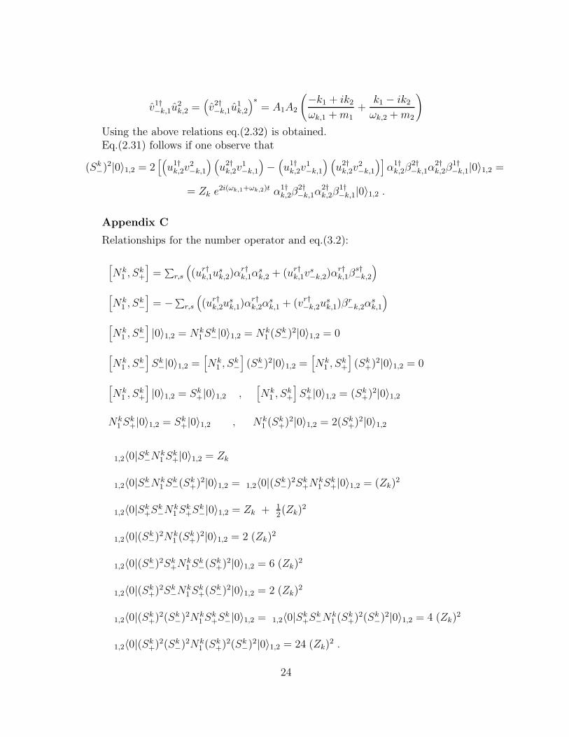
Using the above relations eq.(2.32) is obtained.Eq.(2.31) follows if one observe that

(Sk−)2|0〉1,2 = 2

[(

u1†k,2v

2−k,1

) (

u2†k,2v

1−k,1

)

−(

u1†k,2v

1−k,1

) (

u2†k,2v

2−k,1

)]

α1†k,2β

2†−k,1α

2†k,2β

1†−k,1|0〉1,2 =

= Zk e2i(ωk,1+ωk,2)t α1†k,2β

2†−k,1α

2†k,2β

1†−k,1|0〉1,2 .

Appendix C

Relationships for the number operator and eq.(3.2):

[

Nk1 , Sk

+

]

=∑

r,s

(

(ur†k,1usk,2)α

r†k,1α

sk,2 + (ur†k,1v

s−k,2)α

r†k,1β

s†−k,2

)

[

Nk1 , Sk

−

]

= −∑r,s

(

(ur†k,2usk,1)α

r†k,2α

sk,1 + (vr†−k,2u

sk,1)β

r−k,2α

sk,1

)

[

Nk1 , Sk

−

]

|0〉1,2 = Nk1 Sk

−|0〉1,2 = Nk1 (Sk

−)2|0〉1,2 = 0

[

Nk1 , Sk

−

]

Sk−|0〉1,2 =

[

Nk1 , Sk

−

]

(Sk−)2|0〉1,2 =

[

Nk1 , Sk

+

]

(Sk+)2|0〉1,2 = 0

[

Nk1 , Sk

+

]

|0〉1,2 = Sk+|0〉1,2 ,

[

Nk1 , Sk

+

]

Sk+|0〉1,2 = (Sk

+)2|0〉1,2

Nk1 Sk

+|0〉1,2 = Sk+|0〉1,2 , Nk

1 (Sk+)2|0〉1,2 = 2(Sk

+)2|0〉1,2

1,2〈0|Sk−Nk

1 Sk+|0〉1,2 = Zk

1,2〈0|Sk−Nk

1 Sk−(Sk

+)2|0〉1,2 = 1,2〈0|(Sk−)2Sk

+Nk1 Sk

+|0〉1,2 = (Zk)2

1,2〈0|Sk+Sk

−Nk1 Sk

+Sk−|0〉1,2 = Zk + 1

2(Zk)

2

1,2〈0|(Sk−)2Nk

1 (Sk+)2|0〉1,2 = 2 (Zk)

2

1,2〈0|(Sk−)2Sk

+Nk1 Sk

−(Sk+)2|0〉1,2 = 6 (Zk)

2

1,2〈0|(Sk+)2Sk

−Nk1 Sk

+(Sk−)2|0〉1,2 = 2 (Zk)

2

1,2〈0|(Sk+)2(Sk

−)2Nk1 Sk

+Sk−|0〉1,2 = 1,2〈0|Sk

+Sk−Nk

1 (Sk+)2(Sk

−)2|0〉1,2 = 4 (Zk)2

1,2〈0|(Sk+)2(Sk

−)2Nk1 (Sk

+)2(Sk−)2|0〉1,2 = 24 (Zk)

2 .

24

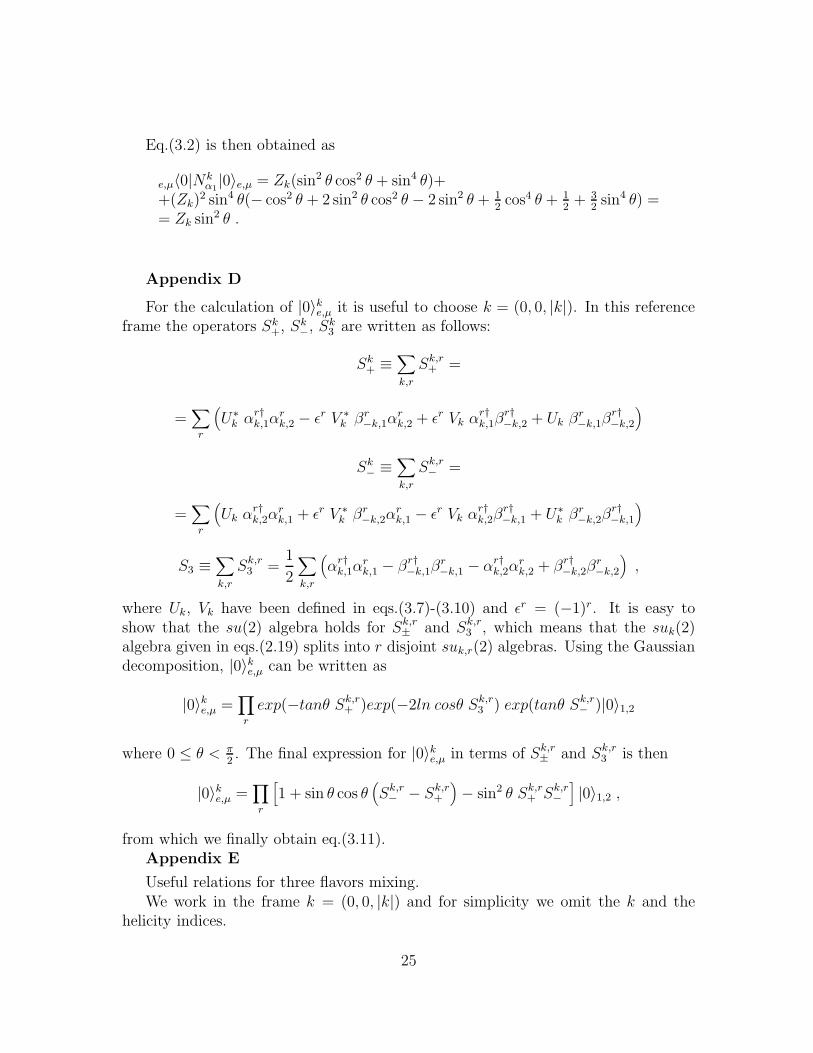
Eq.(3.2) is then obtained as

e,µ〈0|Nkα1|0〉e,µ = Zk(sin

2 θ cos2 θ + sin4 θ)++(Zk)

2 sin4 θ(− cos2 θ + 2 sin2 θ cos2 θ − 2 sin2 θ + 12cos4 θ + 1

2+ 3

2sin4 θ) =

= Zk sin2 θ .

Appendix D

For the calculation of |0〉ke,µ it is useful to choose k = (0, 0, |k|). In this referenceframe the operators Sk

+, Sk−, Sk

3 are written as follows:

Sk+ ≡

∑

k,r

Sk,r+ =

=∑

r

(

U∗k αr†k,1α

rk,2 − ǫr V ∗

k βr−k,1αrk,2 + ǫr Vk αr†k,1β

r†−k,2 + Uk βr−k,1β

r†−k,2

)

Sk− ≡

∑

k,r

Sk,r− =

=∑

r

(

Uk αr†k,2αrk,1 + ǫr V ∗

k βr−k,2αrk,1 − ǫr Vk αr†k,2β

r†−k,1 + U∗

k βr−k,2βr†−k,1

)

S3 ≡∑

k,r

Sk,r3 =

1

2

∑

k,r

(

αr†k,1αrk,1 − βr†−k,1β

r−k,1 − αr†k,2α

rk,2 + βr†−k,2β

r−k,2

)

,

where Uk, Vk have been defined in eqs.(3.7)-(3.10) and ǫr = (−1)r. It is easy toshow that the su(2) algebra holds for Sk,r

± and Sk,r3 , which means that the suk(2)

algebra given in eqs.(2.19) splits into r disjoint suk,r(2) algebras. Using the Gaussiandecomposition, |0〉ke,µ can be written as

|0〉ke,µ =∏

r

exp(−tanθ Sk,r+ )exp(−2ln cosθ Sk,r

3 ) exp(tanθ Sk,r− )|0〉1,2

where 0 ≤ θ < π2. The final expression for |0〉ke,µ in terms of Sk,r

± and Sk,r3 is then

|0〉ke,µ =∏

r

[

1 + sin θ cos θ(

Sk,r− − Sk,r

+

)

− sin2 θ Sk,r+ Sk,r

−

]

|0〉1,2 ,

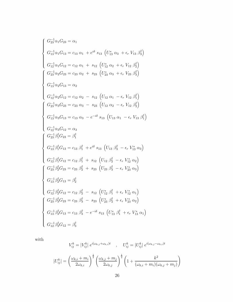
from which we finally obtain eq.(3.11).Appendix E

Useful relations for three flavors mixing.We work in the frame k = (0, 0, |k|) and for simplicity we omit the k and the

helicity indices.

25

G−123 α1G23 = α1

G−113 α1G13 = c13 α1 + eiδ s13

(

U∗13 α3 + ǫr V13 β†

3

)

G−112 α1G12 = c12 α1 + s12

(

U∗12 α2 + ǫr V12 β†

2

)

G−123 α2G23 = c23 α2 + s23

(

U∗23 α3 + ǫr V23 β†

3

)

G−113 α2G13 = α2

G−112 α2G12 = c12 α2 − s12

(

U12 α1 − ǫr V12 β†1

)

G−123 α3G23 = c23 α3 − s23

(

U12 α2 − ǫr V12 β†2

)

G−113 α3G13 = c13 α3 − e−iδ s13

(

U13 α1 − ǫr V13 β†1

)

G−112 α3G12 = α3

G−123 β†

1G23 = β†1

G−113 β†

1G13 = c13 β†1 + eiδ s13

(

U13 β†3 − ǫr V ∗

13 α3

)

G−112 β†

1G12 = c12 β†1 + s12

(

U12 β†2 − ǫr V ∗

12 α2

)

G−123 β†

2G23 = c23 β†2 + s23

(

U23 β†3 − ǫr V ∗

23 α3

)

G−113 β†

2G13 = β†2

G−112 β†

2G12 = c12 β†2 − s12

(

U∗12 β†

1 + ǫr V ∗12 α1

)

G−123 β†

3G23 = c23 β†3 − s23

(

U∗23 β†

2 + ǫr V ∗23 α2

)

G−113 β†

3G13 = c13 β†3 − e−iδ s13

(

U∗13 β†

1 + ǫr V ∗13 α1

)

G−112 β†

3G12 = β†3

withV kij = |V k

ij | ei(ωk,j+ωk,i)t , Ukij = |Uk

ij| ei(ωk,j−ωk,i)t

|Ukij | =

(

ωk,i + mi

2ωk,i

) 12(

ωk,j + mj

2ωk,j

) 12(

1 +k2

(ωk,i + mi)(ωk,j + mj)

)

26

|V kij | =

(

ωk,i + mi

2ωk,i

)12(

ωk,j + mj

2ωk,j

)12(

k

(ωk,j + mj)− k

(ωk,i + mi)

)

where i, j = 1, 2, 3 and j > i, and

|Ukij |2 + |V k

ij |2 = 1 , i = 1, 2, 3 j > i

(

V k23V

k∗13 + Uk∗

23 Uk13

)

= Uk12 ,

(

V k23U

k∗13 − Uk∗

23 V k13

)

= −V k12

(

Uk12U

k23 − V k∗

12 V k23

)

= Uk13 ,

(

Uk23V

k12 + Uk∗

12 V k23

)

= V k13

(

V k∗12 V k

13 + Uk∗12 Uk

13

)

= Uk23 ,

(

V k12U

k13 − Uk

12Vk13

)

= −V k23 .

27

References

1. T.Cheng and L.Li, Gauge Theory of Elementary Particle Physics, ClarendonPress, Oxford, 1989R.E.Marshak, Conceptual Foundations of Modern Particle Physics, World Sci-entific, Singapore, 1993

2. R.Mohapatra and P.Pal, Massive Neutrinos in Physics and Astrophysics, WorldScientific, Singapore, 1991J.N.Bahcall, Neutrino Astrophysics, Cambridge Univ. Press, Cambridge, 1989

3. C.Itzykson and J.B.Zuber, Quantum Field Theory, McGraw-Hill, New York,1980

4. A.Perelomov, Generalized Coherent States and Their Applications, Springer-Verlag, Berlin, 1986

5. S.M.Bilenky and B.Pontecorvo, Phys. Rep. 41 (1978) 225

6. N.N.Bogoliubov. A.A.Logunov, A.I.Osak and I.T.Todorov, General Principles

of Quantum Field Theory, Kluwer Academic Publishers, Dordrech, 1990

7. H.Umezawa, H.Matsumoto and M.Tachiki, Thermo Field Dynamics and Con-

densed States, North-Holland Publ. Co., Amsterdam, 1982H.Umezawa, Advanced Field Theory: Macro, Micro, and Thermal Physics,American Institute of Physics, New York, 1993

8. L.Wolfenstein, Phys. Rev.D17 (1978)S.P.Mikheyev and A.Y.Smirnov, Nuovo Cimento 9C (1986) 17

9. M.Blasone and G.Vitiello, Mixing Transformations in Quantum Field Theory,in preparation, 1994

28