Quantum entanglement in finite-dimensional Hilbert spaces by Szil´ ard Szalay Dissertation presented to the Doctoral School of Physics of the Budapest University of Technology and Economics in partial fulfillment of the requirements for the degree of Doctor of Philosophy in Physics Supervisor: Dr. P´ eter P´ al L´ evay research associate professor Department of Theoretical Physics Budapest University of Technology and Economics 2013 arXiv:1302.4654v1 [quant-ph] 19 Feb 2013

Welcome message from author
This document is posted to help you gain knowledge. Please leave a comment to let me know what you think about it! Share it to your friends and learn new things together.
Transcript
Quantum entanglement
in finite-dimensional Hilbert spaces
by
Szilard Szalay
Dissertation
presented to the Doctoral School of Physics of the
Budapest University of Technology and Economics
in partial fulfillment of the requirements for the degree of
Doctor of Philosophy in Physics
Supervisor: Dr. Peter Pal Levayresearch associate professorDepartment of Theoretical PhysicsBudapest University of Technology and Economics
2013
arX
iv:1
302.
4654
v1 [
quan
t-ph
] 1
9 Fe
b 20
13


To my wife, daughter and son.

v
Abstract. In the past decades, quantum entanglement has been recognized to be the basicresource in quantum information theory. A fundamental need is then the understanding its
qualification and its quantification: Is the quantum state entangled, and if it is, then how
much entanglement is carried by that? These questions introduce the topics of separabilitycriteria and entanglement measures, both of which are based on the issue of classification
of multipartite entanglement. In this dissertation, after reviewing these three fundamental
topics for finite dimensional Hilbert spaces, I present my contribution to knowledge. Mymain result is the elaboration of the partial separability classification of mixed states of
quantum systems composed of arbitrary number of subsystems of Hilbert spaces of arbitrarydimensions. This problem is simple for pure states, however, for mixed states it has not
been considered in full detail yet. I give not only the classification but also necessary and
sufficient criteria for the classes, which make it possible to determine to which class a mixedstate belongs. Moreover, these criteria are given by the vanishing of quantities measuring
entanglement. Apart from these, I present some side results related to the entanglement of
mixed states. These results are obtained in the learning phase of my studies and give someillustrations and examples.

Contents
Acknowledgements ix
Certifications in hungarian xi
List of publications xiii
Thesis statements xv
Prologue xvii
Chapter 1. Quantum entanglement 11.1. Quantum systems 21.2. Composite systems and entanglement 131.3. Quantifying entanglement 281.4. Summary 40
Chapter 2. Two-qubit mixed states with fermionic purifications 432.1. The density matrix 432.2. Measures of entanglement for the density matrix 462.3. Relating different measures of entanglement 522.4. Summary and remarks 55
Chapter 3. All degree 6 local unitary invariants of multipartite systems 573.1. Local unitary invariant polynomials 583.2. Graphs and matrix operations 613.3. Pure state invariants 633.4. Mixed-state invariants 693.5. Algorithm for Sr3/S3 713.6. Summary and remarks 73
Chapter 4. Separability criteria for mixed three-qubit states 754.1. A symmetric family of mixed three-qubit states 764.2. Bipartite separability criteria 784.3. Tripartite separability criteria 864.4. Tripartite entanglement 964.5. Summary and remarks 99
Chapter 5. Partial separability classification 1015.1. Partial separability of tripartite mixed states 1015.2. Generalizations: Partial separability of multipartite systems 1085.3. Summary and remarks 118
Chapter 6. Three-qubit systems and FTS approach 121
vii
viii CONTENTS
6.1. State vectors of three qubits 1226.2. Mixed states of three qubits 1276.3. Generalizations: Three subsystems 1316.4. Summary and remarks 133
Epilogue 135
Bibliography 137
Acknowledgements
This work would not have been possible without the help of several people, whom I wouldlike to mention here.
First and foremost, it is a pleasure to thank my adviser Peter Levay for his supervisingthrough the years of learning and research, and for giving me independence to pursue researchon the ideas that came across my mind. His helpful discussions together with his insight andpassion for research have always been inspiring.
I would like to extend my gratitude to some of my other teachers as well, Denes Petz,Tamas Geszti and Tamas Matolcsi, the lectures and books of whom were guides of great valuein studying quantum mechanics and mathematical physics.
I am grateful to Laszlo Szunyogh, the head of the Department of Theoretical Physics, andGyorgy Mihaly, the head of the Doctoral School of Physics, as well as Maria Vida, my admin-istrator, for the flexible, effective and helpful attitude for administrative issues, supporting mystudies to a large extent. My Ph.D. studies were partially supported by the New Hungary De-velopment Plan (project ID: TAMOP-4.2.1.B-09/1/KMR-2010-0002), the New Szechenyi Plan
of Hungary (project ID: TAMOP-4.2.2.B-10/1–2010-0009) and the Strongly correlated systemsresearch group of the “Momentum” program of the Hungarian Academy of Sciences (project ID:81010-00).
I am gerateful to my parents for supproting my studies financially and in principles as well.I would not be succesful without this.
Last but not least, I thank my wife, Marta, for her faithful love and everlasting support, pro-viding the affectionate and peaceful atmosphere which is an essential condition of any absorbedresearch. I would like to dedicate this piece of work to her and to our children.
ix


Certifications in hungarian
Alulırott Szalay Szilard kijelentem, hogy ezt a doktori ertekezest magam keszıtettem es abbancsak a megadott forrasokat hasznaltam fel. Minden olyan reszt, amelyet szo szerint vagy azonostartalommal, de atfogalmazva mas forrasbol atvettem, egyertelmuen, a forras megadasaval meg-jeloltem.Budapest, 2013. februr 14.
Szalay Szilard
Alulırott Szalay Szilard hozzajarulok a doktori ertekezesem interneten torteno korlatozas nelkulinyilvanossagra hozatalahoz.Budapest, 2013. februr 14.
Szalay Szilard
xi


List of publications
The research articles [1], [4], [5] and [6] are covered by this thesis. The research articles [2]and [3] are the results of another research project done in the related field of Black Hole / Qubitcorrespondence. The publications are listed in chronological order.
[1] Szilard Szalay, Peter Levay, Szilvia Nagy, Janos Pipek,A study of two-qubit density matrices with fermionic purifications,J. Phys. A 41, 505304 (2008) (arXiv: 0807.1804 [quant-ph])
[2] Peter Levay, Szilard Szalay,Attractor mechanism as a distillation procedure,Phys. Rev. D 82, 026002 (2010) (arXiv: 1004.2346 [hep-th])
[3] Peter Levay, Szilard Szalay,STU attractors from vanishing concurrence,Phys. Rev. D 84, 045005 (2011) (arXiv: 1011.4180 [hep-th])
[4] Szilard Szalay,Separability criteria for mixed three-qubit states,Phys. Rev. A 83, 062337 (2011) (arXiv: 1101.3256 [quant-ph])
[5] Szilard Szalay,All degree 6 local unitary invariants of k qudits,J. Phys. A 45, 065302 (2012) (arXiv: 1105.3086 [quant-ph])
[6] Szilard Szalay, Zoltan KokenyesiPartial separability revisited: Necessary and sufficient criteria,Phys. Rev. A 86, 032341 (2012) (arXiv: 1206.6253 [quant-ph])
xiii

Thesis statements
In the past decades, quantum entanglement has been recognized to be the basic resource inquantum information theory. A fundamental need is the understanding of its qualification andits quantification: Is the state entangled, and in this case how much entanglement is carried byit? These questions introduce the topics of separability criteria and entanglement measures, bothof which are based on the problem of classification of multipartite entanglement. In the followingthesis statements I present my contribution to these three issues.
I. I study a 12-parameter family of two-qubit mixed states, arising from a special class oftwo-fermion systems with four single particle states or alternatively from a four-qubitstate vector with amplitudes arranged in an antisymmetric matrix. I obtain a localunitary canonical form for those states. By the use of this I calculate two famousentanglement measures which are the Wooters concurrence and the negativity in aclosed form. I obtain bounds on the negativity for given Wootters concurrence, whichare strictly stronger than those for general two-qubit states. I show that the relevantentanglement measures satisfy the generalized Coffman-Kundu-Wootters formula ofdistributed entanglement. I give an explicit formula for the residual tangle as well.
The publication belonging to this thesis statement is [1] of the list on page xiii.
The main references belonging to this thesis statement are [LNP05, VADM01,CKW00, OV06].
II. Local unitary invariance is a fundamental property of all entanglement measures. Istudy quantities having this property for general multipartite systems. In particular,I give explicit index-free formulas for all the algebraically independent local unitaryinvariant polynomials up to degree six, for finite dimensional multipartite pure andmixed quantum states. I carry out this task by the use of graph-technical methods,which provide illustrations for this rather abstract topic.
The publication belonging to this thesis statement is [5] of the list on page xiii.
The main references belonging to this thesis statement are [HW09, HWW09,Vra11a, Vra11b].
III. I study the noisy GHZ-W mixture and demonstrate some necessary but not sufficientcriteria for different classes of separability of these states. I find that the partialtransposition criterion of Peres and the criteria of Guhne and Seevinck dealing directlywith matrix elements are the strongest ones for different separability classes of this
xv
xvi THESIS STATEMENTS
two-parameter state. I determine a set of entangled states of positive partial transpose.I also give constraints on three-qubit entanglement classes related to the pure SLOCC-classes, and I calculate the Wootters concurrences of the two-qubit subsystems.
The publication belonging to this thesis statement is [4] of the list on page xiii.
The main references belonging to this thesis statement are [Per96, GS10].
IV. I elaborate the partial separability classification of mixed states of quantum systemscomposed of arbitrary number of subsystems of Hilbert spaces of arbitrary dimensions.This extended classification is complete in the sense of partial separability and gives1 + 18 + 1 partial separability classes in the tripartite case contrary to the formerlyknown 1+8+1. I also give necessary and sufficient criteria for the classes by the use ofconvex roof extensions of functions defined on pure states. I show that these functionscan be defined so as to be entanglement-monotones, which is another fundamentalproperty of all entanglement measures.
The publication belonging to this thesis statement is [6] of the list on page xiii.
The main references belonging to this thesis statement are [DCT99, DC00, SU08].
V. For the case of three-qubit systems, by the use of the Freudenthal triple system ap-proach of three-qubit pure state entanglement, I obtain a set of functions on purestates, whose convex roof extensions give necessary and sufficient criteria for the par-tial separability classification. These functions have some advantages over the onesdefined in the general construction, which is given in the previous thesis statement.Moreover, these functions fit naturally for a special three-qubit classification whicharises as the combination of the partial separability classification with the classifica-tion obtained by Acın et. al. for three-qubit mixed states.
The publication belonging to this thesis statement is [6] of the list on page xiii.
The main references belonging to this thesis statement are [BDD+09, DCT99,DC00, ABLS01, SU08].
Prologue
The laws of quantum mechanics proved to be very successful in the description and predictionof the behaviour of the microworld. Among these predictions, however, there were some verysurprising ones which are in connection with the description of composite quantum systems. Inthe formalism of quantum mechanics, the so called entangled (or inseparable) states of compositesystems appear naturally, while the understanding of the correlations of the physical qantitiesmeasured on the subsystems of a system being in an entangled state is a challenge for themind. Namely, these correlations arise from the quantum mechanical interactions between thesubsystems, and they can not be modelled classically, these are the manifestations of the entirelyquantum behaviour of the nature. Entanglement theory is therefore a deep and fundamentalfield of central importance, lying in the very basics of the understanding of the physical world.
An interesting twist of the story is that these nonclassical correlations can be used fornonclassical solutions of classical, moreover, of nonclassical tasks, leading to the idea of quantumcomputation [Fey82]. These nonclassical computational and information theoretical methodsare the subject of the emerging field of quantum information theory, which is the extension ofthe classical information theory for quantum systems, dealing with these quantum correlations[NC00]. The significance of this relatively new field of science is hallmarked, among other things,by the Wolf Prize in Physics in this year.
In the scope of quantum information theory, there are entirely nonclassical, information the-oretical tasks (such as quantum communication with super-dense coding, quantum teleportation,quantum key distribution, quantum cryptography, quantum error correction) and also classicalcomputational tasks (such as quantum algorithms for factoring numbers, for quantum search,and for further tasks.) What is really fascinating is that quantum algorithms significantly out-perform the best known classical algorithms for the same tasks, moreover, they are able to solvesome problems in polynomial time, which problems can not be solved in polynomial time by theknown classical algorithms.
During the run of all the above quantum protocols, the basic resource expended is entan-glement, that is, composite quantum systems being in entangled states. A fundamental needis then the studying of the characterization of entanglement, which is the main concern of thisdissertation. Although the entanglement which is used for quantum information processing tasksis presented mostly in maximally entangled Bell pairs of two qubits, but the structure of entan-glement is far richer than that of two-qubit pure states. We will consider some aspects of thisissue in the present dissertation, here and now we just want to emphasize that the rich structureof multipartite entanglement might provide a lot of opportunities, which are still far from beingexplored and utilized.
The utilization of even the bipartite entanglement is by no means an easy job. Quantummechanics works in microscopic scales, and, due to the environmental decoherence, the mani-festations of this particular behaviour are hard to reach. Effects of entanglement are studiedin many-body systems as well, but an important color in the picture is that the experimental
xvii
xviii PROLOGUE
manipulation of individual quantum objects is not out of reach, as is also illustrated by the NobelPrize in Physics in last year.
The organization of this dissertation is as follows:
In chapter 1, we give a brief review on the fundamental topics of quantum entanglementwhich we deal with. We introduce the main notions and notational conventions andattempt to cover the whole material which will be used in the following chapters. Ourmain concerns are about the qualification of entanglement, that is, deciding about a givenstate whether it is entangled or separable; and the quantification of entanglement, thatis, defining quantities characterizing the “amount of entanglement” carried by a givenstate, doing this in some motivated way. Of course, if we have some evaluated quantitiesin hand which give the amount of entanglement, then the decision of entangledness issolved as well, but we usually do not have such opportunity and even the decision ofentangledness leads to a hard optimization problem. The situation is more complicated inmultipartite systems, where many different kinds of entanglement arise. In the followingchapters we present our contributions to knowledge in these fields.
In chapter 2, we start with a special two-qubit system. Qubit systems are of particularimportance because, on the one hand, qubits are the elementary building blocks ofapplications in quantum information theory, on the other hand, they have a simplemathematical structure leading to explicit results in the quantification of entanglement.Apart from that, systems of bigger size can be embedded into multiqubit systems. Forthe special family of two-qubit states we deal with, we evaluate explicitly some measuresof entanglement, and investigate some relations among those.The material of this chapter covers thesis statement I.
In chapter 3, we continue with a quite general construction of some quantites characterizingquantum states, a construction which is independent of the size of the subsystems.These quantities share the invariance property of the most detailed characterization ofentanglement, so these might provide a natural language for the characterization andeven for the quantitative description of entanglement.The material of this chapter covers thesis statement II.
In chapter 4, after the investigations of the previous two chapters, concerning the charac-terization of quantum states by quantities in some sense, we turn to the problem of thedecision of entangledness. In the literature there are numerous conditions for this. Forthe use of these conditions, various quantities have to be evaluated for a given state.Unfortunately, these quantities are given only implicitly in the most of the cases, andthose ones which can be evaluated explicitly result in sufficient but not necessary criteriaof entanglement only. Here we show some of the criteria of this kind at work, consideringa particular example of a family of three-qubit states.The material of this chapter covers thesis statement III.
In chapter 5, after the particular examples of the previous chapter, we consider the partialseparability problem in general. The partial separability treat every subsystem as afundamental unit, regardless of its size or even of the number of its components, andconcerns the existence of entanglement among the subsystems only. We extend the usualclassification of partial separability and formulate also necessary and sufficient criteriafor the decision of different kinds of entanglement. These criteria are given in terms ofquantities measuring entanglement. The use of these necessary and sufficient criterialeads to untractable hard optimization problems in general, so these criteria can onlybe used for special families of states, similarly to other necessary and sufficient criteria.However, our criteria have the advantage of reflecting clearly the structure of partialseparability, and they work in a similar way for all classes. We work out the tripartite
PROLOGUE xix
case, then we give the general definitions for arbitrary number of subsystems.The material of this chapter covers thesis statement IV.
In chapter 6, after the general constructions of the previous chapter, we turn to the par-ticular system of three qubits again. In this case, thanks to a beautiful mathematicalcoincidence, another set of quantities can be written for the formulation of the necessaryand sufficient criteria given in the previous chapter. Although these quantities are notmeasures of entanglement, but they fit not only for the partial separability classificationbut also for a more interesting classification of three-qubit states which goes a bit beyondpartial separability.The material of this chapter covers thesis statement V.

CHAPTER 1
Quantum entanglement
In quantum systems, correlations having no counterpart in classical physics arise. Purestates showing these strange kinds of correlations are called entangled ones [HHHH09, BZ06],and the existence of these states has so deep and important consequences that Schrodinger hasidentified entanglement to be the characteristic trait of quantum mechanics [Sch35a, Sch35b].
Historically, the nonlocal behaviour of entangled states of bipartite systems was the mainconcern first. Einstein, Podolsky and Rosen in their famous paper [EPR35] showed that underthe assumption of locality, entanglement gives rise to some “elements of reality”, that is, values ofphysical quantities exactly known without measurements, about which quantum mechanics doesnot know, since it gives only statistical answers. Therefore quantum mechanics is incomplete, andthere may exist variables, hidden for quantum mechanics, which determine the outcomes of themeasurements uniquely. What is more interesting, is that any hidden-variable model of quantummechanics is essentially nonlocal [Bel67], which is the famous, experimentally testable result ofBell. Nowadays, it is widely accepted that quantum mechanics is a complete, but statisticaltheory, and only the composite system possesses values of physical quantities, it is not possibleto ascribe values of physical quantities of local subsystems prior to measurements [Bel67].
Recently, the focus of attention in entanglement theory changed from locality issues to moregeneral forms of nonclassical behaviour [HHHH09]. As was mentioned in the Prologue, thenonclassical behaviour of entangled quantum states has far-reaching consequences manifestedin quantum information theory, which is the theory of nonclassical correlations together withapplications [NC00, Cav13].
In this dissertation, we encounter mixed states rather than pure ones, since the formerones play much more important roles in entanglement theory than the latter ones, because ofmultiple reasons. The majority of methods in quantum information theory, as well as the issuesconcerning locality, generally use pure entangled states, which can easily be prepared and whichare easy to use to obtain nonclassical results. However, in a laboratory one can not get rid of theinteraction with the environment perfectly, thus the separable compound state of the system andthe environment evolves into an entangled one, the prepared pure state of the system evolves intoa noisy, mixed one. This was a practical reason for studying mixed state entanglement, however,theoretical ones are much more important. First, in the case of multipartite systems even if thestate of the whole system is pure, the states of its bipartite subsystems are generally mixed ones,which is a hallmark of entanglement in itself [Sch35a, Sch35b]. Moreover, the understandingof classicality in the language of correlations can also be done only for mixed states even in thebipartite case [DV13].
The definition of entanglement and separability of mixed states was given first by Werner[Wer89]. In this paper, he also constructed famous examples for mixed states which are entan-gled and still local in the sense that a local hidden variable model can be constructed for that,describing the usual projective measurements. So we could think that from the point of view ofnonclassicality, entanglement does not grasp the nonclassical behaviour perfectly. However, animportant result, came from quantum information theory, disprove this. Namely, every entangled
1

2 1. QUANTUM ENTANGLEMENT
state can be used for some nonclassical task [Mas08, Mas06, LMR12]. So, for mixed states,nonlocality is considered only as a stronger manifestation of nonclassicality, but entanglement isstill important from the point of view of nonclassicality.
In this chapter, we give a brief review of the fundamental topics we deal with in quantummechanics [vN96, Pet08a, BZ06] and quantum entanglement [HHHH09], with some connec-tions to quantum information theory [Pet08b, NC00, Pre]. We introduce the main notionstogether with the notational conventions, and we attempt to cover the whole material which willbe used in the following chapters. We will see that entanglement in itself is a direct consequenceof the formalism of the mathematical description of quantum mechanics. Because of the reasonsabove, we follow a treatment from the point of view of mixed states. This has advantages andalso disadvantages. Usually, quantum mechanics is built upon the primary role of pure states,resulting in an inductive, better motivated and historically faithful treatment, in the course ofwhich mixed states arise as ensembles or states of subsystems of entangled systems. Here wegive a reverse treatment, which is an axiomatic, deductive and less motivated one, usual inentanglement theory, in the course of which pure states arise as special cases of mixed states.
The organization of this chapter is as follows.
In section 1.1, we start with recalling the general description of singlepartite quantum sys-tems (section 1.1.1) together with the characterization of the mixedness of the states ofthose in the terms of entropic quantities (section 1.1.2). The most important differencesbetween classical and quantum systems appear in these very basic topics. We also givethe detailed description of a single qubit, which is the simplest quantum system (section1.1.3).
In section 1.2, after the issues of singlepartite systems in the previous section, we turn tothe description of compound systems and entanglement. First, we review the generalnon-unitary operations on open quantum systems arising from the quantum interactioninside the bipartite composite of the system with its environment (section 1.2.1), thensome basics about the entanglement in bipartite and multipartite systems (sections 1.2.2and 1.2.3), and finally, the important point where these two topics meet each other, whichis the so called distant lab paradigm (section 1.2.4).
In section 1.3, after the basics of entanglement in the previous section, we turn to issuesrelated to the characterization of entanglement in some particular few-partite systems.First we review some tools for the quantification of bipartite entanglement (section 1.3.1),then we consider the pure and mixed states of general bipartite (sections 1.3.2 and1.3.3) and two-qubit systems (section 1.3.4 and 1.3.5). The structure of multipartiteentanglement is much more complex, we just review some important results for the caseof three-qubit pure and mixed states (sections 1.3.6 and 1.3.7), and of four-qubit purestates (section 1.3.8).
1.1. Quantum systems
In the most part of this dissertation, we deal with quantum states rather than physicalquantities themselves. By state we mean in general something what determines the values ofmeasurable physical quantities in some sense. In classical mechanics, the (pure) state of thesystem is represented by a point in a subset of a 2f dimensional real vector space, or moreprecisely in a simplectic manifold, called phase space, where f denotes the number of the degreesof freedom. In principle, the values of all physical quantities are completely determined by theactual phase point, so physical quantities are then represented by functions on this space. Thecase of quantum mechanics is more subtle. Instead of the real finite dimensional phase spacewe have a complex separable Hilbert space, the rays of that are regarded as (pure) quantum
1.1. QUANTUM SYSTEMS 3
states. Moreover, the values of physical quantities are not determined by the quantum state,only distributions of them.
1.1.1. Description of quantum systems. The mathematical foundations of quantummechanics are due to von Neumann [vN96]. LetH be the complex Hilbert space corresponding toa quantum system. In the whole of this dissertation, we consider systems having finite dimensionalHilbert space only. The dimension of the Hilbert space is denoted by d. In the classical scenario,this corresponds to the discrete phase space of d points. The system in the particular case whend = 2 is called qubit. This case is not only the most simple but also a very exceptional one,there are many mathematical coincidences which hold only in two dimensions. We will see somemanifestations of them in the following.
The dynamical variables of the quantum system, also called observables, are represented bynormal operators acting on H,
A(H) ={A ∈ Lin(H)
∣∣∣ AA† = A†A}.
Operators of this kind admit the spectral decomposition
A =∑i
ai|αi〉〈αi|, where 〈αi′ |αi〉 = δi′
i ,
which is of fundamental importance for the structure of the theory. As we will see, the discreteeigenvalues represent the discrete outcomes of the measurments, which is how quantum mechanicsdescribe the quantized phenomena of the microworld. The dynamical variables in quantummechanics are usually inherited from the classical mechanics, where they take real values. Inthis case the quantum mechanical dynamical variables are represented by self-adjoint operators,having real eigenvalues. (Sometimes, only these operators are called observables.) Another noteis that there is a freedom in the choice of the Hilbert space, as far as the considered observablescan be represented on that.
The state of the quantum system is represented by a self-adjoint positive semidefinite op-erator acting on H, which is normalized, which means in this context that its trace is equal to1. These operators are called statistical operators, or density operators. The set of the states isdenoted by D ≡ D(H), which is then1
D(H) ={% ∈ Lin(H)
∣∣∣ %† = %, % ≥ 0, tr % = 1}.
The self-adjoint operators form a vector space over the field of real numbers. This vector spacecan also be endowed with an inner product and also a metric. The operators of unit traceforms an affin subspace in that, while the positive semidefinite operators form a cone, which isconvex. D(H) is then the intersection of these two, so it is a convex set in the affin subspaceof unit trace in the real vector space of self-adjoint operators acting on H. By virtue of this,the dimension of D(H) is d2 − 1. The π extremal points of D(H) are of the form π = |ψ〉〈ψ|,where |ψ〉 ∈ H is normalized, ‖ψ‖2 = 1. They are called pure states, and they form a 2d − 2-dimensional submanifold of D(H), denoted with P(H). Contrary to the classical scenario, herewe have continuously many pure states even for qubits. The set of states is the convex hull of
1Strictly speaking, the states are the probability measures on the lattice of subspaces of the Hilbert space[FT78], and the set of them is isomorphic to D(H) only for d > 2, which is Gleason’s theorem [Gle57]. In the
pathological d = 2 case there are probability measures to which density operators can not be assigned. We oftenconsider qubits, but we deal only with density operators, and, inaccurately, by states we mean density operatorsonly.
4 1. QUANTUM ENTANGLEMENT
the pure states D(H) = Conv(P(H)
), in other words, every state can be formed by the convex
combination of pure states,
% =
m∑j=1
pjπj , (1.1)
where the m-tuple p = (p1, . . . , pm) of convex combination coefficients is positive and normalizedwith respect to the 1-norm, ‖p‖1 =
∑j pj = 1. The set of such m-tuples, the m − 1-simplex,
is denoted with ∆m−1 ⊂ Rm. The principle of measurement, given in the following paragraphs,enables us to consider this p as a discrete probability distribution. If the convex combinationis not trivial then the state is called mixed state, and its interpretation is that the system is inthe pure state πj with probability pj . If an ensemble of quantum systems being in pure statesπj with mixing weights pj is given, then random sampling results in such a distribution. Notethat here, contrary to the classical scenario, the pure states have intrinsic structure, so a mixedquantum state is not only a probability distribution but a probability distribution together withdirections in the Hilbert space.
A (generalized) measurement on the system is given by a set of measurement operators{Mi ∈ Lin(H)
∣∣∣ i = 1, . . . ,m,∑i
M†iMi = I}.
A selective measurement has m outcomes, resulting in the m post-measurement states:
% 7−→ %′i =Mi%M
†i
trMi%M†i
, with probability qi = trMi%M†i . (1.2a)
(The∑iM†iMi = I resolution of identity ensures that
∑i qi = 1.) Here we have physical access
to the %i outcome states of the measurement, under which we mean that we are able to executedifferent quantum operations on the different outcome systems. Note that the probabilisticnature of the measurements is an inherent property of quantum mechanics, it does not comefrom that the measurement devices are inaccurate and sometimes miss the right output. Quitethe contrary, these principles of quantum measurements are formulated with ideal mesurementdevices. Another point here is that the linearity of the trace in the qi probabilities allows us toconsider the (1.1) convex combination of pure states as a statistical mixture of states, since theprobabilities of the measurement outcomes arise from a weighted average of that of pure states.
The other main difference between the classical and quantum measurement is that the mea-surement inherently affects, disturbes the state of the system. If we carry out the measurementbut forget about which outome we got, that is, we form the mixture of the post-measurementstates, which is the result of a non-selective measurement, we get
% 7−→ %′ =∑i
qi%′i =
∑i
Mi%M†i , (1.2b)
which is not equal to the original state in general. Physically, the measurement device interactswith the system, and this interaction can not be neglected.
In the special case of the von Neumann measurement, which is the archetype of measure-
ments, the measurement operators Mi = Pi are projectors of orthogonal supports, Pi = P †i ,PiPi′ = δii′Pi. In this case, the repeated measurements give the same outcome. The Pi projec-tors arise as the spectral projectors of an observable A, and the measured value of the observablein the case of the ith outcome of the measurement is the ai eigenvalue corresponding to theeigensubspace onto which Pi projects. The expectation value of the measurement is then
〈A〉 ≡∑i
aiqi = trA%, (1.3)
1.1. QUANTUM SYSTEMS 5
in this sense the state % defines a linear functional on the observables. In the next section wewill see how the (1.2) generalized measurement arises.
If the qi = trMi%M†i measurement statistics is the only thing of interest, then it is enough to
deal with the Ei = M†iMi positive operators instead of the Mi measurement operators. The set{Ei} is called Positive Operator Valued Measure (POVM), and the maps % 7→ trEi%, determiningthe measurement statistics, are linear functionals on the states. This makes the use of POVMsmuch more convenient than that of the measurement operators.
The linear structure in the underlying Hilbert space is also important. If the state is pure,sometimes we deal with the state vector |ψ〉 ∈ H instead of the rank one density matrix |ψ〉〈ψ| ∈P(H) ⊂ D(H). In this case, we regard the pure state in the Hilbert space as the phase-equivalenceclass of the state vector. Let {|i〉 | i = 1, . . . , d} be an orthonormal basis in H, sometimes calledcomputational basis, then the state vector can be written as2
|ψ〉 =
d∑i=1
ψi|i〉, where ψi = 〈i|ψ〉 ∈ C.
We use the convention for coefficients with lower indices (ψi)∗ = ψi, which are the 〈ψ|i〉 coeffi-cients of the 〈ψ| = |ψ〉∗ ∈ H∗ dual vector.3
The Hilbert space H is closed under complex-linear combination |ψ〉 =∑j cj |ψj〉, which is
called superposition in this context. This makes the Hilbert space and also P(H) a much moreinteresting place than the classical phase space, and in multipartite systems this is responsible forentanglement. On the other hand, the space of states D is closed under convex combination % =∑j pj |ψj〉〈ψj |, which is called mixing. A fundamental difference between these two constructions
is the possibility of interference. The measurement probabilities in the first and second cases are
qi = tr(Mi|ψ〉〈ψ|M†i
)=∥∥∥∑
j
cjMi|ψj〉∥∥∥2
,
qi = tr(Mi%M
†i
)=∑j
pj
∥∥∥Mi|ψj〉∥∥∥2
.
In the first case, contrary to the second one, qi can be zero even if the vectors Mi|ψj〉 are nonzero,which is a manifestation of the famous phenomenon of quantum interference.
If the system is in a pure state π = |ψ〉〈ψ| ∈ P, and we consider a von Neumann measurementwith the measurement operators being the orthogonal spectral projectors of a nondegenerate
2The indices of the basis run sometimes from 0 to d− 1, especially in the elements of quantum informationtheory, where this practice is rather convenient. But note that in this case all indices, even those of the convex
combination coefficients in (1.1), should run from zero, because Schrodinger’s mixture theorem couples together
these two kinds of summations, as we will see in (1.4) in the next subsection.3In the finite dimensional case, the 〈·|·〉 inner product identifies H∗ with H, and we denote this identification
with the star: ∗ : H → H∗, |ψ〉∗ = 〈ψ|, and since H∗∗ ∼= H in the finite dimensional case, 〈ψ|∗ = |ψ〉. Thiscan be extended to tensors as well. For example θ = θij |i〉 ⊗ 〈j| ∈ K ⊗ H∗ (the ⊗ sign is often omitted in the
case of tensors of this kind), we have θ∗ = (θ∗) ji 〈i| ⊗ |j〉 ∈ K∗ ⊗H, leading to (θ∗) ji = (θij)
∗, which is denoted
simply with θ ji through the identification. Note, however, that the indices of tensors can not be uppered andlowered independently, since 〈·|·〉 is conjugate-linear in the first position. Linear operations act from the left, that
is, Lin(H → K) ∼= K⊗H∗. We have also the transposition, which is the natural operation t : K⊗H∗ →H∗ ⊗K,|i〉 ⊗ 〈j| 7→ 〈j| ⊗ |i〉. This is defined without the inner product, it simply interchanges the Hilbert spaces, so itcan act independently on pairs of indices. Later, more general partial transpositions, reshufflings and general
permutations of Hilbert spaces will also be used. For convenience, we have also the hermitian transpostion
† = ∗ ◦ t : K ⊗ H∗ → H ⊗ K∗, |i〉 ⊗ 〈j| 7→ |j〉 ⊗ 〈i| for the action of linear operations on the dual. For furtherdetails in tensor algebraic constructions, see part 2. in [Mat93], with slightly different notations.
6 1. QUANTUM ENTANGLEMENT
observable, Mi = |αi〉〈αi|, then we get back Born’s Rule
qi = |〈αi|ψ〉|2.The square in that, together with the interference of different measurement outcomes couldhave been the first indications that there is a Hilbert space somewhere in the grounds of themathematical description of quantum mechanics. On the other hand, we can consider thismeasurement as a transformation of the complex ψi = 〈αi|ψ〉 superposition coefficients to thereal qi = |ψi|2 mixing weights. In this sense, the measurement washes away the interference.
The probabilities of the outcomes of the measurements are given by the trace, or the innerproduct, both of them are invariant under the action of the unitary group4 U(H), which is, afterfixing an orthonormal basis, isomorphic with the classical matrix group U(d). For |ψ〉 7→ |ψ′〉 =U |ψ〉 with an U ∈ U(H), we have the same group action on the states and the observables
% 7−→ %′ = U%U†,
A 7−→ A′ = UAU†,
Mi 7−→ M ′i = UMiU†,
since all of them are elements in Lin(H) ∼= H⊗H∗. One can see, which is desired in physics, thatonly the description may depend on the chosen coordinates in H, not the measurement statistics.
There is another role of unitary transformations besides the coordinate transformation inthe Hilbert space, which is the time evolution. In this case the state and the observables aretransformed differently, that is, their “relative angle” in Lin(H) changes. In quantum mechanics,the time evolution of the state of an isolated quantum system is described by a unitary transfor-mation %(0) 7→ %(t) = U(t)%(0)U(t)†, while this time the observables are independent of time,hence not transformed (Schrodinger picture). This evolution operator can be obtained from thevon Neumann equation5
∂%(t)
∂t= −i
[H(t), %(t)
]given with the self-adjoint observable H ∈ A(H) corresponding to the energy of the system,called Hamiltonian, as the time-ordered operator
U(t) = T exp
(−i∫ t
0
H(t′)dt′
).
This reduces to U(t) = exp(−iHt
)if H does not depend on time.
1.1.2. The mixedness of a state. A good summary on the mixedness of the quantumstates can be found in [BZ06]. The decomposition of a mixed state into the ensemble of purestates is, contrary to the classical case, far from unique. In general, the state % can be writtenwith the ensemble{(
pj , |ψj〉〈ψj |) ∣∣∣ p ∈ ∆m−1, ‖ψj‖2 = 1
}as
% =
m∑j=1
pj |ψj〉〈ψj |.
4This is, of course, not a coincidence. The trace is the natural linear map from Lin(H) ∼= H ⊗ H∗ to C,and H∗ is naturally identified with H by the inner product of the Hilbert space, and the unitary group is the
invariance group of the inner product, by definition.5In this dissertation we use metric system in which ~ = 1.
1.1. QUANTUM SYSTEMS 7
The spectral decomposition defines, however, a unique ensemble. It consists of the spectrum andthe orthogonal spectral projections,{(
λi, |ϕi〉〈ϕi|) ∣∣∣ λ ∈ ∆d−1, 〈ϕi′ |ϕi〉 = δii′
},
giving
% =
d∑i=1
λi|ϕi〉〈ϕi|.
There is an elegant theorem, called Schrodinger’s mixture theorem [Sch36] or Gisin-Hughston-Jozsa-Wootters lemma [Gis89, HJW93], which gives all the possible decompositions of a densitymatrix. It relates them to the spectral decomposition in the following way:
√pj |ψj〉 =
d∑i=1
U ji√λi|ϕi〉, (1.4)
where U jis are the entries of an m × d matrix with orthonormal columns, U†U = Id. Themeaning of this matrix of coefficients is clarified later from the point of view of pure statesof bipartite systems (section 1.3.2). The set of such matrices is a compact complex manifoldVd(Cm) ∼= U(m)/U(m− d), which is called Stiefel manifold.
Since we have the quantum state as a mixture of pure states, moreover, as the same mix-ture for different ensembles of pure states, as a natural question arises, how mixed a state isthen? The mixedness of a state is given by the notion of majorization. First we invoke thenotion of majorization for discrete probability distributions. For two probability distributionsp = (p1, . . . , pm) ∈ ∆m−1 and q = (q1, . . . , qm) ∈ ∆m−1, p is majorized by q, denoted with thesymbol �, with the following definition:
p � qdef.⇐⇒
k∑i=1
p↓i ≤k∑i=1
q↓i ∀k = 1, 2, . . . ,m, (1.5)
where ↓ in the superscript means decreasing order. The majorization is clearly reflexive (p � p)and transitive (if p � q and q � r then p � r) but the antisymmetry (if p � q and q � pthen p = q) holds only in a restricted manner: if p � q and q � p then p↓ = q↓. On theother hand, it is clear that p � q does not imply q � p, in other words there exist pairs ofprobability distributions which we can not compare by majorization. Hence the majorizationdefines a partial order on the set of probability distributions up to permutations.
With respect to majorization, the set of discrete probability distributions contains a greatestand a smallest element. One can check that all p ∈ ∆m−1 majorize the uniform distribution andall p is majorized by the distribution containing only one element,
(1/m, 1/m, . . . ) � p � (1, 0, . . . ).
It is generally accepted to use the mathematical definition of majorization for the comparsionof disorderness (mixedness) of discrete probability distributions. If p � q then we can say thatp is more disordered (more mixed) than q, or equivalently, q is more ordered (more pure) thanp, but, as was mentioned before, there are pairs of distributions for which their rank of disordercan not be compared in this sense.
Real-valued functions defined on probability distributions and compatible with majorizationare of particular importance. An f : ∆m−1 → R is Schur-concave if
p � q =⇒ f(p) ≥ f(q). (1.6)
Schur concavity is the definitive property of all (generalized) entropies, which means that if adistribution is more mixed than the other then it has greater entropy. Note that the entropies
8 1. QUANTUM ENTANGLEMENT
can be compared for all pairs of distributions, not only for those which can be compared bymajorization, so comparsion of mixedness by entropies is not the same as by majorization.
The most basic entropy is the Shannon entropy
H(p) = −∑j
pj ln pj , (1.7a)
having the strongest properties among all entropies. The Renyi entropy is defined as
HRq (p) =
1
1− qln∑j
pqj , q > 0, (1.7b)
which is a generalization of the Shannon entropy in the sense that limq→1HRq (p) = H(p). Its
other limits are also notable. For q → 0+, this is the logarithm of the number of nonzero pjs,known as Hartley entropy
HR0 (p) := lim
q→0+HRq (p) = ln |{j | pj 6= 0}|. (1.7c)
For q →∞, it converges to the Chebyshev entropy
HR∞(p) := lim
q→∞HRq (p) = − ln pmax. (1.7d)
The Tsallis entropy is defined as
HTsq (p) =
1
1− q
(∑j
pqj − 1), q > 0, (1.7e)
which is, contrary to the Renyi entropy, a non-additive generalization of the Shannon entropy,limq→1H
Tsq (p) = H(p). Note that the Tsallis entropy is the linear leading term in the power-
series of the Renyi entropy,6 this is why Tsallis entropy is sometimes called linear entropy.How to generalize the above conceptions to the quantum case? A quantum state can be
formed as a mixture from different ensembles, so the p mixing weights are not inherent propertiesof it. However, the spectrum of a state is not only well-defined, but, thanks to Schrodingersmixture theorem (1.4) and the Hardy-Littlewood-Polya lemma [BZ06], it also majorizes everyother mixing weights. So the spectrum is special from the point of view of mixedness, and themajorization of density matrices is defined via the corresponding majorization of their spectra,
% � ω def.⇐⇒ Spect % � Spectω. (1.8)
By virtue of this, we can compare the mixedness of density matrices. On the other hand, becauseof Schur concavity, the entropy of the spectrum is smaller than that of any other mixing weights.Now, if the quantum entropies of a state are defined as the classical entropies of the spectrum,then they are Schur concave in the sense of the majorization of density matrices. Moreover, theentropies above for a quantum state can be written by the density matrix itself without anyreference to the decompositions.
The quantum generalization of the Shannon entropy is called von Neumann entropy
S(%) = − tr(% ln %) = H(Spect %
), (1.9a)
the quantum Renyi entropy is
SRq (%) =
1
1− qln tr %q = HR
q
(Spect %
), q > 0, (1.9b)
6Remember that lnx = (x − 1) − 12
(x − 1)2 + 13
(x − 1)3 − · · · + (−1)k
k(x − 1)k + . . . for 0 < x, the role of
which is played by∑j pqj .
1.1. QUANTUM SYSTEMS 9
while its limits, the quantum Hartley entropy is
SR0 (%) := lim
q→0+SRq (%) = ln rk % = HR
0
(Spect %
), (1.9c)
which is the logarithm of the rank of %, and the quantum Chebyshev entropy
SR∞(%) := lim
q→∞SRq (%) = − ln max Spect % = HR
∞(Spect %
). (1.9d)
The other family, the quantum Tsallis entropy is
STsq (%) =
1
1− q(tr %q − 1
)= HR
q
(Spect %
), q > 0. (1.9e)
An advantage of the Tsallis and Renyi entropies is that they are easy to evaluate for integerq ≥ 2 parameters, when only matrix powers have to be calculated instead of the entire spectrum.
All of the above quantum entropies vanish for pure states and reach their maxima for
% =1
dI, (1.10)
having the uniform distribution as its spectrum. This state is sometimes called white noise,because in this state all outcomes of a measurement of a nondegenerate observable occur withequal probability.
Some other quantities are also in use for the characterization of mixedness. For example thepurity
P (%) = tr %2, (1.11a)
the participiation ratio
R(%) =1
tr %2, (1.11b)
which can be interpreted as an effective number of pure states in the mixture, and the so calledconcurrence-squared
C2(%) =d
d− 1STs
2 (%) =d
d− 1
(1− tr %2
), (1.11c)
the latter is normalized, 0 ≤ C2(%) ≤ 1. All of them are related to the q = 2 quantum Tsallis
(or quantum Renyi) entropy, which is in connection with Euclidean distances in D(H) [BZ06].The Shannon or von Neumann entropies are widely used in classical and quantum statistical
physics, while their generalizations are often considered unphysical or useless, mainly because of,e.g., the non-additivity (non-extensivity) of the Tsallis entropies. An interesting observation ofus is that in entanglement theory, contrary to statistical physics, the generalized entropies oftenprove to be more useful than the original one. We will see in section 4.2.2 that for a family ofthree-qubit states, the generalized entropies for high parameters q give stronger conditions ofentanglement. Here the Renyi and Tsallis entropies lead to the same conditions for the sameparameters q. Another, more sophisticated example for the usefulness of Tsallis entropies canbe found in section 6.3, where it is shown that the additive definition of some of the indicatorfunctions for tripartite systems can be given only by generally non-additive entropies. In this casethe subadditivity seems to be more important than the additivity. We should mention here alsothat Tsallis entropies are sometimes used even in thermodynamics. For example, non-extensivethermodynamical models are developed for the modelling of the behaviour of the quark-gluonplasma produced in heavy-ion collisions, see in [VBBU12] and in the references therein.
10 1. QUANTUM ENTANGLEMENT
1.1.3. The states of a qubit. As an example, consider the case of a qubit, d = dimH =2. Spin degree of freedom of particles having 1/2 spin, or polarization degree of freedom ofphotons are the typical physical systems whose states are described by qubits. In A(H) we havethe linearly independent σ0, σ1, σ2, σ3 Pauli operators, which are self-adjoint, trσν = 2δν0 andobeying the well-known Pauli algebra
σ0σ0 = σ0, σ0σi = σiσ0 = σi, σiσj = δijσ0 + i∑k
εijkσk, (1.12)
where i, j, k ∈ {1, 2, 3}, and εijk denotes the parity of the permutation ijk of 123 if i, j and kare different, othervise εijk is zero. Any density operator can be written with these in the form
% =1
2(σ0 + xσ) , (1.13)
where the x ∈ R3 Bloch vector parametrizes the state, and we use the shorthand notationxσ = x1σ1 + x2σ2 + x3σ3. The characteristic equation of %
λ2 − λ tr %+ det % = 0
allows us to obtain the eigenvalues, and by the use of the Cayley-Hamilton theorem
%2 − % tr %+ I det % = 0
together with the (1.12) algebra of Pauli operators we have that ‖x‖2 = 1− 4 det %, which allowsus to write the eigenvalues in geometrical terms
λ± =1
2
(1±
√1− 4 det %
)=
1
2(1± ‖x‖) .
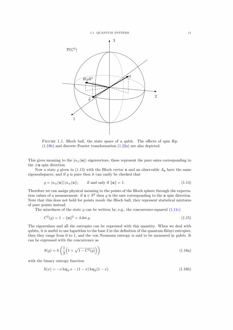
This tells us that % is a proper quantum state of a qubit if and only if ‖x‖2 ≤ 1, while % is apure state if and only if ‖x‖2 = 1. So, for qubits, we have the space of states D(H) ∼= B3, andits extremal points, i.e. the set of pure states P(H) ∼= S2, which are called Bloch ball and Blochsphere in this context (figure 1.1). The ‖x‖2 = 0 center of the ball is the 1/2I white noise.7 Notethat in this case the whole boundary of D(H) is extremal. This does not hold for d > 2, as caneasily be seen by counting the dimensions.8
The only self-adjoint observable in this case is generally of the form9 Au = uσ with u ∈ R3.Because of the (1.12) Pauli algebra, { 1
2σ1,12σ2,
12σ3} obey the commutation relations of the
angular momentum10[1
2σi,
1
2σj
]= i∑k
εijk1
2σk,
so if ‖u‖2 = 1 then Au represents the observable corresponding to a spin measurement in ~/2units, along the direction u. As before, we have that Au has the eigenvalues ±‖u‖. If we multiplythe eigenvalue equation
Au|α±(u)〉 = ±‖u‖|α±(u)〉with 〈α±(u)|σi from the left, using (1.12) we have for the real part that
〈α±(u)|σi|α±(u)〉 = ± ui‖u‖
.
7So, for qubits, σ0 = I, but note that this does not hold for the higher dimensional representations of the
Pauli algebra.8There are some results on the geometry of the state space of a qutrit (d = 3), in which case the Gell-Mann
matrices can be used [SB13, GSSS11]. For general d, the suitable generators of SU(d) can be used.9Adding σ0 only shifts the eigenvalues and leave the eigensubspaces invariant.10Hence they represent the su(2) Lie-algebra of SU(2).
1.1. QUANTUM SYSTEMS 11
˜
HH†
D(C2)
1
2
3
Figure 1.1. Bloch ball, the state space of a qubit. The effects of spin flip(1.19b) and discrete Fourier transformation (1.22a) are also depicted.
This gives meaning to the |α±(u)〉 eigenvectors, these represent the pure sates corresponding tothe ±u spin direction.
Now a state % given in (1.13) with the Bloch vector x and an observable Ax have the sameeigensubspaces, and if % is pure then it can easily be checked that
% = |α±(x)〉〈α±(x)|, if and only if ‖x‖ = 1. (1.14)
Therefore we can assign physical meaning to the points of the Bloch sphere through the expecta-tion values of a measurement: if x ∈ S2 then % is the sate corresponding to the x spin direction.Note that this does not hold for points inside the Bloch ball, they represent statistical mixturesof pure points instead.
The mixedness of the state % can be written by, e.g., the concurrence-squared (1.11c)
C2(%) = 1− ‖x‖2 = 4 det %. (1.15)
The eigenvalues and all the entropies can be expressed with this quantity. When we deal withqubits, it is useful to use logarithm to the base 2 in the definition of the quantum-Renyi entropies,then they range from 0 to 1, and the von Neumann entropy is said to be measured in qubits. Itcan be expressed with the concurrence as
S(%) = h
(1
2
(1 +
√1− C2(%)
))(1.16a)
with the binary entropy function
h(x) = −x log2 x− (1− x) log2(1− x). (1.16b)
12 1. QUANTUM ENTANGLEMENT
It is clear from (1.15) that the concurrence-squared C2(%) (and the von Neumann entropy S(%)as well) is an U(1)× SL(2,C)-invariant quantity for qubits.11 since entropies are invariant onlyunder unitaries in general.
Note that all of the above constructions were carried out without an explicit representationfor the Pauli operators. This abstract approach is very useful in the derivation of the nonlinearBell inequalities, which are recalled in section 1.2.2, and of which multipartite extension is usedin section 4.3.2. Now, after choosing an orthonormal basis {|0〉, |1〉}, the Hilbert space H ∼= C2,and for further use we introduce the usual matrix representation of the Pauli operators
σ0 =
[1 00 1
]= I, σ1 =
[0 11 0
], σ2 =
[0 −ii 0
], σ3 =
[1 00 −1
], (1.17)
which are called Pauli matrices. But there is a matrix of particular importance which has to begiven explicitly,
ε =
[0 1−1 0
], (1.18)
its εij entry is the parity of the permutation ij of 01 if i and j are distinct, othervise zero.With this, the linear transformation ε = εij〈i| ⊗ 〈j| ∈ H∗ ⊗ H∗ ∼= Lin(H → H∗) gives another
identification of H with H∗, which is a basis-dependent one.12 Let 〈ψ| = ε|ψ〉, then
|ψ〉 = ψi|i〉 7−→ |ψ〉 = 〈ψ|∗ = (εii′)∗ψi
′∗|i〉 = εii
′ψi′ |i〉, (1.19a)
where the ˜ = ∗ ◦ ε notation is used. The corresponding operation on D(H)
% = %ij |i〉 ⊗ 〈j| 7−→ % = (ε%ε†)∗ = (εii′%i′
j′εjj′〈i| ⊗ |j〉)∗
= (εii′)∗(%i
′
j′)∗(εjj
′)∗|i〉 ⊗ 〈j| = εii
′% j′
i′ εjj′ |i〉 ⊗ 〈j|(1.19b)
where the˜ = ∗◦Adε notation is used, results in the x 7→ −x space inversion in R3. This operationis called spin-flip (figure 1.1). Note that this is an antilinear operation on H and Lin(H).Antilinear operations are in connection with the time reversal in quantum mechanics. Indeed,a spin changes sign for time reversal, but not for space inversion, being an axial-vector. (Spaceinversion is not even contained in SO(3) ⊂ SO(3, 1), the group of space rotations, represented onLin(H), whose double cover SU(2) ⊂ SL(2,C) is represented on H.)
The characteristic property of ε is the very special transformation behaviour
AtεA = (detA)ε (1.20)
for any A ∈ Lin(H), leading to the invariance under SL(2,C). This makes ε suitable for obtainingLorentz-invariant combinations from Weyl spinors. Although, in nonrelativistic entanglementtheory Lorentz transformations are not involved, but SL(2,C) comes into the picture in a different
11Note that the normalization of a state vector and that of a density matrix are not invariant under theaction of U(1) × SL(2,C). For unnormalized distributions, the STs
q (%) = 1/(1 − q)(tr %q − (tr %)q
)definition of
Tsallis entropies has to be used instead of (1.9e), leading to C2(%) = 2((tr %)q − tr %q
)for qubits.
12Note that we use here a convention different from the one which is used in the representation theoryof the Lorentz group on Dirac and Weyl spinors, where there are two Hilbert spaces, carrying the left-handed
and right handed representations, having undotted and dotted indices, and ε is used for lowering and uppering
indices in both Hilbert spaces. Instead of these, we have upper and lower indices on H and H∗, respectively, and
ε ∈ Lin(H → H∗) and ε∗ ∈ Lin(H∗ → H) are always written out explicitly, and εii′ ≡ (ε∗)ii
′= (εii′ )
∗ = εii′ .
This convention is more convenient when the “default” group action is that of U(2) instead of SL(2,C), whichlatter represents the Lorentz group on two dimensional Hilbert spaces. Note again, however, that in this casechanging index positions can only be done for all indices collectively.
1.2. COMPOSITE SYSTEMS AND ENTANGLEMENT 13
way, making the structure ε still important. A sign of this is that the determinant can also bewritten with the spin-flip given by ε, leading to
C2(%) = 4 det % = 2 tr %%. (1.21)
This characterizes not only the mixedness of a qubit, but, as we will see, its entanglement withits environment. And this is not the only case in which ε comes into the picture, it appears againand again along the issues of the entanglement of qubits. We will meet it in sections 1.3.4, 1.3.5,1.3.6, 1.3.8 and in section 6.1.1 in connection with the Freudenthal triple system approach ofthree-qubit entanglement [BDD+09].
Another operation, which is important in quantum information theory, is the discrete Fouriertransformation
% 7−→ H%H† (1.22a)
given by the unitary involution having the matrix
H =1√2
[1 11 −1
], (1.22b)
which is a Hadamard matrix. This results in a (x1, x2, x3)t 7→ (x3,−x2, x1)t rotation (figure 1.1).
1.2. Composite systems and entanglement
In the classical scenario, the phase space of a composite system arises as the direct productof the phase spaces of the subsystems. In quantum mechanics, however, the Hilbert space ofa bipartite composite quantum system arises as the tensor product of the Hilbert spaces ofthe subsystems. As we will see, this structure along with the superposition is responsible forentanglement.
For two subsystems, the tensor product of the Hilbert spaces of the subsystems is H ≡ H12 =H1 ⊗H2 and d1 = dimH1, d2 = dimH2 and d ≡ d12 = dimH = d1d2, and d = (d1, d2) denotesthe 2-tuple of the local dimensions.13 The set of states D ≡ D12 ≡ D(H12) is defined in thesame way as for singlepartite systems, while the sets of states of the subsystems are D1 ≡ D(H1)and D2 ≡ D(H2). The sets of pure states of the composite system and those of its subsystemsare denoted with P ≡ P12 ≡ P(H12), and P1 ≡ P(H1) and P2 ≡ P(H2). The reduced states of% ∈ D are given by the partial trace operation, %1 = tr2 % ∈ D1 and %2 = tr1 % ∈ D2, which isthe quantum analogy of obtaining marginal distributions. On the other hand, a purification of astate %1 ∈ D1 is a π ∈ P pure state of the composite system from which %1 arises as the reducedstate, that is, %1 = π1 ≡ tr2 π. Such purification exists for all %1 if the other Hilbert space H2 isbig enough, that is, d2 ≥ d1.
Composite systems in quantum mechanics appear basically in two main respects. Namely,when a composite of subsystems playing equal roles is investigated (entanglement theory), andwhen the composite system is regarded as the compound of a system with its environment(theory of open quantum systems). These two cases have the same mathematical description,the difference is physical: we can not execute quantum operations on the environment. Ofcourse, these two fields are strongly interrelated, the distinction is made with respect to theirmain concerns only. In the following, we review the general non-unitary operations on openquantum systems, some basics about the entanglement of bipartite and multipartite systems,and the important point where these two meet each other, which is the so called distant labparadigm.
The main reference on entanglement is [HHHH09].
13If we have the computational bases {|i〉 | i = 1, . . . , d1} ⊂ H1 and {|j〉 | j = 1, . . . , d2} ⊂ H2 of the
subsystems, then the computational basis of the composite system is {|i〉 ⊗ |j〉 | i = 1, . . . , d1, j = 1, . . . , d2} ⊂ H,the element of which is often abbreviated as |i〉 ⊗ |j〉 ≡ |ij〉.
14 1. QUANTUM ENTANGLEMENT
1.2.1. Operations on quantum systems. Here we outline the treatment of open quan-tum systems, following section 2. of [Sag12]. The most general operations on quantum statescan be formulated by the use of completely positive maps. These are the positive maps Φ ∈Lin(Lin(H)→ Lin(H′)
)for which the map extended with identity Φ⊗I ∈ Lin
(Lin(H⊗HEnv)→
Lin(H′ ⊗HEnv))
is also positive for an arbitrary dimensional Hilbert space HEnv correspondingto the environment. (Note that in this general treatment the change of the Hilbert space is alsoallowed. For example, an ancillary system can be coupled to the original system, in which caseH′ = H⊗HAnc, or it can also be dropped, in which case H = H′⊗HAnc.) These maps preservethe positivity of the state not only of the system but also of the compound of the system and itsenvironment—or the reservoir, or the rest of the world—hence the physically relevant transfor-mations must be of this kind. The representation theorem of Kraus states that Φ is completelypositive if and only if it can be written by the Kraus operators Mj ∈ Lin(H → H′) as
Φ(%) =∑j
Mj%M†j ,
which is called the Kraus form of Φ. On the other hand, a completely positive Φ should preservethe trace to be a proper transformation on quantum states. To handle selective measurements,we have to allow a map to decrease the trace too. A completely positive map is trace-preservingif and only if∑
j
M†jMj = I,
and trace non-increasing if and only if∑j
M†jMj ≤ I.
In the light of these, the most general operations on quantum states can be given by the socalled stochastic quantum operation
% 7−→ %′ =Φ(%)
tr Φ(%)
with the trace non-increasing completely positive map Φ. The operation takes place with prob-ability q = tr Φ(%), which is equal to one if and only if Φ is trace-preserving. A trace-preservingcompletely positive map is called deterministic quantum operation, or quantum channel.
We have the following physical prototypes of deterministic quantum operations:
Φ(%) = %⊗ πAnc, (1.23a)
Φ(%) = U%U†, (1.23b)
Φ(%) = trHAnc%, (1.23c)
that is, adding an uncorrelated ancilla, unitary time-evolution, and throwing away a subsys-tem, respectively. The prototype of stochastic quantum operations is a selective von Neumannmeasurement with a projector Pi
Φ(%) = Pi%P†i . (1.23d)
This means that we throw away all but the ith output state, which is a special case of thepostselection operation. If we have only one copy of the state then the operation takes place withprobability q = tr Φ(%), othervise the protocol fails. On the other hand, if the state is present inmultiple copies, then only a fraction of the copies, proportional to q, is left after the operation.We have these two physical interpretations of the decreasing of the trace.
1.2. COMPOSITE SYSTEMS AND ENTANGLEMENT 15
Since the physically relevant transformations are the completely positive ones, the outputsof a measurement are related in general to the input by such transformations. So a generalizedmeasurement is given by a set of completely positive maps {Φi}, which are given by the Krausoperators {Mij} as
Φi(%) =∑j
Mij%M†ij , with probability qi = tr Φi(%), (1.24a)
and which all are trace non-increasing,∑jM
†ijMij ≤ I. However, there is a constraint that the
whole non-selective measurement Φ =∑i Φi, acting as
Φ(%) =∑i
qiΦi(%)
tr Φi(%)=∑i
∑j
Mij%M†ij , (1.24b)
has to be trace preserving,∑ijM
†ijMij = I.
It can be shown that every measurement described by such a {Φi} can be written on anextended system as
Φi(%) = trHAnc
((I⊗ Pi)U(%⊗ πAnc)U†(I⊗ Pi)†
), (1.25)
where {Pi} is a complete set of projection operators having orthogonal support,∑i Pi = I,
PiPj = δijPi. So we have the physical interpretation for the trace non-increasing completelypositive maps corresponding to the measurement outputs: A generalized measurement arisesas a von Neumann measurement on an ancilla, which interacts with the original system. Inother words, every selective generalized measurement (non-unitary stochastic operation) can beconstructed by the use of the elementary, physically motivated steps (1.23a)–(1.23d). It canalso be shown that if the Pi projectors are of rank one, which is the case of measurement withnondegenerate observable, then all Φis are given by only one Kraus operator each. That is,
Mij = Mi for all j, so Φi(%) = Mi%M†i , and we get back the (1.2) formulas of generalized
measurements.On the other hand, we get the trace-preserving operation by summing up Φ =
∑i Φi, which
results in that every trace preserving completely positive map can be written in an extendedsystem as
Φ(%) = trHAnc
(U(%⊗ πAnc)U†
). (1.26)
So we have the physical interpretation for the non-unitary evolution of a system: It can bemodelled by a unitary evolution of an extended system. In other words, every non-selectivegeneralized measurement (non-unitary deterministic operation) can be constructed by the use ofthe elementary, physically motivated steps (1.23a)–(1.23c).
1.2.2. Entanglement in bipartite systems. Now, we consider a composite quantumsystem of two subsystems. The central notion here is that of separable states, which is definedto be the convex sum of tensor products of states
% ∈ Dsepdef.⇐⇒ % =
∑j
p′j%1,j ⊗ %2,j , (1.27a)
where %1,j ∈ D1 and %2,j ∈ D2, and p′ ∈ ∆m′−1, as usual. The motivation of this definitionis that states of this kind can be prepared locally, with the use of classical correlations only[Wer89]. Due to the positivity restriction of the p′js, Dsep is a proper subset of D, and theelements of the set D \ Dsep are called entangled states. That is, entangled states can not bewritten as a convex combination of product states, which is another plausible motivation, sinceclassical joint probability distributions can always be written as a convex combination of product
16 1. QUANTUM ENTANGLEMENT
distributions. The set Dsep is a convex one, and, since the dimensions of the Hilbert spaces ofthe subsystems are finite, we can rewrite its elements (1.27) as14
% ∈ Dsep ⇐⇒ % =∑j
pj(|ψ1,j〉 ⊗ |ψ2,j〉
)(〈ψ1,j | ⊗ 〈ψ2,j |
)(1.27b)
with the different weights p ∈ ∆m−1. Hence the set of separable states is the convex hull ofseparable pure states π = |ψ〉〈ψ|, arising from tensor product vectors of the form |ψ〉 = |ψ1〉⊗|ψ2〉.The set of these is denoted with Psep. The reduced states of a separable pure state are pureones, π1 = |ψ1〉〈ψ1| and π2 = |ψ2〉〈ψ2|. Due to superposition, not all vectors in H1 ⊗ H2
are of this kind. In fact, almost all vectors are not of this kind, so they are called entangledones. As we will see, the reduced states of an entangled pure state are mixed ones, contraryto the classical case, where the marginals of a pure joint probability distribution are pure ones.This was the first embarrassing observation about entanglement, made by Einstein, Podolsky,Rosen and Schrodinger: even if we know exactly the state of the whole system,—i.e. it is in apure state, which contains all the information that quantum mechanics can provide about thesystem—the possible (pure) states of the subsystems are known only with some probabilities[EPR35, Sch35a, Sch35b]. (And what is worse, the ensemble of these pure states is not evenunique.) This means that if we have an ensemble of systems prepared identically in a pureentangled state then we can not choose such measurements on a subsystem which leads to puremeasurement statistics q1 = (1, 0, 0, . . . ).
As an extremal example, consider one of the (pure) Bell-states of two qubits, given by thestate vector
|B〉 =1√2
(|00〉+ |11〉
). (1.28)
Its reduced states %1 = 1/2I, %2 = 1/2I are maximally mixed. But this is only one part of thestory. If a selective measurement is carried out on both subsystems of a system being in the state|B〉〈B| with the observables A⊗ I and I⊗B with A = σ3, B = σ3, (1/2-spin mesurements alongthe z axis) then the outcomes of the two measurements are maximally correlated. Moreover, afterthe selective measurement (1.2a) on the first subsystem only (with A⊗I), the whole state becomea separable pure one, the reduced states of both subsystems are changed to pure ones,15 so thestate of the second subsystem is determined without measurement. What was really embarrassingwith this is that this happens instantaneously even if the measurements are spatially separated.This nonlocal behaviour of entangled states was called “spuckhafte Fernwirkung” (spooky actionat a distance) by Einstein. Note that this nonlocality can not be used for superluminal signalling,because the outcome of the first measurement is trully random. This observation is called “no-signalling”.
Here we have to take a short detour and pose the question: What does it mean that thecorrelation contained in the Bell-state is considered entirely nonclassical? In the case of mixedstates this happens even in the classical scenario. If the joint state of the two subsystems iscorrelated16 then we can obtain information about one subsystem (its state is then updated) byperforming a measurement on the other one. In the quantum scenario, if a state is correlated17
14Here we use that Lin(H1)⊗ Lin(H2) ∼= H1 ⊗H∗1 ⊗H2 ⊗H∗2 ∼= H1 ⊗H2 ⊗H∗1 ⊗H∗2 ∼= Lin(H1 ⊗H2).15Note that a non-selective measurement (1.2b) modifies the state of only that subsystem on which it is
performed, independently of the state.16A joint probability distribution (state of classical compound system) is correlated if it does not arise as a
product of the probability distributions of the subsystems, pij 6= pipj .17A density operator of a compound system is correlated if it does not arise as a tensor product of the density
operators of the subsystems % 6= %1 ⊗ %2. Note that this does not mean entanglement, the set of uncorrelatedstates is a proper subset of the separable states.
1.2. COMPOSITE SYSTEMS AND ENTANGLEMENT 17
then the same happens, which is then not implausible. What is interesting is that in the quantumscenario this happens even if the state of the system is pure. In the classical scenario, if acomposite system is in a pure state then the subsystems are in pure states as well, and such stateis completely uncorrelated. In the quantum scenario, however, the subsystems of a system beingin a pure state can be in mixed states, which means then a new kind of correlation, which is notclassical.
Maybe the most famous topic in connection with entanglement is the topic of the Bellinequalities [Bel67, Pre]. It is related to the problem of the existence of a local hidden variablemodel for the description of a quantum system, which could be a possibility to avoid nonlocality.Namely, it can be possible that quantum mechanics does not provide a complete descriptionof the physical world, and there are variables, hidden for quantum mechanics, which determinethe outcomes of the measurements uniquely. From a complete theory containing these hiddenvariables, the probabilities inherent in quantum mechanics arise in the sense that the preparationof a quantum state does not fix the value of the hidden variable uniquely, and quantum mechanicsarises as an effective theory. Now, the locality principle is not violated if the value of thesehidden variables are fixed during the interaction of the parties, and they are not affected byeach other after the subsystems are moved far away from each other, and considered to becomeisolated. The key discovery here, found by Bell [Bel67], is that if the measurement statisticsare determined by a Local Hidden Variable Model (LHVM) then constraints on the statistics ofcorrelation experiments can be obtained. Instead of Bell’s original inequality, we show here asimplified version, using only two dichotomic18 measurements on each site, proposed by Clauser,Horne, Shimony and Holt (CHSH) [CHSH69]. Let these be denoted with A and A′ in the firstsubsystem, and B and B′ in the second one, all of them have the outcomes ±1. We denote theexpectation value with respect to the hidden variable with 〈·〉, then such a constraint is given bythe CHSH inequality
LHVM =⇒ |〈AB +AB′ +A′B −A′B′〉| ≤ 2. (1.29)
In quantum mechanics, we have the archetype of dichotomic measurements, which is the mea-surement of the spin of a spin-1/2 particle (section 1.1.3). Let the unit vectors describing thedirections of the measurements be denoted with a,a′,b,b′ ∈ S2 ⊂ R3 then the observable of thecorrelation experiment is the following
SCHSH = aσ ⊗ bσ + aσ ⊗ b′σ + a′σ ⊗ bσ − a′σ ⊗ b′σ.
Then the CHSH inequality takes the form
% admits LHVM =⇒ |〈SCHSH〉| = |tr(%SCHSH
)| ≤ 2 for all settings. (1.30)
However, it is known that in quantum mechanics there are states and measurement settingsfor which this bound can be violated, hence the predictions of quantum mechanics can not beobtained by a local hidden variable model. The experiments confirm the predictions of quantummechanics, although there exists loopholes because of the insufficient efficiency of the detectors.
The Bell inequalities and their connection existence of local hidden variable models is a deepand widely studied question [Gis09, LMR12], with heavy physical and philosophical conse-quences [ES02, SKZ13]. There is, however, another application of the Bell inequalities, whichis the detection of entanglement. First of all it can be shown that for pure states, entanglementis necessary and sufficient for the possibility of finding measurement settings for which the CHSHinequality is violated, or alternatively, the CHSH inequality hold for all measurement settings ifand only if the state is separable,
π ∈ Psep ⇐⇒ |tr(πSCHSH
)| ≤ 2 for all settings. (1.31a)
18Dichotomic measurements are measurements having only two outcomes.
18 1. QUANTUM ENTANGLEMENT
However, Werner showed that this does not hold for mixed states, here we have only that
% ∈ Dsep =⇒ |tr(%SCHSH
)| ≤ 2 for all settings. (1.31b)
That is, there are mixed states, which are although entangled but still can be modelled by anLHVM [Wer89]. But these are not the last words about the connection between LHVMs ofdifferent measurement scenarios and entanglement of mixed states. This is a widely studied andvery interesting issue, however, it is out of the scope of this dissertation.19
What is important for us is that (1.31b) can be used for the detection of entanglement,which is a central problem of this dissertation. It is a difficult question to decide whether astate is separable or not, that is, whether the decomposition given in (1.27) exists or not. Thecondition (1.31b) serves also for this purpose. Namely, its negation states that if we can find ameasurement setting for which the CHSH-bound is violated, then the state is entangled.
% /∈ Dsep ⇐= there exists setting giving |tr(%SCHSH
)| � 2. (1.31c)
Unfortunately, this is only a sufficient but not necessary criterion of entanglement, that is, thereare entangled states for which there does not exist such measurement setting for which theentangledness can be detected by this method. Moreover, another difficulty shows up here too,which accompanies us all along, which is the issue of optimization over a huge manifold. In thiscase, for a given state, we have to find a measurement setting, which leads to the violation of theinequality. In other cases, other kinds of optimizations have to be done, which makes the detectionof entanglement difficult even if we have necessary and sufficient criteria of entanglement.
Another way of detecting entanglement is the use of witness operators [HHH96a]. A wit-ness operator is, by definition, an W ∈ Lin(H) self-adjoint observable which has nonnegativeexpectation value for all separable states, but there exists at least one entangled state for whichthe expectation value is negative. In other words, a witness operator defines a D → R linearfunctional % 7→ trW%, the kernel of which, which is a hyperplane in Lin(H), cuts into D butnot into Dsep (figure 1.2). A corollary of the Hahn-Banach theorem is that for every given en-
tangled state there exists a witness operator which detects it [HHH96a, BZ06]. In this sense,witnessing gives rise to a necessary and sufficient condition of entanglement, leading to
% ∈ Dsep ⇐⇒ 〈W 〉 ≡ trW% ≥ 0 for all withesses W. (1.32a)
The characterization of the convex set of separable states Dsep by witness operators (that is, bysupporting hyperplanes) is a hard problem that have not been solved yet. So, for the decisionof separability of a given state the problem of optimization is still exists, since one has to finda witness which detects the entanglement of that given state. We can get necessary but notsufficient condition for separability using only an insufficient set of witnesses
% ∈ Dsep =⇒ 〈W 〉 ≡ trW% ≥ 0 for some withesses W. (1.32b)
One can obtain, for example, the witness corresponding to the CHSH correlation-experiment
WCHSH = 2I⊗ I± SCHSH.
This is actually a family of witnesses parametrized by the a,a′,b,b′ measurement settings. Aswe have from (1.31b), there are entangled states which can not be detected by CHSH inequalityof any settings, this means that the arrangement of the hyperplanes given by WCHSH is not strictenough to clip around Dsep perfectly.
The linear witnessing, which is the reformulation of the linear CHSH-inequalities is notsufficient for the detection of entanglement, but there is, however, a nonlinear extension of thiscriterion, which proved to be a necessary and sufficient one for the two-qubit case. These arecalled quadratic Bell inequalities [US08], although their connection to the existence of LHVM
19For a recent summary for this topic we refer to section IV.C.1 of [HHHH09].
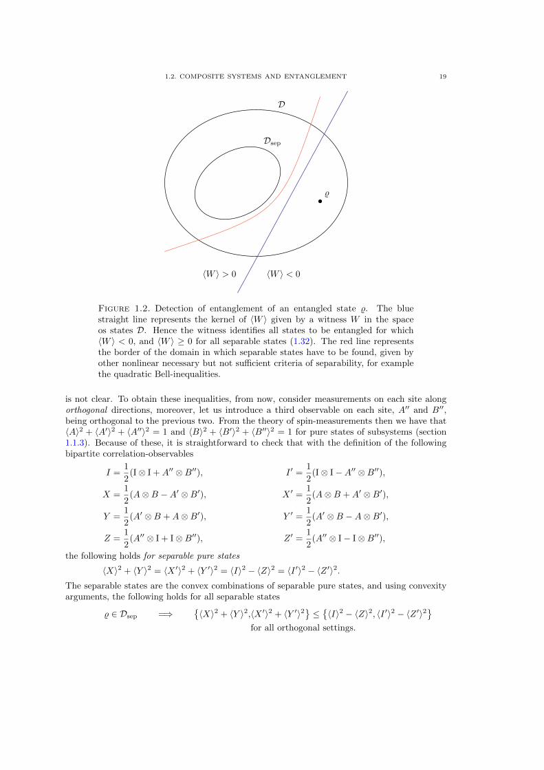
1.2. COMPOSITE SYSTEMS AND ENTANGLEMENT 19
D
Dsep
〈W 〉 > 0 〈W 〉 < 0
Figure 1.2. Detection of entanglement of an entangled state %. The bluestraight line represents the kernel of 〈W 〉 given by a witness W in the spaceos states D. Hence the witness identifies all states to be entangled for which〈W 〉 < 0, and 〈W 〉 ≥ 0 for all separable states (1.32). The red line representsthe border of the domain in which separable states have to be found, given byother nonlinear necessary but not sufficient criteria of separability, for examplethe quadratic Bell-inequalities.
is not clear. To obtain these inequalities, from now, consider measurements on each site alongorthogonal directions, moreover, let us introduce a third observable on each site, A′′ and B′′,being orthogonal to the previous two. From the theory of spin-measurements then we have that〈A〉2 + 〈A′〉2 + 〈A′′〉2 = 1 and 〈B〉2 + 〈B′〉2 + 〈B′′〉2 = 1 for pure states of subsystems (section1.1.3). Because of these, it is straightforward to check that with the definition of the followingbipartite correlation-observables
I =1
2(I⊗ I +A′′ ⊗B′′), I ′ =
1
2(I⊗ I−A′′ ⊗B′′),
X =1
2(A⊗B −A′ ⊗B′), X ′ =
1
2(A⊗B +A′ ⊗B′),
Y =1
2(A′ ⊗B +A⊗B′), Y ′ =
1
2(A′ ⊗B −A⊗B′),
Z =1
2(A′′ ⊗ I + I⊗B′′), Z ′ =
1
2(A′′ ⊗ I− I⊗B′′),
the following holds for separable pure states
〈X〉2 + 〈Y 〉2 = 〈X ′〉2 + 〈Y ′〉2 = 〈I〉2 − 〈Z〉2 = 〈I ′〉2 − 〈Z ′〉2.The separable states are the convex combinations of separable pure states, and using convexityarguments, the following holds for all separable states
% ∈ Dsep =⇒{〈X〉2 + 〈Y 〉2,〈X ′〉2 + 〈Y ′〉2
}≤{〈I〉2 − 〈Z〉2, 〈I ′〉2 − 〈Z ′〉2
}for all orthogonal settings.
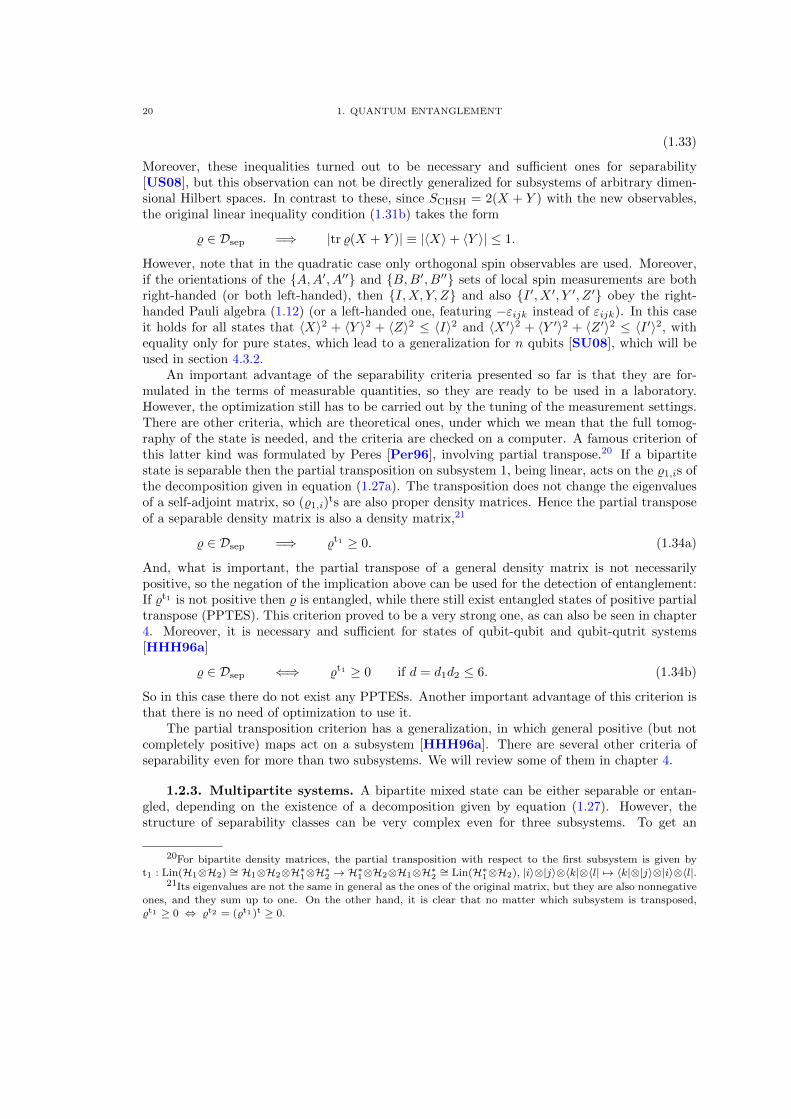
20 1. QUANTUM ENTANGLEMENT
(1.33)
Moreover, these inequalities turned out to be necessary and sufficient ones for separability[US08], but this observation can not be directly generalized for subsystems of arbitrary dimen-sional Hilbert spaces. In contrast to these, since SCHSH = 2(X + Y ) with the new observables,the original linear inequality condition (1.31b) takes the form
% ∈ Dsep =⇒ |tr %(X + Y )| ≡ |〈X〉+ 〈Y 〉| ≤ 1.
However, note that in the quadratic case only orthogonal spin observables are used. Moreover,if the orientations of the {A,A′, A′′} and {B,B′, B′′} sets of local spin measurements are bothright-handed (or both left-handed), then {I,X, Y, Z} and also {I ′, X ′, Y ′, Z ′} obey the right-handed Pauli algebra (1.12) (or a left-handed one, featuring −εijk instead of εijk). In this caseit holds for all states that 〈X〉2 + 〈Y 〉2 + 〈Z〉2 ≤ 〈I〉2 and 〈X ′〉2 + 〈Y ′〉2 + 〈Z ′〉2 ≤ 〈I ′〉2, withequality only for pure states, which lead to a generalization for n qubits [SU08], which will beused in section 4.3.2.
An important advantage of the separability criteria presented so far is that they are for-mulated in the terms of measurable quantities, so they are ready to be used in a laboratory.However, the optimization still has to be carried out by the tuning of the measurement settings.There are other criteria, which are theoretical ones, under which we mean that the full tomog-raphy of the state is needed, and the criteria are checked on a computer. A famous criterion ofthis latter kind was formulated by Peres [Per96], involving partial transpose.20 If a bipartitestate is separable then the partial transposition on subsystem 1, being linear, acts on the %1,is ofthe decomposition given in equation (1.27a). The transposition does not change the eigenvaluesof a self-adjoint matrix, so (%1,i)
ts are also proper density matrices. Hence the partial transposeof a separable density matrix is also a density matrix,21
% ∈ Dsep =⇒ %t1 ≥ 0. (1.34a)
And, what is important, the partial transpose of a general density matrix is not necessarilypositive, so the negation of the implication above can be used for the detection of entanglement:If %t1 is not positive then % is entangled, while there still exist entangled states of positive partialtranspose (PPTES). This criterion proved to be a very strong one, as can also be seen in chapter4. Moreover, it is necessary and sufficient for states of qubit-qubit and qubit-qutrit systems[HHH96a]
% ∈ Dsep ⇐⇒ %t1 ≥ 0 if d = d1d2 ≤ 6. (1.34b)
So in this case there do not exist any PPTESs. Another important advantage of this criterion isthat there is no need of optimization to use it.
The partial transposition criterion has a generalization, in which general positive (but notcompletely positive) maps act on a subsystem [HHH96a]. There are several other criteria ofseparability even for more than two subsystems. We will review some of them in chapter 4.
1.2.3. Multipartite systems. A bipartite mixed state can be either separable or entan-gled, depending on the existence of a decomposition given by equation (1.27). However, thestructure of separability classes can be very complex even for three subsystems. To get an
20For bipartite density matrices, the partial transposition with respect to the first subsystem is given by
t1 : Lin(H1⊗H2) ∼= H1⊗H2⊗H∗1⊗H∗2 →H∗1⊗H2⊗H1⊗H∗2 ∼= Lin(H∗1⊗H2), |i〉⊗|j〉⊗〈k|⊗〈l| 7→ 〈k|⊗|j〉⊗|i〉⊗〈l|.21Its eigenvalues are not the same in general as the ones of the original matrix, but they are also nonnegative
ones, and they sum up to one. On the other hand, it is clear that no matter which subsystem is transposed,%t1 ≥ 0 ⇔ %t2 = (%t1 )t ≥ 0.
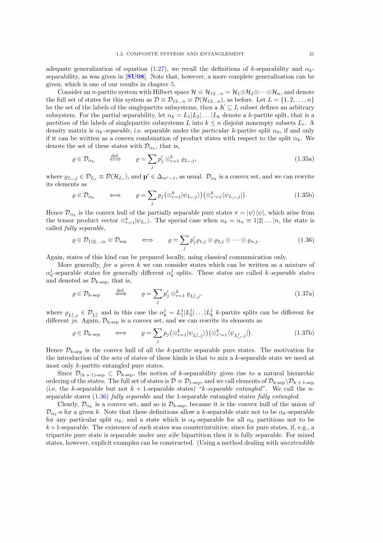
1.2. COMPOSITE SYSTEMS AND ENTANGLEMENT 21
adequate generalization of equation (1.27), we recall the definitions of k-separability and αk-separability, as was given in [SU08]. Note that, however, a more complete generalization can begiven, which is one of our results in chapter 5.
Consider an n-partite system with Hilbert spaceH ≡ H12...n = H1⊗H2⊗· · ·⊗Hn, and denotethe full set of states for this system as D ≡ D12...n ≡ D(H12...n), as before. Let L = {1, 2, . . . , n}be the set of the labels of the singlepartite subsystems, then a K ⊆ L subset defines an arbitrarysubsystem. For the partial separability, let αk = L1|L2| . . . |Lk denote a k-partite split, that is apartition of the labels of singlepartite subsystems L into k ≤ n disjoint nonempty subsets Lr. Adensity matrix is αk-separable, i.e. separable under the particular k-partite split αk, if and onlyif it can be written as a convex combination of product states with respect to the split αk. Wedenote the set of these states with Dαk , that is,
% ∈ Dαkdef.⇐⇒ % =
∑j
p′j ⊗kr=1 %Lr,j , (1.35a)
where %Lr,j ∈ DLr ≡ D(HLr ), and p′ ∈ ∆m′−1, as usual. Dαk is a convex set, and we can rewriteits elements as
% ∈ Dαk ⇐⇒ % =∑j
pj(⊗kr=1|ψLr,j〉
)(⊗kr′=1〈ψLr′ ,j |
). (1.35b)
Hence Dαk is the convex hull of the partially separable pure states π = |ψ〉〈ψ|, which arise fromthe tensor product vector ⊗kr=1|ψLr 〉. The special case when αk = αn ≡ 1|2| . . . |n, the state iscalled fully separable,
% ∈ D1|2|...|n ≡ Dsep ⇐⇒ % =∑j
p′j%1,j ⊗ %2,j ⊗ · · · ⊗ %n,j . (1.36)
Again, states of this kind can be prepared locally, using classical communication only.More generally, for a given k we can consider states which can be written as a mixture of
αjk-separable states for generally different αjk splits. These states are called k-separable statesand denoted as Dk-sep, that is,
% ∈ Dk-sepdef.⇐⇒ % =
∑j
p′j ⊗kr=1 %Ljr,j , (1.37a)
where %Ljr,j ∈ DLjr and in this case the αjk = Lj1|Lj2| . . . |L
jk k-partite splits can be different for
different js. Again, Dk-sep is a convex set, and we can rewrite its elements as
% ∈ Dk-sep ⇐⇒ % =∑j
pj(⊗kr=1|ψLjr,j〉
)(⊗kr′=1〈ψLj
r′ ,j|). (1.37b)
Hence Dk-sep is the convex hull of all the k-partite separable pure states. The motivation forthe introduction of the sets of states of these kinds is that to mix a k-separable state we need atmost only k-partite entangled pure states.
Since D(k + 1)-sep ⊂ Dk-sep, the notion of k-separability gives rise to a natural hierarchicordering of the states. The full set of states isD ≡ D1-sep, and we call elements ofDk-sep\Dk + 1-sep
(i.e. the k-separable but not k + 1-separable states) “k-separable entangled”. We call the n-separable states (1.36) fully separable and the 1-separable entangled states fully entangled.
Clearly, Dαk is a convex set, and so is Dk-sep, because it is the convex hull of the union ofDαk -s for a given k. Note that these definitions allow a k-separable state not to be αk-separablefor any particular split αk, and a state which is αk-separable for all αk partitions not to bek+1-separable. The existence of such states was counterintuitive, since for pure states, if, e.g., atripartite pure state is separable under any a|bc bipartition then it is fully separable. For mixedstates, however, explicit examples can be constructed. (Using a method dealing with unextendible
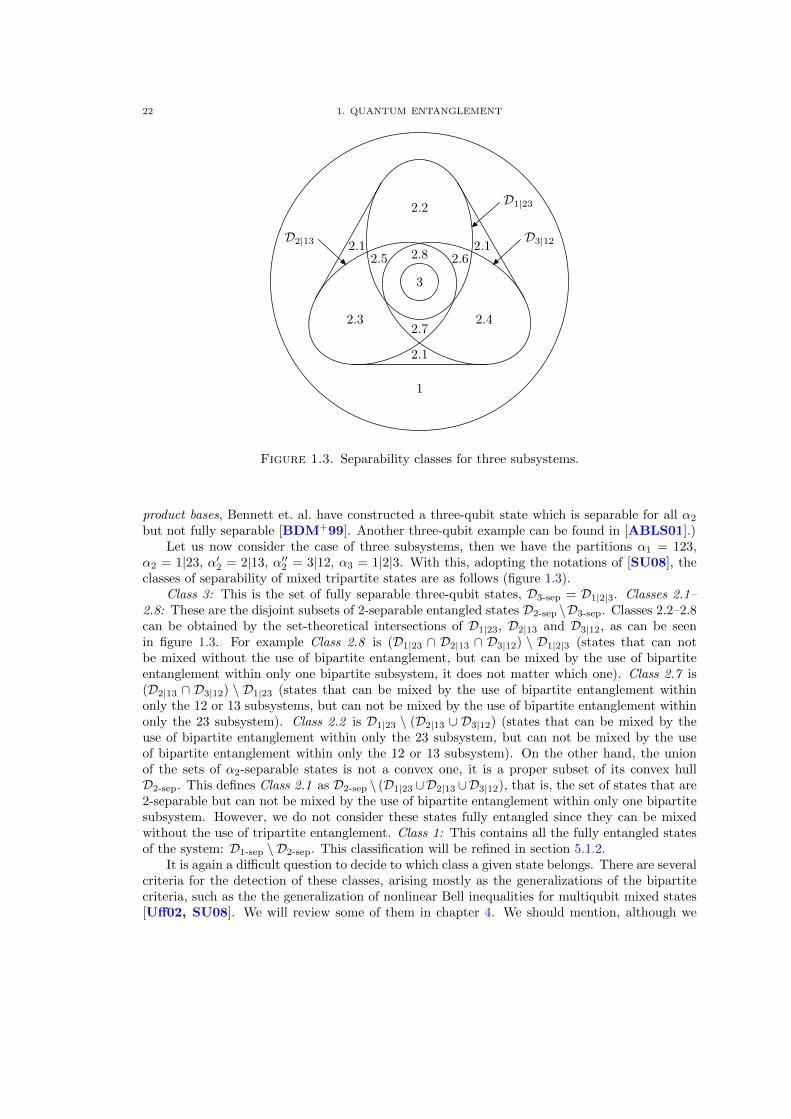
22 1. QUANTUM ENTANGLEMENT
3
2.8
2.2
2.7
2.1
2.3
2.6
2.1
2.4
2.5
2.1
1
D1|23
D2|13 D3|12
Figure 1.3. Separability classes for three subsystems.
product bases, Bennett et. al. have constructed a three-qubit state which is separable for all α2
but not fully separable [BDM+99]. Another three-qubit example can be found in [ABLS01].)Let us now consider the case of three subsystems, then we have the partitions α1 = 123,
α2 = 1|23, α′2 = 2|13, α′′2 = 3|12, α3 = 1|2|3. With this, adopting the notations of [SU08], theclasses of separability of mixed tripartite states are as follows (figure 1.3).
Class 3: This is the set of fully separable three-qubit states, D3-sep = D1|2|3. Classes 2.1–2.8: These are the disjoint subsets of 2-separable entangled states D2-sep \D3-sep. Classes 2.2–2.8can be obtained by the set-theoretical intersections of D1|23, D2|13 and D3|12, as can be seenin figure 1.3. For example Class 2.8 is (D1|23 ∩ D2|13 ∩ D3|12) \ D1|2|3 (states that can notbe mixed without the use of bipartite entanglement, but can be mixed by the use of bipartiteentanglement within only one bipartite subsystem, it does not matter which one). Class 2.7 is(D2|13 ∩ D3|12) \ D1|23 (states that can be mixed by the use of bipartite entanglement withinonly the 12 or 13 subsystems, but can not be mixed by the use of bipartite entanglement withinonly the 23 subsystem). Class 2.2 is D1|23 \ (D2|13 ∪ D3|12) (states that can be mixed by theuse of bipartite entanglement within only the 23 subsystem, but can not be mixed by the useof bipartite entanglement within only the 12 or 13 subsystem). On the other hand, the unionof the sets of α2-separable states is not a convex one, it is a proper subset of its convex hullD2-sep. This defines Class 2.1 as D2-sep \ (D1|23 ∪D2|13 ∪D3|12), that is, the set of states that are2-separable but can not be mixed by the use of bipartite entanglement within only one bipartitesubsystem. However, we do not consider these states fully entangled since they can be mixedwithout the use of tripartite entanglement. Class 1: This contains all the fully entangled statesof the system: D1-sep \ D2-sep. This classification will be refined in section 5.1.2.
It is again a difficult question to decide to which class a given state belongs. There are severalcriteria for the detection of these classes, arising mostly as the generalizations of the bipartitecriteria, such as the the generalization of nonlinear Bell inequalities for multiqubit mixed states[Uff02, SU08]. We will review some of them in chapter 4. We should mention, although we
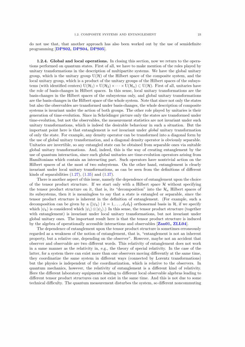
1.2. COMPOSITE SYSTEMS AND ENTANGLEMENT 23
do not use that, that another approach has also been worked out by the use of semidefiniteprogramming [DPS02, DPS04, DPS05].
1.2.4. Global and local operations. In closing this section, now we return to the opera-tions performed on quantum states. First of all, we have to make mention of the roles played byunitary transformations in the description of multipartite systems. We have the global unitarygroup, which is the unitary group U(H) of the Hilbert space of the composite system, and thelocal unitary group, which is a product of the unitary groups of the Hilbert spaces of the subsys-tems (with identified centers) U(H1)×U(H2)× · · · ×U(Hn) ⊂ U(H). First of all, unitaries havethe role of basis-changes in Hilbert spaces. In this sense, local unitary transformations are thebasis-changes in the Hilbert spaces of the subsystems only, and global unitary transformationsare the basis-changes in the Hilbert space of the whole system. Note that since not only the statesbut also the observables are transformed under basis-changes, the whole description of compositesystems is invariant under the action of both groups. The other role played by unitaries is theirgeneration of time-evolution. Since in Schrodinger picture only the states are transformed undertime-evolution, but not the observables, the measurement statistics are not invariant under suchunitary transformations, which is indeed the desirable behaviour in such a situation. But theimportant point here is that entanglement is not invariant under global unitary transformationof only the state. For example, any density operator can be transformed into a diagonal form bythe use of global unitary transformation, and a diagonal density operator is obviously separable.Unitaries are invertible, so any entangled state can be obtained from separable ones via suitableglobal unitary transformations. And, indeed, this is the way of creating entanglement by theuse of quantum interaction, since such global unitaries are time-evolution operators arising fromHamiltonians which contain an interacting part. Such operators have nontrivial action on theHilbert spaces of at the most of two subsystems. On the other hand, entanglement is clearlyinvariant under local unitary transformations, as can be seen from the definitions of differentkinds of separabilities (1.27), (1.35) and (1.37).
There is another aspect of this issue, namely the dependence of entanglement upon the choiceof the tensor product structure. If we start only with a Hilbert space H without specifyingthe tensor product structure on it, that is, its “decomposition” into the Ha Hilbert spaces ofits subsystems, then it is meaningless to say that a state is entangled or separable, since thetensor product structure is inherent in the definition of entanglement. (For example, such adecomposition can be given by a {|ψk〉 | k = 1, . . . , d1d2} orthonormal basis in H, if we specifywhich |ψk〉 is considered which |ψi〉⊗ |ψj〉.) In this sense, the tensor product structure (togetherwith entanglement) is invariant under local unitary transformations, but not invariant underglobal unitary ones. The important result here is that the tensor product structure is inducedby the algebra of operationally accessible interactions and observables [Zan01, ZLL04].
The dependence of entanglement upon the tensor product structure is sometimes erroneouslyregarded as a weakness of the notion of entanglement, that is, “entanglement is not an inherentproperty, but a relative one, depending on the observer”. However, maybe not an accident thatobserver and observable are two different words. This relativity of entanglement does not workin a same manner as the relativity in, e.g., the theory of special relativity. In the case of thelatter, for a system there can exist more than one observers moving differently at the same time,they coordinatize the same system in different ways (connected by Lorentz transformations)but the physics is independent of the coordinatization, which is relative to the observers. Inquantum mechanics, however, the relativity of entanglement is a different kind of relativity.Here the different laboratory equipments leading to different local observable algebras leading todifferent tensor product structures can not exist in the same time. And this is not due to sometechnical difficulty. The quantum measurement disturbes the system, so different noncommuting
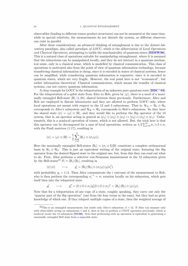
24 1. QUANTUM ENTANGLEMENT
observables (leading to different tensor product structures) can not be measured at the same time,while in special relativity, the measurements do not disturb the system, so different observerscan exist in parallel.
After these considerations, an advanced thinking of entanglement is due to the distant lab-oratory paradigm, also called paradigm of LOCC, which is the abbreviation of Local Operationsand Classical Operations, attempting to tackle the nonclassicality of quantum states [BDSW96].This is a natural class of operations suitable for manipulating entanglement, where it is assumedthat the subsystems can be manipulated locally, and they do not interact in a quantum mechan-ical sense, only in a classical sense, which is modelled by classical communication. This class ofoperations is motivated also from the point of view of quantum information technology, becausetransferring classical information is cheap, since it is encoded in states of classical systems, hencecan be amplified; while transferring quantum information is expensive, since it is encoded inquantum states, which are very fragile. However, the real point here is not “economical”, butrather information theoretical: Classical communication, which means the transfer of classicalsystems, can not convey quantum information.
A clear example for LOCC is the teleportation of an unknown pure quantum state [BBC+93].For the teleportation of a qubit state from Alice to Bob, given by |ϕ〉, there is a need of a maxi-mally entangled Bell-state |B〉 (1.28), shared between them previously. Furthermore, Alice andBob are employed in distant laboratories and they are allowed to perform LOCC only, wherelocal operations are meant with respect to the 12 and 3 subsystems. That is, HA = H1 ⊗ H2
corresponds to Alice’s subsystem and HB = H3 corresponds to Bob’s subsystem. So they havethe shared state |ψ〉 = |ϕ〉 ⊗ |B〉, and they would like to perform the flip operator of the 13system, that is, an operator acting in general as |ψ1〉 ⊗ |ψ2〉 ⊗ |ψ3〉 7→ |ψ3〉 ⊗ |ψ2〉 ⊗ |ψ1〉. Unfor-tunately, this is a nonlocal operation of course, which is not allowed. But, the trick here is thatthis operator can be decomposed for a sum of local operations, written as 1/2
∑3i=0 σi ⊗ I ⊗ σi
with the Pauli matrices (1.17), resulting in
|ψ〉 = |ϕ〉 ⊗ |B〉 =1
2
3∑i=0
|Bi〉 ⊗ (σi|ϕ〉).
Here the maximally entangled Bell-states |Bi〉 = (σi ⊗ I)|B〉 constitute a complete orthonormalbasis in H1 ⊗ H2. This is just an equivalent writing of the original state, featuring the flipoperator from the desired flipped state to the original one, but, from this they can read out whatto do. First, Alice performs a selective von-Neumann measurement in the 12 subsystem givenby the Bell-states22 Pi = |Bi〉〈Bi|, resulting in
|ψ〉〈ψ| 7−→ %′i = |Bi〉〈Bi| ⊗ (σi|ϕ〉〈ϕ|σ†i )
with probability qi = 1/4. Then Alice communicate the i outcome of the measurement to Bob,who is then perform the corresponding σ−1
i = σi rotation locally on his subsystem, which getsitself then into the teleported state
%′i 7−→ %′′i = (I⊗ I⊗ σi)%′i(I⊗ I⊗ σi)† = |Bi〉〈Bi| ⊗ |ϕ〉〈ϕ|.
Note that for a teleportation of one copy of a state, roughly speaking, they carry out only the“quarter part of the flip operation” (one from the four terms in the sum), but they had no priorknowledge of which one. If they teleport multiple copies of a state, then the weighted average of
22This is an entangled measurement, but inside only Alice’s subsystem A = 12. If Alice can measure onlywith observables acting on subsystems 1 and 2, then se has to perform a CNOT operation previously, which is
nonlocal inside the 12 subsystem [NC00]. Note that performing such an operation is equivalent to generating amaximally entangled Bell state from a separable state.

1.2. COMPOSITE SYSTEMS AND ENTANGLEMENT 25
the outcomes results in the overall operation
|ψ〉〈ψ| 7−→ %′′ =
3∑i=0
qi%′′i =
1
2I⊗ 1
2I⊗ |ϕ〉〈ϕ|,
so Alice is left with white noise, the state is fully separable, the entanglement they have sharedbefore the teleportation is used up.23 This is an archetype of the use of entanglement as aresource for manipulating quantum information.
An important note here is that teleportation can not be used for superluminal signallingeither. Although the measurement causes the change of the state in Bob’s laboratory instanta-neously, but he needs the classical information about the outcome of the measurement to get thestate |ϕ〉〈ϕ|, which arrives in a classical channel subluminally. Without this information he hasonly white noise on average.
During the teleportation protocol only LOCC was used, beyond the sharing of entangledstates done previously. But the point of view of the LOCC paradigm came up even in the verybasic grounds of entanglement theory. Namely, even the (1.27) definition of separability was alsomotivated by this approach [Wer89]. Here the %1,j ⊗ %2,j states, prepared locally in distantlaboratories, are uncorrelated for a given j, and the mixing with the weights pj needs classicalcommunication between the laboratories, that is, we have to tell the preparing devices the out-come j of a classical random number generator realizing the probability distribution p. (To haveentangled systems we need a preparing device in which the subsystems can interact in a control-lable, or at least known way.) Therefore, neither local operations nor classical communicationcan not give rise to entanglement. On the other hand, LOCC can decrease entanglement, as wehave seen in the case of the teleportation.
Although LOCC can not increase entanglement, but there are LOCC protocols which obtaina number m of pure maximally entangled (|B〉〈B|)⊗m Bell states (1.28) from a larger number kof least entangled input states %⊗k, which can be pure or mixed ones as well. Such protocols arecalled entanglement distillation protocols [BBP+96, BDSW96, Cla06]. These are importantmethods for quantum information theory since, for instance, they have the ability to recoversome entanglement from states which was originally maximally entangled, then shared betweensubsystems and became mixed with some noise due to the imperfect quantum channels in whichenvironmental decoherence can not be avoided perfectly. On the other hand, such protocolshave important role also in quantum error correction [BDSW96, HHHH09, NC00]. Apartfrom practical reasons of these kinds, distillation is important theoretically as well, because ithas turned out that there are entangled states from which no pure state entanglement can bedistilled out. This gives rise to a distinction between two kinds of entanglement, which are calleddistillable and undistillable ones [HHH98]. The latter is often called bound entanglement, andit is regarded then as a weaker form of entanglement. (Of course, one can not distill entanglementout from separable states, since LOCC can not increase entanglement.) An interesting result isthat all entangled states having positive partial transpose (PPTES) are undistillable [HHH98],and the existence of undistillable states having non-positive partial transpose is still an openquestion [HHHH09, Cla06]. It is also known that there are no such states for two qubits,moreover, all entangled two-qubit states are distillable [HHH97]. It is usually hard to checkwhether a state of positive partial transpose is not separable, there are few explicit examples ofPPTESs in the literature (see a list of references in section 1.2.4 of [Cla06]). One of our results
23Of course Alice can be smart and perform a (σi ⊗ I)−1 = (σi ⊗ I) rotation after each measurement on hersubsystem so as to recover the entanglement in her subsystem, |B〉〈B| ⊗ |ϕ〉〈ϕ|. But this is just the entanglement
which is brought in by the entangled measurement. On the other hand, although they performed the nonlocal flipoperation on average in this way, but not in general, since this works only for the case when the 23 subsystem isin a maximally entangled pure state.
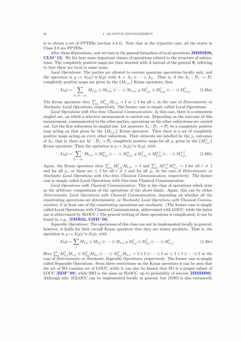
26 1. QUANTUM ENTANGLEMENT
is to obtain a set of PPTESs (section 4.3.4). Note that in the tripartite case, all the states inClass 2.8 are PPTESs.
After these illustrations, now we turn to the general formalism of local operations [HHHH09,CLM+12]. We list here some important classes of operations related to the structure of subsys-tems. The completely positive maps are then denoted with Λ instead of the general Φ, referringto that these are local in some sense.
Local Operations: The parties are allowed to execute quantum operations locally only, andthe operation is % 7→ Λ(%)/ tr Λ(%) with Λ = Λ1 ⊗ · · · ⊗ Λn. That is, if the Λr : Dr → Drcompletely positive maps are given by the {Mr,jr} Kraus operators, then
Λ(%) =∑
j1,j2...,jn
M1,j1 ⊗M2,j2 ⊗ · · · ⊗Mn,jn % M†1,j1⊗M†2,j2 ⊗ · · · ⊗M
†n,jn
. (1.38a)
The Kraus operators obey∑jrM†r,jrMr,jr = I or ≤ I for all r, in the case of Deterministic or
Stochastic Local Operations, respectively. The former case is simply called Local Operations.Local Operations with One-time Classical Communication: In this case, there is a subsystem
singled out, on which a selective measurement is carried out. Depending on the outcome of thismeasurement, communicated to the other parties, operations on the other subsystems are carriedout. Let the first subsystem be singled out. Let moreover Λ1 : D1 → D1 be a completely positivemap acting on that given by the {M1,j1} Kraus operators. Then there is a set of completelypositive maps acting on every other subsystem. Their elements are labelled by the j1 outcomesof Λ1, that is, there are Λj1r : Dr → Dr completely positive maps for all j1 given by the {M j1
r,jr}
Kraus operators. Then the operation is % 7→ Λ(%)/ tr Λ(%), with
Λ(%) =∑j1...,jn
M1,j1 ⊗Mj12,j2⊗ · · · ⊗M j1
n,jn% M†1,j1 ⊗M
j1†2,j2⊗ · · · ⊗M j1†
n,jn. (1.38b)
Again, the Kraus operators obey∑j1M†1,j1M1,j1 = I and
∑jrM j1†r,jr
M j1r,jr
= I for all r 6= 1and for all j1, or these are ≤ I for all r 6= 1 and for all j1, in the case of Deterministic orStochastic Local Operations with One-time Classical Communication, respectively. The formercase is simply called Local Operations with One-time Classical Communication.
Local Operations with Classical Communication: This is the class of operations which ariseas the arbitrary compositions of the operations of the above kinds. Again, this can be eitherDeterministic Local Operations with Classical Communication, depending on whether all theconstituting operations are deterministic, or Stochastic Local Operations with Classical Commu-nication, if at least one of the constituting operations are stochastic. (The former case is simplycalled Local Operations with Classical Communication, abbreviated with LOCC, while the latterone is abbreviated by SLOCC.) The general writing of these operations is complicated, it can befound in, e.g., [DHR02, GHH+08].
Separable Operations: The operations of this class can not be implemented locally in general,however, it holds for their overall Kraus operators that they are tensor products. That is, theoperation is % 7→ Λ(%)/ tr Λ(%), with
Λ(%) =∑j
M1,j ⊗M2,j ⊗ · · · ⊗Mn,j % M†1,j ⊗M
†2,j ⊗ · · · ⊗M
†n,j . (1.38c)
Here∑jM
†1,jM1,j ⊗M†2,jM2,j ⊗ · · · ⊗M†n,jMn,j = I ⊗ I ⊗ · · · ⊗ I or ≤ I ⊗ I ⊗ · · · ⊗ I in the
case of Deterministic or Stochastic Separable Operations, respectively. The former case is simplycalled Separable Operations. From these restrictions on the Kraus operators it can be seen thatthe set of SO contains set of LOCC, while it can also be known that SO is a proper subset ofLOCC [BDF+99], while SSO is the same as SLOCC, up to probability of success [HHHH09].Although only (S)LOCC can be implemented locally in general, but (S)SO is also extensively
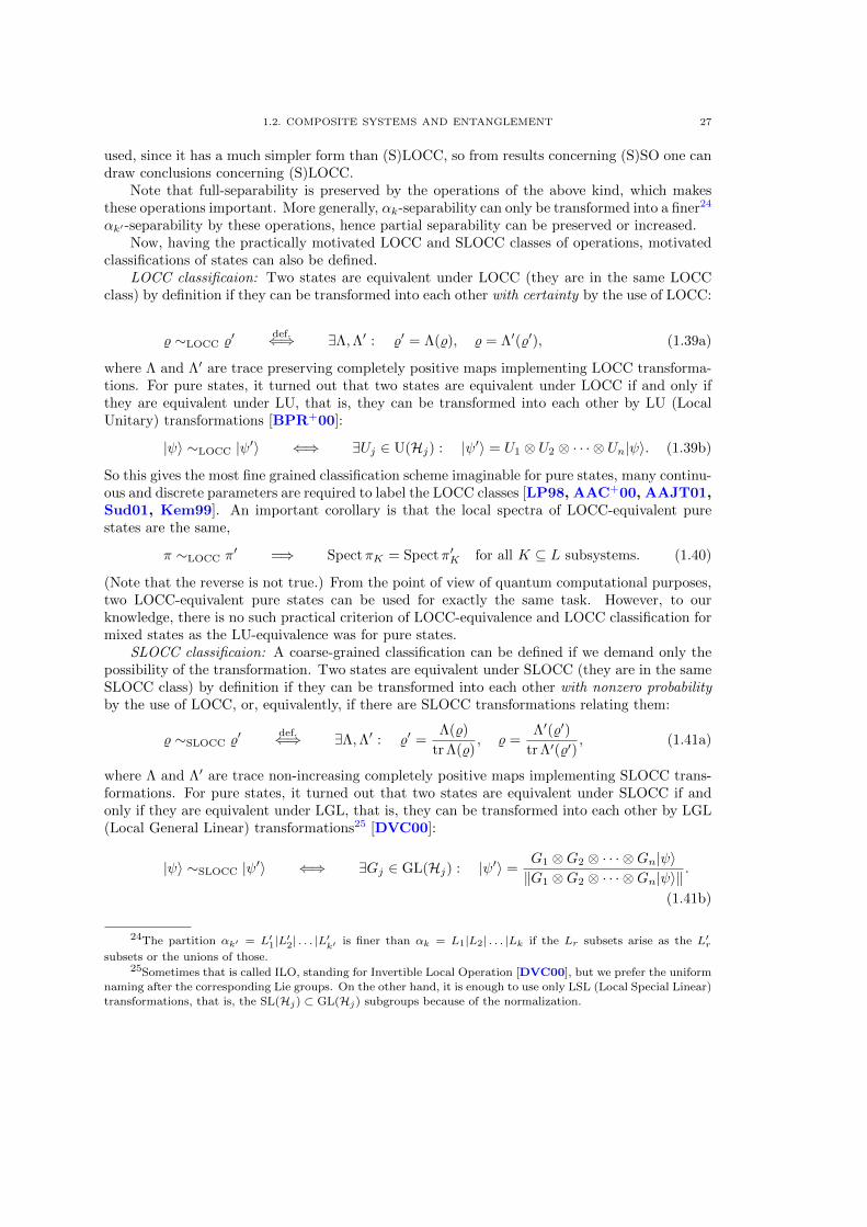
1.2. COMPOSITE SYSTEMS AND ENTANGLEMENT 27
used, since it has a much simpler form than (S)LOCC, so from results concerning (S)SO one candraw conclusions concerning (S)LOCC.
Note that full-separability is preserved by the operations of the above kind, which makesthese operations important. More generally, αk-separability can only be transformed into a finer24
αk′-separability by these operations, hence partial separability can be preserved or increased.Now, having the practically motivated LOCC and SLOCC classes of operations, motivated
classifications of states can also be defined.LOCC classificaion: Two states are equivalent under LOCC (they are in the same LOCC
class) by definition if they can be transformed into each other with certainty by the use of LOCC:
% ∼LOCC %′def.⇐⇒ ∃Λ,Λ′ : %′ = Λ(%), % = Λ′(%′), (1.39a)
where Λ and Λ′ are trace preserving completely positive maps implementing LOCC transforma-tions. For pure states, it turned out that two states are equivalent under LOCC if and only ifthey are equivalent under LU, that is, they can be transformed into each other by LU (LocalUnitary) transformations [BPR+00]:
|ψ〉 ∼LOCC |ψ′〉 ⇐⇒ ∃Uj ∈ U(Hj) : |ψ′〉 = U1 ⊗ U2 ⊗ · · · ⊗ Un|ψ〉. (1.39b)
So this gives the most fine grained classification scheme imaginable for pure states, many continu-ous and discrete parameters are required to label the LOCC classes [LP98, AAC+00, AAJT01,Sud01, Kem99]. An important corollary is that the local spectra of LOCC-equivalent purestates are the same,
π ∼LOCC π′ =⇒ SpectπK = Spectπ′K for all K ⊆ L subsystems. (1.40)
(Note that the reverse is not true.) From the point of view of quantum computational purposes,two LOCC-equivalent pure states can be used for exactly the same task. However, to ourknowledge, there is no such practical criterion of LOCC-equivalence and LOCC classification formixed states as the LU-equivalence was for pure states.
SLOCC classificaion: A coarse-grained classification can be defined if we demand only thepossibility of the transformation. Two states are equivalent under SLOCC (they are in the sameSLOCC class) by definition if they can be transformed into each other with nonzero probabilityby the use of LOCC, or, equivalently, if there are SLOCC transformations relating them:
% ∼SLOCC %′def.⇐⇒ ∃Λ,Λ′ : %′ =
Λ(%)
tr Λ(%), % =
Λ′(%′)
tr Λ′(%′), (1.41a)
where Λ and Λ′ are trace non-increasing completely positive maps implementing SLOCC trans-formations. For pure states, it turned out that two states are equivalent under SLOCC if andonly if they are equivalent under LGL, that is, they can be transformed into each other by LGL(Local General Linear) transformations25 [DVC00]:
|ψ〉 ∼SLOCC |ψ′〉 ⇐⇒ ∃Gj ∈ GL(Hj) : |ψ′〉 =G1 ⊗G2 ⊗ · · · ⊗Gn|ψ〉‖G1 ⊗G2 ⊗ · · · ⊗Gn|ψ〉‖
.
(1.41b)
24The partition αk′ = L′1|L′2| . . . |L′k′ is finer than αk = L1|L2| . . . |Lk if the Lr subsets arise as the L′rsubsets or the unions of those.
25Sometimes that is called ILO, standing for Invertible Local Operation [DVC00], but we prefer the uniform
naming after the corresponding Lie groups. On the other hand, it is enough to use only LSL (Local Special Linear)transformations, that is, the SL(Hj) ⊂ GL(Hj) subgroups because of the normalization.
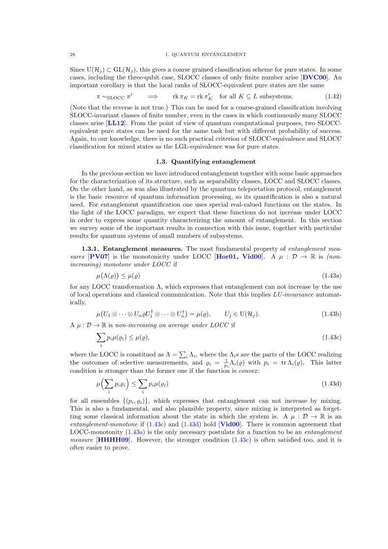
28 1. QUANTUM ENTANGLEMENT
Since U(Hj) ⊂ GL(Hj), this gives a coarse grained classification scheme for pure states. In somecases, including the three-qubit case, SLOCC classes of only finite number arise [DVC00]. Animportant corollary is that the local ranks of SLOCC-equivalent pure states are the same
π ∼SLOCC π′ =⇒ rkπK = rkπ′K for all K ⊆ L subsystems. (1.42)
(Note that the reverse is not true.) This can be used for a coarse-grained classification involvingSLOCC-invariant classes of finite number, even in the cases in which continuously many SLOCCclasses arise [LL12]. From the point of view of quantum computational purposes, two SLOCC-equivalent pure states can be used for the same task but with different probability of success.Again, to our knowledge, there is no such practical criterion of SLOCC-equivalence and SLOCCclassification for mixed states as the LGL-equivalence was for pure states.
1.3. Quantifying entanglement
In the previous section we have introduced entanglement together with some basic approachesfor the characterization of its structure, such as separability classes, LOCC and SLOCC classes.On the other hand, as was also illustrated by the quantum teleportation protocol, entanglementis the basic resource of quantum information processing, so its quantification is also a naturalneed. For entanglement quantification one uses special real-valued functions on the states. Inthe light of the LOCC paradigm, we expect that these functions do not increase under LOCCin order to express some quantity characterizing the amount of entanglement. In this sectionwe survey some of the important results in connection with this issue, together with particularresults for quantum systems of small numbers of subsystems.
1.3.1. Entanglement measures. The most fundamental property of entanglement mea-sures [PV07] is the monotonicity under LOCC [Hor01, Vid00]. A µ : D → R is (non-increasing) monotone under LOCC if
µ(Λ(%)
)≤ µ(%) (1.43a)
for any LOCC transformation Λ, which expresses that entanglement can not increase by the useof local operations and classical communication. Note that this implies LU-invariance automat-ically,
µ(U1 ⊗ · · · ⊗ Un%U†1 ⊗ · · · ⊗ U†n
)= µ(%), Uj ∈ U(Hj). (1.43b)
A µ : D → R is non-increasing on average under LOCC if∑i
piµ(%i) ≤ µ(%), (1.43c)
where the LOCC is constitued as Λ =∑i Λi, where the Λis are the parts of the LOCC realizing
the outcomes of selective measurements, and %i = 1pi
Λi(%) with pi = tr Λi(%). This latter
condition is stronger than the former one if the function is convex :
µ(∑
i
pi%i
)≤∑i
piµ(%i) (1.43d)
for all ensembles {(pi, %i)}, which expresses that entanglement can not increase by mixing.This is also a fundamental, and also plausible property, since mixing is interpreted as forget-ting some classical information about the state in which the system is. A µ : D → R is anentanglement-monotone if (1.43c) and (1.43d) hold [Vid00]. There is common agreement thatLOCC-monotonity (1.43a) is the only necessary postulate for a function to be an entanglementmeasure [HHHH09]. However, the stronger condition (1.43c) is often satisfied too, and it isoften easier to prove.
1.3. QUANTIFYING ENTANGLEMENT 29
If µ is defined only for pure states, µ : P → R, then only (1.43c) makes sense, whoserestriction is∑
j
pjµ(πj) ≤ µ(π). (1.44)
Here {(pj , πj)} is the pure ensemble generated by all the Kraus-operators of all Λis from the inputstate π. Note that not all πj members of the ensemble are accessible physically, only the outcomesof the LOCC, which are formed by partial mixtures of this ensemble [Hor01]. Mathematically,however, the pure state ensemble can also be used, which makes some constructions much simpler.
There are also other properties beyond the monotonities above, which are useful or con-venient for the measuring of bipartite entanglement. For example, a plausible property is thediscriminance, that is, µ : D → R function for bipartite states should vanish exactly for separablestates,
% ∈ Dsep ⇐⇒ µ(%) = 0. (1.45a)
But there are such functions for which only the weak discriminance holds,
% ∈ Dsep =⇒ µ(%) = 0. (1.45b)
We can regard the entanglement carried by the Bell state (1.28) as a unit of entanglement, (thatis, 1 qubit) then a µ : D → R function for bipartite states is normalized if
µ(|B〉〈B|) = 1, (1.45c)
which can be achieved by trivial rescaling, so we are not concerned with this one. Normalizationcan be useful for comparing different measures.
The pure state entanglement measures can be extended to mixed states by the so calledconvex roof extension [BDSW96, Uhl00, Uhl10, RLL09, RLL11]. It is motivated by thepractical approach of the optimal mixing of the mixed state from pure states, that is, using aslittle amount of pure state entanglement as possible. For a continuous function µ : P → R, itsconvex roof extension µ∪ : D → R is defined as
µ∪(%) = min∑i piπi=%
∑i
piµ(πi), (1.46)
where the minimization takes place over all {(pi, πi)} pure state decompositions of %. It followsfrom Schrodinger’s mixture theorem (1.4) that the decompositions of a mixed state into anensemble of m pure states are labelled by the elements of the compact complex Stiefel manifold.On the other hand, the Caratheodory theorem ensures that we need only finite m, or to bemore precise m ≤ (rk %)2 ≤ d2, shown by Uhlmann [Uhl98]. These observations guarantee theexistence of the minimum in (1.46).
Obviously, for pure states the convex roof extension is trivial,
µ∪(π) = µ(π) ∀π ∈ P. (1.47)
The convex roof extension of a function is convex (1.43d), moreover, it is the largest convexfunction taking the same values for pure states as the original function [Uhl98]. The convexroof extensions of pure state measures are good measures of entanglement, because it can beproven [Vid00, Hor01] that if a function µ : P → R is non-increasing on average for purestates (1.44), then its convex roof extension is also non-increasing on average for mixed states26
(1.43c) ∑i
piµ(πi) ≤ µ(π) ⇐⇒∑i
piµ∪(%i) ≤ µ∪(%). (1.48)
26The ⇐ implication is obvious.
30 1. QUANTUM ENTANGLEMENT
From this, µ∪(%) is entanglement-monotone as well. Because of these, for pure states (1.44) iscalled entanglement monotonicity. The convex roof extension preserves the weak discriminanceproperty (1.45b) and also the strong one (1.45b) if we additionally assume that µ ≥ 0. Thisis very useful because strong discriminance for mixed states can be used for the detection ofentanglement, which will exensively be done in chapters 5 and 6. Indeed, let µ : P → [0,∞),then
% ∈ Dsep ⇐⇒ ∃ decomposition % =∑j
pjπj such that πj ∈ Psep
=⇒⇐⇒ ∃ decomposition % =
∑j
pjπj such that µ(πj) = 0
⇐⇒ µ∪(%) = 0,
(1.49)
where in the second implication the upper one is the weak discriminance (1.45b) and the lowerone is the strong discriminance (1.45a), while µ ≥ 0 is necessary for the ⇐ direction of the lastimplication. On the other hand, the normalization (1.45c) property is obviously preserved bythe convex roof extension.
1.3.2. State vectors of bipartite systems. Now, let H = H1 ⊗H2 the Hilbert space ofbipartite systems of dimension d = (d1, d2). A bipartite state vector |ψ〉 ∈ H, having the generalform
|ψ〉 =
d1,d2∑i,j=1
ψij |i〉 ⊗ |j〉,
can be transformed to the so called Schmidt canonical form
|ψ〉 =
dmin∑i=1
√ηi|ϕ1,i〉 ⊗ |ϕ2,i〉 (1.50a)
by suitable local unitary transformations. The existence of this form, also called Schmidt decom-position, makes the entanglement of pure states of bipartite systems simple. Here {|ϕ1,i〉} and{|ϕ2,i〉} are sets of orthonormal vectors in H1 and H2. The nonnegative ηi numbers are calledSchmidt coefficients, and they sum up to one. They form the spectra of the reduced states, whichare therefore the same for both of the subsystems, the only difference can be the degenerancy ofthe zero eigenvalue, since
π1 =
dmin∑i=1
ηi|ϕ1,i〉〈ϕ1,i|, π2 =
dmin∑i=1
ηi|ϕ2,i〉〈ϕ2,i|, (1.50b)
with the pure state π = |ψ〉〈ψ| and its reduced states π1 = tr2 π and π2 = tr1 π, as usual. It isclear that |ψ〉 is separable if and only if it has only one non-zero Schmidt coefficient, which isthen equal to 1.
On the other hand, we can label the LU orbits in H by the Schmidt coefficients (ordered non-increasingly) so they are the only non-local parameters of a bipartite pure state. Alternatively, wecan form an equivalent set of LU-invariants, which can be calculated without the diagonalizationof the local states, which is
Iq(ψ) = trπq1 ≡dmin∑i=1
ηqi , q = 1, 2, . . . , dmin. (1.51)
(I1(ψ) ≡ ‖ψ‖2 equals to 1 if the state vector is normalized, however, during the investigationof orbit structures in H under group actions, this constraint is often relaxed.) Since the LOCC
1.3. QUANTIFYING ENTANGLEMENT 31
equivalence is the same as the LU equivalence for pure states, we have that two states canbe interconverted by the use of LOCC if and only if they have the same invariants (1.51). Abeautiful result here [Nie99] is that a condition can be given even for the LOCC convertibilityby majorization (1.5):
∃Λ LOCC that |ψ′〉 = Λ(|ψ〉) ⇐⇒ η � η′ (1.52)
where η and η′ are the dmin-tuples of Schmidt coefficients of |ψ〉 and |ψ′〉. From this, theLU-equivalence follows as necessary and sufficient condition for LOCC interconvertibility. Un-fortunately, there is no such an elegant condition for the LOCC convertibility of pure states ofsystems composed of more than two subsystems, although the LU-equivalence is still a necessaryand sufficient condition for LOCC interconvertibility (1.39b).
The LOCC equivalence classes have a bit too fine-grained structure, characterized by thedmin−1 real parameters, containing all the pieces of nonlocal information about the state. Whatcan be said about the SLOCC equivalence classes? The Schmidt coefficients are not invariantunder LGL transformations, but their vanishings are that. Therefore the Schmidt rank of thestate, which is the usual matrix rank of the reduced state
rkψ = rkπ1,
is invariant under LGL transformations, moreover, it can easily be seen that there are dmin
SLOCC classes, which are characterized by the Schmidt rank. The set of separable states is oneof them, which is the set of states of rkψ = 1, and
|ψr〉 =
r∑i=1
1√r|i〉 ⊗ |i〉. (1.53)
gives a representative element for the rkψ = r SLOCC class.27
We have seen that the Schmidt decomposition (1.50a) is very useful in the understanding ofthe structure of entanglement of bipartite pure states. In additional, we can also give illustrationto Schrodinger’s mixture theorem (1.4) by the use of that. To this end, let us write the purestate in terms of state vectors in Schmidt canonical form
|ψ〉〈ψ| =∑ii′
√ηi√ηi′ |ϕ1,i〉〈ϕ1,i′ | ⊗ |ϕ2,i〉〈ϕ2,i′ |,
now apply a unitary transformation on the second subsystem
I⊗ U |ψ〉〈ψ|I⊗ U† =∑ii′
√ηi√ηi′ |ϕ1,i〉〈ϕ1,i′ | ⊗ U |ϕ2,i〉〈ϕ2,i′ |U†,
and form the reduced state of the first subsystem
tr2
(I⊗ U |ψ〉〈ψ|I⊗ U†
)=∑ii′
√ηi√ηi′ |ϕ1,i〉〈ϕ1,i′ |
∑j
〈ϕ2,j |U |ϕ2,i〉〈ϕ2,i′ |U†|ϕ2,j〉
=∑j
(∑i
U ji√ηi|ϕ1,i〉
)(∑i′
√ηi′(U
ji′)∗〈ϕ1,i′ |
),
where the decomposition vectors in the form of (1.4) appear in the parentheses. So we can thinkof the freedom in the decomposition of a density matrix as the unitary freedom in the additionalHilbert space of the purification.
As we have also seen, the reduced states of an entangled pure state are mixed ones, which isinterpreted as we know the possible pure states of the subsystem only with some probabilities.So the uncertainty in the pure states of the subsystem presents itself for the quantification of
27It is not difficult to construct the LGL transformation which maps a state |ψ〉 to this canonical form.
32 1. QUANTUM ENTANGLEMENT
entanglement. It can be characterized for example by the von Neumann entropy (1.9a) of thereduced state:
s(ψ) = S(π1) ≡ H(η). (1.54)
But, is this an entanglement measure in the sense of section 1.3.1? The answer is yes, it hasbeen shown in [Vid00, Hor01] that every unitary-invariant and concave function of the reducedstate is non-increasing on average under LOCC (1.44), which is the key property of the functionsmeasuring entanglement. The von Neumann entropy (1.9a), the Tsallis entropies (1.9e) for all
q > 0, and the Renyi entropies (1.9b) for all 0 < q < 1 are known to be concave [BZ06], andall of them are unitary-invariant, so all of them can be used on the right-hand side of (1.54) toget an entanglement measure.28 However, note that the von Neumann entropy of the reducedstate (1.54) is of particular importance due to Schumacher’s noiseless coding theorem, which isthe quantum counterpart of Shannon’s noiseless coding theorem of classical information theory[NC00]. For every generalized entropy we obviously have that s(ψ) = 0 if and only if the stateis separable, that is, the (strong) discriminance property (1.45a) holds.
1.3.3. Mixed states of bipartite systems. For mixed states, for the quantification ofentanglement we can use the convex roof extension (1.46) of pure state measures. They have theoperational meaning of the optimal mixing of the state from pure states with respect to the givenpure state measure. Maybe this is the most plausible method of measuring the entanglementof mixed states. Thanks to (1.48), the resulting function is also an entanglement measure,moreover, it is entanglement monotone. For example, the convex roof extended entanglementfunction (1.54) is
s∪(%) = min∑i piπi=%
∑i
pis(πi), (1.55)
which is called entanglement of formation. (Or generalized entanglement of formation for theRenyi entropies.) Since the (strong) discriminance property (1.45a) holds for the local entropies,it holds also for the convex roof extension of those (1.49), that is,
% ∈ Dsep ⇐⇒ s∪(%) = 0. (1.56)
There are other entanglement measures, which do not arise as convex roof extension ofpure state measures. Such an entanglement measure is the negativity [ZHSL98, EP99]. It isrelated to the notion of partial transposition and the criterion of Peres [Per96]. If the partialtransposed density matrix has negative eigenvalue, which implies entanglement (1.34a), then itstrace, which equals to 1, is less than the trace of its absolute value,29 the latter is called trace-
norm, ‖M‖tr = tr√M†M . It turns out that if we simply take the difference of these two traces
then we get an entanglement measure, which is called negativity
N(%) = ‖%t1‖tr − 1. (1.57)
The negativity is convex (1.43d) and non-increasing on average (1.43c) hence entanglement mono-tone. Moreover, what its greatest advantage is, it is easy to calculate because there is no need ofoptimization, contrary to convex roof measures. Unfortunately, since the positivity of the partialtranspose is only a necessary criterion of separability in general (1.34a), there are entangled statesof zero negativity, hence only weak discriminance (1.45b) holds for the negativity. Because of
28For the von Neumann entropy, this is called entanglement function, and denoted by E(ψ), and for the
Renyi entropies, this is called generalized entanglement function, and denoted by Eq(ψ), but we prefer to use this
more general small letter–capital letter convention (1.54) for functions on the states of the subsystems.29The absolute value of a matrix M is defined by the unique positive square root of the positive matrix
M†M , that is, |M | =√M†M . (If M itself is positive then |M | = M .) The spectrum of |M |, called the set of
singular values of M , consists of the absolute values of the (generally complex) eigenvalues of M .
1.3. QUANTIFYING ENTANGLEMENT 33
(1.34a), however, the strong discriminance (1.45a) holds for qubit-qubit or qubit-qutrit systems.It can easily be shown that the spectrum of the partial transposed density matrix, hence alsothe negativity, is invariant under the action of the LU-group U(H1)×U(H2).
There are several other measures of entanglement [BZ06, HHHH09]. For the sake ofcompleteness, we just make mention of some noteworthy ones, without further use.
For example there are the operational measures entanglement cost and distillable entan-glement [BDSW96, Rai99, PV07], which are in connection with entanglement manipulatingLOCC protocols. The distillable entanglement ED is in connection with the distillation of kcopies of Bell states out from the m copies of a given state %. In the limit of m→∞, the ratior = k/m is characteristic of the state and the distillation protocol used. What is characteristicof only the state % is the supremum of the k/m ratios with respect to all distillation protocols,which is the distillable entanglement
ED(%) = sup{r∣∣∣ limm→∞
(infΛ
∥∥Λ(%⊗m)− (|B〉〈B|)⊗mr∥∥
tr
)= 0}. (1.58a)
The entanglement cost EC is defined via the dual approach, that is, we want to obtain m copiesof a given state % by the expending of k copies of Bell states. Again, the ratio r = k/m ischaracteristic of the state and the protocol used. What is characteristic of only the state % is theinfimum of the k/m ratios with respect to all distillation protocols, which is the entanglementcost
EC(%) = inf{r∣∣∣ limm→∞
(infΛ
∥∥Λ((|B〉〈B|)⊗mr
)− %⊗m
∥∥tr
)= 0}. (1.58b)
Finding optimal LOCC protocols for these purposes makes the evaluation of the distillable en-tanglement and entanglement cost a very hard problem. Both of the distillable entanglementand the entanglement cost are non-increasing on average under LOCC (1.43c) and normalized(1.45c). Since there are bound-entangled states, only the weak discriminance (1.45b) holds forthe distillalble entanglement, while the discriminance of the entanglement cost is not known.
Another interesting and important measure is the squashed entanglement, an additive entan-glement monotone (1.43c)-(1.43d) with good asymptotic properties [CW04, BCY11, AF04],
ES(%12) = inf%123
1
2
(S(%13) + S(%23)− S(%3)− S(%123)
), (1.58c)
where the optimization takes place on all extended %123 states from which the measured statecan be reduced, that is, tr3 %123 = %12, resulting in an especially hard optimization problem. Itis not known whether the discriminance property (1.45a) holds for this measure.
There are also geometrical measures of entanglement, which are in connection with distancesand distinguishability measures in the space of states [BZ06, HHHH09].
1.3.4. State vectors of two qubits. Now, consider the simplest composite system, whichis the system of two qubits, d = (2, 2). A two-qubit state-vector |ψ〉 ∈ H is expressed in thecomputational basis as
|ψ〉 =
1∑i,j=0
ψij |i〉 ⊗ |j〉.
Here we have only two Schmidt coefficients, from which there is only one independent, so allnon-local properties are characterized by only one real parameter. We use here another quantity,which is more convenient than the Schmidt coefficients or even the LU-invariant I2(ψ) given in(1.51). The reduced states are mixed one-qubit states. Their spectra can be expressed in terms
34 1. QUANTUM ENTANGLEMENT
of the concurrence, as was seen in (1.15). So we define the concurrence for a two-qubit pure stateas the concurrence (1.11c), (1.21) of the reduced state
c(ψ) = C(tr2 |ψ〉〈ψ|). (1.59)
Now the (1.54) entanglement of |ψ〉 is
s(ψ) = S(c(ψ)
), (1.60)
where
S(c) = h
(1
2
(1 +
√1− c2
))(1.61)
with the binary entropy function h(x) given in (1.16b). Note that the entanglement s(ψ) andthe concurrence c(ψ) are both good measures of entanglement in the sense of section 1.3.1. Herewe also see that for two qubits, they are related by the monotone increasing function S(c).
Since we have that the concurrence-squared C2 of a one-qubit mixed state is just four timesits determinant, see in (1.15), we have c2(ψ) = 4 det(tr2 |ψ〉〈ψ|), and c(ψ) is just two times theusual determinant of ψ regarded as a matrix, that is,
c(ψ) = 2|detψ|. (1.62)
The determinant can be expressed in terms of the antisymmetric tensor ε, see in (1.18), as
detψ =1
2εii′εjj′ψ
ijψi′j′ , (1.63)
which shows that detψ is invariant under local SL(2,C) transformations. This is also a conse-quence of the (1.20) transformation property of ε. Carrying out the sums, we get the expressionfor the determinant
detψ = ψ00ψ11 − ψ01ψ10,
which shows, that detψ is a permutation-invariant quantity, because of the Schmidt decomposi-tion. On the other hand, the local concurrence c(ψ) (as well as the local von Neumann entropys(ψ)) is then an U(1) × SL(2,C) × SL(2,C)-invariant. The form (1.63) suggests that c(ψ) canalso be written by the use of the spin flip (1.19a) as
c(ψ) = |〈ψ|ψ〉|, (1.64)
where 〈ψ| = ε⊗ ε|ψ〉.The C concurrence (1.11c) is normalized, so 0 ≤ c(ψ) ≤ 1, and the LOCC classes of pure
states of this system are labelled by this one continuous parameter. On the other hand, c(ψ) = 0if and only if rkψ = 1 (the state is separable), and we have two SLOCC classes, the set ofseparable and entangled states, rkψ = 2 for that. If we relax the normalization condition again,then we have the SLOCC classes
• VNull (Class Null): The zero vector of H.• V1|2 (Class 1|2): These non-zero vectors are separable, which are of the form |ψ1〉⊗|ψ2〉.• V12 (Class 12): All the other vectors.
Formally speaking, these classes define disjoint, LGL-invariant subsets ofH, and coverH entirely,H = VNull ∪ V1|2 ∪ V12. Except VNull, these classes are not closed.
For any |ψ〉 ∈ H, it can be determined to which class |ψ〉 belongs by the vanishing of thenorm
n(ψ) = ‖ψ‖2, (1.65a)
and the local entropies
c2a(ψ) = C2(πa) = 4 detπa. (1.65b)
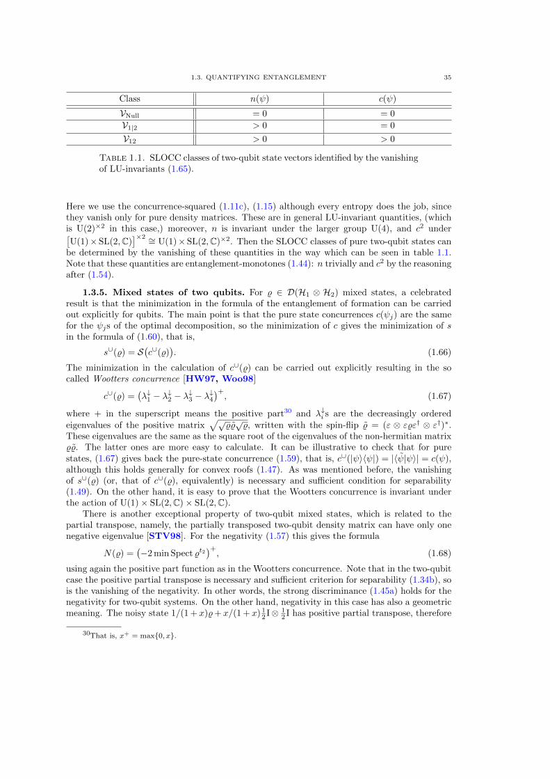
1.3. QUANTIFYING ENTANGLEMENT 35
Class n(ψ) c(ψ)
VNull = 0 = 0
V1|2 > 0 = 0
V12 > 0 > 0
Table 1.1. SLOCC classes of two-qubit state vectors identified by the vanishingof LU-invariants (1.65).
Here we use the concurrence-squared (1.11c), (1.15) although every entropy does the job, sincethey vanish only for pure density matrices. These are in general LU-invariant quantities, (whichis U(2)×2 in this case,) moreover, n is invariant under the larger group U(4), and c2 under[U(1)×SL(2,C)
]×2 ∼= U(1)×SL(2,C)×2. Then the SLOCC classes of pure two-qubit states canbe determined by the vanishing of these quantities in the way which can be seen in table 1.1.Note that these quantities are entanglement-monotones (1.44): n trivially and c2 by the reasoningafter (1.54).
1.3.5. Mixed states of two qubits. For % ∈ D(H1 ⊗ H2) mixed states, a celebratedresult is that the minimization in the formula of the entanglement of formation can be carriedout explicitly for qubits. The main point is that the pure state concurrences c(ψj) are the samefor the ψjs of the optimal decomposition, so the minimization of c gives the minimization of sin the formula of (1.60), that is,
s∪(%) = S(c∪(%)
). (1.66)
The minimization in the calculation of c∪(%) can be carried out explicitly resulting in the socalled Wootters concurrence [HW97, Woo98]
c∪(%) =(λ↓1 − λ
↓2 − λ
↓3 − λ
↓4
)+, (1.67)
where + in the superscript means the positive part30 and λ↓i s are the decreasingly orderedeigenvalues of the positive matrix
√√%%√%, written with the spin-flip % = (ε ⊗ ε%ε† ⊗ ε†)∗.
These eigenvalues are the same as the square root of the eigenvalues of the non-hermitian matrix%%. The latter ones are more easy to calculate. It can be illustrative to check that for purestates, (1.67) gives back the pure-state concurrence (1.59), that is, c∪(|ψ〉〈ψ|) = |〈ψ|ψ〉| = c(ψ),although this holds generally for convex roofs (1.47). As was mentioned before, the vanishingof s∪(%) (or, that of c∪(%), equivalently) is necessary and sufficient condition for separability(1.49). On the other hand, it is easy to prove that the Wootters concurrence is invariant underthe action of U(1)× SL(2,C)× SL(2,C).
There is another exceptional property of two-qubit mixed states, which is related to thepartial transpose, namely, the partially transposed two-qubit density matrix can have only onenegative eigenvalue [STV98]. For the negativity (1.57) this gives the formula
N(%) =(−2 min Spect %t2
)+, (1.68)
using again the positive part function as in the Wootters concurrence. Note that in the two-qubitcase the positive partial transpose is necessary and sufficient criterion for separability (1.34b), sois the vanishing of the negativity. In other words, the strong discriminance (1.45a) holds for thenegativity for two-qubit systems. On the other hand, negativity in this case has also a geometricmeaning. The noisy state 1/(1 + x)%+ x/(1 + x) 1
2 I⊗ 12 I has positive partial transpose, therefore
30That is, x+ = max{0, x}.
36 1. QUANTUM ENTANGLEMENT
it is separable, if and only if 2N(%) ≤ x, so 2N(%) is the minimal relative weight of white noiseneeded to wash out the entanglement in the two-qubit case [VAM01].
1.3.6. State vectors of three qubits. We have seen that the reason for the simplicityof the structure of entanglement of pure states for bipartite systems was the existence of theSchmidt decomposition (1.50a). It is easy to see that pure states of multipartite systems (n ≥ 3)do not admit the usual form of Schmidt decomposition in general. If the state vector is in the
straightforwardly generalized Schmidt form |ψ〉 =∑dmin
i=1
√ηi|i〉⊗|i〉⊗· · ·⊗|i〉, then the states of all
composite subsystems are separable ones (1.27b), although pure states with entangled bipartitesubsystems can easily be constructed even in the case of three qubits. Finding generalizedSchmidt decompositions, that is, LU-canonical forms for systems of more-than-two subsystemsof arbitrary dimensional Hilbert spaces is a difficult problem, which has not been carried out yet.We note here that this problem is solved for the case of three qubits, in which an LU-canonicalform parametrized by six real parameters is obtained [AAC+00, AAJT01], but this particularform can not be generalized in a straightforward manner.
So, we turn to the simplest system which is not bipartite, the system of three qubits. Wehave the Hilbert space H ≡ H123 = H1 ⊗H2 ⊗H3 with d = (2, 2, 2) local dimensions. Here weintroduce a convention being very convenient for the tripartite case. The letters a, b and c arevariables taking their values in the set of labels L = {1, 2, 3}. When these variables appear in aformula, they form a partition of {1, 2, 3}, so they take always different values and the formulais understood for all the different values of these variables automatically. Although, sometimesa formula is symmetric under the interchange of two such variables in which case we keep onlyone of the identical formulas.
Let the three-qubit state vector |ψ〉 ∈ H be expressed in the computational basis |ijk〉 =|i〉 ⊗ |j〉 ⊗ |k〉 as
|ψ〉 =
1∑i,j,k=0
ψijk|ijk〉.
We also have the pure state π = |ψ〉〈ψ| ∈ P(H), and in this tripartite system we have bipartiteand singlepartite subsystems, for which we have the density matrices πbc = tra π ∈ D(Hbc) andπa = trbc π ∈ D(Ha). Now, how to characterize the entanglement in this system and in itssubsystems? We have, for example, the concurrence (1.11c) of singlepartite subsystems C(πa)measuring the entanglement of the subsystem a with the rest of the system, which is bc in thiscase. On the other hand, thanks to the Schmidt decomposition (1.50), all the reduced states ofa three-qubit state are at most of rank two, which makes the calculation of the c∪(πbc) Woottersconcurrences (1.67) of the bipartite reduced states possible in a closed form [CKW00] (see insection 6.1.3). Moreover, these are bounded from above by the concurrence of the one-qubitsubsystem by the so called Coffmann-Kundu-Wootters inequality as follows
c∪2(πab) + c∪
2(πac) ≤ C2(πa). (1.69)
This means that there is a restriction on the entanglement of the subsystem a with subsystemsb and c by its entanglement with the subsystem bc, which is called the monogamy31 of theconcurrence [CKW00]. For example, if a is maximally entangled with b, then it can not beentangled (neither classically correlated) with c, resembling the situation in a marriage, afterwhich this relation of entanglement is named. This is an entirely quantum feature, there isno such restriction on correlations in classical systems. This makes the quantum cryptography
31For a recent introduction to the monogamy, see [KGS12].
1.3. QUANTIFYING ENTANGLEMENT 37
essentially different from its classical counterpart. The generalization of the monogamy relationproved to be true for all n-qubit systems [OV06], which can be written as∑
b 6=a
c∪2(πab) ≤ C2(πa). (1.70)
However, it is known that the concurrence is not monogamous for subsystems of higher than twodimensions [Ou07].
It is interesting to find states which are somehow extremal in the sense of (1.69). It can bechecked that for the W-state [DVC00]
|W〉 =1√3
(|100〉+ |010〉+ |001〉
)(1.71a)
C2(πa) = 2(2/3)2, while c∪2(πab) = c∪
2(πac) = (2/3)2, hence the inequality (1.69) is saturated,
meaning that all the entanglement between the subsystems a and bc is shared in the ab and acsubsystems equally. The other extremal case is that of the Greenberger-Horne-Zeilinger state[GHZ89]
|GHZ〉 =1√2
(|000〉+ |111〉
). (1.71b)
This state is maximally entangled in the sense that its singlepartite subsystems are maximally
mixed, C2(πa) = 1, while its bipartite subsystems are separable c∪2(πab) = c∪
2(πac) = 0. Hence
the difference between the two sides of inequality (1.69) is maximal for |GHZ〉, meaning thatsubsystem a is entangled with bc, but it is not entangled with b or with c individually. Thisinteresting distribution of entanglement is characterized by the difference between the two sidesof the inequality (1.69), which is called residual tangle, or three-tangle τ(ψ)
C2(πa) = c∪2(πab) + c∪
2(πac) + τ(ψ). (1.72)
An important finding [DVC00] is that τ(ψ) is an entanglement monotone (1.44), so all terms inthe above equality are measures of the amount of entanglement. This means that in this three-qubit case there are two kinds of entanglement, that is, (bipartite) entanglement which is sharedamong pairs of qubits, and (tripartite) entanglement which can not be seen in the two-qubitsubsystems, although it is present in the whole three-qubit system.
The explicit form of the three-tangle τ(ψ) is also noteworthy. It is given by Cayley’s (2, 2, 2)hyperdeterminant Detψ [Cay45, GK08, CKW00] as
τ(ψ) = 4|Detψ|, (1.73)
where
Detψ = −1
2εii′εjj′εkk′εll′εmm′εnn′ψ
iklψjk′l′ψi
′mnψj′m′n′ (1.74)
with ε given in (1.18). This writing shows that Detψ is invariant under local SL(2,C) transforma-tions, thanks to (1.20). Carrying out the sums, we get the expression for the hyperdeterminant
Detψ = ψ000ψ111ψ000ψ111 + ψ110ψ001ψ110ψ001 + ψ101ψ010ψ101ψ010 + ψ011ψ100ψ011ψ100
− 2(ψ000ψ111ψ110ψ001 + ψ000ψ111ψ101ψ010+ψ000ψ111ψ011ψ100
+ψ110ψ001ψ101ψ010+ψ110ψ001ψ011ψ100
+ψ101ψ010ψ011ψ100)
+ 4(ψ000ψ110ψ101ψ011 + ψ111ψ001ψ010ψ100
),
which shows that Detψ is a permutation-invariant quantity. In the calculations resulting inthe formulas above, index contractions by ε, which was already used also in the two-qubit case,
38 1. QUANTUM ENTANGLEMENT
appear at all times and in all places. We will see in section 6.1 that these three-qubit resultshave a natural treatment in the terms of LSL-covariants. On the other hand, the constructionof c2 (1.62) and τ (1.73), given by the square of the usual (2, 2) determinant (1.63) and the(2, 2, 2) hyperdeterminant (1.74), can be generalized to n-qubit systems by formulating the indexcontractions with ε [WC01]. Apart from these, the same structure appears in the invariant combapproach of multiqubit entanglement [OS05, OS10, EBOS12].
What can be said about the LOCC and SLOCC classifications of three-qubit pure states? In[Sud01], the following set of algebraically independent LU-invariant homogeneous polynomialsis given for three-qubit state vectors,
I0(ψ) = trπ ≡ ‖ψ‖2, (1.75a)
Ia(ψ) = trπ2a, (1.75b)
I4(ψ) = 3 tr(πb ⊗ πc)πbc − trπ3b − trπ3
c , (1.75c)
I5(ψ) = |Detψ|2, (1.75d)
(the normalization is again relaxed). These invariants are sufficient for the labelling of the LU-orbits, that is, the LOCC classes of three-qubit pure states. The structure of these invariants aremore complicated than that of the invariants (1.51) for two-qubit state vectors. Here I4 is theKempe invariant [Kem99], it is the same for all different b, c ∈ {1, 2, 3} labels. Note that thethree invariants Ia (together with I0 in the unnormalized case), carrying all pieces of informationabout the local density matrices πa, are not sufficient for the characterization the LOCC classes.Therefore there are states different only in the invariants I4 and I5, that is, globally differentstates which are locally the same. This is called hidden nonlocality, and this is a useful resourceof quantum cryptography [Kem99].
While there are infinitely many LOCC classes labelled by six real parameters, it is a cel-ebrated result that there are SLOCC classes of finite number in this three-qubit case, whichis referred as “three qubits can be entangled in two inequivalent ways” [DVC00]. More fully,there are 1 + 1 + 3 + 1 + 1 three-qubit SLOCC classes, that is, subsets invariant under LGLtransformations:
• VNull (Class Null): The zero-vector of H.• V1|2|3 (Class 1|2|3): These vectors are fully separable, which are of the form |ψ1〉 ⊗|ψ2〉 ⊗ |ψ3〉.• Va|bc (three biseparable Classes a|bc), for example: |ψ1〉 ⊗ |ψ23〉 ∈ V1|23, where |ψ23〉 is
not separable.• VW (Class W): This is the first class of tripartite entanglement, when no subsystem can
be separated from the others. A representative element is the standard W state (1.71a)• VGHZ (Class GHZ): This is the second class of tripartite entanglement, the class of
Greenberger-Horne-Zeilinger-type entanglement. A representative element is the stan-dard GHZ state (1.71b).
Formally speaking, these classes define disjoint, LGL-invariant subsets ofH, and coverH entirely,H = VNull ∪V1|2|3 ∪V1|23 ∪V2|13 ∪V3|12 ∪VW ∪VGHZ. Except VNull, these classes are not closed.
For any |ψ〉 ∈ H, it can be determined to which class |ψ〉 belongs by the vanishing of thefollowing quantities: the norm
n(ψ) = ‖ψ‖2, (1.76a)
the local entropies
c2a(ψ) = C2(πa) = 4 detπa, (1.76b)
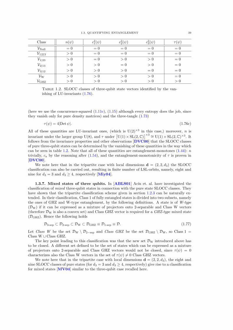
1.3. QUANTIFYING ENTANGLEMENT 39
Class n(ψ) c21(ψ) c22(ψ) c23(ψ) τ(ψ)
VNull = 0 = 0 = 0 = 0 = 0
V1|2|3 > 0 = 0 = 0 = 0 = 0
V1|23 > 0 = 0 > 0 > 0 = 0
V2|13 > 0 > 0 = 0 > 0 = 0
V3|12 > 0 > 0 > 0 = 0 = 0
VW > 0 > 0 > 0 > 0 = 0VGHZ > 0 > 0 > 0 > 0 > 0
Table 1.2. SLOCC classes of three-qubit state vectors identified by the van-ishing of LU-invariants (1.76).
(here we use the concurrence-squared (1.11c), (1.15) although every entropy does the job, sincethey vanish only for pure density matrices) and the three-tangle (1.73)
τ(ψ) = 4|Detψ|. (1.76c)
All of these quantities are LU-invariant ones, (which is U(2)×3 in this case,) moreover, n is
invariant under the larger group U(8), and τ under[U(1)× SL(2,C)
]×3 ∼= U(1)× SL(2,C)×3. Itfollows from the invariance properties and other observations [DVC00] that the SLOCC classesof pure three-qubit states can be determined by the vanishing of these quantities in the way whichcan be seen in table 1.2. Note that all of these quantities are entanglement-monotones (1.44): ntrivially, ca by the reasoning after (1.54), and the entanglement-monotonicity of τ is proven in[DVC00].
We note here that in the tripartite case with local dimensions d = (2, 2, d3) the SLOCCclassification can also be carried out, resulting in finite number of LSL-orbits, namely, eight andnine for d3 = 3 and d3 ≥ 4, respectively [Miy04].
1.3.7. Mixed states of three qubits. In [ABLS01] Acın et. al. have investigated theclassification of mixed three-qubit states in connection with the pure state SLOCC classes. Theyhave shown that the tripartite classification scheme given in section 1.2.3 can be naturally ex-tended. In their classification, Class 1 of fully entangled states is divided into two subsets, namelythe ones of GHZ and W-type entanglement, by the following definitions. A state is of W-type(DW) if it can be expressed as a mixture of projectors onto 2-separable and Class W vectors(therefore DW is also a convex set) and Class GHZ vector is required for a GHZ-type mixed state(DGHZ). Hence the following holds
D3-sep ⊂ D2-sep ⊂ DW ⊂ DGHZ ≡ D1-sep ≡ D. (1.77)
Let Class W be the set DW \ D2−sep and Class GHZ be the set DGHZ \ DW, so Class 1 =Class W ∪ Class GHZ.
The key point leading to this classification was that the new set DW introduced above hasto be closed. A different set defined to be the set of states which can be expressed as a mixtureof projectors onto 2-separable and Class GHZ vectors would not be closed, since τ(ψ) = 0characterizes also the Class W vectors in the set of τ(ψ) 6= 0 Class GHZ vectors.
We note here that in the tripartite case with local dimensions d = (2, 2, d3), the eight andnine SLOCC classes of pure states (for d3 = 3 and d3 ≥ 4, respectively) give rise to a classificationfor mixed states [MV04] similar to the three-qubit case recalled here.
40 1. QUANTUM ENTANGLEMENT
1.3.8. State vectors of four qubits. In the case of four qubits we have the Hilbert spaceH ≡ H1234 = H1 ⊗H2 ⊗H3 ⊗H4 with d = (2, 2, 2, 2) local dimensions. Let the four-qubit statevector |ψ〉 ∈ H be expressed in the computational basis |ijkl〉 = |i〉 ⊗ |j〉 ⊗ |k〉 ⊗ |l〉 as
|ψ〉 =
1∑i,j,k,l=0
ψijkl|ijkl〉.
This case is much more complicated than that of three qubits, even the SLOCC classes arelabelled by continuous parameters.
Let us start with the LSL-invariants, which are necessary to characterize the SLOCC classes.It is known that there are four algebraically independent SL(2,C)×4 invariants [LT03, Lev06]denoted by H,L,M and D. These are quadratic, quartic, quartic and sextic invariants of thecoefficients ψijkl respectively. The invariants H, L and M are given by the expressions
H(ψ) =1
2εii′εjj′εkk′εll′ψ
ijklψi′j′k′l′ =
1
2〈ψ|ψ〉 (1.78a)
with the spin-flipped vector 〈ψ| = ε⊗ ε⊗ ε⊗ ε|ψ〉, and
L(ψ) = detψ(12)(34), (1.78b)
M(ψ) = detψ(31)(24), (1.78c)
N(ψ) = detψ(14)(23), (1.78d)
where ψ(ab)(cd) is a matrix of two indices, which indices are composed of the binary indices
running on subsystems32 ab and cd, and then det is the usual matrix determinant for these 4× 4matrices. The three quantities L, N and M above are not linearly independent because theL(ψ) + M(ψ) + N(ψ) = 0 equation holds. However, any two of them are linearly independent.The sextic generator is
D(ψ) = detB, (1.78e)
given by the 3× 3 matrix B, which is the coefficient-matrix of a bi-quadratic form composed ofthe ψijkl coefficients as
1
2εjj′εkk′(ψ
ijklxitl)(ψi′j′k′l′xi′tl′) =
[x2
0, x0x1, x21
]B
t20t0t1t21
.In the four-qubit case there are continuously many SLOCC classes. However, there is a
classification which concerns not the LSL orbits, but the orbit-types, based on the constructionof an LSL canonical form. In this classification, it turns out that “four qubits can be entangledin nine different ways”, up to permutations of the subsystems [VDMV02, CD07]. Here thedifferent orbit-types are parametrized by complex parameters, which are in connection with theinvariants above. However, the same value of the invariants is only necessary but not sufficientcondition for two states to belong to the same orbit [CD07]. A different approach is given in[LL12].
1.4. Summary
We have seen that the structure of entanglement in multipartite systems is rather complex.We have seen these structures in the examples of some basic systems composed of small numberof qubits. (There are also a small number of other explicit results for few-qutrit systems in the
32That is, for example for ψIJ(14)(23)
the capital indices I = 0, 1, 2, 3 are equivalent to il = 00, 01, 10, 11 in
ψijkl respectively, and so on.
1.4. SUMMARY 41
literature.) All of these results are coming from ad hoc constructions based on mathematical co-incidences making it possible to obtain compact useful and manageable formulas. Unfortunately,these can hardly be generalized, or can not be generalized at all, simply because the structureitself is very complicated.
In the following chapters we present our results, which are of two kinds. In chapters 2, 4and 6 we show such ad hoc results of particular quantum systems, while in chapters 3 and 5 weshow some general results working for arbitrary number of subsystems of arbitrary dimensionalHilbert spaces, with detailed elaboration of the tripartite case.

CHAPTER 2
Two-qubit mixed states with fermionic purifications
As we have seen in section 1.2.2, the most plausible method for the quantification of entangle-ment of mixed states contains an implicit step which is the minimization over the decompositionsin the convex roof construction. This problem is solved for the case of two-qubit states, wherethe result of the minimization can be written in an explicit form, resulting in the celebratedformula of the Wotters concurrence (1.67). However, this formula is still implicit in anothersense: matrix diagonalization is needed to obtain a formula given by the parameters of the state.On the other hand, matrix diagonalization is needed to obtain the negativity (1.68) too.
In this chapter, we investigate a special 12-parameter family of two-qubit density matrices[LNP05], for which the Wootters concurrence and the negativity can be expressed in a closedformula given by the parameters of the state, and we give a detailed explicit characterization ofthe special four-qubit purification of these states.
The material of this chapter covers thesis statement I (page xv). The organization of thischapter is as follows.
In section 2.1, we present the parametrized family of density matrices we wish to study.Using suitable local unitary transformations we transform this family to a canonicalform.
In section 2.2, based on these results we calculate the Wootters concurrence and the neg-ativity (sections 2.2.1 and 2.2.2). We give a formula for the upper and lower boundsof negativity for a given concurrence (section 2.2.3). The mixeness is also calculated(section 2.2.4).
In section 2.3, we consider the special four-qubit purifications of this state. We analyze thestructure of the above quantities together with further ones characterizing four-qubitentanglement and discuss how they are related to each other. In particular we provethat the relevant entanglement measures associated with the four-qubit state satisfy thegeneralized Coffman-Kundu-Wootters inequality of distributed entanglement. For theresidual tangle we derive an explicit formula, containing two from the four algebraicallyindependent four-qubit invariants.
In section 2.4, we give a summary and some remarks.
2.1. The density matrix
The formula for the Wootters concurrence of two-qubit density matrices, given in (1.67), iswritten with the eigenvalues of
√√%%√%, which are hard to express using the matrix elements of
%. However, one can impose some conditions on %, which enables the Wootters concurrence to becalcualted in a closed form. For example, a two-qubit density matrix reduced from a pure three-qubit state is at the most of rank two, which enables the explicit calculation of the Woottersconcurrence in terms of the amplitudes of the original three-qubit state (section 6.1.3). Thiscould be generalized considering two-qubit mixed states reduced from four-qubit pure states.However, every two-qubit density matrix can be reduced from a pure four-qubit state, hence as
43
44 2. TWO-QUBIT MIXED STATES WITH FERMIONIC PURIFICATIONS
an extra constraint we impose an antisymmetry condition on the amplitudes of state vector
|ψ〉 =
1∑i,j,k,l=0
ψijkl|ijkl〉 ∈ H = H1 ⊗H2 ⊗H3 ⊗H4, (2.1a)
as
ψijkl = −ψklij , (2.1b)
that is, we impose antisymmetry in the first and second pairs of indices.An alternative (and more physical) way is the one of imposing such constraints on the
original Hilbert space H ∼= C16 which renders to have a tensor product structure on one of itssix dimensional subspaces H of the form
H4∧4 = (C2 ⊗ C2) ∧ (C2 ⊗ C2) ⊂ H, (2.2)
where ∧ refers to antisymmetrization. As we know quantum tensor product structures areobservable-induced, hence in order to specify this system with a tensor product structure ofequation (2.2) we have to specify the experimentally accessible interactions and measurementsthat account for the admissible operations we can perform on the system. For example we canrealize the system as a pair of fermions with four single particle states where a part of theadmissible operations are local unitary transformations of the form
|ψ〉 7−→ (U ⊗ V )⊗ (U ⊗ V )|ψ〉, U, V ∈ U(2). (2.3)
Taken together with equation (2.1b) this transformation rule clearly indicates that the 12 and 34subsystems form two indistinguishable subsystems of fermionic type. In this sense, the reduceddensity matrices arising from fermionic states that are elements of the tensor product structureas shown by equation (2.2) are called density matrices with fermionic purifications.
Let us parametrize the 6 amplitudes of this normalized four qubit state |ψ〉 with the anti-symmetry property of equation (2.1b) as
ψijkl =1
2
(εikAjl +Bikεjl
), (2.4a)
where ε is given in (1.18), and A and B are symmetric matrices1 of the form
A =
[z1 − iz2 −z3
−z3 −z1 − iz2
]= ε∗(zσ∗), B =
[w1 − iw2 −w3
−w3 −w1 − iw2
]= ε∗(wσ∗),
(2.4b)
where z,w ∈ C3 and the notation of (1.13) is used. It is straightforward to check that thenormalization condition of the state |ψ〉 takes the form
‖ψ‖2 = ‖w‖2 + ‖z‖2 = 1 (2.4c)
The density matrices we wish to study are arising as reduced ones of π = |ψ〉〈ψ| of the form
% := π12 = tr34 |ψ〉〈ψ|.Notice that since the 12 and 34 subsystems are by definition indistinguishable we also have% = π12 = π34.
A calculation of the partial trace yields the following explicit form for %
% =1
4
(I⊗ I + Λ
), (2.5a)
1 Note that, for example, A ∈ H2 ⊗ H4∼= Lin(H∗4 → H2), on the other hand, we regard ε∗ ∈ H2 ⊗ H4
∼=Lin(H∗4 → H2), (the εjls are the coefficients of that) and σ∗1,2,3 ∈ H∗4 ⊗H4
∼= Lin(H∗4 → H∗4). Simillarly on the
Hilbert spaces H1 and H3.
2.1. THE DENSITY MATRIX 45
where Λ is the traceless matrix
Λ = xσ ⊗ I + I⊗ yσ + wσ ⊗ z∗σ + w∗σ ⊗ zσ, (2.5b)
x = iw ×w∗, y = iz× z∗. (2.5c)
Notice that x,y ∈ R3, and xw = xw∗ = yz = yz∗ = 0. Due to this, and the identities
‖x‖2 = ‖w‖4 − |w2|2, ‖y‖2 = ‖z‖4 − |z2|2, (2.6)
it can be checked that Λ satisfies the identity
Λ2 =(1− η2
)I⊗ I, (2.7)
where
η ≡ |w2 − z2|, 0 ≤ η ≤ 1. (2.8)
Notice that the quantity η is just the Schliemann-measure of entanglement for two-fermionsystems with 4 single particle states [SCK+01, LNP05]. Indeed the density matrix % (with asomewhat different parametrization) can alternatively be obtained as a reduced one arising fromsuch fermionic systems after a convenient global U(4) (see in [LNP05]), and a local U(2)×U(2)transformation of the form I⊗ σ2.
Now by employing suitable local unitary transformations we would like to obtain a canonicalform for %. According to equation (2.3) the transformations operating on subsystems 12 orequivalently 34 are of the form U ⊗ V ∈ U(2)×U(2).
As a first step let us consider the unitary transformation
U(u, α) = e−iα2 uσ = cos (α/2) I− i sin (α/2) uσ,
which is a spin-1/2 representation of an SU(2) rotation around the axis u ∈ S2 ⊂ R3, (‖u‖2 = 1)with an angle α. A particular rotation from x to x′ (x′ 6= −x) can be written in the formU(u, α)xσU(u, α)† = x′σ with the parameters u = (x × x′)/(‖x × x′‖) and cosα = xx′/xxleading to the transformation operator
U(u, α) =1√
2‖x‖2(‖x‖2 + x′x)
(‖x‖2I + (xσ)(x′σ)
).
Employing this, we can rotate the vector x and y to the direction of the coordinate axis z asUxxσU†x = rσ3, VyyσV †y = sσ3. In this case the matrices are of the form
Ux :=1√
2r(r + x3)
(rI + σ3(xσ)
), Vy :=
1√2s(s+ y3)
(sI + σ3(yσ)
), (2.9a)
with the parameters
r = ‖x‖, s = ‖y‖. (2.9b)
Moreover, it can be checked that due to the special form of x and y, the transformations aboverotate the third components of w and z into zero,
UxwσU†x = w′σ, w′ = w − wx′
r2 + xx′(x + x′) =
w1 − x1
r+x3w3
w2 − x2
r+x3w3
0
, (2.10a)
VyzσV †y = z′σ, z′ = z− zy′
s2 + yy′(y + y′) =
z1 − y1s+y3
z3
z2 − y2s+y3
z3
0
. (2.10b)
46 2. TWO-QUBIT MIXED STATES WITH FERMIONIC PURIFICATIONS
Every U ∈ U(2) unitary transformation acting on an arbitrary a ∈ C3 as UaσU† = a′σpreserves a2 and ‖a‖2, since 2a2 = tr(aσ)(aσ), and 2‖a‖2 = tr(aσ)†(aσ). Hence
w′2 = w2, z′2 = z2, ‖w′‖2 = ‖w‖2, ‖z′‖2 = ‖z‖2, η′ = η (2.11)
are invariant under local U(2)×U(2) transformations.2
Now by employing the local U(2) × U(2) transformations Ux ⊗ Vy, the density matrix canbe cast to the form,
%′ = (Ux ⊗ Vy) %(U†x ⊗ V †y
)=
1
4(I + Λ′) , (2.12a)
where
Λ′ = rσ3 ⊗ I + I⊗ sσ3 + w′σ ⊗ z′∗σ + w′
∗σ ⊗ z′σ (2.12b)
has the special form3
Λ′ =
α3 · · α1 − iα2
· β3 β1 − iβ2 ·· β1 + iβ2 −β3 ·
α1 + iα2 · · −α3
(2.12c)
with the quantities defined as
α =
ξ1 − ξ2ζ1 + ζ2r + s
∈ R3, β =
ξ1 + ξ2ζ1 − ζ2r − s
∈ R3, (2.12d)
ξ1 = w′1z′∗1 + w′∗1 z
′1, ζ1 = w′2z
′∗1 + w′∗2 z
′1, (2.12e)
ξ2 = w′2z′∗2 + w′∗2 z
′2, ζ2 = w′1z
′∗2 + w′∗1 z
′2. (2.12f)
Thanks to the special X-shape of Λ′, we can regard %′ as the direct sum of two 2 × 2 blocks1/4(I+ασ) and 1/4(I+βσ). Having obtained this canonical form of the reduced density matrix%, now we turn to the calculation of the corresponding entanglement measures.
2.2. Measures of entanglement for the density matrix
In this section we calculate the Wootters concurrence (1.67) and the negativity (1.68) of thisdensity matrix %. Both of these measures are invariant under the local unitary transformationswhich we have used to obtain the canonical form %′, therefore we can calculate them for thecanonical form. Moreover, the steps leading from %′ to the measures leave the X-shape of %′
invariant, so we have to calculate eigenvalues of matrices which are of size 2× 2 only. This keepsthe symbolical calculations in a relatively easy way.
2.2.1. Wootters concurrence. Let us start with the Wootters concurrence (1.67) of thedensity matrix %. As we have mention in section 1.3.5, the the Wootters concurrence is invariantunder U(1) × SL(2,C) × SL(2,C), so we can use the canonical form %′ we have obtained in theprevious section via using the transformation Ux ⊗ Vy ∈ SU(2) × SU(2) ⊂ U(1) × SL(2,C) ×SL(2,C) for its calculation.
2The entanglement measure η is also invariant under the larger group of U(4) transformations.3For better readability, zeroes in matrices are often denoted with dots.
2.2. MEASURES OF ENTANGLEMENT FOR THE DENSITY MATRIX 47
The matrix %′%′ has the same X-shape as %′, with the blocks 1/16(α0I + ασ) and 1/16(β0I +
βσ) where αµ and βν with µ, ν = 0, 1, 2, 3 are quadratic in α and β:
αµ =
1 + α2
1 + α22 − α2
3
2α1 − i2α2α3
2α2 + i2α3α1
0
∈ C4, βν =
1 + β2
1 + β22 − β2
3
2β1 − i2β2β3
2β2 + i2β3β1
0
∈ C4. (2.13)
The eigenvalues of the blocks 1/16(α0I + ασ
)and 1/16
(β0I + βσ
)are 1/16
(α0 ±
√α2)
and
1/16(β0 ±
√β
2)
, respectively. Now, we can express these with the help of the quantities α, β
of (2.13) and get the eigenvalues of %′%′ in the form
Eigv(%′%′
)=
{1
16
(√α2
1 + α22 ±
√1− α2
3
)2
,1
16
(√β2
1 + β22 ±
√1− β2
3
)2}.
Now, using equations (2.12d)-(2.12f), we have to express these as functions of the original quan-tities z2, w2, ‖z‖2 and ‖w‖2. Straightforward calculation shows that
α21 + α2
2 = 2‖w′‖2‖z′‖2 + w′2z′∗2
+ w′∗2z′2 − 2rs, (2.14a)
β21 + β2
2 = 2‖w′‖2‖z′‖2 + w′2z′∗2
+ w′∗2z′2 + 2rs, (2.14b)
1− α23 = 2‖w′‖2‖z′‖2 + w′2w′∗
2+ z′2z′∗
2 − 2rs, (2.14c)
1− β23 = 2‖w′‖2‖z′‖2 + w′2w′∗
2+ z′2z′∗
2+ 2rs. (2.14d)
The formulas above are expressed in terms of quantities invariant under the transformationyielding the canonical form (2.11) so we can simply omit the primes. Hence by using equation(2.6) and (2.8) we can establish that
α21 + α2
2 = 1− α23 − η2, β2
1 + β22 = 1− β2
3 − η2.
For further use, we define the quantities
γ+ := r + s ≡ α3, γ− := r − s ≡ β3. (2.15)
With these, the spectrum of√√
%%√%, which is the same as the square root of the eigenvalues
of %%, is
Spect√√
%%√% =
{1
4
(√1− γ2
+ ±√
1− γ2+ − η2
),
1
4
(√1− γ2
− ±√
1− γ2− − η2
)}.
The greatest one of these is λ↓1 = 1/4(√
1− γ2− +
√1− γ2
− − η2)
, and, after subtracting the
others from it, we get finally the nice formula for the Wootters concurrence (1.67)
c∪(%) =1
2
(√1− η2 − γ2
− −√
1− γ2+
)+
(2.16)
with the quantities defined in equations (2.6), (2.8), (2.9b) and (2.15) containing our basicparameters w and z of %. One can easily check by the definitions (2.15) that
% ∈ Dsep ⇐⇒ η2 ≥ 4rs. (2.17)
Hence the surface dividing the entangled and separable states in the space of these densitymatrices is given by the equation η2 = 4rs, which is a special deformation of the η = 0 Klein-quadric [LNP05]. This can also be seen from the (2.19) formula of negativity, see in the nextsubsection.
48 2. TWO-QUBIT MIXED STATES WITH FERMIONIC PURIFICATIONS
2.2.2. Negativity. The next entanglement measure which we are able to calculate for %is the negativity (1.68), which is defined in this case by the smallest eigenvalue of the partiallytransposed density matrix (section 1.3.5). Since the eigenvalues of the density matrix togetherwith those of its partial transpose are invariant under U(2)× U(2) transformations, we can useagain the canonical form %′ of equation (2.12a).
Consider the %′t2 partial transpose of %′ with respect to the second subsystem. This operationresults in the following transformation of Λ′ of (2.12b)
Λ′t2 = rσ3 ⊗ I + I⊗ sσ3 + w′σ ⊗ (z′∗σ)t + w′
∗σ ⊗ (z′σ)t,
meaning that only z′2 changes to −z′2, thanks to (1.17). By virtue of this, retaining the (2.12e)and (2.12f) definitions of ξ1, ξ2, ζ1, ζ2, and redefining α,β ∈ R3 of equation (2.12d) as
α =
ξ1 + ξ2ζ1 − ζ2r + s
∈ R3, β =
ξ1 − ξ2ζ1 + ζ2r − s
∈ R3, (2.18)
the calculation proceeds as in section 2.2.1. Namely, we can regard %′t2 as the direct sum of theblocks 1/4(I + ασ) and 1/4(I + βσ) again, and the spectrum of %t2 is the union of the spectraof them
Spect(%′
t2)
= Spect(%t2)
=
{1
4
(1± ‖α‖
),
1
4
(1± ‖β‖
)}.
Then straightforward calculation shows that4
‖α‖2 = 1− η2 + 4rs, ‖β‖2 = 1− η2 − 4rs.
The former one leads to the smaller eigenvalue with the minus sign. It follows from the definition(2.15) that γ2
+ − γ2− = 4rs, hence the negativity of % is
N(%) =1
2
(√1− η2 − γ2
− + γ2+ − 1
)+
, (2.19)
with the usual quantities given in equations (2.8) and (2.9b).
2.2.3. Comparsion of Wootters concurrence and negativity. For a two-qubit den-sity matrix we can write the following inequalities between the Wootters concurrence and thenegativity√
(1− c∪)2 + c∪2 − (1− c∪) ≤ N ≤ c∪, (2.20)
which are known from the papers of Verstraete et. al. [VADM01, VABM00]. Our special casewith fermionic correlations may give extra restrictions between these quantities, so we can posethe question, whether we can replace the inequalities in (2.20) by stronger ones. Indeed, we givestronger bounds on the negativity, which are illustrated in figure 2.1.
First, we give a stronger upper bound for the negativity than the one in (2.20). This upperbound is the following:
N(%) ≤ 1
2
(√2−
(1− 2c∪(%)
)2 − 1
), (2.21)
4With the redefined α and β (2.18), only the sign of the term 2rs flips in (2.14a) and in (2.14b). Then theprimes can be dropped again, leading to these expressions.
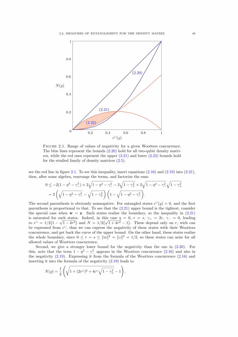
2.2. MEASURES OF ENTANGLEMENT FOR THE DENSITY MATRIX 49
(2.20)
(2.21)
(2.22)
N(%)
c∪(%)
0 0.2 0.4 0.6 0.8 1
0.2
0.4
0.6
0.8
1
Figure 2.1. Range of values of negativity for a given Wootters concurrence.The blue lines represent the bounds (2.20) hold for all two-qubit density matri-ces, while the red ones represent the upper (2.21) and lower (2.22) bounds holdfor the studied family of density matrices (2.5).
see the red line in figure 2.1. To see this inequality, insert equations (2.16) and (2.19) into (2.21),then, after some algebra, rearrange the terms, and factorize the sum:
0 ≤ −2(1− η2 − γ2−) + 2
√1− η2 − γ2
− − 2√
1− γ2+ + 2
√1− η2 − γ2
−
√1− γ2
+
= 2
(√1− η2 − γ2
− −√
1− γ2+
)(1−
√1− η2 − γ2
−
).
The second parenthesis is obviously nonnegative. For entangled states c∪(%) > 0, and the firstparenthesis is proportional to that. To see that the (2.21) upper bound is the tightest, considerthe special case when w = z. Such states realize the boundary, so the inequality in (2.21)is saturated for such states. Indeed, in this case η = 0, r = s, γ+ = 2r, γ− = 0, leadingto c∪ = 1/2
(1 −√
1− 4r2)
and N = 1/2(√
1 + 4r2 − 1). These depend only on r, wich can
be expressed from c∪, thus we can express the negativity of these states with their Woottersconcurrence, and get back the curve of the upper bound. On the other hand, these states realizethe whole boundary, since 0 ≤ r = s ≤ ‖w‖2 = ‖z‖2 = 1/2, so these states can arise for allallowed values of Wootters concurrence.
Second, we give a stronger lower bound for the negativity than the one in (2.20). Forthis, note that the term 1 − η2 − γ2
− appears in the Wootters concurrence (2.16) and also inthe negativity (2.19). Expressing it from the formula of the Wootters concurrence (2.16) andinserting it into the formula of the negativity (2.19) leads to
N(%) =1
2
(√1 + (2c∪)2 + 4c∪
√1− γ2
+ − 1
).
50 2. TWO-QUBIT MIXED STATES WITH FERMIONIC PURIFICATIONS
Since 0 ≤ γ2+ ≡ (r + s)2 ≤ 1, as can be concluded from (2.15), (2.4c) and (2.6), we can obtain a
lower and an upper bound for the negativity for γ2+ = 1 and 0: 1/2
(√1 + (2c∪)2 − 1
)≤ N(%) ≤
1/2(√
1 + (2c∪)2 + 4c∪ − 1)
= c∪. The upper bound is weaker than the one we have in (2.21),actually this is the upper bound in (2.20) valid for general two-qubit density matrices. But thelower bound
1
2
(√1 + (2c∪)2 − 1
)≤ N(%) (2.22)
is stronger in the 0 ≤ c∪ ≤ 1/2 interval that the one in (2.20), see the red line in figure 2.1. To seethat the (2.22) lower bound is the tightest, we need that γ2
+ = 1 can be realized independentlyof the Wootters concurrence. From (2.15), (2.4c) and (2.6), we have that γ2
+ = 1 if and only ifwhen w2 = 0 and z2 = 0. In this case η = 0, r = ‖w‖2, s = ‖z‖2, and γ− = ‖w‖2−‖z‖2, leading
to c∪ = 1/2√
1− γ2− and N = 1/2
(√2 + γ2
− − 1)
. These states realize the whole boundary,
since 0 ≤ γ2− =
(2‖w‖2− 1
)2 ≤ 1, so these states can arise for all allowed values of the Woottersconcurrence.
Summarizing we have√(1− c∪)2 + (c∪)2 − (1− c∪) ≤ 1
2
(√1 + (2c∪)2 − 1
)≤ N ≤ 1
2
(√2− (1− 2c∪)2 − 1
)≤ c∪
(2.23)
where the first and last bounds on the negativity hold for general two-qubit mixed states (2.20),the stronger second (2.22) and third (2.21) bounds hold for the special family of two-qubit mixedstates given in (2.5). For these states 0 ≤ c∪ ≤ 1/2, the first inequality holds only in this interval.
As an illustration, we can obtain examples of states of the canonical form, which are realizingthe boundaries, that is, have maximal or minimal negativity for a given Wootters concurrence.For the upper bound (2.21) we need states for which w′ = z′ for all 0 ≤ r = s ≤ 1/2 parametervalues. This can be achieved by varying the relative phase of w′1 and w′2 (having the samemagnitude) and fixing the lengths ‖w′‖2 = ‖z′‖2 = 1/2. For the lower bound (2.22) we needstates for which w2 = z2 = 0 for all 0 ≤ γ2
− ≤ 1 parameter values. This can be achieved byvarying the relative lengths ‖w′‖2 and ‖z′‖2 and fixing the relative phase of w′1 and w′2 and of z′1and z′2. Summarizing, we introduce the states depending on two parameters ϑ and ϕ as follows
w′ =cosϑ√
2
1eiϕ
0
, z′ =sinϑ√
2
1eiϕ
0
, 0 ≤ 2ϑ, ϕ ≤ π
2, (2.24)
leading to the density matrix
%′ =1
4
1 + sinϕ · · −i sin 2ϑ cosϕ· 1 + cos 2ϑ 1 ·· 1 1− cos 2ϑ ·
i sin 2ϑ cosϕ · · 1− sinϕ
.For these states w′ = z′ if and only if ϑ = π/4, then they have maximal negativity for a givenWootters concurrence (2.21), on the other hand, w2 = z2 = 0 if and only if ϕ = π/2, thenthey have minimal negativity for a given Wootters concurrence (2.22). In both cases, the freeparameter runs through the whole boundary. In general we have r = cos2 ϑ sinϕ, s = sin2 ϑ sinϕ,
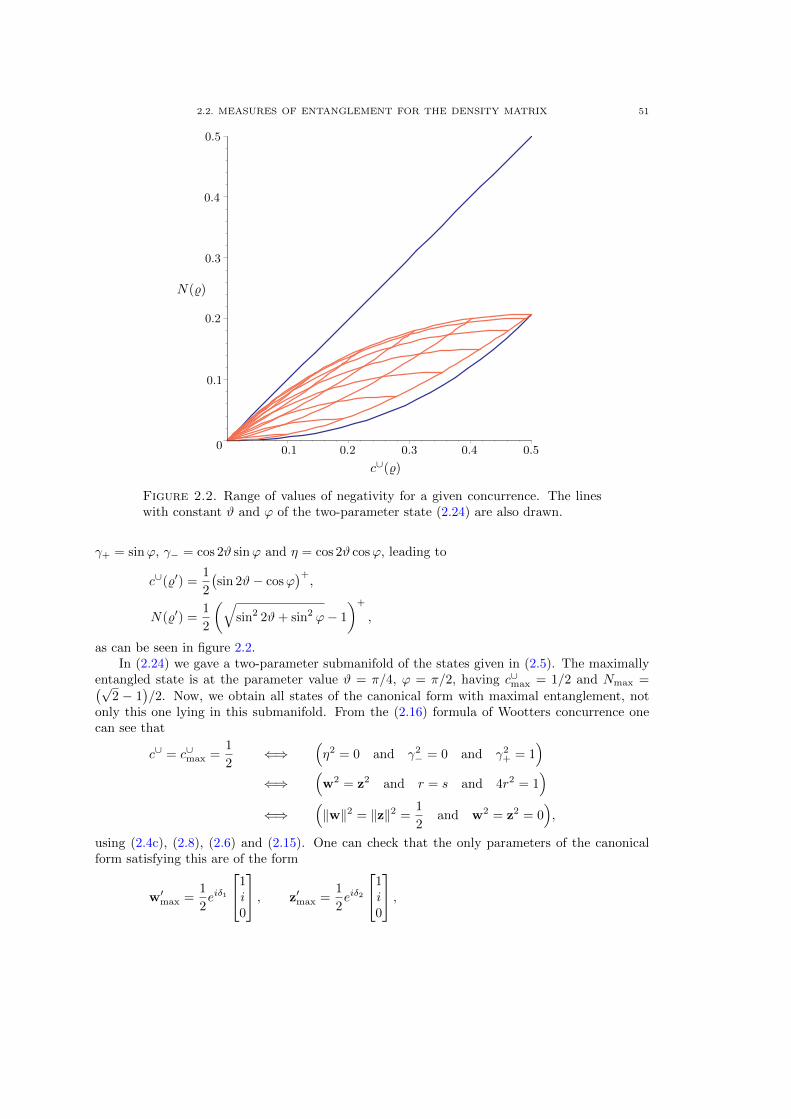
2.2. MEASURES OF ENTANGLEMENT FOR THE DENSITY MATRIX 51
N(%)
c∪(%)
0 0.1 0.2 0.3 0.4 0.5
0.1
0.2
0.3
0.4
0.5
Figure 2.2. Range of values of negativity for a given concurrence. The lineswith constant ϑ and ϕ of the two-parameter state (2.24) are also drawn.
γ+ = sinϕ, γ− = cos 2ϑ sinϕ and η = cos 2ϑ cosϕ, leading to
c∪(%′) =1
2
(sin 2ϑ− cosϕ
)+,
N(%′) =1
2
(√sin2 2ϑ+ sin2 ϕ− 1
)+
,
as can be seen in figure 2.2.In (2.24) we gave a two-parameter submanifold of the states given in (2.5). The maximally
entangled state is at the parameter value ϑ = π/4, ϕ = π/2, having c∪max = 1/2 and Nmax =(√2 − 1
)/2. Now, we obtain all states of the canonical form with maximal entanglement, not
only this one lying in this submanifold. From the (2.16) formula of Wootters concurrence onecan see that
c∪ = c∪max =1
2⇐⇒
(η2 = 0 and γ2
− = 0 and γ2+ = 1
)⇐⇒
(w2 = z2 and r = s and 4r2 = 1
)⇐⇒
(‖w‖2 = ‖z‖2 =
1
2and w2 = z2 = 0
),
using (2.4c), (2.8), (2.6) and (2.15). One can check that the only parameters of the canonicalform satisfying this are of the form
w′max =1
2eiδ1
1i0
, z′max =1
2eiδ2
1i0
,
52 2. TWO-QUBIT MIXED STATES WITH FERMIONIC PURIFICATIONS
leading to the density matrix
%′max =1
4
32 · · ·· 1 eiδ ·· e−iδ 1 ·· · · 1
2
. (2.25)
Here δ = δ1 − δ2 is the only parameter characterizing this maximally entangled density matrixof the canonical form (2.12a) for the family of states given in (2.5).
2.2.4. Mixedness. Tdegree of mixedness of a density matrix can be characterized, forexample, by the purity (1.11a), the participiation ratio (1.11b) and the concurrence-squared(1.11c), among other quantites. As we have seen in section 1.3.2, the latter one, calculated for% = π12, measures the entanglement of the pure state |ψ〉 under the 12|34 split, if we do notconsider this state as a fermionic state, but rather a special four-qubit one. (The fermionicentanglement is a different story [SCK+01, GMW02, GM04].) For our %, thanks to thespecial property (2.7) of Λ, these quantities can easily be calculated, leading to
P (%) =1
4(2− η2),
1
4≤ P (%) ≤ 1
2, (2.26a)
R(%) =4
2− η2, 2 ≤ R(%) ≤ 4, (2.26b)
C2(%) =1
3(2 + η2),
2
3≤ C2(%) ≤ 1, (2.26c)
by virtue of equation (2.8). The concurrence-squared C2(%) never vanishes, which means thatthe four-qubit state vector |ψ〉 with the antisymmetry property (2.1b) is never separable underthe 12|34 split, which is a manifestation of its fermionic nature. On the other hand, its entan-glement (2.26c) increases with η, while the entanglement c∪(%) inside the 12 (or equivalently 34)subsystem (2.16) decreases with that. Although this may be interesting, but this can not lead toa usual monogamy relation (1.70) at this point, (that is, involving Wootters concurrences,) sinceC2(%) is related to a split involving d = 4 qudits. Even if there would be some general relationsinvolving C2(%) on multipartite entanglement in the fashion of monogamy, there are too manyquantities which can not be calculated in a closed form at this point, namely, the entanglementinside the tripartite subsystems with respect to bipartite and tripartite splits. Anyway, the usualmonogamy relation for four qubits (1.70) can be studied, as is done in the next section.
2.3. Relating different measures of entanglement
In this section we would like to discuss the relations of entanglement monogamy for multi-qubit systems (1.70) applied to the four-qubit pure state with the antisymmetry property (2.1b).During this, we calculate the remaining quantities we need, and see how all these quantities arerelated to the important ones characterizing four-qubit pure state entanglement. The latter onesare given in section 1.3.8.
2.3.1. One-qubit subsystems. First of all let us notice that the
π1 = tr234 π = tr2 % =1
2(I + xσ), (2.27a)
π2 = tr134 π = tr1 % =1
2(I + yσ) (2.27b)
reduced density matrices describe the entanglement properties of subsystems 1 and 2 to the restof the system described by the four-qubit state π = |ψ〉〈ψ|. Because of the antisymmetry (2.1b)
2.3. RELATING DIFFERENT MEASURES OF ENTANGLEMENT 53
of |ψ〉, we also have
π3 = π1, π4 = π2. (2.27c)
We can characterize how much these subsystems are entangled with the rest with the concurrence-squares (1.11c) of the states of the subsystems,
C2(π1) = 4 detπ1 = 1− r2, C2(π2) = 4 detπ2 = 1− s2, (2.28a)
and
C2(π3) = C2(π1), C2(π4) = C2(π2). (2.28b)
The concurrence-squared (1.11c) ranges from 0 to 1 in general, and in our case the 0 ≤ C2(πa) ≤ 1bounds can be saturated due to (2.6).
2.3.2. Other two-qubit subsystems. Now turn to the bipartite subsystems. We alreadyknow the Wootters concurrence of the states π12 = π34 = % from (2.16). A straightforwardcalculation of the bipartite density matrices π14 and π23 shows that they again have the formof equation (2.5) with the sign of w is changed in the first case and the vectors w and z areexchanged in the second. Since these transformations do not change the value of the Woottersconcurrence, we have
c∪2(π12) = c∪
2(π14) = c∪
2(π23) = c∪
2(π34). (2.29)
Now the only two-qubit density matrices we have not discussed yet are the ones π13 and π24.Their forms are5
(π13)iki′k′ =1
2
(‖z‖2εikεi′k′ +BikBi′k′
), (2.30a)
(π24)jlj′l′ =1
2
(‖w‖2εjlεj′l′ +AjlAj′l′
). (2.30b)
Recall now that the (2.3) transformation property of the (2.1) four-qubit state gives rise to thecorresponding ones for the reduced density matrices
π13 7−→ (U ⊗ U)π13(U† ⊗ U†),
π24 7−→ (V ⊗ V )π24(V † ⊗ V †).
For U, V ∈ SU(2), due to (1.20) the tensors occurring in (2.30) transform as
ε 7−→ ε,
A 7−→ V AV t,
B 7−→ UBU t.
Using the (2.4b) definition of A we have for example
V AV t = V ε∗(zσ∗)V t = ε∗V ∗(zσ∗)V t = ε∗(V (z∗σ)V †)∗ = ε∗(z′∗σ)∗ = ε∗(z′σ∗),
where by choosing V ≡ Vy of (2.9a) we get the (2.10b) form for z′. Finally these manipulationsyield for π24 the canonical form, which is of X-shape again,
π24 =1
2
κ0 + κ3 · · κ1 − iκ2
· ‖w′‖2 −‖w′‖2 ·· −‖w′‖2 ‖w′‖2 ·
κ1 + iκ2 · · κ0 − κ3
, (2.31)
5Note our convention: Bik = (Bik)∗, Ajl = (Ajl)∗.

54 2. TWO-QUBIT MIXED STATES WITH FERMIONIC PURIFICATIONS
where
κµ =
‖z′‖2
|z′2|2 − |z′1|2−2<(z′1z
′2∗)
−2=(z′1z′2∗)
.Notice that κ2
0 = κ21 + κ2
2 + κ23 = ‖z′‖4 = ‖z‖4, hence the eigenvalues of π24 are
Spectπ24 = {‖w‖2, ‖z‖2, 0, 0},that is, this mixed state is of rank two. The structure of π13 is similar with the roles of w andz exchanged. Following the same steps as in section 2.2.1, we get for the corresponding squaredWootters concurrences the following expressions
c∪2(π13) =
(‖z‖2 − |w2|
)2, c∪
2(π24) =
(‖w‖2 − |z2|
)2. (2.32)
With these, we have all the quantities we need to write the monogamy relations for this four-qubitsystem.
2.3.3. Four-qubit invariants. Before doing this, let us now understand the meaning ofthe invariant η from the four-qubit point of view. In section 1.3.8, the independent SL(2,C)×4-invariant homogeneous polynomials were listed. These polynomials are sufficient for the char-acterization of four-qubit entanglement in some sense, and they show how these fermionic statevectors are embedded in the whole Hilbert-space. A straightforward calculation shows that forthe (2.1) four-qubit state we have M = D = 0, however,
H = −1
2
(z2 + w2
), L =
1
16
(z2 −w2
)2,
hence, due to (2.8)
|L| = 1
16η2.
For convenience we also introduce the quantity
σ :=∣∣w2 + z2
∣∣ = 2|H|. (2.33)
Hence η = |w2−z2| and σ = |w2 +z2| are related to the only nonvanishing four qubit invariantsL and H.
2.3.4. Monogamy of entanglement. Using the (2.8) and (2.33) definitions of η and σand (2.6), one can check that the Wootters concurrences of the 13 and 24 subsystems, given in(2.32), can be written as
c∪2(π13) = s2 +
1
2
(η2 + σ2
)− 2‖z‖2|w2|, (2.34a)
c∪2(π24) = r2 +
1
2
(η2 + σ2
)− 2‖w‖2|z2|. (2.34b)
Since c∪2(π12) = c∪
2(π14), after taking the square of (2.16) we get
c∪2(π12) + c∪
2(π14) = 1− r2 − s2 − 1
2η2 −
√(1− η2 − γ2
−)(
1− γ2+
). (2.35)
Combining this result with equations (2.34) and (2.28) we obtain the equations relating measuresof entanglement which are involved in monogamy
c∪2(π12) + c∪
2(π13) + c∪
2(π14) + Σ1 = C2(π1), (2.36a)
c∪2(π12) + c∪
2(π23) + c∪
2(π24) + Σ2 = C2(π2), (2.36b)
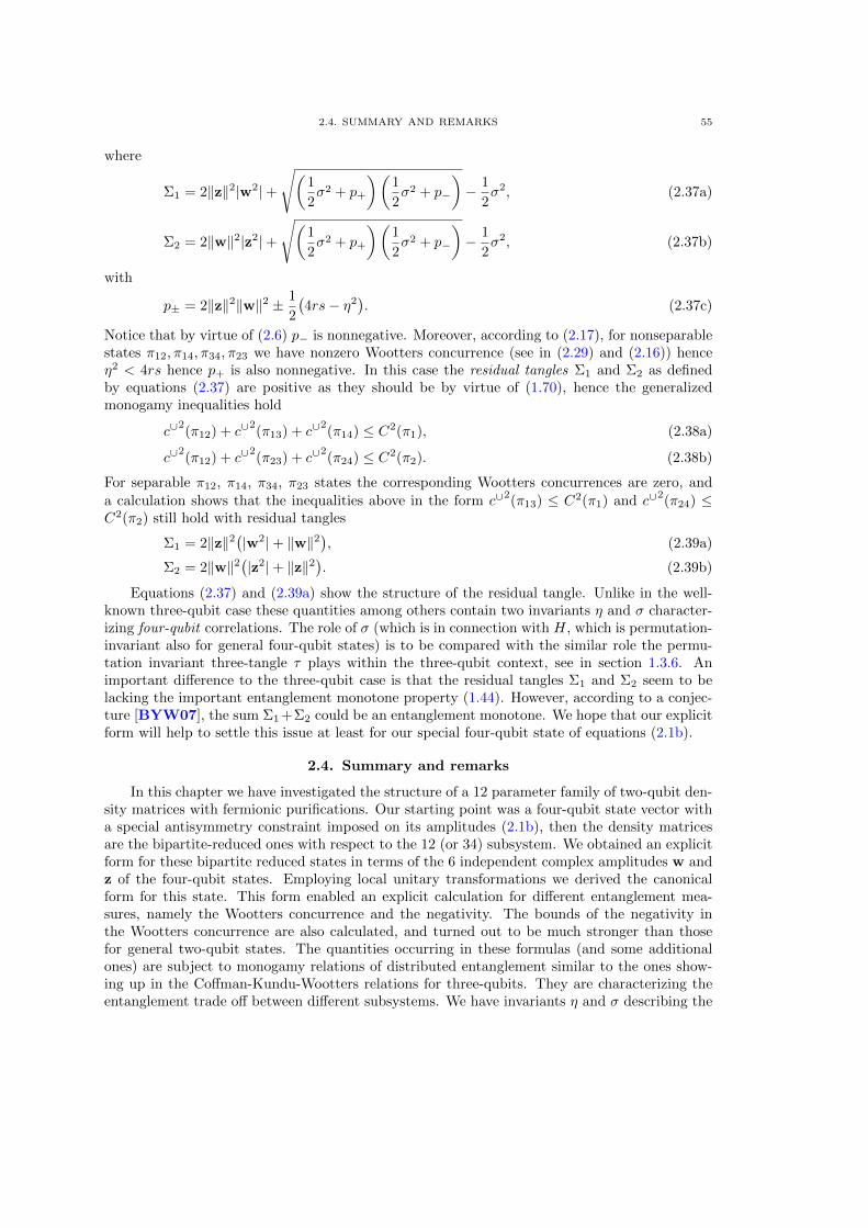
2.4. SUMMARY AND REMARKS 55
where
Σ1 = 2‖z‖2|w2|+
√(1
2σ2 + p+
)(1
2σ2 + p−
)− 1
2σ2, (2.37a)
Σ2 = 2‖w‖2|z2|+
√(1
2σ2 + p+
)(1
2σ2 + p−
)− 1
2σ2, (2.37b)
with
p± = 2‖z‖2‖w‖2 ± 1
2
(4rs− η2
). (2.37c)
Notice that by virtue of (2.6) p− is nonnegative. Moreover, according to (2.17), for nonseparablestates π12, π14, π34, π23 we have nonzero Wootters concurrence (see in (2.29) and (2.16)) henceη2 < 4rs hence p+ is also nonnegative. In this case the residual tangles Σ1 and Σ2 as definedby equations (2.37) are positive as they should be by virtue of (1.70), hence the generalizedmonogamy inequalities hold
c∪2(π12) + c∪
2(π13) + c∪
2(π14) ≤ C2(π1), (2.38a)
c∪2(π12) + c∪
2(π23) + c∪
2(π24) ≤ C2(π2). (2.38b)
For separable π12, π14, π34, π23 states the corresponding Wootters concurrences are zero, and
a calculation shows that the inequalities above in the form c∪2(π13) ≤ C2(π1) and c∪
2(π24) ≤
C2(π2) still hold with residual tangles
Σ1 = 2‖z‖2(|w2|+ ‖w‖2
), (2.39a)
Σ2 = 2‖w‖2(|z2|+ ‖z‖2
). (2.39b)
Equations (2.37) and (2.39a) show the structure of the residual tangle. Unlike in the well-known three-qubit case these quantities among others contain two invariants η and σ character-izing four-qubit correlations. The role of σ (which is in connection with H, which is permutation-invariant also for general four-qubit states) is to be compared with the similar role the permu-tation invariant three-tangle τ plays within the three-qubit context, see in section 1.3.6. Animportant difference to the three-qubit case is that the residual tangles Σ1 and Σ2 seem to belacking the important entanglement monotone property (1.44). However, according to a conjec-ture [BYW07], the sum Σ1 +Σ2 could be an entanglement monotone. We hope that our explicitform will help to settle this issue at least for our special four-qubit state of equations (2.1b).
2.4. Summary and remarks
In this chapter we have investigated the structure of a 12 parameter family of two-qubit den-sity matrices with fermionic purifications. Our starting point was a four-qubit state vector witha special antisymmetry constraint imposed on its amplitudes (2.1b), then the density matricesare the bipartite-reduced ones with respect to the 12 (or 34) subsystem. We obtained an explicitform for these bipartite reduced states in terms of the 6 independent complex amplitudes w andz of the four-qubit states. Employing local unitary transformations we derived the canonicalform for this state. This form enabled an explicit calculation for different entanglement mea-sures, namely the Wootters concurrence and the negativity. The bounds of the negativity inthe Wootters concurrence are also calculated, and turned out to be much stronger than thosefor general two-qubit states. The quantities occurring in these formulas (and some additionalones) are subject to monogamy relations of distributed entanglement similar to the ones show-ing up in the Coffman-Kundu-Wootters relations for three-qubits. They are characterizing theentanglement trade off between different subsystems. We have invariants η and σ describing the
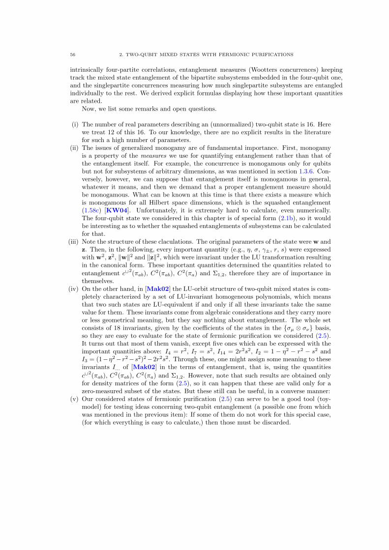
56 2. TWO-QUBIT MIXED STATES WITH FERMIONIC PURIFICATIONS
intrinsically four-partite correlations, entanglement measures (Wootters concurrences) keepingtrack the mixed state entanglement of the bipartite subsystems embedded in the four-qubit one,and the singlepartite concurrences measuring how much singlepartite subsystems are entangledindividually to the rest. We derived explicit formulas displaying how these important quantitiesare related.
Now, we list some remarks and open questions.
(i) The number of real parameters describing an (unnormalized) two-qubit state is 16. Herewe treat 12 of this 16. To our knowledge, there are no explicit results in the literaturefor such a high number of parameters.
(ii) The issues of generalized monogamy are of fundamental importance. First, monogamyis a property of the measures we use for quantifying entanglement rather than that ofthe entanglement itself. For example, the concurrence is monogamous only for qubitsbut not for subsystems of arbitrary dimensions, as was mentioned in section 1.3.6. Con-versely, however, we can suppose that entanglement itself is monogamous in general,whatewer it means, and then we demand that a proper entanglement measure shouldbe monogamous. What can be known at this time is that there exists a measure whichis monogamous for all Hilbert space dimensions, which is the squashed entanglement(1.58c) [KW04]. Unfortunately, it is extremely hard to calculate, even numerically.The four-qubit state we considered in this chapter is of special form (2.1b), so it wouldbe interesting as to whether the squashed entanglements of subsystems can be calculatedfor that.
(iii) Note the structure of these claculations. The original parameters of the state were w andz. Then, in the following, every important quantity (e.g., η, σ, γ±, r, s) were expressedwith w2, z2, ‖w‖2 and ‖z‖2, which were invariant under the LU transformation resultingin the canonical form. These important quantities determined the quantities related to
entanglement c∪2(πab), C
2(πab), C2(πa) and Σ1,2, therefore they are of importance in
themselves.(iv) On the other hand, in [Mak02] the LU-orbit structure of two-qubit mixed states is com-
pletely characterized by a set of LU-invariant homogeneous polynomials, which meansthat two such states are LU-equivalent if and only if all these invariants take the samevalue for them. These invariants come from algebraic considerations and they carry moreor less geometrical meaning, but they say nothing about entanglement. The whole setconsists of 18 invariants, given by the coefficients of the states in the {σµ ⊗ σν} basis,so they are easy to evaluate for the state of fermionic purification we considered (2.5).It turns out that most of them vanish, except five ones which can be expressed with theimportant quantities above: I4 = r2, I7 = s2, I14 = 2r2s2, I2 = 1 − η2 − r2 − s2 andI3 = (1−η2−r2−s2)2−2r2s2. Through these, one might assign some meaning to theseinvariants I... of [Mak02] in the terms of entanglement, that is, using the quantities
c∪2(πab), C
2(πab), C2(πa) and Σ1,2. However, note that such results are obtained only
for density matrices of the form (2.5), so it can happen that these are valid only for azero-measured subset of the states. But these still can be useful, in a converse manner:
(v) Our considered states of fermionic purification (2.5) can serve to be a good tool (toy-model) for testing ideas concerning two-qubit entanglement (a possible one from whichwas mentioned in the previous item): If some of them do not work for this special case,(for which everything is easy to calculate,) then those must be discarded.
CHAPTER 3
All degree 6 local unitary invariants of multipartitesystems
In the previous chapter, we have seen some examples for the occurence of LU-invariant quan-tities for the quantification of entanglement. This was natural, since, as we have seen in section1.2.2, the notion of entanglement of a composite quantum system is invariant under unitary trans-formations on the subsystems. Hence everything that can be said about the entanglement of acomposite system can also be said in the terms of LU-invariants. In this sense, the investigationof LU-invariants is a natural way of studying quantum entanglement.
Important recent developments in this direction are the general results of Hero et. al. [HW09,HWW09] and Vrana [Vra11a, Vra11b] on LU-invariant polynomials for pure quantum states.In [Vra11b], it has been pointed out that the inverse limit (in the local dimensions) of algebrasof LU-invariant polynomials of finite dimensional n-partite quantum systems is free, and analgebraically independent generating set for that has been given. This approach using the inverselimit construction is different from the usual, when the LU orbit structure is investigated first, forgiven local dimensions, and then invariants separating the orbits are being searched for [Rai00,LP98, LPS99, GRB98, Sud01, Mak02, AAJT01]. The structure of algebras of LU-invariantpolynomials for given local dimensions is very complicated, the inverse limit of these [HW09,HWW09, Vra11b], however, has a remarkably simple structure: it is free [Vra11b], and analgebraically independent generating set can be given for that. Moreover, from the results forpure states, one can also obtain algebraically independent LU-invariant polynomials for mixedstates [Vra11b].
In this chapter we give illustrations for these general results on LU-invariant polynomials. Inparticular, we write out explicitly the linearly independent basis of the inverse limit of algebrasand single out the members of the algebraically independent generating set from them in the firstthree graded subspaces of the algebra. We give these polynomials in nice index-free formulas forarbitrary number of subsystems.
The material of this chapter covers thesis statement II (page xv). The organization of thischapter is as follows.
In section 3.1, we introduce the general writings of an LU-invariant polynomial and pre-clude the appearance of identical ones in a less abstract way than was done originallyin [HWW09, Vra11b]. We discuss the cases of pure and mixed quantum states (insection 3.1.1 and 3.1.2).
In section 3.2, following [HWW09, Vra11b], we introduce graphs for the LU-invariantpolynomials (in section 3.2.1). Then we learn to read off matrix operations (such aspartial trace, matrix product, tensorial product or partial transpose) from graphs (insection 3.2.2). If this can be done for a whole graph of an LU-invariant polynomial, thenwe can write an index-free formula for that by these operations.
In section 3.3, we give these index-free formulas for pure state invariants of degree 2, 4and 6 (in section 3.3.1, 3.3.2, and 3.3.3). Using graphs, these formulas can be given forarbitrary number of subsystems.
57
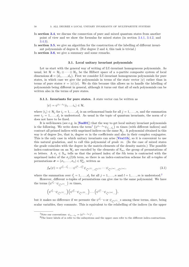
58 3. ALL DEGREE 6 LOCAL UNITARY INVARIANTS OF MULTIPARTITE SYSTEMS
In section 3.4, we discuss the connection of pure and mixed quantum states from anotherpoint of view and we show the formulas for mixed states (in section 3.4.1, 3.4.2, and3.4.3).
In section 3.5, we give an algorithm for the construction of the labelling of different invari-ant polynomials of degree 6. (For degree 2 and 4, this task is trivial.)
In section 3.6, we give a summary and some remarks.
3.1. Local unitary invariant polynomials
Let us start with the general way of writing of LU-invariant homogeneous polynomials. Asusual, let H = H1 ⊗ · · · ⊗ Hn be the Hilbert space of a n-partite composite system of localdimensions d = (d1, . . . , dn). First we consider LU-invariant homogeneous polynomials for purestates, in which case we give the polynomials in terms of the state vector |ψ〉 rather than interms of pure states π = |ψ〉〈ψ|. We do this because this allows us to handle the labelling ofpolynomials being different in general, although it turns out that all of such polynomials can bewritten also in the terms of pure states.
3.1.1. Invariants for pure states. A state vector can be written as
|ψ〉 = ψi1...in |i1 . . . in〉 ∈ H,
where |ij〉 ∈ Hj for ij = 1, . . . , dj is an orthonormal basis for all j = 1, . . . , n, and the summationover ij = 1, . . . , dj is understood. As usual in the topic of quantum invariants, the norm of ψdoes not have to be fixed.
It is well-known (see e.g. in [Sud01]) that the way to get local unitary invariant polynomialsis the following. We write down the term1
(ψi1...inψi′1...i′n
)m times (with different indices) and
contract all primed indices with unprimed indices on the same Hj . A polynomial obtained in thisway is of degree 2m, that is, degree m in the coefficients and also in their complex conjugates.This is the only case in which unitary invariants can arise [Vra11b], so it is convenient to usethis natural gradation, and to call this polynomial of grade m. (In the case of mixed statesthe grade coincides with the degree in the matrix-elements of the density matrix.) The possibleindex-contractions on an Hj are encoded by the elements of Sm, the group of permutations ofm letters. A σj ∈ Sm tells us that the primed index of the lth term is contracted with theunprimed index of the σj(l)th term, so there is an index-contraction scheme for all n-tuples ofpermutations σ = (σ1, . . . , σn) ∈ Snm, written as
fσ(ψ) = ψi11...i
1n · · ·ψi
m1 ...i
mn ψ
iσ1(1)1 ...i
σn(1)n
· · ·ψiσ1(m)1 ...i
σn(m)n
, (3.1)
where the summation over ilj = 1, . . . , dj for all j = 1, . . . , n and l = 1, . . . ,m is understood.2
However, different n-tuples of permutations can give rise to the same polynomial. We have
the terms(ψi
l1...ψ
iσ1(l)1 ...
)m times,(
ψi11...ψ
iσ1(1)1 ...
)(ψi
21...ψ
iσ1(2)1 ...
). . .(ψi
m1 ...ψ
iσ1(m)1 ...
),
but it makes no difference if we permute the ψil1...s or ψ
iσ1(l)1 ...
s among these terms, since, being
scalar variables, they commute. This is equivalent to the relabelling of the indices (in the upper
1Note our conventions: ψi1...in = (ψi1...in )∗.2The lower labels of is refer to the subsystems and the upper ones refer to the different index-contractions.
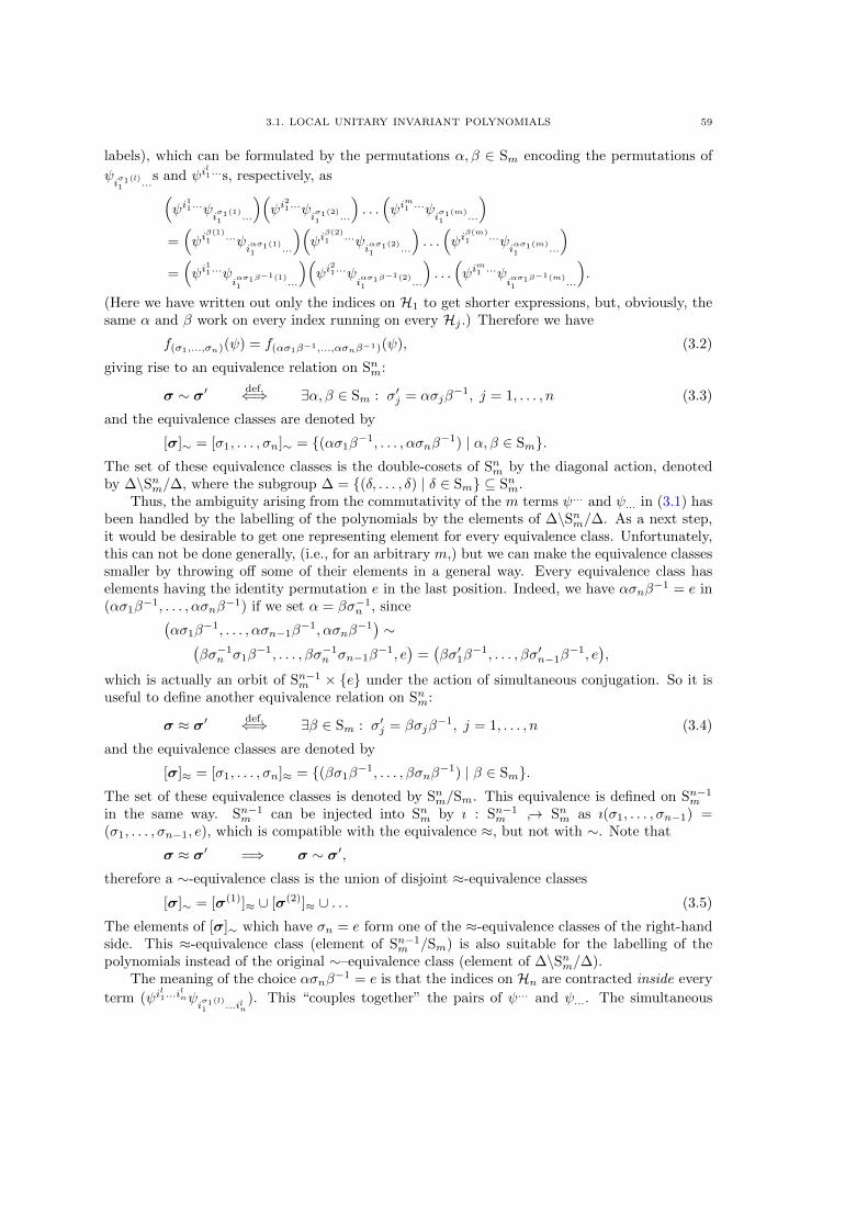
3.1. LOCAL UNITARY INVARIANT POLYNOMIALS 59
labels), which can be formulated by the permutations α, β ∈ Sm encoding the permutations of
ψiσ1(l)1 ...
s and ψil1...s, respectively, as(
ψi11...ψ
iσ1(1)1 ...
)(ψi
21...ψ
iσ1(2)1 ...
). . .(ψi
m1 ...ψ
iσ1(m)1 ...
)=(ψi
β(1)1 ...ψ
iασ1(1)1 ...
)(ψi
β(2)1 ...ψ
iασ1(2)1 ...
). . .(ψi
β(m)1 ...ψ
iασ1(m)1 ...
)=(ψi
11...ψ
iασ1β
−1(1)1 ...
)(ψi
21...ψ
iασ1β
−1(2)1 ...
). . .(ψi
m1 ...ψ
iασ1β
−1(m)1 ...
).
(Here we have written out only the indices on H1 to get shorter expressions, but, obviously, thesame α and β work on every index running on every Hj .) Therefore we have
f(σ1,...,σn)(ψ) = f(ασ1β−1,...,ασnβ−1)(ψ), (3.2)
giving rise to an equivalence relation on Snm:
σ ∼ σ′def.⇐⇒ ∃α, β ∈ Sm : σ′j = ασjβ
−1, j = 1, . . . , n (3.3)
and the equivalence classes are denoted by
[σ]∼ = [σ1, . . . , σn]∼ = {(ασ1β−1, . . . , ασnβ
−1) | α, β ∈ Sm}.The set of these equivalence classes is the double-cosets of Snm by the diagonal action, denotedby ∆\Snm/∆, where the subgroup ∆ = {(δ, . . . , δ) | δ ∈ Sm} ⊆ Snm.
Thus, the ambiguity arising from the commutativity of the m terms ψ... and ψ... in (3.1) hasbeen handled by the labelling of the polynomials by the elements of ∆\Snm/∆. As a next step,it would be desirable to get one representing element for every equivalence class. Unfortunately,this can not be done generally, (i.e., for an arbitrary m,) but we can make the equivalence classessmaller by throwing off some of their elements in a general way. Every equivalence class haselements having the identity permutation e in the last position. Indeed, we have ασnβ
−1 = e in(ασ1β
−1, . . . , ασnβ−1) if we set α = βσ−1
n , since(ασ1β
−1, . . . , ασn−1β−1, ασnβ
−1)∼(
βσ−1n σ1β
−1, . . . , βσ−1n σn−1β
−1, e)
=(βσ′1β
−1, . . . , βσ′n−1β−1, e
),
which is actually an orbit of Sn−1m × {e} under the action of simultaneous conjugation. So it is
useful to define another equivalence relation on Snm:
σ ≈ σ′def.⇐⇒ ∃β ∈ Sm : σ′j = βσjβ
−1, j = 1, . . . , n (3.4)
and the equivalence classes are denoted by
[σ]≈ = [σ1, . . . , σn]≈ = {(βσ1β−1, . . . , βσnβ
−1) | β ∈ Sm}.The set of these equivalence classes is denoted by Snm/Sm. This equivalence is defined on Sn−1
m
in the same way. Sn−1m can be injected into Snm by ı : Sn−1
m ↪→ Snm as ı(σ1, . . . , σn−1) =(σ1, . . . , σn−1, e), which is compatible with the equivalence ≈, but not with ∼. Note that
σ ≈ σ′ =⇒ σ ∼ σ′,
therefore a ∼-equivalence class is the union of disjoint ≈-equivalence classes
[σ]∼ = [σ(1)]≈ ∪ [σ(2)]≈ ∪ . . . (3.5)
The elements of [σ]∼ which have σn = e form one of the ≈-equivalence classes of the right-handside. This ≈-equivalence class (element of Sn−1
m /Sm) is also suitable for the labelling of thepolynomials instead of the original ∼–equivalence class (element of ∆\Snm/∆).
The meaning of the choice ασnβ−1 = e is that the indices on Hn are contracted inside every
term (ψil1...i
lnψ
iσ1(l)1 ...iln
). This “couples together” the pairs of ψ... and ψ.... The simultaneous
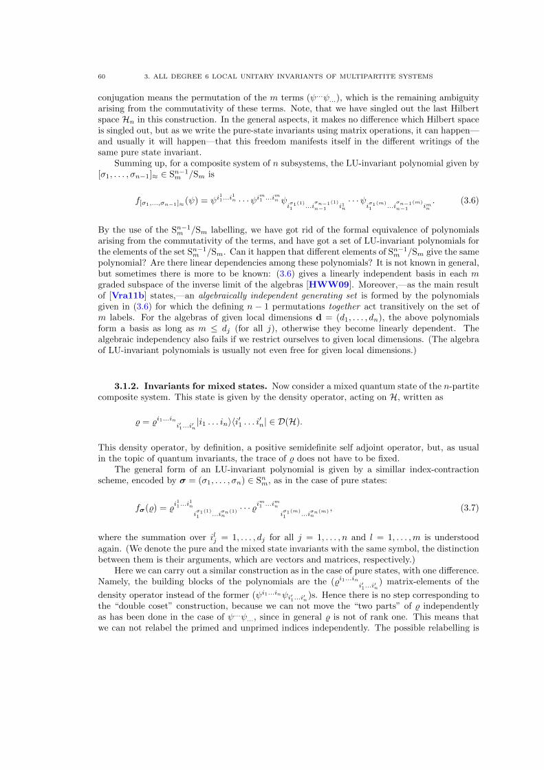
60 3. ALL DEGREE 6 LOCAL UNITARY INVARIANTS OF MULTIPARTITE SYSTEMS
conjugation means the permutation of the m terms (ψ...ψ...), which is the remaining ambiguityarising from the commutativity of these terms. Note, that we have singled out the last Hilbertspace Hn in this construction. In the general aspects, it makes no difference which Hilbert spaceis singled out, but as we write the pure-state invariants using matrix operations, it can happen—and usually it will happen—that this freedom manifests itself in the different writings of thesame pure state invariant.
Summing up, for a composite system of n subsystems, the LU-invariant polynomial given by[σ1, . . . , σn−1]≈ ∈ Sn−1
m /Sm is
f[σ1,...,σn−1]≈(ψ) = ψi11...i
1n · · ·ψi
m1 ...i
mn ψ
iσ1(1)1 ...i
σn−1(1)
n−1 i1n· · ·ψ
iσ1(m)1 ...i
σn−1(m)
n−1 imn. (3.6)
By the use of the Sn−1m /Sm labelling, we have got rid of the formal equivalence of polynomials
arising from the commutativity of the terms, and have got a set of LU-invariant polynomials forthe elements of the set Sn−1
m /Sm. Can it happen that different elements of Sn−1m /Sm give the same
polynomial? Are there linear dependencies among these polynomials? It is not known in general,but sometimes there is more to be known: (3.6) gives a linearly independent basis in each mgraded subspace of the inverse limit of the algebras [HWW09]. Moreover,—as the main resultof [Vra11b] states,—an algebraically independent generating set is formed by the polynomialsgiven in (3.6) for which the defining n − 1 permutations together act transitively on the set ofm labels. For the algebras of given local dimensions d = (d1, . . . , dn), the above polynomialsform a basis as long as m ≤ dj (for all j), otherwise they become linearly dependent. Thealgebraic independency also fails if we restrict ourselves to given local dimensions. (The algebraof LU-invariant polynomials is usually not even free for given local dimensions.)
3.1.2. Invariants for mixed states. Now consider a mixed quantum state of the n-partitecomposite system. This state is given by the density operator, acting on H, written as
% = %i1...ini′1...i′n|i1 . . . in〉〈i′1 . . . i′n| ∈ D(H).
This density operator, by definition, a positive semidefinite self adjoint operator, but, as usualin the topic of quantum invariants, the trace of % does not have to be fixed.
The general form of an LU-invariant polynomial is given by a simillar index-contractionscheme, encoded by σ = (σ1, . . . , σn) ∈ Snm, as in the case of pure states:
fσ(%) = %i11...i
1n
iσ1(1)1 ...i
σn(1)n
· · · %im1 ...i
mn
iσ1(m)1 ...i
σn(m)n
, (3.7)
where the summation over ilj = 1, . . . , dj for all j = 1, . . . , n and l = 1, . . . ,m is understoodagain. (We denote the pure and the mixed state invariants with the same symbol, the distinctionbetween them is their arguments, which are vectors and matrices, respectively.)
Here we can carry out a similar construction as in the case of pure states, with one difference.Namely, the building blocks of the polynomials are the (%i1...ini′1...i′n
) matrix-elements of the
density operator instead of the former (ψi1...inψi′1...i′n)s. Hence there is no step corresponding tothe “double coset” construction, because we can not move the “two parts” of % independentlyas has been done in the case of ψ...ψ..., since in general % is not of rank one. This means thatwe can not relabel the primed and unprimed indices independently. The possible relabelling is
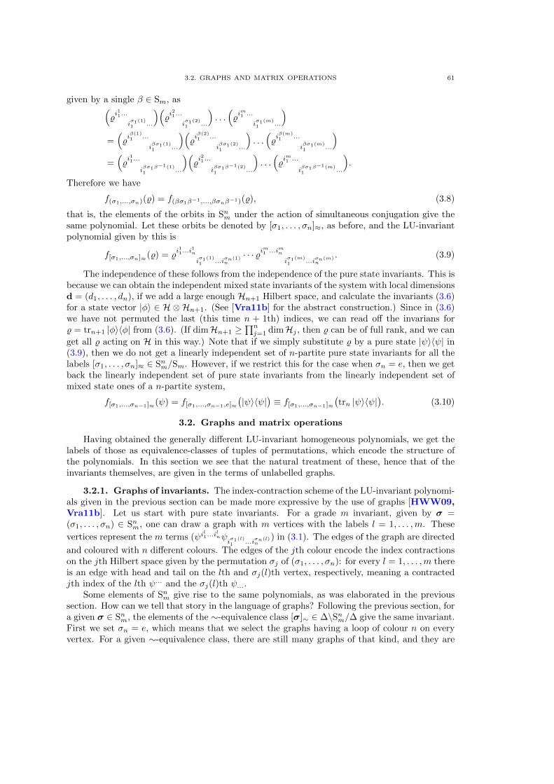
3.2. GRAPHS AND MATRIX OPERATIONS 61
given by a single β ∈ Sm, as(%i11...
iσ1(1)1 ...
)(%i21...
iσ1(2)1 ...
). . .(%im1 ...
iσ1(m)1 ...
)=(%iβ(1)1 ...
iβσ1(1)1 ...
)(%iβ(2)1 ...
iβσ1(2)1 ...
). . .(%iβ(m)1 ...
iβσ1(m)1 ...
)=(%i11...
iβσ1β
−1(1)1 ...
)(%i21...
iβσ1β
−1(2)1 ...
). . .(%im1 ...
iβσ1β
−1(m)1 ...
).
Therefore we have
f(σ1,...,σn)(%) = f(βσ1β−1,...,βσnβ−1)(%), (3.8)
that is, the elements of the orbits in Snm under the action of simultaneous conjugation give thesame polynomial. Let these orbits be denoted by [σ1, . . . , σn]≈, as before, and the LU-invariantpolynomial given by this is
f[σ1,...,σn]≈(%) = %i11...i
1n
iσ1(1)1 ...i
σn(1)n
· · · %im1 ...i
mn
iσ1(m)1 ...i
σn(m)n
. (3.9)
The independence of these follows from the independence of the pure state invariants. This isbecause we can obtain the independent mixed state invariants of the system with local dimensionsd = (d1, . . . , dn), if we add a large enough Hn+1 Hilbert space, and calculate the invariants (3.6)for a state vector |φ〉 ∈ H ⊗Hn+1. (See [Vra11b] for the abstract construction.) Since in (3.6)we have not permuted the last (this time n + 1th) indices, we can read off the invarians for% = trn+1 |φ〉〈φ| from (3.6). (If dimHn+1 ≥
∏nj=1 dimHj , then % can be of full rank, and we can
get all % acting on H in this way.) Note that if we simply substitute % by a pure state |ψ〉〈ψ| in(3.9), then we do not get a linearly independent set of n-partite pure state invariants for all thelabels [σ1, . . . , σn]≈ ∈ Snm/Sm. However, if we restrict this for the case when σn = e, then we getback the linearly independent set of pure state invariants from the linearly independent set ofmixed state ones of a n-partite system,
f[σ1,...,σn−1]≈(ψ) = f[σ1,...,σn−1,e]≈
(|ψ〉〈ψ|
)≡ f[σ1,...,σn−1]≈
(trn |ψ〉〈ψ|
). (3.10)
3.2. Graphs and matrix operations
Having obtained the generally different LU-invariant homogeneous polynomials, we get thelabels of those as equivalence-classes of tuples of permutations, which encode the structure ofthe polynomials. In this section we see that the natural treatment of these, hence that of theinvariants themselves, are given in the terms of unlabelled graphs.
3.2.1. Graphs of invariants. The index-contraction scheme of the LU-invariant polynomi-als given in the previous section can be made more expressive by the use of graphs [HWW09,Vra11b]. Let us start with pure state invariants. For a grade m invariant, given by σ =(σ1, . . . , σn) ∈ Snm, one can draw a graph with m vertices with the labels l = 1, . . . ,m. These
vertices represent the m terms (ψil1...i
lnψ
iσ1(l)1 ...i
σn(l)n
) in (3.1). The edges of the graph are directed
and coloured with n different colours. The edges of the jth colour encode the index contractionson the jth Hilbert space given by the permutation σj of (σ1, . . . , σn): for every l = 1, . . . ,m thereis an edge with head and tail on the lth and σj(l)th vertex, respectively, meaning a contractedjth index of the lth ψ... and the σj(l)th ψ....
Some elements of Snm give rise to the same polynomials, as was elaborated in the previoussection. How can we tell that story in the language of graphs? Following the previous section, fora given σ ∈ Snm, the elements of the ∼-equivalence class [σ]∼ ∈ ∆\Snm/∆ give the same invariant.First we set σn = e, which means that we select the graphs having a loop of colour n on everyvertex. For a given ∼-equivalence class, there are still many graphs of that kind, and they are
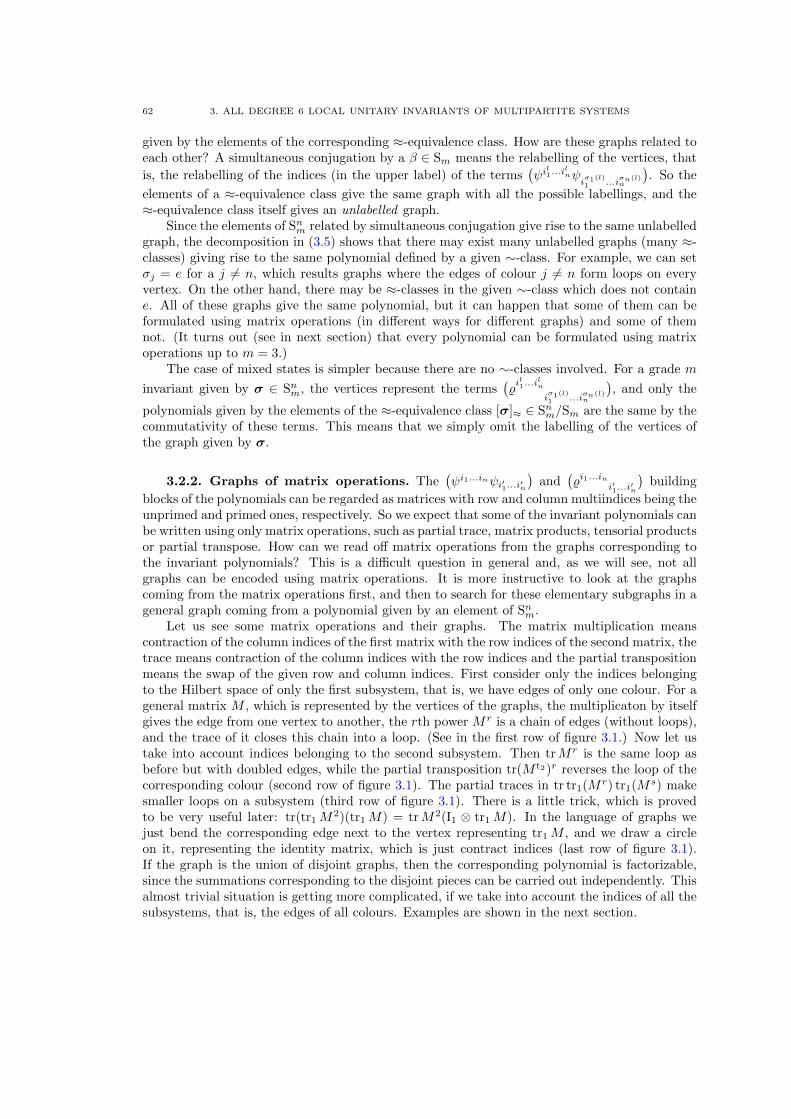
62 3. ALL DEGREE 6 LOCAL UNITARY INVARIANTS OF MULTIPARTITE SYSTEMS
given by the elements of the corresponding ≈-equivalence class. How are these graphs related toeach other? A simultaneous conjugation by a β ∈ Sm means the relabelling of the vertices, that
is, the relabelling of the indices (in the upper label) of the terms(ψi
l1...i
lnψ
iσ1(l)1 ...i
σn(l)n
). So the
elements of a ≈-equivalence class give the same graph with all the possible labellings, and the≈-equivalence class itself gives an unlabelled graph.
Since the elements of Snm related by simultaneous conjugation give rise to the same unlabelledgraph, the decomposition in (3.5) shows that there may exist many unlabelled graphs (many ≈-classes) giving rise to the same polynomial defined by a given ∼-class. For example, we can setσj = e for a j 6= n, which results graphs where the edges of colour j 6= n form loops on everyvertex. On the other hand, there may be ≈-classes in the given ∼-class which does not containe. All of these graphs give the same polynomial, but it can happen that some of them can beformulated using matrix operations (in different ways for different graphs) and some of themnot. (It turns out (see in next section) that every polynomial can be formulated using matrixoperations up to m = 3.)
The case of mixed states is simpler because there are no ∼-classes involved. For a grade m
invariant given by σ ∈ Snm, the vertices represent the terms(%il1...i
ln
iσ1(l)1 ...i
σn(l)n
), and only the
polynomials given by the elements of the ≈-equivalence class [σ]≈ ∈ Snm/Sm are the same by thecommutativity of these terms. This means that we simply omit the labelling of the vertices ofthe graph given by σ.
3.2.2. Graphs of matrix operations. The(ψi1...inψi′1...i′n
)and
(%i1...ini′1...i′n
)building
blocks of the polynomials can be regarded as matrices with row and column multiindices being theunprimed and primed ones, respectively. So we expect that some of the invariant polynomials canbe written using only matrix operations, such as partial trace, matrix products, tensorial productsor partial transpose. How can we read off matrix operations from the graphs corresponding tothe invariant polynomials? This is a difficult question in general and, as we will see, not allgraphs can be encoded using matrix operations. It is more instructive to look at the graphscoming from the matrix operations first, and then to search for these elementary subgraphs in ageneral graph coming from a polynomial given by an element of Snm.
Let us see some matrix operations and their graphs. The matrix multiplication meanscontraction of the column indices of the first matrix with the row indices of the second matrix, thetrace means contraction of the column indices with the row indices and the partial transpositionmeans the swap of the given row and column indices. First consider only the indices belongingto the Hilbert space of only the first subsystem, that is, we have edges of only one colour. For ageneral matrix M , which is represented by the vertices of the graphs, the multiplicaton by itselfgives the edge from one vertex to another, the rth power Mr is a chain of edges (without loops),and the trace of it closes this chain into a loop. (See in the first row of figure 3.1.) Now let ustake into account indices belonging to the second subsystem. Then trMr is the same loop asbefore but with doubled edges, while the partial transposition tr(M t2)r reverses the loop of thecorresponding colour (second row of figure 3.1). The partial traces in tr tr1(Mr) tr1(Ms) makesmaller loops on a subsystem (third row of figure 3.1). There is a little trick, which is provedto be very useful later: tr(tr1M
2)(tr1M) = trM2(I1 ⊗ tr1M). In the language of graphs wejust bend the corresponding edge next to the vertex representing tr1M , and we draw a circleon it, representing the identity matrix, which is just contract indices (last row of figure 3.1).If the graph is the union of disjoint graphs, then the corresponding polynomial is factorizable,since the summations corresponding to the disjoint pieces can be carried out independently. Thisalmost trivial situation is getting more complicated, if we take into account the indices of all thesubsystems, that is, the edges of all colours. Examples are shown in the next section.
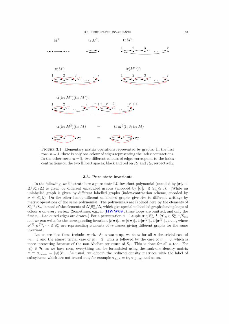
3.3. PURE STATE INVARIANTS 63
M2: trM2: trMr:
1 2 3 r. . .
trMr:
1 2 3 r
. . .
tr(M t2)r:
1 2 3 r
. . .
tr(tr1 Mr)(tr1 M
s):
1 2 r r + 1 r + 2 r + s
. . . . . .
tr(tr1 M2)(tr1 M) = trM2(I1 ⊗ tr1 M)
≡
Figure 3.1. Elementary matrix operations represented by graphs. In the firstrow: n = 1, there is only one colour of edges representing the index contractions.In the other rows: n = 2, two different colours of edges correspond to the indexcontractions on the two Hilbert spaces, black and red onH1 andH2, respectively.
3.3. Pure state invariants
In the following, we illustrate how a pure state LU-invariant polynomial (encoded by [σ]∼ ∈∆\Snm/∆) is given by different unlabelled graphs (encoded by [σ]≈ ∈ Snm/Sm). (While anunlabelled graph is given by different labelled graphs (index-contraction scheme, encoded byσ ∈ Snm).) On the other hand, different unlabelled graphs give rise to different writings bymatrix operations of the same polynomial. The polynomials are labelled here by the elements ofSn−1m /Sm instead of the elements of ∆\Snm/∆, which give special unlabelled graphs having loops of
colour n on every vertex. (Sometimes, e.g., in [HWW09], these loops are omitted, and only thefirst n−1-coloured edges are drawn.) For a permutation n−1-tuple σ ∈ Sn−1
m , [σ]≈ ∈ Sn−1m /Sm,
and we can write for the corresponding invariant [ı(σ)]∼ = [ı(σ)]≈∪ [σ(2)]≈∪ [σ(3)]≈∪ . . . , whereσ(2),σ(3), · · · ∈ Snm are representing elements of ≈-classes giving different graphs for the sameinvariant.
Let us see how these technics work. As a warm-up, we show for all n the trivial case ofm = 1 and the almost trivial case of m = 2. This is followed by the case of m = 3, which ismore interesting because of the non-Abelian structure of S3. This is done for all n too. For|ψ〉 ∈ H, as we have seen, everything can be formulated using the rank-one density matrixπ ≡ π12...n = |ψ〉〈ψ|. As usual, we denote the reduced density matrices with the label ofsubsystems which are not traced out, for example π2...n = tr1 π12...n, and so on.
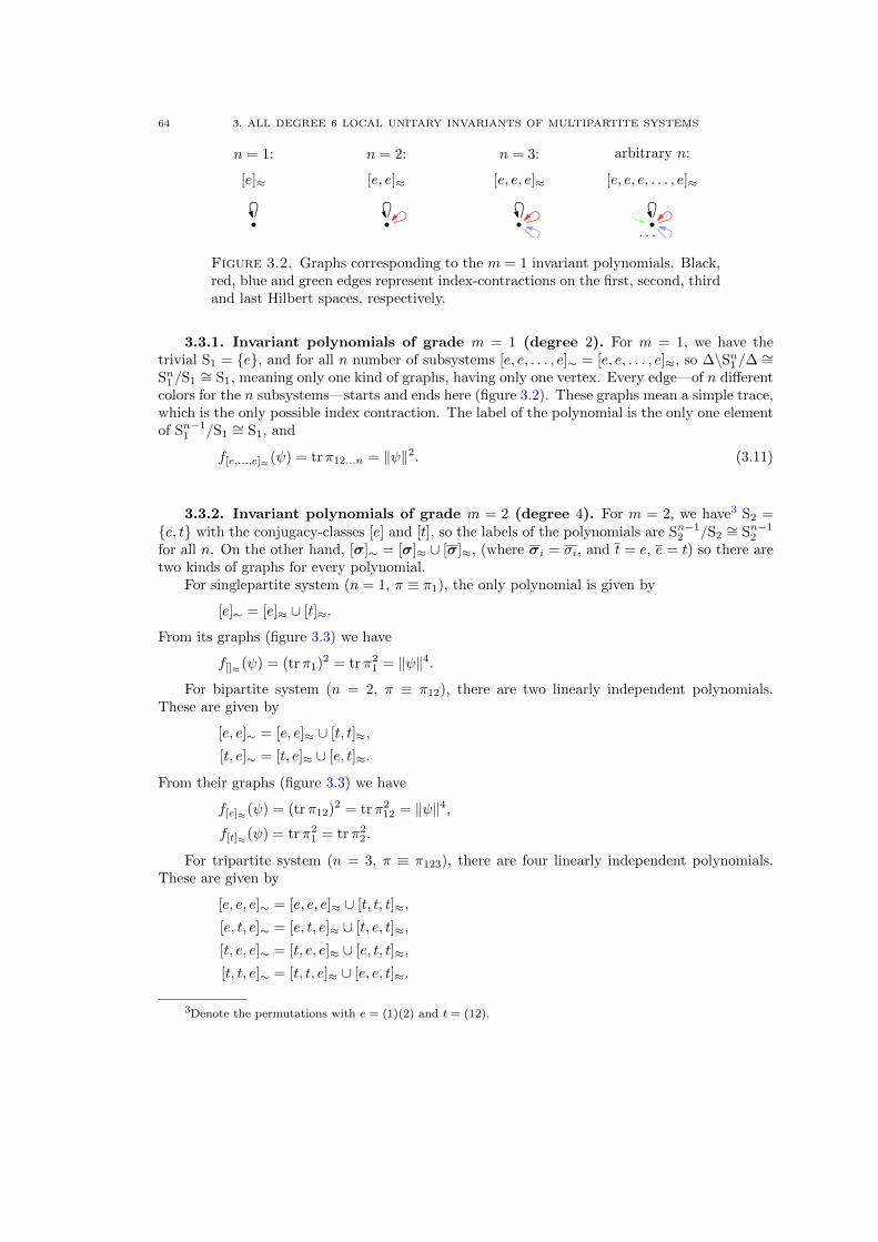
64 3. ALL DEGREE 6 LOCAL UNITARY INVARIANTS OF MULTIPARTITE SYSTEMS
n = 1:
[e]≈
n = 2:
[e, e]≈
n = 3:
[e, e, e]≈
arbitrary n:
[e, e, e, . . . , e]≈
. . .
Figure 3.2. Graphs corresponding to the m = 1 invariant polynomials. Black,red, blue and green edges represent index-contractions on the first, second, thirdand last Hilbert spaces, respectively.
3.3.1. Invariant polynomials of grade m = 1 (degree 2). For m = 1, we have thetrivial S1 = {e}, and for all n number of subsystems [e, e, . . . , e]∼ = [e, e, . . . , e]≈, so ∆\Sn1/∆ ∼=Sn1/S1
∼= S1, meaning only one kind of graphs, having only one vertex. Every edge—of n differentcolors for the n subsystems—starts and ends here (figure 3.2). These graphs mean a simple trace,which is the only possible index contraction. The label of the polynomial is the only one elementof Sn−1
1 /S1∼= S1, and
f[e,...,e]≈(ψ) = trπ12...n = ‖ψ‖2. (3.11)
3.3.2. Invariant polynomials of grade m = 2 (degree 4). For m = 2, we have3 S2 ={e, t} with the conjugacy-classes [e] and [t], so the labels of the polynomials are Sn−1
2 /S2∼= Sn−1
2
for all n. On the other hand, [σ]∼ = [σ]≈ ∪ [σ]≈, (where σi = σi, and t = e, e = t) so there aretwo kinds of graphs for every polynomial.
For singlepartite system (n = 1, π ≡ π1), the only polynomial is given by
[e]∼ = [e]≈ ∪ [t]≈.
From its graphs (figure 3.3) we have
f[]≈(ψ) = (trπ1)2 = trπ21 = ‖ψ‖4.
For bipartite system (n = 2, π ≡ π12), there are two linearly independent polynomials.These are given by
[e, e]∼ = [e, e]≈ ∪ [t, t]≈,
[t, e]∼ = [t, e]≈ ∪ [e, t]≈.
From their graphs (figure 3.3) we have
f[e]≈(ψ) = (trπ12)2 = trπ212 = ‖ψ‖4,
f[t]≈(ψ) = trπ21 = trπ2
2 .
For tripartite system (n = 3, π ≡ π123), there are four linearly independent polynomials.These are given by
[e, e, e]∼ = [e, e, e]≈ ∪ [t, t, t]≈,
[e, t, e]∼ = [e, t, e]≈ ∪ [t, e, t]≈,
[t, e, e]∼ = [t, e, e]≈ ∪ [e, t, t]≈,
[t, t, e]∼ = [t, t, e]≈ ∪ [e, e, t]≈.
3Denote the permutations with e = (1)(2) and t = (12).
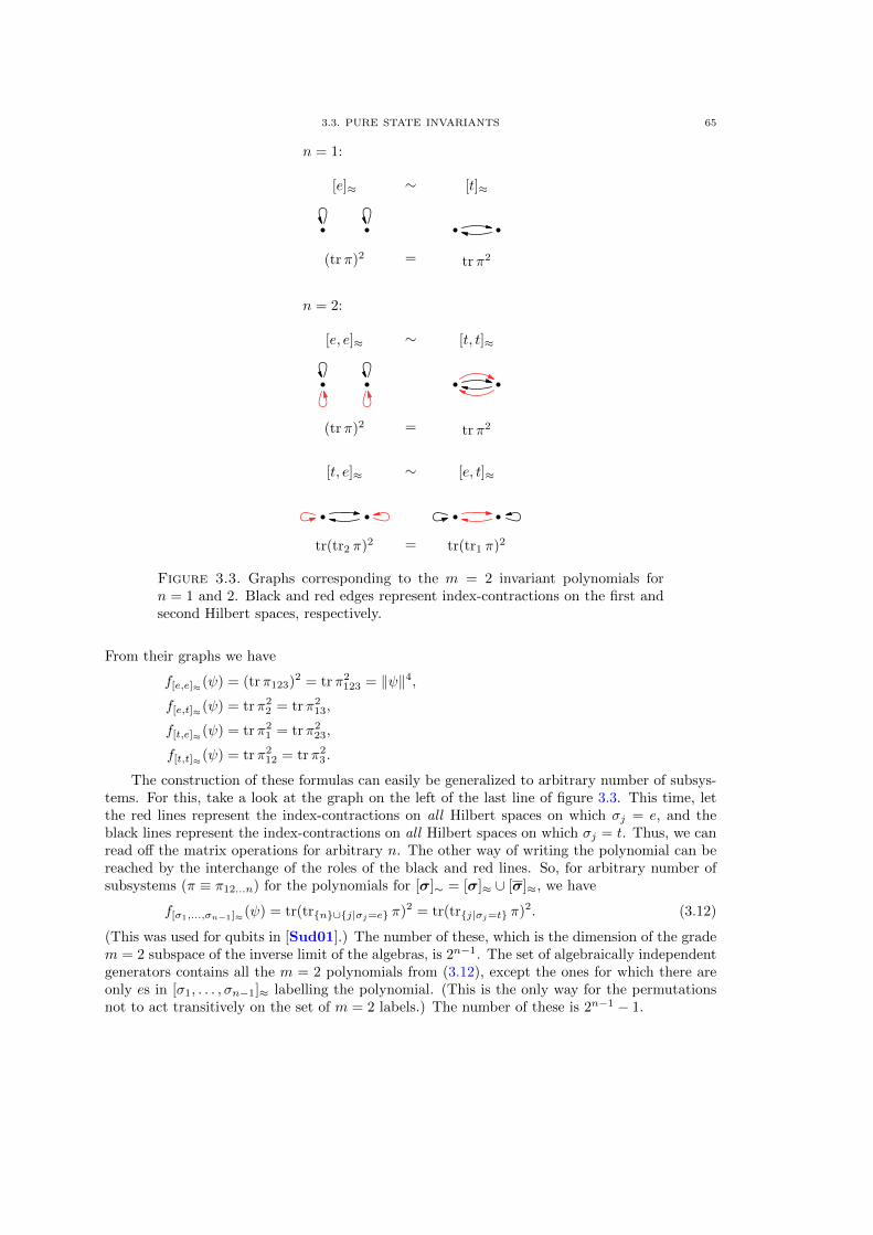
3.3. PURE STATE INVARIANTS 65
n = 1:
[e]≈
(trπ)2
[t]≈
trπ2
∼
=
n = 2:
[e, e]≈
(trπ)2
[t, t]≈
trπ2
∼
=
[t, e]≈
tr(tr2 π)2
[e, t]≈
tr(tr1 π)2
∼
=
Figure 3.3. Graphs corresponding to the m = 2 invariant polynomials forn = 1 and 2. Black and red edges represent index-contractions on the first andsecond Hilbert spaces, respectively.
From their graphs we have
f[e,e]≈(ψ) = (trπ123)2 = trπ2123 = ‖ψ‖4,
f[e,t]≈(ψ) = trπ22 = trπ2
13,
f[t,e]≈(ψ) = trπ21 = trπ2
23,
f[t,t]≈(ψ) = trπ212 = trπ2
3 .
The construction of these formulas can easily be generalized to arbitrary number of subsys-tems. For this, take a look at the graph on the left of the last line of figure 3.3. This time, letthe red lines represent the index-contractions on all Hilbert spaces on which σj = e, and theblack lines represent the index-contractions on all Hilbert spaces on which σj = t. Thus, we canread off the matrix operations for arbitrary n. The other way of writing the polynomial can bereached by the interchange of the roles of the black and red lines. So, for arbitrary number ofsubsystems (π ≡ π12...n) for the polynomials for [σ]∼ = [σ]≈ ∪ [σ]≈, we have
f[σ1,...,σn−1]≈(ψ) = tr(tr{n}∪{j|σj=e} π)2 = tr(tr{j|σj=t} π)2. (3.12)
(This was used for qubits in [Sud01].) The number of these, which is the dimension of the gradem = 2 subspace of the inverse limit of the algebras, is 2n−1. The set of algebraically independentgenerators contains all the m = 2 polynomials from (3.12), except the ones for which there areonly es in [σ1, . . . , σn−1]≈ labelling the polynomial. (This is the only way for the permutationsnot to act transitively on the set of m = 2 labels.) The number of these is 2n−1 − 1.
66 3. ALL DEGREE 6 LOCAL UNITARY INVARIANTS OF MULTIPARTITE SYSTEMS
3.3.3. Invariant polynomials of grade m = 3 (degree 6). For m = 3, we have4 S3 ={e, s, s2, t, ts, ts2} with the conjugacy-classes [e] = {e}, [s] = {s, s2} and [t] = {t, ts, ts2}. Thistime, we have no simple general rule for the splitting of a ∼-class to ≈-classes.
For singlepartite system (n = 1, π ≡ π1), the only polynomial is biven by
[e]∼ = [e]≈ ∪ [t]≈ ∪ [s]≈.
From its graphs (figure 3.4) we have
f[]≈(ψ) = (trπ1)3 = trπ21 trπ1 = trπ3
1 = ‖ψ‖6.
For bipartite system (n = 2, π ≡ π12), there are three linearly independent polynomials.These are given by
[e, e]∼ = [e, e]≈ ∪ [t, t]≈ ∪ [s, s]≈,
[t, e]∼ = [t, e]≈ ∪ [e, t]≈ ∪ [s, t]≈ ∪ [t, s]≈,
[s, e]∼ = [s, e]≈ ∪ [e, s]≈ ∪ [s, s2]≈ ∪ [t, ts]≈
(so S13/S3
∼= {[e], [s], [t]}). From their graphs (figure 3.4) we have
f[e]≈(ψ) = (trπ12)3 = trπ212 trπ12 = trπ3
12 = ‖ψ‖6,f[t]≈(ψ) = (trπa)2 trπ12 = tr(tra π
212)πb,
f[s]≈(ψ) = trπ3a = tr(πta
12)3 = tr(π1 ⊗ π2)π12
for all a, b ∈ {1, 2}, a 6= b.For tripartite system (n = 3, π ≡ π123), it turns out that there are eleven linearly independent
polynomials. These are given by
[e, e, e]∼ = [e, e, e]≈ ∪ [t, t, t]≈ ∪ [s, s, s]≈,
[e, t, e]∼ = [e, t, e]≈ ∪ [t, e, t]≈ ∪ [s, t, s]≈ ∪ [t, s, t]≈,
[t, e, e]∼ = [t, e, e]≈ ∪ [e, t, t]≈ ∪ [t, s, s]≈ ∪ [s, t, t]≈,
[t, t, e]∼ = [t, t, e]≈ ∪ [e, e, t]≈ ∪ [s, s, t]≈ ∪ [t, t, s]≈,
[e, s, e]∼ = [e, s, e]≈ ∪ [s, e, s]≈ ∪ [s, s2, s]≈ ∪ [t, ts, t]≈,
[s, e, e]∼ = [s, e, e]≈ ∪ [e, s, s]≈ ∪ [s2, s, s]≈ ∪ [ts, t, t]≈,
[s, s, e]∼ = [s, s, e]≈ ∪ [e, e, s]≈ ∪ [s, s, s2]≈ ∪ [t, t, ts]≈,
[s, s2, e]∼ = [s, s2, e]≈ ∪ [s, e, s2]≈ ∪ [e, s, s2]≈ ∪ [t, ts, ts2]≈,
[t, s, e]∼ = [t, s, e]≈ ∪ [t, e, s]≈ ∪ [e, t, ts]≈ ∪ [t, s, s2]≈ ∪ [s, t, ts]≈ ∪ [s, t, ts2]≈,
[s, t, e]∼ = [s, t, e]≈ ∪ [e, t, s]≈ ∪ [t, e, ts]≈ ∪ [s, t, s2]≈ ∪ [t, s, ts]≈ ∪ [t, s, ts2]≈,
[t, ts, e]∼ = [t, ts, e]≈ ∪ [e, s, t]≈ ∪ [s, e, t]≈ ∪ [s, s2, t]≈ ∪ [t, ts, s]≈ ∪ [t, ts2, s]≈.
4Denote the permutations with e = (1)(2)(3), t = (12)(3) and s = (123).
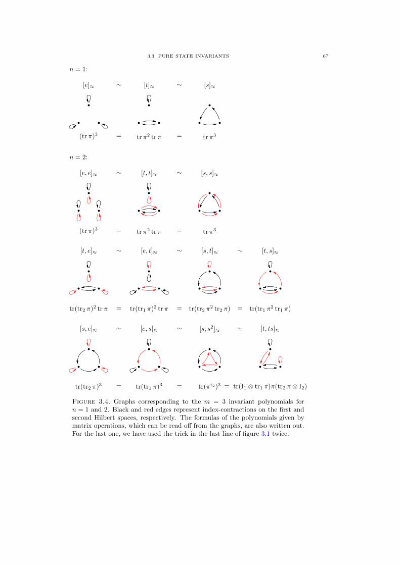
3.3. PURE STATE INVARIANTS 67
n = 1:
[e]≈
(trπ)3
[t]≈
trπ2 trπ
[s]≈
trπ3
∼ ∼
= =
n = 2:
[e, e]≈
(trπ)3
[t, t]≈
trπ2 trπ
[s, s]≈
trπ3
∼ ∼
= =
[t, e]≈
tr(tr2 π)2 trπ
[e, t]≈
tr(tr1 π)2 trπ
[s, t]≈
tr(tr2 π2 tr2 π)
[t, s]≈
tr(tr1 π2 tr1 π)
∼ ∼ ∼
= = =
[s, e]≈
tr(tr2 π)3
[e, s]≈
tr(tr1 π)3
[s, s2]≈
tr(πt2)3
[t, ts]≈
tr(I1 ⊗ tr1 π)π(tr2 π ⊗ I2)
∼ ∼ ∼
= = =
Figure 3.4. Graphs corresponding to the m = 3 invariant polynomials forn = 1 and 2. Black and red edges represent index-contractions on the first andsecond Hilbert spaces, respectively. The formulas of the polynomials given bymatrix operations, which can be read off from the graphs, are also written out.For the last one, we have used the trick in the last line of figure 3.1 twice.
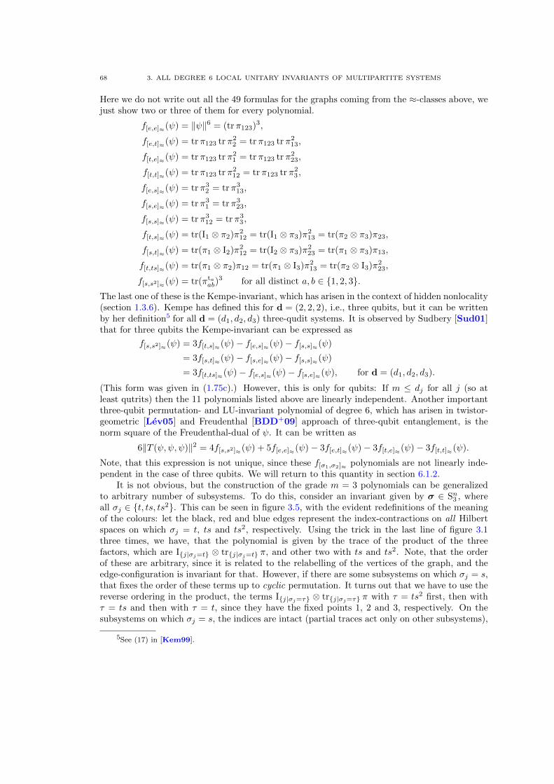
68 3. ALL DEGREE 6 LOCAL UNITARY INVARIANTS OF MULTIPARTITE SYSTEMS
Here we do not write out all the 49 formulas for the graphs coming from the ≈-classes above, wejust show two or three of them for every polynomial.
f[e,e]≈(ψ) = ‖ψ‖6 = (trπ123)3,
f[e,t]≈(ψ) = trπ123 trπ22 = trπ123 trπ2
13,
f[t,e]≈(ψ) = trπ123 trπ21 = trπ123 trπ2
23,
f[t,t]≈(ψ) = trπ123 trπ212 = trπ123 trπ2
3 ,
f[e,s]≈(ψ) = trπ32 = trπ3
13,
f[s,e]≈(ψ) = trπ31 = trπ3
23,
f[s,s]≈(ψ) = trπ312 = trπ3
3 ,
f[t,s]≈(ψ) = tr(I1 ⊗ π2)π212 = tr(I1 ⊗ π3)π2
13 = tr(π2 ⊗ π3)π23,
f[s,t]≈(ψ) = tr(π1 ⊗ I2)π212 = tr(I2 ⊗ π3)π2
23 = tr(π1 ⊗ π3)π13,
f[t,ts]≈(ψ) = tr(π1 ⊗ π2)π12 = tr(π1 ⊗ I3)π213 = tr(π2 ⊗ I3)π2
23,
f[s,s2]≈(ψ) = tr(πtaab)
3 for all distinct a, b ∈ {1, 2, 3}.The last one of these is the Kempe-invariant, which has arisen in the context of hidden nonlocality(section 1.3.6). Kempe has defined this for d = (2, 2, 2), i.e., three qubits, but it can be writtenby her definition5 for all d = (d1, d2, d3) three-qudit systems. It is observed by Sudbery [Sud01]that for three qubits the Kempe-invariant can be expressed as
f[s,s2]≈(ψ) = 3f[t,s]≈(ψ)− f[e,s]≈(ψ)− f[s,s]≈(ψ)
= 3f[s,t]≈(ψ)− f[s,e]≈(ψ)− f[s,s]≈(ψ)
= 3f[t,ts]≈(ψ)− f[e,s]≈(ψ)− f[s,e]≈(ψ), for d = (d1, d2, d3).
(This form was given in (1.75c).) However, this is only for qubits: If m ≤ dj for all j (so atleast qutrits) then the 11 polynomials listed above are linearly independent. Another importantthree-qubit permutation- and LU-invariant polynomial of degree 6, which has arisen in twistor-geometric [Lev05] and Freudenthal [BDD+09] approach of three-qubit entanglement, is thenorm square of the Freudenthal-dual of ψ. It can be written as
6‖T (ψ,ψ, ψ)‖2 = 4f[s,s2]≈(ψ) + 5f[e,e]≈(ψ)− 3f[e,t]≈(ψ)− 3f[t,e]≈(ψ)− 3f[t,t]≈(ψ).
Note, that this expression is not unique, since these f[σ1,σ2]≈ polynomials are not linearly inde-pendent in the case of three qubits. We will return to this quantity in section 6.1.2.
It is not obvious, but the construction of the grade m = 3 polynomials can be generalizedto arbitrary number of subsystems. To do this, consider an invariant given by σ ∈ Sn3 , whereall σj ∈ {t, ts, ts2}. This can be seen in figure 3.5, with the evident redefinitions of the meaningof the colours: let the black, red and blue edges represent the index-contractions on all Hilbertspaces on which σj = t, ts and ts2, respectively. Using the trick in the last line of figure 3.1three times, we have, that the polynomial is given by the trace of the product of the threefactors, which are I{j|σj=t} ⊗ tr{j|σj=t} π, and other two with ts and ts2. Note, that the orderof these are arbitrary, since it is related to the relabelling of the vertices of the graph, and theedge-configuration is invariant for that. However, if there are some subsystems on which σj = s,that fixes the order of these terms up to cyclic permutation. It turns out that we have to use thereverse ordering in the product, the terms I{j|σj=τ} ⊗ tr{j|σj=τ} π with τ = ts2 first, then withτ = ts and then with τ = t, since they have the fixed points 1, 2 and 3, respectively. On thesubsystems on which σj = s, the indices are intact (partial traces act only on other subsystems),
5See (17) in [Kem99].
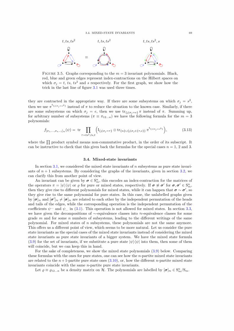
3.4. MIXED-STATE INVARIANTS 69
t, ts, ts2 t, ts, ts2
≡
t, ts, ts2, s
Figure 3.5. Graphs corresponding to the m = 3 invariant polynomials. Black,red, blue and green edges represent index-contractions on the Hilbert spaces onwhich σj = t, ts, ts2 and s respectively. For the first graph, we show how thetrick in the last line of figure 3.1 was used three times.
they are contracted in the appropriate way. If there are some subsystems on which σj = s2,
then we use πt{j|σj=s2} instead of π to reduce the situation to the known case. Similarly, if there
are some subsystems on which σj = e, then we use tr{j|σj=e} π instead of π. Summing up,for arbitrary number of subsystems (π ≡ π12...n) we have the following formula for the m = 3polynomials:
f[σ1,...,σn−1]≈(ψ) = tr∏
τ=ts2,ts,t
(I{j|σj=τ} ⊗ tr{n}∪{j|σj∈{τ,e}} π
t{j|σj=s2}), (3.13)
where the∏
product symbol means non-commutative product, in the order of its subscript. Itcan be instructive to check that this gives back the formulas for the special cases n = 1, 2 and 3.
3.4. Mixed-state invariants
In section 3.1, we considered the mixed state invariants of n subsystems as pure state invari-ants of n + 1 subsystems. By considering the graphs of the invariants, given in section 3.2, wecan clarify this from another point of view.
An invariant can be given by σ ∈ Snm, this encodes an index-contraction for the matrices ofthe operators π = |ψ〉〈ψ| or % for pure or mixed states, respectively. If σ 6≈ σ′ for σ,σ′ ∈ Snm,then they give rise to different polynomials for mixed states, while it can happen that σ ∼ σ′, sothey give rise to the same polynomial for pure states. In this case, the unlabelled graphs givenby [σ]≈ and [σ′]≈ 6= [σ]≈ are related to each other by the independent permutation of the headsand tails of the edges, while the corresponding operation is the independent permutation of thecoefficients ψ... and ψ... in (3.1). This operation is not allowed for mixed states. In section 3.3,we have given the decompositions of ∼-equivalence classes into ≈-equivalence classes for somegrade m and for some n numbers of subsystems, leading to the different writings of the samepolynomial. For mixed states of n subsystems, these polynomials are not the same anymore.This offers us a different point of view, which seems to be more natural. Let us consider the purestate invariants as the special cases of the mixed state invariants instead of considering the mixedstate invariants as pure state invariants of a bigger system. We have the mixed state formula(3.9) for the set of invariants, if we substitute a pure state |ψ〉〈ψ| into them, then some of themwill coincide, but we can keep this in hand.
For the sake of completeness, we show the mixed state polynomials (3.9) below. Comparingthese formulas with the ones for pure states, one can see how the n-partite mixed state invariantsare related to the n+ 1-partite pure state ones (3.10), or, how the different n-partite mixed stateinvariants coincide with the same n-partite pure state invariants.
Let % ≡ %12...n be a density matrix on H. The polynomials are labelled by [σ]≈ ∈ Snm/Sm.
70 3. ALL DEGREE 6 LOCAL UNITARY INVARIANTS OF MULTIPARTITE SYSTEMS
3.4.1. Invariant polynomials of grade m = 1 (degree 1). For m = 1 we have for all n
f[e,...,e]≈(%) = tr %12...n. (3.14)
3.4.2. Invariant polynomials of grade m = 2 (degree 2). For m = 2, for singlepartitesystem (n = 1, % ≡ %1), we have
f[e]≈(%) = (tr %1)2,
f[t]≈(%) = tr %21,
(for a d1 = 2 one-qubit system, the determinant is an element of this subspace, 2 det % =f[e]≈(%)− f[t]≈(%)) for bipartite system (n = 2, % ≡ %12), we have
f[e,e]≈(%) = (tr %12)2,
f[e,t]≈(%) = tr %22,
f[t,e]≈(%) = tr %21,
f[t,t]≈(%) = tr %212,
for tripartite system (n = 3, % ≡ %123), we have
f[e,e,e]≈(%) = (tr %123)2,
f[e,e,t]≈(%) = tr %23,
f[e,t,e]≈(%) = tr %22,
f[e,t,t]≈(%) = tr %223,
f[t,e,e]≈(%) = tr %21,
f[t,e,t]≈(%) = tr %213,
f[t,t,e]≈(%) = tr %212,
f[t,t,t]≈(%) = tr %2123,
and for arbitrary number of subsystems (% ≡ %12...n) we have
f[σ1,...,σn]≈(%) = tr(tr{j|σj=e} %)2. (3.15)
The number of these, which is the dimension of the grade m = 2 subspace of the inverse limitof algebras, is 2n. The set of algebraically independent generators contains all the m = 2polynomials from (3.15), except the ones for which there are only es in [σ1, . . . , σn]≈ labellingthe polynomial. The number of these is 2n − 1.
3.4.3. Invariant polynomials of grade m = 3 (degree 3). For m = 3, for singlepartitesystem (n = 1, % ≡ %1), we have
f[e]≈(%) = (tr %1)3,
f[t]≈(%) = tr %1 tr %21,
f[s]≈(%) = tr %31,
3.5. ALGORITHM FOR SR3 /S3 71
(for a d1 = 3 one-qutrit system, the determinant is an element of this subspace, 6 det % =f[e]≈(%)− 3f[t]≈(%) + 2f[s]≈(%)) for bipartite system (n = 2, % ≡ %12), we have
f[e,e]≈(%) = (tr %12)3,
f[e,t]≈(%) = tr %12 tr %22,
f[t,e]≈(%) = tr %12 tr %21,
f[t,t]≈(%) = tr %12 tr %212,
f[e,s]≈(%) = tr %32,
f[s,e]≈(%) = tr %31,
f[s,s]≈(%) = tr %312,
f[t,s]≈(%) = tr(I1 ⊗ %2)%212,
f[s,t]≈(%) = tr(%1 ⊗ I2)%212,
f[t,ts]≈(%) = tr(%1 ⊗ %2)%12,
f[s,s2]≈(%) = tr(%t112)3 = tr(%t2
12)3,
and for arbitrary number of subsystems (% ≡ %12...n) we have
f[σ1,...,σn]≈(%) = tr∏
τ=ts2,ts,t
(I{j|σj=τ} ⊗ tr{j|σj∈{τ,e}} %
t{j|σj=s2}), (3.16)
where the∏
product symbol means non-commutative product, in the order of its subscript. Thisgives back the formulas for the special cases n = 1 and 2.
3.5. Algorithm for Sr3/S3
The formula in (3.13) gives the gradem = 3 invariant polynomials for a (σ1, . . . , σn−1) ∈ Sn−13
n− 1-tuple of permutations, but the linearly independent ones are labelled by [σ1, . . . , σn−1]≈ ∈Sn−1
3 /S3. Since the group-structure of S3 is not too complicated, we can give an algorithm toconstruct exactly one representative element σ for all orbits [σ]≈, i.e., to construct the elementsof Sr3/S3. The choice r = n − 1 and r = n gives the labels for pure and mixed state invariants,respectively.
Again, S3 = {e, s, s2, t, ts, ts2}, s = (123), t = (12)(3), and its conjugacy classes are [e] = {e},[s] = {s, s2}, [t] = {t, ts, ts2}. First, we write the conjugation table, that is, for β, γ ∈ S3,
βγβ−1 :
β e s s2 t ts ts2
e e s s2 t ts ts2
s e s s2 ts ts2 ts2 e s s2 ts2 t tst e s2 s t ts2 tsts e s2 s ts2 ts tts2 e s2 s ts t ts2
For every position of the list (σ1, . . . , σr) ∈ Sr3 there is a conjugacy class [σj ] of S3, whichremains unchanged under simultaneous conjugation. For a given (σ1, . . . , σr), we would like tosingle out one representative element in the orbit of simultaneous conjugation. To do this, weexamine the orbits.
• If σj = e for all j, we have the trivial orbit of length 1. Besides this case, we do nothave to deal with the positions in which es occur, since σj = e remains unchangedunder simultaneous conjugation.
72 3. ALL DEGREE 6 LOCAL UNITARY INVARIANTS OF MULTIPARTITE SYSTEMS
• If σj ∈ [s] (besides e) for all j, then we can choose the element of [σ]≈ which has s inthe first position in which an element of [s] occurs. These orbits are of length 2.• If σj ∈ [t] (besides e) for all j, then we have two kinds of orbits. If σj is the same for
all j for which σj ∈ [t], then we can choose the element which has t in the first positionin which an element of [t] occurs. These orbits are of length 3. On the other hand, ifthere are at least two different σjs for which σj ∈ [t], then it is not enough to fix onlyone position. It can be checked by the conjugation table above that for the orderedpairs of different elements of [t] there exists exactly one permutation which brings theminto (t, ts) by simultaneous conjugation. So we can uniquely choose the elements whichhave t in the first position in which an element of [t] occurs and ts in the first positionin which a different element of [t] occurs. These orbits are of length 6.• If both [s] and [t] occur (besides e), then we have to fix two positions again. It can be
checked from the conjugation table above that for every pair given by the elements of[s]× [t] there exists exactly one permutation which brings it into (s, t) by simultaneousconjugation. So we can uniquely choose the element which has s in the first positionin which an element of [s] occurs and t in the first position in which an element of [t]occurs. These orbits are of length 6.
With the help of the observations above, we can formulate the following algorithm generatingSr3/S3, that is, the labels of the polynomials.
(1) For every position of the list (σ1, . . . , σr) ∈ Sr3, assign one of the conjugacy-classes ofS3. Do this in all possible ways, and apply the following steps for all of them.
(2) Write e into all positions to which [e] has been assigned.(3) Take the first of the positions to which [s] has been assigned, and write s there. To the
others of such positions, write either s or s2 in all possible ways.(4) If there is no position with [s], then take the first of the positions to which [t] has been
assigned, and write t there. To the following of such positions, write either t or ts inall possible ways, but after the occurrence of the first ts, write either t, ts or ts2 in allpossible ways. On the other hand, if there is at least one position with [s], then takethe first of the positions to which [t] has been assigned, and write t there. To the othersof such positions, write either t, ts or ts2 in all possible ways.
What is the number of the labels obtained in this way? This could be found by the useof some combinatorics, but we do not have to follow that way. If the local dimensions 3 ≤ dj ,
then the elements of Sn−13 /S3 label the linearly independent grade m = 3 invariants, and their
number, the dimension of the grade m = 3 subspace of the inverse limit of the algebras is givenin [HW09, Vra11b]. For m = 3 pure state invariants, this is
|Sn−13 /S3| = 6n−2 + 3n−2 + 2n−2,
while for mixed state invariants, this is
|Sn3/S3| = 6n−1 + 3n−1 + 2n−1
(see also in [oeic]). One can easily check that the set of algebraically independent generatorscontains all the m = 3 polynomials from (3.13) or (3.16), except the ones for which, using thelabelling algorithm above, there are only es and ts in [σ]≈ labelling the polynomial. (This is theway for the permutations not to act transitively on the set of m = 3 labels.) The number ofthese is 6n−2 +3n−2 +2n−2−2n−1 = 6n−2 +3n−2−2n−2 for pure states, and 6n−1 +3n−1−2n−1
for mixed states.
3.6. SUMMARY AND REMARKS 73
3.6. Summary and remarks
In this chapter we have written out explicitly the LU-invariant polynomials for pure andmixed states, given in (3.6) and (3.9), for grades m = 1, 2, 3. This was done for arbitrary numberof subsystems of arbitrary dimensions. New results are given by the nice compact formulas ofgrade m = 3 invariants for pure (3.13) and mixed (3.16) quantum states, and in the algorithmgenerating the different equivalence classes of permutation n-tuples of S3 under simultaneousconjugation, given in section 3.5. The latter is necessary to eliminate identical polynomials.Connections between pure and mixed state invariant polynomials have been illustrated as well.These results are obtained by the use of graphs corresponding to the polynomials [HWW09,Vra11b].
Now, we list some remarks and open questions.
(i) The key point and new feature in this topic, which is not our result, is the independency[HWW09, Vra11b]. The polynomials in (3.6) and (3.9) give the linearly independentbasis of the m graded subspace of the algebra of LU-invariant polynomials if m ≤ dj forall j [HWW09], and some of them (the ones for which the defining permutations to-gether act transitively) become an algebraically independent generating set in the inverselimit of algebras, that is, if dj →∞ for all j [Vra11b]. This independency result showsthe power of the elegant approach using the inverse limit of the algebras of LU-invariantpolynomials.
(ii) However, for a given d = (d1, . . . , dn) system, it seems to be usual [LP98, LPS99]that it is not enough to use only the polynomials of maximal degree 2m, where m ≤ djfor all j, for the separation of the LU-orbits. (According to the relatively simple caseof d = (2, 2, 2) three qubits, where it is known [Sud01, AAJT01], that we need anm = 3, an m = 4 and an m = 6 invariant polynomial beyond the m ≤ 2 ones, namelythe Kempe invariant, the three-tangle, and the Grassl-invariant respectively.) If m � djfor a j, the generators given in (3.6) and (3.9) will not be linearly independent, and thealgebraic relations between them exhibit a complicated structure.
(iii) But maybe this structure is not too complicated if we find the right point of view. Atthis time we have some unpublished results about linearly independent polynomials forgiven d = (d1, . . . , dn) local dimensions.
(iv) Note, that (first) the same degree of the pure state invariants in the coefficients andin their complex conjugate, (second) the much simpler labelling of the mixed state in-variants than that of the pure ones, (third) considering the pure state invariants as thespecial cases of the mixed ones, seem to stress that the density matrices are the naturalobjects in the topic of unitary invariants instead of the state vectors. This approach iswidely supported by the whole machinery of quantum physics, where the elements of thelattice of the subspaces of the Hilbert space are often regarded to be more fundamentalthan the elements of the Hilbert space themselves (chapter 1).
(v) The illustrating polynomials given in this chapter could have been written in a conve-nient index-free form using partial trace, matrix product, tensorial product and partialtranspose for grade m = 1, 2 and 3. However, we note that it can happen that a gradem ≥ 4 invariant polynomial can not be written by using these operations only. At thistime, we can not formulate general necessary and sufficient conditions for this, but wecan give an enlightening example. For the use of matrix operations, we have to writedown the matrices one after the other, this fixes the order of the vertices in some sense.The partial traces form loops of edges. If we can find an ordering of the vertices (up tocyclic permutations), in which these loops of every colours contain only adjacent points
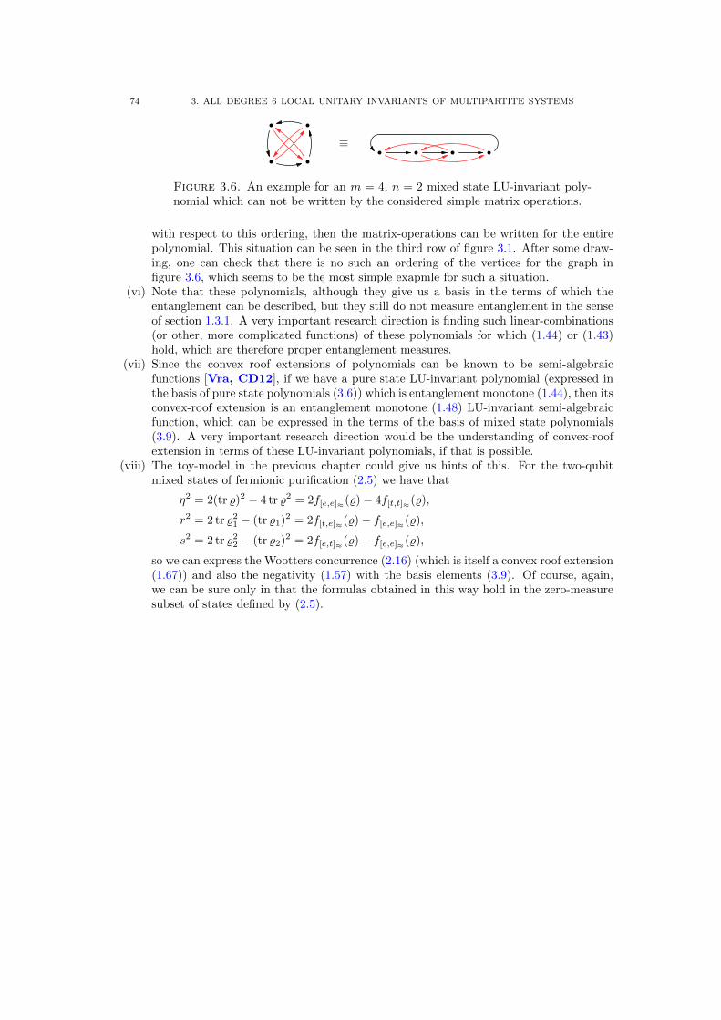
74 3. ALL DEGREE 6 LOCAL UNITARY INVARIANTS OF MULTIPARTITE SYSTEMS
≡
Figure 3.6. An example for an m = 4, n = 2 mixed state LU-invariant poly-nomial which can not be written by the considered simple matrix operations.
with respect to this ordering, then the matrix-operations can be written for the entirepolynomial. This situation can be seen in the third row of figure 3.1. After some draw-ing, one can check that there is no such an ordering of the vertices for the graph infigure 3.6, which seems to be the most simple exapmle for such a situation.
(vi) Note that these polynomials, although they give us a basis in the terms of which theentanglement can be described, but they still do not measure entanglement in the senseof section 1.3.1. A very important research direction is finding such linear-combinations(or other, more complicated functions) of these polynomials for which (1.44) or (1.43)hold, which are therefore proper entanglement measures.
(vii) Since the convex roof extensions of polynomials can be known to be semi-algebraicfunctions [Vra, CD12], if we have a pure state LU-invariant polynomial (expressed inthe basis of pure state polynomials (3.6)) which is entanglement monotone (1.44), then itsconvex-roof extension is an entanglement monotone (1.48) LU-invariant semi-algebraicfunction, which can be expressed in the terms of the basis of mixed state polynomials(3.9). A very important research direction would be the understanding of convex-roofextension in terms of these LU-invariant polynomials, if that is possible.
(viii) The toy-model in the previous chapter could give us hints of this. For the two-qubitmixed states of fermionic purification (2.5) we have that
η2 = 2(tr %)2 − 4 tr %2 = 2f[e,e]≈(%)− 4f[t,t]≈(%),
r2 = 2 tr %21 − (tr %1)2 = 2f[t,e]≈(%)− f[e,e]≈(%),
s2 = 2 tr %22 − (tr %2)2 = 2f[e,t]≈(%)− f[e,e]≈(%),
so we can express the Wootters concurrence (2.16) (which is itself a convex roof extension(1.67)) and also the negativity (1.57) with the basis elements (3.9). Of course, again,we can be sure only in that the formulas obtained in this way hold in the zero-measuresubset of states defined by (2.5).
CHAPTER 4
Separability criteria for mixed three-qubit states
In chapter 2 we investigated some measures of entanglement for a special family of two-qubit mixed states. A good entanglement measure vanishes for separable states, in this sense itprovides a necessary criterion of separability. This idea will return in the next chapter, but nowwe discuss some other methods for the decision of separability, which are easier to calculate andwork also in such cases in which we do not even have the possibility of evaluating a measure, orwe do not have any measures at all.
A mixed state is separable if it can be decomposed to an ensemble of separable pure states,(section 1.2.2). Such a decomposition is not unique, and it is difficult to decide whether for agiven density operator such a decomposition exists at all. One can make some observations forseparable pure states which can be extended to mixed states with the help of convex calculus.The separability criteria obtained in this way are necessary but not sufficient ones. (Or equiv-alently sufficient but not necessary criteria of entanglement.) A widely known example is thepartial transposition criterion of Peres (section 1.2.2). On the other hand one can construct nec-essary and sufficient criteria using sophisticated mathematical methods, dealing, for example,with witness operators, positive but not completely positive maps or semidefinite programming(sections 1.2.2, 1.2.3). Unfortunately these criteria are difficult to use for general density matricesdue to the rapidly growing complexity of the problem, and only the necessary but not sufficientcriteria are used in practice.
In this chapter, we give a comprehensive survey of the necessary but not sufficient criteriaof separability of mixed quantum states. We review and compare the criteria known from theliterature and give a case study of a special two-parameter class of three-qubit density matrices.The form of these density matrices is simple enough to calculate explicitly the set of states forwhich these criteria hold.
The material of this chapter covers thesis statement III (page xv). The organization of thischapter is as follows.
In section 4.1, we introduce the parametrized permutation-invariant family of three-qubitdensity matrices, our concern, and make some observations about the separability classstructure of permutation-invariant three-qubit mixed states. After having set the stage,in the next sections we investigate some criteria for separability classes.
In section 4.2, we consider our quantum-state as a d = (2, 4) qubit-qudit system and we re-call and use some bipartite separability criteria, namely the majorization and the entropycriteria, which are related to the notion of mixedness of the subsystems (sections 4.2.1and 4.2.2), the partial transposition and the reduction criteria, which are particularcases of the positive map criterion (sections 4.2.3 and 4.2.4), and the reshuffling crite-rion, which in addition to the partial transposition criterion is the other one of the twoindependent permutation criteria for bipartite systems (section 4.2.5).
In section 4.3, we consider our quantum-state as a proper d = (2, 2, 2) three-qubit systemand investigate some tripartite criteria for separability classes. We recall the permutation
75
76 4. SEPARABILITY CRITERIA FOR MIXED THREE-QUBIT STATES
criteria for permutation-invariant three-qubit case giving rise to another reshuffling cri-terion (section 4.3.1). Then we use quadratic Bell inequalities (section 4.3.2), and othercriteria using swap operators (section 4.3.3) and explicit expressions of matrix elements(section 4.3.4). The latter makes it possible to determine a set of entangled states ofpositive partial transpose.
In section 4.4, we investigate some other aspects of entanglement. First, the W and GHZclasses of fully entangled mixed states (section 4.4.1), then the entanglement of two-qubitsubsystems by the calculation of the Wootters concurrence (section 4.4.2).
In section 4.5, we give a summary and some remarks.
4.1. A symmetric family of mixed three-qubit states
In this chapter we investigate three-qubit states, so we have the Hilbert space H = H1 ⊗H2⊗H3 of local dimensions d = (2, 2, 2). Let % ∈ D(H) be the mixture of the GHZ state (1.71b),the W state (1.71a) and the white noise (1.10),
% = d1
8I⊗ I⊗ I + g|GHZ〉〈GHZ|+ w|W〉〈W|, (4.1)
where 0 ≤ d, g, w ≤ 1 real numbers are the weights characterizing the mixture, that is, d+g+w =1. In the following sections we plot the subsets of states for which the separability criteria holdon the g-w-plane, that is, we project the probability-simplex onto the d = 0 plane. A point onthis plane determines the third coordinate as d = 1 − g − w. Sometimes it is convenient to usethe rescaled parameters d = d/8, g = g/2, w = w/3.
The GHZ-W mixture (d = 0 line) is well studied. The three tangle (1.73) with its convexroofs, the Wootters concurrences (1.67) the singlepartite concurrences (1.76b) with their convexroofs, and the mixed-state extension of CKW inequality (1.69) were given for this mixture inthe paper of Lohmayer et. al. [LOSU06]. These results give an upper bound for values of thesequantities on the whole simplex defined in equation (4.1), since if f∪(%g,w) = min
∑i pif(ψi)
where the minimum is taken over all decomposition∑i pi|ψi〉〈ψi| = %g,w, and %d,g,w = dI ⊗
I ⊗ I/8 + (1 − d)%g/(1−d),w/(1−d), and f(ψ) = 0 on product states, then f∪(%d,g,w) ≤ (1 −d)f∪(%g/(1−d),w/(1−d)).
The white noise can be regarded in some sense as the “center” of the set of density matrices.Mixing a state with white noise is the way to investigate the effect of environmental decoher-ence [GT09]. A noisy state is usually of full rank, so methods for density matrices of low rank(like range criterion [Hor97], or finding optimal decompositions with respect to some pure-statemeasures) usually fail for such states.
On the other hand, there are exact results for the GHZ-white noise mixture (w = 0 line).In [DCT99] Dur, Cirac and Tarrach, using their results about a special class of GHZ-diagonalstates, have shown that % is fully separable if and only if 0 ≤ g ≤ 1/5. Moreover, it follows fromtheir observations that if the state is separable under a bipartition then it is fully separable, soClass 2.8 is empty for these states (section 1.2.3). In [GS10] Guhne and Seevinck gives necessaryand sufficient condition of tripartite entanglement for GHZ-diagonal states, which contain thenoisy GHZ state: for 1/5 < g ≤ 3/7 the state is 2-separable, yet inseparable under bipartitions,that is, in Class 2.1, and for 3/7 < g ≤ 1 the state is fully entangled, that is, in Class 1.Unfortunately there are no such results for other subsets of the simplex given in equation (4.1).
The noisy GHZ-W mixture given in equation (4.1) is clearly a permutation invariant one,hence the reduced density matrices of % are all of the same form, %12 = %23 = %31 and %1 = %2 =%3. The explicit forms of these matrices are given in equations (4.3b) and (4.3c). What can wesay about the tripartite separability-classes given in section 1.2.3 for permutation-invariant three-qubit states in general? Clearly, if a permutation-invariant state is in Dα2 for a particular α2,
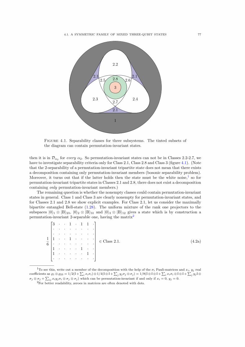
4.1. A SYMMETRIC FAMILY OF MIXED THREE-QUBIT STATES 77
3
2.8
2.2
2.7
2.1
2.3
2.6
2.1
2.4
2.5
2.1
1
Figure 4.1. Separability classes for three subsystems. The tinted subsets ofthe diagram can contain permutation-invariant states.
then it is in Dα2for every α2. So permutation-invariant states can not be in Classes 2.2-2.7, we
have to investigate separability criteria only for Class 2.1, Class 2.8 and Class 3 (figure 4.1). (Notethat the 2-separability of a permutation-invariant tripartite state does not mean that there existsa decomposition containing only permutation-invariant members (bosonic separability problem).Moreover, it turns out that if the latter holds then the state must be the white noise,1 so forpermutation-invariant tripartite states in Classes 2.1 and 2.8, there does not exist a decompositioncontaining only permutation-invariant members.)
The remaining question is whether the nonempty classes could contain permutation-invariantstates in general. Class 1 and Class 3 are clearly nonempty for permutation-invariant states, andfor Classes 2.1 and 2.8 we show explicit examples. For Class 2.1, let us consider the maximallybipartite entangled Bell-state (1.28). The uniform mixture of the rank one projectors to thesubspaces |0〉1 ⊗ |B〉23, |0〉2 ⊗ |B〉31 and |0〉3 ⊗ |B〉12 gives a state which is by construction apermutation-invariant 2-separable one, having the matrix2
1
6
3 · · 1 · 1 1 ·· · · · · · · ·· · · · · · · ·1 · · 1 · · · ·· · · · · · · ·1 · · · · 1 · ·1 · · · · · 1 ·· · · · · · · ·
∈ Class 2.1. (4.2a)
1To see this, write out a member of the decomposition with the help of the σi Pauli-matrices and xi, yj realcoefficients as %1⊗%23 = 1/2(I +
∑i xiσi)⊗ 1/4(I⊗ I +
∑j yjσj ⊗σj) = 1/8(I⊗ I⊗ I +
∑i xiσi⊗ I⊗ I +
∑j yjI⊗
σj ⊗ σj +∑ij xiyjσi ⊗ σj ⊗ σj) which can be permutation-invariant if and only if xi = 0, yj = 0.
2For better readability, zeroes in matrices are often denoted with dots.
78 4. SEPARABILITY CRITERIA FOR MIXED THREE-QUBIT STATES
It can be easily checked that its partial transpose is not positive, (see in (1.34a), this is enoughto be checked for only one subsystem because of the permutation-invariance of the state) so it isnot α2-separable for any 2-partite split, hence it is in Class 2.1. An example for a permutation-invariant state in Class 2.8 is given in equation (14) of [ABLS01] with 0 < a = b = 1/c, havingthe matrix
1
2 + 3(a+ 1
a
)
1 · · · · · · 1· a · · · · · ·· · a · · · · ·· · · 1
a · · · ·· · · · a · · ·· · · · · 1
a · ·· · · · · · 1
a ·1 · · · · · · 1
∈ Class 2.8 if and only if a 6= 1. (4.2b)
This state is entangled if and only if a 6= 1, and it is in Dα2 for all α2 [ABLS01].If we consider the d = (2, 2, 2) three-qubit system as a d = (2, 4) qubit-qudit system then
some well-known and easy-to-use bipartite separability criteria give rise to separability criteriafor⋂α2Dα2
, hence for the union of Class 2.8 and Class 3. (This one is also a convex set since it
is the intersection of convex ones.) First we investigate these criteria.
4.2. Bipartite separability criteria
In this section we consider our system as a d = (2, 4) qubit-qudit system (with Hilbert-spacesHA = H1 and HB = H23) and investigate some criteria of 1|23-separability which means theunion of Classes 2.8 and 3. To do this, we will need the spectra of the density matrix % given inequation (4.1) and of its marginals, having the matrices
% =
d+ g · · · · · · g
· d+ w w · w · · ·· w d+ w · w · · ·· · · d · · · ·· w w · d+ w · · ·· · · · · d · ·· · · · · · d ·g · · · · · · d+ g
, (4.3a)
%23 =
2d+ g + w · · ·
· 2d+ w w ·· w 2d+ w ·· · · 2d+ g
, (4.3b)
%1 =
[4d+ g + 2w ·
· 4d+ g + w
]. (4.3c)
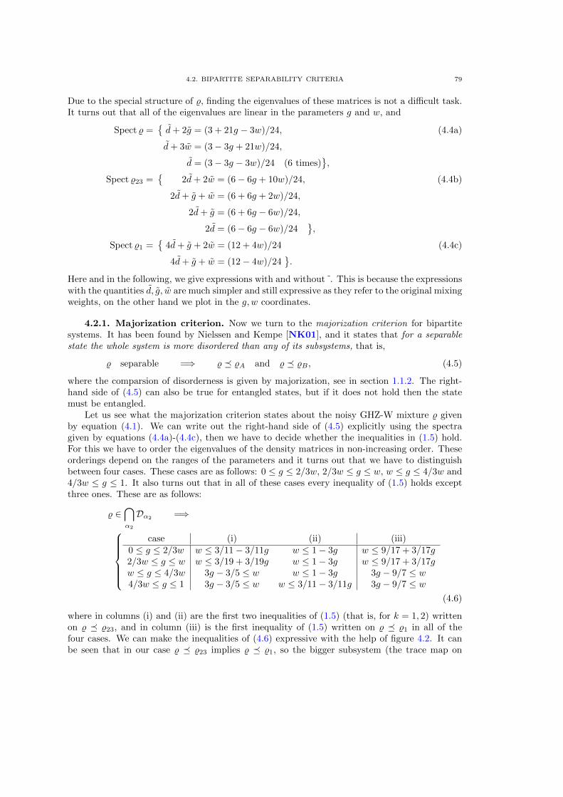
4.2. BIPARTITE SEPARABILITY CRITERIA 79
Due to the special structure of %, finding the eigenvalues of these matrices is not a difficult task.It turns out that all of the eigenvalues are linear in the parameters g and w, and
Spect % ={d+ 2g = (3 + 21g − 3w)/24,
d+ 3w = (3− 3g + 21w)/24,
d = (3− 3g − 3w)/24 (6 times)},
(4.4a)
Spect %23 ={
2d+ 2w = (6− 6g + 10w)/24,
2d+ g + w = (6 + 6g + 2w)/24,
2d+ g = (6 + 6g − 6w)/24,
2d = (6− 6g − 6w)/24},
(4.4b)
Spect %1 ={
4d+ g + 2w = (12 + 4w)/24
4d+ g + w = (12− 4w)/24}.
(4.4c)
Here and in the following, we give expressions with and without . This is because the expressionswith the quantities d, g, w are much simpler and still expressive as they refer to the original mixingweights, on the other hand we plot in the g, w coordinates.
4.2.1. Majorization criterion. Now we turn to the majorization criterion for bipartitesystems. It has been found by Nielssen and Kempe [NK01], and it states that for a separablestate the whole system is more disordered than any of its subsystems, that is,
% separable =⇒ % � %A and % � %B , (4.5)
where the comparsion of disorderness is given by majorization, see in section 1.1.2. The right-hand side of (4.5) can also be true for entangled states, but if it does not hold then the statemust be entangled.
Let us see what the majorization criterion states about the noisy GHZ-W mixture % givenby equation (4.1). We can write out the right-hand side of (4.5) explicitly using the spectragiven by equations (4.4a)-(4.4c), then we have to decide whether the inequalities in (1.5) hold.For this we have to order the eigenvalues of the density matrices in non-increasing order. Theseorderings depend on the ranges of the parameters and it turns out that we have to distinguishbetween four cases. These cases are as follows: 0 ≤ g ≤ 2/3w, 2/3w ≤ g ≤ w, w ≤ g ≤ 4/3w and4/3w ≤ g ≤ 1. It also turns out that in all of these cases every inequality of (1.5) holds exceptthree ones. These are as follows:
% ∈⋂α2
Dα2 =⇒case (i) (ii) (iii)
0 ≤ g ≤ 2/3w w ≤ 3/11− 3/11g w ≤ 1− 3g w ≤ 9/17 + 3/17g2/3w ≤ g ≤ w w ≤ 3/19 + 3/19g w ≤ 1− 3g w ≤ 9/17 + 3/17gw ≤ g ≤ 4/3w 3g − 3/5 ≤ w w ≤ 1− 3g 3g − 9/7 ≤ w4/3w ≤ g ≤ 1 3g − 3/5 ≤ w w ≤ 3/11− 3/11g 3g − 9/7 ≤ w
(4.6)
where in columns (i) and (ii) are the first two inequalities of (1.5) (that is, for k = 1, 2) writtenon % � %23, and in column (iii) is the first inequality of (1.5) written on % � %1 in all of thefour cases. We can make the inequalities of (4.6) expressive with the help of figure 4.2. It canbe seen that in our case % � %23 implies % � %1, so the bigger subsystem (the trace map on
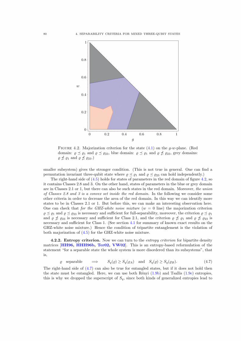
80 4. SEPARABILITY CRITERIA FOR MIXED THREE-QUBIT STATES
w
g
0 0.2 0.4 0.6 0.8 1
0
0.2
0.4
0.6
0.8
1
Figure 4.2. Majorization criterion for the state (4.1) on the g-w-plane. (Reddomain: % � %1 and % � %23, blue domain: % � %1 and % � %23, grey domains:% � %1 and % � %23.)
smaller subsystem) gives the stronger condition. (This is not true in general. One can find apermutation invariant three-qubit state where % � %1 and % � %23 can hold independently.)
The right-hand side of (4.5) holds for states of parameters in the red domain of figure 4.2, soit contains Classes 2.8 and 3. On the other hand, states of parameters in the blue or grey domainare in Classes 2.1 or 1, but there can also be such states in the red domain. Moreover, the unionof Classes 2.8 and 3 is a convex set inside the red domain. In the following we consider someother criteria in order to decrease the area of the red domain. In this way we can identify morestates to be in Classes 2.1 or 1. But before this, we can make an interesting observation here.One can check that for the GHZ-white noise mixture (w = 0 line) the majorization criterion% � %1 and % � %23 is necessary and sufficient for full-separability, moreover, the criterion % � %1
and % � %23 is necessary and sufficient for Class 2.1, and the criterion % � %1 and % � %23 isnecessary and sufficient for Class 1. (See section 4.1 for summary of known exact results on theGHZ-white noise mixture.) Hence the condition of tripartite entanglement is the violation ofboth majorization of (4.5) for the GHZ-white noise mixture.
4.2.2. Entropy criterion. Now we can turn to the entropy criterion for bipartite densitymatrices [HH96, HHH96b, Ter02, VW02]. This is an entropy-based reformulation of thestatement “for a separable state the whole system is more disordered than its subsystems”, thatis,
% separable =⇒ Sq(%) ≥ Sq(%A) and Sq(%) ≥ Sq(%B). (4.7)
The right-hand side of (4.7) can also be true for entangled states, but if it does not hold thenthe state must be entangled. Here, we can use both Renyi (1.9b) and Tsallis (1.9e) entropies,this is why we dropped the superscript of Sq, since both kinds of generalized entropies lead to
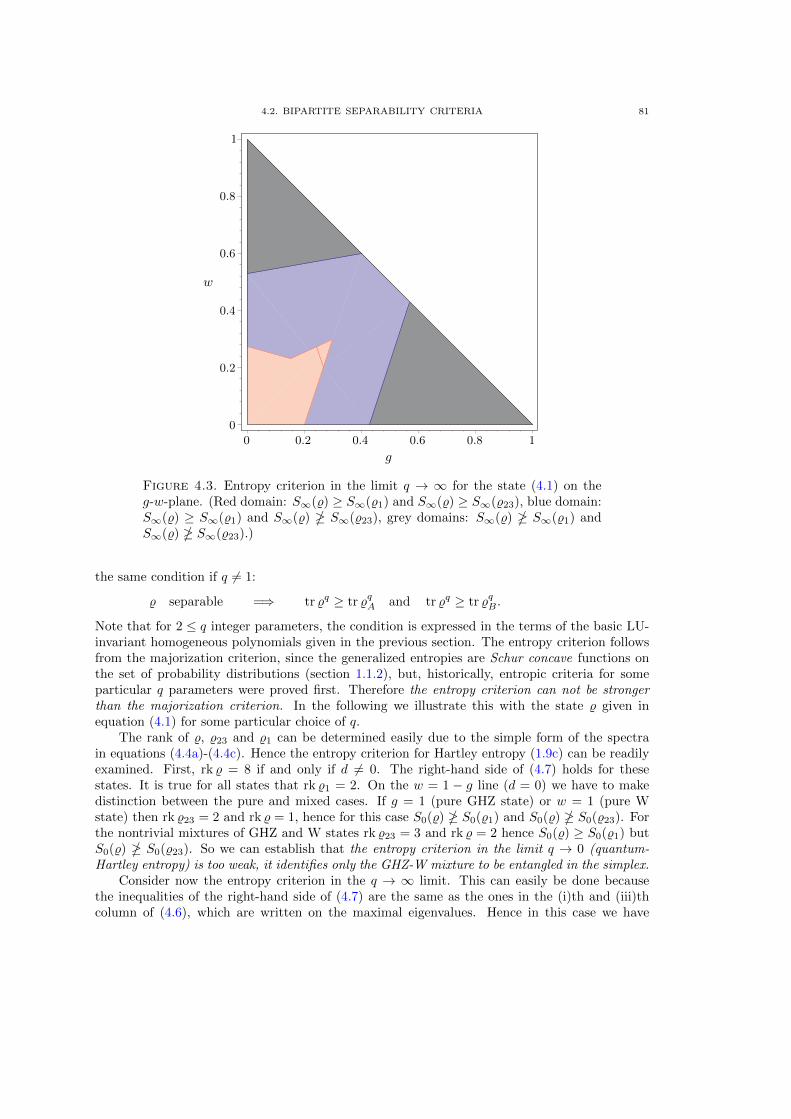
4.2. BIPARTITE SEPARABILITY CRITERIA 81
w
g
0 0.2 0.4 0.6 0.8 1
0
0.2
0.4
0.6
0.8
1
Figure 4.3. Entropy criterion in the limit q → ∞ for the state (4.1) on theg-w-plane. (Red domain: S∞(%) ≥ S∞(%1) and S∞(%) ≥ S∞(%23), blue domain:S∞(%) ≥ S∞(%1) and S∞(%) � S∞(%23), grey domains: S∞(%) � S∞(%1) andS∞(%) � S∞(%23).)
the same condition if q 6= 1:
% separable =⇒ tr %q ≥ tr %qA and tr %q ≥ tr %qB .
Note that for 2 ≤ q integer parameters, the condition is expressed in the terms of the basic LU-invariant homogeneous polynomials given in the previous section. The entropy criterion followsfrom the majorization criterion, since the generalized entropies are Schur concave functions onthe set of probability distributions (section 1.1.2), but, historically, entropic criteria for someparticular q parameters were proved first. Therefore the entropy criterion can not be strongerthan the majorization criterion. In the following we illustrate this with the state % given inequation (4.1) for some particular choice of q.
The rank of %, %23 and %1 can be determined easily due to the simple form of the spectrain equations (4.4a)-(4.4c). Hence the entropy criterion for Hartley entropy (1.9c) can be readilyexamined. First, rk % = 8 if and only if d 6= 0. The right-hand side of (4.7) holds for thesestates. It is true for all states that rk %1 = 2. On the w = 1 − g line (d = 0) we have to makedistinction between the pure and mixed cases. If g = 1 (pure GHZ state) or w = 1 (pure Wstate) then rk %23 = 2 and rk % = 1, hence for this case S0(%) � S0(%1) and S0(%) � S0(%23). Forthe nontrivial mixtures of GHZ and W states rk %23 = 3 and rk % = 2 hence S0(%) ≥ S0(%1) butS0(%) � S0(%23). So we can establish that the entropy criterion in the limit q → 0 (quantum-Hartley entropy) is too weak, it identifies only the GHZ-W mixture to be entangled in the simplex.
Consider now the entropy criterion in the q → ∞ limit. This can easily be done becausethe inequalities of the right-hand side of (4.7) are the same as the ones in the (i)th and (iii)thcolumn of (4.6), which are written on the maximal eigenvalues. Hence in this case we have
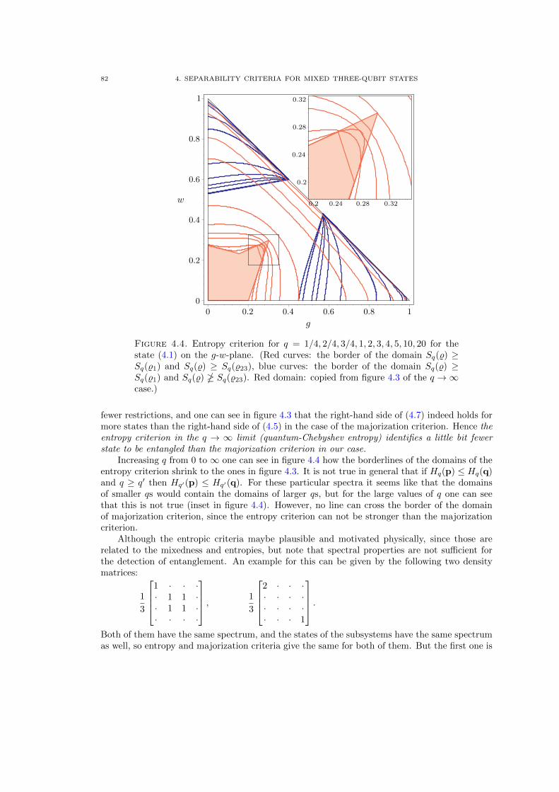
82 4. SEPARABILITY CRITERIA FOR MIXED THREE-QUBIT STATES
w
g
0 0.2 0.4 0.6 0.8 1
0
0.2
0.4
0.6
0.8
1
0.2 0.24 0.28 0.32
0.2
0.24
0.28
0.32
Figure 4.4. Entropy criterion for q = 1/4, 2/4, 3/4, 1, 2, 3, 4, 5, 10, 20 for thestate (4.1) on the g-w-plane. (Red curves: the border of the domain Sq(%) ≥Sq(%1) and Sq(%) ≥ Sq(%23), blue curves: the border of the domain Sq(%) ≥Sq(%1) and Sq(%) � Sq(%23). Red domain: copied from figure 4.3 of the q →∞case.)
fewer restrictions, and one can see in figure 4.3 that the right-hand side of (4.7) indeed holds formore states than the right-hand side of (4.5) in the case of the majorization criterion. Hence theentropy criterion in the q → ∞ limit (quantum-Chebyshev entropy) identifies a little bit fewerstate to be entangled than the majorization criterion in our case.
Increasing q from 0 to ∞ one can see in figure 4.4 how the borderlines of the domains of theentropy criterion shrink to the ones in figure 4.3. It is not true in general that if Hq(p) ≤ Hq(q)and q ≥ q′ then Hq′(p) ≤ Hq′(q). For these particular spectra it seems like that the domainsof smaller qs would contain the domains of larger qs, but for the large values of q one can seethat this is not true (inset in figure 4.4). However, no line can cross the border of the domainof majorization criterion, since the entropy criterion can not be stronger than the majorizationcriterion.
Although the entropic criteria maybe plausible and motivated physically, since those arerelated to the mixedness and entropies, but note that spectral properties are not sufficient forthe detection of entanglement. An example for this can be given by the following two densitymatrices:
1
3
1 · · ·· 1 1 ·· 1 1 ·· · · ·
, 1
3
2 · · ·· · · ·· · · ·· · · 1
.Both of them have the same spectrum, and the states of the subsystems have the same spectrumas well, so entropy and majorization criteria give the same for both of them. But the first one is
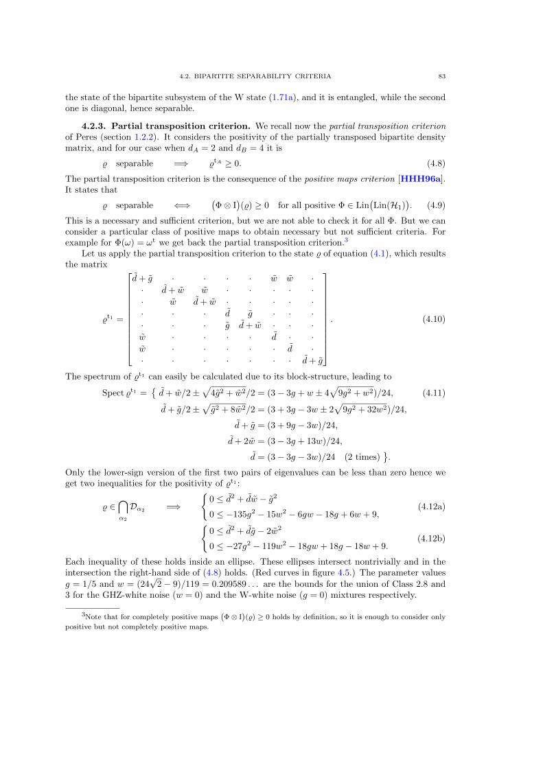
4.2. BIPARTITE SEPARABILITY CRITERIA 83
the state of the bipartite subsystem of the W state (1.71a), and it is entangled, while the secondone is diagonal, hence separable.
4.2.3. Partial transposition criterion. We recall now the partial transposition criterionof Peres (section 1.2.2). It considers the positivity of the partially transposed bipartite densitymatrix, and for our case when dA = 2 and dB = 4 it is
% separable =⇒ %tA ≥ 0. (4.8)
The partial transposition criterion is the consequence of the positive maps criterion [HHH96a].It states that
% separable ⇐⇒(Φ⊗ I
)(%) ≥ 0 for all positive Φ ∈ Lin
(Lin(H1)
). (4.9)
This is a necessary and sufficient criterion, but we are not able to check it for all Φ. But we canconsider a particular class of positive maps to obtain necessary but not sufficient criteria. Forexample for Φ(ω) = ωt we get back the partial transposition criterion.3
Let us apply the partial transposition criterion to the state % of equation (4.1), which resultsthe matrix
%t1 =
d+ g · · · · w w ·· d+ w w · · · · ·· w d+ w · · · · ·· · · d g · · ·· · · g d+ w · · ·w · · · · d · ·w · · · · · d ·· · · · · · · d+ g
. (4.10)
The spectrum of %t1 can easily be calculated due to its block-structure, leading to
Spect %t1 ={d+ w/2±
√4g2 + w2/2 = (3− 3g + w ± 4
√9g2 + w2)/24,
d+ g/2±√g2 + 8w2/2 = (3 + 3g − 3w ± 2
√9g2 + 32w2)/24,
d+ g = (3 + 9g − 3w)/24,
d+ 2w = (3− 3g + 13w)/24,
d = (3− 3g − 3w)/24 (2 times)}.
(4.11)
Only the lower-sign version of the first two pairs of eigenvalues can be less than zero hence weget two inequalities for the positivity of %t1 :
% ∈⋂α2
Dα2=⇒
{0 ≤ d2 + dw − g2
0 ≤ −135g2 − 15w2 − 6gw − 18g + 6w + 9,(4.12a){
0 ≤ d2 + dg − 2w2
0 ≤ −27g2 − 119w2 − 18gw + 18g − 18w + 9.(4.12b)
Each inequality of these holds inside an ellipse. These ellipses intersect nontrivially and in theintersection the right-hand side of (4.8) holds. (Red curves in figure 4.5.) The parameter values
g = 1/5 and w = (24√
2 − 9)/119 = 0.209589 . . . are the bounds for the union of Class 2.8 and3 for the GHZ-white noise (w = 0) and the W-white noise (g = 0) mixtures respectively.
3Note that for completely positive maps(Φ⊗ I
)(%) ≥ 0 holds by definition, so it is enough to consider only
positive but not completely positive maps.
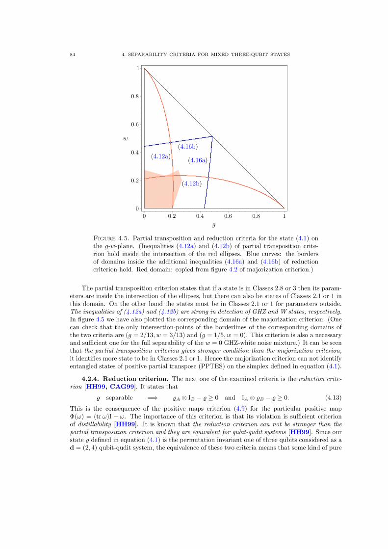
84 4. SEPARABILITY CRITERIA FOR MIXED THREE-QUBIT STATES
w
g
0 0.2 0.4 0.6 0.8 1
0
0.2
0.4
0.6
0.8
1
(4.12a)
(4.12b)
(4.16a)
(4.16b)
Figure 4.5. Partial transposition and reduction criteria for the state (4.1) onthe g-w-plane. (Inequalities (4.12a) and (4.12b) of partial transposition crite-rion hold inside the intersection of the red ellipses. Blue curves: the bordersof domains inside the additional inequalities (4.16a) and (4.16b) of reductioncriterion hold. Red domain: copied from figure 4.2 of majorization criterion.)
The partial transposition criterion states that if a state is in Classes 2.8 or 3 then its param-eters are inside the intersection of the ellipses, but there can also be states of Classes 2.1 or 1 inthis domain. On the other hand the states must be in Classes 2.1 or 1 for parameters outside.The inequalities of (4.12a) and (4.12b) are strong in detection of GHZ and W states, respectively.In figure 4.5 we have also plotted the corresponding domain of the majorization criterion. (Onecan check that the only intersection-points of the borderlines of the corresponding domains ofthe two criteria are (g = 2/13, w = 3/13) and (g = 1/5, w = 0). This criterion is also a necessaryand sufficient one for the full separability of the w = 0 GHZ-white noise mixture.) It can be seenthat the partial transposition criterion gives stronger condition than the majorization criterion,it identifies more state to be in Classes 2.1 or 1. Hence the majorization criterion can not identifyentangled states of positive partial transpose (PPTES) on the simplex defined in equation (4.1).
4.2.4. Reduction criterion. The next one of the examined criteria is the reduction crite-rion [HH99, CAG99]. It states that
% separable =⇒ %A ⊗ IB − % ≥ 0 and IA ⊗ %B − % ≥ 0. (4.13)
This is the consequence of the positive maps criterion (4.9) for the particular positive mapΦ(ω) = (trω)I − ω. The importance of this criterion is that its violation is sufficient criterionof distillability [HH99]. It is known that the reduction criterion can not be stronger than thepartial transposition criterion and they are equivalent for qubit-qudit systems [HH99]. Since ourstate % defined in equation (4.1) is the permutation invariant one of three qubits considered as ad = (2, 4) qubit-qudit system, the equivalence of these two criteria means that some kind of pure
4.2. BIPARTITE SEPARABILITY CRITERIA 85
state entanglement between 1 and 23 can be distilled out from every state of non-positive partialtranspose. In other words in the simplex defined by equation (4.1) there are no bound entangledd = (2, 4) states of non-positive partial transpose, while the entangled states of positive partialtranspose are all bound entangled, which is a general result [HHH98].
We can illustrate the equivalence of the partial transposition and reduction criteria. To dothis we have to examine the positivity of the matrices I1 ⊗ %23 − % and %1 ⊗ I23 − %, which are ofthe form
I1 ⊗ %23 − % =
d+ w · · · · · · −g· d · · −w · · ·· · d · −w · · ·· · · d+ g · · · ·· −w −w · d+ g · · ·· · · · · d+ w w ·· · · · · w d+ w ·−g · · · · · · d
, (4.14a)
%1 ⊗ I23 − % =
3d+ 2w · · · · · · −g· 3d+ g + w −w · −w · · ·· −w 3d+ g + w · −w · · ·· · · 3d+ g + 2w · · · ·· −w −w · 3d+ g · · ·· · · · · 3d+ g + w · ·· · · · · · 3d+ g + w ·−g · · · · · · 3d+ w
.
(4.14b)
Since (trω)I− ω = (εωε†)t for 2× 2 matrices it turns out that
Spect(I1 ⊗ %23 − %) = Spect %t1 , (4.15a)
while
Spect(%1 ⊗ I23 − %) ={
3d+ 3w/2±√
4g2 + w2/2 = (9− 9g + 3w ± 4√
9g2 + w2)/24,
3d+ g ±√
2w = (9 + 3g − 9w ± 8√
2w)/24,
3d+ g + 2w = (9 + 3g + 7w)/24 (2 times),
3d+ g + w = (9 + 3g − w)/24 (2 times)}.
(4.15b)
For I1 ⊗ %23 − % ≥ 0 we have the same conditions as in equations (4.12a)-(4.12b) of the partialtransposition criterion. The additional inequalities arise from the lower-sign version of the firsttwo eigenvalues of %1 ⊗ I23 − %, leading to the criteria
% ∈⋂α2
Dα2 =⇒
{0 ≤ 9d2 − g2 + 9dw + 2w2
0 ≤ −63g2 − 7w2 − 54gw − 162g + 54w + 81,(4.16a){
0 ≤ 3d+ g −√
2w
0 ≤ 3g − (9 + 8√
2)w + 9.(4.16b)
86 4. SEPARABILITY CRITERIA FOR MIXED THREE-QUBIT STATES
The first one of them is true outside a hyperbola, the second one is true under a line. (Bluecurves in figure 4.5.)
It can be seen that the last two inequalities (4.16a)-(4.16b) do not restrict the ones inequations (4.12a)-(4.12b), as it has to be, and because of (4.15a) the reduction criterion and thepartial transposition criterion hold for the same states of the GHZ-W-white noise mixture. Herewe get the stronger condition for the map Φ(ω) = (trω)I − ω acting on the smaller subsystem.We can also observe that the inequalities of (4.16a) and (4.16b) are good in detection of GHZand W state respectively, but not so good as the ones of partial transposition criterion. However,one can check that on the w = 0 GHZ-white noise mixture the reduction criterion I1⊗%23−% ≥ 0and %1⊗ I23− % ≥ 0 is necessary and sufficient for full-separability, the criterion I1⊗ %23− % � 0and %1⊗ I23−% ≥ 0 is necessary and sufficient for Class 2.1, and the criterion I1⊗%23−% � 0 and%1⊗ I23− % � 0 is necessary and sufficient for Class 1 in the same fashion as in the majorizationcriterion of section 4.2.1.
4.2.5. Reshuffling criterion. The reshuffling criterion is independent of the partial trans-position criterion, so it can detect entangled states of positive partial transpose. It states that
% separable =⇒ ‖R(%)‖tr ≤ 1, (4.17)
where the trace-norm is ‖M‖tr = tr√M†M , and the reshuffling map R is defined on matrix
elements as [R(%)]i ji′ j′ = %iji′j′ .
The four nonzero singular values of the 4× 16 reshuffled density matrix
R(%) =
d+ g · · · · d+ w w · · w d+ w · · · · d· · · g w · · · w · · · · · · ·· w w · · · · · · · · · g · · ·
d+ w · · · · d · · · · d · · · · d+ g
,(4.18)
that is, the square root of the nonnegative eigenvalues of R(%)†R(%) are
Spect√R(%)R(%)† =
{1
2
√p1 ± 2
√p2,√g2 + 2w2,
√g2 + 2w2
}, (4.19)
where
p1 =16d2 + 4g2 + 10w2 + 8dg + 12dw,
p2 =64d4 + 9w4 + 64d3g + 96d3w + 12dw3
+ 16d2g2 + 40d2w2 + 4g2w2 + 80d2gw + 16dg2w + 24dgw2.
The sum of them is less or equal than 1 inside a curve of high degree which can be seen infigure 4.6 (red curve). States of Classes 2.8 and 3 must be inside this curve, states outside thiscurve must belong to Classes 2.1 or 1, but one can see that this criterion does not restrict thepartial transposition criterion, it does not detect PPTESs in the GHZ-W-white noise mixture(4.1).
4.3. Tripartite separability criteria
In this section we consider the state given in equation (4.1) as the state of a proper d =(2, 2, 2) three-qubit system and investigate some general 3-qubit k-separability criteria.
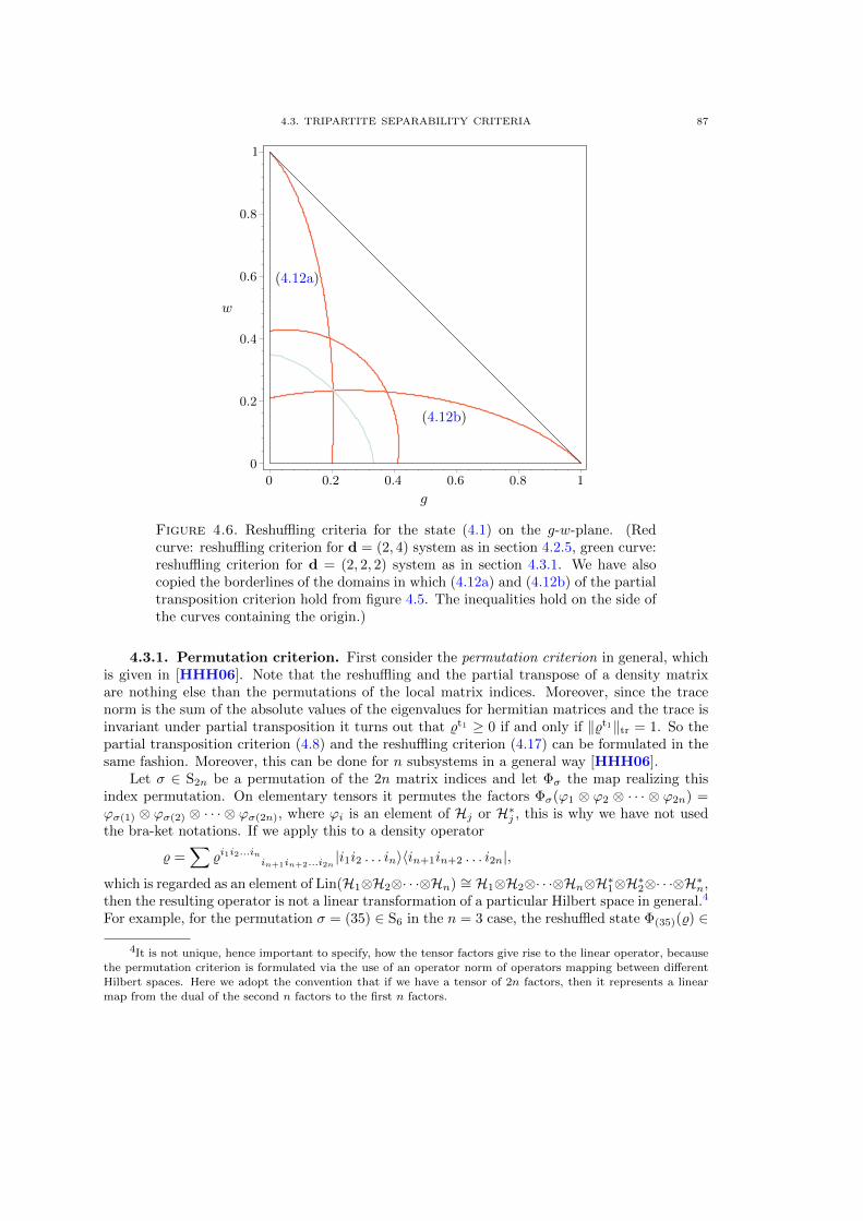
4.3. TRIPARTITE SEPARABILITY CRITERIA 87
w
g
0 0.2 0.4 0.6 0.8 1
0
0.2
0.4
0.6
0.8
1
(4.12a)
(4.12b)
Figure 4.6. Reshuffling criteria for the state (4.1) on the g-w-plane. (Redcurve: reshuffling criterion for d = (2, 4) system as in section 4.2.5, green curve:reshuffling criterion for d = (2, 2, 2) system as in section 4.3.1. We have alsocopied the borderlines of the domains in which (4.12a) and (4.12b) of the partialtransposition criterion hold from figure 4.5. The inequalities hold on the side ofthe curves containing the origin.)
4.3.1. Permutation criterion. First consider the permutation criterion in general, whichis given in [HHH06]. Note that the reshuffling and the partial transpose of a density matrixare nothing else than the permutations of the local matrix indices. Moreover, since the tracenorm is the sum of the absolute values of the eigenvalues for hermitian matrices and the trace isinvariant under partial transposition it turns out that %t1 ≥ 0 if and only if ‖%t1‖tr = 1. So thepartial transposition criterion (4.8) and the reshuffling criterion (4.17) can be formulated in thesame fashion. Moreover, this can be done for n subsystems in a general way [HHH06].
Let σ ∈ S2n be a permutation of the 2n matrix indices and let Φσ the map realizing thisindex permutation. On elementary tensors it permutes the factors Φσ(ϕ1 ⊗ ϕ2 ⊗ · · · ⊗ ϕ2n) =ϕσ(1) ⊗ ϕσ(2) ⊗ · · · ⊗ ϕσ(2n), where ϕi is an element of Hj or H∗j , this is why we have not usedthe bra-ket notations. If we apply this to a density operator
% =∑
%i1i2...inin+1in+2...i2n|i1i2 . . . in〉〈in+1in+2 . . . i2n|,
which is regarded as an element of Lin(H1⊗H2⊗· · ·⊗Hn) ∼= H1⊗H2⊗· · ·⊗Hn⊗H∗1⊗H∗2⊗· · ·⊗H∗n,then the resulting operator is not a linear transformation of a particular Hilbert space in general.4
For example, for the permutation σ = (35) ∈ S6 in the n = 3 case, the reshuffled state Φ(35)(%) ∈
4It is not unique, hence important to specify, how the tensor factors give rise to the linear operator, becausethe permutation criterion is formulated via the use of an operator norm of operators mapping between different
Hilbert spaces. Here we adopt the convention that if we have a tensor of 2n factors, then it represents a linearmap from the dual of the second n factors to the first n factors.
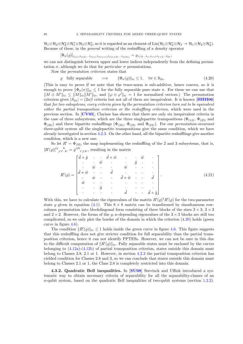
88 4. SEPARABILITY CRITERIA FOR MIXED THREE-QUBIT STATES
H1⊗H2⊗H∗2⊗H∗1⊗H3⊗H∗3, so it is regarded as an element of Lin(H1⊗H∗3⊗H3 → H1⊗H2⊗H∗2).Because of these, in the general writing of the reshuffling of a density operator
[Φσ(%)]iσ(1)iσ(2)...iσ(n);iσ(n+1)iσ(n+2)...iσ(2n)= %i1i2...in,in+1in+2...i2n ,
we can not distinguish between upper and lower indices independently from the defining permu-tation σ, although we do that for particular σ permutations.
Now the permutation criterion states that
% fully separable =⇒ ‖Φσ(%)‖tr ≤ 1, ∀σ ∈ S2n. (4.20)
(This is easy to prove if we note that the trace-norm is sub-additive, hence convex, so it isenough to prove ‖Φσ(π)‖tr ≤ 1 for the fully separable pure state π. For these we can use that‖M ⊗M ′‖tr ≤ ‖M‖tr‖M ′‖tr, and ‖ϕ ⊗ ϕ′‖tr = 1 for normalized vectors.) The permutationcriterion gives |S2n| = (2n)! criteria but not all of them are inequivalent. It is known [HHH06]that for two subsystems, every criteria given by the permutation criterion turn out to be equivalenteither the partial transposition criterion or the reshuffling criterion, which were used in theprevious section. In [CV05], Clarisse has shown that there are only six inequivalent criteria inthe case of three subsystems, which are the three singlepartite transpositions (Φ(14), Φ(25) andΦ(36)) and three bipartite reshufflings (Φ(35), Φ(34) and Φ(24)). For our permutation-invariantthree-qubit system all the singlepartite transpositions give the same condition, which we havealready investigated in section 4.2.3. On the other hand, all the bipartite reshufflings give anothercondition, which is a new one.
So let R′ = Φ(35) the map implementing the reshuffling of the 2 and 3 subsystems, that is,
[R′(%)]ij kj′i′ k′ = %ijki′j′k′ , resulting in the matrix
R′(%) =
d+ g · · d+ w · · w ·· · w · · g · ·· w · · w · · ·
d+ w · · d · · · ·· w · · d+ w · · dw · · · · · · ·· · g · · · · ·· · · · d · · d+ g
. (4.21)
With this, we have to calculate the eigenvalues of the matrix R′(%)†R′(%) for the two-parameterstate % given in equation (4.1). This 8 × 8 matrix can be transformed by simultaneous row-column permutation into blockdiagonal form consisting of three blocks of the sizes 3 × 3, 3 × 3and 2× 2. However, the forms of the g, w-depending eigenvalues of the 3× 3 blocks are still toocomplicated, so we only plot the border of the domain in which the criterion (4.20) holds (greencurve in figure 4.6).
The condition ‖R′(%)‖tr ≤ 1 holds inside the green curve in figure 4.6. This figure suggeststhat this reshuffling does not give stricter condition for full separability than the partial trans-position criterion, hence it can not identify PPTESs. However, we can not be sure in this dueto the difficult computation of ‖R′(%)‖tr. Fully separable states must be enclosed by the curvesbelonging to (4.12a)-(4.12b) of partial transposition criterion, states outside this domain mustbelong to Classes 2.8, 2.1 or 1. However, in section 4.2.3 the partial transposition criterion hasyielded condition for Classes 2.8 and 3, so we can conclude that states outside this domain mustbelong to Classes 2.1 or 1, the Class 2.8 is completely restricted into this domain.
4.3.2. Quadratic Bell inequalities. In [SU08] Seevinck and Uffink introduced a sys-tematic way to obtain necessary criteria of separability for all the separability-classes of ann-qubit system, based on the quadratic Bell inequalities of two-qubit systems (section 1.2.2).

4.3. TRIPARTITE SEPARABILITY CRITERIA 89
Their new criteria generalize some previously known multipartite criteria, such as Laskowski-Zukowski criterion (necessary for k-separability) [LZ05], Mermin-type separability inequalities(necessary for k-separability) [Uff02, GBP98, SS02, NKI02, CGP+02, Roy05], Fidelity-criterion (necessary for 2-separability) [SU01, ZZZ+03] (which is also known as projectionbased witness [TG05]) and Dur-Cirac depolarization criterion (necessary for αk-separability)[DCT99, DC00]. We consider the three-qubit case and get criteria for Class 2.1, Class 2.8 andClass 3 given in section 1.2.3.
The method of Seevinck and Uffink is formulated in a recursive way in terms of three or-thogonal spin-observables on each subsystem, (X(1), Y (1), Z(1)). Here the superscript (1) denotesthat these are single-qubit operators. Let I(1) denote the 2× 2 identity operator, I(1) = I. Fromthe (X(1), Y (1), Z(1), I(1)) one-qubit observables acting on the subsystems 2 and 3 one can form
two sets of two-qubit observables (X(2)x , Y
(2)x , Z
(2)x , I
(2)x ). Here the superscript (2) denotes that
these are two-qubit operators and x = 0, 1 refers to the two sets, which are
X(2)0 =
1
2
(X(1) ⊗X(1) − Y (1) ⊗ Y (1)
), X
(2)1 =
1
2
(X(1) ⊗X(1) + Y (1) ⊗ Y (1)
),
Y(2)0 =
1
2
(Y (1) ⊗X(1) +X(1) ⊗ Y (1)
), Y
(2)1 =
1
2
(Y (1) ⊗X(1) −X(1) ⊗ Y (1)
),
Z(2)0 =
1
2
(Z(1) ⊗ I(1) + I(1) ⊗ Z(1)
), Z
(2)1 =
1
2
(Z(1) ⊗ I(1) − I(1) ⊗ Z(1)
),
I(2)0 =
1
2
(I(1) ⊗ I(1) + Z(1) ⊗ Z(1)
), I
(2)1 =
1
2
(I(1) ⊗ I(1) − Z(1) ⊗ Z(1)
).
(4.22)
(Note that I(2)x s are not identity operators.) From these two-qubit observables and the one-
qubit ones acting on subsystem 1 one can form four sets of three-qubit observables acting on the
full system (X(3)x , Y
(3)x , Z
(3)x , I
(3)x ). Here the superscript (3) denotes that these are three-qubit
operators and x = 0, 1, 2, 3 refers to the four sets, which are
X(3)y =
1
2
(X(1) ⊗X(2)
y/2 − Y(1) ⊗ Y (2)
y/2
), X
(3)y+1 =
1
2
(X(1) ⊗X(2)
y/2 + Y (1) ⊗ Y (2)y/2
),
Y (3)y =
1
2
(Y (1) ⊗X(2)
y/2 +X(1) ⊗ Y (2)y/2
), Y
(3)y+1 =
1
2
(Y (1) ⊗X(2)
y/2 −X(1) ⊗ Y (2)
y/2
),
Z(3)y =
1
2
(Z(1) ⊗ I(2)
y/2 + I(1) ⊗ Z(2)y/2
), Z
(3)y+1 =
1
2
(Z(1) ⊗ I(2)
y/2 − I(1) ⊗ Z(2)
y/2
),
I(3)y =
1
2
(I(1) ⊗ I(2)
y/2 + Z(1) ⊗ Z(2)y/2
), I
(3)y+1 =
1
2
(I(1) ⊗ I(2)
y/2 − Z(1) ⊗ Z(2)
y/2
),
(4.23)
for y = 0, 2. (Again, I(3)x s are not identity operators.)
Now for particular α2, investigating some relations among the expectation-values of theseoperators with respect to the state %, one can get some nontrivial inequalities valid for all % ∈ Dα2
.From these, one can form inequalities valid for a given separability class of section 1.2.3. Herewe recall these criteria for the classes we need to deal with [SU08]
% ∈ D2-sep =⇒√〈X(3)
x 〉2 + 〈Y (3)x 〉2 ≤
∑y 6=x
√〈I(3)y 〉2 − 〈Z(3)
y 〉2 (4.24)
% ∈⋂α2
Dα2 =⇒ maxx
{〈X(3)
x 〉2 + 〈Y (3)x 〉2
}≤ min
x
{〈I(3)x 〉2 − 〈Z(3)
x 〉2}≤ 1/4
(4.25)
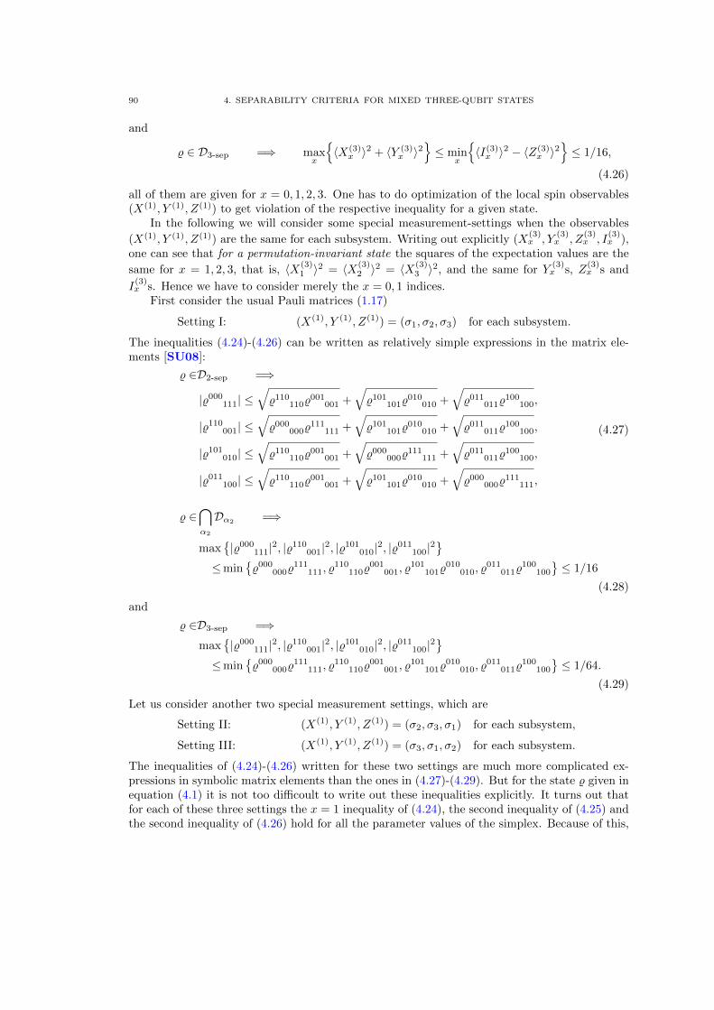
90 4. SEPARABILITY CRITERIA FOR MIXED THREE-QUBIT STATES
and
% ∈ D3-sep =⇒ maxx
{〈X(3)
x 〉2 + 〈Y (3)x 〉2
}≤ min
x
{〈I(3)x 〉2 − 〈Z(3)
x 〉2}≤ 1/16,
(4.26)
all of them are given for x = 0, 1, 2, 3. One has to do optimization of the local spin observables(X(1), Y (1), Z(1)) to get violation of the respective inequality for a given state.
In the following we will consider some special measurement-settings when the observables
(X(1), Y (1), Z(1)) are the same for each subsystem. Writing out explicitly (X(3)x , Y
(3)x , Z
(3)x , I
(3)x ),
one can see that for a permutation-invariant state the squares of the expectation values are the
same for x = 1, 2, 3, that is, 〈X(3)1 〉2 = 〈X(3)
2 〉2 = 〈X(3)3 〉2, and the same for Y
(3)x s, Z
(3)x s and
I(3)x s. Hence we have to consider merely the x = 0, 1 indices.
First consider the usual Pauli matrices (1.17)
Setting I: (X(1), Y (1), Z(1)) = (σ1, σ2, σ3) for each subsystem.
The inequalities (4.24)-(4.26) can be written as relatively simple expressions in the matrix ele-ments [SU08]:
% ∈D2-sep =⇒
|%000111| ≤
√%110
110%001
001 +√%101
101%010
010 +√%011
011%100
100,
|%110001| ≤
√%000
000%111
111 +√%101
101%010
010 +√%011
011%100
100,
|%101010| ≤
√%110
110%001
001 +√%000
000%111
111 +√%011
011%100
100,
|%011100| ≤
√%110
110%001
001 +√%101
101%010
010 +√%000
000%111
111,
(4.27)
% ∈⋂α2
Dα2=⇒
max{|%000
111|2, |%110001|2, |%101
010|2, |%011100|2
}≤min
{%000
000%111
111, %110
110%001
001, %101
101%010
010, %011
011%100
100
}≤ 1/16
(4.28)
and
% ∈D3-sep =⇒max
{|%000
111|2, |%110001|2, |%101
010|2, |%011100|2
}≤min
{%000
000%111
111, %110
110%001
001, %101
101%010
010, %011
011%100
100
}≤ 1/64.
(4.29)
Let us consider another two special measurement settings, which are
Setting II: (X(1), Y (1), Z(1)) = (σ2, σ3, σ1) for each subsystem,
Setting III: (X(1), Y (1), Z(1)) = (σ3, σ1, σ2) for each subsystem.
The inequalities of (4.24)-(4.26) written for these two settings are much more complicated ex-pressions in symbolic matrix elements than the ones in (4.27)-(4.29). But for the state % given inequation (4.1) it is not too difficoult to write out these inequalities explicitly. It turns out thatfor each of these three settings the x = 1 inequality of (4.24), the second inequality of (4.25) andthe second inequality of (4.26) hold for all the parameter values of the simplex. Because of this,
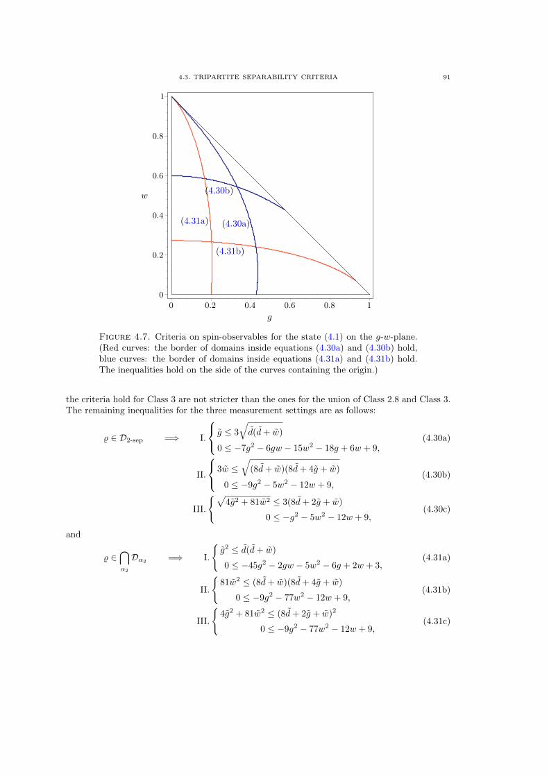
4.3. TRIPARTITE SEPARABILITY CRITERIA 91
w
g
0 0.2 0.4 0.6 0.8 1
0
0.2
0.4
0.6
0.8
1
(4.31a)
(4.31b)
(4.30a)
(4.30b)
Figure 4.7. Criteria on spin-observables for the state (4.1) on the g-w-plane.(Red curves: the border of domains inside equations (4.30a) and (4.30b) hold,blue curves: the border of domains inside equations (4.31a) and (4.31b) hold.The inequalities hold on the side of the curves containing the origin.)
the criteria hold for Class 3 are not stricter than the ones for the union of Class 2.8 and Class 3.The remaining inequalities for the three measurement settings are as follows:
% ∈ D2-sep =⇒ I.
g ≤ 3
√d(d+ w)
0 ≤ −7g2 − 6gw − 15w2 − 18g + 6w + 9,(4.30a)
II.
3w ≤√
(8d+ w)(8d+ 4g + w)
0 ≤ −9g2 − 5w2 − 12w + 9,(4.30b)
III.
{√4g2 + 81w2 ≤ 3(8d+ 2g + w)
0 ≤ −g2 − 5w2 − 12w + 9,(4.30c)
and
% ∈⋂α2
Dα2 =⇒ I.
{g2 ≤ d(d+ w)
0 ≤ −45g2 − 2gw − 5w2 − 6g + 2w + 3,(4.31a)
II.
{81w2 ≤ (8d+ w)(8d+ 4g + w)
0 ≤ −9g2 − 77w2 − 12w + 9,(4.31b)
III.
{4g2 + 81w2 ≤ (8d+ 2g + w)2
0 ≤ −9g2 − 77w2 − 12w + 9,(4.31c)
92 4. SEPARABILITY CRITERIA FOR MIXED THREE-QUBIT STATES
Clearly, the inequality of (4.30c) is weaker than the one of (4.30b), the inequality of (4.31c) is thesame as the one of (4.31b). Moreover, the inequality of (4.31a) is the same as the one of (4.12a)of partial transposition criterion, but the inequality of (4.31b) is strictly weaker than the otherone of partial transposition criterion. So these settings does not give stricter conditions forClasses 2.8 and 3 than partial transposition criterion, however, we get criteria for biseparabilityfor the first time. In figure 4.7 we show the borderlines of the domains of the criteria belongingto Settings I and II. These inequalities restrict Classes 2.1, 2.8 and 3 to be inside the domainenclosed by the blue curves and Classes 2.8 and 3 to be inside the domain enclosed by the redcurves. We can conclude that Settings I and II are strong in detection of GHZ and W staterespectively. One can check that for the w = 0 GHZ-white noise mixture the inequalities of(4.30a) and (4.31a) of Setting I hold if and only if the state is fully separable, (4.30a) is violatedbut (4.31a) holds if and only if the state is in Class 2.1 and both of them are violated if and onlyif the state is fully entangled. For the g = 0 W-white noise mixture, if 3/11 < w then % is inClass 2.1 or Class 1, and if 3/5 < w then % is fully entangled.
However, there are infinitely many criteria depending on the measurement settings and wedo not have a method to find a set of settings leading to the strictest criterion. We have triedsome other randomly chosen settings which can be used to reduce the area where these criteriahold. We could not find settings that give stronger criteria on the w = 0 or g = 0 axes of thesimplex than Settings I and II, respectively. We have found settings that exclude states from thecorresponding classes, but these states are far from these axes, and we have not found settingswhich give stronger conditions for Classes 2.8 and 3 than the partial transposition criterion. Wehave found settings by which the condition for biseparability can be strengthened, but theseconditions are just a little bit stronger far from the axes than the ones in section 4.3.4.
4.3.3. Criteria on matrix elements. In a recent paper [GHH10], Gabriel et. al. havegiven criterion for k-separability, based on their previously derived framework for the detectionof biseparability [HMGH10]. It turns out that for the noisy GHZ-W mixture given in equation(4.1) these criteria give the same results as the ones of quadratic Bell-inequalities, given in theprevious section, but these criteria have the advantage that they can be used in the same formnot only for qubits, but for subsystems of arbitrary, even different dimensions. To our knowledge,these were the first such criteria of k-separability.
Consider some permutation operators acting on H ⊗ H, that is, on the two copies of then-partite Hilbert space H = H1 ⊗H2 ⊗ · · · ⊗ Hn. Let Pas be the operators which swap the athsubsystems of the two copies, that is, Pa|i1i2 . . . in〉 ⊗ |j1j2 . . . jn〉 = |i1i2 . . . ia−1jaia+1 . . . in〉 ⊗|j1j2 . . . ja−1iaja+1 . . . jn〉 where {|ia〉} is basis in Ha. Now for a composite subsystem K ⊆ Lhaving the Hilbert space HK = ⊗a∈KHa let PK =
∏a∈K Pa. The key fact is that for pure
states π, if the state of that subsystem can be separated from the rest of the state then the
corresponding PK leaves the two copies of the state invariant, PK(π⊗ π)P †K = π⊗ π. With thisand convexity arguments, one can get the following criteria for k-separability [GHH10]
% ∈ Dk−sep =⇒√〈φ|(%⊗ %)Ptot|φ〉 ≤
∑i
(k∏r=1
〈φ|PL
(i)r
(%⊗ %)P †L
(i)r
|φ〉
)1/(2k)
,
(4.32)
where |φ〉 ∈ H ⊗ H is a fully separable vector, and the total swap operator is Ptot =∏Na=1 Pa.
Here i runs over all posible k-partite splits α(i)k = L
(i)1 |L
(i)2 | . . . |L
(i)k .
The inequality in (4.32) is written on the matrix elements of % determined by the separabledetection-vector |φ〉. For a given state, optimization on |φ〉 is needed to achieve the violation ofthe right-hand side of (4.32).
4.3. TRIPARTITE SEPARABILITY CRITERIA 93
To apply these criteria to the noisy GHZ-W mixture given in equation (4.1) we have tochoose a suitable detection-vector |φ〉. It turns out that |φGHZ〉 = |000111〉 and its Hadamard-transformed (1.22b) version |φW〉 = H⊗6|φGHZ〉 are good choices for states in the vicinity of GHZand W states respectively, as observed in [GHH10]. With these two vectors we get the samecriteria for 2-separability as the ones in (4.30a) and (4.30b) respectively, and for 3-separabilityas the ones in (4.31a) and (4.31b) respectively. (These were obtained by the criteria on spinobservables in the previous section.) However, (4.31a) and (4.31b) are conditions not only forClass 3, but for the union of Classes 2.8 and 3, so in this sense the quadratic Bell inequalitiesare a bit stronger.
We can not be sure that the detection-vectors above give the strongest conditions at least forthe noisy GHZ and noisy W states. However, it is an interesting observation that the Hadamardtransformation relates not only the two “strong” detection-vectors |φGHZ〉 and |φW〉 but also thetwo “strong” measurement-settings of the previous section (by the transformation σi 7→ HσiH
†):Setting I. (σ1, σ2, σ3) and (σ3,−σ2, σ1), which is equivalent5 to Setting II.
We have tried some other randomly chosen detection-vectors which can be used to reducethe area where the criteria hold, and we get the same observations as at the end of the previoussection. One can strengthen the conditions only far from the w = 0 or g = 0 axes of thesimplex, we have not found detection-vectors which give stronger condition for full-separabilitythan the partial transposition criterion, and we have found settings by which the condition forbiseparability can be strengthened, but these conditions are just a little bit stronger far from theaxes than the ones in section 4.3.4.
4.3.4. Criteria on matrix elements – a different approach. In [GS10] Guhne andSeevinck have given some further biseparability and full-separability criteria on the matrix ele-ments. The idea is that one can derive identities of matrix elements of pure separable states,then these identities can be extended to inequalities on mixed states by a convexity argument.For example, if |ψ〉 is separable under the 1|23 split, then |ψ〉 = |ψ1〉 ⊗ |ψ23〉 has factorized
coefficients ψijk = ψi1ψjk23 . The pure state π = |ψ〉〈ψ| has then factorizable matrix elements
πijki′j′k′ = ψi1ψjk23ψ1,i′ψ23,j′k′ ≡ ψi1ψ
jk23(ψi
′
1 )∗(ψj′k′
23 )∗ for which one can immediately check that
|π000111| =
√π011
011π100
100 holds. Now, we just need that these expressions behave well under
convex combination of the πijki′j′k′ matrix elements, that is, the square root of the product of
two diagonal (hence nonnegative) matrix elements is concave, while the absolute value is convex.Similar reasonings lead to the following criteria:
% ∈ D2-sep =⇒
|%000111| ≤
√%110
110%001
001 +√%101
101%010
010 +√%011
011%100
100,
(4.33a)
|%001010|+ |%001
100|+ |%010100| ≤
√%000
000%011
011 +√%000
000%101
101 +√%000
000%110
110
+(%001
001 + %010010 + %100
100
)/2.
(4.33b)
The criterion (4.33a) is necessary and sufficient for GHZ-diagonal states and can also be obtainedas a special case of the criteria of section 4.3.2 (equation (4.27)). However, this criterion—and the
5This equivalence holds only for permutation-invariant three-qubit states, when the three sets of observables
(X(1), Y (1), Z(1)) are the same for each subsystem. In this case one can check that the quantities 〈X(3)x 〉2 +
〈Y (3)x 〉2 for x = 0, 1, 2, 3 are invariant under the transformation (X(1), Y (1), Z(1)) ↔ (Y (1), X(1), Z(1)) and
(X(1), Y (1), Z(1)) ↔ (X(1),−Y (1), Z(1)). These can be seen by writing out the definitions given in equations(4.23).
94 4. SEPARABILITY CRITERIA FOR MIXED THREE-QUBIT STATES
others in this section—arises from a quite different approach as the one in (4.27). The criterionin (4.33b) is independent of the first one and it is quite strong in detection of W state mixedwith white noise.
Of course these and the following inequalities can be written on local unitary transformeddensity matrices, and optimization under local unitaries might be necessary, but this can leadto very complicated expressions in the original matrix elements. An advantage of the methodrecalled in the previous section is that it handles the matrix indices through the detection vector|φ〉.
By the use of similar reasoning, criteria for full-separability6 can also be obtained [GS10],which are
% ∈ D3-sep =⇒
|%000111| ≤
(%001
001%010
010%011
011%100
100%101
101%110
110
)1/6,(4.34a)
|%001010|+ |%001
100|+ |%010100| ≤
√%000
000%011
011 +√%000
000%101
101 +√%000
000%110
110.
(4.34b)
Criterion (4.34a) is necessary and sufficient for GHZ state mixed with white noise, and (4.34b) isviolated in the vicinity of the W state. Moreover, one can obtain other conditions from (4.34a) bymaking substitutions as follows. Consider a fully separable state vector |ψ〉 = |ψ1〉⊗ |ψ2〉⊗ |ψ3〉,which has factorizable coefficients ψijk = ψi1ψ
j2ψ
k3 . Then the diagonal elements of the pure state
π = |ψ〉〈ψ| are πijkijk = |ψi1|2|ψj2|2|ψk3 |2, leading to the identities
πijkijkπi′j′k′
i′j′k′= πijk
′
ijk′πi′j′k
i′j′k= πij
′k
ij′kπi′jk′
i′jk′= πi
′jk
i′jkπij′k′
ij′k′.
So these kinds of substitutions can be done for the %ijkijk diagonal matrix elements on the right-
hand side of (4.34a). Moreover, the right-hand side of the inequality of (4.34a) can be writtenas
((%001
001)2(%010010)2(%011
011)2(%100100)2(%101
101)2(%110110)2
)1/12,
and with these substitutions we can obtain a third power of four matrix elements under the 12throot. So we can get expressions of four matrix elements on the right-hand side of (4.34a), for
example(%001
001%010
010%100
100%111
111
)1/4. With the substitutions above one can get 28 different
inequalities for (4.34a) with an expression of sixth order under the sixth root on the right-hand side and 12 different ones with an expression of fourth order under the fourth root. Forpermutation-invariant states we have %001
001 = %010010 = %100
100 and %110110 = %101
101 = %011011,
and for our case (4.3a) it also holds that %000000 = %111
111, so the number of different inequalitiesreduces to 8 and 5 respectively. The right-hand sides of inequality (4.34a) which are different for
6Criteria for Dαk can be obtained as well.
4.3. TRIPARTITE SEPARABILITY CRITERIA 95
permutation-invariant matrices are as follows:((%000
000)3(%111111)3
)1/6,(
%001001%
010010%
011011%
100100%
101101%
110110
)1/6,(
%000000(%001
001)2(%110110)2%111
111
)1/6,(
(%000000)2%001
001%110
110(%111111)2
)1/6,(
%000000%
001001%
010010%
100100(%111
111)2)1/6
,((%000
000)2%011011%
101101%
110110%
111111
)1/6,(
(%001001)2%010
010%100
100%110
110%111
111
)1/6,(
%000000%
001001%
011011%
101101(%110
110)2)1/6
and ((%000
000)2(%111111)2
)1/4,(
%010010%
011011%
100100%
101101
)1/4,(
%000000%
001001%
110110%
111111
)1/4,(
%001001%
010010%
100100%
111111
)1/4,(
%000000%
011011%
101101%
110110
)1/4.
It turns out that the strongest conditions for the noisy GHZ-W mixture can be given by the lastone of these and with the original one in (4.34a). (We could also make some substitutions in theright-hand side of (4.34b) but these would not give stronger conditions than the original one.)
Writing out the criteria of biseparability and full separability we get:
% ∈ D2-sep =⇒ g ≤ 3
√d(d+ w), (4.35a)
w ≤√
(d+ g)d+ (d+ w)/2 (4.35b)
and
% ∈ D3-sep =⇒ g ≤ ((d+ w)d)1/2, (4.36a)
g ≤ ((d+ g)d3)1/4, (4.36b)
w ≤√
(d+ g)d. (4.36c)
(See in equation (4.3a).) Clearly, the biseparability condition of (4.35a) is the same as the oneof (4.30a) of the criterion on spin-observables but condition of (4.35b) is strictly stronger thanthe one of (4.30b). (On the g = 0 noisy W state it gives the bound 9/17, which is the strongestfor these states—to our knowledge.) The full-separability condition of (4.36a) is the same as theone of (4.31a) of the criterion on spin-observables (and the one of (4.12a) of partial transpositioncriterion as well) but the condition of (4.36c) is weaker than the one of (4.31b) of the criterionon spin-observables. Hence at this point these criteria are stronger for biseparability but weakerfor full separability than the criteria on spin-observables for our state. But we have anotherfull-separability condition, (4.36b), which can be stronger in a region than the ones based onthe partial transposition criterion. The states of parameters in this region are entangled ones ofpositive partial transpose, no pure state entanglement can be distilled from them. The borders of
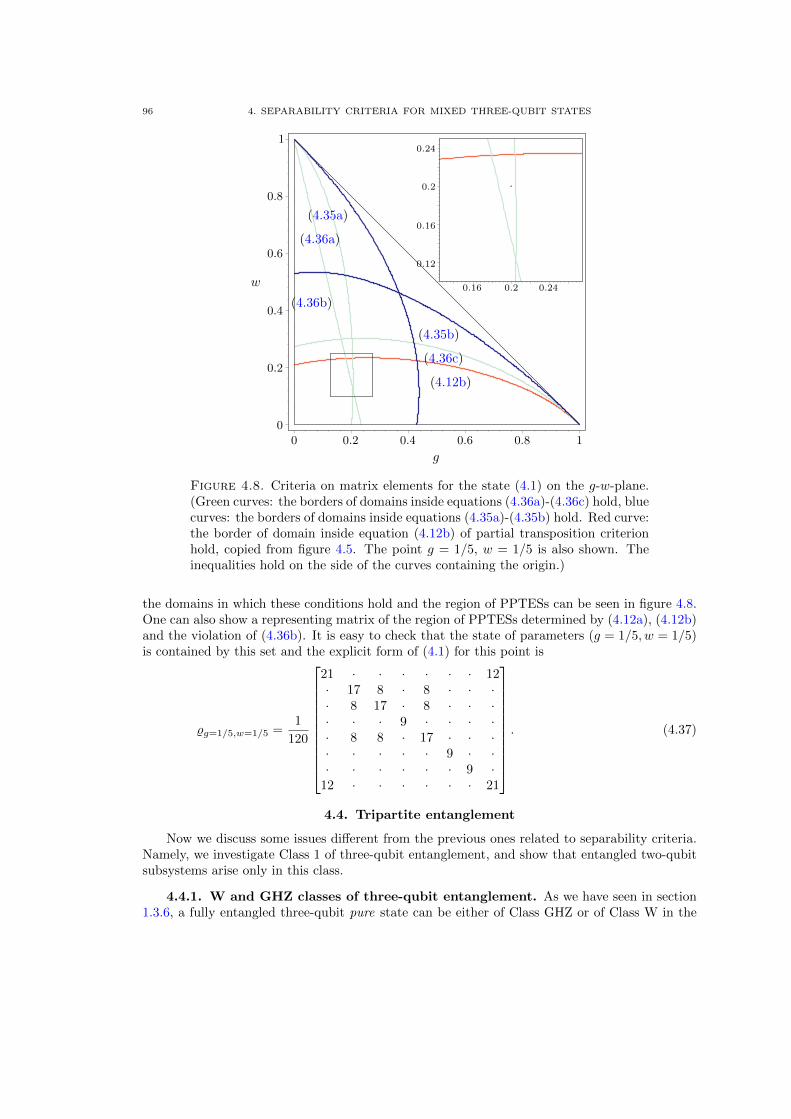
96 4. SEPARABILITY CRITERIA FOR MIXED THREE-QUBIT STATES
w
g
0 0.2 0.4 0.6 0.8 1
0
0.2
0.4
0.6
0.8
1
0.16 0.2 0.24
0.12
0.16
0.2
0.24
(4.36a)
(4.36b)
(4.36c)
(4.12b)
(4.35a)
(4.35b)
Figure 4.8. Criteria on matrix elements for the state (4.1) on the g-w-plane.(Green curves: the borders of domains inside equations (4.36a)-(4.36c) hold, bluecurves: the borders of domains inside equations (4.35a)-(4.35b) hold. Red curve:the border of domain inside equation (4.12b) of partial transposition criterionhold, copied from figure 4.5. The point g = 1/5, w = 1/5 is also shown. Theinequalities hold on the side of the curves containing the origin.)
the domains in which these conditions hold and the region of PPTESs can be seen in figure 4.8.One can also show a representing matrix of the region of PPTESs determined by (4.12a), (4.12b)and the violation of (4.36b). It is easy to check that the state of parameters (g = 1/5, w = 1/5)is contained by this set and the explicit form of (4.1) for this point is
%g=1/5,w=1/5 =1
120
21 · · · · · · 12· 17 8 · 8 · · ·· 8 17 · 8 · · ·· · · 9 · · · ·· 8 8 · 17 · · ·· · · · · 9 · ·· · · · · · 9 ·
12 · · · · · · 21
. (4.37)
4.4. Tripartite entanglement
Now we discuss some issues different from the previous ones related to separability criteria.Namely, we investigate Class 1 of three-qubit entanglement, and show that entangled two-qubitsubsystems arise only in this class.
4.4.1. W and GHZ classes of three-qubit entanglement. As we have seen in section1.3.6, a fully entangled three-qubit pure state can be either of Class GHZ or of Class W in the
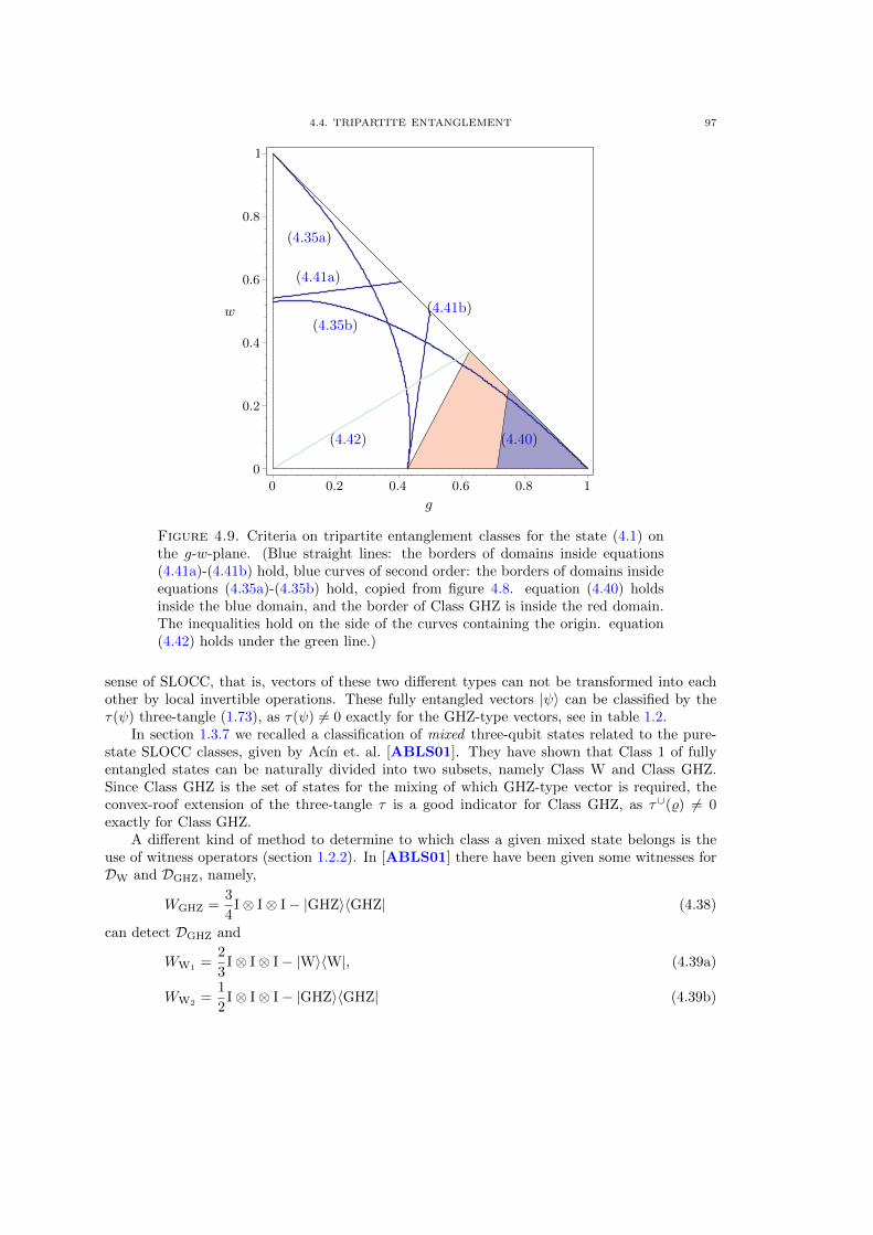
4.4. TRIPARTITE ENTANGLEMENT 97
w
g
0 0.2 0.4 0.6 0.8 1
0
0.2
0.4
0.6
0.8
1
(4.41a)
(4.41b)
(4.40)(4.42)
(4.35a)
(4.35b)
Figure 4.9. Criteria on tripartite entanglement classes for the state (4.1) onthe g-w-plane. (Blue straight lines: the borders of domains inside equations(4.41a)-(4.41b) hold, blue curves of second order: the borders of domains insideequations (4.35a)-(4.35b) hold, copied from figure 4.8. equation (4.40) holdsinside the blue domain, and the border of Class GHZ is inside the red domain.The inequalities hold on the side of the curves containing the origin. equation(4.42) holds under the green line.)
sense of SLOCC, that is, vectors of these two different types can not be transformed into eachother by local invertible operations. These fully entangled vectors |ψ〉 can be classified by theτ(ψ) three-tangle (1.73), as τ(ψ) 6= 0 exactly for the GHZ-type vectors, see in table 1.2.
In section 1.3.7 we recalled a classification of mixed three-qubit states related to the pure-state SLOCC classes, given by Acın et. al. [ABLS01]. They have shown that Class 1 of fullyentangled states can be naturally divided into two subsets, namely Class W and Class GHZ.Since Class GHZ is the set of states for the mixing of which GHZ-type vector is required, theconvex-roof extension of the three-tangle τ is a good indicator for Class GHZ, as τ∪(%) 6= 0exactly for Class GHZ.
A different kind of method to determine to which class a given mixed state belongs is theuse of witness operators (section 1.2.2). In [ABLS01] there have been given some witnesses forDW and DGHZ, namely,
WGHZ =3
4I⊗ I⊗ I− |GHZ〉〈GHZ| (4.38)
can detect DGHZ and
WW1=
2
3I⊗ I⊗ I− |W〉〈W|, (4.39a)
WW2=
1
2I⊗ I⊗ I− |GHZ〉〈GHZ| (4.39b)
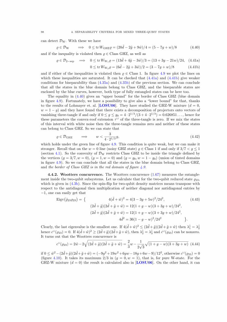
98 4. SEPARABILITY CRITERIA FOR MIXED THREE-QUBIT STATES
can detect DW. With these we have
% ∈ DW =⇒ 0 ≤ trWGHZ% = (20d− 2g + 9w)/4 = (5− 7g + w)/8 (4.40)
and if the inequality is violated then % ∈ Class GHZ, as well as
% ∈ D2−sep =⇒ 0 ≤ trWW1% = (13d+ 4g − 3w)/3 = (13 + 3g − 21w)/24, (4.41a)
0 ≤ trWW2% = (6d− 2g + 3w)/2 = (3− 7g + w)/8 (4.41b)
and if either of the inequalities is violated then % ∈ Class 1. In figure 4.9 we plot the lines onwhich these inequalities are saturated. It can be checked that (4.41a) and (4.41b) give weakerconditions for biseparability than (4.35a) and (4.35b) of the previous section. We can concludethat all the states in the blue domain belong to Class GHZ, and the biseparable states areenclosed by the blue curves, however, both type of fully entangled states can be here too.
The equality in (4.40) gives an “upper bound” for the border of Class GHZ (blue domainin figure 4.9). Fortunately, we have a possibility to give also a “lower bound” for that, thanksto the results of Lohmayer et. al. [LOSU06]. They have studied the GHZ-W mixture (d = 0,w = 1− g) and they have found that there exists a decomposition of projectors onto vectors ofvanishing three-tangle if and only if 0 ≤ g ≤ g0 = 4 · 21/3/(3 + 4 · 21/3) = 0.626851 . . . , hence forthese parameters the convex-roof extension τ∪ of the three-tangle is zero. If we mix the statesof this interval with white noise then the three-tangle remains zero and neither of these statescan belong to Class GHZ. So we can state that
% ∈ DGHZ =⇒ w <3
4 · 21/3g, (4.42)
which holds under the green line of figure 4.9. This condition is quite weak, but we can make itstronger. Recall that on the w = 0 line (noisy GHZ state) % ∈ Class 1 if and only if 3/7 < g ≤ 1(section 4.1). So the convexity of DW restricts Class GHZ to be inside the triangle defined bythe vertices (g = 3/7, w = 0), (g = 1, w = 0) and (g = g0, w = 1− g0) (union of tinted domainsin figure 4.9). So we can conclude that all the states in the blue domain belong to Class GHZ,and the border of Class GHZ is in the red domain of figure 4.9.
4.4.2. Wootters concurrence. The Wootters concurrence (1.67) measures the entangle-ment inside the two-qubit subsystems. Let us calculate that for the two-qubit reduced state %23,which is given in (4.3b). Since the spin-flip for two-qubit density matrices means transpose withrespect to the antidiagonal then multiplication of neither diagonal nor antidiagonal entries by−1, one can easily get that
Eigv(%23%23
)={
4(d+ w)2 = 4(3− 3g + 5w)2/242,
(2d+ g)(2d+ g + w) = 12(1 + g − w)(3 + 3g + w)/242,
(2d+ g)(2d+ g + w) = 12(1 + g − w)(3 + 3g + w)/242,
4d2 = 36(1− g − w)2/242}.
(4.43)
Clearly, the last eigenvalue is the smallest one. If 4(d+ w)2 ≤ (2d+ g)(2d+ g+ w) then λ↓1 = λ↓2hence c∪(%23) = 0. If 4(d+ w)2 ≥ (2d+ g)(2d+ g+ w), then λ↓2 = λ↓3 and c∪(%23) can be nonzero.It turns out that the Wootters concurrence is
c∪(%23) = 2w−2
√(2d+ g)(2d+ g + w) =
2
3w− 1
2√
3
√(1 + g − w)(3 + 3g + w) (4.44)
if 0 ≤ w2− (2d+ g)(2d+ g+ w) = (−9g2 +19w2 +6gw−18g+6w−9)/122, otherwise c∪(%23) = 0(figure 4.10). It takes its maximum 2/3 in (g = 0, w = 1), that is, for pure W-state. For theGHZ-W mixture (d = 0) the result is calculated also in [LOSU06]. On the other hand, it can
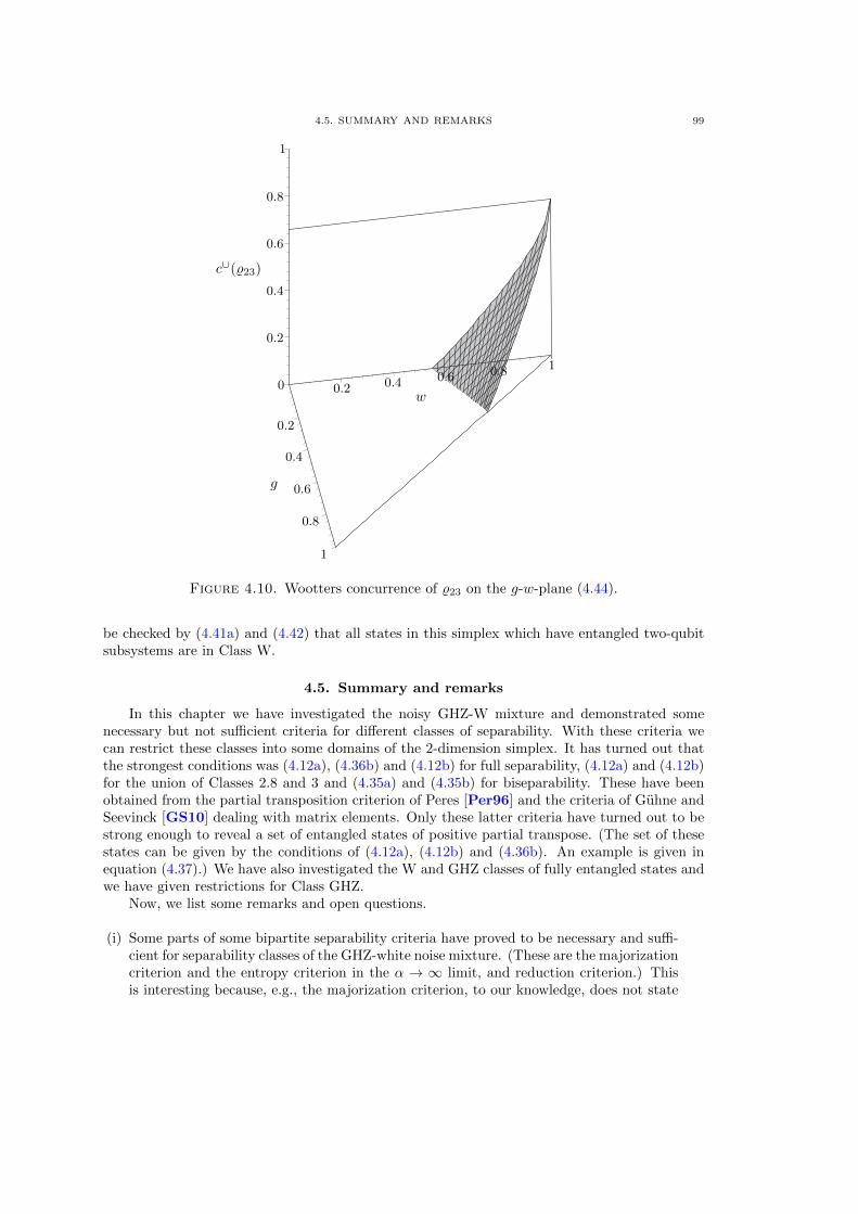
4.5. SUMMARY AND REMARKS 99
c∪(%23)
g
w
0.2
0.4
0.6
0.8
1
0.2 0.4 0.6 0.8 1
0
0.2
0.4
0.6
0.8
1
Figure 4.10. Wootters concurrence of %23 on the g-w-plane (4.44).
be checked by (4.41a) and (4.42) that all states in this simplex which have entangled two-qubitsubsystems are in Class W.
4.5. Summary and remarks
In this chapter we have investigated the noisy GHZ-W mixture and demonstrated somenecessary but not sufficient criteria for different classes of separability. With these criteria wecan restrict these classes into some domains of the 2-dimension simplex. It has turned out thatthe strongest conditions was (4.12a), (4.36b) and (4.12b) for full separability, (4.12a) and (4.12b)for the union of Classes 2.8 and 3 and (4.35a) and (4.35b) for biseparability. These have beenobtained from the partial transposition criterion of Peres [Per96] and the criteria of Guhne andSeevinck [GS10] dealing with matrix elements. Only these latter criteria have turned out to bestrong enough to reveal a set of entangled states of positive partial transpose. (The set of thesestates can be given by the conditions of (4.12a), (4.12b) and (4.36b). An example is given inequation (4.37).) We have also investigated the W and GHZ classes of fully entangled states andwe have given restrictions for Class GHZ.
Now, we list some remarks and open questions.
(i) Some parts of some bipartite separability criteria have proved to be necessary and suffi-cient for separability classes of the GHZ-white noise mixture. (These are the majorizationcriterion and the entropy criterion in the α → ∞ limit, and reduction criterion.) Thisis interesting because, e.g., the majorization criterion, to our knowledge, does not state
100 4. SEPARABILITY CRITERIA FOR MIXED THREE-QUBIT STATES
anything about a density matrix which is majorized by only either of its subsystems.We do not think that this would be more than a coincidence, however, the GHZ state isa very special one so it is an interesting question as to whether this can be generalizedto the n-qubit noisy GHZ state, or to some kinds of generalized GHZ states.
(ii) Another interesting coincidence was that the two settings and measurement vectorsstrong in detection of GHZ and W states are related by local unitary Hadamard trans-formation in the criteria on spin-observables of Seevinck and Uffink (section 4.3.2) andalso in the criteria of Gabriel et. al. (section 4.3.3). The transformation on settings andmeasurement vectors can also be written on the state % 7→ (H⊗3)†%H⊗3, which meansthat we can use the same measurements on the transformed state for the detectionof W state as for the detection of GHZ state. The interesting point here is that thistransformation, being local unitary, does not make a W state from a GHZ state.
(iii) The issue of entangled two-qubit subsystems (section 4.4.2) seems to be interesting. En-tangled two-qubit subsystems arise only in Class W, which is probably the consequenceof the special mixture, but it would be interesting to find some criteria for entangledtwo-qubit subsystems. We will return to this issue in the next chapters, and, as sideresults, we give conditions for this for pure states (section 6.1.3) and for mixed states(section 5.1.3).
CHAPTER 5
Partial separability classification
In section 1.2.3 we have seen how the different partially separable pure states give riseto a classification of mixed states by αk-separable and k-separable states [SU08], written outin the case of three subsystems. Then in the previous chapter we gave some illustrations forrestrictions of some of these classes within a two-parameter simplex of permutation-invariantthree-qubit mixed states.
In this chapter we show that this classification does not take the problem of partial separa-bility of mixed states in the full detail. We extend this classification, moreover, we give necessaryand sufficient criteria for the classes. We call our extended classification PS classification, whichstands for Partial Separability, because this classification is complete in the sense of partial sep-arability, that is, it utilizes all the possible combinations of different kinds of partially separablepure states. We get this finding using the point of view that a state is a mixture of an ensembleof pure states, which leads us to a set of necessary and sufficient criteria for the classes. Wehave seen in section 1.3.3 that in the bipartite case, where a state—either pure or mixed—canbe either separable or entangled, the vanishing of the convex roof extension of local entropies ofpure states is a necessary and sufficient criterion of separability. For us, this is the archetype ofthe general method for the detection of convex subsets by convex roof extensions. However, formore-than-two-partite systems, the partial separability properties have a complicated structure,and, to our knowledge, this method was not used. Instead of that, the usual approach is the useof witness operators, as was done originally for three-qubit systems (section 4.4) or other neces-sary but not sufficient criteria for the detection of convex subsets, some of them were reviewedin chapter 4.
The material of this chapter covers thesis statement IV (page xvi). The organization of thischapter is as follows.
In section 5.1, we elaborate the PS classification for tripartite mixed states. We define thePS subsets (section 5.1.1) and PS classes (section 5.1.2), and we give some examplesfor states which are contained in classes different only under the PS classification (sec-tion 5.1.3). Then we give necessary and sufficient criteria for the identification of the PSclasses and obtain the functions by which these criteria can be formulated (section 5.1.4).
In section 5.2, we generalize the construction for the case of arbitrary number of subsystemsof arbitrary dimensions. We work out the labelling of the PS subsets (section 5.2.1) alongwith that of the PS classes, and give a general conjecture about their non-emptiness (sec-tion 5.2.2). Then we construct the functions identifying the PS subsets and classes withthe minimal requirements (section 5.2.3), and also with stronger requirements leadingto entanglement-monotone functions (section 5.2.4).
In section 5.3, we give a summary and some remarks.
5.1. Partial separability of tripartite mixed states
Here we introduce the PS classification for three subsystems. We have already seen the mainconcept in section 1.2.3, first given in [DCT99, DC00], then used and extended in [SU08,
101
102 5. PARTIAL SEPARABILITY CLASSIFICATION
ABLS01], that we define a density matrix to be the element of a class according to whether itcan or can not be mixed by the use of pure states of some given kinds.
5.1.1. PS subsets. We have H = H1 ⊗ H2 ⊗ H3 with arbitrary d = (d1, d2, d3) localdimensions. Let us introduce some convenient notations for the subsets in the set of extremalpoints P of D given by unit vectors1
P1|2|3 ={π ∈ P
∣∣ π = π1 ⊗ π2 ⊗ π3
}, (5.1a)
Pa|bc ={π ∈ P
∣∣ π = πa ⊗ πbc}, (5.1b)
P123 ≡ P. (5.1c)
We call these pure PS subsets, and they are closed and contain each other in a hierarchic way,which is illustrated in figure 5.1. The meaning of these sets is that their elements can contain “atmost” a given entanglement. We can also introduce the disjoint subsets given by unit vectors ofdifferent partial separability
Q1|2|3 ={π ∈ P
∣∣ π = π1 ⊗ π2 ⊗ π3
}= P1|2|3, (5.2a)
Qa|bc ={π ∈ P
∣∣ π = πa ⊗ πbc, πbc 6= πb ⊗ πc}
= Pa|bc \ P1|2|3, (5.2b)
Q123 ={π ∈ P
∣∣ π 6= πa ⊗ πbc}
= P123 \(P1|23 ∪ P2|13 ∪ P3|12
). (5.2c)
We call these pure PS classes, and they cover P entirely, P = Q1|2|3∪Q1|23∪Q2|13∪Q3|12∪Q123.Except Q1|2|3, none of the above sets are closed. The meaning of these sets is that their elementscontain exactly a given entanglement.
The notion of k-separability and αk-separability, given in [SU08] and recalled in section1.2.3, can be formulated now as the convex hulls of some of the sets (5.2). The 3-separablestates (D3-sep), or equivalently 1|2|3-separable states (D1|2|3) can be mixed from the pure statesof Q1|2|3, that is, they are fully separable. The a|bc-separable states (Da|bc) can be written inthe form
∑i pi%a,i ⊗ %bc,i, (%a,i ∈ D(Ha), %bc,i ∈ D(Hb ⊗Hc),) where we demand only the split
between a and bc, but split between b and c can also occur in the pure state decompositions, sothey can be mixed from the pure states of Q1|2|3 and Qa|bc, that is, of Pa|bc. The 2-separablestates (D2-sep) are of the form
∑i pi%ai,i ⊗ %bici,i, so they can be mixed from the pure states
of Q1|2|3, Q1|23, Q2|13 and Q3|12, that is, of P1|23, P2|13 and P3|12. These states are also ofrelevance, since although they are not separable under any a|bc split, but there is no need ofgenuine tripartite entangled pure state to mix them [SU08]. From the point of view of convexhulls of extremal points, it can be seen better than originally in [SU08] that we can define threenew partial separability sets “between” the a|bc-separable and 2-separable ones. For example,the 2|13-3|12-separable states (D2|13,3|12) are the states which can be mixed from the pure statesof Q1|2|3, Q2|13, and Q3|12, that is, of P2|13, and P3|12. States of this kind are also of relevance,since there is no need of 1|23-separable pure states to mix them, that is, entanglement within23 subsystem. Beyond these, we use the set of 123-separable states (D123), or equivalently 1-separable (D1-sep), which is equal to the full set of states (D). Summarizing, we have the following
1 Remember our convention: The letters a, b and c are variables taking their values in the set of labels L ={1, 2, 3}. When these variables appear in a formula, they form a partition of {1, 2, 3}, so they take always different
values and the formula is understood for all the different values of these variables automatically. Although,sometimes a formula is symmetric under the interchange of two such variables in which case we keep only one ofthe identical formulas.
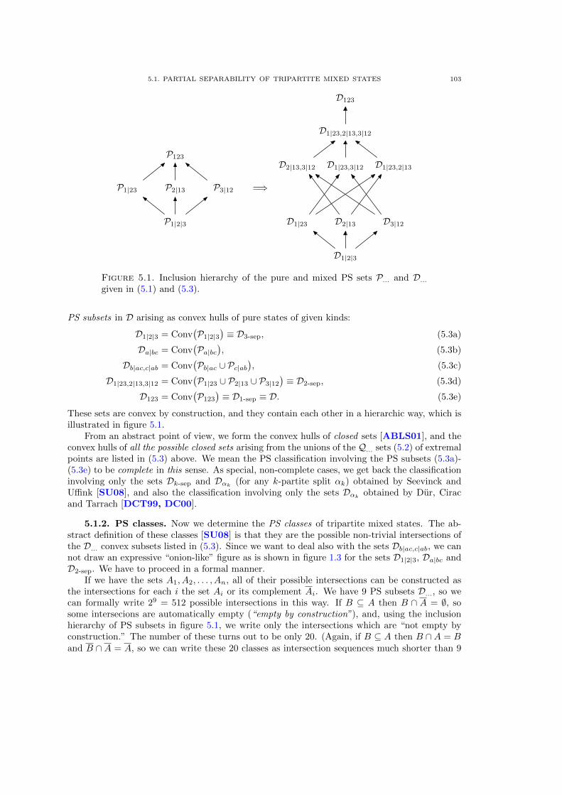
5.1. PARTIAL SEPARABILITY OF TRIPARTITE MIXED STATES 103
P1|2|3
P1|23 P2|13 P3|12
P123
=⇒
D1|2|3
D1|23 D2|13 D3|12
D2|13,3|12 D1|23,3|12 D1|23,2|13
D1|23,2|13,3|12
D123
Figure 5.1. Inclusion hierarchy of the pure and mixed PS sets P... and D...given in (5.1) and (5.3).
PS subsets in D arising as convex hulls of pure states of given kinds:
D1|2|3 = Conv(P1|2|3
)≡ D3-sep, (5.3a)
Da|bc = Conv(Pa|bc
), (5.3b)
Db|ac,c|ab = Conv(Pb|ac ∪ Pc|ab
), (5.3c)
D1|23,2|13,3|12 = Conv(P1|23 ∪ P2|13 ∪ P3|12
)≡ D2-sep, (5.3d)
D123 = Conv(P123
)≡ D1-sep ≡ D. (5.3e)
These sets are convex by construction, and they contain each other in a hierarchic way, which isillustrated in figure 5.1.
From an abstract point of view, we form the convex hulls of closed sets [ABLS01], and theconvex hulls of all the possible closed sets arising from the unions of the Q... sets (5.2) of extremalpoints are listed in (5.3) above. We mean the PS classification involving the PS subsets (5.3a)-(5.3e) to be complete in this sense. As special, non-complete cases, we get back the classificationinvolving only the sets Dk-sep and Dαk (for any k-partite split αk) obtained by Seevinck andUffink [SU08], and also the classification involving only the sets Dαk obtained by Dur, Ciracand Tarrach [DCT99, DC00].
5.1.2. PS classes. Now we determine the PS classes of tripartite mixed states. The ab-stract definition of these classes [SU08] is that they are the possible non-trivial intersections ofthe D... convex subsets listed in (5.3). Since we want to deal also with the sets Db|ac,c|ab, we cannot draw an expressive “onion-like” figure as is shown in figure 1.3 for the sets D1|2|3, Da|bc andD2-sep. We have to proceed in a formal manner.
If we have the sets A1, A2, . . . , An, all of their possible intersections can be constructed asthe intersections for each i the set Ai or its complement Ai. We have 9 PS subsets D..., so wecan formally write 29 = 512 possible intersections in this way. If B ⊆ A then B ∩ A = ∅, sosome intersecions are automatically empty (“empty by construction”), and, using the inclusionhierarchy of PS subsets in figure 5.1, we write only the intersections which are “not empty byconstruction.” The number of these turns out to be only 20. (Again, if B ⊆ A then B ∩A = Band B ∩ A = A, so we can write these 20 classes as intersection sequences much shorter than 9
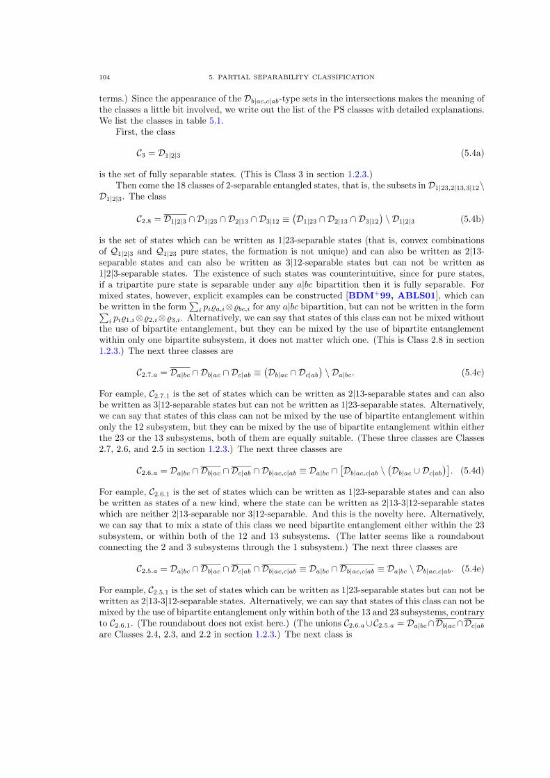
104 5. PARTIAL SEPARABILITY CLASSIFICATION
terms.) Since the appearance of the Db|ac,c|ab-type sets in the intersections makes the meaning ofthe classes a little bit involved, we write out the list of the PS classes with detailed explanations.We list the classes in table 5.1.
First, the class
C3 = D1|2|3 (5.4a)
is the set of fully separable states. (This is Class 3 in section 1.2.3.)Then come the 18 classes of 2-separable entangled states, that is, the subsets in D1|23,2|13,3|12\
D1|2|3. The class
C2.8 = D1|2|3 ∩ D1|23 ∩ D2|13 ∩ D3|12 ≡(D1|23 ∩ D2|13 ∩ D3|12
)\ D1|2|3 (5.4b)
is the set of states which can be written as 1|23-separable states (that is, convex combinationsof Q1|2|3 and Q1|23 pure states, the formation is not unique) and can also be written as 2|13-separable states and can also be written as 3|12-separable states but can not be written as1|2|3-separable states. The existence of such states was counterintuitive, since for pure states,if a tripartite pure state is separable under any a|bc bipartition then it is fully separable. Formixed states, however, explicit examples can be constructed [BDM+99, ABLS01], which canbe written in the form
∑i pi%a,i⊗%bc,i for any a|bc bipartition, but can not be written in the form∑
i pi%1,i⊗%2,i⊗%3,i. Alternatively, we can say that states of this class can not be mixed withoutthe use of bipartite entanglement, but they can be mixed by the use of bipartite entanglementwithin only one bipartite subsystem, it does not matter which one. (This is Class 2.8 in section1.2.3.) The next three classes are
C2.7.a = Da|bc ∩ Db|ac ∩ Dc|ab ≡(Db|ac ∩ Dc|ab
)\ Da|bc. (5.4c)
For eample, C2.7.1 is the set of states which can be written as 2|13-separable states and can alsobe written as 3|12-separable states but can not be written as 1|23-separable states. Alternatively,we can say that states of this class can not be mixed by the use of bipartite entanglement withinonly the 12 subsystem, but they can be mixed by the use of bipartite entanglement within eitherthe 23 or the 13 subsystems, both of them are equally suitable. (These three classes are Classes2.7, 2.6, and 2.5 in section 1.2.3.) The next three classes are
C2.6.a = Da|bc ∩ Db|ac ∩ Dc|ab ∩ Db|ac,c|ab ≡ Da|bc ∩[Db|ac,c|ab \
(Db|ac ∪ Dc|ab
)]. (5.4d)
For eample, C2.6.1 is the set of states which can be written as 1|23-separable states and can alsobe written as states of a new kind, where the state can be written as 2|13-3|12-separable stateswhich are neither 2|13-separable nor 3|12-separable. And this is the novelty here. Alternatively,we can say that to mix a state of this class we need bipartite entanglement either within the 23subsystem, or within both of the 12 and 13 subsystems. (The latter seems like a roundaboutconnecting the 2 and 3 subsystems through the 1 subsystem.) The next three classes are
C2.5.a = Da|bc ∩ Db|ac ∩ Dc|ab ∩ Db|ac,c|ab ≡ Da|bc ∩ Db|ac,c|ab ≡ Da|bc \ Db|ac,c|ab. (5.4e)
For eample, C2.5.1 is the set of states which can be written as 1|23-separable states but can not bewritten as 2|13-3|12-separable states. Alternatively, we can say that states of this class can not bemixed by the use of bipartite entanglement only within both of the 13 and 23 subsystems, contraryto C2.6.1. (The roundabout does not exist here.) (The unions C2.6.a∪C2.5.a = Da|bc∩Db|ac∩Dc|abare Classes 2.4, 2.3, and 2.2 in section 1.2.3.) The next class is
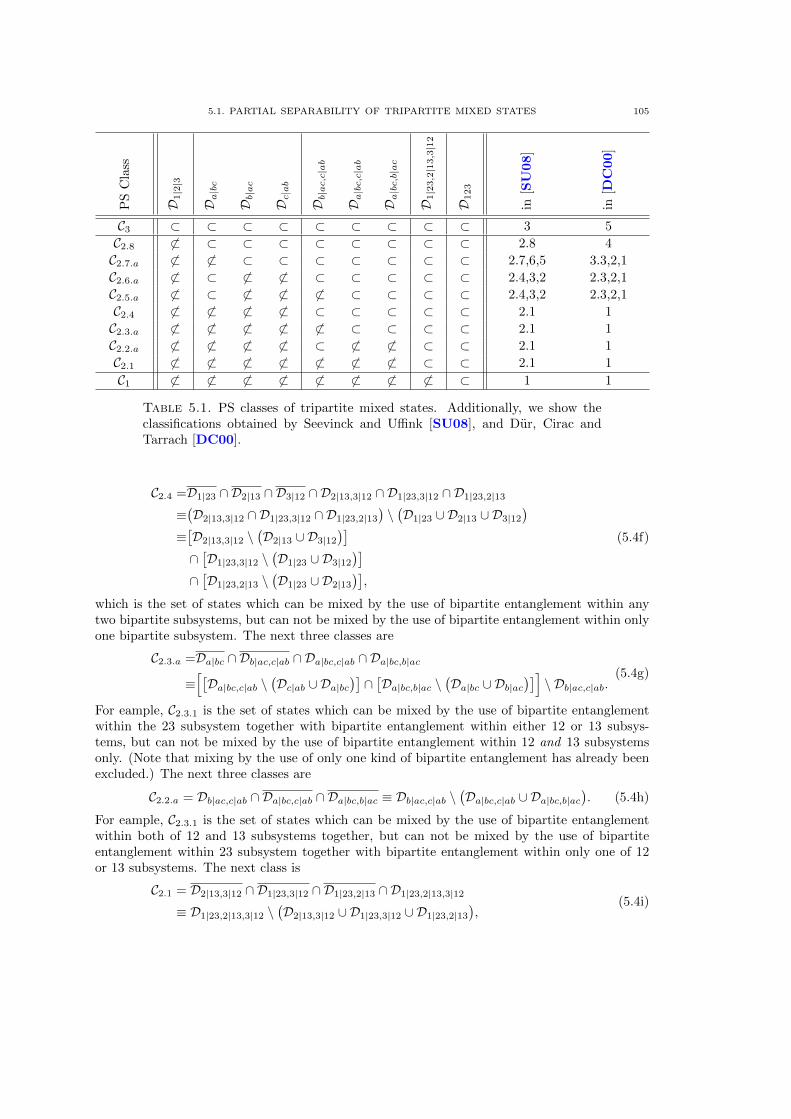
5.1. PARTIAL SEPARABILITY OF TRIPARTITE MIXED STATES 105
PS
Cla
ss
D1|2|3
Da|bc
Db|ac
Dc|ab
Db|ac,c|ab
Da|bc,c|ab
Da|bc,b|ac
D1|2
3,2|1
3,3|1
2
D123
in[S
U08
]
in[D
C00
]
C3 ⊂ ⊂ ⊂ ⊂ ⊂ ⊂ ⊂ ⊂ ⊂ 3 5
C2.8 6⊂ ⊂ ⊂ ⊂ ⊂ ⊂ ⊂ ⊂ ⊂ 2.8 4
C2.7.a 6⊂ 6⊂ ⊂ ⊂ ⊂ ⊂ ⊂ ⊂ ⊂ 2.7,6,5 3.3,2,1
C2.6.a 6⊂ ⊂ 6⊂ 6⊂ ⊂ ⊂ ⊂ ⊂ ⊂ 2.4,3,2 2.3,2,1
C2.5.a 6⊂ ⊂ 6⊂ 6⊂ 6⊂ ⊂ ⊂ ⊂ ⊂ 2.4,3,2 2.3,2,1
C2.4 6⊂ 6⊂ 6⊂ 6⊂ ⊂ ⊂ ⊂ ⊂ ⊂ 2.1 1
C2.3.a 6⊂ 6⊂ 6⊂ 6⊂ 6⊂ ⊂ ⊂ ⊂ ⊂ 2.1 1
C2.2.a 6⊂ 6⊂ 6⊂ 6⊂ ⊂ 6⊂ 6⊂ ⊂ ⊂ 2.1 1
C2.1 6⊂ 6⊂ 6⊂ 6⊂ 6⊂ 6⊂ 6⊂ ⊂ ⊂ 2.1 1
C1 6⊂ 6⊂ 6⊂ 6⊂ 6⊂ 6⊂ 6⊂ 6⊂ ⊂ 1 1
Table 5.1. PS classes of tripartite mixed states. Additionally, we show theclassifications obtained by Seevinck and Uffink [SU08], and Dur, Cirac andTarrach [DC00].
C2.4 =D1|23 ∩ D2|13 ∩ D3|12 ∩ D2|13,3|12 ∩ D1|23,3|12 ∩ D1|23,2|13
≡(D2|13,3|12 ∩ D1|23,3|12 ∩ D1|23,2|13
)\(D1|23 ∪ D2|13 ∪ D3|12
)≡[D2|13,3|12 \
(D2|13 ∪ D3|12
)]∩[D1|23,3|12 \
(D1|23 ∪ D3|12
)]∩[D1|23,2|13 \
(D1|23 ∪ D2|13
)],
(5.4f)
which is the set of states which can be mixed by the use of bipartite entanglement within anytwo bipartite subsystems, but can not be mixed by the use of bipartite entanglement within onlyone bipartite subsystem. The next three classes are
C2.3.a =Da|bc ∩ Db|ac,c|ab ∩ Da|bc,c|ab ∩ Da|bc,b|ac
≡[[Da|bc,c|ab \
(Dc|ab ∪ Da|bc
)]∩[Da|bc,b|ac \
(Da|bc ∪ Db|ac
)]]\ Db|ac,c|ab.
(5.4g)
For eample, C2.3.1 is the set of states which can be mixed by the use of bipartite entanglementwithin the 23 subsystem together with bipartite entanglement within either 12 or 13 subsys-tems, but can not be mixed by the use of bipartite entanglement within 12 and 13 subsystemsonly. (Note that mixing by the use of only one kind of bipartite entanglement has already beenexcluded.) The next three classes are
C2.2.a = Db|ac,c|ab ∩ Da|bc,c|ab ∩ Da|bc,b|ac ≡ Db|ac,c|ab \(Da|bc,c|ab ∪ Da|bc,b|ac
). (5.4h)
For eample, C2.3.1 is the set of states which can be mixed by the use of bipartite entanglementwithin both of 12 and 13 subsystems together, but can not be mixed by the use of bipartiteentanglement within 23 subsystem together with bipartite entanglement within only one of 12or 13 subsystems. The next class is
C2.1 = D2|13,3|12 ∩ D1|23,3|12 ∩ D1|23,2|13 ∩ D1|23,2|13,3|12
≡ D1|23,2|13,3|12 \(D2|13,3|12 ∪ D1|23,3|12 ∪ D1|23,2|13
),
(5.4i)
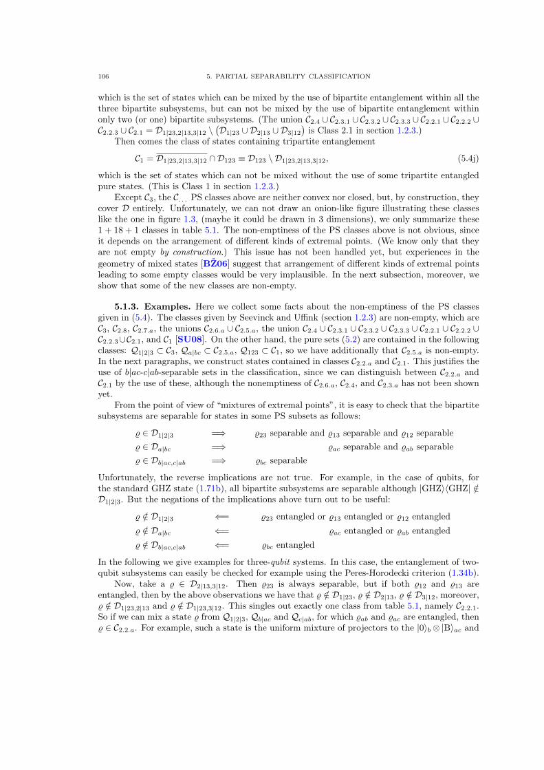
106 5. PARTIAL SEPARABILITY CLASSIFICATION
which is the set of states which can be mixed by the use of bipartite entanglement within all thethree bipartite subsystems, but can not be mixed by the use of bipartite entanglement withinonly two (or one) bipartite subsystems. (The union C2.4 ∪ C2.3.1 ∪ C2.3.2 ∪ C2.3.3 ∪ C2.2.1 ∪ C2.2.2 ∪C2.2.3 ∪ C2.1 = D1|23,2|13,3|12 \
(D1|23 ∪ D2|13 ∪ D3|12
)is Class 2.1 in section 1.2.3.)
Then comes the class of states containing tripartite entanglement
C1 = D1|23,2|13,3|12 ∩ D123 ≡ D123 \ D1|23,2|13,3|12, (5.4j)
which is the set of states which can not be mixed without the use of some tripartite entangledpure states. (This is Class 1 in section 1.2.3.)
Except C3, the C. . . PS classes above are neither convex nor closed, but, by construction, theycover D entirely. Unfortunately, we can not draw an onion-like figure illustrating these classeslike the one in figure 1.3, (maybe it could be drawn in 3 dimensions), we only summarize these1 + 18 + 1 classes in table 5.1. The non-emptiness of the PS classes above is not obvious, sinceit depends on the arrangement of different kinds of extremal points. (We know only that theyare not empty by construction.) This issue has not been handled yet, but experiences in the
geometry of mixed states [BZ06] suggest that arrangement of different kinds of extremal pointsleading to some empty classes would be very implausible. In the next subsection, moreover, weshow that some of the new classes are non-empty.
5.1.3. Examples. Here we collect some facts about the non-emptiness of the PS classesgiven in (5.4). The classes given by Seevinck and Uffink (section 1.2.3) are non-empty, which areC3, C2.8, C2.7.a, the unions C2.6.a ∪ C2.5.a, the union C2.4 ∪ C2.3.1 ∪ C2.3.2 ∪ C2.3.3 ∪ C2.2.1 ∪ C2.2.2 ∪C2.2.3∪C2.1, and C1 [SU08]. On the other hand, the pure sets (5.2) are contained in the followingclasses: Q1|2|3 ⊂ C3, Qa|bc ⊂ C2.5.a, Q123 ⊂ C1, so we have additionally that C2.5.a is non-empty.In the next paragraphs, we construct states contained in classes C2.2.a and C2.1. This justifies theuse of b|ac-c|ab-separable sets in the classification, since we can distinguish between C2.2.a andC2.1 by the use of these, although the nonemptiness of C2.6.a, C2.4, and C2.3.a has not been shownyet.
From the point of view of “mixtures of extremal points”, it is easy to check that the bipartitesubsystems are separable for states in some PS subsets as follows:
% ∈ D1|2|3 =⇒ %23 separable and %13 separable and %12 separable
% ∈ Da|bc =⇒ %ac separable and %ab separable
% ∈ Db|ac,c|ab =⇒ %bc separable
Unfortunately, the reverse implications are not true. For example, in the case of qubits, forthe standard GHZ state (1.71b), all bipartite subsystems are separable although |GHZ〉〈GHZ| /∈D1|2|3. But the negations of the implications above turn out to be useful:
% /∈ D1|2|3 ⇐= %23 entangled or %13 entangled or %12 entangled
% /∈ Da|bc ⇐= %ac entangled or %ab entangled
% /∈ Db|ac,c|ab ⇐= %bc entangled
In the following we give examples for three-qubit systems. In this case, the entanglement of two-qubit subsystems can easily be checked for example using the Peres-Horodecki criterion (1.34b).
Now, take a % ∈ D2|13,3|12. Then %23 is always separable, but if both %12 and %13 areentangled, then by the above observations we have that % /∈ D1|23, % /∈ D2|13, % /∈ D3|12, moreover,% /∈ D1|23,2|13 and % /∈ D1|23,3|12. This singles out exactly one class from table 5.1, namely C2.2.1.So if we can mix a state % from Q1|2|3, Qb|ac and Qc|ab, for which %ab and %ac are entangled, then% ∈ C2.2.a. For example, such a state is the uniform mixture of projectors to the |0〉b⊗ |B〉ac and
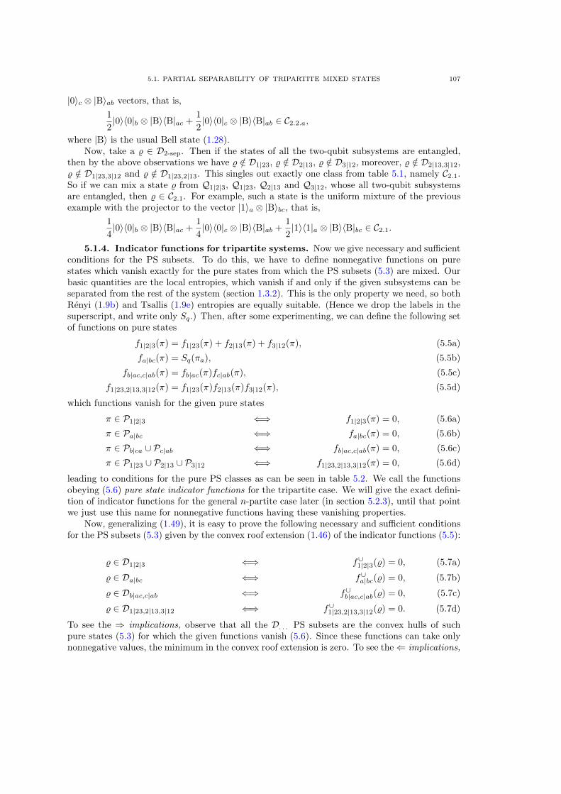
5.1. PARTIAL SEPARABILITY OF TRIPARTITE MIXED STATES 107
|0〉c ⊗ |B〉ab vectors, that is,
1
2|0〉〈0|b ⊗ |B〉〈B|ac +
1
2|0〉〈0|c ⊗ |B〉〈B|ab ∈ C2.2.a,
where |B〉 is the usual Bell state (1.28).Now, take a % ∈ D2-sep. Then if the states of all the two-qubit subsystems are entangled,
then by the above observations we have % /∈ D1|23, % /∈ D2|13, % /∈ D3|12, moreover, % /∈ D2|13,3|12,% /∈ D1|23,3|12 and % /∈ D1|23,2|13. This singles out exactly one class from table 5.1, namely C2.1.So if we can mix a state % from Q1|2|3, Q1|23, Q2|13 and Q3|12, whose all two-qubit subsystemsare entangled, then % ∈ C2.1. For example, such a state is the uniform mixture of the previousexample with the projector to the vector |1〉a ⊗ |B〉bc, that is,
1
4|0〉〈0|b ⊗ |B〉〈B|ac +
1
4|0〉〈0|c ⊗ |B〉〈B|ab +
1
2|1〉〈1|a ⊗ |B〉〈B|bc ∈ C2.1.
5.1.4. Indicator functions for tripartite systems. Now we give necessary and sufficientconditions for the PS subsets. To do this, we have to define nonnegative functions on purestates which vanish exactly for the pure states from which the PS subsets (5.3) are mixed. Ourbasic quantities are the local entropies, which vanish if and only if the given subsystems can beseparated from the rest of the system (section 1.3.2). This is the only property we need, so bothRenyi (1.9b) and Tsallis (1.9e) entropies are equally suitable. (Hence we drop the labels in thesuperscript, and write only Sq.) Then, after some experimenting, we can define the following setof functions on pure states
f1|2|3(π) = f1|23(π) + f2|13(π) + f3|12(π), (5.5a)
fa|bc(π) = Sq(πa), (5.5b)
fb|ac,c|ab(π) = fb|ac(π)fc|ab(π), (5.5c)
f1|23,2|13,3|12(π) = f1|23(π)f2|13(π)f3|12(π), (5.5d)
which functions vanish for the given pure states
π ∈ P1|2|3 ⇐⇒ f1|2|3(π) = 0, (5.6a)
π ∈ Pa|bc ⇐⇒ fa|bc(π) = 0, (5.6b)
π ∈ Pb|ca ∪ Pc|ab ⇐⇒ fb|ac,c|ab(π) = 0, (5.6c)
π ∈ P1|23 ∪ P2|13 ∪ P3|12 ⇐⇒ f1|23,2|13,3|12(π) = 0, (5.6d)
leading to conditions for the pure PS classes as can be seen in table 5.2. We call the functionsobeying (5.6) pure state indicator functions for the tripartite case. We will give the exact defini-tion of indicator functions for the general n-partite case later (in section 5.2.3), until that pointwe just use this name for nonnegative functions having these vanishing properties.
Now, generalizing (1.49), it is easy to prove the following necessary and sufficient conditionsfor the PS subsets (5.3) given by the convex roof extension (1.46) of the indicator functions (5.5):
% ∈ D1|2|3 ⇐⇒ f∪1|2|3(%) = 0, (5.7a)
% ∈ Da|bc ⇐⇒ f∪a|bc(%) = 0, (5.7b)
% ∈ Db|ac,c|ab ⇐⇒ f∪b|ac,c|ab(%) = 0, (5.7c)
% ∈ D1|23,2|13,3|12 ⇐⇒ f∪1|23,2|13,3|12(%) = 0. (5.7d)
To see the ⇒ implications, observe that all the D. . . PS subsets are the convex hulls of suchpure states (5.3) for which the given functions vanish (5.6). Since these functions can take onlynonnegative values, the minimum in the convex roof extension is zero. To see the⇐ implications,
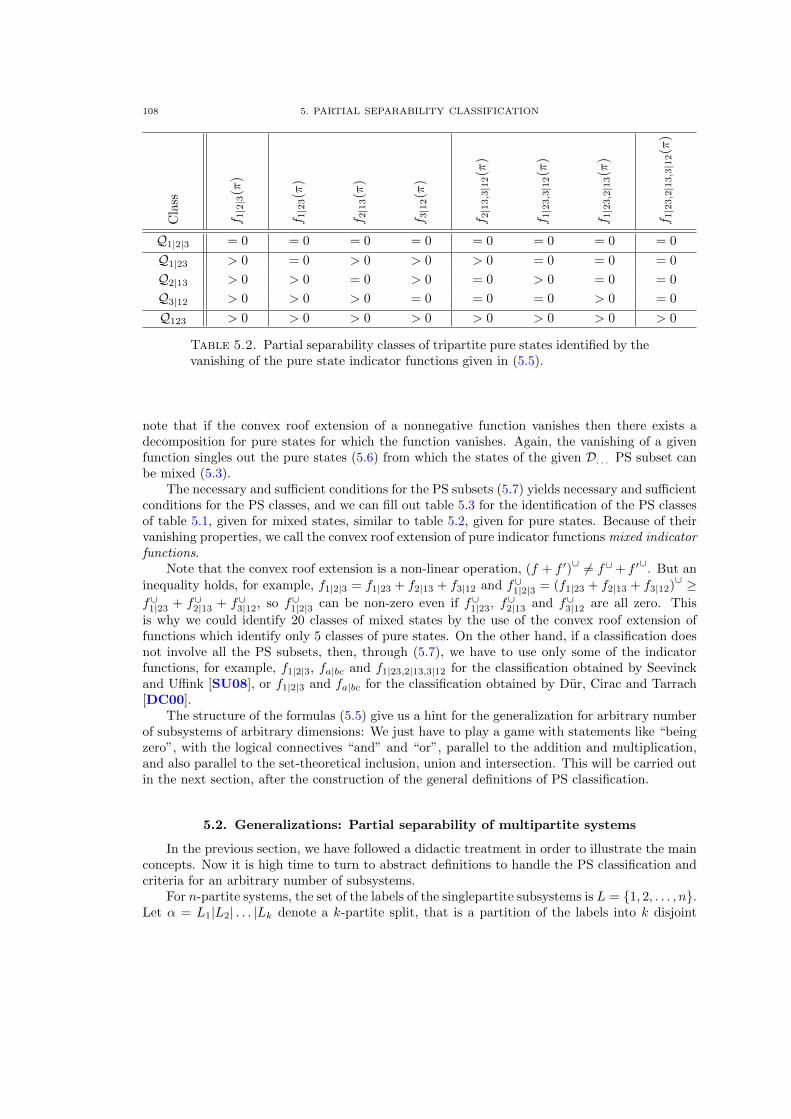
108 5. PARTIAL SEPARABILITY CLASSIFICATION
Cla
ss
f 1|2|3
(π)
f 1|2
3(π
)
f 2|1
3(π
)
f 3|1
2(π
)
f 2|1
3,3|1
2(π
)
f 1|2
3,3|1
2(π
)
f 1|2
3,2|1
3(π
)
f 1|2
3,2|1
3,3|1
2(π
)
Q1|2|3 = 0 = 0 = 0 = 0 = 0 = 0 = 0 = 0
Q1|23 > 0 = 0 > 0 > 0 > 0 = 0 = 0 = 0
Q2|13 > 0 > 0 = 0 > 0 = 0 > 0 = 0 = 0
Q3|12 > 0 > 0 > 0 = 0 = 0 = 0 > 0 = 0
Q123 > 0 > 0 > 0 > 0 > 0 > 0 > 0 > 0
Table 5.2. Partial separability classes of tripartite pure states identified by thevanishing of the pure state indicator functions given in (5.5).
note that if the convex roof extension of a nonnegative function vanishes then there exists adecomposition for pure states for which the function vanishes. Again, the vanishing of a givenfunction singles out the pure states (5.6) from which the states of the given D. . . PS subset canbe mixed (5.3).
The necessary and sufficient conditions for the PS subsets (5.7) yields necessary and sufficientconditions for the PS classes, and we can fill out table 5.3 for the identification of the PS classesof table 5.1, given for mixed states, similar to table 5.2, given for pure states. Because of theirvanishing properties, we call the convex roof extension of pure indicator functions mixed indicatorfunctions.
Note that the convex roof extension is a non-linear operation, (f + f ′)∪ 6= f∪+ f ′
∪. But an
inequality holds, for example, f1|2|3 = f1|23 + f2|13 + f3|12 and f∪1|2|3 = (f1|23 + f2|13 + f3|12)∪ ≥
f∪1|23 + f∪2|13 + f∪3|12, so f∪1|2|3 can be non-zero even if f∪1|23, f∪2|13 and f∪3|12 are all zero. This
is why we could identify 20 classes of mixed states by the use of the convex roof extension offunctions which identify only 5 classes of pure states. On the other hand, if a classification doesnot involve all the PS subsets, then, through (5.7), we have to use only some of the indicatorfunctions, for example, f1|2|3, fa|bc and f1|23,2|13,3|12 for the classification obtained by Seevinckand Uffink [SU08], or f1|2|3 and fa|bc for the classification obtained by Dur, Cirac and Tarrach[DC00].
The structure of the formulas (5.5) give us a hint for the generalization for arbitrary numberof subsystems of arbitrary dimensions: We just have to play a game with statements like “beingzero”, with the logical connectives “and” and “or”, parallel to the addition and multiplication,and also parallel to the set-theoretical inclusion, union and intersection. This will be carried outin the next section, after the construction of the general definitions of PS classification.
5.2. Generalizations: Partial separability of multipartite systems
In the previous section, we have followed a didactic treatment in order to illustrate the mainconcepts. Now it is high time to turn to abstract definitions to handle the PS classification andcriteria for an arbitrary number of subsystems.
For n-partite systems, the set of the labels of the singlepartite subsystems is L = {1, 2, . . . , n}.Let α = L1|L2| . . . |Lk denote a k-partite split, that is a partition of the labels into k disjoint
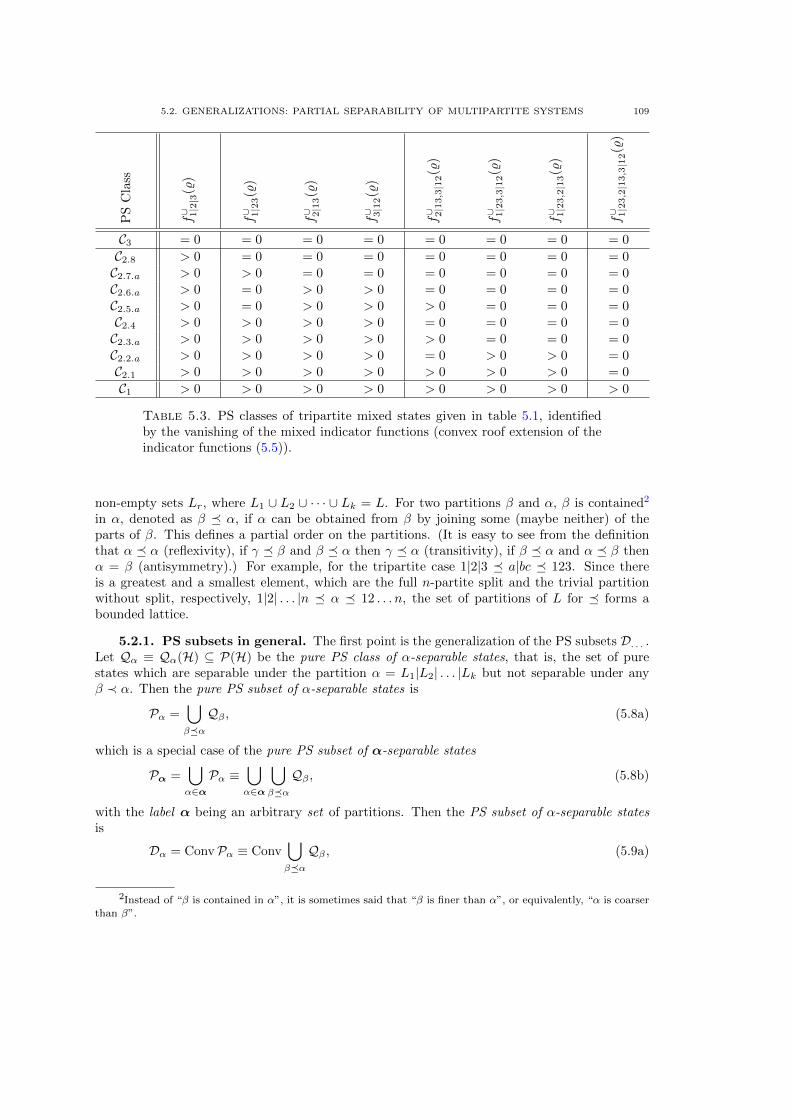
5.2. GENERALIZATIONS: PARTIAL SEPARABILITY OF MULTIPARTITE SYSTEMS 109
PS
Cla
ss
f∪ 1|2|3
(%)
f∪ 1|2
3(%
)
f∪ 2|1
3(%
)
f∪ 3|1
2(%
)
f∪ 2|1
3,3|1
2(%
)
f∪ 1|2
3,3|1
2(%
)
f∪ 1|2
3,2|1
3(%
)
f∪ 1|2
3,2|1
3,3|1
2(%
)
C3 = 0 = 0 = 0 = 0 = 0 = 0 = 0 = 0
C2.8 > 0 = 0 = 0 = 0 = 0 = 0 = 0 = 0C2.7.a > 0 > 0 = 0 = 0 = 0 = 0 = 0 = 0C2.6.a > 0 = 0 > 0 > 0 = 0 = 0 = 0 = 0C2.5.a > 0 = 0 > 0 > 0 > 0 = 0 = 0 = 0C2.4 > 0 > 0 > 0 > 0 = 0 = 0 = 0 = 0C2.3.a > 0 > 0 > 0 > 0 > 0 = 0 = 0 = 0C2.2.a > 0 > 0 > 0 > 0 = 0 > 0 > 0 = 0C2.1 > 0 > 0 > 0 > 0 > 0 > 0 > 0 = 0
C1 > 0 > 0 > 0 > 0 > 0 > 0 > 0 > 0
Table 5.3. PS classes of tripartite mixed states given in table 5.1, identifiedby the vanishing of the mixed indicator functions (convex roof extension of theindicator functions (5.5)).
non-empty sets Lr, where L1 ∪ L2 ∪ · · · ∪ Lk = L. For two partitions β and α, β is contained2
in α, denoted as β � α, if α can be obtained from β by joining some (maybe neither) of theparts of β. This defines a partial order on the partitions. (It is easy to see from the definitionthat α � α (reflexivity), if γ � β and β � α then γ � α (transitivity), if β � α and α � β thenα = β (antisymmetry).) For example, for the tripartite case 1|2|3 � a|bc � 123. Since thereis a greatest and a smallest element, which are the full n-partite split and the trivial partitionwithout split, respectively, 1|2| . . . |n � α � 12 . . . n, the set of partitions of L for � forms abounded lattice.
5.2.1. PS subsets in general. The first point is the generalization of the PS subsets D. . . .Let Qα ≡ Qα(H) ⊆ P(H) be the pure PS class of α-separable states, that is, the set of purestates which are separable under the partition α = L1|L2| . . . |Lk but not separable under anyβ ≺ α. Then the pure PS subset of α-separable states is
Pα =⋃β�α
Qβ , (5.8a)
which is a special case of the pure PS subset of α-separable states
Pα =⋃α∈αPα ≡
⋃α∈α
⋃β�α
Qβ , (5.8b)
with the label α being an arbitrary set of partitions. Then the PS subset of α-separable statesis
Dα = ConvPα ≡ Conv⋃β�α
Qβ , (5.9a)
2Instead of “β is contained in α”, it is sometimes said that “β is finer than α”, or equivalently, “α is coarserthan β”.
110 5. PARTIAL SEPARABILITY CLASSIFICATION
which is a special case of the PS subsets of α-separable states
Dα = ConvPα ≡ Conv⋃α∈αPα ≡ Conv
⋃α∈α
⋃β�α
Qβ ≡ Conv⋃α∈αDα, (5.9b)
with the label α. (In the writing we omit the {. . . } set-brackets, as was seen, e.g., in (5.3c).)The set of k-separable states Dk-sep arises as a special case where the α elements of α are allthe possible k-partite splits. Note that in general the α ∈ α partitions are not required to bek-partite splits for the same k. This freedom can not be seen in the case of three subsystems.
The Qβ sets are not closed if and only if β is not the full n-partite split 1|2| . . . |n, butPα = ∪β�αQβ is closed, so the sets Dα are closed, and convex by construction. Note thatdifferent α labels can give rise to the same Dα sets, in other words, the α 7→ Dα “labellingmap” defined by (5.9b) is surjective but not injective. For the full PS classification we need allthe possible different Dα sets. Because of the non-trivial structure of the lattice of partitions,obtaining all the different PS sets is also a non-trivial task. We can not provide a closed formulafor that, but only an algorithm. Before we do this, we need some constructions.
First, observe that if β � α then Dβ ⊆ Dα, (from definition (5.9a), and the transitivity of �)from which it follows that for the labels β and α, if for every β ∈ β there is an α ∈ α for whichβ � α then Dβ ⊆ Dα. (From definition (5.9b). Later we will prove the reverse too.) Theseobservations motivate the extension of � from the partitions to the labels as
β � αdef.⇐⇒ ∀β ∈ β,∃α ∈ α : β � α. (5.10)
Note that, at this point, the relation � on the labels is not a partial order, only the reflexivityand the transitivity properties hold. The antisymmetry property fails, which is the consequenceof that the definition (5.10) was motivated by the inclusion of the PS sets, and different αscan lead to the same PS set. Independently of this problem, which will be handled later, thefollowing is true.
Proposition 5.2.1. For α,β labels
β � α ⇐⇒ Dβ ⊆ Dα. (5.11)
Proof. This can be shown in the following steps:
Dβ ⊆ Dα(i)⇐⇒ Conv
⋃β∈β
⋃δ�β
Qδ ⊆ Conv⋃α∈α
⋃γ�α
Qγ
(ii)⇐⇒⋃β∈β
⋃δ�β
Qδ ⊆⋃α∈α
⋃γ�α
Qγ
(iii)⇐⇒ ∀β ∈ β,∀δ � β,∃α ∈ α : δ � α(iv)⇐⇒ ∀β ∈ β,∃α ∈ α : β � α(v)⇐⇒ β � α.
The equivalences (i) and (v) are by definition (5.9b) and (5.10), respectively.Equivalence (ii) is the only one where it comes into the picture that the story is about
quantum states. The(ii)⇐= implication holds, since it is true in general that ConvB ⊆ ConvA⇐
B ⊆ A. But to the(ii)=⇒ implication we have to use some special properties coming from geometry.
Obviously, for the extremal points
Extr Conv⋃β∈β
⋃δ�β
Qδ ⊆ Conv⋃β∈β
⋃δ�β
Qδ ⊆ Conv⋃α∈α
⋃γ�α
Qγ ,
5.2. GENERALIZATIONS: PARTIAL SEPARABILITY OF MULTIPARTITE SYSTEMS 111
so π ∈ Extr Conv⋃β∈β
⋃δ�β Qδ is also the element of Conv
⋃α∈α
⋃γ�αQγ . But π is a projector
of rank one, so it is extremal also in Conv⋃α∈α
⋃γ�αQγ . This holds for all such π, so we have
that
Extr Conv⋃β∈β
⋃δ�β
Qδ ⊆ Extr Conv⋃α∈α
⋃γ�α
Qγ .
Any A sets of projectors of rank one have the property that A = Extr ConvA, that is, they are
all extremal points of their convex hulls, which leads to the(ii)=⇒ implication.
Equivalence (iii) comes from set algebra. To see the(iii)=⇒ implication, we note that the Q...
sets are disjoint, so every Qδ on the left-hand side of the inclusion appears on the right-hand side
as a Qγ , which means that ∀β ∈ β, ∀δ � β, ∃α ∈ α so that δ � α. To see the(iii)⇐= implication,
from the condition ∃α so that Qδ ⊆⋃γ�αQγ , but for different δ � βs there may exist different
αs, so⋃δ�β Qδ ⊆
⋃α∈α
⋃γ�αQγ , which holds for all β ∈ β.
Equivalence (iv) comes from the properties of partial ordering. First, � is reflexive on
partitions, that is, β � β, so the(iv)=⇒ implication follows from the δ = β choice. On the other
hand, � is transitive on partitions, which is just the(iv)⇐= implication: for all δ, if δ � β and
β � α then δ � α. �
Again, note that the relations � and ⊆ are defined on non-isomorphic sets, so (5.11) doesnot contradict the fact that the latter is a partial order while the former is not.
The next step is to define those labels for which � is a partial order. A label α is calledproper label, if
∀α, α′ ∈ α, α 6= α′ =⇒ α � α′. (5.12)
With this, we have the following.
Proposition 5.2.2. On the set of proper labels, the relation � defined in (5.10) is a partialorder.
Proof. Reflexivity on labels: We need that α � α, so by definition (5.10) ∀α ∈ α ∃α′ ∈ αfor which α � α′. This holds for the α′ = α choice, since � is reflexive on partitions, α � α.
Transitivity on labels: Suppose that β � α and γ � β, so by definition (5.10) ∀γ ∈ γ ∃β ∈ βfor which γ � β, and for this β ∃α ∈ α for which β � α. Since � is transitive on partitions, wehave that ∀γ ∈ γ ∃α ∈ α for which γ � α, which is γ � α by definition (5.10).
Antisymmetry on proper labels: Let α and β be proper labels. Suppose that β � α andα � β, so by definition (5.10) ∀β ∈ β ∃α ∈ α for which β � α, and for this α ∃β′ ∈ β forwhich α � β′. Since � is transitive on partitions, we have that β � β′. This can be true only ifβ = β′, since β is a proper label, so we have that β � α and α � β. Since � is antisymmetric onpartitions, we have that ∀β ∈ β, ∃α ∈ α for which α = β, which means that β ⊆ α. (The labelsare sets.) Interchanging the roles of α and β, we have that α ⊆ β. Since ⊆ is antisymmetric onsets, we have that β = α. �
A corollary is that the set of proper labels for � forms a bounded lattice, its greatest andsmallest elements are the one-element labels of full n-partite split and the trivial partition withoutsplit, respectively, 1|2| . . . |n � α � 12 . . . n.
Is it true that every PS subset can be labelled by proper label? And different proper labelslead to different PS subsets? In other words, is the α 7→ Dα “labelling map” from the set ofproper labels to the set of PS subsets an isomorphism? The injectivity is the⇐ implication fromthe next observation.

112 5. PARTIAL SEPARABILITY CLASSIFICATION
Proposition 5.2.3. For α, β proper labels
β = α ⇐⇒ Dβ = Dα. (5.13)
Proof. Let α and β be proper labels. The above can be shown in the following steps:
Dβ = Dα(i)⇐⇒ Dβ ⊆ Dα and Dα ⊆ Dβ
(ii)⇐⇒ β � α and α � β
(iii)⇐⇒ β = α.
Equivalence (i) is the antisymmetry of ⊆ on sets, equivalence (ii) is (5.11) on labels, equivalence(iii) is the antisymmetry of � on proper labels. �
If β is a label, then we can obtain a unique proper label from that if we drop every β ∈ βfor which there is a β′ ∈ β for which β � β′. The remaining partitions form a proper label whichwe denote α, and the partitions which have been dropped out form a label which we denote γ.Then β = αγ, which means the union of labels α and γ. (We omit the union sign too.) Ournext observation is useful for this case.
Proposition 5.2.4. For the general labels α and γ,
γ � α ⇐⇒ Dαγ = Dα, (5.14)
Proof. This can be shown in the following steps:
Dαγ = Dα(i)⇐⇒ Dαγ ⊆ Dα and Dα ⊆ Dαγ
(ii)⇐⇒ αγ � α and α � αγ
(iii)⇐⇒ γ � α.
Equivalence (i) is the antisymmetry of ⊆ on sets, equivalence (ii) is (5.11) on labels, (α � αγholds always) equivalence (iii) is from the observation that β � α and β′ � α if and only ifββ′ � α, which can easily be seen from the definition (5.10). �
This means that when we obtain a proper label α from a general label β, as was done above,both of these lead to the same PS subset. Since all PS subsets arise from general labels, theabove shows that they arise also from proper labels, which is the surjectivity of the labelling byproper labels.
Now we have that the set of proper labels is isomorphic to the set of PS subsets. The formerone is much easier to handle. Moreover, (5.11) states now that the lattice of α proper labels withrespect to the partial order � is isomorphic to the lattice of Dα PS subsets with respect to thepartial order ⊆. (This lattice is the generalization of the “inclusion hierarchy” in figure 5.1.) Toget all the PS subsets, we have to obtain all the proper labels. A brute force method for this isto form all the β labels (all the subsets of the set of all partitions), then obtain the proper labelsα as before (β = αγ), and keep the different proper labels obtained in this way. This algorithmis very ineffective, we give a much more optimized one.
To obtain an efficient algorithm generating the proper labels of all PS subsets, it is necessaryto consider the labels as l-tuples of partitions instead of sets of partitions. In this case α =α1, α2, . . . , αl, so the order of the elements is considered to be fixed when an l-tuple is given, andthe αjs are different for different js. (The (. . . ) l-tuple-brackets are omitted. Note that, contraryto the notation used in [SU08], the lower index of the partitions αj here does not refer to the knumber of Lr sets in αj .) Using ordered structure has further advantages beyond the obvious one
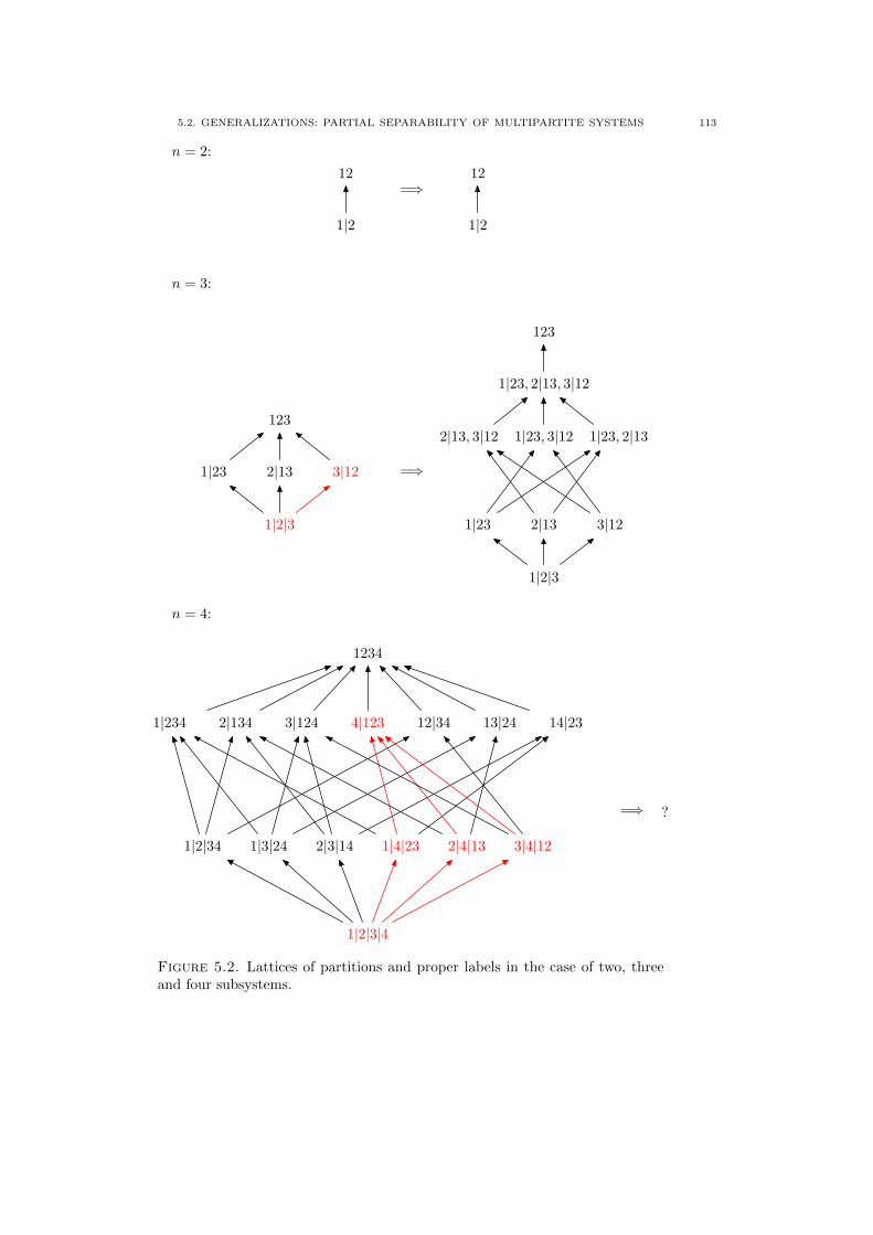
5.2. GENERALIZATIONS: PARTIAL SEPARABILITY OF MULTIPARTITE SYSTEMS 113
n = 2:
1|2
12
=⇒
1|2
12
n = 3:
1|2|3
1|23 2|13 3|12
123
=⇒
1|2|3
1|23 2|13 3|12
2|13, 3|12 1|23, 3|12 1|23, 2|13
1|23, 2|13, 3|12
123
n = 4:
1|2|3|4
1|2|34 1|3|24 2|3|14 1|4|23 2|4|13 3|4|12
1|234 2|134 3|124 4|123 12|34 13|24 14|23
1234
=⇒ ?
Figure 5.2. Lattices of partitions and proper labels in the case of two, threeand four subsystems.
114 5. PARTIAL SEPARABILITY CLASSIFICATION
that a computer stores data sequentially, so implementing sets would mean additional difficulty.Now the algorithm is the following.
Algorithm 5.2.5.
(1) [initialization] Fix an order of the partitions, this defines a lexicographical ordering forl-tuples of partitions. This is denoted by <. (This is to avoid obtaining an l-tuple morethan once and to make the algorithm more optimized.)
(2) [level 1] Using this ordering, we have all the 1-tuples of partitions ordered lexicographi-cally.
(3) [induction step: obtaining the l + 1-tuples of partitions (level l + 1) from the l-tuplesof partitions (level l)] To every α = α1, α2, . . . , αl l-tuples (coming in lexicographicallyordered sequence) we have to append any such partition αl+1 (coming in lexicographi-cally ordered sequence) that(i) αl+1 � αj and αj � αl+1 for all j = 1, 2, . . . , l, and(ii) αl+1 > αl. (Because of the lexicographical order <, it is enough to consider onlythe last (lth) partition.)Then the resulting α = α1, α2, . . . , αl, αl+1 l+ 1-tuples, and also the partitions in everysuch l + 1-tuple are ordered lexicographically.
The algorithm stops when no new partition can be appended to any of the l-tuples, which comesin finite steps, since the number of all the partitions is finite.
This algorithm generates the lattice of proper labels from the lattice of partitions, see in figure5.2. We note, however, that the number of proper labels is so high even for four subsystems (morethan a hundred) that the lattice of proper labels can be handled only in computer.
5.2.2. PS classes in general. The second point is the generalization of the PS classes C...,which are the possible non-trivial intersections of the PS subsets D.... Constructing these needsdirect calculations for a given n, as was done in section 5.1.2.
Let us divide the set of proper labels into two disjoint subsets, α and β, then all the possibleintersections of PS subsets can be labelled by such a pair, which is called class-label, as
Cα,β =⋂α∈αDα ∩
⋂β∈β
Dβ. (5.15)
It can happen that Cα,β = ∅ by construction, by that we mean that its emptiness follows from the
inclusion hierarchy of PS subsets. For example, if Dβ ⊆ Dα for some α ∈ α and β ∈ β, then theintersection above is identically empty. The PS classes for three subsystems in subsection 5.1.2were obtained by the use of this observation. In this general framework, this observation isformulated as follows:
Cα,β = ∅ (i)⇐⇒⋃α∈αDα ∩
⋂β∈β
Dβ = ∅
(ii)⇐⇒⋂β∈β
Dβ ⊆⋃α∈αDα
(iii)⇐= ∃α ∈ α,∃β ∈ β : Dβ ⊆ Dα
(iv)⇐⇒ ∃α ∈ α,∃β ∈ β : β � α.
Proof. Equivalence (i) comes from De Morgan’s law A ∩ B = A ∪B. Equivalence (ii)comes from the identity B ⊆ A⇔ (B ∩A ≡ B \A = ∅). Implication (iii) comes from B ⊆ A⇒(B ∩B′ ⊆ A ∪A′). Equivalence (iv) is (5.11). �
5.2. GENERALIZATIONS: PARTIAL SEPARABILITY OF MULTIPARTITE SYSTEMS 115
Implication (iii) is the point which makes possible to formulate the emptiness of PS classespurely by the use of labels. That is still a question whether implication (iii) can be replaced by astronger one, which leads to condition involving only labels again. (The problem is that we haveno interpretations of ∩ and ∪ in the language of labels.) Our first conjecture is that implication(iii) above is the strongest one which leads to a condition involving only labels.
Summarizing, we have
Cα,β = ∅ ⇐= ∃α ∈ α,∃β ∈ β : β � α. (5.16a)
If the right-hand side holds then we say, according to the conjecture above, that Cα,β is empty
by construction. Since this implication is only one-way, it could happen that Cα,β = ∅ for such
class-label α,β for which the right-hand side does not hold, resulting in a class which is emptybut not by construction. But we think that this can not happen: our second conjecture is thatthere is an equivalence in (5.16a), that is, all the PS classes which are not empty by constructionare non-empty.3 The motivation of this is the same as in the tripartite case (see at the end ofsubsection 5.1.2), where the PS classes conjectured to be non-empty was obtained under thesame assumptions.
An advantage of the formulation by the labelling constructions is, roughly speaking, thatby the use of that “we have separated the algebraic and the geometric part” of the problemof non-emptiness of the classes. At this point, it seems that we have tackled all the algebraicissues of the problem, and these conjectures can not be proven without the investigation of thegeometry of D, more precisely, the geometry of the different kinds of Qα extremal points.
The negation of (5.16a) leads to
Cα,β 6= ∅ =⇒ ∀α ∈ α,∀β ∈ β : β � α, (5.16b)
so if we obtain all α,β class-labels for which the right-hand side of this holds (“non-emptiness-by-construction”) then we will have all the non-empty classes, together with some empty classesif the second conjecture does not hold. Because of the nontrivial structure of the lattice of properlabels, obtaining all the class-labels leading to not-empty-by-construction classes is also a non-trivial task. The number of all the partitions of n grows rapidly [oeib, oeia], which is only thenumber of the PS subsets of α-separability Dα. So the number of all the PS subsets Dα growsmore rapidly, and the number of all the PS classes Cα,β grows even more rapidly. But at least,
it is finite.
5.2.3. Indicator functions in general. The third point is the generalization of the indi-cator functions (5.5). This is carried out in four steps.
(i) Let F : D(HK)→ R be a continuous function for all K ⊂ L, that is, for all subsystems.The only condition on F is
F (%) ≥ 0, with equality if and only if % is pure, (5.17)
for example, the von Neumann entropy, any Tsallis or Renyi entropies are suitable. (Note that theadditional requirements of the features of LU-invariance, convexity, Schur-concavity, additivity,being homogeneous polynomial, etc., are only optional, they are not needed for the construction.)For all K ⊂ L subsystems, let the following functions on pure states be defined
fK : P(H) −→ R,fK(π) = F (πK),
(5.18)
3 This implies the first conjecture above, but it can still happen that implication (iii) can be replaced by astronger condition, so the first conjecture is false. Then the (5.16a) definition of the emptiness-by-constructionchanges, and the second conjecture concerns this new definition.
116 5. PARTIAL SEPARABILITY CLASSIFICATION
where πK = trK(π) with K = L \ K. Then, for the k-partite split α = L1|L2| . . . |Lk, fLridentifies the bipartite split Lr|Lr (where Lr = L \ Lr),
fLr (π) = 0 ⇐⇒ π ∈ PLr|Lr ≡⋃
β�Lr|Lr
Qβ , (5.19)
which is the consequence of (5.17). Note that α is the greatest element which is smaller thanLr|Lr for all r.
(ii) Then the function
fα(π) =
k∑r=1
fLr (π) (5.20)
has the ability to identify the k-partite split α,
fα(π) = 0 ⇐⇒ π ∈ Pα ≡⋃β�α
Qβ . (5.21)
All nonnegative fα functions satisfying (5.21) are called α-indicator functions, not only the onesdefined in (5.20).
(iii) The generalization of (5.20) for more-than-one partitions, that is, for all labels, is definedas
fα(π) =∏α∈α
fα(π), (5.22)
being the generalization of (5.5). It vanishes exactly for the appropriate Qα sets,
fα(π) = 0 ⇐⇒ π ∈ Pα ≡⋃α∈αPα. (5.23)
All nonnegative fα functions satisfying (5.23) are called α-indicator functions, not only the onesdefined in (5.22). For example, in the next chapter for the three-qubit case, a special set ofindicator functions will be given, which will be constructed not by (5.22), but it will still satisfy(5.23).
(iv) Now, the vanishing of their convex roof extension
f∪α(%) = min∑i
pifα(πi)
identify the PS sets,
f∪α(%) = 0 ⇐⇒ % ∈ Dα ≡ ConvPα, (5.24)
being the generalization of (5.7). Indeed, f∪α(%) = 0 if and only if there exists a decomposition% =
∑i piπi such that fα(πi) = 0 for all i (fα is nonnegative), which means that πi ∈ Pα (5.23),
which means that % ∈ Dα.
5.2.4. Entanglement-monotone indicator functions in general. As we have seen insection 1.3.1, entanglement-monotonicity is a fundamental property of all entanglement measures.Here we repeat the constructions above with a slight modification, leading to indicator functionswhich are entanglement-monotones. These are denoted by m in contrast with the general f .
(i) It has been shown in [Vid00, Hor01] that if F : D(HK) → R is unitary-invariant andconcave, then the fK functions defined in (5.18) are non-increasing on average for pure states,that is, they obey (1.44), which is entanglement monotonity for pure states. So let
mK(π) = M(πK) (5.25)
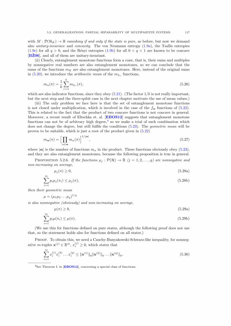
5.2. GENERALIZATIONS: PARTIAL SEPARABILITY OF MULTIPARTITE SYSTEMS 117
with M : D(HK) → R vanishing if and only if the state is pure, as before, but now we demandalso unitary-invariace and concavity. The von Neumann entropy (1.9a), the Tsallis entropies(1.9e) for all q > 0, and the Renyi entropies (1.9b) for all 0 < q < 1 are known to be concave
[BZ06], and all of them are unitary-invariant.(ii) Clearly, entanglement monotone functions form a cone, that is, their sums and multiples
by nonnegative real numbers are also entanglement monotones, so we can conclude that thesums of the functions mK are also entanglement monotones. Here, instead of the original sumsin (5.20), we introduce the arithmetic mean of the mLr functions,
mα(π) =1
k
k∑r=1
mLr (π), (5.26)
which are also indicator functions, since they obey (5.21). (The factor 1/k is not really important,but the next step and the three-qubit case in the next chapter motivate the use of mean values.)
(iii) The only problem we face here is that the set of entanglement monotone functionsis not closed under multiplication, which is involved in the case of the fα functions of (5.22).This is related to the fact that the product of two concave functions is not concave in general.Moreover, a recent result of Eltschka et. al. [EBOS12] suggests that entanglement monotonefunctions can not be of arbitrary high degree,4 so we make a trial of such combination whichdoes not change the degree, but still fulfils the conditions (5.23). The geometric mean will beproven to be suitable, which is just a root of the product given in (5.22)
mα(π) =[∏α∈α
mα(π)]1/|α|
, (5.27)
where |α| is the number of functions mα in the product. These functions obviously obey (5.23),and they are also entanglement monotones, because the following proposition is true in general.
Proposition 5.2.6. If the functions µj : P(H) → R (j = 1, 2, . . . , q) are nonnegative andnon-increasing on average,
µj(π) ≥ 0, (5.28a)m∑i=1
piµj(πi) ≤ µj(π), (5.28b)
then their geometric mean
µ = (µ1µ2 . . . µq)1/q
is also nonnegative (obviously) and non-increasing on average,
µ(π) ≥ 0, (5.29a)m∑i=1
piµ(πi) ≤ µ(π). (5.29b)
(We use this for functions defined on pure states, although the following proof does not usethat, so the statement holds also for functions defined on all states.)
Proof. To obtain this, we need a Cauchy-Bunyakowski-Schwarz-like inequality, for nonneg-
ative m-tuples x(j) ∈ Rm, x(j)i ≥ 0, which states that
m∑i=1
x(1)i x
(2)i . . . x
(q)i ≤ ‖x
(1)‖q‖x(2)‖q . . . ‖x(q)‖q, (5.30)
4See Theorem I. in [EBOS12], concerning a special class of functions.

118 5. PARTIAL SEPARABILITY CLASSIFICATION
where the usual q-norm is
‖x‖q =[ m∑i=1
xqi
]1/q. (5.31)
Indeed, if x(j) = 0 for some j then the inequality holds trivially, else
m∑i=1
x(1)i
‖x(1)‖qx
(2)i
‖x(2)‖q. . .
x(q)i
‖x(q)‖q≡
m∑i=1
[(x
(1)i )q
‖x(1)‖qq(x
(2)i )q
‖x(2)‖qq. . .
(x(q)i )q
‖x(q)‖qq
]1/q
≤m∑i=1
1
q
[(x
(1)i )q
‖x(1)‖qq+
(x(2)i )q
‖x(2)‖qq+ · · ·+ (x
(q)i )q
‖x(q)‖qq
]= 1,
where the inequality follows from the inequality of the arithmetic and geometric means, appliedto all terms in the sum. Using this,
m∑i=1
piµ(πi) =
m∑i=1
pi[µ1(πi)µ2(πi) . . . µq(πi)
]1/q=
m∑i=1
[piµ1(πi)
]1/q[piµ2(πi)
]1/q. . .[piµq(πi)
]1/q≤[ m∑i=1
piµ1(πi)]1/q[ m∑
i=1
piµ2(πi)]1/q
. . .[ m∑i=1
piµq(πi)]1/q
≤[µ1(π)
]1/q[µ2(π)
]1/q. . .[µq(π)
]1/q= µ(π),
where the first inequality is (5.30) for x(j)i =
[piµj(πi)
]1/q, and the second inequality is the
condition (5.28b). �
(iv) Now, mα of (5.27) is entanglement monotone, that is, non-increasing on average forpure states (1.44), so, thanks to (1.48), its convex roof extension
m∪α(%) = min∑i
pimα(πi) (5.32)
is also non-increasing on average (1.43c) so entanglement-monotone, and also identifies the PSsubsets
m∪α(%) = 0 ⇐⇒ % ∈ Dα, (5.33)
as in (5.24).
5.3. Summary and remarks
In this chapter we have constructed the complete PS classification of multipartite quantumstates by the PS classes arising from the PS subsets (5.9b), together with necessary and sufficientconditions for the identification of the PS classes through the necessary and sufficient conditionsfor the identification of the PS subsets (5.24) by indicator functions arising as convex roof ex-tensions of the pure state indicator functions (5.22). The indicator functions can be constructedso as to be entanglement-monotone (subsection 5.2.4). We have also discussed the PS classes inthe tripartite case in detail.
Now, we list some remarks and open questions.
5.3. SUMMARY AND REMARKS 119
(i) As was mentioned before, this PS classification scheme is an extension of the classificationbased on k-separability and αk-separability given by Seevinck and Uffink [SU08], whichis the extension of the classification dealing only with αk-separability given by Dur andCirac [DCT99, DC00].
(ii) The non-emptiness of the new classes was only conjectured. More fully, we could notgive neccessary and sufficient condition for the non-emptiness of the PS classes in thepurely algebraic language of labels. Probably, methods from geometry or calculus wouldbe needed to solve this puzzle (subsection 5.2.2).
(iii) In close connection with this, a further geometry-related conjecture could be draftedabout the non-empty classes: they are of non-zero measure. It is known in the bipartitecase that the separable states are of non-zero measure [ABLS01, BZ06], which canmotivate this conjecture. If the D1|2|...|n PS subset of fully separable states is of non-zero measure, then this is true for all Dα PS subsets. However, the PS classes arise asintersections of these.
(iv) The necessary and sufficient criteria of the classes was given by convex roof extensions,which has advantages and disadvantages.
(v) First of all, convex roof extensions are hard to calculate [RLL09, RLL11]. However, aswe have seen in chapter 4, neccessary and sufficient criteria for the detection of convexsubsets seem always to be hard to calculate, since they always contain an optimizationproblem, such as finding a suitable witness, or positive map, or symmetric extension, orlocal spin mesurements, or detection vector, or local bases, and so on. These optimizationproblems have no solutions in a closed form in general cases.
(vi) Another disadvantage of convex roof extensions is that this is a “clearly theoretical”method, by that we mean that the full tomography of the state is required, then thecriteria are applied by computer. The majority of the other known criteria share thisdisadvantage. Exceptions are the criteria by witnesses (section 1.2.2), and by local spinmesurements (quadratic Bell inequalities, see in section 4.3.2, giving only necessary butnot sufficient criteria) where the criteria can be used in the laboratory, by the tuningof the measurement settings. However, the optimization still has to be done by themeasurement apparatus.
(vii) An advantage of the convex roof extension is that it works independently of the dimen-sions of the subsystems, so the criteria by that work for arbitrary dimensions. However,the numerical optimization depends strongly on the rank of the state, which can be highif the dimension is high, resulting in slow convergence.
(viii) Last, but not least, the greatest advantage of our method is (at least for us) that thecriteria by convex roof extensions have a very transparent structure, they reflect clearlythe complicated structure of the PS classes by construction, which can be seen mostdirectly in (5.24).
(ix) In closing, there is an important question, which can be of research interest as well. ThePS classification is about the issue: “From which kinds of pure entangled states can agiven state be mixed?” Another issue, which is equivalently important from the pointof view of quantum computation but which we have not dealt with, is “Which kinds ofpure entangled states can be distilled out from a given state?” What can be said aboutthis latter?


CHAPTER 6
Three-qubit systems and FTS approach
In the previous chapter, we have obtained the partial separability classification of mixedstates together with necessary and sufficient conditions for the classes. These conditions wereformulated by convex roof extensions of indicator functions defined on pure states. Now we willstudy the case of three qubits, in which a different set of indicator functions can be obtained.The construction is based on a beautiful correspondence which was found between the three-qubit Hilbert space and a particular FTS (Freudenthal Triple System), a correspondence whichis “compatible” with the entanglement of pure three-qubit states [BDD+09]. To our presentknowledge, this construction works only for three qubits, however, these results have advantagesfor the case of three qubits, they have given us the main ideas for the constructions of the previouschapter, and, besides these, they are beautiful and interesting in themselves.
Because the FTS approach is in connection with the SLOCC classification of three-qubit statevectors rather than their partial separability only, what we get for mixed states is a combinationof the PS classification given in the previous chapter and the classification of three-qubit mixedstates given by Acın et. al. (section 1.3.7). So we call this classification PSS classification,which stands for something like “Partial Separability extended by pure-state SLOCC classes”.This classification has the advantage of differentiating between different SLOCC classes of purestates, and also between mixed states depending on which kind of pure entanglement is neededfor the preparation of the state. This is an important advantage, since the PS classification doesnot make distinction between pure states contained in different SLOCC classes but having thesame PS properties (namely, classes W and GHZ), although these states may be suitable fordifferent tasks in quantum information processing. However, in the majority of the cases thereare continuously infinite SLOCC classes of pure states labelled by more-than-one continuousparameters [DVC00, VDMV02, CD07], in which case it is not clear how this classificationcould be carried out, if it could be at all.
The material of this chapter covers thesis statement V (page xvi). The organization of thischapter is as follows.
In section 6.1, we obtain a new set of indicator functions for the three-qubit case. We recallthe LSL-tensors of the FTS approach (section 6.1.1) by which the SLOCC classes can beidentified. Then we obtain a new set of LU-invariants (section 6.1.2) which are suitablefor the role of indicator functions. Some of them are in connection with the Woottersconcurrences of two-qubit subsystems (section 6.1.3).
In section 6.2, we define the PSS classification with the PSS subsets (section 6.2.1), the PSSclasses (section 6.2.2), together with the indicator functions for these (section 6.2.3).
In section 6.3, we try to generalize some functions coming from the FTS approach for thecase of three subsystems of arbitrary dimensions, to obtain indicator functions. We seethat this is evident for full-separability and a|bc-separability (section 6.3.1), this dependson Raggio’s conjecture for b|ac-c|ab-separability (section 6.3.2), and this does not workfor 2-separability (section 6.3.3).
In section 6.4, we give a summary and some remarks.
121
122 6. THREE-QUBIT SYSTEMS AND FTS APPROACH
6.1. State vectors of three qubits
In this section we review and use the FTS approach of three-qubit state vectors.1 So wehave the Hilbert space H = H1⊗H2⊗H3 with the local dimensions d = (2, 2, 2), therefore, afterthe choice of an orthonormal basis {|0〉, |1〉} ⊂ Ha, Ha ∼= C2. The |ψ〉 ∈ H state vectors are notrequired to be normalized in this section, and the 0 ∈ H zero-vector is also allowed. (Physicalstates arise, however, from normalized vectors.)
6.1.1. SLOCC Classification by LSL-covariants. In [BDD+09], Borsten et. al. haverevealed a very elegant correspondence between the three-qubit Hilbert space H ∼= C2⊗C2⊗C2
and the FTS (Freudenthal Triple System) M(J ) ∼= C ⊕ C ⊕ J ⊕ J over the cubic Jordanalgebra J ∼= C ⊕ C ⊕ C. The fundamental point of this correspondence is that the automor-phism group of this FTS is Aut
(M(C ⊕ C ⊕ C)
)= SL(2,C)×3, which is just the relevant LSL
subgroup of GL(2,C)×3, the LGL-group of SLOCC equivalence for three-qubit pure states (sec-tion 1.2.4). This group-theoretical coincidence arises only in the three-qubit case. It has beenshown [BDD+09] that the vectors of different SLOCC classes of entanglement in the three-qubitHilbert space (section 1.3.6) are in one-to-one correspondence with the elements of different rankin the FTS. The rank of an element of an FTS is characterized by the vanishing of some associatedelements, which are covariant (maybe invariant) under the action of the automorphism group, re-sulting in conditions for the SLOCC classes in the Hilbert-space by the vanishing or non-vanishingof SL(2,C)×3 tensors. Hence this classification is manifestly invariant under SLOCC-equivalence[BDD+09], which can not be seen directly in the conventional classification (section 1.3.6), sincethe c2a local entropies are scalars only under U(2)×3. (However, the invariance of the vanishing ofc2as follows easily from the fact that the local rank is invariant under invertible transformations[DVC00].)
To a
|ψ〉 =
1∑i,j,k=0
ψijk|ijk〉
three-qubit state we can assign an element ψ ∈ M(C⊕ C⊕ C), and calculate some associatedquantities needed for the identification of its rank. Here we list these quantities in the form inwhich we will use them. (For the basic definitions of Jordan algebras, Freudenthal triple systemsand the operations and maps defined on them, see in [BDD+09] and in the references therein.)
1 Remember our convention: The letters a, b and c are variables taking their values in the set of labels L ={1, 2, 3}. When these variables appear in a formula, they form a partition of {1, 2, 3}, so they take always different
values and the formula is understood for all the different values of these variables automatically. Although,sometimes a formula is symmetric under the interchange of two such variables in which case we keep only one ofthe identical formulas.
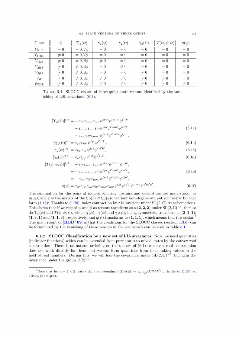
6.1. STATE VECTORS OF THREE QUBITS 123
Class ψ Υφ(ψ) γ1(ψ) γ2(ψ) γ3(ψ) T (ψ,ψ, ψ) q(ψ)
VNull = 0 = 0,∀φ = 0 = 0 = 0 = 0 = 0
V1|2|3 6= 0 = 0,∀φ = 0 = 0 = 0 = 0 = 0
V1|23 6= 0 6= 0,∃φ 6= 0 = 0 = 0 = 0 = 0
V2|13 6= 0 6= 0,∃φ = 0 6= 0 = 0 = 0 = 0
V3|12 6= 0 6= 0,∃φ = 0 = 0 6= 0 = 0 = 0
VW 6= 0 6= 0,∃φ 6= 0 6= 0 6= 0 6= 0 = 0
VGHZ 6= 0 6= 0,∃φ 6= 0 6= 0 6= 0 6= 0 6= 0
Table 6.1. SLOCC classes of three-qubit state vectors identified by the van-ishing of LSL-covariants (6.1).
[Υφ(ψ)]ijk =− εll′εmm′εnn′ψimnψlm′n′φl
′jk
− εmm′εnn′εll′ψljnψl′mn′φim
′k
− εnn′εll′εmm′ψlmkψl′m′nφijn
′,
(6.1a)
[γ1(ψ)]ii′
= εjj′εkk′ψijkψi
′j′k′ , (6.1b)
[γ2(ψ)]jj′
= εkk′εii′ψijkψi
′j′k′ , (6.1c)
[γ3(ψ)]kk′
= εii′εjj′ψijkψi
′j′k′ , (6.1d)
[T (ψ,ψ, ψ)]ijk =− εll′εmm′εnn′ψimnψlm′n′ψl
′jk,
=− εmm′εnn′εll′ψljnψl′mn′ψim
′k,
=− εnn′εll′εmm′ψlmkψl′m′nψijn
′,
(6.1e)
q(ψ) = εii′εjj′εkk′εll′εmm′εnn′ψiklψjk
′l′ψi′mnψj
′m′n′ . (6.1f)
The summation for the pairs of indices occuring upstairs and downstairs are understood, asusual, and ε is the matrix of the Sp(1) ∼= SL(2)-invariant non-degenerate antisymmetric bilinearform (1.18): Thanks to (1.20), index contraction by ε is invariant under SL(2,C) transformations.This shows that if we regard ψ and φ as tensors transform as a (2,2,2) under SL(2,C)×3, then sodo Υφ(ψ) and T (ψ,ψ, ψ), while γ1(ψ), γ2(ψ) and γ3(ψ), being symmetric, transform as (3,1,1),(1,3,1) and (1,1,3), respectively, and q(ψ) transforms as (1,1,1), which means that it is scalar.2
The main result of [BDD+09] is that the conditions for the SLOCC classes (section 1.3.6) canbe formulated by the vanishing of these tensors in the way which can be seen in table 6.1.
6.1.2. SLOCC Classification by a new set of LU-invariants. Now, we need quantities(indicator functions) which can be extended from pure states to mixed states by the convex roofconstruction. There is no natural ordering on the tensors of (6.1) so convex roof constructiondoes not work directly for them, but we can form quantities from them taking values in thefield of real numbers. During this, we will lose the covariance under SL(2,C)×3, but gain theinvariance under the group U(2)×3.
2Note that for any 2 × 2 matrix M , the determinant 2 detM = εii′εjj′MijM i′j′ , thanks to (1.20), so
2 det γa(ψ) = q(ψ).
124 6. THREE-QUBIT SYSTEMS AND FTS APPROACH
Returning from the FTS language to the Hilbert space language, we have vectors
|Υφ(ψ)〉 =
1∑i,j,k=0
[Υφ(ψ)]ijk|ijk〉 ∈ H,
|T (ψ,ψ, ψ)〉 =
1∑i,j,k=0
[T (ψ,ψ, ψ)]ijk|ijk〉 ∈ H,
and local operators
γ1(ψ)ε =
1∑i,i′=0
[γ1(ψ)ε]ii′ |i〉〈i′| ∈ Lin(H1),
γ2(ψ)ε =
1∑j,j′=0
[γ2(ψ)ε]jj′ |j〉〈j′| ∈ Lin(H2),
γ3(ψ)ε =
1∑k,k′=0
[γ3(ψ)ε]kk′ |k〉〈k′| ∈ Lin(H3)
associated to |ψ〉 ∈ H through (6.1) of the FTS language.3 These are just computational aux-iliaries coming from considerations related to the LSL-tensors, not state vectors and local ob-servables of any systems, because they depend nonlinearly on the state vector |ψ〉, moreover,γa(ψ)ε /∈ A(Ha).
Using these, the vanishing conditions of the tensors (6.1) in table 6.1 can be reformulated.Clearly, ψ = 0 if and only if ‖ψ‖2 = 0. Taking a look at Υφ(ψ) in (6.1a) it turns out that Υφ(ψ)can be written in the Hilbert space language as
|Υφ(ψ)〉 = Y (ψ)|φ〉with the operator
Y (ψ) = −γ1(ψ)ε⊗ I⊗ I− I⊗ γ2(ψ)ε⊗ I− I⊗ I⊗ γ3(ψ)ε ∈ Lin(H).
Using this, the vanishing condition of Υφ(ψ) for all φ:
|Υφ(ψ)〉 = 0 ∀|φ〉 ⇐⇒ Y (ψ)|φ〉 = 0 ∀|φ〉⇐⇒ Y (ψ) = 0
⇐⇒ ‖Y (ψ)‖2 = 0,
so we can eliminate the quantifiers and φ from the condition. Since the last implication holdsfor any norm, using the usual complex matrix 2-norm ‖M‖2 = tr(M†M) we have
‖Y (ψ)‖2 = 4(‖γ1(ψ)‖2 + ‖γ2(ψ)‖2 + ‖γ3(ψ)‖2
).
This formula has a remarkably structure. Namely, note that the local concurrence-squared(1.11c), which can be used as a|bc-indicator function (5.5b), arises here as
c2a(ψ) = C2(trbc |ψ〉〈ψ|) = ‖γb(ψ)‖2 + ‖γc(ψ)‖2,and γa(ψ) = 0 if and only if ‖γa(ψ)‖2 = 0. Now turn to the vanishing of T (ψ,ψ, ψ), givenin (6.1e). Again, this vanishes if and only if its norm ‖T (ψ,ψ, ψ)‖2 does.4 This can be calculated
3Note that ε ∈ H∗a⊗H∗a ∼= Lin(Ha →H∗a) ∼= BiLin(Ha×Ha → C), while γa(ψ) ∈ Ha⊗Ha ∼= Lin(H∗a →Ha),so γa(ψ)ε ∈ Lin(Ha →Ha).
4 The quantity ‖T (ψ,ψ, ψ)‖2 appears also in the twistor-geometric approach of three-qubit entanglement, itis proportional to ωABC in [Lev05].
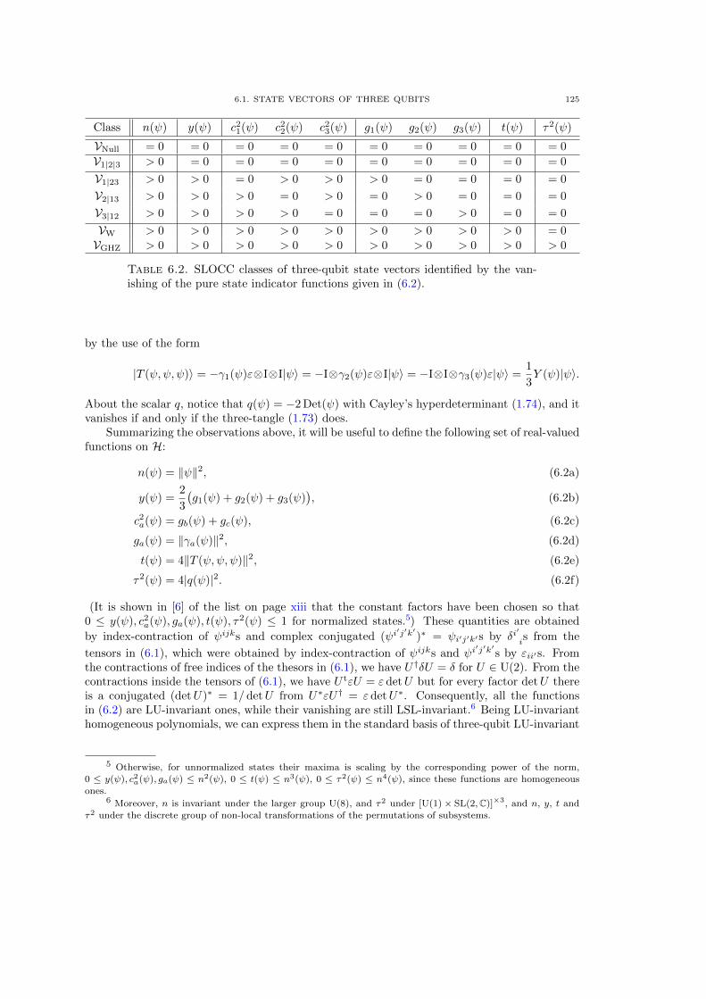
6.1. STATE VECTORS OF THREE QUBITS 125
Class n(ψ) y(ψ) c21(ψ) c22(ψ) c23(ψ) g1(ψ) g2(ψ) g3(ψ) t(ψ) τ2(ψ)
VNull = 0 = 0 = 0 = 0 = 0 = 0 = 0 = 0 = 0 = 0
V1|2|3 > 0 = 0 = 0 = 0 = 0 = 0 = 0 = 0 = 0 = 0
V1|23 > 0 > 0 = 0 > 0 > 0 > 0 = 0 = 0 = 0 = 0
V2|13 > 0 > 0 > 0 = 0 > 0 = 0 > 0 = 0 = 0 = 0
V3|12 > 0 > 0 > 0 > 0 = 0 = 0 = 0 > 0 = 0 = 0
VW > 0 > 0 > 0 > 0 > 0 > 0 > 0 > 0 > 0 = 0VGHZ > 0 > 0 > 0 > 0 > 0 > 0 > 0 > 0 > 0 > 0
Table 6.2. SLOCC classes of three-qubit state vectors identified by the van-ishing of the pure state indicator functions given in (6.2).
by the use of the form
|T (ψ,ψ, ψ)〉 = −γ1(ψ)ε⊗I⊗I|ψ〉 = −I⊗γ2(ψ)ε⊗I|ψ〉 = −I⊗I⊗γ3(ψ)ε|ψ〉 =1
3Y (ψ)|ψ〉.
About the scalar q, notice that q(ψ) = −2 Det(ψ) with Cayley’s hyperdeterminant (1.74), and itvanishes if and only if the three-tangle (1.73) does.
Summarizing the observations above, it will be useful to define the following set of real-valuedfunctions on H:
n(ψ) = ‖ψ‖2, (6.2a)
y(ψ) =2
3
(g1(ψ) + g2(ψ) + g3(ψ)
), (6.2b)
c2a(ψ) = gb(ψ) + gc(ψ), (6.2c)
ga(ψ) = ‖γa(ψ)‖2, (6.2d)
t(ψ) = 4‖T (ψ,ψ, ψ)‖2, (6.2e)
τ2(ψ) = 4|q(ψ)|2. (6.2f)
(It is shown in [6] of the list on page xiii that the constant factors have been chosen so that0 ≤ y(ψ), c2a(ψ), ga(ψ), t(ψ), τ2(ψ) ≤ 1 for normalized states.5) These quantities are obtained
by index-contraction of ψijks and complex conjugated (ψi′j′k′)∗ = ψi′j′k′s by δi
′
is from the
tensors in (6.1), which were obtained by index-contraction of ψijks and ψi′j′k′s by εii′s. From
the contractions of free indices of the thesors in (6.1), we have U†δU = δ for U ∈ U(2). From thecontractions inside the tensors of (6.1), we have U tεU = ε detU but for every factor detU thereis a conjugated (detU)∗ = 1/ detU from U∗εU† = ε detU∗. Consequently, all the functionsin (6.2) are LU-invariant ones, while their vanishing are still LSL-invariant.6 Being LU-invarianthomogeneous polynomials, we can express them in the standard basis of three-qubit LU-invariant
5 Otherwise, for unnormalized states their maxima is scaling by the corresponding power of the norm,
0 ≤ y(ψ), c2a(ψ), ga(ψ) ≤ n2(ψ), 0 ≤ t(ψ) ≤ n3(ψ), 0 ≤ τ2(ψ) ≤ n4(ψ), since these functions are homogeneousones.
6 Moreover, n is invariant under the larger group U(8), and τ2 under [U(1)× SL(2,C)]×3, and n, y, t andτ2 under the discrete group of non-local transformations of the permutations of subsystems.
126 6. THREE-QUBIT SYSTEMS AND FTS APPROACH
homogeneous polynomials (1.75) as
n = I0, (6.3a)
y = 2I20 −
2
3
(I1 + I2 + I3
), (6.3b)
c2a = 2(I20 − Ia
), (6.3c)
ga = I20 + Ia − Ib − Ic, (6.3d)
t =8
3I4 +
10
3I30 − 2I0
(I1 + I2 + I3
), (6.3e)
τ2 = 4I5. (6.3f)
Now, the conditions for the SLOCC classes by the vanishing of the tensors in (6.1) (see intable 6.1) can be reformulated by the vanishing of the functions in (6.2) in the way which canbe seen in table 6.2. Comparing this with table 5.2 we have that the functions y, c2a, ga and tare proper indicator functions for the PS classification of the states of three-qubit systems. Thefunction τ2 completes those for the PSS classification. But, before turning to this, let us discussthe relation of the new functions ga to the entanglement of the two-qubit subsystems.
6.1.3. Entanglement of two-qubit subsystems. The entanglement inside the two-qubitsubsystems can be calculated by the use of the Wootters concurrence (1.67). Recall that, for a
two-qubit state ω, it can be written by the eigenvalues of√√
ωω√ω as
c∪(ω) =(λ↓1 − λ
↓2 − λ
↓3 − λ
↓4
)+.
If the two-qubit mixed state for which the Wootters concurrence-squared is calculated is reducedfrom a pure three-qubit state, then ω = πbc is at the most of rank 2, and
c∪2(πbc) = (λ1 − λ2)2 = trπbcπbc − 2λ1λ2.
One can check that
trπbcπbc = tr γa(ψ)†γa(ψ), (6.4a)
which is just ga(ψ) of (6.2d), and
λ1λ2 = |det γa(ψ)| = |Detψ|, (6.4b)
see in [CKW00]. The Wootters concurrence is then given by
c∪2(πbc) = ga(ψ)− 1
2τ(ψ). (6.5)
As it can be seen, ga(ψ) measures the entanglement in two-qubit subsystems for all vectors whichare not of Class GHZ. Note that this is only a zero-measured subset of all state vectors. Note
also that c∪2(πbc) can not be used instead of ga for the role of an indicator function, because it
can be zero for Class GHZ vectors7 hence does not obey the last line of table 6.2. On the otherhand, the CKW equality (1.72) about entanglement monogamy,
c2a(ψ) = c∪2(πab) + c∪
2(πac) + τ(ψ), (6.6)
is then equivalent to (6.2c).The roof extension relates the concurrence with another important quantity, the fidelity
[Uhl00]. The fidelity between two density matrices ω and σ is F (ω, σ) = tr√√
ωσ√ω, which
7For example the standard GHZ state (1.71b) has separable two-qubit subsystems, for which the Woottersconcurrence vanishes. Such vectors, having maximal three-tangle, form an important subclass of three-qubitentanglement.
6.2. MIXED STATES OF THREE QUBITS 127
is the square root of the transition probability, and it is in connection with distances and dis-tinguishability measures on the space of density matrices [BZ06]. The fidelity of a state withrespect to the spin flip is F (ω, ω), which is just the concave roof extension8 of c. For the two-qubitcase this takes the form [Uhl00]
c∩(ω) = F (ω, ω) = λ1 + λ2 + λ3 + λ4.
Again, for the mixed states of two-qubit subsystems arising from a three-qubit system being ina pure state, the fidelity is
c∩2(πbc) = (λ1 + λ2)2 = trπbcπbc + 2λ1λ2.
Using (6.4a) and (6.4b), it is of the form similar to the concurrence (6.5)
c∩2(πbc) = ga(ψ) +
1
2τ(ψ). (6.7)
Then, using (6.2c), we get a CKW-like equality for the fidelities,
c2a(ψ) = c∩2(πab) + c∩
2(πac)− τ(ψ). (6.8)
On the other hand, from (6.5) and (6.7), ga(ψ) is just the average of the concave and convexroofs and τ(ψ) is their difference,
ga(ψ) =1
2
(c∩
2(πbc) + c∪
2(πbc)
), (6.9a)
τ(ψ) = c∩2(πbc)− c∪
2(πbc). (6.9b)
Hence, on the zero-measured set of non-GHZ pure states, the (two-qubit) convex and concaveroof extensions of local concurrence c are equal, and both of them are equal to the indicatorfunction ga(ψ).
6.2. Mixed states of three qubits
Now, we have the indicator functions y, c2a, ga and t for the PS classification of the states ofthree-qubit systems, and we will also have τ2 for Class W of the classification of Acın et. al. (sec-tion 1.3.7). The PSS classification arises as the combination of these two. Since only the PS classC1 is divided into two PSS classes, obtaining the PSS classification is straightforward. Only forthe sake of completeness, we write out this PSS classification for which these indicator functionscan be used.
6.2.1. PSS subsets. Starting with the extremal points of the space of states, we have thepure states given by the vectors of different SLOCC classes given in section 1.3.6. These are thesame as those of the general tripartite case, given in (5.2), only the set of tripartite entangledpure states Q123 is divided into two disjoint subsets according to the W and GHZ-type three-qubit entanglement. These are denoted with Q123 = QW ∪ QGHZ, and with these we get thepure PSS classes
Q1|2|3 ={π = |ψ〉〈ψ|
∣∣ |ψ〉 ∈ V1|2|3, ‖ψ‖2 = 1}, (6.10a)
Qa|bc ={π = |ψ〉〈ψ|
∣∣ |ψ〉 ∈ Va|bc, ‖ψ‖2 = 1}, (6.10b)
QW ={π = |ψ〉〈ψ|
∣∣ |ψ〉 ∈ VW, ‖ψ‖2 = 1}, (6.10c)
QGHZ ={π = |ψ〉〈ψ|
∣∣ |ψ〉 ∈ VGHZ, ‖ψ‖2 = 1}. (6.10d)
8The concave roof extension is the maximization of the weighted average over the decompositions instead ofthe minimization in (1.46).
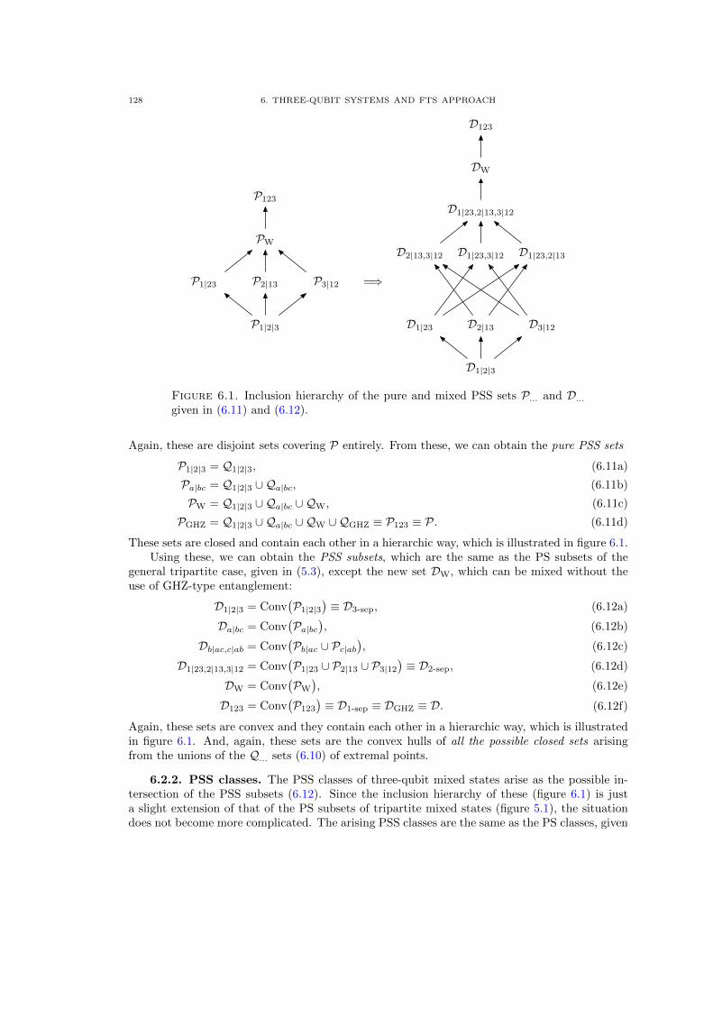
128 6. THREE-QUBIT SYSTEMS AND FTS APPROACH
P1|2|3
P1|23 P2|13 P3|12
PW
P123
=⇒
D1|2|3
D1|23 D2|13 D3|12
D2|13,3|12 D1|23,3|12 D1|23,2|13
D1|23,2|13,3|12
DW
D123
Figure 6.1. Inclusion hierarchy of the pure and mixed PSS sets P... and D...given in (6.11) and (6.12).
Again, these are disjoint sets covering P entirely. From these, we can obtain the pure PSS sets
P1|2|3 = Q1|2|3, (6.11a)
Pa|bc = Q1|2|3 ∪Qa|bc, (6.11b)
PW = Q1|2|3 ∪Qa|bc ∪QW, (6.11c)
PGHZ = Q1|2|3 ∪Qa|bc ∪QW ∪QGHZ ≡ P123 ≡ P. (6.11d)
These sets are closed and contain each other in a hierarchic way, which is illustrated in figure 6.1.Using these, we can obtain the PSS subsets, which are the same as the PS subsets of the
general tripartite case, given in (5.3), except the new set DW, which can be mixed without theuse of GHZ-type entanglement:
D1|2|3 = Conv(P1|2|3
)≡ D3-sep, (6.12a)
Da|bc = Conv(Pa|bc
), (6.12b)
Db|ac,c|ab = Conv(Pb|ac ∪ Pc|ab
), (6.12c)
D1|23,2|13,3|12 = Conv(P1|23 ∪ P2|13 ∪ P3|12
)≡ D2-sep, (6.12d)
DW = Conv(PW
), (6.12e)
D123 = Conv(P123
)≡ D1-sep ≡ DGHZ ≡ D. (6.12f)
Again, these sets are convex and they contain each other in a hierarchic way, which is illustratedin figure 6.1. And, again, these sets are the convex hulls of all the possible closed sets arisingfrom the unions of the Q... sets (6.10) of extremal points.
6.2.2. PSS classes. The PSS classes of three-qubit mixed states arise as the possible in-tersection of the PSS subsets (6.12). Since the inclusion hierarchy of these (figure 6.1) is justa slight extension of that of the PS subsets of tripartite mixed states (figure 5.1), the situationdoes not become more complicated. The arising PSS classes are the same as the PS classes, given
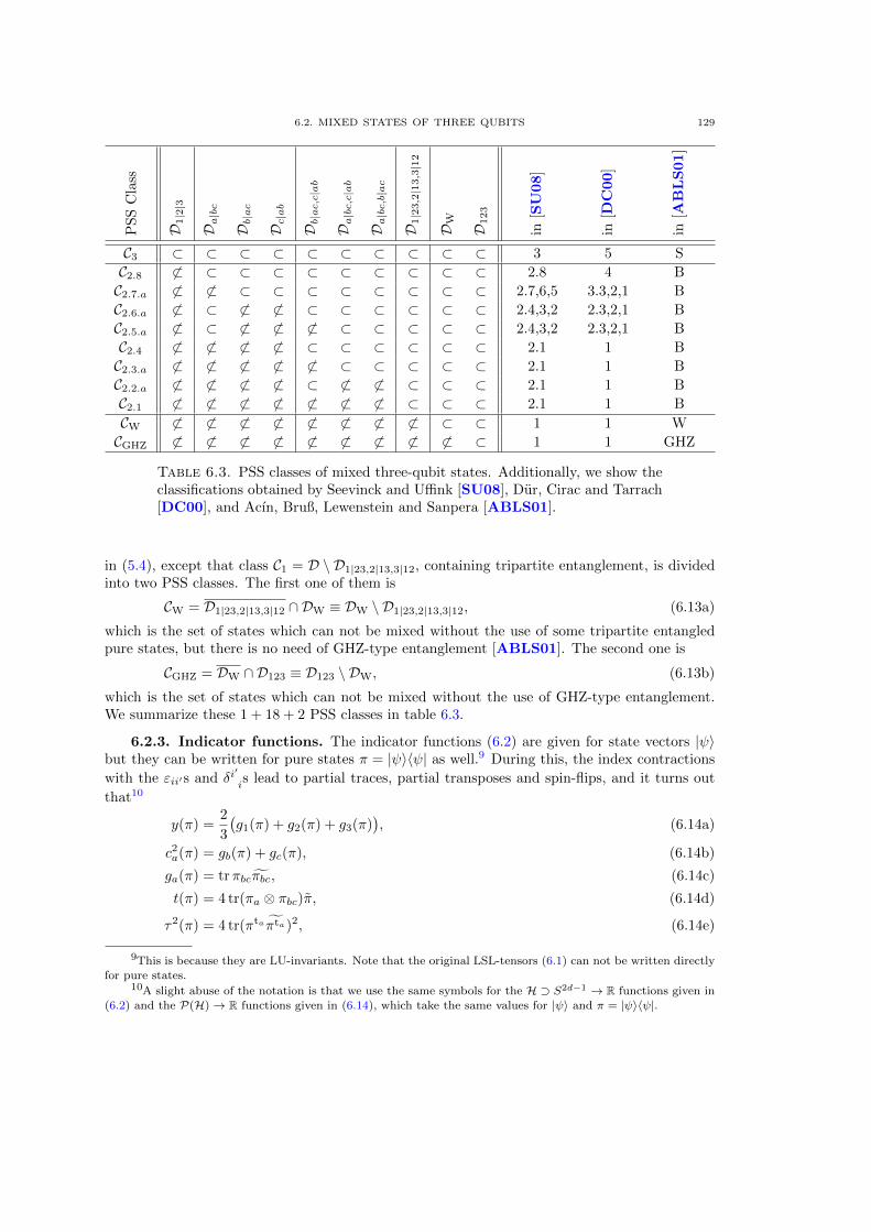
6.2. MIXED STATES OF THREE QUBITS 129P
SS
Cla
ss
D1|2|3
Da|bc
Db|ac
Dc|ab
Db|ac,c|ab
Da|bc,c|ab
Da|bc,b|ac
D1|2
3,2|1
3,3|1
2
DW
D123
in[S
U08
]
in[D
C00
]
in[A
BL
S01
]
C3 ⊂ ⊂ ⊂ ⊂ ⊂ ⊂ ⊂ ⊂ ⊂ ⊂ 3 5 S
C2.8 6⊂ ⊂ ⊂ ⊂ ⊂ ⊂ ⊂ ⊂ ⊂ ⊂ 2.8 4 B
C2.7.a 6⊂ 6⊂ ⊂ ⊂ ⊂ ⊂ ⊂ ⊂ ⊂ ⊂ 2.7,6,5 3.3,2,1 B
C2.6.a 6⊂ ⊂ 6⊂ 6⊂ ⊂ ⊂ ⊂ ⊂ ⊂ ⊂ 2.4,3,2 2.3,2,1 B
C2.5.a 6⊂ ⊂ 6⊂ 6⊂ 6⊂ ⊂ ⊂ ⊂ ⊂ ⊂ 2.4,3,2 2.3,2,1 B
C2.4 6⊂ 6⊂ 6⊂ 6⊂ ⊂ ⊂ ⊂ ⊂ ⊂ ⊂ 2.1 1 B
C2.3.a 6⊂ 6⊂ 6⊂ 6⊂ 6⊂ ⊂ ⊂ ⊂ ⊂ ⊂ 2.1 1 B
C2.2.a 6⊂ 6⊂ 6⊂ 6⊂ ⊂ 6⊂ 6⊂ ⊂ ⊂ ⊂ 2.1 1 B
C2.1 6⊂ 6⊂ 6⊂ 6⊂ 6⊂ 6⊂ 6⊂ ⊂ ⊂ ⊂ 2.1 1 B
CW 6⊂ 6⊂ 6⊂ 6⊂ 6⊂ 6⊂ 6⊂ 6⊂ ⊂ ⊂ 1 1 W
CGHZ 6⊂ 6⊂ 6⊂ 6⊂ 6⊂ 6⊂ 6⊂ 6⊂ 6⊂ ⊂ 1 1 GHZ
Table 6.3. PSS classes of mixed three-qubit states. Additionally, we show theclassifications obtained by Seevinck and Uffink [SU08], Dur, Cirac and Tarrach[DC00], and Acın, Bruß, Lewenstein and Sanpera [ABLS01].
in (5.4), except that class C1 = D \ D1|23,2|13,3|12, containing tripartite entanglement, is dividedinto two PSS classes. The first one of them is
CW = D1|23,2|13,3|12 ∩ DW ≡ DW \ D1|23,2|13,3|12, (6.13a)
which is the set of states which can not be mixed without the use of some tripartite entangledpure states, but there is no need of GHZ-type entanglement [ABLS01]. The second one is
CGHZ = DW ∩ D123 ≡ D123 \ DW, (6.13b)
which is the set of states which can not be mixed without the use of GHZ-type entanglement.We summarize these 1 + 18 + 2 PSS classes in table 6.3.
6.2.3. Indicator functions. The indicator functions (6.2) are given for state vectors |ψ〉but they can be written for pure states π = |ψ〉〈ψ| as well.9 During this, the index contractions
with the εii′s and δi′
is lead to partial traces, partial transposes and spin-flips, and it turns out
that10
y(π) =2
3
(g1(π) + g2(π) + g3(π)
), (6.14a)
c2a(π) = gb(π) + gc(π), (6.14b)
ga(π) = trπbcπbc, (6.14c)
t(π) = 4 tr(πa ⊗ πbc)π, (6.14d)
τ2(π) = 4 tr(πta πta)2, (6.14e)
9This is because they are LU-invariants. Note that the original LSL-tensors (6.1) can not be written directlyfor pure states.
10A slight abuse of the notation is that we use the same symbols for the H ⊃ S2d−1 → R functions given in(6.2) and the P(H)→ R functions given in (6.14), which take the same values for |ψ〉 and π = |ψ〉〈ψ|.
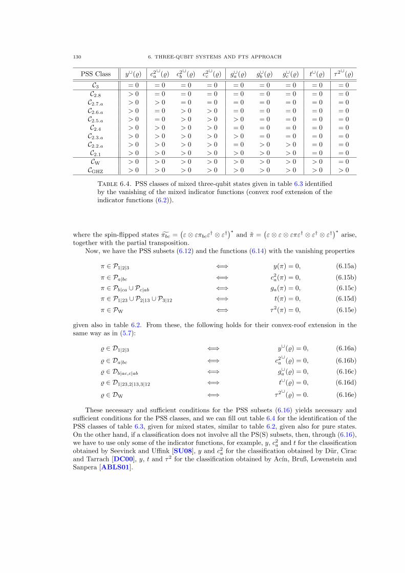
130 6. THREE-QUBIT SYSTEMS AND FTS APPROACH
PSS Class y∪(%) c2a∪
(%) c2b∪
(%) c2c∪
(%) g∪a (%) g∪b (%) g∪c (%) t∪(%) τ2∪(%)
C3 = 0 = 0 = 0 = 0 = 0 = 0 = 0 = 0 = 0
C2.8 > 0 = 0 = 0 = 0 = 0 = 0 = 0 = 0 = 0C2.7.a > 0 > 0 = 0 = 0 = 0 = 0 = 0 = 0 = 0C2.6.a > 0 = 0 > 0 > 0 = 0 = 0 = 0 = 0 = 0C2.5.a > 0 = 0 > 0 > 0 > 0 = 0 = 0 = 0 = 0C2.4 > 0 > 0 > 0 > 0 = 0 = 0 = 0 = 0 = 0C2.3.a > 0 > 0 > 0 > 0 > 0 = 0 = 0 = 0 = 0C2.2.a > 0 > 0 > 0 > 0 = 0 > 0 > 0 = 0 = 0C2.1 > 0 > 0 > 0 > 0 > 0 > 0 > 0 = 0 = 0
CW > 0 > 0 > 0 > 0 > 0 > 0 > 0 > 0 = 0CGHZ > 0 > 0 > 0 > 0 > 0 > 0 > 0 > 0 > 0
Table 6.4. PSS classes of mixed three-qubit states given in table 6.3 identifiedby the vanishing of the mixed indicator functions (convex roof extension of theindicator functions (6.2)).
where the spin-flipped states πbc =(ε ⊗ επbcε† ⊗ ε†
)∗and π =
(ε ⊗ ε ⊗ επε† ⊗ ε† ⊗ ε†
)∗arise,
together with the partial transposition.Now, we have the PSS subsets (6.12) and the functions (6.14) with the vanishing properties
π ∈ P1|2|3 ⇐⇒ y(π) = 0, (6.15a)
π ∈ Pa|bc ⇐⇒ c2a(π) = 0, (6.15b)
π ∈ Pb|ca ∪ Pc|ab ⇐⇒ ga(π) = 0, (6.15c)
π ∈ P1|23 ∪ P2|13 ∪ P3|12 ⇐⇒ t(π) = 0, (6.15d)
π ∈ PW ⇐⇒ τ2(π) = 0, (6.15e)
given also in table 6.2. From these, the following holds for their convex-roof extension in thesame way as in (5.7):
% ∈ D1|2|3 ⇐⇒ y∪(%) = 0, (6.16a)
% ∈ Da|bc ⇐⇒ c2a∪
(%) = 0, (6.16b)
% ∈ Db|ac,c|ab ⇐⇒ g∪a (%) = 0, (6.16c)
% ∈ D1|23,2|13,3|12 ⇐⇒ t∪(%) = 0, (6.16d)
% ∈ DW ⇐⇒ τ2∪(%) = 0. (6.16e)
These necessary and sufficient conditions for the PSS subsets (6.16) yields necessary andsufficient conditions for the PSS classes, and we can fill out table 6.4 for the identification of thePSS classes of table 6.3, given for mixed states, similar to table 6.2, given also for pure states.On the other hand, if a classification does not involve all the PS(S) subsets, then, through (6.16),we have to use only some of the indicator functions, for example, y, c2a and t for the classificationobtained by Seevinck and Uffink [SU08], y and c2a for the classification obtained by Dur, Ciracand Tarrach [DC00], y, t and τ2 for the classification obtained by Acın, Bruß, Lewenstein andSanpera [ABLS01].
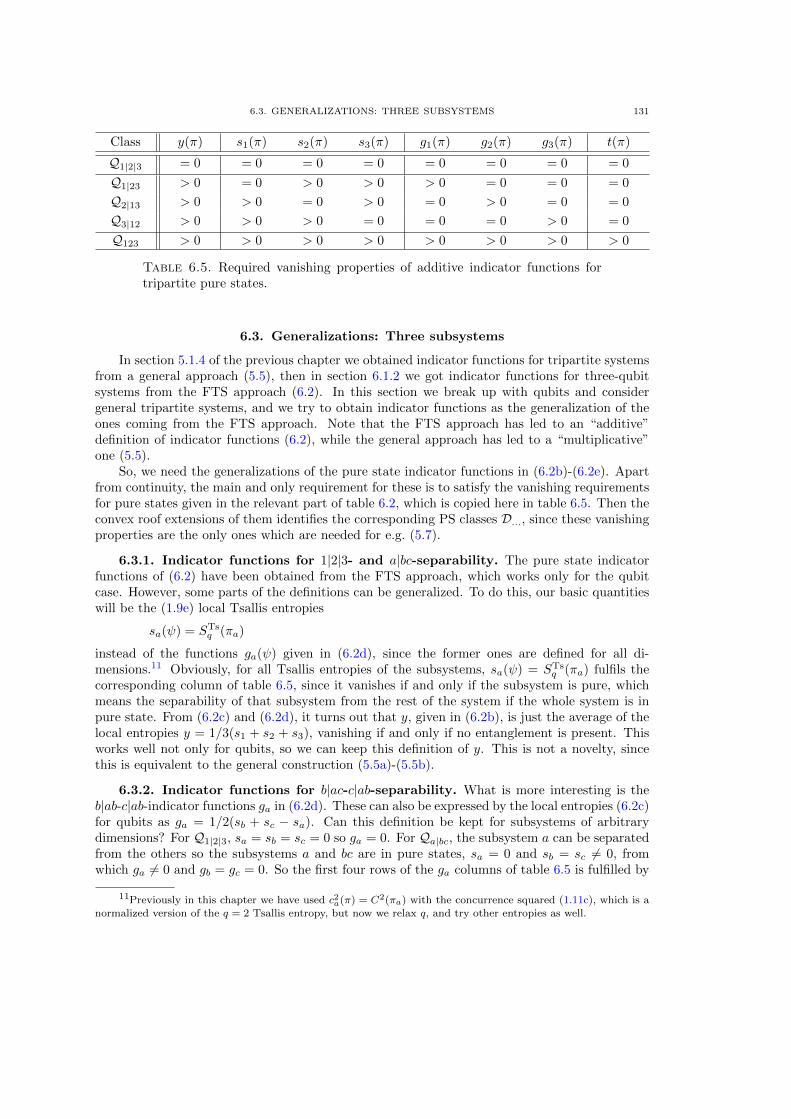
6.3. GENERALIZATIONS: THREE SUBSYSTEMS 131
Class y(π) s1(π) s2(π) s3(π) g1(π) g2(π) g3(π) t(π)
Q1|2|3 = 0 = 0 = 0 = 0 = 0 = 0 = 0 = 0
Q1|23 > 0 = 0 > 0 > 0 > 0 = 0 = 0 = 0
Q2|13 > 0 > 0 = 0 > 0 = 0 > 0 = 0 = 0
Q3|12 > 0 > 0 > 0 = 0 = 0 = 0 > 0 = 0
Q123 > 0 > 0 > 0 > 0 > 0 > 0 > 0 > 0
Table 6.5. Required vanishing properties of additive indicator functions fortripartite pure states.
6.3. Generalizations: Three subsystems
In section 5.1.4 of the previous chapter we obtained indicator functions for tripartite systemsfrom a general approach (5.5), then in section 6.1.2 we got indicator functions for three-qubitsystems from the FTS approach (6.2). In this section we break up with qubits and considergeneral tripartite systems, and we try to obtain indicator functions as the generalization of theones coming from the FTS approach. Note that the FTS approach has led to an “additive”definition of indicator functions (6.2), while the general approach has led to a “multiplicative”one (5.5).
So, we need the generalizations of the pure state indicator functions in (6.2b)-(6.2e). Apartfrom continuity, the main and only requirement for these is to satisfy the vanishing requirementsfor pure states given in the relevant part of table 6.2, which is copied here in table 6.5. Then theconvex roof extensions of them identifies the corresponding PS classes D..., since these vanishingproperties are the only ones which are needed for e.g. (5.7).
6.3.1. Indicator functions for 1|2|3- and a|bc-separability. The pure state indicatorfunctions of (6.2) have been obtained from the FTS approach, which works only for the qubitcase. However, some parts of the definitions can be generalized. To do this, our basic quantitieswill be the (1.9e) local Tsallis entropies
sa(ψ) = STsq (πa)
instead of the functions ga(ψ) given in (6.2d), since the former ones are defined for all di-mensions.11 Obviously, for all Tsallis entropies of the subsystems, sa(ψ) = STs
q (πa) fulfils thecorresponding column of table 6.5, since it vanishes if and only if the subsystem is pure, whichmeans the separability of that subsystem from the rest of the system if the whole system is inpure state. From (6.2c) and (6.2d), it turns out that y, given in (6.2b), is just the average of thelocal entropies y = 1/3(s1 + s2 + s3), vanishing if and only if no entanglement is present. Thisworks well not only for qubits, so we can keep this definition of y. This is not a novelty, sincethis is equivalent to the general construction (5.5a)-(5.5b).
6.3.2. Indicator functions for b|ac-c|ab-separability. What is more interesting is theb|ab-c|ab-indicator functions ga in (6.2d). These can also be expressed by the local entropies (6.2c)for qubits as ga = 1/2(sb + sc − sa). Can this definition be kept for subsystems of arbitrarydimensions? For Q1|2|3, sa = sb = sc = 0 so ga = 0. For Qa|bc, the subsystem a can be separatedfrom the others so the subsystems a and bc are in pure states, sa = 0 and sb = sc 6= 0, fromwhich ga 6= 0 and gb = gc = 0. So the first four rows of the ga columns of table 6.5 is fulfilled by
11Previously in this chapter we have used c2a(π) = C2(πa) with the concurrence squared (1.11c), which is anormalized version of the q = 2 Tsallis entropy, but now we relax q, and try other entropies as well.
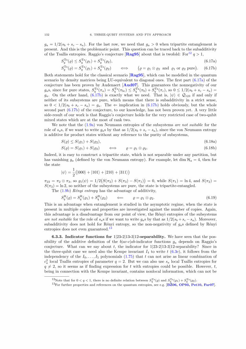
132 6. THREE-QUBIT SYSTEMS AND FTS APPROACH
ga = 1/2(sb + sc − sa). For the last row, we need that ga > 0 when tripartite entanglement ispresent. And this is the problematic point. This question can be traced back to the subadditivityof the Tsallis entropies. Raggio’s conjecture [Rag95] about that is twofold: For12 q > 1,
STsq (%) ≤ STs
q (%1) + STsq (%2), (6.17a)
STsq (%) = STs
q (%1) + STsq (%2) ⇐⇒
(% = %1 ⊗ %2 and %1 or %2 pure
). (6.17b)
Both statements hold for the classical scenario [Rag95], which can be modelled in the quantumscenario by density matrices being LU-equivalent to diagonal ones. The first part (6.17a) of theconjecture has been proven by Audenaert [Aud07]. This guarantees the nonnegativity of ourgas, since for pure states, STs
q (πa) = STsq (πbc) ≤ STs
q (πb) + STsq (πc), so 0 ≤ 1/2(sb + sc − sa) =
ga. On the other hand, (6.17b) is exactly what we need. That is, |ψ〉 ∈ Q123 if and only ifneither of its subsystems are pure, which means that there is subadditivity in a strict sense,so 0 < 1/2(sb + sc − sa) = ga. The ⇐ implication in (6.17b) holds obviously, but the wholesecond part (6.17b) of the conjecture, to our knowledge, has not been proven yet. A very littleside-result of our work is that Raggio’s conjecture holds for the very restricted case of two-qubitmixed states which are at the most of rank two.
We note that the (1.9a) von Neumann entropies of the subsystems are not suitable for therole of sas, if we want to write gas by that as 1/2(sb + sc − sa), since the von Neumann entropyis additive for product states without any reference to the purity of subsystems,
S(%) ≤ S(%1) + S(%2), (6.18a)
S(%) = S(%1) + S(%2) ⇐⇒ % = %1 ⊗ %2. (6.18b)
Indeed, it is easy to construct a tripartite state, which is not separable under any partition, buthas vanishing ga (defined by the von Neumann entropy). For example, let dimHa = 4, then forthe state
|ψ〉 =1
2
(|000〉+ |101〉+ |210〉+ |311〉
)π23 = π2 ⊗ π3, so g1(ψ) = 1/2
(S(π2) + S(π3) − S(π1)
)= 0, while S(π1) = ln 4, and S(π2) =
S(π3) = ln 2, so neither of the subsystems are pure, the state is tripartite-entangled.The (1.9b) Renyi entropy has the advantage of additivity,
SRq (%) = SR
q (%1) + SRq (%2) ⇐= % = %1 ⊗ %2. (6.19)
This is an advantage when entanglement is studied in the asymptotic regime, when the state ispresent in multiple copies and properties are investigated against the number of copies. Again,this advantage is a disadvantage from our point of view, the Renyi entropies of the subsystemsare not suitable for the role of sas if we want to write gas by that as 1/2(sb+ sc− sa). Moreover,subadditivity does not hold for Renyi entropy, so the non-negativity of gas defined by Renyientropies does not even guaranteed.13
6.3.3. Indicator functions for 1|23-2|13-3|12-separability. We have seen that the pos-sibility of the additive definition of the b|ac-c|ab-indicator functions ga depends on Raggio’sconjecture. What can we say about t, the indicator for 1|23-2|13-3|12-separability? Since inthe three-qubit case we need also the Kempe invariant I4 to write t (6.3e), it follows from theindependency of the I0, . . . , I5 polynomials (1.75) that t can not arise as linear combination ofc2a local Tsallis entropies of parameter q = 2. But we can also use sa local Tsallis entropies forq 6= 2, so it seems as if finding expression for t with entropies could be possible. However, t,being in connection with the Kempe invariant, contains nonlocal information, which can not be
12Note that for 0 < q < 1, there is no definite relation between STsq (%) and STs
q (%1) + STsq (%2).
13For further properties and references on the quantum entropies, see e.g. [BZ06, OP93, Pet10, Fur07].
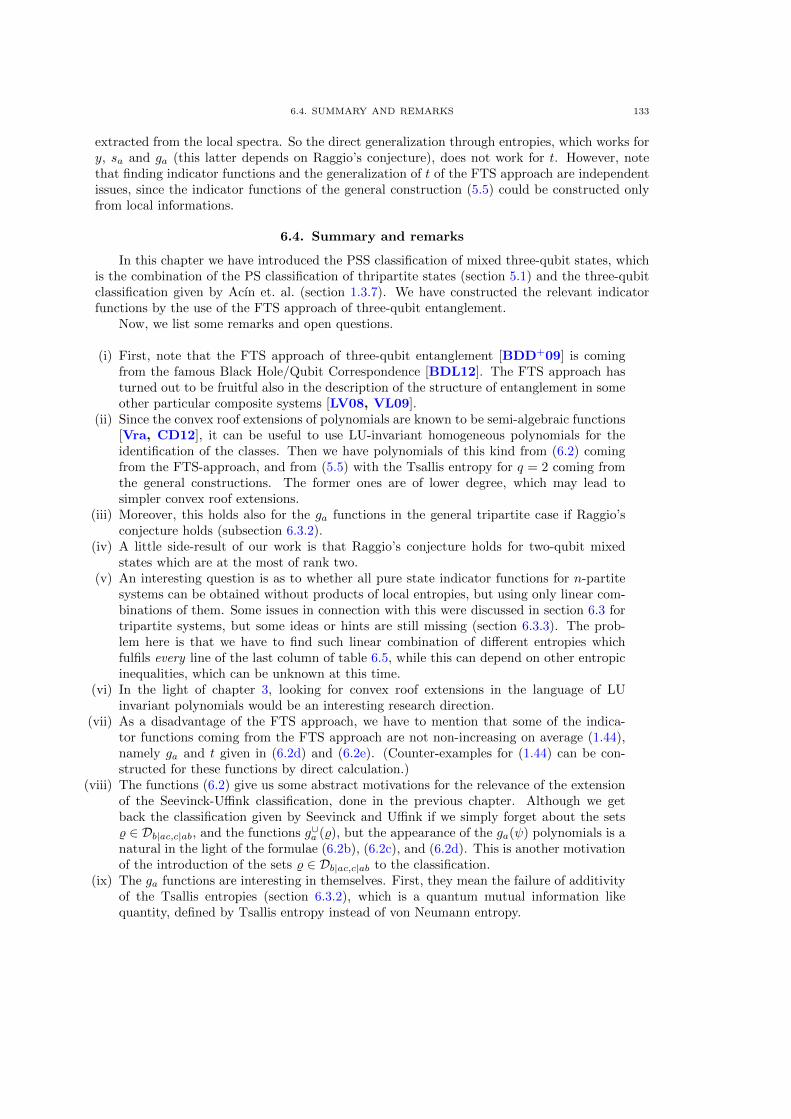
6.4. SUMMARY AND REMARKS 133
extracted from the local spectra. So the direct generalization through entropies, which works fory, sa and ga (this latter depends on Raggio’s conjecture), does not work for t. However, notethat finding indicator functions and the generalization of t of the FTS approach are independentissues, since the indicator functions of the general construction (5.5) could be constructed onlyfrom local informations.
6.4. Summary and remarks
In this chapter we have introduced the PSS classification of mixed three-qubit states, whichis the combination of the PS classification of thripartite states (section 5.1) and the three-qubitclassification given by Acın et. al. (section 1.3.7). We have constructed the relevant indicatorfunctions by the use of the FTS approach of three-qubit entanglement.
Now, we list some remarks and open questions.
(i) First, note that the FTS approach of three-qubit entanglement [BDD+09] is comingfrom the famous Black Hole/Qubit Correspondence [BDL12]. The FTS approach hasturned out to be fruitful also in the description of the structure of entanglement in someother particular composite systems [LV08, VL09].
(ii) Since the convex roof extensions of polynomials are known to be semi-algebraic functions[Vra, CD12], it can be useful to use LU-invariant homogeneous polynomials for theidentification of the classes. Then we have polynomials of this kind from (6.2) comingfrom the FTS-approach, and from (5.5) with the Tsallis entropy for q = 2 coming fromthe general constructions. The former ones are of lower degree, which may lead tosimpler convex roof extensions.
(iii) Moreover, this holds also for the ga functions in the general tripartite case if Raggio’sconjecture holds (subsection 6.3.2).
(iv) A little side-result of our work is that Raggio’s conjecture holds for two-qubit mixedstates which are at the most of rank two.
(v) An interesting question is as to whether all pure state indicator functions for n-partitesystems can be obtained without products of local entropies, but using only linear com-binations of them. Some issues in connection with this were discussed in section 6.3 fortripartite systems, but some ideas or hints are still missing (section 6.3.3). The prob-lem here is that we have to find such linear combination of different entropies whichfulfils every line of the last column of table 6.5, while this can depend on other entropicinequalities, which can be unknown at this time.
(vi) In the light of chapter 3, looking for convex roof extensions in the language of LUinvariant polynomials would be an interesting research direction.
(vii) As a disadvantage of the FTS approach, we have to mention that some of the indica-tor functions coming from the FTS approach are not non-increasing on average (1.44),namely ga and t given in (6.2d) and (6.2e). (Counter-examples for (1.44) can be con-structed for these functions by direct calculation.)
(viii) The functions (6.2) give us some abstract motivations for the relevance of the extensionof the Seevinck-Uffink classification, done in the previous chapter. Although we getback the classification given by Seevinck and Uffink if we simply forget about the sets% ∈ Db|ac,c|ab, and the functions g∪a (%), but the appearance of the ga(ψ) polynomials is anatural in the light of the formulae (6.2b), (6.2c), and (6.2d). This is another motivationof the introduction of the sets % ∈ Db|ac,c|ab to the classification.
(ix) The ga functions are interesting in themselves. First, they mean the failure of additivityof the Tsallis entropies (section 6.3.2), which is a quantum mutual information likequantity, defined by Tsallis entropy instead of von Neumann entropy.
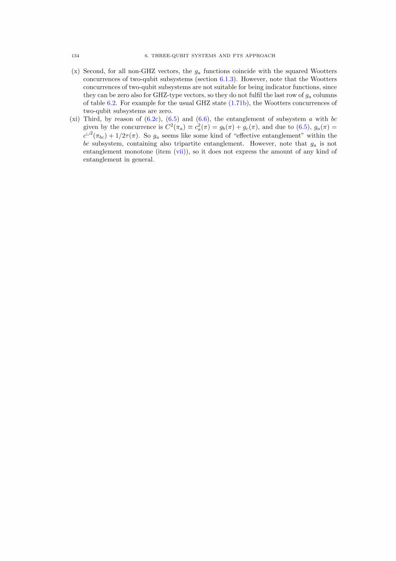
134 6. THREE-QUBIT SYSTEMS AND FTS APPROACH
(x) Second, for all non-GHZ vectors, the ga functions coincide with the squared Woottersconcurrences of two-qubit subsystems (section 6.1.3). However, note that the Woottersconcurrences of two-qubit subsystems are not suitable for being indicator functions, sincethey can be zero also for GHZ-type vectors, so they do not fulfil the last row of ga columnsof table 6.2. For example for the usual GHZ state (1.71b), the Wootters concurrences oftwo-qubit subsystems are zero.
(xi) Third, by reason of (6.2c), (6.5) and (6.6), the entanglement of subsystem a with bcgiven by the concurrence is C2(πa) ≡ c2a(π) = gb(π) + gc(π), and due to (6.5), ga(π) =
c∪2(πbc) + 1/2τ(π). So ga seems like some kind of “effective entanglement” within the
bc subsystem, containing also tripartite entanglement. However, note that ga is notentanglement monotone (item (vii)), so it does not express the amount of any kind ofentanglement in general.
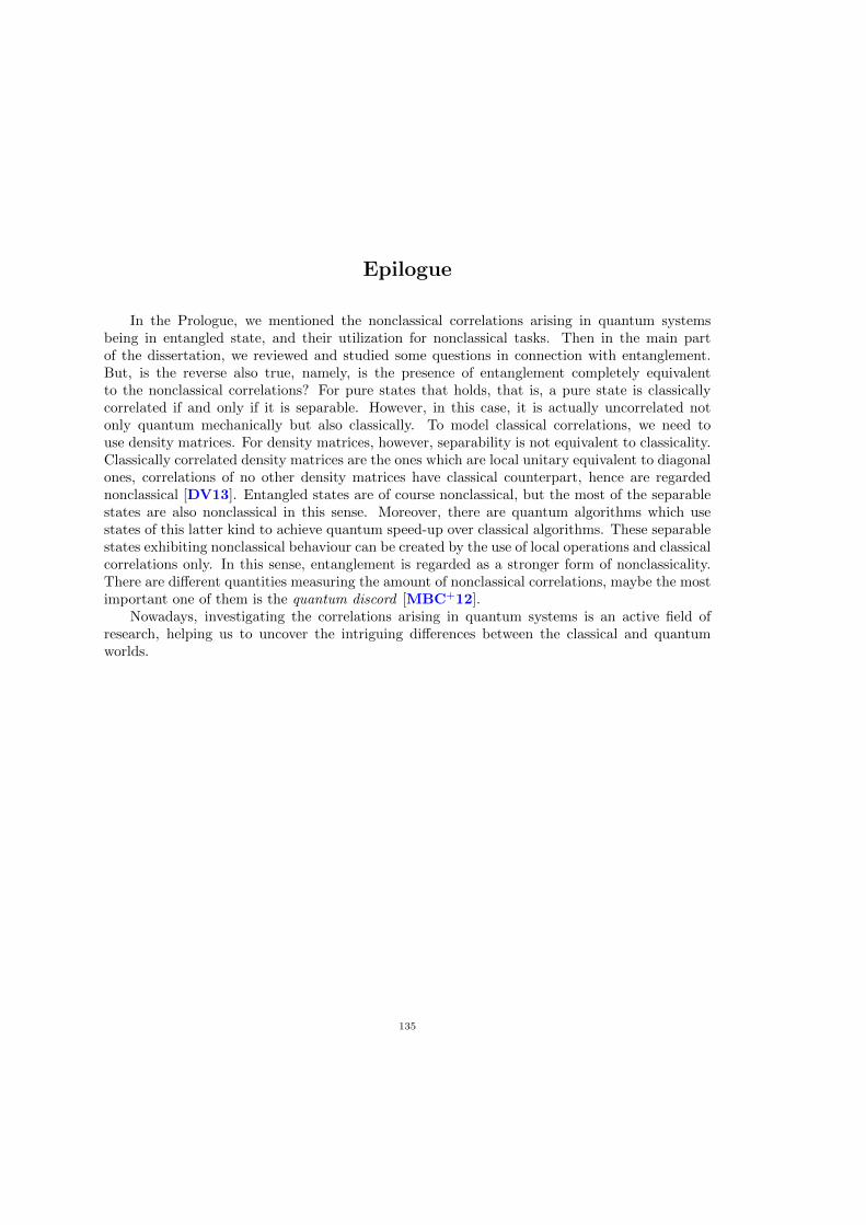
Epilogue
In the Prologue, we mentioned the nonclassical correlations arising in quantum systemsbeing in entangled state, and their utilization for nonclassical tasks. Then in the main partof the dissertation, we reviewed and studied some questions in connection with entanglement.But, is the reverse also true, namely, is the presence of entanglement completely equivalentto the nonclassical correlations? For pure states that holds, that is, a pure state is classicallycorrelated if and only if it is separable. However, in this case, it is actually uncorrelated notonly quantum mechanically but also classically. To model classical correlations, we need touse density matrices. For density matrices, however, separability is not equivalent to classicality.Classically correlated density matrices are the ones which are local unitary equivalent to diagonalones, correlations of no other density matrices have classical counterpart, hence are regardednonclassical [DV13]. Entangled states are of course nonclassical, but the most of the separablestates are also nonclassical in this sense. Moreover, there are quantum algorithms which usestates of this latter kind to achieve quantum speed-up over classical algorithms. These separablestates exhibiting nonclassical behaviour can be created by the use of local operations and classicalcorrelations only. In this sense, entanglement is regarded as a stronger form of nonclassicality.There are different quantities measuring the amount of nonclassical correlations, maybe the mostimportant one of them is the quantum discord [MBC+12].
Nowadays, investigating the correlations arising in quantum systems is an active field ofresearch, helping us to uncover the intriguing differences between the classical and quantumworlds.
135

Bibliography
[AAC+00] A. Acın, A. Andrianov, L. Costa, E. Jane, J. I. Latorre, and R. Tarrach, Generalized schmidt decom-
position and classification of three-quantum-bit states, Phys. Rev. Lett. 85 (2000), 1560–1563.[AAJT01] A. Acın, A. Andrianov, E. Jane, and R. Tarrach, Three-qubit pure-state canonical forms, J. Phys. A
34 (2001), no. 35, 6725.
[ABLS01] A. Acın, D. Bruß, M. Lewenstein, and A. Sanpera, Classification of mixed three-qubit states, Phys.Rev. Lett. 87 (2001), 040401.
[AF04] R Alicki and M Fannes, Continuity of quantum conditional information, J. Phys. A 37 (2004), no. 5,
L55.[Aud07] Koenraad M. R. Audenaert, Subadditivity of q-entropies for q > 1, J. Math. Phys. 48 (2007), no. 8,
083507.
[BBC+93] Charles H. Bennett, Gilles Brassard, Claude Crepeau, Richard Jozsa, Asher Peres, and William K.Wootters, Teleporting an unknown quantum state via dual classical and einstein-podolsky-rosen chan-
nels, Phys. Rev. Lett. 70 (1993), no. 13, 1895–1899.
[BBP+96] Charles H. Bennett, Gilles Brassard, Sandu Popescu, Benjamin Schumacher, John A. Smolin, andWilliam K. Wootters, Purification of noisy entanglement and faithful teleportation via noisy channels,
Phys. Rev. Lett. 76 (1996), 722–725.[BCY11] Fernando G. S. L. Brandao, Matthias Christandl, and Jon Yard, Faithful squashed entanglement,
Comm. Math. Phys. 306 (2011), 805–830.
[BDD+09] L. Borsten, D. Dahanayake, M. J. Duff, W. Rubens, and H. Ebrahim, Freudenthal triple classificationof three-qubit entanglement, Phys. Rev. A 80 (2009), 032326.
[BDF+99] Charles H. Bennett, David P. DiVincenzo, Christopher A. Fuchs, Tal Mor, Eric Rains, Peter W. Shor,
John A. Smolin, and William K. Wootters, Quantum nonlocality without entanglement, Phys. Rev.A 59 (1999), 1070–1091.
[BDL12] Leron Borsten, Michael J. Duff, and Peter Levay, The black-hole/qubit correspondence: an up-to-date
review, arXiv [hep-th] (2012), 1206.3166.[BDM+99] Charles H. Bennett, David P. DiVincenzo, Tal Mor, Peter W. Shor, John A. Smolin, and Barbara M.
Terhal, Unextendible product bases and bound entanglement, Phys. Rev. Lett. 82 (1999), 5385–5388.
[BDSW96] Charles H. Bennett, David P. DiVincenzo, John A. Smolin, and William K. Wootters, Mixed-stateentanglement and quantum error correction, Phys. Rev. A 54 (1996), 3824–3851.
[Bel67] John S. Bell, On the einstein podolsky rosen paradox, Physics 1 (1967), 195.[BPR+00] Charles H. Bennett, Sandu Popescu, Daniel Rohrlich, John A. Smolin, and Ashish V. Thapliyal, Exact
and asymptotic measures of multipartite pure-state entanglement, Phys. Rev. A 63 (2000), 012307.
[BYW07] Yan-Kui Bai, Dong Yang, and Z. D. Wang, Multipartite quantum correlation and entanglement infour-qubit pure states, Phys. Rev. A 76 (2007), 022336.
[BZ06] Ingemar Bengtsson and Karol Zyczkowski, Geometry of quantum states: An introduction to quantumentanglement, Cambridge University Press, New York, NY, USA, 2006.
[CAG99] N. J. Cerf, C. Adami, and R. M. Gingrich, Reduction criterion for separability, Phys. Rev. A 60
(1999), no. 2, 898–909.[Cav13] Carlton M. Caves, Quantum information science: Emerging no more, arXiv [quant-ph] (2013),
1302.1864.
[Cay45] Arthur Cayley, On the theory of linear transformations, Camb. Math. J. 4 (1845), 193–209.[CD07] Oleg Chterental and Dragomir Z. Djokovic, Normal forms and tensor ranks of pure states of four
qubits, Linear Algebra Research Advances, Nova Science Publishers, 2007, pp. 133–167.[CD12] Lin Chen and Dragomir Z. Djokovic, Some semialgebraic sets of states and separability conjectures,
arXiv [quant-ph] (2012), 1206.3775.
[CGP+02] Daniel Collins, Nicolas Gisin, Sandu Popescu, David Roberts, and Valerio Scarani, Bell-type inequal-ities to detect true n-body nonseparability, Phys. Rev. Lett. 88 (2002), 170405.
137

138 BIBLIOGRAPHY
[CHSH69] John F. Clauser, Michael A. Horne, Abner Shimony, and Richard A. Holt, Proposed experiment totest local hidden-variable theories, Phys. Rev. Lett. 23 (1969), 880–884.
[CKW00] Valerie Coffman, Joydip Kundu, and William K. Wootters, Distributed entanglement, Phys. Rev. A
61 (2000), no. 5, 052306.[Cla06] Lieven Clarisse, Entanglement distillation; a discourse on bound entanglement in quantum informa-
tion theory, arXiv [quant-ph] (2006), 0612072v1.
[CLM+12] Eric Chitambar, Debbie Leung, Laura Mancinska, Maris Ozols, and Andreas Winter, Everything youalways wanted to know about locc (but were afraid to ask), arXiv [quant-ph] (2012), 1210.4583.
[CV05] Lieven Clarisse and P Vocjan, On independent permutation separability criteria, Quant. Inf. Comp.
6 (2005), no. 3, 277.[CW04] Matthias Christandl and Andreas Winter, “squashed entanglement”: An additive entanglement mea-
sure, J. Math. Phys. 45 (2004), no. 3, 829–840.[DC00] W. Dur and J. I. Cirac, Classification of multiqubit mixed states: Separability and distillability prop-
erties, Phys. Rev. A 61 (2000), 042314.
[DCT99] W. Dur, J. I. Cirac, and R. Tarrach, Separability and distillability of multiparticle quantum systems,Phys. Rev. Lett. 83 (1999), 3562–3565.
[DHR02] Matthew J. Donald, Micha l Horodecki, and Oliver Rudolph, The uniqueness theorem for entanglement
measures, J. Math. Phys. 43 (2002), no. 9, 4252–4272.[DPS02] Andrew C. Doherty, Pablo A. Parrilo, and Federico M. Spedalieri, Distinguishing separable and en-
tangled states, Phys. Rev. Lett. 88 (2002), no. 18, 187904.
[DPS04] Andrew C. Doherty, Pablo A. Parrilo, and Federico M. Spedalieri, Complete family of separabilitycriteria, Phys. Rev. A 69 (2004), no. 2, 022308.
[DPS05] Andrew C. Doherty, Pablo A. Parrilo, and Federico M. Spedalieri, Detecting multipartite entangle-
ment, Phys. Rev. A 71 (2005), no. 3, 032333.[DV13] Ross Dorner and Vlatko Vedral, Correlations in quantum physics, Int. J. Mod. Phys. B 27 (2013),
no. 01n03, 1345017.[DVC00] W. Dur, G. Vidal, and J. I. Cirac, Three qubits can be entangled in two inequivalent ways, Phys. Rev.
A 62 (2000), 062314.
[EBOS12] Christopher Eltschka, Thierry Bastin, Andreas Osterloh, and Jens Siewert, Multipartite-entanglementmonotones and polynomial invariants, Phys. Rev. A 85 (2012), 022301.
[EP99] Jens Eisert and Martin B. Plenio, A comparison of entanglement measures, J. Mod. Opt. 46 (1999),
no. 1, 145–154.[EPR35] Albert Einstein, Boris Podolsky, and Nathan Rosen, Can quantum-mechanical description of physical
reality be considered complete?, Phys. Rev. 47 (1935), 777.
[ES02] Laszlo E. Szabo, A nyitott jovo problemaja, 1 ed., Typotex, Hungary, 2002.[Fey82] RichardP. Feynman, Simulating physics with computers, Int. J. Theor. Phys. 21 (1982), 467–488.
[FT78] Gyula Fay and Robert Toros, Kvantumlogika, Gondolat Kiado, 1978.
[Fur07] Shigeru Furuichi, Tsallis entropies and their theorems, properties and applications, Aspects of OpticalSciences and Quantum Information, Research Signpost, 2007, pp. 1–86.
[GBP98] N. Gisin and H. Bechmann-Pasquinucci, Bell inequality, bell states and maximally entangled statesfor n qubits, Phys. Lett. A 246 (1998), no. 12, 1 – 6.
[GHH+08] Andrzej Grudka, Micha l Horodecki, Pawe l Horodecki, Ryszard Horodecki, and Marco Piani,
Entanglement-swapping boxes and their communication properties, Phys. Rev. A 77 (2008), 060307.[GHH10] Andreas Gabriel, Beatrix C. Hiesmayr, and Marcus Huber, Criterion for k-separability in mixed
multipartite systems, Quant. Inf. Comp. 10 (2010), no. 9 & 10, 829–836.
[GHZ89] Daniel M. Greenberger, Michael A. Horne, and Anton Zeilinger, Going beyond bell’s theorem, Bell’sTheorem, Quantum Theory and Conceptions of the Universe, Springer, 1989, pp. 69–72.
[Gis89] Nicolas Gisin, Stochastic quantum dynamics and relativity, Helv. Phys. Acta 62 (1989), 363.
[Gis09] Nicolas Gisin, Bell inequalities: Many questions, a few answers, Quantum Reality, RelativisticCausality, and Closing the Epistemic Circle, The Western Ontario Series in Philosophy of Science,
vol. 73, Springer Netherlands, 2009, pp. 125–138.[GK08] Izrail Moiseevich Gel’fand and Andrey V. Kapranov, Mikhail M. adn Zelevinsky, Discriminants,
resultants, and multidimensional determinants, Birkhauser, Boston, 2008.[Gle57] A. M. Gleason, Measures on the closed subspaces of a hilbert space, J. Math. Mech 6 (1957), 885–893.[GM04] GianCarlo Ghirardi and Luca Marinatto, General criterion for the entanglement of two indistinguish-
able particles, Phys. Rev. A 70 (2004), 012109.
[GMW02] GianCarlo Ghirardi, Luca Marinatto, and Tullio Weber, Entanglement and properties of compositequantum systems: A conceptual and mathematical analysis, J. Stat. Phys. 108 (2002), 49–122.
BIBLIOGRAPHY 139
[GRB98] Markus Grassl, Martin Rotteler, and Thomas Beth, Computing local invariants of quantum-bit sys-tems, Phys. Rev. A 58 (1998), no. 3, 1833–1839.
[GS10] Otfried Guhne and Michael Seevinck, Separability criteria for genuine multiparticle entanglement,
New J. Phys. 12 (2010), no. 5, 053002.[GSSS11] Sandeep K. Goyal, B. Neethi Simon, Rajeev Singh, and Sudhavatani Simon, Geometry of the gener-
alized bloch sphere for qutrit, arXiv [quant-ph] (2011), 1111.4427.
[GT09] Otfried Guhne and Geza Toth, Entanglement detection, Phys. Rep. 474 (2009), no. 1-6, 1 – 75.[HH96] Ryszard Horodecki and Michal l Horodecki, Information-theoretic aspects of inseparability of mixed
states, Phys. Rev. A 54 (1996), no. 3, 1838–1843.[HH99] Micha l Horodecki and Pawe l Horodecki, Reduction criterion of separability and limits for a class of
distillation protocols, Phys. Rev. A 59 (1999), no. 6, 4206–4216.
[HHH96a] Micha l Horodecki, Pawe l Horodecki, and Ryszard Horodecki, Separability of mixed states: necessaryand sufficient conditions, Phys. Lett. A 223 (1996), no. 1-2, 1 – 8.
[HHH96b] R. Horodecki, P. Horodecki, and M. Horodecki, Quantum α-entropy inequalities: independent condi-
tion for local realism?, Phys. Lett. A 210 (1996), no. 6, 377 – 381.
[HHH97] Micha l Horodecki, Pawe l Horodecki, and Ryszard Horodecki, Inseparable two spin- 12
density matrices
can be distilled to a singlet form, Phys. Rev. Lett. 78 (1997), 574–577.[HHH98] Micha l Horodecki, Pawe l Horodecki, and Ryszard Horodecki, Mixed-state entanglement and distilla-
tion: Is there a “bound” entanglement in nature?, Phys. Rev. Lett. 80 (1998), no. 24, 5239–5242.[HHH06] Micha l Horodecki, Pawe l Horodecki, and Ryszard Horodecki, Separability of mixed quantum states:
Linear contractions and permutation criteria, Open Sys. Inf. Dyn. 13 (2006), 103–111.
[HHHH09] Ryszard Horodecki, Pawe l Horodecki, Micha l Horodecki, and Karol Horodecki, Quantum entangle-ment, Rev. Mod. Phys. 81 (2009), no. 2, 865–942.
[HJW93] Lane P. Hughston, Richard Jozsa, and William K. Wootters, A complete classification of quantum
ensembles having a given density matrix, Phys. Lett. A 183 (1993), no. 1, 14 – 18.[HMGH10] Marcus Huber, Florian Mintert, Andreas Gabriel, and Beatrix C. Hiesmayr, Detection of high-
dimensional genuine multipartite entanglement of mixed states, Phys. Rev. Lett. 104 (2010), no. 21,
210501.[Hor97] Pawe l Horodecki, Separability criterion and inseparable mixed states with positive partial transposi-
tion, Phys. Lett. A 232 (1997), no. 5, 333 – 339.
[Hor01] Micha l Horodecki, Entanglement measures, Quant. Inf. Comp. 1 (2001), 3.[HW97] Scott Hill and William K. Wootters, Entanglement of a pair of quantum bits, Phys. Rev. Lett. 78
(1997), no. 26, 5022–5025.[HW09] Michael W. Hero and Jeb F. Willenbring, Stable hilbert series as related to the measurement of
quantum entanglement, Discr. Math. 309 (2009), no. 23-24, 6508 – 6514.
[HWW09] Michael W. Hero, Jeb F. Willenbring, and Lauren Kelly Williams, The measurement of quantumentanglement and enumeration of graph coverings, arXiv [math.RT] (2009), no. 0911.0222.
[Kem99] Julia Kempe, Multiparticle entanglement and its applications to cryptography, Phys. Rev. A 60
(1999), no. 2, 910–916.[KGS12] Jeong San Kim, Gilad Gour, and Barry C. Sanders, Limitations to sharing entanglement, Contem-
porary Physics 53 (2012), no. 5, 417–432.[KW04] Masato Koashi and Andreas Winter, Monogamy of quantum entanglement and other correlations,
Phys. Rev. A 69 (2004), 022309.
[Lev05] Peter Levay, Geometry of three-qubit entanglement, Phys. Rev. A 71 (2005), 012334.
[Lev06] Peter Levay, On the geometry of four-qubit invariants, J. Phys. A 39 (2006), no. 30, 9533.[LL12] Xiangrong Li and Dafa Li, Method for classifying multiqubit states via the rank of the coefficient
matrix and its application to four-qubit states, Phys. Rev. A 86 (2012), 042332.
[LMR12] Yeong-Cherng Liang, Lluıs Masanes, and Denis Rosset, All entangled states display some hiddennonlocality, Phys. Rev. A 86 (2012), 052115.
[LNP05] Peter Levay, Szilvia Nagy, and Janos Pipek, Elementary formula for entanglement entropies offermionic systems, Phys. Rev. A 72 (2005), 022302.
[LOSU06] Robert Lohmayer, Andreas Osterloh, Jens Siewert, and Armin Uhlmann, Entangled three-qubit states
without concurrence and three-tangle, Phys. Rev. Lett. 97 (2006), no. 26, 260502.[LP98] N. Linden and S. Popescu, On multi-particle entanglement, Fortschr. Phys. 46 (1998), no. 4-5, 567–
578.
[LPS99] N. Linden, S. Popescu, and A. Sudbery, Nonlocal parameters for multiparticle density matrices, Phys.Rev. Lett. 83 (1999), 243–247.
[LT03] Jean-Gabriel Luque and Jean-Yves Thibon, Polynomial invariants of four qubits, Phys. Rev. A 67
(2003), 042303.
140 BIBLIOGRAPHY
[LV08] Peter Levay and Peter Vrana, Three fermions with six single-particle states can be entangled in twoinequivalent ways, Phys. Rev. A 78 (2008), 022329.
[LZ05] Wies law Laskowski and Marek Zukowski, Detection of n-particle entanglement with generalized bellinequalities, Phys. Rev. A 72 (2005), 062112.
[Mak02] Yuriy Makhlin, Nonlocal properties of two-qubit gates and mixed states, and the optimization of
quantum computations, Quant. Inf. Proc. 1 (2002), 243–252.[Mas06] Lluıs Masanes, All bipartite entangled states are useful for information processing, Phys. Rev. Lett.
96 (2006), 150501.[Mas08] Lluıs Masanes, Useful entanglement can be extracted from all nonseparable states, J. Math. Phys. 49
(2008), no. 2, 022102.
[Mat93] Tamas Matolcsi, Spacetime without reference frames, Akademiai Kiado, 1993.[MBC+12] Kavan Modi, Aharon Brodutch, Hugo Cable, Tomasz Paterek, and Vlatko Vedral, The classical-
quantum boundary for correlations: Discord and related measures, Rev. Mod. Phys. 84 (2012), 1655–
1707.[Miy04] Akimasa Miyake, Multipartite entanglement under stochastic local operations and classical commu-
nication, Int. J. Quant. Inf. 02 (2004), no. 01, 65–77.
[MV04] Akimasa Miyake and Frank Verstraete, Multipartite entanglement in 2 × 2 × n quantum systems,Phys. Rev. A 69 (2004), 012101.
[NC00] Michael A. Nielsen and Isaac L. Chuang, Quantum computation and quantum information, 1 ed.,
Cambridge University Press, October 2000.[Nie99] M. A. Nielsen, Conditions for a class of entanglement transformations, Phys. Rev. Lett. 83 (1999),
436–439.
[NK01] M. A. Nielsen and J. Kempe, Separable states are more disordered globally than locally, Phys. Rev.Lett. 86 (2001), no. 22, 5184–5187.
[NKI02] Koji Nagata, Masato Koashi, and Nobuyuki Imoto, Configuration of separability and tests for mul-tipartite entanglement in bell-type experiments, Phys. Rev. Lett. 89 (2002), 260401.
[oeia] The On-Line Encyclopedia of Integer Sequences, A000041, number of partitions of n.
[oeib] The On-Line Encyclopedia of Integer Sequences, A000110, Bell or exponential numbers: ways ofplacing n labeled balls into n indistinguishable boxes.
[oeic] The On-Line Encyclopedia of Integer Sequences, A074528.
[OP93] Masanori Ohya and Denes Petz, Quantum entropy and its use, 1 ed., Springer Verlag, October 1993.[OS05] Andreas Osterloh and Jens Siewert, Constructing n-qubit entanglement monotones from antilinear
operators, Phys. Rev. A 72 (2005), 012337.
[OS10] Andreas Osterloh and Jens Siewert, The invariant-comb approach and its relation to the balancednessof multipartite entangled states, New J. Phys. 12 (2010), no. 7, 075025.
[Ou07] Yong-Cheng Ou, Violation of monogamy inequality for higher-dimensional objects, Phys. Rev. A 75
(2007), 034305.[OV06] Tobias J. Osborne and Frank Verstraete, General monogamy inequality for bipartite qubit entangle-
ment, Phys. Rev. Lett. 96 (2006), 220503.[Per96] Asher Peres, Separability criterion for density matrices, Phys. Rev. Lett. 77 (1996), no. 8, 1413–1415.
[Pet08a] Denes Petz, Linearis analızis, Akademiai Kiado, 2008.[Pet08b] Denes Petz, Quantum information theory and quantum statistics, Springer, 2008.[Pet10] Denes Petz, From f-divergence to quantum quasi-entropies and their use, Entropy 12 (2010), no. 3,
304–325.
[Pre] John Preskill, Lecture notes on quantum computation, available on the homepage of the author:http://www.theory.caltech.edu/people/preskill/ph229.
[PV07] Martin B. Plenio and Shashank Virmani, An introduction to entanglement measures, Quant. Inf.
Comp. 7 (2007), 1.[Rag95] G. A. Raggio, Properties of q-entropies, J. Math. Phys. 36 (1995), no. 9, 4785–4791.
[Rai99] E. M. Rains, Bound on distillable entanglement, Phys. Rev. A 60 (1999), 179–184.[Rai00] E.M. Rains, Polynomial invariants of quantum codes, IEEE Trans. Inf. Theory 46 (2000), no. 1,
54–59.
[RLL09] Beat Rothlisberger, Jorg Lehmann, and Daniel Loss, Numerical evaluation of convex-roof entangle-ment measures with applications to spin rings, Phys. Rev. A 80 (2009), 042301.
[RLL11] Beat Rothlisberger, Jorg Lehmann, and Daniel Loss, libcreme: An optimization library for evaluating
convex-roof entanglement measures, arXiv [quant-ph] (2011), 1107.4497.[Roy05] S. M. Roy, Multipartite separability inequalities exponentially stronger than local reality inequalities,
Phys. Rev. Lett. 94 (2005), 010402.
BIBLIOGRAPHY 141
[Sag12] Takahiro Sagawa, Second law-like inequalities with quantum relative entropy: An introduction, arXiv[cond-mat] (2012), 1202.0983.
[SB13] Gniewomir Sarbicki and Ingemar Bengtsson, Dissecting the qutrit, J. Phys. A 46 (2013), no. 3, 035306.
[Sch35a] Ervin Schrodinger, Die gegenwrtige situation in der quantenmechanik, Naturwissenschaften 23(1935), 807.
[Sch35b] Ervin Schrodinger, Discussion of probability relations between separated systems, Math. Proc. Camb.
Phil. Soc. 31 (1935), 555.[Sch36] Ervin Schrodinger, Probability relations between separated systems, Math. Proc. Camb. Phil. Soc. 32
(1936), 446–452.[SCK+01] John Schliemann, J. Ignacio Cirac, Marek Kus, Maciej Lewenstein, and Daniel Loss, Quantum cor-
relations in two-fermion systems, Phys. Rev. A 64 (2001), 022303.
[SKZ13] Maximilian Schlosshauer, Johannes Kofler, and Anton Zeilinger, A snapshot of foundational attitudestoward quantum mechanics, arXiv [quant-ph] (2013), 1301.1069.
[SS02] Michael Seevinck and George Svetlichny, Bell-type inequalities for partial separability in n-particle
systems and quantum mechanical violations, Phys. Rev. Lett. 89 (2002), 060401.[STV98] Anna Sanpera, Rolf Tarrach, and Guifre Vidal, Local description of quantum inseparability, Phys.
Rev. A 58 (1998), 826–830.
[SU01] Michael Seevinck and Jos Uffink, Sufficient conditions for three-particle entanglement and their testsin recent experiments, Phys. Rev. A 65 (2001), 012107.
[SU08] Michael Seevinck and Jos Uffink, Partial separability and entanglement criteria for multiqubit quan-
tum states, Phys. Rev. A 78 (2008), no. 3, 032101.[Sud01] Anthony Sudbery, On local invariants of pure three-qubit states, J. Phys. A 34 (2001), no. 3, 643.
[Ter02] Barbara M. Terhal, Detecting quantum entanglement, Theor. Comp. Sci. 287 (2002), no. 1, 313 –
335.[TG05] Geza Toth and Otfried Guhne, Entanglement detection in the stabilizer formalism, Phys. Rev. A 72
(2005), 022340.[Uff02] Jos Uffink, Quadratic bell inequalities as tests for multipartite entanglement, Phys. Rev. Lett. 88
(2002), 230406.
[Uhl98] Armin Uhlmann, Entropy and optimal decompositions of states relative to a maximal commutativesubalgebra, Open Sys. Inf. Dyn. 5 (1998), 209–228.
[Uhl00] Armin Uhlmann, Fidelity and concurrence of conjugated states, Phys. Rev. A 62 (2000), 032307.
[Uhl10] Armin Uhlmann, Roofs and convexity, Entropy 12 (2010), 1799.[US08] Jos Uffink and Michael Seevinck, Strengthened bell inequalities for orthogonal spin directions, Phys.
Lett. A 372 (2008), no. 8, 1205 – 1212.
[VABM00] Frank Verstraete, Koenraad Audenaert, Tijl De Bie, and Bart De Moor, Negativity and concurrenceof mixed 2× 2 states, arXiv [quant-ph] (2000), 0012074.
[VADM01] Frank Verstraete, Koenraad Audenaert, Jeroen Dehaene, and Bart De Moor, A comparison of the
entanglement measures negativity and concurrence, J. Phys. A 34 (2001), no. 47, 10327.[VAM01] Frank Verstraete, Koenraad Audenaert, and Bart De Moor, Maximally entangled mixed states of two
qubits, Phys. Rev. A 64 (2001), 012316.
[VBBU12] Peter Van, Gergely G. Barnafoldi, Tamas S. Bıro, and Karoly Urmossy, Nonadditive thermostatistics
and thermodynamics, arXiv [cond-mat] (2012), 1209.5963.
[VDMV02] F. Verstraete, J. Dehaene, B. De Moor, and H. Verschelde, Four qubits can be entangled in ninedifferent ways, Phys. Rev. A 65 (2002), 052112.
[Vid00] Guifre Vidal, Entanglement monotones, J. Mod. Opt 47 (2000), no. 2, 355–376.
[VL09] Peter Vrana and Peter Levay, Special entangled quantum systems and the freudenthal construction,J. Phys. A 42 (2009), no. 28, 285303.
[vN96] John von Neumann, Mathematical foundations of quantum mechanics, Princeton University Press,1996.
[Vra] Peter Vrana, private communication.
[Vra11a] Peter Vrana, Local unitary invariants for multipartite quantum systems, J. Phys. A 44 (2011), no. 11,115302.
[Vra11b] Peter Vrana, On the algebra of local unitary invariants of pure and mixed quantum states, J. Phys.A 44 (2011), no. 22, 225304.
[VW02] Karl Gerd H. Vollbrecht and Michael M. Wolf, Conditional entropies and their relation to entangle-
ment criteria, J. Math. Phys. 43 (2002), no. 9, 4299–4306.
[WC01] Alexander Wong and Nelson Christensen, Potential multiparticle entanglement measure, Phys. Rev.A 63 (2001), 044301.

142 BIBLIOGRAPHY
[Wer89] Reinhard F. Werner, Quantum states with einstein-podolsky-rosen correlations admitting a hidden-variable model, Phys. Rev. A 40 (1989), no. 8, 4277–4281.
[Woo98] William K. Wootters, Entanglement of formation of an arbitrary state of two qubits, Phys. Rev. Lett.
80 (1998), no. 10, 2245–2248.[Zan01] Paolo Zanardi, Virtual quantum subsystems, Phys. Rev. Lett. 87 (2001), 077901.
[ZHSL98] Karol Zyczkowski, Pawe l Horodecki, Anna Sanpera, and Maciej Lewenstein, Volume of the set ofseparable states, Phys. Rev. A 58 (1998), 883–892.
[ZLL04] Paolo Zanardi, Daniel A. Lidar, and Seth Lloyd, Quantum tensor product structures are observableinduced, Phys. Rev. Lett. 92 (2004), 060402.
[ZZZ+03] B. Zeng, D. L. Zhou, P. Zhang, Z. Xu, and L. You, Criterion for testing multiparticle negative-partial-
transpose entanglement, Phys. Rev. A 68 (2003), 042316.
Related Documents